Sede Amministrativa: Universit` a degli Studi di Padova Dipartimento di Ingegneria Civile Edile e Ambientale Scuola di dottorato in Scienze dell’Ingegneria Civile e Ambientale Ciclo XXVII STUDY OF LARGE DEFORMATION GEOMECHANICAL PROBLEMS WITH THE MATERIAL POINT METHOD Studio di problemi geotecnici a grandi deformazioni con il Material Point Method Direttore della Scuola: Ch.mo Prof. STEFANO LANZONI Supervisore: Ch.mo Prof. PAOLO SIMONINI Co-supervisore: Ch.mo Emer. Prof. PIETER A. VERMEER Dottorando/a: FRANCESCA CECCATO

Welcome message from author
This document is posted to help you gain knowledge. Please leave a comment to let me know what you think about it! Share it to your friends and learn new things together.
Transcript
Sede Amministrativa: Universita degli Studi di Padova
Dipartimento di Ingegneria Civile Edile e Ambientale
Scuola di dottorato in Scienze dell’Ingegneria Civile e Ambientale
Ciclo XXVII
STUDY OF LARGE DEFORMATION
GEOMECHANICAL PROBLEMS WITH THE
MATERIAL POINT METHOD
Studio di problemi geotecnici a grandi deformazioni con il Material
Point Method
Direttore della Scuola: Ch.mo Prof. STEFANO LANZONI
Supervisore: Ch.mo Prof. PAOLO SIMONINI
Co-supervisore: Ch.mo Emer. Prof. PIETER A. VERMEER
Dottorando/a: FRANCESCA CECCATO


“Data! Data! I need data!”, cried Holmes impatiently,
“I can’t make bricks without clay”.
– Sir Arthur Conan Doyle
iii

Summary
The numerical simulation of real geomechanical problems often entails an high
level of complexity; indeed they are often characterized by large deformations, soil-
structure interaction and solid-fluid interaction. Moreover, the constitutive behavior
of soil is highly non-linear. Landslides, dam failure, pile installation, and undrground
excavation are typical examples of large deformation problems in which the interac-
tion between solid a fluid phase as well as the contact between bodies are essential.
This thesis addresses the challenging issue of the numerical simulation of large defor-
mation problems in geomechanics. The standard lagrangian finite element methods
are not well suited to treat extremely large deformations because of severe difficul-
ties related with mesh distortions. The need to overcome their drawbacks urged
researchers to devote considerable effort to the development of more advanced com-
putational techniques such as meshless methods and mesh based particle methods.
In this study, the Material Point Method (MPM), which is a mesh based particle
method, is exploited to simulate large deformation problems in geomechanics. The
MPM simulates large displacements with Lagrangian material points (MP) mov-
ing through a fixed mesh. The MP discretize the continuum body and carry all
the information such as mass, velocity, acceleration, material properties, stress and
strains, as well as external loads. The mesh discretizes the domain where the body
move through; it is used to solve the equations of motion, but it does not store any
permanent information.
In undrained and drained conditions the presence of water can be simulated in a
simplified way using the one-phase formulation. However, in many cases the relative
movement of the water respect to the soil skeleton must be taken into account, thus
requiring the use of the two-phase formulation.
The contact between bodies is simulated with an algorithm specifically developed for
the MPM at the beginning of the century. This algorithm was originally formulated
for the frictional contact. It extension to the adhesive contact is considered in this
thesis, which is well suited to simulate soil-structure interaction in case of cohesive
materials.
In this thesis typical geomechanical problems such as the collapse of a submerged
slope and the simulation of cone penetration testing are considered. Numerical
results are successfully compared with experimental data thus confirming the capa-
bility of the MPM to simulate complex phenomena.
v

Sommario
La simulazione numerica di molti problemi geotecnici e spesso caratterizzata da un
elevato grado di complessita, infatti tipici fenomeni come frane, collasso di rilevati
e installazione di pali necessitanto di tener conto delle grandi defromazioni del ma-
teriale, dell’accoppiamento meccanico tra fase solida e fase liquida e dell’interazione
terreno-struttura. Questa tesi si occupa della simulazione numerica di tali problemi
attraverso il Material Point Method, in particolare vengono considerati il collasso di
un pendio sommerso e la penetrazione del piezocono.
I classici metodi lagrangiani agli elementi finiti, ampiamente utilizzati da decenni,
non sono adatti alla simulazione di grandi deformazioni per i severi problemi con-
seguenti le estreme defromazioni della mesh. La necessita di superare i limiti dei
classici FEM, diversi gruppi di ricerca si sono impegnati, negli ultimi anni, a svilup-
pare nuovi metodi numerici tra cui si ricorda SPH (Lucy 1977), MPM (Sulsky et al.
1994) e PFEM (Idelsohn et al. 2004). Nel Material Point Method il continuo
deformabile e rappresentato da un insieme di punti materiali che si spostano at-
traverso una mesh fissa di elementi finiti. I punti materiali trasportano tutte le
informazioni del corpo come velocita, tensioni, deformazioni, proprieta del mateiale
e carichi, mentre la mesh e utilizzata solo per risolvere le equazioni del moto, ma non
memorizza alcuna informazione permamente; in questo modo si evitano problemi di
distorsione degli elementi finiti.
L’interazione con l’acqua o altri fluidi interstiziali e determinante nel comportamento
del terreno nella maggior parte delle condizioni di carico. In condizione drenate e
non drenate, la presenza dell’acqua puo essere tratta in modo semplificato cosı che
gli spostamenti del terreno possono essere calcolati con l’uso delle equazioni del
continuomo monofase. In molti casi e essenziale tener conto del movimento relativo
tra lo scheletro solido e l’acqua, questo necessita dell’uso della formulazione bifase.
Entrambe queste possibilta di simulare il terreno saturo vengono utilizzate nello
studio dei problemi oggetto di questo studio.
Nel MPM problemi caratterizzati dal contatto fra corpi possono essere simulati con
un algoritmo sviluppato specificatamente per l’MPM all’inizio del secolo (Barden-
hagen et al. 2000c); tale algoritmo viene ripreso in questa tesi ed esteso al caso dei
terreni coesivi per la simulazione dell’interazione terrno-struttura.
vii

Contents
1 Introduction 1
1.1 Layout of the thesis . . . . . . . . . . . . . . . . . . . . . . . . . . . . 4
2 Numerical modeling in geomechanics 7
2.1 Introduction . . . . . . . . . . . . . . . . . . . . . . . . . . . . . . . . 7
2.2 Discontinuous models . . . . . . . . . . . . . . . . . . . . . . . . . . . 10
2.3 Continuous models . . . . . . . . . . . . . . . . . . . . . . . . . . . . 12
2.3.1 Mesh-based methods . . . . . . . . . . . . . . . . . . . . . . . 14
2.3.2 Particle-based methods . . . . . . . . . . . . . . . . . . . . . . 17
2.4 Validation . . . . . . . . . . . . . . . . . . . . . . . . . . . . . . . . . 21
2.5 The Material Point Method: literature review . . . . . . . . . . . . . 21
2.5.1 Historical developments . . . . . . . . . . . . . . . . . . . . . 22
2.5.2 Contact algorithms . . . . . . . . . . . . . . . . . . . . . . . . 24
2.5.3 Multi-phase formulations in MPM . . . . . . . . . . . . . . . . 26
2.5.4 Coupling with other methods . . . . . . . . . . . . . . . . . . 27
3 Formulation of the one-phase MPM 29
3.1 Governing equations . . . . . . . . . . . . . . . . . . . . . . . . . . . 29
3.1.1 Boundary and initial conditions . . . . . . . . . . . . . . . . . 31
3.1.2 Weak form of the momentum equation . . . . . . . . . . . . . 33
3.2 Space discretization . . . . . . . . . . . . . . . . . . . . . . . . . . . . 33
3.3 Time discretization . . . . . . . . . . . . . . . . . . . . . . . . . . . . 36
3.4 Solution procedure . . . . . . . . . . . . . . . . . . . . . . . . . . . . 38
3.4.1 Initialization of material points . . . . . . . . . . . . . . . . . 38
3.4.2 Solution of the governing equations . . . . . . . . . . . . . . . 40
3.5 Applicability of one-phase formulation in soil mechanics . . . . . . . . 43
ix

CONTENTS
3.5.1 Effective stress analysis for elastic soil skeleton . . . . . . . . . 44
4 Formulation of a two-phase MPM 47
4.1 Governing equations . . . . . . . . . . . . . . . . . . . . . . . . . . . 47
4.1.1 Mass conservation . . . . . . . . . . . . . . . . . . . . . . . . . 48
4.1.2 Conservation of momentum . . . . . . . . . . . . . . . . . . . 49
4.1.3 Boundary conditions . . . . . . . . . . . . . . . . . . . . . . . 50
4.1.4 Weak form of momentum equations . . . . . . . . . . . . . . . 51
4.2 Solution procedure . . . . . . . . . . . . . . . . . . . . . . . . . . . . 52
5 Constitutive modeling 57
5.1 Elastic models . . . . . . . . . . . . . . . . . . . . . . . . . . . . . . . 57
5.2 Elastoplastic models . . . . . . . . . . . . . . . . . . . . . . . . . . . 58
5.2.1 The Tresca failure criteria . . . . . . . . . . . . . . . . . . . . 60
5.2.2 The Mohr-Coulomb failure criteria . . . . . . . . . . . . . . . 61
5.2.3 The Modified Cam Clay model . . . . . . . . . . . . . . . . . 62
6 Other numerical aspects 69
6.1 Mitigation of volumetric locking . . . . . . . . . . . . . . . . . . . . . 70
6.2 Dissipation of dynamic waves . . . . . . . . . . . . . . . . . . . . . . 73
6.2.1 Absorbing boundaries . . . . . . . . . . . . . . . . . . . . . . 75
6.2.2 Local damping . . . . . . . . . . . . . . . . . . . . . . . . . . 79
6.3 Mass scaling . . . . . . . . . . . . . . . . . . . . . . . . . . . . . . . . 81
6.4 The contact between bodies . . . . . . . . . . . . . . . . . . . . . . . 81
6.4.1 Formulation . . . . . . . . . . . . . . . . . . . . . . . . . . . . 82
6.4.2 Validation . . . . . . . . . . . . . . . . . . . . . . . . . . . . . 87
6.5 The moving mesh procedure . . . . . . . . . . . . . . . . . . . . . . . 90
7 Validation of the two-phase MPM 93
x

CONTENTS
7.1 One-dimensional wave propagation . . . . . . . . . . . . . . . . . . . 93
7.2 One-dimensional consolidation . . . . . . . . . . . . . . . . . . . . . . 95
7.2.1 Small deformations . . . . . . . . . . . . . . . . . . . . . . . . 97
7.2.2 Large deformations . . . . . . . . . . . . . . . . . . . . . . . . 99
7.2.3 The time step citerium . . . . . . . . . . . . . . . . . . . . . . 102
7.3 Concluding remarks . . . . . . . . . . . . . . . . . . . . . . . . . . . . 104
8 Simulation of the collapse of a submerged slope 107
8.1 Physical model . . . . . . . . . . . . . . . . . . . . . . . . . . . . . . 109
8.2 Geometry, discretization and material parameters of the numerical
model . . . . . . . . . . . . . . . . . . . . . . . . . . . . . . . . . . . 109
8.3 Results . . . . . . . . . . . . . . . . . . . . . . . . . . . . . . . . . . . 111
8.4 Conclusions and future developments . . . . . . . . . . . . . . . . . . 117
9 Simulation of Cone Penetration Testing 119
9.1 Introduction . . . . . . . . . . . . . . . . . . . . . . . . . . . . . . . . 119
9.2 Literature review . . . . . . . . . . . . . . . . . . . . . . . . . . . . . 123
9.2.1 Undrained penetration . . . . . . . . . . . . . . . . . . . . . . 123
9.2.1.1 Theoretical estimations of the cone factor . . . . . . 124
9.2.2 Effect of drainage conditions . . . . . . . . . . . . . . . . . . . 126
9.3 How to simulate CPT? . . . . . . . . . . . . . . . . . . . . . . . . . . 131
9.4 Undrained analyses with Tresca material model . . . . . . . . . . . . 134
9.4.1 Preliminary analyses . . . . . . . . . . . . . . . . . . . . . . . 134
9.4.1.1 Shallow penetration . . . . . . . . . . . . . . . . . . 134
9.4.1.2 Deep penetration . . . . . . . . . . . . . . . . . . . . 138
9.4.2 Results . . . . . . . . . . . . . . . . . . . . . . . . . . . . . . . 139
9.5 Consideration of partially drained conditions with Modified Cam Clay
Model . . . . . . . . . . . . . . . . . . . . . . . . . . . . . . . . . . . 147
xi
CONTENTS
9.5.1 Preliminary analyses . . . . . . . . . . . . . . . . . . . . . . . 150
9.5.2 Results . . . . . . . . . . . . . . . . . . . . . . . . . . . . . . . 154
9.6 Conclusions and future developments . . . . . . . . . . . . . . . . . . 169
10 General conclusions and final remarks 173
A Basics of continuum mechanics 179
A.1 Motion and deformation . . . . . . . . . . . . . . . . . . . . . . . . . 179
A.2 Eulerian and Lagrangian descriptions . . . . . . . . . . . . . . . . . . 181
A.3 Displacement, velocity and acceleration . . . . . . . . . . . . . . . . . 181
A.4 Strain measures . . . . . . . . . . . . . . . . . . . . . . . . . . . . . . 182
A.5 Stress measures . . . . . . . . . . . . . . . . . . . . . . . . . . . . . . 184
B Damped vibrations 185
Bibliography 189
xii

Acknowledgments
I am grateful to many people who had a part in my grow up as a young researcher
and a woman. This PhD experience has been a process of emotional and scientific
maturation which made me a somehow different, and hopefully better, person than
I was three years ago.
I would like to express my gratitude to my supervisor Professor Paolo Simonini
who supported, guided and encouraged me in my engineering study since a was a
bachelor student at the University of Padova.
I wish to thanks all the people working in the MPM group at Deltares (Delft, The
Netherlands), first of all Professor Pieter Vermeer, who gave me the opportunity to
be part of the team, Dr. Lars Beuth and Dr Issam Al-Kafaji for their patience and
for having introduced me to the MPM, Dr. Alex Rohe, Dr. Mario Martinelli and
the PhD students Alba Yerro, Shuhong Tan, Phuong Nguyen and James Fern for
their always present and kind support. Working at Deltares has been an exciting
experience during which I learnt a lot from the scientific and personal point of view.
Thank also to my friends and colleagues in Padova Dr. Fabio Gabrieli, Alberto
Bisson, Silvia Bersan and in Delft Dr. Ana Teixeira, Almar Joling, Maria Varini
who made my hard working days enjoyable with their smiles, talks, coffee and cakes.
Special thanks to all my family and to my boyfriend who cheered me up in the
difficult moments, without them this thesis would not be completed. My final thanks
to all the people who believed in me and my ability and encouraged me to be the
best that I could be.
xiii

1Introduction
Many geomechanical problems such as landslides, dam and embankment failure, pile
driving and underground excavation involve large deformations; despite the consid-
erable evolution of numerical methods, the simulation of this kind of phenomena is
still challenging.
The standard Lagrangian Finite Element Method (UL-FEM) has been successfully
applied for decades in engineering and science, however severe mesh distortions,
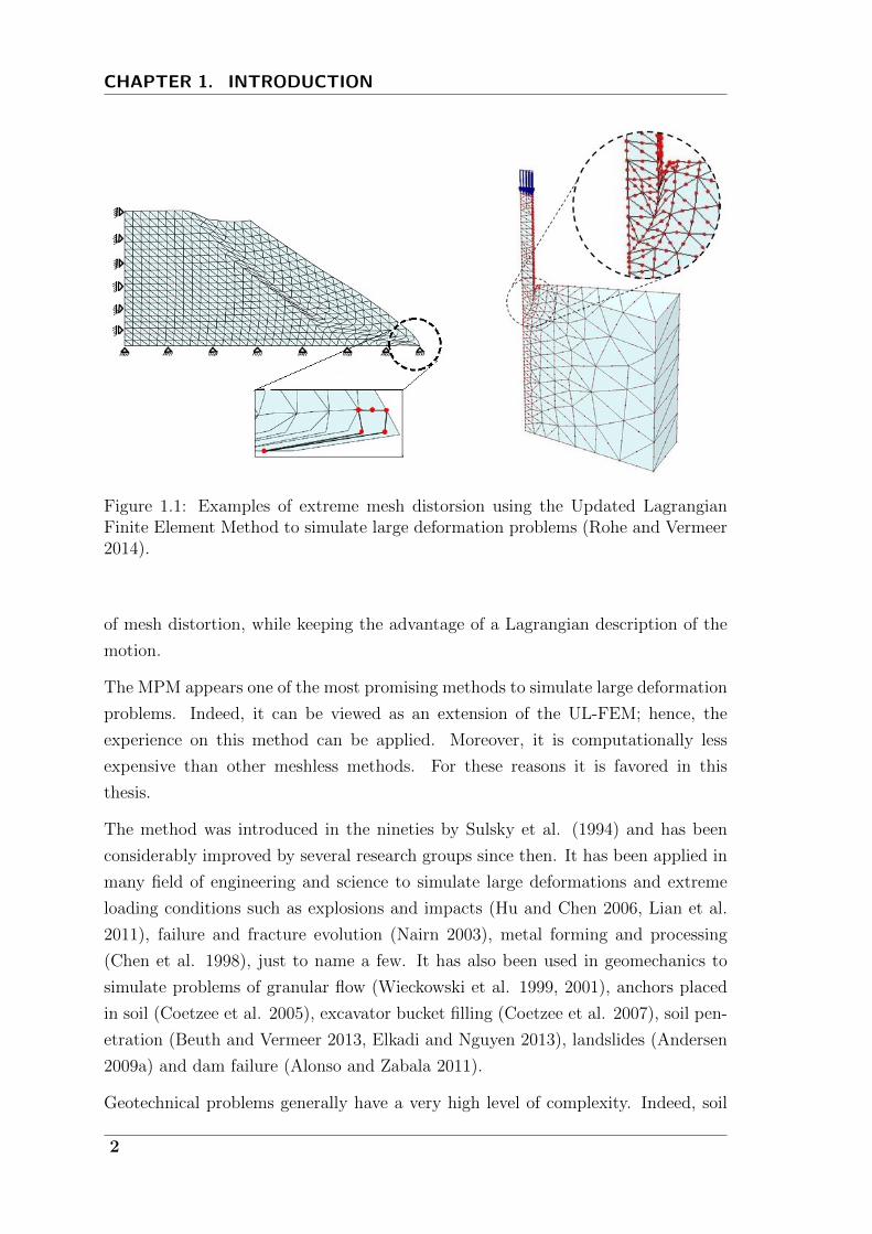
which accompany large deformations, lead to inaccurate results. In some cases it is
even impossible to complete the simulation, as illustrated in Figure 1.1.
Although remeshing techniques and Arbitary Lagrangian-Eulerian (ALE) formula-
tions can overcome the problem, the remapping of state variables arises difficulties
with history dependent materials and the accuracy of results is questionable. The
necessity to solve this problem has encouraged the development of several alternative
methods such as the Discrete Element Methods (DEM), where the soil is represented
as a collection of grains, and meshless or mesh-based particle methods, which are
based on the continuum theory, such as the Smoothed Particles Hydrodynamics
(SPH), the Material Point Method (MPM), and many others.
This thesis deals with advanced numerical modeling of geotechnical problems at
large deformations by mean of the MPM. The attention is focused on the response
of water-saturated soil in drained, partially drained and undrained conditions.
With the MPM, the body is discretized with a set of material points (MP) which
store all the properties of the continuum such as state variables, material properties,
loads and so on. The domain, where the body is moving through, is discretized with
a fixed mesh, which is only used to solve the equations of motion. It simulates large
deformations by MP moving through a background mesh, thus overcoming problems
1
CHAPTER 1. INTRODUCTION
Figure 1.1: Examples of extreme mesh distorsion using the Updated LagrangianFinite Element Method to simulate large deformation problems (Rohe and Vermeer2014).
of mesh distortion, while keeping the advantage of a Lagrangian description of the
motion.
The MPM appears one of the most promising methods to simulate large deformation
problems. Indeed, it can be viewed as an extension of the UL-FEM; hence, the
experience on this method can be applied. Moreover, it is computationally less
expensive than other meshless methods. For these reasons it is favored in this
thesis.
The method was introduced in the nineties by Sulsky et al. (1994) and has been
considerably improved by several research groups since then. It has been applied in
many field of engineering and science to simulate large deformations and extreme
loading conditions such as explosions and impacts (Hu and Chen 2006, Lian et al.
2011), failure and fracture evolution (Nairn 2003), metal forming and processing
(Chen et al. 1998), just to name a few. It has also been used in geomechanics to
simulate problems of granular flow (Wieckowski et al. 1999, 2001), anchors placed
in soil (Coetzee et al. 2005), excavator bucket filling (Coetzee et al. 2007), soil pen-
etration (Beuth and Vermeer 2013, Elkadi and Nguyen 2013), landslides (Andersen
2009a) and dam failure (Alonso and Zabala 2011).
Geotechnical problems generally have a very high level of complexity. Indeed, soil
2

is a multiphase porous medium whose response is highly dependent on the mutual
interaction between solid, fluid and gas. Its mechanical behavior is difficult to model
and, to capture most of its features, constitutive models become very complex. In
addition to this, typical geotechnical problems are characterized by dynamic loading
and often involve the interaction with structures such as a foundation or a wall.
The generation and dissipation of pore pressure under loading can be captured
thanks to the recently implemented dynamic two-phase formulation (Jassim et al.
2013). One of the innovative element of this study is the consideration of partially
drained conditions within a threedimensional numerical model able to simulate large
deformations. To the author knowledge, up to now numerical analyses of large strain
problems considered almost always drained and undrained conditions.
The MPM implementation used in this thesis can simulate the soil-structure in-
teraction. It is modeled with an algorithm specifically developed for the MPM by
Bardenhagen et al. (2001). The original contact algorithm considers only frictional
contact, but it has been extended to the adhesive contact in the frame of this thesis.
This thesis applies the two-phase MPM to the study of typical geomechanical prob-
lems such as the collapse of a submerged slope and the penetration of a cone into
the soil.
Submerged landslides, as well as mud-flows and debris-flows, are often simulated
with hydromechanical models because the soil behaves more like a fluid than a solid
in part of the slide. These models are suitable to study the propagation phase,
but requires the definition of the rheologic characteristics of the material, which
may be difficult to estimate. On the contrary, geotechnical FE models incorporates
advanced constitutive relation to describe soil behavior, but are suitable to simulate
the slope up to the trigger of its failure. The MPM can simulate the soil flow while
the material is described by constitutive models developed in soil mechanics. The
possibility of simulating the initiation, the propagation and the deposition of the
landslide with a single model is of great interest in geotechnics.
The cone penetration test is a common in-situ soil testing technique, used to charac-
terize the soil profile and to estimate soil parameters. It has been deeply studied for
decades. However, to the author knowledge, at the moment there are no truly three-
dimensional numerical simulations of the penetration process which use a realistic
constitutive model, consider the effect of pore pressure dissipation during loading
and the cone rougness. The study described in this thesis gives a contribution in the
understanding of the penetration process, investigating the effect of partial drainage
3
CHAPTER 1. INTRODUCTION
and cone roughness on the measured tip resistance.
1.1 Layout of the thesis
Chapter 2 discusses the basis of the numerical modeling process and briefly presents
the most popular numerical methods. The soil is a collection of grains but can be
regarded as a continuum material at a macro-scale. Following this intrinsic duality
of soil, numerical methods can be classified in discontinuous models and continuum
models. The methods based on the continuum theory are characterized by the way
the body is discretized: the mesh-based methods use a grid or mesh, while the
particle-based methods use a set of material points, also called particles. The latter
overcome problems of mesh distortions and tend to be more suitable to simulate
large deformations.
After an overview of the most recently used numerical methods, a literature study
on the Material Point method is provided. The numbers and quality of publications
about MPM shows that the method is very powerful and promising. It can be
applied in many fields of engineering and science especially for problems involving
large deformations.
Chapter 3 presents the details of the one-phase MPM formulation. First the math-
ematical model is derived; second the governing equations are discretized in time
and space; finally the solution procedure is discussed in detail. Despite the soil is a
multiphase material, this simple formulation can be used in case of undrained and
drained conditions, indeed in these cases the presence of water can be treated in a
simplified way as shown in Section 3.5.
The two-phase formulation is discussed in Chapter 4. The governing equations of
the fluid and solid phase are solved for the velocities of the two phases. This formu-
lation can simulate the generation and dissipation of pore pressures as encoutered
in partially drained conditions. Moreover, it is very well suited to model the be-
havior of saturated soil under dynamic loading conditions (van Esch et al. 2011a).
The solution of the governing equations follows Verruijt (1996). The saturated soil
is discretized with one layer of MP which moves according to the solid velocity as
explained in Section 4.2.
The constitutive modeling of soil is one of the most challenging issues in geomechan-
ics; this theme is discussed in Chapter 5. The most popular elastoplastic models
such as the Mohr-Coulomb, Tresca and Modified Cam Clay are included in this
4
1.1. LAYOUT OF THE THESIS
chapter. To the author’s knowledge this study is one of the first application of the
Modified Cam Clay model within the MPM.
Chapter 6 treats special numerical techniques used to overcome specific problems
such as the volumetric locking typical of low order element, the dissipation of dy-
namic waves, the computational cost of quasi-static simulation, the contact between
bodies and the application of non-zero traction and velocity. Section 6.4 is dedicated
to the contact algorithm, which has a considerable importance for the application
of the MPM to problems involving soil-structure interaction. The original frictional
algorithm (Bardenhagen et al. 2001) is presented and extended to the adhesive
contact type. The new implementation is validated with the problem of the sliding
block.
Chapter 7 is dedicated to the validation of the two-phase formulation. The method
is capable of simulating the propagation of one-dimensional dynamic waves and the
consolidation of a 1D-column for small and large deformations. The use of energy-
dissipation techniques such as viscous boundary and local damping is investigated
too.
A first application of the two-phase MPM to typical large deformation geotechnical
problem is found in Chapter 8. The numerical model simulates the collapse of
a submerged slope in a small-scale laboratory experiment. The complex soil-water
interaction has been taken into account by mean of the two-phase formulation. The
MPM simulation is in excellent agreement with the experimental result.
Chapter 9 shows the possibility to simulate with the MPM the highly complex
problem of the penetration of a cone into the soil, considering partial consolidation
under loading. Simulating the cone penetration for various drainage conditions re-
quires to model the generation and dissipation of pore pressure during penetration,
the constitutive behaviour of soil and the soil-cone contact. The cone penetra-
tion test is a common in-situ soil testing technique; it has been deeply studied for
decades, but numerical simulations of the penetration process in different drainage
conditions are rare. This thesis contributes to achieve a deep understanding of pen-
etration process in partially drained conditions. Numerical results are compared
with experimental data founding good agreement.
This work confirms that MPM is a very promising methods and is very well suited to
geomechanical problems involving large deformations, a summary of the conclusions
and future developments can be found in Chapter 10.
The thesis has two appendices: Appendix A contains the basis of continuum me-
5

CHAPTER 1. INTRODUCTION
chanics, while Appendix B gives and introduction on the damped vibrating sys-
tems. Despite the reader is supposed to be familiar with the concepts of continuum
mechanics and oscillatory systems, the appendices provide a basic knowledge which
can be useful for the understanding of this work.
6
2Numerical modeling in geomechanics
The purpose of this chapter is to introduce the matter of numerical modeling in ge-
omechanics and present the state of the art of the Material Point Method (MPM).
An introduction on the numerical modeling process is presented in Section 2.1; fol-
lowed by an overview of the most popular numerical methods in Sections 2.2 and 2.3.
For the sake of clarity, the considered numerical methods are distinguished on the
basis of the mathematical model on which are based (continuous or discontinuous)
and the discretization method which is applied.
Among the various methods, the MPM has been chosen in this thesis to study large
deformation problems in geomechanics. The number of publications related to the
MPM is growing fast, demonstrating the intense research activity on this subject.
The most important contributes are considered in the literature review discussed in
Section 2.5.
2.1 Introduction
Engineering is fundamentally concerned with modeling; however the use of models
to study reality is common in many fields such aseconomics, anthropology, biology,
chemistry, physics ecc..
‘Scientific understanding proceeds by way of constructing and analyzing mod-
els of the segments or aspects of reality under study. The purpose of these
models is not to give a mirror image of reality, not to include all its elements
in their exact sizes and proportions, but rather to single out and make avail-
able for intensive investigation those elements which are decisive. We abstract
from non-essentials, we blot out the unimportant to get an unobstructed view
7
CHAPTER 2. NUMERICAL MODELING IN GEOMECHANICS
of the important, we magnify in order to improve the range and accuracy of
our observation. A model is, and must be, unrealistic in the sense in which
the word is most commonly used. Nevertheless, and in a sense, paradoxically,
if it is a good model it provides the key to understanding reality.’
This extract from the Baran and Sweezy’s essay (1968) gives a good idea of what a
model is:
• A model is a simplification of the reality. It is important to recognize the
decisive elements which must be included and those which are unessential;
this depends on the purpose of the study.
• A model is an instrument to understand reality and lead decisions to solve a
specific problem.
Engineering is concerned with finding solutions to real problems and this requires to
be able to recognize the essence of the problem and identify the key features which
need to be modeled. One aspect of engineering judgment is the identification of
those features which we believe it is safe to ignore and those which should be taken
into account.
Engineers can use empirical, analytical or numerical models to find practical solu-
tions for their problems. Empirical solutions come from the direct observation of the
physical reality. They are developed to provide satisfactory answers even though the
logical thread cannot always be continuously traced. Analytical solutions seem the
most desirable ones because they usually look very elegant, come from a scientific
theory and are easy to compute; however exact, closed-form solutions are in general
restricted to a limited set of conditions. Numerical models have become more and
more popular thanks to the recent developments in computer technology. They are
based on mathematical models which are solved using specific numerical schemes.
Numerical models are currently the most advanced. Considerable effort has been
put so far to improve them; however they still contain limitations and drawbacks
that encourage further study on this field.
A flow-chart of the numerical modeling process in geomechanics is shown in Fig-
ure 2.1. The real physical system is firstly idealized in a mathematical model. This
model contains the principles of mechanics (conservation’s laws) and the constitu-
tive models of materials. The mathematical model is based on certain assumptions
which lead to the so called idealization error. Secondly the governing equations
are discretized in order to solve a finite system of equations; here the discretization
8

2.1. INTRODUCTION
Figure 2.1: The phases of the numerical modelling (C. Tamagnini)
error is introduced. Thirdly the approximate solution of the discretized equations
is achieved numerically. In this process the approximation error enters the solu-
tion. Finally, an essential step of numerical modeling is the validation; Section 2.4
is dedicated to this phase.
Discretization can be done together with the mathematical idealization, as carried
out in the methods belonging to the Discrete Element family. In this case the
granular material is discretized as a collection of particles representing single soil
grains and micromechanical interactions between particles are modeled.
The soil has an intrinsic duality in the sense that it can be modeled as a continuum
at a macroscopic level or as a particle collection at a micro-meso scale.
For a very long time soil has been modeled according to the continuum theory.
The governing laws are the conservation of mass, the conservation of momentum,
the conservation of energy and the Clausius-Duhem inequality (second principle of
thermodynamic). The constitutive equations of the material are based on its macro-
scopic behavior, which is usually easy to investigate by standard testing procedures.
Only with the arrival of advanced computer technology, modeling soil particles be-
came possible and the methods have been improving fast both from the computa-
tional and theoretical point of view. To follow this approach the knowledge of soil
characteristics at microscopic level is necessary and this is often difficult to achieve
in practice.
9
CHAPTER 2. NUMERICAL MODELING IN GEOMECHANICS
Sections 2.2 and 2.3 provide an overview of the most popular numerical methods
in geomechanics. Recalling the discrete-continuum soil duality, it is clear that we
can firstly distinguish geomechanical computational methods between discontinuous
models and continuum models. In this frame discontinuous models indicate those
which the material is assumed to be made of discrete entities. On the other hand,
the continuum models are based on the assumption of continuity, i.e. the material
conserves its properties regardless the scale. For soil this assumption is not true,
but is acceptable at a macroscopic level.
Discontinuous models differentiate mainly by the way the interactions between in-
dividual particles (and eventually fluids) are modelled. Among continuum models
different approaches can be choosen to discretize the domain and solve the equations;
the main difference lies between mesh-based methods and particle-based methods.
In this thesis mesh-based methods are those in which the discretization and the
solution are based on a grid or mesh, like the finite difference methods (FDM)
and finite element methods (FEM). Particle-based methods are those in which the
discretization is based on a cloud of material points or particles, like smoothed par-
ticle hydrodynamics (SPH), the Material Point Method (MPM), the Particle Finite
Element Method (PFEM).
2.2 Discontinuous models
Discrete models are suitable for those materials which consist in a set of particles,
for example granular materials (cereals, sands ecc.), industrial or chemical pow-
ders, biological solutions (blood, proteins, ecc.), blocky rock masses. Since the late
50s, when the Molecular Dynamic method was developed by Alder and Wainwright
(1959) and Rahman (1964) independently, discrete methods have been growing in
popularity. Several discrete modelling techniques have been developed, including
Monte Carlo method, cellular automata and discrete element method (DEM). The
last one is the most popular in geomechanics. It was originally applied to rock me-
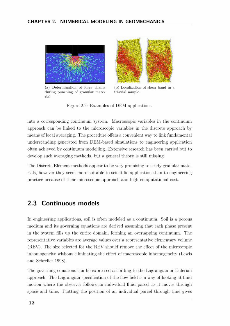
chanics by Cundall and Strack in 1979. Figure 2.2 shows possible applications of
DEM to the study of the behavior of granular material.
The macroscopic behaviour of a particulate matter is determined by the interac-
tions between individual particles as well as interactions with surrounding fluids
and wall. Understanding the microscopic mechanisms which governs these interac-
tions is therefore the key point of the methods. This leads to a truly interdisciplinary
research into particulate matter at particle scale. In recent years, such research has
10

2.2. DISCONTINUOUS MODELS
been rapidly developed worldwide, mainly as a result of the rapid development of
discrete particle simulation technique and computer technology.
The most common DEM formulations are the so-called soft-particle and hard-
particle. The soft-sphere method originally developed by Cundall and Strack (1979)
was the first granular dynamics simulation technique published in the open liter-
ature. In such an approach, particles are permitted to experience minute defor-
mations, and these deformations are used to calculate elastic, plastic and frictional
forces between particles. The motion of particles is described by the well-established
Newton’s laws of motion. A characteristic feature of the soft-sphere models is that
they are capable of handling multiple particle contacts which are of importance
when modelling quasi-static systems. By contrast, in a hard-particle simulation, a
sequence of collisions is processed; often the forces between particles are not explic-
itly considered. Therefore, typically, hard-particle method is most useful in rapid
granular flows.
The particle flow is often coupled with a fluid (gas and/or liquid) flow. To describe
this two-phase flow, DEM has been coupled with computational fluid dynamics
(CFD). The CFD-DEM approach was firstly proposed by Tsuji et al. (1992, 1993),
followed by many others. By this approach, the motion of discrete particles is
described by DEM on the basis of Newton’s laws of motion applied to individual
particles and the flow of continuum fluid by the traditional CFD based on the local
averaged NavierStokes equations (Zhu et al. 2007).
DEM simulations can provide dynamic information, such as the trajectories and
transient forces acting on individual particles. It is well suited to study fundamental
soil behavior during loading, develop and validate constitutive relationships for soil.
The main disadvantage of the DEM is its enormous computational expense. The
maximum number of particles and duration of a virtual simulation is limited by
computational capacity. Typical flows contain billions of particles, but contempo-
rary DEM simulations on large cluster computers have only recently been able to
approach this scale for sufficiently long simulated time. When modeling full-scale
problems a method which minimizes the number of particles is necessary to keep
the problem computationally feasible.
A second issue involves the input parameters, which refer to particle properties
rather than aggregate properties. The DEM parameters must be chosen such that
realistic soil behaviour is modelled (Ting et al. 1989).
By use of a proper averaging procedure, a discrete particle system can be transferred
11
CHAPTER 2. NUMERICAL MODELING IN GEOMECHANICS
(a) Determination of force chainsduring punching of granular mate-rial
(b) Localization of shear band in atriaxial sample.
Figure 2.2: Examples of DEM applications.
into a corresponding continuum system. Macroscopic variables in the continuum
approach can be linked to the microscopic variables in the discrete approach by
means of local averaging. The procedure offers a convenient way to link fundamental
understanding generated from DEM-based simulations to engineering application
often achieved by continuum modelling. Extensive research has been carried out to
develop such averaging methods, but a general theory is still missing.
The Discrete Element methods appear to be very promising to study granular mate-
rials, however they seem more suitable to scientific application than to engineering
practice because of their microscopic approach and high computational cost.
2.3 Continuous models
In engineering applications, soil is often modeled as a continuum. Soil is a porous
medium and its governing equations are derived assuming that each phase present
in the system fills up the entire domain, forming an overlapping continuum. The
representative variables are average values over a representative elementary volume
(REV). The size selected for the REV should remove the effect of the microscopic
inhomogeneity without eliminating the effect of macroscopic inhomogeneity (Lewis
and Schrefler 1998).
The governing equations can be expressed according to the Lagrangian or Eulerian
approach. The Lagrangian specification of the flow field is a way of looking at fluid
motion where the observer follows an individual fluid parcel as it moves through
space and time. Plotting the position of an individual parcel through time gives
12
2.3. CONTINUOUS MODELS
the pathline of the parcel. This can be visualized as sitting in a boat and drifting
down a river. The Eulerian specification of the flow field is a way of looking at fluid
motion that focuses on specific locations in the space through which the fluid flows
as time passes. This can be visualized by sitting on the bank of a river and watching
the water pass the fixed location (Batchelor 2000).
It is always possible to switch from Eulerian to Lagrangian formulation by means
of basic rules. A first classification can distinguish between the numerical models
based on the Eulerian formulation and those based on the Lagrangian formulation.
The Eulerian formulation is mostly used in fluid dynamics, while the Lagrangian
formulation is dominant when the material behavior is history dependent.
Once the governing laws have been derived, the equations have to be discretized.
Here it was decided to distinguish the methods on the basis of the discretization
procedure:
• methods where the domain is discretized with a mesh. This mesh is necessary
to write the approximate solution and solve the problem at each time step.
The mesh stores important information and cannot be changed very easily.
• methods where the deformable body is discretized with a cloud of particles.
Among them a second distinction is possible:
– methods in which the mesh is eventually required to write the approxi-
mate solution and/or to calculate numerically the integrals characterizing
the governing law, but can be destroyed at each time step. The number
of these methods is very large;
– methods in which no mesh is needed in any phase of the solution process.
These methods are rare.
In this thesis the first family of methods is called mesh-based methods and the
second particle-based methods. The main features of some of them are summarized
in the following.
The use of the words meshless and meshfree methods is deliberately avoided since
their use is popular in the literature, but their definition is still confuse. Indeed
Atluri et al (1999):
To be a truly meshless method, the two characteristics should be guaranteed:
One is a non-element interpolation technique, and the other is a non-element
approach for integrating the weak form.
13
CHAPTER 2. NUMERICAL MODELING IN GEOMECHANICS
for De Borst et al.(2012):
meshless or meshfree methods do not require an explicitly defined connectivity
between nodes for the definition of the shape function. Instead, each node has
a domain of influence which does not depend on the arrangement of the nodes.
The domain of influence of a node is the part of the domain over which the
shape function of that specific node is non-zero.
while for Idelshon et al (2003):
A meshless method is an algorithm that satisfies both of the following state-
ments:
• the definition of the shape functions depends only on the node positions.
• the evaluation of the nodes connectivity is bounded in time and it de-
pends exclusively on the total number of nodes in the domain.
moreover Onate et. al (2004) use these terms in a generalized way for their PFEM
method, where a finite element mesh does exist and connects the nodes defining the
discretized domain where the governing equations are solved in the standard FEM
fashion as well as the boundary of the continuum body.
2.3.1 Mesh-based methods
The most popular mesh methods are the finite difference methods (FDM) and the
finite element methods (FEM).
The finite difference approximation for derivatives is the oldest approach to
solve differential equations. It was already known by L. Euler ca. 1768, for the
one dimensional space and was probably extended to dimension two by C. Runge
ca. 1908. The advent of finite difference techniques in numerical applications be-
gan in the early 1950s and their development was stimulated by the emergence of
computers.
It consists in approximating the differential operator by replacing the derivatives in
the equations using differential quotients. The domain is partitioned in space and
time. Approximations of the solution are computed at the space or time points.
It is difficult to name a date for the invention of the finite element methods,
they originated from the need to solve complex elasticity problems in civil and
14
2.3. CONTINUOUS MODELS
aeronautical engineering. Their developments can be traced back to the work by A.
Hrennikoff (1941) and R. Courant (1943). Although the approaches used by these
pioneers are different, they share one essential characteristic: mesh discretization of
a continuous domain into a set of discrete sub-domains, usually called elements.
FEM its real impetus in the 1960s and 70s by the developments of J.H. Argyris and
co-workers at the University of Stuttgart, R.W. Clough and co-workers at UC Berke-
ley, O.C. Zienkiewicz and co-workers at the University of Swansea, and Richard Gal-
lagher and co-workers at Cornell University. Further impetus was provided in these
years by available open source finite element software programs. NASA sponsored
the original version of NASTRAN, and UC Berkeley made the finite element pro-
gram SAP IV widely available. A rigorous mathematical basis to the finite element
methods was provided in 1973 in the publication of Strang and Fix. The method
has since then been generalized for the numerical modeling of physical systems in
a wide variety of engineering disciplines, e.g., electromagnetism, heat transfer, and
fluid dynamics(Robinson and Przemieniecki 1985); see e.g. Zienkiewicz and Taylor
(2005) and Bathe (2006) for an overview.
In Lagrangian FEM, the mesh moves with the material (Fig. 2.3). Hence, the nodes
located at the boundary of the continuum will always remain on the boundary
throughout the computations. This means that the free surface of the continuum is
well defined, allowing easy track of the interface between different materials and sim-
ple imposition of the boundary conditions. Another advantage of Lagrangian FEM
is that, by definition, it does not allow the material to flow between elements and
hence history dependent material behavior can be easily handled as the quadrature
points remain coincident with the material points. However, the mesh distortion
problem makes the method cumbersome in modeling very large deformations.
In Eulerian FEM the computational mesh is fixed while the material is deforming in
time (Fig. 2.3). Large deformation are handled without the problem of mesh distor-
tion that appears in the Lagrangian FEM. As the computational mesh is completely
decoupled from the material, convective terms appear in Eulerian FEM, introducing
numerical difficulties with history-dependent materials.
The most attractive feature of the FEM is its ability to handle complicated geome-
tries and boundaries with relative ease. While FDM in its basic form is restricted
to handle rectangular shapes and simple alterations thereof, the handling of geome-
tries in FEM is theoretically straightforward. On the other hand FDM are easier to
implement.
15

CHAPTER 2. NUMERICAL MODELING IN GEOMECHANICS
Figure 2.3: (a) Initial configuration in FEM, (b) deformed confitugation in La-grangian FEM, (c) deformed configuration in Eulerian FEM.
The quality of an FEM approximation is often higher than the corresponding FDM
approach, but this is extremely problem-dependent and several examples of the
contrary can be provided. Generally, FEM is the most used method in all types of
analysis in structural mechanics while computational fluid dynamics (CFD) tends
to use FDM or other methods like finite volume method (FVM). Both FDM and
FEM are widely used in geomechanics, both for scientific research purposes and
professional applications, thanks also to the large availability of commercial codes.
One of the main shortcomings of Lagrangian FEM, common to other mesh-based
methods, is the inaccuracy generated by big mesh distortions, then the limitations
in modeling large deformations. This can be prevented by remeshing techniques or
using the Arbitray Lagrangian Eulerian (ALE) formulation, but with a signi-
ficative increase of computational requirements.
The key difference between ALE formulation and Lagrangian or Eulerian formula-
tions is that in ALE the reference computational domain can move arbitrarily and
independently of the material. The movement of the reference domain is represented
by a set of grid points, which may be interpreted as the movement of a finite el-
ement mesh. Therefore, in an ALE formulation, the finite element mesh does not
need to adhere to the material during the course of deformation as in Lagrangian
descriptions, and thus the problems of mesh distortions may be avoided (Gadala
and Wang 1998).
Penetration problems in geomechanics are sometimes solved with the Coupled
Eulerian-Lagrangian (CEL) method. In CEL, one material is discretized with
Eulerian mesh (usually the soil), whereas the other is discretized with Lagrangian
mesh. The interaction between the two meshes is modeled using contact algorithm
selected by the user. See e.g. Henke and Grabe (2010), Qiu and Grabe (2011),
16
2.3. CONTINUOUS MODELS
Qiu and Henke (2011), Qiu et al. (2011) for CEL applications in geotechnical
engineering.
2.3.2 Particle-based methods
Particle Methods discretize a continuum body with a collection of particles, also
called material points. All the physical properties are attached to the particles and
not to the elements as in the FEM. For the methods presented in this section a
particle represents part of the continuum (Onate et al. 2004).
A large number of mesh-based methods has been developed, however an extensive
discussion of them exceed the purpose of this thesis. This section provides a short
overview of the most popular particle-based methods which have also been applied
in geomechanics.
The considered methods follow a Lagrangian approach of the governing equations.
Their main advantage is the possibility to deal with large deformations overcoming
the drawbacks associated with mesh distortion encountered in mesh-based methods.
The complexity and computational cost are highly dependent on the specific method;
in general they are higher than FEM and FDM.
The Material Point Method (MPM) has its origin in the Fluid-Implicit Particle
method (FLIP) (Brackbill and Ruppel 1986) and the Particle-In-Cell method (PIC)
(Harlow et al. 1957) developed during the 90s at the Sandia National Laboratories.
The first publication dates back to 1994 by Sulsky et al.. Since then the method has
been applied in many fields where large deformations are of relevance. A literature
review on the method can be found in Section 2.5.
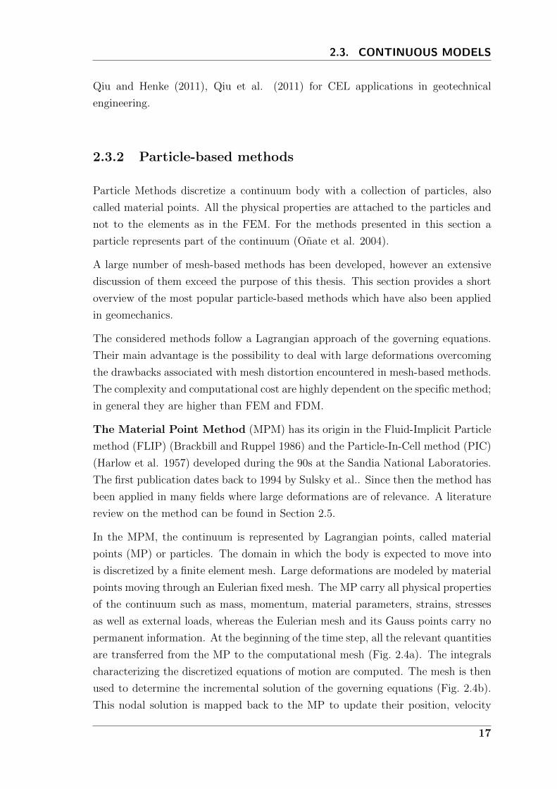
In the MPM, the continuum is represented by Lagrangian points, called material
points (MP) or particles. The domain in which the body is expected to move into
is discretized by a finite element mesh. Large deformations are modeled by material
points moving through an Eulerian fixed mesh. The MP carry all physical properties
of the continuum such as mass, momentum, material parameters, strains, stresses
as well as external loads, whereas the Eulerian mesh and its Gauss points carry no
permanent information. At the beginning of the time step, all the relevant quantities
are transferred from the MP to the computational mesh (Fig. 2.4a). The integrals
characterizing the discretized equations of motion are computed. The mesh is then
used to determine the incremental solution of the governing equations (Fig. 2.4b).
This nodal solution is mapped back to the MP to update their position, velocity
17
CHAPTER 2. NUMERICAL MODELING IN GEOMECHANICS
(a) Quantities are mapped from the MPto the mesh nodes.
(b) The governing equations are solvedat the background mesh which deforms.
(c) Quantities are mapped from thenodes to the MP.
(d) The background mesh can be rede-fined.
Figure 2.4: Calculation steps of MPM
and all the other quantities (Fig. 2.4c). Afterward, the mesh can be reset to the
initial configuration or changed arbitrarily (Fig. 2.4d).
The Lagrangian Integration Point Finite Element Method (FEMLIP) was
first developed for geophysical problems (Moresi et al. 2003), but has been success-
fully applied in geomechanics (Cuomo et al. 2012).
It appears to be very similar to the MPM; indeed material points are used to track
history variables and deformations and the essence of the formulation is the use of
particles as integration points. The difference between MPM is that in FEMLIP
the integration weight is recomputed at each time step in order to obtain the best
approximation of the integral for a given element. Recomputing the particle weights
is a computationally expensive step not required in the Material Point Method. The
18
2.3. CONTINUOUS MODELS
method seems to be well suited for simulating viscoelastic-brittle materials in fluid-
like deformation (Moresi et al. 2003).
The Particle Finite Element Method (PFEM) was presented at the beginning
of this century (Idelsohn et al. 2004, Onate et al. 2004) to solve fluid-structure
interaction problems and has been later applied to geotechnical engineering.
This numerical method uses a Finite Element mesh to discretize the physical domain
and to integrate the differential governing equations. In contrast to classical Finite
Element approximations, the nodes transport their momentum together with all
their physical properties, thus behaving as particles. Their location is updated
according to the equations of motion in a Lagrangian fashion. At the end of each
time step the mesh is regenerated. A fast and robust algorithm, based on the
Delaunay Tessellation is used to generate the new mesh. The mesh not only serves
for the integration of the differential equations, but it is also used to identify the
contacts and to track the free surface.
The Smoothed Particle Hydrodynamics (SPH) was originally developed for
astronomic applications by Lucy (1977) and Gingold and Monaghan (1977). Since
its invention, SPH has been widely applied to many problems in engineering practice
such as quasi-incompressible fluid flow (Monaghan 1994), viscous fluid flow (Takeda
et al. 1994; Morris et al. 1997), high velocity impact of solid (Allahdadi et al. 1993),
geophysical flows (Gutfraind and Savage 1998; Oger and Savage 1999).
Bui et al. (2007, 2008) were the first to apply SPH to elasto-plastic geomateri-
als. Since then, the method has been extended to a wide range of applications
in computational geomechanics such as granular flows, bearing capacity of shallow
foundations, slope failure, soil-structure interaction, seepage flows. An overview of
the developments of the method and its application can be found in Liu and Liu
(2010) and Monaghan (2012)
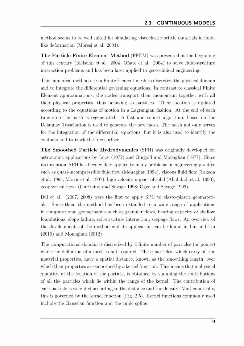
The computational domain is discretized by a finite number of particles (or points)
while the definition of a mesh is not required. These particles, which carry all the
material properties, have a spatial distance, known as the smoothing length, over
which their properties are smoothed by a kernel function. This means that a physical
quantity, at the location of the particle, is obtained by summing the contributions
of all the particles which lie within the range of the kernel. The contribution of
each particle is weighted according to the distance and the density. Mathematically,
this is governed by the kernel function (Fig. 2.5). Kernel functions commonly used
include the Gaussian function and the cubic spline.
19

CHAPTER 2. NUMERICAL MODELING IN GEOMECHANICS
Figure 2.5: Simplified representation of a kernel function.
A detailed comparison between MPM and SPH can be found in Ma et al. (2009).
The MPM is found to have some advantages compared to SHP, e.g. in MPM spa-
tial derivatives are calculated based on a regular computational grid, so that the
time consuming neighbor searching is not required, the boundary conditions can
be applied in MPM as easily as in FEM, and contact algorithms can be efficiently
implemented.
The Element Free Galerkin (EFG) method (Belytschko et al. 1994) and the
Meshless Local Petrov-Galerkin (MLPG) method (Atluri and Zhu 1998) are
both based on the idea of discretizing a problem domain by a particle distribution
and a boundary definition. The field variable is approximated by interpolants to
particle values. Construction of these interpolants requires only points and no mesh
of elements, and is based on a least squares approach. The main difference between
the EFG method and the MLPG method lies in the way the integrals, of the dis-
cretized equations, are calculated. In the former the test and shape functions are
identical (hence the use of Galerkin) and therefore the integrations must be carried
out over the entire domain for each particle. The latter uses different test and shape
functions, which then restrict non-zero terms in the integrals to a zone around each
particle.
These methods can provide smooth solutions, using shape functions of any desired
order of continuity, in contrast to finite element shape functions which hit problems
beyond C1. However several difficulties must be addressed such as the imposition
of essential boundary conditions and the calculation of the integrals.
In the field of geomechanics the EFG method has been applied to model fluid flow
in porous media (Kim 2007; Praveen Kumar et al. 2008) while MLPG has been
used by Ferronato et al. (2007) for predicting subsidence of reservoirs.
From this brief review of particle based method it can be concluded that although
20
2.4. VALIDATION
their introduction in the engineering field is quite recent, they appear very promis-
ing in particular for the ability to handle large deformations. Works on further
developments of these methods and new challenging applications are in progress.
2.4 Validation
Because of the idealization, discretization and numerical errors which inevitably
afflict the analisys, the numerical prediction never completely matches the ”real”
world behavior. The numerical solution can only be a good approximation of reality.
Validation is the process by which the quality of the numerical simulation is assured.
In other words, the correspondence between reality and simulation is quantified.
All validation is done through a comparison of a pattern or a reference model with
the model under study. There are many ways to make a validation, but in general
they are usually classified according to the pattern used in the comparison (Godoy
and Dardati 2001, Aad et al. 2008):
Validation using other numerical solutions. This technique compares the re-
sults to be validated with the results obtained through other numerical meth-
ods previously validated.
Validation using analytical solutions. This type of comparison can be used
when the analytical theory behind the problem is known and direct compar-
ison of the results with the analytical solution is possible. One of the main
problems of this technique is that it can only be used in extremely simple
cases.
Validation using experimental results. With this technique the consistency of
the model with the reality is proved.
2.5 The Material Point Method: literature review
After the first publication about MPM by Sulsky et al. (1994), the method has
been widely applied to many fields of engineering and science and extended with
advanced features. Some of the most important contributions to the development
of the MPM and its applications are discussed in this section. In order to keep the
presentation clear, this survey has been divided in topics.
21
CHAPTER 2. NUMERICAL MODELING IN GEOMECHANICS
2.5.1 Historical developments
The roots of the MPM lie in a more general class of numerical schemes known as
Particle-in-cell methods (PIC). The first PIC technique was developed in the 1950s
(Harlow et al. 1957) and was used primarily for applications in fluid mechanics.
Early implementations suffered from excessive energy dissipation, rendering them
obsolete when compared to other, more valid methods.
Many problems affecting early PIC methods were solved developing the Fluid-
Implicit Particle (FLIP) formulation (Brackbill and Ruppel 1986, Brackbill et al.
1988) in which the particles carry all the information of the continuum, e.g. mass,
momentum, energy and constitutive properties.
In the 90’s Sulsky et al. (1994) considerably extended the FLIP method to the
application for solid mechanics. The weak formulation and the discrete equations
were casted in a form that is consistent with the traditional finite element method.
Furthermore, they applied the constitutive equation at each single particle, avoid-
ing the interpolation of history-dependent variables, as the particles are tracked
throughout the computation. Through this considerable extension, the method was
able to handle history-dependent material behavior. Elements having material with
different parameters or different constitutive equations were automatically treated;
this is a clear advantage over Eulerian FEM. They considered numerical examples
with large rigid body rotation and showed that the energy dissipation which tends
to occur in Eulerian approach did not occur in their approach. This extension was
then applied to different impact problems in plane-strain condition with elastic and
strain hardening plastic material behaviors (Sulsky and Schreyer 1993a).
In the same year (1993), Sulsky and Schreyer extended the application of PIC to
incorporate constitutive laws expressed in terms of Jaumann rate of stress. Further
applications of PIC method to solid mechanics are given in Sulsky et al. (1995).
In 1996, Sulsky and Schreyer named the method as the Material Point Method
and presented its axisymmetric formulation. They applied MPM to upsetting of
billets and Taylor impact problems. They also incorporated the thermal effect in
the constitutive equation.
Most MPM implementations are dynamic codes which employ an explicit time in-
tegration scheme, however implicit time integration has been used by several re-
searchers (Guilkey and Weiss 2001, Guilkey and Weiss 2003, Sulsky and Kaul 2004,
Beuth et al. 2008).
22

2.5. THE MATERIAL POINT METHOD: LITERATURE REVIEW
Although it is possible to use explicit dynamic programs also for the analysis of quasi-
static problems, this is computationally inefficient as explicit integration requires
very small time steps and can lead to long computation times.
Beuth et al. (2008) proposed an implicit time integration scheme for MPM using
quasi-static governing equations. The virtual work equation obtained from the in-
ternal and external static equilibrium of continuum was used as the main governing
equation in the proposed method. This method has been applied to slope failure and
retaining wall problems (Beuth 2011) and numerical simulation of cone penetration
in clay (Beuth and Vermeer 2013).
Bardenhagen and Kober (2004) generalized the discretization procedure of the orig-
inal MPM. Element shape functions together with particle characteristic functions
are introduced in the variational formulation, similarly to other meshless methods.
Different combinations of the shape functions and particle characteristic functions
resulted in a family of methods named the Generalized Interpolation Material Point
Method (GIMP).
The MPM and its extensions have been used for many problems involving extreme
deformations, such as explosion and impact (Hu and Chen 2006, Lian et al. 2011),
failure and fracture evolution (Nairn 2003), biological and cellular materials (Ionescu
et al. 2005, Guilkey et al. 2006), metal forming and processing (Chen et al. 1998),
ice dynamics (Sulsky et al. 2007).
The first attempt in the field of geotechnical engineering can be considered the
simulation of granular flow (Wieckowski et al. 1999, 2001) and subsidence of landfill
covers that include geomembranes (Zhou et al. 1999). Konagai and Johansson
(2001) applied the method to plane-strain compression test, failure of a cliff and
mass flow through a trapdoor. It has been applied to the modeling of anchors placed
in soil (Coetzee et al. 2005), excavator bucket filling (Coetzee et al. 2007), retaining
wall failure (Wickowski 2004), the simulation of experiments related to induced
ground deformations (Johansson and Konagai 2007) and geomembrane response to
settlement in landfills (Zhou et al. 1999). The MPM demonstrated to be suitable
for soil penetration problems such as simulation of the cone penetration test (Beuth
and Vermeer 2013) and pile installation (Elkadi and Nguyen 2013). Numada and
Konagai (2003) were the first to apply the method to soil flows in order to study
the run-out of earthquake-induced slides. The MPM has been also used to model
landslides (Andersen 2009a) and dam failure (Alonso and Zabala 2011).
23
CHAPTER 2. NUMERICAL MODELING IN GEOMECHANICS
2.5.2 Contact algorithms
The MPM is capabe of simulating non-slip contact between different bodies without
a special algorithm. However, in many engineering problems a contact algorithm is
required to model the relative motion at the interface between the contacting bodies.
A simple contact algorithm was proposed by York et al. (1999) to allow the release
of no-slip contact constraint in the standard MPM. In York’s method, if two bodies
are approaching each other, the impenetrability condition is imposed as in standard
MPM. If the bodies are moving away from one another, they move in their own
velocity fields to allow separation.
Hu and Chen (2003) presented a contact/sliding/separation algorithm in the multi-
mesh environment. In their contact algorithm, the normal component of the velocity
of each material particle at the contact surface is calculated in the common back-
ground grid, whereas the tangential component of the velocity is found based on the
respective individual grid. Although aforementioned contact algorithms are efficient
to simulate separation, the friction between contact bodies is not considered.
Bardenhagen et al. (2000c) developed a frictional contact algorithm to model in-
teraction between grains in granular materials. The algorithm allows sliding and
rolling with friction as well as separation between grains, and correctly prohibits
interpenetration. The strength of the algorithm is the automatic detection of the
contact nodes, i.e. a predefinition of the contact surface is not required. It was
further improved by Bardenhagen et al. (2001) and applied to simulate stress prop-
agation in granular materials. This algorithm is the most used in MPM literature
(Andersen 2009a, Bardenhagen et al. 2000a, Bardenhagen et al. 2000b, Coetzee
2003, Al-Kafaji 2013).
Huang and Zhang (2011) focused on the problem of impact and penetration, such
as the perforation of a plate by a projectile. The no-slip contact condition in the
standard MPM creates a great penetration resistance, so that the target absorbs
more impact energy and decreases the projectile velocity. To accurately simulate
the projectile-target interaction improvement of the impenetrability condition was
necessary.
In conventional small-deformation finite element analyses, contact problems are
solved with interface elements; this can be done with the MPM too (Vermeer et al.
2009). Interface elements were used for slope stability problems and to solve the
cone-soil contact in simulation of cone penetration testing with the quasi-static MPM
24
2.5. THE MATERIAL POINT METHOD: LITERATURE REVIEW
(Beuth and Vermeer 2013).
Lim et al. (2014) applied a level-set based contact algorithm (Andreykiv et al. 2012)
to simulate soil-penetration problems such as the installation of offshore foundations.
The idea of the method is to describe the soil and the inclusion with two fully
independent, overlapping domains and use a distributed Lagrange multiplier and
a level set function to provide the necessary contact interaction. This approach is
specific for penetration problems and the extension to other type of applications
seems not straightforward.
Ma et al. (2014) implemented in the GIMPM a new contact algorithm to facilitate
large deformation analysis with smooth, partially rough or rough contact in geotech-
nical engineering. They recognize that the Bardenhagen contact algorithm has two
limitations:
• The accuracy of the contact algorithm becomes questionable when the stiffness
of the contacting materials is very different, such as in the case of interaction
between soft clay and penetrometer or foundation. Unrealistic oscillations of
the velocity and acceleration are observed.
• In the Coulomb friction model, as modelled by Bardenhagen et al. (2001), the
shear stress along the interface is always proportional to the normal stress,
that is, the shear stress can be increased indefinitely with the normal stress.
This mechanism might be reasonable for elastic materials in contact, but it
is unrealistic for cohesive soils under undrained conditions because the shear
stress cannot exceed the undrained shear strength of the soil.
A penalty function is introduced to avoid non-physical oscillation, moreover a maxi-
mum shear stress, irrespective of the normal stress, is incorporated into the Coulomb
friction model for modelling common geotechnical contact conditions. The key con-
cept of the penalty approach is to allow limited interpenetration between the con-
tacting materials. The method showed to be able to reduce numerical oscillations
in the contact force, moreover with an optimal selection of the penalty function
properties, the interpenetration is limited to a very low level, while the accuracy of
the computation is effectively improved.
25
CHAPTER 2. NUMERICAL MODELING IN GEOMECHANICS
2.5.3 Multi-phase formulations in MPM
Many problems that are of interest for geotechnical engineers involve fluid-saturated
soil. The application of MPM to such multiphase problems is recent (Zhang et al.
2007, Zhang et al. 2008, Zhang et al. 2009, Higo et al. 2010, Jassim et al. 2013,
Abe et al. 2013) and the research is in progress.
Zhang et al. (2007) modeled fluid-saturated soil by using two sets or layers of
material points. One set of MP moves according to the solid governing equations,
while a different set of MP moves according to the fluid governing equations. Such a
formulation allows for modeling changes in the water table with time by computing
the movements of the fluid particles in the soil. However, their formulation assumed
only a small deformation of soil because the same interpolation function was used
for both the solid and the fluid layers.
Zhang et al. (2008) proposed a new formulation based on the Eulerian form of the
equation in which they modeled solid grains and compressible fluid material. Volume
fractions, particle densities, and pressures are directly solved at each step without
using time-integrated solutions. They did not use the time-integrated values of
pressures because the volume fractions were calculated using a background mesh as
the control volume and, for most of the time, the control volume is not fully occupied
with material. This leads to errors in pressure increments and an accumulation of
errors in the pressure values.
Zhang et al. (2009) introduced a contact algorithm for the coupled MPM based
on the u-p formulation, i.e. soil displecement (u) and pore water pressure (p) are
the primary variables. They applied the method to predict the dynamic responses
of saturated soil subject to contact/impact. In this formulation only one set of
material points is used; the material points move with the same velocity of the solid
and carry also the information of the liquid.
Higo et al. (2010) proposed a coupled MPM-FDM to model fluid saturated soil.
The MPM was used to represent soil particles and the fluid was calculated using an
Eulerian approach with FDM (due to the availability of the background grid). The
momentum balance equation for the mixture was solved using MPM formulation,
and the continuity equation for the water phase was solved using FDM formulation.
Although the u-p formulation can capture the dynamic response for various scenar-
ios, it has been shown that such a formulation cannot accurately capture two-phase
dynamic behaviour that involves, for example, the propagation of a compression
26

2.5. THE MATERIAL POINT METHOD: LITERATURE REVIEW
wave followed by a second one that is associated with the consolidation process (van
Esch et al. 2011a). The full set of equations including all acceleration terms is re-
quired to capture both waves. Jassim et al. (2013) implemented a velocity-velocity
(v-w) formulation based on the integration steps suggested by Verruijt (2010).
Abe et al. (2013) proposed a soil-pore fluid coupled MPM algorithm based on Biots
mixture theory (1962). The continuum is discretized with two layers of particles,
i.e., a solid soil skeleton layer and a pore water layer. The water layer is used for
calculating the pore-water pressure distribution derived from the equation of state
and the velocities of the water particles based on Darcys law. The solid layer is used
for calculating the effective stress, velocity, and deformation of the soil skeleton. For
demonstrating the applicability of the proposed MPM to geotechnical engineering
problems, a large-scale levee-failure experiment conducted by Iseno et al. (2004)
was simulated. The numerical model showed to be adequate for simulating the
deformation observed after rapid levee failure due to the seepage and migration of
water.
A similar two-layer implementation, with advanced featured to increase the numer-
ical stability, has been proposed by (Bandara and Soga 2015). The method has
been validated by comparing results with those predicted by analytical solutions
and applied to model a levee failure problem using a strain-softening MohrCoulomb
model.
2.5.4 Coupling with other methods
One of the prominent trends in recent years is coupling the MPM with other nu-
merical methods. Such an approach allows analysts to reap the benefits of multiple
solution types and exploit each method’s strengths in multiphysic simulations.
Due to the similarities between MPM and FEM, the combination of these methods
comes naturally. The efficiency of MPM is lower than that of FEM due to the map-
ping between background grid and MP, while the accuracy of calculating the integral
with the MP quadrature, used in MPM, is lower than that of Gauss quadrature,
used in FEM. FEM is, in general, optimal for small deformations, while MPM is
Zhang et al. (2006) developed an explicit Material Point Finite Element Method
(MPFEM) to combine the advantages of both FEM and MPM. In MPFEM, the
user is required to identify a large deformation region which is discretized with a
computational grid. The material domain is discretized by a mesh of finite elements.
27

CHAPTER 2. NUMERICAL MODELING IN GEOMECHANICS
In the large deformation zone, the momentum equations are solved on the compu-
tational grid as in the standard MPM. Elsewhere, they are solved on the FE mesh
as in the traditional Lagrangian FE method. The finite element nodes covered by
the background grid, i.e. in the large deformation zone, are automatically converted
into MPM particles.
Similarly, Lian et al. (2011) proposed a Coupled Finite Element Material Point
(CFEMP) method, in which the body with mild deformation is discretized by finite
elements, while the body with extreme deformation is discretized by MPM particles.
The interaction between them is implemented by contact method carried out on the
back-ground grid. However, the user is required to identify the body which will
experience extreme deformation.
The technique has been further improved in the Adaptive Finite Element Mate-
rial Point (AFEMP) method (Lian et al. 2012). With this technique, bodies are
initially discretized by finite elements, and then the distorted elements are automat-
ically converted into MPM particles when their plastic strain or distortion degree
exceeds a user prescribed value during the simulation process. The interaction be-
tween the remaining finite elements and MPM particles is implemented based on
the background grid. Hence, the material region with mild deformation is modeled
by finite elements, while the material region with extreme deformation is modeled
by MPM particles automatically.
In order to solve problems of multiphase flow, the MPM has been also coupled with
purely Eulerian finite difference or finite volume schemes, e.g., the works presented
by Zhang et al. (2008) and Higo et al. (2010). The soil skeleton and the pore
fluid are discretized by the MPM and FDM, respectively. In this way the governing
equations of different materials or phases are solved by methods well suited to do
so.
28
3Formulation of the one-phase MPM
As already pointed out, this thesis focuses on the application of the MPM to ge-
omechanical problems. Although the soil is a multi-phase material, characterized
by solid particles and fluid or gas filling the pores, in many cases it can be regarded
as an homogeneous single-phase material. With this simplified approach only the
soild velocity field is considered.
The governing equations of the problem are presented in Section 3.1. The formula-
tion is general, not specific for geomechanical problems, therefore it can be applied
to any kind of solid material.
Sections 3.2 and 3.3 explain how the governing equations are discretized in space
and time within the MPM; finally the solution procedure is presented in Section 3.4.
Possible applications of the one-phase formulation in geotechnical engineering are
discussed in section 3.5.
3.1 Governing equations
The analysis of engineering systems requires the idealization of the system, i.e.
the formulation of the mathematical model. One group of fundamental equations
of continuum mechanics arises from the conservation laws. These equations must
always be satisfied by physical systems. Four conservation laws, relevant to thermo-
mechanical systems, are considered here: the conservation of mass, the conservation
of linear momentum, often called conservation of momentum, the conservation of
angular momentum and the conservation of energy.
A detailed derivation of these equations exceed the purpose of this thesis; for more
29

CHAPTER 3. FORMULATION OF THE ONE-PHASE MPM
details the reader should refer to continuum mechanics books. The definition of the
main kinematic and dynamic quantities is in Appendix A.
Conservation of mass. When sources and sinks are neglected, i.e. no mass en-
tering or leaving the domain occupied by the material, the change of mass
with time is zero. The mathematical form of the conservation of mass can be
written as∂ρ
∂t+ ρ
∂vi∂xi
= 0 3.1
with ρ being the mass density of the material, vi is the i-th component of
the velocity and t the time. Equation 3.1 is also referred to as the continuity
equation.
Conservation of momentum. Conservation of momentum implies both, conser-
vation of linear and angular momentums. The conservation of linear momen-
tum represents the equation of motion of a continuum, i.e. Newtons second
law of motion. It relates the motion or the kinetic of a continuum to the
internal and external forces acting upon it. Without going into details of de-
velopment and derivation of the equation, we give the mathematical form of
the conservation of linear momentum as
ρdvidt
=∂σij∂xj
+ ρgi 3.2
in which the term ρgi represents the forces due the self weight of the continuum,
which are the only body forces considered in this thesis and gi stands for the
components of gravitational acceleration, σij is the stress tensor.
The conservation of angular momentum implies that the stress tensor is sym-
metric,i.e.,
σij = σji 3.3
As the conservation of angular momentum adds no new equation, most liter-
ature calls the conservation of linear momentum as the momentum equation.
Conservation of energy. In this thesis heat effects and any source of thermal
energy are disregarded and the mechanical work is considered as the only
source of energy, therefore the conservation of energy takes the form
ρdr
dt= εijσij
3.4
with r being the internal energy per unit mass and εij the deformation rate.
30

3.1. GOVERNING EQUATIONS
The equations given so far apply equally to all material, but they are insufficient to
describe the mechanical behavior of any particular material. To complete the speci-
fication of the mechanical properties of a material additional equation are required,
which are called constitutive equations.
The mechanical constitutive equation of a material specifies the dependence of the
stress in a body on kinematic variables such as the strain tensor or the rate-of-
deformation tensor. In general the stress rate can be a function of the stress state
σij, the temperature T and a vector of internal variables χ. For example:
σij = f(εij, σij, T,χ) 3.5
Here the thermal effects are neglected. The stress response of a body to a defor-
mation is not affected by rigid motion, therefore the constitutive equations should
be invariant under translation and rotation of the frame of reference. This study
adopt the Jaumann stress rate tensor, however different definition of the stress rate
are possible such as the Truesdell rate and the Green-Naghdi of the Cauchy stress
tensor.
An incrementally linear constitutive model assumes the form:
σij = Dijklεkl 3.6
whereDijkl represents the constitutive tensor. Constitutive modeling of soil behavior
is one of the most challenging issue in geo-science. A brief overview of the most
popular constitutive models is given in chapter 5, however is not in the purpose of
this thesis to discuss this issue into details.
3.1.1 Boundary and initial conditions
Let ∂Ω represents the boundary of the domain; two classes of boundary conditions
can be identified: the essential and the natural boundary conditions. The essential
boundary conditions are also called Dirichlet or geometric boundary conditions and
correspond to prescribed displacements or velocities. The part of the boundary
where these conditions are applied is called ∂Ωu. The natural boundary conditions
are also called Neumann or force boundary conditions and corresponds to prescribed
boundary forces. ∂Ωτ denotes the part of the boundary where the traction is applied
as indicated in Figure 3.1.
31
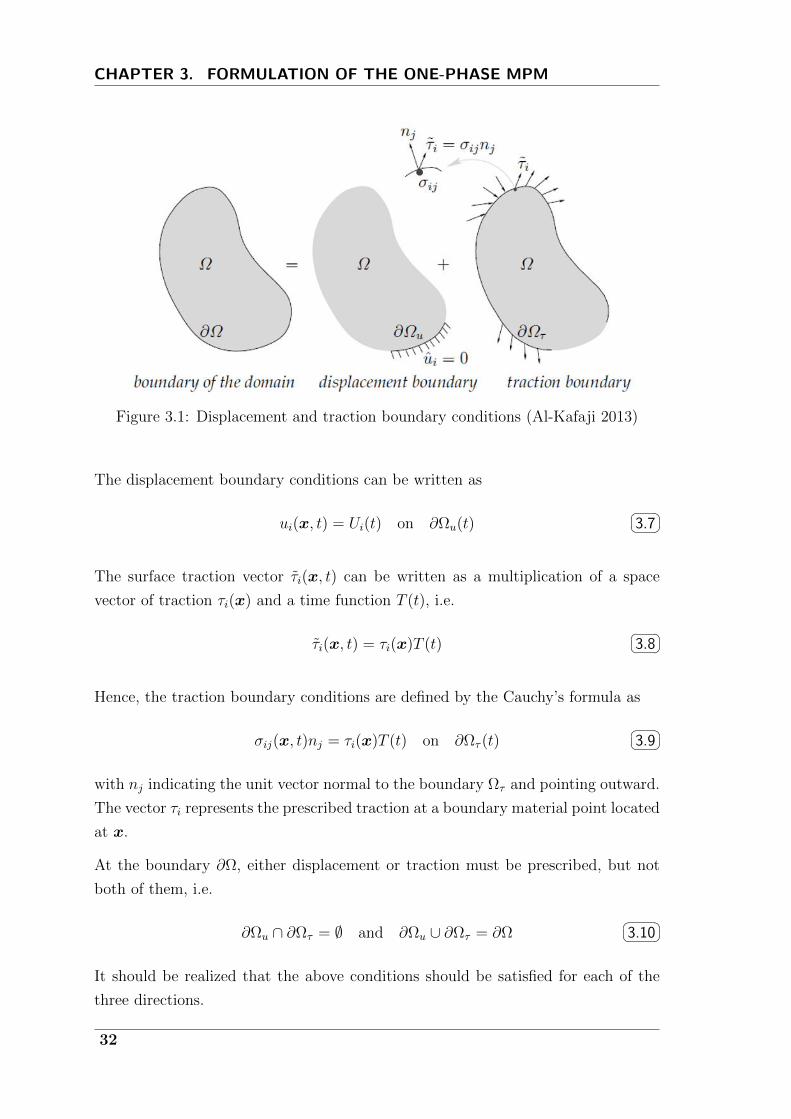
CHAPTER 3. FORMULATION OF THE ONE-PHASE MPM
Figure 3.1: Displacement and traction boundary conditions (Al-Kafaji 2013)
The displacement boundary conditions can be written as
ui(x, t) = Ui(t) on ∂Ωu(t) 3.7
The surface traction vector τi(x, t) can be written as a multiplication of a space
vector of traction τi(x) and a time function T (t), i.e.
τi(x, t) = τi(x)T (t) 3.8
Hence, the traction boundary conditions are defined by the Cauchy’s formula as
σij(x, t)nj = τi(x)T (t) on ∂Ωτ (t) 3.9
with nj indicating the unit vector normal to the boundary Ωτ and pointing outward.
The vector τi represents the prescribed traction at a boundary material point located
at x.
At the boundary ∂Ω, either displacement or traction must be prescribed, but not
both of them, i.e.
∂Ωu ∩ ∂Ωτ = ∅ and ∂Ωu ∪ ∂Ωτ = ∂Ω 3.10
It should be realized that the above conditions should be satisfied for each of the
three directions.
32

3.2. SPACE DISCRETIZATION
The initial conditions are written as
ui(x, t0) = U0i, vi(x, t0) = V0i and σij(x, t0) = σ0ij
3.11
3.1.2 Weak form of the momentum equation
Equation 3.2 is the strong form of the momentum equation, i.e. strong continuity
is required for the field variables. Obtaining the solution for a strong system of
equation is usually very difficult for practical engineering problems.
The weak form is usually an integral form and requires weaker continuity on the
field variables. For this reason a formulation based on the weak form produces a
discrete system of equations that is easier to solve and gives better results, therefore
it is preferred in FE formulations (Quek and Liu 2003).
The momentum equation is now multiplied by a test function or a virtual velocity
ti and is integrated over the current domain occupied by the continuum Ω:
∫Ω
tiρdvidtdΩ =
∫Ω
ti∂σij∂xj
dΩ +
∫Ω
tiρgidΩ 3.12
The test function ti must be kinematically admissible, i.e. it satisfies the essential
boundary conditions and is continuous over the domain.
The use of the Gauss’s theorem, also called the divergence theorem, and the Cauchy’s
formula leads to:∫Ω
tiρdvidtdΩ =
∫∂Ωτ
tiτidS +
∫Ω
tiρgidΩ−∫
Ω
∂ti∂xi
σijdΩ 3.13
which represents the weak form of the momentum equation and will be used in the
formulation of the discrete equations.
It should be noted that the first term in Equation 3.13 represents the inertia; the
second and the third represent the external surface and body forces; the last one
represents the internal force.
3.2 Space discretization
The current section presents the details of the space discretization adopted in the
MPM.
33

CHAPTER 3. FORMULATION OF THE ONE-PHASE MPM
Two kinds of space discretization are used in the MPM. Firstly the initial config-
uration of the analysed body is represented by a cloud of material points (MP).
Secondly the entire region where the body is expected to move is discretized by a
finite element mesh.
Taking advantage of the symmetry of the strain tensor, the strain and its rate can
be represented in a vector form as
ε(x, t) =d
dtε(x, t)
3.14
where
ε(x, t) =[ε11 ε22 ε33 γ12 γ23 γ31
]T 3.15
with εij, i = j being the normal strain in the direction of the xi coordinate and
γij = 2εij, i 6= j being the shear strain in xixj plane.
Similarly, the stress rate vector is
σ(x, t) =d
dtσ(x, t)
3.16
whith
σ(x, t) =[σ11 σ22 σ33 σ12 σ23 σ31
]T 3.17
where σij, i = j is the normal stress in the direction of the xi coordinate and σij, i 6= j
is the shear stress in xixj plane.
The displacement and eventually the velocity and acceleration are approximated by
means of shape functions as:
u(x, t) ≈N (x)u(t) 3.18
v(x, t) ≈N (x)v(t) 3.19
a(x, t) ≈N (x)a(t) 3.20
where N is the matrix of the shape functions, which are identical to the one use in
the FEM. The vectors u(t), v(t) and a(t) contain the nodal values of displacement,
velocity and acceleration respectively. The test function is approximated in the same
way.
The kinematic relation can be written using matrix notation as
ε(x, t) = Lv(x, t) 3.21
34
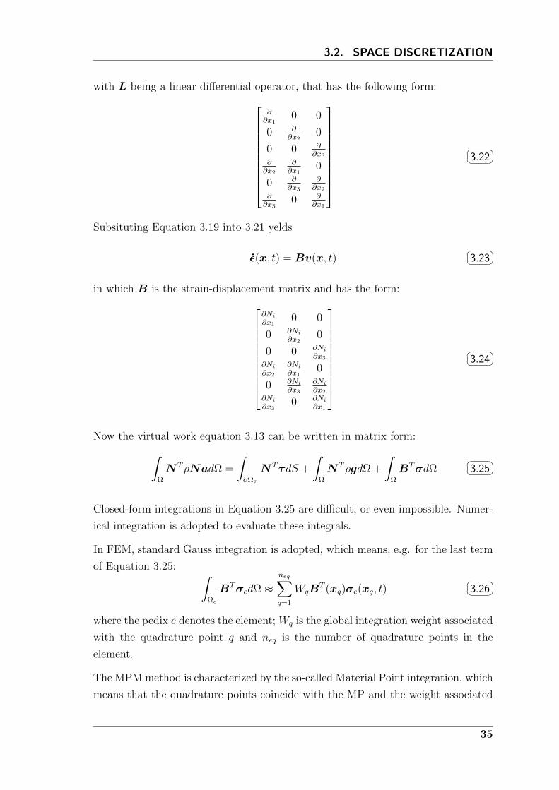
3.2. SPACE DISCRETIZATION
with L being a linear differential operator, that has the following form:
∂∂x1
0 0
0 ∂∂x2
0
0 0 ∂∂x3
∂∂x2
∂∂x1
0
0 ∂∂x3
∂∂x2
∂∂x3
0 ∂∂x1
3.22
Subsituting Equation 3.19 into 3.21 yelds
ε(x, t) = Bv(x, t) 3.23
in which B is the strain-displacement matrix and has the form:
∂Ni∂x1
0 0
0 ∂Ni∂x2
0
0 0 ∂Ni∂x3
∂Ni∂x2
∂Ni∂x1
0
0 ∂Ni∂x3
∂Ni∂x2
∂Ni∂x3
0 ∂Ni∂x1
3.24
Now the virtual work equation 3.13 can be written in matrix form:∫Ω
NTρNadΩ =
∫∂Ωτ
NTτdS +
∫Ω
NTρgdΩ +
∫Ω
BTσdΩ 3.25
Closed-form integrations in Equation 3.25 are difficult, or even impossible. Numer-
ical integration is adopted to evaluate these integrals.
In FEM, standard Gauss integration is adopted, which means, e.g. for the last term
of Equation 3.25: ∫Ωe
BTσedΩ ≈neq∑q=1
WqBT (xq)σe(xq, t)
3.26
where the pedix e denotes the element; Wq is the global integration weight associated
with the quadrature point q and neq is the number of quadrature points in the
element.
The MPM method is characterized by the so-called Material Point integration, which
means that the quadrature points coincide with the MP and the weight associated
35

CHAPTER 3. FORMULATION OF THE ONE-PHASE MPM
to the MP is its volume Ωp. Therefore Equation 3.26 becomes:
∫Ωe
BTσedΩ ≈nep∑p=1
ΩpBT (xp)σp
3.27
where now the pedix p refers to the MP, i.e. nep is the number of MP inside the
element, xp and σp are the position and the stress associated to the MP respectively.
At this step, it is important to emphasized that one of the difference between FEM
and MPM lies on the integration method used to assemble the equation of motion.
The discretized equation of motion, in matrix notation, assumes the form:
Ma = F ext + F grav − F int 3.28
Where M is the mass matrix, i.e.
M =
np∑p=1
mpNT (xp)N (xp)
3.29
which depends on the position of the MP, of mass mp, with respect to the compu-
tational mesh. In order to improve the efficiency of the algorithm, a diagonal form
of the mass matrix, called lumped mass matrix, is used.
The external forces F trac and F grav are calculated as:
F trac ≈nebp∑p=1
NT (ξp)ftracp
3.30
F grav ≈nep∑p=1
NT (ξp)fgravp
3.31
where f tracp and f gravp are the traction and the gravity assign to the MP; details of
MP initialization are in Paragraph 3.4.1.
The internal force F int is calculated according to Equation 3.27.
3.3 Time discretization
Equation 3.28 is discretized in space, but still continuous in time. It represents a
series of second-order ordinary differential equations (ODE) in time. To get a full
36
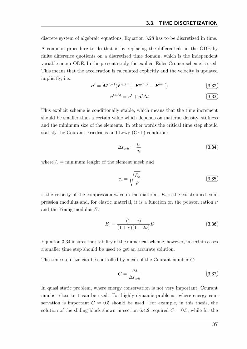
3.3. TIME DISCRETIZATION
discrete system of algebraic equations, Equation 3.28 has to be discretized in time.
A common procedure to do that is by replacing the differentials in the ODE by
finite difference quotients on a discretized time domain, which is the independent
variable in our ODE. In the present study the explicit Euler-Cromer scheme is used.
This means that the acceleration is calculated explicitly and the velocity is updated
implicitly, i.e.:
at = M t,−1(F ext,t + F grav,t − F int,t) 3.32
vt+∆t = vt + at∆t 3.33
This explicit scheme is conditionally stable, which means that the time increment
should be smaller than a certain value which depends on material density, stiffness
and the minimum size of the elements. In other words the critical time step should
statisfy the Courant, Friedrichs and Lewy (CFL) condition:
∆tcrit =lecp
3.34
where le = minimum lenght of the element mesh and
cp =
√Ecρ
3.35
is the velocity of the compression wave in the material. Ec is the constrained com-
pression modulus and, for elastic material, it is a function on the poisson ration ν
and the Young modulus E:
Ec =(1− ν)
(1 + ν)(1− 2ν)E
3.36
Equation 3.34 insures the stability of the numerical scheme, however, in certain cases
a smaller time step should be used to get an accurate solution.
The time step size can be controlled by mean of the Courant number C:
C =∆t
∆tcrit
3.37
In quasi static problem, where energy conservation is not very important, Courant
number close to 1 can be used. For highly dynamic problems, where energy con-
servation is important C ≈ 0.5 should be used. For example, in this thesis, the
solution of the sliding block shown in section 6.4.2 required C = 0.5, while for the
37
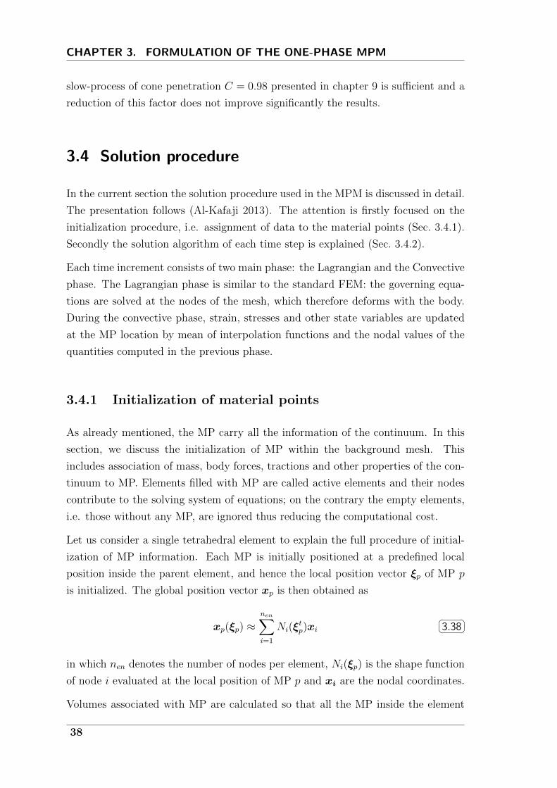
CHAPTER 3. FORMULATION OF THE ONE-PHASE MPM
slow-process of cone penetration C = 0.98 presented in chapter 9 is sufficient and a
reduction of this factor does not improve significantly the results.
3.4 Solution procedure
In the current section the solution procedure used in the MPM is discussed in detail.
The presentation follows (Al-Kafaji 2013). The attention is firstly focused on the
initialization procedure, i.e. assignment of data to the material points (Sec. 3.4.1).
Secondly the solution algorithm of each time step is explained (Sec. 3.4.2).
Each time increment consists of two main phase: the Lagrangian and the Convective
phase. The Lagrangian phase is similar to the standard FEM: the governing equa-
tions are solved at the nodes of the mesh, which therefore deforms with the body.
During the convective phase, strain, stresses and other state variables are updated
at the MP location by mean of interpolation functions and the nodal values of the
quantities computed in the previous phase.
3.4.1 Initialization of material points
As already mentioned, the MP carry all the information of the continuum. In this
section, we discuss the initialization of MP within the background mesh. This
includes association of mass, body forces, tractions and other properties of the con-
tinuum to MP. Elements filled with MP are called active elements and their nodes
contribute to the solving system of equations; on the contrary the empty elements,
i.e. those without any MP, are ignored thus reducing the computational cost.
Let us consider a single tetrahedral element to explain the full procedure of initial-
ization of MP information. Each MP is initially positioned at a predefined local
position inside the parent element, and hence the local position vector ξp of MP p
is initialized. The global position vector xp is then obtained as
xp(ξp) ≈nen∑i=1
Ni(ξtp)xi
3.38
in which nen denotes the number of nodes per element, Ni(ξp) is the shape function
of node i evaluated at the local position of MP p and xi are the nodal coordinates.
Volumes associated with MP are calculated so that all the MP inside the element
38
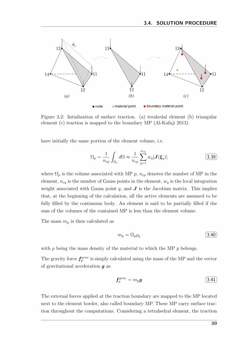
3.4. SOLUTION PROCEDURE
Figure 3.2: Intialization of surface traction. (a) terahedal element (b) triangularelement (c) traction is mapped to the boundary MP (Al-Kafaji 2013).
have initially the same portion of the element volume, i.e.
Ωp =1
nep
∫Ωe
dΩ ≈ 1
nep
neq∑q=1
wq|J(ξq)| 3.39
where Ωp is the volume associated with MP p, nep denotes the number of MP in the
element, neq is the number of Gauss points in the element, wq is the local integration
weight associated with Gauss point q, and J is the Jacobian matrix. This implies
that, at the beginning of the calculation, all the active elements are assumed to be
fully filled by the continuum body. An element is said to be partially filled if the
sum of the volumes of the contained MP is less than the element volume.
The mass mp is then calculated as
mp = Ωpρp 3.40
with ρ being the mass density of the material to which the MP p belongs.
The gravity force f gravp is simply calculated using the mass of the MP and the vector
of gravitational acceleration g as
f gravp = mpg 3.41
The external forces applied at the traction boundary are mapped to the MP located
next to the element border, also called boundary MP. These MP carry surface trac-
tion throughout the computations. Considering a tetrahedral element, the traction
39
CHAPTER 3. FORMULATION OF THE ONE-PHASE MPM
vector τe applied at the triangular surface is interpolated from the nodes of this
surface to the boundary MP. Hence, the traction at boundary MP p is
τe(xp) ≈ntri∑i=1
Ni(ξq)τe(xi) 3.42
where Ni is the shape function of node i of the triangular surface element and ξq are
the coordinates of the boundary MP p inside the parent triangular element. These
coordinates simply represent the projection of the MP on the triangular surface
element. The traction force vector f tracp is then
f tracp = τe(xp)Senebp
=Senebp
ntri∑i=1
Ni(ξp)τe(xi) 3.43
in which nebp denotes the number of boundary MP located next to the loaded surface.
In the initialization of MP, initial conditions, material parameters and constitutive
variables are assigned to them as well. Furthermore, book-keeping is initialized
at this step, including information such as to which element each particle initially
belongs and the initial number of particles per each active finite element.
3.4.2 Solution of the governing equations
In the present section the solution procedure for the MPM, known as modified
Lagrangian algorithm, is presented.
Let us consider the state of a continuum at time t and describe the procedure of
advancing the solution to time t+ ∆t. It consists of the following steps:
1. The momentum equation is initialized. This means that the lumped-mass
matrix M t is computed at the beginning of the time step, the traction force
vector F trac,t is calculated with:
F trac,t = F trac,tT (t) in which F trac,t ≈nebp∑p=1
mpNT (ξtp)f
trac,tp
3.44
40

3.4. SOLUTION PROCEDURE
the gravity force Fgrav,t and the internal force Fint,t are integrated as
F grav,t ≈nep∑p=1
NT (ξtp)fgrav,tp
3.45
F int,t ≈nep∑p=1
BT (ξtp)σtpΩ
tp
3.46
The discrete system of equations is complete:
M tat = F trac,t + F grav,t − F int,t = F t 3.47
2. The system is solved for the nodal accelerations as
at = M t,−1F t 3.48
3. In this step, the velocities of MP are updated using the nodal accelerations
and the shape functions
vt+∆tp = vtp +
nen∑i=1
∆tNi(ξtp)a
ti
3.49
4. The nodal velocities vt+∆t are then calculated from the updated MP momen-
tum solving the following equation
M tvt+∆t ≈nep∑p=1
mpNT (ξtp)v
tp
3.50
5. Nodal velocities are integrated to get nodal incremental displacements
∆ut+∆t = ∆tvt+∆t 3.51
6. Strains at MP are calculated as
∆εt+∆tp = B(ξtp)∆u
t+∆t 3.52
and stresses are updated according to the constitutive relation
7. Volumes associated with MP are updated using the volumetric strain incre-
41
CHAPTER 3. FORMULATION OF THE ONE-PHASE MPM
ment
Ωt+∆tp = (1 + ∆εt+∆t
vol,p ) with ∆εvol = ∆ε11 + ∆ε22 + ∆ε33
3.53
Consequently the density is updated
ρt+∆tp =
ρtp
(1 + ∆εt+∆tvol,p )
3.54
8. Displacements and positions of MP are updated according to
ut+∆tp = utp +
nen∑i=1
N (ξtp)ut+∆ti
3.55
xt+∆tp = xtp +
nen∑i=1
N (ξtp)ut+∆ti
3.56
9. The mesh can be reset and the book-keeping is updated. At this step a new
element is detected for those MP that crossed elements boundary. Conse-
quently the new number of MP per each finite element is determined. The
active and inactive elements are identified and the new local position of each
particle inside the element are obtained.
The reader should have noted that the nodal velocity is not directly computed
from the nodal acceleration, but from the MP momentum. This prevents the so-
called small mass problem (Sulsky et al. 1995). When a MP enters a previously
empty element and remains close to the boundary, the values of the associated shape
functions relative to those element nodes which are far from the MP, i.e. Ni(ξp),
approach zero. As a consequence, the nodal mass approaches zero, leading to a
nearly singular, ill-conditioned mass matrix. The internal force involves the gradient
of the shape function, which is constant inside the element, and hence the right-hand
side term of Equation 3.47 does not approach zero. Unphisical nodal acceleration
can therefore be obtained. The problem is solved on the level of velocity through
steps 3 and 4 of the previous list.
42
3.5. APPLICABILITY OF ONE-PHASE FORMULATION IN SOILMECHANICS
3.5 Applicability of one-phase formulation in soil me-
chanics
Soil is, in general, a mixture of three phases: soild, fluid and gas. The fluid can be
water, oil or other liquid substances; the gas can be air, hydrocarbon or other types
of gas. Considering a soil sample of volume V , the volumes occupied by solid grains,
fluid and gas as separate phases can be identified with Vs, Vf and Vg respectively.
The volume collectively occupied by fluid and gas is also called void volume Vv since
they occupies the pores between soil grains. In this thesis only the presence of water
inside the pores is considered.
The void ratio e and the porosity n can be defined as:
e =VvVs
n =VvV
3.57
The degree of saturation represents the percentage of void volume occupied by the
fluid and is expressed as
Sr =VfVv· 100%
3.58
The soil is said to be dry if Sr = 0% and fully saturated if Sr = 100% otherwise it is
partially saturated. In this thesis partially saturated conditions are not considered.
Considering the soild grain-water mixture different densities can be defined:
Dry density
ρd = (1− n)ρs 3.59
where ρs represents the grain density of the solid phase and usually assumes
values close to 2700 kg/m3.
Saturated density
ρsat = ρd + nρw = (1− n)ρs + nρw 3.60
where ρw is the water density.
Usually the soil density is comprise between these two, since some air is always
included in the pores.
Similarly, the following unit weight can be defined:
43
CHAPTER 3. FORMULATION OF THE ONE-PHASE MPM
Dry unit weight
γd = ρdg 3.61
Saturated unit weight
γsat = ρsatg 3.62
Submerged unit weight
γ′ = γsat − γw 3.63
where g and γw are the gravity and the water unit weight respectively.
In saturated soil, depending on the soil permeability and the rate of load, drained,
partially drained and undrained conditions can be encountered. In drained condi-
tions a negligible excess pore pressure is generated and rapidly dissipates, therefore
it can be neglected. In undrained conditions the rate of load is so fast that there
is a significant generation of excess pore pressure, but negligible relative movement
between solid and fluid phase, therefore pore pressure dissipation can be neglected.
In partially drained conditions excess pore pressure generation and dissipation are
not negligible, therefore a proper formulation, able to take into account the coupled
behavior of solid and water should be used.
In numerical analyses dealing with drained conditions and undrained conditions the
presence of the water can be considered in a simplified way. In the first case the
presence of the water can be neglected and the soil can be regarded as dry. In the
latter, because of the negligible relative movement between solid and water, the
equilibrium of the soil-water mixture can be considered rather than the equilibrium
of soil and water as separate phases. The stress state can be described in terms of
total stresses or effective stresses. In the second case the excess pore pressures can
be computed by means of the so-called Effective Stress Analysis, which is based on
the assumption of strain compatibility between the soil skeleton and the enclosed
pore water (Vermeer 1993); further detail are given in section 3.5.1.
Modelling of dry soil, saturated soil in drained and undrained conditions are the
field of applicability of the one-phase formulation. For partially drained conditions
a fully-coupled two-phase formulation is necessary. This is presented in chapter 4.
3.5.1 Effective stress analysis for elastic soil skeleton
In a saturated soil the total load is constantly divided between fluid a soil skeleton.
According to the effective stress principle, the total stress σij is decomposed into
44

3.5. APPLICABILITY OF ONE-PHASE FORMULATION IN SOILMECHANICS
Figure 3.3: Rappresentation of strain compatibility
effective stress σ′ij and pore pressure pw:
σij = σ′ij + pwδij 3.64
where δij is the Kroneker delta.
A further distinction is made between the steady and the excess pore pressure. The
first one is usually considered as an input, while the second one is generated by the
loading mechanism. Since the time derivative of the steady pore pressure is null,
only the variation in excess pore pressure will be considered.
Which fraction of an applied incremental load is carried by the soil skeleton and
which fraction is carried by the pore water follows from the consideration of strain
compatibility. The stiffnesses of the soil skeleton, the soil minerals and the pore
water must be considered. This, of course, only holds for undrained conditions,
when no dissipation of water with time is considered. The soil minerals can be
considered as incompressible, since their bulk modulus is much higher than the one
of soil skeleton (K ′) and water (Kw). Pore water is mostly assumed to be slightly
more compressible than pure water because some air is always included even for a
fully saturated soil.
Assuming undrained conditions and incompressible soil grains, strain compatibility
requires that the change of volume of the soil-water mixture, due to total load,
corresponds to the change of volume of the soil skeleton, due to effective pressure,
and to the change of volume of the water-filled pores, due to pore water pressure.
In other terms:
εvol =p
Ku
=pw
Kw/n=
p′
K ′
3.65
45
CHAPTER 3. FORMULATION OF THE ONE-PHASE MPM
where Ku is the so-called undrained bulk modulus and represent the stiffness of
the soil mixture in undrained conditions. Eq. 3.65 is valid for an elastic soil skele-
ton; indeed in elastoplastic models the volumetric strain rate may also depend on
deviatoric stresses and in viscoplastic models the time depencency of εvol is included.
Considering the effective stress principle, Equation 3.65, leads to:
Ku = K ′ +Kw
n
3.66
The bulk modulus can be written as a function of the Poisson ratio ν and the shear
modulus G (Eq. 3.67 and 3.68).
K ′ =2G(1 + ν ′)
3(1− 2ν ′)
3.67
Ku =2G(1 + νu)
3(1− 2νu)
3.68
νu indicates the Poisson’s ration of the mixture in undrained conditions and is ap-
proximately 0.5, while the shear modulus G is the same for the mixture and the soil
skeleton.
Inserting Equations 3.67 and 3.68 in Equation 3.66 and solving for the bulk modulus
of water, it leads to:Kw
n=
3(νu − ν ′)(1− 2νu)(1 + ν ′)
K ′ 3.69
Upon sudden loading, a fully saturated soil shows no noteworthy change of volume
and the applied load is found to be carried almost entirely by the pore water. On
the other hand, assuming slight compressibility of the pore water is of advantage for
numerical analyses. Indeed, a high stiffness of the pore water, resulting in a nearly
incompressible material, causes numerical problems such as volumetric locking and
a severe ill-conditioning of the stiffness matrix. In order to prevent numerical prob-
lems, the undrained Poisson ratio is generally set to a value between 0.485 and 0.495.
In this thesis νu = 0.490 is used for undrained calculations.
A useful parameter to represent the fraction of total load carried by the water is
the Skempton’s B-parameter. It is widely used in laboratory practice and can be
written as:
B =pwp
=Kw/n
Ku
=1
1 + K′
Kw/n
3.70
For saturated soil it is close to 1.
46
4Formulation of a two-phase MPM
In geotechnical engineering, problems characterized by the solid-fluid interaction are
very common. As explained in section 3.5, sometimes the presence of the fluid can be
treated in a simplified way; on the other hand, when the relative movement between
solid skeleton and water is important, a fully coupled formulation is essential.
The current Chapter focuses on the MPM formulation to analyze coupled dynamic
two-phase problems. In Section 4.1 the governing equations of the continuum prob-
lem are presented, to move on with the solution procedure within MPM in Sec-
tion 4.2. Since the MPM implementation of the two-phase formulation consists in
a natural extension of the one-phase formulation, many details are omitted; the
reader can find further information in Al-Kafaji (2013). The validation and some
applications of the two-phase formulation are in Chapter 7.
4.1 Governing equations
This section is devoted to the presentation of the governing equations that are
required for the solution of coupled dynamic, two-phase problems. The first complete
theoretical approach describing the coupling between solid and fluid phases was
proposed by Biot (1941) for a linear elastic soil skeleton while considering fluid
seepage based on Darcy’s law, in quasi-static conditions. This work is based on
the early work on porous media by von Terzaghi (1936). Biot’s theory (BT) was
further extended to anisotropic cases (Biot 1955). The dynamic extension of BT
was published in two papers: (a) for low frequency range (Biot 1956c), and (b)
for high frequency range (Biot 1956b). The theory was later extended to finite
deformations in elasticity (Biot 1972). Zienkiewicz and co-workers (Zienkiewicz
47
CHAPTER 4. FORMULATION OF A TWO-PHASE MPM
et al. 1980; Zienkiewicz 1982; Zienkiewicz and Shiomi 1984; Zienkiewicz et al.
1990; Zienkiewicz et al. 1999) extended BT into nonlinear range, i.e. material and
geometric non-linearities, under dynamic loads.
The equations that describe the two-phase physics are: conservation of mass, con-
servation of momentum, and the constitutive relation. In the exact solution, i.e.
no simplifications are considered, the principal unknowns are the displacement of
the soil (u), the relative velocity between solid and fluid or the seepadge velocity
(wr), and the fluid pressure. Due to its complexity this formulation is rarely used in
FEM, however Zienkiewicz et al. (1980) observed that this formulation is necessary
for extremely rapid motions.
In the so-called u-p-formulation the relative acceleration of the fluid is neglected.
The primary variables are the solid displacement and the fluid pressure. Many of the
currently available FEM implementations are based on this formulation due to its
simplicity. This is suitable for low frequency and quasi static problems (Zienkiewicz
et al. 1980).
The well-known consolidation equation neglects all acceleration terms and is there-
fore suitable only for this type of problems.
With the formulation used in this thesis, the equilibrium equations are solved for
the accelerations of water phase and soil skeleton as the primary unknown variables.
This two-phase approach is commonly called v-w-formulation (Verruijt 1996), where
v and w denote the velocities of the solid and liquid phase respectively. This for-
mulation proved to be able to capture the physical response of saturated soil under
dynamic as well as static loading (van Esch et al. 2011a).
The detailed derivations of the governing equations is not discussed here. The
reader can refer to the work by Zienkiewicz and co-workers (1984, 1990 and 1999)
for further details on two-phase formulations and to Verruijt (1996) for more detail
on the applications to dynamic loading. The main focus of the current Section is
to clarify the assumptions which characterize the used formulation and define the
terms of the governing equations.
4.1.1 Mass conservation
The conservation of mass of the solid phase is expressed as:
∂
∂t[(1− n)ρs] +
∂
∂xj[(1− n)ρsvj] = 0
4.1
48
4.1. GOVERNING EQUATIONS
in which vj is the j-th component of the velocity vector of the solid phase.
On denoting the components of the vector of the (true) velocity of the water phase
as wj, the conservation of mass of this phase can be written as:
∂
∂t(nρw) +
∂
∂xj(nρwwj) = 0
4.2
When considering incompressible solid grains and disregarding the spatial variations
in densities and porosity, one can reduce the expression for the conservation of mass
of the solid and water phases to
− ∂n
∂t+ (1− n)
∂vj∂xj
= 0 4.3
and
n∂ρw∂t
+ ρwdn
dt+ nρw
∂wj∂xj
= 0 4.4
respectively. Substituting Equation 4.3 into Equation 4.4 allows to eliminate the
term dndt
. Hence,
n∂ρw∂t
+ ρw(1− n)∂vj∂xj
+ nρw∂wj∂xj
= 0 4.5
The water is assumed to be linearly compressible via the relation
dρwdpw
= − ρwKw
4.6
Substituting Equation 4.6 into Equation 4.5 and rearranging terms yields:
∂pw∂t
=Kw
n
[(1− n)
∂vj∂xj
+ n∂wj∂xj
] 4.7
Equation 4.7 represents the conservation of mass of the saturated soil. It is also
known as storage equation.
4.1.2 Conservation of momentum
The conservation of momentum of the solid phase can be expressed as
(1− n)ρsdvjdt−∂σ′ij∂xi− (1− n)
∂pw∂xj− (1− n)ρsgj −
n2ρwg
k(wj − vj) = 0
4.8
49
CHAPTER 4. FORMULATION OF A TWO-PHASE MPM
where k is the Darcy permeability. It can be expressed in terms of the intrinsic
permeability k and the dynamic viscosity of the water µd as:
k = kρwg
µd
4.9
The conservation of momentum of the liquid phase is written as:
nρwdwjdt− n∂pw
∂xj− nρwgj +
n2ρwg
k(wj − vj) = 0
4.10
the therm (wj − vj) represent the relative velocity of the water respect to the solid.
Adding the momentum of the solid phase (Eq. 4.8), to the momentum of the water
phase (Eq. 4.10), the momentum conservation for the mixture can be written as:
(1− n)ρsdvjdt
+ nρwdwjdt
=∂σij∂xj
+ ρsatgj 4.11
Summarizing, the two-phase problem is described by two momentum equations, i.e.
4.10 for the liquid and 4.11 for the mixture, the storage equation (4.7), and the
constitutive equation for the soil skeleton. These equations are derived neglecting
the spatial variation of densities and porosity, assuming incompressible soil grains,
and assuming the validity of the Darcy’s law.
4.1.3 Boundary conditions
The v-w-formulation requires that the boundary of the domain is the union of the
following components
∂Ω = ∂Ωu ∪ ∂Ωτ = ∂Ωw ∪ ∂Ωp
4.12
where ∂Ωw and ∂Ωp are the prescribed velocity and prescribed pressure boundaries of
the water phase, respectively, whereas ∂Ωu is the prescribed displacement (velocity)
boundary of the solid phase and ∂Ωτ is the prescribed total stress boundary.
The following conditions should also be satisfied at the boundary
∂Ωu ∩ ∂Ωτ = ∅ and ∂Ωw ∩ ∂Ωp = ∅ 4.13
50
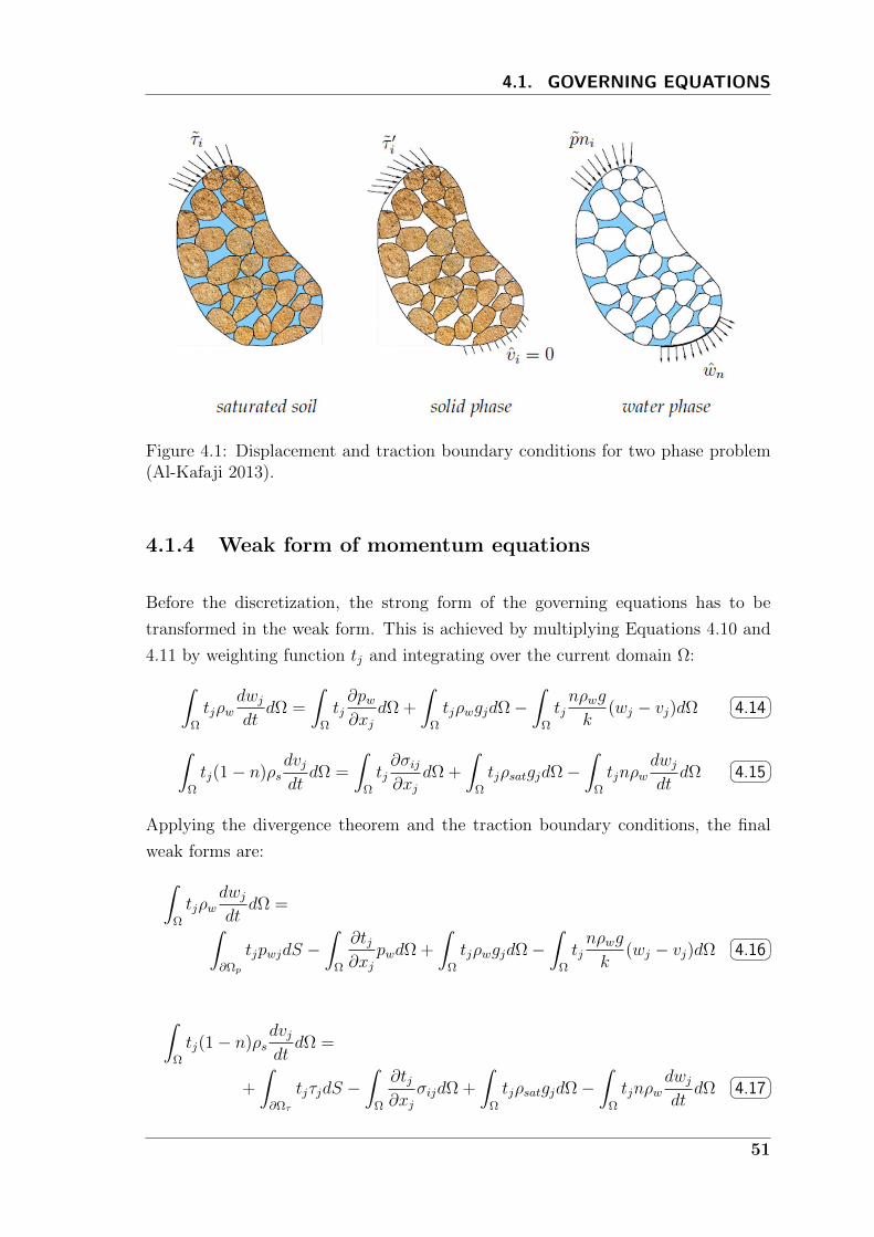
4.1. GOVERNING EQUATIONS
Figure 4.1: Displacement and traction boundary conditions for two phase problem(Al-Kafaji 2013).
4.1.4 Weak form of momentum equations
Before the discretization, the strong form of the governing equations has to be
transformed in the weak form. This is achieved by multiplying Equations 4.10 and
4.11 by weighting function tj and integrating over the current domain Ω:∫Ω
tjρwdwjdt
dΩ =
∫Ω
tj∂pw∂xj
dΩ +
∫Ω
tjρwgjdΩ−∫
Ω
tjnρwg
k(wj − vj)dΩ
4.14
∫Ω
tj(1− n)ρsdvjdtdΩ =
∫Ω
tj∂σij∂xj
dΩ +
∫Ω
tjρsatgjdΩ−∫
Ω
tjnρwdwjdt
dΩ 4.15
Applying the divergence theorem and the traction boundary conditions, the final
weak forms are:∫Ω
tjρwdwjdt
dΩ =∫∂Ωp
tjpwjdS −∫
Ω
∂tj∂xj
pwdΩ +
∫Ω
tjρwgjdΩ−∫
Ω
tjnρwg
k(wj − vj)dΩ
4.16
∫Ω
tj(1− n)ρsdvjdtdΩ =
+
∫∂Ωτ
tjτjdS −∫
Ω
∂tj∂xj
σijdΩ +
∫Ω
tjρsatgjdΩ−∫
Ω
tjnρwdwjdt
dΩ 4.17
51
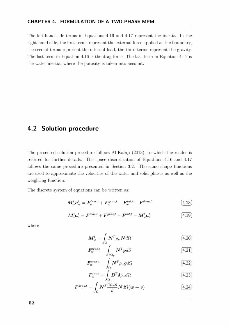
CHAPTER 4. FORMULATION OF A TWO-PHASE MPM
The left-hand side terms in Equations 4.16 and 4.17 represent the inertia. In the
right-hand side, the first terms represent the external force applied at the boundary,
the second terms represent the internal load, the third terms represent the gravity.
The last term in Equation 4.16 is the drag force. The last term in Equation 4.17 is
the water inertia, where the porosity is taken into account.
4.2 Solution procedure
The presented solution procedure follows Al-Kafaji (2013), to which the reader is
referred for further details. The space discretization of Equations 4.16 and 4.17
follows the same procedure presented in Section 3.2. The same shape functions
are used to approximate the velocities of the water and solid phases as well as the
weighting function.
The discrete system of equations can be written as:
M twa
tw = F trac,t
w + F grav,tw − F int,t
w − F drag,t 4.18
M tsa
ts = F trac,t + F grav,t − F int,t − M t
watw
4.19
where
M tw =
∫Ω
NTρwNdΩ 4.20
F trac,tw =
∫∂Ωp
NTpdS 4.21
F grav,tw =
∫Ω
NTρwgdΩ 4.22
F int,tw =
∫Ω
BTδpwdΩ 4.23
F drag,t =
∫Ω
NT nρwg
kNdΩ(w− v)
4.24
52

4.2. SOLUTION PROCEDURE
in which δ =[1 1 1 0 0 0
], and
M ts =
∫Ω
NT (1− n)ρsNdΩ 4.25
M tw =
∫Ω
NTnρwNdΩ 4.26
F trac,t =
∫∂Ωτ
NTτdS 4.27
F grav,t =
∫Ω
NTρsatgdΩ 4.28
F int,t =
∫Ω
BTσdΩ 4.29
Note that in Equations 4.18 and 4.19 the subscript w and s denote that the quantity
is referred to the fluid and water phase respectively; no subscript indicates that the
quantity belongs to the mixture.
The Euler-Cromer scheme is used to integrate the equations in time. From Equa-
tion 4.18 the fluid acceleration at time t is calculated and used to update the fluid
velocity wt+∆t. The solid acceleration is calculated solving Equation 4.19 and used
to update the solid velocity vt+∆t. Incremental strains are calculated at the MP from
the updated velocities, after that the constitutive relations are used to calculate the
stresses and pore water pressure.
In the implementation used for this thesis only one set of MP, representing the solid
phase is considered. This means that the MP store all the informations regarding
the soild and the liquid phase, and their positions are updated according to the solid
displacement. The implementation of two layers of MP, one representing the solid
phase and one representing the fluid phase is an issue of the on-going research and
future development of MPM.
The initialization of MP explained in Section 3.4.1 is easily extended to the two-
phase problem, then no more details are given in this Section.
The solution sequence of a single time step is described in the following:
1. The momentum equations for the fluid and the mixture are initialized by
mapping the significative quantities from the MP to the mesh nodes. The
procedure is similar to step 1 of the algorithm presented in Section 3.4.
2. Equation 4.18 is solved for atw
atw = M t,−1w
[F trac,tw + F grav,t
w − F int,tw − F drag,t
] 4.30
53
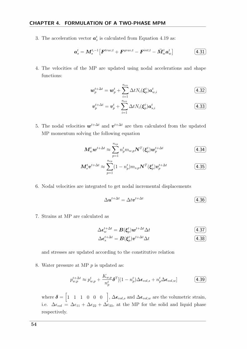
CHAPTER 4. FORMULATION OF A TWO-PHASE MPM
3. The acceleration vector ats is calculated from Equation 4.19 as:
ats = M t,−1s
[F trac,t + F grav,t − F int,t − M t
watw
] 4.31
4. The velocities of the MP are updated using nodal accelerations and shape
functions:
wt+∆tp = wt
p +nen∑i=1
∆tNi(ξtp)a
tw,i
4.32
vt+∆tp = vtp +
nen∑i=1
∆tNi(ξtp)a
ts,i
4.33
5. The nodal velocities wt+∆t and vt+∆t are then calculated from the updated
MP momentum solving the following equation
M tww
t+∆t ≈nep∑p=1
ntpmw,pNT (ξtp)w
t+∆tp
4.34
M tsv
t+∆t ≈nep∑p=1
(1− ntp)ms,pNT (ξtp)v
t+∆tp
4.35
6. Nodal velocities are integrated to get nodal incremental displacements
∆ut+∆t = ∆tvt+∆t 4.36
7. Strains at MP are calculated as
∆εt+∆tw = B(ξtp)w
t+∆t∆t 4.37
∆εt+∆ts = B(ξtp)v
t+∆t∆t 4.38
and stresses are updated according to the constitutive relation
8. Water pressure at MP p is updated as:
pt+∆tw,p ≈ ptw,p +
Kw,p
ntpδT [(1− ntp)∆εvol,s + ntp∆εvol,w]
4.39
where δ =[1 1 1 0 0 0
], ∆εvol,s and ∆εvol,w are the volumetric strain,
i.e. ∆εvol = ∆ε11 + ∆ε22 + ∆ε33, at the MP for the solid and liquid phase
respectively.
54
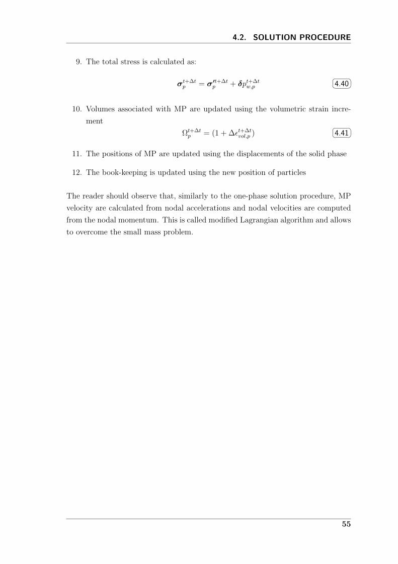
4.2. SOLUTION PROCEDURE
9. The total stress is calculated as:
σt+∆tp = σ′t+∆t
p + δpt+∆tw,p
4.40
10. Volumes associated with MP are updated using the volumetric strain incre-
ment
Ωt+∆tp = (1 + ∆εt+∆t
vol,p ) 4.41
11. The positions of MP are updated using the displacements of the solid phase
12. The book-keeping is updated using the new position of particles
The reader should observe that, similarly to the one-phase solution procedure, MP
velocity are calculated from nodal accelerations and nodal velocities are computed
from the nodal momentum. This is called modified Lagrangian algorithm and allows
to overcome the small mass problem.
55


5Constitutive modeling
The analysis of any problem requires noncontroversial statements of equilibrium and
kinematics or compatibility (the definition of strain) as shown in the previous chap-
ters; the link between these is provided by the relationship between stress change
and strain change: the constitutive response.
Geotechnical journals and conferences abound with constitutive models. However,
the scope of the current chapter is to provide only a brief introduction on the most
popular constitutive equations used in geoengineering. Attention will be focused on
those models used in this thesis. The convention commonly adopted in geomechan-
ics, i.e. compression is positive, is adopted in this chapter.
The choice of the constitutive model to be used for analysis is in the hands of the
modeler. As suggested by Wood (2003), the modeler should develop some awareness
of the particular features of soil history and soil response that are likely to be
important in a particular application and ensure that the adopted constitutive model
is indeed able to reproduce these features. As in all modeling, adequate complexity
should be sought.
5.1 Elastic models
A truly elastic model or hyper-elastic, is defined as a model that does not generate or
dissipate energy in closed load loops. Despite soil exhibits inelastic behavior during
loading, geotechnical engineer have made a good use of the theory of elasticity for
several decades. Elastic descriptions of soil behavior are useful for the wide range
of quick analytical solutions to which they give access. If we need some idea about
the stress distribution around a footing, wall or pile then at least a first estimate
57
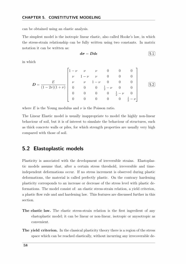
CHAPTER 5. CONSTITUTIVE MODELING
can be obtained using an elastic analysis.
The simplest model is the isotropic linear elastic, also called Hooke’s law, in which
the stress-strain relationship can be fully written using two constants. In matrix
notation it can be written as:
dσ = Ddε 5.1
in which
D =E
(1− 2ν)(1 + ν)
1− ν ν ν 0 0 0
ν 1− ν ν 0 0 0
ν ν 1− ν 0 0 0
0 0 0 12− ν 0 0
0 0 0 0 12− ν 0
0 0 0 0 0 12− ν
5.2
where E is the Young modulus and ν is the Poisson ratio.
The Linear Elastic model is usually inappropriate to model the highly non-linear
behaviour of soil, but it is of interest to simulate the behaviour of structures, such
as thick concrete walls or piles, for which strength properties are usually very high
compared with those of soil.
5.2 Elastoplastic models
Plasticity is associated with the development of irreversible strains. Elastoplas-
tic models assume that, after a certain stress threshold, irreversible and time-
independent deformations occur. If no stress increment is observed during plastic
deformations, the material is called perfectly plastic. On the contrary hardening
plasticity corresponds to an increase or decrease of the stress level with plastic de-
formations. The model consist of: an elastic stress-strain relation, a yield criterion,
a plastic flow rule and and hardening law. This features are discussed further in this
section.
The elastic law. The elastic stress-strain relation is the first ingredient of any
elastoplastic model; it can be linear or non-linear, isotropic or anysotropic as
convenient.
The yield criterion. In the classical plasticity theory there is a region of the stress
space which can be reached elastically, without incurring any irrecoverable de-
58
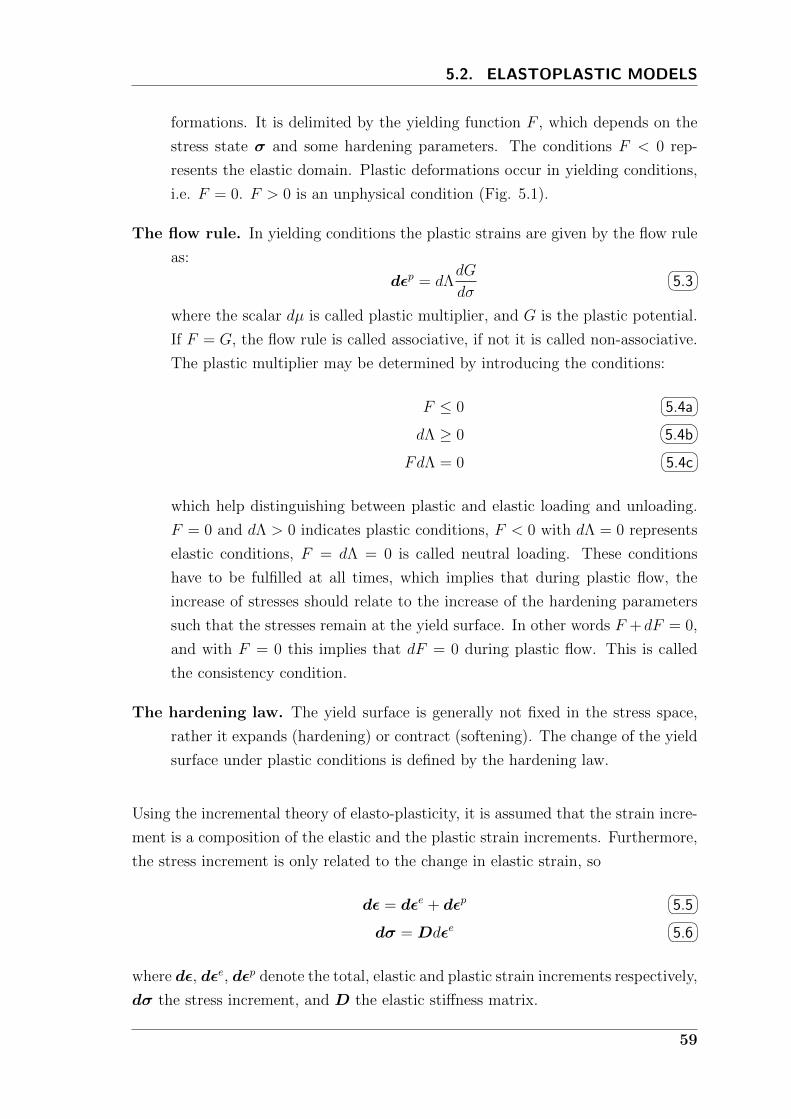
5.2. ELASTOPLASTIC MODELS
formations. It is delimited by the yielding function F , which depends on the
stress state σ and some hardening parameters. The conditions F < 0 rep-
resents the elastic domain. Plastic deformations occur in yielding conditions,
i.e. F = 0. F > 0 is an unphysical condition (Fig. 5.1).
The flow rule. In yielding conditions the plastic strains are given by the flow rule
as:
dεp = dΛdG
dσ
5.3
where the scalar dµ is called plastic multiplier, and G is the plastic potential.
If F = G, the flow rule is called associative, if not it is called non-associative.
The plastic multiplier may be determined by introducing the conditions:
F ≤ 0 5.4a
dΛ ≥ 0 5.4b
FdΛ = 0 5.4c
which help distinguishing between plastic and elastic loading and unloading.
F = 0 and dΛ > 0 indicates plastic conditions, F < 0 with dΛ = 0 represents
elastic conditions, F = dΛ = 0 is called neutral loading. These conditions
have to be fulfilled at all times, which implies that during plastic flow, the
increase of stresses should relate to the increase of the hardening parameters
such that the stresses remain at the yield surface. In other words F + dF = 0,
and with F = 0 this implies that dF = 0 during plastic flow. This is called
the consistency condition.
The hardening law. The yield surface is generally not fixed in the stress space,
rather it expands (hardening) or contract (softening). The change of the yield
surface under plastic conditions is defined by the hardening law.
Using the incremental theory of elasto-plasticity, it is assumed that the strain incre-
ment is a composition of the elastic and the plastic strain increments. Furthermore,
the stress increment is only related to the change in elastic strain, so
dε = dεe + dεp 5.5
dσ = Ddεe 5.6
where dε, dεe, dεp denote the total, elastic and plastic strain increments respectively,
dσ the stress increment, and D the elastic stiffness matrix.
59

CHAPTER 5. CONSTITUTIVE MODELING
Figure 5.1: Yielding function
A large number of elastoplastic models has been proposed to describe the behavior
of geomaterials; no attemps is made here to cover all these models; this section
focuses only on a few of them that are used in this thesis. For further details the
reader can refer to Yu (2007), Davis and Selvadurai (2002) and Wood (2003).
5.2.1 The Tresca failure criteria
For cohesive soils the most used elastoplastic models are those developed by Tresca
and von Mises initially for metals. After a series of tests on metal, Tresca (1884)
concluded that yielding occurs when the shear stress reaches a certain limit value
(τmax):
F1 = 1/2|σ2 − σ3| − τmax 5.7a
F2 = 1/2|σ1 − σ3| − τmax 5.7b
F3 = 1/2|σ1 − σ2| − τmax 5.7c
For cohesive soil in undrained conditions τmax = su, where su is the undrained shear
strength. Equations 5.7 represent an exhagonal prism in the stress space (Fig. 5.2).
Soil exhibits different su for triaxial extension, triaxial compression and simple shear.
However, the model does not incorporate the dependency of soil strength on the
stress path. For numerous geotechnical problems a unique loading type cannot be
specified, therefore a proper average value of the shear strength must be used.
60
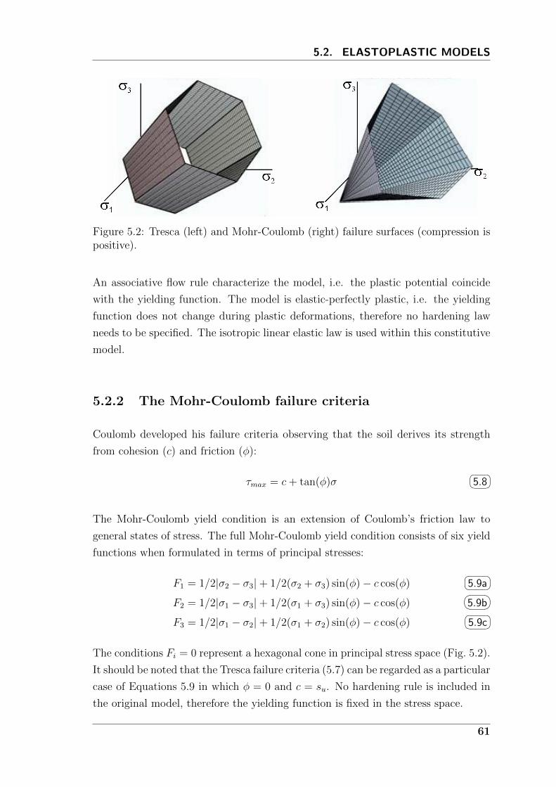
5.2. ELASTOPLASTIC MODELS
Figure 5.2: Tresca (left) and Mohr-Coulomb (right) failure surfaces (compression ispositive).
An associative flow rule characterize the model, i.e. the plastic potential coincide
with the yielding function. The model is elastic-perfectly plastic, i.e. the yielding
function does not change during plastic deformations, therefore no hardening law
needs to be specified. The isotropic linear elastic law is used within this constitutive
model.
5.2.2 The Mohr-Coulomb failure criteria
Coulomb developed his failure criteria observing that the soil derives its strength
from cohesion (c) and friction (φ):
τmax = c+ tan(φ)σ 5.8
The Mohr-Coulomb yield condition is an extension of Coulomb’s friction law to
general states of stress. The full Mohr-Coulomb yield condition consists of six yield
functions when formulated in terms of principal stresses:
F1 = 1/2|σ2 − σ3|+ 1/2(σ2 + σ3) sin(φ)− c cos(φ) 5.9a
F2 = 1/2|σ1 − σ3|+ 1/2(σ1 + σ3) sin(φ)− c cos(φ) 5.9b
F3 = 1/2|σ1 − σ2|+ 1/2(σ1 + σ2) sin(φ)− c cos(φ) 5.9c
The conditions Fi = 0 represent a hexagonal cone in principal stress space (Fig. 5.2).
It should be noted that the Tresca failure criteria (5.7) can be regarded as a particular
case of Equations 5.9 in which φ = 0 and c = su. No hardening rule is included in
the original model, therefore the yielding function is fixed in the stress space.
61
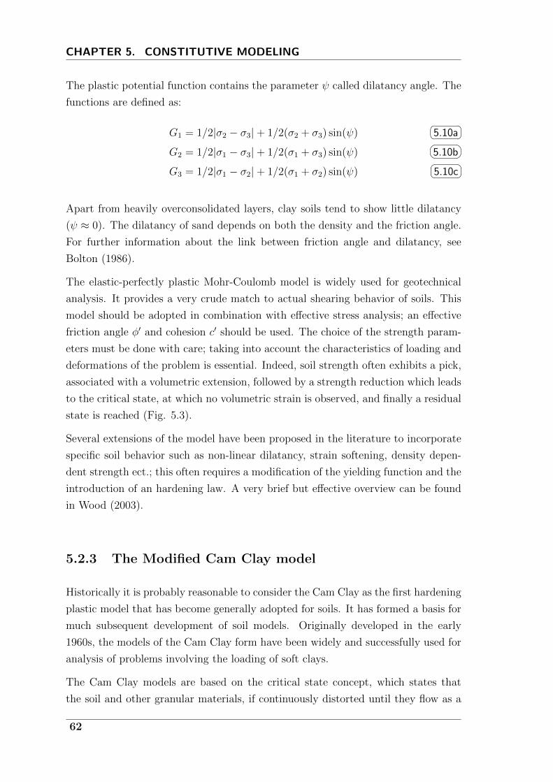
CHAPTER 5. CONSTITUTIVE MODELING
The plastic potential function contains the parameter ψ called dilatancy angle. The
functions are defined as:
G1 = 1/2|σ2 − σ3|+ 1/2(σ2 + σ3) sin(ψ) 5.10a
G2 = 1/2|σ1 − σ3|+ 1/2(σ1 + σ3) sin(ψ) 5.10b
G3 = 1/2|σ1 − σ2|+ 1/2(σ1 + σ2) sin(ψ) 5.10c
Apart from heavily overconsolidated layers, clay soils tend to show little dilatancy
(ψ ≈ 0). The dilatancy of sand depends on both the density and the friction angle.
For further information about the link between friction angle and dilatancy, see
Bolton (1986).
The elastic-perfectly plastic Mohr-Coulomb model is widely used for geotechnical
analysis. It provides a very crude match to actual shearing behavior of soils. This
model should be adopted in combination with effective stress analysis; an effective
friction angle φ′ and cohesion c′ should be used. The choice of the strength param-
eters must be done with care; taking into account the characteristics of loading and
deformations of the problem is essential. Indeed, soil strength often exhibits a pick,
associated with a volumetric extension, followed by a strength reduction which leads
to the critical state, at which no volumetric strain is observed, and finally a residual
state is reached (Fig. 5.3).
Several extensions of the model have been proposed in the literature to incorporate
specific soil behavior such as non-linear dilatancy, strain softening, density depen-
dent strength ect.; this often requires a modification of the yielding function and the
introduction of an hardening law. A very brief but effective overview can be found
in Wood (2003).
5.2.3 The Modified Cam Clay model
Historically it is probably reasonable to consider the Cam Clay as the first hardening
plastic model that has become generally adopted for soils. It has formed a basis for
much subsequent development of soil models. Originally developed in the early
1960s, the models of the Cam Clay form have been widely and successfully used for
analysis of problems involving the loading of soft clays.
The Cam Clay models are based on the critical state concept, which states that
the soil and other granular materials, if continuously distorted until they flow as a
62
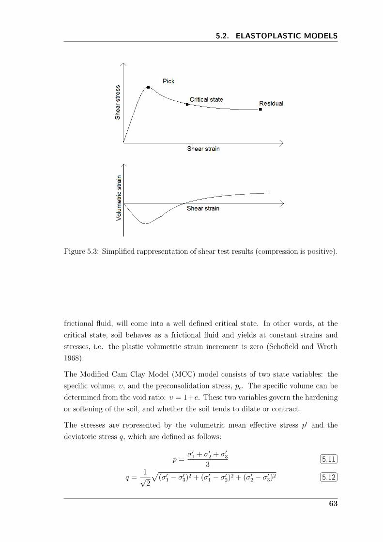
5.2. ELASTOPLASTIC MODELS
Figure 5.3: Simplified rappresentation of shear test results (compression is positive).
frictional fluid, will come into a well defined critical state. In other words, at the
critical state, soil behaves as a frictional fluid and yields at constant strains and
stresses, i.e. the plastic volumetric strain increment is zero (Schofield and Wroth
1968).
The Modified Cam Clay Model (MCC) model consists of two state variables: the
specific volume, υ, and the preconsolidation stress, pc. The specific volume can be
determined from the void ratio: υ = 1+e. These two variables govern the hardening
or softening of the soil, and whether the soil tends to dilate or contract.
The stresses are represented by the volumetric mean effective stress p′ and the
deviatoric stress q, which are defined as follows:
p =σ′1 + σ′2 + σ′3
3
5.11
q =1√2
√(σ′1 − σ′3)2 + (σ′1 − σ′2)2 + (σ′2 − σ′3)2
5.12
63
CHAPTER 5. CONSTITUTIVE MODELING
The volumetric strain and the deviatoric strain are defined as:
εp = ε1 + ε2 + ε3 5.13
εq =
√2
3
√(ε1 − ε3)2 + (ε1 − ε2)2 + (ε2 − ε3)2
5.14
The model assumes that when a soft soil sample is slowly compressed under isotropic
stress and perfectly drained conditions, the relationship between specific volume
and mean effective stress is logaritmic. The first time the soil is loaded with a load
greater than the previous experienced loading, pc, the behaviour follows the isotropic
or virgin compression line (NCL). If the soil afterwards is unloaded, it will follow an
unloading-reloading line (URL). All deformations along the URL are reversible, i.e.
elastic deformations.
The equations of the compression lines can be written as
υ = N − λ ln(p′) 5.15
υ = υs − κ ln(p′) 5.16
where υs and N represents the specific volume at unit stress, and λ and κ the slopes
of the NCL and the URL respectively. The NCL is uniquely defined for a certain
soil, while multiple URL exist depending on the state parameters. An increase in
pc corresponds to a shift from one URL to another.
Sustained shearing of a soil sample eventually leads to a state in which further shear-
ing can occur without any changes in stress or volume. This state is characterized
by the Critical State Line (CSL) which is unique for a given soil, regardless of the
stress path used to bring the sample from any initial condition to the critical state.
The CSL is determined by two equations:
υ = Γ− λ ln(p′) 5.17a
q = Mp′ 5.17b
where Γ is a basic soil parameter representing the specific volume at unit stress,
and M determines the soil strength. The latter can be related to the soil’s critical
friction angle φ′; for triaxial compression it is estimated as:
M =6 sin(φ′)
3− sin(φ′)
5.18
64
5.2. ELASTOPLASTIC MODELS
A detailed description of the main features of the model is provided in the following:
Elastic properties. A change in p′ and q is related to the elastic strain components
by: [dεep
dεep
]=
[1/K ′ 0
0 1/3G
][dp′
dq
] 5.19
where K ′ and G are the effective bulk molulus and the shear modulus of the
soil, which can be defined as:
K ′ =υp′
κ
5.20a
G =3K(1− 2ν)
(2 + 2ν)=
3υp′(1− 2ν)
κ(2 + 2ν)
5.20b
It is worth noting that the moduli are nonlinear as they are function of both
the stress state and the specific volume.
The yield surface. The original Cam clay model proposed a logarithmic yield
surface, but this poses some difficulties in constitutive soil modelling as the
function is not differentiable at all points. The yield surface of the MCC,
however, is an ellipse in the p-q-space, with a center in (pc/2, 0), shown in
Figure 5.4 for q > 0. The equation for the elliptic yield surface is
F = q2 −M2p′(pc − p′) = 0 5.21
The hardening function. The hardening function defines how the yield surface
expands (hardening) or contracts (softening). For MCC we experience soft-
ening behaviour for largely over-consolidated soils, and hardening otherwise.
Cam clay is a volumetric hardening model in which it is assumed that the size
of the yield locus depends only on the plastic volumetric strain. The change
in the hardening parameter pc is derived from the relation between the plastic
volumetric strain dεpp and the plastic change in specific volume dυp, written as
dεpp = −dυpυ
=λ− κυ
dpcpc
5.22
Note the negative sign of dυp which stems from the sign convention normally
used in geotechnical engineering, with compression being positive.
Integrating over a finite interval and solving for ∆pc, the hardening function
65
CHAPTER 5. CONSTITUTIVE MODELING
is written as
∆pc = pc exp[ζ∆εpp] 5.23
where ζ = υ/(λ− κ).
The flow rule. In MCC, the flow rule is associative, i.e G = F . For the stress and
strain invariants, the flow rule is written as[dεep
dεeq
]= dΛ
[dFdp′
dFdq
]= dΛ
[M2(2p′ − pc)
2q
] 5.24
where dΛ is the plastic multiplier which can be found by applying the consis-
tency condition dF = 0, giving
dΛ =
[dFdp′
dFdq
]D
[dεp
dεq
][dFdp′
dFdq
]D[dFdp′
dFdq
]− A
5.25
where A is the plastic resistance modulus defined as
A =∂F
∂pc
∂pc∂εpp
∂εppdΛ
= M2p′ζpcM2(2p′ − pc)
5.26
In summary the Cam clay model has five material properties. There are two elastic
properties κ and G (or ν), two plastic properties M and λ and a reference for volume,
in order to calculate the volumetric strains, which can be the initial void ratio e0.
Figure 5.4 shows the CLS, NCL and URL in the e − ln(p′) plane and the yelding
surface and CSL in the p− q plane. On the right plot, a typical stress path during
undrained triaxial compression of a normal consolidated clay is shown.
The MCC model incorporates many fundamental characteristic of soil behavior such
as non linear compressibility, hardening behavior, occurrence of shear and volumetric
deformations during yielding and fluid-like plastic flow at large deformations. The
real behavior of natural soils is more complicated because factors such as anisotropy
and strain-rate effects play an important role. Indeed, during deposition, clay is
generally compacted vertically under its self-weight, which leads to the arrange-
ment of clay particles in layers rather than a random configuration. Any subsequent
loading, which induces plastic straining, will cause changes of the internal struc-
ture of the clay and, therefore, the initial anisotropy is modified (stress-induced
anisotropy). Moreover, straining can progressively destroy boning between particles
(destructuration) (Burland 1990). In case of cyclic loading things becomes even more
66
5.2. ELASTOPLASTIC MODELS
complicated because aspects such as densification and pressure generation must be
correctly captured.
In the 80s many extensions of the Cam Clay model have been proposed; a brief
review of the most important modifications can be found in Gens and Potts (1988).
Examples of these modifications includes research on the following topics:
• yield surface for heavily overconsolidated clays (e.g. Zienkiewicz and Naylor
1973, Atkinson and Bransby 1978)
• anisotropic yield surfaces for one-dimensionally consolidated soils (e.g. Ohta
and Wroth 1976, Whittle 1993)
• inclusion of plastic deformation within the main yield surface for soils subjected
to cyclic loading (e.g. Dafalias and Herrmann 1980, Carter et al. 1982)
• 3D critical state formulation (e.g. Roscoe and Burland 1968, Zienkiewicz and
Pande 1977)
• modelling of rate-dependent behaviour of clays (e.g. Borjia and Kavazanjian
1985, Kutter and Sathialingam 1992)
In addition to this several more advanced constitutive models, which eventually
deviates from the critical state theory have been proposed (e.g. Pastor et al. 1990,
Modaressi and Laloui 1997, Masin 2005); however the discussion of this subject
exceeds the purpose of the current chapter.
The MCC model has been used in the literature mainly to model soft clay and silt.
It seems not appropriate for stiff clay and sands. Determining its input parameters
is relatively easy, while difficulties often arise with more sophisticated models which
may require considerable non-standard testing.
The numerical implementation of the MCC model, recently introduced in the MPM
code in the frame of this thesis, uses an explicit integration scheme known as
Dorman-Prince method. This method is considered one of the most accurate; more-
over a substepping algorithm and a correction method has been included by Aas
Nost (2011) in the implementation adopted in this study.
67
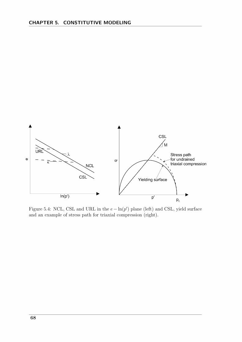
CHAPTER 5. CONSTITUTIVE MODELING
Figure 5.4: NCL, CSL and URL in the e− ln(p′) plane (left) and CSL, yield surfaceand an example of stress path for triaxial compression (right).
68
6Other numerical aspects
The current chapter collects some special techniques adopted in the used MPM
implementation to deal with particular problems:
Enhanced volumetric strain Since low-order finite elements are used within the
MPM, problems of volumetric locking rise when incompressible materials are
considered. Section 6.1 presents a possible solution to this shortcoming.
Dissipation of dynamic waves Numerical simulations with dynamic code may
need the introduction of special procedures to dissipate dynamic waves un-
physically generated, for example, by reflection at boundaries. Absorbing
boundary and local damping can be introduced to achieve this scope as shown
in section 6.2.
Mass scaling Since in explicit code the time step size can be very small and sim-
ulating long-time processes may be computationally expensive, a procedure
called mass scaling, can be used to improve computational efficiency in quasi-
static problems; it is presented in section 6.3.
Contact between bodies Contact problems are very common in engineering. The
problem is discussed in section 6.4.1, where the implemented contact algorithm
is presented and validated.
The moving mesh procedure Because of MP moving through the mesh, the ap-
plication of non-zero traction or kinematics can rise some difficulties. A pos-
sible solution is presented in section 6.5.
Attention will be paid to both one and two-phase formulations.
69
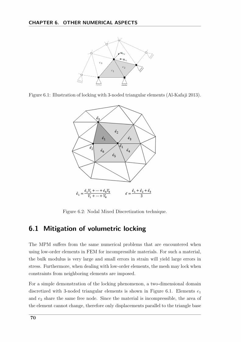
CHAPTER 6. OTHER NUMERICAL ASPECTS
Figure 6.1: Illustration of locking with 3-noded triangular elements (Al-Kafaji 2013).
Figure 6.2: Nodal Mixed Discretization technique.
6.1 Mitigation of volumetric locking
The MPM suffers from the same numerical problems that are encountered when
using low-order elements in FEM for incompressible materials. For such a material,
the bulk modulus is very large and small errors in strain will yield large errors in
stress. Furthermore, when dealing with low-order elements, the mesh may lock when
constraints from neighboring elements are imposed.
For a simple demonstration of the locking phenomenon, a two-dimensional domain
discretized with 3-noded triangular elements is shown in Figure 6.1. Elements e1
and e2 share the same free node. Since the material is incompressible, the area of
the element cannot change, therefore only displacements parallel to the triangle base
70
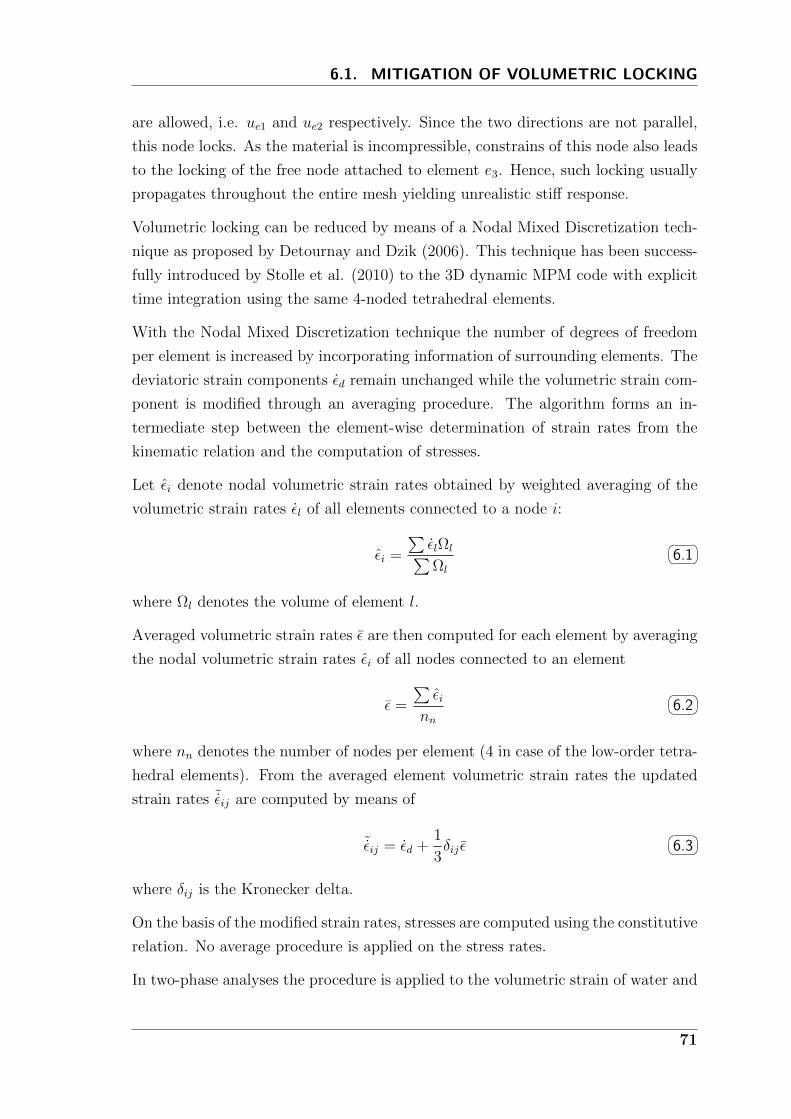
6.1. MITIGATION OF VOLUMETRIC LOCKING
are allowed, i.e. ue1 and ue2 respectively. Since the two directions are not parallel,
this node locks. As the material is incompressible, constrains of this node also leads
to the locking of the free node attached to element e3. Hence, such locking usually
propagates throughout the entire mesh yielding unrealistic stiff response.
Volumetric locking can be reduced by means of a Nodal Mixed Discretization tech-
nique as proposed by Detournay and Dzik (2006). This technique has been success-
fully introduced by Stolle et al. (2010) to the 3D dynamic MPM code with explicit
time integration using the same 4-noded tetrahedral elements.
With the Nodal Mixed Discretization technique the number of degrees of freedom
per element is increased by incorporating information of surrounding elements. The
deviatoric strain components εd remain unchanged while the volumetric strain com-
ponent is modified through an averaging procedure. The algorithm forms an in-
termediate step between the element-wise determination of strain rates from the
kinematic relation and the computation of stresses.
Let εi denote nodal volumetric strain rates obtained by weighted averaging of the
volumetric strain rates εl of all elements connected to a node i:
εi =
∑εlΩl∑Ωl
6.1
where Ωl denotes the volume of element l.
Averaged volumetric strain rates ε are then computed for each element by averaging
the nodal volumetric strain rates εi of all nodes connected to an element
ε =
∑εi
nn
6.2
where nn denotes the number of nodes per element (4 in case of the low-order tetra-
hedral elements). From the averaged element volumetric strain rates the updated
strain rates ˜εij are computed by means of
˜εij = εd +1
3δij ε
6.3
where δij is the Kronecker delta.
On the basis of the modified strain rates, stresses are computed using the constitutive
relation. No average procedure is applied on the stress rates.
In two-phase analyses the procedure is applied to the volumetric strain of water and
71
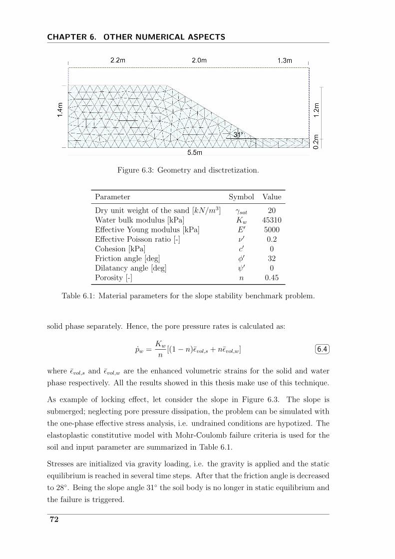
CHAPTER 6. OTHER NUMERICAL ASPECTS
Figure 6.3: Geometry and disctretization.
Parameter Symbol Value
Dry unit weight of the sand [kN/m3] γsat 20Water bulk modulus [kPa] Kw 45310Effective Young modulus [kPa] E ′ 5000Effective Poisson ratio [-] ν ′ 0.2Cohesion [kPa] c′ 0Friction angle [deg] φ′ 32Dilatancy angle [deg] ψ′ 0Porosity [-] n 0.45
Table 6.1: Material parameters for the slope stability benchmark problem.
solid phase separately. Hence, the pore pressure rates is calculated as:
pw =Kw
n[(1− n)εvol,s + nεvol,w]
6.4
where εvol,s and εvol,w are the enhanced volumetric strains for the solid and water
phase respectively. All the results showed in this thesis make use of this technique.
As example of locking effect, let consider the slope in Figure 6.3. The slope is
submerged; neglecting pore pressure dissipation, the problem can be simulated with
the one-phase effective stress analysis, i.e. undrained conditions are hypotized. The
elastoplastic constitutive model with Mohr-Coulomb failure criteria is used for the
soil and input parameter are summarized in Table 6.1.
Stresses are initialized via gravity loading, i.e. the gravity is applied and the static
equilibrium is reached in several time steps. After that the friction angle is decreased
to 28. Being the slope angle 31 the soil body is no longer in static equilibrium and
the failure is triggered.
72
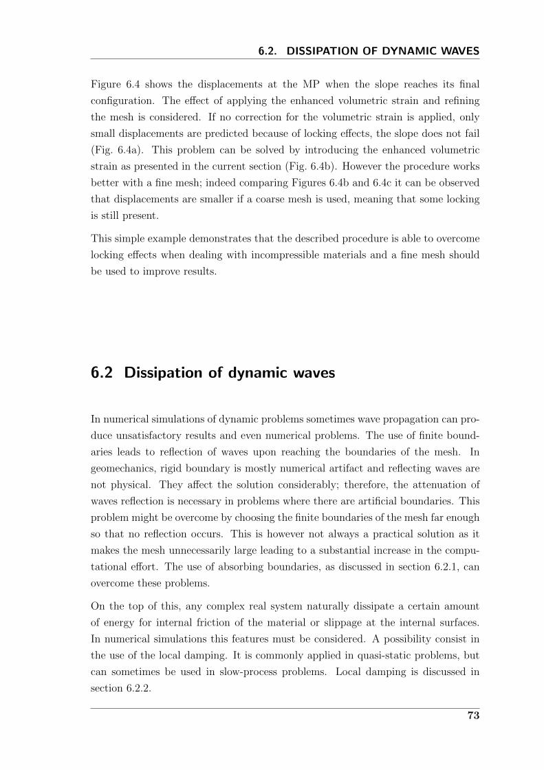
6.2. DISSIPATION OF DYNAMIC WAVES
Figure 6.4 shows the displacements at the MP when the slope reaches its final
configuration. The effect of applying the enhanced volumetric strain and refining
the mesh is considered. If no correction for the volumetric strain is applied, only
small displacements are predicted because of locking effects, the slope does not fail
(Fig. 6.4a). This problem can be solved by introducing the enhanced volumetric
strain as presented in the current section (Fig. 6.4b). However the procedure works
better with a fine mesh; indeed comparing Figures 6.4b and 6.4c it can be observed
that displacements are smaller if a coarse mesh is used, meaning that some locking
is still present.
This simple example demonstrates that the described procedure is able to overcome
locking effects when dealing with incompressible materials and a fine mesh should
be used to improve results.
6.2 Dissipation of dynamic waves
In numerical simulations of dynamic problems sometimes wave propagation can pro-
duce unsatisfactory results and even numerical problems. The use of finite bound-
aries leads to reflection of waves upon reaching the boundaries of the mesh. In
geomechanics, rigid boundary is mostly numerical artifact and reflecting waves are
not physical. They affect the solution considerably; therefore, the attenuation of
waves reflection is necessary in problems where there are artificial boundaries. This
problem might be overcome by choosing the finite boundaries of the mesh far enough
so that no reflection occurs. This is however not always a practical solution as it
makes the mesh unnecessarily large leading to a substantial increase in the compu-
tational effort. The use of absorbing boundaries, as discussed in section 6.2.1, can
overcome these problems.
On the top of this, any complex real system naturally dissipate a certain amount
of energy for internal friction of the material or slippage at the internal surfaces.
In numerical simulations this features must be considered. A possibility consist in
the use of the local damping. It is commonly applied in quasi-static problems, but
can sometimes be used in slow-process problems. Local damping is discussed in
section 6.2.2.
73
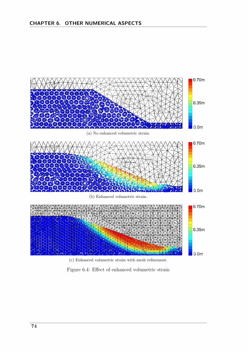
CHAPTER 6. OTHER NUMERICAL ASPECTS
(a) No enhanced volumetric strain.
(b) Enhanced volumetric strain.
(c) Enhanced volumetric strain with mesh refinement.
Figure 6.4: Effect of enhanced volumetric strain
74
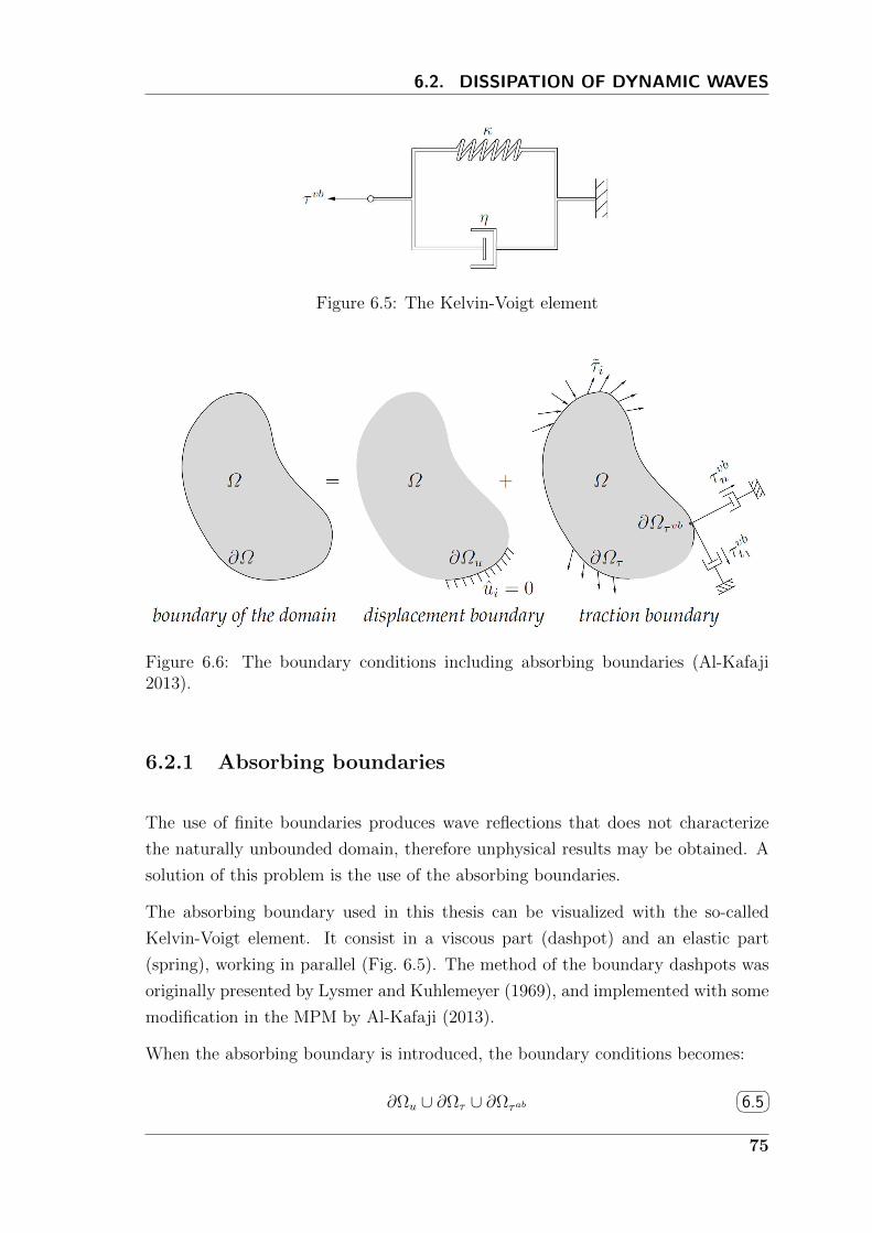
6.2. DISSIPATION OF DYNAMIC WAVES
Figure 6.5: The Kelvin-Voigt element
Figure 6.6: The boundary conditions including absorbing boundaries (Al-Kafaji2013).
6.2.1 Absorbing boundaries
The use of finite boundaries produces wave reflections that does not characterize
the naturally unbounded domain, therefore unphysical results may be obtained. A
solution of this problem is the use of the absorbing boundaries.
The absorbing boundary used in this thesis can be visualized with the so-called
Kelvin-Voigt element. It consist in a viscous part (dashpot) and an elastic part
(spring), working in parallel (Fig. 6.5). The method of the boundary dashpots was
originally presented by Lysmer and Kuhlemeyer (1969), and implemented with some
modification in the MPM by Al-Kafaji (2013).
When the absorbing boundary is introduced, the boundary conditions becomes:
∂Ωu ∪ ∂Ωτ ∪ ∂Ωτab
6.5
75

CHAPTER 6. OTHER NUMERICAL ASPECTS
and
∂Ωi ∩ ∂Ωj = ∅ i, j = u, τ, τab 6.6
being ∂Ωτab the boundary where the Kelvin-Voigt element is applied (Fig. 6.6).
The traction vector corresponding to the absorbing boundary has, in general, three
components, i.e.
τ ab =[τabn τabt1 τabt2
]in which the first is the component normal to the boundary and the other two are
the tangential components.
The response of the Kelvin-Voigt element is described by the following equations:
τabn = −aρcpvn − kpun 6.7a
τabt1 = −bρcsvt1 − ksut1 6.7b
τabt2 = −bρcsvt2 − ksut2 6.7c
where a and b are dimensionless parameters, vn, vt1 and vt2 are the velocities, un,
ut1 and ut2 are the displacements, ρ is the mass density, cp and cs are the speeds of
the compression and shear waves respectively, kp and ks represent the stiffness per
unit area associated to the elastic component.
The wave speeds are functions of the constrained and shear elastic moduli and the
mass density as follows:
cp =
√Ecρ
6.8
cs =
√G
ρ
6.9
Equations 6.7a-6.7c can be expressed in a compact form as:
τabi = −ηijvj − kiui 6.10
The first addend in the right-hand-side of Equation 6.10 represents the traction given
by the dashpot, which is proportional to the velocity. The second addend represents
the traction given by the spring, which is proportional to the displacement.
The virtual work equation (3.12) is rewritten introducing the traction corresponding
76

6.2. DISSIPATION OF DYNAMIC WAVES
to the absorbing boundary:∫Ω
tiρdvidtdΩ =
∫∂Ωτ
tiτidS +
∫∂Ωabτ
tiτabi dS +
∫Ω
tiρgidΩ−∫
Ω
∂ti∂xi
σijdΩ 6.11
introducing Equation 6.10 it yelds to:∫Ω
tiρdvidtdΩ =∫
∂Ωτ
tiτidS −∫∂Ωabτ
tiηijvjdS −∫∂Ωabτ
tikiuidS +
∫Ω
tiρgidΩ−∫
Ω
∂ti∂xi
σijdΩ 6.12
The matrix form of the discretized equation of motion, including the force at the
absorbing boundary, is:
Ma = F trac − F ab + F grav − F int 6.13
in which
F ab = Cv +Ku 6.14
where C is the matrix containing the dashpot coefficients ηij and is therefore called
dashpot matrix, and K is the matrix containing the spring coefficients ki and is
called spring matrix.
In this thesis the dashpot coefficients a and b are assumed equal to one. Lysmer
and Kuhlemeyer (1969) showed that this choice gives the maximum absorption for
both compression and shear wave for a wide range of the incidence angles.
The coefficients kp and ks can be expressed as function of the elastic moduli and a
so-called virtual thikness δ:
kp =Ecδ
6.15
ks =G
δ
6.16
The virtual thickness δ can be interpreted as the thickness of a virtual layer which
extends outside the boundary. Note that for δ → 0 the absorbing boundary reduces
to a rigid bounday; for δ → ∞ it reduces to a dashpot boundary. Spatially un-
bounded domain can therefore be represented with a finite mesh by the use of the
absorbing boundary defined in this section.
For the two-phase formulation, two-sets of Kelvin-Voigt elements need to be defined.
77

CHAPTER 6. OTHER NUMERICAL ASPECTS
For the solid part, the traction at the absorbing boundary represents the traction
applied on the soil skeleton and is therefore proportional to the solid velocity vs and
displacement us. Moreover the dry density ρdry and the effective constrained modu-
lus E ′c should be used to estimate dashpot and spring coefficients in Equation 6.10.
The response of the Kelvin-Voigt element for the water phase has only the normal
component and is given by:
pabw = −aρwcwwn − kwuw,n 6.17
where wn and uw,n are the normal component of water velocity and displacement
respectively. The speed of the compression wave in the water is
cw =
√Kw
ρw
6.18
Taking into account the absorbing boundary term, the momentum equation of the
fluid becomes:
Mwaw = F tracw − F ab
w + F gravw − F int
w − F drag 6.19
where
F abw = Cww +Kwuw
6.20
the momentum equation for the mixture, considering the boundary force, is:
Msas = F trac − F ab + F grav − F int − Mwaw 6.21
Where the absorbing boundary force applied on the mixture is:
F ab = F abw + F ab
s = Cww +Kwuw +Csv +Ksus 6.22
Cw and Kw are the dashpot matrix and the spring matrix for the water phase
respectively.
Since MP move through the mesh, the scheme must be implemented in an incre-
mental form so that displacement and velocity increments of a material point are
only accounted for when it enters the considered element. Hence,
F ab,t = F ab,t−∆t + ∆F vb,t 6.23
78
6.2. DISSIPATION OF DYNAMIC WAVES
where
∆F vb,t = Ct∆v +Kt∆u 6.24
This, of course, is valid for both one-phase and two-phase formulation.
Examples of the application of the viscous boundary can be found in sections 7.1
and 7.2. Appendix B provides some additional basic information on the oscillatory
system and damped vibrations.
6.2.2 Local damping
Natural dynamic systems contain some degree of damping of the vibration energy
within the system; otherwise, the system would oscillate indefinitely when subjected
to driving forces. Damping is due, in part, to energy loss as a result of internal
friction in the intact material and slippage along interfaces, if these are present.
For a dynamic analysis, the damping in the numerical simulation should reproduce
in magnitude and form the energy losses in the natural system when subjected to
a dynamic loading. In soil and rock, natural damping is mainly hysteretic, i.e.
independent of frequency, see Gemant and Jackson (1937) and Wegel and Walther
(1935). This type of damping is difficult to reproduce numerically. However, if a
constitutive model is found that contains an adequate representation of the hysteresis
that occurs in a real material, then no additional damping would be necessary
(Cundall 2001).
Rayleigh damping is commonly used to provide damping that is approximately
frequency-independent over a restricted range of frequencies. However, this kind
of damping introduces body forces that retard the steady state collapse and might
influence the mode of failure (Hart et al. 1988). Cundall (1987) describes a local
non-viscous damping to overcome the difficulty associated with the viscous damping.
An alternative to Rayleigh damping is the so-called local damping. The local damp-
ing force is proportional to the out of balance force f = f ext−f int and acts opposite
to the direction of the velocity. For any degree-of-freedom in the considered system,
the local damping can be described as follows
ma = f + fdamp 6.25
where
fdamp = −α|f | v|v|
6.26
79
CHAPTER 6. OTHER NUMERICAL ASPECTS
is the damping force at the considered degree of freedom. The dimensionless pa-
rameter α is called local damping factor.
In the two-phase formulation the fluid and the solid phase are damped separately.
At any degree of freedom the momentum equation for the water assumes the form:
mwaw = f tracw + f gravw − f intw − fdragw + fdampw
6.27
if fw = f tracw + f gravw − f intw is the unbalanced force for the water, the damping force
for the water can be written as:
fdampw = −αw|fw|w
|w| 6.28
The momentum equation for the mixture is:
msas = −mwaw + f trac + f grav − f int + fdamp 6.29
where
fdamp = fdamps + fdampw
6.30
The out of balance force for the solid phase is f = f trac + f grav − f int, hence the
damping force for the solid can be written as:
fdamps = −αs|f − fw|v
|v| 6.31
In this thesis the local damping factor for the fluid (αw) and the solid (αs) phase
always assume the same value.
Local damping was originally designed for static simulations. However, it has some
characteristics that make it attractive for dynamic simulations if proper values of the
damping coefficient are used. In quasi-static problems high value of α, i.e. 0.7-0.8,
can be used to accelerate convergence. In slow-process problems a small value of α,
i.e. 0.05-0.15, can simulate natural energy dissipation of the material, if it is not
taken into account by the constitutive model. Local damping should not be used or
used only with high care in highly dynamic problem, where wave propagation is of
great importance.
An example of application of local damping for two-phase problem can be found in
section 7.2.
80
6.3. MASS SCALING
6.3 Mass scaling
The simulation of quasi-static or slow-process problems with a dynamic explicit code
can require high computational effort because the time step size is bounded by the
condition 3.34. However, if the inertia effect is negligible, then the time step size can
be artificially increased by scaling the density. Introducing the mass scaling factor
β, the critical time step size increases by a factor√β. Indeed:
∆tβcrit =le√Ecβρ
=√β∆t1crit
6.32
where ∆t1crit is the critical time step for β = 1, i.e. no mass scaling is applied.
Note that in problems involving consolidation, the process is governed by the con-
solidation coefficient cv, which is a function of the permeability k, the unit weight
of the water γw and the soil compressiblity mv. The use of mass scaling should not
affect the consolidation coefficient cv otherwise the consolidation time changes too.
In other terms the unit weight γw must be constant and an eventual reduction of
the gravity is necessary
cv =k
γwmv
=k
(βρw)(g/β)mv
6.33
Mass scaling is a very useful technique to improve computational efficiency of dy-
namic codes in simulating quasi-static ans slow-process motion. However, sensitivity
analysis are necessary to calibrate the mass scaling factor in slow process problems,
indeed extremely high values of β can significantly affect the result. In this thesis
the mass scaling procedure is used to improve computational efficiency when MPM
is applied to the simulation of cone penetration as shown in section 9.4.1.1 where
the effect of the mass scaling factor is also discussed.
6.4 The contact between bodies
Problems of soil-structure interaction are common in geotechnical engineering. MPM
is naturally capable of handling non-slip contact between different bodies, indeed in-
terpenetration cannot occur because the bodies’ velocities belong to the same vector
field. However, when continuum bodies come into contact, in most cases frictional
sliding occurs at the contact surface. To simulate such a sliding interaction a specific
81
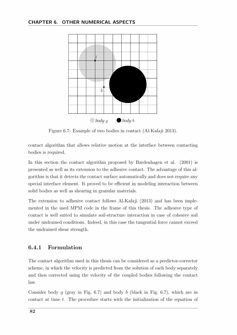
CHAPTER 6. OTHER NUMERICAL ASPECTS
Figure 6.7: Example of two bodies in contact (Al-Kafaji 2013).
contact algorithm that allows relative motion at the interface between contacting
bodies is required.
In this section the contact algorithm proposed by Bardenhagen et al. (2001) is
presented as well as its extension to the adhesive contact. The advantage of this al-
gorithm is that it detects the contact surface automatically and does not require any
special interface element. It proved to be efficient in modeling interaction between
solid bodies as well as shearing in granular materials.
The extension to adhesive contact follows Al-Kafaji (2013) and has been imple-
mented in the used MPM code in the frame of this thesis. The adhesive type of
contact is well suited to simulate soil-structure interaction in case of cohesive soil
under undrained conditions. Indeed, in this case the tangential force cannot exceed
the undrained shear strength.
6.4.1 Formulation
The contact algorithm used in this thesis can be considered as a predictor-corrector
scheme, in which the velocity is predicted from the solution of each body separately
and then corrected using the velocity of the coupled bodies following the contact
law.
Consider body g (gray in Fig. 6.7) and body b (black in Fig. 6.7), which are in
contact at time t. The procedure starts with the initialization of the equation of
82

6.4. THE CONTACT BETWEEN BODIES
Figure 6.8: Cases of approaching bodies (left) and separating bodies (right) (Al-Kafaji 2013).
motion (Eq. 3.47) for each body separately, as well as for the combined system.
The nodal accelerations for each body and the combined system are calculated
solving the momentum equations and then used to predict the nodal velocities at
time t+ ∆t as follows:
vt+∆tg = vtg + ∆tatg
6.34
vt+∆tb = vtb + ∆tatb
6.35
vt+∆t = vt + ∆tat 6.36
Contact nodes are detected by comparing the velocity of a single body (vt+∆tg ,vt+∆t
b )
to that of the combined bodies (vt+∆t). If the velocities differ than the node is
identified as a contact node. For example, considering nodes l and k of body g, it is
clear that at node l the velocity of body g is equal to the one of the combined system,
therefore it is not a contact node and no correction is required. On the contrary,
at node k, which is shared between two bodies, the combined velocity differs from
the single body velocity; consequently this node is defined as a contact node and
correction is required.
When a node is detected as a contact node, the algorithm proceeds with checking
if the bodies are approaching or separating. This is done by comparing the normal
component of the single body velocity with the normal component of the combined
bodies velocity. Hence, the following two cases are possible:
(vt+∆tg − vt+∆t) · ntk > 0 ⇒ approaching
(vt+∆tg − vt+∆t) · ntk < 0 ⇒ separating
where ntk is the unit outward normal to body g at node k. The algorithm allows
83

CHAPTER 6. OTHER NUMERICAL ASPECTS
Figure 6.9: Contact forces for the stick case (Al-Kafaji 2013).
for free separation, i.e. no correction is required in this case and each body moves
with the single body velocity vt+∆tg(b) . If the bodies are approaching, than we need to
check whether sliding occurs.
The predicted relative normal and tangential velocities at an approaching contact
node can be respectively written as:
vt+∆tnorm =
[(vt+∆tg − vt+∆t
)· ntk
]ntk
6.37
vt+∆ttan = ntk ×
[(vt+∆tg − vt+∆t
)× ntk
] 6.38
These components can be used to predict the contact forces at the node as:
f t+∆tnorm =
mtk,g
∆tvt+∆tnorm
6.39
f t+∆ttan =
mtk,g
∆tvt+∆ttan
6.40
where mtk,g is the nodal mass integrated from MP of body g.
The maximum tangential force is:
fmax,t+∆ttan = f t+∆t
adh + µ|f t+∆ttan |
6.41
where f t+∆tadh is the adhesive force at the contact and µ is the friction coefficient.
Depending on the magnitude of the predicted contact forces we can distinguish
84
6.4. THE CONTACT BETWEEN BODIES
between stick and slip contact:
If |f t+∆ttan | < fmax,t+∆t
tan ⇒ stick contact
If |f t+∆ttan | > fmax,t+∆t
tan ⇒ slip contact
In the first case, i.e. the bodies stick to each others, no correction is required and
the velocity corresponds to vt+∆t. In the second case, i.e. the bodies are sliding
one respect to the other, the velocity needs to be corrected in such a way that
no interpenetration is allowed and the magnitude of the tangential force respect
Equation 6.41.
The predicted single body velocity vt+∆tg is corrected to a new velocity vt+∆t
k,g such
that the normal component coincide with the normal component of the combined
bodies velocity, i.e.,
vt+∆tg · ntk = vt+∆t · ntk
6.42
which can also be written as
vt+∆tg = vt+∆t
g + ct+∆tnorm
6.43
where
ct+∆tnorm = −
[(vt+∆tg − vt+∆t
)· ntk
]ntk
6.44
is the correction of the normal component of the predicted velocity.
This correction is equivalent to apply the following normal contact force:
f t+∆tnorm =
mtk,g
∆tct+∆tnorm
6.45
When sliding occurs, the maximum tangential contact force assumes the expression:
f t+∆ttan = fmax,t+∆t
tan t 6.46
with t being a unit vector indicating the direction of the tangent.
Substituting Equation 6.41 into Equation 6.46 we get:
f t+∆ttan =
(f t+∆tadh + µ|f t+∆t
norm|)t
6.47
85
CHAPTER 6. OTHER NUMERICAL ASPECTS
The total contact force is:
f t+∆tcont = f t+∆t
tan + f t+∆tnorm
6.48
which is used to correct the velocity as:
vt+∆tg = vt+∆t
g +f t+∆tcont
mtk,g
∆t 6.49
It can also be written as:
vt+∆tg = vt+∆t
g + ct+∆tnorm + ct+∆t
tan
6.50
where the correction for the tangential component assumes the form:
ct+∆ttan =
∆t
mtk,g
(f t+∆tadh + µ|f t+∆t
norm|)t
6.51
The force introduced by the adhesion a can be expressed as;
f t+∆tadh = aAtk
6.52
where Atk is the contact area associated with the node k. It is integrated from the
contact elements that share node k.
Substituting equations 6.52 and 6.45 in 6.51, the corrected velocity can be written
as:
vt+∆tg = vt+∆t
g −[(vt+∆tg − vt+∆t
)· ntk
]ntk
−[(
vt+∆tg − vt+∆t
)· ntk
]µ+
aAtk∆t
mtk,g
t
6.53
Figure 6.10 illustrates with a flow chart the main steps of the implemented contact
algorithm.
Having calculated the velocity of the contact node k at time t + ∆t, the corrected
acceleration vector at the node must be recalculated as:
atg =vt+∆tg − vtg
∆t
6.54
This corrected acceleration is used to update the MP velocity according to the algo-
86

6.4. THE CONTACT BETWEEN BODIES
Figure 6.10: Flow chart illustrating the contact algorithm.
rithm presented in section 3.4.2. It should be remarked that the contact algorithm is
applied between the Lagrangian phase and the convective phase. Indeed the nodal
velocities are first predicted in the Lagrangian phase, then the corrected nodal veloc-
ities and accelerations are computed by the contact algorithm and these new values
of nodal accelerations are used to compute the velocities at the MP in the convective
phase. The same procedure explained here for body g must be applied to body b.
6.4.2 Validation
The implemented contact algorithm is validated with a benchmark problem consist-
ing in two blocks sliding on the top of each other. The mesh counts of 5265 elements,
3225 of which are initially filled with 4 particles each (Fig. 6.11). The dimensions
of the blocks and their material parameters are summarized in Table 6.2.
The upper block, also called block 1, is pushed by an horizontal force T linearly
increasing with time. The contact is characterized by a friction coefficient µ = 0.25
and an adhesion a = 5kPa. The maximum contact force can be calculated as:
Ftan,max = µFg,1 + aA = 0.25 · 40 + 5 · 2 = 20kN 6.55
where Fg,1 is the weight of the upper block and A is the contact area.
87

CHAPTER 6. OTHER NUMERICAL ASPECTS
Figure 6.11: Geometry and discretization.
Upper block Lower block
Young modulus [kPa] E 15000 75000Poisson ratio [-] ν 0 0Density [kg/m3] ρ 1000 5000High [m] h 2 0.5Lenght [m] l 4 5.5Width [m] d 0.5 0.5
Table 6.2: Geometry and material parameters for the sliding-block benchmark
The two blocks stick to each other while T < F conttan,max; as soon as T > F cont
tan,max
the upper block starts sliding. In order to avoid dynamic effects the rate of loading
should be reasonably small, for example 1kN/s, and the courant number is set to
0.5, i.e. the time step size is 50% of the critical.
Figure 6.12 plots the contact force components as function of the applied external
force. The tangential contact force F conttan increases linearly in time up to its maxi-
mum value and then remains constant. The normal contact force F contnorm is equal to
the weight of block 1. Oscillations are present and increase when the block starts
sliding. They can be reduced by refining the mesh, decreasing the rate of load, or
the time step size.
The kinetic energy of the system and the displacements of four MP are plotted in
Figure 6.13. As expected the kinetic energy is close to zero while T < Ftan,max;
beyond this value it increases suddenly, meaning that the block is sliding. The
88
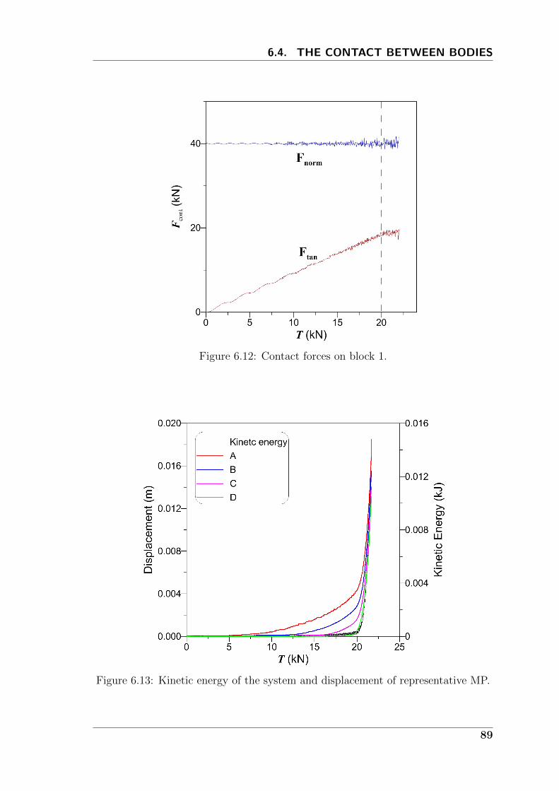
6.4. THE CONTACT BETWEEN BODIES
Figure 6.12: Contact forces on block 1.
Figure 6.13: Kinetic energy of the system and displacement of representative MP.
89
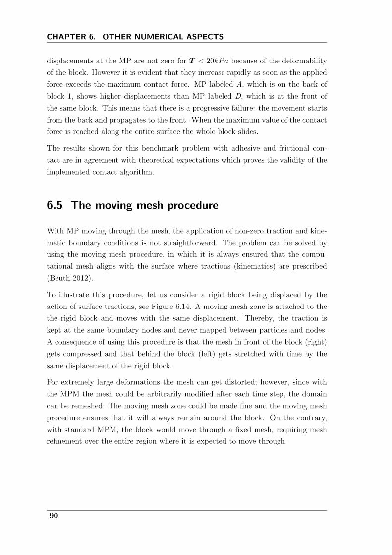
CHAPTER 6. OTHER NUMERICAL ASPECTS
displacements at the MP are not zero for T < 20kPa because of the deformability
of the block. However it is evident that they increase rapidly as soon as the applied
force exceeds the maximum contact force. MP labeled A, which is on the back of
block 1, shows higher displacements than MP labeled D, which is at the front of
the same block. This means that there is a progressive failure: the movement starts
from the back and propagates to the front. When the maximum value of the contact
force is reached along the entire surface the whole block slides.
The results shown for this benchmark problem with adhesive and frictional con-
tact are in agreement with theoretical expectations which proves the validity of the
implemented contact algorithm.
6.5 The moving mesh procedure
With MP moving through the mesh, the application of non-zero traction and kine-
matic boundary conditions is not straightforward. The problem can be solved by
using the moving mesh procedure, in which it is always ensured that the compu-
tational mesh aligns with the surface where tractions (kinematics) are prescribed
(Beuth 2012).
To illustrate this procedure, let us consider a rigid block being displaced by the
action of surface tractions, see Figure 6.14. A moving mesh zone is attached to the
the rigid block and moves with the same displacement. Thereby, the traction is
kept at the same boundary nodes and never mapped between particles and nodes.
A consequence of using this procedure is that the mesh in front of the block (right)
gets compressed and that behind the block (left) gets stretched with time by the
same displacement of the rigid block.
For extremely large deformations the mesh can get distorted; however, since with
the MPM the mesh could be arbitrarily modified after each time step, the domain
can be remeshed. The moving mesh zone could be made fine and the moving mesh
procedure ensures that it will always remain around the block. On the contrary,
with standard MPM, the block would move through a fixed mesh, requiring mesh
refinement over the entire region where it is expected to move through.
90
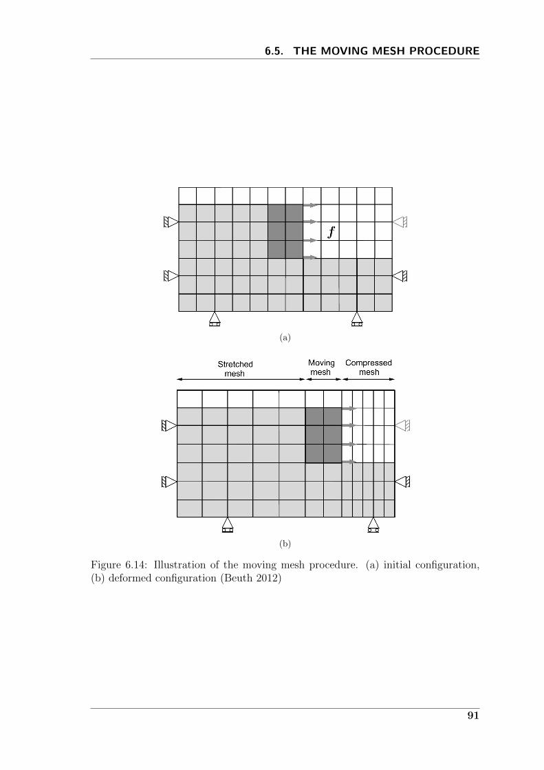
6.5. THE MOVING MESH PROCEDURE
(a)
(b)
Figure 6.14: Illustration of the moving mesh procedure. (a) initial configuration,(b) deformed configuration (Beuth 2012)
91

7Validation of the two-phase MPM
The current chapter is devoted to the validation of the two-phase MPM by the simu-
lation of benchmark problems, for which analytical reference solutions are available.
A simple dynamic problem such as the wave propagation in a porous material is
considered in Section 7.1. The use of absorbing boundary is studied analyzing the
effect of the virtual thickness. Since the problem is characterized by undrained
conditions, results obtained with the one-phase and the two-phase formulations are
compared.
Pore pressure dissipation is considered in Section 7.2, with the one-dimensional
consolidation problem. Results obtained with MPM are compared to Terzaghi’s
analytical solution for small strain problem (Sec. 7.2.1). The introduction of ab-
sorbing boundary and local damping is also investigated; moreover the application
of the mass scaling procedure to improve computational efficiency is discussed. One-
dimensional consolidation for large deformation is considered in Section 7.2.2.
The chapter ends with concluding remarks on the applicability of the used two-phase
MPM implementation.
7.1 One-dimensional wave propagation
The v-w formulation, i.e. soil velocity-water velocity are the primary variables,
is preferred over the v-p formulation because the latter cannot accurately capture
the two-phase dynamic behavior (van Esch et al. 2011a). The capability of the
implemented formulation to capture the undrained wave propagation is shown in
this section.
93

CHAPTER 7. VALIDATION OF THE TWO-PHASE MPM
Parameter Symbol Value
Effective Young modulus [kPa] E ′ 5 · 106
Effective Poisson ratio [-] ν ′ 0Water bulk modulus [kPa] Kw 2 · 106
Porosity [-] n 0.4Dry density [kg/m3] ρdry 1600Water density [kg/m3] ρw 1000Permeability [m/s] k 1.0 · 10−5
Table 7.1: Material parameters for the one-dimensional wave propagation problem.
A 2.5m-long column, discretized with 1000 rows of 6 tetrahedral elements, is in-
stantly loaded by σy = 1kPa. Each element contains 1 MP. Roller boundaries are
prescribed at the lateral surfaces, the bottom is impermeable and fully fixed. Note
that to capture the dynamic behavior of the system a very fine mesh is required.
The material parameters are listed in Table 7.1 The propagation of the undrained
wave is studied following the pore pressure of a MP located at 0.675m from the top
surface.
The wave speed can be calculated with:
cp,u =
√Ec,uρsat
7.1
where Ec,u = E ′(1−ν ′)/[(1+ν ′)(1−2ν ′)]+Kw/n is the undrained confined compres-
sion modulus and ρsat is calculated with Equation 3.60. For the considered problem
cp,u = 2236m/s.
The wave travels through the soil and is expected to reach the considered MP at
t = 3.02 · 10−4s. At the bottom it is reflected and starts traveling upward doubling
the pore pressure of the MP at t = 1.93 · 10−3s; at the top it is reflected again. The
expected normalized pore pressure pw/σy is a function of the undrained confined
compression modulus and the water bulk modulus:
pwσy
=Kw/n
Ec,u= 0.5
7.2
As can be seen from Figure 7.1 the numerical solution agrees well with the theoretical
one. There are some oscillations typical of the numerical solutions in which the load
is applied instantaneously.
The same problem is studied with the introduction of the viscous boundary at the
94
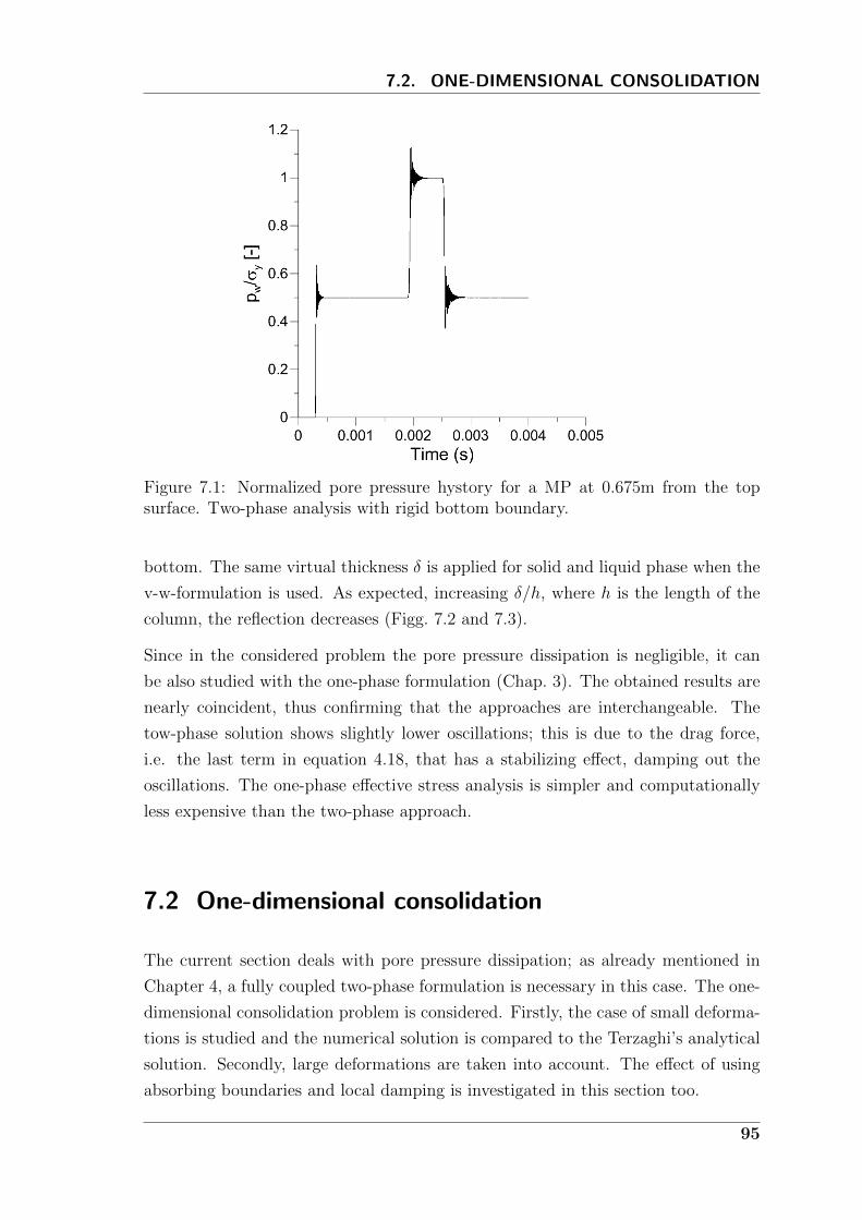
7.2. ONE-DIMENSIONAL CONSOLIDATION
Figure 7.1: Normalized pore pressure hystory for a MP at 0.675m from the topsurface. Two-phase analysis with rigid bottom boundary.
bottom. The same virtual thickness δ is applied for solid and liquid phase when the
v-w-formulation is used. As expected, increasing δ/h, where h is the length of the
column, the reflection decreases (Figg. 7.2 and 7.3).
Since in the considered problem the pore pressure dissipation is negligible, it can
be also studied with the one-phase formulation (Chap. 3). The obtained results are
nearly coincident, thus confirming that the approaches are interchangeable. The
tow-phase solution shows slightly lower oscillations; this is due to the drag force,
i.e. the last term in equation 4.18, that has a stabilizing effect, damping out the
oscillations. The one-phase effective stress analysis is simpler and computationally
less expensive than the two-phase approach.
7.2 One-dimensional consolidation
The current section deals with pore pressure dissipation; as already mentioned in
Chapter 4, a fully coupled two-phase formulation is necessary in this case. The one-
dimensional consolidation problem is considered. Firstly, the case of small deforma-
tions is studied and the numerical solution is compared to the Terzaghi’s analytical
solution. Secondly, large deformations are taken into account. The effect of using
absorbing boundaries and local damping is investigated in this section too.
95
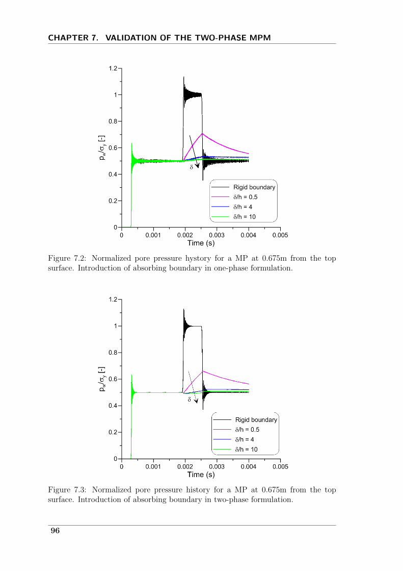
CHAPTER 7. VALIDATION OF THE TWO-PHASE MPM
Figure 7.2: Normalized pore pressure hystory for a MP at 0.675m from the topsurface. Introduction of absorbing boundary in one-phase formulation.
Figure 7.3: Normalized pore pressure history for a MP at 0.675m from the topsurface. Introduction of absorbing boundary in two-phase formulation.
96

7.2. ONE-DIMENSIONAL CONSOLIDATION
Parameter Symbol Value
Effective Young modulus [kPa] E ′ 10000Effective Poisson ratio [-] ν ′ 0Water bulk modulus [kPa] Kw 75000Porosity [-] n 0.3Water density [kg/m3] ρw 1000Permeability [m/s] k 1.0 · 10−3
Table 7.2: Material parameters for the one-dimensional consolidation problem.Small-strain case.
7.2.1 Small deformations
A 1m-soil column, discretized with 40 rows of 6 tetrahedral elements containing 4
MP each, is considered. A linear elastic material model is used, whose parameters
are listed in Table 7.2. These parameters correspond to and undrained Poisson’s
ratio νu = 0.490, which is considered a reasonable approximation of the material
incompressibility in undrained conditions. Higer values of νu, i.e. higher Kw, in-
crease the oscillations of the solution. Roller boundaries are prescribed at the lateral
surfaces, the bottom is fully fixed. The head of the column is permeable and the
bottom is impermeable, therefore the water can flow out of the column from the top
surface and the drainage length h is 1m.
A total stress of 10kPa is applied at the first time step and kept constant during
the analysis. The excess pore pressure is initialized at pw0 = 10kPa, therefore the
load is initially fully carried by the water and the system is in equilibrium. While
water flows out of the column, the pore pressure diminishes and the effective stress
increases, according to the well-known Terzaghi’s one-dimensional consolidation the-
ory.
The process is governed by the consolidation coefficient, defined here as:
cv =k
ρwg(1/E ′c
) 7.3
The non-dimensional time factor can be defined as:
T =cvt
h2
7.4
Figure 7.4 plots the normalized pore pressure pw/pw0 against the normalized depth
y/h as function of the non-dimensional time. There is good agreement between the
97

CHAPTER 7. VALIDATION OF THE TWO-PHASE MPM
Figure 7.4: Normalized pore pressure along depth, comparison between numericaland analytical solution.
numerical and the analytical solution.
Oscillations appears for small values of T , which are due to reflections of dynamic
waves. As discussed in Section 6.2 this noise can be reduced by introducing absorbing
boundary or local damping.
The introduction of the absorbing boundary can effectively reduce wave reflections
for small time factors, but introduces an error for long term consolidation (Fig. 7.5).
Large values of δ improve results at the beginning of the process, but give un-
acceptable overestimation of the pore pressure for long-term. On the other hand
small values of δ do not damp dynamic waves. A compromise between acceptable
oscillation at the beginning of the process and deviation from analytical solution
at long-time process should be found. A constant value of δ = 0.1h is considered
acceptable, but changing the virtual thickness throughout the calculation is also
possible.
The local damping is a valid alternative to the absorbing boundary. In this thesis
the damping factor for the liquid phase coincides with the damping factor for the
solid phase. The damping factor artificially simulates the natural energy dissipation
which characterizes the real material (Cundall 2001); this dissipation is probably
lower for the water than for the soil skeleton, but this is not considered in the
present study even though should be investigated in the future.
98

7.2. ONE-DIMENSIONAL CONSOLIDATION
Dynamic waves are effectively damped, but overestimation of pore pressure at long
term is observed (Fig. 7.6) which increases with the damping factor α. Although
there is the possibility to change the damping factor throughout the calculation,
constant value of α = 0.05 is suggested for this problem.
Both absorbing boundary and local damping can be used to reduce oscillations due
to dynamic effects. The introduction of the viscous boundary can require a reduction
of the time step size to achieve convergence, while this is not necessary in case of
local damping. For example the presented results are obtained using a time step
size of 50% of the critical, in case of absorbing boundary and 98% of the critical in
case of local damping.
Consolidation of real soil deposits can take days, months or years and the numerical
simulation of such processes with explicit dynamic codes becomes totally inefficient.
Being a quasi-static process, the mass scaling procedure (Sec. 6.3) can be adopted.
The use of mass scaling accentuate the dynamic effects and therefore increases the
noise at small time, but this problem disappears at long time.
The material considered in this section is characterized by a very high consolidation
coefficient (cv = 1m2/s); the pore pressure dissipates almost completely in 1s. In this
specific case, the use of mass scaling is not necessary; on the contrary it generates
unacceptable oscillations in the first phase of the consolidation process (Fig. 7.7).
If a lower permeability is considered, i.e. k = 10−5m/s, the consolidation time is
longer (T = 1 correspond to t = 100s ); however, by the use of the mass scaling
procedure, i.e. introducing a mass scaling factor β = 100, the computational time
does not increase dramatically, because the critical time step is larger, and nice
results are obtained throughout the simulation (Fig. 7.8).
7.2.2 Large deformations
This section shows the possibility to simulate consolidation for large deformations.
The same geometry and discretization considered in the previous section is used, but
a much softer material; see material parameters in Table 7.3. A load of σy = 50kPa
is applied at the top surface at the beginning of the calculation and kept constant.
The pore pressure is initialized at 50kPa, which means that the load is initially fully
carried by the water.
As in the previous case, while the pore pressure decreases the effective stress in-
creases, but now this generates considerable vertical deformations and the decrease
99
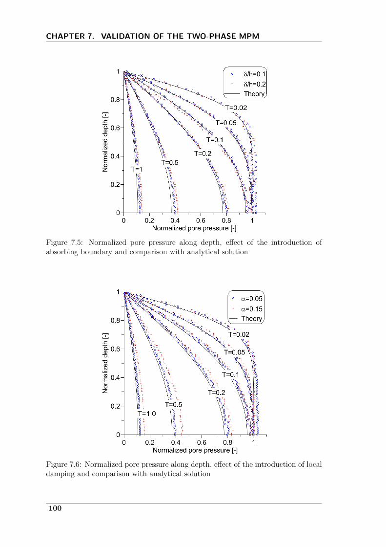
CHAPTER 7. VALIDATION OF THE TWO-PHASE MPM
Figure 7.5: Normalized pore pressure along depth, effect of the introduction ofabsorbing boundary and comparison with analytical solution
Figure 7.6: Normalized pore pressure along depth, effect of the introduction of localdamping and comparison with analytical solution
100

7.2. ONE-DIMENSIONAL CONSOLIDATION
Figure 7.7: Normalized pore pressure along depth, effect of the use of a mass scalingfactor β = 10 in a material with a high consolidation coefficient (cv = 1m2/s)
Figure 7.8: Normalized pore pressure along depth, effect of the use of a mass scalingfactor β = 100 in a material with a consolidation coefficient cv = 0.01m2/s
101

CHAPTER 7. VALIDATION OF THE TWO-PHASE MPM
Parameter Symbol Value
Effective Young modulus [kPa] E ′ 100Effective Poisson ratio [-] ν ′ 0Water bulk modulus [kPa] Kw 750Porosity [-] n 0.3Water density [kg/m3] ρw 1000Permeability [m/s] k 1.0 · 10−2
Table 7.3: Material parameters for the one-dimensional consolidation problem.Large-strain case.
of the column-length is not negligible, therefore the small-strain Terzaghi’s theory
is no longer valid.
This material is characterized by a consolidation coefficient cv = 0.1m2/s; a time
factor TL defined by Equation 7.4 in which h is the initial length of the column can
be considered. Figure 7.9 shows the normalized pore pressure at specific material
points, choosen along the column, against their y coordinate, the value zero corre-
sponds to the bottom of the mesh. Since the drainage-lenght decreases significantly
with the time, the pore pressure dissipation is faster compared with the small strain
case (Fig. 7.4).
As usual in MPM, large deformations are simulated with material points moving
through the mesh. Figure 7.10 shows the change in column-length along time.
7.2.3 The time step citerium
The implemented numerical scheme for the two-phase formulation is conditionally
stable and the critical time step size is defined by Equation 3.34. The reference
velocity is the speed of the undrained wave, which can be determined as:
cp =
√Ec,uρsat
7.5
where Ec,u is the undrained constrained modulus.
However, this condition does not guarantee the stability of the scheme, which ap-
pears to be also dependent on the permeability of the material. Indeed, considering
the simple one-dimensional consolidation problem presented in Section 7.2.1, if the
permeability is decreased to 10−5m/s the solution diverges using a Courant num-
ber of 0.98, but converges if it is reduced to 0.1. With such a low permeability
102
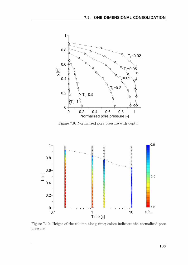
7.2. ONE-DIMENSIONAL CONSOLIDATION
Figure 7.9: Normalized pore pressure with depth.
Figure 7.10: Height of the column along time; colors indicates the normalized porepressure.
103
CHAPTER 7. VALIDATION OF THE TWO-PHASE MPM
the scheme is stable with C = 0.98 if a mass scaling factor β = 100 is used or the
Young modulus is increased by a factor 100. This suggests that permeability, density
and elastic modulus influence the critical time step size. The study of the stability
criterion for the implemented formulation is object of the on-going research.
7.3 Concluding remarks
This chapter shows the validation of the current two-phase MPM implementation
for the simulation of dynamic and quasi-static problems in case of both small and
large deformations involving two-phase materials.
The two-phase dynamic MPM can correctly capture the propagation of the undrained
wave along a column of saturated porous media (Sec. 7.1). The arrival time of the
wave agrees with the analytical solution and no energy dissipation is observed.
The MPM can accurately capture how the pore pressure distribution changes with
time in the one-dimensional consolidation problem (Sec. 7.2); indeed, the numer-
ical result for small strain is in excellent agreement with the analytical solution
by Terzaghi. At large strain, the pore pressure dissipation is faster because the
drainage length decreases with time. With the MPM, the effect of significant soil
deformations on the pore pressure dissipation can easily be taken into account.
In Sections 7.1 and 7.2 it is proved that absorbing boundary can be used to damp
dynamic waves. The rate of damping increases with the virtual thickness δ. The
physical meaning of this parameter is explained in Section 6.2.1; sensitivity analysis
are necessary to choose the most suitable value for the specific problem under-
consideration.
As shown in Section 7.2.1, the local damping can be a valid alternative to solve
problems related to dynamic effects. The local damping factor α must be small in
slow-process problems since it affects the pore pressure at long term (see Fig. 7.6).
In this thesis the same virtual thickness and the same damping factor are applied
for the fluid and the solid phase, however different values can be used and the effect
of this choice will be investigated in the future.
The mass scaling procedure can be used to improve the computational efficiency of
quasi-static and slow-process problems. It increases the noise due to the propagation
and reflection of dynamic waves; this problem is more severe at short time, but
disappears at long term.
104

7.3. CONCLUDING REMARKS
The used two-phase MPM implementation is capable to simulate geomechanical
problems involving pore pressure dissipation with small and large deformations.
105

8Simulation of the collapse of a submerged
slope
The stability of submerged slopes is an important issue in many countries. In the
Netherlands the problem has a great impact in the south-western province of Zee-
land, characterized by numerous islands. The shoreline has been severely damaged
erosion and submarine landslides compromising the safety of the area. The phe-
nomenon needs to be deeply investigated in order to enforce the design of mitigation
techniques.
In order to study the stability of loose sand slopes, small scale laboratory tests were
performed at Deltares (Delft, the Netherlands). To gain a deeper understanding of
the problem, the experiments were enhanced by an advanced numerical study. In-
deed, laboratory tests are affected by scale effects, which may leave some doubts on
the extension of the small-scale observations to the real case. Numerical simulations
can be easily done on the full-scale geometry. Moreover, parametric studies can eas-
ily be performaed to detect the most significant parameters affecting the occurance
and evolution of the landslides.
Slope stability problems have been intensively studied for decades, both experimen-
tally and numerically to understand the mechanics and to predict the failure. Most
of the numerical analyses focus on the identification of the limit condition of static
equilibrium of the slope. The finite element methods (FEM) are popular in this
field because they can represent accurately the geometry of the slope and allow for
incorporation of advanced constitutive models. The shape of the sliding surface
can be well captured with FEM, but the dynamic evolution of the landslide and its
run-out cannot be reproduced.
107
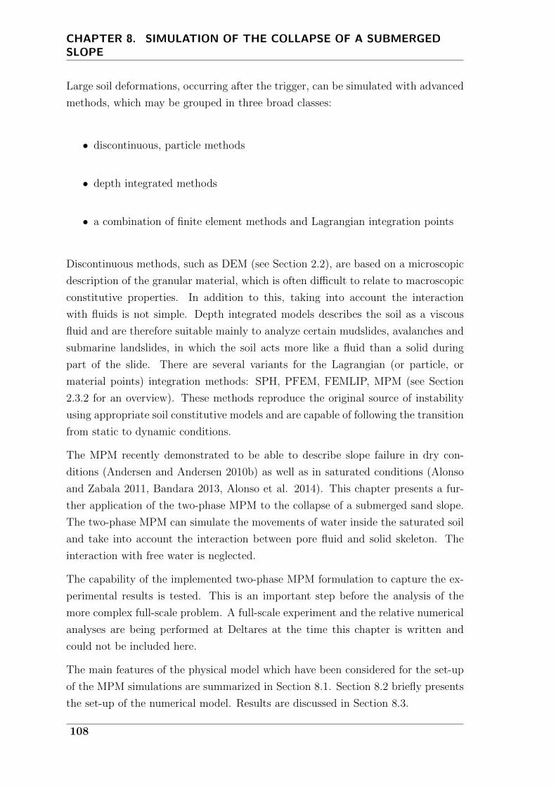
CHAPTER 8. SIMULATION OF THE COLLAPSE OF A SUBMERGEDSLOPE
Large soil deformations, occurring after the trigger, can be simulated with advanced
methods, which may be grouped in three broad classes:
• discontinuous, particle methods
• depth integrated methods
• a combination of finite element methods and Lagrangian integration points
Discontinuous methods, such as DEM (see Section 2.2), are based on a microscopic
description of the granular material, which is often difficult to relate to macroscopic
constitutive properties. In addition to this, taking into account the interaction
with fluids is not simple. Depth integrated models describes the soil as a viscous
fluid and are therefore suitable mainly to analyze certain mudslides, avalanches and
submarine landslides, in which the soil acts more like a fluid than a solid during
part of the slide. There are several variants for the Lagrangian (or particle, or
material points) integration methods: SPH, PFEM, FEMLIP, MPM (see Section
2.3.2 for an overview). These methods reproduce the original source of instability
using appropriate soil constitutive models and are capable of following the transition
from static to dynamic conditions.
The MPM recently demonstrated to be able to describe slope failure in dry con-
ditions (Andersen and Andersen 2010b) as well as in saturated conditions (Alonso
and Zabala 2011, Bandara 2013, Alonso et al. 2014). This chapter presents a fur-
ther application of the two-phase MPM to the collapse of a submerged sand slope.
The two-phase MPM can simulate the movements of water inside the saturated soil
and take into account the interaction between pore fluid and solid skeleton. The
interaction with free water is neglected.
The capability of the implemented two-phase MPM formulation to capture the ex-
perimental results is tested. This is an important step before the analysis of the
more complex full-scale problem. A full-scale experiment and the relative numerical
analyses are being performed at Deltares at the time this chapter is written and
could not be included here.
The main features of the physical model which have been considered for the set-up
of the MPM simulations are summarized in Section 8.1. Section 8.2 briefly presents
the set-up of the numerical model. Results are discussed in Section 8.3.
108
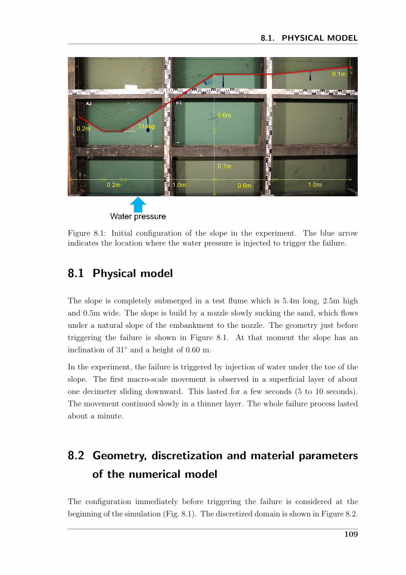
8.1. PHYSICAL MODEL
Figure 8.1: Initial configuration of the slope in the experiment. The blue arrowindicates the location where the water pressure is injected to trigger the failure.
8.1 Physical model
The slope is completely submerged in a test flume which is 5.4m long, 2.5m high
and 0.5m wide. The slope is build by a nozzle slowly sucking the sand, which flows
under a natural slope of the embankment to the nozzle. The geometry just before
triggering the failure is shown in Figure 8.1. At that moment the slope has an
inclination of 31 and a height of 0.60 m.
In the experiment, the failure is triggered by injection of water under the toe of the
slope. The first macro-scale movement is observed in a superficial layer of about
one decimeter sliding downward. This lasted for a few seconds (5 to 10 seconds).
The movement continued slowly in a thinner layer. The whole failure process lasted
about a minute.
8.2 Geometry, discretization and material parameters
of the numerical model
The configuration immediately before triggering the failure is considered at the
beginning of the simulation (Fig. 8.1). The discretized domain is shown in Figure 8.2.
109
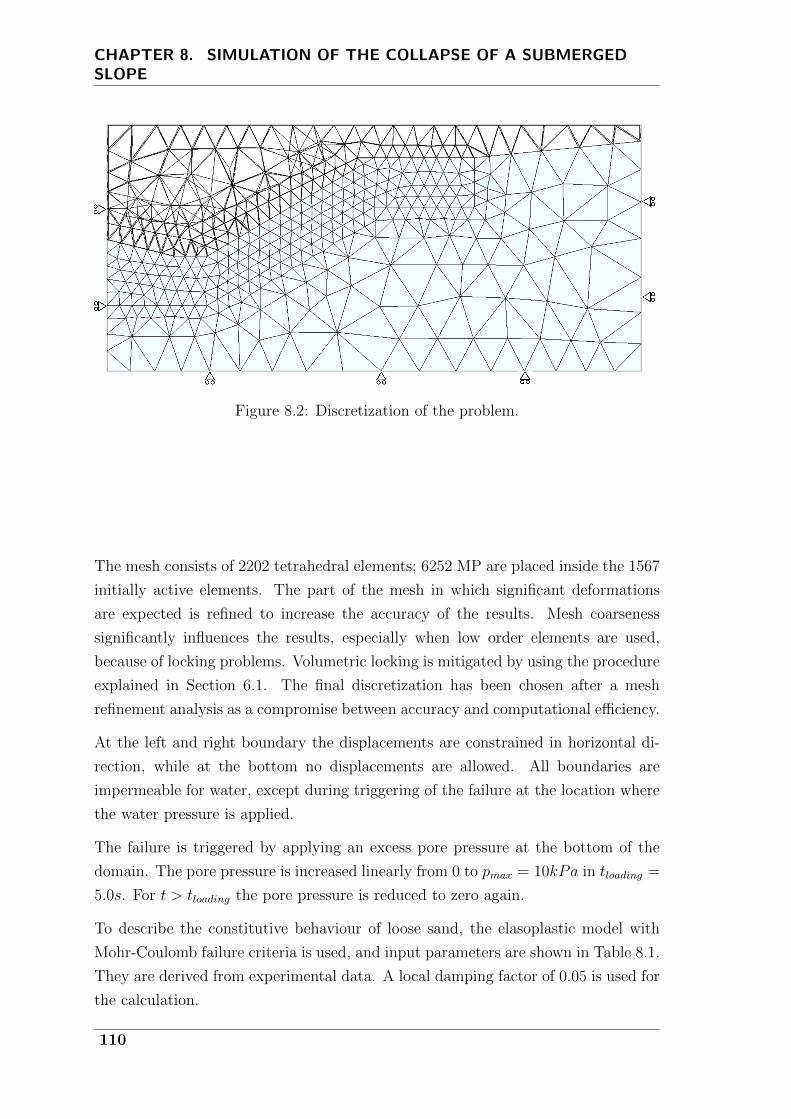
CHAPTER 8. SIMULATION OF THE COLLAPSE OF A SUBMERGEDSLOPE
Figure 8.2: Discretization of the problem.
The mesh consists of 2202 tetrahedral elements; 6252 MP are placed inside the 1567
initially active elements. The part of the mesh in which significant deformations
are expected is refined to increase the accuracy of the results. Mesh coarseness
significantly influences the results, especially when low order elements are used,
because of locking problems. Volumetric locking is mitigated by using the procedure
explained in Section 6.1. The final discretization has been chosen after a mesh
refinement analysis as a compromise between accuracy and computational efficiency.
At the left and right boundary the displacements are constrained in horizontal di-
rection, while at the bottom no displacements are allowed. All boundaries are
impermeable for water, except during triggering of the failure at the location where
the water pressure is applied.
The failure is triggered by applying an excess pore pressure at the bottom of the
domain. The pore pressure is increased linearly from 0 to pmax = 10kPa in tloading =
5.0s. For t > tloading the pore pressure is reduced to zero again.
To describe the constitutive behaviour of loose sand, the elasoplastic model with
Mohr-Coulomb failure criteria is used, and input parameters are shown in Table 8.1.
They are derived from experimental data. A local damping factor of 0.05 is used for
the calculation.
110
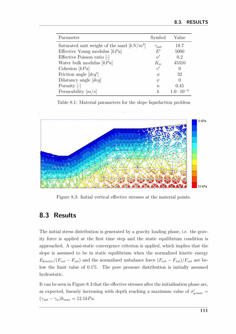
8.3. RESULTS
Parameter Symbol Value
Saturated unit weight of the sand [kN/m3] γsat 18.7Effective Young modulus [kPa] E ′ 5000Effective Poisson ratio [-] ν ′ 0.2Water bulk modulus [kPa] Kw 45310Cohesion [kPa] c′ 0Friction angle [deg′] φ 32Dilatancy angle [deg] ψ 0Porosity [-] n 0.45Permeability [m/s] k 1.0 · 10−4
Table 8.1: Material parameters for the slope liquefaction problem
Figure 8.3: Initial vertical effective stresses at the material points.
8.3 Results
The initial stress distribution is generated by a gravity loading phase, i.e. the grav-
ity force is applied at the first time step and the static equilibrium condition is
approached. A quasi-static convergence criterion is applied, which implies that the
slope is assumed to be in static equilibrium when the normalized kinetic energy
Ekinetic/(Fext − Fint) and the normalized unbalance force (Fext − Fint)/Fext are be-
low the limit value of 0.1%. The pore pressure distribution is initially assumed
hydrostatic.
It can be seen in Figure 8.3 that the effective stresses after the initialisation phase are,
as expected, linearly increasing with depth reaching a maximum value of σ′y,max =
(γsat − γw)hmax = 12.1kPa.
111
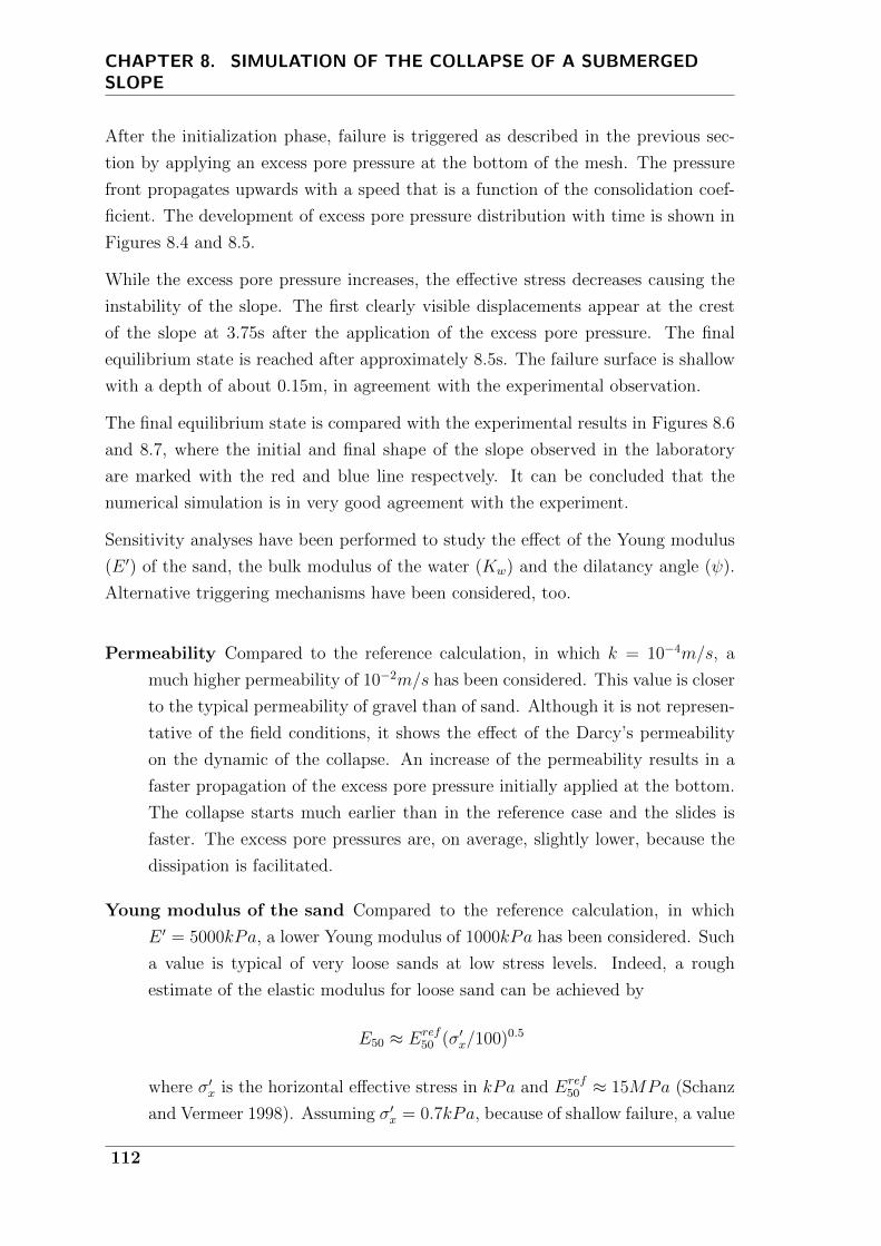
CHAPTER 8. SIMULATION OF THE COLLAPSE OF A SUBMERGEDSLOPE
After the initialization phase, failure is triggered as described in the previous sec-
tion by applying an excess pore pressure at the bottom of the mesh. The pressure
front propagates upwards with a speed that is a function of the consolidation coef-
ficient. The development of excess pore pressure distribution with time is shown in
Figures 8.4 and 8.5.
While the excess pore pressure increases, the effective stress decreases causing the
instability of the slope. The first clearly visible displacements appear at the crest
of the slope at 3.75s after the application of the excess pore pressure. The final
equilibrium state is reached after approximately 8.5s. The failure surface is shallow
with a depth of about 0.15m, in agreement with the experimental observation.
The final equilibrium state is compared with the experimental results in Figures 8.6
and 8.7, where the initial and final shape of the slope observed in the laboratory
are marked with the red and blue line respectvely. It can be concluded that the
numerical simulation is in very good agreement with the experiment.
Sensitivity analyses have been performed to study the effect of the Young modulus
(E ′) of the sand, the bulk modulus of the water (Kw) and the dilatancy angle (ψ).
Alternative triggering mechanisms have been considered, too.
Permeability Compared to the reference calculation, in which k = 10−4m/s, a
much higher permeability of 10−2m/s has been considered. This value is closer
to the typical permeability of gravel than of sand. Although it is not represen-
tative of the field conditions, it shows the effect of the Darcy’s permeability
on the dynamic of the collapse. An increase of the permeability results in a
faster propagation of the excess pore pressure initially applied at the bottom.
The collapse starts much earlier than in the reference case and the slides is
faster. The excess pore pressures are, on average, slightly lower, because the
dissipation is facilitated.
Young modulus of the sand Compared to the reference calculation, in which
E ′ = 5000kPa, a lower Young modulus of 1000kPa has been considered. Such
a value is typical of very loose sands at low stress levels. Indeed, a rough
estimate of the elastic modulus for loose sand can be achieved by
E50 ≈ Eref50 (σ′x/100)0.5
where σ′x is the horizontal effective stress in kPa and Eref50 ≈ 15MPa (Schanz
and Vermeer 1998). Assuming σ′x = 0.7kPa, because of shallow failure, a value
112
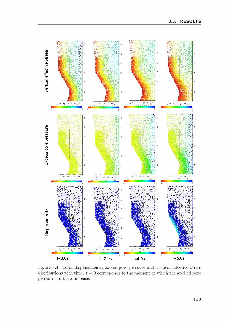
8.3. RESULTS
Figure 8.4: Total displacements, excess pore pressure and vertical effective stressdistributions with time. t = 0 corresponds to the moment at which the applied porepressure starts to increase.
113
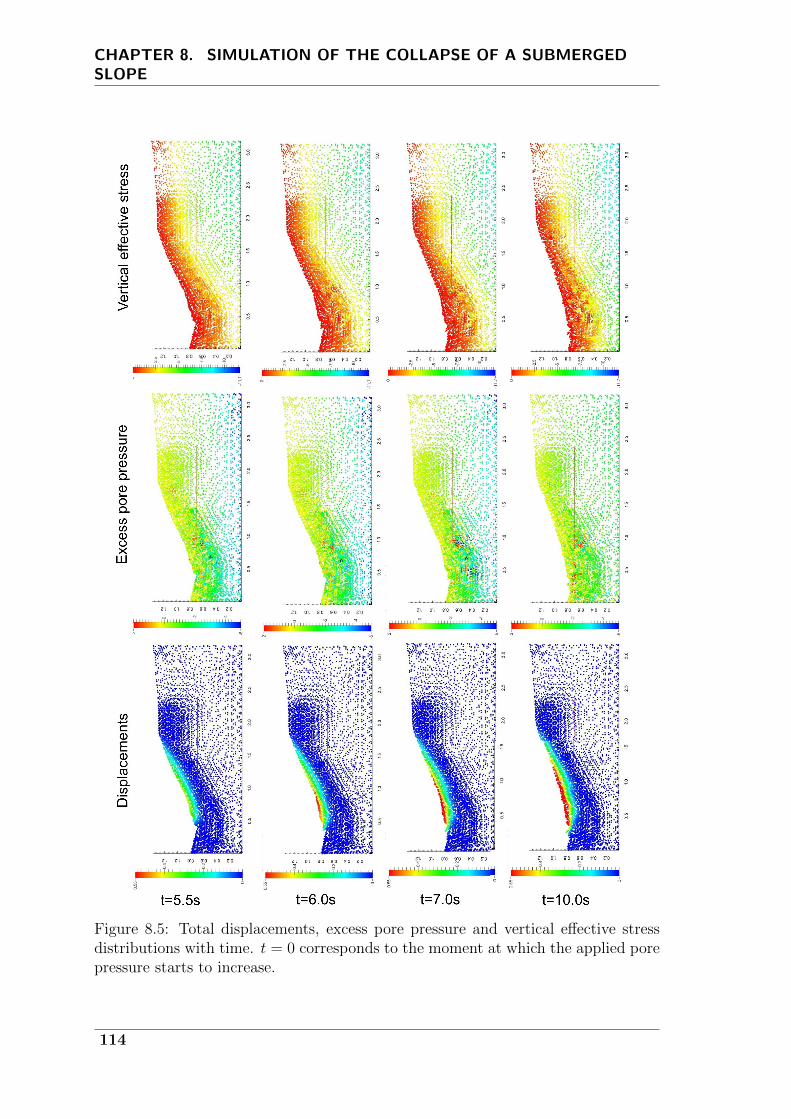
CHAPTER 8. SIMULATION OF THE COLLAPSE OF A SUBMERGEDSLOPE
Figure 8.5: Total displacements, excess pore pressure and vertical effective stressdistributions with time. t = 0 corresponds to the moment at which the applied porepressure starts to increase.
114
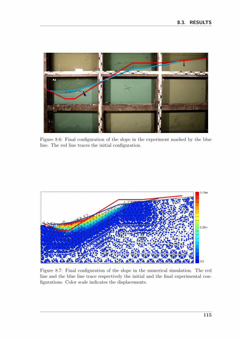
8.3. RESULTS
Figure 8.6: Final configuration of the slope in the experiment marked by the blueline. The red line traces the initial configuration.
Figure 8.7: Final configuration of the slope in the numerical simulation. The redline and the blue line trace respectively the initial and the final experimental con-figurations. Color scale indicates the displacements.
115
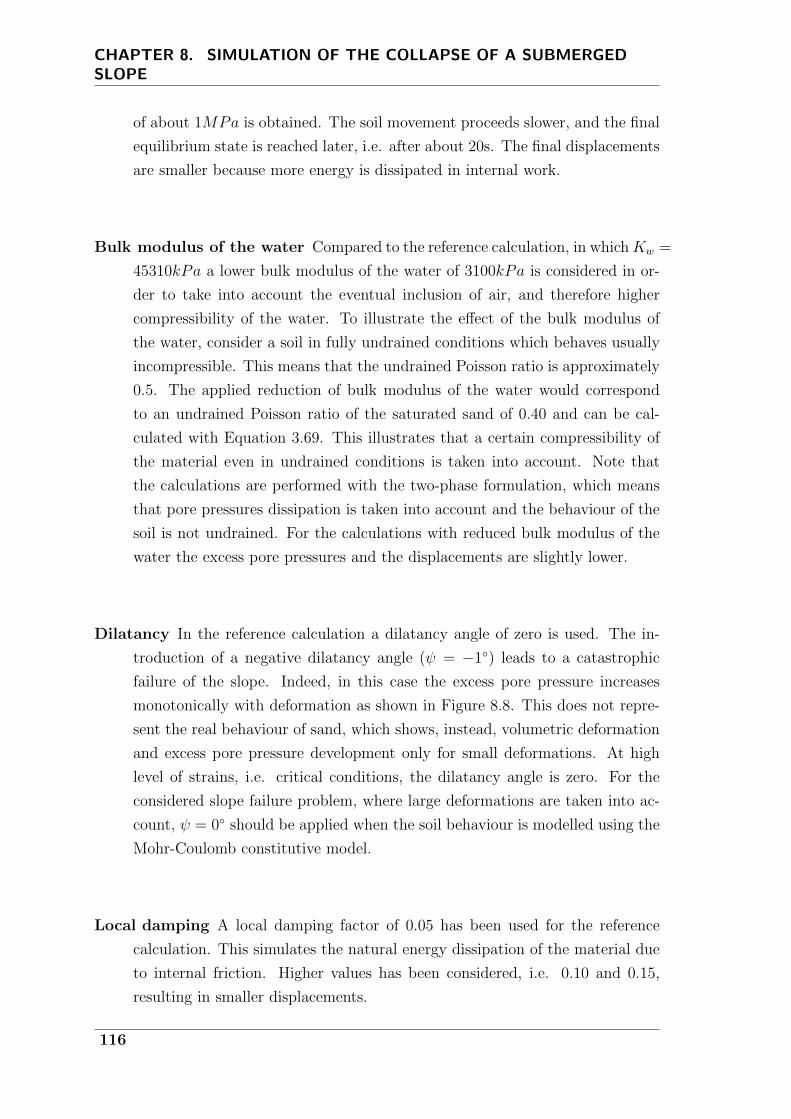
CHAPTER 8. SIMULATION OF THE COLLAPSE OF A SUBMERGEDSLOPE
of about 1MPa is obtained. The soil movement proceeds slower, and the final
equilibrium state is reached later, i.e. after about 20s. The final displacements
are smaller because more energy is dissipated in internal work.
Bulk modulus of the water Compared to the reference calculation, in whichKw =
45310kPa a lower bulk modulus of the water of 3100kPa is considered in or-
der to take into account the eventual inclusion of air, and therefore higher
compressibility of the water. To illustrate the effect of the bulk modulus of
the water, consider a soil in fully undrained conditions which behaves usually
incompressible. This means that the undrained Poisson ratio is approximately
0.5. The applied reduction of bulk modulus of the water would correspond
to an undrained Poisson ratio of the saturated sand of 0.40 and can be cal-
culated with Equation 3.69. This illustrates that a certain compressibility of
the material even in undrained conditions is taken into account. Note that
the calculations are performed with the two-phase formulation, which means
that pore pressures dissipation is taken into account and the behaviour of the
soil is not undrained. For the calculations with reduced bulk modulus of the
water the excess pore pressures and the displacements are slightly lower.
Dilatancy In the reference calculation a dilatancy angle of zero is used. The in-
troduction of a negative dilatancy angle (ψ = −1) leads to a catastrophic
failure of the slope. Indeed, in this case the excess pore pressure increases
monotonically with deformation as shown in Figure 8.8. This does not repre-
sent the real behaviour of sand, which shows, instead, volumetric deformation
and excess pore pressure development only for small deformations. At high
level of strains, i.e. critical conditions, the dilatancy angle is zero. For the
considered slope failure problem, where large deformations are taken into ac-
count, ψ = 0 should be applied when the soil behaviour is modelled using the
Mohr-Coulomb constitutive model.
Local damping A local damping factor of 0.05 has been used for the reference
calculation. This simulates the natural energy dissipation of the material due
to internal friction. Higher values has been considered, i.e. 0.10 and 0.15,
resulting in smaller displacements.
116
8.4. CONCLUSIONS AND FUTURE DEVELOPMENTS
Figure 8.8: Illustration of development of excess pore pressures for different dilatancyangles.
8.4 Conclusions and future developments
The failure of a submerged slope triggered by a sudden increase of water pressure at
the bottom can be successfully simulated using the two-phase MPM implementation.
The numerical results of the deformed slope in the final equilibrium state are in good
agreement with experimental data (Fig. 8.7).
The behavior of sand is complex; the elasto-plastic model with Mohr-Coulomb failure
criteria is a very simplified way of describing its behavior. Deeper understanding
of the failure process could be achieved with more sophisticated material models.
For example the Mohr-Coulomb with strain softening model (Abbo and Sloan 1995)
proved to be able to capture the progressive failure of the slope (Alonso and Zabala
2011; Yerro et al. 2014).
It is of great interest to investigate the behavior of true scale slopes, as found in the
region of Zeeland, whose height ranges between 10 and 50 m. It is expected that the
large-scale slopes would behave differently than slopes in model scale. Numerical
simulations can indicate safe inclination angle in the natural conditions. Revetments
of various types have been used to prevent erosion and improve the stability of the
slope. The effect of a stone revetment will be considered in the future also in the
numerical simulations.
The interaction with free water is neglected in this study; however, future devel-
opments of the MPM will be able to include this effect. The implementation of
117
CHAPTER 8. SIMULATION OF THE COLLAPSE OF A SUBMERGEDSLOPE
multi-layer formulations, i.e. solid and fluid are simulated with two separates sets of
MP, allows to simulate free water, saturated soil as well as soil-water suspensions;
see Bandara (2013), Wieckowski (2013) and Vermeer et al. (2013). These advanced
MPM formulations can simulate erosion-sedimentation processes and therefore close
the gap between geomechanical models and hydromechanical models.
118
9Simulation of Cone Penetration Testing
As shown in Chapter 7 the MPM can be successfully used to simulate large displace-
ment problems, taking into account the generation and dissipation of pore pressure.
The method has been also used to reproduce soil penetration problems such as pile
and spudcan installation (Nuygen et al. 2014).
In this chapter the MPM is applied to simulate the cone penetration test (CPT)
accounting for different drainage conditions. The study of CPT in partially drained
conditions is particularly interesting; indeed partial drainage can characterize cone
penetration in silty soils and arises difficulties in interpreting the measurements
(Schneider et al. 2008b). So far, this problem has been mainly took on experimen-
tally. Indeed, its numerical simulation is extremely complex as large deformations,
soil-cone contact and soil-water coupled mechanical behavior need to be considered.
A description of the cone penetration test and how it is used in geo-engineering is
given in Section 9.1. A brief literature review is found in Section 9.2. The main
features of the numerical model are explained in Section 9.3. Section 9.4 presents
results of MPM simulations in undrained conditions using the Tresca material model,
while in Section 9.5 the effect of partial drainage is considered. The chapter ends
with concluding remarks and future developments of the research (Sec. 9.6).
9.1 Introduction
The Cone Penetration Test (CPT) is a widely used in situ soil testing technique.
It was invented in the Netherlands in 1932 by P. Barentsen, an engineer at Rijk-
swaterstraat (department of public works); in order to get a quick and economic
impression of the structure of the underground. Many technological developments,
119

CHAPTER 9. SIMULATION OF CONE PENETRATION TESTING
Figure 9.1: Standard cone penetrometer.
as well as extensive scientific and theoretical studies on data interpretation, have
been done since then.
CPT consists in a conical tip placed at the end of a series of rods, pushed into the
ground at a constant rate. According to the ISSMFE IRTP standard, the rate of
penetration should be 20mm/s± 5mm/s. The combined resistance to penetration
of the cone and outer surface of a sleeve is measured, as well as the single sleeve
resistance. In the CPTU equipment the pore pressure is measured too. Extra sensors
are available in the market to measure additional soil properties such as the shear
wave velocity and the dielectrical conductivity.
The reference test equipment consists of a 60 cone, with 10cm2 base area and
150cm2 friction sleeve located above the cone. The total force acting on the cone
Qc, divided by the projected area Ac produces the cone resistance qc. The total force
acting on the friction sleeve Fs, divided by the surface area of the friction sleeve As
produces the sleeve friction fs. Depending on the specific device, the pore pressure
can be measured at the tip of the cone, at the cone face or, more often, behind the
cone; the latter is referred to as the u2 position. Figure 9.1 schematically represents
the device.
The CPT has three main applications in the site investigation process:
1. determine sub-surface stratigraphy and identify the present materials,
2. estimate geotechnical parameters,
3. provide results for direct geotechnical design.
The determination of soil stratigraphy and the identification of soil type have typi-
cally been accomplished using charts that link cone parameters to soil type. Early
120
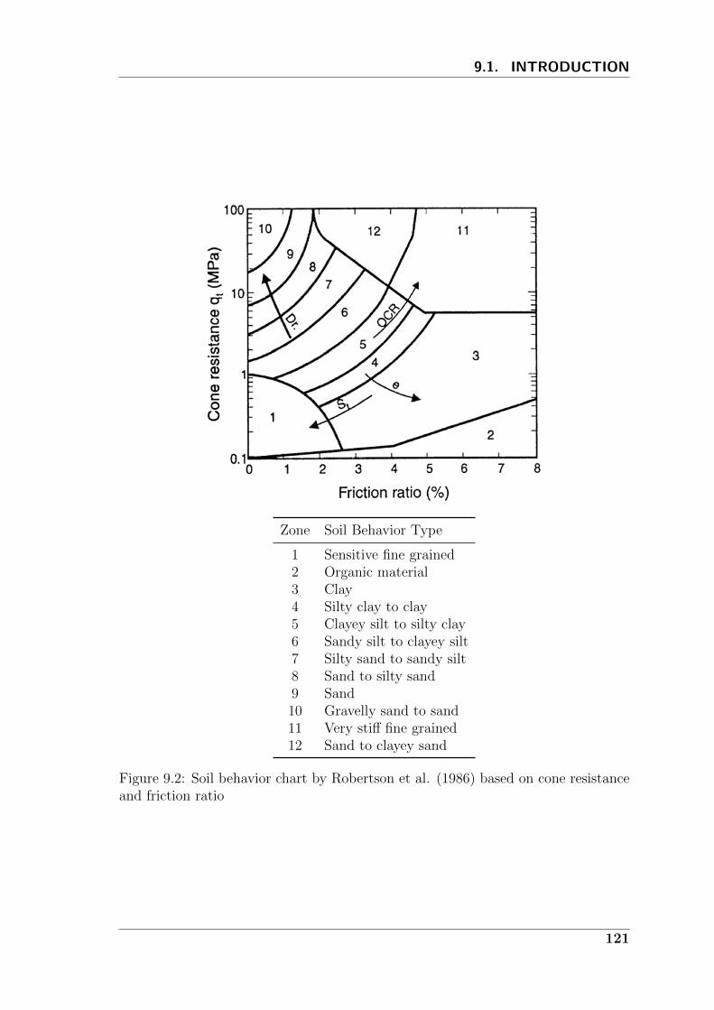
9.1. INTRODUCTION
Zone Soil Behavior Type
1 Sensitive fine grained2 Organic material3 Clay4 Silty clay to clay5 Clayey silt to silty clay6 Sandy silt to clayey silt7 Silty sand to sandy silt8 Sand to silty sand9 Sand10 Gravelly sand to sand11 Very stiff fine grained12 Sand to clayey sand
Figure 9.2: Soil behavior chart by Robertson et al. (1986) based on cone resistanceand friction ratio
121
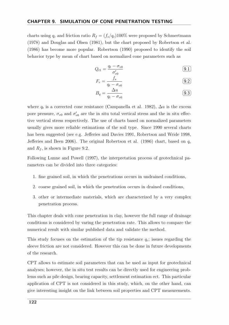
CHAPTER 9. SIMULATION OF CONE PENETRATION TESTING
charts using qc and friction ratio Rf = (fs/qc)100% were proposed by Schmertmann
(1978) and Douglas and Olsen (1981), but the chart proposed by Robertson et al.
(1986) has become more popular. Robertson (1990) proposed to identify the soil
behavior type by mean of chart based on normalized cone parameters such as
Qt1 =qt − σv0
σ′v0
9.1
Fr =fs
qt − σv0
9.2
Bq =∆u
qt − σv0
9.3
where qt is a corrected cone resistance (Campanella et al. 1982), ∆u is the excess
pore pressure, σv0 and σ′v0 are the in situ total vertical stress and the in situ effec-
tive vertical stress respectively. The use of charts based on normalized parameters
usually gives more reliable estimations of the soil type. Since 1990 several charts
has been suggested (see e.g. Jefferies and Davies 1991, Robertson and Wride 1998,
Jefferies and Been 2006). The original Robertson et al. (1986) chart, based on qc
and Rf , is shown in Figure 9.2.
Following Lunne and Powell (1997), the interpretation process of geotechnical pa-
rameters can be divided into three categories:
1. fine grained soil, in which the penetrations occurs in undrained conditions,
2. coarse grained soil, in which the penetration occurs in drained conditions,
3. other or intermediate materials, which are characterized by a very complex
penetration process.
This chapter deals with cone penetration in clay, however the full range of drainage
conditions is considered by varing the penetration rate. This allows to compare the
numerical result with similar published data and validate the method.
This study focuses on the estimation of the tip resistance qc; issues regarding the
sleeve friction are not considered. However this can be done in future developments
of the research.
CPT allows to estimate soil parameters that can be used as input for geotechnical
analyses; however, the in situ test results can be directly used for engineering prob-
lems such as pile design, bearing capacity, settlement estimation ect. This particular
application of CPT is not considered in this study, which, on the other hand, can
give interesting insight on the link between soil properties and CPT measurements.
122
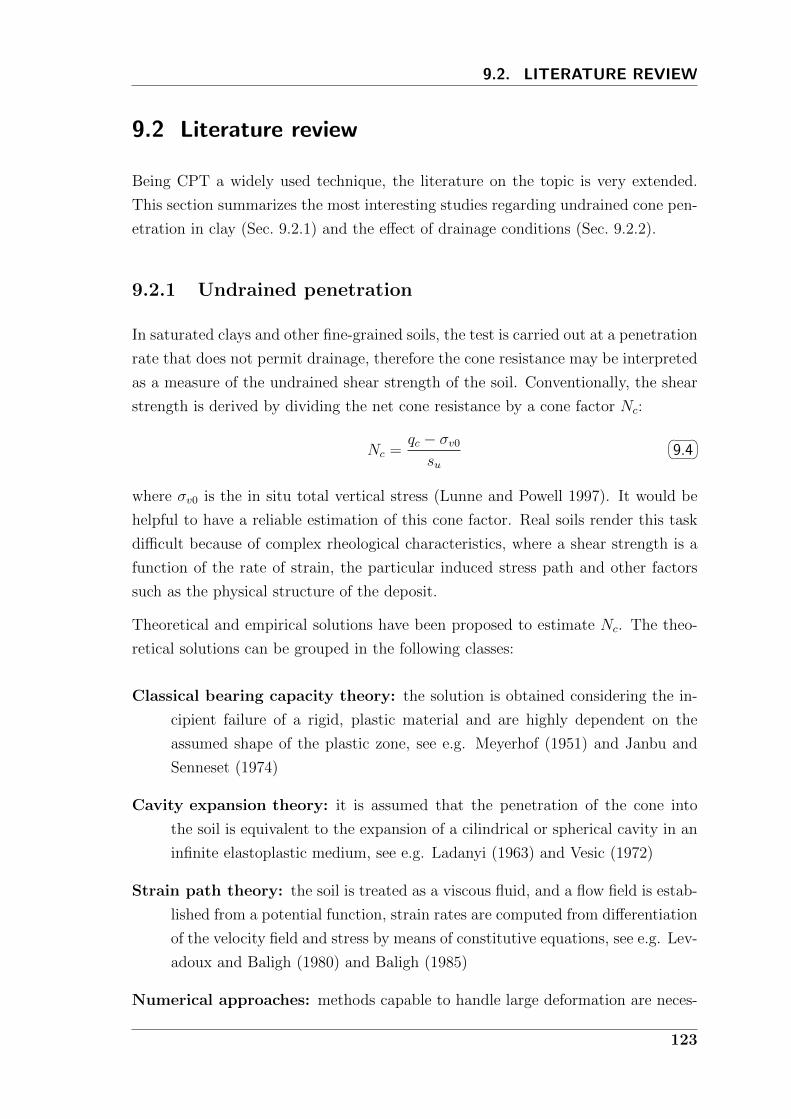
9.2. LITERATURE REVIEW
9.2 Literature review
Being CPT a widely used technique, the literature on the topic is very extended.
This section summarizes the most interesting studies regarding undrained cone pen-
etration in clay (Sec. 9.2.1) and the effect of drainage conditions (Sec. 9.2.2).
9.2.1 Undrained penetration
In saturated clays and other fine-grained soils, the test is carried out at a penetration
rate that does not permit drainage, therefore the cone resistance may be interpreted
as a measure of the undrained shear strength of the soil. Conventionally, the shear
strength is derived by dividing the net cone resistance by a cone factor Nc:
Nc =qc − σv0
su
9.4
where σv0 is the in situ total vertical stress (Lunne and Powell 1997). It would be
helpful to have a reliable estimation of this cone factor. Real soils render this task
difficult because of complex rheological characteristics, where a shear strength is a
function of the rate of strain, the particular induced stress path and other factors
such as the physical structure of the deposit.
Theoretical and empirical solutions have been proposed to estimate Nc. The theo-
retical solutions can be grouped in the following classes:
Classical bearing capacity theory: the solution is obtained considering the in-
cipient failure of a rigid, plastic material and are highly dependent on the
assumed shape of the plastic zone, see e.g. Meyerhof (1951) and Janbu and
Senneset (1974)
Cavity expansion theory: it is assumed that the penetration of the cone into
the soil is equivalent to the expansion of a cilindrical or spherical cavity in an
infinite elastoplastic medium, see e.g. Ladanyi (1963) and Vesic (1972)
Strain path theory: the soil is treated as a viscous fluid, and a flow field is estab-
lished from a potential function, strain rates are computed from differentiation
of the velocity field and stress by means of constitutive equations, see e.g. Lev-
adoux and Baligh (1980) and Baligh (1985)
Numerical approaches: methods capable to handle large deformation are neces-
123

CHAPTER 9. SIMULATION OF CONE PENETRATION TESTING
sary, e.g. ALE (van den Berg 1994, Lu et al. 2004), CEL (Qiu 2014), MPM
(Beuth 2012). An alternative approach for large deformation analysis is the
Eulerian FE formulation; extra terms are included in the governing equations
to account for the rotation of the material and convection of the stress field,
which can lead to mathematical difficulties when complex constitutive models
are adopted (van den Berg et al. 1996).
Since cone penetration is a complex phenomenon, all the theoretical solutions make
several simplifying assumptions regarding soil behavior, failure mechanism and bound-
ary conditions. Theoretical solutions have limitations in modeling the real soil be-
havior. Hence, empirical correlations are sometimes preferred.
The soil undrained shear strength can be estimated from different empirical corre-
lations using alternatively the total cone resistance, the effective cone resistance or
the excess pore pressure. Over the years, a large number of studies have been per-
formed, many of them resulting in cone factor in the range 6-20, more commonly in
the range 9-17, with the shear strength measured in triaxial compression generally
used to normalize the cone resistance (Lunne and Powell 1997).
9.2.1.1 Theoretical estimations of the cone factor
A number of different theoretical solutions have been presented in the litterature,
see Yu and Mitchell (1998) for a short overview. All solutions have shown that, even
for a simple Tresca soil model, the theoretical cone factor is influenced by:
1. The rigidity index Ir = G/su where G is the shear modulus of the soil
2. The in situ stress ratio ∆ = (σv0 − σh0)/(2su) where σv0 and σh0 are the in
situ vertical and horizontal stresses
3. The roughness of the cone αc = a/su where a is shear stress at the contact
surface.
The use of cavity expansion theory allows to obtain relatively simple analytical
solution. A review of cavity expansion theory and its application is provided in
Yu, Herrmann, and Boulanger (2000). With this method the prediction of the cone
resistance requires two steps: first the limit pressure for cavity expansion in soil must
be determined, second the limit pressure must be related to the cone resistance.
124
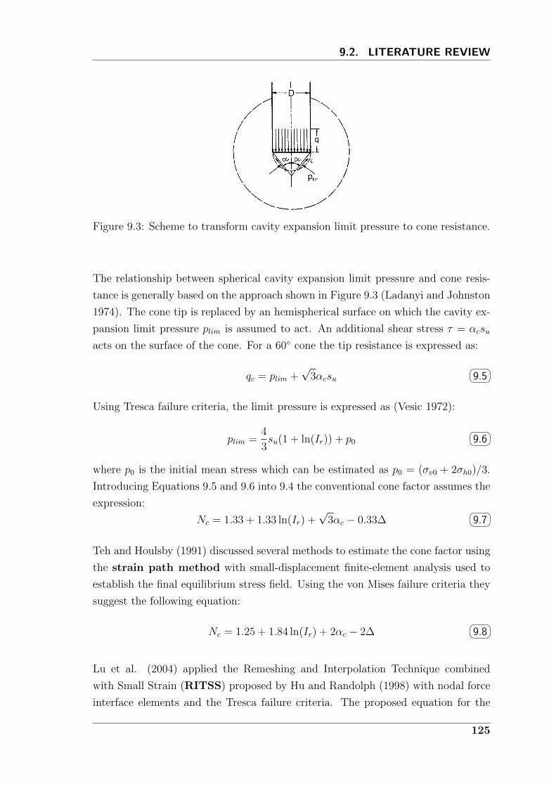
9.2. LITERATURE REVIEW
Figure 9.3: Scheme to transform cavity expansion limit pressure to cone resistance.
The relationship between spherical cavity expansion limit pressure and cone resis-
tance is generally based on the approach shown in Figure 9.3 (Ladanyi and Johnston
1974). The cone tip is replaced by an hemispherical surface on which the cavity ex-
pansion limit pressure plim is assumed to act. An additional shear stress τ = αcsu
acts on the surface of the cone. For a 60 cone the tip resistance is expressed as:
qc = plim +√
3αcsu 9.5
Using Tresca failure criteria, the limit pressure is expressed as (Vesic 1972):
plim =4
3su(1 + ln(Ir)) + p0
9.6
where p0 is the initial mean stress which can be estimated as p0 = (σv0 + 2σh0)/3.
Introducing Equations 9.5 and 9.6 into 9.4 the conventional cone factor assumes the
expression:
Nc = 1.33 + 1.33 ln(Ir) +√
3αc − 0.33∆ 9.7
Teh and Houlsby (1991) discussed several methods to estimate the cone factor using
the strain path method with small-displacement finite-element analysis used to
establish the final equilibrium stress field. Using the von Mises failure criteria they
suggest the following equation:
Nc = 1.25 + 1.84 ln(Ir) + 2αc − 2∆ 9.8
Lu et al. (2004) applied the Remeshing and Interpolation Technique combined
with Small Strain (RITSS) proposed by Hu and Randolph (1998) with nodal force
interface elements and the Tresca failure criteria. The proposed equation for the
125
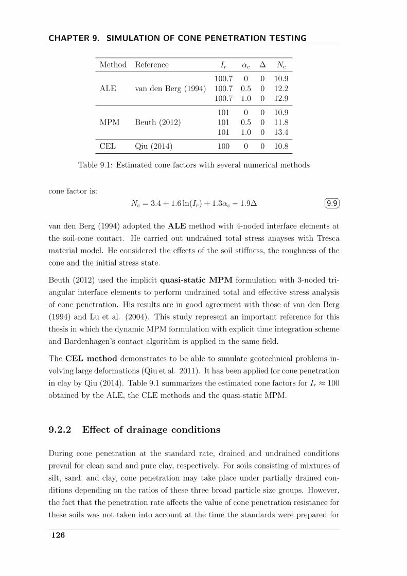
CHAPTER 9. SIMULATION OF CONE PENETRATION TESTING
Method Reference Ir αc ∆ Nc
ALE van den Berg (1994)100.7 0 0 10.9100.7 0.5 0 12.2100.7 1.0 0 12.9
MPM Beuth (2012)101 0 0 10.9101 0.5 0 11.8101 1.0 0 13.4
CEL Qiu (2014) 100 0 0 10.8
Table 9.1: Estimated cone factors with several numerical methods
cone factor is:
Nc = 3.4 + 1.6 ln(Ir) + 1.3αc − 1.9∆ 9.9
van den Berg (1994) adopted the ALE method with 4-noded interface elements at
the soil-cone contact. He carried out undrained total stress anayses with Tresca
material model. He considered the effects of the soil stiffness, the roughness of the
cone and the initial stress state.
Beuth (2012) used the implicit quasi-static MPM formulation with 3-noded tri-
angular interface elements to perform undrained total and effective stress analysis
of cone penetration. His results are in good agreement with those of van den Berg
(1994) and Lu et al. (2004). This study represent an important reference for this
thesis in which the dynamic MPM formulation with explicit time integration scheme
and Bardenhagen’s contact algorithm is applied in the same field.
The CEL method demonstrates to be able to simulate geotechnical problems in-
volving large deformations (Qiu et al. 2011). It has been applied for cone penetration
in clay by Qiu (2014). Table 9.1 summarizes the estimated cone factors for Ir ≈ 100
obtained by the ALE, the CLE methods and the quasi-static MPM.
9.2.2 Effect of drainage conditions
During cone penetration at the standard rate, drained and undrained conditions
prevail for clean sand and pure clay, respectively. For soils consisting of mixtures of
silt, sand, and clay, cone penetration may take place under partially drained con-
ditions depending on the ratios of these three broad particle size groups. However,
the fact that the penetration rate affects the value of cone penetration resistance for
these soils was not taken into account at the time the standards were prepared for
126
9.2. LITERATURE REVIEW
the CPT. This means that the use of correlations developed for sand, in which tests
would be drained, or clay in which tests would be undrained, will not work for soils
in which the penetration at the standard rate takes place under partially drained
conditions.
If the penetration rate is relatively low compared to the pressure dissipation rate, the
soil ahead of the advancing cone consolidates during penetration, thereby developing
larger shear strength and stiffness than it would have under undrained conditions.
The closer the conditions are to fully drained during penetration, the higher the
value of qc.
Another physical process that play a role for soils with large clay content for penetra-
tion under undrained conditions, is the effect of the rate of loading on shear strength
(viscosity effect). The higher the penetration rate is, the larger the undrained shear
strength is, and the larger the tip resistance is. These two physical processes, i.e.
drainage and loading rate effects, have opposite effects on qc (Kim et al. 2008).
A normalized penetration rate has been introduced by Finnie and Randolph (1994):
V =vD
cv
9.10
where v = penetration rate, D = penetrometer diameter and cv = consolidation
coefficient. It has been proved that it is able to characterize the degree of partial
consolidation during penetration. However, for very high penetration rate, if strain-
rate effect are significant, qc increases with v and it is shown to be a function of
v/D (Chung et al. 2006, Lehane et al. 2009). In this chapter attention is focused
on the effect of the drainage conditions; since strain rate effects are neglected, V is
an appropriate parameter to normalize the results.
The research on the effect of penetration rate on the tip resistance comprises nu-
merous experimental data obtained with laboratory tests, such as centrifuge and
calibration chamber tests, and in situ tests (House et al. 2001, Randolph and Hope
2004, Schneider et al. 2007, Kim et al. 2008, Lehane et al. 2009, Jaeger et al. 2010,
Oliveira et al. 2011). Centrifuge tests are mainly performed on kaolin clay (House
et al. 2001, Randolph and Hope 2004, Schneider et al. 2007), however different
type of soil such as natural clay (Chung et al. 2006), mixture of sand and kaolin
(Kim et al. 2008, Jaeger et al. 2010), sand and bentonite (Schneider et al. 2007)
and silt (Oliveira et al. 2011) have been considered. Most of the tests have been
performed on normally consolidated soil; the effect of overconsolidation has been
investigated by Schneider et al. (2007) and Lehane et al. (2009). Different shape of
127
CHAPTER 9. SIMULATION OF CONE PENETRATION TESTING
the penetrometer has been used, such as T-bar, ball, plate and cone.
Experimental evidence shows that a typical backbone curve can be drown in the
qc−log(V ) plane. The cone resistance is constant for high values of V , i.e. undrained
conditions, as well as low values of V , i.e. drained conditions. The range of par-
tially drained conditions highly depends on the penetrometer and soil characteristic.
According to the literature, the transition to fully drained conditions lies between
0.01 and 4; the transition to fully undrained conditions lies in the range 10-100.
Differences can also be attributed to the method used to estimate cv by the differ-
ent authors. Since the water flow is mainly horizontal, the ch is adopted in a few
publications; this choice seems reasonable, but sometimes difficult to put in practice
especially in laboratory tests.
The tip resistance q is usually normalized by a reference penetration resistance qref ;
q/qref is called normalized resistance or resistance ratio. Data can be interpolated
by a function of the form:q
qref= a+
b
1 + cV m
9.11
where a, b, c and m are constants that need to be calibrated. Usually qref is the value
corresponding to the fully undrained penetration. In many publications the results
are presented referring to the net tip resistance qnet = qc − σv0, however also the
total tip resistance can be adopted. In this thesis normalized results are presented
in terms of net tip resistance and undrained net tip resistance, i.e. q = qnet and
qref = (qnet)undrained.
The values assumed by the constants in Equation 9.11 depend on the penetrometer
shape and the type of soil. They seem to vary in a relatively narrow range for
the test performed on kaolin, while results differ for other types of soil. The sum
a + b assumes the meaning of the resistance ratio between drained and undrained
conditions qdrained/qref . As can be deduced from Figure 9.4, the parameter c modifies
the inflection point of the curve, while m influences the curvature.
An alternative expression for the backbone curve has been proposed by Oliveira
et al. (2011), in which a physical meaning can be given to the constants. However,
Equation 9.11 is preferred because it is more popular in the literature.
Only a few authors addressed the problem with numerical techniques (Silva et al.
2006, Yi et al. 2012). In his PhD thesis, Silva (2005) studied the effect of pene-
tration rate and OCR on the tip resistance and pore pressure dissipation using a
coupled cavity expansion-finite element method. In this method, only radial soil de-
formations and water flow are considered, i.e. the bidimensional penetration process
128

9.2. LITERATURE REVIEW
Figure 9.4: Effect of parameters c and m on the curves given by Eq. 9.11 (a = b = 1).
is simulated in a simplified way neglecting axial soil deformation.
The soil is modeled with the Modified Cam Clay model and the tip resistance is
calculated with
qc = σr +µ
tanασ′r
9.12
where σr and σ′r are the total and effective radial stress from the cavity expansion
solution, respectively; µ = interface friction, and α = angle of the cone tip. The
friction coefficient at cone surface is assumed equal to the tangent of the soil friction
angle, i.e. µ = tan(φ).
Silva (2005) normalized the results using the horizontal consolidation coefficient,
estimated with:
ch =k(1 + e)σ′r
λγw
9.13
where k is the Darcy’s permeability, λ is the virgin compression index, e and σ′r
are the void ratio and the horizontal effective stress of the soil adjacent to the cone
immediately after cavity expansion. The author pointed out that the experimental
cv values are comparable to the computed ch (Eq. 9.13) under undrained conditions.
However, the values of ch increase in magnitude as consolidation during penetration
is allowed due to greater change in values of σ′r at low speeds. This affects the shape
of the backbone curve.
He considered OCR values ranging from 1 to 32 showing that, for a given undrained
129

CHAPTER 9. SIMULATION OF CONE PENETRATION TESTING
Figure 9.5: Resistance ratio against normalized penetration velocity for variousmodulus ratio G/p′ according to Yi et al. (2012)
shear strenght, OCR influences the generation of excess pore pressure in undrained
conditions; higher pressures are observed with lower OCR. However, the normalized
pore pressure ∆umax/∆uref (∆umax = maximum excess pore pressure, ∆uref =
excess pore pressure for undrained conditions) is not influenced by the OCR and
only a slight effect on the resistance ratio is observed.
Yi et al. (2012) used the updated Lagrangian FEM with logarithmic strain to study
the effect of partial consolidation during cone penetration on the tip resistance and
excess pore pressure. The influence of soil strength and stiffness on the backbone
curve is investigated. The soil behavior is characterized by the Drucker-Prager
model; further analyses included the effect of volumetric yielding by using the mod-
ified Drucker-Prager cap model. The soil-cone contact is assumed to be smooth
since numerical difficulties were encountered introducing friction at the interface.
This method suffers of problem of mesh distortion in the cone vicinity, which are
controlled by modifying the mesh density and the element aspect ratio through a
trial-and-error process.
This publication shows how the net cone resistance increases with the modulus
ratio (G/p′, p′ = mean effective stress) and the friction angle in the whole range of
drainage conditions. On the other hand, the resistance ratio qnet/qref increases only
with the modulus ratio and is relatively insensitive to the friction angle (Fig. 9.5).
Considering the volumetric yielding, the resistance ratio reduces as λ/κ increases;
for λ/κ between 3 and 5, as common in clay, the reduction is between 5% and 15%.
DeJong and Randolph (2012) analyzed the effect of drainage conditions consid-
ering published experimental data and numerical parametric studies. This study
130

9.3. HOW TO SIMULATE CPT?
addressed the determination of soil behavior type by mean of the charts proposed
by Robertson (1990) and Schneider et al. (2008a). These charts, widely used in
engineering practice, were developed for standard rate of penetration. DeJong and
Randolph (2012) showed that they should not be used for v 6= 2cm/s since the effect
of drainage conditions shifts the data in a different chart area, corresponding to an
inappropriate soil type.
From this literature review it can be concluded that the cone penetration in partially
drained conditions is a complex process which has been mainly studied experimen-
tally. Numerical simulations with cavity expansion theory (Silva et al. 2006) and
FEM (Yi et al. 2012) give an interesting contribution in the comprehension of
the main features of the phenomenon, even though they have some limitations and
drawbacks as previously discussed.
The lack of advanced numerical simulations of cone penetration in partially drained
conditions, together with the importance of a better understanding of the phe-
nomenon for the engineering practice, form the motivation of the present study, in
which the two-phase MPM with contact algorithm is applied to the study of CPT
in different drainage conditions.
9.3 How to simulate CPT?
This section discusses the most important features that a numerical model should
have to simulate the cone penetration and how they are considered in this study. As
already pointed out in Chapter 2, a model is an appropriate simplification of reality,
which means that only the essential features of the real process must be included.
During cone penetration, the soil initially located underneath the tip is pushed aside;
this obviously generates large deformations. The numerical model has to take this
into account. As already shown in previous chapters of this thesis, the MPM is well
suited to simulate large deformations, therefore the study of the cone penetration
process represents an interesting application of the method.
The attention of this study is focused on the cone tip resistance which is calculated
with:
qc =
∑nci=1 Fi,yA
9.14
where the numerator is the sum of the vertical reaction forces Fi,y at the nc nodes
belonging to the cone tip and A is the area of the cone slice which is considered
131
CHAPTER 9. SIMULATION OF CONE PENETRATION TESTING
in the model. Considering a soil element connected to the cone, the reaction force
consists in:
F =
∫V
BTσdV 9.15
where V is the element volume and σ is the total stress.
One of the most difficult issue is the proper simulation of the saturated soil behavior.
On one hand the soil-water interaction must be included. On the other hand, the
constitutive model must be capable to describe the response of the soil under loading
conditions in a good enough way for the considered problem.
As already discussed in Section 3.5 in undrained and drained conditions the soil-
water interaction can be handled in a simplified way by using the one-phase approach
(Chap. 3). In partially drained conditions a fully coupled two-phase approach must
be applied (Chap. 4).
Constitutive modeling of the real soil behavior is challenging because several fac-
tors such as non-linear compressibility, stress-path dependency of shear strength,
anisotropy, internal structure, viscosity and so on should be considered. In engi-
neering practice very simple models, such as Tresca and Mohr-Coulomb, are often
applied. They can give only a crude representation of the soil mechanical response,
but they are easy to use and can give a first idea of the main features of the problem.
Very advanced constitutive models are able to capture several characteristics of soil
behavior, but a certain level of complexity is added to the numerical model and the
input parameters may be not easy to calibrate. The choice of the constitutive model
should guarantee a realistic simulation of the considered problem with an acceptable
level of complexity.
The purpose of this chapter is to simulate cone penetration in clay, therefore the
material model must be selected between those which demonstrated to be suitable
for this type of soil. The undrained behavior of clay is very often modeled with the
elastic perfectly plastic model with Tresca failure criteria (Sec. 5.2.1). This very
simple model does not consider the stress path dependency of the shear strength,
neither the non-linear elastic response of the material, but has been successfully
used to simulate CPT in undrained conditions, see e.g. van den Berg (1994), Lu
et al. (2004) and Beuth et al. (2008).
The Modified Cam Clay model (Schofield and Wroth 1968) has been widely used
to model soft clay both in drained and undrained conditions. It can take into
account the non-linear soil compressibility, the occurance of shear and volumetric
deformations during yielding and the stress-path dependency of the shear strength.
132
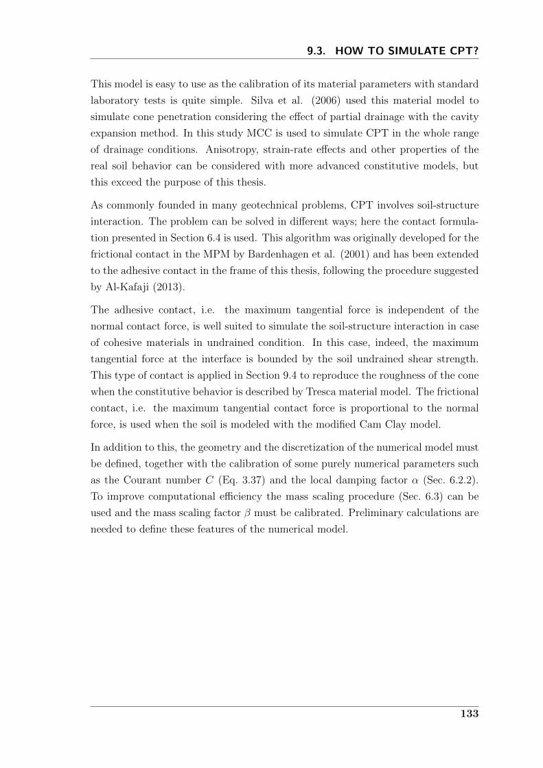
9.3. HOW TO SIMULATE CPT?
This model is easy to use as the calibration of its material parameters with standard
laboratory tests is quite simple. Silva et al. (2006) used this material model to
simulate cone penetration considering the effect of partial drainage with the cavity
expansion method. In this study MCC is used to simulate CPT in the whole range
of drainage conditions. Anisotropy, strain-rate effects and other properties of the
real soil behavior can be considered with more advanced constitutive models, but
this exceed the purpose of this thesis.
As commonly founded in many geotechnical problems, CPT involves soil-structure
interaction. The problem can be solved in different ways; here the contact formula-
tion presented in Section 6.4 is used. This algorithm was originally developed for the
frictional contact in the MPM by Bardenhagen et al. (2001) and has been extended
to the adhesive contact in the frame of this thesis, following the procedure suggested
by Al-Kafaji (2013).
The adhesive contact, i.e. the maximum tangential force is independent of the
normal contact force, is well suited to simulate the soil-structure interaction in case
of cohesive materials in undrained condition. In this case, indeed, the maximum
tangential force at the interface is bounded by the soil undrained shear strength.
This type of contact is applied in Section 9.4 to reproduce the roughness of the cone
when the constitutive behavior is described by Tresca material model. The frictional
contact, i.e. the maximum tangential contact force is proportional to the normal
force, is used when the soil is modeled with the modified Cam Clay model.
In addition to this, the geometry and the discretization of the numerical model must
be defined, together with the calibration of some purely numerical parameters such
as the Courant number C (Eq. 3.37) and the local damping factor α (Sec. 6.2.2).
To improve computational efficiency the mass scaling procedure (Sec. 6.3) can be
used and the mass scaling factor β must be calibrated. Preliminary calculations are
needed to define these features of the numerical model.
133
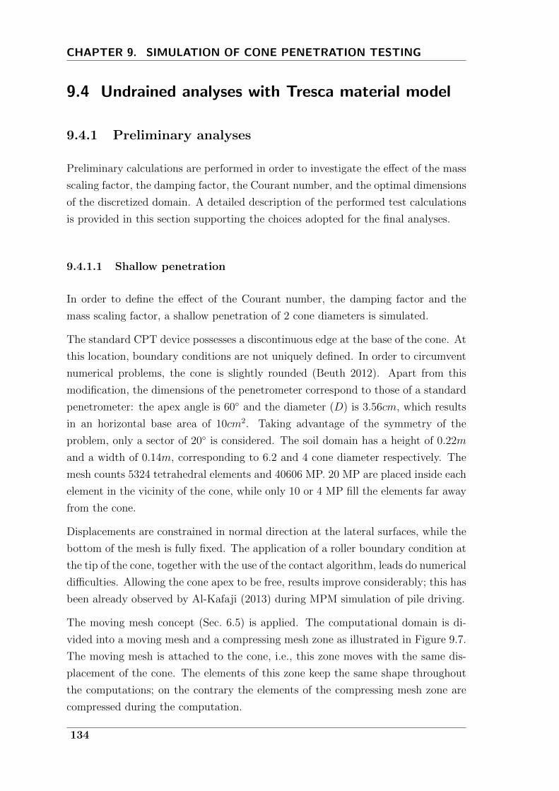
CHAPTER 9. SIMULATION OF CONE PENETRATION TESTING
9.4 Undrained analyses with Tresca material model
9.4.1 Preliminary analyses
Preliminary calculations are performed in order to investigate the effect of the mass
scaling factor, the damping factor, the Courant number, and the optimal dimensions
of the discretized domain. A detailed description of the performed test calculations
is provided in this section supporting the choices adopted for the final analyses.
9.4.1.1 Shallow penetration
In order to define the effect of the Courant number, the damping factor and the
mass scaling factor, a shallow penetration of 2 cone diameters is simulated.
The standard CPT device possesses a discontinuous edge at the base of the cone. At
this location, boundary conditions are not uniquely defined. In order to circumvent
numerical problems, the cone is slightly rounded (Beuth 2012). Apart from this
modification, the dimensions of the penetrometer correspond to those of a standard
penetrometer: the apex angle is 60 and the diameter (D) is 3.56cm, which results
in an horizontal base area of 10cm2. Taking advantage of the symmetry of the
problem, only a sector of 20 is considered. The soil domain has a height of 0.22m
and a width of 0.14m, corresponding to 6.2 and 4 cone diameter respectively. The
mesh counts 5324 tetrahedral elements and 40606 MP. 20 MP are placed inside each
element in the vicinity of the cone, while only 10 or 4 MP fill the elements far away
from the cone.
Displacements are constrained in normal direction at the lateral surfaces, while the
bottom of the mesh is fully fixed. The application of a roller boundary condition at
the tip of the cone, together with the use of the contact algorithm, leads do numerical
difficulties. Allowing the cone apex to be free, results improve considerably; this has
been already observed by Al-Kafaji (2013) during MPM simulation of pile driving.
The moving mesh concept (Sec. 6.5) is applied. The computational domain is di-
vided into a moving mesh and a compressing mesh zone as illustrated in Figure 9.7.
The moving mesh is attached to the cone, i.e., this zone moves with the same dis-
placement of the cone. The elements of this zone keep the same shape throughout
the computations; on the contrary the elements of the compressing mesh zone are
compressed during the computation.
134
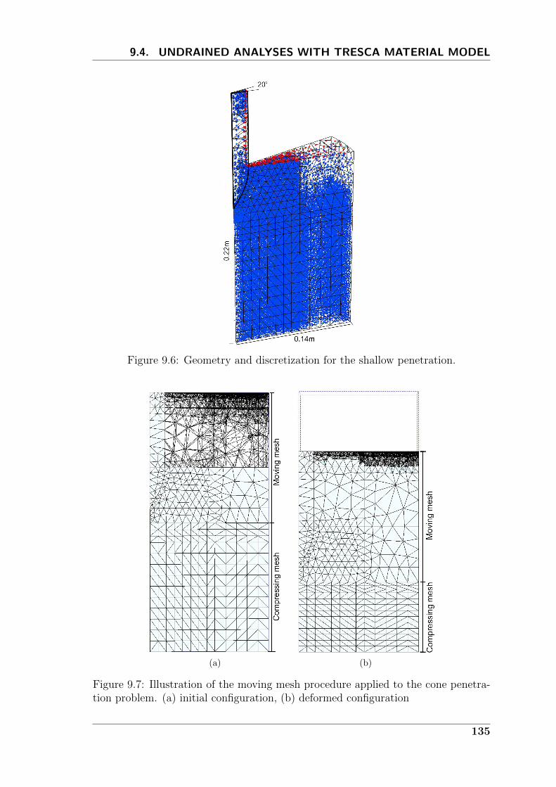
9.4. UNDRAINED ANALYSES WITH TRESCA MATERIAL MODEL
Figure 9.6: Geometry and discretization for the shallow penetration.
(a) (b)
Figure 9.7: Illustration of the moving mesh procedure applied to the cone penetra-tion problem. (a) initial configuration, (b) deformed configuration
135

CHAPTER 9. SIMULATION OF CONE PENETRATION TESTING
Thanks of this procedure, the fine mesh is always kept around the cone and the
occurrence of elements having cone and soil particles is avoided. Moreover, the need
of identifying the new soil-structure interface during the computation is eliminated
as the interface nodes coincide with the geometry of the cone throughout the com-
putation. As a consequence, the unit normal vectors, which are required in the
contact algorithm, do not change and hence the inaccuracy of recomputing them is
eliminated (Al-Kafaji 2013).
Because of the downwards movement of the moving mesh zone, a region with ini-
tially empty elements is required above the soil surface to accommodate the material
during computations. The elements of the compressed zone must have a reasonable
aspect ratio (vertical to radial dimensions) in the initial configuration to avoid ex-
cessive mesh distortion after considerable penetration.
In this preliminary study the penetration of the cone in soft clay under undrained
conditions is simulated. The soil is considered as a weightless material, modeled
with the elastic perfectly plastic model with Tresca failure criteria. The Young’s
modulus is Eu = 6000kPa, the Poisson ratio is νu = 0.49 and the undrained shear
strength is su = 20kPa.
The cone penetrates at a rate of 2cm/s, this means that it’s a slow process; indeed
it has been well simulated by quasi-static numerical formualtions (Beuth 2012). In
simulations of slow processes, mass scaling can be used to improve efficiency. The
original soil density is ρsat = 1700g/cm3, but can be increased by the factor β,
speeding up the calculation by a factor√β. Figure 9.8 shows the tip stress over
the normalized cone displacement for several values of the mass scaling factor. Ex-
tremely high values of β generate high oscillations, especially at the beginning of
the calculation, when dynamic effects are more relevant, together with an overesti-
mation of qc. A mass scaling factor equal to 400 is considered reasonable for this
problem.
Natural materials normally dissipate a certain amount of energy, however the con-
stitutive model often does not take this into account. The introduction of the local
damping allows to dissipate dynamic waves that generate noise in the numerical so-
lution (Sec. 6.2.2); on the other hand the damping factor α should not be too large
in order to avoid overestimation of the tip stress (Fig. 9.9). A value of α = 0.15 is
considered optimal for the considered problem.
In CPT simulation, energy conservation is not an issue, therefore a Courant number
C close to 1 can be used. As shown in Figure 9.10 a reduction of C does not improve
136
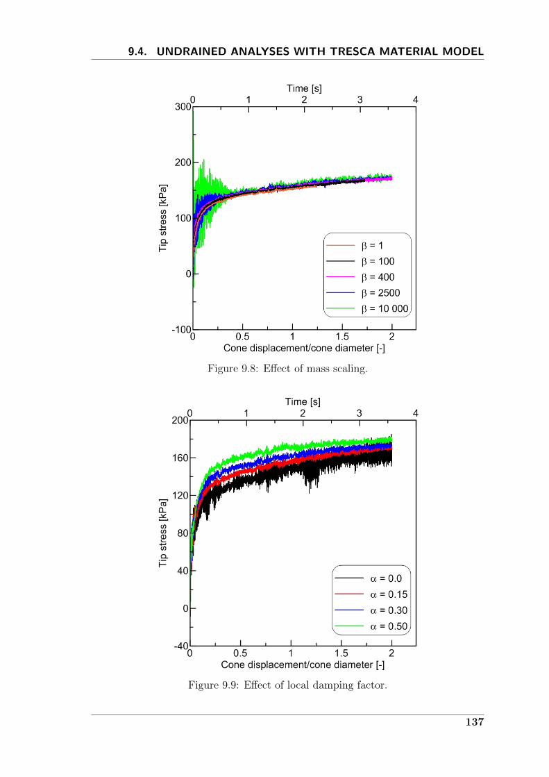
9.4. UNDRAINED ANALYSES WITH TRESCA MATERIAL MODEL
Figure 9.8: Effect of mass scaling.
Figure 9.9: Effect of local damping factor.
137

CHAPTER 9. SIMULATION OF CONE PENETRATION TESTING
Figure 9.10: Effect of the Courant number.
significantly the result.
A large number of MP in the vicinity of the cone permits to have nice results
without increasing dramatically the computational cost. Oscillations can be further
reduced by refining the mesh; this results in high computational effort and is not
considered necessary for the scope of this study. In general the accurancy and the
computational cost increase more with the mesh refinement than with the number
of MP.
9.4.1.2 Deep penetration
In the current section the definition of the optimal geometry to simulate a deep pene-
tration of the cone is discussed. Beuth (2012) observed that the steady state solution
is approximately reached after 6D penetration, therefore the domain should be big
enough to accommodate approximately a penetration of 10D without observing any
boundary effect.
From numerical analyses the radius of the plastic zone is shown to depend on the soil
rigidity index Ir, the initial stress state ∆ and secondly by the roughness of the cone
138
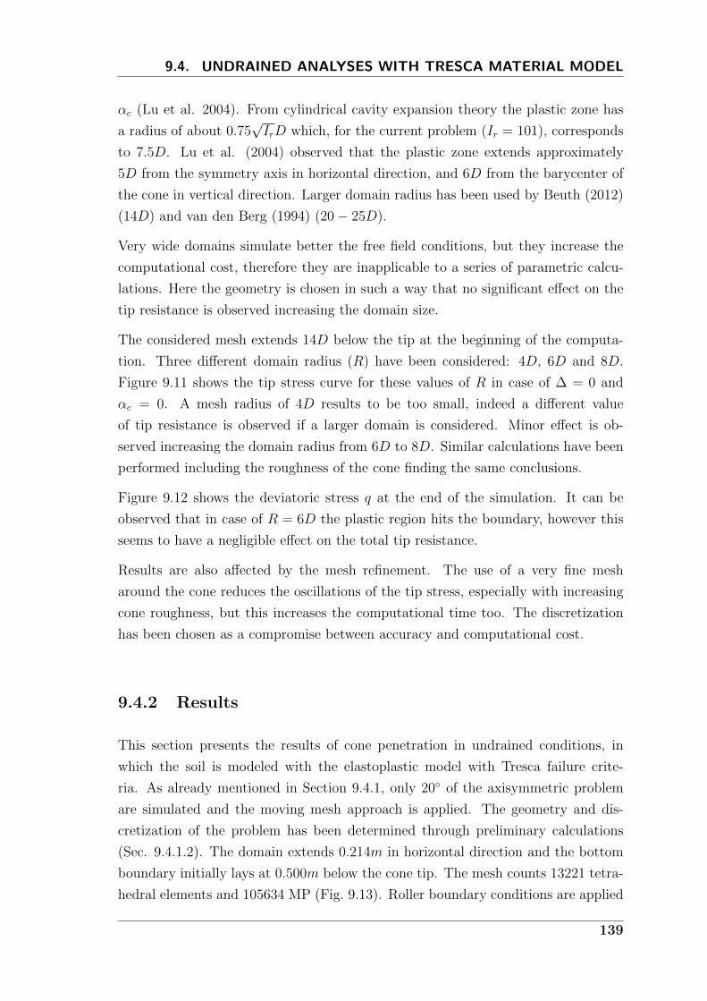
9.4. UNDRAINED ANALYSES WITH TRESCA MATERIAL MODEL
αc (Lu et al. 2004). From cylindrical cavity expansion theory the plastic zone has
a radius of about 0.75√IrD which, for the current problem (Ir = 101), corresponds
to 7.5D. Lu et al. (2004) observed that the plastic zone extends approximately
5D from the symmetry axis in horizontal direction, and 6D from the barycenter of
the cone in vertical direction. Larger domain radius has been used by Beuth (2012)
(14D) and van den Berg (1994) (20− 25D).
Very wide domains simulate better the free field conditions, but they increase the
computational cost, therefore they are inapplicable to a series of parametric calcu-
lations. Here the geometry is chosen in such a way that no significant effect on the
tip resistance is observed increasing the domain size.
The considered mesh extends 14D below the tip at the beginning of the computa-
tion. Three different domain radius (R) have been considered: 4D, 6D and 8D.
Figure 9.11 shows the tip stress curve for these values of R in case of ∆ = 0 and
αc = 0. A mesh radius of 4D results to be too small, indeed a different value
of tip resistance is observed if a larger domain is considered. Minor effect is ob-
served increasing the domain radius from 6D to 8D. Similar calculations have been
performed including the roughness of the cone finding the same conclusions.
Figure 9.12 shows the deviatoric stress q at the end of the simulation. It can be
observed that in case of R = 6D the plastic region hits the boundary, however this
seems to have a negligible effect on the total tip resistance.
Results are also affected by the mesh refinement. The use of a very fine mesh
around the cone reduces the oscillations of the tip stress, especially with increasing
cone roughness, but this increases the computational time too. The discretization
has been chosen as a compromise between accuracy and computational cost.
9.4.2 Results
This section presents the results of cone penetration in undrained conditions, in
which the soil is modeled with the elastoplastic model with Tresca failure crite-
ria. As already mentioned in Section 9.4.1, only 20 of the axisymmetric problem
are simulated and the moving mesh approach is applied. The geometry and dis-
cretization of the problem has been determined through preliminary calculations
(Sec. 9.4.1.2). The domain extends 0.214m in horizontal direction and the bottom
boundary initially lays at 0.500m below the cone tip. The mesh counts 13221 tetra-
hedral elements and 105634 MP (Fig. 9.13). Roller boundary conditions are applied
139
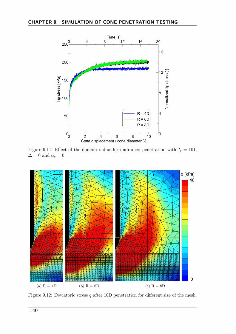
CHAPTER 9. SIMULATION OF CONE PENETRATION TESTING
Figure 9.11: Effect of the domain radius for undrained penetration with Ir = 101,∆ = 0 and αc = 0.
(a) R = 4D (b) R = 6D (c) R = 8D
Figure 9.12: Deviatoric stress q after 10D penetration for different size of the mesh.
140
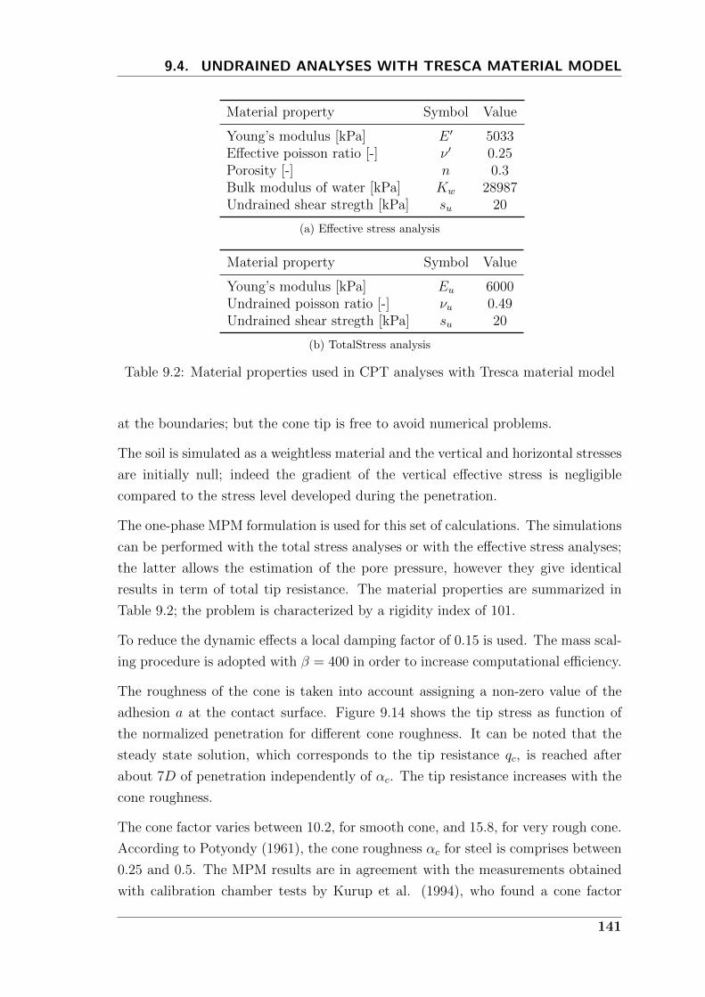
9.4. UNDRAINED ANALYSES WITH TRESCA MATERIAL MODEL
Material property Symbol Value
Young’s modulus [kPa] E ′ 5033Effective poisson ratio [-] ν ′ 0.25Porosity [-] n 0.3Bulk modulus of water [kPa] Kw 28987Undrained shear stregth [kPa] su 20
(a) Effective stress analysis
Material property Symbol Value
Young’s modulus [kPa] Eu 6000Undrained poisson ratio [-] νu 0.49Undrained shear stregth [kPa] su 20
(b) TotalStress analysis
Table 9.2: Material properties used in CPT analyses with Tresca material model
at the boundaries; but the cone tip is free to avoid numerical problems.
The soil is simulated as a weightless material and the vertical and horizontal stresses
are initially null; indeed the gradient of the vertical effective stress is negligible
compared to the stress level developed during the penetration.
The one-phase MPM formulation is used for this set of calculations. The simulations
can be performed with the total stress analyses or with the effective stress analyses;
the latter allows the estimation of the pore pressure, however they give identical
results in term of total tip resistance. The material properties are summarized in
Table 9.2; the problem is characterized by a rigidity index of 101.
To reduce the dynamic effects a local damping factor of 0.15 is used. The mass scal-
ing procedure is adopted with β = 400 in order to increase computational efficiency.
The roughness of the cone is taken into account assigning a non-zero value of the
adhesion a at the contact surface. Figure 9.14 shows the tip stress as function of
the normalized penetration for different cone roughness. It can be noted that the
steady state solution, which corresponds to the tip resistance qc, is reached after
about 7D of penetration independently of αc. The tip resistance increases with the
cone roughness.
The cone factor varies between 10.2, for smooth cone, and 15.8, for very rough cone.
According to Potyondy (1961), the cone roughness αc for steel is comprises between
0.25 and 0.5. The MPM results are in agreement with the measurements obtained
with calibration chamber tests by Kurup et al. (1994), who found a cone factor
141
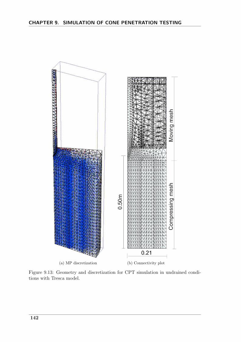
CHAPTER 9. SIMULATION OF CONE PENETRATION TESTING
(a) MP discretization (b) Connectivity plot
Figure 9.13: Geometry and discretization for CPT simulation in undrained condi-tions with Tresca model.
142
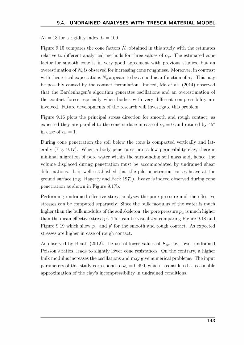
9.4. UNDRAINED ANALYSES WITH TRESCA MATERIAL MODEL
Nc = 13 for a rigidity index Ir = 100.
Figure 9.15 compares the cone factors Nc obtained in this study with the estimates
relative to different analytical methods for three values of αc. The estimated cone
factor for smooth cone is in very good agreement with previous studies, but an
overestimation of Nc is observed for increasing cone roughness. Moreover, in contrast
with theoretical expectations Nc appears to be a non linear function of αc. This may
be possibly caused by the contact formulation. Indeed, Ma et al. (2014) observed
that the Bardenhagen’s algorithm generates oscillations and an overestimation of
the contact forces especially when bodies with very different compressibility are
involved. Future developments of the research will investigate this problem.
Figure 9.16 plots the principal stress direction for smooth and rough contact; as
expected they are parallel to the cone surface in case of αc = 0 and rotated by 45
in case of αc = 1.
During cone penetration the soil below the cone is compacted vertically and lat-
erally (Fig. 9.17). When a body penetrates into a low permeability clay, there is
minimal migration of pore water within the surrounding soil mass and, hence, the
volume displaced during penetration must be accommodated by undrained shear
deformations. It is well established that the pile penetration causes heave at the
ground surface (e.g. Hagerty and Peck 1971). Heave is indeed observed during cone
penetration as shown in Figure 9.17b.
Performing undrained effective stress analyses the pore pressure and the effective
stresses can be computed separately. Since the bulk modulus of the water is much
higher than the bulk modulus of the soil skeleton, the pore pressure pw is much higher
than the mean effective stress p′. This can be visualized comparing Figure 9.18 and
Figure 9.19 which show pw and p′ for the smooth and rough contact. As expected
stresses are higher in case of rough contact.
As observed by Beuth (2012), the use of lower values of Kw, i.e. lower undrained
Poisson’s ratios, leads to slightly lower cone resistances. On the contrary, a higher
bulk modulus increases the oscillations and may give numerical problems. The input
parameters of this study correspond to νu = 0.490, which is considered a reasonable
approximation of the clay’s incompressibility in undrained conditions.
143
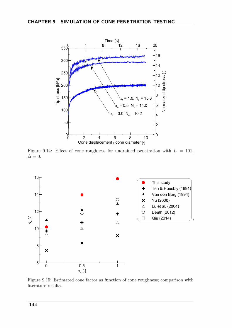
CHAPTER 9. SIMULATION OF CONE PENETRATION TESTING
Figure 9.14: Effect of cone roughness for undrained penetration with Ir = 101,∆ = 0.
Figure 9.15: Estimated cone factor as function of cone roughness; comparison withliterature results.
144

9.4. UNDRAINED ANALYSES WITH TRESCA MATERIAL MODEL
Figure 9.16: Principal stress direction around the cone in case of αc = 0 (left) andαc = 1 (right).
(a) ux (b) uy
Figure 9.17: Horizontal and vertical displacments for αc = 0.
145
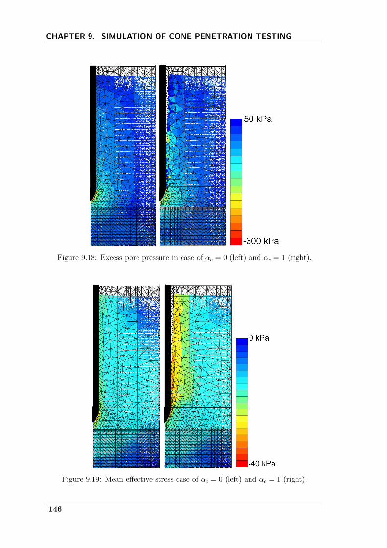
CHAPTER 9. SIMULATION OF CONE PENETRATION TESTING
Figure 9.18: Excess pore pressure in case of αc = 0 (left) and αc = 1 (right).
Figure 9.19: Mean effective stress case of αc = 0 (left) and αc = 1 (right).
146
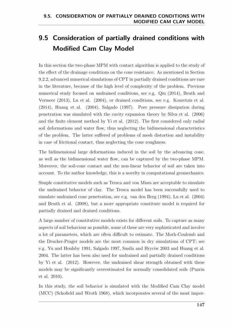
9.5. CONSIDERATION OF PARTIALLY DRAINED CONDITIONS WITHMODIFIED CAM CLAY MODEL
9.5 Consideration of partially drained conditions with
Modified Cam Clay Model
In this section the two-phase MPM with contact algorithm is applied to the study of
the effect of the drainage conditions on the cone resistance. As mentioned in Section
9.2.2, advanced numerical simulations of CPT in partially drained conditions are rare
in the literature, because of the high level of complexity of the problem. Previous
numerical study focused on undrained conditions, see e.g. Qiu (2014), Beuth and
Vermeer (2013), Lu et al. (2004), or drained conditions, see e.g. Kouretzis et al.
(2014), Huang et al. (2004), Salgado (1997). Pore pressure dissipation during
penetration was simulated with the cavity expansion theory by Silva et al. (2006)
and the finite element method by Yi et al. (2012). The first considered only radial
soil deformations and water flow, thus neglecting the bidimensional characteristics
of the problem. The latter suffered of problems of mesh distortion and instability
in case of frictional contact, thus neglecting the cone roughness.
The bidimensional large deformations induced in the soil by the advancing cone,
as well as the bidimensional water flow, can be captured by the two-phase MPM.
Moreover, the soil-cone contact and the non-linear behavior of soil are taken into
account. To the author knowledge, this is a novelty in computational geomechanics.
Simple constitutive models such as Tresca and von Mises are acceptable to simulate
the undrained behavior of clay. The Tresca model has been successfully used to
simulate undrained cone penetration, see e.g. van den Berg (1994), Lu et al. (2004)
and Beuth et al. (2008), but a more appropriate constitute model is required for
partially drained and drained conditions.
A large number of constitutive models exists for different soils. To capture as many
aspects of soil behaviour as possible, some of these are very sophisticated and involve
a lot of parameters, which are often difficult to estimate. The Morh-Coulomb and
the Drucker-Prager models are the most common in dry simulations of CPT; see
e.g. Yu and Houlsby 1991, Salgado 1997, Susila and Hryciw 2003 and Huang et al.
2004. The latter has been also used for undrained and partially drained conditions
by Yi et al. (2012). However, the undrained shear strength obtained with these
models may be significantly overestimated for normally consolidated soils (Puzrin
et al. 2010).
In this study, the soil behavior is simulated with the Modified Cam Clay model
(MCC) (Schofield and Wroth 1968), which incorporates several of the most impor-
147
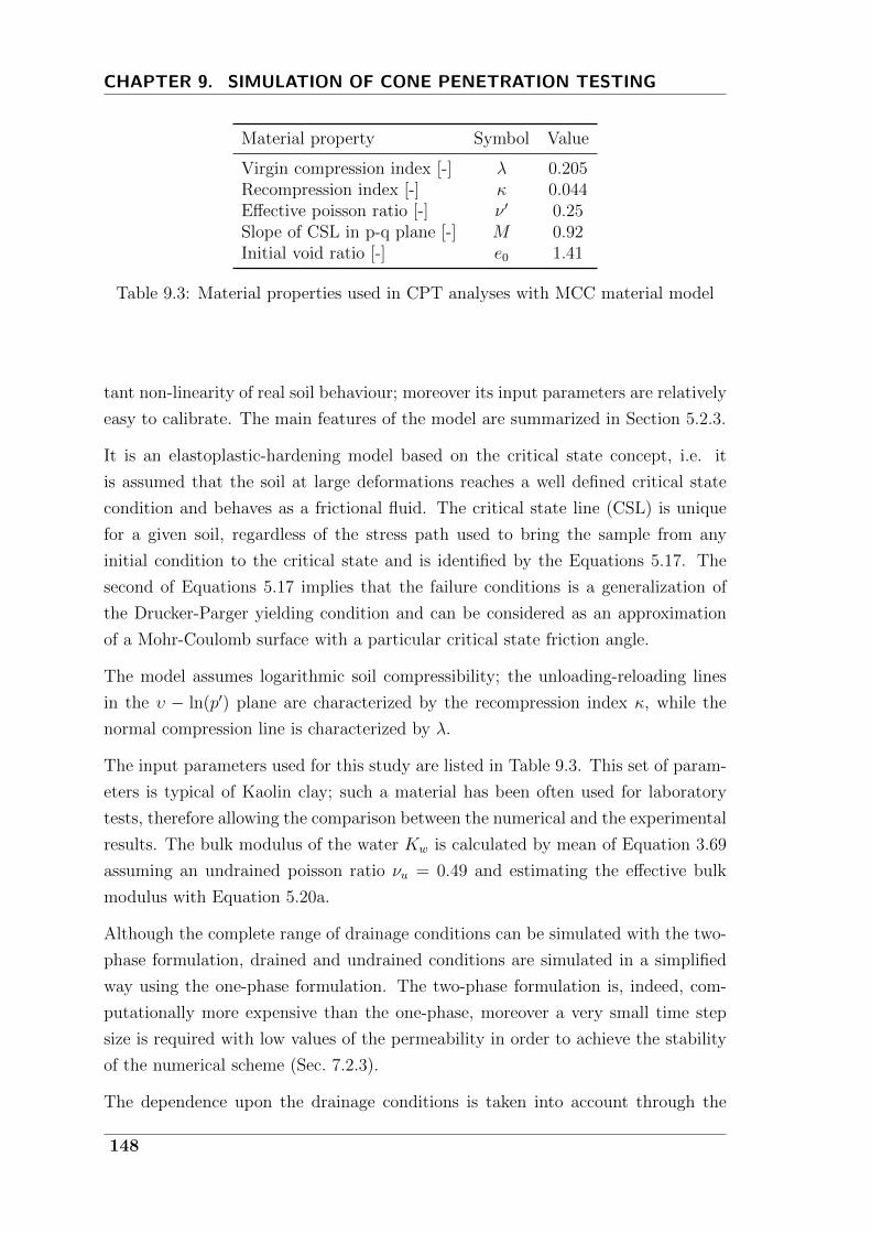
CHAPTER 9. SIMULATION OF CONE PENETRATION TESTING
Material property Symbol Value
Virgin compression index [-] λ 0.205Recompression index [-] κ 0.044Effective poisson ratio [-] ν ′ 0.25Slope of CSL in p-q plane [-] M 0.92Initial void ratio [-] e0 1.41
Table 9.3: Material properties used in CPT analyses with MCC material model
tant non-linearity of real soil behaviour; moreover its input parameters are relatively
easy to calibrate. The main features of the model are summarized in Section 5.2.3.
It is an elastoplastic-hardening model based on the critical state concept, i.e. it
is assumed that the soil at large deformations reaches a well defined critical state
condition and behaves as a frictional fluid. The critical state line (CSL) is unique
for a given soil, regardless of the stress path used to bring the sample from any
initial condition to the critical state and is identified by the Equations 5.17. The
second of Equations 5.17 implies that the failure conditions is a generalization of
the Drucker-Parger yielding condition and can be considered as an approximation
of a Mohr-Coulomb surface with a particular critical state friction angle.
The model assumes logarithmic soil compressibility; the unloading-reloading lines
in the υ − ln(p′) plane are characterized by the recompression index κ, while the
normal compression line is characterized by λ.
The input parameters used for this study are listed in Table 9.3. This set of param-
eters is typical of Kaolin clay; such a material has been often used for laboratory
tests, therefore allowing the comparison between the numerical and the experimental
results. The bulk modulus of the water Kw is calculated by mean of Equation 3.69
assuming an undrained poisson ratio νu = 0.49 and estimating the effective bulk
modulus with Equation 5.20a.
Although the complete range of drainage conditions can be simulated with the two-
phase formulation, drained and undrained conditions are simulated in a simplified
way using the one-phase formulation. The two-phase formulation is, indeed, com-
putationally more expensive than the one-phase, moreover a very small time step
size is required with low values of the permeability in order to achieve the stability
of the numerical scheme (Sec. 7.2.3).
The dependence upon the drainage conditions is taken into account through the
148

9.5. CONSIDERATION OF PARTIALLY DRAINED CONDITIONS WITHMODIFIED CAM CLAY MODEL
Figure 9.20: Schematic reppresentation of the correction for the water velocity atthe contact.
normalized penetration rate V (Eq. 9.10), in which cv can be estimated by:
cv =k(1 + e0)σ′v0
λγw
9.16
where k is the Darcy’s permeability and σ′v0 is the initial vertical effective stress
(Schneider et al. 2007).
In the literature the variation of V is usually achieved by varying the penetration
velocity v, on the contrary in this thesis it is obtained by changing the permeability
k, while keeping v = 0.02m/s. This approach seems closer to what happens in the
field, where D and v are standardized. Moreover, since a dynamic code is used,
modifying the penetration velocity requires new calibration of the Courant number,
the mass scaling factor and the damping factor.
In the two-phase calculations, additional care is required to solve the soil-cone con-
tact. Immediately after solving the momentum equation for the fluid (Eq. 4.18),
the water velocities and accelerations must be corrected to take into account the
presence of the impermeable cone surface. The contact algorithm for the fluid phase
is similar to the one presented in Section 6.4, but no correction for the tangential
component is required because the water-cone contact is assumed to be smooth.
The normal component of the fluid velocity wnorm must be equal to the normal
component of the cone velocity vcone,norm, therefore preventing inflow of water into
the cone (Fig. 9.20). The corrected velocity for the water at the generic node k
149
CHAPTER 9. SIMULATION OF CONE PENETRATION TESTING
assumes the expression:
wt+∆t = wt+∆t −[(wt+∆t − vt+∆t
cone
)· ntk
]ntk
9.17
wherewt+∆t is the predicted water velocity and ntk is the normal unit vector. Having
calculated the velocity of the contact node k at time t+∆t, the corrected acceleration
vector at the node must be recalculated as:
atw =wt+∆t −wt
∆t
9.18
The corrected water acceleration is used in the momentum equation for the mixture
(Eq. 4.19), which is solved to obtain the acceleration of the solid phase.
The velocity of the solid is predicted and then corrected according to the algorithm
presented in Section 6.4. No modifications are required at this step in case of the
two-phase formulation.
Section 9.5.1 discusses the results of preliminary analyses through which the set-
up of the numerical model has been optimized. Section 9.5.2 presents the results of
MPM simulations of CPT allowing for consolidation effects during cone penetration.
Numerical results are compared with experimental data from the literature, thus
confirming the validity of the model.
9.5.1 Preliminary analyses
The problem is simulated as discussed in Section 9.4.1: only 20 of the cone are
simulated, the moving mesh approach is applied, roller boundary conditions for the
soil skeleton are assigned at the lateral boundaries and the bottom is fully fixed.
The radial boundaries of the 20 slice are impermeable since they corresponds to
symmetry axes of the problem. The bottom and the lateral boundary are permeable
according to the choice of Yi et al. (2012). However, if the domain is wide enough
this does not have any significative influence on the results, as observed during
preliminary calculations.
A load of 50kPa is activated at the top surface of the soil, thus simulating an
initial position of the cone at 5m depth. Indeed, assuming a submerged weight of
10kN/m3, the 5m-soil column can be reproduced by such a vertical load. A further
penetration of the cone for 10D is simulated.
The gradient of initial vertical effective stress is negligible compared to the stress
150
9.5. CONSIDERATION OF PARTIALLY DRAINED CONDITIONS WITHMODIFIED CAM CLAY MODEL
level encountered during the penetration. Therefore the material weight is neglected
and the initial stresses are constant with depth. The stresses are initialized by K0
procedure and the clay is considered normally consolidated.
The bottom boundary is located 14D below the cone tip; this dimension affects the
results only for very deep penetration, and is therefore considered suitable for the
considered level of penetration. The results are more sensitive to the mesh radius
R; its effect has been investigated in one-phase calculations as function of the cone
roughness.
Four values of the mesh radius have been considered: 4D, 6D, 8D and 10D. The
refinement of the mesh around and below the cone is identical in the four cases.
Figure 9.21 shows how the tip stress increases as the cone penetrates into the soil in
case of undrained conditions (Fig. 9.21a) and drained conditions (Fig. 9.21b). If the
domain size is too small the steady state conditions are not reached or the obtained
tip resistance differs form the one obtained with a wider domain.
The preliminary analyses show that to simulate drained conditions wider domains
are necessary compared to the case of undrained conditions; the introduction of
the cone roughness increases the required domain radius. This means that the
volume of soil significantly affected by the cone penetration depends on the drainage
conditions. Considerations of computational efficiency and accurancy lead to the
conclusion that a radius of 6D is sufficient for the undrained case, while 8D is
necessary for the drained case. The latter proved to be suitable for the analyses in
partially drained conditions too.
Unacceptable oscillations of the tip stress in undrained conditions appears when
values of the friction coefficient greater or equal to 0.2 are used (Fig. 9.22). A
reduction of the Courant number does not improve the results, not even the increase
of the discretized domain size, but better results are obtained with a very fine mesh
around the cone (Fig. 9.23). Since this increases the computational cost, such a fine
mesh is used only for high friction coefficients in one-phase undrained calculations
and two-phase calculations with low permeablity.
In this set of calculations C = 0.98 and β = 400 revealed to be appropriate in
undrained, drained and partially drained conditions. The damping factor of 0.15 is
suitable for the one-phase analyses, but a smaller value is used for the two-phase
simulations.
As shown in Figure 9.24, high damping (α = 0.15) produces and overestimation of
the pore pressure (Fig. 9.24b) and therefore of the cone resistance (Fig. 9.24a); on the
151
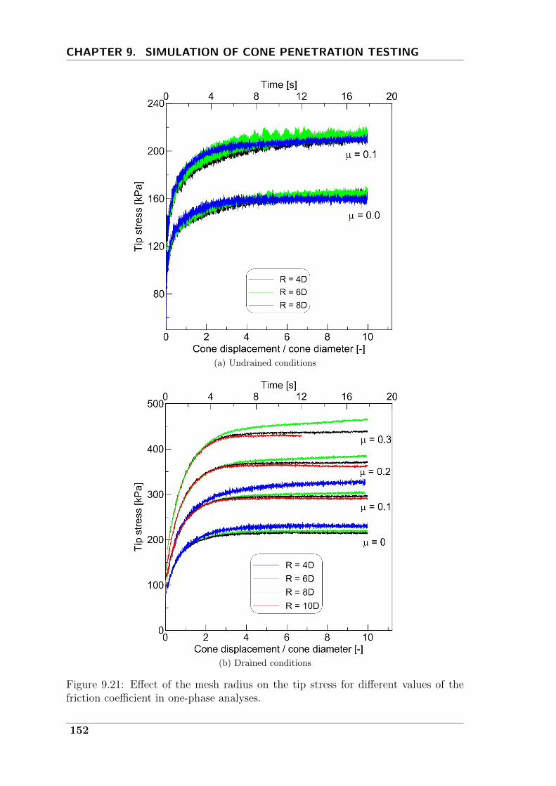
CHAPTER 9. SIMULATION OF CONE PENETRATION TESTING
(a) Undrained conditions
(b) Drained conditions
Figure 9.21: Effect of the mesh radius on the tip stress for different values of thefriction coefficient in one-phase analyses.
152

9.5. CONSIDERATION OF PARTIALLY DRAINED CONDITIONS WITHMODIFIED CAM CLAY MODEL
Figure 9.22: Oscillations of the tip stress for µ = 0.2 (blue line) and 0.3 (red line);improvement of the result with finer mesh (green line)
Figure 9.23: Refinement of the mesh around the cone for analyses with rough cone.The standard is on the left and refined mesh is shown on the right.
153

CHAPTER 9. SIMULATION OF CONE PENETRATION TESTING
contrary, it does not affect the effective stress (Fig. 9.24c). This effect is more severe
for low permeabilities, i.e. high normalized velocities. It can be explained observing
that the local damping artificially reproduces the natural energy dissipation of a
material (Cundall 2001). The dissipation is lower for the fluid than for the soil
skeleton; however, the same value of the damping factor α is applied on both phases.
This leads to an overestimation of the pore pressure, which is more severe when the
importance of this contribute is more significant, i.e. for low permeability.
If no damping is used, severe oscillations of the tip stress are observed and difficulties
in running the calculations till the steady state are encountered in some cases; for
these reasons α = 0.05 is considered a good compromise and an overestimation
smaller than 5% is assumed to affect the tip resistance qc.
9.5.2 Results
In this section the results of MPM simulations of CPT accounting for different
drainage conditions are presented. The effect on the tip resistance of the pore
pressure dissipation during cone penetration is investigated considering also the
relative importance of the effective stress and the pore pressure. The effect of the
initial horizontal stress and the cone roughness on the tip resistance is studied too.
Numerical results are compared with theoretical and experimental data available in
the literature.
The problem is simulated as presented in the previous section. The geometry and
discretization adopted for the undrained penetration coincide with Figure 9.13; for
partially drained and drained conditions the mesh is wider (0.29m) and counts
13221 elements and 105634 material points (Fig. 9.25). The material parameters
are shown in Table 9.3; the soil is assumed normally consolidated and the initial
vertical effective stress is 50kPa.
Figure 9.26 shows the tip stress over the normalized penetration in case of smooth
contact for several values of the normalized velocity V . The tip stress increases
with the cone displacement up to a steady state condition which corresponds to
the tip resistance qc. This steady state condition is reached after a penetration
of approximately 5D in drained conditions and 7D or 8D in partially drained and
undrained conditions.
As expected, the tip resistance increases with the decrease of V , i.e. moving from
undrained to drained conditions. In case of V = 1.2 the tip resistance is only 4%
154
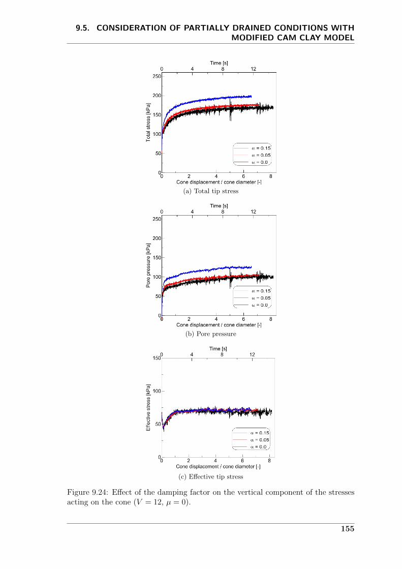
9.5. CONSIDERATION OF PARTIALLY DRAINED CONDITIONS WITHMODIFIED CAM CLAY MODEL
(a) Total tip stress
(b) Pore pressure
(c) Effective tip stress
Figure 9.24: Effect of the damping factor on the vertical component of the stressesacting on the cone (V = 12, µ = 0).
155
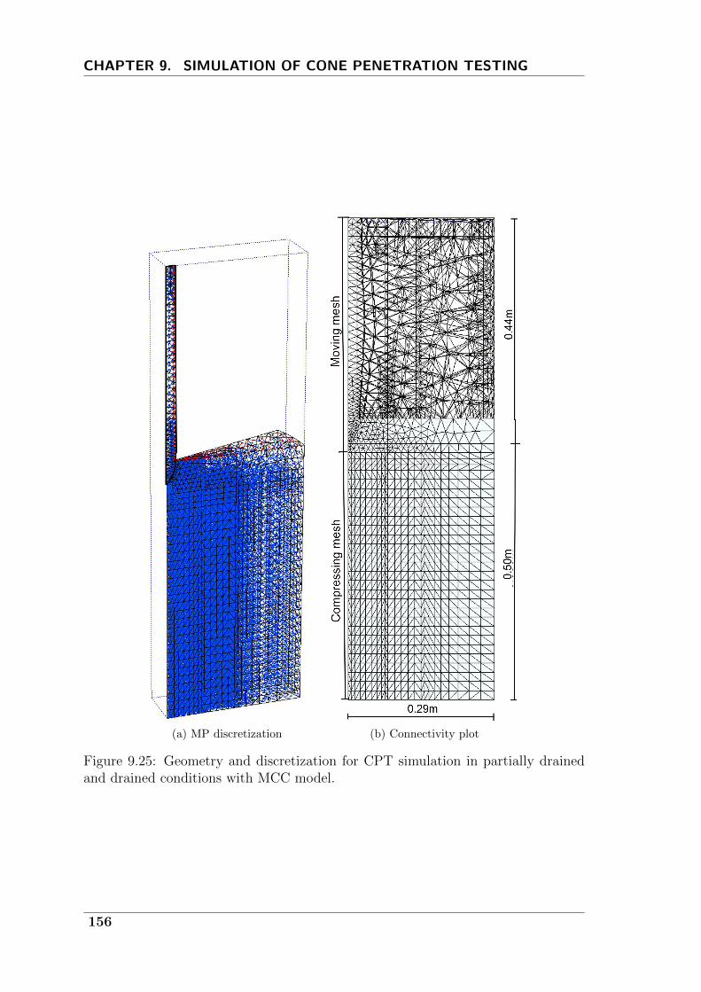
CHAPTER 9. SIMULATION OF CONE PENETRATION TESTING
(a) MP discretization (b) Connectivity plot
Figure 9.25: Geometry and discretization for CPT simulation in partially drainedand drained conditions with MCC model.
156
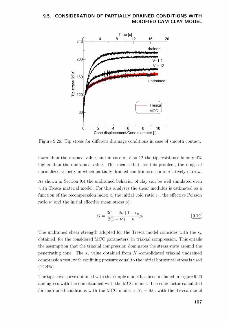
9.5. CONSIDERATION OF PARTIALLY DRAINED CONDITIONS WITHMODIFIED CAM CLAY MODEL
Figure 9.26: Tip stress for different drainage conditions in case of smooth contact.
lower than the drained value, and in case of V = 12 the tip resistance is only 4%
higher than the undrained value. This means that, for this problem, the range of
normalized velocity in which partially drained conditions occur is relatively narrow.
As shown in Section 9.4 the undrained behavior of clay can be well simulated even
with Tresca material model. For this analyses the shear modulus is estimated as a
function of the recompression index κ, the initial void ratio e0, the effective Poisson
ratio ν ′ and the initial effective mean stress p′0:
G =3(1− 2ν ′)
2(1 + ν ′)
1 + e0
κp′0
9.19
The undrained shear strength adopted for the Tresca model coincides with the su
obtained, for the considered MCC parameters, in triaxial compression. This entails
the assumption that the triaxial compression dominates the stress state around the
penetrating cone. The su value obtained from K0-consolidated triaxial undrained
compression test, with confining pressure equal to the initial horizontal stress is used
(12kPa).
The tip stress curve obtained with this simple model has been included in Figure 9.26
and agrees with the one obtained with the MCC model. The cone factor calculated
for undrained conditions with the MCC model is Nc = 9.6, with the Tresca model
157

CHAPTER 9. SIMULATION OF CONE PENETRATION TESTING
is Nc = 9.7 and the one calculated with Equation 9.9, where Ir = 108, ∆ = 0.7 and
α = 0 is 9.55. There is excellent agreement between MPM simulations and reference
literature results.
The accumulated shear strains after 10D penetration for the undrained and drained
conditions are shown in Figure 9.27. In case of smooth contact, extreme shear
deformations, i.e. accumulated deviatoric strain (Eq. 5.14) εq > 10%, extend about
2D in radial direction and 0.5D below the cone for undrained conditions and 1.5D
in radial direction and 0.3D below the cone for drained conditions. The dimensions
of this area of extreme deformations slightly increase with the rough contact.
Figure 9.28 shows the excess pore pressure for two values of the normalized pene-
tration rate V . Approximately undrained behavior is observed for V = 12 at which
the pore pressure is about 150kPa. On the contrary, for V = 1.2 the behavior is
nearly drained and the pressure is about 30kPa. This agrees with considerations on
the tip resistance.
The effective stress path of a point next to the cone surface is plotted in Figure 9.29
as function of the normalized velocity. The initial condition is identical for the
considered cases, the mean effective stress is p′0 = 40kPa and the deviatoric stress
is q0 = 15.5kPa. This stress state lies on the yielding surface (Eq. 5.21) because
the soil is assumed normally consolidated; the initial preconsolidation pressure pc0
is 47kPa.
As the cone penetrates, the soil yields and the stress path moves toward the CSL.
The undrained path is typical for normally consolidated clays. The stress path for a
normalized penetration rate V = 12 approaches the undrained behavior, while the
one for V = 1.2 approaches the drained stress path. The final mean effective stress
and deviatoric stress increase reducing the normalized penetration rate, i.e. moving
from undrained to drained conditions, as result of the pore pressure dissipation
during cone penetration.
The tip resistance can be written as qc = qc,eff +qc,water where qc,eff is the contribute
of the soil effective stress and qc,water is the contribute of the pore pressure. Fig-
ure 9.30 shows how the contribute of the pore pressure increases with the normalized
velocity while the one of the effective stress decreases.
In drained conditions qc,water = 0 and therefore qc = qc,eff because there is no excess
pore pressure generation. In undrained conditions there is a significant generation
of pore pressure with no dissipation which leads to qc,water ≈ 75%qc and qc,eff is even
lower than the initial vertical effective stress. In case of partially drained conditions,
158
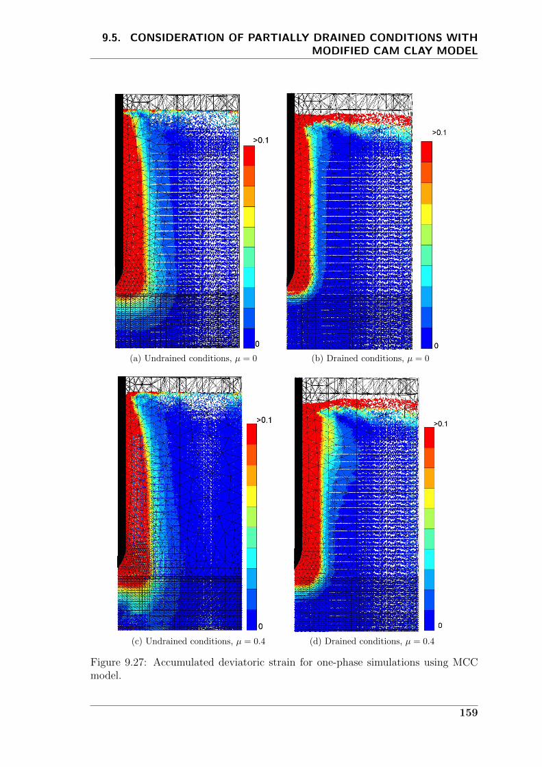
9.5. CONSIDERATION OF PARTIALLY DRAINED CONDITIONS WITHMODIFIED CAM CLAY MODEL
(a) Undrained conditions, µ = 0 (b) Drained conditions, µ = 0
(c) Undrained conditions, µ = 0.4 (d) Drained conditions, µ = 0.4
Figure 9.27: Accumulated deviatoric strain for one-phase simulations using MCCmodel.
159
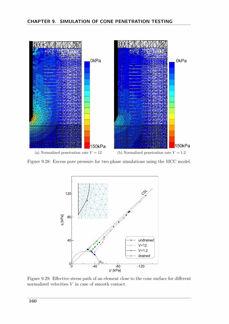
CHAPTER 9. SIMULATION OF CONE PENETRATION TESTING
(a) Normalized penetration rate V = 12 (b) Normalized penetration rate V = 1.2
Figure 9.28: Excess pore pressure for two-phase simulations using the MCC model.
Figure 9.29: Effective stress path of an element close to the cone surface for differentnormalized velocities V in case of smooth contact.
160
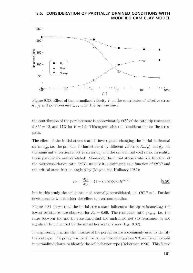
9.5. CONSIDERATION OF PARTIALLY DRAINED CONDITIONS WITHMODIFIED CAM CLAY MODEL
Figure 9.30: Effect of the normalized velocity V on the contributes of effective stressqc,eff and pore pressure qc,water on the tip resistance.
the contribution of the pore pressure is approximately 60% of the total tip resistance
for V = 12, and 17% for V = 1.2. This agrees with the considerations on the stress
path.
The effect of the initial stress state is investigated changing the initial horizontal
stress σ′x0, i.e. the problem is characterized by different values of K0, p′0 and q′0, but
the same initial vertical effective stress σ′v0 and the same initial void ratio. In reality,
these parameters are correlated. Moreover, the initial stress state is a function of
the overconsolidation ratio OCR; usually it is estimated as a function of OCR and
the critical state friction angle φ by (Mayne and Kulhawy 1982):
K0 =σ′h0
σ′v0
= (1− sin(φ))OCRsin(φ) 9.20
but in this study the soil is assumed normally consolidated, i.e. OCR = 1. Further
developments will consider the effect of overconsolidation.
Figure 9.31 shows that the initial stress state influences the tip resistance qc; the
lowest resistances are observed for K0 = 0.69. The resistance ratio q/qref , i.e. the
ratio between the net tip resistance and the undrained net tip resistance, is not
significantly influenced by the initial horizontal stress (Fig. 9.32).
In engineering practice the measure of the pore pressure is commonly used to identify
the soil type. The pore pressure factor Bq, defined by Equation 9.3, is often employed
in normalized charts to identify the soil behavior type (Robertson 1990). This factor
161
CHAPTER 9. SIMULATION OF CONE PENETRATION TESTING
represents a measure of the relative importance of the pore pressure on the net tip
resistance. In the numerical analyses the pore pressure factor is estimated as
Bq =qc,waterqc,net
9.21
where qc,water represents an average of the pore pressures around the cone. On
the contrary, in practice the pore pressure is measured behind the cone. The pore
pressure factor is not significantly influenced by the horizontal stress state (Fig.
9.33).
The cone roughness is simulated assigning a friction coefficient µ which varies be-
tween 0, i.e. smooth contact, and 0.42, i.e. rough contact (tanφ = 0.42). The
friction coefficient depends on the relative dimension of the surface roughness and
the size of the soil particles. Reasonable values of µ for low plasticity clay in contact
with steel lie between 0.2 and 0.35 (Lemos and Vaughan 2000). Potyondy (1961)
suggested an interface friction angle equal to one half the critical soil friction angle,
which corresponds to a friction coefficient of 0.21 in this case.
Figure 9.34 shows how the introduction of the cone roughness increases the tip
resistance in one-phase undarined and drained analses. In undrained conditions,
the cone factor Nc (Eq. 9.4) ranges from 9.6 to 16; this is in agreement with what
was observed in Section 9.4.2 for a similar rigidity index.
A different definition of the cone factor is commonly adopted in drained conditions
(Lunne and Powell 1997):
Nq =qcσ′v0
9.22
It increases linearly with the friction coefficient from a value of 4.3 to 10.2. These
values are extremely low, compared to the usual values assumed for sand, which
varies from 20 to 100 (Lunne and Powell 1997). This can be attributed to the
low modulus ratio G/p′ and friction angle used in this study, where a soft clay is
modeled. The MPM results are in agreement with the study of Yi et al. (2012)
where Nq ≈ 5 is found for smooth contact with a similar friction angle and modulus
ratio.
The cone roughness increases the tip resistance in the entire range of drainage con-
ditions. In drained conditions the increase is linear, while in partially drained and
undrained conditions it is less than linear and seems to stabilize for µ > 0.3 (Fig.
9.35). This non-linear trend is in contrast with other numerical studies in total
stress where the Tresca material model and the adhesive contact are used (see e.g.
162
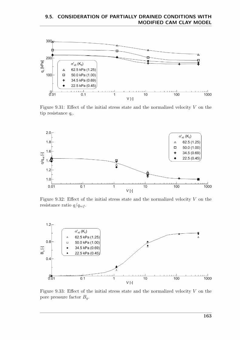
9.5. CONSIDERATION OF PARTIALLY DRAINED CONDITIONS WITHMODIFIED CAM CLAY MODEL
Figure 9.31: Effect of the initial stress state and the normalized velocity V on thetip resistance qc.
Figure 9.32: Effect of the initial stress state and the normalized velocity V on theresistance ratio q/qref .
Figure 9.33: Effect of the initial stress state and the normalized velocity V on thepore pressure factor Bq.
163

CHAPTER 9. SIMULATION OF CONE PENETRATION TESTING
(a) Undrained conditions (b) Drained conditions
Figure 9.34: Tip stress for different values of the friction coefficient µ in one-phaseanalyses.
Lu et al. 2004 and Beuth and Vermeer 2013). The penetration process is a complex
phenomenon to simulate numerically, further investigations are required to explain
this result.
Figure 9.36 shows the resistance ratio as a function of the normalized velocity V for
different values of the friction coefficient µ. The maximum resistance ratio increases
with the cone roughness from a value of 1.4 for µ = 0 to a value of 2.4 for µ = 0.42.
The numerical data can be fitted by the backbones curves represented by Equa-
tion 9.11; the coefficients corresponding to the best fit are included in Figure 9.36.
The coefficient b increases with µ because the maximum resistance ratio is pro-
portional to the friction coefficient. This also affect the rage of partially drained
conditions, which is narrower for smooth cone (V comprises between 0.3 and 50)
than for very rough cone (V comprises between 0.1 and 200).
Figure 9.37 shows that the pore pressure factor is a function of the normalized
velocity and the cone roughness. Lower values of the friction coefficient generate
higher pore pressure factors. This means that the relative importance of the pore
pressure on the tip resistance decreases with the cone roughness.
The results obtained with the MPM are compared with centrifuge model CPT results
by Randolph and Hope (2004) (black dot in Fig. 9.36 and in Fig. 9.37) and numerical
result obtained with the cavity expansion theory by Silva (2005) (dashed line in
164

9.5. CONSIDERATION OF PARTIALLY DRAINED CONDITIONS WITHMODIFIED CAM CLAY MODEL
Figure 9.35: Effect of the friction coefficient µ on the tip resistance qc.
Fig. 9.36).
The backbone curves obtained with the MPM are in good agreement with the ex-
perimental results. Differences can be attributed to the fact that the real tested
material may be characterized by slightly different material parameters form the
one assumed in the numerical model; in particular a higher modulus ratio which
seems to be comprises between 35 and 75 (Yi et al. 2012). Moreover, the ex-
perimental consolidation coefficient, used to calculate the normalized velocity, may
differs from the numerical estimate. There is a slight overestimation of the pore
pressure parameter, especially for undrained conditions, which can attributed to the
use of the MCC model.
The experimental data seems to be well fitted by MPM simulations obtained with
friction coefficient comprises between 0.3 and 0.4. The friction coefficient assumed
by Silva (2005) is equal to the tangent of the soil friction angle. However, for
µ = tan(φ) = 0.42 the MPM gives higher values of the resistance ratio; this can
be explained by the fact that the cavity expansion theory considers only radial
soil deformations, while the MPM simulates the threedimensional process of cone
penetration.
Schneider et al. (2007) published experimental data obtained with centrifuge tests
on kaolin. The material properties of this soil are summarized in Table 9.4. In
165
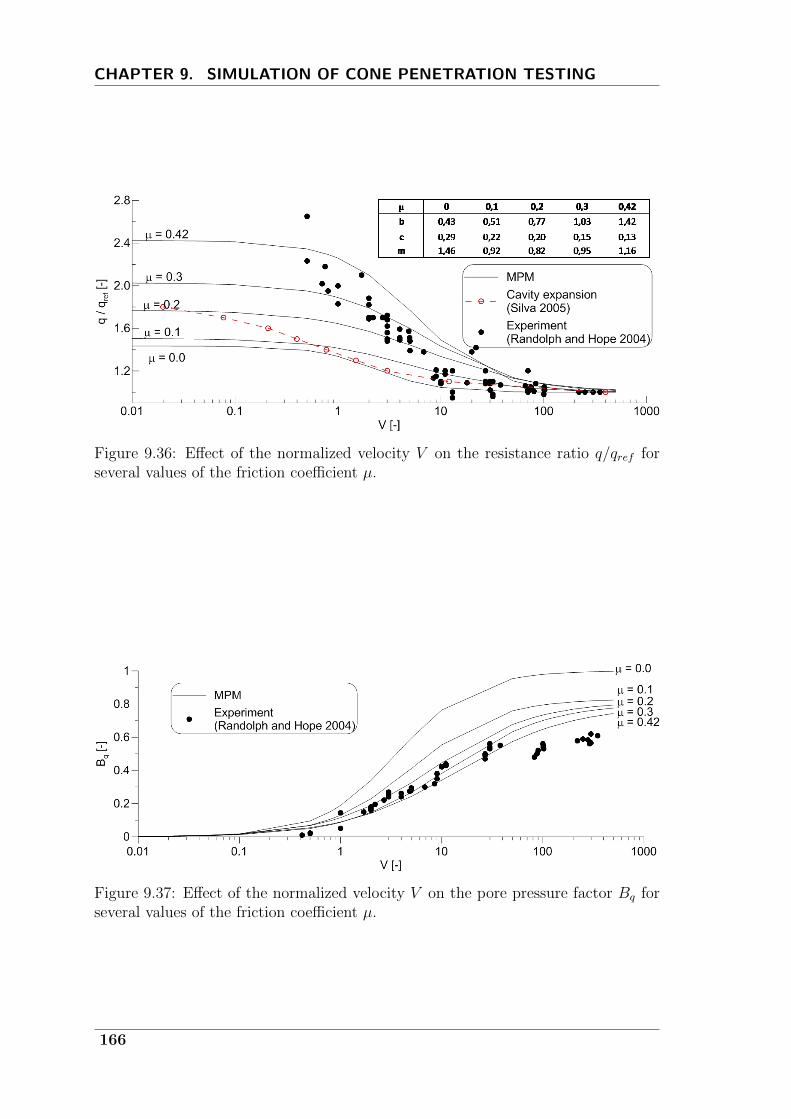
CHAPTER 9. SIMULATION OF CONE PENETRATION TESTING
Figure 9.36: Effect of the normalized velocity V on the resistance ratio q/qref forseveral values of the friction coefficient µ.
Figure 9.37: Effect of the normalized velocity V on the pore pressure factor Bq forseveral values of the friction coefficient µ.
166

9.5. CONSIDERATION OF PARTIALLY DRAINED CONDITIONS WITHMODIFIED CAM CLAY MODEL
Material property Symbol Value
Virgin compression index [-] λ 0.26Recompression index [-] κ 0.06Effective poisson ratio [-] ν ′ 0.25Slope of CSL in p-q plane [-] M 0.92Initial void ratio [-] e0 1.6
Table 9.4: Material properties of the kaolin used by Schneider et al. (2007)
the experiment, the initial vertical effective stress varies from 80kPa to 100kPa
and a penetrometer with a diameter of 10mm is used. The effect of the drainage
conditions is studied by varying the penetration rate from 0.003mm/s to 3mm/s
and the consolidation coefficient is estimated from the soil parameters by Equation
9.16.
Assuming that the cone diameter does not significantly influence the tip resistance,
the same geometry and discretization used in the previous problem is adopted (Fig.
9.25). The initial vertical and horizontal effective stress are 90kPa and 54kPa
respectively. A friction coefficient of 0.28 is assumed reasonable for this problem;
this value corresponds to an interface friction angle equal to 2/3φ (φ = critical
soil friction angle). The normalized velocity is again varied by changing the soil
permeability.
Figure 9.38 shows how the net tip resistance varies with the normalized velocity.
The experimental data are relative to the initial vertical effective stresses between
80kPa and 100kPa, while the MPM results are obtained for σ′v0 = 90kPa. The
tip resistance in drained conditions is very well captured, while there is a slight
overestimation of qc,net for undrained conditions.
Figure 9.39 represents the resistance ratio as a function of the normalized velocity.
It can be observed that the initial vertical effective stress does not significantly
influence the resistance ratio. The maximum q/qref is slightly underestimated and
this is due to the overestimation of the undrained tip resistance.
Numerical results in terms of Bq are in good agreement with the experimental mea-
surements (Fig. 9.40). The overestimation of Bq, which is observed for high nor-
malized velocities, can again be attributed to the soil constitutive model. This
suggests that a further improvement of the results can be achieved by improving the
simulation in undrained conditions, for example with the use of a more advanced
constitutive model. The MPM estimation of cone resistance, resistance ratio and
pore pressure factor are in very good agreement with the experimental data.
167
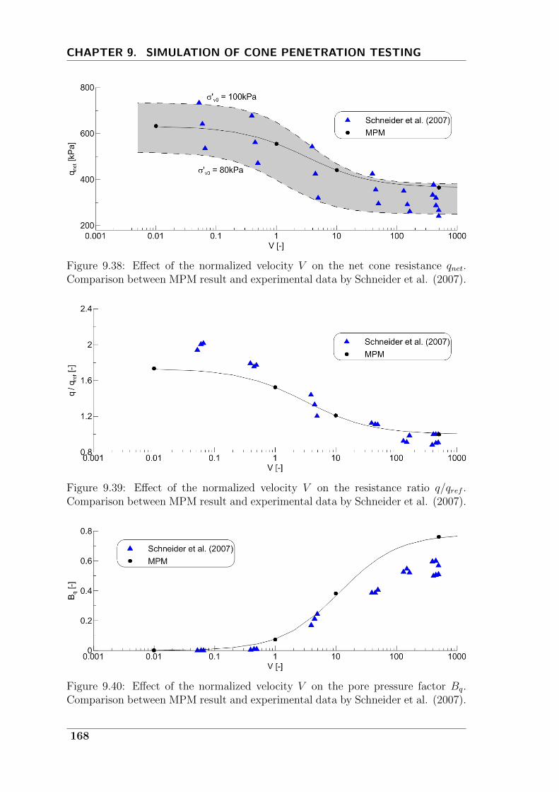
CHAPTER 9. SIMULATION OF CONE PENETRATION TESTING
Figure 9.38: Effect of the normalized velocity V on the net cone resistance qnet.Comparison between MPM result and experimental data by Schneider et al. (2007).
Figure 9.39: Effect of the normalized velocity V on the resistance ratio q/qref .Comparison between MPM result and experimental data by Schneider et al. (2007).
Figure 9.40: Effect of the normalized velocity V on the pore pressure factor Bq.Comparison between MPM result and experimental data by Schneider et al. (2007).
168

9.6. CONCLUSIONS AND FUTURE DEVELOPMENTS
9.6 Conclusions and future developments
In this chapter the MPM has been applied to the simulation of cone penetration in
clay, considering the effect of the drainage conditions, the initial stress state and the
cone roughness on the tip resistance and the pore pressure factor.
Numerical studies of CPT in partially drained conditions are rare because of the
high complexity of the penetration process. Indeed, large deformations, soil-cone
contact, soil-water interaction and non-linear soil constitutive behavior have to be
taken into account.
To the author’s knowledge, there are only a couple of papers on numerical simulation
of CPT including pore pressure dissipation during penetration: Silva et al. (2006),
who used the cylindrical cavity expansion theory coupled with FEM, and Yi et al.
(2012), who used the FEM with logarithmic strain. Despite the these studies give
an important contribution to the understanding of the penetration process, they
have some limitations and drawbacks which are discussed in Section 9.2.2.
The present study adds several novelties to the numerical simulations of soil pene-
tration problems. Indeed, here the bidimensional large deformations of soil and the
bidimensional water flow, induced by the advancing cone, are taken into account.
The effect of cone roughness is investigated and the mechanical response of soil is
simulated with the MCC constitutive model that can capture many non linearities
of the real soil behavior.
The first part of this chapter considers CPT in undrained conditions (Sec. 9.4).
Since the pore pressure dissipation is negligible, the one-phase MPM is used to
simulate the penetration process. The undrained behavior of clay is simulated with
the elatoplastic model with Tresca failure criteria.
The cone factor is a function of the rigidity index, the initial stress state and the
cone roughness. In this study (Ir = 100 and ∆ = 0), cone factors of 10.2, 14.0 and
15.8 are found for cone roughness αc equal to 0, 0.5 and 1 respectively. MPM results
are in excellent agreement with experimental data by Kurup et al. (1994), in which
a cone factor of 13 is found. Good agreement is also found with other analytical
studies for the smooth contact, but a slight overestimation of the cone factor is
observed for rough cone. This may be related to the use of the contact algorithm
proposed by Bardenhagen et al. (2001), as recent studies seems to suggest. Ma
et al. (2014) observed an overestimation of the contact forces when bodies with
very different stiffness are in contact. A more detailed investigation of this problem
169
CHAPTER 9. SIMULATION OF CONE PENETRATION TESTING
should be considered in a future development of the research.
The second part of the chapter introduce the effect of pore pressure dissipation
during cone penetration (Sec. 9.5). A more realistic constitutive model is necessary
to achieve this purpose. The modified Cam Clay model can reproduce several of
the most important characteristic of soft soil behavior and its input parameters are
easy to calibrate. For undrained conditions the tip stress corresponds to the one
obtained with the Tresca material model assuming the undrained shear strength for
triaxial compression.
The tip resistance increases moving from undrained to drained conditions because,
decreasing the penetration rate V , the pressure dissipates and the soil consolidates
therefore developing higher shear strength and stiffness.
The initial stress state influence the tip resistance, but it has a negligible effect
on the resistance ratio (q/qref ) and the pore pressure factor Bq. In this study
the different initial stress states have been simulated by assigning different initial
horizontal stresses while keeping the other parameters constant. In future studies, a
more realistic simulation of different initial conditions, in the same soil, will consider
the relation between K0, overconsolidation ratio OCR and initial void ratio.
The present study shows that the resistance ratio depends on the friction coefficient.
Indeed, for the considered case, its maximum varies between 1.4 for smooth contact
and 2.4 for rough contact.
The cone roughness affects the pore pressure factor too: increasing the friction co-
efficient decreases Bq. This means that the relative importance of the pore pressure
on the tip resistance decreases with the cone roughness. It also influences the range
of partially drained conditions, which is found to be wider for rough cone. A proper
simulation of the soil-cone contact is important for a realistic simulation of the
penetration process.
The MPM simulations with the MCC constitutive model capture very well the ex-
perimental results on kaolin published by Randolph and Hope (2004) and Schneider
et al. (2007) confirming the validity of the method.
The kaolin has a relatively low plasticity index as commonly found also for silt,
which is the soil type where penetration at standard rate can be characterized by
partially drained conditions. The results of this study can be considered a reasonable
representation of real field situations in which partially drained conditions occur.
For isotropically normal consolidated states, the mechanical behavior can be reason-
170
9.6. CONCLUSIONS AND FUTURE DEVELOPMENTS
ably well captured by the MCC model. However, natural clays are anisotropically
consolidated, which has a significant influence on the undrained strength and thus
on the undrained tip resistance (Beuth 2012). In addition to this, strain-rate effects
dominates the behavior at high penetration rates (Randolph 2004). The influence
of soil anisotropy and viscoplasticity will be considered in the future by implement-
ing more advanced constitutive models in the MPM. Different types of soil will be
considered too.
The study can be extended to the pore pressure dissipation subsequent the cone
penetration. This is of particular interest in practice, because the dissipation test is
widely used to estimate the soil’s consolidation coefficient and permeability. Data
interpretation is based on analytical studies which neglect the installation effects and
assume undrained conditions of penetration, see e.g. Baligh and Levadoux (1986),
Teh and Houlsby (1991), Robertson et al. (1992). With the MPM the effects of
cone installation as well as the occurrence of partial pore pressure dissipation during
penetration can be considered. A practical method to estimate the consolidation
coefficient even in case of partially drained cone penetration can be suggested. This
is of practical interests as it allows to extend the dissipation test to silty soil.
171

10General conclusions and final remarks
This thesis addresses the problem of simulating large deformations in geomechanics
accounting for the soil-water interaction. Taking into account large displacements of
soil is necessary in several geotechnical cases. The Material Point Method (MPM)
is a promising tool in this field. This work focuses on its developments and appli-
cations. The aim of this chapter is to summarize the study, draw some conclusions
and define further developments of the research.
The numerical modeling process has been introduced in Chapter 2, including an
overview of the most common numerical methods. Numerical methods improved
considerably in the last decades, increasing the number of problems which can be
studied. Numerical simulations are often cheaper and more feasible than field and
laboratory tests. A large number of variables can be controlled and parametric
studies are possible, thus allowing a deeper understanding of the physical phenom-
ena. The field of computational mechanics is in constant expansion and offers wide
possibilities of research and applications in geoengineering.
The most important developments of the Material Point Method, starting from its
infancy at Los Alamos, where it was originally developed, is discussed in Section 2.5.
From this literature review, it can be concluded that the MPM is a powerful numer-
ical technique, providing possibilities of modeling large deformations, multiphase
materials and interaction between solid bodies. It has been successfully applied to
solve a wide range of problems in different engineering fields and the number of
applications can be further extended.
Chapters 3 and 4 present in detail the MPM formulation and the solution procedure
for the one-phase and two-phase material respectively. The applicability of these
formulations in geomechanics has been discussed. The one-phase formulation is
173

CHAPTER 10. GENERAL CONCLUSIONS AND FINAL REMARKS
suitable for soil in drained and undrained conditions, i.e. when the generation or the
dissipation of pore pressures are negligible, while the two-phase formulation should
be used when both the generation and dissipation of pore pressures are relevant, e.g.
in the case of cone penetration in partially drained condition (Sec 9.5).
The two-phase formulation is validated for small and large deformations in Chapter
7. In the future, the two-phase MPM will be compared with other solutions at
large strain, e.g. Borja et al. (1998), Xie and Leo (2004), Nazem and Sheng (2008),
eventually discussing the source of differences. The possibility to couple large de-
formations and soil-water interaction is extremely interesting in geomechanics. It
allows the study of complex problems in which the generation and dissipation of
pore pressure is a key point such as landslides, debris flows and mud flows.
This study considers only water-saturated soil. Partially saturated soil can be de-
scribed by a three-phase formulation, i.e. the governing equations for the gas phase
are included. The implementation of the three-phase MPM is in progress (Yerro
2014) and will be considered in the future to study problems involving partially sat-
urated soil such as the stability of slopes, embankments and dams under transient
hydraulic conditions.
In this thesis one set of material points, moving with the solid velocity, is used
even when the presence of the water is considered. This one-layer formulation is
acceptable to simulate the saturated soil behavior, but the interaction with free
water cannot be included.
Problems of seepage and erosion-sedimentation, in which part of the domain is oc-
cupied by pure water, part by dry or saturated soil and part by suspensions of
soil particles in water, need to be simulated by two sets of material points. Im-
plementation and developments of this two-layer formulation is the subject of the
on-going work of MPM research groups (Vermeer et al. 2013, Rohe and Vermeer
2014, Martinelli and Rohe 2014).
The possibility of simulating the solid-suspension-fluid transition is extremely im-
portant to study several problems of engineering interest such as injection of fluids
in the ground (jet-grouting), sedimentation of mine waste, stability of submerged
slopes subjected to erosion processes and installation of footings on the seabed.
Geotechnical models consider the saturated soil behavior, while hydromechanical
models consider the fluid and fluidized mixture behavior, but the transition between
these phases and their interaction are hardly considered. Future developments of
the MPM can fill the gap between geomechanical and hydromechanical models. The
174
author thinks that this aspect is one of the most interesting to follow in the future.
In addition to the interaction with fluids, one of the main issue of geotechnical en-
gineering is the constitutive modeling of soil. Despite its importance, this theme is
not the main concern of the present study and has been shortly treated in Chapter
5. Simple models such as Tresca, Mohr-Coulomb and Modified Cam Clay have been
applied in this study. Tresca and Mohr-Coulomb models provide a crude repre-
sentation of soil behavior. However, this is sometimes sufficient in the engineering
practice and they can be used to catch the main features of the considered problem.
The Modified Cam Clay model is more advanced and can better reproduce the non-
linear soil behavior. To the author’s knowledge, this thesis is the first application of
this constitutive model in the study of large deformation problems with a dynamic
MPM code. Simple models may not be able to represent accurately the real soil
behavior, but they are easy to use. Sophisticated models are more realistic, but
they add significative complexity to the simulation and the estimation of input pa-
rameters may be demanding. Implementations and applications of more advanced
constitutive models will be considered in the future.
Many geotechnical problems involve soil-structure interaction; in the MPM there
are several algorithms able to solve contact problems, one of the most popular was
introduced by Bardenhagen et al. (2001). This algorithm was originally developed
for the frictional contact. In cohesive soils under undrained conditions, the maximum
tangential force is independent on the normal contact force and it is often referred
to the undrained shear strength of the soil. In order to simulate this type of contact,
the original algorithm has been enhanced including the adhesive component of the
contact force. This algorithm is presented and validated in Section 6.4 and has been
applied to simulate the contact between cone and undrained clay in Section 9.4.
The use of high friction coefficients with this algorithm requires a fine mesh to
keep an acceptable accuracy. An overestimation of the contact forces when bodies
with very different stiffness are in contact is reported by Ma et al. (2014) and it
is also observed in this thesis with the simulation of CPT in undrained conditions
(Sec. 9.4). A detailed study of the performances of the implemented algorithm for
geomechanical problems is suggested.
The simulation of real problems is difficult because reality is complex and simplifi-
cations are necessary. These simplifications, together with the particular features of
the numerical method, sometimes lead to numerical difficulties. Some of these prob-
lems are discussed in Chapter 6, e.g. volumetric locking for incompressible materials
when low order elements are used and noise due to dynamic waves.
175
CHAPTER 10. GENERAL CONCLUSIONS AND FINAL REMARKS
The use of absorbing boundary and local damping can reduce the noise due to
unphysical dynamic effects. The first virtually simulates the presence of a layer of
material beyond the boundary. The latter represents the natural energy dissipation
of the material. The effects of the virtual thickness and the damping factor are
discussed showing that proper values of these parameters can improve the numerical
results.
On of the most interesting application of the MPM is the study of landslides. This
theme is considered in Chapter 8, in which a laboratory test of slope failure is sim-
ulated. The Mohr-Coulomb model is used to describe the constitutive behavior and
the two-phase formulation is adopted to take into account the interaction with the
water. The method can capture the initialization of the failure, the propagation
of the slide and its final configuration with good agreement with experimental re-
sults. More often the trigger is analyzed with geotechnical FE models, while the
propagation is studied with hydrological models. The possibility of simulating the
slope collapse from the trigger to the deposition with the same methods is of great
interest in geotechnics. Only a few methods, such as DEM and SPH, can satisfy
this need, however they suffer of some disadvantages such as computational effort
and numerical instability. This ability of the MPM will be improved and further
exploited in the future.
The cone penetration problem is studied in Chapter 9. From a detailed literature
review it can be concluded that, despite the CPT has been intensively studied,
numerical simulations of cone penetration, considering the effect of the drainage
conditions, are rare because of the high complexity of the phenomenon. Indeed,
to the author’s knowledge, Silva et al. (2006) and Yi et al. (2012) are the only
contributions. The implemented MPM can simulate large deformations and gener-
ation/dissipation of pore pressure during cone penetration. The soil-cone contact
is simulated realistically and the cone roughness can be taken into account. In ad-
dition to this, the mechanical behavior of clay is simulated with the MCC model,
which is able to capture most of the non linearities of the soil response.
The two-phase MPM can capture the effect of pore pressure dissipation during
cone penetration, showing higher tip resistances in drained and partially drained
conditions than in undrained conditions. The tip resistance and the resistance ratio
are a function of the cone roughness too. Numerical results of this study agree with
experimental evidence therefore confirming the capability of the model to simulate
CPT.
This study confirms that the MPM is a very powerful numerical method. It can
176

be applied to a wide set of physical problems in geotechnical engineering; indeed,
multiphase material, contact between bodies and complex constitutive models can
be considered. Large deformation problems are its preferential field of applicability,
therefore it can be widely used to study geotechnical problems such as landslides,
embankment and dam failure, pile installations etc. The field of applicability can
be further extended by future developments of the method. It is on the interest of
the author to be involved in this research activity.
177

ABasics of continuum mechanics
A basic knowledge in continuum mechanics is fundamental to understand the numer-
ical models based on the continuum approach, such as the FEM and the MPM. This
Appendix summarizes the main issue of continuum mechanics in order to give to the
reader the basic knowledge to understand the mathematical formulation adopted in
this thesis. The exposition follows Belytschko et al. (2013), where the reader can
also find further details.
Continuum mechanics is concerned with models of solids and fluids in which the
properties and response can be characterized by smooth functions of spatial vari-
ables, with at most a limited number of discontinuities. It ignores inhomogeneities
such as molecular, grain or crystal structures. The objective of continuum mechan-
ics is to provide a description to model the macroscopic behavior of fluids, solids
and structures.
A.1 Motion and deformation
Consider a body in an initial state at a time t=0 as shown in Figure A.1; the domain
of the body in the initial state is denoted by Ω0 and called the initial configuration. In
describing the motion of the body and deformation, we also need a configuration to
which various equations are referred; this is called the reference configuration. Unless
we specify otherwise, the initial configuration is used as the reference configuration.
However, other configurations can also be used as the reference configuration. The
significance of the reference configuration lies in the fact that motion is defined with
respect to this configuration.
In this Chapter, the undeformed configuration is considered to be the initial con-
179
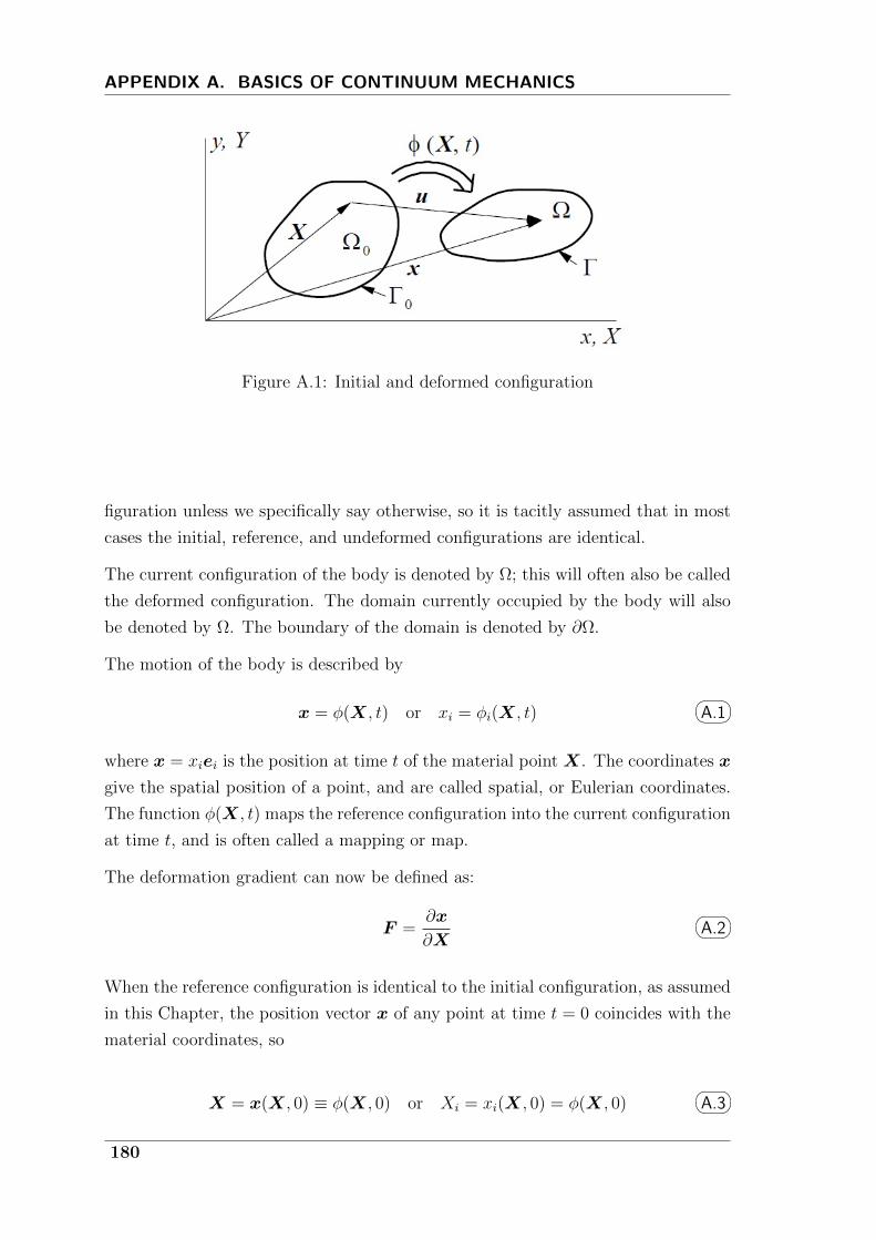
APPENDIX A. BASICS OF CONTINUUM MECHANICS
Figure A.1: Initial and deformed configuration
figuration unless we specifically say otherwise, so it is tacitly assumed that in most
cases the initial, reference, and undeformed configurations are identical.
The current configuration of the body is denoted by Ω; this will often also be called
the deformed configuration. The domain currently occupied by the body will also
be denoted by Ω. The boundary of the domain is denoted by ∂Ω.
The motion of the body is described by
x = φ(X, t) or xi = φi(X, t) A.1
where x = xiei is the position at time t of the material point X. The coordinates x
give the spatial position of a point, and are called spatial, or Eulerian coordinates.
The function φ(X, t) maps the reference configuration into the current configuration
at time t, and is often called a mapping or map.
The deformation gradient can now be defined as:
F =∂x
∂X
A.2
When the reference configuration is identical to the initial configuration, as assumed
in this Chapter, the position vector x of any point at time t = 0 coincides with the
material coordinates, so
X = x(X, 0) ≡ φ(X, 0) or Xi = xi(X, 0) = φ(X, 0) A.3
180
A.2. EULERIAN AND LAGRANGIAN DESCRIPTIONS
A.2 Eulerian and Lagrangian descriptions
Two approaches are used to describe the deformation and response of a continuum.
In the first approach, the independent variables are the material coordinates X and
the time t; this description is called a material description or Lagrangian description.
In the second approach, the independent variables are the spatial coordinates x and
the time t. This is called a spatial or Eulerian description.
In fluid mechanics, it is often impossible and unnecessary to describe the motion with
respect to a reference configuration. For example, if we consider the flow around
an airfoil, a reference configuration is usually not needed for the behavior of the
fluid, which is independent of its history. On the other hand, in solids, the stresses
generally depend on the history of deformation and an undeformed configuration
must be specified to define the strain. Because of the historydependence of most
solids, Lagrangian descriptions are prevalent in solid mechanics.
A.3 Displacement, velocity and acceleration
The displacement is given by the difference between the current position and the
original position (see Fig. A.1), so
u(X, t) = φ(X, t)− φ(X, 0) = φ(X, t)−X or ui = φi(Xj, t)−Xi
A.4
where u(X, t) = uiei. The displacement is often written as
u = x−X or ui = xi −Xi
A.5
The velocity v(X, t) is the rate of change of the position vector x, i.e. the time
derivative with X held constant. Time derivatives with X held constant are called
material time derivatives; or sometimes material derivatives. Material time deriva-
tives are also called total derivatives. The velocity can be written in the various
forms shown below
v(X, t) = x =∂φ(X, t)
∂t=∂u(X, t)
∂t= u
A.6
The superposed dot denotes a material time derivative.
181

APPENDIX A. BASICS OF CONTINUUM MECHANICS
The acceleration a(X, t) is the rate of change of velocity of a material point, or in
other words the material time derivative of the velocity, and can be written in the
forms
a(X, t) = v =∂v(X, t)
∂t=∂2u(X, t)
∂t2
A.7
The above expression is called the material form of the acceleration. When the
velocity is expressed in terms of the spatial coordinates and the time, i.e. in an
Eulerian description as in v(x, t), the material time derivative is obtained as follows:
vi(x, t) =∂vi(x, t)
∂t+∂vi(x, t)
∂xj
∂φj(X, t)
∂t=∂vi∂t
+∂vi∂xj
vj A.8
The second addend is the convective term; ∂vi∂t
is called the spatial time derivative.
A.4 Strain measures
In contrast to linear elasticity, many different measures of strain and strain rate are
used in nonlinear continuum mechanics. Only two of these measures are considered
here:
1. the Green (Green-Lagrange) strain E
2. the rate-of-deformation tensor D, also known as the velocity strain or rate-of-
strain.
In the following, these measures are defined and some key properties are given.
Many other measures of strain and strain rate appear in the continuum mechanics
literature; however, the above are the most widely used in finite element methods.
The Green strain tensor E is defined by
ds2 − dS2 = 2dX ×E × dX or dxidxi − dXidXi = 2dXiEijdXj
A.9
so it gives the change in the square of the length of the material vector dX. The
vector dX pertains to the undeformed configuration. Therefore, the Green strain
measures the difference of the square of the length of an infinitesimal segment in the
current (deformed) configuration and the reference (undeformed) configuration.
182

A.4. STRAIN MEASURES
The Green strain tensor can be written in terms of deformation gradient F as:
E =1
2(F T · F − I)
A.10
The second measure of strain to be considered here is the rate-of-deformation D. It
is also called the velocity strain and the stretching tensor. In contrast to the Green
strain tensor, it is a rate measure of strain.
In order to develop an expression for the rate-of-deformation, we first define the
velocity gradient L by
L =∂v
∂x= (∇v)T or Lij =
∂vi∂xj
A.11
dv = L× dx or dvi = Lijdxj A.12
In the above, the symbol ∇ preceding the function denotes the spatial gradient of
the function, i.e., the derivatives are taken with respect to the spatial coordinates.
The velocity gradient tensor can be decomposed into symmetric and skew symmetric
parts by
L =1
2(L+LT ) +
1
2(L−LT )
A.13
This is a standard decomposition of a second order tensor or square matrix: any
second order tensor can be expressed as the sum of its symmetric and skew symmetric
parts in the above manner.
The rate-of-deformation D is defined as the symmetric part of L, i.e. the first term
on the right hand side of A.13 and the spin W is the skew symmetric part of L,
i.e. the second term on the right hand side of A.13. Using these definitions, we can
write
L = D+W A.14
D =1
2(L+LT )
A.15
W =1
2(L−LT )
A.16
It can be demonstrated that the rate-of-deformation is a measure of the rate of
change of the square of the length of infinitesimal material line segments. The
definition is∂
∂t(ds2) =
∂
∂t(dx · dx) = 2dx ·D · dx ∀dx
A.17
183
APPENDIX A. BASICS OF CONTINUUM MECHANICS
The rate-of-deformation can be related to the rate of the Green strain tensor.
D = F−T · E · F−1 A.18
where F is the deformation gradient.
A.5 Stress measures
In nonlinear problems, various stress measures can be defined. Here the Cauchy
stress tensor will be considered. The expression for the traction t in terms of the
Cauchy stress σ is called Cauchys law or sometimes the Cauchy hypothesis.
t(n) = σ · n A.19
where
t(n) = lim∆A→0
∆T
∆A
A.20
It involves the normal n to the current surface of area A and the force T on the
current surface. For this reason, the Cauchy stress is often called the physical stress
or true stress.
Many constitutive equations are designed in the form of a relation between a stress-
rate and a strain-rate (or the rate of deformation tensor). The mechanical response
of a material should not depend on the frame of reference. In other words, ma-
terial constitutive equations should be frame indifferent (objective). In continuum
mechanics, objective stress rates are time derivatives of stress that do not depend
on the frame of reference. There are numerous objective stress rates in continuum
mechanics, this study adopt the Jaumann stress rate:
σJ = σ −W · σ + σ ·W T A.21
Equation A.21 shows that the material derivative of the Cauchy stress is the sum
of the rate of change due to the material response (term on the left hand side) and
the change of stress due to rotation (last two terms on the right hand side).
184
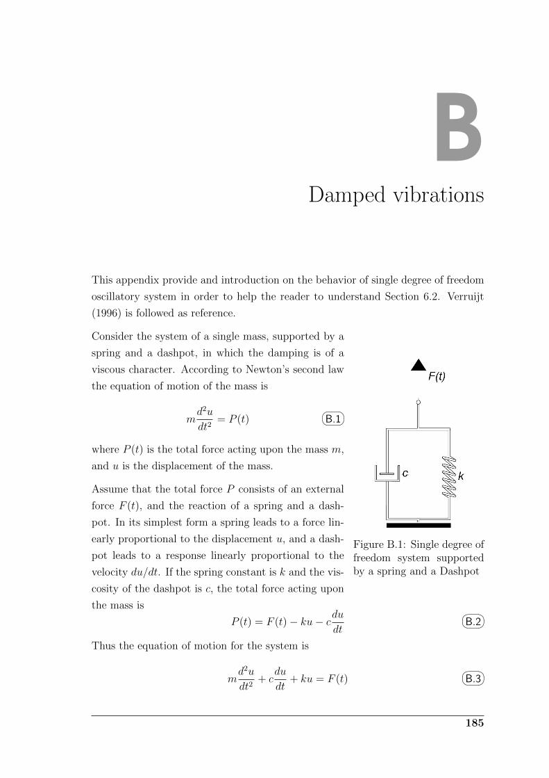
BDamped vibrations
This appendix provide and introduction on the behavior of single degree of freedom
oscillatory system in order to help the reader to understand Section 6.2. Verruijt
(1996) is followed as reference.
Figure B.1: Single degree offreedom system supportedby a spring and a Dashpot
Consider the system of a single mass, supported by a
spring and a dashpot, in which the damping is of a
viscous character. According to Newton’s second law
the equation of motion of the mass is
md2u
dt2= P (t)
B.1
where P (t) is the total force acting upon the mass m,
and u is the displacement of the mass.
Assume that the total force P consists of an external
force F (t), and the reaction of a spring and a dash-
pot. In its simplest form a spring leads to a force lin-
early proportional to the displacement u, and a dash-
pot leads to a response linearly proportional to the
velocity du/dt. If the spring constant is k and the vis-
cosity of the dashpot is c, the total force acting upon
the mass is
P (t) = F (t)− ku− cdudt
B.2
Thus the equation of motion for the system is
md2u
dt2+ c
du
dt+ ku = F (t)
B.3
185
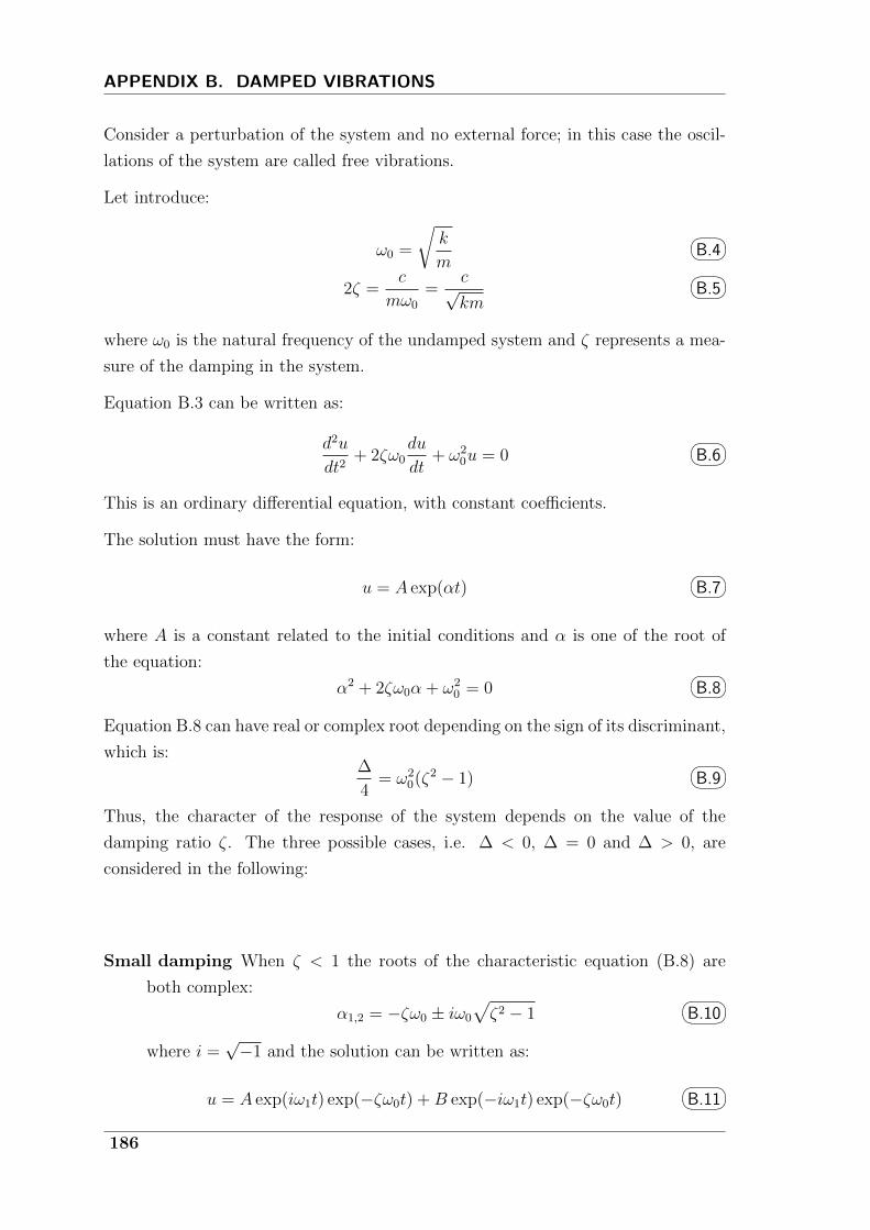
APPENDIX B. DAMPED VIBRATIONS
Consider a perturbation of the system and no external force; in this case the oscil-
lations of the system are called free vibrations.
Let introduce:
ω0 =
√k
m
B.4
2ζ =c
mω0
=c√km
B.5
where ω0 is the natural frequency of the undamped system and ζ represents a mea-
sure of the damping in the system.
Equation B.3 can be written as:
d2u
dt2+ 2ζω0
du
dt+ ω2
0u = 0 B.6
This is an ordinary differential equation, with constant coefficients.
The solution must have the form:
u = A exp(αt) B.7
where A is a constant related to the initial conditions and α is one of the root of
the equation:
α2 + 2ζω0α + ω20 = 0
B.8
Equation B.8 can have real or complex root depending on the sign of its discriminant,
which is:∆
4= ω2
0(ζ2 − 1) B.9
Thus, the character of the response of the system depends on the value of the
damping ratio ζ. The three possible cases, i.e. ∆ < 0, ∆ = 0 and ∆ > 0, are
considered in the following:
Small damping When ζ < 1 the roots of the characteristic equation (B.8) are
both complex:
α1,2 = −ζω0 ± iω0
√ζ2 − 1
B.10
where i =√−1 and the solution can be written as:
u = A exp(iω1t) exp(−ζω0t) +B exp(−iω1t) exp(−ζω0t) B.11
186
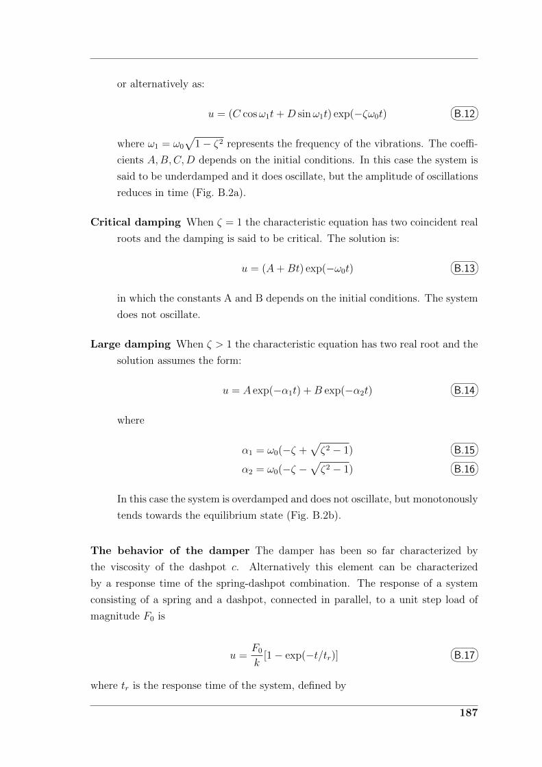
or alternatively as:
u = (C cosω1t+D sinω1t) exp(−ζω0t) B.12
where ω1 = ω0
√1− ζ2 represents the frequency of the vibrations. The coeffi-
cients A,B,C,D depends on the initial conditions. In this case the system is
said to be underdamped and it does oscillate, but the amplitude of oscillations
reduces in time (Fig. B.2a).
Critical damping When ζ = 1 the characteristic equation has two coincident real
roots and the damping is said to be critical. The solution is:
u = (A+Bt) exp(−ω0t) B.13
in which the constants A and B depends on the initial conditions. The system
does not oscillate.
Large damping When ζ > 1 the characteristic equation has two real root and the
solution assumes the form:
u = A exp(−α1t) +B exp(−α2t) B.14
where
α1 = ω0(−ζ +√ζ2 − 1)
B.15
α2 = ω0(−ζ −√ζ2 − 1)
B.16
In this case the system is overdamped and does not oscillate, but monotonously
tends towards the equilibrium state (Fig. B.2b).
The behavior of the damper The damper has been so far characterized by
the viscosity of the dashpot c. Alternatively this element can be characterized
by a response time of the spring-dashpot combination. The response of a system
consisting of a spring and a dashpot, connected in parallel, to a unit step load of
magnitude F0 is
u =F0
k[1− exp(−t/tr)]
B.17
where tr is the response time of the system, defined by
187
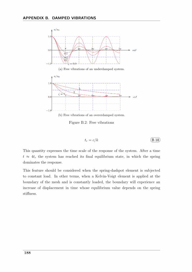
APPENDIX B. DAMPED VIBRATIONS
(a) Free vibrations of an underdamped system.
(b) Free vibrations of an overerdamped system.
Figure B.2: Free vibrations
tr = c/k B.18
This quantity expresses the time scale of the response of the system. After a time
t ≈ 4tr the system has reached its final equilibrium state, in which the spring
dominates the response.
This feature should be considered when the spring-dashpot element is subjected
to constant load. In other terms, when a Kelvin-Voigt element is applied at the
boundary of the mesh and is constantly loaded, the boundary will experience an
increase of displacement in time whose equilibrium value depends on the spring
stiffness.
188
Bibliography
Aad, G., E. Abat, J. Abdallah, A. Abdelalim, A. Abdesselam, O. Abdinov, B. Abi,
M. Abolins, H. Abramowicz, E. Acerbi, et al. (2008). The atlas experiment at
the cern large hadron collider. Journal of Instrumentation 3 (08), S08003.
Aas Nost, H. (2011). Undrained soft soil modelling with the Material Point
Method. Master thesis, Norwegian University of science and technology.
Abbo, A. J. and S. W. Sloan (1995). A smooth hyperbolic approximation to the
mohr-coulomb yield criterion. Computers & Structures 54 (3), 427–441.
Abe, K., K. Soga, and S. Bandara (2013). Material Point Method for Coupled
Hydromechanical Problems. Journal of Geotechnical and Geoenvironmental
Engineering 140, 1–16.
Al-Kafaji, I. K. J. (2013). Formulation of a Dynamic Material Point Method
(MPM) for Geomechanical Problems. Ph. d. thesis, University of Struttgart,
Germay.
Alder, B. J. and T. Wainwright (1959). Studies in molecular dynamics. i. general
method. The Journal of Chemical Physics 31 (2), 459–466.
Allahdadi, F. A., T. C. Carney, J. R. Hipp, L. D. Libersky, and A. G. Petschek
(1993). High strain lagrangian hydrodynamics: a three dimensional sph code
for dynamic material response. Technical report, DTIC Document.
Alonso, E., N. Pinyol, and A. Yerro (2014). Mathematical Modelling of Slopes. In
Procedia Earth and Planetary Science, Volume 9, pp. 64–73. Elsevier B.V.
Alonso, E. and F. Zabala (2011, September). Progressive failure of Aznalcollar
dam using the material point method. Geotechnique 61 (9), 795–808.
Andersen, S. (2009a). Material-point analysis of large-strain problems: Modelling
of landslides. Ph. D. thesis, Aalborg University, Faculty of Engineering and
Science, Research Group for Computational Mechanics.
Andersen, S. (2009b). Material-point analysis of large-strain problems: Modelling
of landslides. Ph. D. thesis, AAlborg University.
Andersen, S. and L. Andersen (2010a, April). Analysis of spatial interpolation in
the material-point method. Computers & Structures 88 (7-8), 506–518.
Andersen, S. and L. Andersen (2010b, April). Modelling of landslides with the
material-point method. Computational Geosciences 14 (1), 137–147.
189
BIBLIOGRAPHY
Andreykiv, A., F. Keulen, D. J. Rixen, and E. Valstar (2012). A level-set-based
large sliding contact algorithm for easy analysis of implant positioning. Inter-
national Journal for Numerical Methods in Engineering 89 (10), 1317–1336.
Atkinson, J. H. and P. L. Bransby (1978). The mechanics of soil. McGraw-Hill
London.
Atluri, S., J. Cho, and H.-G. Kim (1999). Analysis of thin beams, using the
meshless local petrov–galerkin method, with generalized moving least squares
interpolations. Computational Mechanics 24 (5), 334–347.
Atluri, S. and T. Zhu (1998). A new meshless local petrov-galerkin (mlpg) ap-
proach in computational mechanics. Computational mechanics 22 (2), 117–
127.
Augarde, C. and C. Heaney (2009). The use of meshless methods in geotechnics.
In Proceedings of the 1st International Symposium on Computational Geome-
chanics (COMGEO I), Number Comgeo I, Juan-les-Pins, France, pp. 311–320.
Baligh, M. and J. Levadoux (1986). Consolidation after undrained piezocone pen-
etration. II: interpretation. Journal of geotechnical engineering 112 (7), 727–
745.
Baligh, M. M. (1985). Strain path method. Journal of Geotechnical Engineer-
ing 111 (9), 1108–1136.
Bandara, S. and K. Soga (2015, January). Coupling of soil deformation and pore
fluid flow using material point method. Computers and Geotechnics 63, 199–
214.
Bandara, S. S. (2013). Material Point Method to simulate Large Deformation
Problems in Fluid-saturated Granular Medium. Ph. D. thesis, Cambridge, UK.
Baran, S. (1968). Monopoly Capital. An Essay on the American Economic and
Social Order.
Bardenhagen, S. (2002, July). Energy Conservation Error in the Material Point
Method for Solid Mechanics. Journal of Computational Physics 180 (1), 383–
403.
Bardenhagen, S., J. Brackbill, and D. Sulsky (2000a, September). Numerical study
of stress distribution in sheared granular material in two dimensions. Physical
review. E 62 (3), 3882–90.
Bardenhagen, S., J. Brackbill, and D. Sulsky (2000b). Shear deformation in gran-
ular material. In 11th International Detonation Symposium, Snowmass, CO,
pp. 547–555.
190
BIBLIOGRAPHY
Bardenhagen, S., J. Brackbill, and D. Sulsky (2000c, July). The material-point
method for granular materials. Computer Methods in Applied Mechanics and
Engineering 187 (3-4), 529–541.
Bardenhagen, S., J. Guilkey, K. Roessig, J. Brackbill, W. Witzel, and J. Foster
(2001). An improved contact algorithm for the material point method and
application to stress propagation in granular material. Computer Modeling in
Engineering and Sciences 2, 509–522.
Bardenhagen, S. and E. Kober (2004). The generalized interpolation material
point method. Computer Modeling in Engineering and Sciences 5 (6), 477–
495.
Bardet, J. (1992). A viscoelastic model for the dynamic behavior of saturated
poroelastic soils. Journal of applied mechanics 59 (March).
Batchelor, G. K. (2000). An introduction to fluid dynamics. Cambridge university
press.
Bathe, K.-J. (2006). Finite element procedures. Klaus-Jurgen Bathe.
Belytschko, T. and Y. Krongauz (1998). Efg approximation with discontinu-
ous derivatives. International Journal for Numerical Methods in Engineer-
ing 41 (7), 1215–1233.
Belytschko, T., W. K. Liu, B. Moran, and K. Elkhodary (2013). Nonlinear finite
elements for continua and structures (Second ed.). John Wiley & Sons.
Belytschko, T., Y. Y. Lu, and L. Gu (1994). Element-free galerkin methods.
International journal for numerical methods in engineering 37 (2), 229–256.
Beuth, L. (2011). Solution of quasi-static large-strain problems by the material
point method. Internationsl Journal for Numerical and Analytical Methods in
Geomechanics 35 (13), 1451–1465.
Beuth, L. (2012). Formulation and Application of a Quasi-Static Material Point
Method. Ph. d. thesis, University of Struttgart.
Beuth, L., T. Benz, and P. A. Vermeer (2008). Large deformation analysis us-
ing a quasi-static material poin method. Journal of Theoretical and Applied
Mechanics 38 (1-2), 45–60.
Beuth, L., T.Benz, P. A. Vermeer, C. J. Coetzee, P. Bonnier, P. van den Berg, and
T. Benz (2007). Formulation and validation of a quasi-static material point
method. In Proceedings of the 10th international symposium on numerical
methods in Geomechanics (NUMOG), Rhodes, Greece, pp. 189–195.
191

BIBLIOGRAPHY
Beuth, L. and P. A. Vermeer (2013). Large deformation analysis of cone penetra-
tion testing in undrained clay.
Biot, M. (1956a). Theory of propagation of elastic waves in a fluidsaturated porous
solid. I. Lowfrequency range. The Journal of the Acoustical Society of Amer-
ica 28 (2).
Biot, M. (1956b). Theory of propagation of elastic waves in a fuid-saturatedporous
solid. ii. higher frequency range. The Journal of the Acoustical Society of Amer-
ica 28, 179–191.
Biot, M. (1972). Theory of finite deformations of porous solids. Indiana University
Mathematics Journal 21 (7), 597–620.
Biot, M. a. (1941). General Theory of Three-Dimensional Consolidation. Journal
of Applied Physics 12 (2), 155.
Biot, M. a. (1955). Theory of Elasticity and Consolidation for a Porous
Anisotropic Solid. Journal of Applied Physics 26 (2), 182.
Biot, M. A. (1956c). Theory of propagation of elastic waves in a fluid-saturated
porous solid. i. low frequency range. The Journal of the Acoustical Society of
America 28 (2), 168–178.
Bolton, M. (1986). The strength and dilatancy of sands. Geotechnique 36 (1),
65–78.
Borja, R., C. Tamagnini, and E. Alarcon (1998). Elastoplastic consolidation at
finite strain part 2: finite element implementation and numerical examples.
Computer Methods in Applied Mechanics and Engineering 5, 103–122.
Borja, R. I., C. Tamagnini, and A. Amorosi (1997). Coupling plasticity and
energy-conserving elasticity models for clays. Journal of geotechnical and
geoenvironmental engineering 123 (10), 948–957.
Borjia, R. and E. Kavazanjian (1985). A viscoplasticity model for the stress-strain-
time behaviour of wet clays. Geotechnique 35, 283–298.
Brackbill, J. and H. Ruppel (1986). Flip: A method for adaptively zoned, particle-
in-cell calculations of fluid flows in two dimensions. Journal of Computational
Physics 65 (2), 314–343.
Brackbill, J. U., D. B. Kothe, and H. M. Ruppel (1988). Flip: A low-
dissipation, particle-in-cell method for fluid flow. Computer Physics Commu-
nications 48 (1), 25–38.
192
BIBLIOGRAPHY
Bui, H. H., K. Sako, and R. Fukagawa (2007). Numerical simulation of soil–water
interaction using smoothed particle hydrodynamics (sph) method. Journal of
Terramechanics 44 (5), 339–346.
Bui, H. H., K. Sako, R. Fukagawa, and J. Wells (2008). Sph-based numerical
simulations for large deformation of geomaterial considering soil-structure in-
teraction. In The 12th International Conference of International Association
for Computer Methods and Advances in Geomechanics (IACMAG), Volume 1,
pp. 570–578. Citeseer.
Burland, J. (1990). 30th rankine lecture: On the compressibility and shear
strength of natural clays. Gotechnique 40 (3), 327–378.
Campanella, R., D. Gillespie, and P. Robertson (1982). Pore pressures during
cone penetration testing. In A. Verruijt, F. Beringen, and de Leeuw E.H.
(Eds.), Proceedings of the 2nd European Symposium on Penetration Testing,
pp. 507–512. Balkema, Rotterdam.
Carter, J., J. Booker, and C. Wroth (1982). Soil mechanics - Transient and cyclic
loads, Chapter A critical state model for ciclic loading, pp. 219–252. Wiley.
Chen, J.-S., C. M. O. L. Roque, C. Pan, and S. T. Button (1998, August). Analysis
of metal forming process based on meshless method. Journal of Materials
Processing Technology 80-81, 642–646.
Chung, S., M. F. Randolph, and J. A. Schneider (2006). Effect of penetration rate
on penetrometer resistance in clay. Journal of Geotechnical and Geoenviron-
mental Engineering (September), 1188–1196.
Coetzee, C., A. Basson, and P. Vermeer (2007, April). Discrete and continuum
modelling of excavator bucket filling. Journal of Terramechanics 44 (2), 177–
186.
Coetzee, C. J. (2003). The Modelling of Granular Flow Using the Particle-in-Cell
Method. Phd thesis, Stellenbosch.
Coetzee, C. J. (2005). The material point method. Technical Report November,
University of Stellenbosh, Stellenbosh, South Africa.
Coetzee, C. J., P. A. Vermeer, and A. H. Basson (2005, August). The modelling of
anchors using the material point method. International Journal for Numerical
and Analytical Methods in Geomechanics 29 (9), 879–895.
Courant, R. et al. (1943). Variational methods for the solution of problems of
equilibrium and vibrations. Bull. Amer. Math. Soc 49 (1), 1–23.
193

BIBLIOGRAPHY
Cummins, S. and J. Brackbill (2002, August). An Implicit Particle-in-Cell Method
for Granular Materials. Journal of Computational Physics 180 (2), 506–548.
Cundall, P. (1987). Distinct element models of rock and soil structure. Analytical
and computational methods in engineering rock mechanics 4, 129–163.
Cundall, P. (2001). FLAC Manual: A Computer Program for Fast Lagrangian
Analysis of Continua.
Cundall, P. A. and O. D. Strack (1979). A discrete numerical model for granular
assemblies. Geotechnique 29 (1), 47–65.
Cuomo, S., N. Prime, a. Iannone, F. Dufour, L. Cascini, and F. Darve (2012,
August). Large deformation FEMLIP drained analysis of a vertical cut. Acta
Geotechnica.
Dafalias, Y. F. and L. R. Herrmann (1980). Soil mechanics - Transient and cyclic
loads, Chapter Bouclays surface formulation of soil plasticity, pp. 253–282.
Wiley.
Davis, R. O. and A. P. Selvadurai (2002). Plasticity and geomechanics. Cambridge
University Press.
De Borst, R., M. Crisfield, J. Remmers, and C. Verhoosel (2012). Non-linear finite
element analysis of solids and structures. John Wiley & Sons .
De Borst, R. and P. Vermeer (1984). Possibilites and limitations of finite elements
for limit analysis. Geotechnique 34 (2), 199–210.
DeJong, J. and M. Randolph (2012). Influence of Partial Consolidation during
Cone Penetration on Estimated Soil Behavior Type and Pore Pressure Dis-
sipation Measurements. Journal of Geotechnical and geoenvironmental Engi-
neering (July), 777–788.
Detournay, C. and E. Dzik (2006). Nodal mixed discretization for tetrahedral
elements. In 4th international FLAC symposium, numerical modeling in ge-
omechanics. Minnesota Itasca Consulting Group, Inc. Paper, Number 07-02.
Donea, J. and A. Huerta (2004). Arbitrary LagrangianEulerian methods. Ency-
clopedia of Computational Mechanics (1969), 1–38.
Douglas, B. and R. Olsen (1981). Soil classification using electric cone penetrom-
eter. In A. Geotechnical Engineering Division (Ed.), In Proceedings of Sym-
posium on Cone Penetration Testing and Experience, St. Louis, Missouri, pp.
209–227.
194

BIBLIOGRAPHY
Elkadi, A. and P. Nguyen (2013). Mpm validation with centrifuge tests: pilot case
pile installation. Technical Report 1206750-G05-HYE-GG01-Jvm, Deltares,
Delft, The Netherlands.
Ferronato, M., A. Mazzia, G. Pini, and G. Gambolati (2007). A meshless method
for axisymmetric poroelastic simulations: numerical study. Int. J. Numer.
Methods Eng. (70), 13461365.
Finnie, I. and M. Randolph (1994). Punch-through and liquefaction induced fail-
ure of shallow foundations on calcareous sediments. In Proc. 7th Int. Conf. on
Behaviour of Offshore Structures, Boston, pp. 217–230.
Gadala, M. and J. Wang (1998). ALE formulation and its application in solid
mechanics. Computer Methods in Applied Mechanics and engineering 167 (98),
33–55.
Gemant, A. and W. Jackson (1937). Xciii. the measurement of internal friction
in some solid dielectric materials. The London, Edinburgh, and Dublin Philo-
sophical Magazine and Journal of Science 23 (157), 960–983.
Gens, A. and D. Potts (1988). Critical state models in computational geomechan-
ics. Engineering Computations 5 (3), 178–197.
Gingold, R. A. and J. J. Monaghan (1977). Smoothed particle hydrodynamics:
theory and application to non-spherical stars. Monthly notices of the royal
astronomical society 181 (3), 375–389.
Godoy, L. and P. Dardati (2001). Validacion de modelos en mecanica computa-
cional.
Griffiths, D. (1982). Elasto-plastic analyses of deep foundations in cohesive soil.
International Journal for Numerical and Analytical Methods in Geomechan-
ics 6 (2), 211–218.
Guilkey, J. and J. Weiss (2001). An implicit time integration strategy for use with
the material point method. In Proceedings from the First MIT Conference on
Computational Fluid and Solid Mechanics. Citeseer.
Guilkey, J. E., J. B. Hoying, and J. A. Weiss (2006). Computational modeling
of multicellular constructs with the material point method. Journal of biome-
chanics 39 (11), 2074–2086.
Guilkey, J. E. and J. a. Weiss (2003, July). Implicit time integration for the ma-
terial point method: Quantitative and algorithmic comparisons with the finite
element method. International Journal for Numerical Methods in Engineer-
ing 57 (9), 1323–1338.
195
BIBLIOGRAPHY
Gutfraind, R. and S. B. Savage (1998). Flow of fractured ice through wedge-shaped
channels: smoothed particle hydrodynamics and discrete-element simulations.
Mechanics of materials 29 (1), 1–17.
Hagerty, D. J. and R. B. Peck (1971). Heave and lateral movements due to pile
driving. Journal of the Soil Mechanics and Foundations Division 97 (11), 1513–
1532.
Harlow, F. H. (1964). The particle-in-cell computing method for fluid dynamics.
Methods in computational physics 3 (3), 319–343.
Harlow, F. H. and M. Evans (1955). A machine calculation method for hydrody-
namic problems. Technical report.
Harlow, F. H., M. W. Evans, and E. Bromberg (1957). The particle-in-cell method
for hydrodynamic calculations. Technical report, DTIC Document.
Hart, R., P. Cundall, and J. Lemos (1988). Formulation of a three-dimensional dis-
tinct element modelpart ii. mechanical calculations for motion and interaction
of a system composed of many polyhedral blocks. In International Journal of
Rock Mechanics and Mining Sciences & Geomechanics Abstracts, Volume 25,
pp. 117–125. Elsevier.
Henke, S. Qiu, G. and J. Grabe (2010). A coupled eulerian-lagrangian approach to
solve geotechnical problems involving large deformations. In In 7th European
Conference on Numerical Methods in Geotechnical Engineering (NUMGE),
Trondheim, Norway.
Higo, Y., F. Oka, S. Kimoto, Y. Morinaka, Y. Goto, and Z. Chen (2010). A
coupled mpm-fdm analysis method for multi-phase elasto-plastic soils. Soils
and foundations 50 (4), 515–532.
Houlsby, G. (1985). The use of a variable shear modulus in elastic-plastic models
for clays. Computers and Geotechnics 1 (1), 3–13.
Houlsby, G., A. Wheeler, and J. Norbury (1985). Analysis of undrained cone
penetration as a steady flow problem. In Proceedings of the 5th International
Conference on Numerical Methods in Geomechanics, Volume 4, pp. 1767–73.
House, A., J. Oliveira, and M. Randolph (2001). Evaluating the coefficient of con-
solidation using penetration tests. International Journal of Physical Modelling
in Geotechnics 1 (3), 17–26.
Hrennikoff, A. (1941). Solution of problems of elasticity by the frame-work
method. ASME J. Appl. Mech. 8, A619A715.
196
BIBLIOGRAPHY
Hu, W. and Z. Chen (2003, August). A multi-mesh MPM for simulating the
meshing process of spur gears. Computers & Structures 81 (20), 1991–2002.
Hu, W. and Z. Chen (2006). Model-based simulation of the synergistic effects
of blast and fragmentation on a concrete wall using the mpm. International
journal of impact engineering 32 (12), 2066–2096.
Hu, Y. and M. Randolph (1998). A practical numerical approach for large defor-
mation problems in soil. International Journal for Numerical and Analytical
Methods in Geomechanics 22 (5), 327–350.
Huang, P. and X. Zhang (2011). Contact algorithms for the material point method
in impact and penetration simulation. International Journal for numerical
methods in Engineering (July 2010), 498–517.
Huang, W., D. Sheng, S. Sloan, and H. Yu (2004, October). Finite element analysis
of cone penetration in cohesionless soil. Computers and Geotechnics 31 (7),
517–528.
Idelsohn, S. and E. Onate (2003). The meshless finite element method. Interna-
tiona Journal for Numerical Methods in Engineering 58 (4), 1–15.
Idelsohn, S., E. Onate, and F. Del Pin (2003, May). A Lagrangian meshless finite
element method applied to fluidstructure interaction problems. Computers &
Structures 81 (8-11), 655–671.
Idelsohn, S., E. Onate, and F. D. Pin (2004, October). The particle finite element
method: a powerful tool to solve incompressible flows with free-surfaces and
breaking waves. International Journal for Numerical Methods in Engineer-
ing 61 (7), 964–989.
Idelsohn, S., E. Onate, F. D. Pin, and N. Calvo (2006, March). Fluidstructure
interaction using the particle finite element method. Computer Methods in
Applied Mechanics and Engineering 195 (17-18), 2100–2123.
Ionescu, I., J. Guilkey, M. Berzins, R. M. Kirby, and J. Weiss (2005). Compu-
tational simulation of penetrating trauma in biological soft tissues using the
material point method. Studies in health technology and informatics 111, 213–
218.
Iseno, H., H. Kohashi, K. Furumoto, H. Mori, and M. Ohno (2004). Large model
tests of levee reinforcement method with toe drain for seepage failure. In Proc.,
Annual Symp. of Japanese Geotechnical Society, Volume 39, pp. 1255–1256.
Jaeger, R., J. DeJong, R. W. Boulanger, H. E. Low, and M. Randolph (2010).
Variable penetration rate CPT in an intermediate soil. In Omnipress (Ed.),
197

BIBLIOGRAPHY
Proc., 2nd Int. Symp. on Cone Penetration Testing., Madison.
Janbu, N. and K. Senneset (1974). Effective stress interpretation of in situ static
penetration tests. In Proceedings of the 1st European symposium on penetration
testing, Volume 2, pp. 181–93.
Jassim, I., D. Stolle, and P. Vermeer (2013). Two-phase dynamic analysis by mate-
rial point method. International Journal for Numerical and Analytical Meth-
ods in Geomechanicsnumerical and analytical methods in Geomechanics 37,
2502–2522.
Jefferies, M. and K. Been (2006). Soil liquefaction: a critical state approach. CRC
Press.
Jefferies, M. and M. Davies (1991). Soil classification by the cone penetration test:
Discussion. Canadian Geotechnical Journal 28 (1), 173–176.
Johansson, J. and K. Konagai (2007). Fault induced permanent ground defor-
mations: Experimental verification of wet and dry soil, numerical findings
relation to field observations of tunnel damage and implications for design.
Soil Dynamics and Earthquake Engineering 27 (10), 938–956.
Kim, H. Inoue, J. (2007). A stochastic element free seepage flow analysis of het-
erogeneous subsurface. In S. Pande, G. Pietruszczak (Ed.), Numerical Models
in Geomechanics NUMOG X, pp. 225–231. Taylor & Francis Group, London.
Kim, K., M. Prezzi, R. Salgado, and W. Lee (2008). Effect of penetration rate on
cone penetration resistance in saturated clayey soils. Journal of Geotechnical
and Geoenviromental Engineering (August), 1142–1153.
Kiousis, P. D., G. Z. Voyiadjis, and M. T. Tumay (1988). A large strain theory and
its application in the analysis of the cone penetration mechanism. International
Journal for Numerical and Analytical Methods in Geomechanics 12 (1), 45–60.
Konagai, K. and J. Johansson (2001). Lagrangian Particles for Modeling Large
Soil Deformations. In Proc., Seismic Fault-induced failures, pp. 101–108.
Konagai, K., J. Johansson, and H. Itoh (2004). Pseudo-three dimensional la-
grangian particle finite difference method for modeling earthquake induced
soil flows. In 13th World Conference on Earthquake Engineering, Number 547,
Vancouver, B. C: Canada.
Koskinen, M., M. Karstunen, and S. Wheeler (2002). Modelling destructuration
and anisotropy of a soft natural clay.
198
BIBLIOGRAPHY
Kouretzis, G. P., D. Sheng, and D. Wang (2014, March). Numerical simulation
of cone penetration testing using a new critical state constitutive model for
sand. Computers and Geotechnics 56, 50–60.
Kurup, P., G. Voyiadjis, and M. Tumay (1994). Calibration chamber studies of
piezocone test in cohesive soils. Journal of Geotechnical Engineering 120 (1),
81–107.
Kutter, B. L. and N. Sathialingam (1992). Elastic-viscoplastic modelling of the
rate-dependent dehaviour of clays. Geotechnique 42, 427–441.
Ladanyi, B. (1963). Expansion of a cavity in a saturated clay medium. Journal of
the Soil Mechanics and Foundations Division 89 (SM4), 127–161.
Ladanyi, B. and G. Johnston (1974). Behavior of circular footings and plate an-
chors in permafrost. Canadian Geotechnical Journal 11 (4), 531–553.
Lehane, B., C. O’Loughlin, M. Randolph, and C. Gaudin (2009, January). Rate
effects on penetrometer resistance in kaolin. Geotechnique 59 (1), 41–52.
Lemos, L. and P. Vaughan (2000). Clay–interface shear resistance. Geotech-
nique 50 (1), 55–64.
Levadoux, J.-N. and M. M. Baligh (1980). Pore pressure dissipation after cone
penetration. Massachusetts Institute of Technology, Department of Civil En-
gineering, Constructed Facilities Division.
Lewis, R. W. and B. A. Schrefler (1998). The finite element method in the static
and dynamic deformation and consolidation of porous media. John Wiley.
Lian, Y., X. Zhang, and Y. Liu (2011, November). Coupling of finite element
method with material point method by local multi-mesh contact method.
Computer Methods in Applied Mechanics and Engineering 200 (47-48), 3482–
3494.
Lian, Y., X. Zhang, and Y. Liu (2012, October). An adaptive finite element
material point method and its application in extreme deformation problems.
Computer Methods in Applied Mechanics and Engineering 241-244, 275–285.
Lian, Y., X. Zhang, X. Zhou, S. Ma, and Y. Zhao (2011). Numerical simulation
of explosively driven metal by material point method. International Journal
of Impact Engineering 38 (4), 238–246.
Lim, L., A. Andreykiv, and R. Brinkgreve (2014). On the application of the
material point method for offshore foundations. In M. Hicks, Brinkgreve, and
A. Rohe (Eds.), Numerical Methods in geotechnical Engineering. Taylor and
Francis group.
199

BIBLIOGRAPHY
Liu, M. B. and G. R. Liu (2010, February). Smoothed Particle Hydrodynamics
(SPH): an Overview andRecent Developments, Volume 17.
Love, E. and D. Sulsky (2006, July). An unconditionally stable, energymomentum
consistent implementation of the material-point method. Computer Methods
in Applied Mechanics and Engineering 195 (33-36), 3903–3925.
Lu, Q., Y. Hu, M. F. Randolph, and I. C. Bugarski (2004, January). A numerical
study of cone penetration in clay. Geotechnique 54 (4), 257–267.
Lucy, L. B. (1977). A numerical approach to the testing of the fission hypothesis.
The astronomical journal 82, 1013–1024.
Lunne, T. Robertson, P. and J. Powell (1997). Cone Penetration Testing in
Geotechnical Practice. Blackie Academic/Chapman & Hall.
Lysmer, J. and R. L. Kuhlemeyer (1969). Finite dynamic model for infinite media.
In Proc. of ASCE, pp. 859–877.
Ma, J., D. Wang, and M. Randolph (2014). A new contact algorithm in the
material point method for geotechnical simulations. International Journal of
Numerical and Analytical Methods in Geomechanics (March), 1197–1210.
Ma, S., X. Zhang, and X. M. Qiu (2009). Comparison study of mpm and sph
in modeling hypervelocity impact problems. International Journal of Impact
Engineering 36, 272–282.
Martinelli, M. and A. Rohe (2014, December). Soil-water transition with the
material point method: the algorithm. MPM-Dredge workshop, Cambridge.
Masin, D. (2005, April). A hypoplastic constitutive model for clays. International
Journal for Numerical and Analytical Methods in Geomechanics 29 (4), 311–
336.
Mast, C., P. Mackenzie-Helnwein, P. Arduino, G. Miller, and W. Shin (2012,
June). Mitigating kinematic locking in the material point method. Journal of
Computational Physics 231 (16), 5351–5373.
Mayne, P. W. and F. H. Kulhawy (1982). k0-ocr relationships in soil. Journal of
the Geotechnical Engineering Division 108 (6), 851–872.
Meyerhof, G. (1951). The ultimate bearing capacity of foudations. Geotech-
nique 2 (4), 301–332.
Modaressi, H. and L. Laloui (1997). A thermo-viscoplastic constitutive model for
clays. International journal for numerical and analytical methods in geome-
chanics 21 (5), 313–335.
200

BIBLIOGRAPHY
Monaghan, J. (2012, January). Smoothed Particle Hydrodynamics and Its Diverse
Applications. Annual Review of Fluid Mechanics 44 (1), 323–346.
Monaghan, J. J. (1994). Simulating free surface flows with sph. J. Comput.
Phys. (110), 399–406.
Moresi, L., F. Dufour, and H.-B. Muhlhaus (2003). A lagrangian integration point
finite element method for large deformation modeling of viscoelastic geomate-
rials. Journal of Conmputational Physics 184, 476–497.
Morris, J. P., P. J. Fox, and Y. Zhu (1997). Modeling low reynolds number incom-
pressible flows using sph. Journal of computational physics 136 (1), 214–226.
Nairn, J. A. (2003). Material point method calculations with explicit cracks. Com-
puter Modeling in Engineering and Sciences 4 (6), 649–664.
Nazem, M. and D. Sheng (2008). Arbitrary LagrangianEulerian method for larges-
train consolidation problems. International Journal for Numerical and Ana-
lytical Methods in Geomechanics 32 (September 2007), 1023–1050.
Numada, M. and K. Konagai (2003). Material point method for run out analysis
of earthquake-induced long-traveling soil flows. JSCE Journal of Earthquake
Engineering 27, 3–6.
Nuygen, P., A. F. van Tol, A. S. K. Elkadi, and A. Rohe (2014). Modelling of
pile installation using the material point method (mpm). Numerical Methods
in geotechnical Engineering , 271.
Onate, E., M. a. Celigueta, and S. R. Idelsohn (2006, November). Modeling
bed erosion in free surface flows by the particle finite element method. Acta
Geotechnica 1 (4), 237–252.
Onate, E., S. R. Idelsohn, F. Del Pin, and R. Aubry (2004, September). the
Particle Finite Element Method an Overview. International Journal of Com-
putational Methods 01 (02), 267–307.
Oger, L. and S. Savage (1999). Smoothed particle hydrodynamics for cohesive
grains. Computer methods in applied mechanics and engineering 180 (1), 169–
183.
Ohta, H. and C. P. Wroth (1976). Anisotropy and stress reorientation in clay
under load. In Blacksburg (Ed.), Proc. 2nd Int. Conf. on Numerical Methods
in Geomechanics, Volume 1, pp. 319–328.
Oliveira, J., M. Almeida, H. Motta, and M. Almeida (2011). Influence of pene-
tration rate on penetrometer resistance. Journal of Geotechnical and Geoen-
vironmental Engineering 137 (7), 695–703.
201

BIBLIOGRAPHY
Pastor, M., O. Zienkiewicz, and A. Chan (1990). Generalized plasticity and the
modelling of soil behaviour. International Journal for Numerical and Analyt-
ical Methods in Geomechanics 14 (3), 151–190.
Potyondy, J. (1961). Skin friction between various soils and construction materials.
Geotechnique, 339–353.
Praveen Kumar, R., G. Dodagoudar, and B. Rao (2008). Meshfree modelling of
two-dimensional contaminant transport through unsaturated porous media. In
D. Toll, C. Augarde, D. Gallipoli, and S. Wheeler (Eds.), Unsaturated Soils:
Advances in Geo-Engineering, pp. 861866. Taylor & Francis Group, London.
Puzrin, A. M., E. E. Alonso, and N. Pinyol (2010). Geomechanics of failures,
Chapter 6 - Braced excavation collapse: Nicoll Highway, Singapore, pp. 152–
181. Springer Netherlands.
Qiu, G. (2014). Numerical analysis of penetration tests in soils. In J. Grabe (Ed.),
Ports for Container Ships of future generations, Number 1920, Hamburg, Ger-
many, pp. 183–196.
Qiu, G. and J. Grabe (2011, September). Explicit modeling of cone and strip
footing penetration under drained and undrained conditions using a visco-
hypoplastic model. Geotechnik 34 (3), 205–217.
Qiu, G. and J. Grabe (2012, October). Active earth pressure shielding in quay
wall constructions: numerical modeling. Acta Geotechnica 7 (4), 343–355.
Qiu, G. and S. Henke (2011, October). Controlled installation of spudcan foun-
dations on loose sand overlying weak clay. Marine Structures 24 (4), 528–550.
Qiu, G., S. Henke, and J. Grabe (2011, January). Application of a Coupled Eu-
lerianLagrangian approach on geomechanical problems involving large defor-
mations. Computers and Geotechnics 38 (1), 30–39.
Quek, S. and G. Liu (2003). Finite Element Method: A Practical Course: A
Practical Course. Butterworth-Heinemann.
Rahman, A. (1964). Correlations in the motion of atoms in liquid argon. Physical
Review 136 (2A), A405.
Randolph, M. (2004). Characterisation of soft sediments for offshore applications.
In V. da Fonseca and Mayne (Eds.), Proc. 2nd Int. Conf. on Site Characteri-
sation, Porto, Rotterdam, pp. 209–232. Millpress.
Randolph, M., J. Carter, and C. Wroth (1979). Driven piles in claythe effects of
installation and subsequent consolidation. Geotechnique 29 (4), 361–393.
202
BIBLIOGRAPHY
Randolph, M. and S. Hope (2004). Effect of cone velocity on cone resistance
and excess pore pressures. In Proc., Int. Symp. on Engineering Practice and
Performance of Soft Deposits, pp. 147–152. Yodagawa Kogisha Co., Ltd.
Randolph, M. and C. Wroth (1979). An analytical solution for the consolida-
tion around a driven pile. International Journal for Numerical and Analytical
Methods in geomechanics 3 (August 1978), 217–229.
Randolph, M. F. (2003, January). Science and empiricism in pile foundation de-
sign. Geotechnique 53 (10), 847–875.
Robertson, P. (1990). Soil classification using the cone penetration test. Canadian
Geotechnical Journal 27 (1), 151–158.
Robertson, P., J. Sully, D. Woeller, T. Lunne, J. Powell, and D. Gillespie
(1992). Estimating coefficient of consolidation from piezocone tests. Canadian
Geotechnical Journal 29 (v), 539–550.
Robertson, P. and C. Wride (1998). Evaluating cyclic liquefaction potential using
the cone penetration test. Canadian Geotechnical Journal 35 (3), 442–459.
Robertson, P. K., R. Campanella, D. Gillespie, and J. Greig (1986). Use of
piezometer cone data. In Use of in situ tests in geotechnical engineering, pp.
1263–1280. ASCE.
Robinson, J. and J. S. Przemieniecki (1985). Early FEM pioneers. Robinson and
Associates.
Rohe, A. and P. A. Vermeer (2014, July). Multiphase modelling of large defor-
mations using mpm: Applications in geotechnics and soil-water transition.
Colloquium at University of Padova.
Roscoe, K. and J. Burland (1968). Engineering plasticity, Chapter On generalised
stress strain behaviour of wet clay, pp. 535–609. Cambridge University Press,
Cambridge.
Roy, M., R. Blanchet, F. Tavenas, and P. L. Rochelle (1981). Behaviour of a
sensitive clay during pile driving. Canadian Geotechnical Journal 18 (1), 67–
85.
Sagaseta, C. and A. Whittle (2001). Prediction of ground movements due to
pile driving in clay. Journal of Geotechnical and Geoenvironmental Engineer-
ing (January), 55–66.
Salgado, R. (1997). Cavity expansion and penetration resistance in sand. Journal
of Geotechnical and Geoenviromental Engineering , 344–354.
203

BIBLIOGRAPHY
Schanz, T. and P. Vermeer (1998). On the stiffness of sands. Geotechnique 48,
383–387.
Schmertmann, J. H. (1978). Guidelines for cone penetration test (performance
and design). Technical report.
Schneider, J., B. M. Lehane, and F. Schnaid (2007). Velocity effects on piezocone
measurements in normally and over consolidated clays. International Journal
of Physical Modelling in Geotechnics 7 (2), 23–34.
Schneider, J. A., M. F. Randolph, P. W. Mayne, and N. R. Ramsey (2008a).
Analysis of factors influencing soil classification using normalized piezocone tip
resistance and pore pressure parameters. Journal of geotechnical and geoenvi-
ronmental engineering 134 (11), 1569–1586.
Schneider, J. A., M. F. Randolph, P. W. Mayne, and N. R. Ramsey (2008b).
Using Normalized Piezocone Tip Resistance and Pore Pressure Parameters.
Journal of Geotechnical and Geoenvironmental Engineering 134 (November),
1569–1586.
Schofield, A. and P. Wroth (1968). Critical state soil mechanics. McGraw-Hill
London.
Silva, M., D. White, and M. Bolton (2006). An analytical study of the effect of
penetration rate on piezocone tests in clay. International Journal for numerical
and analytical methods in Geomechanics (30), 501–527.
Silva, M. F. (2005). Numerical and physical models of rate effects in soil penetra-
tion. Ph. D. thesis, Cambridge University.
Stolle, D., I. Jassim, and P. Vermeer (2010). Simulation of incompressible prob-
lems in geomechanics. In Computer Methods in Mechanics, pp. 347–361.
Springer.
Strang, G. and G. J. Fix (1973). An analysis of the finite element method, Volume
212. Prentice-Hall Englewood Cliffs, NJ.
Sulsky, D., Z. Chen, and H. Schreyer (1994). A particle method for hystory-
dependent materials. Computer Methods in Applied Mechanics and Engineer-
ing 118 (1-2), 179–196.
Sulsky, D. and a. Kaul (2004, March). Implicit dynamics in the material-point
method. Computer Methods in Applied Mechanics and Engineering 193 (12-
14), 1137–1170.
204

BIBLIOGRAPHY
Sulsky, D. and H. Schreyer (1993a). The particle-in-cell method as a natural
impact algorithm. ASME applied mechanics division publications AMD 180,
219–219.
Sulsky, D. and H. Schreyer (1993b). A particle method with large rotations applied
to the penetration of history-dependent materials. ASME applied mechanics
division publications AMD 171, 95–95.
Sulsky, D. and H. Schreyer (1996). Axisymmetric form of the material point
method with applications to upsetting and Taylor impact problems. Computer
Methods in Applied Mechanics and Engineering 0457825 (96).
Sulsky, D., H. Schreyer, K. Peterson, R. Kwok, and M. Coon (2007). Using the
material-point method to model sea ice dynamics. Journal of Geophysical Re-
search: Oceans (1978–2012) 112 (C2).
Sulsky, D., S.-J. Zhou, and H. L. Schreyer (1995, May). Application of a particle-
in-cell method to solid mechanics. Computer Physics Communications 87 (1-
2), 236–252.
Susila, E. and R. D. Hryciw (2003). Large displacement fem modelling of the cone
penetration test (cpt) in normally consolidated sand. International Journal for
Numerical and Analytical Methods in Geomechanics 27 (7), 585–602.
Takeda, H., S. M. Miyama, and M. Sekiya (1994). Numerical simulation of
viscous flow by smoothed particle hydrodynamics. Progress of Theoretical
Physics 92 (5), 939–960.
Teh, C. and G. Houlsby (1991). An analytical study of the cone penetration test
in clay. Geotechnique 41 (1), 17–34.
Ting, J. M., B. T. Corkum, C. R. Kauffman, and C. Greco (1989). Discrete nu-
merical model for soil mechanics. Journal of Geotechnical Engineering 115 (3),
379–398.
Tsuji, Y., T. Kawaguchi, and T. Tanaka (1993). Discrete particle simulation of
2-dimensional fluidized-bed. Powder Technology 77, 79–87.
Tsuji, Y., T. Tanaka, and T. Ishida (1992). Lagrangian numerical simulation of
plug flow of cohesionless particles in a horizontal pipe. Powder Technology 71,
239–250.
van den Berg, P. (1994). Analysis of soil penetration. Ph. D. thesis, TU Delft,
Delft.
205

BIBLIOGRAPHY
van den Berg, P., R. de Borst, and H. Huetink (1996). An Eulerian Finite Element
Model For Penetration In Layered Soil. International Journal for Numerical
and Analytical Methods in Geomechanics 20, 865–886.
van den Berg, P. and P. Vermeer (1988). Undrained shear strenght from cpt and fi-
nite element computations. In Proocedings of the sixth international conference
on numerical methods in geomechanics, Innsbruck, pp. 1095–1100. Balkema,
Rotterdam.
van Esch, J., P. Bonnier, and H. Teunissen (2008). Biot consolidation and multi-
phase subsurface flow.
van Esch, J., D. Stolle, P. Bonnier, and O. C. Lsl (2009). Consideration of Pore
Pressures in MPM. In Computer Methods in Mechanics, Number May, pp.
1–16.
van Esch, J., D. Stolle, and I. Jassim (2011a). Finite element method for cou-
pled dynamic flow-deformation simulation. In 2nd International Symposium
on Computational Geomechanics (COMGEO II), Cavtat-Dubrovnik, Croatia,.
van Esch, J., D. Stolle, and I. Jassim (2011b). Finite element method for cou-
pled dynamic flow-deformation simulation. In 2nd International Symposium on
Computational Geomechanics (COMGEO II), Number 1, Cavat-Dubrovnik,
Croatia.
Vermeer, P., L. Sittoni, L. Beuth, and Z. Wieckowski (2013). Modeling soil-fluid
and fluid-soil transitions with applications to tailings. In Taylings and Mine
waste, Banff, Alberta, Canada, pp. 305–315.
Vermeer, P. A. (1993). PLAXIS 2D Reference Manual Version 5. Balkema, Rot-
terdam / Brookfield.
Vermeer, P. A., Y. Yuan, L. Beuth, and P. Bonnier (2009). Application of interface
elements with the Material Point Method. In Computer Methods in Mechanics,
Number May, Zielona Gora, Poland.
Verruijt, A. (1996). Soil dynamics. Technische Universiteit, Faculteit Civiele Tech-
niek.
Verruijt, A. (2010). An introduction to soil dynamics, Volume 24. Springer.
Vesic, A. S. (1972). Expansion of cavities in infinite soil mass. Journal of Soil
Mechanics & Foundations Div 98 (sm3).
Walker, J. and H. S. Yu (2006, April). Adaptive finite element analysis of cone
penetration in clay. Acta Geotechnica 1 (1), 43–57.
206
BIBLIOGRAPHY
Wang, Z., C. Zhao, and L. Dong (2009, January). An approximate springdashpot
artificial boundary for transient wave analysis of fluid-saturated porous media.
Computers and Geotechnics 36 (1-2), 199–210.
Wegel, R. and H. Walther (1935). Internal dissipation in solids for small cyclic
strains. Journal of Applied Physics 6 (4), 141–157.
Wheeler, S. (2003). An anisotropic elastoplastic model for soft clays. Canadian
geotechnical journal. . . 418 (1997), 403–418.
Whittle, A. J. (1993). Evaluation of a constitutive model for overconsolidated
clays. Geotechnique 43, 289–313.
Wickowski, Z. (2004, October). The material point method in large strain en-
gineering problems. Computer Methods in Applied Mechanics and Engineer-
ing 193 (39-41), 4417–4438.
Wieckowski, Z. (2001). Analysis of granular flow by the Material Point Method.
In European Conference on Computational Mechanics, Cracow, Poland.
Wieckowski, Z. (2013). Enhancement of the material point method for fluid-
structure interaction and erosion. Technical report, Report on EU-FP7 re-
search project Geo Fluid PIEF-GA-2010-274335.
Wieckowski, Z., S.-k. Youn, and J.-h. Yeon (1999). A particle -in-cell solution to
the silo discharging problem. International Journal for Numerical Methods in
Engineering 45 (February 1998), 1203–1225.
Wood, D. M. (2003). Geotechnical modelling, Volume 1. CRC Press.
Wood, D. M. (2004). Geotechnical Modelling. Abingdon, UK: Taylor & Francis.
Xiao-Fei, P., X. Ai-Guo, Z. Guang-Cai, Z. Ping, Z. Jian-Shi, M. Shang, and
Z. Xiong (2008). Three-dimensional multi-mesh material point method for
solving collision problems. Communications in Theoretical Physics 49 (5),
1129.
Xie, K. and C. Leo (2004, June). Analytical solutions of one-dimensional large
strain consolidation of saturated and homogeneous clays. Computers and
Geotechnics 31 (4), 301–314.
Yerro, A. (2014, December). Mpm for unsaturated soils. MPM-Dredge workshop,
Cambridge.
Yerro, A., E. Alonso, and P. N. (2014). Modelling progressive failure with mpm. In
M. Hicks, Brinkgreve, and A. Rohe (Eds.), Numerical modeling in geotechnical
engineering.
207

BIBLIOGRAPHY
Yerro, A., E. Alonso, and N. Pinyol (2013). The Material Point Method: A promis-
ing computational tool in Geotechnics. In proocending of the 18th International
Conference on Soil Mechanics and Geotechnical Engineering, Paris, pp. 853–
856.
Yi, J., M. Randolph, S. Goh, and F. Lee (2012, August). A numerical study
of cone penetration in fine-grained soils allowing for consolidation effects.
Geotechnique 62 (8), 707–719.
York, A. R., D. Sulsky, and H. L. Schreyer (1999). The material point method for
simulation of thin membranes. International journal for numerical methods in
engineering 44 (10), 1429–1456.
Yu, H. (1993). Discussion:singular plastic fields in steady penetration of a rigid
cone. Journal of Applied Mechanics 60 (4), 1061–1062.
Yu, H., L. Herrmann, and R. Boulanger (2000). Analysis of steady cone penetra-
tion in clay. Journal of Geotechnical and Geoenviromental Engineering (July),
594–605.
Yu, H. and G. Houlsby (1991). Finite cavity expansion in dilatant soils: loading
analysis. Geotechnique 41 (2), 173–183.
Yu, H. and J. Mitchell (1998). Analysis of cone resistance: review of methods.
Journal of Geotechnical and Geoenvironmental Engineering (February), 140–
149.
Yu, H.-S. (2000). Cavity expansion methods in geomechanics. Springer.
Yu, H.-S. (2007). Plasticity and geotechnics, Volume 13. Springer.
Zhang, D. Z., X. Ma, and P. T. Giguere (2011, July). Material point method
enhanced by modified gradient of shape function. Journal of Computational
Physics 230 (16), 6379–6398.
Zhang, D. Z., Q. Zou, W. B. VanderHeyden, and X. Ma (2008, March). Ma-
terial point method applied to multiphase flows. Journal of Computational
Physics 227 (6), 3159–3173.
Zhang, H., K. Wang, and Z. Chen (2009, April). Material point method for
dynamic analysis of saturated porous media under external contact/impact
of solid bodies. Computer Methods in Applied Mechanics and Engineer-
ing 198 (17-20), 1456–1472.
Zhang, H., K. Wang, and Z. Zhang (2007). Material point method for numerical
simulation of failure phenomena in multiphase porous media. In Computational
Mechanics, pp. 36–47. Springer.
208
BIBLIOGRAPHY
Zhang, X., K. Sze, and S. Ma (2006). An explicit material point finite element
method for hyper-velocity impact. International Journal for Numerical Meth-
ods in Engineering 66 (4), 689–706.
Zhou, S., J. Stormont, and Z. Chen (1999). Simulation of geo- membrane response
to settlement in landfills by using the material point method. Int. J. Numer.
Anal. Methods Geomech 23 (15), 1977–1994.
Zhu, H., Z. Zhou, R. Yang, and a.B. Yu (2007, July). Discrete particle simula-
tion of particulate systems: Theoretical developments. Chemical Engineering
Science 62 (13), 3378–3396.
Zienkiewicz, O. (1982). Basic formulation of static and dynamic behaviour of soil
and other porous media. In Numerical methods in geomechanics, pp. 39–55.
Springer.
Zienkiewicz, O., C. Chang, and P. Bettess (1980). Drained, undrained, consolidat-
ing and dynamic behaviour assumptions in soils. Geotechnique 30 (4), 385–395.
Zienkiewicz, O. and D. Naylor (1973). Finite element studies of soils and porous
media. Lect. Finite Elements in Continuum Mechanics , 459–493.
Zienkiewicz, O. and G. Pande (1977). Finite elements in Geomechanics, Chapter
Some useful forms of isotropic yield surfaces for soil and rock mechanics, pp.
179–198.
Zienkiewicz, O. and T. Shiomi (1984). Dynamic behaviour of saturated porous me-
dia; the generalized Biot formulation and its numerical solution. International
Journal for Numerical and Analytical Methods in Geomechanics 8, 71–93.
Zienkiewicz, O. C., A. Chan, M. Pastor, B. Schrefler, and T. Shiomi (1999).
Computational geomechanics. Wiley Chichester.
Zienkiewicz, O. C., a. H. C. Chan, M. Pastor, D. K. Paul, and T. Shiomi (1990,
June). Static and Dynamic Behaviour of Soils: A Rational Approach to Quan-
titative Solutions. I. Fully Saturated Problems. Proceedings of the Royal Soci-
ety A: Mathematical, Physical and Engineering Sciences 429 (1877), 285–309.
Zienkiewicz, O. C. and R. L. Taylor (2005). The finite element method for solid
and structural mechanics. Butterworth-heinemann.
209
Related Documents