Study of Heat and Mass Transfer in Peristalsis with ...

Study of Heat and Mass Transfer in Peristalsis with Variable Fluid Properties

By

Tanzeela Latif

CIIT/FA13-PMT-019/ISB

PhD Thesis In

Mathematics

COMSATS University Islamabad Pakistan

Spring, 2018

ii

COMSATS University Islamabad

Study of Heat and Mass Transfer in Peristalsis with Variable Fluid Properties

A Thesis Presented to

COMSATS University Islamabad

In partial fulfillment

of the requirement for the degree of

PhD Mathematics

By

Tanzeela Latif


Spring, 2018

viii

Dedicated to

My Parents

and

My Husband

ACKNOWLEDGEMENTS

All praise is for the God, the sole constructor and the master of the universe. His grace

bestowed us with the mentor till eternity, Prophet PBUH. I bow my head in humble

gratitude to Allah for all his blessings for all what I am. This is the moment of poised

thankfulness that I have completed my work for the highest educational rank that a

student can reach.

I am indebted to Prof. Dr. Saleem Asghar for his able guidance, foresightedness, and

prompt support throughout the challenging times of the doctoral pursuit. I feel an im-

mense pride to be his PhD student. My regards with gratitude are for Prof. Dr. Shamsul

Qamar, the head of the Department of Mathematics, for paving the way to success and

glory.

I acknowledge the continuous efforts made by Dr. Qamar Hussain for pulling me not only

to measure up to the standards but in raising and reaching the bar as well. His tireless

commitment and enlightenment were the fuel to gear up and finish this academic task in

timely manner.

It was a tedious journey, but the company of my friend Dr. Nida Alvi made it joyful. I

am thankful to Dr. Saqib Zia for his generous support at every hassle during the entire

span of the thesis. They were always there in the time of need. With the support I got

from them, I was able to endure the stressed and difficult stages encountered at any point

in time. They have added value to the cherishable memories I possess.

It would be unjust of me in not mentioning the support that I had received from the

Department of Mathematics at Islamabad Model College for Girls (Post Graduate), G-

10/4. I am grateful that I was relieved of my duties through study leave. It provided me

with an opportunity to work full time on my PhD dissertation. My utmost enthralling

admiration are reserved for this benevolent gesture.

ix

The prayers of my mother, her endless love, her kind and tender care I received from

the moment I was born till the time I shall live can never be rendered with any word of

gratitude. Nevertheless, I owe her the entire deal. She made it all possible. The fruits I

bear are the results of her utter devotion and selfless endeavors.

My compassionate recognition is for my caring husband Dr. Safdar Abbas Khan. He

shared with me all the moments with genuine touch in all these years. I was able to sort

the intellectual conundrums with his affectionate backing.

Lastly and most importantly I owe an immeasurable gratitude to my little darling, my

son, Arham who had to undergo aching hours of separation from his mother for most of

the days during the first year of his life.

Tanzeela Latif


x

ABSTRACT

Study of Heat and Mass Transfer in Peristalsis

with Variable Fluid Properties

The peristaltic transport of Newtonian and non-Newtonian fluid with variable properties

in asymmetrical and symmetrical channel is investigated in this thesis. The effects of

the heat transfer and viscous dissipation with magnetic field are also analyzed. Viscous

dissipation being an irreversible process releases heat in the fluid causing change of tem-

perature in the fluid. The viscosity and thermal conductivity being strong function of

temperature should not be taken as constant but variable. The assumption of constant

properties may lead to serious inadequacies in the flow field. Taking cognizance of this

fact viscosity and thermal conductivity are taken as temperature dependent and in return

space dependent. The analysis of variable fluid properties for channels is then investi-

gated under the influence of other important physical situations having great impact on

the dynamics of fluid flow. Radiation effects have significant impact on the heat transfer

in the fluid. In literature, linear analysis was conducted in peristalsis, which is generally

valid for small temperature differences; nonlinear radiation has been considered in this

study to take greater temperature differences into account. Biomagnetic fluid dynamics

has variety of applications in bioengineering and medical science. Study of peristaltic

motion under the influence of magnetic field play a major role in the treatment of mul-

tiple diseases. Effects of induced magnetic field are also explored. Peristaltic transport

through permeable medium is necessary in the analysis of various processes like urine

through ureters with stones, hindrance in blood flow due to blockage in arteries and

growth of tumors inside the vessels. Another important phenomenon of mass transfer

that has great implication in bio-science has also been addressed. Cross diffusion effects

are observed when heat and mass transfer occur simultaneously. Mass flux is generated

by temperature gradient and this effect is known as Soret effect. Similarly Dufour effects

are observed when concentration gradients cause energy transfer.

xi

Peristaltic problems are mathematically modeled in terms of boundary value problem.

Analytical and semi-analytical solutions are obtained using perturbation method and Ho-

motopy Analysis Method. The results are presented graphically and explained physically.

xii

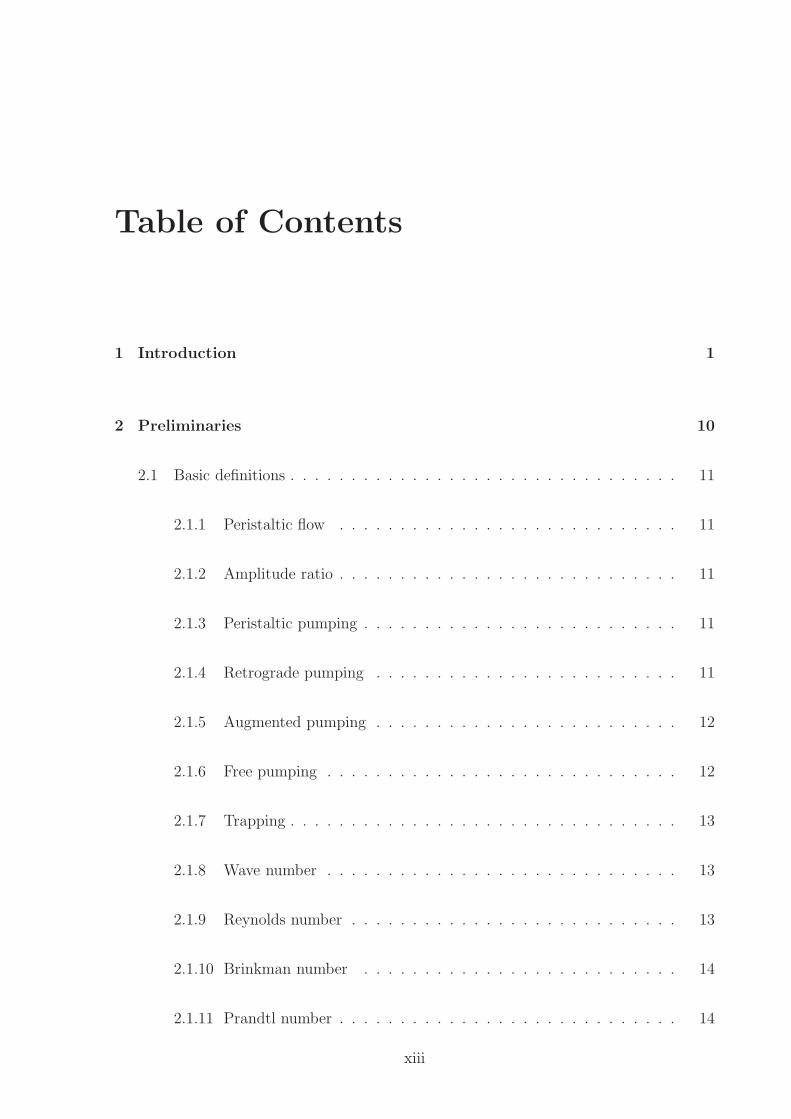
Table of Contents

1 Introduction 1

2 Preliminaries 10

2.1 Basic definitions . . . . . . . . . . . . . . . . . . . . . . . . . . . . . . . . 11

2.1.1 Peristaltic flow . . . . . . . . . . . . . . . . . . . . . . . . . . . . 11

2.1.2 Amplitude ratio . . . . . . . . . . . . . . . . . . . . . . . . . . . . 11

2.1.3 Peristaltic pumping . . . . . . . . . . . . . . . . . . . . . . . . . . 11

2.1.4 Retrograde pumping . . . . . . . . . . . . . . . . . . . . . . . . . 11

2.1.5 Augmented pumping . . . . . . . . . . . . . . . . . . . . . . . . . 12

2.1.6 Free pumping . . . . . . . . . . . . . . . . . . . . . . . . . . . . . 12

2.1.7 Trapping . . . . . . . . . . . . . . . . . . . . . . . . . . . . . . . . 13

2.1.8 Wave number . . . . . . . . . . . . . . . . . . . . . . . . . . . . . 13

2.1.9 Reynolds number . . . . . . . . . . . . . . . . . . . . . . . . . . . 13

2.1.10 Brinkman number . . . . . . . . . . . . . . . . . . . . . . . . . . 14

2.1.11 Prandtl number . . . . . . . . . . . . . . . . . . . . . . . . . . . . 14

xiii

2.1.12 Hartman number . . . . . . . . . . . . . . . . . . . . . . . . . . . 14

2.1.13 Schmidt number . . . . . . . . . . . . . . . . . . . . . . . . . . . 15

2.1.14 Soret effect . . . . . . . . . . . . . . . . . . . . . . . . . . . . . . 15

2.1.15 Dufour effect . . . . . . . . . . . . . . . . . . . . . . . . . . . . . 15

2.2 Governing equations for fluid motion . . . . . . . . . . . . . . . . . . . . 15

2.2.1 Continuity equation . . . . . . . . . . . . . . . . . . . . . . . . . . 15

2.2.2 Momentum equation . . . . . . . . . . . . . . . . . . . . . . . . . 16

2.2.3 Energy equation . . . . . . . . . . . . . . . . . . . . . . . . . . . . 16

2.2.4 Concentration equation . . . . . . . . . . . . . . . . . . . . . . . . 16

2.2.5 Maxwell’s equations . . . . . . . . . . . . . . . . . . . . . . . . . 17

2.2.6 Ohm’s law . . . . . . . . . . . . . . . . . . . . . . . . . . . . . . . 17

2.3 Extra stress tensor for third order fluid . . . . . . . . . . . . . . . . . . . 17

2.4 Solution methodologies . . . . . . . . . . . . . . . . . . . . . . . . . . . . 18

2.4.1 Perturbation solution . . . . . . . . . . . . . . . . . . . . . . . . . 18

2.4.2 Homotopy Analysis Method . . . . . . . . . . . . . . . . . . . . . 19

3 Peristaltic Flow of Nonconstant Viscosity Fluid with Nonlinear Thermal

Radiation 22

3.1 Mathematical Modeling . . . . . . . . . . . . . . . . . . . . . . . . . . . 23

3.1.1 Volume flow rates . . . . . . . . . . . . . . . . . . . . . . . . . . . 27

3.1.2 Boundary conditions . . . . . . . . . . . . . . . . . . . . . . . . . 28

xiv

3.2 Method of solution . . . . . . . . . . . . . . . . . . . . . . . . . . . . . . 29

3.2.1 Convergence of HAM solution . . . . . . . . . . . . . . . . . . . . 34

3.3 Results and Discussion . . . . . . . . . . . . . . . . . . . . . . . . . . . . 35

3.4 Conclusion . . . . . . . . . . . . . . . . . . . . . . . . . . . . . . . . . . . 42

4 Nonlinear Radiative Heat and Mass Transfer in Hydromagnetic Peri-

staltic Flow through Porous Medium 43

4.1 Mathematical formulation of the problem . . . . . . . . . . . . . . . . . . 44

4.2 Method of solution . . . . . . . . . . . . . . . . . . . . . . . . . . . . . . 50

4.2.1 Convergence of HAM solution . . . . . . . . . . . . . . . . . . . . 56

4.3 Results and discussion . . . . . . . . . . . . . . . . . . . . . . . . . . . . 56

4.3.1 Effects on the flow . . . . . . . . . . . . . . . . . . . . . . . . . . 57

4.3.2 Effects on the heat transfer . . . . . . . . . . . . . . . . . . . . . 61

4.3.3 Effects on the concentration . . . . . . . . . . . . . . . . . . . . . 63

4.3.4 Effects on trapping . . . . . . . . . . . . . . . . . . . . . . . . . . 63

4.4 Conclusion . . . . . . . . . . . . . . . . . . . . . . . . . . . . . . . . . . . 64

5 Effect of Induced Magnetic Field on the Peristaltic Flow of Variable

Viscosity Fluid 65

5.1 Statement of the physical model . . . . . . . . . . . . . . . . . . . . . . . 66

5.2 Perturbation Solution . . . . . . . . . . . . . . . . . . . . . . . . . . . . . 69

5.2.1 Zeroth-order system . . . . . . . . . . . . . . . . . . . . . . . . . 70

xv

5.2.2 First-order system . . . . . . . . . . . . . . . . . . . . . . . . . . 71

5.3 Graphical results and discussion . . . . . . . . . . . . . . . . . . . . . . . 74

5.4 Conclusion . . . . . . . . . . . . . . . . . . . . . . . . . . . . . . . . . . . 79

6 Variable Properties of MHD Third Order Fluid with Peristalsis 80

6.1 Problem description . . . . . . . . . . . . . . . . . . . . . . . . . . . . . . 81

6.2 Perturbation Solution . . . . . . . . . . . . . . . . . . . . . . . . . . . . . 87

6.2.1 Zeroth order . . . . . . . . . . . . . . . . . . . . . . . . . . . . . . 89

6.2.2 Order of Γ . . . . . . . . . . . . . . . . . . . . . . . . . . . . . . . 89

6.2.3 Order of α . . . . . . . . . . . . . . . . . . . . . . . . . . . . . . . 89

6.3 Graphical results and discussion . . . . . . . . . . . . . . . . . . . . . . . 91

6.4 Conclusion . . . . . . . . . . . . . . . . . . . . . . . . . . . . . . . . . . . 95

7 Appendix 96

7.1 Appendix A . . . . . . . . . . . . . . . . . . . . . . . . . . . . . . . . . . 97

8 References 99

xvi

List of Figures

2.1 Retrograde pumping . . . . . . . . . . . . . . . . . . . . . . . . . . . . . 12

2.2 Augmented pumping . . . . . . . . . . . . . . . . . . . . . . . . . . . . . 12

2.3 Trapping . . . . . . . . . . . . . . . . . . . . . . . . . . . . . . . . . . . . 13

3.1 Geometry of the problem . . . . . . . . . . . . . . . . . . . . . . . . . . . 24

3.2 ~−curves for ψ, θ and η for a1=0.5, a2=0.5, d=1.5, x=0.1, φ=π/4, Q=0.5,

Rn=0.5, θw = 1.3, α = 0.4, Br = 0.8, Sr=0.9, Sc=0.8 . . . . . . . . . . . 31

3.3 Pressure rise ∆Pλ versus flow rate Q for a1 = 0.4, a2 = 0.6, d = 1.1, φ =

π/2 . . . . . . . . . . . . . . . . . . . . . . . . . . . . . . . . . . . . . . . 32

3.4 Pressure gradient dp/dx versus x for a1 = 0.3, a2 = 0.4, d = 1, Q = 0.5,

φ = π/3 . . . . . . . . . . . . . . . . . . . . . . . . . . . . . . . . . . . . 33

3.5 Velocity u versus y for φ = 12π, a1 = 0.4, x = 0.1, Q = 0.5, a2 = 0.6, d = 1.1 35

3.6 Temperature θ against y for a1 = 0.3, a2 = 0.3, d = 0.8, x = 0.1, φ = 13π,

Q = 1.5 . . . . . . . . . . . . . . . . . . . . . . . . . . . . . . . . . . . . 36

3.7 Temperature profiles for comparison of linear and nonlinear radiations for

two different values of temperature ratio θw with x = 0.1, a1 = 0.3, a2 =

0.3, d = 0.8, φ = π/3, Q = 1.5 . . . . . . . . . . . . . . . . . . . . . . . . 37

3.8 Concentration η versus y for a1 = 0.4, a2 = 0.5, d = 1.5, φ = π/3, Q = 1 38

xvii

3.9 Influence of Rn on trapping for a1=0.4, a2=0.5, φ=π/2, d=1.5, Q=2.31,

α=0.4, θw=1.7, Br=1.6 . . . . . . . . . . . . . . . . . . . . . . . . . . . . 39

3.10 Influence of θw on trapping for a1=0.4, a2=0.5, d=1.5, φ=π/2, Q=2.31,

α=0.4, Rn=0.5, Br=1.5 . . . . . . . . . . . . . . . . . . . . . . . . . . . . 39

3.11 Influence of α on trapping for a1=0.4, a2=0.5, d=1.5, φ=π/2, Q=2.31,

θw=1.3, Rn=0.5, Br=1 . . . . . . . . . . . . . . . . . . . . . . . . . . . . 40


θw=1.1, Rn=0.5, α=0.3 . . . . . . . . . . . . . . . . . . . . . . . . . . . . 41

4.1 ~−curves for ψ, θ and η for a1=0.4, a2=0.4, d=1.6, x=0.1, φ=π/2, Q=0.5,

Rn=0.6, θw=1.3, α=0.5, Br=1, Sr=0.7, Sc=0.5, Df=1, Pr=1.2, K=1.2,

M=1.1 . . . . . . . . . . . . . . . . . . . . . . . . . . . . . . . . . . . . . 48

4.2 Pressure rise ∆Pλ against flow rate Q for d = 1.1, a1 = a2 = 0.5, φ=π/4 . 49

4.3 Pressure gradient dp/dx versus x for a1 = 0.5, a2 = 0.5, d = 1.1, Q = 0.3,

φ = π/4 . . . . . . . . . . . . . . . . . . . . . . . . . . . . . . . . . . . . 51

4.4 Velocity u versus y for φ = π/3, Q = 0.5, x = 0.1, a1 = 0.5, a2 = 0.5, d = 1.5 53

4.5 Temperature profile θ versus y for x = 0.1, a1 = 0.4, a2 = 0.5, d = 1.5,

φ = π/4, Q = 1 . . . . . . . . . . . . . . . . . . . . . . . . . . . . . . . . 55

4.6 Concentration η versus y for x = 0.1, a1 = 0.4, a2 = 0.5, d = 1.5, φ = π/4,

Q = 1 . . . . . . . . . . . . . . . . . . . . . . . . . . . . . . . . . . . . . 58

4.7 Influence of M on trapping for a1=0.5, a2=0.5, d=1.5, φ=π/4, Q=2.31,

θw=1.6, Rn=1.2, Br=0.6, K=0.4, α=0.4, Sr=0.5, Sc=1, Df=1, Pr=1.2 . 59

4.8 Influence of Rn on trapping for a1=0.5, a2=0.5, d=1.5, φ=π/4, Q=2.31,

θw=1.6, M=1, Br=1, K=1.8, α=0.4, Sr=0.5, Sc=1, Df=1, Pr=1.2 . . . 60

xviii


α=0.2, Rn=1.2, Br=1, M=0.7, K=1.8, Sr=1, Sc=0.7, Df=1, Pr=1.2 . . 61

4.10 Influence of α on trapping for a1=0.5, a2=0.5, d=1.5, φ=π/4, Q=2.31,

θw=1.4, Rn=1, Br=1, M=1, K=1.8, Sr=0.6, Sc=0.9, Df=1, Pr=1.2 . . . 62

4.11 Influence of K on trapping for a1=0.5, a2=0.5, d=1.5, φ=π/4, Q=2.31,

θw=1.6, Rn=1.2, Br=0.8, M=1, α=0.4, Sr=1, Sc=0.5, Df=1, Pr=1.2 . . 62

5.1 Pressure Rise ∆Pλ versus Q for d = 1.5, a1 = a2 = 0.5, φ = 14π . . . . . . 71

5.2 Pressure Gradient dp/dx versus x− for a1=0.4, d=1.1, a2=0.5, φ=π/4, Q=2 72

5.3 Velocity u versus y for a1=0.5, d=1.4, a2=0.6, x=0.1, φ=π/2, Q=3 . . . 73

5.4 Temperature θ versus y for a1=0.5, d=1.5, a2=0.6, x=0.1, φ=π/4, Q=2 . 74

5.5 Concentration η versus y for a1=0.5, d=1.5, a2=0.6, x=0.1, φ=π/4, Q=2 75

5.6 Axial Magnetic field bx versus y for a1=0.5, d=1.2, a2=0.4, x=0.1, φ=π/3,

Q=3.7 . . . . . . . . . . . . . . . . . . . . . . . . . . . . . . . . . . . . . 76

5.7 Current Density Jz versus y for a1=0.5, d=1.5, a2=0.5, x=0.1, φ=π/4,

Q=2.5 . . . . . . . . . . . . . . . . . . . . . . . . . . . . . . . . . . . . . 77

6.1 Geometry of the problem . . . . . . . . . . . . . . . . . . . . . . . . . . . 82

6.2 Pressure rise ∆Pλ versus flow rate Q for ϕ = 0.4 . . . . . . . . . . . . . . 83

6.3 Pressure gradient dp/dx versus x for ϕ = 0.4, Q = -0.5 . . . . . . . . . . 85

6.4 velocity u versus y for ϕ = 0.4, Q = 1.8, x = 0.1 . . . . . . . . . . . . . 86

6.5 Temperature profile θ versus y for ϕ = 0.4, Q = 1.8, x = 0.1 . . . . . . 87

6.6 Heat transfer coefficient Z versus x for ϕ = 0.4, Q = 1.8 . . . . . . . . . 88

xix

6.7 Streamlines for variation of α for ϕ = 0.2, Q = 0.97, Br = 0.8, Γ = 0.01,

M = 0.8 . . . . . . . . . . . . . . . . . . . . . . . . . . . . . . . . . . . . 90

6.8 Streamlines for variation of Br for ϕ = 0.2, Q = 0.97, α = 0.4, Γ = 0.01,

M = 0.8 . . . . . . . . . . . . . . . . . . . . . . . . . . . . . . . . . . . . 90

6.9 Streamlines for variation of Γ for ϕ = 0.2, Q = 0.97, α = 0.5, Br = 0.7,

M = 0.7 . . . . . . . . . . . . . . . . . . . . . . . . . . . . . . . . . . . 93

6.10 Streamlines for variation of M for ϕ = 0.2, Q = 0.97, α = 0.5, Br = 0.7,

Γ = 0.01 . . . . . . . . . . . . . . . . . . . . . . . . . . . . . . . . . . . . 93

xx

List of Tables

3.1 Convergence of series solution for a1 = 0.5, a2 = 0.5, d = 1.5, x = 0.1, φ

= π/4, Q = 0.5, α = 0.4, Br = 0.8, Rn = 0.5, θw = 1.3, Sr = 0.9, Sc =

0.8, ~ψ = ~θ = ~η = −0.6. . . . . . . . . . . . . . . . . . . . . . . . . . . 25

3.2 Heat transfer coefficient Z at upper wall for different cross-sections with

fixed α = 0.4, θw = 1.3, Br = 0.8, a1 = 0.5, a2 = 0.5, φ = π/4, d = 1.5,

Q = 0.5 . . . . . . . . . . . . . . . . . . . . . . . . . . . . . . . . . . . . 27


fixed α = 0.4, Rn = 0.5, Br = 0.8, a1 = 0.5, a2 = 0.5, d = 1.5, φ = π/4,

Q = 0.5 . . . . . . . . . . . . . . . . . . . . . . . . . . . . . . . . . . . . 28


fixed Rn = 0.4, θw = 1.3, Br = 0.8, a1 = 0.5, a2 = 0.5, d = 1.5, φ = π/4,

Q = 0.5 . . . . . . . . . . . . . . . . . . . . . . . . . . . . . . . . . . . . 29


fixed Rn = 0.4, θw = 1.3, α = 0.4, a1 = 0.5, a2 = 0.5, d = 1.5, φ = π/4,

Q = 0.5 . . . . . . . . . . . . . . . . . . . . . . . . . . . . . . . . . . . . 30

4.1 Convergence of series solution for a1=0.4, a2=0.4, d=1.6, x=0.1, φ=π/2,

Q=0.5, Rn=0.6, θw=1.3, α=0.5, Br=1, Sr=0.7, Sc=0.5, Df=1, Pr=1.2,

K=1.2, M=1.1, ~ψ = ~θ = ~η = −0.6. . . . . . . . . . . . . . . . . . . . . 45

4.2 Critical values of Q for which ∆Pλ = 0 . . . . . . . . . . . . . . . . . . . 46

xxi

List Of Symbols

(X, Y , t) Dimensional coordinate axes in fixed frame(x, y) Dimensional coordinate axes in wave frame(x, y) Dimensionless coordinate axes in wave frame(U , V ) Dimensional velocity components in fixed frame(u, v) Dimensional velocity components in wave frame(u, v) Dimensionless velocity components in wave frameH Wall shape in fixed frame (symmetric channel)H1 , H2 Upper and lower walls shape (asymmetrical channel)h Dimension less wall shape in wave frame (symmetric channel)h1 , h2 Dimensionless wall shape in wave frame (asymmetric channel)b wave amplitude (symmetric channel)a channel half width (symmetric channel)(b1 , b2) wave amplitude (asymmetric channel)(d1 , d2) channel half width (asymmetric channel)ϕ Amplitude ratio (symmetric channel)(a1 , a2) Amplitude ratio (asymmetric channel)d channel width ratio (asymmetric channel)Tw wall temperature (symmetric channel)T0 , T1 upper and lower wall temperatures (asymmetric channel)C0 , C1 concentration at upper and lower wall (asymmetric channel)φ phase differencec wave speedλ wavelengtht timeB0 applied magnetic fieldB magnetic fieldB1 induced magnetic fieldJ current densityσ electrical conductivityµ dimensional viscosityµ dimensionless viscosityµ0 viscosity at constant temperature T0µw viscosity at constant temperature Twγ dimensional viscosity variation parameterα dimensionless viscosity variation parameterQ dimensional volume flow rate in fixed frame

xxii

F dimensional volume flow rate in wave frameΘ Time mean flow rate over a time period in a fixed frameQ dimensionless time mean flow rate in fixed frameF dimensionless time mean flow rate in wave framek thermal conductivityβ dimensional thermal conductivity parameterǫ dimensionless thermal conductivity parameterP Pressure in fixed framep pressure in wave framep dimensionless pressure∆Pλ pressure rise per wavelengthγi dimensionless material parameters of third order fluid (i = 1, 2, 3)δ wave numberS extra stress tensorI identity tensorM Hartman numberRe Reynold numberAi First three Rivlin-Ericksen tensorsαi , βi material constants of third order fluid in dimensional form (i = 1, 2, 3)ρ fluid densityρf body forcecp specific heatq heat flux vectorL gradient of velocityT fluid temperatureθ dimensionless fluid temperatureθw temperature ratioDm coefficient of mass diffusivitykT thermal diffusion ratioE electrical fieldρe charge densityǫ0 permittivity of free spaceµe permeability of free spaceC concentration of fluidη dimensional concentration of fluidPr Prandtl numberBr Brinkman numberψ stream functionΓ Deborah numberZ heat transfer coefficientcs concentration susceptibilityσ∗ Stephan-Boltzmann constanteb black body emissive powerk∗ mean spectral absorption coefficientK permeability of porous mediumK dimensionless permeability parameterSr Soret numberSc Schmidt number

xxiii

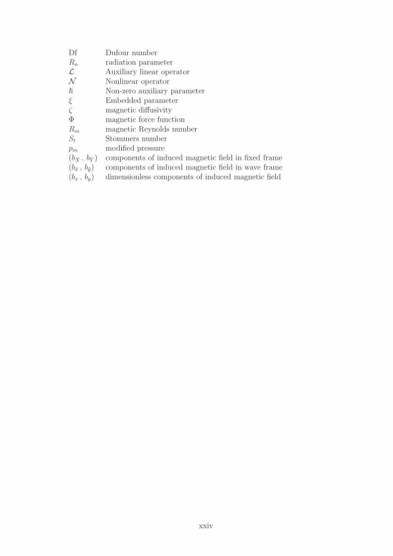
Df Dufour numberRn radiation parameterL Auxiliary linear operatorN Nonlinear operatorℏ Non-zero auxiliary parameterξ Embedded parameterζ magnetic diffusivityΦ magnetic force functionRm magnetic Reynolds numberSt Stommers numberpm modified pressure(bX , bY ) components of induced magnetic field in fixed frame(bx , by) components of induced magnetic field in wave frame(bx , by) dimensionless components of induced magnetic field

xxiv

Chapter 1

Introduction

1

Background and literature survey

The word “peristalsis” is of the Greek origin that means clasping and compressing. Peri-

staltic transport is the movement of fluid in the hollow flexible tube due to the sinusoidal

waves traveling along the walls of the tube.

The periodic contraction and expansion of the ducts results in the rise of pressure gra-

dient that eventually push the fluid forward. Peristalsis is an inherent property of many

physiological vessels having smooth muscles that transport bio-fluids by the propulsive

movements. Physiological examples of peristalsis phenomena include the movement of

food bolus in esophagus, flow of urine from kidney to bladder through ureter, transport

of lymph in lymphatic vessels, movement of ovum in fallopian tube, transport of bile juice

through bile duct and vasomotion of small blood vessels like arterioles, venules and cap-

illaries. Inspired by locomotion of earthworms, peristaltic soft robot has been invented.

Peristaltic phenomena have played an important role in industry and bioengineering. The

peristaltic pumps are used for the transfer of sanitary fluid, additives in food, corrosive

fluids, clean fluids, high solid slurries and noxious fluids. Bio-mechanical apparatus such

as blood pump machine, heart lung machine and pumps in dialysis machines are de-

signed on this principle. As a result, such diversity in applications of peristalsis makes it

a subject of keen interest for researchers, engineers, mathematicians and physicists alike.

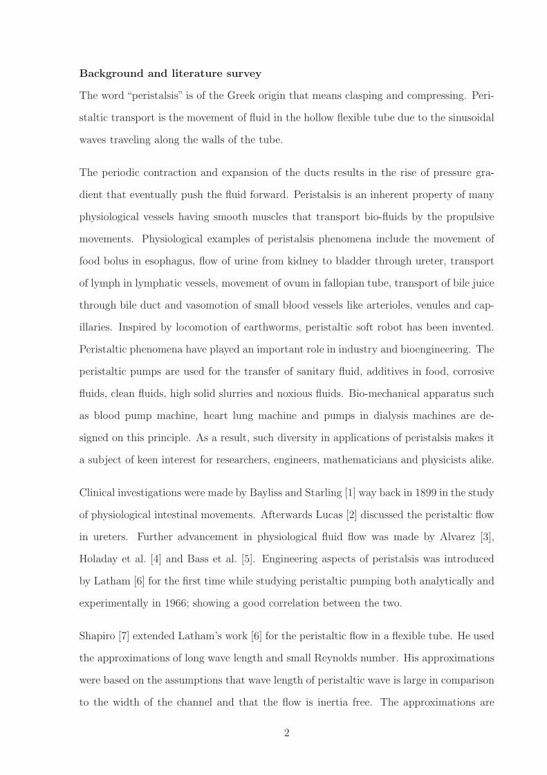
Clinical investigations were made by Bayliss and Starling [1] way back in 1899 in the study

of physiological intestinal movements. Afterwards Lucas [2] discussed the peristaltic flow

in ureters. Further advancement in physiological fluid flow was made by Alvarez [3],

Holaday et al. [4] and Bass et al. [5]. Engineering aspects of peristalsis was introduced

by Latham [6] for the first time while studying peristaltic pumping both analytically and

experimentally in 1966; showing a good correlation between the two.

Shapiro [7] extended Latham’s work [6] for the peristaltic flow in a flexible tube. He used

the approximations of long wave length and small Reynolds number. His approximations

were based on the assumptions that wave length of peristaltic wave is large in comparison

to the width of the channel and that the flow is inertia free. The approximations are

2

well meaning due to the order analysis; as shown by Shapiro for peristalsis in ureter

and gastrointestinal tract. There are number of such references where these conditions

are applicable. Shapiro [7] taking into account the asymmetric and symmetrical channel

discussed velocity profile and pressure rise per wave length. The phenomena of reflux and

trapping were first presented in this study. These phenomenal biological events remained

the motivation of peristalsis study all along. Some subsequent studies of interest are now

mentioned in the following paragraph.

Kiil [8] and Boyarsky [9] provided the detailed study of peristaltic function involved in

the transport of urine in urinary tract. Weinberg [10] studied the peristaltic flow in

the ureter and experimentally discussed phenomenon of trapping by injecting the dye

into the ureteral channel. Further invetigations in this direction were made by Lykoudis

and Roos [11]. They discussed the flow through ureter induced by peristaltic wave of

arbitrary shape. Manton [12] extended the work of Lykoudis and Roos [11] and considered

the inertial and viscous effects which were ignored by them. Barton and Raynor [13]

presented two types of analysis on the peristaltic movement of small intestines. Firstly,

they used the long wavelength approximation and provided the algebraic relation between

the pressure differential across wavelength and the average flow rate. Secondly they

considered the wavelength to be as small as tube radius and determined the same relation

numerically. Lew et al. [14] provided the mathematical analysis on the transport of chyme

in small intestines and also discussed its physiological significance. They studied the flow

of a Newtonian fluid in an infinitely long circular cylindrical tube involving a series of

sharp traveling nodal constrictions. Srivastava and Srivastava [15] studied the peristaltic

mechanism in uniform and non-uniform tubes and established the applicability of their

results in the vas deferens of rhessus monkeys and in small intestines.

Heat Transfer Analysis

Peristalsis mechanism is greatly influenced by the heat transfer phenomenon through the

energy equation. Therefore, physiological and industrial applications require the heat

transfer considerations. Mekheimer and Abd elmaboud [16] discussed the peristaltic

3

transport of a Newtonian fluid in a vertical annulus under the influence of heat transfer

and magnetic field. Tripathi et al. [17] studied the mechanism of swallowing diverse types

of viscoelastic food bolus by taking account of heat transfer effects.

Variable properties of Newtonian and non-Newtonian fluids

We observe that in most of the theoretical consideration of fluid flow the viscous dissipa-

tion is neglected by considering the fluid to be isothermal. However, this assumption is

unrealistic for certain situations which can lead to erroneous results. The consideration of

viscous dissipation requires the fluid properties to be variable due to the heat generated

by viscous dissipation; since viscosity strongly depends upon the temperature. The effects

of viscous dissipation are examined by varying the non-dimensional Brinkman number.

It has also been noticed that viscous heating plays important role in temperature depen-

dence of fluid properties like viscosity and thermal conductivity. It is justified to take

viscosity and thermal conductivity as constant for isotropic fluids but this assumption

is not valid when there is a variation in fluid temperature. There are many engineering

applications that allow significant variations in the viscosity and thermal conductivity of

the fluid. The role of variable fluid properties is highly significant in peristalsis as many

of the fluids like honey, mineral oils, blood, and polymer solutions possess temperature

dependent properties. Further, it is generally not advisable to take constant fluid prop-

erties when peristaltic movement in small blood vessels, lymphatic vessels and intestine

is discussed. Some work done on variable properties of fluids is mentioned below:

Massoudi and Phuoc [18], while considering second grade fluid, suggested that the viscos-

ity must be taken as temperature dependent in the presence of viscous dissipation. In a

vertical channel, the temperature dependent viscosity for peristaltic flow was considered

by Eldabe et al. [19]. Asghar et al. [20] discussed the peristaltic motion of reactive vis-

cous fluid with variable viscosity in a two dimensional channel. The variable viscosity has

been considered by Mekheimer and Abd elmaboud [21] while discussing the peristaltic

transport in asymmetric channel.

Taking into consideration these observations; we incorporate the variable properties of the

fluid for peristaltic transport of Newtonian and non-Newtonian fluid in asymmetrical and

4

symmetrical channels. Naturally, the viscous dissipation will be an essential part of our

discussion. Thus, we take temperature dependent viscosity throughout from chapter 3 to

6 and temperature dependent thermal conductivity in chapter 6. Mathematical implica-

tion of such study is quite high in the sense that the viscosity and thermal conductivity

are no longer constants but variable with temperature dependence. Since, temperature

is a function of space variable; viscosity will also be space dependent and thus plays a

crucial part in viscous diffusion term.

Radiation effects

Radiation effect in peristalsis is a major refinement in the heat transfer analysis that needs

appropriate attention. Thermal radiation in peristalsis has only been considered under

the assumption of linear approximation of radiative heat flux. However, nothing has been

said for the non-linear radiative heat transfer in peristalsis. A few background literature in

this direction is mentioned as: Eldabe et al. [22] explored the effects of thermal radiation

and heat generation on the peristaltic motion of micropolar fluid. Kothandapani and

Prakash [23] presented the influence of radiation and uniform magnetic field on non-

uniform wall induced flow of Williamson nanofluid.

Effects of thermal radiation on peristaltic transport of Sisko fluid is analyzed by Mehmood

and Fetecau [24]. It is noted that all the preceeding papers have taken linear radiation.

This assumption is only suitable for small temperature difference. Practically there are

certain situations in which temperature difference is relatively higher and the linear ap-

proximation is no longer valid. In such case it is imperative to consider the nonlinear

radiative effects. Stefan-Boltzman law further strengthens the argument in favour of non-

linear thermal radiation. According to this law, radiation emitted is proportional to the

fourth power of its absolute temperature. Keeping this in mind, we consider the effects

of nonlinear thermal radiation for the peristaltic transport of fluid in chapters 3 and 4.

Heat and Mass transfer

Heat and mass transfer are kinetic processes that often occur together. Mass flux is cre-

ated due to temperature gradients in the flow known as Soret effect. Similarly, Dufour

5

effect dominates the energy flux created as a result of concentration gradients. Mass

transport has multiple occurrences in biological processes. These processes include res-

piration, perspiration, osmosis and excretion. Industrial applications of mass transport

include dispersion of containment, cooling towers, drying and humidifying.

Srinivas et al. [25] examined the heat and mass transfer flow in a vertical channel with

peristalsis. Sobh [26] analyzed the combined effects of heat and mass transfer on the

peristaltic transport of viscoelastic fluid in tube with slip velocity. Saleem and Haider [27]

developed the mathematical model to study the peristaltic flow of Maxwell fluid with

heat and mass transfer in an asymmetric channel. Hayat et al. [28] studied heat and

mass transfer effects on peristaltic flow of Casson fluid with convective conditions and

chemical reaction. Ramesh [29] discussed the impact of heat and mass transfer on the

peristaltic transport of couple stress fluid in an inclined channel through porous medium.

Taking note of these considerations, we choose to study the combined effects of heat and

mass transfer in chapters 3 to 5 in the framework of peristalsis in channel with variable

properties of fluid.

Biomagnetism

The study of Biomagnetic fluid dynamics is concerned with the mutual interaction of

biological fluid flow and magnetic fields. Such fluids are electrically conducting and

non-magnetic. This area of research has extensive applications in bioengineering and

medical sciences. Blood being biomagnetic fluid; magnetic field is applied to control the

blood pressure, bleeding during surgeries and targeted delivery of drugs. The influence

of magnetic field can be utilized in the magnetic resonance imaging (MRI), treatment of

cancer, tumors and arterial diseases.

Some recent studies can be quoted as: Srinivas and Kothandapani [30] explored the effects

of heat and mass transfer on the peristaltic flow of electrically conducting fluid in the

presence of uniform magnetic field through porous space. Reddy et al. [31] examined the

peristaltic pumping of hydromagnetic Jeffrey fluid with variable viscosity in a uniform

circular tube. MHD peristaltic flow of Jeffrey nanofluid in the presence of viscous dissi-

6

pation, Joule heating and thermal radiation is studied by Hayat et al. [32]. We discuss

MHD in chapters 4 to 6 while incorporating magnetic field in this thesis.

Permeable medium

Study of peristaltic flow through permeable medium is of great significance due to its

applications in biomechanics and engineering. Some parts of human body that can be

considered porous include lungs, tumorous vessels and arterial systems. El Shehawey and

Husseny [33] examined the peristaltic movement of viscous fluid through porous medium

enclosed by two porous plates. Mekheimer [34] determined the characteristics of peri-

staltic flow of a Newtonian fluid in an inclined planar channel filled with homogeneous

porous medium. Hayat et al. [35] studied the wall induced flow of Maxwell fluid through

porous space with Hall effects. Tripathi and Beg [36] studied the peristaltic transport

of generalized Maxwell fluid in a porous medium using homotopy perturbation method.

Hussain et al. [37] investigated the influence of convective boundary conditions on peri-

staltic flow of a viscous fluid in a porous wavy channel. Consideration of porous channel

in the setting of variable properties of fluid is discussed in chapter 4.

Non-Newtonian fluid

Because of the diversity in the molecular structure of fluids, no single constitutive equa-

tion can describe all the fluids. Thus no single constitutive equation can describe all the

fluids. A great deal of manmade, natural, industrial and physiological fluids is considered

as non- Newtonian because of their rheological properties. A good account of peristal-

sis in non- Newtonian fluid is given in the references [38–43]. The choice of third grade

fluid, among non-Newtonian fluids, is important because of its viscoelastic properties and

its applications in physiology, engineering, medical science and polymer industry [44,45].

Third grade fluid involves very complicated constitutive relations and the governing equa-

tions are highly non-linear in nature. The solution presents great mathematical difficulty

in solving and presenting the physics of fluid flow. Some important work undertaken in

the third grade fluid can be summarized as follows:

Fosdick and Rajagopal [46] provided the stability analysis for third order fluids and dis-

7

cussed its thermo dynamical aspect. Siddiqui and Schwarz [47] determined the charac-

teristics of peristaltic action of third order fluid in a channel. Haroun [48] considered

the peristaltic motion of third order fluid in an asymmetric channel and obtained the

asymptotic analytic solution up to the second order in terms of Deborah number. Hayat

et al. [49] analyzed the peristaltic action of third order fluid in a planar channel under

the influence of magnetic field. Eldabe et al. [50] studied the heat and mass transfer

effects on the peristaltic transport of MHD third order fluid in a porous medium. The

consideration of third grade fluid for peristaltic transport of third grade fluid has been

presented in chapter 6 of this thesis.

Perturbation Method and Homotopy Aanalysis Method

The equations are highly nonlinear partial differential equations. The solution is not

tractable as such. The only possibility left is either numerical or approximate analyti-

cal method. The asymptotic perturbation method is very useful to tackle the nonlinear

equation. The essential requirement for its applicability is the existence of small param-

eter and the asymptotic nature of the series solution. Both of these requirements are

well suited for the proposed problem. In this problem, viscosity variation parameter is

naturally very small and thus allow a perturbation solution. We may add that although

the viscosity strongly depends upon the temperature, the variation in viscosity has been

linear and small. This consideration encourages the application of perturbation expan-

sion. The asymptotic nature of the solution is guaranteed. The argument for that is:

We observe that the zeroth order and the first order solutions are uniformly valid and

hence no secular term appears. In the nutshell there are no infinite domain singularity

and it is not a singular perturbation problem. The homotopy analysis method is also

an approximate analytic method to find the solution of nonlinear problems. The con-

vergent solution of the given problem is developed systematically from an initial guess.

The method has seen a great success in solving the problem of fluid dynamics. It will

not be out of place to mention a few papers those have been successfully solved by per-

turbation and homotopy analysis method. We would like to add a few seminal work on

perturbation method. Some of these works were carried by Hayat et al. [51], Srinivas and

8

Muthuraj [52], Mekheimer and Abd elmaboud [21], and Hussain et al. [53]. For homotopy

analysis method, we would like to quote some relevant references [54–57].

Chapter wise organization of the thesis

The thesis basically addresses the peristaltic flow of Newtonian and non-Newtonian fluid

with variable properties in the presence of viscous dissipation. Heat and mass transfer is

also incorporated. The fluid is subjected to non-linear thermal radiation. Analytical and

semi-analytical methods are used to obtain the solutions.

Chapter one contains the motivation of the thesis and literature review.

Chapter two consists of fundamental definitions, governing equations and solution tech-

niques subsequently used in the thesis.

Chapter three is concerned with the influence of heat and mass transfer on peristaltic

transport with variable viscosity viscous fluid in an asymmetric channel with nonlin-

ear thermal radiation. Viscous dissipation effects are also taken into account. This

study is published in Journal of Computational and Theoretical Nanoscience [58].

In chapter four, we consider MHD flow through porous medium with Dufour effects. In

fact, the results of chapter three for peristaltic transport of viscous fluid with variable

viscosity has been extended to the consideration of porous medium and magnetic

field. The work in this chapter has been published in Results in Physics [59].

Chapter five investigates the influence of heat and mass transfer on the peristaltic flow

of Newtonian fluid in the presence of induced magnetic field. In this, we have taken

strong magnetic field so that induced magnetic field may also be considered.

Chapter six deals with the peristalsis transport of temperature dependent viscosity

and thermal conductivity on peristaltic transport of non-Newtonian third order

fluid in a symmetric channel. Effects of viscous dissipation and applied magnetic field

are discussed. The contents of this chapter are published in Results in Physics [60].

9

Chapter 2

Preliminaries

10

This chapter aims at providing with relevant terminologies and laws that are deemed nec-

essary to comprehend peristaltic flows. Governing equations and solution methodologies

are also introduced.

2.1 Basic definitions

The preliminary terminologies pertaining to peristalsis are provided in this section.

2.1.1 Peristaltic flow

The movement of fluid within the duct due to periodic contraction and relaxation of duct

walls is known as peristaltic flow.

2.1.2 Amplitude ratio

The ratio between the amplitude of sinusoidal waves that propagate along the channel

(tube) walls and half of the width (radius) of the channel (tube).

2.1.3 Peristaltic pumping

This is the region where time mean flow rate as well as pressure difference, both are

positive. Here walls of the channel surpass resistance due to pressure gradient, thus fluid

is derived forward.

2.1.4 Retrograde pumping

In the retrograde pumping region, the pressure difference is positive and the non-dimensional

time mean flow rate is negative. Here the pressure gradient causes the fluid to flow in

the opposite direction of the prorogation of wave. The sketch of retrograde pumping is

shown in Figure 2.1.

11

-4 -3 -2 -1 0 1 2 3 4

-1

-0.5

0

0.5

1

Figure 2.1: Retrograde pumping

2.1.5 Augmented pumping

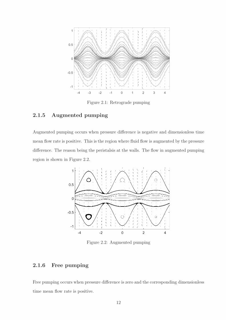
Augmented pumping occurs when pressure difference is negative and dimensionless time

mean flow rate is positive. This is the region where fluid flow is augmented by the pressure

difference. The reason being the peristalsis at the walls. The flow in augmented pumping

region is shown in Figure 2.2.

Figure 2.2: Augmented pumping

2.1.6 Free pumping

Free pumping occurs when pressure difference is zero and the corresponding dimensionless

time mean flow rate is positive.

12

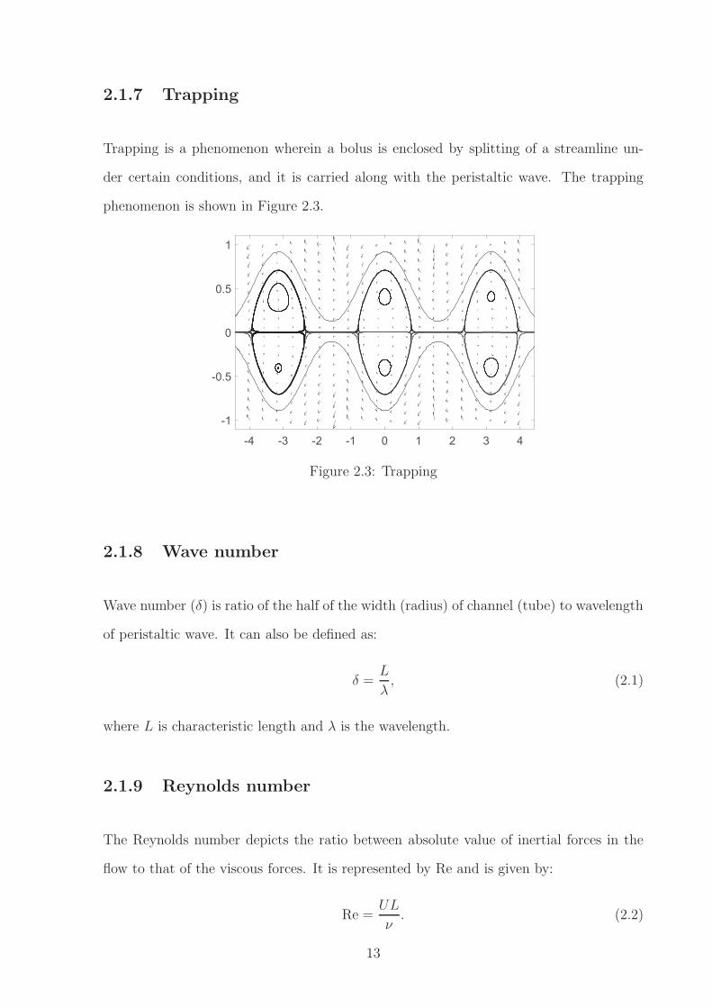
2.1.7 Trapping

Trapping is a phenomenon wherein a bolus is enclosed by splitting of a streamline un-

der certain conditions, and it is carried along with the peristaltic wave. The trapping

phenomenon is shown in Figure 2.3.

-4 -3 -2 -1 0 1 2 3 4

-1

-0.5

0

0.5

1

Figure 2.3: Trapping

2.1.8 Wave number

Wave number (δ) is ratio of the half of the width (radius) of channel (tube) to wavelength

of peristaltic wave. It can also be defined as:

δ =L

λ, (2.1)

where L is characteristic length and λ is the wavelength.

2.1.9 Reynolds number

The Reynolds number depicts the ratio between absolute value of inertial forces in the

flow to that of the viscous forces. It is represented by Re and is given by:

Re =UL

ν. (2.2)

13

Here U is fluid velocity and ν is kinematic viscosity. For low Reynolds number, the viscous

forces in the flow are high as compared to the inertial forces, and laminar flow will tend

to exist. On the other hand, for high Reynolds number, inertial forces are dominant in

comparison to the viscous forces, and turbulent flow develops.

2.1.10 Brinkman number

Brinkman number is the ratio between heat produced through viscous dissipation to that

by molecular conduction. Brinkman number, written Br, is expressed as:

Br =µU2

k(Tw − T0), (2.3)

where µ is dynamic viscosity of fluid, U is velocity of fluid, Tw is wall temperature and

T0 is fluid temperature.

2.1.11 Prandtl number

Prandtl number (Pr) signifies ratio between thermal and momentum diffusivity. Mathe-

matically, it can be written as:

Pr =µcpk. (2.4)

In above expression, cp is the specific heat and k is thermal conductivity.

2.1.12 Hartman number

Hartman number (M) represents the ratio of electromagnetic force to the viscous force.

It is given by the following relation:

M = LB0

√

σ

µ. (2.5)

Here σ is electrical conductivity and B0 is applied magnetic field strength.

14

2.1.13 Schmidt number

It is the ratio between momentum diffusivity (viscosity) and mass diffusivity whose math-

ematical description is as follows:

Sc =µ

ρDm

, (2.6)

where ρ is fluid density and Dm is coefficient of mass diffusivity.

2.1.14 Soret effect

Soret effect, also known as the thermo-diffusion, is the mass flux generated due to tem-

perature gradient.

2.1.15 Dufour effect

Concentration gradient can cause energy flux and this effect is termed as Dufour (Diffusion-

thermo) effect.

2.2 Governing equations for fluid motion

In fluid mechanics, the basic laws that govern the flow behavior of fluid are the con-

servation laws for mass, momentum and energy. These basic laws are used to derive

the continuity, momentum and energy equations. Moreover, an assumption of contam-

inant conservation leads to the concentration equation. These governing equations are

described below.

2.2.1 Continuity equation

The continuity equation describes the law of conservation of mass. For compressible flows,

it can be expressed as

∂ρ

∂t+ ∇ ·

(

ρ V)

= 0, (2.7)

15

where V is the velocity vector, t is time, ρ is fluid density and ∇ is the vector differential

operator. Equation (2.7) takes the following form for incompressible fluids.

∇ · V = 0. (2.8)

2.2.2 Momentum equation

Equation of motion that describes the conservation law for momentum for magnetohy-

drodynamic flow is as follows:

ρ

(

∂V

∂t+ ( V · ∇ )V

)

= ∇ · τ + ρf . (2.9)

In the above expression, τ (= −P I + S) is the Cauchy stress tensor, where P , I and S

respectively represent the pressure, identity tensor and extra stress tensor. The term ρf

represents the body force which varies for different flow situations. In the present thesis,

it represents the Lorentz force which arises due to variation in magnetic field. So,

ρf = J× B, (2.10)

in which J is the current density, B(= B0+ B1) represents the total magnetic filed, with

B0 and B1 respectively as applied and induced magnetic fields.

2.2.3 Energy equation

The energy equation follows the conservation law for energy, comes from the first law of

thermodynamics and in vector form is:

ρcp

(

∂T

∂t+ (V · ∇)T

)

= τ · L + ∇ · (k∇T )− ∇ · qr, (2.11)

where T is the temperature of fluid, cp is the specific heat, qr is the radiative heat flux,

L is the gradient of velocity and k is the thermal conductivity.

2.2.4 Concentration equation

Mass transfer is the transport of chemical species from one location to another by diffusion

and/or convection due to concentration gradients. Mass transfer can be observed in many

16

engineering processes that involve the transport of contaminant by the fluid flow. The

governing equation is derived by considering the mass conservation of contaminant. With

C as the mass concentration of the fluid, the concentration equation is as follows:

∂C

∂t+ (V · ∇)C = Dm∇2C +

DmkTTr

∇2T . (2.12)

In the above equation, kT is the thermal diffusion ratio, Tr is temperature reference and

Dm is the coefficient of mass diffusivity.

2.2.5 Maxwell’s equations

A set of equations that govern the behavior of electromagnetic waves in all physical

situations are called Maxwell’s equations. These equations are:

∇ · E =ρeǫ0, (2.13)

∇ × E = −∂B∂t, (2.14)

∇ · B = 0, (2.15)

∇ × B = µe

(

J+ ǫo∂E

∂t

)

. (2.16)

In above equations, E is the electric field, ρe is charge density, ǫ0 is permittivity of free

space, and µe is permeability of free space.

2.2.6 Ohm’s law

The Ohm’s law is given by the relation

J = σ(

E+ V × B)

. (2.17)

Here σ is an electrical conductivity.

2.3 Extra stress tensor for third order fluid

Extra stress tensor S for third order fluid is defined by

S =(

µ+ β3trA21

)

A1 + α1A2 + α2A21 + β1A3 + β2

(

A1A2 + A2A1

)

, (2.18)

17

with

A1 = L+ L⊤, An+1 =dAn

dt+ AnL+ L⊤An, n = 1, 2. (2.19)

In above equations, µ is the fluid viscosity, Ai are the first three Rivlin-Ericksen tensors

whereas αi and βi are the material constants, for i = 1, 2, 3.

2.4 Solution methodologies

In order to complete the discussion and make it self-contained, the techniques used to solve

the problem of thesis are compactly presented in this section. These are the perturbation

method and the homotopy analysis method.

2.4.1 Perturbation solution

Mathematicians make precise approximations to solve the equations when exact solution

is not possible. Numerical methods and the analytical methods are two ways to obtain

the useful approximations to the solution of an equation. Perturbation method is pre-

ferred because it produces analytic results that show the dependence of exact solutions

on the parameters in a more satisfactory way. Perturbation method may also be utilized

when the problem can not be easily solved numerically. When the mathematical model

of the problem possesses the small or large parameter, perturbation expansions are con-

structed to solve the governing equations. The perturbation method can be applied to

solve complicated algebraic equation, nonlinear differential equation, differential equa-

tions with varying coefficients and complicated integrals. Using perturbation method,

original problem is reduced to a relatively simple equations that are computationally less

expensive. For example, through its application a system of nonlinear differential equa-

tions is transformed to a system of linear differential equations. Thus, if the nonlinear

terms appear in the equation, they involve only functions that have been evaluated ear-

lier. The procedure of solving a differential equation through perturbation method is

18

demonstrated with the following example

du

dy+ u = εu2 ; u(0) = 1 (2.20)

where ε is small perturbation parameter (0 < ε < 1).

In order to solve this equation by using perturbation method, the following form of

expansion is used

u(y; ε) = ε0u0(y) + ε1u1(y) + ε2u2(y) + · · · (2.21)

The substitution of (2.21) in (2.20) gives

du0dy

+ εdu1dy

+ ε2du2dy

+ · · ·+ u0 + εu1 + ε2u2 + · · · = ε(u20 + 2εu0u1 + · · · ) (2.22)

and

u0(0) + εu1(0) + ε2u2(0) + · · · = 1 (2.23)

Equating the coefficients of like terms in equations (2.22) and (2.23) we get

O(1) :du0dy

+ u0 = 0 , u0(0) = 1

O(ε) :du1dy

+ u1 = u20 , u1(0) = 0

O(ε2) :du2dy

+ u2 = 2u0u1 , u2(0) = 0

(2.24)

The solutions of these consecutive equations provide us with individual expressions for

u0(y), u1(y) and u2(y) etc., which when substituted in (2.21) render

u(y; ε) = e−y + ε(e−y − e−2y) + ε2(e−y − 2e−2y + e−3y) + · · · (2.25)

The expression for u(y; ε) in (2.25) gives us the required solution.

2.4.2 Homotopy Analysis Method

Homotopy analysis method (HAM) is a semi-analytical procedure used to solve nonlinear

ordinary and partial differential equations. It was introduced by Liao [54] in 1992 and

based on the concept of homotopy in topology.

19

There are certain characteristics due to which HAM differs from other analytical methods.

First of all, HAM can be applied to the problems that are independent of small/large

physical parameters. Secondly, this method provides an easy way to ensure convergence of

the solution series. Finally, HAM provides an open choice for base functions of solution,

equation type of linear sub-problems and initial guess, so that nonlinear problems are

addressed in an improved tractable manner.

In order to describe the homotopy analysis method, consider nonlinear differential equa-

tion

N [u(y)] = 0. (2.26)

In Equation (2.26) N is a nonlinear operator. Now initial equation is chosen in a way

that its solution u0(y) is easy to find. Liao applied the concept of homoptopy on original

and initial equations and constructed one parameter family of equations, namely the

zeroth-order deformation equation

(1− ξ)L[u(y; ξ)− u0(y)] = ξ~N [u(y; ξ)], (2.27)

where L is auxiliary linear operator, ~ is a non-zero auxiliary parameter, and ξ ∈ [0, 1]

is an embedding parameter. As the embedding parameter ξ varies from 0 to 1, u(y; ξ)

varies from the known solution u0(y) of initial equation to the unknown exact solution

u(y) of the original equation. The use of auxiliary parameter ~ has no physical meaning

but the proper choice of ~ guarantees the convergence of homotopy series.

The zeroth-order equation should be constructed in a way that u(y; ξ) exists for ξ ∈ [0, 1]

and is analytic at ξ = 0 and hence its Maclaurin series about embedding parameter ξ

exists. From the definition of zeroth-order deformation equation, at ξ = 0, we have the

auxiliary equation whose solution is u0(y), i.e.

u(y; 0) = u0(y), (2.28)

For ξ = 1, we have original equation and we can write

u(y; 1) = u(y). (2.29)

20

Using Equation (2.28), the Maclaurin series of u(y; ξ) with respect to ξ is written as

u(y, ξ) ∼ u0(y) +∞∑

m=1

um(y)ξm, um(y) =

1

m!

∂mu(y; ξ)

∂ξm

∣

∣

∣

∣

ξ=0

(2.30)

The convergence control parameter ~ is selected such that the above series solution is

convergent for ξ = 1. Then according to Equation (2.29), we have the homotopy series

solution

u(y) = u0(y) +

∞∑

m=1

um(y). (2.31)

In above equation, the unknown term um(y) is governed by mth-order deformation equa-

tion which can be determined by zeroth-order deformation equation. Note thatmth-order

deformation equations are linear in um(y) and are easy to solve.

L[um(y)− χmum−1(y)] = ℏRm(y), (2.32)

where

χm =

{

0, if m ≤ 1,1, if m > 1.

(2.33)

21

Chapter 3

Peristaltic Flow of Nonconstant Viscosity Fluid with

Nonlinear Thermal Radiation

22

In this chapter, influence of the radiative heat and mass transfer on flow of a peristaltic

fluid with variable viscosity in an asymmetric channel is studied. Effects of viscous dissi-

pation are discussed. In literature, the radiation effects on peristalsis are either ignored

completely or only the linear approximation of heat flux is considered. The linear ap-

proximation is valid for small differences in temperature, whereas assumption of nonlinear

thermal radiation effects is valid for large differences in temperature. The well established

small Reynolds number and large wavelength approximations are invoked. Nonlinear cou-

pled system of equations is solved analytically for the convergent series solutions identi-

fying the interval of convergence. The effects of variable temperature dependent viscosity

and the nonlinear thermal radiation on the field quantities are presented graphically and

discussed.

3.1 Mathematical Modeling

Consider the flow of an incompressible viscous fluid in an asymmetric channel steered by

the peristaltic waves along the channel walls (see Figure 1). The channel is assumed to be

of uniform width d1+d2 and the geometric properties in rectilinear coordinates (X, Y , t),

of upper and lower walls are described by the equations [61–63]:

Y = H1(X, t) = d1 + b1 cos

(

2π

λ

(

X − ct)

)

, (upper wall) (3.1)

Y = H2(X, t) = −d2 − b2 cos

(

2π

λ

(

X − ct)

+ φ

)

, (lower wall) (3.2)

In Equations (3.1) and (3.2), b1 and b2 are wave amplitudes, c is the wave speed, t is the

time, λ is the wavelength, and φ is the phase difference, where φ lies in the interval [0, π].

It should be noted that for φ = 0 and φ = π, we get the symmetric channel and φ = 0

corresponds to the waves out of phase and φ = π corresponds to the waves in phase.

Further φ, di(i = 1, 2) and bi(i = 1, 2) satisfy the following condition

b21 + b22 + 2b1b2 cosφ ≤ (d1 + d2)2, (3.3)

so that the walls of the channel do not coincide. The temperature and concentration at

upper wall is fixed as T0 and C0 respectively while at lower wall by T1 and C1 with an

23

Figure 3.1: Geometry of the problem

assumption that T1 > T0 and C1 > C0.

The fluid viscosity µ(T ) is considered to vary with temperature in the following form [64]:

µ( T ) = µ0 e−γ(T−T0) = µ0

[

1− γ(

T − T0)]

(3.4)

where µ0 is constant viscosity at the temperature T0 and γ is the dimensional viscosity

parameter.

The Rosseland formula for radiative heat flux qr is given by

qr = − 4

3k∗∇(eb), (3.5)

in which k∗ is the mean spectral absorption coefficient. If we take the black body emis-

sive power eb in terms of the absolute temperature T as eb = σ∗T 4 with the Stephan-

Boltzmann constant σ∗ = 5.6697 × 10−8Wm−2K−4 [65] then the formula (3.5) reduces

to

qr = −4σ∗

3k∗∇(T 4). (3.6)

The radiative heat flux qr can be linearized assuming the small temperature differences

within the flow [23, 24, 66, 67]. However if we discard this assumption then the radiative

heat flux in energy equation results in a highly nonlinear radiation term which is the

subject of this chapter.

24

Table 3.1: Convergence of series solution for a1 = 0.5, a2 = 0.5, d = 1.5, x = 0.1, φ = π/4,Q = 0.5, α = 0.4, Br = 0.8, Rn = 0.5, θw = 1.3, Sr = 0.9, Sc = 0.8, ~ψ = ~θ = ~η = −0.6.

No. of it-erations

ψ′′(h1) θ′(h1) η′(h1) ψ′′(h2) θ′(h2) η′(h2)

1 −0.60974 −0.48668 −0.33526 0.71578 −0.19859 −0.335265 −0.55839 −0.48873 −0.22653 0.77285 −0.22073 −0.4150310 −0.55585 −0.48792 −0.22530 0.78109 −0.22009 −0.4180815 −0.55576 −0.48789 −0.22537 0.78183 −0.22002 −0.4182320 −0.55575 −0.48789 −0.22537 0.78190 −0.22001 −0.4182425 −0.55575 −0.48789 −0.22537 0.78190 −0.22001 −0.4182530 −0.55575 −0.48789 −0.22537 0.78190 −0.22001 −0.41825

For two dimensional flow, the velocity vector is given by

V = [U(X, Y , t), V (X, Y , t), 0], (3.7)

in which U is the X− component of velocity, V is the Y−component of velocity.

The governing equations with aforementioned conditions may be read as:

∇ · V = 0, (3.8)

ρ

(

∂V

∂t+ (V · ∇)V

)

= ∇ · τ , (3.9)

ρcp

(

∂T

∂t+ (V · ∇)T

)

= τ · L+ k∇2T − ∇ · qr, (3.10)

∂C

∂t+ (V · ∇)C = Dm∇2C +

DmkTT0

∇2T . (3.11)

In Equations (3.8) to (3.11), L is the gradient of velocity, T is the temperature, C is the

concentration, ρ is the density, cp is the specific heat, k is the thermal conductivity, Dm

is the coefficient of mass diffusivity and kT is the thermal diffusion ratio.

Cauchy stress tensor τ for Newtonian fluid is given by

τ = −P I+ µ(T )(L+ LT ), (3.12)

where P is the fluid pressure and I is the identity tensor.

The boundary conditions for the considered model are:

U = 0, T = T0, C = C0, at Y = H1, (3.13)

U = 0, T = T1, C = C1, at Y = H2. (3.14)

25

Following Shapiro et al. [68] we define wave frame (x, y), the velocities (u, v) and pressure

p by the following transformations:

x = X − ct, y = Y , p (x, y) = P(

X, Y , t)

,

u (x, y) = U(

X, Y , t)

− c , v (x, y) = V(

X, Y , t)

(3.15)

We further introduce the dimensionless quantities:

x =x

λ, y =

y

d1, u =

u

c, v =

v

c, h1 =

H1

d1, h2 =

H2

d1,

p =d21p

µ0cλ, µ(θ) =

µ(T )

µ0, θ =

T − T0T1 − T0

, η =C − C0

C1 − C0, (3.16)

with T = T0(1 + θ(θw − 1)) in which θw = T1/T0 is the temperature ratio.

Using the above transformations and dimensionless quantities in Equations (3.8) to (3.11),

the resulting equations in terms of stream function ψ (u = ∂ψ/∂y, v = −δ∂ψ/∂x) may

be read as

Re δ

(

∂ψ

∂y

∂2ψ

∂x∂y− ∂ψ

∂x

∂2ψ

∂y2

)

= −∂p∂x

+∂

∂y

[

µ(θ)

(

∂2ψ

∂y2− δ2

∂2ψ

∂x2

)]

+ 2δ2∂

∂x

[

µ(θ)∂2ψ

∂x∂y

]

, (3.17)

Re δ3(

∂ψ

∂x

∂2ψ

∂x∂y− ∂ψ

∂y

∂2ψ

∂x2

)

= −∂p∂y

+ δ2∂

∂x

[

µ(θ)

(

∂2ψ

∂y2− δ2

∂2ψ

∂x2

)]

− 2δ2∂

∂y

[

µ(θ)∂2ψ

∂x∂y

]

, (3.18)

RePr δ

(

∂ψ

∂y

∂θ

∂x− ∂ψ

∂x

∂θ

∂y

)

= δ2∂2θ

∂x2+∂2θ

∂y2+ Brµ(θ)

[

4δ2(

∂2ψ

∂x∂y

)2

+

(

∂2ψ

∂y2− δ2

∂2ψ

∂x2

)2]

+ δ2Rn

∂

∂x

[

(1 + (θw − 1)θ)3∂θ

∂x

]

+Rn

∂

∂y

[

(1 + (θw − 1)θ)3∂θ

∂y

]

, (3.19)

Re δ

(

∂ψ

∂y

∂η

∂x− ∂ψ

∂x

∂η

∂y

)

=1

Sc

[

δ2∂2η

∂x2+∂2η

∂y2

]

+ Sr

[

δ2∂2θ

∂x2+∂2θ

∂y2

]

, (3.20)

where the continuity equation (3.8) is vanished automatically. In equations (3.17) to

(3.20) we set the wave number as δ, the Reynolds number as Re, the Brinkman number

as Br, the viscosity parameter as α, the radiation parameter as Rn, the Prandtl number

26

Table 3.2: Heat transfer coefficient Z at upper wall for different cross-sections with fixedα = 0.4, θw = 1.3, Br = 0.8, a1 = 0.5, a2 = 0.5, φ = π/4, d = 1.5, Q = 0.5

xRn

0.0 0.4 1.00.1 0.87325 0.89694 0.914950.2 1.37675 1.52669 1.639530.3 1.58927 1.83006 2.01071

as Pr ,the Soret number as Sr and the Schmidt number as Sc. These are defined by

δ =d1λ, Re =

ρcd1µ0

, Rn =16σ∗T 3

0

3k∗k, Br =

µ0c2

k(T1 − T0), Pr =

µ0cpk

,

Sc =µ0

ρDm

, Sr =ρDmkT (T1 − T0)

µ0T0(C1 − C0), α = γ(T1 − T0). (3.21)

Adopting the long wavelength and low Reynolds number procedure [68], the Equations

(3.17) to (3.20) can be written as:

0 = −∂p∂x

+∂

∂y

(

(1− αθ)∂2ψ

∂y2

)

, (3.22)

0 = −∂p∂y, (3.23)

0 =∂2

∂y2

(

(1− αθ)∂2ψ

∂y2

)

, (3.24)

0 =∂2θ

∂y2+ Br (1− αθ)

(

∂2ψ

∂y2

)2

+Rn

∂

∂y

(

(1 + θ(θw − 1))3∂θ

∂y

)

, (3.25)

0 =∂2η

∂y2+ SrSc

∂2θ

∂y2. (3.26)

Equation (3.23) implies that p is a function of x alone and we get the compatibility

equation (3.24) by cross differentiating the Equations (3.22) and (3.23).

3.1.1 Volume flow rates

The definition of volume flow rate Q in fixed frame is given by

Q =

∫ H1(X,t)

H2(X,t)U(

X, Y , t)

dY . (3.27)

After using Equation (3.15), Equation (3.27) reduces to

Q = F + c(

H1 (x)− H2 (x))

, (3.28)

27

Table 3.3: Heat transfer coefficient Z at upper wall for different cross-sections with fixedα = 0.4, Rn = 0.5, Br = 0.8, a1 = 0.5, a2 = 0.5, d = 1.5, φ = π/4, Q = 0.5

xθw

1.0 1.2 1.40.1 0.78938 0.85914 0.947740.2 1.32824 1.46803 1.645480.3 1.58370 1.76291 1.99033

in which F represent the volume flow rate in wave frame. It is defined by

F =

∫ H1(x)

H2(x)

u (x, y) dy. (3.29)

For a fixed position X , the time-mean flow rate over one period tp (= λ/c) is

Θ =1

tp

∫ tp

0

Qdt. (3.30)

Using Equation (3.28) and then solving the integral in Equation (3.30) gives

Θ = F + c (d1 + d2) . (3.31)

Defining the respective non-dimensional mean flow rates

Q =Θ

cd1and F =

F

cd1, (3.32)

in the fixed and wave frames, we get

Q = F + 1 + d, (3.33)

with

F =

∫ h1(x)

h2(x)

ψydy = ψ [h1 (x)]− ψ [h2 (x)] . (3.34)

3.1.2 Boundary conditions

If we fix ψ [h1 (x)] = F/2 then we should take ψ [h2 (x)] = −F/2. Thus, the relevant

boundary conditions with respect to wave reference frame can be written in the following

form:

ψ =F

2,∂ψ

∂y= −1, θ = 0, η = 0, at y = h1 (x) = 1 + a1 cos [2πx] , (3.35)

ψ = −F2,∂ψ

∂y= −1, θ = 1, η = 1, at y = h2 (x) = −d− a2 cos [2πx+ φ] , (3.36)

28

Table 3.4: Heat transfer coefficient Z at upper wall for different cross-sections with fixedRn = 0.4, θw = 1.3, Br = 0.8, a1 = 0.5, a2 = 0.5, d = 1.5, φ = π/4, Q = 0.5

xα

0.0 0.4 0.60.1 0.94697 0.90093 0.874830.2 1.57729 1.55174 1.537080.3 1.87309 1.87020 1.86854

where a1 (= b1/d1), a2 (= b2/d1), d (= d2/d1). Also φ satisfies the inequality

a21 + a22 + 2a1a2 cos φ ≤ (1 + d)2 . (3.37)

The pressure rise per wavelength is defined as

∆Pλ =

∫ 1

0

(

dp

dx

)

dx. (3.38)

The heat transfer coefficient Z at y = h1(x) is given by

Z =∂h1∂x

∂θ

∂y. (3.39)

3.2 Method of solution

We observe that the system of Equations (3.22) to (3.26) contains highly nonlinear and

coupled differential equations. Since the exact solutions to these equations are difficult to

obtain therefore it seems convenient to construct the approximate series solutions using

homotopy analysis method. On this account, we select the initial guesses as:

ψ0(y) = −F (h1 + h2 − 2y)(h21 − 4h1h2 + h22 + 2(h1 + h2)y − 2y2)

2(h1 − h2)3

+2(h1 + h2 − 2y)(h1 − h2)(h1 − y)(h2 − y)

2(h1 − h2)3,

θ0(y) =h1 − y

h1 − h2, η0(y) =

h1 − y

h1 − h2,

(3.40)

and the chosen linear operators are:

Lψ(ψ) =∂4ψ

∂y4, Lθ(θ) =

∂2θ

∂y2, Lη(η) =

∂2η

∂y2. (3.41)

29

Table 3.5: Heat transfer coefficient Z at upper wall for different cross-sections with fixedRn = 0.4, θw = 1.3, α = 0.4, a1 = 0.5, a2 = 0.5, d = 1.5, φ = π/4, Q = 0.5

xBr

0.0 0.5 1.00.1 0.73192 0.83790 0.942710.2 1.45514 1.51557 1.575810.3 1.85915 1.86606 1.87296

It must be noted that the linear operators satisfy the following properties:

Lψ(C1 + C2y + C3y2 + C4y

3) = 0, Lθ(C5 + C6y) = 0, Lη(C7 + C8y) = 0, (3.42)

wherein C1 to C8 are integral constants. The nonlinear operator equations can be defined

as

Nψ[ψ(y; ξ), θ(y; ξ)] =∂4ψ(y; ξ)

∂y4

− α

[

θ(y; ξ)∂4ψ(y; ξ)

∂y4+ 2

∂θ(y; ξ)

∂y

∂3ψ(y; ξ)

∂y3+∂2θ(y; ξ)

∂y2∂2ψ(y; ξ)

∂y2

]

,

(3.43)

Nθ[ψ(y; ξ), θ(y; ξ)] =∂2θ(y; ξ)

∂y2+ Br

(

∂2ψ(y; ξ)

∂y2

)2

− αθ(y; ξ)

(

∂2ψ(y; ξ)

∂y2

)2

+Rn

3 (θw − 1)3 θ2(y; ξ)

(

∂θ(y; ξ)

∂y

)2

+ (θw − 1)3 θ3(y; ξ)∂2θ(y; ξ)

∂y2

+Rn

3 (θw − 1)2 θ2(y; ξ)∂2θ(y; ξ)

∂y2+ 6 (θw − 1)2 θ(y; ξ)

(

∂θ(y; ξ)

∂y

)2

+Rn

3 (θw − 1)

(

∂θ(y; ξ)

∂y

)2

+ 3 (θw − 1) θ(y; ξ)∂2θ(y; ξ)

∂y2+∂2θ(y; ξ)

∂y2

,

(3.44)

Nη[θ(y; ξ), η(y; ξ)] =∂2η(y; ξ)

∂y2+ SrSc

∂2θ(y; ξ)

∂y2. (3.45)

The zeroth order deformation problem satisfies,

(1− ξ)Lψ[ψ(y; ξ)− ψ0(y)] = ξ~ψNψ[ψ(y; ξ), θ(y; ξ)], (3.46)

(1− ξ)Lθ[θ(y; ξ)− θ0(y)] = ξ~θNθ[ψ(y; ξ), θ(y; ξ)], (3.47)

(1− ξ)Lη[η(y; ξ)− η0(y)] = ξ~ηNη[θ(y; ξ), η(y; ξ)], (3.48)

30

-1.2 -1 -0.8 -0.6 -0.4 -0.2 0hψ

-0.56

-0.559

-0.558

-0.557

-0.556

-0.555

-0.554

-0.553

ψ''(

h1)

21st order of approximation

(a)

-1.2 -1 -0.8 -0.6 -0.4 -0.2 0hψ

0.745

0.750

0.755

0.760

0.765

0.770

0.775

0.780

0.785

ψ''(

h2)


(b)

-1.2 -1 -0.8 -0.6 -0.4 -0.2 0hθ

-0.489

-0.488

-0.487

-0.486

-0.485

-0.484

-0.483

-0.482

-0.481

θ'(h

1)


(c)

-1 -0.8 -0.6 -0.4 -0.2 0hθ

-0.240

-0.235

-0.230

-0.225

-0.220

-0.215

-0.210

-0.205

-0.200

θ'(h

2)


(d)

-1.2 -1 -0.8 -0.6 -0.4 -0.2 0hη

-0.229

-0.228

-0.227

-0.226

-0.225

-0.224

-0.223

-0.222

-0.221

η'(h

1)


(e)

-1 -0.8 -0.6 -0.4 -0.2 0hη

-0.420

-0.415

-0.410

-0.405

-0.400

-0.395

-0.390

-0.385

η'(h

2)


(f)

Figure 3.2: ~−curves for ψ, θ and η for a1=0.5, a2=0.5, d=1.5, x=0.1, φ=π/4, Q=0.5,Rn=0.5, θw = 1.3, α = 0.4, Br = 0.8, Sr=0.9, Sc=0.8

ψ(y; ξ) = F/2,∂ψ(y; ξ)

∂y= −1, θ(y; ξ) = 0, η(y; ξ) = 0, at y = h1, (3.49)

ψ(y; ξ) = −F/2, ∂ψ(y; ξ)∂y

= −1, θ(y; ξ) = 1, η(y; ξ) = 1, at y = h2, (3.50)

where ξ ∈ [0, 1] is an embedding parameter. When ξ = 0 and ξ = 1, we get

ψ(y; 0) = ψ0(y), θ(y; 0) = θ0(y), η(y; 0) = η0(y),

ψ(y; 1) = ψ(y), θ(y; 1) = θ(y), η(y; 1) = η(y). (3.51)

The initial guesses ψ0(y), θ0(y) and η0(y) approach the solutions ψ(y), θ(y) and η(y)

respectively as ξ varies from zero to unity. Expanding ψ(y, ξ), θ(y, ξ) and η(y, ξ) in

31

-1.5 -1 -0.5 0 0.5 1 1.5

Q

-1.5

-1

-0.5

0

0.5

1

1.5

∆ P

λ

Rn = 0Rn = 0.7Rn = 1

(a) θw = 1.6, α = 0.8, Br = 1,

-1.5 -1 -0.5 0 0.5 1 1.5

Q

-1.5

-1

-0.5

0

0.5

1

1.5

∆Pλ

θw

= 1

θw

= 1.4

θw

= 1.6

(b) Rn = 1, α = 0.8, Br = 0.9

-1.5 -1 -0.5 0 0.5 1 1.5

Q

-2

-1.5

-1

-0.5

0

0.5

1

1.5

2

∆ P

λ

α = 0α = 0.4α = 0.8

(c) Rn = 0.5, θw = 1.3, Br = 0.8

-1.5 -1 -0.5 0 0.5 1 1.5

Q

-1

-0.5

0

0.5

1

∆ P

λ

Br = 0Br = 0.5Br = 1

(d) Rn = 0.3, θw = 1.2, α = 0.8

Figure 3.3: Pressure rise ∆Pλ versus flow rate Q for a1 = 0.4, a2 = 0.6, d = 1.1, φ = π/2

Taylor’s series with respect to embedding parameter ξ, we get

ψ(y, ξ) = ψ0(y) +∞∑

m=1

ψm(y)ξm, (3.52)

θ(y, ξ) = θ0(y) +∞∑

m=1

θm(y)ξm, (3.53)

η(y, ξ) = η0(y) +

∞∑

m=1

ηm(y)ξm, (3.54)

where

ψm(y) =1

m!

∂mψ(y; ξ)

∂ξm

∣

∣

∣

∣

∣

ξ=0

, (3.55)

θm(y) =1

m!

∂mθ(y; ξ)

∂ξm

∣

∣

∣

∣

∣

ξ=0

, (3.56)

ηm(y) =1

m!

∂mη(y; ξ)

∂ξm

∣

∣

∣

∣

ξ=0

. (3.57)

32

-0.5 0 0.5

x

-3

-2.5

-2

-1.5

-1

-0.5

dp/d

x

Rn = 0Rn = 0.8Rn = 1.1

(a) α = 0.8, Br = 1, θw = 1.6

-0.5 0 0.5

x

-2.5

-2

-1.5

-1

-0.5

dp/d

x

θw

= 1

θw

= 1.4

θw

= 1.6

(b) α = 0.8, Br = 1.6, Rn = 1

-0.5 0 0.5

x

-4

-3.5

-3

-2.5

-2

-1.5

-1

-0.5

dp/d

x

α = 0α = 0.4α = 0.8

(c) Rn = 0.8, Br = 1, θw = 1.6

-0.5 0 0.5

x

-2

-1.5

-1

-0.5

dp/d

x

Br = 0Br = 0.7Br = 1.4

(d) Rn = 0.2, α = 0.8, θw = 1.6

Figure 3.4: Pressure gradient dp/dx versus x for a1 = 0.3, a2 = 0.4, d = 1, Q = 0.5,φ = π/3

The linear operator, initial guess and auxiliary parameters (~ψ, ~θ and ~η) are chosen in

such a way that the series (3.52) to (3.54) are convergent at ξ = 1. Then one obtains

ψ(y) = ψ0(y) +

∞∑

m=1

ψm(y), (3.58)

θ(y) = θ0(y) +

∞∑

m=1

θm(y), (3.59)

η(y) = η0(y) +

∞∑

m=1

ηm(y). (3.60)

mth order equations are

Lψ[ψm − χmψm−1(y)] = ~ψRψm(y), (3.61)

Lθ[θm − χmθm−1(y)] = ~θRθm(y), (3.62)

Lη[ηm − χmηm−1(y)] = ~ηRηm(y), (3.63)

33

with boundary conditions

ψm(y; ξ) = F/2,∂ψm(y; ξ)

∂y= −1, θm(y; ξ) = 0, ηm(y; ξ) = 0, at y = h1, (3.64)

ψm(y; ξ) = −F/2, ∂ψm(y; ξ)

∂y= −1, θm(y; ξ) = 1, ηm(y; ξ) = 1, at y = h2,

(3.65)

where

Rψm(y) =

∂4ψm−1

∂y4− α

m−1∑

k=0

[

θm−1−k(y)∂4ψk∂y4

+ 2∂θm−1−k

∂y

∂3ψk∂y3

+∂2θm−1−k

∂y2∂2ψk∂y2

]

,

(3.66)

Rθm(y) =

∂2θm−1

∂y2+ Br

m−1∑

k=0

[

∂2ψm−1−k

∂y2∂2ψk∂y2

− αk∑

l=0

θm−1−k∂2ψk−l∂y2

∂2ψl∂y2

]

+ Rn

m−1∑

k=0

k∑

n=0

n∑

l=0

[

3(θw − 1)3θm−1−kθk−n∂θn−l∂y

∂θl∂y

+ (θw − 1)3θm−1−kθk−nθn−l∂2θl∂y2

]

+ Rn

m−1∑

k=0

k∑

l=0

[

3(θw − 1)2θm−1−kθk−l∂2θl∂y2

+ 6(θw − 1)2θm−1−k∂θk−l∂y

∂θl∂y

]

+ Rn

m−1∑

k=0

[

3(θw − 1)∂θm−1−k

∂y

∂θk∂y

+ 3(θw − 1)θm−1−k∂2θk∂y2

]

+Rn

∂2θm−1

∂y2, (3.67)

Rηm(y) =

∂2ηm−1

∂y2+ SrSc

∂2θm−1

∂y2, (3.68)

and

χm =

{

0, m ≤ 11, m > 1.

(3.69)

Solution of the above mth order deformation problem is given by

ψm(y) = ψ∗

m(y) + C1 + C2y + C3y2 + C4y

3, (3.70)

θm(y) = θ∗m(y) + C5 + C6y, (3.71)

ηm(y) = η∗m(y) + C7 + C8y, (3.72)

where ψ∗

m(y), θ∗

m(y) and η∗

m(y) are special solutions.

3.2.1 Convergence of HAM solution

The convergence of approximated solutions obtained by HAM strongly depends on the

auxiliary parameters ~ψ, ~θ and ~η. In order to obtain adequate values of these auxiliary

34

-1 -0.95 -0.9 -0.85 -0.8 -0.75 -0.7 -0.65

u

-0.5

0

0.5

1

yRn = 0Rn = 1Rn = 1.1

(a) θw = 1.6, α = 0.8, Br = 1

-1 -0.95 -0.9 -0.85 -0.8 -0.75 -0.7 -0.65

u

-0.5

0

0.5

1

y

θw

= 1

θw

= 1.5

θw

= 1.6

(b) α = 0.8, Rn = 1.1, Br = 1

-1 -0.95 -0.9 -0.85 -0.8 -0.75 -0.7 -0.65

u

-0.5

0

0.5

1

y

α = 0α = 0.5α = 0.8

(c) θw = 1.3, Rn = 1.1, Br = 1

Figure 3.5: Velocity u versus y for φ = 12π, a1 = 0.4, x = 0.1, Q = 0.5, a2 = 0.6, d = 1.1

parameters, ~-curves are plotted at 21st order of approximation. The permissible ranges

for ~ψ, ~θ and ~η are −0.9 < ~ψ < −0.4, −0.8 < ~θ < −0.3 and −0.8 < ~η < −0.4

as shown in the Figure (3.2). Table 3.1 shows that the series solution converges for all

values of y if we take ~ψ = ~θ = ~η = −0.6.

3.3 Results and Discussion

The purpose of this section is to study the salient features of peristaltic phenomenon

and the heat and mass transfer characteristics under the impact of Rn (thermal radiation

parameter), θw (temperature ratio), α (viscosity parameter), Br (Brinkman number), Sc

(Schmidt number) and Sr (Soret number). The graphs of pressure gradient, pressure rise

per wave length, velocity profile, temperature and concentration distribution are plotted.

Tables for heat transfer coefficient are also prepared. Lastly, the trapping phenomenon is

discussed through streamlines and their behavior under variation of the aforementioned

parameters.

35

0 0.2 0.4 0.6 0.8 1 1.2θ

-0.5

0

0.5

1

y

Rn = 0Rn = 0.4Rn = 1

(a) θw = 1.2, α = 0.2, Br = 1

0 0.2 0.4 0.6 0.8 1 1.2θ

-0.5

0

0.5

1

y

θw

= 1

θw

= 1.3

θw

= 1.6

(b) Rn = 0.3, α = 0.1, Br = 1.3

0 0.2 0.4 0.6 0.8 1θ

-0.5

0

0.5

1

y

α = 0α = 0.4α = 0.8

(c) Rn = 1, θw = 1.2, Br = 1

0 0.2 0.4 0.6 0.8 1θ

-0.5

0

0.5

1

y

Br = 0Br = 0.5Br = 1

(d) Rn = 0.7, θw = 1.3, α = 0.2

0 0.2 0.4 0.6 0.8 1 1.2 1.4θ

-0.5

0

0.5

1

y

θw

= 1

θw

= 1.3

α = 0, 0.3, 0.5

(e) Rn = 0.3, Br=1.6

Figure 3.6: Temperature θ against y for a1 = 0.3, a2 = 0.3, d = 0.8, x = 0.1, φ = 13π,

Q = 1.5

Pressure rise ∆Pλ versus time mean flow rate Q across one wave length for various param-

eters is discussed graphically in Figure 3.3. It is observed that physical parameters have

different effects on the plots of ∆Pλ versus Q depending upon the subdomains wherein Q

varies. Figure 3.3(a) reveals the impact of variation in thermal radiation parameter Rn on

pumping rate ∆Pλ. When Q < 0.07, ∆Pλ shows increasing pattern with increase in Rn.

This pattern reverses and there is a decrease in pumping rate ∆Pλ when Q > 0.07. The

plots in Figure 3.3(b) show the effect of variation in θw on ∆Pλ. By giving increments

to θw, increasing trend in ∆Pλ is seen for Q < 0.08 but the opposite trend is observed

after this critical value. θw = 1 corresponds to the case of linear thermal radiation and

36

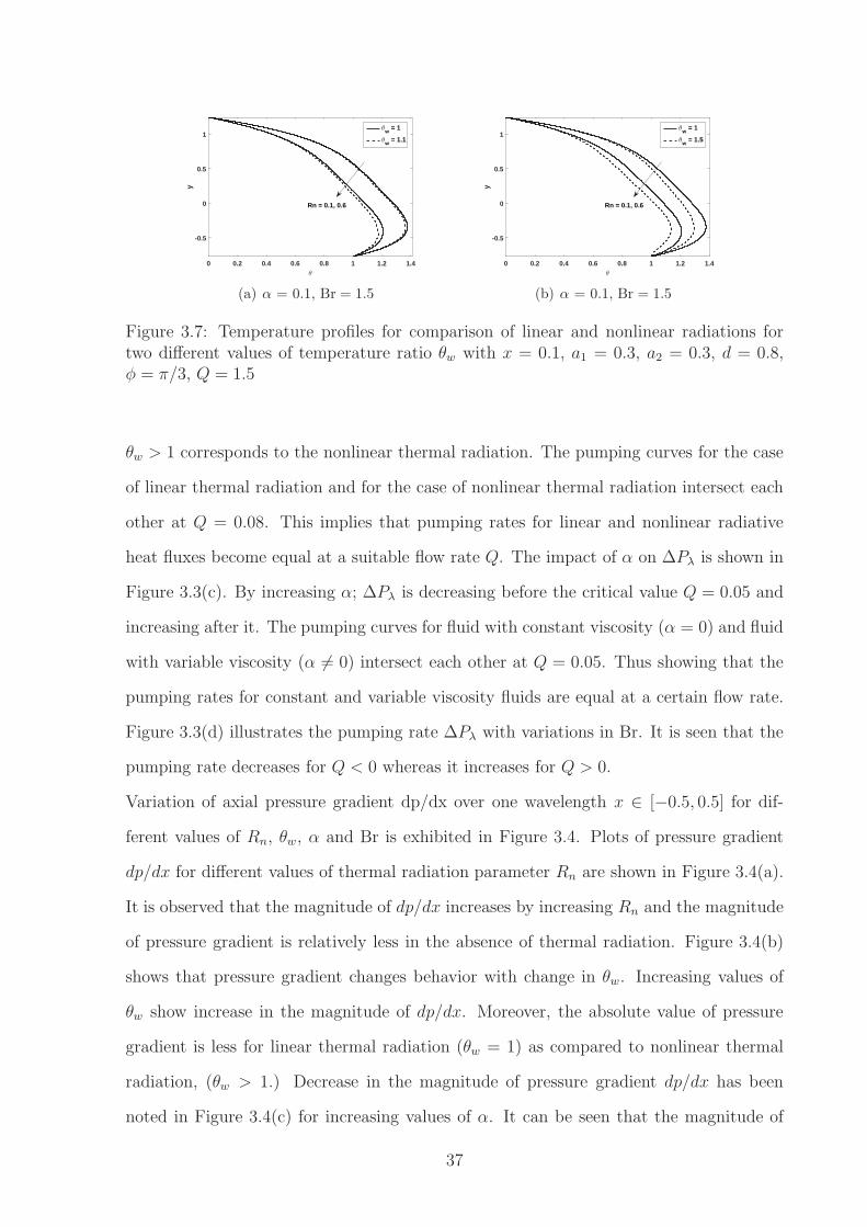
0 0.2 0.4 0.6 0.8 1 1.2 1.4θ

-0.5

0

0.5

1

y

θw

= 1

θw

= 1.1

Rn = 0.1, 0.6

(a) α = 0.1, Br = 1.5

0 0.2 0.4 0.6 0.8 1 1.2 1.4θ

-0.5

0

0.5

1

y

θw

= 1

θw

= 1.5

Rn = 0.1, 0.6

(b) α = 0.1, Br = 1.5

Figure 3.7: Temperature profiles for comparison of linear and nonlinear radiations fortwo different values of temperature ratio θw with x = 0.1, a1 = 0.3, a2 = 0.3, d = 0.8,φ = π/3, Q = 1.5

θw > 1 corresponds to the nonlinear thermal radiation. The pumping curves for the case

of linear thermal radiation and for the case of nonlinear thermal radiation intersect each

other at Q = 0.08. This implies that pumping rates for linear and nonlinear radiative

heat fluxes become equal at a suitable flow rate Q. The impact of α on ∆Pλ is shown in

Figure 3.3(c). By increasing α; ∆Pλ is decreasing before the critical value Q = 0.05 and

increasing after it. The pumping curves for fluid with constant viscosity (α = 0) and fluid

with variable viscosity (α 6= 0) intersect each other at Q = 0.05. Thus showing that the

pumping rates for constant and variable viscosity fluids are equal at a certain flow rate.

Figure 3.3(d) illustrates the pumping rate ∆Pλ with variations in Br. It is seen that the

pumping rate decreases for Q < 0 whereas it increases for Q > 0.

Variation of axial pressure gradient dp/dx over one wavelength x ∈ [−0.5, 0.5] for dif-

ferent values of Rn, θw, α and Br is exhibited in Figure 3.4. Plots of pressure gradient

dp/dx for different values of thermal radiation parameter Rn are shown in Figure 3.4(a).

It is observed that the magnitude of dp/dx increases by increasing Rn and the magnitude

of pressure gradient is relatively less in the absence of thermal radiation. Figure 3.4(b)

shows that pressure gradient changes behavior with change in θw. Increasing values of

θw show increase in the magnitude of dp/dx. Moreover, the absolute value of pressure

gradient is less for linear thermal radiation (θw = 1) as compared to nonlinear thermal

radiation, (θw > 1.) Decrease in the magnitude of pressure gradient dp/dx has been

noted in Figure 3.4(c) for increasing values of α. It can be seen that the magnitude of

37

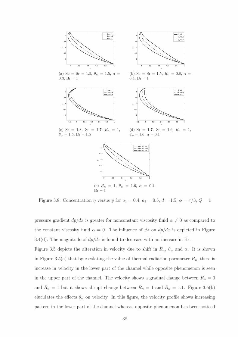
0 0.2 0.4 0.6 0.8 1η

-1

-0.5

0

0.5

1

y

Rn = 0Rn = 0.5Rn = 1

(a) Sc = Sr = 1.5, θw = 1.5, α =0.3, Br = 1

0 0.2 0.4 0.6 0.8 1η

-1

-0.5

0

0.5

1

y

θw

= 1

θw

= 1.4

θw

= 1.6

(b) Sc = Sr = 1.5, Rn = 0.8, α =0.4, Br = 1

-0.2 0 0.2 0.4 0.6 0.8 1η

-1

-0.5

0

0.5

1

y

α = 0α = 0.4α = 0.8

(c) Sr = 1.8, Sc = 1.7, Rn = 1,θw = 1.5, Br = 1.5

-0.2 0 0.2 0.4 0.6 0.8 1η

-1

-0.5

0

0.5

1

y

Br = 0Br = 0.5Br = 1

(d) Sr = 1.7, Sc = 1.6, Rn = 1,θw = 1.6, α = 0.1

0 0.2 0.4 0.6 0.8 1η

-1

-0.5

0

0.5

1

y

Sr(or Sc) = 0Sr(or Sc) = 0.5Sr(or Sc) = 1

(e) Rn = 1, θw = 1.6, α = 0.4,Br = 1

Figure 3.8: Concentration η versus y for a1 = 0.4, a2 = 0.5, d = 1.5, φ = π/3, Q = 1

pressure gradient dp/dx is greater for nonconstant viscosity fluid α 6= 0 as compared to

the constant viscosity fluid α = 0. The influence of Br on dp/dx is depicted in Figure

3.4(d). The magnitude of dp/dx is found to decrease with an increase in Br.

Figure 3.5 depicts the alteration in velocity due to shift in Rn, θw and α. It is shown

in Figure 3.5(a) that by escalating the value of thermal radiation parameter Rn, there is

increase in velocity in the lower part of the channel while opposite phenomenon is seen

in the upper part of the channel. The velocity shows a gradual change between Rn = 0

and Rn = 1 but it shows abrupt change between Rn = 1 and Rn = 1.1. Figure 3.5(b)

elucidates the effects θw on velocity. In this figure, the velocity profile shows increasing

pattern in the lower part of the channel whereas opposite phenomenon has been noticed

38

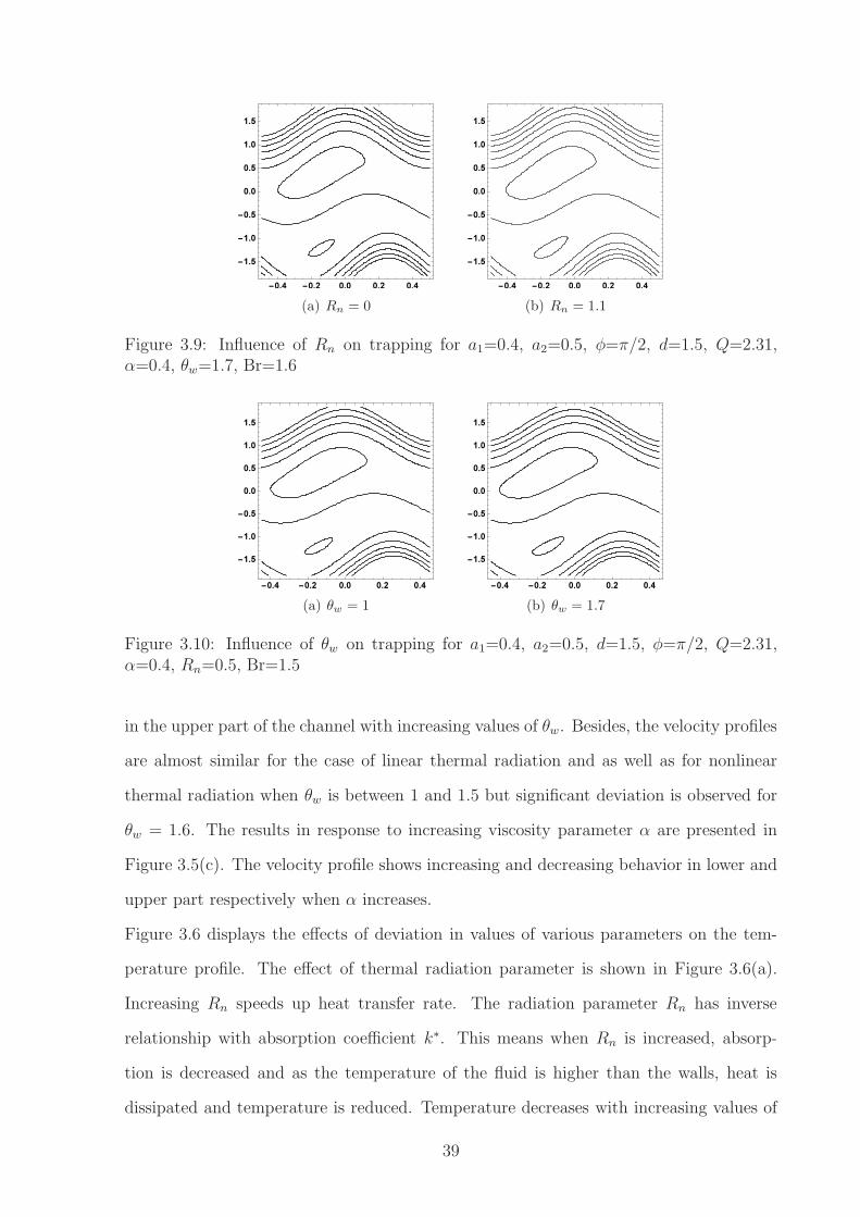
(a) Rn = 0 (b) Rn = 1.1

Figure 3.9: Influence of Rn on trapping for a1=0.4, a2=0.5, φ=π/2, d=1.5, Q=2.31,α=0.4, θw=1.7, Br=1.6

(a) θw = 1 (b) θw = 1.7

Figure 3.10: Influence of θw on trapping for a1=0.4, a2=0.5, d=1.5, φ=π/2, Q=2.31,α=0.4, Rn=0.5, Br=1.5

in the upper part of the channel with increasing values of θw. Besides, the velocity profiles

are almost similar for the case of linear thermal radiation and as well as for nonlinear

thermal radiation when θw is between 1 and 1.5 but significant deviation is observed for

θw = 1.6. The results in response to increasing viscosity parameter α are presented in

Figure 3.5(c). The velocity profile shows increasing and decreasing behavior in lower and

upper part respectively when α increases.

Figure 3.6 displays the effects of deviation in values of various parameters on the tem-

perature profile. The effect of thermal radiation parameter is shown in Figure 3.6(a).

Increasing Rn speeds up heat transfer rate. The radiation parameter Rn has inverse

relationship with absorption coefficient k∗. This means when Rn is increased, absorp-

tion is decreased and as the temperature of the fluid is higher than the walls, heat is

dissipated and temperature is reduced. Temperature decreases with increasing values of

39

(a) α = 0 (b) α = 0.3

Figure 3.11: Influence of α on trapping for a1=0.4, a2=0.5, d=1.5, φ=π/2, Q=2.31,θw=1.3, Rn=0.5, Br=1

θw (see 3.6(b)). In addition, it is remarked that the temperature is low for the case of

nonlinear radiative heat transfer as compared to the linear case. Figure 3.6(c) depicts

that there is a decrease in temperature when α increases. With an increase in α, viscosity

decreases and it causes decrease in viscous dissipation. Eventually, there is decrease in

temperature. Figure 3.6(d) shows that an increment in Brinkman number Br causes rise

in temperature. Figure 3.6(e) is prepared to see the simultaneous effects of α and θw

on temperature. Remarkably, the difference between the curves for linear and nonlinear

thermal radiation is significant for small values of α and the curves tend to get closer

for greater values of α. Increase in α give uniform decrease in temperature for nonlin-

ear thermal radiation. But for linear thermal radiation, there is remarkable decrease in

temperature as we move from constant viscosity to variable viscosity. Comparison of the

results of linear and nonlinear thermal radiation for two different values of Rn is shown

in Figure 3.7. The linear and nonlinear thermal radiation curves are almost the same for

θw = 1.1 which is close to one (see Figure 3.7(a)). However, for values of θw far from

one, significant deviation is observed in the temperature profiles for linear and nonlinear

thermal radiation (see Figure 3.7(b)).

The effects of variations in the values of Rn, θw, α, and Br on heat transfer coefficient Z

at the upper wall are analyzed and presented in Tables 3.2 – 3.5. As shown in Table 3.2,

an increase in thermal radiation parameter Rn leads to an increase in Z and that the heat

transfer rate is low in the absence of radiation. Table 3.3 shows the effect of variation in

40

(a) Br = 0 (b) Br = 1.6

Figure 3.12: Influence of θw on trapping for a1=0.4, a2=0.5, d=1.5, φ=π/2, Q=2.31,θw=1.1, Rn=0.5, α=0.3

θw on Z. The heat transfer coefficient increases with an increase in θw. The table also

reflects that heat transfer rate is high in case of nonlinear thermal radiation as compared

to the linear thermal radiation. The effects of α and Br are respectively shown in Tables

3.4 and 3.5. It is found that α has negative, whereas Br has a positive correlation with

Z.

Figure 3.8 depicts the effect of variations of Rn, θw α, Br, Sr and Sc on concentration

distribution function. It can be seen from Figure 3.8(a) that the thermal radiation pa-

rameter Rn has negative correlation with concentration profile and it is asserted that the

concentration is more in the absence of thermal radiation. Figure 3.8(b) demonstrates

that the effect of θw is to reduce the fluid concentration. Concentration is higher in case

of linear thermal radiation as compared with the nonlinear case. It is evident from the

Figure 3.8(c) that increments in values of α, render an increase in the concentration pro-

file. It is also noticed that concentration is higher for the fluids with variable viscosity

in comparison to fluids with constant viscosity. Figures 3.8(d) and 3.8(e) manifest the

effects of Br, Sr and Sc on concentration profile, revealing that these parameters have

reducing impact on concentration.

Trapping is an important phenomenon of peristaltic mechanism. Herein, an internal cir-

culating bolus is formed and enclosed by streamlines. Physical examples of trapped bolus

are formation of thrombus in blood and movement of food in gastrointestinal tract. Fig-

ures 3.9 – 3.12 demonstrate the effects of Rn, θw, α and Br on trapping. From Figure

41

3.9 we observe that an increase in Rn increases the size of trapped bolus. The figure

also shows that the bolus is small in absence of thermal radiation. It is evident from the

Figure 3.10 that increase in θw yields a slight increase in the size of bolus. It is noticed

in the Figure 3.11 that by increasing α, the size of upper bolus increases while the size

of lower bolus decreases. Figure 3.12 shows that the size of trapped bolus increases with

the increase in Brinkman number Br.

3.4 Conclusion

In this chapter, we have carried out a detailed study to see the effects of nonlinear thermal

radiation on wall induced flow of viscous fluid with temperature dependent viscosity.

Furthermore, we have also investigated the influence of mass transfer. The chief findings

are summarized as follows:

The impact of thermal radiation parameter Rn and temperature ratio θw on pressure rise

and magnitude of pressure gradient is opposite to that of the viscosity parameter α and

Brinkman number Br. It is observed that magnitude of pressure gradient is relatively

small for the case of no thermal radiation. Thermal radiation parameter Rn and viscosity

parameter α do not have the same effect on velocity in the lower part of the channel as

they have in the upper part of the channel. In case of constant viscosity and in the absence

of thermal radiation, velocity is relatively small in the lower part of channel, whereas, the

opposite is true for the upper part. The velocity is almost the same for θw ∈ [1, 1.5]. That

is whether the thermal radiation is linear (θw = 1) or nonlinear (θw > 1), its variation

in this range has no significant effect on the velocity. However, for values of θw > 1.5

there is a remarkable change in the velocity. Increments in Rn, θw and α cause reduction

in temperature, whereas,increasing values of Br cause rise in temperature. Escalating

values of Rn, θw, Br, Sr and Sc have reducing impact on concentration. Concentration is

high for variable viscosity as compared to constant viscosity. Slight increase in the size

of trapped bolus has been observed for increasing values of Rn, θw and Br. The size of

upper bolus increases and lower bolus decreases with an enhancement in α.

42

Chapter 4

Nonlinear Radiative Heat and Mass Transfer in

Hydromagnetic Peristaltic Flow through Porous

Medium

43

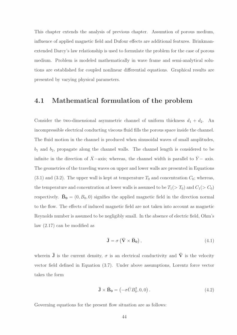
This chapter extends the analysis of previous chapter. Assumtion of porous medium,

influence of applied magnetic field and Dufour effects are additional features. Brinkman-

extended Darcy’s law relationship is used to formulate the problem for the case of porous

medium. Problem is modeled mathematically in wave frame and semi-analytical solu-

tions are established for coupled nonlinear differential equations. Graphical results are

presented by varying physical parameters.

4.1 Mathematical formulation of the problem

Consider the two-dimensional asymmetric channel of uniform thickness d1 + d2. An

incompressible electrical conducting viscous fluid fills the porous space inside the channel.

The fluid motion in the channel is produced when sinusoidal waves of small amplitudes,

b1 and b2, propagate along the channel walls. The channel length is considered to be

infinite in the direction of X−axis; whereas, the channel width is parallel to Y− axis.

The geometries of the traveling waves on upper and lower walls are presented in Equations

(3.1) and (3.2). The upper wall is kept at temperature T0 and concentration C0; whereas,

the temperature and concentration at lower walls is assumed to be T1(> T0) and C1(> C0)

respectively. B0 = (0, B0, 0) signifies the applied magnetic field in the direction normal

to the flow. The effects of induced magnetic field are not taken into account as magnetic

Reynolds number is assumed to be negligibly small. In the absence of electric field, Ohm’s

law (2.17) can be modified as

J = σ(

V × B0

)

, (4.1)

wherein J is the current density, σ is an electrical conductivity and V is the velocity

vector field defined in Equation (3.7). Under above assumptions, Lorentz force vector

takes the form

J× B0 =(

−σUB20 , 0, 0

)

. (4.2)

Governing equations for the present flow situation are as follows:

44

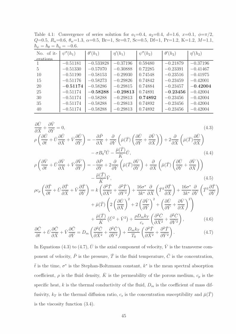
Table 4.1: Convergence of series solution for a1=0.4, a2=0.4, d=1.6, x=0.1, φ=π/2,Q=0.5, Rn=0.6, θw=1.3, α=0.5, Br=1, Sr=0.7, Sc=0.5, Df=1, Pr=1.2, K=1.2, M=1.1,~ψ = ~θ = ~η = −0.6.

No. of it-erations

ψ′′(h1) θ′(h1) η′(h1) ψ′′(h2) θ′(h2) η′(h2)

1 −0.51181 −0.533828 −0.37196 0.59480 −0.21879 −0.371965 −0.51330 −0.57070 −0.30888 0.72285 −0.23391 −0.4146710 −0.51190 −0.58153 −0.29930 0.74548 −0.23516 −0.4197515 −0.51176 −0.58273 −0.29826 0.74842 −0.23459 −0.4200120 −0.51174 −0.58286 −0.29815 0.74884 −0.23457 −0.4200425 −0.51174 −0.58288 −0.29813 0.74891 −0.23456 −0.4200430 −0.51174 −0.58288 −0.29813 0.74892 −0.23456 −0.4200435 −0.51174 −0.58288 −0.29813 0.74892 −0.23456 −0.4200440 −0.51174 −0.58288 −0.29813 0.74892 −0.23456 −0.42004

∂U

∂X+∂V

∂Y= 0, (4.3)

ρ

(

∂U

∂t+ U

∂U

∂X+ V

∂U

∂Y

)

= − ∂P

∂X+

∂

∂Y

(

µ(T )

(

∂U

∂Y+∂V

∂X

))

+ 2∂

∂X

(

µ(T )∂U

∂X

)

− σB02U − µ(T )

KU , (4.4)

ρ

(

∂V

∂t+ U

∂V

∂X+ V

∂V

∂Y

)

= −∂P∂Y

+ 2∂

∂Y

(

µ(T )∂V

∂Y

)

+∂

∂X

(

µ(T )

(

∂U

∂Y+∂V

∂X

))

− µ(T )

KV , (4.5)

ρcp

(

∂T

∂t+ U

∂T

∂X+ V

∂T

∂Y

)

= k

(

∂2T

∂X2+∂2T

∂Y 2

)

+16σ∗

3k∗∂

∂X

(

T 3 ∂T

∂X

)

+16σ∗

3k∗∂

∂Y

(

T 3 ∂T

∂Y

)

+ µ(T )

(

2

(

∂U

∂X

)2

+ 2

(

∂V

∂Y

)2

+

(

∂U

∂Y+∂V

∂X

)2)

+µ(T )

K

(

U2 + V 2)

+ρDmkTcs

(

∂2C

∂X2+∂2C

∂Y 2

)

, (4.6)

∂C

∂t+ U

∂C

∂X+ V

∂C

∂Y= Dm

(

∂2C

∂X2+∂2C

∂Y 2

)

+DmkTT0

(

∂2T

∂X2+∂2T

∂Y 2

)

. (4.7)

In Equations (4.3) to (4.7), U is the axial component of velocity, V is the transverse com-

ponent of velocity, P is the pressure, T is the fluid temperature, C is the concentration,

t is the time, σ∗ is the Stephan-Boltzmann constant, k∗ is the mean spectral absorption

coefficient, ρ is the fluid density, K is the permeability of the porous medium, cp is the

specific heat, k is the thermal conductivity of the fluid, Dm is the coefficient of mass dif-

fusivity, kT is the thermal diffusion ratio, cs is the concentration susceptibility and µ(T )

is the viscosity function (3.4).

45

Table 4.2: Critical values of Q for which ∆Pλ = 0

Rn Q0 θw Q0 α Q0 K Q0

0.0 0.4870 1.0 0.3950 0.0 0.5047 0.4 0.41010.6 0.4668 1.2 0.3800 0.2 0.5049 0.6 0.43930.9 0.4557 1.4 0.3621 0.5 0.5052 1.0 0.46811.2 0.4461 1.6 0.3429 0.8 0.5067 ∞ 0.5285M Q0 Df Q0 Sr(or

Sc)Q0

0.0 0.5241 0.0 0.4649 0.0 0.46490.6 0.4840 0.5 0.4711 0.5 0.47111.0 0.4351 1.0 0.4781 1.0 0.47811.3 0.4011 1.5 0.4865 1.5 0.4865

Following Shapiro et al. [68], we define the wave reference frame (x, y) by the transfor-

mations:[

xy

]

=

[

X − ctY

]

,

[

u (x, y)v (x, y)

]

=

[

U(

X, Y , t)

− cV(

X, Y , t)

]

. (4.8)

Applying transformation (4.8) to Equations (4.3) to (4.7), we get,

∂u

∂x+∂v

∂y= 0, (4.9)

ρ

(

u∂u

∂x+ v

∂u

∂y

)

= −∂p∂x

+∂

∂y

(

µ(T )

(

∂u

∂y+∂v

∂x

))

+ 2∂

∂x

(

µ(T )∂u

∂x

)

− σB02 (u+ c)− µ(T )

K(u+ c) , (4.10)

ρ

(

u∂v

∂x+ v

∂v

∂y

)

= −∂p∂y

+ 2∂

∂y

(

µ(T )∂v

∂y

)

+∂

∂x

(

µ(T )

(

∂u

∂y+∂v

∂x

))

− µ(T )

Kv, (4.11)

ρcp

(

u∂T

∂x+ v

∂T

∂y

)

= k

(

∂2T

∂x2+∂2T

∂y2

)

+16σ∗

3k∗∂

∂x

(

T 3∂T

∂x

)

+16σ∗

3k∗∂

∂y

(

T 3∂T

∂y

)

+ µ(T )

(

2

(

∂u

∂x

)2

+ 2

(

∂v

∂y

)2

+

(

∂u

∂y+∂v

∂x

)2)

+µ(T )

K

(

(u+ c)2 + v2)

+ρDmkTcs

(

∂2C

∂x2+∂2C

∂y2

)

, (4.12)

u∂C

∂x+ v

∂C

∂y= Dm

(

∂2C

∂x2+∂2C

∂y2

)

+DmkTT0

(

∂2T

∂x2+∂2T

∂y2

)

. (4.13)

To make the non-dimensional analysis, we use the dimensionless variables (3.16) and

(3.21) and define Dufour number Df, permeability parameter K, Hartman number M as:

Df =ρDmkT (C1 − C0)

µ0cpcs(T1 − T0), K =

K

d21, M2 =

σB20d

21

µ0. (4.14)

46

Using Equation (4.9), one can write

u =∂ψ

∂yand v = −δ∂ψ

∂x, (4.15)

where ψ (x, y) is the stream function.

Invoking Equations (3.16), (3.21), (4.14) and (4.15) in Equations (4.10) to (4.13) and

applying the long wavelength procedure [68], we arrive at

0 = −∂p∂x

+∂

∂y

(

(1− αθ)∂2ψ

∂y2

)

−(

1− αθ

K

)(

∂ψ

∂y+ 1

)

−M2

(

∂ψ

∂y+ 1

)

, (4.16)

0 = −∂p∂y, (4.17)

0 =∂2

∂y2

(

(1− αθ)∂2ψ

∂y2

)

−(

1− αθ

K

)(

∂2ψ

∂y2

)

−M2

(

∂2ψ

∂y2

)

, (4.18)

0 =∂2θ

∂y2+ Br (1− αθ)

(

∂2ψ

∂y2

)2

+Rn

∂

∂y

(

(1 + θ(θw − 1))3∂θ

∂y

)

+Br (1− αθ)

K

(

∂ψ

∂y+ 1

)2

+ PrDf∂2η

∂y2, (4.19)

0 =∂2η

∂y2+ SrSc

∂2θ

∂y2. (4.20)

The respective dimensionless time mean flow rates Q and F in the fixed frame and the

wave frame can be expressed through the relation:

Q = F + 1 + d, (4.21)

where

F =

∫ h1(x)

h2(x)

∂ψ

∂ydy = ψ(h1(x))− ψ(h2(x)). (4.22)

The dimensionless boundary conditions in wave reference frame can be written as follows:

ψ =F

2,∂ψ

∂y= −1, θ = 0, η = 0, at y = h1(x), (4.23)

ψ = −F2,∂ψ

∂y= −1, θ = 1, η = 1, at y = h2(x). (4.24)

The peristaltic walls (3.1) and (3.2) in dimensionless form are

h1(x) = 1 + a1 cos(2πx), h2(x) = −d− a2 cos(2πx+ φ), (4.25)

47

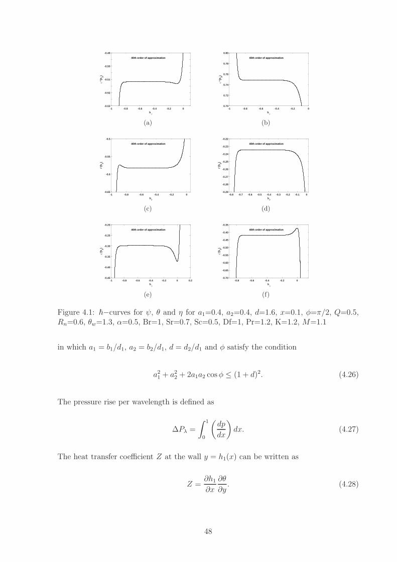
-1 -0.8 -0.6 -0.4 -0.2 0hψ

-0.53

-0.52

-0.51

-0.50

-0.49

ψ''(

h1)

40th order of approximation

(a)

-1 -0.8 -0.6 -0.4 -0.2 0hψ

0.70

0.72

0.74

0.76

0.78

0.80

ψ''(

h2)


(b)

-1 -0.8 -0.6 -0.4 -0.2 0hθ

-0.65

-0.6

-0.55

-0.5

θ'(h

1)


(c)

-0.8 -0.7 -0.6 -0.5 -0.4 -0.3 -0.2 -0.1 0hθ

-0.29

-0.28

-0.27

-0.26

-0.25

-0.24

-0.23

-0.22

θ'(h

2)


(d)

-1 -0.8 -0.6 -0.4 -0.2 0 0.2hη

-0.45

-0.40

-0.35

-0.30

-0.25

-0.20

η'(h

1)


(e)

-0.8 -0.6 -0.4 -0.2 0hη

-0.70

-0.65

-0.60

-0.55

-0.50

-0.45

-0.40

-0.35

η'(h

2)


(f)

Figure 4.1: ~−curves for ψ, θ and η for a1=0.4, a2=0.4, d=1.6, x=0.1, φ=π/2, Q=0.5,Rn=0.6, θw=1.3, α=0.5, Br=1, Sr=0.7, Sc=0.5, Df=1, Pr=1.2, K=1.2, M=1.1

in which a1 = b1/d1, a2 = b2/d1, d = d2/d1 and φ satisfy the condition

a21 + a22 + 2a1a2 cosφ ≤ (1 + d)2. (4.26)

The pressure rise per wavelength is defined as

∆Pλ =

∫ 1

0

(

dp

dx

)

dx. (4.27)

The heat transfer coefficient Z at the wall y = h1(x) can be written as

Z =∂h1∂x

∂θ

∂y. (4.28)

48

-0.4 -0.2 0 0.2 0.4 0.6 0.8 1 1.2

Q

-2

-1

0

1

2

∆ P

λ

Rn = 0.0

Rn = 0.6

Rn = 0.9

Rn = 1.2

(a) θw=1.6, α=0.8, Br=1, M=0.5, K=1,Sr=0.7, Sc=0.9, Df=0.5, Pr=1

-0.4 -0.2 0 0.2 0.4 0.6 0.8 1 1.2

Q

-6

-4

-2

0

2

4

∆ P

λ

θw

= 1.0

θw

= 1.2

θw

= 1.4

θw

= 1.6

(b) Rn=1.2, α=0.8, Br=0.8, M=0.5,K=0.3, Sr=0.7, Sc=0.9, Df=0.5, Pr=1

-0.2 0 0.2 0.4 0.6 0.8 1 1.2

Q

-2

-1.5

-1

-0.5

0

0.5

1

1.5

2

∆ P

λ

α = 0.0α = 0.2α = 0.5α = 0.8

(c) Rn=0.5, θw=1.5, Br=1, K=2,M=0.4, Sr=0.7, Sc=0.9, Df=0.5, Pr=1

-0.5 0 0.5 1

Q

-2

-1

0

1

2

3

∆ P

λ

K = 0.4

K = 0.6

K = 1.0

K → ∞

(d) Rn=1, θw=1.3, α=0.5, Br=1, M=0.5,Sr=0.7, Sc=0.9, Df=0.5, Pr=1

-0.4 -0.2 0 0.2 0.4 0.6 0.8

Q

-1

-0.5

0

0.5

1

1.5

2

2.5

∆ P

λ

M = 0.0

M = 0.6

M = 1.0

M = 1.3

(e) Rn=0.5, θw=1.6, α=0.7, K=2, Br=1,Sr=0.7, Sc=0.9, Df=0.5, Pr=1

-0.5 0 0.5 1 1.5

Q

-2

-1.5

-1

-0.5

0

0.5

1

1.5

2

∆ P

λ

Df = 0.0Df = 0.5Df = 1.0Df = 1.5

(f) Rn=1, θw=1.6, α=0.5, Br=1, M=0.5,K=0.7, Sr=1, Sc=1, Pr=1.4

-0.5 0 0.5 1 1.5

Q

-2

-1.5

-1

-0.5

0

0.5

1

1.5

2

∆ P

λ

Sr = 0.0Sr = 0.5Sr = 1.0Sr = 1.5

(g) Rn=1, θw=1.6, α=0.5, Br=1, M=0.5,K=0.7, Df=1, Pr=1.4, Sc=1

-0.5 0 0.5 1 1.5

Q

-2

-1.5

-1

-0.5

0

0.5

1

1.5

2

∆ P

λ

Sc = 0.0Sc = 0.5Sc = 1.0Sc = 1.5

(h) Rn=1, θw=1.6, α=0.5, Br=1, M=0.5,K=0.7, Df=1, Pr=1.4, Sr=1

Figure 4.2: Pressure rise ∆Pλ against flow rate Q for d = 1.1, a1 = a2 = 0.5, φ=π/4

49

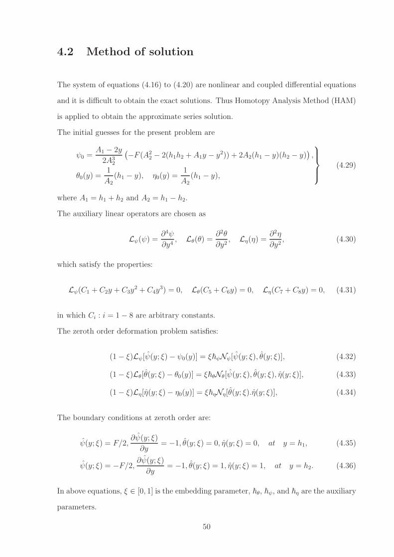
4.2 Method of solution

The system of equations (4.16) to (4.20) are nonlinear and coupled differential equations

and it is difficult to obtain the exact solutions. Thus Homotopy Analysis Method (HAM)

is applied to obtain the approximate series solution.

The initial guesses for the present problem are

ψ0 =A1 − 2y

2A32

(

−F (A22 − 2(h1h2 + A1y − y2)) + 2A2(h1 − y)(h2 − y)

)

,

θ0(y) =1

A2(h1 − y), η0(y) =

1

A2(h1 − y),

(4.29)

where A1 = h1 + h2 and A2 = h1 − h2.

The auxiliary linear operators are chosen as

Lψ(ψ) =∂4ψ

∂y4, Lθ(θ) =

∂2θ

∂y2, Lη(η) =

∂2η

∂y2, (4.30)

which satisfy the properties:

Lψ(C1 + C2y + C3y2 + C4y

3) = 0, Lθ(C5 + C6y) = 0, Lη(C7 + C8y) = 0, (4.31)

in which Ci : i = 1− 8 are arbitrary constants.

The zeroth order deformation problem satisfies:

(1− ξ)Lψ[ψ(y; ξ)− ψ0(y)] = ξ~ψNψ[ψ(y; ξ), θ(y; ξ)], (4.32)

(1− ξ)Lθ[θ(y; ξ)− θ0(y)] = ξ~θNθ[ψ(y; ξ), θ(y; ξ), η(y; ξ)], (4.33)

(1− ξ)Lη[η(y; ξ)− η0(y)] = ξ~ηNη[θ(y; ξ).η(y; ξ)], (4.34)

The boundary conditions at zeroth order are:

ψ(y; ξ) = F/2,∂ψ(y; ξ)

∂y= −1, θ(y; ξ) = 0, η(y; ξ) = 0, at y = h1, (4.35)

ψ(y; ξ) = −F/2, ∂ψ(y; ξ)∂y

= −1, θ(y; ξ) = 1, η(y; ξ) = 1, at y = h2. (4.36)

In above equations, ξ ∈ [0, 1] is the embedding parameter, ~θ, ~ψ, and ~η are the auxiliary

parameters.

50

0 0.2 0.4 0.6 0.8 1

x

-2

-1

0

1

2

3

4

5

dp/d

x

Rn = 0.0

Rn = 0.8

Rn = 1.0

Rn = 1.2

(a) θw=1.8, α=0.9, Br=1, M=0.5,K=0.6, Sr=0.7, Sc=0.9, Df=0.5, Pr=1

0 0.2 0.4 0.6 0.8 1

x

-1

0

1

2

3

4

5

dp/d

x

θw

= 1.0

θw

= 1.5

θw

= 1.7

θw

= 1.9

(b) Rn=1, α=0.8, Br=1.4, M=0.3,K=0.8, Sr=1, Sc=0.9, Df=0.5, Pr=1

0 0.2 0.4 0.6 0.8 1

x

-1

0

1

2

3

4

5

dp/d

x

α = 0.0α = 0.3α = 0.5α = 0.8

(c) Rn=1.2, θw=1.3, Br=1, M=0.5,K=2, Sr=0.7, Sc=0.9, Df=0.5, Pr=1

0 0.2 0.4 0.6 0.8 1

x

-2

-1

0

1

2

3

4

5

dp/d

x

K = 0.4

K = 0.6

K = 1.2

K → ∞

(d) Rn=1.2, θw=1.5, α=0.8, Br=1,M=0.6, Sr=0.7, Sc=0.9, Df=0.5, Pr=1

0 0.2 0.4 0.6 0.8 1

x

-2

0

2

4

6

8

dp/d

x

M = 0.0

M = 1.0

M = 1.5

M = 2.0

(e) Rn=0.9, θw=1.6, α=0.4, Br=1,K=0.8, Sr=0.7, Sc=0.9, Df=0.5, Pr=1

0 0.2 0.4 0.6 0.8 1

x

-0.5

0

0.5

1

1.5

2

2.5

3

dp/d

x

Df = 0.0Df = 0.5Df = 1.0Df = 1.5

(f) Rn=1.2, θw=1.6, α=0.9, Br=1,M=0.8, K=0.6, Sr=0.9, Sc=0.6, Pr=2

0 0.2 0.4 0.6 0.8 1

x

-0.5

0

0.5

1

1.5

2

2.5

3

dp/d

x

Sr = 0.0Sr = 0.5Sr = 1.0Sr = 1.5

(g) Rn=1.2, θw=1.6, α=0.9, Br=1,M=0.8, K=0.6, Df=0.6, Pr=2, Sc=0.9

0 0.2 0.4 0.6 0.8 1

x

-0.5

0

0.5

1

1.5

2

2.5

3

dp/d

x

Sc = 0.0Sc = 0.5Sc = 1.0Sc = 1.5

(h) Rn=1.2, θw=1.6, α=0.9, Br=1,M=0.8, K=0.6, Df=0.6, Pr=2, Sr=0.9

Figure 4.3: Pressure gradient dp/dx versus x for a1 = 0.5, a2 = 0.5, d = 1.1, Q = 0.3,φ = π/4

51

The expressions of nonlinear operators, N1ψ, N1θ, and N1η, are given below as:

N1ψ[ψ(y; ξ), θ(y; ξ)] =∂4ψ(y; ξ)

∂y4

− α

[

θ(y; ξ)∂4ψ(y; ξ)

∂y4+ 2

∂θ(y; ξ)

∂y

∂3ψ(y; ξ)

∂y3+∂2θ(y; ξ)

∂y2∂2ψ(y; ξ)

∂y2

]

−(

M2 +1

K

)

∂2ψ(y; ξ)

∂y2+α

Kθ(y; ξ)

∂2ψ(y; ξ)

∂y2, (4.37)

N1θ[ψ(y; ξ), θ(y; ξ)] =∂2θ(y; ξ)

∂y2+ Br

(

∂2ψ(y; ξ)

∂y2

)2

− αθ(y; ξ)

(

∂2ψ(y; ξ)

∂y2

)2

+Rn

3 (θw − 1)3 θ2(y; ξ)

(

∂θ(y; ξ)

∂y

)2

+ (θw − 1)3 θ3(y; ξ)∂2θ(y; ξ)

∂y2

+Rn

3 (θw − 1)2 θ2(y; ξ)∂2θ(y; ξ)

∂y2+ 6 (θw − 1)2 θ(y; ξ)

(

∂θ(y; ξ)

∂y

)2

+Rn

3 (θw − 1)

(

∂θ(y; ξ)

∂y

)2

+ 3 (θw − 1) θ(y; ξ)∂2θ(y; ξ)

∂y2+∂2θ(y; ξ)

∂y2

+Br

K

(

∂ψ(y; ξ)

∂y

)2

+ 2∂ψ(y; ξ)

∂y+ 1

+ PrDf∂2η(y; ξ)

∂y2

− αBr

K

θ(y; ξ)

(

∂ψ(y; ξ)

∂y

)2

+ 2θ(y; ξ)∂ψ(y; ξ)

∂y+ θ(y; ξ)

, (4.38)

N1η[θ(y; ξ), η(y; ξ)] =∂2η(y; ξ)

∂y2+ SrSc

∂2θ(y; ξ)

∂y2. (4.39)

The initial guesses ψ0(y), θ0(y) and η0(y) approach ψ(y), θ(y) and η(y) respectively as ξ

takes values from 0 to 1. Mathematically,

ψ(y; 0) = ψ0(y), θ(y; 0) = θ0(y), η(y; 0) = η0(y),

ψ(y; 1) = ψ(y), θ(y; 1) = θ(y), η(y; 1) = η(y). (4.40)

Using Taylor’s expansion, one can write

ψ(y, ξ) = ψ0(y) +∞∑

m=1

ψm(y)ξm, ψm(y) =

1

m!

∂mψ(y; ξ)

∂ξm

∣

∣

∣

∣

∣

ξ=0

, (4.41)

θ(y, ξ) = θ0(y) +∞∑

m=1

θm(y)ξm, θm(y) =

1

m!

∂mθ(y; ξ)

∂ξm

∣

∣

∣

∣

∣

ξ=0

, (4.42)

η(y, ξ) = η0(y) +∞∑

m=1

ηm(y)ξm, ηm(y) =

1

m!

∂mη(y; ξ)

∂ξm

∣

∣

∣

∣

ξ=0

. (4.43)

52

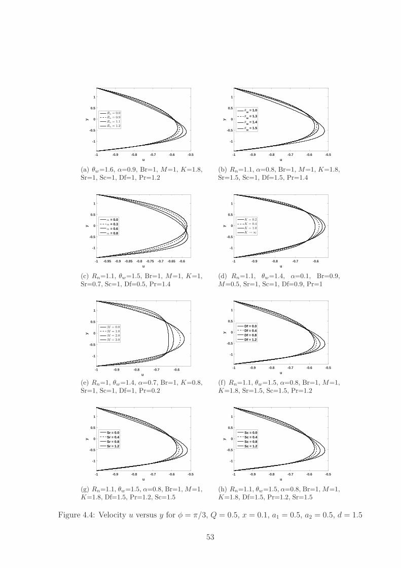
-1 -0.9 -0.8 -0.7 -0.6 -0.5

u

-1

-0.5

0

0.5

1

y

Rn = 0.0

Rn = 0.9

Rn = 1.1

Rn = 1.2

(a) θw=1.6, α=0.9, Br=1, M=1, K=1.8,Sr=1, Sc=1, Df=1, Pr=1.2

-1 -0.9 -0.8 -0.7 -0.6 -0.5

u

-1

-0.5

0

0.5

1

y

θw

= 1.0

θw

= 1.3

θw

= 1.4

θw

= 1.5

(b) Rn=1.1, α=0.8, Br=1, M=1, K=1.8,Sr=1.5, Sc=1, Df=1.5, Pr=1.4

-1 -0.95 -0.9 -0.85 -0.8 -0.75 -0.7 -0.65 -0.6

u

-1

-0.5

0

0.5

1

y

α = 0.0α = 0.3α = 0.6α = 0.8

(c) Rn=1.1, θw=1.5, Br=1, M=1, K=1,Sr=0.7, Sc=1, Df=0.5, Pr=1.4

-1 -0.9 -0.8 -0.7 -0.6

u

-1

-0.5

0

0.5

1

yK = 0.2

K = 0.4

K = 1.0

K → ∞

(d) Rn=1.1, θw=1.4, α=0.1, Br=0.9,M=0.5, Sr=1, Sc=1, Df=0.9, Pr=1

-1 -0.9 -0.8 -0.7 -0.6

u

-1

-0.5

0

0.5

1

y

M = 0.0

M = 1.0

M = 2.0

M = 3.0

(e) Rn=1, θw=1.4, α=0.7, Br=1, K=0.8,Sr=1, Sc=1, Df=1, Pr=0.2

-1 -0.9 -0.8 -0.7 -0.6 -0.5

u

-1

-0.5

0

0.5

1

y

Df = 0.0Df = 0.4Df = 0.8Df = 1.2

(f) Rn=1.1, θw=1.5, α=0.8, Br=1, M=1,K=1.8, Sr=1.5, Sc=1.5, Pr=1.2

-1 -0.9 -0.8 -0.7 -0.6 -0.5

u

-1

-0.5

0

0.5

1

y

Sr = 0.0Sr = 0.4Sr = 0.8Sr = 1.2

(g) Rn=1.1, θw=1.5, α=0.8, Br=1, M=1,K=1.8, Df=1.5, Pr=1.2, Sc=1.5

-1 -0.9 -0.8 -0.7 -0.6 -0.5

u

-1

-0.5

0

0.5

1

y

Sc = 0.0Sc = 0.4Sc = 0.8Sc = 1.2

(h) Rn=1.1, θw=1.5, α=0.8, Br=1, M=1,K=1.8, Df=1.5, Pr=1.2, Sr=1.5

Figure 4.4: Velocity u versus y for φ = π/3, Q = 0.5, x = 0.1, a1 = 0.5, a2 = 0.5, d = 1.5

53

The linear operator, initial guess and auxiliary parameters are chosen in such a manner

that the series (4.41) to (4.43) are convergent at ξ = 1. Hence

ψ(y) = ψ0(y) +

∞∑

m=1

ψm(y), (4.44)

θ(y) = θ0(y) +∞∑

m=1

θm(y), (4.45)

η(y) = η0(y) +∞∑

m=1

ηm(y). (4.46)

Deformation problems at mth order are:

Lψ[ψm(y)− χmψm−1(y)] = ~ψRψm(y), (4.47)

Lθ[θm(y)− χmθm−1(y)] = ~θRθm(y), (4.48)

Lη[ηm(y)− χmηm−1(y)] = ~ηRηm(y), (4.49)

with

Rψ1m(y) =

∂4ψm−1

∂y4− α

m−1∑

k=0

[

θm−1−k(y)∂4ψk∂y4

+ 2∂θm−1−k

∂y

∂3ψk∂y3

+∂2θm−1−k

∂y2∂2ψk∂y2

]

−[

M2 +1

K

]

∂2ψm−1

∂y2+α

K

m−1∑

k=0

θm−1−k∂2ψk∂y2

, (4.50)

Rθ1m(y) =

∂2θm−1

∂y2+ Br

m−1∑

k=0

[

∂2ψm−1−k

∂y2∂2ψk∂y2

− αk∑

l=0

θm−1−k∂2ψk−l∂y2

∂2ψl∂y2

]

+Rn

m−1∑

k=0

k∑

l=0

[

3(θw − 1)2θm−1−kθk−l∂2θl∂y2

+ 6(θw − 1)2θm−1−k∂θk−l∂y

∂θl∂y

]

+Rn

m−1∑

k=0

[

3(θw − 1)∂θm−1−k

∂y

∂θk∂y

+ 3(θw − 1)θm−1−k∂2θk∂y2

]

+ PrDf∂2ηm−1

∂y2

+Br

K

[

2∂ψm−1

∂y− αθm−1

]

− αBr

K

m−1∑

k=0

k∑

n=0

n∑

l=0

θm−1−k

(

∂ψk−l∂y

)(

∂ψl∂y

)

+Br

K

m−1∑

k=0

k∑

l=0

[(

∂ψm−1−k

∂y

)(

∂ψk∂y

)

− 2αθm−1−k∂ψk∂y

]

+Br

K[1− χm]

+Rn

m−1∑

k=0

k∑

n=0

n∑

l=0

[

3(θw − 1)3θm−1−kθk−n∂θn−l∂y

∂θl∂y

+ (θw − 1)3θm−1−kθk−nθn−l∂2θl∂y2

]

+Rn

∂2θm−1

∂y2, (4.51)

Rη1m(y) =

∂2ηm−1

∂y2+ SrSc

∂2θm−1

∂y2. (4.52)

54

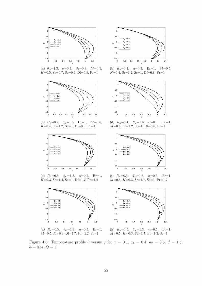
0 0.2 0.4 0.6 0.8 1 1.2θ

-1.5

-1

-0.5

0

0.5

1

y

Rn = 0.0

Rn = 0.2

Rn = 0.4

Rn = 0.7

(a) θw=1.3, α=0.4, Br=0.9, M=0.5,K=0.5, Sr=0.7, Sc=0.9, Df=0.8, Pr=1

0 0.2 0.4 0.6 0.8 1 1.2 1.4θ

-1.5

-1

-0.5

0

0.5

1

y

θw

= 1.0

θw

= 1.2

θw

= 1.4

θw

= 1.6

(b) Rn=0.4, α=0.3, Br=1, M=0.5,K=0.4, Sr=1.2, Sc=1, Df=0.8, Pr=1

0 0.2 0.4 0.6 0.8 1 1.2 1.4 1.6θ

-1.5

-1

-0.5

0

0.5

1

y

α = 0.0α = 0.2α = 0.4α = 0.6

(c) Rn=0.4, θw=1.3, Br=1, M=0.5,K=0.4, Sr=1.2, Sc=1, Df=0.8, Pr=1

0 0.2 0.4 0.6 0.8 1 1.2θ

-1.5

-1

-0.5

0

0.5

1

y

K = 0.2

K = 0.6

K = 1.0

K → ∞

(d) Rn=0.4, θw=1.3, α=0.5, Br=1,M=0.5, Sr=1.2, Sc=1, Df=0.8, Pr=1

0 0.2 0.4 0.6 0.8 1 1.2θ

-1.5

-1

-0.5

0

0.5

1

y

M = 0.0

M = 1.0

M = 1.6

M = 2.2

(e) Rn=0.5, θw=1.3, α=0.5, Br=1,K=0.3, Sr=1.4, Sc=1, Df=1.7, Pr=1.2

0 0.2 0.4 0.6 0.8 1 1.2θ

-1.5

-1

-0.5

0

0.5

1

y

Df = 0.0Df = 0.3Df = 0.6Df = 0.9

(f) Rn=0.5, θw=1.3, α=0.5, Br=1,M=0.5, K=0.3, Sr=1.7, Sc=1, Pr=1.2

0 0.2 0.4 0.6 0.8 1 1.2θ

-1.5

-1

-0.5

0

0.5

1

y

Sr = 0.0Sr = 0.3Sr = 0.6Sr = 0.9

(g) Rn=0.5, θw=1.3, α=0.5, Br=1,M=0.5, K=0.3, Df=1.7, Pr=1.2, Sc=1

0 0.2 0.4 0.6 0.8 1 1.2θ

-1.5

-1

-0.5

0

0.5

1

y

Sc = 0.0Sc = 0.3Sc = 0.6Sc = 0.9

(h) Rn=0.5, θw=1.3, α=0.5, Br=1,M=0.5, K=0.3, Df=1.7, Pr=1.2, Sr=1

Figure 4.5: Temperature profile θ versus y for x = 0.1, a1 = 0.4, a2 = 0.5, d = 1.5,φ = π/4, Q = 1

55

The boundary conditions at this order are

ψm(y; ξ) = F/2,∂ψm(y; ξ)

∂y= −1, θm(y; ξ) = 0, ηm(y; ξ) = 0, at y = h1, (4.53)

ψm(y; ξ) = −F/2, ∂ψm(y; ξ)

∂y= −1, θm(y; ξ) = 1, ηm(y; ξ) = 1, at y = h2,

(4.54)

where

χm =

{

0, m ≤ 11, m > 1.

(4.55)

Solution expressions of mth order deformation problems are given by

ψm(y) = ψ∗

m(y) + C1 + C2y + C3y2 + C4y

3, (4.56)

θm(y) = θ∗m(y) + C5 + C6y, (4.57)

ηm(y) = η∗m(y) + C7 + C8y, (4.58)

where ψ∗

m(y), θ∗

m(y) and η∗

m(y) are special solutions.

4.2.1 Convergence of HAM solution

The convergence of homotopic series solutions is strongly dependent on the values of

the auxiliary parameters: ~ψ, ~θ, and ~η. The admissible values of such parameters

are obtained by plotting the ~-curves at 40th order of approximation (see Figure 4.1).

It is evident that the obtained series solutions are convergent when ~ψ, ~θ and ~η are

−0.8 < ~ψ < −0.3, −0.7 < ~θ < −0.3 and −0.7 < ~η < −0.2 respectively. For this

problem, we select ~ψ = ~θ = ~η = −0.6 and found that the our solutions converge for

all values of y (see Table 4.1).

4.3 Results and discussion

In this section, we intend to discuss the pressure rise per wavelength, pressure gradient,

velocity, temperature, concentration, and trapping under the influence of various im-

portant parameters. Such parameters include the radiation parameter Rn, temperature

56

ratio θw, viscosity parameter α, permeability parameter K, Hartman number M , Dufour

number Df, Soret number Sr, and Schmidt number Sc.

4.3.1 Effects on the flow

The plots of pressure rise ∆Pλ against time-average flow rate Q are presented in Figure

4.2 for different values of the parameters (Rn, θw, α, K, M , Df, Sr, and Sc). It reveals

that there exists a critical value of the flow rate that is denoted by Q0 (Q : ∆Pλ = 0)

and known as free pumping flux. The peristaltic pumping occur when the flow rate Q

fall behind the critical value Q0; however, the augmented pumping occur as the flow

rate Q exceeds from the critical value Q0. Values of free pumping flux Q0 for the above

said parameters are tabulated in Table 4.2. It is clearly shown in Figure 4.2(a) that the

effect of radiation parameter Rn is to increase the pressure rise per wavelength ∆Pλ in

retrograde pumping (∆Pλ > 0, Q < 0) and peristaltic pumping regions (∆Pλ > 0, Q > 0);

whereas it lessens in the augmented pumping region (∆Pλ < 0, Q > 0). It is further

notice from Table 4.2 that the free pumping flux decreases as a result of increasing Rn.

Similar observations can be made through Figure 4.2(b) and Table 4.2 when temperature

ratio parameter θw is increased. Pumping rate is decreasing function of α in retrograde

pumping (∆Pλ > 0, Q < 0) and peristaltic pumping regions (∆Pλ > 0, Q > 0). On

the other hand, in co-pumping region (∆Pλ < 0, Q > 0), it is found to be an increasing

function of α (see Figure 4.2(c)). Table 4.2 depicts that there is increase in Q0 with

an increase in α. Impact of permeability parameter K on pumping performance ∆Pλ

is shown in Figure 4.2(d). It elucidates that pumping ∆Pλ via permeability parameter

K shows decreasing behavior in retrograde pumping (∆Pλ > 0, Q < 0) and peristaltic

pumping regions (∆Pλ > 0, Q > 0). Contrarily, it shows an opposite behavior in co-

pumping region (∆Pλ < 0, Q > 0). It is worth-mentioning that the free pumping flux

for the flow through porous medium is smaller when compared with flow through non-

porous medium (see Table 4.2). In other words, the peristaltic pumping region widens as

we move from porous medium to a non-porous medium. Figure 4.2(e) shows the effect of

57

-0.2 0 0.2 0.4 0.6 0.8 1η

-1.5

-1

-0.5

0

0.5

1

y

Rn = 0.0

Rn = 0.4

Rn = 0.8

Rn = 1.1

(a) θw=1.5, α=0.3, Br=1, M=0.5,K=0.5, Sr=1, Sc=1, Df=0.6, Pr=1

-0.2 0 0.2 0.4 0.6 0.8 1η

-1.5

-1

-0.5

0

0.5

1

y

θw

= 1.0

θw

= 1.2

θw

= 1.4

θw

= 1.6

(b) Rn=0.6, α=0.5, Br=1, M=1.5,K=0.3, Sr=1.3, Sc=1, Df=1, Pr=1

-0.2 0 0.2 0.4 0.6 0.8 1η

-1.5

-1

-0.5

0

0.5

1

y

α = 0.0α = 0.2α = 0.4α = 0.6

(c) Rn=0.6, θw=1.3, Br=1, M=1.5,K=0.3, Sr=1, Sc=1, Df=1, Pr=1

-0.2 0 0.2 0.4 0.6 0.8 1η

-1.5

-1

-0.5

0

0.5

1

y

K = 0.2

K = 0.4

K = 1.0

K → ∞

(d) Rn=0.6, θw=1.3, α=0.4, Br=1,M=1.5, Sr=1, Sc=1, Df=1, Pr=1

-0.4 -0.2 0 0.2 0.4 0.6 0.8 1η

-1.5

-1

-0.5

0

0.5

1

y

M = 0.0

M = 1.0

M = 2.0

M = 3.0

(e) Rn=0.3, θw=1.6, α=0.3, Br=0.9,K=0.3, Sr=0.9, Sc=1.5, Df=0.8, Pr=0.9

-0.2 0 0.2 0.4 0.6 0.8 1η

-1.5

-1

-0.5

0

0.5

1

y

Df = 0.0Df = 0.5Df = 1.0Df = 1.5

(f) Rn=0.6, θw=1.5, α=0.3, Br=1,M=0.5, K=1, Sr=1, Sc=0.9, Pr=0.9

-0.2 0 0.2 0.4 0.6 0.8 1η

-1.5

-1

-0.5

0

0.5

1

y

Sr = 0.0Sr = 0.5Sr = 1.0Sr = 1.5

(g) Rn=0.6, θw=1.6, α=0.3, Br=0.9,M=0.5, K=0.3, Df=0.8, Pr=0.9, Sc=1

-0.2 0 0.2 0.4 0.6 0.8 1η

-1.5

-1

-0.5

0

0.5

1

y

Sc = 0.0Sc = 0.5Sc = 1.0Sc = 1.5

(h) Rn=0.6, θw=1.6, α=0.3, Br=0.9,M=0.5, K=0.3, Df=0.8, Pr=0.9, Sr=1

Figure 4.6: Concentration η versus y for x = 0.1, a1 = 0.4, a2 = 0.5, d = 1.5, φ = π/4,Q = 1

58

(a) M = 0 (b) M = 1.3

Figure 4.7: Influence of M on trapping for a1=0.5, a2=0.5, d=1.5, φ=π/4, Q=2.31,θw=1.6, Rn=1.2, Br=0.6, K=0.4, α=0.4, Sr=0.5, Sc=1, Df=1, Pr=1.2

Hartman number M on ∆Pλ which is exactly opposite to that of K. In Figures 4.2(f) –

4.2(h), the pumping curves are sketched for the parameters Df, Sr, and Sc which arise due

to the consideration of mass transfer phenomenon. It is evident that increasing values

of these parameters reduce the retrograde pumping (∆Pλ > 0, Q < 0) and peristaltic

pumping regions (∆Pλ > 0, Q > 0). However, the pumping performance in co-pumping

region (∆Pλ < 0, Q > 0) and free pumping flux Q0 enhances as a result of increasing

Df, Sr and Sc. Figure 4.3 displays the variation of pressure gradient over one wavelength

x ∈ [0, 1] for different values of involved parameters (Rn, θw, α, K, M , Df, Sr, Sc). It is

important to note that positive pressure gradient is known as adverse pressure gradient

as it resists the flow; however, negative pressure gradient is known as favorable pressure

gradient because it assists the flow. It is clearly shown in Figure 4.3 that the adverse

pressure gradient lies in the region x ∈ [0.24, 0.63], and the favorable pressure gradient

lies in the region x ∈ [0, 0.24] ∪ x ∈ [0.63, 1]. It is observed that increasing values of Rn,

θw, and M increase the adverse pressure gradient whilst the favorable pressure gradient

decreases (see Figures 4.3(a), 4.3(b) and 4.3(e)). Contrary to this situation, the adverse

pressure gradient decreases, and favorable pressure gradient increases when one of α, K,

Df, Sr and Sc is increased (see Figures 4.3(c), 4.3(d) and 4.3(f) – 4.3(h)).

The variation in fluid velocity u under the influence of increasing values of parameters

(Rn, θw, α, K, M , Df, Sr, Sc) is depicted in Figure 4.4. In particular, Figure 4.4(a)

corresponds to the effect of Rn on fluid velocity u. It is clear that fluid velocity u in the

59

(a) Rn = 0 (b) Rn = 1.2

Figure 4.8: Influence of Rn on trapping for a1=0.5, a2=0.5, d=1.5, φ=π/4, Q=2.31,θw=1.6, M=1, Br=1, K=1.8, α=0.4, Sr=0.5, Sc=1, Df=1, Pr=1.2

vicinity of lower walls increases when the radiation parameter Rn is increased. However,

opposite is true as we move away from the lower wall. In general, we can say that the

amplitude of the velocity profile u decreases when the radiation effects are present in the

flow field. This situation remains true when radiation parameter Rn remains fixed and

temperature ratio parameter θw increases (see Figure 4.4(b)). The impact of viscosity

parameter α is depicted in Figure 4.4(c), where we observed that the increasing viscosity

parameter α leads to a fall in the velocity u near the upper wall and a rise near the lower

wall. Figure 4.4(d) shows the influence of permeability parameter K on the velocity. It

illustrate that fluid gains velocity in the channel center; on the other hand, it retards near

the channel walls. The reason being that smaller values of K refer to the porous medium

with high porosity. In this case, porous medium offers more resistance to flow which

in turns reduces the velocity u. Variation in fluid velocity u with increasing Hartman

number M is captured in Figure 4.4(e). We notice that the amplitude of velocity u for

hydrodynamic fluid is greater when compared with the hydromagnetic fluid. This is the

due the fact that when magnetic field is applied, it gives rise to the resistive type force,

called Lorentz force, and this causes decay in velocity. Influence of Dufour number Df

on velocity is shown in Figure 4.4(f). For increasing Df, fluid velocity is increased near

the lower wall of channel while the situation is opposite near the upper wall. Figures

4.4(g) and 4.4(h) are plotted to show the influence of Sr and Sc on velocity distribution.

It is seen that fluid gains velocity near the lower wall of channel while it retards near the

60

(a) θw = 1 (b) θw = 1.9

Figure 4.9: Influence of θw on trapping for a1=0.5, a2=0.5, d=1.5, φ=π/4, Q=2.31,α=0.2, Rn=1.2, Br=1, M=0.7, K=1.8, Sr=1, Sc=0.7, Df=1, Pr=1.2

upper wall with an enhancement in Sr and Sc.

4.3.2 Effects on the heat transfer

Figure 4.5 elucidates the impact of various physical parameters (Rn, θw, α, K, M , Df,

Sr, Sc) on fluid temperature θ. It can be seen in Figure 4.5(a) that radiation parameter

has reducing effect on temperature of the fluid θ. The reason being that the radiation

parameter Rn has inverse relationship with the absorption coefficient k∗. This means

by increasing Rn, heat absorption of fluid is reduced and the excess heat is radiated

away. Consequently the fluid temperature falls down. Figure 4.5(b) reveals the impact

of temperature ratio θw on temperature. It is observed that rising values of θw have

decremental effects on temperature. The plots in Figure 4.5(c) show that there is decrease

in temperature when α increases because increment in α results in low viscosity. In

other words intermolecular forces reduce and viscous dissipation decreases. Figure 4.5(d)

elucidates the influence of permeability parameter K on temperature. We notice that

there is decrease in temperature with enhancement in the K. The heat is produced due to

friction between fluid and porous medium when there is flow of fluid through the porous

medium. As we move from porous medium towards non-porous medium (K → ∞),

there will be less friction and less heat will be generated. So the temperature falls for

large values of K. Hartman number has reducing impact on the temperature as it is

evident from Figure 4.5(e). According to Curie’s law, magnetization varies inversely with

61

(a) α = 0 (b) α = 0.4

Figure 4.10: Influence of α on trapping for a1=0.5, a2=0.5, d=1.5, φ=π/4, Q=2.31,θw=1.4, Rn=1, Br=1, M=1, K=1.8, Sr=0.6, Sc=0.9, Df=1, Pr=1.2

(a) K = 0.2 (b) K → ∞

Figure 4.11: Influence of K on trapping for a1=0.5, a2=0.5, d=1.5, φ=π/4, Q=2.31,θw=1.6, Rn=1.2, Br=0.8, M=1, α=0.4, Sr=1, Sc=0.5, Df=1, Pr=1.2

temperature. It is shown in Figure 4.5(f) that there is rise in temperature when Dufour

number is increased. Physically it is true because the Dufour effect is the generation

of heat flux due to the presence of concentration gradients in the system and so the

temperature is enhanced. Impact of Soret number Sr and Schmidt number Sc is depicted

in Figures 4.5(g) and 4.5(h). Higher values of Sr and Sc are responsible for increment

in temperature. Larger Soret number creates a mass flux because of large temperature

gradients and hence causes significant increase in temperature. Schmidt number stands

for higher viscosity which is responsible for rising temperature of the fluid.

62

4.3.3 Effects on the concentration

Figure 4.6 portrays the variations of pertinent parameters on concentration distribution

function. The dependence of concentration on Rn and θw is respectively portrayed in

Figure 4.6(a) and Figure 4.6(b). It clear that the increasing values of radiation parame-

ter Rn and temperature ratio parameter θw result in an increase in concentration profile

η. It is further noticed that the fluid concentration is enhanced in the presence of ther-

mal radiation. It is clearly shown in Figures 4.6(c) – 4.6(e) that the fluid concentration

increases when one of α, K, and M is increased. The concentration profiles η for dif-

ferent values of Dufour numer Df are drawn in Figure 4.6(f). We observe that Df has a

reducing effect on concentration distribution. The behavior of concentration profile for

the variation of Soret number Sr is shown in Figure 4.6(g). The concentration of the fluid

decreases with an increase in Sr. Change in concentration profile under the influence of Sc

is shown in Figure 4.6(h). It is evident that fluid concentration decreases for rising values

of Schmidt number Sc. In fact, Schmidt number characterizes the ratio of momentum

diffusion rate to mass diffusion rate; therefore, the rate of mass diffusion is low for large

Schmidt number which causes decrease in concentration.

4.3.4 Effects on trapping

Trapping phenomenon can be discussed with the help of Figures 4.8 – 4.7, where the

streamlines are plotted for different values of Rn, θw, α, K, and M . The size of trapped

bolus increases in response to the increasing values of Rn (see Figure 4.8). Figure 4.9

depicts a slight increase in the bolus with an enhancement in θw. It is noticed in Figure

4.10 that the size of upper bolus increases but the size of lower bolus decreases when we

escalate the value of α. Influence of permeability parameter K on trapping is shown in

Figure 4.11. It illustrate that the effect of K on upper and lower bolus is opposite. Figure

4.7 shows that an increase in M yields a decrease in the size of trapped bolus.

63

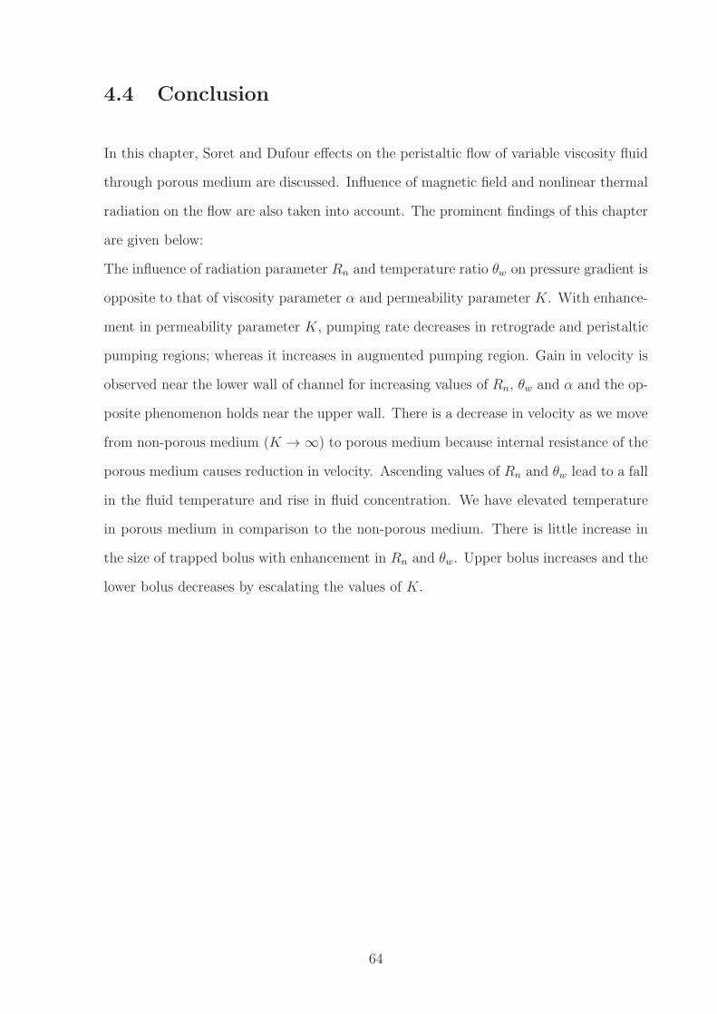
4.4 Conclusion

In this chapter, Soret and Dufour effects on the peristaltic flow of variable viscosity fluid

through porous medium are discussed. Influence of magnetic field and nonlinear thermal

radiation on the flow are also taken into account. The prominent findings of this chapter

are given below:

The influence of radiation parameter Rn and temperature ratio θw on pressure gradient is

opposite to that of viscosity parameter α and permeability parameter K. With enhance-

ment in permeability parameter K, pumping rate decreases in retrograde and peristaltic

pumping regions; whereas it increases in augmented pumping region. Gain in velocity is

observed near the lower wall of channel for increasing values of Rn, θw and α and the op-

posite phenomenon holds near the upper wall. There is a decrease in velocity as we move

from non-porous medium (K → ∞) to porous medium because internal resistance of the

porous medium causes reduction in velocity. Ascending values of Rn and θw lead to a fall

in the fluid temperature and rise in fluid concentration. We have elevated temperature

in porous medium in comparison to the non-porous medium. There is little increase in

the size of trapped bolus with enhancement in Rn and θw. Upper bolus increases and the

lower bolus decreases by escalating the values of K.

64

Chapter 5

Effect of Induced Magnetic Field on the Peristaltic

Flow of Variable Viscosity Fluid

65

This chapter analyses the influence of induced magnetic field on peristaltic flow of viscous

fluid under the effect of heat and mass transfer. Like previous chapters, viscosity of fluid

has dependence on temperature. The problem is modeled with assumptions of large

wavelength and small Reynolds number. Perturbation technique is used to get series

solutions of the coupled differential equations. The impact of various involved parameters

are graphically discussed.

5.1 Statement of the physical model

The flow of electrically conducting viscous fluid in an asymmetric two-dimensional channel

of thickness d1 + d2 is considered. X− axis is taken along the length of the channel and

Y− axis is parallel to the width of the channel. Heat and mass transfer in the channel

occurs due to the difference of temperature and concentration at the walls. The upper

wall is maintained at temperature T0 and concentration C0; whereas the lower wall is

fixed at temperature T1(> T0) and concentration C1(> C0). Sinusoidal waves of small

amplitudes, b1 and b2, and speed c are propagating on the channel walls. Mathematically,

the geometry of the walls is expressed as:

Y = H1(X, t) = d1 + b1 cos

(

2π

λ

(

X − ct)

)

, (5.1)

Y = H2(X, t) = −d2 − b2 cos

(

2π

λ

(

X − ct)

+ φ

)

, (5.2)

in which φ signifies the phase difference and t is the time.

The magnetic field B0(0, B0, 0) is applied in the transverse direction of flow and the

magnetic filed B1(bX(X, Y , t), bY (X, Y , t), 0) is induced. Hence, the total magnetic field

becomes B(bX(X, Y , t), B0 + bY (X, Y , t), 0). In study of magnetohydrodynamics, charge

density is ignored and displacement currents are considered negligible when compared to

the current density. So under these conditions, reduced Maxwell equations are given as

follows:

∇ × E = −∂B∂t, (5.3)

66

∇ · B = 0, (5.4)

∇ × B = µeJ. (5.5)

Ohm’s law may be read as:

J = σ(

E+ V × B)

. (5.6)

In the above equations, σ is the electrical conductivity, E(0, 0, Ez) is the electric field, V

is the velocity field, µe is the permeability of free space and J is the current density.

The present flow situation is governed by the following equations:

∇ · V = 0, (5.7)

ρ

(

∂V

∂t+ (V · ∇)V

)

= ∇ · τ − 1

2µe∇B2 +

1

µe

(

B · ∇)

B, (5.8)

ρcp

(

∂T

∂t+ (V · ∇)T

)

= τ · L+ k∇2T , (5.9)

∂C

∂t+ (V · ∇)C = Dm∇2C +

DmkTT0

∇2T , (5.10)

∂B

∂t= ∇ ×

(

V × B)

+ ζ∇2B. (5.11)

Note that the induction equation (5.11) is written by employing Equations (5.3) to (5.6).

In Equations (5.7) to (5.11), ρ is the density, cp is the specific heat, L(= ∇V) is the gra-

dient of velocity, k is the thermal conductivity, ζ(= 1/σµe) is the magnetic diffusivity, T

is the temperature of fluid, Dm is the coefficient of mass diffusivity, C is the concentration

and kT is the thermal diffusion ratio. τ is the Cauchy stress tensor for Newtonian fluid

given by Equation (3.12).

The flow in fixed frame (X, Y , t) is unsteady and the flow behaves steady in wave frame

(x, y). These two frames are related by following transformations:

(x, y) = (X − ct, Y ), (u, v) = (U − c, V ), p(x, y) = P (X, Y , t). (5.12)

67

Here u, v are the velocities and p is the pressure with respect to the wave reference frame.

In order to non-dimensionalize the problem, following variables are introduced:

p =d21p

µ0cλ, x =

x

λ, u =

u

c, y =

y

d1, v =

v

δc, a1 =

b1d1, a2 =

b2d1, d =

d2d1,

η =C − C0

C1 − C0, Φ =

Φ

B0d1, E =

−EzcB0µe

, µ(θ) =µ(T )

µ0, pm = p+

ReδB2

2ρµec2,

α = γ(T1 − T0), Re =ρcd1µ0

, Rm = σµed1c, Sc =µ0

ρDm

, Br =µ0c

2

(T1 − T0)k,

St =B0

c

√

1

ρµe, h1 =

H1

d1, h2 =

H2

d1, Sr =

ρDmkT (T1 − T0)

µ0T0(C1 − C0), θ =

T − T0T1 − T0

,

bx =bxB0, by =

byB0, δ =

d1λ, Pr =

µ0cpk

. (5.13)

Using the transformation (5.12), dimensionless variables (5.13) and introducing

bx =∂Φ

∂y, by = −δ∂Φ

∂x, (5.14)

we arrive at

∂u

∂x+∂v

∂y= 0, (5.15)

Reδ

(

u∂u

∂x+ v

∂u

∂y

)

= −∂pm∂x

+∂

∂y

(

µ(θ)

(

∂u

∂y+δ2∂v

∂x

))

+ 2δ2∂

∂x

(

µ(θ)∂u

∂x

)

+ δReS2t

(

∂Φ

∂y

∂

∂x− ∂Φ

∂x

∂

∂y

)

∂Φ

∂y+ ReS2

t

∂2Φ

∂y2, (5.16)

Reδ

(

u∂v

∂x+ v

∂v

∂y

)

= −∂pm∂y

+ δ2∂

∂x

(

µ(θ)

(

∂u

∂y+δ2∂v

∂x

))

+ 2δ3∂

∂y

(

µ(θ)∂v

∂y

)

+ δReS2t

(

∂Φ

∂y

∂

∂x− ∂Φ

∂x

∂

∂y

)

∂Φ

∂y, (5.17)

RePr

(

δu∂θ

∂x+ v

∂θ

∂y

)

= δ2∂2θ

∂x2+∂2θ

∂y2

+ µ(θ)Br

[

2δ2

(

(

∂u

∂x

)2

+

(

∂v

∂y

)2)

+

(

∂u

∂y+ δ2

∂v

∂x

)2]

, (5.18)

ReSc

(

δu∂η

∂x+ v

∂η

∂y

)

= δ2∂2η

∂x2+∂2η

∂y2+ SrSc

(

δ2∂2θ

∂x2+∂2θ

∂y2

)

, (5.19)

E = u− δ

(

u∂Φ

∂x+ v

∂Φ

∂y

)

+1

Rm

(

δ2∂2

∂x2+

∂2

∂y2

)

Φ, (5.20)

where µ(θ) = 1 − αθ is the viscosity function, Φ is the magnetic force function, δ is the

wave number, α is the viscosity variation parameter, Re is the Reynolds number, Rm is

the magnetic Reynolds number, Pr is the Prandtl number, Sc is the Schmidt number, Sr

68

is the Soret number, Br is the Brinkman number, St is the Stommers number, E is the

electric field and pm is the modified pressure.

Equations (5.15) to (5.20) under large wavelength and low Reynolds number approxima-

tions reduce to

0 =− ∂pm∂x

+∂

∂y

(

(1− αθ)∂u

∂y

)

+ ReS2t

∂2Φ

∂y2, (5.21)

0 =∂pm∂y

, (5.22)

0 =∂2θ

∂y2+ (1− αθ) Br

(

∂u

∂y

)2

, (5.23)

0 =∂2η

∂y2+ SrSc

∂2θ

∂y2, (5.24)

0 =∂2Φ

∂y2− Rm (E − u) . (5.25)

Using Equation (5.25) in Equation (5.21), we get

0 = −∂pm∂x

+∂

∂y

[

(1− αθ)∂u

∂y

]

+M2(E − u), (5.26)

where M(=√ReRmSt) is the Hartman number.

The relevant boundary conditions in the dimensionless form are given by

u = −1, θ = 0, η = 0, Φ = 0, at y = h1(x), (5.27)

u = −1, θ = 1, η = 1, Φ = 0, at y = h2(x). (5.28)

The dimensionless time mean flow rate Q in fixed frame is given by the following relation

Q = F + 1 + d, (5.29)

where time average flow rate in wave frame F is expressed as

F =

∫ h1(x)

h2(x)

udy. (5.30)

5.2 Perturbation Solution

The resulting system of differential equations is nonlinear and coupled whose closed form

solutions are difficult to obtain. For this purpose, perturbation technique is utilized to

69

obtain series solutions and viscosity variation parameter α << 1 is considered as small

perturbation parameter. We thus express

(u, θ, η,Φ, pm, F ) = (u0, θ0, η0,Φ0, pm0, F0) + α (u1, θ1, η1,Φ1, pm1, F1) . (5.31)

Using Equation (5.31) in Equations (5.23) to (5.28) and collecting the like powers of α,

we get the following system of linear equations:

5.2.1 Zeroth-order system

The zeroth order system of equations with boundary equations are:

dpm0

dx=∂2u0∂y2

+M2(E − u0), (5.32)

∂2θ0∂y2

+ Br

(

∂u0∂y

)2

= 0, (5.33)

∂2η0∂y2

+ SrSc∂2θ0∂y2

= 0, (5.34)

∂2Φ0

∂y2= Rm(E − u0), (5.35)

u0 = −1, θ0 = 0, η0 = 0, Φ0 = 0, at y = h1(x), (5.36)

u0 = −1, θ0 = 1, η0 = 1, Φ0 = 0, at y = h2(x). (5.37)

The solutions of Equations (5.32) to (5.35) satisfying the Equations (5.36) and (5.37) are

given below:

u0 = −c1dpm0

dx+ c2 cosh(My) + c3 sinh(My) + E, (5.38)

θ0 = d1 + d2y + c4y2 − c5 cosh(2My)− c6 sinh(2My), (5.39)

η0 = d3 + d4y − c7y2 + c8 cosh(2My) + c9 sinh(2My), (5.40)

Φ0 = d5 + d6y + c10dpm0

dxy2 + c11 cosh(My) + c12 sinh(My), (5.41)

dpm0

dx=M2

(

c13 + F0M

2 tanh c14 − c13+ E + 1

)

. (5.42)

(5.43)

70

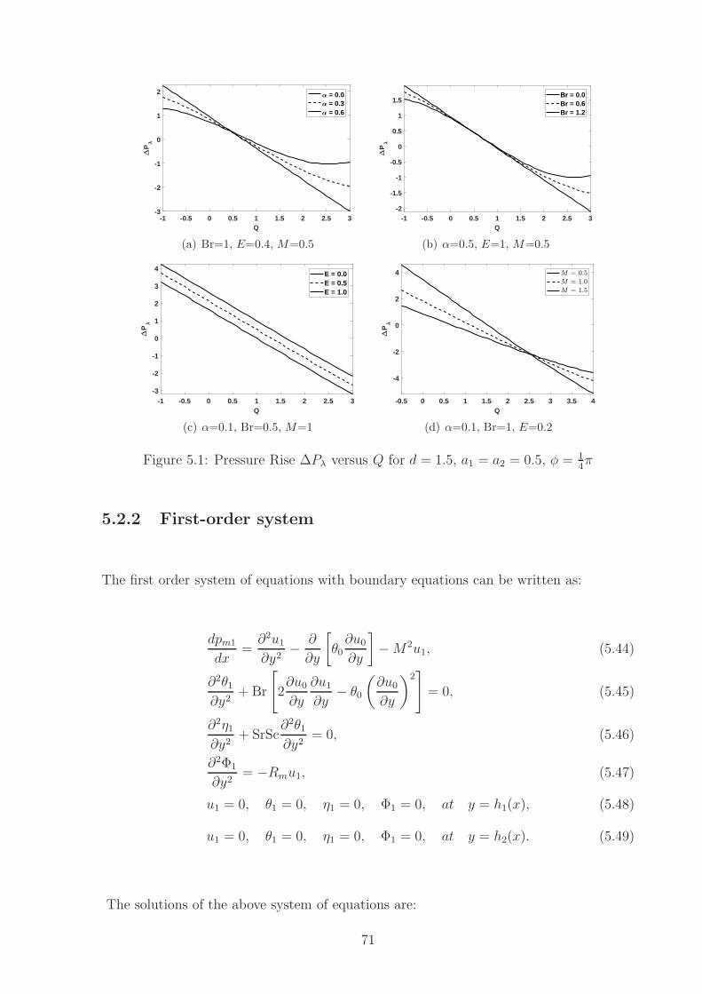
-1 -0.5 0 0.5 1 1.5 2 2.5 3Q

-3

-2

-1

0

1

2

P

= 0.0 = 0.3 = 0.6

(a) Br=1, E=0.4, M=0.5

-1 -0.5 0 0.5 1 1.5 2 2.5 3Q

-2

-1.5

-1

-0.5

0

0.5

1

1.5

P

Br = 0.0Br = 0.6Br = 1.2

(b) α=0.5, E=1, M=0.5

-1 -0.5 0 0.5 1 1.5 2 2.5 3Q

-3

-2

-1

0

1

2

3

4

P

E = 0.0E = 0.5E = 1.0

(c) α=0.1, Br=0.5, M=1

-0.5 0 0.5 1 1.5 2 2.5 3 3.5 4Q

-4

-2

0

2

4

P

(d) α=0.1, Br=1, E=0.2

Figure 5.1: Pressure Rise ∆Pλ versus Q for d = 1.5, a1 = a2 = 0.5, φ = 14π

5.2.2 First-order system

The first order system of equations with boundary equations can be written as:

dpm1

dx=∂2u1∂y2

− ∂

∂y

[

θ0∂u0∂y

]

−M2u1, (5.44)

∂2θ1∂y2

+ Br

[

2∂u0∂y

∂u1∂y

− θ0

(

∂u0∂y

)2]

= 0, (5.45)

∂2η1∂y2

+ SrSc∂2θ1∂y2

= 0, (5.46)

∂2Φ1

∂y2= −Rmu1, (5.47)

u1 = 0, θ1 = 0, η1 = 0, Φ1 = 0, at y = h1(x), (5.48)

u1 = 0, θ1 = 0, η1 = 0, Φ1 = 0, at y = h2(x). (5.49)

The solutions of the above system of equations are:

71

-0.5 0 0.5x

-6

-5

-4

-3

-2

-1

dp/d

x

= 0.0 = 0.3 = 0.6

(a) Br=1, E=0.7, M=0.5

-0.5 0 0.5x

-4.5

-4

-3.5

-3

-2.5

-2

-1.5

-1

-0.5

dp/d

x

Br = 0.0Br = 0.5Br = 1.0

(b) α=0.6, E=0.9, M=0.4

-0.5 0 0.5x

-5

-4

-3

-2

-1

0

dp/d

x

E = 0.0E = 0.5E = 1.0

(c) α=0.3, Br=1, M=1

-0.5 0 0.5x

-5

-4

-3

-2

-1

0

dp/d

x

(d) α=0.2, Br=0.4, E=0.9

Figure 5.2: Pressure Gradient dp/dx versus x− for a1=0.4, d=1.1, a2=0.5, φ=π/4, Q=2

u1 = c15(cosh(My)(c16 + c17y + c18y2 + c19y

3)− c20 cosh(3My) + sinh(My)(c21

+ c22y + c23y2 + c24y

3) + c25 sinh(3My))− c1dpm1

dx, (5.50)

θ1 = d7 + d8y + c26(c27y2 + c28y

3 + c29y4 − cosh(2My)(c30 + c31y + c32y

2

+ c33y3) + c34 cosh(4My) + sinh(2My)(c35 + c36y + c37y

2 + c38y3)

+ c39 sinh(4My)), (5.51)

η1 = c40(cosh(4My)− sinh(4My))(c41 + (sinh(2My) + cosh(2My))(c42 + c43y

+ c44y2 + c45y

3)− (sinh(4My) + cosh(4My))(c46 + c47y + c48y2 + c49y

3

+ c50y4) + (sinh(6My) + cosh(6My))− (c51 + c52y + c53y

2 + c54y3)

− c55(sinh(8My) + cosh(8My))), (5.52)

Φ1 = c56(cosh(3My)− sinh(3My))(c57 + (sinh(2My) + cosh(2My))(c58 + c59y

+ c60y2 + c61y

3) + (sinh(3My) + cosh(3My))(c62 + c63y + c64dpm1

dxy2)

− (sinh(4My) + cosh(4My))(c65 + c66y + c67y2 + c68y

3) + c69(sinh(6My)

+ cosh(6My))), (5.53)

72

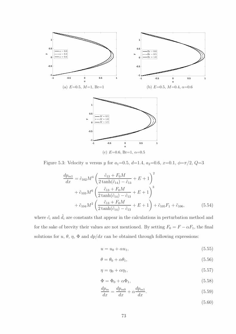
-1 -0.5 0 0.5 1u

-1

-0.5

0

0.5

1

y

(a) E=0.5, M=1, Br=1

-1 -0.5 0 0.5 1u

-1

-0.5

0

0.5

1

y

(b) E=0.5, M=0.4, α=0.6

-1 -0.5 0 0.5 1u

-1

-0.5

0

0.5

1

y

(c) E=0.6, Br=1, α=0.5

Figure 5.3: Velocity u versus y for a1=0.5, d=1.4, a2=0.6, x=0.1, φ=π/2, Q=3

dpm1

dx= c102M

4

(

c13 + F0M

2 tanh(c14)− c13+ E + 1

)2

+ c103M6

(

c13 + F0M

2 tanh(c14)− c13+ E + 1

)3

+ c104M2

(

c13 + F0M

2 tanh(c14)− c13+ E + 1

)

+ c105F1 + c106, (5.54)

where ci and di are constants that appear in the calculations in perturbation method and

for the sake of brevity their values are not mentioned. By setting F0 = F −αF1, the final

solutions for u, θ, η, Φ and dp/dx can be obtained through following expressions:

u = u0 + αu1, (5.55)

θ = θ0 + αθ1, (5.56)

η = η0 + αη1, (5.57)

Φ = Φ0 + αΦ1, (5.58)

dpmdx

=dpm0

dx+ α

dpm1

dx. (5.59)

(5.60)

73

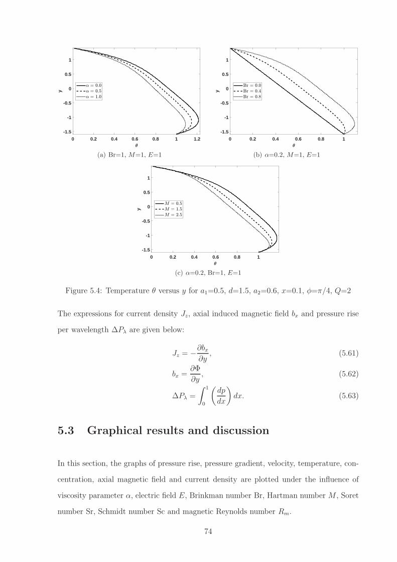
0 0.2 0.4 0.6 0.8 1 1.2

-1.5

-1

-0.5

0

0.5

1y

(a) Br=1, M=1, E=1

0 0.2 0.4 0.6 0.8 1

-1.5

-1

-0.5

0

0.5

1

y

(b) α=0.2, M=1, E=1

0 0.2 0.4 0.6 0.8 1

-1.5

-1

-0.5

0

0.5

1

y

(c) α=0.2, Br=1, E=1

Figure 5.4: Temperature θ versus y for a1=0.5, d=1.5, a2=0.6, x=0.1, φ=π/4, Q=2

The expressions for current density Jz, axial induced magnetic field bx and pressure rise

per wavelength ∆Pλ are given below:

Jz = −∂bx∂y

, (5.61)

bx =∂Φ

∂y, (5.62)

∆Pλ =

∫ 1

0

(

dp

dx

)

dx. (5.63)

5.3 Graphical results and discussion

In this section, the graphs of pressure rise, pressure gradient, velocity, temperature, con-

centration, axial magnetic field and current density are plotted under the influence of

viscosity parameter α, electric field E, Brinkman number Br, Hartman number M , Soret

number Sr, Schmidt number Sc and magnetic Reynolds number Rm.

74

0 0.2 0.4 0.6 0.8 1

-1.5

-1

-0.5

0

0.5

1

y

(a) Br=0.7, Sr=1, Sc=1, M=1, E=0.7

0 0.2 0.4 0.6 0.8 1

-1.5

-1

-0.5

0

0.5

1

y

Br = 0.0Br = 0.4Br = 0.8

(b) α=0.1, Sr=1, Sc=1, M=1, E=1

0 0.2 0.4 0.6 0.8 1

-1.5

-1

-0.5

0

0.5

1

y

Sr = 0.0Sr = 0.4Sr = 0.8

(c) α=0.1, Br=1, Sc=1, M=1, E=1

0 0.2 0.4 0.6 0.8 1

-1.5

-1

-0.5

0

0.5

1

y

Sc = 0.0Sc = 0.4Sc = 0.8

(d) α=0.1, Br=1, Sr=1, M=1, E=1

-0.4 -0.2 0 0.2 0.4 0.6 0.8 1

-1.5

-1

-0.5

0

0.5

1

y

(e) α=0.1, Br=1, Sr=1.2, Sc=1.2, E=1

Figure 5.5: Concentration η versus y for a1=0.5, d=1.5, a2=0.6, x=0.1, φ=π/4, Q=2

The variation of pressure rise per wavelength ∆Pλ versus time mean flow rate Q are

shown in Figure 5.1. Figure 5.1(a) reveals the impact of viscosity parameter α on pump-

ing rate ∆Pλ. When ∆Pλ > 0.32, it shows decreasing pattern for increasing values of

viscosity parameter α. The pattern reverses and there is increase in pumping rate when

∆Pλ < 0.32. The pumping curves for the case of fluid with constant viscosity(α = 0)

and for the case of fluid with temperature dependent viscosity (α 6= 0) intersect each

other at ∆Pλ = 0.32. Thus showing that in free pumping region, the pumping rates for

both cases are equal. Figure 5.1(b) depicts the variation of Br on ∆Pλ. It is observed

75

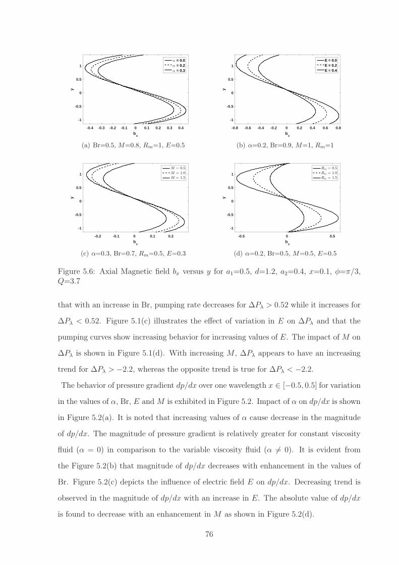
-0.4 -0.3 -0.2 -0.1 0 0.1 0.2 0.3 0.4b

x

-1

-0.5

0

0.5

1y

α = 0.0α = 0.2α = 0.3

(a) Br=0.5, M=0.8, Rm=1, E=0.5

-0.8 -0.6 -0.4 -0.2 0 0.2 0.4 0.6 0.8b

x

-1

-0.5

0

0.5

1

y

E = 0.0E = 0.2E = 0.4

(b) α=0.2, Br=0.9, M=1, Rm=1

-0.2 -0.1 0 0.1 0.2b

x

-1

-0.5

0

0.5

1

y

M = 0.5

M = 1.0

M = 1.5

(c) α=0.3, Br=0.7, Rm=0.5, E=0.3

-0.5 0 0.5b

x

-1

-0.5

0

0.5

1

y

Rm = 0.5

Rm = 1.0

Rm = 1.5

(d) α=0.2, Br=0.5, M=0.5, E=0.5

Figure 5.6: Axial Magnetic field bx versus y for a1=0.5, d=1.2, a2=0.4, x=0.1, φ=π/3,Q=3.7

that with an increase in Br, pumping rate decreases for ∆Pλ > 0.52 while it increases for

∆Pλ < 0.52. Figure 5.1(c) illustrates the effect of variation in E on ∆Pλ and that the

pumping curves show increasing behavior for increasing values of E. The impact ofM on

∆Pλ is shown in Figure 5.1(d). With increasing M , ∆Pλ appears to have an increasing

trend for ∆Pλ > −2.2, whereas the opposite trend is true for ∆Pλ < −2.2.

The behavior of pressure gradient dp/dx over one wavelength x ∈ [−0.5, 0.5] for variation

in the values of α, Br, E andM is exhibited in Figure 5.2. Impact of α on dp/dx is shown

in Figure 5.2(a). It is noted that increasing values of α cause decrease in the magnitude

of dp/dx. The magnitude of pressure gradient is relatively greater for constant viscosity

fluid (α = 0) in comparison to the variable viscosity fluid (α 6= 0). It is evident from

the Figure 5.2(b) that magnitude of dp/dx decreases with enhancement in the values of

Br. Figure 5.2(c) depicts the influence of electric field E on dp/dx. Decreasing trend is

observed in the magnitude of dp/dx with an increase in E. The absolute value of dp/dx

is found to decrease with an enhancement in M as shown in Figure 5.2(d).

76

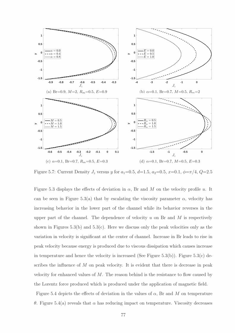
-0.9 -0.8 -0.7 -0.6 -0.5 -0.4 -0.3-1.5

-1

-0.5

0

0.5

1y

(a) Br=0.9, M=2, Rm=0.5, E=0.9

-4 -3 -2 -1 0-1.5

-1

-0.5

0

0.5

1

y

(b) α=0.1, Br=0.7, M=0.5, Rm=2

-0.6 -0.5 -0.4 -0.3 -0.2 -0.1 0 0.1-1.5

-1

-0.5

0

0.5

1

y

(c) α=0.1, Br=0.7, Rm=0.5, E=0.3

-1.5 -1 -0.5 0-1.5

-1

-0.5

0

0.5

1

y

(d) α=0.1, Br=0.7, M=0.5, E=0.3

Figure 5.7: Current Density Jz versus y for a1=0.5, d=1.5, a2=0.5, x=0.1, φ=π/4, Q=2.5

Figure 5.3 displays the effects of deviation in α, Br and M on the velocity profile u. It

can be seen in Figure 5.3(a) that by escalating the viscosity parameter α, velocity has

increasing behavior in the lower part of the channel while its behavior reverses in the

upper part of the channel. The dependence of velocity u on Br and M is respectively

shown in Figures 5.3(b) and 5.3(c). Here we discuss only the peak velocities only as the

variation in velocity is significant at the center of channel. Increase in Br leads to rise in

peak velocity because energy is produced due to viscous dissipation which causes increase

in temperature and hence the velocity is increased (See Figure 5.3(b)). Figure 5.3(c) de-

scribes the influence of M on peak velocity. It is evident that there is decrease in peak

velocity for enhanced values of M . The reason behind is the resistance to flow caused by

the Lorentz force produced which is produced under the application of magnetic field.

Figure 5.4 depicts the effects of deviation in the values of α, Br and M on temperature

θ. Figure 5.4(a) reveals that α has reducing impact on temperature. Viscosity decreases

77

with increasing α and thus there is decrease in intermolecular forces. Eventually there is

a fall in temperature. Figure 5.4(b) is prepared to see the influence of Br on θ and it is

observed that the temperature rises for increasing values of Br. The reason for such be-

havior is that kinetic energy is converted into heat energy due to viscous dissipation and

ultimately the temperature rises. Figure 5.4(c) presents the dependence of temperature

onM . It is seen thatM has negative correlation with temperature because magnetization

has inverse relationship with temperature (Curie’s law).

Figure 5.5 portrays the influence of variations in the involved parameters (α, Br, Sr, Sc

andM) on concentration distribution function η. Figure 5.5(a) manifest the effect of α on

concentration profile and it is noted that α has positive correlation with concentration.

Moreover concentration of constant viscosity fluids is less as compared to the variable

viscosity fluids. Figure 5.5(b) reveals that Br has reducing impact on concentration. Fig-

ures 5.5(c) and 5.5(d) elucidate the dependence of η on Sr and Sc. It is evident that

the rising values of Sr and Sc have decremental effects on concentration. Figure 5.5(e)

demonstrates that increments in M render an increase in concentration.

The plots of axial induced magnetic field bx for different values of α, E, M and Rm are

presented in Figure 5.6 . It is observed in all sub-figures that bx has opposite directions

for y > 0 and y < 0. Figure 5.6(a) shows that magnitude of bx is decreased for increasing

values of α. Figure 5.6(b) demonstrates that rising values of E cause decrease in mag-

nitude of bx. Figure 5.6(c) shows that absolute value of bx is enhanced with increments

in M . The effect of Rm on magnitude of axial magnetic field bx is illustrated in Figure

5.6(d). Magnitude of bx is found to increase for higher values of magnetic Reynolds num-

ber Rm. This is due to the fact that high magnetic Reynolds number are responsible

for high magnetic permeability and thus there is increase in magnitude of axial magnetic

field.

Figure 5.7 displays the variation of pertinent parameters on current density distribution

Jz. Figure 5.7(a) demonstrates the consequence of increasing viscosity parameter α on

Jz. It is noticed that Jz increases in the lower part of the channel and it decreases in the

upper part. It is evident from the Figure 5.7(b) that Jz has negative correlation with E.

78

Figure 5.7(c) presents the effects of deviation in the values of M . With enhancement in

M , Jz shows decreasing behavior at center of the channel while the variation near the

channel walls is not significant. It is noticed in Figure 5.7(d) that for increasing values

Rm, magnitude of Jz increases. This is due to the reason that by increasing magnetic

Reynolds number Rm, electrical conductivity is increased and thus the magnitude of

current density Jz is increased.

5.4 Conclusion

Influence of induced magnetic field on the peristaltic transport of viscous fluid are studied.

Heat and mass transfer effects are also taken into account. Viscosity is taken to be

temperature dependent. The main findings of this chapter can be summarized as follows:

There is an increase in pressure rise for increasing values of electric field E. Decrease

in magnitude of pressure gradient is observed with an enhancement in electric field E

and Hartman number M . Decrease in velocity is observed with enhancement in M .

Temperature of fluid drops for higher values of Hartman number M . Concentration of

variable viscosity fluid is higher in comparison to the constant viscosity fluid. Increments

inM lead to rise in concentration. The effect of electric field E on axial induced magnetic

field is opposite to that of the magnetic Reynolds number Rm. By escalating the magnetic

Reynolds number Rm, the increase in current density at the center of the channel is

observed while the behavior is opposite near the channel walls.

79

Chapter 6

Variable Properties of MHD Third Order Fluid with

Peristalsis

80

This chapter addresses the peristaltic flow of third order fluid with temperature dependent

viscosity and thermal conductivity. The flow is subjected to the magnetic field and

viscous dissipation effects. Assumptions of large wavelength and small Reynolds number

are invoked in mathematical modeling of the problem. Perturbation method is employed

to get the solution of involved system of nonlinear equations. Asymptotic series solutions

are found for the stream function, pressure gradient and temperature. Graphs are plotted

to analyze the effects of pertinent parameters.

6.1 Problem description

Consider a two-dimensional channel (−H < Y < H) of width 2a filled with an electrically

conducting third order fluid. The walls of channel are flexible and are subject to the

temperature Tw (Figure 6.1 ). The flow in the channel is generated when sinusoidal

waves of small amplitude b propagate on the channel walls with constant speed c. The

shape of the walls can be described mathematically as

Y = H(X, t) = a+ b cos(2π

λ(X − ct)), (6.1)

where X and Y are the axes along and perpendicular to the channel walls respectively,

λ is the wavelength and t is the time. It is further assumed that an external magnetic

field B = (0, B0, 0) is applied in the transverse direction of the flow, and the effects due

to viscous dissipation are taken into account.

In the presence of viscous dissipation, temperature of fluid varies; thus the corresponding

changes in fluid properties must be taken into account. While studying the peristaltic

transport in blood vessels, lymphatic vessels and intestines, the assumption of constant

viscosity can lead to inaccuracies. Thus viscosity µ(T ) is assumed to vary linearly with

temperature and given by the Reynold’s law for viscosity [64].

µ(T ) = µw[

1− γ(T − Tw)]

, (6.2)

in which µw is the fluid dynamic viscosity at constant temperature T = Tw, and γ is the

viscosity variation parameter.

81

a

a

λ

c

U

V

X

Y

0

H

−H

T = Tw

T = Tw

b

Figure 6.1: Geometry of the problem

Thermal conductivity of liquid metals has been found to vary linearly with temperature in

the range from 0◦F to 400◦F [69]. This furnishes the relationship of thermal conductivity

k(T ) and temperature as proposed by Arunachalam and Rajappa [70].

k(T ) = kw[

1 + β(T − Tw)]

. (6.3)

Here kw is the thermal conductivity at reference temperature Tw and β is a constant.

Using the above stated conditions, the governing Equations (2.8), (2.9) and (2.11) can be

written in the component form as follows:

∂U

∂X+∂V

∂Y= 0, (6.4)

ρ

(

∂U

∂t+ U

∂U

∂X+ V

∂U

∂Y

)

= − ∂P

∂X+∂SXX∂X

+∂SXY∂Y

− σB20U , (6.5)

ρ

(

∂V

∂t+ U

∂V

∂X+ V

∂V

∂Y

)

= −∂P∂Y

+∂SXY∂X

+∂SY Y∂Y

, (6.6)

ρcp

(

∂T

∂t+ U

∂T

∂X+ V

∂T

∂Y

)

=∂

∂X

(

k(T )∂T

∂X

)

+∂

∂Y

(

k(T )∂T

∂Y

)

+ SXX∂U

∂X

+ SY Y∂V

∂Y+ SXY

(

∂V

∂X+∂U

∂Y

)

. (6.7)

In above equations, P is the pressure, cp is the specific heat and ρ is the density. The

components of the extra stress tensor for third order fluid, SXX , SXY , and SY Y , may be

82

-0.6 -0.4 -0.2 0 0.2 0.4 0.6 0.8 1

Q

-6

-4

-2

0

2

4

6

∆ P

λ

α = 0α = 0.4α = 0.8

(a) Br = 0.8, Γ = 0.01, M = 0.5

-0.6 -0.4 -0.2 0 0.2 0.4 0.6 0.8 1

Q

-6

-4

-2

0

2

4

6

∆ P

λ

Br = 0Br = 0.5Br = 0.9

(b) α = 0.6, Γ = 0.01, M = 0.5

-0.6 -0.4 -0.2 0 0.2 0.4 0.6 0.8 1

Q

-6

-4

-2

0

2

4

6

∆ P

λ

Γ = 0Γ = 0.01Γ = 0.02

(c) α = 0.6, Br = 0.8, M = 0.5

-0.5 0 0.5 1

Q

-8

-6

-4

-2

0

2

4

6

8

∆ P

λ

M = 0M = 1M = 1.5

(d) α = 0.6, Br = 0.8, Γ = 0.01

Figure 6.2: Pressure rise ∆Pλ versus flow rate Q for ϕ = 0.4

read as follows:

SXX = µ(T )(2UX) + α1

(

2UXt + 2UUXX + 2UXY V + 4U2X + 2V 2

X + 2UY VX)

+ α2

(

4U2X + V 2

X + U2Y + 2UY VX

)

+ β1(

4UXXtU + 2UXtt + 2UXXUt + 2UXY Vt

+ 4UXY tV + 12UXtUX + 6VXtVX + 4UY tVX + 2VXtUY + 2UXXXU2 + 14UXXUX U

+ 6UXY U VX + 4UXXY U V + 6VXX VXU + 2VXXUY U + 2UXXUY V + 2UXY V VY

+ 2UXY Y V2 + 12UXY UX V + 6VXY V VX + 2VXY V UY + 4UY Y V VX + 8U3

X + 8UX VXUY)

+ β2(

8UXX UXU + 8UXtUX + 16U3X + 8UXY UX V + 8V 2

XUX + 8UY UX VX + 2UY tUY

+ 2VXtUY + 2UXY UY U + 2VXX UUY + 2UY Y UY V + 2VXY V UY + 4UY VX VY + 4U2Y UX

+ 2UY tVX + 2VXtVX + 2UXY U VX + 2VXX VXU + 2UY Y V VX + 2VXY V VX + 4V 2X VY

+ 4VXUX UY)

+ β3(

8U3X + 8UXUY VX + 8V 2

Y UX + 4V 2XUX + 4U2

Y UX)

, (6.8)

83

SY Y = µ(T )(2VY ) + α1

(

2VXY U + 2U2Y + 2VY t + 2VY Y V + 4V 2

Y + 2UY VX)

+ α2

(

2UY VX + 4V 2Y + U2

Y + V 2X

)

+ β1(

6UY UY t + 2VXtUY + 6UY Y UY V + 6VXY UY V

+ 4VXX UUY + 8VX VY UY + 6UXY UY U + 12VY tVY + 12VXY U VY + 14VY Y V VY + 8V 3Y

+ 2VY tt + 2VXY Ut + 4VXY tU + 2VY Y Vt + 4VY Y tV + 2VXtUY + 2UU tVX + 2VXY UX U

+ 2U2VXXY + 2VY Y VXU + 4VXY Y U V + 2UXY VXU + 2VY Y Y V2 + 2UY Y VX V

)

+ β2(

2UY tUY + 2VXtUY + 2VXXUY U + 2UY Y UY V + 4U2Y UX + 2VXY UY V + 4VY VXUY

+ 2UUXY UY + 2VXUY t + 2VXtVX + 2VXX VXU + 2UY Y VX V + 4UX UY VX + 2VXY VX V

+ 4VY V2X + 2UXY VX U + 8VY tVY + 8VXY VY U + 8VY Y VY V + 8U2

Y VY + 16V 3Y

+ 8VY VXUY)

+ β3(

8VY U2X + 4VY U

2Y + 4VY V

2X + 8VX VY UY + 8VY V

2Y

)

, (6.9)

SXY = 2µ(T )(

UY + VX)

+ α1

(

VX + U VY X + V VY Y + 2U UY + VXt + VXY V + 2VX VY

+ U UX)

+ α2

(

2UY UX + 2VX VY)

+ β1(

UY + VXX + VtUXX + 2U VY Y t

+ V UY Y + 2UY Y tV + 4UXtUY + 3UXUY t + 4UUY UXX + U VY VXX + U2VXXX

+ U VXUY Y + VtVXY + 2V VXY t + 2VY VXt + 4VX VY t + 2UUXY t

+ 5U VX VXY + 2U V VXXY + U2UXXY + 2V UX UY Y + V 2VX

+ 4V UY UXY + UY tUY + 6VY V2Y + 2V U UXXY + U VY VXX + 3V VY VXY

+ V VY UY Y + 3UUX UXY + 4U2X UY + UtUXY + V 2UY Y Y + 4UY V

2X

+ 4VXU2Y + 2VXUX VY + 5V UY UXY

)

+ β2(

2UX UY t + 2UX U VXX

+ 2UX VXt + 2UX V UY Y + 8U2X UY + 2V UX VXY + 2UY V

2Y + 6U2

Y VX

+ 4UX VX VY + 2UUX UXY + 2UY UY t + 6V UY VX − 2U VY UY X + 2U3Y

+ 2VX VY t + 2U VX VXY + 2V VX VY Y + 8VX V2Y + 6UY V

2X + 2UY VXt

+ 2U UY UXX + 2V 3X + 2V UY UXY + 2U VXUXX + 2V VX UXY + 4U2

X VX

+ 2VY UY t + 2VY VXt + 2U VY VXX + 2VXUXt + 2V VY UY Y + 4UXUY

+ 4U VY UXY + 6V UX UY)

+ β3(

4U2X UY + 2U3

Y + 2V 2XUY + 4VXU

2Y

+ 4UY V2Y + 4VXU

2X + 2U2

Y VX + 2V 3X + 4UY V

2X + 4V 2

Y VX)

. (6.10)

84

-0.5 0 0.5

x

0

5

10

15

20

dp/d

x

α = 0α = 0.4α = 0.8

(a) Br = 0.8, Γ = 0.01, M = 0.5

-0.5 0 0.5

x

0

5

10

15

20

dp/d

x

Br = 0Br = 0.4Br = 0.8

(b) α = 0.8, Γ = 0.01, M = 0.5

-0.5 0 0.5

x

0

5

10

15

20

25

30

dp/d

x

Γ = 0Γ = 0.01Γ = 0.02

(c) α = 0.4, Br = 0.5, M = 0.7

-0.5 0 0.5

x

0

5

10

15

20

25

30

dp/d

x

M = 0M = 1.5M = 2.5

(d) α = 0.7, Br = 0.7, Γ = 0.01

Figure 6.3: Pressure gradient dp/dx versus x for ϕ = 0.4, Q = -0.5

Defining the transformations

x = X − ct, y = Y , u(x, y) = U(X, Y , t)− c,

v(x, y) = V (X, Y , t), p(x, y) = P (X, Y , t), (6.11)

wherein u, v and p respectively represent the velocities and pressure corresponding to the

wave reference frame.

We introduce the non-dimensional variables and parameters:

x =x

λ, y =

y

a, u =

u

c, v =

v

δc, p =

a2p

cλµw, δ =

a

λ, h =

H

a, ϕ =

b

a, ψ =

ψ

ca,

µ =µ

µw,S =

a

µwcS, M =

√

σ

µwB0a, Re =

ρca

µw, γ1 =

β1c2

µwa2, γ2 =

β2c2

µwa2,

γ3 =β3c

2

µwa2, k =

k

kw, θ =

T − TwTw

, Pr =µwcpkw

, Br =µwc

2

Twkw, α = γTw,

ǫ = βTw, u =∂ψ

∂y, v = −∂ψ

∂x, (6.12)

where δ, ϕ, M , Re, γi(i = 1, 2, 3), Pr, Br, α, ǫ and ψ are used to denote the wave number,

amplitude ratio, Hartman number, Reynolds number, material parameters, Prandtl num-

ber, Brinkman number, viscosity parameter, thermal conductivity parameter and stream

85

-1 -0.5 0 0.5 1

y

-1

-0.5

0

0.5

1

1.5

u

α = 0α = 0.4α = 0.9

(a) Br = 0.9, Γ = 0.01, M = 0.5

-1 -0.5 0 0.5 1

y

-1

-0.5

0

0.5

1

1.5

u

Br = 0Br = 0.4Br = 0.9

(b) α = 0.6, Γ = 0.01, M = 0.4

-1 -0.5 0 0.5 1

y

-1

-0.5

0

0.5

1

1.5

u

Γ = 0Γ = 0.01Γ = 0.02

(c) α = 0.7, Br = 0.9, M = 2

-1 -0.5 0 0.5 1

y

-1

-0.5

0

0.5

1

1.5

u

M = 0M = 1M = 1.5

(d) α = 0.6, Br = 0.9, Γ = 0.01

Figure 6.4: velocity u versus y for ϕ = 0.4, Q = 1.8, x = 0.1

function respectively.

After using Equations (6.11) and (6.12) in Equations (6.4) to (6.10) and then adopting

the long wavelength and low Reynolds number approximations (see for detail [68]), we

arrive at

0 = −∂p∂x

+∂

∂y

[

(1− αθ)∂2ψ

∂y2+ 2Γ

(

∂2ψ

∂y2

)3]

−M2

(

∂ψ

∂y+ 1

)

, (6.13)

0 = −∂p∂y, (6.14)

0 =∂2

∂y2

[

(1− αθ)∂2ψ

∂y2+ 2Γ

(

∂2ψ

∂y2

)3]

−M2∂2ψ

∂y2, (6.15)

0 =∂

∂y

(

(1 + ǫθ)∂θ

∂y

)

+ Br

[

(1− αθ)

(

∂2ψ

∂y2

)2

+ 2Γ

(

∂2ψ

∂y2

)4]

, (6.16)

in which Γ(= γ2 + γ3) is the Deborah number (Ratio of elastic forces to viscous forces).

Note that continuity equation (6.4) is vanished automatically and the compatibility equa-

tion (6.15) is obtained by taking the cross differentiation of Equations (6.13) and (6.14).

86

-1 -0.5 0 0.5 1

y

0

0.2

0.4

0.6

0.8

1

1.2

θ

α = 0α = 0.2α = 0.4

(a) Br = 0.5, Γ = 0.01, M = 0.5

-1 -0.5 0 0.5 1

y

0

0.1

0.2

0.3

0.4

0.5

0.6

θ

Br = 0.1Br = 0.2Br = 0.3

(b) α = 0.5, Γ = 0.01, M = 0.5

-1 -0.5 0 0.5 1

y

0

0.2

0.4

0.6

0.8

1

θ

Γ = 0Γ = 0.01Γ = 0.02

(c) α = 0.5, Br = 0.5, M = 0.5

-1 -0.5 0 0.5 1

y

0.1

0.2

0.3

0.4

0.5

0.6

0.7

0.8

θ

M = 0M = 1M = 2

(d) α = 0.5, Br = 0.5, Γ = 0.01

Figure 6.5: Temperature profile θ versus y for ϕ = 0.4, Q = 1.8, x = 0.1

The relevant boundary conditions with respect to wave frame are

ψ = 0,∂2ψ

∂y2= 0,

∂θ

∂y= 0, at y = 0, (6.17)

ψ = F,∂ψ

∂y= −1, θ = 0, at y = h(x) = 1 + ϕ cos(2πx). (6.18)

The dimensionless time mean flow rates Q and F in respective fixed and wave reference

frames can be related by the relation

Q = F + 1, (6.19)

with

F =

∫ h(x)

0

∂ψ

∂ydy. (6.20)

6.2 Perturbation Solution

The system of Equations (6.13) to (6.16) comprises nonlinear coupled differential equa-

tions whose closed form solution is difficult to find, so we construct the series solution

by utilizing the asymptotic analysis. In order to achieve this, the viscosity parameter

87

0 0.2 0.4 0.6 0.8 1

x

-60

-40

-20

0

20

40

60

Z

α = 0α = 0.3α = 0.6

(a) Br = 0.9, Γ = 0.01, M = 0.5

0 0.2 0.4 0.6 0.8 1

x

-15

-10

-5

0

5

10

15

Z

Br = 0.1Br = 0.2Br = 0.3

(b) α = 0.3, Γ = 0.01, M = 0.5

0 0.2 0.4 0.6 0.8 1

x

-40

-30

-20

-10

0

10

20

30

40

Z

Γ = 0Γ = 0.01Γ = 0.02

(c) α = 0.3, Br = 0.5, M = 0.5

0 0.2 0.4 0.6 0.8 1

x

-30

-20

-10

0

10

20

30

Z

M = 0M = 2M = 3

(d) α = 0.7, Br = 0.9, Γ = 0.01

Figure 6.6: Heat transfer coefficient Z versus x for ϕ = 0.4, Q = 1.8

α and the thermal conductivity parameter ǫ are taken asymptotically small and of the

same order of magnitude. It may also be recalled that the viscosity parameter γ and

the thermal conductivity parameter β are of the same dimension 1/T . Thus, the energy

equation (6.16) can be written as:

∂

∂y

(

(1 + αθ)∂θ

∂y

)

+ Br

[

(1− αθ)

(

∂2ψ

∂y2

)2

+ 2Γ

(

∂2ψ

∂y2

)4]

= 0. (6.21)

In view of perturbation technique, we write

f = f00 + Γf01 + Γ2f02 + α(

f10 + Γf01 + Γ2f02)

, Γ < 1, α < 1, (6.22)

where f is any flow quantity.

Using Equation (6.22) in the governing equations (6.13), (6.15), (6.17), (6.18) and (6.21),

collecting the coefficients of like powers of α and Γ and dropping the terms of O(Γ2),

O(αΓ) and O(αΓ2), we get the following order systems of linear equations:

88

6.2.1 Zeroth order

∂4ψ00

∂y4−M2 ∂

2ψ00

∂y2= 0, (6.23)

dp00dx

=∂

∂y

(

∂2ψ00

∂y2

)

−M2

(

∂ψ00

∂y+ 1

)

, (6.24)

∂2θ00∂y2

+Br

(

∂2ψ00

∂y2

)2

= 0, (6.25)

ψ00 = 0,∂2ψ00

∂y2= 0,

∂θ00∂y

= 0, at y = 0, (6.26)

ψ00 = F00,∂ψ00

∂y= −1, θ00 = 0, at y = h(x), (6.27)

6.2.2 Order of Γ

∂4ψ01

∂y4−M2 ∂

2ψ01

∂y2= −2

∂2

∂y2

(

∂2ψ00

∂y2

)3

, (6.28)

dp01dx

=∂

∂y

[

∂2ψ01

∂y2+ 2

(

∂2ψ00

∂y2

)3]

−M2∂ψ01

∂y, (6.29)

∂2θ01∂y2

+Br

[

2

(

∂2ψ00

∂y2

)(

∂2ψ01

∂y2

)

+ 2

(

∂2ψ00

∂y2

)4]

= 0, (6.30)

ψ01 = 0,∂2ψ01

∂y2= 0,

∂θ01∂y

= 0, at y = 0, (6.31)

ψ01 = F01,∂ψ01

∂y= 0, θ01 = 0, at y = h(x), (6.32)

6.2.3 Order of α

∂4ψ10

∂y4−M2∂

2ψ10

∂y2=

∂2

∂y2

(

θ00∂2ψ00

∂y2

)

, (6.33)

dp10dx

=∂

∂y

[

∂2ψ10

∂y2− θ00

∂2ψ00

∂y2

]

−M2∂ψ10

∂y, (6.34)

∂2θ10∂y2

+∂

∂y

(

θ00∂θ00∂y

)

+Br

[

2

(

∂2ψ00

∂y2

)(

∂2ψ10

∂y2

)

− θ00

(

∂2ψ00

∂y2

)2]

= 0, (6.35)

ψ10 = 0,∂2ψ10

∂y2= 0,

∂θ10∂y

= 0, at y = 0, (6.36)

ψ10 = F10,∂ψ10

∂y= 0, θ10 = 0, at y = h(x), (6.37)

The above systems are solved by using F00 = F − ΓF01 − αF10 and the final expressions

for ψ, dp/dx and θ thus obtained are shown below:

89

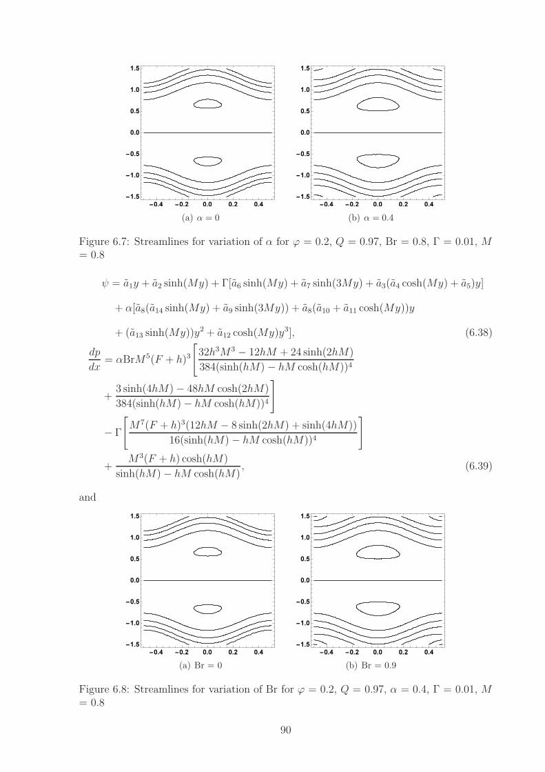
(a) α = 0 (b) α = 0.4

Figure 6.7: Streamlines for variation of α for ϕ = 0.2, Q = 0.97, Br = 0.8, Γ = 0.01, M= 0.8

ψ = a1y + a2 sinh(My) + Γ[a6 sinh(My) + a7 sinh(3My) + a3(a4 cosh(My) + a5)y]

+ α[a8(a14 sinh(My) + a9 sinh(3My)) + a8(a10 + a11 cosh(My))y

+ (a13 sinh(My))y2 + a12 cosh(My)y3], (6.38)

dp

dx= αBrM5(F + h)3

[

32h3M3 − 12hM + 24 sinh(2hM)

384(sinh(hM)− hM cosh(hM))4

+3 sinh(4hM)− 48hM cosh(2hM)


]

− Γ

[

M7(F + h)3(12hM − 8 sinh(2hM) + sinh(4hM))


]

+M3(F + h) cosh(hM)

sinh(hM)− hM cosh(hM), (6.39)

and

(a) Br = 0 (b) Br = 0.9

Figure 6.8: Streamlines for variation of Br for ϕ = 0.2, Q = 0.97, α = 0.4, Γ = 0.01, M= 0.8

90

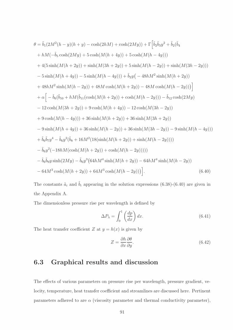
θ = b1(2M2(h− y)(h+ y)− cosh(2hM) + cosh(2My)) + Γ

[

b2b3y2 + b2(b4

+ hM(−b5 cosh(2My) + 5 cosh(M(h + 4y)) + 5 cosh(M(h− 4y)))

+ 4(5 sinh(M(h + 2y)) + sinh(M(3h + 2y)) + 5 sinh(M(h− 2y)) + sinh(M(3h− 2y)))

− 5 sinh(M(h + 4y))− 5 sinh(M(h− 4y))) + b2y(

− 48hM2 sinh(M(h + 2y))

+ 48hM2 sinh(M(h− 2y)) + 48M cosh(M(h + 2y))− 48M cosh(M(h− 2y)))

]

+ α[

− b6(b10 + hM(b11(cosh(M(h + 2y)) + cosh(M(h− 2y)))− b12 cosh(2My)

− 12 cosh(M(3h + 2y)) + 9 cosh(M(h + 4y))− 12 cosh(M(3h− 2y))

+ 9 cosh(M(h− 4y))) + 36 sinh(M(h + 2y)) + 36 sinh(M(3h + 2y))

− 9 sinh(M(h + 4y)) + 36 sinh(M(h− 2y)) + 36 sinh(M(3h− 2y))− 9 sinh(M(h− 4y)))

+ b6b7y4 − b6y

2(b8 + 16M2(18(sinh(M(h + 2y)) + sinh(M(h− 2y))))

− b6y2(−18hM(cosh(M(h + 2y)) + cosh(M(h− 2y)))))

− b6b9y sinh(2My)− b6y3(

64hM4 sinh(M(h+ 2y))− 64hM4 sinh(M(h− 2y))

− 64M3 cosh(M(h + 2y)) + 64M3 cosh(M(h− 2y)))

]

. (6.40)

The constants ai and bi appearing in the solution expressions (6.38)-(6.40) are given in

the Appendix A.

The dimensionless pressure rise per wavelength is defined by

∆Pλ =

∫ 1

0

(

dp

dx

)

dx. (6.41)

The heat transfer coefficient Z at y = h(x) is given by

Z =∂h

∂x

∂θ

∂y. (6.42)

6.3 Graphical results and discussion

The effects of various parameters on pressure rise per wavelength, pressure gradient, ve-

locity, temperature, heat transfer coefficient and streamlines are discussed here. Pertinent

parameters adhered to are α (viscosity parameter and thermal conductivity parameter),

91

Br (Brinkman number), Γ (Deborah number) and M (Hartman number).

The graphs of pressure rise per wavelength ∆Pλ against volume flow rate Q for different

values of involved parameters are plotted in Figure 6.2. The graph of ∆Pλ versus Q is

divided in to different regions depending upon the algebraic signs of ∆Pλ and Q. The

region, where Q < 0 and ∆Pλ > 0, is known as the retrograde pumping region. In this

region, the flow of fluid is because of the pressure gradient and its direction is opposite to

the wave propagation. The peristaltic pumping region occurs when Q > 0 and ∆Pλ > 0.

The resistance of the pressure gradient in this region is overcome by the peristalsis of

the walls and fluid moved in the forward direction. If ∆Pλ = 0 then we have free pump-

ing zone and the corresponding volume flow rate Q is known as free pumping flux. In

copumping region, Q > 0 and ∆Pλ < 0, the pressure difference assists the flow due to

peristalsis of the walls. The effect of α on ∆Pλ is shown in Figure 6.2(a). It is important

to note that increasing α reduces viscosity and raises thermal conductivity and for α = 0,

we attain the fluid with constant viscosity and thermal conductivity. Figure 6.2(a) shows

that in retrograde region, the pressure rise per wavelength decreases with the increase in

α; however, its behavior is opposite in the copumping region. The effects of Br on ∆Pλ

are shown in Figure 6.2(b) and these are similar to that of α. Figures 6.2(c) and 6.2(d)

present the combined effects of Γ andM on pressure rise per wavelength ∆Pλ. It is noted

that ∆Pλ increases with an increase in these parameters in retrograde region whereas it

behaves in opposite manner in copumping region. It can be seen that under all sorts of

variations, ∆Pλ shows no deviation in the peristaltic pumping region.

Figure 6.3 illustrates the influence of α, Br, Γ and M on the pressure gradient dp/dx

within one wavelength i.e., x ∈ [−0.5, 0.5]. The pressure gradient is small at x = 0, which

is the wider part of the channel and this is physically justified as fluid can easily pass

without the assistance of large pressure gradient. While much greater pressure gradient

is required at the narrow part of the channel in order to maintain the same flux of the

fluid to pass through it. From Figures 6.3(a) and 6.3(b), it is evident that in the narrow

part of the channel, where x ∈ [−0.5,−0.2]∪ [0.2, 0.5], the pressure gradient is decreasing

for increasing values of α and Br; however, no variation can be seen in the wider part

92

(a) Γ = 0 (b) Γ = 0.01

Figure 6.9: Streamlines for variation of Γ for ϕ = 0.2, Q = 0.97, α = 0.5, Br = 0.7, M= 0.7

(a) M = 0 (b) M = 1.0

Figure 6.10: Streamlines for variation of M for ϕ = 0.2, Q = 0.97, α = 0.5, Br = 0.7, Γ= 0.01

of the channel. Figures 6.3(c) and 6.3(d) illustrate that pressure gradient is small for

hydrodynamic Newtonian fluid when compared with hydromagnetic third order fluid.

Figure 6.4 shows the impact of α, Br, Γ and M on velocity. We only emphasize on the

peak velocities that occur at the center of the channel as the variation in velocity near

the channel walls is insignificant. It is clear from Figure 6.4(a) that peak velocity has

a positive correlation with α. This is quite relevant to the physical situation because

increase in α causes decrease in viscosity; consequently, the resistance to deformation

due to stresses becomes low which triggers a rise in velocity. It is further manifested in

the figure that fluids with variable viscosity and thermal conductivity have more velocity

than those with constant viscosity and thermal conductivity. The effect of Br on velocity

93

is illustrated in Figure 6.4(b), which demonstrates that fluids with higher Br values have

relatively greater peak velocities. Rising values of Γ enhance the peak velocity of the fluid

as shown in Figure 6.4(c). Moreover, the velocity of third order fluid is high as compared

to that of Newtonian fluid. Hartman number M has decremental effects on peak velocity

of the fluid as is depicted in Figure 6.4(d). The decrease in velocity is caused by the drag

effects of the Lorentz force which itself increases with M .

The temperature profiles θ are plotted against y for different values of α, Br, Γ and M ,

and are displayed in Figures 6.5. We observe from Figure 6.5(a) that temperature θ falls

for increasing values of α. In fact α does not have the same correlation with viscosity as

it has with thermal conductivity. An increase in α causes a decrease in viscosity which

in turn decreases the inter-molecular forces and viscous dissipation. Ultimately, there is

decrease in temperature θ. On the other hand, thermal conductivity is increasing function

of α which explains the decrease in temperature. The reason for such a manifestation

is that an increase in thermal conductivity increases the ability of the fluid to conduct

heat and since the temperature of the fluid is higher than the walls; consequently, it

decreases. Hence, a decrease in viscosity and increase in thermal conductivity decreases

the temperature. Escalating values of Br cause rise in temperature θ. This behavior

is observed because viscous dissipation causes the conversion of kinetic energy to heat

energy and obviously the temperature rises. Figure 6.5(c) shows decrease in temperature

θ for higher values of Γ. The dependence of θ on M is shown in Figure 6.5(d). Rising

values of M have decremental effects on the amplitude of θ because according to Curie’s

law, magnetization is inversely proportional to temperature.

Variation of heat transfer coefficient Z at the wall y = h(x) for various values of sundry

parameters is shown in Figure 6.6. For the sake of demonstration, the wavelength over

the interval [0, 1] is chosen. From the plots in Figure 6.6, it is seen that Z is positive

(negative) on the left (right) of the mean point (x = 0.5). The absolute value, |Z|

decreases for increasing values of α (see Figure 6.6(a)) and increases with Br, Γ and M

(see Figures 6.6(b)–6.6(d)).

An intriguing phenomenon in transport of fluid is trapping. According to this process a

94

bolus is enclosed by splitting of a streamline under certain conditions and it is carried

along with the wave in the wave frame. Trapping is presented by sketching streamlines

in the Figures 6.7–6.10. The trapped bolus is found to expand by increasing α, Br, and

Γ (see Figures 6.7–6.9). However the size of bolus decreases by the rising effects of M as

shown in Figure 6.10

6.4 Conclusion

Peristaltic flow of MHD third order fluid with temperature dependent viscosity and ther-

mal conductivity along with viscous dissipation effects is analyzed using perturbation

technique. The findings of this study are summarized as follows:

It is found that the effects of α (the viscosity and thermal conductivity parameter) are

opposite to that of Γ (third order parameter) on pressure rise per wavelength and pressure

gradient. In contrast to wider part of the channel, good variation is seen in the narrow

part for changing values of α and Γ. Peak velocities are higher for a fluid with variable

viscosity and thermal conductivity in comparison to a fluid with constant viscosity and

thermal conductivity. Similarly, the velocity of third order fluid is more than that of the

Newtonian fluid. The temperature has positive correlation with thermal conductivity and

negative correlation with viscosity. It is noticed that the magnitude of heat transfer co-

efficient Z for a fluid with constant viscosity and constant thermal conductivity is higher

than that of fluid with variable viscosity and variable thermal conductivity. Heat transfer

coefficient of Newtonian fluid is less than the heat transfer coefficient of third order fluid.

Increasing values of α and Γ show increasing trend in the size of the trapped bolus.

95

Chapter 7

Appendix

96

7.1 Appendix A

a1 =FM cosh(hM) + sinh(hM)

hM cosh(hM)− sinh(hM), a2 = − F + h

hM cosh(hM)− sinh(hM),

a3 =M4(F + h)3

16(sinh(hM)− hM cosh(hM))4, a4 = 12M(sinh(hM)− hM cosh(hM)),

a5 =M(12hM − 8 sinh(2hM) + sinh(4hM)), a6 =M4(F + h)3

16(sinh(hM)− hM cosh(hM))4a15,

a7 =M4(F + h)3

16(sinh(hM)− hM cosh(hM))4a16, a8 =

BrM2(F + h)3

384(sinh(hM)− hM cosh(hM))4,

a9 = 3(hM cosh(hM)− sinh(hM)),

a10 =M(

−32h3M3 + 12hM + 48hM cosh(2hM) + a18)

,

a11 = 12M(

4h2M2 − 2 cosh(2hM)− 3)

a16, a12 = − (16BrM2M3(F + h)3)


a13 =24M4Br(F + h)3


a14 = hM(4hMa17 − 9 cosh(3hM)) + 3 sinh(3hM),

a15 = sinh(3hM) + 3hM(4hM sinh(hM)− cosh(3hM)),

a16 = hM cosh(hM)− sinh(hM),

a17 = 3 sinh(3hM) + 2hM(cosh(hM)− 4hM sinh(hM)),

a18 = −24 sinh(2hM)− 3 sinh(4hM),

b1 = − BrM2(F + h)2

8(sinh(hM)− hM cosh(hM))2, b2 =

BrM6(F + h)4

512(hM cosh(hM)− sinh(hM))5,

b3 = 16M2(3hM(4 cosh(hM) + cosh(3hM))− b13),

b4 = b14 + 2hM cosh(hM)(

7 cosh(4hM) + b19

)

,

b5 = 8(5 cosh(hM) + 3(cosh(3hM)− 4hM sinh(hM))),

b6 =Br2M4(F + h)4

12288(hM cosh(hM)− sinh(hM))5,

b7 = −(

320hM5 cosh(hM)− 320M4 sinh(hM))

,

b8 = 16M2(3(4 sinh(hM) + sinh(3hM))− hM(4b15 + 9 cosh(3hM))),

b9 = 96M(

(

6hM − 4h3M3)

cosh(hM) + b20 + hM cosh(3hM))

,

b10 = hM(

16(

b16hM + b22

)

+ 315 cosh(3hM) + 51 cosh(5hM))

+ b17,

97

b11 = 4(

40h2M2 − 33)

, b12 = 32hM sinh(hM)(

−8h2M2 + 6 cosh(2hM) + 15)

,

b13 = sinh(hM)(

12h2M2 + 2 cosh(2hM) + 13)

,

b14 =(

16h2M2 − 25)

sinh(3hM) + sinh(5hM) + b18,

b15 = 8h3M3 sinh(hM) +(

3− 2h2M2)

cosh(hM)− 3hM sinh(3hM),

b16 = −3(

4h2M2 + 9)

sinh(3hM) + b21 + 9hM cosh(3hM),

b17 = −45 sinh(3hM)− 27 sinh(5hM), b18 = 16(

12h4M4 + 18h2M2 + 1)

sinh(hM),

b19 = 60− 72h2M2 − 8(

6h2M2 + 5)

cosh(2hM),

b20 = sinh(hM)(

4h2M2 − 2 cosh(2hM)− 5)

,

b21 = 2(

16h4M4 + 18h2M2 − 9)

sinh(hM), b22 =(

−28h4M4 + 28h2M2 − 6)

cosh(hM)

98

Chapter 8

References

99

[1] Bayliss, W. & Starling, E. (1899). The movements and innervation of the small

intestine. J. Physiol. (Lond.) 24, 99–143.

[2] Lucas, D. (1908). Physiological and Pharmalogical Studies of the Ureter,III. Am.

J. Physiol. 49, 474.

[3] Alvarez, W. (1914). Functional variations in contractions of different parts of the

small intestine. Am. J. Physiol. 35, 177–193.

[4] Holaday, D., Volk, H., & Mandell, J. (1958). Electrical activity of the small intestine

with special reference to the origin of rhythmicity. Am. J. Physiol. 195, 505–515.

[5] P. Bass, C. C. & Lambert, E. (1961). Motor and electric activity of the duodenum.

Am. J. Physiol. 201, 287–291.

[6] Latham, T. (1966). Fluid motion in a peristaltic pump. Master’s thesis, MIT, USA

[7] Shapiro, A. (1967). Pumping and retrograde diffusion in peristaltic waves. Proc.

Workshop in Ureteral Reflux in Children, Natl. Acad. Sci., USA. 109–126.

[8] Kiil, F. (1958). Function of the ureter and renal pelvis. Ann. Surg. 148, 280–291.

[9] Boyarsky, S. (1964). Surgical physiology of the renal pelvis and ureter. Monogr.

Surg. Sci. 1, 173–213.

[10] Weinberg, S. (1970). A theoretical and experimental treatment of peristaltic pumping

and its relation to ureteral function. PhD thesis, MIT, USA

[11] Lykoudis, P. & Roos, R. (1970). The fluid mechanics of the ureter from a lubrication

theory point of view. J. Fluid Mech. 43, 661–674.

100

[12] Manton, M. (1975). Long-wavelength peristaltic pumping at low Reynolds number.

J. Fluid Mech. 68, 467–476.

[13] Barton, C. & Raynor, S. (1968). Peristaltic flow in tubes. Bull. Math. Biophys. 30,

663–680.

[14] Lew, H., Fung, Y., & Lowenstein, C. (1971). Peristaltic carrying and mixing of

chyme in the small intestine (An analysis of a mathematical model of peristalsis of

the small intestine). J. Biomech. 4, 297–315.

[15] Srivastava, L. & Srivastava, V. (1985). Peristaltic transport of a non-Newtonian

fluid: Applications to the vas deferens and small intestine. Ann. Biomed. Eng. 13,

137–153.

[16] Mekheimer, K. & elmaboud, Y. A. (2008). The influence of heat transfer and mag-

netic field on peristaltic transport of a Newtonian fluid in a vertical annulus: Appli-

cation of an endoscope. Phys. Lett. A 372, 1657–1665.

[17] Tripathi, D., Pandey, S., & Beg, O. (2013). Mathematical modelling of heat trans-

fer effects on swallowing dynamics of viscoelastic food bolus through the human

oesophagus. Int. J. Therm. Sci. 70, 41–53.

[18] Massoudi, M. & Phuoc, T. (2004). Flow of a generalized second grade non-Newtonian

fluid with variable viscosity. Continuum Mech. Thermodyn. 16, 529–538.

[19] Eldabe, N., El-Sayed, M., Ghaly, A., & Sayed, H. (2008). Mixed convective heat

and mass transfer in a non-Newtonian fluid at a peristaltic surface with temperature

dependent viscosity. Arch. Appl. Mech. 78, 599–624.

[20] Asghar, S., Hussain, Q., & Hayat, T. (2013). Peristaltic flow of reactive viscous fluid

with temperature dependent viscosity. Math. Comput. Appl. 18, 198–220.

[21] Mekheimer, K. & elmaboud, Y. A. (2014). Simultaneous effects of variable viscosity

and thermal conductivity on peristaltic flow in a vertical asymmetric channel. Can.

J. Phys. 92, 1541–1555.

101

[22] Eldabe, N., Zaghrout, A., Shawky, H., & Awad, A. (2013). Peristaltic transport

of micropolar fluid through porous medium in a symmetric channel with heat and

mass transfer in the presence of generation and radiation. Afr. J. Math. Comput.

Sci. Res. 6, 121–129.

[23] Kothandapani, M. & Prakash, J. (2015). Effects of thermal radiation parameter

and magnetic field on the peristaltic motion of Williamson nanofluids in a tapered

asymmetric channel. Int. J. Heat Mass Transfer 81, 243–245.

[24] O.U. Mehmood, C. F. (2015). A note on radiative heat transfer to peristaltic flow

of Sisko fluid. Appl. Bionics Biomech. 2015. Article-ID: 283892

[25] Srinivas, S., Muthuraj, R., & Sakina, J. (2012). A note on the influence of heat and

mass transfer on a peristaltic flow of a viscous fluid in a vertical asymmetric channel

with wall slip. Chem. Ind. Chem. Eng. Q. 18, 483–493.

[26] Sobh, A. (2012). Peristaltic slip flow of a viscoelastic fluid with heat and mass

transfer in a tube. Math. Probl. Eng. 2012. Article-ID: 815747

[27] Saleem, M. & Haider, A. (2014). Heat and mass transfer on the peristaltic transport

of non-Newtonian fluid with creeping flow. Int. J. Heat Mass Transfer 68, 514–526.

[28] Hayat, T., Yasmin, H., & Al-Yami, M. (2014). Soret and Dufour effects in peristaltic

transport of physiological fluids with chemical reaction: A mathematical analysis.

Comput. Fluid. 89, 242–253.

[29] Ramesh, K. (2016). Influence of heat and mass transfer on peristaltic flow of a

couple stress fluid through porous medium in the presence of inclined magnetic field

in an inclined asymmetric channel. J. Mol. Liq. 219, 256–271.

[30] Srinivas, S. & Kothandapani, M. (2009). The influence of heat and mass transfer

on MHD peristaltic flow through a porous space with compliant walls. Appl. Math.

Comput. 213, 197–208.

102

[31] Reddy, M., Reddy, M., Reddy, B., & Krishna, S. (2012). Peristaltic pumping of

Jeffrey fluid with variable viscosity in a tube under the effect of magnetic field. J.

Math. Comput. Sci. 2, 907–925.

[32] Hayat, T., Shafique, M., Tanveer, A., & Alsaedi, A. (2016). Radiative peristaltic

flow of Jeffrey nanofluid with slip conditions and Joule heating. PLoS One. 11.

Article-ID: e0148002

[33] Shehawey, E. E. & Husseny, S. (2000). Effects of porous boundaries on peristaltic

transport through a porous medium. Acta Mech. 143, 165–177.

[34] Mekheimer, K. (2003). Nonlinear peristaltic transport through a porous medium in

an inclined planar channel. J. Porous. Media. 6, 189–202.

[35] Hayat, T., Ali, N., & Asghar, S. (2007). Hall effects on peristaltic flow of a Maxwell

fluid in a porous medium. Phys. Lett. A 363, 397–403.

[36] Tripathi, D. & Beg, O. (2012). A numerical study of oscillating peristaltic flow of

generalized Maxwell viscoelastic fluids through a porous medium. Transp. Porous.

Media. 95, 337–348.

[37] Hussain, Q., Asghar, S., Hayat, T., & Alsaedi, A. (2015). Heat transfer in a porous

saturated wavy channel with asymmetric convective boundary conditions. J. Cent.

South Univ. 22, 392–401.

[38] Radhakrishnamacharya, G. (1982). Long wavelength approximation to peristaltic

motion of a power law fluid. Rheol. Acta 21, 30–35.

[39] Siddiqui, A. & Schwarz, W. (1994). Peristaltic flow of a second-order fluid in tubes.

J. Non-Newtonian Fluid Mech. 53, 257–284.

[40] Mekheimer, K. (2002). Peristaltic transport of a couple stress fluid in a uniform and

non-uniform channels. Biorheology, 39, 755–765.

[41] Vajravelua, K., Sreenadh, S., & Babu, V. (2005). Peristaltic transport of a Herschel-

Bulkley fluid in an inclined tube. Int. J. Non Linear Mech. 40, 83–90.

103

[42] Tripathi, D. (2011). A mathematical model for the peristaltic flow of chyme move-

ment in small intestine. Math. Biosci. 233, 90–97.

[43] Ramesh, K. & Devakar, M. (2015). The influence of heat transfer on peristaltic trans-

port of MHD second grade fluid through porous medium in a vertical asymmetric

channel. J. Appl. Fluid Mech. 8, 351–365.

[44] Barnes, H., Hutton, J., & Walters, K. (1989). An introduction to Rheology, volume 3

of Rheology Series. Elsevier Science Publishers

[45] Takahashi, T., Ogoshi, H., Miyamoto, K., & Yao, M. (1999). Viscoelastic properties

of commercial plain yoghurts and trial foods for swallowing disorders. Nihon Reoroji

Gakkaishi 27, 169–172.

[46] Fosdick, R. & Rajagopal, K. (1980). Thermodynamics and stability of fluids of third

grade. Proc. R. Soc. Lond. A, Math. Phys. Eng. Sci. 369, 351–377.

[47] Siddiqui, A. & Schwarz, W. (1993). Peristaltic motion of a third-order fluid in a

planar channel. Rheol. Acta 32, 47–56.

[48] Haroun, M. (2007). Effect of Deborah number and phase difference on peristaltic

transport of a third-order fluid in an asymmetric channel. Commun. Nonlinear Sci.

Numer. Simul. 12, 1464–1480.

[49] Hayat, T., Afsar, A., Khan, M., & Asghar, S. (2007). Peristaltic transport of a third

order fluid under the effect of a magnetic field. Comput. Math. Appl. 53, 1074–1087.

[50] Eldabe, N., Ghaly, A., Sallam, S., Elagamy, K., & Younis, Y. (2015). Hall effect on

peristaltic flow of third order fluid in a porous medium with heat and mass transfer.

J. App. Math. Phys. 3, 1138–1150.

[51] Hayat, T., Saleem, N., elmaboud, Y. A., & Asghar, S. (2011). Peristaltic flow of

a second-order fluid in the presence of an induced magnetic field. Int. J. Numer.

Methods Fluids. 67, 537–558.

104

[52] Srinivas, S. & Muthuraj, R. (2010). MHD flow with slip effects and temperature-

dependent heat source in a vertical wavy porous space. Chem. Eng. Comm. 197,

1387–1403.

[53] Hussain, Q., Asghar, S., Hayat, T., & Alsaedi, A. (2015). Heat transfer analysis

in peristaltic flow of MHD Jeffrey fluid with variable thermal conductivity. Appl.

Math. Mech. 36, 499–516.

[54] Liao, S. (1992). The proposed homotopy analysis technique for the solution of

nonlinear problems. PhD thesis, Shanghai Jiao Tong University

[55] Nadeem, S., Akbar, N., Bibi, N., & Ashiq, S. (2010). Influence of heat and mass

transfer on peristaltic flow of a third order fluid in a diverging tube. Commun

Nonlinear Sci Numer Simulat. 15, 2916–2931.

[56] Rashidi, M., Pour, S. M., Hayat, T., & Obaidat, S. (2012). Analytic approximate

solutions for steady flow over a rotating disk in porous medium with heat transfer

by homotopy analysis method. Comput. Fluids. 54, 1–9.

[57] Tripathi, D., Beg, O., & Curiel-Sosa, J. (2014). Homotopy semi-numerical simulation

of peristaltic flow of generalised Oldroyd-B fluids with slip effects. Comput. Method

Biomec. 17, 433–442.

[58] Latif, T., Alvi, N., Hussain, Q., & Asghar, S. (2017). Peristaltic Flow of Nonconstant

Viscosity Fluid with Nonlinear Tehrmal Radiation. Journal of Computational and

Theoretical Nanoscience 14, 2681–2693.

[59] Hussain, Q., Latif, T., Alvi, N., & Asghar, S. (2018). Nonlinear Radiative Peristaltic

Flow of Hydromagnetic Fluid through Porous Medium. Results in Physics 9, 121–

134.

[60] Latif, T., Alvi, N., Hussain, Q., & Ashgar, S. (2016). Variable Properties of MHD

Third Order Fluid with Peristalsis. Results in Physics 6, 963–972.

105

[61] Hussain, Q., Asghar, S., Hayat, T., & Alsaedi, A. (2016). Peristaltic transport

of hydromagnetic Jeffrey fluid with temperature-dependent viscosity and thermal

conductivity. Int. J. Biomath. 9. Article-ID: 1650029

[62] Srinivas, S. & Gayathri, R. (2009). Peristaltic transport of a Newtonian fluid in a

vertical asymmetric channel with heat transfer and porous medium. Appl. Math.

Comput. 215, 185–196.

[63] Kothandapani, M., Prakash, J., & Pushparaj, V. (2015). Analysis of heat and mass

transfer on MHD peristaltic flow through a tapered asymmetric channel. Hin. Pub.

Corp. J. Fluid. 2015, 9.

[64] Tanner, R. (1985). Engineering Rheology. Oxford Science Publications

[65] Rosseland, S. (1931). Astrophysik und Atom-Theoretische Grundlagen. Springer

Verlag, Berlin

[66] Rashidi, M., Ganesh, N., Hakeem, A. A., & Ganga, B. (2014). Buoyancy effect on

MHD flow of nanofluid over a stretching sheet in the presence of thermal radiation.

J. Mol. Liq. 198, 234–238.

[67] Sheikholeslami, M., Ganji, D., & Rashidi, M. (2015). Ferro fluid flow and heat

transfer in a semi annulus enclosure in the presence of magnetic source considering

thermal radiation. J. Taiwan Inst. Chem. Eng. 47, 6–17.

[68] Shapiro, A., Jaffrin, M., & Weinberg, S. (1969). Peristaltic pumping with long

wavelengths at low Reynolds number. J. Fluid Mech. 37, 799–825.

[69] Kays, W. (1966). Convective heat and mass transfer. New York: McGraw–Hill

[70] Arunachalam, M. & Rajappa, N. (1978). Thermal boundary layer in liquid metals

with variable thermal conductivity. Appl. Sci. Res. 34, 179–187.

106

Study of Heat and Mass Transfer in Peristalsis with ...

Documents