Design of Mechanical Systems 3RD SEMESTER PROJECT Study of Fatigue Crack Propagation in Heat Treated Steel Specimen Participants Antoni Knoll Navanith Radhakrishnan Supervisors Jan Schjødt-Thomsen Johnny Jakobsen December 19, 2019

Welcome message from author
This document is posted to help you gain knowledge. Please leave a comment to let me know what you think about it! Share it to your friends and learn new things together.
Transcript
Design of Mechanical Systems
3RD SEMESTER PROJECT
Study of Fatigue Crack Propagation in HeatTreated Steel Specimen
ParticipantsAntoni Knoll
Navanith Radhakrishnan
SupervisorsJan Schjødt-Thomsen
Johnny Jakobsen
December 19, 2019


The Faculty of Engineering and Science
Design of Mechanical Systems
Fibigerstræde 16
9220 Aalborg Øst
http://www.m-tech.aau.dk/
Title:
Project: P3 DMS
Project period: 03.09.19 - 19.12.19
Project group: DMS3 14/23H
Supervisor: Jan Schjødt-Thomsen
Participants:
Antoni Knoll
Navanith Radhakrishnan
Number of pages: 80
Synopsis:
This project deals with the study of fa-
tigue crack propagation in heat treated
steel specimens. The aim is to investi-
gate the crack propagation in four kinds of
Compact Tension specimens, which have
been heat treated in different ways. Ex-
periments were performed on these speci-
mens, where they were subjected to cyclic
loading in a Universal Testing Machine,
with the experimental data being contin-
uously monitored and recorded. A major
point of interest that study focuses on, is
the rate of crack growth and its behaviour
in the heat treated regions of the speci-
mens.
Additional experimental studies were also
conducted to study the effects of heat
treatment on residual stresses. The
hole drilling procedure was performed to
obtain residual stresses in the specimens.
Using experimental data, the Paris equa-
tion was made and comparisons have been
made to obtain further understanding of
the crack propagation.


Preface
This semester project is made by two students from Design of Mechanical Systems at Aalborg
University. The project covers 25 ECTS points per student. Sincere appreciation is expressed
towards Jan Schjødt-Thomsen for his supervision of the project. We would also like to extend
our gratitude to Johnny Jakobsen for his continuous support throughout the entire duration
of the project. Additionally, we thank Klaus Kjær, Søren Erik Brunn and Ole Danielsen for
their help with manufacturing and machining operations in the workshop at the Department of
Materials and Production at Aalborg University.
Reading guide and notation
The Harvard method of referencing is used with the syntax [Last name, Year]. A complete list of
references is found in the end of the report. The references for books are presented with Author,
Title, Edition and Publisher. Internet references are presented with Author, Title, URL and
date of access.
The table of content presents chapters with Arabic numerals and appendixes with Latin letters.
Figures and tables are numbered with chapter and consecutive numbers e.g ”figure 1.1” for first
figure of chapter 1, ”figure 1.2” for the second figure and so on. Description texts are found
beneath each figure and table.
SI units are used throughout the report unless otherwise stated.
v

’
Contents
Chapter 1 Introduction 1
1.1 The Compact Tension Specimen . . . . . . . . . . . . . . . . . . . . . . . . . . . 1
1.1.1 Designing the specimen . . . . . . . . . . . . . . . . . . . . . . . . . . . . 2
1.1.2 Manufacturing . . . . . . . . . . . . . . . . . . . . . . . . . . . . . . . . . 5
1.2 Material Properties . . . . . . . . . . . . . . . . . . . . . . . . . . . . . . . . . . . 6
1.2.1 Preliminary considerations of experimental work . . . . . . . . . . . . . . 7
1.3 Fracture Mechanics and Fatigue - Preliminary Discussion . . . . . . . . . . . . . 10
1.3.1 Cracks as Stress Raisers . . . . . . . . . . . . . . . . . . . . . . . . . . . . 11
1.3.2 The Energy Approach . . . . . . . . . . . . . . . . . . . . . . . . . . . . . 14
1.4 Plasticity at Crack Tip . . . . . . . . . . . . . . . . . . . . . . . . . . . . . . . . . 15
1.5 J-Integral . . . . . . . . . . . . . . . . . . . . . . . . . . . . . . . . . . . . . . . . 17
Chapter 2 Analytical Calculations and Estimation 19
2.1 Stress Intensity Factor . . . . . . . . . . . . . . . . . . . . . . . . . . . . . . . . . 19
2.2 Estimation of SN Curve for S235 . . . . . . . . . . . . . . . . . . . . . . . . . . . 20
2.2.1 Calculating the corrected Endurance Limit . . . . . . . . . . . . . . . . . 23
Chapter 3 Experiments 27
3.1 Measurement of Residual Stress . . . . . . . . . . . . . . . . . . . . . . . . . . . . 27
3.2 Incremental Hole Drilling Method . . . . . . . . . . . . . . . . . . . . . . . . . . . 27
3.2.1 Specimen preparation . . . . . . . . . . . . . . . . . . . . . . . . . . . . . 31
3.2.2 Strain Gage . . . . . . . . . . . . . . . . . . . . . . . . . . . . . . . . . . . 32
3.2.3 Setup of the Experiment . . . . . . . . . . . . . . . . . . . . . . . . . . . . 34
3.2.4 Hole Drilling . . . . . . . . . . . . . . . . . . . . . . . . . . . . . . . . . . 35
3.2.5 Initial Results . . . . . . . . . . . . . . . . . . . . . . . . . . . . . . . . . . 36
3.2.6 Stress Calculation Method . . . . . . . . . . . . . . . . . . . . . . . . . . . 37
3.3 Crack Growth Propagation - Main Experiment . . . . . . . . . . . . . . . . . . . 44
3.3.1 Experimental setup . . . . . . . . . . . . . . . . . . . . . . . . . . . . . . . 44
3.3.2 Force estimation . . . . . . . . . . . . . . . . . . . . . . . . . . . . . . . . 47
3.3.3 Type 1 specimen . . . . . . . . . . . . . . . . . . . . . . . . . . . . . . . . 48
3.3.4 Type 2 specimen . . . . . . . . . . . . . . . . . . . . . . . . . . . . . . . . 49
3.3.5 Type 3 specimen . . . . . . . . . . . . . . . . . . . . . . . . . . . . . . . . 50
3.3.6 Type 4 specimen . . . . . . . . . . . . . . . . . . . . . . . . . . . . . . . . 52
3.3.7 Results . . . . . . . . . . . . . . . . . . . . . . . . . . . . . . . . . . . . . 53
3.3.8 Accuracy . . . . . . . . . . . . . . . . . . . . . . . . . . . . . . . . . . . . 60
3.4 Post Experiment Visual Inspection . . . . . . . . . . . . . . . . . . . . . . . . . . 60
vi

Contents Aalborg University
Chapter 4 Numerical Simulations 63
4.0.1 Simplification of the FEM model . . . . . . . . . . . . . . . . . . . . . . . 63
4.0.2 Modeling of crack tip . . . . . . . . . . . . . . . . . . . . . . . . . . . . . 66
4.0.3 Determining Stress Intensity Factors . . . . . . . . . . . . . . . . . . . . . 68
4.1 Thermal Simulations . . . . . . . . . . . . . . . . . . . . . . . . . . . . . . . . . . 71
Chapter 5 Discussion 75
5.1 Crack Propagation Experiment . . . . . . . . . . . . . . . . . . . . . . . . . . . . 75
5.2 Residual Stress Experiment . . . . . . . . . . . . . . . . . . . . . . . . . . . . . . 79
5.3 Finite element analysis . . . . . . . . . . . . . . . . . . . . . . . . . . . . . . . . . 80
Chapter 6 Conclusion and Further Work 83
Appendix A Type 1 - Specimen 2 85
Appendix B Type 1- Specimen 3 87
Appendix C Type 2 - Specimen 1 89
Appendix D Type 2 - Specimen 2 91
Appendix E Type 2 - Specimen 3 93
Appendix F Type 3 - Specimen 1 95
Appendix G Type 3 - Specimen 2 97
Appendix H Type 3 - Specimen 3 99
Appendix I Type 4 - Specimen 1 101
Appendix J Type 4 - Specimen 3 103
vii


1 — Introduction
The aim of the project was to study fatigue crack propagation in a heat treated steel specimen.
As the behaviour of crack approaching and going through the heat affected zone (HAZ) is
difficult to predict and not entirely known, it was decided to choose this topic. The project
consists of experimental work with addition of numerical analyses and comparison of methods.
The main objective of the experiments is to obtain Paris equation for crack growth in heat
affected structures. This could give eventual possibility of predicting the crack propagation in
such objects. There were also experiments conducted on samples without any welds or heat
treatments. The outcome is a comparison of Paris equations for crack growth in the different
types of specimen used.
An important thing to emphasise is that the study focuses of crack propagation and not on crack
initiation. For this reason Paris equation is the leading law in this investigation. It gives the
fatigue crack growth rate curve and an example is shown in the Fig 1.25. The Paris equation is
given in the Eqn 1.13
Figure 1.1: Fatigue crack growth behavioour typically exhibited by metals (from ?,pp 454
da
dN= C∆Km (1.1)
Numerical analyses was be done using ANSYS. However, performing simulations of experiments
required an alternative approach. To simulate fatigue crack propagation, software’s input is the
same that can be obtained only from experiment. For that reason, there is no sense in comparing
FEM and experimental results, as both approaches would follow the same law. Therefore, crack
length was increased manually and stress intensity factor was calculated for each crack length.
The outcome of the analysis is a comparison of results, but in different form than by Paris Law.
Analysis of results will reveal if standard engineering software is able to accurately predict crack
propagation in materials with induced thermal residual stresses.
1.1 The Compact Tension Specimen
The test specimen chosen for the project is standard Compact Tension (CT) specimen
in accordance with American Society of Testing and Materials (ASTM) and International
1

Group 4.113 1. Introduction
Standards Organization (ISO). It is frequently used to study concepts of fracture mechanics and
fatigue as well as to establish fracture toughness and fatigue crack growth data for a material.
An advantage that the CT specimen has over other specimen types is that the least amount of
test material is required to evaluate crack growth behaviour , when compared to other standard
specimen. As mentioned in [?], standard Compact Tension specimen is a single-edge-notched
and fatigue pre cracked plate which is loaded in tension. The geometry and dimensions of a
general CT specimen are shown in Fig 1.2.
The specimen is subjected to Mode 1 Tensile cyclic loading in the UTM (further discussed in 3
. The fatigue crack initiates from the notch and extends along the specimen. The fatigue crack
is itself a reasonable representation of real life inconsistencies introduced into the material due
to processing techniques and other factors. It is however recommended not to use specimen for
tension-compression testing since there are uncertainties introduced into the loading at the crack
tip. The C(T) specimen of thickness 5mm was used for the all experiments. A few number of
specimens were manufactured with a thickness of 7 mm. After heat treatment (discussed further
in Subsection 1.1.2), thickness was reduced to 5 mm with the required surface finish.
Figure 1.2: Compact Tension C(T) specimen - Standard Proportions
1.1.1 Designing the specimen
The design process for the C(T) specimen was based upon guidelines from [?] and ? which
are standards set by ASTM. They provide an accurate and comprehensive step by step guide
to carry out fatigue testing for different standard specimen. In order to maintain the condition
of plane stress state throughout the specimen, the thickness of the specimen is supposed to be
kept considerably smaller when compared to the other dimensions. As can be seen in Fig1.2,
the main governing parameter is ’W’, which is specified as the width. The thickness ’B’ and
width ’W’ can be varied independently within the given limits.
2

1.1. The Compact Tension Specimen Aalborg University
As per ?, the minimum recommended width is 25mm (1 in.). In this project, the width chosen
for the C(T) specimen is 40 mm. This decision was based on many factors. Firstly, the pre-
made fixtures for load application can be used to avoid the design and manufacturing of new
ones. This, however, saves a tremendous amount of time, a crucial parameter in this case. The
adequately sized specimen is easy to manufacture, to machine and to heat treat evenly. It also
ensures that not a lot of time is consumed for the fatigue crack to propagate along the notch,
since there are multiple samples that need to be tested. It may eventually add up to a lot of
time being consumed just in the experimental part of the project.
Another important aspect in a C(T) specimen, the crack length ’a’ is measured from the crack
tip to the center of the point of load application. The length of machined notch an in the
specimen has to be atleast 0.2W. This requirement is easily satisfied with W=40 mm, which
makes an=8 mm.
To obtain valid results for fatigue crack growth test mentioned in ?, the specimen should be
primarily elastic for all values of force applied. The minimum in plane dimensions that are needed
to meet this requirement are mostly based on empirical data and specific to C(T) specimen
configuration. For a C(T) specimen, the following is required.
(W − a) ≥ (4/π) (K max /σYS)2 (1.2)
where W-a = specimen’s uncracked ligament length and
σYS = 0.2% offset yield strength
The crack notch was designed, keeping in mind the notch design detail as provided in ?. It
is shown in Fig 1.3. A machined knife edge was also designed at the start of the crack notch.
This is to ensure that the used crack gauge can fit inside the notch and be used to measure the
crack opening during the experiment. The knife edge was designed with respect to the details
provided in ?, as is shown in Fig 1.4
3

Group 4.113 1. Introduction
[b]
Figure 1.3: Notch Details
[b]
Figure 1.4: Knife edge design detail
The final CT specimen as designed is shown in Fig 1.5 with width W=40 mm, thickness B as 5
mm and crack length of 8 mm. Fig 1.6 shows an isometric view of the specimen.
Figure 1.5: Dimensions of designed C(T) Specimen
4
1.1. The Compact Tension Specimen Aalborg University
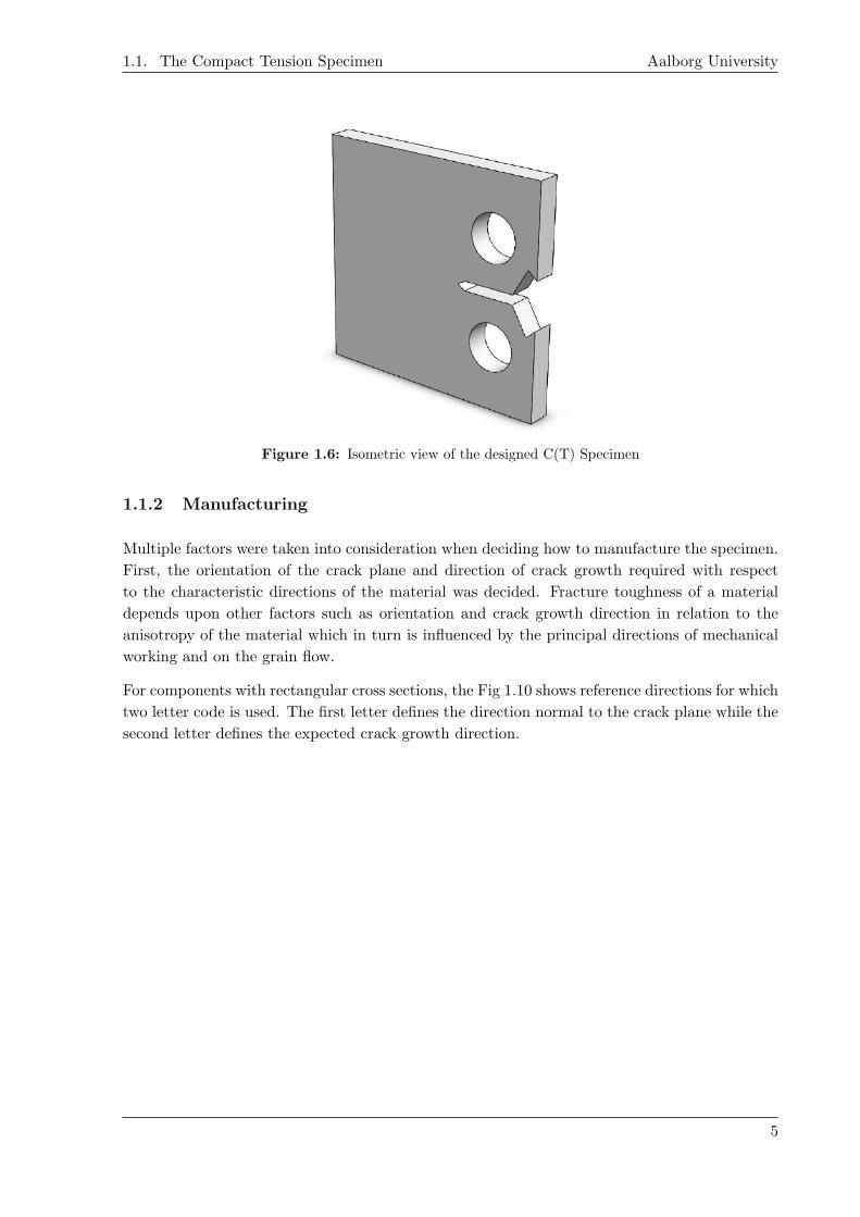
Figure 1.6: Isometric view of the designed C(T) Specimen
1.1.2 Manufacturing
Multiple factors were taken into consideration when deciding how to manufacture the specimen.
First, the orientation of the crack plane and direction of crack growth required with respect
to the characteristic directions of the material was decided. Fracture toughness of a material
depends upon other factors such as orientation and crack growth direction in relation to the
anisotropy of the material which in turn is influenced by the principal directions of mechanical
working and on the grain flow.
For components with rectangular cross sections, the Fig 1.10 shows reference directions for which
two letter code is used. The first letter defines the direction normal to the crack plane while the
second letter defines the expected crack growth direction.
5

Group 4.113 1. Introduction
Figure 1.7: Specimens aligned with Reference Directions
As highlighted in the Fig 1.10, the configuration selected was the T-L one such that the specimen
had the material grains oriented in the direction of crack propagation. It is significant that all
the specimens are manufactured in the same way such that there are minimal inconsistencies in
the specimens.
Additional recommendations for manufacturing the specimen from [?] which were implemented
in this project are
� The machined notch was made by using electrical-discharge machining (EDM) with a notch
root radius ρ = 0.25 mm. This was also the smallest size of the cutting wire available at
the AAU workshop.
� Surface finish was given to ensure that the surfaces are smooth and devoid of any
unwanted/visible flaws. The type of finish was commercial ground finish.
Multiple specimens were manufactured, including spares, out of which 12 specimens (3 of each of
the 4 types of specimens) were used in experiments. Additional details about post manufacturing
treatments done on the specimens are described in Section 1.2.1
1.2 Material Properties
The material properties for Structural Steel S235 (according to EN 1993-1-1:2005+AC2:2009
Sections 3.2.1, 3.2.6) used in this report are as mentioned in Tab 1.1
6

1.2. Material Properties Aalborg University
Sr No Property Value Units Comment
Structural Properties
1 Density 7850 kg/m3
From ?
2 Young’s Modulus 2.1E11 MPa3 Poisson Ratio 0.3 -4 Shear Modulus 81000 MPa5 Yield Strength 235 MPa6 Ultimate Strength 360 MPa7 KIC 110 MPa
√m *
Thermal Properties
7 Melting Point 1420 °C
From ?8 Coefficient of Linear Thermal Expansion 12E-6 °/K9 Conductivity 49 W/m-K10 Specific Heat Capacity 470 J/kg K
Table 1.1: Material Properties of Structural Steel S235
∗ - Due to time constraints, experiments could not be performed to determine the exact Critical
Stress Intensity Factor for S235. Multiple Engineering Design handbooks were scrutinized and
it was found that ? states the Fracture Toughness for Grade A36 Steel as 100 KSI√in which
converts to 110 MPa√m. ASTM A36 steel is considered to be the equivalent of EN S235
Structural steel. Thus 110 MPa√m was considered as a safe and fair assumption for KIC .
Generally low alloy steels have fracture toughness values ranging from 20-200 MPa√m
1.2.1 Preliminary considerations of experimental work
To perform the experiment with as small errors as possible, it was decided to only simulate
welding instead of actually connecting two parts with additional material. According to
literature (lectures from Berin Uni), welding process itself, may result in more than 20
different kind of flaws and errors. To obtain the state of material as it would be when welded,
the samples were heated with the welding rod, without using any filament material. This, in
effect is similar to applying only heat to the region of interest. The result will be the line of
heat affected zone as it is shown in the Fig below.
Figure 1.8: Initial welding trialsFigure 1.9: Initial welding trials
It is desired to study the crack growth in the weld, but also when it starts in front of it and
then grows through the HAZ. The samples are marked with numbers and are shown in the Fig
1.10. Specimen with red path, along the initial crack, is a Type 3 specimen which corresponds
to first case. Specimen with blue path, that is situated across is a Type 4 specimen which
7

Group 4.113 1. Introduction
corresponds to second case. However, as mentioned before, specimen without any treatment
will be tested as well. As it is expected that residual stresses cause eventual different behaviour
of crack propagation in welded metals, it was decided to study their influence. For this purpose
another type of sample is introduced – an annealed one. It was heat treated before being used
in the experiment. Below, the list of types of samples is presented.
Figure 1.10: Type of Specimen determined as per the Weld Path
� Type 1 – These are just the normal CT specimens used without any special treatment
applied. They were used as a reference specimen for the crack propagation experiment
and also to perform certain preliminary trials which consisted of testing the setup of the
Universal Testing Machine.
� Type 2 – These samples were obtained by completely heat treating the CT specimens in
an industrial oven (Heraeus MR170E) at 750°C. Then, they were allowed to cool down
inside the oven itself (natural cooling) to remove any residual stresses that may be present.
The process is also further discussed in Chap 3. This gives a possibility of comparing the
results with those from tests of Type 3 and Type 4 specimens to examine the influence of
residual stresses on crack propagation.
� Type 3 – These samples were made by carrying out TIG welding on the CT specimens
in a direction parallel to the expected direction of crack propagation, as highlighted by
the Red path in Fig 1.10. Experiments on these specimens will reveal the behaviour of
crack along the weld, ie- along the region of high residual stresses. The welding parameter
adjusted and checked for TIG welding was the input current, which influenced the heat
distribution on the surface and penetration through the thickness. After multiple trials
the final setting used for manual TIG welding was to set the input current at 95A, which
generates a welded heat distribution as shown in Fig 1.11
� Type 4 – These samples were made by using spot welding technique where the spot welds
were applied approximately 7mm from the crack tip as shown by the Blue path in Fig
1.10. This was done to examine the crack propagation across the weld. The spot welds
were made after doing experiments on spares. Their aim was to find approximate location
of the spot welds on the specimens such that the heat from the welding procedure would
not affect the geometry of the crack but also to provide enough area such that the crack
8

1.2. Material Properties Aalborg University
can initiate and grow before entering the heat affected region and then propagate across
the spot welds.
Along with the main experiment, certain additional and necessary tests were also executed.
The first of them was to perform a heat treatment procedure on two normal S235 steel blocks
of similar size and thickness as of the actual specimens. Both the samples were annealed at
750°C. After the annealing process, one sample was allowed to slowly cool within the oven The
aim was to reduce all residual stresses within the sample to zero. The other identical sample
was heated in the oven and then cooled down between two big blocks of steel. In this way,
the samples residual stresses should be at similar level as the residual stresses in “the welded
region” in samples of Type 3 and Type 4. After heat treatment and cooling of those two samples,
measurements of residual stresses were taken by incremental hole drilling. The entire procedure
has been discussed in detail in Chapter 3. As a result of these actions, confirmation of zero
residual stresses should be obtained for Type 2 specimen, as well as residual stresses level in
welds in Type 3 and Type 4 specimen. Thanks to that tests, there will not be necessity for
examining the samples prepared for main experiment any more. By that, not only the time of
experimental work will be saved with sufficient accuracy of results, but also influence of residual
stresses can be based on particular values.
Another significant factor for heat treatment is the heat distribution thorough the thickness.
It should be as equal as possible from both the sides of the specimen to avoid different crack
propagation geometries.
Images below show some of the initial tests that were performed on spares to visually inspect
the weld and HAZ formed.
Figure 1.11: TIG Weld trialFigure 1.12: TIG Weld trial - through thickness
distribution of HAZ
Figure 1.13: Spot weld trial
Figure 1.14: Spot weld trial - Location of the spotweld was moved farther away from crack tip.
It was decided that TIG welding is to be used for the Type 3 Specimen, while Spot welding is
to be used for Type 4 specimen.
9
Group 4.113 1. Introduction
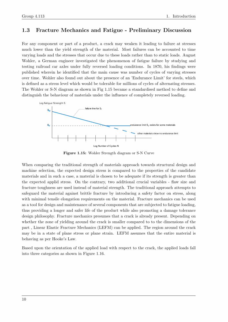
1.3 Fracture Mechanics and Fatigue - Preliminary Discussion
For any component or part of a product, a crack may weaken it leading to failure at stresses
much lower than the yield strength of the material. Most failures can be accounted to time
varying loads and the stresses that occur due to these loads rather than to static loads. August
Wohler, a German engineer investigated the phenomenon of fatigue failure by studying and
testing railroad car axles under fully reversed loading conditions. In 1870, his findings were
published wherein he identified that the main cause was number of cycles of varying stresses
over time. Wohler also found out about the presence of an ’Endurance Limit’ for steels, which
is defined as a stress level which would be tolerable for millions of cycles of alternating stresses.
The Wohler or S-N diagram as shown in Fig 1.15 became a standardised method to define and
distinguish the behaviour of materials under the influence of completely reversed loading.
Figure 1.15: Wohler Strength diagram or S-N Curve
When comparing the traditional strength of materials approach towards structural design and
machine selection, the expected design stress is compared to the properties of the candidate
materials and in such a case, a material is chosen to be adequate if its strength is greater than
the expected applid stress. On the contrary, two additional crucial variables - flaw size and
fracture toughness are used instead of material strength. The traditional approach attempts to
safeguard the material against brittle fracture by introducing a safety factor on stress, along
with minimal tensile elongation requirements on the material. Fracture mechanics can be used
as a tool for design and maintenance of several components that are subjected to fatigue loading,
thus providing a longer and safer life of the product while also promoting a damage tolerance
design philosophy. Fracture mechanics presumes that a crack is already present. Depending on
whether the zone of yielding around the crack is smaller compared to to the dimensions of the
part , Linear Elastic Fracture Mechanics (LEFM) can be applied. The region around the crack
may be in a state of plane stress or plane strain. LEFM assumes that the entire material is
behaving as per Hooke’s Law.
Based upon the orientation of the applied load with respect to the crack, the applied loads fall
into three categories as shown in Figure 1.16.
10

1.3. Fracture Mechanics and Fatigue - Preliminary Discussion Aalborg University
Figure 1.16: Modes of Crack Displacement (adopted from [?], pp267)
Since the scope of this project includes only Tensile loading (Mode 1), the discussion will be
limited only to this case.
1.3.1 Cracks as Stress Raisers
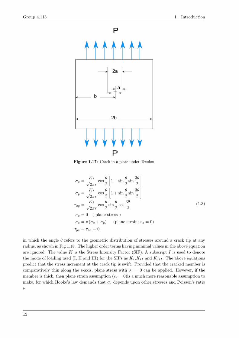
Consider a plate with a crack as shown in Fig 1.17 with a width of 2b, a crack width of 2a in
the center, under tensile loading. The cross section of the crack is in the x-y plane. A polar
coordinate system (r−θ) is set up at the crack tip as the origin. By applying LEFM, for b >> a,
the stresses at the crack tip can be given by the equations as a function of polar coordinates.
11
Group 4.113 1. Introduction
Figure 1.17: Crack in a plate under Tension
σx =KI√2πr
cosθ
2
[1− sin
θ
2sin
3θ
2
]σy =
KI√2πr
cosθ
2
[1 + sin
θ
2sin
3θ
2
]τxy =
KI√2πr
cosθ
2sin
θ
2cos
3θ
2
σz = 0 ( plane stress )
σz = v (σx + σy) (plane strain; εz = 0)
τyz = τzx = 0
(1.3)
in which the angle θ refers to the geometric distribution of stresses around a crack tip at any
radius, as shown in Fig 1.18. The higher order terms having minimal values in the above equation
are ignored. The value K is the Stress Intensity Factor (SIF). A subscript I is used to denote
the mode of loading used (I, II and III) for the SIFs as KI ,KII and KIII . The above equations
predict that the stress increment at the crack tip is swift. Provided that the cracked member is
comparatively thin along the z-axis, plane stress with σz = 0 can be applied. However, if the
member is thick, then plane strain assumption (εz = 0)is a much more reasonable assumption to
make, for which Hooke’s law demands that σz depends upon other stresses and Poisson’s ratio
ν.
12

1.3. Fracture Mechanics and Fatigue - Preliminary Discussion Aalborg University
Figure 1.18: Crack Tip
It can be seen that as r approaches zero, the non zero components of the stress in Eqn 1.3
approach infinity. This is caused specifically since the stresses are inversely proportional to√r.
Therefore there exists a mathematical singularity at the crack tip. There is no fixed value for
the stress at the crack tip. In reality, infinite stress cannot exist in real materials. The material
can withstand the presence of an initial sharp crack in a way that the stress which is infinite
(theoretically) is reduced to a finite value, as illustrated in Fig 1.19. In ductile metals large
plastic deformations occur in and around the crack tip. The region within which the material
yields is called the plastic region/zone. Acute deformations at the crack tip leads to the tip
becoming blunted to a small, but still non zero radius. This makes the crack at the tip no
longer infinite and near the tip, the crack is opened by a finite amount δ, known as the crack
tip opening displacement (CTOD).
Figure 1.19: Finite stress at the crack tip for real materials (Not drawn to scale)
For the plate illustrated in Fig 1.17, if b¿¿a , the stress intensity factor is given by
KI = σ√πa (1.4)
where σ is the nominal stress. It is noteworthy that the stress intensity factor K is directly
proportional to the applied nominal stress and to the square root of the crack width. If the
Mode 1 singular field on the crack plane is considered, the stresses in the x and y direction are
equal since θ = 0, and from Eqn 1.3 they can be represented as
σxx = σyy =KI√2πr
(1.5)
For θ = 0, the shear stress is also 0, which implies that the crack plane is the principal plane
for a pure Mode 1 loading.
13
Group 4.113 1. Introduction
As long as the SIF is lower than a critical threshold value called the Critical Stress Intensity
Factor or Fracture Toughness denoted as KC , the material resists the crack without leading to
brittile fracture. KC is a material property and varies widely depending upon the material and
is also affected by temperature and loading rate. Generally, with an increase in temperature, the
fracture toughness also increases, while a higher rate of loading lowers the fracture toughness,
which is similar to the effect of when decreasing the temperature. Steels of higher strength have
less ductility and have lower fracture toughness when compared to lower strength steels since
ductility parallels fracture toughness in general.
1.3.2 The Energy Approach
This approach towards fracture mechanics states that fracture occurs when the energy that is
available for crack growth is high enough to overcome the resistance of the material, which
may include the plastic work, surface energy or any other kind of energy dissipations which are
affiliated to a propagating crack. This approach was initially proposed by Irwin enter citation
from the bookwhich is equivalent to Griffiths model Also enter citation. An energy release
rate G was defined by Irwin which is the amount of energy available for an increment in crack
length and is expressed as
G = −dΠ
dA(1.6)
The term ’rate’ used in this context does not denote the derivative with respect to time, while
G is the rate of change of Potential energy with the crack area. Thus G is also referred to as
crack extension or driving force.
The Energy Release rate for a configuration as shown in Fig 1.17 is given by
G =πσ2a
E(1.7)
where E is the Young’s Modulus, σ is the nominal/remotely applied stress and ’a’ is the half
crack length.
The energy release rate is also a major driving force for fracture.
Relationship between G and K
Thus, there are two parameters that can be used to define crack growth with G defining the net
change in potential energy that occurs with crack propagation, while the SIF K characterizes
the stresses, strains and displacements at the tip of the crack. It can be said that the energy
release rate defines global behaviour while SIF K acts more like a local parameter.
In the case of Linear elastic materials, G and K are related. For the case of crack in an infinite
plate subjected to uniform tensile stress (Fig 1.17), the equations 1.4 and 1.7 can be combined
to obtained the following relation between the two parameters. for plane stress case
G =K2l
E(1.8)
14
1.4. Plasticity at Crack Tip Aalborg University
For the plane strain case, E is be replaced by E/(1-ν2).
The above mentioned equation is however, also a general equation that is applicable to all
configurations, which has also been proved by Irwin (CITE FROM ANDERSEN BOOK)
for which performed a crack closure analysis.
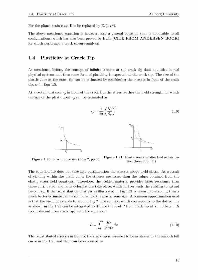
1.4 Plasticity at Crack Tip
As mentioned before, the concept of infinite stresses at the crack tip does not exist in real
physical systems and thus some form of plasticity is expected at the crack tip. The size of the
plastic zone at the crack tip can be estimated by considering the stresses in front of the crack
tip, as in Eqn 1.5.
At a certain distance rp in front of the crack tip, the stress reaches the yield strength for which
the size of the plastic zone rp can be estimated as
rp =1
2π
(KI
Sy
)2
(1.9)
Figure 1.20: Plastic zone size (from ?, pp 50)Figure 1.21: Plastic zone size after load redistribu-
tion (from ?, pp 51)
The equation 1.9 does not take into consideration the stresses above yield stress. As a result
of yielding within the platic zone, the stresses are lesser than the values obtained from the
elastic stress field equations. Therefore, the yielded material provides lesser resistance than
those anticipated, and large deformations take place, which further leads the yielding to extend
beyond rp. If the redistribution of stress as illustrated in Fig 1.21 is taken into account, then a
much better estimate can be computed for the plastic zone size. A common approximation used
is that the yielding extends to around 2rp ? The solution which corresponds to the dotted line
as shown in Fig 1.21 can be integrated to deduce the load P from crack tip at x = 0 to x = R
(point distant from crack tip) with the equation :
P =
∫ R
0
KI√2πx
dx (1.10)
The redistributed stresses in front of the crack tip is assumed to be as shown by the smooth full
curve in Fig 1.21 and they can be expressed as
15
Group 4.113 1. Introduction
σyy = Sy;x < rp
σyy =KI√
2π(x+ δ);x > rp
(1.11)
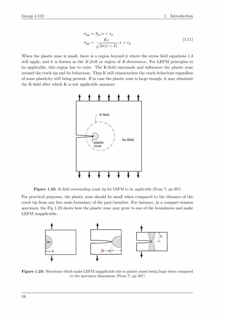
When the plastic zone is small, there is a region beyond it where the stress field equations 1.3
still apply, and it is known as the K-field or region of K-dominance. For LEFM principles to
be applicable, this region has to exist. The K-field surrounds and influences the plastic zone
around the crack tip and its behaviour. Thus K still characterizes the crack behaviour regardless
of some plasticity still being present. If in case the plastic zone is large enough, it may eliminate
the K-field after which K is not applicable anymore.
Figure 1.22: K-field surrounding crack tip for LEFM to be applicable (From ?, pp 387)
For practical purposes, the plastic zone should be small when compared to the distance of the
crack tip from any free ends/boundary of the part/member. For instance, in a compact tension
specimen, the Fig 1.23 shows how the plastic zone may grow to one of the boundaries and make
LEFM inapplicable.
Figure 1.23: Situations which make LEFM inapplicable due to plastic zones being large when comparedto the specimen dimensions (From ?, pp 387)
16

1.5. J-Integral Aalborg University
1.5 J-Integral
Another approach to fracture which is based on the concept of J integral, which is able to handle
even high amounts of yielding. In simple terms, J integral can be defined as the quantity obtained
when evaluating a particular line integral on a path around the crack tip. The J integral is a path
independent integral and acts as a fracture characterizing parameter for nonlinear materials. If
the J-integral is evaluated for a linear elastic material, then it comes out to be equal to the energy
release rate G. In general, the J integral is represented as a path independent line integral as
shown below in Eqn 1.12
J =
∫Γ
[wdy − σijnj
∂ui∂x
ds
](1.12)
with w as the strain energy densitya= and nj is the unit normal for the contour Γ which is
shown in Fig 1.24
Figure 1.24: Finite stress at the crack tip for real materials (Not drawn to scale)
in LEFM, J integral can be used to check whether the crack is stable or not. Just like the SIF K
can be compared with KC , or G being compared to GC , J can also be compared to the material
constant JC . In certain cases, the J-integral may be easier to compute when compared to the
other parameters. However, it is the path independence feature of the J-integral that makes
it very well suited for FE methods since the path can be made away from the crack tip and
thus avoiding the stress singularity at the tip. Upon being used in Finite element methods, the
contour path Γ is chosen such that it passes through the areas where good quality solutions
can be obtained. For situations where crack growth and fracture under plastic loading is to be
considered, the J integral concept can be used.
Fatigue Failure
Fatigue failure is normally categorized into three stages: crack initiation, crack propagation
and sudden fracture due to unstable growth . The duration of the first stage may be short,
while the product spends most of its time in the second stage. It is in this stage that the crack,
if present from inception, or after it is established, grows due to stresses (mainly tensile and
shear) along the planes normal to the maximum stresses acting on it. Even though the crack
propagation rate may be extremely low, in time it adds up over a large number of cycles of use
The third stage is instantaneous. The crack will continue to grow and at some point its size
becomes large enough to raise the stress intensity factor at the crack tip up to the materials
fracture toughness following which sudden failure occurs
The three stages of fatigue crack life is illustrated in the figure below, which is a log-log plot of
da/dN vs ∆K.
17

Group 4.113 1. Introduction
Figure 1.25: Fatigue crack growth behaviour typically exhibited by metals (from ?,pp 454
where initiation, propagation and fracture stages are distinctly visible and represented by I, II
and III. The curve is linear at the middle region for ∆K values, while at the lower and higher
levels of ∆K, this behaviour deviates. The da/dN value approached zero at a threshold value
of ∆K, below which the crack does not grow at all. The crack growth rate increases swiftly for
certain materials at high values of ∆K. For this behaviour, there are two possible explanations-
� The growth rate keeps increasing as Kmax approaches KC and eventually fracture occurs.
� The apparent growth rate da/dN is not a real representation of the crack growth but is
due to the plasticity at the crack tip and its influence on crack growth. At high values of
Kmax, LEFM isnt valid and instead, parameters like ∆J are more appropriate to represent
the fatigue crack growth.
The equation 1.13 represents the linear region (Region II) as shown in Fig 1.25
da
dN= C∆Km (1.13)
where C and m are material constants that can be experimentally determined. According to the
Eqn 1.13, ∆K is the influencing factor on the rate of crack growth and the da/dN is insensitive
to the R ratio in Region II. Various studies have shown that the value of ’m’ can range from 2-4
for majority of metals, provided that there is no corrosive environment acting. The equation is
widely referred to as Paris Law
18

2 — Analytical Calculations and Es-
timation
In this chapter, all analytical calculations and estimations which have been made and used
throughout the project are described briefly
2.1 Stress Intensity Factor
For the sole purpose of comparison and verification, the SIFs for the Type 1 CT specimen was
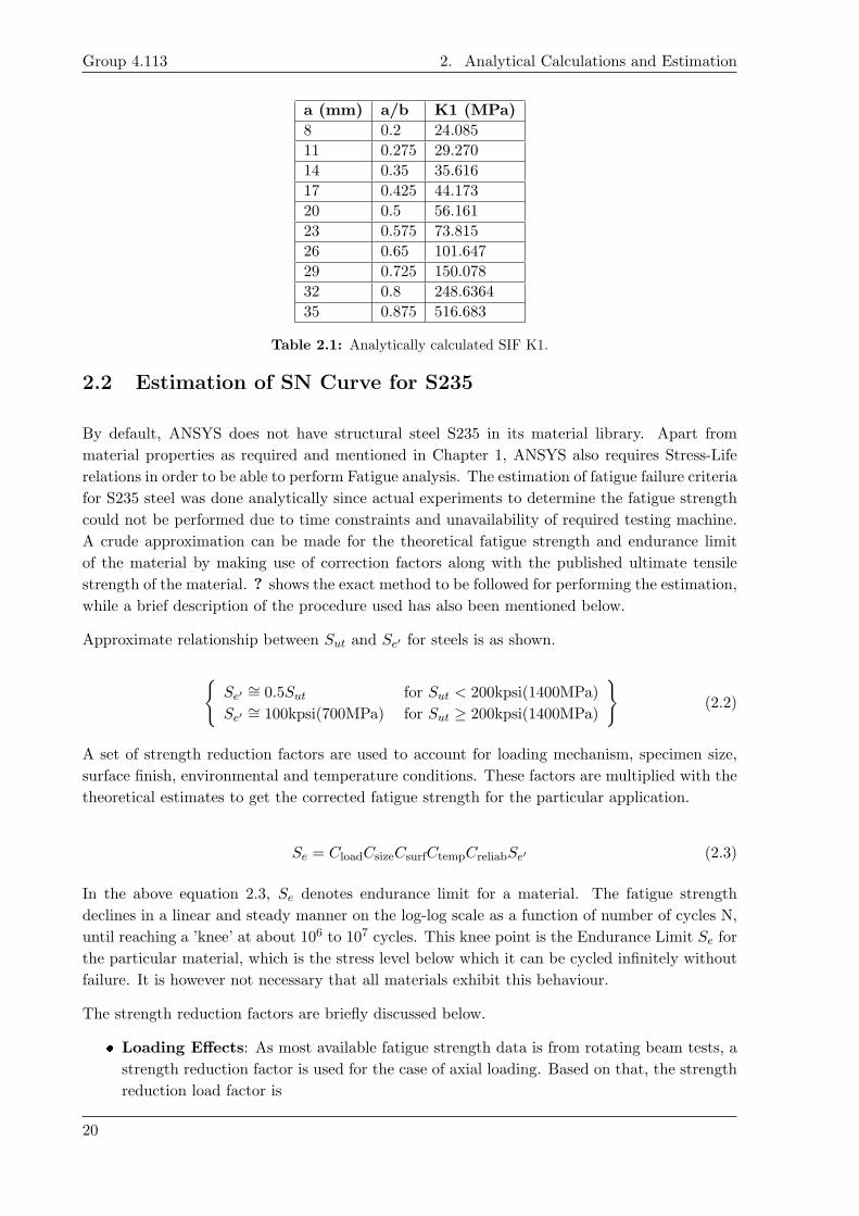
calculated analytically based on formulas as presented in ?, which have also been shown below.
These formulas are specifically applicable for the Compact Tension specimen and have only been
used to obtain estimates of the SIF at different crack lengths.
KI = σ√aFI(a/b, h/b, d/h) (2.1)
where σ = P/b and P is the Force per unit cross sectional area
F1 = 2(2+a/b)
(1−a/b)3/2 ·1√a/b· F2 and the graph shown below (Fig 2.1) has numerical values of F2
Figure 2.1: Graph for values of F2.
A Matlab code was setup to calculate the SIFs at different crack lengths with the required values
of F2 taken fromt the graph corresponding to the ratios: a/b, a/b and a/b The resulting SIFs
have been mentioned in Tab 2.1 below while it has also been compared with solutions from the
experiments and numerical simulation in 5
19
Group 4.113 2. Analytical Calculations and Estimation
a (mm) a/b K1 (MPa)
8 0.2 24.085
11 0.275 29.270
14 0.35 35.616
17 0.425 44.173
20 0.5 56.161
23 0.575 73.815
26 0.65 101.647
29 0.725 150.078
32 0.8 248.6364
35 0.875 516.683
Table 2.1: Analytically calculated SIF K1.
2.2 Estimation of SN Curve for S235
By default, ANSYS does not have structural steel S235 in its material library. Apart from
material properties as required and mentioned in Chapter 1, ANSYS also requires Stress-Life
relations in order to be able to perform Fatigue analysis. The estimation of fatigue failure criteria
for S235 steel was done analytically since actual experiments to determine the fatigue strength
could not be performed due to time constraints and unavailability of required testing machine.
A crude approximation can be made for the theoretical fatigue strength and endurance limit
of the material by making use of correction factors along with the published ultimate tensile
strength of the material. ? shows the exact method to be followed for performing the estimation,
while a brief description of the procedure used has also been mentioned below.
Approximate relationship between Sut and Se′ for steels is as shown.
{Se′ ∼= 0.5Sut for Sut < 200kpsi(1400MPa)
Se′ ∼= 100kpsi(700MPa) for Sut ≥ 200kpsi(1400MPa)
}(2.2)
A set of strength reduction factors are used to account for loading mechanism, specimen size,
surface finish, environmental and temperature conditions. These factors are multiplied with the
theoretical estimates to get the corrected fatigue strength for the particular application.
Se = CloadCsizeCsurfCtempCreliabSe′ (2.3)
In the above equation 2.3, Se denotes endurance limit for a material. The fatigue strength
declines in a linear and steady manner on the log-log scale as a function of number of cycles N,
until reaching a ’knee’ at about 106 to 107 cycles. This knee point is the Endurance Limit Se for
the particular material, which is the stress level below which it can be cycled infinitely without
failure. It is however not necessary that all materials exhibit this behaviour.
The strength reduction factors are briefly discussed below.
� Loading Effects: As most available fatigue strength data is from rotating beam tests, a
strength reduction factor is used for the case of axial loading. Based on that, the strength
reduction load factor is
20

2.2. Estimation of SN Curve for S235 Aalborg University
Bending: Cload = 1
Axial loading: Cload = 0.70
� Size Effects: The specimen used in rotating beam tests are much small (around 5-7 mm
in dia.) If parts larger than this dimension are used, then a strength reduction size factor
needs to be implemented. This is to consider the fact that larger parts may fail at lower
stress values due to the higher probability of a flaw being present in the larger stressed
volume. The expressions used for the size factor are
for d ≤ 0.3 in (8mm) : Csize = 1
for 0.3in < d ≤ 10 in : Csize = 0.869d−0.097
for 8mm < d ≤ 250mm : Csize = 1.189d−0.097
(2.4)
However, the above expressions are valid for cylindrical parts. For parts of other shapes,
? recommends equating the cross sectional area of the non round part, stressed above
95% of its maximum stress with the similarly stressed area of a rotating beam specimen
to obtain an equivalent diameter which can then be used in Equation 2.4.
In the case of a rotating beam specimen, the area A95 that is stressed above 95% of the
maximum stress lies between 0.95d and 1.0d as shown in Figure 2.2.
Figure 2.2: (a) Stress Distribution (b) Area in rotating beam test specimen loaded above 95% ofmaximum stress (Adapted from ?, pp 331)
A95 = π
[d2 − (0.95d)2
4
]= 0.0766d2 (2.5)
The equivalent rotating beam specimen diameter for any cross section can then be written
as
dequiv =√A95/0.0766 (2.6)
The figures 2.3 shows formulas for calculating 95% stressed area for various non round
sections.
21

Group 4.113 2. Analytical Calculations and Estimation
Figure 2.3: Formulas for 95% stressed areas of various cross sections (Adapted from ?, pp 332)
� Surface Effects: The type of surface finish affects the fatigue strength to a certain extent.
Rougher surface finishes reduce the fatigue strength by introducing imperfections. It may
also affect the physical properties of the surface layer. Thus, a strength reduction surface
factor Csurf is implemented to consider the effects of surface finish.
The chart shown in Figure 2.5 provides some advice on choosing the factor depending
upon the surface finish.
Figure 2.4: Surface Factor for different Surface Finishes on Steel (Adapted from ?, pp332
Apart from the chart, ? also provides an equation in exponential form to determine the
reduction factor.
Csurf∼= A (Sut)
b if Csurf > 1.0, set Csurf = 1.0 (2.7)
The values for coefficient ’A’ and exponent ’b’ are mentioned in Table ??. This table is
applicable for use when Sut is in MPa.
22
2.2. Estimation of SN Curve for S235 Aalborg University
Surface Finish A b
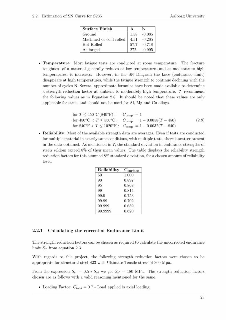
Ground 1.58 -0.085Machined or cold rolled 4.51 -0.265Hot Rolled 57.7 -0.718As forged 272 -0.995
� Temperature: Most fatigue tests are conducted at room temperature. The fracture
toughness of a material generally reduces at low temperatures and at moderate to high
temperatures, it increases. However, in the SN Diagram the knee (endurance limit)
disappears at high temperatures, while the fatigue strength to continue declining with the
number of cycles N. Several approximate formulas have been made available to determine
a strength reduction factor at ambient to moderately high temperature. ? recommend
the following values as in Equation 2.8. It should be noted that these values are only
applicable for steels and should not be used for Al, Mg and Cu alloys.
for T ≤ 450◦C (840◦F) : Ctemp = 1
for 450◦C < T ≤ 550◦C : Ctemp = 1− 0.0058(T − 450)
for 840◦F < T ≤ 1020◦F : Ctemp = 1− 0.0032(T − 840)
(2.8)
� Reliability: Most of the available strength data are averages. Even if tests are conducted
for multiple material in exactly same conditions, with multiple tests, there is scatter present
in the data obtained. As mentioned in ?, the standard deviation in endurance strengths of
steels seldom exceed 8% of their mean values. The table displays the reliability strength
reduction factors for this assumed 8% standard deviation, for a chosen amount of reliability
level.
Reliability Csurface
50 1.00090 0.89795 0.86899 0.81499.9 0.75399.99 0.70299.999 0.65999.9999 0.620
2.2.1 Calculating the corrected Endurance Limit
The strength reduction factors can be chosen as required to calculate the uncorrected endurance
limit Se′ from equation 2.3.
With regards to this project, the following strength reduction factors were chosen to be
appropriate for structural steel S23 with Ultimate Tensile stress of 360 Mpa..
From the expression Se′ = 0.5 ∗ Sut we get Se′ = 180 MPa. The strength reduction factors
chosen are as follows with a valid reasoning mentioned for the same.
� Loading Factor: Cload = 0.7 - Load applied is axial loading
23
Group 4.113 2. Analytical Calculations and Estimation
� Size Effect: Csize = 1 - obtained from calculations as shown below. The 95% of maximum
stress affected area is chosen to be from the crack tip to a distance of 3mm away from the
crack tip, which makes b = 0.003 m and h = 0.005 m. From figure 2.3, we get the formula
for 95% stressed area. Upon substituting this value into equation 2.6, the equivalent
diameter is obtained.
A = 0.05bh = 0.005 ∗ 0.003 ∗ 0.005
A = 0.000075m2
dequiv =√A95/0.0766
∴ dequiv = 0.00312m
Therefore, from equation 2.4, for d ≤ 8 mm, Csize = 1
� Surface Effects: Csurf = 0.95 The specimen used for all the tests except for the 3 specimen
which were completely heat treated in the oven, are considered to be commercially ground.
From Table ??, ’A’ and ’b’ are obtained followed by substituting the obtained values into
equation 2.7.
A = 1.58; b = −0.085
Csurf∼= 1.58 ∗ (360)−0.085 = 0.95
� Temperature: Ctemp = 1 - From equation 2.8. All tests were conducted at an ambient
temperature of 22◦ − 23◦C.
� Reliability: For a reliability of 99.99 % , Creliab is chosen as 0.702.
Therefore, the corrected Se can now be calculated as
Se = 0.7 ∗ 1 ∗ 0.95 ∗ 1 ∗ 0.702 ∗ 180 = 84.02MPa (2.9)
Creating the SN Diagram
The equation 2.3 gives insight into material strength in the high cycle region of the SN Diagram.
For the region from 103 to 106 cycles, similar information can be used to construct the complete
SN Diagram. Assuming that the material strength at 103 cycles is Sm, the following estimates
can be made
Bending: Sm = 0.9Sut
Axial loading: Sm = 0.75Sut
In this case, since loading applied is axial, Sm = 0.75∗360 = 270 Mpa. The SN diagram is made
on log-log scale, where the x-axis runs from 103 to 106 cycles or more. The value obtained for
Sm from the aforementioned equations is plotted at N= 103 cycles.
24

2.2. Estimation of SN Curve for S235 Aalborg University
For a material exhibiting a knee, the corrected Se obtained is plotted at 106 cycles. The points
Sm and Se are joined by a straight line. The curve continues horizontally beyond Se. The
equation of the line from Sm to Se is given by
S(N) = aN b
logS(N) = log a+ b logN(2.10)
where S(N) is the fatigue strength at any value of N, and a,b are constant coefficients defined
by the boundary conditions. The y-intercept for any case is S(N) = Sm at N = N1 = 103. At
the point of endurance limit, S(N) = Se at N = N2 = 106.
Substitute boundary conditions in 2.10 and solve simultaneously for values of ’a’ and ’b’ with
the equations below
b = 1z log
(SmSe
)where z = logN1 − logN2
log(a) = log (Sm)− b log (N1) = log (Sm)− 3b(2.11)
A table with values of ’z’ corresponding to equation 2.10 is given below
N2 z
1.0E6 -3.0005.0E6 -3.6991.0E7 -4.0005.0E7 -4.6991.0E8 -5.0005.0E8 -5.6991.0E9 -6.0005.0E9 -6.699
Therefore, for S235 structural steel,
b = −1
3log
(270
84.02
)∴ b = −0.169
log(a) = log (270)− 0.169 log (1000) = log (270)− 3 ∗ 0.169 log(a) = 2.9384
∴ a = 867.76
Substituting the values for ’a’ and ’b’ obtained above in equation 2.10, provides
S(N) = 867.76 ∗N−0.169 (2.12)
Substituting N = 104 and 105 respectively in the above equation 2.12, we get the following values
for estimated fatigue strength of S235 steel.
25

Group 4.113 2. Analytical Calculations and Estimation
At N =104cycles: S(N) = 867.76 ∗ (104)−0.169
∴ S(N) = 182.97Mpa
At N =105cycles: S(N) = 867.76 ∗ (105)−0.169
∴ S(N) = 123.99Mpa
The final SN diagram was then plotted with the obtained values with the Stresses on the y-axis
and Number of Cycles on the x-axis on a log-log scale as illustrated below:
Figure 2.5: Final estimated SN curve for S235 Structural Steel
26

3 — Experiments
3.1 Measurement of Residual Stress
Residual stresses are self equilibrating stresses within a material/structure that are independent
of the presence of any external loads, which means that local areas with tensile and compressive
forces add up to generate a zero force and moment resultant within the whole volume of the
material or structure. Almost all manufacturing/machining process create residual stresses,
while they might also be generated during the service life of the manufactured component. The
residual stresses may be created due to the following mechanisms.
1. Non uniform plastic deformation: Those that occur during manufacturing processes which
involve changes in shape of material like forging, bending, extrusion and also with surface
deformation.
2. Surface modification: Residual stresses occur during machining operations, grinding,
plating, peening and carburizing and during service by corrosion or oxidation.
3. Material phase/density change: This happens often in the presence of high temperature
gradients like during welding, casting, quenching, heat treatment, phase transformation of
metals, hardening treatments etc.
Shrinkage and solidification can cause large tensile and compressive residual stresses in welds.
While in the molten state, the weld material is free from stresses and can support residual
stresses only after it solidifies. The hot weld metal and heat-affected zone (HAZ) cool over a
larger temperature range than the surrounding cooler material and hence it shrinks more. In
order to compensate for dimensional continuity, large longitudinal tensile residual stresses are
generated in the weld metal and HAZ balanced by compressive stresses in the surrounding metal.
Sometimes residual stresses have an effect similar to that of an applied mean stress. However,
it is beneficial to have compressive residual stresses, which can be introduced by yielding a thin
surface layer in tension, leading to the underlying material attempting to recover its original
shape and size by elastic deformation, which forces the surface layer into compression. As a
result of careful machining, smoother surfaces that are formed improve resistance to fatigue
although some processes may do more harm than good due to introduction of tensile residual
stresses.
3.2 Incremental Hole Drilling Method
The hole drilling method is one of the most widely used general purpose procedures to measure
the near surface residual stresses in an isotropic linearly elastic material. The procedure is easy
to use, standardized and offers good accuracy and reliability. This procedure involves attaching
a strain gage rosette to the surface of the specimen, followed by drilling a hole at the geometric
center of the attached rosette while measuring the relieved strains. Figure 3.2 shows a general
representation of the hole drilling procedure. A sequence of equations are then used to calculate
the residual stresses from the measured strains. One major use of the hole drilling method is
27

Group 4.113 3. Experiments
on welding components which may have residual stresses due to change in phase, temperature
fluctuation in the HAZ or shrinkage due to unequal cooling after welding is complete.
Figure 3.1: Hole Drilling method
The incremental hole drilling procedure was set up and performed as per the ASTM Standard
?. The hole drilling method is considered to be ”semi destructive” as the damage it causes
to the surface is often only localized and does not in most cases alter the usability of the test
specimen. For this reason, since the specimen designed for experiments are not expendable, a
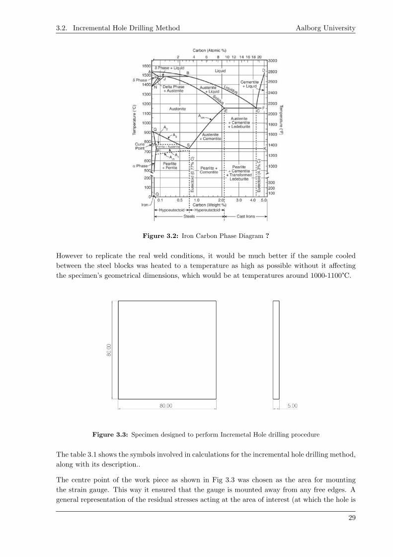
simple specimen as shown in Fig 3.3 was used to check the residual stresses after heat treating the
same in an industrial oven Heraeus MR170E at 750°C, which is above the eutectoid temperature
(A1 point) for Iron which in this case is 723°C from the Iron Carbon Phase diagram (Fig).
Two equally identical specimens were heated in the oven and allowed to cure at 750°C for 1
hour. Following that, one of the specimen was removed and allowed to cool down to room
temperature between two steel blocks while the other was left within the oven and allowed to
cool down naturally. This procedure helps in relieving any residual stresses the specimen may
have. Cooling one of the specimen between two blocks of steel was done to replicate the heat
transmission behaviour occurring during and after a normal welding procedure, where heat is
immediately transmitted to material surrounding the HAZ and to the atmosphere. The rate of
cooling of both the specimens was different which significantly affects the residual stresses in
the specimen.
28
3.2. Incremental Hole Drilling Method Aalborg University
Figure 3.2: Iron Carbon Phase Diagram ?
However to replicate the real weld conditions, it would be much better if the sample cooled
between the steel blocks was heated to a temperature as high as possible without it affecting
the specimen’s geometrical dimensions, which would be at temperatures around 1000-1100°C.
Figure 3.3: Specimen designed to perform Incremetal Hole drilling procedure
The table 3.1 shows the symbols involved in calculations for the incremental hole drilling method,
along with its description..
The centre point of the work piece as shown in Fig 3.3 was chosen as the area for mounting
the strain gauge. This way it ensured that the gauge is mounted away from any free edges. A
general representation of the residual stresses acting at the area of interest (at which the hole is
29

Group 4.113 3. Experiments
Table 3.1: List of symbols used in this section and their descriptions.
Symbols Description
a calibration constant for isotropic stresses
b calibration constant for shear stresses
ajk calibration matrix for isotropic stresses
bjk calibration matrix for shear stresses
D diameter of the gage circle
D0 diameter of the drilled hole
E Young’s modulus
j number of hole depth steps so far
k sequence number for hole depth steps
P uniform isotropic (equi-biaxial) stress
Pk isotropic stress within hole depth step k
p uniform isotropic (equi-biaxial) strain
pk isotropic strain after hole depth step k
Q uniform 45° shear stress
Qk 45° shear stress within hole depth step k
q uniform 45° shear strain
qk 45° shear strain after hole depth step k
T uniform x-y shear stress
Tk x-y shear stress within hole depth step k
t x-y shear strain
tk x-y shear strain after hole depth step k
T (superscript) matrix transpose
αP regularization factor for P stresses
αQ regularization factor for Q stresses
αT regularization factor for T stresses
βclockwise angle from the x-axis (gage 1) to themaximum principal stress direction
ε relieved strain for “uniform” stress case
εjrelieved strain measured after j hole depth stepshave been drilled
V Poisson’s ratio
θ angle of strain gage from the x-axis
σmax maximum (more tensile) principal stress
αmin minimum (more compressive) principal stress
σx uniform normal x-stress
(σx)k normal x-stress within hole depth step k
σy uniform normal y-stress
(σy)k normal y-stress within hole depth step k
τxy uniform shear xy-stress
(τxy)k shear xy-stress within hole depth step k
30

3.2. Incremental Hole Drilling Method Aalborg University
to be drilled) is shown in Fig 3.4 . The figure shows the case of residual stresses acting uniformly
throughout the specimen, in which the in-plane stresses are σx, σy and τxy. These stresses act
throughout the thickness.
Figure 3.4: Hole Geometry and Residual Stresses
Following the procedures mentioned in ?, residual stress measurements can be made for thin
and thick specimen. The specimen type is differentiated as mentioned below
� Thin specimen - Workpieces whose material thickness is small compared to the strain gage
circle diameters.
� Thick specimen - Workpieces whose material thickness is large compared to the strain gage
circle diameters.
Even though the figure shows that the residual stresses are uniformly distributed and acting
over the entire region of interest, it is not necessarily for this to hold true in reality. The stresses
relieved from the surface by drilling the hole depends only upon the stresses already existing at
the boundaries of the hole.
3.2.1 Specimen preparation
A smooth surface finish is required for applying the strain gage onto the specimen. After the
heat treatment, the surface of the specimen was polished thoroughly using a 400 grit sandpaper
to ensure a smooth and even surface. It was decided to not perform any grinding since the
process would alter the dimension of the specimen and also to avoid the possibility of inducing
any external stresses on the specimen. The figure 3.5 shows a ’TYPE A’ strain gage mounted
31

Group 4.113 3. Experiments
on the slowly cooled specimen with wiring to connect the gage to the required transducer for
data acquisition..
Figure 3.5: Strain gage installed on a specimen
Inappropriate surface preparation leads to poor gage bonding, which in turn affects accuracy of
results, giving false values for residual stresses.
Terminology for specimen:
The sample/specimen which was allowed to cool down within the oven shall be referred to as
Annealed specimen and the specimen that was cooled between two blocks of steel shall be referred
to as Quenched. These terms have been used only for ease of identification and explanation in
the report.
3.2.2 Strain Gage
Due to immense technological progress, modern day strain gages are able to make steady
and accurate measurements, which is beneficial since hole drilling strains are extremely small,
reaching values around low hundreds of microstrain or maybe even less in certain cases. There
are standardized hole drilling gages available which further enables the calibration constants used
to evaluate the strains to also be standardized. This vastly improves the process of computing
the final principal stresses. The figure 3.6 below shows the 3 different types of rosettes generally
used in hole drilling experiments.
Figure 3.6: Standardized Hole Drilling Gages (adapted from ?, pp32)
32

3.2. Incremental Hole Drilling Method Aalborg University
The ’Type A’ strain gage rosette as shown in Figure 3.7 which shows a detailed visual of the
gage, was attached to the centre of both the heat treated specimen, as per recommendations
provided in ?. The strain gage used was EA-06-062RE-120 (3.8) manufactured by Micro-
Measurements, USA.
Figure 3.7: Geometry of a standard 3-element CW Hole Drilling Rosette
Figure 3.8: Stain Gage used in the Experiment.
The strain gage factors for each grid of a gage is mentioned in the table 3.2 below.
Grid Gage Factor (at 24◦ C)
1 2.100± 0.5%2 2.065± 0.5%3 2.110± 0.5%NOM 2.09± 2.0%
Table 3.2: Gage factors for Strain Gage used in Hole-Drilling experiment.
33

Group 4.113 3. Experiments
3.2.3 Setup of the Experiment
The experiment was setup and performed on the MAHO MH 800 E 4-axes tool milling
machine. The machine is CNC programmable and had pre built functions to perform the
hole drilling procedure and required only the parameters to be fed into it before initiating the
procedure.
The specimen was carefully and properly mounted on the available workspace. Prior to initiating
the experiment, holes of 4 mm were drilled on each of the four corners of both the specimen
in the Deckel Maho DMU 60T Vertical machining center at the AAU workshop . This was
done so that the specimen could be screwed onto a flat Aluminium base and held in position
thereby inducing zero or minimal stresses onto the specimen when it is held in position, while
the hole drilling procedure is carried out. Since the position of the holes was far away from the
region of interest for the experiment, there are no significant effects or influence on the region
of interest by carrying out the drilling process at the corners of the specimen for ease of fixing
the specimen. The Aluminium base was clamped to the workspace using mechanical clampers.
The entire setup for the experiment is as shown in Figs 3.9 and 3.20
Figure 3.9: Complete setup of the experiment
34

3.2. Incremental Hole Drilling Method Aalborg University
Figure 3.10: Close up view of the specimen on the workbench.
3.2.4 Hole Drilling
Orbital drilling was performed in order to avoid any damage to the cutting tool and the specimen.
Orbital drilling offers several advantages over regular/plunge drilling like :
� There is more area for drilled debris to exit.
� There is less tangential and axial force applied on the specimen during the drilling
procedure when compared to the axial forces while using a plunge drilling cutter.
� Heat introduced into the system is lesser which leads to faster settling of strain
measurements as well as a comparatively much lesser increase in temperature at the critical
parts of the gage.
� Wearing down of the drilling cutter is also reduced.
As the hole is drilled, the residual stresses in the material around the hole are partially
relieved which were then measured at specific sequence of steps (hole depth) using a Full bridge
transducer. The frequency of recording was set to 5Hz so as to obtain output data for every
second of the experiment. This data obtained was then processed and filtered to provide only
the necessary data which was further used to calculate the residual stresses.
35

Group 4.113 3. Experiments
The below mentioned parameters were set for the experiment
Hole diameter: 2mm
Hole depth increment: 0.05 mm
Number of increment steps: 40
Total depth: 2mm
Speed of rotation of drill: 3150 RPM (Max available RPM)
Post Hole Drilling Inspection
Upon completion of the hole drilling experiment, the hole drilled was carefully examined under
a microscope to check for the quality of the drilled hole and its position in the center of the
gage.
The figure 3.11 displays the holes drilled in both the slow cooled and quenched specimen. It can
be seen that in both the specimen, the holes were drilled slightly off center.
In the quenched specimen the hole was drilled approximately 120 µm off center (Approx. 6.3%
off center). In the annealed specimen, the hole was drilled approximately 46 µm off center (Ap-
prox 2.3% off center) towards Grid 1.
Figure 3.11: Position of drilled hole with respect to the gage center for a) Quenched Specimen and b)Slow cooled specimen
It is hard to conclude whether such a small deviation in the position of the hole off the center
of the strain gage has an extremely significant effect on the results obtained.
3.2.5 Initial Results
The initial results are the basic plot of strains vs time which was continuously recorded during the
experiment. Figs show the plots for the Annealed specimen and quenched specimen respectively
36

3.2. Incremental Hole Drilling Method Aalborg University
Figure 3.12: Stresses vs Time plot for the Annealed specimen
Figure 3.13: Stresses vs Time plot for the Quenched specimen
In the above plots, the flat regions visible was the time when there was no drilling happening
while the valleys represent the time when the hole drilling operation was being performed. For
both the speciments, the strain gauge grids were connected to the channels in the transducer as
mentioned below.
Channel 0 was connected to Grid 1
Channel 1 was connected to Grid 2
Channel 2 was connected to Grid 3
From the monitored data, further calculations were performed after extracting the strain values
at regular time intervals
3.2.6 Stress Calculation Method
Mathematical expressions based on Linear Theory of Elasticity are used to evaluate the strains
relieved by the hole drilling method. In the case of a uniformly distributed stress, the surface
strain relief measured is given by the equation 3.1
37

Group 4.113 3. Experiments
ε =1 + v
Eaσx + σy
2
+1
Ebσx − σy
2cos 2θ
+1
Ebτxy sin 2θ
(3.1)
where a and b are calibration constants which indicate the strains relieved due to unit stresses
within the hole depth. The values for the calibration constants are tabulated and available in ?.
In the case of non uniformly distributed stresses, the surface strain relief at hole depth step ’j’
is dependant upon the residual stresses that already existed in all the depth steps 1 ≤ k ≤ j
and is given by the equation 3.2
εj =1 + v
E
j∑k=1
ajk ((σx + σy) /2)k
+1
E
j∑k=1
bjk ((σx − σy) /2)k cos 2θ
+1
E
j∑k=1
bjk (τxy) sin 2θ
(3.2)
where ajk and ¯bjk are calibration constants which indicate the relieved strains due to unit stresses
within hole step ’k’. Numerical values of the calibration constants are available in ?.
After a series of holes have been drilled, the measured releived strains provide enough information
to calculate stresses σx, σy and τxy for each step. The corresponding principal stresses σmax and
σmin and their orientation β can then be calculated. Only near surface stresses can be evaluated
using the hole drilling method since the influence of internal stresses decreases with their depth
from the surface.
For this study, it was considered that the residual stresses were not distributed uniformly through
the depth of the specimen. In many instances, the residual stresses are majorly non uniform ,
especially when closer to the surface. Heat treatment and surface treatment procedures produce
non uniform residual stresses.
The Integral Method procedure was followed for calculating the residual stresses after processing
the data obtained from the experiment was strictly in accordance with that mentioned in ?. It
is one of the best methods to opt for when considering highly non uniform residual stresses.
This method however requires extremely precise data measurements since the calculations are
sensitive to errors in strain measurements. The errors are proportionately much larger when
compared to strain measurement errors especially for stresses away from the surface. The
Integral method is takes into consideration that the measured strains during the hole drilling
procedure is due to the cumulative results of the stresses that originally existed at all the depth
locations of the total hole depth being relieved. Thus the individual influence of the stresses at
each depth towards measuring the total strains is taken into account. These individual stresses
are then obtained by calculations using the total strain measurements. In this method, the
38

3.2. Incremental Hole Drilling Method Aalborg University
location of the stresses are fixed with respect to the increment in hole depth made during the
drilling procedure. It is assumed that the residual stress within each hole hole depth increment
is constant.
A short description of the steps followed is mentioned below.
1. The graphs of strains ε1, ε2 and ε3 vs hole depth were plotted to check for smoothness of
data.
Figure 3.14: Strains vs Hole depth plot-Annealed specimen
Figure 3.15: Strains vs Hole depth plot-Quenched specimen
2. The following combination strain vectors were then calculated.
pj = (ε3 + ε1)j /2
qj = (ε3 − ε1)j /2
tj = (ε3 + ε1 − 2ε2)j /2
(3.3)
where the subscript ’j’ denotes serial numbers of the hole depth steps corresponding to
the successive sets of the measured strains - ε1, ε2 and ε3.
39

Group 4.113 3. Experiments
3. The standard errors in the combinations was then calculated.
p2std =
∑n−3j=1
(pj−3pj+1+3pj+2−pj+3)2
20(n−3)
q2std =
∑n−3j=1
(qj−3qj+1+3qj+2−pj+3)2
20(n−3)
t2std =∑n−3
j=1(tj−3tj+1+3tj+2−tj+3)2
20(n−3)
(3.4)
where ’n’ = number of sets of strain data at the different hole depth steps. The summation
was carried out over the range 1 ≤ j ≤ n− 3.
4. For calculating the calibration matrices ajk and bjk, the calibration data was obtained
from specific Tables in ?.
5. The Integral Method was used to calculate the residual stresses. The following matrix
equations were then solved to calculate residual stresses within each hole depth.
aP =E
1 + vp
bQ = Eq
bT = Et
(3.5)
wherePk =
((σy)k + (σx)k
)/2
Qk =((σy)k + (σx)k
)/2
Tk = (τxy)k
(3.6)
The combinations strains p, q and t are as defined in Eqn 3.3. The calculations involving
the above equations are effective in the case of less number of hole depth steps. In the
case of a large number of hole depths being made, the calibration matrices ajk and bjk are
ill conditioned, which makes it very difficult to calculate even though a solution exists.
6. To reduce the effect of small errors in the measured strains, the Tikhonov Regularization
procedure as described in ? was followed., which is also briefly described below
Regularization procedure smoothens the stress results.
The tri-diagonal ”second derivative” matrix ’c’ was formed as
c =
0 0
−1 2 −1
−1 2 −1
−1 2 −1
0 0
(3.7)
where the number of rows is equal to the number of hole depth steps used. The 1st and
the last two rows in this matrix have zeros while all other rows contain [−121] centered
along the diagonal.
Implemented the Tikhonov second derivative regularization using and combining matrix
c and Eqns 3.5.
(aTa + αpc
Tc)P =
E
1 + vaTp(
bTb + αQcTc
)Q = Eb
Tq(
bTb + αT cTc
)T = Eb
Tt
(3.8)
40

3.2. Incremental Hole Drilling Method Aalborg University
in the above equations, the factors αP, αQ and αT determine the amount of regularization
used. Setting the values of the regularization factors as zero makes Eqn 3.8 equivalent
to Eqn 3.5. As larger positive factors are chosen, the smoothing is increased. If the
regularization is insufficient, it leaves excessive noise in the calculated stresses.
10−4 was set as initial values of the factors αP, αQ and αT, and the aformentioned Eqn
3.8 were solved for the stresses P, Q and T
7. Since regularization was performed, the unregularized strains corresponding to the
calculated strains P, Q and T do not correspond to the actual strains p,q and t. To
indicate the strain differences, misfit vectors are introduced followed by calculating their
room mean square values.
pmisfit =p− 1 + v
EaP
qmisfit = q− 1
EbQ
tmisfit = t− 1
EbT
(3.9)
p2rms = 1
n
∑nj=1 (pmisfit)
2j
q2rms = 1
n
∑nj=1 (qmisfit)
2j
t2rms = 1n
∑nj=1 (tmisfit)
2j
(3.10)
The condition then applied is that if the values of p2rms, q
2rms and r2
rms are within 5% of
the values of p2std, p
2std and p2
std from Eqn 3.4, the calculated values of P , Q and T are
accepted.
If not, new guesses are made of the regularization factors involved in the Tikhonov
Regularization procedure. In this case, the calculated values were not within the required
condition and thus the new guesses of the regularization were made iteratively numerous
times as per the formulas mentioned below till the values of P , Q and T reached acceptable
values.
(αP )new =p2std
p2rms
(αP )old
(αQ)new =q2std
q2rms
(αQ)old
(αT )new =t2stdt2rms
(αT )old
(3.11)
8. Once the values of P , Q and T were obtained, the Cartesian stresses were calculated
(σx)j = Pj −Qj(σy)j = Pj +Qj
(τxy)j = Tj
(3.12)
following which the Principle stresses and direction were computed by
41

Group 4.113 3. Experiments
(σmax)k , (σmin)k = Pk ±√Q2k + T 2
k
βk =1
2arctan
(−Tk−Qk
) (3.13)
βk denotes the direction of orientation of the principle stress.
Even though Principle stresses and its direction was evaluated at every step, Cartesian
stresses were used to plot and study the residual stresses due to ease of comparison. The
final results obtained are illustrated below.
Figure 3.16: Stresses vs Hole depth plot for the Annealed specimen - Before data smoothening
Figure 3.17: Stresses vs Hole depth plot for the Annealed specimen - After data smoothening
42

3.2. Incremental Hole Drilling Method Aalborg University
Figure 3.18: Stresses vs Hole depth plot for the Quenched specimen - Before data smoothening
Figure 3.19: Stresses vs Hole depth plot for the Quenched specimen - After data smoothening
The interpretation of results from the experiment have been thoroughly
discussed further in Chap 5
In general, the standard deviations for the accuracy of measurement are much larger in the case
of non uniform stress measurement when compared to the uniform stress measurement. Some
factors that affect precision and accuracy of measurement include drill misalignments, presence
of large strain gradients close to the surface, smaller gage outputs from the initial hole drilling
steps etc.
43

Group 4.113 3. Experiments
3.3 Crack Growth Propagation - Main Experiment
Fatigue crack propagation experiment is the main study in this project. The procedure followed
is according to the Standard ? by ASTM. As mentioned in introduction, there were four types
of compact tension specimen tested, which are:
� Type 1 – basic specimen without any treatment
� Type 2 – annealed specimen
� Type 3 – specimen with applied heat along crack direction
� Type 4 – specimen with applied heat across crack direction
Main objective of this experiment was, to obtain Paris law for all types of specimen. Samples
were loaded in mode 1, such that only tensile forces are considered. To get Paris equation, stress
intensity factor K1 is needed which can be calculated through the relation with applied force
and crack length. Therefore, it is the crack length that is to be obtained from experiments. It
can be obtained with various compliance methods as well as with visual method. For all cases in
this experiment,the crack length is calculated using Crack Mouth Opening Compliance method
given in ? , which requires measurements of crack mouth opening. Hence, direct output from
experiment is the measured distance between the two teeth on the knife edge of specimen.
Each specimen type and detailed experimental procedures are explained further ahead in this
chapter.
3.3.1 Experimental setup
Fig 3.20 presents the general experimental setup with all major devices used during experiment.
Figure 3.20: Experimental setup for crack propagation experiment
1. Sample
2. Universal Testing Machine (UTM)
3. Crack opening displacement gauge (CODG)
4. High resolution camera
44
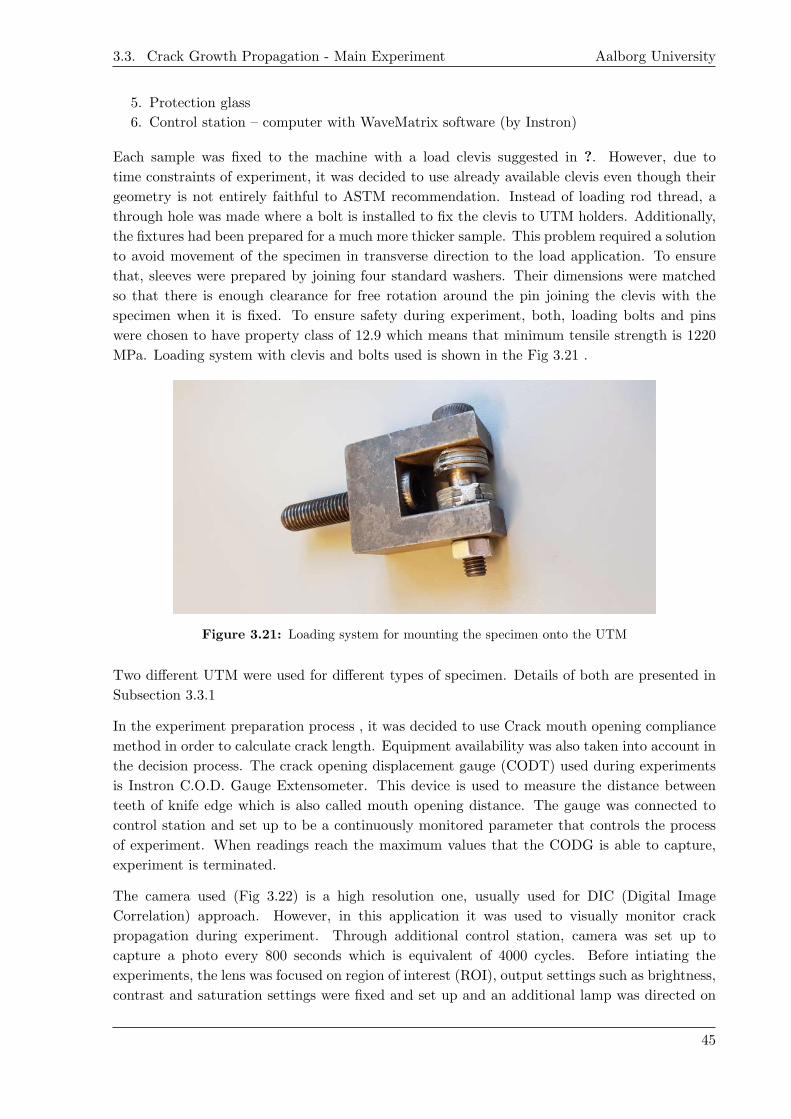
3.3. Crack Growth Propagation - Main Experiment Aalborg University
5. Protection glass
6. Control station – computer with WaveMatrix software (by Instron)
Each sample was fixed to the machine with a load clevis suggested in ?. However, due to
time constraints of experiment, it was decided to use already available clevis even though their
geometry is not entirely faithful to ASTM recommendation. Instead of loading rod thread, a
through hole was made where a bolt is installed to fix the clevis to UTM holders. Additionally,
the fixtures had been prepared for a much more thicker sample. This problem required a solution
to avoid movement of the specimen in transverse direction to the load application. To ensure
that, sleeves were prepared by joining four standard washers. Their dimensions were matched
so that there is enough clearance for free rotation around the pin joining the clevis with the
specimen when it is fixed. To ensure safety during experiment, both, loading bolts and pins
were chosen to have property class of 12.9 which means that minimum tensile strength is 1220
MPa. Loading system with clevis and bolts used is shown in the Fig 3.21 .
Figure 3.21: Loading system for mounting the specimen onto the UTM
Two different UTM were used for different types of specimen. Details of both are presented in
Subsection 3.3.1
In the experiment preparation process , it was decided to use Crack mouth opening compliance
method in order to calculate crack length. Equipment availability was also taken into account in
the decision process. The crack opening displacement gauge (CODT) used during experiments
is Instron C.O.D. Gauge Extensometer. This device is used to measure the distance between
teeth of knife edge which is also called mouth opening distance. The gauge was connected to
control station and set up to be a continuously monitored parameter that controls the process
of experiment. When readings reach the maximum values that the CODG is able to capture,
experiment is terminated.
The camera used (Fig 3.22) is a high resolution one, usually used for DIC (Digital Image
Correlation) approach. However, in this application it was used to visually monitor crack
propagation during experiment. Through additional control station, camera was set up to
capture a photo every 800 seconds which is equivalent of 4000 cycles. Before intiating the
experiments, the lens was focused on region of interest (ROI), output settings such as brightness,
contrast and saturation settings were fixed and set up and an additional lamp was directed on
45
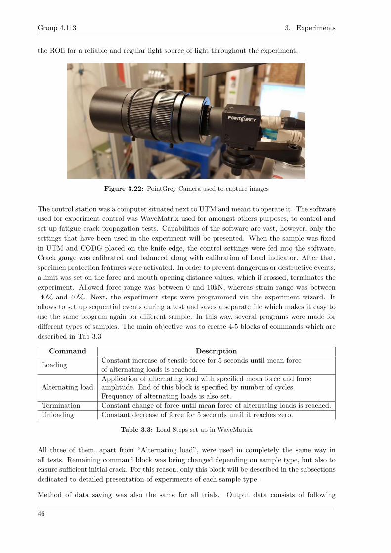
Group 4.113 3. Experiments
the ROIi for a reliable and regular light source of light throughout the experiment.
Figure 3.22: PointGrey Camera used to capture images
The control station was a computer situated next to UTM and meant to operate it. The software
used for experiment control was WaveMatrix used for amongst others purposes, to control and
set up fatigue crack propagation tests. Capabilities of the software are vast, however, only the
settings that have been used in the experiment will be presented. When the sample was fixed
in UTM and CODG placed on the knife edge, the control settings were fed into the software.
Crack gauge was calibrated and balanced along with calibration of Load indicator. After that,
specimen protection features were activated. In order to prevent dangerous or destructive events,
a limit was set on the force and mouth opening distance values, which if crossed, terminates the
experiment. Allowed force range was between 0 and 10kN, whereas strain range was between
-40% and 40%. Next, the experiment steps were programmed via the experiment wizard. It
allows to set up sequential events during a test and saves a separate file which makes it easy to
use the same program again for different sample. In this way, several programs were made for
different types of samples. The main objective was to create 4-5 blocks of commands which are
described in Tab 3.3
Command Description
LoadingConstant increase of tensile force for 5 seconds until mean forceof alternating loads is reached.
Alternating loadApplication of alternating load with specified mean force and forceamplitude. End of this block is specified by number of cycles.Frequency of alternating loads is also set.
Termination Constant change of force until mean force of alternating loads is reached.
Unloading Constant decrease of force for 5 seconds until it reaches zero.
Table 3.3: Load Steps set up in WaveMatrix
All three of them, apart from “Alternating load”, were used in completely the same way in
all tests. Remaining command block was being changed depending on sample type, but also to
ensure sufficient initial crack. For this reason, only this block will be described in the subsections
dedicated to detailed presentation of experiments of each sample type.
Method of data saving was also the same for all trials. Output data consists of following
46

3.3. Crack Growth Propagation - Main Experiment Aalborg University
parameters: total cycles, elapsed cycles, maximum load, minimum load, maximum strain,
minimum strain. For 10 first cycles, parameters were saved for each one, whereas for next
90 cycles, parameters were saved every 10 cycles. To avoid huge amount of data, after first 100
cycles, parameters were saved every 100 cycles.
All experiments were conducted in Aalborg University laboratories (East campus). Environ-
mental conditions in rooms are meant to be constant all the time. During experiments room
temperature was 22 to 23 °C.
Equipment used
The Tab 3.4 below contains the details of the equipments used for the experiments.
Equipment Description
UTM 1 100kN hydraulic (INSTRON Schenck Hydropuls PSB)UTM 2 10kN electrical (INSTRON E10000 +LC 10kN 2527-102)CODG Instron C.O.D Gauge Extensometer (10 mm Gauge travel)Camera Make: Pointgrey ; Image Capturing software: FlyCapture 2
Table 3.4: Details of equipment used for the experiment.
3.3.2 Force estimation
One of the first steps of experiment preparation was to estimate the force to apply on the
specimen. Before that, a known fact was that the tests should be performed only with tensile
loading, so that compressive stresses would not close the crack and to ensure that the stress
ratio R = σminσmax
should be positive. However, it was also desired to avoid big influence of mean
stresses. For those reasons, it was decided to apply forces with R = 0,1, which is a standard
for these type of tests. The next step was to calculate value of force corresponding to maximal
stress intensity factor Kmax. To do that, general formula (reference) could be used. In ? similar
formula is presented, where geometry factor for C(T) specimen is given, but also instead of
stresses, K is dependent on applied force. This formula () is given below.
∆K =∆P
B√W
(2 + α)
(1− α)3/2
(0.886 + 4.64α− 13.32α2 + 14.72α3 − 5.6α4
)(3.14)
Where: ∆ – difference between maximal and minimal value K – stress intensity factor P –
applied force B – specimen thickness W – specimen width α = a/W – crack length divided by
specimen width
By reformulating the Equation 3.14 to obtain force and substituting the appropriate values,
including ∆K with value of Kmax, maximal force for crack propagation can be obtained.
Calculations gave the result as
Pmax = 25813,2N (3.15)
47
Group 4.113 3. Experiments
Although, it is known that if this force value would be applied, crack would become unstable
and grow very fast until total failure of specimen. Conclusion from there, was that smaller force
is needed, but big enough to result in crack initiation. The next step was to estimate the right
force, on the basis of estimated time of experiment. Having known that the time for conducting
experiments on the UTM Machine was strongly limited , it was desired to perform all tests in
as little time as possible.
Lifetime estimation was performed with several assumptions. Crack growth rate was set to be
constant of value 1,1∗10(−8) mcycle which is according to recommendation of ?. Second assumption
was the frequency of applied alternating loads which was set to 5 Hz. Accordingly, a spreadsheet
was created where Kmax was calculated using Eqn 3.14 and referred to time of experiment. As
an end of virtual experiment, it was set a time when calculated Kmax exceeded KIC . With all
these conditions, applied force is a variable and time of experiment is desired output.
Pmean Pmax T[h]
7000 12727 ∼5011000 20000 ∼176000 10909 ∼62
Table 3.5: The time duration of the experiment.
Some results of time estimation are presented in Table 3.5. On its basis, it was decided that
Pmax to be applied as 12727N. Estimated time was acceptable and force seemed small enough to
avoid big plastic zone. However, it was advised by experienced laboratory staff to apply much
smaller force in the beginning. For this reason, in the end of force considerations, it was decided
to use following force values. Each row of Table 3.6 corresponds to one test performed on trial
sample for 30 minutes. The purpose of such a trial was to find if applied force was enough to
initiate crack. If the trial succeeded, the corresponding force was chosen to be appropriate to
perform the actual experiment.
3.3.3 Type 1 specimen
Specimen features
This type of specimen is the regular one and was manufactured as described in 1 and shown in
Fig 3.23
Pmean (N) Pmax (N)2000 36363000 54544000 72725000 90905500 10000
Table 3.6: Load values to be applied to the Specimens
48

3.3. Crack Growth Propagation - Main Experiment Aalborg University
Figure 3.23: Type 1 Specimen before the experiment
Sample no UTM no Meanforce [N]
Load fre-quency[Hz]
Precracklength[mm]
Alternating load
1 1 4000 5 ∼1,5 (equalto strain1,76%)
Constant
2,3 1 4000 - 3000 5 ∼4 (equal tostrain 1,76%)
Not constant: initial forceis changing under event ofreaching 1,76% strain
Experiment details
After the very first experiment, it was decided to modify the alternating load command block.
In the beginning of experiments for samples 2 and 3, the load remained the same as for sample
1. However, after reaching crack length of 12 mm, which is equivalent to 4 mm of precrack, the
applied mean force was decreased. The purpose of this action was to decrease crack propagation
speed and be able to capture more data towards the end of the experiment when crack propagates
rapidly.
3.3.4 Type 2 specimen
Specimen features
The manufacturing and heat treatment procedure for this sample was performed as mentioned
in Chap 1 and the specimen is shown in Fig 3.24
49
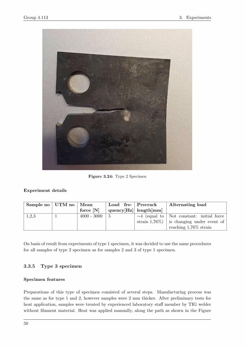
Group 4.113 3. Experiments
Figure 3.24: Type 2 Specimen
Experiment details
Sample no UTM no Meanforce [N]
Load fre-quency[Hz]
Precracklength[mm]
Alternating load
1,2,3 1 4000 - 3000 5 ∼4 (equal tostrain 1,76%)
Not constant: initial forceis changing under event ofreaching 1,76% strain
On basis of result from experiments of type 1 specimen, it was decided to use the same procedures
for all samples of type 2 specimen as for samples 2 and 3 of type 1 specimen.
3.3.5 Type 3 specimen
Specimen features
Preparations of this type of specimen consisted of several steps. Manufacturing process was
the same as for type 1 and 2, however samples were 2 mm thicker. After preliminary tests for
heat application, samples were treated by experienced laboratory staff member by TIG welder
without filament material. Heat was applied manually, along the path as shown in the Figure
50

3.3. Crack Growth Propagation - Main Experiment Aalborg University
(one from introduction), on both sides. The last step was to grind samples by 1mm from each
side to obtain 5 mm thickness. The reason for doing that was that applied heat resulted in local
melting of material on surfaces. Whereas this, could influence crack propagation trial.
Fig 3.25 below shows sample after grinding. As visible, the samples prepared for crack
propagation experiment had experienced a minute amount of melting of material in crack tip.
However, this phenomenon was present only near surfaces, while sharp crack tip still existed
through the thickness.
Figure 3.25: Type 3 Specimen after grinding procedure
Experiment details
Sample no UTM no Meanforce [N]
Load fre-quency[Hz]
Precracklength[mm]
Alternating load
1 1 5500 - 3000- 4000
5 ∼4 (equal tostrain 2,5%)
Not constant: (two) ini-tial forces are changing un-der event of reaching 2,5%strain
2,3 1 5500 - 4000 5 ∼4 (equal tostrain 2,5%)
Not constant: initial forceis changing under event ofreaching 2,5% strain
The initial, procedure was the same as for Type 2 specimen, though, after 1 hour of trial,
crack did not initiated. For that reason test of forces was conducted (like described in the end
of Subchapter (force estimation)). As a result, applied mean force became 5500N. In test for
sample 1, mean force was decreased due to strain reaching 1,76%. After that, mean force of
3000N occurred not to be enough for crack to propagate and higher mean force was introduced.
However, 1,76% strain occurred to not correspond to precrack length of 4mm. To find strains
corresponding to 4mm of precrack, another tests were done. By several trials, final procedure
was established and applied to samples 2 and 3. All this departures from procedure for specimen
Type 1 and 2, are believed to be caused by heat treatment. Changes in procedures were expected,
however, could not be predicted which of them would be suitable to perform experiment in right
way without additional trials.
51
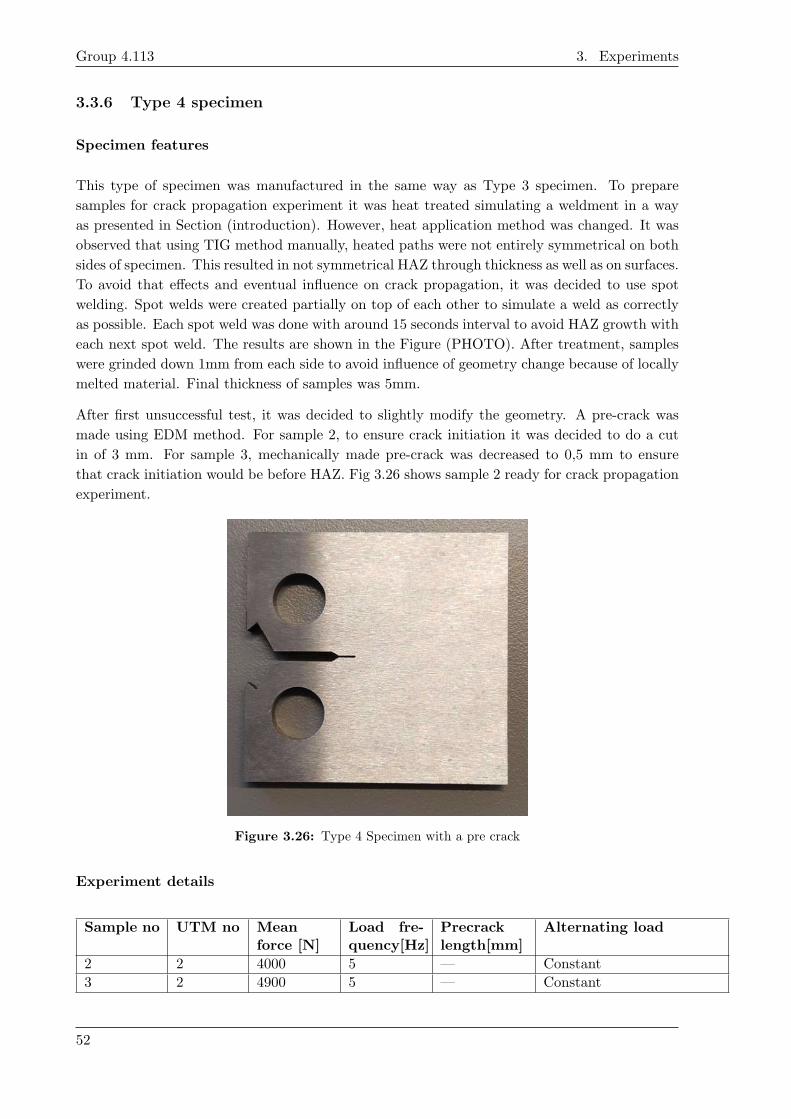
Group 4.113 3. Experiments
3.3.6 Type 4 specimen
Specimen features
This type of specimen was manufactured in the same way as Type 3 specimen. To prepare
samples for crack propagation experiment it was heat treated simulating a weldment in a way
as presented in Section (introduction). However, heat application method was changed. It was
observed that using TIG method manually, heated paths were not entirely symmetrical on both
sides of specimen. This resulted in not symmetrical HAZ through thickness as well as on surfaces.
To avoid that effects and eventual influence on crack propagation, it was decided to use spot
welding. Spot welds were created partially on top of each other to simulate a weld as correctly
as possible. Each spot weld was done with around 15 seconds interval to avoid HAZ growth with
each next spot weld. The results are shown in the Figure (PHOTO). After treatment, samples
were grinded down 1mm from each side to avoid influence of geometry change because of locally
melted material. Final thickness of samples was 5mm.
After first unsuccessful test, it was decided to slightly modify the geometry. A pre-crack was
made using EDM method. For sample 2, to ensure crack initiation it was decided to do a cut
in of 3 mm. For sample 3, mechanically made pre-crack was decreased to 0,5 mm to ensure
that crack initiation would be before HAZ. Fig 3.26 shows sample 2 ready for crack propagation
experiment.
Figure 3.26: Type 4 Specimen with a pre crack
Experiment details
Sample no UTM no Meanforce [N]
Load fre-quency[Hz]
Precracklength[mm]
Alternating load
2 2 4000 5 — Constant
3 2 4900 5 — Constant
52

3.3. Crack Growth Propagation - Main Experiment Aalborg University
Sample 1 is not placed in the Tab ?? due to unexpected failure during experiment. The crack
initiated in a wrong location and its path of propagation was unlike any of the previous. More
details about this failure mentioned in the discussion section of 5. To avoid similar behaviours,
it was decided to increase mean force to increase stress intensity in initial crack tip. Mean force
was kept for entire experiment as crack growth rate was observed to be very small. Because of
that, no pre-crack length is indicated in the table. Experiment of sample 2 terminated after more
than 300 000 cycles and due to limited time for using UTM, mean force in sample 3 experiment
was increased. However, because of force limits of UTM ( 10kN ), it was recommended by
laboratory staff not to exceed maximum force of 9000 N, considering safety factor. Finally it
was decided to apply mean force of 4900N what corresponds to maximum force of 8910N.
3.3.7 Results
Calculations
The output of experiments was a file of .csv format. To process the data, it was imported
to excel spreadsheet where proper formulas were included. They were prepared in advance
according to ? and ? . After that, they were copied to excel files where data from each
experiment was imported. Details of calculation process is given below. At first, crack mouth
opening displacement is calculated from strain measurement:
Vm =εmax100
∗ initial mouth opening (3.16)
where εmax – maximal mouth opening during 1 cycle
Initial mouth opening – opening of knife edge measured for each sample (should be 10 mm in each
samples, but it slightly deviates (order of 0,01mm) from sample to sample due to inaccuracies
in preparation process)
The next step was to calculate U parameter from 3.17
U =1
1 +√
E′BeVmP
(3.17)
Vm – crack mouth opening displacement
P – applied force
E′ – in this case is equal to E (for plane stress)
Be – equal to B in the case of this specimen
Finally crack length ’a’ could be calculated with Eqn
a
w= 1.000− 4.500 · U + 13.157 · U2 − 172.551 · U3 + 879.944 · U4 − 1514.671 · U5 (3.18)
Where U – parameter obtained from Eqn 3.17
W – specimen width (depth).
53
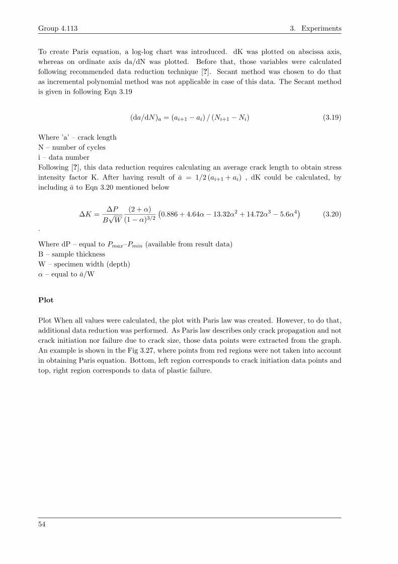
Group 4.113 3. Experiments
To create Paris equation, a log-log chart was introduced. dK was plotted on abscissa axis,
whereas on ordinate axis da/dN was plotted. Before that, those variables were calculated
following recommended data reduction technique [?]. Secant method was chosen to do that
as incremental polynomial method was not applicable in case of this data. The Secant method
is given in following Eqn 3.19
(da/dN)a = (ai+1 − ai) / (Ni+1 −Ni) (3.19)
Where ’a’ – crack length
N – number of cycles
i – data number
Following [?], this data reduction requires calculating an average crack length to obtain stress
intensity factor K. After having result of a = 1/2 (ai+1 + ai) , dK could be calculated, by
including a to Eqn 3.20 mentioned below
∆K =∆P
B√W
(2 + α)
(1− α)3/2
(0.886 + 4.64α− 13.32α2 + 14.72α3 − 5.6α4
)(3.20)
.
Where dP – equal to Pmax–Pmin (available from result data)
B – sample thickness
W – specimen width (depth)
α – equal to a/W
Plot
Plot When all values were calculated, the plot with Paris law was created. However, to do that,
additional data reduction was performed. As Paris law describes only crack propagation and not
crack initiation nor failure due to crack size, those data points were extracted from the graph.
An example is shown in the Fig 3.27, where points from red regions were not taken into account
in obtaining Paris equation. Bottom, left region corresponds to crack initiation data points and
top, right region corresponds to data of plastic failure.
54

3.3. Crack Growth Propagation - Main Experiment Aalborg University
Figure 3.27: da/dN vs ∆K dismissed datapoints
As a result, a plot with crack propagation data was made. Power law trend line for data was
created using R2 method. The equation of the trend line is a desired Paris equation.
55
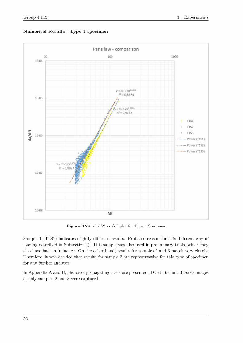
Group 4.113 3. Experiments
Numerical Results - Type 1 specimen
Figure 3.28: da/dN vs ∆K plot for Type 1 Specimen
Sample 1 (T1S1) indicates slightly different results. Probable reason for it is different way of
loading described in Subsection (). This sample was also used in preliminary trials, which may
also have had an influence. On the other hand, results for samples 2 and 3 match very closely.
Therefore, it was decided that results for sample 2 are representative for this type of specimen
for any further analyses.
In Appendix A and B, photos of propagating crack are presented. Due to technical issues images
of only samples 2 and 3 were captured.
56
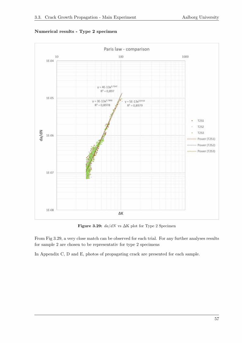
3.3. Crack Growth Propagation - Main Experiment Aalborg University
Numerical results - Type 2 specimen
Figure 3.29: da/dN vs ∆K plot for Type 2 Specimen
From Fig 3.29, a very close match can be observed for each trial. For any further analyses results
for sample 2 are chosen to be representativ for type 2 specimens
In Appendix C, D and E, photos of propagating crack are presented for each sample.
57
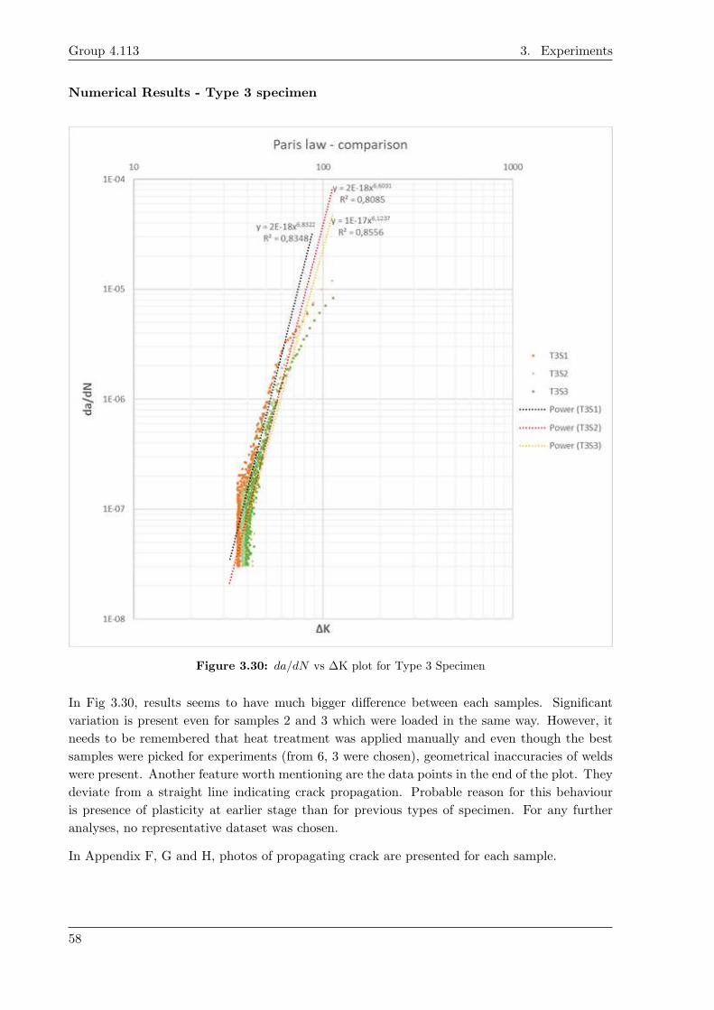
Group 4.113 3. Experiments
Numerical Results - Type 3 specimen
Figure 3.30: da/dN vs ∆K plot for Type 3 Specimen
In Fig 3.30, results seems to have much bigger difference between each samples. Significant
variation is present even for samples 2 and 3 which were loaded in the same way. However, it
needs to be remembered that heat treatment was applied manually and even though the best
samples were picked for experiments (from 6, 3 were chosen), geometrical inaccuracies of welds
were present. Another feature worth mentioning are the data points in the end of the plot. They
deviate from a straight line indicating crack propagation. Probable reason for this behaviour
is presence of plasticity at earlier stage than for previous types of specimen. For any further
analyses, no representative dataset was chosen.
In Appendix F, G and H, photos of propagating crack are presented for each sample.
58

3.3. Crack Growth Propagation - Main Experiment Aalborg University
Numerical Results - Type 4 specimen
Figure 3.31: da/dN vs ∆K plot for Type 4 Specimen
For this type of specimen, the plot is no longer a straight line and this behaviour was actually
expected. When the crack crosses the HAZ, it was anticipated that its growth rate would change
due to residual stresses and this is what might have happened in these samples. In this case,
since the crack growth rate changes there is no sense of creating Paris equation, but in was done
for a record, in sake of keeping procedures the same for each type of specimen. Results presented
in the Figure () significantly differs between each other. Datasets varies not only in values but
also in profile of curves. The reason for that may be different way of force application. However,
it is suspected that there is another reason for data disparity like geometric inaccuracies of welds
or differences in residual stresses. For further analyses both datasets are considered.
In Appendix I and J , photos of propagating crack are presented. .
59

Group 4.113 3. Experiments
Paris equation comparison
For convenience, Table ?? was created for easy comparison of Paris equation parameters.
Type Sample C n R2
1 1 1e-12 3,269 0,921 2 3e-12 3,109 0,881 3 3e-12 3,084 0,88
2 1 5e-13 3,642 0,902 2 4e-13 3,755 0,902 3 3e-13 3,789 0,90
3 1 2e-18 6,832 0,833 2 2e-18 6,603 0,813 3 1e-17 6,124 0,86
4 2 6e-16 5,177 0,824 3 7e-17 5,677 0,83
3.3.8 Accuracy
Chapter 11 from ? presents details about precision of experiments. Main contribution to
errors are measurements of applied forces together with measurements of crack mouth opening.
According to the Standard,, +/-2% of force variation results in +/- 4% to +/- 10% variation
of da/dN, at corresponding dK. It was verified, that during experiments in this study, force
measurement did not deviate more than 1% from target value and usually it was less than 0,5%.
Consequently, it is assumed that errors from this source are smaller than given in the Standard.
However, [?] also mentions that the crack opening measurements have bigger contribution to
error, but also it is more complicated to assess that contribution. The reason for that is the
difficulty in isolating the error from the measurement, because of its coupling to inherent material
variations as well as to analysis procedures. Section 11.11 in ? describes in detail about inter
laboratory tests conducted to study the overall measure of variability da/dN vs ∆K.
3.4 Post Experiment Visual Inspection
A small post experiment visual inspection was performed on the specimens specifically of Type
3 and Type 4 to identify the heat affected zone via chemical etching procedure. This was
performed by using ammonium persulphate etch solution, which has the unique ability to reveal
the microstructure of iron. A fresh solution of the chemical was prepared by the laboratory staff
which was then applied onto the surface of the specimens using cotton swabs. The swab was
rubbed over the specimen with pressure. An etching period of approximately 2 minutes is more
than enough to for the heat affected regions to become distinctly visible.
Figures below show the etched surfaces of the specimens where the heat affected/welded regions
are clearly visible.
60
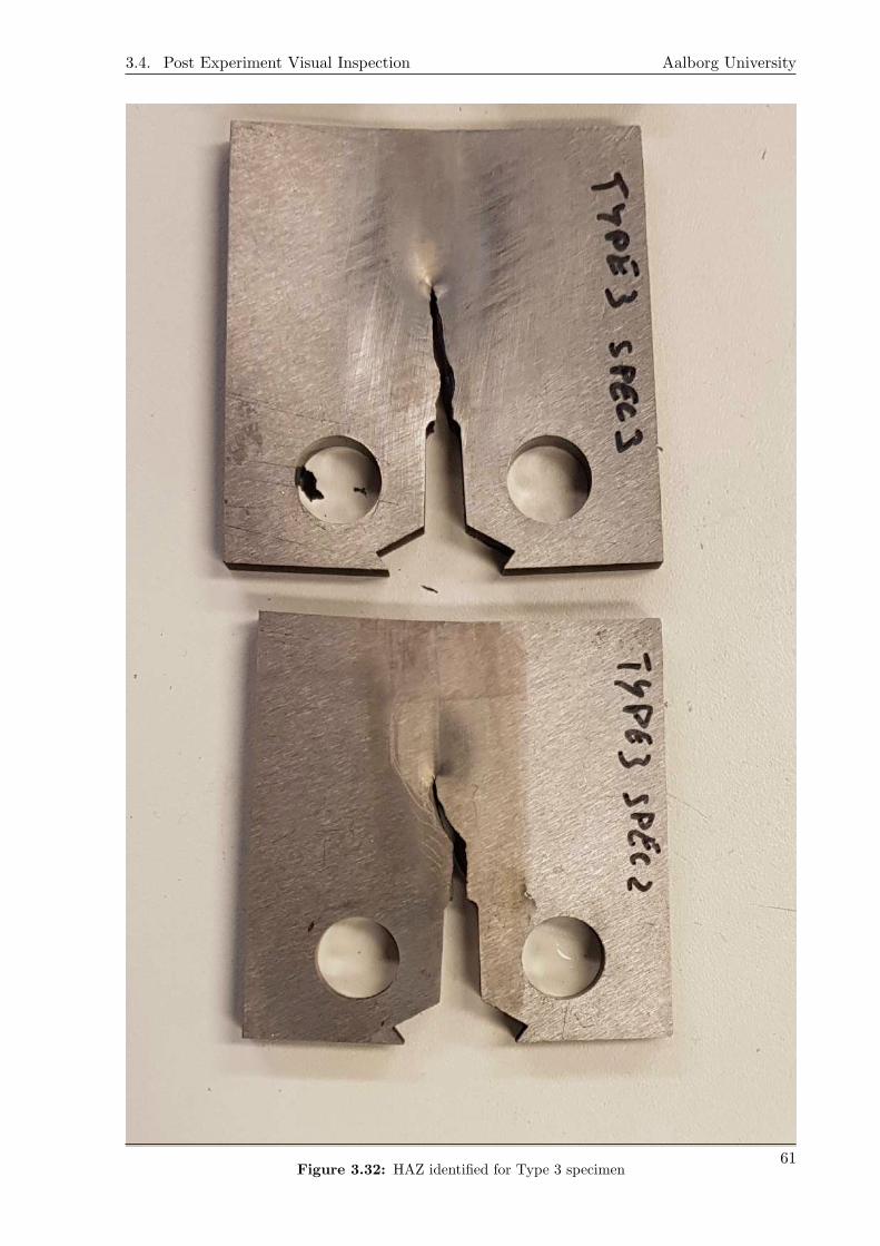
3.4. Post Experiment Visual Inspection Aalborg University
Figure 3.32: HAZ identified for Type 3 specimen61

Group 4.113 3. Experiments
Figure 3.33: HAZ identified for Type 4 specimen
It is interesting to note that the weld spots from spot welding performed for Type 4 specimen
is clearly visible after performing the etching procedure
62

4 — Numerical Simulations
Numerical simulations for various the different kinds of specimens was carried out in order
to simulate the actual experiments performed and study their behaviour. These simulations
were carried out on ANSYS APDL and Workbench CAE software. ANSYS is capable of
handling FEM simulations for fracture and fatigue analyses with different add-ons available
which help obtain important information from simulations. Most of the analyses were conducted
on simplified 2D models with constant thickness.
The presence of high stress gradients at the crack tip demands more elements to be concentrated
in and around the region to capture the stress values. This is achieved by making use of special
Crack-tip elements offered by ANSYS. The figure 4.1 below shows 2D and 3D representations
of the region around the crack tip and the terminology used. The edge or crack tip is referred
to as ’crack tip’ in 2D analysis and as ’crack front’ in a 3D analysis.
Figure 4.1: Crack type and its terminology (a) 2D Crack (b) 3D crack (Adapted from ?, pp 9)
4.0.1 Simplification of the FEM model
In order to ease the process of FEM simulations, the model used was simplified as much as
possible. For 2D, symmetry of the model was utilised in whichever cases it was applicable. The
CT specimen was reduced from its actual shape to a more simplified model which itself was
obtained after multiple simulations done in APDL. The series of images below (4.2, 4.3 and 4.4)
breaks down the entire simplification procedure performed.
63

Group 4.113 4. Numerical Simulations
Figure 4.2: Full 2D model Figure 4.3: 2D symmetry model
Figure 4.4: Final Simplified 2D model
In Fig 4.4, the point P represents the point of application of load, while the point C represents
the crack tip. It was identified that, if the UX degree of freedom at the point of load application
is not fixed while applying the force P, the specimen experience Mode 1 and Mode II loading
together due to the large magnitude of force applied. This also directly and significantly affected
the calculated SIF values.
This model was obtained after performing multiple simulations on the full 2D model 4.2. Initially
, symmetry was considered since the model is symmetrical in shape along the x-axis. Further
more, simulations also showed that applying the load at the nodes on the circumference of the
hole via multiple stiff connectors through a node in the center of the hole (Fig 4.5) produced
the same results as when applying the load at the position of the center of the hole (Fig 4.4),
eliminating the need to model the hole.
64

Aalborg University
Figure 4.5: Stiff connectors from center of the hole to all nodes on its periphery
Furthermore, a smaller semicircular region with radius of 1 mm was made at the crack tip of
the final 2D model (Fig), which acts as a sphere of influence within which the crack tip elements
could be generated densely while outside the region, the mesh size and density did not influence
the results in any significant manner. This has also been discussed further in detail in the
next section. This was done to prevent extremely skewed triangular elements being formed just
around the crack tip mesh, which may affect computation of the stress values. Even though
the stresses at the crack tip approach infinity and it is not possible to accurately determine the
exact value of the stresses at the crack tip, using a sphere of influence helped set up a much
better mesh.
Figure 4.6: Splitting the entire model into 3 sections
65
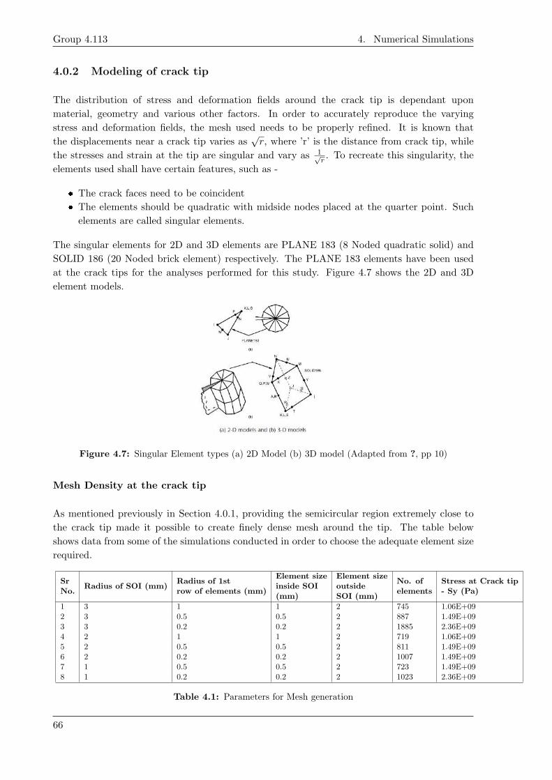
Group 4.113 4. Numerical Simulations
4.0.2 Modeling of crack tip
The distribution of stress and deformation fields around the crack tip is dependant upon
material, geometry and various other factors. In order to accurately reproduce the varying
stress and deformation fields, the mesh used needs to be properly refined. It is known that
the displacements near a crack tip varies as√r, where ’r’ is the distance from crack tip, while
the stresses and strain at the tip are singular and vary as 1√r. To recreate this singularity, the
elements used shall have certain features, such as -
� The crack faces need to be coincident
� The elements should be quadratic with midside nodes placed at the quarter point. Such
elements are called singular elements.
The singular elements for 2D and 3D elements are PLANE 183 (8 Noded quadratic solid) and
SOLID 186 (20 Noded brick element) respectively. The PLANE 183 elements have been used
at the crack tips for the analyses performed for this study. Figure 4.7 shows the 2D and 3D
element models.
Figure 4.7: Singular Element types (a) 2D Model (b) 3D model (Adapted from ?, pp 10)
Mesh Density at the crack tip
As mentioned previously in Section 4.0.1, providing the semicircular region extremely close to
the crack tip made it possible to create finely dense mesh around the tip. The table below
shows data from some of the simulations conducted in order to choose the adequate element size
required.
SrNo.
Radius of SOI (mm)Radius of 1strow of elements (mm)
Element sizeinside SOI(mm)
Element sizeoutsideSOI (mm)
No. ofelements
Stress at Crack tip- Sy (Pa)
1 3 1 1 2 745 1.06E+092 3 0.5 0.5 2 887 1.49E+093 3 0.2 0.2 2 1885 2.36E+094 2 1 1 2 719 1.06E+095 2 0.5 0.5 2 811 1.49E+096 2 0.2 0.2 2 1007 1.49E+097 1 0.5 0.5 2 723 1.49E+098 1 0.2 0.2 2 1023 2.36E+09
Table 4.1: Parameters for Mesh generation
66

Aalborg University
In order to obtain results by implementing a good mesh across the model, it was decided to
proceed with elements with the specification as mentioned in Table 4.1, Sr No 8. It was found
upon additional simulations that further reducing the element sizes and other parameters did
not influence results significantly. Eventhough it is known that the stress values at the crack tip
cannot be perfectly computed, Stress in y-direction was computed to check how accurately the
different meshes were able to capture the results. The study showed that the values of radius of
the 1st row of elements at the crack tip and the ratio of element size of 2nd row of elements to
the 1st row of elements had more influence on the accuracy of results obtained. The number of
elements in the radial direction around the crack tip can also be controlled in APDL. This was
set to 10 elements since it was found that using a lower number created uneven distribution of
elements around the crack tip, at times even skewing the elements??, whereas increasing it to a
much higher value had no significant impact on the accuracy of results obtained.
Figure 4.8: Improper mesh at crack tip obtained by setting lower number of elements in rthe radialdirection around the crack tip
The final mesh obtained is shown in Fig 4.9 below.. Fig 4.18 shows a detailed version of the
mesh in the crack tip.
Figure 4.9: Final mesh of the simplified 2D model
67

Group 4.113 4. Numerical Simulations
Figure 4.10: Mesh at the crack tip
4.0.3 Determining Stress Intensity Factors
In order to establish a comparison between the experiments and numerical simulations, the
Stress Intensity Factor at the crack tip for different crack tip lengths was determined, which
could then be plotted to obtain more information. Fracture parameters like SIF can be computed
in the Post Processing stage of the analysis. The displacement extrapolation method was used
to calculate the SIFs at various crack lengths. This process is however limited to linear elastic
problems having homogeneous, isotropic material at the crack tip. A more crucial requirement
is that the x-axis must be parallel to the crack face and the y-axis perpendicular to the crack
face. Thus a local coordinate system is created at the crack tip as shown in Fig 4.14
Figure 4.11: A local coordinate system ’11’ generated at the crack tip
68

Aalborg University
During the post processing stage, this local coordinate system was set as the active model
coordinate system and the results coordinate system. A path is then to be generated with the
first node as the crack tip. For a half-crack or symmetrical mode, 2 additional nodal points are
required, both along the crack face, but behind the crack tip. The path was then defined as
shown in Figures
Figure 4.12: Half crack model path definition(From ?, pp 35)
Figure 4.13: Path definition in simulations
Then using the Nodal Calculations option in the General Postprocessor, it was specified that
the model was in plane stress state and that a half-crack model was defined, followed by which
Ansys calculates the SIF K1 for mode 1 loading and displays the result in the format as shown
in Fig
Figure 4.14: SIF value displayed in APDL calculated by displacement extrapolation
Analysis of Type 1 Specimen
For the Type 1 specimen, the SIF KI for the crack at different lengths is as follows
Sr No. Crack Length (mm) No. of elements K1 (MPa/m)
1 8 863 26.552 11 866 30.173 14 863 35.464 17 860 42.445 20 863 52.336 23 864 67.267 26 861 91.498 29 870 134.59 32 863 223.310 35 866 466.5
Table 4.2: K1 from Displacement Interpolation for Type 1 Specimen
69

Group 4.113 4. Numerical Simulations
A contour plot (Fig) of stress in y-direction was generated to visually check if the stress
distribution at the crack tip was as expected. The Sy values in front of the crack were extracted
and plotted against distance, which generated a graph as shown in Fig Both the plots showed
that the stress distribution conformed with the expected behaviour as per theoretical knowledge.
Figure 4.15: Stress in Y direction Contour plot
Figure 4.16: Sy vs distance plot
70

4.1. Thermal Simulations Aalborg University
4.1 Thermal Simulations
Thermal-structural simulations were performed to completely capture the effects of heat
application during the heat treatment and welding procedures performed on specimens of Type
2, 3 and 4. ANSYS permits importing thermal loads from a thermal analysis onto a structural
simulation. This imported load is in the form of mechanical strains. Typical interesting thermal
quantities that are usually studied are - temperature distributions, heat gain/loss, thermal
gradients and fluxes. Nodal temperatures are calculated by finite element method and then that
data is used for further calculations of thermal quantities. ANSYS is capable of handling all 3
modes of heat transfer: Conduction, Convection and Radiation.
For a thermal analysis, the most apt element used for the analyses was the Solid 8 Node
PLANE77 element. It is a quadrilateral 2D solid element with temperature DOFs at every
node. An advantage of using this element is that while switching over to a structural analysis
after thermal, the PLANE77 thermal element is converted automatically into the PLANE183
structural element which is also the crack tip element used to model the crack tip for a regular
structural analysis.
Initial simulations involved only steady state analyses which ignores the heat application effects
over a time period. This was however later changed to transient analyses to account for the
effect of heat addition and cooling over time, which the specimens experienced. .
For ease of demonstrating how the thermal analyses was performed, the procedure followed for
only Type 3 specimen is mentioned. The method used for type 4 specimen was exactly the
same as for type 2 and type 3, with the only difference being area of heat application. Some
additional details about the simulation are mentioned below
� Crack length - 17 mm (At this point, the crack is well inside the heat affected zone)
� Load Applied : Max Static load during the experiments on Type 3 specimen - 7270.
� BCs : Symmetry
The analyses were setup in the following way.
� The initial steps of a thermal analysis are just like any normal structural analysis. A
2D model was set up on ANSYS APDL and required material properties as previously
mentioned in Chap 1 were fed in. Temperature scale was set to °C.
� The mesh generated was similar to that of the structural analysis for Type 1 specimen,
where a sphere of influence was defined at the crack tip within which the density of elements
was high.
� During the modelling of the specimens of Type 3 and 4, the area of heat application was
modelled as a rectangular section where temperature load of 1300°C was applied. This
applied temperature is a rough estimate of the temperature at the surface of the specimen
at the onset of the surface slightly melting when welding is performed. The Fig below
illustrates the temperature load application for Type 3 Specimen. The only difference
between that of a Type 3 specimen and Type 4 specimen is the area of temperature
application.
71
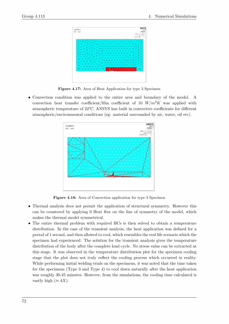
Group 4.113 4. Numerical Simulations
Figure 4.17: Area of Heat Application for type 3 Specimen
� Convection condition was applied to the entire area and boundary of the model. A
convection heat transfer coefficient/film coefficient of 10 W/m2K was applied with
atmospheric temperature of 22°C. ANSYS has built in convective coefficients for different
atmospheric/environmental conditions (eg: material surrounded by air, water, oil etc).
Figure 4.18: Area of Convection application for type 3 Specimen
� Thermal analysis does not permit the application of structural symmetry. However this
can be countered by applying 0 Heat flux on the line of symmetry of the model, which
makes the thermal model symmetrical.
� The entire thermal problem with required BCs is then solved to obtain a temperature
distribution. In the case of the transient analysis, the heat application was defined for a
period of 1 second, and then allowed to cool, which resembles the real life scenario which the
specimen had experienced. The solution for the transient analysis gives the temperature
distribution of the body after the complete load cycle. No stress value can be extracted at
this stage. It was observed in the temperature distribution plot for the specimen cooling
stage that the plot does not truly reflect the cooling process which occurred in reality.
While performing initial welding trials on the specimens, it was noted that the time taken
for the specimens (Type 3 and Type 4) to cool down naturally after the heat application
was roughly 30-45 minutes. However, from the simulations, the cooling time calculated is
vastly high (≈ 4X).
72

4.1. Thermal Simulations Aalborg University
The Fig 4.19 and 4.20 below shows the temperature distribution in the specimen after
time step of 1 sec (Immediately after heat application) and after 10,800 seconds, even
after which the specimen had not reached room temperature..
Figure 4.19: Temperature distribution in the specimen 1 second after heat application
Figure 4.20: Temperature distribution in the specimen 108000 seconds after heat application
However, it was considered that there would be no influence on residual stresses at this
level of temperature and it was decided that further analysis could be performed
73

Group 4.113 4. Numerical Simulations
� Following the thermal analysis, the analysis mode was then switched to structural analysis
along with switching the elements from PLANE 77 to PLANE 183. No changes were made
in the geometry or the mesh which was retained as it is, from the thermal simulation
performed before.
� It is at this stage that the thermal loads from the previous analysis are imported into
Ansys which automatically detects and applies the imported loads onto the geometry.
The symmetry BC also was applied at this stage after having switched to the structural
analysis module.
Upon solving the FEM problem at this stage, the Sy stress distribution plot obtained was
unanticipated. The stresses seemed to be concentrated at the crack tip and resembled the
stress distribution at the crack tip similar to Fig PUT REFERENCE TO IMAGE
OF STRESS PLOTS FROM TYPE 1 ANALYSIS
� However, upon further applying the appropriate load and BCs, K1 = 56.72MPa was
obtained for the crack length.
Figure 4.21: SIF for Type 3 specimen at a = 17 mm.
Upon further inspection, it was found that importing the thermal load had no influence at all.
This was verified by modelling and performing the exactly similar analyses on specimen of Type
1, 2, 3 and 4. The crack length was set as 17mm. The force applied on all the models was set
to 7270 N and the SIFs were calculated, which have been tabulated below
Type of Specimen K1 calculated (Mpa)
Type 1 56.72Type 2 56.75Type 3 56.71Type 4 56.73
Table 4.3: Calculated SIFs for all specimen models under the same loading and BCs.
Since the results obtained from the performed numerical simulations were vague, further
simulations would require a non linear material modeling with mechanical and thermal properties
varying with time. Further discussion about thermal analysis has been done in Chap 5
74

5 — Discussion
5.1 Crack Propagation Experiment
An important issue to discuss in this part is plasticity. It was present in experiments for each
sample type, but in different moments. However, for each sample, at some point, material
behaviour was similar. When crack was propagating fast and stress intensity factor became
high, plastic behaviour was occurring. It is shown in the Fig 5.1
Figure 5.1: Crack growth plot
In photos of each specimen from Appendices (for each sample type), plastic behaviour can be
observed as well. Especially in the last pictures, plastic deformations are visible as well as surface
depression caused by Poisson effect. As shown in the Figure 1.25, crack growth propagation
should be terminated by unstable crack growth which, in the graph da/dN – ∆K is indicated
by very steep line (almost vertical), in last section of plot. Such unstable behaviour would result
in sudden failure of specimen. In case of performed experiments, samples experienced plastic
deformations, which resulted in violation of protection values for strains and termination of trial.
The explanation of this phenomena is that due to large crack and high stress intensity factor,
uncracked material is no longer able to sustain large stresses. They are so big in comparison to
material yield stress that causes plastic zone bigger than uncracked material in front of crack
tip. At this point, a question of influence of plasticity before above situation was raised. As per
? , there is a condition to check whether LEFM (linear elastic fracture mechanics) is applicable.
75
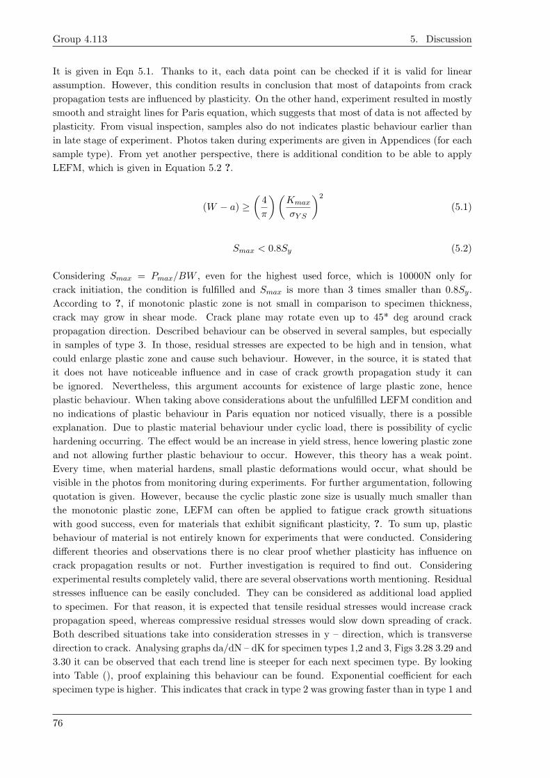
Group 4.113 5. Discussion
It is given in Eqn 5.1. Thanks to it, each data point can be checked if it is valid for linear
assumption. However, this condition results in conclusion that most of datapoints from crack
propagation tests are influenced by plasticity. On the other hand, experiment resulted in mostly
smooth and straight lines for Paris equation, which suggests that most of data is not affected by
plasticity. From visual inspection, samples also do not indicates plastic behaviour earlier than
in late stage of experiment. Photos taken during experiments are given in Appendices (for each
sample type). From yet another perspective, there is additional condition to be able to apply
LEFM, which is given in Equation 5.2 ?.
(W − a) ≥(
4
π
)(Kmax
σY S
)2
(5.1)
Smax < 0.8Sy (5.2)
Considering Smax = Pmax/BW , even for the highest used force, which is 10000N only for
crack initiation, the condition is fulfilled and Smax is more than 3 times smaller than 0.8Sy.
According to ?, if monotonic plastic zone is not small in comparison to specimen thickness,
crack may grow in shear mode. Crack plane may rotate even up to 45* deg around crack
propagation direction. Described behaviour can be observed in several samples, but especially
in samples of type 3. In those, residual stresses are expected to be high and in tension, what
could enlarge plastic zone and cause such behaviour. However, in the source, it is stated that
it does not have noticeable influence and in case of crack growth propagation study it can
be ignored. Nevertheless, this argument accounts for existence of large plastic zone, hence
plastic behaviour. When taking above considerations about the unfulfilled LEFM condition and
no indications of plastic behaviour in Paris equation nor noticed visually, there is a possible
explanation. Due to plastic material behaviour under cyclic load, there is possibility of cyclic
hardening occurring. The effect would be an increase in yield stress, hence lowering plastic zone
and not allowing further plastic behaviour to occur. However, this theory has a weak point.
Every time, when material hardens, small plastic deformations would occur, what should be
visible in the photos from monitoring during experiments. For further argumentation, following
quotation is given. However, because the cyclic plastic zone size is usually much smaller than
the monotonic plastic zone, LEFM can often be applied to fatigue crack growth situations
with good success, even for materials that exhibit significant plasticity, ?. To sum up, plastic
behaviour of material is not entirely known for experiments that were conducted. Considering
different theories and observations there is no clear proof whether plasticity has influence on
crack propagation results or not. Further investigation is required to find out. Considering
experimental results completely valid, there are several observations worth mentioning. Residual
stresses influence can be easily concluded. They can be considered as additional load applied
to specimen. For that reason, it is expected that tensile residual stresses would increase crack
propagation speed, whereas compressive residual stresses would slow down spreading of crack.
Both described situations take into consideration stresses in y – direction, which is transverse
direction to crack. Analysing graphs da/dN – dK for specimen types 1,2 and 3, Figs 3.28 3.29 and
3.30 it can be observed that each trend line is steeper for each next specimen type. By looking
into Table (), proof explaining this behaviour can be found. Exponential coefficient for each
specimen type is higher. This indicates that crack in type 2 was growing faster than in type 1 and
76
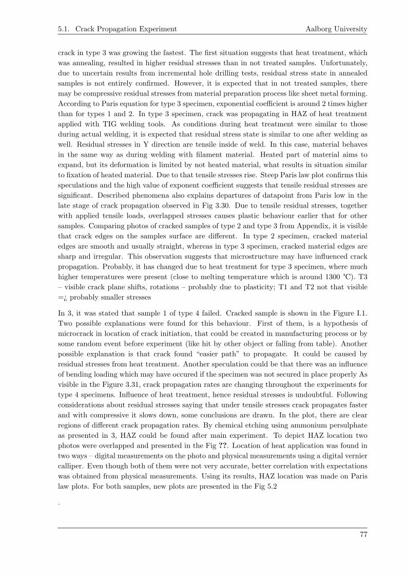
5.1. Crack Propagation Experiment Aalborg University
crack in type 3 was growing the fastest. The first situation suggests that heat treatment, which
was annealing, resulted in higher residual stresses than in not treated samples. Unfortunately,
due to uncertain results from incremental hole drilling tests, residual stress state in annealed
samples is not entirely confirmed. However, it is expected that in not treated samples, there
may be compressive residual stresses from material preparation process like sheet metal forming.
According to Paris equation for type 3 specimen, exponential coefficient is around 2 times higher
than for types 1 and 2. In type 3 specimen, crack was propagating in HAZ of heat treatment
applied with TIG welding tools. As conditions during heat treatment were similar to those
during actual welding, it is expected that residual stress state is similar to one after welding as
well. Residual stresses in Y direction are tensile inside of weld. In this case, material behaves
in the same way as during welding with filament material. Heated part of material aims to
expand, but its deformation is limited by not heated material, what results in situation similar
to fixation of heated material. Due to that tensile stresses rise. Steep Paris law plot confirms this
speculations and the high value of exponent coefficient suggests that tensile residual stresses are
significant. Described phenomena also explains departures of datapoint from Paris low in the
late stage of crack propagation observed in Fig 3.30. Due to tensile residual stresses, together
with applied tensile loads, overlapped stresses causes plastic behaviour earlier that for other
samples. Comparing photos of cracked samples of type 2 and type 3 from Appendix, it is visible
that crack edges on the samples surface are different. In type 2 specimen, cracked material
edges are smooth and usually straight, whereas in type 3 specimen, cracked material edges are
sharp and irregular. This observation suggests that microstructure may have influenced crack
propagation. Probably, it has changed due to heat treatment for type 3 specimen, where much
higher temperatures were present (close to melting temperature which is around 1300 °C). T3
– visible crack plane shifts, rotations – probably due to plasticity; T1 and T2 not that visible
=¿ probably smaller stresses
In 3, it was stated that sample 1 of type 4 failed. Cracked sample is shown in the Figure I.1.
Two possible explanations were found for this behaviour. First of them, is a hypothesis of
microcrack in location of crack initiation, that could be created in manufacturing process or by
some random event before experiment (like hit by other object or falling from table). Another
possible explanation is that crack found “easier path” to propagate. It could be caused by
residual stresses from heat treatment. Another speculation could be that there was an influence
of bending loading which may have occured if the specimen was not secured in place properly As
visible in the Figure 3.31, crack propagation rates are changing throughout the experiments for
type 4 specimens. Influence of heat treatment, hence residual stresses is undoubtful. Following
considerations about residual stresses saying that under tensile stresses crack propagates faster
and with compressive it slows down, some conclusions are drawn. In the plot, there are clear
regions of different crack propagation rates. By chemical etching using ammonium persulphate
as presented in 3, HAZ could be found after main experiment. To depict HAZ location two
photos were overlapped and presented in the Fig ??. Location of heat application was found in
two ways – digital measurements on the photo and physical measurements using a digital vernier
calliper. Even though both of them were not very accurate, better correlation with expectations
was obtained from physical measurements. Using its results, HAZ location was made on Paris
law plots. For both samples, new plots are presented in the Fig 5.2
.
77
Group 4.113 5. Discussion
Figure 5.2: Revised crack growth plot.
Fig 5.3 shows findings about residual stresses in weld from FEA ?
Figure 5.3: Residual Stress Distribution - Longitudnal, Transverse and Through thickness stress (Topto bottom respectively)
From there it was expected to see fast growing crack inside red region in the Figure and slowly
growing crack before and after red zone. Although, graphs reveal that crack propagation enters
area of applied heat with high speed and leaves it propagating slower. Expected profile of
crack propagation curve is shown in the Fig 5.4. As there is significant mismatch between
experimental results and expected outcome, for further discussion, residual stress state is desired
to be known. Another feature of obtained graphs is worth mentioning. Datapoints of the last
stage of experiment for type 4 specimen are matching in line with datapoints of corresponding
stage of experiment for type 1 specimen. This indicates that when crack was propagating out
of HAZ, it behaved like in unaffected material. Thanks to that, end of HAZ can be estimated,
but also it shows reproducibility and correctness of conducted experiment as crack propagation
rate in type 4 in not heat affected material is the same as for not treated specimen (type 1).
78

5.2. Residual Stress Experiment Aalborg University
Figure 5.4: Expected profile
5.2 Residual Stress Experiment
Before experiment certain results were expected to get from incremental hole drilling experiment.
For annealed sample, anticipated outcome was to obtain ideally zero stresses. However, from
[?], it was known that small stresses should appear due to experimental procedure. On the
other hand, for sample cooled between blocks of steel, significant stresses were expected and
what is more, changing through the thickness. For both cases, stresses for each direction should
behave following the same pattern. To conduct experiment, special kind of strain gauge was
used. It is very accurate and sensitive device which is an advantage but requires almost perfect
preparations to avoid errors. To do that, wires and equipment were checked several times
and inspected by experience laboratory staff. Although, one strain gauge for quenched sample
drifted and the reason for that was not found. Temperature was suspected to influence readings,
however, if it would be source of error, all 3 strain gauges would be affected. Attachment to
milling machine? table also influenced readings. Even though, individual fixation method
was introduced, after placing the samples, gauges indications were not zero. Many attempts
were done to fix specimens without inducing mechanical strains, but they did not succeeded.
Magnitude of induced mechanical stresses was checked and noted. After that strain gauges
were balanced and ready for experiment. To ensure that only thermal stresses were measured,
mechanically induced stresses were subtracted from final results. Even though it is probable
that they had contribution to overall error. Another source of error could be applied resolutions
of drilling machine, which were much smaller than recommended by ?. After data reduction
and exporting strain data for each depth level, small fluctuations in data are visible. They
could be caused by magnetic fields, which probably are present in the workshop. Final results of
stresses in the samples are not only affected because of those, but also resulted in big disparity
and inconsistency. To eliminate fluctuations, it was decided to perform smoothing of readings.
As visible in the Fig ?? using trendline with very good fitting, final results were improved
significantly. They seem still dispersed for first 2 points , in case of annealed sample, but the
rest points follow the same tendencies. As it is partially expected behaviour, it can be assumed
as a successful experiment. However, the magnitude of calculated stresses is high compared to
expected values, probably due to many sources of errors. This results of incremental hole drilling
79

Group 4.113 5. Discussion
for annealed specimen, are treated more like a hint for residual stress state than as a valuable
and accurate outcome. Experiment was exposed to many unpredictable sources of errors from
which some of those were impossible to detect. What is more, according to ?, no smoothing
of data is required. This means, that proper results of experiment are those in the Figure (),
however, they are not trustworthy. For specimen cooled between two blocks of metal, results
have to be dismissed. Even after smoothing, calculated stresses varies between each other on
most of depth levels, while they should be equal or very close. The magnitude of y – stresses is
also high, what makes this results improbable and inconsistent.
5.3 Finite element analysis
For FEA, adequate preparation process was done. Many configurations of specimen and load
application was prepared, carefully studied and compared between each other. Mesh refinement
was performed cautiously, including dividing body into several areas to use different mesh
density. All in all, simulations were conducted with care and awareness, so they are considered
to be well performed with accurate results in context of numerical modelling. However, to
announce the results to be possible to predict crack growth propagation, comparison of results
from experiment and FEA needs to be done. Figure () shows crack length against maximum
stress intensity factor graph. Since, crack was moved manually, there is not cycles parameter.
For that reason, it is impossible to obtain Paris law plot and comparison is given in following
way (as in Figure()). Above graph compares results for sample 2 of type 1 specimen with results
from FEA. As visible in the above graph results are matching almost perfectly. This suggests
that simulations were performed correctly. However, similar comparison was done for annealed
specimen (type 2, sample 2) and very close correlation was found as well. This comparison is
shown in the Figure (). As FEM simulation was done without including residual stresses influence
and experimental results of those two types of specimen were similar, it is assumed that FEA
could be used for both cases. Probably, if Paris law could be obtained from numerical analysis,
differences would be more significant. To verify numerical results even more, comparison to
analytical calculations was done. Figure5.5 , shows that analytical solution is not as close to
experimental results as simulations, therefore analytical calculations are not taken into account.
80

5.3. Finite element analysis Aalborg University
Figure 5.5: Comparison of solutions
In order to perform simulation accounting for residual stresses in specimen types 3 and 4,
additional simulations were required. Since residual stresses were induced by temperature, it
is clear that thermal analysis had to be introduced. To obtain desired results, many models
and trials were done. Tests consisted of improving from static analysis, through transient, to
transient with cooling time. Each time analyses were closer to reality and closer to obtain
residual stresses. However, this improvement was not enough. It was found that in most
complicated analysis, stresses induced by temperature, after cooling were very small and did
not have any influence on fracture parameters as shown in 4.3 From there it was concluded
that, since linear material was used, after removing thermal loads, stresses were decreasing
together with temperature. In the end, it was found that to obtain residual stresses induced by
temperature, not only nonlinear material model is needed but also material properties dependant
on temperature. Unfortunately, due to time constrains to perform additional experiments to find
temperature dependent properties as well as lack of accessible data in this area, final analysis
containing all mentioned features could not be performed.
81


6 — Conclusion and Further Work
The Paris law was obtained for all types of samples from experimental work. The results mainly
indicate a smooth trend and it seems that no serious errors were made. Outcome of all crack
propagation experiments was as expected except for one specimen of Type 4 for which the
crack growth was unusual. Although, there is enough material to analyse and to be
able to see reproducibility, hence assess correctness of procedures. Therefore, the
experimental study was successful and satisfying.
On the other hand, there are some aspects of the project that did not go well and requires
further actions. In case of Type 4 specimen, a single Paris equation is not enough to describe
crack propagation. Due to existence of non-uniform residual stresses along the crack, the growth
rate changes with crack length. To describe crack propagation behaviour, in this case another
method should be used. One of possibilities could be division of crack propagation plot to several
straight sections and describing them with Paris equation. However, any new method could be
introduced or, as proposed, an already known method could be modified and implemented. For
all types of specimen, influence of plasticity is not entirely known in the crack growth propagation
experiment. More attention should have been paid to this issue to be able to clearly state which
datapoints were affected by plastic deformations. One possible solution could be to consider
crack growth propagation through J integral approach. First step could be to do it by FEA and
compare results with those that already exist and predicts stress intensity factors at given crack
length using LEFM approach. Further steps could be conducting experiments following ? ,
which gives the procedure for experiment of crack propagation with J-integral approach. On the
other hand, the easiest solution to account for plasticity would be by using a stronger material,
with higher yield stresses. This would lead to the LEFM approach being completely applicable.
This would ensure that plastic behaviour does not affect crack growth and make results more
reliable and comparable. It is visible very clearly that residual stresses have influenced crack
propagation significantly. From very close correlation of FEM fracture results with both, type
1 and type 2 specimens, it is concluded that residual stress states in those does not differ
a lot. Even such small change of residual stresses causes a noticeable change in Paris law,
which can be observed in the Table ?? . From this study, where residual stresses are induced
by heat application, it is concluded that crack propagation is significantly affected by them.
Special care should be taken in cases where tensile residual stresses are present, such as in
welds. Then crack tends to propagate faster which may result in shorter life of the component.
According to study of residual stresses, incremental hole drilling was found to be difficult to
conduct with many sources of errors. Results were inaccurate and unreliable. What is more,
results for one sample had to be discarded due to improbable values and inconsistent stress
profiles. For better results other method should be used and preferably one that could capture
residual stresses locally, like in welds. Apart from experimental method another approach to get
residual stresses was used. Numerical analysis was performed to find thermally induced residual
stress state. However, it was unsuccessful. It was found that such simulation is complex and
requires transient thermal and structural analysis with nonlinear material model and material
parameters dependant on temperature. On basis of this findings, it is concluded that thermo-
structural coupled, transient analysis should be done, using Chaboche material model (found
83
Group 4.113 6. Conclusion and Further Work
in ? to fit best for this application) and temperature dependent material properties (at least:
density, conductivity, expansion coefficient, stress-strain relation, Poisson ratio, specific heat).
Even such analysis may not be sufficient to obtain very accurate results. However, for this study,
it is assumed that quantitative results are not as important as qualitative, which means that
more desired result would be contours of residual stresses than very accurate values. As a result,
proper analysis of the influence ofr esidual stresses on crack propagation in experiments could
be done.
Further Work Additionally the following tasks if performed would enhance the study and
results obtained, thus providing a much more deeper perspective on crack propagation in welds
and heat affected zones.
� Performing FEA in order to find residual stresses induced by applied heat-A more
comprehensive FEM modeling and setup will definitely improve results from analyses.
This can be done by considering the recommendations mentioned above.
� Finding a method to describe cases of crack propagation through nonuniform residual
stresses (case of type 4 specimen)
� Closer insight into influence of plasticity – trials with J-integral approach
� Numerical assessment of errors from experiments Study of influence of microstructure in
heat treated specimens- Perhaps an in depth look at how the microstructure is affected
by heat treatment and welding procedures will give a better understanding of how a crack
propagates through such a region.
�
84
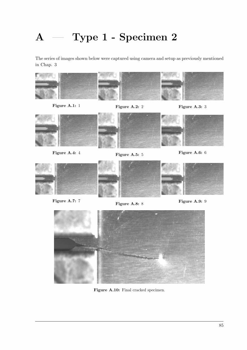
A — Type 1 - Specimen 2
The series of images shown below were captured using camera and setup as previously mentioned
in Chap. 3
Figure A.1: 1 Figure A.2: 2 Figure A.3: 3
Figure A.4: 4 Figure A.5: 5 Figure A.6: 6
Figure A.7: 7Figure A.8: 8
Figure A.9: 9
Figure A.10: Final cracked specimen.
85

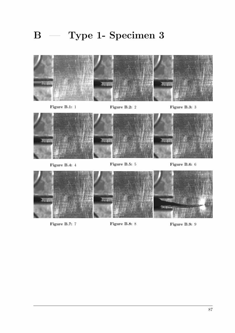
B — Type 1- Specimen 3
Figure B.1: 1 Figure B.2: 2 Figure B.3: 3
Figure B.4: 4 Figure B.5: 5 Figure B.6: 6
Figure B.7: 7 Figure B.8: 8 Figure B.9: 9
87


C — Type 2 - Specimen 1
Figure C.1: 1 Figure C.2: 2 Figure C.3: 3
Figure C.4: 4 Figure C.5: 5 Figure C.6: 6
Figure C.7: 7 Figure C.8: 8 Figure C.9: 9
89


D — Type 2 - Specimen 2
Figure D.1: 1 Figure D.2: 2 Figure D.3: 3
Figure D.4: 4 Figure D.5: 5 Figure D.6: 6
Figure D.7: 7 Figure D.8: 8 Figure D.9: 9
91


E — Type 2 - Specimen 3
Figure E.1: 1 Figure E.2: 2
Figure E.3: 3 Figure E.4: 4
93


F — Type 3 - Specimen 1
Figure F.1: 1 Figure F.2: 2
Figure F.3: 3 Figure F.4: 4
95


G — Type 3 - Specimen 2
Figure G.1: 1 Figure G.2: 2
Figure G.3: 3 Figure G.4: 4
97


H — Type 3 - Specimen 3
Figure H.1: 1 Figure H.2: 2
Figure H.3: 3 Figure H.4: 4
99


I — Type 4 - Specimen 1
Due to unavailability of the camera while performing the experiment for Specimen 1, an image
of only the final cracked specimen was available.
Figure I.1: Final cracked specimen.
101


J — Type 4 - Specimen 3
Figure J.1: 1 Figure J.2: 2
Figure J.3: 3 Figure J.4: 4
Figure J.5: 5 Figure J.6: 6
103
Related Documents