Study of bismuth complexation with amino acids and biologically active molecules Dhuneshan Govender A Dissertation submitted to the Faculty of Science, University of the Witwatersrand, Johannesburg, in fulfilment of the requirements for the degree of Master of Science March 2015

Welcome message from author
This document is posted to help you gain knowledge. Please leave a comment to let me know what you think about it! Share it to your friends and learn new things together.
Transcript

Study of bismuth complexation with amino acids and biologically active molecules
Dhuneshan Govender
A Dissertation submitted to the Faculty of Science, University of the Witwatersrand, Johannesburg, in fulfilment of the requirements for the degree of Master of Science March 2015
ii
DECLARATION
I declare that this Dissertation is my own, unaided work. It is being submitted for the Degree of
Master of Science at the University of the Witwatersrand, Johannesburg. It has not been
submitted before for any degree or examination at any other University.
_______________________________________
(Signature of candidate)
_______________day of _________20________________in_____________

iii
Abstract
Bismuth(III) has been used in the medicinal industry for many years, but its mechanism of
action is not fully understood and there is very little information on thermodynamic and
kinetic parameters for complex formation. Amino acids are the building blocks of life and
so, by initially simply determining the complexing ability of various amino acids with
bismuth, an indication of how bismuth could interact in the body can slowly be
developed and could assist in the eventual development and design of more effective
bismuth containing drugs.
Bi3+ has the ability to form insoluble hydrolysis products which precipitate around pH 2 in
the presence of a background electrolyte and therefore studies need to be conducted
from low pH where it is still soluble. In this study, stability constants have been
determined using polarographic-pH titrations. The sudden drop in current was used to
identify the approximate pH of precipitation of Bi3+ species and the shift in potentials as
pH increased were used to evaluate stability constants. One of the major issues with
employing polarography in low pH regions (below pH 2) is the presence of the diffusion
junction potential which contributes large errors to the measured potentials and
therefore needs to be corrected for. Since KNO3 was used as the supporting electrolyte,
and Bi3+ forms complexes with nitrate as well as hydrolyses at these low pHs,
determination of the free Bi3+ potential (needed to calculate the stability constants) also
had to be determined indirectly.
In order to run the multi-hour polarographic-pH titrations, automated procedures using
NOVA software were developed and validated. Automation of these experiments was key
to ensuring reproducibility of the procedure and all the measurements.

iv
Complex formation studies between Bi3+ and the three amino acids, namely glutamic acid
(Glu), histidine (His) and glutamine (Gln) were conducted in 0.5 M KNO3 solutions at 25⁰C.
It was demonstrated that a very large excess of ligand was required in order for complex
formation to take place. Studies with Glu and His produced fully reversible reduction
waves as required, but that with Gln produced quasi-reversible reduction waves and this
also needed to be accounted for.

v
Acknowledgments
I thank my supervisor, Dr Caren Billing, for her endless support during my experimental
work and for her help during this dissertation.
I thank the School of Chemistry for allowing me to complete my M.Sc. and for the
willingness of all colleagues to assist in times of need.
I thank the NRF for their financial support and allowing me to attend the IC2013
Conference to present part of the work in this study.
I thank my Mother, Sister and Brother who stood by me during the pursuit my M.Sc.

vi
Table of Contents
Abstract i
Acknowledgments v
Table of Contents vi
List of Figures ix
List of Tables xiv
Chapter 1: Introduction
1.1. Properties and Industrial Uses of Bismuth 1
1.2. Bismuth-Medicinal Uses 2
1.3. Bismuth complex formation 5
1.4. Amino Acids 8
1.5. Polarography 11
1.6. Aims 14
Chapter 2: The development of automated procedures using NOVA software to study metal-
ligand complexation
2.1 Introduction 17
2.2 Instrumental Setup 19
2.3 Glass Electrode Calibration Procedure 21
2.4 Development of the NOVA procedure for the polarographic-pH titration 30
2.4.1. Part A 32
2.4.2. Part B 42
2.5 References 44
Chapter 3: Experimental Procedures
3.1. Introduction 45
3.2. Glass Electrode Calibration 45
3.3. Polarographic Studies 48
3.3.1 Polarographic-pH titrations: Experiments in the absence of ligand 50
3.3.2. Polarographic-pH titrations: Experiments in the presence of ligand 52
3.3.3 Fitting the polarograms 53

vii
3.3.4. Calculation of formation constants for Bi3+-amino acid complexes 55
3.4. Investigating the bismuth precipitation product from a nitric acid solution 56
3.5. X-Ray Diffraction 56
3.6. References 59
Chapter 4: Initial Bi3+ complexation studies
4.1. Introduction 60
4.2. Glass Electrode Calibration and determination of pH values. 61
4.3. Calculation of the diffusion junction potential, Ej 64
4.4. Precipitation of Bi3+-hydroxy nitrate species 66
4.5. Determination of the free Bi3+ potential, E(Bifree) 67
4.6. Initial Bi3+-amino acid complexation studies 72
4.8. Powder X-ray Diffraction of Bi3+precipitate 77
4.7. Conclusion 79
4.8. References 81
Chapter 5: Bi3+-Glutamic Acid Complexation
5.1 Introduction 82
5.2 Aim 84
5.3 Experimental 84
5.4 Results 84
5.4.1. Modelling the Pb2+-Glu system 84
5.4.2 Bi3+ complexation with Glutamic acid 87
5.5 Conclusion 102
5.6 References 104
Chapter 6: Bi3+-Histidine Complexation
6.1. Introduction 105
6.2. Aim 107
6.3. Experimental 108
6.4. Results and discussion 108
6.4.1. Initial data inspection 108
6.4.2 Slope analysis 113

viii
6.4.3. Determining Bi-His complexes and respective log β 115
6.5 Conclusion 125
6.6. References 127
Chapter 7: Bi3+-Glutamine Complexation
7.1. Introduction 128
7.2. Aim 130
7.3. Experimental 131
7.4. Results and discussion 131
7.4.1. Initial data inspection 131
7.4.2 Slope analysis 138
7.4.3 Determining Bi-Gln complexes and respective log β 141
7.5 Conclusion 145
7. 6 References 147
Chapter 8: Final Conclusion 148
Appendices 152
ix
List of Figures
1.1: The structures of (a) bismuth subsalicylate[7a, 7c]
and (b) colloidal bismuth subcitrate (CBS).
1.2: General formula for α-amino acids, showing the deprotonated and protonated forms. The sidechain R
varies depending on the amino acid type and these are given in Table 1.2.
1.3: A typical direct current polarogram indicating the wave produced, the diffusion limited current, Id, the
half wave potential, E1/2, and the residual current.
1.4: An illustration of Ej whereby the hydrogen ions move much faster across the reference electrode frit
due to its high mobility compared to the K+ ions. The result is a surplus of positive charge at the inner
face of the reference electrode and negative charge on the outer face of the reference electrode.
2.1: Schematic of the general instrumental setup.
2.2: Schematic of the instrumental setup during the glass electrode calibration procedure.
2.3: Initial lines of NOVA code showing instrumentation and signals to be measured during the glass
electrode calibration procedure.
2.4: Commands for initialising devices and controlling the stirring and purging.
2.5: Autolab Control tab showing the method by which the purger is turned on and allowed to continuously
purge throughout the experiment.
2.6: Repeat for each value command tree showing the parameters used for measuring the signals during
the glass electrode calibration.
2.7: The custom commands used to plot the measured data during the experiment, and the commands
used to perform calculations on the measured signals and save the data.
2.8: The three repeat loops in the glass electrode calibration to allow for longer equilibration times before
measurements made close to the end point of the titration.
2.9: Potential difference vs volume added plot for the titration of 0.9945 M HNO3 with 0.1012 M KOH at
25.0 ⁰C. The end point region is highlighted to show the sharp change in gradient associated with
measurement of potential difference, hence a longer equilibration time is needed.
2.10: Schematic of the instrumental setup during the polarographic-pH titration procedure together with a
flow diagram of the procedure.
2.11: Initial steps in the procedure used for Part A of the polarographic-pH titration.
2.12: Various repeat loop commands were utilized to run the required experiment, namely the repeat for
each value command as the primary tree command and the repeat n times command used to control
the Dosino additions and run the pH threshold test.
2.13: Command tree showing the pH measurement process. The nested procedure command for the pH
threshold test is also shown.
2.14: The layout of the pre-programmed Sampled DC Polarography command.
2.15: The parameters used for the DC polarogram as inputted into the NOVA software.
x
2.16: Highlighting the link (square brackets on the right) between the measured signals and the graphs
plotted as well as the data saved in ASCII files.
2.17: Highlighting the calculate signal commands which were linked to columns in ASCII data files for
saving.
2.18: Closing commands for the validation of the NOVA procedure.
2.19: Repeat loops were utilised in the same manner as Part A. Part B was set to begin at the pH at which
part A ended, therefore the first value in the loop command was pH 2.3.
2.20: In Part B the export ASCII data commands are highlighted to emphasise that the directory and file
names for the respective data must be changed.
2.21: Closing Commands for the validation of Part B.
3.1: Typical DC polarogram showing the reduction of Bi3+
and Tl+ -
and H2. [Bi3+
] = 9.95 x 10⁻⁶
M, [Tl+] = 3.98 x
10-5
M, µ = 0.5 M, T = 25 C
3.2: An example of an ECFC and a refined CCFC for a Bi3+
-amino acid system.
3.3: Schematic of the PXRD process whereby X-rays are emitted from an X-Ray Source and travel toward
and reflect of a crystal/crystalline powder sample. The reflected X-rays are then detected and the
structure of the complex must be calculated from the respective intensities and 2θ values which are
present in the spectrum.[13]
4.1: Potential difference at the glass electrode vs calculated pH for 0.1 M HNO3 solution titrated with 0.1 M
KOH solution (both in 0.4 M KNO3) at 25.0 ⁰C.
4.2: Glass electrode calibration curve in pH range 1 - 2 showing both the linear trendline (black) and the
quadratic trendline (red) fitted.
4.3: Half-wave potentials of Tl+ vs pH showing the determination of Ej and E(TlFree). ([Tl
+] = 1 x 10
-5 M).
4.4: Calculated Ej vs pH for Tl+ from a polarographic-pH titration.
4.5: Id values for Bi3+
vs pH for titrations with no ligand added showing dilution and then precipitation at pH
~2.6. [Bi3+
] = 1 x 10⁻⁵
M, µ= 0.5 M NO3-.
4.6: Species distribution diagram of Bi3+
nitrate and hydroxide species for [Bi3+
] = 1 x 10⁻⁵
M and [NO3-] =
0.5 M at 25 ⁰C.
4.7: E1/2 values of Bi3+
vs pH showing EJ corrections, as well as corrections for shifts due to formation of Bi3+
nitrate and hydroxide species or just Bi3+
hydroxide species. [Bi3+
] = 1 x 10⁻⁵
M and µ = 0.5 M.
4.8: Diffusion limited current vs pH for () Glutamic Acid, () Glycine, () Methionine and ()Glutamine at
[ligand]:[metal] = 100. [Bi3+
] = 1 x 10⁻⁵
M.
4.9: Ej corrected E1/2 for Bi3+
vs pH plot for experiments where [L]:[M] 100 and L refers to () Glutamic
Acid, () Glycine, () Methionine and () Glutamine. () shows values in absence of ligand where
Bi3+
is only present ( [Bi3+
] = 1 x 10⁻⁵
M).
4.10: Various thiolate ligands attached to the bismuth metal ion shows its ability to vary coordination
numbers for various ligands.[12b]
xi
4.11. PXRD pattern collected from isolated precipitate as described by Chapter 3.4. The calculated PXRD
pattern from single crystal data by Lazarini[7]
, showing Bi6O5(OH)3(NO3)5(H2O)3, is superimposed onto
the pattern.
5.1: Structure of fully protonated glutamic acid indicating the respective pKa values.[2]
5.2: Structure of fully protonated glutaric acid.
5.3: Species distribution diagram for the Pb2+
-Glu system where [Glu]:[Pb2+
] = 100 and [Pb2+
] = 1 x 10⁻⁵
M at
25⁰C.
5.4: Species distribution diagram for the Pb2+
-Glu system where [Glu]:[Pb2+
] = 1000 and [Pb2+
] = 1 x 10⁻⁵
M
at 25⁰C.
5.5: Species distribution diagram for the Pb2+
-Glu system where [Glu]:[Pb2+
] = 100 and [Pb2+
] = 1 x 10⁻⁴
M at
25⁰C.
5.6: Species distribution diagram of glutamic acid in aqueous solutions at 25⁰C.
5.7: Id vs pH for Bi3+
from solutions with [Glu]:[Bi3+
] = 2000 and [ Bi3+
] = 1 x 10⁻⁵
M.
5.8: E1/2 for Bi3+
vs pH with [Glu]:[Bi3+
] = 2000 showing both the experimental and Ej corrected E1/2 values.
5.9: E1/2 for Bi3+
vs pH with () no ligand added and () [Glu]:[Bi3+
] = 2000.
5.10: E1/2 for Bi3+
vs pH for the three experiments where [Glu]:[Bi3+
] = () 2000, () 3000 and () 5000.
5.11: Graph indicating the extent of reversibility, ɣ, vs pH for the Bi3+
polarograms for [Glu]:[Bi3+
] = ()
2000, () 3000 and () 5000.
5.12: Diagram illustrating the predominant ligand species in a specific pH range and the calculated slopes
which indicate the type of complex which could be present in solution.
5.13: Ej corrected E1/2 for Bi3+
vs pH with [Glu]:[Bi3+
] = 5000. Slope analysis has been completed in different
pH ranges in order to help predict which Bi3+
-Glu complexes are present in solution.
5.14: Species distribution diagram of Bi3+
species vs pH in a NO3¬ solution at 25⁰C in pH range 1 - 5. [Bi
3+] = 1
x 10-5
M.
5.15: CCFC and ECFC for a Bi3+
-Glu complexes where [Glu]:[Bi3+
] = 2000.
5.16: CCFC and ECFC for a Bi3+
-Glu complexes where [Glu]:[Bi3+
] = 3000.
5.17: CCFC and ECFC for a Bi3+
-Glu complexes where [Glu]:[Bi3+
] = 5000.
5.18: Species distribution diagram for the Bi3+
-Glu system where [Glu]:[Bi3+
] = 5000, [Bi3+
] = 1 x 10⁻⁵
M and
[NO3-] =0.5 M. The formation constant used were those calculated using the true E(BiFree).
5.19: Species distribution diagram for the Bi3+
-Glu system where [Glu]:[Bi3+
] = 5000, [Bi3+
] = 1 x 10⁻⁵
M and
[NO3-] =0.5 M. The formation constant used were those calculated using E(BiFree)OH.
5.20: Proposed structure of the Bi-Glu-H2 complex.
5.21: An unlikely structure for the Bi-Glu-H complex.
5.22: Suggested structure for the Bi-Glu-H complex.
6.1: Fully protonated Histidine with pKa1
= 1.8, pKa2 = 6.11 and pKa
3 = 9.1 at 0.5 M ionic strength and
25⁰C.[2]

xii
6.2: Structure of the imidazole ring which forms part of histidine.
6.3: The reaction showing the removal of the carboxyl moiety in His to form histamine. [12]
6.4: Diffusion limited current vs pH for [His]:[Bi3+
] = 5000, [Bi3+
] = 1 x 10⁻⁵
M, μ = 0.5 M.
6.5: Diffusion limited current vs pH for [His]:[Bi3+
] = 7000, [Bi3+
] = 1 x 10⁻⁵
M, μ = 0.5 M.
6.6: Experimental polarograms from the polarographic-pH titration conducted with [His]:[Bi3+
] = 7000 at
different pHs, namely, a) 2.0, b) 2.3, c) 2.4, d) 2.7 and e) 3.6.
6.7: ɣ vs pH for the Bi3+
at the three different [His]:[Bi3+
] of () 4000, () 5000 and () 7000.
6.8: Ej corrected E1/2 vs pH for Bi3+
containing His. [His]:[Bi3+
] = () 4000, () 5000 and () 7000.
6.9: Diagram of the predominant ligand species in specific pH ranges and the calculated slopes which
indicate the type of complex which could be present in solution.
6.10: Slope analysis on the Ej corrected E1/2 for Bi3+
vs pH plot with [His]:[Bi3+
] = 4000.
6.11: Slope analysis on the Ej corrected E1/2 for Bi3+
vs pH plot with [His]:[Bi3+
] = 7000.
6.12: The ECFCs calculated using either E(Bifree) and E(Bifree)OH values and the CCFCs determined by including
the Bi-His-H2 and Bi-His-H complexes in the species model.
6.13: The ECFC (points) calculated using E(Bifree)OH and the CCFCs (lines) determined taking only the Bi-His-H
complex or only the Bi-His-H2 into account at a time.
6.14: Species distribution diagram for [His]:[Bi3+
] = 4000, [Bi3+
] = 1 x 10⁻⁵
M and [NO3-] =0.5 M. The log β
values were calculated using a) E(Bifree) and b) E(Bifree)OH and the values used are for the 4000 ratio only
(Table 6.1).
6.15: Species distribution diagram for [His]:[Bi3+
] = 5000, [Bi3+
] = 1 x 10⁻⁵
M and [NO3-] =0.5 M. The log β
values were calculated using a) E(Bifree) and b) E(Bifree)OH and the values used are for the 5000 ratio only
(Table 6.1).
6.16: The ECFCs calculated using the true E(Bifree) value and the corresponding CCFCs (which produced the
results in Table 6.1) for the experiments at the [His]:[Bi3+
] values indicated.
6.17: Species distribution diagrams for [His]:[Bi3+
] = 7000, [Bi3+
] = 1 x 10⁻⁵
M and [NO3-] =0.5 M.The log β
values were calculated using a) E(Bifree) and b) E(Bifree)OH and the values used are for the 4000 ratio for
MLH2, the 7000 ratio for ML and the average for the 4000 and 7000 ratios for MLH (Table 6.1).
7.1: Structure of fully protonated Gln.
7.2: Id vs pH for Bi3+
with Gln added Where [Gln]:[Bi3+
] = (X) 2000, () 3000 () 4000 and () 5000. Only
data before precipitation is shown.
7.3: Ej corrected E1/2 of Bi3+
vs pH with Gln added. [Gln]:[Bi3+
] = () 2000, () 3000, () 4000 and () 5000.
7.4: Ej corrected E1/2 of Bi3+
vs pH with [Gln]:[Bi3+
] = () 3000 and () 5000 and also in the absence of Gln
().
7.5: Values of ɣ indicating reversibility vs pH for [Gln]:[Bi3+
] = () 2000, () 3000, () 4000 and () 5000.
7.6: DC polarograms for [Gln]:[Bi3+
] = 4000 indicating the decrease in reversibility of electron transfer
illustrated by the drawn out reduction wave.
xiii
7.7: A quasi-reversible polarogram where the slow electron transfer region is highlighted and reversible fit
is superimposed where Id and capacitance was fixed and ɣ set equal to 1.
7.8: Graph showing that the () quasi-reversible E1/2 and () reversible E1/2 values for Bi3+
for [Gln]:[Bi3+]
= 4000 do not differ greatly.
7.9: Diagram of the predominant ligand species in a specific pH range and the calculated slopes which
indicate the type of complex which could be present in solution.
7.10: Slope analysis of the Ej corrected reversible E1/2 of Bi3+
where [Glu]:[Bi3+
] = 5000 which indicates the
formation of two types of complexes, Bi-Gln-H and Bi-Gln.
7.11: Shift in E1/2 of Bi3+
vs pH for [Gln]:[Bi3+
] = () 2000, () 3000, () 4000 and () 5000.
7.12: The ECFCs (points) (calculated using the true E(Bifree)OH and the corresponding CCFCs (lines) for
[Gln]:[Bi3+
] = () 2000 and () 5000.
7.13: Species distribution diagrams for [Gln]:[Bi3+
] = (a) 3000 and (b) 5000, where log β values were
calculated using the true E(BiFree) as given in Table 7.1
xiv
List of Tables
1.1: Table showing different ligands attached to the Bismuth metal ions with their respective log K
values.[4]
1.2: The twenty common amino acids with the structural representations of their respective sidechains.[32]
1.3: Log β values for various metal ions with aspartic and glutamic acids at 25C and in 0.1 M NaClO4
solutions. [34]
4.1: Acceptable slope ranges for the calibration of glass electrode as described by Billing and Cukrowski.[4]
4.2: Log β values for hydrolysis of Bi3+
in solution at 25 ⁰C, µ = 0.5 M.[3b]
4.3: Log β values for the formation of Bi3+
nitrate species at 25 ⁰C.[9]
4.4: The E(Mfree) values for Bi3+
and Tl+, as well as the ΔE(Mfree) values.
5.1: Calculated log β values for the formation of the Bi3+
-Glu complexes using using both the E(Bifree) and
E(Bifree)OH values and the 3D-CFC software. (Charges were omitted in equilibria reactions.)
6.1: Calculated log β values for the formation of the Bi3+
-His complexes using using both the E(Bifree) values
and the 3D-CFC software. (Charges were omitted in equilibria reactions.)
7.1: Table showing the log β values for the respective Bi-Gln complexes (at 0.5 M ionic strength and 25C)
using 3D-CFC[11]
. “Rev” was calculated using the reversible E1/2 values and “Quasi” the quasi-reversible
E1/2 values.
8.1: Log K values for the formation of Bi3+
amino acid complexes in solution at 25 ⁰C and µ = 0.5 M (KNO3).
The values in italics indicate which constants give the more representative values for the particular
species when using the two E(BiFree) values in the calculations.
A 1.1: Experimental parameters used in NOVA for the polarographic- pH titrations.
A 1.2: Initial parameter estimates for the fitting of Bi3+
and Tl+ DC polarograms
A 1.3: Instrument settings for the Bruker D2 Phaser
A 2.1: Pb hydroxide species log β for species distribution diagrams plotted in Chapter 5 as a comparison to
Bi3+
-Glu.[1]
A 2.2: Ga3+
log β for complexation with hydroxide in 0.3M NO3 solutions at 25⁰C.[1]

1
Chapter 1: Introduction
1.1. Properties and Industrial Uses of Bismuth
Bismuth is the heaviest of the Group 15 elements with an ionic and covalent radius of
1.08 Å (for Bi3+) and 1.52 Å, respectively.[1] Bismuth forms the least stable 5+ oxidation
state within the group, with its most stable form being Bi3+.[1] Due to the high reactivity of
bismuth in nature, it is almost never found in its pure state, but rather occurs as an oxide
or sulphide. The bismuth crystals found in nature are often very aesthetically pleasing
due to the unique patterns associated with the different types of crystals. This causes
different wavelengths of light to be seen, thus displaying a rainbow of colours, however,
the bismuth crystal is generally found with a white, silver-pink hue.[2]
Elemental bismuth is one of very few substances where the liquid phase is more dense
than its solid phase (such as antimony and water).[2] The property of expanding (by
approximately 3%) when cooling is responsible for much of bismuth’s commercial uses
such as low-melting typesetting alloys and in soldering or plumbing (for joining pipes),
where it compensates for the contraction of the other alloying components.[2-3] Bismuth
alloys have been known to have varying melting points[3-4] with some comparable to that
of ice, hence a bismuth-alloy casting can be covered by plastic or other material to form
intricate machine parts. The bismuth-alloy core is simply removed by melting it in hot
water and pouring it out. The use of low-melting bismuth alloys is widespread in fire
fighting sprinkler systems in buildings where the bismuth alloy trigger system melts when
heat is applied to it, causing the seal to break and the water to extinguish the fire.
More recently, there have been studies focused on bismuth in its nanoparticle state.
Bismuth nanoparticles (BNPs) have been of great interest due to their use in a variety of
fields, from catalysis to biosensing.[5] Due to the high surface area of BNPs, they have also
been extensively studied for their use in determining the concentrations of trace
elements found in the environment and hence the extent to which metals have
contaminated a certain area.[6]
2
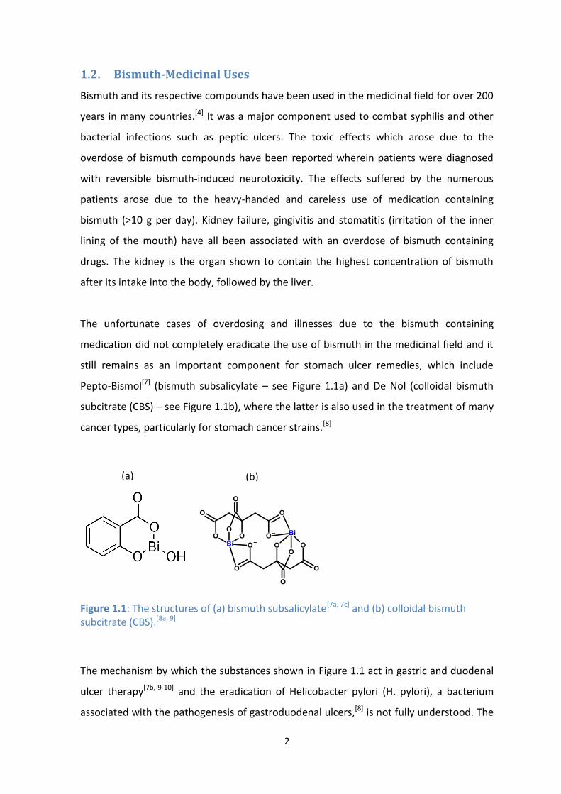
1.2. Bismuth-Medicinal Uses
Bismuth and its respective compounds have been used in the medicinal field for over 200
years in many countries.[4] It was a major component used to combat syphilis and other
bacterial infections such as peptic ulcers. The toxic effects which arose due to the
overdose of bismuth compounds have been reported wherein patients were diagnosed
with reversible bismuth-induced neurotoxicity. The effects suffered by the numerous
patients arose due to the heavy-handed and careless use of medication containing
bismuth (>10 g per day). Kidney failure, gingivitis and stomatitis (irritation of the inner
lining of the mouth) have all been associated with an overdose of bismuth containing
drugs. The kidney is the organ shown to contain the highest concentration of bismuth
after its intake into the body, followed by the liver.
The unfortunate cases of overdosing and illnesses due to the bismuth containing
medication did not completely eradicate the use of bismuth in the medicinal field and it
still remains as an important component for stomach ulcer remedies, which include
Pepto-Bismol[7] (bismuth subsalicylate – see Figure 1.1a) and De Nol (colloidal bismuth
subcitrate (CBS) – see Figure 1.1b), where the latter is also used in the treatment of many
cancer types, particularly for stomach cancer strains.[8]
Figure 1.1: The structures of (a) bismuth subsalicylate[7a, 7c] and (b) colloidal bismuth subcitrate (CBS).[8a, 9]
The mechanism by which the substances shown in Figure 1.1 act in gastric and duodenal
ulcer therapy[7b, 9-10] and the eradication of Helicobacter pylori (H. pylori), a bacterium
associated with the pathogenesis of gastroduodenal ulcers,[8] is not fully understood. The
(a) (b)
3
standard pH of the stomach is approximately pH 1.3-3.5.[11] It has been suggested[10c] that
bismuth’s ease in hydrolyzing (as will be discussed in detail in section 1.3) and
precipitating plays an important role in the mechanism. The precipitated bismuth-
hydroxy products and the antimicrobial active, such as salicylate, attach to the surface of
the ulcer or affected area.[10c] Alternatively, the longer remission times achieved with
bismuth therapies are probably due to eradication of the organism by bismuth. Clinical
studies with colloidal bismuth subcitrate and bismuth subsalisylate have shown that
patients treated with bismuth alone experience a slower relapse than patients treated
with other ulcer-healing agents[12] possibly due to the bactericidal action of these
complexes against H. pylori.
Rantidine bismuth citrate (RBC) is another type of medicinal complex which has been
used extensively in the treatment of stomach ulcers and the structure may be closely
related to that of Na2[Bi2(citrate)].7H2O, which contains highly stable dimeric units of
[Bi(cit)2Bi]2.[13] It is the potential action of these bismuth citrate units to inhibit the uptake
of Fe(III) into some bacteria, thereby allowing the eradication of the bacteria. It is also
possible to envisage dimeric bismuth citrate units inhibiting the uptake of Fe(II) into some
types of bacteria, since Fe(II) also forms a dimeric citrate complex.[14]
There have also been reports of organic bismuth thiolates having anti-tumour capabilities
and reducing the toxicity of some platinum-based anti-cancer agents.[15] Recent in-vitro
studies have shown bismuth to be an active HIV-I inhibitor[16], from chronically infected
H9 cells.[17] Although an interesting observation, the research with bismuth containing
drugs against HIV is at a very premature stage, however, the proven medicinal
characteristics of bismuth cannot be ignored and therefore could result in an effective
HIV drug in due time.
Due to the formation of radioactive isotopes, bismuth can also be used in radioactive
therapy. 212Bi is known to be a strong alpha-particle emitter with a short half-life of one
hour.[18] The isotope has been extensively used in targeted radioactive therapy against
cancer once it has been complexed to ligands such as diethylene-triaminepentaacetate
4
(DTPA) and 1,4,7,10-tetra-azacyclododecane-1,4,7,10-tetraacetate (DOTA) and then
further complexed with monoclonal antibodies.[19]
1.3. Bismuth complex formation
Pearson’s hard soft acid base (HSAB) theory[20] has been widely used to classify elements
according to characteristics relating to their atomic centres radii, charge, number of
empty orbitals in the valence shell, electronegativity, solvation ability and whether they
possess high or low energy HOMOs or LUMOs. According to Pearson’s theory,[20] soft
metal ions prefer ligands with soft donor atoms and hard metal ions prefer HSAB ligands
with hard donor atoms. Bi3+ is thus classified as borderline[20-21] and illustrates that it is
able to form many different complexes with different ligands.[4, 22] These complexes show
many varying characteristics and impart stability onto the metal ion or in some cases
result in it becoming more reactive, depending on the type of ligand which complexes.
Bismuth is able to complex with glutathione (GSH) forming the complex [Bi(H-GSH)3].
Binding/Formation constants have been reported from studies[23] of competition
reactions between EDTA (logK 29.6 ) and GSH(log 31.4)[4] for the ML3 species. Other types
of ligands studied[4] which have been shown to exhibit complexing behaviour with
bismuth include allyls, alkoxides, hydroxides and thiol containing compounds.
The table below indicates formation constants of other types of ligands which have been
studied for the formation of ML species, and report their respective log K1 values.
5
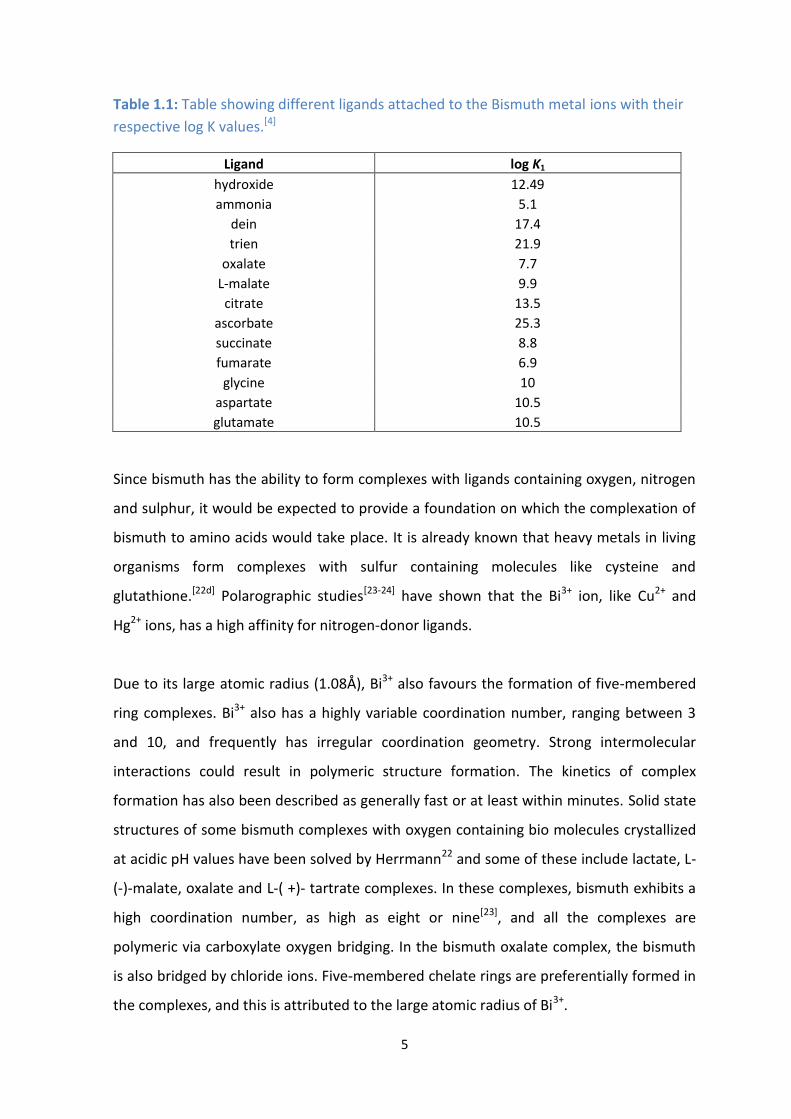
Table 1.1: Table showing different ligands attached to the Bismuth metal ions with their
respective log K values.[4]
Ligand log K1
hydroxide 12.49
ammonia 5.1
dein 17.4
trien 21.9
oxalate 7.7
L-malate 9.9
citrate 13.5
ascorbate 25.3
succinate 8.8
fumarate 6.9
glycine 10
aspartate 10.5
glutamate 10.5
Since bismuth has the ability to form complexes with ligands containing oxygen, nitrogen
and sulphur, it would be expected to provide a foundation on which the complexation of
bismuth to amino acids would take place. It is already known that heavy metals in living
organisms form complexes with sulfur containing molecules like cysteine and
glutathione.[22d] Polarographic studies[23-24] have shown that the Bi3+ ion, like Cu2+ and
Hg2+ ions, has a high affinity for nitrogen-donor ligands.
Due to its large atomic radius (1.08 ), Bi3+ also favours the formation of five-membered
ring complexes. Bi3+ also has a highly variable coordination number, ranging between 3
and 10, and frequently has irregular coordination geometry. Strong intermolecular
interactions could result in polymeric structure formation. The kinetics of complex
formation has also been described as generally fast or at least within minutes. Solid state
structures of some bismuth complexes with oxygen containing bio molecules crystallized
at acidic pH values have been solved by Herrmann22 and some of these include lactate, L-
(-)-malate, oxalate and L-( +)- tartrate complexes. In these complexes, bismuth exhibits a
high coordination number, as high as eight or nine[23], and all the complexes are
polymeric via carboxylate oxygen bridging. In the bismuth oxalate complex, the bismuth
is also bridged by chloride ions. Five-membered chelate rings are preferentially formed in
the complexes, and this is attributed to the large atomic radius of Bi3+.

6
In aqueous solutions Bi3+ readily hydrolyses, thus the formation of Bi3+-hydroxide
complexes are particularly difficult to avoid, even in very acidic solutions. To increase the
complexity of the system, it has been found that some of the Bi-OH complexes formed
are insoluble and precipitate at pH >2. Early work by Granier and Sillen[25] laid the
foundation for the studies of bismuth hydrolysis. Initially the studies showed that not
only complexes of the form Bi-OHn occurred in solution, but it was suggested that
polynuclear species such as Bi2O4+, Bi3O25+ and Bi4O3
6+ also existed. Although a
breakthrough at the time, improvements in analytical methods and minimizations in
errors of the electrodes used showed that the main polynuclear species formed under
the conditions used was Bi6(OH)126+.[26] In recent times the acceptance of the Bi9(OH)n,
where n =20, 21 and 22 are formed in aqueous solutions. As with all chemical reactions
the ability for a complex to form depends on the reaction conditions. Studies by Olin[27],
Bidleman[28] and later by Hataye[29] were able to show that in very dilute solutions of the
hexamer was not present in solution, but rather the mononuclear Bi(OH)2+ species was
present. Since Bi3+ hydrolysis will always be a factor in aqueous solutions, methods used
to determine Bi3+-ligand formation constants must take these bismuth hydroxide
complexes into account. The methodology used in this work will be discussed in Chapter
4.
The background or supporting electrolyte used in metal-ligand studies is of relatively
great importance when determining stability constants as they are used in high
concentrations to maintain ionic strengths of solutions. Sodium or potassium
perchlorates and nitrates are the most commonly used background electrolytes.[30] These
are used as they are weakly complexing and so should not have a significant affect in
metal-ligand complexation. Studies by Maroni and Spiro[31] and Hataye et al.[29] all agreed
that perchlorate is not bound strongly enough to the hydrolysed bismuth complex and as
such allowed close examination of the bismuth-hydroxide products formed. Nitrate
backgrounds were also studied by Maroni and Spiro[31] who concluded that the major
complexes formed were Bi(NO3)n3-n, Bi(OH)(NO3)n
2-n, Bi(OH)2(NO3)n1-n and Bi(OH)3(NO3)n
–n.
At pH greater than 2, bismuth tends to become highly insoluble due to the formation of
Bi-hydroxy-nitrate species or Bi3+ hexamers. The formation of these species at such a low
pH limits the window in which solution based studies can be conducted as significant

7
complexation must occur at pH less than 2, making it susceptible to many errors which
will be discussed later.
1.4. Amino Acids
Amino acids are the building blocks of life as they make up all proteins and exist in organs
which are important for humans and animals to survive. α-amino acids are naturally
occurring and are made up of an amine group which is located on the carbon atom
immediately adjacent to the carboxylic acid group and a sidechain denoted by R in Figure
1.2 (Table 1.2) indicates the structure of R-sidechain. Humans are able to synthesize
approximately ten of these amino acids in amounts which are vital for survival. The other
ten, which must be supplemented via ingestion, are described as essential amino acids
because they are considered necessary components in our diet for energy production. All
proteins contain one or more of the essential amino acids. During the formation of
proteins and enzymes, the amino acids are joined together via peptide bonds to form
polypeptide chains. The grouping together of polypeptide chains by sulfide bridges then
allows the formation of the specific protein.
R
Figure 1.2: General formula for α-amino acids, showing the deprotonated and protonated forms. The sidechain R varies depending on the amino acid type and these are given in Table 1.2.
+ H+
- H+
⇄
+ H+
- H+
⇄
R R

8
Table 1.2: The twenty common amino acids with the structural representations of their
respective sidechains.[32]
Amino Acid Sidechain Amino Acid Sidechain
Glycine H
Threonine HC(OH)-CH3
Alanine CH3
Asparagine CH2-C(O)-NH2
Valine CH-(CH3)2
Glutamine CH2-CH2-C(O)-NH2
Leucine CH2-CH-(CH3)2
Tyrosine
Isoleucine C(CH3)CH2CH3
Cysteine CH2-SH
Methionine CH2-CH2-S-CH3
Lysine (CH2)4-NH3+
Proline
Arginine
Phenylalanine
Histidine
Tryptophan
Aspartic Acid CH2-COOH
Serine CH2-OH Glutamic Acid CH2-CH2-COOH
As can be seen in Figure 1.2, the amino acid skeleton has a central carbon atom,
surrounded by 4 different sidechains (except in the case of glycine) which makes the
amino acid chiral. A chiral molecule has no plane of symmetry and is therefore not
superimposable on its mirror image. It can exist in two forms, right-handed or left-
handed, defined by the term enantiomer. The chiral character of an amino acid allows it
to be utilized in a large number of important chemical reactions in the human body.
Proteins and enzymes are highly selective molecules. The chirality of the amino acid
constituents thus allows their selectivity to be tailor made only for the substance they are
interacting with, ensuring the reactions which are taking place are both optimal and
correct. The different sidechain moieties occurring in amino acids allow them to perform
a multitude of functions, hence their biological importance.
9
From Figure 1.2 it is noted that the amino acids contain at least two sites available for
complexation. The amino acid skeleton has both O and N donor ligands and, depending
on the R-sidechain, an additional donor atom could be present. The pKa of the donor
atoms are dependent on the type of sidechain present on the amino acid which contain
the electron donating or withdrawing groups. The complexation of Bi3+ with amino acids
has been reported, firstly for the use of biosensing and secondly as more efficient drug
carrying molecules.[4, 22a, 33] Although some studies on complex formation between Bi3+
and amino acids have been looked at before, very few formation constants have been
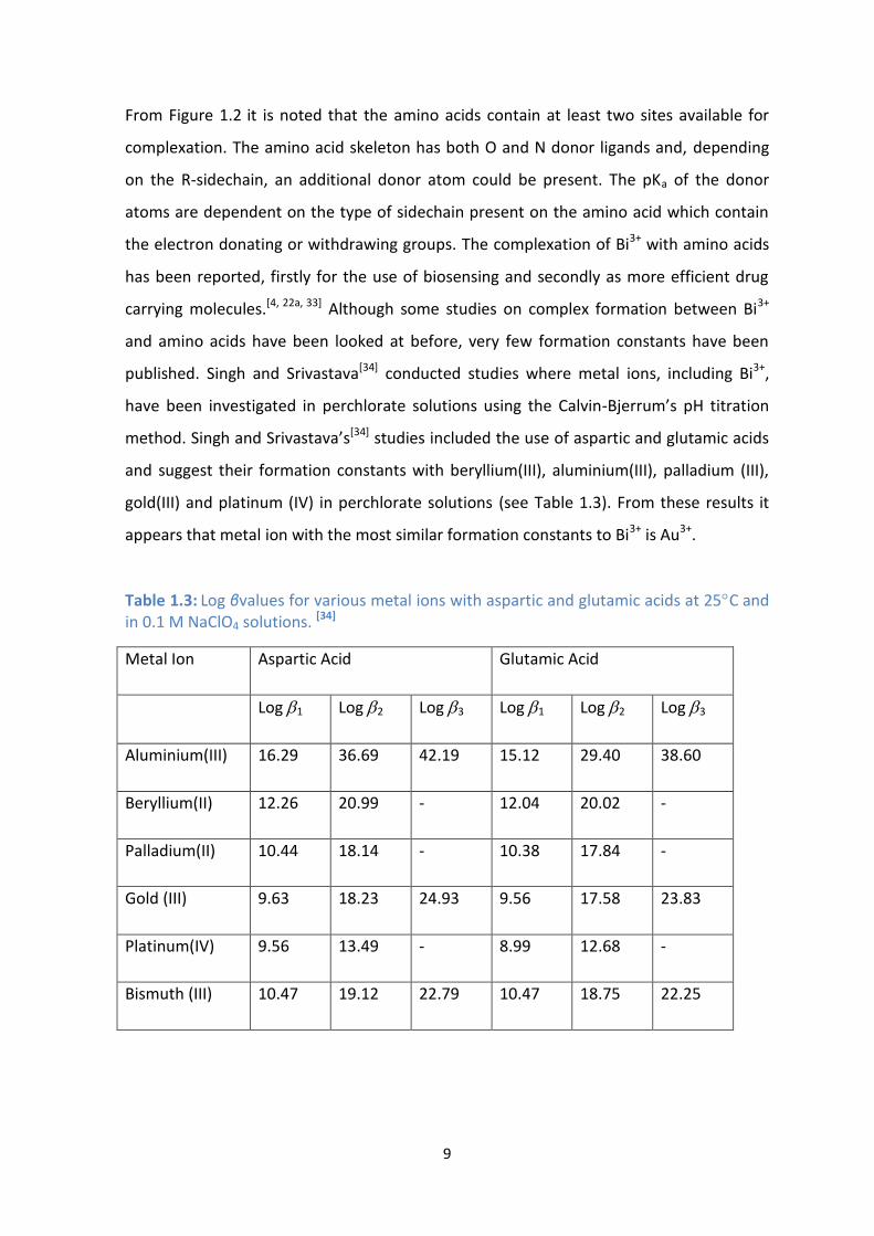
published. Singh and Srivastava[34] conducted studies where metal ions, including Bi3+,
have been investigated in perchlorate solutions using the Calvin-Bjerrum’s pH titration
method. Singh and Srivastava’s[34] studies included the use of aspartic and glutamic acids
and suggest their formation constants with beryllium(III), aluminium(III), palladium (III),
gold(III) and platinum (IV) in perchlorate solutions (see Table 1.3). From these results it
appears that metal ion with the most similar formation constants to Bi3+ is Au3+.
Table 1.3: Log βvalues for various metal ions with aspartic and glutamic acids at 25C and in 0.1 M NaClO4 solutions. [34]
Metal Ion Aspartic Acid Glutamic Acid
Log 1 Log 2 Log 3 Log 1 Log 2 Log 3
Aluminium(III) 16.29 36.69 42.19 15.12 29.40 38.60
Beryllium(II) 12.26 20.99 - 12.04 20.02 -
Palladium(II) 10.44 18.14 - 10.38 17.84 -
Gold (III) 9.63 18.23 24.93 9.56 17.58 23.83
Platinum(IV) 9.56 13.49 - 8.99 12.68 -
Bismuth (III) 10.47 19.12 22.79 10.47 18.75 22.25

10
1.5. Polarography
Polarography is an electroanalytical technique invented by Jaroslav Heyrovsky in 1929.[35]
It allows the analysis of the effect that an applied potential at a dropping mercury
electrode (DME) in an electrolytic cell has on the current flowing in the cell. Varying the
potential at the electrode results in the oxidation or reduction of the electro-active
species in solution provided it occurs in the potential region of interest; this results in an
increase in current and hence a peak or wave on the polarogram (depending on which
electrochemical technique is used). Different electro-active species have characteristic
reduction potentials and thus polarography also gives an indication as to what electro-
active species is present in solution. Due to the fact that the transfer of electrons results
in an increase in current, the higher the concentration of the electro-active species
present in solution (and hence at the electrode surface) the greater the current.
There are three electrodes in a polarographic cell, namely the reference electrode,
counter electrode and working electrode. The reference electrode facilitates
measurement of the potential at the working electrode. The counter electrode acts as
either the anode or cathode (the opposite of the working electrode) to complete the
circuit and allow electron flow to counteract the charge experienced by the working
electrode. In polarography, the working electrode used is a DME. The DME provides a
fresh mercury drop, and thus a new surface for the electrode reaction to occur, at each
potential step. This ensures that there are no remnants from previous reactions which
may be left on it.
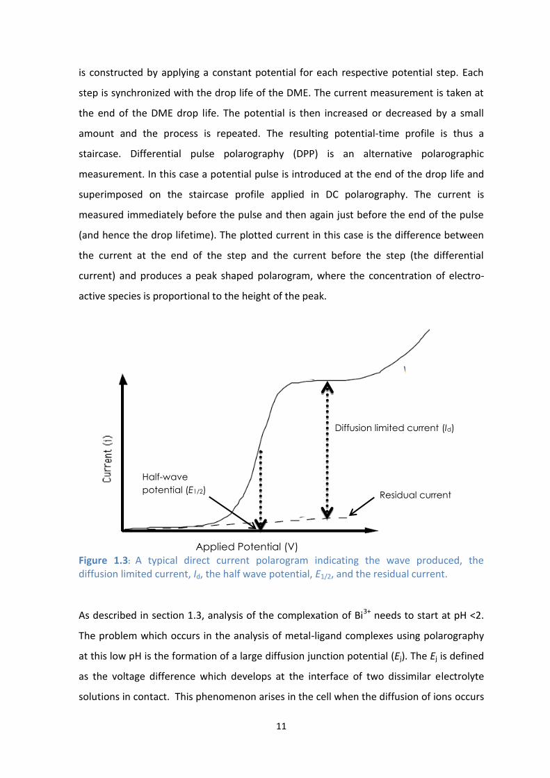
A direct current (DC) polarogram has an S-shaped curve as can be seen in Figure 1.3 At
low overpotentials, a non-faradaic current is present, but as the applied potential
increases there is a sharp increase in the current which indicates the oxidation or
reduction of an electro-active species depending whether the potential is moving in a
positive or negative direction, respectively. The diffusion limited current, Id, is the
difference between the current at the plateau of the wave and the residual or non-
faradaic current. The half-wave potential, E1/2, is the potential midway up the wave and
this value indicates the type of electro-active species being oxidized or reduced under
specific reaction conditions. DC polarography is defined as the physico-chemical
technique based on the recording of current vs voltage curves.[36] A current-voltage curve
11
is constructed by applying a constant potential for each respective potential step. Each
step is synchronized with the drop life of the DME. The current measurement is taken at
the end of the DME drop life. The potential is then increased or decreased by a small
amount and the process is repeated. The resulting potential-time profile is thus a
staircase. Differential pulse polarography (DPP) is an alternative polarographic
measurement. In this case a potential pulse is introduced at the end of the drop life and
superimposed on the staircase profile applied in DC polarography. The current is
measured immediately before the pulse and then again just before the end of the pulse
(and hence the drop lifetime). The plotted current in this case is the difference between
the current at the end of the step and the current before the step (the differential
current) and produces a peak shaped polarogram, where the concentration of electro-
active species is proportional to the height of the peak.
Figure 1.3: A typical direct current polarogram indicating the wave produced, the diffusion limited current, Id, the half wave potential, E1/2, and the residual current.
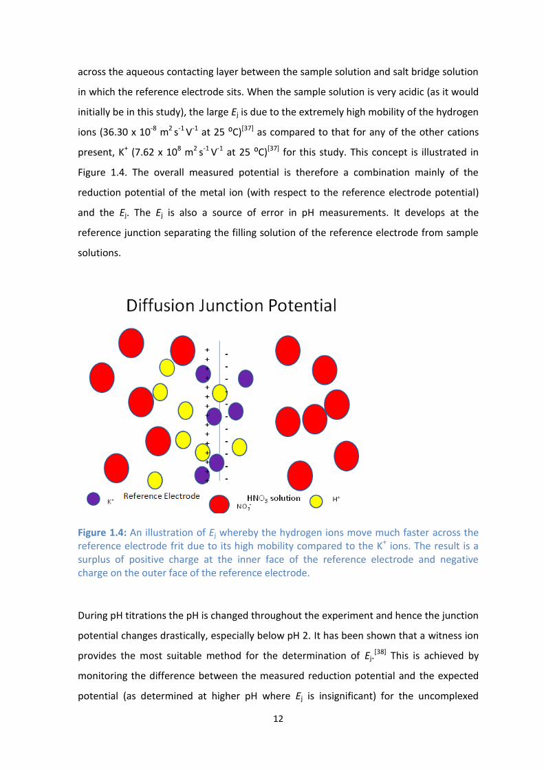
As described in section 1.3, analysis of the complexation of Bi3+ needs to start at pH <2.
The problem which occurs in the analysis of metal-ligand complexes using polarography
at this low pH is the formation of a large diffusion junction potential (Ej). The Ej is defined
as the voltage difference which develops at the interface of two dissimilar electrolyte
solutions in contact. This phenomenon arises in the cell when the diffusion of ions occurs
Applied Potential (V)
Diffusion limited current (Id)
Half-wave
potential (E1/2) Residual current
12
across the aqueous contacting layer between the sample solution and salt bridge solution
in which the reference electrode sits. When the sample solution is very acidic (as it would
initially be in this study), the large Ej is due to the extremely high mobility of the hydrogen
ions (36.30 x 10⁻⁸ m2 s-1 V-1 at 25 ⁰C)[37] as compared to that for any of the other cations
present, K+ (7.62 x 10⁸ m2 s-1 V-1 at 25 ⁰C)[37] for this study. This concept is illustrated in
Figure 1.4. The overall measured potential is therefore a combination mainly of the
reduction potential of the metal ion (with respect to the reference electrode potential)
and the Ej. The Ej is also a source of error in pH measurements. It develops at the
reference junction separating the filling solution of the reference electrode from sample
solutions.
Figure 1.4: An illustration of Ej whereby the hydrogen ions move much faster across the reference electrode frit due to its high mobility compared to the K+ ions. The result is a surplus of positive charge at the inner face of the reference electrode and negative charge on the outer face of the reference electrode.
During pH titrations the pH is changed throughout the experiment and hence the junction
potential changes drastically, especially below pH 2. It has been shown that a witness ion
provides the most suitable method for the determination of Ej.[38] This is achieved by
monitoring the difference between the measured reduction potential and the expected
potential (as determined at higher pH where Ej is insignificant) for the uncomplexed

13
witness ion. This process will be fully discussed in Chapter 4. The witness ion which will
be used is thallium(I) because it forms very weak complexes and hence is not expected to
coordinate with the ligands to be studied, especially in acidic solutions. The thallium data
must be taken very accurately to ensure no unwanted processes are occurring which will
influence the value of the calculated Ej at each respective pH.
The analysis of the Bi3+-ligand complexation will be done by polarography employing pH
titrations, starting with solutions containing Bi3+ and the ligand at low pH (about pH
0.31) and then titrating by a base solution. A negative shift in the reduction potential of
bismuth will occur as bismuth is complexed by the ligand as pH of the solution is
increased. As Bi3+ complexes with ligand, it becomes more difficult to reduce the metal
ion centre and thus more energy is required to enable the electron transfer, and more
negative reduction potentials have to be applied. A requirement which must be used in
order to allow satisfactory analysis of the metal-ligand complexation is that the
concentration of the ligand must be at least about 100 times greater than that of the
metal studied.
1.6. Aims
The main aim of this work is to learn about the interaction between Bi3+ and amino acids.
Polarographic methods will be used to determine which complexes are formed between
Bi3+ and the amino acid ligands and their respective formation constants will be
evaluated. A greater understanding of this chemistry will shed some light on the
behaviour of Bi3+ once placed inside the body and be a step closer to potentially develop
and design more effective Bi3+ containing drugs.
Additionally, it is intended to get a new polarographic-potentiometric autotitration
system fully functioning. This would include developing and testing procedures using
NOVA[39] software which is supplied with the newer Autolab potentiostats.
14
1.7 References
[1] F. A. Cotton and W. G., Advanced Inorganic Chemistry - A Comprehensive Text, John Wiley and
Sons Inc., New York, 1980.
[2] Lenntech-Elements-Bismuth, http://www.lenntech.com/periodic/elements/bi.htm, (Date
Accessed: 30-08-2011)
[3] Bismuth Compunds and Materials of High Purity and Reactivity,
http://www.solid.nsc.ru/eng/develop/bismuth_eng.htm, (Date Accessed: 28-08-2011)
[4] H. Sun, H. Li and P. J. Sadler, Chem. Ber. Recueil.,1997, 130, 669.
[5] C. C. Mayorga-Martinez, M. Cadevall, M. Guix, J. Ros and A. Merkoçi, Biosensors and
Bioelectronics,2013, 40, 57.
[6] S. Caudle, W. Steven, R. Spidle and A. Wanyeka, Abstracts of Papers, 245th ACS National
Meeting & Exposition, New Orleans, LA, United States, April 7-11, 2013,2013, 859.
[7] a) E. Asato, Chem. Lett.,1992, 1967; b) U. Dittes, B. K. Keppler and B. Nuber, Angew.Chem. Int.
Ed.(English),1996, 35, 67; c) M. Abrams and B. Murrer, Science,1993, 261, 725.
[8] a) A. K. Jha and R. G. Mendiratta, J. Mater. Sci.,1996, 31, 1735; b) N. Burford, M. D. Eelman and
T. S. Cameron, Chemical Communications,2002, 1402.
[9] E. Asato, K. Katsura, M. Mikuriya, U. Turpeinen, I. Mutikainen and J. Reedijk, Inorg.
Chem.,1995, 34, 2447.
[10] a) E. Asato, C. M. Hol, F. B. Hulsbergen, N. T. M. Klooster and J. Reedijk, Inorg. Chim.
Acta,1993, 214, 159; b) J. R. Partington, History of Chemistry, Macmillian, London, 1961. 1; c) T. E.
Sox and C. A. Olson, Antimicrob. Agents.Chemother.,1989, 33, 2075.
[11] E. N. Marieb and K. Hoehn in Human Anatomy and Physiology, 1 Benjamin Cummings, San
Francisco, 2010.
[12] a) B. J. Marshall, C. S. Goodwin and R. J. Warren, Lancet,1988, 2, 1437; b) A. J. Wagstaff, P.
Benfield and J. P. Monk, Drugs,1988, 36, 132.
[13] a) P. J. Barrie, M. I. Djuran, M. A. Mazid, M. Mcpartlin, P. J. Sadler, J. I. Scowcn and H. Sun, J.
Chem. Soc. Dalton Trans.,1996, 2417; b) H. Sun, Ph.D, Universitv of London, 1996
[14] I. Shweky, A. Bino, D. P. Goldberg and S. J. Lippard, Inorg. Chem.,1994, 33, 5161.
[15] P. Köpf-Maier and T. Klapötke, Inorg.Chim. Acta.,1988, 152, 49.
[16] N. Yang, J. A. Tanner, Z. Wang, J. D. Huang, B.-J. Zheng, N. Zhu and H. Sun, Chem.
Commun.,2007, 4413.
[17] N. Mahmood, A. Burke, R. M. Anner and B. M. Anner, Antiviral. Chem. Chemother.,1995, 6,
187.
[18] R. W. Kozak, R. Waldman, W. Atcher and A. Gansow, Triends Biotech,1986, 4, 259.

15
[19] R. W. Kozak, W. Atcher, A. Gansow, M. Friedman, J. J. Hines and T. A. Waldman, Proc. Natl.
Acad. Sci. U.S.A.,1986, 83, 474.
[20] A. E. Martell and R. D. Hancock, Metal Complexes in Aqueous Solutions, Plenum Press, New
York, 1996. 46.
[21] S. Ahrland, Inorg. Chim. Acta.,1983, 154.
[22] a) J. Reglinkski, Chemistry of Arsenic, Antimony and Bismuth, Blackie Academic &
Professional, London 1998; b) R. D. Hancock, I. Cukrowski, I. Antunes, E. Cukrowska, J. Mashishi
and K. Brown, Polyhedron,1995, 14, 1699; c) R. D. Hancock, I. Cukrowski, J. Baloyi and J. Mashishi,
J. Chem. Soc., Dalton Trans.,1993, 2895; d) J. R. Frausto and R. J. P. Williams in The Biological
Chemistry of the Elements, Vol. 3 Clarendon Press, Oxford, 1991, 538.
[23] L. J. Farrugia, F. J. Lawlor and N. C. Norman, J. Chem. Soc. Dalton Trans.,1995, 1163.
[24] a) P. Kiprof, W. Scherer, L. Pajdla, E. Herdtweck and W. A. Herrmann in Metals in Biology and
Medicine. Part 3. Bismuth Lactate: Synthesis and Structure of a Hydroxycarboxylate Complex, 23
WILEY-VCH Verlag, 1992; b) H. Sun, H. Li, I. Harvey and P. J. Sadler, J. Biol.l Chem.,1999, 274,
29094.
[25] F. Graner and L. G. Sillén, Acta. Chem. Scand.,1947, 1, 631.
[26] F. Graner, Olin A. and L. G. Sillén, Acta. Chem. Scand.,1956, 10, 476.
[27] A. Olin, Acta Chem. Scand.,1957, 11, 1445.
[28] T. F. Bidleman, Anal. Chim. Acta.,1971, 56, 221.
[29] I. Hataye, H. Suganuma, Ikegami H. and T. Kuchiki, Bull. Chem. Soc. Japan,1982, 55, 1475.
[30] a) G. Sposito and K. M. Holtzclaw, Soil Sci. Soc. Am. J.,1979, 47; b) P. M. May and R. A.
Bulman, The Present Status of Chelating Agents in Medicine, Progress in Medicinal Chemistry, 20,
Elsevier, 1983, 225
[31] M. V.A. and T. G. Spiro, J. Am. Chem. Soc.,1966, 88, 1410.
[32] D. Voet and J. G. Voet in Biochemistry, Vol. 3 Wiley, United States of America, 2004, 736.
[33] a) R. Chen, C. Gao, Y. Wu, H. Wang, H. Zhou, Y. Liu, P. Sun, X. Feng and T. Chen, Chem.
Comm.,2011, 47, 8136; b) P. J. Sadler, H. Li and H. Sun, Coord. Chem. Rev.,1999, 185–186, 689.
[34] M. K. Singh and M. N. Srivastava, J. Inorg. Nucl. Chem.,1972, 34, 2067.
[35] Jaroslav Heyrovski, http://en.wikipedia.org/wiki/Jaroslav-Heyrovsk%C3%BD, (Date Accessed:
2013-07-31)
[36] P. Zuman, Acta Chim. Slov.,2009, 56, 18.
[37] R. A. Robinson, R. H. Stokes and Electrolyte Solutions – The Measurement and Interpretation
of Conductance, Chemical Potential and Diffusion in Solutions of Simple Electrolytes, Butterworth
and Co, London, 1959.

16
[38] C. Billing, I. Cukrowski and B. Jordan, Electroanal.,2013, 25, 2221.
[39] Metrohm-Autolab, NOVA, 2012, (Utrecht, Netherlands)

17
Chapter 2: The development of automated procedures using NOVA
software to study metal-ligand complexation
2.1 Introduction
The study of metal ligand complexation using polarography has, in recent times been
heavily dependent on computer process power, computer software and auxiliary
instruments which are able to collect the copious amounts of data generated during an
experimental run. Previous studies[1] have shown that the use of powerful computer
hardware and software have aided in many breakthroughs regarding the understanding
of polarography. Computer simulations have helped understand the double layer effect
and its effect on the background of DPP polarograms as described by Josephine and
Christie[1] and therefore illustrate that in order to generate the most compelling electro-
analytical data, the main foundation on which to build upon is the use of hardware and
software capable of matching the stringent experimental needs.
Previous work[2] in the University of Witwatersrand electrochemistry laboratory
developed a virtual system for the collection of raw data for metal-ligand equilibria
studies, glass electrode potentiometric studies and sampled direct current polarographic
studies. Although the development of technology had made great strides at the time of
the work,[2] no single instrument was available which could fully automate all the
components needed to complete a voltammetric titration experiment. What transpired
was the development of a dedicated computer controlled instrumental setup capable of
automated titration and pH-polarographic titrations. The automated system was made
up of a Bioanalytical Systems (BAS) CV27 potentiostat and a Metrohm VA stand,
automated burette (a Dosimat), pH meter and stirrer. All components were connected to
an interface built in-house capable of linking to a computer central processing unit (CPU).
The software used to develop the system was LABVIEW,[3] an acronym for Laboratory
Virtual Instrument Engineering Workbench, and is a general purpose programming
environment designed as a complete set of applications for instrumental and process
control for a variety of experiments. The LABVIEW[3] software was used to develop an

18
automated process specific for the application of metal-ligand studies. Functions, user
interface and overall look of the automation programme were tailor made to suit the
needs of the experiment and therefore an extremely useful tool at the time. The
experiments run could also be subjected to subtle changes with current integration time
on the mercury electrode which is able to minimize noise, a useful characteristic in times
when noise could make data collection impossible. The LABVIEW[3] automated
experimental system afforded efficient and reproducible experiments and was
successfully utilised in metal-ligand studies thereafter.[2]
Although the LABVIEW[3] system worked well for many years, the system did have some
disadvantages which became more apparent as technology was being developed in both
hardware and software. LABVIEW[3] was chosen for the automation of instruments since
it was powerful and flexible in its application, but the licence to use these developmental
features is very costly and training had to be done before the development work could be
started. As it stood, the LABVIEW[3] system was also only set up to for a single
electroanalytical technique, direct current polarography. As described earlier, the
interface between the instruments and computer had to be developed solely for this
automation development, which meant that if a component failed it would be difficult to
troubleshoot as the people involved in the development were no longer there and no
schematics of the system were available. Finally, the BAS CV27 potentiostat used in this
setup was more than 30 years old and almost impossible to replace if it had failed.
Continuity plans for the experimental work needed to be put in place should certain
components stop working.
Fairly recently, Eco Chemie (a member of the Metrohm group) developed the Autolab
302N potentiostat controlled by NOVA[4] software. Through various interfaces it was able
to connect to the VA stand, a magnetic stirrer and a Dosino (an automated burette), and
a pH module (pX1000) was installed to enable pH and temperature measurements. In
turn, all of these instruments would be able to be controlled by the computer using the [4]
software. Initially this setup seemed an excellent contingency plan in case of failure of the
LABVIEW[3] system, however, the NOVA[4] software would allow for the development of a
brand new automated system not only capable of performing all the functions utilised in

19
the LABVIEW[3] system, but also utilising all other electroanalytical techniques provided
by NOVA. [4]
It was therefore one of the aims of this project to develop a new automated system to
run the pH-polarographic titrations. Not only would a new system contribute to greater
stability, it would also afford us more flexibility and the option to other electroanalytical
techniques if required.
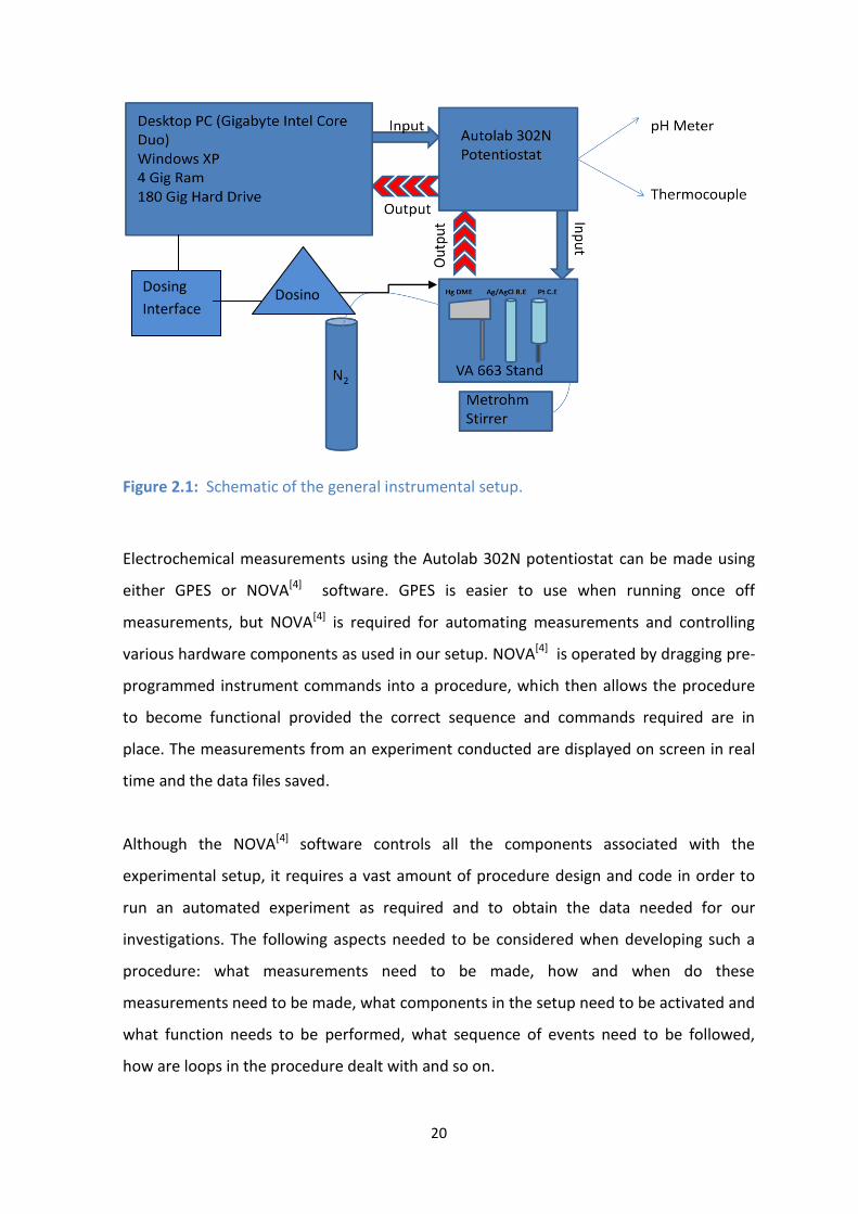
2.2 Instrumental Setup
Figure 2.1 shows a schematic diagram of the instrumental setup used throughout this
work where all components were supplied by Metrohm. The Autolab 302N
potentiostat/galvanostat (designed by Eco Chemie and supplied by Metrohm) was used
and a pH (pX1000) module was installed in the potentiostat which allows both a glass
electrode and thermocouple to be connected. A low current (ECD) module was also
installed for other applications which allows for measurements down to 100 pA, but this
was not need for this work as the potentiostat has a default current range of 10 nA to 1 A
which was sufficient. The 663 VA stand houses the electrochemical cell (although the
polarographic cell was connected directly to the potentiostat leads) and the valves used
to control the nitrogen purge gas, as well as the flow of gas to the mercury drop
electrode and the drop knocker. These valves are controlled via the IME663 interface.
The 800 Dosino with a 20 mL burette (an automated burette used for dispensing the
titrant) and magnetic stirrer were connected to the 846 Dosing Interface which was
directly connected to the PC via USB. As can be seen in Figure 2.1, the desktop PC running
NOVA[4] software controls all components attached to it including the potentiostat,
which in turn controls the components it communicates to. Stability and formation
constants for Metal-ligand studies are dependent on the temperature at which the
respective studies are completed. Temperature plays an important role as it is able to
affect the rates and stability of reactions occurring thus it was important for temperature
to be monitored during the entirety of our experiments. A Metrohm homemade water
bath containing a thermostat was used connected to the jacketed cell in order for the
temperature to be regulated strictly to 25 ± 0.1⁰C.
20
Figure 2.1: Schematic of the general instrumental setup.
Electrochemical measurements using the Autolab 302N potentiostat can be made using
either GPES or NOVA[4] software. GPES is easier to use when running once off
measurements, but NOVA[4] is required for automating measurements and controlling
various hardware components as used in our setup. NOVA[4] is operated by dragging pre-
programmed instrument commands into a procedure, which then allows the procedure
to become functional provided the correct sequence and commands required are in
place. The measurements from an experiment conducted are displayed on screen in real
time and the data files saved.
Although the NOVA[4] software controls all the components associated with the
experimental setup, it requires a vast amount of procedure design and code in order to
run an automated experiment as required and to obtain the data needed for our
investigations. The following aspects needed to be considered when developing such a
procedure: what measurements need to be made, how and when do these
measurements need to be made, what components in the setup need to be activated and
what function needs to be performed, what sequence of events need to be followed,
how are loops in the procedure dealt with and so on.
Dosing
Interface Dosino
21
Three main NOVA[4] procedures were developed, one for each experimental procedure
required to in the investigation of the complexation of bismuth with biologically active
molecules. These were (i) the glass electrode calibration, (ii) the polarographic-pH
titration starting in solutions containing metal ions (Bi3+ and Tl+) (i.e. ligand-free
polarographic-pH titrations) and (iii) the polarographic-pH titration where the solutions
contain the metal ions and ligand of choice (i.e. metal-ligand complexation studies by
polarographic-pH titrations).
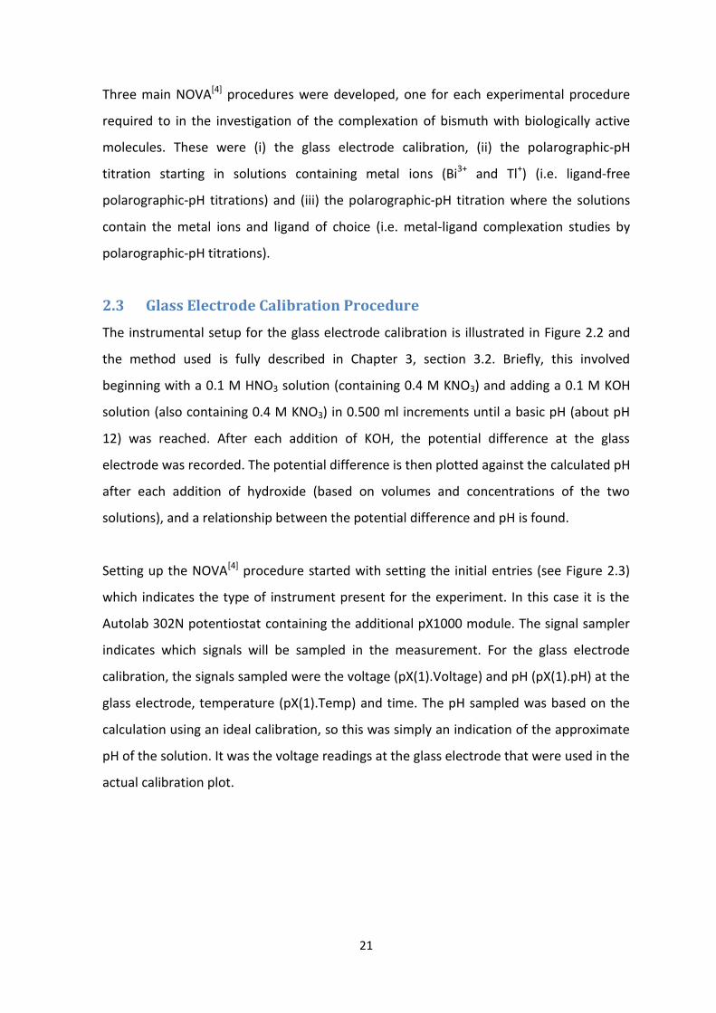
2.3 Glass Electrode Calibration Procedure
The instrumental setup for the glass electrode calibration is illustrated in Figure 2.2 and
the method used is fully described in Chapter 3, section 3.2. Briefly, this involved
beginning with a 0.1 M HNO3 solution (containing 0.4 M KNO3) and adding a 0.1 M KOH
solution (also containing 0.4 M KNO3) in 0.500 ml increments until a basic pH (about pH
12) was reached. After each addition of KOH, the potential difference at the glass
electrode was recorded. The potential difference is then plotted against the calculated pH
after each addition of hydroxide (based on volumes and concentrations of the two
solutions), and a relationship between the potential difference and pH is found.
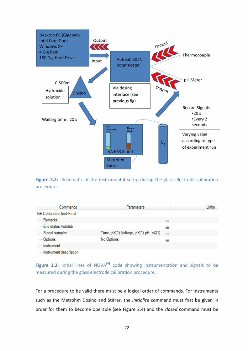
Setting up the NOVA[4] procedure started with setting the initial entries (see Figure 2.3)
which indicates the type of instrument present for the experiment. In this case it is the
Autolab 302N potentiostat containing the additional pX1000 module. The signal sampler
indicates which signals will be sampled in the measurement. For the glass electrode
calibration, the signals sampled were the voltage (pX(1).Voltage) and pH (pX(1).pH) at the
glass electrode, temperature (pX(1).Temp) and time. The pH sampled was based on the
calculation using an ideal calibration, so this was simply an indication of the approximate
pH of the solution. It was the voltage readings at the glass electrode that were used in the
actual calibration plot.
22
Figure 2.2: Schematic of the instrumental setup during the glass electrode calibration
procedure.
Figure 2.3: Initial lines of NOVA[4] code showing instrumentation and signals to be
measured during the glass electrode calibration procedure.
For a procedure to be valid there must be a logical order of commands. For instruments
such as the Metrohm Dosino and Stirrer, the initialize command must first be given in
order for them to become operable (see Figure 2.4) and the closed command must be
Via dosing
interface (see
previous fig)
Hydroxide
solution
Varying value
according to type
of experiment run
23
given once their function is complete in order for a procedure to be valid. Thus the
Dosino initialize command must be dragged into the procedure window and within the
settings tab, the serial number of the Dosino in use must be entered. The Metrohm
magnetic stirrer must also be initialised in the same way and its respective serial number
must also be entered in the stirrer initialize tab. The stirrer speed can be set in the
command tab (between values of 1 and 10) and in order to stop the stirrer, the stirrer
speed must be set to 0.
The Autolab control (see Figure 2.4) is a major component of the experiment. This
command activates the potentiostat, which then allows it to control commands sent to
the VA stand, and in this case activates the N2 purger. The NOVA[4] software ensures its
reproducibility and accuracy by making time a major component of the experiment. Time
is constantly measured in order to optimize the procedures and so any command which
entails the measurement of a certain signal or the timing of a command, must be placed
within a timed procedure command.
The cell was set up by adding 25.00 mL of the HNO3 solution using a Dosimat and placing
the glass electrode and thermocouple in the cell. Before any measurement of signals or
addition of base, the glass electrode calibration requires that all carbon dioxide (and
oxygen for the polarographic experiments) be removed from the cell. This is done by
purging with N2 for approximately 1 min/ml of solution and stirring throughout. In Figure
2.4 it can be seen that the stirrer speed was set to 3 and stirring continued throughout
the procedure until the stirrer speed was set to 0 to stop it. Stirring allowed the titrant to
always be uniformly dispersed once added to the cell. The purge command is placed
within a timed procedure so the solution was initially purged for 1800 s, after which the
purging was stopped. During the measurement of signals and addition of base, the purger
was kept on to remove carbon dioxide and oxygen introduced into the system due the
addition of the base. This command is not a timed procedure as it must be done
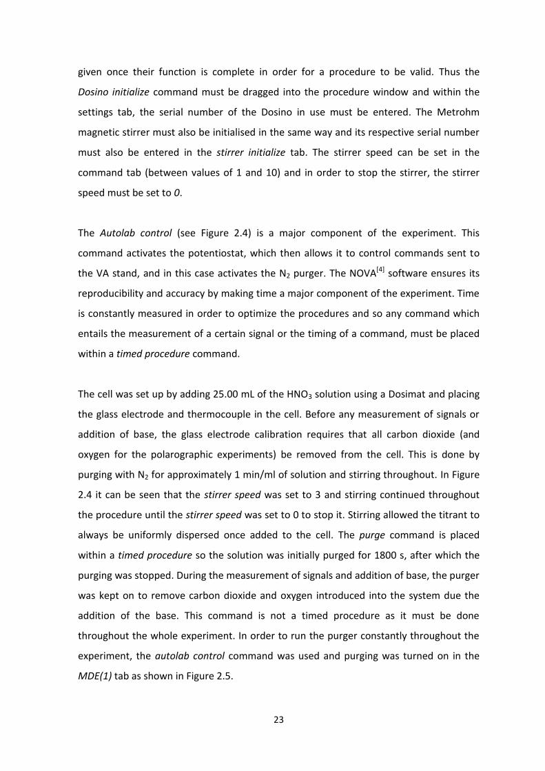
throughout the whole experiment. In order to run the purger constantly throughout the
experiment, the autolab control command was used and purging was turned on in the
MDE(1) tab as shown in Figure 2.5.

24
Figure 2.4: Commands for initialising devices and controlling the stirring and purging.
In Figure 2.5 there is also an option to turn a stirrer on, however, this option does not
refer to the magnetic stirrer, but rather the rotating stirrer controlled by the VA stand via
the IME663 interface. All other options in this Autolab control command tree did not
need to be changed as the glass electrode experiment does not require any
measurement of current or applied voltage via working, reference or counter electrodes.
The glass electrode calibration experiment was conducted by adding 0.500 ml increments
of KOH solution while purging and stirring. The system was then allowed to equilibrate
before the voltage at the glass electrode and temperature at the thermocouple were
recorded. Since the experiment required multiple additions of base, a repeat for each
value command was utilized (see Figure 2.6 ). This loop repeats the commands which are
placed within it for each value of a specified parameter. The parameter of importance in
this experiment was the 0.500 ml of base which was added multiple times in order for the
titration to be done. As can be seen in Figure 2.6, within the Dosino dose command, the
volume (ml) sub command is linked to the parameter link command for the repeat loop.
This is indicated by the square bracket shown on the right of the commands. The loop is
25
thus repeated for each value specified in the repeat for each value command (i.e. the
addition of 0.500 ml as many times as stipulated).
Figure 2.5: Autolab Control tab showing the method by which the purger is turned on and
allowed to continuously purge throughout the experiment.
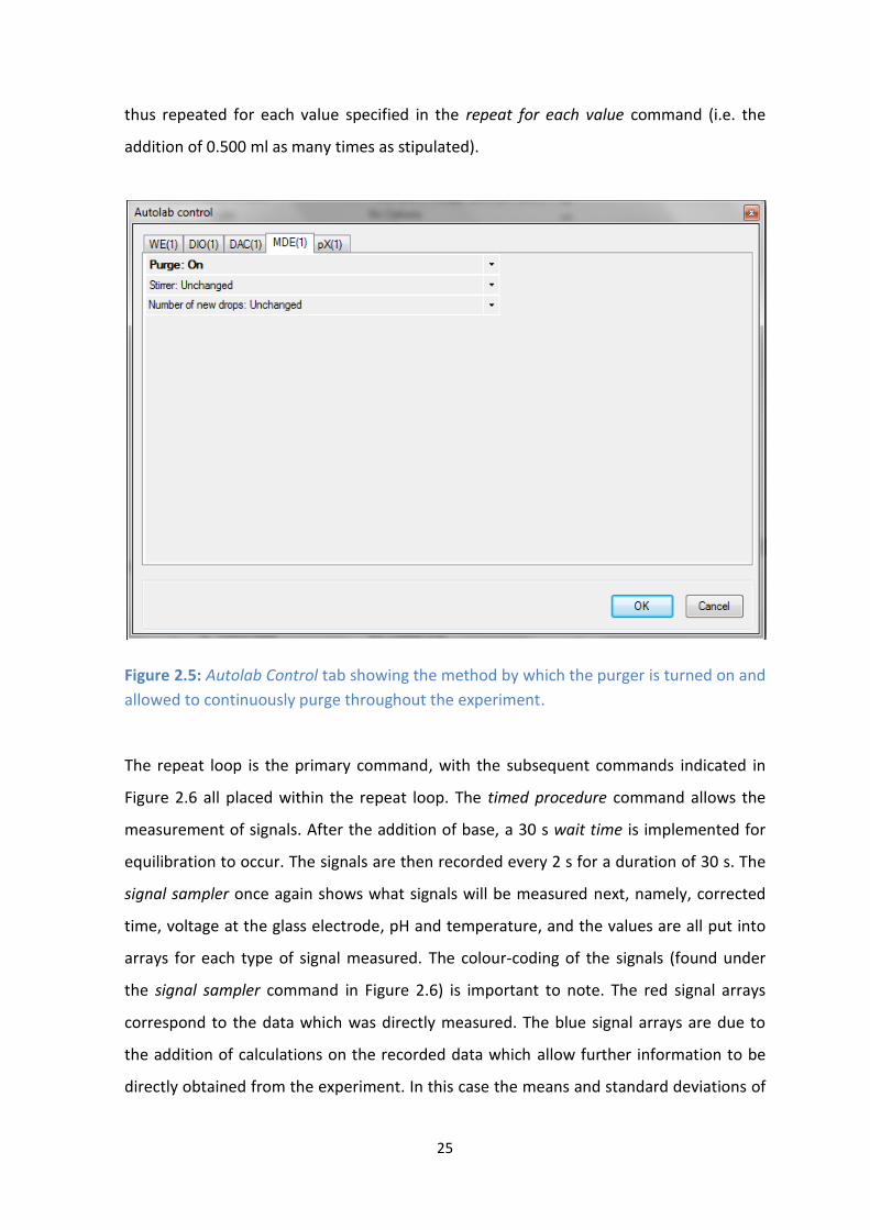
The repeat loop is the primary command, with the subsequent commands indicated in
Figure 2.6 all placed within the repeat loop. The timed procedure command allows the
measurement of signals. After the addition of base, a 30 s wait time is implemented for
equilibration to occur. The signals are then recorded every 2 s for a duration of 30 s. The
signal sampler once again shows what signals will be measured next, namely, corrected
time, voltage at the glass electrode, pH and temperature, and the values are all put into
arrays for each type of signal measured. The colour-coding of the signals (found under
the signal sampler command in Figure 2.6) is important to note. The red signal arrays
correspond to the data which was directly measured. The blue signal arrays are due to
the addition of calculations on the recorded data which allow further information to be
directly obtained from the experiment. In this case the means and standard deviations of
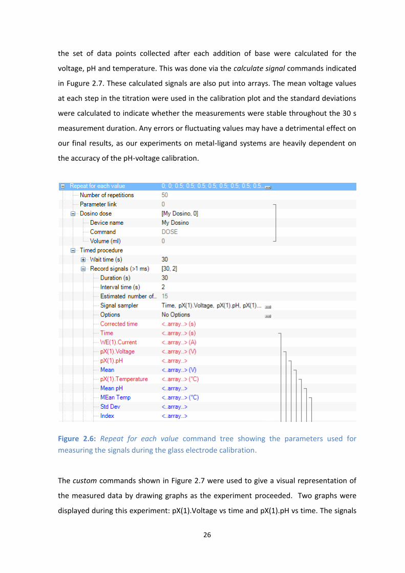
26
the set of data points collected after each addition of base were calculated for the
voltage, pH and temperature. This was done via the calculate signal commands indicated
in Fugure 2.7. These calculated signals are also put into arrays. The mean voltage values
at each step in the titration were used in the calibration plot and the standard deviations
were calculated to indicate whether the measurements were stable throughout the 30 s
measurement duration. Any errors or fluctuating values may have a detrimental effect on
our final results, as our experiments on metal-ligand systems are heavily dependent on
the accuracy of the pH-voltage calibration.
Figure 2.6: Repeat for each value command tree showing the parameters used for
measuring the signals during the glass electrode calibration.
The custom commands shown in Figure 2.7 were used to give a visual representation of
the measured data by drawing graphs as the experiment proceeded. Two graphs were
displayed during this experiment: pX(1).Voltage vs time and pX(1).pH vs time. The signals
27
which are sampled (as indicated in red in Figure 2.6) were linked to the custom command
via links, indicated but square brackets on the right of the commands.
The signals that were measured and calculated were saved in an ASCII file via the Export
ASCII data command. The data required are linked to the respective columns in which the
data must appear in the ASCII data file and are saved into the directory designated by the
user. Within the Export ASCII data command, the File mode command determines how
the data file should be saved. For the glass electrode calibration this option was set to
append which allows the file to be rewritten and the data for the successive repeat loops
to be added. Thus all the data measured for each repeat in the loop is then saved in one
row and the completion of the next repeat saves the data in the next row of the file. The
ASCII data file can then be opened in a spreadsheet in order to extract and utilize the
experimental data.
The calibration procedure developed contained three repeat loops (Figure 2.8). It was
decided to programme the procedure this way so as to take changing equilibration times
into account. During the titration, equilibration times vary according to where along the
titration curve the experiment is. At the beginning and near the end of the pH titration,
0.500 ml additions of base cause very little change in the pH, as indicated in the titration
curve in Figure 2.9. However, near the end point the addition of 0.500 ml of base results
in a large change in pH and as there is a large drift as the signal, so equilibration times in
this region were made longer to obtain more stable values. It was therefore decided to
have an initial repeat loop for the 0.500 ml additions up to a total of approximately 24 ml
of base. The exact volume depended on the expected endpoint as determined by the
standardised concentrations of the acid and base solutions used. During this repeat loop
the wait time was set to 30 s. Thereafter a second repeat loop was included to add base
for 4 repeats (collectively 2 ml of base added) around the end point of the titration and
the wait time was changed to 300 s. This allowed adequate time for the system to reach
equilibrium before measuring the signals. Standard deviations of the data collected in this
region were <10-5 mV signifying stable measurements. A third repeat loop was
programmed to the same specifications as the first repeat loop. Here, the number of

28
0.500 ml additions were repeat until the desired stop volume was reached, which was
approximately 40 ml of base in total for the glass electrode calibration procedure.
Figure 2.7: The custom commands used to plot the measured data during the
experiment, and the commands used to perform calculations on the measured signals
and save the data.
Figure 2.8: The three repeat loops in the glass electrode calibration to allow for longer
equilibration times before measurements made close to the end point of the titration.

29
Figure 2.9: Potential difference vs volume added plot for the titration of 0.9945 M HNO3
with 0.1012 M KOH at 25.0 ⁰C. The end point region is highlighted to show the sharp
change in gradient associated with measurement of potential difference, hence a longer
equilibration time is needed.
2.4 Development of the NOVA procedure for the polarographic-pH
titration
Due to limitations in the NOVA[4] software, a single experimental procedure which
completes the entire metal-ligand experiment was unable to be employed. The multi-
hour experiment unfortunately pushed the limits of the computers available due to the
fact that NOVA[4] stores all the collected data in the RAM of the computer while the
experiment is running and only saves the data to the hard drive once the entire
experiment is complete. Since a large volume of data is generated during our experiment,
there is insufficient RAM to successful complete of the entire experiment. The
functioning of the NOVA[4] software was thus dependant on the computer available. It
was decided to divide the experiment into two separate procedures, called Part A and
Part B. This would allow the RAM of the computer to store the first part of the
experiment, before carrying on with the next, thus preventing the computer RAM from
running out of space.
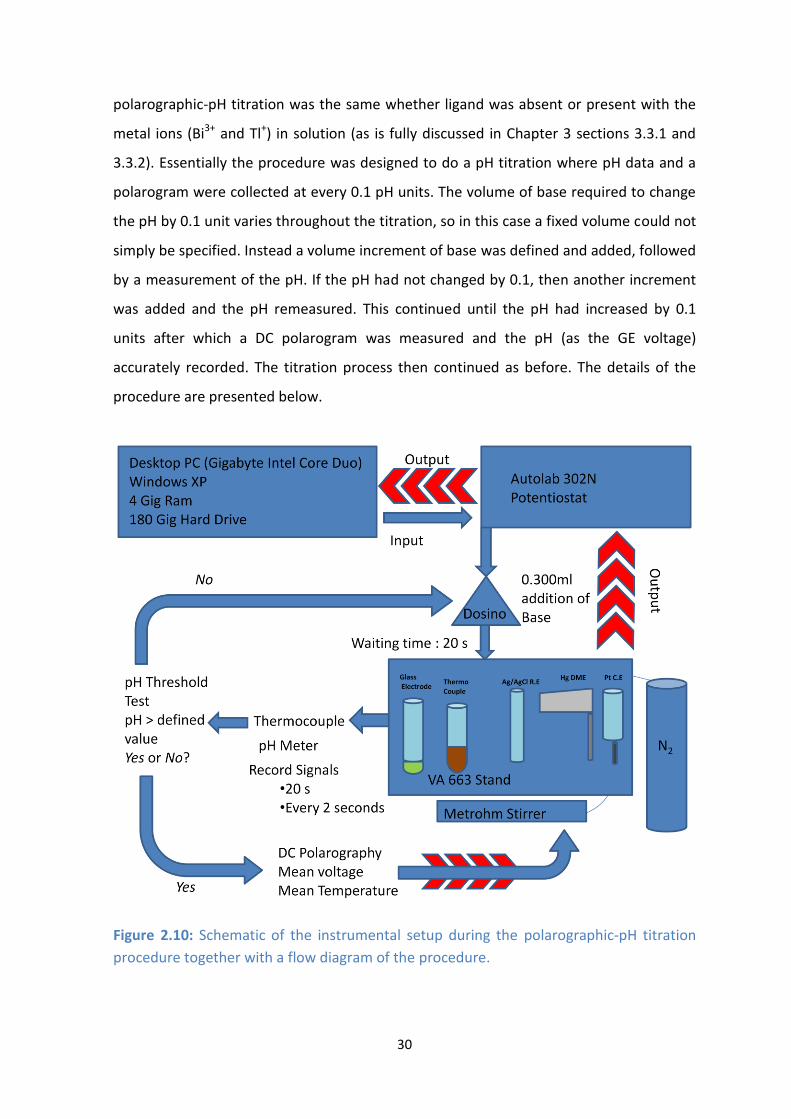
Figure 2.10 shows a graphical representation of instrumental setup and the procedure
used in both Part A and B, as will be discussed in detail shortly. The procedure for the
-400
-300
-200
-100
0
100
200
300
400
0 5 10 15 20 25 30 35 40
Po
ten
tial
Dif
fere
nce
(m
V)
Volume of base added(ml)
Potential difference (mV) vs volume of base added (mL)
End point region
30
polarographic-pH titration was the same whether ligand was absent or present with the
metal ions (Bi3+ and Tl+) in solution (as is fully discussed in Chapter 3 sections 3.3.1 and
3.3.2). Essentially the procedure was designed to do a pH titration where pH data and a
polarogram were collected at every 0.1 pH units. The volume of base required to change
the pH by 0.1 unit varies throughout the titration, so in this case a fixed volume could not
simply be specified. Instead a volume increment of base was defined and added, followed
by a measurement of the pH. If the pH had not changed by 0.1, then another increment
was added and the pH remeasured. This continued until the pH had increased by 0.1
units after which a DC polarogram was measured and the pH (as the GE voltage)
accurately recorded. The titration process then continued as before. The details of the
procedure are presented below.
Figure 2.10: Schematic of the instrumental setup during the polarographic-pH titration
procedure together with a flow diagram of the procedure.
31
2.4.1. Part A
As described in section 2.2 of this chapter, the opening command lines in a NOVA[4]
procedure hold details of the type of potentiostat used and the signals which are to be
measured. Figure 2.11 shows that the signals measured in this experiment were pH
(pX(1).pH), voltage at the glass electrode (pX(1).voltage), temperature
(pX(1).temperature), and the applied potential by the potentiostat and the current and
actual measured potential at the working electrode (WE(1).Current and WE(1).Potential,
respectively) for the polarographic data.
A nested procedure is a tool used for measurements that cannot be added to a timed
procedure. The nested procedure command allows analysis and essential hardware
commands to be grouped together. It is then easier to let one nested procedure contain
all commands, than selecting each command individually. The first entry in the nested
procedure is a message box which allows for the software to communicate with the user
via text and is useful when certain actions need to be emphasised. The message box was
utilized as a check that the Dosino to be used was prepared and ready to conduct the
experiment. The Dosino had to be prepared manually before the start of the experiment
to ensure the removal of air bubbles from the dosing system and that the solution in the
outlet tubing was replaced by fresh solution as it may have absorbed CO2 on standing. A
further safety check which was added, is that the message box does not go away until the
user clicks the yes tab, indicating that the Dosino is prepared and ready for use. Only then
will NOVA[4] proceed to the next command. As before, the Dosino and magnetic stirrer
must be initialised because they are used at various stages throughout the experiment.
The next command is a timed procedure which houses the purge command while stirring
the solution for a user-defined time period. This was generally set for a short time as the
solution was deoxygenated in the initial data collection before the automated titration
was commenced, as discussed in Chapter 3 (section 3.3.1).

32
Figure 2.11: Initial steps in the procedure used for Part A of the polarographic-pH
titration.
Figure 2.12 shows that the experimental procedure used to control the base addition to
change the pH begins with a repeat loop. The repeat for each value command was used
and within it the pH values were entered at which DC polarograms must be measured. As

33
discussed, a DC polarogram was required after a change in pH of 0.1 unit. Since initially a
0.1 M HNO3 solution (containing lower concentrations of metal ions and ligand) was in
the cell, the start pH was about 1 and so the repeat values inputted into the command
are 1, 1.1, 1.2, 1.3 and so on until a final pH of approximately 2.3. The Dosino was set to
add base in 0.300 ml increments for Part A. This ensured that the 0.1 pH step was never
exceeded by a single addition, but that the increment was not so small as to spend
unnecessarily long times on this step in the procedure.
Figure 2.12: Various repeat loop commands were utilized to run the required experiment,
namely the repeat for each value command as the primary tree command and the repeat
n times command used to control the Dosino additions and run the pH threshold test.
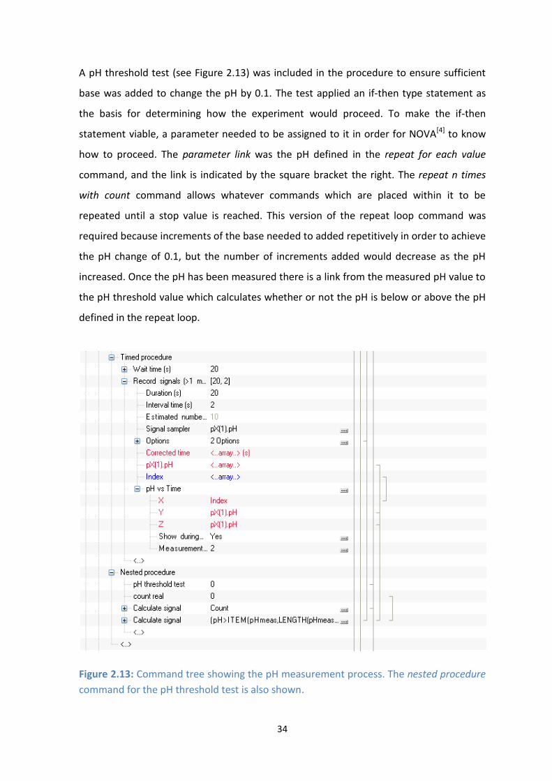
34
A pH threshold test (see Figure 2.13) was included in the procedure to ensure sufficient
base was added to change the pH by 0.1. The test applied an if-then type statement as
the basis for determining how the experiment would proceed. To make the if-then
statement viable, a parameter needed to be assigned to it in order for NOVA[4] to know
how to proceed. The parameter link was the pH defined in the repeat for each value
command, and the link is indicated by the square bracket the right. The repeat n times
with count command allows whatever commands which are placed within it to be
repeated until a stop value is reached. This version of the repeat loop command was
required because increments of the base needed to added repetitively in order to achieve
the pH change of 0.1, but the number of increments added would decrease as the pH
increased. Once the pH has been measured there is a link from the measured pH value to
the pH threshold value which calculates whether or not the pH is below or above the pH
defined in the repeat loop.
Figure 2.13: Command tree showing the pH measurement process. The nested procedure
command for the pH threshold test is also shown.

35
In practice, the Dosino is programmed to dispense 0.300 ml increments of base at a time,
while stirring and purging throughout. After each addition of base, a timed procedure
allows a waiting time of 20 s for equilibration of the system. Then a record signals
command allows the pH to be measured every 2 s for a 20 s interval (see Figure 2.13).
The signal sampler tab shows that the only signal being recorded during this particular
phase of the procedure is the pX(1).pH signal (and the corrected time as always). While
the signals are being recorded, NOVA[4] can display a plot of the data, which was set to
plot of pH vs index. The index array is the number of readings taken, which in this case is
numbers 1 to 10 (as pH is measured every 2 s for 20 s, implying 10 readings). This plot
was useful to monitor the progress of the experiment and it also indicated whether the
experiment was running according to the given settings.
The nested procedure which follows was the second component which contributed to the
programming of the if-then type statement. The pH threshold test allowed the NOVA[4]
software to determine if it should carry on adding base or proceed to record a DC
polarogram. The first calculate signal command gives the formula for the pH threshold
test to obey. The second calculate signal command determines whether the pH is greater
than that in the parameter link (shown in Figure 2.12). IF the pH is smaller than the
valued defined by the parameter link, the pH threshold test returns a 0, which THEN
causes the repeat n times with count loop to continue adding another increment of base.
The procedure is repeated until there is a change in pH of 0.1 units. This will cause the
signal calculated to be greater than that of the parameter link, which in turn causes the
pH threshold test to return a value of 1 to the repeat n times with count loop and hence
the repeat loop is stopped. The procedure then moves on to the measurement of the
sampled DC polarograms, the glass electrode voltage and temperature of the solution.
The sampled DC polarography procedure is built into the NOVA[4] software, however, it
can be amended to an extent according to the needs of the experiment. In our
experiment (see Figure 2.14), the solution was purged for 400 s to remove oxygen
introduced from the addition of the base before the DC polarogram is taken. The stirrer
speed was also set to 3 so that it continued to mix the solution while purging. Once the
purging was complete, the stirrer speed was set to 0 so that no stirring occurred during
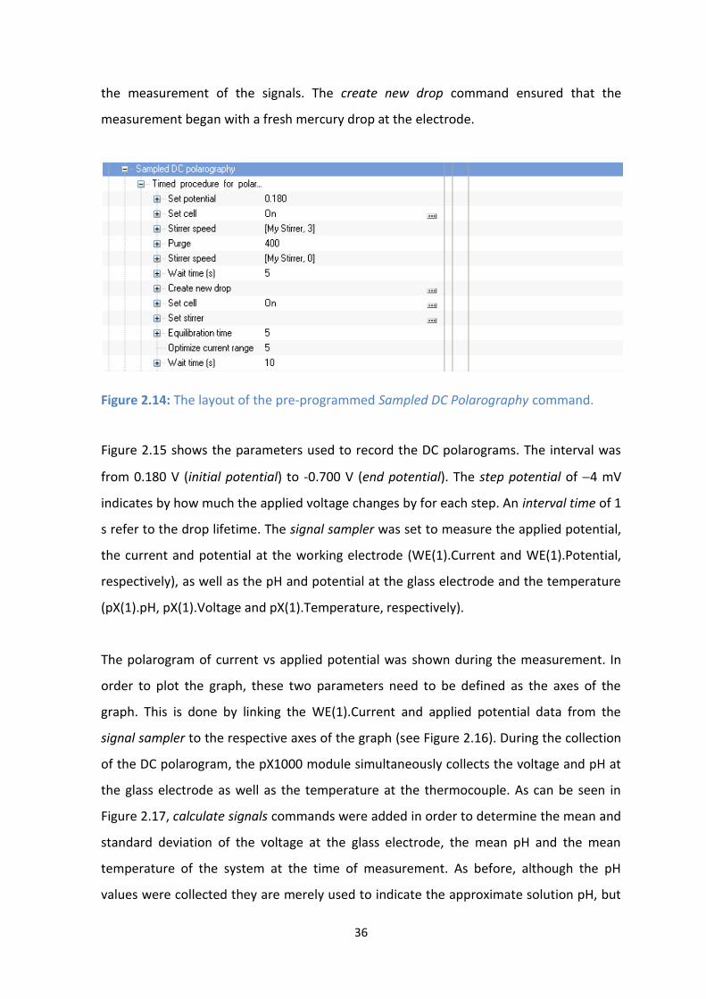
36
the measurement of the signals. The create new drop command ensured that the
measurement began with a fresh mercury drop at the electrode.
Figure 2.14: The layout of the pre-programmed Sampled DC Polarography command.
Figure 2.15 shows the parameters used to record the DC polarograms. The interval was
from 0.180 V (initial potential) to -0.700 V (end potential). The step potential of 4 mV
indicates by how much the applied voltage changes by for each step. An interval time of 1
s refer to the drop lifetime. The signal sampler was set to measure the applied potential,
the current and potential at the working electrode (WE(1).Current and WE(1).Potential,
respectively), as well as the pH and potential at the glass electrode and the temperature
(pX(1).pH, pX(1).Voltage and pX(1).Temperature, respectively).
The polarogram of current vs applied potential was shown during the measurement. In
order to plot the graph, these two parameters need to be defined as the axes of the
graph. This is done by linking the WE(1).Current and applied potential data from the
signal sampler to the respective axes of the graph (see Figure 2.16). During the collection
of the DC polarogram, the pX1000 module simultaneously collects the voltage and pH at
the glass electrode as well as the temperature at the thermocouple. As can be seen in
Figure 2.17, calculate signals commands were added in order to determine the mean and
standard deviation of the voltage at the glass electrode, the mean pH and the mean
temperature of the system at the time of measurement. As before, although the pH
values were collected they are merely used to indicate the approximate solution pH, but

37
the voltage values together with the glass electrode calibration curve were used to
determine at actual pH.
Figure 2.15: The parameters used for the DC polarogram as inputted into the NOVA[4]
software.
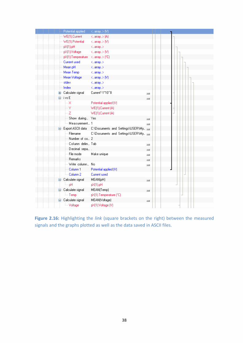
38
Figure 2.16: Highlighting the link (square brackets on the right) between the measured
signals and the graphs plotted as well as the data saved in ASCII files.

39
Figure 2.17: Highlighting the calculate signal commands which were linked to columns in
ASCII data files for saving.
The signals collected were saved in two distinct ways. Firstly, data for each DC
polarogram was saved in a file containing two columns for each respective signal (applied
potential and WE(1).Current) using the export ASCII data command and linking the

40
columns to the required signals that must be saved (Figure 2.17). On hindsight, the
WE(1).Potential rather than the applied potential should have been used, but in general
the difference between these values was negligible. Since a polarogram was collected at
each pH value, it was ensured that the data for each polarogram was saved in a separate
file. In order to achieve this, the file mode was set to make unique. Each file
(corresponding to one polarogram) uses the root file name followed by a number given in
sequential order. Secondly, data collected via the pX1000 module was also needed and it
was decided to save the calculated mean and the standard deviation of the voltage, the
mean pH and the pH threshold test. The pH threshold test value is able to show us how
many times the dosing increment was added before the loop could complete itself. This
then allowed us to calculate the volume of KOH added by multiplying the threshold
number by the dispensing volume. Since four signals were required, the number of
columns was set to 4 and all collected data was saved in a single file for the entire
experiment by setting the file mode to append under the export ASCII data command
(Figure 2.17). The ASCII file was also given a name and a specific directory the on the hard
drive for later analysis. The temperature measured at the thermocouple electrode was
also monitored closely. This was to ensure that the temperature remained constant at
25.0 ± 0.2 ⁰C since the calculations of stability constants are highly dependent on
temperature. The temperature of the cell throughout the measurement was viewed in
the analysis tab of the NOVA[4] software and any deviations throughout the entire
measurement procedure could be highlighted.
Once the DC polarogram collected at pH 2.3 is complete (i.e. the last pH listed in the
repeat loop), NOVA[4] software begins the ending phase for the procedure. In order for
Part A to be valid, the Dosino and stirrer must be closed using the Dosino close and stirrer
close commands (Figure 2.18). The cell is also turned off, but the purger and stirrer are
set to be on because while Part B of the experiment is being selected, O2 contamination is
minimised.

41
Figure 2.18: Closing commands for the validation of the NOVA[4] procedure.
2.4.2. Part B
Part B for the polarographic-pH titration follows a similar procedure to Part A, and only
the changes are highlighted here. The Dosino was programmed to add base in smaller
increments of 0.025 ml. This was to ensure that data was not missed near the end point
of the titration as the pH increases sharply even with small amounts of base added. The
pH values for the repeat for each value loop were also changed; since Part A ended at a
pH 2.3, Part B was set to begin with pH 2.3 and then increase in 0.1 pH steps up to a final
pH value (Figure 2.19). In our experiments, the pH at which the procedure stops was
generally set to pH 10.
Another important change which needed to be made in Part B was the naming of the files
which contain data from the DC polarogram and pX1000 module respectively (Figure
2.20). The file names and directory for these files must be inputted by the user to ensure
all data is collected and saved and that no data is overwritten. All other measurements
and command lines are the same as those described in Part A.
Part B was completed by switching off the Dosino and stirrer using the Dosino close and
Stirrer close commands (Figure 2.21). The timed procedure command which houses the
Autolab control command was used to switch the purger off and finally the cell was
switched off to prevent any potentials being applied across the electrodes while the cell
was being emptied and cleaned.
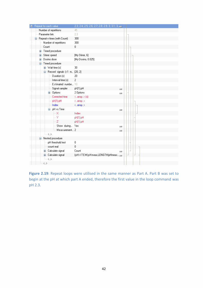
42
Figure 2.19: Repeat loops were utilised in the same manner as Part A. Part B was set to
begin at the pH at which part A ended, therefore the first value in the loop command was
pH 2.3.
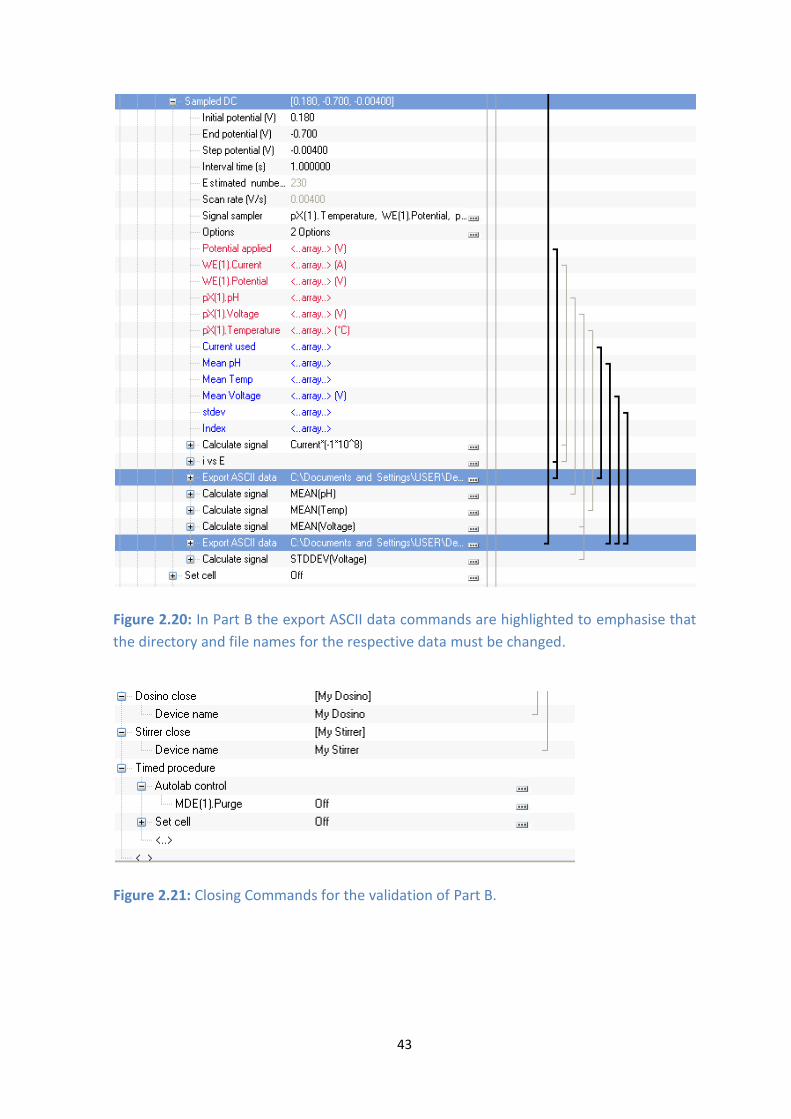
43
Figure 2.20: In Part B the export ASCII data commands are highlighted to emphasise that
the directory and file names for the respective data must be changed.
Figure 2.21: Closing Commands for the validation of Part B.
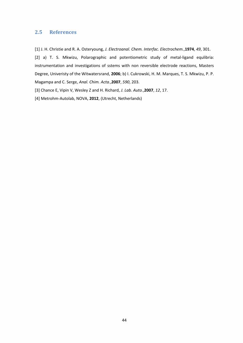
44
2.5 References
[1] J. H. Christie and R. A. Osteryoung, J. Electroanal. Chem. Interfac. Electrochem.,1974, 49, 301.
[2] a) T. S. Mkwizu, Polarographic and potentiometric study of metal-ligand equlibria:
instrumentation and investigations of sstems with non reversible electrode reactions, Masters
Degree, Univeristy of the Witwatersrand, 2006; b) I. Cukrowski, H. M. Marques, T. S. Mkwizu, P. P.
Magampa and C. Serge, Anal. Chim. Acta.,2007, 590, 203.
[3] Chance E, Vipin V, Wesley Z and H. Richard, J. Lab. Auto.,2007, 12, 17.
[4] Metrohm-Autolab, NOVA, 2012, (Utrecht, Netherlands)
45
Chapter 3: Experimental Procedures
3.1. Introduction
The experimental technique for the analysis of Bi3+ and its ability to complex with ligands
was chosen to be polarography. The majority of metal-ligand studies in the past have
utilized glass electrode potentiometry (GEP) in order to determine formation constants of
the respective complexes in solution. Although GEP is a tried and tested technique, as
was discussed in Chapter 1, Bi3+ hydrolyses at low pH and begins to precipitate at about
pH 2, thus its coordination chemistry must be studied from pH below 2. GEP studies
generally only start from pH 2 as it has been well documented that the formation
constants determined by GEP using measurements below this pH have large errors. This
is because only the measurement of the H+ concentration in solution is utilized in these
calculations. It is the concentration of H+ due to the deprotonation of the ligand on
complex formation that is important, but determining this value accurately in a solution
below pH 2, where there is already be a large number of H+ ions present from the strong
acid background solution is impossible.
Polarography is also an ideal technique to use in these studies as low total metal ion
concentrations can be used to postpone or suppress precipitation and a large ligand-to-
metal ion concentration ratio, which is required for these measurements, also promotes
complex formation at lower pH. When using polarography to determine stability
constants, the formation of the Bi3+ hydroxide complexes, unfortunately, leads to an
increased number of experiments and calculations that have to be done. These will be
described in this chapter as well as in Chapter 4.
3.2. Glass Electrode Calibration
In order to calibrate the glass electrode, an acid-base titration was performed. Solutions
of 0.1 M HNO3 and 0.1 M KOH, were made by diluting the appropriate volumes of
concentrated HNO3 (65%, Merck) and KOH (45%, Sigma-Aldrich) and 0.4 M KNO3 (Sigma-
46
Aldrich) was added to both solutions. The salt was added to maintain the ionic strength of
solutions close to 0.5 M throughout the titration. It was important that the ionic strength
of these solutions was kept constant since the concentration of H+ (not its activity) was
used in calculations, thus the activity coefficients need to remain constant throughout
the experiment.
The KOH solution was standardized by dissolving ~0.5 g potassium hydrogen
phthalate (Sigma-Aldrich), previously dried at 100 ⁰C for at least two hours and then
accurately weighed, in 5 mL of deionised water. The resulting solution was placed in a
cell connected to the Metrohm Titrino Plus autotitrator. Nitrogen gas was bubbled
through the solution so as to remove carbon dioxide and oxygen from the cell. The
solution was purged while the potassium hydrogen phthalate was allowed to dissolve.
The KOH solution was contained in a Metrohm dosing unit attached to the autotitrator
and then allowed to titrate the potassium hydrogen phthalate solution while the pH
was measured using a Metrohm Ecotrode glass electrode. The standardization of the
KOH was repeated until a standard deviation less than 0.001 M was achieved. Once the
KOH solution was standardized, it was then used to standardize the HNO3 solution. An
exact volume of 10.00 mL HNO3 was placed into the reaction vessel and then titrated
with KOH as before. The HNO3 standardization was also repeated until a standard
deviation less than 0.001 M was achieved.
The glass electrode used throughout this work was a Metrohm pH glass electrode (also
termed Ecotrode), contains an incorporated 3 M KCl Ag/AgCl reference electrode. The
glass electrode was calibrated by titration. Using a Metrohm Dosimat, 25.00 mL of
HNO3 was placed into a jac ket ed - cell connected to a waterbath and then allowed to
reach 25.0 ± 0.1 ⁰C (monitored using Metrohm thermocouple) while purging with N2 gas.
The automated glass electrode calibration procedure developed using Autolab NOVA
software as described in detail in Section 2.3 was used. The programme allowed the
addition of 40.00 mL of KOH in 0.500 mL increments to increase the pH. The potential
difference at the glass electrode and the temperature were measured after each
addition of 0.500 mL KOH. Enough KOH was added to allow the titration to surpass the
47
end point because the potential difference at the glass electrode was needed in both the
acidic and basic regions for the calibration.
After standardization of the 0 .1 M KOH and HNO3 solutions, the concentrations were
accurately known. Knowing the chemical equation to be:
HNO3 + KOH → KNO3 + H2O
the concentration of H+ ions can then be calculated after each addition of 0.500 mL KOH.
Therefore pH can be calculated after each addition of KOH. It is important to note that in
this work the pH is calculated using the concentration of H+ ions in solution, thus pH = -
log [H+]. The potential difference at the glass electrode obtained after each step of the
titration was then plotted against calculated pH.
A procedure developed recently by Billing and Cukrowski[1] to calibrate the glass
electrode in very acidic solutions by employing both linear and quadratic functions to fit
the calibration graph was used. A linear function was fitted throughout all data points,
and a quadratic function fitted through the acidic region so as to compensate for any
slight curvature shown by glass electrodes in very acidic medium. The observed
curvature is due to the diffusion junction potential at the reference electrode
contained within the glass electrode. The acid error which occurs at low pH could also
contribute to the slight curvature. This error is due to the large concentration of H+ ions
present which cause a saturation effect at the membrane of the glass electrode,
however, since the lowest pH used in the majority of this study was 1, the acid error is
not likely to be significant. When titrations were started in highly acidic solutions (pH
~0.3)[1] the deviation from linearity in the potential difference versus pH response is
much greater than the deviation seen when started at pH 1, the pH which measurement
commenced in this work. The higher the pH, the greater the decrease in [H+] and so the
error due to diffusion junction potential decreases. Although not a standard practice, the
quadratic equation was used so as to accurately represent the relationship between
potential difference and pH even if the diffusion junction potential caused linearity to be
compromised and hence minimize the error in pH calculations.
In order to calculate the pH values from measured potential values at the glass electrode
during polarographic-pH titration experiments, the quadratic equation was used in very
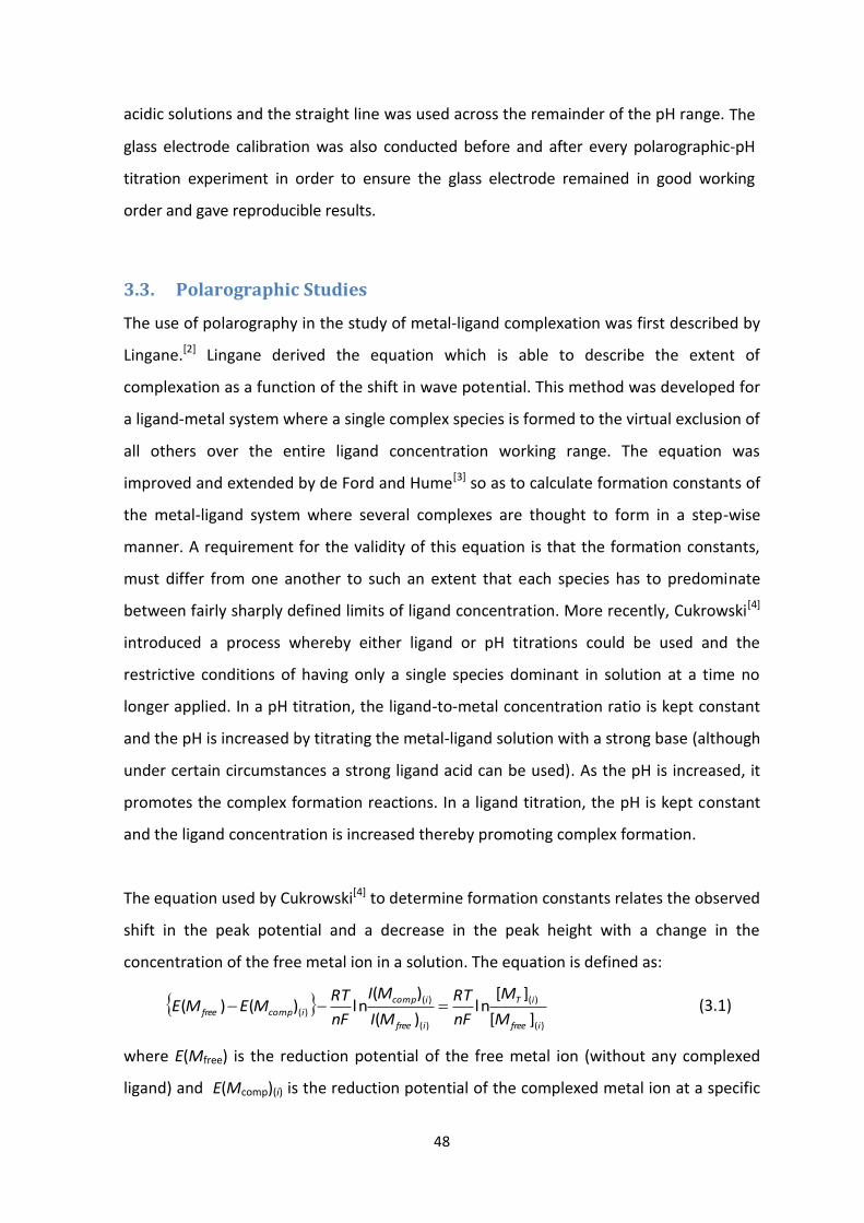
48
acidic solutions and the straight line was used across the remainder of the pH range. The
glass electrode calibration was also conducted before and after every polarographic-pH
titration experiment in order to ensure the glass electrode remained in good working
order and gave reproducible results.
3.3. Polarographic Studies
The use of polarography in the study of metal-ligand complexation was first described by
Lingane.[2] Lingane derived the equation which is able to describe the extent of
complexation as a function of the shift in wave potential. This method was developed for
a ligand-metal system where a single complex species is formed to the virtual exclusion of
all others over the entire ligand concentration working range. The equation was
improved and extended by de Ford and Hume[3] so as to calculate formation constants of
the metal-ligand system where several complexes are thought to form in a step-wise
manner. A requirement for the validity of this equation is that the formation constants,
must differ from one another to such an extent that each species has to predominate
between fairly sharply defined limits of ligand concentration. More recently, Cukrowski[4]
introduced a process whereby either ligand or pH titrations could be used and the
restrictive conditions of having only a single species dominant in solution at a time no
longer applied. In a pH titration, the ligand-to-metal concentration ratio is kept constant
and the pH is increased by titrating the metal-ligand solution with a strong base (although
under certain circumstances a strong ligand acid can be used). As the pH is increased, it
promotes the complex formation reactions. In a ligand titration, the pH is kept constant
and the ligand concentration is increased thereby promoting complex formation.
The equation used by Cukrowski[4] to determine formation constants relates the observed
shift in the peak potential and a decrease in the peak height with a change in the
concentration of the free metal ion in a solution. The equation is defined as:
)(
)(
)(
)(
)(][
][ln
)(
)(ln)()(
ifree
iT
ifree
icomp
icompfreeM
M
nF
RT
MI
MI
nF
RTMEME (3.1)
where E(Mfree) is the reduction potential of the free metal ion (without any complexed
ligand) and E(Mcomp)(i) is the reduction potential of the complexed metal ion at a specific
49
pH or ligand concentration, depending on the type of titration done; [MT] and [Mfree]
indicate the total and free metal ion concentrations at each step in the titration,
respectively; I(Mcomp) is the reduction current of the labile wave or peak recorded at each
step; I(Mfree) is the current observed from the reduction of the metal ion Mn+(aq) at the
pH value with the assumption that complexes of the metal ion were not formed. The
term )(
)(
)(
)(ln
ifree
icomp
MI
MI
nF
RT is generally referred to as the correction factor and is also very close
to zero in most cases.[2] This is true if the rate of diffusion of the complexed species is
similar to that of uncomplexed hydrated species and if all species formed are labile. ΔE
represents the difference between E(Mfree) and E(Mcomp)(i), i.e. the shift in the half-wave
or peak potential observed at each ith pH value or ligand concentration to which the
metal-ligand system was adjusted in the polarographic cell by titration with base or ligand
solution, respectively. Thus the left-hand side of the equation 3.1 is thus called the
corrected ΔE and is determined using the experimental data obtained from the
polarographic titration experiment. In this work only pH titrations were used, the reason
for which will become evident in later chapters. All further discussions will thus refer to
pH titrations. In this case, the left-hand side of the equation plotted vs pH is called the
experimental complex formation curve (ECFC) and the right-hand side of the equation
plotted vs pH forms the calculated complex formation curve (CCFC)
The right-hand side of equation 3.1 is solved by employing mass balance equations of all
possible species in solution. The mass balance equation for all species containing the
metal ion is:
(3.2)
Since the initial [MT] added to the solution is known, [MT](i) is determined at each step in
the titration by simply taking dilution into account. The [Hfree] is determined from
measuring the pH using the glass electrode and if r is a negative value it rather indicates
[OHfree]. The [Lfree] is determined from a second mass balance equation (equation 3.3)
since the initial [LT] is once again known and , [LT](i) is found by accounting for dilution.
(3.3)

50
The concentrations of the free metal ion and the free ligand at each pH, as well as the
stability constants, , are refined simultaneously using a non-linear least squares
refinement method. This is achieved by predicting the species present and giving initial
estimates of their log β values such that the difference between the ECFC and the CCFC is
minimised. In this refinement process, the stability constants for the metal-hydroxide
complexes, the protonation constants for the ligand and the dissociation constant for
water are all kept constant.
3.3.1 Polarographic-pH titrations: Experiments in the absence of ligand
This section describes the procedures used in the polarographic-pH titration of solutions
containing the Bi3+ and Tl+ (as the witness ion) but no ligand. The results were used to
obtain the free metal ion potential of bismuth (E(Bifree)) and thallium (E(Tlfree)).
An exact volume of 25.00 mL 0.1 M HNO3 (containing 0.4 M KNO3) was added to a
jacketed-cell. The cell was equipped with a dropping mercury electrode (DME), a 3 M
KCl Ag/AgCl reference electrode inserted into a 0.5 M KNO3 salt bridge, a platinum
counter electrode, a glass electrode and a thermocouple (used to monitor the solution
temperature throughout the experiment). All components used were supplied by
Metrohm. After purging the solution with N2 for 30 minutes, a background
polarogram was recorded to ensure that there were no reduction processes occurring
in the region of our analysis due to impurities.
Using a Hamilton syringe, 25.0 µL of a 0.0100 M Bi(NO3)3 (Merck) stock solution containing
1 M HNO3 and 100.0 µL of 0.0100 M TlNO3 (Sigma Aldrich) stock solution made up in 0.5 M
HNO3 were added to the reaction cell. The solution was purged again and polarograms
were collected such that at least three overlapped so as to ensure accurate analysis of the
reduction waves and that sufficient purging had taken place.
Using the NOVA method discussed in Chapter 2, Section 2.4, 0.1 M KOH (containing 0.4 M
KNO3) was added using a Dosino in 0.300 mL increments, until a final pH of 2.3 was
reached in Part A, then KOH was added in increments of 0.025 mL until the end of the
51
titration in Part B. The addition of the KOH results in an increase of pH and polarograms
were recorded only once enough KOH was added to cause an increase of about 0.1 pH
units. The potential difference at the glass electrode was also accurately measured during
the collection of the DC polarogram. Titrations were continued until a pH of 8 was
reached so that an accurate value of E(Tlfree) could be calculated.
The parameters used in these polarographic-pH titration experiments are shown in Table
A 1.1 in Appendix 1. The initial pause is the wait time before the experiment starts. It is
important to allow all equipment to be properly initialized and for the computer to
interface with the various components. The sample rate is how often the signals (in this
case the potential difference at the glass electrode and the temperature) are measured.
The sample rate is set at 2 seconds to allow for more stable measurements. The pH step
indicates that a polarogram must be measured after each 0.1 pH unit change. Dose refers
to the volume increment of base added by the Dosino. The polarographic parameters
indicate how the DC polarogram was measured. The initial and final potential gives the
potential range over which the DC polarogram is recorded. The step potential is the
incremental change in applied potential (toward more negative values) at each new drop.
The interval time is the mercury drop life. The stop conditions refer to the pH at which
the titration must be terminated. It is impossible to change the pH by only 0.1 unit when
adding 0.1 M hydroxide to solutions around pH 7 due to the very small buffer capacity of
the solution in this region, so only approximate values that will cause termination of the
experiment. In this work the Bi3+ precipitates as a Bi-hydroxy-nitrate species long before
pH 8, however, the experiment was allowed to continue in order to obtain all Tl+ data
which was used to calculate the free metal ion potential of thallium as accurately as
possible.

52
3.3.2. Polarographic-pH titrations: Experiments in the presence of ligand
This section describes the procedures used in the polarographic-pH titration of solutions
once again containing the Bi3+ and Tl+, but in this case amino acid is added to the solution.
These results were used together with that in section 3.3.1 to study bismuth-amino acid
complexation.
The polarographic-pH titration experiment was run using the same parameters given in

53
except the stop condition was now set to pH 10 to ensure that there was always
sufficient data to analyze where necessary. In these experiments, 25.00 mL of the HNO3
solution was also added to a jacketed-cell containing the same components stated above.
The metal ions (Bi3+ and Tl+) were added and polarograms recorded as before. Ligand
(accurately weighed to five decimal places) was then added to the cell and the system
was purged. Three overlapping polarograms were collected with purging occurring
between measurments to ensure no oxygen was present in the cell. Only then were the
automated NOVA procedures initiated. The amino acids reported in this study will
predominantly be Glutamic Acid, Histidine and Glutamine, however, Chapter 4 will show
that other amino acids such as methionine and cysteine were also studied in order to
demonstrate their complexing behavior with Bi3+.
3.3.3 Fitting the polarograms
In order to determine the parameters from the recorded DC polarograms, the following
equation was fitted to each polarogram:
(3.4)
where
(3.5)
and Id represents the diffusion limited current, Ib represents the background current, n
represents the number of electrons transferred, E1/2 represents the half-wave potentials
for reduction of metal ions and ɣ represents the steepness of the wave. For a reversible
electron transfer process, the ɣ value is equal to 1 and this implies that the rate of
electron transfer is greater than the rate of mass transport and is described by Nernstian
behavior. However, as described in previous work[5], a ɣ value for stability constant
determination in the range of 0.9 - 1.0 was sufficient to indicate that the electron
transfer process is fully reversible. A value between 0.9 - 0.5 indicates that the electron
transfer process is quasi-reversible and a value less than 0.5 shows that the electron
transfer process is irreversible.

54
The background current of the polarograms is described by equation 3.5 where the
straight line terms refers to the capacitance current. The exponential term (cdx) takes into
account the exponential curvature of mercury oxidation (at the start of the Bi(III)
reduction wave) and hydrogen reduction (at the end of the Tl(I) reduction wave in acidic
solutions) Since the entire polarogram is too complicated to fit all at once (Figure 3.1), the
data was split into two separate data sets, one containing the Bi3+ reduction data and the
other the Tl+ data. Equation 3.2 was then fitted to each reduction wave separately.
Figure 3.1: Typical DC polarogram showing the reduction of Bi3+ and Tl+ -and H2. [Bi3+] =
9.95 x 10⁻⁶ M, [Tl+] = 3.98 x 10⁻⁵ M, µ = 0.5 M, T = 25 C
Since the reduction waves are fitted using a non-linear curve fitting programme, initial
estimates of E1/2, Id, ɣ and background values were required. The estimates given are
shown in Table A 1.2. in Appendix 1 and these values are then refined iteratively. Once
all the parameters were found, the values for E1/2, Id and ɣ were all plotted against pH,
for Bi3+ and Tl+, respectively, and then analysed further.
3.3.4. Calculation of formation constants for Bi3+-amino acid complexes
The 3D-CFC programme[6] was used to calculate the formation constant of the predicted
solution species. This software essentially applies equation 3.1 to entered data. Initial
parameters that need to be inputted into the software include the initial concentrations
of total Bi3+ and ligand being studied and the total volume of the solution before any
0
1
2
3
4
5
6
7
8
-0.8 -0.7 -0.6 -0.5 -0.4 -0.3 -0.2 -0.1 0 0.1 0.2 0.3
Cu
rre
nt
(10
-8A
)
Applied Potential (V)
H2 evolution
Tl+ Reduction
Bi3+
Reduction
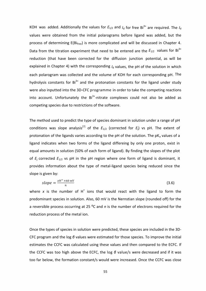
55
KOH was added. Additionally the values for E1/2 and Id for free Bi3+ are required. The Id
values were obtained from the initial polarograms before ligand was added, but the
process of determining E(Bifree) is more complicated and will be discussed in Chapter 4.
Data from the titration experiment that need to be entered are the E1/2 values for Bi3+
reduction (that have been corrected for the diffusion junction potential, as will be
explained in Chapter 4) with the corresponding Id values, the pH of the solution in which
each polarogram was collected and the volume of KOH for each corresponding pH. The
hydrolysis constants for Bi3+ and the protonation constants for the ligand under study
were also inputted into the 3D-CFC programme in order to take the competing reactions
into account. Unfortunately the Bi3+-nitrate complexes could not also be added as
competing species due to restrictions of the software.
The method used to predict the type of species dominant in solution under a range of pH
conditions was slope analysis[7] of the E1/2 (corrected for Ej) vs pH. The extent of
protonation of the ligands varies according to the pH of the solution. The pKa values of a
ligand indicates when two forms of the ligand differeing by only one proton, exist in
equal amounts in solution (50% of each form of ligand). By finding the slopes of the plot
of Ej corrected E1/2 vs pH in the pH region where one form of ligand is dominant, it
provides information about the type of metal-ligand species being reduced since the
slope is given by:
(3.6)
where x is the number of H+ ions that would react with the ligand to form the
predominant species in solution. Also, 60 mV is the Nernstian slope (rounded off) for the
a reversible process occurring at 25 ⁰C and n is the number of electrons required for the
reduction process of the metal ion.
Once the types of species in solution were predicted, these species are included in the 3D-
CFC program and the log β values were estimated for those species. To improve the initial
estimates the CCFC was calculated using these values and then compared to the ECFC. If
the CCFC was too high above the ECFC, the log β value/s were decreased and if it was
too far below, the formation constant/s would were increased. Once the CCFC was close
56
to overlapping with that of the ECFC, the values are refined to obtain a more accurate fit
and to determine the standard deviation for the formation constant. Figure 3.2 gives an
example of the ECFC and CCFC after the refinement process, illustrating that they should
overlap throughout the pH range in order to be confident that the species predicted are
correct and that their log β values are accurate.
Figure 3.2: An example of an ECFC and a refined CCFC for a Bi3+-amino acid system.
0
20
40
60
80
100
120
1 1.5 2 2.5 3 3.5 4 4.5 5
Co
rre
cte
d D
E/m
V
pH
ECFC
CCFC
57
3.4. Investigating the bismuth precipitation product from a nitric acid
solution
A 1 L 0.1 M HNO3 solution was made and to it bismuth nitrate salt was added to it and
dissolved such that [Bi3+] = 1 x 10⁻² M. The solution was then left to equilibrate for 3 hours.
A pH electrode, calibrated using buffers, was used to monitor the pH of the solution.
Concentrated KOH (11.5 M) was then added dropwise to the solution at a rate of 1 drop
every 4 minutes while stirring. This was continued until precipitation occurred and then
left to stand for 1 day. The precipitate was isolated using ACE 11.0 cm, 5 µm pore size filter
paper and placed in a desiccator until all moisture was removed. The precipitate was then
studied by Powder X-Ray Diffraction (PXRD) using a zero background holder. An
experiment was also run where 1 L 0.1 M HNO3 solution was made and both bismuth
nitrate and glutamic acid (Glu) was added to it such that [Bi3+] = 1 x 10⁻² M and the ratio
[Glu]:[Bi3+]= 1000. Concentrated KOH was then added until precipitation occurred and the
precipitate isolated and allowed to dry. The powder was then analysed using PXRD.
3.5. X-Ray Diffraction
The insoluble Bi3+ species which was indicated by a drop in Id when polarography was
employed proved a real obstacle in the full analysis of whether a Bi3+- amino acid complex
was forming. Additionally, the type of species which was precipitating was not fully
known and only the previous literature studies by Olin[8], Bidleman[9] and Hataye[10]
allowed an indication of the species present in solution. It was decided that a
rudimentary exercise be performed in order to gain a better understanding of what type
of Bi3+ species was precipitating. Powder x-ray diffraction (PXRD) was therefore employed
in order to see if the species precipitating could be isolated and analysed.
PXRD involved targeting x-rays at the isolated precipitate sample and then the diffracted
x-rays were measured. The K-alpha radiation is directed toward a detector once it has hit
and diffracted off the specimen.[11] These x-rays, which are generated by an x-ray tube,
are filtered to produce monochromatic radiation which is collimated and then directed
toward the sample. The interaction of the incident rays with the powder produces a
diffracted ray undergoing constructive interference when conditions satisfy Bragg's Law.

58
Bragg's Law is given as nλ = 2d sinθ[11] where λ is the wavelength of the x-ray, d is the
spacing of the crystal layers (path difference), θ is the incident angle (the angle between
incident ray and the scatter plane) and n is an integer. Subsequently, a spectrum in terms
of intensity and 2θ are produced and the powder pattern can then be used to cross
reference against other PXRD patterns of known structures within the ICSD.[11-12]
Figure 3.3: Schematic of the PXRD process whereby X-rays are emitted from an X-Ray
Source and travel toward and reflect of a crystal/crystalline powder sample. The reflected
X-rays are then detected and the structure of the complex must be calculated from the
respective intensities and 2θ values which are present in the spectrum.[13]
The instrument to be used will be a Bruker D2 phaser diffractometer. The isolated
precipitate was transferred to a pestle and mortar and ground until a fine powder was
achieved. The powder was then placed onto a zero background stand and placed into the
D2 diffractometer (instrument settings are shown in Appendix 1). PXRD (demonstrated in
the schematic in Figure 3.3) is a useful technique for this study because once the XRD
component of analysis has been completed, it can readily be compared with other PXRD

59
patterns or a suitable programme, such as Mercury, can be used to convert single crystal
XRD data to predict the theoretical PXRD pattern. In our work we aim to examine the Bi3+-
hydroxy-nitrate precipitates and also investigate whether in the presence of ligand it is
simply the Bi3+-hydroxy-nitrate species that forms, or whether an amino acid is still bound
to Bi3+ in the precipitate.

60
3.6. References
[1] C. Billing and I. Cukrowski, S. Afr. J. Chem.,2009, 62, 168.
[2] J. J. Lingane, Chem. Rev.,1941, 29, 1.
[3] D. Deford and D. N. Hume, J. Am. Chem. Soc.,1951, 73, 5321.
[4] I. Cukrowski, Anal. Chim. Acta.,1996, 336, 23.
[5] I. Cukrowski, H. M. Marques, T. S. Mkwizu, P. P. Magampa and C. Serge, Anal. Chim.
Acta.,2007, 590, 203.
[6] P. Franklyn and I. Cukrowski, 3D-CFC software, University of the Witwatersrand, 2003,
Windows Version 1.2, (unpublished)
[7] I. Cukrowski, Electroanal.,1997, 9, 699.
[8] A. Olin, Acta. Chem. Scand.,1957, 11, 1445.
[9] T. F. Bidleman, Anal. Chim. Acta.,1971, 56, 221.
[10] I. Hataye, H. Suganuma, Ikegami H. and T. Kuchiki, Bull. Chem. Soc. Japan,1982, 55, 1475.
[11] G. I. Analysis in Single Crystal X-Ray Diffraction, 2012 Science Education and Resource
Centre, Montana State Univeristy, 2012.
[12] A. Belsky, M. Hellenbrandt, V. L. Karen and P. Luksch, Acta. Cryst.,2002, B58, 364.
[13] C. Morris, B. Sieve and H. Bullen, An Introduction to X-Ray Diffraction, Highland Heights, KY
41099.

60
Chapter 4: Initial Bi3+ complexation studies
4.1. Introduction
The study of Bi3+ complexation with amino acids using polarography is not a technique
which has been commonly used. Previous studies, as shown in Chapter 1, have utilized
potentiometric studies in order to monitor complex formation. To monitor the success
of our polarographic pH titrations, an initial analysis was completed. Studies by Lingane[1]
and furthermore by Cukrowski[2] have shown that the successful complexation of a metal
ion to a ligand, studied using polarography, will cause a shift in E1/2. The aim of this
Chapter is to show that the pH-polarographic studies completed in our study illustrate
that complexation between Bi3+ and the respective amino acid ligand is actually
occurring.
As described in Chapter 1 and Chapter 3, the calibration of the glass electrode used in this
work was vital for the robustness of the data collected. Due to Bi3+ being largely insoluble
in nitrate solutions above pH ~2, the initial work without ligand in solution took place in
the pH range of 1 – 2. The calibration of the glass electrode was completed and its results
were used to determine the worthiness of the glass electrode during the polarographic-
pH titrations. This chapter will also aim to show how the determination of Ej was
accomplished using Tl+ data and subsequently determining the Ej correction on Bi3+.
Previous work[2a, 3] have shown the optimal conditions in terms of [L]:[M] for studies using
polarography, however, during this work for the [L]:[M] conditions needed to be
reassessed for amino acid ligands reacting with Bi3+. Evidence presented in this chapter
will show that conditions which proved fruitful in other studies, could not be employed in
this study due to the complicated chemistry associated with Bi3+.
4.2. Glass Electrode Calibration and determination of pH values.
The glass electrode calibrations were conducted in order to determine an accurate
relationship between pH and voltage measured at the glass electrode. Figure 4.1 shows
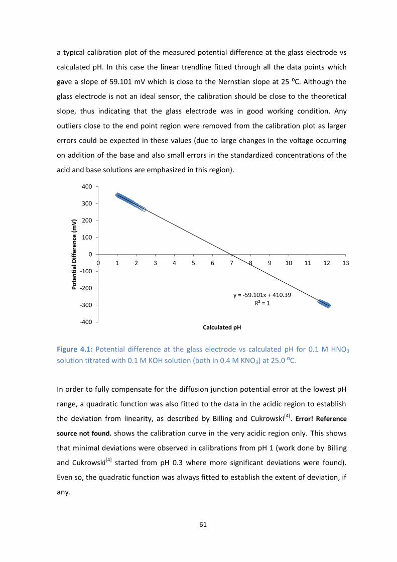
61
a typical calibration plot of the measured potential difference at the glass electrode vs
calculated pH. In this case the linear trendline fitted through all the data points which
gave a slope of 59.101 mV which is close to the Nernstian slope at 25 ⁰C. Although the
glass electrode is not an ideal sensor, the calibration should be close to the theoretical
slope, thus indicating that the glass electrode was in good working condition. Any
outliers close to the end point region were removed from the calibration plot as larger
errors could be expected in these values (due to large changes in the voltage occurring
on addition of the base and also small errors in the standardized concentrations of the
acid and base solutions are emphasized in this region).
Figure 4.1: Potential difference at the glass electrode vs calculated pH for 0.1 M HNO3
solution titrated with 0.1 M KOH solution (both in 0.4 M KNO3) at 25.0 ⁰C.
In order to fully compensate for the diffusion junction potential error at the lowest pH
range, a quadratic function was also fitted to the data in the acidic region to establish
the deviation from linearity, as described by Billing and Cukrowski[4]. Error! Reference
source not found. shows the calibration curve in the very acidic region only. This shows
that minimal deviations were observed in calibrations from pH 1 (work done by Billing
and Cukrowski[4] started from pH 0.3 where more significant deviations were found).
Even so, the quadratic function was always fitted to establish the extent of deviation, if
any.
y = -59.101x + 410.39 R² = 1
-400
-300
-200
-100
0
100
200
300
400
0 1 2 3 4 5 6 7 8 9 10 11 12 13
Po
ten
tial
Dif
fere
nce
(m
V)
Calculated pH

62
Figure 4.2: Glass electrode calibration curve in pH range 1 - 2 showing both the linear
trendline (black) and the quadratic trendline (red) fitted.
The pH of the solution at each step in the polarographic-pH titration was calculated using
the potential difference measured by the glass electrode and the calibration curves
that were determined before and after each experiment. The pH values were taken from
the quadratic curve only at the at the lowest pH values if the function was below the
linear curve, and then subsequently calculated using the linear function for the
remainder of the pH range. The results were only considered acceptable if the standard
deviation between the calculated pH values using the before and after calibrations was
less than 0.002 units. The average pH values from the two calibrations were then used.
A suggestion to test the condition of the glass electrode was given by Billing and
Cukrowski[4] which gives guidelines to limits of acceptable slopes for the data fitted in
either the acidic or basic regions. These guideline are shown in Table 4.1. Although the
tests were applied to titrations using 0.5 M acid and base solutions,[4] it was always
checked that the calibrations for this work fell in the suggested limits.
y = 4.5548x2 - 66.987x + 415.95 R² = 0.9999
y = -59.101x + 410.39 R² = 1
250
270
290
310
330
350
370
1 1.2 1.4 1.6 1.8 2 2.2
Po
ten
tial
Dif
fere
nce
(m
V)
Calculated pH
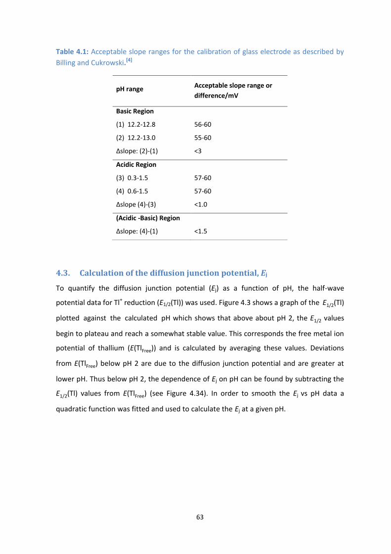
63
Table 4.1: Acceptable slope ranges for the calibration of glass electrode as described by
Billing and Cukrowski.[4]
4.3. Calculation of the diffusion junction potential, Ej
To quantify the diffusion junction potential (Ej) as a function of pH, the half-wave
potential data for Tl+ reduction (E1/2(Tl)) was used. Figure 4.3 shows a graph of the E1/2(Tl)
plotted against the calculated pH which shows that above about pH 2, the E1/2 values
begin to plateau and reach a somewhat stable value. This corresponds the free metal ion
potential of thallium (E(TlFree)) and is calculated by averaging these values. Deviations
from E(TlFree) below pH 2 are due to the diffusion junction potential and are greater at
lower pH. Thus below pH 2, the dependence of Ej on pH can be found by subtracting the
E1/2(Tl) values from E(TlFree) (see Figure 4.34). In order to smooth the Ej vs pH data a
quadratic function was fitted and used to calculate the Ej at a given pH.
pH range Acceptable slope range or
difference/mV
Basic Region
(1) 12.2-12.8 56-60
(2) 12.2-13.0 55-60
∆slope: (2)-(1) <3
Acidic Region
(3) 0.3-1.5 57-60
(4) 0.6-1.5 57-60
∆slope (4)-(3) <1.0
(Acidic -Basic) Region
∆slope: (4)-(1) <1.5
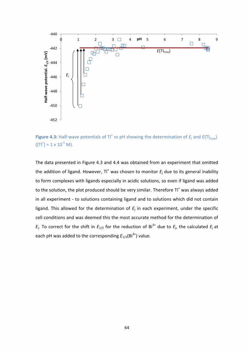
64
Figure 4.3: Half-wave potentials of Tl+ vs pH showing the determination of Ej and E(TlFree).
([Tl+] = 1 x 10⁻⁵ M).
The data presented in Figure 4.3 and 4.4 was obtained from an experiment that omitted
the addition of ligand. However, Tl+ was chosen to monitor Ej due to its general inability
to form complexes with ligands especially in acidic solutions, so even if ligand was added
to the solution, the plot produced should be very similar. Therefore Tl+ was always added
in all experiment - to solutions containing ligand and to solutions which did not contain
ligand. This allowed for the determination of Ej in each experiment, under the specific
cell conditions and was deemed this the most accurate method for the determination of
Ej. To correct for the shift in E1/2 for the reduction of Bi3+ due to Ej, the calculated Ej at
each pH was added to the corresponding E1/2(Bi3+) value.
-452
-450
-448
-446
-444
-442
-440
0 1 2 3 4 5 6 7 8 9
Hal
f-w
ave
po
ten
tial
. E 1
/2 (
mV
)
pH
Ej
E(TlFree)
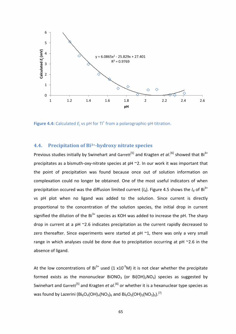
65
Figure 4.4: Calculated Ej vs pH for Tl+ from a polarographic-pH titration.
4.4. Precipitation of Bi3+-hydroxy nitrate species
Previous studies initially by Swinehart and Garrett[5] and Kragten et al.[6] showed that Bi3+
precipitates as a bismuth-oxy-nitrate species at pH ~2. In our work it was important that
the point of precipitation was found because once out of solution information on
complexation could no longer be obtained. One of the most useful indicators of when
precipitation occured was the diffusion limited current (Id). Figure 4.5 shows the Id of Bi3+
vs pH plot when no ligand was added to the solution. Since current is directly
proportional to the concentration of the solution species, the initial drop in current
signified the dilution of the Bi3+ species as KOH was added to increase the pH. The sharp
drop in current at a pH ~2.6 indicates precipitation as the current rapidly decreased to
zero thereafter. Since experiments were started at pH ~1, there was only a very small
range in which analyses could be done due to precipitation occurring at pH ~2.6 in the
absence of ligand.
At the low concentrations of Bi3+ used (1 x10⁻⁵M) it is not clear whether the precipitate
formed exists as the mononuclear BiONO3 (or Bi(OH)2NO3) species as suggested by
Swinehart and Garrett[5] and Kragten et al.[6] or whether it is a hexanuclear type species as
was found by Lazerini (Bi6O4(OH)4(NO3)6 and Bi6O5(OH)3(NO3)5).[7]
y = 6.0865x2 - 25.829x + 27.401 R² = 0.9769
0
1
2
3
4
5
6
1 1.2 1.4 1.6 1.8 2 2.2 2.4 2.6
Cal
cula
ted
Ej (
mV
)
pH
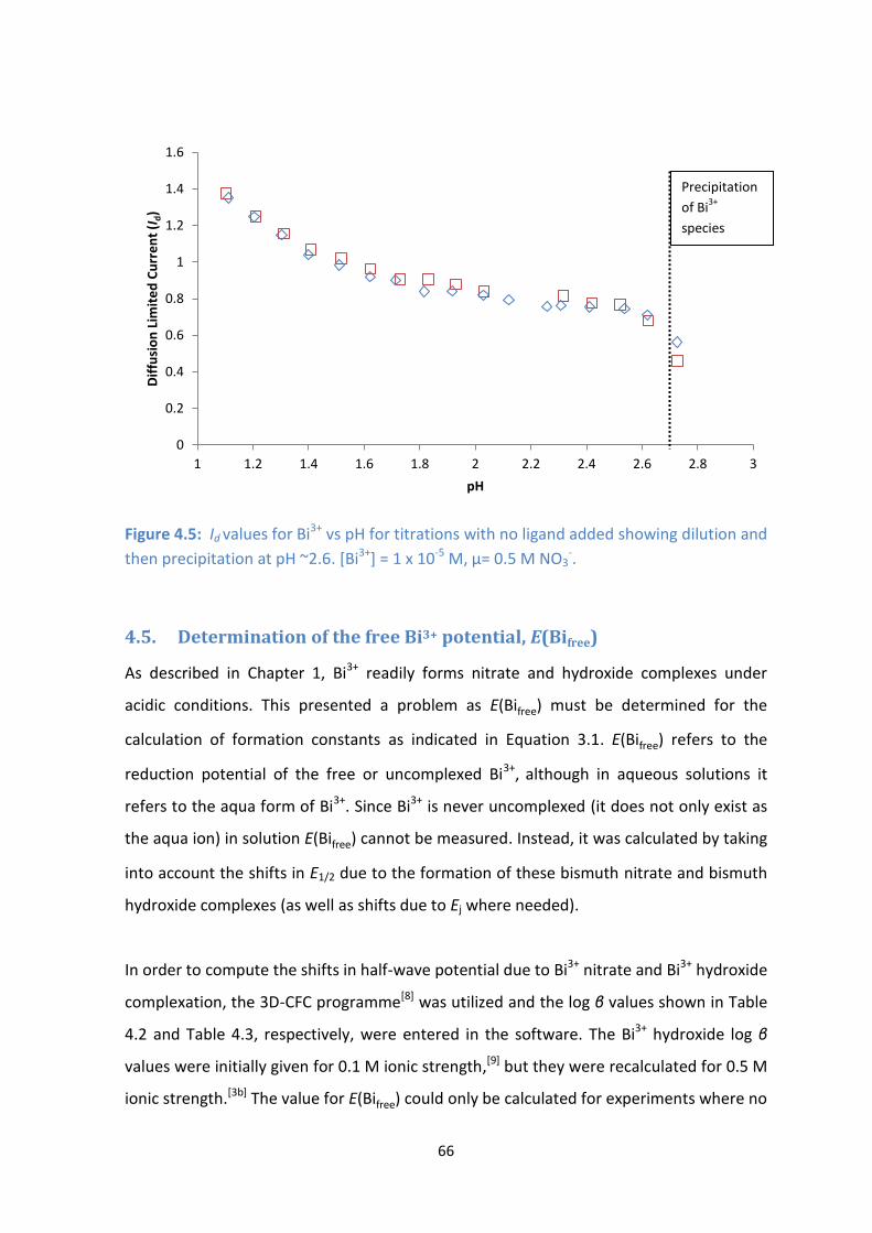
66
Figure 4.5: Id values for Bi3+ vs pH for titrations with no ligand added showing dilution and
then precipitation at pH ~2.6. [Bi3+] = 1 x 10⁻⁵ M, µ= 0.5 M NO3-.
4.5. Determination of the free Bi3+ potential, E(Bifree)
As described in Chapter 1, Bi3+ readily forms nitrate and hydroxide complexes under
acidic conditions. This presented a problem as E(Bifree) must be determined for the
calculation of formation constants as indicated in Equation 3.1. E(Bifree) refers to the
reduction potential of the free or uncomplexed Bi3+, although in aqueous solutions it
refers to the aqua form of Bi3+. Since Bi3+ is never uncomplexed (it does not only exist as
the aqua ion) in solution E(Bifree) cannot be measured. Instead, it was calculated by taking
into account the shifts in E1/2 due to the formation of these bismuth nitrate and bismuth
hydroxide complexes (as well as shifts due to Ej where needed).
In order to compute the shifts in half-wave potential due to Bi3+ nitrate and Bi3+ hydroxide
complexation, the 3D-CFC programme[8] was utilized and the log β values shown in Table
4.2 and Table 4.3, respectively, were entered in the software. The Bi3+ hydroxide log β
values were initially given for 0.1 M ionic strength,[9] but they were recalculated for 0.5 M
ionic strength.[3b] The value for E(Bifree) could only be calculated for experiments where no
0
0.2
0.4
0.6
0.8
1
1.2
1.4
1.6
1 1.2 1.4 1.6 1.8 2 2.2 2.4 2.6 2.8 3
Dif
fusi
on
Lim
ite
d C
urr
en
t (I
d)
pH
Precipitation
of Bi3+
species
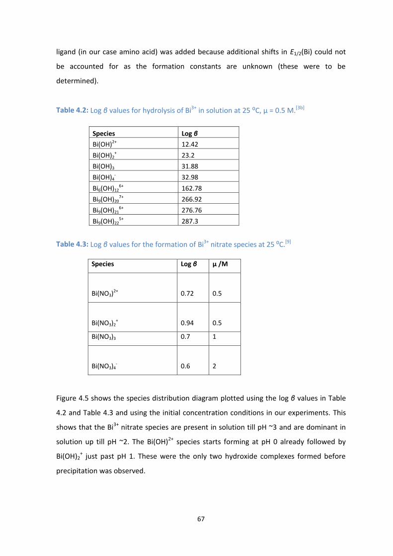
67
ligand (in our case amino acid) was added because additional shifts in E1/2(Bi) could not
be accounted for as the formation constants are unknown (these were to be
determined).
Table 4.2: Log β values for hydrolysis of Bi3+ in solution at 25 ⁰C, µ = 0.5 M.[3b]
Species Log β
Bi(OH)2+ 12.42
Bi(OH)2+ 23.2
Bi(OH)3 31.88
Bi(OH)4- 32.98
Bi6(OH)126+ 162.78
Bi9(OH)207+ 266.92
Bi9(OH)216+ 276.76
Bi9(OH)225+ 287.3
Table 4.3: Log β values for the formation of Bi3+ nitrate species at 25 ⁰C.[9]
Figure 4.5 shows the species distribution diagram plotted using the log β values in Table
4.2 and Table 4.3 and using the initial concentration conditions in our experiments. This
shows that the Bi3+ nitrate species are present in solution till pH ~3 and are dominant in
solution up till pH ~2. The Bi(OH)2+ species starts forming at pH 0 already followed by
Bi(OH)2+ just past pH 1. These were the only two hydroxide complexes formed before
precipitation was observed.
Species Log β µ /M
Bi(NO3)2+ 0.72 0.5
Bi(NO3)2+ 0.94 0.5
Bi(NO3)3 0.7 1
Bi(NO3)4- 0.6 2
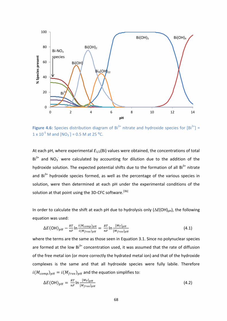
68
Figure 4.6: Species distribution diagram of Bi3+ nitrate and hydroxide species for [Bi3+] =
1 x 10⁻⁵ M and [NO3-] = 0.5 M at 25 ⁰C.
At each pH, where experimental E1/2(Bi) values were obtained, the concentrations of total
Bi3+ and NO3- were calculated by accounting for dilution due to the addition of the
hydroxide solution. The expected potential shifts due to the formation of all Bi3+ nitrate
and Bi3+ hydroxide species formed, as well as the percentage of the various species in
solution, were then determined at each pH under the experimental conditions of the
solution at that point using the 3D-CFC software.[3b]
In order to calculate the shift at each pH due to hydrolysis only (E(OH)pH), the following
equation was used:
ln
ln
(4.1)
where the terms are the same as those seen in Equation 3.1. Since no polynuclear species
are formed at the low Bi3+ concentration used, it was assumed that the rate of diffusion
of the free metal ion (or more correctly the hydrated metal ion) and that of the hydroxide
complexes is the same and that all hydroxide species were fully labile. Therefore
and the equation simplifies to:
ln
(4.2)
0
20
40
60
80
100
0 2 4 6 8 10 12 14
% S
pe
cie
s p
rese
nt
pH
Bi-NO3
species
Bi3+
Bi(OH)
Bi(OH)2
Bi9(OH)22
Bi(OH)3 Bi(OH)4
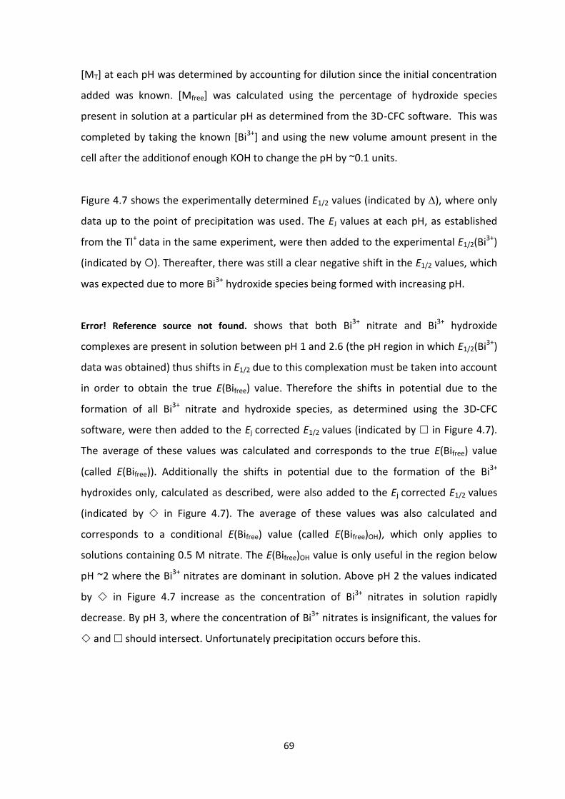
69
[MT] at each pH was determined by accounting for dilution since the initial concentration
added was known. [Mfree] was calculated using the percentage of hydroxide species
present in solution at a particular pH as determined from the 3D-CFC software. This was
completed by taking the known [Bi3+] and using the new volume amount present in the
cell after the additionof enough KOH to change the pH by ~0.1 units.
Figure 4.7 shows the experimentally determined E1/2 values (indicated by ), where only
data up to the point of precipitation was used. The EJ values at each pH, as established
from the Tl+ data in the same experiment, were then added to the experimental E1/2(Bi3+)
(indicated by ). Thereafter, there was still a clear negative shift in the E1/2 values, which
was expected due to more Bi3+ hydroxide species being formed with increasing pH.
Error! Reference source not found. shows that both Bi3+ nitrate and Bi3+ hydroxide
complexes are present in solution between pH 1 and 2.6 (the pH region in which E1/2(Bi3+)
data was obtained) thus shifts in E1/2 due to this complexation must be taken into account
in order to obtain the true E(Bifree) value. Therefore the shifts in potential due to the
formation of all Bi3+ nitrate and hydroxide species, as determined using the 3D-CFC
software, were then added to the Ej corrected E1/2 values (indicated by in Figure 4.7).
The average of these values was calculated and corresponds to the true E(Bifree) value
(called E(Bifree)). Additionally the shifts in potential due to the formation of the Bi3+
hydroxides only, calculated as described, were also added to the Ej corrected E1/2 values
(indicated by in Figure 4.7). The average of these values was also calculated and
corresponds to a conditional E(Bifree) value (called E(Bifree)OH), which only applies to
solutions containing 0.5 M nitrate. The E(Bifree)OH value is only useful in the region below
pH ~2 where the Bi3+ nitrates are dominant in solution. Above pH 2 the values indicated
by in Figure 4.7 increase as the concentration of Bi3+ nitrates in solution rapidly
decrease. By pH 3, where the concentration of Bi3+ nitrates is insignificant, the values for
and should intersect. Unfortunately precipitation occurs before this.
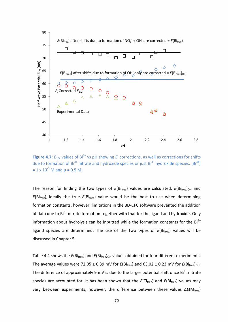
70
Figure 4.7: E1/2 values of Bi3+ vs pH showing EJ corrections, as well as corrections for shifts
due to formation of Bi3+ nitrate and hydroxide species or just Bi3+ hydroxide species. [Bi3+]
= 1 x 10⁻⁵ M and µ = 0.5 M.
The reason for finding the two types of E(Bifree) values are calculated, E(Bifree)OH and
E(Bifree). Ideally the true E(Bifree) value would be the best to use when determining
formation constants, however, limitations in the 3D-CFC software prevented the addition
of data due to Bi3+ nitrate formation together with that for the ligand and hydroxide. Only
information about hydrolysis can be inputted while the formation constants for the Bi3+
ligand species are determined. The use of the two types of E(Bifree) values will be
discussed in Chapter 5.
Table 4.4 shows the E(Bifree) and E(Bifree)OH values obtained for four different experiments.
The average values were 72.05 ± 0.39 mV for E(Bifree) and 63.02 ± 0.23 mV for E(Bifree)OH.
The difference of approximately 9 mV is due to the larger potential shift once Bi3+ nitrate
species are accounted for. It has been shown that the E(Tlfree) and E(Bifree) values may
vary between experiments, however, the difference between these values ΔE(Mfree)
40
45
50
55
60
65
70
75
80
1 1.2 1.4 1.6 1.8 2 2.2 2.4 2.6 2.8
Hal
f-w
ave
Po
ten
tial
E1/
2 (m
V)
pH
Experimental Data
EJ Corrected E1/2
E(Bifree) after shifts due to formation of OH- only are corrected = E(Bifree)OH
E(Bifree) after shifts due to formation of NO3- + OH- are corrected = E(Bifree)

71
remains constant and so it was very useful in Bi-ligand studies.[3b] The differences were
calculated as follows:
ΔE(Mfree) = E(Tlfree) and E(Bifree) (4.3)
ΔE(Mfree)OH = E(Tlfree) and E(Bifree)OH (4.4)
These values as well as the average values are also given in Table 4.4.
Table 4.4: The E(Mfree) values for Bi3+ and Tl+, as well as the ΔE(Mfree) values.
Exp. E(Tlfree) /mV E(Bifree) /mV E(Mfree) /mV E(Bifree)OH /mV E(Mfree)OH /mV
1 -442.75 72.22 514.96 62.83 505.58
2 -442.55 71.87 514.42 63.32 505.88
3 -442.67 72.50 515.17 63.10 505.77
4 -441.92 71.61 513.53 62.84 504.76
Average 514.5 Average 505.5
S.D. 0.7 S.D. 0.5
RSD 0.14 RSD 0.10
In order to determine the E(Bifree) value in an experiment where the amino acid ligand is
added, the Tl+ potential data from that experiment was used to firstly determine E(Tlfree).
Then, applying either equation 4.3 or 4.4 and using the average ΔE(Mfree) or ΔE(Mfree)OH
values, respectively, the value of E(Bifree) or E(Bifree)OH can be determined for the ligand
experiment, respectively. With a precise study as to how the metal ions (in the absence of
ligand) behave during the polarographic-pH titration, an important link between Bi3+ and
Tl+ reduction potentials has been established, as well as having a mechanism by which to
determine E(Bifree), which was found in terms of the true E(Bifree) and the conditional
E(Bifree)OH.[10]
4.6. Initial Bi3+-amino acid complexation studies
In previous complexation studies using polarography[2a, b, 11] it was found that
[ligand]:[metal] used ranged from 10 to 100 for ligand titrations and from approximately
50-200 for pH titrations. Using polarographic-pH titration studies, many new complexes
and their respective log β were able to be found, illustrating its success in monitoring

72
metal-ligand complexation. It was thus decided to conduct amino acid complexation
studies using the conditions similar to those used in previous metal-ligand studies.
Therefore [ligand]:[metal] was set at about 100 with the initial [Bi3+] = 1 x 10⁻⁵M. In these
initial experiments the background solution consisted of 0.5 M HNO3 and the titrant was
0.5 M KOH. It was later decided that since no complexation occurred at the lower pH
range, to rather start in 0.1 M HNO3 solutions where 0.4 M KNO3 could be added to
control the ionic strength better. The experimental parameters used were those set out
in Chapter 3, section 3.3. The amino acids considered were glycine (Gly), methionine
(Met), glutamic acid (Glu), cysteine (Cys) and glutamine (Gln).
As described in section 4.3, the diffusion limited current is an important indicator as to
when precipitation occurs. Figure 4.8 shows the Id vs pH plot for several amino acids
when [ligand]:[metal] 100, and indicates that precipitation occurs around pH 2. It is in
this pH range that precipitation was detected when no ligand was added to the solution,
implying that complexation did not take place with the amino acids and the precipitate
formed was most likely a Bi3+-hydroxy nitrate species. It is expected that complex
formation would be indicated by increased solubility of the Bi3+ ion and precipitation
occurring at a higher pH.
It should be noted that the initial experiments with the various amino acid were
conducted using on the older Labview system described in Chapter 2, except for the
initial Gln studies which were conducted using the new NOVA system. The values of Id for
the Gln system were thus slightly different to that for the other amino acids shown in
Figure 4.8. Also, precipitation occurred at slightly higher pH since the titration was done a
bit faster using the NOVA system (as was also observed when no ligand was added to the
solution). This kinetic effect was observed previously by Billing.[2a, b, 11]
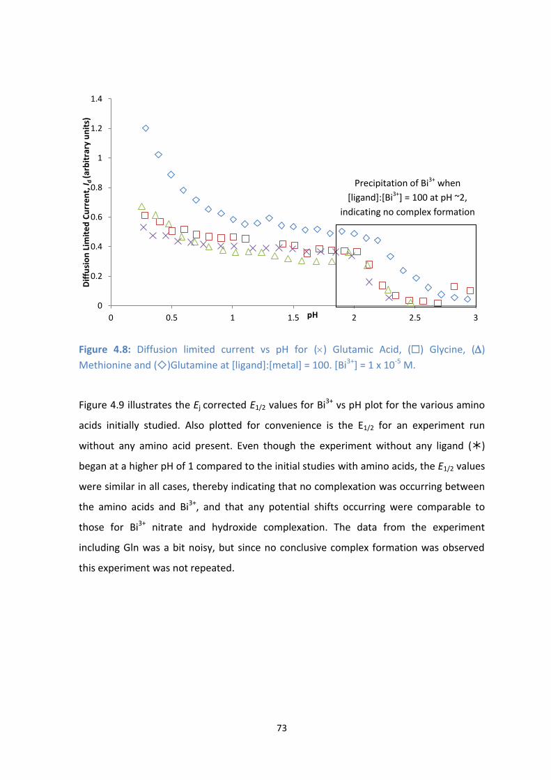
73
Figure 4.8: Diffusion limited current vs pH for () Glutamic Acid, () Glycine, ()
Methionine and ()Glutamine at [ligand]:[metal] = 100. [Bi3+] = 1 x 10⁻⁵ M.
Figure 4.9 illustrates the Ej corrected E1/2 values for Bi3+ vs pH plot for the various amino
acids initially studied. Also plotted for convenience is the E1/2 for an experiment run
without any amino acid present. Even though the experiment without any ligand ()
began at a higher pH of 1 compared to the initial studies with amino acids, the E1/2 values
were similar in all cases, thereby indicating that no complexation was occurring between
the amino acids and Bi3+, and that any potential shifts occurring were comparable to
those for Bi3+ nitrate and hydroxide complexation. The data from the experiment
including Gln was a bit noisy, but since no conclusive complex formation was observed
this experiment was not repeated.
0
0.2
0.4
0.6
0.8
1
1.2
1.4
0 0.5 1 1.5 2 2.5 3
Dif
fusi
on
Lim
ite
d C
urr
en
t, I d
(arb
itra
ry u
nit
s)
pH
Precipitation of Bi3+ when
[ligand]:[Bi3+] = 100 at pH ~2,
indicating no complex formation

74
Figure 4.9: Ej corrected E1/2 for Bi3+ vs pH plot for experiments where [L]:[M] 100 and L
refers to () Glutamic Acid, () Glycine, () Methionine and () Glutamine. () shows
values in absence of ligand where Bi3+ is only present ( [Bi3+] = 1 x 10⁻⁵ M).
Bismuth has been shown to be thiophillic[12] and as a result the most well studied bismuth
ligand complexes are those in which the ligands contain thiolate groups. These types of
complexes are vital in the coordination chemistry of bismuth, as described by Atwood et
al.[13] and some complexes are pictured in Figure 4.10. In these complexes, bismuth
exhibits coordination numbers of three, four, five and six with thiolate ligands. Due to the
fact that Bi3+ is a borderline metal ion, it is not unexpected for it to bind strongly to the
thiolate-sulphur which is considered to be a soft donor group.
40
45
50
55
60
65
70
0 0.5 1 1.5 2 2.5 3
Hal
f-w
ave
Po
ten
tial
, E 1
/2 (m
V)
pH
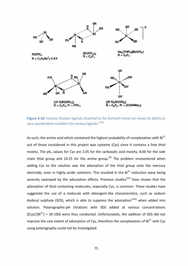
75
Figure 4.10: Various thiolate ligands attached to the bismuth metal ion shows its ability to
vary coordination numbers for various ligands.[12b]
As such, the amino acid which contained the highest probability of complexation with Bi3+
out of those considered in this project was cysteine (Cys) since it contains a free thiol
moiety. The pKa values for Cys are 2.05 for the carboxylic acid moiety, 8.00 for the side
chain thiol group and 10.25 for the amine group.[9] The problem encountered when
adding Cys to the solution was the adsorption of the thiol group onto the mercury
electrode, even in highly acidic solutions. This resulted in the Bi3+ reduction wave being
severely swamped by the adsorption effects. Previous studies[14] have shown that the
adsorption of thiol containing molecules, especially Cys, is common. These studies have
suggested the use of a molecule with detergent-like characteristics, such as sodium
dodecyl sulphate (SDS), which is able to suppress the adsorption[14a] when added into
solution. Polarographic-pH titrations with SDS added at various concentrations
([Cys]:[Bi3+] = 20-100) were thus conducted. Unfortunately, the addition of SDS did not
improve the vast extent of adsorption of Cys, therefore the complexation of Bi3+ with Cys
using polarography could not be investigated.
76
4.8. Powder X-ray Diffraction of Bi3+precipitate
As described in Chapter 1, Bi3+ precipitates due to the formation of insoluble Bi-hydroxide
species at low pH and the initial analysis of amino acid complexation with Bi3+ gave
evidence to this. Studies by Moussa and Sammour[15] showed that in solutions containing
Bi3+, HClO4 and chloride, the precipitate formed was the solid bismuth-oxy-chloride
species, BiOCl. Kragten[16] was able to predict the formation of BiONO3 species in nitrate
solutions, however, studies[7a, 17] building upon this work were able to show that the
species which could possibly be forming is the hexameric structure, Bi6O4(OH)4(NO3)6.
Due to precipitation being a major obstacle in this study, it was thus decided to attempt
to isolate the Bi3+ precipitate at pH ~2. The solutions of Bi3+ and NO3 were prepared
according to Chapter 3.4. The white precipitate was isolated and then analysed by PXRD
(Section 3.5). The PXRD pattern obtained is shown in Figure 4.11 and included in the
PXRD pattern is the superimposed calculated PXRD pattern obtained from single crystal
data studied by Lazarini.[7] The PXRD patterns show that the precipitate formed consists
of the hexamer or hydroxy-nitrate species of Bi3+, Bi6O5(OH)3(NO3)5(H2O)3 , partly
described by Granier et al.[18] The experimental method used to isolate the precipitate
used a [Bi3+] = 1 x 10⁻² M solution whereas during the polarographic analysis [Bi3+] = 1 x 10-
5 M. However, the latter would not allow a significant amount of precipitate, if any to be
isolated.
The success of isolating the Bi-hydroxy-nitrate precipitate then begged the question of
whether adding a substantial amount of amino acid to the system, would allow for the
isolation of an insoluble Bi-hydroxy-amino acid complex or was the Bi-hydroxy-nitrate
species simply formed in this case too. Since work on glutamic acid (Glu) had already been
initiated, the ratio used for attempting isolation of precipitates was [Glu]:[Bi3+] = 1000. The
precipitate formed was analysed by PXRD, but the pattern produced could only be
compared to the PXRD pattern of L-glutamine, showing that the complex formation was
difficult to achieve. The only reason higher [Glu]:[Bi3+] was not used is because the large
amount of amino acid needed in the solution was at the limit of the solubility of Glu.

77
Figure 11. PXRD pattern collected from isolated precipitate as described by Chapter 3.4. The calculated PXRD pattern from single crystal data by Lazarini[7], showing Bi6O5(OH)3(NO3)5(H2O)3, is superimposed onto the pattern (in red).
Bi-OH 1.6
01-070-1226 (C) - Bismuth Oxide Hydroxide Nitrate Hydrate - Bi6O5(OH)3(NO3)5(H2O)3 - Y: 174.77 % - d x by: 1. - WL: 1.78897 - Monoclinic - a 17.15200 - b 9.18100 - c 17.75200 - alpha 90.000 - beta 127.830 - gam
Operations: Background 1.000,1.000 | Import
Bi-OH 1.6 - File: d2_13_162.raw - Type: Locked Coupled - Start: 10.000 ° - End: 90.006 ° - Step: 0.026 ° - Step time: 185. s - Temp.: 25 °C (Room) - Time Started: 0 s - 2-Theta: 10.000 ° - Theta: 5.000 ° - Chi: 0.00 ° -
Lin
(Cou
nts)
0
1000
2000
3000
4000
5000
6000
7000
8000
9000
10000
11000
12000
13000
14000
15000
16000
17000
18000
19000
2-Theta - Scale
11 20 30 40 50
78
4.7. Conclusion
For experiments where [amino acid]: [Bi3+] = 100, it was noted that precipitation occurred
at a similar point to experiments whereon amino acid was present. Additionally, the
potential shifts were similar in the absence or presence of amino acid indicating the lack
of complexation. These observations indicate that there is very little or no complexation
occurring at this [amino acid]:[Bi3+] . The aim of this study was to show the complexation
of Bi3+ with amino acids and the question now was how we could possibly do this. The
answer to this question came in the form of Le Chatelier’s Principle. As described by Le
Chatelier in his proposal for the equilibrium of a chemical reaction, if large concentrations
of reactants or products are added to the chemical system, the system will shift in the
direction which will allow for the chemical equilibrium to once again be reached. Using
this theory, it was decided to introduce a large concentration of ligand to the the system
under analysis. The increase in the [amino acid]:[Bi3+] would theoretically drive the
equilibrium of the complexing reaction in the forward direction, allowing Bi3+ complexes
to form with the respective ligands. The [Bi3+] was not increased as this would allow
precipitation to occur at an even lower pH, making our window of study even smaller.
Although studies initially began at lower concentrations, the change to higher [amino
acid]:[Bi3+] is a more direct indication of what could be occurring within the body, as the
concentration of amino acids would be much greater than 100 times more than Bi3+. This
work will be discussed further in Chapters 5-7.
In the case of studying Cysteine as a ligand, we did not develop a procedure around the
adsorption of the free thiol moiety to the mercury electrode. One of the most interesting
techniques which could be utilized is the Anodic Stripping Voltammetry (ASV).[19] ASV
involves firstly pre-concentrating a metal onto a solid electrode surface or into a mercury
drop, at negative potentials[19]. The metal is then selectively oxidized during an anodic
potential sweep which allows very low detection limits. ASV is a useful technique to be
used in this study as it may negate the precipitation of bismuth from solution since it will
be plated into the mercury electrode[19].

79
PXRD analysis of the Bi3+ precipitate where [Bi3+] = 1 x 10⁻² M, showed that the Bi3+
hexamer Bi6O5(OH)3(NO3)5(H2O)species was formed. With the addition of glutamic acid as
the ligand, no complexation was found and PXRD analysis of the precipitate showed that it
consisted of L-glutamic acid.
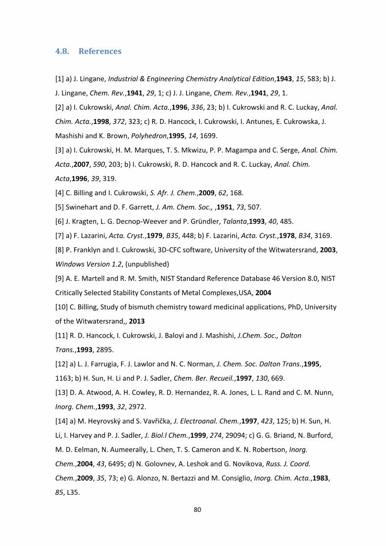
80
4.8. References
[1] a) J. Lingane, Industrial & Engineering Chemistry Analytical Edition,1943, 15, 583; b) J.
J. Lingane, Chem. Rev.,1941, 29, 1; c) J. J. Lingane, Chem. Rev.,1941, 29, 1.
[2] a) I. Cukrowski, Anal. Chim. Acta.,1996, 336, 23; b) I. Cukrowski and R. C. Luckay, Anal.
Chim. Acta.,1998, 372, 323; c) R. D. Hancock, I. Cukrowski, I. Antunes, E. Cukrowska, J.
Mashishi and K. Brown, Polyhedron,1995, 14, 1699.
[3] a) I. Cukrowski, H. M. Marques, T. S. Mkwizu, P. P. Magampa and C. Serge, Anal. Chim.
Acta.,2007, 590, 203; b) I. Cukrowski, R. D. Hancock and R. C. Luckay, Anal. Chim.
Acta,1996, 39, 319.
[4] C. Billing and I. Cukrowski, S. Afr. J. Chem.,2009, 62, 168.
[5] Swinehart and D. F. Garrett, J. Am. Chem. Soc., ,1951, 73, 507.
[6] J. Kragten, L. G. Decnop-Weever and P. Gründler, Talanta,1993, 40, 485.
[7] a) F. Lazarini, Acta. Cryst.,1979, B35, 448; b) F. Lazarini, Acta. Cryst.,1978, B34, 3169.
[8] P. Franklyn and I. Cukrowski, 3D-CFC software, University of the Witwatersrand, 2003,
Windows Version 1.2, (unpublished)
[9] A. E. Martell and R. M. Smith, NIST Standard Reference Database 46 Version 8.0, NIST
Critically Selected Stability Constants of Metal Complexes,USA, 2004
[10] C. Billing, Study of bismuth chemistry toward medicinal applications, PhD, University
of the Witwatersrand,, 2013
[11] R. D. Hancock, I. Cukrowski, J. Baloyi and J. Mashishi, J.Chem. Soc., Dalton
Trans.,1993, 2895.
[12] a) L. J. Farrugia, F. J. Lawlor and N. C. Norman, J. Chem. Soc. Dalton Trans.,1995,
1163; b) H. Sun, H. Li and P. J. Sadler, Chem. Ber. Recueil.,1997, 130, 669.
[13] D. A. Atwood, A. H. Cowley, R. D. Hernandez, R. A. Jones, L. L. Rand and C. M. Nunn,
Inorg. Chem.,1993, 32, 2972.
[14] a) M. eyrovský and S. Vavřička, J. Electroanal. Chem.,1997, 423, 125; b) H. Sun, H.
Li, I. Harvey and P. J. Sadler, J. Biol.l Chem.,1999, 274, 29094; c) G. G. Briand, N. Burford,
M. D. Eelman, N. Aumeerally, L. Chen, T. S. Cameron and K. N. Robertson, Inorg.
Chem.,2004, 43, 6495; d) N. Golovnev, A. Leshok and G. Novikova, Russ. J. Coord.
Chem.,2009, 35, 73; e) G. Alonzo, N. Bertazzi and M. Consiglio, Inorg. Chim. Acta.,1983,
85, L35.

81
[15] A. A. Moussa and H. M. Sammour, J. Chem. Soc.,1960, 2151.
[16] J. Kragten, L. G. Decnop-Weever and P. Gründler, Talanta,(1993), 40, 485.
[17] a) B. Sundvall, Inorg. Chem.,1986, 22, 1906; b) B. Sundvall, Acta. Chem. Scand.,1979,
A33, 219; c) I. Grenthe and I. Toth, Inorg. Chem.,1985, 24, 2405.
[18] F. Graner, A. Olin and L. G. Sillén, Acta. Chem. Scand.,1956, 10, 476.
[19] Electroanalytical Chemistry-Anodic Stripping Voltammetry,
www2.chemistry.msu.edu/courses/cem837/Anodic%20Stripping%20Voltammetry.pdf,
(Date Accessed: 12-05-2012)

84
Chapter 5: Bi-Glutamic Acid Complexation
5.1 Introduction
Glutamic acid (Glu) is one of the twenty common amino acids. It helps with the
transportation of potassium across the blood-brain barrier, although it itself does not
pass this barrier that easily.[1] Figure 5.1 shows the fully protonated Glu. As can be seen,
there are 3 potential sites which can be protonated and the protonation constants are
pKa1 = 9.49, pKa
2 = 4.07 and pKa3 = 2.16 at 25⁰C and 0.5 M ionic strength.[2] This show the
versatility of Glu to perform a range of functions due to its degrees of freedom regarding
the potential complexing sites. To associate the protonation site of Glu with a particular
protonation constant it was compared to similar molecules. Glutaric acid (Figure 5.2),
which has the carboxylic acids in the same positions as that for Glu, has protonation
constants of pKa1 = 4.87, and pKa
2 = 4.10 at 25⁰C and 0.5 M ionic strength.[2] Glutaric acid
lacks the amine group on C2, thus both pKa values are similar as the moieties present are
equivalent and it is expected that the carboxylic acid furthest from the amine group in
Glu would have a similar pKa value. In Glu, the carboxylic acid adjacent to the amine
group will be affected by the electronic properties of this electronegative amine group
and therefore will have a lower a pKa, hence the value of 2.16 is associated with this
moiety. The NH3+ present in Glu remains protonated to the highest pH and therefore it is
allocated the pKa = 9.49.
Figure 5.1: Structure of fully protonated glutamic acid indicating the respective pKa
values.[2b]
pKa3=2.16
pKa2= 9.49
pKa1=4.07

85
Figure 5.2: Structure of fully protonated glutaric acid.[2a]
Glu is used as fuel in the brain, and attaches itself to nitrogen atoms in the process of
forming glutamine. The resulting action allows the detoxification of the body from
ammonia, a natural byproduct of the body utilizing energy. This action is the only way in
which the brain can be detoxified from ammonia, an important process of ensuring the
growth and maintenance of a healthy brain and subsequent function. The detoxification
action of Glu is also important for the rest of the body, where it is an important aid in
cellular metabolism where it plays an important role in the body's disposal of excess or
waste nitrogen. In humans, dietary proteins are broken down by digestion into amino
acids, which serve as metabolic fuel for other functional roles in the body.
The process by which Glu achieves its detoxification action is by firstly undergoing
deamination, an oxidative reaction catalysed by glutamate dehydrogenase[3] and is
illustrated by the chemical equation :
Glu + H2O + NADP+ → α-ketoglutarate + NADPH + NH4+
Ammonia is excreted predominantly as urea, synthesised in the liver.[2a, 3] Transamination
can thus be linked to deamination, effectively allowing nitrogen from the amine groups of
amino acids to be removed, via a glutamate as an intermediate, and finally excreted from
the body in the form of urea. The fluid produced by the prostate gland also contains
amounts of Glu and may play a role in the normal function of the prostate.[2a, 3]
Along with the ability to dispose of waste nitrogen, Glu also serves an important role in
the action of neurotransmitters.[4] Glutamate is stored in vesicles near the beginning of
the pre-synaptic nerve. Once the appropriate nerve impulses are triggered, a signal is

86
sent to release the glutamate molecules which travel to the nerve, and allows the
electrochemical signal to be passed on to the brain, thereby resulting in the intended
reaction.[4]
5.2 Aim
Results presented in Chapter 4 show that the complexation of Bi3+ with amino acid
ligands at [L]:[M] = 100 did not occur before Bi3+ formed a precipitate. The aim of this
study is to investigate the conditions at which complex formation will be favored before
Bi3+ precipitates. The study will also aim to investigate the best approach to calculating
the stability constants in a medium conducive to Bi3+ forming complexes with NO3- at low
pH especially when the ligand of interest (glutamic acid in this case) is rather weakly
binding.
5.3 Experimental
Experiments were run as in Chapter 3 using the NOVA procedures developed in Chapter
2. In order to drive the complexation reaction of Bi3+ with Glu, experiments were run with
[Glu]:[Bi3+] significantly greater than 100. Here three experiments were run with
[Glu]:[Bi3+] of 1970, 3076 and 5000 (these experiments will be referred to as the rounded
values of 2000, 3000 and 5000). On addition of Glu to the solution, particularly for the
highest ratio, the pH of the solution increased. In hindsight the pH should then have been
adjusted closer to the starting pH 1 before starting to titrate with KOH, but instead data
was analysed from the pH the solution had attained.
5.4 Results
5.4.1. Modelling the Pb2+-Glu system
Since amino acids are such a large component of biological systems, many have studies
have been conducted where complexation to biological metal ions such as Cu, Fe and Zn
were used. Complexation of Bi3+ with Glu is not well studied, so it was decided to see
what happens to the species in solution when the solution conditions were changed by
modelling the Pb2+-Glu system since Pb2+ is isoelectronic with Bi3+.

87
For the Pb2+ system it is seen that the MLH, ML and ML2 species form (log β = 11.43, 4.53
and 6.80, respectively, at 25⁰C at 1M ionic strength).[2b] In the species distribution
diagram (Figure 5.3) using the conditions [Pb2+] = 1 x 10⁻⁵ M, and [Glu]:[Pb] = 100 (i.e. that
used in the experiments with Bi3+ in Chapter 4), both the ML and MLH species were
present above pH 3 but only to small extents and the ML2 species is not formed under
these conditions. The fact that the MLH species forms gives evidence that protonated
species are viable. The formation constants of PbOH are shown in the Appendix 2.
Figure 5.3: Species distribution diagram for the Pb2+-Glu system where [Glu]:[Pb2+] = 100 and [Pb2+] = 1 x 10⁻⁵ M at 25⁰C.
Moreover, when the [Pb2+]:[Glu] was increased to 1000 (Figure 5.4), we see the
formation of the MLH species in a much higher percentage and it starts forming at pH ~2.
It can also be seen that significantly more of the ML species forms, almost three times
greater than that of when [Pb]:[Glu] = 100. The formation of the ML2 species also occurs
above pH ~7 which indicates that as the concentration of the ligand is increased while
that of the metal ion is kept the same, complexation increases as expected from Le
Chatelier’s principle.[5] An additional consideration is that since the Glu concentration is
0
10
20
30
40
50
60
70
80
90
100
0 2 4 6 8 10 12 14
% S
pec
ies
Pre
sen
t
pH
Pbfree
PbLH PbL
PbOH
Pb3(OH)4
Pb(OH)2
Pb(OH)3

88
increased, the concentration of deprotonated Glu (deprotonated to varying extents
depending on pH) also increases. The increase in concentration of these deprotonated
species must also have an effect in driving the reaction forward.
Figure 5.4: Species distribution diagram for the Pb2+-Glu system where [Glu]:[Pb2+] = 1000 and [Pb2+] = 1 x 10⁻⁵ M at 25⁰C.
For interest, it was also decided to view how the increase in [Pb2+] affects the species
formed. As can be seen in Figure 5.5, when [Pb2+] = 1 x 10⁻⁴ M and [Glu]:[ Pb2+] = 100, the
MLH and ML species are once again much higher when compared to that in Figure 5.3
where [Pb2+] = 1 x 10⁻⁵ M and [Glu]:[ Pb2+] = 100. It was realized that in keeping
[Glu]:[Pb2+] = 100, both the [Pb2+] and [Glu] was increased 10-fold. Although a viable
option when studying Pb2+, this was not a chosen method when performing experimental
studies with Bi3+ because by increasing [Bi3+], precipitation of the Bi-hydroxy-nitrate
species would occur at lower pH and decrease the already small window of analysis. The
investigation into how Pb2+ complexes with Glu illustrates that by increasing either [M] or
[L] results in promoting complex formation.
0
10
20
30
40
50
60
70
80
90
100
0 2 4 6 8 10 12 14
% S
pec
ies
Pre
sen
t
pH
Pbfree
PbLH
PbL
PbOH
Pb3(OH)4
Pb(OH)2
Pb(OH)3
PbL2

89
Figure 5.5: Species distribution diagram for the Pb2+-Glu system where [Glu]:[Pb2+] = 100 and [Pb2+] = 1 x 10⁻⁴ M at 25⁰C.
5.4.2 Bi3+ complexation with Glutamic acid
As described in Chapter 4, the initial studies with [Glu]:[Bi3+] = 100 indicated no
complexation occurred and precipitation ensued at pH ~2 (see Figure 4.8), the region we
would expect Bi3+ (with a concentration of ~10-5 M) to precipitate if 0.5 M NO-3 were
present. One of the possible reasons for no significant complexation formation taking
place at low pHs is that the third protonation constant of Glu is 2.16.[2b] At the low
[Glu]:[Bi3+] of 100 there is not enough deprotonated Glu to allow complex formation with
the Bi3+. If considering only the form in which the ligand is present, Figure 5.6 shows that
~90% of Glu exists in the form Glu-H3 at pH 1 and therefore only 10% of the singly
deprotonated Glu is available for complexation at that pH. Above pH 2.2 the dominant
species present is Glu-H2, however, at this stage Bi3+ is close to precipitation in the NO3-
solution. As was also illustrate using the Pb-Glu system, the concentration of Glu plays an
important role in the formation of complexes with metal ions since at different pHs there
are different percentages of protonated and deprotonated species present in solution.
0
10
20
30
40
50
60
70
80
90
100
0 2 4 6 8 10 12 14
% S
pec
ies
Pre
sen
t
pH
Pbfree
PbLH
PbL
PbOH
Pb3(OH)4 Pb(OH)2
Pb(OH)3
PbL2

90
For example, consider a solution at pH 1 where 10% of Glu is in the form Glu-H2. If the
solution contains 1 x 10⁻⁵ M metal ion and [Glu]:[M] = 100, then 10% of 1 x 10⁻³ M = 1 x
10-4 M Glu-H2. However, when the [Glu]:[M] = 1000, 10% of 1 x 10⁻² M results in [Glu-H2] =
1 x 10⁻³ M available to complex to the metal ion in solution.
Figure 5.6: Species distribution diagram of glutamic acid in aqueous solutions at 25⁰C.
Increasing the [Glu]:[Bi3+] to 2000 ( or more precisely 1970) and still using [Bi3+] = 1 x 10⁻⁵
M resulted in the Bi3+ only precipitating at pH ~4.5 (Figure 5.7) which indicates that some
soluble Bi-Glu complex formed under these conditions.
0
10
20
30
40
50
60
70
80
90
100
1 2 3 4 5 6 7 8 9 10 11 12 13 14
% S
pe
cie
s P
rese
nt
pH
Glu-H3
Glu-H2 Glu-H Glu
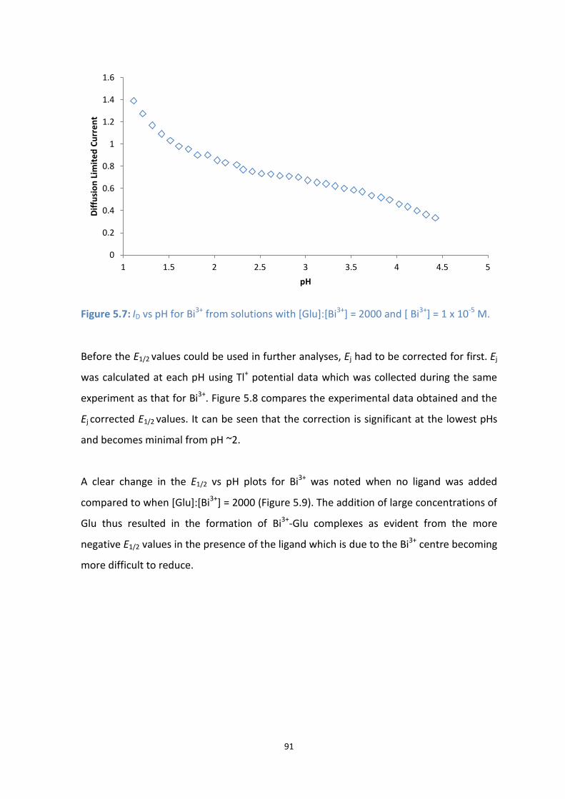
91
Figure 5.7: ID vs pH for Bi3+ from solutions with [Glu]:[Bi3+] = 2000 and [ Bi3+] = 1 x 10⁻⁵ M.
Before the E1/2 values could be used in further analyses, Ej had to be corrected for first. Ej
was calculated at each pH using Tl+ potential data which was collected during the same
experiment as that for Bi3+. Figure 5.8 compares the experimental data obtained and the
Ej corrected E1/2 values. It can be seen that the correction is significant at the lowest pHs
and becomes minimal from pH ~2.
A clear change in the E1/2 vs pH plots for Bi3+ was noted when no ligand was added
compared to when [Glu]:[Bi3+] = 2000 (Figure 5.9). The addition of large concentrations of
Glu thus resulted in the formation of Bi3+-Glu complexes as evident from the more
negative E1/2 values in the presence of the ligand which is due to the Bi3+ centre becoming
more difficult to reduce.
0
0.2
0.4
0.6
0.8
1
1.2
1.4
1.6
1 1.5 2 2.5 3 3.5 4 4.5 5
Dif
fusi
on
Lim
ite
d C
urr
en
t
pH

92
Figure 5.8: E1/2 for Bi3+ vs pH with [Glu]:[Bi3+] = 2000 showing both the experimental and Ej corrected E1/2 values.
Figure 5.9: E1/2 for Bi3+ vs pH with () no ligand added and () [Glu]:[Bi3+] = 2000.
As can be seen in Figure 5.10, an increase in [Glu] results in greater negative shifts in E1/2
as the pH is increased. The type of complexes formed and the resulting concentrations of
these complexes would all contribute to the extent of the negative shift in E1/2 all showing
that that complexes between Bi3+ and Glu were indeed forming. An indication of both
-40
-30
-20
-10
0
10
20
30
40
50
60
0 0.5 1 1.5 2 2.5 3 3.5 4 4.5 5
Hal
f-w
ave
po
ten
tial
, E 1
/2 (
mV
)
pH
0
10
20
30
40
50
60
70
1 1.5 2 2.5 3 3.5
Hal
f-w
ave
po
ten
tial
E1
/2
pH
Experimental E1/2
Ej Corrected E1/2
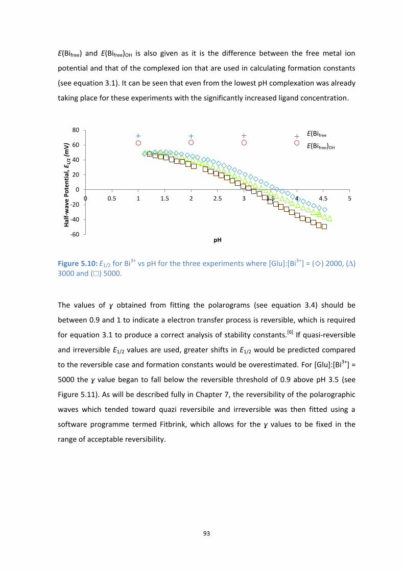
93
E(Bifree) and E(Bifree)OH is also given as it is the difference between the free metal ion
potential and that of the complexed ion that are used in calculating formation constants
(see equation 3.1). It can be seen that even from the lowest pH complexation was already
taking place for these experiments with the significantly increased ligand concentration.
Figure 5.10: E1/2 for Bi3+ vs pH for the three experiments where [Glu]:[Bi3+] = () 2000, () 3000 and () 5000.
The values of ɣ obtained from fitting the polarograms (see equation 3.4) should be
between 0.9 and 1 to indicate a electron transfer process is reversible, which is required
for equation 3.1 to produce a correct analysis of stability constants.[6] If quasi-reversible
and irreversible E1/2 values are used, greater shifts in E1/2 would be predicted compared
to the reversible case and formation constants would be overestimated. For [Glu]:[Bi3+] =
5000 the ɣ value began to fall below the reversible threshold of 0.9 above pH 3.5 (see
Figure 5.11). As will be described fully in Chapter 7, the reversibility of the polarographic
waves which tended toward quazi reversibile and irreversible was then fitted using a
software programme termed Fitbrink, which allows for the ɣ values to be fixed in the
range of acceptable reversibility.
-60
-40
-20
0
20
40
60
80
0 0.5 1 1.5 2 2.5 3 3.5 4 4.5 5
Hal
f-w
ave
Po
ten
tial
, E1/
2 (m
V)
pH
E(Bifree
E(Bifree)OH
94
Figure 5.11: Graph indicating the extent of reversibility, ɣ, vs pH for the Bi3+ polarograms
for [Glu]:[Bi3+] = () 2000, () 3000 and () 5000.
One of the most useful methods used to predict the type of metal-ligand species formed
in solution is to analyse the slopes[7] of the Ej corrected E1/2 vs pH graphs. As described in
Chapter 3, Section 3.3.4, in a specific pH range there is a dominant form of ligand species
present in solution, where these forms vary only by the extent of their protonation. We
find the slopes of the graph using equation 3.6 within a pH range, which should indicate
the type of species present in solution that is being reduced at the electrode. As an
example, slope analysis conducted on the [Glu]:[Bi3+] = 5000 data is illustrated here. The
reduction of the Bi3+-Glu species results in the formation amalgamated Bi0 and the bond/s
with Glu is/are then broken. Glu remains in solution and the pH of the solution is then the
major determinant of the extent to which Glu would be protonated. Using the predicted
complexes (Bi-Glu-H2 , Bi-Glu-H and Bi-Glu in this case), we take into account the number
of electrons required to reduce the Bi3+ centre and the number of protons required to
form the predominant ligand species at that respective pH range.
Figure 5.12 gives the expected slopes for the reduction of suggested species in the
indicated pH ranges. Below pH 2.16, the expected slope for the reduction of the Bi-Glu-H2
complex is 20 mV. As can be seen in Figure 5.13, a slope of 20 mV was found for the
experimental data in the same pH region, thus indicating that the Bi-Glu-H2 complex
0.7
0.75
0.8
0.85
0.9
0.95
1
1.05
0 0.5 1 1.5 2 2.5 3 3.5 4 4.5 5
ɣ
pH
Quasi-reversible electron
transfer process
Reversible electron
transfer process
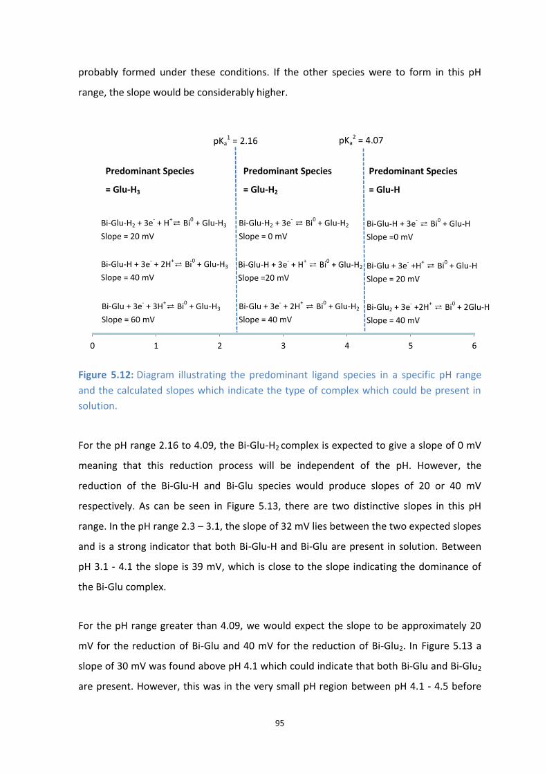
95
probably formed under these conditions. If the other species were to form in this pH
range, the slope would be considerably higher.
Figure 5.12: Diagram illustrating the predominant ligand species in a specific pH range
and the calculated slopes which indicate the type of complex which could be present in
solution.
For the pH range 2.16 to 4.09, the Bi-Glu-H2 complex is expected to give a slope of 0 mV
meaning that this reduction process will be independent of the pH. However, the
reduction of the Bi-Glu-H and Bi-Glu species would produce slopes of 20 or 40 mV
respectively. As can be seen in Figure 5.13, there are two distinctive slopes in this pH
range. In the pH range 2.3 – 3.1, the slope of 32 mV lies between the two expected slopes
and is a strong indicator that both Bi-Glu-H and Bi-Glu are present in solution. Between
pH 3.1 - 4.1 the slope is 39 mV, which is close to the slope indicating the dominance of
the Bi-Glu complex.
For the pH range greater than 4.09, we would expect the slope to be approximately 20
mV for the reduction of Bi-Glu and 40 mV for the reduction of Bi-Glu2. In Figure 5.13 a
slope of 30 mV was found above pH 4.1 which could indicate that both Bi-Glu and Bi-Glu2
are present. However, this was in the very small pH region between pH 4.1 - 4.5 before
0 1 2 3 4 5 6
pKa1 = 2.16 pKa
2 = 4.07
Bi-Glu-H2 + 3e- + H
+⇄ Bi
0 + Glu-H3
Slope = 20 mV
Bi-Glu-H2 + 3e- ⇄ Bi
0 + Glu-H2
Slope = 0 mV
Bi-Glu-H + 3e- + 2H
+⇄ Bi
0 + Glu-H3
Slope = 40 mV
Bi-Glu + 3e- + 3H
+⇄ Bi
0 + Glu-H3
Slope = 60 mV
Bi-Glu-H + 3e- + H
+ ⇄ Bi
0 + Glu-H2
Slope =20 mV
Bi-Glu + 3e- + 2H
+ ⇄ Bi
0 + Glu-H2
Slope = 40 mV
Bi-Glu + 3e- +H
+ ⇄ Bi
0 + Glu-H
Slope = 20 mV
Bi-Glu-H + 3e- ⇄ Bi
0 + Glu-H
Slope =0 mV
Predominant Species
= Glu-H2
Predominant Species
= Glu-H3
Predominant Species
= Glu-H
Bi-Glu2 + 3e- +2H
+ ⇄ Bi
0 + 2Glu-H
Slope = 40 mV

96
precipitation occurred. From the species distribution diagram in Figure 5.6 it can be seen
that at pH 4.5 there is still ~30% Glu-H2 in solution. Thus in this narrow pH range it could
be that on reduction of Bi-Glu, both Glu-H and Glu-H2 are produced, thereby giving an
average slope of ~30 mV.
Figure 5.13: Ej corrected E1/2 for Bi3+ vs pH with [Glu]:[Bi3+] = 5000. Slope analysis has been completed in different pH ranges in order to help predict which Bi3+-Glu complexes are present in solution.
The 3D-CFC programme[8] was used to plot the ECFC and CCFC as described in Chapter 3.
The two free Bi3+ potential values, determined as discussed in Chapter 4, were utilized in
order to obtain a better representation of the formation constants of complexes formed
between Bi3+ and Glu. This is as a result of existing speciation software being unable to
take into account the existence of NO3- species simultaneously with the OH- and ligand
(of interest) species. The ECFC and CCFC were therefore plotted using both E(Bifree) and
E(Bifree)OH values which were calculated as described in section 4.5. By determining log β
values using both E(BiFree) and E(BiFree)OH, we can conclude that the true log β for the
respective Bi3+-Glu complexes is between these two values. The reason for this deduction
is that initially below pH 1 the Bi3+ nitrate species predominate in solution (Figure 5.14). If
the true E(Bifree) value is used, then shifts due to the formation of Bi3+ nitrates could
y = -20x + 72 R² = 0.9904
y = -32x + 100 R² = 0.9944
y = -39x + 122 R² = 0.9979
y = -30x + 84 R² = 0.9897
-60
-40
-20
0
20
40
60
0 0.5 1 1.5 2 2.5 3 3.5 4 4.5 5
Hal
f-w
ave
po
ten
tial
, E1/
2, (
mV
)
pH

97
erroneously be allocated to the formation of Bi3+-Glu complexes. Thus the value of
E(Bifree)OH is rather used in the low pH region to give better estimates of the formation
constants. However, as pH increases the concentration of these Bi3+ nitrate species begin
to decrease and that for the Bi3+ hydroxide species increase. Above pH 3 the Bi3+ nitrate
species are negligible and there is no need to account for nitrate as a competing ligand.
Above pH 3 when using the true E(Bifree) value, good approximations of the formation
constants are obtained. Between pH 1-3 the formation constants should be between the
values calculated using the two E(Bifree) values. We actually really need software that can
account for the competition between decreasing Bi3+ nitrate species, increasing Bi3+
hydroxide species as well as the formation of the Bi3+-Glu species which we propose are
forming.
Figure 5.14: Species distribution diagram of Bi3+ species vs pH in a NO3¬ solution at 25⁰C
in pH range 1 - 5. [Bi3+] = 1 x 10⁻⁵ M.
Figure 5.15 to 5.17 show the ECFC and CCFC curves calculated using the true E(Bifree) for
the Bi3+-Glu complexes for the various [Glu]:[Bi3+] values. As described in Chapter 3, the
CCFC is fitted to the ECFC (using equation 3.1) by refining the formation constants for the
respective Bi3+-Glu complexes formed in solution. Using the information from the slope
analysis, we were able to deduce that three Bi3+-Glu complexes were predicted to form in
0
20
40
60
80
100
0 0.5 1 1.5 2 2.5 3 3.5 4 4.5 5
% S
pe
cie
s p
rese
nt
pH
Use E(Bifree)OH
Significant
competition
with NO3-
Use E(Bifree)
Negligible
competition
with NO3-
Bi-NO3
species
Bi3+
Bi(OH) Bi(OH)2
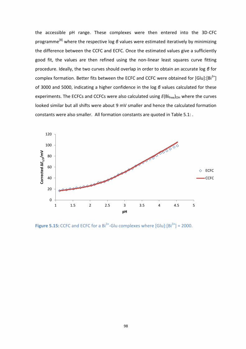
98
the accessible pH range. These complexes were then entered into the 3D-CFC
programme[8] where the respective log β values were estimated iteratively by minimizing
the difference between the CCFC and ECFC. Once the estimated values give a sufficiently
good fit, the values are then refined using the non-linear least squares curve fitting
procedure. Ideally, the two curves should overlap in order to obtain an accurate log β for
complex formation. Better fits between the ECFC and CCFC were obtained for [Glu]:[Bi3+]
of 3000 and 5000, indicating a higher confidence in the log β values calculated for these
experiments. The ECFCs and CCFCs were also calculated using E(Bifree)OH where the curves
looked similar but all shifts were about 9 mV smaller and hence the calculated formation
constants were also smaller. All formation constants are quoted in Table 5.1: .
Figure 5.15: CCFC and ECFC for a Bi3+-Glu complexes where [Glu]:[Bi3+] = 2000.
0
20
40
60
80
100
120
1 1.5 2 2.5 3 3.5 4 4.5 5
Co
rre
cte
d Δ
E 1/2
/mV
pH
ECFC
CCFC

99
Figure 5.16: CCFC and ECFC for a Bi3+-Glu complexes where [Glu]:[Bi3+] = 3000.
Figure 5.17: CCFC and ECFC for a Bi3+-Glu complexes where [Glu]:[Bi3+] = 5000.
The species model required to fit the data consisted of Bi-Glu-H2, Bi-Glu-H and the Bi-Glu
complexes except, as can be seen in Table 5.1: , the log β value for Bi-Glu-H for the ratio
[Glu]:[Bi3+] = 2000 could not be refined and could be a result of the low [Glu]:[Bi3+] ratio
used. For the remaining two experiments the Bi-Glu-H species was required to give a
good fit and the log β values for Bi-Glu-H were reproducible. The average log β values for
the three complexes are given in Table 5.1: the standard deviation for the three
experiments, where the latter indicated good reproducibility.
0
20
40
60
80
100
120
1 1.5 2 2.5 3 3.5 4 4.5 5
Co
rre
cte
d Δ
E 1/2
/mV
pH
ECFC
CCFC
0
10
20
30
40
50
60
70
80
90
1 1.5 2 2.5 3 3.5 4
Co
rre
cte
d Δ
E 1/2
/mV
pH
ECFC
CCFC
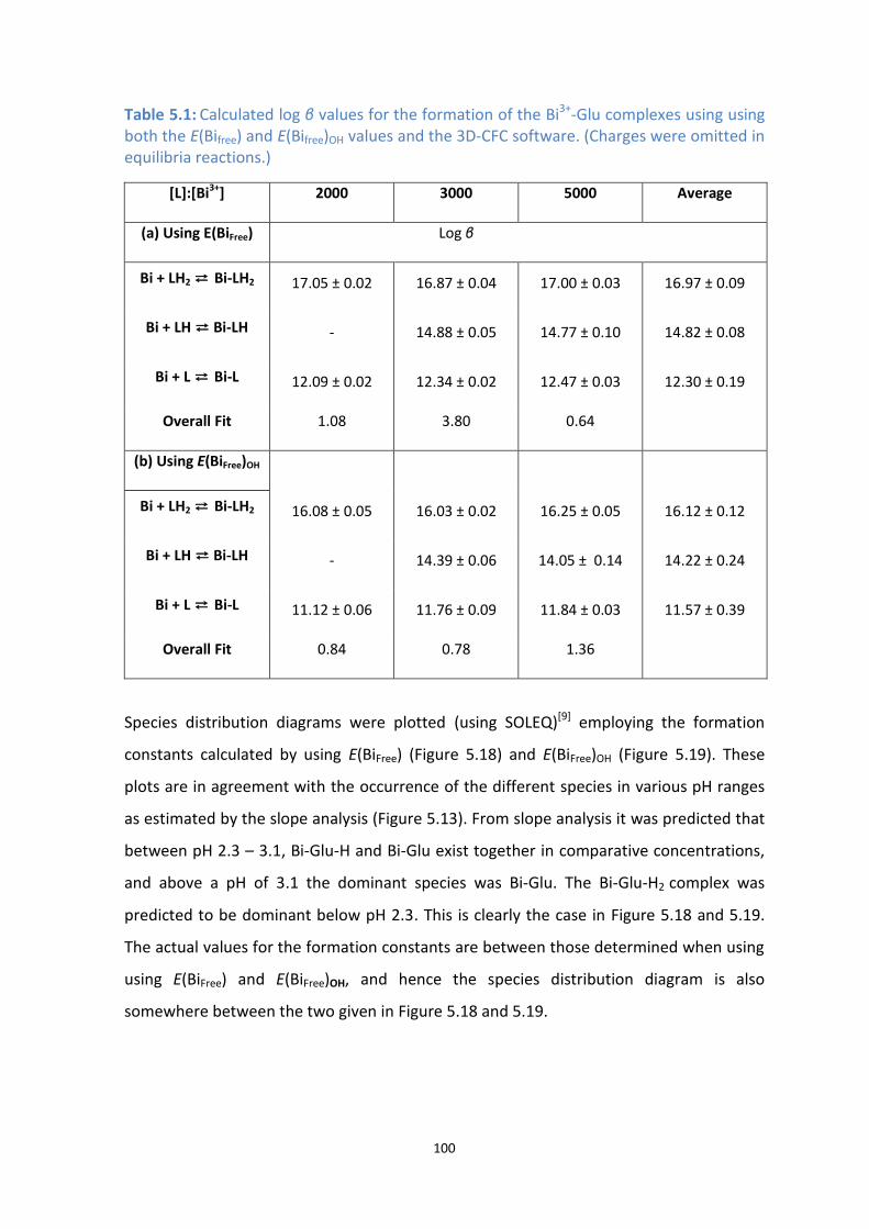
100
Table 5.1: Calculated log β values for the formation of the Bi3+-Glu complexes using using both the E(Bifree) and E(Bifree)OH values and the 3D-CFC software. (Charges were omitted in equilibria reactions.)
[L]:[Bi3+] 2000 3000 5000 Average
(a) Using E(BiFree)
Log β
Bi + LH2 ⇄ Bi-LH2 17.05 ± 0.02 16.87 ± 0.04 17.00 ± 0.03 16.97 ± 0.09
Bi + LH ⇄ Bi-LH - 14.88 ± 0.05 14.77 ± 0.10 14.82 ± 0.08
Bi + L ⇄ Bi-L 12.09 ± 0.02 12.34 ± 0.02 12.47 ± 0.03 12.30 ± 0.19
Overall Fit 1.08 3.80 0.64
(b) Using E(BiFree)OH
Bi + LH2 ⇄ Bi-LH2 16.08 ± 0.05 16.03 ± 0.02 16.25 ± 0.05 16.12 ± 0.12
Bi + LH ⇄ Bi-LH - 14.39 ± 0.06 14.05 ± 0.14 14.22 ± 0.24
Bi + L ⇄ Bi-L 11.12 ± 0.06 11.76 ± 0.09 11.84 ± 0.03 11.57 ± 0.39
Overall Fit 0.84 0.78 1.36
Species distribution diagrams were plotted (using SOLEQ)[9] employing the formation
constants calculated by using E(BiFree) (Figure 5.18) and E(BiFree)OH (Figure 5.19). These
plots are in agreement with the occurrence of the different species in various pH ranges
as estimated by the slope analysis (Figure 5.13). From slope analysis it was predicted that
between pH 2.3 – 3.1, Bi-Glu-H and Bi-Glu exist together in comparative concentrations,
and above a pH of 3.1 the dominant species was Bi-Glu. The Bi-Glu-H2 complex was
predicted to be dominant below pH 2.3. This is clearly the case in Figure 5.18 and 5.19.
The actual values for the formation constants are between those determined when using
using E(BiFree) and E(BiFree)OH, and hence the species distribution diagram is also
somewhere between the two given in Figure 5.18 and 5.19.
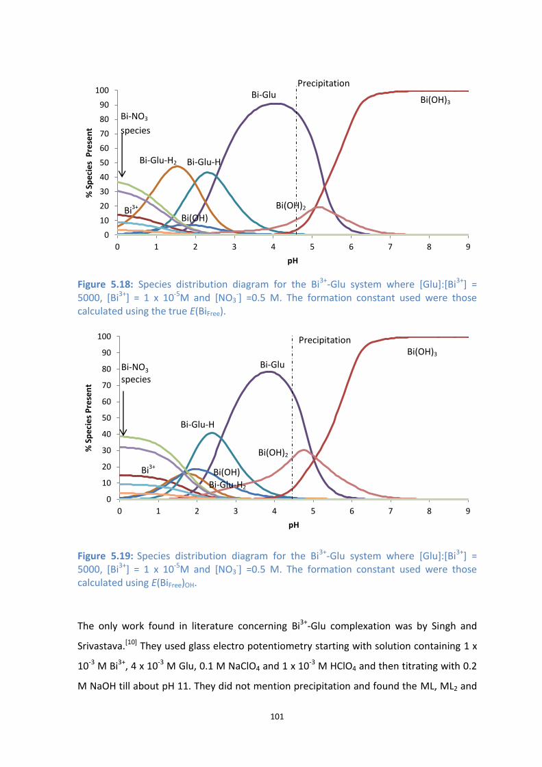
101
Figure 5.18: Species distribution diagram for the Bi3+-Glu system where [Glu]:[Bi3+] = 5000, [Bi3+] = 1 x 10⁻⁵M and [NO3
-] =0.5 M. The formation constant used were those calculated using the true E(BiFree).
Figure 5.19: Species distribution diagram for the Bi3+-Glu system where [Glu]:[Bi3+] = 5000, [Bi3+] = 1 x 10⁻⁵M and [NO3
-] =0.5 M. The formation constant used were those calculated using E(BiFree)OH.
The only work found in literature concerning Bi3+-Glu complexation was by Singh and
Srivastava.[10] They used glass electro potentiometry starting with solution containing 1 x
10-3 M Bi3+, 4 x 10⁻³ M Glu, 0.1 M NaClO4 and 1 x 10⁻³ M HClO4 and then titrating with 0.2
M NaOH till about pH 11. They did not mention precipitation and found the ML, ML2 and
0
10
20
30
40
50
60
70
80
90
100
0 1 2 3 4 5 6 7 8 9
% S
pe
cie
s P
rese
nt
pH
0
10
20
30
40
50
60
70
80
90
100
0 1 2 3 4 5 6 7 8 9
% S
pe
cie
s P
rese
nt
pH
Bi-NO3 species
Bi-Glu-H2 Bi-Glu-H
Bi-Glu
Bi(OH)2
Bi(OH)3
Precipitation
Bi-Glu-H2
Bi-Glu-H
Bi-Glu
Bi(OH)2
Precipitation
Bi-NO3
species
Bi3+
Bi(OH)
Bi(OH)3
Bi(OH) Bi3+

102
ML3 species in solution. It has been shown that Bi3+ is more soluble in ClO4- than NO3
-
solutions.[11]However, perchlorates were not used in this work as it the reduction of Bi3+ is
not reversible in this medium.[12]Since Bi3+ is even less soluble in a Cl- medium[11], the
results in NO3- solutions should be more indicative of what could happen in the body.
The log β values determined for the ML, ML2 and ML3 species were 10.47, 18.75 and
22.25, respectively.
Previous studies[13] conducted on glutamic acid complexation with various metal ions
shows that the range log β values for complex formation is extremely broad. The only
metal ion which behaved similar to Bi3+ was gallium(III). It was interesting to note that the
solution species found were Ga-Glu-H2, Ga-Glu-H and Ga-Glu with log β values of 16.97,
12.78 and 11.3, respectively.[13] These formation constants are similar those found for the
Bi3+-Glu complexes in this study. One of the most important findings was the presence of
the MLH2 complex to substantiate our finding the Bi-Glu-H2 complex, especially since it
could be contentious due to its presence in a pH region predominated by the formation
of Bi3+ nitrate complexes. Ga3+ also forms an insoluble Ga(OH)3 species with a log Ksp of -
37[13] which results in precipitation just above pH 4, thus these species were also found
under acidic conditions. Appendix 2 shows the species distribution diagrams of Ga3+ with
Glu. It is interesting to note that by increasing the [Glu]:[Ga3+] = 5000, as in this study
with Bi3+ formation of insoluble Ga(OH)3 is delayed to pH ~ 5.
Looking at the possible structure of the Bi-Glu-H2 complex where Glu has only one
deprotonated site, it is suggested that deprotonation of the carboxylic group with pKa =
2.16 occurs and the Bi3+ coordinates to two oxygens as shown in Figure 5.20 This type of
coordination was seen before in the crystal structure of the MLH species for the Cd2+-
picolinic acid (2-pyridinecarboxylic acid) system.[14]

103
Bi3+
Figure 5.20: Proposed structure of the Bi-Glu-H2 complex.
The Bi-Glu-H complex could have two possible chelation structures. Coordination could
occur via both carboxylic acid groups as they are deprotonated before the amine group,
as shown in Figure 5.21. However, this is not likely as a large 8-membered ring system is
formed which is very unstable.
Bi3+
Figure 5.21: An unlikely structure for the Bi-Glu-H complex.
In literature[15] it was shown that chelation via the amide and carboxylate groups is
favoured at a neutral pH, however, from the species distribution diagrams it was seen
that the Bi-Glu-H species is at its maximum concentration between about pH 2-3. Another
consideration is that amino acids form zwitterions which allow an internal transfer of a
hydrogen ion from the –COOH group to the –NH2 group to leave an ion with both positive
and negative charges.[2a] The zwitterions are in equilibrium with the non-zwitterion form
of the molecule. This tells us that even though one site on the amino acid is deprotonated
first (i.e. at lower pH), the equilibria for the internal transfer of the hydrogen ion could
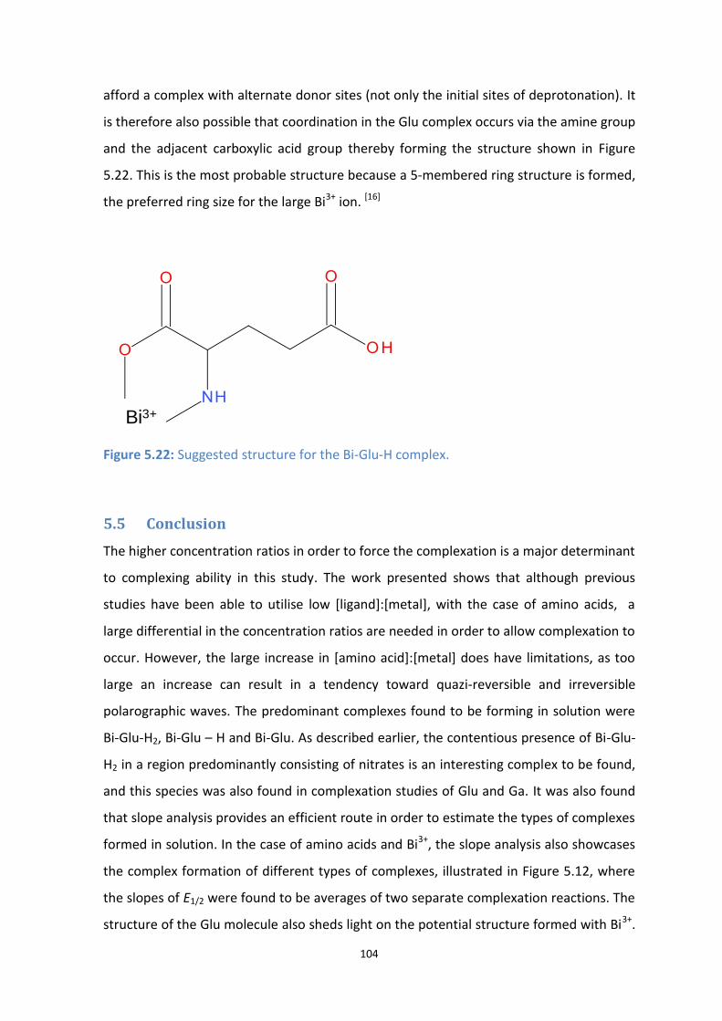
104
afford a complex with alternate donor sites (not only the initial sites of deprotonation). It
is therefore also possible that coordination in the Glu complex occurs via the amine group
and the adjacent carboxylic acid group thereby forming the structure shown in Figure
5.22. This is the most probable structure because a 5-membered ring structure is formed,
the preferred ring size for the large Bi3+ ion. [16]
Bi3+
Figure 5.22: Suggested structure for the Bi-Glu-H complex.
5.5 Conclusion
The higher concentration ratios in order to force the complexation is a major determinant
to complexing ability in this study. The work presented shows that although previous
studies have been able to utilise low [ligand]:[metal], with the case of amino acids, a
large differential in the concentration ratios are needed in order to allow complexation to
occur. However, the large increase in [amino acid]:[metal] does have limitations, as too
large an increase can result in a tendency toward quazi-reversible and irreversible
polarographic waves. The predominant complexes found to be forming in solution were
Bi-Glu-H2, Bi-Glu – H and Bi-Glu. As described earlier, the contentious presence of Bi-Glu-
H2 in a region predominantly consisting of nitrates is an interesting complex to be found,
and this species was also found in complexation studies of Glu and Ga. It was also found
that slope analysis provides an efficient route in order to estimate the types of complexes
formed in solution. In the case of amino acids and Bi3+, the slope analysis also showcases
the complex formation of different types of complexes, illustrated in Figure 5.12, where
the slopes of E1/2 were found to be averages of two separate complexation reactions. The
structure of the Glu molecule also sheds light on the potential structure formed with Bi3+.
105
Figure 5.20, Figure 5.21 and Figure 5.22 all show possible sites of coordination between
Bi3+ and Glu, with the five-membered ring structure present in Figure 5.22 being the most
likely candidate.
The successful complexation between Bi3+ and Glu provides us an idea as to how the Bi3+
ion could behave in a physiological environment rich in glutamic acid. The high
concentration of Cl- present in the body shows that Bi3+ will most certainly be complexed
by these Cl- ions and they will actively be in competition with any other type of ligand
able to complex with Bi3+. Therefore it is important to note the overall complexation of
Bi3+ in the body is, in part, largely dependent on the environment it finds itself at different
stages in the biological system. As shown earlier, an environment with high
concentrations of Glu could result in Bi3+ complexation as observed in our study.

106
5.6 References
[1] Q. R. Smith, J. Nutr., 2000 130, 1016.
[2] a) D. Voet and J. G. Voet in Biochemistry, Vol. 3 Wiley, United States of America, 2004, 736; b)
A. E. Martell and R. M. Smith, NIST Standard Reference Database 46 Version 8.0, NIST Critically
Selected Stability Constants of Metal Complexes,USA, 2004
[3] C. Spanaki and A. Plaitakis, Neurotox. Res., 2012 21, 117.
[4] M. Liguz-Lecznar and J. Skangiel-Kramska, Acta. Neurobiol. Exp.,2007, 67, 207.
[5] L. Pauling in College Chemistry, 3 Freeman, San Francisco, CA, 1964.
[6] I. Cukrowski, H. M. Marques, T. S. Mkwizu, P. P. Magampa and C. Serge, Anal. Chim.
Acta.,2007, 590, 203.
[7] I. Cukrowski, Electroanal.,1997, 9, 699.
[8] P. Franklyn and I. Cukrowski, 3D-CFC software, University of the Witwatersrand, 2003,
Windows Version 1.2, (unpublished)
[9] L. D. Petit and K. J. Powell, Academic Software, IUPAC,2002.
[10] M. K. Singh and M. N. Srivastava, J. Inorg. Nucl. Chem.,1972, 34, 2067.
[11] J. Kragten, L. G. Decnop-Weever and P. Gründler, Talanta,(1993), 40, 485.
[12] A. M. Bond, Electrochim. Acta. ,1972, 17 76.
[13] a) E. A. Zekharova and V. N. Kumok, J. Gen. Chem.,1968, 38, 1868; b) P. Bianco, J. Haladjian
and R. Pilard, J. Chim. Phys.,1973, 73, 280.
[14] C. Billing, D. C. Levendis and V. L. Vieira, S. Afr. J. Chem.,2011, 64, 38.
[15] S. Sajadi, Natural Science,2010, 2, 85.
[16] A. E. Martell and R. D. Hancock, Metal Complexes in Aqueous Solutions, Plenum Press, New
York, 1996. 46.
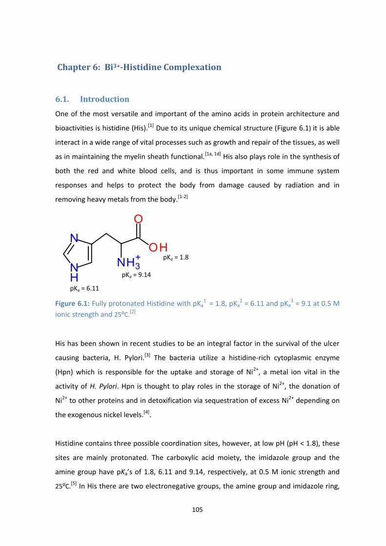
105
Chapter 6: Bi3+-Histidine Complexation
6.1. Introduction
One of the most versatile and important of the amino acids in protein architecture and
bioactivities is histidine (His).[1] Due to its unique chemical structure (Figure 6.1) it is able
interact in a wide range of vital processes such as growth and repair of the tissues, as well
as in maintaining the myelin sheath functional.[1a, 1d] His also plays role in the synthesis of
both the red and white blood cells, and is thus important in some immune system
responses and helps to protect the body from damage caused by radiation and in
removing heavy metals from the body.[1-2]
Figure 6.1: Fully protonated Histidine with pKa1 = 1.8, pKa
2 = 6.11 and pKa3 = 9.1 at 0.5 M
ionic strength and 25⁰C.[2]
His has been shown in recent studies to be an integral factor in the survival of the ulcer
causing bacteria, H. Pylori.[3] The bacteria utilize a histidine-rich cytoplasmic enzyme
(Hpn) which is responsible for the uptake and storage of Ni2+, a metal ion vital in the
activity of H. Pylori. Hpn is thought to play roles in the storage of Ni2+, the donation of
Ni2+ to other proteins and in detoxification via sequestration of excess Ni2+ depending on
the exogenous nickel levels.[4].
Histidine contains three possible coordination sites, however, at low pH (pH < 1.8), these
sites are mainly protonated. The carboxylic acid moiety, the imidazole group and the
amine group have pKa’s of 1.8, 6.11 and 9.14, respectively, at 0.5 M ionic strength and
25⁰C.[5] In His there are two electronegative groups, the amine group and imidazole ring,
pKa = 1.8
pKa = 6.11
pKa = 9.14

106
which cause the pKa of the carboxylic acid to be very acidic. In order to ensure correct pKa
values were assigned to correct sites on His, it was decided to consider related structures
or moieties. The pKa for imidazole (Figure 6.2) is given as 7.15 at 0.5 M ionic strength at
25⁰C[5] close to the value of 6.11 of the moiety in His. Additionally, the ascribed pKa’s for
the carboxylic acid and amine moieties tie in with that seen for Glu in Chapter 5 and
glycine (2.39 and 9.54, respectively, also at 0.5 M ionic strength and 25⁰C[5]).
Complexation to a metal ion such as Bi3+ would really only be possible if there is sufficient
ligand deprotonated at at least one of these sites.
Figure 6.2: Structure of the imidazole ring which forms part of histidine.
One of the most interesting characteristics of the His structure is the imidazole sidechain.
The imidazole ring is planar, satisfying the conditions for aromaticity, and is structurally
related to the pyridine and pyrrole systems. The lone pair on the nitrogen in position 3 is
delocalized round the ring while that on the nitrogen in position 1 is localized in the sp2
orbital. The interactions of His with other amino acids and metallic cations in proteins can
be classified into five types. (1) Cation-π interactions[6] can occur where the imidazole
aromatic ring can interact with metallic or organic cations. On the other hand, the fully
protonated form of His is an organic cation which can interact with other aromatic amino
acids.[7] (2) π-π stacking interactions[7] are possible as the imidazole sidechain is a
conjugative π-plane which can form stacking interactions with the aromatic side chains of
other amino acids. (3) Hydrogen-π interactions[8] can be formed between the polar
hydrogen atom of His and other aromatic amino acids in a ‘T’-orientation. (4) Coordinate
bond interactions[9] can occur since the basic nitrogen atom in the imidazole sidechain
has a lone electron pair which can coordinate to metallic cations, such as Zn2+ and Ca2+.
(5) Hydrogen bond interactions[10] are possible through the polar hydrogen atom of the
imidazole (the hydrogen-bond donor) and the basic nitrogen atom which is a hydrogen-
1
2

107
bond acceptor. The unique behaviour of His has been discussed in literature from
different aspects.[6c, 11]
His is also the precursor of the very important amine, histamine, which is formed by its
decarboxylation in the presence of the enzyme histidine decarboxylase (see Figure
6.3).[12] Histamine is released by the immune system cells in response to allergic
reactions. Many sufferers find it hard to function when high levels of histamine are
present, therefore anti-histamines are used to reduce the overall effect that histamines
strive toward.
Figure 6.3: The reaction showing the removal of the carboxyl moiety in His to form histamine. [13]
Studies on the coordination of His to various metal ions have been done and the
equilibrium constants obtained for metals such as Ni, Cu and Zn[14] using mainly
potentiometry. As expected, no previous work was performed where Bi3+ was complexed
with His. The conflict between the idea that H. Pylori uses the histidine-rich Hpn enzyme
which acts as a storage for Ni2+, a metal ion also vital in the activity of the bacteria, and
the fact that Bi3+ acts as an antibacterial to H. Pylori,[3] makes this study intriguing and it
would be interesting to compare the complexing behaviour of His with Ni2+ and Bi3+.
6.2. Aim
The aim of this study was to investigate whether similar conditions to those used in the
study of Bi3+-Glu complexation would be sufficient to lead to complex formation before
precipitation of Bi3+. His was considered since pKa1 = 1.8 for the carboxylic acid moiety,
compared to 2.16 for Glu, thus His should be singly deprotonated at a lower pH.
108
However, pKa2 = 6.11 for His, significantly greater than that for Glu (pKa
2 = 4.07). It would
therefore be interesting to see which of these ligands would produce more stable
complexes and more successfully prevent precipitation at higher pH.
6.3. Experimental
Experiments were run as for the Bi3+-Glu studies, again at three ligand to metal
concentration ratios. In this case, [His]:[Bi3+] of 4000, 5000 and 7005 was used and as
before these experiments will be referred to as the rounded values (4000, 5000 and
7000).
6.4. Results and discussion
6.4.1. Initial data inspection
In order to investigate the complexing ability of His with Bi3+, a polarographic-pH titration
experiment was initially run at a [His]:[Bi3+] = 2000. However, even at this high ratio,
precipitation of Bi3+ occurred at a pH ~2. Although an unexpected result, it was decided to
increase the [His]:[Bi3+] to 5000. It was hoped that by adding an even larger amount of
ligand, the chemical equilibrium would be forced toward complexation, as noted in our
Bi3+-Glu studies (Chapter 5).
As can be seen in Figure 6.4, the increase in [His]:[Bi3+] to 5000 extended the solubility
range of Bi3+ to pH ~3.1, not a very wide range. It must be stated that when the ligand
was added to the system, the pH shot up to 1.7. This was due to the basic nature of the
amino acid which became protonated itself using the H+ ions from the nitric acid solution.
The increase in pH is not favorable as it prevents data polarographic data being collected
in the pH range of pH 1 to pH 1.7. As mentioned in Chapter 5, we should have decreased
the pH by adding more HNO3 and would be suggested as a future betterment to this
study.
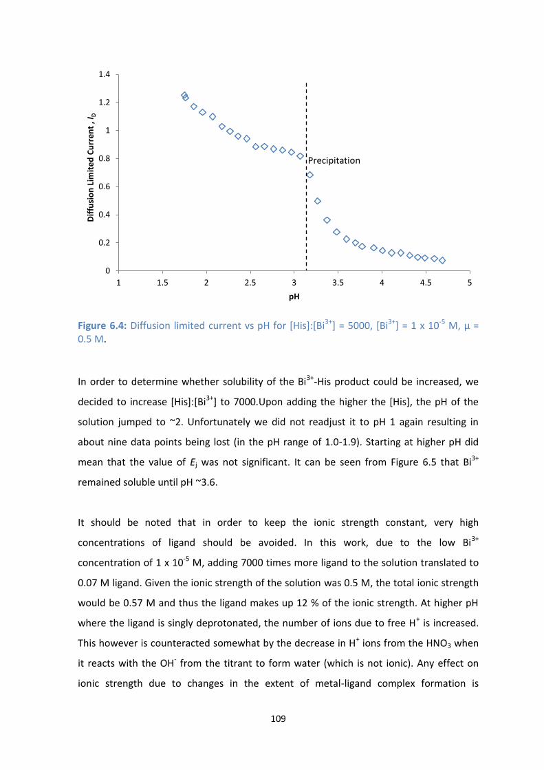
109
Figure 6.4: Diffusion limited current vs pH for [His]:[Bi3+] = 5000, [Bi3+] = 1 x 10⁻⁵ M, μ = 0.5 M.
In order to determine whether solubility of the Bi3+-His product could be increased, we
decided to increase [His]:[Bi3+] to 7000.Upon adding the higher the [His], the pH of the
solution jumped to ~2. Unfortunately we did not readjust it to pH 1 again resulting in
about nine data points being lost (in the pH range of 1.0-1.9). Starting at higher pH did
mean that the value of Ej was not significant. It can be seen from Figure 6.5 that Bi3+
remained soluble until pH ~3.6.
It should be noted that in order to keep the ionic strength constant, very high
concentrations of ligand should be avoided. In this work, due to the low Bi3+
concentration of 1 x 10⁻⁵ M, adding 7000 times more ligand to the solution translated to
0.07 M ligand. Given the ionic strength of the solution was 0.5 M, the total ionic strength
would be 0.57 M and thus the ligand makes up 12 % of the ionic strength. At higher pH
where the ligand is singly deprotonated, the number of ions due to free H+ is increased.
This however is counteracted somewhat by the decrease in H+ ions from the HNO3 when
it reacts with the OH- from the titrant to form water (which is not ionic). Any effect on
ionic strength due to changes in the extent of metal-ligand complex formation is
0
0.2
0.4
0.6
0.8
1
1.2
1.4
1 1.5 2 2.5 3 3.5 4 4.5 5
Dif
fusi
on
Lim
ite
d C
urr
en
t , I
D
pH
Precipitation

110
negligible since the Bi3+ concentration is significantly lower the other components
present. Thus a balance had to be reached where the concentration of ligand was high
enough for complex formation to occur, but not too high to affect the ionic strength
significantly.
Figure 6.5: Diffusion limited current vs pH for [His]:[Bi3+] = 7000, [Bi3+] = 1 x 10⁻⁵ M, μ = 0.5 M.
Figure 6.6 shows selected DC polarograms indicating just the Bi3+ reduction wave
obtained during the polarographic-pH titration where [His]:[Bi3+] = 7000. Starting at the
initial polarogram obtained at pH ~2, there is a clear negative shift in the E1/2(Bi3+) values
as pH is increased which is an indication of complex formation. Figure 6.6 also highlights
the current decrease due to increased dilution as more KOH solution is added to raise the
pH.
0
0.2
0.4
0.6
0.8
1
1.2
1.4
1.6
1 1.5 2 2.5 3 3.5 4 4.5 5
Dif
fusi
on
Lim
ite
d C
urr
ent
, ID
pH
Precipitation

111
Figure 6.6: Experimental polarograms from the polarographic-pH titration conducted with [His]:[Bi3+] = 7000 at different pHs, namely, a) 2.0, b) 2.3, c) 2.4, d) 2.7 and e) 3.6.
As described in Chapter 5, the E1/2 values, obtained from fitting equation 3.4 to the
polarograms, must be for reversible reduction waves (i.e. 0.9 < ɣ <1) to apply equation
3.1 to determine formation constants. As can be seen from Figure 6.7, the values for ɣ for
the Bi3+-His studies are above 0.9 in all cases, thereby indicating reversible reduction
processes. For the two points that lie slightly above ɣ = 1.00, the discrepancy is due to
fitting errors, but this small error does not affect the E1/2 or Id values significantly.
The Ej corrected E1/2 values for Bi3+ for the three experiments are shown in Figure 6.8.
There is a clear shift of the E1/2 values in the negative direction, a strong indication of
complex formation. For the experiments where [His]:[Bi3+] = 5000 and only considering
the pH range 1.7-3.0, the difference in E1/2 values was 22 mV for L = His and 36 mV for L =
Glu. This would generally imply greater complex formation for the Bi3+-Glu system than
the Bi3+-His system if a similar type of species is formed in that pH range.
0
0.2
0.4
0.6
0.8
1
1.2
1.4
1.6
1.8
-0.25 -0.2 -0.15 -0.1 -0.05 0 0.05 0.1 0.15 0.2
Cu
rre
nt
Applied Potential (V)
Negative shift in E1/2
with increasing pH is
indicative of complex
formation. ID
a b c d
e
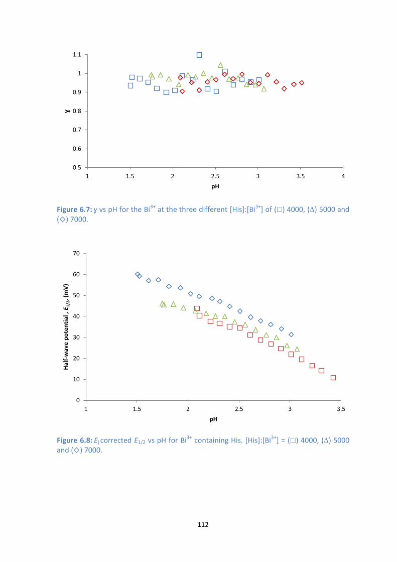
112
Figure 6.7: ɣ vs pH for the Bi3+ at the three different [His]:[Bi3+] of () 4000, () 5000 and () 7000.
Figure 6.8: Ej corrected E1/2 vs pH for Bi3+ containing His. [His]:[Bi3+] = () 4000, () 5000 and () 7000.
0.5
0.6
0.7
0.8
0.9
1
1.1
1 1.5 2 2.5 3 3.5 4
ɣ
pH
0
10
20
30
40
50
60
70
1 1.5 2 2.5 3 3.5
Hal
f-w
ave
po
ten
tial
, E 1
/2, (
mV
)
pH
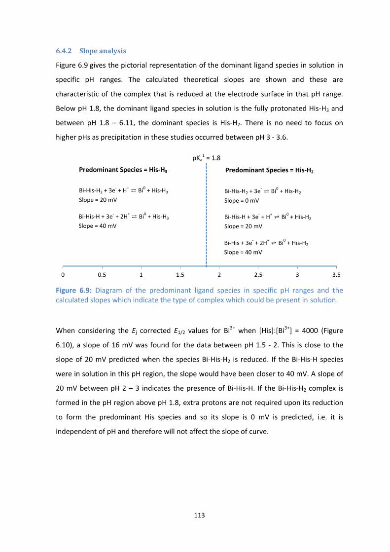
113
6.4.2 Slope analysis
Figure 6.9 gives the pictorial representation of the dominant ligand species in solution in
specific pH ranges. The calculated theoretical slopes are shown and these are
characteristic of the complex that is reduced at the electrode surface in that pH range.
Below pH 1.8, the dominant ligand species in solution is the fully protonated His-H3 and
between pH 1.8 – 6.11, the dominant species is His-H2. There is no need to focus on
higher pHs as precipitation in these studies occurred between pH 3 - 3.6.
Figure 6.9: Diagram of the predominant ligand species in specific pH ranges and the calculated slopes which indicate the type of complex which could be present in solution.
When considering the Ej corrected E1/2 values for Bi3+ when [His]:[Bi3+] = 4000 (Figure
6.10), a slope of 16 mV was found for the data between pH 1.5 - 2. This is close to the
slope of 20 mV predicted when the species Bi-His-H2 is reduced. If the Bi-His-H species
were in solution in this pH region, the slope would have been closer to 40 mV. A slope of
20 mV between pH 2 – 3 indicates the presence of Bi-His-H. If the Bi-His-H2 complex is
formed in the pH region above pH 1.8, extra protons are not required upon its reduction
to form the predominant His species and so its slope is 0 mV is predicted, i.e. it is
independent of pH and therefore will not affect the slope of curve.
0 0.5 1 1.5 2 2.5 3 3.5
pKa1 = 1.8
Bi-His-H2 + 3e- + H
+ ⇄ Bi
0 + His-H3
Slope = 20 mV
Bi-His-H2 + 3e- ⇄ Bi
0 + His-H2
Slope = 0 mV
Bi-His-H + 3e- + 2H
+ ⇄ Bi
0 + His-H3
Slope = 40 mV
Bi-His-H + 3e- + H
+ ⇄ Bi
0 + His-H2
Slope = 20 mV
Predominant Species = His-H2 Predominant Species = His-H3
Bi-His + 3e- + 2H
+ ⇄ Bi
0 + His-H2
Slope = 40 mV

114
Figure 6.10: Slope analysis on the Ej corrected E1/2 for Bi3+ vs pH plot with [His]:[Bi3+] = 4000.
It was described earlier that upon addition of the large excess of His, the pH of the
solution increased to pH 2. Slope analysis of the Ej corrected E1/2 for Bi3+ vs pH when
[His]:[Bi3+] = 7000 (Figure 6.11) gave a slope of 20 mV between pH 2 - 3, which indicates
reduction of the Bi-His-H complex. With this experiment only starting at pH 2 (due to the
high concentration of His added), species formed below pH 2 would not be detected,
such as the Bi-His-H2 complex predicted in the [His]:[Bi3+] = 4000 experiment. Above pH 3
the slope increased to 29 mV which could indicate that both the Bi-His-H and the Bi-His
complexes were together in solution. The Bi-His was not predicted before as it would only
form at the highest pHs where precipitation had already occurred in previous
experiments. The Bi-His-OH species was also considered since precipitation occurred
straight after the formation of the new species. The reduction reaction that occurs,
however, would be expected to be Bi-His-OH + 3e- + 3H+ ⇄ Bi0 + His-H2 +H2O in the pH
range 3 – 3.6 thereby giving a slope of 60 mV which is significantly greater than that
observed
y = -16.24x + 84.165 R² = 0.9553
y = -20.096x + 92.545 R² = 0.9917
0
10
20
30
40
50
60
70
1 1.5 2 2.5 3 3.5
Hal
f-w
ave
po
ten
tial
, E 1
/2, (
mV
)
pH
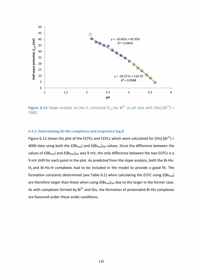
115
Figure 6.11: Slope analysis on the Ej corrected E1/2 for Bi3+ vs pH plot with [His]:[Bi3+] = 7000.
6.4.3. Determining Bi-His complexes and respective log β
Figure 6.12 shows the plot of the ECFCs and CCFCs which were calculated for [His]:[Bi3+] =
4000 data using both the E(Bifree) and E(Bifree)OH values. Since the difference between the
values of E(Bifree) and E(Bifree)OH was 9 mV, the only difference between the two ECFCs is a
9 mV shift for each point in the plot. As predicted from the slope analysis, both the Bi-His-
H2 and Bi-His-H complexes had to be included in the model to provide a good fit. The
formation constants determined (see Table 6.1) when calculating the ECFC using E(Bifree)
are therefore larger than those when using E(Bifree)OH due to the larger in the former case.
As with complexes formed by Bi3+ and Glu, the formation of protonated Bi-His complexes
are favoured under these acidic conditions.
y = -29.277x + 110.79 R² = 0.9988
y = -20.001x + 82.956 R² = 0.9854
0
5
10
15
20
25
30
35
40
45
50
1 1.5 2 2.5 3 3.5 4
Hal
f-w
ave
po
ten
tial
, E 1
/2 (
mV
)
pH

116
Figure 6.12: The ECFCs calculated using either E(Bifree) and E(Bifree)OH values and the CCFCs determined by including the Bi-His-H2 and Bi-His-H complexes in the species model.
In order to fully determine whether the complexes were indeed contributing to the
formation of the curves, it was decided to fit the ECFC by either taking only the formation
of the Bi-His-H complex or only the Bi-His-H2 complex into account. As an example, Figure
6.13 shows the ECFC calculated using the E(Bifree)OH value and fitted when accounting for
only one of the species at a time. The standard deviation of fitting was 2.61 when only Bi-
His-H was used, 1.37 when only Bi-His-H2 was used and 0.82 when both complexes were
included. The log β values obtained were 15.36 0.05 for Bi-His-H and 17.41 0.05 for
Bi-His-H2, both values being larger than that obtained when both species were
incorporated into the model (see Table 6.1). When only a single species is used in
calculating the CCFC, an averaging effect occurs throughout the pH range giving CCFCs
that do not fit well in the extreme pH regions of the plot.
0
10
20
30
40
50
60
1 1.5 2 2.5 3 3.5
Co
rre
cte
d Δ
E 1/2
/mV
pH
Using E(Bifree)
Using E(Bifree)OH
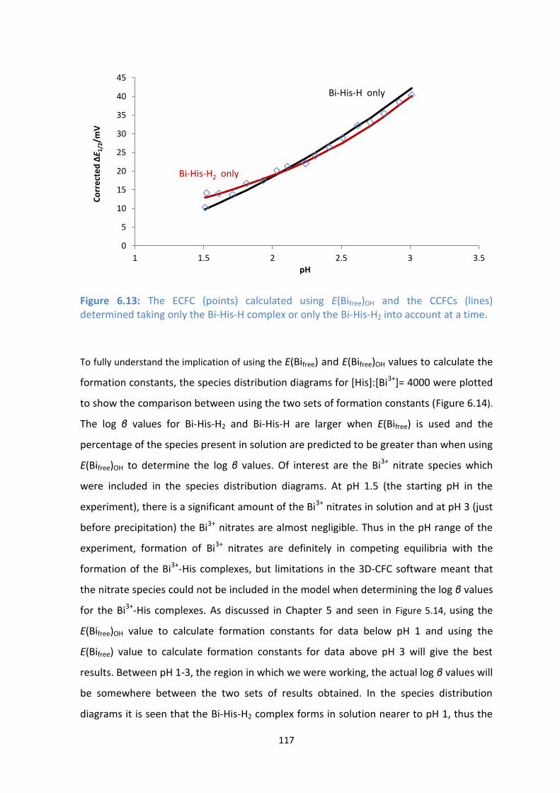
117
Figure 6.13: The ECFC (points) calculated using E(Bifree)OH and the CCFCs (lines) determined taking only the Bi-His-H complex or only the Bi-His-H2 into account at a time.
To fully understand the implication of using the E(Bifree) and E(Bifree)OH values to calculate the
formation constants, the species distribution diagrams for [His]:[Bi3+]= 4000 were plotted
to show the comparison between using the two sets of formation constants (Figure 6.14).
The log β values for Bi-His-H2 and Bi-His-H are larger when E(Bifree) is used and the
percentage of the species present in solution are predicted to be greater than when using
E(Bifree)OH to determine the log β values. Of interest are the Bi3+ nitrate species which
were included in the species distribution diagrams. At pH 1.5 (the starting pH in the
experiment), there is a significant amount of the Bi3+ nitrates in solution and at pH 3 (just
before precipitation) the Bi3+ nitrates are almost negligible. Thus in the pH range of the
experiment, formation of Bi3+ nitrates are definitely in competing equilibria with the
formation of the Bi3+-His complexes, but limitations in the 3D-CFC software meant that
the nitrate species could not be included in the model when determining the log β values
for the Bi3+-His complexes. As discussed in Chapter 5 and seen in Figure 5.14, using the
E(Bifree)OH value to calculate formation constants for data below pH 1 and using the
E(Bifree) value to calculate formation constants for data above pH 3 will give the best
results. Between pH 1-3, the region in which we were working, the actual log β values will
be somewhere between the two sets of results obtained. In the species distribution
diagrams it is seen that the Bi-His-H2 complex forms in solution nearer to pH 1, thus the
0
5
10
15
20
25
30
35
40
45
1 1.5 2 2.5 3 3.5
Co
rre
cte
d Δ
E 1/2
/mV
pH
Bi-His-H only
Bi-His-H2 only

118
log β value found using E(Bifree)OH would be closer to the real value and since the Bi-His-H
complex it is formed nearer to pH 3, the log β value found using E(Bifree) would be more
representative in this case. The species distribution diagrams thus showed us which
species are present in a solution at a specific pH as well as indicate the other potential
complexes which are in competition with the formation of the Bi-His complexes.
Therefore allowing us to establish an idea at which the pH our calculated complexes
begin to form.
Table 6.1: Calculated log β values for the formation of the Bi3+-His complexes using using both the E(Bifree) values and the 3D-CFC software. (Charges were omitted in equilibria reactions.)
Figure 6.14 shows the a comparison between the species distribution diagrams for the
study where [His]:[Bi3+]= 4000. As can be seen, the formation of the Bi-His-H2 and Bi-His-
H species is more favoured when E(BiFree) was used to calculate the log β values for the
respective complexes, with the species percentage of Bi-His-H2 = 38% and the Bi-His-H =
[L]:[Bi3+] 4000 5000 7000
(a) using E(BiFree)
Log β
Bi3+ + L + H2 ⇄Bi-LH2 17.92 ± 0.06 18.01 ± 0.05 -
Bi3+ + L + H ⇄ Bi-LH 16.17 ± 0.03 15.88 ± 0.04 16.18 ± 0.02
Bi3+ + L ⇄ Bi-L 12.48 ± 0.12
Overall Fit 1.06 0.16 1.67
(b) using E(BiFree)OH
Bi3+ + L + H2 ⇄Bi-LH2 17.26 ± 0.15 17.50 ± 0.04 -
Bi3+ + L + H ⇄ Bi-LH 14.97 ± 0.15 - 15.60 ± 0.03
Bi3+ + L ⇄ Bi-L 10.59 ± 0.34
Overall Fit 0.82 0.28 1.45
119
75%. However, when E(BiFree)(OH) was used, the percentage of species present for the
respective complexes drops to below 20 %. This once again illustrates the limitations in
software used to calculate log β values. 3DCFC is unable to incorporate the formation of
Bi-OH and Bi-NO3 complexes simultaneously. It is also evident that when E(Bifree)OH is
used, the log β values are smaller than those calculated when E(Bifree) is utilized. The
difference between the two is that when E(Bifree), the complexation due to NO3-
complexes is taken into account, hence increasing formation of Bi-His complexes. It must
be noted however, that the formation of Bi-NO3 and Bi-OH complexes begin to form from
pH 0 and these actively compete with the formation of our Bi-His complexes.
For the [His]:[Bi3+]= 5000, it can be seen from Table 6.1 that the complexes which have
been calculated to have formed are the Bi-His-H2 and Bi-His-H with log β values of 18.01
and 15.88 respectively for E(BiFree) . The Bi-His complex was unable to be calculated
possibly due to it forming in such low amounts and unable to overcome the large
competition with Bi(OH) species since a [His]:[Bi3+] = 5000. It can be seen in Figure 6.15,
that the formation of the insoluble Bi(OH)2 complex from pH ~2 . The result illustrates
that even at a [His]:[Bi3+] = 5000, the ratio is not large enough to fully favour the
complexation of Bi-His complexes. Using E(BiFree)OH, the only complex determined to be
forming was that of Bi-His-H2 and Figure 6.15 b) shows that initially there is a large
competition for the Bi3+ ion with nitrates. Unfortunately, this has a large effect on the
percentage of Bi-His-H2 species formed, with the percentage of species present at
approximately 38% at pH ~1.7. The formation of the insoluble Bi(OH) species once again
plays a large role in competing with His for the Bi3+ ion leading to less soluble Bi3+
complexes forming and precipitating out of solution.
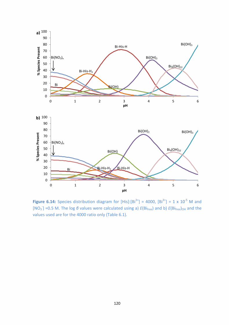
120
Figure 6.14: Species distribution diagram for [His]:[Bi3+] = 4000, [Bi3+] = 1 x 10⁻⁵ M and
[NO3-] =0.5 M. The log β values were calculated using a) E(Bifree) and b) E(Bifree)OH and the
values used are for the 4000 ratio only (Table 6.1).
0
10
20
30
40
50
60
70
80
90
100
0 1 2 3 4 5 6
% S
pe
cie
s P
rese
nt
pH
0
10
20
30
40
50
60
70
80
90
100
0 1 2 3 4 5 6
% S
pe
cie
s P
rese
nt
pH
Bi(NO3)x
Bi(OH)
Bi-His-H
Bi-His-H2
Bi(OH)2
Bi9(OH)22
9
Bi(OH)3
b)
a)
Bi(NO3)x
Bi-His-H
Bi(OH)3
Bi9(OH)22
9
Bi(OH)
Bi(OH)2
Bi-His-H2 Bi
Bi

121
Figure 6.15: Species distribution diagram for [His]:[Bi3+] = 5000, [Bi3+] = 1 x 10⁻⁵ M and
[NO3-] =0.5 M. The log β values were calculated using a) E(Bifree) and b) E(Bifree)OH and the
values used are for the 5000 ratio only (Table 6.1).
From the experiment where [His]:[Bi3+] = 7000, the ECFC could be fitted when including
the Bi-His-H and Bi-His complexes as predicted by the slope analysis. The Bi-His-H2
complex could not be included in the model as log β values would not refine, probably
since the concentration of Bi-His-H2 was too low as this experiment was only started at
pH ~2. In order to determine this log β value at this ratio the solution will have to be
acidified first and data obtained at lower pHs. The ECFC and CCFC are plotted in Figure
0
10
20
30
40
50
60
70
80
90
100
0 1 2 3 4 5 6
% S
pe
cie
s P
rese
nt
pH
0
10
20
30
40
50
60
70
80
90
100
0 1 2 3 4 5 6
% S
pe
cie
s p
rese
nt
pH
Bi(NO3)x
Bi-His-H
Bi(OH)3
Bi9(OH)2
29
Bi(OH)
Bi(OH)2
Bi-His-H2
Bi
Bi(NO3)x
Bi(OH)3
Bi9(OH)22
Bi(OH)
Bi(OH)2
Bi-His-H2
Bi
a)
b)
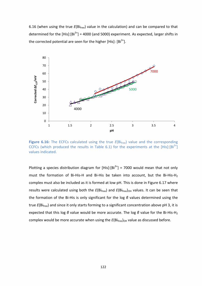
122
6.16 (when using the true E(Bifree) value in the calculation) and can be compared to that
determined for the [His]:[Bi3+] = 4000 (and 5000) experiment. As expected, larger shifts in
the corrected potential are seen for the higher [His]: [Bi3+].
Figure 6.16: The ECFCs calculated using the true E(Bifree) value and the corresponding CCFCs (which produced the results in Table 6.1) for the experiments at the [His]:[Bi3+] values indicated.
Plotting a species distribution diagram for [His]:[Bi3+] = 7000 would mean that not only
must the formation of Bi-His-H and Bi-His be taken into account, but the Bi-His-H2
complex must also be included as it is formed at low pH. This is done in Figure 6.17 where
results were calculated using both the E(Bifree) and E(Bifree)OH values. It can be seen that
the formation of the Bi-His is only significant for the log β values determined using the
true E(Bifree) and since it only starts forming to a significant concentration above pH 3, it is
expected that this log β value would be more accurate. The log β value for the Bi-His-H2
complex would be more accurate when using the E(Bifree)OH value as discussed before.
0
10
20
30
40
50
60
70
80
1 1.5 2 2.5 3 3.5 4
Co
rre
cte
d Δ
E 1/2
/mV
pH
7000
4000
5000

123
Figure 6.17: Species distribution diagrams for [His]:[Bi3+] = 7000, [Bi3+] = 1 x 10⁻⁵ M and
[NO3-] =0.5 M. The log β values were calculated using a) E(Bifree) and b) E(Bifree)OH and the
values used are for the 4000 ratio for MLH2, the 7000 ratio for ML and the average for the
4000 and 7000 ratios for MLH (Table 6.1).
Since the first pKa of the His molecule is 1.82, it is likely that the complex formation is
occurring via the carboxyl moiety of His. As with the formation of the Bi-Glu complexes,
the low pKa of the amino acid carboxyl groups seems to be most favoured. As described
in literature, the pKa is the point at which 50% of the acid is deprotonated, and so at a pH
of 1.82, 50% of the [His] is deprotonated and so results in the higher potential in
complexing ability with Bi3+.
0
10
20
30
40
50
60
70
80
90
100
0 1 2 3 4 5 6
% S
pe
cie
s p
rese
nt
pH
0
10
20
30
40
50
60
70
80
90
100
0 1 2 3 4 5 6
% S
pe
cie
s p
rese
nt
pH
Bi
Bi
Bi(NO3)x
Bi(NO3)x
Bi-His-H2
Bi-His-H2
Bi-His-H
Bi-His-H
Bi-His
Bi(OH)
Bi(OH)
Bi(OH)2
Bi(OH)2
Bi(OH)3
Bi(OH)3
Bi9(OH)22
Bi9(OH)22
a)
b)
124
Studying the species distribution diagrams of the Bi-His complexes at different [His]:[Bi3+],
we are able to see that there are two potential complexes which form due to the
deprotonated carboxyl moeity of the His molecule. Due to the high [His]:[Bi3+], more
deprotonated molecules of the His are preset, and are thus able to complex with the
Bi3+.Due to the structural similarities of His, it is thus proposed that the structure of the
Bi-His complexes are similar to those proposed in Chapter 5 for the Bi-Glu complexes.
With the pKa values which were shown earlier, the deprotonation of the carboxlic acid
moiety and amine group of the His molecule could allow for coordination to Bi3+ via a
five-membered ring, a structure which is more stable than other complexes which could
form.
Previous studies[5] have been completed where His was complexed metal ions such as
Cu(II), Zn(II), Cd(II), Ni(II) and Pb(II). One of the most interesting comparisons would be
the complexation of His with the Pb2+, which is isoelectronic to Bi3+. Studies[5] conducted
with the Pb2+ ion were conducted in ionic strength of 0.1 M and 3.0 M at 25oC. Although
it was that the species formed were Pb-His, Pb-(His)2, Pb-(His-H)2 and Pb-(His2-H) with log
K of 5.94, 10.11, 6.22, and 7.04 respectively[5]. These values are much smaller than those
determined for our Bi-His-H2 and Bi-His-H complexes (Table 6.1). Due to the similarity of
the Ga3+ ion to Bi3+ in terms of Glu, as was seen in Chapter 5, it was also decided to
compare the formation constants of Ga3+ with His. Interestingly, Ga3+ was shown to form
Ga-His, Ga-His-H and Ga-His-H2 complexes[15], the same complexes seen to form in this
study with Bi3+. Even more interesting was the fact that the formation constants were
calculated to be 12.50, 15.15 and 18.12[15] respectively at 3.0 M NO3 at 25⁰C, very similar
to the values presented in Table 6.1 ( 12.48 for ML, 16.07(average) for MLH and 17.97 for
the MLH2 complex). The Ga3+ ion seems to behave in a very similar manner to Bi3+ when
complexed with amino acids as was shown in Chapter 5. One of the most important
findings in other metal-ion-His complex studies is that with the varying ionic strength the
log K values differed and since our studies were conducted at constant ionic strength of
0.5 M, we found different formation constants for our respective complexes. We also
found different types of complexes forming than those reported in literature, and the
most important reasons for this could be that the pH range in which our study was
completed was very low and highly acidic (pH 1-pH 4). At these low pH values, the

125
carboxyl group of His becomes best suited to form the complex with Bi3+ hence leading to
the large formation constants which have been determined. Previous studies have been
able to complex the His molecule with other metal ions via the imidazole and amine
groups via a strong chelation effect, but once again these complexes are favoured at
higher pH, and we are unable to reach these pH ranges due to the insolity of Bi3+. No
previous Bi-His complex formation studies wherein formation constants are reported
were found. The low pH range solubility of Bi3+ does prove a huge hurdle to overcome.
6.5 Conclusion
The results presented show that the complexation of an amino acid to Bi3+ has complex
chemistry associated with it. Initial studies (Chapter 4) have shown that at low [His]:[Bi3+]
(=100), complexation is not significant enough to allow the Bi3+ to form soluble Bi-His.
However, by increasing [His]:[Bi3+] to values greater than 4000 allowed the formation of
soluble Bi-His complexes and therefore increasing the pH range of Bi3+ to ~3.5. Although
the [His]:[Bi3+]= 700 used, the reversibility of the polarographic waves remained within
the accepted range of reversibility (0.9-1), indicating that the large His concentration
does not affect the reversibility of Bi3+, unlike Glu in Chapter 5 and Glutamine to a larger
extent in Chapter 7.
The predominant species determined to be forming in solution are the Bi-His-H2, Bi-His-H
and Bis-H complexes with log β values of 17.97, 16.08 and 12.48 respectively at 0.5M
ionic strength at 25⁰C. Slope analysis of the E1/2 values showed that the species forming
could be estimated from the slope of the E1/2 vs pH (Figure 6.10 and Figure 6.11). The
slope analysis also showed the formation of Bi-His-H2 complex, albeit in small amounts
when [His]:[Bi3+] =7000 and it was not possible to calculate the associated log β. The
addition of [His]:[Bi3+] = 7000 already showed an increase in the overall ionic strength of
the solution so by increasing [His]:[Bi3+] could result affecting this ionic strength even
more. One of the major improvements to this work would be to adjust the pH of the
solution to pH ~1, thereby allowing more of the Bi-His-H2 complexes to form in larger
quantities for the log β to be determined.

126
Studies where the complexation of Ga3+ with amino acids have once again showed
similarities to the results we have obtained in this study with Bi3+. The complexes formed
when His complexes with Ga3+ are reported to be the same as the complexes we have
identified in this study with log β values also corresponding surprisingly well. The results
once again show that the Ga3+ ion behaves in a very similar manner to Bi3+ when placed in
a situation where complexation is required with an amino acid, as was seen in Chapter 5.
Our studies have therefore shown that Bi3+ is able to complex quite strongly with His at
low pH levels, however the concentration ratio of [His]:[Bi3+] needs to be significantly
high (>4000 times).
127
6.6. References
[1] a) F. Li, D. Fitz, F. D.G. and B. M. Rode, Amino Acids,2010, 38, 287; b) M. Remko, D. Fitz and B.
M. Rode, Amino Acids,2010, 39, 1309; c) K. Uchida, Amino Acids,2003, 25, 249; d) A. Martinez,
Amino Acids,1995, 9, 285.
[2] A. Reddy and G. N. Sastry, J. Phys. Chem.,2005, 109.
[3] R. Ge, X. Sun, D. Wang, Q. Zhou and H. Sun, Biochim. Biophys. Acta.,2011, 1813, 1422.
[4] a) G. Ruiguang, S. Xuesong, G. Qing, R. M. Watt, J. A. Tanner, B. C. Y. Wong, H. H. Xia, H. Jian-
Dong, H. Qing-Yu and S. Hongzhe, J. Bio. Inorg. Chem.,2007, 12, 831; b) H. Li and H. Sun, Curr. Op.
Chem. Bio.,2012, 16, 74.
[5] A. E. Martell and R. M. Smith, NIST Standard Reference Database 46 Version 8.0, NIST Critically
Selected Stability Constants of Metal Complexes,USA, 2004
[6] a) L. K. Engerer and T. P. Hansua, J. Org. Chem.,2011, 76, 42; b) A. Reddy and G. N. Sastry, J.
Phys. Chem. ,2005, 109; c) U. D. Priyakumar, M. Punnagai, G. P. Krishna Mohan and G. N. Sastry,
Tetrahedron,2004, 60, 3037.
[7] a) P. Mignon, S. Loverix, J. Steyaert and P. Geerlings, Nucl. Acid. Res.,2005, 33, 1779; b) G.
Stefan, Angew. Chem. Int. Ed. (English),2008, 47, 3430.
[8] a) R. M. Hughes and M. L. Walters, J. Am. Chem. Soc.,2006, 128, 13586; b) E. A. Meyer, R. K.
Castellano and F. Diederich, Angew. Chem. Int. Ed.(English),2003, 42, 1210.
[9] S. O. Kang, M. A. Hossain and K. Bowman-James, Coord. Chem. Rev.,2000, 250, 3038.
[10] a) M. Henry, Chem. Phys. Chem.,2002, 3, 561; b) M. Henry, Chem. Phys. Chem.,2002, 3, 607.
[11] L. J. Andrews and R. M. Keefer in Molecular complexes in organic chemistry., Vol. Holden-
Day, San-Francisco, 1964.
[12] D. Voet and J. G. Voet in Biochemistry, Vol. 3 Wiley, United States of America, 2004, 736.
[13] Histamine, http://www.en.wikipedia.org/wiki/Histamine, (Date Accessed: 2014-05-03)
[14] R. Leberman and B. R. Rabin, Trans. Far. Soc.,1959, 55, 1660.
[15] P. Bianco, J. Haladjian and R. Pilard, J. Less-Common Met.,1978, 58, 58.
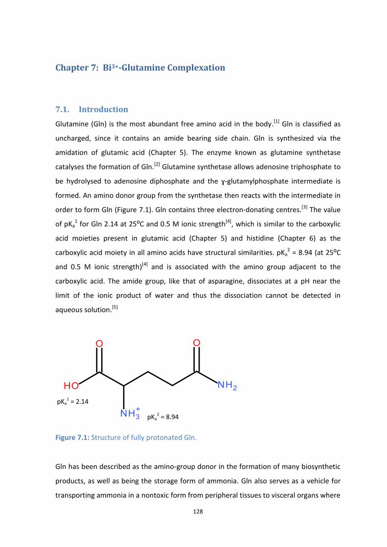
128
Chapter 7: Bi3+-Glutamine Complexation
7.1. Introduction
Glutamine (Gln) is the most abundant free amino acid in the body.[1] Gln is classified as
uncharged, since it contains an amide bearing side chain. Gln is synthesized via the
amidation of glutamic acid (Chapter 5). The enzyme known as glutamine synthetase
catalyses the formation of Gln.[2] Glutamine synthetase allows adenosine triphosphate to
be hydrolysed to adenosine diphosphate and the ɣ-glutamylphosphate intermediate is
formed. An amino donor group from the synthetase then reacts with the intermediate in
order to form Gln (Figure 7.1). Gln contains three electron-donating centres.[3] The value
of pKa1 for Gln 2.14 at 25⁰C and 0.5 M ionic strength[4], which is similar to the carboxylic
acid moieties present in glutamic acid (Chapter 5) and histidine (Chapter 6) as the
carboxylic acid moiety in all amino acids have structural similarities. pKa2 = 8.94 (at 25⁰C
and 0.5 M ionic strength)[4] and is associated with the amino group adjacent to the
carboxylic acid. The amide group, like that of asparagine, dissociates at a pH near the
limit of the ionic product of water and thus the dissociation cannot be detected in
aqueous solution.[5]
Figure 7.1: Structure of fully protonated Gln.
Gln has been described as the amino-group donor in the formation of many biosynthetic
products, as well as being the storage form of ammonia. Gln also serves as a vehicle for
transporting ammonia in a nontoxic form from peripheral tissues to visceral organs where
pKa1 = 2.14
pKa2 = 8.94

129
the ammonia can be excreted as ammonium ions in the kidneys or converted to urea in
the liver. The importance of Gln within the biological system is thus paramount to the
functioning and survival of an organism. Gln is produced in the muscles and is distributed
by the blood to the organs that need it. It has also shown to be a helpful agent in the gut
function, the immune system and other essential processes in the body, especially in
times of stress. It is also important for providing "fuel" (nitrogen and carbon) to many
different cells in the body.[5b]
One of the most important aspects of Gln in the human body is that it performs a central
role in nitrogen metabolism. After surgery or traumatic injury, nitrogen is necessary to
repair the wounds and keep the vital organs functioning. About one third of this nitrogen
comes from Gln.[5b] If the body uses more Gln than the muscles can make (i.e. during
times of stress), muscle wasting can occur. [5b] This often occurs in people suffering from
HIV and in cancer patients, so Gln is used as a supplement to prevent weight loss due to
muscle wasting.[6]
Gln is also used to protect the immune system and digestive system in people undergoing
radio-chemotherapy for cancer of the oesophagus. Recent studies[7] have shown that L-
Gln may help prevent toxic side effects of chemotherapy and radiation therapy (by
preventing of damage to normal tissue, including peripheral nerves) and possibly also
increase the effectiveness of some chemotherapy drugs.
The complexing ability of Gln has been studied previously with various metal ions,[8] and
studies have shown that the complexation, although difficult, is possible and thus it was
decided to study its complexation with Bi3+. One of the important factors contributing to
the complexation of amino acids with metal ions is the size of the ring formed due to
complex formation. In amino acids, bonding through the carboxylic acid and adjacent
amine groups results in 5-membered rings being formed, which is what was proposed for
the Glu molecule in Chapter 5 and His molecule in Chapter 6. It is the polar side chains
that need consideration to see whether tridentate chelates can form. Berthon[8] describes
the formation of the chelate rings as highly dependent on the type of side chain present
on the respective amino acid. Both asparagine and Gln contain an amide functional group

130
which is at the β and ɣ-positions respectively. Thus if these amino acids behave as
tridentate ligands, asparagine will form 6-membered rings and Gln 7-membered rings
when chelated through the amide group.[8] Previous studies have attempted to
characterise a possible participation of the amide group in the coordination of several
metal ions.[9] Given the unfavourable size of the chelate rings potentially involved, Gln
displays only a very weak tridentate capability with Co2+ and Ni2+ and exclusively behaves
as a bidentate ligand with Cu2+.[10] This is in line with the fact that the formation of Cu-Gln
complexes is not accompanied by any stereoselective effect.[11] Since Bi3+ is a large metal
ion, formation of small rings are preferred, thus it would be expected that coordination
through the amide group not occur significantly. It is important to understand these
characteristics as they influence whether Bi3+-Gln complexes would form and if so, how
stable the complex would be.
7.2. Aim
Since it is not expected that Gln form strong complexes with Bi3+, it was decided to
investigate whether complexes could be formed under acidic conditions by adding the
large excess of Gln in solution (as in our previous studies). Polarography was again
employed and data used determine the log β values if complexes were formed.
7.3. Experimental
Initial findings in Chapter 4, where experiments were run with relatively low [Gln]:[Bi3+] of
100, showed that precipitation occurred at pH ~2 thus indicating that complex formation
was most likely not taking place. Experiments were therefore run as before at a higher
[Gln]:[Bi3+] of 2000, 3076, 4081 and 5075 and these experiments will be referred to as the
rounded values (2000, 3000, 4000 and 5000).
An additional complication was found in the study of Bi3+-Gln complexation. The
polarographic waves became increasingly less reversible at higher pH (as the titration
proceeded) and also as the [Gln]:[Bi3+] was increased. This was problematic because in
order to use equation 3.1 to determine the formation constants all the values for E(Mfree)
and E(Mcomp) must be for reversible electron transfer processes. As discussed in section
3.3.3, a value of ɣ between 0.9-1 (obtained when fitting a polarogram using equation 3.4)
131
indicates a reversible process. Values of ɣ between 0.5-0.9 indicate quasi-reversible
electron transfer. Thus it was necessary to determine the reversible E1/2 values from the
quasi-reversible waves. A more detailed explanation will be made in the discussion. In
order to determine the effect of accounting for the non-reversibility of the reduction of
the Bi-Gln complexes, the formation constants will be reported when analysing data both
before and after correction for non-reversibility was made.
7.4. Results and discussion
7.4.1. Initial data inspection
As seen in Figure 4.8, when [Gln]:[Bi3+] = 100 precipitation started occurring at pH= ~2.3.
It was expected that by increasing the [Gln]:[Bi3+] ratio, precipitation would be postponed
to high pH’s due to complex formation as seen with the previous experiments conducted
with Glu and His in Chapters 5 and 6 respectively.
Figure 7.2 shows the Id vs pH plot for the experiment where [Gln]:[Bi3+] = 2000, 3000,
4000 and 5000 which shows that precipitation had only been delayed by about 0.5 pH
units in this case signifying that only weak Bi3+-Gln complexes were formed. The increase
in solubility of the experiment where [Gln]:[Bi3+] = 3000 is an anomalous result and is not
part of the trend seen with the other [Gln]:[Bi3+] ratios. Gln with its lack of an extra
complexing site seems to not greatly favour the complexation with Bi3+. Although we
expected the complexation to increase as more Gln was added, it was seen that
precipitation of the Bi3+ occurred at approximately the same pH for all [Gln]:[Bi3+] ratios.
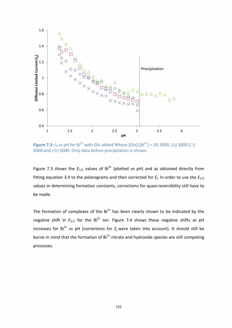
132
Figure 7.2: Id vs pH for Bi3+ with Gln added Where [Gln]:[Bi3+] = (X) 2000, () 3000 () 4000 and () 5000. Only data before precipitation is shown.
Figure 7.3 shows the E1/2 values of Bi3+ (plotted vs pH) and as obtained directly from
fitting equation 3.4 to the polarograms and then corrected for Ej. In order to use the E1/2
values in determining formation constants, corrections for quasi-reversibility still have to
be made.
The formation of complexes of the Bi3+ has been clearly shown to be indicated by the
negative shift in E1/2 for the Bi3+ ion. Figure 7.4 shows these negative shifts as pH
increases for Bi3+ vs pH (corrections for Ej were taken into account). It should still be
borne in mind that the formation of Bi3+ nitrate and hydroxide species are still competing
processes.
0.4
0.6
0.8
1
1.2
1.4
1.6
1 1.5 2 2.5 3 3.5 4
Dif
fusi
on
Lim
ite
d C
urr
en
t (I
d)
pH
Precipitation
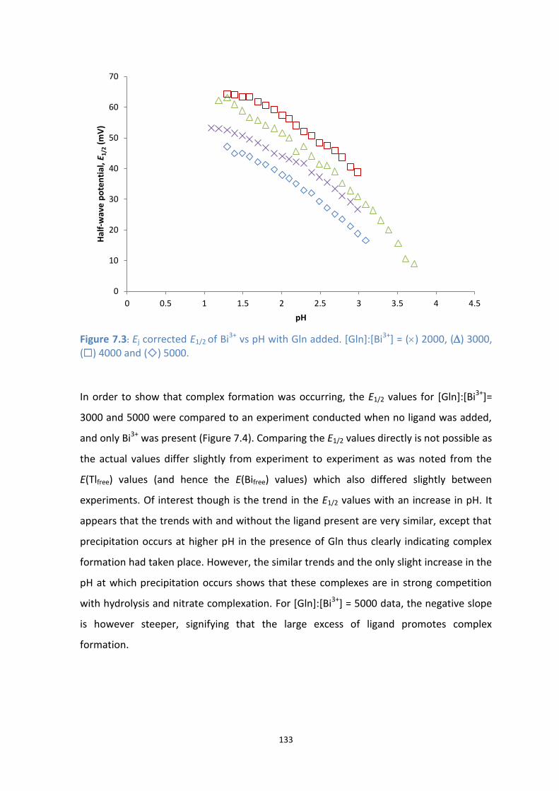
133
Figure 7.3: Ej corrected E1/2 of Bi3+ vs pH with Gln added. [Gln]:[Bi3+] = () 2000, () 3000, () 4000 and () 5000.
In order to show that complex formation was occurring, the E1/2 values for [Gln]:[Bi3+]=
3000 and 5000 were compared to an experiment conducted when no ligand was added,
and only Bi3+ was present (Figure 7.4). Comparing the E1/2 values directly is not possible as
the actual values differ slightly from experiment to experiment as was noted from the
E(Tlfree) values (and hence the E(Bifree) values) which also differed slightly between
experiments. Of interest though is the trend in the E1/2 values with an increase in pH. It
appears that the trends with and without the ligand present are very similar, except that
precipitation occurs at higher pH in the presence of Gln thus clearly indicating complex
formation had taken place. However, the similar trends and the only slight increase in the
pH at which precipitation occurs shows that these complexes are in strong competition
with hydrolysis and nitrate complexation. For [Gln]:[Bi3+] = 5000 data, the negative slope
is however steeper, signifying that the large excess of ligand promotes complex
formation.
0
10
20
30
40
50
60
70
0 0.5 1 1.5 2 2.5 3 3.5 4 4.5
Hal
f-w
ave
po
ten
tial
, E 1
/2 (
mV
)
pH
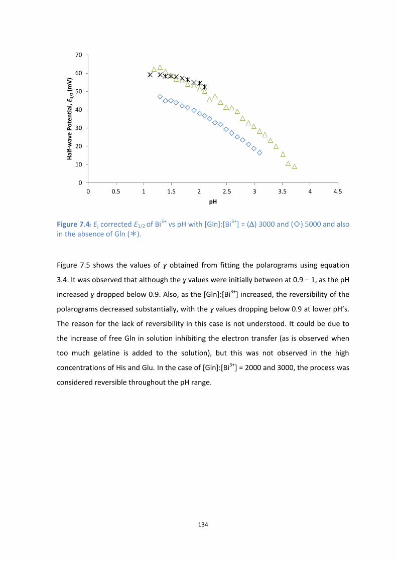
134
Figure 7.4: Ej corrected E1/2 of Bi3+ vs pH with [Gln]:[Bi3+] = () 3000 and () 5000 and also in the absence of Gln ().
Figure 7.5 shows the values of ɣ obtained from fitting the polarograms using equation
3.4. It was observed that although the ɣ values were initially between at 0.9 – 1, as the pH
increased ɣ dropped below 0.9. Also, as the [Gln]:[Bi3+] increased, the reversibility of the
polarograms decreased substantially, with the ɣ values dropping below 0.9 at lower pH’s.
The reason for the lack of reversibility in this case is not understood. It could be due to
the increase of free Gln in solution inhibiting the electron transfer (as is observed when
too much gelatine is added to the solution), but this was not observed in the high
concentrations of His and Glu. In the case of [Gln]:[Bi3+] = 2000 and 3000, the process was
considered reversible throughout the pH range.
0
10
20
30
40
50
60
70
0 0.5 1 1.5 2 2.5 3 3.5 4 4.5
Hal
f-w
ave
Po
ten
tial
, E1/
2 (m
V)
pH
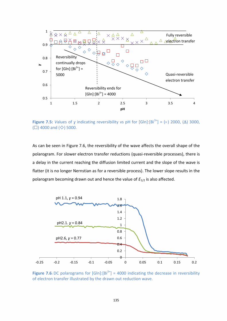
135
Figure 7.5: Values of ɣ indicating reversibility vs pH for [Gln]:[Bi3+] = () 2000, () 3000, () 4000 and () 5000.
As can be seen in Figure 7.6, the reversibility of the wave affects the overall shape of the
polarogram. For slower electron transfer reductions (quasi-reversible processes), there is
a delay in the current reaching the diffusion limited current and the slope of the wave is
flatter (it is no longer Nernstian as for a reversible process). The lower slope results in the
polarogram becoming drawn out and hence the value of E1/2 is also affected.
Figure 7.6: DC polarograms for [Gln]:[Bi3+] = 4000 indicating the decrease in reversibility of electron transfer illustrated by the drawn out reduction wave.
0.5
0.6
0.7
0.8
0.9
1
1 1.5 2 2.5 3 3.5 4
ɣ
pH
0
0.2
0.4
0.6
0.8
1
1.2
1.4
1.6
1.8
-0.25 -0.2 -0.15 -0.1 -0.05 0 0.05 0.1 0.15 0.2
pH 1.1, ɣ = 0.94
pH2.1. ɣ = 0.84
pH2.6, ɣ = 0.77
Fully reversible
electron transfer
Reversibility ends for
[Gln]:[Bi3+] = 4000
Reversibility
continually drops
for [Gln]:[Bi3+] =
5000 Quasi-reversible
electron transfer

136
As there is no other means of determining the complexing ability when quasi-reversible
waves are produced, a method to determine the reversible potentials from these waves
had to be used. A non-linear least squares fitting program called Precision Curve Fitter[12]
was used to fit a single polarographic wave at a time using a process that will be
described shortly.
One of the ways in which we were able to compensate for the change in reversibility of
the Bi-Gln complex was to fix the ɣ value to the reversible value of 1. This was done by
firstly fitting the Bi3+ polarogram using Precision Curve Fitter where all parameters (Id,
E1/2, ɣ and the capacitance current (a, b c, d) were solved for using equations 3.4 and 3.5.
Quasi-reversible electron transfer processes results in a delay of the current in reaching
the diffusion limited value, but value of Id is independent of the electron transfer kinetics.
As a result, the Id calculated initially using Precision Curve Fitter will remain the same and
can therefore be fixed. The capacitance current or background can also be fixed as no
electron transfer process is occurring at this point, therefore it will not be affected by the
quasi-reversibility. To force a reversible process, ɣ was fixed to 1 and the points along the
slope of the polarogram that deviated from the Nernstian behavior and lead to the drawn
out polarogram were deleted. The Precision Curve Fitter[12] allows the parameters
mentioned to be fixed and therefore the only parameter to be refined was E1/2. Figure 7.7
gives an example of how a quasi-reversible polarographic wave was fitted to obtain the
reversible E1/2 value.
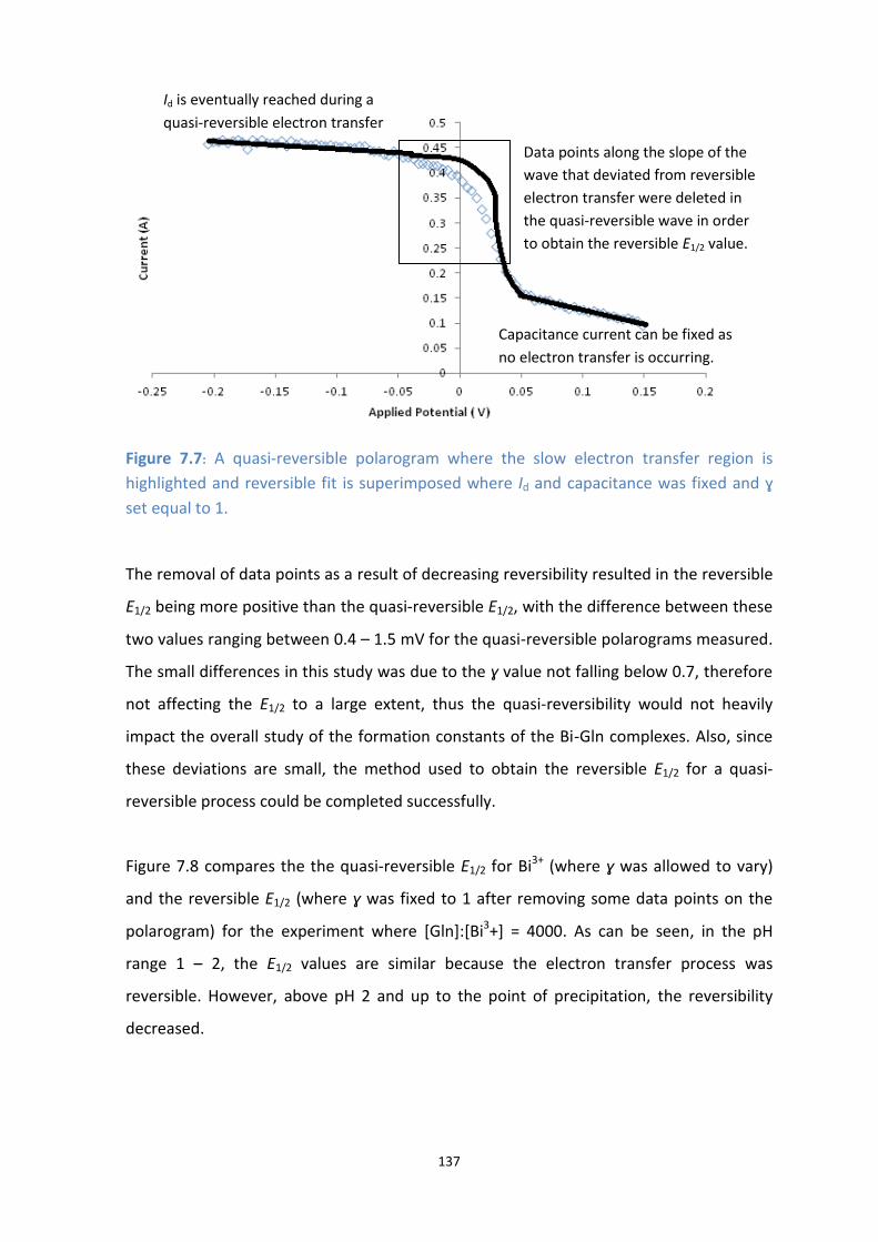
137
Figure 7.7: A quasi-reversible polarogram where the slow electron transfer region is
highlighted and reversible fit is superimposed where Id and capacitance was fixed and ɣ
set equal to 1.
The removal of data points as a result of decreasing reversibility resulted in the reversible
E1/2 being more positive than the quasi-reversible E1/2, with the difference between these
two values ranging between 0.4 – 1.5 mV for the quasi-reversible polarograms measured.
The small differences in this study was due to the ɣ value not falling below 0.7, therefore
not affecting the E1/2 to a large extent, thus the quasi-reversibility would not heavily
impact the overall study of the formation constants of the Bi-Gln complexes. Also, since
these deviations are small, the method used to obtain the reversible E1/2 for a quasi-
reversible process could be completed successfully.
Figure 7.8 compares the the quasi-reversible E1/2 for Bi3+ (where ɣ was allowed to vary)
and the reversible E1/2 (where ɣ was fixed to 1 after removing some data points on the
polarogram) for the experiment where [Gln]:[Bi3+] = 4000. As can be seen, in the pH
range 1 – 2, the E1/2 values are similar because the electron transfer process was
reversible. However, above pH 2 and up to the point of precipitation, the reversibility
decreased.
Data points along the slope of the
wave that deviated from reversible
electron transfer were deleted in
the quasi-reversible wave in order
to obtain the reversible E1/2 value.
Id is eventually reached during a
quasi-reversible electron transfer
Capacitance current can be fixed as
no electron transfer is occurring.

138
Figure 7.8: Graph showing that the () quasi-reversible E1/2 and () reversible E1/2 values for Bi3+ for [Gln]:[Bi3+] = 4000 do not differ greatly.
7.4.2 Slope analysis
Figure 7.9 indicates the dominant species of Gln in the system in various pH ranges. Gln
contains only two proton donor sites with pKa values of 2.14 and 8.94,[4] thus both sites
are mainly protonated below pH 2.14. Since precipitation occurs at pH ~3, it was
expected that only two dominant ligand species, Gln-H2 and Gln-H, could form. In the
studies with Glu and His (Chapters 5 and 6) we found that precipitation occurred at a pH
of approximately 4.5 and 3.5 respectively. These amino acids have a greater ability to
stabilise complex formation due to their extra donor site. Complexation with Gln could be
inhibited due to the lack of the additional binding site and due to minimal complex
formation we would expect precipitation to occur at a lower pH than Glu and His.
0
10
20
30
40
50
60
70
1.0 1.5 2.0 2.5 3.0
Hal
f-w
ave
Po
ten
tial
, E1/
2 (m
V)
pH
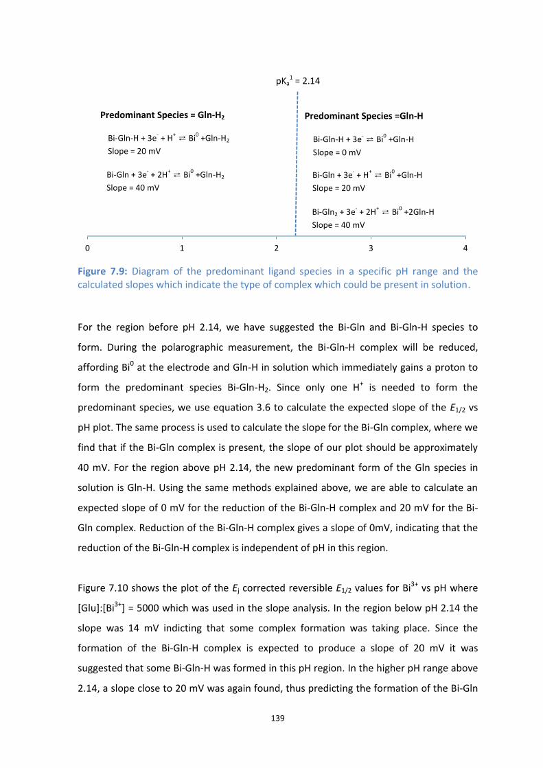
139
Figure 7.9: Diagram of the predominant ligand species in a specific pH range and the calculated slopes which indicate the type of complex which could be present in solution.
For the region before pH 2.14, we have suggested the Bi-Gln and Bi-Gln-H species to
form. During the polarographic measurement, the Bi-Gln-H complex will be reduced,
affording Bi0 at the electrode and Gln-H in solution which immediately gains a proton to
form the predominant species Bi-Gln-H2. Since only one H+ is needed to form the
predominant species, we use equation 3.6 to calculate the expected slope of the E1/2 vs
pH plot. The same process is used to calculate the slope for the Bi-Gln complex, where we
find that if the Bi-Gln complex is present, the slope of our plot should be approximately
40 mV. For the region above pH 2.14, the new predominant form of the Gln species in
solution is Gln-H. Using the same methods explained above, we are able to calculate an
expected slope of 0 mV for the reduction of the Bi-Gln-H complex and 20 mV for the Bi-
Gln complex. Reduction of the Bi-Gln-H complex gives a slope of 0mV, indicating that the
reduction of the Bi-Gln-H complex is independent of pH in this region.
Figure 7.10 shows the plot of the Ej corrected reversible E1/2 values for Bi3+ vs pH where
[Glu]:[Bi3+] = 5000 which was used in the slope analysis. In the region below pH 2.14 the
slope was 14 mV indicting that some complex formation was taking place. Since the
formation of the Bi-Gln-H complex is expected to produce a slope of 20 mV it was
suggested that some Bi-Gln-H was formed in this pH region. In the higher pH range above
2.14, a slope close to 20 mV was again found, thus predicting the formation of the Bi-Gln
0 1 2 3 4
Bi-Gln-H + 3e- + H
+ ⇄ Bi
0 +Gln-H2
Slope = 20 mV
Predominant Species = Gln-H2 Predominant Species =Gln-H
Bi-Gln + 3e- + 2H
+ ⇄ Bi
0 +Gln-H2
Slope = 40 mV
Bi-Gln-H + 3e- ⇄ Bi
0 +Gln-H
Slope = 0 mV
Bi-Gln + 3e- + H
+ ⇄ Bi
0 +Gln-H
Slope = 20 mV
Bi-Gln2 + 3e- + 2H
+ ⇄ Bi
0 +2Gln-H
Slope = 40 mV
pKa1 = 2.14

140
complex. The Bi-Gln-H complex formation in this region is considered to be independent
of pH due to the reduction of the complex resulting in the formation the predominant
ligand species in solution, Gln-H at this pH, along with Bi0.
The complex formation studies between Bi3+ and Glu (Chapter 5) and His (Chapter 6)
showed similarities with Gln in that all three results showed the formation of a
protonated Bi3+-amino acid complexes at low pH. Whereas Bi-Glu-H2 and Bi-His-H2 were
found in the pH range 1 to approximately 2, Bi-Gln-H was instead found. This is due to Gln
only having two protonation sites and the amide group does not really take part in
complexation.
Figure 7.10: Slope analysis of the Ej corrected reversible E1/2 of Bi3+ where [Glu]:[Bi3+] = 5000 which indicates the formation of two types of complexes, Bi-Gln-H and Bi-Gln.
Slope analysis allows us to predict the species which could possibly be forming in solution
in different pH ranges during the pH-polarographic titration.[13] The predicted species can
then be included in the 3D-CFC programme[9] to see if it fits the experimental data and to
refine the respective formation constants.
y = -13.852x + 64.513 R² = 0.9794
y = -21.966x + 82.605 R² = 0.9988
0
5
10
15
20
25
30
35
40
45
50
0 0.5 1 1.5 2 2.5 3 3.5 4
Hal
f-w
ave
Po
ten
tial
, E1
/2 (
mV
)
pH
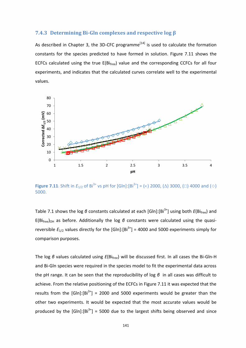
141
7.4.3 Determining Bi-Gln complexes and respective log β
As described in Chapter 3, the 3D-CFC programme[14] is used to calculate the formation
constants for the species predicted to have formed in solution. Figure 7.11 shows the
ECFCs calculated using the true E(Bifree) value and the corresponding CCFCs for all four
experiments, and indicates that the calculated curves correlate well to the experimental
values.
Figure 7.11: Shift in E1/2 of Bi3+ vs pH for [Gln]:[Bi3+] = () 2000, () 3000, () 4000 and () 5000.
Table 7.1 shows the log β constants calculated at each [Gln]:[Bi3+] using both E(Bifree) and
E(Bifree)OH as before. Additionally the log β constants were calculated using the quasi-
reversible E1/2 values directly for the [Gln]:[Bi3+] = 4000 and 5000 experiments simply for
comparison purposes.
The log β values calculated using E(Bifree) will be discussed first. In all cases the Bi-Gln-H
and Bi-Gln species were required in the species model to fit the experimental data across
the pH range. It can be seen that the reproducibility of log β in all cases was difficult to
achieve. From the relative positioning of the ECFCs in Figure 7.11 it was expected that the
results from the [Gln]:[Bi3+] = 2000 and 5000 experiments would be greater than the
other two experiments. It would be expected that the most accurate values would be
produced by the [Gln]:[Bi3+] = 5000 due to the largest shifts being observed and since
0
10
20
30
40
50
60
70
80
1 1.5 2 2.5 3 3.5 4
Co
rre
cte
d Δ
E 1/2
(m
V)
pH
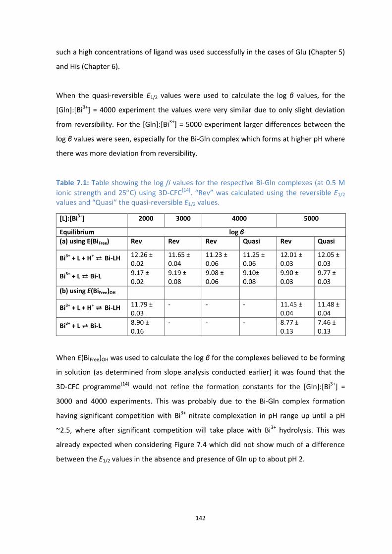
142
such a high concentrations of ligand was used successfully in the cases of Glu (Chapter 5)
and His (Chapter 6).
When the quasi-reversible E1/2 values were used to calculate the log β values, for the
[Gln]:[Bi3+] = 4000 experiment the values were very similar due to only slight deviation
from reversibility. For the [Gln]:[Bi3+] = 5000 experiment larger differences between the
log β values were seen, especially for the Bi-Gln complex which forms at higher pH where
there was more deviation from reversibility.
Table 7.1: Table showing the log values for the respective Bi-Gln complexes (at 0.5 M
ionic strength and 25C) using 3D-CFC[14]. “Rev” was calculated using the reversible E1/2 values and “Quasi” the quasi-reversible E1/2 values.
[L]:[Bi3+] 2000 3000 4000 5000
Equilibrium log β
(a) using E(BiFree) Rev Rev Rev Quasi Rev Quasi
Bi3+ + L + H+ ⇄ Bi-LH 12.26 ± 0.02
11.65 ± 0.04
11.23 ± 0.06
11.25 ± 0.06
12.01 ± 0.03
12.05 ± 0.03
Bi3+ + L ⇄ Bi-L 9.17 ± 0.02
9.19 ± 0.08
9.08 ± 0.06
9.10± 0.08
9.90 ± 0.03
9.77 ± 0.03
(b) using E(BiFree)OH
Bi3+ + L + H+ ⇄ Bi-LH 11.79 ± 0.03
- - - 11.45 ± 0.04
11.48 ± 0.04
Bi3+ + L ⇄ Bi-L 8.90 ± 0.16
- - - 8.77 ± 0.13
7.46 ± 0.13
When E(BiFree)OH was used to calculate the log β for the complexes believed to be forming
in solution (as determined from slope analysis conducted earlier) it was found that the
3D-CFC programme[14] would not refine the formation constants for the [Gln]:[Bi3+] =
3000 and 4000 experiments. This was probably due to the Bi-Gln complex formation
having significant competition with Bi3+ nitrate complexation in pH range up until a pH
~2.5, where after significant competition will take place with Bi3+ hydrolysis. This was
already expected when considering Figure 7.4 which did not show much of a difference
between the E1/2 values in the absence and presence of Gln up to about pH 2.

143
Interestingly, log β values could be calculate for both the [Gln]:[Bi3+] = 2000 and 5000
data when using E(BiFree)OH. Figure 7.12 shows the ECFCs (calculated using E(BiFree)OH) and
CCFCs used to calculate the log β values for [Gln]:[Bi3+]= 2000 and 5000. The shifts in E1/2
are greater for [Gln]:[Bi3+] = 5000 compared to that of 2000, showing a greater extent of
complex formation when [Gln]:[Bi3+] = 5000. It is thus expected that the values for
[Gln]:[Bi3+] = 5000 would produce more accurate results
Figure 7.12: The ECFCs (points) (calculated using the true E(Bifree)OH and the
corresponding CCFCs (lines) for [Gln]:[Bi3+] = () 2000 and () 5000.
Figure 7.13 shows the species distribution diagram for [Gln]:[Bi3+] = (a) 3000 and (b) 5000.
The log β values used for the Bi3+-Gln complexes are those in Table 7.1 when using the
true E(Bifree) and reversible E1/2 values. For [Gln]:[Bi3+] = 3000 the Bi-Gln-H complex begins
to form at slightly lower pH than Bi(OH)2+, but is shown to always be present in solution
together with the Bi3+ nitrate species and Bi(OH) and is never really dominant in solution
at any pH. The formation of the Bi(OH)2+ also completely swamps the Bi-Gln complex
which is only able to reach approximately 20% (and only begins to form at pH ~1). It is
therefore not surprising that the log β values could not be refined for this data set when
using the E(Bifree)OH value. When the log β values for [Gln]:[Bi3+] = 5000 was used and with
the larger excess of ligand, the formation of the Bi-Gln-H complex (~50%) and the Bi-Gln
complex (70%) occurred to a much greater extent, again indicating the benefit of using
0
10
20
30
40
50
60
1 1.5 2 2.5 3 3.5
Co
rre
cte
d Δ
E1/2
(m
V)
pH

144
high [Gln]:[Bi3+]. The species distribution diagram again indicate that the log β value for
Bi-Gln-H calculate using the E(Bifree)OH value and that for Bi-Gln calculate using the true
E(Bifree) value would give the most representative results.
Figure 7.13: Species distribution diagrams for [Gln]:[Bi3+] = (a) 3000 and (b) 5000, where log β values were calculated using the true E(BiFree) as given in Table 7.1.
Although literature on Bi-Gln complexes is extremely limited, formation constants of 9.81
and 17.25 were determined for the ML and ML2 species for Bi-Gln complexes,
respectively.[15] These studies were conducted in perchlorate solutions and began above
0
10
20
30
40
50
60
70
80
90
100
0 1 2 3 4 5 6
% S
pe
cie
s p
rese
nt
pH
0
10
20
30
40
50
60
70
80
90
100
0 1 2 3 4 5 6
% S
pe
cie
s p
rese
nt
pH
Bi3+
Bi-Gln-H
Bi-Gln
Bi(NO3)x Bi(OH)3
Bi(OH)
Bi3+
Bi(OH)2
Bi9(OH)22
Bi(NO3)x Bi-Gln-H
Bi(OH)
Bi-Gln
Bi(OH)2
Bi9(OH)22
Bi(OH)3
(b)
(a)
Precipitation
Precipitation
145
pH 2. It was interesting to note that the log β of 9.90 ± 0.03 for the Bi-Gln complex where
[Gln]:[Bi3+] = 5000 calculated using the true E(Bifree) and which has been indicated as the
value for which we consider to have the greatest confidence in, compared to that in
literature. No Bi-Gln-H complex was reported in literature as these studies were stared
above pH 2. An additional experiment should be run at around [Gln]:[Bi3+] = 7000 to allow
the determination of more accurate log β values as the higher [Gln]:[Bi3+] results in
complex formation to a greater extent.
Studies[8] involving the complexation of Gln with a variety of other metal ions have been
done, however as described by Berthon[8], the comparison to each other is difficult due to
studies being conducted under completely different experimental conditions. For Pb2+, a
metal ion which is isoelectronic with Bi3+, the complexation with Gln has been performed
in two different media, and the study in the NaNO3 electrolyte gave information about
Pb-(Gln)-OH2,[8, 16] and the study in the NaClO4 electrolyte gave information about Pb-Gln,
Pb-(Gln)2 and Pb-(Gln)3 complexes. The NIST[4] database unfortunately does not contain
formation constants for Ga3+ with glutamine, however, recent studies conducted by
Sharma[17] did produce results when working in 0.1 M KNO3 solutions. They showed that
the complexes formed were Ga-Glu, Ga-Glu2 and Ga-Glu3 with stability constants of 1.35,
6.5 and what is assumed to be 13.50 (quoted as 1.350 in the publication but which
cannot be correct), respectively at 30⁰C. The polarographic waves in this study also
showed non-reversibility, as was seen in our studies with [Gln]:[Bi3+] > 3000. It is not sure
how accurate these values are because when using their experimental conditions ([Ga3+]
= 1 mM, [Gln]:[Ga3+] = 10 – 30 and solution pH = 3.5) to plot a species distribution
diagram, it was indicated that no complexation with Gln occurred and precipitation took
place before pH 3.5.
7.5 Conclusion
The complexation between Bi3+ and Gln, although difficult to achieve in nitrate solutions,
produced two complexation products, Bi-Gln-H and Bi-Gln. This however requires large
[Gln]:[Bi3+] ratios.
146
The complexation of Gln with Bi3+ has shown that when polarographic techniques are
used, the transfer of electrons tends to be quasi-reversible as [Gln]:[Bi3+] increases
(>3000). Since fully reversible waves are required for the calculation of log β values, the
reversible E1/2 values had to first be determined from the quasi-reversible waves.
However, the differences between the two E1/2 values were not great due to only small
deviations from reversibility indicated by ɣ values not dropping below about 0.7.
Gln complexation with Bi3+ appears to need a large [Gln]:[Bi3+] ratio in order for
complexation sufficient to occur and to override competition with the formation of
hydroxide and nitrates. This was only really seen where [Gln]:[Bi3+] = 5000 and further
experiments should be run at ratios higher than this. Thus as shown in Table 7.1, the
reproducibility of the log β was not ideal due to insufficient complex formation at the
lower [Gln]:[Bi3+] ratios. However, the quasi-reversibility would increase with further
addition of Gln in solution and possibly even result in irreversible electron transfer taking
place.
Although the results presented in this study do differ, it must be taken into account that
Berthon[8] has described the complexation of Gln with metal ions as being tentative at
best, with only a few metal complexes, such as Cu2+ (Cu-Gln and Cu-Gln2),[18] being
recommended as a true representation of the complex formation. The intricate chemistry
which governs the formation of Gln complexes with metal ions is still in the process of
being understood. In future the actual Bi3+-Gln complexes formed in solution could be
investigated using electrospray ionisation-mass spectrometry.
147
7. 6 References [1] a) J. T. Brosnan, J. Nutr.,2013, 133, 2068; b) W. J. Lee, R. A. Hawkins, J. R. Vina and D. R.
Peterson, Am. J. Phys.,1998, 274, 1101.
[2] R. Minet, F. Villie, M. Marcollet, D. Meynial-Denis and L. Cynober, Clinica. Chimica. Acta.,1997,
268, 121.
[3] C. K. Mathews, K. E. van Holde and K. Ahern, Biochemistry, Addison Wesley Publishing
Company, New York, 2002.
[4] A. E. Martell and R. M. Smith, NIST Standard Reference Database 46 Version 8.0, NIST Critically
Selected Stability Constants of Metal Complexes,USA, 2004
[5] a) A. C. Baxter and D. R. Williams, J. Chem. Soc. Dalton Trans.,1974, 1117; b) P. Newsholme, M.
M. R. Lima, T. C. Pithon and R. B. Bazottes, Braz. J. Med. Biol. Res.,2011, 36, 153.
[6] a) C. M. Noyer, D. Simon, D. Borczuk, A. Branst, M. J. Lee and V. Nehra, Am. J.
Gastroenterol.,1998, 93, 972; b) K. J. Shabert, C. Winslow, J. M. Lacey and D. W. Wilmore,
Nutrition,1999, 11, 860; c) C. Kulkarni, K. S. Kulkarni and B. R. Hamsa, Indian. J. Pharmacol.,2005,
36, 148.
[7] Y. Xiayo, C. Bi, Y. Fan, C. Cui, X. Zang and D. Q. Ping, Int. J. Oncol.,2008, 33.
[8] G. Berthon, Pure. Appl. Chem.,1995, 67.
[9] R. B. Martin, 'Metal Ions in Biological Systems', 20, M. Dekker, 1986, 21
[10] A. Gergely, I. Nagypal and E. Farkas, J. Inorg. Nucl. Chem.,1975, 37, 551.
[11] J.H. Ritsma, G. A. Wiegers and F. Jellinek, Recl. Truv. Chim. ,1965, 84, 1577.
[12] G. Brink, Precision Curve Fitter, University of the Witwatersrand, 1995, (unpublished)
[13] I. Cukrowski, Electroanal.,1997, 9, 699.
[14] P. Franklyn and I. Cukrowski, 3D-CFC software, University of the Witwatersrand, 2003,
Windows Version 1.2, (unpublished)
[15] M. K. Singh and M. N. Srivastava, J. Inorg. Nucl. Chem.,1972, 34, 2067.
[16] a) T. T. Lai and M. C. Chen, Talanta,1969, 16, 544; b) A.M. Corrie, M. L. D. Touche and D. R.
Williams, J. Am. Chem. Soc.,1973, 2561.
[17] V. Sharma and K. D. Gupta, Monat. Fur. Chem.,2011, 142, 481.
[18] a) A. Kayali and G. Berthon, Polyhedron,1982, 1, 371; b) A. Cole, C. Furnival, Z. X. Huang, D.
Ceri Jones, P. M. May, G. L. Smith, J. Whittaker and D. R. Williams, Inorg. Chim. Acta.,1965, 108,
165.
148
Chapter 8: Final Conclusion
The procedures developed using the NOVA software (as discussed in Chapter 2) allowed
for the automation of the entire polarographic-pH titration method and proved to be a
major success. Initial development of the software showed some limitations in the
NOVA[1] software when carrying out the many functions needed for the polarographic
studies completed in this work. However, with the support from EcoChemie (the
suppliers of NOVA[1]) who wrote new commands that were needed, the development of
the automated procedures began taking shape. Validation of the NOVA procedures for
GE calibrations and polarographic studies were carried out as described in Chapter 4.
Once the methodology was robust and reproducible, the amino acid complexation
studies with Bi3+ were initiated. The NOVA[1] software replaced the older LABVIEW[2]
software which was previously used and more costly to develop further. Due to its
successful use in monitoring complex formation in this study, it can be a concluded that
the NOVA[1] software will be used in many other polarographic-pH titrations and the
backbone of the procedures developed can be used to extend this application to
incorporate other electrochemical measurements.
The study of Bi3+ and its complexing ability by different ligands is not straight-forward.
Previous work[3] had shown that precipitation of Bi3+ occurs due to the formation of Bi-
hydroxy-nitrate complexes and this happened around pH 2-2.5 under the conditions used
in this work. The first major breakthrough to the success of this study was the realization
that previous work using relatively low [ligand]:[metal] (of around 100-200) would not
suffice when investigating complexation of Bi3+ with amino acids. Le Chateliers’ principle
provided the answer to ensuring that Bi3+ complexation with amino acids could be
achieved. By increasing [ligand]:[metal] to magnitudes of greater than 2000, Bi3+
remained soluble to higher pHs due to complexation taking place with the amino acid
ligands (as shown in Chapters 5-7).

149
The use of polarography, and by extension the pH titration associated with increasing the
pH of the solution to promote complex formation, proved to be successful in these
studies. Table 8.1 summarises the results and is given in terms of log K values for complex
formation between Bi3+ and the amino acid in the given protonated form, rather than in
terms of log β values as quoted in each chapter. These clearly show the small extent of
complex formation with the protonated forms of the ligand. This implies that there
certainly are Bi3+ nitrate species present below pH 2 and that the stability constants
calculated using the E(Bifree)OH values would give more accurate results. For the Bi-L
species which form at higher pH, the stability constants calculated using the true E(Bifree)
values would provide the more accurate results. Due to the strong competition between
nitrate and amino acid species at low pH, it highlights the importance of developing
software that takes competition with nitrates into account, something the 3D-CFC
software[4] does not do.
Table 8.1: Log K values for the formation of Bi3+amino acid complexes in solution at 25 ⁰C and µ = 0.5 M (KNO3). The values in italics indicate which constants give the more
representative values for the particular species when using the two E(BiFree) values in the
calculations.
Ligand (L) Glu His Gln
Equilibrium log K
(a) using E(BiFree)
Bi3+ + LH2 ⇄ Bi-LH2 3.4 2.7
Bi3+ + LH+ ⇄ Bi-LH 5.3 7.0 3.1
Bi3+ + L ⇄ Bi-L 12.3 12.5 9.8
(b) using E(BiFree)OH
Bi3+ + LH2 ⇄ Bi-LH2 2.6 2.0
Bi3+ + LH+ ⇄ Bi-LH 4.7 6.2 2.5
Bi3+ + L ⇄ Bi-L 11.6 10.6 7.5
From the results in Table 8.1, the complexing ability of Glu and His was fairly comparable
with the Bi-L-H2 complex being more stable with Glu and the Bi-L-H complex being more
150
stable with His. The stability of the Bi-L complexes was comparable. The addition of a
large excess of His in particular (as compared to Bi3+ concentration) lead to a significant
increase in the pH of the initial solution. For future work the pH should be adjusted to
about pH ~1 before the titration experiment in initiated to obtain data across a wider pH
range.
The study with Gln was interesting in itself since, by maintaining a high [ligand]:[metal]
ratio (>3000), the polarographic reduction waves became quasi-reversible. The reversible
E1/2 values had to be obtained from these quasi-reversible waves before the data could
be used to determine stability constants. The difference between the reversible and
quasi-reversible E1/2 values was at most 1.5 mV since values of ɣ only went down to about
0.7. Only the Bi-L-H and Bi-L complexes were formed with Gln and their stability was
significantly lower than that for Glu and His.
One of the most interesting observations in this study is the similarity in both the types of
species formed and the actual formation constants between Ga3+ and Bi3+ with Glu and
His.[5] Unfortunately the NIST database[6] did not contain information about Ga3+ with
glutamine, and those found in literature did not appear to be reliable[7]. The fact that Ga3+
also readily hydrolyses and precipitates from solution at fairly low pH confirms what we
have found in our studies with Bi3+.
This study has shown that Bi3+ can be complexed by Glu, His and Gln, all amino acids
which are integral building blocks for proteins, provided the amino acid is in large excess.
However, to extrapolate these results to predict how Bi3+ could behave in the body would
be premature. Proteins are large molecules with a unique chemistry, however, by
isolating its building blocks (i.e. amino acids), an insight of how Bi3+ could interact in the
body was achieved. This could prove extremely beneficial in the design of new and
effective bismuth drugs, which could potentially increase the efficacy of its action.
151
8.1 References
[1] Metrohm-Autolab, NOVA, 2012, (Utrecht, Netherlands)
[2] Chance E, Vipin V, Wesley Z and H. Richard, J. Lab. Auto.,2007, 12, 17.
[3] M. V.A. and T. G. Spiro, J. Am. Chem. Soc.,1966, 88, 1410.
[4] P. Franklyn and I. Cukrowski, 3D-CFC software, University of the Witwatersrand, 2003,
Windows Version 1.2, (unpublished)
[5] a) P. Bianco, J. Haladjian and R. Pilard, J. Chim. Phys.,1973, 73, 280; b) P. Bianco, J. Haladjian
and R. Pilard, J. Less-Common Met.,1978, 58, 58; c) E. A. Zekharova and V. N. Kumok, J. Gen.
Chem.,1968, 38, 1868.
[6] A. E. Martell and R. M. Smith, NIST Standard Reference Database 46 Version 8.0, NIST Critically
Selected Stability Constants of Metal Complexes,USA, 2004
[7] V. Sharma and K. D. Gupta, Monat. Fur. Chem.,2011, 142, 481.
152
Appendices
Appendices
Appendix 1
Supplementary information for Chapter 3 –PXRD 153
Appendix 2
Supplementary information for Chapter 5 155
Appendix 3
Supplementary information for Chapter 6 157

153
Appendix 1
Supplementary information for Chapter 3 –PXRD
Table A 1.1: Experimental parameters used in NOVA for the polarographic- pH titrations.
Potentiometric Parameters
Initial pause 20 s
Sample rate 2 s
Dose 0.300 mL up to pH 2.3, thereafter 0.025 mL
pH step 0.1
Polarographic Parameters
Purge 400 s
Initial potential 0.180 V
Final potential 0.700 V
Step potential -4 mV
Interval time (drop life) 1 s
Rest time 5 s
Stop Condition
Stop pH 8
Table A 1.2: Initial parameter estimates for the fitting of Bi3+ and Tl+ DC polarograms
Parameters Estimates for Bi3+ Estimates for Tl+
Id 1.5 x 10⁻⁸A 4.5 x 10⁻⁸A
E1/2 0.05 V -0.45 V
ɣ 1 1
a 1 1
b 1 1
c -0.001 0.001
d 1 -1
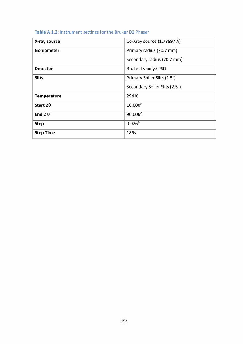
154
Table A 1.3: Instrument settings for the Bruker D2 Phaser
X-ray source Co-Xray source (1.78897 Å)
Goniometer Primary radius (70.7 mm)
Secondary radius (70.7 mm)
Detector Bruker Lynxeye PSD
Slits Primary Soller Slits (2.5°)
Secondary Soller Slits (2.5°)
Temperature 294 K
Start 2θ 10.000⁰
End 2 θ 90.006⁰
Step 0.026⁰
Step Time 185s

155
Appendix 2
Supplementary information for Chapter 5
Pb2+ is isoelectronic with Bi3+. The complexation of Pb2+ with amino acids thus had the
potential to show comparisons to Bi3+. Bi3+ also has the ability to form hydroxide products
from pH as pH ~2. The Pb2+ hydroxide log β were thus used to compare Bi3+ and Pb2+
complexation with Glu.
Table A2.1: Pb hydroxide species log β for species distribution diagrams plotted in
Chapter 5 as a comparison to Bi3+-Glu.[1]
Pb-hydroxide
species Log β
Pb OH 6.3
Pb (OH)2 10.9
Pb (OH)3 13.7
Pb2 (OH) 7.7
Pb3 (OH)4 34
Pb4 (OH)4 37.6
Pb6(OH)8 71.5
Ga3+ has been shown to exhibit complex formation with Glu and His with log β values
which are comparable (see Chapter 5 and Chapter 6). Table A2.2 shows the Ga3+ -
hydroxide complexes which are found to be in solution and the subsequent species
distribution diagram plotted with Glu as the ligand, where [Glu]:[Ga3+] = 100 and 5000. It
is interesting to note that species are able to form at low [Glu]:[Ga3+], whereas our study
has shown that a large excess in ligand is required in order to achieve complex formation.
More interestingly, is the formation of the Ga-Glu-H2 complex at both [Glu]:[Ga3+],
indicating that it is indeed a complex which could be forming.
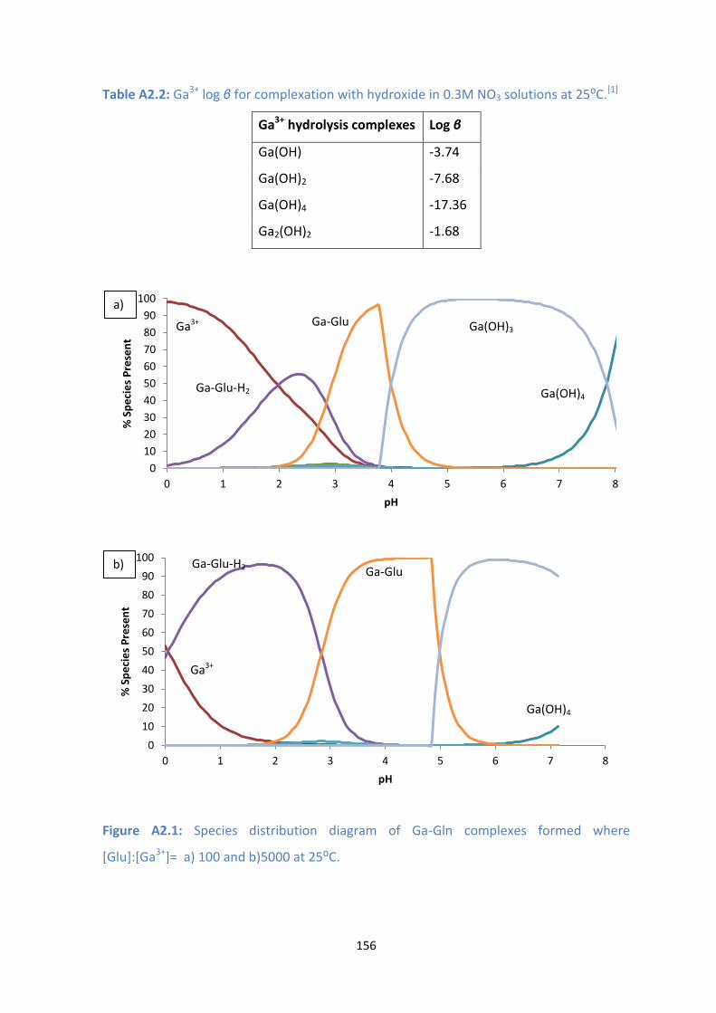
156
Table A2.2: Ga3+ log β for complexation with hydroxide in 0.3M NO3 solutions at 25⁰C.[1]
Ga3+ hydrolysis complexes Log β
Ga(OH) -3.74
Ga(OH)2 -7.68
Ga(OH)4 -17.36
Ga2(OH)2 -1.68
Figure A2.1: Species distribution diagram of Ga-Gln complexes formed where
[Glu]:[Ga3+]= a) 100 and b)5000 at 25⁰C.
0
10
20
30
40
50
60
70
80
90
100
0 1 2 3 4 5 6 7 8
% S
pe
cie
s P
rese
nt
pH
0
10
20
30
40
50
60
70
80
90
100
0 1 2 3 4 5 6 7 8
% S
pe
cie
s P
rese
nt
pH
Ga-Glu-H2
Ga-Glu
Ga(OH)4
Ga(OH)4
Ga(OH)3
Ga-Glu-H2 Ga-Glu
Ga3+
Ga3+
a)
b)

157
Appendix 3
Supplementary information for Chapter 6
Figure A3.1: Species distribution diagram of Ga-His complexes formed where [Glu]:[Ga3+] = a) 100 and b)5000 at 3.0 M NO3 at 25⁰C
Species distribution diagram of Ga3+ with His at [His]:[Ga3+] = 100 and 5000. It can be
seen that the formation of Ga-His-H2, Ga-His-H and Ga-His are formed in high
percentages, a possible reason as to why the three complexes were found in literature.
0
10
20
30
40
50
60
70
80
90
100
0 1 2 3 4 5 6 7 8
% S
pe
cie
s P
rese
nt
pH
0
10
20
30
40
50
60
70
80
90
100
0 1 2 3 4 5 6 7 8
% S
pe
cie
s P
rese
nt
pH
Ga-His-H2
Ga-His-H
Ga-His
Ga(OH)3
Ga(OH)4
Ga-His-H2
Ga-His-H
Ga-His Ga(OH)3
Ga(OH)4
Ga3+
Ga3+
a)
b)

158
References [1] A. E. Martell and R. M. Smith, NIST Standard Reference Database 46 Version 8.0, NIST
Critically Selected Stability Constants of Metal Complexes,USA, 2004
Related Documents