Study Notes of “Introduction to MATRIX ALGEBRA” (Autar K. Kaw, 2002) Yin Zhao [email protected] Update on November 30, 2014 Introduction This document is the study notes of “Introductionto MATRIX ALGEBRA” which was written by Autar K. Kaw, University of South Florida. The free printable PDF format textbook can be downloaded via the following link: http://mathforcollege.com/ma/textbook/index.html. Contents 1 Introduction 3 1.1 Summary .................................. 3 1.2 Selected Problems ............................ 6 2 Vectors 9 2.1 Summary .................................. 9 2.2 Selected Problems ............................ 11 3 Binary Matrix Operations 15 3.1 Summary .................................. 15 3.2 Selected Problems ............................ 17 4 Unary Matrix Operations 22 4.1 Summary .................................. 22 4.2 Selected Problems ............................ 24 5 System of Equations 30 5.1 Summary .................................. 30 5.2 Selected Problems ............................ 32 1

Welcome message from author
This document is posted to help you gain knowledge. Please leave a comment to let me know what you think about it! Share it to your friends and learn new things together.
Transcript
Study Notes of“Introduction to MATRIX ALGEBRA”
(Autar K. Kaw, 2002)
Update on November 30, 2014
Introduction
This document is the study notes of “Introduction to MATRIX ALGEBRA”which was written by Autar K. Kaw, University of South Florida. The freeprintable PDF format textbook can be downloaded via the following link:http://mathforcollege.com/ma/textbook/index.html.
Contents
1 Introduction 31.1 Summary . . . . . . . . . . . . . . . . . . . . . . . . . . . . . . . . . . 31.2 Selected Problems . . . . . . . . . . . . . . . . . . . . . . . . . . . . 6
2 Vectors 92.1 Summary . . . . . . . . . . . . . . . . . . . . . . . . . . . . . . . . . . 92.2 Selected Problems . . . . . . . . . . . . . . . . . . . . . . . . . . . . 11
3 Binary Matrix Operations 153.1 Summary . . . . . . . . . . . . . . . . . . . . . . . . . . . . . . . . . . 153.2 Selected Problems . . . . . . . . . . . . . . . . . . . . . . . . . . . . 17
4 Unary Matrix Operations 224.1 Summary . . . . . . . . . . . . . . . . . . . . . . . . . . . . . . . . . . 224.2 Selected Problems . . . . . . . . . . . . . . . . . . . . . . . . . . . . 24
5 System of Equations 305.1 Summary . . . . . . . . . . . . . . . . . . . . . . . . . . . . . . . . . . 305.2 Selected Problems . . . . . . . . . . . . . . . . . . . . . . . . . . . . 32
1
6 Gaussian Elimination 436.1 Summary . . . . . . . . . . . . . . . . . . . . . . . . . . . . . . . . . . 436.2 Selected Problems . . . . . . . . . . . . . . . . . . . . . . . . . . . . 43
7 LU Decomposition 467.1 Summary . . . . . . . . . . . . . . . . . . . . . . . . . . . . . . . . . . 467.2 Selected Problems . . . . . . . . . . . . . . . . . . . . . . . . . . . . 48
8 Gauss-Seidel Method 518.1 Summary . . . . . . . . . . . . . . . . . . . . . . . . . . . . . . . . . . 518.2 Selected Problems . . . . . . . . . . . . . . . . . . . . . . . . . . . . 56
9 Adequacy of Solutions 599.1 Summary . . . . . . . . . . . . . . . . . . . . . . . . . . . . . . . . . . 599.2 Selected Problems . . . . . . . . . . . . . . . . . . . . . . . . . . . . 64
10 Eigenvalues and Eigenvectors 7010.1 Summary . . . . . . . . . . . . . . . . . . . . . . . . . . . . . . . . . . 7010.2 Selected Problems . . . . . . . . . . . . . . . . . . . . . . . . . . . . 75
2
1 Introduction
1.1 Summary
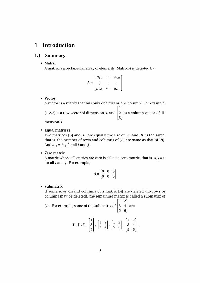
• MatrixA matrix is a rectangular array of elements. Matrix A is denoted by
A =
a11 · · · a1n...
......
am1 · · · amn
• Vector
A vector is a matrix that has only one row or one column. For example,
[1,2,3] is a row vector of dimension 3, and
123
is a column vector of di-
mension 3.
• Equal matricesTwo matrices [A] and [B ] are equal if the size of [A] and [B ] is the same,that is, the number of rows and columns of [A] are same as that of [B ].And ai j = bi j for all i and j .
• Zero matrixA matrix whose all entries are zero is called a zero matrix, that is, ai j = 0for all i and j . For example,
A =[
0 0 00 0 0
]
• SubmatrixIf some rows or/and columns of a matrix [A] are deleted (no rows orcolumns may be deleted), the remaining matrix is called a submatrix of
[A]. For example, some of the submatrix of
1 23 45 6
are
[1], [1,2],
135
,
[1 23 4
],
[1 25 6
],
1 23 45 6
.
3
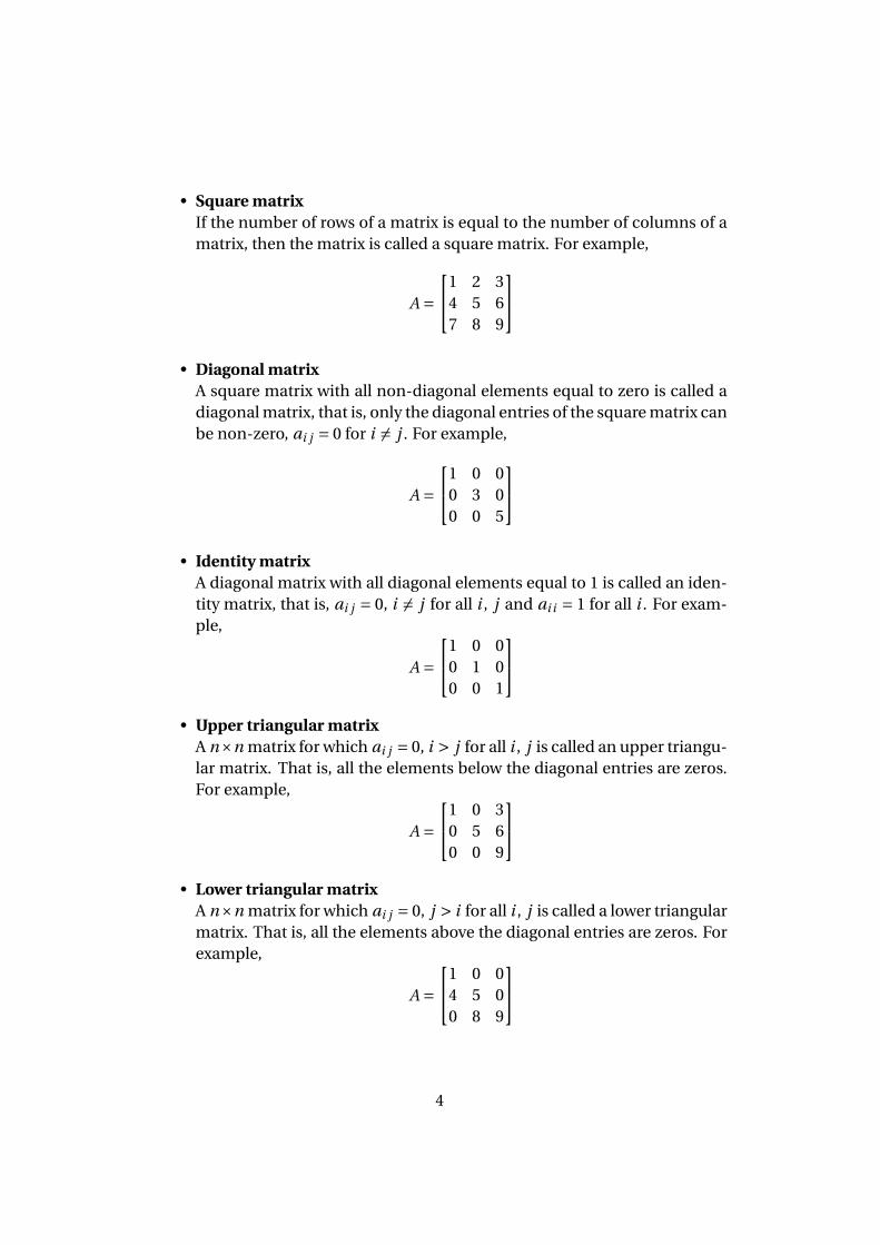
• Square matrixIf the number of rows of a matrix is equal to the number of columns of amatrix, then the matrix is called a square matrix. For example,
A =1 2 3
4 5 67 8 9
• Diagonal matrix
A square matrix with all non-diagonal elements equal to zero is called adiagonal matrix, that is, only the diagonal entries of the square matrix canbe non-zero, ai j = 0 for i 6= j . For example,
A =1 0 0
0 3 00 0 5
• Identity matrix
A diagonal matrix with all diagonal elements equal to 1 is called an iden-tity matrix, that is, ai j = 0, i 6= j for all i , j and ai i = 1 for all i . For exam-ple,
A =1 0 0
0 1 00 0 1
• Upper triangular matrix
A n×n matrix for which ai j = 0, i > j for all i , j is called an upper triangu-lar matrix. That is, all the elements below the diagonal entries are zeros.For example,
A =1 0 3
0 5 60 0 9
• Lower triangular matrix
A n×n matrix for which ai j = 0, j > i for all i , j is called a lower triangularmatrix. That is, all the elements above the diagonal entries are zeros. Forexample,
A =1 0 0
4 5 00 8 9
4
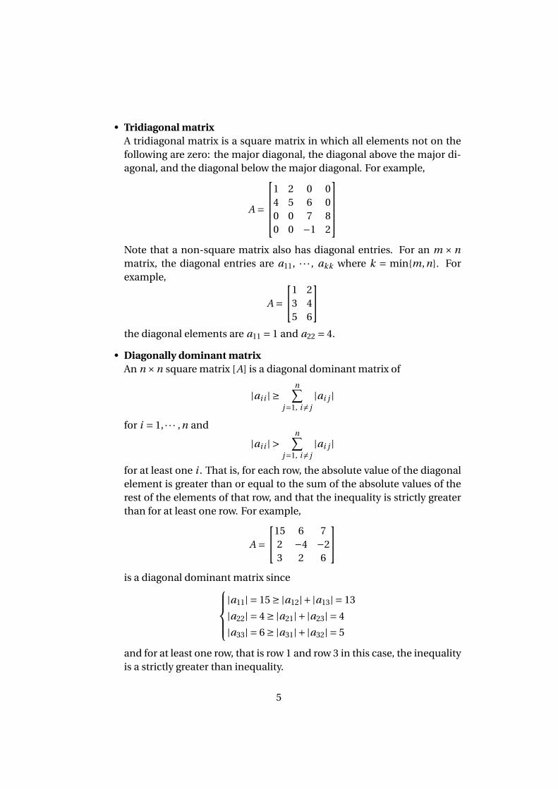
• Tridiagonal matrixA tridiagonal matrix is a square matrix in which all elements not on thefollowing are zero: the major diagonal, the diagonal above the major di-agonal, and the diagonal below the major diagonal. For example,
A =
1 2 0 04 5 6 00 0 7 80 0 −1 2
Note that a non-square matrix also has diagonal entries. For an m ×nmatrix, the diagonal entries are a11, · · · , akk where k = min{m,n}. Forexample,
A =1 2
3 45 6
the diagonal elements are a11 = 1 and a22 = 4.
• Diagonally dominant matrixAn n ×n square matrix [A] is a diagonal dominant matrix of
|ai i | ≥n∑
j=1, i 6= j|ai j |
for i = 1, · · · ,n and
|ai i | >n∑
j=1, i 6= j|ai j |
for at least one i . That is, for each row, the absolute value of the diagonalelement is greater than or equal to the sum of the absolute values of therest of the elements of that row, and that the inequality is strictly greaterthan for at least one row. For example,
A =15 6 7
2 −4 −23 2 6
is a diagonal dominant matrix since
|a11| = 15 ≥ |a12|+ |a13| = 13
|a22| = 4 ≥ |a21|+ |a23| = 4
|a33| = 6 ≥ |a31|+ |a32| = 5
and for at least one row, that is row 1 and row 3 in this case, the inequalityis a strictly greater than inequality.
5
1.2 Selected Problems
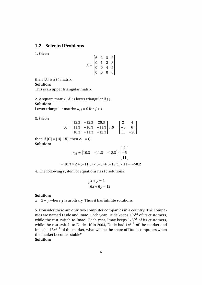
1. Given
A =
6 2 3 90 1 2 30 0 4 50 0 0 6
then [A] is a ( ) matrix.Solution:This is an upper triangular matrix.
2. A square matrix [A] is lower triangular if ( ).Solution:Lower triangular matrix: ai j = 0 for j > i .
3. Given
A =12.3 −12.3 20.3
11.3 −10.3 −11.310.3 −11.3 −12.3
, B = 2 4−5 611 −20
then if [C ] = [A] · [B ], then c31 = ().Solution:
c31 =[10.3 −11.3 −12.3
] · 2−511
= 10.3×2+ (−11.3)× (−5)+ (−12.3)×11 =−58.2
4. The following system of equations has ( ) solutions.{x + y = 2
6x +6y = 12
Solution:x = 2− y where y is arbitrary. Thus it has infinite solutions.
5. Consider there are only two computer companies in a country. The compa-nies are named Dude and Imac. Each year, Dude keeps 1/5th of its customers,while the rest switch to Imac. Each year, Imac keeps 1/3r d of its customers,while the rest switch to Dude. If in 2003, Dude had 1/6th of the market andImac had 5/6th of the market, what will be the share of Dude computers whenthe market becomes stable?Solution:
6
Since we want when the market is stable, the market share should not changefrom year to year. Let D and M denote the market of Dude and Imac, respec-tively. Thus we have{
Dn = 15 D + 2
3 M
Mn = 45 D + 1
3 M⇒
[Dn
Mn
]=
[15
23
45
13
]·[
DM
]Dn = D and Mn = M eventually. That is{
45 D − 2
3 M = 0
D +M = 1⇒
{D = 5
11
M = 611
Hence the final market share of Dude will be5
11.
6. Three kids - Jim, Corey and David receive an inheritance of $2,253,453. Themoney is put in three trusts but is not divided equally to begin with. Corey’strust is three times that of David’s because Corey made an A in Dr. Kaw’s class.Each trust is put in an interest generating investment. The three trusts of Jim,Corey and David pays an interest of 6%, 8%, 11%, respectively. The total interestof all the three trusts combined at the end of the first year is $190,740.57. Theequations to find the trust money of Jim (J), Corey (C) and David (D) in a matrixform is ( ).Solution:From the given conditions, we have
J +C +D = 2253453
C = 3D
0.06J +0.08C +0.11D = 190740.57
⇒
J +C +D = 2253453
C −3D = 0
0.06J +0.08C +0.11D = 190740.57
⇒ 1 1 1
0 1 −30.06 0.08 0.11
· J
CD
= 2253453
0190740.57
7. Which of the following matrices are strictly diagonally dominant?
A =15 6 7
2 −4 23 2 6
, B =5 6 7
2 −4 23 2 −5
, C =5 3 2
6 −8 27 −5 12
.
7
Solution:For A,
|a11| = 15 > |a12|+ |a13| = 13
|a22| = 4 = |a21|+ |a23| = 4
|a33| = 6 > |a31|+ |a32| = 5
So it is strictly diagonal dominant.For B ,
|b11| = 5 < |b12|+ |b13| = 13
So it is not strictly diagonal dominant.For C ,
|c11| = 5 = |c12|+ |c13| = 5
|c22| = 8 = |c21|+ |c23| = 8
|c33| = 12 = |c31|+ |c32| = 12
So it is not strictly diagonal dominant.
8
2 Vectors
2.1 Summary
• VectorA vector is a collection of numbers in a definite order. If it is a collectionof n numbers, it is called a n-dimensional vector. For example,
~A =1
23
, ~B = [4 5 6
].
• Addition of vectorsTwo vectors can be added only if they are of the same dimension and theaddition is given by
~A+~B =
a1...
an
+
b1...
bn
=
a1 +b1...
an +bn
• Null vector
A null vector (i.e. zero vector) is where all the components of the vectorare zero. For example,
0000
• Unit vector
A unit vector ~U is defined as
~U =
u1...
un
where √
u21 +·· ·+u2
n = 1
• Scalar multiplication of vectorsIf k is a scalar and ~A is a n-dimensional vector, then
k~A = k
a1...
an
=
ka1...
kan
9
• Linear combination of vectorsGiven ~A1, ~A2, · · · , ~Am as m vectors of same dimension n, and if k1, k2, · · · ,km are scalars, then
k1~A1 +k2~A2 +·· ·+km~Am
is a linear combination of the m vectors.
• Linearly independent vectorsA set of vectors ~A1, ~A2, · · · , ~Am are considered to be linearly independentif
k1~A1 +k2~A2 +·· ·+km~Am =~0has only one solution of k1 = k2 = ·· · = km = 0.
• RankFrom a set of n-dimension vectors, the maximum number of linearly in-dependent vectors in the set is called the rank of the set of vectors. Notethat the rank of the vectors can never be greater than the vectors dimen-sion.
• Dot productLet ~A = [
a1, · · · , an]
and ~B = [b1, · · · , bn
]be two n-dimensional
vectors. Then the dot product (i.e. inner product) of the two vectors ~Aand ~B is defined as
~A ·~B = a1b1 +·· ·+anbn =n∑
i=1ai bi
• Some useful results
– If a set of vectors contains the null vector, the set of vectors is linearlydependent.
– If a set of m vectors is linearly independent, then a subset of the mvectors also has to be linearly independent.
– If a set of vectors is linearly dependent, then at least one vector canbe written as a linear combination of others.
– If the dimension of a set of vectors is less than the number of vectorsin the set, then the set of vectors is linearly dependent.
10
2.2 Selected Problems
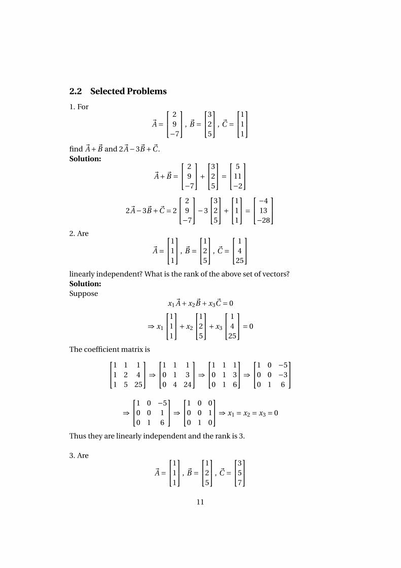
1. For
~A = 2
9−7
, ~B =3
25
, ~C =1
11
find ~A+~B and 2~A−3~B +~C .Solution:
~A+~B = 2
9−7
+3
25
= 5
11−2
2~A−3~B +~C = 2
29−7
−3
325
+1
11
= −4
13−28
2. Are
~A =1
11
, ~B =1
25
, ~C = 1
425
linearly independent? What is the rank of the above set of vectors?Solution:Suppose
x1~A+x2~B +x3~C = 0
⇒ x1
111
+x2
125
+x3
14
25
= 0
The coefficient matrix is1 1 11 2 41 5 25
⇒1 1 1
0 1 30 4 24
⇒1 1 1
0 1 30 1 6
⇒1 0 −5
0 0 −30 1 6
⇒1 0 −5
0 0 10 1 6
⇒1 0 0
0 0 10 1 0
⇒ x1 = x2 = x3 = 0
Thus they are linearly independent and the rank is 3.
3. Are
~A =1
11
, ~B =1
25
, ~C =3
57
11
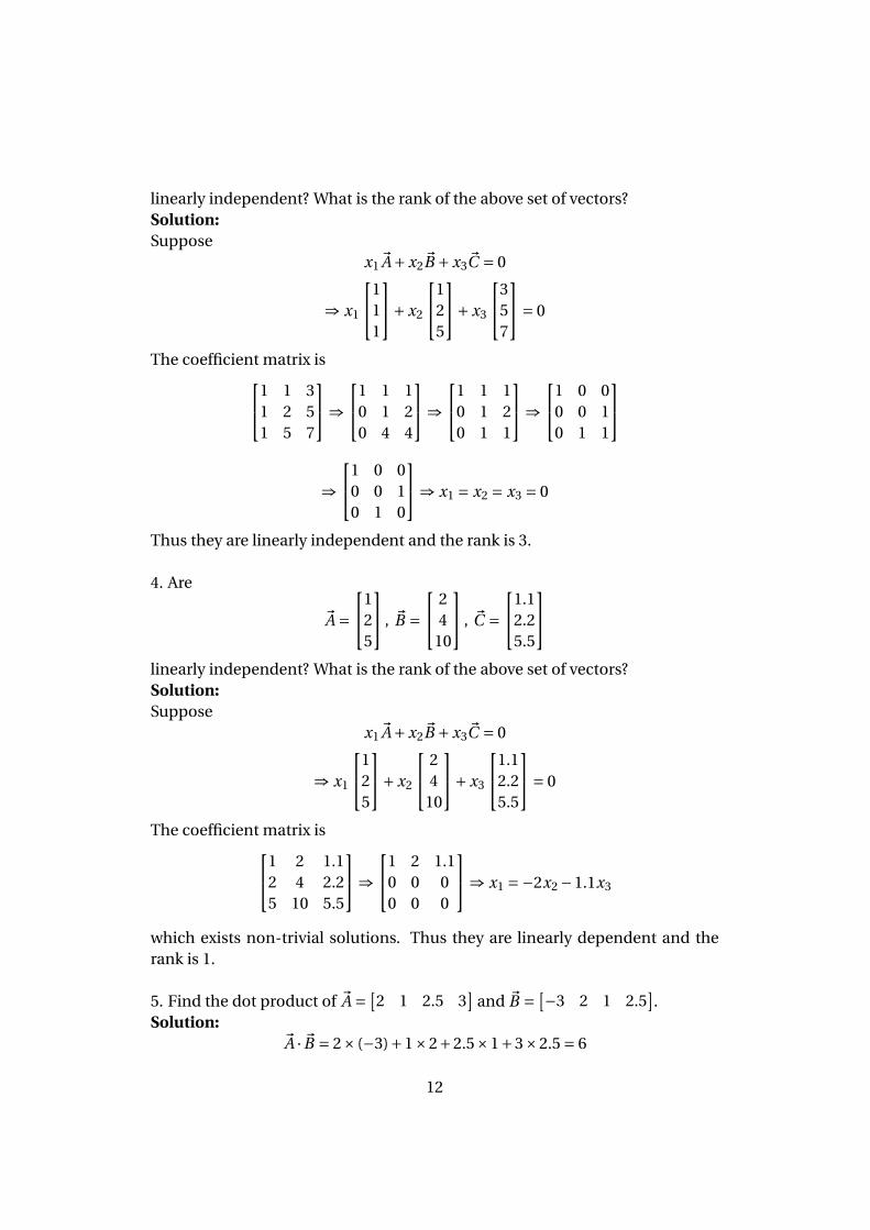
linearly independent? What is the rank of the above set of vectors?Solution:Suppose
x1~A+x2~B +x3~C = 0
⇒ x1
111
+x2
125
+x3
357
= 0
The coefficient matrix is1 1 31 2 51 5 7
⇒1 1 1
0 1 20 4 4
⇒1 1 1
0 1 20 1 1
⇒1 0 0
0 0 10 1 1
⇒1 0 0
0 0 10 1 0
⇒ x1 = x2 = x3 = 0
Thus they are linearly independent and the rank is 3.
4. Are
~A =1
25
, ~B = 2
410
, ~C =1.1
2.25.5
linearly independent? What is the rank of the above set of vectors?Solution:Suppose
x1~A+x2~B +x3~C = 0
⇒ x1
125
+x2
24
10
+x3
1.12.25.5
= 0
The coefficient matrix is1 2 1.12 4 2.25 10 5.5
⇒1 2 1.1
0 0 00 0 0
⇒ x1 =−2x2 −1.1x3
which exists non-trivial solutions. Thus they are linearly dependent and therank is 1.
5. Find the dot product of ~A = [2 1 2.5 3
]and ~B = [−3 2 1 2.5
].
Solution:~A ·~B = 2× (−3)+1×2+2.5×1+3×2.5 = 6
12
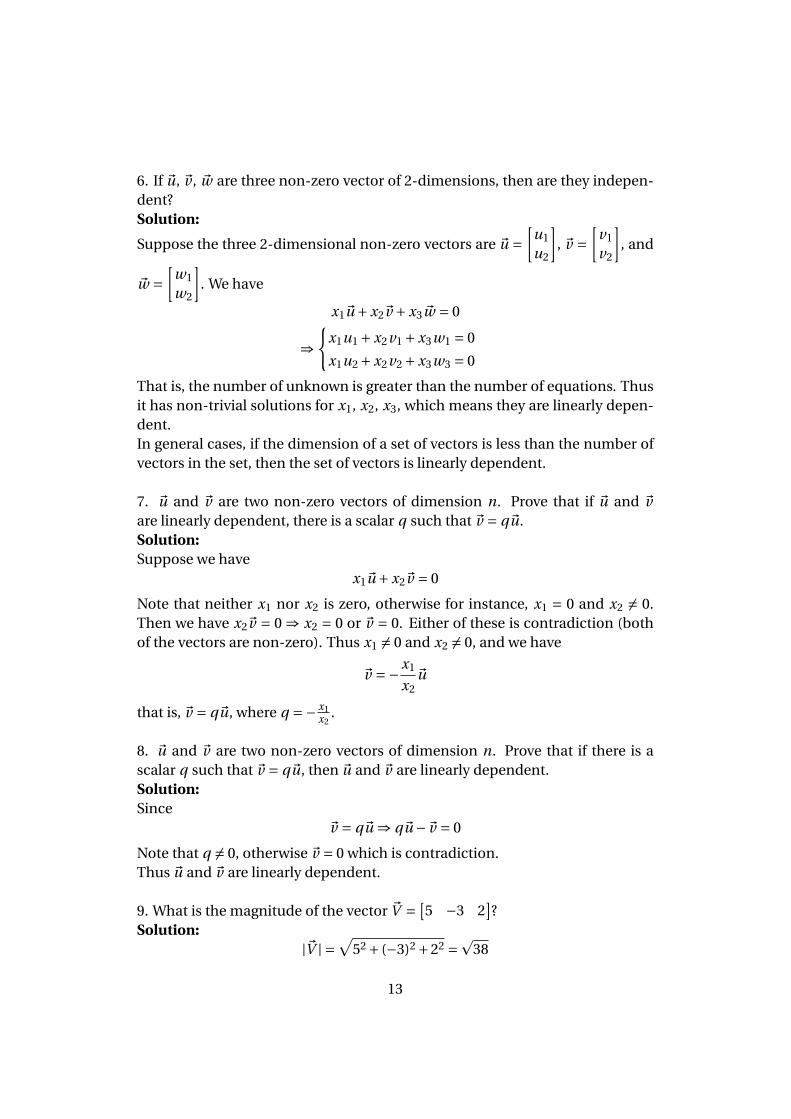
6. If ~u, ~v , ~w are three non-zero vector of 2-dimensions, then are they indepen-dent?Solution:
Suppose the three 2-dimensional non-zero vectors are ~u =[
u1
u2
], ~v =
[v1
v2
], and
~w =[
w1
w2
]. We have
x1~u +x2~v +x3~w = 0
⇒{
x1u1 +x2v1 +x3w1 = 0
x1u2 +x2v2 +x3w3 = 0
That is, the number of unknown is greater than the number of equations. Thusit has non-trivial solutions for x1, x2, x3, which means they are linearly depen-dent.In general cases, if the dimension of a set of vectors is less than the number ofvectors in the set, then the set of vectors is linearly dependent.
7. ~u and ~v are two non-zero vectors of dimension n. Prove that if ~u and ~vare linearly dependent, there is a scalar q such that ~v = q~u.Solution:Suppose we have
x1~u +x2~v = 0
Note that neither x1 nor x2 is zero, otherwise for instance, x1 = 0 and x2 6= 0.Then we have x2~v = 0 ⇒ x2 = 0 or ~v = 0. Either of these is contradiction (bothof the vectors are non-zero). Thus x1 6= 0 and x2 6= 0, and we have
~v =−x1
x2~u
that is, ~v = q~u, where q =− x1x2
.
8. ~u and ~v are two non-zero vectors of dimension n. Prove that if there is ascalar q such that ~v = q~u, then ~u and ~v are linearly dependent.Solution:Since
~v = q~u ⇒ q~u −~v = 0
Note that q 6= 0, otherwise ~v = 0 which is contradiction.Thus ~u and ~v are linearly dependent.
9. What is the magnitude of the vector ~V = [5 −3 2
]?
Solution:|~V | =
√52 + (−3)2 +22 =p
38
13
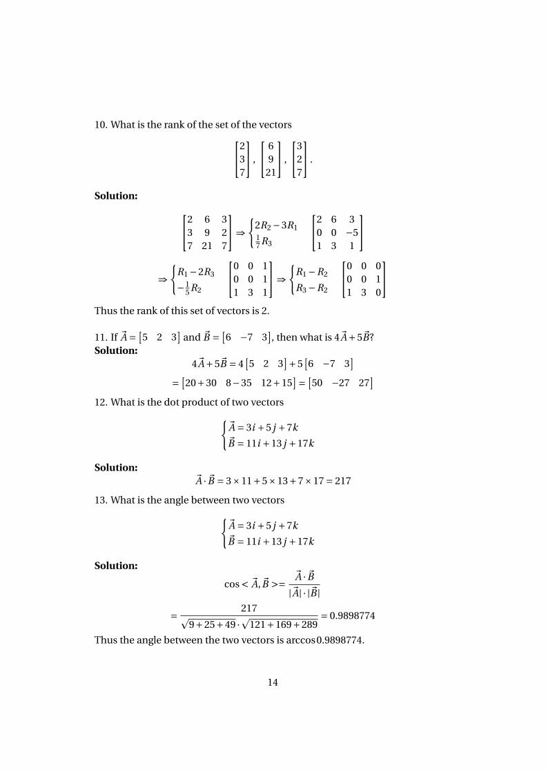
10. What is the rank of the set of the vectors237
,
69
21
,
327
.
Solution: 2 6 33 9 27 21 7
⇒{
2R2 −3R117 R3
2 6 30 0 −51 3 1
⇒{
R1 −2R3
−15 R2
0 0 10 0 11 3 1
⇒{
R1 −R2
R3 −R2
0 0 00 0 11 3 0
Thus the rank of this set of vectors is 2.
11. If ~A = [5 2 3
]and ~B = [
6 −7 3], then what is 4~A+5~B?
Solution:4~A+5~B = 4
[5 2 3
]+5[6 −7 3
]= [
20+30 8−35 12+15]= [
50 −27 27]
12. What is the dot product of two vectors{~A = 3i +5 j +7k~B = 11i +13 j +17k
Solution:~A ·~B = 3×11+5×13+7×17 = 217
13. What is the angle between two vectors{~A = 3i +5 j +7k~B = 11i +13 j +17k
Solution:
cos < ~A,~B >=~A ·~B
|~A| · |~B |= 217p
9+25+49 ·p121+169+289= 0.9898774
Thus the angle between the two vectors is arccos0.9898774.
14
3 Binary Matrix Operations
3.1 Summary
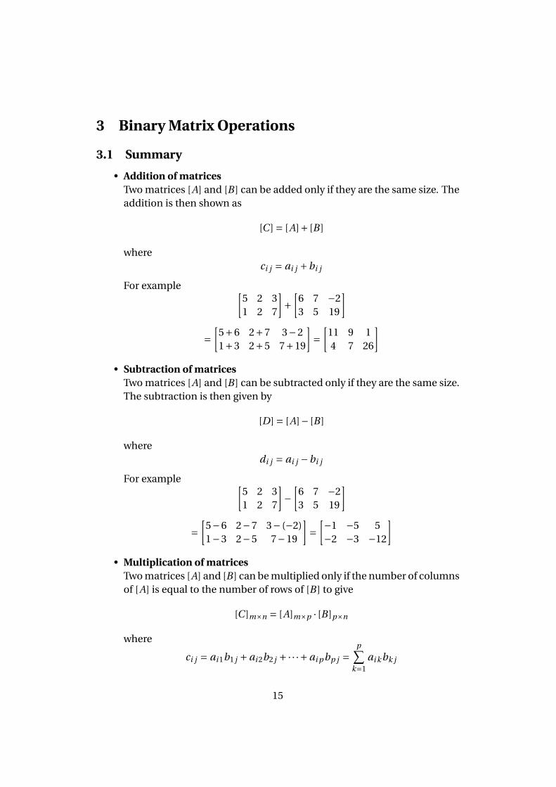
• Addition of matricesTwo matrices [A] and [B ] can be added only if they are the same size. Theaddition is then shown as
[C ] = [A]+ [B ]
whereci j = ai j +bi j
For example [5 2 31 2 7
]+
[6 7 −23 5 19
]
=[
5+6 2+7 3−21+3 2+5 7+19
]=
[11 9 14 7 26
]• Subtraction of matrices
Two matrices [A] and [B ] can be subtracted only if they are the same size.The subtraction is then given by
[D] = [A]− [B ]
wheredi j = ai j −bi j
For example [5 2 31 2 7
]−
[6 7 −23 5 19
]
=[
5−6 2−7 3− (−2)1−3 2−5 7−19
]=
[−1 −5 5−2 −3 −12
]• Multiplication of matrices
Two matrices [A] and [B ] can be multiplied only if the number of columnsof [A] is equal to the number of rows of [B ] to give
[C ]m×n = [A]m×p · [B ]p×n
where
ci j = ai 1b1 j +ai 2b2 j +·· ·+ai p bp j =p∑
k=1ai k bk j
15
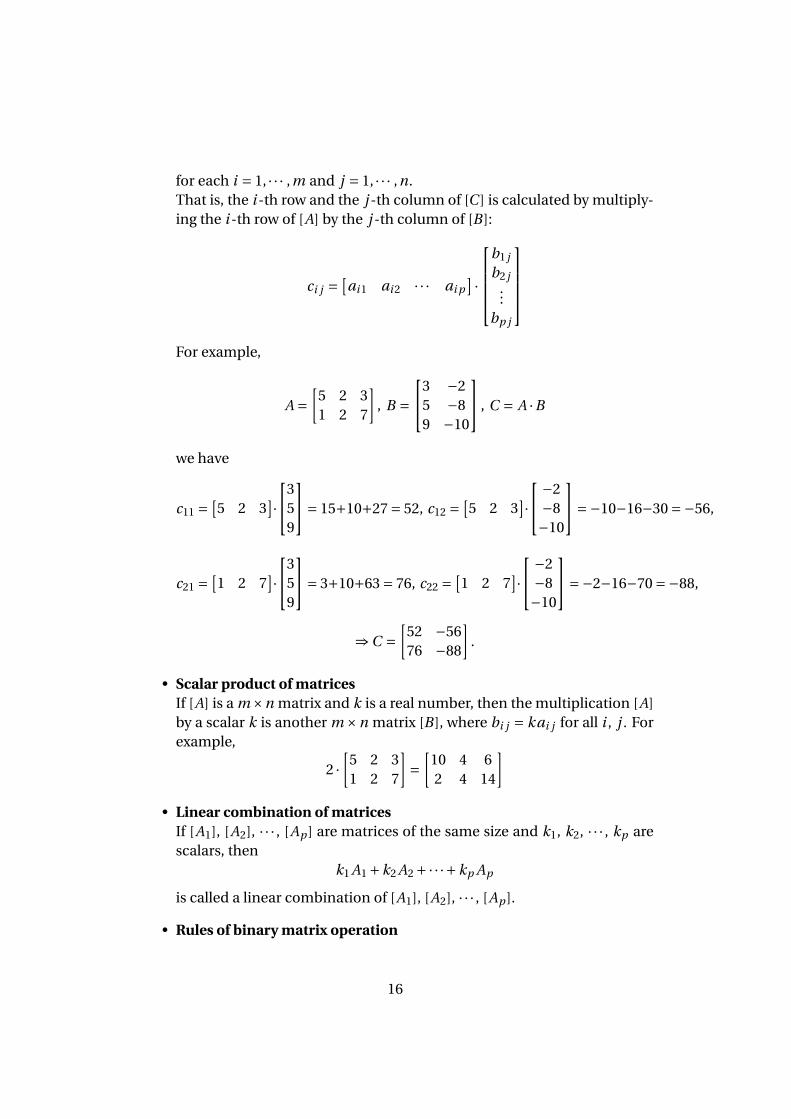
for each i = 1, · · · ,m and j = 1, · · · ,n.That is, the i -th row and the j -th column of [C ] is calculated by multiply-ing the i -th row of [A] by the j -th column of [B ]:
ci j =[ai 1 ai 2 · · · ai p
] ·
b1 j
b2 j...
bp j
For example,
A =[
5 2 31 2 7
], B =
3 −25 −89 −10
, C = A ·B
we have
c11 =[5 2 3
]·3
59
= 15+10+27 = 52, c12 =[5 2 3
]· −2−8−10
=−10−16−30 =−56,
c21 =[1 2 7
]·3
59
= 3+10+63 = 76, c22 =[1 2 7
]· −2−8−10
=−2−16−70 =−88,
⇒C =[
52 −5676 −88
].
• Scalar product of matricesIf [A] is a m×n matrix and k is a real number, then the multiplication [A]by a scalar k is another m ×n matrix [B ], where bi j = kai j for all i , j . Forexample,
2 ·[
5 2 31 2 7
]=
[10 4 62 4 14
]• Linear combination of matrices
If [A1], [A2], · · · , [Ap ] are matrices of the same size and k1, k2, · · · , kp arescalars, then
k1 A1 +k2 A2 +·· ·+kp Ap
is called a linear combination of [A1], [A2], · · · , [Ap ].
• Rules of binary matrix operation
16
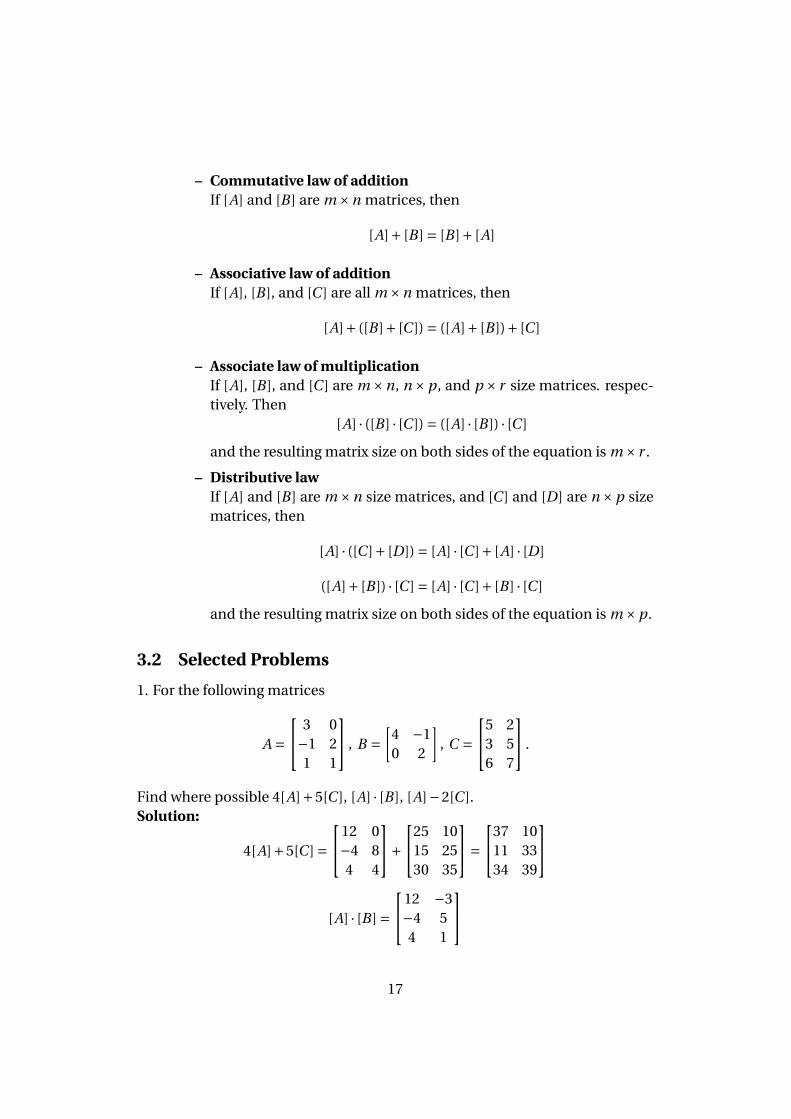
– Commutative law of additionIf [A] and [B ] are m ×n matrices, then
[A]+ [B ] = [B ]+ [A]
– Associative law of additionIf [A], [B ], and [C ] are all m ×n matrices, then
[A]+ ([B ]+ [C ]) = ([A]+ [B ])+ [C ]
– Associate law of multiplicationIf [A], [B ], and [C ] are m ×n, n ×p, and p × r size matrices. respec-tively. Then
[A] · ([B ] · [C ]) = ([A] · [B ]) · [C ]
and the resulting matrix size on both sides of the equation is m × r .
– Distributive lawIf [A] and [B ] are m ×n size matrices, and [C ] and [D] are n ×p sizematrices, then
[A] · ([C ]+ [D]) = [A] · [C ]+ [A] · [D]
([A]+ [B ]) · [C ] = [A] · [C ]+ [B ] · [C ]
and the resulting matrix size on both sides of the equation is m ×p.
3.2 Selected Problems
1. For the following matrices
A = 3 0−1 21 1
, B =[
4 −10 2
], C =
5 23 56 7
.
Find where possible 4[A]+5[C ], [A] · [B ], [A]−2[C ].Solution:
4[A]+5[C ] =12 0−4 84 4
+25 10
15 2530 35
=37 10
11 3334 39
[A] · [B ] =12 −3−4 54 1
17
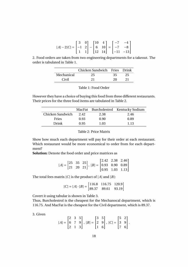
[A]−2[C ] = 3 0−1 21 1
−10 4
6 1012 14
= −7 −4−7 −8−11 −13
2. Food orders are taken from two engineering departments for a takeout. Theorder is tabulated in Table 1.
Chicken Sandwich Fries DrinkMechanical 25 35 25
Civil 21 20 21
Table 1: Food Order
However they have a choice of buying this food from three different restaurants.Their prices for the three food items are tabulated in Table 2.
MacFat Burcholestrol Kentucky SodiumChicken Sandwich 2.42 2.38 2.46
Fries 0.93 0.90 0.89Drink 0.95 1.03 1.13
Table 2: Price Matrix
Show how much each department will pay for their order at each restaurant.Which restaurant would be more economical to order from for each depart-ment?Solution: Denote the food order and price matrices as
[A] =[
25 35 2521 20 21
], [B ] =
2.42 2.38 2.460.93 0.90 0.890.95 1.03 1.13
The total fees matrix [C ] is the product of [A] and [B ]:
[C ] = [A] · [B ] =[
116.8 116.75 120.989.37 89.61 93.19
]Covert it using tabular is shown in Table 3.Thus, Burcholestrol is the cheapest for the Mechanocal department, which is116.75. And MacFat is the cheapest for the Civil department, which is 89.37.
3. Given
[A] =2 3 5
6 7 92 1 3
, [B ] =3 5
2 91 6
, [C ] =5 2
3 97 6
.
18
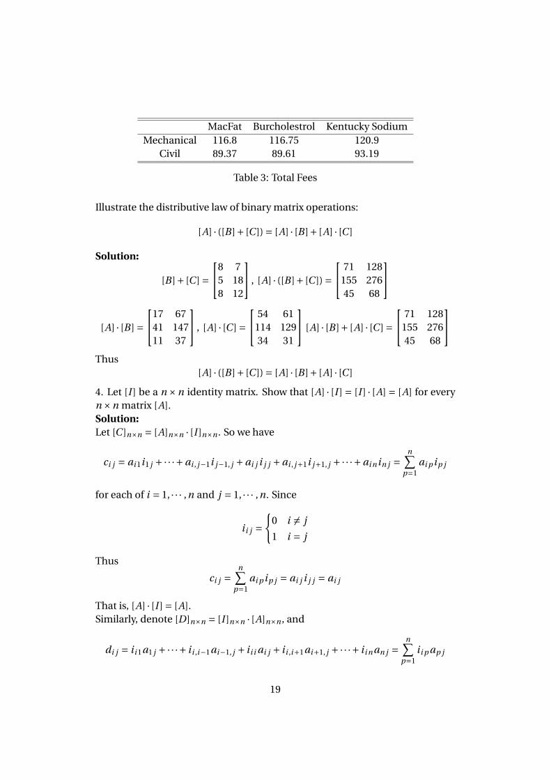
MacFat Burcholestrol Kentucky SodiumMechanical 116.8 116.75 120.9
Civil 89.37 89.61 93.19
Table 3: Total Fees
Illustrate the distributive law of binary matrix operations:
[A] · ([B ]+ [C ]) = [A] · [B ]+ [A] · [C ]
Solution:
[B ]+ [C ] =8 7
5 188 12
, [A] · ([B ]+ [C ]) = 71 128
155 27645 68
[A] · [B ] =17 67
41 14711 37
, [A] · [C ] = 54 61
114 12934 31
[A] · [B ]+ [A] · [C ] = 71 128
155 27645 68
Thus
[A] · ([B ]+ [C ]) = [A] · [B ]+ [A] · [C ]
4. Let [I ] be a n ×n identity matrix. Show that [A] · [I ] = [I ] · [A] = [A] for everyn ×n matrix [A].Solution:Let [C ]n×n = [A]n×n · [I ]n×n . So we have
ci j = ai 1i1 j +·· ·+ai , j−1i j−1, j +ai j i j j +ai , j+1i j+1, j +·· ·+ai nin j =n∑
p=1ai p ip j
for each of i = 1, · · · ,n and j = 1, · · · ,n. Since
ii j ={
0 i 6= j
1 i = j
Thus
ci j =n∑
p=1ai p ip j = ai j i j j = ai j
That is, [A] · [I ] = [A].Similarly, denote [D]n×n = [I ]n×n · [A]n×n , and
di j = ii 1a1 j +·· ·+ ii ,i−1ai−1, j + ii i ai j + ii ,i+1ai+1, j +·· ·+ ii n an j =n∑
p=1ii p ap j
19
Because ii j = 1 when i = j , otherwise ii j = 0. Thus,
di j =n∑
p=1ii p ap j = ai j
That is, [I ] · [A] = [A].
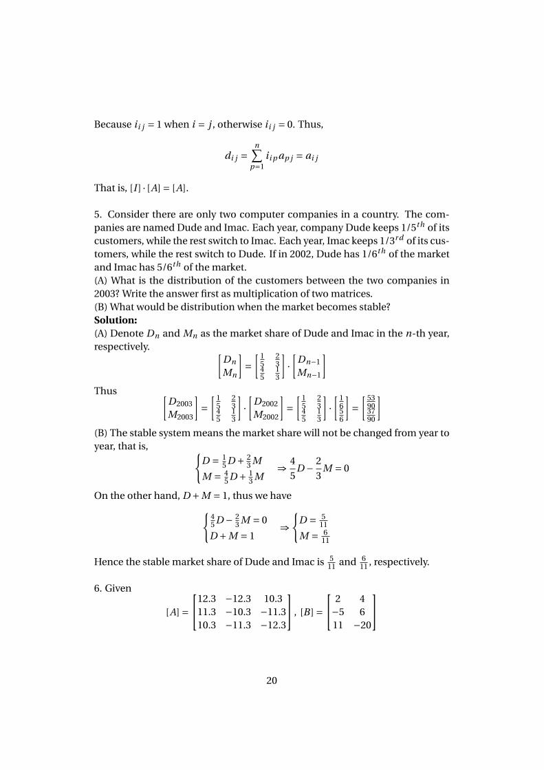
5. Consider there are only two computer companies in a country. The com-panies are named Dude and Imac. Each year, company Dude keeps 1/5th of itscustomers, while the rest switch to Imac. Each year, Imac keeps 1/3r d of its cus-tomers, while the rest switch to Dude. If in 2002, Dude has 1/6th of the marketand Imac has 5/6th of the market.(A) What is the distribution of the customers between the two companies in2003? Write the answer first as multiplication of two matrices.(B) What would be distribution when the market becomes stable?Solution:(A) Denote Dn and Mn as the market share of Dude and Imac in the n-th year,respectively. [
Dn
Mn
]=
[15
23
45
13
]·[
Dn−1
Mn−1
]Thus [
D2003
M2003
]=
[15
23
45
13
]·[
D2002
M2002
]=
[15
23
45
13
]·[1
656
]=
[53903790
](B) The stable system means the market share will not be changed from year toyear, that is, {
D = 15 D + 2
3 M
M = 45 D + 1
3 M⇒ 4
5D − 2
3M = 0
On the other hand, D +M = 1, thus we have{45 D − 2
3 M = 0
D +M = 1⇒
{D = 5
11
M = 611
Hence the stable market share of Dude and Imac is 511 and 6
11 , respectively.
6. Given
[A] =12.3 −12.3 10.3
11.3 −10.3 −11.310.3 −11.3 −12.3
, [B ] = 2 4−5 611 −20
20
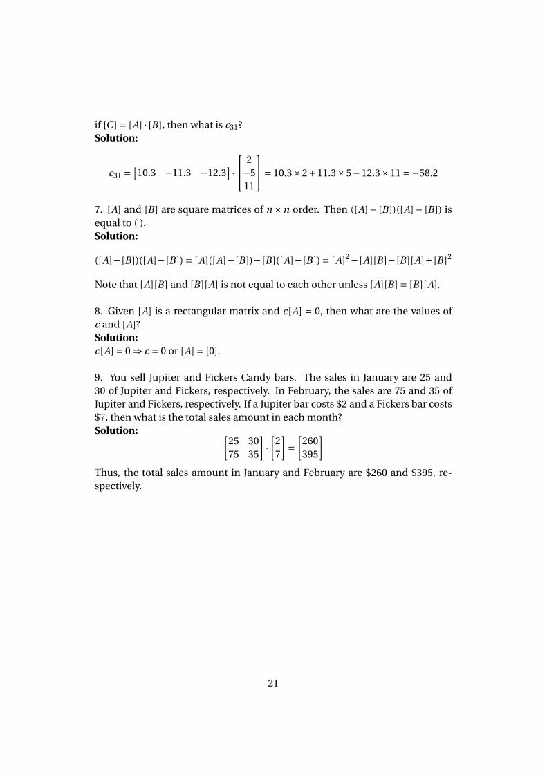
if [C ] = [A] · [B ], then what is c31?Solution:
c31 =[10.3 −11.3 −12.3
] · 2−511
= 10.3×2+11.3×5−12.3×11 =−58.2
7. [A] and [B ] are square matrices of n ×n order. Then ([A]− [B ])([A]− [B ]) isequal to ( ).Solution:
([A]−[B ])([A]−[B ]) = [A]([A]−[B ])−[B ]([A]−[B ]) = [A]2−[A][B ]−[B ][A]+[B ]2
Note that [A][B ] and [B ][A] is not equal to each other unless [A][B ] = [B ][A].
8. Given [A] is a rectangular matrix and c[A] = 0, then what are the values ofc and [A]?Solution:c[A] = 0 ⇒ c = 0 or [A] = [0].
9. You sell Jupiter and Fickers Candy bars. The sales in January are 25 and30 of Jupiter and Fickers, respectively. In February, the sales are 75 and 35 ofJupiter and Fickers, respectively. If a Jupiter bar costs $2 and a Fickers bar costs$7, then what is the total sales amount in each month?Solution: [
25 3075 35
]·[
27
]=
[260395
]Thus, the total sales amount in January and February are $260 and $395, re-spectively.
21
4 Unary Matrix Operations
4.1 Summary
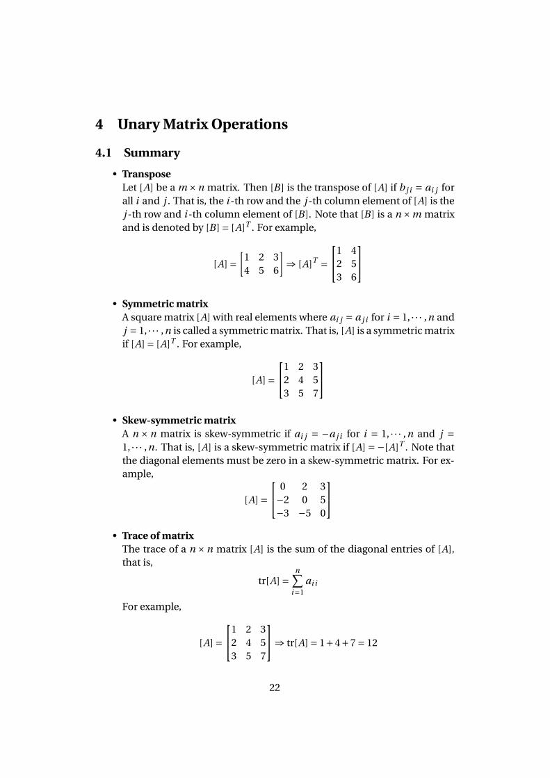
• TransposeLet [A] be a m ×n matrix. Then [B ] is the transpose of [A] if b j i = ai j forall i and j . That is, the i -th row and the j -th column element of [A] is thej -th row and i -th column element of [B ]. Note that [B ] is a n ×m matrixand is denoted by [B ] = [A]T . For example,
[A] =[
1 2 34 5 6
]⇒ [A]T =
1 42 53 6
• Symmetric matrix
A square matrix [A] with real elements where ai j = a j i for i = 1, · · · ,n andj = 1, · · · ,n is called a symmetric matrix. That is, [A] is a symmetric matrixif [A] = [A]T . For example,
[A] =1 2 3
2 4 53 5 7
• Skew-symmetric matrix
A n ×n matrix is skew-symmetric if ai j = −a j i for i = 1, · · · ,n and j =1, · · · ,n. That is, [A] is a skew-symmetric matrix if [A] =−[A]T . Note thatthe diagonal elements must be zero in a skew-symmetric matrix. For ex-ample,
[A] = 0 2 3−2 0 5−3 −5 0
• Trace of matrix
The trace of a n ×n matrix [A] is the sum of the diagonal entries of [A],that is,
tr[A] =n∑
i=1ai i
For example,
[A] =1 2 3
2 4 53 5 7
⇒ tr[A] = 1+4+7 = 12
22
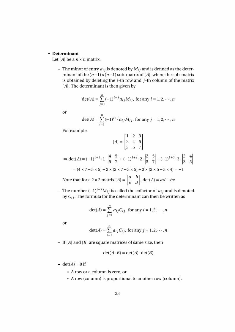
• DeterminantLet [A] be a n ×n matrix.
– The minor of entry ai j is denoted by Mi j and is defined as the deter-minant of the (n−1)×(n−1) sub-matrix of [A], where the sub-matrixis obtained by deleting the i -th row and j -th column of the matrix[A]. The determinant is then given by
det(A) =n∑
j=1(−1)i+ j ai j Mi j , for any i = 1,2, · · · ,n
or
det(A) =n∑
i=1(−1)i+ j ai j Mi j , for any j = 1,2, · · · ,n
For example,
[A] =1 2 3
2 4 53 5 7
⇒ det(A) = (−1)1+1 ·1 ·
∣∣∣∣4 55 7
∣∣∣∣+ (−1)1+2 ·2 ·∣∣∣∣2 53 7
∣∣∣∣+ (−1)1+3 ·3 ·∣∣∣∣2 43 5
∣∣∣∣= (4×7−5×5)−2× (2×7−3×5)+3× (2×5−3×4) =−1
Note that for a 2×2 matrix [A] =[
a bc d
], det(A) = ad −bc.
– The number (−1)i+ j Mi j is called the cofactor of ai j and is denotedby Ci j . The formula for the determinant can then be written as
det(A) =n∑
j=1ai j Ci j , for any i = 1,2, · · · ,n
or
det(A) =n∑
i=1ai j Ci j , for any j = 1,2, · · · ,n
– If [A] and [B ] are square matrices of same size, then
det(A ·B) = det(A) ·det(B)
– det(A) = 0 if
* A row or a column is zero, or
* A row (column) is proportional to another row (column).
23
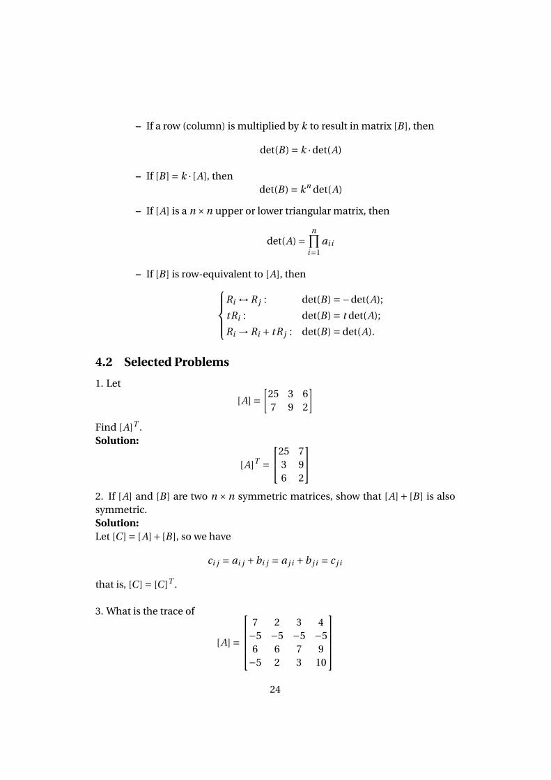
– If a row (column) is multiplied by k to result in matrix [B ], then
det(B) = k ·det(A)
– If [B ] = k · [A], thendet(B) = kn det(A)
– If [A] is a n ×n upper or lower triangular matrix, then
det(A) =n∏
i=1ai i
– If [B ] is row-equivalent to [A], thenRi ↔ R j : det(B) =−det(A);
tRi : det(B) = t det(A);
Ri → Ri + tR j : det(B) = det(A).
4.2 Selected Problems
1. Let
[A] =[
25 3 67 9 2
]Find [A]T .Solution:
[A]T =25 7
3 96 2
2. If [A] and [B ] are two n ×n symmetric matrices, show that [A]+ [B ] is alsosymmetric.Solution:Let [C ] = [A]+ [B ], so we have
ci j = ai j +bi j = a j i +b j i = c j i
that is, [C ] = [C ]T .
3. What is the trace of
[A] =
7 2 3 4−5 −5 −5 −56 6 7 9−5 2 3 10
24
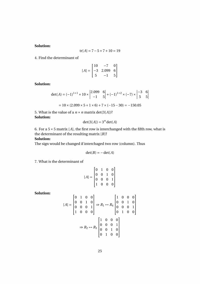
Solution:tr[A] = 7−5+7+10 = 19
4. Find the determinant of
[A] =10 −7 0−3 2.099 65 −1 5
Solution:
det(A) = (−1)1+1 ×10×∣∣∣∣2.099 6−1 5
∣∣∣∣+ (−1)1+2 × (−7)×∣∣∣∣−3 6
5 5
∣∣∣∣= 10× (2.099×5+1×6)+7× (−15−30) =−150.05
5. What is the value of a n ×n matrix det(3[A])?Solution:
det(3[A]) = 3n det(A)
6. For a 5×5 matrix [A], the first row is interchanged with the fifth row, what isthe determinant of the resulting matrix [B ]?Solution:The sign would be changed if interchaged two row (column). Thus
det(B) =−det(A)
7. What is the determinant of
[A] =
0 1 0 00 0 1 00 0 0 11 0 0 0
Solution:
[A] =
0 1 0 00 0 1 00 0 0 11 0 0 0
⇒ R1 ↔ R4
1 0 0 00 0 1 00 0 0 10 1 0 0
⇒ R2 ↔ R3
1 0 0 00 0 0 10 0 1 00 1 0 0
25
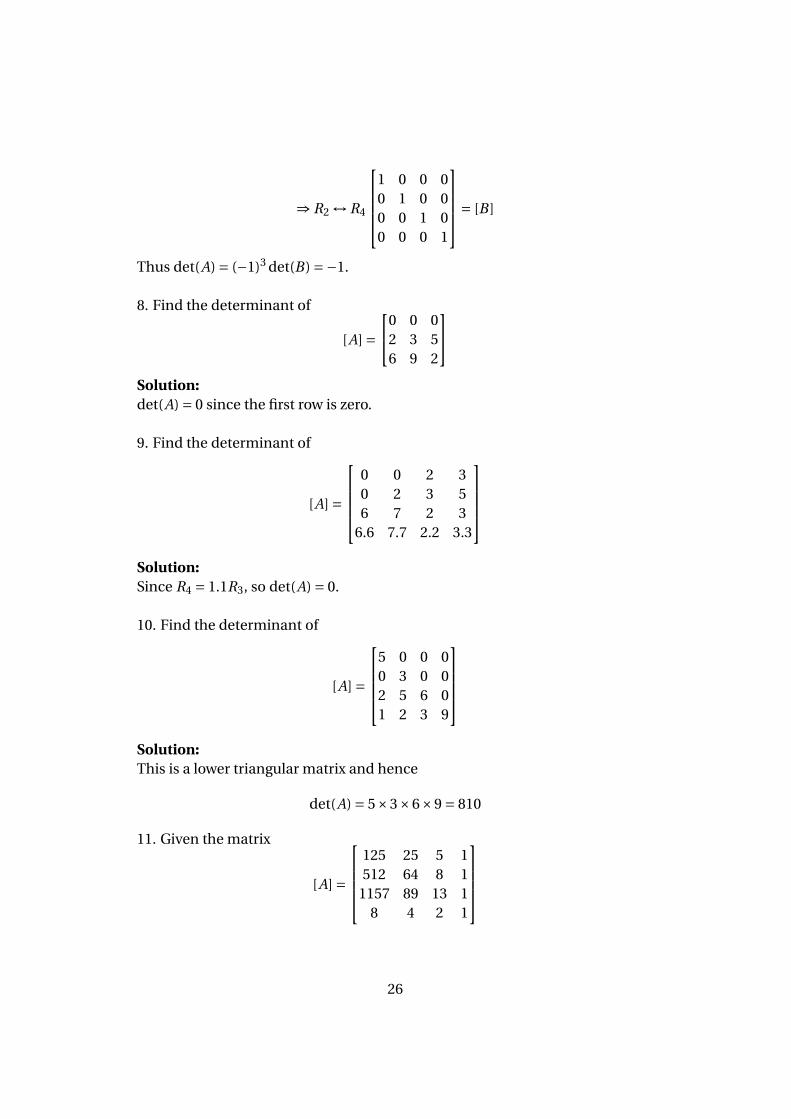
⇒ R2 ↔ R4
1 0 0 00 1 0 00 0 1 00 0 0 1
= [B ]
Thus det(A) = (−1)3 det(B) =−1.
8. Find the determinant of
[A] =0 0 0
2 3 56 9 2
Solution:det(A) = 0 since the first row is zero.
9. Find the determinant of
[A] =
0 0 2 30 2 3 56 7 2 3
6.6 7.7 2.2 3.3
Solution:Since R4 = 1.1R3, so det(A) = 0.
10. Find the determinant of
[A] =
5 0 0 00 3 0 02 5 6 01 2 3 9
Solution:This is a lower triangular matrix and hence
det(A) = 5×3×6×9 = 810
11. Given the matrix
[A] =
125 25 5 1512 64 8 1
1157 89 13 18 4 2 1
26
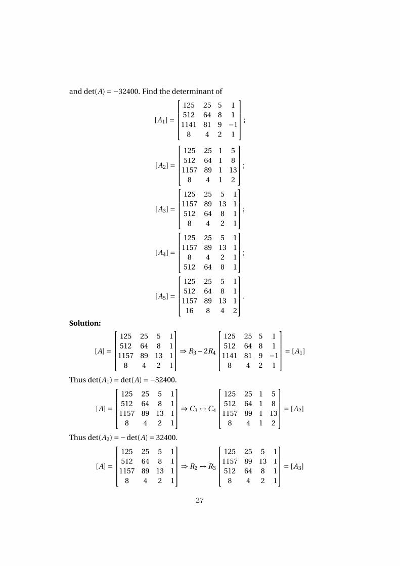
and det(A) =−32400. Find the determinant of
[A1] =
125 25 5 1512 64 8 1
1141 81 9 −18 4 2 1
;
[A2] =
125 25 1 5512 64 1 8
1157 89 1 138 4 1 2
;
[A3] =
125 25 5 1
1157 89 13 1512 64 8 1
8 4 2 1
;
[A4] =
125 25 5 1
1157 89 13 18 4 2 1
512 64 8 1
;
[A5] =
125 25 5 1512 64 8 1
1157 89 13 116 8 4 2
.
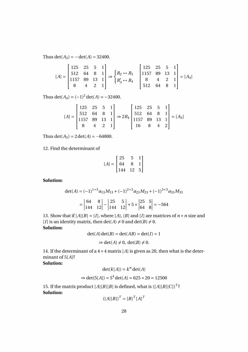
Solution:
[A] =
125 25 5 1512 64 8 1
1157 89 13 18 4 2 1
⇒ R3 −2R4
125 25 5 1512 64 8 1
1141 81 9 −18 4 2 1
= [A1]
Thus det(A1) = det(A) =−32400.
[A] =
125 25 5 1512 64 8 1
1157 89 13 18 4 2 1
⇒C3 ↔C4
125 25 1 5512 64 1 8
1157 89 1 138 4 1 2
= [A2]
Thus det(A2) =−det(A) = 32400.
[A] =
125 25 5 1512 64 8 1
1157 89 13 18 4 2 1
⇒ R2 ↔ R3
125 25 5 1
1157 89 13 1512 64 8 1
8 4 2 1
= [A3]
27
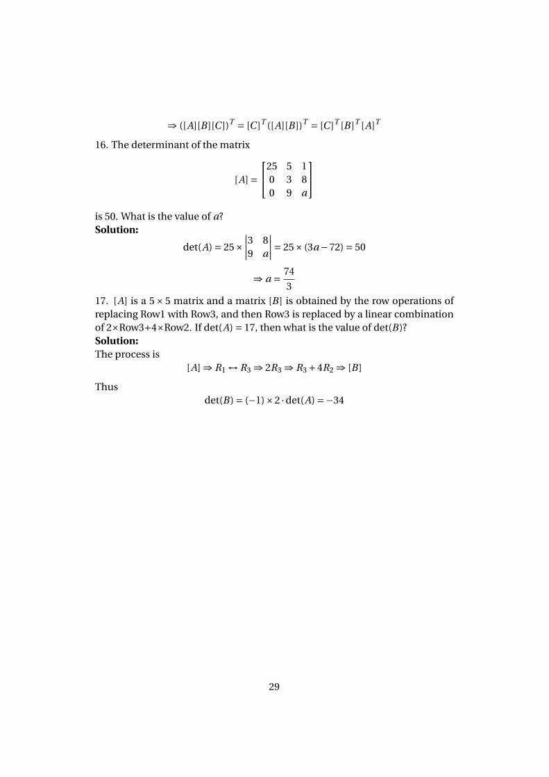
Thus det(A3) =−det(A) = 32400.
[A] =
125 25 5 1512 64 8 1
1157 89 13 18 4 2 1
⇒{
R2 ↔ R3
R ′3 ↔ R4
125 25 5 1
1157 89 13 18 4 2 1
512 64 8 1
= [A4]
Thus det(A4) = (−1)2 det(A) =−32400.
[A] =
125 25 5 1512 64 8 1
1157 89 13 18 4 2 1
⇒ 2R4
125 25 5 1512 64 8 1
1157 89 13 116 8 4 2
= [A5]
Thus det(A5) = 2det(A) =−64800.
12. Find the determinant of
[A] = 25 5 1
64 8 1144 12 5
Solution:
det(A) = (−1)1+3a13M13 + (−1)2+3a23M23 + (−1)3+3a33M33
=∣∣∣∣ 64 8144 12
∣∣∣∣− ∣∣∣∣ 25 5144 12
∣∣∣∣+5×∣∣∣∣25 564 8
∣∣∣∣=−564
13. Show that if [A][B ] = [I ], where [A], [B ] and [I ] are matrices of n×n size and[I ] is an identity matrix, then det(A) 6= 0 and det(B) 6= 0.Solution:
det(A)det(B) = det(AB) = det(I ) = 1
⇒ det(A) 6= 0, det(B) 6= 0.
14. If the determinant of a 4×4 matrix [A] is given as 20, then what is the deter-minant of 5[A]?Solution:
det(k[A]) = kn det(A)
⇒ det(5[A]) = 54 det(A) = 625×20 = 12500
15. If the matrix product [A][B ][B ] is defined, what is ([A][B ][C ])T ?Solution:
([A][B ])T = [B ]T [A]T
28
⇒ ([A][B ][C ])T = [C ]T ([A][B ])T = [C ]T [B ]T [A]T
16. The determinant of the matrix
[A] =25 5 1
0 3 80 9 a
is 50. What is the value of a?Solution:
det(A) = 25×∣∣∣∣3 89 a
∣∣∣∣= 25× (3a −72) = 50
⇒ a = 74
3
17. [A] is a 5× 5 matrix and a matrix [B ] is obtained by the row operations ofreplacing Row1 with Row3, and then Row3 is replaced by a linear combinationof 2×Row3+4×Row2. If det(A) = 17, then what is the value of det(B)?Solution:The process is
[A] ⇒ R1 ↔ R3 ⇒ 2R3 ⇒ R3 +4R2 ⇒ [B ]
Thusdet(B) = (−1)×2 ·det(A) =−34
29
5 System of Equations
5.1 Summary
• Consistent and inconsistent systemA system of equations
[A][X ] = [B ]
where [A] is called the coefficient matrix, [B ] is called the right hand sidevector and [X ] is called the solution vector. This system is consistent ifthere is a solution, and it is inconsistent if there is no solution. However,a consistent system of equations does not mean a unique solution, that is,a consistent system of equations may have a unique solution or infinitesolutions.
• Rank
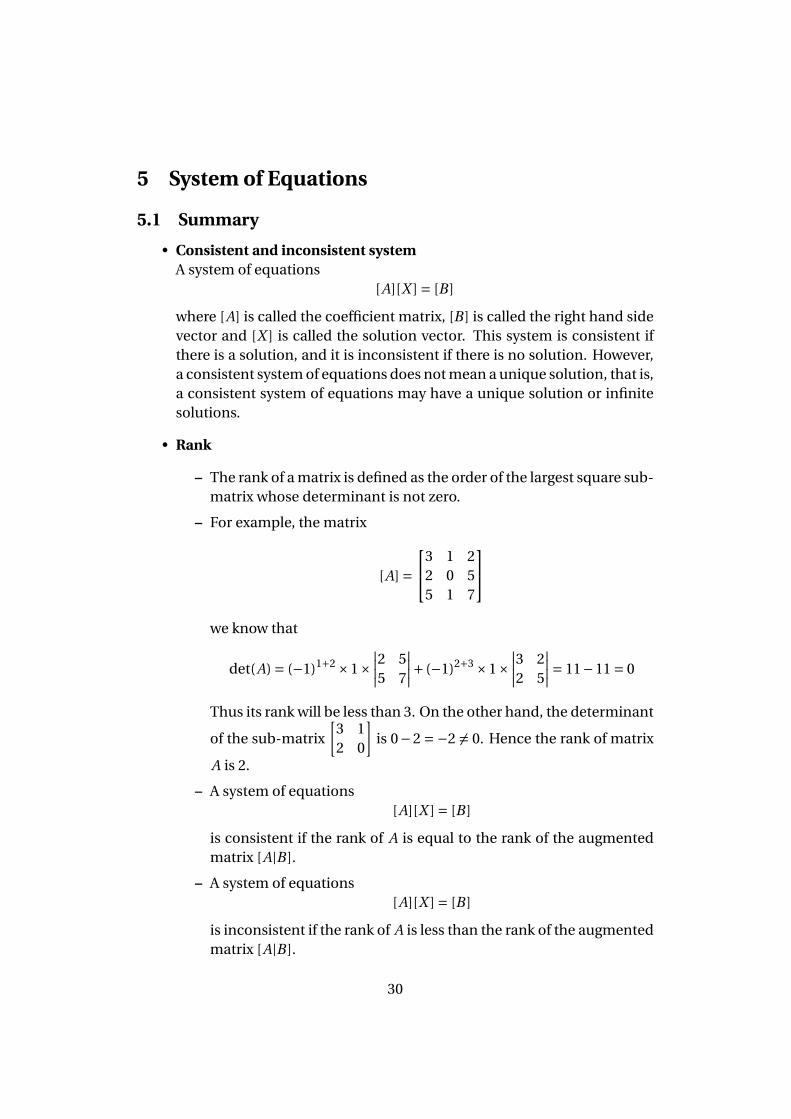
– The rank of a matrix is defined as the order of the largest square sub-matrix whose determinant is not zero.
– For example, the matrix
[A] =3 1 2
2 0 55 1 7
we know that
det(A) = (−1)1+2 ×1×∣∣∣∣2 55 7
∣∣∣∣+ (−1)2+3 ×1×∣∣∣∣3 22 5
∣∣∣∣= 11−11 = 0
Thus its rank will be less than 3. On the other hand, the determinant
of the sub-matrix
[3 12 0
]is 0−2 =−2 6= 0. Hence the rank of matrix
A is 2.
– A system of equations[A][X ] = [B ]
is consistent if the rank of A is equal to the rank of the augmentedmatrix [A|B ].
– A system of equations[A][X ] = [B ]
is inconsistent if the rank of A is less than the rank of the augmentedmatrix [A|B ].
30
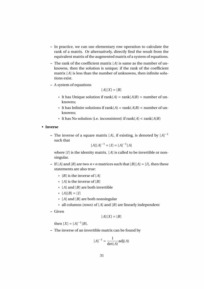
– In practice, we can use elementary row operation to calculate therank of a matrix. Or alternatively, directly find the result from theequivalent matrix of the augmented matrix of a system of equations.
– The rank of the coefficient matrix [A] is same as the number of un-knowns, then the solution is unique; if the rank of the coefficientmatrix [A] is less than the number of unknowns, then infinite solu-tions exist.
– A system of equations[A][X ] = [B ]
* It has Unique solution if rank(A) = rank(A|B) = number of un-knowns;
* It has Infinite solutions if rank(A) = rank(A|B) < number of un-knowns;
* It has No solution (i.e. inconsistent) if rank(A) < rank(A|B)
• Inverse
– The inverse of a square matrix [A], if existing, is denoted by [A]−1
such that[A][A]−1 = [I ] = [A]−1[A]
where [I ] is the identity matrix. [A] is called to be invertible or non-singular.
– If [A] and [B ] are two n×n matrices such that [B ][A] = [I ], then thesestatements are also true:
* [B ] is the inverse of [A]
* [A] is the inverse of [B ]
* [A] and [B ] are both invertible
* [A][B ] = [I ]
* [A] and [B ] are both nonsingular
* all columns (rows) of [A] and [B ] are linearly independent
– Given[A][X ] = [B ]
then [X ] = [A]−1[B ].
– The inverse of an invertible matrix can be found by
[A]−1 = 1
det(A)adj(A)
31
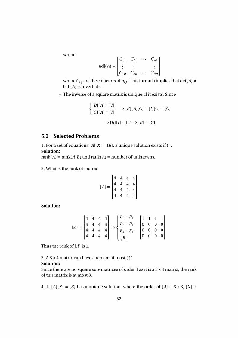
where
adj(A) =
C11 C21 · · · Cn1...
......
C1n C2n · · · Cnn
where Ci j are the cofactors of ai j . This formula implies that det(A) 6=0 if [A] is invertible.
– The inverse of a square matrix is unique, if it exists. Since{[B ][A] = [I ]
[C ][A] = [I ]⇒ [B ][A][C ] = [I ][C ] = [C ]
⇒ [B ][I ] = [C ] ⇒ [B ] = [C ]
5.2 Selected Problems
1. For a set of equations [A][X ] = [B ], a unique solution exists if ( ).Solution:rank(A) = rank(A|B) and rank(A) = number of unknowns.
2. What is the rank of matrix
[A] =
4 4 4 44 4 4 44 4 4 44 4 4 4
Solution:
[A] =
4 4 4 44 4 4 44 4 4 44 4 4 4
⇒
R2 −R1
R3 −R1
R4 −R114 R1
1 1 1 10 0 0 00 0 0 00 0 0 0
Thus the rank of [A] is 1.
3. A 3×4 matrix can have a rank of at most ( )?Solution:Since there are no square sub-matrices of order 4 as it is a 3×4 matrix, the rankof this matrix is at most 3.
4. If [A][X ] = [B ] has a unique solution, where the order of [A] is 3× 3, [X ] is
32
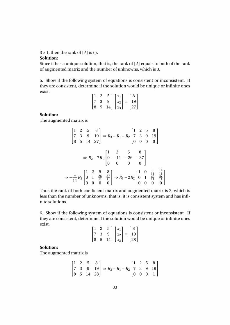
3×1, then the rank of [A] is ( ).Solution:Since it has a unique solution, that is, the rank of [A] equals to both of the rankof augmented matrix and the number of unknowns, which is 3.
5. Show if the following system of equations is consistent or inconsistent. Ifthey are consistent, determine if the solution would be unique or infinite onesexist. 1 2 5
7 3 98 5 14
x1
x2
x3
= 8
1927
Solution:The augmented matrix is1 2 5 8
7 3 9 198 5 14 27
⇒ R3 −R1 −R2
1 2 5 87 3 9 190 0 0 0
⇒ R2 −7R1
1 2 5 80 −11 −26 −370 0 0 0
⇒− 1
11R2
1 2 5 80 1 26
113711
0 0 0 0
⇒ R1 −2R2
1 0 311
1411
0 1 2611
3711
0 0 0 0
Thus the rank of both coefficient matrix and augmented matrix is 2, which isless than the number of unknowns, that is, it is consistent system and has infi-nite solutions.
6. Show if the following system of equations is consistent or inconsistent. Ifthey are consistent, determine if the solution would be unique or infinite onesexist. 1 2 5
7 3 98 5 14
x1
x2
x3
= 8
1928
Solution:The augmented matrix is1 2 5 8
7 3 9 198 5 14 28
⇒ R3 −R1 −R2
1 2 5 87 3 9 190 0 0 1
33
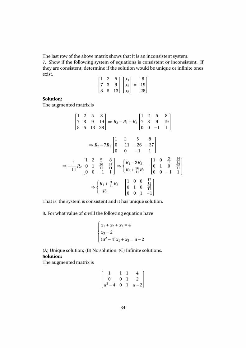
The last row of the above matrix shows that it is an inconsistent system.7. Show if the following system of equations is consistent or inconsistent. Ifthey are consistent, determine if the solution would be unique or infinite onesexist. 1 2 5
7 3 98 5 13
x1
x2
x3
= 8
1928
Solution:The augmented matrix is1 2 5 8
7 3 9 198 5 13 28
⇒ R3 −R1 −R2
1 2 5 87 3 9 190 0 −1 1
⇒ R2 −7R1
1 2 5 80 −11 −26 −370 0 −1 1
⇒− 1
11R2
1 2 5 80 1 26
113711
0 0 −1 1
⇒{
R1 −2R2
R2 + 2611 R3
1 0 311
1411
0 1 0 6311
0 0 −1 1
⇒{
R1 + 311 R3
−R3
1 0 0 1711
0 1 0 6311
0 0 1 −1
That is, the system is consistent and it has unique solution.
8. For what value of a will the following equation havex1 +x2 +x3 = 4
x3 = 2
(a2 −4)x1 +x3 = a −2
(A) Unique solution; (B) No solution; (C) Infinite solutions.Solution:The augmented matrix is 1 1 1 4
0 0 1 2a2 −4 0 1 a −2
34
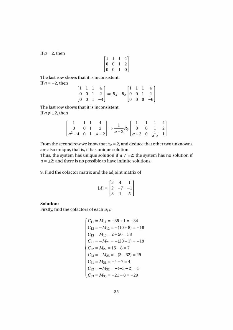
If a = 2, then 1 1 1 40 0 1 20 0 1 0
The last row shows that it is inconsistent.If a =−2, then 1 1 1 4
0 0 1 20 0 1 −4
⇒ R3 −R2
1 1 1 40 0 1 20 0 0 −6
The last row shows that it is inconsistent.If a 6= ±2, then 1 1 1 4
0 0 1 2a2 −4 0 1 a −2
⇒ 1
a −2R3
1 1 1 40 0 1 2
a +2 0 1a−2 1
From the second row we know that x2 = 2, and deduce that other two unknownsare also unique, that is, it has unique solution.Thus, the system has unique solution if a 6= ±2; the system has no solution ifa =±2; and there is no possible to have infinite solutions.
9. Find the cofactor matrix and the adjoint matrix of
[A] =3 4 1
2 −7 −18 1 5
Solution:Firstly, find the cofactors of each ai j :
C11 = M11 =−35+1 =−34
C12 =−M12 =−(10+8) =−18
C13 = M13 = 2+56 = 58
C21 =−M21 =−(20−1) =−19
C22 = M22 = 15−8 = 7
C23 =−M23 =−(3−32) = 29
C31 = M31 =−4+7 = 4
C32 =−M32 =−(−3−2) = 5
C33 = M33 =−21−8 =−29
35
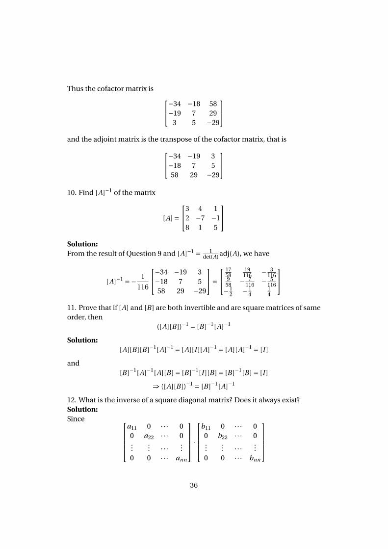
Thus the cofactor matrix is −34 −18 58−19 7 29
3 5 −29
and the adjoint matrix is the transpose of the cofactor matrix, that is−34 −19 3
−18 7 558 29 −29
10. Find [A]−1 of the matrix
[A] =3 4 1
2 −7 −18 1 5
Solution:From the result of Question 9 and [A]−1 = 1
det(A) adj(A), we have
[A]−1 =− 1
116
−34 −19 3−18 7 558 29 −29
= 17
5819
116 − 3116
958 − 7
116 − 5116
−12 −1
414
11. Prove that if [A] and [B ] are both invertible and are square matrices of sameorder, then
([A][B ])−1 = [B ]−1[A]−1
Solution:[A][B ][B ]−1[A]−1 = [A][I ][A]−1 = [A][A]−1 = [I ]
and[B ]−1[A]−1[A][B ] = [B ]−1[I ][B ] = [B ]−1[B ] = [I ]
⇒ ([A][B ])−1 = [B ]−1[A]−1
12. What is the inverse of a square diagonal matrix? Does it always exist?Solution:Since
a11 0 · · · 00 a22 · · · 0...
... · · · ...0 0 · · · ann
·
b11 0 · · · 0
0 b22 · · · 0...
... · · · ...0 0 · · · bnn
36
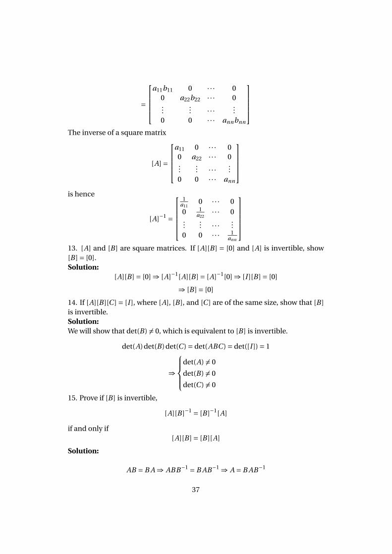
=
a11b11 0 · · · 0
0 a22b22 · · · 0...
... · · · ...0 0 · · · annbnn
The inverse of a square matrix
[A] =
a11 0 · · · 00 a22 · · · 0...
... · · · ...0 0 · · · ann
is hence
[A]−1 =
1
a110 · · · 0
0 1a22
· · · 0...
... · · · ...0 0 · · · 1
ann
13. [A] and [B ] are square matrices. If [A][B ] = [0] and [A] is invertible, show[B ] = [0].Solution:
[A][B ] = [0] ⇒ [A]−1[A][B ] = [A]−1[0] ⇒ [I ][B ] = [0]
⇒ [B ] = [0]
14. If [A][B ][C ] = [I ], where [A], [B ], and [C ] are of the same size, show that [B ]is invertible.Solution:We will show that det(B) 6= 0, which is equivalent to [B ] is invertible.
det(A)det(B)det(C ) = det(ABC ) = det([I ]) = 1
⇒
det(A) 6= 0
det(B) 6= 0
det(C ) 6= 0
15. Prove if [B ] is invertible,
[A][B ]−1 = [B ]−1[A]
if and only if[A][B ] = [B ][A]
Solution:
AB = B A ⇒ ABB−1 = B AB−1 ⇒ A = B AB−1
37
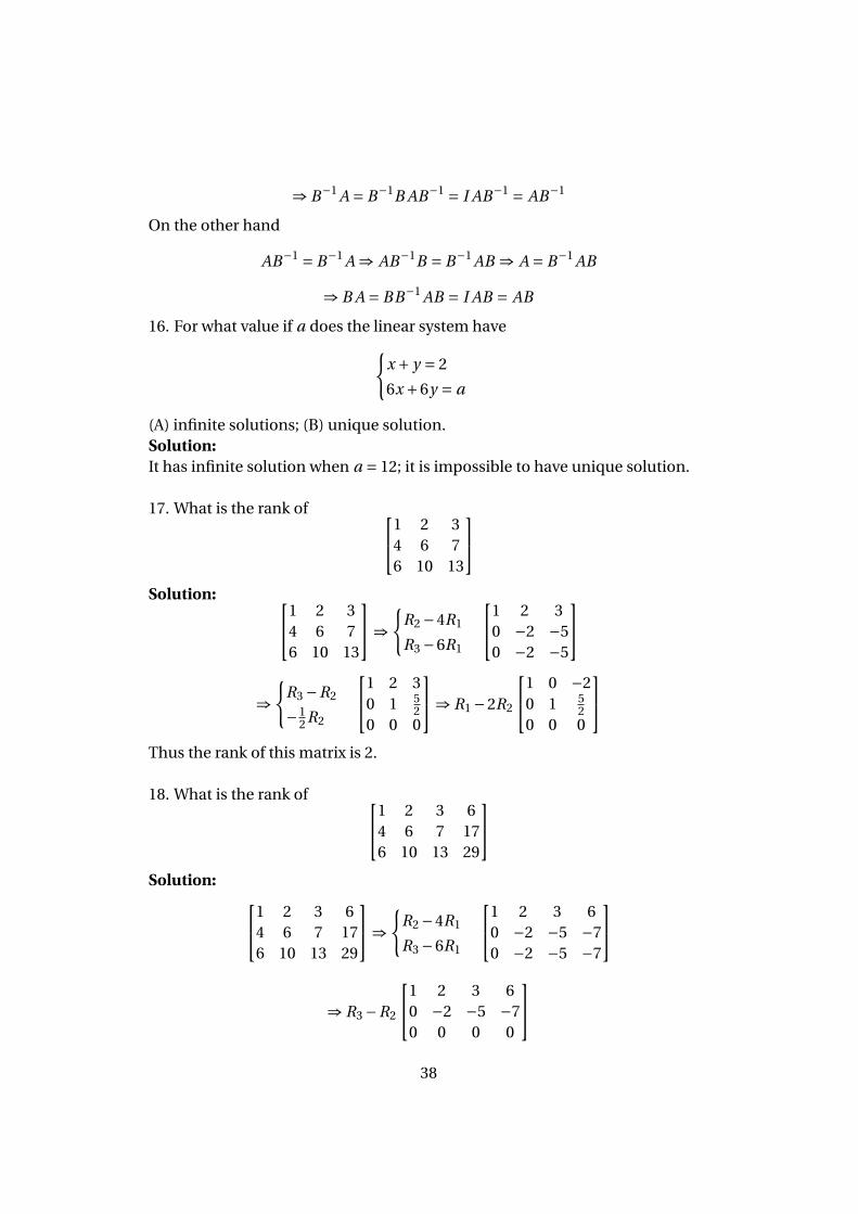
⇒ B−1 A = B−1B AB−1 = I AB−1 = AB−1
On the other hand
AB−1 = B−1 A ⇒ AB−1B = B−1 AB ⇒ A = B−1 AB
⇒ B A = BB−1 AB = I AB = AB
16. For what value if a does the linear system have{x + y = 2
6x +6y = a
(A) infinite solutions; (B) unique solution.Solution:It has infinite solution when a = 12; it is impossible to have unique solution.
17. What is the rank of 1 2 34 6 76 10 13
Solution: 1 2 3
4 6 76 10 13
⇒{
R2 −4R1
R3 −6R1
1 2 30 −2 −50 −2 −5
⇒{
R3 −R2
−12 R2
1 2 30 1 5
20 0 0
⇒ R1 −2R2
1 0 −20 1 5
20 0 0
Thus the rank of this matrix is 2.
18. What is the rank of 1 2 3 64 6 7 176 10 13 29
Solution: 1 2 3 6
4 6 7 176 10 13 29
⇒{
R2 −4R1
R3 −6R1
1 2 3 60 −2 −5 −70 −2 −5 −7
⇒ R3 −R2
1 2 3 60 −2 −5 −70 0 0 0
38
The rank of this matrix is 2.
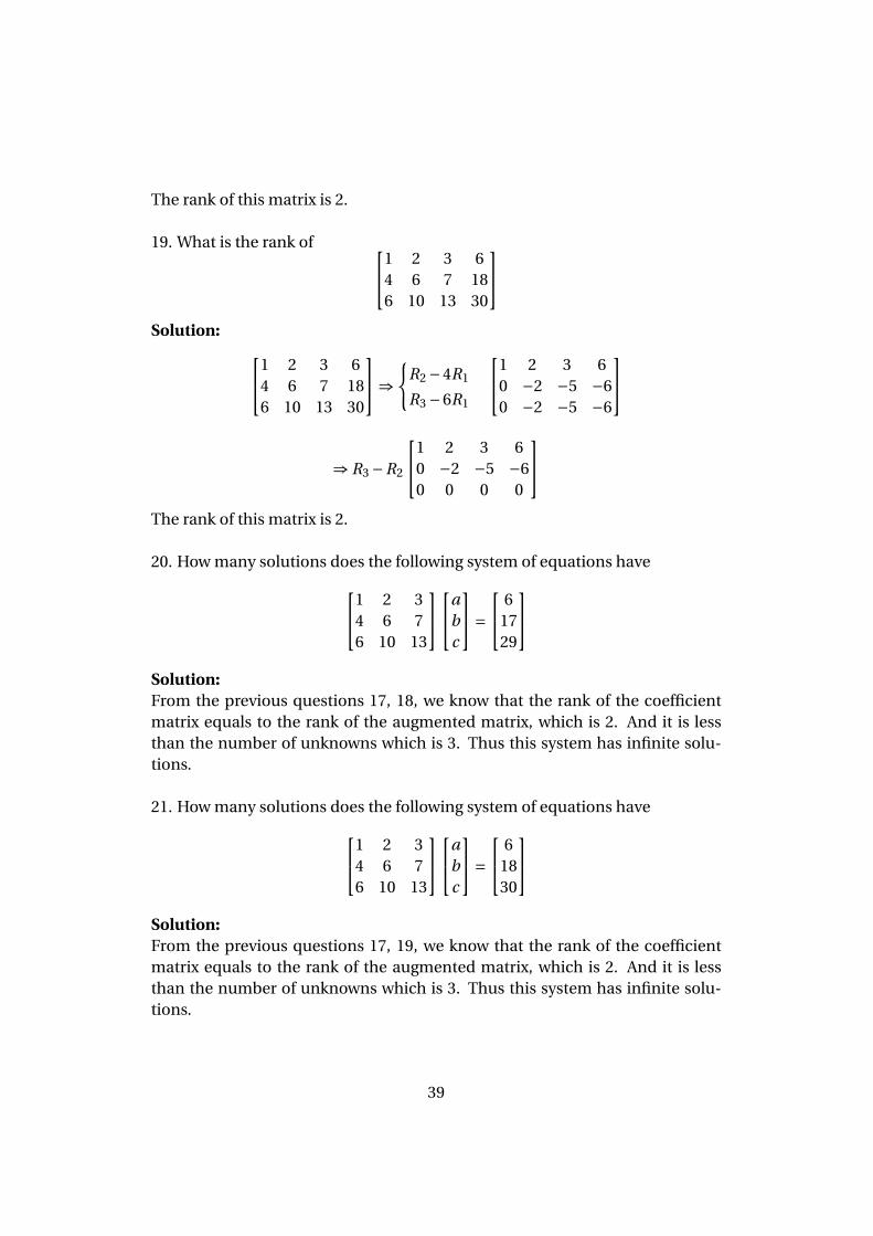
19. What is the rank of 1 2 3 64 6 7 186 10 13 30
Solution: 1 2 3 6
4 6 7 186 10 13 30
⇒{
R2 −4R1
R3 −6R1
1 2 3 60 −2 −5 −60 −2 −5 −6
⇒ R3 −R2
1 2 3 60 −2 −5 −60 0 0 0
The rank of this matrix is 2.
20. How many solutions does the following system of equations have1 2 34 6 76 10 13
abc
= 6
1729
Solution:From the previous questions 17, 18, we know that the rank of the coefficientmatrix equals to the rank of the augmented matrix, which is 2. And it is lessthan the number of unknowns which is 3. Thus this system has infinite solu-tions.
21. How many solutions does the following system of equations have1 2 34 6 76 10 13
abc
= 6
1830
Solution:From the previous questions 17, 19, we know that the rank of the coefficientmatrix equals to the rank of the augmented matrix, which is 2. And it is lessthan the number of unknowns which is 3. Thus this system has infinite solu-tions.
39

22. Find the second column of the inverse of1 2 04 5 00 0 13
Solution:
The second column of the product is
010
, which is the product of the given
matrix and the second column of its inverse, say
x1
x2
x3
. Thus we have
1 2 04 5 00 0 13
x1
x2
x3
=0
10
⇒
x1 +2x2 = 0
4x1 +5x2 = 1
13x3 = 0
⇒
x1 = 2
3
x2 =−13
x3 = 0
⇒ 2
3−1
30
23. Write out the inverse of
1 0 0 00 2 0 00 0 4 00 0 0 5
Solution:
1 0 0 00 1
2 0 00 0 1
4 00 0 0 1
5
24. Solve [A][X ] = [B ] for [X ] if
[A]−1 =10 −7 0
2 2 52 0 6
and
[B ] = 7
2.56.012
40
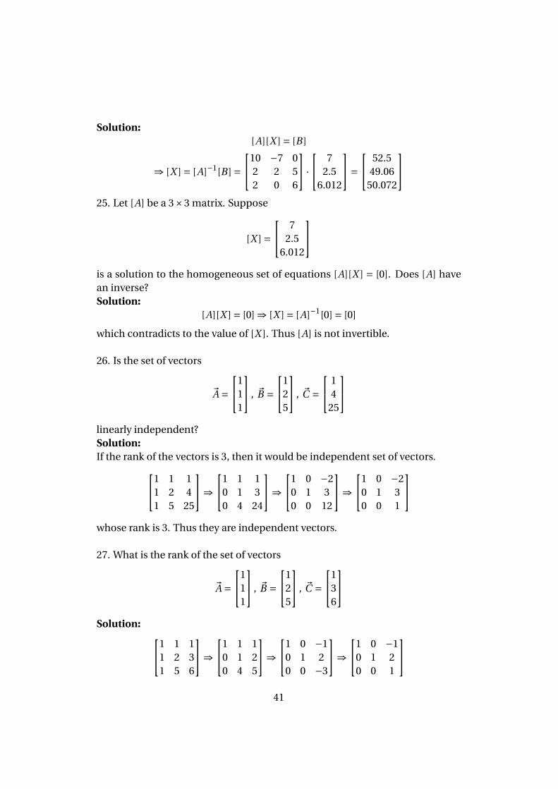
Solution:[A][X ] = [B ]
⇒ [X ] = [A]−1[B ] =10 −7 0
2 2 52 0 6
· 7
2.56.012
= 52.5
49.0650.072
25. Let [A] be a 3×3 matrix. Suppose
[X ] = 7
2.56.012
is a solution to the homogeneous set of equations [A][X ] = [0]. Does [A] havean inverse?Solution:
[A][X ] = [0] ⇒ [X ] = [A]−1[0] = [0]
which contradicts to the value of [X ]. Thus [A] is not invertible.
26. Is the set of vectors
~A =1
11
, ~B =1
25
, ~C = 1
425
linearly independent?Solution:If the rank of the vectors is 3, then it would be independent set of vectors.1 1 1
1 2 41 5 25
⇒1 1 1
0 1 30 4 24
⇒1 0 −2
0 1 30 0 12
⇒1 0 −2
0 1 30 0 1
whose rank is 3. Thus they are independent vectors.
27. What is the rank of the set of vectors
~A =1
11
, ~B =1
25
, ~C =1
36
Solution: 1 1 1
1 2 31 5 6
⇒1 1 1
0 1 20 4 5
⇒1 0 −1
0 1 20 0 −3
⇒1 0 −1
0 1 20 0 1
41
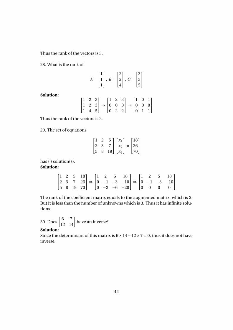
Thus the rank of the vectors is 3.
28. What is the rank of
~A =1
11
, ~B =2
24
, ~C =3
35
Solution: 1 2 3
1 2 31 4 5
⇒1 2 3
0 0 00 2 2
⇒1 0 1
0 0 00 1 1
Thus the rank of the vectors is 2.
29. The set of equations 1 2 52 3 75 8 19
x1
x2
x3
=18
2670
has ( ) solution(s).Solution:1 2 5 18
2 3 7 265 8 19 70
⇒1 2 5 18
0 −1 −3 −100 −2 −6 −20
⇒1 2 5 18
0 −1 −3 −100 0 0 0
The rank of the coefficient matrix equals to the augmented matrix, which is 2.But it is less than the number of unknowns which is 3. Thus it has infinite solu-tions.
30. Does
[6 7
12 14
]have an inverse?
Solution:Since the determinant of this matrix is 6×14−12×7 = 0, thus it does not haveinverse.
42
6 Gaussian Elimination
6.1 Summary
• Gaussian elimination consists of two steps:
– Forward Elimination of UnknownsIn this step, the unknown is eliminated in each equation startingwith the first equation. This way, the equations are reduced to oneequation and one unknown in each equation.
– Back SubstitutionIn this step, starting from the last equation, each of the unknowns isfound.
• More about determinant
– Let [A] be a n×n matrix. Then if [B ] is a n×n matrix that results fromadding or subtracting a multiple of one row (column) to another row(column), then det(A) = det(B).
– Let [A] be a n×n matrix that is upper triangular, lower triangular ordiagonal, then
det(A) = a11 ×a22 ×·· ·×ann =n∏
i=1ai i
This implies that if we apply the forward elimination steps of Gaus-sian elimination method, the determinant of the matrix stays thesame according to the previous result. Then since at the end of theforward elimination steps, the resulting matrix is upper triangular,the determinant will be given by the above result.
6.2 Selected Problems
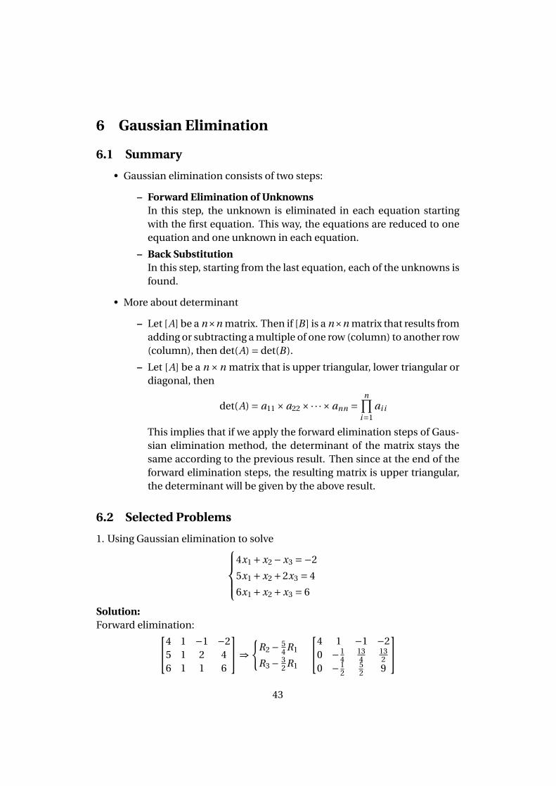
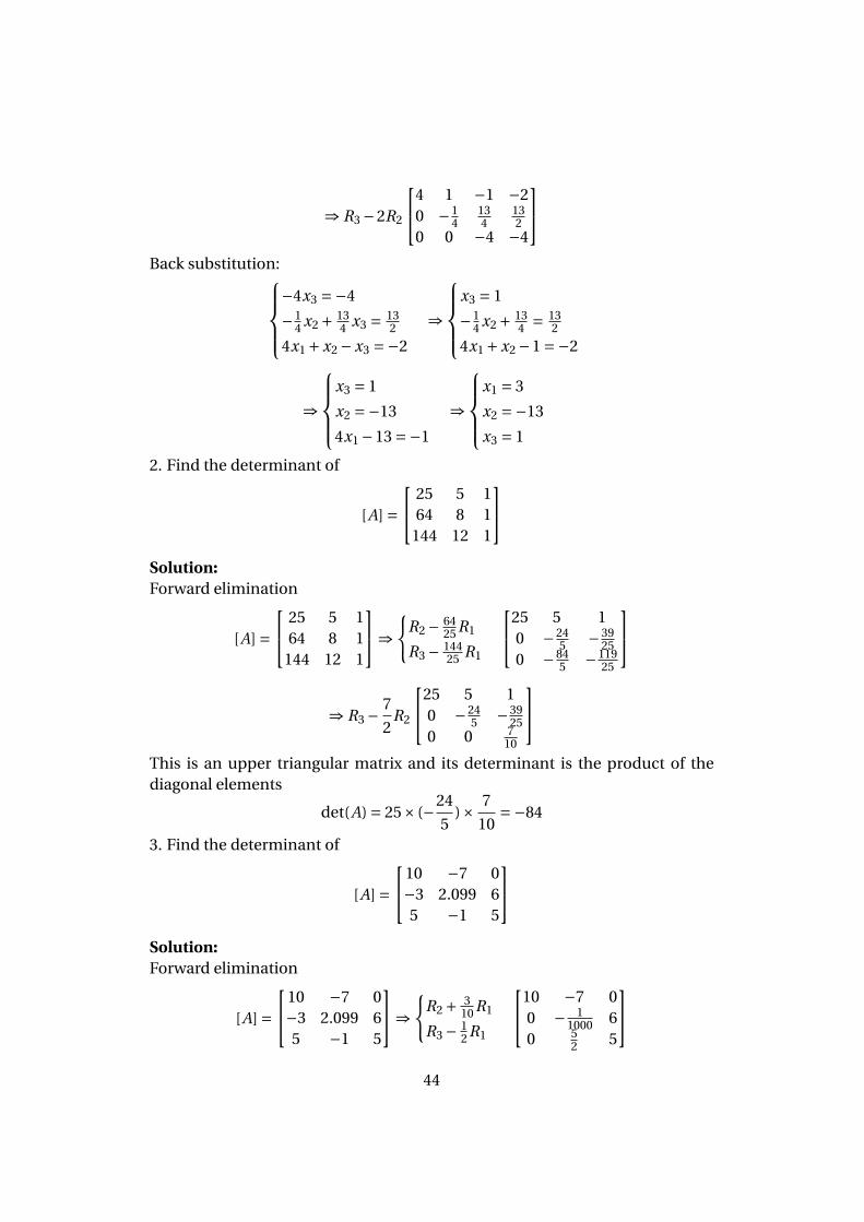
1. Using Gaussian elimination to solve4x1 +x2 −x3 =−2
5x1 +x2 +2x3 = 4
6x1 +x2 +x3 = 6
Solution:Forward elimination:4 1 −1 −2
5 1 2 46 1 1 6
⇒{
R2 − 54 R1
R3 − 32 R1
4 1 −1 −20 −1
4134
132
0 −12
52 9
43
⇒ R3 −2R2
4 1 −1 −20 −1
4134
132
0 0 −4 −4
Back substitution:
−4x3 =−4
−14 x2 + 13
4 x3 = 132
4x1 +x2 −x3 =−2
⇒
x3 = 1
−14 x2 + 13
4 = 132
4x1 +x2 −1 =−2
⇒
x3 = 1
x2 =−13
4x1 −13 =−1
⇒
x1 = 3
x2 =−13
x3 = 1
2. Find the determinant of
[A] = 25 5 1
64 8 1144 12 1
Solution:Forward elimination
[A] = 25 5 1
64 8 1144 12 1
⇒{
R2 − 6425 R1
R3 − 14425 R1
25 5 10 −24
5 −3925
0 −845 −119
25
⇒ R3 − 7
2R2
25 5 10 −24
5 −3925
0 0 710
This is an upper triangular matrix and its determinant is the product of thediagonal elements
det(A) = 25× (−24
5)× 7
10=−84
3. Find the determinant of
[A] =10 −7 0−3 2.099 65 −1 5
Solution:Forward elimination
[A] =10 −7 0−3 2.099 65 −1 5
⇒{
R2 + 310 R1
R3 − 12 R1
10 −7 00 − 1
1000 60 5
2 5
44
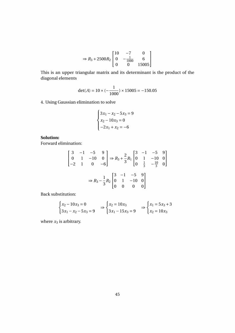
⇒ R3 +2500R2
10 −7 00 − 1
1000 60 0 15005
This is an upper triangular matrix and its determinant is the product of thediagonal elements
det(A) = 10× (− 1
1000)×15005 =−150.05
4. Using Gaussian elimination to solve3x1 −x2 −5x3 = 9
x2 −10x3 = 0
−2x1 +x2 =−6
Solution:Forward elimination: 3 −1 −5 9
0 1 −10 0−2 1 0 −6
⇒ R3 + 2
3R1
3 −1 −5 90 1 −10 00 1
3 −103 0
⇒ R3 − 1
3R2
3 −1 −5 90 1 −10 00 0 0 0
Back substitution:{
x2 −10x3 = 0
3x1 −x2 −5x3 = 9⇒
{x2 = 10x3
3x1 −15x3 = 9⇒
{x1 = 5x3 +3
x2 = 10x3
where x3 is arbitrary.
45
7 LU Decomposition
7.1 Summary
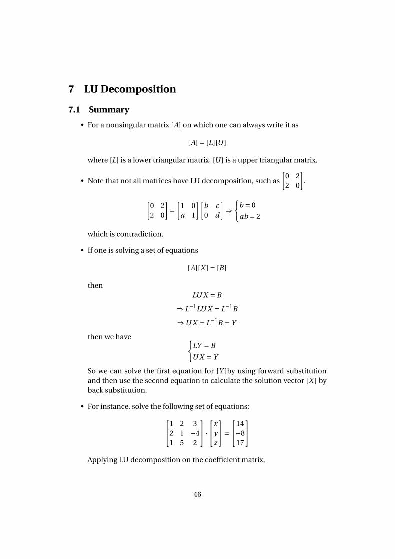
• For a nonsingular matrix [A] on which one can always write it as
[A] = [L][U ]
where [L] is a lower triangular matrix, [U ] is a upper triangular matrix.
• Note that not all matrices have LU decomposition, such as
[0 22 0
].
[0 22 0
]=
[1 0a 1
][b c0 d
]⇒
{b = 0
ab = 2
which is contradiction.
• If one is solving a set of equations
[A][X ] = [B ]
thenLU X = B
⇒ L−1LU X = L−1B
⇒U X = L−1B = Y
then we have {LY = B
U X = Y
So we can solve the first equation for [Y ]by using forward substitutionand then use the second equation to calculate the solution vector [X ] byback substitution.
• For instance, solve the following set of equations:1 2 32 1 −41 5 2
·x
yz
=14−817
Applying LU decomposition on the coefficient matrix,
46
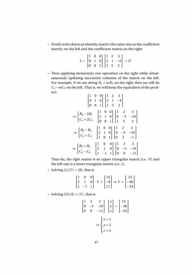
– Firstly write down an identity matrix (the same size as the coefficientmatrix) on the left and the coefficient matrix on the right.
L ←1 0 0
0 1 00 0 1
1 2 32 1 −41 5 2
→U
– Then applying elementary row operation on the right while simul-taneously updating successive columns of the matrix on the left.For example, if we are doing R1 +mR2 on the right then we will doC2−mC1 on the left. That is, we will keep the equivalent of the prod-uct. 1 0 0
0 1 00 0 1
1 2 32 1 −41 5 2
⇒{
R2 −2R1
C1 +2C2
1 0 02 1 00 0 1
1 2 30 −3 −101 5 2
⇒{
R3 −R1
C1 +C3
1 0 02 1 01 0 1
1 2 30 −3 −100 3 −1
⇒{
R3 +R2
C2 −C3
1 0 02 1 01 −1 1
1 2 30 −3 −100 0 −11
Thus far, the right matrix is an upper triangular matrix (i.e. U ) andthe left one is a lower triangular matrix (i.e. L).
– Solving [L][Y ] = [B ], that is1 0 02 1 01 −1 1
·Y =14−817
⇒ Y = 14−36−33
– Solving [U ][X ] = [Y ], that is1 2 3
0 −3 −100 0 −11
·x
yz
= 14−36−33
⇒
x = 1
y = 2
z = 3
47
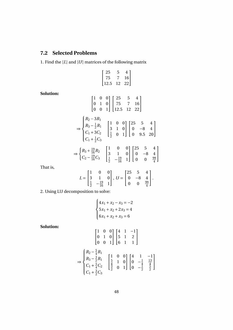
7.2 Selected Problems
1. Find the [L] and [U ] matrices of the following matrix 25 5 475 7 16
12.5 12 22
Solution: 1 0 0
0 1 00 0 1
25 5 475 7 16
12.5 12 22
⇒
R2 −3R1
R3 − 12 R1
C1 +3C2
C1 + 12C3
1 0 03 1 012 0 1
25 5 40 −8 40 9.5 20
⇒{
R3 + 1916 R2
C2 − 1916C3
1 0 03 1 012 −19
16 1
25 5 40 −8 40 0 99
4
That is,
L =1 0 0
3 1 012 −19
16 1
, U =25 5 4
0 −8 40 0 99
4
.
2. Using LU decomposition to solve:4x1 +x2 −x3 =−2
5x1 +x2 +2x3 = 4
6x1 +x2 +x3 = 6
Solution: 1 0 00 1 00 0 1
4 1 −15 1 26 1 1
⇒
R2 − 5
4 R1
R3 − 32 R1
C1 + 54C2
C1 + 32C3
1 0 054 1 032 0 1
4 1 −10 −1
4134
0 −12
52
48
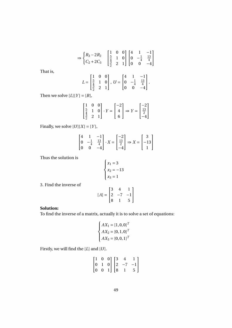
⇒{
R3 −2R2
C2 +2C3
1 0 054 1 032 2 1
4 1 −10 −1
4134
0 0 −4
That is,
L =1 0 0
54 1 032 2 1
, U =4 1 −1
0 −14
134
0 0 −4
.
Then we solve [L][Y ] = [B ],1 0 054 1 032 2 1
·Y =−2
46
⇒ Y =−2
132−4
Finally, we solve [U ][X ] = [Y ],4 1 −1
0 −14
134
0 0 −4
·X =−2
132−4
⇒ X = 3−13
1
Thus the solution is
x1 = 3
x2 =−13
x3 = 1
3. Find the inverse of
[A] =3 4 1
2 −7 −18 1 5
Solution:To find the inverse of a matrix, actually it is to solve a set of equations:
AX1 = [1,0,0]T
AX2 = [0,1,0]T
AX3 = [0,0,1]T
Firstly, we will find the [L] and [U ].1 0 00 1 00 0 1
3 4 12 −7 −18 1 5
49
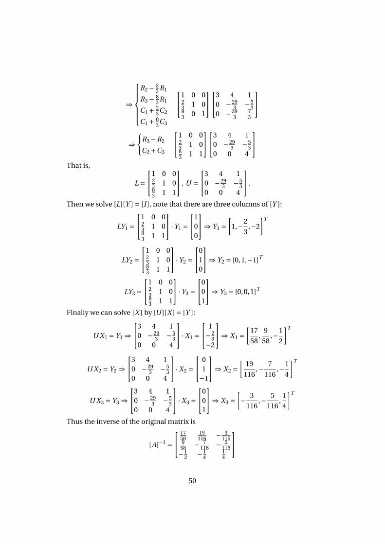
⇒
R2 − 2
3 R1
R3 − 83 R1
C1 + 23C2
C1 + 83C3
1 0 023 1 083 0 1
3 4 10 −29
3 −53
0 −293
73
⇒{
R3 −R2
C2 +C3
1 0 023 1 083 1 1
3 4 10 −29
3 −53
0 0 4
That is,
L =1 0 0
23 1 083 1 1
, U =3 4 1
0 −293 −5
30 0 4
.
Then we solve [L][Y ] = [I ], note that there are three columns of [Y ]:
LY1 =1 0 0
23 1 083 1 1
·Y1 =1
00
⇒ Y1 =[
1,−2
3,−2
]T
LY2 =1 0 0
23 1 083 1 1
·Y2 =0
10
⇒ Y2 = [0,1,−1]T
LY3 =1 0 0
23 1 083 1 1
·Y3 =0
01
⇒ Y3 = [0,0,1]T
Finally we can solve [X ] by [U ][X ] = [Y ]:
U X1 = Y1 ⇒3 4 1
0 −293 −5
30 0 4
·X1 = 1−2
3−2
⇒ X1 =[
17
58,
9
58,−1
2
]T
U X2 = Y2 ⇒3 4 1
0 −293 −5
30 0 4
·X2 = 0
1−1
⇒ X2 =[
19
116,− 7
116,−1
4
]T
U X3 = Y3 ⇒3 4 1
0 −293 −5
30 0 4
·X3 =0
01
⇒ X3 =[− 3
116,− 5
116,
1
4
]T
Thus the inverse of the original matrix is
[A]−1 = 17
5819
116 − 3116
958 − 7
116 − 5116
−12 −1
414
50
8 Gauss-Seidel Method
8.1 Summary
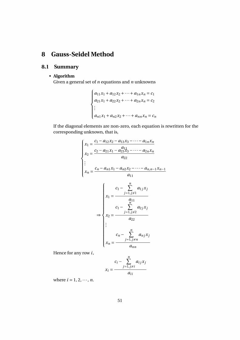
• AlgorithmGiven a general set of n equations and n unknowns
a11x1 +a12x2 +·· ·+a1n xn = c1
a21x1 +a22x2 +·· ·+a2n xn = c2...
an1x1 +an2x2 +·· ·+ann xn = cn
If the diagonal elements are non-zero, each equation is rewritten for thecorresponding unknown, that is,
x1 = c1 −a12x2 −a13x3 −·· ·−a1n xn
a11
x2 = c2 −a21x1 −a23x3 −·· ·−a2n xn
a22...
xn = cn −an1x1 −an2x2 −·· ·−an,n−1xn−1
a11
⇒
x1 =c1 −
n∑j=1, j 6=1
a1 j x j
a11
x2 =c1 −
n∑j=1, j 6=2
a2 j x j
a22...
xn =cn −
n∑j=1, j 6=n
an j x j
ann
Hence for any row i ,
xi =ci −
n∑j=1, j 6=i
ai j x j
ai i
where i = 1, 2, · · · , n.
51
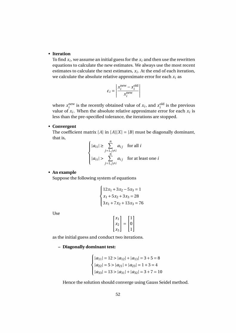
• IterationTo find xi , we assume an initial guess for the xi and then use the rewrittenequations to calculate the new estimates. We always use the most recentestimates to calculate the next estimates, xi . At the end of each iteration,we calculate the absolute relative approximate error for each xi as
εi =∣∣∣∣∣xnew
i −xoldi
xnewi
∣∣∣∣∣where xnew
i is the recently obtained value of xi , and xoldi is the previous
value of xi . When the absolute relative approximate error for each xi isless than the pre-specified tolerance, the iterations are stopped.
• ConvergentThe coefficient matrix [A] in [A][X ] = [B ] must be diagonally dominant,that is,
|ai i | ≥n∑
j=1, j 6=iai j for all i
|ai i | >n∑
j=1, j 6=iai j for at least one i
• An exampleSuppose the following system of equations
12x1 +3x2 −5x3 = 1
x1 +5x2 +3x3 = 28
3x1 +7x2 +13x3 = 76
Use x1
x2
x3
=1
01
as the initial guess and conduct two iterations.
– Diagonally dominant test:|a11| = 12 > |a12|+ |a13| = 3+5 = 8
|a22| = 5 > |a21|+ |a23| = 1+3 = 4
|a33| = 13 > |a31|+ |a32| = 3+7 = 10
Hence the solution should converge using Gauss Seidel method.
52
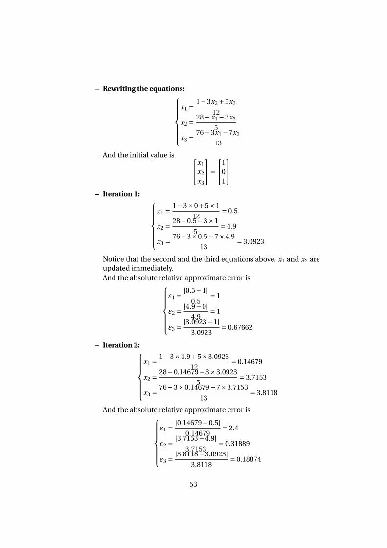
– Rewriting the equations:x1 = 1−3x2 +5x3
12x2 = 28−x1 −3x3
5x3 = 76−3x1 −7x2
13
And the initial value is x1
x2
x3
=1
01
– Iteration 1:
x1 = 1−3×0+5×1
12= 0.5
x2 = 28−0.5−3×1
5= 4.9
x3 = 76−3×0.5−7×4.9
13= 3.0923
Notice that the second and the third equations above, x1 and x2 areupdated immediately.And the absolute relative approximate error is
ε1 = |0.5−1|0.5
= 1
ε2 = |4.9−0|4.9
= 1
ε3 = |3.0923−1|3.0923
= 0.67662
– Iteration 2:x1 = 1−3×4.9+5×3.0923
12= 0.14679
x2 = 28−0.14679−3×3.0923
5= 3.7153
x3 = 76−3×0.14679−7×3.7153
13= 3.8118
And the absolute relative approximate error isε1 = |0.14679−0.5|
0.14679= 2.4
ε2 = |3.7153−4.9|3.7153
= 0.31889
ε3 = |3.8118−3.0923|3.8118
= 0.18874
53
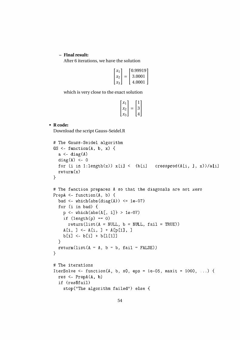
– Final result:After 6 iterations, we have the solutionx1
x2
x3
=0.99919
3.00014.0001
which is very close to the exact solutionx1
x2
x3
=1
34
• R code:
Download the script Gauss-Seidel.R
# The Gauss-Seidel algorithm
GS <- function(A, b, x) {
a <- diag(A)
diag(A) <- 0
for (i in 1:length(x)) x[i] <- (b[i] - crossprod(A[i, ], x))/a[i]
return(x)
}
# The function prepares A so that the diagonals are not zero
PrepA <- function(A, b) {
bad <- which(abs(diag(A)) <= 1e-07)
for (i in bad) {
p <- which(abs(A[, i]) > 1e-07)
if (length(p) == 0)
return(list(A = NULL, b = NULL, fail = TRUE))
A[i, ] <- A[i, ] + A[p[1], ]
b[i] <- b[i] + b[l[1]]
}
return(list(A = A, b = b, fail = FALSE))
}
# The iterations
IterSolve <- function(A, b, x0, eps = 1e-05, maxit = 1000, ...) {
res <- PrepA(A, b)
if (res$fail)
stop("The algorithm failed") else {
54
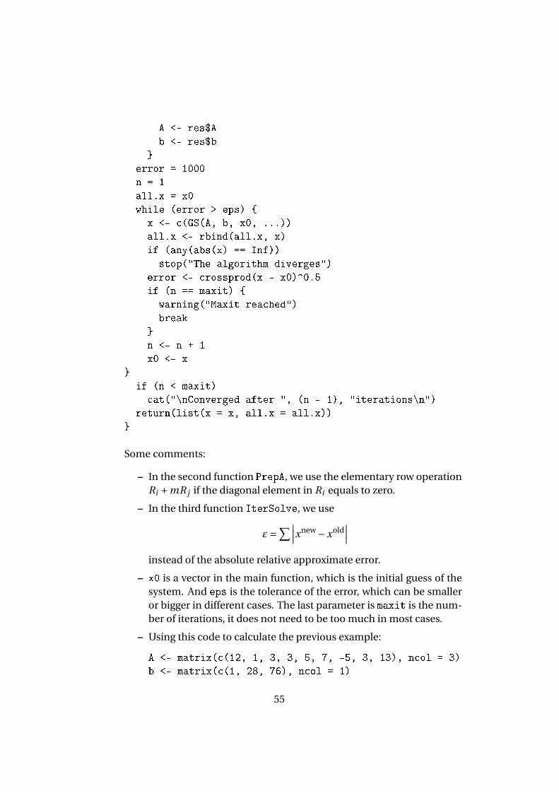
A <- res$A
b <- res$b
}
error = 1000
n = 1
all.x = x0
while (error > eps) {
x <- c(GS(A, b, x0, ...))
all.x <- rbind(all.x, x)
if (any(abs(x) == Inf))
stop("The algorithm diverges")
error <- crossprod(x - x0)^0.5
if (n == maxit) {
warning("Maxit reached")
break
}
n <- n + 1
x0 <- x
}
if (n < maxit)
cat("\nConverged after ", (n - 1), "iterations\n")
return(list(x = x, all.x = all.x))
}
Some comments:
– In the second function PrepA, we use the elementary row operationRi +mR j if the diagonal element in Ri equals to zero.
– In the third function IterSolve, we use
ε=∑∣∣∣xnew −xold∣∣∣
instead of the absolute relative approximate error.
– x0 is a vector in the main function, which is the initial guess of thesystem. And eps is the tolerance of the error, which can be smalleror bigger in different cases. The last parameter is maxit is the num-ber of iterations, it does not need to be too much in most cases.
– Using this code to calculate the previous example:
A <- matrix(c(12, 1, 3, 3, 5, 7, -5, 3, 13), ncol = 3)
b <- matrix(c(1, 28, 76), ncol = 1)
55
IterSolve(A, b, c(1, 0, 1))$x
# Result
# Converged after 11 iterations
# [1] 1 3 4
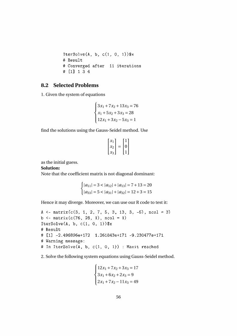
8.2 Selected Problems
1. Given the system of equations3x1 +7x2 +13x3 = 76
x1 +5x2 +3x3 = 28
12x1 +3x2 −5x3 = 1
find the solutions using the Gauss-Seidel method. Usex1
x2
x3
=1
01
as the initial guess.Solution:Note that the coefficient matrix is not diagonal dominant:{
|a11| = 3 < |a12|+ |a13| = 7+13 = 20
|a33| = 5 < |a31|+ |a32| = 12+3 = 15
Hence it may diverge. Moreover, we can use our R code to test it:
A <- matrix(c(3, 1, 2, 7, 5, 3, 13, 3, -5), ncol = 3)
b <- matrix(c(76, 28, 1), ncol = 1)
IterSolve(A, b, c(1, 0, 1))$x
# Result
# [1] -2.496896e+172 1.261843e+171 -9.230477e+171
# Warning message:
# In IterSolve(A, b, c(1, 0, 1)) : Maxit reached
2. Solve the following system equations using Gauss-Seidel method.12x1 +7x2 +3x3 = 17
3x1 +6x2 +2x3 = 9
2x1 +7x2 −11x3 = 49
56
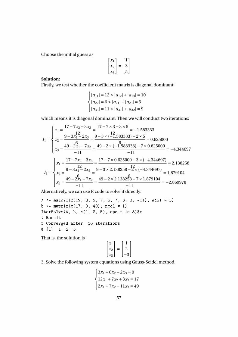
Choose the initial guess as x1
x2
x3
=1
35
Solution:Firstly, we test whether the coefficient matrix is diagonal dominant:
|a11| = 12 > |a12|+ |a13| = 10
|a22| = 6 > |a21|+ |a23| = 5
|a33| = 11 > |a31|+ |a32| = 9
which means it is diagonal dominant. Then we will conduct two iterations:
I1 =
x1 = 17−7x2 −3x3
12= 17−7×3−3×5
12=−1.583333
x2 = 9−3x1 −2x3
6= 9−3× (−1.583333)−2×5
6= 0.625000
x3 = 49−2x1 −7x2
−11= 49−2× (−1.583333)−7×0.625000
−11=−4.344697
I2 =
x1 = 17−7x2 −3x3
12= 17−7×0.625000−3× (−4.344697)
12= 2.138258
x2 = 9−3x1 −2x3
6= 9−3×2.138258−2× (−4.344697)
6= 1.879104
x3 = 49−2x1 −7x2
−11= 49−2×2.138258−7×1.879104
−11=−2.869978
Alternatively, we can use R code to solve it directly:
A <- matrix(c(12, 3, 2, 7, 6, 7, 3, 2, -11), ncol = 3)
b <- matrix(c(17, 9, 49), ncol = 1)
IterSolve(A, b, c(1, 3, 5), eps = 1e-8)$x
# Result
# Converged after 16 iterations
# [1] 1 2 -3
That is, the solution is x1
x2
x3
= 1
2−3
3. Solve the following system equations using Gauss-Seidel method.
3x1 +6x2 +2x3 = 9
12x1 +7x2 +3x3 = 17
2x1 +7x2 −11x3 = 49
57
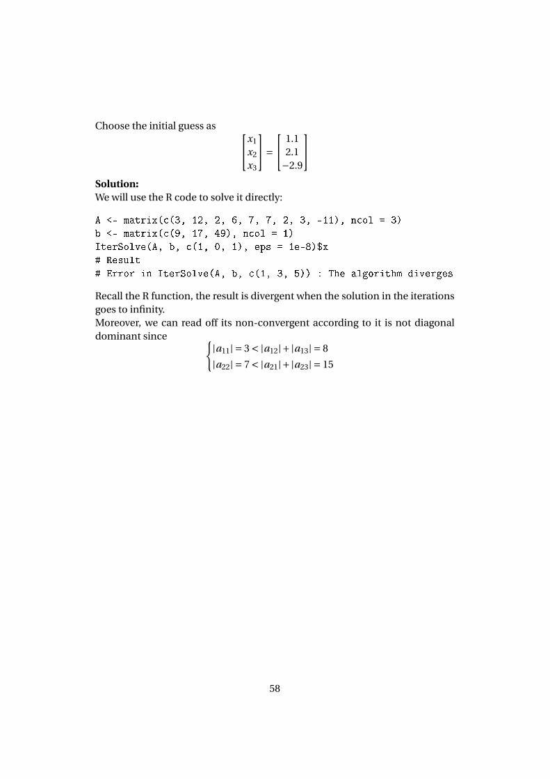
Choose the initial guess as x1
x2
x3
= 1.1
2.1−2.9
Solution:We will use the R code to solve it directly:
A <- matrix(c(3, 12, 2, 6, 7, 7, 2, 3, -11), ncol = 3)
b <- matrix(c(9, 17, 49), ncol = 1)
IterSolve(A, b, c(1, 0, 1), eps = 1e-8)$x
# Result
# Error in IterSolve(A, b, c(1, 3, 5)) : The algorithm diverges
Recall the R function, the result is divergent when the solution in the iterationsgoes to infinity.Moreover, we can read off its non-convergent according to it is not diagonaldominant since {
|a11| = 3 < |a12|+ |a13| = 8
|a22| = 7 < |a21|+ |a23| = 15
58
9 Adequacy of Solutions
9.1 Summary
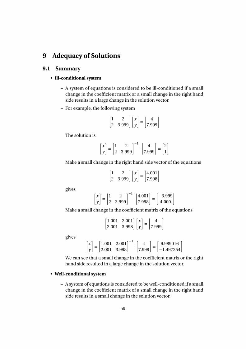
• Ill-conditional system
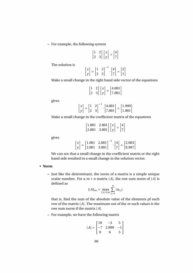
– A system of equations is considered to be ill-conditioned if a smallchange in the coefficient matrix or a small change in the right handside results in a large change in the solution vector.
– For example, the following system[1 22 3.999
][xy
]=
[4
7.999
]The solution is [
xy
]=
[1 22 3.999
]−1
·[
47.999
]=
[21
]Make a small change in the right hand side vector of the equations[
1 22 3.999
][xy
]=
[4.0017.998
]gives [
xy
]=
[1 22 3.999
]−1
·[
4.0017.998
]=
[−3.9994.000
]Make a small change in the coefficient matrix of the equations[
1.001 2.0012.001 3.998
][xy
]=
[4
7.999
]gives [
xy
]=
[1.001 2.0012.001 3.998
]−1
·[
47.999
]=
[6.989016−1.497254
]We can see that a small change in the coefficient matrix or the righthand side resulted in a large change in the solution vector.
• Well-conditional system
– A system of equations is considered to be well-conditioned if a smallchange in the coefficient matrix of a small change in the right handside results in a small change in the solution vector.
59
– For example, the following system[1 22 3
][xy
]=
[47
]The solution is [
xy
]=
[1 22 3
]−1
·[
47
]=
[21
]Make a small change in the right hand side vector of the equations[
1 22 3
][xy
]=
[4.0017.001
]gives [
xy
]=
[1 22 3
]−1
·[
4.0017.001
]=
[1.9991.001
]Make a small change in the coefficient matrix of the equations[
1.001 2.0012.001 3.001
][xy
]=
[47
]gives [
xy
]=
[1.001 2.0012.001 3.001
]−1
·[
47
]=
[2.0030.997
]We can see that a small change in the coefficient matrix or the righthand side resulted in a small change in the solution vector.
• Norm
– Just like the determinant, the norm of a matrix is a simple uniquescalar number. For a m ×n matrix [A], the row sum norm of [A] isdefined as
‖A‖∞ = max1≤i≤m
n∑j=1
|ai j |
that is, find the sum of the absolute value of the elements pf eachrow of the matrix [A]. The maximum out of the m such values is therow sum norm if the matrix [A].
– For example, we have the following matrix
[A] =10 −3 5−7 2.099 −10 6 5
60
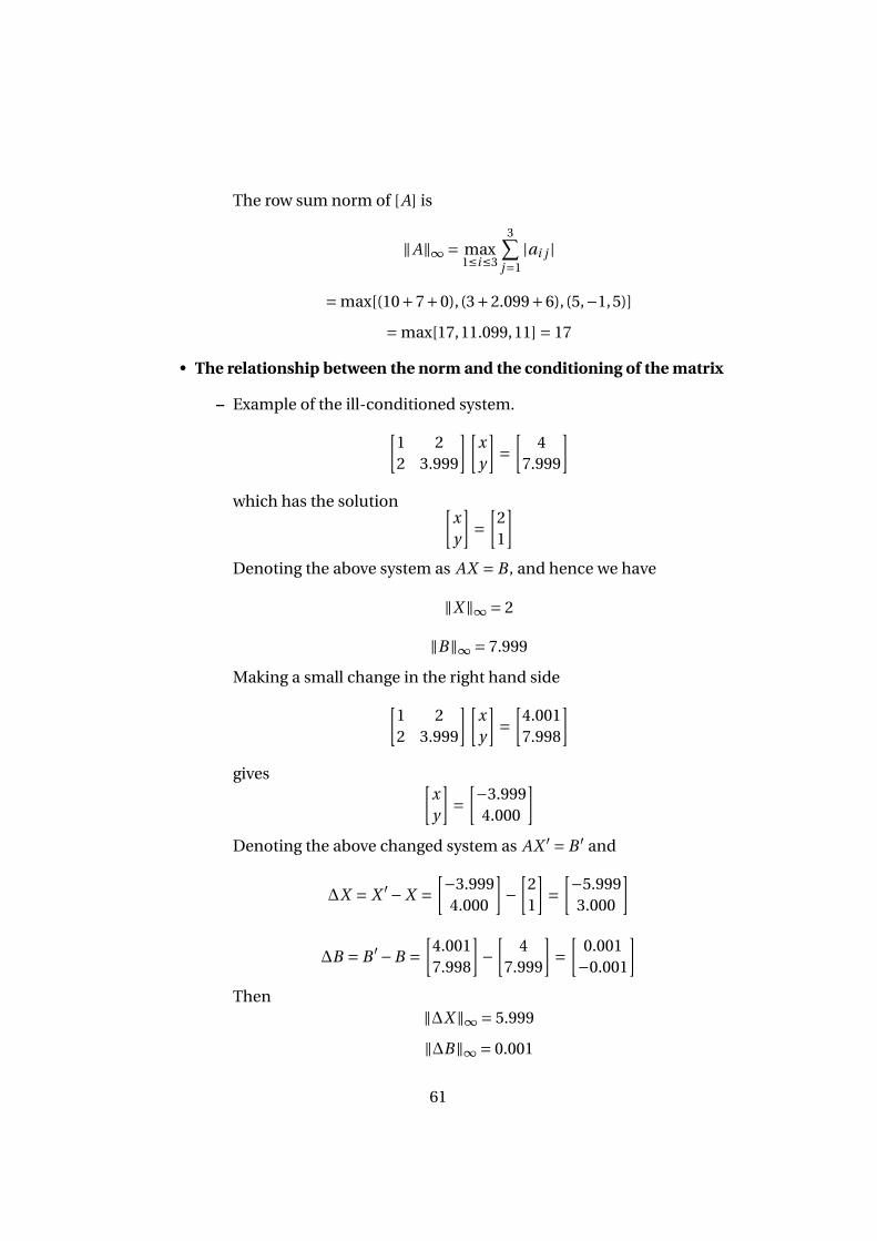
The row sum norm of [A] is
‖A‖∞ = max1≤i≤3
3∑j=1
|ai j |
= max[(10+7+0), (3+2.099+6), (5,−1,5)]
= max[17,11.099,11] = 17
• The relationship between the norm and the conditioning of the matrix
– Example of the ill-conditioned system.[1 22 3.999
][xy
]=
[4
7.999
]which has the solution [
xy
]=
[21
]Denoting the above system as AX = B , and hence we have
‖X ‖∞ = 2
‖B‖∞ = 7.999
Making a small change in the right hand side[1 22 3.999
][xy
]=
[4.0017.998
]gives [
xy
]=
[−3.9994.000
]Denoting the above changed system as AX ′ = B ′ and
∆X = X ′−X =[−3.999
4.000
]−
[21
]=
[−5.9993.000
]
∆B = B ′−B =[
4.0017.998
]−
[4
7.999
]=
[0.001−0.001
]Then
‖∆X ‖∞ = 5.999
‖∆B‖∞ = 0.001
61
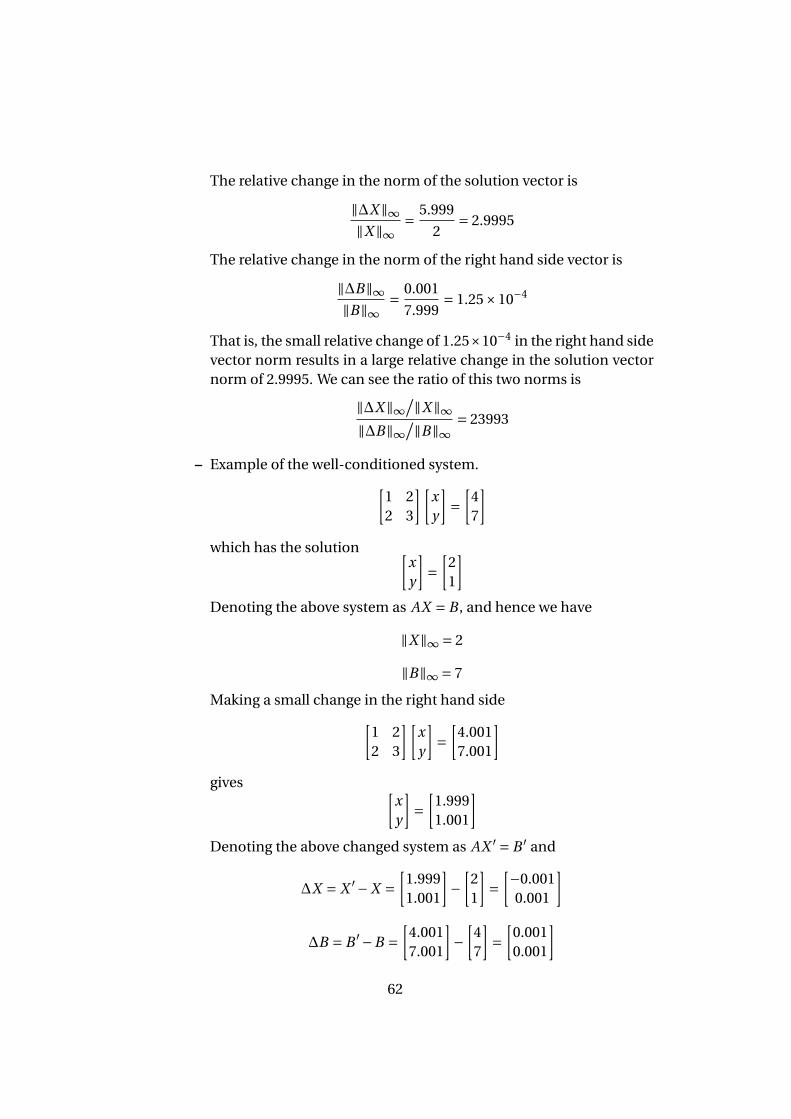
The relative change in the norm of the solution vector is
‖∆X ‖∞‖X ‖∞
= 5.999
2= 2.9995
The relative change in the norm of the right hand side vector is
‖∆B‖∞‖B‖∞
= 0.001
7.999= 1.25×10⁻⁴
That is, the small relative change of 1.25×10⁻⁴ in the right hand sidevector norm results in a large relative change in the solution vectornorm of 2.9995. We can see the ratio of this two norms is
‖∆X ‖∞/‖X ‖∞
‖∆B‖∞/‖B‖∞
= 23993
– Example of the well-conditioned system.[1 22 3
][xy
]=
[47
]which has the solution [
xy
]=
[21
]Denoting the above system as AX = B , and hence we have
‖X ‖∞ = 2
‖B‖∞ = 7
Making a small change in the right hand side[1 22 3
][xy
]=
[4.0017.001
]gives [
xy
]=
[1.9991.001
]Denoting the above changed system as AX ′ = B ′ and
∆X = X ′−X =[
1.9991.001
]−
[21
]=
[−0.0010.001
]
∆B = B ′−B =[
4.0017.001
]−
[47
]=
[0.0010.001
]62
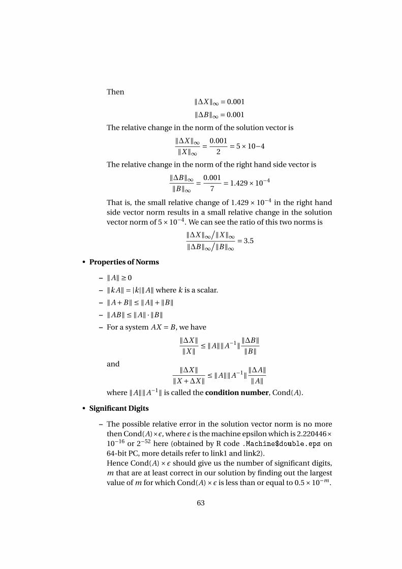
Then‖∆X ‖∞ = 0.001
‖∆B‖∞ = 0.001
The relative change in the norm of the solution vector is
‖∆X ‖∞‖X ‖∞
= 0.001
2= 5×10⁻⁴
The relative change in the norm of the right hand side vector is
‖∆B‖∞‖B‖∞
= 0.001
7= 1.429×10⁻⁴
That is, the small relative change of 1.429× 10⁻⁴ in the right handside vector norm results in a small relative change in the solutionvector norm of 5×10⁻⁴. We can see the ratio of this two norms is
‖∆X ‖∞/‖X ‖∞
‖∆B‖∞/‖B‖∞
= 3.5
• Properties of Norms
– ‖A‖ ≥ 0
– ‖k A‖ = |k|‖A‖ where k is a scalar.
– ‖A+B‖ ≤ ‖A‖+‖B‖– ‖AB‖ ≤ ‖A‖ ·‖B‖– For a system AX = B , we have
‖∆X ‖‖X ‖ ≤ ‖A‖‖A−1‖‖∆B‖
‖B‖and ‖∆X ‖
‖X +∆X ‖ ≤ ‖A‖‖A−1‖‖∆A‖‖A‖
where ‖A‖‖A−1‖ is called the condition number, Cond(A).
• Significant Digits
– The possible relative error in the solution vector norm is no morethen Cond(A)×ε, where ε is the machine epsilon which is 2.220446×10⁻¹⁶ or 2−52 here (obtained by R code .Machine$double.eps on64-bit PC, more details refer to link1 and link2).Hence Cond(A)× ε should give us the number of significant digits,m that are at least correct in our solution by finding out the largestvalue of m for which Cond(A)×ε is less than or equal to 0.5×10−m .
63
– How many significant digits can I trust in the solution of the follow-ing system of equations? [
1 22 3
][xy
]=
[47
]For
A =[
1 22 3
]and
A−1 =[−3 2
2 −1
]Then
‖A‖∞ = 5, ‖A−1‖∞ = 5 ⇒ Cond(A) = ‖A‖∞‖A−1‖∞ = 25
ThusCond(A)×ε≤ 0.5×10−m
⇒ 25×ε≤ 0.5×10−m
⇒ log(25×ε) ≤ log(0.5×10−m)
⇒ m ≤ 13.95459
That is, 13 digits are at least correct in the solution vector.
9.2 Selected Problems
1. What factors does the adequacy of the solution of simultaneous linear equa-tions depend on?Solution:The product of condition number Cond(A) = ‖A‖‖A−1‖ and machine epsilon ε.
2. If a system of equations [A][X ] = [B ] is ill-conditioned, thenA. det(A) = 0B. Cond(A) = 1C. Cond(A) is largeD. ‖A‖ is largeSolution:If the system is ill-conditioned, then the condition number Cond(A) = ‖A‖‖A−1‖is large. The correct answer is C.
3. If Cond(A) = 104 and ε= 0.119×10⁻⁶, then in [A][X ] = [B ], at least how many
64
significant digits are correct in the solution?Solution:
Cond(A)×ε≤ 0.5×10−m
⇒ 104 ×0.119×10−6 ≤ 0.5×10−m
⇒ m ≤ log(0.5)− log(0.119×10⁻²)
log(10)= 2.623423
Thus at least 2 significant digits are correct in the solution.
4. Make a small change in the coefficient matrix of[1 22 3.999
][xy
]=
[4
7.999
]and find
‖∆X ‖∞/‖X ‖∞
‖∆A‖∞/‖A‖∞
Solution:The solution of the original system is[
xy
]=
[21
]Making a small change in the coefficient matrix as[
1.001 2.0012.001 4.000
][xy
]=
[4
7.999
]and the solution is [
xy
]=
[5999−2999
]Hence the row sum norms are
‖X ‖ = 2, ‖∆X ‖ = 5997, ‖A‖ = 5.999, ‖∆A‖ = 0.002
Thus the ratio is
‖∆X ‖∞/‖X ‖∞
‖∆A‖∞/‖A‖∞
= 5997/
2
0.002/
5.999= 8994001
65
It is a large number. Hence we can conclude that this system is ill-conditioned.On the other hand, we can calculate the condition number of the coefficient
matrix, note that A−1 =[−3999 2000
2000 −1000
], and hence
‖A‖‖A−1‖ = 5.999×5999 = 35988
which is also a large number.
5. Make a small change in the coefficient matrix of[1 22 3
][xy
]=
[47
]and find
‖∆X ‖∞/‖X ‖∞
‖∆A‖∞/‖A‖∞
Solution:The solution of the original system is[
xy
]=
[21
]Making a small change in the coefficient matrix as[
1.001 2.0012.001 3.001
][xy
]=
[47
]and the solution is [
xy
]=
[2.0030.997
]Hence the row sum norms are
‖X ‖ = 2, ‖∆X ‖ = 0.003, ‖A‖ = 5, ‖∆A‖ = 0.002
Thus the ratio is‖∆X ‖∞
/‖X ‖∞‖∆A‖∞
/‖A‖∞= 0.003
/2
0.002/
5= 3.75
It is a small number. Hence we can conclude that this system is well-conditioned.On the other hand, we can calculate the condition number of the coefficient
matrix, note that A−1 =[−3 2
2 −1
], and hence
‖A‖‖A−1‖ = 5×5 = 25
66
which is also a small number.
6. Prove ‖∆X ‖‖X ‖ ≤ ‖A‖‖A−1‖‖∆B‖
‖B‖Solution:The key point is ‖X Y ‖ ≤ ‖X ‖‖Y ‖. Let AX = B , then if B is changed to B ′, the Xis changed to X ′, such that
AX ′ = B ′
Hence we haveAX = B , AX ′ = B ′
⇒∆X = X ′−X = A−1B ′− A−1B = A−1∆B
⇒‖∆X ‖ ≤ ‖A−1‖‖∆B‖and
AX = B ⇒‖B‖ = ‖AX ‖ ≤ ‖A‖‖X ‖Multiply the above inequalities and obtain
‖∆X ‖‖B‖ ≤ ‖A−1‖‖∆B‖‖A‖‖X ‖
⇒ ‖∆X ‖‖X ‖ ≤ ‖A‖‖A−1‖‖∆B‖
‖B‖7. Prove ‖∆X ‖
‖X +∆X ‖ ≤ ‖A‖‖A−1‖‖∆A‖‖A‖
Solution:Similar to the previous question, we have
AX = B , A′X ′ = B
⇒ AX = A′X ′ = (A+∆A)(X +∆X ) = AX + A∆X +∆AX +∆A∆X
⇒ A∆X +∆AX +∆A∆X = [0]
⇒∆A(X +∆X ) =−A∆X
⇒∆X =−A−1∆A(X +∆X ) ≤ ‖A−1‖‖∆A‖‖X +∆X ‖⇒‖A‖∆X ≤ ‖A‖‖A−1‖‖∆A‖‖X +∆X ‖
⇒ ‖∆X ‖‖X +∆X ‖ ≤ ‖A‖‖A−1‖‖∆A‖
‖A‖
67
8. Prove that Cond(A) ≥ 1.Solution:
Cond(A) = ‖A‖‖A−1‖ ≥ ‖A A−1‖ = ‖I‖ = 1
9. For
[A] =10 −7 0−3 2.099 65 −1 5
gives
[A]−1 =−0.1099 −0.2333 0.2799−0.2999 −0.3332 0.39990.04995 0.1666 6.664×10⁻⁵
(A) What is the condition number of [A]?(B) How many significant digits can we at least trust in the solution of [A][X ] =B if ε= 0.1192×10⁻⁶?Solution:(A) Cond(A) = ‖A‖‖A−1‖ = 17×1.033 = 17.561(B)
Cond(A)×ε≤ 0.5×10−m
⇒ 17.561×0.1192×10−6 ≤ 0.5×10−m
⇒ m ≤ 5.378145
Hence 5 significant digits can be trusted in the solution.
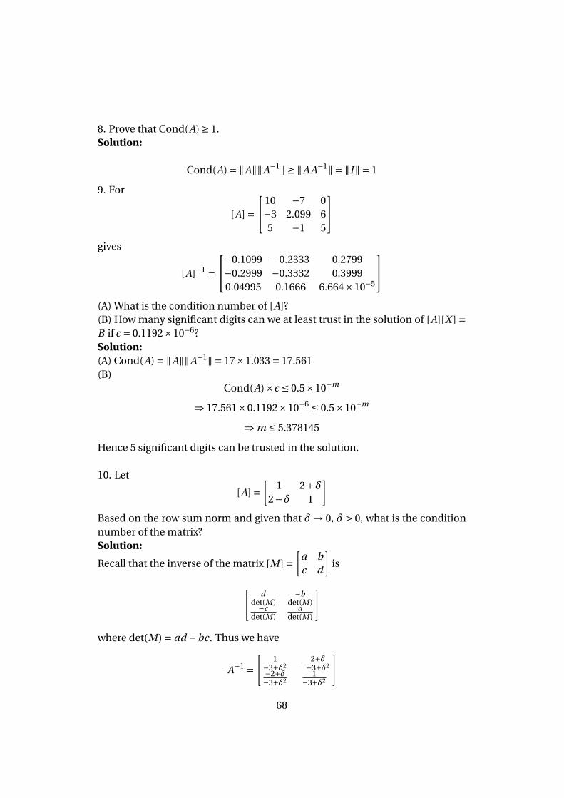
10. Let
[A] =[
1 2+δ2−δ 1
]Based on the row sum norm and given that δ→ 0, δ> 0, what is the conditionnumber of the matrix?Solution:
Recall that the inverse of the matrix [M ] =[
a bc d
]is
[d
det(M)−b
det(M)−cdet(M)
adet(M)
]
where det(M) = ad −bc. Thus we have
A−1 =[
1−3+δ2 − 2+δ
−3+δ2−2+δ−3+δ2
1−3+δ2
]
68
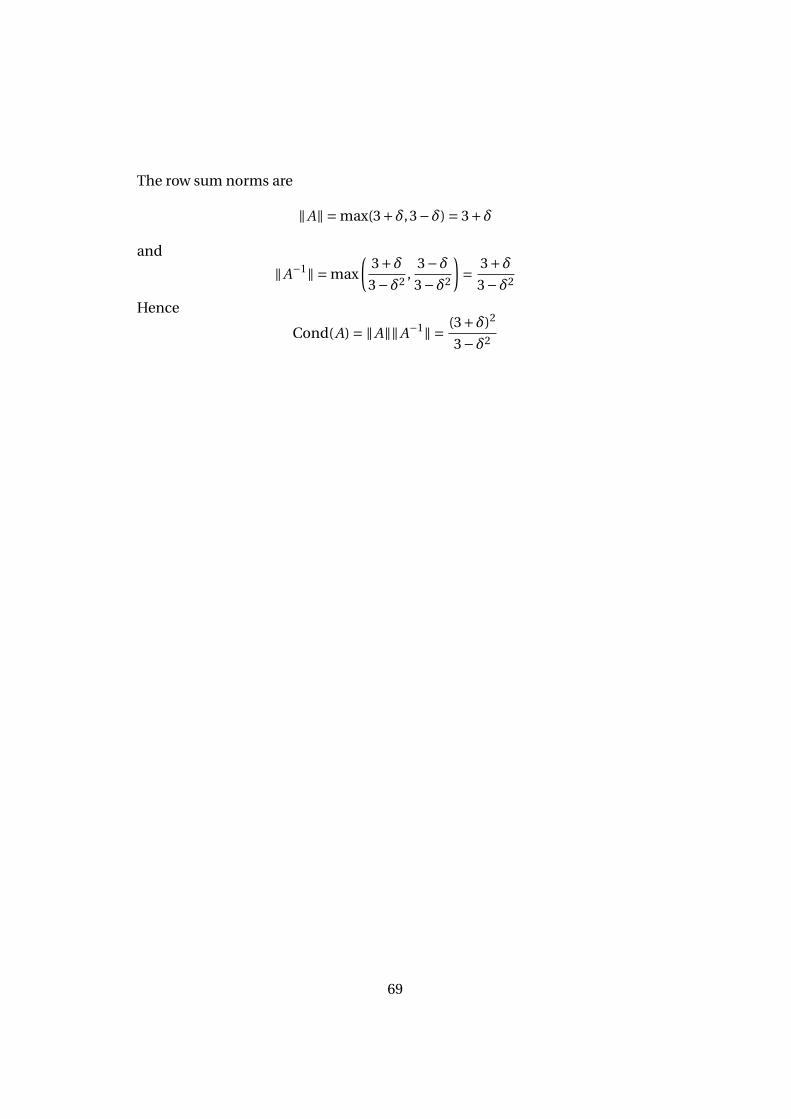
The row sum norms are
‖A‖ = max(3+δ,3−δ) = 3+δ
and
‖A−1‖ = max
(3+δ3−δ2
,3−δ3−δ2
)= 3+δ
3−δ2
Hence
Cond(A) = ‖A‖‖A−1‖ = (3+δ)2
3−δ2
69
10 Eigenvalues and Eigenvectors
10.1 Summary
• DefinitionIf [A] is a n ×n matrix, then [X ] 6=~0 is an eigenvector of [A] if
[A][X ] =λ[X ]
where λ is a scalar and [X ] 6= 0.The scalar λ is called the eigenvalue of [A] and [X ] is called the eigenvec-tor corresponding to the eigenvalue λ.
• Finding eigenvalue and eigenvector
– To find the eigenvalues of a n ×n matrix [A], we have
AX =λX
⇒ AX −λX = 0
⇒ (A−λI )X = 0
For the above set of equations to have a non-zero solution
det(A−λI ) = 0
The above equation is called the characteristic equation of [A], whichgives
λn + c1λn−1 +·· ·+cn = 0
Hence this polynomial has n roots.
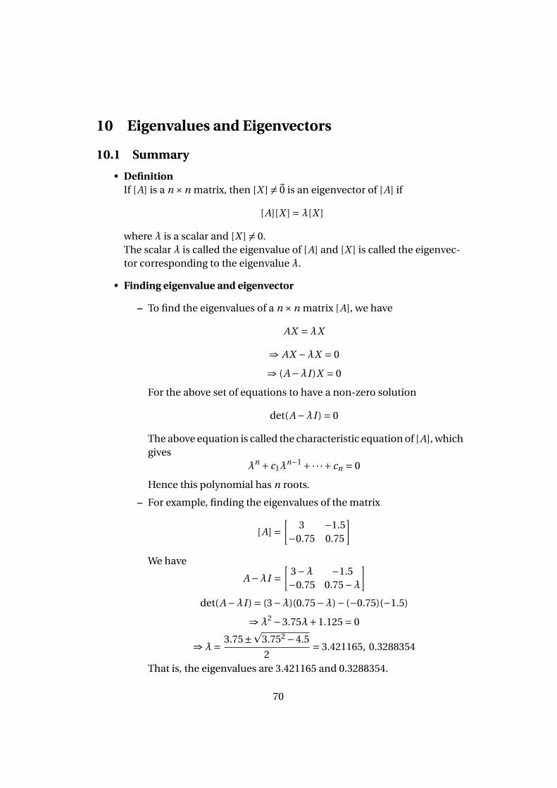
– For example, finding the eigenvalues of the matrix
[A] =[
3 −1.5−0.75 0.75
]We have
A−λI =[
3−λ −1.5−0.75 0.75−λ
]det(A−λI ) = (3−λ)(0.75−λ)− (−0.75)(−1.5)
⇒λ2 −3.75λ+1.125 = 0
⇒λ= 3.75±p
3.752 −4.5
2= 3.421165, 0.3288354
That is, the eigenvalues are 3.421165 and 0.3288354.
70
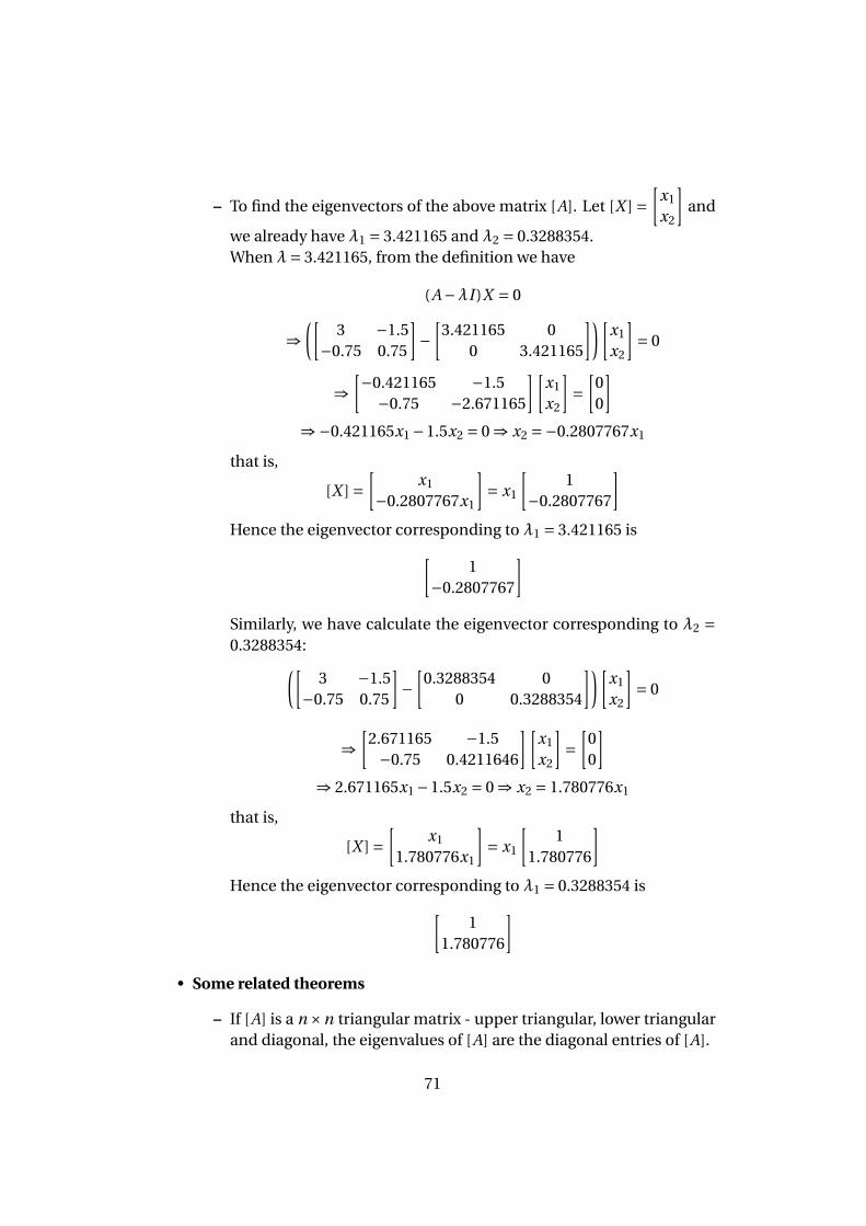
– To find the eigenvectors of the above matrix [A]. Let [X ] =[
x1
x2
]and
we already have λ1 = 3.421165 and λ2 = 0.3288354.When λ= 3.421165, from the definition we have
(A−λI )X = 0
⇒([
3 −1.5−0.75 0.75
]−
[3.421165 0
0 3.421165
])[x1
x2
]= 0
⇒[−0.421165 −1.5
−0.75 −2.671165
][x1
x2
]=
[00
]⇒−0.421165x1 −1.5x2 = 0 ⇒ x2 =−0.2807767x1
that is,
[X ] =[
x1
−0.2807767x1
]= x1
[1
−0.2807767
]Hence the eigenvector corresponding to λ1 = 3.421165 is[
1−0.2807767
]Similarly, we have calculate the eigenvector corresponding to λ2 =0.3288354:([
3 −1.5−0.75 0.75
]−
[0.3288354 0
0 0.3288354
])[x1
x2
]= 0
⇒[
2.671165 −1.5−0.75 0.4211646
][x1
x2
]=
[00
]⇒ 2.671165x1 −1.5x2 = 0 ⇒ x2 = 1.780776x1
that is,
[X ] =[
x1
1.780776x1
]= x1
[1
1.780776
]Hence the eigenvector corresponding to λ1 = 0.3288354 is[
11.780776
]• Some related theorems
– If [A] is a n×n triangular matrix - upper triangular, lower triangularand diagonal, the eigenvalues of [A] are the diagonal entries of [A].
71
– λ= 0 is an eigenvalue of [A] if [A] is a singular (non-invertible) ma-trix.
– [A] and [A]T have the same eigenvalues.
– Eigenvalues of a symmetric matrix are real.
– Eigenvectors of a symmetric matrix are orthogonal, but only for dis-tinct eigenvalues.
– |det(A)| is the product of the absolute values of the eigenvalues of[A].
• Power Method
– One of the most common methods used for finding eigenvalues andeigenvectors is the power method. It is used to find the largest eigen-value in an absolute sense. Note that if this largest eigenvalues is re-peated, this method will not work. Also this eigenvalue needs to bedistinct.
– The method is as follows:
1. Assume a guess X (0) for the eigenvector in
AX =λX
equation. One of the entries of X (0) needs to be unity.
2. FindY (1) = AX (0)
3. Scale Y (1) so that the chosen unity component remains unity.
Y (1) =λ(1)X (1)
4. Repeat steps 2 and 3 with X = X (1) to get X (2).
5. Repeat steps 2 and 3 until the value of the eigenvalue converges.
– For example, using the power method, find the largest eigenvalueand the corresponding eigenvectors of
[A] = 1.5 0 1−0.5 0.5 −0.5−0.5 0 0
72
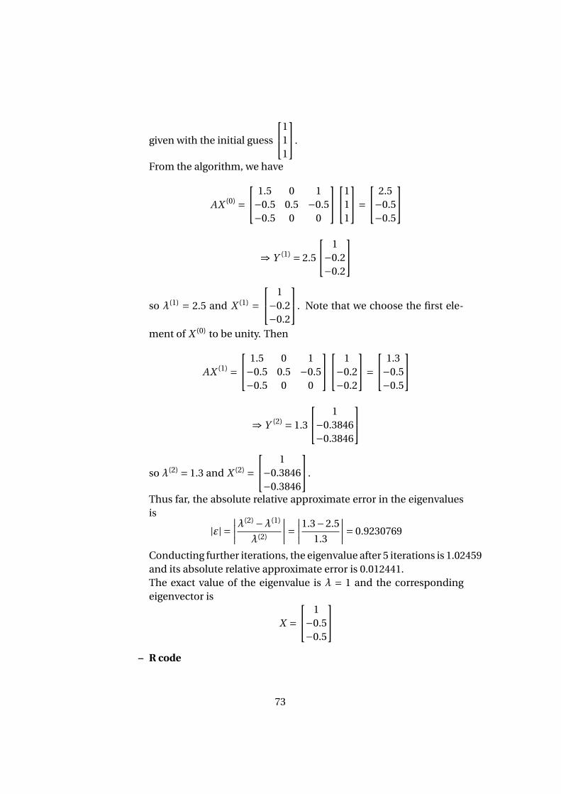
given with the initial guess
111
.
From the algorithm, we have
AX (0) = 1.5 0 1−0.5 0.5 −0.5−0.5 0 0
111
= 2.5−0.5−0.5
⇒ Y (1) = 2.5
1−0.2−0.2
so λ(1) = 2.5 and X (1) = 1−0.2−0.2
. Note that we choose the first ele-
ment of X (0) to be unity. Then
AX (1) = 1.5 0 1−0.5 0.5 −0.5−0.5 0 0
1−0.2−0.2
= 1.3−0.5−0.5
⇒ Y (2) = 1.3
1−0.3846−0.3846
so λ(2) = 1.3 and X (2) = 1−0.3846−0.3846
.
Thus far, the absolute relative approximate error in the eigenvaluesis
|ε| =∣∣∣∣λ(2) −λ(1)
λ(2)
∣∣∣∣= ∣∣∣∣1.3−2.5
1.3
∣∣∣∣= 0.9230769
Conducting further iterations, the eigenvalue after 5 iterations is 1.02459and its absolute relative approximate error is 0.012441.The exact value of the eigenvalue is λ = 1 and the correspondingeigenvector is
X = 1−0.5−0.5
– R code
73
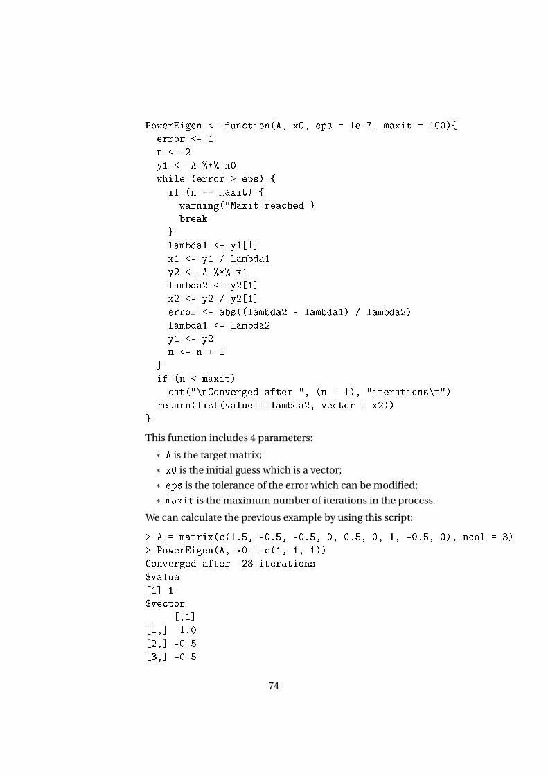
PowerEigen <- function(A, x0, eps = 1e-7, maxit = 100){
error <- 1
n <- 2
y1 <- A %*% x0
while (error > eps) {
if (n == maxit) {
warning("Maxit reached")
break
}
lambda1 <- y1[1]
x1 <- y1 / lambda1
y2 <- A %*% x1
lambda2 <- y2[1]
x2 <- y2 / y2[1]
error <- abs((lambda2 - lambda1) / lambda2)
lambda1 <- lambda2
y1 <- y2
n <- n + 1
}
if (n < maxit)
cat("\nConverged after ", (n - 1), "iterations\n")
return(list(value = lambda2, vector = x2))
}
This function includes 4 parameters:
* A is the target matrix;
* x0 is the initial guess which is a vector;
* eps is the tolerance of the error which can be modified;
* maxit is the maximum number of iterations in the process.
We can calculate the previous example by using this script:
> A = matrix(c(1.5, -0.5, -0.5, 0, 0.5, 0, 1, -0.5, 0), ncol = 3)
> PowerEigen(A, x0 = c(1, 1, 1))
Converged after 23 iterations
$value
[1] 1
$vector
[,1]
[1,] 1.0
[2,] -0.5
[3,] -0.5
74
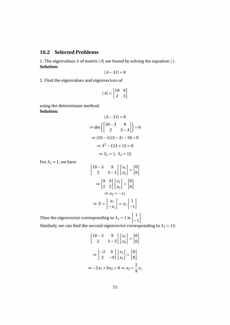
10.2 Selected Problems
1. The eigenvalues λ of matrix [A] are found by solving the equation ( ).Solution:
|A−λI | = 0
2. Find the eigenvalues and eigenvectors of
[A] =[
10 92 3
]using the determinant method.Solution:
|A−λI | = 0
⇒ det
([10−λ 9
2 3−λ])
= 0
⇒ (10−λ)(3−λ)−18 = 0
⇒λ2 −13λ+12 = 0
⇒λ1 = 1, λ2 = 12
For λ1 = 1, we have [10−λ 9
2 3−λ][
x1
x2
]=
[00
]
⇒[
9 92 2
][x1
x2
]=
[00
]⇒ x2 =−x1
⇒ X =[
x1
−x1
]= x1
[1−1
]
Thus the eigenvector corresponding to λ1 = 1 is
[1−1
].
Similarly, we can find the second eigenvector corresponding to λ2 = 12:[10−λ 9
2 3−λ][
x1
x2
]=
[00
]
⇒[−2 9
2 −9
][x1
x2
]=
[00
]⇒−2x1 +9x2 = 0 ⇒ x2 = 2
9x1
75

⇒ X =[
x129 x1
]= x1
[129
]⇒
[92
]
Thus the eigenvector corresponding to λ2 = 12 is
[92
].
3. Find the eigenvalues and eigenvectors of
[A] = 4 0 1−2 0 12 0 1
using the determinant method.Solution:First of all, we can read off that λ = 0 is an eigenvalue of this matrix since it issingular. Then from the definition we have
|A−λI | = 0
⇒ det
4−λ 0 1−2 −λ 12 0 1−λ
= 0
⇒ (4−λ) [(−λ)(1−λ)−0]+ [1 · (0+2λ)] = 0
⇒ (4−λ)(λ2 −λ)+2λ= 0
⇒λ(−λ2 +5λ−4+2) = 0
⇒λ(λ2 −5λ+2) = 0
⇒λ1 = 0, λ2 = 4.561553, λ3 = 0.4384472.
For λ1 = 0, we have 4−λ 0 1−2 −λ 12 0 1−λ
x1
x2
x3
=0
00
⇒ 4 0 1−2 0 12 0 1
x1
x2
x3
=0
00
The coefficient matrix is 4 0 1
−2 0 12 0 1
⇒ 0 0 3−2 0 10 0 2
⇒ 0 0 0−2 0 00 0 2
76
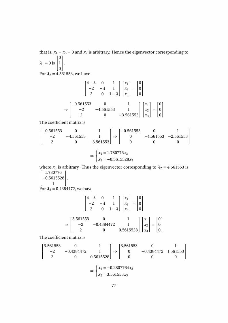
that is, x1 = x3 = 0 and x2 is arbitrary. Hence the eigenvector corresponding to
λ1 = 0 is
010
.
For λ2 = 4.561553, we have4−λ 0 1−2 −λ 12 0 1−λ
x1
x2
x3
=0
00
⇒−0.561553 0 1
−2 −4.561553 12 0 −3.561553
x1
x2
x3
=0
00
The coefficient matrix is−0.561553 0 1
−2 −4.561553 12 0 −3.561553
⇒−0.561553 0 1
0 −4.561553 −2.5615530 0 0
⇒{
x1 = 1.780776x3
x2 =−0.5615528x3
where x3 is arbitrary. Thus the eigenvector corresponding to λ2 = 4.561553 is 1.780776−0.5615528
1
.
For λ3 = 0.4384472, we have4−λ 0 1−2 −λ 12 0 1−λ
x1
x2
x3
=0
00
⇒3.561553 0 1
−2 −0.4384472 12 0 0.5615528
x1
x2
x3
=0
00
The coefficient matrix is3.561553 0 1
−2 −0.4384472 12 0 0.5615528
⇒3.561553 0 1
0 −0.4384472 1.5615530 0 0
⇒{
x1 =−0.2807764x3
x2 = 3.561553x3
77
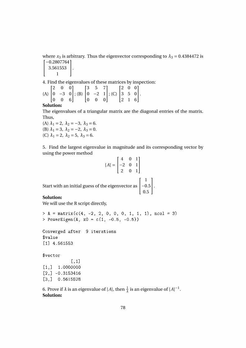
where x3 is arbitrary. Thus the eigenvector corresponding to λ3 = 0.4384472 is−0.28077643.561553
1
.
4. Find the eigenvalues of these matrices by inspection:
(A)
2 0 00 −3 00 0 6
; (B)
3 5 70 −2 10 0 0
; (C)
2 0 03 5 02 1 6
.
Solution:The eigenvalues of a triangular matrix are the diagonal entries of the matrix.Thus,(A) λ1 = 2, λ2 =−3, λ3 = 6.(B) λ1 = 3, λ2 =−2, λ3 = 0.(C) λ1 = 2, λ2 = 5, λ3 = 6.
5. Find the largest eigenvalue in magnitude and its corresponding vector byusing the power method
[A] = 4 0 1−2 0 12 0 1
Start with an initial guess of the eigenvector as
1−0.50.5
.
Solution:We will use the R script directly,
> A = matrix(c(4, -2, 2, 0, 0, 0, 1, 1, 1), ncol = 3)
> PowerEigen(A, x0 = c(1, -0.5, -0.5))
Converged after 9 iterations
$value
[1] 4.561553
$vector
[,1]
[1,] 1.0000000
[2,] -0.3153416
[3,] 0.5615528
6. Prove if λ is an eigenvalue of [A], then 1λ is an eigenvalue of [A]−1.
Solution:
78
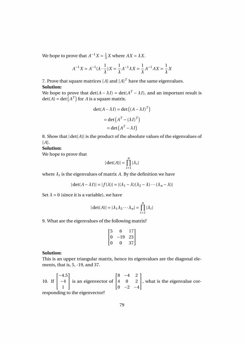
We hope to prove that A−1X = 1λ
X where AX =λX .
A−1X = A−1(λ · 1
λ)X = 1
λA−1λX = 1
λA−1 AX = 1
λX
7. Prove that square matrices [A] and [A]T have the same eigenvalues.Solution:We hope to prove that det(A −λI ) = det(AT −λI ), and an important result isdet(A) = det
(AT
)for A is a square matrix.
det(A−λI ) = det((A−λI )T )
= det(
AT − (λI )T )= det
(AT −λI
)8. Show that |det(A)| is the product of the absolute values of the eigenvalues of[A].Solution:We hope to prove that
|det(A)| =n∏
i=1|λi |
where λi is the eigenvalues of matrix A. By the definition we have
|det(A−λI )| = | f (λ)| = |(λ1 −λ)(λ2 −λ) · · · (λn −λ)|
Set λ= 0 (since it is a variable), we have
|det(A)| = |λ1λ2 · · ·λn | =n∏
i=1|λi |
9. What are the eigenvalues of the following matrix?5 6 170 −19 230 0 37
Solution:This is an upper triangular matrix, hence its eigenvalues are the diagonal ele-ments, that is, 5, -19, and 37.
10. If
−4.5−41
is an eigenvector of
8 −4 24 0 20 −2 −4
, what is the eigenvalue cor-
responding to the eigenvector?
79
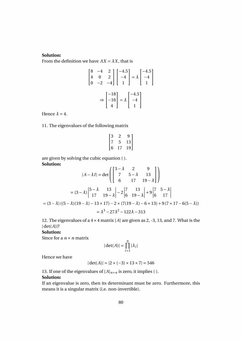
Solution:From the definition we have AX =λX , that is8 −4 2
4 0 20 −2 −4
−4.5−41
=λ−4.5
−41
⇒−18−16
4
=λ−4.5
−41
Hence λ= 4.
11. The eigenvalues of the following matrix3 2 97 5 136 17 19
are given by solving the cubic equation ( ).Solution:
|A−λI | = det
3−λ 2 97 5−λ 136 17 19−λ
= (3−λ)
∣∣∣∣5−λ 1317 19−λ
∣∣∣∣−2
∣∣∣∣7 136 19−λ
∣∣∣∣+9
∣∣∣∣7 5−λ6 17
∣∣∣∣= (3−λ) ((5−λ)(19−λ)−13×17)−2× (7(19−λ)−6×13)+9(7×17−6(5−λ))
=λ3 −27λ2 −122λ−313
12. The eigenvalues of a 4×4 matrix [A] are given as 2, -3, 13, and 7. What is the|det(A)|?Solution:Since for a n ×n matrix
|det(A)| =n∏
i=1|λi |
Hence we have|det(A)| = |2× (−3)×13×7| = 546
13. If one of the eigenvalues of [A]n×n is zero, it implies ( ).Solution:If an eigenvalue is zero, then its determinant must be zero. Furthermore, thismeans it is a singular matrix (i.e. non-invertible).
80
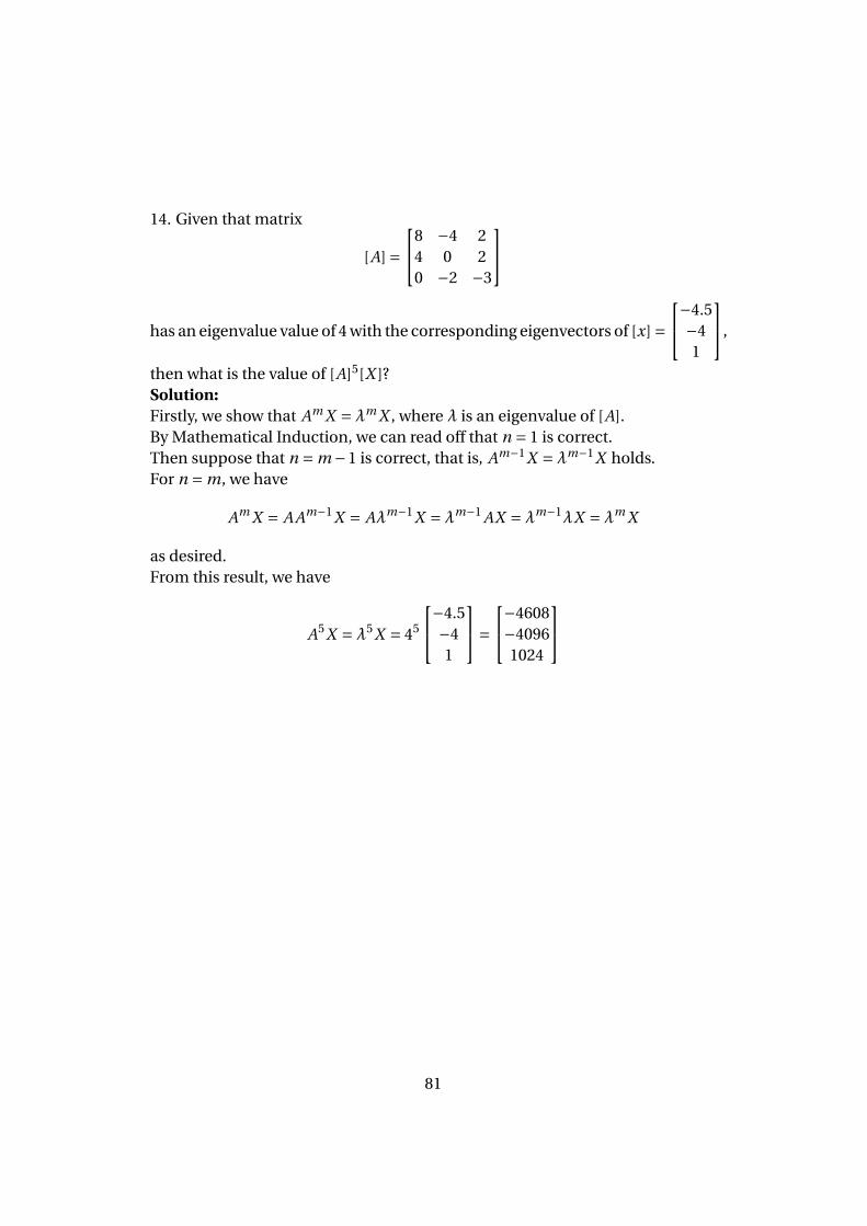
14. Given that matrix
[A] =8 −4 2
4 0 20 −2 −3
has an eigenvalue value of 4 with the corresponding eigenvectors of [x] =−4.5
−41
,
then what is the value of [A]5[X ]?Solution:Firstly, we show that Am X =λm X , where λ is an eigenvalue of [A].By Mathematical Induction, we can read off that n = 1 is correct.Then suppose that n = m −1 is correct, that is, Am−1X =λm−1X holds.For n = m, we have
Am X = A Am−1X = Aλm−1X =λm−1 AX =λm−1λX =λm X
as desired.From this result, we have
A5X =λ5X = 45
−4.5−41
=−4608−40961024
81
Related Documents