Studies of Quantum Chromodynamics with the ALEPH detector

EUROPEAN ORGANIZATION FOR NUCLEAR RESEARCH

CERN / PPE 96{186

December 13th, 1996

Studies of Quantum Chromodynamics

with the ALEPH Detector

The ALEPH Collaboration

Abstract

Previously published and as yet unpublished QCD results obtained with the ALEPH

detector at LEP1 are presented. The unprecedented statistics allows detailed stud-

ies of both perturbative and non-perturbative aspects of strong interactions to be

carried out using hadronic Z and tau decays. The studies presented include precise

determinations of the strong coupling constant, tests of its avour independence,

tests of the SU(3) gauge structure of QCD, study of coherence e�ects, and mea-

surements of single-particle inclusive distributions and two-particle correlations for

many identi�ed baryons and mesons.

To appear in Physics Reports

R. Barate, D. Buskulic, D. Decamp, P. Ghez, C. Goy, J.-P. Lees, A. Lucotte, M.-N. Minard, J.-Y. Nief, P. Odier,

B. Pietrzyk

Laboratoire de Physique des Particules (LAPP), IN2P3-CNRS, 74019 Annecy-le-Vieux Cedex, France

M.P. Casado, M. Chmeissani, P. Comas, J.M. Crespo, M. Del�no, E. Fernandez, M. Fernandez-Bosman,

Ll. Garrido,15 A. Juste, M. Martinez, S. Orteu, C. Padilla, I.C. Park, A. Pascual, J.A. Perlas, I. Riu, F. Sanchez,

F. TeubertInstitut de Fisica d'Altes Energies, Universitat Autonoma de Barcelona, 08193 Bellaterra (Barcelona),Spain7

A. Colaleo, D. Creanza, M. de Palma, G. Gelao, G. Iaselli, G. Maggi, M. Maggi, N. Marinelli, S. Nuzzo,

A. Ranieri, G. Raso, F. Ruggieri, G. Selvaggi, L. Silvestris, P. Tempesta, A. Tricomi,3 G. Zito

Dipartimento di Fisica, INFN Sezione di Bari, 70126 Bari, Italy

X. Huang, J. Lin, Q. Ouyang, T. Wang, Y. Xie, R. Xu, S. Xue, J. Zhang, L. Zhang, W. Zhao

Institute of High-Energy Physics, Academia Sinica, Beijing, The People's Republic of China8

D. Abbaneo, R. Alemany, A.O. Bazarko, P. Bright-Thomas, M. Cattaneo, F. Cerutti, H. Drevermann,

R.W. Forty, M. Frank, R. Hagelberg, J. Harvey, P. Janot, B. Jost, E. Kneringer, J. Knobloch, I. Lehraus,

T. Lohse, G. Lutters, P. Mato, A. Minten, R. Miquel, Ll.M. Mir,2 L. Moneta, T. Oest,20 A. Pacheco, J.-

F. Pusztaszeri, F. Ranjard, P. Rensing,12 G. Rizzo, L. Rolandi, D. Schlatter, M. Schmelling,24 M. Schmitt,

O. Schneider, W. Tejessy, I.R. Tomalin, A. Venturi, H. Wachsmuth, A. Wagner

European Laboratory for Particle Physics (CERN), 1211 Geneva 23, Switzerland

Z. Ajaltouni, A. Barr�es, C. Boyer, A. Falvard, C. Ferdi, P. Gay, C . Guicheney, P. Henrard, J. Jousset, B. Michel,

S. Monteil, J-C. Montret, D. Pallin, P. Perret, F. Podlyski, J. Proriol, P. Rosnet, J.-M. Rossignol

Laboratoire de Physique Corpusculaire, Universit�e Blaise Pascal, IN2P3-CNRS, Clermont-Ferrand,63177 Aubi�ere, France

T. Fearnley, J.B. Hansen, J.D. Hansen, J.R. Hansen, P.H. Hansen, B.S. Nilsson, B. Rensch, A. W�a�an�anen

Niels Bohr Institute, 2100 Copenhagen, Denmark9

G. Daskalakis, A. Kyriakis, C. Markou, E. Simopoulou, I. Siotis, A. Vayaki, K. Zachariadou

Nuclear Research Center Demokritos (NRCD), Athens, Greece

A. Blondel, G. Bonneaud, J.C. Brient, P. Bourdon, A. Roug�e, M. Rumpf, A. Valassi,6 M. Verderi, H. Videau

Laboratoire de Physique Nucl�eaire et des Hautes Energies, Ecole Polytechnique, IN2P3-CNRS, 91128Palaiseau Cedex, France

D.J. Candlin, M.I. Parsons

Department of Physics, University of Edinburgh, Edinburgh EH9 3JZ, United Kingdom10

E. Focardi,21 G. Parrini

Dipartimento di Fisica, Universit�a di Firenze, INFN Sezione di Firenze, 50125 Firenze, Italy

M. Corden, C. Georgiopoulos, D.E. Ja�e

Supercomputer Computations Research Institute, Florida State University, Tallahassee, FL 32306-4052, USA 13;14

A. Antonelli, G. Bencivenni, G. Bologna,4 F. Bossi, P. Campana, G. Capon, D. Casper, V. Chiarella, G. Felici,

P. Laurelli, G. Mannocchi,5 F. Murtas, G.P. Murtas, L. Passalacqua, M. Pepe-Altarelli

Laboratori Nazionali dell'INFN (LNF-INFN), 00044 Frascati, Italy

L. Curtis, S.J. Dorris, A.W. Halley, I.G. Knowles, J.G. Lynch, V. O'Shea, C. Raine, P. Reeves, J.M. Scarr,

K. Smith, P. Teixeira-Dias, A.S. Thompson, E. Thomson, F. Thomson, R.M. Turnbull

Department of Physics and Astronomy, University of Glasgow, Glasgow G12 8QQ,United Kingdom10

U. Becker, O. Buchm�uller, C. Geweniger, G. Graefe, P. Hanke, G. Hansper, H. Hepp, V. Hepp, E.E. Kluge,

A. Putzer, M. Schmidt, J. Sommer, H. Stenzel, K. Tittel, S. Werner, M. Wunsch

R. Beuselinck, D.M. Binnie, W. Cameron, P.J. Dornan, M. Girone, S. Goodsir, E.B. Martin, A. Moutoussi,

J. Nash, J.K. Sedgbeer, A.M. Stacey, M.D. Williams

Department of Physics, Imperial College, London SW7 2BZ, United Kingdom10

G. Dissertori, P. Girtler, D. Kuhn, G. Rudolph

Institut f�ur Experimentalphysik, Universit�at Innsbruck, 6020 Innsbruck, Austria18

A.P. Betteridge, C.K. Bowdery, P. Colrain, G. Crawford, A.J. Finch, F. Foster, G. Hughes, T. Sloan,

M.I. Williams

Department of Physics, University of Lancaster, Lancaster LA1 4YB, United Kingdom10

T. Barczewski, A. Galla, I. Giehl, A.M. Greene, C. Ho�mann, K. Jakobs, K. Kleinknecht, G. Quast, B. Renk,

E. Rohne, H.-G. Sander, H. Schmidt, F. Steeg, P. van Gemmeren, C. Zeitnitz

Institut f�ur Physik, Universit�at Mainz, 55099 Mainz, Fed. Rep. of Germany16

J.J. Aubert, C. Benchouk, A. Bonissent, G. Bujosa, D. Calvet, J. Carr, P. Coyle, C. Diaconu, F. Etienne,

N. Konstantinidis, O. Leroy, P. Payre, D. Rousseau, M. Talby, A. Sadouki, M. Thulasidas, K. Trabelsi

Centre de Physique des Particules, Facult�e des Sciences de Luminy, IN2P3-CNRS, 13288 Marseille,France

M. Aleppo, F. Ragusa21

Dipartimento di Fisica, Universit�a di Milano e INFN Sezione di Milano, 20133 Milano, Italy

R. Berlich, W. Blum, V. B�uscher, H. Dietl, F. Dydak,21 G. Ganis, C. Gotzhein, H. Kroha, G. L�utjens, G. Lutz,

W. M�anner, H.-G. Moser, R. Richter, A. Rosado-Schlosser, S. Schael, R. Settles, H. Seywerd, R. St. Denis,

H. Stenzel, W. Wiedenmann, G. Wolf

Max-Planck-Institut f�ur Physik, Werner-Heisenberg-Institut, 80805 M�unchen, Fed. Rep. of Germany16

J. Boucrot, O. Callot,21 S. Chen, Y. Choi,26 A. Cordier, M. Davier, L. Du ot, J.-F. Grivaz, Ph. Heusse,

A. H�ocker, A. Jacholkowska, M. Jacquet, D.W. Kim,19 F. Le Diberder, J. Lefran�cois, A.-M. Lutz, I. Nikolic,

H.J. Park,19 M.-H. Schune, S. Simion, J.-J. Veillet, I. Videau, D. Zerwas

Laboratoire de l'Acc�el�erateur Lin�eaire, Universit�e de Paris-Sud, IN2P3-CNRS, 91405 Orsay Cedex,France

P. Azzurri, G. Bagliesi, G. Batignani, S. Bettarini, C. Bozzi, G. Calderini, M. Carpinelli, M.A. Ciocci, V. Ciulli,

R. Dell'Orso, R. Fantechi, I. Ferrante, L. Fo�a,1 F. Forti, A. Giassi, M.A. Giorgi, A. Gregorio, F. Ligabue,

A. Lusiani, P.S. Marrocchesi, A. Messineo, F. Palla, G. Sanguinetti, A. Sciab�a, P. Spagnolo, J. Steinberger,

R. Tenchini, G. Tonelli,25 C. Vannini, P.G. Verdini

Dipartimento di Fisica dell'Universit�a, INFN Sezione di Pisa, e Scuola Normale Superiore, 56010 Pisa,Italy

G.A. Blair, L.M. Bryant, J.T. Chambers, Y. Gao, M.G. Green, T. Medcalf, P. Perrodo, J.A. Strong,

J.H. von Wimmersperg-Toeller

Department of Physics, Royal Holloway & Bedford New College, University of London, Surrey TW20OEX, United Kingdom10

V. Bertin, D.R. Botterill, R.W. Cli�t, T.R. Edgecock, S. Haywood, P. Maley, P.R. Norton, J.C. Thompson,

A.E. Wright

Particle Physics Dept., Rutherford Appleton Laboratory, Chilton, Didcot, Oxon OX11 OQX, UnitedKingdom10

B. Bloch-Devaux, P. Colas, S. Emery, W. Kozanecki, E. Lan�con, M.C. Lemaire, E. Locci, P. Perez, J. Rander,

J.-F. Renardy, A. Roussarie, J.-P. Schuller, J. Schwindling, A. Trabelsi, B. Vallage

CEA, DAPNIA/Service de Physique des Particules, CE-Saclay, 91191 Gif-sur-Yvette Cedex, France17

S.N. Black, J.H. Dann, R.P. Johnson, H.Y. Kim, A.M. Litke, M.A. McNeil, G. Taylor

Institute for Particle Physics, University of California at Santa Cruz, Santa Cruz, CA 95064, USA22

A. Beddall, C.N. Booth, R. Boswell, C.A.J. Brew, S. Cartwright, F. Combley, I. Dawson, M.S. Kelly, M. Lehto,

W.M. Newton, J. Reeve, L.F. Thompson

Department of Physics, University of She�eld, She�eld S3 7RH, United Kingdom10

A. B�ohrer, S. Brandt, G. Cowan, E. Feigl, C. Grupen, J. Minguet-Rodriguez, F. Rivera, P. Saraiva, L. Smolik,

F. Stephan

Fachbereich Physik, Universit�at Siegen, 57068 Siegen, Fed. Rep. of Germany16

M. Apollonio, L. Bosisio, R. Della Marina, G. Giannini, B. Gobbo, G. Musolino

Dipartimento di Fisica, Universit�a di Trieste e INFN Sezione di Trieste, 34127 Trieste, Italy

J. Rothberg, S. Wasserbaech

Experimental Elementary Particle Physics, University of Washington, WA 98195 Seattle, U.S.A.

S.R. Armstrong, P. Elmer, Z. Feng,27 D.P.S. Ferguson, Y.S. Gao,23 S. Gonz�alez, J. Grahl, T.C. Greening,

O.J. Hayes, H. Hu, P.A. McNamara III, J.M. Nachtman, W. Orejudos, Y.B. Pan, Y. Saadi, I.J. Scott, J. Walsh,

Sau Lan Wu, X. Wu, J.M. Yamartino, M. Zheng, G. Zobernig

Department of Physics, University of Wisconsin, Madison, WI 53706, USA11

1Now at CERN, 1211 Geneva 23, Switzerland.2Supported by Direcci�on General de Investigaci�on Cient���ca y T�ecnica, Spain.3Also at Dipartimento di Fisica, INFN, Sezione di Catania, Catania, Italy.4Also Istituto di Fisica Generale, Universit�a di Torino, Torino, Italy.5Also Istituto di Cosmo-Geo�sica del C.N.R., Torino, Italy.6Supported by the Commission of the European Communities, contract ERBCHBICT941234.7Supported by CICYT, Spain.8Supported by the National Science Foundation of China.9Supported by the Danish Natural Science Research Council.10Supported by the UK Particle Physics and Astronomy Research Council.11Supported by the US Department of Energy, grant DE-FG0295-ER40896.12Now at Dragon Systems, Newton, MA 02160, U.S.A.13Supported by the US Department of Energy, contract DE-FG05-92ER40742.14Supported by the US Department of Energy, contract DE-FC05-85ER250000.15Permanent address: Universitat de Barcelona, 08208 Barcelona, Spain.16Supported by the Bundesministerium f�ur Bildung, Wissenschaft, Forschung und Technologie, Fed. Rep. of

Germany.17Supported by the Direction des Sciences de la Mati�ere, C.E.A.18Supported by Fonds zur F�orderung der wissenschaftlichen Forschung, Austria.19Permanent address: Kangnung National University, Kangnung, Korea.20Now at DESY, Hamburg, Germany.21Also at CERN, 1211 Geneva 23, Switzerland.22Supported by the US Department of Energy, grant DE-FG03-92ER40689.23Now at Harvard University, Cambridge, MA 02138, U.S.A.24Now at Max-Plank-Instit�ut f�ur Kernphysik, Heidelberg, Germany.25Also at Istituto di Matematica e Fisica, Universit�a di Sassari, Sassari, Italy.26Permanent address: Sung Kyun Kwan University, Suwon, Korea.27Now at The Johns Hopkins University, Baltimore, MD 21218, U.S.A.

Contents

1 Introduction 1

1.1 QCD : : : : : : : : : : : : : : : : : : : : : : : : : : : : : : : : : : : : : : : : : : 2

1.1.1 QCD Lagrangian and Fundamental Properties : : : : : : : : : : : : : : : 2

1.1.2 The Process e+e� ! hadrons : : : : : : : : : : : : : : : : : : : : : : : : 5

1.2 The ALEPH Detector : : : : : : : : : : : : : : : : : : : : : : : : : : : : : : : : 7

1.2.1 Particle tracking : : : : : : : : : : : : : : : : : : : : : : : : : : : : : : : 7

1.2.2 Speci�c Ionization Measurement : : : : : : : : : : : : : : : : : : : : : : : 9

1.2.3 Calorimetry : : : : : : : : : : : : : : : : : : : : : : : : : : : : : : : : : : 9

1.2.4 The Trigger System : : : : : : : : : : : : : : : : : : : : : : : : : : : : : : 10

1.2.5 The Identi�cation of K0 mesons and � Hyperons : : : : : : : : : : : : : 10

1.2.6 Energy Flow Determination : : : : : : : : : : : : : : : : : : : : : : : : : 11

1.2.7 Heavy Quark Tagging : : : : : : : : : : : : : : : : : : : : : : : : : : : : 11

1.3 Data Analysis Overview : : : : : : : : : : : : : : : : : : : : : : : : : : : : : : : 12

1.3.1 Track and Event Selection : : : : : : : : : : : : : : : : : : : : : : : : : : 12

1.3.2 Corrections for Detector E�ects : : : : : : : : : : : : : : : : : : : : : : : 13

2 Global Event Structure and Tuning of Model Parameters 15

2.1 De�nition of Observables : : : : : : : : : : : : : : : : : : : : : : : : : : : : : : : 15

2.2 Analysis Technique and Results : : : : : : : : : : : : : : : : : : : : : : : : : : : 17

2.3 Tuning of QCD Models : : : : : : : : : : : : : : : : : : : : : : : : : : : : : : : : 18

2.3.1 Description of the Models : : : : : : : : : : : : : : : : : : : : : : : : : : 26

2.3.2 Fitting of Model Parameters : : : : : : : : : : : : : : : : : : : : : : : : : 28

2.3.3 Discussion of the Results : : : : : : : : : : : : : : : : : : : : : : : : : : : 30

3 Hard QCD 34

3.1 Parton Spins : : : : : : : : : : : : : : : : : : : : : : : : : : : : : : : : : : : : : : 34

3.1.1 Quark Spin : : : : : : : : : : : : : : : : : : : : : : : : : : : : : : : : : : 34

3.1.2 Gluon Spin : : : : : : : : : : : : : : : : : : : : : : : : : : : : : : : : : : 35

3.2 Measurements of the Strong Coupling Constant : : : : : : : : : : : : : : : : : : 37

3.2.1 Z Hadronic Width : : : : : : : : : : : : : : : : : : : : : : : : : : : : : : 39

3.2.2 The Hadronic Width of the Tau : : : : : : : : : : : : : : : : : : : : : : : 40

3.2.3 Event Shapes and Jet Rates : : : : : : : : : : : : : : : : : : : : : : : : : 44

3.2.4 Scaling Violations in Fragmentation Functions : : : : : : : : : : : : : : : 50

3.2.5 Summary of �s measurements : : : : : : : : : : : : : : : : : : : : : : : : 54

3.2.6 The Running of �s : : : : : : : : : : : : : : : : : : : : : : : : : : : : : : 54

3.3 Angular Dependence of Event Shapes : : : : : : : : : : : : : : : : : : : : : : : : 56

1

3.4 Test of the Flavour Independence of �s : : : : : : : : : : : : : : : : : : : : : : : 60

3.5 Colour Factors of QCD : : : : : : : : : : : : : : : : : : : : : : : : : : : : : : : : 61

3.5.1 Determination using four-jet events : : : : : : : : : : : : : : : : : : : : : 63

3.5.2 Determination using two- and three-jet events : : : : : : : : : : : : : : : 64

3.5.3 Information from the running of �s : : : : : : : : : : : : : : : : : : : : : 67

3.5.4 Summary : : : : : : : : : : : : : : : : : : : : : : : : : : : : : : : : : : : 68

4 Semi-Soft QCD 70

4.1 Coherence Phenomena : : : : : : : : : : : : : : : : : : : : : : : : : : : : : : : : 70

4.1.1 Inclusive Distribution of � lnxp : : : : : : : : : : : : : : : : : : : : : : : 71

4.1.2 Energy Dependence of the Peak of the � lnxp Distribution : : : : : : : : 74

4.1.3 Particle-Particle Correlations : : : : : : : : : : : : : : : : : : : : : : : : 77

4.1.4 Energy-Multiplicity-Multiplicity Correlations : : : : : : : : : : : : : : : : 79

4.1.5 Particle Flow in Interjet Regions (String E�ect) : : : : : : : : : : : : : : 80

4.2 Charged Particle Multiplicities : : : : : : : : : : : : : : : : : : : : : : : : : : : : 84

4.2.1 Data analysis : : : : : : : : : : : : : : : : : : : : : : : : : : : : : : : : : 85

4.2.2 Model Independent Results : : : : : : : : : : : : : : : : : : : : : : : : : 86

4.2.3 Energy Dependence of the Charged Multiplicity Distribution : : : : : : : 88

4.2.4 Charged Particle Multiplicities in Rapidity Windows : : : : : : : : : : : 90

4.3 Intermittency : : : : : : : : : : : : : : : : : : : : : : : : : : : : : : : : : : : : : 93

4.4 Subjet Structure of Hadronic Events : : : : : : : : : : : : : : : : : : : : : : : : 95

4.4.1 Subjet Structure of Two- and Three-Jet Events : : : : : : : : : : : : : : 96

4.4.2 Subjet Structure of Identi�ed Quark and Gluon Jets : : : : : : : : : : : 98

4.5 Properties of Tagged Jets in Symmetric Three-Jet Events : : : : : : : : : : : : : 100

4.5.1 Data Analysis : : : : : : : : : : : : : : : : : : : : : : : : : : : : : : : : : 101

4.5.2 Unfolding of the Jet Properties : : : : : : : : : : : : : : : : : : : : : : : 102

4.5.3 Measured Quark and Gluon Jet Properties : : : : : : : : : : : : : : : : : 103

4.6 Prompt Photon Production : : : : : : : : : : : : : : : : : : : : : : : : : : : : : 105

4.6.1 Isolated Photon Studies : : : : : : : : : : : : : : : : : : : : : : : : : : : 105

4.6.2 \Democratic" Analysis : : : : : : : : : : : : : : : : : : : : : : : : : : : : 107

5 Hadronization 113

5.1 Search for Free Quarks : : : : : : : : : : : : : : : : : : : : : : : : : : : : : : : : 113

5.2 Inclusive Production of Identi�ed Hadrons : : : : : : : : : : : : : : : : : : : : : 114

5.2.1 Identi�ed Stable Charged Particles : : : : : : : : : : : : : : : : : : : : : 114

5.2.2 Single Photons : : : : : : : : : : : : : : : : : : : : : : : : : : : : : : : : 118

5.2.3 Neutral Pions : : : : : : : : : : : : : : : : : : : : : : : : : : : : : : : : : 120

2

5.2.4 � and �0 Mesons : : : : : : : : : : : : : : : : : : : : : : : : : : : : : : : : 122

5.2.5 Light Strange Particles : : : : : : : : : : : : : : : : : : : : : : : : : : : : 124

5.2.6 Heavy Strange Particles : : : : : : : : : : : : : : : : : : : : : : : : : : : 126

5.2.7 Neutral Vector Mesons : : : : : : : : : : : : : : : : : : : : : : : : : : : : 132

5.2.8 Charged Vector Mesons : : : : : : : : : : : : : : : : : : : : : : : : : : : 136

5.2.9 Summary and Discussion : : : : : : : : : : : : : : : : : : : : : : : : : : : 137

5.3 Two-Particle Correlations : : : : : : : : : : : : : : : : : : : : : : : : : : : : : : 139

5.3.1 Proton-Antiproton Correlations : : : : : : : : : : : : : : : : : : : : : : : 140

5.3.2 Strangeness Correlations : : : : : : : : : : : : : : : : : : : : : : : : : : : 142

5.3.3 Bose-Einstein Correlations : : : : : : : : : : : : : : : : : : : : : : : : : : 146

6 Summary 151

A Rl and R� for Arbitrary Colour Factors 153

A.1 The Running Coupling Constant and Masses : : : : : : : : : : : : : : : : : : : : 153

A.2 Theoretical Predictions for R : : : : : : : : : : : : : : : : : : : : : : : : : : : : 154

A.3 The Theoretical Prediction for Rl : : : : : : : : : : : : : : : : : : : : : : : : : : 155

A.4 The Theoretical Prediction for R� : : : : : : : : : : : : : : : : : : : : : : : : : 156

3

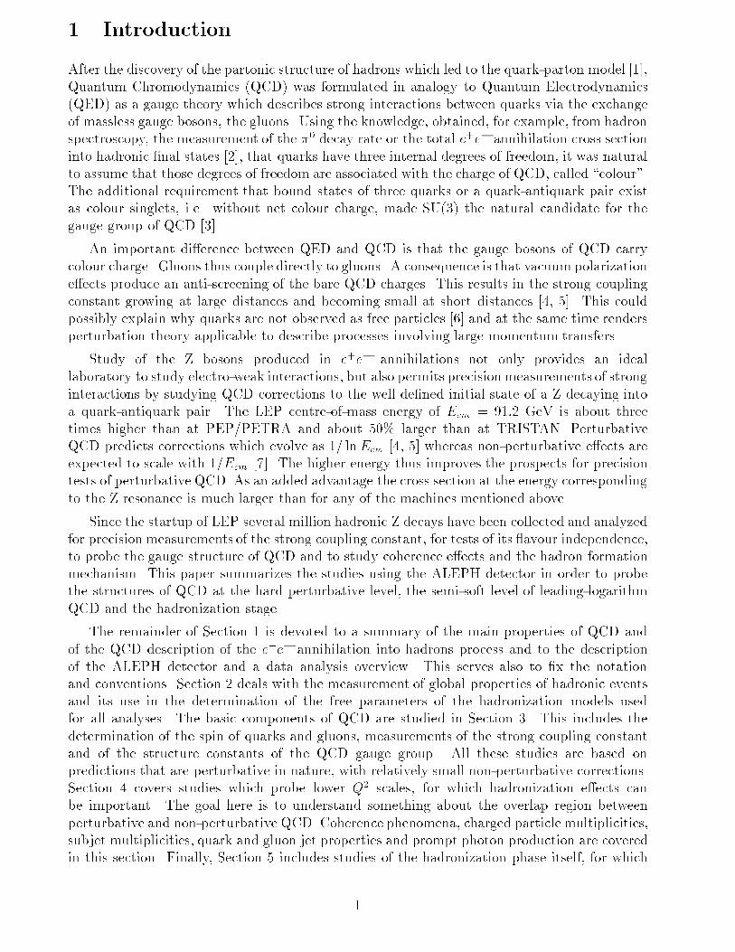
1 Introduction

After the discovery of the partonic structure of hadrons which led to the quark-parton model [1],

Quantum Chromodynamics (QCD) was formulated in analogy to Quantum Electrodynamics

(QED) as a gauge theory which describes strong interactions between quarks via the exchange

of massless gauge bosons, the gluons. Using the knowledge, obtained, for example, from hadron

spectroscopy, the measurement of the �0 decay rate or the total e+e� annihilation cross section

into hadronic �nal states [2], that quarks have three internal degrees of freedom, it was natural

to assume that those degrees of freedom are associated with the charge of QCD, called \colour".

The additional requirement that bound states of three quarks or a quark-antiquark pair exist

as colour singlets, i.e. without net colour charge, made SU(3) the natural candidate for the

gauge group of QCD [3].

An important di�erence between QED and QCD is that the gauge bosons of QCD carry

colour charge. Gluons thus couple directly to gluons. A consequence is that vacuum polarization

e�ects produce an anti-screening of the bare QCD charges. This results in the strong coupling

constant growing at large distances and becoming small at short distances [4, 5]. This could

possibly explain why quarks are not observed as free particles [6] and at the same time renders

perturbation theory applicable to describe processes involving large momentum transfers.

Study of the Z bosons produced in e+e� annihilations not only provides an ideal

laboratory to study electro-weak interactions, but also permits precision measurements of strong

interactions by studying QCD corrections to the well de�ned initial state of a Z decaying into

a quark-antiquark pair. The LEP centre-of-mass energy of Ecm = 91:2 GeV is about three

times higher than at PEP/PETRA and about 50% larger than at TRISTAN. Perturbative

QCD predicts corrections which evolve as 1= lnEcm [4, 5] whereas non-perturbative e�ects are

expected to scale with 1=Ecm [7]. The higher energy thus improves the prospects for precision

tests of perturbative QCD. As an added advantage the cross section at the energy corresponding

to the Z resonance is much larger than for any of the machines mentioned above.

Since the startup of LEP several million hadronic Z decays have been collected and analyzed

for precision measurements of the strong coupling constant, for tests of its avour independence,

to probe the gauge structure of QCD and to study coherence e�ects and the hadron formation

mechanism. This paper summarizes the studies using the ALEPH detector in order to probe

the structures of QCD at the hard perturbative level, the semi-soft level of leading-logarithm

QCD and the hadronization stage.

The remainder of Section 1 is devoted to a summary of the main properties of QCD and

of the QCD description of the e+e� annihilation into hadrons process and to the description

of the ALEPH detector and a data analysis overview. This serves also to �x the notation

and conventions. Section 2 deals with the measurement of global properties of hadronic events

and its use in the determination of the free parameters of the hadronization models used

for all analyses. The basic components of QCD are studied in Section 3. This includes the

determination of the spin of quarks and gluons, measurements of the strong coupling constant

and of the structure constants of the QCD gauge group. All these studies are based on

predictions that are perturbative in nature, with relatively small non-perturbative corrections.

Section 4 covers studies which probe lower Q2 scales, for which hadronization e�ects can

be important. The goal here is to understand something about the overlap region between

perturbative and non-perturbative QCD. Coherence phenomena, charged particle multiplicities,

subjet multiplicities, quark and gluon jet properties and prompt photon production are covered

in this section. Finally, Section 5 includes studies of the hadronization phase itself, for which

1

there are essentially no �rm QCD predictions. The inclusive production of identi�ed hadrons

is studied here in detail, together with two-particle correlations. These kinds of studies could

some day shed some light on the mechanism of con�nement. Here, they are essentially used to

study and compare the present hadronization models, and to �x some of their free parameters.

This paper includes summaries of previously published results as well as updates, with

more statistics, of previously published analyses. There are also a number of analyses that are

presented here for the �rst time:

� Determinations of the spin of quarks and gluons are presented in Sections 3.1.1 and 3.1.2,

respectively.

� Oriented event shape distributions are studied in Section 3.3.

� A measurement of the QCD colour factors with two- and three-jet events is shown in

Section 3.5.2. Another analysis using information from the running of �s is shown in

Section 3.5.3.

� Two studies of coherence phenomena using particle-particle correlations and energy-

multiplicity-multiplicity correlations are presented in Sections 4.1.3 and 4.1.4, respectively.

� The string e�ect is studied in Section 4.1.5

� Analyses of the inclusive production of identi�ed single photons, neutral pions and strange

hyperons are presented in Sections 5.2.3, 5.2.2 and 5.2.6.

� Proton-antiproton correlations are studied in Section 5.3.1.

1.1 QCD

In this section the basics of QCD and its application to the reaction e+e� ! hadrons are brie y

reviewed. This serves primarily to de�ne notation and summarize the theoretical framework of

the analyses.

1.1.1 QCD Lagrangian and Fundamental Properties

Strong interaction phenomena currently are best understood in the framework of QCD, which

describes the interactions of spin-1=2 quarks and spin-1 gluons (collectively called partons).

The quarks are described by Dirac �elds q which come in one of six avours, q = u; d; s; c; b; t.

Quarks were �rst introduced by Gell-Mann [8] and Zweig [9] in 1964 to describe the spectrum

of observed hadrons. Several years later, experiments on deep inelastic electron-nucleon

scattering provided evidence that nucleons are composed of point-like constituents, which were

subsequently identi�ed with quarks [10, 11].

In addition to avour, the quarks q are characterized by the quantum number colour, i.e.

qa with a = 1; : : : ; Nc. The number of colours Nc in QCD must be at least three to construct

a totally asymmetric wave function for the �++ baryon, which consists of three u quarks.

Measurements of the �0 lifetime and the total cross section for e+e� ! hadrons lead to

Nc = 3. The concepts of quarks and colour were ultimately merged into a gauge theory of

strong interactions based on the gauge group SU(3). (The historical development of QCD is

described, e.g., in [12].)

2

The Lagrangian of QCD is constructed along similar lines to that of QED. It is given by

(see, e.g., [13])

L =X

q=u;d;:::

qa (i �D� �mq)ab qb � 1

4FA��F

A�� ; (1)

where the covariant derivative is

(D�)ab = �ab � @� + i gs tAabG

A� (2)

and the �eld strength tensor is

FA�� = @�G

A� � @�G

A� � gs f

ABC GB� G

C� : (3)

Here the gauge particles of the theory, called gluons, are represented by vector �elds GA� , where

A = 1; : : : ; 8. It is understood here that repeated indices are summed (0; 1; 2; 3 for Lorentz

indices �; �; 1; 2; 3 for the colour indices a and b; 1; : : : ; 8 for the indices A;B;C). The 3 � 3

matrices tA are the generators of the group SU(3) (see, e.g., [14]). They satisfy the commutation

relations

[tA; tB] = i fABC tC ; (4)

where fABC are the structure constants of SU(3). The coupling of the quark and gluon �elds

is given in Eq. (1) by the coupling strength gs or equivalently

�s =g2s4�

: (5)

A guiding principle in determining the form of the Lagrangian (1) is that it should remain

invariant under a local SU(3) gauge transformation:

qa ! Uab qb (6)

qa ! U�ab qb

GA� ! GA

� + @�!(x) + gs fABC !B(x)GC

� ; (7)

where the 3 � 3 matrix U is

U = exp��i gs !A(x) tA

�(8)

and !A(x) (A = 1; : : : 8) are arbitrary real quantities which depend in general on the space-time

coordinates x = (t; ~x). A gluon mass term of the formm2gG

A�G

�A would violate gauge invariance

and hence is not allowed.

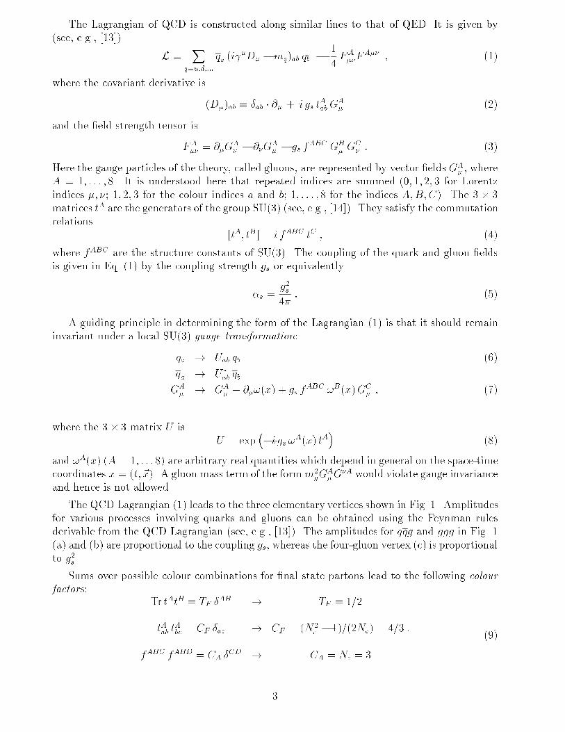
The QCD Lagrangian (1) leads to the three elementary vertices shown in Fig. 1. Amplitudes

for various processes involving quarks and gluons can be obtained using the Feynman rules

derivable from the QCD Lagrangian (see, e.g., [13]). The amplitudes for qqg and ggg in Fig. 1

(a) and (b) are proportional to the coupling gs, whereas the four-gluon vertex (c) is proportional

to g2s .

Sums over possible colour combinations for �nal state partons lead to the following colour

factors:Tr tAtB = TF �

AB ! TF = 1=2

tAab tAbc = CF �ac ! CF = (N2

c � 1)=(2Nc) = 4=3 :

fABC fABD = CA �CD ! CA = Nc = 3

(9)

3

(a)

q

q

g

(b)

g

g

g

(c)

g

g

g

g

Figure 1: Elementary vertices of QCD: (a) quark-gluon vertex, (b) triple gluon vertex, (c) four-gluon

vertex.

These relations hold for a general colour gauge theory with gauge group SU(Nc); the numerical

values given are for Nc = 3. The colour factor CF is proportional to the probability for the

branching q ! qg, CA gives the corresponding value for g ! gg and TF for g ! qq.

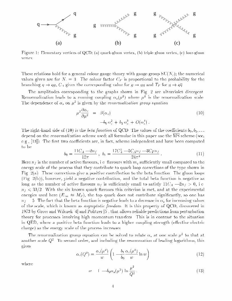
The amplitudes corresponding to the graphs shown in Fig. 2 are ultraviolet divergent.

Renormalization leads to a running coupling �s(�2) where �2 is the renormalization scale.

The dependence of �s on �2 is given by the renormalization group equation

�2@�s

@�2= �(�s) (10)

= �b0 �2s + b1 �3s + O(�4s) :

The right-hand side of (10) is the beta function of QCD. The values of the coe�cients b0; b1; : : :

depend on the renormalization scheme used; all formulae in this paper use the MS scheme (see,

e.g., [13]). The �rst two coe�cients are, in fact, scheme independent and have been computed

to be

b0 =11CA � 2nf

12�; b1 =

17C2A � 5CAnf � 3CFnf

24�2: (11)

Here nf is the number of active avours, i.e. avours with mq su�ciently small compared to the

energy scale of the process that they contribute to quark loop corrections of the type shown in

Fig. 2(a). These corrections give a positive contribution to the beta function. The gluon loops

(Fig. 2(b)), however, yield a negative contribution, and the total beta function is negative as

long as the number of active avours nf is su�ciently small to satisfy 11CA � 2nf > 0, i.e.

nf < 33=2. With the six known quark avours this criterion is met, and at the experimental

energies used here (Ecm � MZ), the top quark does not contribute signi�cantly, so one has

nf = 5. The fact that the beta function is negative leads to a decrease in �s for increasing values

of the scale, which is known as asymptotic freedom. It is this property of QCD, discovered in

1973 by Gross and Wilczek [4] and Politzer [5], that allows reliable predictions from perturbation

theory for processes involving high momentum transfers. This is in contrast to the situation

in QED, where a positive beta function leads to a higher coupling strength (e�ective electric

charge) as the energy scale of the process increases.

The renormalization group equation can be solved to relate �s at one scale �2 to that at

another scale Q2. To second order, and including the resummation of leading logarithms, this

gives

�s(Q2) =

�s(�2)

w

1 � b1

b0

�s(�2)

wlnw

!(12)

where

w = 1 � b0�s(�2) ln

�2

Q2: (13)

4

g

q

g g

g

g

(a) (b)

Figure 2: Virtual corrections to the gluon propagator: (a) quark loop, (b) gluon loop.

1.1.2 The Process e+e� ! hadrons

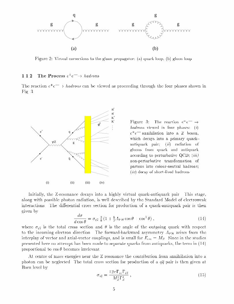
The reaction e+e� ! hadrons can be viewed as proceeding through the four phases shown in

Fig. 3.

e-

e+

γ/Z

q

q-

g

π+

π-

K+

K-

φ0...

(i) (ii) (iii) (iv)

Figure 3: The reaction e+e� !hadrons viewed in four phases: (i)

e+e� annihilation into a Z boson,

which decays into a primary quark-

antiquark pair; (ii) radiation of

gluons from quark and antiquark

according to perturbative QCD; (iii)

non-perturbative transformation of

partons into colour-neutral hadrons;

(iv) decay of short-lived hadrons.

Initially, the Z-resonance decays into a highly virtual quark-antiquark pair. This stage,

along with possible photon radiation, is well described by the Standard Model of electroweak

interactions. The di�erential cross section for production of a quark-antiquark pair is then

given byd�

d cos �= �qq

38 (1 +

83AFB cos � + cos2 �) ; (14)

where �qq is the total cross section and � is the angle of the outgoing quark with respect

to the incoming electron direction. The forward-backward asymmetry AFB arises from the

interplay of vector and axial-vector couplings, and is small for Ecm =MZ . Since in the studies

presented here no attempt has been made to separate quarks from antiquarks, the term in (14)

proportional to cos � becomes irrelevant.

At centre of mass energies near the Z resonance the contribution from annihilation into a

photon can be neglected. The total cross section for production of a qq pair is then given at

Born level by

�qq =12��ee�qq

M2Z�

2Z

; (15)

5

where MZ is the mass of the Z boson, and �ee, �qq, and �Z are the partial widths for Z decay

into e+e�, qq and the total width, respectively. Summing over the kinematically accessible

quark avours q = u; d; s; c; b and taking account of higher order corrections, such as initial

state photon radiation, results in a total hadronic cross section of around 30 nb. It is this large

cross section that makes possible the high statistics measurements presented here.

Final states having more partons in addition to the primary quark-antiquark pair can be

described by QCD using perturbation theory. To �rst order in �s, the di�erential cross section

for e+e� ! qqg is given by [15]

d2�

dx1dx2= �qq

CF�s

2�

x21 + x22(1 � x1)(1� x2)

; (16)

where

xi = 2Ei=Ecm (17)

are the parton energies normalized to the maximum allowed energy Ecm=2 with i = 1; 2; 3

(= q; q; g). Exact matrix elements have been computed only to second order in �s, and can be

found in [16]. This describes a maximum of four partons in the �nal state, qqgg or qqqq.

For predictions of �nal states with larger numbers of partons, one can use the parton shower

approach, based on the leading logarithm approximation. The main idea here is to reorganize

the perturbative expansion so that the terms with leading collinear singularities are summed to

all orders [17]. The result for the cross section can then be reinterpreted as a sequence of parton

branchings q ! qg, g ! gg and g ! qq. The virtual mass Q of the partons decreases after

each decay, which leads to a corresponding increase in the strong coupling �s(Q2). The shower

is terminated at some virtuality cut-o� Q0, below which �s becomes so large that perturbation

theory is no longer valid. At this point, other calculation techniques (e.g. phenomenological

models) must be invoked to describe the production of �nal state hadrons.

In order to include leading infrared singularities (where the energy of the emitted gluon

vanishes) one must account for the e�ects of soft gluon interference. It has been shown that the

e�ect of this interference is completely destructive to leading order outside of an angle-ordered

region for each parton decay [18]. That is, one can preserve the probabilistic interpretation of

the cascade simply by restricting the phase space allowed for each parton branching such that

the opening angles always decrease. The phase space constraint leads to a suppression of the

number of soft partons. Quantities sensitive to angular ordering are investigated in Section 4.1.

In principle QCD should be able to provide a complete description of hadronic �nal states,

including the transformation of partons into colour neutral hadrons (hadronization). At present,

however, this task is computationally impossible, since the low momentum-transfer (or virtual

mass) scale Q0 involved in hadronization leads to a coupling constant �s(Q20) too large to allow

meaningful predictions from perturbation theory. In place of QCD predictions for hadronization

one needs to introduce phenomenological models. If both the perturbative description and

the models were perfect, the value of Q0 would be arbitrary. In practice, Q0 is adjusted to

achieve the best overall description of the data; typical values are in the range 0.6{1.6 GeV,

corresponding to �s(Q20) � 0.3{0.5 (cf. Section 2.3).

Several approaches to the hadronization stage have been developed and implemented as

Monte Carlo event generators. These programs begin by generating an initial quark-antiquark

pair (possibly accompanied by initial state photon radiation) using the di�erential cross section

6

given by the electroweak Standard Model. The evolution of the parton system is treated with

some implementation of the perturbative techniques mentioned above, i.e. �xed-order matrix

elements or parton showers. The resulting system of partons will be referred to in the following

as the \parton level" of an event generator.

Models for relating the parton and hadron levels involve phenomenological constructs

such as clusters and strings. Although the hadron production mechanisms can be quite

di�erent in di�erent models, they possess important common features, e.g. local conservation

of quantum numbers such as charge, avour, and baryon number. A more detailed description

of hadronization models is given in Section 2.3.1.

1.2 The ALEPH Detector

The ALEPH detector operating at the CERN LEP electron-positron collider is designed to

study a wide range of phenomena produced in electron-positron collisions at centre of mass

energies up to 200 GeV. The results presented in this paper have been obtained at the Z

resonance where the events produced from Z decays can be complex, with particles distributed

over 4� in solid angle. In the case of hadronic decays the events can have high multiplicity

with around twenty charged particles and a similar number of neutrals. The detector thus was

designed to have high three-dimensional granularity, hermetic coverage and accurate vertexing.

The detector and its performance have been described in detail elsewhere [19, 20]; an overview,

containing only essential information, is presented in this section. The detector is constructed

from independent modular subdetectors, arranged as a cylindrical \barrel" section closed by

two \endcaps". The overall dimensions of the detector are approximately 12� 12� 12 m3 and

its weight is about 3000 tonnes. A schematic diagram is given in Fig. 4.

Because of the creation of e+e� pairs from photons, the loss of energy by electrons and

multiple Coulomb scattering, it is important that the material traversed by radiation from the

interaction point is kept to a minimum. The ALEPH beam pipe, which holds the LEP machine

vacuum, is a thin 5.5 m long tube which traverses the detector. The tube has an inner diameter

of 106 mm and is made from 1.1 mm thick beryllium in the 760 mm long central region. The

thickness of materials traversed by particles in passing through the detector is a function of

the polar angle; for angles greater than 40 degrees the total material, including the beam pipe,

preceding the electromagnetic calorimeter is less than 0.25 radiation lengths.

The origin of the ALEPH coordinate system is the theoretical beam crossing point, the

midpoint of the straight section between the two nearest LEP quadrupoles. The positive x-axis

points towards a vertical line through the LEP centre and is horizontal by de�nition. The

positive z axis is along the nominal e� beam direction. The y direction is orthogonal to x and

z and points upwards.

1.2.1 Particle tracking

The tracking system involves three detectors: a silicon vertex detector, a conventional drift

chamber and a large time projection chamber. These are contained within a 1.5 T magnetic

�eld, produced by a superconducting magnet coil, in order to obtain accurate measurement of

the momenta of charged particles.

The silicon vertex detector (VDET) [21] is used for particle tracking close to the electron-

positron interaction point and vertex detector hits are used also to provide additional precision

for tracks already reconstructed in the outer tracking detectors. The VDET consists of two

7

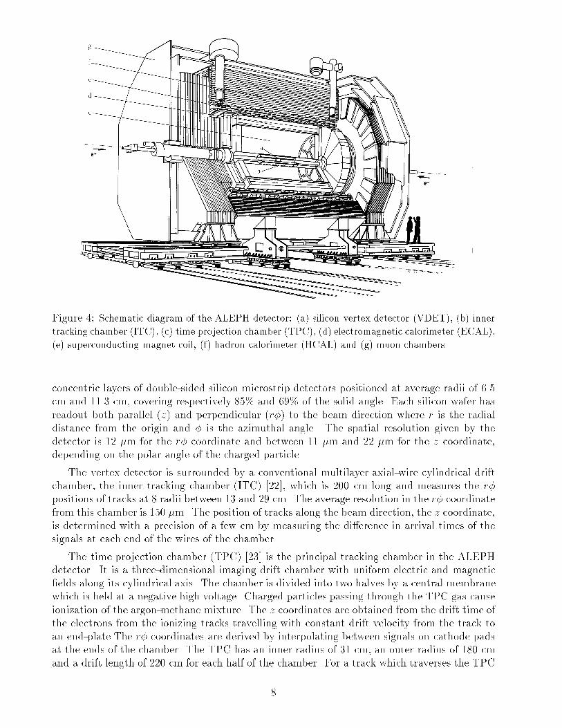
Figure 4: Schematic diagram of the ALEPH detector: (a) silicon vertex detector (VDET), (b) inner

tracking chamber (ITC), (c) time projection chamber (TPC), (d) electromagnetic calorimeter (ECAL),

(e) superconducting magnet coil, (f) hadron calorimeter (HCAL) and (g) muon chambers.

concentric layers of double-sided silicon microstrip detectors positioned at average radii of 6.5

cm and 11.3 cm, covering respectively 85% and 69% of the solid angle. Each silicon wafer has

readout both parallel (z) and perpendicular (r�) to the beam direction where r is the radial

distance from the origin and � is the azimuthal angle. The spatial resolution given by the

detector is 12 �m for the r� coordinate and between 11 �m and 22 �m for the z coordinate,

depending on the polar angle of the charged particle.

The vertex detector is surrounded by a conventional multilayer axial-wire cylindrical drift

chamber, the inner tracking chamber (ITC) [22], which is 200 cm long and measures the r�

positions of tracks at 8 radii between 13 and 29 cm. The average resolution in the r� coordinate

from this chamber is 150 �m. The position of tracks along the beam direction, the z coordinate,

is determined with a precision of a few cm by measuring the di�erence in arrival times of the

signals at each end of the wires of the chamber.

The time projection chamber (TPC) [23] is the principal tracking chamber in the ALEPH

detector. It is a three-dimensional imaging drift chamber with uniform electric and magnetic

�elds along its cylindrical axis. The chamber is divided into two halves by a central membrane

which is held at a negative high voltage. Charged particles passing through the TPC gas cause

ionization of the argon-methane mixture. The z coordinates are obtained from the drift time of

the electrons from the ionizing tracks travelling with constant drift velocity from the track to

an end-plate.The r� coordinates are derived by interpolating between signals on cathode pads

at the ends of the chamber. The TPC has an inner radius of 31 cm, an outer radius of 180 cm

and a drift length of 220 cm for each half of the chamber. For a track which traverses the TPC

8

up to 21 space coordinates and 338 samples of ionization energy loss can be determined. After

all corrections to the data an azimuthal coordinate resolution in the TPC of up to 173 �m in

r� and a longitudinal resolution in the z direction of up to 740 �m is obtained.

The track �nding e�ciency in the TPC has been studied using both Monte Carlo simulation

and visual scanning of events. In hadronic Z events, 98.6% of tracks that cross at least four

pad rows in the TPC are successfully reconstructed; the small ine�ciency due to track overlaps

and small gaps in the detector is reproduced to better than 10�3 by the simulation.

Using the combined information from the TPC, ITC and VDET a transverse momentum

resolution of �(1=pT ) = 0:6 � 10�3 (GeV/c)�1 has been measured with 45 GeV muons from

Z decays. The impact parameter resolution of charged particles measured in hadronic decays

can be parametrized as �(�) = 25�m+ 95�m=p (GeV/c)�1 in both the r� and rz views. As

discussed later, an important use of the precision impact parameter measurement is to detect

b hadrons via their lifetime.

1.2.2 Speci�c Ionization Measurement

In addition to its role as a tracking device, the TPC serves to separate particle species according

to measurements of their speci�c energy loss by ionization, dE=dx. The data from the TPC

sense wires, located in the end-plates, are used for the dE=dx measurement. Tracks must be at

least 3 cm apart in z in order to be resolved for dE=dx purposes. For tracks which have at least

50 dE=dx measurements it is found that dE=dx is very e�ective for electron identi�cation,

with greater than 3 � separation up to a momentum of about 8 GeV/c. In the relativistic

rise region, the region of most interest in the ALEPH experiment, the pion-kaon separation is

roughly constant at about 2 �, while the kaon-proton separation is about 1 �. Therefore, kaon

and proton identi�cation can be accomplished only on a statistical basis but, nonetheless, is an

important means of reducing combinatorial background in many analyses.

1.2.3 Calorimetry

The electromagnetic calorimeter (ECAL) consists of a \barrel" surrounding the TPC and closed

at each end by an \end-cap". It lies inside the superconducting magnet coil to minimize the

amount of material preceding it and covers 98% of the full solid angle. The barrel and two end-

caps each comprise 12 modules constructed from 45 layers of lead interleaved with proportional

wire chambers. The energy and position of each shower is read out using small cathode pads

with dimensions of around 30 mm � 30 mm. The cathode pads in each layer of the wire

chambers are connected internally to form \towers" oriented towards the interaction point.

Each tower is read out in three sections in depth of four, nine and nine radiation lengths.

There are some 74,000 towers in all, each with an angular width of about 0:9�� 0:9�. The highgranularity of the pads leads to excellent identi�cation of electrons and photons within jets.

The wire signals have very low noise and are used in an energy trigger which can work at a

threshold as low as 200 MeV.

In order to reduce the sensitivity of the photon energy measurement to hadronic background

and clustering e�ects, the energy is estimated from the signals in the four central towers of an

electromagnetic cluster. The energy resolution for electrons in the energy range from 1 to 45

GeV is �(E)=E = (0:18=qE=GeV+0:009). The angular resolution for electromagnetic showers

is approximately �(�; �) = (2:5=qE=GeV + 0:25) mrad.

9

The hadron calorimeter (HCAL) is used together with the electromagnetic calorimeter to

measure hadronic energy deposits and is also part of the muon identi�cation system. It consists

of 23 layers of limited streamer tubes 9�9 mm2 in cross-section between layers of iron absorber

each 50 mm thick, giving a total of 7.2 interaction lengths at 90�. The iron provides the

ux return for the magnetic �eld and also serves as a muon �lter. The calorimeter has a

tower readout similar to the ECAL with pads of angular size about 3:7� � 3:7� and is read out

capacitively in 4788 projective towers. Digital readout from aluminum strips running the whole

length of each tube provides a two-dimensional view of the development of hadronic showers.

The pad and strip readout again provide important redundancy in energy measurements. The

wire signals are used for triggering. The energy resolution of the calorimeter is 0:85=qE=GeV

for hadronic showers. The whole of HCAL is rotated by about 2� relative to ECAL to avoid

overlapping of the small gaps (\cracks") between modules.

Luminosity measurements are obtained with a precision of better than 0.1% via three

complementary calorimeters positioned close to the beam pipe at a distance of approximately

260 cm from, and on both sides of, the interaction point. These calorimeters also improve the

hermeticity of the detector by providing solid angle coverage down to 24 mrad from the beam

axis.

Outside the iron are two double layers of streamer tubes, the muon chambers, which provide

two space coordinates for particles leaving the detector.

1.2.4 The Trigger System

The ALEPH triggering system is organized into three levels. Level one decides whether or

not to read out all detector elements. The level two trigger simply seeks to verify a level one

charged track trigger by replacing the ITC tracking information with the more accurate TPC

tracking information available 50 �s after the beam crossing. A level three software trigger is

used to reject background such as beam-gas interactions and o�-momentum particles hitting

the vacuum chamber or collimators.

Hadronic Z decays are collected using a level one trigger in which deposits in the

electromagnetic calorimeter (total-energy trigger) have an energy greater than 6 GeV in the

barrel or 3 GeV in either endcap or greater than 1.5 GeV in both endcaps in coincidence.

An independent trigger requires that track segments in the drift chamber coincide with hits

in a module of the hadron calorimeter, so requiring a certain penetration depth (muon-track

trigger). This trigger is sensitive to muons and, with lower e�ciency, to hadrons. Asking for

either of these trigger requirements to be satis�ed provides an e�ciency of greater than 99.9%

for selected hadronic decays.

1.2.5 The Identi�cation of K0 mesons and � Hyperons

Charged particle tracks which do not originate from the main interaction point can arise from

neutral particles, such as K0's and �'s, which decay inside the tracking volume to produce a

characteristic V 0 signature.

An algorithm to identify V 0s considers all pairs of oppositely charged particle tracks with

momentum larger than 150 MeV/c and with more than �ve TPC coordinates and tests for the

hypothesis that they originate from a common secondary vertex. The parameters of the �t are

the track momenta and the coordinates of the secondary vertex. In order to ensure a separation

between primary and secondary vertices, the proper lifetime of a given V 0 hypothesis is required

10

to be between 0.2 and 5 times the expected lifetime. Since combinatorial background peaks

strongly at forward decay angles, the cosine of the decay angle is required to be less than 0.85

for K0s and 0.95 for �s. Furthermore, the distance of closest approach from the V 0 direction

to the primary vertex is required to be less than 1.0 cm in the transverse plane. When a useful

measurement of the speci�c ionization (dE=dx) is available for a given track of a V 0 candidate

it is required to be within three standard deviations of the expected value. Finally, a signi�cant

reduction in background is obtained by requiring a successful kinematical V 0 �t, constrained

by the mass hypothesis and the primary vertex.

1.2.6 Energy Flow Determination

The simplest way to determine the total energy of an event recorded in the ALEPH detector

is to sum the raw energy found in all calorimetric cells without performing any particle

identi�cation. This method yields a resolution of �(E)=E = 1:2=qE=GeV for hadronic decays

of the Z. In order to improve the resolution, an energy ow reconstruction algorithm has been

developed making use of track momenta and taking advantage of the photon, electron and

muon identi�cation capabilities of the detector. In a �rst stage, charged particle tracks and

calorimeter clusters are subjected to a sequence of \cleaning" operations, using the information

from the tracking detectors and taking advantage of the redundancy in the readout of both

calorimeters. The \cleaned" charged particle tracks are extrapolated to the calorimeters and

groups of topologically connected tracks and clusters, called \calorimeter objects", are formed.

Charged-particle tracks identi�ed as electrons or muons and neutral electromagnetic energy

objects identi�ed as photons are removed from the \calorimetric objects". All the particles

remaining in the calorimeter objects should be charged or neutral hadrons. The charged

hadron energy in a given object can be determined from the tracking information. The excess

calorimetric energy is assigned to neutral hadrons. A direct identi�cation of neutral hadrons

has not been attempted. The result of the above procedure is a set of \energy ow objects",

or particles characterized by their energy and momenta. The energy resolution is reproduced

by �(E) = (0:59 � 0:03)qE=GeV + (0:6� 0:3) GeV.

1.2.7 Heavy Quark Tagging

A large number of boosted b hadrons are produced at the Z resonance in the ALEPH experiment.

A high purity sample of b hadrons can be obtained by identifying their semi-leptonic decay

modes. However, this approach yields relatively low statistics when the semi-leptonic branching

ratio is combined with the lepton identi�cation e�ciency. A large increase in statistics can be

gained by using the fact that the long lifetime and large mass of b hadrons give their decay

products large impact parameters, de�ned as the distance of closest approach between a track

and the b production point. The b hadrons produced in Z decays travel typically several

mm before decaying into several charged particles, including the decay products of secondary

charmed hadrons. The masses of the �nal decay products are an order of magnitude less than

those of the b hadrons, resulting in highly energetic decays. Thus b�b events are characterized

by the presence of many charged tracks with signi�cant impact parameters with respect to the

Z decay point. Charmed hadrons have similar decay lengths but are lighter and their decays

have lower charged multiplicities. The precise three-dimensional tracking information available

from the VDET then can be exploited to provide accurate impact parameter measurements

and thus allow a separation of b's from other hadrons. The typical primary vertex resolution is

11

about 50 �m for the horizontal coordinate, 10 �m for the vertical and 60 �m along the beam

direction. The impact parameter resolution is about 70 �m.

The tracks in an event are clustered into jets, the jet de�nition having been optimized to

reproduce the directions of b hadrons within b�b events. The b production point is reconstructed

for each event by combining the beam spot position with the track information for the particular

event. The tracks are associated to their nearest jet and they are projected onto the plane

perpendicular to this jet. This projection removes the bias due to tracks coming from secondary

vertices, in the approximation that the jet axis reproduces the direction of the decaying particle.

The projected tracks are then combined with the beam spot position to �nd the primary vertex.

The sensitivity to lifetime is increased by determining a sign for each three-dimensional

impact parameter using the jet direction. The sign is positive if the point of closest approach

between the track and the b direction is in the same hemisphere as the track, the hemisphere

being de�ned by the plane perpendicular to the b direction and containing the b production

point.

By combining the impact parameter information from all tracks within an event, a tag

variable can be constructed which can be used to distinguish b�b events from those of lighter

quarks. The e�ciency for tagging b's is correlated to the purity of the b sample. Within the

angular acceptance of the VDET, a tagging e�ciency in excess of 60% is achieved for a typical

b purity of 80%.

1.3 Data Analysis Overview

In this section the general framework of the analyses will be described, including the selection of

tracks, photons and other reconstructed objects, event selection, and the correction of measured

quantities for various detector related e�ects. The exact procedures vary somewhat from one

analysis to the next, and the di�erences from the general methods outlined here will be explained

as required for each individual case.

1.3.1 Track and Event Selection

The event selection for most of the studies is based on tracks of charged particles. Tracks are

selected that have at least four measured space coordinates from the TPC, a polar angle in

the range 20� < � < 160�, and a transverse momentum with respect to the beam direction of

p? > 0:2 GeV. In addition, the closest radial distance of approach of the extrapolated track to

the beam line, d0, is required to be less than 2 cm, and the z coordinate of the point of closest

radial approach, z0, is required to be less than 5 cm.

Using the selected tracks, the sphericity axis and the total charged energy Ech =P

iEi =Pi

qp2i +m2

� are computed. (The sphericity axis is described in Section 2.1.) Events are

selected that have at least �ve charged tracks, Ech > 15 GeV, and for which the polar angle

of the sphericity axis is in the range 35� < �sph < 145�. The latter cut (not required for

all analyses) ensures that the event is well contained within the detector. For data taken

by the ALEPH detector between 1991 and 1994 these cuts result in approximately 2 million

selected events. Most of the analyses presented use only a subset of these data. The largest

background contribution is from events of the type e+e� ! �+��, which are estimated to make

up approximately 0:26% of the selected events. For most of the analyses considered, this can be

neglected; in individual cases (e.g. the study of scaling violations in fragmentation functions) a

background subtraction was carried out using a Monte Carlo model.

12

1.3.2 Corrections for Detector E�ects

Before a measured quantity can be compared with theoretical predictions or with the results

of other measurements it must �rst be corrected for various detector related e�ects, such as

geometrical acceptance, detector e�ciency and resolution, decays, particle interactions with the

material of the detector and the e�ects of event and track selection, and also for the e�ect of

initial state photon radiation. For most of the analyses presented this is done with multiplicative

correction factors C, relating the measured value of a quantity X, such as a bin content, to the

corrected value,

Xcorrected = Xmeasured � C : (18)

For distributions, the correction factors are computed individually for each bin. Several

analyses, e.g. Sections 2, 4.2, involve a more sophisticated unfolding procedure; this is described

in the corresponding sections.

The correction factors are computed according to the following procedure. First, hadronic

events with the mixture of primary quark avours as predicted by the Standard Model are

generated using the program HVFL, which incorporates several components. The initial quark-

antiquark pair and intial state photon radiation are generated with the program DYMU [24].

These are then passed to the Lund Parton Shower Model [25] (program JETSET version 7.3), in

which the decay properties of heavy avour (b and c) hadrons have been signi�cantly extended.

The events are processed through the detector simulation program to produce simulated

raw data, which are then processed by the same reconstruction and analysis programs as used

for the real data. From these data the value of the observable in question is computed yielding

XMC+det: sim:.

A second set of Monte Carlo data is then generated, but here with initial state radiation

turned o�, and with all particles having mean lifetimes less than 10�9 seconds required to

decay, and all other particles being treated as stable. In this way the charged particles de�ned

to belong to the �nal state correspond approximately to those which are actually seen in the

detector. For example, decay products of K0S mesons and strange baryons are included as

�nal state particles, whereas K0L mesons are treated as stable. This second data set is used to

compute the corresponding observable Xgenerator . The correction factor C is the ratio of the

two quantities,

C =Xgenerator

XMC+det: sim:

: (19)

Depending on the analysis, the quantity Xgenerator may be computed using all particles,

including neutrals (even if the measurement was only based on charged particles) or it may

be computed using some well-de�ned subset of the particles, e.g. only charged. Application

of the factors de�ned in this way results in measurements corrected to a well-de�ned particle

composition and centre of mass energy without initial state radiation.

Although the correction factors are to a good approximation independent of the event

generator used, a residual dependence remains and must be taken into account in the estimation

of systematic errors. For example, in analyses where only charged particles are measured, but

where the quantity Xgenerator in (19) is computed using all particles (including neutrals), one

relies on the Monte Carlo model to describe the e�ect of the neutrals on the observable. Another

source of generator dependence arises from the smearing of distributions due to �nite resolution.

These e�ects are taken into account (\unfolded") by the technique described above, but the

result is only correct to the extent that the distributions in nature are the same as those in the

Monte Carlo model. One straightforward way of approaching this problem would be to compute

13

the correction factors with several di�erent Monte Carlo generators in order to estimate their

model dependence. This is impractical, however, because of the large amount of computing

time required by the detector simulation.

Most of the analyses use the following approximate technique to estimate the generator

dependence of the correction factors. Instead of using data processed by the full detector

simulation, a highly simpli�ed simulation is performed by merely applying the same cuts on

energy, transverse momentum, geometry, etc. as used for the real analysis. In some cases,

�nite energy resolution is simulated by smearing the generated energies according to the

parameterized response of the detector. Simpli�ed correction factors can then be computed

as

Csimplified =Xgenerator

XMC+cuts

: (20)

These factors can be computed for a variety of event generators, and the spread in the resulting

values is taken as a contribution to the systematic uncertainty. For many quantities (especially

distributions of event-shape variables) the simpli�ed correction factors are qualitatively very

similar to the factors based on the full detector simulation, indicating that the corrections

are largely determined by cuts on geometry and energy, and/or by the correction for neutral

particles if only charged particle information is used in the measurement.

The systematic errors due to model dependence of the correction factors are highly correlated

from bin-to-bin. This is also the case for systematic uncertainties due to the modelling of the

detector, which in most analyses are estimated by varying the experimental cuts in a certain

range. In cases where the distribution is used to derive a further quantity (e.g. �s, Section 3.2),

these correlations can be taken into account by correcting the distribution with di�erent sets

of simpli�ed factors or by using di�erent sets of cuts, obtaining the derived quantity from each

alternative distribution, and then using the spread in the resulting values as a measure of its

systematic error.

14

2 Global Event Structure and Tuning of Model

Parameters

In this section event-shape and charged particle inclusive distributions are presented. The

analysis here represents an update of Ref. [26]. The distributions are used along with other

measurements of identi�ed hadrons to tune the parameters of QCD event generators in

Section 2.3.

2.1 De�nition of Observables

Distributions of the following event-shape variables,

- S, sphericity;

- A, aplanarity;

- T , thrust;

- Tminor;

- ln(1=y3), where y3 is the two-jet resolution variable (see below);

- � =M2h=s, heavy jet mass;

- C parameter;

- O, oblateness;

and the following inclusive distributions,

- xp, scaled momentum ( = 2j~pj=Ecm);

- y, rapidity with respect to the thrust axis;

- pin? , component of momentum in the event plane along ~n2 (see below);

- pout? , component of momentum out of the event plane along ~n1 (see below);

have been measured.

The variables above are de�ned in the following way. Sphericity and aplanarity are obtained

from the eigenvalues of the momentum tensor M�� =P

j p�jp�j, where � and � refer to the x,

y and z directions, and the sum is carried out over all of the selected particles in the event.

Normalizing the eigenvalues Qi such that Q1 + Q2 + Q3 = 1, and ordering them such that

0 < Q1 < Q2 < Q3, one de�nes the sphericity as S = 32(Q1 + Q2) and the aplanarity as

A = 32Q1. The eigenvector ~n3 determines the sphericity axis, and ~n2 and ~n3 de�ne the event

plane. The sphericity (0 � S � 1) approaches zero for extreme two-jet events and unity for

spherical events. The aplanarity (0 � A � 0:5) is a measure of event atness, approaching zero

for planar events.

The thrust of an event is de�ned as T = max(P

j jpkjj=P

j jpjj) where the sum is over all

the selected particles in the event and pk refers to the momentum component along the axis for

15

which T is maximum (the thrust axis). The direction perpendicular to the thrust axis relative

to which the corresponding sum of parallel momenta is maximized is called the major axis, and

the axis perpendicular to the thrust and major axes is the minor axis. The major and minor

values are de�ned as Tmajor (minor) =P

j jpkjj=P

j jpj j where pk is the momentum component

along the major (minor) axis. The thrust (0:5 < T < 1) approaches unity for extreme two-jet

events, and the minor value approaches zero for planar events. The oblateness O is de�ned as

O = Tmajor � Tminor.

The heavy jet mass is de�ned by �rst separating the event into two hemispheres by means

of a plane perpendicular to the thrust axis and computing the invariant mass of the particles

in each. The larger of the two masses isMh, and the event-shape variable � is de�ned as M2h=s.

The C parameter is de�ned as C = 3(�1�2 + �1�3 + �2�3), where �1; �2, and �3 are the

eigenvalues of the linear momentum tensor M0

�� =P

ipi�pi�jpij =

Pi jpij.

The single particle inclusive distributions of transverse momentum in and out of the event

plane provide an additional measure of the overall event shape. These can be de�ned as

pin? = j~p � ~n2j and pout? = j~p � ~n1j where ~n1 and ~n2 are normalized eigenvectors of the momentum

tensor.

The rapidity of a particle is de�ned as y = 12 ln[(E + pk)=(E � pk)]. Here, pk refers to the

component of the momentumparallel to the thrust axis, and the energy, E, is obtained from the

particle's momentum assuming the pion mass. The detector corrections are then constructed

such that the �nal corrected distribution corresponds to the true hadron masses.

The event-shape variable y3 as well as the n-jet rates for n = 2; 3; 4; 5 are obtained using a

jet clustering algorithm. Such algorithms are used in a number of the analyses in this paper and

therefore will be de�ned in some detail here. For each pair of particles i and j in an event one

computes a measure of their \distance" yij. Two distance measures or metrics are commonly

used. In the so-called JADE algorithm [27] it is de�ned as

yij =2Ei Ej (1� cos �ij)

E2vis

; (21)

where Ei and Ej are the particles' energies, �ij their opening angle, and Evis the total energy

of all of the particles used in the event. In the so-called Durham (or \k?") algorithm [28] the

distance measure is de�ned as

yij =2min(E2

i ; E2j )(1 � cos �ij)

E2vis

: (22)

The pair of particles with the smallest value of yij is replaced by a pseudoparticle (cluster).

The four-momentum of the cluster is then computed according to one of several recombination

schemes. Most commonly used is the \E" scheme, where the four momentum of the cluster is

taken to be the sum of the four momenta of particles i and j, p� = p�i +p�j . Another possibility

is the \E0" scheme, where the energy of the cluster is given by the sum E = Ei + Ej , and the

cluster momentum is given by scaling the three components of ~pi + ~pj such that the invariant

mass of the cluster is zero. Similarly, in the \P0" scheme the momenta are added and the

energy sum Ei + Ej is scaled to give a massless cluster.

The clustering procedure is repeated until all of the yij are greater than a given threshold,

ycut (the jet resolution parameter). The number of jets is de�ned to be the number of remaining

clusters. Alternatively one can use the algorithm to de�ne the event-shape variable y3 by

16

continuing the clustering until exactly three clusters remain. The smallest value of yij in this

con�guration is de�ned as y3. In this way one obtains a single number for each event, whose

distribution is sensitive to the probability of hard gluon radiation leading to a three-jet topology.

2.2 Analysis Technique and Results

The analysis is based on charged particle tracks (except for the n-jet rates; see below), since

this allows for an accurate tuning of model parameters. The track and event selection followed

the description in Section 1.3.1. In addition, for events with 5 or 6 tracks it was required that

the invariant mass of at least one hemisphere be greater than the � mass. This reduces the

background from �+�� events to negligible levels, and results in 571800 accepted events from

the 1992 data taking period at a centre of mass energy Ecm = 91:2 GeV.

In order to be able to compare more easily with other experiments, the n-jet rates were

computed using both charged and neutral particles (see Section 1.2.6). Hadronic events were

selected by requiring a total visible energy of at least 50% of Ecm, at least 15 reconstructed

particles (charged or neutral), and that the polar angle of the thrust axis be in the range

30� < �thrust < 150�. The cut on the number of particles e�ectively eliminates background

from �+�� events.

For the single particle inclusive distributions, corrections for detector related e�ects were

made by means of bin-by-bin factors as described in Section 1.3.2. For these distributions

the bin size was chosen to be always at least twice as large as the detector resolution. For

the charged particle distributions of y, pin? and pout? , the correction factors were constructed

such that the event axis and event plane correspond to charged particles only. Multiplicative

correction factors were also applied to the n-jet rates.

The event-shape distributions were corrected by means of a matrix method. As with

the technique of bin-by-bin factors, the matrix method used here introduces a certain model

dependence; this is taken into account when estimating the systematic errors. In order to

minimize this model dependence, the distributions were not corrected to account for neutral

particles, i.e. the results represent what would be obtained with charged particles only. The

matrix method allows one to use smaller bin sizes than would be reliable with bin-by-bin

corrections; they were chosen here to be somewhat smaller than twice the corresponding

detector resolution.

The matrix correction method was performed in the following way. Monte Carlo events

passing the event selection criteria were used to �ll a two-dimensional histogram. The

probability that an event is generated with xgen in interval j, given that it is observed with xrecin interval i, is given by

Bji =HijPkHik

;

where Hij is the number of events where the pair (xrec; xgen) falls into the interval (i; j). The

matrix B relates the generated and reconstructed Monte Carlo distributions,

DMCj;gen(x)�xj =

Xi

BjiDMCi;rec(x)�xi ;

where �x is the bin width. This can be used to correct the data,

Ddataj;corr(x)�xj =

�Ci(x)Xi

BjiDdatai;rec(x)�xi ;

17

where the additional factor

�Ci(x) =DMCi;gen(no cuts; no ISR)

DMCi;gen(cuts; ISR)

corrects for initial state radiation (ISR) as well as for the fact that the generated distribution

depends on the event selection cuts. This procedure is to �rst approximation independent of

the Monte Carlo generator used. A possible model dependence cannot be excluded, however,

since the matrix B depends on the input Monte Carlo distribution. It has been found that

the di�erences between the results of the matrix method and those of the bin-by-bin factors

method are of the order of the errors of the data.

Systematic uncertainties have been estimated by individually varying all track and event

selection cuts. The maximum change in each bin with respect to the standard set of cuts is

included in the systematic error. The largest sources of error (approximately 0.5%) were found

to be in the low momentum region (xp � 0:01) when changing the cuts on the number of TPC

coordinates (from 4 to 7) and on the minimum transverse momentum (from 0.2 GeV to 0.3

GeV). In addition, a systematic error due to model dependence was estimated by computing

simpli�ed correction factors based on the models JETSET [25, 29], ARIADNE [30] and

HERWIG, [31] as described in Section 1.3.2. The di�erence between the JETSET and HERWIG

correction factors gave approximately a 1% error in the xp distribution around xp � 0:01, and

a 1{2% error in the event-shape distributions in the heavily populated regions. The total

systematic error is given as the quadratic sum of the contributions from cut dependence and

model dependence, and the bin-to-bin uctuations of the errors have been smoothed.

As a further check, the ratio of positive to negative particle rates was found to be reproduced

by the detector simulation to better than 0.6% overall and to within 1.2% at low momenta.

The reported distributions give the summed contributions of positive and negative particles,

and the uncertainty resulting from this check is small compared to the other errors given above.

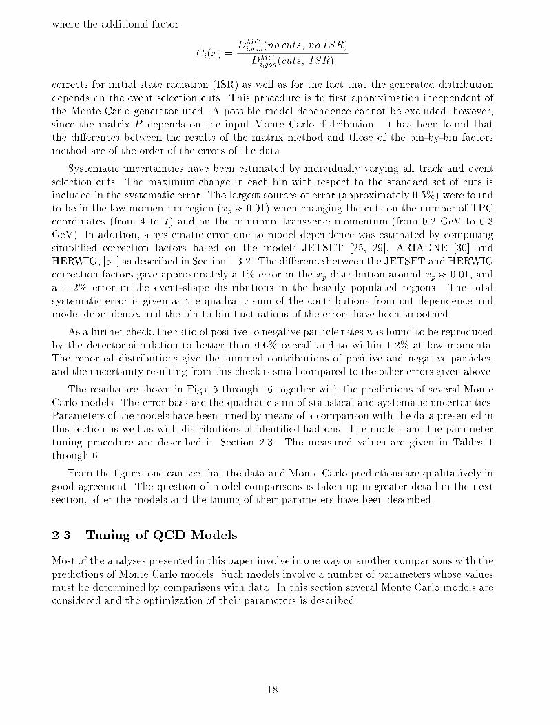
The results are shown in Figs. 5 through 16 together with the predictions of several Monte

Carlo models. The error bars are the quadratic sum of statistical and systematic uncertainties.

Parameters of the models have been tuned by means of a comparison with the data presented in

this section as well as with distributions of identi�ed hadrons. The models and the parameter

tuning procedure are described in Section 2.3. The measured values are given in Tables 1

through 6.

From the �gures one can see that the data and Monte Carlo predictions are qualitatively in

good agreement. The question of model comparisons is taken up in greater detail in the next

section, after the models and the tuning of their parameters have been described.

2.3 Tuning of QCD Models

Most of the analyses presented in this paper involve in one way or another comparisons with the

predictions of Monte Carlo models. Such models involve a number of parameters whose values

must be determined by comparisons with data. In this section several Monte Carlo models are

considered and the optimization of their parameters is described.

18

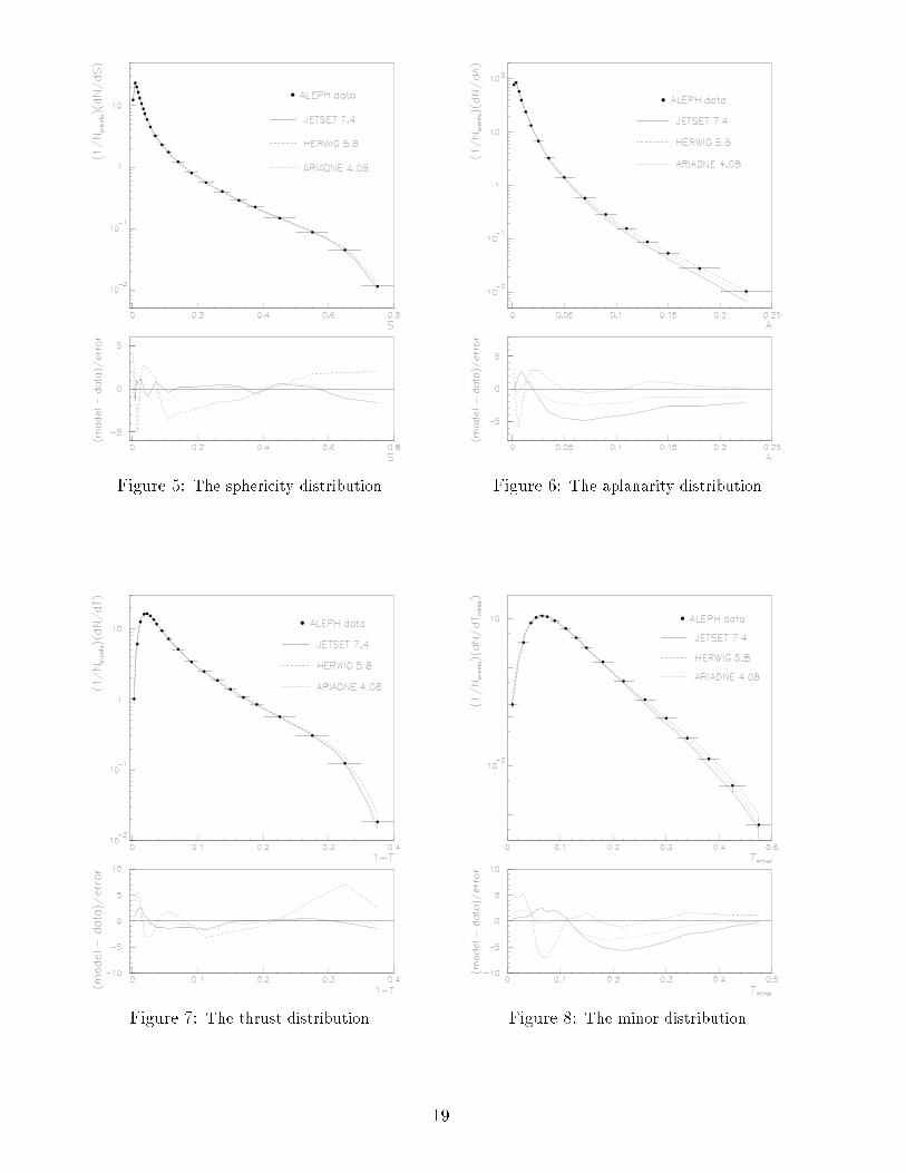
Figure 5: The sphericity distribution. Figure 6: The aplanarity distribution.

Figure 7: The thrust distribution. Figure 8: The minor distribution.

19

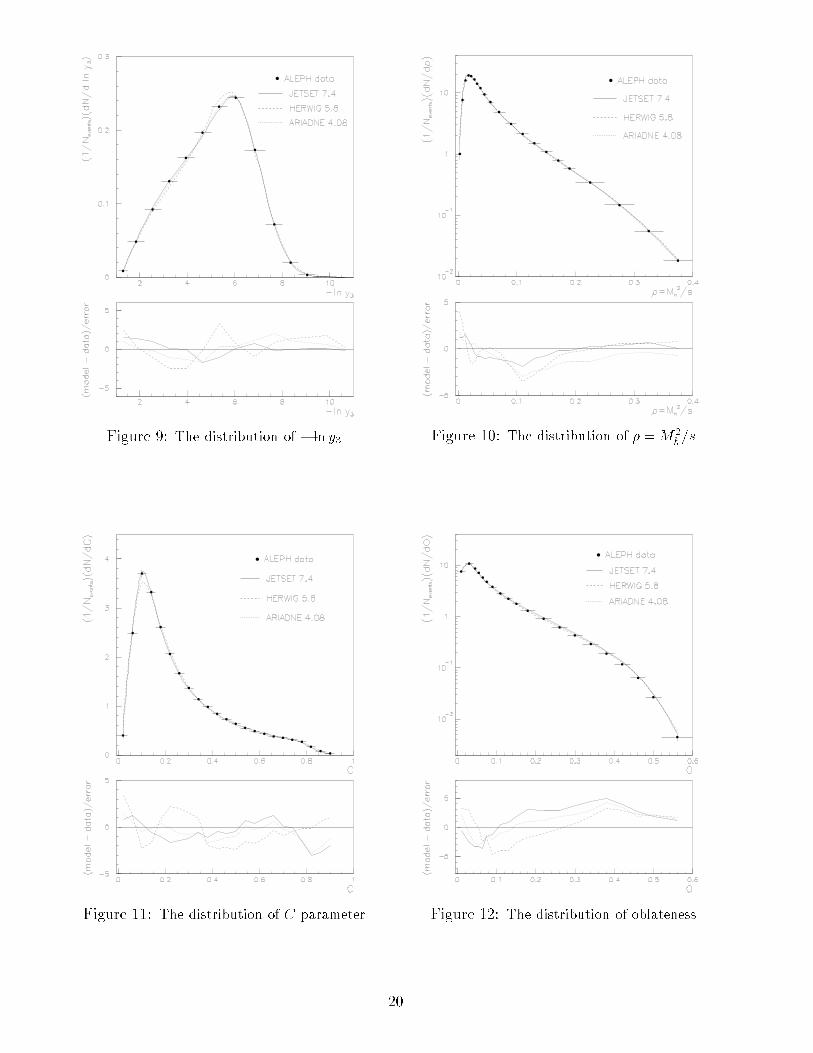
Figure 9: The distribution of � ln y3. Figure 10: The distribution of � =M2h=s.

Figure 11: The distribution of C parameter. Figure 12: The distribution of oblateness.

20

Figure 13: The inclusive distribution of xp =

p=pbeam for charged particles.

Figure 14: The inclusive distribution of rapidity

y for charged particles with respect to the thrust

axis.

Figure 15: The inclusive distribution of pin? for

charged particles, using the event plane based

on the sphericity tensor.

Figure 16: The inclusive distribution of pout? for

charged particles, using the event plane based

on the sphericity tensor.

21

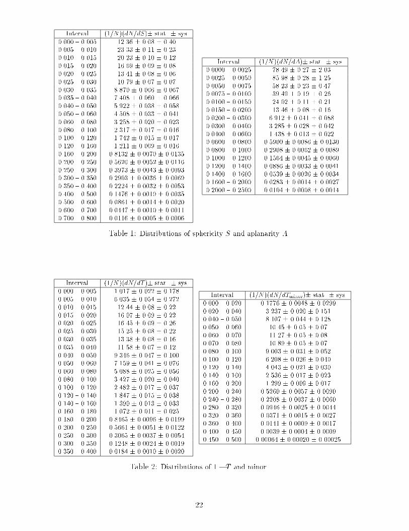
Interval (1=N )(dN=dS)� stat. � sys.

0.000 { 0.005 12.36 � 0.08 � 0.40

0.005 { 0.010 23.33 � 0.11 � 0.23

0.010 { 0.015 20.23 � 0.10 � 0.12

0.015 { 0.020 16.69 � 0.09 � 0.08

0.020 { 0.025 13.41 � 0.08 � 0.06

0.025 { 0.030 10.79 � 0.07 � 0.07

0.030 { 0.035 8.870 � 0.066 � 0.067

0.035 { 0.040 7.408 � 0.060 � 0.066

0.040 { 0.050 5.922 � 0.038 � 0.058

0.050 { 0.060 4.508 � 0.033 � 0.041

0.060 { 0.080 3.258 � 0.020 � 0.023

0.080 { 0.100 2.317 � 0.017 � 0.016

0.100 { 0.120 1.742 � 0.015 � 0.017

0.120 { 0.160 1.211 � 0.009 � 0.016

0.160 { 0.200 0.8132 � 0.0070 � 0.0135

0.200 { 0.250 0.5626 � 0.0052 � 0.0116

0.250 { 0.300 0.3973 � 0.0043 � 0.0093

0.300 { 0.350 0.2903 � 0.0036 � 0.0069

0.350 { 0.400 0.2224 � 0.0032 � 0.0053

0.400 { 0.500 0.1476 � 0.0019 � 0.0035

0.500 { 0.600 0.0861 � 0.0014 � 0.0020

0.600 { 0.700 0.0447 � 0.0010 � 0.0011

0.700 { 0.800 0.0116 � 0.0005 � 0.0006

Interval (1=N )(dN=dA)� stat. � sys.

0.0000 { 0.0025 78.49 � 0.27 � 2.03

0.0025 { 0.0050 85.98 � 0.28 � 1.25

0.0050 { 0.0075 58.23 � 0.23 � 0.47

0.0075 { 0.0100 39.49 � 0.19 � 0.26

0.0100 { 0.0150 24.02 � 0.11 � 0.21

0.0150 { 0.0200 13.46 � 0.08 � 0.16

0.0200 { 0.0300 6.912 � 0.041 � 0.088

0.0300 { 0.0400 3.285 � 0.028 � 0.042

0.0400 { 0.0600 1.438 � 0.013 � 0.022

0.0600 { 0.0800 0.5900 � 0.0086 � 0.0130

0.0800 { 0.1000 0.2908 � 0.0062 � 0.0089

0.1000 { 0.1200 0.1564 � 0.0045 � 0.0060

0.1200 { 0.1400 0.0886 � 0.0033 � 0.0041

0.1400 { 0.1600 0.0539 � 0.0026 � 0.0034

0.1600 { 0.2000 0.0283 � 0.0014 � 0.0027

0.2000 { 0.2500 0.0104 � 0.0008 � 0.0014

Table 1: Distributions of sphericity S and aplanarity A.

Interval (1=N )(dN=dT )� stat. � sys.

0.000 { 0.005 1.017 � 0.022 � 0.178

0.005 { 0.010 6.035 � 0.054 � 0.272

0.010 { 0.015 12.44 � 0.08 � 0.22

0.015 { 0.020 16.07 � 0.09 � 0.22

0.020 { 0.025 16.45 � 0.09 � 0.26

0.025 { 0.030 15.25 � 0.08 � 0.22

0.030 { 0.035 13.38 � 0.08 � 0.16

0.035 { 0.040 11.58 � 0.07 � 0.12

0.040 { 0.050 9.346 � 0.047 � 0.100

0.050 { 0.060 7.159 � 0.041 � 0.076

0.060 { 0.080 5.088 � 0.025 � 0.056

0.080 { 0.100 3.427 � 0.020 � 0.040

0.100 { 0.120 2.482 � 0.017 � 0.037

0.120 { 0.140 1.847 � 0.015 � 0.038

0.140 { 0.160 1.390 � 0.013 � 0.033

0.160 { 0.180 1.072 � 0.011 � 0.025

0.180 { 0.200 0.8465 � 0.0096 � 0.0199

0.200 { 0.250 0.5661 � 0.0051 � 0.0122

0.250 { 0.300 0.3065 � 0.0037 � 0.0054

0.300 { 0.350 0.1248 � 0.0024 � 0.0019

0.350 { 0.400 0.0184 � 0.0010 � 0.0020

Interval (1=N )(dN=dTminor)� stat. � sys.

0.000 { 0.020 0.1776 � 0.0048 � 0.0299

0.020 { 0.040 3.237 � 0.020 � 0.151

0.040 { 0.050 8.107 � 0.044 � 0.128

0.050 { 0.060 10.45 � 0.05 � 0.07

0.060 { 0.070 11.27 � 0.05 � 0.08

0.070 { 0.080 10.89 � 0.05 � 0.07

0.080 { 0.100 9.003 � 0.031 � 0.052

0.100 { 0.120 6.208 � 0.026 � 0.040

0.120 { 0.140 4.043 � 0.021 � 0.030

0.140 { 0.160 2.536 � 0.017 � 0.023

0.160 { 0.200 1.299 � 0.009 � 0.017

0.200 { 0.240 0.5260 � 0.0057 � 0.0090

0.240 { 0.280 0.2208 � 0.0037 � 0.0060

0.280 { 0.320 0.0946 � 0.0025 � 0.0044

0.320 { 0.360 0.0371 � 0.0015 � 0.0027

0.360 { 0.400 0.0141 � 0.0009 � 0.0017

0.400 { 0.450 0.0039 � 0.0004 � 0.0009

0.450 { 0.500 0.00064 � 0.00020 � 0.00025

Table 2: Distributions of 1� T and minor.

22

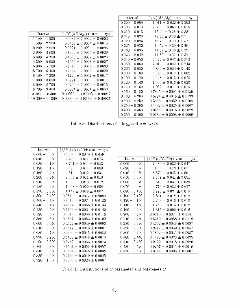
Interval (1=N )(dN=dy3)� stat. � sys.

1.100 { 1.500 0.0084 � 0.0002 � 0.0003

1.500 { 2.200 0.0483 � 0.0004 � 0.0015

2.200 { 2.900 0.0921 � 0.0005 � 0.0026

2.900 { 3.600 0.1306 � 0.0006 � 0.0029

3.600 { 4.300 0.1623 � 0.0007 � 0.0026

4.300 { 5.000 0.1969 � 0.0008 � 0.0027

5.000 { 5.700 0.2318 � 0.0009 � 0.0030

5.700 { 6.400 0.2442 � 0.0009 � 0.0029

6.400 { 7.300 0.1729 � 0.0007 � 0.0017

7.300 { 8.000 0.0721 � 0.0005 � 0.0014

8.000 { 8.700 0.0200 � 0.0003 � 0.0015

8.700 { 9.400 0.0034 � 0.0001 � 0.0006

9.400 { 10.300 0.00036 � 0.00003 � 0.00012

10.300 { 11.000 0.00004 � 0.00001 � 0.00007

Interval (1=N )(dN=d�)� stat. � sys.

0.000 { 0.005 1.011 � 0.022 � 0.202

0.005 { 0.010 7.656 � 0.060 � 0.818

0.010 { 0.015 15.90 � 0.08 � 0.83

0.015 { 0.020 19.36 � 0.09 � 0.71

0.020 { 0.025 18.73 � 0.09 � 0.57

0.025 { 0.030 16.52 � 0.09 � 0.40

0.030 { 0.035 14.07 � 0.08 � 0.32

0.035 { 0.040 11.89 � 0.07 � 0.32

0.040 { 0.050 9.422 � 0.047 � 0.312

0.050 { 0.060 7.013 � 0.040 � 0.243

0.060 { 0.080 4.839 � 0.024 � 0.140

0.080 { 0.100 3.125 � 0.019 � 0.062

0.100 { 0.120 2.138 � 0.015 � 0.029

0.120 { 0.140 1.506 � 0.013 � 0.020

0.140 { 0.160 1.089 � 0.011 � 0.019

0.160 { 0.180 0.7835 � 0.0091 � 0.0159

0.180 { 0.200 0.5794 � 0.0078 � 0.0133

0.200 { 0.250 0.3466 � 0.0039 � 0.0108

0.250 { 0.300 0.1482 � 0.0025 � 0.0067

0.300 { 0.350 0.0554 � 0.0015 � 0.0029

0.350 { 0.400 0.0182 � 0.0008 � 0.0009

Table 3: Distributions of � ln y3 and � =M2h=s.

Interval (1=N )(dN=dC)� stat. � sys.

0.000 { 0.040 0.4008 � 0.0046 � 0.0581

0.040 { 0.080 2.490 � 0.011 � 0.075

0.080 { 0.120 3.701 � 0.014 � 0.083

0.120 { 0.160 3.323 � 0.014 � 0.060

0.160 { 0.200 2.613 � 0.012 � 0.034

0.200 { 0.240 2.065 � 0.011 � 0.019

0.240 { 0.280 1.666 � 0.010 � 0.012

0.280 { 0.320 1.368 � 0.009 � 0.008

0.320 { 0.360 1.142 � 0.008 � 0.007

0.360 { 0.400 0.9815 � 0.0077 � 0.0090

0.400 { 0.440 0.8419 � 0.0071 � 0.0120

0.440 { 0.480 0.7324 � 0.0066 � 0.0144

0.480 { 0.520 0.6394 � 0.0061 � 0.0140

0.520 { 0.560 0.5518 � 0.0056 � 0.0118

0.560 { 0.600 0.4897 � 0.0053 � 0.0102

0.600 { 0.640 0.4322 � 0.0049 � 0.0093

0.640 { 0.680 0.3817 � 0.0046 � 0.0087

0.680 { 0.720 0.3499 � 0.0045 � 0.0082

0.720 { 0.760 0.3156 � 0.0046 � 0.0074

0.760 { 0.800 0.2742 � 0.0056 � 0.0073

0.800 { 0.840 0.1691 � 0.0056 � 0.0057

0.840 { 0.880 0.0804 � 0.0048 � 0.0038

0.880 { 0.920 0.0339 � 0.0049 � 0.0025

0.920 { 1.000 0.0059 � 0.0025 � 0.0007

Interval (1=N )(dN=dO)� stat. � sys.

0.000 { 0.020 7.480 � 0.030 � 0.047

0.020 { 0.040 10.80 � 0.03 � 0.07

0.040 { 0.050 8.679 � 0.045 � 0.061

0.050 { 0.060 7.107 � 0.041 � 0.051

0.060 { 0.070 5.816 � 0.037 � 0.038

0.070 { 0.080 4.776 � 0.033 � 0.027

0.080 { 0.100 3.775 � 0.021 � 0.019

0.100 { 0.120 2.841 � 0.018 � 0.018

0.120 { 0.140 2.243 � 0.016 � 0.019

0.140 { 0.160 1.783 � 0.014 � 0.018

0.160 { 0.200 1.315 � 0.009 � 0.016

0.200 { 0.240 0.9010 � 0.0071 � 0.0141

0.240 { 0.280 0.6210 � 0.0058 � 0.0119

0.280 { 0.320 0.4302 � 0.0048 � 0.0087

0.320 { 0.360 0.2917 � 0.0039 � 0.0057

0.360 { 0.400 0.1892 � 0.0031 � 0.0037

0.400 { 0.440 0.1175 � 0.0025 � 0.0025

0.440 { 0.480 0.0639 � 0.0018 � 0.0020

0.480 { 0.520 0.0267 � 0.0011 � 0.0016

0.520 { 0.600 0.0044 � 0.0003 � 0.0007

Table 4: Distributions of C parameter and oblateness O.

23

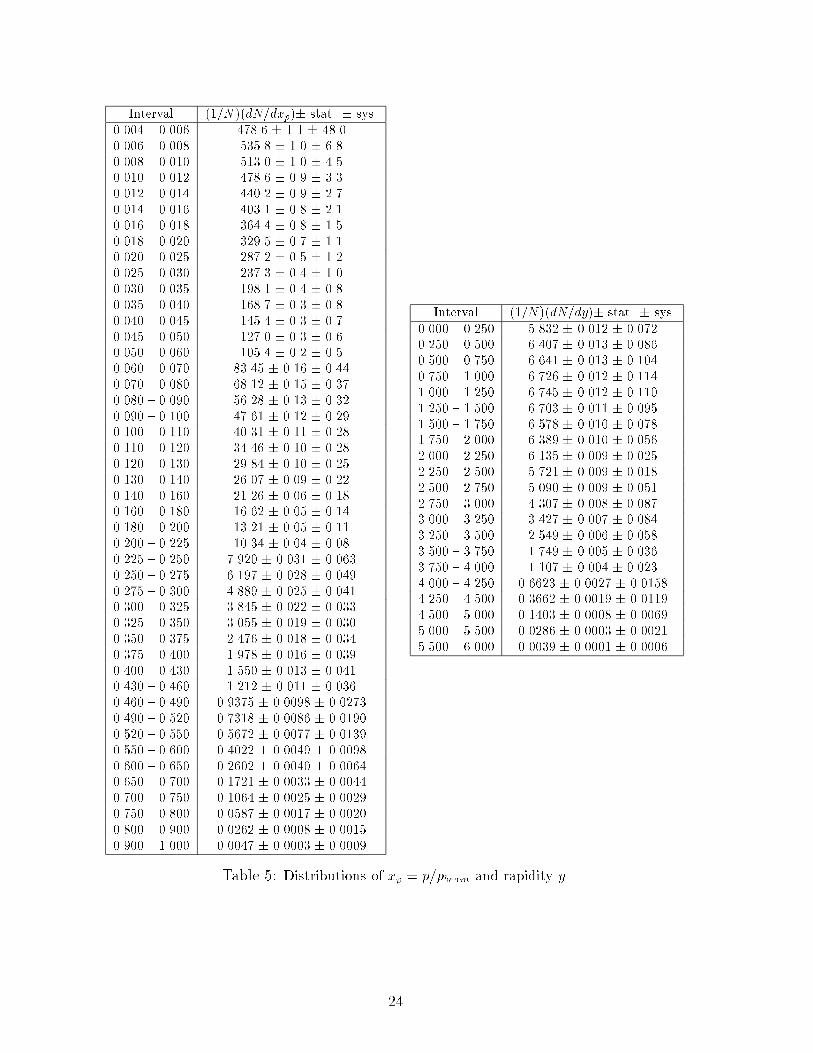
Interval (1=N )(dN=dxp)� stat. � sys.

0.004 { 0.006 478.6 � 1.1 � 48.0

0.006 { 0.008 535.8 � 1.0 � 6.8

0.008 { 0.010 513.0 � 1.0 � 4.5

0.010 { 0.012 478.6 � 0.9 � 3.3

0.012 { 0.014 440.2 � 0.9 � 2.7

0.014 { 0.016 403.1 � 0.8 � 2.1

0.016 { 0.018 364.4 � 0.8 � 1.5

0.018 { 0.020 329.5 � 0.7 � 1.1

0.020 { 0.025 287.2 � 0.5 � 1.2

0.025 { 0.030 237.3 � 0.4 � 1.0

0.030 { 0.035 198.1 � 0.4 � 0.8

0.035 { 0.040 168.7 � 0.3 � 0.8

0.040 { 0.045 145.4 � 0.3 � 0.7

0.045 { 0.050 127.0 � 0.3 � 0.6

0.050 { 0.060 105.4 � 0.2 � 0.5

0.060 { 0.070 83.45 � 0.16 � 0.44

0.070 { 0.080 68.12 � 0.15 � 0.37

0.080 { 0.090 56.28 � 0.13 � 0.32

0.090 { 0.100 47.61 � 0.12 � 0.29

0.100 { 0.110 40.31 � 0.11 � 0.28

0.110 { 0.120 34.46 � 0.10 � 0.28

0.120 { 0.130 29.84 � 0.10 � 0.25

0.130 { 0.140 26.07 � 0.09 � 0.22

0.140 { 0.160 21.26 � 0.06 � 0.18

0.160 { 0.180 16.62 � 0.05 � 0.14

0.180 { 0.200 13.21 � 0.05 � 0.11

0.200 { 0.225 10.34 � 0.04 � 0.08

0.225 { 0.250 7.920 � 0.031 � 0.063

0.250 { 0.275 6.197 � 0.028 � 0.049

0.275 { 0.300 4.889 � 0.025 � 0.041

0.300 { 0.325 3.845 � 0.022 � 0.033

0.325 { 0.350 3.055 � 0.019 � 0.030

0.350 { 0.375 2.476 � 0.018 � 0.034

0.375 { 0.400 1.978 � 0.016 � 0.039

0.400 { 0.430 1.550 � 0.013 � 0.041

0.430 { 0.460 1.212 � 0.011 � 0.036

0.460 { 0.490 0.9375 � 0.0098 � 0.0273

0.490 { 0.520 0.7318 � 0.0086 � 0.0190

0.520 { 0.550 0.5672 � 0.0077 � 0.0139

0.550 { 0.600 0.4022 � 0.0049 � 0.0098

0.600 { 0.650 0.2602 � 0.0040 � 0.0064

0.650 { 0.700 0.1721 � 0.0033 � 0.0044

0.700 { 0.750 0.1064 � 0.0025 � 0.0029

0.750 { 0.800 0.0587 � 0.0017 � 0.0020

0.800 { 0.900 0.0262 � 0.0008 � 0.0015

0.900 { 1.000 0.0047 � 0.0003 � 0.0009

Interval (1=N )(dN=dy)� stat. � sys.

0.000 { 0.250 5.832 � 0.012 � 0.072

0.250 { 0.500 6.407 � 0.013 � 0.086

0.500 { 0.750 6.641 � 0.013 � 0.104

0.750 { 1.000 6.726 � 0.012 � 0.114

1.000 { 1.250 6.745 � 0.012 � 0.110

1.250 { 1.500 6.703 � 0.011 � 0.095

1.500 { 1.750 6.578 � 0.010 � 0.078

1.750 { 2.000 6.389 � 0.010 � 0.056

2.000 { 2.250 6.135 � 0.009 � 0.025

2.250 { 2.500 5.721 � 0.009 � 0.018

2.500 { 2.750 5.090 � 0.009 � 0.051

2.750 { 3.000 4.307 � 0.008 � 0.087

3.000 { 3.250 3.427 � 0.007 � 0.084

3.250 { 3.500 2.549 � 0.006 � 0.058

3.500 { 3.750 1.749 � 0.005 � 0.036

3.750 { 4.000 1.107 � 0.004 � 0.023

4.000 { 4.250 0.6623 � 0.0027 � 0.0158

4.250 { 4.500 0.3662 � 0.0019 � 0.0119

4.500 { 5.000 0.1403 � 0.0008 � 0.0069

5.000 { 5.500 0.0286 � 0.0003 � 0.0021

5.500 { 6.000 0.0039 � 0.0001 � 0.0006

Table 5: Distributions of xp = p=pbeam and rapidity y.

24

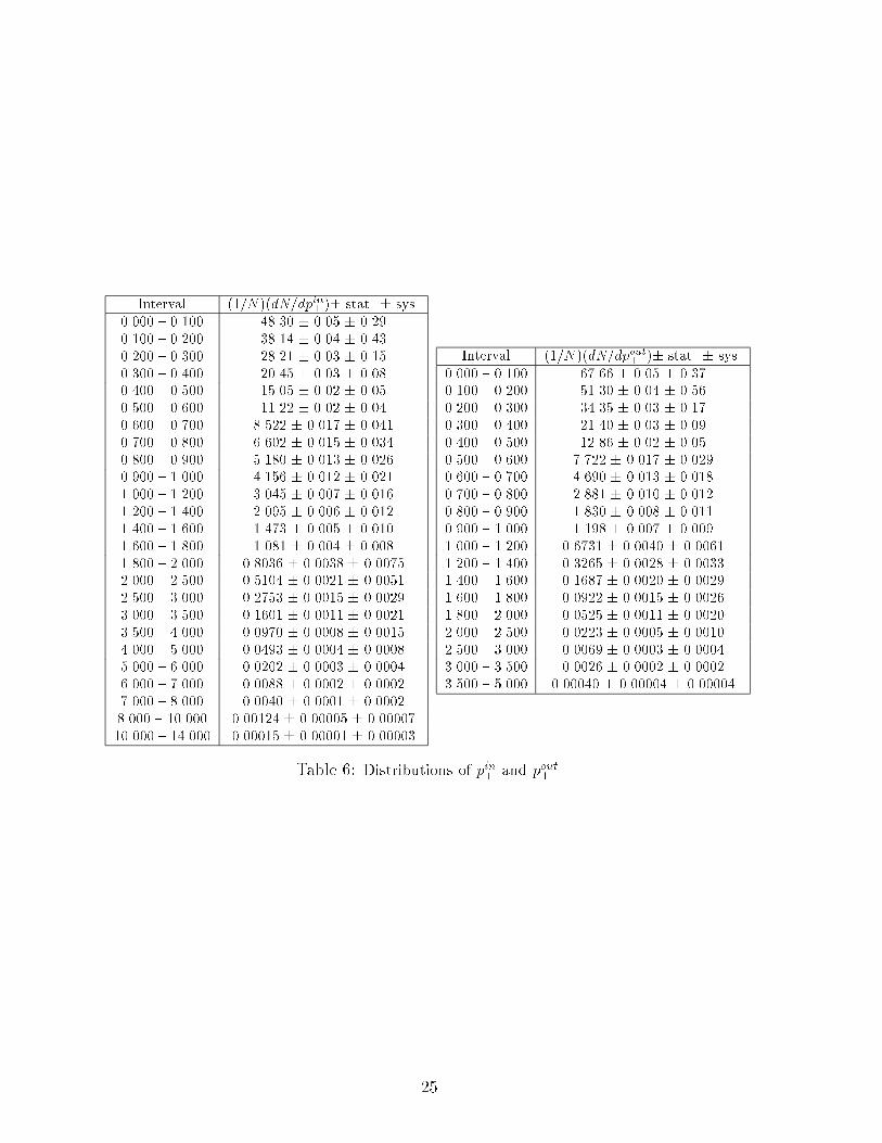
Interval (1=N )(dN=dpin?)� stat. � sys.

0.000 { 0.100 48.30 � 0.05 � 0.29

0.100 { 0.200 38.14 � 0.04 � 0.43

0.200 { 0.300 28.21 � 0.03 � 0.15

0.300 { 0.400 20.45 � 0.03 � 0.08

0.400 { 0.500 15.05 � 0.02 � 0.05

0.500 { 0.600 11.22 � 0.02 � 0.04

0.600 { 0.700 8.522 � 0.017 � 0.041

0.700 { 0.800 6.602 � 0.015 � 0.034

0.800 { 0.900 5.180 � 0.013 � 0.026

0.900 { 1.000 4.156 � 0.012 � 0.021

1.000 { 1.200 3.045 � 0.007 � 0.016

1.200 { 1.400 2.095 � 0.006 � 0.012

1.400 { 1.600 1.473 � 0.005 � 0.010

1.600 { 1.800 1.081 � 0.004 � 0.008

1.800 { 2.000 0.8036 � 0.0038 � 0.0075

2.000 { 2.500 0.5104 � 0.0021 � 0.0051

2.500 { 3.000 0.2753 � 0.0015 � 0.0029

3.000 { 3.500 0.1601 � 0.0011 � 0.0021

3.500 { 4.000 0.0970 � 0.0008 � 0.0015

4.000 { 5.000 0.0493 � 0.0004 � 0.0008

5.000 { 6.000 0.0202 � 0.0003 � 0.0004

6.000 { 7.000 0.0088 � 0.0002 � 0.0002

7.000 { 8.000 0.0040 � 0.0001 � 0.0002

8.000 { 10.000 0.00124 � 0.00005 � 0.00007

10.000 { 14.000 0.00015 � 0.00001 � 0.00003

Interval (1=N )(dN=dpout?

)� stat. � sys.

0.000 { 0.100 67.66 � 0.05 � 0.37

0.100 { 0.200 51.30 � 0.04 � 0.56

0.200 { 0.300 34.35 � 0.03 � 0.17

0.300 { 0.400 21.40 � 0.03 � 0.09

0.400 { 0.500 12.86 � 0.02 � 0.05

0.500 { 0.600 7.722 � 0.017 � 0.029

0.600 { 0.700 4.690 � 0.013 � 0.018

0.700 { 0.800 2.881 � 0.010 � 0.012

0.800 { 0.900 1.830 � 0.008 � 0.011

0.900 { 1.000 1.198 � 0.007 � 0.009

1.000 { 1.200 0.6731 � 0.0040 � 0.0061

1.200 { 1.400 0.3265 � 0.0028 � 0.0033

1.400 { 1.600 0.1687 � 0.0020 � 0.0029

1.600 { 1.800 0.0922 � 0.0015 � 0.0026

1.800 { 2.000 0.0525 � 0.0011 � 0.0020

2.000 { 2.500 0.0223 � 0.0005 � 0.0010

2.500 { 3.000 0.0069 � 0.0003 � 0.0004

3.000 { 3.500 0.0026 � 0.0002 � 0.0002

3.500 { 5.000 0.00040 � 0.00004 � 0.00004

Table 6: Distributions of pin? and pout? .

25

2.3.1 Description of the Models

Lund Parton Shower Model (JETSET)

In the Lund Parton Shower (PS) model (program JETSET version 7.4 [25, 29]), the evolution

of the parton system is treated as a branching process based on the leading logarithm

approximation (LLA). In this picture partons undergo decays of the type q ! qg, g ! gg

and g ! qq. The probability for the decay of a parton a with virtual mass ma into partons b

and c is given by the Altarelli-Parisi (\DGLAP") equation (see, e.g., [13]),

dPa!bc

dt=

Zdz�s(Q

2)

2�Pa!bc(z) ; (23)

where the evolution parameter t is related to the parent's virtual mass and to the QCD scale

parameter � by t = ln(m2a=�

2). The strong coupling constant �s(Q2) is evaluated at Q2 equal

to the transverse momentum squared of the branching. Pa!bc(z) is the Altarelli-Parisi splitting

function. This function is also used to generate the energy fractions z and 1 � z carried by

the daughters. The decay angle is determined by two-body kinematics once the parent and

daughter masses and energy fractions have been �xed.

For the �rst branchings of the initial quark and antiquark, an acceptance-rejection technique

is applied so as to reproduce the O(�s) three-jet cross section. Coherence e�ects are included by

requiring that the emission angles of successive branchings always decrease (angular ordering).

Certain other higher order e�ects are also included, such as the azimuthal distribution in

gluon decays from spin and coherence e�ects. The parton shower is stopped when the parton

virtualities drop below a cut-o�, Mmin (for parameter values see Table 8).

The conversion of the partons into hadrons is accomplished with the Lund String Model

[29]. Gluons are associated with momentum carrying kinks in the string. Hadron production

results from a breaking of the string which can be interpreted as virtual quark-antiquark pair

production in a ux-tube. The quarks' (equal and opposite) transverse momenta are generated

according to a Gaussian distribution of width �q. Longitudinal hadron momenta are determined

by means of phenomenological fragmentation functions: the Lund symmetric function with

parameters a and b for light (u,d,s) quarks, and the Peterson function [32] with parameters �cand �b for c and b quarks.

The probabilities for uu and dd production within the string are assumed to be equal, and

the probability for ss is left as a free parameter, called in the following s=u (in the JETSET

program PARJ(2)). Baryon production is included by allowing diquark-antiquark pairs to be

created; the probability for this to occur is given by the parameter qq=q (PARJ(1)). Meson

production in the string between the baryon and antibaryon (the \popcorn" mechanism) is

also allowed, and occurs with a relative frequency given by the parameter PARJ(5) = 0:5 (its

default value). The popcorn mechanism is investigated further in Section 5.3.

To describe baryons at high momenta it has been found necessary to activate the parameter

PARJ(19) (LBS, leading baryon suppression factor) which suppresses diquark production in the

breakup closest to the endpoint of the string. Without this parameter, the Lund symmetric

fragmentation function would predict an increase in the proton fraction at high momenta, which

is contrary to observation (see Section 5.2, Fig. 64(b)).

The production rates of L = 1 mesons, (S = 0; J = 1) and (S = 1; J = 0; 1; 2), are

controlled by the four parameters PARJ(14-17). In the �tting procedure described below, only

the JP = 2+ rate is taken as a free parameter and the other rates are related by invoking spin

26

counting in the ratio 0+ : 1+ : 2+ = 1 : 3 : 5. In addition, PARJ(14) = PARJ(16) is assumed,

i.e., the rate of (S = 0; J = 1) is set equal to the rate of (S = 1; J = 1).

Ideal mixing is used for the avour-diagonal neutral mesons with the exception of the

pseudoscalar nonet, where a mixing angle of 9:7� is taken. Bose-Einstein correlations are not

included in the �t performed here.

HERWIG

The HERWIG Monte Carlo (version 5.8) [31] is also based on a parton branching process,

as described for JETSET. Instead of the parton virtual mass for the evolution parameter,

HERWIG uses t = ln(�2a=�2), where �a is de�ned by

�a = Ea

p�bc ;

�bc =pb�pcEbEc

;(24)

for the branching a! bc where pb; pc; Eb and Ec are the four-momenta and energies of partons

b and c. Angular ordering of successive branchings is approximately equivalent to ordering of

the �bc. The argument z of the Altarelli-Parisi splitting functions is taken to be the daughter's

energy fraction, and the scale for �s is the transverse momentum squared of the branching.

Azimuthal asymmetries for gluon decays both from coherence and spin e�ects are included.

The treatment of hard gluon emission is improved by matching the parton shower cross section

to the O(�s) matrix element.

The hadronization in HERWIG is modelled with a cluster mechanism. At the end of the

parton shower, all gluons split into quark-antiquark pairs. Neighboring qq pairs form colour-

neutral clusters which (usually) decay into two hadrons. Special treatment is given to very

light clusters, which are allowed to \decay" into a single hadron, and to very heavy clusters

(mass > Mcl;max) which can decay further into clusters before decaying into hadrons. Baryons

are produced from cluster decays into baryon-antibaryon pairs, i.e. clusters themselves always

have baryon number of zero. If a cluster contains a quark that originated in the perturbative

phase of the parton shower (i.e. not from the non-perturbative gluon splitting) then the angular

distribution for the hadron that contains this quark is given by an exponential distribution in

1 � cos � peaked in the quark's direction, with mean value given by the parameter CLSMR.

The global event-shape and hadron momentum spectrum are largely determined by the

parameters, � and Q0, governing the parton shower, and to a lesser extent by the thresholds

for clusters of too high or too low mass. The hadron avour composition is mainly determined

by the available phase space in cluster decay (i.e. by the cluster mass spectrum), and also by

an additional parameter PWT(3) which gives the probability for ss production in cluster decay.

ARIADNE

Instead of formulating the perturbative QCD cascade in terms of quark and gluon decays,

the ARIADNE Monte Carlo (version 4.08) [30] uses the complementary language of colour

dipoles [33]. In this approach, the initially produced colour dipole (the qq pair) radiates a

gluon according to the �rst order QCD matrix element. The resulting qqg system is then

treated as two independent dipoles, between the quark and gluon, and between the gluon and

antiquark. Each successive gluon emission creates a new dipole, all of which are assumed to

radiate independently. This approach naturally takes into account coherence e�ects, azimuthal

27

dependence of gluon decays, and an exact O(�s) description of hard gluon radiation which must

be inserted by hand into the parton cascade approach used in JETSET and HERWIG.

The free parameters in the perturbative phase of ARIADNE are the QCD scale � and

the minimum transverse momentum allowed in dipole emission pmin? . The non-perturbative

hadron production in ARIADNE is accomplished with the Lund String Model as described for

JETSET.

2.3.2 Fitting of Model Parameters

The determination of model parameters is based on comparison with the measured event-shape

and inclusive distributions presented in Section 2, as well as with distributions of identi�ed

hadrons given in Section 5.2. Speci�cally, the following quantities were used:

� event-shape distributions S; A; 1 � T; Tminor; � ln y3;

� charged particle inclusive distributions xp = p=pbeam; pout? ; pin? ;

� inclusive spectra of � = � lnxp for the neutral V0 particlesK0 and �0, and for the charged

pions, kaons and (anti)protons;

� inclusive spectra of x = E=Ebeam for the mesons �(x > 0:1), �0(x > 0:1) �0, K�0, K�+,�0, !0;

� the mean multiplicities of the L = 1 mesons f2, f0 and of the hyperons ��, �(1385),�(1530)0, �. Multiplicities for the f0 and f2 mesons are taken from [34].

The dependence of measurable quantities on the model parameters does not exist in

analytical form. Instead, Monte Carlo calculations of these quantities at various locations

in parameter space have to be performed, and a parametrization for the dependence of each

bin on the model parameters is determined. It is reasonable to assume, and has been con�rmed

in practice, that the dependence is smooth, though not necessarily linear.

The method used in the previous ALEPH publication [26] was based on 2nd order

polynomials to parametrize the distributions. The fast (quadratic) rise of computer time with

the number of parameters limited the practical application to n � 6 parameters. Since then, the

increasing accuracy of the experimental data and the demands of the physics analyses made it

desirable to �t many more parameters. The prominent example is the large number of JETSET

string model parameters. Therefore it was necessary to go to a linear approach.

A measurable quantity (e.g. the contents of interval j of a distribution, or the mean

multiplicity of a given particle) will be denoted by Mj and the set of model parameters to

be determined by xi; i = 1; : : : ; n. Starting with a given set of initial values xi0, a set of 4N

Monte Carlo events is generated (typically N = 1 million) and the histograms of the various

distributions are �lled. For each parameter, four more points in the parameter space are

considered, situated at distances

��xleft; ��xleft=2; �xright=2; �xright;

from the initial value xi0. At each of these four points, and for each parameter, N Monte Carlo

events are generated and the histograms stored.

28

As an option, the four points can all be set to the left or right side of xi0, which is important

in case a parameter has to obey a physical constraint. An example is the cut-o� mass of the

parton shower which is not allowed to be smaller than �QCD.

A linear expression

Mj(xi) = mij + aij(xi � xi0)

is �tted for each measured quantity Mj and each parameter xi, yielding a slope aij and o�set

mij. If the �t is not acceptable (�

2 probability less than 10%) a quadratic expression is tried

and used to monitor the parameter region for which the linear expression is acceptable. The

actual parameter �t is always performed using the linear terms only. The entire process of

Monte Carlo event generation is then repeated, moving the central values xi0 accordingly, until

the �nal �tted values of the parameters all remain within the linear ranges and change by less

than their errors.

The model parameters are �tted by minimizing the �2 function

�2 =Xj

Mdata

j �MMCj (~x)

�dataj

!2(25)

with respect to the parameters ~x, where the sum runs over all of the measured quantities.

The errors �dataj are taken to be the quadratic sums of statistical and systematic uncertainties;

Monte Carlo errors are small compared to these and are neglected.

By using Eq. (25) it is implicitly assumed that the experimental data points are uncorrelated.

This is not true in general, however, since there are both intrinsic correlations between variables

as well as systematic errors from the correction procedure which introduce correlations between

neighboring bins. As a result, the errors on the �tted parameters and the corresponding �2

values should only be regarded as giving a rough measure of statistical uncertainty and relative

goodness-of-�t.

As has been observed previously [26], model predictions for the rate of particle production

transverse to the event plane for pout? greater than about 1 GeV are low by up to 30%. A correct

description of this region seems outside the capabilities of current QCD parton shower models.

Therefore the regions pout? � 0:7 GeV, A � 0:06 and Tminor � 0:2 are excluded from the �t.

As a result the QCD scale parameter of JETSET �QCD is reduced by about 25 MeV, and the

multijet regions of the sphericity, thrust, and y3 distributions are better described.

Because of the large number of parameters (15) in JETSET and ARIADNE, the following

special treatment is necessary. First, the parameters �c and �b controlling the fragmentation of

hadrons containing c and b quarks are adjusted so as to describe the corresponding measured

hxi values [35, 36, 37]. The probability for a meson containing a c or b quark to have spin 1

is set to 0.65, which represents a compromise between the values of 0.55 (0.75) necessary to

describe charm (bottom) hadrons separately [35, 38]. The heavy vector meson probability of

0.65 together with the tensor meson parameter PARJ(17) = 0:2 provides a good description

of the measured fraction of B��=B [38]. The parameter PARJ(17) is held �xed at 0.20 in

the following since it also gives a good description of light tensor meson (f2) production.

Furthermore, the parameter a is �xed to 0.4, since it is found to be highly correlated with

the parameter b.

The remaining JETSET and ARIADNE parameters are then separated into the following

two groups:

� the general fragmentation parameters: �QCD, Mmin, �q, b;

29

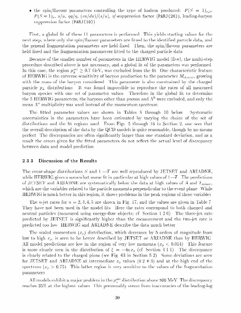
� the spin/ avour parameters controlling the type of hadron produced: P (S = 1)u;d,

P (S = 1)s, s=u, qq=q, (su=du)=(s=u), �0-suppression factor (PARJ(26)), leading-baryon

suppression factor (PARJ(19)).

First, a global �t of these 11 parameters is performed. This yields starting values for the

next step, where only the spin/ avour parameters are �tted to the identi�ed particle data, and

the general fragmentation parameters are held �xed. Then, the spin/ avour parameters are

held �xed and the fragmentation parameters �tted to the charged particle data.

Because of the smaller number of parameters in the HERWIG model (�ve), the multi-step

procedure described above is not necessary, and a global �t of the parameters was performed.

In this case, the region pout? � 0:7 GeV, was excluded from the �t. One characteristic feature

of HERWIG is the extreme sensitivity of baryon production to the parameterMcl;max, growing

with the mass of the baryon considered. This parameter is also constrained by the charged

particle p? distributions. It was found impossible to reproduce the rates of all measured

baryon species with one set of parameter values. Therefore in the global �t to determine

the 5 HERWIG parameters, the baryons other than proton and �0 were excluded, and only the

mean �0 multiplicity was used instead of the momentum spectrum.

The �tted parameter values are shown in Tables 8 through 10 below. Systematic

uncertainties in the parameters have been estimated by varying the choice of the set of

distributions and the �t regions used. From Figs. 5 through 16 in Section 2, one sees that

the overall description of the data by the QCD models is quite reasonable, though by no means

perfect. The discrepancies are often signi�cantly larger than one standard deviation, and as a

result the errors given for the �tted parameters do not re ect the actual level of discrepancy

between data and model prediction.

2.3.3 Discussion of the Results

The event-shape distributions S and 1 � T are well reproduced by JETSET and ARIADNE,

while HERWIG gives a somewhat worse �t in particular at high values of 1�T . The predictionsof JETSET and ARIADNE are systematically below the data at high values of A and Tminor,

which are the variables related to the particle momenta perpendicular to the event plane. While

HERWIG is much better in this region, it shows problems in the peak regions of these variables.

The n-jet rates for n = 2; 3; 4; 5 are shown in Fig. 17, and the values are given in Table 7.

They have not been used in the model �ts. Here the rates correspond to both charged and

neutral particles (measured using energy- ow objects; cf. Section 1.2.6). The three-jet rate

predicted by JETSET is signi�cantly higher than the measurement and the two-jet rate is

predicted too low. HERWIG and ARIADNE describe the data much better.

The scaled momentum (xp) distribution, which decreases by 5 orders of magnitude from

low to high xp, is seen to be better described by JETSET or ARIADNE than by HERWIG.

All model predictions are low in the region of very low momenta (xp < 0:014). This feature

is more clearly seen in the distribution of � = � lnxp (cf. Section 4.1.1). The discrepancy

is clearly related to the charged pions (see Fig. 63 in Section 5.2). Some deviations are seen

for JETSET and ARIADNE at intermediate xp values (0.2{0.3) and at the high end of the

spectrum (xp > 0:75). This latter region is very sensitive to the values of the fragmentation

parameters.

All models exhibit a major problem in the pout? distribution above 800 MeV. The discrepancy

reaches 35% at the highest values. This presumably stems from inaccuracies of the leading-log

30

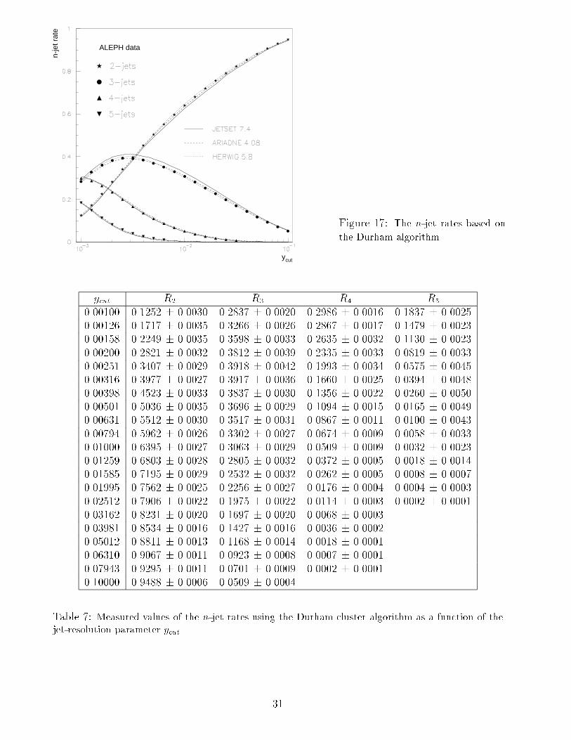
ycut

n-je

t rat

eALEPH data

Figure 17: The n-jet rates based on

the Durham algorithm.

ycut R2 R3 R4 R5

0.00100 0.1252 � 0.0030 0.2837 � 0.0020 0.2986 � 0.0016 0.1837 � 0.0025

0.00126 0.1717 � 0.0035 0.3266 � 0.0026 0.2867 � 0.0017 0.1479 � 0.0023

0.00158 0.2249 � 0.0035 0.3598 � 0.0033 0.2635 � 0.0032 0.1130 � 0.0023

0.00200 0.2821 � 0.0032 0.3812 � 0.0039 0.2335 � 0.0033 0.0819 � 0.0033

0.00251 0.3407 � 0.0029 0.3918 � 0.0042 0.1993 � 0.0034 0.0575 � 0.0045

0.00316 0.3977 � 0.0027 0.3917 � 0.0036 0.1660 � 0.0025 0.0394 � 0.0048

0.00398 0.4523 � 0.0033 0.3837 � 0.0030 0.1356 � 0.0022 0.0260 � 0.0050

0.00501 0.5036 � 0.0035 0.3696 � 0.0029 0.1094 � 0.0015 0.0165 � 0.0049

0.00631 0.5512 � 0.0030 0.3517 � 0.0031 0.0867 � 0.0011 0.0100 � 0.0043

0.00794 0.5962 � 0.0026 0.3302 � 0.0027 0.0674 � 0.0009 0.0058 � 0.0033

0.01000 0.6395 � 0.0027 0.3063 � 0.0029 0.0509 � 0.0009 0.0032 � 0.0023

0.01259 0.6803 � 0.0028 0.2805 � 0.0032 0.0372 � 0.0005 0.0018 � 0.0014

0.01585 0.7195 � 0.0029 0.2532 � 0.0032 0.0262 � 0.0005 0.0008 � 0.0007

0.01995 0.7562 � 0.0025 0.2256 � 0.0027 0.0176 � 0.0004 0.0004 � 0.0003

0.02512 0.7906 � 0.0022 0.1975 � 0.0022 0.0114 � 0.0003 0.0002 � 0.0001

0.03162 0.8231 � 0.0020 0.1697 � 0.0020 0.0068 � 0.0003

0.03981 0.8534 � 0.0016 0.1427 � 0.0016 0.0036 � 0.0002

0.05012 0.8811 � 0.0013 0.1168 � 0.0014 0.0018 � 0.0001

0.06310 0.9067 � 0.0011 0.0923 � 0.0008 0.0007 � 0.0001

0.07943 0.9295 � 0.0011 0.0701 � 0.0009 0.0002 � 0.0001

0.10000 0.9488 � 0.0006 0.0509 � 0.0004

Table 7: Measured values of the n-jet rates using the Durham cluster algorithm as a function of the

jet-resolution parameter ycut.

31

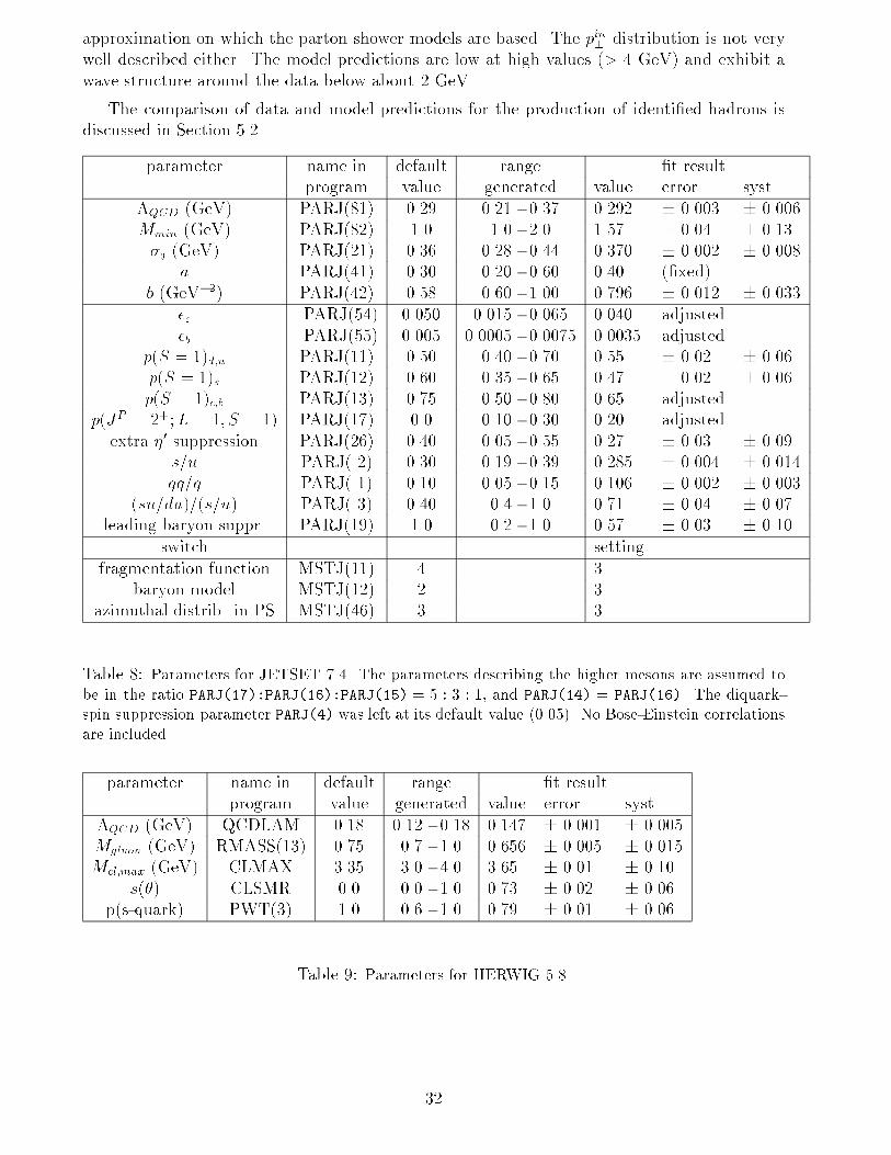
approximation on which the parton shower models are based. The pin? distribution is not very

well described either. The model predictions are low at high values (> 4 GeV) and exhibit a

wave structure around the data below about 2 GeV.

The comparison of data and model predictions for the production of identi�ed hadrons is

discussed in Section 5.2.

parameter name in default range �t result

program value generated value error syst.

�QCD (GeV) PARJ(81) 0.29 0.21 - 0.37 0.292 � 0.003 � 0.006

Mmin (GeV) PARJ(82) 1.0 1.0 - 2.0 1.57 � 0.04 � 0.13

�q (GeV) PARJ(21) 0.36 0.28 - 0.44 0.370 � 0.002 � 0.008

a PARJ(41) 0.30 0.20 - 0.60 0.40 (�xed)

b (GeV�2) PARJ(42) 0.58 0.60 - 1.00 0.796 � 0.012 � 0.033

�c {PARJ(54) 0.050 0.015 - 0.065 0.040 adjusted

�b {PARJ(55) 0.005 0.0005 - 0.0075 0.0035 adjusted

p(S = 1)d;u PARJ(11) 0.50 0.40 - 0.70 0.55 � 0.02 � 0.06

p(S = 1)s PARJ(12) 0.60 0.35 - 0.65 0.47 � 0.02 � 0.06

p(S = 1)c;b PARJ(13) 0.75 0.50 - 0.80 0.65 adjusted

p(JP = 2+;L = 1; S = 1) PARJ(17) 0.0 0.10 - 0.30 0.20 adjusted

extra �0 suppression PARJ(26) 0.40 0.05 - 0.55 0.27 � 0.03 � 0.09

s=u PARJ( 2) 0.30 0.19 - 0.39 0.285 � 0.004 � 0.014

qq=q PARJ( 1) 0.10 0.05 - 0.15 0.106 � 0.002 � 0.003

(su=du)=(s=u) PARJ( 3) 0.40 0.4 - 1.0 0.71 � 0.04 � 0.07

leading baryon suppr. PARJ(19) 1.0 0.2 - 1.0 0.57 � 0.03 � 0.10

switch setting

fragmentation function MSTJ(11) 4 3

baryon model MSTJ(12) 2 3

azimuthal distrib. in PS MSTJ(46) 3 3

Table 8: Parameters for JETSET 7.4. The parameters describing the higher mesons are assumed to

be in the ratio PARJ(17):PARJ(16):PARJ(15) = 5 : 3 : 1, and PARJ(14) = PARJ(16). The diquark-

spin suppression parameter PARJ(4) was left at its default value (0.05). No Bose-Einstein correlations

are included.

parameter name in default range �t result

program value generated value error syst.

�QCD (GeV) QCDLAM 0.18 0.12 - 0.18 0.147 � 0.001 � 0.005

Mgluon (GeV) RMASS(13) 0.75 0.7 - 1.0 0.656 � 0.005 � 0.015

Mcl;max (GeV) CLMAX 3.35 3.0 - 4.0 3.65 � 0.01 � 0.10

s(�) CLSMR 0.0 0.0 - 1.0 0.73 � 0.02 � 0.06

p(s-quark) PWT(3) 1.0 0.6 - 1.0 0.79 � 0.01 � 0.06

Table 9: Parameters for HERWIG 5.8.

32

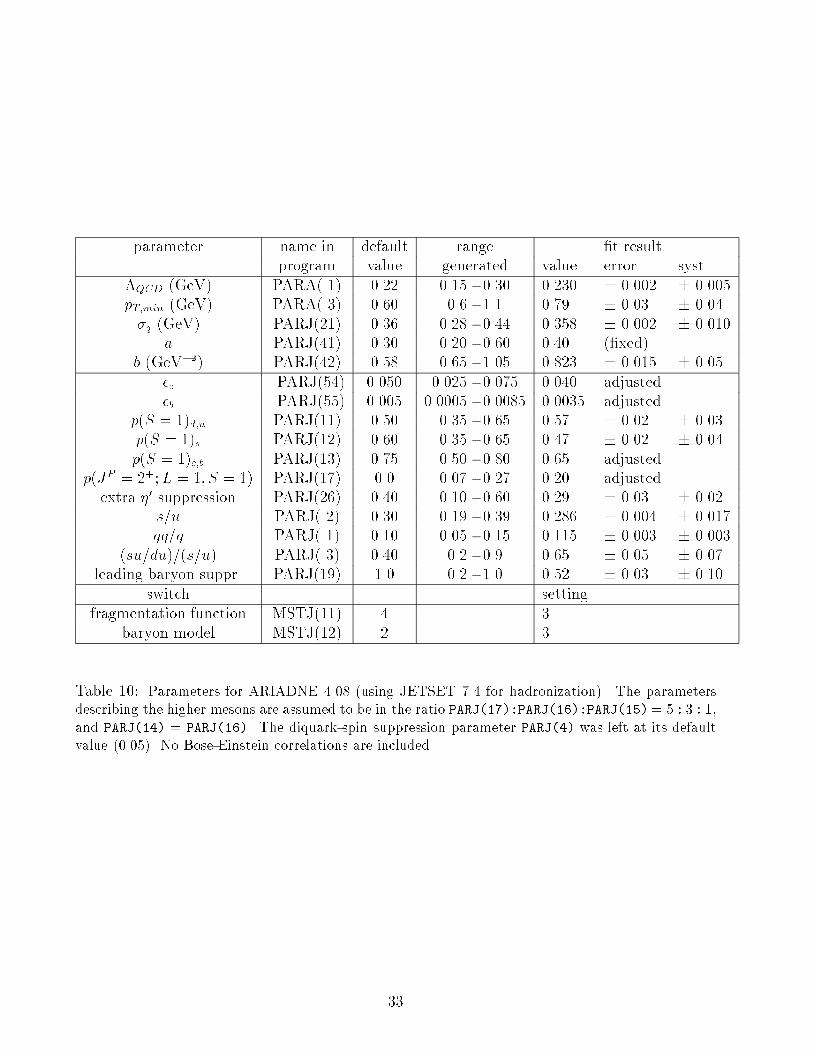
parameter name in default range �t result

program value generated value error syst.

�QCD (GeV) PARA( 1) 0.22 0.15 - 0.30 0.230 � 0.002 � 0.005

pT;min (GeV) PARA( 3) 0.60 0.6 - 1.1 0.79 � 0.03 � 0.04

�q (GeV) PARJ(21) 0.36 0.28 - 0.44 0.358 � 0.002 � 0.010

a PARJ(41) 0.30 0.20 - 0.60 0.40 (�xed)

b (GeV�2) PARJ(42) 0.58 0.65 - 1.05 0.823 � 0.015 � 0.05

�c {PARJ(54) 0.050 0.025 - 0.075 0.040 adjusted

�b {PARJ(55) 0.005 0.0005 - 0.0085 0.0035 adjusted

p(S = 1)d;u PARJ(11) 0.50 0.35 - 0.65 0.57 � 0.02 � 0.03

p(S = 1)s PARJ(12) 0.60 0.35 - 0.65 0.47 � 0.02 � 0.04

p(S = 1)c;b PARJ(13) 0.75 0.50 - 0.80 0.65 adjusted

p(JP = 2+;L = 1; S = 1) PARJ(17) 0.0 0.07 - 0.27 0.20 adjusted

extra �0 suppression PARJ(26) 0.40 0.10 - 0.60 0.29 � 0.03 � 0.02

s=u PARJ( 2) 0.30 0.19 - 0.39 0.286 � 0.004 � 0.017

qq=q PARJ( 1) 0.10 0.05 - 0.15 0.115 � 0.003 � 0.003

(su=du)=(s=u) PARJ( 3) 0.40 0.2 - 0.9 0.65 � 0.05 � 0.07

leading baryon suppr. PARJ(19) 1.0 0.2 - 1.0 0.52 � 0.03 � 0.10

switch setting

fragmentation function MSTJ(11) 4 3

baryon model MSTJ(12) 2 3

Table 10: Parameters for ARIADNE 4.08 (using JETSET 7.4 for hadronization). The parameters

describing the higher mesons are assumed to be in the ratio PARJ(17):PARJ(16):PARJ(15)= 5 : 3 : 1,

and PARJ(14) = PARJ(16). The diquark-spin suppression parameter PARJ(4) was left at its default

value (0.05). No Bose-Einstein correlations are included.

33

3 Hard QCD

In this section attention is given primarily to the basic components of QCD. First, the spin

properties of the fundamental �elds, quarks and gluons, are measured. Although this has been

done years ago in experiments at lower centre-of-mass energies, it is still interesting to see with

LEP data, which, because of the smaller non-perturbative e�ects, exhibit jet con�gurations

that resemble more closely the underlying parton structure of the events.

A large fraction of the section is devoted to the measurement of the only free parameter

of QCD, �s. Di�erent methods have been used and are presented in Section 3.2. Also a

compilation of �s determinations at di�erent energies and accelerators is shown, and the running

of �s with the scale is established from them. A study of the interplay between event shape

and event orientation is presented, and the independence of the strong coupling constant from

the quark avour, as predicted in QCD, is checked using b-quark enriched samples.

Finally, the structure of the gauge group on which QCD is based, SU(3), can be probed,

because the QCD predictions depend on the structure constants of the group. Two-, three- and

four-jet events are used to measure these constants and exclude other possible gauge groups for

the strong interactions.

3.1 Parton Spins

It is a well established fact that quarks are spin-1/2 particles [39] and gluons are spin-1

particles [40]. It is instructive nevertheless to look at the experimental data collected at LEP

in order to assess the sensitivity of the measurements to the spin assignment for the building

blocks of the nucleon.

3.1.1 Quark Spin

The quark spin can be inferred from the angular distribution of the thrust axis in hadronic

Z decays. This axis is a rather good approximation for the direction of the primary quarks

produced in the process e+e� ! qq ! hadrons. Since one cannot distinguish q and q, the

angle � between the incoming beam and the direction of the �nal state quarks is always taken

in the range 0 � � � 90�. From the fact that the Z has spin 1 and ignoring the masses of

initial and �nal state particles, the angular distribution can be determined from simple angular

momentum arguments. One obtains

d�

d cos �/ 1 + cos2� and

d�

d cos �/ 1� cos2� (26)

for spin-1/2 and scalar quarks, respectively. By measuring the direction of the thrust axis, i.e.

�THRUST instead of �, these simple predictions are modi�ed by higher order QCD corrections

and hadronization e�ects which, however, turn out to be very small.

The analysis is based on roughly 60,000 accepted hadronic events from the 1992 data and

the same number of HVFL Monte Carlo events processed through the same reconstruction

program, with standard track and event selection criteria.

The results are shown in Fig. 18. The dotted lines show the Monte Carlo prediction obtained

for the primary quarks from the Z decay without cuts. The upper curve gives the Monte Carlo

result for spin-1/2 quarks and the lower one for spin-0 quarks. The experimental distribution

34

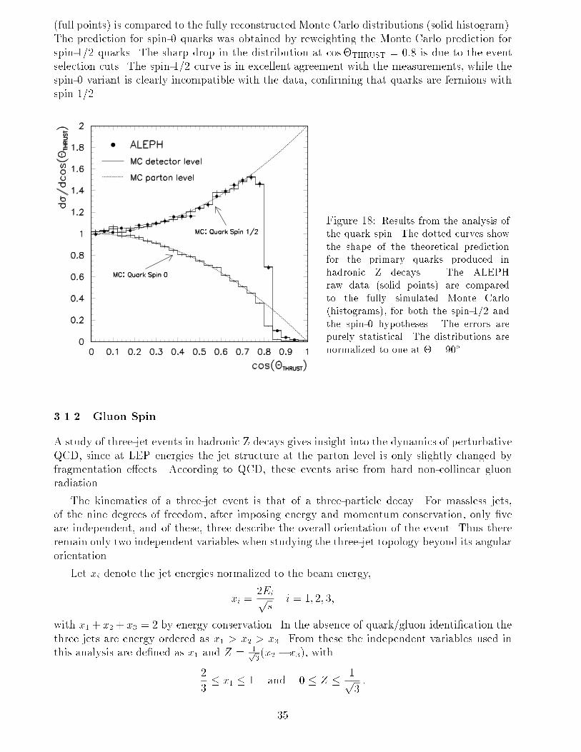
(full points) is compared to the fully reconstructed Monte Carlo distributions (solid histogram).

The prediction for spin-0 quarks was obtained by reweighting the Monte Carlo prediction for

spin-1/2 quarks. The sharp drop in the distribution at cos �THRUST = 0:8 is due to the event

selection cuts. The spin-1/2 curve is in excellent agreement with the measurements, while the

spin-0 variant is clearly incompatible with the data, con�rming that quarks are fermions with

spin 1/2.

Figure 18: Results from the analysis of

the quark spin. The dotted curves show

the shape of the theoretical prediction

for the primary quarks produced in

hadronic Z decays. The ALEPH

raw data (solid points) are compared

to the fully simulated Monte Carlo

(histograms), for both the spin-1/2 and

the spin-0 hypotheses. The errors are

purely statistical. The distributions are

normalized to one at � = 90�.

3.1.2 Gluon Spin

A study of three-jet events in hadronic Z decays gives insight into the dynamics of perturbative

QCD, since at LEP energies the jet structure at the parton level is only slightly changed by

fragmentation e�ects. According to QCD, these events arise from hard non-collinear gluon

radiation.

The kinematics of a three-jet event is that of a three-particle decay. For massless jets,

of the nine degrees of freedom, after imposing energy and momentum conservation, only �ve

are independent, and of these, three describe the overall orientation of the event. Thus there

remain only two independent variables when studying the three-jet topology beyond its angular

orientation.

Let xi denote the jet energies normalized to the beam energy,

xi =2Eips

i = 1; 2; 3;

with x1+ x2+ x3 = 2 by energy conservation. In the absence of quark/gluon identi�cation the

three jets are energy ordered as x1 > x2 > x3. From these the independent variables used in

this analysis are de�ned as x1 and Z = 1p3(x2 � x3), with

2

3� x1 � 1 and 0 � Z � 1p

3:

35

These two variables can be represented in a triangular Dalitz plot. Figure 19 shows the available

phase space for energy-ordered three-jet events and typical jet con�gurations corresponding to

di�erent regions of the phase space.

Figure 19: Phase space for x1 > x2 > x3. The arrow length is proportional to the jet energy.

The three-jet Dalitz plot allows a determination of the gluon spin. The di�erential cross

section for the process e+e� ! qq g has been calculated at leading order both for the vector

and the scalar gluon hypothesis. For a vector gluon the leading order matrix element, not

requiring any identi�cation of quarks or gluons in the �nal state, is [15]

d�v

dx1dx2/"

x21 + x22(1� x1)(1� x2)

+ Permutations(1; 2; 3)

#(27)

This distribution shows two types of singularities, collinear singularities x1 ! 1 or x2 ! 1

and an infrared singularity x1 ! 1 and x2 ! 1, i.e. Z ! 1=p3. In practical applications

these singularities are avoided by restricting the phase space to a singularity-free subspace, for

example by using the Durham algorithm to de�ne three-particle �nal states.

The corresponding di�erential cross section for a scalar gluon is [41]

d�s

dx1 dx2/"

x23(1� x1)(1 � x2)

+ Permutations(1; 2; 3)� 10

Pa2qP

a2q + v2q

#: (28)

Here vq and aq are the vector and axial-vector couplings of a quark to the Z boson. The sum is

taken over all active avours. The collinear singularities appear again, but as a consequence of

the helicity non-conserving coupling of a scalar gluon to the quark current, there is no infrared

singularity. This di�erence in the singularity structure of the matrix elements can be exploited

to determine the spin of the gluon by studying the projection of the cross section onto the Z

axis.

ALEPH data atps =MZ from 1992 have been analyzed. Hadronic events were selected by

requiring at least �ve good charged tracks with a total energy larger than 10% of the centre-of-

mass energy. The analysis then was performed with all charged tracks and neutral objects given

36

by the energy ow package, described in 1.2.6. For the �nal selection the events had to ful�l

two further selection criteria: the angle between the beam and the thrust axis had to be larger

than 300 and the total visible energy was required to be larger than 50% of the centre-of-mass

energy.

Three-jet events were selected by the Durham cluster algorithm with the E recombination

scheme, with a cuto� parameter ycut = 0:009. In total, 193740 events were retained. The

jets were then projected onto the event plane and the jet energies reconstructed from the jet

directions, using

xi =2Eips=

2 sin i3P

j=1sin j

i = 1; 2; 3 ; (29)

where i is the angle subtended by jets j and k, with fi; j; kg any permutation of f1; 2; 3g. Thisformula strictly only holds for massless jets. Since the emphasis lies on a comparison between

data and theoretical models for massless partons, Eq. (29) was taken as the de�nition of the

experimental observables.

The raw experimental distribution was corrected for detector e�ects such as geometrical

acceptance, detection e�ciency and resolution, and e�ects from initial state radiation using

simulated Monte Carlo events from the hadronic event generator HVFL. The size of the

corrections was of the order of 5%.

Figure 20 compares the corrected data to the theoretical Z distributions for vector and

scalar gluon models. In both cases e�ects from perturbative higher orders and hadronization

e�ects were estimated from the di�erence between the leading order analytical formula Eq. (27)

or Eq. (28) and the JETSET prediction for the leading order matrix element for massless quarks

plus hadronization. As those e�ects have never been studied for the scalar gluon model, the

full size of those higher order e�ects was taken as the theoretical uncertainty, even though this

leads to a clear overestimate of the true uncertainties in the case of the vector gluon.

The impact of the missing perturbative higher orders or mass e�ects can be estimated by

comparing leading order and next-to-leading order matrix elements or massless and massive

leading order calculations for the vector gluon. Generally the di�erences turn out to be

negligible.

One �nds, even with rather generous assessments of the theoretical uncertainties, that the

scalar gluon model is in clear disagreement with the data, and thus can be ruled out as a serious

candidate for an alternative to QCD. The vector gluon model provides a very good description

of the data.

3.2 Measurements of the Strong Coupling Constant

The strong coupling constant, �s, is the only free parameter of QCD. Its measurement in

di�erent processes serves as a stringent test of the theory, which has to be able to describe

a wide range of phenomena with the same value of �s(MZ), after running to the appropriate

energy scale.

The observables which lead to a measurement of �s at LEP can be divided into two broad

categories: inclusive and non-inclusive. The �rst category includes the measurement of the total

hadronic decay widths of both the Z boson and the tau lepton. In the second category belong

jet-rate measurements, global event shape variables and scaling violations in fragmentation

functions.

37

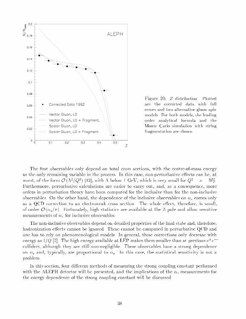
Figure 20: Z distribution. Plotted

are the corrected data with full

errors and two alternative gluon spin

models. For both models, the leading

order analytical formula and the

Monte Carlo simulation with string

fragmentation are shown.

The �rst observables only depend on total cross sections, with the centre-of-mass energy

as the only remaining variable in the process. In this case, non-perturbative e�ects can be, at

worst, of the form O (�2=Q2) [42], with � below 1 GeV, which is very small for Q2 = s =M2Z .

Furthermore, perturbative calculations are easier to carry out, and, as a consequence, more

orders in perturbation theory have been computed for the inclusive than for the non-inclusive

observables. On the other hand, the dependence of the inclusive observables on �s comes only

as a QCD correction to an electroweak cross section. The whole e�ect, therefore, is small,

of order O (�s=�). Fortunately, high statistics are available at the Z pole and allow sensitive

measurements of �s for inclusive observables.

The non-inclusive observables depend on detailed properties of the �nal state and, therefore,

hadronization e�ects cannot be ignored. These cannot be computed in perturbative QCD and

one has to rely on phenomenological models. In general, these corrections only decrease with

energy as 1=Q [7]. The high energy available at LEP makes them smaller than at previous e+e�

colliders, although they are still non-negligible. These observables have a strong dependence

on �s and, typically, are proportional to �s. In this case, the statistical sensitivity is not a

problem.

In this section, four di�erent methods of measuring the strong coupling constant performed

with the ALEPH detector will be presented, and the implications of the �s measurements for

the energy dependence of the strong coupling constant will be discussed.

38

3.2.1 Z Hadronic Width

One of the theoretically best understood determinations of the strong coupling constant comes

from the measurement of the hadronic width of the Z boson or rather, from the ratio of

the hadronic and the leptonic widths, Rl = �h=�l. The sensitivity to �s comes from the

increase in the Z partial width to hadron �nal states due to the e�ect of both virtual and

real gluon radiation. This is an inclusive measurement at very high Q2 � 104 GeV2. Hence,

non-perturbative e�ects are negligibly small. In addition, it is one of the few observables for

which the perturbative prediction is known to O (�3s) [43].

The dependence of Rl on �s can be parametrized as [44]:

Rl = Rewl �0@1 + 1:06

�s(MZ)

�

!+ 0:9

�s(MZ)

�

!2� 15

�s(MZ)

�

!3+O

�s(MZ)

�

!41A ; (30)

where Rewl = 19:932 for a top mass of 175 GeV and a Higgs mass of 300 GeV. This expression

includes b quark mass e�ects up to O(�2s), top quark mass e�ects to O(�sG�m2t ) and QED

corrections to O(��s). The overall QCD correction is only of the order of 4%. Therefore, a

useful determination of �s requires a very precise measurement of Rl.

It should be noted that the top quark and Higgs mass dependence of Rl is only moderate

(see [44], for example). This is so because the loop corrections to the Z propagator diagram

cancel in the ratio �h=�l. The only residual dependence comes from vertex corrections and

photon-Z mixing. For the same reasons, new physics which would mainly manifest itself through

propagator corrections would contribute little to Rl. However, a deviation of the Z branching

ratios from the Minimal Standard Model predictions would a�ect the determination of �s with

this method.

To obtain Rl one needs to select hadronic and leptonic events. The methods are described

in detail in [45]. The hadronic event selection is similar to that presented in Section 1.3.

The leptonic event selection exploits the low multiplicity of the event as well as the particular

characteristics of Bhabha, �-pair and � -pair �nal states. The resulting cross sections for data

taken in 1989-1995 are given in [46] for the energies around and at the Z peak.

The method for extracting Rl consists of �tting the measured cross sections as a function

of centre-of-mass energy,ps, to the theoretical prediction [45]:

�f �f(s) =

Z s

4m2f

ds0H(s; s0)�̂f �f(s0) ; (31)

where H(s; s0) is the so-called radiator function which takes care of initial state radiation

corrections. The reduced cross section �̂ is written as

�̂f �f(s) = �0f �f �s�2Z

(s �M2Z)

2+�s�ZMZ

�2 + ( � Z) + j j2 ; (32)

where the two last terms represent the interference between the photon- and Z-mediated

amplitudes and the photon contribution, respectively, and are taken from theory. This

parametrization assumes the validity of QED for the photon exchange part and also takes from

the Minimal Standard Model the interference between the photon- and Z-mediated amplitudes.

This interference is very small around the Z resonance. In the case of Bhabha scattering, f = e,

one has to add the t-channel photon- and Z-exchange diagrams, also taken from theory. The

39

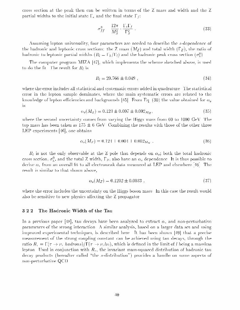
cross section at the peak then can be written in terms of the Z mass and width and the Z

partial widths to the initial state �e and the �nal state �f :

�0f �f =12�

M2Z

� �e�f�2Z

: (33)

Assuming lepton universality, four parameters are needed to describe the s-dependence of

the hadronic and leptonic cross sections: the Z mass (MZ) and total width (�Z), the ratio of

hadronic to leptonic partial widths (Rl = �h=�l) and the hadronic peak cross section (�0h).

The computer program MIZA [47], which implements the scheme sketched above, is used

to do the �t. The result for Rl is

Rl = 20:766 � 0:049 ; (34)

where the error includes all statistical and systematic errors added in quadrature. The statistical

error in the lepton sample dominates, where the main systematic errors are related to the

knowledge of lepton e�ciencies and backgrounds [45]. From Eq. (30) the value obtained for �sis

�s(MZ) = 0:123 � 0:007 � 0:002MH; (35)

where the second uncertainty comes from varying the Higgs mass from 60 to 1000 GeV. The

top mass has been taken as 175 � 6 GeV. Combining the results with those of the other three

LEP experiments [46], one obtains

�s(MZ) = 0:124 � 0:004 � 0:002MH: (36)

Rl is not the only observable at the Z pole that depends on �s; both the total hadronic

cross section, �0h, and the total Z width, �Z , also have an �s dependence. It is thus possible to

derive �s from an overall �t to all electroweak data measured at LEP and elsewhere [46]. The

result is similar to that shown above,

�s(MZ) = 0:1202 � 0:0033 ; (37)

where the error includes the uncertainty on the Higgs boson mass. In this case the result would

also be sensitive to new physics a�ecting the Z propagator.

3.2.2 The Hadronic Width of the Tau

In a previous paper [48], tau decays have been analyzed to extract �s and non-perturbative

parameters of the strong interaction. A similar analysis, based on a larger data set and using

improved experimental techniques, is described here. It has been shown [49] that a precise

measurement of the strong coupling constant can be achieved using tau decays, through the

ratio R� = �(� ! �� hadrons)=�(� ! �� l�l), which is de�ned in the limit of l being a massless

lepton. Used in conjunction with R� , the invariant mass-squared distribution of hadronic tau

decay products (hereafter called \the s-distribution") provides a handle on some aspects of

non-perturbative QCD.

40

Theoretical Predictions

Predictions have been made for R� and moments of the s-distribution, including perturbative

and non-perturbative contributions [49, 50]. Confronting these QCD predictions with data

permits the extraction of �s and non-perturbative terms. The moments considered are

Dkl = Rkl=R� = h(1 � sm2�)k( sm2�)li. The prediction for R� � R00 and the moments reads

Rkl = Rklparton SEW jV j2 f1 + �pert(�s) + �mass(mq) + �NPg (38)

where SEW is an electroweak correction factor and jV j2 the relevant CKM matrix element(s)

squared. The perturbative correction �pert is known to the three loop level. The mass

correction term �mass accounts for the non-zero strange quark mass. The non-perturbative

contributions are estimated in the framework of the so-called SVZ approach [42]. The prediction

takes the form of a 1=m2� expansion: �NP / P

D=4;6:::CDO(D)=(�m2� )

D=2. Non-perturbative

contributions at order D = 2 are expected to vanish in this approach; the �rst non-perturbative

contribution appears in the D = 4 terms.

In the following, no �=K separation is attempted. The expected s-distribution coming from

the kaon decay modes is subtracted from the experimental s-distribution. The kaon modes are

not taken into account in the theoretical predictions, except for R� , which is extracted from

inclusive observables.

Measurement of R�

The R� ratio is derived from the measurement of the tau leptonic width, obtained from the

electron and muon branching ratios, Be and B�, and from the tau lifetime, �� , assuming

e� �� � universality. The data up to 1993 were analyzed for the leptonic branching

ratios [51]. The electronic and muonic branching ratios are Be = (17:79 � 0:13)% and

B� = (17:31 � 0:12)%. The measurement of the tau lifetime is described in [52] and results

in �� = 293:7� 3:1 fs, using data collected from 1990 to 1992. From these three measurements

three determinations of the tau branching ratio into a massless lepton and neutrinos, Bl, can

be obtained. They can be combined to give Bl = 0:1783 � 0:0008, yielding

R� = 3:636 � 0:025: (39)

Invariant Mass-Squared Spectrum of Hadronic Tau Decays

To reconstruct the s-distribution of hadronic tau decays, a selection of �+�� events with an

e�ciency of (78.1� 0.1)% is �rst performed [51]. The overall non-tau background contribution

in the hadronic modes, obtained from Monte Carlo simulation corrected with data, amounts

to (0.6 � 0.2)%. Subsequently, charged particles are identi�ed as electrons, muons or hadrons

using a Maximum Likelihood procedure described in [51]. Photons and �0s are reconstructed

and the invariant mass of the hadronic �nal state is computed from the charged particles and

the �0s. Finally, the detector e�ects are unfolded from the reconstructed spectrum and the

moments are calculated.

The moments that have been chosen are D1l; l = 0; 1; 2; 3. The choice of k = 1 is made in

order to suppress the weight in the analysis of the region close to the end point of the spectrum,

s ' m2� , which has large experimental errors.

41

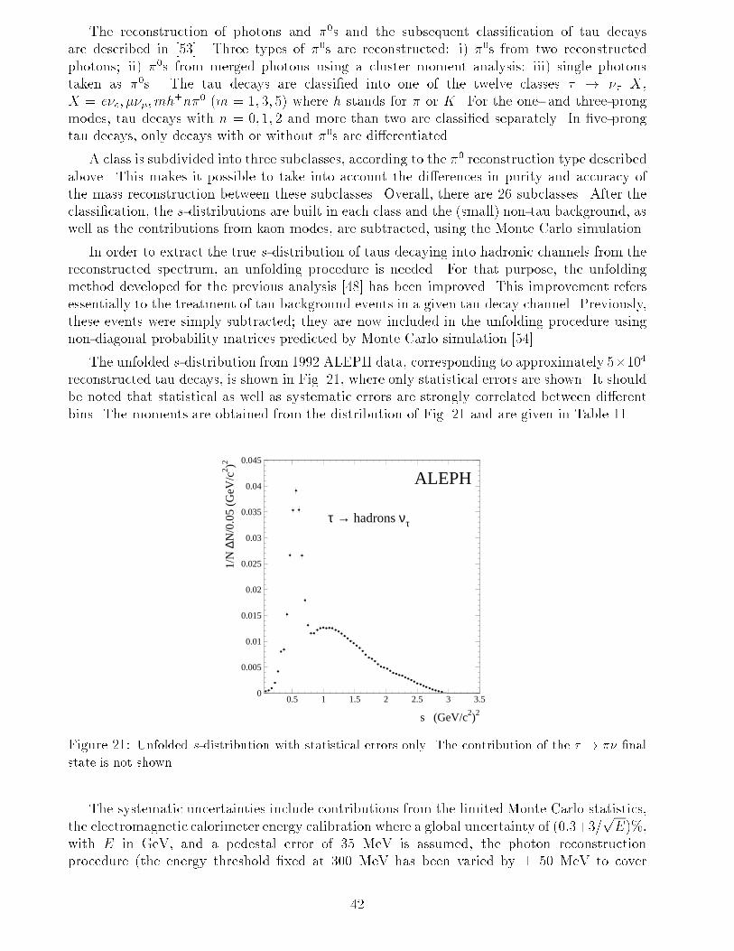
The reconstruction of photons and �0s and the subsequent classi�cation of tau decays

are described in [53]. Three types of �0s are reconstructed: i) �0s from two reconstructed

photons; ii) �0s from merged photons using a cluster moment analysis; iii) single photons

taken as �0s. The tau decays are classi�ed into one of the twelve classes � ! �� X,

X = e�e; ���;mh�n�0 (m = 1; 3; 5) where h stands for � or K. For the one- and three-prong

modes, tau decays with n = 0; 1; 2 and more than two are classi�ed separately. In �ve-prong

tau decays, only decays with or without �0s are di�erentiated.

A class is subdivided into three subclasses, according to the �0 reconstruction type described

above. This makes it possible to take into account the di�erences in purity and accuracy of

the mass reconstruction between these subclasses. Overall, there are 26 subclasses. After the

classi�cation, the s-distributions are built in each class and the (small) non-tau background, as

well as the contributions from kaon modes, are subtracted, using the Monte Carlo simulation.

In order to extract the true s-distribution of taus decaying into hadronic channels from the

reconstructed spectrum, an unfolding procedure is needed. For that purpose, the unfolding

method developed for the previous analysis [48] has been improved. This improvement refers

essentially to the treatment of tau background events in a given tau decay channel. Previously,

these events were simply subtracted; they are now included in the unfolding procedure using

non-diagonal probability matrices predicted by Monte Carlo simulation [54].

The unfolded s-distribution from 1992 ALEPH data, corresponding to approximately 5�104reconstructed tau decays, is shown in Fig. 21, where only statistical errors are shown. It should

be noted that statistical as well as systematic errors are strongly correlated between di�erent

bins. The moments are obtained from the distribution of Fig. 21 and are given in Table 11.

s (GeV/c2)2

1/N

∆N

/0.0

5 (G

eV/c2 )2

τ → hadrons ντ

ALEPH

0

0.005

0.01

0.015

0.02

0.025

0.03

0.035

0.04

0.045

0.5 1 1.5 2 2.5 3 3.5

Figure 21: Unfolded s-distribution with statistical errors only. The contribution of the � ! �� �nal

state is not shown.

The systematic uncertainties include contributions from the limited Monte Carlo statistics,

the electromagnetic calorimeter energy calibration where a global uncertainty of (0:3+3=pE)%,

with E in GeV, and a pedestal error of 35 MeV is assumed, the photon reconstruction

procedure (the energy threshold �xed at 300 MeV has been varied by � 50 MeV to cover

42

eventual ine�ciencies in the low-energy photon reconstruction, an excess of fake photons

of roughly 20% found in the data at low energy was simulated in the Monte Carlo to

estimate the corresponding systematic uncertainty), the �0 reconstruction, the charged particle

identi�cation, the reconstruction of the three-prong modes where the reconstruction e�ciency

of highly collimated tracks was studied in addition to e�ects coming from secondary nuclear

interactions, the non-tau background subtraction and �nally the unfolding procedure. The

dominant systematic errors are those coming from the understanding of the electromagnetic

calorimeter.

l 0 1 2 3

D1l� 0.7228 0.1569 0.0570 0.0256

�[stat] 0.0019 0.0007 0.0005 0.0003

�[exp] 0.0060 0.0020 0.0013 0.0008

�[theo] 0.0034 0.0029 0.0004 0.0002

Table 11: The measured moments of the hadronic invariant mass-squared distribution, together with

their statistical, total experimental and theoretical errors.

Fit Results

The ratio R� and the four D1l momentmeasurements are combined with their experimental and

theoretical covariance matrices in a �t for �s and the three main non-perturbative terms. The

results are given in Table 12. The �rst column shows the global �t result, the second gives the

result of a �t for �s using R� only, using as input for the non-perturbative terms the estimates

quoted in [49] and the last column, a �t for �s using the moments only. The two experimentally

uncorrelated determinations of �s using R� or the moments are in good agreement.

R�+D1l R� D1l

�s 0:353 � 0:022 0:366 � 0:024 0:365 � 0:055

h�s�ggi +0:004 � 0:012 0.02 � 0.02 0.02 � 0.02

O(6) �0:001 � 0:002 0.002 � 0.002 0.002 � 0.002

O(8)) +0:002 � 0:002 0.0 � 0.007 0.0 � 0.007

�2=d:o:f: 0.1 | 1.1

Table 12: Fit results for ALEPH 1992 data. The unit for the dimension D term is GeVD. Numbers

in italics are input values to the �ts.

Taking into account the results of Table 12 and their correlations shown in Table 13, one

can extract the total non-perturbative contribution to R� :

�R� = 3 � �NP (40)

�NP = (�0:02 � 0:5)%

Extrapolating the �s measurement from the tau mass scale to the Z mass scale according to

the method of ref. [55], yields

�s(MZ) = 0:1221 � 0:0015exp � 0:0018theo � 0:0010extrap ; (41)

43

ALEPH �s h�s�ggi O(6)

h�s�ggi �0:41 | |

O(6) +0:41 �0:91 |

O(8) �0:39 +0:92 �0:98

Table 13: Correlation coe�cients between �s and the measured non-perturbative terms.

where the �rst (second) error accounts for experimental (theoretical) uncertainties and the third

error re ects uncertainties in the extrapolation.

The estimates of theoretical uncertainties are performed as in ref. [48]. The largest

uncertainty stems from the missing fourth order coe�cient of the perturbative expansion. The

contribution of the theoretical uncertainties to the overall error is numerically equal to the

contributions of experimental uncertainties, where the latter are dominated by the statistical

error on the leptonic branching ratios. However, the nature of the theoretical uncertainties and

the proper procedure to be used to evaluate them are still unclear. As a result, a range of

estimates can be found in the literature: the theoretical precision of the �s(MZ) determination

from R� alone is evaluated as � 0:003 in [56], � 0:005 in [57] and � 0:006 in [58].

3.2.3 Event Shapes and Jet Rates

The topology of hadronic events in e+e� collisions is modi�ed by the e�ects of gluon radiation,

giving rise to events which di�er from the collimated two-jet topology coming from the

fragmentation of pure q�q events. Since the amount of gluon radiation is directly proportional

to the strong coupling constant, studying the topology of hadronic decays of the Z boson will

provide a measurement of �s(MZ).

The strategy consists of �nding variables which characterize the \three-jetness" of the event.

In order to be able to perform reliable perturbative calculations, the variables have to be infrared

and collinear safe, i.e. insensitive to soft and/or collinear gluon emission.

Many variables have been de�ned which ful�l these properties [59]. One of the most widely

used is the thrust, T , de�ned in Section 2. The thrust distribution is shown in Fig. 7. The

thrust can take values from 0.5, corresponding to a totally spherical event, to 1, corresponding

to a perfect two-jet event. Multiple soft gluon emission and fragmentation e�ects populate

the region close to T = 1, where most of the events lie. This is the so-called two-jet region.

Hard gluon emission creates the tail of the distribution towards lower values of T . The thrust

distribution is in itself already proportional to �s in leading order,

1

�

d�

dT/ �sA(T ) + � � � ;

which implies that the distribution is statistically very sensitive to �s. This can be extended

to the other event shape variables that are analyzed. They, in general, will be called y, with

y = 0 corresponding to the two-jet limit, i.e., for thrust, y = 1� T .

The data analysis follows exactly that explained in Section 1.3, and is based only on charged

particles. The experimental systematic errors, as de�ned in Section 2, are larger than the

statistical errors but considerably smaller than the theoretical uncertainties.

44

Analysis Using Second Order QCD Predictions

The QCD predictions for all the event shape variable distributions are known to second order

in �s [16], i.e.

1

�

d�

dy=�s(�)

2��A(y) +

�s(�)

2�

!2�"B(y) + 2�b0 ln

�2

s

!�A(y)

#: (42)

The functions A(y) and B(y) are speci�c for every event shape variable and contain the full

information of the second order matrix elements. The parameter � denotes the arbitrary

renormalization scale used for the calculation. A complete all-order calculation would not

depend on the value of � chosen. However, a truncated second order prediction does, and this

will create a large uncertainty in the �nal result.

The prediction corresponds to a partonic �nal state with, at most, four partons. To

obtain a prediction for multi-hadronic �nal states, the above expression is convoluted with

the predictions obtained from phenomenological hadronization models. By using the Lund

second order matrix element model [60] tuned to the data, not only hadronization corrections

but also perturbative higher order e�ects are e�ectively included, although for a �xed value of

�s.

The ratio of the predictions of this model at hadron and parton level are shown in Fig. 22

for two di�erent variables: the di�erential two-jet rate using the JADE scheme, y3, and the

oblateness, O. While di�erences between hadron and parton level are minor for the former

(mean value close to zero and small width), they are much bigger for the latter. Therefore, y3should be considered a more reliable variable for the measurement of �s than O.

For each event shape variable considered, the measured distribution corrected for detector

e�ects is �tted to the convolution of the second order prediction with the higher order and

hadronization corrections resulting from the phenomenological models. By using a number

of them di�ering either in higher orders (models based on the exact second order QCD [60]

and models implementing leading-logarithm parton showers [61]) or in the hadronization phase

(models based on string fragmentation [61] and models based on cluster fragmentation [62]),

systematic errors due to hadronization and higher order uncertainties are obtained. Details can

be found in ref. [63].

The results are shown in Table 14 for the event shape variables analyzed in [63]. The

renormalization scale has been �xed to � =MZ=2, that is, half-way between the centre-of-mass

energy and the non-perturbative scale. It can be seen that the best measurement is by far that

provided by the di�erential two-jet rate, y3. Therefore, this was chosen as the �nal result of

the analysis, leading to:

�s(MZ) = 0:121 � 0:002(stat)� 0:003(sys) � 0:007(theo) (43)

for � =MZ=2. If the renormalization scale is changed to the bottom quark mass or to MZ , the

result varies by �0:012 and +0:007, respectively.

Analysis Using Pre-Clustered Event Shape Variables in Second Order QCD

As has been seen in the previous section, higher order and hadronization e�ects prevent the

e�ective use of most of the existing event shape variables to determine �s accurately. An idea to

improve the situation was presented in [64], where the event shape variables are not computed

45

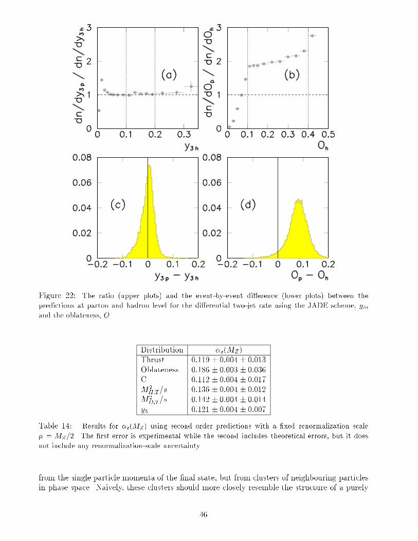
Figure 22: The ratio (upper plots) and the event-by-event di�erence (lower plots) between the

predictions at parton and hadron level for the di�erential two-jet rate using the JADE scheme, y3,

and the oblateness, O.

Distribution �s(MZ)

Thrust 0:119 � 0:004 � 0:013

Oblateness 0:186 � 0:003 � 0:036

C 0:112 � 0:004 � 0:017

M2H;T=s 0:136 � 0:004 � 0:012

M2D;T=s 0:142 � 0:004 � 0:014

y3 0:121 � 0:004 � 0:007

Table 14: Results for �s(MZ) using second order predictions with a �xed renormalization scale

� = MZ=2. The �rst error is experimental while the second includes theoretical errors, but it does

not include any renormalization-scale uncertainty.

from the single particle momenta of the �nal state, but from clusters of neighbouring particles

in phase space. Naively, these clusters should more closely resemble the structure of a purely

46

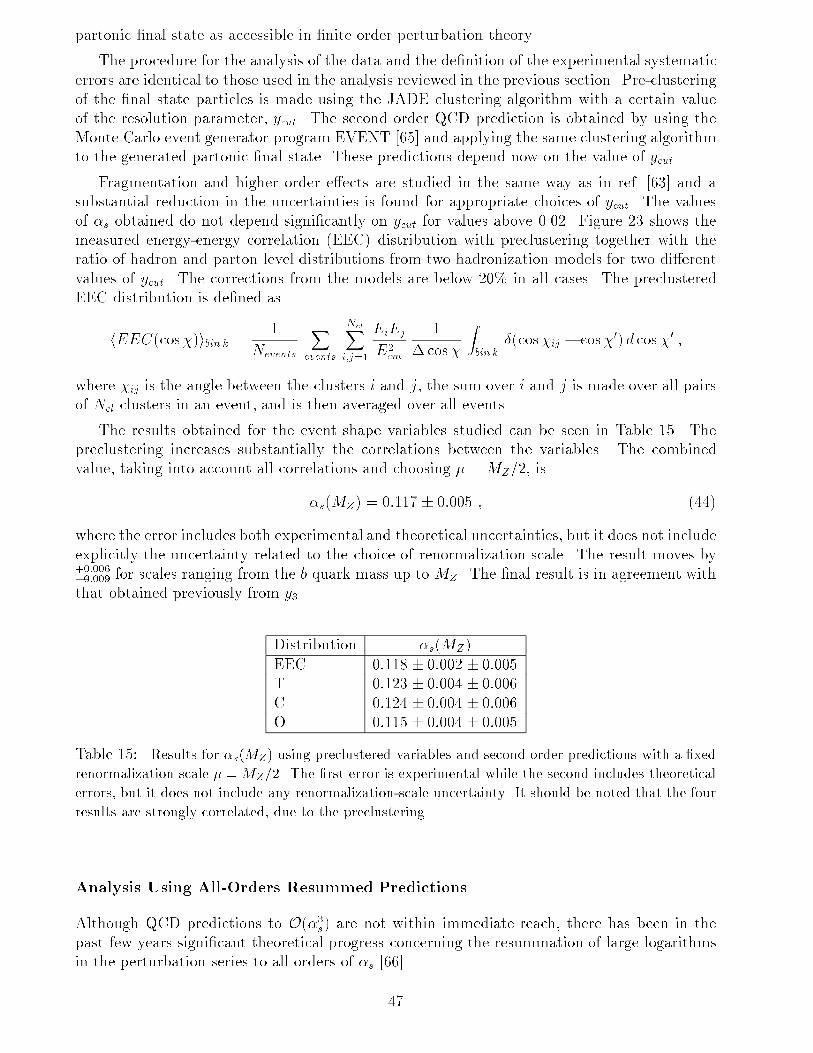
partonic �nal state as accessible in �nite order perturbation theory.

The procedure for the analysis of the data and the de�nition of the experimental systematic

errors are identical to those used in the analysis reviewed in the previous section. Pre-clustering

of the �nal state particles is made using the JADE clustering algorithm with a certain value

of the resolution parameter, ycut. The second order QCD prediction is obtained by using the

Monte Carlo event generator program EVENT [65] and applying the same clustering algorithm

to the generated partonic �nal state. These predictions depend now on the value of ycut.

Fragmentation and higher order e�ects are studied in the same way as in ref. [63] and a

substantial reduction in the uncertainties is found for appropriate choices of ycut. The values

of �s obtained do not depend signi�cantly on ycut for values above 0.02. Figure 23 shows the

measured energy-energy correlation (EEC) distribution with preclustering together with the

ratio of hadron and parton level distributions from two hadronization models for two di�erent

values of ycut. The corrections from the models are below 20% in all cases. The preclustered

EEC distribution is de�ned as

hEEC(cos�)ibin k = 1

Nevents

Xevents

NclXi;j=1

EiEj

E2cm

1

�cos�

Zbin k

�(cos�ij � cos�0) d cos �0 ;

where �ij is the angle between the clusters i and j, the sum over i and j is made over all pairs

of Ncl clusters in an event, and is then averaged over all events.

The results obtained for the event shape variables studied can be seen in Table 15. The

preclustering increases substantially the correlations between the variables. The combined

value, taking into account all correlations and choosing � =MZ=2, is

�s(MZ) = 0:117 � 0:005 ; (44)

where the error includes both experimental and theoretical uncertainties, but it does not include

explicitly the uncertainty related to the choice of renormalization scale. The result moves by+0:006�0:009 for scales ranging from the b quark mass up to MZ. The �nal result is in agreement with

that obtained previously from y3.

Distribution �s(MZ)

EEC 0:118 � 0:002 � 0:005

T 0:123 � 0:004 � 0:006

C 0:124 � 0:004 � 0:006

O 0:115 � 0:004 � 0:005

Table 15: Results for �s(MZ) using preclustered variables and second order predictions with a �xed

renormalization scale � =MZ=2. The �rst error is experimental while the second includes theoretical

errors, but it does not include any renormalization-scale uncertainty. It should be noted that the four

results are strongly correlated, due to the preclustering.

Analysis Using All-Orders Resummed Predictions

Although QCD predictions to O(�3s) are not within immediate reach, there has been in the

past few years signi�cant theoretical progress concerning the resummation of large logarithms

in the perturbation series to all orders of �s [66].

47

Figure 23: EEC distribution with preclustering together with the ratio of hadron and parton level

distributions from two hadronization models for two di�erent values of ycut. The vertical dashed lines

indicate the �t range.

These higher order calculations are similar to the parton shower calculations implemented

in the Monte Carlo programs which most successfully describe the data. The corrections due to

the transition between partons and hadrons and their uncertainty will be smaller. Furthermore,

the uncertainties related to the renormalization scale will be reduced since higher orders are

partially included. Finally, the range of validity of the predictions will extend further into the

two-jet region.

For a general event shape variable Y for which the theoretical prediction can be

exponentiated, the resummed prediction for the cumulative distribution, de�ned by

R (y; �s) =1

�tot�(Y < y) ; (45)

can be written in the following way:

lnR (y; �s) = L � fLL(�sL) + fNLL(�sL) + subleading terms ; (46)

where L = � ln y becomes large in the two-jet region. The functions fLL and fNLL depend only

on the product of �s and L. The �rst two terms in Eq. (46) represent the leading and the next-to-

leading logarithms. They have been computed for a number of variables, including thrust [67],

heavy jet mass [68] and di�erential two-jet rate with the Durham cluster algorithm [69]. The

48

calculation of the next-to-leading logarithm function used in this analysis is not complete for

the last variable1.

The expansion of Eq. 46 in powers of �s is shown in Table 16. The �rst column (/ �ns Ln+1)

represents the leading logarithms, the second column (/ �ns Ln) the next-to-leading logarithms

and the �rst two rows represent the completeO(�2s) predictions [16, 59]. An improved prediction

Leading Log Next-to-Leading Log Subleading

First Order �sL2 �sL �s : : :

Second Order �2sL3 �2sL

2 �2sL �2s : : :

Third Order �3sL4 �3sL

3 �3sL2 �3sL �3s : : :

......

...

Table 16: Schematic representation of the order by order expansion of theoretical prediction in

leading logarithms, next-to-leading logarithms and subleading logarithms.

can thus be constructed by combining the exact second order predictions with the leading and

next-to-leading logarithms of Eq. (46), starting in O(�3s). There are several ways this matching

can be done [71], either for lnR (\lnR matching") or for R (\R matching"). They di�er in

exactly which terms are being exponentiated. Di�erences start always at O (�3s).

In ref. [71] the variables thrust, heavy jet mass and di�erential two-jet rate with the

Durham cluster algorithm have been used to measure �s within the framework of the resummed

predictions. Raw data distributions are corrected for detector e�ects following the scheme

outlined in Section 1.3.

The parton-level predictions have been folded with hadronization e�ects obtained from

parton shower models JETSET 7.2 and HERWIG 5.3 to obtain predictions at the hadron level,

which are compared with the data. The data and the QCD �t are shown in Fig. 24.

The �nal result for each distribution is

�s(MZ)jy3 = 0:1257 � 0:0010stat � 0:0025syst � 0:0007hadr � 0:0043theo

�s(MZ)jT = 0:1263 � 0:0008stat � 0:0010syst � 0:0028hadr � 0:0065theo (47)

�s(MZ)j� = 0:1243 � 0:0010stat � 0:0033syst � 0:0042hadr � 0:0057theo ;

where the �rst error is statistical, the second estimates the experimental systematics, the third

concerns the hadronization correction, and the last is the estimate of theoretical uncertainties.

The hadronization uncertainty takes into account, among other things, the di�erences in the

results obtained when folding the parton distributions with di�erent hadronization models.

The theoretical uncertainty covers the uncertainty due to the choice of matching scheme

as well as the variation of the renormalization scale used in the calculation in the range

�1 � ln�2=s � +1. The central values are given at �2 = s. In contrast with most analyses

using second order QCD, this analysis using resummed predictions does not prefer values of �

much smaller than the centre-of-mass energy.

Combining the three previous results (47), taking into account all correlations, leads to the

�nal result for the strong coupling constant

�s(MZ) = 0:1251 � 0:0009stat � 0:0021syst � 0:0007hadr � 0:0038theo = 0:125 � 0:005 : (48)

1Recently, a �rst work on the complete resummation of the next-to-leading terms has appeared [70].

49

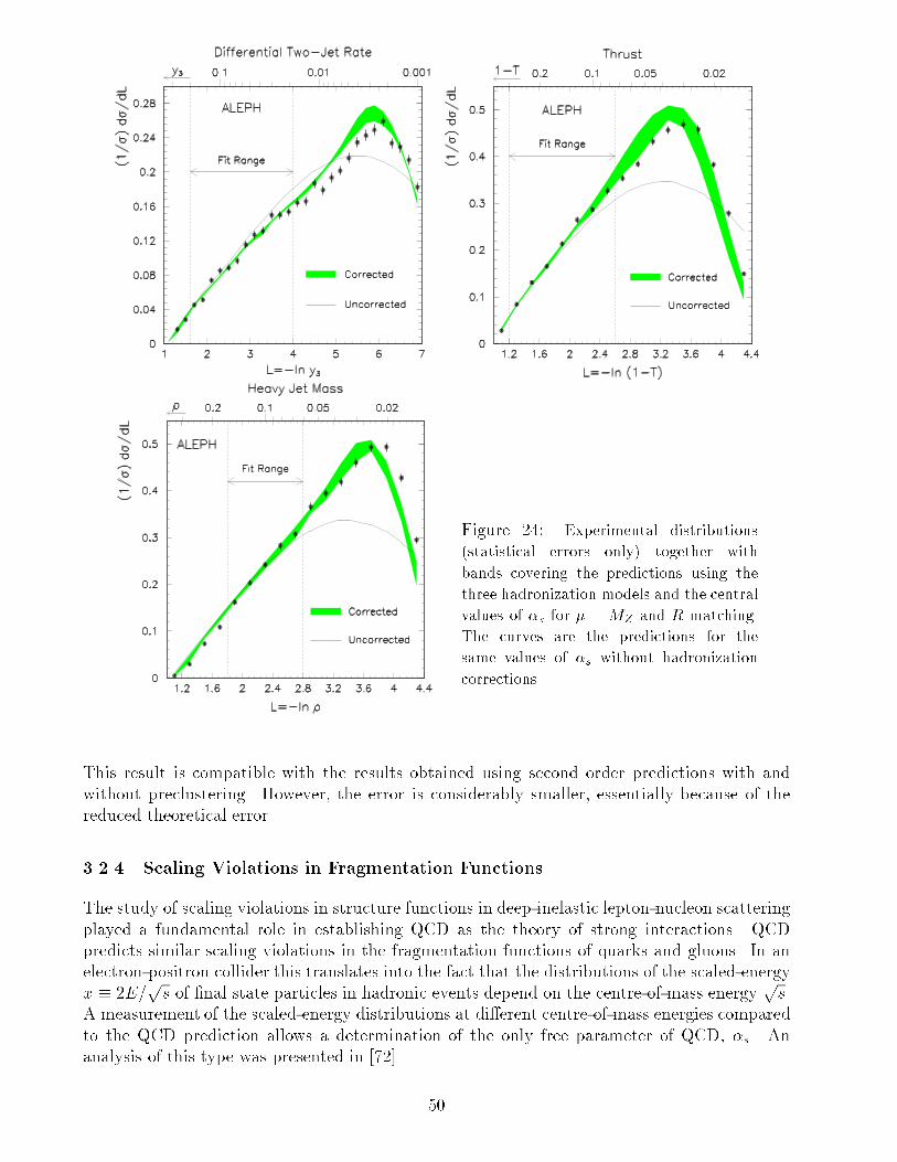
Figure 24: Experimental distributions

(statistical errors only) together with

bands covering the predictions using the

three hadronization models and the central

values of �s for � = MZ and R matching.

The curves are the predictions for the

same values of �s without hadronization

corrections.

This result is compatible with the results obtained using second order predictions with and

without preclustering. However, the error is considerably smaller, essentially because of the

reduced theoretical error.

3.2.4 Scaling Violations in Fragmentation Functions

The study of scaling violations in structure functions in deep-inelastic lepton-nucleon scattering

played a fundamental role in establishing QCD as the theory of strong interactions. QCD

predicts similar scaling violations in the fragmentation functions of quarks and gluons. In an

electron-positron collider this translates into the fact that the distributions of the scaled-energy

x � 2E=ps of �nal state particles in hadronic events depend on the centre-of-mass energy

ps.

A measurement of the scaled-energy distributions at di�erent centre-of-mass energies compared

to the QCD prediction allows a determination of the only free parameter of QCD, �s. An

analysis of this type was presented in [72].

50

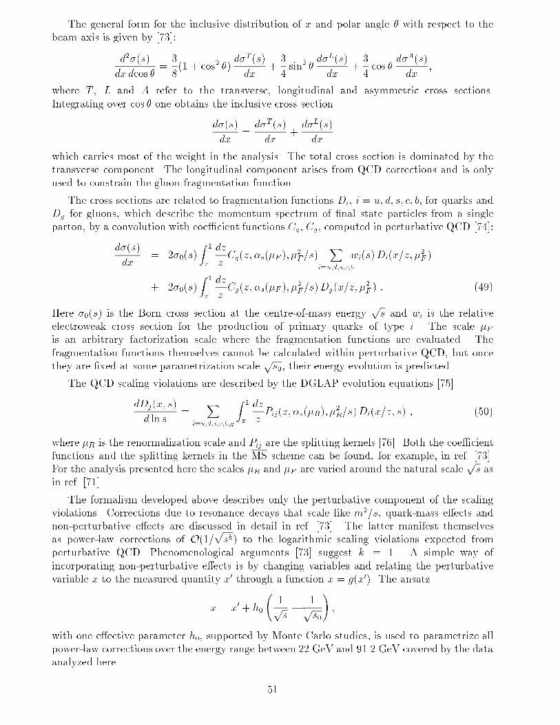
The general form for the inclusive distribution of x and polar angle � with respect to the

beam axis is given by [73]:

d2�(s)

dx dcos �=

3

8(1 + cos2 �)

d�T (s)

dx+3

4sin2 �

d�L(s)

dx+3

4cos �

d�A(s)

dx;

where T , L and A refer to the transverse, longitudinal and asymmetric cross sections.

Integrating over cos � one obtains the inclusive cross section

d�(s)

dx=d�T (s)

dx+d�L(s)

dx

which carries most of the weight in the analysis. The total cross section is dominated by the

transverse component. The longitudinal component arises from QCD corrections and is only

used to constrain the gluon fragmentation function.

The cross sections are related to fragmentation functions Di; i = u; d; s; c; b, for quarks and

Dg for gluons, which describe the momentum spectrum of �nal state particles from a single

parton, by a convolution with coe�cient functions Cq, Cg, computed in perturbative QCD [74]:

d�(s)

dx= 2�0(s)

Z 1

x

dz

zCq(z; �s(�F ); �

2F=s)

Xi=u;d;s;c;b

wi(s)Di(x=z; �2F )

+ 2�0(s)Z 1

x

dz

zCg(z; �s(�F ); �

2F=s)Dg(x=z; �

2F ) : (49)

Here �0(s) is the Born cross section at the centre-of-mass energyps and wi is the relative

electroweak cross section for the production of primary quarks of type i. The scale �Fis an arbitrary factorization scale where the fragmentation functions are evaluated. The

fragmentation functions themselves cannot be calculated within perturbative QCD, but once

they are �xed at some parametrization scaleps0, their energy evolution is predicted.

The QCD scaling violations are described by the DGLAP evolution equations [75]

dDj(x; s)

d ln s=

Xi=u;d;s;c;b;g

Z 1

x

dz

zPij(z; �s(�R); �

2R=s)Di(x=z; s) ; (50)

where �R is the renormalization scale and Pij are the splitting kernels [76]. Both the coe�cient

functions and the splitting kernels in the MS scheme can be found, for example, in ref. [73].

For the analysis presented here the scales �R and �F are varied around the natural scaleps as

in ref. [71].

The formalism developed above describes only the perturbative component of the scaling

violations. Corrections due to resonance decays that scale like m2=s, quark-mass e�ects and

non-perturbative e�ects are discussed in detail in ref. [73]. The latter manifest themselves

as power-law corrections of O(1=psk) to the logarithmic scaling violations expected from

perturbative QCD. Phenomenological arguments [73] suggest k = 1. A simple way of

incorporating non-perturbative e�ects is by changing variables and relating the perturbative

variable x to the measured quantity x0 through a function x = g(x0). The ansatz

x = x0 + h0

1ps� 1p

s0

!;

with one e�ective parameter h0, supported by Monte Carlo studies, is used to parametrize all

power-law corrections over the energy range between 22 GeV and 91.2 GeV covered by the data

analyzed here.

51

Because the fragmentation functions depend on the quark mass, and the relative cross

section for each avour depends onps, a measurement of �s from scaling violations in

inclusive momentum distributions requires knowledge of the fragmentation functions for all

quark avours at one energy. Information about the various quark avours is extracted from

the data, by controlling the avour composition of the data sample using appropriate tagging

techniques. The impact parameter tag described in Section 1.2 is used to select a b quark

enriched sample and a light (u,d,s) quark enriched sample. The same technique combined with

a tag based on shape variables [78] is applied to obtain a c quark enriched sample. The scaled

energy distribution is measured in an inclusive sample and in the three tagged samples.

Equations (49) and (50) show that the gluon fragmentation function is also needed. A direct

measurement of the gluon fragmentation function is obtained from three-jet events where jets

from well separated gluons are tagged by default when the other two jets contain long-lived

particles (Section 4.5). The gluon fragmentation function is also extracted by measuring the

longitudinal and transverse cross sections, which are related to the gluon fragmentation function

according to [73]

1

�tot

d�L

dx=�s

2�

Z 1

x

dz

z

"1

�tot

d�T

dz+ 4

�z

x� 1

�Dg(z)

#+O(�2s) : (51)

Truncating the above expression at O(�s), the parameter �s becomes an e�ective leading-order

coupling constant which must not be confused with the next-to-leading order running coupling

constant appearing in Eqs. (49),(50). Because of this, it will be referred to as �s in the following.

The longitudinal and transverse cross sections are measured by weighting the double-

di�erential cross section with respect to x and cos � with the appropriate weight to project

onto the (1 + cos2 �) component (transverse) or the sin2 � component (longitudinal).

Systematic errors in all distributions, due to imperfect detector simulation or biases due

to the hadron production model used to correct the data, are estimated using the techniques

described in Section 2. On top of those, additional systematic errors are assigned to the

longitudinal and transverse distributions (especially sensitive to tracking ine�ciencies at low

angles) [72] and a 1% normalization error is attributed to all distributions, according to the

�ndings of ref. [79]. Systematic uncertainties speci�c to the avour tagging procedures are

treated separately in the �s determination. Figure 25 shows the measured distributions. One

clearly sees the di�erence between light and heavy avour enriched samples. The errors include

all bin-to-bin errors (statistical and systematic) added in quadrature as well as an overall 1%

normalization error. Systematic errors dominate everywhere. The transverse distribution is

almost identical to the unweighted distribution for all avours and is not shown.

In addition to the ALEPH data, inclusive charged particle spectra from TASSO [80] atps = 22, 35 and 45 GeV, MARK II [81] and TPC/2 [82] at

ps = 29 GeV, CELLO [83] atp

s = 35 GeV, AMY [84] atps = 55 GeV and DELPHI [85] at

ps = 91.2 GeV have been

used in the analysis. Lower-energy data were not used because of the possible larger size of the

power-law corrections.

The fragmentation functions for the di�erent avours and for the gluon are parametrized

using the functional form

xDi(x; s0) = Ni

(1� x)aixbi exp��c ln2 x

�Z 0:8

0:1dx (1� x)aixbi exp

��c ln2 x

� ;

52

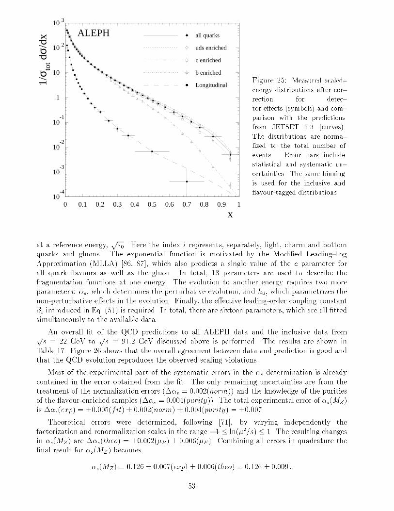
10-4

10-3

10-2

10-1

1

10

10 2

10 3

0 0.1 0.2 0.3 0.4 0.5 0.6 0.7 0.8 0.9 1

x

1/σ to

t dσ/

dxall quarks

uds enriched

c enriched

b enriched

Longitudinal

ALEPH

Figure 25: Measured scaled-

energy distributions after cor-

rection for detec-

tor effects (symbols) and com-

parison with the predictions

from JETSET 7.3 (curves).

The distributions are norma-

lized to the total number of

events. Error bars include

statistical and systematic un-

certainties. The same binning

is used for the inclusive and

avour-tagged distributions.

at a reference energy,ps0. Here the index i represents, separately, light, charm and bottom

quarks and gluons. The exponential function is motivated by the Modi�ed Leading-Log

Approximation (MLLA) [86, 87], which also predicts a single value of the c parameter for

all quark avours as well as the gluon. In total, 13 parameters are used to describe the

fragmentation functions at one energy. The evolution to another energy requires two more

parameters: �s, which determines the perturbative evolution, and h0, which parametrizes the

non-perturbative e�ects in the evolution. Finally, the e�ective leading-order coupling constant

�s introduced in Eq. (51) is required. In total, there are sixteen parameters, which are all �tted

simultaneously to the available data.

An overall �t of the QCD predictions to all ALEPH data and the inclusive data fromps = 22 GeV to

ps = 91:2 GeV discussed above is performed. The results are shown in

Table 17. Figure 26 shows that the overall agreement between data and prediction is good and

that the QCD evolution reproduces the observed scaling violations.

Most of the experimental part of the systematic errors in the �s determination is already

contained in the error obtained from the �t. The only remaining uncertainties are from the

treatment of the normalization errors (��s = 0:002(norm)) and the knowledge of the purities

of the avour-enriched samples (��s = 0:004(purity)). The total experimental error of �s(MZ)

is ��s(exp) = �0:005(fit)� 0:002(norm) � 0:004(purity) = �0:007.Theoretical errors were determined, following [71], by varying independently the

factorization and renormalization scales in the range �1 � ln(�2=s) � 1. The resulting changes

in �s(MZ) are ��s(theo) = �0:002(�R) � 0:006(�F ). Combining all errors in quadrature the

�nal result for �s(MZ) becomes

�s(MZ) = 0:126 � 0:007(exp) � 0:006(theo) = 0:126 � 0:009 :

53

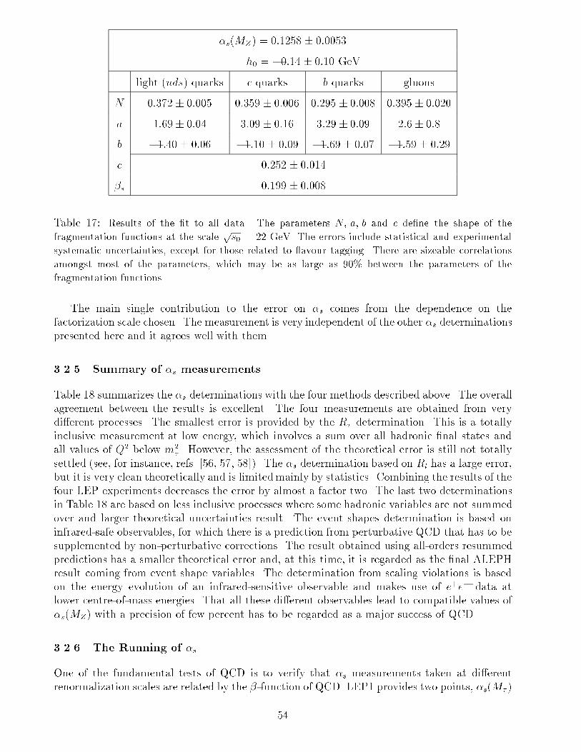
�s(MZ) = 0:1258 � 0:0053

h0 = �0:14 � 0:10 GeV

light (uds) quarks c quarks b quarks gluons

N 0:372 � 0:005 0:359 � 0:006 0:295 � 0:008 0:395 � 0:020

a 1:69� 0:04 3:09 � 0:16 3:29 � 0:09 2:6� 0:8

b �1:40 � 0:06 �1:10 � 0:09 �1:69 � 0:07 �1:59 � 0:29

c 0:252 � 0:014

�s 0:199 � 0:008

Table 17: Results of the �t to all data. The parameters N; a; b and c de�ne the shape of the

fragmentation functions at the scaleps0 = 22 GeV. The errors include statistical and experimental

systematic uncertainties, except for those related to avour tagging. There are sizeable correlations

amongst most of the parameters, which may be as large as 90% between the parameters of the

fragmentation functions.

The main single contribution to the error on �s comes from the dependence on the

factorization scale chosen. The measurement is very independent of the other �s determinations

presented here and it agrees well with them.

3.2.5 Summary of �s measurements

Table 18 summarizes the �s determinations with the four methods described above. The overall

agreement between the results is excellent. The four measurements are obtained from very

di�erent processes. The smallest error is provided by the R� determination. This is a totally

inclusive measurement at low energy, which involves a sum over all hadronic �nal states and

all values of Q2 below m2� . However, the assessment of the theoretical error is still not totally

settled (see, for instance, refs. [56, 57, 58]). The �s determination based on Rl has a large error,

but it is very clean theoretically and is limitedmainly by statistics. Combining the results of the

four LEP experiments decreases the error by almost a factor two. The last two determinations

in Table 18 are based on less inclusive processes where some hadronic variables are not summed

over and larger theoretical uncertainties result. The event shapes determination is based on

infrared-safe observables, for which there is a prediction from perturbative QCD that has to be

supplemented by non-perturbative corrections. The result obtained using all-orders resummed

predictions has a smaller theoretical error and, at this time, it is regarded as the �nal ALEPH

result coming from event shape variables. The determination from scaling violations is based

on the energy evolution of an infrared-sensitive observable and makes use of e+e� data at

lower centre-of-mass energies. That all these di�erent observables lead to compatible values of

�s(MZ) with a precision of few percent has to be regarded as a major success of QCD.

3.2.6 The Running of �s

One of the fundamental tests of QCD is to verify that �s measurements taken at di�erent

renormalization scales are related by the �-function of QCD. LEP1 provides two points, �s(M� )

54

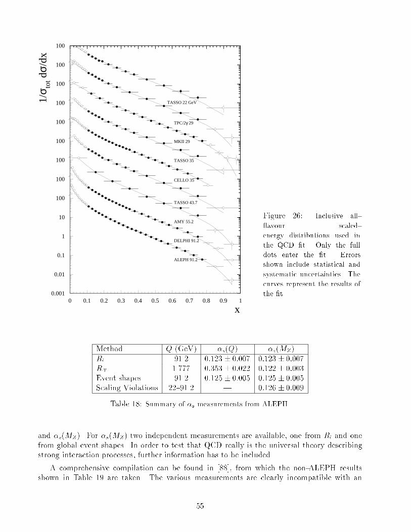
0 0.1 0.2 0.3 0.4 0.5 0.6 0.7 0.8 0.9 1

100

100

100

100

100

100

100

100

100

10

1

0.1

0.01

0.001

TASSO 22 GeV

TPC/2γ 29

MKII 29

TASSO 35

CELLO 35

TASSO 43.7

AMY 55.2

DELPHI 91.2

ALEPH 91.2

x

1/σ to

t dσ/

dx

Figure 26: Inclusive all-

avour scaled-

energy distributions used in

the QCD �t. Only the full

dots enter the �t. Errors

shown include statistical and

systematic uncertainties. The

curves represent the results of

the �t.

Method Q (GeV) �s(Q) �s(MZ)

Rl 91.2 0:123 � 0:007 0:123 � 0:007

R� 1.777 0:353 � 0:022 0:122 � 0:003

Event shapes 91.2 0:125 � 0:005 0:125 � 0:005

Scaling Violations 22{91.2 | 0:126 � 0:009

Table 18: Summary of �s measurements from ALEPH.

and �s(MZ). For �s(MZ) two independent measurements are available, one from Rl and one

from global event shapes. In order to test that QCD really is the universal theory describing

strong interaction processes, further information has to be included.

A comprehensive compilation can be found in [88], from which the non-ALEPH results

shown in Table 19 are taken. The various measurements are clearly incompatible with an

55

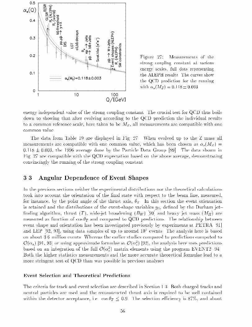
l

Figure 27: Measurements of the

strong coupling constant at various

energy scales, full dots representing

the ALEPH results. The curves show

the QCD prediction for the running

with �s(MZ) = 0:118� 0:003.

energy independent value of the strong coupling constant. The crucial test for QCD thus boils

down to showing that after evolving according to the QCD prediction the individual results

to a common reference scale, here taken to be MZ , all measurements are compatible with one

common value.

The data from Table 19 are displayed in Fig. 27. When evolved up to the Z mass all

measurements are compatible with one common value, which has been chosen as �s(MZ) =

0:118 � 0:003, the 1996 average done by the Particle Data Group [89]. The data shown in

Fig. 27 are compatible with the QCD expectation based on the above average, demonstrating

convincingly the running of the strong coupling constant.

3.3 Angular Dependence of Event Shapes

In the previous sections neither the experimental distributions nor the theoretical calculations

took into account the orientation of the �nal state with respect to the beam line, measured,

for instance, by the polar angle of the thrust axis, �T . In this section the event orientation

is retained and the distributions of the event-shape variables y3, de�ned by the Durham jet-

�nding algorithm, thrust (T ), wide-jet broadening (BW ) [90] and heavy jet mass (MH) are

measured as function of cos �T and compared to QCD predictions. The relationship between

event shape and orientation has been investigated previously by experiments at PETRA [91]

and LEP [92, 93], using data samples of up to around 105 events. The analysis here is based

on about 3.6 million events. Whereas the earlier studies compared to predictions computed to

O(�s) [91, 93] or using approximate formulae at O(�2s) [92], the analysis here uses predictionsbased on an integration of the full O(�2s) matrix elements using the program EVENT2 [94].

Both the higher statistics measurements and the more accurate theoretical formulae lead to a

more stringent test of QCD than was possible in previous analyses.

Event Selection and Theoretical Predictions

The criteria for track and event selection are described in Section 1.3. Both charged tracks and

neutral particles are used and the reconstructed thrust axis is required to be well contained

within the detector acceptance, i.e. cos �T � 0:9. The selection e�ciency is 87%, and about

56

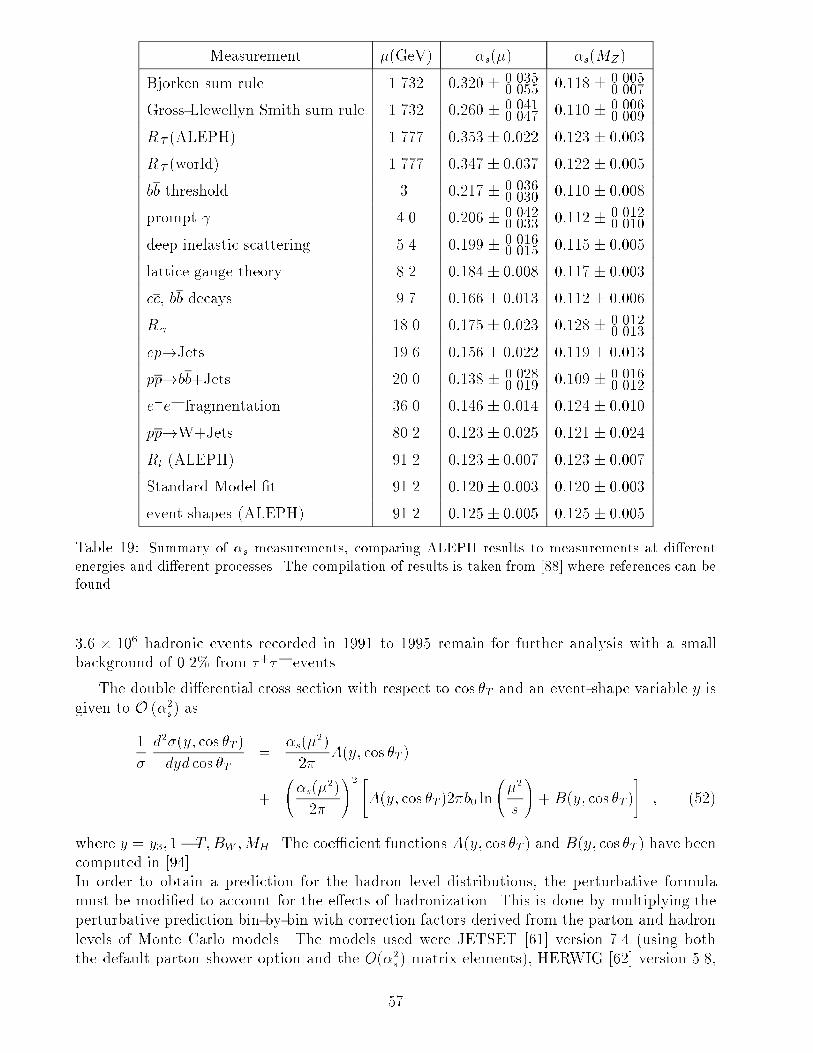
Measurement �(GeV) �s(�) �s(MZ)

Bjorken sum rule 1.732 0:320 � 0.0350.055 0:118 � 0.005

0.007

Gross-Llewellyn Smith sum rule 1.732 0:260 � 0.0410.047 0:110 � 0.006

0.009

R� (ALEPH) 1.777 0:353 � 0:022 0:123 � 0:003

R� (world) 1.777 0:347 � 0:037 0:122 � 0:005

bb threshold 3. 0:217 � 0.0360.030 0:110 � 0:008

prompt 4.0 0:206 � 0.0420.033 0:112 � 0.012

0.010

deep inelastic scattering 5.4 0:199 � 0.0160.015 0:115 � 0:005

lattice gauge theory 8.2 0:184 � 0:008 0:117 � 0:003

cc, bb decays 9.7 0:166 � 0:013 0:112 � 0:006

R 18.0 0:175 � 0:023 0:128 � 0.0120.013

ep!Jets 19.6 0:156 � 0:022 0:119 � 0:013

pp!bb+Jets 20.0 0:138 � 0.0280.019 0:109 � 0.016

0.012

e+e� fragmentation 36.0 0:146 � 0:014 0:124 � 0:010

pp!W+Jets 80.2 0:123 � 0:025 0:121 � 0:024

Rl (ALEPH) 91.2 0:123 � 0:007 0:123 � 0:007

Standard Model �t 91.2 0:120 � 0:003 0:120 � 0:003

event shapes (ALEPH) 91.2 0:125 � 0:005 0:125 � 0:005

Table 19: Summary of �s measurements, comparing ALEPH results to measurements at di�erent

energies and di�erent processes. The compilation of results is taken from [88] where references can be

found.

3:6 � 106 hadronic events recorded in 1991 to 1995 remain for further analysis with a small

background of 0.2% from �+�� events.

The double di�erential cross section with respect to cos �T and an event-shape variable y is

given to O (�2s) as

1

�

d2�(y; cos �T )

dyd cos �T=

�s(�2)

2�A(y; cos �T )

+

�s(�

2)

2�

!2 "A(y; cos �T )2�b0 ln

�2

s

!+B(y; cos �T )

#; (52)

where y = y3; 1�T;BW ;MH . The coe�cient functions A(y; cos �T ) and B(y; cos �T ) have been

computed in [94].

In order to obtain a prediction for the hadron level distributions, the perturbative formula

must be modi�ed to account for the e�ects of hadronization. This is done by multiplying the

perturbative prediction bin-by-bin with correction factors derived from the parton and hadron

levels of Monte Carlo models. The models used were JETSET [61] version 7.4 (using both

the default parton shower option and the O(�2s) matrix elements), HERWIG [62] version 5.8,

57

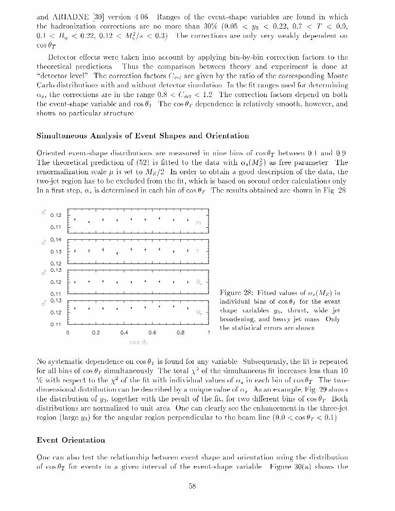
and ARIADNE [30] version 4.06. Ranges of the event-shape variables are found in which

the hadronization corrections are no more than 30% (0:05 < y3 < 0:22, 0:7 < T < 0:9,

0:1 < Bw < 0:22, 0:12 < M2h=s < 0:3). The corrections are only very weakly dependent on

cos �T .

Detector e�ects were taken into account by applying bin-by-bin correction factors to the

theoretical predictions. Thus the comparison between theory and experiment is done at

\detector level". The correction factors Cdet are given by the ratio of the corresponding Monte

Carlo distributions with and without detector simulation. In the �t ranges used for determining

�s, the corrections are in the range 0:8 < Cdet < 1:2. The correction factors depend on both

the event-shape variable and cos �T . The cos �T dependence is relatively smooth, however, and

shows no particular structure.

Simultaneous Analysis of Event Shapes and Orientation

Oriented event-shape distributions are measured in nine bins of cos �T between 0.1 and 0.9.

The theoretical prediction of (52) is �tted to the data with �s(M2Z) as free parameter. The

renormalization scale � is set to MZ=2. In order to obtain a good description of the data, the

two-jet region has to be excluded from the �t, which is based on second order calculations only.

In a �rst step, �s is determined in each bin of cos �T . The results obtained are shown in Fig. 28.

Figure 28: Fitted values of �s(MZ) in

individual bins of cos �T for the event

shape variables y3, thrust, wide jet

broadening, and heavy jet mass. Only

the statistical errors are shown.

No systematic dependence on cos �T is found for any variable. Subsequently, the �t is repeated

for all bins of cos �T simultaneously. The total �2 of the simultaneous �t increases less than 10

% with respect to the �2 of the �t with individual values of �s in each bin of cos �T . The two-

dimensional distribution can be described by a unique value of �s. As an example, Fig. 29 shows

the distribution of y3, together with the result of the �t, for two di�erent bins of cos �T . Both

distributions are normalized to unit area. One can clearly see the enhancement in the three-jet

region (large y3) for the angular region perpendicular to the beam line (0:0 < cos �T < 0:1).

Event Orientation

One can also test the relationship between event shape and orientation using the distribution

of cos �T for events in a given interval of the event-shape variable. Figure 30(a) shows the

58

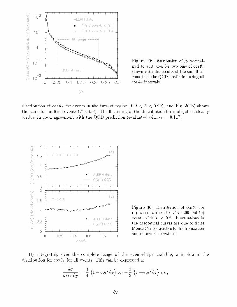
Figure 29: Distribution of y3 normal-

ized to unit area for two bins of cos �Tshown with the results of the simultan-

eous �t of the QCD prediction using all

cos �T intervals.

distribution of cos �T for events in the two-jet region (0:9 < T < 0:99), and Fig. 30(b) shows

the same for multijet events (T < 0:8). The attening of the distribution for multijets is clearly

visible, in good agreement with the QCD prediction (evaluated with �s = 0:117).

Figure 30: Distribution of cos �T for

(a) events with 0:9 < T < 0:99 and (b)

events with T < 0:8. Fluctuations in

the theoretical curves are due to �nite

Monte Carlo statistics for hadronization

and detector corrections.

By integrating over the complete range of the event-shape variable, one obtains the

distribution for cos �T for all events. This can be expressed as

d�

d cos �T=

3

4

�1 + cos2 �T

��U +

3

2

�1 � cos2 �T

��L ;

59

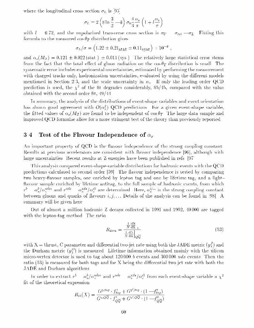
where the longitudinal cross section �L is [95]

�L = 2

�8 ln

3

2� 3

��04

3

�s

�

�1 + l

�s

�

�

with l = 0:72, and the unpolarized transverse cross section is �U = �tot � �L. Fitting this

formula to the measured cos �T distribution gives

�L=� =�1:22 � 0:21stat � 0:11syst

�� 10�2 ;

and �s(MZ) = 0:121 � 0:022 (stat.) � 0:011 (sys.). The relatively large statistical error stems

from the fact that the total e�ect of gluon radiation on the cos �T distribution is small. The

systematic error includes experimental uncertainties, estimated by performing the measurement

with charged tracks only, hadronization uncertainties, evaluated by using the di�erent models

mentioned in Section 2.3, and the scale uncertainty in �s. If only the leading order QCD

prediction is used, the �2 of the �t degrades considerably, 85/45, compared with the value

obtained with the second order �t, 49/44.

In summary, the analysis of the distributions of event-shape variables and event orientation

has shown good agreement with O(�2s) QCD predictions. For a given event-shape variable,

the �tted values of �s(MZ) are found to be independent of cos �T . The large data sample and

improved QCD formulae allow for a more stringent test of the theory than previously reported.

3.4 Test of the Flavour Independence of �s

An important property of QCD is the avour independence of the strong coupling constant.

Results at previous accelerators are consistent with avour independence [96], although with

large uncertainties. Recent results at Z energies have been published in refs. [97].

This analysis compared event-shape-variable distributions for hadronic events with the QCD

predictions calculated to second order [59]. The avour independence is tested by comparing

two heavy- avour samples, one enriched by lepton tag and one by lifetime tag, and a light-

avour sample enriched by lifetime antitag, to the full sample of hadronic events, from which

rb = �bs=�udscs and ruds = �udss =�cbs are determined. Here, �ij:::s is the strong coupling constant

between gluons and quarks of avours i; j; : : : Details of the analysis can be found in [98]. A

summary will be given here.

Out of almost a million hadronic Z decays collected in 1991 and 1992, 40 000 are tagged

with the lepton-tag method. The ratio

Rdata =

1NdNdX

���b

1NdNdX

���QQ

(53)

with X = thrust, C parameter and di�erential two-jet rate using both the JADE metric (yJ3 ) and

the Durham metric (yD3 ) is measured. Lifetime information obtained mainly with the silicon

micro-vertex detector is used to tag about 120 000 b events and 300 000 uds events. Then the

ratio (53) is measured for both tags and for X being the di�erential two jet rate with both the

JADE and Durham algorithms.

In order to extract rb = �bs=�udscs and ruds = �udss =�cbs from each event-shape variable a �2

�t of the theoretical expression

Rth(X) =Gq;tag � f qtag +Gq0;tag � (1� f

qtag)

Gq;QQ � f qQQ

+Gq0;QQ � (1� fq

QQ)

60

is performed to the measured ratio (53). Here the fractions f qtag and fq

QQ, respectively, denote

the purities of the tagged quark type q in the tagged and the corresponding untagged hadronic

sample. The function G includes the theoretical prediction for the distribution of X as well as

all the corrections in order to compare it directly with uncorrected data:

Gq;S (Xi) =Xj

Mqdet(Xi;Xj) � V q;S

cut (Xj) � V qQED(Xj) � V q

had(Xj) � F q(Xj) ;

where

F q(Xj) =�q0

�qT

�24�qs(�)

2�A(Xj) � V q

mass +

�qs(�)

2�

!2 A(Xj) � V q

mass2�b0 ln�2

M2Z

+B(Xj)

!35 ;

with �q0 the Born-level cross section for massless quarks of type q and �qT the total cross section

including mass e�ects[99]. Here S stands for any sample, tag or untagged. F q(Xj) is the second

order QCD prediction including mass e�ects to O (�s) and the terms in the expression for G

correspond to corrections for detector resolution, selection cuts, QED initial state radiation and

hadronization, respectively.

The results of the �ts can be found in Table 20. The quality of the �ts is good as can be seen,

lepton tag lifetime tag

Thrust C param. yJ3 yD3 yJ3 yD3rb 0.993 0.969 1.027 1.014 1.024 1.033

Stat. err. � 0:011 � 0:013 � 0:014 � 0:014 � 0:008 � 0:009

Syst. err. � 0:019 � 0:020 � 0:032 � 0:030 � 0:037 � 0:031

ruds | | | | 0.974 0.968

Stat. err. | | | | � 0:011 � 0:012

Syst. err. | | | | � 0:023 � 0:022

Table 20: Results for the determination of rb and ruds for each method used.

for example, for yD3 with the lepton b-tag in Fig. 31. The main contributions to the systematic

error have a theoretical origin: they come from the uncertainty in the mass corrections, in the

hadronization corrections and in the renormalization scale.

Combining the di�erent variables and tags, taking into account their correlations, leads to

the �nal result:

rb =�bs�udscs

= 1:002 � 0:009(stat:)� 0:005(syst:)� 0:021(theo:)

ruds =�udss

�cbs= 0:971 � 0:009(stat:)� 0:011(syst:)� 0:018(theo:) ;

which is consistent with the avour independence of the strong coupling

constant.

3.5 Colour Factors of QCD

Measurements of the colour factors of QCD can be used to verify that the dynamics is described

by an unbroken SU(3) gauge symmetry. The static quark model describes hadrons as bound

61

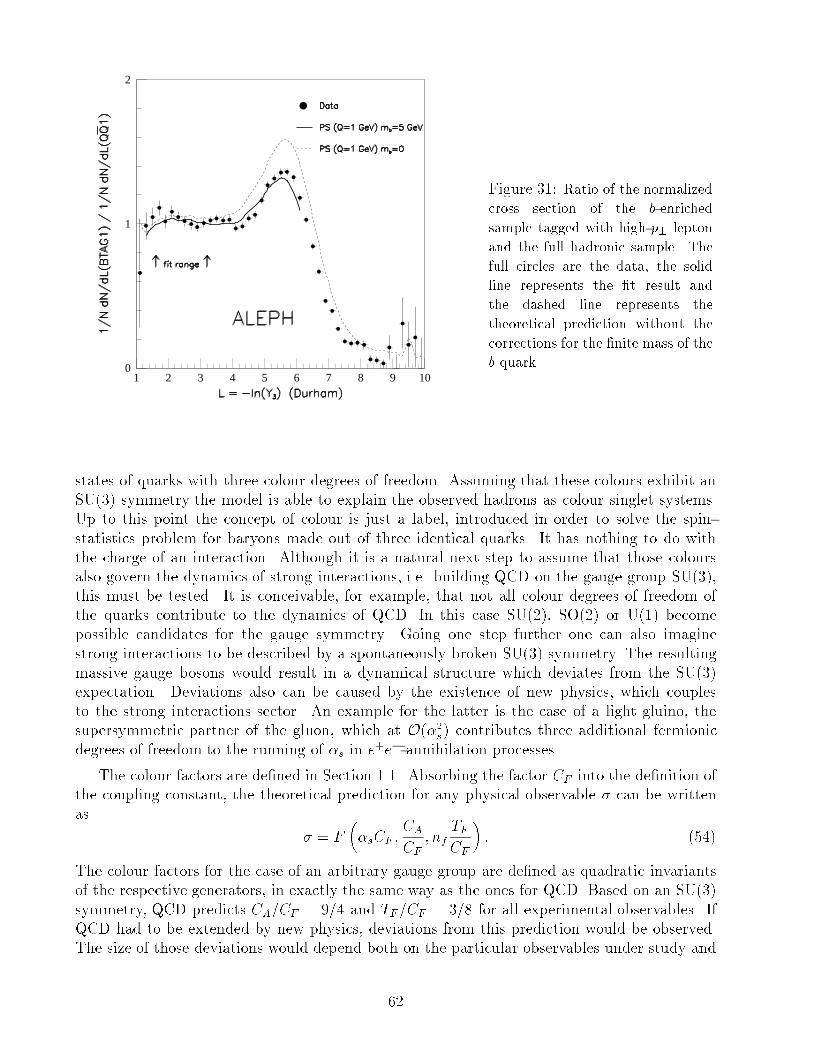
0

1

2

1 2 3 4 5 6 7 8 9 10

Figure 31: Ratio of the normalized

cross section of the b-enriched

sample tagged with high-p? lepton

and the full hadronic sample. The

full circles are the data, the solid

line represents the �t result and

the dashed line represents the

theoretical prediction without the

corrections for the �nite mass of the

b quark.

states of quarks with three colour degrees of freedom. Assuming that these colours exhibit an

SU(3) symmetry the model is able to explain the observed hadrons as colour singlet systems.

Up to this point the concept of colour is just a label, introduced in order to solve the spin-

statistics problem for baryons made out of three identical quarks. It has nothing to do with

the charge of an interaction. Although it is a natural next step to assume that those colours

also govern the dynamics of strong interactions, i.e. building QCD on the gauge group SU(3),

this must be tested. It is conceivable, for example, that not all colour degrees of freedom of

the quarks contribute to the dynamics of QCD. In this case SU(2), SO(2) or U(1) become

possible candidates for the gauge symmetry. Going one step further one can also imagine

strong interactions to be described by a spontaneously broken SU(3) symmetry. The resulting

massive gauge bosons would result in a dynamical structure which deviates from the SU(3)

expectation. Deviations also can be caused by the existence of new physics, which couples

to the strong interactions sector. An example for the latter is the case of a light gluino, the

supersymmetric partner of the gluon, which at O(�2s) contributes three additional fermionic

degrees of freedom to the running of �s in e+e�-annihilation processes.

The colour factors are de�ned in Section 1.1. Absorbing the factor CF into the de�nition of

the coupling constant, the theoretical prediction for any physical observable � can be written

as

� = F

��sCF ;

CA

CF

; nfTF

CF

�: (54)

The colour factors for the case of an arbitrary gauge group are de�ned as quadratic invariants

of the respective generators, in exactly the same way as the ones for QCD. Based on an SU(3)

symmetry, QCD predicts CA=CF = 9=4 and TF=CF = 3=8 for all experimental observables. If

QCD had to be extended by new physics, deviations from this prediction would be observed.

The size of those deviations would depend both on the particular observables under study and

62

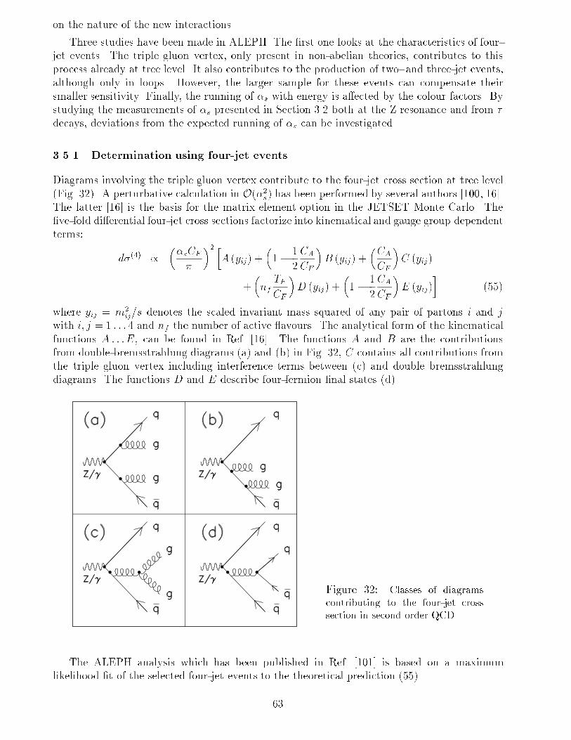
on the nature of the new interactions.

Three studies have been made in ALEPH. The �rst one looks at the characteristics of four-

jet events. The triple gluon vertex, only present in non-abelian theories, contributes to this

process already at tree level. It also contributes to the production of two- and three-jet events,

although only in loops. However, the larger sample for these events can compensate their

smaller sensitivity. Finally, the running of �s with energy is a�ected by the colour factors. By

studying the measurements of �s presented in Section 3.2 both at the Z resonance and from �

decays, deviations from the expected running of �s can be investigated.

3.5.1 Determination using four-jet events

Diagrams involving the triple gluon vertex contribute to the four-jet cross section at tree level

(Fig. 32). A perturbative calculation in O(�2s) has been performed by several authors [100, 16].

The latter [16] is the basis for the matrix element option in the JETSET Monte Carlo. The

�ve-fold di�erential four-jet cross sections factorize into kinematical and gauge group dependent

terms:

d�(4) /��sCF

�

�2 �A (yij) +

�1� 1

2

CA

CF

�B (yij) +

�CA

CF

�C (yij)

+

�nfTF

CF

�D (yij) +

�1 � 1

2

CA

CF

�E (yij)

�(55)

where yij = m2ij=s denotes the scaled invariant mass squared of any pair of partons i and j

with i; j = 1 : : : 4 and nf the number of active avours. The analytical form of the kinematical

functions A : : :E, can be found in Ref. [16]. The functions A and B are the contributions

from double-bremsstrahlung diagrams (a) and (b) in Fig. 32, C contains all contributions from

the triple gluon vertex including interference terms between (c) and double bremsstrahlung

diagrams. The functions D and E describe four-fermion �nal states (d).

Figure 32: Classes of diagrams

contributing to the four-jet cross

section in second order QCD.

The ALEPH analysis which has been published in Ref. [101] is based on a maximum

likelihood �t of the selected four-jet events to the theoretical prediction (55).

63

Using the PTCLUS clustering algorithm [102] for charged and neutral particles, 4148 four-

jet events were found in the 1989 and 1990 data samples for which the minimal scaled invariant

mass squared of all pairs of clusters i and j ful�lled min(yij) > ycut = 0:03. Using jets

reconstructed with the PTCLUS algorithm, this value for ycut was found to result in the best

compromise between high statistics and small hadronization corrections resulting from a clean

separation of the four jets. In addition the angle to the beam axis for each jet is required

to be above 20 degrees, the number of charged tracks or neutrals per jet at least two and

the sum of the six scaled invariant masses squared above 0.95. Finally, before comparison to

the theoretical prediction, the yij are rescaled such that the sum becomes unity, i.e. to ful�l

momentum conservation for four massless partons.

The colour factors are determined from the data by a maximum likelihood �t of the second

order theoretical prediction, i.e. by maximizing

lnL =Xi

ln�i(CA=CF ; TF=CF )

�tot(CA=CF ; TF=CF )(56)

with respect to CA=CF and TF=CF . The sum runs over all selected four-jet events. For each

event �i denotes the folded four-jet cross section obtained by summing over all permutations of

parton-type assignments to the jets, thereby taking into account that no identi�cation is made

of parton type or quark avour, and �tot is the corresponding total cross section. The ratio

�i=�tot is the probability density to observe the given set of �ve kinematical variables yjk in a

particular event i as function of the colour factors.

After the �t the results were corrected for detector resolution and fragmentation e�ects.

The corrections were determined from the Lund matrix element model, where the shifts

between parton level and �nal measurements were mapped as function of the colour factors by

reweighting a set of Monte Carlo events that were passed through the full detector simulation

and analysis chain.

The �nal result is

CA=CF = 2:24 � 0:32stat � 0:25syst

TF=CF = 0:58 � 0:17stat � 0:21syst :

The systematic error comes mainly from fragmentation uncertainties and unknown higher order

corrections, estimated from the JETSET model. The result is shown in Fig. 33 in the two-

dimensional plot of TF=CF versus CA=CF including its 68% con�dence level contour. The

result is in agreement with QCD. Any Abelian theory (CA = 0) is ruled out with more than

�ve standard deviations.

3.5.2 Determination using two- and three-jet events

The di�erential cross section for three jet production can be expressed in terms of normalized

momenta xi = 2pi=ps. The leading order matrix element is given by Eq. (16). In second order

QCD, the colour factor ratios TF=CF and CA=CF contribute to three-parton �nal states via loop

corrections. The corresponding negative divergences are cancelled by adding infrared divergent

four-parton �nal states with small invariant masses. The contributions both from three-parton

�nal states and four-parton �nal states were calculated using the program EVENT, which is the

numerical basis of [59] and is derived from the ERT matrix elements [16]. Since no jet tagging

was done, the xi variables are ordered, x1 � x2 � x3. Taking x1 and x2 as the independent

64

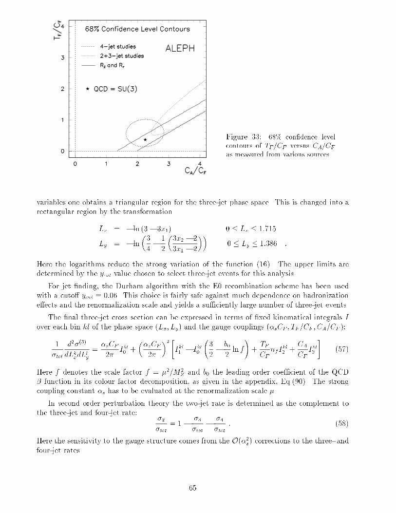
Figure 33: 68% con�dence level

contours of TF =CF versus CA=CF

as measured from various sources.

variables one obtains a triangular region for the three-jet phase space. This is changed into a

rectangular region by the transformation

Lx = � ln (3 � 3x1) 0 � Lx � 1:715

Ly = � ln

�3

4� 1

2

�3x2 � 2

3x1 � 2

��0 � Ly � 1:386 :

Here the logarithms reduce the strong variation of the function (16). The upper limits are

determined by the ycut value chosen to select three-jet events for this analysis.

For jet �nding, the Durham algorithm with the E0 recombination scheme has been used

with a cuto� ycut = 0:06. This choice is fairly safe against much dependence on hadronization

e�ects and the renormalization scale and yields a su�ciently large number of three-jet events.

The �nal three-jet cross section can be expressed in terms of �xed kinematical integrals I

over each bin kl of the phase space (Lx; Ly) and the gauge couplings (�sCF ; TF=CF ; CA=CF ):

1

�tot

d2�(3)

dLkxdLly

=�sCF

2�Ikl0 +

��sCF

2�

�2 "Ikl1 � Ikl0

3

2� b0

2ln f

!+TF

CF

nfIkl2 +

CA

CF

Ikl3

#(57)

Here f denotes the scale factor f = �2=M2Z and b0 the leading order coe�cient of the QCD

� function in its colour factor decomposition, as given in the appendix, Eq.(90). The strong

coupling constant �s has to be evaluated at the renormalization scale �.

In second order perturbation theory the two-jet rate is determined as the complement to

the three-jet and four-jet rate:�2

�tot= 1� �3

�tot� �4

�tot: (58)

Here the sensitivity to the gauge structure comes from the O(�2s) corrections to the three- andfour-jet rates.

65

Data analysis and results

From the 1992 data, 614478 hadronic events have been selected using charged tracks and neutral

objects from the energy ow analysis. The event and charged track selection used the standard

criteria. For the �nal event selection, the total visible energy Evis was required to be in excess

of 0:5ps and the momentum imbalance of all accepted tracks and objects along the beam

direction smaller than 40% of the visible energy.

Furthermore, cuts on jet reconstruction quality have been applied. The angle between the

jet axis and the beam axis must lie between 20 and 160 degrees. There must be at least two

tracks or neutral objects in a jet. The sum of the normalized invariant masses yij must be

greater than 0.95. These cuts yield a �nal sample of 111041 three-jet events and a two-jet

rate of �2=�tot = 0:801. In order to compare the data jets with ideal three-parton events, the

normalized invariant masses yij are scaled to ful�lP

ij yij = 1.

For the �t procedure, the theoretical prediction Eq.(57) is transformed to detector level

using the Monte Carlo probabilities for a three-parton event in bin kl at parton level to migrate

to bin ij at detector level. The background from genuine two- and four-parton events which

enter the three-jet sample is added. The measured two-jet rate is corrected to parton level and

compared to the prediction Eq.(58).

The systematic uncertainties of this analysis were determined by varying the renormalization

scale over the range MZ=2 < � < 2MZ and by changing the jet quality cuts such that

the accepted three-jet rate varies by 10%. In addition, the sensitivity to two- and four-jet

background in the three-jet sample and the uncertainties in the hadronization corrections were

studied by using the HERWIG 5.4 and the ARIADNE 4.4 models instead of the JETSET 7.3

parton shower model. An estimate of the importance of higher order corrections was obtained by

using the JETSET 7.3 parton shower model with the parton level de�ned by the four partons

with the highest virtuality, thus e�ectively removing the e�ect of branchings beyond those

allowed by an O(�2s) calculation. Finally, the systematic error associated with the kinematic

rescaling was taken to be the di�erence between the nominal scaling of the yij and the result

of the reconstruction of the kinematics when projecting all jets into the event plane.

The information from these systematic variations around the nominal analysis has been

converted into a covariance matrix for the systematic error:

Cij =nX

k=1

�(xi)k�(xj)k;

where �(xi)k is the change in xi 2 f�sCF ; TF=CF ; CA=CFg compared to the nominal analysis

under the systematic variation of k. For the �nal result the systematic covariance matrix thus

obtained was added to the covariance matrix of the statistical errors.

The dominant error for the combined result comes from hadronization, which contributes

roughly twice as much as the statistical error. Next largest is the error from the renormalization

scale variation (for the colour factors) and the error from kinematical rescaling (for �s CF ). The

errors arising from background and experimental cuts are comparatively small.

The combined measurements from two- and three-jet events yield the result:

�sCF = 0:210 � 0:016stat � 0:048systCA=CF = 4:49 � 0:75stat � 1:12systTF=CF = 2:01 � 0:49stat � 0:86syst ;

66

where the errors quoted are the statistical and the systematic uncertainties. The results are

highly correlated, with correlation coe�cients �(�sCF ; TF=CF ) = 0:761, �(�sCF ; CA=CF ) =

0:539 and �(CA=CF ; TF=CF ) = 0:956. From the total uncertainties the �2 probability of the

SU(3) expectation for nf = 5 is 52%. The result is shown in Fig. 33. Abelian groups with

CA = 0 and TF > 0 are only consistent with the measurement at a con�dence level below

2 � 10�6.

3.5.3 Information from the running of �s

ALEPH measurements of the strong coupling constant �s both on the Z resonance and from

� decays have been presented in Section 3.2. The consistency of these measurements with the

running expected from QCD over this large energy range provides a powerful constraint on the

dynamical structure of the theory of strong interactions.

The running of the strong coupling constant is a function of the gauge structure of the

theory of strong interactions and thus allows constraints to be placed on the colour factor

ratios. However, a consistent analysis cannot be based directly on available measurements

of �s, because those usually are determined under the assumption that QCD is based on an

SU(3) symmetry. To probe the gauge structure itself, thus also requires a reevaluation of �s at

di�erent energy scales. For many of the rather involved measurements of the strong coupling

constant this is not easily achieved. Exceptions are the measurements of �s from Rl and R� .

These are conceptually very simple and span a very large energy range.

The theoretical predictions for Rl and R� for arbitrary gauge groups are described in

Appendix A. In this evaluation the evolution equations for the coupling constant and quark

masses were integrated numerically. This ensures that all terms are retained which in principle

are known.

The analysis was performed as follows: For a given set of colour factor ratios (x; y) the

strong coupling constant a � a(MZ) = (�s(MZ)CF )=(2�) was determined by minimizing

�2exp =(Rl

obs �Rl(a; x; y))2

�2(Rl)+(R�

obs �R� (a; x; y))2

�2(R� )

with respect to a. Here the errors �(Rl) and �(R� ) are the purely experimental errors of the

two measurements, i.e. the value of a is determined independently of all assumptions about the

theoretical uncertainties and the �2 has a well de�ned statistical meaning. In a second step,

the theoretical uncertainties are taken into account. Now a is kept �xed at the �tted value and

a covariance matrix is determined for the theoretical uncertainties of Rl and R� .

The theoretical prediction depends on a set of n independent parameters pk with

uncertainties �pk. The resulting covariance matrix for Rl and R� then is given by

Cij(R) =nX

k=1

�(Ri)k�(Rj)k;

where �(Ri)k is the change in Ri when varying the parameter pk by �pk.

The relevant parameters and their uncertainties are listed in Table 21. For the quark masses

the MS running masses are related to the pole masses by Eq.(93) in Appendix A. Following [103]

the pole mass can be identi�ed with the constituent mass of the quarks, which leads to the

values given in Table 21. The value for the mass of the top quark is taken from the direct

measurement [104]. For the determination of the theoretical error for Rl and R� the \light"

67

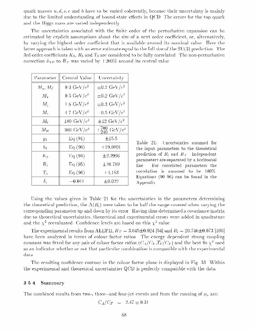
quark masses u; d; s; c and b have to be varied coherently, because their uncertainty is mainly

due to the limited understanding of bound-state e�ects in QCD. The errors for the top quark

and the Higgs mass are varied independently.

The uncertainties associated with the �nite order of the perturbative expansion can be

estimated by explicit assumptions about the size of a next order coe�cient, or, alternatively,

by varying the highest order coe�cient that is available around its nominal value. Here the

latter approach is taken with an error estimate equal to the full size of the SU(3) prediction. The

3rd order coe�cientsK3, R3 and T3 are considered to be fully correlated. The non-perturbative

correction �NP to R� was varied by �200% around its central value.

Parameter Central Value Uncertainty

Mu;Md 0.3 GeV/c2 �0:2 GeV/c2Ms 0.5 GeV/c2 �0:2 GeV/c2Mc 1.6 GeV/c2 �0:3 GeV/c2Mb 4.7 GeV/c2 �0:5 GeV/c2

Mt 180 GeV/c2 �12 GeV/c2

MH 300 GeV/c2 �700240 GeV/c2

g1 Eq.(91) �15:5b2 Eq.(90) �19:0801K3 Eq.(94) �2:2996R3 Eq.(95) �40:789T3 Eq.(96) �4:183�c �0:011 �0:022

Table 21: Uncertainties assumed for

the input parameters to the theoretical

prediction of Rl and R� . Independent

parameters are separated by a horizontal

line. For correlated parameters the

correlation is assumed to be 100%.

Equations (90{96) can be found in the

Appendix.

Using the values given in Table 21 for the uncertainties in the parameters determining

the theoretical prediction, the �(Ri) were taken to be half the range covered when varying the

corresponding parameter up and down by its error. Having thus determined a covariance matrix

due to theoretical uncertainties, theoretical and experimental errors were added in quadrature

and the �2 reevaluated. Con�dence levels are based on this �2 value.

The experimental results fromALEPH,R� = 3:645�0:024 [54] andRl = 20:746�0:073 [106]have been analyzed in terms of colour factor ratios. The energy dependent strong coupling

constant was �tted for any pair of colour factor ratios (CA=CF ,TF=CF ) and the best �t �2 used

as an indicator whether or not that particular combination is compatible with the experimental

data.

The resulting con�dence contour in the colour factor plane is displayed in Fig. 33. Within

the experimental and theoretical uncertainties QCD is perfectly compatible with the data.

3.5.4 Summary

The combined results from two-, three- and four-jet events and from the running of �s are:

CA=CF = 2:47� 0:31

68

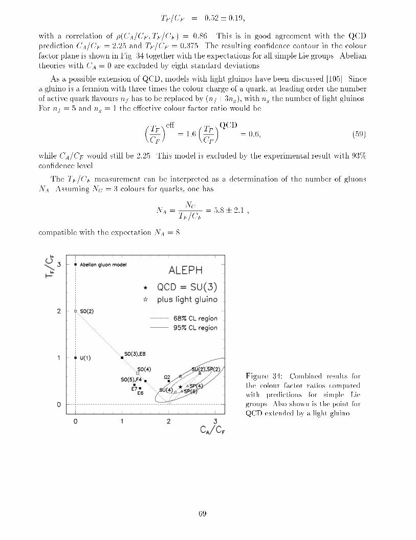
TF=CF = 0:52� 0:19;

with a correlation of �(CA=CF ; TF=CF ) = 0:86. This is in good agreement with the QCD

prediction CA=CF = 2:25 and TF=CF = 0:375. The resulting con�dence contour in the colour

factor plane is shown in Fig. 34 together with the expectations for all simple Lie groups. Abelian

theories with CA = 0 are excluded by eight standard deviations.

As a possible extension of QCD, models with light gluinos have been discussed [105]. Since

a gluino is a fermion with three times the colour charge of a quark, at leading order the number

of active quark avours nf has to be replaced by (nf+3ng), with ng the number of light gluinos.

For nf = 5 and ng = 1 the e�ective colour factor ratio would be

�TF

CF

�e�= 1:6

�TF

CF

�QCD= 0:6; (59)

while CA=CF would still be 2:25. This model is excluded by the experimental result with 93%

con�dence level.

The TF=CF measurement can be interpreted as a determination of the number of gluons

NA. Assuming NC = 3 colours for quarks, one has

NA =NC

TF=CF

= 5:8� 2:1 ;

compatible with the expectation NA = 8.

Figure 34: Combined results for

the colour factor ratios compared

with predictions for simple Lie

groups. Also shown is the point for

QCD extended by a light gluino.

69

4 Semi-Soft QCD

In this section a number of quantities related to the so-called \semi-soft" regime of QCD are

investigated. The observables considered here are sensitive to multiple gluon radiation at low

energies and small emission angles. As a consequence, perturbative predictions typically contain

terms corresponding to logarithms of gluon energies or emission angles which are non-negligible

at every order of �s. Reliable predictions can be obtained by resumming such terms (so-called

\leading", \next-to-leading" logarithms, etc.) to all orders. This is the basis of the parton

shower approach introduced in Section 1.1. Various calculations, depending on what terms are

included, are abbreviated as LLA, NLLA, MLLA (modi�ed leading-log approximation), etc.

An additional common aspect of analyses considered in this section is that hadronization

plays a signi�cant role. The theoretical predictions for the observables here are thus less well

understood than those for so-called \hard" processes considered in the previous section, i.e.

those involving large momentum transfers. A variety of di�erent observables are considered,

each of which helps to build up a picture of the production of �nal state particles. For some

quantities, the perturbatively predicted features are easily recognized in the �nal state hadrons;

in others, such features are washed out by hadronization e�ects.

In Section 4.1, quantities are considered for which gluon interference e�ects are particularly

important. Section 4.2 presents measurements of the multiplicity distribution of charged

particles. An investigation of intermittency e�ects in multiplicity distributions in rapidity

space is presented in Section 4.3. In Section 4.4, the internal structure of quark and

gluon jets is investigated by clustering the particles within the jets into \subjets", and

in Section 4.5, measurements of charged particle distributions in quark and gluon jets are

presented. Section 4.6 contains an analysis of prompt photon production; this provides

information on the evolution of a parton cascade since the virtual mass of a quark decreases

by means of both gluon and photon radiation.

4.1 Coherence Phenomena

In this section measurements of particle distributions are described which are expected to be

sensitive to e�ects of QCD coherence (gluon interference). The measured quantities include the

inclusive single particle momentum distribution, the two-particle and multiplicity-multiplicity

correlation, and the three-particle energy-multiplicity-multiplicity correlation. In addition,

interjet coherence is studied using the particle and momentum ow between jets in three-jet

events. Various explanations for the observed e�ects are considered.

The existence of two phases in the description of hadron production, the �rst calculable with

perturbation theory and the second not, leads to a fundamental di�culty in investigations of

coherence e�ects. Often it is found that a quantum mechanical e�ect at the parton level can be

e�ectively parametrized in the hadronization stage. It is di�cult therefore to make conclusive

statements about the perturbative level. More important are the constraints placed on the

hadronization mechanism using the assumption that the parton level is given by perturbative

QCD. That is, one learns whether the hadronization is such that certain parton level e�ects

are washed out or not, and, as a result, one obtains information about the nature of parton

con�nement.

70

4.1.1 Inclusive Distribution of � lnxp

One of the simplest quantities sensitive to coherence is the single particle inclusive momentum

distribution. In order to examine the low momentum region more closely, one can transform to

the variable � = � lnxp, where xp = p=pbeam. As discussed in Section 1.1.2, an e�ect of gluon

interference at the parton level is the suppression of soft gluons, which is implemented in the

parton-shower approach by means of angular ordering [18]. In order to relate the parton-level

predictions for D(�) = (1=�tot)(d�=d�) to hadron-level measurements, some assumption about

the hadronization stage must be made. The simplest ansatz is the hypothesis of Local Parton-

Hadron Duality (LPHD) [86, 107]. This states that the perturbatively computed spectrum for

partons DQCD(�) should be directly proportional to the corresponding distribution for hadrons,

Dhad(�),

Dhad(�) = khadDQCD(�) ; (60)

where the constant khad must be determined by comparing the prediction to experimental data.

More detailed treatments of hadronization and particle decays are provided by Monte Carlo

models, such as JETSET, HERWIG and ARIADNE (see Section 2.3.1), all of which also include

angular ordering of parton emissions.

The analysis presented here is based on charged particles without particle identi�cation.

The inclusive charged particle spectrum Dch(�) = (1=�tot)(d�=d�) was measured using the

same data (571800 events) and analysis technique as for the distributions given in Section 2

(see also Section 1.3.1). Corrections for detector e�ects were made using bin-by-bin correction

factors as described in Section 1.3.2. Systematic uncertainties were estimated by variation

of the experimental cuts, which leads to errors in the central region (2:4 < � < 4:8) of the

distribution of around 0.2 { 0.5%. In addition, the model dependence of the correction factors

was investigated by means of simpli�ed correction factors as described in Section 1.3.2 using

the models JETSET, HERWIG and ARIADNE. This leads to systematic errors of 0.3 { 1.0%

in the central region.

The measured � distribution is given in Table 22 and is shown in Fig. 35 along with the

predictions of the models JETSET version 7.4, HERWIG version 5.8 and ARIADNE version

4.08. The important parameters of these models have been tuned to ALEPH data as described

in Section 2.3. The data and model predictions are seen to be in qualitatively good agreement,

although the data lie signi�cantly above the predicted values at high values of � (low momenta).

The � distribution can be compared directly to the perturbative QCD prediction by

invoking the LPHD relation (60). At the parton level, the inclusive gluon distribution

DMLLA(�;Ecm;�; Q0) has been computed [86] using the modi�ed leading-log approximation

(MLLA), which includes the e�ects of angular ordering. The MLLA prediction contains in

principle three parameters: the centre of mass energy Ecm, the QCD scale parameter, �, and

a virtuality cuto�, Q0. The minimum parton virtuality Q0 de�nes the boundary between

the perturbative and non-perturbative phases. One would like Q0 to be large enough so

that the strong coupling constant �s(Q20) is small, implying ln(Q0=�) > 1. Evaluation of

DMLLA(�;Ecm;�; Q0) turns out to be computationally di�cult except for the special case Q0 =

�, the so-called limiting spectrum. It has been argued [86], however, that DMLLA(�;Ecm;�; Q0)

should change very little when Q0 is decreased from � � e to � (i.e. ln(Q0=�) decreasing from 1

to 0) so that one expects that the limiting spectrum, with which the data are compared here,

gives a reasonable approximation for the parton level.

71

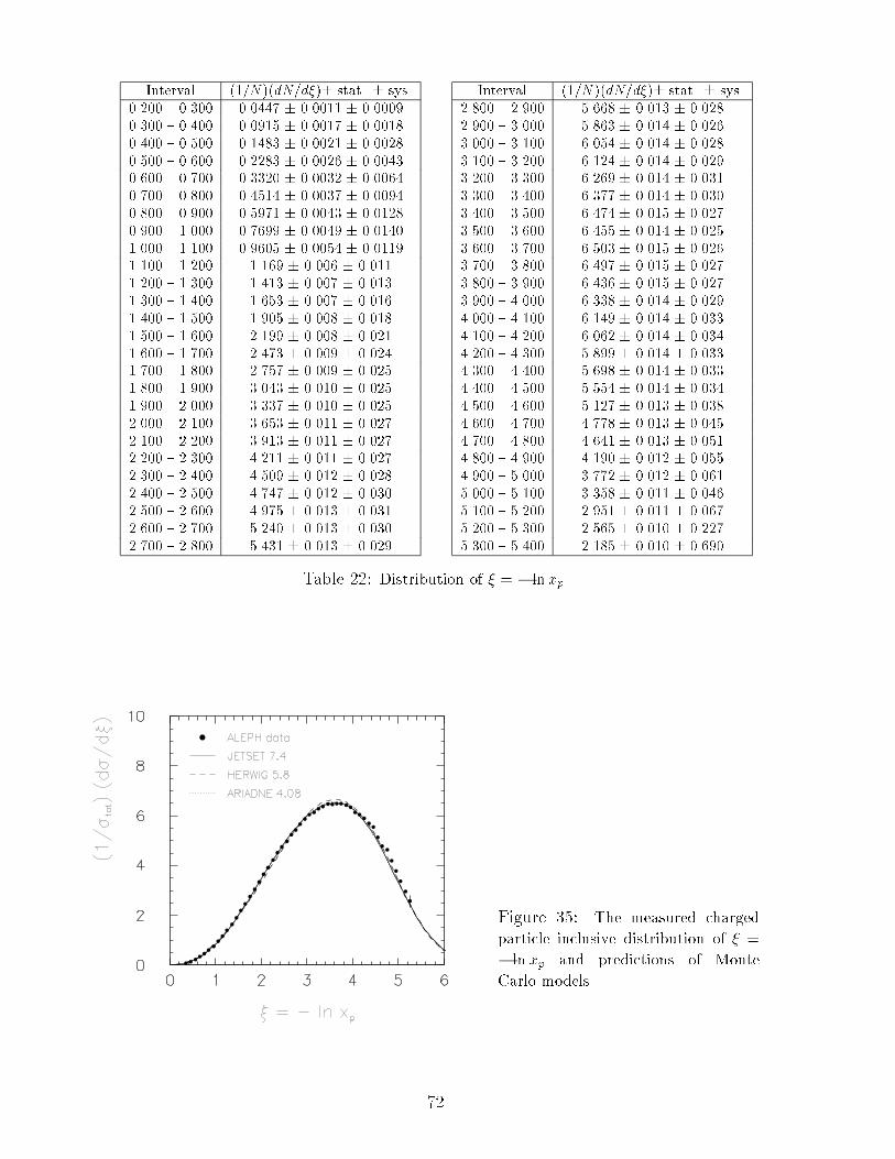
Interval (1=N )(dN=d�)� stat. � sys.

0.200 { 0.300 0.0447 � 0.0011 � 0.0009

0.300 { 0.400 0.0915 � 0.0017 � 0.0018

0.400 { 0.500 0.1483 � 0.0021 � 0.0028

0.500 { 0.600 0.2283 � 0.0026 � 0.0043

0.600 { 0.700 0.3320 � 0.0032 � 0.0064

0.700 { 0.800 0.4514 � 0.0037 � 0.0094

0.800 { 0.900 0.5971 � 0.0043 � 0.0128

0.900 { 1.000 0.7699 � 0.0049 � 0.0140

1.000 { 1.100 0.9605 � 0.0054 � 0.0119

1.100 { 1.200 1.169 � 0.006 � 0.011

1.200 { 1.300 1.413 � 0.007 � 0.013

1.300 { 1.400 1.653 � 0.007 � 0.016

1.400 { 1.500 1.905 � 0.008 � 0.018

1.500 { 1.600 2.199 � 0.008 � 0.021

1.600 { 1.700 2.473 � 0.009 � 0.024

1.700 { 1.800 2.757 � 0.009 � 0.025

1.800 { 1.900 3.043 � 0.010 � 0.025

1.900 { 2.000 3.337 � 0.010 � 0.025

2.000 { 2.100 3.653 � 0.011 � 0.027

2.100 { 2.200 3.913 � 0.011 � 0.027

2.200 { 2.300 4.211 � 0.011 � 0.027

2.300 { 2.400 4.509 � 0.012 � 0.028

2.400 { 2.500 4.747 � 0.012 � 0.030

2.500 { 2.600 4.975 � 0.013 � 0.031

2.600 { 2.700 5.240 � 0.013 � 0.030

2.700 { 2.800 5.431 � 0.013 � 0.029

Interval (1=N )(dN=d�)� stat. � sys.

2.800 { 2.900 5.668 � 0.013 � 0.028

2.900 { 3.000 5.863 � 0.014 � 0.026

3.000 { 3.100 6.054 � 0.014 � 0.028

3.100 { 3.200 6.124 � 0.014 � 0.029

3.200 { 3.300 6.269 � 0.014 � 0.031

3.300 { 3.400 6.377 � 0.014 � 0.030

3.400 { 3.500 6.474 � 0.015 � 0.027

3.500 { 3.600 6.455 � 0.014 � 0.025

3.600 { 3.700 6.503 � 0.015 � 0.026

3.700 { 3.800 6.497 � 0.015 � 0.027

3.800 { 3.900 6.436 � 0.015 � 0.027

3.900 { 4.000 6.338 � 0.014 � 0.029

4.000 { 4.100 6.149 � 0.014 � 0.033

4.100 { 4.200 6.062 � 0.014 � 0.034

4.200 { 4.300 5.899 � 0.014 � 0.033

4.300 { 4.400 5.698 � 0.014 � 0.033

4.400 { 4.500 5.554 � 0.014 � 0.034

4.500 { 4.600 5.127 � 0.013 � 0.038

4.600 { 4.700 4.778 � 0.013 � 0.045

4.700 { 4.800 4.641 � 0.013 � 0.051

4.800 { 4.900 4.190 � 0.012 � 0.055

4.900 { 5.000 3.772 � 0.012 � 0.061

5.000 { 5.100 3.358 � 0.011 � 0.046

5.100 { 5.200 2.951 � 0.011 � 0.067

5.200 { 5.300 2.565 � 0.010 � 0.227

5.300 { 5.400 2.185 � 0.010 � 0.690

Table 22: Distribution of � = � ln xp.

Figure 35: The measured charged

particle inclusive distribution of � =

� ln xp and predictions of Monte

Carlo models.

72

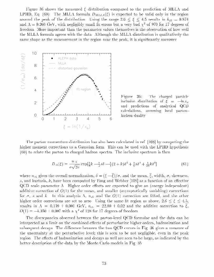
Figure 36 shows the measured � distribution compared to the prediction of MLLA and

LPHD, Eq. (60). The MLLA formula DMLLA(�) is expected to be valid only in the region

around the peak of the distribution. Using the range 2:6 � � � 4:5 results in kch = 0:874

and � = 0:266 GeV, with negligibly small �t errors but a very bad �2 of 970 for 17 degrees of

freedom. More important than the parameter values themselves is the observation of how well

the MLLA formula agrees with the data. Although the MLLA distribution is qualitatively the

same shape as the measurement in the region near the peak, it is signi�cantly narrower.

Figure 36: The charged particle

inclusive distribution of � = � ln xpand predictions of analytical QCD

calculations, assuming local parton-

hadron duality.

The parton momentum distribution has also been calculated in ref. [108] by computing the

higher moment corrections to a Gaussian form. This can be used with the LPHD hypothesis

(60) to relate the parton to charged hadron spectra. The inclusive spectrum is then

Dch(�) =nch

�p2�

exp[18k � 12s� � 1

4(2 + k)�2 + 16s�

3 + 124k�

4] (61)

where nch gives the overall normalization, � = (� � �)=�, and the mean, �, width, �, skewness,

s, and kurtosis, k, have been computed by Fong and Webber [108] as a function of an e�ective

QCD scale parameter �. Higher order e�ects are expected to give an (energy independent)

additive correction of O(1) for the mean, and smaller (asymptotically vanishing) corrections

for �, s and k. In this analysis �, nch and the O(1) correction are �tted, and the other

higher order corrections are set to zero. Using the same �t region as above, 2:6 � � � 4:5,

results in � = 0:139 � 0:001 GeV, nch = 22:80 � 0:02 and the additive correction to �,

O(1) = �1:350 � 0:007 with a �2 of 128 for 17 degrees of freedom.

The discrepancies observed between the parton-level QCD formulae and the data can be

interpreted as a limit on the combined e�ects of perturbative higher orders, hadronization and

subsequent decays. The di�erence between the two QCD curves in Fig. 36 gives a measure of

the uncertainty at the perturbative level; this is seen to be not negligible, even in the peak

region. The e�ects of hadronization and decays as well are seen to be large, as indicated by the

better description of the data by the Monte Carlo models in Fig. 35.

73

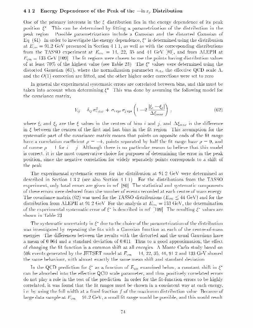
4.1.2 Energy Dependence of the Peak of the � lnxp Distribution

One of the primary interests in the � distribution lies in the energy dependence of its peak

position ��. This can be determined by �tting a parametrization of the distribution in the

peak region. Possible parametrizations include a Gaussian and the distorted Gaussian of

Eq. (61). In order to investigate the energy dependence, �� is determined using the distribution

at Ecm = 91:2 GeV presented in Section 4.1.1, as well as with the corresponding distributions

from the TASSO experiment at Ecm = 14, 22, 35 and 44 GeV [80], and from ALEPH at

Ecm = 133 GeV [109]. The �t regions were chosen to use the points having distribution values

of at least 70% of the highest value (see Table 23). The �� values were determined using the

distorted Gaussian (61), where the normalization parameter nch, the e�ective QCD scale �,

and the O(1) correction are �tted, and the other higher order corrections were set to zero.

In general the experimental systematic errors are correlated between bins, and this must be

taken into account when determining ��. This was done by assuming the following model for

the covariance matrix,

Vij = �ij �2i stat + �i sys �j sys

1� 2

j�i � �j j��max

!; (62)

where �i and �j are the � values in the centres of bins i and j, and ��max is the di�erence

in � between the centres of the �rst and last bins in the �t region. This assumption for the

systematic part of the covariance matrix means that points on opposite ends of the �t range

have a correlation coe�cient � = �1, points separated by half the �t range have � = 0, and

of course � = 1 for i = j. Although there is no particular reason to believe that this model

is correct, it is the most conservative choice for purposes of determining the error in the peak

position, since the negative correlation for widely separately points corresponds to a shift of

the peak.

The experimental systematic errors for the distribution at 91.2 GeV were determined as

described in Section 1.3.2 (see also Section 4.1.1). For the distributions from the TASSO

experiment, only total errors are given in ref. [80]. The statistical and systematic components

of these errors were deduced from the number of events recorded at each centre of mass energy.

The covariance matrix (62) was used for the TASSO distributions (Ecm � 44 GeV) and for the

distribution from ALEPH at 91.2 GeV. For the analysis at Ecm = 133 GeV, the determination

of the experimental systematic error of �� is described in ref. [109]. The resulting �� values areshown in Table 23.

The systematic uncertainty in �� due to the choice of the parametrization of the distribution

was investigated by repeating the �ts with a Gaussian function at each of the centre-of-mass

energies. The di�erences between the results with the distorted and the usual Gaussians have

a mean of 0.064 and a standard deviation of 0.011. Thus to a good approximation, the e�ect

of changing the �t function is a common shift at all energies. A Monte Carlo study based on

50k events generated by the JETSET model at Ecm = 14, 22, 35, 44, 91.2 and 133 GeV showed

the same behaviour, with almost exactly the same mean shift and standard deviation.

In the QCD prediction for �� as a function of Ecm examined below, a constant shift in ��

can be absorbed into the e�ective QCD scale parameter, and thus positively correlated errors

do not play a role in the test of the prediction. In order for the �t-function errors to be highly

correlated, it was found that the �t ranges must be chosen in a consistent way at each energy,

i.e. by using the full width at a �xed fraction f of the maximum distribution value. Because of

large data sample at Ecm = 91:2 GeV, a small �t range would be possible, and this would result

74

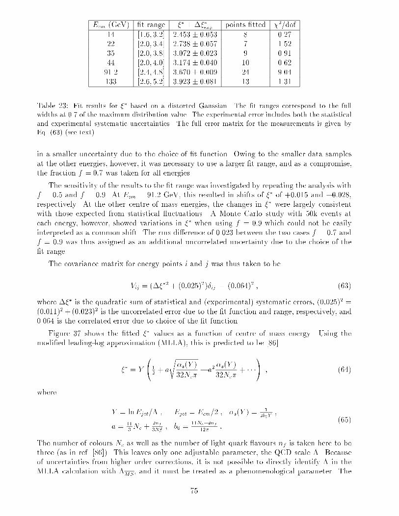
Ecm (GeV) �t range �� ����exp points �tted �2=dof

14 [1:6; 3:2] 2:453 � 0:053 8 0.27

22 [2:0; 3:4] 2:738 � 0:057 7 1.52

35 [2:0; 3:8] 3:072 � 0:023 9 0.91

44 [2:0; 4:0] 3:174 � 0:040 10 0.62

91.2 [2:4; 4:8] 3:670 � 0:009 24 9.04

133 [2:6; 5:2] 3:923 � 0:081 13 1.31

Table 23: Fit results for �� based on a distorted Gaussian. The �t ranges correspond to the full

widths at 0.7 of the maximum distribution value. The experimental error includes both the statistical

and experimental systematic uncertainties. The full error matrix for the measurements is given by

Eq. (63) (see text).

in a smaller uncertainty due to the choice of �t function. Owing to the smaller data samples

at the other energies, however, it was necessary to use a larger �t range, and as a compromise,

the fraction f = 0:7 was taken for all energies.

The sensitivity of the results to the �t range was investigated by repeating the analysis with

f = 0:5 and f = 0:9. At Ecm = 91:2 GeV, this resulted in shifts of �� of +0:015 and �0:028,respectively. At the other centre of mass energies, the changes in �� were largely consistent

with those expected from statistical uctuations. A Monte Carlo study with 50k events at

each energy, however, showed variations in �� when using f = 0:9 which could not be easily

interpreted as a common shift. The rms di�erence of 0.023 between the two cases f = 0:7 and

f = 0:9 was thus assigned as an additional uncorrelated uncertainty due to the choice of the

�t range.

The covariance matrix for energy points i and j was thus taken to be

Vij = (���2 + (0:025)2)�ij + (0:064)2 ; (63)

where ��� is the quadratic sum of statistical and (experimental) systematic errors, (0:025)2 =

(0:011)2+(0:023)2 is the uncorrelated error due to the �t function and range, respectively, and

0.064 is the correlated error due to choice of the �t function.

Figure 37 shows the �tted �� values as a function of centre of mass energy. Using the

modi�ed leading-log approximation (MLLA), this is predicted to be [86]

�� = Y

0@12 + a

s�s(Y )

32Nc�� a2

�s(Y )

32Nc�+ � � �

1A ; (64)

where

Y = lnEjet=� ; Ejet = Ecm=2 ; �s(Y ) =1

2b0Y;

a = 113Nc +

2nf3N2

c; b0 =

11Nc�2nf12�

:(65)

The number of colours Nc as well as the number of light quark avours nf is taken here to be

three (as in ref. [86]). This leaves only one adjustable parameter, the QCD scale �. Because

of uncertainties from higher order corrections, it is not possible to directly identify � in the

MLLA calculation with �MS, and it must be treated as a phenomenological parameter. The

75

two quantities are nevertheless expected to be of approximately the same magnitude. The �rst

term in (64), 12Y , is the leading order prediction (Double Logarithmic Approximation, DLA).

In the formula (64) for �� versus Ecm, a constant shift in �� can be absorbed (to leading

order) into the e�ective QCD scale parameter �. Therefore the correlated uncertainty of 0.064 is

not important in the comparison of the data with the QCD curves, and only the uncorrelated

components of the errors are shown. The MLLA curve gives �2 = 1:3 and the DLA curve

�2 = 31:0 for 5 degrees of freedom.

Equation (64) takes no account of quark avour or mass e�ects. Monte Carlo studies show,

however, that the �� values are sensitive to the event avour, and furthermore the mixture of

avours varies as a function of the centre-of-mass energy. By comparing the �� values predictedfor the Standard Model mixture of avours to that of light quarks only, a correction factor for

the avour dependence can be derived and applied to Eq. (64) as ��corr = �� � C(Ecm). This

was done by determining the ratio C = ��(all avours)=��(uu only) using the JETSET model

at several points in the energy range 12 GeV < Ecm < 180 GeV, which was then parametrized

by a function C(Ecm) = a + b exp(�Ecm=c), with a = 0:976, b = 0:0612, and c = 31:3 GeV.

This correction decreases from 1.02 to 0.99 in the energy region between 14 and 44 GeV, and

is almost constant for Ecm > 44 GeV.

When this is applied to the QCD predictions, the quality of the �t becomes somewhat worse,

with �2 = 62:0 for DLA and �2 = 10:6 for MLLA for �ve degrees of freedom. The general

picture remains that the higher order e�ects included in the MLLA improve the description of

the data. The very good �2 value from the MLLA without avour correction, however, must

be partially accidental. The �tted curves including the avour correction are shown in Fig. 37.

Fitted curves without the avour correction can be found in [109].

Figure 37: The peak position of

the � ln xp distribution, ��, as a

function of the centre of mass energy,

and the leading order (DLA) and

next-to-leading order (MLLA) QCD

predictions including a correction for

the energy dependence of the quark

avour mixture (see text). In addition

to the error bars shown, there is a

correlated uncertainty of 0.064 due to

the choice of �t function.

In determining the �� values in Table 23, the �t ranges were all determined by the full

width at f = 0:7 of the maximum distribution value. This procedure was necessary in order

to have highly correlated errors due to the choice of �t function, and led to a relatively large

�t range at 91.2 GeV (2:4 � � � 4:8). In order to compare with measurements from other

experiments, however, one can reduce the �t range at 91.2 GeV to give a smaller total error.

Using e.g. the full width at a fraction f = 0:9 of the maximum gives 2:9 < � < 4:3. This results

in �� = 3:642 with the distorted Gaussian and 3.610 with a Gaussian, i.e. a di�erence of 0.032.

Taking the distorted Gaussian for the best value, the di�erence with respect to the Gaussian

76

for the �t-function error, and the di�erence of 0.028 between �ts using f = 0:7 and f = 0:9 for

the �t-range error, one obtains

��(91.2 GeV) = 3:642 � 0:017 (exp.) � 0:032 (�t function) � 0:028(�t range)

= 3:642 � 0:046 :

This result is in agreement with the values reported by OPAL [110] of �� = 3:603 �0:013 (stat.) � 0:040 (sys.), and by L3 [111], �� = 3:71 � 0:01 (stat.) � 0:05 (sys.).

4.1.3 Particle-Particle Correlations

As �rst pointed out in [112], coherence e�ects related to angular ordering can be investigated

with the particle-particle correlation function, PPC. This is de�ned by considering two elements

of solid angle d~a and d~b, with an opening angle � = cos�1(~a � ~b). The function PPC(�) is

constructed as a measure of the probability to �nd a particle in both d~a and d~b. In terms of

the two-particle inclusive cross section, it is de�ned as

PPC(�) =

Z Z1

�

d�(e+e� ! a+ b+X)

d~ad~b

�(cos�1(~a � ~b)� �) d~ad~b ; (66)

which can be determined experimentally using charged particles as

hPPC(�)ibin k = 1

Nevents

Xevents

NchXi;j=1

1

N2ch

1

��

Zbin k

�(�ij � �0) d�0 : (67)

Here �ij is the angle between the particles i and j, the sum over i and j is made over all

pairs of Nch charged particles in an event, and is then averaged over all events. The quantity

PPC(�) is similar in construction to the energy-energy correlation EEC described in Section

3.2, with the di�erence that each pair of particles is weighted by wij = 1=N2ch, rather than by

the product of the particles' scaled energies, wij = EiEj=E2cm. Also in analogy with the EEC,

the particle-particle correlation asymmetry, PPCA(�), can be constructed as

PPCA(�) = PPC(� � �)� PPC(�) : (68)

A measurement of the PPCA based on charged particles was carried out with approximately

800000 hadronic events recorded by the ALEPH detector in 1992{93. The hadronic event

selection and correction procedure for detector e�ects were carried out as described in Sections

1.3.1 and 1.3.2, respectively. Systematic uncertainties were estimated by variation of the track

and event selection criteria. In addition, the model dependence of the correction factors was

estimated by constructing simpli�ed corrections with several models, as described in Section

1.3.2.

Figure 38(a) shows the measured PPCA as a function of the angle � along with the

predictions of several parton-shower based Monte Carlo models. The models are in good

agreement with the data, with the exception of NLLjet, for which a discrepancy is seen in

the region 10� < � < 40�. Figure 38(b) shows the data compared with the same models,

with the di�erence that the angular ordering in the parton shower has not been included. (For

HERWIG and ARIADNE this option is not possible.) The parameters of the models were

77

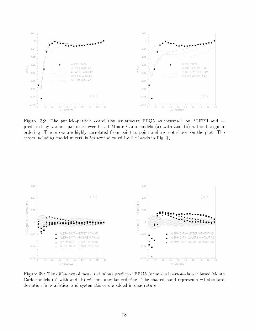
Figure 38: The particle-particle correlation asymmetry PPCA as measured by ALEPH and as

predicted by various parton-shower based Monte Carlo models (a) with and (b) without angular

ordering. The errors are highly correlated from point to point and are not shown on the plot. The

errors including model uncertainties are indicated by the bands in Fig. 39.

Figure 39: The di�erence of measured minus predicted PPCA for several parton-shower based Monte

Carlo models (a) with and (b) without angular ordering. The shaded band represents �1 standard

deviation for statistical and systematic errors added in quadrature.

78

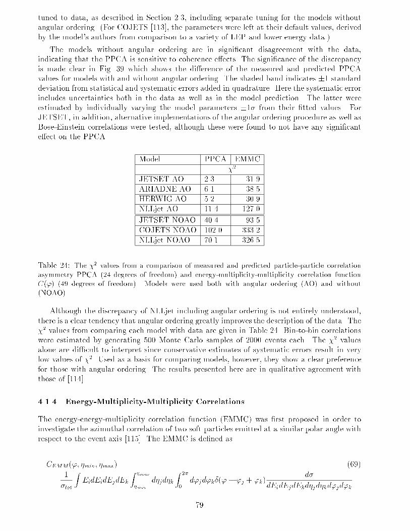
tuned to data, as described in Section 2.3, including separate tuning for the models without

angular ordering. (For COJETS [113], the parameters were left at their default values, derived

by the model's authors from comparison to a variety of LEP and lower energy data.)

The models without angular ordering are in signi�cant disagreement with the data,

indicating that the PPCA is sensitive to coherence e�ects. The signi�cance of the discrepancy

is made clear in Fig. 39 which shows the di�erence of the measured and predicted PPCA

values for models with and without angular ordering. The shaded band indicates �1 standarddeviation from statistical and systematic errors added in quadrature. Here the systematic error

includes uncertainties both in the data as well as in the model prediction. The latter were

estimated by individually varying the model parameters �1� from their �tted values. For

JETSET, in addition, alternative implementations of the angular ordering procedure as well as

Bose-Einstein correlations were tested, although these were found to not have any signi�cant

e�ect on the PPCA.

Model PPCA EMMC

�2

JETSET AO 2.3 31.9

ARIADNE AO 6.1 38.5

HERWIG AO 5.2 30.9

NLLjet AO 11.4 127.0

JETSET NOAO 40.4 93.5

COJETS NOAO 102.0 333.2

NLLjet NOAO 70.1 326.5

Table 24: The �2 values from a comparison of measured and predicted particle-particle correlation

asymmetry PPCA (24 degrees of freedom) and energy-multiplicity-multiplicity correlation function

C(') (49 degrees of freedom). Models were used both with angular ordering (AO) and without

(NOAO).

Although the discrepancy of NLLjet including angular ordering is not entirely understood,

there is a clear tendency that angular ordering greatly improves the description of the data. The

�2 values from comparing each model with data are given in Table 24. Bin-to-bin correlations

were estimated by generating 500 Monte Carlo samples of 2000 events each. The �2 values

alone are di�cult to interpret since conservative estimates of systematic errors result in very

low values of �2. Used as a basis for comparing models, however, they show a clear preference

for those with angular ordering. The results presented here are in qualitative agreement with

those of [114].

4.1.4 Energy-Multiplicity-Multiplicity Correlations

The energy-energy-multiplicity correlation function (EMMC) was �rst proposed in order to

investigate the azimuthal correlation of two soft particles emitted at a similar polar angle with

respect to the event axis [115]. The EMMC is de�ned as

CEMM('; �min; �max) = (69)

1

�tot

ZEidEidEjdEk

Z �max

�min

d�jd�k

Z 2�

0d'jd'k�('� 'j + 'k)

d�

dEidEjdEkd�jd�kd'jd'k

79

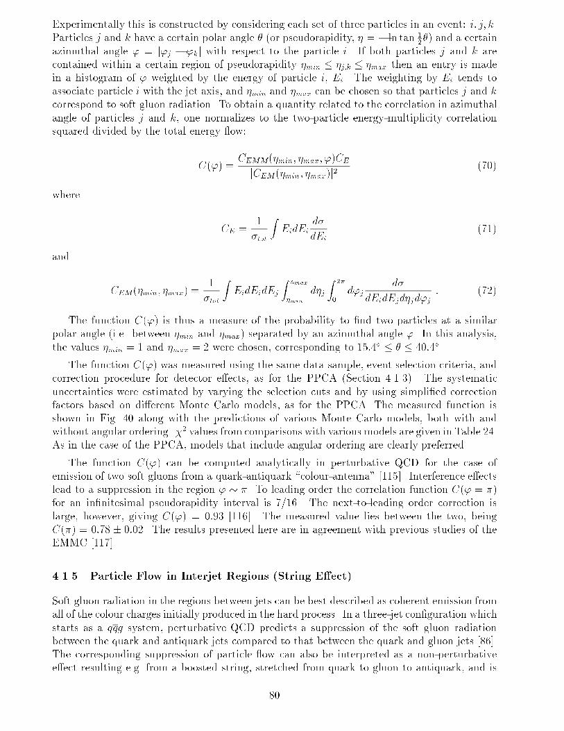
Experimentally this is constructed by considering each set of three particles in an event: i; j; k.

Particles j and k have a certain polar angle � (or pseudorapidity, � = � ln tan 12�) and a certain

azimuthal angle ' = j'j � 'kj with respect to the particle i. If both particles j and k are

contained within a certain region of pseudorapidity �min � �j;k � �max then an entry is made

in a histogram of ' weighted by the energy of particle i, Ei. The weighting by Ei tends to

associate particle i with the jet axis, and �min and �max can be chosen so that particles j and k

correspond to soft gluon radiation. To obtain a quantity related to the correlation in azimuthal

angle of particles j and k, one normalizes to the two-particle energy-multiplicity correlation

squared divided by the total energy ow:

C(') =CEMM(�min; �max; ')CE

jCEM(�min; �max)j2(70)

where

CE =1

�tot

ZEidEi

d�

dEi

(71)

and

CEM(�min; �max) =1

�tot

ZEidEidEj

Z �max

�min

d�j

Z 2�

0d'j

d�

dEidEjd�jd'j: (72)

The function C(') is thus a measure of the probability to �nd two particles at a similar

polar angle (i.e. between �min and �max) separated by an azimuthal angle '. In this analysis,

the values �min = 1 and �max = 2 were chosen, corresponding to 15:4� � � � 40:4�.

The function C(') was measured using the same data sample, event selection criteria, and

correction procedure for detector e�ects, as for the PPCA (Section 4.1.3). The systematic

uncertainties were estimated by varying the selection cuts and by using simpli�ed correction

factors based on di�erent Monte Carlo models, as for the PPCA. The measured function is

shown in Fig. 40 along with the predictions of various Monte Carlo models, both with and

without angular ordering. �2 values from comparisons with various models are given in Table 24.

As in the case of the PPCA, models that include angular ordering are clearly preferred.

The function C(') can be computed analytically in perturbative QCD for the case of

emission of two soft gluons from a quark-antiquark \colour-antenna" [115]. Interference e�ects

lead to a suppression in the region ' � �. To leading order the correlation function C(' = �)

for an in�nitesimal pseudorapidity interval is 7=16. The next-to-leading order correction is

large, however, giving C(') = 0:93 [116]. The measured value lies between the two, being

C(�) = 0:78 � 0:02. The results presented here are in agreement with previous studies of the

EMMC [117].

4.1.5 Particle Flow in Interjet Regions (String E�ect)

Soft gluon radiation in the regions between jets can be best described as coherent emission from

all of the colour charges initially produced in the hard process. In a three-jet con�guration which

starts as a qqg system, perturbative QCD predicts a suppression of the soft gluon radiation

between the quark and antiquark jets compared to that between the quark and gluon jets [86].

The corresponding suppression of particle ow can also be interpreted as a non-perturbative

e�ect resulting e.g. from a boosted string, stretched from quark to gluon to antiquark, and is

80

Figure 40: The energy-multiplicity-multiplicity correlation function C(') as measured by ALEPH

and as predicted by various parton-shower based Monte Carlo models (a) with and (b) without angular

ordering.

hence known as the string e�ect. This e�ect was �rst observed experimentally by the JADE

collaboration [118] and later by other experiments at PETRA, PEP and LEP [119].

In this analysis the string e�ect has been investigated by measuring the particle and

momentum ow in the interjet regions of three-jet events. Approximately 112000 three-

jet events were selected using the Durham clustering algorithm (see Section 2.1) with a jet

resolution parameter of ycut = 0:009. Both charged and neutral particles (energy- ow objects

as described in Section 1.2) were used in the analysis. In addition to the standard event selection

cuts described in Section 1.3.1, the angle between the normal vector to the event plane and the

beam direction was required to be less than 60� in order to ensure good particle acceptance in

the interjet regions.

The three jets were ordered according to their energies, E1 > E2 > E3, estimated from the

jet directions (projected onto the event plane) assuming energy and momentum conservation

for massless jets. QCD based Monte Carlo models such as JETSET predict that the lowest

energy jet is most frequently the gluon jet (70%) and the highest energy jet is most often a

quark (or antiquark) jet (94%). The angle in the event plane ' is de�ned to be zero for the

highest energy jet (jet 1) as shown in Fig. 41. The reduced angle '0 of a particle between jets

i and k is de�ned as

'0 ='� �i

�k � �i

;

where �i and �k are the jet angles. Interjet regions are de�ned as covering the central 40% of

the reduced angle between jets (0:3 < '0 < 0:7).

The particle distribution as a function of '0 (without detector corrections) is shown in

Fig. 42. Also shown is the prediction of the JETSET model including simulation of detector

e�ects; this is seen to describe the data quite well.

After correction for detector e�ects according to the bin-by-bin procedure described in

Section 1.3.2, the ratio of particle yields in the region between jets 1 and 3, N1;3, (primarily

81

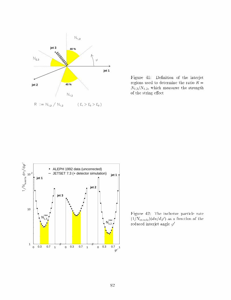
jet 1

jet 2

jet 3 40 %

40 %

Figure 41: De�nition of the interjet

regions used to determine the ratio R =

N1;3=N1;2, which measures the strength

of the string e�ect.

1

10

10 2

0 1 0 1 0 1

ALEPH 1992 data (uncorrected)JETSET 7.3 (+ detector simulation)

jet 1

jet 3

jet 2

jet 1

N1,3

N1,2

raw

raw

0.3 0.3 0.30.7 0.7 0.7 / // /

Figure 42: The inclusive particle rate

(1=Nevents)(dn=d'0) as a function of the

reduced interjet angle '0.

82

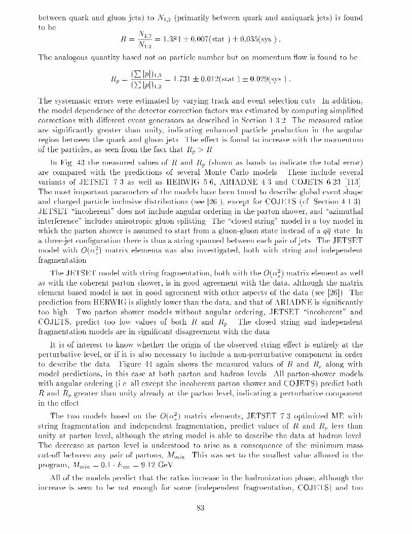
between quark and gluon jets) to N1;2 (primarily between quark and antiquark jets) is found

to be

R =N1;3

N1;2

= 1:384 � 0:007(stat.)� 0:035(sys.) :

The analogous quantity based not on particle number but on momentum ow is found to be

Rp =(P jpj)1;3(P jpj)1;2

= 1:731 � 0:012(stat.) � 0:029(sys.) :

The systematic errors were estimated by varying track and event selection cuts. In addition,

the model dependence of the detector correction factors was estimated by computing simpli�ed

corrections with di�erent event generators as described in Section 1.3.2. The measured ratios

are signi�cantly greater than unity, indicating enhanced particle production in the angular

region between the quark and gluon jets. The e�ect is found to increase with the momentum

of the particles, as seen from the fact that Rp > R.

In Fig. 43 the measured values of R and Rp (shown as bands to indicate the total error)

are compared with the predictions of several Monte Carlo models. These include several

variants of JETSET 7.3 as well as HERWIG 5.6, ARIADNE 4.3 and COJETS 6.23 [113].

The most important parameters of the models have been tuned to describe global event shape

and charged particle inclusive distributions (see [26]), except for COJETS (cf. Section 4.1.3).

JETSET \incoherent" does not include angular ordering in the parton shower, and \azimuthal

interference" includes anisotropic gluon splitting. The \closed string" model is a toy model in

which the parton shower is assumed to start from a gluon-gluon state instead of a qq state. In

a three-jet con�guration there is thus a string spanned between each pair of jets. The JETSET

model with O(�2s) matrix elements was also investigated, both with string and independent

fragmentation.

The JETSET model with string fragmentation, both with the O(�2s) matrix element as well

as with the coherent parton shower, is in good agreement with the data, although the matrix

element based model is not in good agreement with other aspects of the data (see [26]). The

prediction from HERWIG is slightly lower than the data, and that of ARIADNE is signi�cantly

too high. Two parton shower models without angular ordering, JETSET \incoherent" and

COJETS, predict too low values of both R and Rp. The closed string and independent

fragmentation models are in signi�cant disagreement with the data.

It is of interest to know whether the origin of the observed string e�ect is entirely at the

perturbative level, or if it is also necessary to include a non-perturbative component in order

to describe the data. Figure 44 again shows the measured values of R and Rp along with

model predictions, in this case at both parton and hadron levels. All parton-shower models

with angular ordering (i.e. all except the incoherent parton shower and COJETS) predict both

R and Rp greater than unity already at the parton level, indicating a perturbative component

in the e�ect.

The two models based on the O(�2s) matrix elements, JETSET 7.3 optimized ME with

string fragmentation and independent fragmentation, predict values of R and Rp less than

unity at parton level, although the string model is able to describe the data at hadron level.

The decrease at parton level is understood to arise as a consequence of the minimum mass

cut-o� between any pair of partons, Mmin. This was set to the smallest value allowed in the

program, Mmin = 0:1 � Ecm = 9:12 GeV.

All of the models predict that the ratios increase in the hadronization phase, although the

increase is seen to be not enough for some (independent fragmentation, COJETS) and too

83

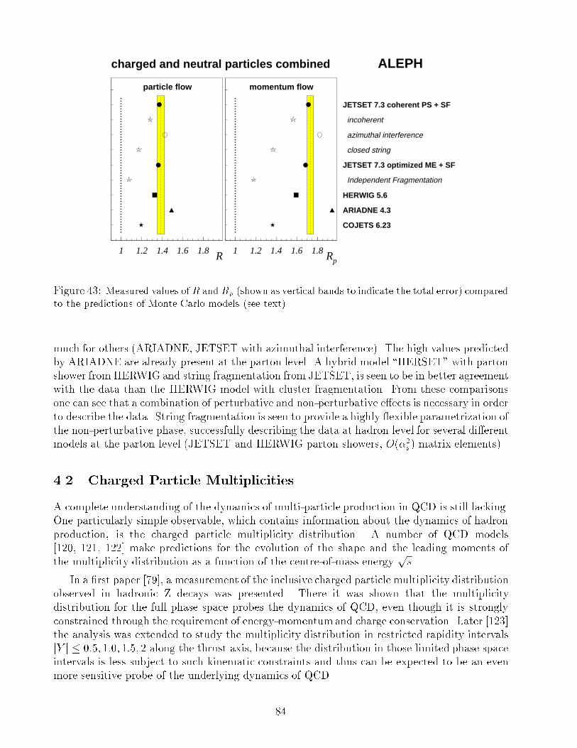
1 1.2 1.4 1.6 1.8 1 1.2 1.4 1.6 1.8

particle flow momentum flow

JETSET 7.3 coherent PS + SF

incoherent

azimuthal interference

closed string

JETSET 7.3 optimized ME + SF

Independent Fragmentation

HERWIG 5.6

ARIADNE 4.3

COJETS 6.23

R Rp

ALEPHcharged and neutral particles combined

Figure 43: Measured values of R and Rp (shown as vertical bands to indicate the total error) compared

to the predictions of Monte Carlo models (see text).

much for others (ARIADNE, JETSET with azimuthal interference). The high values predicted

by ARIADNE are already present at the parton level. A hybrid model \HERSET" with parton

shower fromHERWIG and string fragmentation from JETSET, is seen to be in better agreement

with the data than the HERWIG model with cluster fragmentation. From these comparisons

one can see that a combination of perturbative and non-perturbative e�ects is necessary in order

to describe the data. String fragmentation is seen to provide a highly exible parametrization of

the non-perturbative phase, successfully describing the data at hadron level for several di�erent

models at the parton level (JETSET and HERWIG parton showers, O(�2s) matrix elements).

4.2 Charged Particle Multiplicities

A complete understanding of the dynamics of multi-particle production in QCD is still lacking.

One particularly simple observable, which contains information about the dynamics of hadron

production, is the charged particle multiplicity distribution. A number of QCD models

[120, 121, 122] make predictions for the evolution of the shape and the leading moments of

the multiplicity distribution as a function of the centre-of-mass energyps.

In a �rst paper [79], a measurement of the inclusive charged particle multiplicity distribution

observed in hadronic Z decays was presented. There it was shown that the multiplicity

distribution for the full phase space probes the dynamics of QCD, even though it is strongly

constrained through the requirement of energy-momentumand charge conservation. Later [123]

the analysis was extended to study the multiplicity distribution in restricted rapidity intervals

jY j � 0:5; 1:0; 1:5; 2 along the thrust axis, because the distribution in those limited phase space

intervals is less subject to such kinematic constraints and thus can be expected to be an even

more sensitive probe of the underlying dynamics of QCD.

84

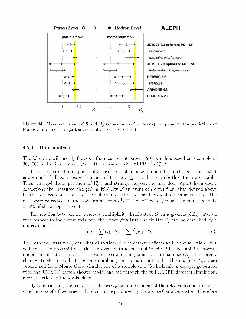
1 1.5 1 1.5

particle flow momentum flow

JETSET 7.3 coherent PS + SF

incoherent

azimuthal interference

JETSET 7.3 optimized ME + SF

Independent Fragmentation

HERWIG 5.6

ARIADNE 4.3

COJETS 6.23

HERSET

Hadron LevelParton Level

R Rp

ALEPH

Figure 44: Measured values of R and Rp (shown as vertical bands) compared to the predictions of

Monte Carlo models at parton and hadron levels (see text).

4.2.1 Data analysis

The following will mainly focus on the most recent paper [123], which is based on a sample of

300; 000 hadronic events atps =MZ measured with ALEPH in 1992.

The true charged multiplicity of an event was de�ned as the number of charged tracks that

is obtained if all particles with a mean lifetime � � 1 ns decay while the others are stable.

Thus, charged decay products of K0S's and strange baryons are included. Apart from decay

corrections the measured charged multiplicity of an event can di�er from that de�ned above

because of acceptance losses or secondary interactions of particles with detector material. The

data were corrected for the background from e+e� ! �+�� events, which contribute roughly

0.26% of the accepted events.

The relation between the observed multiplicity distribution Oi in a given rapidity interval

with respect to the thrust axis, and the underlying true distribution Tj can be described by a

matrix equation

Oi =Xj

Gij � Tj =Xj

eGij"j � Tj: (73)

The response matrix Gij describes distortions due to detector e�ects and event selection. It is

de�ned as the probability "j that an event with a true multiplicity j in the rapidity interval

under consideration survives the event selection cuts, times the probability eGij to observe i

charged tracks instead of the true number j in the same interval. The matrices Gij were

determined from Monte Carlo simulations of a sample of 1.6M hadronic Z decays, generated

with the JETSET parton shower model and fed through the full ALEPH detector simulation,

reconstruction and analysis chain.

By construction, the response matrices Gij are independent of the relative frequencies with

which events of a �xed true multiplicity j are produced by the Monte Carlo generator. Therefore

85

they are only weakly dependent on the actual choice of the generator. The rms spread of the

measured multiplicities around the true values varies from � 1:8 to � 3:7 units when the true

multiplicity goes from ntrue = 8 to ntrue = 30, almost independent of the size of the rapidity

window under consideration.

Inverting Eq. (73), a model independent estimate for the true distributions Tj was extracted

from the measurements. However, trying to correct for distortions by naively inverting Eq. (73)

results in instabilities due to the statistical uctuations in the measurements (see e.g. [124]).

Several ways of tackling the inverse problem Eq. (73) for �nite statistics are discussed in the

literature [125]. The basic idea always is to supplement the measurements by an additional

constraint that stabilizes the unfolding result. In this analysis the \Method of reduced cross-

entropy" (MRX) [126] was used to correct the measured distribution for smearing e�ects. After

that the \unsmeared" distribution was corrected for e�ciency.

In a second analysis, parametric models were studied. Here the true distribution Tj = Pj(~�)

is given either as a function of a parameter vector ~� or by the predictions from di�erent

Monte Carlo models. Given as input the respective true distributions Tj, the matrices Gij

were employed as convenient means to incorporate the e�ect of the full detector simulation.

Multiplying Tj with the response matrix the results were compared directly with the raw

measurements. In the case of parametric models the parameters were determined by a standard

least squares �t.

The multiplicity distributions were corrected for the e�ect of initial state radiation by

applying a set of bin-by-bin correction factors, determined from the JETSET model. Except

for the lowest multiplicity bins this correction turned out to be entirely negligible. In the

model independent analysis the corrections were applied to the unfolded distributions. For

the parametric �ts the e�ects of initial state radiation were included before folding with the

response matrix.

4.2.2 Model Independent Results

The unfolded charged particle multiplicity distribution of hadronic Z decays is given in Table 25.

Note that as a consequence of the correction procedure, the errors are correlated. Since the

selection criteria require at least �ve observed charged tracks per event there is no information

about the probability of having a hadronic Z decay with only two charged tracks. The

probability for a Z to produce four charged tracks can still be estimated, although with large

errors, because, due to smearing e�ects, there is still a small chance that those events pass the

selection criteria.

The errors given in Tables 25 and 27 have been updated with respect to those reported

in [123] in the following way. In the nominal analysis, the unfolding matrix is based on the

JETSET Monte Carlo. The systematic error due to model dependence has been estimated by

constructing a response matrix based on HERWIG. Since a high statistics sample of HERWIG

events was not available, a complete unfolding based on this matrix was not possible. The

matrix could be used in conjunction with the unfolded distribution from the nominal analysis,

however, to obtain a prediction OHERWIGi for the observed distribution according to Eq. (73).

The same procedure can be done with the distribution unfolded with the JETSET-based matrix

to obtain OJETSETi . (This is very similar, but not identical, to the actual observed distribution.)

From each of these distributions, the mean multiplicity was determined, and the di�erence �n

was taken as the systematic error in the mean due to model dependence.

86

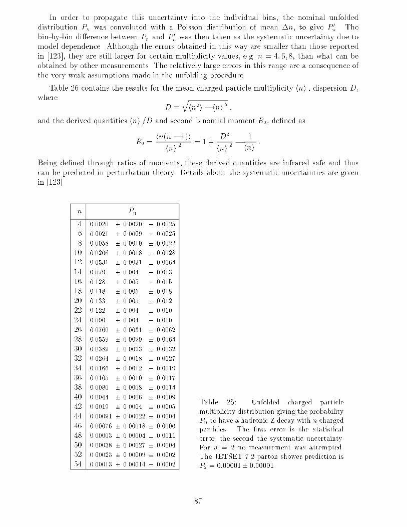
In order to propagate this uncertainty into the individual bins, the nominal unfolded

distribution Pn was convoluted with a Poisson distribution of mean �n, to give P 0n. The

bin-by-bin di�erence between Pn and P 0n was then taken as the systematic uncertainty due to

model dependence. Although the errors obtained in this way are smaller than those reported

in [123], they are still larger for certain multiplicity values, e.g. n = 4; 6; 8, than what can be

obtained by other measurements. The relatively large errors in this range are a consequence of

the very weak assumptions made in the unfolding procedure.

Table 26 contains the results for the mean charged particle multiplicity hni , dispersion D,where

D =qhn2i � hni 2 ;

and the derived quantities hni =D and second binomial moment R2, de�ned as

R2 =hn(n � 1)ihni 2 = 1 +

D2

hni 2 �1

hni :

Being de�ned through ratios of moments, these derived quantities are infrared safe and thus

can be predicted in perturbation theory. Details about the systematic uncertainties are given

in [123].

n Pn

4 0.0020 � 0.0020 � 0.0025

6 0.0021 � 0.0009 � 0.0025

8 0.0058 � 0.0010 � 0.0022

10 0.0266 � 0.0018 � 0.0028

12 0.0531 � 0.0031 � 0.0064

14 0.079 � 0.004 � 0.013

16 0.128 � 0.005 � 0.015

18 0.118 � 0.005 � 0.018

20 0.133 � 0.005 � 0.012

22 0.122 � 0.004 � 0.010

24 0.090 � 0.004 � 0.010

26 0.0760 � 0.0031 � 0.0062

28 0.0559 � 0.0029 � 0.0064

30 0.0389 � 0.0023 � 0.0032

32 0.0264 � 0.0018 � 0.0027

34 0.0166 � 0.0012 � 0.0019

36 0.0105 � 0.0010 � 0.0017

38 0.0080 � 0.0008 � 0.0014

40 0.0044 � 0.0006 � 0.0009

42 0.0019 � 0.0004 � 0.0005

44 0.00091 � 0.00022 � 0.0004

46 0.00076 � 0.00018 � 0.0006

48 0.00003 � 0.00004 � 0.0011

50 0.00038 � 0.00027 � 0.0004

52 0.00023 � 0.00009 � 0.0002

54 0.00013 � 0.00014 � 0.0002

Table 25: Unfolded charged particle

multiplicity distribution giving the probability

Pn to have a hadronic Z decay with n charged

particles. The �rst error is the statistical

error, the second the systematic uncertainty.

For n = 2 no measurement was attempted.

The JETSET 7.2 parton shower prediction is

P2 = 0:00001� 0:00001.

87

hni = 20:91 � 0:03 � 0:22

D = 6:425 � 0:031 � 0:087

hni =D = 3:255 � 0:019 � 0:055

R2 = 1:0466 � 0:0008 � 0:0029

Table 26: Leading moments of

the charged particle multiplicity

distribution. The �rst error is

the statistical error, the second the

systematic uncertainty of the result.

4.2.3 Energy Dependence of the Charged Multiplicity Distribution

KNO scaling

Originally derived by starting from the Feynman scaling [127] behaviour for multi-particle

production, the KNO [120] scaling hypothesis predicts that the shape of the multiplicity

distribution plotted in the form hni Pn versus z = n=hni is independent ofps. In Fig. 45 (a)

the multiplicity distribution measured in [79] and plotted in KNO form is compared to data atps = 43:6 GeV and

ps = 29 GeV measured by the TASSO and HRS collaborations [128, 129].

It can be seen that in the energy rangeps = 29 � 91:2 GeV the data are in remarkable

agreement with the expectations from KNO scaling. Also shown is the distribution from the

JETSET 7.2 parton shower model, tuned atps = 91:2 GeV [26], which provides a very good

description of the data. KNO scaling further implies the ratio hni =D to be independent ofps. Measurements of this ratio between 12 GeV and 91.25 GeV [128, 130, 131] are shown

in Fig. 45 (b). The data are well described by a constant with CKNO = 3:23 � 0:05 with a

�2=NDF = 5:0=8. The energy dependence of hni =D is also found to be well reproduced by

the JETSET model without retuning parameters, i.e. approximate KNO scaling appears to be

a natural consequence of the parton shower approach to multi-particle production.

The Mean Charged Particle Multiplicity

As a consequence of the running of the strong coupling constant �s, a next-to-leading order

QCD calculation [59] in the framework of the MLLA+LPHD predicts an energy dependence of

the mean multiplicity of the form

hn(Ecm)i = KLPHD � �Bs (Ecm) � exp�A=q�s(Ecm)

�

with coe�cients A =p864�=(33�2nf ) � 2:265 and B = (297+22nf )=(1188�72nf ) � 0:4915

for nf = 5 active quark avours, and �s(Ecm) as given in Section 1.1. The free parameters

are the phenomenological normalization constant KLPHD and the value of the strong coupling

at the scale of the Z mass, �s(MZ). Figure 46(a) shows how the QCD prediction compares to

the data, taken from a compilation of results in [132]. Taking �s(MZ) = 0:118 a perfect �t is

obtained with KLPHD = 0:0822 and �2=ndf = 5:2=20. Also shown is the prediction from the

JETSET 7.2 parton shower model with parameters �xed atps = 91:2 GeV [26], which follows

the QCD curve very closely.

For the QCD prediction it has been assumed that the multiplicity of the �nal state is

a function of only the centre-of-mass energy. This is only approximately true, because the

multiplicity from primary b quarks is higher than from light avours and because the avour

composition changes between photon and Z mediated reactions. Assuming that the di�erence

88

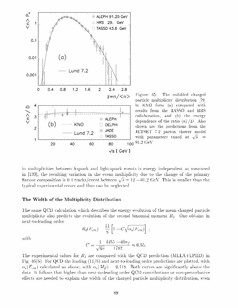
Figure 45: The unfolded charged

particle multiplicity distribution [79]

in KNO form (a) compared with

results from the TASSO and HRS

collaboration, and (b) the energy

dependence of the ratio hni =D. Also

shown are the predictions from the

JETSET 7.2 parton shower model

with parameters tuned atps =

91:2 GeV.

in multiplicities between b-quark and light-quark events is energy independent as measured

in [133], the resulting variation in the event multiplicity due to the change of the primary

avour composition is 0.4 tracks/event betweenps = 12 � 91:2 GeV. This is smaller than the

typical experimental errors and thus can be neglected.

The Width of the Multiplicity Distribution

The same QCD calculation which describes the energy evolution of the mean charged particle

multiplicity also predicts the evolution of the second binomial moment R2. One obtains in

next-to-leading order

R2(Ecm) =11

8

�1� C

q�s(Ecm)

�;

with

C =1p6�

4455 � 40nf

1782� 0:55:

The experimental values for R2 are compared with the QCD prediction (MLLA+LPHD) in

Fig. 46(b). For QCD the leading (11/8) and next-to-leading order predictions are plotted, with

�s(Ecm) calculated as above, with �s(MZ) = 0:118. Both curves are signi�cantly above the

data. It follows that higher than next-to-leading order QCD contributions or non-perturbative

e�ects are needed to explain the width of the charged particle multiplicity distribution, even

89

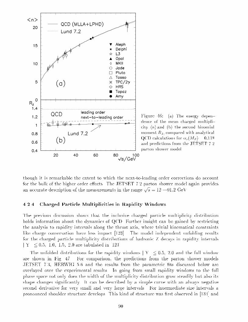
Figure 46: (a) The energy depen-

dence of the mean charged multipli-

city hni and (b) the second binomial

moment R2, compared with analytical

QCD calculations for �s(MZ) = 0:118

and predictions from the JETSET 7.2

parton shower model.

though it is remarkable the extent to which the next-to-leading order corrections do account

for the bulk of the higher order e�ects. The JETSET 7.2 parton shower model again provides

an accurate description of the measurements in the rangeps = 12 � 91:2 GeV.

4.2.4 Charged Particle Multiplicities in Rapidity Windows

The previous discussion shows that the inclusive charged particle multiplicity distribution

holds information about the dynamics of QCD. Further insight can be gained by restricting

the analysis to rapidity intervals along the thrust axis, where trivial kinematical constraints

like charge conservation have less impact [123]. The model independent unfolding results

for the charged particle multiplicity distributions of hadronic Z decays in rapidity intervals

j Y j � 0:5; 1:0; 1:5; 2:0 are tabulated in [123].

The unfolded distributions for the rapidity windows j Y j � 0:5; 2:0 and the full window

are shown in Fig. 47. For comparison, the predictions from the parton shower models

JETSET 7.3, HERWIG 5.6 and the results from the parametric �ts discussed below are

overlayed over the experimental results. In going from small rapidity windows to the full

phase space not only does the width of the multiplicity distribution grow steadily but also its

shape changes signi�cantly. It can be described by a simple curve with an always negative

second derivative for very small and very large intervals. For intermediate size intervals a

pronounced shoulder structure develops. This kind of structure was �rst observed in [134] and

90

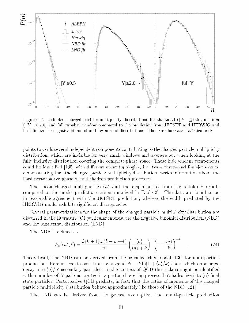
10-5

10-4

10-3

10-2

10-1

0 10 20 30 40 50

P(n

)

|Y|≤0.5

ALEPH

JetsetHerwigNBD fitLND fit

0 10 20 30 40 50

|Y|≤2.0

0 10 20 30 40 50n

full Y

Figure 47: Unfolded charged particle multiplicity distributions for the small (j Y j � 0:5), medium

(j Y j � 2:0) and full rapidity window compared to the prediction from JETSET and HERWIG and

best �ts to the negative-binomial and log-normal distributions. The error bars are statistical only.

points towards several independent components contributing to the charged particle multiplicity

distribution, which are invisible for very small windows and average out when looking at the

fully inclusive distribution covering the complete phase space. These independent components

could be identi�ed [135] with di�erent event topologies, i.e. two-, three- and four-jet events,

demonstrating that the charged particle multiplicity distribution carries information about the

hard perturbative phase of multihadron production processes.

The mean charged multiplicities hni and the dispersion D from the unfolding results

compared to the model predictions are summarized in Table 27. The data are found to be

in reasonable agreement with the JETSET prediction, whereas the width predicted by the

HERWIG model exhibits signi�cant discrepancies.

Several parametrizations for the shape of the charged particle multiplicity distribution are

discussed in the literature. Of particular interest are the negative binomial distribution (NBD)

and the log-normal distribution (LND).

The NDB is de�ned as

Pn(hni; k) = k(k + 1):::(k + n� 1)

n!

hnihni + k

!n 1 +

hnik

!�k: (74)

Theoretically the NBD can be derived from the so-called clan model [136] for multiparticle

production. Here an event consists on average of N = k ln(1 + hni=k) clans which on average

decay into hni=N secondary particles. In the context of QCD those clans might be identi�ed

with a number of N partons created in a parton showering process that hadronize into hni �nalstate particles. Perturbative QCD predicts, in fact, that the ratios of moments of the charged

particle multiplicity distribution behave approximately like those of the NBD [121].

The LND can be derived from the general assumption that multi-particle production

91

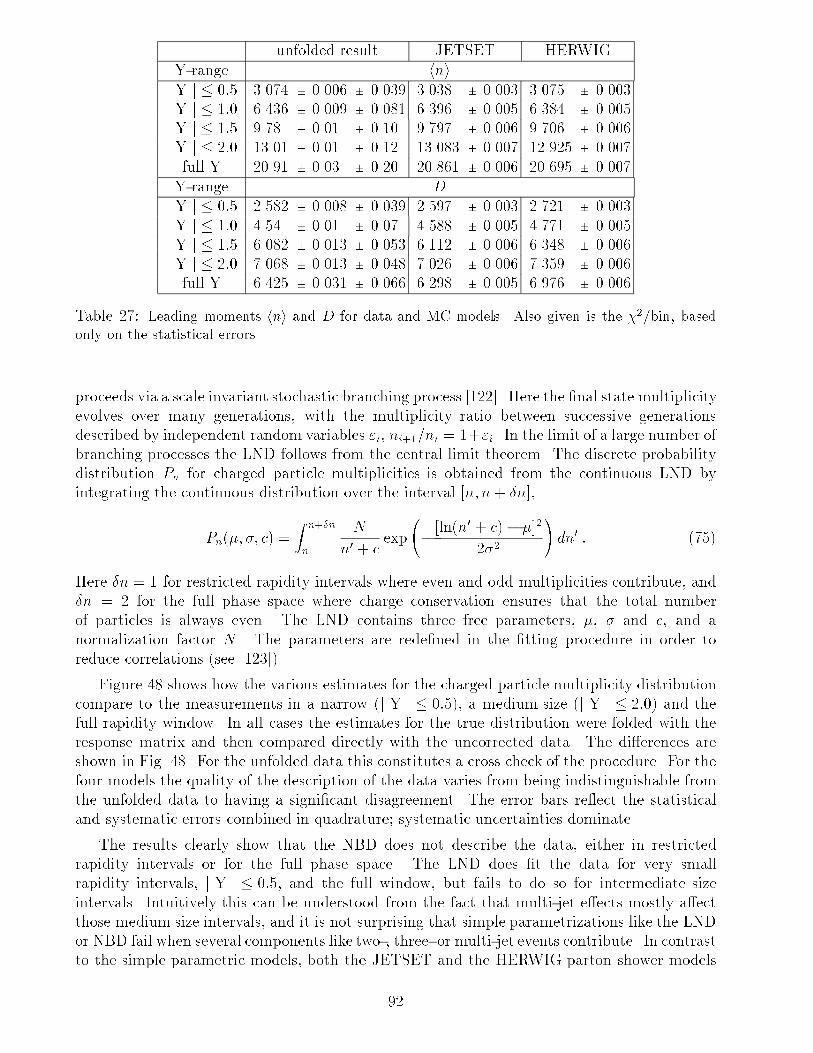
unfolded result JETSET HERWIG

Y-range hnij Y j � 0:5 3.074 � 0.006 � 0.039 3.038 � 0.003 3.075 � 0.003

j Y j � 1:0 6.436 � 0.009 � 0.081 6.396 � 0.005 6.384 � 0.005

j Y j � 1:5 9.78 � 0.01 � 0.10 9.797 � 0.006 9.706 � 0.006

j Y j � 2:0 13.01 � 0.01 � 0.12 13.083 � 0.007 12.925 � 0.007

full Y 20.91 � 0.03 � 0.20 20.861 � 0.006 20.695 � 0.007

Y-range D

j Y j � 0:5 2.582 � 0.008 � 0.039 2.597 � 0.003 2.721 � 0.003

j Y j � 1:0 4.54 � 0.01 � 0.07 4.588 � 0.005 4.771 � 0.005

j Y j � 1:5 6.082 � 0.013 � 0.053 6.112 � 0.006 6.348 � 0.006

j Y j � 2:0 7.068 � 0.013 � 0.048 7.026 � 0.006 7.359 � 0.006

full Y 6.425 � 0.031 � 0.066 6.298 � 0.005 6.976 � 0.006

Table 27: Leading moments hni and D for data and MC models. Also given is the �2=bin, based

only on the statistical errors.

proceeds via a scale invariant stochastic branching process [122]. Here the �nal state multiplicity

evolves over many generations, with the multiplicity ratio between successive generations

described by independent random variables "i, ni+1=ni = 1+"i. In the limit of a large number of

branching processes the LND follows from the central limit theorem. The discrete probability

distribution Pn for charged particle multiplicities is obtained from the continuous LND by

integrating the continuous distribution over the interval [n; n+ �n],

Pn(�; �; c) =

Z n+�n

n

N

n0 + cexp

� [ln(n0 + c)� �]2

2�2

!dn0 : (75)

Here �n = 1 for restricted rapidity intervals where even and odd multiplicities contribute, and

�n = 2 for the full phase space where charge conservation ensures that the total number

of particles is always even. The LND contains three free parameters, �, � and c, and a

normalization factor N . The parameters are rede�ned in the �tting procedure in order to

reduce correlations (see [123]).

Figure 48 shows how the various estimates for the charged particle multiplicity distribution

compare to the measurements in a narrow (j Y j � 0:5), a medium size (j Y j � 2:0) and the

full rapidity window. In all cases the estimates for the true distribution were folded with the

response matrix and then compared directly with the uncorrected data. The di�erences are

shown in Fig. 48. For the unfolded data this constitutes a cross check of the procedure. For the

four models the quality of the description of the data varies from being indistinguishable from

the unfolded data to having a signi�cant disagreement. The error bars re ect the statistical

and systematic errors combined in quadrature; systematic uncertainties dominate.

The results clearly show that the NBD does not describe the data, either in restricted

rapidity intervals or for the full phase space. The LND does �t the data for very small

rapidity intervals, j Y j � 0:5, and the full window, but fails to do so for intermediate size

intervals. Intuitively this can be understood from the fact that multi-jet e�ects mostly a�ect

those medium size intervals, and it is not surprising that simple parametrizations like the LND

or NBD fail when several components like two-, three- or multi-jet events contribute. In contrast

to the simple parametric models, both the JETSET and the HERWIG parton shower models

92

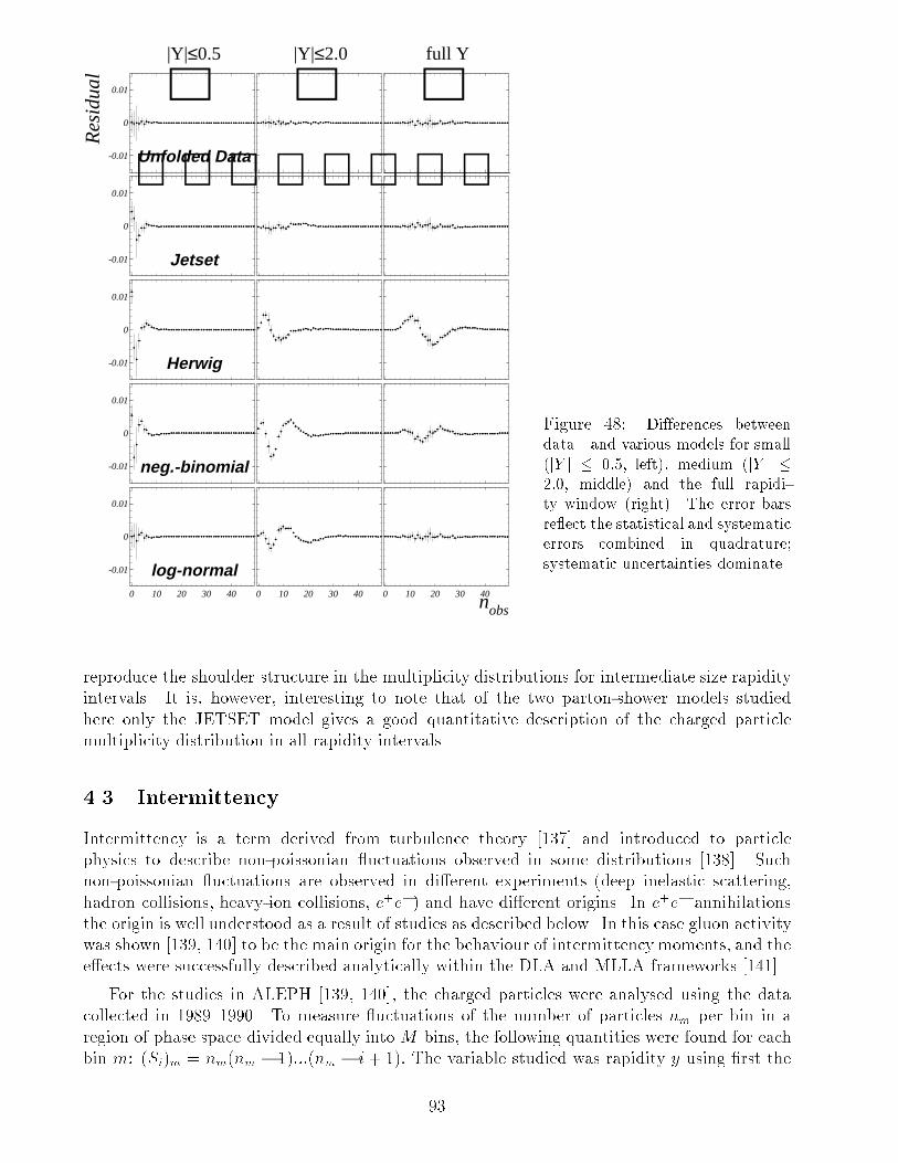
-0.01

0

0.01

0 10 20 30 40

log-normal0 10 20 30 40 0 10 20 30 40

nobs

-0.01

0

0.01

neg.-binomial

-0.01

0

0.01

Herwig

-0.01

0

0.01

Jetset

-0.01

0

0.01

Unfolded Data

|Y|≤0.5

Re

sid

ua

l

|Y|≤2.0 full Y

Figure 48: Differences between

data and various models for small

(jY j � 0:5, left), medium (jY j �2:0, middle) and the full rapidi-

ty window (right). The error bars

re ect the statistical and systematic

errors combined in quadrature;

systematic uncertainties dominate.

reproduce the shoulder structure in the multiplicity distributions for intermediate size rapidity

intervals. It is, however, interesting to note that of the two parton-shower models studied

here only the JETSET model gives a good quantitative description of the charged particle

multiplicity distribution in all rapidity intervals.

4.3 Intermittency

Intermittency is a term derived from turbulence theory [137] and introduced to particle

physics to describe non-poissonian uctuations observed in some distributions [138]. Such

non-poissonian uctuations are observed in di�erent experiments (deep inelastic scattering,

hadron collisions, heavy-ion collisions, e+e�) and have di�erent origins. In e+e� annihilations

the origin is well understood as a result of studies as described below. In this case gluon activity

was shown [139, 140] to be the main origin for the behaviour of intermittency moments, and the

e�ects were successfully described analytically within the DLA and MLLA frameworks [141].

For the studies in ALEPH [139, 140], the charged particles were analysed using the data

collected in 1989{1990. To measure uctuations of the number of particles nm per bin in a

region of phase space divided equally into M bins, the following quantities were found for each

bin m: (Si)m = nm(nm � 1):::(nm � i+ 1): The variable studied was rapidity y using �rst the

93

di�erential moments [139], de�ned by

(fi)m =h(Si)mihNii ; (76)

where the average is taken over all events. This quantity is sensitive to the uctuations in the

mth bin from event to event. The intermittent behaviour was further examined [140] using the

standard factorial moments F of order i,

Fi(M) =h 1M

PMm=1(Si)miM i

hNii : (77)

The moments in Eqs. (76) and (77) average to unity if the uctuations of particles in the bins

are Poissonian. Higher moments are sensitive to larger clusters of particles within the bins and

include information contained in the lower moments. A power-law dependence of Fi(M) with

respect to M hints at self-similar processes in the generation of particles. The data are shown

in Fig. 49 for one-dimensional factorial moments F2(M) in y.

Figure 49: The second factorial

moment F2(M) in rapidity space.

Comparison of di�erent Monte Carlo

models with varying amounts of

parton cascading. The solid line

is to guide the eye for the default

JETSET Monte Carlo prediction and

the dotted lines for other versions of

the model.

Using the di�erential moments of Eq.(76), it could be clearly demonstrated that the

behaviour of the intermittency moments is mainly due to the emission of hard gluons [139].

For example, the third di�erential moment rises to about eight at jyj ' 1, which contains,

in addition to particles from two-jet events, an enhanced activity from three-jet events. That

is, the multijet structure of e+e� ! hadrons causes the rapidity distribution of the charged

particles to vary with the event topology and, for example, the moments to F2(M) to increase

with decreasing bin size as seen in Fig. 49. If events of a given topology are selected (e.g., with

a cut in thrust), the di�erential and factorial moments in one dimension remain close to unity

when decreasing the bin size.

94

The comparison [140] is shown in Fig. 49 of ALEPH data with �ve models available within

the Lund parton shower Monte Carlo, JETSET 7.3 [25]:

PS: The full (default) parton shower model. This gives an average of 7.8 partons before the

onset of string fragmentation.

ERT: The model with second order matrix elements according to Ellis, Ross, and Terrano [16].

This allows up to four partons before string fragmentation.

MEOPT: The second order matrix elements model with optimized renormalization scale. The

latter improves the agreement of ERT with the experimental four-jet rate.

ABEL: Abelian parton shower model. The triple gluon vertex has been switched o� in the

otherwise full shower development.

QQBAR: A model with no gluons. The primary quark-antiquark-pair are hooked together with

a straight string which then fragments according to JETSET 7.3. Only two partons are allowed.

All models except QQBAR and ABEL were �t to a set of ALEPH inclusive and exclusive

distributions [26], which do not include the factorial moments. In the cases of QQBAR and

ABEL the fragmentation parameters were adjusted to reproduce the measured average thrust

and multiplicity.

It is seen in Fig. 49 that the moments with only two quarks indicate nearly Poissonian

behavior (QQBAR). The main mechanism driving the moments upward is the emission of one

or two hard gluons (ERT, MEOPT). The full shower cascade (PS) is necessary to fully describe

the data. The cascading is insu�cient without the triple gluon vertex (ABEL).

4.4 Subjet Structure of Hadronic Events

Analyses using subjets have proven to be useful in order to investigate the internal structure

of quark and gluon jets. The general procedure followed in this section was �rst introduced

in Ref. [142]. Subjets in two- and three-jet events are de�ned in the following way. First, jets

are de�ned using an iterative clustering procedure (the Durham algorithm [28]), as described

in Section 2.1.

Two- and/or three-jet events are selected using an initial value of the resolution parameter,

ycut = y1. In order to investigate the jets' internal structure, the particles of the individual

jets are clustered using a smaller value of the resolution parameter y0 (< y1) so that subjets

are resolved. QCD predicts di�erences in the subjet structure of quark and gluon jets. In the

parton shower picture, these di�erences are understood to arise mainly from the di�erent colour

factors which enter into the probabilities for a gluon to emit another gluon, proportional to

CA = 3, and the probability for a quark to emit a gluon, proportional to CF = 4=3. As long

as the subjet resolution parameter y1 is su�ciently large, one expects a direct correspondence

between the parton level predictions of QCD and hadron level measurements.

In a �rst analysis, the subjet multiplicity of two- and three-jet events is measured without

determining whether the jet originated from a quark or from a gluon. Similar studies have

been reported in [143, 144]. In a second analysis, gluon jets are identi�ed by requiring evidence

of long-lived hadrons containing b or c quarks in two jets out of a three-jet event, and the

remaining jet is then taken as a gluon jet candidate. By combining the results from this jet

sample with those where all jets are used, the individual subjet structure of quark and gluon

jets can be inferred.

95

4.4.1 Subjet Structure of Two- and Three-Jet Events

Although QCD makes speci�c predictions for identi�ed quark and gluon jets, it is di�cult

experimentally to identify jets as such. An analysis was therefore carried out to measure

the subjet multiplicity in two- and three-jet events, M2 and M3, without quark or gluon jet

identi�cation. The two-jet sample consists predominantly of an initial qq system followed by

soft gluon radiation, whereas the three-jet sample is enriched by events with a single hard

(high k?) gluon. The initial qq or qqg system continues to radiate gluons, whereby the quark-

gluon coupling is proportional to the QCD colour factor CF = 4=3, whereas the gluon-gluon

coupling is proportional to CA = 3. Thus one expects the three jet sample to have a higher

subjet multiplicity than the two-jet sample. For asymptotically high energies and small y0 one

expects [142]

R =M3 � 3

M2 � 2! 2CF + CA

2CF

=17

8: (78)

The ratio as de�ned here is equivalent toM3=M2 in the limit that the multiplicities are large.

Subtracting the initial number of jets leads to a faster expected convergence to the asymptotic

prediction of (78), and simpli�es the interpretation of the results in the region where y0 is close

to y1 (i.e.M2 only slightly larger than two, M3 only slightly larger than three).

The measurements of M2 and M3 presented here are based on charged particles only. The

track and event selection criteria are described in Section 1.3.1. Using data collected in 1992

yielded a sample of approximately 300,000 hadronic events at an energy of Ecm = 91:2 GeV.

The measurements have been corrected for detector related e�ects using multiplicative

correction factors C as described in Section 1.3.2. These factors are computed as a function of

the subjet resolution parameter y0, and are applied to the subjet multiplicity minus the number

of jets selected with ycut = y1, i.e.

(Mn(y0)� n)corrected = (Mn(y0)� n)measured � C(y0) (79)

with n = 2; 3. In order to minimize systematic errors, the correction factors have been computed

so as to take into account charged particles only. Comparisons with Monte Carlo models are

then also made using only charged particles. The correction factors do not depend strongly on

y0 and are typically in the range 1:00 < C < 1:12.

In order to estimate the systematic uncertainty from the generator dependence of the

correction factors, approximate factors were derived from several Monte Carlo models, as

described in Section 1.3.2. The approximate correction factors reproduced the overall form

of the factors based on the full detector simulation, and they di�ered among each other by

typically less than 1% to 2%. It was checked that the corrected jet multiplicities are not

sensitive to the event and track selection criteria by varying all of the cuts. No evidence for a

systematic dependence was found beyond the one percent level.

Based on the studies of the generator dependence of the correction factors and variation of

the cuts, an overall systematic error of 2% is assigned to the mean subjet multiplicitiesM2� 2

and M3 � 3. This is conservative for small y0, where the subjet multiplicity tends toward the

charged particle multiplicity for the event sample in question. (In Section 4.2 it is shown that

the mean charged multiplicity is measured in ALEPH with a systematic error of about 1:2%.)

For the ratio R = (M3 � 3)=(M2 � 2), the systematic errors largely cancel. The remaining

96

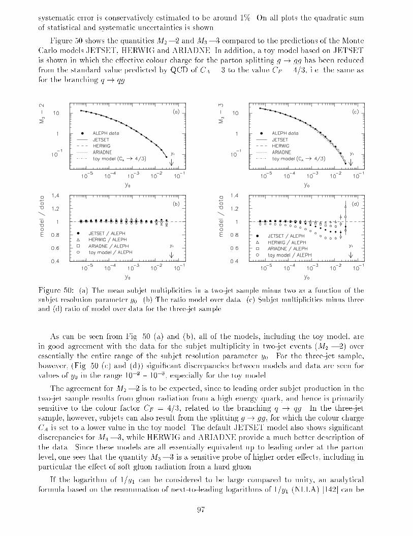
systematic error is conservatively estimated to be around 1%. On all plots the quadratic sum

of statistical and systematic uncertainties is shown.

Figure 50 shows the quantitiesM2�2 andM3�3 compared to the predictions of the Monte

Carlo models JETSET, HERWIG and ARIADNE. In addition, a toy model based on JETSET

is shown in which the e�ective colour charge for the parton splitting g ! gg has been reduced

from the standard value predicted by QCD of CA = 3 to the value CF = 4=3, i.e. the same as

for the branching q! qg.

Figure 50: (a) The mean subjet multiplicities in a two-jet sample minus two as a function of the

subjet resolution parameter y0. (b) The ratio model over data. (c) Subjet multiplicities minus three

and (d) ratio of model over data for the three-jet sample.

As can be seen from Fig. 50 (a) and (b), all of the models, including the toy model, are

in good agreement with the data for the subjet multiplicity in two-jet events (M2 � 2) over

essentially the entire range of the subjet resolution parameter y0. For the three-jet sample,

however, (Fig. 50 (c) and (d)) signi�cant discrepancies between models and data are seen for

values of y0 in the range 10�2 { 10�3, especially for the toy model.

The agreement for M2� 2 is to be expected, since to leading order subjet production in the

two-jet sample results from gluon radiation from a high energy quark, and hence is primarily

sensitive to the colour factor CF = 4=3, related to the branching q ! qg. In the three-jet

sample, however, subjets can also result from the splitting g! gg, for which the colour charge

CA is set to a lower value in the toy model. The default JETSET model also shows signi�cant

discrepancies for M3� 3, while HERWIG and ARIADNE provide a much better description of

the data. Since these models are all essentially equivalent up to leading order at the parton

level, one sees that the quantityM3� 3 is a sensitive probe of higher order e�ects, including in

particular the e�ect of soft gluon radiation from a hard gluon.

If the logarithm of 1=y1 can be considered to be large compared to unity, an analytical

formula based on the resummation of next-to-leading logarithms of 1=y1 (NLLA) [142] can be

97

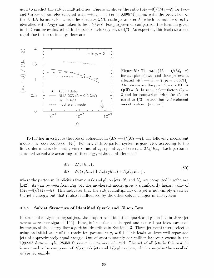
used to predict the subjet multiplicities. Figure 51 shows the ratio (M3 � 3)=(M2 � 2) for two-

and three- jet samples selected with � ln y1 = 5 (y1 = 0:00674) along with the prediction of

the NLLA formula, for which the e�ective QCD scale parameter � (which cannot be directly

identi�ed with �MS) was taken to be 0:5 GeV. For purposes of comparison the formula given

in [142] can be evaluated with the colour factor CA set to 4=3. As expected, this leads to a less

rapid rise in the ratio as y0 decreases.

Figure 51: The ratio (M3� 3)=(M2� 2)

for samples of two- and three-jet events

selected with � ln y1 = 5 (y1 = 0:00674).

Also shown are the predictions of NLLA

QCD with the usual colour factors CA =

3 and for comparison with the CA set

equal to 4=3. In addition an incoherent

model is shown (see text).

To further investigate the role of coherence in (M3 � 3)=(M2 � 2), the following incoherent

model has been proposed [145]. For M3, a three-parton system is generated according to the

�rst order matrix element, giving values of xq; xq and xg, where xi = 2Ei=Ecm. Each parton is

assumed to radiate according to its energy, without interference:

M2 = 2Nq(Ecm) ;

M3 = Nq(xqEcm) +Nq(xqEcm) +Ng(xgEcm) ;(80)

where the parton multiplicities from quark and gluon jets, Nq and Ng, are computed in reference

[142]. As can be seen from Fig. 51, the incoherent model gives a signi�cantly higher value of

(M3 � 3)=(M2 � 2). This indicates that the subjet multiplicity of a jet is not simply given by

the jet's energy, but that it also is in uenced by the other colour charges in the system.

4.4.2 Subjet Structure of Identi�ed Quark and Gluon Jets

In a second analysis using subjets, the properties of identi�ed quark and gluon jets in three-jet

events were investigated [146]. Here, information on charged and neutral particles was used

by means of the energy ow algorithm described in Section 1.3. Three-jet events were selected

using an initial value of the resolution parameter y1 = 0:1. This leads to three well separated

jets of approximately equal energy. Out of approximately one million hadronic events in the

1992-93 data sample, 28350 three-jet events were selected. The set of all jets in this sample

is assumed to be composed of 2=3 quark jets and 1=3 gluon jets, which comprise the so-called

mixed jet sample.

98

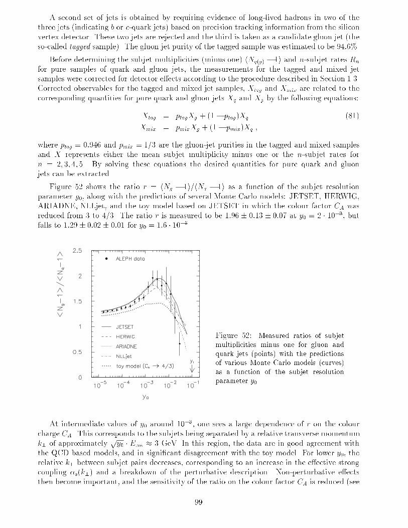
A second set of jets is obtained by requiring evidence of long-lived hadrons in two of the

three jets (indicating b or c-quark jets) based on precision tracking information from the silicon

vertex detector. These two jets are rejected and the third is taken as a candidate gluon jet (the

so-called tagged sample). The gluon jet purity of the tagged sample was estimated to be 94:6%.

Before determining the subjet multiplicities (minus one) hNq(g) � 1i and n-subjet rates Rn

for pure samples of quark and gluon jets, the measurements for the tagged and mixed jet

samples were corrected for detector e�ects according to the procedure described in Section 1.3.

Corrected observables for the tagged and mixed jet samples, Xtag and Xmix are related to the

corresponding quantities for pure quark and gluon jets Xq and Xg by the following equations:

Xtag = ptagXg + (1 � ptag)Xq (81)

Xmix = pmixXg + (1� pmix)Xq ;

where ptag = 0:946 and pmix = 1=3 are the gluon-jet purities in the tagged and mixed samples

and X represents either the mean subjet multiplicity minus one or the n-subjet rates for

n = 2; 3; 4; 5. By solving these equations the desired quantities for pure quark and gluon

jets can be extracted.

Figure 52 shows the ratio r = hNg � 1i=hNq � 1i as a function of the subjet resolution

parameter y0, along with the predictions of several Monte Carlo models: JETSET, HERWIG,

ARIADNE, NLLjet, and the toy model based on JETSET in which the colour factor CA was

reduced from 3 to 4=3. The ratio r is measured to be 1:96 � 0:13 � 0:07 at y0 = 2 � 10�3, butfalls to 1:29 � 0:02 � 0:01 for y0 = 1:6 � 10�5.

Figure 52: Measured ratios of subjet

multiplicities minus one for gluon and

quark jets (points) with the predictions

of various Monte Carlo models (curves)

as a function of the subjet resolution

parameter y0.

At intermediate values of y0 around 10�3, one sees a large dependence of r on the colour

charge CA. This corresponds to the subjets being separated by a relative transverse momentum

k? of approximatelypy0 � Ecm � 3 GeV. In this region, the data are in good agreement with

the QCD based models, and in signi�cant disagreement with the toy model. For lower y0, the

relative k? between subjet pairs decreases, corresponding to an increase in the e�ective strong

coupling �s(k?) and a breakdown of the perturbative description. Non-perturbative e�ects

then become important, and the sensitivity of the ratio on the colour factor CA is reduced (see

99

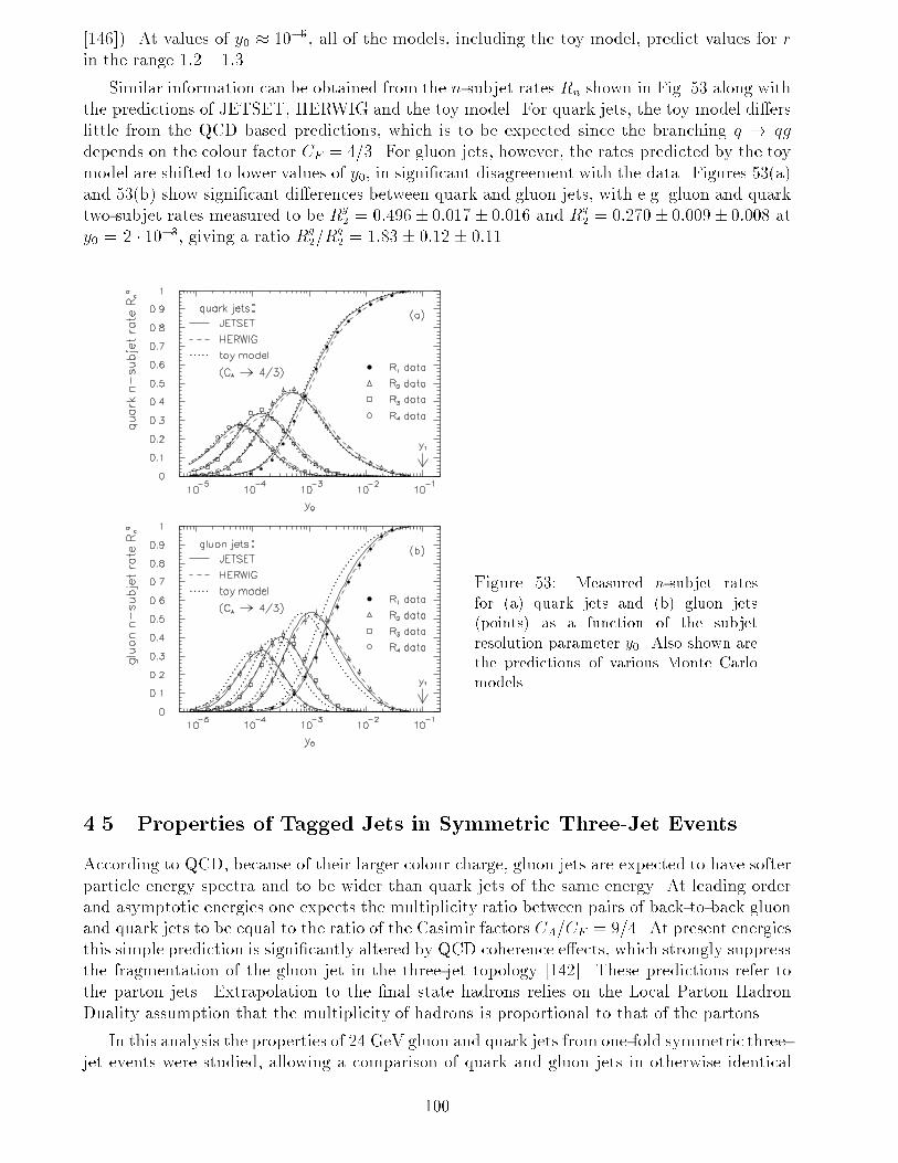
[146]). At values of y0 � 10�5, all of the models, including the toy model, predict values for r

in the range 1:2 { 1:3.

Similar information can be obtained from the n-subjet rates Rn shown in Fig. 53 along with

the predictions of JETSET, HERWIG and the toy model. For quark jets, the toy model di�ers

little from the QCD based predictions, which is to be expected since the branching q ! qg

depends on the colour factor CF = 4=3. For gluon jets, however, the rates predicted by the toy

model are shifted to lower values of y0, in signi�cant disagreement with the data. Figures 53(a)

and 53(b) show signi�cant di�erences between quark and gluon jets, with e.g. gluon and quark

two-subjet rates measured to be Rg2 = 0:496� 0:017� 0:016 and R

q2 = 0:270� 0:009� 0:008 at

y0 = 2 � 10�3, giving a ratio Rg2=R

q2 = 1:83 � 0:12 � 0:11.

Figure 53: Measured n-subjet rates

for (a) quark jets and (b) gluon jets

(points) as a function of the subjet

resolution parameter y0. Also shown are

the predictions of various Monte Carlo

models.

4.5 Properties of Tagged Jets in Symmetric Three-Jet Events

According to QCD, because of their larger colour charge, gluon jets are expected to have softer

particle energy spectra and to be wider than quark jets of the same energy. At leading order

and asymptotic energies one expects the multiplicity ratio between pairs of back-to-back gluon

and quark jets to be equal to the ratio of the Casimir factors CA=CF = 9=4. At present energies

this simple prediction is signi�cantly altered by QCD coherence e�ects, which strongly suppress

the fragmentation of the gluon jet in the three-jet topology [142]. These predictions refer to

the parton jets. Extrapolation to the �nal state hadrons relies on the Local Parton Hadron

Duality assumption that the multiplicity of hadrons is proportional to that of the partons.

In this analysis the properties of 24 GeV gluon and quark jets from one-fold symmetric three-

jet events were studied, allowing a comparison of quark and gluon jets in otherwise identical

100

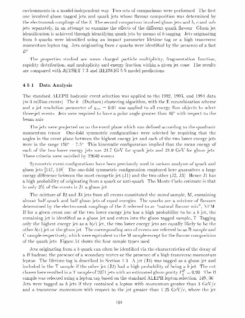
environments in a model-independent way. Two sets of comparisons were performed. The �rst

one involved gluon tagged jets and quark jets whose avour composition was determined by

the electroweak couplings of the Z. The second comparison involved gluon jets and b, c and uds

jets separately, in an attempt to examine the e�ects of the di�erent quark avour. Gluon jet

identi�cation is achieved through identifying quark jets by means of b tagging. Jets originating

from b quarks were identi�ed using an impact parameter lifetime tag or a high transverse

momentum lepton tag. Jets originating from c quarks were identi�ed by the presence of a fast

D�.

The properties studied are mean charged particle multiplicity, fragmentation function,

rapidity distribution, and multiplicity and energy fraction within a given jet cone. The results

are compared with JETSET 7.3 and HERWIG 5.5 model predictions.

4.5.1 Data Analysis

The standard ALEPH hadronic event selection was applied to the 1992, 1993, and 1994 data

(� 3 million events). The k? (Durham) clustering algorithm, with the E recombination scheme

and a jet resolution parameter of ycut = 0:01 was applied to all energy ow objects to select

three-jet events. Jets were required to have a polar angle greater than 40� with respect to the

beam axis.

The jets were projected on to the event plane which was de�ned according to the quadratic

momentum tensor. One-fold symmetric con�gurations were selected by requiring that the

angles in the event plane between the highest energy jet and each of the two lower energy jets

were in the range 150� � 7:5�. This kinematic con�guration implied that the mean energy of

each of the two lower energy jets was 24:7 GeV for quark jets and 24:0 GeV for gluon jets.

These criteria were satis�ed by 22640 events.

Symmetric event con�gurations have been previously used in various analyses of quark and

gluon jets [147, 148]. The one-fold symmetric con�guration employed here guarantees a large

energy di�erence between the most energetic jet (J1) and the two other (J2, J3). Hence J1 has

a high probability of originating from a quark or anti-quark. The Monte Carlo estimate is that

in only 3% of the events is J1 a gluon jet.

The mixture of J2 and J3 jets from all events constituted the mixed sample, M, containing

almost half quark and half gluon jets of equal energies. The quarks are a mixture of avours

determined by the electro-weak couplings of the Z referred to as \natural avour mix", NFM.

If for a given event one of the two lower energy jets has a high probability to be a b jet, the

remaining jet is identi�ed as a gluon jet and enters into the gluon tagged sample, T. Tagging

only the highest energy jet as a b(c) jet, the two lower energy jets are equally likely to be the

other b(c) jet or the gluon jet. The corresponding sets of events are referred to as B sample and

C sample respectively, which were equivalent to the M sample except for the avour composition

of the quark jets. Figure 54 shows the four sample types used.

Jets originating from a b quark can often be identi�ed via the characteristics of the decay of

a B hadron: the presence of a secondary vertex or the presence of a high transverse momentum

lepton. The lifetime tag is described in Section 1.3. A jet (J3) was tagged as a gluon jet and

included in the T sample if the other jet (J2) had a high probability of being a b jet. The cut

chosen here resulted in a T sample of 2071 jets with an estimated gluon purity P Tg = 0:90. The B

sample was selected using a lepton tag based on the standard ALEPH lepton selection [149, 36].

Jets were tagged as b jets if they contained a lepton with momentum greater than 3 GeV/c

and a transverse momentum with respect to the jet greater than 1.25 GeV/c, where the jet

101

q bb

Emax Emax Emax

(M) (T) (B)

θ

g

TAG

TAG

b b or gq or g g or q g or b

θ θ

(C)

θ

TAG

c

c or g g or c

Emax

Figure 54: The four tagging

con�gurations: the 50%

quark-gluon (M)ixed sample,

the gluon (T)agged sample,

and the (B)-quark and (C)-

quark enriched mixed samples.

direction was determined without the lepton. A lepton in the highest energy jet de�nes the B

sample, which contains 436 events and the avour composition is: 88% b, 6.1% c and 5% uds.

The �nal event sample, C, was selected by requiring the presence of a high momentum D� inthe highest energy jet. The D� were reconstructed via their D� ! D0� decay with subsequent

D0 ! K� decays, as described in [150]. Their energy was required to be more than 20 GeV.

The selected sample consists of 70 � 3% c events and no light quark events [151]. From the

22640 symmetric events, only 20 contained such a fast D�.

4.5.2 Unfolding of the Jet Properties

The analysis is based on the comparison of jets which have had no tagging criteria applied

directly to them. Hence the bias introduced by the tagging method is kept to a minimum.

Pure quark and gluon jet properties can be extracted from the four samples via a simple

unfolding procedure if the quark avour composition and the gluon purity of the samples are

known. These parameters were estimated from JETSET Monte Carlo events.

The gluon purity, de�ned as the ratio of the number of correctly tagged gluon jets over the

number of jets tagged as gluon jets, was estimated fromMonte Carlo events using the procedure

described in [152] to relate each reconstructed jet to its parent parton. For the chosen topology

a unique assignment was found in 99% of all cases.

For a jet sample whose gluon purity and fractions of the di�erent quark avours have been

estimated to be Pg and Puds, Pb, Pc, respectively, the measured value of an observable A may

be expressed as

A = Pg Ag + PudsAuds + PcAc + PbAb ; (82)

where Ag(q) is the corresponding value for pure gluon (quark) jets. The four di�erent samples

M, T, B and C yield four such equations which can be solved simultaneously allowing a direct

comparison of the properties of the gluon and the di�erent avour quark jets. The high statistics

samples, M and T, can also be used together as the quark avour composition of the T sample

was tuned to be similar to the M composition, to relate gluon jet and NFM quark jet properties.

Ideally, the samples should consist of events where the jets are produced in the same

kinematical con�gurations and the tagging procedure should not introduce a bias. While

(almost) identical kinematics are ensured by using symmetric events, the existence of a tagging

bias cannot be excluded. Using JETSET Monte Carlo events, bias corrections factors were

determined by comparing the value of the observable Ag(q) from the sample of all gluon (quark)

jets in the symmetric con�guration (i.e., from the M sample) to the value ABiasg(q) measured from

correctly identi�ed gluon (quark) jets from the tagged samples. Only in the properties of the

102

jets in the T sample a small bias, typically less than 2%, was found. In the case of the quark

and gluons in the B and C samples the bias was determined to be zero within the Monte Carlo

statistics.

The unfolded results were �nally corrected for detector e�ects. These were estimated by

comparing the properties of quark and gluon jets generated by the JETSET model before

and after detector simulation. These corrections carried statistical and systematic (model

dependent) errors. The latter were estimated by comparing the detector correction factors

extracted from the JETSET and HERWIG models.

4.5.3 Measured Quark and Gluon Jet Properties

The results discussed below are presented with statistical and systematic errors. The systematic

errors include contributions from the evaluation of the gluon purity, the avour composition of

the various samples, the tagging bias and the detector corrections. The dominant uncertainties,

2{5% in the central region of the distributions, come from the latter two.

The raw charged particle multiplicities measured for the jets in the respective samples are

hnT i = 8:230 � 0:069, hnM i = 7:686 � 0:015, hnBi = 8:042 � 0:101 and hnCi = 7:842 � 0:558.

The unfolded values, corrected for bias and detector e�ects are: hngluoni = 9:90 � 0:10(stat)�0:27(syst), hnudsi = 7:90 � 0:44(stat) � 0:26(syst), hnbi = 9:32 � 0:27(stat) � 0:27(syst) and

hnci = 8:37�1:64(stat)�0:28(syst). The di�erence between b and light-quark jet multiplicities

is consistent with the result of ref. [153]. For the natural avour mix at the Z one �nds

hnNFM (quark)i = 8:286 � 0:09(stat) � 0:22(syst). The ratios Rg=q between gluon and quark

multiplicities are obtained as

Rg=NFM = 1:194 � 0:027(stat)� 0:019(syst)

Rg=uds = 1:249 � 0:084(stat)� 0:022(syst)

Rg=b = 1:060 � 0:041(stat)� 0:020(syst)

Rg=c = 1:183 � 0:221(stat)� 0:021(syst)

The result Rg=NFM is signi�cantly larger than unity; it agrees with other LEP results [147],

con�rming the higher charged particle multiplicity of gluon jets. It is signi�cantly lower than the

naive asymptotic prediction of CA=CF = 9=4. The JETSET Monte Carlo predicts hngluoni =10:16 and hnNFM i = 7:92 leading to a ratio of Rg=NFM = 1:28 (with negligible statistical errors).

The same analysis with the HERWIG Monte Carlo model yields hngluoni = 9:48, hnNFMi = 7:63

and Rg=NFM = 1:24. Finally the multiplicity ratio was determined at the parton-level of the

JETSET Monte Carlo. The result, Rpart = 1:29, is again very similar to the hadron-level result,

suggesting that the observed di�erence between quark and gluon jets does have a perturbative

origin.

The measurement of Rg=b indicates that for the energy scales involved, the additional particle

multiplicity arising from the B hadron decay masks the di�erence between b quark and gluon

jet multiplicity. This e�ect is present in JETSET and HERWIG which give Rg=b = 1:077 and

Rg=b = 1:003 respectively. These measurements are also in agreement with recent results given

in [154]. The unfolded ratio of gluon to light quark multiplicity is hence greater than the

corresponding gluon/NFM quark ratio. The prediction for Rg=uds from JETSET and HERWIG

are Rg=uds=1.377 and Rg=uds=1.344 respectively, i.e somewhat higher but within the errors of

that measured. The large statistical errors do not allow �rm conclusions about the gluon to c

quark multiplicity ratio.

103

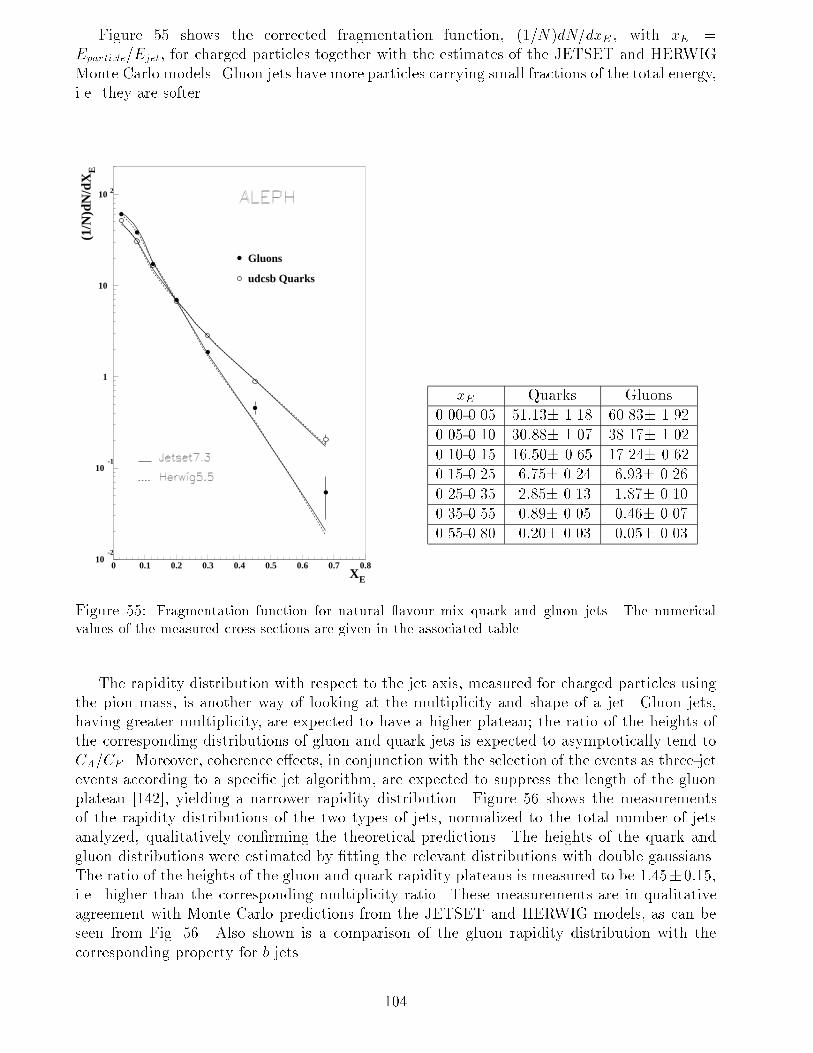
Figure 55 shows the corrected fragmentation function, (1=N)dN=dxE , with xE =

Eparticle=Ejet, for charged particles together with the estimates of the JETSET and HERWIG

Monte Carlo models. Gluon jets have more particles carrying small fractions of the total energy,

i.e. they are softer.

10-2

10-1

1

10

10 2

0 0.1 0.2 0.3 0.4 0.5 0.6 0.7 0.8

Gluons

udcsb Quarks

XE

(1/N

)dN

/dX

E

xE Quarks Gluons

0.00-0.05 51:13� 1.18 60.83� 1.92

0.05-0.10 30:88� 1.07 38.17� 1.02

0.10-0.15 16:50� 0.65 17.24� 0.62

0.15-0.25 6:75� 0.24 6:93� 0.26

0.25-0.35 2:85� 0.13 1:87� 0.10

0.35-0.55 0:89� 0.05 0:46� 0.07

0.55-0.80 0:20� 0.03 0:05� 0.03

Figure 55: Fragmentation function for natural avour mix quark and gluon jets. The numerical

values of the measured cross sections are given in the associated table.

The rapidity distribution with respect to the jet axis, measured for charged particles using

the pion mass, is another way of looking at the multiplicity and shape of a jet. Gluon jets,

having greater multiplicity, are expected to have a higher plateau; the ratio of the heights of

the corresponding distributions of gluon and quark jets is expected to asymptotically tend to

CA=CF . Moreover, coherence e�ects, in conjunction with the selection of the events as three-jet

events according to a speci�c jet algorithm, are expected to suppress the length of the gluon

plateau [142], yielding a narrower rapidity distribution. Figure 56 shows the measurements

of the rapidity distributions of the two types of jets, normalized to the total number of jets

analyzed, qualitatively con�rming the theoretical predictions. The heights of the quark and

gluon distributions were estimated by �tting the relevant distributions with double gaussians.

The ratio of the heights of the gluon and quark rapidity plateaus is measured to be 1:45�0:15,

i.e. higher than the corresponding multiplicity ratio. These measurements are in qualitative

agreement with Monte Carlo predictions from the JETSET and HERWIG models, as can be

seen from Fig. 56. Also shown is a comparison of the gluon rapidity distribution with the

corresponding property for b jets.

104

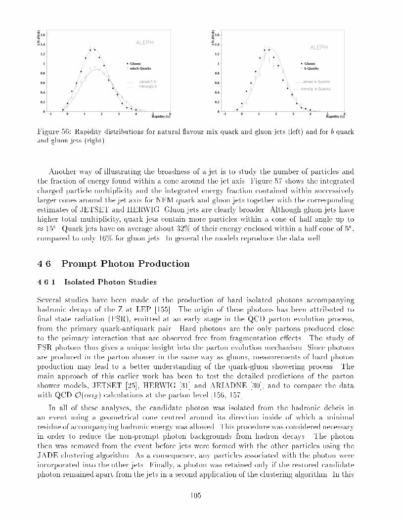
0

0.2

0.4

0.6

0.8

1

1.2

1.4

1.6

-1 0 1 2 3 4 5 6Rapidity (η)

1/N

dN

/dη

Gluonsudscb Quarks

0

0.2

0.4

0.6

0.8

1

1.2

1.4

1.6

-1 0 1 2 3 4 5 6Rapidity (η)

1/N

dN

/dη

Gluonsb Quarks

Figure 56: Rapidity distributions for natural avour mix quark and gluon jets (left) and for b quark

and gluon jets (right).

Another way of illustrating the broadness of a jet is to study the number of particles and

the fraction of energy found within a cone around the jet axis. Figure 57 shows the integrated

charged particle multiplicity and the integrated energy fraction contained within successively

larger cones around the jet axis for NFM quark and gluon jets together with the corresponding

estimates of JETSET and HERWIG. Gluon jets are clearly broader. Although gluon jets have

higher total multiplicity, quark jets contain more particles within a cone of half angle up to

� 15�. Quark jets have on average about 32% of their energy enclosed within a half cone of 5�,compared to only 16% for gluon jets. In general the models reproduce the data well.

4.6 Prompt Photon Production

4.6.1 Isolated Photon Studies

Several studies have been made of the production of hard isolated photons accompanying

hadronic decays of the Z at LEP [155]. The origin of these photons has been attributed to

�nal state radiation (FSR), emitted at an early stage in the QCD parton evolution process,

from the primary quark-antiquark pair. Hard photons are the only partons produced close

to the primary interaction that are observed free from fragmentation e�ects. The study of

FSR photons thus gives a unique insight into the parton evolution mechanism. Since photons

are produced in the parton shower in the same way as gluons, measurements of hard photon

production may lead to a better understanding of the quark-gluon showering process. The

main approach of this earlier work has been to test the detailed predictions of the parton

shower models, JETSET [25], HERWIG [31] and ARIADNE [30], and to compare the data

with QCD O(��S) calculations at the parton level [156, 157]

In all of these analyses, the candidate photon was isolated from the hadronic debris in

an event using a geometrical cone centred around its direction inside of which a minimal

residue of accompanying hadronic energy was allowed. This procedure was considered necessary

in order to reduce the non-prompt photon backgrounds from hadron decays. The photon

then was removed from the event before jets were formed with the other particles using the

JADE clustering algorithm. As a consequence, any particles associated with the photon were

incorporated into the other jets. Finally, a photon was retained only if the restored candidate

photon remained apart from the jets in a second application of the clustering algorithm. In this

105

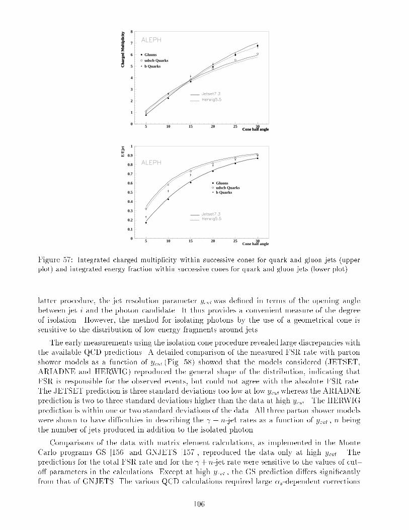
0

1

2

3

4

5

6

7

8

5 10 15 20 25 30

Gluons

Cone half angle

Cha

rged

Mul

tiplic

ity

udscb Quarks

Cone half angle

Cha

rged

Mul

tiplic

ity

b Quarks

0

0.1

0.2

0.3

0.4

0.5

0.6

0.7

0.8

0.9

1

5 10 15 20 25 30

Gluons

Cone half angle

E/E

jet

udscb Quarksb Quarks

Figure 57: Integrated charged multiplicity within successive cones for quark and gluon jets (upper

plot) and integrated energy fraction within successive cones for quark and gluon jets (lower plot).

latter procedure, the jet resolution parameter ycutwas de�ned in terms of the opening angle

between jet i and the photon candidate. It thus provides a convenient measure of the degree

of isolation. However, the method for isolating photons by the use of a geometrical cone is

sensitive to the distribution of low energy fragments around jets.

The early measurements using the isolation cone procedure revealed large discrepancies with

the available QCD predictions. A detailed comparison of the measured FSR rate with parton

shower models as a function of ycut (Fig. 58) showed that the models considered (JETSET,

ARIADNE and HERWIG) reproduced the general shape of the distribution, indicating that

FSR is responsible for the observed events, but could not agree with the absolute FSR rate.

The JETSET prediction is three standard deviations too low at low ycut whereas the ARIADNE

prediction is two to three standard deviations higher than the data at high ycut . The HERWIG

prediction is within one or two standard deviations of the data. All three parton shower models

were shown to have di�culties in describing the + n-jet rates as a function of ycut , n being

the number of jets produced in addition to the isolated photon.

Comparisons of the data with matrix element calculations, as implemented in the Monte

Carlo programs GS [156] and GNJETS [157], reproduced the data only at high ycut . The

predictions for the total FSR rate and for the + n-jet rate were sensitive to the values of cut-

o� parameters in the calculations. Except at high ycut , the GS prediction di�ers signi�cantly

from that of GNJETS. The various QCD calculations required large �s-dependent corrections

106

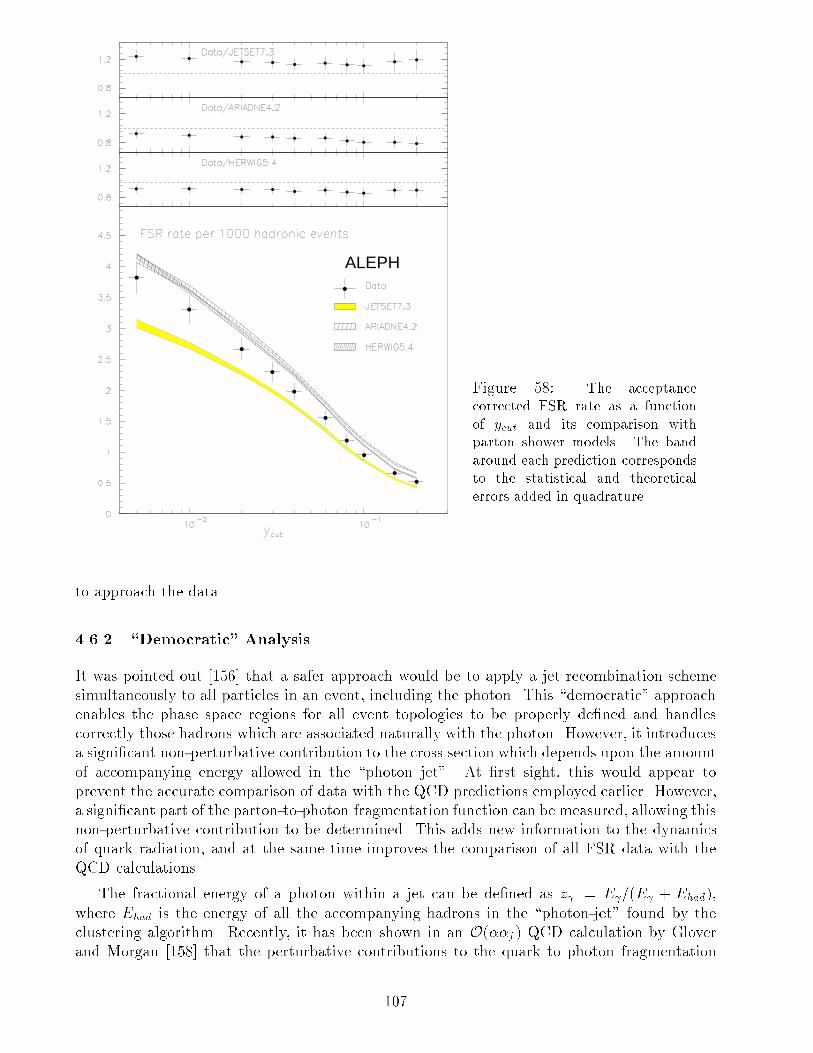
ALEPH

Figure 58: The acceptance

corrected FSR rate as a function

of ycut and its comparison with

parton shower models. The band

around each prediction corresponds

to the statistical and theoretical

errors added in quadrature.

to approach the data.

4.6.2 \Democratic" Analysis

It was pointed out [156] that a safer approach would be to apply a jet recombination scheme

simultaneously to all particles in an event, including the photon. This \democratic" approach

enables the phase space regions for all event topologies to be properly de�ned and handles

correctly those hadrons which are associated naturally with the photon. However, it introduces

a signi�cant non-perturbative contribution to the cross section which depends upon the amount

of accompanying energy allowed in the \photon jet". At �rst sight, this would appear to

prevent the accurate comparison of data with the QCD predictions employed earlier. However,

a signi�cant part of the parton-to-photon fragmentation function can be measured, allowing this

non-perturbative contribution to be determined. This adds new information to the dynamics

of quark radiation, and at the same time improves the comparison of all FSR data with the

QCD calculations.

The fractional energy of a photon within a jet can be de�ned as z = E =(E + Ehad),

where Ehad is the energy of all the accompanying hadrons in the \photon-jet" found by the

clustering algorithm. Recently, it has been shown in an O(��s ) QCD calculation by Glover

and Morgan [158] that the perturbative contributions to the quark to photon fragmentation

107

function, D(z ), can be evaluated, thus allowing the non-perturbative part of the D(z )

function to be determined from the data. At the Z, the measured value of D(z ) is the average

of the D(z ) functions for the combination of the two u-type and three d-type quark avours

weighted by their respective electro-weak couplings and electric charges. Thus, D(z ) can be

obtained from the normalized di�erential two-jet cross section:

1

�had

d�(2-jet)

dz = D(z )GLEP

where GLEP is twice the ratio of the FSR correction to the total hadronic cross section at the

Z. From currently measured values [159] GLEP = 2:51�10�4. This normalization does not take

into account any other source of avour dependence in the fragmentation function.

Selection of Events with Final State Photons

For the \democratic analysis" the hadronic Z decays were selected using standard procedures

described in Section 1.3. The overall e�ciency of the photon selection is 55�2:4% and is almost

independent of the energy of the photon. The contribution from non-prompt photons, mainly

�0's, is determined from Monte Carlo. The accuracy of this simulation was studied in [160].

For each event with at least one selected photon, jets were constructed using all the energy ow

objects of the event and treating the photon equally with all the other particles. The particle

clustering was performed using the Durham algorithm [28]. An event was kept if at least one

jet contained a selected photon with z > 0:7. This procedure was repeated successively for

thirteen di�erent ycut values increasing from 0.001 to 0.33. For each value of ycut , the event

sample then was divided into three categories corresponding to jet topologies of two, three and

� 4 jets, where the number of jets includes the photon jet.

Since the non-perturbative part of D(z ) is naturally associated with the hadronization

process, the measured jet rates are not corrected back to the parton level.

Analysis of Two-Jet Events

At the primary parton level, two-jet topologies correspond to qq events where either the q

and q coalesce to form one jet or one of the quarks radiates (or fragments into) a photon which

remains part of the quark jet. In the absence of radiated gluons, the �rst case leads to completely

isolated photons with z = 1 whereas the second populates the full z distribution. Thus, it is

expected that the quark-to-photon fragmentation function, D(z ), will decrease monotonically

towards z = 1 where the isolated component becomes the principal contribution.

Figure 59 shows the corrected di�erential z distributions normalized to the total hadronic

event sample for four values of ycut . A downward trend is observed up to z = 0:95, and

the isolated photon peak in the �nal bin 0:99 < z < 1:0 is clearly evident. However, it

appears that a fraction of this isolated component populates the 0:95 < z < 0:99 bin. This

broadening e�ect becomes more pronounced with increasing ycut . Both the ARIADNE and

HERWIG parton-shower Monte Carlos ascribe this to the association of soft hadrons produced

in the parton shower to the photon jet by the clustering algorithm. No such e�ect is observed

at the parton level. This is the only portion of the z distribution where signi�cant di�erences

between hadron and parton levels appear.

108

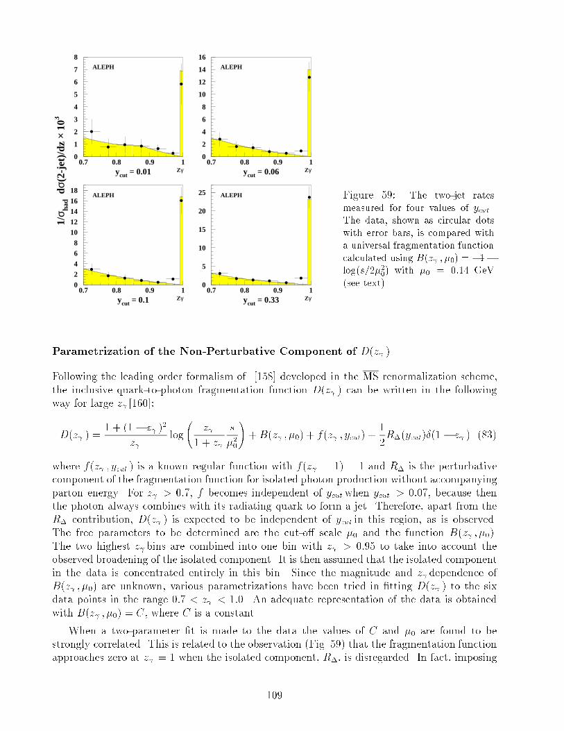
0

1

2

3

4

5

6

7

8

0.7 0.8 0.9 10

2

4

6

8

10

12

14

16

0.7 0.8 0.9 1

0

24

68

1012

1416

18

0.7 0.8 0.9 10

5

10

15

20

25

0.7 0.8 0.9 1

1/σ ha

d d

σ(2-

jet)

/dz

× 10

3

Zγycut = 0.01

ALEPH

Zγycut = 0.06

ALEPH

Zγycut = 0.1

ALEPH

Zγycut = 0.33

ALEPH Figure 59: The two-jet rates

measured for four values of ycut .

The data, shown as circular dots

with error bars, is compared with

a universal fragmentation function

calculated using B(z ; �0) = �1�log(s=2�20) with �0 = 0:14 GeV

(see text).

Parametrization of the Non-Perturbative Component of D(z )

Following the leading order formalism of [158] developed in the MS renormalization scheme,

the inclusive quark-to-photon fragmentation function D(z ) can be written in the following

way for large z [160]:

D(z ) =1 + (1� z )

2

z log

z

1 + z

s

�20

!+B(z ; �0) + f(z ; ycut) +

1

2R�(ycut)�(1� z ) (83)

where f(z ; ycut ) is a known regular function with f(z = 1) = 1 and R� is the perturbative

component of the fragmentation function for isolated photon production without accompanying

parton energy. For z > 0:7, f becomes independent of ycut when ycut > 0:07, because then

the photon always combines with its radiating quark to form a jet. Therefore, apart from the

R� contribution, D(z ) is expected to be independent of ycut in this region, as is observed.

The free parameters to be determined are the cut-o� scale �0 and the function B(z ; �0).

The two highest z bins are combined into one bin with z > 0:95 to take into account the

observed broadening of the isolated component. It is then assumed that the isolated component

in the data is concentrated entirely in this bin. Since the magnitude and z dependence of

B(z ; �0) are unknown, various parametrizations have been tried in �tting D(z ) to the six

data points in the range 0:7 < z < 1:0. An adequate representation of the data is obtained

with B(z ; �0) = C, where C is a constant.

When a two-parameter �t is made to the data the values of C and �0 are found to be

strongly correlated. This is related to the observation (Fig. 59) that the fragmentation function

approaches zero at z = 1 when the isolated component, R�, is disregarded. In fact, imposing

109

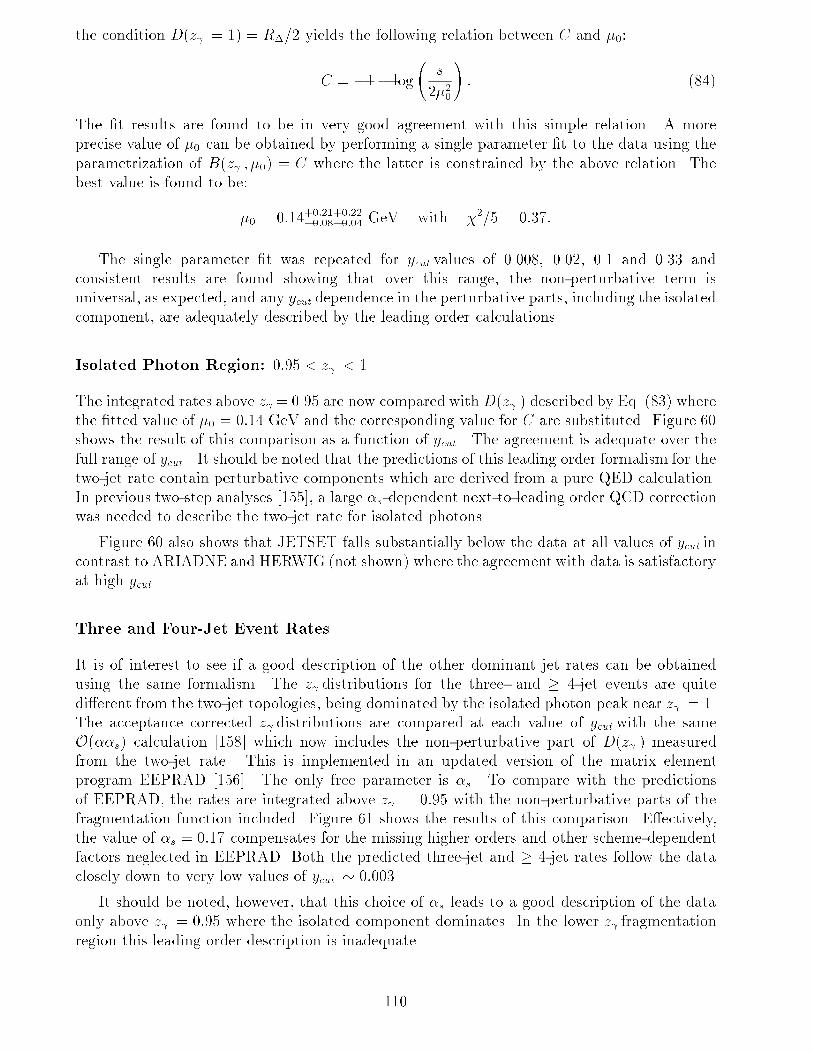
the condition D(z = 1) = R�=2 yields the following relation between C and �0:

C = �1� log

s

2�20

!: (84)

The �t results are found to be in very good agreement with this simple relation. A more

precise value of �0 can be obtained by performing a single parameter �t to the data using the

parametrization of B(z ; �0) = C where the latter is constrained by the above relation. The

best value is found to be:

�0 = 0:14+0:21+0:22�0:08�0:04 GeV with �2=5 = 0:37:

The single parameter �t was repeated for ycut values of 0.008, 0.02, 0.1 and 0.33 and

consistent results are found showing that over this range, the non-perturbative term is

universal, as expected, and any ycut dependence in the perturbative parts, including the isolated

component, are adequately described by the leading order calculations.

Isolated Photon Region: 0:95 < z < 1

The integrated rates above z = 0.95 are now compared withD(z ) described by Eq. (83) where

the �tted value of �0 = 0:14 GeV and the corresponding value for C are substituted. Figure 60

shows the result of this comparison as a function of ycut . The agreement is adequate over the

full range of ycut . It should be noted that the predictions of this leading order formalism for the

two-jet rate contain perturbative components which are derived from a pure QED calculation.

In previous two-step analyses [155], a large �s-dependent next-to-leading order QCD correction

was needed to describe the two-jet rate for isolated photons.

Figure 60 also shows that JETSET falls substantially below the data at all values of ycut in

contrast to ARIADNE and HERWIG (not shown) where the agreement with data is satisfactory

at high ycut .

Three and Four-Jet Event Rates

It is of interest to see if a good description of the other dominant jet rates can be obtained

using the same formalism. The z distributions for the three- and � 4-jet events are quite

di�erent from the two-jet topologies, being dominated by the isolated photon peak near z = 1.

The acceptance corrected z distributions are compared at each value of ycut with the same

O(��s) calculation [158] which now includes the non-perturbative part of D(z ) measured

from the two-jet rate. This is implemented in an updated version of the matrix element

program EEPRAD [156]. The only free parameter is �s. To compare with the predictions

of EEPRAD, the rates are integrated above z = 0:95 with the non-perturbative parts of the

fragmentation function included. Figure 61 shows the results of this comparison. E�ectively,

the value of �s = 0:17 compensates for the missing higher orders and other scheme-dependent

factors neglected in EEPRAD. Both the predicted three-jet and � 4-jet rates follow the data

closely down to very low values of ycut � 0:003.

It should be noted, however, that this choice of �s leads to a good description of the data

only above z = 0:95 where the isolated component dominates. In the lower z fragmentation

region this leading order description is inadequate.

110

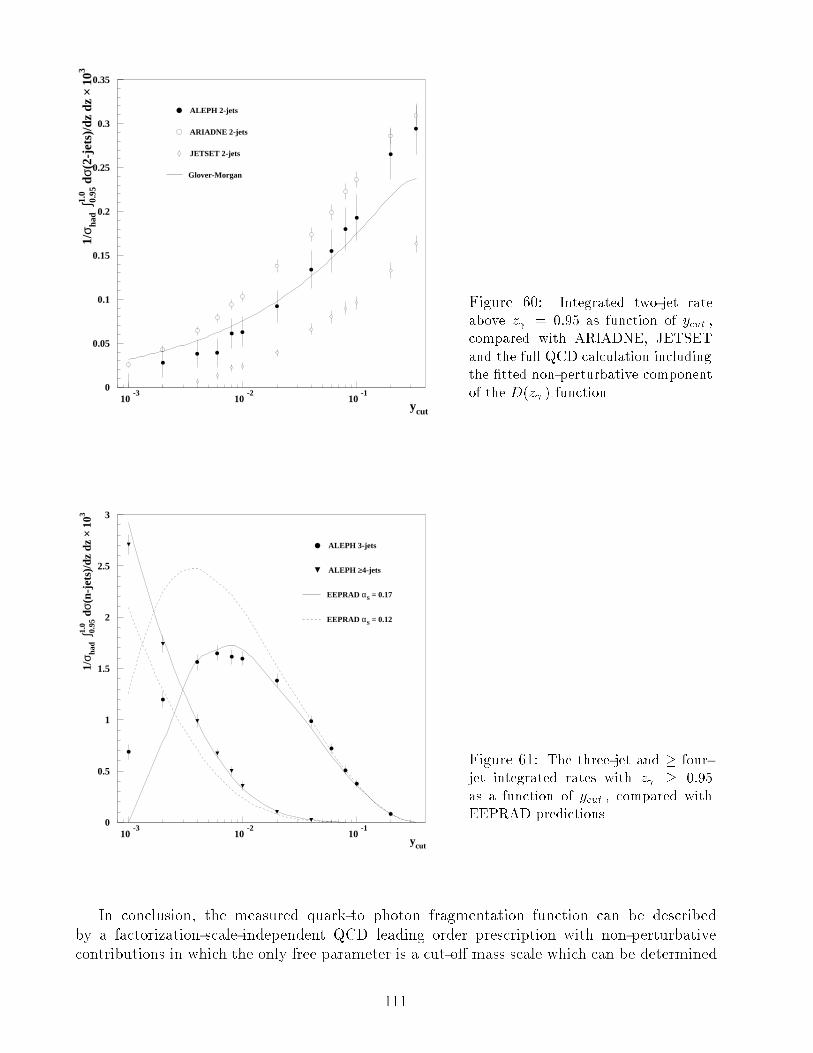
0

0.05

0.1

0.15

0.2

0.25

0.3

0.35

10-3

10-2

10-1

ALEPH 2-jets

ARIADNE 2-jets

JETSET 2-jets

Glover-Morgan

ycut

1/σ ha

d ∫1.

00.

95 d

σ(2-

jets

)/dz

dz ×

103

Figure 60: Integrated two-jet rate

above z = 0:95 as function of ycut ,

compared with ARIADNE, JETSET

and the full QCD calculation including

the �tted non-perturbative component

of the D(z ) function.

0

0.5

1

1.5

2

2.5

3

10-3

10-2

10-1

ALEPH 3-jets

ALEPH ≥4-jets

EEPRAD αS = 0.17

EEPRAD αS = 0.12

ycut

1/σ ha

d ∫1.

00.

95 d

σ(n-

jets

)/dz

dz ×

103

Figure 61: The three-jet and � four-

jet integrated rates with z � 0:95

as a function of ycut , compared with

EEPRAD predictions.

In conclusion, the measured quark-to photon fragmentation function can be described

by a factorization-scale-independent QCD leading order prescription with non-perturbative

contributions in which the only free parameter is a cut-o� mass scale which can be determined

111

from the data. A satisfactory description of all aspects of the measured two-jet rates then can

be found. The other dominant jet rates can be described using the same formalism with a large

value of �s to take into account uncalculated higher orders.

112

5 Hadronization

A measurement of the composition of the hadronic �nal state in e+e� annihilation is

fundamental to an understanding of the fragmentation of quarks and gluons into hadrons. While

no calculable theory yet exists for this process, a number of phenomenological models have

evolved, falling into two broad classes: \string" fragmentation and \cluster" fragmentation, as

exempli�ed by the JETSET [25] and HERWIG [31] Monte Carlos, respectively. The models

contain a large number of parameters controlling the spin/ avour assignment of the produced

hadrons. As already discussed in Section 2.3, these parameters have been tuned using the data

presented in this section. Therefore, one can speak of \model predictions" only in a restricted

sense. Nevertheless, it is important to see how well all measurements are described within the

framework of a certain model.

In the model calculations three di�erent sources for the observed hadrons can be

distinguished: leading particles containing the initial quark of the Z ! q�q decay, direct

fragmentations products and decay products of heavier particles. Since the production of

heavy quarks in the fragmentation chain is strongly suppressed, hadrons containing b or c

quarks are expected to be leading particles or decay products of them. The ALEPH results

on bottom and charm production from Z decay have been discussed elsewhere [35, 36, 37].

In this section experimental results on the inclusive production of identi�ed light hadrons are

presented, summing over all initial quark avours and all sources. In the �rst section, 5.1, a

search for free quarks is presented.

5.1 Search for Free Quarks

Quarks cannot exist as free particles and therefore fragment into the well known hadrons. As

a prelude to the study of these hadrons in this section, the test of this fundamental property

of QCD by ALEPH in the early days of LEP is reviewed brie y.

The ALEPH search for free quarks [6] was performed with the data from the years 1989 and

1990, corresponding to about 180,000 Z events, using the ionization measurement of charged

particles in the TPC. ParticlesX with unexpected ionization such as free quarks with fractional

charge or heavy particles were searched for. At the Z peak, quarks are produced with high

momenta and might become free without contradicting earlier limits. The search is valid for

particles which are long-lived and have an interaction length comparable to or larger than that

of the known stable hadrons, so that they are observable in the TPC.

The particles X for which limits were derived could appear in pairs, inclusively with jets

(e+e� ! X �X + hadrons) or exclusively. Also the case in which the particle could appear

singly along with other hadronic activity and in which conservation laws would be maintained

via production of a low mass partner were studied.

In the data, no candidates were found for masses above 5 GeV/c2. The limit for the

production of new charged particles can be expressed in terms of the dimuon cross section.

The 90% C.L. limits [6] are shown in Fig. 62 for the inclusive production of charged particles

with unexpected mass and charge, assuming a momentum distribution for the new particles

according to E dNdp3

= const. This can be considered as a parametrization for the fragmentation

function for the production of massive particles (see [6] for an alternative assumption and for

further references). It is seen that these results extend the limits given by previous experiments

into the mass range 15 { 45 GeV/c2.

113

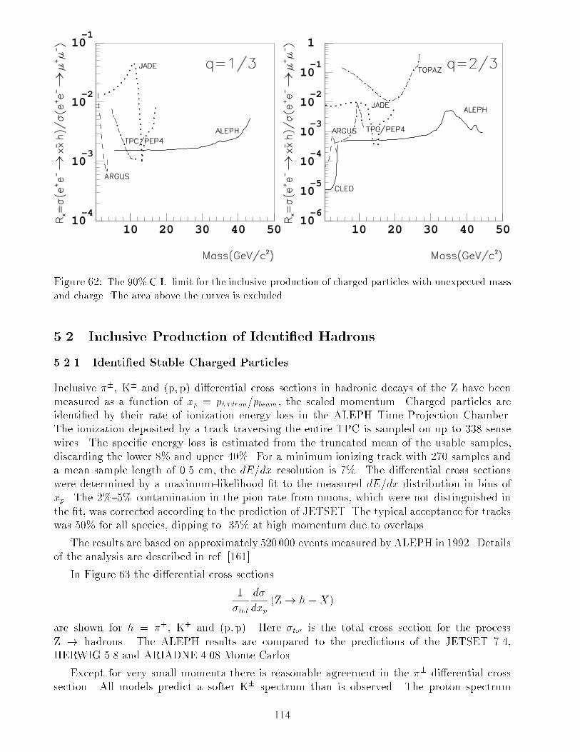
10-4

10-3

10-2

10-1

10 20 30 40 5010-6

10-5

10-4

10-3

10-2

10-1

1

10 20 30 40 50

Figure 62: The 90% C.L. limit for the inclusive production of charged particles with unexpected mass

and charge. The area above the curves is excluded.

5.2 Inclusive Production of Identi�ed Hadrons

5.2.1 Identi�ed Stable Charged Particles

Inclusive ��, K� and (p; �p) di�erential cross sections in hadronic decays of the Z have been

measured as a function of xp = phadron=pbeam, the scaled momentum. Charged particles are

identi�ed by their rate of ionization energy loss in the ALEPH Time Projection Chamber.

The ionization deposited by a track traversing the entire TPC is sampled on up to 338 sense

wires. The speci�c energy loss is estimated from the truncated mean of the usable samples,

discarding the lower 8% and upper 40%. For a minimum ionizing track with 270 samples and

a mean sample length of 0.5 cm, the dE=dx resolution is 7%. The di�erential cross sections

were determined by a maximum-likelihood �t to the measured dE=dx distribution in bins of

xp. The 2%{5% contamination in the pion rate from muons, which were not distinguished in

the �t, was corrected according to the prediction of JETSET. The typical acceptance for tracks

was 50% for all species, dipping to 35% at high momentum due to overlaps.

The results are based on approximately 520 000 events measured by ALEPH in 1992. Details

of the analysis are described in ref. [161].

In Figure 63 the di�erential cross sections

1

�tot

d�

dxp(Z! h+X)

are shown for h = ��, K� and (p; �p). Here �tot is the total cross section for the process

Z ! hadrons. The ALEPH results are compared to the predictions of the JETSET 7.4,

HERWIG 5.8 and ARIADNE 4.08 Monte Carlos.

Except for very small momenta there is reasonable agreement in the �� di�erential cross

section. All models predict a softer K� spectrum than is observed. The proton spectrum

114

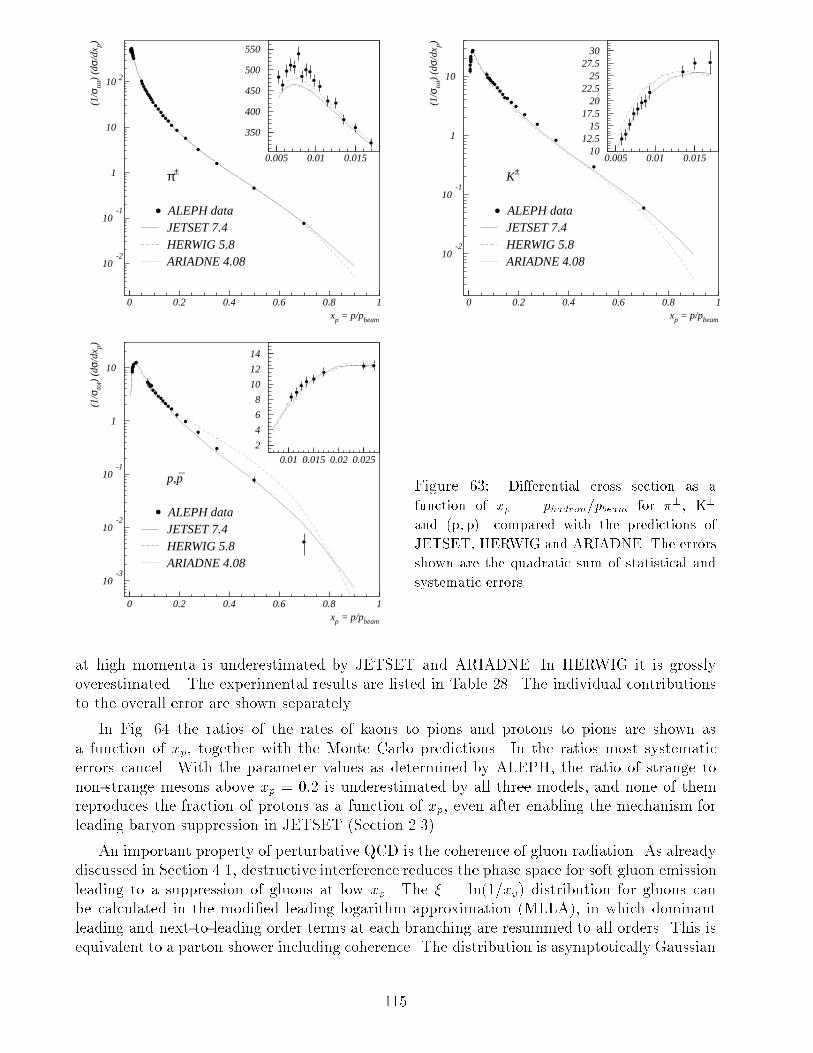
10-2

10-1

1

10

10 2

0 0.2 0.4 0.6 0.8 1xp = p/pbeam

(1/σ

tot)

(dσ/

dx p)

350

400

450

500

550

0.005 0.01 0.015

ALEPH dataJETSET 7.4HERWIG 5.8ARIADNE 4.08

π±

10-2

10-1

1

10

0 0.2 0.4 0.6 0.8 1xp = p/pbeam

(1/σ

tot)

(dσ/

dx p)

1012.5

1517.5

2022.5

2527.5

30

0.005 0.01 0.015

ALEPH dataJETSET 7.4HERWIG 5.8ARIADNE 4.08

K±

10-3

10-2

10-1

1

10

0 0.2 0.4 0.6 0.8 1xp = p/pbeam

(1/σ

tot)

(dσ/

dx p)

2

4

6

8

10

12

14

0.01 0.015 0.02 0.025

ALEPH dataJETSET 7.4HERWIG 5.8ARIADNE 4.08

p,p̄Figure 63: Differential cross section as a

function of xp = phadron=pbeam for ��, K�

and (p; �p) compared with the predictions of

JETSET, HERWIG and ARIADNE. The errors

shown are the quadratic sum of statistical and

systematic errors.

at high momenta is underestimated by JETSET and ARIADNE. In HERWIG it is grossly

overestimated . The experimental results are listed in Table 28. The individual contributions

to the overall error are shown separately.

In Fig. 64 the ratios of the rates of kaons to pions and protons to pions are shown as

a function of xp, together with the Monte Carlo predictions. In the ratios most systematic

errors cancel. With the parameter values as determined by ALEPH, the ratio of strange to

non-strange mesons above xp = 0:2 is underestimated by all three models, and none of them

reproduces the fraction of protons as a function of xp, even after enabling the mechanism for

leading baryon suppression in JETSET (Section 2.3).

An important property of perturbative QCD is the coherence of gluon radiation. As already

discussed in Section 4.1, destructive interference reduces the phase space for soft gluon emission

leading to a suppression of gluons at low xp. The � = ln(1=xp) distribution for gluons can

be calculated in the modi�ed leading logarithm approximation (MLLA), in which dominant

leading and next-to-leading order terms at each branching are resummed to all orders. This is

equivalent to a parton shower including coherence. The distribution is asymptotically Gaussian

115

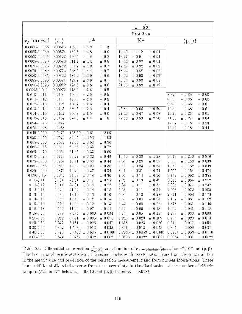
1�tot

d�dxp

xp interval hxpi �� K� (p; �p)0.0050-0.0055 0.00526 482.9 � 5.9 � 1.3

0.0055-0.0060 0.00574 462.6 � 4.8 � 0.9 12.40 � 1.12 � 0.01

0.0060-0.0065 0.00622 496.5 � 4.6 � 0.8 13.27 � 0.91 � 0.01

0.0065-0.0070 0.00673 511.2 � 4.4 � 0.8 15.33 � 0.90 � 0.01

0.0070-0.0075 0.00722 507.7 � 4.2 � 0.7 17.43 � 0.92 � 0.02

0.0075-0.0080 0.00773 538.5 � 4.4 � 0.7 18.33 � 0.88 � 0.02

0.0080-0.0085 0.00822 484.2 � 3.9 � 0.6 19.62 � 0.90 � 0.02

0.0085-0.0090 0.00871 499.7 � 3.9 � 0.7 20.02 � 0.86 � 0.05

0.0090-0.0095 0.00922 494.6 � 3.8 � 0.6 21.66 � 0.88 � 0.12

0.0095-0.010 0.00972 473.9 � 3.6 � 0.5

0.010-0.011 0.0105 460.9 � 2.5 � 0.5 8.32 � 0.35 � 0.00

0.011-0.012 0.0115 425.6 � 2.3 � 0.5 8.95 � 0.36 � 0.00

0.012-0.013 0.0125 420.7 � 2.3 � 0.4 9.80 � 0.36 � 0.01

0.013-0.014 0.0135 380.5 � 2.2 � 0.4 25.84 � 0.66 � 0.50 10.30 � 0.38 � 0.01

0.014-0.016 0.0147 360.8 � 1.5 � 0.6 27.46 � 0.47 � 0.68 10.70 � 0.26 � 0.01

0.016-0.018 0.0167 324.0 � 1.4 � 1.8 27.63 � 0.53 � 2.20 11.58 � 0.27 � 0.04

0.024-0.026 0.0247 12.37 � 0.18 � 0.23

0.026-0.028 0.0268 12.46 � 0.18 � 0.44

0.045-0.050 0.0470 103.96 � 0.61 � 2.09

0.050-0.055 0.0520 89.95 � 0.53 � 1.02

0.055-0.060 0.0570 78.96 � 0.50 � 0.90

0.060-0.065 0.0619 69.36 � 0.35 � 0.72

0.065-0.070 0.0669 61.35 � 0.33 � 0.60

0.070-0.075 0.0719 55.27 � 0.32 � 0.49 10.60 � 0.30 � 1.28 5.315 � 0.216 � 0.876

0.075-0.080 0.0769 49.91 � 0.30 � 0.44 9.53 � 0.26 � 0.98 5.008 � 0.183 � 0.639

0.080-0.085 0.0819 44.33 � 0.29 � 0.38 9.15 � 0.23 � 0.83 4.445 � 0.162 � 0.549

0.085-0.090 0.0870 40.24 � 0.27 � 0.34 8.41 � 0.21 � 0.71 4.555 � 0.154 � 0.474

0.090-0.10 0.0942 35.38 � 0.18 � 0.30 7.96 � 0.14 � 0.56 3.742 � 0.092 � 0.355

0.10-0.11 0.104 29.51 � 0.17 � 0.25 7.26 � 0.13 � 0.47 3.355 � 0.084 � 0.292

0.11-0.12 0.114 24.91 � 0.16 � 0.22 6.34 � 0.11 � 0.37 2.905 � 0.077 � 0.232

0.12-0.13 0.124 21.06 � 0.14 � 0.18 5.63 � 0.11 � 0.32 2.653 � 0.072 � 0.205

0.13-0.14 0.134 18.16 � 0.13 � 0.16 4.94 � 0.10 � 0.28 2.371 � 0.068 � 0.178

0.14-0.15 0.144 15.46 � 0.12 � 0.15 4.39 � 0.09 � 0.24 2.137 � 0.064 � 0.162

0.15-0.16 0.154 13.64 � 0.12 � 0.13 4.22 � 0.09 � 0.22 1.878 � 0.061 � 0.146

0.16-0.18 0.169 11.00 � 0.07 � 0.11 3.63 � 0.06 � 0.18 1.696 � 0.041 � 0.118

0.18-0.20 0.189 8.484 � 0.066 � 0.094 3.10 � 0.05 � 0.15 1.299 � 0.036 � 0.099

0.20-0.25 0.222 5.621 � 0.035 � 0.071 2.245 � 0.029 � 0.109 0.966 � 0.020 � 0.073

0.25-0.30 0.272 3.181 � 0.026 � 0.047 1.538 � 0.025 � 0.076 0.614 � 0.017 � 0.054

0.30-0.40 0.342 1.563 � 0.013 � 0.028 0.841 � 0.013 � 0.043 0.305 � 0.009 � 0.031

0.40-0.60 0.476 0.4495 � 0.0051 � 0.0100 0.2936 � 0.0053 � 0.0146 0.0784 � 0.0034 � 0.0110

0.60-0.80 0.674 0.0767 � 0.0021 � 0.0021 0.0596 � 0.0022 � 0.0031 0.0054 � 0.0011 � 0.0022

Table 28: Di�erential cross section 1�tot

d�dxp

as a function of xp = phadron=pbeam for ��, K�and (p; �p).

The �rst error shown is statistical; the second includes the systematic errors from the uncertainties

in the mean value and resolution of the ionization measurement and from nuclear interactions. There

is an additional 3% relative error from the uncertainty in the distribution of the number of dE=dx

samples (5% for K� below xp = 0:010 and (p; �p) below xp = 0:018).

116

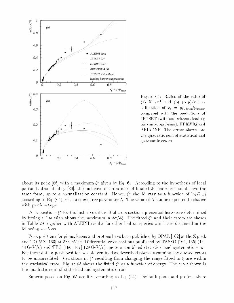
0

0.2

0.4

0.6

0.8

1

0 0.2 0.4 0.6 0.8 1xp = p/pbeam

ratio

K/π

0

0.1

0.2

0.3

0.4

0 0.2 0.4 0.6 0.8 1xp = p/pbeam

ratio

p/π

ALEPH data

JETSET 7.4

HERWIG 5.8

ARIADNE 4.08

JETSET 7.4 without

leading baryon suppression

(a)

(b)Figure 64: Ratios of the rates of

(a) K�=�� and (b) (p; �p)=�� as

a function of xp = phadron=pbeam,

compared with the predictions of

JETSET (with and without leading

baryon suppression), HERWIG and

ARIADNE. The errors shown are

the quadratic sum of statistical and

systematic errors.

about its peak [86] with a maximum �? given by Eq. 64. According to the hypothesis of local

parton-hadron duality [86], the inclusive distributions of �nal-state hadrons should have the

same form, up to a normalization constant. Hence, �? should vary as a function of ln(Ecm)

according to Eq. (64), with a single free parameter �. The value of � can be expected to change

with particle type.

Peak positions �? for the inclusive di�erential cross sections presented here were determined

by �tting a Gaussian about the maximum in d�=d�. The �tted �? and their errors are shown

in Table 29 together with ALEPH results for other hadron species which are discussed in the

following sections.

Peak positions for pions, kaons and protons have been published by OPAL [162] at the Z peak

and TOPAZ [163] at 58GeV=c. Di�erential cross sections published by TASSO [164, 165] (14{

44GeV=c) and TPC [166, 167] (29GeV=c) quote a combined statistical and systematic error.

For these data a peak position was determined as described above, assuming the quoted errors

to be uncorrelated. Variations in �? resulting from changing the range �tted in � are within

the statistical error. Figure 65 shows the �tted �? as a function of energy. The error shown is

the quadratic sum of statistical and systematic errors.

Superimposed on Fig. 65 are �ts according to Eq. (64). For both pions and protons there

117

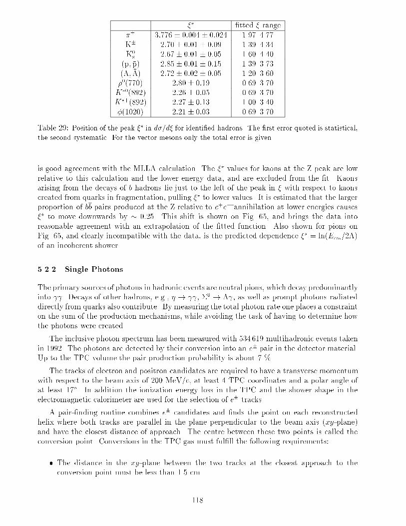
�? �tted � range

�� 3:776 � 0:004 � 0:024 1.97{4.77

K� 2:70� 0:01 � 0:09 1.39{4.34

K0S

2:67� 0:01 � 0:05 1.60{4.40

(p; �p) 2:85� 0:01 � 0:15 1.39{3.73

(�; ��) 2:72� 0:02 � 0:05 1.20{3.60

�0(770) 2:80 � 0:19 0.69{3.70

K�0(892) 2:26 � 0:05 0.69{3.70

K�+(892) 2:27 � 0:13 1.00{3.40

�(1020) 2:21 � 0:03 0.69{3.70

Table 29: Position of the peak �? in d�=d� for identi�ed hadrons. The �rst error quoted is statistical,

the second systematic. For the vector mesons only the total error is given.

is good agreement with the MLLA calculation. The �? values for kaons at the Z peak are low

relative to this calculation and the lower energy data, and are excluded from the �t. Kaons

arising from the decays of b hadrons lie just to the left of the peak in � with respect to kaons

created from quarks in fragmentation, pulling �? to lower values. It is estimated that the larger

proportion of bb pairs produced at the Z relative to e+e� annihilation at lower energies causes

�? to move downwards by � 0:25. This shift is shown on Fig. 65, and brings the data into

reasonable agreement with an extrapolation of the �tted function. Also shown for pions on

Fig. 65, and clearly incompatible with the data, is the predicted dependence �? = ln(Ecm=2�)

of an incoherent shower.

5.2.2 Single Photons

The primary sources of photons in hadronic events are neutral pions, which decay predominantly

into . Decays of other hadrons, e.g., � ! , �0 ! � , as well as prompt photons radiated

directly from quarks also contribute. By measuring the total photon rate one places a constraint

on the sum of the production mechanisms, while avoiding the task of having to determine how

the photons were created.

The inclusive photon spectrum has been measured with 534 619 multihadronic events taken

in 1992. The photons are detected by their conversion into an e� pair in the detector material.

Up to the TPC volume the pair production probability is about 7 %.

The tracks of electron and positron candidates are required to have a transverse momentum

with respect to the beam axis of 200 MeV/c, at least 4 TPC coordinates and a polar angle of

at least 17�. In addition the ionization energy loss in the TPC and the shower shape in the

electromagnetic calorimeter are used for the selection of e� tracks.

A pair-�nding routine combines e� candidates and �nds the point on each reconstructed

helix where both tracks are parallel in the plane perpendicular to the beam axis (xy-plane)

and have the closest distance of approach. The centre between these two points is called the

conversion point. Conversions in the TPC gas must ful�ll the following requirements:

� The distance in the xy-plane between the two tracks at the closest approach to the

conversion point must be less than 1.5 cm.

118

1

1.5

2

2.5

3

3.5

4

4.5

10 102

Ecm [GeV]

ξ*

π±

K±

p,p̄

Figure 65: Position of the peak �? in d�d�

as a function of centre-of-mass energy for pions, kaons and

protons for the inclusive di�erential cross sections presented here (�lled points) and those of other

experiments (TASSO [164], [165], TPC/2 [166], [167], TOPAZ [163] and OPAL [162]). The solid

lines are �ts to, from top to bottom, pion, kaon and proton data according to Eq. (64), assuming

three avours. The arrow represents the estimated shift in �? for kaons at the Z peak due to b hadron

decays, and is to be compared with the extrapolation of Eq. (64) (dashed line). The dot-dashed line

is the prediction for an incoherent parton shower model.

119

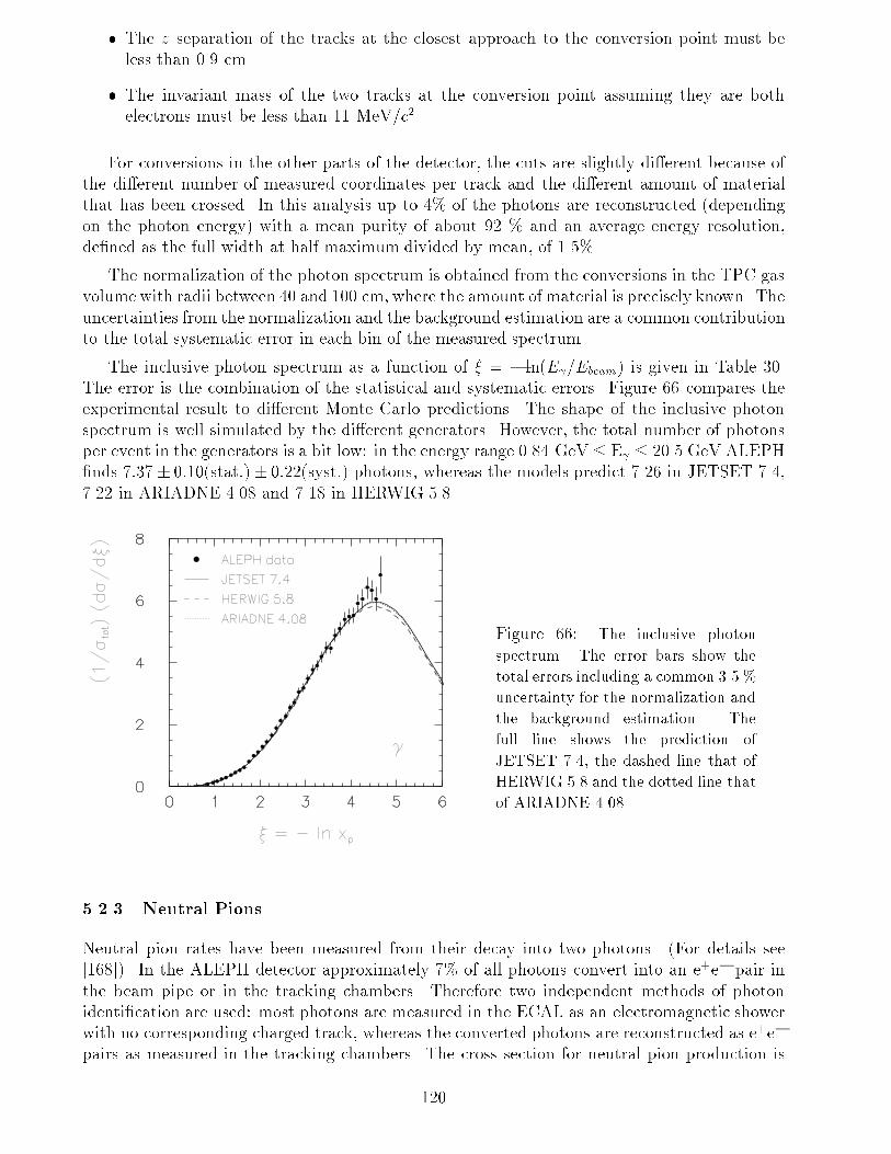
� The z separation of the tracks at the closest approach to the conversion point must be

less than 0.9 cm.

� The invariant mass of the two tracks at the conversion point assuming they are both

electrons must be less than 11 MeV/c2.

For conversions in the other parts of the detector, the cuts are slightly di�erent because of

the di�erent number of measured coordinates per track and the di�erent amount of material

that has been crossed. In this analysis up to 4% of the photons are reconstructed (depending

on the photon energy) with a mean purity of about 92 % and an average energy resolution,

de�ned as the full width at half maximum divided by mean, of 1.5%.

The normalization of the photon spectrum is obtained from the conversions in the TPC gas

volume with radii between 40 and 100 cm, where the amount of material is precisely known. The

uncertainties from the normalization and the background estimation are a common contribution

to the total systematic error in each bin of the measured spectrum.

The inclusive photon spectrum as a function of � = � ln(E =Ebeam) is given in Table 30.

The error is the combination of the statistical and systematic errors. Figure 66 compares the

experimental result to di�erent Monte Carlo predictions. The shape of the inclusive photon

spectrum is well simulated by the di�erent generators. However, the total number of photons

per event in the generators is a bit low: in the energy range 0.84 GeV � E � 20.5 GeV ALEPH

�nds 7:37� 0:10(stat:)� 0:22(syst:) photons, whereas the models predict 7.26 in JETSET 7.4,

7.22 in ARIADNE 4.08 and 7.18 in HERWIG 5.8 .

Figure 66: The inclusive photon

spectrum. The error bars show the

total errors including a common 3.5 %

uncertainty for the normalization and

the background estimation. The

full line shows the prediction of

JETSET 7.4, the dashed line that of

HERWIG 5.8 and the dotted line that

of ARIADNE 4.08.

5.2.3 Neutral Pions

Neutral pion rates have been measured from their decay into two photons. (For details see

[168]). In the ALEPH detector approximately 7% of all photons convert into an e+e� pair in

the beam pipe or in the tracking chambers. Therefore two independent methods of photon

identi�cation are used: most photons are measured in the ECAL as an electromagnetic shower

with no corresponding charged track, whereas the converted photons are reconstructed as e+e�

pairs as measured in the tracking chambers. The cross section for neutral pion production is

120

� interval (1=�tot)(d�=d�)

0:0� 0:1 0.0001 � 0.0018

0:1� 0:2 0.0045 � 0.0039

0:2� 0:3 0.0143 � 0.0096

0:3� 0:4 0.0185 � 0.0078

0:4� 0:5 0.0251 � 0.0075

0:5� 0:6 0.0256 � 0.0071

0:6� 0:7 0.046 � 0.014

0:7� 0:8 0.055 � 0.017

0:8� 0:9 0.087 � 0.016

0:9� 1:0 0.136 � 0.020

1:0� 1:1 0.182 � 0.036

1:1� 1:2 0.246 � 0.031

1:2� 1:3 0.300 � 0.039

1:3� 1:4 0.383 � 0.027

1:4� 1:5 0.457 � 0.055

1:5� 1:6 0.538 � 0.048

1:6� 1:7 0.625 � 0.043

1:7� 1:8 0.815 � 0.055

1:8� 1:9 0.996 � 0.059

1:9� 2:0 1.126 � 0.066

2:0� 2:1 1.300 � 0.075

2:1� 2:2 1.458 � 0.081

2:2� 2:3 1.662 � 0.083

2:3� 2:4 1.899 � 0.092

� interval 1=�totd�=d�

2:4� 2:5 2.12 � 0.10

2:5� 2:6 2.27 � 0.11

2:6� 2:7 2.55 � 0.13

2:7� 2:8 2.73 � 0.12

2:8� 2:9 3.06 � 0.13

2:9� 3:0 3.19 � 0.14

3:0� 3:1 3.49 � 0.14

3:1� 3:2 3.79 � 0.16

3:2� 3:3 3.91 � 0.16

3:3� 3:4 4.20 � 0.17

3:4� 3:5 4.49 � 0.19

3:5� 3:6 4.47 � 0.19

3:6� 3:7 4.88 � 0.21

3:7� 3:8 5.11 � 0.21

3:8� 3:9 5.41 � 0.23

3:9� 4:0 5.50 � 0.24

4:0� 4:1 5.53 � 0.25

4:1� 4:2 5.92 � 0.29

4:2� 4:3 6.06 � 0.30

4:3� 4:4 6.43 � 0.36

4:4� 4:5 6.34 � 0.34

4:5� 4:6 6.07 � 0.40

4:6� 4:7 6.83 � 0.60

4:7� 4:8 8.3 � 3.5

Table 30: Measured inclusive photon cross section. The errors include statistical and systematic

uncertainties.

extracted from the invariant mass distributions of photon pairs which is parameterized in terms

of a Gaussian for the signal and a background function.

The total �0 rate is determined from a sample with two conversions which has lower

statistics, but gives the smallest systematic error (6.4%), mainly because the detector material

in the TPC gas volume is known to 1%. The higher statistics of �0 mesons reconstructed via

one converted and one calorimetric photon is used to measure the shape of the �0 spectrum.

In this way the analysis is less sensitive to the uncertainties of the photon reconstruction in

the ECAL. The corrected results are given in Table 31 and plotted in Fig. 67. The measured

mean multiplicity per event for �0s with momentum fraction larger than 0.025 is found to be

4:80 � 0:07 � 0:31, where the �rst error is statistical and the second is systematic.

The �0 spectrum is extrapolated into the momentumrange below xp = 0:025 using the shape

predicted by the JETSET 7.4 model. The experimental result is hn�0i = 9:63�0:13�0:62�0:12,where the third error is the uncertainty of the extrapolation taken from the di�erence between

JETSET 7.4 and HERWIG 5.8 and the variation of the model parameters. This ALEPH

measurement is in good agreement with the predictions of JETSET 7.4 (hn�0i = 9:67) and

HERWIG 5.8 (hn�0i = 9:59). The neutral pion data have not been used in the tuning of the

model parameters (see sect. 2.3).

121

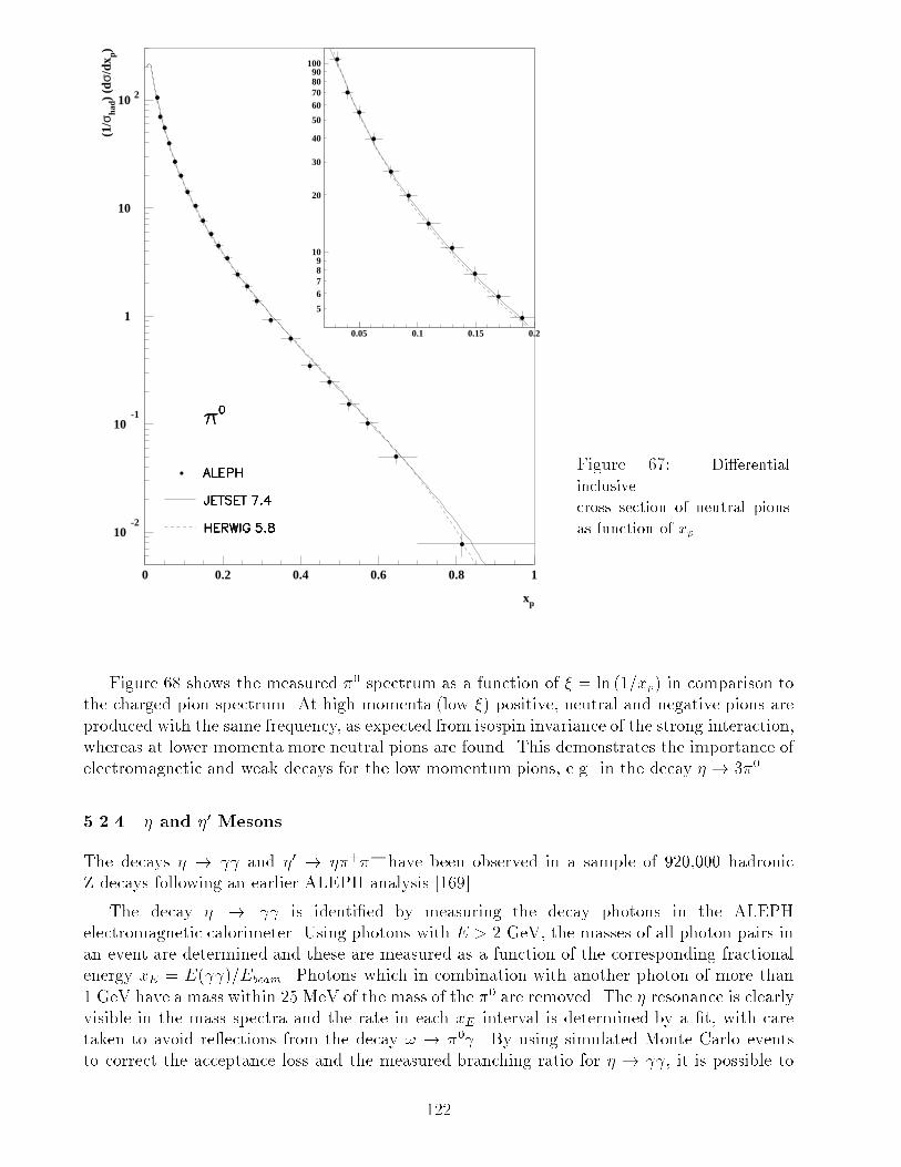
10-2

10-1

1

10

10 2

0 0.2 0.4 0.6 0.8 1

xp

(1/σ

had)

(dσ

/dx p)

•

5

6789

10

20

30

40

50

60708090

100

0.05 0.1 0.15 0.2

Figure 67: Di�erential

inclusive

cross section of neutral pions

as function of xp.

Figure 68 shows the measured �0 spectrum as a function of � = ln (1=xp) in comparison to

the charged pion spectrum. At high momenta (low �) positive, neutral and negative pions are

produced with the same frequency, as expected from isospin invariance of the strong interaction,

whereas at lower momenta more neutral pions are found. This demonstrates the importance of

electromagnetic and weak decays for the low momentum pions, e.g. in the decay � ! 3�0.

5.2.4 � and �0 Mesons

The decays � ! and �0 ! ��+�� have been observed in a sample of 920,000 hadronic

Z decays following an earlier ALEPH analysis [169].

The decay � ! is identi�ed by measuring the decay photons in the ALEPH

electromagnetic calorimeter. Using photons with E > 2 GeV, the masses of all photon pairs in

an event are determined and these are measured as a function of the corresponding fractional

energy xE = E( )=Ebeam. Photons which in combination with another photon of more than

1 GeV have a mass within 25 MeV of the mass of the �0 are removed. The � resonance is clearly

visible in the mass spectra and the rate in each xE interval is determined by a �t, with care

taken to avoid re ections from the decay ! ! �0 . By using simulated Monte Carlo events

to correct the acceptance loss and the measured branching ratio for � ! , it is possible to

122

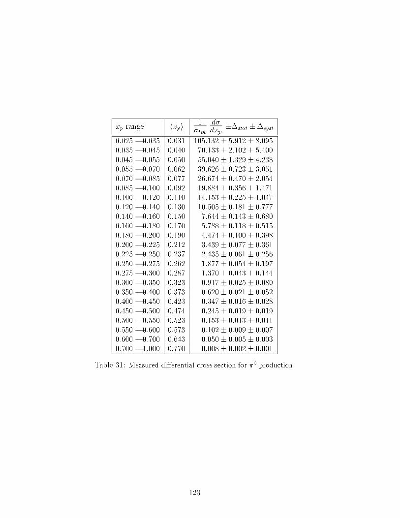
xp range hxpi 1�tot

d�dxp

��stat ��syst

0:025 � 0:035 0:031 105:132 � 5:912 � 8:095

0:035 � 0:045 0:040 70:133 � 2:102 � 5:400

0:045 � 0:055 0:050 55:040 � 1:329 � 4:238

0:055 � 0:070 0:062 39:626 � 0:723 � 3:051

0:070 � 0:085 0:077 26:674 � 0:470 � 2:054

0:085 � 0:100 0:092 19:884 � 0:356 � 1:471

0:100 � 0:120 0:110 14:153 � 0:225 � 1:047

0:120 � 0:140 0:130 10:505 � 0:181 � 0:777

0:140 � 0:160 0:150 7:644 � 0:143 � 0:680

0:160 � 0:180 0:170 5:788 � 0:118 � 0:515

0:180 � 0:200 0:190 4:474 � 0:100 � 0:398

0:200 � 0:225 0:212 3:439 � 0:077 � 0:361

0:225 � 0:250 0:237 2:435 � 0:061 � 0:256

0:250 � 0:275 0:262 1:877 � 0:054 � 0:197

0:275 � 0:300 0:287 1:370 � 0:043 � 0:144

0:300 � 0:350 0:323 0:917 � 0:025 � 0:080

0:350 � 0:400 0:373 0:620 � 0:021 � 0:052

0:400 � 0:450 0:423 0:347 � 0:016 � 0:028

0:450 � 0:500 0:474 0:245 � 0:019 � 0:019

0:500 � 0:550 0:523 0:153 � 0:013 � 0:011

0:550 � 0:600 0:573 0:102 � 0:009 � 0:007

0:600 � 0:700 0:643 0:050 � 0:005 � 0:003

0:700 � 1:000 0:770 0:008 � 0:002 � 0:001

Table 31: Measured di�erential cross section for �0 production.

123

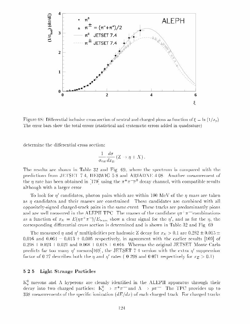
0

1

2

3

4

0 2 4 6

ξ

(1/σ

had)

(dσ

/dξ)

• •

•

Figure 68: Di�erential inclusive cross section of neutral and charged pions as function of � = ln (1=xp).

The error bars show the total errors (statistical and systematic errors added in quadrature).

determine the di�erential cross section:

1

�tot

d�

dxE(Z! � +X) :

The results are shown in Table 32 and Fig. 69, where the spectrum is compared with the

predictions from JETSET 7.4, HERWIG 5.8 and ARIADNE 4.08. Another measurement of

the � rate has been obtained in [170] using the �+���0 decay channel, with compatible results

although with a larger error.

To look for �0 candidates, photon pairs which are within 100 MeV of the � mass are taken

as � candidates and their masses are constrained. These candidates are combined with all

oppositely-signed charged-track pairs in the same event. These tracks are predominantly pions

and are well measured in the ALEPH TPC. The masses of the candidate ��+�� combinations

as a function of xE = E(��+��)=Ebeam show a clear signal for the �0, and as for the �, the

corresponding di�erential cross section is determined and is shown in Table 32 and Fig. 69.

The measured � and �0 multiplicities per hadronic Z decay for xE > 0:1 are 0:282� 0:015�0:016 and 0:064 � 0:013 � 0:005 respectively, in agreement with the earlier results [169] of

0:298 � 0:023 � 0:021 and 0:068 � 0:018 � 0:016. Whereas the original JETSET Monte Carlo

predicts far too many �0 mesons[169], the JETSET 7.4 version with the extra �0 suppressionfactor of 0.27 describes both the � and �0 rates ( 0.298 and 0.071 respectively for xE > 0:1).

5.2.5 Light Strange Particles

K0s mesons and � hyperons are cleanly identi�ed in the ALEPH apparatus through their

decay into two charged particles: K0s ! �+�� and � ! p��. The TPC provides up to

338 measurements of the speci�c ionization (dE=dx) of each charged track. For charged tracks

124

�

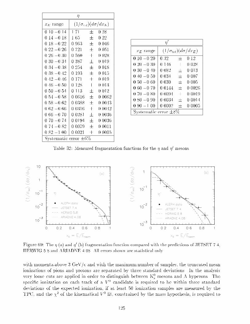
xE range (1=�tot)(d�=dxE)

0.10 - 0.14 1.71 � 0.28

0.14 - 0.18 1.65 � 0.22

0.18 - 0.22 0.963 � 0.046

0.22 - 0.26 0.721 � 0.051

0.26 - 0.30 0.560 � 0.028

0.30 - 0.34 0.387 � 0.019

0.34 - 0.38 0.254 � 0.018

0.38 - 0.42 0.193 � 0.015

0.42 - 0.46 0.171 � 0.019

0.46 - 0.50 0.128 � 0.013

0.50 - 0.54 0.113 � 0.012

0.54 - 0.58 0.0616 � 0.0062

0.58 - 0.62 0.0388 � 0.0043

0.62 - 0.66 0.0316 � 0.0042

0.66 - 0.70 0.0281 � 0.0036

0.70 - 0.74 0.0194 � 0.0036

0.74 - 0.82 0.0079 � 0.0011

0.82 - 1.00 0.0021 � 0.0005

Systematic error �6%

�0

xE range (1=�tot)(d�=dxE)

0.10 - 0.20 0.32 � 0.12

0.20 - 0.30 0.146 � 0.028

0.30 - 0.40 0.082 � 0.013

0.40 - 0.50 0.034 � 0.007

0.50 - 0.60 0.030 � 0.005

0.60 - 0.70 0.0144 � 0.0026

0.70 - 0.80 0.0094 � 0.0019

0.80 - 0.90 0.0034 � 0.0014

0.90 - 1.00 0.0002 � 0.0005

Systematic error �8%

Table 32: Measured fragmentation functions for the � and �0 mesons.

Figure 69: The � (a) and �0 (b) fragmentation function compared with the predictions of JETSET 7.4,

HERWIG 5.8 and ARIADNE 4.08. All errors shown are statistical only.

with momenta above 3 GeV/c and with the maximum number of samples, the truncated mean

ionizations of pions and protons are separated by three standard deviations. In the analysis

very loose cuts are applied in order to distinguish between K0s mesons and � hyperons. The

speci�c ionization on each track of a V 0 candidate is required to be within three standard

deviations of the expected ionization, if at least 50 ionization samples are measured by the

TPC, and the �2 of the kinematical V 0 �t, constrained by the mass hypothesis, is required to

125

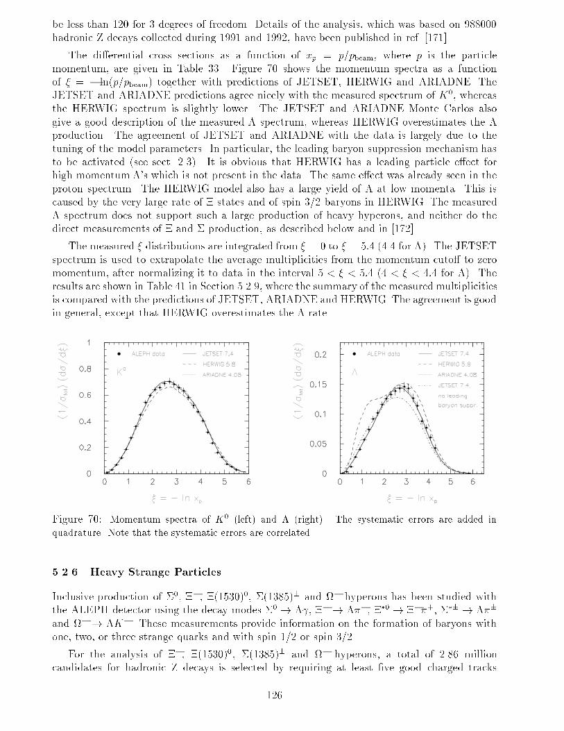
be less than 120 for 3 degrees of freedom. Details of the analysis, which was based on 988000

hadronic Z decays collected during 1991 and 1992, have been published in ref. [171].

The di�erential cross sections as a function of xp = p=pbeam, where p is the particle

momentum, are given in Table 33. Figure 70 shows the momentum spectra as a function

of � = � ln(p=pbeam) together with predictions of JETSET, HERWIG and ARIADNE. The

JETSET and ARIADNE predictions agree nicely with the measured spectrum of K0, whereas

the HERWIG spectrum is slightly lower. The JETSET and ARIADNE Monte Carlos also

give a good description of the measured � spectrum, whereas HERWIG overestimates the �

production. The agreement of JETSET and ARIADNE with the data is largely due to the

tuning of the model parameters. In particular, the leading baryon suppression mechanism has

to be activated (see sect. 2.3). It is obvious that HERWIG has a leading particle e�ect for

high momentum �'s which is not present in the data. The same e�ect was already seen in the

proton spectrum. The HERWIG model also has a large yield of � at low momenta. This is

caused by the very large rate of � states and of spin 3/2 baryons in HERWIG. The measured

� spectrum does not support such a large production of heavy hyperons, and neither do the

direct measurements of � and � production, as described below and in [172].

The measured � distributions are integrated from � = 0 to � = 5:4 (4.4 for �). The JETSET

spectrum is used to extrapolate the average multiplicities from the momentum cuto� to zero

momentum, after normalizing it to data in the interval 5 < � < 5:4 (4 < � < 4:4 for �). The

results are shown in Table 41 in Section 5.2.9, where the summary of the measured multiplicities

is compared with the predictions of JETSET, ARIADNE and HERWIG. The agreement is good

in general, except that HERWIG overestimates the � rate.

Figure 70: Momentum spectra of K0 (left) and � (right). The systematic errors are added in

quadrature. Note that the systematic errors are correlated.

5.2.6 Heavy Strange Particles

Inclusive production of �0, ��, �(1530)0, �(1385)� and � hyperons has been studied with

the ALEPH detector using the decay modes �0 ! � , �� ! ���, ��0 ! ���+, ��� ! ���

and � ! �K�. These measurements provide information on the formation of baryons with

one, two, or three strange quarks and with spin 1/2 or spin 3/2.

For the analysis of ��, �(1530)0, �(1385)� and � hyperons, a total of 2.86 million

candidates for hadronic Z decays is selected by requiring at least �ve good charged tracks

126

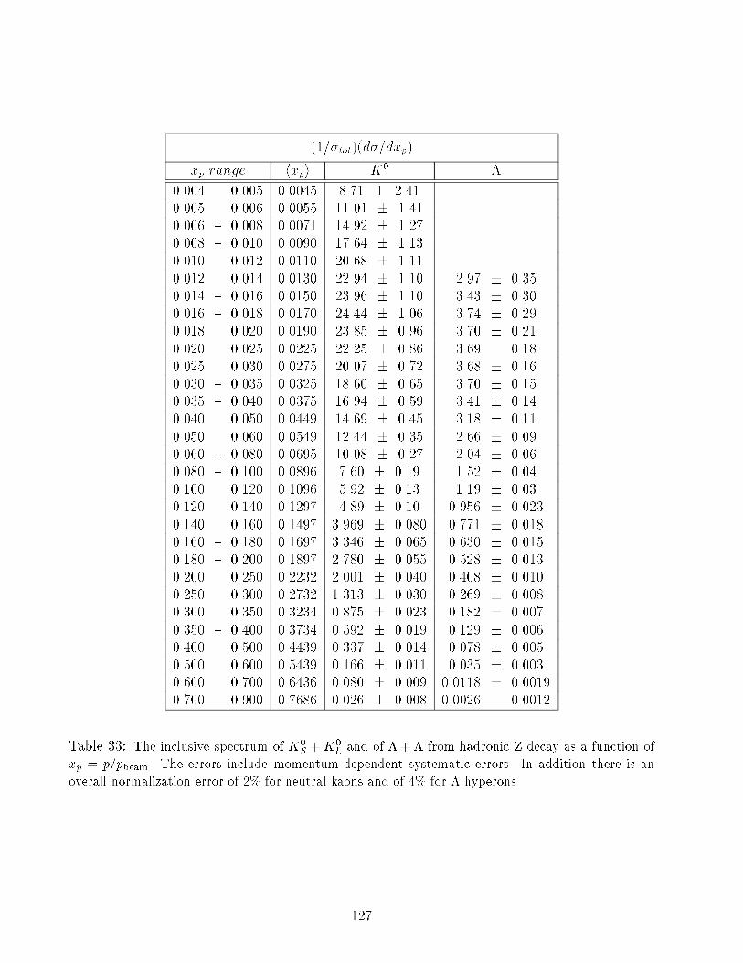
(1=�tot)(d�=dxp)

xp range hxpi K0 �

0.004 { 0.005 0.0045 8.71 � 2.41

0.005 { 0.006 0.0055 11.01 � 1.41

0.006 { 0.008 0.0071 14.92 � 1.27

0.008 { 0.010 0.0090 17.64 � 1.13

0.010 { 0.012 0.0110 20.68 � 1.11

0.012 { 0.014 0.0130 22.94 � 1.10 2.97 � 0.35

0.014 { 0.016 0.0150 23.96 � 1.10 3.43 � 0.30

0.016 { 0.018 0.0170 24.44 � 1.06 3.74 � 0.29

0.018 { 0.020 0.0190 23.85 � 0.96 3.70 � 0.21

0.020 { 0.025 0.0225 22.25 � 0.86 3.69 � 0.18

0.025 { 0.030 0.0275 20.07 � 0.72 3.68 � 0.16

0.030 { 0.035 0.0325 18.60 � 0.65 3.70 � 0.15

0.035 { 0.040 0.0375 16.94 � 0.59 3.41 � 0.14

0.040 { 0.050 0.0449 14.69 � 0.45 3.18 � 0.11

0.050 { 0.060 0.0549 12.44 � 0.35 2.66 � 0.09

0.060 { 0.080 0.0695 10.08 � 0.27 2.04 � 0.06

0.080 { 0.100 0.0896 7.60 � 0.19 1.52 � 0.04

0.100 { 0.120 0.1096 5.92 � 0.13 1.19 � 0.03

0.120 { 0.140 0.1297 4.89 � 0.10 0.956 � 0.023

0.140 { 0.160 0.1497 3.969 � 0.080 0.771 � 0.018

0.160 { 0.180 0.1697 3.346 � 0.065 0.630 � 0.015

0.180 { 0.200 0.1897 2.780 � 0.055 0.528 � 0.013

0.200 { 0.250 0.2232 2.001 � 0.040 0.408 � 0.010

0.250 { 0.300 0.2732 1.313 � 0.030 0.269 � 0.008

0.300 { 0.350 0.3234 0.875 � 0.023 0.182 � 0.007

0.350 { 0.400 0.3734 0.592 � 0.019 0.129 � 0.006

0.400 { 0.500 0.4439 0.337 � 0.014 0.078 � 0.005

0.500 { 0.600 0.5439 0.166 � 0.011 0.035 � 0.003

0.600 { 0.700 0.6436 0.080 � 0.009 0.0118 � 0.0019

0.700 { 0.900 0.7686 0.026 � 0.008 0.0026 � 0.0012

Table 33: The inclusive spectrum of K0S +K0

L and of � + �� from hadronic Z decay as a function of

xp = p=pbeam. The errors include momentum dependent systematic errors. In addition there is an

overall normalization error of 2% for neutral kaons and of 4% for � hyperons.

127

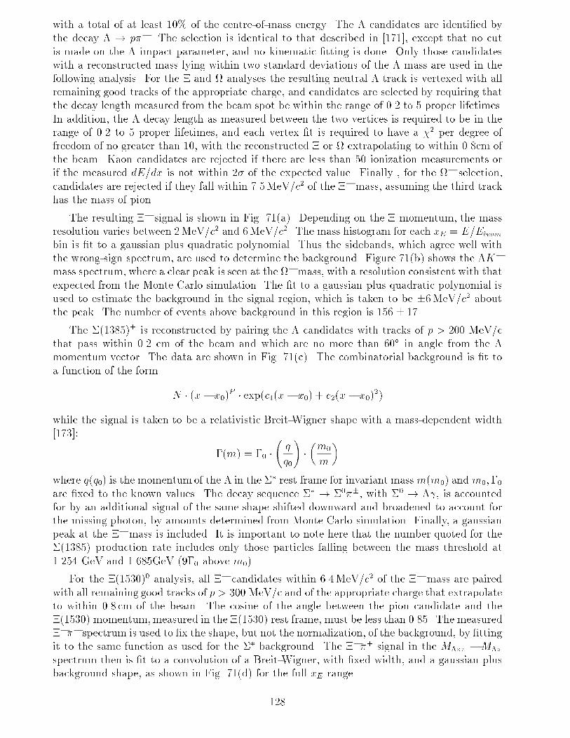
with a total of at least 10% of the centre-of-mass energy. The � candidates are identi�ed by

the decay � ! p��. The selection is identical to that described in [171], except that no cut

is made on the � impact parameter, and no kinematic �tting is done. Only those candidates

with a reconstructed mass lying within two standard deviations of the � mass are used in the

following analysis. For the � and analyses the resulting neutral � track is vertexed with all

remaining good tracks of the appropriate charge, and candidates are selected by requiring that

the decay length measured from the beam spot be within the range of 0.2 to 5 proper lifetimes.

In addition, the � decay length as measured between the two vertices is required to be in the

range of 0.2 to 5 proper lifetimes, and each vertex �t is required to have a �2 per degree of

freedom of no greater than 10, with the reconstructed � or extrapolating to within 0.8cm of

the beam. Kaon candidates are rejected if there are less than 50 ionization measurements or

if the measured dE=dx is not within 2� of the expected value. Finally , for the � selection,

candidates are rejected if they fall within 7.5MeV/c2 of the �� mass, assuming the third track

has the mass of pion.

The resulting �� signal is shown in Fig. 71(a). Depending on the � momentum, the mass

resolution varies between 2MeV/c2 and 6MeV/c2. The mass histogram for each xE = E=Ebeam

bin is �t to a gaussian plus quadratic polynomial. Thus the sidebands, which agree well with

the wrong-sign spectrum, are used to determine the background. Figure 71(b) shows the �K�

mass spectrum, where a clear peak is seen at the � mass, with a resolution consistent with that

expected from the Monte Carlo simulation. The �t to a gaussian plus quadratic polynomial is

used to estimate the background in the signal region, which is taken to be �6MeV/c2 about

the peak. The number of events above background in this region is 156 � 17.

The �(1385)� is reconstructed by pairing the � candidates with tracks of p > 200 MeV/c

that pass within 0.2 cm of the beam and which are no more than 60� in angle from the �

momentum vector. The data are shown in Fig. 71(c). The combinatorial background is �t to

a function of the form

N � (x� x0)P � exp(c1(x� x0) + c2(x� x0)

2)

while the signal is taken to be a relativistic Breit-Wigner shape with a mass-dependent width

[173]:

�(m) = �0 � q

q0

!��m0

m

�

where q(q0) is the momentum of the � in the �� rest frame for invariant mass m(m0) and m0;�0are �xed to the known values. The decay sequence �� ! �0��, with �0 ! � , is accounted

for by an additional signal of the same shape shifted downward and broadened to account for

the missing photon, by amounts determined from Monte Carlo simulation. Finally, a gaussian

peak at the �� mass is included. It is important to note here that the number quoted for the

�(1385) production rate includes only those particles falling between the mass threshold at

1.254 GeV and 1.685GeV (9�0 above m0).

For the �(1530)0 analysis, all �� candidates within 6.4MeV/c2 of the �� mass are paired

with all remaining good tracks of p > 300 MeV/c and of the appropriate charge that extrapolate

to within 0.8 cm of the beam. The cosine of the angle between the pion candidate and the

�(1530) momentum,measured in the �(1530) rest frame, must be less than 0.85. The measured

���� spectrum is used to �x the shape, but not the normalization, of the background, by �tting

it to the same function as used for the �� background. The ���+ signal in the M��� �M��

spectrum then is �t to a convolution of a Breit-Wigner, with �xed width, and a gaussian plus

background shape, as shown in Fig. 71(d) for the full xE range.

128

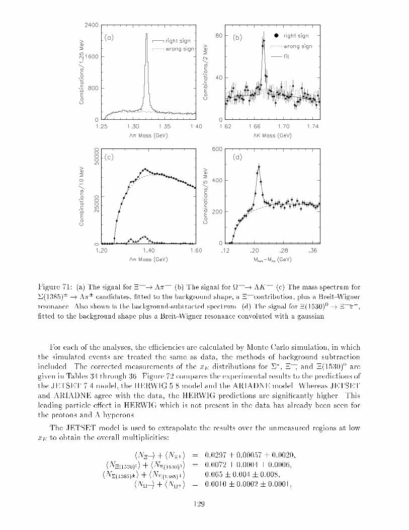
Figure 71: (a) The signal for �� ! ���. (b) The signal for � ! �K�. (c) The mass spectrum for

�(1385)� ! ��� candidates, �tted to the background shape, a �� contribution, plus a Breit-Wigner

resonance. Also shown is the background-subtracted spectrum. (d) The signal for �(1530)0 ! ���+,�tted to the background shape plus a Breit-Wigner resonance convoluted with a gaussian.

For each of the analyses, the e�ciencies are calculated by Monte Carlo simulation, in which

the simulated events are treated the same as data, the methods of background subtraction

included. The corrected measurements of the xE distributions for ��, ��, and �(1530)0 are

given in Tables 34 through 36. Figure 72 compares the experimental results to the predictions of

the JETSET 7.4 model, the HERWIG 5.8 model and the ARIADNE model. Whereas JETSET

and ARIADNE agree with the data, the HERWIG predictions are signi�cantly higher. This

leading particle e�ect in HERWIG which is not present in the data has already been seen for

the protons and � hyperons.

The JETSET model is used to extrapolate the results over the unmeasured regions at low

xE to obtain the overall multiplicities:

hN��i+ hN��+i = 0:0297 � 0:00057 � 0:0020;

hN�(1530)0i+ hN��(1530)0i = 0:0072 � 0:0004 � 0:0006;

hN�(1385)�i + hN��(1385)�i = 0:065 � 0:004 � 0:008;

hN�i+ hN�+ i = 0:0010 � 0:0002 � 0:0001;

129

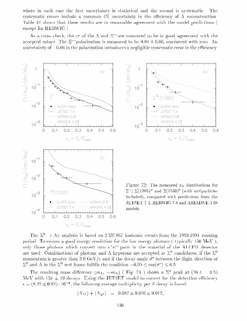
where in each case the �rst uncertainty is statistical and the second is systematic. The

systematic errors include a common 4% uncertainty in the e�ciency of � reconstruction.

Table 41 shows that these results are in reasonable agreement with the model predictions (

except for HERWIG ).

As a cross check, the c� of the � and �� are measured to be in good agreement with the

accepted values. The �� polarization is measured to be 0:04 � 0:06, consistent with zero. An

uncertainty of �0:06 in the polarization introduces a negligible systematic error in the e�ciency.

Figure 72: The measured xE distributions for

��, �(1385)� and �(1530)0 (with antiparticles

included), compared with predictions from the

JETSET 7.4, HERWIG 5.8 and ARIADNE 4.08

models.

The �0 ! � analysis is based on 2 337 867 hadronic events from the 1992-1994 running

period. To ensure a good energy resolution for the low energy photons ( typically 150 MeV ),

only those photons which convert into e+e� pairs in the material of the ALEPH detector

are used. Combinations of photons and � hyperons are accepted as �0 candidates, if the �0

momentum is greater than 3.0 GeV/c and if the decay angle #� between the ight direction of

�0 and � in the �0 rest frame ful�lls the condition �0:95 � cos(#�) � 0:5.

The resulting mass di�erence (m� � m�) ( Fig. 73 ) shows a �0 peak at (76.4 � 0.5)

MeV with 158 � 19 decays. Using the JETSET model to correct for the detection e�ciency

� = (8:22� 0:82) � 10�4, the following average multiplicity per Z decay is found:

hN�0i+ hN��0 i = 0:082 � 0:010 � 0:012;

130

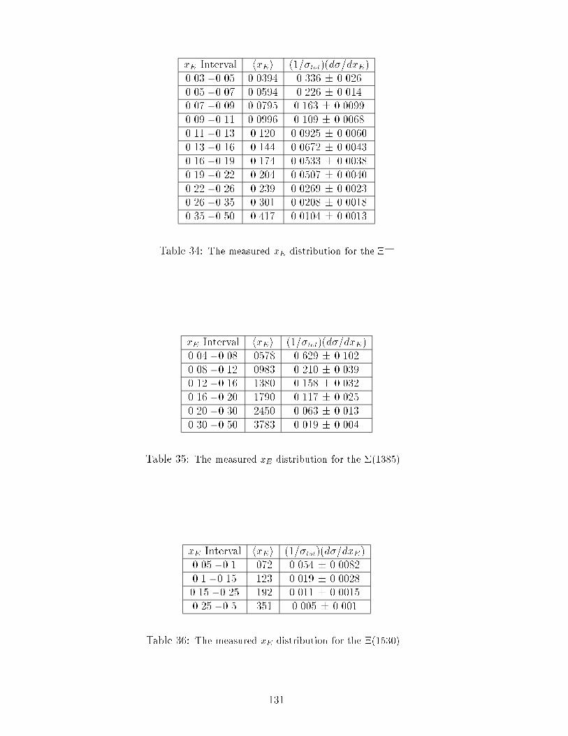
xE Interval hxEi (1=�tot)(d�=dxE)

0.03 - 0.05 0.0394 0.336 � 0.026

0.05 - 0.07 0.0594 0.226 � 0.014

0.07 - 0.09 0.0795 0.163 � 0.0099

0.09 - 0.11 0.0996 0.109 � 0.0068

0.11 - 0.13 0.120 0.0925 � 0.0060

0.13 - 0.16 0.144 0.0672 � 0.0043

0.16 - 0.19 0.174 0.0533 � 0.0038

0.19 - 0.22 0.204 0.0507 � 0.0040

0.22 - 0.26 0.239 0.0269 � 0.0023

0.26 - 0.35 0.301 0.0208 � 0.0018

0.35 - 0.50 0.417 0.0104 � 0.0013

Table 34: The measured xE distribution for the ��.

xE Interval hxEi (1=�tot)(d�=dxE)

0.04 - 0.08 .0578 0.629 � 0.102

0.08 - 0.12 .0983 0.210 � 0.039

0.12 - 0.16 .1380 0.158 � 0.032

0.16 - 0.20 .1790 0.117 � 0.025

0.20 - 0.30 .2450 0.063 � 0.013

0.30 - 0.50 .3783 0.019 � 0.004

Table 35: The measured xE distribution for the �(1385).

xE Interval hxEi (1=�tot)(d�=dxE)

0.05 - 0.1 .072 0.054 � 0.0082

0.1 - 0.15 .123 0.019 � 0.0028

0.15 - 0.25 .192 0.011 � 0.0015

0.25 - 0.5 .351 0.005 � 0.001

Table 36: The measured xE distribution for the �(1530).

131

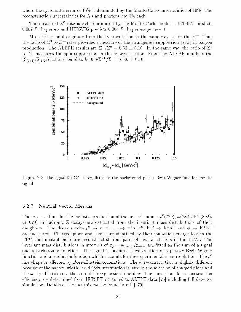
where the systematic error of 15% is dominated by the Monte Carlo uncertainties of 10%. The

reconstruction uncertainties for �'s and photons are 5% each.

The measured �0 rate is well reproduced by the Monte Carlo models. JETSET predicts

0.087 �0 hyperons and HERWIG predicts 0.064 �0 hyperons per event.

Most �0's should originate from the fragmentation in the same way as for the ��. Thus

the ratio of �0 to �� rates provides a measure of the strangeness suppression (s=u) in baryon

production. The ALEPH results are ��=�0 = 0:36 � 0:10. In the same way the ratio of ��

to �0 measures the spin suppression in the hyperon sector. From the ALEPH numbers the

(S(3=2)/S(1=2)) ratio is found to be 0.5����=�0 = 0:40 � 0:10.

0

25

50

75

100

125

150

0 0.025 0.05 0.075 0.1 0.125 0.15

com

bina

tions

/ 2.

5 M

eV/c2

MΛ γ - MΛ [GeV/c2]

ALEPH data

JETSET 7.3

background

Figure 73: The signal for �0 ! � , �tted to the background plus a Breit-Wigner function for the

signal.

5.2.7 Neutral Vector Mesons

The cross sections for the inclusive production of the neutral mesons �0(770), !(782), K�0(892),�(1020) in hadronic Z decays are extracted from the invariant mass distributions of their

daughters. The decay modes �0 ! �+��, ! ! �+���0, K�0 ! K��� and � ! K+K�

are measured. Charged pions and kaons are identi�ed by their ionization energy loss in the

TPC, and neutral pions are reconstructed from pairs of neutral clusters in the ECAL. The

invariant mass distributions in intervals of xp = phadron=pbeam are �tted as the sum of a signal

and a background function. The signal is taken as a convolution of a p-wave Breit-Wigner

function and a resolution function which accounts for the experimental mass resolution. The �0

line shape is a�ected by Bose-Einstein correlations. The ! reconstruction is slightly di�erent

because of the narrow width: no dE/dx information is used in the selection of charged pions and

the ! signal is taken as the sum of three gaussian functions. The corrections for reconstruction

e�ciency are determined from JETSET 7.3 tuned to ALEPH data [26] including full detector

simulation. Details of the analysis can be found in ref. [170].

132

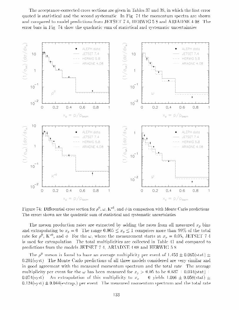
The acceptance-corrected cross sections are given in Tables 37 and 38, in which the �rst error

quoted is statistical and the second systematic. In Fig. 74 the momentum spectra are shown

and compared to model predictions from JETSET 7.4, HERWIG 5.8 and ARIADNE 4.08. The

error bars in Fig. 74 show the quadratic sum of statistical and systematic uncertainties.

Figure 74: Di�erential cross section for �0, !, K�0, and � in comparison with Monte Carlo predictions.

The errors shown are the quadratic sum of statistical and systematic uncertainties.

The meson production rates are extracted by adding the rates from all measured xp bins

and extrapolating to xp = 0. The range 0:005 � xp � 1 comprises more than 99% of the total

rate for �0, K�0, and �. For the !, where the measurement starts at xp = 0:05, JETSET 7.4

is used for extrapolation. The total multiplicities are collected in Table 41 and compared to

predictions from the models JETSET 7.4, ARIADNE 4.08 and HERWIG 5.8 .

The �0 meson is found to have an average multiplicity per event of 1:453 � 0:065(stat) �0:201(syst). The Monte Carlo predictions of all three models considered are very similar and

in good agreement with the measured momentum spectrum and the total rate. The average

multiplicity per event for the ! has been measured for xp > 0:05 to be 0:637 � 0:034(stat) �0:074(syst). An extrapolation of this multiplicity to xp = 0 yields 1:066 � 0:058(stat) �0:124(syst) � 0:044(extrap:) per event. The measured momentum spectrum and the total rate

133

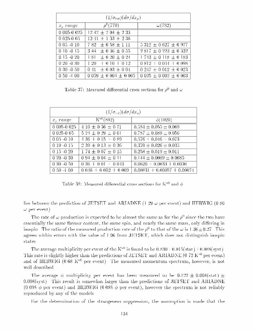
(1=�tot)(d�=dxp)

xp range �0(770) !(782)

0.005-0.025 12.42 � 2.04 � 2.33

0.025-0.05 12.41 � 1.33 � 2.36

0.05 -0.10 7.82 � 0.58 � 1.11 5.312 � 0.627 � 0.977

0.10 -0.15 3.44 � 0.36 � 0.55 2.817 � 0.223 � 0.332

0.15 -0.20 1.81 � 0.20 � 0.24 1.743 � 0.118 � 0.183

0.20 -0.30 1.20 � 0.10 � 0.12 0.812 � 0.044 � 0.098

0.30 -0.50 0.41 � 0.03 � 0.04 0.247 � 0.012 � 0.023

0.50 -1.00 0.059 � 0.004 � 0.005 0.025 � 0.002 � 0.003

Table 37: Measured di�erential cross sections for �0 and !.

(1=�tot)(d�=dxp)

xp range K�0(892) �(1020)

0.005-0.025 4.10 � 0.36 � 0.71 0:584 � 0:055 � 0:069

0.025-0.05 5.24 � 0.29 � 0.61 0:787 � 0:089 � 0:056

0.05 -0.10 4.36 � 0.15 � 0.89 0:576 � 0:046 � 0:073

0.10 -0.15 2.39 � 0.13 � 0.36 0:370 � 0:026 � 0:035

0.15 -0.20 1.74 � 0.07 � 0.15 0:258 � 0:019 � 0:011

0.20 -0.30 0.94 � 0.04 � 0.11 0:144 � 0:0089 � 0:0085

0.30 -0.50 0.36 � 0.01 � 0.043 0:0620 � 0:0033 � 0:0030

0.50 -1.00 0.046 � 0.002 � 0.009 0:00831 � 0:00057 � 0:00074

Table 38: Measured di�erential cross sections for K�0 and �.

lies between the prediction of JETSET and ARIADNE (1.29 ! per event) and HERWIG (0.86

! per event).

The rate of ! production is expected to be almost the same as for the �0 since the two have

essentially the same avour content, the same spin, and nearly the same mass, only di�ering in

isospin. The ratio of the measured production rate of the �0 to that of the ! is 1:36�0:27. This

agrees within errors with the value of 1.06 from JETSET, which does not distinguish isospin

states.

The average multiplicity per event of the K�0 is found to be 0:830�0:015(stat)�0:088(syst).

This rate is slightly higher than the predictions of JETSET and ARIADNE (0.72 K�0 per event)and of HERWIG (0.68 K�0 per event). The measured momentum spectrum, however, is not

well described.

The average � multiplicity per event has been measured to be 0:122 � 0:004(stat) �0:008(syst). This result is somewhat larger than the predictions of JETSET and ARIADNE

(0.098 � per event) and HERWIG (0.088 � per event), however the spectrum is not reliably

reproduced by any of the models.

For the determination of the strangeness suppression, the assumption is made that the

134

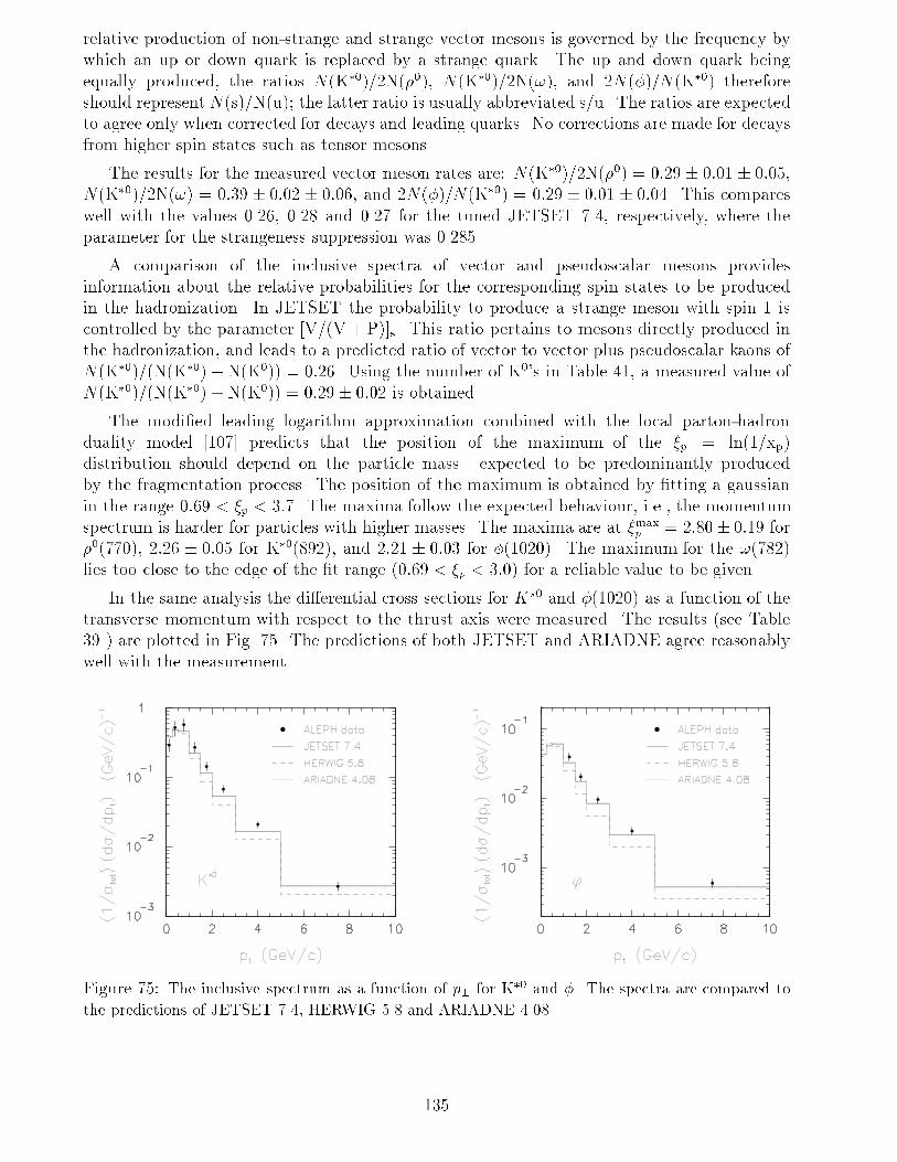
relative production of non-strange and strange vector mesons is governed by the frequency by

which an up or down quark is replaced by a strange quark. The up and down quark being

equally produced, the ratios N(K�0)=2N(�0), N(K�0)=2N(!), and 2N(�)=N(K�0) therefore

should representN(s)=N(u); the latter ratio is usually abbreviated s/u. The ratios are expected

to agree only when corrected for decays and leading quarks. No corrections are made for decays

from higher spin states such as tensor mesons.

The results for the measured vector meson rates are: N(K�0)=2N(�0) = 0:29 � 0:01 � 0:05,

N(K�0)=2N(!) = 0:39 � 0:02 � 0:06, and 2N(�)=N(K�0) = 0:29 � 0:01 � 0:04. This compares

well with the values 0.26, 0.28 and 0.27 for the tuned JETSET 7.4, respectively, where the

parameter for the strangeness suppression was 0.285.

A comparison of the inclusive spectra of vector and pseudoscalar mesons provides

information about the relative probabilities for the corresponding spin states to be produced

in the hadronization. In JETSET the probability to produce a strange meson with spin 1 is

controlled by the parameter [V=(V + P)]s. This ratio pertains to mesons directly produced in

the hadronization, and leads to a predicted ratio of vector to vector plus pseudoscalar kaons of

N(K�0)=(N(K�0) + N(K0)) = 0:26. Using the number of K0's in Table 41, a measured value of

N(K�0)=(N(K�0) + N(K0)) = 0:29� 0:02 is obtained.

The modi�ed leading logarithm approximation combined with the local parton-hadron

duality model [107] predicts that the position of the maximum of the �p = ln(1=xp)

distribution should depend on the particle mass. expected to be predominantly produced

by the fragmentation process. The position of the maximum is obtained by �tting a gaussian

in the range 0:69 < �p < 3:7. The maxima follow the expected behaviour, i.e., the momentum

spectrum is harder for particles with higher masses. The maxima are at �maxp = 2:80� 0:19 for

�0(770), 2:26 � 0:05 for K�0(892), and 2:21 � 0:03 for �(1020). The maximum for the !(782)

lies too close to the edge of the �t range (0:69 < �p < 3:0) for a reliable value to be given.

In the same analysis the di�erential cross sections for K?0 and �(1020) as a function of the

transverse momentum with respect to the thrust axis were measured. The results (see Table

39 ) are plotted in Fig. 75. The predictions of both JETSET and ARIADNE agree reasonably

well with the measurement.

Figure 75: The inclusive spectrum as a function of p? for K�0 and �. The spectra are compared to

the predictions of JETSET 7.4, HERWIG 5.8 and ARIADNE 4.08.

135

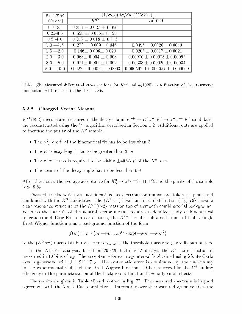
p? range (1=�tot)(d�=dp?)(GeV=c)�1

(GeV=c) K?0 �(1020)

0.-0.25 0.296 � 0.027 � 0.056

0.25-0.5 0.528 � 0.036� 0.128

0.5 -1.0 0.586 � 0.018 � 0.115

1:0� 1:5 0.273 � 0.009� 0.046 0:0395 � 0:0028 � 0:0040

1:5� 2:0 0.146� 0.006� 0.020 0:0205 � 0:0017 � 0:0021

2:0� 3:0 0.068� 0.004 � 0.008 0:00970 � 0:00073 � 0:00097

3:0� 5:0 0.021� 0.001 � 0.002 0:00338 � 0:00026 � 0:00034

5:0� 10:0 0.0027� 0.0002 � 0.0003 0:000597 � 0:000057 � 0:000060

Table 39: Measured di�erential cross sections for K?0 and �(1020) as a function of the transverse

momentum with respect to the thrust axis.

5.2.8 Charged Vector Mesons

K��(892) mesons are measured in the decay chain: K�+ ! K0�+;K0 ! �+��. K0 candidates

are reconstructed using the V 0 algorithm described in Section 1.2. Additional cuts are applied

to increase the purity of the K0 sample:

� The �2/ d.o.f. of the kinematical �t has to be less than 5.

� The K0 decay length has to be greater than 3cm.

� The �+�� mass is required to be within �40MeV of the K0 mass.

� The cosine of the decay angle has to be less than 0.9.

After these cuts, the average acceptance for K0S ! �+�� is 34.8 % and the purity of the sample

is 94.5 %.

Charged tracks which are not identi�ed as electrons or muons are taken as pions and

combined with the K0 candidates. The (K0 ��) invariant mass distribution (Fig. 76) shows a

clear resonance structure at the K��(892) mass on top of a smooth combinatorial background.

Whereas the analysis of the neutral vector mesons requires a detailed study of kinematical

re ections and Bose-Einstein correlations, the K�� signal is obtained from a �t of a single

Breit-Wigner function plus a background function of the form

f(m) = p1 � (m�mthresh)p2 � exp(�p3m� p4m

2)

to the (K0 ��) mass distribution. Here mthresh is the threshold mass and pi are �t parameters.

In the ALEPH analysis, based on 290220 hadronic Z decays, the K�� cross section is

measured in 10 bins of xE. The acceptance for each xE interval is obtained using Monte Carlo

events generated with JETSET 7.3. The systematic error is dominated by the uncertainty

in the experimental width of the Breit-Wigner function. Other sources like the V 0 �nding

e�ciency or the parametrization of the background function have only small e�ects.

The results are given in Table 40 and plotted in Fig. 77. The measured spectrum is in good

agreement with the Monte Carlo predictions. Integrating over the measured xE range gives the

136

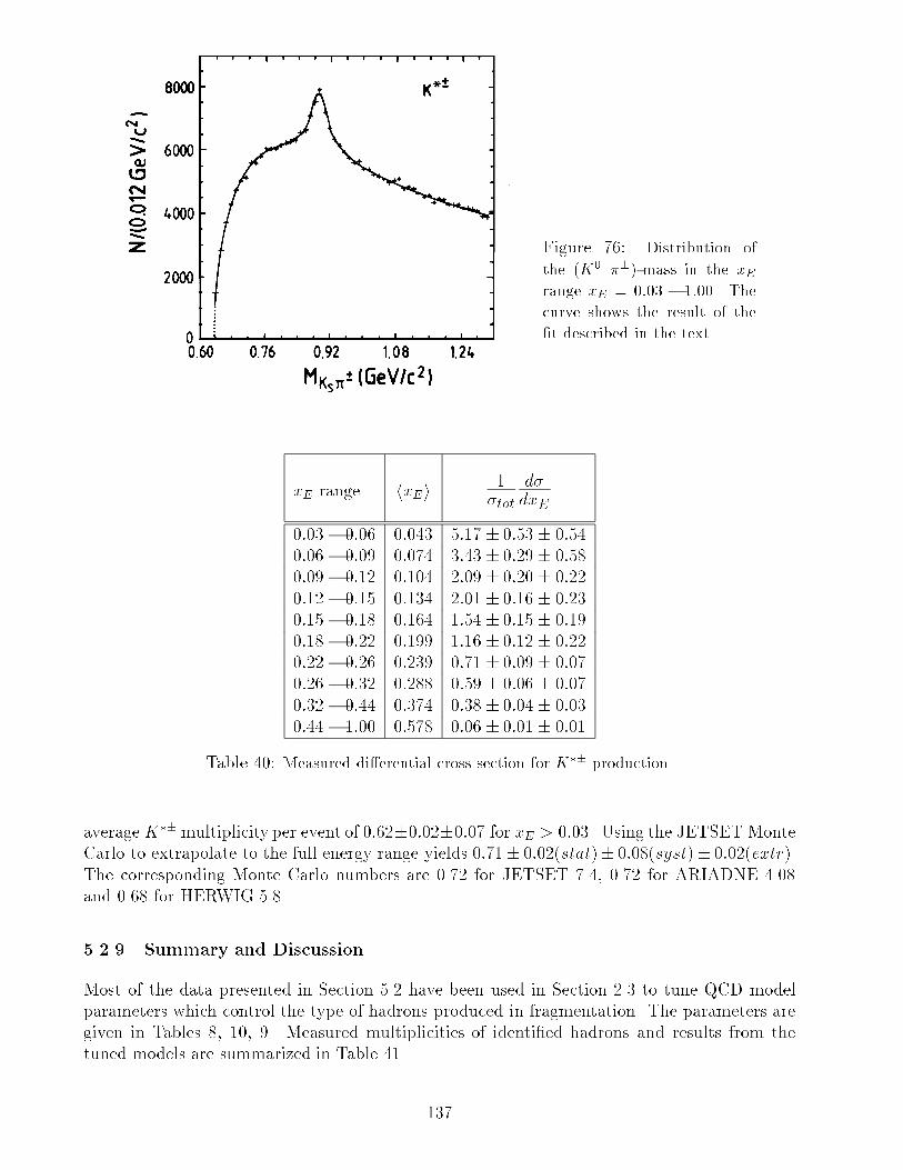
Figure 76: Distribution of

the (K0 ��)-mass in the xErange xE = 0:03 � 1:00. The

curve shows the result of the

�t described in the text.

xE range hxEi 1�tot

d�dxE

0:03� 0:06 0:043 5:17 � 0:53 � 0:54

0:06� 0:09 0:074 3:43 � 0:29 � 0:58

0:09� 0:12 0:104 2:09 � 0:20 � 0:22

0:12� 0:15 0:134 2:01 � 0:16 � 0:23

0:15� 0:18 0:164 1:54 � 0:15 � 0:19

0:18� 0:22 0:199 1:16 � 0:12 � 0:22

0:22� 0:26 0:239 0:71 � 0:09 � 0:07

0:26� 0:32 0:288 0:59 � 0:06 � 0:07

0:32� 0:44 0:374 0:38 � 0:04 � 0:03

0:44� 1:00 0:578 0:06 � 0:01 � 0:01

Table 40: Measured di�erential cross section for K�� production.

averageK�� multiplicity per event of 0:62�0:02�0:07 for xE > 0:03. Using the JETSET Monte

Carlo to extrapolate to the full energy range yields 0:71� 0:02(stat)� 0:08(syst)� 0:02(extr).

The corresponding Monte Carlo numbers are 0.72 for JETSET 7.4, 0.72 for ARIADNE 4.08

and 0.68 for HERWIG 5.8.

5.2.9 Summary and Discussion

Most of the data presented in Section 5.2 have been used in Section 2.3 to tune QCD model

parameters which control the type of hadrons produced in fragmentation. The parameters are

given in Tables 8, 10, 9. Measured multiplicities of identi�ed hadrons and results from the

tuned models are summarized in Table 41.

137

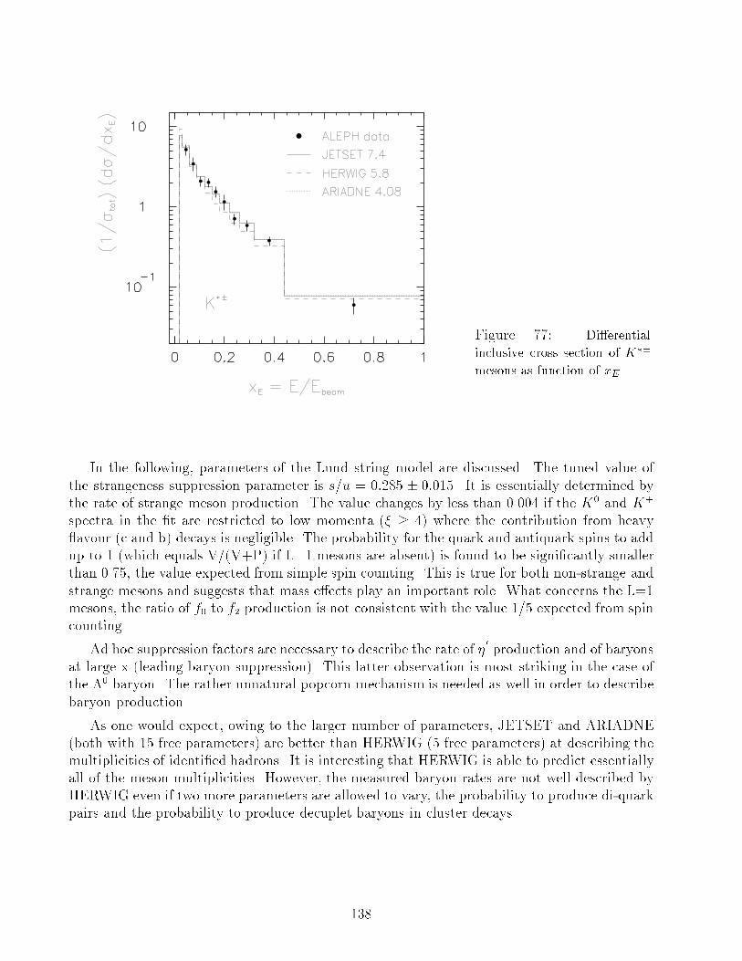
Figure 77: Di�erential

inclusive cross section of K��

mesons as function of xE .

In the following, parameters of the Lund string model are discussed. The tuned value of

the strangeness suppression parameter is s=u = 0:285 � 0:015. It is essentially determined by

the rate of strange meson production. The value changes by less than 0.004 if the K0 and K+

spectra in the �t are restricted to low momenta (� � 4) where the contribution from heavy

avour (c and b) decays is negligible. The probability for the quark and antiquark spins to add

up to 1 (which equals V/(V+P) if L=1 mesons are absent) is found to be signi�cantly smaller

than 0.75, the value expected from simple spin counting. This is true for both non-strange and

strange mesons and suggests that mass e�ects play an important role. What concerns the L=1

mesons, the ratio of f0 to f2 production is not consistent with the value 1/5 expected from spin

counting.

Ad hoc suppression factors are necessary to describe the rate of �0

production and of baryons

at large x (leading baryon suppression). This latter observation is most striking in the case of

the �0 baryon. The rather unnatural popcorn mechanism is needed as well in order to describe

baryon production.

As one would expect, owing to the larger number of parameters, JETSET and ARIADNE

(both with 15 free parameters) are better than HERWIG (5 free parameters) at describing the

multiplicities of identi�ed hadrons. It is interesting that HERWIG is able to predict essentially

all of the meson multiplicities. However, the measured baryon rates are not well described by

HERWIG even if two more parameters are allowed to vary, the probability to produce di-quark

pairs and the probability to produce decuplet baryons in cluster decays.

138

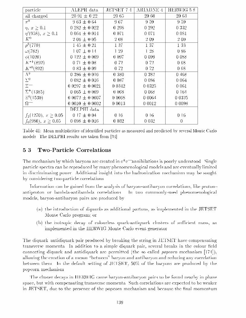
particle ALEPH data JETSET 7.4 ARIADNE 4 HERWIG 5.8

all charged 20.91 � 0.22 20.65 20.60 20.63

�0 9.63 � 0.64 9.67 9.59 9.59

�; x � 0:1 0.282 � 0.022 0.298 0.292 0.332

�0(958); x � 0:1 0.064 � 0.014 0.071 0.071 0.081

K0 2.06 � 0.05 2.08 2.09 2.00

�0(770) 1.45 � 0.21 1.37 1.37 1.33

!(782) 1.07 � 0.14 1.29 1.28 0.86

�(1020) 0.122 � 0.009 0.097 0.099 0.088

K�+(892) 0.71 � 0.08 0.72 0.72 0.68

K�0(892) 0.83 � 0.09 0.72 0.72 0.68

�0 0.386 � 0.016 0.380 0.382 0.468

�0 0.082 � 0.016 0.087 0.086 0.064

�� 0.0297 � 0.0021 0.0342 0.0325 0.061

��(1385) 0.065 � 0.009 0.068 0.068 0.164

�0(1530) 0.0072 � 0.0007 0.0068 0.0064 0.0325

� 0.0010 � 0.0002 0.0013 0.0012 0.0098

DELPHI data

f2(1270); x � 0:05 0.17 � 0.04 0.16 0.16 0.16

f0(980); x � 0:05 0.098 � 0.016 0.032 0.032 0

Table 41: Mean multiplicities of identi�ed particles as measured and predicted by several Monte Carlo

models. The DELPHI results are taken from [34].

5.3 Two-Particle Correlations

The mechanism by which baryons are created in e+e� annihilations is poorly understood. Single

particle spectra can be reproduced bymany phenomenological models and are eventually limited

in discriminating power. Additional insight into the hadronization mechanism may be sought

by considering two-particle correlations.

Information can be gained from the analysis of baryon{antibaryon correlations, like proton-

antiproton or lambda-antilambda correlations. In two commonly-used phenomenological

models, baryon-antibaryon pairs are produced by

(a) the introduction of diquarks as additional partons, as implemented in the JETSET

Monte Carlo program; or

(b) the isotropic decay of colourless quark-antiquark clusters of su�cient mass, as

implemented in the HERWIG Monte Carlo event generator.

The diquark{antidiquark pair produced by breaking the string in JETSET have compensating

transverse momenta. In addition to a simple diquark pair, several breaks in the colour �eld

connecting diquark and antidiquark are permitted (the so called popcorn mechanism [174]),

allowing the creation of a meson \between" baryon and antibaryon and reducing any correlation

between them. In the default setting of JETSET, 50% of the baryons are produced by the

popcorn mechanism.

The cluster decays in HERWIG cause baryon-antibaryon pairs to be found nearby in phase

space, but with compensating transverse momenta. Such correlations are expected to be weaker

in JETSET, due to the presence of the popcorn mechanism and because the �nal momentum

139

of the baryon depends on the additional quark needed to accompany the diquark produced in

a separate string break.

Additional information is obtained from studies of correlations between strange hadrons,

which allow measurement of strangeness suppression factors in the hadron formation

mechanism. Finally, the study of Bose-Einstein correlations between identical particles allows

measurement of the size of the particle emitting region.

5.3.1 Proton-Antiproton Correlations

In this analysis, correlations between protons and antiprotons are studied in rapidity, azimuth

and cos �?, the angle between the proton and the sphericity axis in the proton{antiproton rest

frame. Hereafter, proton will refer to both protons and antiprotons unless speci�ed otherwise.

Data selection

Data taken with the ALEPH detector at LEP in 1992 and 1993 were used. A total of 1 027 801

events was selected with standard event selection requirements. Monte Carlo events were

generated with HVFL03 [36] and HERWIG 5.6 and then passed through a simulation of the

detector.

Protons were identi�ed by their speci�c ionization energy loss, dE=dx. Tracks were required

to have a dE=dx estimated from at least 150 wire measurements. The momentum range

1:35 < p < 2:35GeV=c, corresponding to the cross-over of the dE=dx bands for p, K and

�, was excluded. In order to reduce the contamination due to protons arising from nuclear

interactions in the detector material, tracks were required to originate from within a cylinder

of radius 0.5 cm and length 4.0 cm centred on the interaction point. Given a good dE=dx

measurement, �i was calculated for the mass hypotheses i = e, �, K and p:

�i =(dE=dx)meas � (dE=dx)i

�i:

A proton was selected if j�pj < 3 and j�e;�;Kj > 1:5. At low momentum the sample is

virtually 100% pure with a � 60% e�ciency, due mainly to the requirement of at least 150

dE=dx measurements. However, there is an excess of protons over antiprotons, due to protons

originating from interactions in the material of the detectors. At high momentum, where the

mean dE=dx for K and p are only � 1� apart, the purity is � 70% with an e�ciency of

only � 16% due to the j�e;�;Kj cut. Although the fragmentation parameters of both JETSET

and HERWIG previously had been tuned to reproduce global event-shape and charged-particle

inclusive distributions [26], some di�erence in purity was observed using these models separately.

This arose from the di�erent hadron fractions in the two models.

The numbers of unlike-sign and like-sign pairs selected in the data were 22177 and 11820

respectively. Events in which exactly two protons were found were accepted. The oppositely-

charged pair sample contains misidenti�ed hadrons and protons and antiprotons arising from

di�erent baryon{antibaryon pairs. Monte Carlo studies show that this background is well

reproduced by the distribution of like-sign pairs. These have been subtracted in the corrected

distributions.

Biases resulting from the dE=dx selection, from jet reconstruction and from the backgrounds

(arising from misidenti�cation and from protons created in nuclear interactions in the material

of the detector) were investigated and found to be small.

140

Correlation Studies

Using the selected proton pairs, correlations have been studied in the following variables:

rapidity y, azimuth ' and cos �? (the angle between proton and sphericity axis in the proton-

antiproton rest frame). The distributions were corrected with a sample of JETSET 7.3 events

generated without initial state radiation and with the default setting of 50% popcorn production

of baryons. � and other weakly-decaying baryons as well as K0Swere required to decay. The

baryons remaining are thus protons and neutrons. In comparisons of data with Monte Carlo

simulations, parameters relating to baryon production were �xed at their default settings unless

speci�ed otherwise.

The rapidity y is calculated with respect to the sphericity axis, assuming the proton mass

for each track

y =1

2ln

E + pL

E � pL

!:

Figure 78 shows the corrected like-sign subtracted rapidity distribution for antiprotons, given a

tagging proton in �ve ranges of y. Since the primary interest is in the strength of any correlation,

the histograms have been normalized to unit area. There is a clear local compensation of baryon

number. The strength of this correlation in JETSET is in fair agreement with the data, while

HERWIG predicts narrower distributions.

Hadrons nearby in rapidity may receive a common sideways boost in multi-jet events, leading

to a correlation in azimuthal angle '. In order to investigate this possibility, the distribution

in 'jet about the jet axis has been measured.

Jets were constructed using the Durham algorithm with ycut = 0:0025. This results in

rates of 23%, 39% and 38% for events with two, three and four or more jets, respectively.

The azimuth 'jet was measured in the plane perpendicular to the jet axis for proton pairs in

which both particles were associated with the same jet. The axes are chosen so that 'jet = 0

points out of the event plane, as de�ned by the sphericity tensor major and semi-major axes.

Figure 79 shows the like-sign subtracted corrected 'jet distribution compared with JETSET

and HERWIG and with random unlike-sign pairs. The histograms are normalized to unit area.

The data show a slight enhancement at �'jet = �, when the tagging proton is out of the event

plane, which is well reproduced by JETSET. HERWIG peaks more prominently at �, indicating

a stronger transverse momentum compensation. Varying the popcorn fraction in JETSET does

not result in signi�cant changes in the length of correlations in azimuth.

The angle between proton and sphericity axis in the proton{antiproton rest frame, �?, was

�rst used to discriminate between baryon production models by the TPC/2 collaboration [175].

Proton{antiproton pairs arising from the isotropic decay of a mesonic quark cluster have a at

distribution in cos �?, whereas in a string-like mechanism the momentum di�erence is expected,

on average, to lie along the string direction. Figure 80 shows the like-sign subtracted, corrected

j cos �?j distribution, compared with the predictions of HERWIG and JETSET. The histograms

are normalized to unit area. HERWIG, in which protons arise from the decay of colourless

quark{antiquark clusters, has a at distribution. The data, however, peak at j cos �?j = 1, and

are well reproduced by JETSET. The distribution of randomly-chosen unlike-pairs peaks much

more narrowly at j cos �?j = 1 than do proton{antiproton pairs.

In summary, proton{antiproton correlations in hadronic Z decays have been studied in

rapidity, azimuth and cos �?, the angle between proton and sphericity axis in the proton{

antiproton rest frame. A strong local compensation of baryon number in rapidity is observed:

given a tagging proton, 70% of the excess of additional antiprotons over additional protons is

141

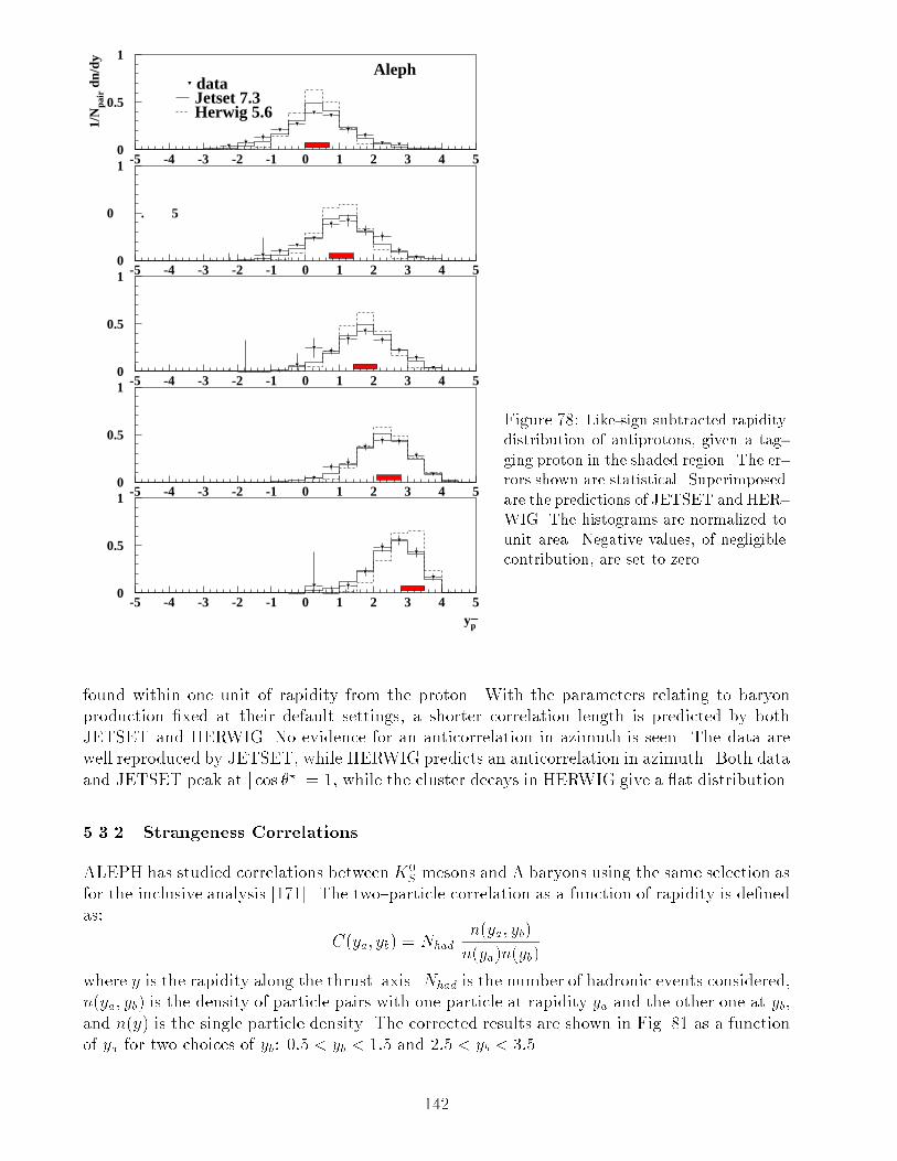
0

0.5

1

-5 -4 -3 -2 -1 0 1 2 3 4 5

dataJetset 7.3Herwig 5.6

Aleph1/

Npa

ir d

n/dy

0

0 . 5

1

-5 -4 -3 -2 -1 0 1 2 3 4 5

0

0.5

1

-5 -4 -3 -2 -1 0 1 2 3 4 5

0

0.5

1

-5 -4 -3 -2 -1 0 1 2 3 4 5

0

0.5

1

-5 -4 -3 -2 -1 0 1 2 3 4 5yp̄

Figure 78: Like-sign subtracted rapidity

distribution of antiprotons, given a tag-

ging proton in the shaded region. The er-

rors shown are statistical. Superimposed

are the predictions of JETSET and HER-

WIG. The histograms are normalized to

unit area. Negative values, of negligible

contribution, are set to zero.

found within one unit of rapidity from the proton. With the parameters relating to baryon

production �xed at their default settings, a shorter correlation length is predicted by both

JETSET and HERWIG. No evidence for an anticorrelation in azimuth is seen. The data are

well reproduced by JETSET, while HERWIG predicts an anticorrelation in azimuth. Both data

and JETSET peak at j cos �?j = 1, while the cluster decays in HERWIG give a at distribution.

5.3.2 Strangeness Correlations

ALEPH has studied correlations betweenK0S mesons and � baryons using the same selection as

for the inclusive analysis [171]. The two{particle correlation as a function of rapidity is de�ned

as:

C(ya; yb) = Nhad

n(ya; yb)

n(ya)n(yb)

where y is the rapidity along the thrust{axis. Nhad is the number of hadronic events considered,

n(ya; yb) is the density of particle pairs with one particle at rapidity ya and the other one at yb,

and n(y) is the single particle density. The corrected results are shown in Fig. 81 as a function

of ya for two choices of yb: 0:5 < yb < 1:5 and 2:5 < yb < 3:5.

142

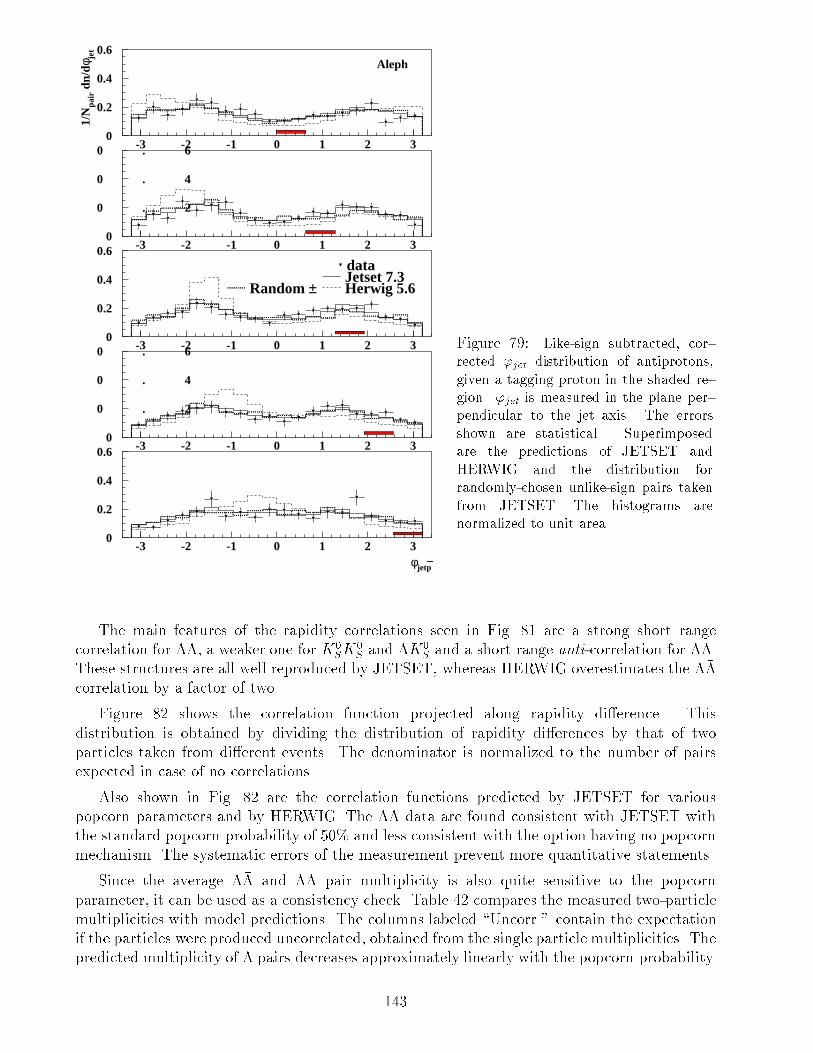
0

0.2

0.4

0.6

-3 -2 -1 0 1 2 3

Aleph

1/N

pair d

n/dφ

jet

0

0 . 2

0 . 4

0 . 6

-3 -2 -1 0 1 2 3

0

0.2

0.4

0.6

-3 -2 -1 0 1 2 3

dataJetset 7.3Herwig 5.6Random ±

0

0 . 2

0 . 4

0 . 6

-3 -2 -1 0 1 2 3

0

0.2

0.4

0.6

-3 -2 -1 0 1 2 3φjetp̄

Figure 79: Like-sign subtracted, cor-

rected 'jet distribution of antiprotons,

given a tagging proton in the shaded re-

gion. 'jet is measured in the plane per-

pendicular to the jet axis. The errors

shown are statistical. Superimposed

are the predictions of JETSET and

HERWIG and the distribution for

randomly-chosen unlike-sign pairs taken

from JETSET. The histograms are

normalized to unit area.

The main features of the rapidity correlations seen in Fig. 81 are a strong short range

correlation for ���, a weaker one for K0SK

0S and �K0

S and a short range anti-correlation for ��.

These structures are all well reproduced by JETSET, whereas HERWIG overestimates the ���

correlation by a factor of two.

Figure 82 shows the correlation function projected along rapidity di�erence. This

distribution is obtained by dividing the distribution of rapidity di�erences by that of two

particles taken from di�erent events. The denominator is normalized to the number of pairs

expected in case of no correlations.

Also shown in Fig. 82 are the correlation functions predicted by JETSET for various

popcorn parameters and by HERWIG. The ��� data are found consistent with JETSET with

the standard popcorn probability of 50% and less consistent with the option having no popcorn

mechanism. The systematic errors of the measurement prevent more quantitative statements.

Since the average ��� and �� pair multiplicity is also quite sensitive to the popcorn

parameter, it can be used as a consistency check. Table 42 compares the measured two-particle

multiplicities with model predictions. The columns labeled \Uncorr." contain the expectation

if the particles were produced uncorrelated, obtained from the single particle multiplicities. The

predicted multiplicity of � pairs decreases approximately linearly with the popcorn probability.

143

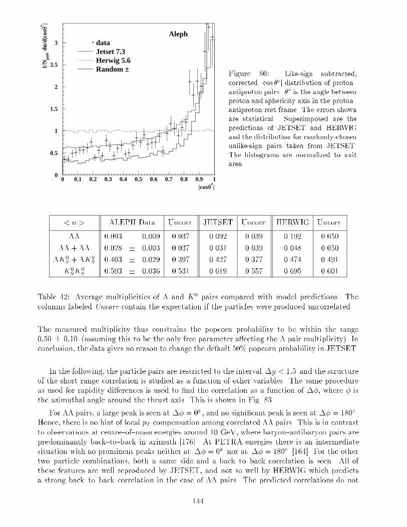
0

0.5

1

1.5

2

2.5

3

0 0.1 0.2 0.3 0.4 0.5 0.6 0.7 0.8 0.9 1

dataJetset 7.3Herwig 5.6Random ±

Aleph

|cosθ*|

1/N

pair d

n/d|

cosθ

* |

Figure 80: Like-sign subtracted,

corrected j cos �?j distribution of proton{

antiproton pairs. �? is the angle between

proton and sphericity axis in the proton{

antiproton rest frame. The errors shown

are statistical. Superimposed are the

predictions of JETSET and HERWIG

and the distribution for randomly-chosen

unlike-sign pairs taken from JETSET.

The histograms are normalized to unit

area.

< n > ALEPH Data Uncorr. JETSET Uncorr. HERWIG Uncorr.

��� 0:093 � 0:009 0.037 0.092 0.039 0.192 0.050

�� + ���� 0:028 � 0:003 0.037 0.031 0.039 0.048 0.050

�K0S +

��K0S 0:403 � 0:029 0.397 0.427 0.377 0.474 0.491

K0SK

0S 0:593 � 0:036 0.531 0.619 0.557 0.695 0.601

Table 42: Average multiplicities of � and K0 pairs compared with model predictions. The

columns labeled Uncorr contain the expectation if the particles were produced uncorrelated.

The measured multiplicity thus constrains the popcorn probability to be within the range

0:50 � 0:10 (assuming this to be the only free parameter a�ecting the � pair multiplicity). In

conclusion, the data gives no reason to change the default 50% popcorn probability in JETSET.

In the following, the particle pairs are restricted to the interval �y < 1:5 and the structure

of the short range correlation is studied as a function of other variables. The same procedure

as used for rapidity di�erences is used to �nd the correlation as a function of ��, where � is

the azimuthal angle around the thrust axis. This is shown in Fig. 83.

For ��� pairs, a large peak is seen at �� = 0� , and no signi�cant peak is seen at �� = 180� .Hence, there is no hint of local pT compensation among correlated ��� pairs. This is in contrast

to observations at centre{of{mass energies around 10 GeV, where baryon{antibaryon pairs are

predominantly back{to{back in azimuth [176]. At PETRA energies there is an intermediate

situation with no prominent peaks neither at �� = 0� nor at �� = 180� [164]. For the other

two{particle combinations, both a same{side and a back{to{back correlation is seen. All of

these features are well reproduced by JETSET, and not so well by HERWIG which predicts

a strong back{to{back correlation in the case of ��� pairs. The predicted correlations do not

144

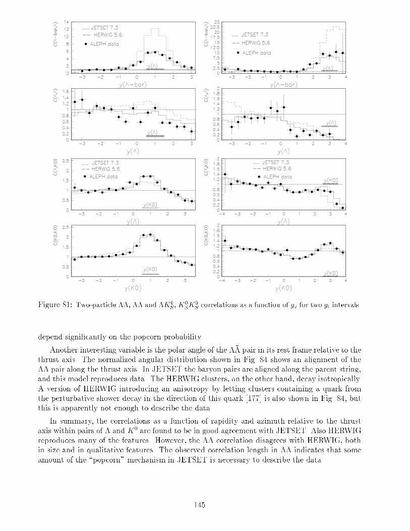
Figure 81: Two-particle ���, �� and �K0S, K

0SK

0S correlations as a function of ya for two yb intervals.

depend signi�cantly on the popcorn probability.

Another interesting variable is the polar angle of the ��� pair in its rest frame relative to the

thrust axis. The normalized angular distribution shown in Fig. 84 shows an alignment of the

��� pair along the thrust axis. In JETSET the baryon pairs are aligned along the parent string,

and this model reproduces data. The HERWIG clusters, on the other hand, decay isotropically.

A version of HERWIG introducing an anisotropy by letting clusters containing a quark from

the perturbative shower decay in the direction of this quark [177] is also shown in Fig. 84, but

this is apparently not enough to describe the data.

In summary, the correlations as a function of rapidity and azimuth relative to the thrust

axis within pairs of � and K0 are found to be in good agreement with JETSET. Also HERWIG

reproduces many of the features. However, the ��� correlation disagrees with HERWIG, both

in size and in qualitative features. The observed correlation length in ��� indicates that some

amount of the \popcorn" mechanism in JETSET is necessary to describe the data.

145

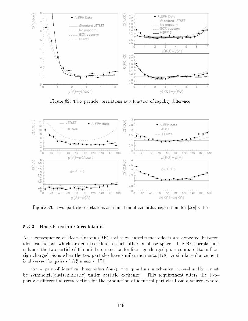
Figure 82: Two{particle correlations as a function of rapidity di�erence.

Figure 83: Two{particle correlations as a function of azimuthal separation, for j�yj < 1:5.

5.3.3 Bose-Einstein Correlations

As a consequence of Bose-Einstein (BE) statistics, interference e�ects are expected between

identical bosons which are emitted close to each other in phase space. The BE correlations

enhance the two particle di�erential cross section for like-sign charged pions compared to unlike-

sign charged pions when the two particles have similar momenta [178]. A similar enhancement

is observed for pairs of K0S mesons [171].

For a pair of identical bosons(fermions), the quantum mechanical wave-function must

be symmetric(antisymmetric) under particle exchange. This requirement alters the two-

particle di�erential cross section for the production of identical particles from a source, whose

146

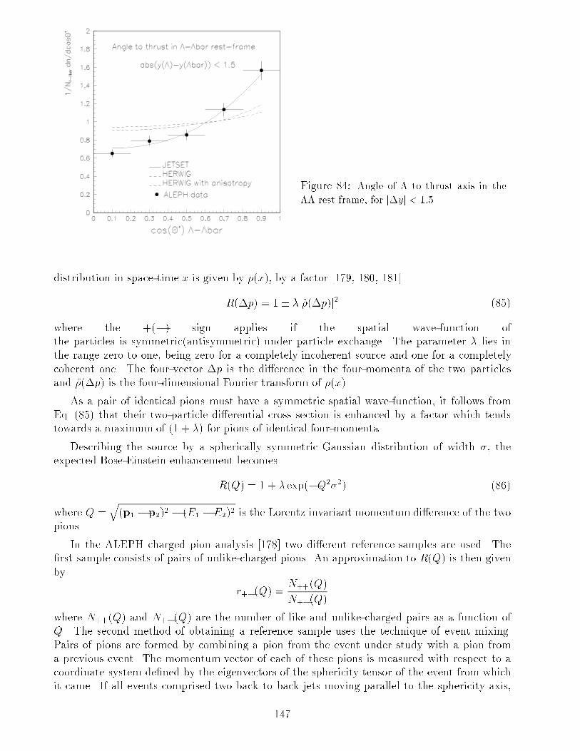
Figure 84: Angle of � to thrust axis in the

��� rest frame, for j�yj < 1:5.

distribution in space-time x is given by �(x), by a factor [179, 180, 181]

R(�p) = 1� �j~�(�p)j2 (85)

where the +(�) sign applies if the spatial wave-function of

the particles is symmetric(antisymmetric) under particle exchange. The parameter � lies in

the range zero to one, being zero for a completely incoherent source and one for a completely

coherent one. The four-vector �p is the di�erence in the four-momenta of the two particles

and ~�(�p) is the four-dimensional Fourier transform of �(x).

As a pair of identical pions must have a symmetric spatial wave-function, it follows from

Eq. (85) that their two-particle di�erential cross section is enhanced by a factor which tends

towards a maximum of (1 + �) for pions of identical four-momenta.

Describing the source by a spherically symmetric Gaussian distribution of width �, the

expected Bose-Einstein enhancement becomes

R(Q) = 1 + � exp(�Q2�2) (86)

where Q =q(p1 � p2)2 � (E1 �E2)2 is the Lorentz invariant momentum di�erence of the two

pions.

In the ALEPH charged pion analysis [178] two di�erent reference samples are used. The

�rst sample consists of pairs of unlike-charged pions. An approximation to R(Q) is then given

by

r+�(Q) =N++(Q)

N+�(Q)

where N++(Q) and N+�(Q) are the number of like and unlike-charged pairs as a function of

Q. The second method of obtaining a reference sample uses the technique of event mixing.

Pairs of pions are formed by combining a pion from the event under study with a pion from

a previous event. The momentum vector of each of these pions is measured with respect to a

coordinate system de�ned by the eigenvectors of the sphericity tensor of the event from which

it came. If all events comprised two back to back jets moving parallel to the sphericity axis,

147

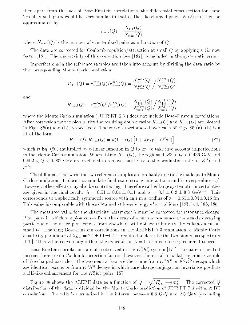
then apart from the lack of Bose-Einstein correlations, the di�erential cross section for these

`event-mixed' pairs would be very similar to that of the like-charged pairs. R(Q) can then be

approximated by

rmix(Q) =N++(Q)

Nmix(Q)

where Nmix(Q) is the number of event-mixed pairs as a function of Q.

The data are corrected for Coulomb repulsion/attraction at small Q by applying a Gamow

factor [181]. The uncertainty of this correction (see [182]) is included in the systematic error.

Imperfections in the reference samples are taken into account by dividing the data ratio by

the corresponding Monte Carlo prediction:

R+�(Q) = rdata+� (Q)=rMC+� (Q) =

Ndata++ (Q)

Ndata+� (Q)

�NMC++ (Q)

NMC+� (Q)

and

Rmix(Q) = rdatamix (Q)=rMCmix (Q) =

Ndata++ (Q)

Ndatamix (Q)

�NMC++ (Q)

NMCmix (Q)

where the Monte Carlo simulation ( JETSET 6.3 ) does not include Bose-Einstein correlations.

After correction for the pion purity the resulting double ratios R+�(Q) and Rmix(Q) are plotted

in Figs. 85(a) and (b), respectively. The curve superimposed over each of Figs. 85 (a), (b) is a

�t of the form

R+�(Q); Rmix(Q) = �(1 + �Q)h1 + � exp(�Q2�2)

i(87)

which is Eq. (86) multiplied by a linear function in Q to try to take into account imperfections

in the Monte Carlo simulation. When �tting R+�(Q), the regions 0:388 < Q < 0:436 GeV and

0:502 < Q < 0:932 GeV are excluded to remove sensitivity to the production rates of K0's and

�0's.

The di�erences between the two reference samples are probably due to the inadequate Monte

Carlo simulation. It does not simulate �nal state strong interactions and it overproduces �0.However, other e�ects may also be contributing. Therefore rather large systematic uncertainties

are given in the �nal result: � = 0:51 � 0:04 � 0:11 and � = 3:3 � 0:2 � 0:8 GeV�1. This

corresponds to a spherically symmetric source with an r.m.s. radius of � = 0:65�0:04�0:16 fm.

This value is comparable with those obtained at lower energy e+e� colliders [183, 184, 185, 186].

The measured value for the chaoticity parameter � must be corrected for resonance decays.

Pion pairs in which one pion comes from the decay of a narrow resonance or a weakly decaying

particle and the other pion comes from elsewhere will not contribute to the enhancement at

small Q. Enabling Bose-Einstein correlations in the JETSET 7.3 simulation, a Monte Carlo

chaoticity parameter of �MC = 2:1�0:1�0:1 is required to describe the two pion mass spectrum

[170]. This value is even larger than the expectation � = 1 for a completely coherent source.

Bose-Einstein correlations are also observed in the K0SK

0S system [171]. For pairs of neutral

mesons there are no Coulomb correction factors, however, there is also no data reference sample

of like-charged particles. The two neutral kaons either come from K0K0 or �K0 �K0 decays which

are identical bosons or from K0 �K0 decays in which case charge conjugation invariance predicts

a BE-like enhancement for the K0SK

0S pairs [187].

Figure 86 shows the ALEPH data as a function of Q =qM2

KK � 4m2K . The corrected Q

distribution of the data is divided by the Monte Carlo prediction of JETSET 7.3 without BE

correlation. The ratio is normalized in the interval between 0.6 GeV and 2.5 GeV (excluding

148

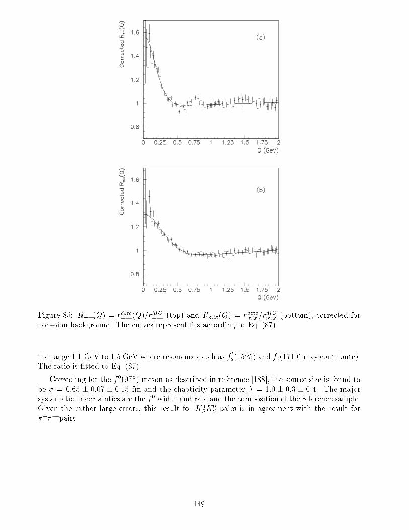
Figure 85: R+�(Q) = rdata+� (Q)=rMC+� (top) and Rmix(Q) = rdatamix =r

MCmix (bottom), corrected for

non-pion background. The curves represent �ts according to Eq. (87).

the range 1.1 GeV to 1.5 GeV where resonances such as f0

2(1525) and f0(1710) may contribute).

The ratio is �tted to Eq. (87).

Correcting for the f0(975) meson as described in reference [188], the source size is found to

be � = 0:65 � 0:07 � 0:15 fm and the chaoticity parameter � = 1:0 � 0:3 � 0:4. The major

systematic uncertainties are the f0 width and rate and the composition of the reference sample.

Given the rather large errors, this result for K0SK

0S pairs is in agreement with the result for

�+�� pairs.

149

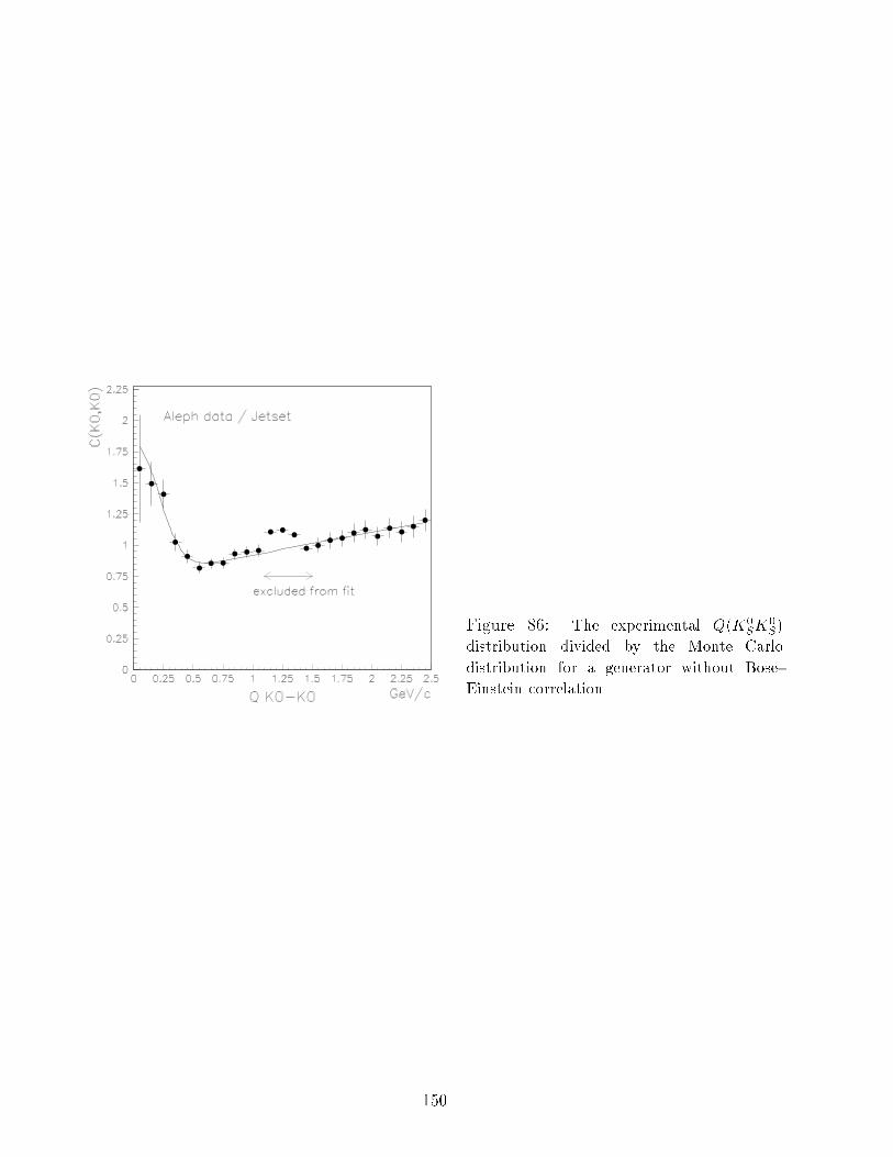
Figure 86: The experimental Q(K0SK

0S)

distribution divided by the Monte Carlo

distribution for a generator without Bose-

Einstein correlation.

150

6 Summary

With the high statistics data collected in hadronic Z decays signi�cant progress in the

understanding of the dynamics of QCD has been achieved, spanning the hard perturbative

regime, the parton showering process and the non-perturbative region of hadron formation.

The strong coupling constant �s has been measured from R� at the scale of the tau mass,

from scaling violations in fragmentation functions betweenps = 22 GeV and

ps = MZ , and

from the analysis of global event shape variables and Rl at the scale of the Z mass. The energy

evolution is consistent with the running expected from QCD.

Testing the structure of QCD, it has been con�rmed that quarks have spin 1/2 and that

gluons have spin 1. The non-Abelian nature of QCD requires the strong coupling constant to

be avour independent, consistent with the experimental �ndings for the ratios �s(b)=�s(udsc)

and �s(uds)=�s(bc). Information about the gauge structure of strong interactions has been

obtained from measurements of the colour factors from the study of kinematical correlations in

multi-jet events and the running of the strong coupling constant between the scale of the � and

the Z mass. Combining all information, the ALEPH results for the colour factor ratios show

that the gauge structure of QCD is compatible with the expectation for an unbroken SU(3)

symmetry, while it is incompatible with the predictions based on many other gauge groups,

including any Abelian model.

Experimental evidence was shown that the parton showering process proceeds like in

a self-similar branching process as implemented in coherent parton shower models. The

importance of coherence e�ects is demonstrated by the energy evolution of inclusive momentum

spectra and charged particle multiplicities, both of which are quantitatively described by the

modi�ed leading-log approximation (MLLA) and local parton-hadron duality (LPHD), and by

comparing measured particle-particle correlation functions with predictions from various Monte

Carlo models. Studies of the string e�ect show that colour coherence is present both in the

perturbative and the non-perturbative phase of hadronic Z decays.

The high statistics data available at LEP for the �rst time facilitated detailed comparisons

between quark and gluon jets in three jet events, showing di�erences which result from the

di�erent colour charges of quarks and gluons. The gluon jet was found to be wider than an

equivalent quark jet with higher multiplicities and a softer momentum spectrum. However,

the di�erences observed at the level of the �nal state hadrons were much smaller than the

expectations for asymptotic energies, which is understood to be at least partly caused by colour

coherence e�ects. Another sensitive probe of quark/gluon di�erences is the study of subjet

multiplicities, which, looking closer to the hard perturbative regime, independently con�rmed

the di�erent colour charges of the two kinds of partons.

Prompt photon production in hadronic events provides a unique window for looking into

the early stages on the parton showering process free from fragmentation e�ects. The studies

with isolated photons in hadronic events have shown inadequacies in the treatment of photon

radiation during the parton showering process in all models studied. Measuring prompt

photons also inside jets has allowed the �rst determination of the quark-to-photon fragmentation

function. Using this information, the description of the data has improved substantially.

The detailed understanding of the hadronization stage still relies on phenomenological

models, which, however, are quite successful in describing the relative production rates and

momentum spectra of the �nal state particles. Measurements were presented for identi�ed

pions, kaons and protons, strange mesons and baryons, vector mesons and single photons.

More detailed information about the dynamics of hadron formation was obtained from the

151

study of two-particle correlations. It was found that the JETSET and ARIADNE string

models successfully parametrize two-particle correlations related to strangeness and baryon

number. Most of the parameters in JETSET and ARIADNE have a rather natural physical

meaning, in that they correspond to suppression e�ects for heavier particles, which are di�cult

to predict from �rst principles. The baryon spectra, however, require at least two rather

unnatural parameters, the so-called leading baryon suppression and popcorn; this casts some

doubt on the validity of the baryon production scheme via diquarks. HERWIG, with far fewer

parameters, is able to predict essentially all of the meson multiplicities, while it reproduces far

less well the baryon rates. Finally, the source size, or equivalently the hadronization scale, was

measured by means of Bose-Einstein correlations to be around 0.65 fm.

This paper has summarized the ALEPH results on QCD based on most of the LEP I data,

taken between 1989 and 1995. The higher centre-of-mass energies available at LEP II, which

started in November 1995, as well as the development of new theoretical and experimental

techniques, will allow for additional tests of QCD in the future.

152

Appendix

A Rl and R� for Arbitrary Colour Factors

This section contains a compilation of the ingredients that go into the theoretical prediction

for Rl and R� for arbitrary colour factors. Although the QCD (SU(3)) expressions are well

known, the ones for the general case that the dynamics of strong interactions is described by

any unbroken gauge symmetry based on a simple Lie group, i.e. a theory with one universal

coupling constant and massless gluons, are rather scattered through the literature.

It is convenient to rede�ne the coupling constant such that the amplitude for gluon emission

from a quark is independent of the gauge group of the theory. Also absorbing a factor of 2�

yields

a =�sCF

2�:

The predictions of the theory for nF quark degrees of freedom then can be expressed as function

of the free parameter a and the variables

x =CA

CF

; y =TF

CF

and z = y � nf :

All expressions apply for the MS renormalization scheme.

A.1 The Running Coupling Constant and Masses

The variation of the strong coupling constant a and renormalized masses m with the

renormalization scale of the theory is described by a coupled system of di�erential equations:

da

d ln�= �b0a2 � b1a

3 � b2a4 : : : (88)

d lnm

d ln�= �g0a� g1a

2 : : : (89)

The coe�cients bi and gi depend on the speci�c theory, with the leading coe�cients given

by [189, 190, 103, 191]:

b0 =11

3x� 4

3z

b1 =17

3x2 � 10

3xz � 2z

b2 =2857

216x3 � 1415

108x2z +

158

108xz2 � 205

36xz +

11

9z2 +

1

2z (90)

g0 = 3

g1 =3

4+97

12x� 5

3z (91)

Equation (88) determines how the strong coupling constant evolves for a �xed number of

active avours. The treatment of avour thresholds is described in [192]. It turns out that the

153

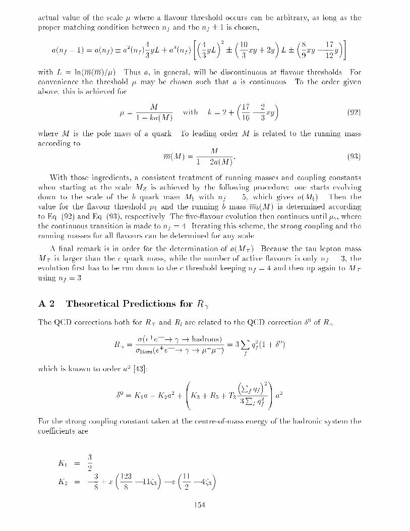
actual value of the scale � where a avour threshold occurs can be arbitrary, as long as the

proper matching condition between nf and the nf � 1 is chosen,

a(nf � 1) = a(nf)� a2(nf)4

3yL+ a3(nf )

"�4

3yL

�2��10

3xy + 2y

�L �

�8

9xy � 17

12y

�#

with L = ln(m(m)=�). Thus a, in general, will be discontinuous at avour thresholds. For

convenience the threshold � may be chosen such that a is continuous. To the order given

above, this is achieved for

� =M

1 + ka(M)with k = 2 +

�17

16� 2

3xy

�(92)

where M is the pole mass of a quark. To leading order M is related to the running mass

according to

m(M) =M

1 + 2a(M): (93)

With those ingredients, a consistent treatment of running masses and coupling constants

when starting at the scale MZ is achieved by the following procedure: one starts evolving

down to the scale of the b quark mass Mb with nf = 5, which gives a(Mb). Then the

value for the avour threshold �b and the running b mass mb(M) is determined according

to Eq. (92) and Eq. (93), respectively. The �ve- avour evolution then continues until �b, where

the continuous transition is made to nf = 4. Iterating this scheme, the strong coupling and the

running masses for all avours can be determined for any scale.

A �nal remark is in order for the determination of a(M� ). Because the tau lepton mass

M� is larger than the c quark mass, while the number of active avours is only nf = 3, the

evolution �rst has to be run down to the c threshold keeping nf = 4 and then up again to M�using nf = 3.

A.2 Theoretical Predictions for R

The QCD corrections both for R� and Rl are related to the QCD correction �0 of R

R =�(e+e� ! ! hadrons)

�Born(e+e� ! ! �+��)

= 3Xf

q2f (1 + �0)

which is known to order a3 [43]:

�0 = K1a+K2a2 +

0B@K3 +R3 + T3

�Pf qf

�23P

f q2f

1CA a3

For the strong coupling constant taken at the centre-of-mass energy of the hadronic system the

coe�cients are

K1 =3

2

K2 = �3

8+ x

�123

8� 11�3

�� z

�11

2� 4�3

�

154

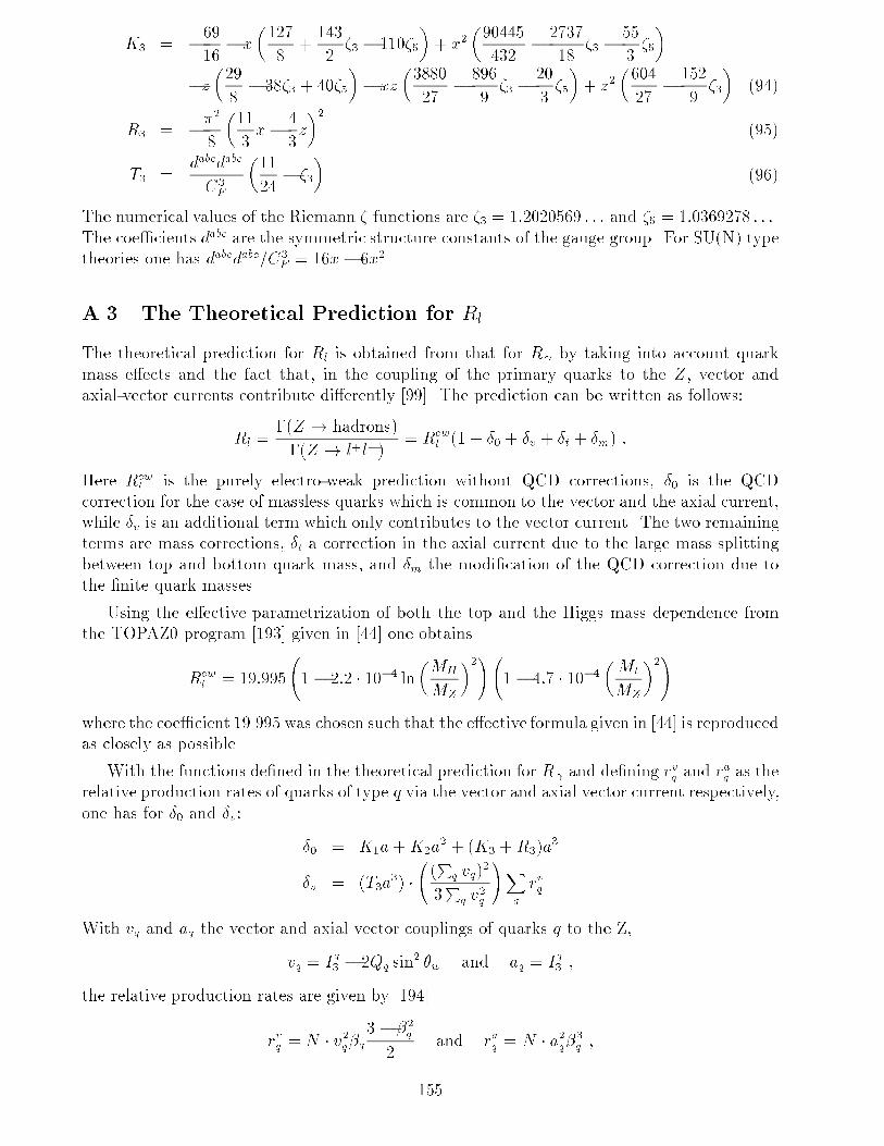
K3 = �69

16� x

�127

8+143

2�3 � 110�5

�+ x2

�90445

432� 2737

18�3 � 55

3�5

�

�z�29

8� 38�3 + 40�5

�� xz

�3880

27� 896

9�3 � 20

3�5

�+ z2

�604

27� 152

9�3

�(94)

R3 = ��2

8

�11

3x� 4

3z

�2(95)

T3 =dabcdabc

C3F

�11

24� �3

�(96)

The numerical values of the Riemann � functions are �3 = 1:2020569 : : : and �5 = 1:0369278 : : :.

The coe�cients dabc are the symmetric structure constants of the gauge group. For SU(N) type

theories one has dabcdabc=C3F = 16x� 6x2.

A.3 The Theoretical Prediction for Rl

The theoretical prediction for Rl is obtained from that for R by taking into account quark

mass e�ects and the fact that, in the coupling of the primary quarks to the Z, vector and

axial-vector currents contribute di�erently [99]. The prediction can be written as follows:

Rl =�(Z ! hadrons)

�(Z ! l+l�)= Rew

l (1 + �0 + �v + �t + �m) :

Here Rewl is the purely electro-weak prediction without QCD corrections, �0 is the QCD

correction for the case of massless quarks which is common to the vector and the axial current,

while �v is an additional term which only contributes to the vector current. The two remaining

terms are mass corrections, �t a correction in the axial current due to the large mass splitting

between top and bottom quark mass, and �m the modi�cation of the QCD correction due to

the �nite quark masses.

Using the e�ective parametrization of both the top and the Higgs mass dependence from

the TOPAZ0 program [193] given in [44] one obtains

Rewl = 19:995

1� 2:2 � 10�4 ln

�MH

MZ

�2! 1 � 4:7 � 10�4

�Mt

MZ

�2!

where the coe�cient 19.995 was chosen such that the e�ective formula given in [44] is reproduced

as closely as possible.

With the functions de�ned in the theoretical prediction for R and de�ning rvq and r

aq as the

relative production rates of quarks of type q via the vector and axial vector current respectively,

one has for �0 and �v:

�0 = K1a+K2a2 + (K3 +R3)a

3

�v = (T3a3) �

(P

q vq)2

3P

q v2q

!Xq

rvq

With vq and aq the vector and axial vector couplings of quarks q to the Z,

vq = Iq3 � 2Qq sin2 �w and aq = Iq3 ;

the relative production rates are given by [194]

rvq = N � v2q�q3 � �2q

2and raq = N � a2q�3q ;

155

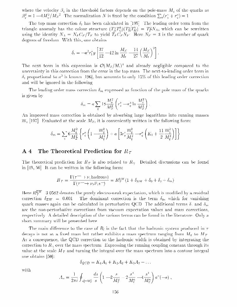
where the velocity �q in the threshold factors depends on the pole-mass Mq of the quarks as

�2q = 1� 4M2q =MZ

2. The normalization N is �xed by the conditionP

q(rvq + raq ) = 1.

The top mass correction �t has been calculated in [195]. The leading order term from the

triangle anomaly has the colour structure (T ajiT

bij)(T

alkT

bkl) = T 2

FNA, which can be rewritten

using the identity NA = NFCF =TF to yield TFCFNF . Here NF = 3 is the number of quark

degrees of freedom. With this, one obtains

�t = �a2rab y"37

12� 12 ln

MZ

Mt

� 14

27

�MZ

Mt

�2#:

The next term in this expression is O(MZ=Mt)4 and already negligible compared to the

uncertainty in this correction from the error in the top mass. The next-to-leading order term in

�t proportional to a3 is known [196], but amounts to only 15% of this leading order correction

and will be ignored in the following.

The leading order mass correction �m expressed as function of the pole mass of the quarks

is given by

�m = aXq

18M2

q

M2Z

rvq � raq ln

M2q

M2Z

!:

An improved mass correction is obtained by absorbing large logarithms into running masses

mq [197]. Evaluated at the scale MZ, it is conveniently written in the following form:

�m =Xq

6M2

q

M2Z

(raq

1 � m2

q

M2q

!+ a

"3rvq

m2q

M2q

� raq

K1 +

11

2

m2q

M2q

!#)

A.4 The Theoretical Prediction for R�

The theoretical prediction for R� is also related to R . Detailed discussions can be found

in [49, 50]. It can be written in the following form:

R� =�(�� ! ��hadrons)

�(�� ! ���ee�)= REW

� (1 + �EW + �0 + �c + �m)

Here REW� =3.0582 denotes the purely electro-weak expectation, which is modi�ed by a residual

correction �EW = 0:001. The dominant correction is the term �0, which for vanishing

quark masses again can be calculated in perturbative QCD. The additional terms �c and �mare the non-perturbative corrections from vacuum expectation values and mass corrections,

respectively. A detailed description of the various terms can be found in the literature. Only a

short summary will be presented here.

The main di�erence to the case of Rl is the fact that the hadronic system produced in �

decays is not at a �xed mass but rather exhibits a mass spectrum ranging from M� to M� .

As a consequence, the QCD correction to the hadronic width is obtained by integrating the

correction to R over the mass spectrum. Expressing the running coupling constant through its

value at the scale M� and turning the integral over the mass spectrum into a contour integral

one obtains [50]:

�QCD = K1A1 +K2A2 +K3A3 + : : :

with

An =1

2�i

Ijsj=M2

�

ds

s

1 � 2

s

M2�

+ 2s3

M6�

� 4s4

M8�

!an(�s) ;

156

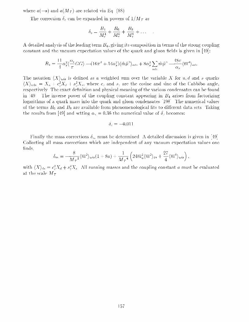
where a(�s) and a(M� ) are related via Eq. (88).

The correction �c can be expanded in powers of 1/M� as

�c =B4

M4�

+B6

M6�

+B8

M8�

+ : : : :

A detailed analysis of the leading termB4, giving its composition in terms of the strong coupling

constant and the vacuum expectation values of the quark and gluon �elds is given in [49]:

B4 =11

4�2sh

�s

�GGi � (16�2 + 54�2s)hm̂�̂3iuds + 8�2s

Xuds

m̂�̂3 � 48�

�shm4iuds

The notation hXiuds is de�ned as a weighted sum over the variable X for u; d and s quarks

hXiuds = Xu + c2cXd + s2cXs, where cc and sc are the cosine and sine of the Cabbibo angle,

respectively. The exact de�nition and physical meaning of the various condensates can be found

in [49]. The inverse power of the coupling constant appearing in B4 arises from factorizing

logarithms of a quark mass into the quark and gluon condensates [198]. The numerical values

of the terms B6 and B8 are available from phenomenological �ts to di�erent data sets. Taking

the results from [49] and setting �s = 0:36 the numerical value of �c becomes:

�c = �0:011

Finally the mass corrections �m must be determined. A detailed discussion is given in [49].

Collecting all mass corrections which are independent of any vacuum expectation values one

�nds,

�m = � 8

M�2 hm2iuds(1 + 8a) +

1

M�4

�24m2

uhm2ids + 27

4hm4iuds

�;

with hXids = c2cXd + s2cXs. All running masses and the coupling constant a must be evaluated

at the scale M� .

157

References

[1] J. D. Bjorken and E. A. Paschos, Phys. Rev. 185 (1969) 1975.

[2] M. Y. Han and Y. Nambu, Phys. Rev. B139 (1965) 1006;

E. Reya, Phys. Rep. 69 (1981) 195.

[3] H. Fritzsch, M. Gell-Mann and H. Leutwyler, Phys. Lett. B47 (1973) 365.

[4] D. J. Gross and F. Wilczek, Phys. Rev. Lett. 30 (1973) 1343.

[5] H. D. Politzer, Phys. Rev. Lett. 30 (1973) 1346.

[6] D. Buskulic et al., ALEPH collaboration, Phys. Lett. B303 (1993) 198.

[7] B. R. Webber, Phys. Lett. B339 (1994) 148;

Yu. L. Dokshitzer and B. R. Webber, Phys. Lett. B352 (1995) 451;

P. Nason and M. Seymour, Nucl. Phys. B454 (1995) 291;

R. Akhoury and V. I. Zakharov, Phys. Lett. B357 (1995) 646; Nucl. Phys. B465 (1996)

295;

M. Beneke and V. M. Braun, Nucl. Phys. B454 (1995) 253.

[8] M. Gell-Mann, Phys. Lett. 8 (1964) 214.

[9] G. Zweig, CERN-TH 401 and TH 412 (1964).

[10] E. D. Bloom et al., Phys. Rev. Lett. 23 (1969) 930;

M. Breidenbach et al., Phys. Rev. Lett. 23 (1969) 935.

[11] R. P. Feynman, Photon Hadron Interactions, Benjamin, New York, 1972.

[12] P. M. Zerwas and H. A. Kastrup, eds., QCD 20 Years Later, World Scienti�c, Singapore

(1993).

[13] G. Altarelli, Phys. Rep. 81 (1982) 1.

[14] D. H. Perkins, Introduction to High Energy Physics, Addison-Wesley, Menlo Park,

California, 1987.

[15] J. Ellis, M. K. Gaillard, G. Ross Nucl. Phys. B111 (1976) 253.

[16] R. K. Ellis, D. A. Ross and A. E. Terrano, Nucl. Phys. B178 (1981) 421.

[17] A. Altarelli and G. Parisi, Nucl. Phys. B126 (1977) 298;

Yu. L. Dokshitzer, Sov. Phys. JETP 46 (1977) 641.

[18] B. I. Ermolaev, V. S. Fadin, ZhETF Pis'ma 33 (1981) 285;

A. H. Mueller, Phys. Lett. B104 (1981) 161;

V. S. Fadin, Yad. Fiz. 36 (1982).

[19] D. Decamp et al., ALEPH Collaboration, Nucl. Instr. Methods A294 (1990) 121.

[20] D. Buskulic et al., ALEPH Collaboration, Nucl. Instr. Methods A360 (1995) 481.

[21] G. Batignani et al., 1991 IEEE Nuclear Science Symposium, Santa Fe, IEEE. Trans. Nucl.

Sci. NS-39(4/5) (1992) Vol. 1, p. 438.

158

[22] G. J. Barber et al., Nucl. Instr. Methods A279 (1989) 212.

[23] W. B. Atwood et al., Nucl. Instr. Methods A306 (1991) 446.

[24] J. E. Campagne and R. Zitoun, Z. Phys. C43 (1989) 469.

[25] T. Sj�ostrand, Comp. Phys. Comm. 82 (1994) 74.

[26] D. Buskulic et al., ALEPH Collaboration, Z. Phys. C55 (1992) 209.

[27] W. Bartel et al., JADE Collaboration, Z. Phys. C33 (1986) 23; S. Bethke et al., JADE

Collaboration, Phys. Lett. B213 (1988) 235.

[28] Proceedings of the Durham Workshop, W. J. Stirling, J. Phys. G: Nucl. Part. Phys. 17

(1991) 1567;

N. Brown and W. J. Stirling, Phys. Lett. B252 (1990) 657;

S. Bethke et al., Nucl. Phys. B370 (1992) 310.

[29] B. Andersson et al., Phys. Rep. 97 (1983) 31.

[30] L. L�onnblad, Comp. Phys. Comm. 71 (1992) 15.

[31] G. Marchesini et al., Comp. Phys. Comm. 67 (1992) 465.

[32] C. Peterson et al., Phys. Rev. D27 (1983) 105.

[33] G. Gustafson, Phys. Lett. B175 (1986) 453;

G. Gustafson, U. Pettersson, Nucl. Phys. B306 (1988) 746;

B. Anderson et al., Z. Phys. C43 (1989) 621;

B. Anderson, G. Gustafson, L. L�onnblad, Nucl. Phys. B339 (1990) 393.

[34] P. Abreu et al., DELPHI Collaboration, Z. Phys. C65 (1995) 587.

[35] D. Buskulic et al., ALEPH Collaboration, Z. Phys. C62 (1994) 1.

[36] D. Buskulic et al., ALEPH Collaboration, Z. Phys. C62 (1994) 179.

[37] D. Buskulic et al., ALEPH Collaboration, Phys. Lett. B357 (1995) 699.

[38] D. Buskulic et al., ALEPH Collaboration, Z. Phys. C69 (1996) 393.

[39] G. Hanson et al., Phys. Rev. Lett. 35 (1975) 1609.

[40] R. Brandelik et al., TASSO Collaboration, Phys. Lett. B97 (1980) 453;

Ch. Berger et al., PLUTO Collaboration, Phys. Lett. B97 (1980) 459.

[41] E. Laermann, K.H. Streng, P.M. Zerwas, Z. Phys. C3 (1980), 289; Erratum Z. Phys.

C52 (1991) 352.

[42] M. A. Shifman, A. L. Vainshtein and V. I. Zakharov, Nucl. Phys. B147 (1979) 385.

[43] L. R. Surguladze and M. A. Samuel, Phys. Rev. Lett. 66 (1991) 560;

S. G. Gorishny, A. L. Kataev and S. A. Larin, Phys. Lett. B259 (1991) 144.

[44] T. Hebbeker et al., Phys. Lett. B331 (1994) 165.

159

[45] D. Buskulic et al., ALEPH Collaboration, Z. Phys. C62 (1994) 539.

[46] J. Alcaraz et al., The LEP Electroweak Working Group and the SLD Heavy Flavour

Group, LEPEWWG/96-02.

[47] M. Martinez et al., Z. Phys. C49 (1991) 645.

[48] D. Buskulic et al., ALEPH Collaboration, Phys. Lett. B307 (1993) 209.

[49] E. Braaten, S. Narison and A. Pich, Nucl. Phys. B373 (1992) 581.

[50] F. Le Diberder and A. Pich, Phys. Lett. B286 (1992) 147; ibid. 289 (1992) 165.

[51] D. Buskulic et al., ALEPH Collaboration, Z. Phys. C70 (1996) 561.

[52] D. Buskulic et al., ALEPH Collaboration, Z. Phys. C70 (1996) 549.

[53] D. Buskulic et al., ALEPH Collaboration, Z. Phys. C70 (1996) 579.

[54] L. Du ot, in Proceedings of the QCD 94 Conference, ed. S. Narison, Nucl. Phys.

(Proc. Suppl.) 39B (1995) 322.

[55] W. Bernreuther and W. Wetzel, Nucl. Phys. B197 (1982) 228.

[56] A. Pich, in Proceedings of the QCD 94 Conference, ed. S. Narison, Nucl. Phys.

(Proc. Suppl.) 39B (1995) 326.

[57] P. Ball, M. Beneke and V. M. Braun, Nucl. Phys. B452 (1995) 563.

[58] G. Altarelli, P. Nason and G. Ridol�, Z. Phys. C68 (1995) 257.

[59] Z. Kunszt et al., in Proceedings of the Workshop on Z Physics at LEP, eds. G. Altarelli,

R. Kleiss and C. Verzegnassi, CERN Report 89-08, p. 373{453.

[60] T. Sj�ostrand and M. Bengtsson, Comp. Phys. Comm. 43 (1987) 367.

[61] M. Bengtsson and T. Sj�ostrand, Phys. Lett. B185 (1987) 435.

[62] G. Marchesini and B. Webber, Cavendish-HEP-88/7; Nucl. Phys. B310 (1988) 461;

I. Knowles, Nucl. Phys. B310 (1988) 571.

[63] D. Decamp et al., ALEPH Collaboration, Phys. Lett. B255 (1991) 623.

[64] D. Decamp et al., ALEPH Collaboration, Phys. Lett. B257 (1991) 479.

[65] P. Nason, program EVENT, private communication.

[66] S. Catani et al., Nucl. Phys. B407 (1993) 3, and references therein.

[67] S. Catani et al., Phys. Lett. B263 (1991) 491.

[68] S. Catani, G. Turnock and B. R. Webber, Phys. Lett. B272 (1991) 368.

[69] S. Catani et al., Phys. Lett. B269 (1991) 432.

[70] G. Dissertori and M. Schmelling, Phys. Lett. B361 (1995) 167.

160

[71] D. Decamp et al., ALEPH Collaboration, Phys. Lett. B284 (1992) 163.

[72] D. Buskulic et al., ALEPH Collaboration, Phys. Lett. B357 (1995) 487; and Erratum,

ibid. B364 (1995) 247.

[73] P. Nason and B. R. Webber, Nucl. Phys. B421 (1994) 473.

[74] G. Altarelli, R. K. Ellis, G. Martinelli and S.-Y. Pi, Nucl. Phys. B160 (1979) 301.

[75] V. N. Gribov and L. N. Lipatov, Sov. J. Nucl. Phys. 15 (1972) 78;

G. Altarelli, G. Parisi, Nucl. Phys. B126 (1977) 298;

Yu. L. Dokshitzer, Sov. Phys. JETP 46 (1977) 641.

[76] G. Gurci, W. Furmanski and R. Petronzio, Nucl. Phys. B175 (1980) 27;

W. Furmanski and R. Petronzio, Phys. Lett. B97 (1980) 437.

[77] D. Buskulic et al., ALEPH Collaboration, Phys. Lett. B313 (1993) 535.

[78] D. Buskulic et al., ALEPH Collaboration, Phys. Lett. B313 (1993) 549.

[79] D. Decamp et al., ALEPH Collaboration, Phys. Lett. B273 (1991) 181.

[80] W. Braunschweig et al., TASSO Collaboration, Z. Phys. C47 (1990) 187.

[81] A. Petersen et al., MARK II Collaboration, Phys. Rev. D37 (1988) 1.

[82] H. Aihara et al., TPC/2 Collaboration, Phys. Rev. Lett. 61 (1988) 1263; updated in

G. D. Cowan, internal note TPC-LBL-94-01.

[83] O. Podobrin, CELLO Collaboration, Ph. D. thesis, Universit�at Hamburg. See also

ref. [85].

[84] Y. K. Li et al., AMY Collaboration, Phys. Rev. D41 (1990) 2675.

[85] P. Abreu et al., DELPHI Collaboration, Phys. Lett. B311 (1993) 408.

[86] See, for instance, Yu. L. Dokshitzer et al., Basics of Perturbative QCD, Editions Fron-

ti�eres, Gif-sur-Yvette (France) 1991, and references therein.

[87] C. P. Fong and B. R. Webber, Nucl. Phys. B355 (1991) 54.

[88] M. Schmelling, Status of the strong coupling constant, plenary talk at the XXVIII

International Conference on High Energy Physics, Warsaw, July 1996. To appear in the

Proceedings.

[89] R. M. Barnett et al., Particle Data Group, Phys. Rev. D54 (1996) 1.

[90] S. Catani, G. Turnock and B. R. Webber, Phys. Lett. B295 (1992) 269.

[91] W. Braunschweig et al., TASSO Collaboration, Z. Phys. C47 (1990) 181.

[92] B. Adeva et al., L3 Collaboration, Phys. Lett. B263 (1991) 551.

[93] P. Abreu et al., DELPHI Collaboration, Phys. Lett. B274 (1992) 498.

[94] M. H. Seymour, program EVENT2, private communication;

S. Catani and M. H. Seymour, Phys. Lett. B378 (1996) 287.

161

[95] B. Lampe, Phys. Lett. B301 (1993) 435.

[96] R. D. Schamberger et al., CUSB Collaboration, Phys. Lett. B138 (1984) 225;

S. E. Csorna et al., CLEO Collaboration, Phys. Rev. Lett. 56 (1986) 1221;

H. Albrecht et al., ARGUS Collaboration, Phys. Lett. B199 (1987) 291;

W. Kwong et al., Phys. Rev. D37 (1988) 3210;

W. Braunschweig et al., TASSO Collaboration, Z. Phys. C44 (1989) 365;

A. Geiser, UA1 Collaboration, in Proceedings of the 27th Rencontre de Moriond: QCD

and High Energy Hadronics Interactions, Les Arcs, France, ed. J. Tran Thanh Van

(Editions Fronti�eres) (1991) p. 159 �.

[97] B. Adeva et al., L3 Collaboration, Phys. Lett. B271 (1991) 461;

R. Akers et al., OPAL Collaboration, Z. Phys. C60 (1993) 397;

P. Abreu et al., DELPHI Collaboration, Phys. Lett. B307 (1993) 221;

R. Akers et al., OPAL Collaboration, Z. Phys. C65 (1995) 31;

K. Abe et al., SLD Collaboration, Phys. Rev. D53 (1996) 2271.

[98] D. Buskulic et al., ALEPH Collaboration, Phys. Lett. B355 (1995) 381.

[99] T. Hebbeker, PITHA 91/08; Phys. Rep. 217 (1991) 69.

[100] J.G. K�orner, G. Schierholz and J. Willrodt, Nucl. Phys. B185 (1981) 365;

K.J.F. Gaemers and J.A.M. Vermaseren, Z. Phys. C7 (1980) 81;

D. Danckaert et al., Phys. Lett. B114 (1982) 203.

[101] ALEPH Collaboration, D. Decamp et al., Phys. Lett. B284 (1992) 151.

[102] J.M. Scarr, I. ten Have, ALEPH-NOTE 89 - 150.

[103] R. Tarrach, Nucl. Phys. B183 (1981) 384.

[104] F. Abe et al., CDF Collaboration, Phys. Rev. Lett. 74 (1995) 2626;

S. Abachi et al., D0 Collaboration, Phys. Rev. Lett. 74 (1995) 2632.

[105] See, for instance, I. Antoniadis, J. Ellis, D.V. Nanopoulos, Phys. Lett. B262 (1991) 109.

[106] M. G. Alviggi et al., LEP Electroweak Working Group, LEPEWWG 95-01.

[107] Ya. I. Azimov et al., Z. Phys. C27 (1985) 65; Z. Phys. C31 (1986) 213.

[108] C. P. Fong and B. R. Webber, Phys. Lett. B229 (1989) 289.

[109] D. Buskulic et al., ALEPH Collaboration, CERN-PPE/96-43 (1996).

[110] M. Z. Akrawy et al., OPAL Collaboration, Phys. Lett. B247 (1990) 617.

[111] B. Adeva et al., L3 Collaboration, Phys. Lett. B259 (1991) 199.

[112] M. Chmeisanni, I.F.A.E., Universitat Autonoma de Barcelona, Annual Report (1992) 49.

[113] R. Odorico, University of Bologna report DFUB 92-6 (1992).

[114] M. Acciarri et al., L3 Collaboration, Phys. Lett. B353 (1995) 145.

[115] Yu. L. Dokshitzer et al., Phys. Lett. B245 (1990) 243.

162

[116] Yu. L. Dokshitzer, G. Marchesini, G. Oriani, Nucl. Phys. B387 (1990) 675.

[117] P. D. Acton et al., OPAL Collaboration, Z. Phys. C58 (1992) 207.

[118] W. Bartel et al., JADE Collaboration, Phys. Lett. B101 (1981) 129; Z. Phys. C21

(1983) 37.

[119] A. Aihara et al., TPC/2 Collaboration, Z. Phys. C28 (1985) 31;

M. Altho� et al., TASSO Collaboration, Z. Phys. C29 (1985) 29;

P. D. Sheldon et al., MARK II Collaboration, Phys. Rev. Lett. 57 (1986) 1398;

P. Aarnio et al., DELPHI Collaboration, Phys. Lett. B240 (1990) 271;

M. Z. Akrawy et al., OPAL Collaboration, Phys. Lett. B261 (1991) 334.

[120] Z. Koba, H. B. Nielsen, P. Olesen, Nucl. Phys. B40 (1972) 317.

[121] E. D. Malaza, B. R. Webber, Phys. Lett. B149 (1984) 501;

E. D. Malaza, B. R. Webber, Nucl. Phys. B267 (1986) 702.

[122] S. Carius, G. Ingelmann, Phys. Lett. B252 (1990) 647;

R. Szwed, G. Wrochna, Z. Phys. C47 (1990) 447;

R. Szwed, G. Wrochna, A. K. Wr�oblewski, Mod. Phys. Lett. A5 (1990) 981.

[123] D. Buskulic et al., ALEPH Collaboration, Z. Phys. C69 (1995) 15

[124] V. Blobel, DESY 84-118 (1984).

[125] V. B. Anikeev and V. P. Zhigunov, Phys. Part. Nucl. 24 (4) (1993) 424.

[126] M. Schmelling, Nucl. Instr. Methods A340 (1994) 400.

[127] R. P. Feynman, Phys. Rev. Lett. 23 (1969) 1415.

[128] W. Braunschweig et al., TASSO Collaboration, Z. Phys. C45 (1989) 193.

[129] D. Bender et al., HRS Collaboration, Phys. Rev. D31 (1985) 1.

[130] P. Abreu et al., DELPHI Collaboration, Z. Phys. C50 (1991) 185.

[131] W. Bartel et al., JADE Collaboration, Z. Phys. C20 (1983) 187.

[132] M. Schmelling, Physica Scripta 51 (1995) 683.

[133] R. Akers et al., OPAL Collaboration, Z. Phys. C61 (1994) 209.

[134] R. E. Ansorge et al., UA5 Collaboration, Z. Phys. C43 (1989) 357.

[135] P. Abreu et al., DELPHI Collaboration, Z. Phys. C52 (1991) 511.

[136] A. Giovannini and L. Van Hove, Z. Phys. C30 (1986) 391.

[137] Ya. B. Zel'dovich et al., Sov. Phys. Usp. 30 (1987) 353.

[138] A. Bialas and R. Peschanski, Nucl. Phys. B273 (1986) 703.

[139] D. Decamp et al., ALEPH Collaboration, Z. Phys. C53 (1992) 21.

163

[140] V. Raab, \Intermittenz bei 91 GeV in der Reaktion e+e� ! Hadronen," Diplomarbeit

an der Technischen Universit�at M�unchen (1991), MPI-PhE/92-06.

[141] W. Ochs and J. Wosiek, Phys. Lett. B68 (1993) 144;

Yu. L. Dokshitzer and C. M. Dremin, Nucl. Phys. B402(1993)139;

Ph. Brax, J. L. Meunier and R. Peschanski, Z. Phys. C62 (1994) 649;

W. Ochs and J. Wosiek, Z. Phys. C68 (1995) 269.

[142] S. Catani et al., Nucl. Phys. B377 (1992) 445; Nucl. Phys. B383 (1992) 419;

[143] R. Akers et al., OPAL Collaboration, Z. Phys. C63 (1994) 363.

[144] O. Adriani et al., L3 Collaboration, Phys. Rep. 236 (1993) 207.

[145] B. Webber, private communication.

[146] D. Buskulic et al., ALEPH Collaboration, Phys. Lett. B346 (1995) 389.

[147] M. Z. Akrawy et al., OPAL Collaboration, Phys. Lett. B261 (1991)334;

R. Akers et al., OPAL Collaboration, Z. Phys. C68 (1995) 179;

P. Abreu et al., DELPHI Collaboration, Z. Phys. C70 (1996) 179;

D. Buskulic et al., ALEPH Collaboration, Phys. Lett. B346 (1995) 389.

[148] M. Derrick et al., HRS Collaboration, Phys. Lett. B165 (1985) 449;

P. Abreu et al., DELPHI Collaboration, Z. Phys. C56 (1992) 63.

[149] D. Buskulic et al., ALEPH Collaboration, Nucl. Instr. Methods A346 (1994) 461;

[150] D. Decamp et al., ALEPH Collaboration, Phys. Lett. B266 (1991) 218.

[151] D. Buskulic et al., ALEPH Collaboration, Phys. Lett. B352 (1995) 479.

[152] D. Buskulic et al., ALEPH Collaboration, Phys. Lett. B384 (1996) 353.

[153] R. Akers et al., OPAL Collaboration, Phys. Lett. B352 (1995) 176.

[154] G. Alexander et al., OPAL Collaboration, Z. Phys. C69 (1996) 543.

[155] P. D. Acton et al., OPAL Collaboration, Z. Phys. C58 (1993) 405;

D. Buskulic et al., ALEPH Collaboration, Z. Phys. C57 (1993) 17;

P. Abreu et al., DELPHI Collaboration, Z. Phys. C53 (1992) 555;

O. Adriani et al., L3 Collaboration, Phys. Lett. B292 (1992) 472.

[156] E. W. N. Glover and W. J. Stirling, Phys. Lett. B295 (1992) 128.

[157] G. Kramer and H. Spiesberger, \Matrix element calculation of quark bremsstrahlung in

O(��S)", DESY 92-022 (1992), contribution to the Workshop on Photon Radiation from

Quarks, Annecy, France, 1991.

[158] E. W. N. Glover and A. G. Morgan, Z. Phys. C62 (1994) 311.

[159] The LEP Collaborations and the LEP Electroweak Working Group, CERN-PPE/93-157.

[160] D. Buskulic et al., ALEPH Collaboration, Z. Phys. C69 (1996) 365.

164

[161] D. Decamp et al., ALEPH Collaboration, Z. Phys. C66 (1995) 355.

[162] R. Akers et al., OPAL Collaboration, Z. Phys. C63 (1994) 181.

[163] R. Itoh et al., Phys. Rev. Lett. 345 (1995) 335.

[164] M. Altho� et al., TASSO Collaboration, Z. Phys. C17 (1983) 5.

[165] W. Braunschweig et al., TASSO Collaboration, Z. Phys. C42 (1989) 189.

[166] H. Aihara et al., TPC Collaboration, Phys. Rev. Lett. 61 (1988) 1263.

[167] G. D. Cowan, University of California, LBL-24715 (1988).

[168] R. Barate et al., ALEPH Collaboration, CERN-PPE/96-168.

[169] D. Decamp et al., ALEPH Collaboration, Phys. Lett. B292 (1992) 210.