STUDIES OF MILLIMETER-WAVE ATMOSPHERIC NOISE ABOVE MAUNA KEA

arX

iv:0

904.

3943

v3 [

astr

o-ph

.IM

] 2

0 N

ov 2

009

Studies of Millimeter-Wave Atmospheric Noise Above Mauna Kea

J. Sayers1,6,7, S. R. Golwala2, P. A. R. Ade3, J. E. Aguirre3, J. J. Bock1, S. F. Edgington2,

J. Glenn5, A. Goldin1, D. Haig3, A. E. Lange2, G. T. Laurent5, P. D. Mauskopf3,

H. T. Nguyen1, P. Rossinot2, and J. Schlaerth5

ABSTRACT

We report measurements of the fluctuations in atmospheric emission (atmo-

spheric noise) above Mauna Kea recorded with Bolocam at 143 and 268 GHz from

the Caltech Submillimeter Observatory (CSO). The 143 GHz data were collected

during a 40 night observing run in late 2003, and the 268 GHz observations were

made in early 2004 and early 2005 over a total of 60 nights. Below ≃ 0.5 Hz,

the data time-streams are dominated by atmospheric noise in all observing con-

ditions. The atmospheric noise data are consistent with a Kolmogorov-Taylor

(K-T) turbulence model for a thin wind-driven screen, and the median ampli-

tude of the fluctuations is 280 mK2 rad−5/3 at 143 GHz and 4000 mK2 rad−5/3 at

268 GHz. Comparing our results with previous ACBAR data, we find that the

normalization of the power spectrum of the atmospheric noise fluctuations is a

factor of ≃ 80 larger above Mauna Kea than above the South Pole at millime-

ter wavelengths. Most of this difference is due to the fact that the atmosphere

above the South Pole is much drier than the atmosphere above Mauna Kea.

However, the atmosphere above the South Pole is slightly more stable as well:

the fractional fluctuations in the column depth of precipitable water vapor are

a factor of ≃√

2 smaller at the South Pole compared to Mauna Kea. Based

1Jet Propulsion Laboratory, California Institute of Technology, 4800 Oak Grove Drive, Pasadena, CA

91109

2Division of Physics, Mathematics, & Astronomy, California Institute of Technology, Mail Code 59-33,

Pasadena, CA 91125

3Physics and Astronomy, Cardiff University, 5 The Parade, P. O. Box 913, Cardiff CF24 3YB, Wales, UK

4University of Pennsylvania, 209 South 33rd St, Philadelphia, PA 19104

5Center for Astrophysics and Space Astronomy & Department of Astrophysical and Planetary Sciences,

University of Colorado, 389 UCB, Boulder, CO 80309

6NASA Postdoctoral Program Fellow

[email protected]

– 2 –

on our atmospheric modeling, we developed several algorithms to remove the

atmospheric noise, and the best results were achieved when we described the

fluctuations using a low-order polynomial in detector position over the 8 arcmin

field of view (FOV). However, even with these algorithms, we were not able to

reach photon-background-limited instrument photometer (BLIP) performance at

frequencies below ≃ 0.5 Hz in any observing conditions. We also observed an

excess low-frequency noise that is highly correlated between detectors separated

by . (f/#)λ; this noise appears to be caused by atmospheric fluctuations, but

we do not have an adequate model to explain its source. We hypothesize that the

correlations arise from the classical coherence of the EM field across a distance

of ≃ (f/#)λ on the focal plane.

Subject headings: atmospheric effects: instrumentation

1. Introduction

A number of wide-field ground-based mm/submm imaging arrays have been commis-

sioned during the past 15 years, including SCUBA (Holland et al. 1999), MAMBO (Kreysa et al.

1998), Bolocam (Glenn et al. 1998), SHARC II (Dowell et al. 2003), APEX-SZ (Dobbs et al.

2006), LABOCA (Kreysa et al. 2003), ACT (Kosowsky 2003), and SPT (Ruhl et al. 2004).

Since these cameras are operated at ground-based telescopes, they all see emission from water

vapor in the atmosphere. In almost all cases, the raw data from these cameras is dominated

by atmospheric noise caused by fluctuations in this emission.1 All of these cameras make use

of the fact that the atmospheric water vapor is in the near field, and therefore most of the

fluctuations in the atmospheric emission are recorded as a common-mode signal among all of

the detectors (Jenness et al. 1998; Borys et al. 1999; Reichertz et al. 2001; Weferling et al.

2002; Archibald et al. 2002). Most of the atmospheric noise can be removed from the data

by subtracting this common-mode signal, and this method has been shown to be at least

as effective as the traditional beam-switching or chopping techniques (Conway et al. 1965;

Weferling et al. 2002; Archibald et al. 2002).

1 The column depth of oxygen in the atmosphere also produces a non-negligible amount of emission, a

factor of a few less than the emission from water vapor under typical conditions at Mauna Kea. However,

the oxygen in the atmosphere is well mixed, and therefore fluctuations in the emission are minimal. In

contrast, the temperature of the atmosphere tends to be close to the condensation point of the water vapor,

and causes the water vapor to be poorly mixed in the atmosphere. Therefore, there are in general significant

fluctuations in the emission from water vapor (Masson 1994).

– 3 –

However, this subtraction does not allow recovery of BLIP performance on scales where

the atmospheric signal is largest (i.e., at low frequencies in the time-stream data). In the

case of Bolocam, the majority of the atmospheric fluctuations can be removed by subtraction

of the common mode signal; but the residual atmospheric noise still limited the sensitivity

of our data, thus motivating further study of these atmospheric fluctuations. This study

focused on two main topics: 1) determining the phenomenology of the atmospheric noise

(i.e., could it be modeled in a simple and robust way) and 2) finding more effective ways to

remove the atmospheric noise based on this modeling.

1.1. Instrument Description

Bolocam is a large format, millimeter-wave camera designed to be operated at the

CSO, and ≃ 115 optical detectors were used for the observations described in this paper.

Cylindrical waveguides and a metal-mesh filter are used to define the passbands for the

detectors, which can be centered at either 143 or 268 GHz with a ≃ 15% fractional bandwidth.

Note that, for either configuration, the entire focal plane uses the same passband. A cold

(4 K) Lyot stop is used to define the illumination of the 10.4 m primary mirror with a

diameter of ≃ 8 meters, and the resulting far-field beams have full-width half-maximums

(FWHMs) of 60 or 30 arcsec (143 or 268 GHz). The detector array, which utilizes silicon

nitride micromesh (spider-web) bolometers (Mauskopf et al. 1997), has a hexagonal geometry

with nearby detectors separated by 40 arcsec, and the FOV is approximately 8 arcmin.

The optical efficiency from the cryostat window to the detectors is 8% at 143 GHz and

19% at 268 GHz; at each frequency approximately half of the loss in efficiency is due to

coupling to the Lyot stop and half is due to inefficiencies (reflection, standing waves, or loss)

in the metal-mesh filter stack. At 143 GHz the typical optical load from the atmosphere is

relatively small (≃ 0.5 pW or 10 K), but the total optical load is ≃ 4 pW (80 K), most of

which is sourced by warm surfaces inside the relay optics box. The atmosphere contributes an

optical load of 5−15 pW (20-60 K) per detector at 268 GHz, and there is an additional load of

≃ 10 pW (40 K) due to the warm and cold optics. Optical shot and Bose noise contribute in

roughly equal amounts to the total photon noise at each observing frequency, with the BLIP

NEPγ ≃ 1.5 mK/√

Hz (2.3 mKCMB/√

Hz) at 143 GHz and the BLIP NEPγ ≃ 0.8 mK/√

Hz

(4.5 mKCMB/√

Hz) at 268 GHz.2 More details of the Bolocam instrument can be found in

Glenn et al. (1998), Glenn et al. (2003), Haig et al. (2004), and Sayers (2007).

2 The subscript CMB is used throughout this paper to denote CMB temperatures; all temperatures given

without a subscript refer to Rayleigh-Jeans temperatures.

– 4 –

The data we describe in this paper were collected during three separate observing runs

at the CSO: a 40 night run at 143 GHz in late 2003, a 10 night run at 268 GHz in early 2004,

and a 50 night run at 268 GHz in early 2005. For the 143 GHz observations, we focused on

two science fields, one centered on the Lynx field at 08h49m12s, +44d50m24s (J2000) and

one coinciding with the Subaru/XMM Deep Survey (SXDS or SDS1) centered at 02h18m00s,

-5d00m00s (J2000). The 268 GHz observations were all focused on the COSMOS field at

10h00m29s, +2d12m21s (J2000). All three of these fields are blank, which means they

contain very little astronomical signal. Therefore, our data are well suited to measure the

signal caused by emission from the atmosphere. To map these fields, we raster-scanned

the telescope parallel to the RA or dec axis at 4 arcmin/sec for the 143 GHz observations

and 2 arcmin/sec for the 268 GHz observations.3 Throughout this paper, we will refer to

single scans and single observations; a scan is one raster across the field and is ≃ 15 seconds

(≃ 30− 60 arcmin) in length and an observation is a set of ≃ 15− 20 scans that completely

map the science field, which takes ≃ 10 minutes. Our total data set contains approximately

1000 observations at each observing frequency, with the 143 GHz data split evenly among

Lynx and SDS1. Flux calibration was determined from observations of Uranus, Neptune, and

Mars, and nearby quasars were used for pointing reconstruction. A more detailed description

of the data is given in Sayers et al. (2009) and Aguirre et al. (2009).

1.2. Typical Observing Conditions

Since atmospheric noise from water vapor is generally the limiting factor in the sensi-

tivity of broadband, ground-based, millimeter-wave observations, the premier sites for these

observations, which include Mauna Kea, Atacama, and the South Pole, are extremely dry.

On Mauna Kea, the CSO continuously monitors the atmospheric opacity with a narrow-

band, heterodyne τ -meter that measures the optical depth at 225 GHz (τ225) (Chamberlin

2004). Since τ225 is a monotonically increasing function of the column depth of precipitable

water vapor in the atmosphere, these τ225 measurements can be used to quantify the dry-

ness of the atmosphere above Mauna Kea. Historically, the median value of τ225 is 0.091

3 Slower scan speeds improve our observing efficiency by reducing the fractional amount of time spent

turning the telescope around between scans (the CSO turnaround time is approximately 10 seconds regardless

of scan speed), but faster scan speeds improve the instantaneous sensitivity of the camera by moving the

signal band to higher frequencies where there is less atmospheric noise. Several scan speeds were tried at each

observing frequency to find the best combination of observing efficiency and instantaneous sensitivity, and

we found that 4 arcmin/sec is optimal for 143 GHz observations and 2 arcmin/sec is optimal for 268 GHz

observations. Note that it may be possible to optimize the CSO telescope drive servo to improve the

turnaround time, but this has not been attempted.

– 5 –

during winter nights, which corresponds to a column depth of precipitable water vapor of

CPW = 1.68 mm (Pardo et al. 2005, 2001a,b). The 25th and 75th centiles at Mauna Kea

are 1.00 and 2.92 mm. Note that the 25th, 50th, and 75th centiles of our data sets closely

match these historical averages, so our data are a fair representation of the average conditions

on Mauna Kea. For comparison, the median value of CPW at the ALMA site in Atacama

is ≃ 1.00 mm during winter nights, while the median value at the South Pole is around

0.25 mm during the winter (Radford and Chamberlin 2000; Lane 1998; Peterson et al. 2003;

Stark et al. 2001).4

2. Kolmogorov-Taylor/Thin-Screen Atmospheric Model

The K-T model of turbulence provides a good description of air movement in the atmo-

sphere (Kolmogorov 1941; Taylor 1938; Tatarskii 1961). According to the model, processes

such as convection and wind shear inject energy into the atmosphere on large length scales,

of order several kilometers (Kolmogorov 1941; Wright 1996). This energy is transferred

to smaller scales by eddy currents, until it is dissipated by viscous forces at Kolmogorov

microscales, corresponding to the smallest scales in turbulent flow and of order several mil-

limeters for the atmosphere (Kolmogorov 1941). For a three-dimensional volume, the model

predicts a power spectrum for the fluctuations from this turbulence that is proportional to

|~q|−11/3, where ~q is a three-dimensional spatial frequency with units of 1/length. The same

spectrum holds for particulates that are passively entrained in the atmosphere, such as water

vapor (Tatarskii 1961).

For our analysis, we adopted the two-dimensional thin-screen model described by Lay and Halverson

(2000), and a schematic of this thin-screen model is given in Figure 2. This model assumes

that the fluctuations in water vapor occur in a turbulent layer at a height hav with a thickness

∆h, where hav ≫ ∆h. This layer is moved horizontally across the sky by wind at an angular

velocity ~w. Given these assumptions and following the notation of Bussmann et al. (2005),

the three-dimensional Kolmogorov-Taylor power spectra reduces to

P (~α) = B2ν(sin ǫ)(1−b)|~α|−b, (1)

where B2ν is the amplitude of the power spectrum at zenith, ǫ is the elevation angle of the

telescope, ~α is the two-dimensional angular frequency with units of 1/radians, and b is the

power law of the model (equal to 11/3 for the K-T model). Note that B2ν has units of mK2

rad−5/3 for b = 11/3.

4 Note that the scaling between CPW and opacity is different at the three sites due to the different

atmospheric conditions at each location. See Figure 1.

– 6 –

3. Fitting Bolocam Data to the K-T Theory

3.1. Calculating the Wind Velocity

If the angular wind velocity, ~w, is assumed to be constant and the spatial structure

of the turbulent layer is static on the time scales required for the wind to move the layer

past our beams (Taylor 1938), then detectors aligned with the angular wind velocity will see

the same atmospheric emission, but at different times (Church 1995). Making reasonable

assumptions for the wind speed (10 m/s) and height of the turbulent layer (1 km) yields an

angular speed of approximately 30 arcmin/sec for the layer. Note that this is much faster

than our maximum scan speed of 4 arcmin/sec. Since the diameter of the Bolocam focal

plane is 8 arcmin, the angular wind velocity and spatial structures only need to be stable for a

fraction of a second to make our assumption valid. To look for these time-lagged correlations,

we computed the relative cross power spectrum between every pair of bolometers, described

by

xPSDi,j(fm) =Di(fm)∗Dj(fm)

√

|Di(fm)|2√

|Dj(fm)|2,

where xPSDi,j(fm) is the relative cross PSD between bolometers i and j, Di(fm) is the

Fourier transform of the data time-stream for bolometer i at Fourier space sample m, and

fm is the frequency (in Hz) of sample m.

If two bolometers see the same signal at different times, then the cross PSD of these

bolometers will have a phase angle described by

tan−1(xPSD) = Θf = 2πf∆t

where f is the frequency in Hz and ∆t is the time difference (in sec) between the signal

recorded by the two bolometers. Therefore, the slope of a linear fit to Θf versus f will

be proportional to ∆t. If the simple atmospheric model we have assumed is correct, then

∆t/θpair should be a sinusoidally varying function of the relative angle on the focal plane

between the bolometer pair, φpair, where θpair is the angular separation of the two bolometers

(i.e., if one bolometer is located at position (x1, y1) and another bolometer is located at

position (x2, y2), then φpair = tan−1( y2−y1

x2−x1

) and θpair =√

(x2 − x1)2 + (y2 − y1)2). Some

examples of 2π∆t/θpair versus φpair are given in Figure 3. In general, the model provides

an excellent fit for roughly half of our data (typically the data collected in better weather

as quantified by the time-stream RMS). The remaining data tend to contain several outliers

and/or features in addition to the underlying sinusoid given by the model.

The model fits also provide an estimate of the angular wind speed, with

|~w| = θpair/∆t,

– 7 –

where θpair ≃ 40 arcsec for adjacent detectors on the Bolocam focal plane. Histograms

showing the angular wind speed for all of our observations at both 143 and 268 GHz are

given in Figure 4. Note that the median angular wind speed is 31 arcmin/sec for the 143 GHz

data and 35 arcmin/sec for the 268 GHz data, which is approximately what we expected for

a physically reasonable model of the atmosphere.

3.2. Instantaneous Correlations

Equation 1 can be converted from a power spectrum in angular frequency space to

a correlation function as a function of angular separation. Since the power spectrum is

azimuthally symmetric, we can write P (~α) as P (α), where α = |~α|. This power spectrum

will produce a correlation function according to

C(θ) = 2π

∫

∞

αmin

dα α P (α) J0(2παθ), (2)

where θ is the angular separation in radians, αmin is the maximum length scale of the

turbulence, and J0 is the 0th-order Bessel function of the first kind.

To compare our data to this model, we calculated the correlation between the time-

streams of every bolometer pair according to

Cij =1

N

∑

n

dindjn,

where Cij is the correlation between bolometer i and bolometer j in mK2, N is the number

of time-stream samples, and din is the time-stream data for bolometer i at time sample n.

A single correlation value for each pair was calculated for each ≃ 15-second-long scan made

while observing one of the science fields, and then averaged over the twenty scans in one

complete observation of the field. Therefore, we have assumed that the atmospheric noise

conditions do not change over the ≃ 10-minute-long observation and are independent of the

scan direction, which is reasonable given that the typical angular wind speed is much larger

than our scan speed. The Cij were then binned as a function of angular separation between

bolometer i and bolometer j to give correlation as a function of θ.

Ideally, we would like to compare our data directly to the theoretical model using Equa-

tion 2. However, evaluating the integral in Equation 2 is non-trivial, especially when the

effects of Bolocam’s finite beams, data processing, etc. are included. Therefore, we have de-

termined the theoretical correlation function based on the K-T model via simulation. First,

we generate 50 two-dimensional projections (i.e., maps) of the atmospheric fluctuation sig-

nal according to the power spectrum given in Equation 1. In each of these realizations,

– 8 –

the phases of the different spatial frequency components are taken to be random. Next, we

convolve each map with the profile of a Bolocam beam.5 Then, we generate time-stream

data by moving the atmospheric fluctuation map across our detector array at a rate given by

the angular wind speed we calculated in Section 3.1. These simulated time-streams are then

processed in the same way as our real data, including removing the mean signal level from

each ≃ 15-second-long scan. Finally, we determine the values of Cij for the simulated data,

averaging over all 50 realizations, and bin these Cij as a function of bolometer separation.

The shape of the theoretical C(θ) determined from these simulations will depend not

only on the value of the power law index, b, but also on the height of the turbulent layer,

h. Any reasonable value of h will be in the near field for Bolocam, so the physical size of

the beam profiles (in meters) will be approximately independent of h, which means that

the angular size of the beams in the turbulent layer will be a function of h. Therefore, a

change in the height of the turbulent layer will cause a change in the way that the angular

emission profile of the atmosphere is smoothed by the Bolocam beams, which will result in a

different profile for C(θ). Thus, in principle, our measured correlation profiles as a function

of separation are sensitive to both b and h (along with B2ν). However, as we explain below

and show in Figure 6, we obtain no meaningful constraint on h because our measurement

uncertainty on C(θ) is large compared to the variations in C(θ) with h.

Initially, we assumed that both the height h and the power law index b were unknown,

and ran simulations over a grid of values for each parameter. In our grid the values of b

ran from 2/3 to 20/3 in steps of 1/2, and the values of h were 375, 500, 750, 1000, 1500,

2000, 3000, 4000, and 6000 m. Note that we used an irregular step size for h because the

beam size is proportional to 1/h. Since the computation time required for our simulation is

substantial, we were only able to run the full grid of 121 different parameter values over a

randomly selected subset of 96 143 GHz observations (approximately 10% of our 143 GHz

data). After computing the best fit value of B2ν for each observation and each grid point,

we determined what values of h and b provided the best fit to the data. Note that the

data from adjacent bolometer pairs is discarded before fitting a model, due to the excess

correlations between these pairs (see Section 5.1). Additionally, the constraints on b or h for

a single observation are not very precise because there is a wide range of combinations of b

and h that will produce very similar model profiles. Some examples of data with model fits

overlaid are given in Figure 5. We found the average best fit value of the power law b is 3.3

5 Since the far field distance for Bolocam is tens of kilometers, we assume that the atmospheric fluctuations

occur in the near field. Therefore, the Bolocam beams can be well approximated by the primary illumination

pattern, which is approximately a top hat with a diameter of 8 m. This means that the angular size of the

beam will depend on the height of the turbulent layer.

– 9 –

with a standard deviation of 1.1, indicating that our data are consistent with the K-T model

prediction of b = 11/3. Note that Bussmann et al. (2005) previously found the atmosphere

above the South Pole to be consistent with the K-T model (b = 3.9 ± 0.6 when only high

signal to noise scans are included, b = 4.1 ± 0.8 when all scans are included) using ACBAR

data that was sensitive to much different physical scales in the atmosphere (≃ 1.5 m beams

and a ≃ 1 deg FOV).6 Figure 6 shows that the best-fit values of h were uniformly distributed

over the allowed range, indicating our data do not meaningfully constrain h.

We have so far assumed that the beams have a tophat profile while passing through the

atmosphere. If the profile is not a tophat and/or varies among pixels, then our simulation

will predict a C(θ) that is too flat. However, given that the data are consistent with the

K-T model prediction of b = 11/3, there is no indication that such an effect is significant.

3.3. Atmospheric Noise Amplitude

After showing that our data are consistent with the K-T model, we repeated the analysis

of Section 3.2 for all of our data. For each observation we generated 50 simulated atmospheric

noise maps with the value of b fixed at 11/3 and the value of h fixed at 1000 m. We set

b = 11/3 because this is the power law predicted by the theory and is consistent with our

data. The value of h was chosen based on independent measurements of the water vapor

profile above Mauna Kea (e.g., Pardo et al. (2001b), estimated from Hilo radiosonde data).

Note that our primary result, a measurement of the distribution of B2ν , does not depend

strongly on the choice of h because the best-fit value of B2ν is fairly insensitive to h.7 For

the 143 GHz data, the quartile values of B2ν are 100, 280, and 980 mK2 rad−5/3, and for the

268 GHz data the quartile values are 1100, 4000, and 14000 mK2 rad−5/3. Note that the

uncertainty in these values due to our flux calibration is approximately 12%. Plots of the

cumulative distribution function of B2ν at each frequency are given in Figure 7.

A reasonable phenomenological expectation is that the fractional fluctuations in the

6 For ACBAR, the primary mirror is ≃ 1.5 m in diameter and adjacent detectors are separated by

16 arcmin. As a result, the typical separation between ACBAR beams is larger than the diameter of a

single beam as they pass through the water vapor in atmosphere (i.e., each ACBAR beam passes through

a different column of atmosphere). In contrast, the ≃ 10 m primary at the CSO and 40 arcsec separation

between adjacent Bolocam detectors means that there is significant overlap between the beams as they pass

through the water vapor in the atmosphere.

7 Varying h over the physically reasonable range that we allowed in Section 3.2 (375 − 6000 m) causes

B2ν to vary by ±15% compared to the value of B2

ν at h = 1000 m. This variation is comparable to the

uncertainty in B2ν due to our flux calibration uncertainty.

– 10 –

column depth of water vapor are independent of the amount of water vapor (i.e., δCPW ∝CPW ). Since

B2ν ∝ (δǫτ )

2B

2atm,

where ǫτ = 1−eτν is the emissivity of the atmosphere and Batm = 2ν2

c2kBTatm is the brightness

of the atmosphere in the Rayleigh-Jeans limit, this means that

B2ν ∝

(

dǫτ

dCPWδCPW

)2

B2atm ∝

(

dǫτ

dCPWCPW

)2

B2atm.

Note that τν is the total opacity of the atmosphere at observing frequency ν. To test the

validity of this expectation, we first considered the data in each observing band separately.

The data sets for each observing band spanned a wide range of weather conditions, and in

general our predicted scaling fit the data fairly well over the entire range.8 See Figure 8.

Additionally, we can test our assumption that δCPW ∝ CPW by comparing the values of B2ν at

143 GHz to the values at 268 GHz. For our bands, the median value of(

dǫτ

dCPWCPW

)2

B2atm,

based on the Pardo ATM model (Pardo et al. 2005, 2001a,b), is approximately 16 times

larger for the 268 GHz data compared to the 143 GHz data. The ratio of the values of B2ν

for the two frequencies is 11, 14, and 14 for the three quartiles, indicating that most of the

observed difference in B2ν between the two observing bands can be accounted for by assuming

that δCPW ∝ CPW .

3.4. Comparing Mauna Kea to the South Pole and Atacama

At the South Pole, the median column depth of precipitable water vapor is ≃ 0.25 mm,

roughly 6−7 times lower than the median value at Mauna Kea. Therefore, the amplitude of

the atmospheric noise at the the South Pole is expected to be much lower than the amplitude

at Mauna Kea. Using our data, along with ACBAR data collected at the South Pole, we

can make a direct comparison of the amplitude of the atmospheric noise between the two

locations. ACBAR had observing bands centered at 151 and 282 GHz, very close to the

Bolocam bands, along with a third band centered at 222 GHz. For the 2002 observing

season, Bussmann et al. (2005) determined that the quartile values of B2ν for the 151 GHz

band are 3.7, 10, and 37 mK2 rad−5/3, and the quartile values of B2ν for the 282 GHz band

are 28, 74, and 230 mK2 rad−5/3. Therefore, the amplitude of the atmospheric noise is a

factor of ≃ 25 different for the Bolocam and ACBAR bands at ≃ 150 GHz, and a factor of

8 During the course of our observations 0.5 . CPW . 3.5 mm, and the value of(

dǫτ

dCPWCPW

)2

B2atm varies

by almost two orders of magnitude over this range of CPW .

– 11 –

≃ 50 different for the bands at ≃ 275 GHz. Additionally, the ratio of B2ν between Bolocam

and ACBAR is similar for all three quartiles in both observing bands, indicating that the

relative variations in B2ν are comparable at both locations. See Table 1.

Our phenomenological expectation of constant fractional fluctuations in CPW (i.e., δCPW

CPW

is on average the same at both locations) implies that the ratio of(

dǫτ

dCPWCPW

)2

B2atm should

predict the ratio of B2ν . This prediction, again based on the Pardo ATM model (Pardo et al.

2005, 2001a,b),9 is that the ratio of B2ν should be 12 for the ≃ 150 GHz bands and 21 for

the ≃ 275 GHz bands.10 These predicted scalings are much lower than the observed scalings

of 25 and 50, indicating that the value of(

δCPW

CPW

)2

is a factor of ≃ 2 lower at the South

Pole compared to Mauna Kea. Consequently, in addition to the South Pole being on average

much drier than Mauna Kea, we conclude that the fractional fluctuations in the column

depth of water vapor are also lower by a factor of ≃√

2.

Thus, because(

δCPW

CPW

)2

is a factor of ≃ 2 larger at Mauna Kea compared to the South

Pole, and because the median value of C2PW is a factor of ≃ 40 larger at Mauna Kea compared

to the South Pole, we find that B2ν is a factor of ≃ 80 larger at Mauna Kea compared to

the South Pole for mm-wave observations. Additionally, Bussmann et al. (2005), using the

results in Lay and Halverson (2000), found that the value of B2ν is a factor of ≃ 30 lower

at the South Pole compared to the ALMA site in Atacama. Therefore, we can infer that

B2ν is a factor of ≃ 3 lower at the ALMA site compared to Mauna Kea. Since the value

of(

dǫτ

dCPWCPW

)2

B2atm is a factor of ≃ 3.5 lower at the ALMA site than Mauna Kea for the

median observing conditions at each location, we find that the value of(

δCPW

CPW

)2

is similar

9 Note that by adjusting the input parameters, the Pardo ATM model can be matched to the conditions

at the South Pole.

10 We have used the measured Bolocam and ACBAR bandpasses, along with the Pardo ATM model

(Pardo et al. 2005, 2001a,b), to determine the value of(

dǫτ

dCPWCPW

)2

B2atm for each instrument for the median

observing conditions at their respective sites. Although the Bolocam and ACBAR bands are similar, there

are important differences; not only are the Bolocam bands centered at lower frequencies than the ACBAR

bands, but the ≃ 150 GHz Bolocam band is significantly narrower as well. Since the value of(

dǫτ

dCP W

)2

is

in general a strong function of observing frequency, these subtle differences in the observing bands produce

noticeable differences in the predicted value of B2ν . Additionally, differences in the atmosphere above each

location can cause significant differences in the value of(

dǫτ

dCP W

)2

for a given value of CPW . Specifically, the

ratio of(

dǫτ

dCPW

)2

between Bolocam and ACBAR is ≃ 0.30 for the ≃ 150 GHz bands and ≃ 0.45 for the

≃ 275 GHz bands.

– 12 –

for Mauna Kea and the ALMA site.11 Therefore, the fractional fluctuations in the column

depth of precipitable water vapor appear to be the same at Mauna Kea and the ALMA

site, but they are significantly lower at the South Pole; these lower fluctuations at the South

Pole may be due to the lack of diurnal variations at that site. We emphasize that these

are statements about the fluctuations in CPW , and thus relate only to atmospheric noise. In

shorter wavelength bands with higher opacity, it may be that signal attenuation and photon

noise due to the absolute opacity are more important than atmospheric noise in determining

the quality of a given site.

3.5. Map Variance as a Function of Atmospheric Conditions

Although it is useful to determine the amplitude of the fluctuations in atmospheric

emission, the quality of our data is characterized by the residual noise level after removing

as much atmospheric noise as possible. We will use the difference between the measured map

variance, σ2map, and the expected map variance in the absence of atmospheric noise, σ2

white,

as a proxy for this residual noise level. Note that these maps are produced after removing

most of the atmospheric noise using the average subtraction algorithm given in Section 4.1,

and σ2white is estimated from the noise level of the map at high spatial frequency where the

atmospheric noise is negligible.

As expected, we find a correlation between σ2map−σ2

white and B2ν , although there is quite a

bit of scatter in the amount of residual atmospheric noise for a given value of B2ν . See Figure 9.

Most of this scatter is likely due to the fact that the residual noise is inversely proportional to

the amount of correlation in the atmospheric signal over our FOV; this correlation depends

not only on the value of B2ν , but also on the the height and angular wind speed of the

turbulent layer. Since the atmosphere is in the near field for Bolocam, an increase in the

height of the turbulent layer reduces the overlap of the beams from individual detectors.

Thought of in a different way, a decrease in the height of the turbulent layer implies that

the beam smoothing of the atmospheric signal is extended to larger spatial scales, making

the atmospheric signal more uniform over the fixed angular scale of our FOV. Therefore, for

a fixed value of B2ν , there will be less correlation in the atmospheric signal over the FOV

as the height of the turbulent layer increases. Additionally, the angular wind speed of the

turbulent layer will influence the amount of atmospheric noise in the data because our scan

11 The median value of CPW at the Cerro Chajnantor site under consideration for the Cornell-Caltech

Atacama Telescope (CCAT) is approximately 0.83 mm, so the median value of B2ν

should be about 30%

lower at the CCAT site compared to the ALMA site.

– 13 –

speed is much slower than the angular wind speed. This means that a higher angular wind

speed will modulate the atmospheric noise to higher frequencies in the time-stream data; at

higher frequencies more of the atmospheric noise will be in our signal band and less of the

noise will be removed using the subtraction algorithms described in Section 4. Also, note

that, in the best conditions, our data approach the white noise limit, and these conditions

can occur over a relatively wide range of values for B2ν . Thus, we find that while B2

ν (and

also CPW based on our assumption that B2ν ∝

(

dǫτ

dCPWCPW

)2

B2atm) is not a precise predictor

of σ2map − σ2

white, there is a general trend of less residual map noise at lower values of B2ν

(CPW ).

3.6. Summary

In summary, the K-T thin-screen model appears to provide an adequate description

of the atmospheric signal in our data. We find the angular speed of the thin-screen to

be approximately 30 arcmin/sec, although roughly half of our data contain some features

that cannot be explained with a single angular wind velocity. The turbulent layer has a

power law exponent of b = 3.3 ± 1.1, consistent with the K-T prediction of b = 11/3. If

we assume that b = 11/3, then the median amplitude of the atmospheric fluctuations is

280 mK2 rad−5/3 at 143 GHz and 4000 mK2 rad−5/3 at 268 GHz. These amplitudes are

≃ 80 times larger than the amplitudes found at similar observing frequencies at the South

Pole using ACBAR (Bussmann et al. 2005). Most of the scaling in B2ν between observing

frequencies and locations can be accounted for by assuming that the fractional fluctuations

in the column depth of precipitable water vapor, δCPW

CPW, are constant. However, the data

indicate that δCPW

CPWis a factor of ≃

√2 smaller at the South Pole compared to Mauna Kea.

We thus find that the bulk of the reduction in atmospheric noise at the South Pole is due

to the consistently low value of CPW at that site, and the lower fractional fluctuations in

the precipitable water vapor only reduce the RMS of the atmospheric noise by an additional

factor of ≃√

2. Additionally, after removing as much atmospheric noise as possible, we

find a correlation between the value of B2ν and the amount of residual atmospheric noise in

our data, although it is likely that the height and angular speed of the turbulent layer also

influence the amount of residual atmospheric noise.

– 14 –

4. Atmospheric Noise: Removal

In this section we describe various atmospheric noise removal techniques, including

one based on the relatively unsophisticated common-mode assumption and several based

on the properties of the atmospheric noise determined from our fits to the K-T model.

Additionally, we summarize the results of subtracting the atmospheric noise using adaptive

principle component analysis (PCA). Note that in this Section, along with Section 5, our

analysis focuses entirely on the 143 GHz data.

4.1. Average Template Subtraction

Our most basic method for removing atmospheric noise is to subtract the signal that is

common to all of the bolometers. Initially, a template is constructed according to

Tn =

∑i=Nb

i=1 c−1i din

∑i=Nb

i=1 c−1i

(3)

where n is the sample number, Nb is the number of bolometers, ci is the relative responsivity

of bolometer i, din is the signal recorded by bolometer i at sample number n, and Tn is the

template. The relative responsivity is required to account for the fact that the bolometer

response (in nV) to a given signal (in mK) is slightly different from one bolometer to the

next. A separate template is computed for each ≃ 15-second-long scan. After the template

is computed, it is correlated with the signal from each bolometer to determine the correlation

coefficient, with

c̃i =

∑j=Ns

j=1 Tndin∑j=Ns

j=1 T 2n

. (4)

c̃i is the correlation coefficient of bolometer i and Ns is the number of samples in the ≃ 15-

second-long scan.12 Next, the ci in Equation 3 are set equal to the values of c̃i found from

Equation 4, and a new template is computed. The process is repeated until the values of

ci stabilize. We generally iterate until the average fractional change in the cis is less than

1 × 10−8, which takes five to ten iterations. If the cis fail to converge after 100 iterations,

then the scan is discarded from the data. This algorithm generally removes the majority of

the atmospheric noise, as shown in Figure 10.

12 The best-fit correlation coefficients change from one scan to the next, typically by a couple percent.

– 15 –

4.2. Wind Model

Since the moving screen atmospheric model given in Section 3.1 provided a fairly good

description of our data, we attempted to improve our atmospheric noise removal algorithm by

applying the appropriate time delay/advance to every bolometer prior to average subtraction.

The angular wind velocity for each observation was determined using the formalism described

in Section 3.1, and from this angular wind velocity we computed the time delay/advance

for each bolometer based on its location on the focal plane. If the spatial structure of the

atmospheric emission is static on the timescales of the delay/advance, then the shifted beam

centers will be pointed at the same location in the turbulent layer for bolometers aligned

parallel to the angular wind velocity. Therefore, the atmospheric signal in these shifted

time-streams will be identical for these bolometers, modulo uncertainties in the angular

wind velocity, slight differences in the beam profiles, etc. See Section 3.2 for a discussion

of the impact of the latter. For the typical angular speeds of the turbulent layer, the shifts

are of order 1 sample, and we used a linear interpolation to account for shifts that are a

fraction of a sample. Note that this linear interpolation acts as a low-pass filter on our data;

to preserve the PSDs of our time-streams, we correct for this attenuation in frequency space.

See Appendix A. We applied the appropriate shift to the time-stream of each bolometer

before performing average subtraction, but this did not seem to reduce the post-subtraction

noise PSD relative to time-instantaneous average subtraction. See Figure 10. Therefore, we

abandoned this atmospheric noise subtraction algorithm.

4.3. Higher-Order Template Subtraction

Based on the K-T model fits, we were able to determine which spatial Fourier modes

cause the atmospheric emission to become uncorrelated over our 8 arcmin FOV. Our time-

stream PSDs show that most of the atmospheric noise signal is at frequencies below 0.1 Hz,

and the atmospheric noise becomes negligible at frequencies above 0.5 Hz. Therefore, most

of the atmospheric fluctuations occur on long time-scales, which correspond to large spatial

scales. To convert these temporal frequencies to angular frequencies, we divide by the the

angular wind speed we determined for the thin-screen model, which we found in Section 3.1

to be approximately 30 arcmin/sec. This means that most of the atmospheric noise is at

small angular frequencies with α < 300−1 arcmin−1, and the atmospheric noise is negligible

for angular frequencies larger than α = 60−1 arcmin−1. We can therefore conclude that

very little atmospheric signal is sourced by spatial modes with wavelengths smaller than

our FOV. Note that Jenness et al. (1998), based on the atmospheric noise in SCUBA data

and making reasonable assumptions for the height and angular speed of the turbulent layer,

– 16 –

found a similar scale for the atmospheric fluctuations.

Since most of the atmospheric signal is caused by power in spatial modes with wave-

lengths much larger than our FOV, the signal will be slowly varying over our focal plane.

Therefore, we decided to model the atmospheric fluctuations using a low-order two-dimensional

polynomial in detector position. This is similar to the method used by SHARC II to remove

atmospheric noise (Kovacs 2008). Additionally, Borys et al. (1999) attempted a similar pla-

nar subtraction with SCUBA, although with limited success.

For planar and quadratic subtraction, including the special case of average subtraction

described in Section 4.1, the algorithm is implemented as follows. The data are modeled

according to~dn = CS ~pn,

where ~dn is a vector with nb elements representing the bolometer data at time sample n, C

is a diagonal nb × nb element matrix with the relative responsivity of each bolometer, S is

an nb × nparams element matrix, and ~pn is a vector with nparams elements. nb is the number

of bolometers, n is the sample number within the ≃ 15-second-long scan, and nparams is the

number of fit parameters. S is based on the geometry of the focal plane, with nparams = 1/3/6

for average/planar/quadratic subtraction and

Si1 = 1 Si2 = xi Si3 = yi

Si4 = xiyi Si5 = x2i Si6 = y2

i

where ~x and ~y are vectors with nb elements that contain the x and y coordinate of each

bolometer on the focal plane. The ~pn are the nparams atmospheric noise templates, which are

obtained by minimizing

χ2n = ( ~dn − CS ~pn)T ( ~dn − CS ~pn) (5)

with respect to ~pn.13 For a given time sample n, the values of ~pn give the coefficients for

each term in the polynomial expansion of the atmospheric signal over the focal plane at that

13 We have assumed that the individual bolometer intrinsic (i.e., non-atmospheric) noises at time sample

n are not correlated with each other so that the covariance matrix is diagonal. The noises of the different

bolometers are sufficiently similar, once corrected for relative responsivity via C, that the noise covariance

matrix can in fact be taken to be a multiple of the identity matrix. The χ2 statistic is thus proportional

to a statistically rigorous χ2, though it is not normalized correctly. The normalization is unimportant for

our purposes. If these assumptions are incorrect, then our estimators of the atmospheric templates will not

be minimum variance estimators; they will, however, be unbiased. We also have implicitly assumed that we

should determine ~pn at each point in time independently, which relies on the assumption that the intrinsic

noise of a given bolometer is uncorrelated with itself in time (i.e., white in frequency space). This is also a

reasonably valid assumption, and, again, if it is incorrect, then our estimators are not maximally efficient

but remain unbiased.

– 17 –

particular time. A single element in the vector ~pn, when considered over all the samples in a

scan, gives the time dependence of that particular coefficient. Essentially, each element in ~pn

can be thought of as a data time-stream that gives the amplitude of the atmospheric signal

with a particular spatial dependence over the focal plane. Minimizing Equation 5 yields

~pn = (STS)−1STC−1 ~dn. (6)

Once ~pn is known, we can construct an atmospheric template analogous to Equation 3 for

each bolometer according to~Tn = S ~pn. (7)

Note that ~Tn varies from bolometer to bolometer as prescribed by the assumed two-dimensional

polynomial form and the best-fit polynomial coefficients ~pn. A correlation coefficient is then

computed for each bolometer according to Equation 4, a new matrix C is computed accord-

ing to these correlation coefficients, and a new template is computed according to Equations

6 and 7. The process is repeated until the fractional change in the values of the correlation

coefficients is less than one part in 108.

In general, the PSDs of the higher-order templates are ≃ 5 times smaller than the PSD

of the 0th-order template for bolometers halfway between the center and the edge of the

focal plane. As expected, the ratio of the higher-order templates to the 0th-order template

increases as the weather becomes worse. Some typical power spectra of the ~pi are shown in

Figure 11.

Compared to average sky subtraction, a slight reduction in noise, most noticeable at low

frequencies, can be seen in the time-streams. See Figure 10. However, the difference in the

noise level of a map made from co-adding all ≃ 500 observations of the Lynx science field is

far more dramatic. See Figure 13. The reason such a small change in the time-stream PSDs

produces such a large change in the map PSDs is because planar and quadratic subtraction

reduce the amount of residual atmospheric-noise correlations remaining in the time-streams

of the bolometers. Figures 14 and 15 illustrate this reduction in the bolometer-bolometer

correlations with quadratic subtraction.

However, the higher-order templates also remove more astronomical signal compared to

average subtraction. Therefore, a single observation of a given astronomical source shape

will have an optimal subtraction algorithm based on the noise level of the data and the

amount of signal attenuation. For an extended source, (e.g., a CMB anisotropy, which is

usually modeled as flat in Cℓℓ(ℓ+1)/2π at large ℓ, where ℓ is angular multipole)14, we found

that average subtraction was optimal for ≃ 50% of the observations, planar subtraction was

14 A flat CMB anisotropy signal profile is used throughout this paper to quantify the sensitivity of our

– 18 –

optimal for ≃ 42% of the observations, and quadratic subtraction was optimal for ≃ 8%

of the observations. Average and planar subtraction provide very similar sensitivity to a

flat CMB power spectrum, likely because the CMB signal is nearly indistinguishable from

the atmospheric noise signal for linear variations over our 8 arcmin FOV. See Figure 13.

For point-like sources, we found that average subtraction was optimal for ≃ 37% of the

observations, planar subtraction was optimal for ≃ 49% of the observations, and quadratic

subtraction was optimal for ≃ 14% of the observations. Most observations were optimally

processed with the same algorithm for both point-like and extended objects, indicating that

weather is the primary factor in determining which subtraction algorithm will be optimal

for a given observation. However, observations of point sources show a slight preference for

planar and quadratic subtraction compared to extended sources. This is because the higher-

order subtraction algorithms attenuate signal primarily on large scales, so extended objects

are more sensitive to the signal loss caused by these algorithms.

4.4. Adaptive Principal Component Analysis (PCA)

We have also used an adaptive PCA algorithm to remove atmospheric noise from Bolo-

cam data (Laurent et al. 2005; Murtagh and Heck 1987). The motivation for this algorithm

is to produce a set of statistically independent modes, which hopefully convert the widespread

spatial correlations into a small number of high variance modes. First, consider the mean-

subtracted bolometer data for a single scan to be a matrix, d, with nb × ns elements. As

usual, nb denotes the number of bolometers and ns denotes the number of samples in a scan.

For our adaptive PCA algorithm, we first calculate a covariance matrix, C, with nb × nb

elements according to

C = ddT .

Next, C is diagonalized in the standard way to produce a set of eigenvalues (λi) and eigen-

vectors (~φi), where i is the index of the eigenvector and ~φ contains nb elements. The jth

element of the ith eigenvector, (φi)j, indicates the contribution of the jth bolometer to the

ith eigenvector. The ith eigenvalue gives the contribution of the ith eigenvector to the total

variance of the data. Eigenvectors with large eigenvalues thus carry most of the noise in

data and to test our subtraction algorithms. This signal shape was chosen because: 1) the 143 GHz data

were collected primarily to look for CMB anisotropies (Sayers et al. 2009), 2) it has a similar power spectrum

to the atmospheric noise, making it a good indicator of the amount of atmospheric noise, and 3) several

large-format instruments have also been commissioned at mm wavelengths to study the CMB anisotropies

at the South Pole (e.g., SPT (Ruhl et al. 2004)) and at Atacama (APEX-SZ and ACT (Dobbs et al. 2006;

Kosowsky 2003)).

– 19 –

the time-stream data. A transformation matrix, R, is then formed from the eigenvectors

according to

R = ( ~φ1, ~φ2, ..., ~φnb).

This transformation matrix is used to decompose the data into eigenfunctions, ~Φi, with

( ~Φ1, ~Φ2, ..., ~Φnb)T = Φ = dRT .

These eigenfunctions are the time-dependent amplitude of the corresponding eigenvector in

the time-stream data; the eigenvalue λi is the variance of that time-dependent eigenfunction.

At this point, we compute the logarithm for all of the eigenvalues, and then determine the

standard deviation of that distribution. All of the eigenvalues with a logarithm more than

three standard deviations from the mean are cut, and then a new standard deviation is

calculated. The process is repeated until there are no more outliers with large eigenvalues.

Next, all of the eigenvector columns ~φi in R that correspond to the cut eigenvalues are set

to zero, yielding a new transformation matrix, R′. When reconstructing the data, setting

these columns in R equal to zero is equivalent to discarding the cut eigenvectors. Finally,

we transform back to the original basis, with the adaptive PCA cleaned data, d′, computed

according to

d′ = ΦR′.

In general, the eigenfunction, ~Φi, corresponding to the largest eigenvalue is nearly equal to

the template created for average sky subtraction. Therefore, the physical interpretation of

the leading order eigenfunction is fairly well understood. However, it is not obvious what

signal(s) the lower-order eigenfunctions correspond to.

Typically, adaptive PCA only removes one or two eigenvectors from the 143 GHz data.

In good weather, adaptive PCA produces slightly better time-stream noise PSDs than av-

erage subtraction, while average subtraction produces slightly better noise PSDs in bad

weather. See Figure 12. However, adaptive PCA attenuates much more signal than aver-

age subtraction at low frequencies, which means that average subtraction produces a better

post-subtraction S/N compared to adaptive PCA subtraction in all conditions. Therefore,

adaptive PCA was never the optimal subtraction algorithm for our analysis of blankfield

data. Note that for observations of bright sources an iterative map-making technique can be

used to recover a substantial amount of the signal that is lost in the process of subtracting

the atmospheric noise (Enoch et al. 2006). Such flux recovery may change which subtraction

algorithm that is optimal for a given observation.

– 20 –

4.5. Prospects for Improving Atmospheric Noise Subtraction

Although none of our subtraction algorithms allow us to reach BLIP limited performance

with Bolocam below ≃ 0.5 Hz, this does not mean that BLIP performance is impossible from

Mauna Kea. SuZIE I.5 was able to achieve instrument-limited performance15 down to 10 mHz

at 150 GHz at the CSO by subtracting a combination of spatial and spectral common-mode

signals (Mauskopf 1997). The initial subtraction of the spatial common mode signal was

obtained by differencing detectors separated by ≃ 4 arcmin and removed the atmospheric

noise to within a factor of two of the instrument noise level below a couple hundred mHz.

In addition, SuZIE I.5 had three observing bands (143, 217, and 269 GHz) per spatial

pixel, which allowed determination of the correlated signal over a range of frequencies. The

remaining atmospheric noise at low frequency was removed down to the instrument noise

level by subtracting this spectral common-mode signal.

SuZIE II was able to employ a similar subtraction method, using observing bands at

143, 221, and 355 GHz for each spatial pixel (Benson 2004). Additionally, SuZIE II had a

much lower instrument noise level at 150 GHz compared to SuZIE I.5, within 50% of the

BLIP limit. Similar to Bolocam, SuZIE II reached the instrument noise level at frequencies

above a couple hundred mHz by subtracting a spatial common mode signal. However, by

subtracting the spectral common mode signal, SuZIE II achieved instrument noise limited

performance below 100 mHz, and was within a factor of 1.5 of the instrument noise limit at

10 mHz. Therefore, spectral subtraction of the atmospheric noise does provide a method to

achieve nearly BLIP performance from the CSO. The MKIDCam CSO facility camera, due

to be deployed in 2010, will make use of these lessons; it will have 576 pixels each sensing

4 colors, thus providing the ability to perform both spatial and spectral subtraction of the

atmospheric noise (Glenn et al. 2008).

Additionally, scanning the telescope more quickly can increase the amount of astronom-

ical signal band that is free from atmospheric noise. As long as the telescope scan speed is

slower than the angular wind speed of the turbulent layer, the atmospheric noise power spec-

trum will remain unchanged in the time-stream data as the telescope scan speed is increased.

For Bolocam at the CSO, this means that the atmospheric noise will remain below ≃ 0.5 Hz

for scan speeds below the average angular wind speed of ≃ 30 arcmin/sec. Increasing the

scan speed for Bolocam observations from 2− 4 arcmin/sec to 30 arcmin/sec would increase

the half-width of the beam profile from ≃ 1− 2 Hz to ≃ 10− 20 Hz, significantly increasing

the amount of astronomical signal band that is at frequencies above the atmospheric noise.

15 For reference, SuZIE I.5’s BLIP limit was a factor of ≃ 3 below the instrument noise limit at 100 mHz

and a factor of ≃ 6 below the instrument noise limit at 10 mHz.

– 21 –

Unfortunately, we are not able to collect Bolocam data at these fast scan speeds because

it is impossible/inefficient to scan the CSO telescope faster than a few arcmin/sec. See

footnote 3.

5. Residual Time-Stream Correlations

5.1. Adjacent Bolometer Correlations

There is a large excess correlation, above what is predicted by the K-T model of the

atmosphere, between the time-streams of adjacent bolometers for 143 GHz Bolocam obser-

vations. This excess correlation appears mainly at low frequencies in the time-stream data

(f ≤ 1 Hz), and can be seen in the data in both of the following ways: 1) a residual offset

between the correlation value for adjacent bolometers and the K-T model (see Figure 5)

and as 2) a non-zero fractional correlation between adjacent bolometers after subtracting

most of the atmospheric noise (see Figures 14 and 15 and Table 2). On average, this excess

correlation between adjacent bolometers is ≃ 2 mK2 for f ≤ 1 Hz. However, the amount

of excess correlation depends on the amplitude of the atmospheric fluctuations; when the

observations are sorted by the value of B2ν , the average excess correlation in the lowest quar-

tile is . 1 mK2 and the average excess correlation in the highest quartile is & 5 mK2. See

Table 2. Since the amplitude of this excess correlation depends on the value of B2ν ,

16 and

since it has a rising spectrum at low frequency,17 the source of this correlated noise appears

to be atmospheric fluctuations.

In addition to the excess correlation between adjacent bolometers, there is also excess

noise in the bolometer time-streams at low frequencies. After accounting for the electronics

noise, photon noise, and atmospheric noise, there is an excess of ≃ 4 mK2 for f ≤ 1 Hz.

This excess noise increases when the value of B2ν increases, so it also appears to be sourced

by the atmosphere, and thus we interpret it as excess correlation at zero spacing that should

be considered together with the excess correlation between adjacent bolometers. Given this

≃ 4 mK2 of excess low-frequency time-stream noise, we speculate that the ≃ 2 mK2 of excess

correlated noise between adjacent detectors is explained by the fact that adjacent detectors

are separated by less than the smallest possible size of a spatial mode of the electromagnetic

16 At 143 GHz the total optical load is almost independent of atmospheric conditions because most of the

load is not sourced by the atmosphere. See Section 1.1. Therefore, there will only be a very weak correlation

between B2ν

and the amount of photon noise.

17 The Bolocam electronics noise is white down to . 10 mHz, so the only noise in the time-stream data

with a rising spectrum at low frequency is the atmospheric noise.

– 22 –

field (EM) field that propagates through the optical system and arrives at the focal plane.18

The 143 GHz Bolocam optics provide a detector spacing of 0.7(f/#)λ, compared to the

diffraction spot size of ≃ (f/#)λ, which means there will be significant correlations in the

signal recorded by adjacent detectors. Using the optical properties of the telescope and

Bolocam optics, along with the geometry of the focal plane, we calculated the amount of

correlation between adjacent bolometers for a beam-filling source (like the atmosphere). The

result is that approximately 50% of the 143 GHz power received by adjacent bolometers is

completely correlated, which is what we observe in this excess low-frequency noise.

Although this excess noise appears to be caused by atmospheric fluctuations, we do not

have an adequate model to explain its source. The excess noise appears in single detector

time-streams (along with adjacent detectors for the reasons argued above), which means it

must be localized to a single beam. Additionally, since the noise appears at low frequencies

in the time-streams, it must be sourced by fluctuations larger than 2 − 4 arcmin.19 But,

the Bolocam beams for adjacent pixels are only separated by 40 arcsec; dozens of pixels

are separated by less than 2 − 4 arcmin. Therefore, fluctuations with an angular size of

2 − 4 arcmin will cause correlations between a large number of Bolocam detectors, not just

adjacent ones. An alternate explanation is motivated by the fact that the median amount

of excess low-frequency noise (≃ 4 mK2) is much less than the total amount of atmospheric

noise in the Bolocam data below 1 Hz (≃ 240 mK2). Therefore, this excess noise could

be explained by atmospheric fluctuations at a reasonable height if there is an optical non-

ideality that couples 1−2% of the beam to the atmosphere in a manner that is uncorrelated

across the array, excluding the adjacent bolometer correlations discussed above.

This excess correlated noise is difficult to remove because it is only correlated among

bolometers that are close to each other on the focal plane. We have attempted to remove

this noise by constructing localized templates using the data from a bolometer and the ≤ 6

bolometers that are adjacent to it on the focal plane. We have removed these localized

templates from the data both before and after applying our atmospheric noise removal al-

gorithm to the data. Unfortunately, subtracting these templates from the data resulted in

18 This fact is a consequence of the spatial coherence of the EM field from classical electromag-

netism. It is interesting to note that the same effect holds for photon noise in addition to atmospheric

noise, since pixels separated by . (f/#)λ form an intensity interferometer of the kind first discussed by

Hanbury Brown and Twiss (1956, 1957, 1958). Therefore, atmospheric noise and photon noise (both the

shot noise and wave noise terms) will be correlated for pixels separated by . (f/#)λ. We discuss this

correlated photon noise below.

19 Since the telescope scan speed is 2 − 4 arcmin/sec, noise appearing below 1 Hz must be sourced by

modes larger than 2 − 4 arcmin.

– 23 –

an unacceptable amount of signal attenuation, and not all of the locally correlated noise was

removed.

Additionally, as a consequence of the Bolocam detector spacing, we expect the atmo-

spheric photon noise will also be ≃ 50% correlated between adjacent detectors. Since the

photon noise has a white spectrum, these correlations will have a larger effect at high fre-

quencies in the time-stream data where there is almost no contamination from atmospheric

noise. For Bolocam, the median white noise of 5 mK2/Hz is composed of 2.5 mK2/Hz of

detector plus electronics noise and 2.5 mK2/Hz of photon noise. At frequencies above 2.5 Hz,

well above the sky noise, the median correlation between adjacent bolometer time-streams

is 5%, which means the median correlated noise is 5 × 0.05 = 0.3 mK2/Hz. As mentioned

above, EM-field overlap between adjacent pixels implies that 50% of the photon noise should

be correlated, yielding an expectation of 1.3 mK2/Hz of correlated white noise, roughly 4

times the observed value.

We speculate that this deficit of correlation in the photon noise is explained by the fact

that high-angle scattering to warm surfaces in the relay optics is the dominant source of

optical loading.20 Such scattering does not necessarily preserve the correlation of the EM-

field between adjacent pixels in the way that it is preserved for the transmitted beam. The

EM-field correlations between adjacent pixels are only guaranteed to be preserved for the

10% of our optical loading that is received from the atmosphere via the transmitted beam.

However, we caution that we have no positive evidence supporting this scattering hypothesis

for the observed deficit of correlated photon noise between adjacent detectors.

Finally, our hypothesis of EM-field overlap between adjacent detectors implies that the

atmospheric noise will also be ≃ 50% correlated between adjacent detectors as a result of

our spacing. However, since most of the fluctuation power in the atmosphere is at large

scales, the atmospheric noise in these detectors is already highly correlated. Therefore, the

excess adjacent bolometer correlations will only appear in the atmospheric noise that the K-

T model predicts will be uncorrelated (i.e., the difference between the K-T model prediction

for adjacent bolometers and bolometers with zero separation). The median amount of noise

predicted by the K-T model to be uncorrelated between adjacent bolometers is ≃ 0.2 mK2,

which means there will be ≃ 0.1 mK2 of correlated noise between adjacent bolometers that

is not predicted by the K-T model. This means that the atmospheric noise will only cause

an excess correlated noise signal of ≃ 0.1 mK2 between adjacent detectors.

20 Physical optics calculations with ZEMAX indicate that overillumination of the relay optics is negligible,

and optical tests with a cold source indicate very high angle scattering, not mirror spillover, produces most

of our observed optical load.

– 24 –

In summary, there is an excess noise that appears at low frequencies in the Bolocam

time-stream data. The amount of excess noise depends on the amplitude of the atmospheric

fluctuations, and it is approximately ≃ 50% correlated between adjacent detectors. We

hypothesize that this correlation is due to the EM-field overlap engendered by the geometry

of the optical system and the physical separation between adjacent detectors. The available

evidence suggests that this excess noise is due to the atmosphere, but we emphasize that we

do not have a physical model to explain it, nor do we have direct evidence for our EM-field

overlap hypothesis.

5.2. Sensitivity Losses Due to Residual Atmospheric Noise and Adjacent

Bolometer Correlations

Ideally, the noise in our data would be uncorrelated between bolometers and have a

white spectrum. This is approximately what we would expect if instrumental or photon

noise was the dominant source of unwanted signal in our data time-streams. However, our

data contains a significant amount of noise with a rising spectrum at low frequency. Some of

this noise is due to residual atmospheric noise, and some is due to the excess low frequency

noise described in Section 5.1. As mentioned in Section 5.1, the excess low frequency noise

(along with some residual atmospheric noise and photon noise) is highly correlated among

adjacent bolometers. Additionally, there are correlations between all bolometer pairs on

the focal plane due to the residual atmospheric noise. Finally, the atmospheric template

used in our subtraction algorithms is constructed as a superposition of all the bolometer

time-streams, so removing this template from each bolometer time-stream will cause it to

be slightly correlated with every other bolometer time-stream.

To understand how these non-idealities affect our data, we have generated two sets of

simulated data. A different simulated data set was generated for each detector for each ≃ 10-

minute-long observation, based on the measured PSD of each bolometer for each observation.

One simulated data set contains randomly generated data with the same noise PSD as our

actual data, except the simulated data is completely uncorrelated between bolometers. The

second set was generated using a flat noise spectrum (i.e., white noise), based on the white

noise level observed in our actual data at high frequency. This simulated data set provides a

best-case scenario for Bolocam. For each simulation we generated data corresponding to all

of the 143 GHz observations of the Lynx science field, and the results are shown in Figure 16.

Additionally, we made a map from our actual data after masking off 79 of the 115 detectors.

This data set includes 36 detectors, all of which are separated by & 1.3(f/#)λ, allowing us

to test if the time-stream correlations are isolated to adjacent bolometer pairs. The results

– 25 –

from this data set are also shown in Figure 16.

At high spatial frequency (ℓ & 10000), the simulated data sets produce noise levels

that are similar to our actual data, which implies that the correlations between detectors

occur at low frequency and are caused by the atmospheric noise. However, both simulated

data sets have a much lower noise level than our actual data at low spatial frequencies. To

quantify the difference between the simulated data sets and our actual data set, we have

estimated the uncertainty in determining the amplitude of a flat CMB power spectrum (see

Sayers et al. (2009) for details of the calculation). Additionally, we estimated the uncertainty

in determining the amplitude of a flat CMB power spectrum for the data set that contains

our actual data for 36 detectors. This uncertainty was multiplied by 36/115 to account for

the degradation caused by masking off 79 detectors. The results are shown in Table 3. The

simulated data indicate that our uncertainty on the amplitude of a flat CMB power spectrum

would be improved by a factor of ≃ 1.6 if the detector time-streams were uncorrelated, and

by another factor of ≃ 1.7 if the time-streams had a white spectrum instead of a rising

spectrum at low frequency due to the residual atmospheric noise.

Additionally, after correcting for the loss of 79 detectors, the data set with 36 detectors

produces a similar result to the simulated data set based on our actual noise spectra. This

indicates that the correlations between time-streams of non-adjacent bolometers are negligi-

ble. The implication is that, if we had used larger horns (in (f/#)λ) while maintaining the

same number of detectors, we would have improved our sensitivity in µK2CMB by a factor

of 1.6. By going to larger horns, we would also have had a larger FOV, which would have

had both positive (e.g., sensitivity to larger scales) and negative (e.g., less uniform map

coverage) effects on our data.21 It seems likely that these negative effects would have been

small compared to the large gain in sensitivity we would have obtained by eliminating the

excess correlations between adjacent bolometer time-streams. Another implication is that,

at fixed detector count, it is more advantageous from the atmospheric noise point-of-view

to use & (f/#)λ pixel spacing and increase the FOV than it is to hold the FOV fixed and

sample it more finely with . (f/#)λ pixel spacing. Increasing the Bolocam FOV was not

possible by the time this effect was observed, but this lesson is being applied for MKIDCam.

21 Additionally, there would be less correlation in the atmospheric noise signal over a larger FOV. How-

ever, given how well the K-T model describes the correlations as a function of separation in our data (see

Figure 5), the correlation over an 8 arcmin subregion of the FOV would be approximately equal to what we

observed. Therefore, similar atmospheric noise removal could be obtained by performing the atmospheric

noise subtraction algorithms on subregions of the larger FOV and/or subtracting higher-order polynomials.

– 26 –

6. Conclusions

We have studied the atmospheric noise above Mauna Kea at millimeter wavelengths

from the CSO using Bolocam. Under all observing conditions, the data time-streams are

dominated by atmospheric noise at frequencies below ≃ 0.5 Hz. The data are consistent

with a K-T turbulence model for a thin wind-driven screen, and the median amplitude of

the fluctuations is 280 mK2 rad−5/3 at 143 GHz and 4000 mK2 rad−5/3 at 268 GHz. Based

on a comparison to the ACBAR data in Bussmann et al. (2005), we conclude that these

atmospheric noise fluctuation amplitudes are a factor of ≃ 80 larger than they would be

at the South Pole for identical observing bands. This large difference in atmospheric noise

amplitudes is due primarily to the South Pole being a much drier site than Mauna Kea,

with a small factor of ≃ 2 arising from the fact that the fractional fluctuations in the

column depth of water vapor are a factor of ≃√

2 lower at the South Pole. Based on our

atmospheric modeling, we developed several algorithms to remove atmospheric noise, and the

best results were achieved when we described the fluctuations using a low-order polynomial

in detector position over the 8 arcmin focal plane. However, even with these algorithms, we

were not able to obtain BLIP performance at frequencies below ≃ 0.5 Hz in any observing

conditions. Therefore, we conclude that BLIP performance is not possible from Mauna Kea

below ≃ 0.5 Hz for broadband ≃ 1−2 mm receivers with subtraction of a spatial atmospheric

template on scales of several arcmin. We also observed an excess low-frequency noise that is

highly correlated between detectors separated by . (f/#)λ; this noise appears to be caused

by atmospheric fluctuations, but we do not have an adeqaute model to explain its source.

We hypothesize that the correlations arise from the classical coherence of the EM field across

a distance of ≃ (f/#)λ on the focal plane.

7. Acknowledgements

We acknowledge the assistance of: Minhee Yun and Anthony D. Turner of NASA’s Jet

Propulsion Laboratory, who fabricated the Bolocam science array; Toshiro Hatake of the

JPL electronic packaging group, who wirebonded the array; Marty Gould of Zen Machine

and Ricardo Paniagua and the Caltech PMA/GPS Instrument Shop, who fabricated much

of the Bolocam hardware; Carole Tucker of Cardiff University, who tested metal-mesh re-

flective filters used in Bolocam; Ben Knowles of the University of Colorado, who contributed

to the software pipeline, the day crew and Hilo staff of the Caltech Submillimeter Obser-

vatory, who provided invaluable assistance during commissioning and data-taking for this

survey data set; high school teacher Tobias Jacoby and high school students Jonathon Graff,

Gloria Lee, and Dalton Sargent, who helped as summer research assistants; and Kathy Denis-

– 27 –

ton, who provided effective administrative support at Caltech. Bolocam was constructed and

commissioned using funds from NSF/AST-9618798, NSF/AST-0098737, NSF/AST-9980846,

NSF/AST-0229008, and NSF/AST-0206158. J. Sayers and G. Laurent were partially sup-

ported by NASA Graduate Student Research Fellowships, J. Sayers was partially supported

by a NASA Postdoctoral Program Fellowship, J. Aguirre was partially supported by a Jan-

sky Postdoctoral Fellowship, and S. Golwala was partially supported by a R. A. Millikan

Postdoctoral Fellowship at Caltech. The research described in this paper was carried out at

the Jet Propulsion Laboratory, California Institute of Technology, under a contract with the

National Aeronautics and Space Administration.

Facilities: CSO.

A. Appendix Material

In order to account for the time lags and advances between bolometer time-streams that

are described by the K-T thin-screen model, we in general have to shift the time-streams by

a fractional number of samples. For example, if a given bolometer time-stream is advanced

by ∆tb seconds, then we will account for this advance by shifting the time-stream according

to

d′

n =

(

1 −∣

∣

∣

∣

∆tb∆t

∣

∣

∣

∣

)

dn +

∣

∣

∣

∣

∆tb∆t

∣

∣

∣

∣

dn+∆tb/∆t (A1)

where d′

n is the interpolated data time-stream, dn is the original data time-stream, ∆t is

the time between samples, and n is the sample number. Note that we have assumed that

∆tb < ∆t, since shifts by integer multiples of ∆t are trivial. Alternatively, this shift can be

performed in frequency space by applying

Sm =

(

1 −∣

∣

∣

∣

∆tb∆t

∣

∣

∣

∣

+

∣

∣

∣

∣

∆tb∆t

∣

∣

∣

∣

e−sign(∆tb)i2πfm∆t

)

(A2)

to the Fourier transform of the time-stream data, where fm is frequency in Hz and m is

the frequency-space index. Sm acts like a filter, and, for all non-zero frequencies, |Sm| < 1.

Therefore, to preserve the noise properties of our data, we divide the Fourier transform of

the shifted time-stream by |Sm|. In summary, we shift the time-stream data according to

Equation A1, then correct for the filtering effects of this shift in frequency-space by dividing

by |Sm|.

REFERENCES

Aguirre, J. E. et al, in preparation

– 28 –

Archibald, E. N. et al., 2002, MNRAS, 336, 1

Benson, B. A., 2004, PhD Thesis, Stanford

Borys, C. et al., 1999, MNRAS, 308, 527

Bussmann, R. S., Holzapfel, W. L., and Kuo, C. L., 2005, ApJ, 622, 1343

Chamberlin, R. A., 2004, PASAu, 21, 264

Church, S. E., 1995, MNRAS, 272, 551

Conway, R. G. et al., 1965, MNRAS, 131, 159

Dobbs, M. et al., 2006, New Astr. Rev., 50, 960

Dowell, C. D. et al., 2003, Proc. SPIE, 4855, 73

Enoch, M. et al., 2006, ApJ, 638, 293

Glenn, J. et al., 1998, Proc. SPIE, 3357, 326

Glenn, J. et al., 2003, Proc. SPIE, 4855, 30

Glenn, J. et al., 2008, Proc. SPIE, 7020, 10

Haig, D. J. et al., 2004, Proc. SPIE, 5498, 78

Hanbury Brown, R. and Twiss, R. Q., 1956, Nature, 178, 1046

Hanbury Brown, R. and Twiss, R. Q., 1957, Proc. Roy. Soc. Lon. A, 242, 300

Hanbury Brown, R. and Twiss, R. Q., 1958, Proc. Roy. Soc. Lon. A, 243, 291

Holland, W. S. et al., 1999, MNRAS, 303, 659

Jenness, T. et al., 1998, Proc. SPIE, 3357, 638

Kreysa, E. et al., 1998, Proc. SPIE, 3357, 319

Kreysa, E. et al., 2003, Proc. SPIE, 4855, 41

Kolmogorov, A. N., 1941, ANSSSR, 30, 301

Kosowsky, A., 2003, New Astr. Rev., 47, 939

Kovacs, A., 2008 preprint (astro-ph/0805.3928)

– 29 –

Lane, A. P., 1998, Astro Antarctica, 141, 289

Laurent, G. T. et al., 2005, ApJ, 623, 742

Lay, O. P. and Halverson, N. W., 2000, ApJ, 543, 787

Masson, C. R., 1994, IAU Colloq 140, 59, 87

Murtagh, F. and Heck, A., 1987, Multivariate Data Analysis, Kluwer Academic Publishers,

Boston

Mauskopf, P. D. et al., 1997, Appl. Opt., 36, 765

Mauskopf, P. D., 1997, PhD Thesis, University of California at Berkeley

Pardo, J. R., Cernicharo, J., and Serabyn, E., 2001a, ITAP, 49, 1683

Pardo, J. R., Serabyn, E., and Cernicharo, J., 2001b, JQSRT, 68, 419

Pardo, J. R. et al., 2005, JQRST, 96, 537

Peterson, J. B. et al., 2003, 115, 383 Publ Astron Soc Pac

Radford, S. J. and Chamberlin, R. A., 2000, ALMA memo 334

Reichertz, L. A. et al., 2001, A&A, 379, 735

Ruhl, J. et al., 2004, Proc. SPIE, 5498, 11

Sayers, J., 2007, PhD Thesis, Caltech

Sayers, J. et al., 2009, ApJ, 690, 1597

Stark, A. A., et al., 2001, Publ Astron Soc Pac, 113, 567

Tatarskii, V. I., 1961, Wave Propagation in a Turbulent Medium, McGraw-Hill, New York

Taylor, G. I., 1938, Proc. R. Soc. Lond. A, 164, 476

Weferling, B. et al., 2002, A&A, 383, 1088

Wright, M. C. H., 1996, Publ Astron Soc Pac, 108, 520

This preprint was prepared with the AAS LATEX macros v5.2.

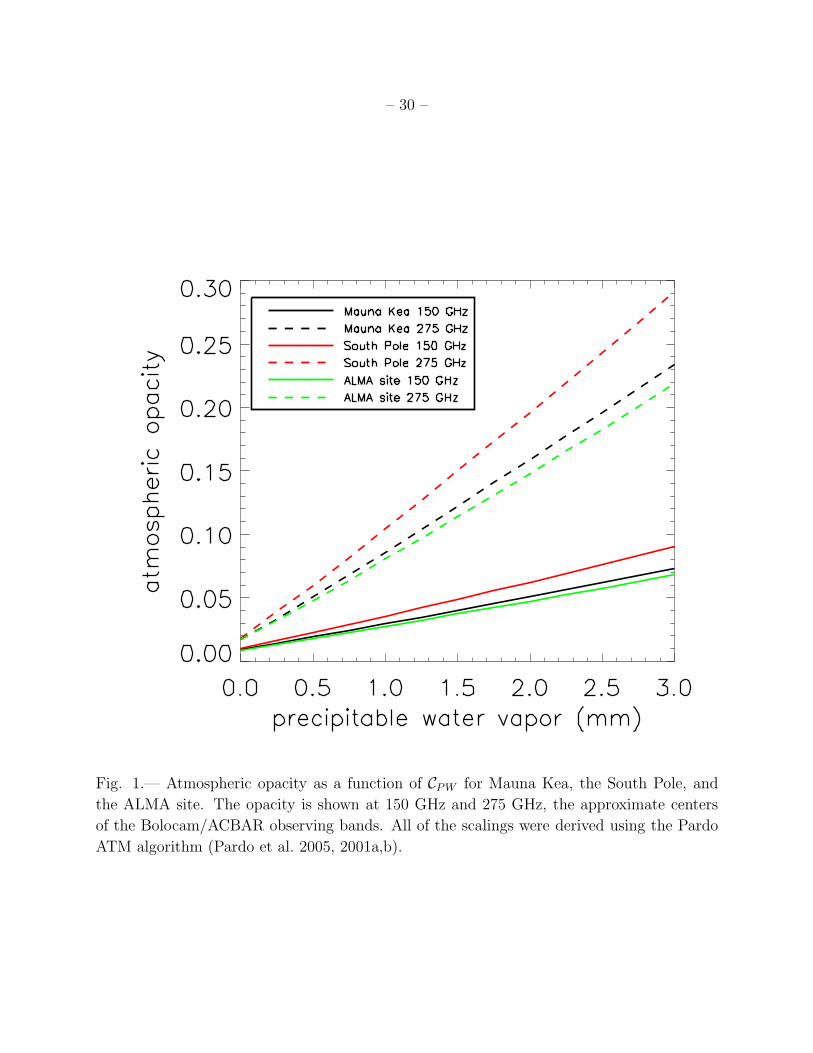
– 30 –

Fig. 1.— Atmospheric opacity as a function of CPW for Mauna Kea, the South Pole, and

the ALMA site. The opacity is shown at 150 GHz and 275 GHz, the approximate centers

of the Bolocam/ACBAR observing bands. All of the scalings were derived using the Pardo

ATM algorithm (Pardo et al. 2005, 2001a,b).

– 31 –

Fig. 2.— A diagram of the thin-screen turbulence model described by Lay and Halverson

(2000) that is used throughout this paper.

– 32 –

θ θ

Fig. 3.— Plots of(∆Θf /∆f)

θpairaveraged over all bolometer pairs and all scans for a single

observation. This slope is binned according to φpair, and the sinusoidal fit predicted from

the thin-screen K-T model is overlaid in red. In general, roughly half our data are well

described by this model, with a typical example shown in the left-hand plot. The other half

of the data tend to contain outliers and/or additional features; the right-hand plot shows an

example of one of these data sets.

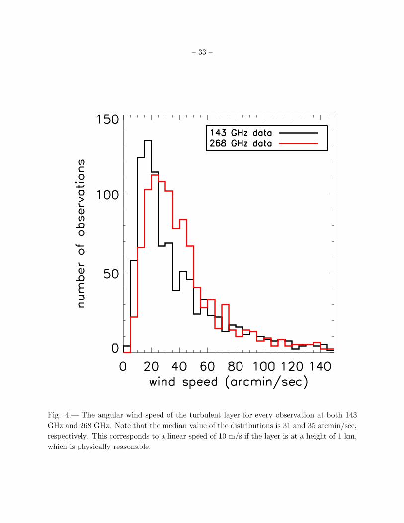
– 33 –

Fig. 4.— The angular wind speed of the turbulent layer for every observation at both 143

GHz and 268 GHz. Note that the median value of the distributions is 31 and 35 arcmin/sec,

respectively. This corresponds to a linear speed of 10 m/s if the layer is at a height of 1 km,

which is physically reasonable.

– 34 –

Fig. 5.— Plots of the average correlation between bolometer pairs as a function of separation

between the bolometers. The top row shows data from a 143 GHz observation taken when

the amplitude of the atmospheric noise is better than average, and the bottom row shows

data from a 143 GHz observation taken when the amplitude of the atmospheric noise is worse

than average. The model fits overlaid on the left plots show a range of power law indices, b,

at the best fit value of h for the data set. The model fits overlaid on the right plots show

a range of heights, h, at the best fit value of b for the data set. The χ2 value of the model

fit for these two observations is similar, and is at roughly the 30th centile of our complete

set of data (i.e., 1/3 of our observations produce a better fit to the K-T model, and 2/3

of our observations produce a worse fit to the K-T model). Therefore, the quality of the

model fit for these observations is fairly typical. Note the degeneracy between b and h in the

general shape of the model fits, which makes it difficult to constrain either value precisely

for a single observation, especially h. These plots clearly show the excess correlation among

adjacent bolometers, and note that the adjacent bolometer correlations are discarded when

fitting the K-T model to the data.

– 35 –

Fig. 6.— The histogram on the left shows the best fit value of the power law exponent b for

the K-T model of the atmosphere for a randomly selected subset of 96 143 GHz observations.

The mean is 3.3 and the standard deviation is 1.1, indicating that our data are consistent with

the K-T model prediction of b = 11/3, which is shown as a red vertical line. The histogram

on the right shows the best fit value for the height of the turbulent layer. The uniform

distribution of h over the allowed range indicates that we do not meaningfully constrain h.

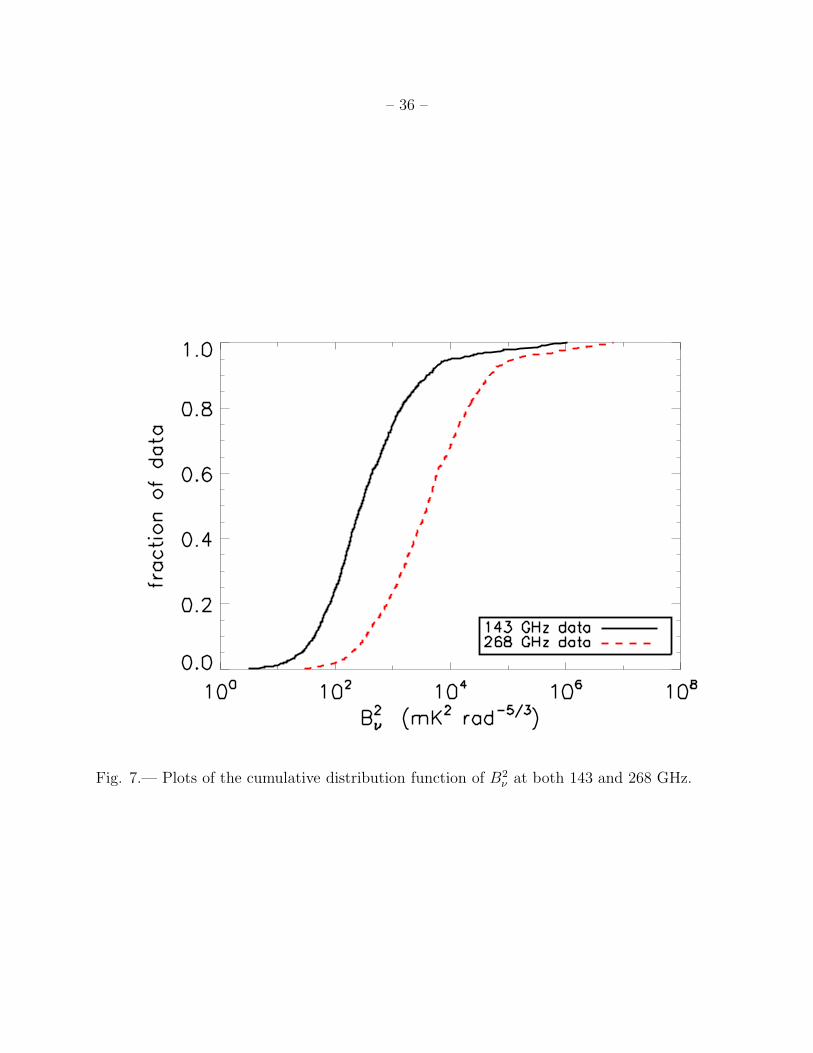
– 36 –

Fig. 7.— Plots of the cumulative distribution function of B2ν at both 143 and 268 GHz.

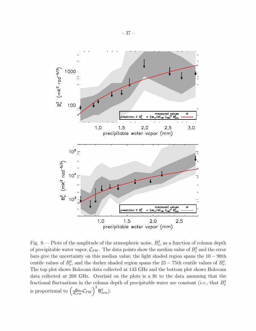
– 37 –

Fig. 8.— Plots of the amplitude of the atmospheric noise, B2ν , as a function of column depth

of precipitable water vapor, CPW . The data points show the median value of B2ν and the error

bars give the uncertainty on this median value; the light shaded region spans the 10 − 90th

centile values of B2ν , and the darker shaded region spans the 25 − 75th centile values of B2

ν .

The top plot shows Bolocam data collected at 143 GHz and the bottom plot shows Bolocam

data collected at 268 GHz. Overlaid on the plots is a fit to the data assuming that the

fractional fluctuations in the column depth of precipitable water are constant (i.e., that B2ν

is proportional to(

dǫτ

dCPWCPW

)2

B2atm).

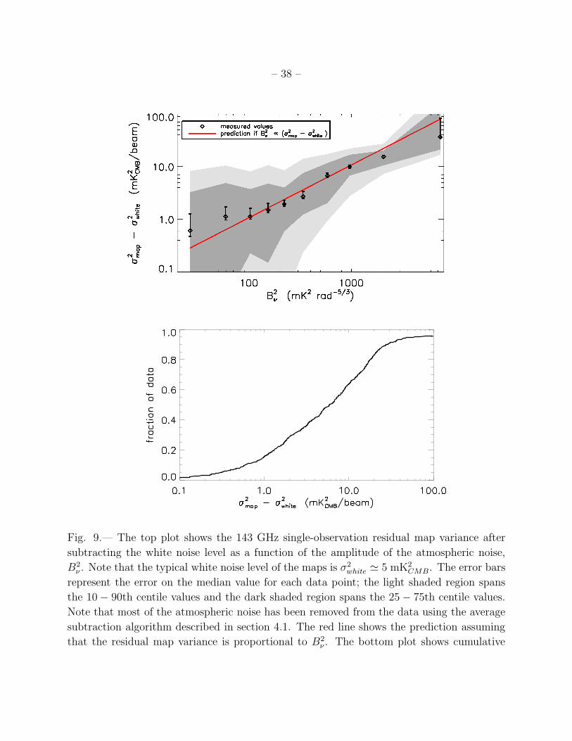
– 38 –

Fig. 9.— The top plot shows the 143 GHz single-observation residual map variance after

subtracting the white noise level as a function of the amplitude of the atmospheric noise,

B2ν . Note that the typical white noise level of the maps is σ2

white ≃ 5 mK2CMB. The error bars

represent the error on the median value for each data point; the light shaded region spans

the 10 − 90th centile values and the dark shaded region spans the 25 − 75th centile values.

Note that most of the atmospheric noise has been removed from the data using the average

subtraction algorithm described in section 4.1. The red line shows the prediction assuming

that the residual map variance is proportional to B2ν . The bottom plot shows cumulative

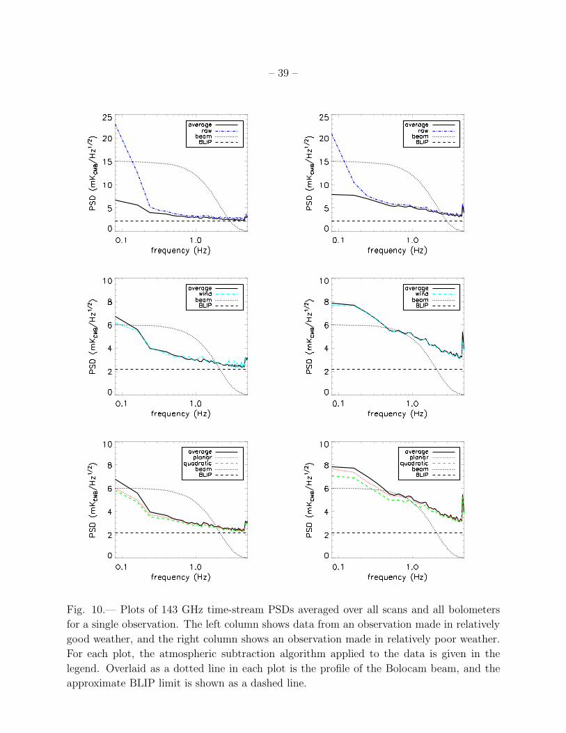
– 39 –

Fig. 10.— Plots of 143 GHz time-stream PSDs averaged over all scans and all bolometers

for a single observation. The left column shows data from an observation made in relatively

good weather, and the right column shows an observation made in relatively poor weather.

For each plot, the atmospheric subtraction algorithm applied to the data is given in the

legend. Overlaid as a dotted line in each plot is the profile of the Bolocam beam, and the

approximate BLIP limit is shown as a dashed line.

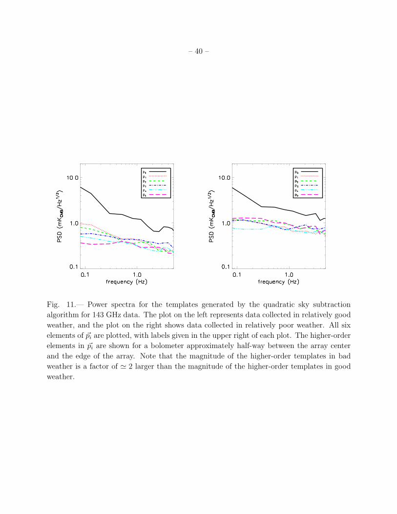
– 40 –

Fig. 11.— Power spectra for the templates generated by the quadratic sky subtraction

algorithm for 143 GHz data. The plot on the left represents data collected in relatively good

weather, and the plot on the right shows data collected in relatively poor weather. All six

elements of ~pi are plotted, with labels given in the upper right of each plot. The higher-order

elements in ~pi are shown for a bolometer approximately half-way between the array center

and the edge of the array. Note that the magnitude of the higher-order templates in bad

weather is a factor of ≃ 2 larger than the magnitude of the higher-order templates in good

weather.

– 41 –

Fig. 12.— Plots of 143 GHz time-stream PSDs averaged over all scans and all bolometers

for a single observation for average subtraction and PCA subtraction. The left plot shows

data from an observation made in relatively good weather, and the right plot shows an

observation made in relatively poor weather. Overplotted as dotted lines is the S/N for each

subtraction method (in arbitrary units), calculated by dividing the window function for a

CMB shaped signal by the noise PSD. Note that the S/N is significantly higher for average

subtraction compared to PCA subtraction at low frequencies because average subtraction

attenuates much less signal.

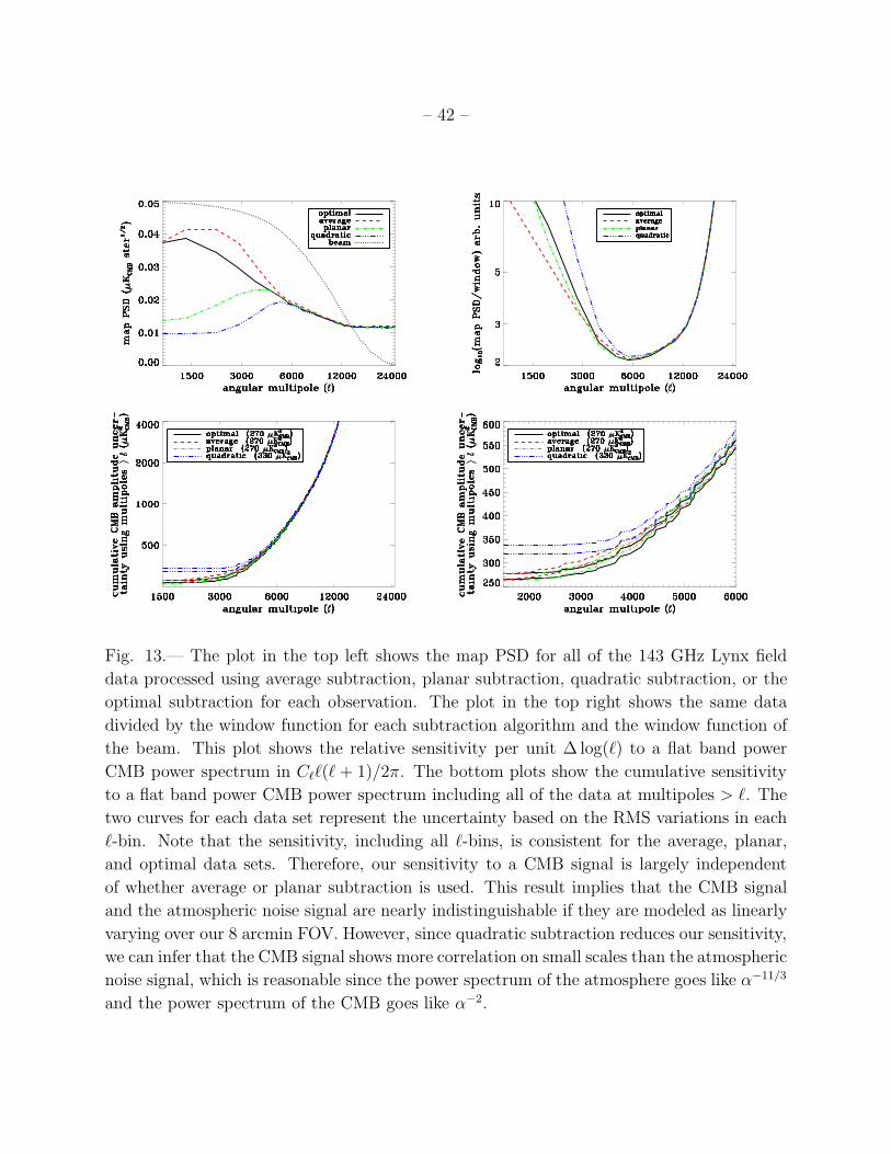
– 42 –

Fig. 13.— The plot in the top left shows the map PSD for all of the 143 GHz Lynx field

data processed using average subtraction, planar subtraction, quadratic subtraction, or the

optimal subtraction for each observation. The plot in the top right shows the same data

divided by the window function for each subtraction algorithm and the window function of

the beam. This plot shows the relative sensitivity per unit ∆ log(ℓ) to a flat band power

CMB power spectrum in Cℓℓ(ℓ + 1)/2π. The bottom plots show the cumulative sensitivity

to a flat band power CMB power spectrum including all of the data at multipoles > ℓ. The

two curves for each data set represent the uncertainty based on the RMS variations in each

ℓ-bin. Note that the sensitivity, including all ℓ-bins, is consistent for the average, planar,

and optimal data sets. Therefore, our sensitivity to a CMB signal is largely independent

of whether average or planar subtraction is used. This result implies that the CMB signal

and the atmospheric noise signal are nearly indistinguishable if they are modeled as linearly

varying over our 8 arcmin FOV. However, since quadratic subtraction reduces our sensitivity,

we can infer that the CMB signal shows more correlation on small scales than the atmospheric

noise signal, which is reasonable since the power spectrum of the atmosphere goes like α−11/3

and the power spectrum of the CMB goes like α−2.

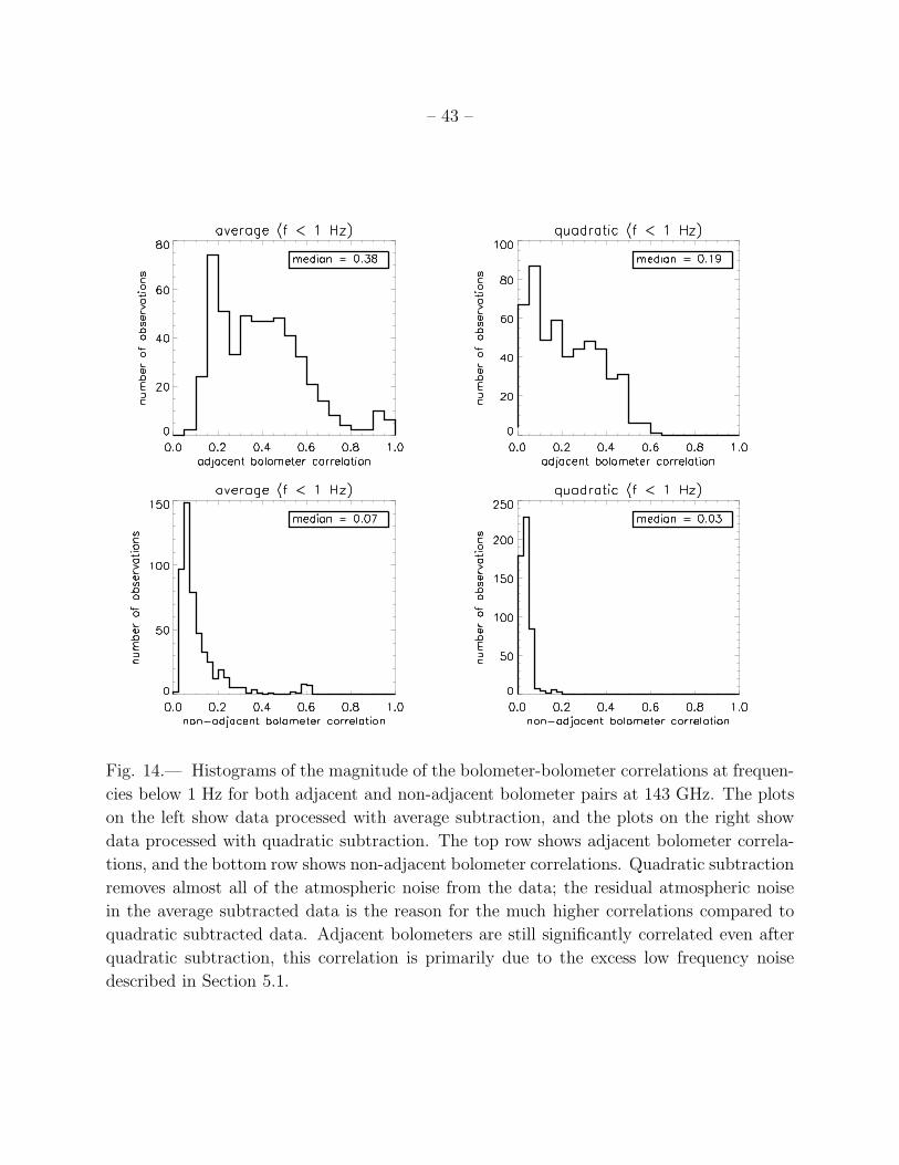
– 43 –

Fig. 14.— Histograms of the magnitude of the bolometer-bolometer correlations at frequen-

cies below 1 Hz for both adjacent and non-adjacent bolometer pairs at 143 GHz. The plots

on the left show data processed with average subtraction, and the plots on the right show

data processed with quadratic subtraction. The top row shows adjacent bolometer correla-

tions, and the bottom row shows non-adjacent bolometer correlations. Quadratic subtraction

removes almost all of the atmospheric noise from the data; the residual atmospheric noise

in the average subtracted data is the reason for the much higher correlations compared to

quadratic subtracted data. Adjacent bolometers are still significantly correlated even after

quadratic subtraction, this correlation is primarily due to the excess low frequency noise

described in Section 5.1.

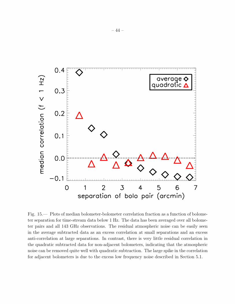
– 44 –

Fig. 15.— Plots of median bolometer-bolometer correlation fraction as a function of bolome-

ter separation for time-stream data below 1 Hz. The data has been averaged over all bolome-

ter pairs and all 143 GHz observations. The residual atmospheric noise can be easily seen

in the average subtracted data as an excess correlation at small separations and an excess

anti-correlation at large separations. In contrast, there is very little residual correlation in

the quadratic subtracted data for non-adjacent bolometers, indicating that the atmospheric

noise can be removed quite well with quadratic subtraction. The large spike in the correlation

for adjacent bolometers is due to the excess low frequency noise described in Section 5.1.

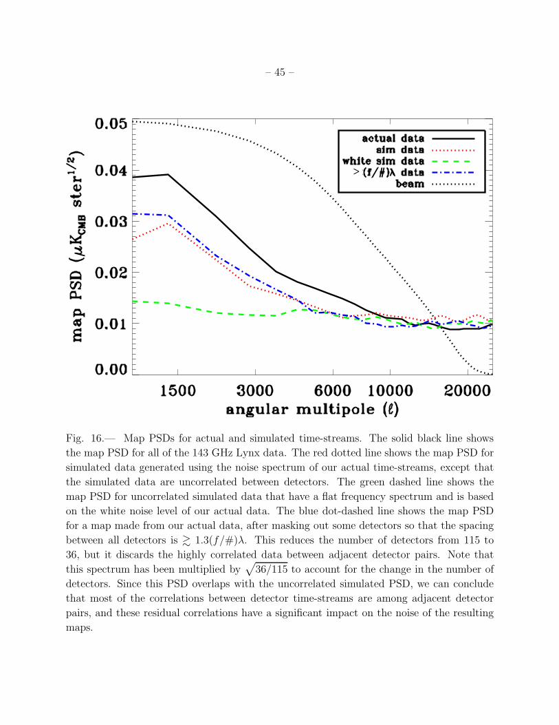
– 45 –

>

Fig. 16.— Map PSDs for actual and simulated time-streams. The solid black line shows

the map PSD for all of the 143 GHz Lynx data. The red dotted line shows the map PSD for

simulated data generated using the noise spectrum of our actual time-streams, except that

the simulated data are uncorrelated between detectors. The green dashed line shows the

map PSD for uncorrelated simulated data that have a flat frequency spectrum and is based

on the white noise level of our actual data. The blue dot-dashed line shows the map PSD

for a map made from our actual data, after masking out some detectors so that the spacing

between all detectors is & 1.3(f/#)λ. This reduces the number of detectors from 115 to

36, but it discards the highly correlated data between adjacent detector pairs. Note that

this spectrum has been multiplied by√

36/115 to account for the change in the number of

detectors. Since this PSD overlaps with the uncorrelated simulated PSD, we can conclude

that most of the correlations between detector time-streams are among adjacent detector

pairs, and these residual correlations have a significant impact on the noise of the resulting

maps.

– 46 –

Table 1. Atmospheric Noise Amplitude (B2ν)

instrument frequency quartile 1 quartile 2 quartile 3

Bolocam 143 GHz 100 mK2 rad−5/3 280 mK2 rad−5/3 980 mK2 rad−5/3

ACBAR 151 GHz 3.7 mK2 rad−5/3 10 mK2 rad−5/3 37 mK2 rad−5/3

Bolocam/ACBAR 27 28 26

Bolocam 268 GHz 1100 mK2 rad−5/3 4000 mK2 rad−5/3 14000 mK2 rad−5/3

ACBAR 282 GHz 28 mK2 rad−5/3 74 mK2 rad−5/3 230 mK2 rad−5/3

Bolocam/ACBAR 39 54 61

Note. — The observed quartile values of B2ν for the two Bolocam observing bands from

Mauna Kea and two of the ACBAR observing bands from the South Pole. The ratio of

B2ν for the two instruments is given for each of the bands (≃ 150 and ≃ 275 GHz.)

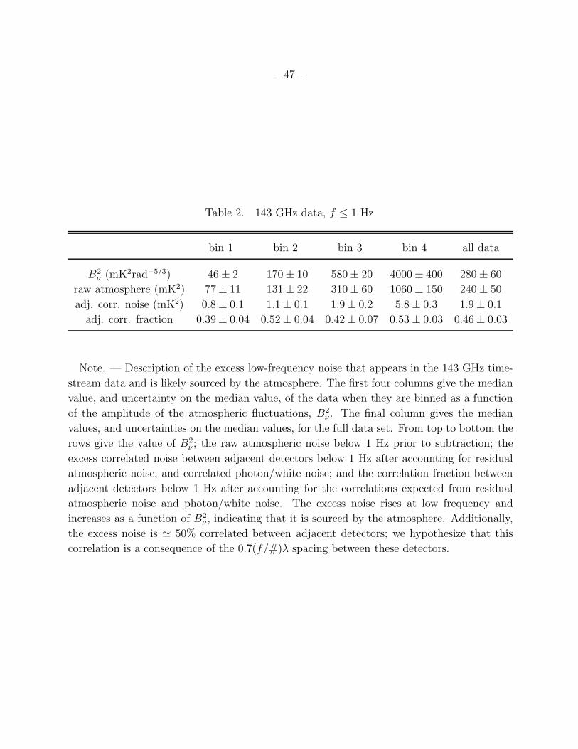
– 47 –

Table 2. 143 GHz data, f ≤ 1 Hz

bin 1 bin 2 bin 3 bin 4 all data

B2ν (mK2rad−5/3) 46 ± 2 170 ± 10 580 ± 20 4000 ± 400 280 ± 60

raw atmosphere (mK2) 77 ± 11 131 ± 22 310 ± 60 1060 ± 150 240 ± 50

adj. corr. noise (mK2) 0.8 ± 0.1 1.1 ± 0.1 1.9 ± 0.2 5.8 ± 0.3 1.9 ± 0.1

adj. corr. fraction 0.39 ± 0.04 0.52 ± 0.04 0.42 ± 0.07 0.53 ± 0.03 0.46 ± 0.03

Note. — Description of the excess low-frequency noise that appears in the 143 GHz time-

stream data and is likely sourced by the atmosphere. The first four columns give the median

value, and uncertainty on the median value, of the data when they are binned as a function

of the amplitude of the atmospheric fluctuations, B2ν . The final column gives the median

values, and uncertainties on the median values, for the full data set. From top to bottom the

rows give the value of B2ν ; the raw atmospheric noise below 1 Hz prior to subtraction; the

excess correlated noise between adjacent detectors below 1 Hz after accounting for residual

atmospheric noise, and correlated photon/white noise; and the correlation fraction between

adjacent detectors below 1 Hz after accounting for the correlations expected from residual

atmospheric noise and photon/white noise. The excess noise rises at low frequency and

increases as a function of B2ν , indicating that it is sourced by the atmosphere. Additionally,

the excess noise is ≃ 50% correlated between adjacent detectors; we hypothesize that this

correlation is a consequence of the 0.7(f/#)λ spacing between these detectors.

– 48 –

Table 3. Lynx data

data type data spectrum CMB amplitude uncertainty

actual data actual data 270 µK2CMB

simulated actual data 170 µK2CMB

simulated white 100 µK2CMB

actual data, > (f/#)λ actual data 170 (550) µK2CMB

Note. — The estimated uncertainty on measuring the amplitude of a flat

CMB power spectrum for all of the 143 GHz Lynx observations. The four

data sets include: our actual data, simulated data using our actual time-

stream noise spectra, simulated data using our actual time-stream white

noise level, and our actual data after masking off 79 of our 115 detectors

so that the spacing between all detectors is & 1.3(f/#)λ. For the two

simulated data sets the bolometer time-streams are uncorrelated. The

results for the second and fourth data sets are similar, after accounting

for the reduction in detector number in the fourth set, indicating that

the majority of the correlations between our detector time-streams are

between adjacent detector pairs. The results show that our sensitivity to

a CMB amplitude is reduced by a factor of ≃ 1.6 due to these correlations,

and by another factor of ≃ 1.7 due to the residual atmospheric noise in

our data at low frequencies.