Structured Feature Learning for Pose Estimation

Structured Feature Learning for Pose Estimation

Xiao Chu Wanli Ouyang Hongsheng Li Xiaogang Wang

Department of Electronic Engineering, The Chinese University of Hong Kong

[email protected] [email protected] [email protected]

[email protected]

Abstract

In this paper, we propose a structured feature learning

framework to reason the correlations among body joints

at the feature level in human pose estimation. Different

from existing approaches of modeling structures on score

maps or predicted labels, feature maps preserve substan-

tially richer descriptions of body joints. The relationships

between feature maps of joints are captured with the intro-

duced geometrical transform kernels, which can be easily

implemented with a convolution layer. Features and their

relationships are jointly learned in an end-to-end learning

system. A bi-directional tree structured model is proposed,

so that the feature channels at a body joint can well receive

information from other joints. The proposed framework im-

proves feature learning substantially. With very simple post

processing, it reaches the best mean PCP on the LSP and

FLIC datasets. Compared with the baseline of learning fea-

tures at each joint separately with ConvNet, the mean PCP

has been improved by 18% on FLIC. The code is released

to the public. 1

1. Introduction

Human pose estimation is to estimate the locations of

body joints from images. It can assist a variety of vision

tasks such as action recognition [29, 33], tracking [6], per-

son re-identification [32], and human computer interaction.

Despite the long history of efforts, it is still a challenging

problem. The large variation in limb orientation, clothing,

viewpoints, background clutters, truncation, and occlusion

make localization of body joints difficult.

Independent prediction of body joint locations from ap-

pearance score maps can be refined by modeling the spa-

tial relationship among correlated body joints [35, 5, 19].

On score maps, the information at a location is summarized

1The code can be found at http://www.ee.cuhk.edu.hk/

˜xgwang/projectpage_structured_feature_pose.html.

For more technical details, please contact the corresponding authors Wanli

Ouyang and Xiaogang Wang

(2)

I1

I2

…

ConvNet Structured2feature Score2maps

Input2image

(1)

e1

e2

e3

e4

e5

e6

e7

a b c d

h1

h2

h3

h4

h5

h6

h7

e

e1

e2

e3

e4

e5

e6

e7

h1

h2

h3

h4

h5

h6

h7

e5

e4

h2

h6

Figure 1. (1) Our approach jointly learns feature maps at differ-

ent body joints and the spatial and co-occurrence relationships be-

tween feature maps. The information from different joints passes

at the feature level. (a) Two input images (I1 and I2) with different

poses. (c) Responses of feature channels for elbow (e1-e7). (I1,

b) is the response map of e5 for image I1. (I2, b) is the response

map of e4 for image I2. Similarly, (d) and (e) show the response

maps and responses of different feature channels for lower arm.

into a single probability value, indicating the likelihood of

the existence of the corresponding body joint. For example,

if a location on the score map of elbow has a large response,

we can only reach the conclusion that this location may be-

long to elbow, but cannot tell the in-plane and out-plane

rotation of the elbow, the orientations of the upper arm and

the lower arm associated with it, whether it is covered with

clothes, and its occlusion status. Such detailed information

is valuable for predicting the locations of other body joints,

but is missed from the score maps, which makes structural

learning among body joints much less effective.

We observe that these types of information are well pre-

served at the feature level, where hierarchical feature repre-

sentations are learned with Convolutional Networks (Con-

vNets) [16, 36, 22, 23, 24]. Fig. 1 shows the responses of

feature maps of elbow and lower arm for different input im-

ages. Given the V-shaped elbow covered with clothes in I1,

14715

the feature channel e5 has the largest response as shown in

(I1, c). In the meanwhile, the feature channel h2 for lower

arm has the largest response in (I1, e). Given the straight

elbow uncovered with clothes in I2, the feature channels e4and h6 have the largest responses to elbow and lower arm

respectively. It indicates that different feature channels are

activated for different visual patterns. The feature maps of

different joints also have strong correlations. In Fig. 1, e5is positively correlated with h2 and anti-correlated with h6.

Both the spatial distribution of the responses and the seman-

tic meaningful description of body joints are encoded at the

feature maps by activating different channels.

Some existing works [35, 5, 19] employed mixtures clus-

tered from spatial configuration among neighboring body

joints. However, the number of mixtures for each body

joint (fewer than 20) is incomparable to hundreds of fea-

ture channels from ConvNets, which not only include spa-

tial configuration of body joints, but also other information

such as occlusion status and clothing. Hence, we propose

to exploit the structure information of body joints at the fea-

ture level. Our proposed approach shows that the spatial

and co-occurrence relationship among feature maps can be

modeled by a set of geometrical transform kernels. These

kernels can be implemented with convolution and the rela-

tionships can be learned in and end-to-end learning system.

It is important to design proper information flow between

body joints, so that features at a joint can be optimized by

receiving messages from highly correlated joints and will

not be disturbed by less correlated joints in distance. A

bi-directional tree-structured model is proposed. The pro-

posed model connects correlated joints and passes messages

in both directions along the tree. Therefore, every joint can

receive information from all the neighboring joints.

The contributions of this work are summarized as three-

fold. First, it proposes an end-to-end learning framework to

capture rich structural information among body joints at the

feature level for pose estimation. Second, it is shown that

the relationships among feature maps of neighboring body

joints can be learned by the introduced geometrical trans-

form kernels and can be easily implemented with convolu-

tional layers. Third, a bi-directional tree-structured model

is proposed, so that each joint can receive information from

all the correlated joints and optimize its features.

Experimental results show that the proposed approach

can improve feature learning substantially. Compared with

learning features at each joint separately with ConvNet, it

improves the mean PCP by 18% on the FLIC dataset. It also

reaches the highest mean PCP 80.8% on the LSP dataset

and 95.2% on the FLIC dataset. This work focuses on fea-

ture learning and only adopts very simple post processing. It

already outperforms the state-of-the-art method which em-

ployed sophisticated post processing techniques with a large

margin.

2. Related Works

Previous pose estimation works can be divided into two

groups. The first is to model the geometrical distribution of

body joints [35, 30, 31, 19, 9, 6, 1, 11, 25, 2, 21, 17, 34, 7]

which can be viewed as post processing on detection score

maps and prediction labels. They are mainly based on hand-

crafted features. The Pictorial Structure Model [11] de-

fined pairwise terms to represent relationship between body

joint locations. Later, Yang et al. [35] proposed the flexi-

ble mixture-of-parts model to combine part detection results

with a tree-structured model, which provided simple and

exact inference. Nevertheless, it is believed that the tree-

structured model is “oversimplified”. In light of this, many

works introduced more complex structures, and researchers

have obtained improvement in performance. Loopy struc-

ture [31], latent variable [25], poselet [19, 31] and strong

appearance [20] modeled structural information at different

levels. They investigated different structures to model the

spatial constraints among body joints on score maps. In

our work, a bi-directional tree is used to model the correla-

tion among feature maps. In the future, the investigations

on structures in previous works can be incorporated in our

framework to guide the message passing at the feature level.

The second group focus on more powerful feature gen-

erators such as ConvNets [28, 10, 5, 27, 26, 4, 10]. The

use of deep models brings large progress [14, 18]. Deep-

Pose [28] used ConvNet to regress joint locations with mul-

tiple steps. Chen et al. [5] used ConvNet features and built

up image-dependent pairwise relations to measure relation-

ship among body joints. Fan et al. [10] combined local and

global features to jointly predict joint locations. Tompson

et al. [27, 26] implemented the multi-resolution deep model

and Markov random field within an end-to-end joint train-

ing framework. Carreira and Malik [4] proposed to build

up dependency among input and output spaces. In order

to iteratively refine prediction results, they concatenated the

body joint location predictions at the previous steps with

the image as the input of current step. However, existing

ConvNet models either learned the pair-wise relationship

among body joints from score maps or did not learn pair-

wise relationship. Learning relationship among parts at the

feature level was not investigated.

3. Structural Feature Learning

3.1. Feature maps of body joints

ConvNets employ multiple layers to learn hierarchical

feature representations of input images. Features in lower

layers capture low-level information, while those in higher

layers can represent more abstract concepts, such as poses,

attributes and object categories. Widely used ConvNets

(e.g. AlexNet [16], Clarifai [36], Overfeat [22], GoogleNet

[24], and VGG [23]) employ fully connected (fc) layers fol-

4716

(a1) (a2)

(b1) (b2)

(c1) (c2)

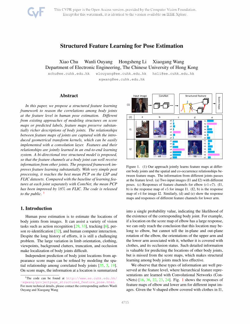
Figure 2. Examples of response maps of different images to the

same feature channels. (a) A feature channel for the neck. (b) A

feature channel for the left wrist. (c) A feature channel for the left

lower arm.

lowing convolutional layers to capture the global informa-

tion. In fully convolutional nets (fcn), 1 × 1 convolution is

used to replace fc layers. In this work, we use fully convo-

lutional VGG net [23] as the base model and extract feature

maps in the fcn7 layer.

Each body joint has a separate set of 128 feature maps.

All the joints share lower layers up to the fcn6 layer, which

has 4, 096 feature channels. Denote hfcn6(x, y) as the fea-

ture vector obtained at location (x, y) in the fcn6 layer and

it is a 4, 096 dimensional vector. The 128 dimensional fea-

ture vector for body joint k at (x, y) in the fcn7 layer is

computed as

hkfcn7(x, y) = f(hfcn6(x, y)⊗w

kfcn7 + bfcn6), (1)

where ⊗ denotes convolution, f is a nonlinear function,

wkfcn7 is the filter bank for joint k including 128 filters,

bfcn6 is the bias, and hkfcn7 is the feature tensor contains

128 feature maps for joint k.

The feature maps of body joints contain rich information

and detailed descriptions of human poses and appearance.

Fig. 2 shows the response maps of different images to the

same feature channels. In (a1) and (a2), a feature channel

for the neck is chosen. All the images in (a1) have high re-

sponses to this feature channel and the highest responding

regions locate on necks. Persons in these images all look to

the left with similar 3D orientations of head. Images in (a2)

have much lower responses to this feature channel and their

highest responding regions distribute randomly. Persons in

these images have various head orientations different than

those in (a1). Therefore, this feature channel captures spe-

cific head orientations. Similarly, the feature channel for the

left wrist in (b) describes left wrists occluding left shoulders

when persons hold cups or cell phones. The feature channel

in (c) can effectively localize downward lower arms without

clothes covered.

3.2. Information passing

Since spatial distributions and semantic meaning of fea-

ture maps obtained at different joints are highly correlated,

passing the rich information contained in feature maps be-

tween joints can effectively improve features learned at each

joint. In previous works, messages could be passed by dis-

tance transfer [12, 35, 18] and Conditional Random Field

(CRF) [37, 15]. We show that under a fully convolutional

neural network, messages can be passed between feature

maps through the introduced geometrical transform kernels.

The FCN filters and the kernels can be jointly learned.

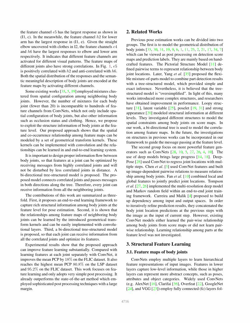
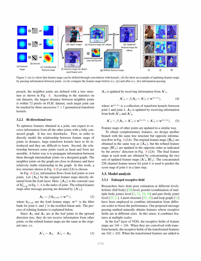
Fig. 3 (a)-(c) shows that convolution with asymmetric

kernels could geometrically shift the feature responses. (a)

is a feature map assuming Gaussian distribution. (b) are

different kernels for illustration. (c) are the transformed

feature maps after convolution. The feature map has been

shifted towards different directions and sum up to different

values.

In order to illustrate the process of information passing,

an example is shown in Figure 3 (d)-(g). Given an input

image in (d), its feature maps for elbow and lower arm are

shown in (e) and (f). One of the lower-arm feature maps hm

has high response, since its feature channel describes down-

ward lower arm without clothes covered. Another elbow

feature map en also has high response and it is positively

correlated with hm. One expects to use hm to reduce false

alarms and enhance the responses on the right elbow. It is

not suitable to directly add en to hm, since there is a spatial

mismatch between the two joints. Instead, we first shift hm

towards the right elbow through the geometrical transform

kernels and then add the transformed feature maps to en.

The refined feature maps in (h) have much better predic-

tion. Since each feature map captures detailed pose infor-

mation of the joint, the relative spatial distribution between

the two maps is stable and the kernel can be easily learned.

Since some elbow feature maps may be anti-correlated with

hm, their kernels could have negative values to prevent un-

related feature channels from generating false alarms. (i)-

(k) show more examples to demonstrate the effectiveness of

information passing between joints on feature learning. The

geometric constraints among body joints could be consoli-

dated by shifting feature map of one body joint towards its

nearby joints. The information passing described above can

be easily implemented with convolution layers.

3.2.1 Stacked transform kernels

The kernel size decides how far a feature map can be

shifted. In order to reduce the number of parameters

and also support the cases when neighboring joints are in

distance, we employ successive convolutions geometrical

transform kernels to approximate a large kernel. Each con-

volution is followed by a nonlinear transform. In our ap-

4717

(f)$Feature$maps$for$down2

ward$lower$arm

(e)$Feature$maps$for$elbow (h)$Updated$

feature$maps$for$

elbow

(g)$Shifted$ feature$maps

(d)$Input$image

⨁

⨂

⨂

(a)$Feature$

maps$(c)$Transformed$

feature$maps

(b)$Kernel

⨂

⨂

(i) (j) (k)

Learned$kernel$

ℎ$

%&

Figure 3. (a)-(c) show that feature maps can be shifted through convolution with kernels. (d)-(h) show an example of updating feature maps

by passing information between joints. (i)-(k) compare the featuer maps before (i.e. (j)) and after (i.e. (k)) information passing.

proach, the neighbor joints are defined with a tree struc-

ture as shown in Fig. 4. According to the statistics on

our datasets, the largest distance between neighbor joints

is within 72 pixels on FLIC dataset, such target joint can

be reached by three successive 7× 7 geometrical transform

kernels.

3.2.2 Bi-directional tree

To optimize features obtained at a joint, one expect to re-

ceive information from all the other joints with a fully con-

nected graph. It has two drawbacks. First, in order to

directly model the relationship between feature maps of

joints in distance, large transform kernels have to be in-

troduced and they are difficult to learn. Second, the rela-

tionship between some joints (such as head and foot) are

unstable. A better way is to propagate information between

them through intermediate joints on a designed graph. The

neighbor joints on the graph are close in distance and have

relatively stable relationship in the graph. In this work, a

tree structure shown in Fig. 4 (2,a) and (2,b) is chosen.

In Fig. 4 (2,a), information flows from leaf joints to root

joints. Let {Ak} be the original feature maps directly ob-

tained from the fcn6 layer. Here, {Ak} is the concrete case

of hkfcn6 in Eq. 1. k is the index of joint. The refined feature

maps after message passing are denoted by {A′

k}.

Ak = f(hfcn6 ⊗wak), (2)

where hfcn6 are the fcn6 feature maps, wak is the filter

bank for joint k, and f is the rectified linear unit. The pro-

cess of refining features is explained below.

Since A5 and A6 are at the leaf joints in the upward

direction tree, they do not receive information from other

joints, so the refined feature maps are the same as the origi-

nal ones, i.e.

A′

5 = A5, A′

6 = A6. (3)

A4 is updated by receiving information from A′

5,

A′

4 = f(A4 +A′

5 ⊗wa5,a4), (4)

where wa5,a4 is a collection of transform kernels between

joint 5 and joint 4. A3 is updated by receiving information

from both A′

4 and A′

6,

A′

3 = f(A3 +A′

4 ⊗wa4,a3 +A

′

6 ⊗wa6,a3). (5)

Feature maps of other joints are updated in a similar way.

To obtain complementary features, we design another

branch with the same tree structure but opposite informa-

tion flow in Fig. 4 (2,b). The original feature maps {Bk} are

obtained in the same way as {Ak}, but the refined feature

maps {B′

k} are updated in the opposite order as indicated

by the arrows’ direction in Fig. 4 (2,b). The final feature

maps at each node are obtained by concatenating the two

sets of updated feature maps [A′

k,B′

k]. The concatenated

256 channel feature tensor for joint k is used to predict the

score map of joint k in a later step.

3.3. Model analysis

3.3.1 Enlarged receptive field

Researchers have done pose estimation at different levels:

holistic (full body) [28] level, poselet (combination of mul-

tiple body joints) level [3, 31, 25, 19] and part (body joint)

level [35, 11]. Latent structure [25, 30] and loop graph [31]

have been employed to combine information from differ-

ent scales to boost the performance. Our proposed message

passing method naturally obtains features whose receptive

fields are in different sizes. In this sense, it combines fea-

tures at multiple scales.

In the fcn7 layer of VGG, the receptive fields of feature

maps are 188 × 188. When they are convolved with trans-

form kernels, the receptive fields of the transformed features

are 332× 332. When the transformed features are added to

4718

vv

CNN

Input)image

v … vv

……

(2))Structured)feature)learning

1×1 convolution

Upward)Direction

(1))Part>features

448

(2,a)

Downward)Direction

(2,b)

(3))Prediction

…

Joint)3

Joint4

Joint6

#$ = &(()*+,⨂./$)

#, = &(()*+,⨂./,)

……

56

19

56

Score)

map

Joint5

…

#, ′ = #,

#$ ′ = #$

#2 = &(()*+,⨂./2) #2 ′ = &(#2 + #$ ′⨂.

/$,/2)

#5 = &(()*+,⨂./5) #5 ′ = &(#5 + #2 ′⨂.

/2,/5

+#, ′⨂./,,/5)

#6

#7#5

#2

#$ #,

#8

#9

#:#6;

<6

<7<5

<2

<$ <,

<8

<9

<:<6;

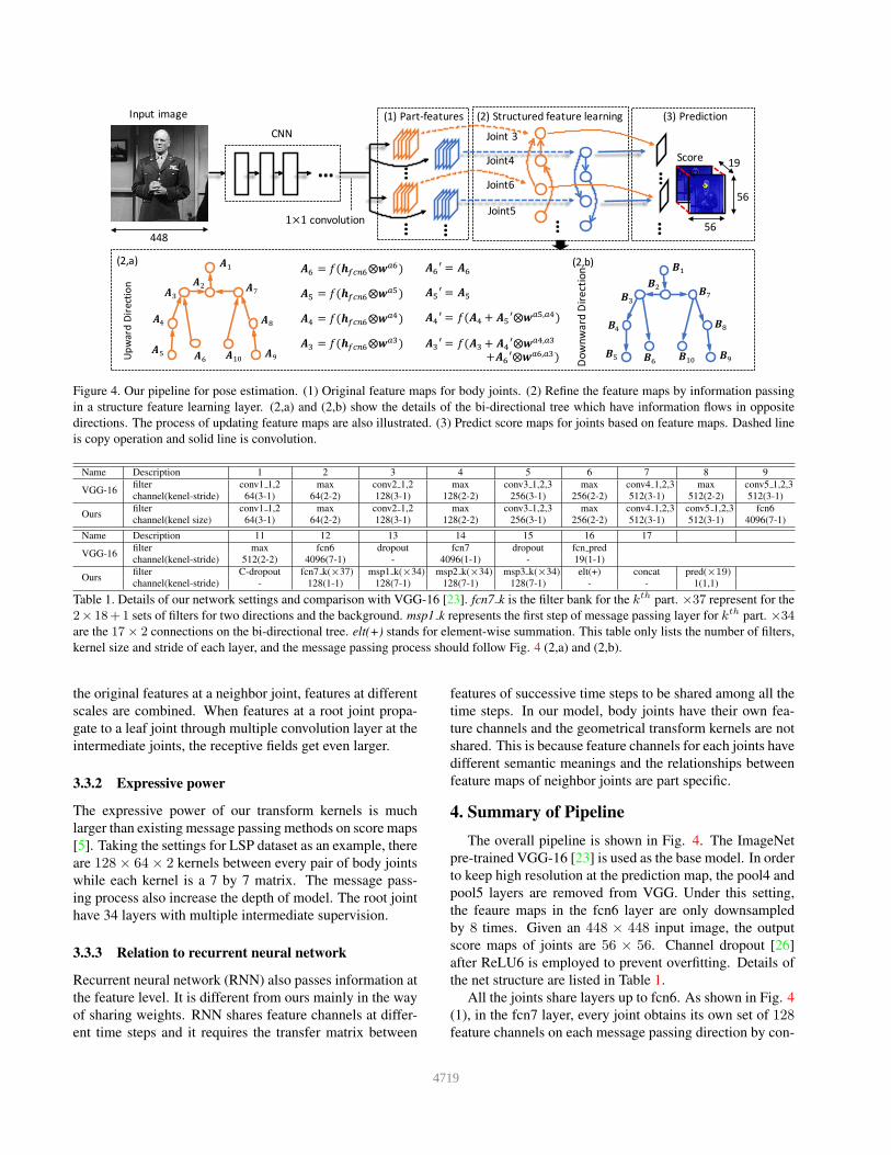
Figure 4. Our pipeline for pose estimation. (1) Original feature maps for body joints. (2) Refine the feature maps by information passing

in a structure feature learning layer. (2,a) and (2,b) show the details of the bi-directional tree which have information flows in opposite

directions. The process of updating feature maps are also illustrated. (3) Predict score maps for joints based on feature maps. Dashed line

is copy operation and solid line is convolution.

Name Description 1 2 3 4 5 6 7 8 9

VGG-16filter conv1 1,2 max conv2 1,2 max conv3 1,2,3 max conv4 1,2,3 max conv5 1,2,3

channel(kenel-stride) 64(3-1) 64(2-2) 128(3-1) 128(2-2) 256(3-1) 256(2-2) 512(3-1) 512(2-2) 512(3-1)

Oursfilter conv1 1,2 max conv2 1,2 max conv3 1,2,3 max conv4 1,2,3 conv5 1,2,3 fcn6

channel(kenel size) 64(3-1) 64(2-2) 128(3-1) 128(2-2) 256(3-1) 256(2-2) 512(3-1) 512(3-1) 4096(7-1)

Name Description 11 12 13 14 15 16 17

VGG-16filter max fcn6 dropout fcn7 dropout fcn pred

channel(kenel-stride) 512(2-2) 4096(7-1) - 4096(1-1) - 19(1-1)

Oursfilter C-dropout fcn7 k(×37) msp1 k(×34) msp2 k(×34) msp3 k(×34) elt(+) concat pred(×19)

channel(kenel-stride) - 128(1-1) 128(7-1) 128(7-1) 128(7-1) - - 1(1,1)

Table 1. Details of our network settings and comparison with VGG-16 [23]. fcn7 k is the filter bank for the kth part. ×37 represent for the

2× 18+1 sets of filters for two directions and the background. msp1 k represents the first step of message passing layer for kth part. ×34

are the 17× 2 connections on the bi-directional tree. elt(+) stands for element-wise summation. This table only lists the number of filters,

kernel size and stride of each layer, and the message passing process should follow Fig. 4 (2,a) and (2,b).

the original features at a neighbor joint, features at different

scales are combined. When features at a root joint propa-

gate to a leaf joint through multiple convolution layer at the

intermediate joints, the receptive fields get even larger.

3.3.2 Expressive power

The expressive power of our transform kernels is much

larger than existing message passing methods on score maps

[5]. Taking the settings for LSP dataset as an example, there

are 128× 64× 2 kernels between every pair of body joints

while each kernel is a 7 by 7 matrix. The message pass-

ing process also increase the depth of model. The root joint

have 34 layers with multiple intermediate supervision.

3.3.3 Relation to recurrent neural network

Recurrent neural network (RNN) also passes information at

the feature level. It is different from ours mainly in the way

of sharing weights. RNN shares feature channels at differ-

ent time steps and it requires the transfer matrix between

features of successive time steps to be shared among all the

time steps. In our model, body joints have their own fea-

ture channels and the geometrical transform kernels are not

shared. This is because feature channels for each joints have

different semantic meanings and the relationships between

feature maps of neighbor joints are part specific.

4. Summary of Pipeline

The overall pipeline is shown in Fig. 4. The ImageNet

pre-trained VGG-16 [23] is used as the base model. In order

to keep high resolution at the prediction map, the pool4 and

pool5 layers are removed from VGG. Under this setting,

the feaure maps in the fcn6 layer are only downsampled

by 8 times. Given an 448 × 448 input image, the output

score maps of joints are 56 × 56. Channel dropout [26]

after ReLU6 is employed to prevent overfitting. Details of

the net structure are listed in Table 1.

All the joints share layers up to fcn6. As shown in Fig. 4

(1), in the fcn7 layer, every joint obtains its own set of 128feature channels on each message passing direction by con-

4719

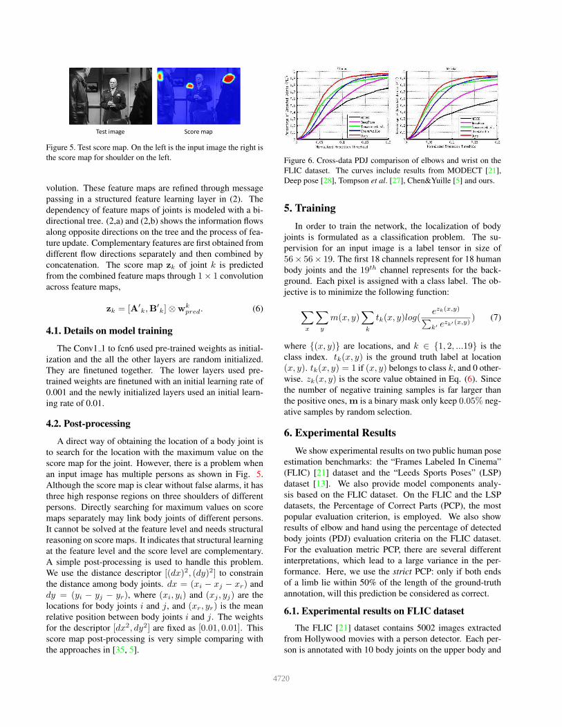
Test%image Score%map

Figure 5. Test score map. On the left is the input image the right is

the score map for shoulder on the left.

volution. These feature maps are refined through message

passing in a structured feature learning layer in (2). The

dependency of feature maps of joints is modeled with a bi-

directional tree. (2,a) and (2,b) shows the information flows

along opposite directions on the tree and the process of fea-

ture update. Complementary features are first obtained from

different flow directions separately and then combined by

concatenation. The score map zk of joint k is predicted

from the combined feature maps through 1× 1 convolution

across feature maps,

zk = [A′

k,B′

k]⊗wkpred. (6)

4.1. Details on model training

The Conv1 1 to fcn6 used pre-trained weights as initial-

ization and the all the other layers are random initialized.

They are finetuned together. The lower layers used pre-

trained weights are finetuned with an initial learning rate of

0.001 and the newly initialized layers used an initial learn-

ing rate of 0.01.

4.2. Post­processing

A direct way of obtaining the location of a body joint is

to search for the location with the maximum value on the

score map for the joint. However, there is a problem when

an input image has multiple persons as shown in Fig. 5.

Although the score map is clear without false alarms, it has

three high response regions on three shoulders of different

persons. Directly searching for maximum values on score

maps separately may link body joints of different persons.

It cannot be solved at the feature level and needs structural

reasoning on score maps. It indicates that structural learning

at the feature level and the score level are complementary.

A simple post-processing is used to handle this problem.

We use the distance descriptor [(dx)2, (dy)2] to constrain

the distance among body joints. dx = (xi − xj − xr) and

dy = (yi − yj − yr), where (xi, yi) and (xj , yj) are the

locations for body joints i and j, and (xr, yr) is the mean

relative position between body joints i and j. The weights

for the descriptor [dx2, dy2] are fixed as [0.01, 0.01]. This

score map post-processing is very simple comparing with

the approaches in [35, 5].

Figure 6. Cross-data PDJ comparison of elbows and wrist on the

FLIC dataset. The curves include results from MODECT [21],

Deep pose [28], Tompson et al. [27], Chen&Yuille [5] and ours.

5. Training

In order to train the network, the localization of body

joints is formulated as a classification problem. The su-

pervision for an input image is a label tensor in size of

56× 56× 19. The first 18 channels represent for 18 human

body joints and the 19th channel represents for the back-

ground. Each pixel is assigned with a class label. The ob-

jective is to minimize the following function:

∑

x

∑

y

m(x, y)∑

k

tk(x, y)log(ezk(x,y)∑k′ ezk′ (x,y)

) (7)

where {(x, y)} are locations, and k ∈ {1, 2, ...19} is the

class index. tk(x, y) is the ground truth label at location

(x, y). tk(x, y) = 1 if (x, y) belongs to class k, and 0 other-

wise. zk(x, y) is the score value obtained in Eq. (6). Since

the number of negative training samples is far larger than

the positive ones, m is a binary mask only keep 0.05% neg-

ative samples by random selection.

6. Experimental Results

We show experimental results on two public human pose

estimation benchmarks: the “Frames Labeled In Cinema”

(FLIC) [21] dataset and the “Leeds Sports Poses” (LSP)

dataset [13]. We also provide model components analy-

sis based on the FLIC dataset. On the FLIC and the LSP

datasets, the Percentage of Correct Parts (PCP), the most

popular evaluation criterion, is employed. We also show

results of elbow and hand using the percentage of detected

body joints (PDJ) evaluation criteria on the FLIC dataset.

For the evaluation metric PCP, there are several different

interpretations, which lead to a large variance in the per-

formance. Here, we use the strict PCP: only if both ends

of a limb lie within 50% of the length of the ground-truth

annotation, will this prediction be considered as correct.

6.1. Experimental results on FLIC dataset

The FLIC [21] dataset contains 5002 images extracted

from Hollywood movies with a person detector. Each per-

son is annotated with 10 body joints on the upper body and

4720

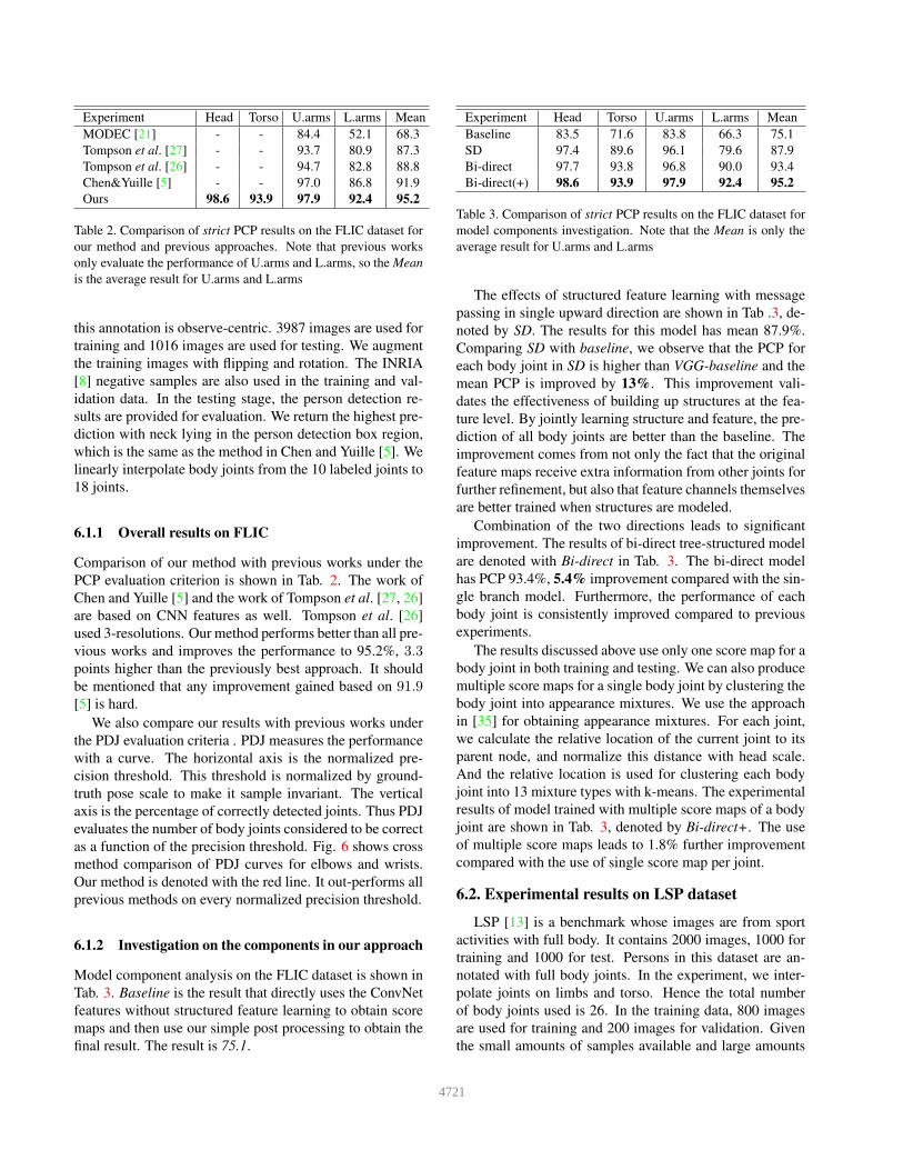
Experiment Head Torso U.arms L.arms Mean

MODEC [21] - - 84.4 52.1 68.3

Tompson et al. [27] - - 93.7 80.9 87.3

Tompson et al. [26] - - 94.7 82.8 88.8

Chen&Yuille [5] - - 97.0 86.8 91.9

Ours 98.6 93.9 97.9 92.4 95.2

Table 2. Comparison of strict PCP results on the FLIC dataset for

our method and previous approaches. Note that previous works

only evaluate the performance of U.arms and L.arms, so the Mean

is the average result for U.arms and L.arms

this annotation is observe-centric. 3987 images are used for

training and 1016 images are used for testing. We augment

the training images with flipping and rotation. The INRIA

[8] negative samples are also used in the training and val-

idation data. In the testing stage, the person detection re-

sults are provided for evaluation. We return the highest pre-

diction with neck lying in the person detection box region,

which is the same as the method in Chen and Yuille [5]. We

linearly interpolate body joints from the 10 labeled joints to

18 joints.

6.1.1 Overall results on FLIC

Comparison of our method with previous works under the

PCP evaluation criterion is shown in Tab. 2. The work of

Chen and Yuille [5] and the work of Tompson et al. [27, 26]

are based on CNN features as well. Tompson et al. [26]

used 3-resolutions. Our method performs better than all pre-

vious works and improves the performance to 95.2%, 3.3points higher than the previously best approach. It should

be mentioned that any improvement gained based on 91.9[5] is hard.

We also compare our results with previous works under

the PDJ evaluation criteria . PDJ measures the performance

with a curve. The horizontal axis is the normalized pre-

cision threshold. This threshold is normalized by ground-

truth pose scale to make it sample invariant. The vertical

axis is the percentage of correctly detected joints. Thus PDJ

evaluates the number of body joints considered to be correct

as a function of the precision threshold. Fig. 6 shows cross

method comparison of PDJ curves for elbows and wrists.

Our method is denoted with the red line. It out-performs all

previous methods on every normalized precision threshold.

6.1.2 Investigation on the components in our approach

Model component analysis on the FLIC dataset is shown in

Tab. 3. Baseline is the result that directly uses the ConvNet

features without structured feature learning to obtain score

maps and then use our simple post processing to obtain the

final result. The result is 75.1.

Experiment Head Torso U.arms L.arms Mean

Baseline 83.5 71.6 83.8 66.3 75.1

SD 97.4 89.6 96.1 79.6 87.9

Bi-direct 97.7 93.8 96.8 90.0 93.4

Bi-direct(+) 98.6 93.9 97.9 92.4 95.2

Table 3. Comparison of strict PCP results on the FLIC dataset for

model components investigation. Note that the Mean is only the

average result for U.arms and L.arms

The effects of structured feature learning with message

passing in single upward direction are shown in Tab .3, de-

noted by SD. The results for this model has mean 87.9%.

Comparing SD with baseline, we observe that the PCP for

each body joint in SD is higher than VGG-baseline and the

mean PCP is improved by 13%. This improvement vali-

dates the effectiveness of building up structures at the fea-

ture level. By jointly learning structure and feature, the pre-

diction of all body joints are better than the baseline. The

improvement comes from not only the fact that the original

feature maps receive extra information from other joints for

further refinement, but also that feature channels themselves

are better trained when structures are modeled.

Combination of the two directions leads to significant

improvement. The results of bi-direct tree-structured model

are denoted with Bi-direct in Tab. 3. The bi-direct model

has PCP 93.4%, 5.4% improvement compared with the sin-

gle branch model. Furthermore, the performance of each

body joint is consistently improved compared to previous

experiments.

The results discussed above use only one score map for a

body joint in both training and testing. We can also produce

multiple score maps for a single body joint by clustering the

body joint into appearance mixtures. We use the approach

in [35] for obtaining appearance mixtures. For each joint,

we calculate the relative location of the current joint to its

parent node, and normalize this distance with head scale.

And the relative location is used for clustering each body

joint into 13 mixture types with k-means. The experimental

results of model trained with multiple score maps of a body

joint are shown in Tab. 3, denoted by Bi-direct+. The use

of multiple score maps leads to 1.8% further improvement

compared with the use of single score map per joint.

6.2. Experimental results on LSP dataset

LSP [13] is a benchmark whose images are from sport

activities with full body. It contains 2000 images, 1000 for

training and 1000 for test. Persons in this dataset are an-

notated with full body joints. In the experiment, we inter-

polate joints on limbs and torso. Hence the total number

of body joints used is 26. In the training data, 800 images

are used for training and 200 images for validation. Given

the small amounts of samples available and large amounts

4721

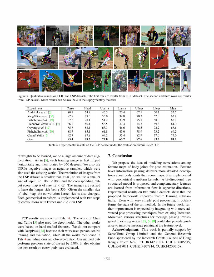
Figure 7. Qualitative results on FLIC and LSP datasets. The first row are results from FLIC dataset. The second and third rows are results

from LSP dataset. More results can be avalibale in the supplymentary material

Experiment Torso Head U.arms L.arms U.legs L.legs Mean

Andriluka et al. [2] 80.9 74.9 46.5 26.4 67.1 60.7 55.7

Yang&Ramanan [35] 82.9 79.3 56.0 39.8 70.3 67.0 62.8

Pishchulin et al. [19] 87.5 78.1 54.2 33.9 75.7 68.0 62.9

Eichner&Ferrari et al. [9] 86.2 80.1 56.5 37.4 74.3 69.3 64.3

Ouyang et al. [17] 85.8 83.1 63.3 46.6 76.5 72.2 68.6

Pishchulin et al. [20] 88.7 85.1 61.8 45.0 78.9 73.2 69.2

Chen&Yuille [5] 92.7 87.8 69.2 55.4 82.9 77.0 75.0

Ours 95.4 89.6 77.0 65.2 87.6 83.2 81.1

Table 4. Experimental results on the LSP dataset under the evaluation criteria strict PCP

of weights to be learned, we do a large amount of data aug-

mentation. As in [5], each training image is first flipped

horizontally and then rotated by 360 degrees. We also use

INRIA negative images as negative samples, which were

also used the existing works. The resolution of images from

the LSP dataset is smaller than FLIC, so we use a smaller

size of input, i.e. 336 × 336, and the corresponding out-

put score map is of size 42 × 42. The images are resized

to have the longer side being 336. Given the smaller size

of label map, the convolution kernel size is also changed.

Each geometrical transform is implemented with two steps

of convolutions with kernel size 7× 7 on LSP.

PCP results are shown in Tab. 4. The work of Chen

and Yuille [5] also used the deep model. The other works

were based on hand-crafted features. We do not compare

with DeepPose [28] because their work used person-centric

training and evaluation, while all the works mentioned in

Tab. 4 including ours are observe-centric. Our method out-

performs previous state-of-the-art by 5.8%. It also obtains

the best result on every body part evaluated.

7. Conclusion

We propose the idea of modeling correlations among

feature maps of body joints for pose estimation. Feature

level information passing delivers more detailed descrip-

tions about body joints than score maps. It is implemented

with geometrical transform kernels. A bi-directional tree

structured model is proposed and complementary features

are learned from information flow in opposite directions.

Experimental results on two public datasets show that the

proposed framework improves feature learning substan-

tially. Even with very simple post processing, it outper-

forms the state-of-the-art method. In the future work, fur-

ther improvement is expected by integrating with more ad-

vanced post processing techniques from existing literature.

Moreover, various structures for message passing investi-

gated in existing works [35, 5, 19] could also provide guid-

ance to improve message passing at the feature level.

Acknowledgment: This work is partially support by

SenseTime Group Limited and the General Research

Fund sponsored by the Research Grants Council of Hong

Kong (Project Nos. CUHK14206114, CUHK14205615,

CUHK417011, CUHK14207814, CUHK14203015).

4722

References

[1] M. Andriluka, L. Pishchulin, P. Gehler, and B. Schiele. 2d

human pose estimation: New benchmark and state of the art

analysis. In CVPR, 2014. 2

[2] M. Andriluka, S. Roth, and B. Schiele. Pictorial structures

revisited: people detection and articulated pose estimation.

In CVPR, 2009. 2, 8

[3] L. Bourdev, S. Maji, T. Brox, and J. Malik. Detecting peo-

ple using mutually consistent poselet activations. In ECCV,

2010. 4

[4] J. Carreira, P. Agrawal, K. Fragkiadaki, and J. Malik. Human

pose estimation with iterative error feedback. arXiv preprint

arXiv:1507.06550, 2015. 2

[5] X. Chen and A. L. Yuille. Articulated pose estimation by a

graphical model with image dependent pairwise relations. In

NIPS, 2014. 1, 2, 5, 6, 7, 8

[6] N.-G. Cho, A. L. Yuille, and S.-W. Lee. Adaptive occlu-

sion state estimation for human pose tracking under self-

occlusions. Pattern Recognition, 46(3):649–661, 2013. 1,

2

[7] X. Chu, W. Ouyang, W. Yang, and X. Wang. Multi-task re-

current neural network for immediacy prediction. In ICCV,

2015. 2

[8] N. Dalal and B. Triggs. Histograms of oriented gradients for

human detection. In CVPR, 2005. 7

[9] M. Eichner and V. Ferrari. Appearance sharing for collective

human pose estimation. In ACCV, 2012. 2, 8

[10] X. Fan, K. Zheng, Y. Lin, and S. Wang. Combining lo-

cal appearance and holistic view: Dual-source deep neu-

ral networks for human pose estimation. arXiv preprint

arXiv:1504.07159, 2015. 2

[11] P. F. Felzenszwalb and D. P. Huttenlocher. Pictorial struc-

tures for object recognition. IJCV, 61(1):55–79, 2005. 2,

4

[12] R. Girshick, F. Iandola, T. Darrell, and J. Malik. De-

formable part models are convolutional neural networks.

arXiv preprint arXiv:1409.5403, 2014. 3

[13] S. Johnson and M. Everingham. Clustered pose and nonlin-

ear appearance models for human pose estimation. In BMVC,

2010. 6, 7

[14] K. Kang, W. Ouyang, H. Li, and X. Wang. Object detection

from video tubelets with convolutional neural networks. In

CVPR, 2016. 2

[15] P. Krahenbuhl and V. Koltun. Efficient inference in fully

connected crfs with gaussian edge potentials. arXiv preprint

arXiv:1210.5644, 2012. 3

[16] A. Krizhevsky, I. Sutskever, and G. Hinton. Imagenet clas-

sification with deep convolutional neural networks. In NIPS,

2012. 1, 2

[17] W. Ouyang, X. Chu, and X. Wang. Multi-source deep learn-

ing for human pose estimation. In CVPR, 2014. 2, 8

[18] W. Ouyang, X. Wang, X. Zeng, S. Qiu, P. Luo, Y. Tian, H. Li,

S. Yang, Z. Wang, C.-C. Loy, and X. Tang. Deepid-net: De-

formable deep convolutional neural networks for object de-

tection. In CVPR, 2015. 2, 3

[19] L. Pishchulin, M. Andriluka, P. Gehler, and B. Schiele. Pose-

let conditioned pictorial structures. In CVPR, 2013. 1, 2, 4,

8

[20] L. Pishchulin, M. Andriluka, P. Gehler, and B. Schiele.

Strong appearance and expressive spatial models for human

pose estimation. In ICCV, December 2013. 2, 8

[21] B. Sapp and B. Taskar. Modec: Multimodal decomposable

models for human pose estimation. In CVPR, 2013. 2, 6, 7

[22] P. Sermanet, D. Eigen, X. Zhang, M. Mathieu, R. Fergus,

and Y. LeCun. Overfeat: Integrated recognition, localization

and detection using convolutional networks. arXiv preprint

arXiv:1312.6229, 2013. 1, 2

[23] K. Simonyan and A. Zisserman. Very deep convolutional

networks for large-scale image recognition. arXiv preprint

arXiv:1409.1556, 2014. 1, 2, 3, 5

[24] C. Szegedy, W. Liu, Y. Jia, P. Sermanet, S. Reed,

D. Anguelov, D. Erhan, V. Vanhoucke, and A. Rabi-

novich. Going deeper with convolutions. arXiv preprint

arXiv:1409.4842, 2014. 1, 2

[25] Y. Tian, C. L. Zitnick, and S. G. Narasimhan. Exploring the

spatial hierarchy of mixture models for human pose estima-

tion. In ECCV. 2012. 2, 4

[26] J. Tompson, R. Goroshin, A. Jain, Y. LeCun, and C. Bregler.

Efficient object localization using convolutional networks. In

CVPR, 2015. 2, 5, 7

[27] J. J. Tompson, A. Jain, Y. LeCun, and C. Bregler. Joint train-

ing of a convolutional network and a graphical model for

human pose estimation. In NIPS, 2014. 2, 6, 7

[28] A. Toshev and C. Szegedy. Deeppose: Human pose estima-

tion via deep neural networks. In CVPR, 2014. 2, 4, 6, 8

[29] C. Wang, Y. Wang, and A. L. Yuille. An approach to pose-

based action recognition. In CVPR, 2013. 1

[30] F. Wang and Y. Li. Beyond physical connections: Tree mod-

els in human pose estimation. In CVPR, 2013. 2, 4

[31] Y. Wang, D. Tran, and Z. Liao. Learning hierarchical pose-

lets for human parsing. In CVPR, 2011. 2, 4

[32] T. Xiao, H. Li, W. Ouyang, and X. Wang. Learning deep fea-

ture representations with domain guided dropout for person

re-identification. In CVPR, 2016. 1

[33] R. Xu, P. Agarwal, S. Kumar, V. N. Krovi, and J. J. Corso.

Combining skeletal pose with local motion for human ac-

tivity recognition. In Articulated Motion and Deformable

Objects, pages 114–123. Springer, 2012. 1

[34] W. Yang, W. Ouyang, H. Li, and X. Wang. End-to-end learn-

ing of deformable mixture of parts and deep convolutional

neural networks for human pose estimation. In CVPR, 2016.

2

[35] Y. Yang and D. Ramanan. Articulated human detection with

flexible mixtures of parts. PAMI, 35(12):2878–2890, 2013.

1, 2, 3, 4, 6, 7, 8

[36] M. D. Zeiler and R. Fergus. Visualizing and under-

standing convolutional neural networks. arXiv preprint

arXiv:1311.2901, 2013. 1, 2

[37] S. Zheng, S. Jayasumana, B. Romera-Paredes, V. Vineet,

Z. Su, D. Du, C. Huang, and P. Torr. Conditional ran-

dom fields as recurrent neural networks. arXiv preprint

arXiv:1502.03240, 2015. 3

4723