Structure-water solubility modeling of aliphatic alcohols using the weighted path numbers

STRUCTURE–WATER SOLUBILITY MODELING OFALIPHATIC ALCOHOLS USING THE WEIGHTED PATH

NUMBERS*

D. AMICa, S.C. BASAKb, B. LUCICc, S. NIKOLICc,† and N. TRINAJSTICc

aFaculty of Agriculture, The Josip Juraj Strossmayer University, HR-31001 Osijek, The Republic ofCroatia; bNatural Resources Research Institute, University of Minnesota, Duluth, MN 55811, USA;

cThe Rugjer Boskovic Institute, Department of Physical Chemistry, Bijenicka 54, P.O. Box 180HR-10002 Zagreb, The Republic of Croatia

(Received 17 September 2000; In final form 25 April 2001)

The structure–water solubility modeling of aliphatic alcohols was performed using the weighted path numbers.Aliphatic alcohols were represented by weighted trees. The weight of the edge representing C–O bond was taken tobe x, while the weights of C–C bonds were taken to be all equal to one. Four (one-, two-, three- and four-descriptor)models with weighted path numbers were considered. They were compared with models based on surface areas ofaliphatic alcohols, models based on the vertex-connectivity indices for the corresponding alkanes, models based onorthogonal valence vertex-connectivity indices, models based on valence vertex- and edge-connectivity indices withoptimum exponents and models based on weighted line graphs. The main result of this comparative study is that themodels based on two, three, or four weighted path numbers posses the best statistical characteristics of all modelsconsidered in this paper. In addition, the predictive performance of these models was also tested using thetraining/test set partition. Very good and stable predictions for 19 test set compounds were obtained. For this data setwe find, in all performed tests of models, that optimum x values are in the range 3.0–4.0. This result supports viewsabout the potential of the weighted path numbers for deriving high quality structure–property models.

Keywords: Aliphatic alcohols; Structure–property modeling; Water solubility; Weighted paths

INTRODUCTION

In this paper, we report on modeling the water solubility of aliphatic alcohols using recently

proposed molecular descriptors named the weighted path numbers [1,2]. We are interested in

the physicochemical and biological properties of alcohols for some time because they are

toxic materials and thus represent dangerous environmental pollutants [3–5]. The toxic

action of alcohols on the higher organisms, presumably through the phenomenon of narcosis,

depends on their solubility in water. The lower alcohols: methanol, ethanol, and propanol

mix with water in any ratio, while this is not the case with other aliphatic alcohols, especially

ISSN 1062-936X q 2002 Taylor & Francis Ltd

DOI: 10.1080/10629360290002776

*Presented at the 9th International Workshop on Quantitative Structure–Activity Relationships in EnvironmentalSciences (QSAR 2000), September 16–20, 2000, Bourgas, Bulgaria

†Corresponding author. E-mail: [email protected]

SAR and QSAR in Environmental Research, 2002 Vol. 13 (2), pp. 281–295

higher ones. Alcohols are also technologically important materials and are used in the

manufacture of a number of products. And again their usefulness in this respect also depends,

among other things, on their solubility in water.

Our aim in this paper is to investigate how structure–water solubility models based on

weighted path numbers compare to models based on descriptors with prescribed values for

vertex and edge weights [6,7]. Already almost fifty years ago Platt [8] advocated the use of

path numbers in the structure–property modeling. However, the significance of Platt’s

proposal was overlooked until the resurrection of the chemical graph theory in early

seventies [9].

It should be pointed out that there are more than 1800 (empirical and theoretical)

molecular descriptors available [10] for use in QSAR/QSPR modeling, but we are still

lacking good descriptors for many molecular properties of interest [11,12]. It is especially

difficult to unearth good descriptors to handle diverse heterosystems [13]. This was the

motivation behind the effort by Randic and his coworkers when they introduced the concept

of optimal descriptors to treat molecules with structural features such as double bonds,

heteroatoms and heterobonds [1,2,14–19]. Of course, there are a number of other authors

who are trying to do the same, that is, to discover the best possible descriptors for modeling a

given molecular property [7,20–24].

WEIGHTED PATH NUMBERS

Apliphatic alcohols will be represented by weighted graphs [25]. As an example, a weighted

graph wG representing the hydrogen-depleted skeleton of 3,3-dimethyl-1-butanol is shown in

Fig. 1.

A path Pl(l is the length of the path) is a sequence of adjacent edges, which do not pass

through the same vertex more than once [26]. Note that P1 is equal to the number of edges in

FIGURE 1 A labeled weighted graph wG representing the hydrogen-depleted skeleton of 3,3-dimethyl-1-butanol.Black dot denotes the position of oxygen and x stands for the weight of C–O bond. Weights of C–C bonds are takento be one.

D. AMIC et al.282

the graph. A weighted path contains weighted edges. In the case of aliphatic alcohols, the

weight of the edge representing C–O bond is taken to be x, while the weights of edges

representing C–C bonds are all equal to one (see Fig. 1). The count of paths and weighted

paths in a weighted graph wG, given in Fig. 1, is illustrated in Table I. The length of a path

containing the edge with weight x is simply denoted by x.

The weighted path numbers for 3,3-dimethyl-1-butanol are equal to the sums of weighted

paths over all vertices in a graph divided by 2, since each vertex is counted twice. If we

assume x ¼ 1; then the count ðP1 ¼ 6; P2 ¼ 8; P3 ¼ 4; P4 ¼ 3Þ represents paths in

2,2-dimethylpentane. If x is left undefined, then it can be viewed as a variable to be adjusted

from regression analysis to obtain the smallest standard error of estimate for a regression that

is considered. This is the idea on which the use of variable topological indices is based

[1,2,14–19]. However, so far the use of variable descriptors was very little exploited in

QSAR/QSPR modeling [27,28].

RESULTS AND DISCUSSION

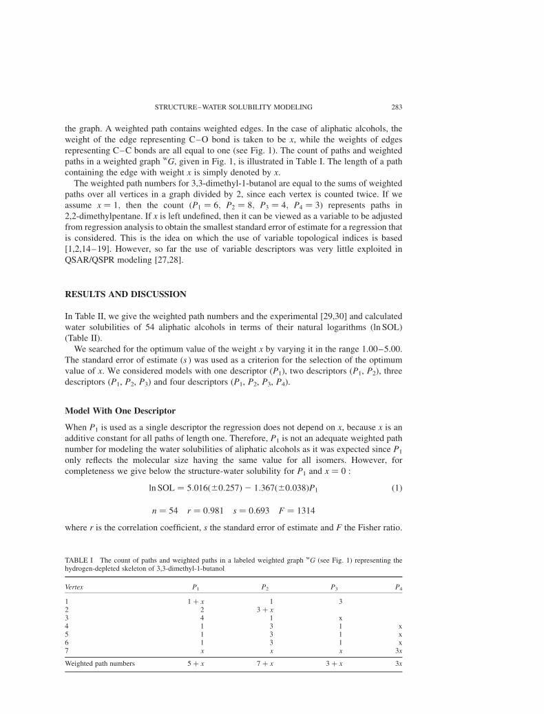
In Table II, we give the weighted path numbers and the experimental [29,30] and calculated

water solubilities of 54 aliphatic alcohols in terms of their natural logarithms (ln SOL)

(Table II).

We searched for the optimum value of the weight x by varying it in the range 1.00–5.00.

The standard error of estimate (s ) was used as a criterion for the selection of the optimum

value of x. We considered models with one descriptor (P1), two descriptors (P1, P2), three

descriptors (P1, P2, P3) and four descriptors (P1, P2, P3, P4).

Model With One Descriptor

When P1 is used as a single descriptor the regression does not depend on x, because x is an

additive constant for all paths of length one. Therefore, P1 is not an adequate weighted path

number for modeling the water solubilities of aliphatic alcohols as it was expected since P1

only reflects the molecular size having the same value for all isomers. However, for

completeness we give below the structure-water solubility for P1 and x ¼ 0 :

ln SOL ¼ 5:016ð^0:257Þ2 1:367ð^0:038ÞP1 ð1Þ

n ¼ 54 r ¼ 0:981 s ¼ 0:693 F ¼ 1314

where r is the correlation coefficient, s the standard error of estimate and F the Fisher ratio.

TABLE I The count of paths and weighted paths in a labeled weighted graph wG (see Fig. 1) representing thehydrogen-depleted skeleton of 3,3-dimethyl-1-butanol

Vertex P1 P2 P3 P4

1 1 þ x 1 32 2 3 þ x3 4 1 x4 1 3 1 x5 1 3 1 x6 1 3 1 x7 x x x 3x

Weighted path numbers 5 þ x 7 þ x 3 þ x 3x

STRUCTURE–WATER SOLUBILITY MODELING 283

TABLE II The weighted path numbers, experimental, calculated (fitted and cross-validated), and predicted water solubilities of 54 aliphatic alcohols using the best two-descriptor model

No. Compound P1 P2 P3 P4

ln SOL

exp. calc-FIT calc-CV calc/prd

1 2-Methyl-1-propanol 3 þ x 3 þ x 2x 0 0.0227 0.093 0.099 0.0882 2-Butanol 3 þ x 2 þ 2x 1 þ x 0 0.0658 0.611 0.643 0.605*3 3-Methyl-1-butanol 4 þ x 4 þ x 2 þ x 2x 21.1680 21.205 21.208 21.2044 2-Methyl-1-butanol 4 þ x 4 þ x 2 þ 2x x 21.0584 21.205 21.215 21.204*5 2-Pentanol 4 þ x 3 þ 2x 2 þ x 1 þ x 20.6349 20.687 20.689 20.6866 3-Pentanol 4 þ x 3 þ 2x 2 þ 2x 1 20.4861 20.687 20.695 20.6867 3-Methyl-2-butanol 4 þ x 4 þ 2x 2 þ 2x 0 20.4050 20.457 20.459 20.461*8 2-Methyl-2-butanol 4 þ x 4 þ 3x 2 þ x 0 0.3386 0.291 0.288 0.2829 3-Hexanol 5 þ x 4 þ 2x 3 þ 2x 2 þ x 21.8326 21.986 21.990 21.977

10 3-Methyl-3-pentanol 5 þ x 5 þ 3x 4 þ 2x 1 20.8301 21.007 21.017 21.010*11 2-Methyl-2-pentanol 5 þ x 5 þ 3x 3 þ x 2 þ x 21.1178 21.007 21.001 21.0112 2-Methyl-3-pentanol 5 þ x 5 þ 2x 3 þ 3x 2 21.6094 21.756 21.759 21.75213 3-Methyl-2-pentanol 5 þ x 5 þ 2x 4 þ 2x 1 þ x 21.6399 21.756 21.758 21.752*14 2,3-Dimethyl-2-butanol 5 þ x 6 þ 3x 4 þ 2x 0 20.8510 20.777 20.771 20.78515 3,3-Dimethyl-1-butanol 5 þ x 7 þ x 3 þ x 3x 22.5903 22.043 22.029 22.04516 3,3-Dimethyl-2-butanol 5 þ x 7 þ 2x 3 þ 3x 0 21.4106 21.295 21.291 21.302*17 4-Methyl-1-pentanol 5 þ x 5 þ x 3 þ x 2 þ x 22.2828 22.504 22.514 22.49518 4-Methyl-2-pentanol 5 þ x 5 þ 2x 3 þ x 2 þ 2x 21.8140 21.756 21.754 21.75219 2-Ethyl-1-butanol 5 þ x 5 þ x 4 þ 2x 1 þ 2x 22.7871 22.504 22.491 22.495*20 2-Methyl-2-hexanol 6 þ x 6 þ 3x 4 þ x 3 þ x 22.4734 22.306 22.296 22.30121 3-Methyl-3-hexanol 6 þ x 6 þ 3x 5 þ 2x 3 þ x 22.2634 22.306 22.308 22.30122 3-Ethyl-3-pentanol 6 þ x 6 þ 3x 6 þ 3x 3 21.9173 22.306 22.328 22.301*23 2,3-Dimethyl-2-pentanol 6 þ x 7 þ 3x 6 þ 2x 2 þ x 22.0025 22.075 22.081 22.07624 2,3-Dimethyl-3-pentanol 6 þ x 7 þ 3x 6 þ 3x 2 21.9379 22.075 22.086 22.07625 2,4-Dimethyl-2-pentanol 6 þ x 7 þ 3x 4 þ x 4 þ 2x 22.1456 22.075 22.070 22.076*26 2,4-Dimethyl-3-pentanol 6 þ x 7 þ 2x 4 þ 4x 4 22.8018 22.824 22.824 22.81927 2,2-Dimethyl-3-pentanol 6 þ x 8 þ 2x 4 þ 4x 3 22.6437 22.593 22.592 22.59428 3-Heptanol 6 þ x 5 þ 2x 4 þ 2x 3 þ x 23.1942 23.284 23.286 23.269*29 4-Heptanol 6 þ x 5 þ 2x 4 þ 2x 3 þ 2x 23.1966 23.284 23.286 23.26930 2,2,3-Trimethyl-3-pentanol 7 þ x 10 þ 3x 8 þ 4x 3 22.9318 22.913 22.910 22.91731 2-Octanol 7 þ x 6 þ 2x 5 þ x 4 þ x 24.7560 24.583 24.579 24.560*32 2-Ethyl-1-hexanol 7 þ x 7 þ x 6 þ 2x 4 þ 2x 24.9967 25.101 25.104 25.07833 2-Nonanol 8 þ x 7 þ 2x 6 þ x 5 þ x 26.3200 25.881 25.869 25.85234 3-Nonanol 8 þ x 7 þ 2x 6 þ 2x 5 þ x 26.1193 25.881 25.875 25.852*35 4-Nonanol 8 þ x 7 þ 2x 6 þ 2x 5 þ 2x 25.9522 25.881 25.879 25.852

D.

AM

ICet

al.

28

4

Table II – continued

No. Compound P1 P2 P3 P4 ln SOL

exp. calc-FIT calc-CV calc/prd

36 5-Nonanol 8 þ x 7 þ 2x 6 þ 2x 5 þ 2x 25.7446 25.881 25.885 25.85237 2,6-Dimethyl-4-heptanol 8 þ x 9 þ 2x 6 þ 2x 5 þ 4x 25.7764 25.421 25.407 25.401*38 3,5-Dimethyl-4-heptanol 8 þ x 9 þ 2x 8 þ 4x 5 þ 2x 25.2983 25.421 25.425 25.40139 2,2-Diethyl-1-pentanol 8 þ x 10 þ x 10 þ 3x 6 þ 3x 25.5728 25.939 25.949 25.91940 7-Methyl-1-octanol 8 þ x 8 þ x 6 þ x 5 þ x 25.7446 26.399 26.424 26.369*41 3,5,5-Trimethyl-1-hexanol 8 þ x 11 þ x 7 þ x 7 þ 2x 25.7699 25.708 25.707 25.69442 1-Dodecanol 11 þ x 10 þ x 9 þ x 8 þ x 210.6800 210.525 210.509 210.46843 1-Butanol 3 þ x 2 þ x 1 þ x 0 0.0953 20.137 20.163 20.137*44 1-Pentanol 4 þ x 3 þ x 2 þ x 1 þ x 21.3471 21.436 21.443 21.42945 2,2-Dimethyl-1-propanol 4 þ x 6 þ x 3x 0 20.6463 20.745 20.749 20.75446 1-Hexanol 5 þ x 4 þ x 3 þ x 2 þ x 22.7181 22.734 22.735 22.720*47 2-Hexanol 5 þ x 4 þ 2x 3 þ x 2 þ x 21.9951 21.986 21.986 21.97748 1-Heptanol 6 þ x 5 þ x 4 þ x 3 þ x 24.0745 24.033 24.030 24.01249 1-Octanol 7 þ x 6 þ x 5 þ x 4 þ x 25.4015 25.331 25.328 25.303*50 1-Nonanol 8 þ x 7 þ x 6 þ x 5 þ x 26.9078 26.629 26.615 26.59451 1-Decanol 9 þ x 8 þ x 7 þ x 6 þ x 28.2208 27.9280 27.910 27.886*52 1-Tetradecanol 13 þ x 12 þ x 11 þ x 10 þ x 212.7720 213.122 213.186 213.05153 1-Pentadecanol 14 þ x 13 þ x 12 þ x 11 þ x 214.6140 214.420 214.373 214.342*54 1-Hexadecanol 15 þ x 14 þ x 13 þ x 12 þ x 215.5875 215.718 215.761 215.634

*Prediction for 19 test set molecules is indicated by asterisks (last column). Remaining 35 molecules are used for training and for model generation. Optimum x value ðx ¼ 3:3Þ for the two-descriptor model (based onP1 and P2) is selected according to the fitted statistical parameters on the training set (35 compounds).

ST

RU

CT

UR

E–

WA

TE

RS

OL

UB

ILIT

YM

OD

EL

ING

285

Best Model With Two Descriptors

In Table III, we give the standard error of estimate for various values of x and this is shown in

Fig. 2.

The best two-descriptor model is obtained for x ¼ 3:25 :

ln SOL ¼ 8:209ð^0:136Þ2 1:529ð^0:015ÞP1 þ 0:230ð^0:011ÞP2 ð2Þ

n ¼ 54 r ¼ 0:9980 s ¼ 0:227 F ¼ 6363

This model is much improved over the above model. The standard error of estimate has

dramatically decreased from s ¼ 0:693 to s ¼ 0:227:

Best Model With Three Descriptors

In Table IV, we give the standard error of estimate for various values of x and this is

graphically shown in Fig. 3.

The best three-descriptor model is obtained for x ¼ 3:75 :

ln SOL ¼ 8:880ð^0:136Þ2 1:515ð^0:014ÞP1 þ 0:190ð^0:011ÞP2

þ 0:024ð^0:009ÞP3 ð3Þ

n ¼ 54 r ¼ 0:9982 s ¼ 0:215 F ¼ 4698

This model is only slightly better than model (2).

Best Model With Four Descriptors

In Table V, we give the standard error of estimate for various values of x and this is shown in

Fig. 4.

The best four-descriptor model is obtained for x ¼ 3:65 :

ln SOL ¼ 8:701ð^0:147Þ2 1:506ð^0:020ÞP1 þ 0:193ð^0:011ÞP2

þ 0:023ð^0:009ÞP3 þ 0:008ð^0:009ÞP4 ð4Þ

n ¼ 54 r ¼ 0:9983 s ¼ 0:216 F ¼ 3508

This model is comparable to the model (3).

TABLE III The standard error ofestimate (s ) for various values of xwhen two weighted paths (P1, P2) areused as descriptors. Asterisks denote theoptimum values of x and s

x s

1.00 0.373792.00 0.255513.00 0.227213.25* 0.22663*3.50 0.227324.00 0.231035.00 0.24199

D. AMIC et al.286

Leave-One-Out Cross-Validated Model

Among the listed models (2)–(4), there is not much difference. Therefore, we selected,

according to the Ockham’s Razor Principle [31], a model with least number of parameters,

that is, the two-descriptor model (2) for calculating fitted values of ln SOL. They are reported

in Table II under heading (ln SOL)calc-FIT.

We also used the leave-one-out cross-validation technique as a criterion for checking the

quality of the model (2) [32]. Since the obtained cross-validated statistical parameters

ðrcv ¼ 0:998; scv ¼ 0:237Þ are close to the fitted values, the good quality of model (2) is thus

confirmed.

FIGURE 2 A plot of the path weight x against the standard error of estimate s for two descriptors (P1, P2).

TABLE IV The standard error ofestimate (s ) for various values of xwhen three weighted paths (P1, P2, P3)are used as descriptors. Asterisks denotethe optimum values of x and s

x s

1.00 0.368802.00 0.251593.00 0.219793.25 0.217183.30 0.216833.40 0.216243.50 0.215823.55 0.215683.60 0.215573.65 0.215473.70 0.215413.75* 0.21538*3.80 0.215393.90 0.215444.00 0.215584.25 0.216255.00 0.21975


The cross-validated values are reported in Table II under heading (ln SOL)calc-CV. A plot

(ln SOL)exp vs. (ln SOL)calc-CV is shown in Fig. 5.

Predictive Performance of the Weighted-Paths Based Models

In addition, following suggestions of reviewers, predictive performance of the models

containing two, three and four weighted paths were examined. For the training (selection of

optimal x ) 35 randomly selected molecules were used, and remaining 19 molecules were

FIGURE 3 A plot of the path weight x against the standard error of estimate s for three descriptors (P1, P2, P3).

TABLE V The standard errorof estimate (s ) for various valuesof x when four weighted paths(P1, P2, P3, P4) are used asdescriptors. Asterisks denote theoptimum values of x and s

x s

1.00 0.366322.00 0.251073.00 0.219003.25 0.216903.30 0.216653.40 0.216253.50 0.216003.55 0.215943.60 0.215913.65* 0.21588*3.70 0.215903.75 0.215943.80 0.216013.90 0.216204.00 0.216464.25 0.217394.50 0.218595.00 0.22145

D. AMIC et al.288

FIGURE 4 A plot of the path weight x against the standard error of estimate s for four descriptors (P1, P2, P3, P4).

FIGURE 5 A plot of (ln SOL)exp against (ln SOL)calc-CV.

TABLE VI Statistical parameters of the models obtained in the training/test set partition

Weighted Paths x rtrain strain rtest stest

P1, P2 3.3 0.9987 0.181 0.9969 0.282P1, P2, P3 4.0 0.9989 0.160 0.9970 0.277P1, P2, P3, P4 4.0 0.9989 0.160 0.9970 0.276

In the first column weighted paths involved in the models are given. x is the weight of the edge representing C–O bond. rtrain and rtest

are correlation coefficients calculated on 35 molecules from the training set and on 19 molecules from the test set, respectively. strain

and stest are standard error of estimate calculated on 35 molecules from the training set and standard error of prediction calculated on19 molecules from the test set, respectively. Prediction for the test set molecules is made using model developed on the training set.


used for testing the predictive model quality. Test set molecules are indicated by asterisks in

the last column in Table II. Statistical parameters of the models obtained for this training/test

set partition are given in Table VI. The best two-descriptor model developed for 35 training

set molecules involved P1 and P2 calculated for x ¼ 3:3: For the training set we obtained

s ¼ 0:181: Standard error of prediction for the test set compounds is 0.281.

The best three- and four-descriptor models involved paths calculated for x ¼ 4:0: Three-

descriptor model contains P1, P2, and P3 and gives s ¼ 0:160 on the training set. The

standard error of prediction on the test set compounds is s ¼ 0:276: The best four descriptor

models (with P1, P2, P3, P4) is also obtained for x ¼ 4:0 and produces s ¼ 0:160 in training

and s ¼ 0:275 in prediction on the test set. We see that inclusion of P3 and P4 does not

produce significant improvement of the models quality, and we take the two-descriptor

model as the best one. This particular selection is in accordance with the selection of the best

model based on the cross-validated parameters. Moreover, there is only a small difference

between x values selected according to the best fitted or cross-validated parameters, and

those selected according the best predictive parameters.

In order to see good predictive quality of the best two-descriptor model containing P1 and

P2, we give scatter plot (ln SOL)exp vs. (ln SOL)calc for 35 training set compounds (black

circles), and, in the same plot, (ln SOL)exp vs. (ln SOL)pred for 19 test set compounds (open

circles) (Fig. 6).

Comparison With Models Reported in the Literature

We list below several structure–water solubility models of aliphatic alcohols based on

different molecular descriptors that are reported last 25 years in the literature.

Models Based on Surface Areas of Aliphatic Alcohols

An early attempt to model water solubility of aliphatic alcohols is by Amidon et al. [29].

These authors produced three models between the water solubility of aliphatic alcohols and

FIGURE 6 A plot of (ln SOL)exp against (ln SOL)calc for 35 molecules from the training set (black circles) and(ln SOL)exp against (ln SOL)pred for 19 molecules from the test set (open circles).

D. AMIC et al.290

their surface areas. They adopted the definition of molecular surface area from Hermann

[33]: A molecule is considered as a collection of spheres with each radius located at the

nuclear center. To each radius on the solute molecule (aliphatic alcohol), a radius for the

solvent (water) is added to give a surface. This approach has the convenient property of

eliminating from the total surface area of a molecule those areas that are not exposed or

accessible to the solvent. Another advantage of Hermann’s procedure is that it allows

computation of the individual atom contributions to the total surface area. This permits

division of the total surface area of a molecule into group contributions, e.g. hydrocarbon and

hydroxyl group parts of alcohols, and the group contribution to the solubility can be

estimated. Standard bond length and bond angles were used for all aliphatic alcohols

considered. It should be also pointed out that long time ago (in 1925) one of the first attempts

to relate a molecular property to critical structural features is due to Langmuir [34] who

related intermolecular interactions in the liquid state to the surface energy. Recently (in

1999) Mebane et al. [35] pointed out that the surface area is an important descriptor to use in

the structure–property modeling.

Amidon et al. [29] have considered only 51 aliphatic alcohols, omitting those which are

solid at the room temperature. Their first model relates ln SOL and the total surface area

(TSA) in A2:

ln SOL ¼ 11:78 2 0:043 TSA ð5Þ

n ¼ 51 r ¼ 0:974 s ¼ 0:499

Their second model relates ln SOL with the surface area of the hydrocarbon part of the

aliphatic alcohol. Amidon et al. [29] calculated the hydrocarbon surface area (HYSA) by

substracting the hydyroxyl group surface area (OHSA) from TSA: HYSA ¼ TSA 2 OHSA:They obtained the following not particularly good model:

ln SOL ¼ 8:94 2 0:0396 HYSA ð6Þ

n ¼ 54 r ¼ 0:94 s ¼ 0:706

The best empirical model of Amidon et al. [29] is a two-descriptor model that relates

ln SOL with the HYSA and the OHSA:

ln SOL ¼ 12:41 2 0:043 HYSA 2 0:060 OHSA ð7Þ

n ¼ 51 r ¼ 0:978 s ¼ 0:462

The TSA and HYSA are highly intercorrelated quantities, the value of r being 0.994.

Models (5) and (7) are somewhat better than the one-descriptor model (1), while models (2)–

(4) from above possess better statistical characteristics.

Kier–Hall–Murray Models

Hall, Kier and Murray [36] were first to study the structure–water solubility of aliphatic

alcohols using topological indices. Their first model has been derived in 1975 before Kier

and Hall [37] introduced the valence vertex-connectivity index. Therefore, Hall, Kier and

Murray [36] used the vertex-connectivity index x in the original Randic’s formulation for

hydrocarbons [38]. Hence, Hall, Kier and Murray [36] instead of computing the vertex-

connectivity index for aliphatic alcohols computed x for the related alkanes. In spite of this,

they obtained a decent model comparable to models based on surface areas of aliphatic


alcohols and to our model (1):

ln SOL ¼ 6:702 2 2:666x ð8Þ

n ¼ 51 r ¼ 0:978 s ¼ 0:455

When they used the empirical parameter cOH that takes care about the environment of the

OH group, that is, whether we deal with primary, secondary or tertiary alcohols, the two-

descriptor model considerable improves:

ln SOL ¼ 9:204 2 2:630x 2 4:390cOH ð9Þ

n ¼ 50 r ¼ 0:991 s ¼ 0:289

Model Based on Orthogonal Descriptors

A very good two-descriptor structure–water solubility model for aliphatic alcohols can be

obtained using ordered orthogonal descriptors [39–41] which includes explicitly the OH

group [4]:

ln SOL ¼ 23:666ð^0:037Þ2 2:689ð^0:479ÞVV 2 6:336ð^0:479ÞVOH ð10Þ

n ¼ 54 r ¼ 0:997 s ¼ 0:273 F ¼ 4479

where the symbol V stands for orthogonal descriptors. The valence vertex-connectivity indices

are used as the basis set. The structure–water solubility model for aliphatic alcohols based on

four ordered orthogonal descriptors including the OH group is a very good model, better than any

other model from above except three models (2)–(4) based on the weighted path numbers:

ln SOL ¼ 23:666ð^0:033Þ2 2:689ð^0:025Þ 1VV 2 1:225ð^0:116Þ 3VV

2 0:650ð^0:324Þ 4VV þ 5:747ð^0:510Þ VOH ð11Þ

n ¼ 54 r ¼ 0:998 s ¼ 0:240 F ¼ 2897

Model Based on the Valence Vertex-Connectivity Index With Optimum Exponent

The following is the best structure–water solubility model for aliphatic alcohols based on the

valence vertex-connectivity index with the optimum value of the exponent [42] equal to

20.425 [43]:

ln SOL ¼ 5:864ð^0:210Þ2 2:418ð^0:050ÞðxVÞ½20:425� ð12Þ

n ¼ 54 r ¼ 0:989 s ¼ 0:526 F ¼ 2320

where (x V)[20.425] is a shorthand notation for the valence vertex-connectivity indices

calculated using the value of 20.425 for the exponent in Eq. (12). There is a slight

improvement over the structure–water solubility model when the valence vertex-

connectivity indices are computed using the standard value for the exponent, that is, 20.5:

ln SOL ¼ 5:814ð^0:211Þ2 2:671ð^0:056ÞðxVÞ½20:5� ð13Þ

n ¼ 54 r ¼ 0:989 s ¼ 0:531 F ¼ 2279

D. AMIC et al.292

Model Based on the Valence Edge-Connectivity Index With Optimum Exponent

The same approach as above is applied to the use of the valence edge-connectivity index 1 V

[44,45]. The best structure–water solubility model for aliphatic alcohols based on the

valence edge-connectivity index with the optimum value of the exponent equal to 20.675 is

[43]:

ln SOL ¼ 5:527ð^0:167Þ2 3:306ð^0:056Þð1VÞ½20:675� ð14Þ

n ¼ 54 r ¼ 0:992 s ¼ 0:434 F ¼ 3426

where (1 V)[20.675] is a shorthand notation for the valence edge-connectivity indices

calculated using the value of 20.675 for the exponent in (14). This is a better model than the

structure–water solubility model based on the valence edge-connectivity indices with the

standard value for the exponent, that is, 20.5:

ln SOL ¼ 6:210ð^0:282Þ2 2:727ð^0:074Þð1VÞ½20:5� ð15Þ

n ¼ 54 r ¼ 0:982 s ¼ 0:680 F ¼ 1368

Model (14) is better than models (1), (6), (12), (13) and (15) and is comparable to models

(5), (7) and (8). It falls behind two-, three- and four-descriptor models based on weighted

paths numbers, the Kier–Hall–Murray two-descriptor model and models based on

orthogonal descriptors.

Model Based on Weighted Line Graphs

The same approach as in last two previous subsections is also applied to the use of the

valence edge-connectivity index computed for the weighted line graphs [25]. The best

structure–water solubility model for aliphatic alcohols, represented by weighted line graphs,

based on the valence edge-connectivity index with the optimum value of the exponent equal

to 20.85 is [43]:

ln SOL ¼ 4:899ð^0:247Þ2 4:078ð^0:109Þ½1VðLÞ�½20:85� ð16Þ

n ¼ 54 r ¼ 0:981 s ¼ 0:674 F ¼ 1392

where [1 V(L)][20.85] is a shorthand notation for the valence edge-connectivity indices of line

graphs L, calculated using the value of 20.85 for the exponent in Eq. (16). This is a much

better model than the structure–water solubility model based on the standard value of the

exponent, that is, 20.50:

ln SOL ¼ 4:367ð^1:106Þ2 1:942ð^0:256Þ½eVðLÞ�½20:50� ð17Þ

n ¼ 54 r ¼ 0:725 s ¼ 2:447 F ¼ 58

Model (17) is the worst model of all models listed here, while the model (16) is

comparable to models (1), (6) and (15).

CONCLUDING REMARKS

In the present work, we compared four structure–water solubility models of aliphatic

alcohols based on the weighted path numbers among themselves and with a number of


models based on a variety of descriptors. The comparison was based on the correlation

coefficient and standard error of estimate. The result of this comparative study is that two-,

three- and four-descriptor models based on the weighted path numbers are superior to all

other models reviewed here. We have found that the optimal values of the weight of the edge

representing C–O bond (x ) for the studied data set is in the range 3.0–4.0, instead of x ¼ 1:0in the case when non-weighted paths were used. The high quality of these models suggests

that they can be used with confidence for predicting the water solubilities of yet unknown

higher aliphatic alcohols, if such a need arises.

Acknowledgements

This work was supported in part by the Ministry of Science and Technology of the Republic

of Croatia via Grants 00980606 (BL, SN and NT), 106N407 (BL) and 079301 (DA). A part

of this work was completed during the stay of SN and NT at the Center for Water and the

Environment, Natural Resources Research Institute (NRRI), University of Minnesota,

Duluth, Minnesota 55811, USA. SCB and SN and NT (during their stay at NRRI) were

supported, in part, by Grants F49620-94-1-0401 and F49620-96-1-0330 from the United

States Air Force. We thank referees for their helpful comments.

References

[1] Randic, M. and Basak, S.C. (1999) “Optimal molecular descriptors based on weighted path numbers”, J. Chem.Inf. Comput. Sci. 39, 261–266.

[2] Randic, M. and Pompe, M. (1999) “On characterization of the CC double bond in alkenes”, SAR QSAREnviron. Res. 10, 451–471.

[3] Roy, A.B., Basak, S.C., Harriss, D.K. and Magnuson, V.R. (1984) “Neighborhood complexities and symmetryof chemical graphs and their biological applications”, In: Avula, X.J.R., Kalman, R.E., Lipais, A.I. and Rodin,E.Y., eds, Mathematical Modelling in Science and Technology (Pergamon Press, New York), pp. 745–775.

[4] Lucic, B., Nikolic, S., Trinajstic, N., Juric, A. and Mihalic, Z. (1995) “A structure–property study of thesolubility of aliphatic alcohols in water”, Croat. Chem. Acta 68, 417–434.

[5] Nikolic, S. and Trinajstic, N. (1998) “Modeling the aqueous solubility of aliphatic alcohols”, SAR QSAREnviron. Res. 9, 117–126.

[6] Barysz, M., Jashari, G., Lall, R.S., Srivastava, V.K. and Trinajstic, N. (1983) “On the distance matrix containingheteroatoms”, In: King, R.B., ed, Chemical Applications of Topology and Graph Theory (Elsevier,Amsterdam), pp. 222–227.

[7] Ivanciuc, O., Ivanciuc, T., Cabrol-Bass, D. and Balaban, A.T. (2000) “Comparison of weighting schemes formolecular graph descriptors: Application in quantitative structure–retention relationship models foralkylphenols in gas–liquid chromatography”, J. Chem. Inf. Comput. Sci. 40, 732–743.

[8] Platt, J.R. (1952) “Prediction of isomeric differences in paraffin properties”, J. Phys. Chem. 56, 328–336.[9] Hosoya, H. (1971) “Topological index. A newly proposed quantity characterizing the topological nature of

structural isomers of saturated hydrocarbons”, Bull. Chem. Soc. Jpn 44, 2332–2339.[10] Todeschini, R. and Consonni, V. (2000) The Handbook of Molecular Descriptors (Wiley-VCH, New York).[11] Devillers, J. and Balaban, A.T. (1999) Topological Indices and Related Descriptors in QSAR and QSPR

(Gordon and Breach Science Publisher, Amsterdam), p. 811.[12] Karelson, M. (2000) Molecular Descriptors in QSAR/QSPR (Wiley-Interscience, New York), p. 430.[13] Katritzky, A.R., Maran, U., Lobanov, V.S. and Karelson, M. (2000) “Structurally diverse quantitative

structure–property relationship correlations of technologically relevant physical properties”, J. Chem. Inf.Comput. Sci. 40, 1–18.

[14] Randic, M., Hansen, P. and Jurs, P.C. (1988) “Search for useful graph theoretical invariants of molecularstructure”, J. Chem. Inf. Comput. Sci. 28, 60–68.

[15] Randic, M. (1991) “Novel graph theoretical approach to heteroatom in quantitative structure–activityrelationship”, Chemom. Intell. Lab. Syst. 12, 970–980.

[16] Randic, M. (1991) “On computation of optimal parameters for multivariate analysis of structure–propertyrelationship”, J. Comput. Chem. 12, 792–980.

[17] Randic, M. (1991) “Search for optimal molecular descriptors”, Croat. Chem. Acta 64, 43–54.[18] Randic, M. and Basak, S.C. (2000) “Multiple regression analysis with optimal molecular descriptors”, SAR

QSAR Environ. Res. 11, 1–23.

D. AMIC et al.294

[19] Randic, M. and Basak, S.C. (2000) “Variable molecular descriptors”, In: Sinha, D.K., Basak, S.C., Mohanty,R.K. and Busamallick, I.N., eds, Some Aspects of Mathematical Chemistry (Visva-Bharati University Press,Santiniketan).

[20] Balaban, A.T. (1997) From Chemical Topology to Three-Dimensional Geometry (Plenum Press, New York),p. 420.

[21] Gute, B.D. and Basak, S.C. (1997) “Predicting acute toxicity (LC50) of benzene derivatives using theoreticalmolecular descriptors: A hierarchical QSAR approach”, SAR QSAR Environ. Res. 7, 117–131.

[22] Plavsic, D., Trinajstic, N., Amic, D. and Soskic, M. (1998) “Comparison between the structure–boiling pointrelationships with different descriptors for condensed benzenoids”, N. J. Chem. 22, 1075–1078.

[23] Karelson, M., Maran, U., Wang, Y. and Katritzky, A.R. (1999) “QSPR and QSAR models derived using largemolecular descriptors spaces”, Coll. Czech. Chem. Commun. 64, 1551–1571.

[24] Pogliani, L. (1996) “A strategy for molecular modeling of a physicochemical property using a linearcombination of connectivity indexes”, Croat. Chem. Acta 69, 95–109.

[25] Basak, S.C., Nikolic, S., Trinajstic, N., Amic, D. and Beslo, D. (2000) “QSPR Modeling: Graph ConnectivityIndices versus Line Graph Connectivity Indices”, J. Chem. Inf. Comput. Sci. 40, 927–933.

[26] Chartrand, G. (1977) Graph as Mathematical Models, (Prindle, Weber and Schmidt, Boston), pp. 41–42.[27] Randic, M. and Pompe, M. (2000) “The variable molecular descriptors based on distance related matrices”,

J. Chem. Inf. Comput. Sci. 40, 575–581.[28] Amic, D., Lucic, B., Nikolic, S., Trinajstic, N. Variable Wiener number, manuscript in preparation.[29] Amidon, G.L., Yalkowsky, S.H. and Leung, S. (1974) “Solubility of nonelectrolytes in polar solvents. II.

Solubility of aliphatic alcohols in water”, J. Pharm. Sci. 63, 1858–1866.[30] Weast, R.B. (1987) CRC Handbook of Chemistry and Physics, 67th Ed. (CRC Press, Inc., Boca Raton, FL), 3rd

printing.[31] Hoffmann, R., Minkin, V.I. and Carpenter, B.K. (1996) “Ockham’s razor in chemistry”, Bull. Soc. Chim.

France 133, 117–130.[32] Lucic, B. and Trinajstic, N. (1997) “New development in QSPR/QSAR modeling based on topological

indices”, SAR QSAR Environ. Res. 7, 45–62.[33] Hermann, R.B. (1972) “The theory of hydrophobic bonding. II. The correlation of hydrocarbon solubility in

water with solvent cavity surface area”, J. Phys. Chem. 76, 2754–2759.[34] Langmuir, I. (1925) “The distribution and orientation of molecules”, Colloid. Symp. Monogr. 3, 49–75.[35] Mebane, R.C., Schanley, S.A., Rybolt, T.R. and Bruce, C.D. (1999) “The correlation of physical properties of

organic molecules with computed molecular surface areas”, J. Chem. Edu. 76, 688–693.[36] Hall, L.H., Kier, L.B. and Murray, W.J. (1975) “Molecular connectivity. II. Relationship to water solubility and

boiling point”, J. Pharm. Sci. 64, 1974–1977.[37] Kier, L.B. and Hall, L.H. (1976) “Molecular connectivity. VII. Specific treatment of heterosystems”, J. Pharm.

Sci. 65, 1806–1809.[38] Randic, M. (1975) “On characterization of molecular branching”, J. Am. Chem. Soc. 97, 6609–6615.[39] Randic, M. (1991) “Orthogonal molecular descriptors”, N. J. Chem. 15, 517–525.[40] Lucic, B., Nikolic, S., Trinajstic, N. and Juretic, D. (1995) “The structure–property models can be improved

using the orthogonalized descriptors”, J. Chem. Inf. Comput. Sci. 35, 532–538.[41] Lucic, B., Nikolic, S., Trinajstic, N., Juretic, D. and Juric, A. (1995) “A novel QSPR approach to

physicochemical properties of the a-amino acids”, Croat. Chem. Acta 68, 435–450.[42] Amic, D., Beslo, D., Lucic, B., Nikolic, S. and Trinajstic, N. (1998) “The vertex-connectivity index revisited”,

J. Chem. Inf. Comput. Sci. 38, 819–822.[43] Nikolic, S., Trinajstic, N., Amic, D., Beslo, D. and Basak, S.C. (2001) “Modeling the solubility of aliphatic

alcohols in water. Graph connectivity indices versus line graph connectivity indices”. In: QSAR/QSPR Studiesby Molecular Descriptors (Nova Science Publishers, Commack), pp. 63–81.

[44] Estrada, E. (1995) “Edge adjacency relationships and a novel topological index related to molecular volume”,J. Chem. Inf. Comput. Sci. 35, 31–33.

[45] Estrada, E. (1995) “Edge adjacency relationships in molecular graphs containing heteroatoms: A newtopological index related to molecular volume”, J. Chem. Inf. Comput. Sci. 35, 701–707.


Structure-water solubility modeling of aliphatic alcohols using the weighted path numbers

Documents