Structure matter 2 - Home | USU

SM 2 1

Structure of matter, 2 Quantum electrodynamics Quantum electrodynamics (QED) is the quantitatively best physical theory yet developed. Where it has been tested, it agrees with experiment to at least a few parts in 1011! It is a theory of how charged particles and photons interact. It starts with electrons, for example, described by the Dirac Equation, interacting with photons described by a suitable electromagnetic potential energy. The latter cannot be due only to electrostatics because an electric field in one frame of reference is an electric and a magnetic field in a second frame moving relative to the first; so is

inadequate. If we write the Dirac Equation become .

This is the same as . In this form, it looks like the energy is being transformed by subtracting the electric potential energy from it. But special relativity treats energy and momentum on the same footing, so should be incorporated into , for example, as

, that is,

. (1) In electromagnetism, the field is called the electromagnetic “vector potential.” (Formally, the

magnetic field is derived from by taking its curl: (where ). The

electric field is (where ).) When the Maxwell Equations are

written in terms of the scalar ( ) and vector potentials ( ), we find

. (2) The left hand sides of both of the latter equations correspond to field equations derived from the relativistic energy-momentum relation for (spin-1) massless free particles; the right hand sides are the sources of the potentials, namely, the charge and current densities associated with the fields in (1). These densities, in turn, are related to the square of the field. In other words, Equations (1) and (2) are a set of coupled, nonlinear partial differential equations. As you might guess, finding exact solutions for general conditions is impossible. We have to be content with approximate solutions. Example: Electrons in atoms obey (1), which contains both relativistic and magnetic effects. To first order where the electromagnetic part is approximately just the electrostatic Coulomb interaction, (1) predicts only smallish relativistic corrections to the Schrödinger description. In hydrogen, the corrections lead to an about 1% lowering in the energy levels. In heavier atoms, however, the corrections are more significant. In Pb, for example, the energy levels are lowered by several eV. Indeed, it has been argued that 80% of the potential difference generated in lead-acid batteries is due to relativistic corrections to the Schrödinger predictions. In this sense, your car starts because of relativistic quantum mechanics.

U = qEφE

U = qEφE + ′U Eopψ = c

α ipop +ηmc

2 + qEφE + ′U( )ψ (Eop − qEφE )ψ = c

!α i!pop +ηmc

2 + ′U( )ψ

′U pop

cα i ( pop − qE

AE )

(Eop − qEφE )ψ = c

α i ( pop − qEAE )+ηmc

2⎡⎣ ⎤⎦ψ

AE

AE

B = curl(

AE ) curl(

AE ) = ∇×

AE

EE = −grad(φE )−

∂AE

∂tgrad(φE ) = ∇φE

φE AE

Eop2 φE − c2 pop

2 φE = −(c)2 ρE ε0 , Eop2AE − c2 pop

2AE = −(c)2µ0

JE

ψψ

SM 2 2

Quantum field theory QED was historically the first true quantum field theory. Quantum field theory is all about creating and annihilating particle states. A particle state can be thought of as a vector whose components are the numbers of particles with all of the values of energy, momentum, and spin that the associated field equations (e.g., (1) and (2)) allow. These vectors are not like electromagnetic fields; for example, they don’t “live” in spacetime. Instead, they live in an abstract "particle number space." Quantum field theory describes how to transform one particle state into another. Quantum field theoretic calculations are mathematically challenging, so we won’t do any–we'll only talk about the results. The s-t diagram to the right depicts the usual formulation of QFT. At time there are (3 in the diagram) free (noninteracting) particles each with well-defined masses, spins, energies, and momenta, and at time there are

(4 in the diagram) free particles each with their own well-defined masses, spins, energies, and momenta. (Particle number need not be conserved, because pure energy can be converted into mass [and vice versa]–as long as various other conservation laws are obeyed.) In between, in the s-t blob designated S, the particles interact, possibly changing types and dynamical properties. The "in state" and "out state" are abstract vectors, denoted Iinstate> and Ioutstate>, respectively, that enumerate how many particles of each type there are and what their intrinsic (i.e., mass and spin) and extrinsic (i.e., energy and momentum) properties are. The transition from "in" to "out" is formally expressed as Ioutstate> = S Iinstate>, where S is the so-called “scattering-matrix” (or more compactly, “S-matrix”).

All of the details of the interactions are contained in S through the definition: ;

This is a generalization of the expression , where is just a number. In this expression is the identity matrix (1s along the diagonal, 0s everywhere else) and is a matrix that describes how particle states interact. For example, electrons interact electromagnetically, so, in this case, INT will describe the coupling of electron and electromagnetic fields. Each successive term in this expansion involves interactions of ever-greater complexity. In general, the in- and out-vectors can have many components (i.e., states) each, representing many input conditions (states) with corresponding possible outputs. The quantity is the element of the S matrix that connects the specific in-state to the specific out-

state . It is a complex number called the “transition amplitude.” The real number is the transition probability for the process . In addition to probability, the transition amplitude is used to calculate all of the experimentally measurable quantities. Note that if there are no interactions, the in- and out-states are identical. If they are not identical, then the lead term, , in the expansion above contributes nothing to . The term INTfi corresponds to a direct interaction between the particles in the in- and out-states. All of the interactions in the standard model are mediated by other particles; that is, there are always intermediate states between i and f. Consequently, INTfi = 0. On the other hand, the term INT2

fi does not vanish. In fact, INT2fi =

INTfs∙INTsi, where INTsi transforms the in-state into all possible intermediate states s and INTfs transforms s into the out-state. The “all possible” part here requires summing (integrating) over all

Tin N

Tout

′N

S ≡ exp(INT) = I + INT + 12! INT2 + 1

3! INT3 + ...+ 1n! INTn + ...

exp(x) = 1+ x + 12! x2 + ... x

I INT

S fi i

f S fi

2

i → f

I

S fi

T

x

in

out

S

SM 2 3

energies, momenta, and spins allowed by conservation laws for the intermediary states. Higher order terms in involve additional intermediary states. Back to QED The field interactions underlying QED involve products of charged fields and electromagnetic potentials: charged fields only interact through electromagnetism and, because they carry no electric charge, electromagnetic fields do not interact with one another. S-matrix calculations require evaluating integrals involving many such field product interactions. In the late 1940s, Richard Feynman introduced an important calculational tool that vastly simplifies QED calculations. The tool is a pictorial method for assessing the most important processes involving "real" and "virtual" charged particles and photons and for quantitatively determining the associated probability and energy of the electromagnetic phenomena.

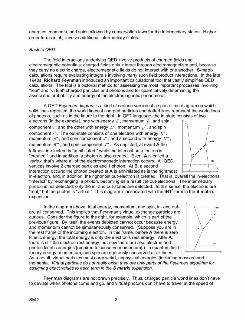
A QED Feynman diagram is a kind of cartoon version of a space-time diagram on which solid lines represent the world lines of charged particles and dotted lines represent the world lines of photons, such as in the figure to the right. In QFT language, the in-state consists of two electrons (in the example), one with energy , momentum , and spin component , and the other with energy , momentum , and spin component . The out-state consists of one electron with energy , momentum , and spin component , and a second with energy , momentum , and spin component . As depicted, at event A the leftmost in-electron is “annihilated,” while the leftmost out-electron is “created,” and in addition, a photon is also created. Event A is called a vertex; that’s where all of the electromagnetic interaction occurs. All QED vertices involve 2 charged particles and 1 photon. At B, a second interaction occurs: the photon created at A is annihilated as is the rightmost in-electron, and, in addition, the rightmost out-electron is created. That is, overall the in-electrons “interact” by “exchanging” a photon, becoming as a result the out-electrons. The intermediary photon is not detected; only the in- and out-states are detected. In this sense, the electrons are “real,” but the photon is “virtual.” This diagram is associated with the INT2 term in the S matrix expansion. In the diagram above, total energy, momentum, and spin, in- and out-, are all conserved. This implies that Feynman’s virtual exchange particles are curious. Consider the figure to the right, for example, which is part of the previous figure. By itself, the events depicted cannot occur because energy and momentum cannot be simultaneously conserved. (Suppose you are in the rest frame of the incoming electron. In this frame, before A there is zero kinetic energy; the total energy is only the electron’s rest energy. After A, there is still the electron rest energy, but now there are also electron and photon kinetic energies [required to conserve momentum].) In quantum field theory energy, momentum, and spin are rigorously conserved at all times. As a result, virtual particles must carry weird, unphysical energies (including masses) and momenta. Virtual particles do not really exist; they are only parts of the Feynman algorithm for assigning exact values to each term in the S matrix expansion. Feynman diagrams are not drawn precisely. Thus, charged particle world lines don’t have to deviate when photons come and go, and virtual photons don’t have to travel at the speed of

S fi

E !p

s ′E ! ′p

′s ′′E ! ′′p ′′s ′′′E

! ′′′p ′′′s

T

x

A

in

out

T

x

in

out

A

B

SM 2 4

light–they can just go from one charge to another instantaneously! For each possible diagram, Feynman’s rules assign an “amplitude,” a complex-valued function of energy, momentum, and spin that describes the nature of the charged particle-photon interaction. The absolute square of the amplitude is used in integrals over all virtual particle energies, momenta, and spins to produce the INT terms in the S matrix.

In drawing Feynman diagrams for QED there are some rules. (1) A massive particle (e.g., an electron or a quark) has a world line with arrow pointing upward in time. (2) A massive anti-particle (e.g., a positron or an anti-quark) has a world line with arrow pointing downward in time. (This doesn’t mean that anti-particles come out of the future, it’s just a convention to keep straight what’s happening.) (3) When a photon interacts with a charged particle it does so at a vertex consisting of 3 prongs, consisting of 2 charged particle world lines and 1 photon world line (this is necessary to guarantee charge conservation). This is called a minimal interaction vertex. (4) Diagrams showing an allowed process can be rotated or flipped to show other allowed processes.

To see how these rules work let’s take the second diagram above and rotate it by 90˚ to the right. We get something like the first figure to the right. This shows a photon annihilating and spontaneously creating a positron (to the left) and an electron (to the right) at A. (Note that the positron ages in the upward direction even though its world line arrow points down.) This process is called “virtual pair creation.” If that figure is flipped over (a “time reversal” transformation), we get the second figure on the right. There, a positron (on the right) annihilates with an electron (on the left) at A to create a virtual photon. To produce either real pair-creation or real pair-annihilation requires at least two real photons. But according to the rules stated above, vertices can only have three lines each. Thus, an acceptable pair creation process might be as shown to the right below. In that figure, the rightmost photon creates a real electron and a virtual positron at A, after which the virtual positron absorbs the leftmost photon at B, and “becomes” real. Thus, there are two real photons in the in-state and a real electron-positron pair in the out-state—and, overall, momentum and energy are conserved. Note that the net effect of all of this is that two photons (of total energy equal to at least 1.02 MeV, i.e., the sum of the out-particles masses) can effectively “collide” to create a pair of particles. This is not expected from Maxwell’s theory of electromagnetism, which predicts that two beams of light just pass through each other without alteration. Inasmuch as pair creation via two-photon collision is now well established experimentally, it is clear that Maxwell’s equations are only an approximation to electromagnetic phenomena.

Feynman diagrams can have lots of adornments, such as the ones in the

figure to the right. Note that along one of the virtual photon world lines shown, a virtual positron-electron pair suddenly appears, then quickly disappears. Adornments like the ones shown are less and less likely the more vertices are involved. The QED amplitude at each vertex has a weighting factor that is proportional to the square root of the “fine structure constant”

(where is the Coulomb force constant and is the electronic charge). This dimensionless ratio measures the intrinsic strength of electromagnetic interactions; it shows up, for example, in all calculations involving electrons in atoms. Because the INT terms are also squared in calculating rates and probabilities, a diagram with two vertices contributes about 104 times more to a QED calculation than one with four

T

αE = kEe2 c ≈1/137 kE = 1 4πε0 e

T

x

T

x

A

T

x

A

T

x

A

B

SM 2 5

vertices. Relatively speaking, calculations in QED converge rapidly with increasing diagram complexity.

The statement that QED calculations rapidly converge is a bit glib. It turns out that the energy-momentum integrals in QED calculations involving closed loops, such as the Feynman diagram above, are infinite! Feynman found that you could get rid of all these embarrassing infinities by cutting off the integrations over energy, momentum, and spin and substituting the measured values of electric charge and electronic mass whenever you had to. A theory of this kind, where infinities can be made finite by the substitution of a small number of measured quantities, is called renormalizable. For example, QED can be made into a nice, tame theory by the proper substitutions of particle charge and mass. Among the many triumphs of the renormalization trick probably the most impressive is the calculation of the magnetic moment of the electron. Dirac’s relativistic electron wave equation predicts that the magnetic

moment of the electron should be , where is the electron’s mass, and ,

“the gyromagnetic ratio,” equals 2 exactly. QED, on the other hand, predicts that is modified by all kinds of virtual particles (because of the higher order terms in the S matrix expansion), and that when these are taken into account = 2.00231930444. Extraordinarily precise measurements of

(made possible by extraordinarily precise frequency measurements) give 2.00231930438 with an uncertainty of 8 in the last decimal place. This is an agreement to a few parts in 1011! Never before in human history has there been such an amazing agreement between theory and experiment. QED makes many other predictions, most notably in the realm of atomic and laser physics. In all cases it has been demonstrated to be correct. Despite its quirky (and, to this day, somewhat puzzling) renormalization rule, QED must really be correct. Incidentally, among the diagrams that had to be included to get this level of precision are those shown to the right (where time runs to the right, instead of up). Each has 7 vertices, and the whole calculation took one person two years to complete (before such calculations were automated).

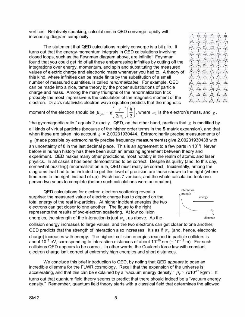
QED calculations for electron-electron scattering reveal a

surprise: the measured value of electric charge has to depend on the total energy of the real in-particles. At higher incident energies the two electrons can get closer to one another. The figure to the right represents the results of two-electron scattering. At low collision energies, the strength of the interaction is just , as above. As the collision energy increases to large values, and the two electrons can get closer to one another, QED predicts that the strength of interaction also increases. It’s as if (and, hence, electronic charge) increases with energy. The highest collision energies reached in particle colliders is about 1012 eV, corresponding to interaction distances of about 10–10 nm (= 10–19 m). For such collisions QED appears to be correct. In other words, the Coulomb force law with constant electron charge isn’t correct at extremely high energies and short distances.

We conclude this brief introduction to QED, by noting that QED appears to pose an incredible dilemma for the FLWR cosmology. Recall that the expansion of the universe is accelerating, and that this can be explained by a “vacuum energy density,” @ 7x10-27 kg/m3. It turns out that quantum field theory seems to predict that there should indeed be a “vacuum energy density.” Remember, quantum field theory starts with a classical field that determines the allowed

µspin = g

e2me

⎛⎝⎜

⎞⎠⎟2

⎛⎝⎜

⎞⎠⎟ me g

g

g

g

α E

α E

ρV

interaction strength

distance

αE

energy

SM 2 6

energies, momenta, and spins of the particles associated with it. The quantum field then creates and annihilates such particles. The quantum field has a formal operator that measures the energy of any particle state. For electromagnetism, its form is . The part first annihilates a particle state then recreates it, while multiplying the state by the number of particles with the requisite energy, momentum, and spin. That is, the

“measures” the number of particles of a given kind in a particle state. If the starting particle state is the “vacuum” of the electromagnetic field, it contains no particles (photons) to annihilate, so the action of the acting on the vacuum effectively reduces the

to just for each value of energy, momentum, and spin. The “vacuum energy density,” then, is the sum of all allowed values, which is infinite.

Nature might not abhor a vacuum, but it certainly abhors infinity. As in the renormalization

trick discussed above, the sum probably should be cut off somehow. One argument goes like this. The Schwarzschild radius is . Suppose the here is and that

(by suspiciously invoking the Heisenberg Uncertainty Principle). This leads to the

result , a distance known as the Planck length (the putative distance where general relativity is no longer a proper description of spacetime) and an associated energy

. At these scales there is no sensible physical theory (yet), so at this energy there is no longer any meaning to QED. Adding up all of the allowed energies below this cutoff gives a value @ 1094 kg/m3! Thus, if the vacuum energy density of the FLWR universe is attributed to

both the vacuum energy of QED and a cosmological constant—that is, —the

cosmological constant has to be negative and has to reduce 1094 kg/m3 to about 10–26 kg/m3, an exact subtraction trick of around 120 digits!!!! The discrepancy of a factor 10120 between and is one of the worst predictions in human intellectual history. Its resolution awaits a new theory combining general relativity and quantum mechanics, requiring, perhaps, a whole new way of thinking about the world (e.g., string theory?).

energy operator = !ω (number operator +1 2)

number operator

number operator

energy operator

energy operator !ω 2

!ω 2

rS = 2GM / c2 M ΔE / c2

ΔE ≈ c 2rS

rS = Gc / c4 ≈1.6x10−35m

≈ 6x1027 eV

ρQED

ρV = Λc2

8πG+ ρQED

ΛρV

ρQED