Structure and stability in exploited marine fish communities: quantifying critical transitions

Structure and stability in exploited marine fish communities:quantifying critical transitions

BRIAN PETRIE,1,* KENNETH T. FRANK,1

NANCY L. SHACKELL1 AND WILLIAM C.LEGGETT2

1Fisheries and Oceans Canada, Ocean Sciences Division,Bedford Institute of Oceanography, 1 Challenger Drive, PO Box1006, Dartmouth, Nova Scotia, B2Y 4A2, Canada2Department of Biology, Queen’s University, Kingston, OntarioK7L 3N6, Canada

ABSTRACT

Correlations between time series of the abundance ofpredator and prey fish species in heavily exploitedwestern North Atlantic marine fisheries vary tempo-rally but are generally positive in southern, warmerwaters and negative in northern, colder ones. Thecorrelations provide an index of trophic structure anddynamics. We construct a framework to quantifycritical thresholds between states in which the pred-ator–prey correlations are positive or negative. We doso by developing a quantitative model of the distri-bution of the correlations between predator (15 spe-cies) and prey (8 species) functional groups based onthe annual predator depletion rates and bottom tem-peratures (or alternatively species richness). Themodel accounts for 58% of the variance of the corre-lations with a root mean square error of 0.3. This indexof trophic structure indicates that warmer, species-rich, southern fish populations resist transformationfrom positive to negative predator–prey correlations atexploitation rates that can be double those in thecolder, relatively species-poor, northern areas. Themodel can be used to set limits for exploitation ratesthat preserve the functional relationships betweenpredator–prey groups in emerging fisheries, and toassess the potential for and measures required toachieve recovery of degraded fish communities.

Key words: exploitation, marine fish populations,predator–prey relationships, thresholds, trophiccascades, trophic structure

INTRODUCTION

The dramatic reduction ⁄ elimination of top predatorsfrom exploited marine ecosystems has led repeatedly topopulation explosions of mesopredators and plankti-vores. This loss has resulted in profound ecosystemtransformations (Jackson et al., 2001; Levin et al.,2006; Oguz and Gilbert, 2007). Analogous changeshave also occurred in terrestrial ecosystems (Schmitzet al., 2000; Berger et al., 2001; Bowyer et al., 2005;Soule et al., 2005; Terborgh et al., 2007). A recentexample from the Northwest Atlantic involved cas-cading changes in four trophic levels and nitrate con-centrations following the collapse of cod and otherdemersal fish species (Frank et al., 2005). Frank et al.(2005) found negative correlations between time seriesof adjacent trophic levels and indirect effects, i.e.,positive correlations between time series separated by atrophic level (e.g., level 4 and level 2). This and otherexamples (Myers and Worm, 2003; Hjermann et al.,2004; Bascompte et al., 2005; Horwood et al., 2006)have led to a call for a more integrated, ecosystemapproach to fisheries management (Quinn et al., 1993;Pikitch et al., 2004; Huggett, 2005). Central to thisapproach is the concept of ‘ecosystem over-fishing’(Murawski, 2000; Sissenwine and Murawski, 2004;Steele and Collie, 2005), a common attribute of whichis a fisheries-induced imbalance between predator andprey abundances, generally at the highest trophic lev-els. A fundamental challenge in moving to an ecosys-tem-based approach is the development of the ability todefine quantitatively, and ultimately predict, how thestate of these ecosystems is modified by directed fishingand, increasingly, by environmental change.

A central question for those committed to theecosystem-based approach to fishery management isthe extent to which apex predators can be depletedbefore the resulting instability leads to large scaleecosystem transformation. A clear example of suchtransformations is found in the Northwest Atlanticwhere the collapse of cod and other top predators wasfollowed by up to 1000-fold increases in the biomass offorage fishes following their release from predation(Bundy, 2005; Bundy and Fanning, 2005; Savenkoffet al., 2007a,b). Apex predator collapse was followed

*Correspondence. e-mail: [email protected]

Received 1 February 2008

Revised version accepted 10 December 2008

FISHERIES OCEANOGRAPHY Fish. Oceanogr. 18:2, 83–101, 2009

� 2009 The Authors. doi:10.1111/j.1365-2419.2009.00500.x 83

by cascading effects at all lower trophic levels (Franket al., 2006). Some idealized models predict specificrelationships between predator and prey communities.For example, Lotka–Volterra theory predicts thatpredator–prey populations should behave cyclicallyand, by extension, that top predator biomass shouldeventually recover if exploitation is curtailed oreliminated (May et al., 1979). Smooth, asymptoticconvergence to steady state populations occur even inthe case of heavy exploitation (May et al., 1979).Cyclical variability and recovery of top predator bio-mass to prior levels has frequently occurred in terres-trial systems (Yom-Tov et al., 2007) but in the marineenvironment, recovery from collapse is less certain(Hutchings and Reynolds, 2004), and in many for-merly cod-dominated fish communities in the North-west Atlantic, the expected recovery of these toppredators has not occurred in spite of reduction orcessation of exploitation for more than a decade(Shelton et al., 2006; Brander, 2007). In these fisher-ies, the now highly abundant (due to lack of preda-tion) forage species appear capable of consumingand ⁄ or out-competing the eggs and larvae of theirformer predators, thereby preventing their recovery. Ineffect, the once-dominant apex predators move to alower level in the trophic hierarchy and become prey,while their former prey assume the role of top preda-tors. This role reversal limits the supply of new recruitsto the populations of once-dominant predators andinhibits stock recovery (May et al., 1979; Swain andSinclair, 2000; Shin and Cury, 2004). Role reversalsoccur less frequently in terrestrial ecosystems in whichtop predators typically occupy the same trophic levelthroughout life (Frank and Leggett, 1994).

Equally detrimental to the capacity of these dis-turbed fish populations to recover from such pertur-bations is the observed parallel decline in individualgrowth rate (a product both of selective fishing andenvironmental change) of several apex species (Choiet al., 2004; Brander, 2007). Size is strongly correlatedwith a broad suite of life history traits that influencepopulation productivity and stability (Roff, 1992;Olsen et al., 2004; Swain et al., 2007) and the strengthof ecological interactions such as predation (Postet al., 2008). Reductions in body size thus have anegative effect on reproductive success and ⁄ or preda-tion efficiency, thereby increasing the susceptibility oftop predators to collapse and the fish community tomajor trophic changes.

We investigate eastern North American conti-nental shelf fisheries that have been subjected toannual biomass depletion rates for cod in excess of50% and for which fishing is the largest contributor to

mortality and has been identified as a prime cause offisheries collapse in parts of the area (Hutchings, 1996;Frank et al., 2005). Species richness and ocean tem-perature have also been identified as important to thetrophic balance in this region (Frank et al., 2006).Worm and Myers (2003) and Frank et al. (2005, 2006,2007) have shown that correlations between predatorand prey time series are a measure of the trophicbalance within the fish community and possibly withinthe ecosystem. Our approach is an empirical investi-gation of the relationships between predator–prey timeseries, referenced to the total annual depletion ofstocks and bottom temperature ⁄ species richness.

Our objectives are:• to develop a quantitative, first-order model relatingpatterns in the governing dynamics, represented bypredator–prey functional group correlations, of fishpopulations in the Northwest Atlantic to local varia-tion in exploitation, ocean temperature and speciesrichness, variables that are readily measurable, and forwhich a rich database exists;• to use the model to characterize the susceptibility offish communities to transitions in their governingdynamics in response to exploitation and environ-mental change;• to test the model using independent data from otherregions.

METHODS

Assessment of trophic structure

Trophic structure is a major characteristic of ecosys-tems and has been defined as the partitioning of bio-mass among trophic levels (Leibold et al., 1997). Inthis study, we focus on the top two trophic levels,namely, the top predatory fish and their prey. Fol-lowing Frank et al. (2006), time series of abundancedata for functional groups of predators and their prey(see below) were subjected to correlation analysis tocharacterize the pattern of trophic interactions, i.e.,the balance or imbalance between predators and prey,as they relate to fish community structure. For fishcommunities in which the abundance and ecologicalrole of top predators remains intact, positive correla-tions between predator and prey abundance areexpected. Conversely, where top predator abundancehas been greatly reduced and their ecological roledestabilized (e.g., through a focussed fishing effort),negative correlations between predator and preyshould be evident. Such analyses of time series datacan provide a meaningful diagnostic of dynamicchanges in trophic structure in continental shelf fishcommunities (Worm and Myers, 2003; Richardson

84 B. Petrie et al.

� 2009 The Authors, Fish. Oceanogr., 18:2, 83–101.

and Schoeman, 2004; Frank et al., 2006). We note thatit is possible to obtain a positive correlation in situa-tions where both predator and prey functional groupsare subjected to excessive exploitation. This is not thecase in the Northwest Atlantic areas we examine.

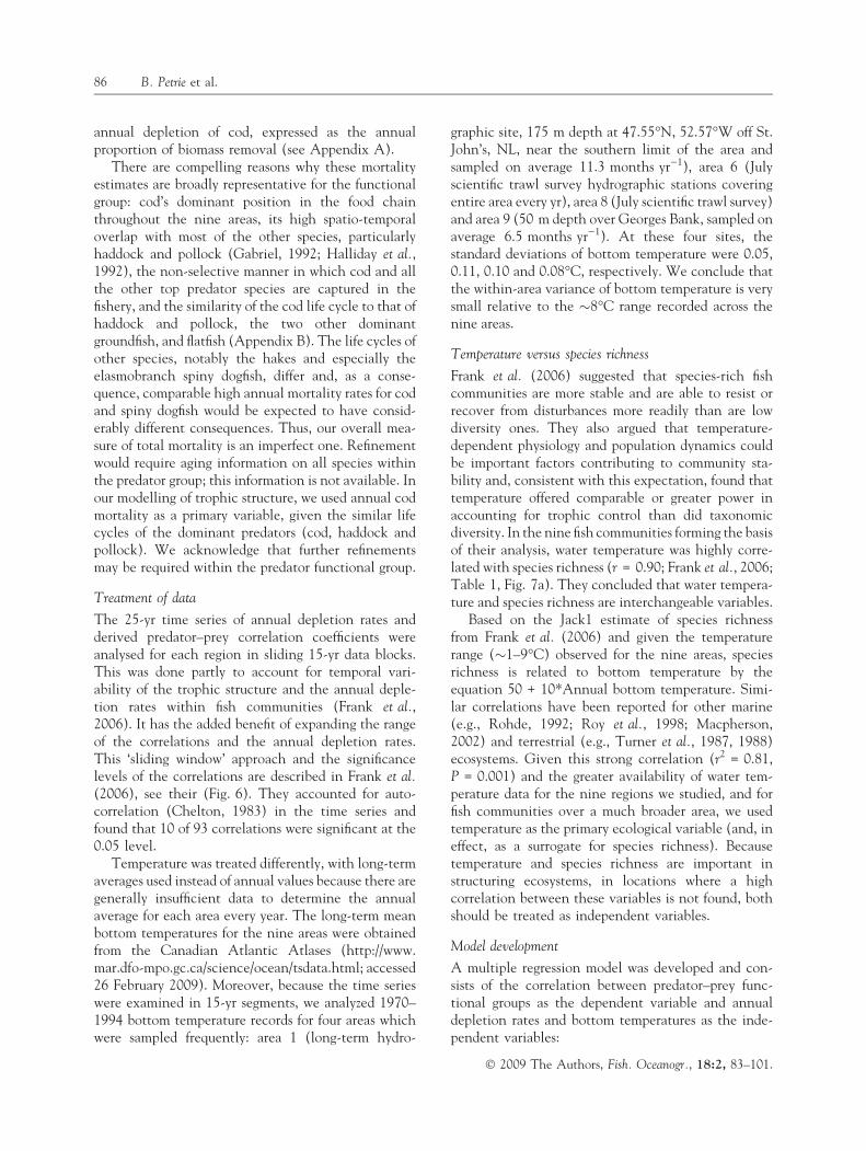
We used the East Coast of North America StrategicAssessment Project (Mahon et al., 1998) database todevelop time series of abundance of predator and preyfunctional groups. These data originate from annualscientific trawl surveys in nine areas in the NorthwestAtlantic (Fig. 1) from 1970 to 1994, and form one ofthe most comprehensive, fishery-independent dataseries in the world. All species data were expressed asnumbers per tow. The nine areas are large,140 000 km2 on average with a range of 54 000 km2

(area 7)–392 000 km2 (area 1).In this region the dominant predator species, and

hence those comprising the predator group, areAtlantic cod Gadus morhua, haddock Melanogrammusaeglefinus, pollock Pollachius virens, longfin hakeUrophycis chesteri, silver hake Merluccius bilinearis,white hake Urophycis tenuis, red hake Urophycis chuss,redfish Sebastes spp., thorny skate Amblyraja radiata,spiny dogfish Squalus acanthias, Greenland halibutReinhardtius hippoglossoides, American plaice Hippo-glossoides platessoides, winter flounder Pseudopleuronec-tes americanus, witch flounder Glyptocephalus

cynoglossus, and yellowtail flounder Limanda ferruginea.All 15 of these species have been commerciallyexploited, often in mixed fisheries that are prosecutedthroughout the continental shelf in depths of <200 m.

The prey species group consists of eight species:arctic cod Boreogadus saida, Atlantic argentineArgentina silus, Atlantic mackerel Scomber scombrus,butterfish Peprilus triacanthus, alewife Alosa pseudoha-rengus, herring Clupea harengus, capelin Mallotus villo-sus, and northern sand lance Ammodytes dubius.Commercial exploitation of these species (herringbeing the exception) has been relatively low or non-existent relative to that experienced by most of thegroundfish species listed above.

Annual depletion of top predators

Annual fishing mortality is the most informativemeasure of fishing pressure; however, the only mor-tality estimate available from stock assessments acrossthe nine areas is for Atlantic cod. We therefore usedestimates for cod to represent annual mortality of thepredator functional group. Sinclair (1996; is Table 4)and NEFSC (2005) decomposed the estimates of totalmortality, derived from Virtual Population Analyses,into fisheries and natural components by assuming aconstant, instantaneous natural mortality rate (M) of0.2 yr)1. We recombined their results to derive an

Figure 1. Map showing locations of Northwest Atlantic fish communities (1–9) for which correlations between functionalgroup predator–prey time series were calculated and a multiple regression model was developed with annual depletion rate andbottom temperature as independent variables. Also identified are nine of 10 fish communities examined in an independent testof the regression. Flemish Cap (FC), West Greenland (WG), Iceland (I), Faeroe Shelf (FS), Irish Sea (IrS), North Sea (NS),Iberian Seas (IbS), Barents Sea (BS), and the Baltic Sea (BlS). The NE Pacific area is not shown. The background oceantemperature is the annual average value (0–200 m) for the North Atlantic Ocean with selected isotherms (�C) shown, and isfrom the World Ocean Atlas 2005 (http://www.nodc.noaa.gov/OC5/WOA05/pr_woa05.html; accessed 27 February 2009). Thesouthward (northward) extent of colder (warmer) water on the western (eastern) side of the ocean reflects the influence of theLabrador (North Atlantic) Current.

Critical transitions in predator–prey correlations 85


annual depletion of cod, expressed as the annualproportion of biomass removal (see Appendix A).

There are compelling reasons why these mortalityestimates are broadly representative for the functionalgroup: cod’s dominant position in the food chainthroughout the nine areas, its high spatio-temporaloverlap with most of the other species, particularlyhaddock and pollock (Gabriel, 1992; Halliday et al.,1992), the non-selective manner in which cod and allthe other top predator species are captured in thefishery, and the similarity of the cod life cycle to that ofhaddock and pollock, the two other dominantgroundfish, and flatfish (Appendix B). The life cycles ofother species, notably the hakes and especially theelasmobranch spiny dogfish, differ and, as a conse-quence, comparable high annual mortality rates for codand spiny dogfish would be expected to have consid-erably different consequences. Thus, our overall mea-sure of total mortality is an imperfect one. Refinementwould require aging information on all species withinthe predator group; this information is not available. Inour modelling of trophic structure, we used annual codmortality as a primary variable, given the similar lifecycles of the dominant predators (cod, haddock andpollock). We acknowledge that further refinementsmay be required within the predator functional group.

Treatment of data

The 25-yr time series of annual depletion rates andderived predator–prey correlation coefficients wereanalysed for each region in sliding 15-yr data blocks.This was done partly to account for temporal vari-ability of the trophic structure and the annual deple-tion rates within fish communities (Frank et al.,2006). It has the added benefit of expanding the rangeof the correlations and the annual depletion rates.This ‘sliding window’ approach and the significancelevels of the correlations are described in Frank et al.(2006), see their (Fig. 6). They accounted for auto-correlation (Chelton, 1983) in the time series andfound that 10 of 93 correlations were significant at the0.05 level.

Temperature was treated differently, with long-termaverages used instead of annual values because there aregenerally insufficient data to determine the annualaverage for each area every year. The long-term meanbottom temperatures for the nine areas were obtainedfrom the Canadian Atlantic Atlases (http://www.mar.dfo-mpo.gc.ca/science/ocean/tsdata.html; accessed26 February 2009). Moreover, because the time serieswere examined in 15-yr segments, we analyzed 1970–1994 bottom temperature records for four areas whichwere sampled frequently: area 1 (long-term hydro-

graphic site, 175 m depth at 47.55�N, 52.57�W off St.John’s, NL, near the southern limit of the area andsampled on average 11.3 months yr)1), area 6 (Julyscientific trawl survey hydrographic stations coveringentire area every yr), area 8 (July scientific trawl survey)and area 9 (50 m depth over Georges Bank, sampled onaverage 6.5 months yr)1). At these four sites, thestandard deviations of bottom temperature were 0.05,0.11, 0.10 and 0.08�C, respectively. We conclude thatthe within-area variance of bottom temperature is verysmall relative to the �8�C range recorded across thenine areas.

Temperature versus species richness

Frank et al. (2006) suggested that species-rich fishcommunities are more stable and are able to resist orrecover from disturbances more readily than are lowdiversity ones. They also argued that temperature-dependent physiology and population dynamics couldbe important factors contributing to community sta-bility and, consistent with this expectation, found thattemperature offered comparable or greater power inaccounting for trophic control than did taxonomicdiversity. In the nine fish communities forming the basisof their analysis, water temperature was highly corre-lated with species richness (r = 0.90; Frank et al., 2006;Table 1, Fig. 7a). They concluded that water tempera-ture and species richness are interchangeable variables.

Based on the Jack1 estimate of species richnessfrom Frank et al. (2006) and given the temperaturerange (�1–9�C) observed for the nine areas, speciesrichness is related to bottom temperature by theequation 50 + 10*Annual bottom temperature. Simi-lar correlations have been reported for other marine(e.g., Rohde, 1992; Roy et al., 1998; Macpherson,2002) and terrestrial (e.g., Turner et al., 1987, 1988)ecosystems. Given this strong correlation (r2 = 0.81,P = 0.001) and the greater availability of water tem-perature data for the nine regions we studied, and forfish communities over a much broader area, we usedtemperature as the primary ecological variable (and, ineffect, as a surrogate for species richness). Becausetemperature and species richness are important instructuring ecosystems, in locations where a highcorrelation between these variables is not found, bothshould be treated as independent variables.

Model development

A multiple regression model was developed and con-sists of the correlation between predator–prey func-tional groups as the dependent variable and annualdepletion rates and bottom temperatures as the inde-pendent variables:

86 B. Petrie et al.


r ¼ fðAnnual Depletion;Bottom TemperatureÞ; ð1Þ

where we define the correlation ‘r’ as the trophicstructure index. Both independent variables have beenshown to be relevant to fish community restructuring(Frank et al., 2006, 2007). Several modelling appro-aches were assessed including fitting the correlationswith linear and quadratic functions of bottom tem-perature and annual depletion rates, and generalizedlinear modeling. In practice, all fits accounted forequivalent variances and exhibited virtually identicalresidual root mean square differences between theobservations and the fit. Consequently, we adopted thesimpler linear fit.

These predator–prey correlations are generallysubject to large uncertainty because the data seriesare strongly autocorrelated (Frank et al., 2006) andare the greatest source of model error. To evaluatethe multivariate linear regression, we ran 1000 sim-ulations based on the correlations and their 0.05confidence levels (determined from the effectivenumber of degrees of freedom of the time series in

the Supplementary On-line Material; Frank et al.,2006).

We note that the predator–prey correlations couldvary at smaller spatial scales within the nine large areaswe investigated. However, the random stratified sam-pling of the fisheries surveys, the source of our data,should provide adequate spatial representation andreliable estimates of predator and prey abundances forthe areas we consider. Nonetheless, because the sizes ofour nine areas vary by a factor of 7, we checked therelationship between area size and predator–prey cor-relations and species richness. The area ⁄ predator–preycorrelation was weak (r2 = 0.17), with the magnitude ofr determined primarily by area 1. The area ⁄ speciesrichness relationship was weaker (r2 = 0.09); however,positive relationships are expected at smaller geo-graphic scales, e.g., banks (Frank and Shackell, 2001).

RESULTS

Fish community structure, as indexed by the func-tional group predator–prey correlations (Fig. 6, Frank

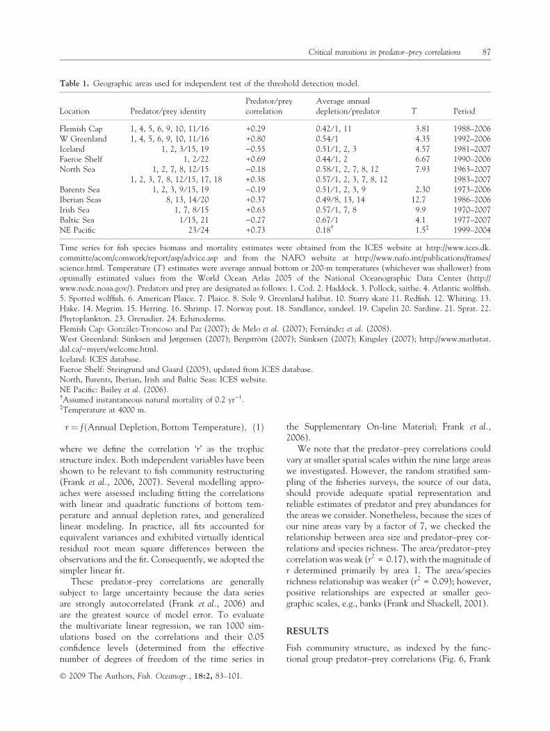
Table 1. Geographic areas used for independent test of the threshold detection model.

Location Predator ⁄ prey identityPredator ⁄ preycorrelation

Average annualdepletion ⁄ predator T Period

Flemish Cap 1, 4, 5, 6, 9, 10, 11 ⁄ 16 +0.29 0.42 ⁄ 1, 11 3.81 1988–2006W Greenland 1, 4, 5, 6, 9, 10, 11 ⁄ 16 +0.80 0.54 ⁄ 1 4.35 1992–2006Iceland 1, 2, 3 ⁄ 15, 19 )0.55 0.51 ⁄ 1, 2, 3 4.57 1981–2007Faeroe Shelf 1, 2 ⁄ 22 +0.69 0.44 ⁄ 1, 2 6.67 1990–2006North Sea 1, 2, 7, 8, 12 ⁄ 15

1, 2, 3, 7, 8, 12 ⁄ 15, 17, 18)0.18+0.38

0.58 ⁄ 1, 2, 7, 8, 120.57 ⁄ 1, 2, 3, 7, 8, 12

7.93 1963–20071983–2007

Barents Sea 1, 2, 3, 9 ⁄ 15, 19 )0.19 0.51 ⁄ 1, 2, 3, 9 2.30 1973–2006Iberian Seas 8, 13, 14 ⁄ 20 +0.37 0.49 ⁄ 8, 13, 14 12.7 1986–2006Irish Sea 1, 7, 8 ⁄ 15 +0.63 0.57 ⁄ 1, 7, 8 9.9 1970–2007Baltic Sea 1 ⁄ 15, 21 )0.27 0.67 ⁄ 1 4.1 1977–2007NE Pacific 23 ⁄ 24 +0.73 0.18� 1.5� 1999–2004

Time series for fish species biomass and mortality estimates were obtained from the ICES website at http://www.ices.dk.committe/acom/comwork/report/asp/advice.asp and from the NAFO website at http://www.nafo.int/publications/frames/science.html. Temperature (T) estimates were average annual bottom or 200-m temperatures (whichever was shallower) fromoptimally estimated values from the World Ocean Atlas 2005 of the National Oceanographic Data Center (http://www.nodc.noaa.gov/). Predators and prey are designated as follows: 1. Cod. 2. Haddock. 3. Pollock, saithe. 4. Atlantic wolffish.5. Spotted wolffish. 6. American Plaice. 7. Plaice. 8. Sole 9. Greenland halibut. 10. Starry skate 11. Redfish. 12. Whiting. 13.Hake. 14. Megrim. 15. Herring. 16. Shrimp. 17. Norway pout. 18. Sandlance, sandeel. 19. Capelin 20. Sardine. 21. Sprat. 22.Phytoplankton. 23. Grenadier. 24. Echinoderms.Flemish Cap: Gonzalez-Troncoso and Paz (2007); de Melo et al. (2007); Fernandez et al. (2008).West Greenland: Sunksen and Jørgensen (2007); Bergstrom (2007); Sunksen (2007); Kingsley (2007); http://www.mathstat.dal.ca/~myers/welcome.html.Iceland: ICES database.Faeroe Shelf: Steingrund and Gaard (2005), updated from ICES database.North, Barents, Iberian, Irish and Baltic Seas: ICES website.NE Pacific: Bailey et al. (2006).�Assumed instantaneous natural mortality of 0.2 yr)1.�Temperature at 4000 m.



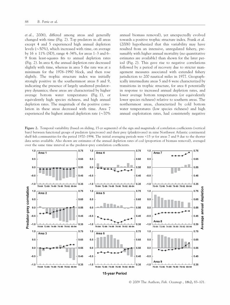
et al., 2006), differed among areas and generallychanged with time (Fig. 2). Top predators in all areasexcept 4 and 5 experienced high annual depletionlevels (�50%), which increased with time, on averageby 16 ± 11% (SD), range 4–34%, for areas 1–3 and 6–9 from least-squares fits to annual depletion rates(Fig. 2). In area 4, the annual depletion rate decreasedslightly with time, whereas in area 5 the rate was at aminimum for the 1976–1990 block, and then roseslightly. The trophic structure index was initiallystrongly positive in the southernmost areas 8 and 9,indicating the presence of largely unaltered predator–prey dynamics; these areas are characterized by higheraverage bottom water temperatures (Fig. 1), orequivalently high species richness, and high annualdepletion rates. The magnitude of the positive corre-lation in these areas decreased with time. Area 7experienced the highest annual depletion rate (�70%

annual biomass removal), yet unexpectedly evolvedtowards a positive trophic structure index. Frank et al.(2006) hypothesized that this variability may haveresulted from an intensive, unregulated fishery, pre-sumably with higher annual mortality (no quantitativeestimates are available) than shown for the later per-iod (Fig. 2). This gave rise to negative correlationsfollowed by a period of recovery due to stricter man-agement measures associated with extended fisheryjurisdiction to 200 nautical miles in 1977. Geograph-ically intermediate areas 5 and 6 were characterized bytransitions in trophic structure, for area 6 potentiallyin response to increased annual depletion rates, andlower average bottom temperatures (or equivalentlylower species richness) relative to southern areas. Thenorthernmost areas, characterized by cold bottomwater temperatures (low species richness) and highannual exploitation rates, had consistently negative

Figure 2. Temporal variability (based on sliding, 15-yr segments) of the sign and magnitude of correlation coefficients (verticalbars) between functional groups of predators (piscivores) and their prey (planktivores) in nine Northwest Atlantic continentalshelf fish communities for the period 1970–1994. The initial averaging periods were <15 yr for areas 7 and 9 due to the shorterdata series available. Also shown are estimates of the annual depletion rates of cod (proportion of biomass removal), averagedover the same time interval as the predator–prey correlation coefficients.

88 B. Petrie et al.


predator–prey correlations (areas 1 and 2) and a sharptransition in trophic structure (area 3) indicative ofperturbed predator–prey dynamics and altered trophicstates. Overall, the magnitude of the negative corre-lations tended to increase with time in these north-ernmost areas.

The linear multiple regression, with the annualdepletion rate and bottom temperature as independentvariables, was:

r ¼ 1:1ð�0:28Þ þ 0:14ð�0:02Þ � Tbottom

� 3:1ð�0:55Þ �Annual Depletion ð2Þ

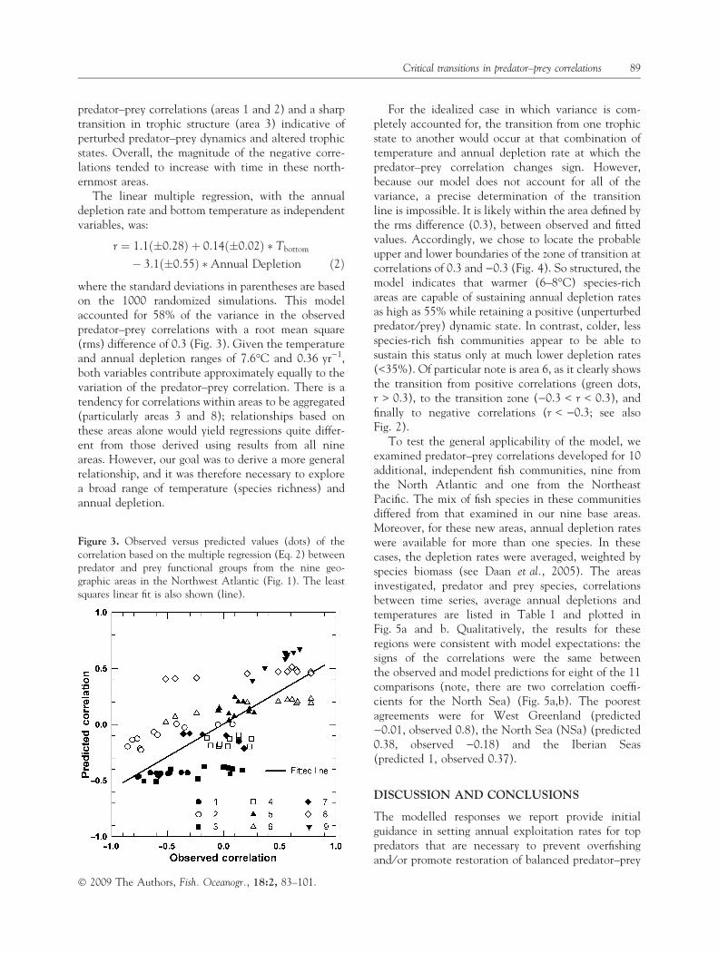
where the standard deviations in parentheses are basedon the 1000 randomized simulations. This modelaccounted for 58% of the variance in the observedpredator–prey correlations with a root mean square(rms) difference of 0.3 (Fig. 3). Given the temperatureand annual depletion ranges of 7.6�C and 0.36 yr)1,both variables contribute approximately equally to thevariation of the predator–prey correlation. There is atendency for correlations within areas to be aggregated(particularly areas 3 and 8); relationships based onthese areas alone would yield regressions quite differ-ent from those derived using results from all nineareas. However, our goal was to derive a more generalrelationship, and it was therefore necessary to explorea broad range of temperature (species richness) andannual depletion.

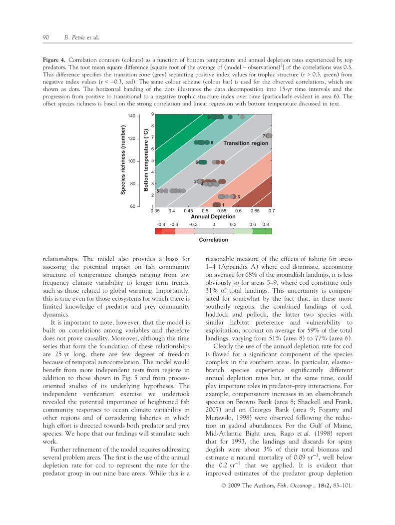
For the idealized case in which variance is com-pletely accounted for, the transition from one trophicstate to another would occur at that combination oftemperature and annual depletion rate at which thepredator–prey correlation changes sign. However,because our model does not account for all of thevariance, a precise determination of the transitionline is impossible. It is likely within the area defined bythe rms difference (0.3), between observed and fittedvalues. Accordingly, we chose to locate the probableupper and lower boundaries of the zone of transition atcorrelations of 0.3 and )0.3 (Fig. 4). So structured, themodel indicates that warmer (6–8�C) species-richareas are capable of sustaining annual depletion ratesas high as 55% while retaining a positive (unperturbedpredator ⁄ prey) dynamic state. In contrast, colder, lessspecies-rich fish communities appear to be able tosustain this status only at much lower depletion rates(<35%). Of particular note is area 6, as it clearly showsthe transition from positive correlations (green dots,r > 0.3), to the transition zone ()0.3 < r < 0.3), andfinally to negative correlations (r < )0.3; see alsoFig. 2).

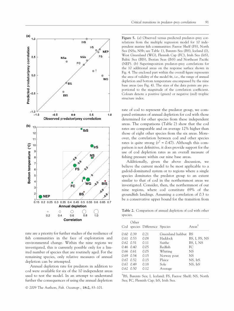
To test the general applicability of the model, weexamined predator–prey correlations developed for 10additional, independent fish communities, nine fromthe North Atlantic and one from the NortheastPacific. The mix of fish species in these communitiesdiffered from that examined in our nine base areas.Moreover, for these new areas, annual depletion rateswere available for more than one species. In thesecases, the depletion rates were averaged, weighted byspecies biomass (see Daan et al., 2005). The areasinvestigated, predator and prey species, correlationsbetween time series, average annual depletions andtemperatures are listed in Table 1 and plotted inFig. 5a and b. Qualitatively, the results for theseregions were consistent with model expectations: thesigns of the correlations were the same betweenthe observed and model predictions for eight of the 11comparisons (note, there are two correlation coeffi-cients for the North Sea) (Fig. 5a,b). The poorestagreements were for West Greenland (predicted)0.01, observed 0.8), the North Sea (NSa) (predicted0.38, observed )0.18) and the Iberian Seas(predicted 1, observed 0.37).

DISCUSSION AND CONCLUSIONS

The modelled responses we report provide initialguidance in setting annual exploitation rates for toppredators that are necessary to prevent overfishingand ⁄ or promote restoration of balanced predator–prey

Figure 3. Observed versus predicted values (dots) of thecorrelation based on the multiple regression (Eq. 2) betweenpredator and prey functional groups from the nine geo-graphic areas in the Northwest Atlantic (Fig. 1). The leastsquares linear fit is also shown (line).



relationships. The model also provides a basis forassessing the potential impact on fish communitystructure of temperature changes ranging from lowfrequency climate variability to longer term trends,such as those related to global warming. Importantly,this is true even for those ecosystems for which there islimited knowledge of predator and prey communitydynamics.

It is important to note, however, that the model isbuilt on correlations among variables and thereforedoes not prove causality. Moreover, although the timeseries that form the foundation of these relationshipsare 25 yr long, there are few degrees of freedombecause of temporal autocorrelation. The model wouldbenefit from more independent tests from regions inaddition to those shown in Fig. 5 and from process-oriented studies of its underlying hypotheses. Theindependent verification exercise we undertookrevealed the potential importance of heightened fishcommunity responses to ocean climate variability inother regions and of considering fisheries in whichhigh effort is directed towards both predator and preyspecies. We hope that our findings will stimulate suchwork.

Further refinement of the model requires addressingseveral problem areas. The first is the use of the annualdepletion rate for cod to represent the rate for thepredator group in our nine base areas. While this is a

reasonable measure of the effects of fishing for areas1–4 (Appendix A) where cod dominate, accountingon average for 68% of the groundfish landings, it is lessobviously so for areas 5–9, where cod constitute only31% of total landings. This uncertainty is compen-sated for somewhat by the fact that, in these moresoutherly regions, the combined landings of cod,haddock and pollock, the latter two species withsimilar habitat preference and vulnerability toexploitation, account on average for 59% of the totallandings, varying from 51% (area 8) to 77% (area 6).

Clearly the use of the annual depletion rate for codis flawed for a significant component of the speciescomplex in the southern areas. In particular, elasmo-branch species experience significantly differentannual depletion rates but, at the same time, couldplay important roles in predator–prey interactions. Forexample, compensatory increases in an elasmobranchspecies on Browns Bank (area 8; Shackell and Frank,2007) and on Georges Bank (area 9; Fogarty andMurawski, 1998) were observed following the reduc-tion in gadoid abundances. For the Gulf of Maine,Mid-Atlantic Bight area, Rago et al. (1998) reportthat for 1993, the landings and discards for spinydogfish were about 3% of their total biomass andestimate a natural mortality of 0.09 yr)1, well belowthe 0.2 yr)1 that we applied. It is evident thatimproved estimates of the predator group depletion

Figure 4. Correlation contours (colours) as a function of bottom temperature and annual depletion rates experienced by toppredators. The root mean square difference [square root of the average of (model – observations)2] of the correlations was 0.3.This difference specifies the transition zone (grey) separating positive index values for trophic structure (r > 0.3, green) fromnegative index values (r < )0.3, red). The same colour scheme (colour bar) is used for the observed correlations, which areshown as dots. The horizontal banding of the dots illustrates the data decomposition into 15-yr time intervals and theprogression from positive to transitional to a negative trophic structure index over time (particularly evident in area 6). Theoffset species richness is based on the strong correlation and linear regression with bottom temperature discussed in text.

90 B. Petrie et al.


rate are a priority for further studies of the resilience offish communities in the face of exploitation andenvironmental change. Within the nine regions weinvestigated, this is currently possible only for a lim-ited number of species that are routinely aged. For theremaining species, only relative measures of annualdepletion can be attempted.

Annual depletion rate for predators in addition tocod were available for six of the 10 independent areasused to test the model. In an attempt to understandfurther the consequences of using the annual depletion

rate of cod to represent the predator group, we com-pared estimates of annual depletion for cod with thosedetermined for other species from these independentareas. The comparisons (Table 2) show that the codrates are comparable and on average 12% higher thanthose of eight other species from the six areas. More-over, the correlation between cod and other speciesrates is quite strong (r2 = 0.47). Although this com-parison is not definitive, it does provide support for theuse of cod depletion rates as an overall measure offishing pressure within our nine base areas.

Additionally, given the above discussion, webelieve the current model to be most applicable to agadoid-dominated system or to regions where a singlespecies dominates the predator group to an extentsimilar to that of cod in the northernmost areas weinvestigated. Consider, then, the northernmost of ournine regions, where cod constitute 69% of thegroundfish landings. Assuming a correlation of 0.3 tobe a conservative upper bound for the transition from

0.15 0.2 0.25 0.3 0.35 0.4 0.45 0.5 0.55 0.6 0.65 0.71

2

3

4

5

6

7

8

9

10

11

12

13

BS

FS

FC

I

NS

WG

IbS

IrS

BlS

NEP

Annual depletion

Bo

tto

m t

emp

erat

ure

(°C

)

0.2 0.6 1.0

Correlation

0.8

0.6

0.3

0

−0.3

−0.6

−0.8

0.80.4

(a)

(b)

Figure 5. (a) Observed versus predicted predator–prey cor-relations from the multiple regression model for 10 inde-pendent marine fish communities: Faeroe Shelf (FS), NorthSea (NSa, NSb; see Table 1), Barents Sea (BS), Iceland (I),West Greenland (WG), Flemish Cap (FC), Irish Sea (IrS),Baltic Sea (BlS), Iberian Seas (IbS) and Northeast Pacific(NEP). (b) Superimposition predator–prey correlations forthe 10 additional areas on the response surface shown inFig. 4. The enclosed part within the overall figure representsthe area of validity of the model fit, i.e., the range of annualdepletion and bottom temperature encompassed by the ninebase areas (see Fig. 4). The sizes of the data points are pro-portional to the magnitude of the correlation coefficient.Colours denote a positive (green) or negative (red) trophicstructure index.

Table 2. Comparison of annual depletion of cod with otherspecies.

CodOtherspecies Difference Species Areas�

0.60 0.39 0.21 Greenland halibut BS0.61 0.53 0.08 Haddock BS, I, FS, NS0.62 0.51 0.11 Saithe BS, I, NS0.46 0.40 0.05 Redfish FC0.66 0.61 0.05 Whiting NS0.69 0.54 0.15 Norway pout NS0.67 0.52 0.15 Plaice NS, IrS0.67 0.49 0.18 Sole NS, IrS0.62 0.50 0.12 Average

�BS, Barents Sea; I, Iceland; FS, Faeroe Shelf; NS, NorthSea; FC, Flemish Cap; IrS, Irish Sea.



an unaltered to altered state, the transition point forarea 1, the region with the coldest temperature(1.2�C), would be expected to occur at an annualdepletion rate of 29%. This is 11% greater than theassumed pre-collapse northern cod annual naturalmortality of 18% (mean = 0.2 yr)1) and was wellwithin the recommended management strategy thatcalled for exploitation not to exceed natural mortality(Walters and Maguire, 1996). However, the realizedannual depletion rate of northern cod prior to collapsewas 54%, twice the maximum annual depletion ratethat our model indicates would be sustainable whilemaintaining a positive predator ⁄ prey balance and apositive trophic structure index (Fig. 4). Predator–preycorrelations in area 1 during the pre-collapse periodwere consistently negative (r = )0.56, SD = 0.14).Strict adherence to the management advice (Rivardand Maguire, 1993; Sinclair, 1996) in place at thetime might well have prevented the collapse of toppredators and the resulting trophic imbalance thatoccurred in this cold water fish community.

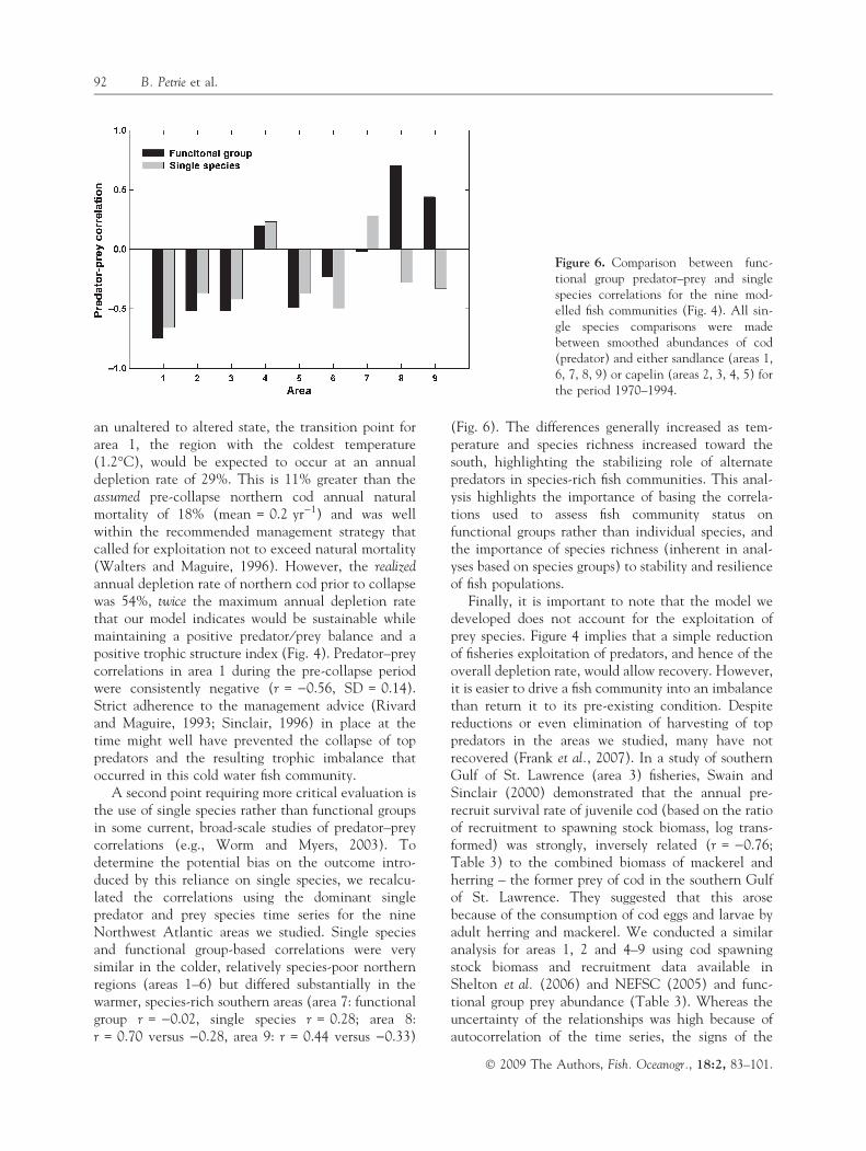
A second point requiring more critical evaluation isthe use of single species rather than functional groupsin some current, broad-scale studies of predator–preycorrelations (e.g., Worm and Myers, 2003). Todetermine the potential bias on the outcome intro-duced by this reliance on single species, we recalcu-lated the correlations using the dominant singlepredator and prey species time series for the nineNorthwest Atlantic areas we studied. Single speciesand functional group-based correlations were verysimilar in the colder, relatively species-poor northernregions (areas 1–6) but differed substantially in thewarmer, species-rich southern areas (area 7: functionalgroup r = )0.02, single species r = 0.28; area 8:r = 0.70 versus )0.28, area 9: r = 0.44 versus )0.33)

(Fig. 6). The differences generally increased as tem-perature and species richness increased toward thesouth, highlighting the stabilizing role of alternatepredators in species-rich fish communities. This anal-ysis highlights the importance of basing the correla-tions used to assess fish community status onfunctional groups rather than individual species, andthe importance of species richness (inherent in anal-yses based on species groups) to stability and resilienceof fish populations.

Finally, it is important to note that the model wedeveloped does not account for the exploitation ofprey species. Figure 4 implies that a simple reductionof fisheries exploitation of predators, and hence of theoverall depletion rate, would allow recovery. However,it is easier to drive a fish community into an imbalancethan return it to its pre-existing condition. Despitereductions or even elimination of harvesting of toppredators in the areas we studied, many have notrecovered (Frank et al., 2007). In a study of southernGulf of St. Lawrence (area 3) fisheries, Swain andSinclair (2000) demonstrated that the annual pre-recruit survival rate of juvenile cod (based on the ratioof recruitment to spawning stock biomass, log trans-formed) was strongly, inversely related (r = )0.76;Table 3) to the combined biomass of mackerel andherring – the former prey of cod in the southern Gulfof St. Lawrence. They suggested that this arosebecause of the consumption of cod eggs and larvae byadult herring and mackerel. We conducted a similaranalysis for areas 1, 2 and 4–9 using cod spawningstock biomass and recruitment data available inShelton et al. (2006) and NEFSC (2005) and func-tional group prey abundance (Table 3). Whereas theuncertainty of the relationships was high because ofautocorrelation of the time series, the signs of the

Figure 6. Comparison between func-tional group predator–prey and singlespecies correlations for the nine mod-elled fish communities (Fig. 4). All sin-gle species comparisons were madebetween smoothed abundances of cod(predator) and either sandlance (areas 1,6, 7, 8, 9) or capelin (areas 2, 3, 4, 5) forthe period 1970–1994.

92 B. Petrie et al.


correlations between cod juvenile survival rates andfunctional group prey abundance were consistentlynegative for the five areas where the cod stocks hadcollapsed and failed to recover. Conversely, the cor-relations were positive for two of the three areas inwhich cod collapses did not occur. These results areconsistent with the predator–prey role reversalhypothesis.

While reduced fishing pressure on predators did notbring about a rapid recovery, an acceptance of theimportance of role reversal implies that the culling ofprey species could promote recovery of the predatorcomplex. In fact, Lessard et al. (2005) suggested thatthere will be situations when ecosystem managementmay require the use of direct, active controls to hastenrecovery and ⁄ or reduce extinction risks. In a recentexample, Persson et al. (2007) report that removal oflarge Arctic charr (Salvalinus alpinus), the prey species,allowed brown trout (Salmo trutta), the predatordepleted by overfishing, to recover in a large Norwe-gian lake. In this case, the governing factor was notrole reversal but size-selective feeding by the trout.However, the work of Lessard et al. (2005) and Yodzis(2001) highlight the complexity of ecosystems andtheir response to external forcing such as a cull.

A further confounding factor for the correlationapproach we employed could arise from fisheriesdirected towards prey species. For the time frame weexamined in our nine base areas, the only significantprey species fished is herring in areas 3 and 8. Incontrast, significant prey fisheries operate in the North

Sea (instantaneous fishing mortalities, F (yr)1), of 0.6for herring and sandeel), Iceland (F = 0.32, herring),the Irish Sea (F = 0.52, herring), the Baltic Sea(F = 0.25, herring; 0.31, sprat), and the Iberian Seas(F = 0.27, sardines). Although simultaneous fishing ofpredator and prey species could maintain balance inthe fish community, it could also lead to positivecorrelations even though both groups were beingdangerously depleted.

Rapid, large changes in fishing effort could also giverise to misleading correlations. Idealized models ofmulti-species fisheries predict positive correlations asprey fisheries are initiated, changing to negative cor-relations as predator and prey populations adjust tonew equilibria (e.g., Fig 4 in May et al., 1979). Themagnitude and time scales of the adjustment dependon the growth rates of the populations under consid-eration. However, in the nine base areas we studiedinitially, 86% of the year-to-year changes in instan-taneous fishing mortality are within 0.1 (see Fig. 2).We conclude that such changes were not a factor inour analyses.

As noted previously, three of the correlations de-rived from the independent areas used for verification[West Greenland, the Iberian Seas and the North Sea(1963–2007 series)] differed substantially from thepredictions of the model. The West Greenland serieswas the shortest (15 yr) and the correlation wasdominated by a recent surge in Greenland halibut in2004 and cod in 2005 (Sunksen and Jørgensen, 2007).The predator–prey correlation based only on the cod

Table 3. Analysis of the effect of func-tional group prey abundance and juve-nile cod survival rates in nine areasthroughout the northwest Atlantic.

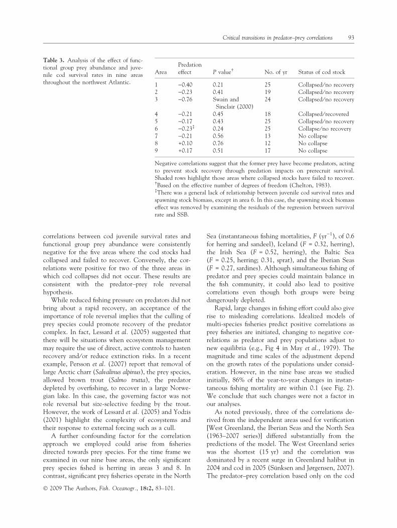
AreaPredationeffect P value� No. of yr Status of cod stock

1 )0.40 0.21 25 Collapsed ⁄ no recovery2 )0.23 0.41 19 Collapsed ⁄ no recovery3 )0.76 Swain and

Sinclair (2000)24 Collapsed ⁄ no recovery

4 )0.21 0.45 18 Collapsed ⁄ recovered5 )0.17 0.43 25 Collapsed ⁄ no recovery6 )0.23� 0.24 25 Collapse ⁄ no recovery7 )0.21 0.56 13 No collapse8 +0.10 0.76 12 No collapse9 +0.17 0.51 17 No collapse

Negative correlations suggest that the former prey have become predators, actingto prevent stock recovery through predation impacts on prerecruit survival.Shaded rows highlight those areas where collapsed stocks have failed to recover.�Based on the effective number of degrees of freedom (Chelton, 1983).�There was a general lack of relationship between juvenile cod survival rates andspawning stock biomass, except in area 6. In this case, the spawning stock biomasseffect was removed by examining the residuals of the regression between survivalrate and SSB.



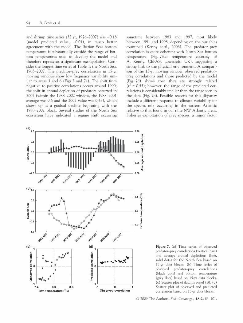
and shrimp time series (32 yr, 1976–2007) was )0.18(model predicted value, )0.01), in much betteragreement with the model. The Iberian Seas bottomtemperature is substantially outside the range of bot-tom temperatures used to develop the model andtherefore represents a significant extrapolation. Con-sider the longest time series of Table 1: the North Sea,1963–2007. The predator–prey correlations in 15-yrmoving windows show low frequency variability sim-ilar to areas 3 and 6 (Figs 2 and 7a). The shift fromnegative to positive correlations occurs around 1990;the shift in annual depletion of predators occurred in2002 (within the 1988–2002 window, the 1988–2001average was 0.6 and the 2002 value was 0.43), whichshows up as a gradual decline beginning with the1988–2002 block. Several studies of the North Seaecosystem have indicated a regime shift occurring

sometime between 1983 and 1997, most likelybetween 1991 and 1998, depending on the variablesexamined (Kenny et al., 2006). The predator–preycorrelation is quite coherent with North Sea bottomtemperature (Fig. 7b,c; temperature courtesy ofA. Kenny, CEFAS, Lowestoft, UK), suggesting astrong link to the physical environment. A compari-son of the 15-yr moving window, observed predator–prey correlations and those predicted by the model(Fig. 7d) shows that they are strongly related(r2 = 0.55); however, the range of the predicted cor-relations is considerably smaller than the range seen inthe data (Fig. 7d). Possible reasons for this disparityinclude a different response to climate variability forthe species mix occurring in the eastern Atlanticrelative to that found in our nine NW Atlantic areas.Fisheries exploitation of prey species, a minor factor

(a)

(b)

(c) (d) Figure 7. (a) Time series of observedpredator–prey correlations (vertical bars)and average annual depletions (line,solid dots) for the North Sea based on15-yr data blocks. (b) Time series ofobserved predator–prey correlations(black dots) and bottom temperature(grey dots) based on 15-yr data blocks.(c) Scatter plot of data in panel (B). (d)Scatter plot of observed and predictedcorrelation based on 15-yr data blocks.

94 B. Petrie et al.


and therefore neglected in the model’s nine base areas,was, however, clearly an important factor for theNorth Sea and other eastern Atlantic regions.

The ability to predict and avoid fish communityimbalances, resulting from the differential exploitationof top predators relative to their prey, would constitutea major advance in the science of the management ofmarine resources. The model we report provides a firstapproximation to this end and illustrates the potentialof an ecosystem approach to resource managementthat is based on easily derived input variables. More-over, the demonstration that temperature, whetheroperationally independent, as a surrogate for, or incombination with quantitative measures of speciesrichness, can be used as an effective input to themodel, makes it readily applicable even to emergingfisheries. We suspect that the temperature dependenceof fish community status revealed by the model relatesboth to its effect on metabolic ⁄ demographic rates andon species richness (Allen et al., 2002). In this con-text, the increased resiliency of the more southernNorthwest Atlantic fish communities probably resultsfrom both higher growth rates (a consequence of thetemperature dependence of growth; Brander, 2007)and the greater species richness at the higher trophiclevels. This increased species richness allows alternatetop predators to assume the niche vacated by heavilyor over-exploited top predator species, thereby main-taining positive predator ⁄ prey balances. The com-pensatory increases in elasmobranch species onBrowns (area 8) and Georges (area 9) Banks followingthe reduction in gadoid abundance there, are animportant examples of this effect (Fogarty and Mu-rawski, 1998; Shackell and Frank, 2007).

Finally, primarily because of the potential forpredator–prey role reversals, marine ecosystemsappear to be less amenable to rehabilitation thanterrestrial ones (Griffith et al., 1989; Ripple andBeschta, 2003; Kauffman et al., 2007; Seddon et al.,2007). For this reason, an even more accuratedetermination of the critical limits of fish communitytransformation than we have been able to provide isvital to the progress of the evolving science of marineecosystem management. The maintenance of fishcommunity balances over periods of prolongedexploitation or environmental change, demands thatthe balance between functional groups remain withinthe bounds that permit renewal (successful repro-duction) and regulation (keeping prey in check). Ourmodel provides an initial framework for the identi-fication of these boundaries, and insight into theecological basis of, and geographical variability in,the presence ⁄ absence of profound fish community

restructuring and recovery in response to exploitationand environmental variability.

ACKNOWLEDGEMENTS

We thank Dr M. Sinclair, M. Fogarty, C. Hannah,J. Fisher and I. Perry for critical feedback on earlierversions of the manuscript. Mr. R. Pettipas andL. Petrie provided significant technical support.D. Gonzalez-Troncoso, C. Fernandez, H. Hovgaard,O. Jørgensen, A. Kenny, M. Kingsley and K. Sunksenprovided useful advice on the location and quality offisheries time series, in one case (C.F.) by providing atime series in advance of publication. We thank thethree external referees for their insightful, usefuladvice that improved the paper considerably. Thisresearch was supported by Fisheries and OceansCanada and the Natural Sciences and EngineeringResearch Council of Canada Discovery Grant programawards to K.T.F. and W.C.L.

REFERENCES

Allen, A.P., Brown, J.H. and Gillooly, J.F. (2002) Global bio-diversity, biochemical kinetics, and the energetic-equiva-lence rule. Science 297:1545–1548.

Bailey, D.M., Ruhl, H.A. and Smith, K.L. Jr (2006) Long-termchange in benthopelagic fish abundance in the abyssalnortheast Pacific Ocean. Ecology 83:549–555.

Bascompte, J., Melian, C.J. and Sala, E. (2005) Interactionstrength combinations and the overfishing of a marine foodweb. Proc. Natl. Acad. Sci. USA 102:5443–5447.

Berger, J., Stacey, P.B., Bellis, L. and Johnson, M.P. (2001) Amammalian predator–prey imbalance: grizzly bears and wolfextinction affect avian neotropical migrants. Ecol. Appl.11:947–960.

Bergstrom, B. (2007) Results of the Greenland Bottom TrawlSurvey for Northern shrimp (Pandalus borealis) off WestGreenland (NAFO Sub area 1 and Division 0A), 1988–2007. NAFO SCR Doc 07 ⁄ 71, 44p.

Bowyer, R.T., Person, D.K. and Pierce, B.M. (2005) Detectingtop-down versus bottom-up regulation of ungulates by largecarnivores: implications for conservation of biodiversity. In:Large Carnivores and the Conservation of Biodiversity. J.C. Ray,K.H. Redford, R.S. Steneck & J. Berger (eds) Covelo, CA:Island Press, pp. 342–361.

Brander, K.M. (2007) The role of growth changes in the declineand recovery of North Atlantic cod stocks since 1970. ICESJ. Mar. Sci. 64:211–217.

Bundy, A. (2005) Structure and functioning of the easternScotian Shelf ecosystem before and after the collapse ofgroundfish stocks in the early 1990s. Can. J. Fish. Aquat. Sci.62:1453–1473.

Bundy, A. and Fanning, L.P. (2005) Can Atlantic cod (Gadusmorhua) recover? Exploring trophic explanations for thenon-recovery of the cod stock on the eastern ScotianShelf, Canada. Can. J. Fish. Aquat. Sci. 62:1474–1489.



Chelton, D. (1983) Effects of sampling errors in statisticalestimation. Deep-Sea Res. 30:1083–1103.

Choi, J.S., Frank, K.T., Leggett, W.C. and Drinkwater, K.(2004) Transition to an alternate state in a continental shelfecosystem. Can. J. Fish. Aquat. Sci. 61:505–510.

Daan, N., Gislason., H., Pope, J.G. and Rice, J.C. (2005)Changes in the North Sea fish community: evidence ofindirect effects of fishing? ICES J. Mar. Sci. 62:177–188.

Fernandez, C., Cervino, S., Saborido-Rey, F. and AntonioVazquez, A. (2008) Assessment of the Cod Stock in NAFODivision 3M. NAFO SCR Doc 08 ⁄ 26, 79p.

Fogarty, M.J. and Murawski, S.A. (1998) Large-scale disturbanceand the structure of marine systems: fishery impacts onGeorges Bank. Ecol. Appl. 8(Suppl.):S6–S22.

Frank, K.T. and Leggett, W.C. (1994) Fisheries ecology in thecontext of ecological and evolutionary theory. Annu. Rev.Ecol. Syst. 25:401–422.

Frank, K.T. and Shackell, N.L. (2001) Area-dependent patternsof finfish diversity in a large marine ecosystem. Can. J. Fish.Aquat. Sci. 58:1703–1707.

Frank, K.T., Petrie, B., Choi, J.S. and Leggett, W.C. (2005)Trophic cascades in a formerly cod-dominated ecosystem.Science 308:1621–1623.

Frank, K.T., Petrie, B., Shackell, N.L. and Choi, J.S. (2006)Reconciling differences in trophic control in mid-latitudemarine ecosystems. Ecol. Lett. 9:1096–1105.

Frank, K.T., Petrie, B. and Shackell, N.L. (2007) The ups anddowns of trophic control in continental shelf ecosystems.Trends Ecol. Evol. 22:236–242.

Gabriel, W.L. (1992) Persistence of demersal fish assemblagesbetween Cape Hatteras and Nova Scotia, NorthwestAtlantic. J. Northw. Atl. Fish. Sci. 14:29–46.

Gonzalez-Troncoso, D. and Paz, X. (2007) Some ecologicalindices in Flemish Cap derived from the surveys conductedby EU between 1988 and 2006. NAFO SCR Doc 07 ⁄ 65, 26p.

Griffith, B., Scott, J.M., Carpenter, J.W. and Reed, C. (1989)Translocation of species as a conservation tool: status andstrategy. Science 245:477–480.

Halliday, R.G., Peacock, F.G. and Burke, D.L. (1992) Devel-opment of management measures for the groundfish fisheryin Atlantic Canada. Mar. Policy 16:411–426.

Hjermann, D.O., Ottersen, G. and Stenseth, N.C. (2004)Competition among fishermen and fish causes the collapse ofBarents Sea capelin. Proc. Natl. Acad. Sci. USA 101:11679–11684.

Horwood, J., O’Brien, C. and Darby, C. (2006) North Sea codrecovery? ICES J. Mar. Sci. 63:961–968.

Huggett, A.J. (2005) The concept and utility of ‘ecologicalthresholds’ in biodiversity conservation. Biol. Cons.124:301–310.

Hutchings, J.A. (1996) Spatial and temporal variation in thedensity of northern cod and a review of hypotheses for thestock’s collapse. Can. J. Fish. Aquat. Sci. 53:943–962.

Hutchings, J.A. and Reynolds, J.D. (2004) Marine fish popula-tion collapses: consequences for recovery and extinction risk.Bioscience 54:297–309.

Jackson, J.B.C., Kirby, M.X., Berger, W.H. et al. (2001) His-torical overfishing and the recent collapse of coastal eco-systems. Science 293:629–637.

Kauffman, M.J., Varley, N., Smith, D.W., Stahler, D.R.,MacNulty, D.R. and Boyce, M.S. (2007) Landscape hetero-geneity shapes predation in a newly restored predator–preysystem. Ecol. Lett. 10:690–700.

Kenny, A.J., Kershaw, P., Beare, D. et al. (2006) Integratedassessment of the North Sea to identify the relationship betweenhuman pressures and ecosystem state changes – implications formarine management. Rep. ICES Regional Group for the NorthSea, (REGNS) 36p. http://www.ices.dk/iceswork/working-groups (last accessed 27 February 2009).

Kingsley, M.C.S. (2007) A provisional assessment of the shrimpstock off West Greenland in 2007. NAFO SCR Doc 07 ⁄ 70,25p.

Kumar, A.B. and Deepthi, G.R. (2006) Trawling and by-catch:implications on marine ecosystems. Curr. Sci. 90:922–931.

Leibold, M.A., Chase, J.M., Shurin, J.B. and Downing, A.L.(1997) Species turnover and the regulation of trophicstructure. Annu. Rev. Ecol. Syst. 28:467–494.

Lessard, R.B., Martell, S.J.D., Walters, C.J., Essington, T.E. andKitchell, J.F. (2005) Should ecosystem managementinvolve active control of species abundances? Ecol. Society10:pp. 23.(online) http://www.ecologyandsociety.org/vol10/iss2/art1/ (last accessed 27 February 2009).

Levin, P.S., Holmes, E.E., Piner, K.R. and Harvey, C.J. (2006)Shifts in a Pacific Ocean fish assemblage: the potentialinfluence of exploitation. Conserv. Biol. 4:1181–1190.

Macpherson, E. (2002) Large-scale species-richness gradients inthe Atlantic Ocean. Proc. R. Soc. Lond. B Biol. Sci.269:1715–1720.

Mahon, R., Brown, S.K., Zwanenberg, K.C.T. et al. (1998)Assemblages and biogeography of demersal fishes of the eastcoast of North America. Can. J. Fish. Aquat. Sci. 55:1704–1738.

Mandelman, J.W. and Farrington, M.A. (2007) The estimatedshort-term discard mortality of a trawled elasmobranch, thespiny dogfish (Squalus acanthias). Fish. Res. 83:238–245.

May, R.M., Beddington, J.R., Clark, C.W., Holt, S.J. and Laws,R.M. (1979) Management of multispecies fisheries. Science205:267–277.

de Melo, A.A., Saborido-Rey, F. and Alpoim, R. (2007) An XSAbased assessment of Beaked Redfish (S. mentella and S. fasci-atus) in NAFO Division 3M. NAFO SCR Doc 07 ⁄ 47, 43p.

Murawski, S.A. (2000) Definitions of overfishing from an eco-system perspective. ICES J. Mar. Sci. 57:649–658.

Myers, R.A. and Cadigan, N.G. (1995) Was an increase innatural mortality responsible for the collapse of northerncod? Can. J. Fish. Aquat. Sci. 52:1274–1285.

Myers, R.A. and Worm, B. (2003) Rapid worldwide depletion ofpredatory fish communities. Nature 423:280–283.

NEFSC. (2005) Assessment of 19 Northeast Groundfish Stocksthrough 2004. In: 2005 Groundfish Assessment Review Meeting(2005 GARM), Northeast Fisheries Science Center ReferenceDocument 05–13, 15–19 August, 2005. R.K., Mayo & M.,Terceiro (eds) Woods Hole, Massachusetts: Northeast Fish-eries Science Center, pp. 12–21.

Oguz, T. and Gilbert, D. (2007) Abrupt transitions of the top-down controlled Black Sea pelagic ecosystem during 1960–2000: evidence for regime-shifts under strong fisheryexploitation and nutrient enrichment modulated by climate-induced variations. Deep-Sea Res. 54:220–242.

Olsen, E.M., Heino, M., Lilly, G.R. et al. (2004) Maturationtrends indicative of rapid evolution preceded the collapse ofnorthern cod. Nature 428:932–935.

Persson, L., Amundsen, P.-A., De Roos, A.M., Klemetsen, A.,Knudsen, R. and Primicerio, R. (2007) Culling prey pro-motes predator recovery – alternative states in a whole-lakeexperiment. Science 316:1743–1746.

96 B. Petrie et al.


Pikitch, E.K., Santora, C., Babcock, E.A. et al. (2004) Ecosys-tem-based fishery management. Science 305:346–347.

Post, D.M., Palkovacs, E.P., Schielke, E.K. and Dodson, S.I.(2008) Intraspecific variation in a predator affects commu-nity structure and cascading trophic interactions. Ecology89:2019–2032.

Quinn, J.F., Wing, S.R. and Botsford, L.W. (1993) Harvestrefugia in marine invertebrate fisheries: models and appli-cations to the red-sea urchin, Strongylocentrotus franciscanus.Am. Zool. 33:537–550.

Rago, P.J., Sosebee, K.A., Brodziak, J.K.T., Murawski, S.A. andAnderson, E.D. (1998) Implications of recent increases incatches on the dynamics of Northwest Atlantic spiny dogfish(Squalus acanthias). Fish. Res. 39:165–181.

Richardson, A.J. and Schoeman, D.S. (2004) Climate impact onplankton ecosystems in the northeast Atlantic. Science305:1609–1612.

Ripple, W.J. and Beschta, R.L. (2003) Wolf reintroduction,predation risk, and cottonwood recovery in YellowstoneNational Park. Forest Ecol. Manage. 184:299–313.

Rivard, D. and Maguire, J.-J. (1993) Reference points for fish-eries management: the eastern Canadian experience. In: RiskEvaluation and Biological Reference Points for Fisheries Man-agement. S.J. Smith, J.J. Hunt & D. Rivard (eds) Can. Spec.Publ. Fish. Aquat. Sci. 120:31–57.

Roff, D.A. (1992) The Evolution of Life Histories: Theory andAnalysis. London: Chapman & Hall.

Rohde, K. (1992) Latitudinal gradients in species diversity: thesearch for the primary cause. Oikos 65:514–527.

Roy, K., Jablonski, D., Valentine, J.W. and Rosenberg, G.(1998) Marine latitudinal diversity gradients: tests of causalhypotheses. Proc. Natl Acad. Sci. USA 95:3699–3702.

Savenkoff, C.F., Castonguay, M., Chabot, D., Hammill, M.O.,Bourdages, H. and Morissette, L. (2007a) Changes in thenorthern Gulf of St Lawrence ecosystem estimated by inversemodeling: evidence of a fishery-induced regime shift? Estuar.Coast. Shelf Sci. 73:711–724.

Savenkoff, C.F., Swain, D.P., Hanson, J.M. et al. (2007b) Effectof fishing and predation in a heavily exploited ecosystem:comparing periods before and after the collapse of groundfishin the southern Gulf of St Lawrence (Canada). Ecol. Modell.204:115–128.

Schmitz, O.J., Maback, P.A. and Beckerman, A.P. (2000)Trophic cascades in terrestrial systems: a review of the effectsof carnivore removal on plants. Am. Nat. 155:141–153.

Seddon, P.J., Armstrong, D.P. and Maloney, R.F. (2007)Developing the science of reintroduction biology. Conserv.Biol. 21:303–312.

Shackell, N.L. and Frank, K.T. (2007) Compensation inexploited marine fish communities on the Scotian Shelf,Canada. Mar. Ecol. Prog. Ser. 336:235–247.

Shelton, P.A. and Lilly, G.R. (2000) Interpreting the collapse ofthe northern cod stocks from survey and catch data. Can.J. Fish. Aquat. Sci. 57:2230–2239.

Shelton, P.A., Sinclair, A.F., Chouinard, G.A., Mohn, R. andDuplisea, D.E. (2005) Fishing under low productivityconditions is further delaying recovery of NorthwestAtlantic cod (Gadus morhua) Can. J. Fish. Aquat. Sci.63:235–238.

Shin, Y.-J. and Cury, P. (2004) Using an individual-basedmodel of fish assemblages to study the response of sizespectra to changes in fishing. Can. J. Fish. Aquat. Sci.61:414–431.

Sinclair, A. (1996) Recent declines in cod species stocks in theNorthwest Atlantic. NAFO Sci. Coun. Studies 24:41–52.

Sinclair, A.F. (2001) Natural mortality of cod (Gadus morhua)in the southern Gulf of St Lawrence. ICES J. Mar. Sci. 58:1–10.

Sissenwine, M. and Murawski, S. (2004) Moving beyond‘intelligent tinkering’: advancing an ecosystem approach tofisheries. Mar. Ecol. Prog. Ser. 274:291–295.

Soule, M.E., Estes, J.A., Miller, B. and Honnold, D.L.. (2005)Strongly interacting species: conservation policy, manage-ment, and ethics. Bioscience 55:168–176.

Steele, J.H. and Collie, J.S. (2005) Chapter 22. Functionaldiversity and stability of coastal ecosystems. In: The Sea: Vol.13. The Global Coastal Ocean. A. Robinson & K. Brink (eds).Harvard University Press, pp. 785–820.

Steingrund, P. and Gaard, E. (2005) Relationship betweenphytoplankton production and cod production on the FaeroeShelf. ICES J. Mar. Sci. 62:163–176.

Sunksen, K. (2007) A preliminary estimate of Atlantic cod(Gadus morhua) biomass in West Greenland offshore waters(NAFO Subarea 1) for 2007 and recent changes in thespatial overlap with Northern shrimp (Pandalus borealis).NAFO SCR Doc 07 ⁄ 73, 10p.

Sunksen, K. and Jørgensen, O.A. (2007) Biomass and abun-dance of demersal fish stocks off West Greenland estimatedfrom the Greenland Shrimp Survey, 1988–2006. NAFO SCRDoc 07 ⁄ 28, 31p.

Swain, D.P. and Sinclair, A.F. (2000) Pelagic fishes and the codrecruitment dilemma in the northwest Atlantic. Can. J. Fish.Aquat. Sci. 57:1321–1325.

Swain, D.P., Sinclair, A.F. and Hanson, M.J. (2007) Evolu-tionary response to size-selectivity mortality in an exploitedfish population. Proc. Biol. Sci. 274:1015–1022.

Terborgh, J., Lopez, L., Nunez, P. et al. (2007) Ecologicalmeltdown in predator-free forest fragments. Science294:1923–1926.

Turner, R.G., Gatehouse, C.M. and Corey, C.A. (1987) Doessolar energy control organic diversity? Butterflies, moths andthe British climate. Oikos 48:195–205.

Turner, R.G., Lennon, J.J. and Lawrenson, J.A. (1988) Britishbird species distributions and the energy theory. Nature335:539–541.

Walters, C. and Maguire, J.-J. (1996) Lessons for stock assess-ment from the northern cod collapse. Rev. Fish Biol. Fish.6:125–137.

Worm, B. and Myers, R.A. (2003) Meta-analysis of cod-shrimpinteractions reveals top-down control in oceanic food webs.Ecology 84:162–173.

Yodzis, P. (2001) Must top predators be culled for the sake offisheries? Trends Ecol. Evol. 16:78–84.

Yom-Tov, Y., Yom-Tov, S., MacDonald, D. and Yom-Tov, E.(2007) Population cycles and changes in body size of thelynx in Alaska. Oecologia 152:239–244.



Appendix A

Virtual population analysis based on commerciallandings and fishery-independent surveys provide theinput data to estimate the total mortality (Z) whichtypically is decomposed into fishing (F) and natural(M) mortality. Total mortality of cod, instead of fish-ing mortality alone, was chosen as the measure ofimpact on the predator trophic level for two reasons:first, the trophic structure is affected by total mortality,regardless of its source, within a functional group;secondly, in the available analyses, natural mortality ofcod was assumed to be constant (M = 0.2 yr)1). Thisassumption has been vigorously debated, with nogeneral agreement having been reached (Myers andCadigan, 1995; Shelton and Lilly, 2000; Sinclair,2001). Sinclair (2001) demonstrated that M for cod inthe southern Gulf of St. Lawrence (area 2, Fig. 1) wasgreater than 0.2 during a moratorium on fishing, afterthe resident cod stock had collapsed. He suggestedthat M may have increased before the stock collapsedbut the evidence was weak. Myers and Cadigan(1995), in their analysis of M for northern cod (area 1,Fig. 1), found no evidence that M had increased justprior to stock collapse in the early 1990s. Someauthors have found that the models used to recon-struct the population dynamics of cod fit better whenM is allowed to vary (Shelton and Lilly, 2000).Despite this debate, it is reasonable to conclude thatmost of the estimated total mortality is attributable tofishing. During the mid-1980s when cod stock bio-masses were high, fishing mortality was in excess of thefishery management target levels and increasing.Fishery managers were uncertain about the necessityto reduce F and ad hoc measures were adopted tomaintain or increase landings (Rivard and Maguire,1993; Sinclair, 1996).

Appendix B

Without exception, the dominant groundfish speciesin each of the nine areas examined was Atlantic cod,

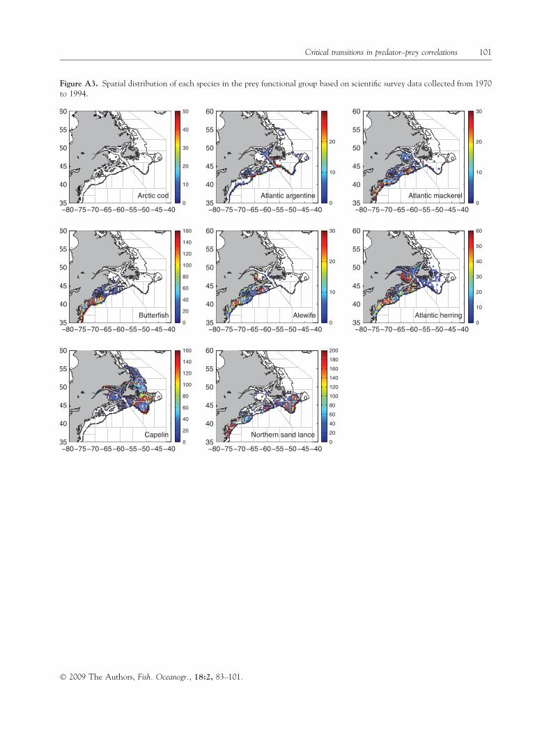
whose average annual contribution to total groundfishlandings ranged from �70% in the northern areas to�20% in the south (Table A1). There was also a highdegree of similarity between the time series of landingsof all groundfish species (made up of several differentspecies) and that of cod (Table A1, Fig. A1); more-over, in areas 6 and 8, a combined quota for cod,haddock and pollock was instituted in 1989 because ofthe strong spatial overlap among these species (Hall-iday et al., 1992). The principal gear type used in thesecommercial fisheries is the bottom trawl (Table A1), agear widely known to have low selectivity (Kumar andDeepthi, 2006). This is illustrated by a comparison ofbottom trawl catch composition relative to that offixed gear (hook and line) on the eastern Scotian Shelf(area 6 of Fig. 1) from 1998 to 2003. Bottom trawldeployments over this interval landed 72–110 speciescompared to 39–50 species for fixed gear. Figure A2illustrates the strong spatial overlap of cod with mostother species in the predator functional group. Thesedata support our use of cod as a surrogate for andindicator of the overall index of disturbance to the toppredator level in the nine northwest Atlantic areasinvestigated. Figure A3 shows the spatial distributionsof species within the prey functional group.

The strong overlap of species and the low selectivityof gear implies that mortality of non- or lightly fishedspecies would be similar to that of cod. The non- orlightly fished species would constitute bycatch and dieafter being discarded. However, recent work indicatesthat fish that do not have swim bladders exhibit greatervariability in their survival rate after discarding andthat some species of flatfish appear to have relativelygood chances of post-capture survival (Suuronen,2005). Moreover, Mandelman and Farrington (2007)indicated that the mortality rate of trawled dogfish waswell below the 50% bycatch discard mortality rate usedin current fishery models. However, they acknowl-edged that discard mortalities may increase rapidly ascatch weights rise above 200 kg, i.e., as the cod endsbecome more heavily packed.

98 B. Petrie et al.


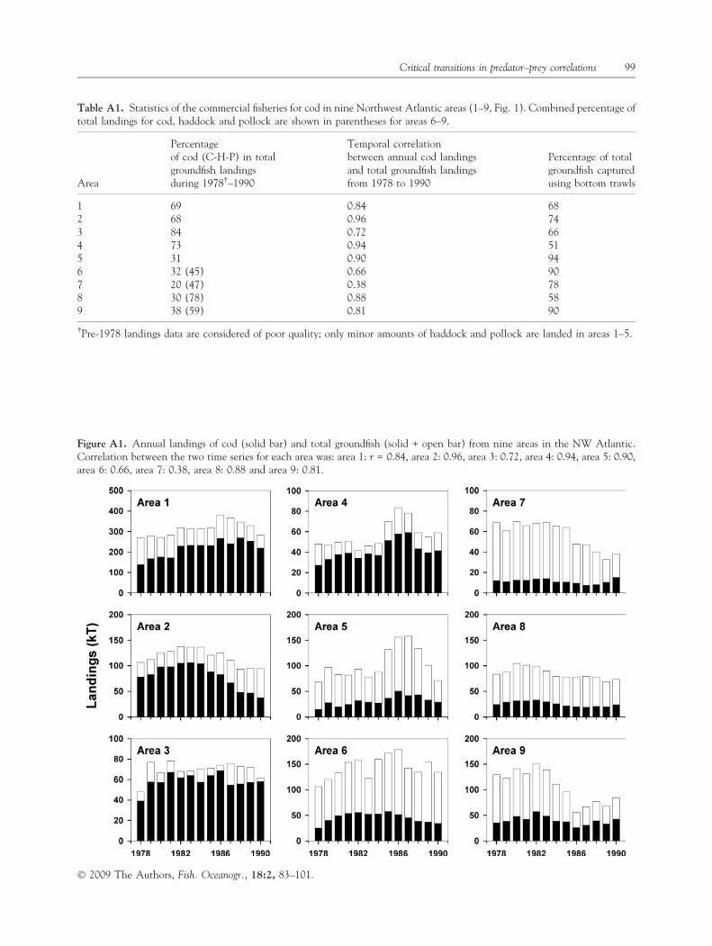
Table A1. Statistics of the commercial fisheries for cod in nine Northwest Atlantic areas (1–9, Fig. 1). Combined percentage oftotal landings for cod, haddock and pollock are shown in parentheses for areas 6–9.

Area

Percentageof cod (C-H-P) in totalgroundfish landingsduring 1978�–1990

Temporal correlationbetween annual cod landingsand total groundfish landingsfrom 1978 to 1990

Percentage of totalgroundfish capturedusing bottom trawls

1 69 0.84 682 68 0.96 743 84 0.72 664 73 0.94 515 31 0.90 946 32 (45) 0.66 907 20 (47) 0.38 788 30 (78) 0.88 589 38 (59) 0.81 90

�Pre-1978 landings data are considered of poor quality; only minor amounts of haddock and pollock are landed in areas 1–5.

Figure A1. Annual landings of cod (solid bar) and total groundfish (solid + open bar) from nine areas in the NW Atlantic.Correlation between the two time series for each area was: area 1: r = 0.84, area 2: 0.96, area 3: 0.72, area 4: 0.94, area 5: 0.90,area 6: 0.66, area 7: 0.38, area 8: 0.88 and area 9: 0.81.



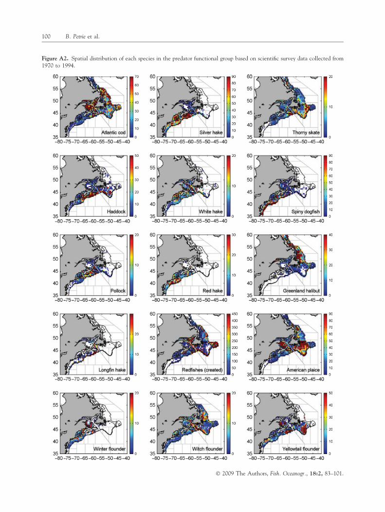
Figure A2. Spatial distribution of each species in the predator functional group based on scientific survey data collected from1970 to 1994.

100 B. Petrie et al.


−80−75−70−65−60−55–50−45−4035

40

45

50

55

60

Arctic cod0

10

20

30

40

50

−80−75−70−65−60−55−50−45−4035

40

45

50

55

60

Atlantic argentine0

10

20

−80−75−70−65−60−55−50−45−4035

40

45

50

55

60

Atlantic mackerel0

10

20

30

−80−75−70−65−60−55−50−45−4035

40

45

50

55

60

Butterfish0

20

40

60

80

100

120

140

160

−80−75−70−65−60−55−50−45−4035

40

45

50

55

60

Alewife0

10

20

30

−80−75−70−65−60−55−50−45−4035

40

45

50

55

60

Atlantic herring0

10

20

30

40

50

60

−80−75−70−65−60−55−50−45−4035

40

45

50

55

60

Capelin0

20

40

60

80

100

120

140

160

−80−75−70−65−60−55−50−45−4035

40

45

50

55

60

Northern sand lance0

20

40

60

80

100

120

140

160

180

200

Figure A3. Spatial distribution of each species in the prey functional group based on scientific survey data collected from 1970to 1994.



Structure and stability in exploited marine fish communities: quantifying critical transitions

Documents