Welcome message from author
This document is posted to help you gain knowledge. Please leave a comment to let me know what you think about it! Share it to your friends and learn new things together.
Transcript


Structural Steel Design to Eurocode 3and AISC Specifications


Structural Steel Design to Eurocode 3and AISC Specifications
By
Claudio Bernuzzi
and
Benedetto Cordova

This edition first published 2016© 2016 by John Wiley & Sons, Ltd
Registered OfficeJohn Wiley & Sons, Ltd, The Atrium, Southern Gate, Chichester, West Sussex, PO19 8SQ, United Kingdom
Editorial Offices9600 Garsington Road, Oxford, OX4 2DQ, United KingdomThe Atrium, Southern Gate, Chichester, West Sussex, PO19 8SQ, United Kingdom
For details of our global editorial offices, for customer services and for information about how to apply forpermission to reuse the copyright material in this book please see our website at www.wiley.com/wiley-blackwell.
The right of the author to be identified as the author of this work has been asserted in accordance with the UKCopyright, Designs and Patents Act 1988.
All rights reserved. No part of this publication may be reproduced, stored in a retrieval system, or transmitted,in any form or by any means, electronic, mechanical, photocopying, recording or otherwise, except aspermitted by the UK Copyright, Designs and Patents Act 1988, without the prior permission of the publisher.
Designations used by companies to distinguish their products are often claimed as trademarks. All brandnames and product names used in this book are trade names, service marks, trademarks or registeredtrademarks of their respective owners. The publisher is not associated with any product or vendor mentionedin this book.
Limit of Liability/Disclaimer of Warranty: While the publisher and author(s) have used their best efforts inpreparing this book, they make no representations or warranties with respect to the accuracy or completenessof the contents of this book and specifically disclaim any implied warranties of merchantability or fitness for aparticular purpose. It is sold on the understanding that the publisher is not engaged in rendering professionalservices and neither the publisher nor the author shall be liable for damages arising herefrom. If professionaladvice or other expert assistance is required, the services of a competent professional should be sought.
Based on Progetto e verifica delle strutture in acciaio by Claudio Bernuzzi.© Ulrico Hoepli Editore S.p.A., Milano, 2011. Published in the Italian language.
Library of Congress Cataloging-in-Publication data applied for.
ISBN: 9781118631287
A catalogue record for this book is available from the British Library.
Wiley also publishes its books in a variety of electronic formats. Some content that appears in print may not beavailable in electronic books.
Cover image: photovideostock/Getty
Set in 10/12pt Minion by SPi Global, Pondicherry, India
1 2016

Contents
Preface x
1 The Steel Material 11.1 General Points about the Steel Material 1
1.1.1 Materials in Accordance with European Provisions 41.1.2 Materials in Accordance with United States Provisions 7
1.2 Production Processes 101.3 Thermal Treatments 131.4 Brief Historical Note 141.5 The Products 151.6 Imperfections 18
1.6.1 Mechanical Imperfections 191.6.2 Geometric Imperfections 22
1.7 Mechanical Tests for the Characterization of the Material 241.7.1 Tensile Testing 251.7.2 Stub Column Test 271.7.3 Toughness Test 291.7.4 Bending Test 321.7.5 Hardness Test 32
2 References for the Design of Steel Structures 342.1 Introduction 34
2.1.1 European Provisions for Steel Design 352.1.2 United States Provisions for Steel Design 37
2.2 Brief Introduction to Random Variables 372.3 Measure of the Structural Reliability and Design Approaches 392.4 Design Approaches in Accordance with Current Standard Provisions 44
2.4.1 European Approach for Steel Design 442.4.2 United States Approach for Steel Design 47
3 Framed Systems and Methods of Analysis 493.1 Introduction 493.2 Classification Based on Structural Typology 513.3 Classification Based on Lateral Deformability 52
3.3.1 European Procedure 533.3.2 AISC Procedure 56
pg3085
Typewritten Text
3.4 Classification Based on Beam-to-Column Joint Performance 563.4.1 Classification According to the European Approach 573.4.2 Classification According to the United States Approach 603.4.3 Joint Modelling 61
3.5 Geometric Imperfections 633.5.1 The European Approach 633.5.2 The United States Approach 67
3.6 The Methods of Analysis 683.6.1 Plasticity and Instability 693.6.2 Elastic Analysis with Bending Moment Redistribution 763.6.3 Methods of Analysis Considering Mechanical Non-Linearity 783.6.4 Simplified Analysis Approaches 80
3.7 Simple Frames 843.7.1 Bracing System Imperfections in Accordance with EU Provisions 883.7.2 System Imperfections in Accordance with AISC Provisions 893.7.3 Examples of Braced Frames 92
3.8 Worked Examples 96
4 Cross-Section Classification 1074.1 Introduction 1074.2 Classification in Accordance with European Standards 108
4.2.1 Classification for Compression or Bending Moment 1104.2.2 Classification for Compression and Bending Moment 1104.2.3 Effective Geometrical Properties for Class 4 Sections 115
4.3 Classification in Accordance with US Standards 1184.4 Worked Examples 121
5 Tension Members 1345.1 Introduction 1345.2 Design According to the European Approach 1345.3 Design According to the US Approach 1375.4 Worked Examples 140
6 Members in Compression 1476.1 Introduction 1476.2 Strength Design 147
6.2.1 Design According to the European Approach 1476.2.2 Design According to the US Approach 148
6.3 Stability Design 1486.3.1 Effect of Shear on the Critical Load 1556.3.2 Design According to the European Approach 1586.3.3 Design According to the US Approach 162
6.4 Effective Length of Members in Frames 1666.4.1 Design According to the EU Approach 1666.4.2 Design According to the US Approach 169
6.5 Worked Examples 172
7 Beams 1767.1 Introduction 176
7.1.1 Beam Deformability 176
vi Contents

7.1.2 Dynamic Effects 1787.1.3 Resistance 1797.1.4 Stability 179
7.2 European Design Approach 1847.2.1 Serviceability Limit States 1847.2.2 Resistance Verifications 1867.2.3 Buckling Resistance of Uniform Members in Bending 190
7.3 Design According to the US Approach 1997.3.1 Serviceability Limit States 1997.3.2 Shear Strength Verification 2007.3.3 Flexural Strength Verification 204
7.4 Design Rules for Beams 2287.5 Worked Examples 233
8 Torsion 2438.1 Introduction 2438.2 Basic Concepts of Torsion 245
8.2.1 I- and H-Shaped Profiles with Two Axes of Symmetry 2508.2.2 Mono-symmetrical Channel Cross-Sections 2528.2.3 Warping Constant for Most Common Cross-Sections 255
8.3 Member Response to Mixed Torsion 2588.4 Design in Accordance with the European Procedure 2638.5 Design in Accordance with the AISC Procedure 265
8.5.1 Round and Rectangular HSS 2668.5.2 Non-HSS Members (Open Sections Such as W, T, Channels, etc.) 267
9 Members Subjected to Flexure and Axial Force 2689.1 Introduction 2689.2 Design According to the European Approach 271
9.2.1 The Resistance Checks 2719.2.2 The Stability Checks 2749.2.3 The General Method 280
9.3 Design According to the US Approach 2819.4 Worked Examples 284
10 Design for Combination of Compression, Flexure, Shear and Torsion 30310.1 Introduction 30310.2 Design in Accordance with the European Approach 30810.3 Design in Accordance with the US Approach 309
10.3.1 Round and Rectangular HSS 31010.3.2 Non-HSS Members (Open Sections Such as W, T, Channels, etc.) 310
11 Web Resistance to Transverse Forces 31111.1 Introduction 31111.2 Design Procedure in Accordance with European Standards 31211.3 Design Procedure in Accordance with US Standards 316
12 Design Approaches for Frame Analysis 31912.1 Introduction 31912.2 The European Approach 319
Contents vii
12.2.1 The EC3-1 Approach 32012.2.2 The EC3-2a Approach 32112.2.3 The EC3-2b Approach 32112.2.4 The EC3-3 Approach 322
12.3 AISC Approach 32312.3.1 The Direct Analysis Method (DAM) 32312.3.2 The Effective Length Method (ELM) 32712.3.3 The First Order Analysis Method (FOM) 32912.3.4 Method for Approximate Second Order Analysis 330
12.4 Comparison between the EC3 and AISC Analysis Approaches 33212.5 Worked Example 334
13 The Mechanical Fasteners 34513.1 Introduction 34513.2 Resistance of the Bolted Connections 345
13.2.1 Connections in Shear 34713.2.2 Connections in Tension 35413.2.3 Connection in Shear and Tension 358
13.3 Design in Accordance with European Practice 35813.3.1 European Practice for Fastener Assemblages 35813.3.2 EU Structural Verifications 363
13.4 Bolted Connection Design in Accordance with the US Approach 36913.4.1 US Practice for Fastener Assemblage 36913.4.2 US Structural Verifications 376
13.5 Connections with Rivets 38213.5.1 Design in Accordance with EU Practice 38313.5.2 Design in Accordance with US Practice 383
13.6 Worked Examples 384
14 Welded Connections 39514.1 Generalities on Welded Connections 395
14.1.1 European Specifications 39714.1.2 US Specifications 39914.1.3 Classification of Welded Joints 400
14.2 Defects and Potential Problems in Welds 40114.3 Stresses in Welded Joints 403
14.3.1 Tension 40414.3.2 Shear and Flexure 40614.3.3 Shear and Torsion 408
14.4 Design of Welded Joints 41114.4.1 Design According to the European Approach 41114.4.2 Design According to the US Practice 414
14.5 Joints with Mixed Typologies 42014.6 Worked Examples 420
15 Connections 42415.1 Introduction 42415.2 Articulated Connections 425
15.2.1 Pinned Connections 42615.2.2 Articulated Bearing Connections 427
viii Contents

15.3 Splices 42915.3.1 Beam Splices 43015.3.2 Column Splices 431
15.4 End Joints 43415.4.1 Beam-to-Column Connections 43415.4.2 Beam-to-Beam Connections 43415.4.3 Bracing Connections 43715.4.4 Column Bases 43815.4.5 Beam-to-Concrete Wall Connection 441
15.5 Joint Modelling 44415.5.1 Simple Connections 45015.5.2 Rigid Joints 45415.5.3 Semi-Rigid Joints 458
15.6 Joint Standardization 462
16 Built-Up Compression Members 46616.1 Introduction 46616.2 Behaviour of Compound Struts 466
16.2.1 Laced Compound Struts 47116.2.2 Battened Compound Struts 473
16.3 Design in Accordance with the European Approach 47516.3.1 Laced Compression Members 47716.3.2 Battened Compression Members 47716.3.3 Closely Spaced Built-Up Members 478
16.4 Design in Accordance with the US Approach 48016.5 Worked Examples 482
Appendix A: Conversion Factors 491Appendix B: References and Standards 492Index 502
Contents ix
Preface
Over the last century, design of steel structures has developed from very simple approaches basedon a few elementary properties of steel and essential mathematics to very sophisticated treatmentsdemanding a thorough knowledge of structural and material behaviour. Nowadays, steel designutilizes refined concepts of mechanics of material and of theory of structures combined withprobabilistic-based approaches that can be found in design specifications.
This book intends to be a guide to understanding the basic concepts of theory of steel structuresas well as to provide practical guidelines for the design of steel structures in accordance with bothEuropean (EN 1993) and United States (ANSI/AISC 360-10) specifications. It is primarilyintended for use by practicing engineers and engineering students, but it is also relevant to alldifferent parties associated with steel design, fabrication and construction.
The book synthesizes the Authors’ experience in teaching Structural Steel Design at theTechnical University of Milan-Italy (Claudio Bernuzzi) and in design of steel structures forpower plants (Benedetto Cordova), combining their expertise in comparing and contrastingboth European and American approaches to the design of steel structures.
The book consists of 16 chapters, each structured independently of the other, in order to facili-tate consultation by students and professionals alike. Chapter 1 introduces general aspects such asmaterial properties and products, imperfection and tolerances, also focusing the attention on test-ing methods and approaches. The fundamentals of steel design are summarized in Chapter 2,where the principles of structural safety are discussed in brief to introduce the different reliabilitylevels of the design. Framed systems and methods of analysis, including simplified methods, arediscussed in Chapter 3. Cross-sectional classification is presented in Chapter 4, in which specialattention has been paid to components under compression and bending. Design of singlemembers is discussed in depth in Chapter 5 for tension members, in Chapter 6 for compressionmembers, in Chapter 7 for members subjected to bending and shear, in Chapter 8 for membersunder torsion, and in Chapter 9 for members subjected to bending and compression. Chapter 10deals with design accounting for the combination of compression, flexure, shear and torsion.
Chapter 11 addresses requirements for the web resistance design and Chapter 12 deals with thedesign approaches for frame analysis. Chapters 13 and 14 deal with bolted and welded connec-tions, respectively, while the most common type of joints are described in Chapter 15, including asummary of the approach to their design. Finally, built-up members are discussed in Chapter 16.Several design examples provided in this book are directly chosen from real design situations. Allexamples are presented providing all the input data necessary to develop the design. The differentcalculations associated with European and United States specifications are provided in twoseparate text columns in order to allow a direct comparison of the associated procedures.
Last, but not least, the acknowledge of the Authors. A great debt of love and gratitude to ourfamilies: their patience was essential to the successful completion of the book.
We would like to express our deepest thanks to Dr. Giammaria Gabbianelli (University ofPavia-I) and Dr. Marco Simoncelli (Politecnico di Milano-I) for the continuous help in preparing

figures and tables and checking text.We are also thankful to prof. Gian Andrea Rassati (Universityof Cincinnati-U.S.A.) for the great and precious help in preparation of chapters 1 and 13.Finally, it should be said that, although every care has been taken to avoid errors, it would be
sanguine to hope that none had escape detection. Authors will be grateful for any suggestion thatreaders may make concerning needed corrections.
Claudio Bernuzzi and Benedetto Cordova
Preface xi


CHAPTER 1
The Steel Material
1.1 General Points about the Steel Material
The term steel refers to a family of iron–carbon alloys characterized by well-defined percentageratios of main individual components. Specifically, iron–carbon alloys are identified by the carbon(C) content, as follows:
• wrought iron, if the carbon content (i.e. the percentage content in terms of weight) is higherthan 1.7% (some literature references have reported a value of 2%);
• steel, when the carbon content is lower than the previously mentioned limit. Furthermore, steelcan be classified into extra-mild (C < 0.15%), mild (C = 0.15 0.25%), semi-hard (C = 0.250.50%), hard (C = 0.50 0.75%) and extra-hard (C > 0.75%) materials.
Structural steel, also called constructional steel or sometimes carpentry steel, is characterized bya carbon content of between 0.1 and 0.25%. The presence of carbon increases the strength of thematerial, but at the same time reduces its ductility and weldability; for this reason structural steel isusually characterized by a low carbon content. Besides iron and carbon, structural steel usuallycontains small quantities of other elements. Some of them are already present in the iron oreand cannot be entirely eliminated during the production process, and others are purposely addedto the alloy in order to obtain certain desired physical or mechanical properties.Among the elements that cannot be completely eliminated during the production process, it is
worth mentioning both sulfur (S) and phosphorous (P), which are undesirable because theydecrease the material ductility and its weldability (their overall content should be limited toapproximately 0.06%). Other undesirable elements that can reduce ductility are nitrogen (N), oxy-gen (O) and hydrogen (H). The first two also affect the strain-ageing properties of the material,increasing its fragility in regions in which permanent deformations have taken place.The most important alloying elements that may be added to the materials are manganese
(Mn) and silica (Si), which contribute significantly to the improvement of the weldabilitycharacteristics of the material, at the same time increasing its strength. In some instances, chro-mium (Cr) and nickel (Ni) can also be added to the alloy; the former increases the materialstrength and, if is present in sufficient quantity, improves the corrosion resistance (it is usedfor stainless steel), whereas the latter increases the strength while reduces the deformability ofthe material.
Structural Steel Design to Eurocode 3 and AISC Specifications, First Edition. Claudio Bernuzzi and Benedetto Cordova.© 2016 John Wiley & Sons, Ltd. Published 2016 by John Wiley & Sons, Ltd.
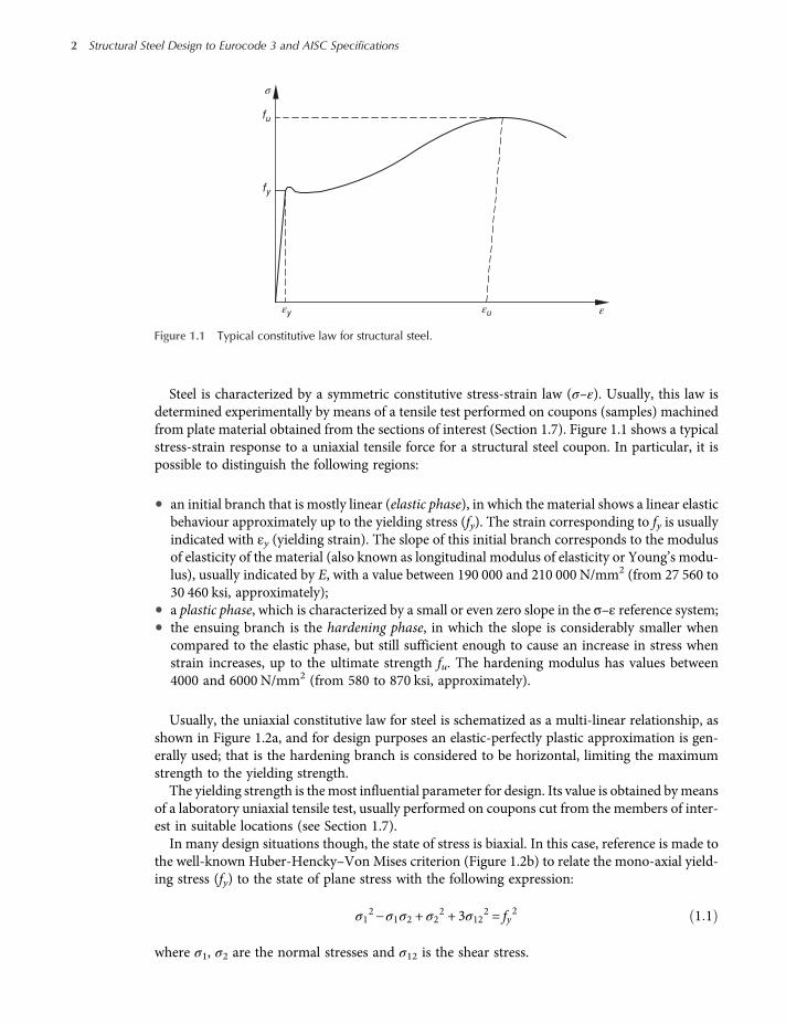
Steel is characterized by a symmetric constitutive stress-strain law (σ–ε). Usually, this law isdetermined experimentally by means of a tensile test performed on coupons (samples) machinedfrom plate material obtained from the sections of interest (Section 1.7). Figure 1.1 shows a typicalstress-strain response to a uniaxial tensile force for a structural steel coupon. In particular, it ispossible to distinguish the following regions:
• an initial branch that is mostly linear (elastic phase), in which the material shows a linear elasticbehaviour approximately up to the yielding stress (fy). The strain corresponding to fy is usuallyindicated with εy (yielding strain). The slope of this initial branch corresponds to the modulusof elasticity of the material (also known as longitudinal modulus of elasticity or Young’s modu-lus), usually indicated by E, with a value between 190 000 and 210 000 N/mm2 (from 27 560 to30 460 ksi, approximately);
• a plastic phase, which is characterized by a small or even zero slope in the σ–ε reference system;• the ensuing branch is the hardening phase, in which the slope is considerably smaller when
compared to the elastic phase, but still sufficient enough to cause an increase in stress whenstrain increases, up to the ultimate strength fu. The hardening modulus has values between4000 and 6000 N/mm2 (from 580 to 870 ksi, approximately).
Usually, the uniaxial constitutive law for steel is schematized as a multi-linear relationship, asshown in Figure 1.2a, and for design purposes an elastic-perfectly plastic approximation is gen-erally used; that is the hardening branch is considered to be horizontal, limiting the maximumstrength to the yielding strength.
The yielding strength is themost influential parameter for design. Its value is obtained bymeansof a laboratory uniaxial tensile test, usually performed on coupons cut from the members of inter-est in suitable locations (see Section 1.7).
In many design situations though, the state of stress is biaxial. In this case, reference is made tothe well-known Huber-Hencky–Von Mises criterion (Figure 1.2b) to relate the mono-axial yield-ing stress (fy) to the state of plane stress with the following expression:
σ12−σ1σ2 + σ2
2 + 3σ122 = fy
2 1 1
where σ1, σ2 are the normal stresses and σ12 is the shear stress.
fu
fy
εy εu
σ
ε
Figure 1.1 Typical constitutive law for structural steel.
2 Structural Steel Design to Eurocode 3 and AISC Specifications

In the case of pure shear, the previous equation is reduced to:
σ12 = τ12 =fy3= τy 1 2
With reference to the principal stress directions 1 and 2 , the yield surface is represented by anellipse and Eq. (1.1) becomes:
σ12 + σ2
2− σ1 σ2 = fy2 1 3
εy ε
fy
Elastic
phase
Plastic
phase
Hardening
phase
σ(a)
σ1′/fy
σ2′/fy
1.0
–1.0
–1.00
(b)
1.0
Figure 1.2 Structural steel: (a) schematization of the uniaxial constitutive law and (b) yield surface for biaxialstress states.
The Steel Material 3

1.1.1 Materials in Accordance with European Provisions
The European provisions prescribe the following values for material properties concerning struc-tural steel design:
The mechanical properties of the steel grades most used for construction are summarized inTables 1.1a and 1.1b, for hot-rolled and hollow profiles, respectively, in terms of yield strength(fy) and ultimate strength (fu). Similarly, Table 1.2 refers to steel used for mechanical fasteners.With respect to the European nomenclature system for steel used in high strength fasteners,the generic tag (j.k) can be immediately associated to themechanical characteristics of thematerialexpressed in International System of units (I.S.), considering that:
• j k 10 represents the yielding strength expressed in N/mm2;• j 100 represents the failure strength expressed in N/mm2.
Table 1.1a Mechanical characteristics of steels used for hot-rolled profiles.
EN norm and steel grade
Nominal thickness t
t ≤ 40mm 40mm< t ≤ 80mm
fy (N/mm2) fu (N/mm2) fy (N/mm2) fu (N/mm2)
EN 10025-2S 235 235 360 215 360S 275 275 430 255 410S 355 355 510 335 470S 450 440 550 410 550EN 10025-3S 275 N/NL 275 390 255 370S 355 N/NL 355 490 335 470S 420 N/NL 420 520 390 520S 460 N/NL 460 540 430 540EN 10025-3S 275 M/ML 275 370 255 360S 355 M/ML 355 470 335 450S 420 M/ML 420 520 390 500S 460 M/ML 460 540 430 530EN 10025-5S 235 W 235 360 215 340S 355 W 355 510 335 490EN 10025-6S 460 Q/QL/QL1 460 570 440 550
Density: ρ = 7850 kg/m3 (= 490 lb/ft3)Poisson’s coefficient: ν = 0.3Longitudinal (Young’s) modulus of elasticity: E = 210 000 N/mm2 (= 30 460 ksi)Shear modulus:
G=E
2 1 + νCoefficient of linear thermal expansion: α = 12 × 10−6 per C (=6.7 × 10⁻⁶ per F)
4 Structural Steel Design to Eurocode 3 and AISC Specifications

The details concerning the designation of steels are covered in EN 10027 Part 1 (Designationsystems for steels – Steel names) and Part 2 (Numerical system), which distinguish the followinggroups:
• group 1, in which the designation is based on the usage and on the mechanical or physicalcharacteristics of the material;
• group 2, in which the designation is based on the chemical content: the first symbol may be aletter (e.g. C for non-alloy carbon steels or X for alloy steel, including stainless steel) or anumber.
With reference to the group 1 designations, the first symbol is always a letter. For example:
• B for steels to be used in reinforced concrete;• D for steel sheets for cold forming;• E for mechanical construction steels;• H for high strength steels;• S for structural steels;• Y for steels to be used in prestressing applications.
Table 1.1b Mechanical characteristics of steels used for hollow profiles.
EN norm and steel grade
Nominal thickness t
t ≤ 40mm 40mm < t ≤ 65mm
fy (N/mm2) fu (N/mm2) fy (N/mm2) fu (N/mm2)
EN 10210-1S 235 H 235 360 215 340S 275 H 275 430 255 410S 355 H 355 510 335 490S 275 NH/NLH 275 390 255 370S 355 NH/NLH 355 490 335 470S 420 NH/NLH 420 540 390 520S 460 NH/NLH 460 560 430 550EN 10219-1S 235 H 235 360S 275 H 275 430S 355 H 355 510S 275 NH/NLH 275 370S 355 NH/NLH 355 470S 460 NH/NLH 460 550S 275 MH/MLH 275 360S 355 MH/MLH 355 470S420 MH/MLH 420 500S 460 NH/NLH 460 530
Table 1.2 Nominal yielding strength values (fyb) and nominal failure strength (fub) for bolts.
Bolt class 4.6 4.8 5.6 5.8 6.8 8.8 10.9
fyb (N/mm2) 240 320 300 400 480 640 900fub (N/mm2) 400 400 500 500 600 800 1000
The Steel Material 5

Focusing attention on the structural steels (starting with an S), there are then three digitsXXX that provide the value of the minimum yielding strength. The following term is relatedto the technical conditions of delivery, defined in EN 10025 (‘Hot rolled products of structuralsteel’) that proposes the following five abbreviations, each associated to a different productionprocess:
• the AR (As Rolled) term identifies rolled and otherwise unfinished steels;• the N (Normalized) term identifies steels obtained through normalized rolling, that is a rolling
process in which the final rolling pass is performed within a well-controlled temperature range,developing a material with mechanical characteristics similar to those obtained through a nor-malization heat treatment process (see Section 1.2);
• the M (Mechanical) term identifies steels obtained through a thermo-mechanical rollingprocess, that is a process in which the final rolling pass is performed within a well-controlledtemperature range resulting in final material characteristics that cannot be obtained throughheat treating alone;
• theQ (Quenched and tempered) term identifies high yield strength steels that are quenched andtempered after rolling;
• the W (Weathering) term identifies weathering steels that are characterized by a considerablyimproved resistance to atmospheric corrosion.
The YY code identifies various classes concerning material toughness as discussed in thefollowing. Non-alloyed steels for structural use (EN 10025-2) are identified with a code afterthe yielding strength (XXX), for example:
• YY: alphanumeric code concerning toughness: S235 and S275 steels are provided in groupsJR, J0 and J2. S355 steels are provided in groups JR, J0, J2 and K2. S450 steels are provided ingroup J0 only. The first part of the code is a letter, J or K, indicating a minimum value oftoughness provided (27 and 40 J, respectively). The next symbol identifies the temperatureat which such toughness must be guaranteed. Specifically, R indicates ambient temperature,0 indicates a temperature not higher than 0 C and 2 indicates a temperature not higherthan −20 C;
• C: an additional symbol indicating special uses for the steel;• N, AR or M: indicates the production process.
Weldable fine grain structural steels that are normalized or subject to normalized rolling (EN10025-3); that is, steels characterized by a granular structure with an equivalent ferriting grain sizeindex greater than 6, determined in accordance with EN ISO 643 (‘Micrographic determination ofthe apparent grain size’), are defined by the following codes:
• N: for the production process;• YY: for the toughness class. The L letter identifies toughness temperatures not lower than
−50 C; in the absence of the letter L, the reference temperature must be taken as −20 C.
Fine grain steels obtained through thermo-mechanical rolling processes (EN 10025-4) are iden-tified by the following code:
• M: for the production process;• YY: for the toughness class. The letter L, as discussed previously, identifies toughness temper-
atures no lower than −50 C; in the absence of the letter L, the reference temperature must betaken to be −20 C.
6 Structural Steel Design to Eurocode 3 and AISC Specifications

Weathering steels for structural use (EN 10025-5) are identified by the following code:
• the YY code indicates the toughness class: these steels are provided in classes J0, J2 and K2,indicating different toughness requirements at different temperatures.
• the W code indicates the weathering properties of the steel;• P indicates an increased content of phosphorous;• N or AR indicates the production process.
Quenched and tempered high-yield strength plate materials for structural use (EN 10025-6) areidentified by the following codes:
• Q code indicates the production process;• YY: identifies the toughness class. The letter L indicates a specified minimum toughness tem-
perature of −40 C, while code L1 refers to temperatures not lower than −60 C. In the absence ofthese codes, the minimum toughness values refer to temperatures no lower than −20 C.
In Europe, it is mandatory to use steels bearing the CE marks, in accordance with the require-ments reported in the Construction Products Regulation (CPR) No. 305/2011 of the EuropeanCommunity. The usage of different steels is allowed as long as the degree of safety (not lower thanthe one provided by the current specifications) can be guaranteed, accompanied by adequate the-oretical and experimental documentation.
1.1.2 Materials in Accordance with United States Provisions
The properties of structural steel materials are standardized by ASTM International (formerlyknown as the American Society for Testing and Materials). Numerous standards are availablefor structural applications, generally dedicated to the most common product families. In the fol-lowing, some details are reported.
1.1.2.1 General StandardsASTMA6 (Standard Specification for General Requirements for Rolled Structural Steel Bars, Plates,Shapes and Sheet Piling) is the standard that covers the general requirements for rolled structuralsteel bars, plates, shapes and sheet piling.
1.1.2.2 Hot-Rolled Structural Steel ShapesTable 1.3 summarizes key data for the most commonly used hot-rolled structural shapes.
• W-ShapesASTM A992 is the most commonly used steel grade for all hot-rolled W-Shape members.This material has a minimum yield stress of 50 ksi (356 MPa) and a minimum tensilestrength of 65 ksi (463 MPa). Higher values of the yield and tensile strength can be guar-antee by ASTM A572 Grades 60 or 65 (Grades 42 and 50 are also available) or ASTMA913 Grades 60, 65 or 70 (Grace 50 is also available). If W-Shapes with atmospheric cor-rosion resistance characteristics are required, reference can be made to ASTM A588 orASTM A242 selecting 42, 46 or 50 steel Grades. Finally, W-Shapes according to ASTMA36 are also available.
• M-Shapes and S-ShapesThese shapes have been produced up to now in ASTM A36 steel grade. From some steel pro-ducers they are now available in ASTM A572 Grade 50. M-Shapes with atmospheric corrosionresistance characteristics can be obtained by using ASTM A588 or ASTM A242 Grade 50.
The Steel Material 7

• ChannelsSee what is stated about M- and S-Shapes.
• HP-ShapesASTM A572 Grade 50 is the most commonly used steel grade for these cross-section shapes. Ifatmospheric corrosion resistance characteristics are required for HP-Shapes, ASTM A588 orASTM A242 Grade 46 or 50 can be used. Other materials are available, such as ASTM A36,ASTM A529 Grades 50 or 55, ASTM A572 Grades 42, 55, 60 and 65, ASTM A913 Grades50, 60, 65, 70 and ASTM A992.
• AnglesASTM A36 is the most commonly used steel grade for these cross-sections shapes. Atmos-pheric corrosion resistance characteristics of the angles can be guaranteed by using ASTMA588 or ASTM A242 Grades 46 or 50. Other available materials: ASTM A36, ASTM A529Grades 50 or 55, ASTM A572 Grades 42, 50, 55 and 60, ASTM A913 Grades 50, 60, 65 and70 and ASTM A992.
• Structural TeesStructural tees are produced cutting W-, M- and S-Shapes, to make WT-, MT- and ST-Shapes.Therefore, the same specifications for W-, M- and S-Shapes maintain their validity.
Table 1.3 ASTM specifications for various structural shapes (from Table 2-3 of the AISC Manual ).
Steel type ASTM designation
Fyminimumyield stress(ksi)
Futensilestress(ksi)
Applicable shape series
W M S HP C MC LHSSrectangular
HSSround Pipe
Carbon A36 36 58–80A53 Gr. B 35 60A500 Gr. B 42 58
46 58Gr. C 46 62
50 62A501 36 58A529 Gr. 50 50 65–100
Gr. 55 55 70–100High strength lowalloy
A572 Gr. 42 42 60Gr. 50 50 65Gr. 55 55 70Gr. 60 60 75Gr. 65 65 80
A618 Gr. I and II 50 70Gr. III 50 65
A913 50 50 6060 60 7565 65 8070 70 90
A992 50–65 65Corrosion resistanthigh strengthlow-alloy
A242 42 6346 6750 70
A588 50 70A847 50 70
= Preferred material specification.= Other applicable material specification.=Material specification does not apply.
8 Structural Steel Design to Eurocode 3 and AISC Specifications

• Square, Rectangular and Round HSSASTM A500 Grade B (Fy = 46 ksi and Fu = 58 ksi) is the most commonly used steel grade forthese shapes. ASTM A550 Grade C (Fy = 50 ksi and Fu = 62 ksi) is also used. Rectangular HSSwith atmospheric corrosion resistance characteristics can be obtained by using ASTM A847.Other available materials are ASTM A501 and ASTM A618.
• Steel PipesASTM A53 Grade B (Fy = 35 ksi and Fu = 60 ksi) is the only steel grade available for theseshapes.
1.1.2.3 Plate ProductsAs to plate products, reference can be made to Table 1.4.
• Structural platesASTM A36 Fy = 36 ksi (256 MPa) for plate thickness equal to or less then 8 in. (203 mm),Fy = 32 ksi (228 MPa) for higher thickness and Fu = 58 ksi (413 MPa) is the most commonlyused steel grade for structural plates. For other materials, reference can be made toTable 1.4.
• Structural barsData related to structural plates are valid also for bars with the exception that ASTM A514 andA852 are not admitted.
Table 1.4 Applicable ASTM specifications for plates and bars (from Table 2-4 of the AISC Manual).
Steel type
Fyminimumyieldstress (ksi)
Futensilestress(ksi)
Plates and bars
ASTMdesignation
To 0.75inclusive
Over0.75–1.25
Over1.25–1.5
Over1.5–2incl.
Over2–2.5incl.
Over2.5–4incl.
Over4–5incl.
Over5–6incl.
Over6–8incl.
Over8
Carbon A36 32 58–8036 58–80
A529 Gr. 50 50 70–100Gr. 55 55 70–100
High strength lowalloy
A572 Gr. 42 42 60Gr. 50 50 65Gr. 55 55 70Gr. 60 60 75Gr. 65 65 80
Corrosionresistant highstrengthlow alloy
A242 42 6346 6750 70
A588 42 6346 6750 70
Quenched andtempered alloy
A514 90 100–130100 110–130
Quenchedand temperedlow alloy
A852 70 90–110
= Preferred material specification.= Other applicable material specification.=Material specification does not apply.
The Steel Material 9

1.1.2.4 SheetsASTMA606 and ASTMA1011 are the twomain standards for metal sheets. The former deals withweathering steel, the latter standardizes steels with improved formability that are typically used forthe production of cold-formed profiles.
1.1.2.5 High-Strength FastenersASTM A325 and A490 are the standards dealing with high-strength bolts used in structural steelconnections. The nominal failure strength of A325 bolts is 120 ksi (854 MPa), without an upperlimit, while the nominal failure strength of A490 bolts is 150 ksi (1034MPa), with an upper limitof 172 ksi (1224MPa) per ASTM, limited to 170 ksi (1210MPa) by the structural steel provisions.ASTM F1852 and F2280 are standards for tension-control bolts, characterized by a splined endthat shears off when the desired pretension is reached. Loosely, A325 (and F1852) bolts corres-pond to 8.8 bolts in European standards and A490 (and F2280) bolts correspond to 10.9 bolts.
ASTM F436 standardizes hardened steel washers for fastening applications. ASTM F959 is thestandard for direct tension indicator washers, which are a special category of hardened washerswith raised dimples that flatten upon reaching the minimum pretension force in the fastener.
ASTM A563 standardizes carbon and alloy steel nuts.ASTM A307 is the standard for steel anchor rods; it is also used for large-diameter fasteners
(above 1½-in.). ASTM F1554 is the preferred standard for anchor rods.ASTM 354 standardizes quenched and tempered alloy steel bolts.ASTM A502 is the standard of reference for structural rivets.
1.2 Production Processes
Steel can be obtained by converting wrought iron or directly by means of fusion of metal scrapand iron ore. Ingots are obtained from these processes, which then can be subject to hot- orcold-mechanical processes, eventually becoming final products (plates, bars, profiles, sheets,rods, bolts, etc.). These products, examined in detail in Section 1.5, can be obtained in variousways that can be practically summarized into the following techniques:
• forming process by compression or tension (e.g. forging, rolling, extrusion);• forming process by flexure and shear.
Among these processes, the most important is the rolling process in both its hot- and cold-vari-ations, by which most products used in structural applications (referred to as rolled products) areobtained. In the hot-rolling process, steel ingots are brought to a temperature sufficient to softenthe material (approximately 1200 C or 2192 F), they first travel through a series of juxtaposedcounter-rotating rollers (primary rolling – Figure 1.3) and are roughed into square or rectangularcross-section bars.
These semi-worked products are produced in different shapes that can be then further rolled toobtain plates, large- or medium-sized profiles or small-sized profiles, bars and rounds. This add-itional process is called secondary rolling, resulting in the final products.
For example, in order to obtain the typical I-shaped profiles, the semi-worked products, at atemperature slightly above 1200 C (or 2192 F), are sent to the rolling train and its initiallyrectangular cross-section is worked until the desired shape is obtained. Figure 1.4 shows someof the intermediate cross-sections during the rolling process, until the final I-shape product isobtained.
10 Structural Steel Design to Eurocode 3 and AISC Specifications

The rolling process improves the mechanical characteristics of the final product, thanks to thecompressive forces applied by the rollers and the simultaneous thinning of the cross-section thatfavours the elimination of gases and air pockets that might be initially present. At the same time,the considerable deformations imposed by the rolling process contribute to refine the grain struc-ture of the material, with remarkable advantages regarding homogeneity and strength. In suchprocesses, in addition to the amount of deformations, also the rate of deformations is a veryimportant factor in determining the final characteristics of the product.Cold rolling is performed at the ambient temperature and it is frequently used for non-ferrous
materials to obtain higher strengths through hardening at the price of an often non-negligible lossof ductility. When cold-rolling requires excessive strains, the metal can start showing cracksbefore the desired shape is attained, in which case additional cycles of heat treatments and coldforming are needed (Section 1.3).The forming processes by bending and shear consist of bending thin sheets until the desired
cross-section shape is obtained. Typical products obtained by these processes are cold-formedprofiles, for which the thickness must be limited to a few millimetres in order to attain the desireddeformations. Figure 1.5 shows the intermediate steps to obtain hollow circular cold-formed pro-files by means of continuous formation processes.It can be seen that the coil is pulled and gradually shaped until the desired final product is
obtained. Figure 1.6 instead shows the main intermediate steps of the punch-and-die processto obtain some typical profiles currently used in structural applications. With this second workingtechnique, thicker sheets can be shaped into profiles with thicknesses up to 12–15 mm(0.472–0.591 in.), while the limit value of the coil thickness for continuous formation processesis approximately 5 mm (0.197 in.). As an example, Figure 1.7 shows some intermediate steps of the
Figure 1.3 Rolling process.
Figure 1.4 Intermediate steps of the rolling process for an I-shape profile.
The Steel Material 11

cold-formation process of a stiffened channel profile, with regular perforations, typically used forsteel storage pallet racks and shelving structures.
Another important category of steel products obtained with punch-and-die processes is repre-sented by metal decking, currently used for slabs, roofs and cladding.
(a)
(a)
(b)
(c)
(c) (d)
(d)(b)
Figure 1.5 Continuous formation of circular hollow cold-formed profiles.
Figure 1.6 Punch-and-die process for cold-formed profiles.
12 Structural Steel Design to Eurocode 3 and AISC Specifications

1.3 Thermal Treatments
Steel products, just like other metal products, can be subject to special thermal treatments in ordertomodify their molecular structure, thus changing their mechanical properties. The basic molecu-lar structures are cementite, austenite and ferrite. Transition from one structure to anotherdepends on temperature and carbon content. The main thermal treatments commonly used,which are briefly described in the following, are annealing, normalization, tempering, quenching,pack-hardening and quenching and tempering:
• annealing is the thermal cycle that begins with the heating to a temperature close to or slightlyabove the critical temperature (corresponding to the temperature at which the ferrite-austenitetransition is complete); afterwards the temperature is maintained for a predetermined amountof time and then the material is slowly cooled to ambient temperature. Generally, annealingleads to a more homogenous base material, eliminating most defects due to solidifying process.Annealing is applied to either ingots, semi-worked products or final products. Annealing ofworked products is useful to increase ductility, which might be reduced by hardening duringthe mechanical processes of production, or to release some residual stresses related to non-uniform cooling or production processes. In particular, annealing can be used on welded partsthat are likely to be mired by large residual stresses due to differential cooling;
• normalization consists of heating the steel to a temperature between 900 and 925 C (approxi-mately between 1652 and 1697 F), followed by very slow cooling. Normalization eliminates theeffects of any previous thermal treatment;
• tempering is a thermal process that, similar to annealing, consists of heating the materialslightly above the critical temperature followed by a sudden cooling, aimed at preventingany readjustment of the molecular matrix. The main advantage of the tempering process isrepresented by an increase of hardness that is, however, typically accompanied by a loss of duc-tility of the material;
• quenching consists of heating the tempered part up to a moderate temperature for an extendedamount of time, improving the ductility of the material;
• pack-hardening is a process that consists of heating of a part when in contact with solid, liquidor gaseous materials that can release carbon. It is a surface treatment that is employed to form aharder layer of material on the outside surface (up to a depth of several millimetres), in order toimprove the wearing resistance;
Quenching and tempering can be applied sequentially, resulting in a remarkable strengthimprovement of ordinary carbon steels, without appreciably affecting the ductility of the product.High strength bolts used in steel structures are typically quenched and tempered.
Figure 1.7 Cold-formation images of a stiffened channel profile.
The Steel Material 13

1.4 Brief Historical Note
Iron refinement has taken place for millennia in partially buried furnaces, fuelled by bellowsresulted in a spongy iron mass, riddled of impurities that could only be eliminated by repeatedhammering, resulting in wrought iron. That product had modest mechanical properties and couldbe welded by forging; that is, by heating the parts to join to a cherry red colour (750–850 C or1382–1562 F) and then pressing them together, typically by hammering. Wrought iron productscould be superficially hardened by tempering them in a bath of cold water or oil and the finalproduct was called steel. Note that these terms have different implications nowadays.
In thirteenth century Prussia, thanks to an increase in the height of the interred furnaces andthe consequent increase in the amount of air forced in the oven by hydraulically actuated bellows,the maximum attainable temperatures were increased. Consequently, a considerably differentmaterial from steel was obtained, namely cast iron. Cast iron was a brittle material that, oncecooled, could not be wrought. On the other hand, cast iron in its liquid state could be poured intomoulds, assuming whatever shape was desired. A further heating in an open oven, resulting in acarbon-impoverished alloy, allowed for malleable iron to be obtained.
In the past, the difficulties associated with the refinement of iron ore have limited the applicationsof this material to specific fields that required special performance in terms of strength or hardness.Applications in construction were limited to ties for arches and masonry structures, or connectionelements for timber construction. The industrial revolution brought a new impulse in metal con-struction, starting in the last decades of the eighteenth century. The invention of the steam engineallowed hydraulically actuated bellows to be replaced, resulting in a further increase of the airintake and the other significant advantage of locating the furnaces near iron mines, instead of for-cing them to be close to rivers. In 1784, in England, Henry Cort introduced a new type of furnace,the puddling furnace, in which the process of eliminating excess carbon by oxidation took placethanks to a continuous stirring of the molten material. The product obtained (puddled iron)was then hammered to eliminate the impurities. An early rolling process, using creased rollers, fur-ther improved the quality of the products, which was worked into plates and square cross-sectionmembers. Starting in the second half of the nineteenth century, several other significant improve-ments were introduced. In 1856, at the Congress of the British Society for the Scientific Progress,Henry Bessemer announced his patented process to rapidly convert cast iron into steel. Bessemer’sinnovative idea consisted of the insufflation of the air directly into themolten cast iron, so that mostof the oxygen in the air could directly combine with the carbon in the molten material, eliminatingit in the form of carbon oxide and dioxide in gaseous form.
The first significant applications of cast iron in buildings and bridges date back to the last dec-ades of the eighteenth century. An important example is the cast iron bridge on the Severn River atIronbridge Gorge, Shropshire, approximately 30 km (18.6 miles) from Birmingham in the UK. Itis an arched bridge and it was erected between 1775 and 1779. The structure consisted of fivearches, placed side by side, over a span of approximately 30 m (98 ft), each made of two partsrepresenting half of an arch, connected at the key without nails or rivets.
The expansion of the railway industry, with the specific need for stiff and strong structurescapable of supporting the large weights of a train without large deformations, provided a furtherspur to the development of bridge engineering. Between 1844 and 1850 the Britannia Bridge(Pont Britannia) on the Menai River (UK) was built; this bridge represents a remarkable exampleof a continuously supported structure over five supports, with two 146 m (479 ft) long centralspans and two 70 m (230 ft) long side spans. The bridge had a closed tubular cross-section, insidewhich the train would travel, and it was made of puddled iron connected by nails. RobertStephenson, William Fairbairn and Eaton Hodgkinson were the main designers, who had totackle a series of problems that had not been resolved yet at the time of the design. Being a stat-ically indeterminate structure, in order to evaluate the internal forces, B. Clapeyron studied the
14 Structural Steel Design to Eurocode 3 and AISC Specifications

structure applying the three-moment equation that he had recently developed. For the staticbehaviour of the cross-section, based on experimental tests on scaled models of the bridge,N. Jourawsky suggested some stiffening details to prevent plate instability. The Britannia Bridgealso served as a stimulus to study riveted and nailed connections, wind action and the effectsof temperature changes.With respect to buildings, the more widespread use of metals contributed to the development
of framed structures. Around the end of the 1700s, cast iron columns were made with square,hollow circular or a cross-shaped cross-section. The casting process allowed reproduction ofthe classical shapes of the column or capital, often inspired by the architectural styles of theancient Greeks or Romans, as can be seen in the catalogues of column manufacturers ofthe age. The first applications of cast iron to bending elements date back to the last years ofthe 1700s and deal mostly with floor systems made by thin barrel vaults supported by cast ironbeams with an inverted T cross-section. During the first decades of the nineteenth centurystudies were commissioned to identify the most appropriate shape for these cast iron beams.Hodgkinson, in particular, reached the conclusion that the optimal cross-section was anunsymmetrical I-shape with the compression flange up to six times smaller than the tensionflange, due to the difference in tensile and compressive strengths of the material. Following thiscriterion, spans up to 15 m could be accommodated.The first significant example of a structure with linear cast iron elements (beams and columns)
is a seven-storey industrial building in Manchester (UK), built in 1801. Nearing halfway throughthe century, the use of cast iron slowed to a stop, to be replaced by the use of steel. Plates andcorner pieces made of puddle iron had been already available since 1820 and in 1836 I-shape pro-files started to be mass produced.More recent examples of the potential for performance and freedom of expression allowed by
steel are represented by tall buildings and skyscrapers. The prototype of these, theHome InsuranceBuilding, was built in 1885 in Chicago (USA) with a 12 storey steel frame with rigid connectionsand masonry infills providing additional stiffness for lateral forces. In the same city, in 1889, theRand–McNally building was erected, with a nine-storey structural frame entirely made of steel.Early in the twentieth century, the first skyscrapers were built in Chicago and New York
(USA), characterized by unprecedented heights. In New York in 1913, the Woolworth Buildingwas built, a 60-storey building reaching a height of 241 m (791 ft); in 1929 the Chrysler Building(318 m or 1043 ft) was built and in 1930 the Empire State Building (381 m or 1250 ft) was built.Other majestic examples are the steel bridges built around the world: in 1890, near Edinburgh(UK) the Firth of Forth Bridge was built, possessing central spans of 521 m (1709 ft), while in1932 the George Washington Bridge was built in New York; a suspension bridge over a spanof 1067 m (3501 ft).Many more references can be found in specialized literature, both with respect to the develop-
ment of iron working and the history of metal structures.
1.5 The Products
A first distinction among steel products for the construction industry can be made between linearand plane products. The formers are mono-dimensional elements (i.e. elements in which thelength is considerably greater than the cross-sectional dimensions).Plane products, namely sheet metal, which are obtained from plate by an appropriate working
process, have two dimensions that are substantially larger than their thickness. Plane products areused in the construction industry to realize floor systems, roof systems and cladding systems. Inparticular, these products are most typical:
The Steel Material 15

• ribbed metal decking for bare steel applications, furnished with or without insulating material,used for roofing and cladding applications. These products are typically used to span lengths upto 12 m or 39 ft (ribbed decking up to 200 mm/7.87 in. depth are available nowadays). In thecase of roofing systems for sheds, awnings and other relatively unimportant buildings, non-insulated ribbed decking is usually employed. The extremely light weight of these systemsmakes them very sensitive to vibrations. These products are also commercialized with addedinsulation (Figure 1.8), installed between two outer layers of metal decking (as a sandwichpanel). For special applications, innovative products have been manufactured, such as theribbed arched element shown in Figure 1.9, meant for long-span applications
• ribbed decking products for concrete decks: these products are usually available in thicknessesfrom 0.6 to 1.5 mm (0.029–0.059 in.) and with depths from 55 mm (2.165 in.) to approximately200 mm (7.87 in.). A typical application of these products is the construction of composite ornon-composite floor systems: typically, the ribbed decking is never less than 50 mm (2 in.,approximately) deep and the thickness of the concrete above the top of the ribs is never lessthan 40 mm (1.58 in.) thick. The ribbed decking element functions as a stay-in-place formand may or may not be accounted for as a composite element to provide strength to the floorsystem (Figure 1.10). If composite action is desired, the ribbed decking may have additionalridges and other protrusions in order to guarantee shear transfer between steel and concrete.When composite action is not required, the ribbed decking can be smooth and it just functionsas a stay-in-place form. In either case, welded wire meshes or bi-directional reinforcing barsshould be placed at the top fibre of the slab to prevent cracking due to creep and shrinkageor due to concentrated vertical loads on the floor.
The choice of cladding and the detailing of ribbed decking elements for roofing and flooringsystems (both bare steel and composite) are usually based on tables provided by the manufactur-ers. For instance, in manufacturers’ catalogues tables are generally provided in which the main
Metal decking
Insulation
Figure 1.8 Typical insulated element.
Tie
F F
L
Figure 1.9 Example of a special ribbed decking product.
16 Structural Steel Design to Eurocode 3 and AISC Specifications

utility data from the commercial and structural points of view are presented: the weight per unitarea, the maximum span as a function of dead and live loads and the maximum deflection as afunction of the support configuration. Figure 1.11 schematically shows an example of the typicaltables developed by manufactures for a bare steel deck: the product is provided with differentthicknesses (from 0.6 to 1.5 mm or 0.029 to 0.059 in.): for each thickness, the maximum loadis shown as a function of the span.An aspect that is sometimes overlooked in the design phase is the fastening system of the clad-
ding or roofing panels to the supporting elements, which has to transfer the forces mainly asso-ciated with snow, wind and thermal loads. Depending on the configuration of a cladding or aroofing panel with respect to the direction of wind, it can be subject to either a positive or a nega-tive pressure. In the case of cladding, negative (upward) pressures are typically less demandingthan positive (downward) pressures. Similarly, negative pressures on roofing systems are typicallyless controlling than snow or roof live loads. This said, the fastening details between cladding orroofing panels and their supporting elements must be appropriately sized, also taking into accountthe fact that in the corner regions of a building, or in correspondence to discontinuities such aswindows or ceiling openings, local effects might arise causing large values of positive or negativepressures, even when wind speeds are not particularly elevated (Figure 1.12). Concerning thermalvariations, it is necessary to make sure that the panels and the fastening systems are capable ofsustaining increases or decreases of temperature, mostly due to sun/UV exposure. A rule of thumbthat can be followed for maximum ranges of temperature variation, applicable to panels of dif-ferent colours, in hypothetical summer month and a south-west exposure, is as follows:
• ±18 C (64.4 F) for reflecting surfaces;• ±30 C (86 F) for light coloured surfaces;• ±42 C (107.6 F) for dark coloured surfaces.
The fastening systems usually comprise screws with washers to distribute loads more evenly. Insome instances, local deformations of thin decks can occur at the fastening locations, causing apotential for leaks.
Concrete
Electroweldedwire mesh
Metaldecking
Figure 1.10 Typical steel-concrete composite floor system.
The Steel Material 17

1.6 Imperfections
The behaviour of steel structures, and thus the load carrying capacity of their elements, depends,sometimes very significantly, on the presence of imperfections. Depending on their nature, imper-fections can be classified as follows:
• mechanical or structural imperfections;• geometric imperfections.
Product: XYZ H = 75 mm
Distance between supports: span length [m]
Distance between supports: span length [m]
Thickness 0.7 mm
H
0.8 mm 1.5 mm
11.02
6.28
94.71
31.79
1.50
0.6 mm
0.7 mm
0.8 mm
1.0 mm
1.2 mm
1.5 mm
1.75 2.00 2.25
443
550
660
922
1151
1147
2.75 3.00 3.25 3.50 3.75 5
1.50 1.75 2.00 2.25
554
688
832
1152
1438
1846
2.75 3.00 3.25 3.50 3.75 5
Thickness
0.6 mm
0.7 mm
0.8 mm
1.0 mm
1.2 mm
1.5 mm
Thickness
Weight [kg/m2]
Weight [kg/m]
Section modulus [cm3/m]
Second moment of area [cm4/m]
Figure 1.11 Example of a design table for a bare steel ribbed decking product.
Figure 1.12 Regions that are typically subject to local effects of wind loads.
18 Structural Steel Design to Eurocode 3 and AISC Specifications

1.6.1 Mechanical Imperfections
The term mechanical or structural imperfections indicates the presence of residual stresses and/or the lack of homogeneity of the mechanical properties of the material across the cross-sectionof the element (e.g. yielding strength or failure strength varying across the thickness of flangesand web). Residual stresses are a self-equilibrating state of stress that is locked into the elementas a consequence of the production processes, mostly due to non-uniform plastic deformationsand to non-uniform cooling. If reference is made, for example, to a hot-rolled prismatic memberat the end of the rolling process, the temperature is approximately around 600 C (1112 F); thecross-sectional elements with a larger exposed surface and a smaller thermal mass, will cooldown faster than other more protected or thicker elements. The cooler regions tend to shrinkmore than the warmer regions, and this shrinkage is restrained by the connected warmerregions. As a consequence, a stress distribution similar to that shown in Figure 1.13b takes place,with tensile stresses that oppose the shrinkage of the perimeter regions and compressive stressesthat equilibrate them in the inner regions. When the warmer regions finally cool down, plasticphenomena contribute to somewhat reduce the residual stresses (Figure 1.13c). Once again,the perimeter regions that have reached the ambient temperature restrain the shrinkage of theinner regions during their cooling process and as a consequence, once cooling has completed,the outside regions are subject to compressive stresses, while the inside regions show tensile stres-ses (Figure 1.13d).Figure 1.14 shows the distributions of residual stresses during the cooling phase after the hot-
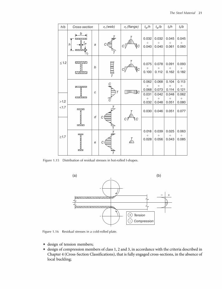
rolling process for a typical I-beam profile and in particular, the phases span from (a), end ofthe hot-rolling process, to (d), the instant at which the whole profile is at ambient temperature.The magnitude and the distribution of residual stresses depend on the geometric characteristics ofthe cross-section and, in particular, on the width to thickness ratio of its elements (flangesand webs).For I-shaped elements, Figure 1.15 shows the distribution of residual stresses (σr) as a function
of the width/thickness ratio of the cross-sectional elements: terms h and b refer to the height of theprofile and to the width of the flange, respectively, while tw and tf indicate web and flange thick-ness, respectively. Stocky profiles; that is, those that have a height/width ratio not greater than 1.2,show tensile residual stresses in the middle of the flanges and compressive residual stresses at theextremes of the flanges, while in the web there can be either tensile or compressive residual stres-ses, depending on the geometry. For slenderer profiles with h/b ≥ 1.7, the middle part of theflanges show prevalently tensile residual stresses, while compressive residual stresses can be foundin the middle region of the web.Residual stresses can affect the load carrying capacity of member, especially when they are sub-
ject to compressive forces. For larger cross-sections, the maximum values of the residual stressescan easily reach the yielding strength of the material.
(a) (b) (c) (d)
+
+
++
Tension Compression–
– – –
Figure 1.13 Residual stress distribution in a hot-rolled rectangular profile during the cooling phase (temporaryfrom a to d).
The Steel Material 19

In the case of cold-formed profiles and plates, the raw product is a hot- or cold-rolled sheet. Ifthe rolling process is performed at ambient temperature, the outermost fibres, in contact with therollers, tend to stretch, while the central fibres remain undeformed. As a consequence, a self-equilibrated residual state of stress arises, such as the one shown in Figure 1.16, due to the dif-ferential elongation of the fibres in the cross-section.
In the case of hot-rolling of a plate, the residual stresses develop similarly to those presented forthe rectangular (Figure 1.13) and for the I-shaped (Figure 1.14) sections.
In the case of cold-formed profiles or metal decks, an additional source of imperfections is thecold-formation process. The bending processes in fact alter the mechanical properties of thematerial in the vicinity of the corners. In order to permanently deform the material, the processbrings it beyond its yielding point so that the desired shape can be attained. As an example, Figure1.17 shows the values of the yielding strength (fy) and of the ultimate strength (fu) for the virginmaterial compared to the same values for the cold-formed profile at different locations. It is appar-ent how the cold-formation process increases both yielding and failure strengths, with a largerimpact on the yielding strength.
From the design standpoint, recent provisions on cold-formed profiles, among which part 1–3of Eurocode 3 (EN-1993-1-3) allows account for a higher yielding strength of the material, dueto the cold-formation process, when performing the following design checks:
+
–
Tension
Compression
T0
(a)
T
(d)+
+
+–
––
(b)
–
T1
+
+
–
–
+
T2
(c)
–+ +
+
–
–
Figure 1.14 Distribution of residual stresses during the cooling phase of an I-shape.
20 Structural Steel Design to Eurocode 3 and AISC Specifications
• design of tension members;• design of compression members of class 1, 2 and 3, in accordance with the criteria described in
Chapter 4 (Cross-Section Classifications), that is fully engaged cross-sections, in the absence oflocal buckling;
h/b
≤ 1.2
>1.2
<1.7
≥1.7
h
b
b
c
d
e
a C
T
σr (web) σr (flange)
C C
0.032
÷0.040
0.075
÷0.100
0.062
÷0.068
0.031
÷0.032
0.018
÷0.028
0.039
÷0.056
0.025
÷0.043
0.063
÷0.085
0.042
÷0.048
0.048
÷0.051
0.062
÷0.080
0.068
÷0.073
0.104
÷0.114
0.113
÷0.121
0.078
÷0.112
0.091
÷0.162
0.093
÷0.182
0.032
÷0.040
0.045
÷0.061
0.045
÷0.060
tw/h tw/b tf/h tf/b
T
C
C
C
C
C
C C
0.030 0.046 0.051 0.077
T
T
T
T
C
T
T
T
TC
T
T
tw
tf
Cross-section
Figure 1.15 Distribution of residual stresses in hot-rolled I-shapes.
+–
Tension
Compression
+
–
(a) (b)
Figure 1.16 Residual stresses in a cold-rolled plate.
The Steel Material 21

• design of flexural members with compression elements of class 1, 2 and 3 (i.e. with fullyengaged compression elements, in the absence of local buckling).
The stub column test (Section 1.7.2) can be used to experimentally evaluate the increase ofstrength of a cold-formed member; alternatively, the post-forming average yielding strength fyacan be evaluated based on the virgin material’s yielding and ultimate strength (fyb and fu, respect-ively) as follows:
fya = fyb +fu− fyb k n t2
Ag1 4a
fya ≤fyb + fu
21 4b
inwhich coefficient k accounts for the typeof process (k = 5 in all the cases except for the continuousformationwith rollers forwhich k = 7has tobe adopted),Ag is the gross areaof the cross-section,n isthe number of 90 bends with an inner radius r ≤ 5 t (bends at angles different than 90 are takeninto account with fractions of n) and t is the thickness of the plate or coil before forming.
Theaveragevalueof the increasedyieldingstrength fybcannotbeusedwhencalculating theeffectivecross-section area, orwhendesigningmembers that, after the cold formingprocess, havebeen subjectto heat treatments such as annealing, which reduce the residual stresses due to cold forming.
1.6.2 Geometric Imperfections
The term geometric imperfections refers to those differences that can be found between thetheoretical shape and real size of themembers, or of the structural systems as awhole, and the actualmembers or as-built structure. In particular, geometric imperfections can be subdivided into:
• cross-sectional imperfections;• member imperfections;• structural system imperfections.
Cross-sectional imperfections are related to the dimensional variation of the cross-sectionalelements with respect to the nominal dimensions and can be ascribed essentially to the productionprocess. Different values of area, moments of inertia and section moduli can influence the per-formance of the cross-section (e.g. in terms of load-carrying capacity or bending moment
K J H G
Strength(before forming)
Yielding(before forming)
AA BC D E F GH J K L MNOPQ
Q
B
C
D
E
F
500
450
400
350
300fy
ft
ft,fy (Nmm–2)
250
P
O
N
M
L
Figure 1.17 Variation of the mechanical properties of the material after cold-formation.
22 Structural Steel Design to Eurocode 3 and AISC Specifications

resistance). Tolerances are established by standards for the final products, not only in terms ofmaximum difference between actual and nominal linear dimensions, but also with reference to:
• perpendicularity tolerance between cross-sectional elements;• tolerances with respect to axes of symmetry;• straightness tolerance.
Figure 1.18 shows few examples of parameters to be measured for the tolerance checks for anI-shaped section.Among member imperfections, the longitudinal (bow) imperfection is certainly the most
important. It consists essentially of a deviation of the axis of the element from the ideal straightline and is caused by the production process. This out-of-straightness defect can cause load eccen-tricity, as well as an increased susceptibility to buckling phenomena.Structural system imperfections can be ascribed to various causes, such as variability in the
lengths of framing members, lack of verticality of columns and of horizontality of beams, errorsin the location of foundations, errors in the placement of the connections and so on. These imper-fections must be carefully accounted for during the global analysis phase. In a very simplified butefficient way, additional fictitious forces (notional loads) can be applied to the structure to repro-duce the effects of imperfections. For example, the lack of verticality of columns in sway frames isaccounted for by adding horizontal forces to the perfectly vertical columns (Figure 1.19), propor-tional to the resultant vertical force Fi acting on each floor.This design simplification can be explained directly with reference to a cantilever column of
height h with an out-of-plumb imperfection and subject to a vertical force N at the top. The add-itional bending momentM due to the lack of verticality, expressed by angle φ (Figure 1.20), can beapproximated at the fixed end as:
M =N h tan φ 1 5
Within the small displacement hypothesis (thus approximating tan (φ) with the angle φ itself ),the effect of this imperfection can be assimilated to that of a fictitious horizontal force F acting atthe top of the column and causing the same bending moment at the base of the column. The mag-nitude of F is thus given by:
F =Mh=Nϕ 1 6
(b)
b1 b2
(c)
f
t
(a)
tb
Figure 1.18 Additional tolerance checks for I-shapes: (a) perpendicularity tolerance, (b) symmetry tolerance and(c) straightness tolerance.
The Steel Material 23

1.7 Mechanical Tests for the Characterization of the Material
An in-depth knowledge of the mechanical characteristics of steel, as well as of any other structuralmaterial, is of paramount importance for design verification checks. Additionally, besides themandatory tests performed at the factory on base materials and worked products, it is oftenimportant to perform laboratory tests on coupons cut from plane and linear in-situ productsin order to validate the design hypotheses with actual material characteristics.
For each laboratory test there are very specific standardization requirements. Globally ISO(International Organization for Standardization) and in Europe CEN (European Committee forStandardization) standardization requirements are provided, whereas in the US, the ASTM isthe governing body, emanating standards that contain detailed instructions on the geometry ofthe coupons, on the testing requirements, on the equipment to be used and on the presentationand use of the test results.
Among the most important tests for the characterization of steel there are: chemical analysis,macro- and micro-graphic testing. In particular, chemical analysis is very important to determinethe main properties of steel, among which are weldability, ductility and resistance to corrosion,and to determine the percentage of carbon and other desired and undesired alloying elements.
F1
φF2
F3
(a)
φF1
φF2
φF3
F1
F2
F3
(b)
Figure 1.19 Horizontal notional loads equivalent to the imperfections for a sway frame.
N
(a) (b)
N N
hφ
N
φN
φN
Figure 1.20 Imperfect column (a) and horizontal equivalent force (b).
24 Structural Steel Design to Eurocode 3 and AISC Specifications

Some alloying elements have no direct impact on thematerial strength, but play a key role in thedetermination of other properties, such as weldability and corrosion resistance. As discussed inthe introductory section, in addition to carbon and iron, impurities can be present that can have adetrimental effect on the behaviour of the material, such as favouring brittleness. Since it is vir-tually impossible and uneconomical to completely eliminate such impurities, it is important toverify that their content is within acceptable limits. Due to these considerations, based on thegrade of steel considered, the standards specifying material characteristics (EN 10025, ASTMA992, ASTMA36, ASTMA490 are some examples) contain tables defining the maximum percentcontent of some alloying elements (typically, carbon – C, silica – Si, phosphorous – P, sulfur – Sand nitrogen –N) or a range of acceptability for other alloying elements (such as manganese –Mn, chromium – Cr, molybdenum –Mo and copper – Cu).Chemical analyses can be performed either on the molten material (ladle analysis) or on the
final product (product analysis), even after it has been erected, by means of a sample site extrac-tion. It is possible that the limits prescribed for the chemical makeup of the material can be dif-ferent, based on whether the analysis has been performed on the ladle material or on the finalproduct (in general, the values prescribed for the analysis on molten material are more stringentthan the ones on the final product).The weldability property is directly related to a carbon equivalent value (CEV), based on the
results of the analysis on the ladle material, defined as follows:
CEV=C+Mn6
+Cr +Mo+V
5+Ni +Cu
151 7
in which C indicates the percentage content of carbonium, Mn for manganese, Cr for chromium,Cu for copper, Mo for molybdenum and Ni for nickel.In order to ensure good weldability characteristics, the material should have as low a CEV as
possible, with maximum values prescribed by the various standards.Themacrographic test is performed to establish the de-oxidation and the de-carbonation indices
of steel, related to weldability. The micrographic test allows analysis of the crystalline structure ofsteel and its grain size and the ability to relate somemechanical characteristics of the material to itsmicro-structure as well as to investigate the effects that thermal treatments have on the material.In the following, a brief description of some of the most important mechanical laboratory tests
performed on structural steel is presented.
1.7.1 Tensile Testing
The most important and well-known mechanical test is the uniaxial tensile test. This test allowsmeasurement of some important mechanical characteristics of steel (yield strength, ultimatestrength, percentage elongation at failure and the complete stress-strain curve, as discussed inSection 1.1). The test consists of the application of a tensile axial force to a sample obtainedaccording to specific standards (EN ISO 6892-1 and ASTM 370-10). The tensile force is appliedwith an intensity that increases with an established rate, recording the extension Δ over a gaugelength L0 in the middle of the sample (Figure 1.21).The stress σ is calculated dividing the measured applied force by the nominal cross-sectional
area of the coupon (Anom), while the strain ε is calculated by means of change of the gauge length:
ε=ΔL0
=Ld−L0L0
1 8
in which Ld is the distance between the gauge marks during loading.
The Steel Material 25

For steel materials with a carbon percentage of up to 0.25%, that is for structural steels, thetypical stress-strain relationship is shown in Figure 1.22. The initial branch of the curve is veryclose to linear elastic.
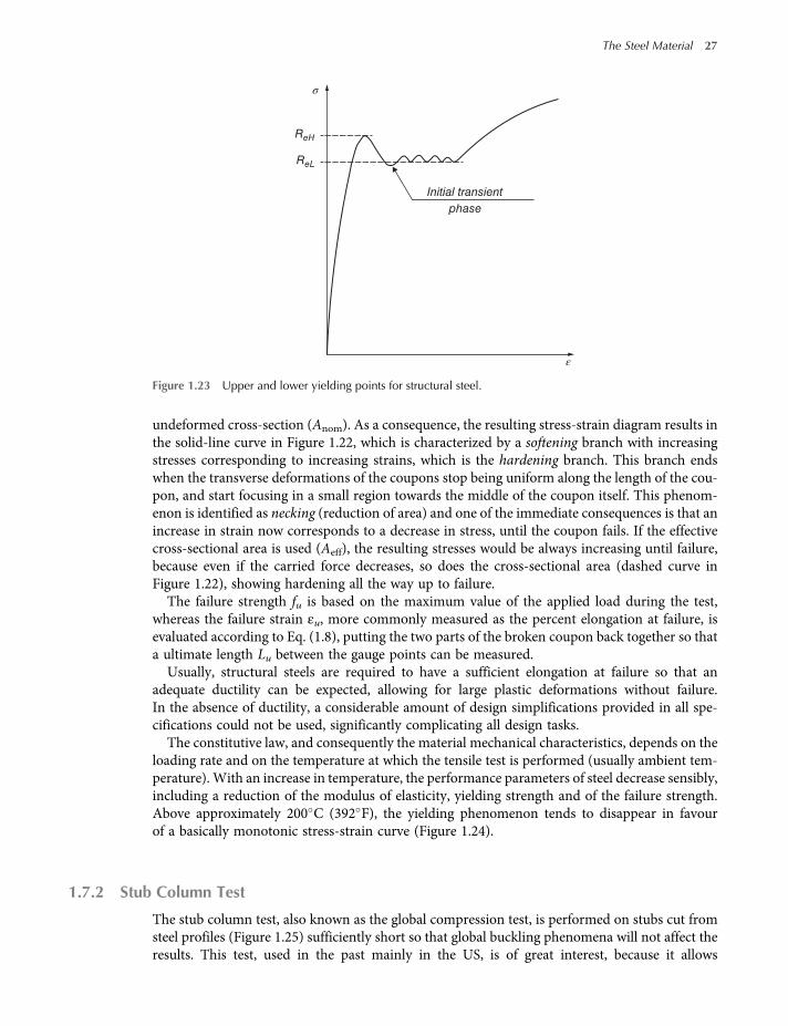
From the slope of the initial branch of the σ–ε curve, the longitudinal elasticmodulus or Young’smodulus, canbe calculated asE = tan(α).Once the value of the stress indicatedwith f0 in the figure isreached,which canbe defined as the limit of proportionality, there is nomore direct proportionalitybetween stress and strain, but thematerial still behaves elastically.Corresponding to a stress fy, yield-ing occurs and the stress-strain response is characterized by a slightly undulating response that issubstantially horizontal due to the onset plastic deformations (Figure 1.23).
It is worth noting that low-carbon steels usually show two distinct values of the yielding stress:an upper yielding point, ReH, after which the strains increase with a local decrease of the stress, anda lower yielding point, ReL, at which there are no appreciable reductions in the stress associatedwith an increase in strain. The upper yielding point ReH is significantly affected by the load rate,unlike the lower yielding point, which is substantially independent of the rate and is thus usuallytaken as the yielding strength to be used for design, that is fy = ReL.
Until the yielding stress is reached, the transverse deformations of the coupon due to Poisson’seffect are very small. The effective cross-sectional area of the coupon (Aeff) is considered, with asmall approximation, to be equal to the nominal cross-sectional area (Aeff = Anom). For higherlevels of the applied force, the transverse deformations are not negligible anymore, but for thesake of practicality the stress is always calculated making reference to the nominal area of the
S
S
d
a
a
L0
L0
Figure 1.21 Typical sample for rolled products.
ft
N=
A
N
N
Anom
Aeff
fy
tgα= E
f0
α
εεu
σ
Figure 1.22 Typical stress-strain (σ–ε) relationship for structural steels.
26 Structural Steel Design to Eurocode 3 and AISC Specifications
undeformed cross-section (Anom). As a consequence, the resulting stress-strain diagram results inthe solid-line curve in Figure 1.22, which is characterized by a softening branch with increasingstresses corresponding to increasing strains, which is the hardening branch. This branch endswhen the transverse deformations of the coupons stop being uniform along the length of the cou-pon, and start focusing in a small region towards the middle of the coupon itself. This phenom-enon is identified as necking (reduction of area) and one of the immediate consequences is that anincrease in strain now corresponds to a decrease in stress, until the coupon fails. If the effectivecross-sectional area is used (Aeff), the resulting stresses would be always increasing until failure,because even if the carried force decreases, so does the cross-sectional area (dashed curve inFigure 1.22), showing hardening all the way up to failure.The failure strength fu is based on the maximum value of the applied load during the test,
whereas the failure strain εu, more commonly measured as the percent elongation at failure, isevaluated according to Eq. (1.8), putting the two parts of the broken coupon back together so thata ultimate length Lu between the gauge points can be measured.Usually, structural steels are required to have a sufficient elongation at failure so that an
adequate ductility can be expected, allowing for large plastic deformations without failure.In the absence of ductility, a considerable amount of design simplifications provided in all spe-cifications could not be used, significantly complicating all design tasks.The constitutive law, and consequently the material mechanical characteristics, depends on the
loading rate and on the temperature at which the tensile test is performed (usually ambient tem-perature). With an increase in temperature, the performance parameters of steel decrease sensibly,including a reduction of the modulus of elasticity, yielding strength and of the failure strength.Above approximately 200 C (392 F), the yielding phenomenon tends to disappear in favourof a basically monotonic stress-strain curve (Figure 1.24).
1.7.2 Stub Column Test
The stub column test, also known as the global compression test, is performed on stubs cut fromsteel profiles (Figure 1.25) sufficiently short so that global buckling phenomena will not affect theresults. This test, used in the past mainly in the US, is of great interest, because it allows
Initial transient
phase
ReH
σ
ε
ReL
Figure 1.23 Upper and lower yielding points for structural steel.
The Steel Material 27

measurement of a stress-strain curve for the whole cross-section of a member, not just for a cou-pon cut from it.
The stub column test, in fact, provides the mechanical properties of the materials averaging outthe structural imperfections of the profile due, for instance, to the presence of residual stresses orto different yielding of failure strengths in various parts of the profile (web, flanges, etc.). Someprofiles, in fact, due to the production process, may show a variation of mechanical propertiesacross the thickness and also have a non-uniform distribution of residual stresses. An equivalentyielding strength (fy,eq) can be evaluated as a function of the experimental load that causes yieldingof the specimen (Py,exp) and of the cross-sectional area (A) as follows:
σ
T ≃ 20°C
T ≃ 200°C
T ≃ 400°C
ε
Figure 1.24 Influence of temperature on the constitutive law of steel.
Figure 1.25 Testing of a specimen in a stub column test.
28 Structural Steel Design to Eurocode 3 and AISC Specifications
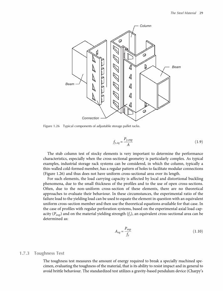
fy,eq =Py, expA
1 9
The stub column test of stocky elements is very important to determine the performancecharacteristics, especially when the cross-sectional geometry is particularly complex. As typicalexamples, industrial storage rack systems can be considered, in which the column, typically athin-walled cold-formed member, has a regular pattern of holes to facilitate modular connections(Figure 1.26) and thus does not have uniform cross-sectional area over its length.For such elements, the load carrying capacity is affected by local and distortional buckling
phenomena, due to the small thickness of the profiles and to the use of open cross-sections.Often, due to the non-uniform cross-section of these elements, there are no theoreticalapproaches to evaluate their behaviour. In these circumstances, the experimental ratio of thefailure load to the yielding load can be used to equate the element in question with an equivalentuniform cross-section member and then use the theoretical equations available for that case. Inthe case of profiles with regular perforation systems, based on the experimental axial load cap-acity (Pexp) and on the material yielding strength (fy), an equivalent cross-sectional area can bedetermined as:
Aeq =Pexpfy
1 10
1.7.3 Toughness Test
The toughness test measures the amount of energy required to break a specially machined spe-cimen, evaluating the toughness of the material, that is its ability to resist impact and in general toavoid brittle behaviour. The standardized test utilizes a gravity-based pendulum device (Charpy’s
Column
Connection
Beam
Beam
Figure 1.26 Typical components of adjustable storage pallet racks.
The Steel Material 29

pendulum) and the specimen is a rectangular bar with a suitable notch having a standardizedshape (Figure 1.27). The impact is provided by a hammer suspended above the specimen thatis released starting at a relative height h. Upon impacting the specimen, which is restrained bytwo supports at its ends, the hammer continues its swing climbing on the opposite side to anew relative height h0 (with h0 < h). The difference between h and h0 is proportional to the energyabsorbed by the specimen, Ep, that is:
Ep =G h – h0 1 11
in which G is the weight of the hammer.Toughness is measured by the ratio between the energy Ep and the area of the notched cross-
section of the specimen. The tougher is the metal, the smaller the height h0.Toughness values depend on the shape of the specimen and in particular on the details of the
notch. Among standardized notch types, it is worth mentioning the types: type KV, type Kcu, typeKeyhole, type Messenger and type DVM. Usually toughness decreases as the mechanical strengthincreases and it is greatly influenced by the testing temperature, which affects the crack formationand propagation.
A temperature value can be identified, referred to as transition temperature, below whichtoughness is reduced so much to be unacceptable, due to the excessive brittleness of the material.For special applications (structures in extremely cold climates, freezing plants, etc.), metals with avery low transition temperature must be used. Toughness is expressed in energy units, usuallyJoules, at a specified temperature. Sometimes, the code used to identify toughness (e.g. JR, J0or J2) follows the identification of the steel type. For structural steel, the minimum toughnessrequired is usually 27 J, as already briefly discussed in Section 1.1. Table 1.5 contains an exampleof required toughness values for various European designations.
h
h0
Sample
Hammer
mass
Figure 1.27 Charpy V-notch test.
30 Structural Steel Design to Eurocode 3 and AISC Specifications

For welded steel construction, and especially for those structures subject to low temperatures, itis advisable to choose steels with good toughness at low temperatures. Thermo-mechanical rollingtypically produces these kinds of steel. It is also worth keeping in mind that good toughness alsocorresponds to good weldability.Despite the fact that the ductility of a particular class of steel can be evaluated by means of
laboratory tests, the same material in special conditions could show a fragile behaviour associatedwith a sudden failure at low stresses, even below yielding.Fragile behaviour depends on several factors. Among these, the temperature at which the elem-
ent is subject to in-service can cause this type of failure.With reference to the Charpy V-notch test,indicating with Av(T) the work performed by the hammer as a function of the test temperature(T), a diagram similar to the one in Figure 1.28 can be obtained, characterized by the followingthree regions:
• region A, corresponding to higher temperatures, with higher toughness values, indicating amaterial capable of undergoing large plastic deformations;
• region C, corresponding to lower temperatures, with very small toughness values and thus ele-vated brittleness;
• region B, between regions A and C, is the transition zone and is characterized by a very variablebehaviour, with a rapid decrease in toughness as the temperature decreases.
C
B
27J
T27J T [°C]
Av (T)
A
Figure 1.28 Energy associated with the toughness test as a function of the testing temperature.
Table 1.5 Codes used for toughness requirement (Charpy V-notch).
Test temperature ( C)
Minimum value of energy
27 J 40 J 60 J
20 JR LR KR0 J0 L0 K0−20 J2 L2 K2−30 J3 L3 K3−40 J4 L4 K4−50 J5 L5 K5−60 J6 L6 K6
The Steel Material 31

Brittle failure can also be influenced by the rate of increase of stresses, as there is the possibilityof localized overstresses that could practically prevent the onset of plastic deformations, causingsudden failures. The width of the three regions in Figure 1.28 is a function of the chemical com-position of the steel. In particular, the transition temperature can be lowered by acting on thecontent of carbon, manganese and nickel, and/or with annealing or quenching and tempering heattreatments.
1.7.4 Bending Test
The bending test is used to evaluate the capacity of the material to withstand large plastic deform-ations at ambient temperature without cracking. The specimen, usually with a solid rectangularcross-section (but circular or rectangular solid specimens can also be used) is subject to a plasticdeformation by means of a continuous bending action without load reversal. In detail, as shown inFigure 1.29, the specimen is placed over two roller bearings with radius R and then a force isapplied by means of another roller with diameter D until the ends of the specimen form an angleα with respect to each other.
The values of R andD depend on the size of the specimen. At the end of the test, the specimen’sbottom face is examined to ascertain that no cracks have formed.
1.7.5 Hardness Test
Hardness, for metals, represents the resistance that the material opposes to the penetration ofanother body and thus allows gathering of information on the resistance to scratching, to abra-sion, to friction wear and to localized pressure.
The hardness test measures the capacity of the material to absorb energy and can also providean estimate of the material strength. The test itself consists in the measurement of the indentationleft on the specimen surface by a steel sphere that is pressed onto the specimen with a predeter-mined amount of force for a predetermined amount of time (Figure 1.30).
Depending on the shape of the tip penetrating device, there are various hardness tests that arechosen based on the material to be tested. Among these, the Brinell Hardness Test, the VickersHardness Test and the Rockwell Hardness Test are the most important.
The ISO 18265 norm, ‘Metallic Materials Conversion of Hardness Values’, has been specificallywritten to provide conversion values among the various types of hardness tests.
DD
α
F
R R
a
a
bR R
Figure 1.29 Bending test.
32 Structural Steel Design to Eurocode 3 and AISC Specifications

Thanks to the somewhat direct relationship between hardness and strength, hardness testing issometimes used to evaluate the tensile strength of metal elements in the field when a destructivetest is not an option. In the past, several research projects have been conducted to establish a cor-relation between hardness and tensile strength in some materials. It is worth mentioning that, in1989, the Technical Report ISO/TR 10108 ‘Steel-Conversion of Hardness Values to Tensile StrengthValues’ was published, reporting the range of tensile strength values corresponding to experimen-tally measured hardness.
(a) (b)
(c)
Figure 1.30 Hardness test: (a) durometer, (b) conical tip and (c) spherical tip.
The Steel Material 33

CHAPTER 2
References for the Design of SteelStructures
2.1 Introduction
A structure has to be designed and executed in such a way that, during its intended life, it willsupport all load applied, with an appropriate degree of reliability and in an economical way.A very important task of each designer is to size the skeleton frame to be safe for the entire lifeof the structure. This condition is guaranteed if, from the construction stage until decommission-ing due to old age, this condition is satisfied for each component of the structure:
Effects of actions < Resistance 2 1
With regard to internal forces and moments, on the basis of the structural model, designersmust select the loads and individuate the load combinations of interest. It is essential to estimatethe loads acting on the structure defining their values appropriately, that is without exaggeration(otherwise, the resulting system could be too heavy and un-economical) but at the same timeavoiding load values that are too low, which would lead to unsafe design.
As far as the resistance is concerned, suitable design limits are fixed by codes, which refer to theperformance of the cross-section as well as of the parts of whole structural systems. Designers haveto evaluate them correctly.
A fundamental requisite of design is that the structure must be safe throughout its use, other-wise all the subjects contributing to the safety of building are responsible, that is designer, projectmanager, builders, acceptance test engineers and so on.
The concept of building safety is very old. Babylonian king, Hammurabi, about 4000 years agoimposed the law of retaliation to builders, with a penalty proportional to the social class of mem-bership of the parties involved. In this code, which is the first significant example of treaty law, itwas prescribed that:
• If a builder builds a house for someone and completes it, the owner should give him a fee of twoshekels in money for each sar of surface (rule 228).
• If a builder builds a house for someone, and does not construct it properly, and the house which hebuilt falls and kills its owner, then the builder should be put to death (rule 229).
• If it kills the son of the owner the son of that builder should be put to death (rule 230).• If it kills a slave of the owner, then he should pay slave for slave to the owner of the house
(rule 231).
Structural Steel Design to Eurocode 3 and AISC Specifications, First Edition. Claudio Bernuzzi and Benedetto Cordova.© 2016 John Wiley & Sons, Ltd. Published 2016 by John Wiley & Sons, Ltd.

It is important to note the attention given to the concept of durability by this very old code: eventhen it was assumed that a fundamental requirement of the construction was no damage shouldoccur during its entire life.About two centuries ago, Napoleon Bonaparte introduced the concept of responsibility
extended to the first decade of age of the construction. In addition to the builder, thepresence of a technician (e.g. the designer) was required too, sharing all the responsibilitiesand, eventually prison, in case of collapse or damage within a decade from putting the structureinto service.
2.1.1 European Provisions for Steel Design
In 1975, the Commission of the European Community decided on an action programme in thefield of construction, based on article 95 of the Treaty, with the objective of eliminating all thetechnical obstacles to trade and the harmonization of technical specifications. Within this actionprogramme, the Commission took the initiative to establish a set of harmonized technical rules forthe design of construction works that, in the first stage, would serve as an alternative to thenational rules in force in the Member States and, ultimately, would replace them. For 15 years,the Commission, with the help of a Steering Committee with Representatives of Member States,conducted the development of the Eurocodes programme, which led to the first generation ofEuropean codes in the 1980s.The Structural Eurocode programme comprises the following standards consisting of 10 parts:
EN 1990 – Eurocode 0: Basis of structural design;EN 1991 – Eurocode 1: Actions on structures;EN 1992 – Eurocode 2: Design of concrete structures;EN 1993 – Eurocode 3: Design of steel structures;EN 1994 – Eurocode 4: Design of composite steel and concrete structures;EN 1995 – Eurocode 5: Design of timber structures;EN 1996 – Eurocode 6: Design of masonry structures;EN 1997 – Eurocode 7: Geotechnical design;EN 1998 – Eurocode 8: Design of structures for earthquake resistance;EN 1999 – Eurocode 9: Design of aluminium structures.
The Eurocode standards provide common structural design rules for everyday use for thedesign of whole structures and component products of both traditional and innovative nature.Unusual forms of construction or design conditions are not specifically covered and additionalexpert consideration will be required by the designer in such cases.The National Standards implementing Eurocodes comprise the full text of the Eurocode
(including any annexes), as published by CEN, which may be preceded by a National Title Pageand National Foreword, and may be followed by a National Annex. This may only contain infor-mation on those parameters that are left open in the Eurocode for national choice, known asNationally Determined Parameters, to be used for the design of buildings and civil engineeringworks to be constructed in the country concerned, that is:
• values and/or classes where alternatives are given in Eurocodes,• values to be used where a symbol only is given in Eurocodes,• country specific data (geographical, climatic, etc.), for example, a snow map,• the procedure to be used where alternative procedures are given in Eurocodes,• references to non-contradictory complementary information to assist the user to apply
Eurocodes.
References for the Design of Steel Structures 35

There is a need for consistency between the harmonized technical specifications for construc-tion products and the technical rules for works.
The EN 1993 (in the following identified as EC3 or Eurocode 3) is intended to be used withEurocodes EN 1990 (Basis of Structural Design), EN 1991 (Actions on structures) and EN1992 to EN 1999, when steel structures or steel components are referred to.
EN 1993-1 is the first of six parts of EN 1993 (Design of Steel Structures), to which thisbook refers to. It gives generic design rules intended to be used with the other parts EN1993-2 to EN 1993-6. It also gives supplementary rules applicable only to buildings. EN1993-1 comprises 12 subparts EN 1993-1-1 to EN 1993-1-12 each addressing specific steelcomponents, limit states or materials. In the following, the list of all the EN 1993 documentsis presented:
EN 1993-1: Eurocode 3: Design of steel structures – Part 1, which is composed by:EN 1993-1-1: Eurocode 3: Design of steel structures – Part 1-1: General rules and rules for
buildings;EN 1993-1-2: Eurocode 3: Design of steel structures – Part 1-2: General rules – Structural fire
design;EN 1993-1-3: Eurocode 3 –Design of steel structures – Part 1-3: General rules – Supplementary
rules for cold-formed members and sheeting;EN 1993-1-4: Eurocode 3 –Design of steel structures – Part 1-4: General rules – Supplementary
rules for stainless steels;EN 1993-1-5: Eurocode 3 –Design of steel structures – Part 1-5: Plated structural elements;EN 1993-1-6: Eurocode 3 –Design of steel structures – Part 1-6: Strength and Stability of Shell
Structures;EN 1993-1-7: Eurocode 3 –Design of steel structures – Part 1-7: Plated structures subject to out
of plane loading;EN 1993-1-8: Eurocode 3: Design of steel structures – Part 1-8: Design of joints;EN 1993-1-9: Eurocode 3: Design of steel structures – Part 1-9: Fatigue;EN 1993-1-10: Eurocode 3: Design of steel structures – Part 1-10: Material toughness and
through-thickness properties;EN 1993-1-11: Eurocode 3 –Design of steel structures – Part 1-11: Design of structures with
tension components;EN 1993-1-12: Eurocode 3 –Design of steel structures – Part 1-12: Additional rules for the
extension of EN 1993 up to steel grades S 700;EN 1993-2: Eurocode 3 –Design of steel structures – Part 2: Steel Bridges;EN 1993-3-1: Eurocode 3 –Design of steel structures – Part 3-1: Towers, masts and chimneys –
Towers and masts;EN 1993-3-2: Eurocode 3 –Design of steel structures – Part 3-2: Towers, masts and chimneys –
Chimneys;EN 1993-4-1: Eurocode 3 –Design of steel structures – Part 4-1: Silos;EN 1993-4-2: Eurocode 3 –Design of steel structures – Part 4-2: Tanks;EN 1993-4-3: Eurocode 3 –Design of steel structures – Part 4-3: Pipelines;EN 1993-5: Eurocode 3 –Design of steel structures – Part 5: Piling;EN 1993-6: Eurocode 3 –Design of steel structures – Part 6: Crane supporting structures.
Numerical values for partial factors and other reliability parameters are recommended as basicvalues that provide an acceptable level of reliability. They have been selected assuming that anappropriate level of workmanship and quality management applies.
36 Structural Steel Design to Eurocode 3 and AISC Specifications

2.1.2 United States Provisions for Steel Design
The main specification to apply for the design of steel structures in United States is ANSI/AISC360-10 ‘Specification for Structural Steel Buildings’ that addresses steel constructions as well ascomposite constructions: steel acting compositely with reinforced concrete. This specificationstates design requirements (stability and strength) for steel members and composite construc-tions, design of connections, fabrication and erection, Quality Control and Quality Assurance.AISC 360-10 does not address minimum loads to be used: this topic is covered by ASCE/SEI 7-
10 ‘Minimum Design Loads for Buildings and Other Structures’ in the absence of an applicablespecific local, regional or national building code.AISC 360-10 does not cover seismic design: for seismic resistant structures the specifications to
be applied are: ANSI/AISC 341-10 ‘Seismic Provisions for Structural Steel Buildings’ and ANSI/AISC 358-10 ‘Prequalified Connections for Seismic Applications’. The first one gives additionalrules for design and fabrication of steel structure to be used in seismic areas, the second one givesdesign methods for designing connections to be used in seismic resistant structures.Finally, AISC 303-10 ‘Code of Standard Practice for Steel Buildings and Bridges’ addresses
design, purchase, fabrication and erection of structural steel.Very useful tools for the designer are the AISCmanuals: mainly theAISC 325 Steel Construction
Manual and AISC 327 Seismic Design Manual, which discuss very interesting design examples tohelp in design activity.
2.2 Brief Introduction to Random Variables
All the variables involved in the design phase, both for determining resistance and stress distri-bution in cross-sections and members, are random in nature and not deterministic. As anexample, with reference to the strength of materials, the imperfect homogeneity always presentin samples for laboratory tests, as well as in structural in-situ elements, prevents association ofan univocal value to resistance properties (such as, for example the yielding stress or the ultimatestrength). Similarly, the set of internal forces and moments on structural members due to actingloads cannot be determined exactly because of the major sources of uncertainty and approxima-tion involved in the parameters used for their definition.Random variables are characterized by a number that expresses the probability (indicated as
prob or pr) of their occurrence. In the following, Y indicates the considered random variable(e.g. the measurement associated to a length, to a force, to weight or to the value of the force actingon a structure) and y represents the generic value assumed; the probability is identified by the termprob or pr. The analytical treatment is based principally on the following two functions:
Relative Probability Density Function (PDF) (Figure 2.1), fY (y), defined as:
fY y dy = prob y <Y ≤ y + dy = pr y <Y ≤ y + dy 2 2
Cumulate Density Function (CDF), FY (y), defined as:
FY y = prob Y ≤ y = pr Y ≤ y 2 3
The PDF describes the relative likelihood for this random variable to take on a given value. Theprobability of the random variable falling within a particular range of values is given by the inte-gral of this variable density over that range that is given by the area under the density function but
References for the Design of Steel Structures 37

above the horizontal axis and between the lowest and greatest values of the range. The PDF is non-negative everywhere, and its integral over the entire space is equal to one.
∞
−∞
fY y dy = 1 2 4
The cumulative PDF (CDF) represents the probability that the random variable in questiontakes a value not exceeding y and is linked to the PDF from the integral relationship:
FY y =
y
−∞
fY c dc 2 5
To better understand the correspondence between the functions PDF and CDF, it can be con-sidered Figure 2.2. The area under the PDF function in the range between –∞ and y1, or equallybetween –∞ and y2, finds a corresponding value of the abscissa of the CDF, FY (y1) and FY (y2),respectively.
As an example of distribution of random variable, the density probability function of the weightper unit volume of both the concrete and the steel material are presented in Figure 2.3. Note thatthe curve of the concrete is extended on a portion of the abscissa axis appreciably wider than that
y1 y2
dy dy
fY (y)
Y
Figure 2.1 Example of the probability density function (PDF).
fY (y) fY (y)
fY (y2)
fY (y1)
Y Yy1 y2y1 y2
1
Figure 2.2 Probability density function and cumulate density function.
38 Structural Steel Design to Eurocode 3 and AISC Specifications

corresponding to the steel, due to the relevant heterogeneity of the first material with respect to thelatter.As already mentioned, all the quantities interested in the check of Eq. (2.1) are random vari-
ables, and the data to be used in the design phase should be chosen based on reasonable probabilityvalues (or equally, acceptable risk levels) in relation to what they express. Actually, some of them(for example geometrical data or the eccentricity of loads) are, in most cases, taken as determin-istic in order to simplify design. As discussed in the following, for the resistance, reference is madeto low probabilistic values; that is to values with a high probability of being exceeded (95%).Otherwise, if actions are considered, high values (i.e. values with a reduced probability of beingexceeded: 5%) are assumed for design.In Figure 2.3 the values currently adopted for concrete and steel weight of the structural elem-
ents are indicated. (2400 kg/m3 (149.83 lb/ft3) to 7850 kg/m3 (490.06 lb/ft3) for concrete and steel,respectively). These values, like all the weights per unit of volume of both structural and non-structural elements usually correspond to the value that has a 95% probability of not beingexceeded, or the 5% probability of being exceeded, and are defined 95% fractile or 95% charac-teristic values.
2.3 Measure of the Structural Reliability and Design Approaches
In the last century there has been a significant evolution of the philosophy of the structural reli-ability and, as a consequence, of the design methods. Nowadays, very sophisticated approaches areavailable, able to account for the variability of the main parameters governing design. It should benoted that these calculation methods currently in use are characterized by precision awareness.Because of the uncertainties of different type and nature that intervene in the design, the structureis always characterized by a well-defined level of risk. As a consequence, it is not possible to designa structure characterized by a zero level of failure probability: every structure has a probability offailure strictly depending by design, erection phase and maintenance during its use. To betterunderstand this concept, reference can be made to Figure 2.4, where probability of failure andcosts are measured by the abscissa and ordinate axis, respectively, of the considered referencesystems.If the initial cost of construction is considered (curve for the erection phase), also including
design, a 100% safe structure is associated with infinite costs. The decrease in the cost of construc-tion corresponds to an increase in failure probability. Furthermore, costs associated with repairingphases during the construction life have to be considered, when both moderate (curve b) andsevere (curve c) damages could occur. It can be noted that costs associated with these damagesincrease with increasing failure probability. By adding the initial construction cost with theone of moderate or severe damages, the resulting curves (d and e, respectively) are characterized
2400 kg/m3 7850 kg/m3
Density
SteelConcrete
F
Figure 2.3 Probability density function for the weight per unit volume of the concrete and the steel.
References for the Design of Steel Structures 39

by a similar trend, with a minimum zone representing a good compromise between cost and over-all level of risk (optimal design with the maximum benefits and the minimum costs).
In this brief discussion about reliability measurement and design methods, reference is made toresistance (R) and the effects of actions (E), which are considered generic random variables, neg-lecting all the functional relationships that contribute to define them.
There are two significant relationships between R and E to measure the structural safety:
• the reliability level, or the safe margin, Z, which is defined by the difference between R and E:
Z =R – E 2 6
• the safety factor, γ, which is given by the ratio between R and E
γ =R E 2 7
The reliability level of a structure can be directly estimated by the exact methods, distinguishedin level IV and level III methods, depending on whether or not the human factor is considered tobe a cause of failure. Considering the resistance, R, and the effects of actions, E, as independentrandom variables, they can be represented in a three-dimensional reference system where the ver-tical axis expresses the associated PDF of failure (Figure 2.5). Furthermore, level IV methods arereliability methods that compare a structural prospect with a reference prospect. Principles ofengineering economic analysis under uncertainty are consequently taken into account by consid-ering cost and benefits of construction, maintenance, repair and consequences of failure. Methodsof the III level include numerical integration, approximate analytical methods and simulationmethods.
In the plane R–E, the safe zone (R > E) and the unsafe zone (R < E) are delimited by the bisectorplane containing point with R = E and the subtended volume identifies the failure probability (Pr),
Costs
d = a + c
e = a + b
Severe damages (c)
Moderate damages (b)
Erection phase (a)
Moderate
damage
Pr0 Severe
damage
Figure 2.4 Example of the relationship between costs and probability of an unsuccessful outcome.
40 Structural Steel Design to Eurocode 3 and AISC Specifications

that is it directly measures the safety of the construction. The use of such methods is extremelycomplex and expensive in terms of required resources as well as high engineering competenciesand is justified only for structures of exceptional importance, such as, for example, nuclear powerplants or large-scale infrastructure.The level II methods are characterized by a degree of complexity lower than those just presented
and are based on the assumption that resistance and effects of actions are statistically independentfrom each other. With reference to the safety margin Z (Eq. (2.6)), the failure probability is rep-resented by the area under the Probability Density Function (PDF) curve up to the point ofabscissa Z = 0, that is the hatched area in Figure 2.6 and it is expressed by the value of FZ (0), as:
Pr = FZ 0 =
0
−∞
fZ z dz 2 8
P
E = R
(E,R)
R
S
E = R
U
Volume = Pr
E
PE,R
Figure 2.5 Assessment of failure probability.
z = 0z
Fz(0)
fz
Figure 2.6 Safe domain in accordance with level II methods.
References for the Design of Steel Structures 41

Assuming that resistance and the effects of actions both have a Gaussian type distribution, it canbe convenient instead to make reference to the safety margin (Z) to a normalized safety margin, u,defined as:
u =z−ηzσz
2 9
where ηz is the average value of the Z and σz is its standard deviation.Failure probability depends on the CDF of variable U through the relationship:
Pr = 1 – FU β 2 10
where β is the so-called safety index.Increasing the safety index, the failure probability decreases. The graphical mean of β is pre-
sented in Figure 2.7, where the normalized resistance (φ) and the normalized effects of actions(Ψ ), are respectively defined as:
φ=r−ηRσR
2 11a
ψ =e−ηEσE
2 11b
It can be noted that β is the smallest distance from the straight line (or generally from the hyper-plane) forming the boundary between the safe domain and the failure domain, that is the domaindefined by the failure event. It should be noted that this definition of the reliability index does notdepend on the limit state function but rather the boundary between the safe domain and the fail-ure domain. The point on the failure surface with the smallest distance to origin is commonlydenoted the design point or most likely failure point.
Unlike top level methods (level III and IV), the level II approaches assess the value of β andverify that it complies with the limiting design conditions established by codes that are generallydefined by using level III methods.
Level I methods are the ones directly used for routine design, which are also identified asextreme value methods. It is assumed that all relevant variables xk can be modelled by randomvariables (or stochastic processes). Both resistance (R) and the effects of the actions (E) areassumed to be statically independent and they can be expressed as:
R= gR x1,x2,x3,…, xm 2 12a
E = gE xm+ 1,xm + 2,…,xn 2 12b
φ
β ψ
Figure 2.7 Safety index.
42 Structural Steel Design to Eurocode 3 and AISC Specifications

These methods refer to suitable values that are lower than the mean ones for the resistance andgreater than the mean ones for the effects of actions (Figure 2.8). Inserting these values in theprevious equations, the design value Rd and Ed are hence directly defined. The measure of securityis satisfied if E does not exceed R and this condition implicitly guarantees that the limits of allowedprobability are not exceeded.The so-called semi-probabilistic limit state method belongs to the family of level I methods for
practical design purposes. Its name is due to the fact that the variability of R and E is taken intoaccount in a simplified way by introducing appropriate safety coefficients γ. They can be distin-guished into reduction coefficients, γm (such as the ones for materials), and amplifying coeffi-cients, γf (such as the ones for actions). Limit state is defined as a state at which the structure(or one of its key components) cannot longer perform its primary function or no longer meetsthe conditions for which it was conceived. A distinction is required between ultimate limit statesand serviceability limit states.The limit states that concern the safety of people and/or the safety of the structure are classified
as ultimate limit states.The limit states that concern the functioning of the structure or structural members under nor-
mal use, the comfort of people and the appearance of the construction works, are classified asserviceability limit states. The verification of serviceability limit states should be based on suitablecriteria concerning the following aspects:
• deformations that affect appearance, comfort of users or the functioning of the structure(including the functioning of machines or services) or the damage caused to finishes ornon-structural members;
• vibrations that cause discomfort to people or that limit the functional effectiveness of thestructure;
• damage that is likely to adversely affect the appearance, the durability or the functioning of thestructure.
The level 0 methods, which have been widely applied in the past to structural design, do notconsider the probabilistic aspects. The most known and used method belonging to this family is
PR
PE
PE
Ek
E
U
E = R
S
PE,R
R
Rk
PR(R)
(E)
(E,R)
Figure 2.8 Verification in accordance with first level approaches.
References for the Design of Steel Structures 43

the so-called method of allowable stresses, which requires a direct comparison between the valuesof themaximum stress and the allowable resistance of thematerial in any critical point of themorestressed cross-section of members. In general, the following criticisms can be moved to the allow-able stress design (ASD) method:
• safety factors are large which can create the mistaken belief that designers have always very highsafety margins;
• it is impossible to determine the probability of collapse of the structure;• the verification of the local stress state is based on assumptions excessively simplified because
some important phenomena are not considered that influence it (with reference to reinforcedconcrete structures, e.g. the effects of inelastic deformations and cracking phenomena areignored);
• the effects induced by forces cannot be clearly distinguished from those produced bydistortions;
• it is not possible to organize checks against the various events that designers have to avoid whenthey do not depend directly from the acting stress level (e.g. corrosion, fire etc.).
2.4 Design Approaches in Accordance with Current Standard Provisions
As the aim of this book is to provide an introduction to the design of the steel structures, no dataare reported in the following about the basis of structural design. However, some base indicationsare required for the determination of the effects on the buildings and for the evaluation of theresistance of the structural components.
2.4.1 European Approach for Steel Design
The design value Fd of an action F can be expressed in general terms as:
Fd = γf ψ Fk 2 13
where γf is a partial factor for the action taking into account the possibility of unfavourable devi-ations from the representative value, ψ is the combination coefficient and Fk is the characteristicvalue of the action.
The combination ψ coefficients (Table 2.1) take into account the fact that maximum actionscannot occur simultaneously. Representative values of a variable action are:
• ψ0Fk: rare combination value used for the ultimate limit state verification and irreversible ser-viceability limit states;
• ψ1Fk: a frequency value used for the verification of ultimate limit states involving accidentalactions and for verifications of reversible serviceability limit states. As an example, for civiland commercial buildings the frequency value is chosen so that the time in which it is exceededis 0.01 (1%) of the reference period; for road traffic loads on bridges (the frequency value isgenerally assessed on the basis of a return period of 1 week);
• ψ2Fk: the quasi-permanent value used for the verification of ultimate limit states involving acci-dental actions and for the verification of reversible serviceability limit states. Quasi-permanentvalues are also used for the calculation of long-term effects.
The actions must be combined in accordance with the considered limit states in order to achievethe most unfavourable effects, taking into account the reduced probability of their simultaneous
44 Structural Steel Design to Eurocode 3 and AISC Specifications

actions with the respective most unfavourable values. The load combinations of the semi-probabilistic limit state method, which coincide with the ones to adopt for the verification atthe ultimate limit states, are symbolically expressed by the relationship:
Fd = γG1G1 + γG2G2 + γPPk + γQ1Q1k +n
i= 2
γQi ψ0iQik 2 14
where the signs + and Σ mean the simultaneous application of the respective addenda, the coef-ficients γ represent amplification factors, the subscript k indicates the characteristic value while Gidentifies the permanent loads (subscript 1 for permanent structural and subscript 2 for non-structural), Q is the variable loads, P is the possible action of prestressing and ψ0i is the coefficientof the combination of actions.Table 2.2 provides the γ values of the coefficients of the actions to be assumed for the ultimate
limit state checks. The symbols in the table have the following meaning:
• γG1 partial factor for the weight of the structure, as well as the weight of the soil;• γG2 partial coefficient of the weights of non-structural elements;• γQi partial coefficient of the variable actions.• γP prestressing coefficient, taken equal to unity (γP = 1.0).
Table 2.1 Proposed values of the ψ combination coefficients (from Table A1.1 of EN 1990).
Action ψ0 ψ1 ψ2
Imposed loads in buildings, category (see EN 1991-1-1) 0.7 0.5 0.3Category A: domestic, residential areasCategory B: office areas 0.7 0.5 0.3Category C: congregation areas 0.7 0.7 0.6Category D: shopping areas 0.7 0.7 0.6Category E: storage areas 1.0 0.9 0.8Category F: traffic area, vehicle weight ≤ 30kN 0.7 0.7 0.6Category G: traffic area, 30 kN < vehicle weight ≤ 160 kN 0.7 0.5 0.3Category H: roofs 0 0 0Snow loads on buildings (see EN 1991-1-3)a 0.7 0.5 0.2Finland, Iceland, Norway, SwedenRemainder of CEN member states, for sites 0.7 0.5 0.2Located at altitude H > 1000m a.s.l.Remainder of CEN member states, for sites 0.5 0.2 0.0Located at altitude H ≤ 1000m a.s.l.Wind loads on buildings (see EN 1991-1-4) 0.6 0.2 0.0Temperature (non-fire) in buildings (see EN 1991-1-5) 0.6 0.5 0.0
a For countries not mentioned, see relevant local conditions.Note: The ψ values may be set by the National Annex.
Table 2.2 Proposed values of action coefficient γF for verification at ultimate limit states.
γF EQU A1-STR A2-GEO
Structural dead load Favourable γG1 0.9 1.0 1.0Unfavourable 1.1 1.3 1.0
Non-structural dead load Favourable γG2 0.0 0.0 0.0Unfavourable 1.5 1.5 1.3
Variable action Favourable γQi 0.0 0.0 0.0Unfavourable 1.5 1.5 1.3
References for the Design of Steel Structures 45

The following ultimate limit states have to be verified where they are relevant:
• EQU: loss of static equilibrium of the structure or any part of it considered as a rigid body, whereminor variations in the value or the spatial distribution of actions from a single source are sig-nificant and the strengths of construction materials or ground are generally not governing;
• STR: internal failure or excessive deformation of the structure or structural members, includingfootings, piles, basement walls and so on, where the strength of construction materials of thestructure governs;
• GEO: failure or excessive deformation of the ground where the strengths of soil or rock aresignificant in providing resistance;
• FAT: fatigue failure of the structure or structural members.
With reference to the serviceability limit states, the following load combinations have to beconsidered:
• characteristic combination, which is usually adopted for the irreversible limit states isdefined as:
Fd =G1 +G2 + Pk +Q1k +n
i= 2
ψ0iQik 2 15a
• frequent combination, which is normally used for reversible limit states is defined as:
Fd =G1 +G2 +Pk +ψ1iQ1k +n
i = 2
ψ2iQik 2 15b
• quasi-permanent combination, which is normally used for long-term effects and the appearanceof the structure is defined as:
Fd =G1 +G2 +Pk +n
i= 1
ψ2iQik 2 15c
In addition, when relevant, the following action combination has to be considered:
• combinations of actions for seismic design situations:
E +G1 +G2 +P +n
i= 1
ψ2i Qik 2 16a
• combinations of actions for accidental design situations:
G1 +G2 + P +Ad +n
i= 1
ψ2i Qik 2 16b
As to the design resistances, the design values Xd of material properties are defined as:
Xd =Xk
γMj2 17
where Xk and γMj are the characteristic value and the material safety coefficient.
46 Structural Steel Design to Eurocode 3 and AISC Specifications

Partial factors γMj for buildings may be defined in the National Annex. The following numericalvalues are recommended for buildings:
• γM0 = 1.00, to be used for resistance checks;• γM1 = 1.00, to be used for stability checks;• γM2 = 1.25, to be used for connection design.
In EU countries, different values can be recommended by the National document for the appli-cation of Eurocode and, in particular, designers have generally to adopt, in accordance with theindication of several EU countries, γM0 = γM1 = 1.05 and γM2 = 1.35.
2.4.2 United States Approach for Steel Design
Differently from Eurocodes, AISC 360-10 allows use of the semi-probabilistic limit state methodas well as the working stress (allowable stress) design method. The first method is called Load andResistance Factor Design (LRFD) and the second one ASD. The two methods are specified asalternatives and the ASDmethod is maintained for those who have been using it in the past (seniorengineers), before LRFD method was introduced.The conceptual verification Eq. (2.1) is expressed in AISC 360-10 in the following way:
(a) for LRFD:
Ru ≤ϕRn 2 18(b) for ASD:
Ru ≤Rn Ω 2 19
where Ru is the required strength, Rn is the nominal strength, ϕ is the resistance factor, ϕRn isthe design strength, Ω is the safety factor and Rn/Ω is the allowable strength.
Required strength (RS) has to be less or equal to design strength (LRFD) or allowable strength(ASD) and has to be computed for appropriate loading combinations. RS assumes different valuesif evaluated in accordance with LRFD or with ASD. Actually, ASCE/SEI 7 document (MinimumDesign Loads for Buildings and Other Structures) proposes two different sets of loading combin-ations for the two methods. Loading combinations for the two methods are:
LRFD method ASD method
(1) 1.4D (1) D(2) 1.2D + 1.6L + 0.5(Lr or S or R) (2) D + L(3) 1.2D + 1.6(Lr or S or R) + (L or 0.5W) (3) D + (Lr or S or R)(4) 1.2D + 1.0W + L + 0.5(Lr or S or R) (4) D + 0.75L + 0.75(Lr or S or R)(5) 1.2D + 1.0E + L + 0.2S (5) D + (0.6W or 0.7E)(6) 0.9D + 1.0W (6a) D + 0.75L + 0.75(0.6W) + 0.75(Lr or S or R)
(6b) D + 0.75L + 0.75(0.7E) + 0.75S(7) 0.9D + 1.0E (7) 0.6D + 0.6W
(8) 0.6D + 0.7E
where D is the dead load, E is the earthquake load, L is the live load, Lr is the roof live load, R is therain load, S is the snow load and W is the wind load.
References for the Design of Steel Structures 47

Required strength has to be determined by structural analysis for the appropriate load combin-ations listed previously. The specification allows for elastic, inelastic or plastic structural analysis.Nominal strength calculation depends on the member stresses (tension, compression, flexure andshear) and will be addressed more in detail in the following chapters. The resistance factor ϕ is lessthan or equal to 1.0. It reduces the nominal strength taking into account approximations in thetheory, variations in mechanical properties and dimension of members.
The safety factor Ω is greater than or equal to 1.0 and is used in the ASD method, and reducesthe nominal strength to allowable strength.
Both ϕ and Ω factors vary according to the kind of internal forces acting on the member(tension, compression, flexure, shear), as shown in the following chapters.
48 Structural Steel Design to Eurocode 3 and AISC Specifications

CHAPTER 3
Framed Systems and Methods of Analysis
3.1 Introduction
A building is a fairly complex structural system, where linear members (beams, columns and diag-onals), floors and roof, diaphragms and cladding interact with each other via different connectiontypes. In steel constructions, especially for residential, office and industrial buildings, the skeletonframe has a three-dimensional configuration, which is generally well-distinguished (Figure 3.1)from secondary (non-structural) components.With reference to framed systems regular in plane and in elevation (Figure 3.2), that is to very
common configurations in steel construction practice, it is possible and convenient to base thedesign on suitable planar models (Figure 3.3). As a consequence, if the assumption of a rigid flooris satisfied, as generally occurs in routine design, the sizing phase can result simplified and, at thesame time, characterized by a satisfactory degree of safety. Hence, it appears of paramountimportance to correctly size the structural components, simultaneously guaranteeing full corres-pondence between the model calculation and the structure.The steel framed systems can be classified with respect to different criteria, each of them asso-
ciated with specific aims. By focusing attention on the most commonly used criteria, which arealso considered by international standards, the following discriminating elements can be selectedfor frame classification:
• the structural typology: braced and unbraced frames can be identified, on the basis of the pres-ence/absence of a specific structural system (i.e. the bracing system) able of transfer to the foun-dation all the horizontal actions;
• the frame stability to lateral loads: no-sway and sway frames can be identified on the basis of theinfluence of the second order effects on the structural response;
• the degree of flexural continuity associated with joints: simple, rigid and semi-continuous framemodels can be selected on the basis of the structural performance of beam-to-column joints aswell as base-plate connections.
It is important to observe that these three classification criteria are independent from each otherand provide direct information on the design path to follow.
Structural Steel Design to Eurocode 3 and AISC Specifications, First Edition. Claudio Bernuzzi and Benedetto Cordova.© 2016 John Wiley & Sons, Ltd. Published 2016 by John Wiley & Sons, Ltd.

Bracing system
Column
Fire protection
Floor
Lightweight concrete
Precast
caldding
Profiled
composite
decking
Sprayed fire
protection
Figure 3.1 Building and framed system.
Figure 3.2 Three-dimensional framed system.
Figure 3.3 Planar frame model.
50 Structural Steel Design to Eurocode 3 and AISC Specifications

3.2 Classification Based on Structural Typology
The distinction between braced frames and unbraced frames is due to the presence or absence,respectively, of the structural system (i.e. the bracing system) able to transfer to the foundationall the horizontal actions mainly due to wind, earthquakes and any geometrical imperfection. Thebracing systems can be identified from an engineering point of view as the part of the structureable to reduce the transverse displacements of the overall structural system by at least 80%. Simi-larly, the frame can be considered braced if the stiffness of the bracing system is at least five timesgreater than the one related to the remaining part of the frame.The bracing system can be typically realized by means of reinforced concrete elements, such as
concrete cores, used typically for containing stairs and/or uplifts (Figure 3.4a), or concrete shearwalls (Figure 3.4b), or by using specific steel systems (Figure 3.4c). In absence of bracing systems,the skeleton frame is unbraced (Figure 3.4d) and some of the structural elements, already designedto sustain all the vertical loads, also transfer directly the horizontal loads to the foundation. Thebracing system must be designed to withstand:
• all the horizontal actions directly applied to the frame;• all the horizontal actions directly applied to the bracing system;• all the effects associated with initial imperfections of both the bracing systems as well as of the
remaining parts of the frame. Usually these effects are taken into account by means of theequivalent geometric imperfections or the equivalent additional horizontal actions(notional loads).
If a frame is suitably braced, the design procedure is significantly simplified: with reference tothe generic load condition (Figure 3.5), gravity load can be considered to be acting on the soleframed system while the bracing system is subjected to horizontal and vertical load.
(a) (b)
(c) (d)
Figure 3.4 Common frame typologies (a–d).
Framed Systems and Methods of Analysis 51

3.3 Classification Based on Lateral Deformability
The distinction between sway and no-sway frames is associated with frame lateral stability, that iswith the relevance of the second order effects on the structural response in terms of transversedisplacements (and consequently, also in terms of additional bending moments and shearactions). From a purely theoretical point of view, any unbraced frame has to be considered, strictlyspeaking, to be a sway frame, characterized by elements affected by mechanical and geometricimperfections (3.6). For each load condition, transversal displacements are hence expected. Ref-erence is therefore made to the relevance of second order effects and the frame can be classified as:
• a no-sway frame: if the lateral displacements are so small to give a negligible increase of internalforces and moments. This situation typically occurs when, in the absence of bracing systems,columns are characterized by great values of the moment of inertia or transverse forces arevery small;
• a sway frame: if the transverse displacements influence significantly the values of internal forcesand moments (especially, shear forces and bending moments). This situation typically occurswhen, in the absence of bracing systems, the columns are very slender or very high lateral loadsact on the frame.
From an engineering point of view, the second order effects are generally considered negligibleif they are less than 10% of those resulting from a first order analysis, which is based on theassumption that internal forces and moments can be determined with reference to theundeformed configuration.
As an example, the first order top transverse displacement (δ) of the cantilever beam inFigure 3.6, loaded by axial (N) and horizontal (F) forces, is given by:
δ=Fh3
3EI3 1
On the other hand, the bending moment M at the base of the column (usually by means ofequilibrium criteria applied to the non-deformed configuration) assumes the value:
M = Fh 3 2a
Furthermore, with reference to the deformed configuration, the bending moment at the fixedend can be expressed as:
M = Fh+Nδ= Fh +NFh3
3EI3 2b
F1
H1
Hi
H1
Hi
+=
F2 F3 F1 F2 F3
Figure 3.5 Simplified models for the design of braced frames.
52 Structural Steel Design to Eurocode 3 and AISC Specifications

On the basis of the definition previously introduced, second order effects are not negligible if,with reference to the critical section (i.e. the one restrained at the bottom of the cantilever), thefollowing condition is satisfied:
NFh3
3EI> 0 1 Fh 3 3
If the frame is braced, then it can be considered to be a no-sway frame, that is the additionalinternal forces or moments due to lateral displacements can be neglected.It is important to note that there is no equivalence between the terms braced frame and no-sway
frame, because they refer to two different aspects of the structural behaviour. The former is asso-ciated with the structural strength and provides guidance related to the relevant mechanism totransfer of horizontal forces; the latter is related to the transversal deformability.
3.3.1 European Procedure
European provisions related to the methods of analysis are reported in the general part of Eurocode3 part 1-1 (EN 1993-1-1). A design based on an overall first order analysis is admitted and the framehas to be considered to be a no-sway frame for a given load condition if the value of the elastic criticalload multiplier, αcr, fulfils the following conditions, depending on the type of structural analysis:
• Elastic analysis:
αcr =FcrFEd
≥ 10 3 4a
• Plastic analysis:
αcr =FcrFEd
≥ 15 3 4b
where FEd is the total vertical design load for the considered loading condition and Fcr is theelastic critical load associated with the first anti-symmetric deformed buckling shape.
It should be noted that term, Fcr, or equivalently the load multiplier, αcr, which governEqs. (3.4a) and (3.4b), can be evaluated directly bymeans of the use of finite element (FE) buckling
F
N
F
N
δ
h
Figure 3.6 Cantilever beam in the initial and deformed configuration.
Framed Systems and Methods of Analysis 53

analysis, which requires the knowledge of the elastic [K]E and geometric [K]G stiffness matrices.The latter depends strictly on the value of the axial load in the elements, despite the fact that, insome refined formulations, the dependence from shear forces, bending and torsional momentshas also been implemented. It is worth noticing that special care should be paid to the interpret-ation of the buckling analysis results and, as an example, the frame of Figure 3.7 can be considered,where the X-bracing system is composed by diagonal members only resistant to tension(Figure 3.7a). Most common FE commercial software packages do not consider the fact that, whenthe compressed diagonals buckle, the structure is, however, safe because of the resistance of thetension diagonals.
Owing to the lack of a FE mono-lateral truss element resisting to tension only (i.e. a rope elem-ent) in the library of the most commonly used FE analysis software, a truss element resisting bothto tension and compression is usually adopted by designers to model the diagonals (Figure 3.7b).The elastic critical load multipliers associated with deformed shapes similar to the ones inFigure 3.8 could be obtained, which are related to buckling shapes out of any interest for designpurposes: when the diagonals in the model buckle, however, the structure is safe due the presence,in each panel, of the other diagonal in tension (not modelled). As a consequence, the sole bucklingdeformed shape of interest for designers in the one related to the overall buckling mode presentedin Figure 3.9.
A simplified approach, which is based on the studies conducted by Horne between 1970 and1980 and is nowadays proposed bymodern steel design codes, allows us to assess the elastic criticalload, Fcr, of a sway frame (Figure 3.10), regular in plant and elevation, as:
Fcr minh Hδ i
3 5
where δ is the inter-storey drift evaluated by means of a first order analysis, h is the inter-storey height and H is the resulting horizontal force at the base of the inter-storey(horizontal reaction at the bottom of the storey of both the horizontal loads and fictitioushorizontal loads).
(a)
(b)
Figure 3.7 Example of planar braced frame with diagonal members resisting to sole tension: (a) the frame and(b) model for the structural analysis.
54 Structural Steel Design to Eurocode 3 and AISC Specifications

Figure 3.8 Typical buckling modes that are not relevant for design purposes.
Figure 3.9 Deformed configuration due to lateral frame instability.
F2
2
i = 2
H2=T2a+T2b+T2c
H1=T1a+T1b+T1c
i = 1
1F1
h2
δ2
δ1
T2a T2b T2c
T1a T1b T1c
h1
Figure 3.10 Application of Horne’s method.
Framed Systems and Methods of Analysis 55

The frame is classified as sway-frame and, as a consequence the deformed shape does not sig-nificantly affect the values of internal forces and bending moments as well as the frame reactions,if, for each storey:
using elastic analysisFEdFcr
maxδ Vh H i
≤ 0 1 3 6a
using plastic analysisFEdFcr
maxδ Vh H i
≤ 0 067 3 6b
3.3.2 AISC Procedure
The AISC Specifications admit an approach based on first order theory when all the followingassumptions are satisfied:
(a) the structure supports gravitational loads through vertical elements and/or walls and/orframes;
(b) in all stories the following condition is fulfilled:
α Δsecond-order,max Δfirst-order,max ≤ 1 5 3 7a
where Δsecond - order,max is the maximum second order drift, Δfirst - order,max is the maximumfirst order drift, and α = 1 for load and resistance factor design (LFRD) and α = 1.6 for allow-able stress design (ASD);
(c) the required axial compressive strengths of all members whose flexural stiffness contributes tolateral stability of the structure satisfy the limitation:
αPrPy
≤ 0 5 3 7b
where Pr is the required axial compression strength, computed using LFRD or ASD load com-binations and Py (= FyAg) is the axial yield strength.
A more detailed illustration of AISC methods for overall analysis, based on first order as well assecond order theory, is shown in Chapter 12, Section 12.3.
3.4 Classification Based on Beam-to-Column Joint Performance
The degree of flexural continuity associated with the beam-to-column joints influences signifi-cantly the response of the whole structural system. In detail, as discussed in Section 15.5, referenceis made to the joint response in terms of M–Φ curve, which is intended to be the relationshipbetween themomentM at the beam end and the relative rotationΦ between the beam and column(Figure 3.11a). The following frame typologies can be identified:
simple frame: each joint can be modelled via a perfect hinge allowing a relative rotation betweenthe beam end and the column without any transmission of bending moment (curve a inFigure 3.11b). In this case, due to the presence of hinges in correspondence of each
56 Structural Steel Design to Eurocode 3 and AISC Specifications

beam-to-column joint, a specific bracing system is always required to provide lateral stability tothe frame, as discussed more in detail in Section 3.7;
rigid frame or frame with rigid nodes: each joint does not allow any relative rotation between thebeam end and the column and bending moments are transferred at the joint locations (curve bin Figure 3.11b);
semi-continuous frame; that is, a frame with semi-rigid joints: each joint allows a relative rotationbetween the beam end and the column transmitting bending moments at the joint location(curve c in Figure 3.11b).
From the theoretical point of view, as widely observed one century ago experimentally andreported in detail in technical literature, each type of beam-to-column joint is characterized bya well-defined degree of flexural stiffness and bending resistance. Nowadays, the semi-continuousframe model is included in the most updated standard steel codes, such as the European and theUnited States specifications. Furthermore, it should be noted that the influence of the actual jointbehaviour could sometimes be irrelevant for a safe design and, as a consequence, the ideal modelsof simple and rigid frames still maintain their validity for a quite wide class of structures. From apractical point of view, the choice of the joint design model depends on degree of flexural con-tinuity provided by joints, which is influenced not only by the joint detailing (see Chapter 15) butalso by the whole structure and, in particular, by the characteristics of the beam connected byjoints.
3.4.1 Classification According to the European Approach
Eurocode 3 deals with beam-to-column joint classification in its part 1-8 (EN 1993-1-8: Eurocode3: Design of steel structures – Part 1-8: Design of joints). In particular, the joint classificationdepends on joint performances in terms of rotational stiffness (Sj). On the basis of the value ofthe initial joint rotational stiffness (Sj,ini) the following types of joints can be identified:
• rigid joints (region 1 in Figure 3.12) if:
Sj, ini ≥ kbEIbLb
3 8a
where E is the modulus of elasticity, Ib and Lb are the moment of inertia and the length of thebeam, respectively, and term kb takes into account the type of frame (kb = 8 for braced framesand kb = 25 unbraced frames);
M
(a)
ϕ
(b)
ϕ
M
Curve b
Curve c
Curve a
Figure 3.11 (a) Definition of the moment and of the rotation for a joint. (b) Typical moment-rotation relationships.
Framed Systems and Methods of Analysis 57

• semi-rigid (region 2 in Figure 3.12) if:
0 5EIbLb
≤ Sj, ini ≤ kbEIbLb
3 8b
• pin or flexible joints (region 3 in Figure 3.12) if:
Sj, ini ≤ 0 5EIbLb
3 8c
Furthermore, joints are also classified on the basis of their bending resistance (Mj,Rd), which iscompared with that of the connected beam (Mpl,Rd). The following types of joints can be identified:
• full strength joint, if:
Mj,Rd ≥Mpl,Rd 3 9a
• partial strength joints, if:
0 25Mpl,Rd ≤Mj,Rd ≤Mpl,Rd 3 9b
• pin or flexible joints, if:
Mj,Rd ≤ 0 25Mpl,Rd 3 9c
Both stiffness and resistance joint classification criteria can be usefully linked. From the jointmoment-rotation (M–Φ) relationship, it appears to be convenient to make reference to them – ϕrelationship where non-dimensional moment (m) and rotation (ϕ) are, respectively, defined as:
m=M
Mpl,Rd3 10a
ϕ=ϕEIb
LbMpl,Rd3 10b
MJ
1
2
3
ϕ
Figure 3.12 Domains for joint classification.
58 Structural Steel Design to Eurocode 3 and AISC Specifications

The m −ϕ joint curve has to be compared with the code requirements for stiffness and resist-ance, which allow for the definition of the three separated regions presented in Figure 3.13 andrefer to both cases of braced and unbraced frames.Examples of joint classification are presented in Figure 3.14 where it is possible to identify:
curve (a): rigid full strength joint;curve (b): semi-rigid partial strength joint;curve (c): semi-rigid joint for stiffness and pin joint for resistance;curve (d): pin joint.
1
1/4
0
0.040.125
0.20 0.50 ϕ
Rigid
m
Semi-rigid
Flexible
Braced frames
Unbraced frames
Figure 3.13 European joint classification criteria.
(b)
(a)1.2
m
1.0
0.8
0.6
0.4
0.2
00 0.1 0.2 0.3 0.4 0.5 0.6 ϕ
RigidEC3-Upper bound
(c)Flexible(d)
Semi-rigid
EC3-Lower bound
Figure 3.14 Example of classification of typical non-dimensional moment-rotation relationships.
Framed Systems and Methods of Analysis 59

3.4.2 Classification According to the United States Approach
Joint classification is reported in the Chapter B.6 ‘Design of Connections’ of AISC 360-10. AsEurocode 3, AISC Specifications identify three different types of beam-to-column connection:
(a) Simple connections, transmitting a negligible bending moment (pin joints);(b) Fully restrained (FR) moment connections, transferring bending moment with a very negli-
gible rotation between the beam and the column at the joint location (rigid joints);(c) Partially restrained (PR) moment connections, transferring bending moment but the rotation
between the connected members is non-negligible (semi-rigid joints).
More details can be found in the AISC Commentary where the classification of joints is pro-posed similarly to Eurocode 3 on the basis of joint response in terms of rotational stiffness (K) andflexural bending resistance (Mn). Furthermore, unlike Eurocode, AISC suggests to computeinstead of the initial stiffness the secant stiffness evaluated at service load, because the last oneis considered more representative of the actual behaviour of the connection. The secant stiffness(pedix S) is defined as:
KS =MS
θS3 11
where θS is the rotation experienced when service loads act.By expressing all the parameters in S.I. units, depending on the value of the secant joint rota-
tional stiffness (KS) the following type of joints can be identified:
• fully restrained (rigid) connections (zone 1 in Figure 3.15) if:
KS ≥ 20EIbLb
3 12a
FR
1
Mom
ent,
M PR
0.03Rotation, ϑ (radians)
20EIL
2EIL
Mn
Mn
Mn
ks
Mp,beam
ϑs
ϑs
ϑs
ϑu
ϑu
ϑu
M(ϑ)
Simple
2
3
Figure 3.15 Domains for US joint classification.
60 Structural Steel Design to Eurocode 3 and AISC Specifications

where E is the modulus of elasticity, Ib and Lb are the moment of inertia and the length of thebeam, respectively;
• partially restrained (semi-rigid) connections (zone 2 in Figure 3.15) if:
2EIbLb
≤KS ≤ 20EIbLb
3 12b
• simple (pin or flexible) connections (zone 3 in Figure 3.15) if:
KS ≤ 2EIbLb
3 12c
Furthermore, joints are classified also on the basis of their bending resistance (Mn). AISC statesthatMn can be theoretically evaluated on the basis of a suitable ultimate limit-state model or dir-ectly obtained from experimental test on specimen adequately representative of the beam-to-column joints. If moment-rotation curve does not show a defined peak load, thenMn can be takenas the moment at the rotation of 0.02 rad (20 mrad).According to strength and ductility (rotation capacity), joint performance is compared with the
plastic moment of the beam (Mp,beam) and the following types of connections are identified:
• full strength connections, if:
Mn ≥Mp,beam 3 13a
• partial strength connections, if, in correspondence to the value of rotation of 0.02 rad:
0 20Mp,beam ≤Mn ≤Mp,beam 3 13b
• pin or flexible connections, if, in correspondence of the value of rotation of 0.02 rad:
Mn ≤ 0 20Mp,beam 3 13c
With reference to moment connections (full or partial strength), AISC stresses the importanceof guaranteeing an adequate level of ductility (rotation capacity) not only for seismic zones butalso for connections under static loading, due to the levels of rotation sometimes required by theplastic analysis approach (see Section 3.6.1) In particular, connection rotation capacity is definedas the rotation exhibited when the strength of the connection is dropped to 80% ofMn, or 0.03 rad(30 mrad) if there is no significant drop ofMn for larger rotations. The rotation limit of 0.03 rad isnot only required for special moment frames in seismic provisions but also for moment-resistingframes under static loads.
3.4.3 Joint Modelling
The assumption of the semi-continuous frame model leads to a distribution of internal forces andbending moments, which is intermediate between those associated with the simple and rigidframe models. Figure 3.16 refers to a portal frame under gravity beam load: for the three different
Framed Systems and Methods of Analysis 61

beam-to-column joint types (i.e. hinged, semi-rigid and rigid joint) the distribution of the bendingmoment diagram along the beam and the columns are represented in the same figure. It can benoted that:
• in the case of the rigid frame model, a severe distribution of bending moments acts on columns,while the bending moment distribution on the beam underestimates the mid-span momentand overestimates the beam end moments. In this case also the overall frame stiffness is sig-nificantly over-estimated, leading to neglect of the importance of second order effects;
• in the case of a simple frame, the distribution of bending moments on the beam is the mostsevere with respect to the distribution associated with the semi-continuous model, leadingto overestimate the midspan moment but it implies the design of columns subjected to soleaxial load (i.e. bending moments on columns are neglected);
• in the case of a semi-continuous frame, that is considering the actual joint behaviour as previouslymentioned, the moment distribution is contained within the range associated with the simple andrigid framemodel bending distributions. Furthermore, it is important to remark that this approachallows for themost correct design of all the structural components, hence leading to an optimal useof the material but also to an increase of safety degree of the design. Figure 3.17 proposes somepractical solutions to model beam-column semi-rigid joints, which are characterized by differ-ent degrees of accuracy and complexity. A simplified but efficient approach, especially whenhigh levels of accuracy are not required in the analysis, consists of the use of an equivalent shortbeam (Figure 3.17a). Its moment of inertia Ib can be defined assuming the equivalence of theflexural beam behaviour and the rotational stiffness one via the relationship:
Ib =S LbE
3 14
where Lb is the length interested by the joints, which is typically considered half of the columnwidth (hc/2), E is the Young's modulus and S is the joint stiffness.
More refined formulations are available in recent finite element analysis packages with a libraryoffering directly the rotational spring element (Figure 3.17b) or allowing for non-linear analysis,hence making it possible to correctly simulate joint behaviour, eventually also including the rigidbehaviour of the nodal panel zone (Figure 3.17c).
Rigid frame
(rigid joints)
Semi-continuous frame
(semi-rigid joints)
Simple frame
(pin joints)
Figure 3.16 Influence of the degree of continuity provided by beam-to-column joints on the distribution ofinternal moments.
62 Structural Steel Design to Eurocode 3 and AISC Specifications

3.5 Geometric Imperfections
As alreadymentioned in Section 1.6.2, geometric imperfections can be subdivided into cross-sectional,member and structural system imperfections.In the following, main requirements of the considered design codes are proposed.
3.5.1 The European Approach
In accordance with the European design procedure, the initial out-of-straightness is considered bymeans of a system of equivalent horizontal forces. Defining e0 as the maximum out-of-straightness imperfection with respect to the ideal configuration (Figure 3.18), it is possible toobtain a system of uniformly distributed loads of a magnitude q that can generate a maximumbending moment equal to the moment that would be caused by imperfections in the presenceof axial forces NEd (calculated as NEd e0), as follows:
q=8e0NEd
L23 15
hc/2 L0
A B
A
(a)
(b)
(c)
A′
A≡A′
Rigid link
Rigid link
B
C≡C′D≡D′
B′
B≡B′
hc/2
hc/2
hc
hb
hb
D′D
C′C
A′A
Figure 3.17 Approaches for the modelling of semi-rigid joints: equivalent beam element (a), rotational spring(b) and springs plus rigid bars (c).
Framed Systems and Methods of Analysis 63

Depending on the analysis method used and on the choice of stability curve (see Chapter 6), theEC3 reference values for this imperfection are shown in Table 3.1. It should be noted that themember imperfection values should be reduced by the National Annex, via a factor k, iflateral-torsional buckling is accounted for in second order analysis. EC3 recommends use ofk = 0.5 in the absence of a more detailed value.
Eurocode 3 allows us to neglect the effects of out-of-straightness imperfections when large lat-eral forces are applied to the structural system. In particular, for sway frames, the effects of imper-fections can be neglected if:
NEd < 0 25Ncr 3 16
in which NEd is the axial force acting on the element and Ncr is the critical elastic buckling load forthe member.
Structural system imperfections can be ascribed to various causes, such as variability in lengthsof the framingmembers, lack of verticality of the columns and of horizontality of the beams, errorsin the location of the base restraints, errors in the placement of the connections and so on.
NEd NEd
NEdNEd
eoq
qL
2
qL
2
LL
Out-of-straightness
imperfection
Figure 3.18 Horizontal forces equivalent to out-of-straightness imperfection.
Table 3.1 Maximum values of member imperfections.
L eo
Stability curve e0/L (global elastic analysis) e0/L (global plastic analysis)
a0 1/350 1/300a 1/300 1/250b 1/250 1/200c 1/200 1/150d 1/150 1/100
64 Structural Steel Design to Eurocode 3 and AISC Specifications

As already mentioned in Section 1.6.2, structural system imperfections must be taken intoaccount carefully during the global analysis phase. This can be done in a simplified way by addingfictitious forces (notional loads) applied to the structure to reproduce suitably the effects of imper-fections. For example, the lack of verticality of columns in sway frames is considered by addinghorizontal forces to the perfectly vertical columns (Figure 3.19). These horizontal forces are pro-portional to the resultant vertical force Fi acting on each floor.This design simplification can be explained considering a cantilever column of height h with an
out-of-plumb imperfection and subject to a vertical forceN acting at the top. The additional bend-ing momentM that develops due to the lack of verticality (Figure 3.20) can be approximated at thefixed end as:
M =N h tan φ 3 17
F1
(a) (b)
F2φ
F3
F1
F2
F3
φF1
φF2
φF3
Figure 3.19 Horizontal notional loads equivalent to the imperfections to a sway frame. Imperfect frame (a) andhorizontal equivalent forces (b).
N N
h
φ
φN
φN
N N
(a) (b)
Figure 3.20 Horizontal forces equivalent to the imperfection. Imperfect column (a) and horizontal equivalentforces (b)
Framed Systems and Methods of Analysis 65
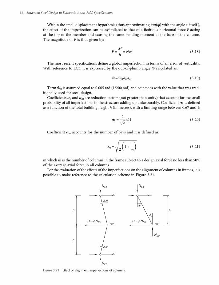
Within the small displacement hypothesis (thus approximating tan(φ) with the angle φ itself ),the effect of the imperfection can be assimilated to that of a fictitious horizontal force F actingat the top of the member and causing the same bending moment at the base of the column.The magnitude of F is thus given by:
F =Mh=Nφ 3 18
The most recent specifications define a global imperfection, in terms of an error of verticality.With reference to EC3, it is expressed by the out-of-plumb angle Φ calculated as:
Φ=Φ0αhαm 3 19
Term Φ0 is assumed equal to 0.005 rad (1/200 rad) and coincides with the value that was trad-itionally used for steel design.
Coefficients αh and αm are reduction factors (not greater than unity) that account for the smallprobability of all imperfections in the structure adding up unfavourably. Coefficient αh is definedas a function of the total building height h (in metres), with a limiting range between 0.67 and 1:
αh =2
h≤ 1 3 20
Coefficient αm accounts for the number of bays and it is defined as:
αm =12
1 +1m
3 21
in whichm is the number of columns in the frame subject to a design axial force no less than 50%of the average axial force in all columns.
For the evaluation of the effects of the imperfections on the alignment of columns in frames, it ispossible to make reference to the calculation scheme in Figure 3.21.
NEd
NEd
NEd
h h
h
Hi=ϕNEd Hi=ϕNEd
NEd
ϕ
ϕϕ/2
ϕ/2
Figure 3.21 Effect of alignment imperfections of columns.
66 Structural Steel Design to Eurocode 3 and AISC Specifications

In case of frames subject to large horizontal forces, the effects of the imperfections can be neg-lected because of the relative magnitude of their effects with respect to the effects of the lateralloads. In particular, if HEd represents the resultant horizontal forces at the base of all columnsin one floor and QEd the resultant vertical force acting at the base of all columns in that floor,the imperfections can be neglected if:
HEd ≥ 0 15QEd 3 22
3.5.2 The United States Approach
The approach followed by the ANSI/AISC 360-10 Specification, which is used in the UnitedStates, is in part quite similar to the one recommended by Eurocode 3. In particular, the followingdistinction has been made:
• local imperfections, such as out-of-straightness of individual members are not explicitly takeninto account into design analysis, but rather their effects are implicitly included into designequations that involve stability checks;
• system imperfections, the most important of which is certainly the out-of-plumb imperfectionof columns are explicitly addressed in the Specification.
The US Specification allows the designer to directly include structural system imperfections inthe analysis by modelling the structure with the largest admissible shifts (looseness) of the beam-column nodes in the directions that would most affect global stability of the system. As an alter-native to the direct modelling of the system imperfections via the use of non-straight members, theSpecification also allows the designer to account for them by means of a set of notional loads,applied to the structure, and corresponding to the effects of the imperfections on the stabilityof the structure. The nominal load approach is valid for any structure, but the Specification pro-vides guidance only for structures that carry gravity forces predominantly through vertical elem-ents, such as columns, walls or frames.The value of the notional loads, similar to what is prescribed in Eurocode 3, is as follows:
Ni = 0 002Yi 3 23
in which Ni is the notional load applied at level i and Yi is the total gravity load applied at level i.The 0.002 coefficient corresponds to an initial out-of-plumbness ratio of a column of 1/500 (asso-ciated with an angle of 2 mrad). The Specification allows for designer to use a different value of theratio if it can be appropriately justified. These notional loads must be applied to the structure in aconfiguration such that it will have the most influence on the stability of the building. The Spe-cification also allows the designer to apply the notional loads to combinations including gravityloads only, and not lateral loads, for situations in which the ratio of maximum second order driftto maximum first order drift is equal to or less than 1.7. In addition to the consideration of initialimperfections, the Direct Analysis Method outlined in the Specification (see Section 12.3.1) alsorequires that the stiffness of all elements that contribute to the stability of the structure must bereduced to 80%. Furthermore, an additional reduction factor must be applied to the flexural stiff-ness of all members contributing to the stability of the structure (e.g. beams and columns in a fullyrestrainedmoment-resisting frame). This additional reduction factor, indicated by τb, is a functionof the ratio of the required axial compressive strength to the yielding compressive strength of themember considered. When the axial force demand is less or equal to 50% of the axial yielding
Framed Systems and Methods of Analysis 67

strength of the member, no further reduction is necessary (i.e. τb = 1). If the demand is higher,then the stiffness reduction factor is calculated as:
τb = 4PrPy
1−PrPy
3 24
As an alternative to using the stiffness reduction factor τb, the Specification also allows us toapply an additional notional load equal to 0.001Yi at all levels and for all load combinations.
3.6 The Methods of Analysis
Structural analysis is a very important phase of the design aimed at the evaluation of displace-ments as well as internal forces and bending and torsional moments associated with the most sig-nificant load combinations. As a consequence, appropriate analysis approaches characterized bydifferent degrees of accuracy and complexity have to be selected by designers, depending on theimportance of the framed system, as well as by the required level of structural safety.
The most simple methods of analysis are the first order elastic methods, that is the ones based onthe assumptions of a linear elastic constitutive law of the material, small displacements and infini-tesimal deformations: as an example, the slope deflection method is the most commonly usedmethod belonging to this family and the virtual work principle is the most known by engineers.In accordance with these methods, the internal forces and moments on the members of the struc-ture are determined by making reference to the undeformed configuration, that is, only the equi-librium equations are used neglecting the compatibility conditions, or more practically, the effectsof deformations. The assumptions adopted by the first order elastic methods significantly simplifythe behaviour of the structures, because of the presence of mechanical and geometrical non-lin-earities. In particular, in several cases it is not possible to ignore:
• the mechanical non-linearity, which is due to the actual material constitutive law, already intro-duced in Section 1.1 with reference to the material constitutive law. The stress-strain curve is infact typically non-linear, assumed in a simplified way as an elastic-perfect plastic relationship oras an elastic-plastic with strain hardening. Furthermore, beam-to-column and base-plate jointmoment-rotation curves are typically non-linear.
• the geometrical non-linearity, which is due to the slenderness of the structure or of its compo-nents: the second order effects are the consequences of the lateral displacements of the struc-tures that can increase significantly shear forces and bending moments with respect to the oneobtained by imposing equilibrium conditions on the undeformed structure.
The layout of the types of analysis which can be currently executed for routine design is pre-sented in Figure 3.22.
Type of analysis
ElasticFirst order
Second order
First order
Second orderElasto-plastic
Figure 3.22 Layout of the types of structural analysis.
68 Structural Steel Design to Eurocode 3 and AISC Specifications
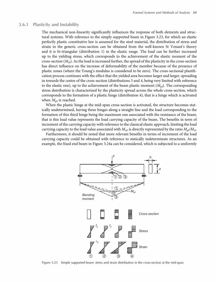
3.6.1 Plasticity and Instability
The mechanical non-linearity significantly influences the response of both elements and struc-tural systems. With reference to the simply supported beam in Figure 3.23, for which an elasticperfectly plastic constitutive law is assumed for the steel material, the distribution of stress andstrain in the generic cross-section can be obtained from the well-known St Venant’s theoryand it is bi-triangular (distribution 1) in the elastic range. The load can be further increasedup to the yielding stress, which corresponds to the achievement of the elastic moment of thecross-section (Mel). As the load is increased further, the spread of the plasticity in the cross-sectionhas direct influence on the increase of deformability of the member because of the presence ofplastic zones (where the Young’s modulus is considered to be zero). The cross-sectional plastifi-cation process continues with the effect that the yielded area becomes larger and larger, spreadingin towards the centre of the cross-section (distributions 3 and 4, being very limited with referenceto the elastic one), up to the achievement of the beam plastic moment (Mpl). The correspondingstress distribution is characterized by the plasticity spread across the whole cross-section, whichcorresponds to the formation of a plastic hinge (distribution 4), that is a hinge which is activatedwhen Mpl is reached.When the plastic hinge at the mid-span cross-section is activated, the structure becomes stat-
ically undetermined, having three hinges along a straight line and the load corresponding to theformation of this third hinge being the maximum one associated with the resistance of the beam;that is this load value represents the load carrying capacity of the beam. The benefits in term ofincrement of the carrying capacity with reference to the classical elastic approach, limiting the loadcarrying capacity to the load value associated withMel, is directly represented by the ratioMpl/Mel.Furthermore, it should be noted that more relevant benefits in terms of increment of the load
carrying capacity could be obtained with reference to statically indeterminate structures. As anexample, the fixed end beam in Figure 3.24a can be considered, which is subjected to a uniformly
1
1
2
2
3
3
1 2 3
Cross-section
Stress
fy
Bending
moment
Mel
F b
d
fy
εy
Strain
4
Figure 3.23 Simple supported beam: stress and strain distribution in the cross-section at the mid-span.
Framed Systems and Methods of Analysis 69

distributed load q increasing from zero until collapse is achieved. A perfect rigid plastic behaviouris assumed to represent the moment-curvature (M–χ) beam relationship (Figure 3.24b).
In the elastic range, the bending moment is characterized by a parabolic distribution with theend moment values twice the mid-span moment. By increasing the load, bending moment valuesincrease proportionally till the value of the plastic beammoment,Mpl, is reached at the beam ends,which can be associated with the load qcp defined as:
qcp =12Mpl
L23 25
The bending moment distribution, corresponding to this situation is presented in Figure 3.25.At the beam ends, two plastic hinges have been activated and the beam now can be consideredstatically determinate.
With reference to the fixed-end beam in the Figure 3.23, it should be noted that when theload activates these first plastic hinges, the structure does not collapse. Due to the presence of thesetwo plastic hinges the deformability is significantly increased with reference to the one associatedwith the initial built-up one in elastic range. A further increment of the uniform load, Δq, can besustained until the plastic beam bending resistance of the mid-span cross-section is achieved(Figure 3.26), which corresponds to a load increment Δqu, defined as:
Δqu =4Mpl
L23 26a
When this third plastic hinge is activated, three hinges are located along the longitudinal beamaxis, which corresponds to a complete collapse mechanism (Figure 3.27). Collapse load, qu, ishence defined as:
qu = qcp +Δqu =16Mpl
L23 26b
q
(a)
qL2/12
qL2/24
M
Mpl
Mpl
x
(b)
Figure 3.24 Bending moment distribution in a built-in beam (a) and typical moment-curvature relationship of thebeam cross-section (b).
Mpl Mpl
Mpl
Mpl/2
qcp= 12Mpl/L2
Figure 3.25 Bending moment diagram at the formation of the first two plastic hinges.
70 Structural Steel Design to Eurocode 3 and AISC Specifications

In case of statically indeterminate structures, like the one in this example, it should be noted thata complete collapse mechanism could be developed only if the member cross-section where theplastic hinge develops has an adequate ductility level, that is, it is able to provide adequate rota-tional capacity. The first two plastic hinges at the beam ends transform the fixed ends in simplesupports on which plastic bending moments act as externally applied loads: as a consequence, thesimply supported beam, subjected to a further distributed load Δqu at its ends (where plastichinges are located) undergoes rotation θpl, which can be evaluated, on the basis of the well-knowntheory of structures, as:
θpl =MplL
6EI3 26c
where E and I are the modulus of elasticity and the moment of inertia of the beam, respectively.These two examples show that a design approach based on limits associated with the achieve-
ment of the yielding stress could result in something very conservative, which corresponds to theachievement of the elastic bending moment (Mel) in correspondence to one cross-section of thewhole structure. Benefits associated with the spreading of plasticity are not negligible: with ref-erence to simply supported beams, collapse is achieved when the maximum value of the bendingmoment is equal to the beam plastic moment (Mpl) and the associated increment of the load car-rying capacity is usually expressed via the shape coefficient, αshape, defined as:
αshape =Mpl
Mel=Wpl
Wel3 27
whereWel andWpl are the elastic and the plastic sectionmodulus of the cross-section, respectively.Furthermore, it should be noted that, with reference to the second example, as generally occurs
in case of statically indeterminate structures, the increment of the load carrying capacity with
Mpl Mpl
+
qcp = 12Mpl/L2
Mpl
Mpl/2
Δq
Δqu ·L2
8
Figure 3.26 Bending moment distribution after the first two plastic hinges at the beam ends.
qu
MplMpl
Mpl
Figure 3.27 Collapse mechanism for the built-in beam.
Framed Systems and Methods of Analysis 71

respect to the one associated with a design approach based on the achievement of the elastic bend-ing moment (Mel) is significantly greater than term αshape, owing to the moment re-distribution.Table 3.2 shows the values of the shape factor (αshape) for the most common types of hot-rolledprofiles for different EU steel grades. It should be noted that some profiles cannot reach the plasticmoment because of their local buckling and therefore the value of the shape factor obtained viaEq. (3.27) cannot be used and reference must be made to unity, as better explained in Chapter 4.
In case or regular frames, the typical collapse mechanisms that could occur (Figure 3.28) are:
• beam mechanism;• panel (lateral) mechanism;• mixed mechanism.
More details related to the rigid plastic analysis of regular sway frames with semi-rigid beam-to-column and base plate joints are proposed in Chapter 15.
A very important phenomenon affecting member behaviour and, as a consequence, the wholestructural performance, is the local buckling that typically affects thin-walled members, that ismembers with components characterized by a high value ratio between the component width
Table 3.2 Value of the shape coefficient (αshape) for the European I beams (IPE) and European wide flange beams(HE) for steel grade S235, S275, S355, S420 and S460.
Standards IPEbeamsa
Wide flange HEA beams
Wide flange HEBbeamsa
Wide flange HEMbeamsa
S235S 275
S355
S420
S460
IPE 80 1.15 HEA 100 1.14 1.14 1.14 1.14 HEB 100 1.16 HEM 100 1.24IPE 100 1.15 HEA 120 1.13 1.13 1.13 1.13 HEB 120 1.15 HEM 120 1.22IPE 120 1.15 HEA 140 1.12 1.12 1.12 1.12 HEB 140 1.14 HEM 140 1.20IPE 140 1.14 HEA 160 1.11 1.11 1.11 1.11 HEB 160 1.14 HEM 160 1.19IPE 160 1.14 HEA 180 1.11 1.11 1.11b 1.11b HEB 180 1.13 HEM 180 1.18IPE 180 1.14 HEA 200 1.10 1.10 1.10b 1.10b HEB 200 1.13 HEM 200 1.17IPE 200 1.14 HEA 220 1.10 1.10 1.10b 1.10b HEB 220 1.12 HEM 220 1.17IPE 220 1.13 HEA 240 1.10 1.10 1.10b 1.10b HEB 240 1.12 HEM 240 1.18IPE 240 1.13 HEA 260 1.10 1.10b 1.10b 1.10b HEB 260 1.12 HEM 260 1.17IPE 270 1.13 HEA 280 1.10 1.10b 1.10b 1.10b HEB 280 1.11 HEM 280 1.16IPE 300 1.13 HEA 300 1.10 1.10b 1.10b 1.10b HEB 300 1.11 HEM 300 1.17IPE 330 1.13 HEA 320 1.10 1.10 1.10b 1.10b HEB 320 1.12 HEM 320 1.17IPE 360 1.13 HEA 340 1.10 1.10 1.10 1.10b HEB 340 1.12 HEM 340 1.16IPE 400 1.13 HEA 360 1.10 1.10 1.10 1.10 HEB 360 1.12 HEM 360 1.16IPE 450 1.13 HEA 400 1.11 1.11 1.11 1.11 HEB 400 1.12 HEM 400 1.16IPE 500 1.14 HEA 450 1.11 1.11 1.11 1.11 HEB 450 1.12 HEM 450 1.15IPE 550 1.14 HEA 500 1.11 1.11 1.11 1.11 HEB 500 1.12 HEM 500 1.15IPE 600 1.14 HEA 550 1.11 1.11 1.11 1.11 HEB 550 1.12 HEM 550 1.15— — HEA 600 1.12 1.12 1.12 1.12 HEB 600 1.13 HEM 600 1.15— — HEA 650 1.12 1.12 1.12 1.12 HEB 650 1.13 HEM 650 1.15— — HEA 700 1.13 1.13 1.13 1.13 HEB 700 1.13 HEM 700 1.15— — HEA 800 1.13 1.13 1.13 1.13 HEB 800 1.14 HEM 800 1.15— — HEA 900 1.14 1.14 1.14 1.14 HEB 900 1.15 HEM 900 1.15— — HEA1000 1.15 1.15 1.15 1.15 HEB1000 1.15 HEM1000 1.16— — HEA1100 1.16 1.16 1.16 1.16 HEB1100 1.16 HEM1100 1.17
a For all the considered steel grades.bUsing this steel grade plastic moment cannot be reached due to local buckling phenomena (αshape = 1).
72 Structural Steel Design to Eurocode 3 and AISC Specifications

and thickness. This form of instability affects the compressed portions of the cross-section and ischaracterized by a deformed shape with half-waves of amplitude comparable with the transversedimensions of the section of the element (Figure 3.29).The types of analysis previously described are characterized by a different degree of complexity
and are able to simulate the frame response more or less accurately. As an example, Figure 3.30relates to a frame subjected to a gravity load on each floor (P is the resulting value of the
Figure 3.28 Typical collapse mechanisms for steel frames.
N
G
M
Figure 3.29 Examples of local buckling of thin walled members.
Framed Systems and Methods of Analysis 73

distributed gravity load on each beam) and a horizontal force, βP, applied on each floor (β is con-stant and depends on the considered load condition).
The relationships between the applied load P and the lateral top displacement v are presented inthe figure, which have been determined via different approaches for the structural analysis(Figure 3.22). Increasing the value of the applied loads from zero, it can be noted that theresponses associated with the different types of analysis coincide to each other in their initial por-tion, that is for the lowest values of P. Remarkable differences can be noted when the yield of thematerial is achieved and/or the influence of the second order effects becomes non-negligible. Inparticular, the curve associated with second order elastic analysis tends asymptotically to the elas-tic critical load for sway mode Pcr. By means of first order elasto-plastic analysis the collapse load,Pp, associated with a complete collapse mechanism is generally greater than the corresponding oneobtained from an elasto-plastic second order analysis in which the failure occurs by interactionbetween plasticity and instability.
It should be noted that, for each considered load condition, the deformed shape of the frame isalways characterized by transversal displacements and hence a second order elastic analysis isalways recommended to approximate the actual frame response. However, errors associated withthe assumption of small displacements and infinitesimal deformations, on which elastic first orderanalysis is based, should be very negligible in many cases. As a consequence, this last type of ana-lysis, characterized by remarkable simplicity, can be used for routine design when the consideredload level is significantly far from the critical buckling load, that is, the condition expressed byEq. (3.4) for the European approach or by Eq. (3.7) for the US approach are fulfilled.
The choice of the method of analysis for steel framed systems depends not only on the struc-tural typology and on the relevance of second order effects on frame response, but also on the typeof cross-section of members as well as on the size of each of its components (flange, web, stiffener,etc.). In case of thin-walled members, that is members of its cross-section components with highvalues of ratio width over thickness, the local instability phenomena might occur in the elasticrange, hence preventing the spread of plasticity in the cross-section, that is, the achievementnot only of the plastic moment but also of the elastic moment.
3.6.1.1 Remarks on the European PracticeEurocode 3 proposes a criterion for the classification of cross-sections based on the slendernessratio (width over thickness ratio) of each compressed component of the cross-section, as well as onother factors, described more in detail in Chapter 4. In particular, with reference to the flexural
PFirst order elastic
First order
elasto-plastic
βP
βP
ψ0
Second order
elasto-plasticSecond orderelasto-plasticwith local buckling
Second order elastic
pl = Pv
V
P
Pcr
Pp
Pu
Figure 3.30 Influence of the type of analysis on the response of sway frames.
74 Structural Steel Design to Eurocode 3 and AISC Specifications

response in terms of relationships between the moment (M) and the curvature (χ), the followingfour classes of cross-sections (Figure 3.31) are defined:
• Class 1 cross-sections, which are those able to guarantee a plastic hinge providing adequaterotational capacity for plastic analysis without reduction of the resistance (plastic or ductilesections);
• Class 2 cross-sections, which are those able to guarantee, as a class 1 cross-section does, plasticmoment resistance, but have limited rotational capacity because of local buckling (compactsections);
• Class 3 cross-sections, which are those able to sustain yielding stresses only in the morecompressed fibres when an elastic stress distribution is considered because of the localbuckling phenomena hampering the spread of plasticity along the cross-section (semi-compactsections);
• Class 4 cross-sections, which are those subjected to local buckling phenomena before theattainment of yielding stress in one or more parts of the cross-section (slender sections).
It should be noted that, in case of compressed member, no distinctions can be observed in theperformance of the elements of the first three classes, owing to the stress distribution in axiallyloaded cross-sections limited to yielding strength.The possible choices for structural analysis and member verification checks are summarized in
Table 3.3. The load carrying capacity of the cross-section has to be evaluated with reference to the
M
Mpl
Mel
X
12
3
4
Figure 3.31 Moment-curvature (M–χ) relationships for the different classes of cross-sections considered inaccordance with the European approach.
Table 3.3 Methods of analysis and associated approaches for verification checks.
Method of analysis Approach to evaluate load carrying capacity of cross-section Cross-section class
(E) (E) Alla
(E) (P) Classes 1 and 2(E) (EP) Alla
(P) (P) Class 1(EP) (EP) Alla
a In the case of class 4, reference has to be made to the effective geometric properties (see Chapter 4).
Framed Systems and Methods of Analysis 75

axial load (tension and compression) and to the bending and torsional moment. The followingapproaches can be adopted:
• Elastic method (E): a linear elastic response is assumed till the achievement of the yieldingstrength. This method can be applied to verify all the cross-section classes; in case of class4, reference has to be made to the effective geometrical properties;
• Plastic method (P): the complete spread of plasticity is assumed in the cross-section, whichbelongs to classes 1 or 2;
• Elasto-plastic method (EP): reference is made to the actual material constitutive law, generallysimplified by an elastic-perfectly plastic relationship or with an elastic-plastic with strain hard-ening relationship.
3.6.1.2 Remarks on the US PracticeAISC cross-section classification criteria are based, as in Eurocode 3, on the steel grade and on thewidth-to-thickness ratios distinguished for stiffened elements (elements supported along two edgesparallel to the direction of the compression force) and unstiffened elements (elements supportedalong only one edge parallel to the direction of the compression force). As discussed in Chapter 4,cross-sections are classified on the basis of type of load acting on the element (i.e. compression andbending).
Members in compression are distinguishable in:
• slender elements, which are subject to local buckling, reducing their compression strength;• non-slender elements, never affected by local buckling.
Members in flexure are distinguishable in:
• compact elements, which are able to develop a fully plastic stress distribution with an associatedrotation capacity of approximately 30 mrad before the onset of local buckling;
• noncompact elements, which can develop partial yielding in compression elements before localbuckling occurs, but cannot develop a full plastic stress distribution because of local buckling;
• slender elements, which have some cross-section components (flanges and/or web) affected byelastic buckling before that yielding is achieved.
Contrary to the European approach, which assumes the same classification criteria for bothstatic and seismic design, it must be remarked that AISC Seismic provisions propose a differentclassification criteria when profiles are used in seismic areas.
The main analysis method suggested by AISC is the elastic method (Chapter C of AISC 360-10):as explained in the following, a linear elastic response is until the achievement of yielding strength.This method can be applied to verify all the cross-section classes. Furthermore, in its Appendix 1,the AISC specifications give more details related to the design by inelastic analysis. Any methodthat uses inelastic analysis is allowed, if some general conditions are fulfilled: among them, secondorder effects and stiffness reduction due to inelasticity are addressed. These methods may includethe use of non-linear finite element analysis; more details about this topic are reported inChapter 12.
3.6.2 Elastic Analysis with Bending Moment Redistribution
Elastic analysis is based on the assumption that the response is linear, that is the behaviour ofthe material is in the linear branch of its stress-strain constitutive law, whatever the stress level
76 Structural Steel Design to Eurocode 3 and AISC Specifications

is. Furthermore, in case of braced frames or non-sway frames, a first order analysis providesresults with an adequate accuracy for design purposes. However, if local buckling phenomenado not occur, the resulting design can be quite conservative due to neglecting benefits associ-ated with the spread of plasticity in the cross-sections and in the structural members, as shownin the examples of Figures 3.23 and 3.24. As for the design of concrete reinforced structures, aswell as in case of steel frames, an elastic redistribution of the bending moments more accuratelyapproximates the actual bending moment distribution in the post-elastic range.European provisions (EC3) allow for the plastic redistribution of moments in continuous
beams. In particular, at first, an elastic analysis is required: on the basis of the bending momentdiagram it can be the case that some peak moments exceed the value of the moment resistance and15% of the beam plastic resistance is admitted as maximum degree of redistribution. The parts inexcess of the vicinity of these peakmoments may be redistributed in anymember, provided that allthese following assumptions are fulfilled:
• all the members in which the moments have been reduced belong to Class 1 or Class 2(Figure 3.31);
• lateral torsional buckling of the members is prevented;• the internal forces and bending moments in the structure guarantee the equilibrium under the
applied loads.
With reference to continuous beams, usually the redistribution degree is selected to increase thebenefits in terms of load carrying capacity associated with plastic design. In particular, if doublysymmetrical beams are used, this approach leads to reduce the difference, after redistribution(subscripts R), between the peak bending negative (hogging) moment,M−
R , and the peak positive(sagging) one,M +
R . This method is discussed in the following with reference to a beam having twoequal spans in Figure 3.32. If termsM + andM− indicate, the maximum and the minimum valuesof the elastic bending moments, respectively, the redistribution degree is given by the ratio ΔM/M− , where ΔM represents the reduction of the bending moment value at the internal supportlocation due to redistribution. An optimal use of the material is guaranteed if M−
R =M +R , that
is the absolute values of the peak moments after redistribution are equal. As a consequence,on the basis of the equilibrium condition, the reduction ΔM of the negative peak elastic momentM− can be evaluated in this case as:
ΔM =M− − M +
1 +xL
3 28
where x indicates the distance between the load application cross-section and the external supportand L is the beam length.After the redistribution, if bending moments are within the elastic limit, the evaluation of the
beam deflection can be carried out by traditional elastic analysis methods.Moment redistribution is allowed also by AISC Specifications (Chapter B, Section B3.7), if the
following conditions are fulfilled:
(a) the cross-sections are classified as compact;(b) the unbraced lengths near the points where plastic hinges occur are limited to the values
stated in Section F13.5 of AISC 360-10;(c) bending moments are not due to loads on cantilevers;(d) yielding strength, Fy is not greater than 65 ksi (450 MPa);
Framed Systems and Methods of Analysis 77

(e) connections are FR (Fully Restrained);(f) elastic analysis has been carried out.
If all these conditions are met, then the negative moments can be taken as 9/10 of computedvalues and the maximum positive moment shall be increased of 1/10 of the average negativemoment.
3.6.3 Methods of Analysis Considering Mechanical Non-Linearity
As was introduced previously, the response of steel structures can be remarkably affected by thenon-linearity associated with the steel material as well as with components and connections. Theframes can be modelled for structural analysis and design using the following approaches:
• elasto-plastic analysis with plastification of the cross-sections and/or joints where plastic hingesare located;
• non-linear plastic analysis considering the partial plastification of members in plastic zones;• rigid plastic analysis neglecting the elastic behaviour between hinges.
Attention is focused briefly here on the last model, which is the most commonly used and alsobecause of the possibility for it to be employed with calculations by hand, as shown in Chapter 15for semi-continuous frames. It should be noted that plastic global analysis may be used if the
X
F
L
(a)
(b)
(c)
L
M –
M –R
M +
M +R
ΔM
X
F
Figure 3.32 Example of elastic analysis with bending moment redistribution.
78 Structural Steel Design to Eurocode 3 and AISC Specifications

members are able to provide an adequate rotational capacity guaranteed with reference to therequired redistributions of bending moments. As a prerequisite for plastic global analysis, thecross-sections of the members where the plastic hinge are located must have adequate rotationalcapacity, that is, must be able to sustain rotation of no less than that required at the plastic hingelocation. Furthermore, this design approach can only be used if at each plastic hinge position thecross-section has efficient lateral and torsional restraints with appropriate resistance to lateralforces and torsion induced by local plastic deformations.In order to apply the plastic analysis approach in Europe, the steel material must have adequate
ductility requirements to undergo plastic rotation without failure: a minimum level of ductility isrequired, which can be guaranteed if the following conditions are fulfilled:
fufy≥ 1 1 3 29a
Δ ≥ 15 3 29b
εu ≥ 15εy 3 29c
where ε represents the strain, f is related to the strength, subscripts y and u are related to yieldingand rupture, respectively, and Δ% represents the percentage elongation at failure.It is worth noting that the limits provided by these equations should be more appropriately
re-defined in the National Annex and hence the previously mentioned values have to be con-sidered as recommended. Furthermore, Eurocode 3 describes the cross-section requirementsfor plastic global analysis. In particular, it is explicitly required that at the plastic hinge loca-tions the cross-section of the member containing the plastic hinge must have a rotational cap-acity that is no less than the one required by calculations. Class 1 is a prerequisite for uniformmembers to have sufficient rotational capacity at the plastic hinge location. Furthermore, if atransverse force exceeding 10% of the shear resistance of the cross-section is applied to the webat the plastic hinge location, web stiffeners should be provided within a distance along themember of h/2 from the plastic hinge position (with h representing the depth of the memberat this location).In case of non-uniform members, that is if the cross-section of the members varies along their
length (tapered members), additional criteria have to be fulfilled adjacent to plastic hinge loca-tions. In particular, it is required that:
• the thickness of the web is constant (and not reduced) for a distance each way along the mem-ber from the plastic hinge location of at least 2d (with d representing the clear depth of the webat the plastic hinge location);
• the compression flange can be classified in Class 1 for a distance each way along the memberfrom the plastic hinge location of not less than the greater between 2d and the distance to theadjacent point at which the moment in the member has fallen to 0.8 times the plastic momentresistance at the point concerned.
For plastic design of a frame, regarding cross-section requirements, the capacity of plastic redis-tribution of moments may be assumed to be sufficient if the previously introduced requirementsare satisfied for all members. It should be noted that these requirements can be neglected whenmethods of plastic global analysis are used, which consider the actual stress-strain constitutive lawalong the member including (i) the combined effect of local cross-section and (ii) the overallmember buckling phenomena.
Framed Systems and Methods of Analysis 79

According to AISC, it is recommended to use steel for members subject to plastic hinging with aspecified minimum yield stress not greater than 65 ksi (450 MPa). Furthermore, members whereplastic hinges can occur have to be doubly symmetrical belonging to the compact class and thelaterally unbraced length has to be limited to values reported in Appendix 1 Section 3 of AISC360-10.
3.6.4 Simplified Analysis Approaches
As introduced previously, the structural analysis of steel frames could require very refined finiteelement analysis packages capable of taking into account both geometrical and mechanical non-linearity. In the past, refined analysis tools were not available to designers, due to absence or verylimited availability of computers and structural analysis software programs. As a consequence,design was carried out using simplified methods to approximate structural response and estimatethe set of displacements, internal forces and moments with an adequate degree of accuracy andgenerally on the safe side. These approaches are, however, still very important because they can beused nowadays for the initial (presizing) phase of the design as well as to check qualitatively theresults of more refined finite element structural analysis. In the following, reference is made to themost commonly used simplified approaches for routine design, which are:
• the Merchant–Rankine formula;• the Equivalent Lateral Force Procedure;• the Amplified Sway Moment Method.
3.6.4.1 The Merchant-Rankine FormulaIn case of sway frames, the ultimate load multiplier, αu, for the considered load condition can beevaluated by means of the Merchant–Rankine formula, which allows us to take into account theinfluence of both plasticity and instability phenomena. In particular, the elastic-plastic secondorder load multiplier, αu, can be directly evaluated via the expression:
1αu
=1αcr
+1αu
3 30a
where αcr is the critical load multiplier of the frame and αu is the elastic-plastic load multiplierassociated with a first order rigid or elastic-plastic analysis.
Term αu can be re-defined as:
αu =αuαcrαu + αcr
3 30b
The Merchant–Rankine formula should be applied preferably if term αcr ranges between 4 and10 times αu, that is the reference design condition is sufficiently far from the critical one.
3.6.4.2 The Equivalent Lateral Force ProcedureSecond order effects, in terms of both displacement and bending moments can be evaluated byusing the Equivalent Lateral Force Procedure, which is an example of indirect method for secondorder analysis via iterative elastic first order analysis. This procedure assumes that no relevantaxial deformations occur in the members and the second order effects are due only to the
80 Structural Steel Design to Eurocode 3 and AISC Specifications

horizontal displacements. The principle of this procedure is shown in Figure 3.34, which refers tothe internal column of a generic inter-storey of a sway frame with a height of hj. A first orderanalysis allows us to evaluate the internal axial force Nj and the inter-storey drift Δvj associatedwith the deformed shape of the frame, as in the case of the previously introduced cantilever beam(Figure 3.6). With reference to the deformed shape of the column, an additional bending momentcan be evaluated as Nj Δvj, due to the inter-storey drift. This additional bending moment isreplaced by an equivalent couple of horizontal forces FΔj (i.e. the so-called equivalent lateral force)having intensity equal to NjΔvj/hj and acting at the end of the considered column. A new firstorder elastic analysis is hence required, which is based on the new load condition also includingall the terms FΔj evaluated for all the columns and new values of the inter-storey drift have to beevaluated; they expected to be greater than the one previously determined. As a consequence ofthe updated value of the additional bending moment, a new equivalent lateral force has to beadded to the initial load condition (Figure 3.33).The procedure, which can be stopped when the differences between two subsequent steps are
very limited, generally requires a few iterations to approximate accurately the effects of the geo-metrical non-linearity. A very slow convergence (i.e. number of iterations greater than 6 or 7) isdue to a load condition too close to the elastic critical one. This means that the application of themethod is out of its scope and hence a more refined approach is required to execute second orderelastic analysis. The problem of the convergence of this procedure is briefly discussed in the fol-lowing Example E3.3.Before starting with the application of the method, the parameter for the convergence check has
to be defined: typically, reference is made to the value of the horizontal displacement of the nodeon the roof, the maximum inter-storey drift or the additional force updating load condition. Theflow-chart of the method is presented in Figure 3.34 and the evaluation of the equivalent lateralforce is presented in Figure 3.35 with reference to the case of a multi-storey frame. In particular,identifying with terms v and q the transversal absolute displacement and the vertical loads actingon the beams, respectively, and with subscripts 1 and 2 the first and second floor, respectively, thefollowing steps have to be evaluated:
• evaluation of the additional bending moments due to lateral displacements:
MΔ2 = Σq2Li v2 – v1 = Σq2Li Δv2 3 31a
MΔ1 = Σq1Li v1 = Σq1Li Δv1 3 31b
ΔVJ
FΔJ
FΔJ
FΔJ=
NJ NJ
NJNJ
NJ·ΔVJhJhJ
Figure 3.33 Evaluation of the equivalent lateral force.
Framed Systems and Methods of Analysis 81

• evaluation of the equivalent lateral forces for each inter-storey:
FΔ2 =MΔ2
h23 32a
FΔ1 =MΔ1
h13 32b
• evaluation of the equivalent lateral force to be applied to each storey:
ΔF2 = FΔ2 3 33a
ΔF1 = FΔ1 – FΔ2 3 33b
3.6.4.3 The Amplified Sway Moment MethodThe Amplified Sway Moment Method allows for an indirect allowance for second order effects,which requires a set of first order elastic analysis. Two different procedures can be followed,
Initial loadingcondition
First orderanalysis (elastic)
Check ofconvergence
Up-date ofthe loadingcondition
Satisfied
Not satisfied
Evaluation ofsecond order
response
Figure 3.34 Flow-chart of the equivalent lateral force procedure.
F2 q2
F1
FΔ2 ΔF2
ΔF1
F2
F1FΔ2
FΔ1
FΔ1
q1
q2
q1
Figure 3.35 Evaluation of the equivalent lateral force in a multi-storey frame.
82 Structural Steel Design to Eurocode 3 and AISC Specifications

depending on the frame geometry, which requires structural analysis on different service framesand, in particular, one of the following cases has to be selected:
• symmetrical frame with vertical loads symmetrically distributed;• other cases.
The approximate evaluation of the second order effects via this method is based on the amp-lification of the bending moments associated with the lateral displacement of the frame. The amp-lification factor, β, is defined as:
β =1
1−VEd
Vcr
=αcr
αcr −13 34
where VEd is the design vertical load for the loading condition of interest and Vcr is the associatedelastic critical load for sway mode (or, equivalently, αcr represents the elastic critical load multi-plier for sway mode associated with the considered load condition, that is αcr =Vcr/VEd).This method can be generally adopted if VEd Vcr ≤ 0 33 (in some codes the limit is 0.3) or
equivalently if αcr > 3.In case of vertical loads symmetrically distributed on a symmetric frame (Figure 3.36a), the
following steps have to be executed:
• first order elastic analysis of the frame loaded only by the vertical load (Figure 3.36b): termMV
represents the associated bending moment distribution;• first order elastic analysis of the frame loaded by the sole horizontal load (Figure 3.36c): term
MH represents the associated bending moment distribution;• approximation of the second order bending moment distribution (MII) on the frame as:
MII =MV + β MH 3 35
In other cases, that is with reference to non-symmetrical frames and/or to vertical loads non-symmetrically distributed (Figure 3.37a), the amplified sway moment method is applied throughthe following steps:
• first order elastic analysis of the frame loaded by the sole vertical loads with additional fictitiousrestraints embedding all the horizontal displacements (Figure 3.37b): term Ri represents thehorizontal reaction on the generic additional restraint;
Fq
(a)q
(b)
F
(c)
Figure 3.36 Set of frames (a–c) in case of symmetry of both frame and vertical loading condition.
Framed Systems and Methods of Analysis 83

• first order elastic analysis of the frame loaded by the sole vertical loads (Figure 3.37c): termMV
represents the associated bending moment distribution;• first order elastic analysis of the frame in Figure 3.37d loaded by the horizontal loads: termMH
represents the associated bending moment distribution;• first order elastic analysis of the frame in Figure 3.37e loaded by forces opposite to the hori-
zontal reactions Ri on the additional restraint: term MVF represents the associated bendingmoment distribution;
• approximation of the second order bending moment distribution (MII) on the frame is thefollowing:
MII =MV + β MH + β – 1 MVF 3 36
3.7 Simple Frames
If beam-to-column joints behave like hinges, the structural system is statically undetermined orcharacterized by an excessive deformability to lateral loads. As a consequence, appropriate bracingsystems are definitely required to transfer to the foundation all the horizontal forces acting on thestructure (Figure 3.38), which are for routine design cases where generally the forces simulate theeffects of wind load, geometrical imperfections and seismic actions.
The most common types of bracing systems adopted in structural steel buildings are (Figure 3.39):
• X-cross bracing system, if there is an overlap of the diagonal members at the centre of the bracedpanel (Figure 3.39a), which are connected at the beam-to-column joint locations. It should be
F
(a)
q
(d)
F
(c)
q(b)
qRi
(e)
Ri
Figure 3.37 Set of frames (a–e) for the application of the amplified swaymomentmethod in case of unsymmetricalstructures and/or unsymmetrically distributed vertical loads.
84 Structural Steel Design to Eurocode 3 and AISC Specifications

noted that a full use of openings (i.e. doors and windows) should be hampered or limited, bythis type of bracing.
• K-bracing system, if both diagonal members are connected at the mid-span beam cross-section(Figure 3.39b).
• eccentric bracing system, if the diagonal members are connected at different beam cross-sections (Figure 3.39c).
Two different approaches can be adopted for bracing design:
• bracing members are designed considering the fact that diagonals resist both to tension andcompression forces. In this case, quite low values of slenderness are required so that the dif-ferences in the diagonal responses associated with tension and compression forces are negli-gible. Cross- or K-bracing systems (Figures 3.39a and 3.40a, respectively) under lateralloads behave as the trussed beams, characterized by diagonal members resisting both tensionand compression. In case of eccentric bracing systems, the girder behaves like a beam-columnunder both hogging and sagging bending moments (Figure 3.41b);
• bracing members are designed considering the sole diagonals under tension, that is the com-pressed diagonals are not affected by the transfer force mechanisms. This requires very slenderdiagonal members. Cross-bracing systems also behave as trussed beams in this case while thebeam of K (Figure 3.40c) and eccentric (Figure 3.41c) bracing systems are subjected to axialload and bending moments.
It should be noted that hinges in simple frames are usually assumed to be located at the inter-section between beam and column longitudinal axes and this assumption significantly simplifiesstructural analysis. Internal forces and moments can in fact be evaluated with reference to elem-entary models related to isolated members: typically simply supported beams and a pinned-supported column.The spatial portal frame in Figure 3.42 can be considered when discussing the correct location
of the bracing system, which is a very important aspect for design. In accordance with major code
Figure 3.38 Typical simple frame.
(a) (b) (c)
Figure 3.39 Typical bracing panels.
Framed Systems and Methods of Analysis 85

provisions, wind effects are generally considered as acting alternately along a principal x- or y-axisand, as a consequence, vertical bracings are required both in transversal and longitudinal direc-tions. The presence of vertical bracings in simple frames does not hamper relative displacementbetween the top and the bottom of each column: due to the presence of vertical bracing, eachframe is only braced efficiently in its vertical plane. However, the connections are spatial hingesand hence the whole spatial framed system is unstable, as is shown in Figure 3.43 where typicaldeformed shapes associated with the absence of the roof bracings are presented for the portalframe of Figure 3.42 and for the single storey frame in Figure 3.44. To prevent these movements,a horizontal bracing system is hence required on each floor and on the roof. In several cases, thebracing floor should be required only for the erection phase, due to the fact that generally the slabof each floor and the metal decking of the roof should provide sufficient stiffness to transfer hori-zontal forces to vertical bracing systems. However, it could become generally uneconomical toremove these temporary bracings, which are often conveniently encased in the concrete of theslab or located between the slab and the ceiling.
With regards to the minimum horizontal forces to be transferred to foundations, three verticalbracing systems suitably located are required. Each braced floor, as well as the roof, can in fact beconsidered as a rigid body in its plane, with 3 degrees of freedom and requiring at least 3 degrees ofrestraint suitably located. It is usually assumed that each vertical bracing restraints a horizontal
H
(a) (b) (c)
Figure 3.40 Transfer force mechanism in a K-bracing system.
H
(a) (b) (c)
Figure 3.41 Transfer force mechanism in an eccentric bracing system (a–c).
Wx
X
Y
Wy
Figure 3.42 Vertical bracing in a three-dimensional portal frame.
86 Structural Steel Design to Eurocode 3 and AISC Specifications

displacement and hence can be modelled as an elastic support for each floor and the roof, or in asimplified way, as a simple support, neglecting its lateral deformability. As a consequence, at leastthree restraints, corresponding to three vertical bracing systems have to be appropriately locatedin order to avoid unstable structural system (Figure 3.44). Furthermore, with reference to the bra-cing system for each floor, it should be noted that it is not necessary to brace any span delimited bycontiguous columns to transfer horizontal load to foundations via vertical bracings. To betterexplain these concepts, Figure 3.44 can be considered, which shows examples of appropriate bra-cing systems for single-storey steel frames with one bay in the transversal direction (y) and twobays in the longitudinal direction (x). Wind action, which has been simulated via nodal forces, isindicated with Wx and Wy, depending on the x or y wind direction.
Vertical bracing
Figure 3.43 Liability due to the absence of horizontal bracings.
x
x
x
y
y
x
y
z
y
z
x
z
y
y
z
Wy
Wy
Wx Wx Wx
RyWy
RyWy
RyWx
RyWx
RxWx
RyWx RxWx
RyWy
Figure 3.44 Example of an efficiently braced single storey frame.
Framed Systems and Methods of Analysis 87

When wind acts along the y direction, the corresponding forcesWy are transferred directly viathe vertical longitudinal k-bracings which are symmetrically located and loaded by RyWy forces.Otherwise, if wind acts along the x direction, the resulting forceWx is transferred directly via thehorizontal bracing to the sole transversal horizontal bracing located along the x direction, whichresults in loading by an RxWx force. In this case, for the overall structural equilibrium, longitudinalvertical bracings are loaded by a couple of forces of intensity equal to RyWx, which are required tobalance the torsion due to the presence of one transversal vertical bracing, eccentrically located inplant with respect to the centroid.
3.7.1 Bracing System Imperfections in Accordance with EU Provisions
As required by major standards, structural analysis of bracing systems providing lateral framestability has to include the effects of imperfections and generally an equivalent geometric imper-fection of the members to be restrained is considered in the form of an initial bow imperfection e0defined as:
e0 =12
1 +1m
L500
= αmL500
3 37
where L is the span of the bracing system and m is the number of members to be restrained.From a practical point of view, instead of modelling a frame with imperfect members, it appears
more convenient to make reference to a perfect frame simulating the imperfection via additionalnotional loads, as previously discussed in Chapter 1.
For convenience, the effects of the initial bow imperfection of the members to be restrained by abracing system may be replaced by the equivalent force qs (Figure 3.45) given by:
qs =8 e0 + δq NEd
L23 38
where δq is the in-plane deflection of the bracing system due to the q load plus any external loadscalculated from first order analysis and NEd is the design axial force acting on members.
NEd NEd
qs
1
e0
L
Figure 3.45 Equivalent force in the bracing system.
88 Structural Steel Design to Eurocode 3 and AISC Specifications

When the bracing system is required to stabilize the compression flange of a beam of constantheight h, the axial force NEd, representing the action associated with the elements to brace on thebracing systems can be expressed as:
NEd =MEd
h3 39
where MEd is the maximum moment in the beam and h is the distance between flange centroids(or, approximately, the depth of the beam).If the beam to brace is subjected to external compression, axial force NEd should include a part
of the compression force. Furthermore, at points where members are spliced, bracing system hasto be verified to resist to a local force Fd applied to it by each beam or compression member that isspliced at that point, conventionally assumed as equal to:
Fd =αm NEd
1003 40
where NEd is the axial compressive force (Figure 3.45).
3.7.2 System Imperfections in Accordance with AISC Provisions
The definition of the imperfections of the bracing systems is directly treated in AISC 360-10Appendix 6 ‘Stability Bracings for Columns and Beams’ that addresses the minimum strengthand stiffness that a bracing systemmust have in order to provide a braced point in a column, beamor beam-column. For bracing systems providing lateral frame stability, the effects of imperfectionshave to be included in structural analysis by means of an equivalent geometric imperfection of themembers to be restrained, in the form of an initial bow imperfection, Δ0, defined as:
Δ0 =L500
3 41a
where L is the span of the bracing system.Term Δ0 is independent on the number of compressed members to be restrained and the value
L/500 is consistent with the maximum frame out-of-plumbness specified in AISC Code of Stand-ard Practice for Steel Buildings and Bridges. In AISC 360-10 Commentary of Appendix 6, a lesssevere formulation of Eq. (3.41a) is suggested:
Δ0 =L
500 n03 41b
where n0 is the number of columns stabilized by the bracing (it corresponds to m of Eq. (3.37)).In the same Commentary, it is permitted to use a reduced value of Δ0 defined in Eq. (3.41b)
when combining stability forces with the wind or the seismic forces on bracings. Nevertheless, thecriteria reported hereafter for defining strength and stiffness of bracing systems, are based on Δ0
values derived from Eq. (3.41a).AISC Specifications identify the following two categories of bracing systems:
• column braces, which fix locations along column length so that the column unbraced length canbe assumed equal to the distance between two adjacent fixed points.
• beam braces, which prevent lateral displacement (lateral bracings) and/or torsional rotation ofthe beam (torsional bracings). Lateral bracings are usually connected in correspondence with
Framed Systems and Methods of Analysis 89

the beam compression flange, while torsional bracings can be attached at any cross-sectionallocation. Torsional bracings can either be located at discrete points along the length of thebeam, or attached continuously along the length.
For both column and beam bracings, AISC defines:
(a) relative bracings, which work efficiently controlling the movement at one end of unbracedlength, A, with respect to the other end of unbraced length, B (see Figure 3.46a).
(b) nodal bracings, which work efficiently controlling the column or beammovements only at thebraced point without any direct interaction with the adjacent braced points (see Figure 3.46b).
For any type of bracing, that is column or beam, nodal or relative bracings, the AISC requiresverification of their strength and their stiffness to give designers minimum values, as specified inthe following:
(1) Relative column bracings(a) Required strength:
Prb = 0 004Pr 3 41c
(b) Required stiffness:
βbr = k2PrLb
3 41d
(2) Nodal column bracings(a) Required strength:
Prb = 0 01Pr 3 41e
(b) Required stiffness:
βbr = k8PrLb
3 41f
where Pr is the required strength in axial compression using LFRD or ASD combinations, Lb isthe unbraced length, expressed in inches and k= 1 ϕ= 1 0 75 (ASD); k =Ω = 2.00 (LFRD).
It is possible to size the brace to provide the lower stiffness determined by using the max-imum unbraced length associated with the required strength.
(3) Relative lateral beam bracings(a) required strength:
Prb = 0 008MrCd h0 3 41g
(b) required stiffness:
βbr = k4MrCd
Lbh03 41h
90 Structural Steel Design to Eurocode 3 and AISC Specifications

P P
(a)
P P
Relative Nodal
A
B
C
D
Rig
id a
but
men
t
Strut
L
Lb Lb
Diagonal
(b)
Relative
Lateralbracing
Torsionalbrace
Rigidsupport
Nodal Crossframe(nodal)
K = 1.0
P P
P P
typ.brace
Figure 3.46 Types of bracings according to AISC specifications (a) column bracing and (b) beam bracing.
Framed Systems and Methods of Analysis 91

(4) Nodal lateral beam bracings(a) required strength:
Prb = 0 02MrCd h0 3 41i
(b) required stiffness:
βbr = k10MrCd
Lbh03 41j
where Mr is the required flexural strength using LFRD or ASD combinations, h0 is the dis-tance between flange centroids, expressed in inches and Cd = 1.0 except for the brace closestto the inflection point in a beam subject to double curvature bending, in which case it whenCd = 2.0 and k = 1 ϕ= 1 0 75 (ASD); k =Ω = 2.00 (LFRD).
(5) Nodal torsional beam bracings(a) required strength:
Mrb =0 024MrLnCbLb
3 41k
where Cb is the modification factor defined in Chapter F of AISC 360-10 (see Chapter 8), Lb isthe length of span and n is the number of nodal braced points within the span.(b) required stiffness:
βTb =βT
1− βTβsec
3 41l
where βT is the overall brace system stiffness and βsec is the web distortional stiffness, includ-ing the effect of web transverse stiffeners.
These stiffness values are defined as:
βT = k2 4LM2
r
nEIyC2b
3 41m
βsec =3 3Eh0
1 5h0t3w12
+tstb3s12
3 41n
where E is the modulus of elasticity of steel, Iy is the out-of-plane moment of inertia, tw and tstare the thickness of the beam web and of the web stiffener, respectively, k= 1 ϕ= 1 0 75(ASD); k =Ω = 3.00 (LFRD) and bs is the stiffener width for one-sided stiffeners, or twicethe individual.
If the torsional bracing is continuous, then the ratio L/n in Eqs. (3.41k) and (3.41m) has tobe assumed as equal to unity.
3.7.3 Examples of Braced Frames
With reference to civil and commercial steel buildings, typical examples of braced multi-storeyframes are represented in the Figures 3.47–3.49, which also propose the structural schemes toevaluate internal actions and reactions of the horizontal bracing systems. Figures 3.47 and 3.48
92 Structural Steel Design to Eurocode 3 and AISC Specifications
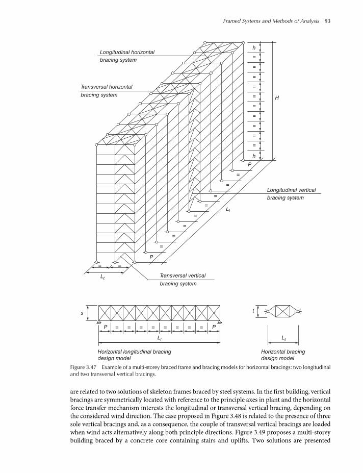
are related to two solutions of skeleton frames braced by steel systems. In the first building, verticalbracings are symmetrically located with reference to the principle axes in plant and the horizontalforce transfer mechanism interests the longitudinal or transversal vertical bracing, depending onthe considered wind direction. The case proposed in Figure 3.48 is related to the presence of threesole vertical bracings and, as a consequence, the couple of transversal vertical bracings are loadedwhen wind acts alternatively along both principle directions. Figure 3.49 proposes a multi-storeybuilding braced by a concrete core containing stairs and uplifts. Two solutions are presented
Longitudinal horizontalh
h
=
=
=
=
=
=
=
=
=
= =
=
=
=
=
=
=
=
=
=
P
H
bracing system
Longitudinal vertical
bracing system
Ll
Lt
s t
Horizontal bracing
design model
Horizontal longitudinal bracing
design model
Lt
P = = = = = = = =
Ll
P
P
bracing system
Transversal horizontal
bracing system
Transversal vertical
Figure 3.47 Example of a multi-storey braced frame and bracing models for horizontal bracings: two longitudinaland two transversal vertical bracings.
Framed Systems and Methods of Analysis 93

differing for the type of the core cross-section: open or closed (boxed) cross-section. For bothcases, pre-sizing (preliminary design) can be developed by considering each wall of the core asan independent cantilever beam embedded at its base.
As for the industrial steelwork, Figure 3.50 represents the most common typologies of single-storey frames. It should be noted that also in the case of rigid frames, the roof bracing system is,however, required (Figure 3.50a) to stabilize triangulated roof beams, that is, to reduce their
1 2
x
3b
A
B
A B
ya
F1
F2
F3
q
L
R1
R3R2
a
a
1
2
3
Figure 3.48 Example of a multi-storey braced frame and bracing models for horizontal bracings: one longitudinaland two transversal vertical bracings.
94 Structural Steel Design to Eurocode 3 and AISC Specifications

effective out-of-plane length. It is possible to also adopt hybrid structural scheme: a rigid frame inthe transversal direction and a simple frame in the longitudinal direction (Figure 3.50b).The bracing systems on the roof, which are required by the presence of the lattice beams, trans-
fer the horizontal forces to vertical bracings. Figure 3.50c refers to the case of simple frame modelto be adopted for the whole single storey building.It should be noted that the bracing systems are also of fundamental importance in order to
provide stability during the erection of the building.
b
b
F1 F1
F2 F2+F3
F2a+2F3a
(a)
(b)
F3a/b
F1+F2+F3
F3
F1
F2
F3
L
p p
b
p =
= = = = = = = =
= = = = = = = p
a
a
a
a
Figure 3.49 Example of a multi-storey braced frame with a closed (a) or open (b) concrete bracing core.
Framed Systems and Methods of Analysis 95

3.8 Worked Examples
Example E3.1 Individuation of the Bracing System
With reference to the frames in Figure E3.1.1, composed of two rigid portal frames connected via a non-deformable truss element, evaluate whether frame 2 braces frame 1.
(a)
(b)
(c)
Figure 3.50 Common structural typologies for industrial buildings (a and b).
Frame 1
Column: HE260A
Girder: IPE330
Frame 2
Column: HE300M
Girder: IPE60010 m
14 m 18 m
Figure E3.1.1
96 Structural Steel Design to Eurocode 3 and AISC Specifications
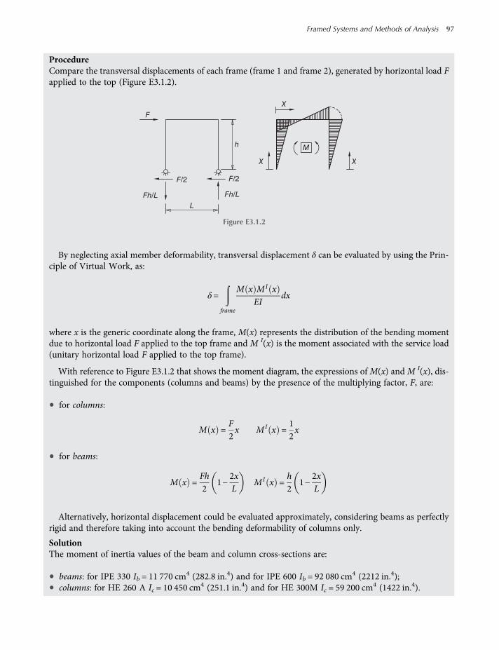
ProcedureCompare the transversal displacements of each frame (frame 1 and frame 2), generated by horizontal load Fapplied to the top (Figure E3.1.2).
By neglecting axial member deformability, transversal displacement δ can be evaluated by using the Prin-ciple of Virtual Work, as:
δ=
frame
M x MI xEI
dx
where x is the generic coordinate along the frame, M(x) represents the distribution of the bending momentdue to horizontal load F applied to the top frame and M I(x) is the moment associated with the service load(unitary horizontal load F applied to the top frame).
With reference to Figure E3.1.2 that shows the moment diagram, the expressions ofM(x) andM I(x), dis-tinguished for the components (columns and beams) by the presence of the multiplying factor, F, are:
• for columns:
M x =F2x MI x =
12x
• for beams:
M x =Fh2
1−2xL
MI x =h2
1−2xL
Alternatively, horizontal displacement could be evaluated approximately, considering beams as perfectlyrigid and therefore taking into account the bending deformability of columns only.
SolutionThe moment of inertia values of the beam and column cross-sections are:
• beams: for IPE 330 Ib = 11 770 cm4 (282.8 in.4) and for IPE 600 Ib = 92 080 cm4 (2212 in.4);• columns: for HE 260 A Ic = 10 450 cm4 (251.1 in.4) and for HE 300M Ic = 59 200 cm4 (1422 in.4).
F
h
X
X
M
X
F/2 F/2
Fh/L Fh/L
L
Figure E3.1.2
Framed Systems and Methods of Analysis 97

Frame displacement is computed via the expression:
δ= 2
h
0
1EIc
F2x
12x dx +
L
0
1EIb
Fh2
1−2xL
h2
1−2xL
dx
By solving integrals, it results in:
δ= 2Fh3
12EIc+Fh2L12EIb
Applying this formula to frame 1, it results δ = 0.0123 F, hence the frame stiffness is Kframe1 =Fδ= 81 20
kNm
(5.56 kips/ft). For frame 2 it results δ = 0.0021 F, hence the frame stiffness is Kframe2 =Fδ= 472 51
kNm
(32.38 kips/ft).
The ratio of the lateral stiffness of the two frames is:
Kframe2
Kframe1=472 5181 20
= 5 82
So the result is that frame 2 acts efficiently as bracing system for frame 1.
By neglecting shear deformation of the beam and considering its axial and flexural stiffness as infinite, it ispossible to refer to the auxiliary structure in Figure E3.1.3. The approximate stiffness of generic frame K∗ isgiven as:
K∗ =Fδ=12EIch3
The ratio between the approximate stiffness of the two frames is:
K∗frame2
K∗frame1
=
12EI 2c
h3
12EI 1c
h3
=I 1c
I 2c
=5920010450
= 5 67
This simplifiedmethod, neglecting the beam deformation, provides the result that frame 2 acts efficiently asa bracing system for frame 1.
Figure E3.1.3
98 Structural Steel Design to Eurocode 3 and AISC Specifications

Example E3.2 Selection of the EU Analysis Design Approach
With reference to the cantilever beam in Figure E3.2.1, for which a 100 mm (3.94 in.) width hollow squaresection (HSS) is used, evaluate the sensibility to transversal displacements (i.e. classify the frame), when:
Case (a): HSS thickness is 5 mm (0.197 in.) and
I = 283 × 104mm4 6 78 in 4 ;
Case (b): HSS thickness is 10 mm (0.394 in.) and
I = 474 × 104mm4 11 39 in 4 ;
Free end is loaded by an axial force N = 50 kN (11.24 kips) and a transversal force F = 5 kN (1.12 kips).
ProcedureAccording to the Eurocode prescriptions, the elastic buckling load has to be evaluated, for both loading cases,assuming: L0 = 2h = 4000 mm (13.12 ft). Reference is made to Euler’s theory and to the following formula:
Fcr =π2EIL20
SolutionMain results and indications about the type of analysis are listed in Table E3.2.1.
F
N
2.0
0m
Figure E3.2.1
Table E3.2.1 Indications of analysis type according to European codes.
Case (a) Case (b)
FEd 50 kN (11.24 kips) 50 kN (11.24 kips)
Fcr =π2EIL20
366.59 kN (82.4 kips) 614.01 kN (138.0 kips)
Fcr/FEd 7.33 12.28Analysis type: elastic Second order First orderAnalysis type: plastic Second order Second order
Framed Systems and Methods of Analysis 99

Using an engineering approach, the bending moment at column base has to be evaluated, taking intoaccount the first order term only, equal to F h, and evaluating second order moment as a function of displace-ment at column top, δ, with the following formula:
N δ=NFh3
3EI
The calculation results are shown in Table E3.2.2. Also in this case, for the thinner tube a second orderelastic analysis is always required.
Example E3.3 Second Order Approximate Analysis via the Equivalent Lateral ForceProcedure
With reference to the cantilever beam in Figure E3.3.1, approximate its second order frame response in thefollowing cases:
(a) HE 280 A member: moment of inertia I = 13 670 cm4 (328.4 in.4);(b) HE 160 M member: moment of inertia I = 5098 cm4 (122.5 in.4).
At the cantilever top Q, F and M act where:
• Q is the axial load equal to 640 kN (143.9 kips)• F is the lateral force equal to 10 kN (2.25 kips)• M is the bending moment equal to 40 kNm (29.5 kip-ft).
ProcedureIn these applications the influence of the axial deformability of the column on the value of the top lateraldisplacement is neglected.
Table E3.2.2 Indications of the type of analysis using an engineering approach.
Case a Case b
F h 10 kNm (7.38 kip-ft) 10 kNm (7.38 kip-ft)
N δ=NFh3
3EI
1.1218 kNm (0.827 kip-ft) 0.6697 kNm (0.494 kip-ft)
N δ/F h 0.1122 0.0700
Q
MF
h
Figure E3.3.1
100 Structural Steel Design to Eurocode 3 and AISC Specifications

In order to appraise the convergence of the approach, top horizontal cantilever displacement is considereddefining a tolerance limit equal to 2%.
Case (a): Column realized with a Profile HE 280 A.
The main iterative calculations are herein reported.
• Iteration 0: First order elastic analysis of cantilever loaded as stated before.– top lateral displacement calculation:
δ0 =Fh3
3EI+Mh2
2EI= 0 0502 m 1 98 in
– additional shear force calculation:
ΔF0 =Qδ0h
= 5 35 kN 1 20kips
– incremented applied load:
F1 = F +ΔF0 = 15 35 kN 3 45 kips
• Iteration 1: First order elastic analysis of cantilever consequently to iteration 0.– top lateral displacement calculation:
δ1 =F1h3
3EI+Mh2
2EI= 0 0636 m 2 50 in
– additional shear force calculation:
ΔF1 =Qδ1h
= 6 78 kN 1 52 kips
– incremented applied load:
F2 = F +ΔF1 = 16 78 kN 3 77 kips
– convergence check:
δ1δ0
= 1 27 > 2
• Iteration 2: First order elastic analysis of cantilever loaded consequently to iteration 1.– top lateral displacement calculation:
δ2 =F2h3
3EI+Mh2
2EI= 0 0672 m 2 65 in
Framed Systems and Methods of Analysis 101

– additional shear force calculation:
ΔF2 =Qδ2h
= 7 17 kN 1 61 kips
– incremented applied load:
F3 = F +ΔF2 = 17 17 kN 3 86 kips
– convergence check:
δ2δ1
= 1 06 > 2
• Iteration 3: First order elastic analysis of cantilever loaded consequently to iteration 2.– top lateral displacement calculation:
δ3 =F3h3
3EI+Mh2
2EI= 0 0681 m 2 68 in
– additional shear force calculation:
ΔF3 =Qδ3h
= 7 27 kN 1 63 kips
– incremented applied load:
F4 = F +ΔF3 = 17 27 kN 3 88 kips
– convergence check:
δ3δ2
= 1 01≤ 2
Second order response of the structure has been evaluated, estimating a top lateral displacement equalto 68.1 mm (2.68 in.), that is greater by about 36% than the one found by first order analysis. Comparingfirst and second order bending moments at the column base, a difference of about 44% can be observed, thatis first order analysis underestimates considerably the bending moment at the column base due to lateraldeflection.
Case (b): Column realized with a profile HE 160M.
Iterative calculations are herein reported, considering in this case a more flexible column.
• Iteration 0: First order elastic analysis of cantilever loaded as stated before.– top lateral displacement calculation:
δ0 =Fh3
3EI+Mh2
2EI= 0 1345 m 5 30 in
102 Structural Steel Design to Eurocode 3 and AISC Specifications

– additional shear force calculation:
ΔF0 =Qδ0h
= 14 35 kN 3 23kips
– incremented applied load:
F1 = F +ΔF0 = 24 35 kN 5 47 kips
• Iteration 1: First order elastic analysis of cantilever loaded consequently to iteration 0.– top lateral displacement calculation:
δ1 =F1h3
3EI+Mh2
2EI= 0 2310 m 9 09 in
– additional shear force calculation:
ΔF1 =Qδ1h
= 24 64 kN 5 54kips
– incremented applied load:
F2 = F +ΔF1 = 34 64 kN 7 79 kips
– convergence check:
δ1δ0
= 1 72 > 2
• Iteration 2: First order elastic analysis of cantilever loaded consequently to iteration 1.– top lateral displacement calculation:
δ2 =F2h3
3EI+Mh2
2EI= 0 3002 m 11 82 in
– additional shear force calculation:
ΔF2 =Qδ2h
= 32 02 kN 7 20kips
– incremented applied load:
F3 = F +ΔF2 = 42 02 kN 9 45 kips
– convergence check:
δ2δ1
= 1 30 > 2
Framed Systems and Methods of Analysis 103

• Iteration 3: First order elastic analysis of cantilever loaded consequently to iteration 2.– top lateral displacement calculation:
δ3 =F3h3
3EI+Mh2
2EI= 0 3499 m 13 78 in
– additional shear force calculation:
ΔF3 =Qδ3h
= 37 32 kN 8 39 kips
– incremented applied load:
F4 = F +ΔF3 = 47 32 kN 10 64 kips
– convergence check:
δ3δ2
= 1 17 > 2
• Iteration 4: First order elastic analysis of cantilever loaded consequently to iteration 3.– top lateral displacement calculation:
δ4 =F4h3
3EI+Mh2
2EI= 0 3855m 15 18 in
– additional shear force calculation:
ΔF4 =Qδ4h
= 41 12 kN 9 24 kips
– incremented applied load:
F5 = F +ΔF4 = 51 12 kN 11 49 kips
– convergence check:
δ4δ3
= 1 10 > 2
It must be underlined that, by reducing the flexural stiffness of the column by about two-thirds, conver-gence becomes slower, as can be detected by iterations 7 and 8, listed next.
• Iteration 7: First order elastic analysis of cantilever loaded consequently to iteration 6 (iterations 5 and 6have been omitted for the sake of simplicity).– top lateral displacement calculation:
δ7 =F7h3
3EI+Mh2
2EI= 0 4425 m 17 42 in
104 Structural Steel Design to Eurocode 3 and AISC Specifications

– additional shear force calculation:
ΔF7 =Qδ7h
= 47 20 kN 10 61 kips
– incremented applied load:
F8 = F +ΔF7 = 57 20 kN 12 86 kips
– convergence check:
δ7δ6
= 1 03 > 2
• Iteration 8: First order elastic analysis of cantilever loaded consequently to iteration 7.– top lateral displacement calculation:
δ8 =F8h3
3EI+Mh2
2EI= 0 4520 m 17 80 in
– additional shear force calculation:
ΔF8 =Qδ8h
= 48 21 kN 10 84 kips
– incremented applied load:
F9 = F +ΔF8 = 58 21 kN 13 09 kips
– convergence check:
δ8δ7
= 1 02
RemarksIt should be noted that in case (b) with amore flexible column, the number of iterations required for satisfyingconvergence criteria is greater than the one of case (a) with a stiffer column. To explain this difference, thecurve plotted in Figure E3.3.2 can be considered, the lateral displacement is plotted versus the ratio betweenthe load multiplier (α) over the critical one (αcr).
In case (a), with a stiffer member, a second order approximate analysis is performed for a structure with anelastic flexural buckling load equal to:
Pcr =π2EIL20
=π2 210000 13670 104
2 6000 2 = 1967 5 kN 442 3 kips
Axial load acting on the structure (640 kN, 143.9 kips) is considerably lower than buckling load (640/1967.5 = 0.325).
Framed Systems and Methods of Analysis 105
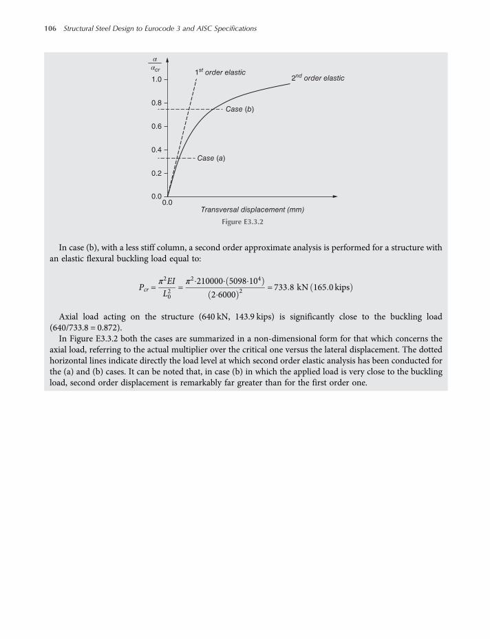
In case (b), with a less stiff column, a second order approximate analysis is performed for a structure withan elastic flexural buckling load equal to:
Pcr =π2EIL20
=π2 210000 5098 104
2 6000 2 = 733 8 kN 165 0 kips
Axial load acting on the structure (640 kN, 143.9 kips) is significantly close to the buckling load(640/733.8 = 0.872).In Figure E3.3.2 both the cases are summarized in a non-dimensional form for that which concerns the
axial load, referring to the actual multiplier over the critical one versus the lateral displacement. The dottedhorizontal lines indicate directly the load level at which second order elastic analysis has been conducted forthe (a) and (b) cases. It can be noted that, in case (b) in which the applied load is very close to the bucklingload, second order displacement is remarkably far greater than for the first order one.
1.0
αcr
α
0.8
0.6
0.4
0.2
0.00.0
Case (a)
Case (b)
1st order elastic2nd order elastic
Transversal displacement (mm)
Figure E3.3.2
106 Structural Steel Design to Eurocode 3 and AISC Specifications

CHAPTER 4
Cross-Section Classification
4.1 Introduction
As previously discussed in Section 1.1, the steelmaterial is characterized by a symmetrical mono-axial stress-strain (σ–ε) constitutive law, which can be determined by monotonic tension tests onsamples taken from the base material before the working process or from the products in corres-pondence of appropriate locations. The response of steel members can, however, be significantlydifferent in tension or compression, owing to the relevant influence of the buckling phenomena.The instability of compressed steel members as well as of all the members realized with othermaterials can be distinguished in:
• overall buckling or Euler buckling, which affects the element throughout its length (or a relevantportion of it). More details can be found in Chapter 6 for columns, interested by flexural,torsional and flexural-torsional buckling modes, in Chapter 7 for beams, interested by lat-eral-torsional buckling modes and in Chapter 9 for beam-columns subjected to a complexinteraction between axial and flexural instability;
• local buckling, already introduced in Section 3.6.1, which affects the compressed plates formingthe cross-section, characterized by relatively short wavelength buckling.
Furthermore, there is a third type of instability, the so-called distortional buckling, which hasbeen extensively investigated in recent decades. As the term directly suggests, this buckling modetakes place as a consequence of the distortion of cross-sections (Figure 4.1): with reference tothin-walled members, that is the members mainly interested by this phenomenon, distortionalbuckling is characterized by relative displacements of the fold-line of the cross-section and theassociated wave-length is generally in the range delimited by one of local buckling and one ofglobal buckling.It should be noted that local and distortional buckling, which can be considered ‘sectional
modes’, can interact with each other and the design of cold formed steel members is very complex.For the European design, the reference is EC3-1-3 (Supplementary rules for cold-formed membersand sheetings) and for the US the Code provisions governing design of these members are theAmerican Iron and Steel Institute (AISI) ‘North American specification for the design of cold-formed of steel members’.As already mentioned in Chapter 3, the classification of a cross-section is necessary in order
to select the appropriate analysis method as well as the suitable approaches to the member
Structural Steel Design to Eurocode 3 and AISC Specifications, First Edition. Claudio Bernuzzi and Benedetto Cordova.© 2016 John Wiley & Sons, Ltd. Published 2016 by John Wiley & Sons, Ltd.

verification checks. Furthermore, with reference to earthquakes and, consequently, seismic loads,the design strategy is based on the so-called capacity design, and the classification of profiles is veryimportant too, owing to the role played by the post-elastic ductile response.
Generally speaking, any cross-section is composed of different plate elements, such as flangesand webs, which fall into in two categories (Figure 4.2):
• internal or stiffened elements, simply supported along two edges parallel to the direction of thecompressive stress (longitudinal axis of the element);
• outstand (external) or unstiffened elements, simply supported along one edge and free on theother edge parallel to the direction of the compressive stress.
The cross-section classification depends mainly on the width-to-thickness ratio of each plate,either totally or partially in compression.
4.2 Classification in Accordance with European Standards
The cross-section classification has already been introduced in Chapter 3 in terms of perform-ances guaranteed by the four classes and the associated moment-curvature relationships havebeen presented in Figure 3.31. The requirements for the classification criteria are proposed inthe general part of EC3 (i.e. EN 1993-1-1): the limiting proportions for compression elementsof class 1–3 are presented in the following Tables 4.1–4.3. When any of the compression elementsof a cross-section does not fulfil the limits given in these tables, the section is classified as slender(class 4) and local buckling must be adequately taken into account into design by defining effectivecross-sections.
As can be noted from the tables, the limiting value of the width-to-thickness ratio (b/t) of thegeneric plate element under compression depends on the steel grade via a suitable reductionmaterial factor ε= 235 fy , where fy is the yield strength of the considered steel (expressed in
Figure 4.1 Typical deformed cross-section for distortional buckling.
Internal
InternalInternal
InternalOutstand
Outstand
WebWeb
Web
FlangeFlange Flange
Figure 4.2 Internal or outstand elements.
108 Structural Steel Design to Eurocode 3 and AISC Specifications

MPa). In more general cases, the compression elements forming a cross-section under compres-sion could belong to different classes and the cross-section has to be classified on the basis of themost unfavourable (highest) class of its compression elements. Table 4.1 proposes the classifica-tion criteria for internal compression elements, Tables 4.2 and 4.3 are related to the classificationof outstand flanges and of angles and tubular circular cross-sections, respectively.If a cross-section has a class 3 web and class 1 or 2 flanges, it should be classified as a class 3
cross-section, which from the design point of view can achieve the elastic moment without anyspreading of plasticity along the cross-section andmember. In this case, an alternative is admitted:the web can be treated as an equivalent class 2 web containing a hole in its compressed parts
Table 4.1 Maximum width-to-thickness ratios for compression elements, from EN 1993-1-1: Table 5.2 (sheet 1 of 3).
Internal compression elements
tw tw tw tw
tf
c c c h Axis of
bending
tftf tf
Axis of
bending
tf
b
bbb
ClassElement subject to
bendingElement subject tocompression
Element subject to bending andcompression
Stress distribution in element(compression positive)
c h
fy
fy
–
+
c h
fy
fy
–
+
cαc
h
fy
fy
+
–
1 c/t ≤ 72 ε c/t ≤ 33 ε When a > 0.5: c/t ≤ 396 ε/(13 a − 1)When a < 0.5: c/t ≤ 36 ε/a
2 c/t ≤ 83 ε c/t ≤ 38 ε When a > 0.5: c/t ≤ 456 ε/(13 a − 1)When a < 0.5: c/t ≤ 41.5 ε/a
Stress distribution in element(compression positive)
c
c/2
c/2h
fy
fy
+
hc
fy+
+
c h
fy
fy
–
ψ
3 c/t ≤ 124 ε c/t ≤ 42 ε When ψ > −1: c/t ≤ 42 ε/(0.67+ 0.33ψ)
When ψ ≤ −1 a: c/t ≤ 62 ε(1 − ψ) −ψ
ε= 235 fy fy 235 275 355 420 460ε 1.00 0.92 0.81 0.75 0.71
a ψ ≤ −1 applies where either the compression stress σ < fy, or the tensile strain εy > fy/E.
Cross-Section Classification 109

(Figure 4.3). As a consequence, reference can be made to a class 2 profile and the effective parts(i.e. the ones contributing to the cross-section resistance) of this web have a length equal to 20 ε tw,where ε is the reduction material factor previously defined. The main advantage of this approachis the possibility of using the plastic verification criteria for cross-section checks.
4.2.1 Classification for Compression or Bending Moment
Classification of cross-sections for axial load or for the bending moment only depends on the geo-metrical and mechanical parameters, as shown in the worked examples proposed in Section 4.4.
4.2.2 Classification for Compression and Bending Moment
The presence of both the compression and bending moment on the generic plate (or on the cross-section member) generates a stress distribution between that related to pure compression and thatassociated with the presence of the sole bending moment. In many cases, a plate componentbelongs to the same class under compression and under flexure: as a consequence, when theyact simultaneously, the cross-section class is directly determined, that is it is the same as for com-ponents subjected to an axial load and bending moment. Otherwise, in case of classes that aredifferent for compression and bending, the class for compression and bending must be evaluatedby considering the values of the design force and moment (NEd and MEd, respectively). In thefollowing, reference is made for compression combined with bending for an internal web and this
Table 4.2 Maximum width-to-thickness ratios for compression elements from EN 1993-1-1: Table 5.2 (sheet 2 of 3).
Outstand flanges
t t
t
tc c c c
Class Flange subject to compression
Flange subject to bending and compression
Tip in compression Tip in tension
Stress distribution inelement (compression positive)
c
+
c
αc
+
–
c
+
–
αc
1 c/tf ≤ 9 ε c/tf ≤ 9 ε/α c/tf ≤ 9 ε/α α2 c/tf ≤ 10 ε c/tf ≤ 10 ε/α c/tf ≤ 10 ε/α αStress distribution inelement (compression positive)
c
+
c
+
c
–+
3 c/tf ≤ 14 ε c/tf ≤ 21∙ε∙ kσ0.5 a c/tf ≤ 21∙ε∙ kσ
0.5 a
ε= 235 fy fy 235 275 355 420 460
ε 1.00 0.92 0.81 0.75 0.71
a For kσ see EN 1993-1-5.
110 Structural Steel Design to Eurocode 3 and AISC Specifications

Table 4.3 Maximum width-to-thickness ratios for compression elements, from EN 1993-1-1: Table 5.2 (sheet 3 of 3).
Refer also to ‘outstandflanges’ (see sheet 2 of 3)
Angles Does not apply to angles in continuous contact withother componentsh
t
t
b
Class Section in compressionStress distribution acrosssection (compression positive)
fy
fy
+
+
–
t
3 ht ≤ 15 ε
b+ h2t
≤ 11 5 ε
Tubular sections
td
Class Section in bending and/or compression1 d t ≤ 50 ε2
2 d t ≤ 70 ε2
3 d t ≤ 90 ε2
Note: for d t > 90 ε2 see EN 1993-1-6
ε= 235 fy fy 235 275 355 420 460ε 1.00 0.92 0.81 0.75 0.71ε2 1.00 0.85 0.66 0.56 0.51
4
3
2
20 εtw
20 εtw
+
–
–
fy
fy
2 1
Figure 4.3 Effective class 2 webmethod: compression (1), tension (2), plastic neutral axis (3) and neglected area (4)of the web.
Cross-Section Classification 111

case is typical for doubly symmetrical profiles under eccentric axial load or mono-symmetric pro-files under pure bending.
4.2.2.1 Bending and Compression about a Strong AxisIf internal elements (web) are considered, reference has to be made to Table 4.1. Normal stressdistribution on the web depends on the value of the design axial load by means of parameter α forprofiles able to resist in the plastic range (classes 1 and 2). Otherwise, in case of elastic normalstress distribution, reference has to be made to parameter ψ (classes 3 and 4). With referenceto the case of a neutral axis located in the web, α ranges between 0.5 (bending) and 1 (compres-sion) and ψ ranges between −1 (bending) and 1 (compression).
With reference to the normal stress plastic distribution, it should be convenient to use the super-position principle separately considering the stress distribution associated with the axial load (NEd)and the one associatedwith the bendingmoment (MEd) (see Figure 4.4). It can be noted thatNEd actson the central part of the web on a zone of extension x, as it results from equilibrium condition:
NEd = xtw fy 4 1a
where tw is the thickness of the web and fy is the yield strength.
Thedesignbendingmoment (MEd(N)) associatedwith the stressdistribution inFigure4.4, is givenby:
MEd N =Mpl−tw x2 fy
44 1b
where Mpl is the plastic flexural resistance of the member.The depth (x) of the web under pure axial load can be expressed as:
x = 2α – 1 c 4 2a
where factor α identifies the contribution of the web subjected to compression force, expressed asα c where c is the web depth.
The axial design load, NEd, and the correspondent bending design moment, MEd(N), can beexpressed, respectively, as:
NEd = 2α – 1 c twfy 4 2b
MEd N =Mpl –tw 2α − 1 c 2fy
44 2c
Factor α depends strictly on the value of the acting axial load as:
α=12
1 +1cNEd
twfy4 3
C
fV fV
(1 –α)C
(1 –α)C
+×=
fy fy
fy
fy
NEdαC
Figure 4.4 Superimposition of the stress distribution diagram associated with a plastic web under compressionand bending.
112 Structural Steel Design to Eurocode 3 and AISC Specifications

In the case of class 3 and class 4 profiles, the axial force is transferred by the whole components(web and flanges) of the cross-section, which has an elastic response; that is the typical triangulardistribution of stresses and strains governed by St Venant’s theory. As a consequence, with referenceto Figure 4.5, normal stresses σ, depending on the area A and on the section modulus Wel of thecross-section, can be divided into σN and σM, associated with axial load and bending moments,respectively. By using the superposition principle, top and bottom stresses are expressed as:
ψ fy = σN – σM 4 4
fy = σN + σM 4 5
Design axial load NEd acting on the member can be used to evaluate σN as:
σN =NEd
A4 6a
By using the similar approach presented for the plastic cases, the bending moment associatedwith the stress distribution in Figure 4.5, which is related to an elastic web under compression andbending, MEd(N), can be obtained as:
MEd N = fy – σN Wel 4 6b
where Wel is the elastic section modulus.
From the previous equations, we can obtain:
fy +ψ fy = 2NEd
A4 7
Term ψ can be directly associated with the design axial load (NEd) as:
ψ = 2NEd
A fy−1 4 8
It should be noted that for a direct use of this approach it is possible to define, for each set ofstandard profiles the value of the axial load NEd associated with the boundary from class 1 to class2. In particular, in case of portion of the web with themaximum compression stress greater that thetension one (α > 0.5) in absolute values, the classification boundary that is reported in Table 4.1 is:
ct=
396 ε13 α−1
4 9
where ε has been already introduced to account for the yielding strength fy, being defined as:
ε=235
fy MPa4 10
ψ fy
σN
σM
–σM
fy
NEd
Figure 4.5 Superimposition of the stress distribution diagram associated with an elastic web under compressionand bending.
Cross-Section Classification 113

At the boundary between 1 and 2 classes, term α is:
α=396 ε+ c tw13 c tw
4 11
By substituting α in Eq. (4.2b,c), the value of the limit design axial load (N1−2Ed
) and bending
moment (M1−2Ed
) are defined as:
N1−2Ed
= 2396 ε+ c tw13 c tw
−1 c tw fy 4 12a
M1−2Ed
=Mpl−2396 ε+ c tw13 c tw
−1 c2
tw
4fy 4 12b
Similarly, N2−3Ed
and M2−3Ed
, which are related the transition between classes 2 and 3, areexpressed by:
N2−3Ed
= 2456 ε+ c tw13 c tw
−1 c tw fy 4 13a
M2−3Ed
=Mpl−2456 ε+ c tw13 c tw
−1 c2
tw
4fy 4 13b
The same approach can be adopted with reference to an elastic stress distribution (classes 3 and4) by taking into account the relation between the axial load and the parameter ψ characterizingthe stress distribution of the web under bending and compression. Transition values of axial forceand bendingmoment in correspondence of the classification boundary between the classes 3 and 4are given by:
N3−4Ed
=12
42 ε−0 67 c tw0 33 c tw
+ 1 A fy 4 14a
M3−4Ed
= fy−fy2
42 ε−0 67 c tw0 33 c tw
+ 1 Wel 4 14b
The values of axial load and bending moment at the transition between classes 1 and 2(Eq. (4.12a,b)), classes 2 and 3 (Eq. (4.13a,b)) and classes 3 and 4 (Eq. (4.14a,b)), together withthe value of the moment resistance (MLim ) and of the axial load resistance (NLim) define a M-Ndomain depending on the cross-section geometry and steel grade. Figure 4.6 refers to the moregeneral situation of the profile in class 1 for bending and in class 4 for compression. Designershave to classify the member on the basis of the design values of the axial force and bendingmoment; that is on the basis of the position of the generic point P (NEd, MEd) in this domain.No univocally defined criteria are codified in EC3 to identify the cross-section class on the basisofNEd andMEd. Few alternatives can be adopted by designers. As an example, reference should bemade to Figure 4.6 related to the more generic case of member in class 1 under flexure and class 4under compression: if N and M increase proportionally (path A) the profile results in class 3,otherwise, if the axial force is constant and only the bending moment increases (path B), the pro-file is classified as class 2.
As a general remark associated with the classification procedure for elements subjected to com-pression and bending, it has to be noted that the same member could belong to different classes,
114 Structural Steel Design to Eurocode 3 and AISC Specifications

owing to the variability of the values of the acting bending moments along its longitudinal axis, astypically occurs when a beam column in a rigid or semi-continuous frame is considered.
4.2.2.2 Bending and Compression about a Weak AxisAll the concepts previously discussed for bending about the strong axis can be extended to thecase of bending about the weak axis. It should be noted that, in case of bending about the weakaxis of I- and H-shaped profiles, the classification criterion only has to be applied to the flanges.The web is always in class 1, due to the presence of the neutral axis located at the midline of thethickness of the web. The approach already presented for the definition of the domains M-N canhence be applied and, by using the superposition principle, it can be convenient to separate thestate of stress due to axial force from the one associated with the bending moment (Figure 4.7).
4.2.3 Effective Geometrical Properties for Class 4 Sections
As already mentioned, for class 4 cross-sections it is assumed that parts of the area under com-pression due to local instability phenomena do not have any resistance (lost area): typically, thecompressed portions of the cross-sections, which have to be neglected for the resistance checks,are the parts close to the free end of an outstand flange or the central part of an internal com-pressed element. As an example, reference can be made to Figure 4.8 related to typical cases ofcross-section properties reduced for local buckling phenomena when a member is subjected tocompression (a) or flexure (b). In the first case, it should be noted that the effective cross-section
3
A
BM [KNm]
MEdA
Nlim4 N [kN]
NEd3 – 4– MEd
3 – 4
NEd2– 3– MEd
2– 3
NEd1– 2– MEd
1– 2
21
Figure 4.6 Example of classification moment (M)-axial load (N) classification domain.
+ +=
(a) (b)
=
Figure 4.7 Stress distributions due to axial load (a) and bending (b) about a minor axis.
Cross-Section Classification 115

is subjected to an eccentric axial load due to the shift of the centroid from the gross to the effectivecross-section; that is the cross-section is subjected to an additional bending moment. From thedesign point of view, it is necessary to evaluate the effective cross-section (i.e. grosssection minus all the lost parts) in accordance with the procedures specified in EN 1993-1-5(Design of steel structures – Part 1–5: Plated structural elements). In particular, the referencesare Tables 4.1 and 4.2 and are reproduced here in Figures 4.9 and 4.10. In case of a class 4 circularhollow cross-section, reference has to be made to EN 1993-1-6 (Design of steel structures – Part1–6: Strength and Stability of Shell Structures).
The effective area of a compressed plate Ac,eff can be obtained from the gross area, Ac, as:
Ac,eff = ρAc 4 15
Reduction factor ρ is defined as:
• Internal compression elements (webs):
ρ= 1 0 if λp ≤ 0 673 4 16a
ρ= λp−0 055 3 +ψ λp2≤ 1 if λp > 0 673 and 3 +ψ ≥ 0 4 16b
Neutral axis
Neutral axis
Effective cross-section
Effective cross-section
Gross cross-section
Gross cross-section
eM
eM
eN
GG
(a)
(b)
G′
Neutral axis of the
effective cross-section
Neutral axis of the
effective cross-section
Neutral axis of the
effective cross-section
Non-effective
(lost area)
Non-effective
(lost) area
Non-effective
(lost) area
Non-effective
(lost) area
Figure 4.8 Gross and effective cross-sections in the case of axial load (a) and flexure (b).
116 Structural Steel Design to Eurocode 3 and AISC Specifications

Stress distribution (compression positive) Effectivep width beff
ψ = 1:
1>ψ ≥ 0:
be2= beff– be1
bc bt
be1
σ1 σ2
be2b–
be1
σ1 σ2
be2b–
be1
σ1σ2be2
b–
ψ <0:
beff= ρ bc= ρb–/(1– ψ)
be1= 0.4 beff be2= 0.6 beff
Buckling factor kσ 4.0 8.2 / (1.05 + ψ)
1> ψ >0 0
7.81 7.81– 6.29 ψ + 9.78 ψ 2
0 > ψ > –1ψ = σ1/σ1 –1
23.9 5.98 (1– ψ)2
–1> ψ > –31
beff= ρ b–
be1= 0.5 beff
beff= ρ b–
2beff
5 – ψbe1=
be2= 0.5 beff
Figure 4.9 Rules for the evaluation of the effective width of internal compression elements (a–c: from Table 4.1of EN 1993-1-5).
beff
σ1σ2
σ2
σ1
σ1
σ2
σ2
σ1
bc
c
bt
beff
beff
beff
bc bt
beff= ρ c
beff= ρ c
c
1> ψ ≥ 0:
1>ψ ≥ 0:
1 ≥ ψ ≥ –3
1>ψ > 0ψ = σ2/σ1
ψ = σ2/σ1
01.70 1.7–5ψ + 17.1ψ 2
0 > ψ > –1 –123.8
1
ψ <0:
Buckling factor kσ
Buckling factor kσ
Stress distribution (compression positive) Effectivep width beff
0.43
10.43
0.57 0.57 – 0.21ψ + 0.07ψ 20.85
0 –1
0.578/(ψ + 0.34)
ψ <0:
beff= ρbc= ρc/(1–ψ)
beff= ρbc= ρc/(1–ψ)
Figure 4.10 Rules for the evaluation of the effective width of outstanding compression elements (a–d: fromTable 4.2 of EN 1993-1-5).
Cross-Section Classification 117

• Outstand compression elements (flanges):
ρ= 1 0 if λp ≤ 0 748 4 17a
ρ= λp−0 188 λp2≤ 1 if λp > 0 748 4 17b
where:
λp =fyσcr
=b t
28 4ε kσ; ε=
235
fy N mm2
The width b has to be evaluated in accordance with Tables 4.1–4.3, where the reference is madeto term c instead of b.
Term ψ represents the ratio between the values of the plate end stresses while kσ is the bucklingfactor, which can be evaluated from Figures 4.9 and 4.10 on the basis of the distribution of thenormal stresses.
4.3 Classification in Accordance with US Standards
As already mentioned, AISC 360-10 addresses classification of cross-sections in Chapter B,Section B4; the code deals with members subjected to axial load and members subjected to bend-ing in a different way:
• members subjected to axial load are distinguished as non-slender or slender;• members subjected to flexure are distinguished as compact, non-compact or slender.
The classification for members subjected to axial load and bending is absent in the USapproach.
Classifications criteria are listed in Table B4.1.a of AISC specifications (reproduced inTable 4.4a) for compressed members and in Table B4.1b (reproduced in Table 4.4b) for membersin bending.
Classification criteria are based, as in the EC3 code, on steel grade and on width-to-thicknessratios for stiffened elements (elements supported along two edges parallel to the direction ofthe compression force, typically webs of I- or C-shaped sections) and unstiffened elements (elem-ents supported along only one edge parallel to the direction of the compression force, typicallyflanges of I- or C-shaped sections).
AISC code defines:
(a) for members subjected to axial load:λr, that is width-to-thickness ratio that defines non-slender/slender limit;
(b) for members subject to flexure:λp, that is width-to-thickness ratio that defines compact/non-compact limit;λr, that is width-to-thickness ratio that defines non-compact/slender limit.
It should be noted that:
• US flange width is one-half of full flange width, while in EC3 it is the outstanding part of theflange (one-half of full flange width less one-half of web thickness less the fillet or corner radius);
• US web width of rolled sections, as in EC3 code, is the clear distance between flanges less thefillet or corner radius at both flanges;
118 Structural Steel Design to Eurocode 3 and AISC Specifications

• US web width of built-up sections is the clear distance between flanges, while in EC3 it isdefined as for hot-rolled sections.
Classification of flanges of built-up members depends not only on width-to-thickness ratio ofthe flange itself but also on that of the web, by means of parameter kc:
kc =4
h tw4 18
Table 4.4a Width-to-thickness ratios for members subject to axial compression (from Table B4.1a of AISC 360-10).
Case Description of element
Width tothicknessratio
Limiting width-to-thickness ratio λr(non-slender/slender) Examples
Unstiffened elements
1 Flanges of rolled I-shaped sections, platesprojecting from rolled I-shaped sections;outstanding legs of pairs of anglesconnected with continuous contact,flanges of channels and flanges of tees
b/t0 56
EFy
b
b
b
b
bt
t
t
t
h
t
2 Flanges of built-up I-shaped sections andplates or angle legs projecting from built-up I-shaped sections
b/t0 64
kcEFy h
t
t
b
b
3 Legs of single angles, legs of double angleswith separators and all other unstiffenedelements
b/t0 45
EFy
b b
t t
t b
b
t
4 Stems of tees d/t0 75
EFy
t d
Stiffened elements
5 Webs of doubly-symmetric I-shapedsections and channels
h/tw1 49
EFy h ht
w tw
6 Walls of rectangular HSS and boxes ofuniform thickness
b/t1 40
EFy
t
b
7 Flange cover plates and diaphragm platesbetween lines of fasteners or welds
b/t1 40
EFy
bbt t
8 All other stiffened elements b/t1 49
EFy t
b
9 Round HSS D/t0 11
EFy
t
D
HSS, hollow square section.
Cross-Section Classification 119

where h and tw are width and thickness of web panel, respectively.This parameter accounts for the stiffening effect of web on flange: more slender webs
give a lower degree of stiffening on flanges. This effect is not considered in EC3 classificationcriteria.
Table 4.4b Width-to-thickness ratios for members subject to flexure (from Table B4.1b of AISC 360-10).
Case Description of element
Width-to-thicknessratio
Limiting width-to-thickness ratio
Examplesλp (compact/non-compact)
λr (non-compact/slender)
10 Flanges of rolledI-shaped sections,channels and tees
b/t0 38
EFy
1 00EFy
t tt
b bb
11 Flanges of doubly andsingly symmetricI-shaped built-upsections
b/t0 38
EFy
0 95kcEFL
tt
b b
h
12 Legs of single angles b/t0 54
EFy
0 91EFy
b
bt
t
13 Flanges of all I-shapedsections and channelsin flexure about theweak axis
b/t0 38
EFy
1 00EFy
bb
tt
14 Stems of tees d/t0 84
EFy
1 03EFy
dt
15 Webs of doublysymmetric I-shapedsections and channels
h/tw3 76
EFy
5 70EFy h h
tw
tw
16 Webs of singlysymmetric I-shapedsections
hc/tw hchp
EFy
0 54Mp
My−0 09
2 ≤ λr
5 70EFy
tw
hp
PNAPNA CGCG2
hp
2
hc
2
hc
2
17 Flanges of rectangularHSS and boxes ofuniform thickness
b/t1 12
EFy
1 40EFy
t
b
18 Flange cover plates anddiaphragm platesbetween lines offasteners or welds
b/t1 12
EFy
1 40EFy
b
ttb
19 Webs of rectangular HSSand boxes
h/t2 42
EFy
5 70EFy
t h
20 Round HSS D/t0 07
EFy
0 31EFy
D
t
120 Structural Steel Design to Eurocode 3 and AISC Specifications

4.4 Worked Examples
Example E4.1 Classification of a Member for Compression
Determine the class of IPE 550 profile S 275 steel grade under axial compression load.
Geometrical data
Height h, d 550mm (21.7 in.)
y
r
z
h
zb
y
tw
tf
Flange width bw 210mm (8.3 in.)Flange thickness tf 17.2 mm (0.677 in.)Web thickness tw 11.1 mm (0.437 in.)Corner radius r 24mm (0.945 in.)
Material data:
S 275 steel grade fy = 275MPa (Fy = 39.9 ksi)
EC3 procedure AISC procedure
For S 275 steel grade
ε=235fy
=235275
= 0 924
Flange Flange
ct=bw− tw− 2 r
2 tf=210−11 1− 2 × 24
2 × 17 2
=150 934 4
= 4 39≤ 9ε= 9 × 0 924= 8 32
bt=
bw2 tf
=8 3
2 × 0 677= 6 13 <
= 0 56EFy
= 0 56 ×2900039 9
= 15 1
Flange is class 1 Flange is non-slender
Web Web
ct=h− 2 tf − 2 r
tw
=550− 2 × 17 2 − 2 × 24
11 1
=467 611 1
= 42 2 > 42ε= 42 × 0 924= 38 83
htw=d− 2 tf − 2 r
tw
=21 7− 2 × 0 677 − 2 × 0 945
0 437
=18 460 437
= 42 2 > 1 49EFy
= 1 49 ×2900039 9
= 40 2
Web is class 4 Web is slender
S 275 steel IPE 550 section, subject to axial load, has class 1flanges and class 4 web, therefore it is classified asclass 4
S 275 steel IPE 550 section, subject to axial load, has non-slenderflanges and slender web, therefore, it is classifiedas slender
Cross-Section Classification 121

Example E4.2 Classification of a Member for Flexure about the Major Axis
Determine class of a HEA 280 profile in S 420 steel grade bent along its major axis.
Geometrical data
Height h, d 270mm (10.63 in.)z
b
y y
r
z
h
tw
tfFlange width bw 280mm (11.02 in.)Flange thickness tf 13 mm (0.512 in.)Web thickness tw 8 mm (0.315 in.)Corner radius r 24 mm (0.945 in.)
Material data:
S 420 steel grade fy = 420MPa (Fy = 60.9 ksi)
EC3 procedure AISC procedure
For S 420 steel grade
ε=235fy
=235420
= 0 748
Flange Flange
ct=b− tw− 2 r
2 tf
=280−8− 2 × 24
2 × 13=22426
= 8 62
Limiting width-to-thickness ratio compact/non-compact
λp = 0 38EFy
= 0 38 ×2900060 9
= 8 29
Limiting value class 1/class 2 Limiting width-to-thickness ratio non-compact/slender
ct= 9 ε= 6 732
λr = 1 0EFy
= 1 0 ×2900060 9
= 21 8
Limiting value class 2/class 3 bt=
bw2 tf
=11 02
2 × 0 512= 10 76c
t= 10 ε= 7 480
Limiting value class 3/class 4ct= 14 ε= 10 472
Flange is class 3 Flange is non-compactWeb Web: limiting width-to-thickness ratio compact/non-compact
ct=h− 2 tf − 2 r
tw
=270− 2 × 13 − 2 × 24
8
=1968
= 24 5≤ 72 ε= 72 × 0 748 = 53 86
λp = 3 76EFy
= 3 76 ×2900060 9
= 82 0
Limiting width-to-thickness ratio non-compact/slender
λr = 5 70EFy
= 5 70 ×2900060 9
= 124 4
htw
=d− 2 tf − 2 r
tw=
=10 63− 2 × 0 512 − 2 × 0 945
0 315=7 7160 315
= 24 5
Web is class 1 Web is compact
S 420 steel HEA 280 section, subjected to flexure, has class 3flanges and class 1 web, therefore, it is classified as class 3
S 420 steel HEA 280 section, subjected to flexure, has classnon-compact flanges and compact web, therefore, it isclassified as non-compact
122 Structural Steel Design to Eurocode 3 and AISC Specifications

ExampleE4.3 Classificationof aMemberunderAxial LoadandFlexure about theMajorAxis
Consider an S 275 steel IPE 600 profile subjected to axial load and bending moments about its strong axis anddetermine the classification domain.
Geometrical data
Height h, d 600mm (23.62 in.)
z
zb
y
r
y h
tw
tf
Flange width bw 220mm (8.66 in.)Flange thickness tf 19 mm (0.748 in.)Web thickness tw 12 mm (0.472 in.)Corner radius r 24 mm (0.945 in.)Area A 156 cm2 (24.18 in.2)Elastic modulus We, S 3070 cm3 (187.3 in.3)Plastic modulus Wpl, Z 3512 cm3 (214.3 in.3)
Material data:
S 275 steel grade fy = 275MPa (Fy = 39.9 ksi)
EC3 procedure AISC procedure
Determine boundary axial load values asexplained in Example E4.1
For members subjected to flexure and axial load AISC prescribesto compute classification in case of axial load only and in caseof bending moment only
For S 275 steel grade (1) Axial load
ε=235fy
=235275
= 0 924
Flange Flange
ct=b− tw− 2 r
2 tf=220−12− 2 × 24
2 × 19
=16038
= 4 21≤ 9 ε= 9 × 0 924 = 8 32
bt=
bw2 tf
=8 66
2 × 0 748= 5 79 <
= 0 56EFy
= 0 56 ×2900039 9
= 15 1
Flange is class 1 Flange is non-slender
Web in compression Web
ct=h− 2 tf − 2 r
tw
=600− 2 × 19 − 2 × 24
12=51412
= 42 83 > 42 ε= 42 × 0 924= 38 83
htw
=d− 2 tf − 2 r
tw=23 62− 2 × 0 748 − 2 × 0 945
0 472
=20 230 472
= 42 9 > 1 49EFy
= 1 49 ×2900039 9
= 40 2
Web in compression is class 4 Web is slender
Web in flexure S 275 steel IPE 600 section, subjected to axial load, has non-slender flanges and slender web, therefore it is classified asslender
ct=h− 2 tf − 2 r
tw=600− 2 × 19 − 2 × 24
12
=51412
= 42 83 < 72 ε= 72 × 0 924= 66 56
(Continued )
Cross-Section Classification 123

EC3 procedure AISC procedure
Web in flexure is class 1 (2) Flexure
If member is subjected to axial load and bending, class for thesection changes depends on the entity of axial load
FlangeLimiting width-to-thickness ratio compact/non-compact
λp = 0 38EFy
= 0 38 ×29 00039 9
= 10 24
The parameter α for transition from class 1 to class 2 istherefore determined
Limiting width-to-thickness ratio non-compact/slender
α=396 ε+ c tw13 c tw
=396× 0 924 + 42 83
13 × 42 83= 0 7341 λr = 1 0
EFy
= 1 0 ×29 00039 9
= 26 96
bt=
bw2 tf
=8 66
2 × 0 748= 5 79
Flange is compact
In case of pure flexure, limit moment MLim coincides withplastic moment, and is determined as follows
Web
MLim =Mpl =Wpl fy = 3512 × 275 10−3
= 965 8 kNm 712 3kip-ft
Limiting width-to-thickness ratio compact/non-compact
λp = 3 76EFy
= 3 76 ×29 00039 9
= 101 4
Compute with Eqs. (4.12a) and (4.12b) limit values foraxial load and bending moment at transition from class 1 toclass 2
Limiting width-to-thickness ratio non-compact/slender
N1−2Ed
= 2 α−1 c tw fy
= 2 × 0 7341−1 × 514 × 12 × 275 10−3
= 794 2 kN 174 5 kips
λr = 5 70EFy
= 5 70 ×29 00039 9
= 153 7
M1−2Ed
=Mpl −2396 ε+ c tw13 c tw
−1 c2
tw
4fy
= 965 8−2 ×
396× 0 924 + 42 8313 × 42 83
−1 × 5142
× 12
4× 275 10−6 = 965 8 – 47 8 = 918 0 kNm 178 5kip-ft
htw=d− 2 tf − 2 r
tw=23 62− 2 × 0 748 − 2 × 0 945
0 472
=20 230 472
= 42 9
Web is compact
S 275 steel IPE 600 section, subjected to flexure, has class compactflanges and compact web, therefore, it is classified ascompact
In the same way, limit values for axial load and bendingmoment at transition from class 2 to class 3 shall be
Being the section non-slender for axial load only, the nominalcompressive strength Pn shall be
N2−3Ed
= 2456 ε+ c t13 c t
−1 d tw fy
= 2456× 0 924 + 42 83
13 42 83−1 × 514 × 12 × 275 10−3
= 2 × 0 8337−1 514 × 12 × 275 10−3
= 1131 9 kN 254 5kips
Pn = FcrAg = 0 658QFyFe QFyAg
(Continued)
124 Structural Steel Design to Eurocode 3 and AISC Specifications

EC3 procedure AISC procedure
M2−3Ed
=Mpl −2456 ε+ c tw13 c tw
−1 c2
tw
4fy
= 965 8−2 ×
456 × 0 924+ 42 8313 × 42 83
−1 × 5142
× 12
4
× 275 10−6 = 965 8 −97 1 = 868 7 kNm 640 7 kips− ft
For low slenderness KL/r value, Fe QFy , therefore,this expression can be approximated asPn = FcrAg =QFyAg
Q=Qs Qa
Qs = 1 (flanges are non-slender)
Using the same method also for elastic behaviour, taking intoaccount the relationship between axial load and parameter ψ ,related to elastic stress distribution in web, limit values for axialload and bending moment at transition from class 3 to class4 are computed according to Eqs. (4.14a) and (4.14b)
Compute Qa because the web is slender
htw
= 42 9 > 1 49Ef= 1 49 ×
2900039 9
= 40 2
N3−4Ed
=12
42 ε−0 67 c t0 33 c t
+ 1 A fy
=12
42 × 0 924−0 67 × 42 830 33 × 42 83
+ 1 × 156 × 275 10−1
=12
0 7154 + 1 × 156 × 275 10−1
= 3682 kN 827 7kips
(f = Fcr = 39.9 ksi)
M3−4Ed
= fy −12
42 ε−0 67 c tw0 33 c tw
+ 1 fy Wel
= 275−12×
42 × 0 924−0 67 × 42 830 33 × 42 83
+ 1 × 275
× 3069 10−6
= 275−235 87 × 3069 10−6 = 120 1kNm 88 6 kip-ft
Then:
be = 1 92tEf
1−0 34b t
Ef
= 1 92 × 0 472 ×2900039 9
× 1−0 3442 8
×2900039 9
= 19 2 in < h = 20 23 in 488mm < 514mm
The compressive strength for axial load only Npl computed usinggross area is
Effective area Ae
Npl =A fy = 156× 275 10−1 = 4290 kN 964 4 kips Ae =Ag − h−be tw = 24 18− 20 23−19 2 × 0 472
= 23 69 in 2 152 8 cm2
When Npl is larger than limit axial load at transition fromclass 3 to class 4, there are no limitations for compressivestrength
Qa =Ae Ag = 23 69 24 18 = 0 98
The section is class 4 due to high web slenderness, therefore,compressive strength shall be computed using the effective area(for a definition, see Section 4.3.3, for the calculation, seeExample E6.1)
Q=Qs Qa = 1 × 0 98 = 0 98
Aeff = 149 5 cm2 23 17 in 2
Then member compressive strength for axial load only NLim
shall be:Pn =QFyAg = 0 98 × 39 9 × 24 18 = 945 5kips4206 kN
NLim =Aeff fy = 149 5 × 275 10−1 = 4112 kN 924 4 kips
(Continued)
Cross-Section Classification 125

Example E4.4 Classification of a Member for Flexure about the Minor Axis
Determine the class of an S 460 steel HEA 280 profile in flexure around its major axis.
Geometrical data
Height h, d 270mm (10.63 in.) Z
Z
b
y y
r
h
tw
tf
Flange width bw 280mm (11.02 in.)Flange thickness tf 13 mm (0.512 in.)Web thickness tw 8 mm (0.315 in.)Corner radius r 24 mm (0.945 in.)
Material data:
S 460 steel grade fy = 460MPa (Fy = 66.7 ksi)
EC3 procedure AISC procedure
For S 460 steel
ε=235fy
=235460
= 0 715
Flange Flange
ct=b− tw− 2 r
2 tf
=280−8− 2 × 24
2 × 13=22426
= 8 62
bt=
bw2 tf
=11 02
2 × 0 512= 10 76
Limit width-to-thickness ratio from class 1 to class 2 Limiting width-to-thickness ratio compact/non-compactct= 9 ε= 6 432
λp = 0 38EFy
= 0 38 ×2900066 7
= 7 92
Limit width-to-thickness ratio from class 2 to class 3 Limiting width-to-thickness ratio non-compact/slender
ct= 10 ε= 7 146
λr = 1 0EFy
= 1 0 ×2900066 7
= 20 9
bt=
bw2 tf
=11 02
2 × 0 512= 10 76
Limit width-to-thickness ratio from class 3 to class 4ct= 14 ε= 10 01
Flange is class 3 Flange is non-compact
Web Web
Web buckling is not a limit state for flexure around a minor axis,so web classification is not applicable in this case
Web buckling is not a limit state for flexure around a minoraxis, so web classification is not applicable in this case
S 460 steel HEA 280 section, subjected to flexure around minoraxis, has class 3 flanges and class 2 web, therefore, it is classifiedas class 3
S 460 steel HEA 280 section, subjected to flexure aroundminor axis, has class 3 flanges, therefore, it is classified asclass 3
126 Structural Steel Design to Eurocode 3 and AISC Specifications

Example E4.5 Comparison between US and EC3 Classification Approaches
As shown in the chapter, similarities and differences can be detected in the EU and US classification criteria.The example herein proposed presents a direct comparison related to the application of both codes to the samecross-section.Consider an I-shaped doubly symmetrical built-up welded section, bent about the major axis as in
Figure E4.5.1, composed of a 600 × 10 mm web plate and 20 mm-thick flanges. Increase the flange widthbf and, for each value, compute the section classification, the nominal flexural strengthMn according to AISCspecifications, and the characteristic resistance bending moment My,Rk according to EC3.
Note:Mn andMy,Rk are the names by which in AISC 360-10 and EC3, respectively, the product of relevantvalue for section modulus (plastic, elastic or effective) and relevant value for minimum steel stress (yielding orcritical) is indicated. Design values for flexural strength are obtained, in both codes, by multiplying such valueswith proper safety factors: ϕb and Ωb in AISC, γM0 in EC3, and they represent flexural strength of a beamsection if lateral torsional buckling of the beam is prevented (see Chapter 7).
Geometrical parameters:
i = 600mm (23.6 in.)tw = 10mm (0.39 in.)bf = variablet = 20mm (0.79 in.)a = 7mm (0.28 in.)A = 30 000mm2 (46.5 in.2)Iy = 248 720 cm4 (5976 in.4)
Material properties:
Steel grade : ASTM A992 Fy = 50 ksi 345 MPa Fu = 65 ksi 448 MPa
(1) Compute web class:(a) According to EC3:
cw = h−2a= 600−2 × 7 = 586mm 23 1 in
b
Cf
Cw
bf
a
h
a
t
tw
Figure E4.5.1 Geometrical parameters.
Cross-Section Classification 127

cwtw
=58610
= 58 6 < 72235fy
= 72 ×235345
= 59 4 class 1
(b) According to AISC 360-10:
htw
=60010
= 60 < 3 76EFy
= 3 76 ×2900050
= 90 6 Compact
(2) Compute values of bf that define boundaries between classes(a) According to EC3:
• boundary between class 1 and class 2:
cf = 9235fy
t = 9 ×235345
× 20 = 148mm
bf = 2cf + 2a+ tw = 2 × 148 + 2 × 7 + 10 = 321mm 12 6 in
• boundary between class 2 and class 3:
cf = 10235fy
t = 10 ×235345
× 20 = 165mm
bf = 2cf + 2a+ tw = 2 × 165 + 2 × 7 + 10 = 354mm 13 9 in
• boundary between class 3 and class 4:
cf = 14235fy
t = 14 ×235345
× 20 = 231mm
bf = 2cf + 2a+ tw = 2 × 231 + 2 × 7 + 10 = 486mm 19 1 in
(b) According to AISC 360-10:• boundary between compact and non-compact:
bf = 2b= 2 0 38EFy
t = 2 × 0 38 ×2900050
× 20 = 366mm 14 4 in
• boundary between non-compact and slender:
kc =4
h tw=
4
600 10= 0 52
FL = 0 7Fy = 0 7 × 50 = 35 ksi 241MPa
bf = 2b= 2 0 95kcEFL
t = 2 × 0 95 ×0 52 × 29000
35× 20 = 788mm 31 0 in
128 Structural Steel Design to Eurocode 3 and AISC Specifications

(3) Compute My,Rk and Mn for the previously computed values of bf:(a) ComputeMy,Rk according to EC3. In Tables E4.5.1a (with S.I. units) and E4.5.1b (with US units) val-
ues for My,Rk are listed. They have been computed for bf values previously chosen. In addition, bf =600 mm (23.6 in.) and 700 mm (27.6 in.) have been added. Values in the last three columns are theapplicable values for My,Rk. Applicable formulas are actually:
For class 1 and 2 My,Rk =Wpl,y fy E4 5 1
For class 3 My,Rk =Wel,y fy E4 5 2
For class 4 My,Rk =Weff ,y fy E4 5 3
Note that for bf = 354 mm (13.9 in.) two values for My,Rk are valid: 1662 kNm (1226 kip-ft) and 1825kNm (1347 kip-ft), because this value for bf is the boundary between a class 2 flange and a class 3 flange,and therefore between a class 2 section and a class 3 section, so that My,Rk can be computed withEq. (E4.5.1) in the first case and Eq. (E4.5.2) in the second case, and there is no continuity betweenthe two formulas.Calculations of Wel,y and Wpl,y are straightforward.Calculation ofWeff,y shall be performed according to Section 4.2.3. As an example, computeWeff,y for
bf = 600 mm (23.6 in.). Refer to Figure E4.5.2 for symbols.
Table E4.5.1a Values of My,Rk for different bf values – EC3 (S.I. units).
bf (mm) Class Wel,y (cm3) Weff,y (cm
3) Wpl,y (cm3)
My,Rk (kNm)
Wel,y fy Weff ,y fy Wpl,y fy
321 1/2 4420 4420 4880 1525 1525 1684
354 2/3 4816 4816 5290 1662 1662 1825366 3 4961 4961 5438 1712 1712 1876486 3/4 6403 6403 6926 2209 2209 2389600 4 7773 6838 8340 2682 2359 2877700 4 8974 7119 9580 3096 2456 3305788 4 10 032 7311 10 731 3461 2522 3702
Table E4.5.1b Values of My,Rk for different bf values – EC3 (US units).
bf (in.) Class Wel,y (in.3) Weff,y (in.
3) Wpl,y (in.3)
My,Rk (kip-ft)
Wel,y fy Weff ,y fy Wpl,y fy
12.6 1/2 269.7 269.7 297.8 1125 1125 1242
13.9 2/3 293.9 293.9 322.8 1226 1226 134714.4 3 302.7 302.7 331.8 1263 1263 1385
19.1 3/4 390.7 390.7 422.7 1630 1630 176323.6 4 474.3 417.3 508.9 1979 1741 212327.6 4 547.6 434.4 584.6 2285 1813 243931.0 4 612.2 446.1 654.8 2554 1861 2732
Cross-Section Classification 129

ψ = 1 constant stress along the flange
kσ = 0 57−0 21ψ + 0 07ψ2 = 0 57−0 21 × 1 + 0 07 × 12 = 0 43
bcf = 0 5 bf − tw−2r = 0 5 × 600 – 10 – 2 × 7 = 288mm
λpf =fyσcr
=bcf tf
28 4ε kσ=
288 20
28 4 × 235 345 × 0 43= 0 937 > 0 673
ρf = λpf −0 188 λ2pf = 0 937−0 188 0 9372 = 0 853
Effective area:
Aeff ,x =A−2 1−ρf bcf tf = 30000 – 2 × 1 – 0 853 × 288 × 20 = 28307mm2 = 283 1 cm2
Compute shifting yG of the centroid of effective section with respect to the gross one:
yG =2 1−ρf bcf tf
H2−tf2
A−2 1−ρf bcf tf=
2 × 1−0 853 × 288 × 206402
−202
30000−2 × 1−0 853 × 288 × 20
= 18 52mm = 1 852 cm
Effective moment of inertia:
Ieff ,y = Iy−2112
1−ρf bcf t3f −2 1−ρf bcf tf
H2−tf2
2
−Aeff y2G
= 248720−2112
1−0 853 × 288 × 203 10−4 +
−2 × 1−0 853 × 288 × 20 ×6402
−202
2
10−4 +
−283 1 × 1 8522 = 231490 cm4 5562 in 4
(1 – ρf)bcf(1 – ρf)bcf
bcf
bcw
btw
hw H
tw
bf
–1 < ψ < 0
σ
yG
tfr
ψσ
Figure E4.5.2 Geometrical parameters for calculation of Weff,y.
130 Structural Steel Design to Eurocode 3 and AISC Specifications

Effective modulus of section:
Weff ,y =Ieff ,y
H2+ yG
=231490
640 10−1
2+ 1 852
= 6838 cm3 417 3 in 3
(b) Compute Mn according to AISC 360-10. For the chosen bf values, section belongs to compact(bf ≤ 366 mm) and non-compact (366 mm ≤ bf ≤ 788 mm) classes.• if the section is compact, Mn is computed with Eq. (7.61):
Mn =Mp = FyZ
• if the section is non-compact, Mn is computed with Eq. (7.69):
Mn =Mp− Mp−0 7FySxλ−λpfλrf −λpf
• if the section is slender, Mn is computed with Eq. (7.70):
Mn =0 9EkcSx
λ2
where:
kc = 0 52 see before ;
λ= bf 2tf is the width-to-thickness ratio variable ;
λpf = 0 38 E Fy = 0 38 × 29000 50 = 9 2
Term λpf is the limiting width-to-thickness ratio for a compact flange;
λrf = 0 95 kcE FL = 0 95 × 0 52 × 29000 35 = 19 7
Term λrf is the limiting width-to-thickness ratio for a non-compact flange.Results are reported in Tables E4.5.2a (S.I. units) and E4.5.2b (US units).
Table E4.5.2a Values of Mn for different bf values –AISC (S.I. units).
bf (mm) Class S (cm3) Z (cm3) λ=bf2tf Mp (kNm) Mn (kNm)
321 C 4420 4880 8.0 1684 1684354 C 4816 5290 8.9 1825 1825366 C/NC 4961 5438 9.2 1876 1876486 NC 6403 6926 12.2 2389 2150600 NC 7773 8340 15.0 2877 2324700 NC 8974 9580 17.5 3305 2406788 NC/S 10 032 10 731 19.7 3702 2425
Cross-Section Classification 131

It can be noted that for bf = 366 mm (14.4 in.) section turns from compact to non-compact but values ofMn,computed with formulas for compact and non-compact sections are the same: no discontinuity in formulas.For bf = 788 mm (31.0 in.) cross-section changes from non-compact to slender. Computing Mn with
formula for slender sections results in:
Mn =0 9EkcSx
λ2=0 9 × 29000 × 0 52 × 612 2
19 7212 = 1790 kip-ft
It should be noted that there is no discontinuity in formulas passing from non-compact to slender sections.Finally, in Figure E4.5.3M − bf curves are reported, where M represents Mn (AISC) and My,Rk (EC3). It
should be noted that:
(a) all the EC3 curves represent a discontinuity in My,Rk values passing cross-section from class 2 to class 3,due to hard (sharp) change of formula, that passes from plastic to elastic modulus without transition;
(b) there are no discontinuities in AISC formulas passing from compact to non-compact and to slendersections;
(c) AISC compact class corresponds to EC3 classes 1 and 2: nominal flexural strength values obtained usingthe two codes are the same in this range;
Table E4.5.2b Values of Mn for different bf values –AISC (US units).
bf (in.) Class S (in.3) Z (in.3) λ=bf2tf Mp (kip-ft) Mn (kip-ft)
12.6 C 269.7 297.8 8.0 1242 124213.9 C 293.9 322.8 8.9 1347 134714.4 C/NC 302.7 331.8 9.2 1385 138519.1 NC 390.7 422.7 12.2 1763 158723.6 NC 474.3 508.9 15.0 2123 171527.6 NC 547.6 584.6 17.5 2439 177631.0 NC/S 612.2 654.8 19.7 2732 1790
2700
2500
2300
2100
1900
1700
1500200 300 400 500 600 700 800 900
bf [mm]
M [
kN
m]
4
EC3
3
EC3
AISC
AISC
AISC
S
2
C
1
NC
EC3
Figure E4.5.3 Comparison between Mn (AISC) and My,Rk (EC3) computed for various values of bf.
132 Structural Steel Design to Eurocode 3 and AISC Specifications

(d) non-compact class covers approximately EC3 class 3 but extends on initial part of class 4 accordingto EC3;
(e) term λrf, width-to-thickness ratio computed for flanges of welded sections separates non-compact fromslender sections, depending on parameter kc that takes into account the influence of flange and web localbuckling. As a consequence, Mn curves computed for non-compact welded flanges depend also on webwidth-to-thickness ratio: a less slender web (with a higher width-to-thickness ratio) would lead to higherMn values.
Cross-Section Classification 133

CHAPTER 5
Tension Members
5.1 Introduction
Usually members in tension are made with hot-rolled profiles, typically angles or channels: inother cases, cold-formed profiles can be conveniently used. Load carrying capacity of tensionmembers is essentially governed by:
• distribution of the residual stresses due to the manufacturing process;• connection details of the element ends.
The load carrying capacity at the connection location depends on the effective area (Figure 5.1).When the force transfer mechanism is analysed in correspondence with the cross-section cen-troid, the effective (or net) area corresponds to the gross area appropriately reduced for the pres-ence of holes. In case of staggered holes, the effective area has to be assumed to be the minimumbetween the effective one evaluated with reference to a straight section and the one associated witha suitable multi-linear piece line passing through the holes.
The effective cross-sectional area has to be evaluated according to standards provisions. Thedesign of members under tensile force can be based on the selection of a member with across-section greater than the minimum area Amin, which can be evaluated on the basis of tensiledesign load N, such as:
Amin =Nfd
5 1
where fd is the design tension limit strength.
5.2 Design According to the European Approach
Members in tension subjected to the design axial force NEdmust satisfy the following condition atevery section, in accordance with European provisions:
NEd ≤Nt,Rd 5 2
Structural Steel Design to Eurocode 3 and AISC Specifications, First Edition. Claudio Bernuzzi and Benedetto Cordova.© 2016 John Wiley & Sons, Ltd. Published 2016 by John Wiley & Sons, Ltd.

Design tension resistance, Nt,Rd of the cross-section has to be assumed to be theminimum between the plastic resistance of the gross cross-section, Npl,Rd, and the ultimateresistance of the net cross-section in correspondence of the connection, Nu,Rd, which are,respectively, defined as:
Npl,Rd =A fyγM0
5 3a
Nu,Rd = 0 9Anet fuγM2
5 3b
where A and Anet represent the gross area and the net area in correspondence of the holes, respect-ively, and fy and fu are the yield and ultimate strength, respectively, with γM0 and γM2 representingthe material partial safety factors.It should be noted that term Npl,Rd is associated with ductile failure due to the attainment of the
yield strength, while Nu,Rd, is related to a brittle failure in the connection section (governed by theattainment of the ultimate strength). In case of seismic loads, the well-established capacity designapproach requires a ductile behaviour of member under tension (i.e. Nu,Rd > Npl,Rd), which couldbe guaranteed if:
Anet ≥fyfu
γM2
γM0
A0 9
5 4
With reference to single or coupled angles connected via one leg, the effective area to be con-sidered to evaluate the tensile load carrying capacity, assuming the force transfer mechanism isassociated with only one leg.When a single angle is used, reference has to bemade to the criterion reported in EN 1993-1-8: a
single angle in tension connected by a single row of bolts in one leg may be treated as concen-trically loaded over an effective net section for which the design ultimate resistance, Nu,Rd, hasto be determined as:
• with one bolt (Figure 5.2a):
Nu,Rd =2 0 e2−0 5d0 t fu
γM25 5a
Figure 5.1 Connection detail for a member in tension.
Tension Members 135

• with two bolts (Figure 5.2b):
Nu,Rd =β2 Anet fu
γM25 5b
• with three or more bolts (Figure 5.2c):
Nu,Rd =β3 Anet fu
γM25 5c
where e2 is the distance from the axis of the hole to the outer edge of the element in the directionorthogonal to the force, d0 is the diameter of the hole, terms β2 and β3 are reduction factorsdepending on the pitch p1 as given in Table 5.1.
For an intermediate value of p1 the value of β may be determined by linear interpolation andγM2 is the safety coefficient and Anet is the effective area.
It should be noted that for an unequal-leg angle connected by its smaller leg, the resisting areaAnet should be taken as equal to the net section area of an equivalent equal-leg angle of leg sizeequal to that of the smaller leg.
In case of staggered holes for fasteners (Figure 5.3), collapse could occur along a multi-linearpath and the total area to be deduced for the evaluation of the net area (Anet) has to be consideredthe greater between:
• the maximum sum of the sectional area of the holes (Af) in any cross-section perpendicular tothe member axis;
e1
(a)
(b) (c)e1 e1p1 p1 p1
e2
d0
Figure 5.2 Single angle connected by one leg via (a) one bolt, (b) two bolts and (c) three bolts.
Table 5.1 Reduction factors β for angles connected via a single leg.
Pitch p1 ≤2.5 d0 ≥5 d0Two bolts β2 = 0.4 β2 = 0.7Three bolts or more β3 = 0.5 β3 = 0.7
136 Structural Steel Design to Eurocode 3 and AISC Specifications

• the sum of the sectional areas of all holes in any diagonal or multi-linear line extending pro-gressively across the member or part of the member less s2t/(4p) for each gauge space in thechain of holes, which can be expressed as:
t n d0−s2 t4 p
5 6
where t is the thickness, n is the number of holes along the considered line, d0 is the hole diam-eter and terms p and s have to be assumed in accordance with Figure 5.3.
Term p indicates the staggered pitch, which corresponds to the spacing of the centres ofcontinuous holes in the chain measured parallel to the axis member. Term smeasures the spacingof the centre of the same two holes measured perpendicular to the member axis.
5.3 Design According to the US Approach
LRDF approach ASD approach
Tension member design in accordance with theUS provisions for load and resistance factor design(LRFD) satisfies the requirements of AISCSpecification when the design tensile strengthϕtPn of each structural component equals orexceeds the required tensile strength Pudetermined on the basis of the LRFD loadcombinations, that is:
Pu ≤ϕtPn 5 7
where ϕt is the tensile resistance factor and Pnrepresents the nominal tensile strength
Design according to the provisions for allowablestrength design (ASD) satisfies the requirementsof AISC Specification when the allowable tensilestrength Pn/Ωt of each structural component equalsor exceeds the required tensile strength Padetermined on the basis of theASD load combinations,that is:
Pa ≤Pn Ωt 5 8
where Ωt is the tensile safety factor and Pn representsthe nominal tensile strength
p
S S S S
Figure 5.3 Typical connection in tension with staggered holes.
Tension Members 137

Pn has to be determined as the minimum value obtained according to the limit states of tensileyielding and tensile rupture:
Pn =min Pn,y;Pn,u 5 9
(a) For tensile yielding in the member gross section (ductile failure), the resistance is defined as:
Pn,y = FyAg 5 10
where Fy is the specified minimum yield stress and Ag is the gross area of the member. In thiscase Ωt = 1.67 and ϕt = 0 90.
(b) For tensile rupture in the member net section (brittle failure), the resistance is defined as:
Pn,u = FuAe 5 11
where Fu is the specified minimum tensile strength and Ae is the effective net area of the mem-ber. In this case Ωt = 2.00 and ϕt = 0 75.
As a comparison with Eurocode approach, the product between the minimum tensile strengthand the effective net area is reduced by 0.9/γM2 = 0.9/1.25 = 0.72 (see Eq. (5.3b)) that is a bit moresevere than ϕt = 0 75.
The effective net area Ae has to be determined as follows:
(a) For tension members where the tension load is transmitted directly to each of the cross-sectional elements by fasteners:
Ae =An 5 12
where An is the net area of the member, computed as indicated in Section 5.2 but consideringany bolt hole 1/16 in. (2 mm) greater than the nominal dimension of the hole.
(b) For tension members where the tension load is transmitted to some but not all of the cross-sectional elements by fasteners or welds:
Ae =AnU 5 13
where U is the shear lag factor, determined as shown in Table 5.2.
For welded members also An should be determined as shown in Table 5.2.In case of bracing members in seismic zones, for Special Concentrically Braced Frames (SCBF),
the effective area must not be less than the gross area (see AISC 341-10, F2.5b(3)).
138 Structural Steel Design to Eurocode 3 and AISC Specifications

Table 5.2 Shear leg factors for connections to tension members (from Table D3.1 of AISC 360-10).
Description of element Shear lag factor, U Example
1 All tension members where thetension load is transmitted directly toeach of the cross-sectional elements byfasteners or welds (except as in Cases 4, 5and 6)
U = 1 —
2 All tension members, except plates andHSS, where the tension load istransmitted to some but not all of thecross-sectional elements by fasteners orlongitudinal welds or by longitudinalwelds in combination with transversewelds. (Alternatively, for W, M, S andHP, Case 7 may be used. For angles, Case8 may be used.)
U = 1−x l x
x
xx
3 All tension members where the tensionload is transmitted only by transversewelds to some but not all of the cross-sectional elements
U = 1 and An = area of thedirectly connected elements
—
4 Plates where the tension load istransmitted by longitudinal welds only
U = 1 if l ≥ 2w
W
U = 0 87 if 2w > l ≥ 1 5wU = 0 75 if 1 5w > l ≥w
5 Round HSS with a single concentricgusset plate
U = 1 if l ≥ 1 3D
D
U = 1−x l if D≤ l < 1 3D;x =D π
6 Rectangular HSS With a singleconcentricgusset plate
U = 1−x l if l ≥H H
B
x =B2 + 2BH4 B+H
With two sidegusset plates
U = 1−x l if l ≥H —
x =B2
4 B+H
7 W, M, S or HPShapes or Tees cutfrom these shapes.(If U is calculatedper Case 2, thelarger value ispermitted to beused.)
Flange connectedwith three ormore fastenersper line in thedirection ofloading
U = 0.90 if bf ≥ 2/3d —U = 0.85 if bf < 2/3d
Web connectedwith four ormore fastenersper line in thedirection ofloading
U = 0.70 —
(Continued)
Tension Members 139
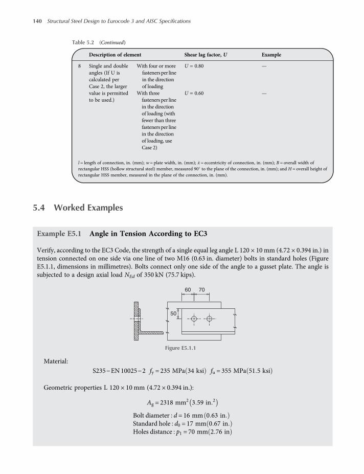
5.4 Worked Examples
Example E5.1 Angle in Tension According to EC3
Verify, according to the EC3 Code, the strength of a single equal leg angle L 120 × 10 mm (4.72 × 0.394 in.) intension connected on one side via one line of two M16 (0.63 in. diameter) bolts in standard holes (FigureE5.1.1, dimensions in millimetres). Bolts connect only one side of the angle to a gusset plate. The angle issubjected to a design axial load NEd of 350 kN (75.7 kips).
Material:
S235−EN10025−2 fy = 235 MPa 34 ksi fu = 355 MPa 51 5 ksi
Geometric properties L 120 × 10 mm (4.72 × 0.394 in.):
Ag = 2318 mm2 3 59 in 2
Bolt diameter d = 16 mm 0 63 inStandard hole d0 = 17 mm 0 67 inHoles distance p1 = 70 mm 2 76 in
Table 5.2 (Continued)
Description of element Shear lag factor, U Example
8 Single and doubleangles (If U iscalculated perCase 2, the largervalue is permittedto be used.)
With four or morefastenersper linein the directionof loading
U = 0.80 —
With threefasteners per linein the directionof loading (withfewer than threefasteners per linein the directionof loading, useCase 2)
U = 0.60 —
l = length of connection, in. (mm); w = plate width, in. (mm); x = eccentricity of connection, in. (mm); B = overall width ofrectangular HSS (hollow structural steel) member, measured 90 to the plane of the connection, in. (mm); and H = overall height ofrectangular HSS member, measured in the plane of the connection, in. (mm).
60 70
50
Figure E5.1.1
140 Structural Steel Design to Eurocode 3 and AISC Specifications

Calculate the available tensile yield strength (Eq. (5.3a)):
Npl,Rd =A fyγM0
=2318 × 235
1 0010−3 = 544 7kN 122 5 kips
Calculate the available tensile rupture strength (Eq. (5.3b)):Being pitch p1 (= 70mm) ranging between 2.5 d0 (= 42.5mm) and 5 d0 (= 85mm), term β2, is evaluated
from Table 5.1 by linear interpolation and the value of 0.594 is assumed:
Nu,Rd =β2 Anet fu
γM2=0 594 × 2318− 10 × 17 × 360
1 2510−3 = 367 5kN 82 6 kips
Check NEd = 350kN≤Nt,Rd = 367 5kN 75 7 < 82 6 kips OK
Example E5.2 Joint of a Tension Chord of a Trussed Beam According to EC3
Verify, in accordance with EC3, the splice connection in Figure E5.2.1 (dimensions in millimetres), whichconnects the end of two members of the chord of a trussed beam and transfers a design axial tension loadNEd of 2250 kN (506 kips).
The flanges of the beam are composed by 340 × 16 mm (13.4 × 0.63 in.) plates and a plate 260 × 12 mm(10.2 × 0.472 in.) forms the beam web. Single cover plates 340 × 16 mm (13.4 × 0.63 in.) are bolted to thebeam flange in normal holes (d0 = 26 mm = 1.02 in.).Material:
S235−EN10025−2 fy = 235 MPa 34 ksi fu = 355 MPa 51 5 ksi
50
50
80
80
60 60 60 60
80
80 80 80 80 80 80 80 80
340
1616
1616
260 324
Figure E5.2.1
Tension Members 141

Area of the chord:
Ab = 2 bf tf + bw tw = 2 × 340 × 16 + 260 × 12 = 14000mm2 21 7 in 2
Area of the cover plates:
Ag = 2 × 340 × 16 = 10880mm2 15 88 in 2
Bolt diameter d = 24mm 0 945 inStandard hole d0 = 26mm 1 02 in
Verification for plastic collapse. Calculate the tensile yield strength of the cover plates (being their arealower than the one of the H-shaped profile):
Npl,Rd =Af fyγM0
=10880 × 235
1 0010−3 = 2556 8kN 575 kips
Check NEd = 2250kN≤Npl,Rd = 2556 8 kN 506 < 575 kips OK
Verification for brittle collapse. Due to the presence of staggered holes (Figure E5.2.2), the total area todeduce to the gross resisting area has to be considered the minimum between (Eq. (5.6)):
2 × 26 × 16 = 832 mm2 1 29 in 2
and t n d0−s2 t4 p
= 4 × 26 × 16 − 2 ×802 × 164 × 80
= 1024 mm2 1 587 in 2
Anet = 10880−2 × 1024 = 8832 mm2 13 69 in 2
It should be noted that coefficient 2 is due to the presence of two cover plates.
Nu,Rd = 0 9Anet fuγM2
= 0 9 ×8832 × 355
1 2510−3 = 2257 5 kN 507 5 kips
Check NEd = 2250 kN≤Nu,Rd = 2257 5 kN 506 < 507 5 kips OK
50
50
80
80
80
8080808060 60
Figure E5.2.2
142 Structural Steel Design to Eurocode 3 and AISC Specifications

Example E5.3 Single Angle Tension Member, Connected on One Side by Bolts,According to AISC 360-10
Verify, according to AISC Code, both ASD and LRFD, the strength of a L5 × 5 ×⅜ (L127 × 127 × 9.5), ASTMA36, with one line of two ⅝ in. diameter bolts in standard holes.Bolts connect only one side of the angle to a gusset. The angle is subjected to a dead load of 15 kips (66.7 kN)
and a live load of 30 kips (133.4 kN) in tension (Figure E5.3.1).
Material:
ASTMA36 Fy = 36 ksi 248 MPa Fu = 58 ksi 400 MPa
Geometric properties L5 × 5 ×⅜ (L127 × 127 × 9.5):Ag = 3.61 in.2 (2329 mm2) y = x = 1 39 in. (35.3 mm)
Bolt diameter d = 58 in 15 9 mm
Standard hole dh = 11 16 in 17 5 mmHoles distance l = 2− 3/4 in 70 mm
Calculate the required tensile strength:
LFRD Pu = 1 2 × 15 + 1 6 × 30 = 66 kips 294 kNASD Pa = 15 + 30 = 45 kips 200 kN
Calculate the available tensile yield strength:
Pn = FyAg = 36 × 3 61 = 130 kips 578 kN
LFRD ϕtPn = 0 90 × 130 = 117 kips 520 kN
ASD Pn Ωt = 130 1 67 = 77 8 kips 346 kN
Calculate the available tensile rupture strength:Calculate U from Table D3.1 of AISC 360-10 Case 2 (see Table 5.2):
U = 1−xl= 1−
1 3923 4
= 0 50
L5×5×3/8
2–3/4 in
1.39 in
5/8″ Dia bolts in
standard holes.
Figure E5.3.1
Tension Members 143

Calculate net area An:
An =Ag − dh +1
16 t = 3 61− 1116 +
116 × 3
8 = 3 33 in 2 2148mm2
Standard hole diameter shall be taken as 1/16 in. (2 mm) greater then nominal dimension of the hole (seeAISC 360-10, B4.3b).Calculate effective net area Ae:
Ae =AnU = 3 33 × 0 50 = 1 66 in 2 1074mm2
Pn = FuAe = 58 × 1 66 = 95 5 kips 429 kN
LFRD ϕtPn = 0 75 × 96 5 = 72 4 kips 322 kN
ASD Pn Ωt = 96 5 2 00 = 48 3 kips 215 kN
The L5 × 5 ×⅜ (L127 × 127 × 9.5) tensile strength is governed by the tensile rupture limit state.
LFRD ϕtPn = 72 4 kips > Pu = 66 kipsOK
ASD Pn Ωt = 48 3 kips > Pa = 45 kipsOK
Example E5.4 Development of Example E5.2 in Accordance with AISC 360-10
Compute the available tensile strength of profile and flange cover plates for required tensile strength (LRFD)of 506 kips (2250 kN). Geometrical details are represented in Figure E5.4.1 where dimensions are reportedboth in millimetres and in inches.
50
50
80
80 (3.15 in)
80
8080808060 60
27.7 mm
(1.09 in)146 mm
(5.75 in)
292 mm
(11.5 in)
12 mm
(0.47 in)
340 mm (13.4 in)
320 mm (12.6 in)
16 mm
(0.63 in)
Figure E5.4.1
144 Structural Steel Design to Eurocode 3 and AISC Specifications

Material:
S235 Fy = 34 1 ksi 235 MPa Fu = 52 2 ksi 360 MPa
Geometric properties of profile:
Ag = 21.7 in.2 (14 000 mm2) x = 5.75 in. (146 mm) (referred to the tee-section)
Geometric properties of plates:
Ag = 2 × 13 4 × 0 63 = 15 88 in 2 10890 mm2
Bolt diameter d = 0 945 in 24 mmStandard hole dh = 1 02 in 26 mmHoles distance l = 4 × 3 15 = 12 60 in 4 × 80 = 320 mm see figure E5 4 1
Calculate the available tensile yield strength of the profile:
Pn,profile = FyAg = 34 1 × 21 7 = 740 kips 3292 kN
LFRD ϕtPn,profile = 0 90 × 740 = 666 kips 2963 kN
ASD Pn,profile Ωt = 740 1 67 = 443 kips 1971 kN
Calculate the available tensile yield strength of flange cover plates:
Pn,plates = FyAg = 34 1 × 16 88 = 576 kips 2562 kN
LFRD ϕtPn,plates = 0 90 × 576 = 518 kips 2304 kN
ASD Pn,plates Ωt = 576 1 67 = 345 kips 1535 kN
The available tensile strength is the minimum value between those of profile and flange cover plates, whichmust be greater or equal to the required tensile strength:
ϕtPn =min ϕtPn,profile;ϕtPn,plates =min 666 kips; 518 kips = 518 > 506 kipsOK
Verify now the available tensile strength at the connection.Calculate the available tensile rupture strength of the profile:Calculate U as the larger of the values from Table D3.1 of AISC 360-10 cases 2 and 7 in Table 5.2:Case 2 – check as two T-shapes:
U = 1−xl= 1−
1 0912 6
= 0 913
Case 7
bf = 13 4 in ; d = 11 5 in ; bf ≥ 2 3 d U = 0 90
Tension Members 145

Use U = 0.913Calculate the net area An:
An =Ag −2 t n dh +1
16 −s2t4p
=
= 21 7−2 × 0 63 × 4 × 1 02 + 116 −
3 152 × 0 634 × 3 15
= 18 22 in 2 11750mm2
The calculations are similar to those of Example E5.2 except that the standard hole diameter should betaken as 1/16 in. (2 mm) greater than nominal dimension of the hole (see AISC 360-10, B4.3b).Calculate the effective net area Ae:
Ae =AnU = 18 22 × 0 913 = 15 63 in 2 10730mm2
Pn = FuAe = 52 2 × 16 63 = 865 kips 3848 kN
LFRD ϕtPn = 0 75 × 865 = 649 kips 2887 kN
ASD Pn Ωt = 865 2 00 = 423 kips 1926 kN
The profile tensile strength is 649 kips (2887 kN) and it is governed by the tensile rupture limit state.Calculate the available tensile rupture strength of flange cover plates:
U = 1
Calculate the net area An:
An =Ag −2 t n dh +1
16 −s2t4p
=
= 16 88−2 × 0 63 × 4 × 1 02 + 116 −
3 152 × 0 634 × 3 15
= 13 41 in 2 8652mm2
Calculate the effective net area Ae:
Ae =AnU = 13 41 × 1 = 13 41 in 2 8652mm2
Pn = FuAe = 52 2 × 13 41 = 700 kips 3114 kN
LFRD ϕtPn = 0 75 × 700 = 525 kips 2335 kN
ASD Pn Ωt = 700 2 00 = 350 kips 1557 kN
The flange cover plates tensile strength is 518 kips (2304 kN) and it is governed by the tensile yieldinglimit state.The available rupture strength is the minimum value between the rupture strength of profile and flange
cover plates, and it must be greater or equal to the required tensile strength:
ϕtPn =min ϕtPn,profile;ϕtPn,plates =min 649 kips; 525 kips = 525 > 506 kipsOK
146 Structural Steel Design to Eurocode 3 and AISC Specifications

CHAPTER 6
Members in Compression
6.1 Introduction
Amember is considered to be compressed when subjected to an axial force applied at its centroidor if it is loaded by an eccentric axial force with a very small eccentricity. In accordance with thecurrent design practice, eccentricity is considered to be sufficiently small when it is less than1/1000 of the member length.
6.2 Strength Design
Pure compression on steel members is, in general, associated with instability phenomena due totheir inherent slenderness. As a consequence, strength design must often be accompanied by sta-bility design.
6.2.1 Design According to the European Approach
Strength design for a compression member subjected to a centric axial force NEd at a given cross-section is performed by comparing the demand to the axial resistance capacity Nc,Rd, that is:
NEd ≤Nc,Rd 6 1
The design compressive strength, Nc,Rd, is defined as a function of the cross-sectional class,identified as:
• cross-sections of class 1, 2 or 3:
Nc,Rd =A fyγM0
6 2a
• cross-sections of class 4:
Nc,Rd =Aeff fyγM0
6 2b
Structural Steel Design to Eurocode 3 and AISC Specifications, First Edition. Claudio Bernuzzi and Benedetto Cordova.© 2016 John Wiley & Sons, Ltd. Published 2016 by John Wiley & Sons, Ltd.

in which A and Aeff are the gross cross-section area and the effective cross-section area, respect-ively, fy is the yielding strength of the material and γM0 is the partial safety factor.
Local instability phenomena only penalize the axial force-carrying capacity for cross-sectionsbelonging to class 4 because failure occurs at a stress level considerably smaller than the yieldingstress. When the cross-section of the compression member is characterized by a single axis ofsymmetry, an additional flexural actionΔMEdmay arise, due to the eccentricity between the grosscross-section centroid (on which the axial force is nominally applied) and the centroid of theresisting cross-section (Figure 4.8).
6.2.2 Design According to the US Approach
The AISC Specification does not distinguish between strength and stability design, but rather fol-lows a unified approach accounting for global and resistance stability effects in the calculation ofthe design strength. As such, the AISC approach is described within the following section devotedto stability checks.
6.3 Stability Design
For a compression member in absence of imperfections and assuming a linear-elastic constitutivelaw (Euler column), a value of the axial force can be found to trigger element instability, calledelastic critical load, Ncr. This phenomenon can take place flexurally, torsionally or with a combin-ation of a flexural and a torsional behaviour: the Figure 6.1 shows the configuration of a genericcross-section in the undeformed and in the deformed position, respectively, for each of theseinstability phenomena.
Compression members having typical I- or H-shaped cross-section with two axes of symmetryare generally interested by flexural buckling, owing to the fact that the torsional buckling, generallyoccurs when the column has a very limited length, out of interest for many routine design appli-cations. Cruciform sections, T-sections, angles and, in general, all cross-sectional shapes in whichall the elements converge into a single point, are generally sensitive to torsional buckling phenom-ena. Furthermore, cross-sections with one axis of symmetry are prone to flexural-torsional buck-ling in many cases instead of the torsional one, owing to the fact that both cross-sectional centroidand shear centre lie on the axis of symmetry but are often not coincident.
If flexural buckling takes place before any other instability phenomena, the associated criticalload Ncr,F is defined on the basis of equilibrium stability criteria as follows:
0′
0′
0
(a) (b) (c)
00
Figure 6.1 Typical global instability configurations: (a) flexural, (b) torsional and (c) flexural-torsional.
148 Structural Steel Design to Eurocode 3 and AISC Specifications

Ncr,F =minπ2EIyL20,y
,π2EIzL20,z
6 3
in which E is Young’s modulus of the material, I is the moment of inertia, L0 is the effective lengthof the member (equal to the actual length of the member for a pinned-pinned column) and sub-scripts y and z indicate the principal axes of the cross-section.From the design standpoint, it is sometimes convenient to refer to the critical stress, σcr, instead
of the critical axial load. The critical stress, based on the flexural buckling modes, is defined asfollows:
σcr =Ncr,F
A=min
π2Eρ2yL20,y
,π2Eρ2zL20,z
=minπ2E
λ2y,π2E
λ2z6 4
in which A is the gross cross-sectional area of the column, ρ is the radius of gyration ρ= I A
and λ is the slenderness of the compression member λ= L0 ρ .The slenderness to be used, λ, is the larger of those calculated in the y and z directions, that
is λ =max(λy, λz). For example, it is possible to make reference to the compression member inFigure 6.2, restrained in different ways in the x–y and x–z planes, where the x-axis is the onealong the length of the member. The effective length in the x–y plane has to be taken asL/4 (i.e. L0z = 2.25 m, 6.38 ft), whereas in the x–z plane it is L/2 (L0y = 4.5 m, 14.76 ft).The theory of Euler column has no practical applications for structural design, due to the
hypothetical linear-elastic material and to the absence of geometrical imperfections. The behav-iour of compression members is always influenced by:
• the non-linear constitutive law for a material that is limited in strength, characterized by a post-elastic branch associating large strains to small increments of stress (for practical purposes,such material can be approximated by an elastic-perfectly plastic law or by an elastic-plasticlaw with hardening, as discussed in Chapter 1);
Z Z
Z Z Z Z
N N
y
y
y
y
y y
Lateralrestraints
2.2
52.2
5
9.0
m
2.2
52.2
5
Figure 6.2 Influence of the restraints on the effective length.
Members in Compression 149

• the mechanical and geometrical imperfections, mostly due to the production process and aris-ing during the fabrication and erection phases.
In compression members with a gross cross-section area A in the absence of imperfections butwith a strength limited to the material yielding, fy, the critical load cannot exceed the yielding force(squash load) for the cross-section (fy A). The stability curve associated with this case is shown inFigure 6.3, in terms of the stress (σ) versus slenderness (λ) relationship. The intersection betweenthe curve associated with Eq. (6.4) and the horizontal line corresponding to the yielding stress, fy,identifies point P, the abscissa of which (λp) is called proportionality slenderness, and is defined asfollows:
λp = πEfy
6 5
As an example, Table 6.1 summarizes the values of the proportionality slenderness for the steelgrades commonly used in EC3.
The value of the proportionality slenderness for a perfect compression member (a situationquite far from reality) can be immediately associated with the failure mode of the member:
• when λ < λp, failure is due to full plasticization of the cross-section (squashing failure);• when λ > λp, failure is due to buckling phenomena;• when λ = λp, failure is due to simultaneous squashing and buckling of the member.
Plastic
collapse
Collapse due to
elastic instabilitySafe
zone
Euler’s
curve
fy
P
λp λ
σcr
σ
Figure 6.3 Capacity domain in terms of stress (σ) and slenderness (λ) relationship for a compression member.
Table 6.1 Values of the proportionality slenderness.
Steel gradeElements with thickness≤ 40mm (≤1.58 in.)
Elements with thickness> 40mm (≤1.58 in.)
S 235 λp = 93.91 λp = 98.18S 275 λp = 86.81 λp = 90.15S 355 λp = 76.41 λp = 78.66S 420 λp = 70.25 λp = 72.90S 460 λp = 67.12 λp = 69.43
150 Structural Steel Design to Eurocode 3 and AISC Specifications

In industrial compression members, mechanical and geometrical imperfections are always pre-sent, significantly affecting their axial load carrying capacity. In particular, initial imperfectionsare usually approximated via a sinusoidal deflected shape of the member (bow imperfection):when the applied axial force N increases, the lateral deflection δ increases as well and, as a con-sequence, the flexural effects due to load eccentricity increase too. The member is really subjectedto a combination of axial force andbendingmoment.As an example, for a simply supported-pinnedcolumn the mid-length section is subjected to the largest flexural moment (equal toN δ). With anincrease in the axial force, the maximum stress in the outer fibres of the cross-section alsoincreases, up to yielding. The response of a real compression member in terms of a force-lateral displacement relationship (Figure 6.4a), initially coincides with the one of an ideal member(perfectly elastic constitutive law) with an initial imperfection. This is due to the fact that thematerial is initially within its elastic range. The dashed curve in Figure 6.4a tends asymptoticallyto the elastic critical load value (Ncr), and the relationship between the lateral displacement (δ) andthe axial force N can be approximated in terms of the initial imperfection of the member (δ0), as:
δ= δ01
1−NNcr
6 6
The mid-length cross-section is subjected to combined axial and bending stresses, and the max-imum stress can be estimated as shown in Figure 6.4b as:
σ =NA+N δ
W=NA+N δ0W
1
1−NNcr
6 7
Once the yielding stress is locally reached, a non-negligible stiffness reduction occurs related tothe lower (ideally null) value of the material elastic modulus in the fibres that exceed the yieldingstrain. Consequently, the behaviour of an industrial compression member deviates from that of anideally elastic member, showing an increasingly larger flexural deformability. The load value Nu,smaller than the elastic critical load Ncr, corresponds to the attainment of the member load carry-ing capacity. Further increments of the transverse displacement δ require that equilibrium canonly be attained upon a decrement of the applied load.When comparing the stress-slenderness curves for the ideal member with that for the industrial
member, it can be observed that, by incorporating geometrical and mechanical imperfections viaterm δ0 and by considering a strength limit for the material, the load-carrying capacity can be
(a) (b)
N
N
N’
N
+ =
Nδ
Nδ
Post–elastic
response
Elastic response
Ncr
Nu
δ0
δ0
δ
δ
Figure 6.4 Load-transverse displacement relationship for a real compression member with initial imperfectionδ0 (a) and stress state in the mid-length section (b).
Members in Compression 151

greatly reduced with respect to the ideal behaviour (Figure 6.5). The slenderness level at which theload carrying capacity becomes smaller than the squash load reduces from λp to approxi-mately 0.2λp.
From the design standpoint, a compression member is checked against instability by enforcinga maximum value of stress (capped at the yielding stress) defined as a function of the followingparameters:
• element slenderness: from a purely theoretical standpoint, in the case of non-sway frames, theeffective length of a member of length L varies generally between 0.5L and L (Figure 6.6a),whereas columns of sway frames are characterized by effective lengths varying between Land infinity (Figure 6.6b);
• cross-sectional shape: depending on the production process and on the shape of the cross-sec-tion, residual stresses that develop during production process can affect buckling behaviour andthis effect is taken into account via the definition of suitable imperfections (as an example, bowimperfection δ0);
• steel grade: residual stresses can represent a non-negligible fraction of the yielding strength ofthe material, thus reducing the load-carrying capacity when compared to an ideally stress-freecross-section.
As an alternative to the design check in terms of stress typically associated with allowable stressdesign approach, it is possible to directly compare the design axial demand with the design load-carrying capacity of the member according to the semi-probabilistic limit-state approach recom-mended by more recent design standards.
Plastic limit
0.2 λp
Euler’s curve
Stability curve forreal members
fy
λp λ
σ
Figure 6.5 Stability curve for a compression member with or without imperfections.
BB
(a) (b)
A
A
Figure 6.6 Typical deformation for non-sway and sway frames.
152 Structural Steel Design to Eurocode 3 and AISC Specifications

Design against instability of compression members requires an accurate calculation of theeffective length L0, which can be defined as the distance between two contiguous inflection pointsof the buckled shape or, equivalently, the effective length factor k (with L0 = k L). In the case ofisolated columns, as well as in the case of truss members, the effective length can be determined onthe basis of simple considerations on the restraints at the member ends and thus the buckled con-figuration of the member. The most common situations related to isolated members are summar-ized in Figure 6.7, which can be associated with a practical evaluation of the effective length onlywhen the load is applied at one end of the member.Modifying the load distribution but maintaining the same resultant applied load, the critical
load varies. This corresponds to a change in the slenderness of the considered member or, in otherwords, to an effective length value different from the one associated with the load applied at oneend. As an example, Figure 6.8 shows some numerical results related to a simply-supportedpinned member in terms of effective length L0. Reference is made to the cases of a single loadapplied at the member end, of two loads applied at equally spaced locations or, more generally,of loads applied at n equally spaced cross-sections with a force of intensity N/n, maintaining thesame end restraints for all cases and the same base reaction force N.It can be noted that increasing the number of the loaded cross-sections, the value of the effective
length decreases thus exemplifying also the influence of the load conditions on the stabilityresponse of a compression member.
P P P P
L L LLL0
L0= 2L L0= L L0= 0.7L L0= 0.5L
L0
L0L0
C
C
C
Figure 6.7 Typical cases of buckled shapes for a single compression member.
Number of load points n = 1
N
N N N
N/2
N/2n = 1 n = 2 n = 3
N/3
N/3
N/3
n = 2 n = 3 n = 4 n = 5 n = 10
Value of each load N/2 N/3 N/4 N/5 N/10
Effective length L0 L 0.87·L 0.83·L 0.80·L 0.79·L 0.76·L
N
Figure 6.8 Load conditions and corresponding values of the effective length for the compression membersconsidered.
Members in Compression 153

As already mentioned, there are situations in which torsional or flexural-torsional instabilitytake place before the achievement of the flexural instability, depending on the cross-sectionalshape of the member considered.
In particular, when considering a generic cross-section with at least one axis of symmetry, theelastic torsional critical load Ncr,T can be evaluated as:
Ncr,T =1ρ20
GIt +π2EIwL2T
6 8a
where E and G are the elastic and shear modulus of the material, respectively, It is the torsionalcoefficient, Iw is the warping coefficient, Ic is the polar moment of inertia with respect to the shearcentre and LT is the effective length of the compression member for torsional buckling.
with ρ20 = ρ2y + ρ
2z + y
20 + z
20 6 8b
where y0 and z0 represent the distance between the shear centre and the cross-section centroidalong the y–y and z–z axes, respectively, and ρ is the radius of inertia.
More details on the calculation of the torsional and warping coefficients, as well as a discussionon the shear centre of a cross-section, are provided in Chapter 8 devoted to torsion. For cross-sections with at least one axis of symmetry (y–y axis), the elastic flexural-torsional critical loadcan be theoretically estimated as:
Ncr,TF =Ncr,y
2β1 +
Ncr,T
Ncr,y− 1−
Ncr,T
Ncr,y
2
−4y0ρ0
2Ncr,T
Ncr,y6 9a
in which coefficient β is defined as:
β = 1−y0ρ0
2
6 9b
Usually, in design practice only flexural buckling is considered, even though all buckling modesshould be investigated, obtaining stability curves such as those shown in Figure 6.9 that refers toan equal-leg angle shape.
Ncr,z
z
y
L0
NNcr,y
Ncr,FT
Ncr,T
Figure 6.9 Stability curves for an equal-leg angle considering flexural, torsional and flexural-torsional buckling.
154 Structural Steel Design to Eurocode 3 and AISC Specifications

In the common case of hot-rolled I-shaped sections, flexural buckling is generally by far thedominant phenomenon. When considering bi-symmetrical cross-sections, only relatively heavycross-sections, with very low slenderness, can be affected by torsional buckling before the flexuralbuckling occurs.
6.3.1 Effect of Shear on the Critical Load
The well-established Euler approach neglects the shear deformations for the evaluation of the crit-ical load. In some cases (e.g. short beams or built-up latticed columns), it is important to accountfor the contribution of shear, which can affect significantly the member response.The shear deformability of a infinitesimal element of a beam subjected at its ends to a shear
force V(x) can be written as a function of the longitudinal coordinate x by means of the shearstrain γ(x), defined as (Figure 6.10):
vT = γ x = χTT xGA
6 10
where χT is the shear factor of the cross section (see Chapter 7), A is the cross-sectional area andGis the shear modulus of the material.The variation of γ (x) along the longitudinal axis of the beam generates an additional curvature
that can be expressed as:
vT x = γ x = χTT xGA
6 11
where vT (x) is the contribution to the transverse deflection due to shear.If the member under consideration is prismatic (i.e. if its cross-section does not change along
the length), by approximating the total curvature with the second derivative of the lateral deflec-tion, it results in:
v x = vF x + vT x = −M xEI
+ χTT xGA
6 12
Within the small displacement hypothesis, we can obtain (Figure 6.11):
V x =N x v x 6 13a
where N(x) is the internal axial force.
T
T
γ
dx
Figure 6.10 Shear deformation of an infinitesimal element of a beam.
Members in Compression 155

If the axial force is constant (i.e.N(x) =N = P), taking the derivative of Eq. (6.13a) this results in:
V x =N v x 6 13b
The elastic curvature equation thus becomes:
v x = vF x + vT x = −M xEI
+ χTN v xGA
6 14a
Now, by expressing the internal bendingmoment with reference to the deformed configuration,that is by imposing that M (x) =N v (x), it results in:
v x +N
E I 1−χTNG A
v x = 0 6 14b
By defining α2 =N
E I 1−χTNG A
, the differential Eq. (6.14b) can be expressed as:
v x + α2v x = 0 6 15
It is worth mentioning that Eq. (6.15) is formally identical to that used for the determination ofthe elastic critical load in the presence of purely flexural deformations, with the difference repre-sented by the meaning of term α2. The solution to Eq. (6.15) is of the form:
v x =A cos α x +B sen α x 6 16
in which A and B are the constants of integration that can be calculated on the basis of the bound-ary conditions, that is based on the restraints at the ends of the column.
For a simply supported compression member (with an effective length equal to L) when x = 0 itmust be v(0) = 0, resulting in:
B= 0 6 17a
Similarly, by imposing a zero transverse displacement at x = L (v(L) = 0):
A sin α L = 0 6 17b
N
N
N
Ndvdx
=V I
V
T
Figure 6.11 Second order effects on a simply supported compression member.
156 Structural Steel Design to Eurocode 3 and AISC Specifications

With reference to Eq. (6.17b), besides the trivial solution (i.e. A = 0), it is possible to find a non-trivial solution when α L = π. The axial force value that satisfies this condition is the elastic criticalload obtained by taking into account the shear deformability of the compression member, indi-cated in the following with Ncr,id. Solving for α results in:
α2 =π2
L26 18
Equating, Eq. (6.18) with the definition of α2 is modified in:
Ncr, id =π2 E IL2
1
1 +χTG A
π2E IL2
6 19
Using the definition of Euler critical load (Ncr) obtained neglecting the shear contribution, theexpression in Eq. (6.19) becomes:
Ncr, id =Ncr1
1 +χTG A
Ncr
=Ncr
1 +Ncr
Sv
=1
1Ncr
+1Sv
6 20
in which the term Sv represents the shear stiffness of the member considered, the contribution thatis usually negligible for solid cross-section hot-rolled standard profiles.When considering built-up compression members, the approach is based on the concept of
equivalent slenderness (or interchangeably of equivalent effective length, Leq, which can alsobe expressed in terms of an effective length amplification factor kβ,eq). The more accurate evalu-ation of the critical load can be expressed in alternative modes, such as:
Ncr, id =π2EIL2
1
1 +χTGA
π2EIL2
=π2EI
1 + π2χTρ
L
2 EG
L2=
π2EI
kβ,eqL2 =
π2EI
Leq2 6 21
where ρ is the radius of gyration of the built-up cross section.It can be noted that in Eq. (6.21) the effective length amplification factor (kβ,eq) should be
defined as:
kβ,eq = 1 + π2 χTρ
L
2 EG
6 22
The value of Ncr,id can thus be calculated following the same approach used for Ncr and theeffective length (and, consequently, the slenderness) is correspondingly modified. When geom-etry, restraints and load conditions are kept the same, the critical load Ncr,id is always smaller thanthe Euler critical load, Ncr, being the slenderness value obtained when accounting for the contri-bution of shear deformations always larger than that obtained with flexural contributions alone.The same approach of shifting the focus from ideal to real compression members that was dis-
cussed for the case of negligible shear deformations can be followed. Namely, reference can bemade to stability curves in the specifications that account for the presence of imperfections,residual stresses and potential overages with respect to the yielding strength.
Members in Compression 157

6.3.2 Design According to the European Approach
The stability check for a compression member subjected to a design axial force NEd is satisfiedwhen the demand is smaller than its design capacity Nb,Rd, that is if:
NEd ≤Nb,Rd 6 23
The design capacity against instability of a compression member is calculated as a function ofthe cross-sectional class, as follows:
• cross-sections of class 1, 2 or 3:
Nb,Rd = χ AfyγM1
6 24a
• cross-sections of class 4:
Nb,Rd = χ AefffyγM1
6 24b
where A is the gross cross-sectional area, Aeff is the effective cross-sectional area (accounting forlocal buckling phenomena), fy is the yielding strength of the material, χ is a reduction factor andγM1 is the partial safety factor.
More specifically, coefficient χ is the reduction factor for the appropriate buckling mode cal-culated as follows:
χ =1
φ+ φ2−λ2with χ ≤ 1 6 25a
in which the coefficient φ is defined as:
φ= 0 5 1 + α λ−0 2 + λ2
6 25b
where α is the imperfection coefficient (defined in Table 6.2), which is a function of the stabilitycurve chosen according to Table 6.3a for hot-rolled and built-up sections and in Table 6.3b forcold-formed sections.
Factor χ can also be obtained from Table 6.4 by interpolation as a function of theappropriate stability curve based on Table 6.3a or 6.3b, and of the relative slenderness λ, definedas follows:
Table 6.2 Values of α for the various stability curves.
Stability curve a0 a b c d
Imperfection coefficient α 0.13 0.21 0.34 0.49 0.76
158 Structural Steel Design to Eurocode 3 and AISC Specifications
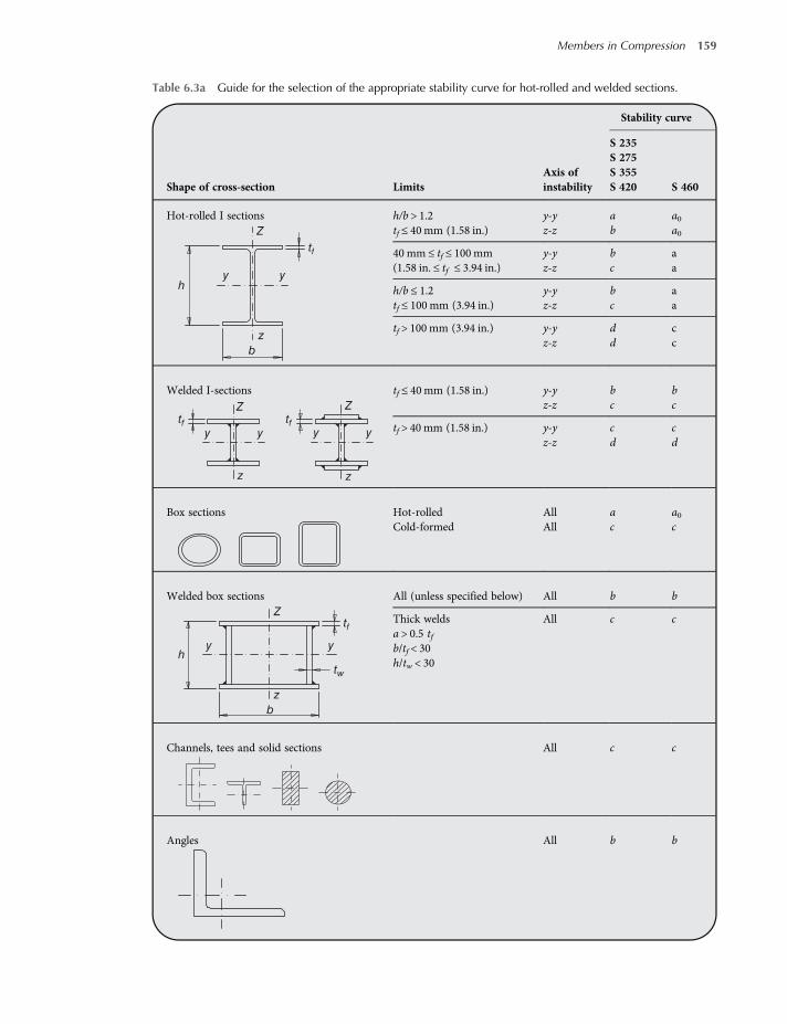
Table 6.3a Guide for the selection of the appropriate stability curve for hot-rolled and welded sections.
Shape of cross-section LimitsAxis ofinstability
Stability curve
S 235
S 460
S 275S 355S 420
Hot-rolled I sections
tf
Z
yyh
z
b
h/b > 1.2 y-y a a0tf ≤ 40mm (1.58 in.) z-z b a0
40 mm ≤ tf ≤ 100mm y-y b a(1.58 in. ≤ tf ≤ 3.94 in.) z-z c a
h/b ≤ 1.2 y-y b atf ≤ 100mm (3.94 in.) z-z c a
tf > 100mm (3.94 in.) y-y d cz-z d c
Welded I-sections
tf tf
Z Z
yy yy
z z
tf ≤ 40mm (1.58 in.) y-y b bz-z c c
tf > 40 mm (1.58 in.) y-y c cz-z d d
Box sections Hot-rolled All a a0Cold-formed All c c
Welded box sections
tf
tw
Z
yh
z
b
y
All (unless specified below) All b b
Thick welds All c ca > 0.5 tfb/tf < 30h/tw < 30
Channels, tees and solid sections All c c
Angles All b b
Members in Compression 159

• cross-sections of class 1, 2 or 3:
λ=A fyNcr
6 26a
• cross-sections of class 4:
λ=Aeff fyNcr
6 26b
in which Ncr is the elastic critical load for the appropriate buckling mode (flexural, torsional orflexural-torsional).
Table 6.3b Guide for the selection of the appropriate stability curve for cold-formed sections.
Shape of cross-sectionAxis ofinstability
Stabilitycurve
If using fyb (see Section 1.6.1) All bIf using fya (this should be used only if the grosscross-sectional area is the effective area:Aeff = Ag)
All c
y y y y
z z
zz
y-y az-z b
All b
All c
160 Structural Steel Design to Eurocode 3 and AISC Specifications

As discussed in the previous section, for I-shapes with at least one axis of symmetry, torsionalinstability can usually be neglected, while for cross-sections having all elements converging intoone point (cruciform sections, angles, tees) torsional buckling often governs the design.When flexural buckling governs the design, the value of relative slenderness λ can be calculated
as follows:
• cross-sections of class 1, 2 or 3:
λ=A fyNcr
=Lcri
1λl
6 27a
• cross-sections of class 4:
λ=Aeff fyNcr
=Lcri
Aeff
Aλl
6 27b
Table 6.4 Values of coefficient χ for design checks according to EC3.
λ
Coefficient χ
a0 a B c d
0.0 1.0000 1.0000 1.0000 1.0000 1.00000.1 1.0000 1.0000 1.0000 1.0000 1.00000.2 1.0000 1.0000 1.0000 1.0000 1.00000.3 0.9859 0.9775 0.9641 0.9491 0.92350.4 0.9701 0.9528 0.9261 0.8973 0.85040.5 0.9513 0.9243 0.8842 0.8430 0.77930.6 0.9276 0.8900 0.8371 0.7854 0.71000.7 0.8961 0.8477 0.7837 0.7247 0.64310.8 0.8533 0.7957 0.7245 0.6622 0.57970.9 0.7961 0.7339 0.6612 0.5998 0.52081.0 0.7253 0.6656 0.5970 0.5399 0.46711.1 0.6482 0.5960 0.5352 0.4842 0.41891.2 0.5732 0.5300 0.4781 0.4338 0.37621.3 0.5053 0.4703 0.4269 0.3888 0.33851.4 0.4461 0.4179 0.3817 0.3492 0.30551.5 0.3953 0.3724 0.3422 0.3145 0.27661.6 0.3520 0.3332 0.3079 0.2842 0.25121.7 0.3150 0.2994 0.2781 0.2577 0.22891.8 0.2833 0.2702 0.2521 0.2345 0.20931.9 0.2559 0.2449 0.2294 0.2141 0.19202.0 0.2323 0.2229 0.2095 0.1962 0.17662.1 0.2117 0.2036 0.1920 0.1803 0.16302.2 0.1937 0.1867 0.1765 0.1662 0.15082.3 0.1779 0.1717 0.1628 0.1537 0.13992.4 0.1639 0.1585 0.1506 0.1425 0.13022.5 0.1515 0.1467 0.1397 0.1325 0.12142.6 0.1404 0.1362 0.1299 0.1234 0.11342.7 0.1305 0.1267 0.1211 0.1153 0.10622.8 0.1216 0.1182 0.1132 0.1079 0.09972.9 0.1136 0.1105 0.1060 0.1012 0.09373.0 0.1063 0.1036 0.0994 0.0951 0.0882
Members in Compression 161

in which λl represents the proportionality slenderness (already defined in Eq. (6.5) and indi-cated with λp), Lcr is the effective length of the member under consideration (previously iden-tified as L0), A and Aeff are the gross cross-section and effective area, respectively, and i is theradius of gyration of the cross-section (already identified as ρ).
When the governing buckling mode is torsional or flexural-torsional, the relative slenderness isdefined as follows:
• cross-sections of class 1, 2 or 3:
λT =A fyNcr
6 28a
• cross-sections of class 4:
λT =Aeff fyNcr
6 28b
in which Ncr is defined as:
Ncr =Ncr,TF withNcr <Ncr,T 6 28c
where Ncr,TF in Eq. (6.9a) and Ncr,T in Eq. (6.8a) represent the elastic critical load for flexural-torsional and torsional buckling, respectively.
6.3.3 Design According to the US Approach
LRFD approach ASD approach
Design according to the provisions for load and resistancefactor design (LRFD) satisfies the requirements of AISCSpecification when the design compressive strength ϕcPn ofeach structural component equals or exceeds the requiredcompressive strength Pu determined on the basis of the LRFDload combinations
Design according to the provisions for allowablestrength design (ASD) satisfies therequirements of AISC Specification when theallowable compressive strength Pn/Ωc of eachstructural component equals or exceeds therequired compressive strength Pa determinedon the basis of the ASD load combinations
Design has to be performed in accordance with the followingequation:
Pu ≤ϕcPn 6 29
where ϕc is the compressive resistance factor (ϕc = 0 90)
Design has to be performed in accordance withthe following equation:
Pa ≤ Pn Ωc 6 30
where Ωc is the compressive safety factor(Ωc = 1.67)
The nominal compressive strength Pn is determined as:
Pn = FcrAg 6 31
The critical stress Fcr is referred to the limit state of flexural buckling as well as for torsional andflexural-torsional buckling. AISC Specifications give different expressions for Fcr, which depends
162 Structural Steel Design to Eurocode 3 and AISC Specifications

on the cross-section type and are different for non-slender and slender element sections. AISC spe-cifications provides specific rules for the following cases:
(a) Generic doubly symmetrical members;(b) Particular generic doubly symmetrical members;(c) Singly symmetrical members;(d) Unsymmetrical members;(e) Single angles with b/t≤ 20;(f) Single angles with b/t > 20;(g) T-shaped compression members.
(a) Generic doubly-symmetric members:When generic doubly-symmetric members are considered, such as typical hot-rolled wideflange columns, except those listed in (b), only flexural buckling has to be taken into account.The critical stress Fcr is determined as follows:
a1 WhenKLr
≤ 4 71E
QFyor
QFyFe
≤ 2 25 Fcr = 0 658QFyFe QFy 6 32
a2 WhenKLr
> 4 71E
QFyor
QFyFe
> 2 25 Fcr = 0 877Fe 6 33
where K is the effective length buckling factor (see Section 6.4), ρ is the ratius of gyration andFe is the elastic buckling stress determined according to the following equation:
Fe =π2E
KLr
2 6 34
It should be noted that Q is the net reduction factor accounting for all slender compressionelements. Its value is equal to 1.0 for non-slender elements, so it must be considered for slen-der elements only, and in this case it has to be determined according to section E6 of AISC360-10. It is worth mentioning that the design of thin-walled member is beyond the scope ofthe present volume.
(b) Particular generic doubly-symmetric members:Flexural and torsional buckling has to be considered in case of particular generic doubly-symmetric members, such as cruciform members, built-up members or genericdoubly-symmetric members with torsional unbraced length exceeding lateral unbracedlength:
The critical stress Fcr is determined with Eqs. (6.32) and (6.33) but Fe is the minimumof the values computed with Eq. (6.34) and with the following expression accounting forthe torsional buckling:
Fe =π2ECw
KzL2 +GJ
1Ix + Iy
6 35
Members in Compression 163
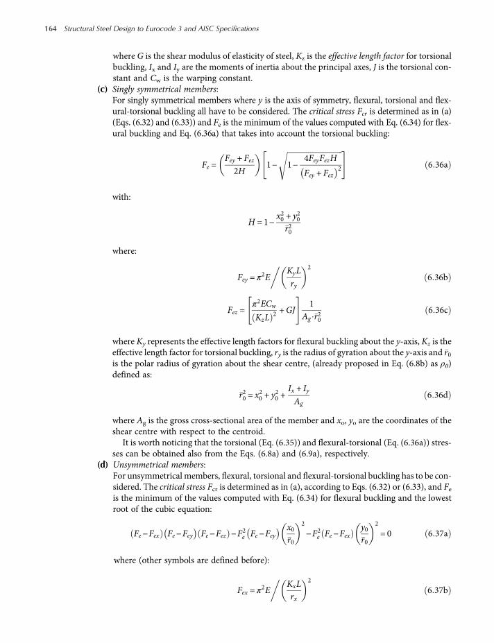
where G is the shear modulus of elasticity of steel, Kz is the effective length factor for torsionalbuckling, Ix and Iy are the moments of inertia about the principal axes, J is the torsional con-stant and Cw is the warping constant.
(c) Singly symmetrical members:For singly symmetrical members where y is the axis of symmetry, flexural, torsional and flex-ural-torsional buckling all have to be considered. The critical stress Fcr is determined as in (a)(Eqs. (6.32) and (6.33)) and Fe is the minimum of the values computed with Eq. (6.34) for flex-ural buckling and Eq. (6.36a) that takes into account the torsional buckling:
Fe =Fey + Fez2H
1− 1−4FeyFezH
Fey + Fez2 6 36a
with:
H = 1−x20 + y
20
r20
where:
Fey = π2E
KyL
ry
2
6 36b
Fez =π2ECw
KzL2 +GJ
1Ag r20
6 36c
where Ky represents the effective length factors for flexural buckling about the y-axis, Kz is theeffective length factor for torsional buckling, ry is the radius of gyration about the y-axis and r0is the polar radius of gyration about the shear centre, (already proposed in Eq. (6.8b) as ρ0)defined as:
r20 = x20 + y
20 +
Ix + IyAg
6 36d
where Ag is the gross cross-sectional area of the member and xo, yo are the coordinates of theshear centre with respect to the centroid.
It is worth noticing that the torsional (Eq. (6.35)) and flexural-torsional (Eq. (6.36a)) stres-ses can be obtained also from the Eqs. (6.8a) and (6.9a), respectively.
(d) Unsymmetrical members:For unsymmetrical members, flexural, torsional and flexural-torsional buckling has to be con-sidered. The critical stress Fcr is determined as in (a), according to Eqs. (6.32) or (6.33), and Feis the minimum of the values computed with Eq. (6.34) for flexural buckling and the lowestroot of the cubic equation:
Fe−Fex Fe−Fey Fe−Fez −F2e Fe−Fey
x0r0
2
−F2e Fe−Fex
y0r0
2
= 0 6 37a
where (other symbols are defined before):
Fex = π2E
KxLrx
2
6 37b
164 Structural Steel Design to Eurocode 3 and AISC Specifications

(e) Single angles with b/t≤ 20:The limitation b/t ≤ 20 applies to all currently produced hot-rolled angles. If angles haveonly one leg fixed to a gusset plate by welding or by a bolted connection with at leasttwo bolts and there are no intermediate transverse loads, they can be treated as axiallyloaded members, neglecting the effect of load eccentricity and considering flexural buck-ing only, but adjusting the member slenderness. So Fcr has to be determined as in cases a1and a2, and Fe is evaluated in accordance with Eq. (6.34) using for KL/r the followingvalues:For equal-leg angles or unequal-leg angles connected through the longer leg that are individ-ual members or are web members of planar trusses with adjacent web members attached tothe same side of the gusset plate or chord:
whenLrx
≤ 80:
KLr
= 72 + 0 75Lrx
6 38
whenLrx
> 80:
KLr
= 32 + 1 25Lrx
6 39
For equal-leg angles or unequal-leg angles connected through the longer leg that are webmembers of box or space trusses with adjacent web members attached to the same side ofthe gusset plate or chord:
whenLrx
≤ 75:
KLr
= 60 + 0 80Lrx
6 40
whenLrx
> 75:
KLr
= 45 +Lrx
6 41
where rx is the radius of gyration about the geometric axis parallel to the connected leg.(f) Single angles with b/t > 20:
The limitation b/t > 20 applies to fabricated angles. Like any asymmetric member, Fcr has to bedetermined as in (a) and Fe is the minimum of the values computed with Eq. (6.34) for flexuralbuckling and the lowest root of the cubic Eq. (6.37a).
(g) T-shaped compression members:For T-shaped compression members flexural and flexural-torsional buckling has to be con-sidered. Flexural buckling shall be verified computing Fcr according to Eqs. (6.32) and (6.33)computing Fe according to Eq. (6.34). For flexural-torsional buckling Fcr has to be determinedaccording to the following equation:
Fcr =Fcry + Fcrz
2H1− 1−
4FcryFcrzH
Fcry + Fcrz2 6 42a
Members in Compression 165

where Fcry is taken as Fcr of Eqs. (6.32) and (6.33) for flexural buckling about the y-axis ofsymmetry, KL/r = KyL/ry and:
Fcrz =GJ
Agr206 42b
6.4 Effective Length of Members in Frames
A key aspect related to the design of a compression member of length L is the evaluation of theeffective length, L0, or equivalently of theK length factor, of members in frames (with L0 = K L). Infew design cases, reference can be made to isolated members, already briefly discussed inSection 6.3. In general, the authors’ option is to use a buckling analysis for determining the min-imum αcr value associated with the buckling mode of interest. The critical load Ncr can be
easily determined via equation αcr =Ncr
NEd, with NEd equal to the design axial load. Finally, from
Ncr, critical length Lcr for flexural buckling can be computed as:
Lcr = L0 = πE INcr
= πE I
αcr NEd6 43
Furthermore, reference should be made to simplified approaches currently used in accordancewith both the EU and US steel design practice, based on the use of alignment charts. These havebeen determined with reference to assumptions of idealized conditions which seldom exist in realstructures. These assumptions are as follows:
(1) behaviour of the steel material is purely elastic;(2) all members have constant cross section;(3) all joints are rigid;(4) for columns in frames with inhibited sidesway, rotations at opposite ends of the restraining
beams are equal in magnitude and opposite in direction, producing single curvature bending;(5) for columns in frames with uninhibited sidesway, rotations at opposite ends of the restraining
beams are equal in magnitude and direction, producing reverse curvature bending;
(6) the stiffness parameter defined as L P EI of all the columns is equal;(7) joint restraint is distributed to the column above and below the joint in proportion to EI/L for
the two columns;(8) all columns buckle simultaneously;(9) no significant axial compression force exists in the girders.
6.4.1 Design According to the EU Approach
As regards to European design, reference should be made to the old ENV edition of EC3(ENV 1993-1-1:2004), relative to columns belonging to non-sway or sway frames. To this purposeFigure 6.12 for a non-sway frame, and to Figure 6.13 for a sway frame can be considered. Bothfigures provide the ratio Lcr/L as a function of distribution factors η1 and η2, related to the twoends of the column, and defined as follows:
η1 =Kc
Kc +K11 +K12; η2 =
Kc
Kc +K21 +K226 44
166 Structural Steel Design to Eurocode 3 and AISC Specifications

where: Kc = Ic hc is the column stiffness coefficient, Kij = kij Iij Lij is the effective beam stiffnesscoefficient and coefficient kij depends on the beam restraints (Tables 6.5 and 6.6).Term I expresses the moment of inertia, h and L are the lengths of the column and of the beam,
respectively, and subscripts are represented in Figures 6.12 and 6.13.Formulas (6.44) are valid for columns of single-story buildings. For columns of multi-story
buildings, if ratio N/Ncr is almost constant among all columns, an alternative approach can beused, which is based on the evaluation of the end column stiffness, defined with reference to
1.0
0.9η1
0.8
0.7
0.6
0.5
0.4
0.3
0.2
0.1
Fixed
Fixed
0.0 0.1 0.2 0.3 0.4 0.5 0.6 0.7 0.8 0.9 1.0
N
N
KcL
K21
K11
K12
K22
Distribution factor η2
Distribution factor η1
Pinned
(a) (b)
Pinned
1.00.950.90.85
0.80.75
0.70.6750.650.6250.60.5750.550.5250.5
η2
Figure 6.12 Buckling length ratio Lcr/L for a column in a non-sway mode (a) and distribution factor for column in anon-sway mode (b).
1.0 5.0
∞4.0
3.02.8
2.6
2.4
2.22.0
1.9
1.8
1.71.61.5
1.41.3
1.251.2
1.151.1
1.051.0
0.9η1
0.8
0.7
0.6
0.5
0.4
0.3
0.2
0.1
Fixed
Fixed
0.0 0.1 0.2 0.3 0.4 0.5 0.6 0.7 0.8 0.9 1.0N
N
Kc
K21
K11
K12
K22
Distribution factor η2
Distribution factor η1
Pinned
(a) (b)
Pinnedη2
Figure 6.13 Buckling length ratio Lcr/L for a column in a swaymode (a) and distribution factor for column in a swaymode (b).
Members in Compression 167

the restraining effects of the upper and the lower column stiffness (K1 and K2, respectively) as (seeFigure 6.14):
η1 =Kc +K1
Kc +K1 +K11 +K12; η2 =
Kc +K2
Kc +K2 +K21 +K226 45
Alternatively, for direct evaluation via Figure 6.12 or 6.13, the following more conservativeapproach can be used:
(a) non-sway frames:
K = Lcr L= 0 5 + 0 14 η1 + η2 + 0 055 η1 + η22 6 46
Table 6.5 Effective stiffness coefficient Kij for a beam in a frame without concrete floor slabs.
Conditions of rotational restraint at far end of beam Kij
Fixed 1 0 Iij LijPinned 0 75 Iij LijRotation as at near end (double curvature) 1 5 Iij LijRotation equal and opposite to that at near end (single curvature) 0 5 Iij LijGeneral case. Rotation θa at near end, θb at far end 1 + 0 5
θbθa
Iij Lij
Table 6.6 Reduced beam stiffness coefficients Kij due to axial compression.
Conditions of rotational restraint at far end of beam Kij
Fixed 1 0IijLij
1−0 4NNE
Pinned 0 75IijLij
1−1 0NNE
Rotation as at near end (double curvature) 1 5IijLij
1−0 2NNE
Rotation equal and opposite to that at near end (single curvature) 0 5IijLij
1−1 0NNE
NE = π2EIij L2ij (If N represents tension, it must be considered = 0)
Column being
designed
K12
K22
Kc
K1
K11
K21
K2Distribution
factor η2
Distribution
factor η1
Figure 6.14 Distribution factor for continuous columns.
168 Structural Steel Design to Eurocode 3 and AISC Specifications

(b) sway frames:
K = Lcr L=1−0 2 η1 + η2 −0 12η1η21−0 8 η1 + η2 + 0 6η1η2
6 47
For calculating beam stiffness coefficients Kij that are functions of beam restraints, formulas ofTable 6.5 have to be used.If beams are subjected to large compression axial loads, stiffness values have to be reduced
according to formulas of the Table 6.6.For beams supporting reinforced concrete slabs, a higher stiffness has to be taken into account,
using formulas of Table 6.7.
6.4.2 Design According to the US Approach
In accordance with the US practice, simplified methods to calculate the effective length factor Kare admitted. For columns belonging to a moment frame system, alignment chart with sideswayinhibited (Figure 6.15) and with uninhibited sidesway (Figure 6.16) can be used. The parameter Ggoverning the use of the alignment charts is defined as:
G=
EcIcLcEgIgLg
6 48
where I and L are the moment of inertia and the member length, respectively, E is the Young’smodulus and subscripts c and g indicate columns and beams (girders), respectively.The summation Σ is extended to all the members rigidly connected to the node of interest and
subscripts A and B (Figures 6.15 and 6.16) identify the upper and lower joints of the consideredcolumn.Therefore, in order to use these values for K, some adjustments are suggested by AISC 360-10
Commentary. In particular, for isolated columns, theoretical K values and recommended designvalues should be adopted as recommended in Table 6.8. Furthermore, for columns in frames withsidesway inhibited and sidesway uninhibited, the corrections herein described should be applied.For sidesway inhibited frames, these adjustments for different beam end conditions are
required:
• if the far end of a girder is fixed, multiply the flexural stiffness (EI/L)g of the member by 2.0;• if the far end of the girder is pinned, multiply the flexural stiffness (EI/L)g of the member by 1.5.
Table 6.7 Effective stiffness coefficient Kij for a beam in a building frame with concrete floor slabs.
Loading conditions for the beam
Kij
Non-sway mode Sway mode
Beam directly supporting concrete floor slabs 1 0 Iij Lij 1 0 Iij LijOther beams with direct loads 0 75 Iij Lij 1 0 Iij LijBeams with end moments only 0 5 Iij Lij 1 5 Iij Lij
Members in Compression 169

50.0
10.05.04.03.0
2.0
1.00.90.80.7
0.6
0.5
1.0
0.9
0.8
0.7
0.6
0.5
0.4
0.3
0.2
0.1
0.0
50.0∞
θA θA
θA
θB
θA
θA
θB
θBθB
θB
10.0
5.04.03.0
2.0
1.00.90.80.7
0.6
0.5
0.4
0.3
P
P
c3
c1
b4
b2A
Bb3
b1
c2
0.2
0.1
0.0
K GBGA∞
Figure 6.15 Alignment chart–sidesway inhibited (no-sway frames). From Figure C-A-7.1 of AISC 360-10.
50.0100.0
10.0
10.020.0
20.0
30.0
5.0
5.0
6.07.08.0
4.0
4.0
3.0
3.0
2.0
2.0
1.0
0.0
50.0100.0
10.0
20.0
30.0
5.0
6.07.08.0
4.0
3.0
2.0
1.0
0.0
θA
θA
θB
Δ Δ
Δ
θA
θA
θA
θB
θB
θB
θB
P
P
c3
c1
b4
b2A
B
b3
b1
c2
1.0
1.5
K GBGA
∞∞
∞
Figure 6.16 Alignment chart–sidesway uninhibited (sway frames). From Figure C-A-7.2 of AISC 360-10.
170 Structural Steel Design to Eurocode 3 and AISC Specifications

For sidesway uninhibited frames and girders with different boundary conditions, the modifiedgirder length, Lg, should be used instead of the actual girder length, which is defined as:
Lg = Lg 2−MF
MN6 49
whereMF is the far end girder moment andMN is the near end girder moment from a first-orderanalysis of the frame.The ratio of the two momentsMF andMN is positive if the girder is in reverse curvature. IfMF/
MN is more than 2.0, then Lg becomes negative, in which case G is negative and the alignmentchart equation must be used.For sidesway uninhibited frames, these adjustments for different beam end conditions are
admitted:
• if the far end of a girder is fixed, multiply the (EI/L)g of the member by 2/3;• if the far end of the girder is pinned, multiply the (EI/L)g of the member by 0.5.
For girders with significant axial load, for both sidesway conditions, multiply the (EI/L)g by thefactor 1−Q Qcr where Q is the axial load in the girder and Qcr is the in-plane buckling load of thegirder based on K = 1.0.To account for inelasticity in columns, for both sidesway conditions, replace (Ec Ic) with τb(EcIc)
for all columns in the expression forGA andGB. The stiffness reduction factor, τb, has already beendefined with reference to DAM approach presented in Eq. (12.12).For columns with different end conditions, if they are supported by a foundation with a
pinned connection, G should theoretically be infinity. Owing to the fact that usually pinnedconnections are not true friction-free pins, so G can be taken as 10 for practical design. Other-wise, if columns are rigidly connected to foundations, G should be 0, but it is prudent to takeit as 1.0.One important assumption in the use of the alignment charts is that all beam-column connec-
tions are fully restrained (FR connections). As seen previously, when the far end of a beam doesnot have an FR connection that behaves as assumed, an adjustment must be made, which implies areduction of the beam stiffness. When a beam connection at the column of interest is a shear onlyconnection (no moment can be transferred) then that beam cannot participate in the restraint ofthe column and it cannot be considered in the Σ(EI/L)g term of the equation for G. Only FR con-nections can be used directly in the determination ofG. Partially restrained (PR) connections witha well-known moment-rotation response can be utilized, but the (EI/L)g of each beam must beadjusted to account for the connection flexibility.
Table 6.8 Theoretical and recommended AISC values of the effective length factor (K) for isolated column.
End condition restrains
Top End translation Fixed Fixed Free Fixed Free FreeEnd rotation Fixed Free Fixed Free Free Fixed
Bottom End translation Fixed Fixed Fixed Fixed Fixed FixedEnd rotation Fixed Fixed Fixed Free Fixed Free
Theoretical K value 0.5 0.7 1.0 1.0 2.0 2.0Recommended design value when ideal condition areapproximated
0.85 0.8 1.20 1.0 2.1 2.0
Members in Compression 171

6.5 Worked Examples
Example E6.1. HE-Shaped Column Available Strength Calculation According to EC3
Calculate the available strength of an EN 10025 S235 steel (fy = 235MPa (34 ksi)) HE 200 B. The column is7.5 m (24.6 ft) long, pinned at its top and bottom in both axes, with a strong axis unbraced length of 7.5 m(24.6 ft) and a weak axis and torsional unbraced length of 3.75 m (12.3 ft).
HE 200 B properties
Height h 200mm (6.87 in.) z
z
b
hy y
r
tf
tw
Flange width b 200mm (6.87 in.)Flange thickness tf 15 mm (0.59 in.)Web thickness tw 9 mm (0.35 in.)Corner radius r 18 mm (0.71 in.)Area A 78.1 cm2 (12.11 in.2)Moment of inertia about a strong axis Iy 5696 cm4 (136.8 in.4)Moment of inertia about a weak axis Iz 2003 cm4 (48.12 in.4)
Design procedureAccording to EC3, the column design curves are different for buckling about the y-axis and buckling about thez-axis. So it is not certain that the maximum compressive strength is associated with the minimum slender-ness. Therefore, column strength calculation should be performed by taking into consideration member slen-derness about both principal axes. The following steps have to be executed:
• cross-section classification;• evaluation of elastic flexural buckling load about strong axis (Ncr,y);• evaluation of relative slenderness about strong axis (λy);• choose the column design curve for flexural buckling about strong axis and computation of reduction fac-
tor for buckling about strong axis (χy);• evaluation of elastic flexural buckling load about weak axis (Ncr,z);• evaluation of relative slenderness about weak axis (λz);• choose the column design curve for flexural buckling about weak axis and computation of reduction factor
for buckling about weak axis (χz);• choose the minimum reduction factor (χ =min (χy, χz)) and calculate column available strength (Nb,Rd).
Section classification (Section 4.2.1). For S 235 steel grade: ε = 1
Flange c tf = 200 – 9− 2 × 18 2 × 15 = 5 2≤ 9 Class 1
Web d tw = 200 – 2 × 15 – 2 × 18 9 = 14 9≤ 33 Class 1
S 235 steel HE 200 B cross section is a class 1 section if subjected to axial load.
172 Structural Steel Design to Eurocode 3 and AISC Specifications

Calculate the elastic critical buckling stress about strong axis (Eq. (6.3)):
Ncr,y =π2EIyLo,y2
=π2 × 210000 × 5696 104
7500210−3 = 2098 78 kN 471 8 kips
Calculate the relative slenderness about strong axis (Eq. (6.26a)):
λy =A fyNcr,y
=7808 × 2352098 78 103
= 0 935
Calculate the reduction factor χy: referring to curve b to be used for buckling about strong axis (y–y axis) inTable 6.3a of HE 200 B profile, reference has to be made (Table 6.4):
λ χ
0.9 0.66121.0 0.5970
Linear interpolation gives χy = 0.6386.Calculate elastic critical buckling stress about weak axis:
Ncr,z =π2EIzLo,z2
=π2 × 210000 × 2003 104
3750210−3 = 2952 1 kN 663 6 kips
Calculate the relative slenderness about weak axis (Eq. (6.26a)):
λz =A fyNcr,z
=7808 × 2352952 1 103
= 0 788
Calculate the reduction factor χz: referring to curve c, to be used for buckling about weak axis (z–z axis) inTable 6.3a of HE 200 B profile, reference has to be made (Table 6.4):
λ χ
0.7 0.72470.8 0.6622
Linear interpolation gives χz = 0.6693.Calculate the available column strength (Eq. (6.24a)): let’s consider as reduction factor χ the lower value
between χy and χz:
Nb,Rd = χ AfyγM1
= 0 6387 × 7808 ×2351 00
10−3 1171 9 kN 263 5 kips
Members in Compression 173
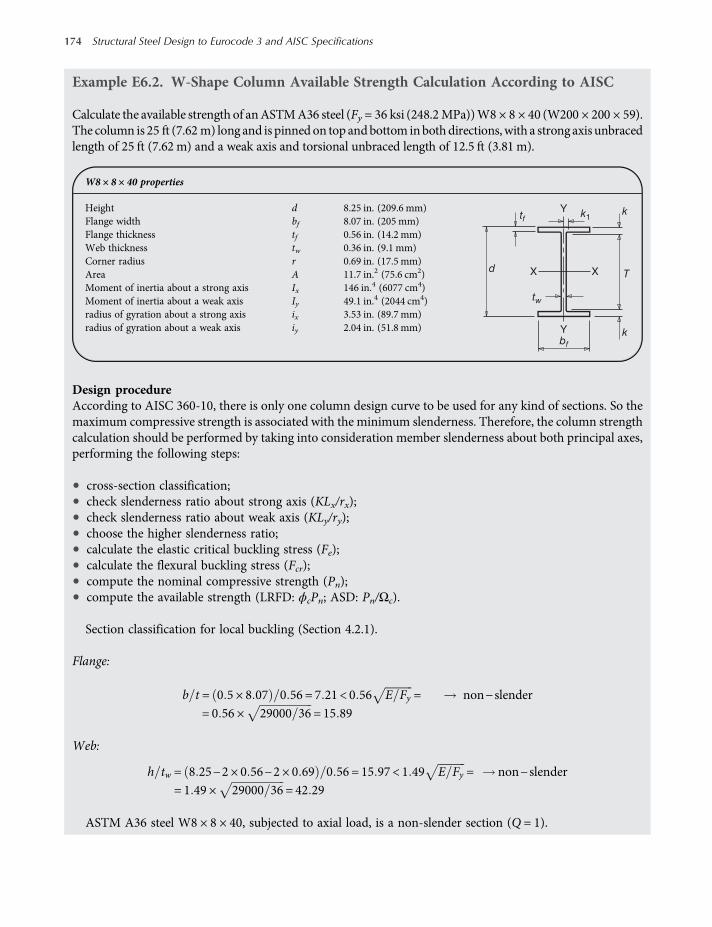
Example E6.2. W-Shape Column Available Strength Calculation According to AISC
Calculate the available strength of anASTMA36 steel (Fy = 36 ksi (248.2MPa))W8 × 8 × 40 (W200 × 200 × 59).The column is 25 ft (7.62 m) long and is pinned on top andbottom inbothdirections, with a strong axis unbracedlength of 25 ft (7.62 m) and a weak axis and torsional unbraced length of 12.5 ft (3.81 m).
W8× 8 × 40 properties
Height d 8.25 in. (209.6 mm)
k
k1ktf
X TXd
tw
Y
Ybf
Flange width bf 8.07 in. (205 mm)Flange thickness tf 0.56 in. (14.2 mm)Web thickness tw 0.36 in. (9.1 mm)Corner radius r 0.69 in. (17.5 mm)Area A 11.7 in.2 (75.6 cm2)Moment of inertia about a strong axis Ix 146 in.4 (6077 cm4)Moment of inertia about a weak axis Iy 49.1 in.4 (2044 cm4)radius of gyration about a strong axis ix 3.53 in. (89.7 mm)radius of gyration about a weak axis iy 2.04 in. (51.8 mm)
Design procedureAccording to AISC 360-10, there is only one column design curve to be used for any kind of sections. So themaximum compressive strength is associated with the minimum slenderness. Therefore, the column strengthcalculation should be performed by taking into consideration member slenderness about both principal axes,performing the following steps:
• cross-section classification;• check slenderness ratio about strong axis (KLx/rx);• check slenderness ratio about weak axis (KLy/ry);• choose the higher slenderness ratio;• calculate the elastic critical buckling stress (Fe);• calculate the flexural buckling stress (Fcr);• compute the nominal compressive strength (Pn);• compute the available strength (LRFD: ϕcPn; ASD: Pn/Ωc).
Section classification for local buckling (Section 4.2.1).
Flange:
b t = 0 5 × 8 07 0 56 = 7 21 < 0 56 E Fy = non−slender
= 0 56 × 29000 36 = 15 89
Web:
h tw = 8 25−2 × 0 56−2 × 0 69 0 56 = 15 97 < 1 49 E Fy = non−slender
= 1 49 × 29000 36 = 42 29
ASTM A36 steel W8 × 8 × 40, subjected to axial load, is a non-slender section (Q = 1).
174 Structural Steel Design to Eurocode 3 and AISC Specifications

Check the slenderness ratio about both axes (by assuming K = 1.0)
KLxrx
=1 × 25 0 12
3 53= 84 9 governs
KLyry
=1 × 12 5 12
2 04= 73 5
Calculate via Eq. (6.34) the elastic critical buckling stress (Fe).
Fe =π2E
KLxrx
2 =3 142 × 29000 ksi
84 9 2 = 39 7 ksi 273 2MPa
Calculate the flexural buckling stress (Fcr).
Check limit: 4 71E
QFy= 4 71 ×
290001 × 36
= 133 7 > 84 9
BecauseKLxrx
≤ 4 71E
QFythen, based on Eq. (6.32):
Fcr = 0 658QFyFe QFy = 0 658
1×3639 7 × 1 × 36 = 24 61 ksi 169 7MPa
Compute via Eq. (7.31) the nominal compressive strength (Pn).
Pn = FcrAg = 24 61 × 11 7 = 286 9 kips 1281 kN
Compute the available strength.
LFRD ϕcPn = 0 90 × 287 9 = 259 1 kips 1153 kN
ASD Pn Ωc = 287 9 1 67 = 172 4 kips 767 1 kN
Members in Compression 175

CHAPTER 7
Beams
7.1 Introduction
Members subjected to bending are also generally affected by shear forces, which have to beadequately considered in all the safety checks. Furthermore, the design of beams has to take intoaccount both serviceability (mainly, check on deflections and dynamic effects) and ultimate limitstates, including, in addition to resistance, stability verifications when relevant.
Preliminarily to the design rules of beams, in the following some key aspects related to theresponse of elements under flexure and shear are briefly discussed.
7.1.1 Beam Deformability
The deflection limits provided in any specification can be generally used only as a guide to theserviceability of the structure and may not be taken as an absolute guide to satisfactory perform-ance in the cases of interest for routine design. It is the responsibility of the designer to verify thatthe limits used in the design are appropriate for the structure under consideration.
Maximum deflections (usually in the elastic range), v, can be evaluated on the basis of theelastic theory of structures and thenmust be compared with the standard limit, vLim, ensuring that:
v ≤ vLim 7 1
The elastic beam deflection should always be considered to be the sum of two contributions, oneassociated with the flexural deformability, vF, and one associated with the shear deformability, vT, as:
v = vF + vT 7 2
Term vF is usually reported in the designer manuals for the most common routine design cases.Term vT is rarely offered in literature and can be evaluated using the principle of virtual work. Inthe case of isolated beam of length L, the following expression can be used:
vT =
L
o
χTT xG A
T1 x dx 7 3
Structural Steel Design to Eurocode 3 and AISC Specifications, First Edition. Claudio Bernuzzi and Benedetto Cordova.© 2016 John Wiley & Sons, Ltd. Published 2016 by John Wiley & Sons, Ltd.

where terms T(x) and T1(x) represent the shear distribution on the beam associated with the loadcondition and the service condition (characterized by a unitary concentrated force applied wherethe displacement has to be evaluated), respectively, G is the shear modulus, A is the cross-sectionarea and χT is the shear factor.Shear factor,χT, is adimensionless coefficient, dependingontheshapeof the cross-section. Its value
is always greater than unity and it increases with the increase of the deviation of the shear stress dis-tribution fromauniformdistribution.A correct evaluationof χT canbe obtained fromthe expression:
χT =AI2
y
y
S2ibidy 7 4
where I is the moment of inertia, y and y are the cross-section limits, S is the first moment of areaof the part of the cross-section (below the chord with a width bi with reference to the neutral axis)and A is the cross-section area.As an example, in case of rectangular solid cross-sections the result is χT = 1.2, while for I- and
H-shaped European profiles (typically, IPE and HE profiles) the value of χT is always greater than2 and in particular:
• for IPE profiles χT ranges between 2.2 and 2.6;• for HEA and HEB profiles χT ranges between 2.1 and 4.7;• for HEM profiles χT ranges between 2.1 and 4.4.
As alternative to the exact definition of the shear factor by Eq. (7.4), a simplified formula can beapplied in cases of I- and H-shaped doubly symmetrical profiles under flexure in the web plane: anapproximate estimation of χT is given by:
χT =AAw
7 5
where A and Aw are the area of the cross-section and the area of the sole web, respectively.The errors due to Eq. (7.5) are extremely limited: not more than 5% for the IPE profiles and
always less than 9% for HE profiles.The influence of the contribution to the overall deflection due to shear deformability depends
on the load condition as well as on the beam slenderness, which can be defined as the ratiobetween the beam length (L) and its depth (H). As an example, in the following the results ofa parametric analysis are presented with reference to the case of simply supported beam underuniformly distributed loads where all the IPE and HE profiles have been considered.In case of a beam slenderness equal to 6 (i.e. L = 6H) the results are that:
• for IPE profiles vT ranges from 24 to 30% of vF;• for HEA and HEB profiles vT ranges from 23 to 58% of vF;• for HEM profiles vT ranges from 23 to 49% of vF.
In case of beam slenderness equal to 12 (i.e. L = 12 H) the influence of vT is significantly reducedand the results are that:
• for IPE profiles vT ranges from 6 to 7% of vF;• for HEA and HEB profiles vT ranges from 6 to 15% of vF;• for HEM profiles vT ranges from 6 to 12% of vF.
Beams 177

7.1.2 Dynamic Effects
In several design cases, dynamic effects need to be taken into account to ensure that vibrations donot impair the efficiency of the structure at the serviceability limit state. The vibrations of struc-tures on which people can walk have to be limited to avoid significant discomfort to users andlimits should be specified for each project and agreed with the client. To achieve a more than sat-isfactory vibration behaviour of buildings and of their structural main members under serviceabil-ity conditions, the following aspects, amongst others, have to be considered:
• the comfort of the user;• the functioning of the structure or its structural members (e.g. cracks in partitions, damage to
cladding, sensitivity of building contents to vibrations).
Other aspects should be considered for each project and agreed with the client: problems asso-ciated with dynamic effects can also be due to moving plant and machinery.
Referring to the literature for a more complete discussion on this topic, it should be noted thatin case of free vibration of an isolated beam of length L, the natural (fundamental) beam fre-quency, f0, expressed in hertz (i.e. cycles per second), can be estimated as:
f0 =KEI
m L47 6a
where K is a coefficient accounting for the restraint conditions, E the dynamic elastic modulus ofthe material, I the moment of inertia and m represents the mass per unit length.
Term K can be evaluated as:
K =α
2π7 6b
For the most common cases of beam end restraints, the following values are proposed inliterature:
• α = 9.869 (K = 1.57) for a simply supported beam;• α = 22.37 (K = 3.56) for a fixed-end beam;• α = 3.516 (K = 0.56) for a cantilever beam;• α = 14.538 (K = 2.45) for a simply supported-fixed end beam.
With reference to the current design practice, generally, the direct calculation of f0 is avoided,owing to the difficulties in the evaluation of the dynamic characteristics of the steel materials. Itappears more preferable to use an approximated approach based on a direct evaluation ofdisplacements. As an example, in case of a simply supported beam of length L with a uniformmass m, the displacement δm can be estimated neglecting the contribution due to shear deform-ability, as:
δm =5 mg L4
384 E I7 7
where g is the acceleration due to gravity (conventionally assumed as g = 9805.5 mm/s2 (386 in./s2), m is the mass per unit length, E the Young’s modulus and I the moment of inertia.
178 Structural Steel Design to Eurocode 3 and AISC Specifications

Substituting term m L4 in the previous equation and considering the maximum displacementδmax, the frequency (expressed in hertz) can be approximated as:
f0 =17 75
δmax mm≈
18
δmax mm7 6c
Using the US system of units, the result is:
f0 =3 54
δmax in7 6d
For the serviceability limit state, the natural frequency of vibrations of the structure or of astructural member should be kept above appropriate values in order to avoid the phase (ampli-tude) resonance during normal use. Frequency limit depends upon the function of the buildingand the source of the vibration, and is agreed with the client and/or the relevant authority. If thenatural frequency of vibrations of the structure obtained via this simplified approach is lower thanthe appropriate value, a more refined analysis of the dynamic response of the structure, includingthe consideration of damping, should be performed. The most severe load combination, with ref-erence to the displacement δmax should be considered in order to base the vibration verification onthe lower values of frequency (fundamental frequency).
7.1.3 Resistance
In design practice, members generally have cross-sections with at least one axis of symmetry andone of the most frequent cases is the check for mono-axial bending, where one of the principalaxes is also an axis of flexure. Furthermore, it should be noted that the more general case is the bi-axial bending, that is the bending axis does not coincide with the principal axis. With reference toFigure 7.1 the resulting bending moment M is given by the equation:
M = My12 +Mz1
2 7 8
where My1 and Mz1 represent the moments acting on the generic planes y1 and z1.The simplest method to analyse biaxial bending is to replace the momentsMy1 andMz1 by their
principal plane static equivalents My and Mz calculated from:
My =My1 cosα+Mz1 senα 7 9a
Mz = −My1 senα+Mz1 cosα 7 9b
in which α is the angle between the y1- and z1-axes and the principal y- and z-axes, as shown inFigure 7.1b.From a practical point of view the superposition principle is frequently used and themono-axial
bending approach is extended to the case of bi-axial bending.
7.1.4 Stability
Open section beams bent in their stiffer principle plane are susceptible to a type of bucklingdeflecting sideways and twisting (Figure 7.2), the so-called lateral instability, lateral-torsionalor flexural-torsional instability. In particular, this form of instability is due to the compression
Beams 179

force acting on a part of the profile causing instability with lateral deflection partially prevented bythe tension part of the profile, which generates twist. Design standards consider lateral–torsionalbuckling as one of the ultimate limit states that must be checked for steel members in bending,when relevant. The buckling resistance assessment is usually based on appropriate buckling curvesand requires the computation of the elastic critical moment, which is strongly dependent on sev-eral factors such as, the bending moment distribution, the restraints at the end supports and incorrespondence of the load points, the beam cross-section, the distance between the load appli-cation point and the shear centre.
Due to the presence of both lateral and torsional deformations, a rigorous design approach isvery complex but few simplifications are admitted. Beam design, taking into account lateral–torsional buckling, essentially consists of assessing the maximum moment that can safely be car-ried from knowledge of the section material and geometrical cross-section properties, therestraints provided and the arrangement of the applied loading. It should be noted that the eccen-tricity between the load application point and the shear centre plays an important role in the beamresponse. As an example, in case of I- or H-shaped cantilever beam in Figure 7.2, it can be notedthat when the load is applied on the top flange or on the bottom flange, the load carrying capacity
Deflection in a
non-principal plane
Plane of
momentPrincipal
plane
Mz1
My1
My1
Mz1
Mz
My
M
M
y1 (v1= 0)y1
y y
z1
z1
z
(a) (b)
zPlane of
deflection
Principal bending moments
My and Mz
α α
Figure 7.1 Bending in a non-principal plane: (a) deflection in a non-principal plane and (b) principal bendingmoments My and Mz.
Translation
Rotation
FF
F
Figure 7.2 Deformed beam configurations associated with lateral torsional buckling. From Figure C-C2.3 ofAISC 360-10.
180 Structural Steel Design to Eurocode 3 and AISC Specifications

is significantly different, due to the fact that the load at the top flange has a negative effect (desta-bilizing load) with reference to lateral stability. Otherwise, load applied on the bottom flange sta-bilizes the beam response.With reference to the design of civil and industrial structures, it should be noted that the floor
slab could restraint efficiently the lateral buckling of the beams. However, buckling resistance hasto be considered for the erection stage, in presence of load condition generally less severe than theone associated with the normal usage but without any restraint to lateral buckling. Furthermore,beam instability has to be considered in many cases for the roof beams, due to quite limited effectof metal sheeting in preventing the beam buckling. Verification criteria proposed for members inbending susceptible of lateral buckling are based on the value of the elastic critical moment (Mcr)and its evaluation, which in many cases is quite fairly complex, can be made by using numerical ortheoretical approaches.By exploiting the potentiality of finite elements (FEs) commercial analysis packages
and their refined pre- and post-processors, it appears convenient, for design purposes, togenerate complex three-dimensional refined meshes, especially in case of isolated beams.Available software pre-processors allow modelling exactly the shape of the profile with anaccurate description (Figure 7.3a) of its components (web and flanges) by using shell or solidelements. As in case of the columns in the frames, an elastic buckling analysis or an incrementalsecond order elastic analysis can be carried out on beams (Figure 7.3b,c) and attention has to bepaid to the buckling deformed shape of interest for practical design, owing to the possibility that asimplified modelling of restraints or of the load introduction zones could lead to local bucklingmodes not relevant for design purposes (Figure 7.3d). In case of sub-frames or more complexframed systems, this modelling approach could lead to a large number of degrees of freedomas well as to an excessive number of elements in the zones where elements are connected and/or loaded.Furthermore, beam formulations that are implemented in the most commonly used FE analysis
packages neglect the warping of the cross-sections as well as all the associated effects and, as aconsequence cannot be used to evaluate Mcr directly. As alternative, the well-established theor-etical approach to evaluate directly the elastic critical momentsMcr can be used, which have beenproposed in literature for most common cases of load cases and restraints, mainly with referenceto profiles with bi- and mono-symmetrical I- and H-shaped cross-sections.With reference to the more general case of mono-symmetrical I- or H-shaped unequal flange
member (Figure 7.4), if the axis of symmetry is also axis of flexure and the moment distribution isconstant (uniform) across the element (equal opposite moments applied at the beam ends), thecritical elastic moment (Mcr,u) can be evaluated as:
Mcr,u =π2EIzkzL
2 GIt +π2EIwkwL
2 +βy2
π2EIzkzL
2
2
+βy2
π2EIzkzL
2 7 10
where L is the distance between two consecutive restrained cross-sections, E andG are the Young’sand the tangential elasticity modulus of material, respectively, Iz is the moment of inertia along theweak axis, Iw and It are the warping and the torsion constant, respectively.Terms kw and kz take into account the restraints of the cross-section.Term kw is an effective length factor accounting for warping end restraint, ranging from 0.5 (full
fixity) to 1.0 (no fixity): kw = 0.7 is recommended for one end fixed and the other end free.Term kz is an effective length factor accounting for rotation about y–y axis: it varies from 0.5 for
full fixity to 1.0 for no fixity, with 0.7 for one end fixed and the other end free.
Beams 181

(a) (b)
(d)(c)
Figure 7.3 Three-dimensional shell models for a steel beams: the mesh (a) and typical critical deformed shapesobtained via buckling analysis in case of wide flangeHE beam (b), standard I beam (c) andwide flange beam (d) for ahigh mode.
Transversal
load
z
C
O
za
zs
y
Figure 7.4 Mono-symmetrical unequal flange I profiles.

Term βy is the Wagner coefficient, accounting for the eventual coincidence between shearcentre and centroid. If the reference system has the origin in the centroid O (at a distance zsof form centroid C), βy is defined as:
βy = 2 zs−1Iy
A
y2z + z3 dA 7 11
For the sake of simplicity, reference can be made to Figure 7.5 relating to the cases of simplebending for mono-symmetrical cross-section members.This approach allows us to evaluate the elastic critical moment of the beam under uniform
moment distribution,Mcr,u. Usually, bending moment distribution along the beam is not uniformand, as a consequence, standard codes propose the use of an equivalent uniform moment factor(EUMF) to be used to compute the elastic critical moment referred to the actual bending momentdistribution by means of the expression:
Mcr = EUMF Mcr,u 7 12
Several approaches to evaluate the EUMF term are available nowadays. One of the most effi-cient ones was proposed by Serna et al., who recently carried out a critical review of some of theseapproaches to evaluating EUMF coefficients recommended bymodern steelwork standards. It hasbeen shown that, whilst codes may lead to conservative values for simply supported beams, non-conservative values are obtained in the case of support types designed to restrict lateral bendingand warping. The following general closed-form expression was hence proposed to assess EUMFcoefficient:
Z
Z
C
C
C
0
C
00
0
Zs
Zs
Y
Y
Figure 7.5 Bending load cases for mono-symmetrical unequal flange I profiles.
Beams 183

EUMF =
k A1 +1− k
2A2
2
+1− k
2A2
A17 13
where terms A1, A2 and k are defined as:
A1 =M2
max + 9k M22 + 16 M2
3 + 9k M24
1 + 9k+ 16 + 9k M2max
7 14a
A2 =Mmax + 4 M1 + 8 M2 + 12 M3 + 8 M4 + 4 M5
37 M2max
7 14b
k= kz kw 7 14c
It is worth mentioning that coefficient k depends on the same kz and kw coefficients alreadydefined (Eq. (7.10)), accounting for both lateral bending (kz) and warping (kw) restraints atthe end supports (see Eq. (7.14c)).
Bending moments M1–M5 are defined in Figure 7.6, which considers their absolute value.For lateral bending and warping free at both end supports (i.e. kz = kw = k = 1), EUMF coeffi-
cient results in a more simple expression as:
EUMF =35 M2
max
M2max + 9 M2
2 + 16 M23 + 9 M2
47 15
7.2 European Design Approach
Verification rules for beam elements are discussed in this sub-chapter, which are in accordancewith the requirements reported in EN 1993-1-1.
7.2.1 Serviceability Limit States
7.2.1.1 DeformabilityThe current version of EN 1993-1-1 does not report any practical indications related to the deflec-tion limits, which should be specified in the National Annex that each UE country has to develop.Reference is made to the general principles reported in EN 1990 – (basis of design) Annex A1.4,where no values are directly specified for limiting the vertical beam deflections. In the previousversion of EN 1993-1-1, that is ENV 1993-1, suitable limits were proposed for the most common
L/4
M1
M1
M2
M2
M3
M3
M4 M4M5
Mmax
Mmax= M5
L/4 L/4 L/4L/4 L/4 L/4
L/4
Figure 7.6 Moment diagrams and moment values for Eq. (7.14a,b).
184 Structural Steel Design to Eurocode 3 and AISC Specifications

cases encountered in routine design. In addition to the contribution to deflection due to dead load(δ1) and to the variable-live load (δ2), the possible presence of a precamber (hogging) in theunloaded phase δ0 is also considered, which should be required for manufacture in order to limitthe total vertical deflection in-service.Table 7.1 refers to simply supported beams and proposes the ENV deflection limits on both the
sagging deflection in the final stage relative to the straight line joining the supports (δmax) and thedeflection due to variable-live load (δ2) in service.
7.2.1.2 VibrationsAs for deflection limits, the current version of EN 1993-1-1 does not report any practical indica-tion that is related to vibration checks, in this case also making reference to the contents of theNational Annex or to the general principle of EN 1990 –Annex A1.4.4, where no values arerecommended. As for beam deflection, the ENV 1993-1 proposes practical indications to be usedfor routine building design when the possibility of vibrations could cause discomfort to the users.In particular, it is required that:
• the fundamental frequency of floors in dwellings and offices should not be less than 3 cycles/s(i.e. f0 > 3 Hz). This may be deemed to be satisfied when the sum of δ1 + δ2 (see Table 7.1) is lessthan 28 mm (1.1 in.);
• the fundamental frequency of floors used for dancing and gymnasium should not be less than 5cycles/s (i.e. f0 > 5 Hz). This may be deemed to be satisfied when the sum δ1 + δ2 (see Table 7.1)is less than 10 mm (0.39 in.).
Table 7.1 Recommended limiting values for vertical deflections from ENV 1993-1-1.
Conditions
Limits
δmax = δ1 + δ2 − δ0 δ2
Roofs generally L200
L250
Roofs frequently carrying personnel other than for maintenance L250
L300
Floors generally L250
L300
Floors and roofs supporting plaster or other brittle finish or non-flexiblepartitions
L250
L350
Floors supporting columns (unless the deflection has been included in theglobal analysis for the ultimate limit states)
L400
L500
Where δmax can impair appearance of the building L250
—
δ0 = precamber (hogging) of the beam in the unloaded state (state 0)δ1 = variation of the deflection of the beam due to permanent loads immediately after loading (state 1)δ2 = variation of the deflection of the beam due to variable loading plus any time dependant deformations due topermanent load (state 2)
(2)(1)
L
δ2
δ1(0) δ
δ
Beams 185

7.2.2 Resistance Verifications
Flexural verifications have to take into account the presence of the shear force.
7.2.2.1 Bending ResistanceThe design value of the bending moment, MEd, at each cross-section, must satisfy the condition:
MEd ≤Mc,Rd 7 16a
where Mc,Rd represents the bending resistance of cross-section determined by considering theeventual presence of fastener holes.
The design resistance Mc,Rd for bending about one principal axis of a cross-section is deter-mined, in case of absence of shear forces, on the basis of the cross-section class as described next:
• for class 1 or 2 cross-sections:
Mc,Rd =Mpl,Rd =WplfyγM0
7 16b
where Wpl is the plastic section modulus, fy is the yield strength and γM0 is the partial safetyfactor.
• for class 3 cross-sections:
Mc,Rd =Mel,Rd =Wel,minfyγM0
7 16c
where Wel,min is the elastic section modulus related to the more stressed point.• for class 4 cross-sections:
Mc,Rd =Weff ,minfyγM0
7 16d
where Weff,min is the effective section modulus evaluated with reference to the effective cross-section, defined in accordance with the criteria summarized in Chapter 4.
Fastener holes in the tension flange may be ignored provided that the following condition forthe tension flange is fulfilled:
Af ,net 0 9 fuγM2
≥Af fyγM0
7 17
where Af and Af,net represent the gross area and the effective area of the tension flange, respect-ively, and γM0 and γM2 are partial safety factors.
It should be noted that fastener holes in tension zone of the web are not allowed, providedthat the limit given in Eq. (7.17) is satisfied for the complete tension zone, including the tensionflange plus the tension zone of the web. Moreover, fastener holes except for oversize and slottedholes in compression zone of the cross-section are not allowed, provided that they are filled byfasteners.
186 Structural Steel Design to Eurocode 3 and AISC Specifications

7.2.2.2 Shear ResistanceThe design value of the shear force VEd at each cross-section must not be greater than the designshear resistance, Vc,Rd, that is the following conditions must be fulfilled:
VEd ≤Vc,Rd 7 18
7.2.2.3 Plastic DesignFor plastic design Vc,Rd has to be assumed as the design plastic shear resistance, Vpl,Rd, which canbe evaluated as:
Vpl,Rd =Avfy 3
γM07 19
where Av is the shear area, fy is the yield strength and γM0 is the partial safety factor.The shear area Av may be taken as follows:
• rolled I- and H-shaped sections, with load parallel to the web:
Av =A−2btf + tw + 2r tf withAv ≥ η h t
• rolled channel sections, with load parallel to the web:
Av =A−2btf + tw + r tf
• rolled T-shaped section, with load parallel to the web:
Av =A−btf + tw + 2rtf2
• welded T-shaped section, with load parallel to the web:
Av = tw h−tf2
• welded I-, H-shaped and box sections, with load parallel to the web:
Av = ηΣ hwtw
• welded I-, H-shaped, channel and box sections, with load parallel to the flanges:
Av =A−Σ hwtw
• rolled rectangular hollow sections of uniform thickness with load parallel to the depth:
Av =Ah b+ h
• rolled rectangular hollow sections of uniform thickness with load parallel to the width:
Av =Ab b+ h
Beams 187

• circular hollow sections and tubes of uniform thickness:
Av = 2A π
where A is the cross-section area, b and h are the overall width and depth, respectively, hw is thedepth of the web, r is the root radius, t is the thickness and subscripts f and w are related to theflange and the web, respectively.
Furthermore, it should be noted that in case of not constant web thickness, tw has to be taken asthe minimum thickness. The value of coefficient η is defined in EN 1993-1-5, which recommendsη = 1.2 for S235 to S460 steel grades and η = 1.0 for steel grades over S460. Alternatively, this val-ued should be reported in the National Annexes implementing the Eurocodes but, however, it canbe conservatively assumed equal to unity (η = 1.0).
7.2.2.4 Elastic DesignTo verify the design shear resistance Vc,Rd in Eq. (7.18), the following criterion for a critical pointof the cross-section may be used unless the buckling verification in Section 5 of EN 1993-1-5 hasto be fulfilled:
τEd ≤fy3 γM0
7 20a
where fy is the yield strength and γM0 is the partial safety factor.Tangential stress τEd due to shear force must be evaluated as:
τEd =VEd SI t
7 20b
where VEd is the design value of the shear force, S is the first moment of the area above on eitherside of the examined point, I is the moment of inertia of the whole cross-section and t is the thick-ness at the examined point.
Shear buckling for stocky webs does not have to be considered in the following cases:
• for unstiffened webs:
hwtw
> 72ε
η7 21a
• for transversely stiffened webs:
dtw
> 31ε
ηkτ 7 21b
where hw and tw are the depth and the thickness of the web, respectively, ε = 235 fy MPa , η isthe coefficient already introduced for the evaluation of shear area and kτ is the shear bucklingcoefficient.
188 Structural Steel Design to Eurocode 3 and AISC Specifications

In the case of absence of longitudinal stiffeners, defining a as the distance between two rigidtransverse stiffeners, the following values are proposed in EN 1993-1-5:
• when a ≥ hw:
kτ = 5 34 + 4hwa
2
7 22
• when a < hw:
kτ = 4 + 5 34hwa
2
7 23
7.2.2.5 Shear-Torsion InteractionFor combined shear force and torsional moment, the plastic shear resistance accounting for tor-sional effects should be reduced from Vpl,Rd to Vpl,T,Rd and the design shear force VEd must satisfythe condition:
VEd ≤Vpl,T ,Rd 7 24
For the most common cases reduced shear resistance Vpl,T,,Rd is defined as:
• for an I- or H-shaped section:
Vpl,T ,Rd =Vpl,Rd 1−τt,Ed
1 25γM0
fy3
7 25a
• for a channel section:
Vpl,T ,Rd =Vpl,Rd 1−τt,Ed
1 25γM0
fy3
−τw,Ed
1γM0
fy3
7 25b
• for a structural hollow section:
Vpl,T ,Rd =Vpl,Rd 1−τt,Ed
1γM0
fy3
7 25c
7.2.2.6 Bending and Shear ResistanceIn case of shear force acting on beams, allowance must be made for its effects on the momentresistance. In particular, if the design shear force VEd is less than half of the plastic shear resistanceVpl,Rd (i.e. VEd < 0.5 Vpl,Rd), its effect on the moment resistance may be neglected, except when theshear buckling reduces the section resistance. Otherwise, the reduced moment resistance should
Beams 189

be taken as the design resistance of the cross-section, based on a reduced yield strength, fy,red,defined as:
fy,red = 1−ρ fy 7 26
where fy is the yield strength and ρ is a reduction factor defined as:
ρ=2 VEd
Vpl,Rd−1
2
7 27a
In case of torsion (see Chapter 8), a suitably reduced shear plastic resistance Vpl,T,Rd has to beconsidered instead of Vpl,Rd when VEd > 0.5 Vpl,T,Rd. Term ρ is consequently defined as:
ρ=2 VEd
Vpl,T ,Rd−1
2
7 27b
For I- and H-shaped cross-sections with equal flanges bent about the major axis, the reduceddesign plastic resistance moment allowing for the shear force, My,V,Rd, can alternatively beobtained as:
My,V ,Rd = Wpl,y−ρ Aw
2
4 tw
fyγM0
7 28
where Aw is the web area of the cross-section (Aw = hw tw).In Figure 7.7 the resistant moment-shear (M–V) domain is proposed for doubly symmetrical
H- and I-shaped profiles when loads are applied parallel to the web. By increasing the value of theshear force, the contribution of the bending moment transferred by the web decreases (Mv) up tothe limit case of bending moment resistance due to the sole flanges (Mf).
7.2.3 Buckling Resistance of Uniform Members in Bending
Beams with sufficient restraints along the compression flange are not susceptible to lateral-torsional buckling. Furthermore, the beams with certain types of cross-sections, such as squareor circular hollow sections, fabricated circular tubes or square box sections are also less susceptibleto lateral-torsional buckling. On the contrary, in case of laterally unrestrained beammembers sub-jected to major axis (y–y axis) bending, verification against this phenomenon is required. Defining
Mpl
Mr
0
My
Mr
0.5 Vpl Vpl
Shear
Mom
ent
Figure 7.7 Bending moment-shear resistance domain.
190 Structural Steel Design to Eurocode 3 and AISC Specifications

MEd as the design value of the moment andMb,Rd the design buckling resistance moment, it mustbe guaranteed that:
MEd ≤Mb,Rd 7 29
It should be noted that the design approach proposed for beams subjected to lateral-torsionalbuckling is broadly similar to that used for compression members (columns in Chapter 6). Inparticular, the design buckling resistance moment Mb,Rd of a laterally unrestrained beam isdefined as:
Mb,Rd = χLT WyfyγM1
7 30
where Wy is the appropriate section modulus, depending on the class of cross-section, fy is theyield strength, χLT is a reduction factor and γM1 is the safety coefficient.As to the sectionmodulus,Wy, for class 1 or 2 cross-sections is the plastic modulus (Wy =Wpl,y),
for class 3 the elastic modulus (Wy =Wel) and for class 4 the effective modulus (Wy =Weff,y).As to the reduction factor χLT, two different approaches are proposed: the general approach and
the more refined approach for doubly symmetrical I- and H-shaped profiles.
7.2.3.1 The General ApproachThe reduction factor for lateral-torsional buckling, χLT, is given by expression:
χLT =1
ϕLT + ϕ2LT −λLT
2with χLT ≤ 1 7 31
Term ϕLT is defined as:
ϕLT = 0 5 1 + αLT λLT −0 2 + λLT2
7 32
where αLT is the imperfection factor corresponding to the appropriate buckling curve, which maybe obtained from the National Annex or by considering the Eurocode recommended values inTable 7.2.Buckling curve depends on the type of cross-section as well as on the ratio between the overall
depth (h) and the overall width (b) of the beam, in accordance with the indications in Table 7.3.Relative slenderness for lateral-torsional buckling, λLT , is defined as:
λLT =Wy fyMcr
7 33
where Mcr is the elastic critical moment for lateral-torsional buckling based on gross cross-sectional properties and taking into account the actual load condition, the real momentdistribution and the lateral restraint, fy, is the yield strength and Wy is the appropriatecross-section modulus already presented with reference to the Eq. (7.30).
Table 7.2 Eurocode recommended values for the imperfection factor αLT for lateral torsional buckling curves.
Buckling curve a b c d
Imperfection factor αLT 0.21 0.34 0.49 0.76
Beams 191

7.2.3.2 The Method for I- or H-Shaped ProfilesFor the lateral torsional buckling (LTB) verification of rolled or equivalent welded sections I- orH-shaped beams, the values of χLT for the appropriate relative slenderness can be determined as:
χLT =1
ϕLT + ϕ2LT −β λLT
2, with χLT ≤ 1 and χLT ≤ 1 λLT
27 34
Term ϕLT is expressed as:
ϕLT = 0 5 1 + αLT λLT −λLT ,0 + β λ2LT 7 35
The parameters β and λLT ,0 as well as any limitation of validity concerning the beam depth orh/b ratio may be given in the National Annex. For rolled sections or equivalent welded sections,λLT , 0 = 0.4 (maximum value) and β = 0.75 (minimum value) are recommended to be used byselecting the buckling curve in accordance with Table 7.4.
In order to account for the moment distribution between the lateral restraints of the members,the reduction factor χLT,mod may be modified as follows:
χLT ,mod =χLTf
with χLT ,mod ≤ 1 7 36
The values of term f should be defined in the National Annex; the following minimum value is,however, recommended:
f = 1−0 5 1−kc 1−2 λLT −0 82
with f ≤ 1 7 37
where kc is a correction factor according to Table 7.5.A critical phase in the evaluation of the buckling bending resistance is the assessment of the
elastic critical moment for lateral-torsional buckling, Mcr, which is the key parameter defining
Table 7.3 Recommended values for the lateral torsional buckling curves using the general approach.
Cross-section Limit Stability curve
Rolled I-sections h/b ≤ 2 ah/b > 2 b
Welded I-sections h/b ≤ 2 ch/b > 2 d
Other cross-sections — d
Table 7.4 Recommendation for the lateral torsional buckling curve selection using the approachproposed for rolled sections or equivalent welded sections.
Cross-section Limit Stability curve
Rolled I-sections h/b ≤ 2 bh/b > 2 c
Welded I-sections h/b ≤ 2 ch/b > 2 d
192 Structural Steel Design to Eurocode 3 and AISC Specifications

the relative slenderness λLT in Eq. (7.33). In the current edition of EN 1993-1-1 no practical indi-cations are given for the evaluation ofMcr. It is declared thatMcr has to be evaluated on the basis ofgross cross-sectional properties and by taking into account the load conditions, the effectivemoment distribution and the lateral restraints. Hence Equation (7.10) has very limited directuse for the evaluation ofMcr, owing to the fact that no practical indications are provided for rou-tine design. The reasons for the omission of suitable formulations for routine design and theabsence of practical guidance for designers seems to be associated with the complexity of the prob-lem. As a reference, however, Eurocode 9 for aluminium structures (EN 1999-1-1 Eurocode 9:Design of aluminium structures – Part 1-1: General structural rules) proposes in its Annex I([informative] – Lateral torsional buckling of beams and torsional or torsional-flexural bucklingof compressed members) should be considered, being a very important and practical guidancefor the evaluation of the elastic critical moment of beams.Another important reference for the evaluation of Mcr should be Annex F of the previous ver-
sion of EN 1993-1-1 (i.e. Annex F of ENV 1993-1-1), where expressions for the evaluation ofMcr
have been proposed. With reference to a beam of uniform cross-section, symmetrical about itsminor axis, for bending about themajor axis, the elastic critical moment for lateral-torsional buck-ling (Figure 7.8) can be obtained as:
Mcr =C1π2EIzkzL
2
kzkw
2 IwIz
+kzL
2GItπ2EIz
+ C2zg −C3zj2
− C2zg −C3zj 7 38
It can be noted that several parameters affect the value of the elastic critical load. Term Iw is thewarping constant, zg is the distance between the load application point and the shear centre, that iszg = za − zs (in general this term is positive when loads acting towards the shear centre, i.e. thegravity loads are applied above the shear centre, in accordance with Figure 7.5) and zj is a par-ameter with units of length, which is equivalent to term βj in Eq. (7.11) divided by 2, defined as:
Table 7.5 Correction factors kc.
Moment distribution kc
ψ= 11.0
–1 ≤ψ≤ 1
11,33−0,33ψ
0.94
0.90
0.91
0.86
0.77
0.82
Beams 193

zj = zS−0 5Iy
A
y2 + z2 zdA 7 39
Furthermore, it should be noted that parameter zj reflects the degree of asymmetry of the cross-section with reference to the y–y axis; in case of I- and H-shaped profiles, the following values areassumed:
• zj = 0 in case of doubly symmetrical cross-section;• zj > 0 if the flange with the largest moment of inertia about the z–z axis is compressed at the
beam location with the maximum bending moment;• zj < 0 if the flange with the lowest moment of inertia about the z–z axis is compressed at the
beam location with the maximum bending moment.
Terms kw and kz are the effective length factor dealing with warping end restraint and rotationabout the y–y axis, respectively, already introduced with reference to Eq. (7.10).
Coefficients C1, C2 and C3 depend on the shape of the bending moment diagram (i.e. by the loadconditions), and on the support conditions. These coefficients are reported in Tables 7.6a and 7.6bfor the most common design cases in accordance with those in Annex F of ENV 1993-1-1, whichrecent studies have demonstrated to be incorrect in few cases. Reference should be made to Tables7.7a and 7.7b, proposing more correct values on the basis of the studies carried out by Boissonadeet al. and published in 2006 in the ECCS document n.119 (Rules for member stability in EN1993-1-1).
Furthermore, in case of I-shaped profiles with one axis of symmetry, a simplified formula isproposed to evaluate warping constant Iw on the basis of the height hs of the profile (or, morecorrectly, as the distance between the shear centres of the flanges):
Iw = βf 1−βf Iz h2s 7 40
z
y
C
G
za
zs
Transversal
load
Figure 7.8 Mono-symmetrical cross-section (symmetry about the minor axis).
194 Structural Steel Design to Eurocode 3 and AISC Specifications

Table 7.6a Coefficients C1, C2 and C3 for beams with end moments (Annex F of ENV 1993-1-1).
Load and support conditions Bending moment diagram Value for kz
Value for coefficient
C1 C2 C3
ψMM ψ= +1 1.0 1.000 — 1.0000.7 1.000 1.1130.5 1.000 1.144
ψ=+3/4 1.0 1.141 — 0.9980.7 1.270 1.5650.5 1.305 2.283
ψ= + 1/2 1.0 1.323 — 0.9920.7 1.473 1.5560.5 1.514 2.271
ψ= + 1/4 1.0 1.563 — 0.9770.7 1.739 1.5310.5 1.788 2.235
ψ= 0 1.0 1.879 — 0.9390.7 2.092 1.4730.5 2.150 2.150
ψ= – 1/4 1.0 2.281 — 0.8550.7 2.538 1.3400.5 2.609 1.957
ψ= – 1/2 1.0 2.704 — 0.6760.7 3.009 1.0590.5 3.093 1.546
ψ= – 3/4 1.0 2.927 — 0.3660.7 3.009 0.5750.5 3.093 0.837
ψ= – 1 1.0 2.752 — 0.0000.7 3.063 0.0000.5 3.149 0.000
Table 7.6b Coefficients C1, C2 and C3 for intermediate transverse load (Annex F of ENV 1993-1-1).
Load and support conditions Bending moment diagram Value for kz
Value for coefficient
C1 C2 C3
W 1.0 1.132 0.459 0.5250.5 0.972 0.304 0.980
W 1.0 1.285 1.562 0.7530.5 0.712 0.652 1.070
F 1.0 1.365 0.553 1.7300.5 1.070 0.432 3.050
F 1.0 1.565 1.267 2.6400.5 0.938 0.715 4.800
= = = =
F1.0 1.046 0.430 1.1200.5 1.010 0.410 1.890

Table 7.7b Coefficients C1, C2 and C3 in case of intermediate transverse loading proposed by Boissonade et al.in the ECCS doc. No. 119.
Loading and support conditions Bending moment diagram Value for kz
Value for coefficient
C1 C2 C3
W 1.0 1.12 0.45 0.5250.5 0.97 0.36 0.478
F 1.0 1.35 0.59 0.4110.5 1.05 0.48 0.338
F
= = = =
F 1.0 1.04 0.42 0.5620.5 0.95 0.31 0.539
Table 7.7a Coefficients C1, C2 and C3 for beams with end moments proposed by Boissonade et al. in theECCS doc. No. 119.
Loading and supportconditions Bending moment diagram
Valuefor kz
Value for coefficient
C1
C3
ψf ≤ 0 ψf > 0
M ψM ψ= + 1 1.0 1.00 1.0000.5 1.05 1.019
ψ= + 3/4 1.0 1.14 1.0000.5 1.19 1.017
ψ= + 1/2 1.0 1.31 1.0000.5 1.37 1.000
ψ= + 1/4 1.0 1.52 1.0000.5 1.60 1.000
ψ= 0 1.0 1.77 1.0000.5 1.86 1.000
ψ= – 1/4 1.0 2.06 1.000 0.8500.5 2.15 1.000 0.650
ψ= – 1/2 1.0 2.35 1.000 1.3−1.2 ψf
0.5 2.42 0.950 0.77−ψf
ψ= – 3/4 1.0 2.60 1.000 0.55−ψf
0.5 2.45 0.850 0.35− ψf
ψ= – 1 1.0 2.60 − ψf − ψf
0.5 2.45 0.125−0.7 ψf −0.125−0.7 ψf
Term ψ f is defined as: ψ f =Ifc − IftIfc + Ift
, where Ifc and Ift are the moment of inertia of the compression and the tension flange, respectively,
related to the weak axis of the cross-section (z–z axis).In case of bi-symmetrical cross-section ψ f = 0 while ψ f > 0 for mono-symmetrical cross-section when the greater flange is incompression.
Term C1 must be divided by 1.05 whenπ
kwLE IwG IT
≤ 1,0 but C1 ≥ 1.0.

where hs is the distance between the shear centre of the webs and parameter βf is defined as:
βf =Ifc
Ifc + Ift7 41
where Ifc and Ift are the moments of inertia referred to the weak axis related to the compressionand tension flanges, respectively.As to the evaluation of zj, the following approximated equations can be used:
• if βf > 0.5:
zj = 0 8 2βf −1hS2
7 42a
• if βf < 0.5:
zj = 1 0 2βf −1hS2
7 42b
In the case of compression with a stiffened flange:
if βf > 0.5:
zj = 0 8 2βf −1 1 +hLh
hs2
7 42c
if βf < 0.5:
zj = 1 0 2βf −1 1 +hLh
hs2
7 42d
where hL is the height of the stiffener.In case of doubly-symmetrical I- or H-shaped profiles (zj = 0) the expression of Mcr simpli-
fies to:
Mcr =C1π2EIzkzL
2
kzkw
2 IWIz
+kzL
2GItπ2EIz
+ C2zg2−C2zg 7 43
Furthermore, in case of absence of end stiffeners, warping constant IW can be evaluated as:
IW =IZ h− tf
2
47 44
where h is the height of the profile and tf is the thickness of the flanges.If the load is applied directly on the shear centre (zg = 0), from Eq. (7.38) the expression of the
critical moment Mcr becomes:
Beams 197

Mcr =C1π2EIzkzL
2
kzkw
2 IwIz
+kzL
2GItπ2EIz
7 45
In case of fixed ends, that is restraints to lateral translation as well as to rotation of the com-pressed flange (kz = kw = 1), Eq. (7.45) becomes:
Mcr =C1π2EIzL2
IwIz
+L2GItπ2EIz
7 46
Simplified methods for beams in buildings with restraints are available with great advantages tosimplifying design. In case of members with discrete lateral restraint to the compression flange,lateral torsional buckling (LTB) can be neglected if the length Lc between restraints or the resultingrelative slenderness λf of the equivalent compression flange satisfies:
λf =kc Lcif ,z λ1
≤ λc0Mc,Rd
My,Ed7 47
where kc is a slenderness correction factor for moment distribution between restraints (seeTable 7.5), λ1 is the material slenderness (Eq. (6.5)), Mc,Rd is the moment resistance based onan appropriate section modulus corresponding to the compression flange and My,Ed is the max-imum design value of the bending moment within the restraint spacing.
Furthermore, term if,z is the radius of gyration of the equivalent (effective) compression part ofthe cross-section composed of the compression flange plus 1/3 of the compressed part of the webarea, about the minor axis of the cross-section:
if ,z =Ieff , f
Aeff , f + 13Aeff ,w,c
7 48a
where Ieff,f is the effective moment of inertia of the compression flange about the minor axis of thesection, Aeff,f is the effective area of the compression flange and Aeff,w,c is the effective area of thecompressed part of the web.
The slenderness limit λc0, which is related to the equivalent flange under compression, should,however, be given in the National Annex. In Eurocode 3 it is proposed:
λc,0 = λLT ,0 + 0 1 7 48b
where term λLT ,0 has been already introduced in Eq. (7.35).If the slenderness of the compression flange λf exceeds the limit given in Eq. (7.47) the design
buckling resistance moment may be evaluated with reference to an equivalent compression flange(isolated flange method). In particular, the buckling moment resistance, Mb,Rd, can be evalu-ated as:
Mb,Rd = kFl χ Mc,Rd 7 49
where kFl is the modification factor accounting for the conservatism of the equivalent comp-ression flange, which may be given in the National Annex, or alternatively can be assumed as1.1 (kFl = 1.1).
198 Structural Steel Design to Eurocode 3 and AISC Specifications

Term χ is the reduction factor of the equivalent compression flange determined on the basis ofrelative slenderness λf evaluated with reference to the flange buckling, which could occur only inthe flange plane, owing to the presence of the web restraining efficiently buckling along the weakaxis of the flange.Buckling curve c has to be adopted except for welded sections for which curve b has to be con-
sidered provided that:
htf≤ 44
235fy N mm2
7 50
where h is the overall depth of the cross-section and tf is the thickness of the compression flange.
7.3 Design According to the US Approach
The main verification rules for beam elements are proposed in the following, which are mainly inaccordance with the requirements reported in AISC 360-10 and in ASCE 7-10 Appendix C.
7.3.1 Serviceability Limit States
7.3.1.1 DeformabilityBoth AISC 360-10 chapter L and ASCE 7-10 Appendix C do not provide any detailed informationabout the allowable limits for beam deflections, due to the fact that such limits depend on thenon-structural elements sustained by steel structures. Both codes report the historical(traditional) deflection limits used in US practice for designing steel beams, which are listed inTable 7.8.
7.3.1.2 VibrationsAs for deflection limits, both AISC 360-10 and ASCE 7-10 do not provide precise prescriptions.ASCE 7-10, in the commentary to Appendix C, states that:
Many common human activities impact dynamic forces to a floor at frequencies (or harmon-ics) in the range of 2 to 6 Hz […] As a general rule, the natural frequency of structural elementsshould be greater than 2,0 times the frequency of any steady-state excitation to which they areexposed unless vibration isolation is provided.
So, according to this point, at least a limit frequency of 3 Hz should be maintained for floorssubjected to normal human activity (homes, offices, floors mainly subjected to walking), while forbuildings hosting activities rhythmic in nature (dancing, aerobic exercise, etc.) higher limitsshould be adopted in design.AISC 360-10 suggests, for a more detailed approach, to refer to the AISC publication Design
Guide 11 (Floor Vibration Due to Human Activity by Murray et al., 1997).
Table 7.8 Historical (traditional) limits for beam vertical deflections in accordancewith AISC 360-10 and ASCE 7-10.
Conditions Limits
Roof beams subjected to full nominal live loadL240
Floor beams subjected to full nominal live loadL360
Beams 199

7.3.2 Shear Strength Verification
Shear strength verification is addressed in chapter G of AISC 360-10 code.
LRFD approach ASD approach
Design according to the provisions for load andresistance factor design (LRFD) satisfies therequirements of AISC Specification when the designshear strength ФvVn equals or exceeds the requiredshear strength Vu, that is the maximum shear alongthe beam, determined on the basis of the LRFD loadcombinations. Design has to be performed inaccordance with the following equation:
Vu ≤ϕvVn 7 51
whereϕv is the shear resistance factor (= 0.90 except incases indicated in Table 7.9) and Vn represents thenominal shear strength.
Design according to the provisions for allowablestrength design (ASD) satisfies the requirements ofAISC Specification when the allowable shear strengthVn equals or exceeds the required shear strength Va,that is the maximum shear along the beam,determined on the basis of the ASD loadcombinations. Design has to be performed inaccordance with the following equation:
Va ≤Vn Ωv 7 52
where Ωv is the shear safety factor (= 1.67 except incases indicated in Table 7.9) and Vn represents thenominal shear strength.
Two methods are permitted for computing nominal shear strength Vn:
(1) the method based on the minimum shear strength between limit states of shear yielding andshear buckling;
(2) the method that also considers post buckling strength of web panels.
According to AISC code, there is no effect of shear stresses on flexural strength of across-section, so verifications for shear and bending are not connected or mutually influenced.
7.3.2.1 Method (1)AISC 360-10 Section G2.1. This method applies to webs of singly or doubly symmetrical membersand channels subjected to shear in the plane of a stiffened or unstiffened web. Conservatively, itcan be used also in lieu of method 2, if the designer does not want to take advantage of the post-buckling increment of shear strength.
The nominal shear strength Vn is:
Vn = 0 6FyAwCv 7 53
whereAw = d tw is the area of web, the overall section depth (d) times the web thickness (tw) andCv
is a coefficient that takes into account the shear buckling, which assumes the values indicated inTable 7.9.
Stiffeners are not required if:
(a) h tw ≤ 2 46 E Fy(b) the available shear strength computed with kv = 5 is greater than the required shear strength
(Table 7.10).
In Table 7.11 the values for ϕv, Ωv and Cv for ASTM A6 W, M, S and HP profiles are listed forFy = 50 ksi (345MPa). It can be noted that many hot rolled cross-sections belong to typology (a) as
200 Structural Steel Design to Eurocode 3 and AISC Specifications

defined in Table 7.9 and just few of them belong to typology (b). Cv factor is in general equal to1.00; values less than 1.00 are related to M profiles only.
7.3.2.2 Method (2)Method 2 in AISC 360-10 Section G3.2 applies to I-shaped built-up members, with properlyspaced thin webs and transverse stiffeners. The method takes into account the extra strengthdeveloped by web panels, bounded on top and bottom by flanges and on each side by stiffeners,after buckling. When buckling occurs, significant diagonal tension field actions form in the webpanels while stiffeners act as vertical compressed members. The whole beam behaves as a trussgirder: flanges are the chords, web panels the diagonal in tension and stiffeners the vertical elem-ent in compression. In order to account for the tension field actions, the following conditions mustbe respected:
(a) a h≤ 3 and a h≤ 260 h tw2
Table 7.10 Evaluation of kv.
Section type Condition kv
Web without transverse stiffeners h tw < 260a 5
Web with transverse stiffeners a h > 3 0or
a h >260h tw
2
5
a h≤ 3,0or
a h≤260h tw
2
5 +5
a h 2
Tee-shaped sections — 1.2
aAll ASTM A6 W, S and HP shapes respect this condition.a = clear distance between transverse stiffeners.
Table 7.9 Cv values for method 1.
Typology Condition(s) Cv
(a) Webs of hot-rolled I-shaped sections h tw ≤ 2 24 E Fy 1.0a
(b) Webs of all other doubly-symmetrical and singly-symmetrical shapes(typically built-up welded I-shaped sections) and channels, exceptround HSS
h tw ≤ 1 10 kvE Fy 1.0
1 10 kvE Fy < h twh tw ≤ 1 37 kvE Fy
1 10 kvE Fyh tw
h tw > 1 37 E Fy 1 51 kvE
h tw2Fy
a For this case, assume ϕv = 1 00; Ωv = 1 50.h for rolled shapes, the distance between flanges, minus corner radii;
for built-up welded sections, the clear distance between flanges;for tee-shapes, the overall depth;
tw is the web thickness;kv is a web plate buckling coefficient, to be determined as indicated in Table 7.10
Beams 201

(b) 2Aw Afc +Aft ≤ 2 5(c) h bfc ≤ 6 0 and h bft ≤ 6 0
where Afc is the area of compression flange, Aft is the area of tension flange, bfc is the width ofcompression flange and bft is the width of tension flange.
In addition, tension field action cannot be taken into account for end panels without stiffenerson their end side. Furthermore, there is also the following requirement on themoment of inertia ofstiffeners (Ist):
Ist ≥ bt3wj with j=
2 5
a h 2 −2≥ 0 5 7 54
where Ist is computed about an axis in the web centre for stiffener pairs, or about the face in con-tact with the web plate for single stiffeners and b =min(a; h).
This requirement for stiffeners is also valid for dimensioning stiffeners, if used when membersare verified in accordance with the method 1.
If all these conditions are satisfied, the nominal shear strength Vn accounting for tension fieldaction has to be taken in accordance with the symbols already defined:
Vn = 0 6FyAw if h tw ≤ 1 10 kvE Fy 7 55
Table 7.11 ϕv, Ωv and Cv for ASTM A6 hot rolled sections with Fy = 50 ksi.
Shape Types ϕv Ωv Cv Types ϕv Ωv Cv
W44 × 335-262 (a) 1.00 1.50 1.00 M12.5 × 12.4 (b) 0.90 1.67 0.81W44 × 230 (b) 0.90 1.67 1.00 M12.5 × 11.6 0.81W40 × 593-167 (a) 1.00 1.50 1.00 M12 × 11.8 0.96W40 × 149 (b) 0.90 1.67 1.00 M12 × 10.8 0.87W36 × 800-150 (a) 1.00 1.50 1.00 M12 × 10 0.80W36 × 135 (b) 0.90 1.67 1.00 M10 × 9 1.00W33 × 387-130 (a) 1.00 1.50 1.00 M10 × 8 0.94W33 × 118 (b) 0.90 1.67 1.00 M10 × 7.5 0.84W30 × 391-99 (a) 1.00 1.50 1.00 M8 × 6.5 1.00W30 × 90 (b) 0.90 1.67 1.00 M8 × 6.2 1.00W27 × 539-84 (a) 1.00 1.50 1.00 M6 × 4.4 1.00W24 × 370-62 M6 × 3.7 1.00W24 × 55 (b) 0.90 1.67 1.00 M5 × 17.9 1.00W21 × 201-44 (a) 1.00 1.50 1.00 M4 × 6 1.00W18 × 311-35 M4 × 4.08 1.00W16 × 100-31 M4 × 3.45 1.00W16 × 26 (b) 0.90 1.67 1.00 M4 × 3.2 1.00W14 × 730-22 (a) 1.00 1.50 1.00 M3 × 2.9 1.00W12 × 336-16 S (all) (a) 1.00 1.50 1.00W12 × 14 (b) 0.90 1.67 1.00 HP (all) (a) 1.00 1.50 1.00W10 × 112-12 (a) 1.00 1.50 1.00W8 × 67-10W6 × 25-7.5W5 × 19-16W4 × 13
202 Structural Steel Design to Eurocode 3 and AISC Specifications

Vn = 0 6FyAw Cv +1−Cv
1 15 1 + ah
2if h tw > 1 10 kvE Fy 7 56
With method (2), stiffeners cannot be avoided, which have to meet in addition to the require-ment provided in Eq. (7.54) as well as the following:
(a) b t st ≤ 0 56 E Fyst
(b) Ist ≥ Ist1 + Ist2− Ist1Vr −Vc1
Vc2−Vc1
where (b/t)st is the width-to-thickness ratio of the stiffener and Fyst is the minimum yield stress ofthe stiffener material.Other terms introduced in the previous equations are defined as:
Ist1 = bt2wj (see Eq. (7.54));
Ist2 =h4ρ1 3
st
40
FywE
1 5
;
ρst =maxFywFyst
;1 0 ;
where Fyw is the minimum yield stress of the web material, Vr is the larger of the required shearstrength in the adjacent web panels, computed using LRFD or ASD load combinations, Vc1 is thesmaller of the available shear strength in the adjacent web panels, with Vn computed with method(1), Vc2 is the smaller of the available shear strength in the adjacent web panels, with Vn computedwith method (2).Special provisions are given, in AISC specifications, for rectangular hollow square section (HSS)
and box-shaped members. Verifications have to be performed according to method (1), with:
Aw = 2 h t
where h is the width resisting to the shear force, computed as the clear distance between flangesless the inside corners radius on each side, t is the design wall thickness (taken 0.93 time the nom-inal thickness for electric-resistance-welded (ERW) HSS, and equal to the nominal thickness forsubmerged-arc-welded (SAW) HSS), tw = t and kc = 5.Furthermore, for round HSS, the nominal shear strength is:
Vn = 0 5FcrAg 7 57
with:
Fcr =max1 60E
LvD
Dt
54
;0 78E
Dt
32
≤ 0 6Fy 7 58
where Ag is the gross cross-section area of section, D is the outside diameter, Lv is the distancefrom maximum to zero shear force and t is the design wall thickness (taken equal to 0.93 timethe nominal thickness for ERW HSS and equal to the nominal thickness for SAW HSS).
Beams 203

It should be noted that in Eq. (7.58), the value 0.6Fy represents the yielding limit state, whileboth the terms defining Fcr represent shear buckling limit state. For all standard sections, yieldinglimit state usually controls shear strength.
7.3.3 Flexural Strength Verification
Flexural strength verification is addressed in chapter F of AISC 360-10 specifications. The Codegives rules for determining the nominal flexural strength of the cross-section,Mn, as the minimumvalue among values computed for each applicable limit state.
AISC identifies the following limit states to be considered for beams in bending:
• Global section yielding, for doubly symmetrical sections (Y);• Local buckling (LB);• Compression flange yielding, for simply symmetrical sections (CFY);• Tension flange yielding, for simply symmetrical sections (TFY);• Lateral torsional buckling (LTB);• Flange local buckling (FLB);• Web local buckling (WLB)• Leg local buckling, for single angles (LLB);• Web leg local buckling, for double angles (DALB);• Tee stem local buckling in flexural compression (TSLB).
The listed limit states take into account the three main collapse mechanisms:
• yielding of the cross-section;• lateral-torsional buckling of the beam;• local buckling of webs and/or flanges.
LRFD approach ASD approach
Design according to the provisions for load andresistance factor design (LRFD) satisfies therequirements of AISC Specification when the designflexural strength ϕbMn of each structural componentequals or exceeds the required flexural strength Mu;that is, the maximum bending moment along thebeam, determined on the basis of the LRFD loadcombinations. Design has to be performed inaccordance with the following equation:
Mu ≤ϕbMn 7 59
where ϕb is the flexural resistance factor (ϕb = 0.90)and Mn represents the nominal flexural strength
Design according to the provisions for allowablestrength design (ASD) satisfies the requirements ofAISC Specification when the allowable flexuralstrength Mn/Ωb of each structural component equalsor exceeds the required flexural strength Ma; that is,the maximum bending moment along the beam,determined on the basis of the ASD loadcombinations. Design has to be performed inaccordance with the following equation:
Ma ≤Mn Ωb 7 60
where Ωb is the flexural safety factor (Ωb = 1.67)and Mn represents the nominal flexural strength
AISC specifications provide the expressions for the nominal flexural strength Mn in all thefollowing cases (Table 7.12):
(a) Doubly symmetrical compact I-shaped members and channels bent about their major axis;(b) Doubly symmetrical compact I-shaped members with compact webs and non-compact or
slender flanges bent about their major axis;
204 Structural Steel Design to Eurocode 3 and AISC Specifications

(c) Other I-shaped members with compact or non-compact webs, compact, non-compact or slenderflanges, bent about their major axis;
(d) Doubly symmetrical and singly symmetrical I-shaped members with slender webs, compact,non-compact or slender flanges, bent about their major axis;
(e) I-shaped members and channels bent about their minor axis;(f) Square and rectangular HSS and box-shaped members;(g) Round HSS;(h) Tees loaded in the plane of symmetry;(i) Double angles loaded in the plane of symmetry;(j) Single angles;(k) Rectangular bar and rounds;(l) Unsymmetrical shapes.
Table 7.12 Appropriate limit states for flexural strength verification (from Table F1.1 of AISC 360-10).
Case Section type and classification
AISC 360-10
Applicable limitsstates
Chapter F applicablesection
(a) C
C
C
C
F2 YLTB
(b) NC,S
C
F3 LTBFLB
(c) C,NC,S
NC C,NC
C,NC,S F4 CFYLTBFLBTFY
(d) C,NC,S C,NC,S
SS
F5 CFYLTBFLBFTY
(e)C,NC,S
C,NC,S F6 YFLB
(f ) C,NC,SC,NC,S
C,NCC,NC
F7 YFLBWLB
(Continued )
Beams 205

7.3.3.1 (a) Doubly Symmetrical Compact I-Shaped Members and Channels Bentabout Their Major AxisThis case is applicable to almost all ASTMA6W, S, M, C andMC shapes. The relevant limit statesfor compact I-shaped members and channels are:
• yielding of the whole section;• lateral torsional buckling.
The nominal flexural strengthMn is the lowest value obtained according to the previously listedlimit states. Lb is defined as the beam length between points that are either braced against lateraldisplacement of the compression flange or braced against twist of the cross-section and Lp isdefined as:
Lp = 1 76ryEFy
7 61
Table 7.12 (Continued)
Case Section type and classification
AISC 360-10
Applicable limitsstates
Chapter F applicablesection
(g) F8 YLB
(h) C,NC,S F9 YLTBFLBTSLB
(i) C,NC,S F9 YLTBFLBDALB
(j) F10 YLTBLLB
(k) F11 YLTB
(l) Unsymmetrical shapes, other than singleangles
F12 All limit states
206 Structural Steel Design to Eurocode 3 and AISC Specifications

If Lb ≤ Lp then lateral-torsional buckling does not occur and the nominal strengthMn is deter-mined by the yielding limit state (plastic moment):
Mn =Mp = FyZx 7 62
If Lb > Lp, then lateral-torsional buckling governs the design verification. In this case beamshould collapse for:
(a) inelastic lateral-torsional buckling, if Lp < Lb ≤ Lr. The nominal flexural strength Mn is:
Mn =Cb Mp− Mp−0 7FySxLb−LpLr−Lp
≤Mp 7 63
(b) elastic lateral-torsional buckling, if Lb > Lr. The nominal flexural strength Mn is:
Mn = FcrSx ≤Mp 7 64
where:
Fcr =Cbπ2E
Lbrts
2 1 + 0 078J cSxh0
Lbrts
2
7 65a
The expression (7.65a) has to be applied for load on the centroid of the section. If the loads areapplied on the top flange, the following alternative equation may be conservatively applied:
Fcr =Cbπ2E
Lbrts
2 7 65b
The length Lr is defined as:
Lr = 1 95rtsE
0 7Fy
J cSxh0
+J cSxh0
2
+ 6 760 7FyE
2
7 66
where h0 is the distance between the flange centroids, E is the modulus of elasticity, J is the tor-sional constant, Sx is the elastic section modulus taken about the x-axis, c is equal to the unity for
doubly-symmetrical shapes or c=h02
IyCw
for channels and rts is defined as:
rts =IyCw
Sx7 67
In Table 7.13 the decision-making process for computing Mn is summarized and in Figure 7.9the typical Mn–Lp curve is plotted.
Beams 207

The Cb coefficient in Eqs. (7.63) and (7.65a) is a modification factor that takes into account thenon-uniform bending moment diagrams in the beam. If the beam is subjected to a constant bend-ing moment along the length Lb, then:
Cb = 1
The same value applies to cantilevers. In all the other cases:
Cb =12 5Mmax
2 5Mmax + 3MA + 4MB + 3MC7 68
where Mmax is the absolute value of maximum moment in the unbraced length Lb, and MA, MB
andMC are the absolute values of moment at the quarter point of Lb, at the centre line of Lb and atthe three-quarter point of Lb.
Table 7.13 Compute of Mn for case (a).
Compute Mp, Lp, Lr, Cb
Is Lb ≤ Lp? Yes Mn =Mp
No Is Lb ≤ Lr? Yes Compute Mn,LTB =Mn of Eq. (7.63)Mn =minimum of Mn,LTB and Mp
No Loads applied at the centroid Compute Mn,LTB =Mn of Eqs. (7.64) and (7.65a)Mn =minimum of Mn,LTB and Mp
Loads applied at the top flange Compute Mn,LTB =Mn of Eqs. (7.64) and (7.65b)Mn =minimum of Mn,LTB and Mp
Basic strength x Cb
0.7FySx
Cb= 1.0 (Basic strength)
Elastic LTB
LrLp
Mp
Mp
0
0Lpd
Unbraced length, Lb
Inelastic LTB
Plastic design
No
min
al fle
xu
ral str
en
gth
, M
n
Figure 7.9 Mn as a function of Lb. From Figure C-F1.2 of AISC 360-10.
208 Structural Steel Design to Eurocode 3 and AISC Specifications

The most common values of isolated beams are reported in Table 7.14, which proposes theassociated Cb coefficients.For doubly symmetrical members with no transverse loading between brace points and
moments at the ends equal to M1 and M2, Cb can be also computed with good approximationfrom the following equation, already contained in former editions of AISC specifications:
Cb = 1 75 + 1 05M1
M2+ 0 3
M1
M2
2
7 69
Table 7.14 Values of Cb in most common cases (From Table 3-1 of the AISC Manual).
Load Lateral bracing along span Cb
P None (load at midpoint)1.32
At load point1.67 1.67
P P None (load at third points)
1.14
At load points
1.67 1.671.00
P P P None (load at quarter points)
1.14
At load points
1.67 1.671.11 1.11
W
None1.14
At midpoint1.30 1.30
At third points1.45 1.01 1.45
At quarter points1.52 1.521.06 1.06
At fifth points1.56 1.12 1.00 1.561.12
None 1
None 2.27
None 1.67
Cantilever None 1
Beams 209

7.3.3.2 (b) Doubly Symmetrical I-Shaped Members with Compact Websand Non-Compact or Slender Flanges Bent about Their Major AxisJust a few shapes have non-compact flanges for Fy = 50 ksi (345MPa). They are: W21 × 48,W14 × 99, W14 × 90, W12 × 65, W10 × 12, W8 × 31, W8 × 10, W6 × 15, W6 × 9, W6 × 7.5 andM4 × 6. All other ASTM A6W, S and M shapes with Fy ≤ 50 ksi (345 MPa) have compact flanges,so they belong to case (a).
The relevant limit states for members belonging to this case are:
• lateral torsional buckling;• compression flange local buckling.
The nominal flexural strengthMn is the lowest value obtained according to the previously listedlimit states.
For the lateral buckling limit state Mn is computed as in case (a).For the compression FLB, AISC specifications provide the following expressions for Mn:
(1) for cross-sections with non-compact flanges:
Mn =Mp− Mp−0 7FySxλ−λpfλrf −λpf
7 70
(2) for cross-sections with slender flanges:
Mn =0 9EkcSx
λ27 71
where λ= bf 2tf , λpf = 0 38 E Fy is the limiting width-to-thickness ratio for a compact
flange (see Section 4.3), λrf = 1 0 E Fy is the limiting width-to-thickness ratio for a non-
compact flange (see Section 4.3), kc = 4 h tw (with 0.35 ≤ kc ≤ 0.76) and the distance hdefined in Section 4.3
In Table 7.15 the decision-making process for computingMn is summarized and in Figure 7.10the qualitative curve Mn–λ is outlined.
7.3.3.3 (c) Other I-Shaped Members with Compact or Non-Compact Webs, Compact,Non-Compact or Slender Flanges, Bent about Their Major AxisThis case applies to doubly symmetrical I-shaped members and singly symmetrical I-shapedmembers with a web attached to the mid-width of the flanges, bent about their major axis, withwebs that are not slender. It applies mainly to welded I-shaped beams.
The relevant limit states for members belonging to this case are:
• compression flange yielding;• compression flange local buckling (FLB);• lateral torsional buckling;• tension flange yielding.
The nominal flexural strengthMn is the lowest value obtained according to the previously listedlimit states. For compression flange yielding, AISC specifications provide the following expressionsfor Mn:
Mn =RpcMyc 7 72
210 Structural Steel Design to Eurocode 3 and AISC Specifications
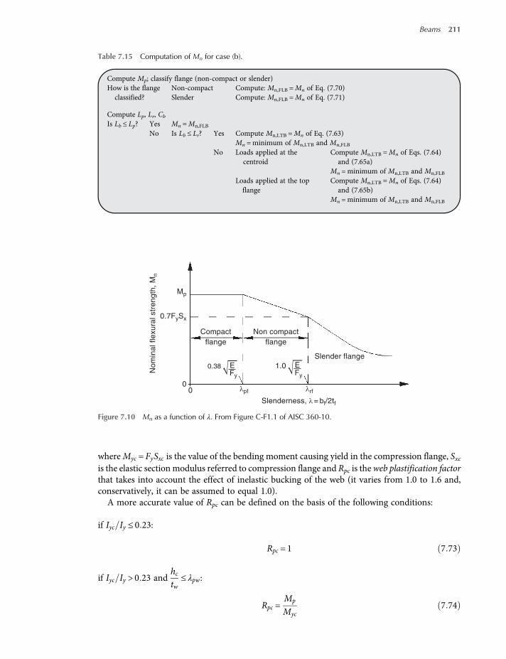
whereMyc = FySxc is the value of the bending moment causing yield in the compression flange, Sxcis the elastic section modulus referred to compression flange and Rpc is theweb plastification factorthat takes into account the effect of inelastic bucking of the web (it varies from 1.0 to 1.6 and,conservatively, it can be assumed to equal 1.0).A more accurate value of Rpc can be defined on the basis of the following conditions:
if Iyc Iy ≤ 0 23:
Rpc = 1 7 73
if Iyc Iy > 0 23 andhctw
≤ λpw:
Rpc =Mp
Myc7 74
Table 7.15 Computation of Mn for case (b).
Compute Mp; classify flange (non-compact or slender)How is the flangeclassified?
Non-compact Compute: Mn,FLB =Mn of Eq. (7.70)Slender Compute: Mn,FLB =Mn of Eq. (7.71)
Compute Lp, Lr, Cb
Is Lb ≤ Lp? Yes Mn =Mn,FLB
No Is Lb ≤ Lr? Yes Compute Mn,LTB =Mn of Eq. (7.63)Mn =minimum of Mn,LTB and Mn,FLB
No Loads applied at thecentroid
Compute Mn,LTB =Mn of Eqs. (7.64)and (7.65a)
Mn =minimum of Mn,LTB and Mn,FLB
Loads applied at the topflange
Compute Mn,LTB =Mn of Eqs. (7.64)and (7.65b)
Mn =minimum of Mn,LTB and Mn,FLB
No
min
al fle
xu
ral str
en
gth
, M
n
0.7FySx
Mp
Compact Non compact
Slenderness, λ = bf/2tf
Slender flange
1.00.38 EFy
flange flange
00 λpf λrf
EFy
Figure 7.10 Mn as a function of λ. From Figure C-F1.1 of AISC 360-10.
Beams 211

if Iyc Iy > 0 23 andhctw
> λpw:
Rpc =Mp
Myc−
Mp
Myc−1
λ−λpwλrw−λpw
≤Mp
Myc7 75
where Mp = FyZx ≤ 1 6FySxc, λ= hc tw, term λpw =
hchp
EFy
0 54Mp
My−0 09
2 ≤ 5 70EFy
is the limiting
slenderness ratio for a compact web (see Section 4.3) and term λrw = 5 70EFy
is the limiting
slenderness ratio for a non-compact web (see Section 4.3).With reference to Figure 7.11, this results in:
hc = 2 y− tfc ; hp =A−2Ac
tw; Sxc =
Ixy; Sxt =
Ixd−y
For compression FLB, AISC specifications provide the following expressions for Mn that areslightly different from those obtained via Eqs. (7.70) and (7.71) of case (b):
(1) For sections with non-compact flanges:
Mn =RpcMyc− RpcMyc−FLSxcλ−λpfλrf −λpf
7 76
(2) For sections with slender flanges:
Mn =0 9EkcSxc
λ27 77
where λ= bfc 2tfc, λpf = 0 38 E Fy is the limiting width-to-thickness ratio for a compact
flange (see Section 4.3), λrf = 1 0 E Fy is the limiting width-to-thickness ratio for a non-
compact flange (see Section 4.3), kc = 4 h tw (with 0.35 ≤ kc ≤ 0.76) and the distance hdefined in Section 4.3).
Plastic neutral axis
Centroidal axis
Elastic stressdistribution
Plastic stressdistribution
hc/2 hp/2
Ac
Fy
y
d
Aw
At
tft
tfc
Figure 7.11 Elastic and plastic stress distribution for case (c). From Figure C-F411 of AISC 360-10.
212 Structural Steel Design to Eurocode 3 and AISC Specifications

The stress FL is determined as follows:
(1) if Sxt Sxc ≥ 0 7:
FL = 0 7Fy 7 78
(2) if Sxt Sxc < 0 7:
FL =SxtSxc
Fy ≥ 0 5Fy 7 79
For cross-sections with compact flange this limit state does not apply, obviously.For lateral-torsional buckling, AISC provisions are very close to those in case (a).
(1) If Lb ≤ Lp, then lateral-torsional buckling does not occur, Lp being different than in case (a),defined as:
Lp = 1 1rtEFy
7 80
where rt is the effective radius of gyration for lateral torsional buckling, defined as:
rt =bfc
12h0d+16aw
h2
h0d
7 81a
with:
aw =hctwbfctfc
7 81b
where bfc is the width of compression flange and tfc is the thickness of compression flange.(2) if Lp < Lb ≤ Lr:
Mn =Cb RpcMyc− RpcMyc−FLSxcLb−LpLr−Lp
≤RpcMyc 7 82
(3) if Lb > Lr:
Mn = FcrSxc ≤RpcMyc 7 83
where:
Myc = FySxc 7 84
Beams 213

Fcr =Cbπ2E
Lbrt
2 1 + 0 078J
Sxch0
Lbrt
2
7 85
If Iyc Iy ≤ 0 23 then J = 0, with Iyc representing the moment of inertia of compression flangeabout the y-axis. The length Lr is defined as:
Lr = 1 95rtEFL
JSxch0
+J
Sxch0
2
+ 6 76FLE
2
7 86
For tension flange yielding:
(1) if Sxt ≥ Sxc, the limit state of tension flange yielding does not apply.(2) if Sxt < Sxc:
Mn =RptMyt 7 87
where Myt = FySxt is the moment that causes yield in the tension flange, Sxt is the elasticsection modulus referred to tension flange and Rpt is the web plastification factor correspondingto tension flange yielding limit state, which is defined as:
ifhctw
≤ λpw:
Rpt =Mp
Myt7 88
ifhctw
> λpw:
Rpt =Mp
Myt−
Mp
Myt−1
λ−λpwλrw−λpw
≤Mp
Myt7 89
where Mp = FyZx ≤ 1 6FySxc, λ= hc tw, λpw =
hchp
EFy
0 54Mp
My−0 09
2≤ 5 70
EFy
is the limiting slender-
ness ratio for a compact web (see Section 4.3), λrw = 5 70EFy
is the limiting slenderness ratio for a
non-compact web (see Section 4.3).
In Table 7.16 the decision-making process for computing Mn is summarized.
214 Structural Steel Design to Eurocode 3 and AISC Specifications

7.3.3.4 (d) Doubly Symmetrical and Singly Symmetrical I-Shaped Members with SlenderWebs, Compact, Non-Compact or Slender Flanges, Bent about Their Major AxisThis case applies to doubly symmetrical I-shaped members and singly symmetrical I-shapedmembers with a slender web attached to the mid-width of the flanges, bent about their major axis.It applies mainly to welded I-shaped beams. Case (d) is then similar to case (c), with the differencethat the webs are slender, while in case (c) they are compact or non-compact. The relevant limitstates for this case are:
• compression flange yielding;• compression flange local buckling;• lateral torsional buckling;• tension flange yielding.
The nominal flexural strengthMn is the lower value obtained according to the previously listedlimit states.For compression flange yielding, AISC specifications provide the following expressions for Mn:
Mn =RpgMyc 7 90
where Myc = FySxc is the moment that causes yield in the compression flange, Sxc is the elasticsection modulus referred to compression flange and Rpg is the bending strength reduction factor,defined as:
Rpg = 1−aw
1200 + 300aw
hctw
−5 7EFy
≤ 1 0 7 91
where aw has been defined previously, Eq. (7.81b), but in this case aw ≤ 1.0
Table 7.16 Computation of Mn for case (c) (from Figure C-F10.1 of AISC 360-10).
Compute Myc, Sxc, Rpc
Classify flange (compact, non-compact or slender)How is the flangeclassified?
Compact Compute: Mn,CF =Mn,CFY =Mn of Eq. (7.72)Non-compact Compute: Mn,CF =Mn,FLB =Mn of Eq. (7.76)Slender Compute: Mn,CF =Mn,FLB =Mn of Eq. (7.77)
Compute SxtIs Sxt < Sxc? Yes Compute Rpt
Compute: Mn,TF Y =Mn of Eq. (7.87)No Tension flange yielding is not applicable
Compute Lp, Lr, Cb
Is Lb ≤ Lp? Yes Choose the minimum of Mn,CF and Mn,TFY (if applicable)No Is Lb ≤ Lr? Yes Compute Mn,LTB =Mn of Eq. (7.82);
Choose the minimum of Mn,LTB, Mn,CF and Mn,TFY
(if applicable)No Compute Mn,LTB =Mn of Eq. (7.83);
Choose the minimum of Mn,LTB, Mn,CF and Mn,TFY
(if applicable)
Beams 215

For compression FLB, AISC specifications provide the following expressions for Mn:
(1) for sections with non-compact flanges:
Mn =Rpg Fy− 0 3Fyλ−λpfλrf −λpf
Sxc 7 92
(2) for sections with slender flanges:
Mn =Rpg0 9Ekcbf2tf
2 Sxc 7 93
where λ= bfc 2tfc, λpf = 0 38 E Fy is the limiting width-to-thickness ratio for a compact
flange (see Section 4.3), λrf = 1,0 E Fy is the limiting width-to-thickness ratio for a non-
compact flange (see Section 4.3), kc = 4 h tw (where 0.35 ≤ kc ≤ 0.76) and h is the distancedefined in Section 4.3.
For sections with compact flange this limit state does not apply, obviously.For lateral-torsional buckling, AISC provisions are very close to those of case (a).
(1) if Lb ≤ Lp, then lateral-torsional buckling does not occur, with Lp defined by Eq. (7.80).(2) if Lp < Lb ≤ Lr:
Mn =CbRpg Fy− 0 3FyLb−LpLr−Lp
Sxc ≤RpgMyc 7 94
(3) if Lb > Lr:
Mn =RpgFcrSxc ≤RpgMyc 7 95
where:
Myc = FySxc 7 96
Fcr =Cbπ2E
Lbrt
2 7 97
where Iyc is the moment of inertia of compression flange about the y-axis.
It should be noted that the Eq. (7.97) to evaluate Fcr is equal to that of case (c) Eq. (7.85) withJ = 0. This causes a discontinuity in transition between cases (c) and (d). So, in case of a weldedI-shaped beam with Fy = 50 ksi (345MPa) and a web slenderness h/tw = 137 (non-compact web),case (c) has to be used for verification; if h/tw = 138 (slender web) then it is necessary to switchverification to case (d). In any case, the differences are generally small and acceptable from anengineering point of view.
The length Lr is defined as:
Lr = πrtE
0 7Fy7 98
where rt is the effective radius of gyration for lateral torsional buckling, defined by Eq. (7.81a).
216 Structural Steel Design to Eurocode 3 and AISC Specifications
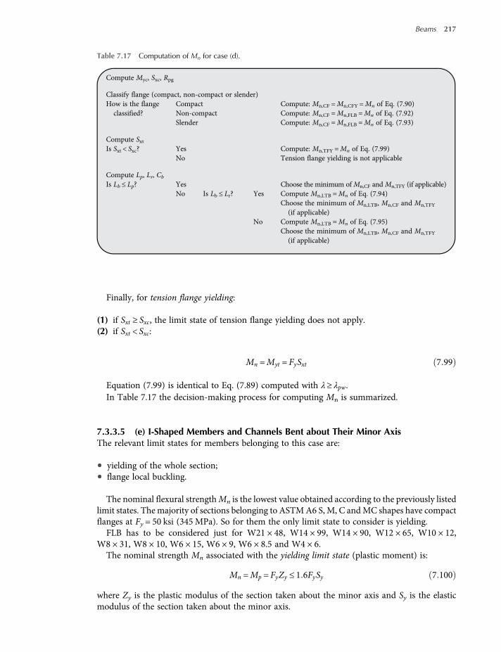
Finally, for tension flange yielding:
(1) if Sxt ≥ Sxc, the limit state of tension flange yielding does not apply.(2) if Sxt < Sxc:
Mn =Myt = FySxt 7 99
Equation (7.99) is identical to Eq. (7.89) computed with λ≥ λpw.In Table 7.17 the decision-making process for computing Mn is summarized.
7.3.3.5 (e) I-Shaped Members and Channels Bent about Their Minor AxisThe relevant limit states for members belonging to this case are:
• yielding of the whole section;• flange local buckling.
The nominal flexural strengthMn is the lowest value obtained according to the previously listedlimit states. The majority of sections belonging to ASTMA6 S, M, C andMC shapes have compactflanges at Fy = 50 ksi (345 MPa). So for them the only limit state to consider is yielding.FLB has to be considered just for W21 × 48, W14 × 99, W14 × 90, W12 × 65, W10 × 12,
W8 × 31, W8 × 10, W6 × 15, W6 × 9, W6 × 8.5 and W4 × 6.The nominal strength Mn associated with the yielding limit state (plastic moment) is:
Mn =Mp = FyZy ≤ 1 6FySy 7 100
where Zy is the plastic modulus of the section taken about the minor axis and Sy is the elasticmodulus of the section taken about the minor axis.
Table 7.17 Computation of Mn for case (d).
Compute Myc, Sxc, Rpg
Classify flange (compact, non-compact or slender)How is the flangeclassified?
Compact Compute: Mn,CF =Mn,CFY =Mn of Eq. (7.90)Non-compact Compute: Mn,CF =Mn,FLB =Mn of Eq. (7.92)Slender Compute: Mn,CF =Mn,FLB =Mn of Eq. (7.93)
Compute SxtIs Sxt < Sxc? Yes Compute: Mn,TFY =Mn of Eq. (7.99)
No Tension flange yielding is not applicable
Compute Lp, Lr, Cb
Is Lb ≤ Lp? Yes Choose the minimum ofMn,CF andMn,TFY (if applicable)No Is Lb ≤ Lr? Yes Compute Mn,LTB =Mn of Eq. (7.94)
Choose the minimum of Mn,LTB, Mn,CF and Mn,TFY
(if applicable)No Compute Mn,LTB =Mn of Eq. (7.95)
Choose the minimum of Mn,LTB, Mn,CF and Mn,TFY
(if applicable)
Beams 217

For compression FLB, AISC specifications provide the following expressions for Mn:
(1) For sections with non-compact flanges:
Mn =Mp− Mp−0 75FySyλ−λpfλrf −λpf
7 101
(2) For sections with slender flanges:
Mn =0 69ESy
λ27 102
where λ= b tf , b is the length of the outstand part of the flange (for flanges of I-shaped mem-
bers b = bf/2 and for channels, b is the full nominal dimension of the flange), λpf = 0 38 E Fyis the limiting width-to-thickness ratio for a compact flange (see Section 4.3), λrf = 1 0 E Fyis the limiting width-to-thickness ratio for a non-compact flange (see Section 4.3) and forI-shaped members and Sy is the elastic modulus taken about the y-axis (for a channel, it isthe minimum section modulus).
For sections with compact flange this limit state does not apply, obviously.
7.3.3.6 (f) Square and Rectangular HSS and Box-Shaped MembersThis case applies to members bent about either axis, having compact or non-compact webs andcompact, non-compact or slender flanges. The relevant limit states for members belonging to thiscase are:
• yielding of the whole section;• flange local buckling;• web local buckling.
Square and rectangular HSS are not subjected to lateral-torsional buckling, due to their hightorsional resistance, so lateral-torsional buckling is not a relevant limit state for these sections.The nominal flexural strength Mn is the lowest value obtained according to the previously listedlimit states.
The nominal strength Mn associated with the yielding limit state (plastic moment) is:
Mn =Mp = FyZ 7 103
where Z is the plastic modulus of the section taken about the flexural axis.For compression FLB, AISC specifications provide the following expressions for Mn:
for sections with non-compact flanges:
Mn =Mp− Mp−FyS 3 57btf
FyE−4 0 ≤Mp 7 104
where S is the elastic modulus of the section taken about the flexural axis.
218 Structural Steel Design to Eurocode 3 and AISC Specifications

for sections with slender flanges:
Mn = FySe 7 105
where Se is the effective modulus of the section taken about the flexural axis, and determined withthe effective width, be, of the compression flange, computed as:
be = 1 92tfEFy
1−0 38b tf
EFy
≤ b 7 106
For sections with compact flanges this limit state does not apply, obviously.As to the web local buckling, if webs are compact, this limit state is not applicable. If they are
non-compact AISC specifications provide the following expression for Mn:
Mn =Mp− Mp−FySx 0 305htw
FyE−0 738 ≤Mp 7 107
7.3.3.7 (g) Round HSSThis case applies to round HSS (hot-formed seamless pipes, ERW pipes and fabricated tubing) forwhich the following condition is verified:
D t < 0 45EFy
The relevant limit states for round HSS are:
• yielding;• local buckling.
As in case of square and rectangular HSS, also round HSS are not subjected to lateral-torsionalbuckling. The nominal flexural strength Mn is the lower value obtained according to the previ-ously listed limit states. The nominal strength Mn associated with the yielding limit state (plasticmoment) is:
Mn =Mp = FyZ 7 108
where Z is the plastic modulus of the section.For local buckling, AISC specifications provide the following expressions for Mn:
(1) for non-compact sections 0 07EFy
<D t ≤ 0 31EFy
:
Mn =0 021ED t
+ Fy S 7 109
where S is the elastic modulus of the section, D is the diameter of the section and t is thethickness of the cross-section.
Beams 219

(2) for slender sections 0 31EFy
<D t < 0 45EFy
:
Mn =0 33ED t
S 7 110
For compact sections this limit state does not apply.Significant values of Mn for round HSS are listed in Table 7.18.
7.3.3.8 (h) Tees Loaded in the Plane of SymmetryThe relevant limit states for tees are:
• yielding;• lateral-torsional buckling;• flange leg local buckling;• Stem local buckling.
The nominal flexural strengthMn is the lowest value obtained according to the previously listedlimit states.
The nominal strength Mn associated with the yielding limit state (plastic moment) is:
(1) if the stem is in tension:
Mn =Mp = FyZx ≤ 1 6My 7 111
(2) if the stem is in compression:
Mp =Mp = FyZx ≤My 7 112
where My = FySx.
Table 7.18 Values of Mn for round HSS, case (g).
Section classification D/t Mn Limit state
Compact< 0 07
EFy
Mp Y
Non-compactFrom 0 07
EFy
1.3My LB
To 0 31EFy
1.06My LB
SlenderFrom 0 31
EFy
1.06My LB
To 0 45EFy
0.73My LB
220 Structural Steel Design to Eurocode 3 and AISC Specifications

For lateral torsional buckling, nominal flexural strength is computed as follows.
(1) if the stem is in tension:
Mn =Mcr =π
LbEIyGJ + 2 3
dLb
IyJ+ 1 + 2 3
dLb
IyJ
2
7 113
(2) If the stem is in compression:
Mn =Mcr =π
LbEIyGJ −2 3
dLb
IyJ+ 1 + 2 3
dLb
IyJ
2
7 114
For tee FLB, AISC specifications provide the following expressions for Mn:
(1) for tees with a non-compact flange in flexural compression:
Mn =Mp− Mp−0 75FySxcλ−λpfλrf −λpf
≤ 1 6My 7 115
(2) for tees with a slender flange in flexural compression:
Mn =0 7ESxc
λ27 116
where λ= bf 2tf , λpf = 0 38 E Fy is the limiting width-to-thickness ratio for a compact
flange (see Section 4.3) and λrf = 1 0 E Fy is the limiting width-to-thickness ratio for anon-compact flange (see Section 4.3).
For sections with compact flange this limit state does not apply, obviously.Finally, if reference is made to the local buckling of stem in flexural compression, for this
limit state:
(1) for a compact stem d tw ≤ 0 84EFy
:
Mn = FySx 7 117
(2) for a non-compact stem 0 84EFy
< d tw ≤ 1 03EFy
:
Mn = 2 55−1 84dtw
FyE
FySx 7 118
Beams 221

(3) for a slender stem d tw > 1 03EFy
:
Mn =0 69E
dtw
2 Sx 7 119
In Table 7.19 the decision-making process for computing Mn is summarized.
7.3.3.9 (i) Double Angles Loaded in the Plane of SymmetryThis case applies to double angles loaded in the plane of symmetry. The relevant limit states fordouble angles are:
• yielding;• lateral-torsional buckling;• double angle flange legs local buckling;• double angle web legs local buckling.
The nominal flexural strengthMn is the lowest value obtained according to the previously listedlimit states. The nominal strengthMn associated with the yielding limit state (plastic moment) is:
(1) if the web legs are in tension:
Mn =Mp = FyZx ≤ 1 6My 7 120
(2) if the web legs are in compression:
Mp =Mp = FyZx ≤My 7 121
where My = FySx
Table 7.19 Values of Mn for tees, case (h).
Stem in tension Compute Mn,Y =Mn of Eq. (7.111) YCompute Mn,LTB =Mn of Eq. (7.113) LTB
Compact flange — FLBNon-compact flange Compute Mn,FLB =Mn of Eq. (7.115)Slender flange Compute Mn,FLB =Mn of Eq. (7.116)Mn =min{Mn,Y; Mn,LTB; Mn,FLB}
Stem in compression Compute Mn,Y =Mn of Eq. (7.112) YCompute Mn,LTB =Mn of Eq. (7.114) LTB
Compact stem Compute Mn,TSLB =Mn of Eq. (7.117) TSLBNon-compact stem Compute Mn,TSLB =Mn of Eq. (7.118)Slender stem Compute Mn,TSLB =Mn of Eq. (7.119)Mn =min{Mn,Y; Mn,LTB; Mn,TSLB}
222 Structural Steel Design to Eurocode 3 and AISC Specifications

For lateral torsional buckling, nominal flexural strength is computed as follows.
(1) if the web legs are in tension:
Mn =Mcr =π
LbEIyGJ + 2 3
dLb
IyJ+ 1 + 2 3
dLb
IyJ
2
7 122
(2) if the web legs are in compression:
Mn =Mcr =π
LbEIyGJ −2 3
dLb
IyJ+ 1 + 2 3
dLb
IyJ
2
7 123
For flange leg local buckling, AISC specifications provide the following expressions for Mn:
(1) for angles with non-compact legs 0 54EFy
<bt≤ 0 91
EFy
:
Mn = 2 43−1 72λFyE
FySc ≤ 1 5FySc 7 124
(2) for angles with slender legsbt> 0 91
EFy
:
Mn =0 71E
λ2Sc 7 125
where λ= b t, b is the full width of the flange legs in compression, t is the thickness of angleand Sc is the elastic section modulus of the leg in compression.
For sections with a compact flange this limit state does not apply. Finally, with reference to thelocal buckling of web legs in flexural compression:
(1) for angles with non-compact legs 0 54EFy
<bt≤ 0 91
EFy
:
Mn = 2 43−1 72λFyE
FySc ≤ 1 5FySc 7 126
(2) for angles with slender legsbt> 0 91
EFy
:
Beams 223

Mn =0 71E
λ2Sc 7 127
where λ= b t, b is the full width of web legs in flexural compression, t is the thickness of angleand Sc is the elastic section modulus of the toe in compression.
For sections with compact flange this limit state does not apply.In Table 7.20 the decision-making process for computing Mn is summarized.
7.3.3.10 (j) Single AnglesThis case applies to single equal-leg or unequal-leg angles, with or without continuous lateral-torsional restraint along their length. If single angles are not laterally restrained along their length,the relevant limit states are:
• yielding;• lateral-torsional buckling;• local leg buckling.
The nominal flexural strengthMn is the lowest value obtained according to the previously listedlimit states. The nominal strength Mn associated with the yielding limit state is:
Mn = 1 5My 7 128
where My is the yield moment about the bending axis.As can be seen, the strength is not referred to plastic moment but limited to a shape factor of 1.5
applied to the yield moment. Shape factors for angles range from 1.73 to 1.96 actually, soEq. (7.128) is intended to be quite conservative.
For lateral torsional buckling, AISC specifications consider different cases:
7.3.3.10.1 Laterally Unrestrained Unequal-Leg Single Angle
(1) subjected to bending moment about the major principal axis(a) If Me ≤My:
Mn = 0 92−0 17Me
MyMe 7 129
Table 7.20 Values of Mn for double angles, case (i).
Web legs in tension Compute Mn,Y =Mn of Eq. (7.120) YCompute Mn,LTB =Mn of Eq. (7.122) LTB
Compact flange leg — FLBNon-compact flange leg Compute Mn,FLB =Mn of Eq. (7.124)Slender flange leg Compute Mn,FLB =Mn of Eq. (7.125)Mn =min{Mn,Y; Mn,LTB; Mn,FLB}
Web legs in compression Compute Mn,Y =Mn of Eq. (7.121) YCompute Mn,LTB =Mn of Eq. (7.123) LTB
Compact web leg — DALBNon-compact web leg Compute Mn,DALB =Mn of Eq. (7.126)Slender web leg Compute Mn,DALB =Mn of Eq. (7.127)Mn =min{Mn,Y; Mn,LTB; Mn,DALB}
224 Structural Steel Design to Eurocode 3 and AISC Specifications

(b) If Me <My:
Mn = 1 92−1 17My
MeMy ≤ 1 5My 7 130
Me is evaluated as:
Me =4 9EIzCb
L2bβ2w + 0 052
Lbtrz
2
+ βw 7 131
where Me is the elastic lateral-torsional buckling moment, Cb is computed using Eq. (7.68),but Cb ≤ 1.5; My is the yield moment about the bending axis, Iz is the minor principal axismoment of inertia, rz is the radius of gyration about the minor principal axis, t is the thicknessof the angle leg and term βw represents a section property, to be chosen from Table 7.21 withpositive sign for short leg in compression and negative sign for long leg in compression.
(2) subjected to a generically oriented bending moment(a) Resolve moment into components along both principal axes.(b) For component along the major principal axis, compute Mn as in (1).(c) Verify the angle for biaxial bending, according to Section 9.3.
7.3.3.10.2 Laterally Unrestrained Equal-Leg Single Angle
(1) subject to a bending moment about the major principal axis(a) If Me ≤My:
Mn = 0 92−0 17Me
MyMe 7 132
Table 7.21 βw values for angles.
Angle size βwin. (mm) in. (mm)
8 × 6 (203 × 152) 3.31 (84.1)8 × 4 (203 × 102) 5.48 (139)7 × 4 (178 × 102) 4.37 (111)6 × 4 (152 × 102) 3.14 (79.8)6 × 3½ (152 × 89) 3.69 (93.7)5 × 3½ (127 × 89) 2.40 (61)5 × 3 (127 × 76) 2.99 (75.9)4 × 3½ (102 × 89) 0.87 (22.1)4 × 3 (102 × 76) 1.65 (41.9)3½ × 3 (89 × 76) 0.82 (22.1)3½ × 2½ (89 × 64) 1.62 (41.1)3 × 2½ (76 × 64) 0.86 (21.8)3 × 2 (76 × 51) 1.56 (39.6)2½ × 2 (64 × 51) 0.85 (21.6)2½ × 1½ (64 × 38) 1.49 (37.8)Equal leg 0
Beams 225

(b) If Me <My :
Mn = 1 92−1 17My
MeMy ≤ 1 5My 7 133
where Cb is computed using Eq. (7.68), with the limitation Cb ≤ 1.5, My is the yieldingmoment about the bending axis, t is the thickness of the angle leg, b is the full width ofleg and Me is the elastic lateral-torsional buckling moment defined as:
Me =0 46Eb2t2Cb
Lb7 134
It should be noted that Eqs. (7.132) and (7.133) are identical to Eqs. (7.129) and (7.130).(2) subjected to a generically oriented bending moment
(a) resolve the moment into components along the two principal axes.(b) for components along the major principal axis, compute Mn as in (1a).(c) verify the angle for biaxial bending, according to Section 9.3.
The same procedure as for unequal-leg angles has to be adopted.(3) subjected to bending moment about one of the geometric axes of the angle (alternative to
method 2b)(a) if Me ≤My:
Mn = 0 92−0 17Me
0 8MyMe 7 135
(b) if Me <My:
Mn = 1 92−1 17My
Me0 8My ≤ 1 5 0 8My 7 136
where My is the yield moment about the geometric axis, Me is the elastic lateral-torsionalbuckling moment, computed as follows:(c) with maximum compression at the toe:
Me =0 66Eb4tCb
L2b1 + 0 78
Lbtb2
2
−1 7 137
(d) with maximum tension at the toe:
Me =0 66Eb4tCb
L2b1 + 0 78
Lbtb2
2
+ 1 7 138
If there is a lateral-torsional restraint at the point of maximum moment, Eqs. (7.135) and(7.136) shall be used substituting 0.8My with My, and (Eqs. (7.137) and (7.138)) become:
226 Structural Steel Design to Eurocode 3 and AISC Specifications

Me = 1 250 66Eb4tCb
L2b1 + 0 78
Lbtb2
2
−1 7 139
Me = 1 250 66Eb4tCb
L2b1 + 0 78
Lbtb2
2
+ 1 7 140
Method (2c) for equal-leg angles is a simplification of the more general method (2b).When bending is applied about one leg of an unrestrained single angle, the angle will
deflect not only in the bending direction but also laterally, and the maximum stress at theangle tip will be approximately 25% greater than the calculated stress using the geometricaxis section modulus.
Finally, the limit state of local buckling has to be considered when the toe of the leg is incompression and the section is not compact; AISC provides the following expressionsfor Mn:
(1) for cross-sections with non-compact legs:
Mn = 2 43−1 72bt
FyE
FySc 7 141
(2) for cross-sections with slender legs:
Mn =0 71E
bt
2 Sc 7 142
where Sc is the elastic section modulus of the toe in compression relative to the axis of bend.For bending about one of the geometric axes of equal-leg axes with no lateral-torsionalrestraint, Sc is taken equal to 80% of the geometric axis section modulus.
7.3.3.11 (k) Rectangular Bar and RoundsThis case applies to solid bars with a rectangular and round cross-section. The relevant limitstates are:
• yielding;• lateral-torsional buckling.
Lateral-torsional buckling occurs only for rectangular bars, when depth is larger than width;otherwise the only limit state is the attainment of a full plastic moment.The nominal flexural strengthMn is the lower value obtained according to the previously listed
limit states.The nominal strength Mn associated with the yielding limit state (plastic moment) is:
Mn =Mp = FyZ ≤ 1 6My 7 143
Beams 227

For lateral-torsional buckling AISC prescribes:
(1) for rectangular bars withLbdt2
≤0 08EFy
bent about theirmajor axis, this limit state does not occur.
(2) for rectangular bars with0 08EFy
<Lbdt2
≤1 9EFy
bent about their major axis:
Mn =Cb 1 52−0 274Lbdt2
FyE
My ≤Mp 7 144
(3) for rectangular bars withLbdt2
>1 9EFy
bent about their major axis:
Mn =1 9ECb
Lbdt2
Sx ≤Mp 7 145
(4) for rectangular bars bent about their minor axis and for round bars this limit state doesnot occur.
7.3.3.12 (l) Unsymmetrical ShapesIn this case all unsymmetrical shapes (except angles) are grouped. AISC prescriptions are quitegeneric. The limit states to be considered are:
• yielding;• lateral-torsional buckling;• local buckling.
Critical stresses for the last two limit states are to be defined by textbooks, handbooks or by FEanalysis.
7.4 Design Rules for Beams
With reference to the beam design, the member of an appropriate cross-section must be selectedby considering the need to fulfil all the specific requirements related to the service condition aswell resistance and ultimate stability limit-state. As a consequence, this choice can be based on thedesigner experience and/or on the use of suitable rules related to the application of the criteria toverify for safety checks.
In case of uniform doubly-symmetrical I- or H-shaped beams, appropriate equations can beeasily obtained to define the minimum value of the moment of inertia (Imin) as well as thesection modulus (Wmin) required to guarantee the safety of the profile.
With reference to a simply supported beam having a span L, with a uniformly distributed load,comprising of dead (g) and live load (q) contribution, the following limit conditions can beconsidered:
5384
g + q L4
E Imin= δLim 7 146a
32
g + q L2
8 Wmin= fd 7 146b
228 Structural Steel Design to Eurocode 3 and AISC Specifications

where E is the modulus of elasticity of the material, δLim is the maximum displacement compatiblewith the beam use and fd is the design strength for the material.These limit conditions regard the deflection and resistance criteria for the beam, respectively,
for which the associated load safety factors in accordance with the European practice can be takenin this pre-sizing phase equal to 1.5 (i.e. γg1 = γg2 = γq = 1.5). It should be noted that on the basis ofthe computed value of Imin andWmin two different cross-section types are generally identified andthe greater has to be adopted for verification checks.For three different load conditions common in simply supported beams, Table 7.22 proposes
the equation to be used to evaluate Imin and Wmin.With reference to I- or H-shaped bi-symmetrical profiles, moment of inertia (I) and
section modulus (W) are directly connected to each other via the beam depth (H) by means ofthe relationship:
W =2 IH
7 147
The displacement limit δLim can be considered to be the displacement (δLim,tot ) associated withthe total load or the displacement (δLim,2) due to sole variable load. For practical design purposes,tables of immediate applicability for the selection of the depth of the profile can easily be devel-oped. As an example, Table 7.23 deals with two common load cases: for each of them and fordifferent steel grades, with reference both to floor and roof beams two values ofHmin are proposed,differing for the considered displacement limit, the first one associated with total loads δLim,tot andthe second one with variable loads δLim,2. In particular the following limits have been considered:
• floor beam: δLim,tot = L/250 and δLim,2 = L/300;• roof beam: δLim,tot = L/200 and δLim,2 = L/250.
As an example related to the main steps to evaluate expressions presented in Table 7.23, the caseof beam with uniform load is considered with reference to the displacement limit δLim,tot. FromEq. (7.147), substituting the expressions in Table 7.22 we can obtain:
Wmin =32
g + q L2
8 fd=
2 IHmin
=2
Hmin
5384
g + q L4
E δLim, tot7 148
Table 7.22 Indications for the minimum geometrical characteristics of cross-sections.
Load condition Imin Minimum moment of inertia Wmin Minimum section modulus
g,q
Imin =5384
g + q L4
E δLimWmin =
32
g + q L2
8 fd
P
LImin =
148
Pg +Pq L3
E δLimWmin =
32
Pg +Pq L
4 fd
P
x x x
P
Imin =23648
Pg +Pq L3
E δLimWmin =
32
Pg +Pq L
3 fd
Beams 229

As a consequence, the minimum beam depth, Hmin, can be expressed as:
Hmin = 25384
L2
E δLim, tot
2 8 fd3
7 149
As an example, considering the value of elastic modulus in accordance with the European prac-tice (i.e. E = 210 000 N/mm2), Hmin expressed in millimetres, can be evaluated as:
Hmin =fd L2
1512000 δLim, tot7 150
In the same way, by considering the displacement limit δ2 associated with the sole live load, wecan obtain:
Wmin =32
g + q L2
8 fd=
2 IHmin
=2
Hmin
5348
q L4
E δLim,27 151
Term Hmin is obtained from:
Hmin = 25384
qL2
g + q E δLim,2
2 8 fd3
7 152
Table 7.23 Value of Hmin: α = q/(g + q); β = Pq/(Pg + Pq) for European steel grades.
Steel grade
S 235 S 275 S 355 S 420 S 460
Floor beam (Hmin = minimum beam depth)
gq
L
L27
L23
2L35
L15
2L27
α2L45
αL19
α2L29
α2L25
α2L23
Pg
L
Pq2L67
2L57
L22
2L37
L17
βL28
βL24
β2L37
β2L31
βL14
Roof beam (Hmin =minimum beam depth)
g
q
L
2L67
2L57
L22
2L37
L17
αL27
α2L23
α2L35
αL15
α2L27
Pq
Pg
L
L42
L36
2L55
2L47
2L43
β2L67
β2L57
βL22
β2L37
βL17
230 Structural Steel Design to Eurocode 3 and AISC Specifications

As to units, if forces are measured in newton and dimensions in millimetres, by substitutingdirectly the value of E, we can obtain:
Hmin =fd
1512000 δLim,2
qL2
g + q7 153
It should be noted from Table 7.23 thatHmin increases with the increase of the steel grade. Thisapparent nonsense is due to the fact that the choice of a better quality of steel, which correspondsto a deeper beam with respect to a beam selected with a lower steel grade, is associated with ahigher distance between parallel beams; that is with a greater load carrying capacity.With reference to the AISC 360-10 code, Eqs. (7.146a) and (7.146b) can be rewritten as:
5384
qL4
EImin=
5384
α g + q L4
EImin= δLim 7 154a
g + q L2
8=FyZmin
Ωb7 154b
where α= q g + q is the displacement computed with reference to live load only.Equation (7.154b) is written with reference to ASD. Table 7.24 represents the equation to be
used to evaluate Imin and Zmin for three different load conditions common in simply sup-ported beams.Table 7.25 corresponds to the ‘translation’ of Table 7.23 into AISC code. The main differ-
ences are:
(1) consider one value for δLim, computed for live loads only. In particular the following data havebeen assumed:Floor beam: δLim = L/360;Roof beam: δLim = L/240.
(2) consider the following steel grades 36, 42, 46 and 50 (Fy [ksi]).(3) refer to ASD for calculations.
It should be noted that, in accordance with AISC code notation, term d is used instead of H toidentify the section height.
Table 7.24 Indications for the minimum geometrical characteristics of cross-sections (AISC-ASD).
Load condition Imin –Minimum moment of inertia Wmin –Minimum section modulus
g,qImin =
5384
α g + q L4
E δLimZmin =Ωb
g + q L4
8Fy
P
LImin =
148
β Pg +Pq L3
E δLimZmin =Ωb
Pg +Pq L
4Fy
P P
x xx Imin =23648
β Pg + Pq L3
E δLimZmin =Ωb
Pg +Pq L
3Fy
α= q g + q ; β =Pq Pg +Pq ; Ωb = 1,67
Beams 231

As a consequence, the rewritten Eq. (7.147), using AISC symbols, is:
Z =2Id
7 155
The approach to evaluate the expressions is presented in Table 7.25. Also in this case, a beamwith uniform load is considered with reference to the displacement limit δLim. From Eq. (7.155),by substituting the expressions in Table 7.24 we can obtain:
Zmin =Ωbg + q L2
8Fy=
2 Idmin
=2
dmin
5384
α g + q L4
E δLim7 156
As a consequence, dmin can be expressed as:
dmin = 25384
L2
EδLim
8αFyΩb
7 157
Table 7.25 Value of dmin: α = q/(g + q); β = Pq/(Pg + Pq) for ASTM steel grades.
Steel grade (Fy (ksi))
36 42 46 50
Floor beam (dmin =minimum beam depth)
g
q
L α2L36
α2L31
α2L28
α2L26
Pg
L
Pq
βL22
βL19
β2L35
β2L32
Roof beam (dmin = minimum beam depth)
g
q
L αL27
αL23
α2L42
α2L39
Pg
L
Pq
β2L67
β2L58
βL26
β2L48
232 Structural Steel Design to Eurocode 3 and AISC Specifications
By considering the value of elastic modulus in accordance with the US practice (i.e. E = 29 000ksi), the minimum beam depth dmin is:
dmin =αFy L2
232450 δLim7 158
If reference is made to δLim = L/360 for the floor beams and δLim = L/240 for the roof beams, wecan obtain:
• for floor beams: dmin =α L
646 Fy
• for roof beams: dmin =α L
969 Fy
For beams with a concentrated load at midspan, from Eq. (7.155), by substituting the expres-sions in Table 7.24 we can obtain:
Zmin =ΩbPg +Pq L
4Fy=
2 Idmin
=2
dmin
148
β Pg + Pq L3
E δLim7 159
As a consequence, dmin can be expressed as:
dmin = 2148
L2
EδLim
4βFyΩb
7 160
By considering the US value of elastic modulus again (i.e. E = 29 000 ksi), the minimum beamdepth dmin is:
dmin =βFy L2
290580 δLim7 161
If δLim is L/360 for floor beams and L/240 for roof beams, we can obtain:
• for floor beams: dmin =α L
807 Fy
• for roof beams: dmin =α L
1210 Fy
7.5 Worked Examples
Example E7.1 Beam Design in Accordance with the EU Approach
Verify a S275 IPE 300 simply supported beam (Figure E7.1.1) in accordance with EC3, which is subjected to auniform dead load of 5.0 kN/m (0.343 kip/ft) and a uniform live load of 10.0 kN/m (0.685 kip/ft). Two casesare considered that differ for the load condition: loads are applied at the shear centre or on the top flange. Thebeam is not braced against lateral-torsional buckling along its entire length. Warping and lateral rotation arefree at both ends; lateral displacement and torsion are prevented at both ends.
Beams 233

Geometrical properties:
H = 300 mm 11 8 in Jy = 8356 cm4 200 8 in 4
bf = 150 mm 5 91 in Jz = 603 8 cm4 14 51 in 4
tf = 10 7 mm 0 42 in It = 20 1 cm4 0 483 in 4
tw = 7 1 mm 0 28 in Iw = 125934 1 cm6 469 in 6
r = 15 mm 0 59 in Wpl,y = 628 4 cm3 37 35 in 3
L= 5 m 16 4 ft Wel,y = 557 1 cm3 34 0 in 3
Lcr,LT = 5 m A= 53 8 cm2 7 34 in 2
Material properties:
Steel S275 fy = 275 MPa 34 08 ksi fu = 430 MPa 62 37 ksi
Flange c tf = 150 – 7 1 – 2 × 15 2 × 10 7 = 5 3≤ 8 3 Class 1
Web d tw = 300 – 2 × 10 7 – 2 × 15 7 1 = 35 0≤ 66 Class 1
Section Class 1
Loads:
Dead load qp = 5 0 kN m 0 343 kip ft
Live load qs = 10 0 kN m 0 685 kip ft
Factorized load q= 1 35 × 5 0 + 1 5 × 10 0 = 21 75 kN m 1 49 kip f t
Maximum total load deflection permitted fp = L 400
Shear strength verification.Maximum design shear force:
VEd = 21 75 × 5 2 = 54 4 kN 12 2 kips
Shear area:
Av =A−2btf + tw + 2r tf = 53 8 102− 2 × 150 × 10 7 + 7 1 + 2 × 15 × 10 7
= 2567mm2 = 25 7 cm2 4 0 in 2
L
q
MEd
Figure E7.1.1
234 Structural Steel Design to Eurocode 3 and AISC Specifications

Design shear resistance:
Vc,Rd =Avfy3 γM0
=2567 × 275
3 × 1 010−3 = 407 6 kN 91 6 kips
VEd Vc,Rd = 54 4 407 6 = 0 13 < 0 50 no influence on design resistance for bending
Flexural strength verification.Maximum design bending moment:
MEd = 21 75 × 52 8 = 68 0 kNm 50 2 kip-ft
Design resistance for bending:
Mc,Rd =Wyfy γM0 = 628 4 × 275 1 00 10−3 = 172 8 kNm > 68 0 kNm OK
127 5 kips-ft > 50 2 kip-ft
Deflection verification.Computed deflection at midspan:
f =5384
qL4
EJy=
5384
5 0 + 10 0 10−2 × 5004
21000 × 8356= 0 69 cm 0 272 in < fp
= 500 400 = 1 25 cm 0 492 in OK
Lateral-torsional buckling (LTB) verification.
(a) Verification According to EC3 –General ApproachCompute critical moment using Eq. (7.43) (with C3 zj = 0 because section is symmetrical and then zj = 0)considering the load applied to the shear centre:
Mcr =C1π2EJzkzL
2
kzkw
2 IwJz
+kL 2GItπ2EJz
+ C2zg2−C2zg
= 1 132 ×3,142 × 21000 × 603,8
1 × 500 2
×11
2 125934 1603 8
+1 × 500 2 × 8077 × 20,13 142 × 21000 × 603 8
+ 0 459 × 0 2−0 459 × 0 10−2 = 130 8 kNm
96 5 kip− ft
Assume:
kz = kw = 1 (free rotation in horizontal plane and warping at both end)zg = 0 (load applied at the shear centre)C1 = 1.132 (see Table 7.6b); C2 = 0.459;E = 21 000 kN/cm2 (30 460 ksi); G = 8077 kN/cm2 (11710 ksi).
Beams 235

Compute relative slenderness (Eq. (7.33)):
λLT =WyfyMcr
=628 4 × 27 50130 8 102
= 1 15
Choose, according to Tables 7.2 and 7.3, the imperfection factor αLT:
αLT = 0 21 rolled I-sections withH b ≤ 2
Hence:
ΦLT = 0 5 1 + αLT λLT −0 2 + λ2LT = 0 5 1 + 0 21 1 15−0 2 + 1 152 = 1 26
χLT =1
ΦLT + ΦLT2−λ
2LT
=1
1 26 + 1 262−1 152= 0 563 ≤ 1
And finally:
Mb Rd = χLTWyfyγM1
= 0 563 ×628 4 × 27 50
1 0010−2 = 97 3 kNm 71 8 kip-ft
LTB check will then be:
MEd = 68 0 kNm≤Mb,Rd = 97 3 kNm OK
Consider now the load applied on top flange of the beam. The distance from the shear centre to the top ofbeam flange is:
zg = 150 mm 5 9 in
Critical moment varies as follows:
Mcr = 1 132 ×3 142 × 21000 × 603 8
1 × 500 2
×11
2 125934 1603 8
+1 × 500 2 × 8077 × 20 13 142 × 21000 × 603 8
+ 0 459 × 15 2−0 459 × 15 10−2 = 97 5 kNm
71 9 kip-ft
Hence:
λLT =WyfyMcr
=628 4 × 27 5097 5 × 100
= 1 33
ΦLT = 0 5 1 + αLT λLT −0 2 + λ2LT = 0 5 1 + 0 21 1 33−0 2 + 1 332 = 1 505
236 Structural Steel Design to Eurocode 3 and AISC Specifications

χLT =1
ΦLT + ΦLT2−λ
2LT
=1
1 503 + 1 5032−1 332= 0 453 ≤ 1
Mb,Rd = χLTWyfyγM1
= 0 454 ×628 4 × 27 50
1 0010−2 = 78 3 kNm 57 6 kip-ft
LTB check will then be:
MEd = 68 0 kNm ≤Mb,Rd = 78 3 kNm OK
(b) Verification According to EC3 –Method for I- or H-Shaped Profiles (see Section 6.3.2.3)Consider loads applied to the shear centre (zg = 0).Critical moment and relative slenderness are the same as in case (a). Hence:
Mcr = 130 8 kNm 96 5 kip-ft ;λLT = 1 15
Compute f factor (Eq. (7.37)):Assume correction factor kc = 0.94 (from Table 7.7)
λLT ,0 = 0 4; β = 0 75
f = 1−0 5 1−kc 1−2 0 λLT −0 82
= 1−0 5 1−0 94 1−2 0 1 15−0 8 2 = 0 977
f shall be ≤ 1.Assume αLT = 0.34 (From Tables 7.2 and 7.4 (note: Table 7.4 and not Table 7.3, because this leads to adifferent value for αLT).Hence:
ΦLT = 0 5 1 + αLT λLT −λLT , 0 + βλ2LT
= 0 5 1 + 0 34 1 15−0 4 + 0 75 × 1 152 = 1 123
χLT =1
ΦLT + ΦLT2−βλ
2LT
=1
1 123 + 1 1232−0 75 × 1 152= 0 609
It results in:
χLT = 0 609≤ 1; χLT = 0 609≤1
λ2LT
=1
1 152= 0 756;
χLTf
=0 6090 977
= 0 623≤ 1
And finally:
Mb,Rd =χLTf
WyfyγM1
= 0 623 ×628 4 × 27 50
1 0010−2 = 107 7 kNm 79 4 kip-ft
The LTB check will then be:
MEd = 68 0 kNm ≤Mb,Rd = 107 7 kNm OK
Beams 237

The value of Mb,Rd is greater than that computed using the general method.Consider now loads applied on top flange (zg = 150 mm).Mcr = 97.5 kNm (71.9 kip-ft); λLT = 1.33 (unchanged values respect to case (a).Compute f factor (Eq. (7.37)):Assume correction factor kc = 0.94 (from Table 7.5)
λLT ,0 = 0 4; β = 0 75
f = 1−0 5 1−kc 1−2 0 λLT −0 82
= 1−0 5 1−0 94 1−2 0 1 33−0 8 2 = 0 987
f shall be ≤ 1.Assume αLT = 0.34 (From Tables 7.2 and 7.4 (note: Table 7.4 and not Table 7.3, because this leads to a dif-ferent value for αLT ).Hence:
ΦLT = 0 5 1 + αLT λLT −λLT 0 + βλ2LT = 0 5 1 + 0 34 1 33−0 4 + 0 75 × 1 332 = 1 322
χLT =1
ΦLT + ΦLT2−βλ
2LT
=1
1 322 + 1 3222−0 75 × 1 332= 0 507
It results in:
χLT = 0 507≤ 1; χLT = 0 507≤1
λ2LT
=1
1 332= 0 565;
χLTf
=0 5070 987
= 0 514≤ 1
And finally:
Mb,Rd =χLTf
WyfyγM1
= 0 514 ×628 4 × 27 50
1 0010−2 = 88 8 kNm 65 5 kip-ft
The LTB check will then be:
MEd = 68 0 kNm≤Mb,Rd = 88 8 kNm OK
Also with loads applied on top flange, the value of Mb,Rd is greater than that computed using the generalmethod.In Table E7.1.1 the different values computed for both EC3 methods and for loads applied at the shear
centre and on top flange are reported.
Table E7.1.1 LTB results.
Code
Mb,Rd (kNm)
zg = 0mm zg = 150mm
(a) General approach (EC3 – Section 6.3.2.2) 97.3 78.3(b) Approach for I- and H-shaped profiles (EC3 – Section 6.3.2.3) 107.7 88.8
238 Structural Steel Design to Eurocode 3 and AISC Specifications

Example E7.2 Beam Design in Accordance with the US Approach
Verify an ASTM A992W12 × 30 simply supported beam (Figure E7.2.1) in accordance with AISC, loaded bya uniform dead load of 0.40 kip/ft (5.8 kN/m) (first load case) and a uniform live load (second load case) of0.70 kip/ft (10.2 kN/m). Loads are applied at the shear centre or on the top flange. The beam is not bracedagainst lateral-torsional buckling along its entire length.Warping and lateral rotation free at both ends; lateraldisplacement and torsion prevented at both ends.
Geometrical properties:
d = 12 3 in 312 mm Ag = 7 79 in 2 56 7 cm2
bf = 6 52 in 166 mm Zx = 43 1 in 3 706 3 cm3
tf = 0 44 in 11 2 mm Sx = 37 6 in 3 632 5 cm3
tw = 0 26 in 6 6 mm Zy = 9 56 in 3 156 7 cm3
k= 0 74 in 18 8 mm Sy = 6 24 in 3 102 3 cm3
L= 17 ft 5 18 m Ix = 238 in 4 9906 cm4
Lx = 17 ft Iy = 20 3 in 4 845 cm4
Ly = 17ft J = 0 457 in 4 19 cm4
Lb = 17 ft Cw = 720 in 6 193300 cm6
rx = 5 21 in 13 2 cm
ry = 1 52 in 3 9 cm
Material properties:
Steel : ASTM A992 Fy = 50 ksi 345 MPa Fu = 65 ksi 448 MPa
Limit the live load deflection to L/360.Loads:wD = 0.40 kip/ft (5.8 kN/m); wL = 0.70 kip/ft (10.2 kN/m)
LRFD: wu = 1.2 × 0.40 + 1.6 × 0.70 = 1.6 kip/ft (23.4 kN/m)
ASD: wa = 0.40 + 0.70 = 1.1 kip/ft (16.1 kN/m)
Y
L
Wu, Wa
Mu, Ma
tf
tw
k1
k
k
Xd X T
Ybf
L
Figure E7.2.1
Beams 239

The required shear strength is:
LRFD Vu =wuL 2 = 1 6 × 17 2 = 13.6 kips (60.5 kN)
ASD Va =waL 2 = 1 1 × 17 2 = 9.4 kips (41.8 kN)
The required flexural strength is:
LRFD Mu =wuL2
8=1 6 × 172
8= 57.8 kip-ft (78.4 kNm)
ASD Ma =waL2
8=1 1 × 172
8= 39.7 kip-ft (58.9 kNm)
Section classification for local buckling.Flange:
b t = 0 5 × 6 52 0 44 = 7 41 < 0 38 E Fy = 0 38 × 29000 50 = 9 15 compact
Web:
h tw = 12 3−2 × 0 74 0 26 = 41 6 < 3 76 E Fy = 3 76 × 29000 50 = 90 6 compact
ASTM A992 steel W12 × 30, subjected to bending moment, is a compact section.
Check for deflection.
Compute deflection at midspan:
f =5384
wLL4
EIx=
5384
0 7 12 × 17 × 12 4
29000 × 238= 0 19 in 0 49 cm <
= 17 × 12 360 = 0 57 in 1 45 cm OK
Verification of shear.
Shear area:
Aw = d tw = 12 3 × 0 26 = 3 2 in 2 20 6 cm2
h tw = 12 3−2 × 0 74 0 26 = 41 6≤ 2 24 E Fy = 2 24 × 29000 50 = 53 9
Apply Method 1 (AISC 360-10 Section G2.1).Cv = 1.0Nominal shear strength Vn:
Vn = 0 6FyAwCv = 0 6 × 50 × 3 2 × 1 0 = 96 0 kips 427 kN
Compute the available shear strength.
240 Structural Steel Design to Eurocode 3 and AISC Specifications

LRFD: ΦbMn = 1 00 × 96 0 = 96.0 kips (427 kN) > Vu = 13.6 kips
ASD: Vn Ωv = 96 0 1 50 = 64.0 kips (285 kNm) > Va = 9.4 kips
Verification of bending.Apply verifications of case (a):(a) Doubly symmetrical compact I-shaped members and channels bent about their major axis.Compute plastic moment:
Mp = Fy ×Zx = 50 × 43 1 12 = 179 6 kip-ft 243 5 kNm
Flexural strength corresponding to lateral torsional buckling limit state MLT):Compute the modification factor Cb.
Mmax =MB = 57 8 kip-ft
MA =MC =wL2
L4−
wL4
12L4
=332
wL2 =332
× 1 6 × 172 = 43 4 kip-ft 58 8 kNm
Cb =12 5Mmax
2 5Mmax + 3MA + 4MB + 3MC=
12 5 × 57 82 5 × 57 8 + 3 × 43 4 + 4 × 57 8 + 3 × 43 4
= 1 136
Lp = 1 76ryEFy
= 1 76 × 1 52 ×2900050
= 64 4 in 12 = 5 37 ft 1 64m
rts =IyCw
Sx=
20 3 × 72038 6
= 1 770 in 4 5 cm
c = 1 (doubly symmetrical I-shape)
ho = d – tf = 12 3 – 0 44 = 11 86 in 301 2 mm
Lr = 1 95rtsE
0 7Fy
J cSxh0
+J cSxh0
2
+ 6 760 7FyE
2
= 1 95 × 1 770 ×290000 7 × 50
0 457 × 138 6 × 11 86
+0 457 × 1
38 6 × 11 86
2
+ 6 76 ×0 7 × 5029000
2
= 187 3 in 12 = 15 6 ft 4 76m
Lb = 17 ft > Lr = 15 6 ft
Hence:
(a) Consider loads applied at the shear centre.
Fcr =Cbπ2E
Lbrts
2 1 + 0 078J cSxh0
Lbrts
2
Beams 241

=1 136 × π2 × 29000
17 121 770
2 1 + 0 0780 457 × 1
38 6 × 11 8617 121 770
2
= 34 9 ksi 241 MPa
MLTB = FcrSx = 34 9 × 37 6 12 = 112 3 kip-ft 152 3 kNm
Compute the nominal flexural strength (Mn).
Mn =min Mp;MLTB =min 179 6; 112 3 = 112 3 kip-ft 152 3 kNm
Compute the available strength.
LRFD: ΦbMn = 0 90 × 112 3 = 101.1 kip-ft (137.1 kN)
ASD: Mn Ωb = 112 3 1 67 = 67.3 kip-ft (91.2 kN)
(b) Consider now loads applied on the top flange.
Fcr =Cbπ2E
Lbrts
2 =1 136 × π2 × 29000
17 121 770
2 = 24 5 ksi 169 MPa
MLTB = FcrSx = 24 5 × 38 6 12 = 77 7 kip-ft 106 8 kNm
Compute the nominal flexural strength (Mn).
Mn =min Mp;MLTB =min 179 6; 77 7 = 77 7 kip-ft 106 8 kNm
Compute the available strength.
LRFD: ΦbMn = 0 90 × 78 7 = 70.9 kip-ft (96.1 kNm)
ASD: Mn Ωb = 78 7 1 67 = 47.1 kip-ft (63.9 kNm)
In Table E7.2.1 computed values for design and allowable flexural strength are summarized.
Table E7.2.1 Values for design and allowable flexural strength.
Code
ΦbMn,Mn/Ωb (kip-ft)
Loads at shear centre Loads on top flange
AISC 360-10 Section F2 – LRFD 101.1 70.9AISC 360-10 Section F2 –ASD 67.3 47.1
242 Structural Steel Design to Eurocode 3 and AISC Specifications

CHAPTER 8
Torsion
8.1 Introduction
Sole pure torsion very rarely acts in steel structures. Most commonly, torsion occurs in combin-ation with shear forces and bending moments. Although torsion does not generally have predom-inant effects on stress distribution in steel structures (compared to those associated with bendingmoments, shear or axial forces), the response of steel members under torsion is quite complex topredict and, if possible, the design has to be developed in order to reduce the effects associatedwith torsion. A fundamental role in the study of the torsional response of steel members is playedby the shear centre. If this point lies on the line of application of an external load, no rotation of thecross-section occurs. Otherwise, the cross-section rotates with respect to an axis through thispoint, parallel to the longitudinal member axis; that is, torsional moments result from any appliedforce that does not pass through the shear centre.In some cases, the shear centre can be directly determined. If a cross-section has two axes of
symmetry, the shear centre coincides with its centroid as it does when the cross-section has apoint of symmetry (typically unstiffened Z-shaped and stiffened Z-shaped members). In the caseof L-, V- and T-shaped members – that is cross-sections composed by thin rectangular elementsthat intersect at a common point – this point is the shear centre. By neglecting the general case ofcross-sections without any axis of symmetry, which is extremely unusual in steel constructionpractice, when a cross-section has one axis of symmetry the shear centre lies on this axis andits position can be determined on the basis of the traditional approaches of the theory of struc-tures. If reference is made to thin-walled open cross-sections with constituent elements of equalthickness t, Table 8.1 can be considered for the most commonly used cross-section. It reports, foreach of them, the expression of the eccentricity between shear centre and centroid.The resistance of a structural member to torsional moment, T, may be considered to be the sum
of two components: pure torsional moment, Tt, also identified as St Venant’s torsion or the uniformtorsional moment and warping torsional moment, Tω or non-uniform torsional moment. From anequilibrium condition, this results in:
T =Tt +Tω 8 1
Pure torsion assumes that a cross-section that is plane in absence of torsion remains plane andonly rotation occurs. As an example, a circular shaft subjected to torsion presents a situationwhere pure torsion exists as the only torsion action. Warping torsion is characterized by the
Structural Steel Design to Eurocode 3 and AISC Specifications, First Edition. Claudio Bernuzzi and Benedetto Cordova.© 2016 John Wiley & Sons, Ltd. Published 2016 by John Wiley & Sons, Ltd.

out-of-plane effect that arises when the flanges are laterally displaced during twisting, analogousto bending from laterally applied loads. Hence, the warping concept is strictly dependent onrejecting the assumption of planarity of the cross-section, which can be easily understood withreference to the beam-to-column rigid joint presented in Figure 8.1. In case of beam flanges freeto deform in their own plane (i.e. cross-section planarity is not respected) warping occurs withoutthe development of any warping torsional moment. Otherwise, if appropriate warping restraints,such as horizontal and/or diagonal stiffeners, are placed at the joint location, warping is preventedand a non-uniform torsional moment acts on the joint.
In steel structures, thin-walled open cross-sections are frequently used, which are composed byplates of three geometric dimensions (length, width and thickness) with an order of magnitudedifference between them. In these cases St Venant’s theory underestimates the resistance of thesection and, therefore, the design phase requires the use of more sophisticated approaches, such asthe ones based on the studies related to open thin-walled beams developed by Vlasov.
In cases of closed solid or boxed cross-section, pure torsion dominates the torsionalresponse of the members and warping torsion can be neglected (Tt Tω) for routine design.Otherwise, in case of open cross-sections, as in case of channels, I- and H-shaped profiles,warping torsion is relevant and in many design cases the contribution of pure torsion canbe neglected (Tω Tt).
Table 8.1 Position of the shear centre C (point O identifies the centroid of cross-section).
C
O
e
h
b
e =3b
2
h + 6bO
C
e
h
b
b1
e = b3h2b+ 6h2b1−8b31
h3 + 6h2b + 6h2b1 + 8b31−12hb21
C
Oe
h
b2
b2
e =b31h
b31 + b32
b1e
C
O
b
h
e = b3h2b+ 6h2b1−8b31
h3 + 6h2b + 6h2b1 + 8b31 + 12hb21
C
O
a
e
e = 0 707a
e
O
b
C
ae = 0 707ab2
3a−2b
2a3− a−b 3
C e h
O
b
e = 0 5h2
h+ b
Cr
e
O
αα
e = 2rsinα−αcosαα−sinαcosα
244 Structural Steel Design to Eurocode 3 and AISC Specifications

8.2 Basic Concepts of Torsion
On the basis of St Venant’s theory, uniform torsion induces distortion that is caused by the rota-tion of the cross-sections around the longitudinal axis and the angle of rotation per unit length θL;that is, the rate of twist, which can be expressed as:
θL =dθdx
=θ
L= constant 8 2
where L is the member length and θ represents the relative rotation between two cross-sections atthe longitudinal distance of x, or equivalently is the difference between the rotation of the cross-section of abscissa x and the one of abscissa zero (i.e. x = 0).The angle of rotation per unit length can be associated with the moment of pure torsion, Tt,
through the following equation:
Tt =G Itdθdx
8 3
whereG is the shear modulus and It is the torsion constant (termG It is the torsional rigidity of themembers).The shear stress distribution due to uniform torsion (Figure 8.2) can be obtained according to
different methodologies, depending on the shape of the cross-section.
Circular cross-section: For members with solid or hollow circular cross-section, the shear stressesvary linearly with the distance from the shear centre (Figure 8.2a) and the maximum shearstress is:
τt,max =Tt RIp
8 4a
where R is the external cross-section radius and Ip is the polar moment of inertia.In case of solid cross-sections of radius R, the polar moment of inertia is Ip = π R4/2 while in
case of a circular hollow cross-section, if R and Ri identify the external and internal radius,respectively, it results in Ip = π(R4 − Ri
4)/4.
(a) (b)
Figure 8.1 Free warping (a) and restrained warping and (b) in a beam-to-column rigid joint.
Torsion 245

Hollow closed cross-section: In the case of thin-walled members with hollow closed cross-sections,such as square or rectangular (Figure 8.2b), Bredt’s theory can be used. Shear stresses distribu-tion varies along the cross-section such that the shear flow (τ t) is constant and the maximumshear stress, τt,max, is:
τt,max =Tt
2 Ω t8 4b
where Ω is the area defined by the middle line of the closed cross-section and t is the thickness.Open cross-section: In the case of thin-walled open cross-sections, that is cross-sections composed
by plates with the width-to-thickness ratio (b/t) approximately greater than 10, the maximumshear stress, τt,max, in the plate of maximum thickness t can be evaluated as:
τt,max =Tt tIt
8 4c
By neglecting the presence of the re-entrant corners between the plates constituting the cross-section (in case of I- or H-shaped members, in correspondence of the intersection between theweb and the flange), that is neglecting the presence of the fillet regions where cross-section com-ponents are joined, It, can be evaluated as:
It =n
i= 1
bi t3i3
8 5a
where n is the number of plates of the cross-section and, for each of them, bi and ti indicate thewidth and the thickness, respectively of the i-plate.
Furthermore, the re-entrant corners between the beam flanges and the web for hot-rolled pro-files and the welding fillets in welded beams can significantly increase the value of It obtained fromEq. (8.5a). In case of connected elements of the same thickness t, the contribution ΔIt to the totaltorsional inertia of each corner can be estimated as:
ΔIt = p+ q N t 4 8 5b
τt
τt τt
RTt Tt Ttt
tt,max
C CC
(a) (b) (c)
Figure 8.2 Pure torsion shear stresses for circular (a), rectangular hollow (b) and open cross-section (c).
246 Structural Steel Design to Eurocode 3 and AISC Specifications

where N is the ratio between the height of the corner and the thickness of the connected elementsand p and q are empirical constants, the values of which are proposed in technical literature (usu-ally, for hot-rolled angles p = 0.99 and q = 0.22 are frequently adopted).The theoretical approaches to evaluate the stress distribution in the cross-section as applied to
plates become complex, as both normal and tangential stresses are affected by warping asexplained in the following. Though essentially the angle of twist is unaffected, the maximum shearstress, τt,max, can be evaluated as:
τt,max = αTt
a b28 5c
where α depends on the ratio between the depth-to-width ratio (a/b), which can be evaluated dir-ectly from Table 8.2.If equal angles are considered, with legs of length a and thickness t, term It can be evaluated as:
It =2 a− 2 +N t t3
3+ 0 99 + 0 22N t 4 8 5d
Alternative to this equation, a more accurate expression of It is:
It = at313−0 21
ta
1−t4
12a4+ a− t t3
13−0 105
ta− t
1−t4
192 a− t 4 +
+ 0 07 + 0 076rt
2 2t + 3r− 2 2r + t 24
8 5e
where r is the root radius (fillet radius) between the legs with the limitation of t < 2r.Warping torsion,which typically occurs in thin-walled open cross-sections (e.g. I- andH-profiles
and channels), is much more complex to deal with. In order to better understand the effects asso-ciated with warping torsion, reference can be made to the cantilever beam presented in Figure 8.3,which is loaded by a transversal force F parallel to the flanges and applied to the top flange. Thisload condition can be correctly considered as the sum of a symmetrical (Figure 8.3b) and a hemi-symmetrical load case, described in part (b) and (c), respectively, of the figure.Equal loads F/2 applied to the beam flanges inflect the beam along the weak axis and cross-
sections keep their planarity when the symmetrical al load condition is considered.On the basis of St Venant’s bending theory, flanges are affected by a linear distribution of lon-
gitudinal normal stresses, σw, and by a parabolic distribution of shear stresses, τw. Otherwise,when flanges are affected by opposite horizontal forces, each flange bends along its plane withrotation and displacements opposite to the ones of the other flange. Also for this hemi-symmetrical load condition, flanges are affected by a linear distribution of longitudinal normalstresses, σw, and by a parabolic distribution of shear stresses, τw, but the cross-sections donot remain plane because of the warping occurrence. Furthermore, due to torsion, additionalshear stresses τT act on the cross-section. The resulting stress distribution is hence quitecomplex, as is presented in Figure 8.4 where the distribution of the shear stresses due to pure
Table 8.2 Value of α for a rectangular cross-section (with a > b).
a/b 1.0 1.2 1.5 2.0 2.5 3.0 4.0 5.0 ∞α 4.81 4.57 4.33 4.07 3.88 3.75 3.55 3.44 3
Torsion 247

torsion τt (Figure 8.4a), is shown together with the distributions of both shear stresses τω(Figure 8.4b) and normal stresses σx,ω (Figure 8.4c), due to non-uniform torsion.
Functionw(x), which describes the warping effects, that is the field of displacements of the mid-line of the cross-section in the x-direction (longitudinal axis of the member), can be expressed as:
w x =ωdθdx
8 6
where ω is the sectorial area defined as:
ω=ω s =
N
0
rt s ds 8 7
The sectorial area is the double of the area swept by the radius rt(s), which moves along themidline of the cross-section (Figure 8.5) from the point s = 0 to the point under consideration(the swept area is generally taken to be positive when radius rt(s) rotates in the positive direction).The term rt(s) is generally assumed to be the distance between the shear centre (point C) and theaxis tangent to the cross-section in point s.
Making reference to the compatibility conditions, longitudinal strain εx,ω takes place due todisplacement w along the longitudinal member (x-axis), which can be expressed as:
x
F F/2
F/2 F/2
F/2
y
z
(a) (b) (c)
Figure 8.3 Torsion in an open cross-section member: the loading condition (a) considered as the sum of asymmetrical (b) and a hemi-symmetrical loading condition (c).
τT
τw(0)
τw(0)
σx,w(0)
σx,w(0)
σx,w(0)
σx,w(0)+
+
–
–
τw(1)
τw(0)
τw(1)
τw(0)
τT h / 2
h / 2
(a) (b) (c)
Figure 8.4 Distribution of stresses in the cantilever beam of Figure 8.3 due to pure torsion (shear stresses τt in (a))and to the non-uniform torsion shear stresses τω in (b) and normal stresses σx,ω in (c).
248 Structural Steel Design to Eurocode 3 and AISC Specifications
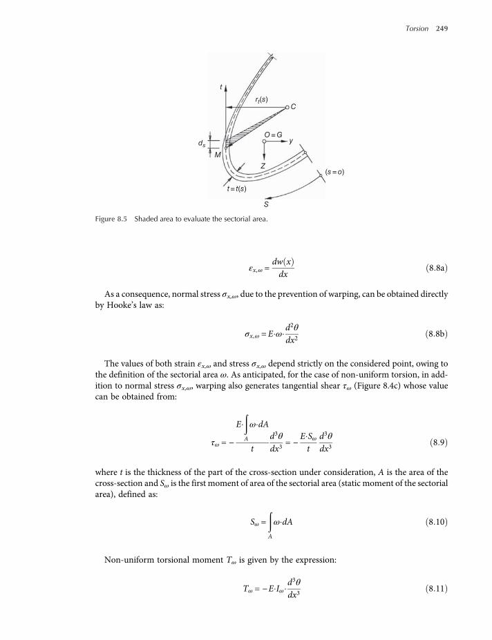
εx,ω =dw xdx
8 8a
As a consequence, normal stress σx,ω, due to the prevention of warping, can be obtained directlyby Hooke’s law as:
σx,ω =E ωd2θdx2
8 8b
The values of both strain εx,ω and stress σx,ω depend strictly on the considered point, owing tothe definition of the sectorial area ω. As anticipated, for the case of non-uniform torsion, in add-ition to normal stress σx,ω, warping also generates tangential shear τω (Figure 8.4c) whose valuecan be obtained from:
τω = −
E
A
ω dA
td3θdx3
= −E Sωt
d3θdx3
8 9
where t is the thickness of the part of the cross-section under consideration, A is the area of thecross-section and Sω is the first moment of area of the sectorial area (static moment of the sectorialarea), defined as:
Sω =
A
ω dA 8 10
Non-uniform torsional moment Tω is given by the expression:
Tω = −E Iωd3θdx3
8 11
rt(s)C
O = G
Z
y
(s = o)
S
t = t(s)
M
ds
t
Figure 8.5 Shaded area to evaluate the sectorial area.
Torsion 249

where Iω is the moment of inertia of the sectorial area (sectorial moment of inertia) defined as:
Iω =
A
ω2 dA 8 12
By substituting previous equations, non-uniform shear stress τω can be expressed as:
τω =Tω SωIω t
8 13
Generally, with reference to non-uniform torsion, a new variable is conveniently introduced,which is identified as bimoment (B).
With reference to the cantilever beam in Figure 8.3, beam flanges are forced to bend in theirplane. This bending generates clockwise rotation in one flange and anti-clockwise rotation in theother one so as resulting effect two equal and opposite bending moments and rotations are gen-erated. This force system, which is induced in the flanges by warping restraint, that is the bimo-ment, is usually identified with symbol B, and is expressed as:
B=B x =
x
0
Tω c dc= −E Iωd2θdx2
8 14a
Bimoment B has the measurement unit of force × length2 (moment × distance) and in the caseof the cantilever beam of Figure 8.3 can be expressed as:
B= 2F2h2
L−x 8 14b
Normal stress (σx,ω) associated with the warping torsion can be also expressed as:
σx,ω =BIωω 8 15
8.2.1 I- and H-Shaped Profiles with Two Axes of Symmetry
As previously mentioned, for I- and H-shaped cross-sections with two axes of symmetry, theshear centre coincides with the centroid. By identifying with b and h the flange width andthe beam depth, respectively, alternative to Eq. (8.5a), torsional constant can be evaluated moreaccurately as:
It =2 b−0 63tb t3f
3+
h− tf t3w3
+2twtf
0 145 + 0 1rtf
r + tw 2 2 + r + tf2−r2
2r + tf
4
8 16
where r is the fillet radius and tf and tw are the thickness of the flange and of the web, respectively.The sectorial area (ω) associated with each half flange, can be approximated as:
ω=ω s =h− tf2
s
0
ds=h− tf s
28 17a
250 Structural Steel Design to Eurocode 3 and AISC Specifications

Functions Sω and Iω are given, respectively, by expressions:
Sω =
s
0
h− tf s
2tf ds =
h− tf tf s2
48 18a
Iω =
A
ω2 dA=
s
0
h− tf s
2
2
tf ds =h− tf
2tf s3
128 19a
Figure 8.6 proposes the distribution of ω and Sω functions for the doubly symmetrical I- andH-shaped profiles.For design purposes, reference has to be made to themaximum value of these functions in order
to base the design on more severe verification conditions. By substituting with the variable s thevalues of the relevant coordinates, which are referred to the midline of the cross-section (s = b), wecan obtain:
ωmax = bh− tf4
8 17b
Sω,max = b2 tf h− tf
168 18b
Iω = 4h− tf
2tf b3
12 8≈Iz
h− tf2
2
8 19b
where Iz is the moment of inertia along the weak axis of the cross-section.By re-considering the example of the cantilever beam in Figure 8.3, the stress distribution and
the maximum value of σx,ω and τω can be evaluated by simple considerations. In particular, tor-sional moment T is due to the horizontal force and can expressed as T = F 2 h− tf , as it resultsfrom the load condition in Figure 8.3c.Bimoment B acting at the restrained cross-section end of the cantilever (x = L), where warping
is totally prevented, assumes the value B=T L and the maximum normal stress (σx,ω,max) acting atthe flange boundary can be evaluated as:
ω Sω
(a) (b)
Figure 8.6 Distribution of ω (a) and Sω (b) in case of a bi-symmetrical I- and H-shaped profile.
Torsion 251

σx,ω,max x =BIω
ω=T L
Izh− tf2
2b
h− tf4
=T LIz
bh− tf
8 20
Maximum shear stress (τω,max) corresponds with the centroid of the flange at the fixed canti-lever end (where warping is totally prevented, being T = Tω) and assumes the value:
τω,max =Tω SωIω t
=T b2
tf h− tf16
Izh− tf2
2
tf
8 21
It should be noted that the design value of both σx,ω and τω should also be obtained by applyingthe bending beam theory to the beam flanges. With reference to the case in Figure 8.3, by approxi-mating the moment of inertia of the beam flange in its plane Izf as Izf = tf b3 12 and neglecting thepresence of the corners between the beam flanges and the web, maximum normal stress (σx,ω,max)can be obtained as:
σx,ω,max x =F L
b2
Izf=
T
h− tfL
b2
tf b3
12
= 6T L
h− tf tf b28 22
In a similar way, by considering the shear distribution of a rectangular cross-section based onthe Jourawsky’s approach for the flange, the definition of the maximum shear stress (τω,max) is:
τω max =32
T
h− tf
1b tf
8 23
It isworthmentioning thatEq. (8.22) coincideswithEq. (8.20) if Iz is evaluatedneglecting thewebcontribution (i.e. Iz = b3tf 6). Under this assumption, Eqs. (8.21) and (8.23) are also coincident.
8.2.2 Mono-symmetrical Channel Cross-Sections
The case of a channel cross-section with one axis of symmetry is considered here with reference toflanges and webs of different thickness (Figure 8.7). It can be convenient to evaluate, at first, theshear centre location (point C), usually measured by the distance e from the midline of the web, onthe basis of the distribution of the shear stresses. By considering Jourawski’s theory, a shear forceVz, applied to the cross-section in a direction parallel to the web, is balanced by a shear flow dis-tribution (τ t), which is obtained by the product between the shear stress (τ) and the thickness (t).As to τ t, a parabolic distribution acts on the web of resultant Vw and parallel to the web, and alinear distribution is in each flange of resultant Vf and parallel to the flange. By considering theequilibrium conditions, external force (Vz) is balanced by the shear stresses resultant (Vw), that isVw = Vz, and the resulting force on each flange generates a torsional moment.
As previously mentioned, the shear centre (C) is located where no torsion occurs when flexuralshears act in planes passing through that location. This definition is used to identify the position of
252 Structural Steel Design to Eurocode 3 and AISC Specifications

the shear centre. In particular, the equilibrium condition with reference to the rotation of thecross-section is satisfied if:
Vz e=Vw e=Vf h− tf 8 24a
As a consequence, distance e can be obtained directly as:
e=Vf h− tf
Vw8 24b
If Iy identified the moment of inertia with reference to the y–y axis of the cross-section, shearstresses can be directly obtained by means of the Jourawsky approach. In particular, at the inter-section between the flange and the web, due to the constant values of the shear flow (τj tj), it can beassumed:
τf tf = τω tw =Vz
Iy
b− tw 2 tf h− tf2
8 25a
where t is the thickness, subscripts f andw are related to the flange and the web, respectively, and hand b are the width and the height of the channel, respectively.At the centre of the web, in correspondence with the symmetry axis, the shear stress τwc is given
by expression:
τwc tw =Vz
Iy
b− tw 2 tf h− tf2
+Vz
Iy
h− tf2tw
88 25b
Resulting forces Vf and Vw can be expressed as
Vf =τf tf b− tw 2
28 26
Vw = τf tf h− tf +23
τwc−τw tw h− tf 8 27
Vz
Vw
y hC
O
eb– tw/2
tf
tfτwc tw
τw tw
τf tf
τf tf
zVf
tw
b
Figure 8.7 Distribution of the shear stresses in a channel loaded on the shear centre.
Torsion 253

By substituting the expressions of the resulting forces in Eq. (8.24b) the shear centre positioncan be identified on the basis of the sole geometry of the cross-section as:
e =3 b− tw 2 2 tf
6 b− tw 2 tf + h− tf tw8 28
As for the case of I- andH-shaped profiles, torsional properties can be easily evaluated for chan-nel cross-sections. In Figure 8.8a,b the distribution of the sectorial area,ω, and the first moment ofthe sectorial area, Sω, are indicated, which can be qualitatively associated with the distribution ofthe normal stresses σx,ω and shear stresses τω.
As to the distribution of the sectorial area in the key points of the cross-section, the followingvalues have to be considered:
ωA =h− tf2
b−tw2−e 8 29a
ωB = −eh− tf2
8 29b
As to the local values defining the distribution of the first moment of the sectorial area, the result is:
SωB =tf b−
tw2
h− tf
2b2−tw4−e 8 30a
Sω1 = SωB−tw e h− tf
2
88 30b
Sω2 =tf h− tf
4b−
tw2
−e2
8 30c
Second moment of sectorial area (warping constant) can be expressed as:
Iω =b−
tw2
3
h− tf2tf
12
2 h− tf tw + 3 b−tw2
tf
h− tf tw + 6 b−tw2
tf8 31
ωB
ωA
SωB
Sω2
Sω1
ωA
ωB
ωω
(a) (b)
Figure 8.8 Distribution for a channel section of: (a) sectorial area (ω) and (b) first moment of area of the sectorialarea (Sω).
254 Structural Steel Design to Eurocode 3 and AISC Specifications

8.2.3 Warping Constant for Most Common Cross-Sections
As alreadymentioned, in case of L-, T- and V-shaped profiles, that is amember with cross-sectionscomposed by thin plates having a commonpoint of intersection that is the shear centre, thewarpingconstant is always zero (Iω = 0); otherwise it has to be computed.Warping constants are reported inTable 8.3 for some of the most common shapes of cross-section in which the centroid coincideswith the shear centre, assuming that all the constituent plates have equal thickness t.Table 8.4 proposes the warping constant Iω for some of the most common cross-sections with
one axis of symmetry, under assumption of constant thickness of plates forming cross-section.Furthermore, with reference to the more general cases of cross-section composed of plates of
different thickness, a simplified procedure can be used to evaluate cross-section constants, whichrequires division of the cross-section into n plates, each of them identified with a progressive num-ber (from 1 to n). Nodes are inserted between the parts, which are numbered from 0 to n (Figure8.9). As a consequence the generic plate i is defined by nodes i − 1 and i. Each node has coordinatesyi and zi and each part has a thickness ti, which is constant for the plate. In the following theexpression of the main geometrical properties relevant for torsional design are proposed:
• Area A is the sum of the area of plates forming the cross-section:
A=n
i= 1
dAi =n
i= 1
ti yi−yi−12+ zi−zi−1
2 8 32
• Moments of inertia Sy0, and Sz0 are defined with respect to original y0 - and z0 -axis:
Sy0 =n
i= 1
zi + zi−1dAi
28 33a
Sz0 =n
i= 1
yi + yi−1dAi
28 33b
• Coordinates zgc and ygc of the centroid:
zgc =Sy0A
8 34a
ygc =Sz0A
8 34b
Table 8.3 Warping constants when the centroid is coincident with the shear centre.
b
t
Oh
tw
Iω =h2tb3
24t
O
b
h
Iω =h2tb3
12b+ 2h2b+ h
b
t
O h
b1
Iω =tb2
248b31 + 6h
2b1 + h2b+ 12b21h
b
t
Oh
b1
Iω =tb2
248b31 + 6h
2b1
+ h2b−12b21h
Torsion 255

4
5 6
2 1
0
12
11
13
3
n
t1
t2
Y–
tn
t3
7
8
10
Z
Z–
Yα
9
α
η
ξ
Figure 8.9 Cross-section nodes.
Table 8.4 Warping constants for mono-symmetrical cross-sections.
b
O
Ch
e
Iω =h2b3t12
2h+ 3bh+ 6b
b
b1
h OC
e
Iω = t
h2b2
2b1 +
b3−e−
2eb1b
+2b21h
+
+h2e2
2b+ b1 +
h6+2b21h
+2b313
b+ e 2
b1
b
O
Ch
e
Iω = t
h2b2
2b1 +
b3−e−
2eb1b
−2b21h
+
+h2e2
2b+ b1 +
h6−2b21h
+2b313
b+ e 2
a
e
C
O
b Iω =ta4b3
64a+ 3b
2a3− a−b 3
e
r
Oαα
C
Iω =2tr5
3α3−6
sinα−αcosα 2
α−sinαcosα
256 Structural Steel Design to Eurocode 3 and AISC Specifications

• Moments of inertia Iy0, Iz0 and Iyz0 defined with respect to the original y0 - and z0 -axis:
Iy0 =n
i= 1
zi2 + zi−1
2 + zi zi−1dAi
38 35a
Iz0 =n
i= 1
yi2+ yi−1
2+ yi yi−1
dAi
38 35b
Iyz0 =n
i= 1
2 yi−1 zi−1 + 2yi zi + yi−1 zi + yi zi−1dAi
68 35c
• Moments of inertia, Iy, Izo and Iyzwith respect to the y- and z-axis passing through the centroid:
Iy = Iy0−A z2gc 8 36a
Iz = Iz0−A y2gc 8 36b
Iyz = Iyz0−Sy0 Sz0A
8 36c
• Principal axes:
α=12arctan
2IyzIz − Iy
if Iz− Iy 0 otherwise α= 0 8 37
Iξ =12
Iy + Iz − Iz −Iy2+ 4 I2yz 8 38a
Iη =12
Iy + Iz + Iz− Iy2+ 4 I2yz 8 38b
• Sectorial coordinates:
ω0 = 0 8 39a
ω0i = yi−1z1−yiz1−1 8 39b
ωi =ωi−1 +ω0 8 39c
• Mean values of the sectorial coordinate:
Iω =n
i= 1
ωi−1 +ωidAi
28 40
• Sectorial constants:
Iyω = Iyω0−Sz0 IωA
=
=n
i= 1
2 yi−1 ωi−1 + 2yi ωi + yi−1 ωi + yi ωi−1dAi
6−Sz0 IωA
8 41a
Torsion 257

Izω = Izω0−Sy0 IωA
=
=n
i= 1
2 zi−1 ωi−1 + 2zi ωi + zi−1 ωi + zi ωi−1dAi
6−Sy0 IωA
8 41b
Iωω = Iωω0−I2ωA
=n
i= 1
ωi2 + ωi−1
2 +ωi ωi−1dAi
3−I2ωA
8 42
• Shear centre coordinates IyIz− I2yz 0 :
ysc =IzωIz − IyωIyzIyIz − I2yz
8 43a
zsc =− IyωIy− IzωIyz
IyIz − I2yz8 43b
• Warping constant (Iw):
Iw = Iωω + zsc Iyω−ysc Izω 8 44
• Torsion constants (It):
It =n
i= 1
dAit2i3
8 45
8.3 Member Response to Mixed Torsion
Member response to mixed torsion, in both statically determinate and indeterminate structures,depends strictly on the torsional restraints at its end. Traditional ideal restraints of fixed ends,typically used for members in bending, can be differently classified when torsion is considered.In Figure 8.10 two types of torsional restraints are presented:
(a) simple torsional restraint (identified, for sake of simplicity as STR), which can absorb the tor-sional end moment but cannot prevent warping and hence is completely free (i.e. no planarityof cross-section is guaranteed by this restraint);
(b) fixed torsional restraint (FTR), which can absorb torsional end moment and prevent warpingcompletely.
As already mentioned, the applied torsional moment is resisted by a combination of uniformand warping torsion. As results from Eq. (8.1), by substituting the definitions given by Eqs. (8.3)and (8.11), we can obtain:
T =G Itdθdx
−E Iωd3θdx3
8 46a
258 Structural Steel Design to Eurocode 3 and AISC Specifications

Reference can be made suitably to the torsion parameter λT, defined as λT = G It E Iω, whichindicates the dominant type of torsion. In case of uniform torsion, λT is very large, as for thin-walledclosed-section members whose torsional rigidities are very high (members with narrow rectangularsections, angle and tee-sections, whose warping rigidities are negligible). On the other hand, if thesecond component of resistance due to torsional loading completely dominates with respect to thefirst, the member is in a limiting state of non-uniform torsion referred to as warping torsion. Thismay occur when the torsion parameter λT is very limited, which is the case for some very thin-walledopen sections (such as light gauge cold-formed sections) whose torsional rigidities are very small.By introducing the λT term, Eq. (8.46a) can be re-written as:
TG It
=dθdx
−1
λ2T
d3θdx3
8 46b
The differential equation permits the following general solution:
θ x = a+ b sinh λTx + c cosh λTx + θp 8 47
where a, b and c are constants depending on the boundary conditions and θp is the particularsolution, associated with both loading and restraints conditions.In case of the cantilever beam of length L represented in Figure 8.11, by considering a concen-
trate torsional moment applied at the free end (x = L) and the fixed end (x = 0) able to totally pre-vent the restraint, the particular solution θp is:
θp =TG It
x 8 48
Top flange
Bottom flange
Plate APlate A
y
z
STR
FTR
(a)
(b)
Plate B
Ld
Figure 8.10 Examples of torsional restraints: (a) simple support restraining torsion (warping is free) and (b) fullyfixed restraint to torsion (warping is prevented).
Torsion 259

Boundary conditions for this case are listed next:
• at the restrain location (x = 0), rotation is zero θ = 0 and warping is totally preventeddθdx
= 0 ; by considering the general solution expressed by Eq. (8.47), we can obtained:
a+ c= 0 8 49a
λTb+TG It
= 0 8 49b
• at the free end, where the load is applied (x = L), the bimoment is zerod2θdx2
= 0 and hence, by
deriving the Eq. (8.47) twice, it results in:
b λ2T sinh λTL + c λ2T cosh λTL = 0 8 49c
The constants assume the following values:
a= −c= −T
λTGIttanh λTL 8 50
b= −T
λTGIt8 51
Rotation is expressed as:
θ x =T
λTGItλTx +
sinh λT L−xcosh λTL
− tanh λTL 8 52
At the free end the value of rotation is: θ L =T
λTGItλTL− tanh λTL
Pure torsional moment is expressed as:
Tt =T 1−cosh λT L−xcosh λTL
8 53
Warping moment is expressed as:
Tω =Tcosh λT L−xcosh λTL
8 54
FTR
y
x
T
z
Figure 8.11 Cantilever beam loaded by a torsional moment at the free end (x = L) with torsional restraintpreventing warping at the fixed end (x = 0).
260 Structural Steel Design to Eurocode 3 and AISC Specifications

Bimoment is expressed as:
B= −TλT
sinh λT L−xcosh λTL
8 55
At the restraint location (x = 0) where rotation and warping are prevented, only the warpingmoment acts (T = Tω). At the free end, the applied external torsional moment is balanced bythe sole pure torsion (T = Tt) where the warping moment is zero. Bimoment B at this location
assumes the maximum value; that is: B x = 0 = −TλT
tanh λTL .
In order to appraise the distribution of the two types of torsional contributions balancing exter-nal torque T applied to the free end of the cantilever beam, the ratios Tt(x)/T and Tω x T areplotted versus x/L in Figure 8.12. The rotation is considered and the ratio θ(x)/θ(L) is plotted inthe figure too.Furthermore, the case of a beam of length L, simply supported at its ends for torsional moments
and loaded at midspan (x = L/2) by a torque moment T could also be interesting for design pur-poses (Figure 8.13).The general solution expressed by Eq. (8.47) admits as particular solution, θp;
θp =T
2GItx 8 56
1.0
0.8
0.6
0.4
0.2
0.0
0 0.25
Tt(x)
Tω(x)
T
T
θ (x)
θ (L)
0.5 0.75 1x / L
Figure 8.12 Distribution of pure and warping torsion along the cantilever beam (x = 0 and x = L indicate fixed endand free end, respectively) and ratio between the rotation at generic cross-section x and the one at the free end.
STR
y
x
z
STR
T
Figure 8.13 Beam restrained at its ends by torsional supports and loaded at the midspan (x = L/2) by a torque.
Torsion 261

Boundary conditions for this case are:
at the beam ends (i.e. x = 0 and x = L) rotation is fully restrained θ = 0 but warping is free and, as
a consequence the bimoment is zerod2θdx2
= 0 .With reference to the cross-section at the loca-
tion x = 0, we can obtain:
a+ c= 0 8 57a
c= 0 8 57b
From these conditions, the result is a = 0.
In the loaded cross-section (x = L/2) warping is assumed to be completely preventeddθdx
= 0
and, as a consequence, it results in:
b= −T
2λTGIt
1cosh λTL 2
8 58
Rotation θ(x) is expressed as:
θ x =T
2λTGItλx−
sinh λTxcosh λTL 2
8 59a
In correspondence of the loaded cross-section, the rotation assumes the maximum value:
θmax x =L2
=T
2λTGItλT
L2− tanh
λTL2
8 59b
The pure torsional moment is expressed as:
Tt =T2
1−cosh λTx
cosh λTL 28 60a
At the beam ends, the maximum value of the pure torsional moment is:
Tt x = 0 =Tt x = L =GItdθdx
=T2
1−1
cosh λTL 28 60b
The bimoment is expressed as:
B= −EIωd2θdx2
= −T2λT
sinh λTxcosh λTL 2
8 61a
The maximum value of the bimoment is achieved at the loaded cross-section x =L2
:
B x =L2
= −EIωd2θdx2
= −T2λT
tanh λTL 2 8 61b
262 Structural Steel Design to Eurocode 3 and AISC Specifications

The warping moment is expressed as:
Tω = −EIωd3θdx3
=T2
cosh λTxcosh λTL 2
8 62a
The maximum value of the non-uniform bending moment is at the loaded cross-section:
TωL2
= −EIωd3θdx3
=T2
8 62b
The same approach adopted for the beams in Figures 8.11 and 8.13, can be used for other casesof practical interest for routine design. For different load cases and types of restraints Tables 8.5and 8.6 report key data for torsional design that are related to concentrated and distributed tor-sional loads, respectively.
8.4 Design in Accordance with the European Procedure
Part 1-1 in EC3 gives limited guidance for the design of torsion members. While both elasticand plastic analyses are generally discussed, only very approximate methods of elastic analysisare specifically discussed for torsion members. Furthermore, while both first yield andplastic design resistances are referred to with regards to bending, only the first yield designresistance is specifically discussed for torsion members: there is no guidance onsection classification for torsion members, or on how to account for the effects of local bucklingon design resistance.
Table 8.5 Key data for the torsional design in the case of a concentrated torsional load.
STR
x
T
y
z
θmax L =TL
IωEλ2T
θ'max L =−T
IωEλ2T
θ''max L = 0 θ'''max 0 = 0
FTR T
y
x
z
θmax L =T
IωEλ3T
λTL− tanhλTL θ'max L =−T
IωEλ2T
1−1
coshλTL
θ''max 0 =T
IωEλTtanhλTL θ'''max 0 =
TIωE
T
yx
z
STRSTR θmaxL2
=T
2IωEλ3T
λTL2
− tanhλTL2
θ'max0L
=±T
2IωEλ2T
1−1
cosh λTL 2
θ''maxL2
=−T
2IωEλTtanh
λTL2
θ'''maxL2
=T
2IωE
TFTRFTR
xy
z
θmaxL2
=T
IωEλ3T
λTL4
− tanhλTL4
θ'maxL4
=T
2IωEλ2T
1−1
cosh λTL 4
θ''max
0L2L
=+−+
T2IωEλT
tanhλTL4
θ'''max =−T2IωE
Torsion 263

For members subjected to torsion, if distortional deformations may be disregarded, the designvalue of the torsional moment TEd at each cross-section has to satisfy the condition:
TEd ≤TRd 8 63
where TRd is the design torsional resistance at the cross-section.In particular, as already discussed, the total torsional moment TEd at any cross-section should
be considered as the sum of two internal effects:
TEd =Tt,Ed +Tw,Ed 8 64
where Tt,Ed is the internal St Venant torsion and Tw,Ed is the internal warping torsion.The values of Tt,Ed and Tw,Ed at any cross-section may be determined from TEd by an elastic
analysis taking into account the section properties of the member, the conditions of restraintat the supports and the distribution of the actions along the member.
It is required to take into account the following stresses due to torsion:
• shear stresses τt,Ed due to St Venant torsion Tt,Ed;• normal stresses σw,Ed due to the bimoment BEd and shear stresses τw,Ed due to warping tor-
sion Tw,Ed.
As a simplification, in cases of a member with a closed hollow cross-section, such as a structuralhollow section, EC3 allows the assumption that the effects of torsional warping can be neglected.
Table 8.6 Key data for the torsional design in the case of a uniform torsional load.
STRy
x
z
tθmax L =
tL2
2IωEλ2T
θ'max 0 =t
IωEλ3T
λTL− tanhλTL2
θ''maxL2
=− t
IωEλ2T
1−1
coshλTL2
θ'''max0L
=+−
t2IωEλT
tanhλTL
t
FTRy
x
z
θmax L =t
IωEλ4T
1 +λ2TL
2
2−1 + λTLsinhλTL
coshλTL
θ''max 0 =t
IωEλ2T
1 + λTLsinhλTLcoshλTL
−1 θ'''max 0 =tLIωE
STR STR
t
yx
z
θmaxL2
=t
IωEλ4T
λ2TL2
8+
1cosh λTL 2
−1
θ'max0L
=+−
t
IωEλ3T
λTL2
− tanhλTL2
θ''maxL2
=t
IωEλ2T
1cosh λTL 2
−1 θ'''max0L
=−+
tIωEλT
tanhλTL2
t
FTR FTR
xy
z
θmaxL
2 =tL
2IωEλ3T
λTL4
− tanhλTL4
+ θ''max0L
=t
IωEλ2T
λTL2tanh λTL 2
−1
−θ''maxL
2 =− t
IωEλ2T
1−λTL
2sinh λTL 2θ'''max
0L
=−+
tL2IωE
264 Structural Steel Design to Eurocode 3 and AISC Specifications

In the case of a member with an open cross-section, such as I- or H-shaped profiles, according toEC3 it may be assumed that the effects of St Venant torsion can be neglected.Furthermore, as already mentioned in Section 7.2.2, for combined shear force and torsional
moment the plastic shear resistance accounting for torsional effects should be reduced fromVpl,Rd to Vpl,T,Rd and the design shear force VEd must satisfy the condition:
VEd ≤Vpl,T ,Rd 8 65
The Eq. (7.25) are herein re-proposed for the sake of clarity. For themost common casesVpl,T,Rd
is defined as:
• for an I- or H-shaped section:
Vpl,T ,Rd =Vpl,Rd 1−τt,Ed
1,25γM0
fy3
8 66
• for channel sections:
Vpl,T ,Rd =Vpl,Rd 1−τt,Ed
1 25γM0
fy3
−τw,Ed
1γM0
fy3
8 67
• for structural hollow sections:
Vpl,T ,Rd =Vpl,Rd 1−τt,Ed
1γM0
fy3
8 68
8.5 Design in Accordance with the AISC Procedure
Torsion is addressed in AISC 360-10, Chapter H3. An important help for computing torsionfor open shapes comes from AISC Design Guide 9 ‘Torsional Analysis of Structural SteelMembers’.Chapter H3 deals mainly with torsion for hollow structural sections (HSS). These types of
cross-sections can be often subjected to torsional moments. For HSS sections, according toAISC, stresses due to restrained warping can be disregarded and it can be assumed that allthe torsional moment is resisted by pure (St Venant) torsional stresses. So for HSS it is possibleto define torsional strength in terms of a resisting torsional moment and not in terms of torsionalstresses. This allows for verifying HSS members subjected to compression, bending moment,shear and torsional moments in terms of actions and not stresses. On the contrary, for opencross-section members in which warping is not completely unrestrained, torsional resistance
Torsion 265

is exhibited as the sum of that due to pure (St Venant) torsion and that due to restrained warp-ing. The contribution of each of them depends on the angle of rotation θ and its derivatives; so itdepends, as already discussed, on section properties, type of loads and type of restraints, and itmust be determined for each design case. Such open cross-section members are, in most cases,subjected not only to torsion but also to bending moments, shear and axial loads and somedetails of their design are discussed in Chapter 10. Pure torsion is very unlikely actually andtorsion in open cross-section should be avoided with proper design strategies or at least reducedto a secondary action. AISC Specifications prescribe then for open sections to compute stressesdue to any kind of generalized forces (axial, bending, shear and torsion) and compare them withdefined allowable stresses.
8.5.1 Round and Rectangular HSS
LRFD approach ASD approach
Using load and resistance factor design (LRFD), designtorsional strength Tc, is defined as:
Tc =ϕTTn 8 69
where ϕT = 0 90 and Tn is the nominal torsional strength
Using allowable strength design (ASD), allowabletorsional strength Tc, is defined as:
Tc =Tn ΩT 8 70
where ΩT = 1 67 and Tn is the nominal torsionalstrength
Nominal torsional strength, Tn, is computed with the formula:
Tn = FcrC 8 71
where C is the HSS torsional constant and Fcr is the critical stress that takes account of local buck-ling and initial imperfections.
(a) For a round HSS:
Fcr =max1 23E
LD
Dt
5 4;0 60E
Dt
3 2≤ 0 60Fy 8 72
where L is the length of the member and D is the outside diameter.(b) For a rectangular HSS:
Fcr = 0 60Fy if h t ≤ 2 45EFy
8 73a
Fcr =0 6Fy 2 45 E Fy
ht
if 2 45EFy
< h t ≤ 3 07EFy
8 73b
266 Structural Steel Design to Eurocode 3 and AISC Specifications

Fcr =0 458π2E
ht
2 if 3 07EFy
< h t ≤ 260 8 73c
where h is the flat width of longer HSS side and t the design wall thickness.
The torsional constant C should be taken as:
(a) For a round HSS:
C =π D4−D4
i
32D 2≈π D− t 2t
28 74
where Di is the inside diameter.(b) For a rectangular HSS:
C = 2A0t 8 75a
where A0 is the area bounded by the midline of the section.
Assuming an outside corner radius of 2t conservatively, the midline radius is 1.5t and the tor-sional constant C consequently becomes:
C = 2 B− t H− t t−4 5 4−π t3 8 75b
If a round or rectangular HSS member is subjected to a torsional moment Tt, computed withLRFD or ASD load combinations and torsion is the only internal action, then verification is:
Tt ≤Tc 8 76
where Tc is the design torsional strength (LRFD) or allowable torsional strength (ASD).In the case of axial load, bending moments and shear, then the verification is performed accord-
ing to Section 10.3.
8.5.2 Non-HSS Members (Open Sections Such as W, T, Channels, etc.)
For such members, torsion is sustained as pure torsion and restrained warping torsion.Considering the common case of I- or H-shaped profiles:
(a) pure (St Venant) torsion generates shear stress τt in any part of the section (flanges and web);(b) restrained warping torsion generates normal stress σw and shear stress τw in the flanges.
As previously discussed, the distribution of torsional moment between pure and restrainedwarping torsion depends on rotation angle and its derivatives; that is on type of load, restraintsand cross-section geometry. In evaluating stresses due to torsion, a helpful tool is the AISC DesignGuide 9 and its Appendix B. Verifications for pure torsion are generally meaningless becausetorsion for this kind of section is very often associated with stresses due to axial load, bendingmoments and shear. So AISC 360-10 proposes a verification for combined actions that arediscussed in Section 10.3.
Torsion 267
CHAPTER 9
Members Subjected to Flexureand Axial Force
9.1 Introduction
Members subjected to flexure and axial forces are commonly identified as beam-columns. Theyare frequently encountered in routine design when:
• the axial force is eccentric with reference to the cross-section centroid;• the compressed element is also subjected to transverse load inducing flexure (typically, beams
in simple frames loaded by gravity loads but also interested by axial forces due to the effects ofhorizontal forces);
• the vertical elements, which belong to a rigid or to a semi-continuous frame, are loaded at theirends by bending moments transferred by beams;
• thin-walled elements are subjected to axial load on the centroid of the gross section, which doesnot coincide with the one of the effective cross-section (Figure 4.8a).
When the centre of pressure lies on one of the twomain planes of inertia, the cross-section is inter-ested by compression and in-plane bending, while the more general case is related to compressionand bi-axial bending. For beam-columns the absence of instability phenomena is very rare and forthis reason themore severe design checks are generally the ones related to overall member stability.
Deformability: When the deflection vBC of a beam-column has to be evaluated, a simplifiedapproach can be adopted, which consists of suitably amplifying the deflection vv due to theloads normal to the beam, to take into account the presence of axial load. In detail, thebeam-column displacement vBC can be estimated as:
vBC =1
1−NNcr
vv 9 1
where N represents the design axial load and Ncr the critical buckling load with reference to thebending plane.
Resistance: Resulting from the basis of the theory of structures, in case of members subjected toaxial load (N) and bending moment (M), which are suitably constrained against instability,checks must be made on the most stressed cross-section. In order to allow for a generalappraisal of the safety of the beam-column, reference can be made to the well-known
Structural Steel Design to Eurocode 3 and AISC Specifications, First Edition. Claudio Bernuzzi and Benedetto Cordova.© 2016 John Wiley & Sons, Ltd. Published 2016 by John Wiley & Sons, Ltd.

St Venant’s theory and the maximum stress σ, resulting from the linear combination of axialload and bending moment, is expressed as:
σ =NA+MW
9 2
where A and W are the area and the section modulus of the cross-section, respectively.On the other hand, if verifications refer the performance of the whole cross-section, accord-
ing to the limit state design philosophy (already introduced with reference to the shear andbending moment interaction), the design bending resistance must be suitably reduced forthe presence of axial load.
Stability: A beam-column can be affected by the buckling phenomena already introduced forbeams (see Chapter 7) and columns (see Chapter 6), on the basis of the influence of severalfactors, which can be associated, for example with cross-section geometry, the presence ofend and/or intermediate restraints, the load condition and so on. When an unrestrainedbeam-column is bent about its major axis, it may buckle by deflecting laterally and twistingin correspondence of a load that could be significantly lower than the maximum load predictedby an in-plane analysis. If the shear centre is coincident with the cross-section centroid, twotypical kinds of instability (Figure 9.1) can be observed:
flexural buckling, if the member restraints efficiently hamper the sole buckling of the compressionflangebymeansofdeflectionof themember intheplane thatcontains theeccentricityof the load;
lateral-torsional (flexural-torsional) buckling, when the instability is associated with the typicaldeflection due to the buckling of members in bending.
If the shear centre does not coincide with the centroid, design should be governed by flexural-torsional buckling, as well as in the case of a predominant axial load on the bending moment.When stability has to be accounted for into design, the buckling conditions are defined bythe interaction between critical axial load (Ncr) and bending moment (Mcr). As an example,Figure 9.2 presents typical Ncr–Mcr curves for a simply supported column under uniform (ψ =1) or gradient (ψ 1) end moment distributions.An efficient and quite simple way to account for the buckling interaction between the axial load
and the bending moment is to approximate the critical buckling moment Mcr,(N) of the beam-column reducing the one of the beam (Mcr) in the presence of the axial load N. In particular,two cases can be distinguished, depending on the symmetry of the cross-section:
• Mono-symmetrical cross-section:
Mcr N =C1π2EIzkzL
2
kzkW
2 IWIz
+kL 2GItπ2EIz
fM N + C2zg −C3zj2
− C2zg −C3zj
9 3a
B
B
U
N
M
B
B
(b)(a)
U
M
N
Figure 9.1 Typical deformed shapes for flexural buckling (a) flexural torsional buckling (b).
Members Subjected to Flexure and Axial Force 269

where function fM(N) is defined as:
fN N = 1−N
Ncr,y1−
NNcr,FT 1
1−N
Ncr,FT 29 3b
with:
Ncr,FT 1,2 =12
Ncr,y
1−y0i0
2 1 +Ncr,T
Ncr,y± 1 +
Ncr,T
Ncr,y
2
−4y0i0
2Ncr,T
Ncr,y 9 3c
All the terms in these equations have already been discussed with reference to the axial buck-ling of columns (Chapter 6) and to the lateral buckling of beams (Chapter 7).
• Bi-symmetrical cross-section:
Mcr N =Mcr fB N 9 4a
where Mcr is given by Eq. (7.42) for the beam (i.e. element under pure flexure) and fB(N) isdefined as:
fB N = 1−N
Ncr,y1−
NNcr,z
1−N
Ncr,T9 4b
90000
80000
70000
60000
50000
40000
30000
20000
10000
00 10000000 20000000 30000000 40000000 Mcr
[Nmm]
Centroid
MN N
Ncr
[N]
ψM
Figure 9.2 Typical axial force-bending moment buckling domains for different values of the end ratio moment (ψ ).
270 Structural Steel Design to Eurocode 3 and AISC Specifications

The flexural (Ncr,y andNcr,z) and the torsional (Ncr,T) critical loads have been already definedin Chapter 6.
The influence of buckling phenomena on the response of industrial beam-columns can be evalu-ated by defining the interaction domains between axial forces and bending moments in the twoprincipal planes of cross-section. With reference to the more general case of compression andbiaxial bending in which flexural buckling governs design, typical interaction domains are pro-posed in Figure 9.3 in a non-dimensional form. In case of compact cross-section profiles, designaxial load NEd is divided by the squash load (Ny) and the design bending moments related to y–yand z–z axis (Med,y and Med,z, respectively) are divided by the corresponding plastic moment(MRd,y and MRd,z).As to the design practice, with reference to contents of the most recent Codes of practice, insteadof complex formulations that allow local definition of the interaction domains, simplified criteriasuitable for design purposes are proposed that guarantee a safe design.
9.2 Design According to the European Approach
European provisions deal with the most common cases in design practice and in particular pro-vide design rules for members with bi-symmetrical cross-sections. Rules to evaluate both strengthand stability of some of the most common cases typical of routine design are discussed in thegeneral part of EC3 (EN 1993-1-1).
9.2.1 The Resistance Checks
It should be noted that, in general, y- and z-axis identify the strong and weak cross-section axes. Incases of profiles with a cross-section in classes 1 and 2, a requirement is that the acting bendingmoment MEd does not exceed the design moment resistance MN,Rd, which is the plastic momentreduced in the presence of the axial load NEd on the considered cross-section, that is:
MEd ≤MN ,Rd 9 5
Lower slenderness
Higher slenderness
Mz,Ed/Wp/z fy Mz,Ed/ Wp/y fy
NEd/ Afy
1
1 1
Figure 9.3 Typical axial load (N)-bending moments interaction domain (M).
Members Subjected to Flexure and Axial Force 271

For a rectangular solid section without bolt fastener holes, reduced bending resistance MN,Rd canbe evaluated as:
MN ,Rd =Mpl,Rd 1−NEd
Npl,Rd
2
9 6
whereMpl,Rd andNpl,Rd represent the design plastic resistance of the gross cross-section to bendingmoments (see Chapter 7) and to normal forces (see Chapter 6), respectively.In case of doubly symmetrical I- and H-shaped sections or other similar sections (typically built-up welded profiles), allowance does not need to be made for the effect of the axial force on theplastic resistance moment about the y–y axis (parallel to the flanges) when both the followingconditions are satisfied:
NEd ≤ 0 25 Npl,Rd 9 7a
NEd ≤0 5 hw tw fy
γM09 7b
For doubly-symmetrical I- and H-shaped sections, allowance does not need to be made for theeffects of the axial force on the plastic resistance moment about the z–z axis (parallel to theweb) when:
NEd ≤hw tw fyγM0
9 8
where hw and tw are the height and the thickness of the web, respectively.For cross-sections where bolt fastener holes do not have to be considered, the following approxi-mations may be used for standard rolled I- or H-sections and for welded I- or H-shaped sectionswith equal flanges:
• bending resistance about the y–y axis:
MN ,y,Rd =Mpl,y,Rd1−n
1−0 5 a9 9a
with the limitation:
MN ,y,Rd ≤Mpl,y,Rd 9 9b
• bending resistance about the z–z axis:if n ≤ a:
MN ,z,Rd ≤Mpl,z,Rd 9 10a
if n > a;
MN ,z,Rd =Mpl,z,Rd 1−n−a1−a
29 10b
272 Structural Steel Design to Eurocode 3 and AISC Specifications

where n and a are defined, respectively, as:
n=NEd
Npl,Rd9 11
a=A− 2 b tf
A≤ 0 5 9 12
where A is the cross-section area and b and tf are the width and the thickness of the flange,respectively.
In case of rectangular structural hollow sections of uniform thickness and for welded box sec-tions with equal flanges and equal webs, the following approximations are used if the effect of boltfastener holes can be neglected:
MN ,y,Rd =Mpl,y,Rd1−n
1−0 5aw≤Mpl,y,Rd 9 13a
MN ,z,Rd =Mpl,z,Rd1−n
1−0 5af≤Mpl,z,Rd 9 13b
where terms aw and af depend on the type of cross-section.In particular, the following cases are directly considered by the Code:
hollow profiles (b and h are the width and the height of the cross-section, respectively with a thick-ness t):
aw =A−2 b t
A≤ 0 5 9 14a
af =A−2 h t
A≤ 0 5 9 14b
welded box sections (b and h are the width of the flanges of thickness tf and the height of web ofthickness tw, respectively):
aw =A−2 h tf
A≤ 0 5 9 15a
af =A−2 b tw
A≤ 0 5 9 15b
For bi-axial bending, the member verification can be based on the following criterion:
My,Ed
MN ,y,Rd
α
+Mz,Ed
MN ,z,Rd
β
≤ 1 9 16
in which α and β coefficients may conservatively be taken as unity or otherwise can be deducedfrom Table 9.1 on the basis of the value of n defined by Eq. (9.11).
Members Subjected to Flexure and Axial Force 273

For class 3 and class 4 cross-sections, when shear force is absent or its effect is negligible, themaximum longitudinal stress σx,Ed due to moment and axial force taking into account the boltfastener holes if relevant, must fulfil the condition:
σx,Ed ≤fyγM0
9 17
For a class 4 cross-section, the following additional condition has to be fulfilled:
NEd
Aeff fyγM0
+My,Ed +NEd eNy
Weff ,y fyγM0
+Mz,Ed +NEd eNz
Weff ,z fyγM0
≤ 1 9 18
where eNy and eNz represent the shift of the relevant centroidal axis when the cross-section is sub-jected to compression only, along the y–y and z–z axis, respectively, Aeff is the effective area of thecross-section when subjected to uniform compression andWeff,min is the effective section modulus(corresponding to the fibre with the maximum elastic stress).
9.2.2 The Stability Checks
EC3 proposes a criterion for verification of members under bi-axial bending, which can be appliedfor the sole case of uniform members with double symmetric cross-sections not susceptible todistortional deformations (Figure 4.1). In particular, two cases are considered:
• members that are not susceptible to torsional deformations, for example circular hollow sec-tions or sections with suitable torsional restraints and hence no lateral-torsional buckling isexpected;
• members that are susceptible to torsional deformations, for example members with open cross-sections not restrained against torsion.
The proposed interaction formulas are based on the modelling of simply supported single spanmembers with end fork conditions and with or without continuous lateral restraints, which aresubjected to compression forces, endmoments and/or transverse loads. Second order effects of thesway system have to be taken into account, either by the end moments of the member or by meansof appropriate buckling lengths, respectively.Members that are subjected to combined bending moments along the y–y and z–z axis,My,Ed andMz,Ed, respectively, and axial compression NEd must satisfy the conditions:
NEd
χy NRkγM1
+ kyyMy,Ed +ΔMy,Ed
χLTMy,RkγM1
+ kyzMz,Ed +ΔMz,Ed
Mz,RkγM1
≤ 1 9 19a
Table 9.1 Values of α and β coefficients for bi-axial bending verification.
Cross-section type α βI- and H-sections α = 2 β = 5 n with β ≥ 1Circular hollow sections α = 2 β = 2Rectangular hollow sections
α=1 66
1−1 13 n2with α ≤ 6 β =
1 661−1 13 n2
with β ≤ 6
274 Structural Steel Design to Eurocode 3 and AISC Specifications

NEd
χz NRkγM1
+ kzyMy,Ed +ΔMy,Ed
χLTMy,RkγM1
+ kzzMz,Ed +ΔMz,Ed
Mz,RkγM1
≤ 1 9 19b
where χy and χz are the reduction factors due to flexural buckling, χLT is the reduction factor due tolateral buckling, subscript Rk identifies the characteristic value for resistance to be evaluated in accord-ance with Table 9.2, additional moment ΔM is due to the shift between the gross and the effectivecentroid of the cross-section for class 4members and kyy, kyz, kzy and kzz are the interaction factors.It should be noted that, for members not susceptible to torsional deformation, it is assumedχLT = 1.0; that is no reductions of the bending performance due to lateral-torsional buckling.
The interaction factors kyy, kyz, kzy and kzz depend on the approach, which has to be selectedfrom two alternatives: alternative method 1 (AM1) and alternative method 2 (AM2), which areconsidered respectively in Annex A and Annex B of EN 1993-1-1. As to the use of these methods,it should be noted that the AM2 formulation, proposed by Austrian and German researchers, isgenerally less complex, quicker and simpler than the AM1 developed by a team of French andBelgian researchers. Therefore, AM2 can be regarded as a simplified approach whereas AM1 rep-resents a more exact and general approach.
Finally, it shouldbenoted that theNationalAnnexesof theEuropean countries should give a choicefromAM1orAM2. Furthermore, it isworthmentioning that in the present edition of EN1993-1-1 norules are given for the stability verification checks of beam-columns with one axis of symmetry.
9.2.2.1 Alternative Method 1 (AM1)According to method 1, a member is not susceptible to torsional deformation if the torsional con-stant, IT, is not lower than the second moment of area about y-axis, Iy. That is if the followingcondition is fulfilled:
IT > Iy 9 20
Furthermore, when IT ≤ Iy the following can occur:
if λo ≤ λo, lim there is no risk of lateral flexural buckling;if λo > λo, lim lateral flexural buckling can occur.
Term λo represents the relative slenderness for lateral buckling under constant moment (criticalmoment Mcr,0), already defined in Eq. (7.33), here re-proposed for simplicity:
λo =Wpl,yfyMcr,0
9 21
Table 9.2 Values for NRk, MRk and ΔMi,Ed.
NRk = fy Ai; MRk = fy Wi
Class 1 2 3 4
Ai A A A Aeff
Wy Wpl,y Wpl,y Wel,y Weff,y
Wz Wpl,z Wpl,z Wel,z Weff,z
ΔMy,Ed 0 0 0 eN,y Neda
ΔMz,Ed 0 0 0 eN,z Neda
a Terms eN,y and eN,z represent the eccentricity between the gross and the effective cross-section.
Members Subjected to Flexure and Axial Force 275

Term λo, lim is defined, for a doubly symmetrical cross-section as:
λo, lim = 0 2 C1 1−NEd
Ncr,z1−
NEd
Ncr,T
49 22
where axial critical load Ncr,z and Ncr,T are related to the buckling along z–z axis and the torsionalbuckling, respectively, and the equivalent uniform moment coefficient C1 has been already intro-duced with reference to lateral buckling (Tables 7.6 and 7.7).
In accordance with this method, coefficients kyy, kyz, kzy, kzz can be deduced from Table 9.3 formembers not susceptible to torsional deformations and in Table 9.4 for members susceptible totorsional deformations.
Additional terms reported in Tables 9.3 and 9.4 are:
μy =
1−NEd
Ncr,y
1−χyNEd
Ncr,y
and μz =1−
NEd
Ncr,z
1−χzNEd
Ncr,z
9 23a
Table 9.3 Coefficients kij for members not susceptible to torsional deformations.
Interactionfactors
Plastic cross-sectionalproperties class 1, class 2
Elastic cross-sectionalproperties class 3, class 4
kyy Cmyμy
1−NEd
Ncr,y
1Cyy
Cmyμy
1−NEd
Ncr,y
kyz Cmzμy
1−NEd
Ncr,z
1Cyz
0 6wz
wy
Cmzμy
1−NEd
Ncr,z
kzyCmy
μz
1−NEd
Ncr,y
1Czy
0 6wy
wz
Cmyμz
1−NEd
Ncr,y
kzz Cmzμz
1−NEd
Ncr,z
1Czz
Cmzμz
1−NEd
Ncr,z
Table 9.4 Coefficients kij for members susceptible to torsional deformations.
Interactionfactors
Plastic cross-sectionalproperties class 1, class 2
Elastic cross-sectionalproperties class 3, class 4
kyy CmyCmLTμy
1−NEd
Ncr,y
1Cyy
CmyCmLTμy
1−NEd
Ncr,y
kyz Cmzμy
1−NEd
Ncr,z
1Cyz
0 6wz
wy
Cmzμy
1−NEd
Ncr,z
kzyCmyCmLT
μz
1−NEd
Ncr,y
1Czy
0 6wy
wz
CmyCmLTμz
1−NEd
Ncr,y
kzz Cmzμz
1−NEd
Ncr,z
1Czz
Cmzμz
1−NEd
Ncr,z
276 Structural Steel Design to Eurocode 3 and AISC Specifications
wy =Wpl,y
Wel,y≤ 1 5 andwz =
Wpl,z
Wel,z≤ 1 5 9 23b
In absence of lateral-flexural buckling it results in Cmy =Cmy,0, Cmz =Cmz,0 and CmLT = 1 0.In case of lateral-flexural buckling:
Cmy =Cmy,0 + 1−Cmy,0εyaLT
1 + εyaLT9 24a
Cmz =Cmz,0 9 24b
CmLT =C2my
aLT
1− NEdNcr,z
1− NEdNcr,T
≥ 1with aLT = 1−ITIy
≥ 0 9 24c
• for members of classes 1, 2 and 3:
εy =My,Ed
NEd
AWel,y
9 25a
• for members of class 4:
εy =My,Ed
NEd
Aeff
Weff ,y9 25b
Coefficients Cmy,0 and Cmz,0, accounting for the moment distribution along the overallmembers, are reported in Table 9.5. Interaction coefficients Cyy, Cyz, Czy and Czz, which accountfor plasticity phenomena, are defined as:
Cyy = 1 + wy−1 2−1 6wy
C2my λmax + λ
2max
γM1NEd
fyAi−bLT ≥
Wel,y
Wpl,y9 26a
Cyz = 1 + wz−1 2−14w5zC2mzλ
2max
γM1NEd
fyAi−cLT ≥ 0 6
wz
wy
Wel,z
Wpl,z9 26b
Czy = 1 + wy−1 2−14w5y
C2myλ
2max
γM1NEd
fyAi−dLT ≥ 0 6
wy
wz
Wel,y
Wpl,y9 26c
Czz = 1 + wz −1 2−1 6wz
C2mz λmax + λ
2max −eLT
γM1NEd
fyAi≥Wel,z
Wpl,z9 26d
Auxiliary terms of the previous equations are:
bLT = 0 5 aLT λ20
γM0My,Ed
χLT fyWpl,y
γM0Mz,Ed
fyWpl,z9 27a
cLT = 10 aLTλ20
5 + λ4z
γM0My,Ed
CmyχLT fyWpl,y9 27b
Members Subjected to Flexure and Axial Force 277

dLT = 2 aLTλ0
0 1 + λ4z
γM0My,Ed
CmyχLTfyWpl,y
γM0Mz,Ed
CmzfyWpl,z9 27c
eLT = 1 7 aLTλ0
0 1 + λ4z
γM0My,Ed
CmyχLT fyWpl,y9 27d
where λmax =max λy;λz with λy =AifyNcr,y
and λz =AifyNcr,z
.
9.2.2.2 Alternative Method 2 (AM2)In accordance with the AM2, lateral buckling can be ignored, that is the members can be con-sidered not susceptible to torsional deformations. It happens when:
• members have circular hollow cross-sections.• members have rectangular hollow sections with h b≤ 10 λz , where λz is the relative slender-
ness relative to the weak axis (z-axis) and h and b represent the depth and width of the cross-section, respectively.
• members with open cross-sections, such as I- or H-shaped cross-sections, are torsionally andlaterally restrained at the compression level;
The values of the interaction coefficient kyy, kyz, kzy, kzz are reported in Tables 9.6 and 9.7 forthe cases of member non-susceptible to torsional deformation and member susceptible totorsional deformation, respectively. Table 9.8 presents the values of equivalent uniform momentfactor, Cm.
Table 9.5 Coefficient Cmi,0.
Moment diagram Value
–1≤ ψ ≤1
ψ M1M1
Cmi, 0 = 0 79 + 0 21ψ + 0 36 ψ −0 33NEd
Ncr, i
M(x)
M(x)
Cmi, 0 = 1 +π2EIi δi
L2 Mi,Ed x−1
NEd
Ncr, i
Mi,Ed (x) is the maximum moment along the y- or z-axis; δi is themaximum deflection along the member.
Cmi, 0 = 1−0 18NEd
Ncr, i
Cmi,0 = 1 + 0 03NEd
Ncr, i
278 Structural Steel Design to Eurocode 3 and AISC Specifications

Table 9.7 Interaction factors kij for members susceptible to torsional deformations.
Interactionfactors
Design assumptions
Elastic cross-sectional propertiesclass 3, class 4
Plastic cross-sectional propertiesclass 1, class 2
kyy kyy from Table 9.6 kyy from Table 9.3
kyz kyz from Table 9.6 kyz from Table 9.3
kzy1−
0 05 λzCmLT −0 25
NEd
χz NRk γM1
≥ 1−0 05
CmLT −0 25NEd
χz NRk γM1
1−0 1 λz
CmLT −0 25NEd
χz NRk γM1
≥ 1−0 1
CmLT −0 25NEd
χz NRk γM1
for λz ≤ 0 4kzy = 0 6 + λz
≤ 1−0 1 λz
CmLT −0 25NEd
χz NRk γM1
kzz kzz from Table 9.6 kzz from Table 9.6
Table 9.6 Interaction factors kij for members not susceptible to torsional deformations.
InteractionFactors Type of sections
Design assumptions
Elastic cross-sectional propertiesclass 3, class 4
Plastic cross-sectional propertiesclass 1, class 2
kyy I, RHSCmy 1 + 0 6 λy
NEd
χy NRk γM1
≤Cmy 1 + 0 6NEd
χy NRk γM1
Cmy 1 + λy −0 2NEd
χy NRk γM1
≤Cmy 1 + 0 8NEd
χy NRk γM1
kyz I, RHS kzz 0 6 kzz
kzy I, RHS 0 8 kyy 0 6 kyy
kzz I
Cmz 1 + 0 6 λzNEd
χz NRk γM1
≤Cmz 1 + 0 6NEd
χz NRk γM1
Cmz 1 + 2 λz −0 6NEd
χz NRk γM1
≤Cmz 1 + 1 4NEd
χz NRk γM1
RHSCmz 1 + λz −0 2
NEd
χz NRk γM1
≤Cmz 1 + 0 8NEd
χz NRk γM1
For I- and H-sections and RHS sections under axial compression and uniaxial bending My,Ed may be kzy = 0.
Members Subjected to Flexure and Axial Force 279

9.2.3 The General Method
EC3 proposes a quite new and very promising method, the so-called General Method, for thestability design of structural components having some geometrical, loading or supporting irregu-larities. In particular, this method, which generally requires the use of finite element analysis,allows us to assess the lateral and lateral-torsional buckling resistance of steel components thatare subject to compression and/or mono-axial bending in the plane, such as single members,built-up or not, uniform or not members, those with complex support conditions and planeframes or sub-frames composed of such members.The National Annex specifies the field and limits of application of this method, for which it isexplicitly required that members do not contain plastic hinges. An elastic structural analysisallows for the evaluation of the internal forces and moments associated with the considered loadconditions, accounting for the effects due to in plane geometrical deformation and the global aswell as local imperfections. Overall resistance to out-of-plane buckling for any structural compo-nent is verified when:
χopαult,k
γM1≥ 1 0 9 28
where αult,k is the minimum load multiplier with reference to the resistance of the most criticalcross-section considering its in-plane behaviour without taking lateral or lateral torsional bucklinginto account and χop is the reduction factor for lateral and lateral torsional buckling.Usually, term αult,k can be determined via a cross-section resistance check as:
1αult,k
=NEd
NRk+My,Ed
My,Rk9 29
The term χop is evaluated on the basis of the value of the global non-dimensional slenderness λopdefined as:
λop =αult,kαcr,op
9 30
Table 9.8 Equivalent uniform moment factors Cm in Tables 9.6 and 9.7.
Moment diagram
Cmy and Cmz and CmLT
Range Uniform loading Concentrated load
ψMM
−1 ≤ψ ≤ 1 0.6 + 0.4 ψ ≥ 0.4
ψMh
αs= M
s/M
h
Mh
Ms
0 ≤ αs ≤ 1 −1 ≤ψ ≤ 1 0.2 + 0.8 αs ≥ 0.4 0.2 + 0.8 αs ≥ 0.4−1 ≤ αs ≤ 0 0 ≤ψ ≤ 1 0.1 − 0.8 αs ≥ 0.4 −0.8 αs ≥ 0.4
−1 ≤ψ < 0 0.1 (1−ψ) − 0.8 αs ≥ 0.4 0.2 (−ψ) − 0.8 αs ≥ 0.4
ψMhM
h
αh= M
h/M
s
Ms
0 ≤ αh ≤ 1 −1 ≤ψ ≤ 1 0.95 + 0.05 αh 0.90 + 0.10 αh−1 ≤ αh < 0 0 ≤ψ ≤ 1 0.95 + 0.05 αh 0.90 + 0.10 αh
−1 ≤ψ < 0 0.95 + 0.05 αh(1 + 2ψ) 0.90 + 0.10 αh(1 + 2ψ)
For members with sway buckling mode the equivalent uniform moment factor are Cmy = 0.9 and Cmz = 0.9
Cmy, Cmz and CmLT are obtained according to the bending moment diagram between the relevant braced points asfollows:
Moment factor Bending axis Points braced in directionCmy y–y z–zCmz z–z y–yCmLT y–y y–y
280 Structural Steel Design to Eurocode 3 and AISC Specifications

where αcr,op is the minimum multiplier for the in plane design loads to reach the elastic criticalresistance of the structural component with regards to lateral or lateral torsional buckling withoutaccounting for in plane flexural buckling.The reduction factor χop may be determined from either of the following methods:
• the minimum value of χ for lateral buckling according to the equation for compressedelements (see Chapter 6) and χLT for lateral torsional buckling according to equation for mem-bers under flexure (see Chapter 7). Both the χ and χLT reduction factors have to be evaluatedwith reference to the global non-dimensional slenderness λop . It should be noted that if termαult,K is determined by the cross-sectional check (Eq. 9.29), this method leads to:
NEd
NRkγM1
+My,Ed
My,RkγM1
≤ χop 9 31
• a value interpolated between the values χ and χLT (as determined in previous point) usingthe formula for αult,K corresponding to the critical cross-section. Alternatively, if αult,k is deter-mined by the cross-section check, this method leads to:
NEd
χ NRk γM1+
My,Ed
χLT My,Rk γM1≤ 1 9 32
9.3 Design According to the US Approach
AISC 360-10 specifications address design rules for members subjected to flexure and axial forcein its Chapter H. This chapter actually contains provisions for ‘Design of members for CombinedForces and Torsion’, therefore, its scope is more general. AISC 360-10 provides specific rules forthe following cases:
(a) Doubly and singly symmetrical members subjected to flexure and compression;(b) Doubly and singly symmetrical members subjected to flexure and tension;(c) Doubly symmetrical rolled compact members subjected to single axis flexure andcompression;
(d) Unsymmetrical and other members subjected to flexure and axial force.
(a) Doubly and singly symmetrical members subjected to flexure and compression. Provisions ofthis section (H1.1 in the code) apply typically to:
rolled wide-flange shapes;welded H sections;channels;tee-shapes;round, square and rectangular HSS;solid rounds, squares, rectangles and diamonds.
The Code requires that:
(1) When Pr Pc ≥ 0 2:
PrPc
+89
Mrx
Mcx+Mry
Mcy≤ 1 0 9 33
Members Subjected to Flexure and Axial Force 281

(2) When Pr Pc < 0 2:
Pr2Pc
+Mrx
Mcx+Mry
Mcy≤ 1 0 9 34
where Pr is the required axial strength, using LFRD or ASD load combinations, Pc is the avail-able axial strength and Mrx, Mry are the required flexural strength, about the x- and y-axes,respectively, using LFRD or ASD load combinations.
LFRD approach ASD approach
Term Pc (design axial strength) is defined as: Pc =ϕcPn(Section 6.3.3);
Term Pc (allowable axial strength)is defined as: Pc =Pn Ωc
(Section 6.3.3);Terms Mcx, Mcy are the available flexural strength (design flexural
strength) about the x- and y-axes, respectively, defined(Section 7.3.3) as:
Terms Mcx, Mcy are the available flexuralstrength (available flexural strength)about the x- and y-axes, respectively,defined (Section 7.3.3) as:
Mcx =ϕbMnx Mcx =Mnx Ωb
Mcy =ϕbMny Mcy =Mny Ωb
The method is valid if the compression flange satisfies the following condition:
0 1≤IycIy
≤ 0 9 9 35
where Iyc is the moment of inertia of the compression flange about y-axis and Ic is the moment ofinertia of the whole section about y-axis.
This limitation is fulfilled for all the I- and H-shaped hot-rolled profiles (for W, M and HPshapes Iyc/Iy ranges from 0.49 to 0.51, S-shapes from 0.57 to 0.62, for C and MC channels from0.20 to 0.35). For welded sections, obviously it must be checked case by case.
(b) Doubly and singly symmetrical members subjected to flexure and tension (H1.2 in the code).The verification for this case is exactly the same as for (a) case: the conditions (9.33) and(9.34) have to be applied. Taking into account that axial tension increases the bending stiffnessof members, and therefore is beneficial for lateral-torsional buckling, AISC Code allows for anincrease in the Cb factor using a C b factor (modified lateral torsional buckling modificationfactor), according to the following expression:
Cb =Cb 1 +αPrPey
; with Pey =π2EIyL2b
9 36
where Cb is the lateral torsional buckling modification factor computed as in Section 7.3.3, andα is 1.0 for LFRD and equals 1.6 for ASD.
282 Structural Steel Design to Eurocode 3 and AISC Specifications

(c) Doubly symmetrical rolled compact members subjected to single axis flexure and compression(H1.3 in the code). For doubly symmetrical hot-rolled compact sections with (KL)z ≤ (KL)yand subjected to bending about the x-axis only (Mry/Mcy < 0.05), AISC Code gives an optionalmethod for verification. The following conditions must be fulfilled:
when Pr Pcx ≥ 0 2:
PrPcx
+89
Mrx
Mcx≤ 1 0 9 37
when Pr Pcx < 0 2:
Pr2Pcx
+Mrx
Mcx≤ 1 0 9 38
PrPcy
1 5−0 5PrPcy
+Mrx
CbMcx
2
≤ 1 0 9 39
where Pcx is the available axial strength, determined in the plane of bending and M cx is theavailable lateral torsional strength for x-axis bending, determined using Cb = 1.
Equations (9.37) and (9.38) take into account the limit state of in-plane instability, whileEq. (9.39) considers the limit state of out-of-plane buckling and lateral-torsional buckling.For cases where the axial limit state design is in accordance with the out-of-plane bucklingand the flexural limit state is the lateral-torsional buckling, case (a) should result quite conser-vative with respect to the case (c).
(d) Unsymmetrical and other members subjected to flexure and axial force (H2 in the code). Forgeneric members, not covered in cases (a), (b) or (c), AISC Code allows for use of the followingequation:
fraFca
+frbwFcbw
+frbzFcbz
≤ 1 0 9 40
where, fra is the required axial stress at the point of consideration, Fca is the available axial stressat the point of consideration, frbw, frbz are the required flexural stresses at the point of consid-eration and Fcbw, Fcbz are the available flexural stresses at the point of consideration;
Furthermore, it should be noted that the subscripts w and z indicate the major and the minorprincipal axis of the cross-section.
LFRD approach ASD approach
Fca =ϕcFcr Fca =FcrΩc
Fcbw,cbz =ϕcMnw,nz
Sw,zFcbw,cbz =
Mnw,nz
ΩbSw,z
whereMnw,Mnz are the nominal flexural strengths in thew- and z-directions (see Section 8.3.3).Equation (9.40) allows us to then verify the section using stress values and not strengths and
it could also be used for members covered by the design case (a).
Members Subjected to Flexure and Axial Force 283

9.4 Worked Examples
Example E9.1 Beam-Column Design According to the EU Approach
Verify whether a S275 HEA 260 column, belonging to a braced frame, subjected to combined compressionforce and bending in both axes, is able to support the design axial force andmoments listed here (second orderacting along both cross-sectional effects are included). The column is pinned at its end and subjected to auniformly distributed load along both the axes. The unbraced length is 4 m (13.1 ft) in both axes. The columnis not braced along its height (lateral-torsional buckling is not prevented).
Geometrical properties:
tf
tw
y y h
bz
z
H = 250mm (9.84 in.) A = 86.8 cm2 (13.45 in.2)
bf = 260 mm (9.2 in.) Wpl,y = 919.8 cm3 (56.13 in.3)
tf = 12.5 mm (0.49 in.) Wel,y = 836.4 cm3 (51.04 in.3)
tw = 7.5 mm (0.295 in.) Wpl,z = 430.2 cm3 (26.25 in.3)
r = 24mm (0.95 in.) Wel,z = 282.1 cm3 (17.22 in.3)
L = 4m (13.1 ft) Jy = 10 450 cm4 (251.1 in.4)
Lcr,y = L Jz = 3667.6 cm4 (88.11 in.4)
Lcr,z = L It = 52.4 cm4 (1.26 in.4)
Lcr,LT = L Iw = 516 400 cm6 (1923 in.6)
Material properties:
Steel S275 fy = 275 MPa 34 ksi fu = 430 MPa 62 ksi
Axial load and maximum moments at the member midspan:
NEd = 400 kN 89 9 kips
My,Ed = 71 kNm 52 4 kips-ft
Mz,Ed = 30 kNm 22 1 kips-ft
AM1 Check According to EC3 Alternative Method 1.(a) Section Classification
• Compression:
Flange c tf = 260 – 7 5 – 2 × 24 2 × 12 5 = 8 2≤ 8 3 Class 1
Web d tw = 250 – 2 × 12 5 – 2 × 24 7 5 = 23 6≤ 30 3 Class 1
Section Class 1
• Bending:
Flange c tf = 260 – 7 5 – 2 × 24 2 × 12 5 = 8 2≤ 8 3 Class 1
Web d tw = 250 – 2 × 12 5 – 2 × 24 7 5 = 23 6≤ 66 Class 1
Section Class 1
For combined axial load and bending, the section is therefore classified as Class 1.
284 Structural Steel Design to Eurocode 3 and AISC Specifications

(b) Compression
Compression : unbraced length Lcr,y = βyL = 1 0 × 4 0 = 4 0 = 4 m 13 1 ft ;
Lcr,z = βzL= 1 0 × 4 0 = 4 0 = 4 m 13 1 ft
Evaluation of the elastic critical buckling load about both principal axes:
Ncr,y = π2 EJyL2cr,y
= π2 ×21000 × 10450
4002= 13536 8 kN 3043 kips
Ncr,z = π2 EJzL2cr,z
= π2 ×21000 × 3667 6
4002= 4750 9 kN 1068 kips
Evaluation of the relative slenderness and associated reduction factor χ about both axes:
λy =A fyNcr,y
=86 8 × 27 5013536 8
= 0 420;λz =A fyNcr,z
=86 8 × 27 50
4750 9= 0 709
Φy = 0 5 1 + αy λy−0 2 + λ2y = 0 5 × 1 + 0 34 × 0 420−0 2 + 0 4202 = 0 626
χy =1
Φy + Φ2y −λ
2y
=1
0 626 + 0 6262−0 4202= 0 918
Φz = 0 5 1 + αz λz −0 2 + λ2z = 0 5 × 1 + 0 49 × 0 709−0 2 + 0 7092 = 0 876
χz =1
Φz + Φ2z −λ
2z
=1
0 876 + 0 8762−0 7092= 0 719
Available column strength in axial compression about the y–y and z–z axes are:
Nby,Rd =χyAifyγM1
=0 918 × 86 8 × 27 50
1 00= 2191 9 kN 492 8 kips
Nbz,Rd =χzAifyγM1
=0 719 × 86 8 × 27 50
1 00= 1717 0 kN 386 kips
(c) Lateral-Torsional Buckling (EC3 Section 6.3.2.3 Method)Consider k = kw = 1 (rotation around the vertical axis and warping not prevented at both ends), zg = 0(load applied at centroid); and C1 = 1.127; C2 = 0.454 (uniformly distributed load).
Members Subjected to Flexure and Axial Force 285

Critical moment:
Mcr =C1π2EJzkLcr,LT
2
kkw
2 IwJz
+kLcr,LT
2GItπ2EJz
+ C2zg2−C2zg
= 1 127 ×π2 × 21000 × 3667 6
1 × 400 2
11
2
×5164003667 6
+1 × 400 2 × 8077 × 52 4π2 × 21000 × 3667 6
10−2
= 811 7 kNm 598 7 kips− ft
Terms containing zg have been disregarded because zg = 0.
λLT =WyfyMcr
=919 4 × 27 50811 7 102
= 0 558; λLT ,0 = 0 2; β = 1;
αLT = 0, kc = 0 94;
f = 1−0 5 1−kc 1−2 0 λLT −0 82
= 1−0 5 × 1−0 94 × 1−2 0 × 0 558−0 8 2 = 0 974
ΦLT = 0 5 1 + αLT λLT −λLT , 0 + βλ2LT = 0 5 × 1 + 0 34 × 0 558−0 2 + 1 × 0 5582 = 0 717
χLT =1
ΦLT + ΦLT2−λ
2LT
=1
0 717 + 0 7172−0 5582= 0 857 ≤ 1
χLT ,mod = χLT f = 0 857 0 974 = 0 880
Calculate flexural strength for bending along the y–y and z–z axes:
Mb,Rd = χLT ,modWyfyγM1
= 0 880 ×919 8 × 27 50
1 0010−2 = 222 8 kNm 164 2 kips− ft
Mz,Rd =WyfyγM1
=430 2 × 27 50
1 0010−2 = 118 3 kNm 87 3 kips− ft
(d) Combined compression and bending
μy =
1−NEd
Ncr,y
1−χyNEd
Ncr,y
=1−
40013536 8
1−0 918 ×400
13536 8
= 0 998;
wy =Wpl,y
Wel,y=919 8836 4
= 1 100
286 Structural Steel Design to Eurocode 3 and AISC Specifications

μz =1−
NEd
Ncr,z
1−χzNEd
Ncr,z
=1−
4004750 9
1−0 719 ×400
4750 9
= 0 975;
wz =Wpl,z
Wel,z=430 2282 1
= 1 525 > 1 500 hence wz = 1 500
Calculate Cmy,0 and Cmz,0 parameters accounting for a bending moment diagram shape.
Cmy,0 = 1 + 0 03NEd
Ncr,y= 1 + 0 03 ×
40013536 8
= 1 001
Cmz, 0 = 1 + 0 03NEd
Ncr,z= 1 + 0 03 ×
4004750 9
= 1 003
Check if the section is subjected to flexural-torsional buckling.
It = 52 4 cm4 < Iy = 10450 cm4
In accordance with the criteria proposed in Eq. (9.8) the result is that the cross-section should be susceptibleof torsional deformations. Then calculate:
Mcr,0 =π2EIzL2cr,LT
IwIz
+L2cr,LTGItπ2EIz
=π2 × 21000 × 3667 6
4002×
5164003667 6
+4002 × 8077 × 52 4π2 × 21000 × 3667 6
10−2
= 720 3 kNm 531 3 kips− ft
Ncr,TF =Ncr,T =A
Iy + IzGIt +
π2EIwL2cr,T
=86 8
10450 + 3667 6× 8077 × 52 4 +
π2 × 21000 × 5164004002
= 6715 1 kN 1510 kips
λ0 lim = 0 2 C1 1−NEd
Ncr,z1−
NEd
Ncr,TF
4= 0 2 × 1 127 × , 1−
4004750 9
× 1−400
6715 14
= 0 205
λ0 =Wpl,yfyMcr,0
=919 8 × 27 50720 3 102
= 0 593 > λ0 lim = 0 205;
Being λ0 > λ0 lim the section can be subjected to flexural-torsional buckling.Compute the Cmy, Cmz and CmLT parameters.
aLT = 1−ITIy
= 1−52 410450
= 0 995≥ 0; εy =My,Ed
NEd
AWel,y
=71 × 100 × 86 8400 × 836 4
= 1 842;
Members Subjected to Flexure and Axial Force 287

Cmy =Cmy,0 + 1−Cmy,0εyaLT
1 + εyaLT= 1 001 + 1−1 001 ×
1 842 × 0 995
1 + 1 842 × 0 995= 1 00; Cmz =Cmz, 0 = 1 003
CmLT =C2my
aLT
1−NEd
Ncr,z1−
NEd
Ncr,T
= 1 002 ×0 995
1−400
4750 9× 1−
4006715 1
= 1 073≥ 1
Compute the interaction parameters Cyy, Cyz, Czy, Czz:
λmax =max λy;λz =max 0 427; 0 709 = 0 709;
bLT = 0 5aLTλ20
γM0My,Ed
χLT fyWpl,y
γM0Mz,Ed
fyWpl,z= 0 5 × 0 995 × 0 5932 ×
1 00 × 71 102
0 857 × 27 50 × 919 8×1 00 × 30 102
27 50 × 430 2= 0 014
cLT = 10aLTλ20
5 + λ4z
γM0My,Ed
CmyχLT fyWpl,y
= 10 × 0 995 ×0 5932
5 + 0 7094×
1 00 × 71 102
1 00 × 0 880 × 27 50 × 919 8= 0 212
dLT = 2aLTλ0
0 1 + λ4z
γM0My,Ed
CmyχLT fyWpl,y
γM0Mz,Ed
CmzfyWpl,z
= 2 × 0 995 ×0 593
0 1 + 0 7094×
1 00 × 71 102
1 00 × 0 880 × 27 50 × 919 8×
1 00 × 30 102
1 003 × 27 50 × 430 2= 0 269
eLT = 1 7aLTλ0
0 1 + λ4z
γM0My,Ed
CmyχLT fyWpl,y
= 1 7 × 0 995 ×0 593
0 1 + 0 7094×
1 00 × 71 102
1 00 × 0 880 × 27 50 × 919 8= 0 906
Cyy = 1 + wy−1 2−1 6wy
C2my λmax + λ
2max
γM1NEd
fyAi−bLT
= 1 + 1 1−1 × 2−1 61 1
1 02 × 0 709 + 0 7092 ×1 00 × 40027 50 × 86 8
−0 014 = 1 003
≥Wel,y
Wpl,y=836 4919 8
= 0 909
Cyz = 1 + wz −1 2−14w5zC2mzλ
2max
γM1NEd
fyAi−cLT
= 1 + 1 5−1 × 2−141 55
1 0032 × 0 7092 ×1 00 × 40027 50 × 86 8
−0 212 = 0 984
≥ 0 6wz
wy
Wel,z
Wpl,z= 0 6 ×
1 51 1
×282 1430 2
= 0 459
288 Structural Steel Design to Eurocode 3 and AISC Specifications
Czy = 1 + wy−1 2−14w5y
C2myλ
2max
γM1NEd
fyAi−dLT
= 1 + 1 1−1 × 2−141 15
1 002 × 0 7092 ×1 00 × 40027 50 × 86 8
−0 269 = 0 933
≥ 0 6wy
wz
Wel,y
Wpl,y= 0 6 ×
1 11 5
×836 4919 8
= 0 467
Czz = 1 + wz−1 2−1 6wz
C2mz λmax + λ
2max −eLT
γM1NEd
fyAi
= 1 + 1 5−1 × 2−1 61 5
1 0032 × 0 709 + 0 7092 −0 906 ×1 00 × 40027 50 × 86 8
= 0 983
≥Wel,z
Wpl,z=282 1430 2
= 0 656
Compute kij:
kyy =CmyCmLTμy
1−NEd
Ncr,y
1Cyy
= 1 0 × 1 073 ×0 998
1−400
13536 8× 1 003
= 1 100
kyz =Cmzμy
1−NEd
Ncr,z
1Cyz
0 6wz
wy= 1 003 ×
0 998
1−400
4750 9× 0 984
× 0 6 ×1 51 1
= 0 778
kzy =CmyCmLTμz
1−NEd
Ncr,y
1Czy
0 6wy
wz= 1 0 × 1 073 ×
0 975
1−400
13536 8× 0 933
× 0 6 ×1 11 5
= 0 593
kzz =Cmzμz
1−NEd
Ncr,z
1Czz
= 1 003 ×0 975
1−400
4750 9× 0 983
= 1 086
And finally compute Eqs. (9.19a) and (9.19b):
NEd
Nby,Rd+ kyy
My,Ed + eN ,yNEd
Mb,Rd+ kyz
Mz,Ed + eN ,zNEd
Mz,Rd=
4002191 9
+ 1 10 ×71
222 8+ 0 778 ×
30118 3
= 0 18 + 0 35 + 0 20 = 0 73≤ 1
NEd
Nbz,Rd+ kzy
My,Ed + eN ,yNEd
Mb,Rd+ kzz
Mz,Ed + eN ,zNEd
Mz,Rd=
4001717 0
+ 0 593 ×71
222 8+ 1 086 ×
30118 3
= 0 23 + 0 19 + 0 28 = 0 70≤ 1
AM2 Check according to EC3 Alternative Method 2Compute parameters Cmy, Cmz and CmLT, using Table B.3 of EN 1993-1-1 Annex B.
αh =Mh Ms = 0 0 71 0 = 0; ψ = 0
(same value for the moment about the z–z axis)
Members Subjected to Flexure and Axial Force 289

Cmy =Cmz =CmLT = 0 95 + 0 05αh = 0 95 + 0 05 × 0 = 0 95
Compute kij.
kyy =Cmy 1 + λy−0 2γM1NEd
χyfyAi= 0 95 × 1 + 0 420−0 2 ×
1 00 × 4000 918 × 27 50 × 86 8
= 0 936
≤Cmy 1 + 0 8γM1NEd
χyfyAi= 0 95 × 1 + 0 8 ×
1 00 × 4000 918 × 27 50 × 86 8
= 1 089
kzz =Cmz 1 + 2λz−0 6γM1NEd
χzfyAi= 0 95 × 1 + 2 × 0 709−0 6 ×
1 00 × 4000 719 × 27 50 × 86 8
= 1 071
≤Cmz 1 + 1 4γM1NEd
χzfyAi= 0 95 × 1 + 1 4 ×
1 00 × 4000 719 × 27 50 × 86 8
= 1 260
kyz = 0 6kzz = 0 6 × 1 071 = 0 643; λz = 0 709 > 0 4; hence:
kzy = 1−0 1λz
CmLT −0 25γM1NEd
χzfyAi= 1−
0 1 × 0 7090 95−0 25
×1 00 × 400
0 719 × 27 50 × 86 8= 0 975
≥ 1−0 1
CmLT −0 25γM1NEd
χzfyAi= 1−
0 10 95−0 25
×1 00 × 400
0 719 × 27 50 × 86 8= 0 967
And finally compute Eqs. (9.19a) and (9.19b):
NEd
Nby,Rd+ kyy
My,Ed + eN ,yNEd
Mb,Rd+ kyz
Mz,Ed + eN ,zNEd
Mz,Rd=
4002191 9
+ 0 936 ×71
222 8+ 0 643 ×
30118 3
= 0 18 + 0 30 + 0 16 = 0 64≤ 1
NEd
Nbz,Rd+ kzy
My,Ed + eN ,yNEd
Mb,Rd+ kzz
Mz,Ed + eN ,zNEd
Mz,Rd=
4001717 0
+ 0 967 ×71
222 8+ 1 071 ×
30118 3
= 0 23 + 0 32 + 0 27 = 0 82≤ 1
Summarizing main results obtained with both methods, safety indexes are directly compared in thefollowing table:
Method Safety index
AM1-Method 1 – EN 1993-1-1 Annex A 0.73AM2-Method 2 – EN 1993-1-1 Annex B 0.82
Example E9.2 Beam-Column Design According to the US Approach H1.1
Verify whether an ASTM A99 W10 × 49 column, belonging to a braced frame, subjected to combined com-pression and bending along in both axes, is able to support the axial forces and moments listed here (secondorder effects included) The column is pinned at its ends and subjected to a uniformly distributed load along
290 Structural Steel Design to Eurocode 3 and AISC Specifications

the cross-section axes. The unbraced length is 13.5 ft (4.1 m) along both axes. The column is not braced alongits height (lateral-torsional buckling not prevented).
Geometrical properties:
Xtw
bf
k
tf
d X T
kY
Y
k1 d = 10 in. (254mm) Ag = 14.4 in.2 (93 cm2)bf = 10 in. Zx = 60.4 in.3 (986.1 cm3)tf = 0.56 in. (14.2 mm) Sx = 54.6 in.3 (892.1 cm3)tw = 0.34 in. (8.6 mm) Zy = 28.3 in.3 (463.3 cm3)k = 1.06 in. (26.9 mm) Sy = 18.7 in.3 (305.5 cm3)L = 13.5 ft (4.12 m) Ix = 272 in.4 (11 290 cm4)Lx = 13.5 ft Iy = 93.4 in.4 (3880 cm4)Ly = 13.5 ft J = 1.39 in.4 (57.94 cm4)Lb = 13.5 ft Cw = 2070 in.6 (552 900 cm6)rx = 4.35 in. (11.02 cm) ry = 2.54 in. (6.45 cm)
Material properties:
Steel : ASTMA992 Fy = 50 ksi 345 MPa Fu = 65 ksi 448 MPa
Axial load and maximum moments at the midspan:
LFRD ASD
Pu = 100 kips (445 kN) Pa = 65 kips (289 kN)Mux = 53 kips-ft (71.9 kNm) Max = 35 kips-ft (47.5 kNm)Muy = 22 kips-ft (29.8 kNm) May = 14.7 kips-ft (19.9 kNm)
Verification according to AISC 360-10 H1.1: ‘Doubly and Singly Symmetric Members Subjected to Flexureand Compression’.
(1) Axial StrengthSection classification for local buckling.
Flange:
b t = 0 5 × 10 0 56 = 8 92 < 0 56 E Fy = 0 56 × 29000 50 = 13 49 non−slender
Web:
h tw = 10−2 × 1 06 0 34 = 23 17 < 1 49 E Fy = 1 49 × 29000 50 = 35 88 non−slender
ASTMA36 steel W10 × 49, subjected to axial load, is a non-slender section (Q = 1).Check slenderness ratioabout both axes (assuming K = 1.0)
KLxrx
=1 × 13 5 12
4 35= 37 2
KLyry
=1 × 13 5 12
2 54= 63 8 governs
Calculate the elastic critical buckling stress (Fe).
Members Subjected to Flexure and Axial Force 291

Fe =π2E
KLyry
2 =π2 × 29000
63 8 2 = 70 4 ksi 485MPa
Calculate flexural buckling stress (Fcr).
Check limit 4 71E
QFy= 4 71 ×
290001 × 50
= 113 4 > 63 8
BecauseKLyry
≤ 4 71E
QFythen:
Fcr = 0 658QFyFe QFy = 0 658
1×5070 4 × 1 × 50 = 37 14 ksi 256MPa
Compute the nominal compressive strength (Pn).
Pn = FcrAg = 37 14 × 14 4 = 534 8 kips 2379 kN
Compute the available strength.
LFRD: ϕcPn = 0 90 × 534 8 = 481 3 kips 2141 kNASD: Pn Ωc = 534 8 1 67 = 320 2 kips 1424 kN
(2) Flexural StrengthSection classification for local buckling.
Flange:
b t = 0 5 × 10 0 56 = 8 92 < 0 38 E Fy = 0 38 × 29000 50 = 9 15 compact
Web:
h tw = 10−2 × 1 06 0 34 = 23 17 < 3 76 E Fy = 3 76 × 29000 50 = 90 55 compact
ASTM A36 steel W10 × 49, subjected to flexure, is a compact section.Plastic moment:
Mp = Fy ×Zx = 50 × 60 4 12 = 251 7 kips-ft 341 3 kNm
Flexural strength corresponding to lateral torsional buckling limit state (MLT):Cb = 1 136 (uniformly distributed load)
Lp = 1 76ryEFy
= 1 76 × 2 54 ×2900050
= 107 7 in 12 = 8 98 ft 2 74m
rts =IyCw
Sx=
93 4 × 207054 6
= 2 838 in 7 21 cm
292 Structural Steel Design to Eurocode 3 and AISC Specifications

c = 1 (doubly-symmetric I-shape)
ho = d – tf = 10 – 0 56 = 9 44 in
Lr = 1 95rtsE
0 7Fy
J cSxh0
+J cSxh0
2
+ 6 760 7FyE
2
= 1 95 × 2 838 ×290000 7 × 50
1 39 × 154 6 × 9 44
+1 39 × 1
54 6 × 9 44
2
+ 6 76 ×0 7 × 5029000
2
= 379 in 12 = 31 6 ft 9 63m
Lp = 8.98 ft < Lb = 13.5 ft ≤ Lr = 31.6 ft; Hence:
MLT =Cb Mp− Mp−0 7FySxLb−LpLr−Lp
= 1 136 × 251 7− 251 7−0 7 × 50 × 54 6 1213 5−8 9831 6−8 98
= 264 9 kips− ft 359 2 kNm
Compute the nominal flexural strength (Mn).
Mn =min Mp;MLT =min 251 7; 264 9 = 251 7 kips-ft 341 3 kNm
Compute the available strength.
LFRD: ϕbMn = 0 90 × 251 7 = 226 5 kips 307 kNASD: Mn Ωb = 251 7 1 67 = 150 7 kips 204 3 kN
(3) Verification for Axial Load and Bending Moments
LFRD:
Pr = Pu = 100 kips 445 kN
Mrx =Mux = 53 kips-ft 71 9 kNm
Mry =Muy = 22 kips-ft 29 8 kNm
Pc =ϕcPn = 481 3 kips 2141 kN
Mcx =ϕbMn = 226 5 kips 307 kN
FyZy = 50 × 28 3 12 = 117 9 kips-ft ≤ 1 6FySy = 1 6 × 50 × 18 7 12 = 124 7 kips-ft
Hence:
Mcy =ϕbFyZy = 0 90 × 117 9 = 1061 kips− ft 143 9 kNm
PrPc
=100481 3
= 0 21 ≥ 0 20
PrPc
+89
Mrx
Mcx+Mry
Mcy=
100481 3
+89
53226 5
+22
106 1= 0 21 +
890 23 + 0 21 = 0 60 < 1 0
Members Subjected to Flexure and Axial Force 293

Example E9.2 Beam-ColumnDesign According to the US Approaches H1.1, H1.3 andH2
Verify whether an ASTM A992 W40 × 264 member, subjected to combined compression and bending aboutthe x-axis only, is able to support the axial forces and bending moment listed here (second order effectsincluded), using AISC 360-10 H1.1, H1.3 and H2 methods. The member is pinned and subjected to a uni-formly distributed load along the x-axis. The unbraced length is 45 ft along both axes. The member is notbraced along its height (lateral-torsional buckling not prevented).
Geometrical properties:
X
Y
Y
X Ttw
bf
tf
d
k
kk1 d = 40 in. (1016mm) Ag = 77.6 in.2 (500.6 cm2)bf = 11.9 in. (302mm) Zx = 1130 in.3 (18 520 cm3)tf = 1.73 in. (43.9 mm) Sx = 971 in.3 (15 910 cm3)tw = 0.96 in. (24.4 mm) Zy = 132 in.3 (2163 cm3)k = 2.91 in. (73.9 mm) Sy = 82.6 in.3 (1354 cm3)L = 45 ft (13.72m) Ix = 19 400 in.4 (807 500 cm4)Lx = 45 ft Iy = 493 in.4 (20 520 cm4)Ly = 45 ft J = 56.1 in.4 (2335 cm4)Lb = 45 ft Cw = 181 000 in.6 (4 860 000 cm6)rx = 15.8 in. (40.1 cm) ry = 2.52 in. (6.4 cm)
Material properties:
Steel : ASTMA992 Fy = 50 ksi 345 MPa Fu = 65 ksi 448 MPa
ASD:
Pr = Pa = 65 kips 289 kN
Mrx =Max = 35 kips-ft 47 5 kNm
Mry =May = 14 7 kips-ft 19 9 kNm
Pc =Pn Ωc = 320 2 kips 1424 kN
Mcx =Mn Ωb = 150 7 kips 204 3 kN
FyZy = 50 × 28 3 12 = 117 9 kips-ft ≤ 1 6FySy = 1 6 × 50 × 18 7 12 = 124 7 kips-ft
Hence:
Mcy = FyZy Ωb = 117 9 1 67 = 70 6 kips− ft 95 7 kNm
PrPc
=65
320 2= 0 21 ≥ 0 20
PrPc
+89
Mrx
Mcx+Mry
Mcy=
65320 2
+89
35150 7
+14 770 6
= 0 21 +890 23 + 0 21 = 0 60 < 1 0
294 Structural Steel Design to Eurocode 3 and AISC Specifications

Axial load and maximum moments acting at the midspan:
LFRD ASD
Pu = 500 kips (2224 kN) Pa = 325 kips (1446 kN)Mux = 1000 kips-ft (1356 kNm) Max = 660 kips-ft (895 kNm)Muy = 0 May = 0
(a) Verification According to AISC 360-10 H1.1: ‘Doubly and Singly-Symmetric Members Subjectedto Flexure and Compression’.(a1) Axial StrengthSection classification for local buckling.
Flange:
b t = 0 5 × 11 9 1 73 = 3 44 < 0 56 E Fy = 0 56 × 29000 50 = 13 49 non−slender
Web:
h tw = 40−2 × 2 91 0 96 = 35 6 < 1 49 E Fy = 1 49 × 29000 50 = 35 88 non−slender
ASTM A36 steel W40 × 264, subjected to axial load, is a non-slender section (Q = 1).Check slenderness ratio about both axes (assuming K = 1.0)
KLxrx
=1 × 45 12
15 8= 34 2
KLyry
=1 × 45 12
2 52= 107 1 governs
Calculate the elastic critical buckling stress (Fe).
Fe =π2E
KLyry
2 =π2 × 29000
107 1 2 = 24 9 ksi 172MPa
Calculate flexural buckling stress (Fcr).
Check limit: 4 71E
QFy= 4 71 ×
290001 × 50
= 113 4 > 107 1
Because KLyry
≤ 4 71E
QFythen:
Fcr = 0 658QFyFe QFy = 0 658
1×5024 9 × 1 × 50 = 21 6 ksi 149MPa
Members Subjected to Flexure and Axial Force 295

Compute the nominal compressive strength (Pn).
Pn = FcrAg = 21 6 × 77 6 = 1676 kips 7455 kN
Compute the available strength.
LFRD: ϕcPn = 0 90 × 1676 = 1508 4 kips 6710 kNASD: Pn Ωc = 1676 1 67 = 1003 7 kips 4465 kN
(a2) Flexural StrengthSection classification for local buckling.
Flange:
b t = 0 5 × 11 9 1 73 = 3 44 < 0 38 E Fy = 0 38 × 29000 50 = 9 15 compact
Web:
h tw = 10−2 × 2 91 0 96 = 35 6 < 3 76 E Fy = 3 76 × 29000 50 = 90 6 compact
ASTM A36 steel W40 × 264, subjected to flexure, is a compact section.Plastic moment:
Mp = Fy ×Zx = 50 × 1130 12 = 4708 kips-ft 6383 kNm
Flexural strength corresponding to lateral torsional buckling limit state MLT:Cb = 1.136 (uniformly distributed load)
Lp = 1 76ryEFy
= 1 76 × 2 52 ×2900050
= 106 8 in 12 = 8 9 ft 2 71m
rts =IyCw
Sx=
493 × 181000971
= 3 12 in 7 92 cm
c = 1 (doubly symmetrical I-shape)
ho = d – tf = 40 – 1 73 = 38 27 in
Lr = 1 95rtsE
0 7Fy
J cSxh0
+J cSxh0
2
+ 6 760 7FyE
2
= 1 95 × 3 12 ×290000 7 × 50
56 1 × 1971 × 38 27
+56 1 × 1
971 × 38 27
2
+ 6 76 ×0 7 × 5029000
2
= 356 1 in 12 = 29 7 ft 9 04m
296 Structural Steel Design to Eurocode 3 and AISC Specifications

Lb = 45 ft > Lr = 29.7 ft; Hence:
Fcr =Cbπ2E
Lbrts
2 1 + 0 078J cSxh0
Lbrts
2
=1 136 × π2 × 29000
45 123 12
2 1 + 0 07856 1 × 1
971 × 38 2745 123 12
2
= 23 09 ksi 159 2MPa
MLT = FcrSx = 23 1 × 971 12 = 1868 kips− ft 2533 kNm
Compute the nominal flexural strength (Mn).
Mn =min Mp;MLT =min 4708; 1868 = 1868 kips-ft 2533 kNm
Compute the available strength.
LFRD: ϕbMn = 0 90 × 1868 = 1682 kips− ft 2280 kNmASD: Mn Ωb = 1868 1 67 = 1119 kips− ft 1517 kNm
(a3) Verification for Axial Load and Bending Moments
LFRD:
Pr = Pu = 500 kips 2224 kN
Mrx =Mux = 1000 kips-ft 1356 kNm
Mry =Muy = 0
Pc =ϕcPn = 1508 kips 6710 kN
Mcx =ϕbMn = 1682 kips 2280 kN
PrPc
=5001508
= 0 33 ≥ 0 20
PrPc
+89
Mrx
Mcx=
5001508
+89
10001682
= 0 33 +890 59 = 0 86 < 1 0
ASD:
Pr =Pa = 325 kips 1446 kN
Mrx =Max = 660 kips-ft 895 kNm
Mry =May = 0
Pc =Pn Ωc = 1004 kips 4465 kN
Mcx =Mn Ωb = 1119 kips− ft 1517 kNm
Members Subjected to Flexure and Axial Force 297

PrPc
=3251004
= 0 32 ≥ 0 20
PrPc
+89
Mrx
Mcx+Mry
Mcy=
3251004
+89
6601119
= 0 32 +890 59 = 0 85 < 1 0
(b) Verification According to AISC 360-10 H1.3: ‘Doubly-Symmetric Rolled Compact MembersSubjected to Single Flexure and Compression’.(b1) Axial Strength for In-Plane InstabilityCheck slenderness ratio about the x-axis only (assuming K = 1.0)
KLxrx
=1 × 45 12
15 8= 34 2
Calculate the elastic critical buckling stress (Fe).
Fe =π2E
KLxrx
2 =π2 × 29000
34 2 2 = 245 ksi 1689MPa
Calculate the flexural buckling stress (Fcr).
Check limit: 4 71E
QFy= 4 71 ×
290001 × 50
= 113 4 > 34 2
BecauseKLyry
≤ 4 71E
QFythen:
Fcr = 0 658QFyFe QFy = 0 658
1×50245 × 1 × 50 = 45 9 ksi 317MPa
Compute the nominal compressive strength (Pn).
Pn = FcrAg = 45 9 × 77 6 = 3562 kips 15850 kN
Compute the available strength.
LFRD: ϕcPn = 0 90 × 3562 = 3206 kips 14260 kNASD: Pn Ωc = 3562 1 67 = 2133 kips 9489 kN
(b2) Axial Strength for Out-of-Plane InstabilityCheck slenderness ratio about the y-axis only (assuming K = 1.0)
KLyry
=1 × 45 12
2 52= 107 1
Calculate the elastic critical buckling stress (Fe).
298 Structural Steel Design to Eurocode 3 and AISC Specifications

Fe =π2E
KLyry
2 =π2 × 29000
107 1 2 = 24 9 ksi 172MPa
Calculate flexural buckling stress (Fcr).
Check limit: 4 71E
QFy= 4 71 ×
290001 × 50
= 113 4 > 107 1
BecauseKLyry
≤ 4 71E
QFythen:
Fcr = 0 658QFyFe QFy = 0 658
1×5024 9 × 1 × 50 = 21 6 ksi 149MPa
Compute the nominal compressive strength (Pn).
Pn = FcrAg = 21 6 × 77 6 = 1676 kips 7456 kN
Compute the available strength.
LFRD: ϕcPn = 0 90 × 1676 = 1509 kips 6710 kN
ASD: Pn Ωc = 1676 1 67 = 1004 kips 4465 kN
(b3) Flexural Strength in the Plane of BendingPlastic moment:
Mn =Mp = Fy ×Zx = 50 × 1130 12 = 4708 kips-ft 6383 kNm
Compute the available strength.
LFRD: ϕbMn = 0 90 × 4708 = 4237 kips− ft 5745 kNm
ASD: Mn Ωb = 4708 1 67 = 2819 kips− ft 3923 kNm
(b4) Flexural Strength Out of the Plane of BendingPlastic moment:
Mp = Fy ×Zx = 50 × 1130 12 = 4708 kips-ft 6383 kNm
Flexural strength corresponding to lateral torsional buckling limit state MLT determined using Cb = 1:
Lp = 8 9 ft 2 71m
Lr = 29 7 ft 9 04m
Members Subjected to Flexure and Axial Force 299

Lb = 45 ft > Lr = 29.7 ft; Hence:
Fcr =Cbπ2E
Lbrts
2 1 + 0 078J cSxh0
Lbrts
2
=1 0 × π2 × 29000
45 123 12
2 1 + 0 07856 1 × 1
971 × 38 2745 123 12
2
= 20 3 ksi 140 1MPa
Compute the nominal flexural strength (Mn).
Mn = MLT = Fcr Sx = 20.3 × 971/12 = 1643 kips-ft (2230 kNm)
Compute the available strength.
LFRD: ϕbMn = 0 90 × 1643 = 1480 kips− ft 2007 kNm
ASD: Mn Ωb = 1643 1 67 = 985 kips− ft 1335 kNm
(b5) Verification for In-Plane Instability
LFRD:
Pr = Pu = 500 kips 2224 kN
Mrx =Mux = 1000 kips-ft 1356 kNm
Pc =ϕcPn = 3206 kips 14260 kN
Mcx =ϕbMn = 4237 kips− ft 5745 kNm
PrPc
=5003206
= 0 16 < 0 20
Pr2Pc
+Mrx
Mcx=
5002 × 3206
+10004237
= 0 08 + 0 24 = 0 32 < 1 0
ASD:
Pr =Pa = 325 kips 1446 kN
Mrx =Max = 660 kips-ft 895 kNm
Pc =Pn Ωc = 2133 kips 9489 kN
Mcx =Mn Ωb = 2819 kips− ft 3923 kNm
PrPc
=3252133
= 0 15 < 0 20
Pr2Pc
+Mrx
Mcx=
3252 × 2133
+6602819
= 0 08 + 0 23 = 0 31 < 1 0
300 Structural Steel Design to Eurocode 3 and AISC Specifications

(b6) Verification for Out-of-Plane Buckling and Lateral-Torsional Buckling
LFRD:
Pr =Pu = 500 kips 2224 kN
Mrx =Mux = 1000 kips-ft 1356 kNm
Pcy =ϕcPn = 1509 kips 6710 kN
Mcx =ϕbMn = 1480 kips− ft 2007 kNm
PrPcy
1 5−0 5PrPcy
+Mrx
CbMcx
=5001509
1 5−0 55001509
+1000
1 136 × 1480
2
= 0 80 < 1 0
ASD:
Pr =Pa = 325 kips 1446 kN
Mrx =Max = 660 kips-ft 895 kNm
Pcy = Pn Ωc = 1004 kips 4465 kN
Mcx =Mn Ωb = 985 kips− ft 1335 kNm
PrPcy
1 5−0 5PrPcy
+Mrx
CbMcx
=3251004
1 5−0 53251004
+660
1 136 × 985
2
= 0 78 < 1 0
(c) Verification According to AISC 360-10 H2: ‘Unsymmetric and Other Members Subjected toFlexure and Axial Force’.
LFRD:
fra =PuAg
=50077 6
= 6 44 ksi 44 4MPa
frbw =Mux
Sx=1000 12971
= 12 4 ksi 85 2MPa
Fca =ϕcFcr = 0 90 × 21 6 = 19 4 ksi 134MPa
Fcbw =ϕbMn
Sx=0 90 × 1869 12
971= 20 8 ksi 143MPa
fraFca
+frbwFcbw
=6 4419 4
+12 420 8
= 0 33 + 0 60 = 0 93 < 1 0
ASD:
fra =PaAg
=32577 6
= 4 19 ksi 28 9MPa
frbw =Mux
Sx=660 12971
= 8 16 ksi 56 2MPa
Members Subjected to Flexure and Axial Force 301

Fca =FcrΩc
=21 61 67
= 12 9 ksi 89 2MPa
Fcbw =Mn
ΩbSx=
1869 121 67 × 971
= 13 8 ksi 95 3MPa
fraFca
+frbwFcbw
=4 1912 9
+8 1613 8
= 0 32 + 0 59 = 0 91 < 1 0
Verification results are summarized in the following table in terms of values of the safety index (SI):
Verification according to:
Safety index
LFRD ASD
(a) H1.1 0.86 0.85(b) H1.3 0.80 0.78(c) H2 0.93 0.91
In this case, verification according to paragraph H1.1 of AISC 360-10 produces slightly more conservativeresults than the one according to paragraph H1.3. Verifications according to paragraph H2 are much moreconservative. Curves representing the bilinear interaction equations of paragraph H1.1 and the parabolicinteraction equation of paragraph H1.3, for the LFRD verification are shown in Figure E9.3.1.
1600
1500
1400
1300
1200
1100
1000
900
800
700
600
500
400
300
200
100
0
0 200 400 600
Mrx (kips-ft)
Pr
(kip
s)
800 1000 1200 1400 1600 1800
H1.3
H1.1
Figure E9.3.1 P-M interaction curves; Example E9.3, LFRD verification.
302 Structural Steel Design to Eurocode 3 and AISC Specifications

CHAPTER 10
Design for Combination of Compression,Flexure, Shear and Torsion
10.1 Introduction
In routine design, structural analysis is usually carried out by means of commercial finiteelement (FE) analysis packages. For all the mono-dimensional elements (columns, beams,beam-columns, diagonals, etc.) used to model the skeleton frame, a set of internal forces andmoments is proposed from these very refined software tools for each load condition. As a con-sequence, the designer has to refer, for verification checks, to the values of axial load, shear forcesand bendingmoments about the principal cross-section axes and torsional moment, which act atthe time.In many cases, the member cross-sections present two axes of symmetry and hence the shear
centre (C) is coincident with the centroid (O). Structural analysis is usually carried out via FEanalysis programs with libraries offering 6 degrees of freedom (DOFs) beam formulations: foreach node, three displacements (u, v and w) and three rotations (φx, φy and φz) are employed(Figure 10.1) to evaluate displacements, internal forces and moments, and hence to obtain theoutput data necessary to develop the required design verification checks.Furthermore, if open mono-symmetrical cross-sections are used, the shear centre does not
coincide with the centroid and the warping of the cross-section remarkably influences themember response. Suitable 7 DOF beam formulations accounting for warping effects havealready been proposed in literature and are now implemented in few FE general purpose com-mercial analysis packages. As shown in Figure 10.2, in the case of FE formulation for mono-symmetrical cross-sections, the eccentricity between the shear centre (C) and the centroid (O)has to be taken into account. Usually, reference is made to the shear centre for the definitionof all the internal displacements except for the axial displacement u0. Shear forces (Fy and Fz),uniform torsional moment (Mt) and bimoment (B) are defined on the shear centre (C)(Figure 10.2) while the axial force (N) and bending moments (My and Mz) refer to the centroid(O). Cross-section warping θ, that is the 7 DOF necessary to model non-bi-symmetric cross-section, is defined as:
θ = θ x = −dφx
dx10 1
As to the FE 7 DOF formulation details, warping terms can be found in the torsionalcoefficients of the local elastic stiffness matrix [K]j
E of the beam element. From a practical point
Structural Steel Design to Eurocode 3 and AISC Specifications, First Edition. Claudio Bernuzzi and Benedetto Cordova.© 2016 John Wiley & Sons, Ltd. Published 2016 by John Wiley & Sons, Ltd.

of view, in addition to the presence of bimoment (B) and a different value of the torsionalmoment (Mt), a relevant influence of warping is expected also in the value of the bendingmoments and consequently, in the shear forces. It is worth mentioning that the complex mutualinteractions of the transferred end member forces, governed by the traditional equilibrium andcompatibility principles, should lead to significant differences of the set of displacements,internal forces and moments with respect to the ones associated with a 6 DOF beamformulation.
For members with a mono-symmetrical cross-section, FE beam formulations are significantlydifferent if compared with the ones adopted for bi-symmetrical cross-sections. Let us denote j andk as the two nodes of the generic beam, the governing matrix displacement equations of the FEelement can be written in a general form, valid with reference to both elastic [K]E and geometric[K]G stiffness matrices, such as:
K jj
K kj
K jk
K kk
u ju k
=f j
f k10 2
With reference to the more general case of 7 DOFs beam formulation, the nodal displacement,{u}j and {u}k and the associated force vectors, { f }j and { f }k, can be defined (Figure 10.2), respect-ively, as:
z
Mz
φz
φx
φy
w
uo
x
yv
N
Fz
Fy
O=C
My
Mx
Figure 10.1 Displacements, internal forces and moments for bi-symmetrical cross-section members.
z
Mz
φz
φx
θ
φyuo
x
y
B
N
Fz
Ws
ys
vs
xs
Fy
O CMyMx
Figure 10.2 Displacements, internal forces and moments for mono-symmetrical cross-section members.
304 Structural Steel Design to Eurocode 3 and AISC Specifications

u j =
uovsws
φx
φyφz
θ
10 3a
f j =
NFyFzMt
My
Mz
B
10 3b
TheseFE formulations are very complex, especially for thatwhich concerns thedefinitionof the geo-metric stiffness matrix [K]G, otherwise these are quite simple with reference to the elastic matrix [K]E.If reference is made to a beam element of length Lb by considering its area (A), moments of inertia(Izand Iy) along theprincipal axes,uniformandnonuniformtorsional constants (Itand Iw, respectively)and assuming E and G representing the Young’s and tangential material modulus, respectively, thestiffness elastic sub-matrices K E
jj (or equivalently K Ekk) and K E
jk (or K Ekj) can be written as:
K Ejj =
EALb
0 0 0 0 0 0
12EIzL3b
0 0 06EIzL2b
0
12EIyL3b
0 −6EIyL2b
0 0
GItLb
+12EIwL3b
+15GItLb
0 0 −6EIwL2b
+330
GIt
Symmetric4EIyLb
0 0
4EIzLb
0
4EIwLb
+430
GItLb
10 4a
K Ejk =
−EALb
0 0 0 0 0 0
−12EIzL3b
0 0 06EIzL2b
0
−12EIyL3b
0 −6EIyL2b
0 0
−GItLb
+12EIwL3b
+15GItLb
0 0 −6EIwL2b
+330
GIt
6EIyL2b
2EIyLb
0 0
−6EIzL2b
2EIzLb
0
+6EIwL2b
+330
GIt2EIwLb
−130
GItLb
10 4b
Design for Combination of Compression, Flexure, Shear and Torsion 305

Terms between brackets relate to the sole formulations including the 7 DOF (warping), whichdirectly influences also the terms associated with uniform torsion; that is term (4,4). It should benoted that classical 6 DOF beam formulations are characterized, for that concerning the elasticstiffness matrix [K]E and, in particular, the uniform torsion contribution, by the presence of
termGItLb
, while in the 7 DOF formulation the contribution12EIwL3b
+15GItLb
has to be directly
added (for K Ejj) in sub-matrix Eq. (10.4a) or subtracted (for K E
jj) in sub-matrix Eq. (10.4b)
toGItLb
.
Furthermore, with reference to the geometric stiffness matrix, [K]G, the traditional 6 DOF beamformulations allow us to satisfactorily approximate the geometric non-linearities based on the solevalue of the internal axial load N.Otherwise, in the case of beam formulations including warping,bending moments (My and Mz), torsional moment (Mt), bi-moment (Bw) and shear actions(Fy and Fz) also contribute significantly to the geometric stiffness, [K]G, containing terms alsostrictly dependent on the distance between the load application point and shear centre.
Furthermore, these formulations that take into account the coupling between flexure andtorsion are the only ones also capable of directly capturing the overall flexural-torsional bucklingof the frame as well as of isolated columns, beams and beam-columns.
Current design practice neglects warping effects for both analysis and verification checks andthis could lead, in a few cases, to a very non-conservative design. More adequate resistance checkcriteria are required for mono-symmetrical profiles also including the contribution due tobi-moment (BEd) acting on the cross-section.
Accounting for warping torsion, reference should be made to the equation:
NEd
NRd+My,Ed
My,Rd+Mz,Ed
Mz,Rd+BEd
BRd≤ 1 10 5a
where BRd is the bimoment section capacity defined as:
BRd =Iw
ωmaxfy 10 5b
where Iw is the warping constant and ωmax is the maximum value of the static moment of thesectorial area.
Furthermore, it is worth mentioning that in case of axial force, shear, bending and torsion anaccurate check of the state of stresses is required in each cross-section of interest. As discussed inChapter 8, normal σw,Ed(y, z) and shear τw,Ed(y, z) stresses due to bimoment BEd in a general pointP of coordinate (y,z) defined with reference to the cross-section centroid (Figure 10.2), can beexpressed as:
σw,Ed y,z =BEd
Iwω y,z 10 6a
τw,Ed y,z =Tw
Iw
Sω y,zt
10 6b
where Tw represents the non-uniform torsional moment and t is the thickness of the cross-section.The use of Eq. (10.5a) in resistance checks could lead to a slightly conservative design, owing
to the fact that the maximum of the sectorial area (ωmax), and its first moment of area (Sω,max),
306 Structural Steel Design to Eurocode 3 and AISC Specifications

are generally not at the same location where stresses due to bending moments reach the maximumvalues. As a consequence, it should be more appropriate, in order to guarantee an optimal use ofthe material, to evaluate the local distribution of the normal stresses summing the values of thestresses occurring at the same point of the cross-section. As an example, the distributions of thesectorial area ω(y,z) and of its first moment Sω,max(y,z) are presented in Figure 10.3 for a typicalmono-symmetrical cross-section used for the upright for vertical members in industrial storagesystems.With reference to the sole case of axial load, bending moments and the bimoment acting on the
cross-section, the influence of warping effects on the location of the maximum normal stress canbe appraised via Figure 10.4. Assuming the sign conventions of Figure 10.2, maximum normalstress is in point D if the sole axial load and positive bending moments are considered. Otherwise,if bimoment BEd acts on cross-section, maximum stress is in correspondence of point F BEd > 0or point B if BEd < 0 .More generally, this figure also indicates the point where the normal stress is maximum when
the axial load is negative (compression) and moments are positive or negative. It appears fromTable 10.1 that if the normal stresses due to warping are neglected, that is σ = σ N ,My,Mz , or
considered, that is σ = σ N ,My,Mz ,Bw , the point with the maximum stress coincides only ifall the moments are negative, otherwise, as already mentioned, a moderate member oversizingis possible when Eq. (10.5a,b) is used.
F E D
G
H
G′
F′ E′ D′
A′
A
B′C′I′H′
C
C O
I
L
B
F
F
E
E
D
D
G G
H y
z
ys
zs
yo
zo
H
ωnSω
A A
B′ B′C′ C′H′ H′
C C
I′
I
L
I′
I
LB B
y
z
(a)
(b)
Figure 10.3 Example of amono-symmetrical cross-section and distribution of the sectorial areaωn (a) and the staticmoment of the sectorial area Sω (b).
Design for Combination of Compression, Flexure, Shear and Torsion 307

10.2 Design in Accordance with the European Approach
In Part 1-1 of EC3, which regards the general rules and the rules for building, the non-coincidencebetween the shear centre and thecentroidof the cross-section is ignored and theverificationchecksofbeam-columns are referred mainly to bi-symmetrical I-shaped and hollow cross-sections. Severalresearch activities are currently in progress in Europe to improve these rules in order to also includethecaseof I-shaped (withunequal flanges) cross-sectionmembersbutnoadequate attentionseems to
σ= σ(–N, + My, + Mz)
x
y
z
xD′ D′
F′
(a) σ= σ(–N, + My, + Mz, + B)(b)
z
y
D′
B′σ= σ(–N, + My, + Mz, – B)(c)
× G
xy
z
Figure 10.4 Example of the influence of the bimomentB on the location of themaximumnormal stress in the cross-section (a–c).
Table 10.1 Influence of warping on the location of the more stressed cross-section point.
F E D
G
H
G′
F′ E′ D′
A′
A
B′C′I′H′
C
O
IL
BYo
Zo
N Mz My σ = σ (N, My,Mz) point
B σ = σ (N, My,Mz, B) point
− + + D + F− B
− + − D + B− F
− − + F + F− B
− − − F + B− F
308 Structural Steel Design to Eurocode 3 and AISC Specifications

have been paid, up to now, to the more complex case of mono-symmetrical cross-sections. As to aresistance check, a very general yield criterion is proposed in the European codes for elastic verifica-tion:with reference to the critical point of the cross-section, the following conditionhas tobe fulfilled:
σx,Edfy
2
+σz,Edfy
2
−σx,Edfy
σz,Edfy
+ 3τEdfy
2
≤ 1 10 6
where σx,Ed and σz,Ed are the design values of the local longitudinal and transverse stress, respect-ively, τEd is thedesignvalueof the local shear stress and fy represents thedesignyielding stress (i.e. thevalue of the yielding stress divided by thematerial safety factor associatedwith the considered code).It should be noted that it is clearly recommended in EC3 part 1-1 to account for the stresses due
to torsion in Eq. (10.6) and, in particular:
• the shear stress τEd has to include the contribution τt,Ed due to St Venant torsion Tt,Ed and τw,Eddue to the warping torsion Tw,Ed;
• the normal stress σx,Ed has to include σw,Ed due to the bimoment BEd.
No practical indications are provided to designers for the correct evaluation of stresses τw,Ed andσw,Ed, which usually could require very complex computations due to the mono-symmetry of thecross-section.As to cold-formed members, which are considered in Part 1-3 of EC3, it should be noted that
very general statements are provided with regard to the possible influence of torsional moments.The direct stresses (σN,Ed) due to the axial force NEd and the ones associated with bendingmomentsMy,Ed (σMy,Ed) andMz,Ed (σMz,Ed), respectively, should be based on the relative effectivecross-sections. Properties of the gross cross-section have to be considered to evaluate the shearstresses τ due to transverse shear forces, τFy,Ed and τFz,Ed, the shear stresses due to uniform torsion,τt,Ed, and both the normal, σw,Ed, and shear stresses, τw,Ed, due to warping.The total direct stress σtot,Ed and the total shear stress τtot,Ed must be, respectively, obtained as:
σtot,Ed = σN ,Ed + σMy,Ed + σMz,Ed + σw,Ed 10 6a
τtot,Ed = τFy,Ed + τFz,Ed + τt,Ed + τw,Ed 10 6b
In cross-sections subjected to torsion, it is a requirement that the following conditions have tobe satisfied:
σtot,Ed ≤ fya 10 7a
τtot,Ed ≤ fya 3 10 7b
σtot,Ed2 + 3 τtot,Ed2 ≤ 1 1 fya 10 7c
where fya is the increasedaverageyield strengthdue to the formingprocess, alreadydefinedbyEq. (1.4).
10.3 Design in Accordance with the US Approach
Elements subjected to combined stresses due to axial load, bending moment, shear and torsion,are addressed in AISC 360-10 at Chapter H3. Two cases are treated: (i) round and rectangular HSSsections and (ii) all other cases; that is, open sections.
Design for Combination of Compression, Flexure, Shear and Torsion 309

10.3.1 Round and Rectangular HSS
If an HSSmember is subjected to an axial load Pr, a bending momentMr a shearVr and a torsionalmoment Tr, all computed with LRFD (load resistance factor design) or ASD (allowable stressdesign) loading combinations, then the verification is:
PrPc
+Mr
Mc+
Vr
Vc+Tr
Tc
2
≤ 1 0 10 8
where Pc is the design (LRFD) or allowable (ASD) tensile or compressive strength, (see Chapters 5and 6), Mc is the design (LRFD) or allowable (ASD) flexural strength, (see Chapter 7), Vc is thedesign (LRFD) or allowable (ASD) shear strength (see Chapter 7) and Tc is the design (LRFD) orallowable (ASD) torsional strength, (see Chapter 8).
Torsional effects can be neglected if Tr ≤ 0.20 Tc.
10.3.2 Non-HSS Members (Open Sections Such as W, T, Channels, etc.)
For such members, verification for combined stresses has to be performed comparing the designstresses with limit stress for the limit state considered. The procedure according to AISC 360-10 isthe following:
(a) choose a member cross-section (midspan, support, etc.);(b) compute the normal stresses σ in any point of the selected cross-section due to axial load and
bending moments (according to LRFD or ASD loading combinations);(c) compute the shear stresses τ in any point of the selected cross-section due to shear (according
to LRFD or ASD loading combinations);(d) compute shear stress τt in any point of the selected section due to pure (St Venant) torsion
(according to LRFD or ASD loading combinations) (see Chapter 8);(e) compute normal stress σw and shear stress τw in any point of the selected section due to
restrainedwarping torsion (according to LRFDorASD loading combinations) (see Chapter 8);(f) sum in any point the normal stresses (σ + σw) and the shear stresses (τ + τt + τw), and find the
maximum values σmax and τmax;(g) for limit state of yielding under normal stress verify that:
LRFD approach ASD approach
σmax ≤φTFy σmax ≤ Fy ΩT
(h) for limit state of yielding under shear stress verify that:
LRFD approach ASD approach
τmax ≤φT 0 6Fy τmax ≤ 0 6Fy ΩT
where φT = 0 90; ΩT = 1 67.(i) the Fcr tension associated with the buckling limit states (usually lateral-torsional buckling and
local buckling) has to be evaluated and stresses shall be compared with Fcr value, if Fcr < Fy.
310 Structural Steel Design to Eurocode 3 and AISC Specifications

CHAPTER 11
Web Resistance to Transverse Forces
11.1 Introduction
In many cases, beams are attached to other members at their ends via connections (i.e. web cleats,header plates by other components introduced in Chapter 15) with large forces applied at theselocations. Similarly, concentrated loads at intermediate locations may be applied by other beamsconnected to the web of the main beam. Furthermore, in case of beams subjected to heavy con-centrated loads applied directly through their flanges, the associated local effects are very relevant(Figure 11.1) and appropriate verification checks are required. In particular, forces appliedthrough one flange may be resisted by shear forces in the web or transferred through the webdirectly to the other beam flange.Three different failure modes have to be considered when transverse forces are applied on web
(Figure 11.2):
• web crushing (a): high compressive stresses developed in relatively thin webs cause crushingfailure directly adjacent to the flange. The load is spread from the stiff bearing length overan appropriate length to the beam web;
• web crippling (b): a localized buckling phenomenon is associated with the crushingof the web close to the flange that is directly loaded, accompanied by plastic flangedeformations;
• web buckling (c): web failure is due to a compression load as a result of web buckling as a verticalstrut. Effective buckling length depends on the combinations of rotational and out-of-planedisplacement restraints provided by flanges. This failure mode occurs when the forces are dir-ectly transferred through the web to a reaction at the other flange.
When a web has non-adequate bearing capacity, it may be strengthened by adding one or morepairs of load-bearing stiffeners. These stiffeners increase the yield and buckling resistances signifi-cantly improving the performance of the original members.Independent of the values of the acting force, stiffeners are strongly recommended in corres-
pondence of each cross-section where concentrated loads are applied as well as in correspondenceof the member restraints.
Structural Steel Design to Eurocode 3 and AISC Specifications, First Edition. Claudio Bernuzzi and Benedetto Cordova.© 2016 John Wiley & Sons, Ltd. Published 2016 by John Wiley & Sons, Ltd.

11.2 Design Procedure in Accordance with European Standards
Practical indications to evaluate the design resistance of the webs of rolled beams and welded gir-ders are given in EN 1993-1-5 (Plated structural elements). In previous ENV 1993-1-1 three dif-ferent equations were proposed to check separately the web with reference to the previouslyintroduced failure modes (Figure 11.2), that is resistance, web crippling and web buckling.Now a unified approach is proposed, which is based on a combined method. An essential pre-requisite is to have the compression flange adequately restrained in the lateral direction andthe following cases are directly considered (Figure 11.3):
• load applied through the flange and resisted by shear forces in the web (case a);• load applied through one flange and transferred through the web directly (case b);• load applied through one flange adjacent to an unstiffened end (case c).
For unstiffened or stiffened webs, loaded by a web transverse force FEd, it is required that:
FEd ≤ FRd 11 1
where FRd is the design resistance to local buckling defined as:
FRd =fyw Leff tw
γM111 2
where fyw and tw are the yielding strength and the thickness of the web, respectively, Leff is theeffective length and γM1 is the partial safety coefficient.
R R
Figure 11.1 Example of failure due to large transverse forces on the beam web.
(a) (b) (c)
Figure 11.2 Different types of patch loading and buckling kF coefficients: web crushing (a), web crippling (b) andweb buckling (c).
312 Structural Steel Design to Eurocode 3 and AISC Specifications

Effective length for resistance to transverse forces depends on the effective loaded length, ly, andon a reduction factor due to local buckling (χF):
Leff = χF ly 11 3
The reduction factor for effective length for resistance (χF) is defined as:
χF =0 5
λF≤ 1 0 11 4
Relative slenderness λF is defined as:
λF =ly tw fywFcr
11 5
where Fcr is the critical force, approximated as:
Fcr = 0 9 kFE t3whw
11 6
where E is the Young’s modulus and the coefficient kF depends on the type of loading and thegeometry of the loaded zones.The proposed buckling coefficients were derived assuming that the rotation of the flange is pre-
vented at the load application point, as generally occurs.For webs with transversal stiffeners, the recommended values of kF are presented in Figure 11.3.
In the case of longitudinal stiffeners, in absence of more specific indications directly provided bythe National Annex, term kF is defined as:
kF = 6+ 2hwa
2
+ 5 44b1a−0 21 γs 11 7
where b1 is the depth of the loaded sub-panel (clear distance between the loaded flange and thestiffener) and the coefficient γs is:
γs = 10 9Isl, 1hw t3w
≤ 13ahw
3
+ 210 0 3−b1a
11 8
FS
a
FS FS
V1.S V2.S V2.SSS SS SSChw
2
a
hwkF= 6 + 2
2
a
hwkF= 3.5 + 2 hw
2ss+ c
kF
= 2 + 6 ≤ 6
(a) (c)(b)
Figure 11.3 Different types of patch loading and buckling kF coefficients: loads applied to the flange and resistedby shear forces in the web (a), transferred through the web directly (b) and adjacent to an unstiffened end (c).
Web Resistance to Transverse Forces 313

where Isl,1 is the moment of inertia of the stiffener closest to the loaded flange, including contrib-uting parts of the web.
It should be noted that Eq. (11.7) is valid for the case (a) in Figure 11.3 and if:
0 05≤b1a≤ 0 3 11 9a
b1hw
≤ 0 3 11 9b
A very important parameter is the length ly over which the web is supposed to yield. The firststep is to determine the loaded length on top of the flange (Ss), which has to be done in accordancewith the Figure 11.4 assuming a load spread angle of 45 .
For the case of loading from two rollers the model requires two checks:
• check for the combined influence of the two loads with ss as the distance between the loads;• check for the loads considered individually with ss = 0.
For types (a) and (b) in Figure 11.4 length ly is defined, with the limitation of not exceedingthe distance between adjacent transverse stiffeners (i.e. ly < a) as:
ly = ss + 2tf 1 + m1 +m2 11 10
Coefficients m1 and m2 are defined, respectively, as:
m1 =fyf bffyw tw
11 11a
m2 = 0 02hwtf
2
if λF > 0 5 11 11b
m2 = 0 if λF ≤ 0 5 11 11c
For type (c) the effective loaded length ly has to be assumed as the smallest value obtained fromthe following three equations:
ly = le + tfm1
2+
letf
2
+m2 11 12a
ly = le + tf m1 +m2 11 12b
45°
FS FS FS FS FS
SS SS SS SS SS= 0t1
Figure 11.4 Definition of stiff loaded length.
314 Structural Steel Design to Eurocode 3 and AISC Specifications

le =kF E t2w2fyw hw
≤ ss + c 11 12c
A summary of the procedure is proposed next:
• use Eq. (11.11a): m1 =fyf bffyw tw
• use Eq. (11.11b): m2 = 0 02hwtf
2
if λF > 0 5
• use Eq. (11.11c): m2 = 0 if λF ≤ 0 5
• use Eq. (11.10): ly = ss + 2tf 1 + m1 +m2
• use Eq. (11.6): Fcr = 0 9 kFE t3whw
• use Eq. (11.5): λF =ly tw fywFcr
• use Eq. (11.4): χF =0 5
λF
• use Eq. (11.3): Leff = χF ly
• use Eq. (11.3): FRd =fyw Leff tw
γM1
When checking the buckling resistance in the presence of stiffeners, the resisting cross-sectionmaybe taken as the gross area comprising the stiffeners plus a plate width equal to 15ε tw on either side ofthe stiffeners, avoiding any overlap of contributing parts to adjacent stiffeners (Figure 11.5).The effective length of the compression member is taken as the stiffener length hw, or as 0.75hw
if flange restraints act to reduce the stiffener end rotations during buckling, and reference has to bemade to stability curve c, already introduced for compression members (see Chapter 6).Intermediate transverse stiffeners that act as a rigid support at the boundary of inner web panels
have to be checked for strength and stiffness. Minimum stiffness for an intermediate transversestiffener to be considered rigid is expressed in terms of minimum moment of inertia, Ist, as:
Ist ≥ 1 5h3
wt3w
a2if
haw
< 2 11 13a
Ist ≥ 0 75 hw t3w ifhaw
≥ 2 11 13b
If the relevant requirements are not met, transverse stiffeners are considered flexible. Require-ments provided in Eqs. (11.13a) and (11.13b) assure that at the ultimate shear resistance the lateral
t
15εt 15εt 15εt 15εt
AS AS
e
Figure 11.5 Effective cross-section of stiffener.
Web Resistance to Transverse Forces 315

deflection of intermediate stiffeners remains small if compared with the one of the web. These con-ditions were derived from linear elastic buckling theory but the minimum stiffness was increasedfrom 3 (for long panels) to 10 times (for short panels) to take the post-buckling behaviour intoaccount. These requirements are relatively easy to meet and do not require very strong stiffeners.
11.3 Design Procedure in Accordance with US Standards
At paragraph J10, AISC 360-10 addresses the problem of webs with concentrated forces.A different formula is presented for each web failure mode.
(1) Web local yielding: This failure mode is what has been previously identified as web crushing(Figure 11.2a). The force that causes web yielding can be compression or tension.The available strength is defined as:
ϕRn for LFRD ϕ= 1 00 ;
Rn Ω forASD Ω= 1 50
Rn is the nominal strength and shall be determined as follows:(a) when the concentrated force to be resisted is applied at a distance from the member end
greater or equal than member depth d:
Rn = Fywtw 5k + lb 11 14a
(b) when the concentrated force to be resisted is applied at a distance from the member endless then member depth:
Rn = Fywtw 2 5k+ lb 11 14b
where Fyw is the minimum yield stress of web material, k is the distance from outer face ofthe flange to the web toe of the fillet, lb, is the length of bearing and tw is web thickness.
(2) Web local crippling: The force that causes web crippling (Figure 11.2b) can be compression only.The available strength is defined as:
ϕRn for LFRD ϕ= 0 75 ;
Rn Ω forASD Ω= 2 00
Rn is the nominal strength and shall be determined as follows:(a) when the concentrated force to be resisted is applied at a distance from the member
end ≥0.5d:
Rn = 0 80t2w 1 + 3lbd
twtf
1 5 EFywtftw
11 15a
(b) when the concentrated force to be resisted is applied at a distance from the member end<0.5d and lb/d≤ 0.2:
Rn = 0 40t2w 1 + 3lbd
twtf
1 5 EFywtftw
11 15b
316 Structural Steel Design to Eurocode 3 and AISC Specifications

(c) when the concentrated force to be resisted is applied at a distance from the member end<0.5d and lb/d > 0.2:
Rn = 0 40t2w 1 +
4lbd
−0 2twtf
1 5 EFywtftw
11 15c
where d is the full nominal depth of the section.(3) Web sidesway buckling: This failure mode happens when a concentrated load, acting down-
ward, is applied on the top flange of a beam supported at ends. The upper flange can be bracedor not. The web is then compressed and buckles sidesway (Figure 11.6).
The available strength is defined as:
ϕRn for LFRD ϕ= 0 85 ;
Rn Ω forASD Ω= 1 76
Rn is the nominal strength and shall be determined as follows:(a) when compression flange is restrained against rotation and (h/tw)/(Lb/bf) ≤ 2.3:
Rn =Crt3wtfh2
1 + 0 4h twLb bf
3
11 16a
If (h/tw)/(Lb/bf) > 2.3, the limit state of web sidesway buckling does not apply.(b) when compression flange is not restrained against rotation and (h/tw)/(Lb/bf) ≤ 1.7:
Rn =Crt3wtfh2
0 4h twLb bf
3
11 16b
If (h/tw)/(Lb/bf) > 1.7, the limit state of web sidesway buckling does not apply.The constant Cr has to be assumed equal to:
• 960 000 ksi (6.62 106 MPa) when Mu <My (LRFD (load and resistance factor design)) or1.5Ma <My (ASD (allowable strength design)), where Mu is the required flexural strengthusing LRFD combinations, Ma is the required flexural strength using ASD combinationsand My is the moment at the location of the force;
• 480 000 ksi (3.31 106 MPa) when Mu ≥My (LRFD) or 1.5Ma ≥My (ASD).
Tension flange
Brace
Web sidesway
buckle
Figure 11.6 Web sidesway buckling.
Web Resistance to Transverse Forces 317

(4) Web compression buckling. This failure mode happens when two concentrated compressionforces are applied at both flanges, causing web buckling (Figure 11.3b).The available strength is:
ϕRn for LFRD ϕ = 0 90 ;
Rn Ω forASD Ω = 1 67
Rn is the nominal strength and shall be determined as follows:
Rn =24t3w EFyw
h11 17
If the two forces are applied at a distance from themember end<d/2,Rnwill be reduced by 50%.When the web is not able to bear the stresses computed here, stiffeners have to be added.Regarding dimensioning of transverse full depth bearing stiffeners, the member properties
have to be determined using an effective length of 0.75h and a cross section composed of twostiffeners, and a strip of web having a width of 25tw at interior stiffeners and 12tw at the ends ofmembers (a direct comparison with Figure 11.6 allows us to directly appraise the differencesfrom European procedures).
318 Structural Steel Design to Eurocode 3 and AISC Specifications

CHAPTER 12
Design Approaches for Frame Analysis
12.1 Introduction
The routine design of a steel structure is usually carried out following two different steps:
(1) structural analysis of the overall frame, which has to be executed selecting the method ofanalysis and evaluating, on the basis of the most severe load combinations, internal forcesand moments for each member;
(2) safety checks of each member and joint, which have to be carried out on the basis of thecriteria discussed in the previous chapters.
The structural analysis of the overall frame also allows estimation of the most relevant displace-ment associated with the considered load conditions, which have to be defined for services as wellas ultimate loading conditions (see Chapter 2).As to the frame horizontal limit displacement, in absence of direct indications, European prac-
tice should to be referred to the limits presented in the previous version of EC3 (ENV 1993-1-1)and proposed in Table 12.1 in terms of maximum frame displacement ratio Δ/H and inter-storeydrift ratio δ/h, with H and h representing the overall and the inter-storey height, respectively.Also, the AISC Specifications prescribe the evaluation of total frame drift ratio Δ/H and inter-
storey drift ratio δ/ h under service loads in order to guarantee the serviceability of the structure(integrity of interior partitions and external cladding, mainly). Drift under ultimate load combin-ations has to be evaluated in order to avoid collisionwith adjacent structures. No specificmaximumvalues are listed directly in Specifications. In the Commentary, some typical drift limit ratios aresuggested (see Table 12.2) to designers.Structural analysis according to EC3 and AISC code is discussed in the following paragraphs. It
was decided to move this chapter to follow the ones related to isolated member verifications forthe sake of clarity, especially with regard mainly to the proposed comparative example.
12.2 The European Approach
As already discussed with reference to the methods of analysis, when the conditions expressed byEqs. (3.4a) and (3.4b) are not fulfilled, according to EC3 code it is necessary to perform a secondorder analysis taking into account initial imperfections (out-of-straightness imperfections of
Structural Steel Design to Eurocode 3 and AISC Specifications, First Edition. Claudio Bernuzzi and Benedetto Cordova.© 2016 John Wiley & Sons, Ltd. Published 2016 by John Wiley & Sons, Ltd.

single members and lack-of-verticality imperfections of the whole structural system) and secondorder effects.
EC3 in Section 5.2.2 (clauses (3) and (7)) proposes the following methods for performing suchanalysis, identified (and named) by authors as:
• EC3-1 rigorous second order analysis with global and local imperfections;• EC3-2a rigorous second order analysis with global imperfections;• EC3-2b approximated second order analysis with global imperfections;• EC3-3 first order analysis.
A summary of main features of EC3 four methods for frame analysis and verifications isproposed in Table 12.3.
12.2.1 The EC3-1 Approach
The rigorous second order analysis with global and local imperfections takes into account:
• all initial imperfections (out-of-straightness imperfectionsof singlemembers and lack-of-verticalityimperfections of the whole structural system);
• second order effects.
Both lack-of-verticality imperfections and out-of-straightness imperfections of single memberscan be taken into account (a) by a direct modelling or (b) by means of equivalent horizontal dis-tributed loads, according to Section 3.5.1. If such analysis has been performed, no further memberstability verifications are required and hence designers have to execute only resistance checks.
Table 12.1 Deflection limit ratios for structures under horizontal load according to ENV 1993-1-1.
Type of framed system Recommended limiting values for horizontal deflections according to EC3
δ/h Δ/H
H
h
Δ δ
Portal frames without gantry cranes 1/150Other portal frames 1/300Multi-storey frames 1/300 1/500
Table 12.2 Deflection limit ratios for structures under horizontal load according to AISC.
Every type of framed system Recommended limiting values for horizontal deflections
δ/h Δ/H
H
h
Δ δ
Range of common values 1/200 1/1001/600 1/600
Most widely used values 1/400 1/4001/500 1/500
320 Structural Steel Design to Eurocode 3 and AISC Specifications

12.2.2 The EC3-2a Approach
The rigorous second order analysis with global imperfections takes into account the lack-of-verticality imperfections but neglects the member out-of-straightness imperfections. However,for frames sensitive to second order effects, out-of-straightness imperfections should be taken intoaccount, provided that the member is not pinned at both ends and:
NEd > 0 25Ncr 12 1
in which NEd is the design axial force acting on the element and Ncr is the critical elastic bucklingload for the member.After this type of second order analysis, member stability has to be checked according to rele-
vant criteria of Section 6.3 of EC3. In such verifications, the code declares that, structure shall beconsidered a no-sway frame and buckling lengths shall be made equal to system (geometrical)lengths. EC3 formulas for stability verifications of beam-columns actually take into account boththe member second order effects and the member (out-of-straightness) imperfections, disre-garded in global second order analysis as said before.
12.2.3 The EC3-2b Approach
The approximated second order analysis with global imperfections neglects the out-of-straightnessimperfections of single members but considers all structural system imperfections. This method isapplicable if:
10 > αcr > 3
Table 12.3 Summary of the key features of the EC3 methods of analysis for frames.
Feature
Methods according to EC3
1) 2a) 2b) 3)
Type of analysis Second order analysis First order analysis
Lack-of-verticalityimperfections
Yes (direct modelling or notional nodal loads) No
Out-of-straightnessimperfections
Yes (direct modelling ornotional nodal loads)
No
Global second ordereffects
Yes by direct analysis Yes amplifying lateral
loads by1
1− 1 αcr
No
Member (local) secondorder effects
Yes by direct analysis No
Member stability checks No Yes according to EC3, Section 6.3
Buckling length — System (geometrical) lengths Effective lengths(buckling analysis ordeterminedusing graphs of ENVcode)
Design Approaches for Frame Analysis 321

Frames must have a regular distribution of horizontal and vertical loads, as well as memberstiffnesses at the various stories. As the method is based on a first order analysis, second ordereffects have to be considered in an approximate way, amplifying the moments by means of factorβ, already introduced in Eq. (3.34), depending on the critical load multiplier of the frame (αcr),defined as:
β =1
1−1αcr
12 2
As alternative to the evaluation of αcr via a finite element (FE) buckling analysis, the critical loadmultiplier should be calculated in regular framed systems bymeans of the following approximatedformula, based on Horne’s method:
αcr =HEd
VEd
hδH,Ed
12 3
where HEd is the design value of horizontal reaction at the bottom of the storey to the appliedhorizontal loads and to the fictitious horizontal loads, simulating frame imperfections, VEd isthe total vertical load on the structure at the bottom of the storey, h is the height of the storeyand δH,Ed is the drift of the storey.
Values of the second order amplification factor defined by Eq. (12.2) are listed in Table 12.4 as afunction of αcr. It can be noted that such a factor varies from 1.11 to 1.50 when this type of analysisis admitted.
After the structural analysis, member stability has to be checked according to relevant criteria ofSection 6.3 of EC3. In such verifications, the code declares that a structure shall be considered a no-sway frame and buckling lengths shall be put equal to system (geometrical) lengths as in methodEC3-2a. It is worth mentioning that method EC3-2b is actually similar to the EC3-2a one, withthe difference that the direct second order analysis is substituted by first order analysis with asimplified evaluation of second order effects.
12.2.4 The EC3-3 Approach
The first order analysis neglects the imperfections and second order effects and member stability ischecked according to relevant criteria of Section 6.3 of EC3. The code declares that bucklinglengths shall not be the system (geometrical) lengths but effective lengths evaluated on the basisof global buckling mode of the frame, considered a sway frame.
EC3 code does not provide any further detail about the more convenient and reliable approachto determine members buckling lengths.
Table 12.4 Second order amplification factor as a function of αcr.
αcr
1
1−1αcr αcr
1
1−1αcr
3 1.50 7 1.174 1.33 8 1.145 1.25 9 1.136 1.20 10 1.11
322 Structural Steel Design to Eurocode 3 and AISC Specifications

12.3 AISC Approach
Frame analysis and design is addressed mainly in Chapter C ‘Design for Stability’ of AISC 360-10,and also in Appendix 6–8 of the same specifications. The aim of Chapter C is providing methodsfor assuring:
• the stability of the whole frame;• the stability of each element (beam, column, bracing) of the frame.
In order to assure stability, the following effects have to be taken into account:
(a) flexural, shear and axial member deformations;(b) second order effects: global effects of loads acting on displaced structure (P-Δ), local effects of
loads acting on the deflected shape of a member between joints (P-δ);(c) geometric imperfections;(d) stiffness reduction due to partial yielding and residual stresses;(e) uncertainty in stiffness and strength.
AISC 360-10, although allows use of ‘any rational method of design for stability that considersall of the listed effects’, it actually suggests three methods for design:
(1) the Direct Analysis Method;(2) the Effective Length Method;(3) the First Order Analysis method.
12.3.1 The Direct Analysis Method (DAM)
This is the main suggested method and it is addressed in Sections C2 and C3 of the specifications.It can be applied in every case without limitations. The designer has to follow these steps:
(1) to compute the required strength of each member of the frame;(2) to define the member available strengths;(3) to verify that they are greater or at least equal to the required strength values.
For computing the required strength, direct analysis method (DAM) approach requires a sec-ond order analysis, considering both P-δ and P-Δ effects, together with flexural, shear and axialmember deformations.All the P-δ effects can be neglected in the analysis of the structure, but they must be taken into
account in the strength evaluation for individual members subjected to compression and flexure(beam-columns), if the following conditions are satisfied:
(a) the structure supports gravitational loads through vertical elements (columns and/or wallsand/or frames);
(b) no more than one-third of total vertical loads is supported by columns belonging to themoment-resisting frame acting in the direction being considered;
(c) in all stories:
α Δ2nd−order,max Δ1st−order,max ≤ 1 7
Design Approaches for Frame Analysis 323

where Δ2nd−order,max is the maximum second order drift, Δ1st−order,max is the maximum firstorder drift, and α = 1 for load and resistance factor design (LRFD) and = 1.6 for allowablestrength design (ASD).
It should be stated that:
(1) in order to evaluate second order effects, structural analysis has to be performed with limitloads and not with allowable loads that are lower. So, even if the designer uses the ASDmethod, analysis has to be done with limit loads. The mean ratio between limit state(LRFD) and allowable (ASD) loads is 1.6 from Code; then α = 1.6 is the coefficient to usefor switching from LRFD to ASD verifications;
(2) a second order analysis by hand calculations cannot be performed, except in few very simplecases, but it is necessary inmost cases to carry out a structural analysis bymeans of FEmethodcomputer programs and several commercial FE analysis packages are nowadays adequate toperform such analysis considering both P-Δ and P-δ effects. Furthermore, AISC 360-10 pro-vides two simple benchmark problem cases for verifying the software capability to take intoaccount one or both the second order effect (i.e. P-δ and P-Δ effects). Such test cases aresummarized in Figures 12.1 and 12.2;
Axial force, P[kips]
0 150 300 450
Mmid [kips-in.] 235[235]
270[269]
316[313]
380[375]
δmid [in.]
δmid [mm]
0.202[0.197]
0.230[0.224]
0.269[0.261]
0.322[0.311]
Axial force, P[kN]
0 667 1334 2001
Mmid [kNm]26.6
[26.6]
30.5
[30.4]
35.7
[35.4]
43.0
[42.4]
5.13
[5.02]
5.86
[5.71]
6.84
[6.63]
8.21
[7.91]
Major axis bending
W14 × 48 (W360 × 72)
E = 29,000 ksi (200 GPa)
Analyses include axial, flexural and shear deformation
[Values in brackets] neglecting shear deformations
P
0.2
00 k
ip/ft (2
.92 k
N/m
)
28.0
ft (8
.53 m
)
δ
Figure 12.1 AISC benchmark problem Case 1 (P-δ effects). From Figure C-C2.2 of AISC 360-10.
Axial force, P
[kips]0 100 150 200
Mbase [kips-in.] 336[336]
470[469]
601[598]
856[848]
Δtid [in.]
Δtip [mm]
0.907[0.901]
1.34[1.33]
1.77[1.75]
2.60[2.56]
Axial force, P
[kN]0 445 667 890
Mbase [kNm]38.0[38.0]
53.2[53.1]
68.1[67.7]
97.2[96.2]
23.1
[22.9]
34.2
[33.9]
45.1
[44.6]
66.6
[65.4]
Major axis bending
W14 × 48 (W360 × 72)
E = 29,000 ksi (200 GPa)
Analyses include axial, flexural and shear deformation
[Values in brackets] neglecting shear deformations
1.0 kip
(4.45 kN)
28.0
ft (8
.53 m
)
P
Δ
Figure 12.2 AISC benchmark problem Case 2 (P-Δ effects). From Figure C-C2.3 of AISC 360-10.
324 Structural Steel Design to Eurocode 3 and AISC Specifications

(3) AISC specifications allow, in lieu of a rigorous second order analysis, to use the approximatemethod of the second order analysis approach provided in Appendix 8 of the Specification(see Section 12.3.4);
(4) As a principle, P-δ effects influence P-Δ effects, and then they should be taken into account instructural analysis. It should be noted that, when second order effects are not very high(α Δ2nd−order,max Δ1st−order,max ≤ 1 7), it is permitted to consider them separately: P-Δ effectsin structural analysis and P-δ effects in verifications of isolated members. In such case, P-δeffects can be evaluated in a simplified way using the method defined in Appendix 8 ofthe Specification (see Section 12.3.4), hence allowing a more usual second order analysis (withP-Δ effects only).
The second order structural analysis model also has to take into account the initial imperfec-tions of the structure, which mainly consists of the out-of-plumbness of columns. Their max-imum acceptable values are addressed in AISC 303-10 ‘Code of Standard Practice for SteelBuilding and Bridges’ and reported in Figure 12.3. The standard tolerance is H/500, whereH is the storey height, which is reduced to L/1000 when L is the column length between braceor framing point.Such an initial imperfection must be taken into account in one of the two following modes:
(1) by direct modelling;(2) by notional loads.
If the designer chooses to incorporate out-of-plumbness values in the structural model, theirentity has to be not smaller than the recommended values previously introduced. Otherwise, if thedesigner prefers to use the (easier) method of notional loads, (i.e. reference is made to a perfectframe), at every floor level lateral loads are applied to frame, whose magnitude is:
Ni = 0 002αYi 12 4
where α = 1 for LRFD and = 1.6 for ASD, Ni is the notional load applied at level i and Yi is thegravity load applied at level i, from LRFD or ASD load combination.The value of notional loads is based, as mentioned before, on the tolerance of H/500 on out-of-
plumbness of columns. The value of horizontal notional force Ni generating the same additionalmoment when a vertical load Yi acts, can be easily derived from the equivalence (Figure 12.4):
1
1
1
500
500
500
Splice
Splice
Braced point
L
L
Braced point
Braced point
L/1000
L/1000
Figure 12.3 AISC 303-10 column out-of-plumbness tolerances.
Design Approaches for Frame Analysis 325

Ni H =YiH500
12 5
Hence:
Ni = 0 002 Yi 12 6
Notional loads have to be applied in all the load combinations but then they can be applied inload combinations containing gravitational loads only, when:
α Δ2nd−order,max Δ1st−order,max ≤ 1 7
A further very important aspect that has to be included in the structural analysis model is thereduction in stiffness. Due to the partial yielding occurring in structural elements because of highlevels of stress, accentuated by the presence of residual stresses, the structure suffers a reduction instiffness that in turn decreases stability. To take this into account, AISC prescribes to reduce to80% all the stiffnesses of the members that contribute to the stability of the whole structure.In addition, all the flexural stiffnesses of members that are considered to contribute to the stabilityof the structure have to be reduced by a factor τb computed as:
ifα PrPy
≤ 0 5:
τb = 1 0 12 7
ifα PrPy
> 0 5:
τb = 4αPrPy
1−αPrPy
12 8
Ni
Ni
Yi
Yi
H/500
H
Figure 12.4 AISC notional loads Ni.
326 Structural Steel Design to Eurocode 3 and AISC Specifications

where α = 1 for LRFD and =1.6 for ASD, Pr is the required axial compression strength computedusing LRFD or ASD load combinations and Py = FyAg is the axial yield strength.
Figure 12.5 shows the variation of τb coefficient versus the ratio αPr/Py.It is possible to apply notional loads at all floor levels that are added to those of Eq. (12.6), in lieu
of using τb lower than unity (τb < 1.0). These additive notional loads are defined as
Ni = 0 001αYi 12 9
If τb is used, from a practical point of view the designer has to change the axial stiffness EA to0.8EA, and the flexural stiffness EI to 0.8τbEI. When τb = 1, every stiffness has to be multiplied by0.8. In this case the easiest way to reduce stiffness is to change directly the elastic modulus E to 0.8E.As an alternative to a second order analysis, an approximate (easier) second order analysis can
be performed, according to the method outlined in Appendix 8 of the Specification (seeSection 12.3.4).Once the designer has computed the required strength of each member of the frame by
means of the second order analysis (rigorous or approximate), the available member strengthshave to be defined. This step has to be performed in accordance with the relevant provisionsfor elements in compression, bending and shear as discussed in Chapters 6 and 7. In such veri-fications the code declares that the effective length factor K shall be taken to be unity. As said before,if a rigorous second order analysis has been performed but P-δ effects have not been incorporated,they have to be considered in the beam-column verifications, amplifying the moments by factorB1, according to Appendix 8 (see Section 12.3.4). A conceptual scheme of DAM is presented inTable 12.5.
12.3.2 The Effective Length Method (ELM)
This method is an alternative to the DAM, and it is addressed in the Appendix 7. The effectivelength method (ELM) can be applied if the following conditions are fulfilled:
(a) the structure supports gravitational loads through vertical elements (columns and/or wallsand/or frames);
(b) in all stories: α Δ2nd−order,max Δ1st−order,max ≤ 1 5 or: B2 ≤ 1.5
1.1
1
0.9
0.8
0.7
0.6
0.50 0.1 0.2 0.3 0.4 0.5 0.6 0.7 0.8 0.9
αPr
Py
τb
Figure 12.5 τb coefficient.
Design Approaches for Frame Analysis 327

The definition of term B2 is proposed in Section 12.3.4.According to this method, the designer also has to compute the required strength of each mem-
ber of the frame; then designer has to define the available member strengths and verify that theyare greater or at least equal to the required strength values.
For computing the required strength, ELM prescribes to perform a second order analysis, as inDAM but with the following differences:
(a) stiffness reduction has not to be applied;(b) imperfections has to be taken into account by notional loads, applied in gravity-only load
combinations.
Being the ratio α Δ2nd−order,max Δ1st−order,max ≤ 1 5, and therefore <1.7, it is permitted to con-sider P-Δ effects in the structural analysis and P-δ effects in the verifications of isolated members.
Once the designer has computed the required strength of each member, he has to define theavailable member strengths. This has to be performed with the relevant provisions for elements incompression, bending and shear (see Chapters 6 and 7). In such verifications the code declaresthat the effective length factor K shall be taken as follows:
(1) In braced frame systems, or shear wall systems, that is when lateral loads are not sustained byflexural resistance of beams and columns:
K = 1
(2) In moment frame systems, that is when lateral loads are sustained by flexural resistance ofbeams and columns:(a) If α Δ2nd−order,max Δ1st−order,max ≤ 1 1:
K = 1
Table 12.5 Summary of the direct analysis method.
Applicability: always
Second order analysis Member verifications
α Δ2nd−order,max
Δ1st−order,max> 1 7?
Initial imperfections Adjustmentsto stiffness
P-δ and P-Δeffects insecond orderanalysis?
P-Δ effectsonly insecond orderanalysis?
YES NO Directmodelling
Notionalloads(0.2% ofverticalloads)
0.8EA Internal actionsfrom secondorder analysisand K = 1
Internal actionsfromsecond orderanalysis, butmomentsamplified byB1 forbeam-column(Appendix 8)and K = 1
P-δ and P-Δeffects
P-Δ effects only(P-δ effects inmemberverifications!)
0.8τbEI or0.8EA +notionalloads(0.1% ofverticalloads)
Alternative to second order analysis:
Approximate second order analysis (Appendix 8)
328 Structural Steel Design to Eurocode 3 and AISC Specifications

(b) If α Δ2nd−order,max Δ1st−order,max > 1 1:K or Fe (elastic critical buckling stress) determinedfrom a sidesway buckling analysis, or for isolated columns with simple conditions of endrestraints, using the values in Table 6.8.
A conceptual scheme of the Effective Length Method is presented in Table 12.6.
12.3.3 The First Order Analysis Method (FOM)
Another method alternative to the DAM is the First Order Analysis Method, also addressed inAppendix 7. It can be applied if the following conditions are fulfilled:
(a) the structure supports gravitational loads through vertical elements (columns and/or wallsand/or frames);
(b) in all stories: α Δ2nd−order,max Δ1st−order,max ≤ 1 5 or B2 ≤ 1.5;(c) the required axial compressive strengths of all members whose flexural stiffness contributes to
lateral stability of the structure satisfy the limitation:
αPrPy
≤ 0 5
where α = 1 for LRFD and = 1.6 for ASD, Pr is the requited axial compression strength,computed using LRFD or ASD load combinations and Py = FyAg is the axial yield strength.
According to this method the designer has to compute the required strength of each member ofthe frame; then he has to define the member available strengths and verify that they are greater or, atleast, equal to the required strength values. For computing the required strength, FOM, unlike DAMandELM, prescribes performance of a first order analysis, with the following additional requirement:
additional lateral loads have to be applied to every load combination, together with relevant loads,and their values are defined as:
Ni = 2 1αΔL max
Yi ≥ 0 0042Yi 12 10
where α = 1 for LRFD and = 1.6 for ASD Ni is the additional lateral load applied at level i, Yi isthe gravity load applied at level i, from LRFD or ASD load combination, Δ is the first orderinter-storey drift and L is the height of the storey.
Table 12.6 Summary of the effective length method.
Applicability: α Δ2nd−order,max Δ1st−order,max ≤ 1 5 or: B2 ≤ 1.5
Second order analysis Member verifications
P-Δ effects only(P-δ effectsin memberverifications!)
Initial imperfections Adjustmentsto stiffness
Notional loads (0.2%of vertical loads)
NO Internal actions from second order analysis, butmoments amplified by B1 for beam-columns(Appendix 8)
K = 1 K from alignmentcharts
Alternative to second order analysis:
Approximate second order analysis (Appendix 8)
Design Approaches for Frame Analysis 329

The minimum value 0.0042Yi is based on the assumption of a minimum first order drift ratiodue to any effect of Δ/L = 1/500.
First order analysis is permitted without any reduction in stiffnesses.The additional lateral loads take into accountP-Δ effects in structural analysis. ForP-δ effects in veri-
ficationsof singlemembers, designer has to apply to beam-columnmoments theB1 amplifier defined inAppendix 8 of the Specification (see Section 12.3.4). Members will be verified assuming K = 1.
A conceptual scheme of First Order Analysis Method is presented in Table 12.7.
12.3.4 Method for Approximate Second Order Analysis
As already mentioned, AISC specifications allow use of an alternative procedure for performing asecond order analysis required by both the DAM and the Effective Length Method. Such alter-native procedure is called the Approximate Second Order Analysis and is outlined in Appendix8, which deals with first order analysis, simulating second order effects, both P-δ and P-Δ, by amp-lifications of internal stresses in members.
The procedure can be applied if the structure supports gravity loads mainly through verticalcolumns, walls or frames. The method consists of the following steps:
(1) create a structural FE model;(2) restrain the model against sidesway by means of additional (fictitious) restraints;(3) for each load combination (LRFD or ASD) compute first order momentsMnt and axial loads
Pnt; compute lateral reactions at additional restraints;(4) remove additional restraints, load the model with the previously computed lateral reactions,
compute first order moments Mlt and axial loads Plt;(5) compute, for each member subjected to axial load and bending moments and for each dir-
ection of bending, the B1 multiplier that takes into account for P-δ effects;(6) compute, for each storey and each direction of lateral translation, the B2 multiplier that takes
into account P-Δ effects;(7) compute required second order flexural strength Mr and axial strength Pr for all members
with the following formulas:
Mr =B1Mnt +B2Mlt 12 11
Pr = Pnt +B2Plt 12 12
Table 12.7 Summary of the first order analysis method.
Applicability: α Δ2nd−order,max Δ1st−order,max ≤ 1 5 or: B2 ≤ 1.5 αPr Py ≤ 0 5
First order analysis Member verifications
P-Δ effects bymeans ofadditionallateral loads(P-δ effects inmemberverifications!)
Initialimperfectionsand P-Δeffects
Adjustmentsto stiffness
Additionallateral loads(2.1(Δ/L)max
% of verticalloads, butnot less than0.42%)
NO Internal actions from second order analysis, but momentsamplified by B1 for beam-columns (Appendix 8)
K = 1
330 Structural Steel Design to Eurocode 3 and AISC Specifications

For structures where gravity loads cause negligible lateral displacements, this procedure can besimplified as follows:
(1) create a structural model;(2) load the structurewith gravity loads onlyof each loadcombination (LRFDorASD)andcompute
first order momentsMnt and axial loads Pnt;(3) load the structurewith lateral loads onlyof each load combination (LRFDorASD)and compute
first order momentsMlt and axial loads Plt;(4) compute, for each member subjected to axial load and bending moments and each direction
of bending, the B1 multiplier that takes into account P-δ effects;(5) compute, for each storey and each direction of lateral translation, the B2 multiplier that takes
into account P-Δ effects;(6) compute required second order flexural strengthMr and axial strength Pr for all members as
for step (7) in the previous list.
The multiplier B1, as previously mentioned, takes into account P-δ effects. It has to be calculatedfor each member subjected to axial load and bending, and for each direction of bending, with thefollowing formula:
B1 =Cm
1−αPrPe1
≥ 1 12 13
where α = 1 for LRFD and = 1.6 for ASD, Pr is the requited axial compression strength, computedusing LRFD or ASD load combinations and Pe1 is the elastic critical buckling strength of the mem-ber in the plane of bending, which is defined as:
Pe1 = π2 EI ∗
L212 14
where (EI)∗ is the flexural stiffness depending on the method of analysis used and Cm is a coef-ficient that takes into account the shape of bending moment diagram, and has to be computed foreach plane of bending.It should be noted that (EI)∗ has to be assumed equal to 0.8τbEI for DAM or to EI for effective
length and the first order analysis method.For beam-columns not directly loaded between supports in the plane of bending, term Cm is
given by:
Cm = 0 6−0 4M1
M212 15
where M1 is the smaller moment and M2 the larger one and the ratio M1/M2 is positive if themember is bent in reverse curvature, negative if it is bent in simple curvature.For beam-columns subjected to transverse loads between supports:
Cm = 1 12 16
It must be noted that B1 is computed for each bending direction, so actually the designer has toapply distinct B1x and B1y multipliers for the two member axes.
Design Approaches for Frame Analysis 331

The multiplier B2, on the other hand, takes into account P-Δ effects. It has to be calculated foreach storey and for each direction of bending, with the following formula:
B2 =1
1−αPstoryPe,story
≥ 1 12 17
where α = 1 for LRFD and = 1.6 for ASD, Pstory is the total vertical load supported by the storey(according to LRFD or ASD load combinations), including columns that are not part of the lateralforce resisting system and Pe,story is the elastic critical buckling strength for the storey in the dir-ection of translation considered, determined by sidesway buckling analysis as:
Pe,story =RMH LΔH
12 18
where RM = 1−0 15Pmf
Pstoryaccounts for the influence of P-δ effects on P-Δ, L is the height of the
storey, H is the storey shear, in the direction of translation considered produced by the lateralforces used to computeΔH (first order inter-storey drift due to lateral forces acting in the directionof translation considered and computed using the required stiffness) and Pmf is the total verticalload in columns that are part of the lateral force resisting system.
If ΔH varies over the plan area, an average drift value (or the maximum value, conservatively)shall be used.
The RM factor varies from 0.85, when all the columns of the storey belong to a moment resistingframe, to 1.0, when there are no moment frames in the storey.
12.4 Comparison between the EC3 and AISC Analysis Approaches
As can be observed from the previous paragraphs, there are some similarities and differencesbetween EC3 and AISC methods for frame stability, as stated directly in the AISC 360-10 Com-mentary, C2, about the DAM:
While the precise formulation of this method is unique to AISC Specification, some of its featureshave similarities to other major design specifications around the world, including the Eurocodes,the Australian standard, the Canadian standard and ACI 318 (ACI, 2008).
Some of the differences between the two codes are:
(1) AISC 360-10 appears to be easier to use. The three methods, the Direct Analysis Method, theEffective Length Method and the First Order Analysis Method, are clearly explained andthe procedures to apply them are well illustrated. EC3 methods are not so clearly defined:the names of methods (EC3-1, EC3-2a, EC3-2b and EC3-3) we reported in Table 12.3 arenot present in the Code and have been introduced by authors here for the sake of clarity.
(2) AISC DAM and EC3-1 are quite similar: both prescribe a second order analysis that takes intoany initial imperfections. There are some relevant differences anyway:(a) AISC method prescribes a reduction in stiffness, not addressed in EC3: remarkable
differences are hence expected for analysis results.(b) Out-of-straightness member imperfections can be taken into account by means of
notional member loads according to EC3, and this is necessary if axial load in columnsis greater than 25% of critical load. AISC on the contrary states that such imperfections donot need to be considered in the analysis because they are already accounted for in thecompression member design rules.
332 Structural Steel Design to Eurocode 3 and AISC Specifications

(c) If second order effects and initial imperfections have been taken into account in theanalysis, EC3 states that no further stability member verification is needed. AISC, onthe contrary, prescribes performing member verifications with K = 1.
(d) According to both codes, if the structure is not very sensitive to second order effects, theanalysis can consider P-Δ effects only and disregard P-δ effects, but includes them inmember verifications. This is possible, according to EC3, if:
αcr ≥ 3 12 19
according to AISC, if:
α Δ2nd−order,max Δ1st−order,max ≤ 1 7 12 20
These two limitations are conceptually similar. The ratio of second order drift to firstorder drift in a storey may be taken, actually, as the B2 multiplier (Eq. (12.17)) defined inAISC Appendix 8. Taking into account the Eq. (12.18), we can write:
B2 =1
1−αPstoryPe, story
=1
1−1
RMH L
αPstory ΔH
≤ 1 7 12 21
The quantity HL/αPstoryΔH of AISC is equivalent to the term αcr contained in EC3,Eq. (12.3). Considering also that RM, if all the columns are part of the moment-resistingframe, is equal to 0.85, Eq. (12.21) becomes:
B2 =1
1−αPstoryPe, story
=1
1−1
0 85 αcr
≤ 1 7 12 22
For values of B2 less or equal to 1.7, this means:
αcr ≥ 2 85 12 23
As can be seen, Eq. (12.23), derived from AISC, is very close to Eq. (12.19) belonging to EC3.(3) EC3 method-2a is then equivalent to AISC DAM if P-δ effects are not taken into account.(4) If P-δ effects can be disregarded in analysis, they must be taken into account in member verifi-
cations. Using AISC Specification, this is done applying the B1 multiplier defined in Appendix 8becauseAISCformulas forbeam-columnsdonot take intoaccountP-δ effects. IfEC3code isusedthis amplification is not necessary because EC3 formulas take into account directly P-δ effects.
(5) EC3 method-2b is quite similar to AISC DAM, when P-δ effects are not taken into accountand a rigorous second order analysis is substituted by an approximate second order analysisaccording to Appendix 8. Both EC3 and AISC methods prescribe first order analysis withamplification of the effects due to lateral loads. It should be noted that B2 multiplier, definedin AISC code, takes into account the interaction between P-Δ and P-δ effects by means of RM
coefficient, while EC3 multiplier Eq. (12.2) does not.(6) EC3 method-3 can be considered similar to AISC effective length method. Graphs to be
employed for computing effective buckling lengths are different between the two codes.(7) AISC first order method has no correspondence in EC3 methods. It uses first order analysis
like EC3 method-3, but the notional loads that take into account the out-of-straightnessimperfections are incremented to simulate P-Δ effects, and buckling lengths are computedusing K = 1.
Design Approaches for Frame Analysis 333

12.5 Worked Example
Example 12.1 Structural Analysis According to the EC3 and US Codes
Verify an ASTMA992W10 × 60 cantilever column (Figure E12.1.1). Its height L is 15 ft (4.57 m).The nom-inal loads are a vertical concentrated load P of 200 kips (889.6 kN) and a horizontal concentrated loadH of9.7 kips (43.1 kN). In correspondence with the external flange of the column, a metal sheeting is efficientlyconnected so that the column can be considered fully braced for out-of-plane buckling as well as for lateral-torsional buckling.
Geometrical properties of cantilever:
d = 10 2 in 259 mm Ag = 17 6 in 2 113,5 cm2
bf = 10 1 in 257 mm Zy Wpl = 74 6 in 3 1222 cm3
tf = 0 68 in 17 3 mm Sy Wel = 66 7 in 3 1093 cm3
tw = 0 42 in 10 7 mm Iy = 341 in 4 14190 cm4
k = 1 18 in 30 0 mm ry = 4 39 in 11 15 cmL= 15 ft 4 57 m
Material properties:
Steel : ASTM A992 Fy = 50 ksi 345 MPa Fu = 65 ksi 448 MPa
European Approaches
EC3-1: in accordance with this approach, a second order analysis is required accounting for all the imper-fections (both global and local). Verification is developed by considering only the resistance check of themorestressed member cross-section members.Global imperfections (out-of-plumbness angle Φ0) are taken into account via a notional horizontal load
(Ni) evaluated in accordance with Eq. (3.19):
Φ0 = 1 200;m = 1;αm = 0 5 1 +1m
= 1;αh =2
L=
2
4 57= 0 936
Hi = 0 00468P = 0 00468 × 889 6 = 4 16 kN 0 935 kips
H
Metalsheeting
Cantilever
tf
tw
bf
k
Yd
YT
h
P
Figure E12.1.1
334 Structural Steel Design to Eurocode 3 and AISC Specifications

Local (bow) imperfections are taken into account by assuming an out-of-straightness in according to theEuropean procedure (Chapter 3). With reference at the stability curve b in plastic analysis (Table 3.1):
e0 =1200
; k e0 = 0 54570200
= 11 42mm
Term k (k = 0.5) has been introduced because of the later-torsional buckling is prevented. Owing to theabsence of clear indication in EC3 about the design procedure, it was decided to simulate bow imperfectionvia a uniformly distributed notional load.
A suitable value of the uniformly distributed horizontal load qi applied along the member (Figure E12.1.2)has been evaluated, with second order analysis, in order to have the same top displacement.
An iterative procedure based on a second order analysis has been adopted to evaluate the qi value corres-ponding to the top displacement of 11.42 mm. From FE analysis, this results in qi = 4.50 N/m
Key data associated with the load condition in Figure E12.1.2, assuming E = 210 000MPa (30 460 ksi):
First order displacement ΔH,1st = 58 46 mm 2 30 inSecond order displacement ΔH,2nd = 81 33 mm 3 21 inFirst order moment MI = 262 98 kNm 2327 kip-inSecond order moment at the base MII = 335 55 kNm 3146 kip-in
Then a resistance check of the column base cross-section is performed via the criterion described inSection 9.2.1.
At first it is necessary to check if the axial load influences the bending resistance: being
n=NEd
Npl,Rd= 0 227 < 0 25 but NEd >
0 5 hw tw fyγM0
≡⊳889600 > 367304
Reference has to be made to the reduced bending resistance for verification. In accordance with Eq. (9.9a),term a has to be computed:
a=A− 2 b tf
A≤ 0 5
P P
ke0H
(a) (b)
Hiq
i qi
Figure E12.1.2
Design Approaches for Frame Analysis 335

It results in a = 0.216 and hence:
MN ,y,Rd =Mpl,y,Rd1−n
1−0 5 a= 421 59 106 0 867 = 365 51 106Nmm
Evaluation of the safety index SIEC3−1:
SIEC3−1 =MEd
MN ,Rd=335 55365 51
= 0 92
EC3-2a: in accordance with this approach a second order analysis is only required for accounting the globalimperfection via the additional horizontal force Fi = 4.16 kN (0.935 kips), the computation of which has beenalready presented with reference to the EC3 method 1; load condition is presented in Figure E12.1.3.A stability check is permitted with reference to the system length. A second order analysis has been executedon the structures presented in Figure E12.1.3 and the main results are:
First order displacement ΔH,1st = 50 5 mm 1 98 inSecond order displacement ΔH,2nd = 72 61 mm 2 86 inFirst order moment MI = 215 99 kNm 1915 kip-inSecond order moment at the base MII = 281 81 kNm 2494 kip-in
Method 1:From the original approach expressed by Eq. (9.19) it has been assumed that reduction coefficient χz and χLTare equal to unity, being flexural buckling about a weak axis and flexural torsional buckling embedded by themetal sheeting. Hence, reference has to be made to the following equation for verification checks:
NEd
χy NRkγM1
+ kyyMy,Ed
My,RkγM1
≤ 1
Evaluation of term χy:
Ncr,y =π2E IyL20,y
=π2 210000 14190 104
45702= 14082 103N
H
P
Hi
Figure E12.1.3
336 Structural Steel Design to Eurocode 3 and AISC Specifications

λy =A fyNcr
=11350 34514082 103
= 0 527
φ= 0 5 1 + α λ−0 2 + λ2
= 0 5 1 + 0 34 0 527−0 2 + 0 5272 = 0 695
χy =1
ϕ+ ϕ2−λ2y=
1
0 695 + 0 6952−0 5272= 0 871
Coefficients kij are evaluated with reference to both the approaches recommended in Appendices A andB of EC3.
Alternative Method 1 in Appendix A of EC3 (AM1)
μy =
1−NEd
Ncr,y
1−χyNEd
Ncr,y
= 0 992
It has been assumed:
Cmy =Cmi,0 = 0 79 + 0 21ψ + 0 36 ψ −0 33NEd
Ncr, i= 0 782
It results in:
Cyy = 1 + wy−1 2−1 6wy
C2my λmax + λ
2max
γM1NEd
fyAi−bLT ≥
Wel,y
Wpl,y
where
λmax = λy wy =Wpl,y
Wel,y≤ 1 5 wy =
12221093
= 1 118
bLT = 0 5 aLT λ20
γM0My,Ed
χLT fyWpl,y
γM0Mz,Ed
fyWpl,z= 0
Cyy = 1 + wy−1 2−1 6wy
C2my λmax + λ
2max
γM1NEd
fyAi−bLT ≥
Wel,y
Wpl,y= 1 034
kyy =Cmyμy
1−NEd
Ncr,y
1Cyy
= 0 7820 992
1−889 614082
11 034
= 0 799
Evaluation of the safety index SIEC3−2aAM1 :
SIEC3−2aAM1 =889 6 103
0 872 11350 3451
+ 0 799281 81 106
1222 103 3451
= 0 26 + 0 54 = 0 80
Alternative Method 2 in Appendix B of EC3 (AM2)Cmy = 0 6 + 0 4ψ ≥ 0 4ψ= 0 due to the gradient moment distribution with a top moment equal to zero.
Design Approaches for Frame Analysis 337

kyy =Cmy 1 + λy−0 2NEd
χy NRk γM1
≤Cmy 1 + 0 8NEd
χy NRk γM1
It results in kyy = 0.651
Evaluation of the safety index SIEC3−2aAM2 :
SIEC3−2aAM2 =889 6 103
0 872 11350 3451
+ 0 651281 81 106
1222 103 3451
= 0 26 + 0 44 = 0 70
EC3-2b: in accordance with this approach, the effects of global imperfection are accounted for in simplifiedway, increasing the first order moment via the amplification coefficient β.There are two different but equivalent ways to estimate the amplification coefficient β:
(1) The first one with the use of the elastic critical load multiplier obtained by a FE buckling analysis:
αcr,FEM = 3 95 βFEM =1
1−1αcr
= 1 34
(2) The second one with the use of the elastic critical load multiplier obtained by Horne’s method:
αcr,H =HP
hΔH, 1st
=43 1 + 4 16 4570889 6 52 98
= 4 583 βH =1
1−1αcr
= 1 279
Taking into account that method 2b should be used when second order FE analysis packages are not avail-able, it has been decided to use the αcr,H value estimated viaHorne’s approach, which corresponds to β = 1.279.
First order displacement ΔH,1st = 50 5 mm 1 98 inFirst order moment MI = 215 99 kNm 1912 kip-inSecond order moment at the base MII = 276 03 kNm 2443 kip-in
Method 1:Terms χy and kyy have been already evaluated with reference to the method 2a. Alternative Method 1 inAppendix A of EC3
Evaluation of the safety index SIEC3−2bAM1 :
SIEC3−2bAM1 =889 6 103
0 872 11350 3451
+ 0 799276 03 106
1222 103 3451
= 0 26 + 0 52 = 0 78
Alternative Method 2 in Appendix B of EC3
Evaluation of the safety index SIEC3−2bAM2 :
SIEC3−2bAM2 =889 6 103
0 872 11350 3451
+ 0 651276 03 106
1222 103 3451
= 0 26 + 0 43 = 0 69
EC3-3: in accordance with this approach, a first order analysis is required without the effects of imperfection.
MI = 41 3 × 4 57 = 196 97 kNm 1743 kip-in
338 Structural Steel Design to Eurocode 3 and AISC Specifications

The column check will be performed with P = 889.6 kN andM = 196.97 kNm and using as effective lengthLeff = 2 × 4.57 = 9.14 m (359.8 in.).
As to the beam-column verification check, reference is made to the moment distribution presented inFigure E12.1.4.
Evaluation of term χy:
Ncr,y =π2E IyL20,y
=π2 210000 14190 104
2 4570 2 = 3520 5 103N
λy =A fyNcr
=11350 3453520 5 103
= 1 055
φ= 0 5 1 + α λ−0 2 + λ2 = 0 5 1 + 0 34 1 055−0 2 + 1 0552 = 1 202
χy =1
ϕ+ ϕ2−λ2y=
1
1 202 + 1 2022−1 0552= 0 563
Coefficients kij are evaluated with reference to both the approaches recommended in the appendices A andB of EC3.
Alternative Method 1 in Appendix A of EC3
μy =
1−NEd
Ncr,y
1−χyNEd
Ncr,y
= 0 871
Following the indication of the Code, for the case in Figure E12.1.4, it has been assumed:
Cmy,0 = 1−0 18NEd
Ncr,y= 0 955
P
P
2hH + Hi
Figure E12.1.4
Design Approaches for Frame Analysis 339

λ0, lim = 0 2 C1 1−NEd
Ncr,z1−
NEd
Ncr,T
4= 0 232
It was obtained by considering the column that was not subjected to a torsional and out-of-plane bucklingmode (Ncr,z and Ncr,T tends to infinity).
λ0 =My,Rk
Mcr, 0= 0 701 > 0 232 = λ0, lim
Cmy =Cmy, 0 + 1−Cmy,0εyaLT
1 + εyaLT= 0 955
aLT = 1−ItIy≥ 0 It is greater than Iy, therefore, aLT = 0
It results in:
Cyy = 1 + wy−1 2−1 6wy
C2my λmax + λ
2max
γM1NEd
fyAi−bLT ≥
Wel,y
Wpl,y
wy =Wpl,y
Wel,y≤ 1 5 wy =
12221093
= 1 118
bLT = 0 5 aLT λ20
γM0My,Ed
χLT fyWpl,y
γM0Mz,Ed
fyWpl,z= 0
Cyy = 1 + wy−1 2−1 6wy
C2my λmax + λ
2max
γM1NEd
fyAi−bLT ≥
Wel,y
Wpl,y= 0 978
kyy =Cmyμy
1−NEd
Ncr,y
1Cyy
= 0 9550 871
1−889 63520 5
10 978
= 1 138
Evaluation of the safety index SIEC3−3AM1 :
SIEC3−3AM1 =889 6 103
0 563 11350 3451
+ 1 138196 97 106
1222 103 3451
= 0 40 + 0 53 = 0 93
Alternative Method 2 in Appendix B of EC3Cmy = 0 90 + 0 10αh αh = 0 due to the moment distribution in Figure E12.1.4.
kyy =Cmy 1 + λy−0 2NEd
χy NRk γM1
≤Cmy 1 + 0 8NEd
χy NRk γM1
It is assumed kyy = 1.191.
Evaluation of the safety index SIEC3−3AM2 :
340 Structural Steel Design to Eurocode 3 and AISC Specifications

SIEC3−3AM2 =889 6 103
0 563 11350 3451
+ 1 191196 97 106
1222 103 3451
= 0 40 + 0 56 = 0 96
US-DAMta: Direct Analysis Method with true second order analysisReduction of the yield strength for compression:
Fel =π2E
KL ry2 =
286218 53
15 12 4 39 2 = 170 2 ksi 1173 8MPa
Fcr = 0 658FyFel Fy = 0 658
50170 24 50 = 44 22 ksi 304 9MPa
Notional horizontal load to take into account out-of-plumbness imperfections:
Ni = 0 002P = 0 002 × 200 = 0 4 kips 1 78 kNTotal horizontal load:
Htot = 9 7 + 0 4 = 10 1 kips 44 9 kN
Displacement at the top computed by taking into account second order effects and stiffness reduction(E = 0.8 × 29 000 ksi = 23 200 ksi (160 000MPa)):
ΔH,2nd = 3 79 in 96 21 mm
Displacement of the first order at the top:
ΔH,1st = 2 48 in 62 92 mm
Second order moment at the base:
MII = 2574 kip-in 290 97 kNm
First order moment is:
MI = 10 1 × 15 12 = 1818 kip-in 205 4 kNm
The increment of the moment considering second order effects is now lower than in the previous exercise:
2574 1818 = 1 42
Evaluation of the safety index SIUS−DAMta (with P = 200 kips and M = 2574 kip-in.) will be:
SIUS−DAMta =P
ϕcPn+89
MϕbMn
=200
0 9 778 21+89
25740 9 3730
= 0 28 + 0 68 = 0 96
Design Approaches for Frame Analysis 341

The check has been done with K = 1.
US-DAMapp: Direct Analysis Method with approximate second order analysisCompute:
RM = 1−0 15Pmf
Pstory= 1−0 15
200200
= 0 85
B2 =1
1−αPstoryPe, story
=1
1−1RMH L
P ΔH, 1st
=1
1− 1
0 8510 1 × 15 12200 × 2 48
= 1 473
Second order moment at the base:
MII =B2 MI = 1 473 × 1818 = 2677 kip-in 302 50 kNm
Evaluation of the safety index SIUS−DAMapp (with P = 200 kips and M = 2677 kip-in.) will be:
SIUS−DAMapp =P
φcPn+89
MφbMn
=200
0 9 778 21+89
26770 9 3730
= 0 28 + 0 71 = 0 99
Now the approximate method for second order analysis gives a result that is also very close to that obtainedwith a true second order analysis.It must be outlined that B2, by means of the RM coefficient, accounts for the influence of P-δ effects on P-Δ.
AISC-ELM:The method is applicable if:
Δ2nd−order
Δ1st−order≤ 1 5 or B2 ≤ 1 5
In our case:
Δ2nd−order
Δ1st−order=3 692 48
= 1 49 < 1 5 and B2 = 1 473 < 1 5
So the method is applicable.It has to be noted that the previous limitation has been evaluated with displacements obtained with direct
analysis; that is, with reduced stiffness. By applying the effective length method we can use the nominal (non-reduced) stiffness. Then we compute the structure performing a second order analysis with nominal stiffness(E = 29 000 ksi (199 900MPa)) and with P = 200 kips (889.6 kN) and H = 10.1 kips (44.9 kN). We get:
ΔH,2nd = 2 69 in 68 31 mm
Displacement of the first order at the top:
ΔH,1st = 1 98 in 50 41 mm
Second order moment at the base:
MII = 2368 kip-in 267 64 kNm
342 Structural Steel Design to Eurocode 3 and AISC Specifications

First order moment is:
MI = 10 1 × 15 12 = 1818 kip-in 205 4 kNm
The increment of the moment considering second order effects is now:
2368 1818 = 1 30
The column check shall be performed with the effective length of a cantilever (K = 2) and with P = 200 kipsand M = 2368 kip-in. The result will be:
Fel =π2E
KL ry2 =
286218 53
2 15 12 4 39 2 = 42 56 ksi 293 451MPa
Fcr = 0 658FyFel Fy = 0 658
5042,56 50 = 30 59 ksi 210 916MPa
Evaluation of the safety index SIUS−ELM (with P = 200 kips and M = 2368 kip-in.) will be:
SIUS−ELM =P
ϕcPn+89
MϕbMn
=220
0 9 538 384+89
23680 9 3730
= 0 41 + 0 63 = 1 04
AISC-FOM:
The method is applicable becauseΔ2nd−order
Δ1st−order≤ 1 5 and B2 ≤ 1.5.
With this method we perform a first order analysis but we compute horizontal notional loads as follows:
Ni = 2 1ΔH, 1st
LP = 2 1
1 9815 12
200 = 4 62 kips 20 60 kN
Total horizontal load:
Htot = 9 7 + 0 4 + 4 62 = 14 72 kips 65 47 kN
First order moment:
MI = 14 72 × 15 12 = 2650 kip-in 299 45 kNm
The first order moment must be amplified by B1 to take into account P-δ effects:
Pe1 = π2 EI
KL 2 = π2 29000 × 341
1 × 15 12 2 = 3012 kips 13400 kN ; Cm = 0 6
B1 =Cm
1− PrPe1
=0 6
1− 2003012
= 0 64 < 1 thenB1 = 1
Design Approaches for Frame Analysis 343

The safety index SIUS−FOM shall be performed with the nominal length (K = 1) and with P = 200 kips andM = 2650 kip-in. The result will be:
SIUS−FOM =P
ϕcPn+89
MϕbMn
=200
0 9 778 21+89
26500 9 3730
= 0 28 + 0 72 = 1 00
In Table E12.1.1 a summary of verification results is reported.In addition to the value of the Safety Index, the design value of the bending moment (MEd) and the shear
(VEd) at the base restraint are also reported together with the lateral displacement at the top end (δtop).
RemarksFrom Table E12.1.1 it can be observed that European approaches lead to Safety Index values characterized bya great dispersion, ranging from 0.69 to 0.96. The US approaches are characterized by Safety Index values witha more limited dispersion, ranging from 0.96 to 1.04.Finally it is worth to mention that, in general, US approaches are more severe than the European ones,
leading to greater Safety Index value.
EC3-1 rigorous second order analysis with all imperfections;EC3-2a rigorous second order analysis with global imperfections;EC3-2b approximated second order analysis with global imperfections;EC3-3 first order analysis;US-DAMta AISC direct analysis method with true second order analysis;US-DAMapp AISC direct analysis method with approximate second order analysis;US-ELM AISC effective length method;US FOM AISC first order analysis method.
Table E12.1.1 Summary of verification results.
MethodNEd (kN)(Pr (kips))
MEd (kNm)(Mr (kip-in.))
Safetyindex
VEd (kN)(Vr (kips))
δtop (mm)(δtop (in.))
EC3-1 889.60 (200) 335.55 (3146) 0.92 67.78 (15.25) 81.33 (3.21)EC3-2a AM1 889.60 (200) 281.81 (2494) 0.80 47.26 (10.63) 72.61 (2.86)
AM2 0.70EC3-2b AM1 889.60 (200) 276.03 (2443) 0.78 63.32 (14.24) 67.67 (2.66)
AM2 0.69EC3-3 AM1 889.60 (200) 196.97 (1746) 0.93 43.10 (9.69) 44.09 (1.74)
AM2 0.96US-DAMta 889.60 (200) 290.97 (2574) 0.96 44.90 (10.10) 96.21 (3.79)US-DAMapp 889.60 (200) 302.50 (2677) 0.99 66.14 (14.87) 92.68 (3.65)US-ELM 889.60 (200) 267.64 (2368) 1.04 44.90 (10.10) 68.31 (2.69)US-FOM 889.60 (200) 299.45 (2650) 1.00 65.47 (14.73) 69.89 (2.75)
344 Structural Steel Design to Eurocode 3 and AISC Specifications

CHAPTER 13
The Mechanical Fasteners
13.1 Introduction
Mechanical fasteners are generally realized bymeans of bolts, pins and rivets, which make possiblethe erection of the skeleton frame in a much reduced time frame, especially when compared withthe one required when site welds are employed. The most common mechanical fasteners are theones using bolts. They are generally composed of (Figure 13.1):
• a bolt, that is a metal pin with a head (usually hexagonal) and a partially or totally threadedshank (Figure 13.1a). Bolt diameter for structural applications ranges between 12 and 36mmin accordance with European practice and between ½ and 1-½ in. in accordance with USpractice;
• a nut (usually hexagonal, Figure 13.1b);• one or more washers (usually round, Figure 13.1c), when necessary.
Where vibrations could occur and the nut might loosen, lock nuts or spring washers can be usedefficiently.As mentioned in Chapter 1, various steel components are available with different grades and
steel grades for bolts; nuts and washers have to be selected in accordance with the requirements ofspecifications.Basic concepts regarding the design approaches for bolted connections are presented here,
leaving the discussion about the requirements associated with EU and US standards to the lastsub-sections.
13.2 Resistance of the Bolted Connections
Design strengthof bolted connections is usually evaluatedby conventional approaches that, throughsuitable formulas, allow an interpretation of the actual behaviour of connections and stress distri-butions. In many cases, in fact, it is impossible to determine the effective distribution of stressesin the connection, due to the great variability of geometrical as well as mechanical parameters influ-encing connection response and hence a realistic assumption of internal forces, in equilibriumwiththe external forces on the connection, appears adequate in many cases for design purposes. Despitethe fact that nowadays the refined capabilities of finite element analysis packages allowdevelopment
Structural Steel Design to Eurocode 3 and AISC Specifications, First Edition. Claudio Bernuzzi and Benedetto Cordova.© 2016 John Wiley & Sons, Ltd. Published 2016 by John Wiley & Sons, Ltd.

of advanced connectionmodels to simulate response ofmain connection components (Figure 13.2),design of connections is generally based on simplified models that require in many cases onlyhand written calculations. These models are based on the first elementary principle of the limitanalysis theory (the so called static theorem or theorem on the lower edge of the limit loads):
…any distribution of forces, where all internal forces (in this case, bolt forces) are in equilibriumwith the external forces in such a way that nowhere the internal load-carrying resistance (thedesign resistance of the bolts) is exceeded, gives a lower bound to the design resistance of theconnection.
To use this principle on the safe side, brittle and buckling phenomena have to be avoided andthe geometry of the connection must fulfil special requirements for the newly introducedapproaches to simple unions and based on simplifying assumptions (e.g. ‘static equal commitmentof each bolt’).
Bolt head
Bolt length
Unthreated part Threated part
Nominal diameter
Resistant threated area
(a) (b) (c)
Figure 13.1 Examples of bolt (a), nut (b) and washer (c).
Figure 13.2 Finite element model for beam-to-column joints.
346 Structural Steel Design to Eurocode 3 and AISC Specifications

The distribution of forces in the connection may, hence, be arbitrarily determined in whateverrational way is best, provided that:
• the assumed internal forces are balanced with the applied design forces and moments;• each part of the connection is able to resist the applied forces and moments;• the deformations imposed by the chosen distribution are within the deformation capacity of the
fasteners, welds and the other key parts of the connection.
Each bolt it usually modelled as point mass, making reference to its centroid. A uniform stressdistribution is taken along the holes and both the deformation of the plates as well as the stressconcentration in correspondence of the holes, due to pluri-axial state of stresses, are usuallyneglected.Connections can be classified on the basis of the acting loads as follows:
• connections in shear;• connections in tension;• connections simultaneously in tension and shear.
13.2.1 Connections in Shear
A connection is affected by shear when the plates connected via bolts are loaded by forces parallelto the contact planes. The basic case presented in Figure 13.3 is related to a connection subjected toan external force Fv, which is applied to one plate and is transmitted to the other two platesthrough one bolt connecting all three plates together. The bolt can be considered to be a simplysupported beam loaded at its midspan. External plates are considered as support restraints whilethe central one loads the structure. Two shear planes can be distinguished, each of them associatedwith the common surface of two contiguous plates.Different responses are expected, depending on two different modes to transfer the shear load,
which make possible the distinction between bearing connections and slip-resistant connections.
13.2.1.1 Bearing ConnectionsIt is required that the plates must be connected to each other achieving a firm contact and notightening of the bolt is required. With reference to Figure 13.3, it should be noted that whenthe load increases, the bolt shank comes into contact with the surface of the hole plates, causingthe spread of plasticity in the contact zone due to the hole diameter greater than the one of the bolt.When increasing the load, the extension of the part of the plate in contact with the bolt shank inplastic range increases too. From the design point of view, these effects are neglected, plasticitybeing located in a very limited portion of the connection, without any influence on the overallconnection performances.In the pre-sizing phase, or when using the allowable stress design approach, the effects of the
forces transferred between bolts and plates can be appraised directly with reference to the tangen-tial stress (τ) acting on each shear plane, which is evaluated on the basis of the effective bolt area ofthe shear plane. The acting force can be transferred through the unthreaded area (A) or thethreaded area (Ares) and hence τ can be expressed as:
τ =V
n Ares13 1a
The Mechanical Fasteners 347

τ =Vn A
13 1b
where V is the total shear force on the bolt and n is the number of shear planes.Curve (a) in Figure 13.4 presents the connection response in terms of the relationship between
the applied shear force, V, versus the relative displacement, ΔL, between points A and B -(Figure 13.3) in two adjacent connected plates. The response is linear in the first branch up towhen the yielding of components is achieved. Failure of the shear connection can be due toone of the following mechanisms:
• bolt failure (Figure 13.5a)• plate bearing (Figure 13.5b)• tension failure of the plate (Figure 13.5c)• shear failure of the plate (Figure 13.5d).
In Figure 13.6 typical bearing failure is presented. Due to the difficulty of correctly evaluatingthe actual bearing pressure distribution, a conventional value is assumed. In particular, bearingpressure between bolt and plate can be approximated with reference to the mean value of the bear-ing stress, σbear:
σbear =Vt d
13 2
where V is the acting shear force per shear plane, t is the minimum thickness of connected platesand d is the bolt diameter.
As to the conventional bearing resistance, a design value is considered, which is based onstrength of the plate suitably increased to account for the benefits associated with the complexspatial stress distribution along the hole.
Fv/2
Fv
Fv/2 A
B
B
Figure 13.3 Typical connection in shear.
V
ΔL
Vc
Vb
c
b
a
Figure 13.4 Influence of degree of tightening on the behaviour of bolted joints: relationship between the appliedload and the relative displacement of plates in Figure 13.3.
348 Structural Steel Design to Eurocode 3 and AISC Specifications

13.2.1.2 Slip Resistant Connection or Connection with Pre-Loaded JointsPre-loading of bolts can be explicitly required for slip resistance, seismic connections, fatigueresistance, execution purposes or as a quality measure (e.g. for durability). Tightening involvesthe application of a twisting moment to the bolt before external forces are applied. This producesconnected plate shortening and bolt shank elongation. Only a portion of the twisting momentapplied to tighten the bolt is absorbed by friction between plate and bolt on one side, and plateand nut on the other side of the mechanical fastener. The remaining twisting moment is carried bythe bolt shank. Thus, once the bolt is tightened, the joint is loaded by self-balanced stresses asso-ciated with the bolt in tension and the compression in the plates and with the torsion of the boltand plate/bolt friction. Tightening increases joint performance, mainly with reference to service-ability limit states. Furthermore, it should be noted that:
• in shear joints, tightening prevents plate slippage and, therefore, inelastic settlements in thestructure;
V/2 V/2
V V V V
(a) (c) (d)(b)
VVV
Figure 13.5 Typical failure modes for a shear connection: bolt failure (a), plate bearing (b), tension failure of theplate (c) and shear failure of the plate (d).
Figure 13.6 Typical deformation holes due to a bearing.
The Mechanical Fasteners 349

• in tension joints, tightening prevents plate separation (reducing corrosion dangers) and signifi-cantly improves fatigue resistance. However, tightening must not exceed a certain limit, toavoid attaining joint ultimate capacity.
As to curves (b) and (c) in Figure 13.4, four different branches can be identified:
(1) The load increases from zero but no relative displacement is observed; force transmission isdue to friction between the plates until friction limit of the joint is reached, which depends onthe degree of preload. Curve (c) is related to a connection with a pre-load degree greater thanthe one of case (b);
(2) For a level of shear equal to the friction limit, slippage occurs suddenly due to the bolt-holeclearance and it stops when the shank bolt is in contact with the plate holes. During this phase,the applied load is practically constant, coincident with the friction limit load;
(3) After the contact, the V-ΔL relationship coincides with the one of the bearing connection(curve (a)). The response is practically linear until the elastic limit of the connection is reachedeither in the connected plates or in the bolt;
(4) Finally, in plastic range, a significant deformation takes place for moderate load incrementsuntil the connection failure load is achieved.
Slip-resistant joints are required when inelastic settlements of connections must be avoided inorder to reduce the deformability of the structure or to fulfil some functional requirements. Thevalue of the force at which slippage occurs depends upon bolt tightening, surface treatment andnumber of surfaces in contact (nf). With reference to the case of a connection with a single bolt, themaximum value of the force transferred by friction, FLim, can be estimated as:
FLim = nf μ Ns 13 3
where μ is the friction coefficient.As far as the tightening of the bolts is concerned, the following methods are commonly used:
• torque method: bolts are tightened using a torque wrench offering a suitable operating range.Hand or power operated wrenches may be used. Impact wrenches may be used for the first stepof tightening for each bolt. The tightening torque has to be applied continuously and smoothly;
• combined method: bolts are tightened using the torque method until a significant degree of pre-load is reached and then a specified part turn is applied to the turned part of the assembly.
• HRC tightening method: this method is used with special bolts, named HRC bolts (Figure 13.7).They are tightened via specific shear wrench equipped with two co-axial sockets, which react bytorque one against the other: the outer socket, which engages the nut, rotates clockwise whilethe inner socket, which engages the spline end of the bolt, rotates counter-clockwise.
• direct tension indicator (DTI): this method requires the use of special compressible washers(Figure 13.8), such as DTIs, which indicate that the required minimum preload has beenachieved, monitoring the force in the bolt.
When several bolts are placed in a row, as indicated in Figure 13.9a, and assuming elastic behav-iour, an uneven distribution of forces occurs. This distribution can easily be found when twoextreme situations are considered. Assuming infinitely stiff bolts and weak plates, all the boltsremain undeformed and parallel to each other. Each piece of plate between two contiguous boltstherefore has the same length, the same strain and, consequently, also the same stress. It can benoted from Figure 13.9b that the forces in the plates between bolt 1 and bolt 2 are: 0.5 F, 1.0 F and
350 Structural Steel Design to Eurocode 3 and AISC Specifications

0.5 F. But this also applies to the plates between bolts 2 and 3 and between bolts 3 and 4. As aconclusion based on the equilibrium condition, bolts 1 and 4 transmit the full load F while theother bolts are unloaded, Otherwise, by considering infinitely stiff plates and weak bolts, platesbetween the bolts do not deform. Every bolt has the same deformation and therefore is loadedto the same extent. As appears to be the case from Figure 13.9c, every bolt carries 0.5 F, thatis 0.25 F per shear area. The effective distribution of forces in routine design cases is between thesetwo extremes.The difference between the forces in the outer bolts and the inner bolts is greater when the
stiffness of the plates is low. This situation occurs generally when the connection is longer (severalbolts) and the plate thickness is quite small compared to the bolt diameter.The part of the connection between the outer bolts must be designed to be as short and stiff as
possible in order to minimize the differences between the values of the force in each bolt. In prac-tice, however, it is normally admitted to assume an even distribution of forces, owing to the plastic
Figure 13.7 Example of an HRC bolt.
Indicator
Gap
Nut face washer
Nut face washer
Figure 13.8 Example of a washer used as a direct tension indicator.
The Mechanical Fasteners 351

deformation capacity of the bolts and plates and to the force redistribution occurringbetween bolts.
As the deformation capacity of plates is generally much higher than the deformation capacity ofthe bolts, it is strongly recommended to design the connection such that yielding of the plates inbearing occurs before yielding of the bolts in shear, in order to guarantee a ductile failure ratherthan a brittle failure.
With reference to the resistance of the plate, as previously mentioned, stress distribution in thecorrespondence of the hole is non-uniform, with higher stress values in correspondence of thehole. Furthermore, plastic redistribution at failure occurs with a uniform stress distributionand this justifies the use in design of a mean value of stress, assumed for sake of simplicity constantin elastic range (Figure 13.10) and conventionally considered equal to:
σ =VAn
13 4
whereV is the shear force and An the net area of the cross-section of the plate, that is the gross areareduced for the presence of the hole.
(a)
(b)
(c)
2F2F
2F
2F2F
F
F
FF
F
F
F
F
F
F
t
t
2t
F/2 F/2 F/2
2F2F F/23F/2
F/4 F/2 3F/4
3F/4
1 2 3 4
1 2 3 4
0
F
FFF 0
F/2 F/2 F/20
0
F/4 F/20
0
Figure 13.9 Bolted connectionwith four bolts (a): bolt forces per shear area in the case of stiff bolts andweak platesand (b) in the cases of weak bolts and stiff plates (c).
352 Structural Steel Design to Eurocode 3 and AISC Specifications

In connections with more than one bolt, a correct evaluation of the resistant area for the platescould become complex, depending on the ultimate load for tension and shear as a function of thepossible failure path (Figure 13.11). Following an empirical rule, from the safe side, the resistantarea can be considered to be the one corresponding to the shortest path passing through one ormore holes (Figure 13.11): the main rules for estimating an appropriate value of the reduced areahave already been introduced for tension member verification (Chapter 6).Tominimize the weakness of cross-section for the presence of holes, it is possible to increase the
number of the holes from the end to the centre of the connection, as shown in Figure 13.12. It isworth noting that this causes an increase in the dimension of the joint.As it happens in some practical cases discussed in Chapter 15 dealing with joints, the design
load Fv can be eccentric with reference to the centroid of the fasteners, the result of this is theconnection is subject to shear and torsion (Figure 13.13). If e identifies the value of the force eccen-tricity, the connection is subjected to a torsional moment T = Fv e. Using the superimpositionprinciple, bolt design can be conventionally based on the evaluation of the shear force actingon the bolt associated with the shear (Fv) force and the torsion moment (T), identified as Vand VT,I, respectively.
σmax
σ
b
(a) (b)
σmin
σm
ϕ ϕ
Figure 13.10 Distribution of the stress in the plate of a bearing connection in elastic (a) and plastic (b) range.
FV FV
a b
a b
L(b – b)< L(a – a)
Figure 13.11 Example of possible failure paths of different lengths.
V V
Figure 13.12 Bearing connection with a different number of bolts per line.
The Mechanical Fasteners 353

The actual response of this connection is quite difficult to be predicted. The position of theinstantaneous centre of rotation of the joint is not constant. As the applied loads increase, theirregular distribution of friction forces, the material elastic behaviour and the hole/bolt clearancemodify its position. Furthermore, considering the force redistribution from the most to the lessloaded bolt due to local plasticity around the holes, it is preferable to use a simplified approach,which assumes, on the safe side, infinitely stiff plates and perfectly elastic bolts.
Shear force, Fv, is equally divided between the bolts in the same direction (Figure 13.13a) andthe shear force V per each shear plane of each bolt can be evaluated as:
V =FVnf n
13 5
where nf is the number of shear resisting plane per bolt and n is the number of the bolts.The torsional moment is balanced by shear forces acting on the bolts normal to the line joining
the bolt to the centre of gravity and proportionally to the distance from the bolt centroid to thecentre of gravity of all the bolts (Figure 13.13b). With reference to the generic i-bolt, the shearforce VT,i per shear plane can be evaluated as:
VT , i =FV e ai
nfn
i= 1
a2i
13 6
where ai is the distance between the centroid of all the bolts and that of the single i-bolt.The value of the resulting force on each bolt can be obtained via a vectorial sum of the con-
tributes V and VT,i (Figure 13.13c) and, for design purposes, reference has to be made to the max-imum force value. In case of only one bolt row, contribution V is perpendicular to VT,i and theresulting force Vi is obtained as:
Vi = V2 +V2T, i 13 7
13.2.2 Connections in Tension
Tension occurs when the plates connected via bolts are loaded by a force normal to the contactplane; that is parallel to the bolt axis. As in case of bearing connection, the response of a
(a) (b)
+ =
(c)VT,1
V1
V2
V4V3
V5
V6
VT,3
VT,2
VT,4
VT,6
VT,5
V V
V
V V
V
TT
FV
FV
Figure 13.13 Typical force distribution due to a bearing connection with eccentric shear.
354 Structural Steel Design to Eurocode 3 and AISC Specifications

connection in tension is quite difficult to predict. In order to analyse this problem from a quali-tative point of view, a brief discussion is proposed with reference to the very simple tension con-nection in Figure 13.14. If the flange is sufficiently stiff, its deformation can be disregarded and thebolts can be assumed to be in pure tension (case a) and the failure of the joint is expected to be dueto failure of the bolts. Otherwise, if the flange is more flexible, the presence of prying forces, Q,depending on the stiffness of both flanges and bolts as well as on the applied load, increases thevalue of the axial load transferred via bolts. Connection failure may be due to bolts, flange or toboth components.In order to better appraise the tightening effects, reference can be made to the response of the
tension connection presented in Figure 13.15a, which is realized by one bolt. Figure 13.15b pre-sents two typical relationships between the applied external load N to the connection and boltelongation ΔL, which are related to the case of non-tightened bolt (curve a) and tightened bolt(curve b). In addition, the applied external load N is plotted versus the axial force acting inthe bolt shank Nb. in Figure 13.15c. It can be noted that:
Nb Nb Nb NbQ Q
N
(a) (b)
N
Figure 13.14 Influence of the stiffness of plate and bolts of the force transfer mechanism: stiff plate and flexiblebolts (a) or flexible plate and stiff bolts (b).
N
N
N
N
1, 1Ns
(a)
(a) (c)(b)
(a)
(b)
(b)
Ns Ns
1, 1Ns
1, 1NsΔLΔLsNs
Nu Nu
Nu
Nb
Figure 13.15 Connection in tension (a): relationship (b) between the applied tension force (N) and the bolt shankelongation (ΔL) and relationship (c) between the applied tension force (N) and the axial load on the bolt shank (Nb).
The Mechanical Fasteners 355

• in case of non-tightened bolt (curve a), as N increases, Nb increases too by an equal amount(Figure 13.15c) and once the elastic limit has been reached, the response is in the plastic rangeuntil failure is achieved at a load level equal to Nu.
• in case of tightened bolt (curve b), in absence of external force, the tightened tensile force Ns
causes a shank elongation ΔLs. As the external load N is applied and increases, tension force Nb
in the shank increases very slowly (Figure 13.15b), due to the fact that N is mainly transferredby decompression of plates. For a value of N slightly greater than NS (approximately, 1.1 NS),the separation of the plates occurs, load is transferred via the bolt and the ultimate load Nu isindependent on tightening effects.
In case of tension force applied on the centroid of the bolts, it is assumed that the design load isbalanced by forces equal on each bolt. Otherwise, if a bending moment also acts, the evaluation ofthe bolt forces is usually based on the assumption of stiff plate.
As an example, the connection in Figure 13.16 can be considered, which is composed of twoequal leg angles bolted to the web of a stocky cantilever and to the column flange of H-shapedprofiles. Angle legs on the plane a are subjected to shear force and torsion moment and, as a con-sequence, the shear force on the bolts can be evaluated via the approach already discussed for thecase of shear force eccentric with respect to the centroid of the bolts (Figure 13.13). Angle legs onplane b are subjected to shear force and bending moment, and the bolts are subjected to shear andtension force. The behaviour of this cross-section may be considered similar to that of a typicalreinforced concrete cross-section: in this case, tension is absorbed by the bolts and compression bythe contact pressure between the angle legs and the column flange. Assumptions similar to the onerelated to the allowable stress design approach for concrete structures can be adopted in this caseand, in particular, linear elastic behaviour of the materials, bolts not resisting compression, theplate not resisting tension and full planarity of the cross-sections.
To evaluate x, which identifies the distance between the neutral axis and the leg bottom (i.e. thezone of the leg where the maximum stress, σmax, acts), the equilibrium translation condition canbe imposed. The resultant force of the compression stresses on the plate is balanced by the result-ant force of the tension bolt forces. Considering the previously mentioned hypotheses, it can bededuced:
12
2 B x2 =n
i= 1
Abi yi−x 13 8a
Fv Fv
Plane aPlane b B
H
B σmax
x
yi
Figure 13.16 Example of connection under shear and torsion (plane a) and shear and bending (plane b).
356 Structural Steel Design to Eurocode 3 and AISC Specifications

where yi is the distance between the centroid of the bolt (having areaAbi) and the bottom of the legand B is the width of the single leg.Variable x can be obtained by solving the correspondent quadratic equation:
B x2 +n
i= 1
Abi x −n
i = 1
Abi yi = 0 13 8b
The solution of practical interest is:
x =12 B
−n
i= 1
Abi +n
i= 1
Abi
2
+ 4 Bn
i= 1
Abi yi 13 9
If bolts are located in the leg zone under compression (for the i-bolt, it occurs if x > yi) the pos-ition of the neutral axis has to be re-evaluated by excluding the contribution of the bolts in thecompression zone. On the basis of the computed value of x, internal forces and maximum stressescan be directly evaluated. At first, it is necessary to evaluate the moment of inertia of the effectiveresisting cross-section, which is given by:
J =2 B x3
3+
n
i= k + 1
Abi yi−x2 13 10
Maximum stress in the compression zone is:
σmax =M xJ
13 11a
Maximum tension force on the bolts is given by:
Nmax =M Ai ymax−x
J13 11b
As clearly already stated when discussing the limit state approaches to design connections, thereare different possibilities to evaluate internal forces and stresses. Other criteria can hence be fol-lowed to evaluate an equilibrated force distribution. As an example, all the bolts should be con-sidered to be in tension and hence the neutral axis coincides with the bottom of the leg (x = 0). As aconsequence, the maximum tension bolt force, obtained from Eq. (13.11b) considering x = 0, is:
Nmax =M Abi ymax
n
j= k+ 1
Abj y2j
13 12
In a similar way, it should be possible to avoid the direct calculation of the position of neutralaxis by putting arbitrarily x =H/6, where H is the leg depth. Maximum compressive stress at thebottom of the leg is:
The Mechanical Fasteners 357

σmax =M
H6
I=
MH6
B H3
324+
n
i= k+ 1
Abi yi−H6
2 13 13a
Maximum tensile force on the bolt is:
Nmax =M Abi ymax−
H6
B H3
324+
n
j= k + 1
Abj yj−H6
2 13 13b
13.2.3 Connection in Shear and Tension
The approaches previously introduced for the case of sole shear force and sole tension force on theconnection can be combined each other in order to be used for the more general case of shear andtension. In many practical cases, tension and shear act simultaneously on bolts, as it occurs also onthe bolts of the plane b in Figure 13.16. According to the various limit states, different interactionformulas have been defined that can be applied to assess bolt strength.
In case of pre-loaded bolts, slippage load is reduced by the presence of axial load. As to theultimate resistance, a simplified domain is used for the design under combined axial tensionand shear on the shank. More details about the requirements for verification are presented inthe following parts, in accordance with European and United States design provisions.
13.3 Design in Accordance with European Practice
The main criteria associated with assembly techniques are presented first. A short description ofthe structural verification criteria in accordance with European practice is given afterwards.
13.3.1 European Practice for Fastener Assemblages
Particular care should be paid to assembly techniques of site bolted connections. To this aim, itshould be noted that Chapter 8 (Mechanical fastenings) of the EN 1090-2 (Execution of steel struc-tures and aluminium structures – Part 2: Technical requirements for steel structures) deals withmechanical fasteners, giving important and useful information, some of them herein summarized.
13.3.1.1 BoltsAs mentioned in the Introduction in Section 13.1, the minimum nominal fastener diameter usedfor structural bolting is 12 mm (M12 bolt), except for thin gauge components and sheeting. Boltlength has to be chosen such that after tightening appropriate requirements are met for bolt endprotrusion beyond the nut face and the thread length. Furthermore, length of protrusion isrequired to be at least the length of one thread pitch measured from the outer face of the nutto the end of the bolt.
• For non-preloaded bolts, at least one full thread (in addition to the thread run out) are requiredto remain clear between the bearing surface of the nut and the unthreaded part of the shank.
• For preloaded bolts according to EN 14399-3 and EN 14399-7, at least four full threads (inaddition to the thread run out) have to remain clear between the bearing surface of the nut
358 Structural Steel Design to Eurocode 3 and AISC Specifications

and the unthreaded part of the shank. For preloaded bolts according to EN 14399-4 and EN14399-8, clamp lengths have to be in accordance with those specified in Table A.1 of EN14399-4.
13.3.1.2 NutsIt is required that nuts run freely on their partnering bolt, which is easily checked during handassembly. Any nut and bolt assembly where the nut does not run freely has to be discarded. If apower tool is used, either of the following two checks may be used:
• for each new batch of nuts or bolts, their compatibility may be checked by hand assembly beforeinstallation;
• for mounted bolt assemblies but prior to tightening, sample nuts may be checked for free-running by hand after initial loosening.
Nuts have to be assembled so that their designation markings are visible for inspectionafterwards.
13.3.1.3 WashersWashers are not required when non-preloaded bolts are used in normal round holes, but recom-mended anyway to avoid damage to steel painting. If used, it must be specified as to whether wash-ers must be placed under the nut or the bolt head (whichever is rotated) or both. For single lapconnections with only one bolt row, washers are required under both bolt head and the nut.Washers used under heads of preloaded bolts have to be chamfered according to EN 14399-6and positioned with the chamfer towards the bolt head. Washers according to EN 14399-5 haveto be used only under nuts. Plain washers (or, if necessary, hardened taper washers) have to beused for preloaded bolts as follows:
• for 8.8 bolts, a washer has to be used under the bolt head or the nut, whichever is to be rotated;• for 10.9 bolts, washers have to be used under both the bolt head and the nut.
Plate washers have to be used for connections with long slotted and oversized holes. One add-itional plate washer or up to three washers with a maximum combined thickness of 12mmmay beused in order to adjust the grip length of bolt assemblies, to be placed on the side that is not turned.Dimensions and steel grades of plate washers have to be clearly specified (never thinner than 4mm).The EN 1090-2 standard also contains detailed guidance on tightening systems for high
strength bolts, which is briefly summarized in the following. Prior to assembly, for anymechanicalfasteners it is strongly recommended to free the contact surfaces from all contaminants, such asoil, dirt or paint. Burrs have to be removed preventing solid seating of the connected parts. Fur-thermore, it is important to guarantee that uncoated surfaces have to be freed from all films of rustand other loose material. Particular care is required in order not to damage or smooth the rough-ened surface. Areas around the perimeter of the tightened connection have to be left untreateduntil any inspection of the connection has been completed.The connected components have to be drawn together in order to achieve firm contact, even-
tually using shims to adjust the fit. Each bolt assembly has to be brought at least to a snug-tightcondition, which can generally be taken as the one achievable by the effort of one man using anormal sized spanner without an extension arm and can be set as the point at which a percussionwrench starts hammering.
The Mechanical Fasteners 359

The tightening process has to be carried out from bolt to bolt of the group, starting from themost rigid part of the connection and moving progressively towards the least rigid part. Inorder to achieve a uniform snug-tight condition, more than one cycle of tightening may benecessary. As an example, it is worth mentioning that the most rigid part of a cover plateconnection of an I-shaped section is commonly in the middle of the connection bolt groupand the most rigid parts of end plate connections of I-shaped cross-sections are usually besidethe flanges.
The bolt has to protrude from the face of the nut after tightening not less than one fullthread pitch.
Torque wrenches used in all steps of the torque method have to guarantee accuracy no greaterthan ±4% according to EN ISO 6789 (Assembly tools for screws and nuts. Hand torque tools –Requirements and test methods for design conformance testing, quality conformance testing andrecalibration procedure). Each wrench has to be checked for accuracy at least weekly and, in caseof pneumatic wrenches, every time the hose length is changed. For torque wrenches used in thefirst step of the combined method these requirements are modified to ±10% for the accuracy andyearly for the periodicity.
The following methods are considered for tightening the bolts:
(1) Torque method: The bolts have to be tightened using a torque wrench offering a suitable oper-ating range. Hand or power operated wrenches may be used as well as impact wrenches for thefirst step of tightening of each bolt. The tightening torque has to be applied continuously andsmoothly. Tightening by the torque method comprises the two following steps at least:(a) the wrench has to be set to a torque value of about 0.75 of the torque reference values. This
first step has to be completed for all bolts in one connection prior to commencement ofthe second step;
(b) the wrench has to be set to a torque value of 1.10 of the torque reference values.(2) Combined method: Tightening by the combined method is applied in two subsequent steps:
(a) a torque wrench offering a suitable operating range has to be used. The wrench has tobe set to a torque value of about 0.75 torque reference values. This first step has tobe completed for all bolts of one connection before the commencement of the secondstep.
(b) a specified part turn is applied to the turned part of the assembly. The position of the nutrelative to the bolt threads has to be marked after the first step, using a marking crayon ormarking paint, so that the final rotation of the nut relative to the thread in this second stepcan be easily determined. The second step has to be executed in accordance with the val-ues indicated in Table 13.1.
In Tables 13.2a and 13.2b the minimum free space for tightening hexagonal screws, bolts andnuts are reported for single-head wrench and slugging wrench, respectively. Symbols used in thetables are presented in Figure 13.17.
Table 13.1 Additional rotation for the combined method (8.8 and 10.9 bolts).
Rotation value to apply for the second step (II) of tighteningDegrees Part turn
t < 2d 60 1/62d ≤ t < 6d 90 1/46d ≤ t ≤ 10d 120 1/3
t = total nominal thickness of the parts to be connected, including all packs and washers and d = diameter of the bolt.
360 Structural Steel Design to Eurocode 3 and AISC Specifications

Table 13.2a Minimum free space for tightening hexagonal screws, bolts and nuts (mm) for engineer’s wrench(single-head) and box wrench (single-head).
Bolt diameter S
Engineer’s wrench (single-head) Box wrench (single-head)
f g h K
M12 22 23.5 45 18.25 35M14 24 25 48 19.75 38M16 27 28 55 21.75 42M18 30 30 60 23.75 46M20 32 31.5 62.5 25.25 49M22 36 37 73 28.25 55M24 41 41.5 82.5 32.25 63M27 46 45 90 36.25 71M30 50 47 96.5 39.25 77M36 60 51.5 109.5 48 93
All values are in millimetres.
S f
g
h
h
S
h
k
Figure 13.17 Symbols used to define the minimum free space.
Table 13.2b Minimum free space for tightening hexagonal screws, bolts and nuts (mm) for slugging wrench (openend) and slugging wrench (box).
Bolts diameter S
Slugging wrench (open end) Slugging wrench (box)
f g h K
M16 27 32 58 24.5 47M18 30 32 60 27 52M20 32 34 64 28 54M22 36 37 70 31 60M24 41 41 80 34 66M27 46 46 89 38.5 75M30 50 51 98 41 80M36 60 60 116 48 94
All values are in millimetres.
The Mechanical Fasteners 361

13.3.1.4 Clearances for Bolts and PinsThe definition of the nominal hole diameter combined with the nominal diameter of the bolt to beused in the hole determines whether the hole is ‘normal’ or ‘oversize’. The terms ‘short’ and ‘long’applied to slotted holes refer to the two types of holes used for the structural design of preloadedbolts. These terms may be used also to designate clearances for non-preloaded bolts. Specialdimensions should be specified for movement joints. No indications are given in EN 1993-1-8on the nominal clearance for bolts and pins, which are reported in Table 13.3 and are deriveddirectly from EN 1090-2, where this topic is dealt with.
As to the positioning of the holes for fasteners, minimum and maximum spacing and end andedge distances for bolts and rivets are given in Table 13.4, which refers to the symbols presented in
Table 13.3 Nominal clearances for bolts and pins (values in millimetres).
Type of holes
Nominal bolt or pin diameter d (mm)
12 14 16 18 20 22 24 ≥27
Normal round holes 1 2 3Oversize round holes 3 4 6 8Short slotted holes (on the length) 4 6 8 10Long slotted holes (on the length) 1.5 d
Table 13.4 Minimum and maximum spacing, end and edge distances (using millimetres).
Distances andspacings(Figure 13.12) Minimum
Maximum
Structures made from steels conforming to EN 10025except steels conforming to EN 10025-5
Structures madefrom steels
conforming to EN10025-5
Steel exposed to theweather or othercorrosive influences
Steel not exposed to theweather or othercorrosive influences
Steel usedunprotected
End distance e1 1.2d0 4 t + 40mm — The larger of 8 t or125 mm
End distance e2 1.2d0 4 t + 40mm — The larger of 8 t or125 mm
Distance e3 inslotted holes
1.5d0 — — —
Distance e4 inslotted holes
1.5d0 — — —
Spacing p1 2.2d0 The smaller of 14 t or200 mm
The smaller of 14 t or200 mm
The smaller of 14tmin
or 175 mmSpacing p1,0 — The smaller of 14 t or
200 mm— —
Spacing p1,i — The smaller of 28 t or200 mm
— —
Spacing p2 2.4d0 The smaller of 14 t or200 mm
The smaller of 14 t or200 mm
The smaller of 14tmin
or 175 mm
t is the thickness of the thinner outer connected part.
362 Structural Steel Design to Eurocode 3 and AISC Specifications

Figure 13.18. In case of end and edge distances for connections in structures subjected to fatigue,reference has to be made to the requirements given in EN 1993-1-8.Maximum values for spacing, edge and end distance are unlimited, except for exposed tension
members to prevent corrosion and for compression members, to avoid local buckling and to pre-vent corrosion in exposed members.
13.3.2 EU Structural Verifications
Part 1–8 of Eurocode 3, that is EN 1993-1-8 (Design of Steel Structures – Part 1–8: Design of Joints)deals with connections that are divided in two groups depending on the type of loading: shear andtension connections.As to shear connections, bolted connections loaded by shear forces should be designed accord-
ing to one of the following categories:
• Category A – Bearing type: bolts from class 4.6 up to and including class 10.9 should be used. Nopreloading and special provisions for contact surfaces are required. The design ultimate shearload should not exceed the design shear resistance.
External row
Internal row
Tension Tension
𝜌1 .0
≤ 14t and ≤ 200 mm
𝜌1.1
≤ 28t and ≤ 400 mm
Compression
𝜌1
≤ 14t and ≤ 200 mm
𝜌2≤ 14t and ≤ 200 mm
Compression
Direction of the
load application
𝜌1
𝜌2
e1
e2
p2> 1.2
L > 2.4d0
L
p2
p2
e4
e3
d0
0.5d0
(a) (b)
(c) (d)
(e)
Figure 13.18 Symbols for end distance and spacing for holes in accordance with En 1993-1-8: (a) normal holes,(b) staggered holes, (c) staggered holes for compression members, (d) tension member and (e) slotted holes.
The Mechanical Fasteners 363

• Category B – Slip resistant at serviceability limit states: high resistant preloaded bolts are usedand slip does not occur at the serviceability limit state. The design serviceability shear loadshould not exceed the design slip resistance. The design ultimate shear load should not exceedeither the design shear resistance or the design bearing resistance.
• Category C – Slip resistant at ultimate limit states: preloaded high resistant bolts are used andslip does not occur at the ultimate limit state. The design ultimate shear load should not exceedeither the design slip resistance or the design bearing resistance. In addition to connections intension, the design plastic resistance of the net cross-section in correspondence with the boltholes has to be checked at the ultimate limit state.
As to tension connections, the design has to be developed with reference to one of the followingcategories:
• Category D – tension connection non-preloaded: bolts from class 4.6 up to and including class10.9 are used and no preloading is required. This category must not be used where the con-nections are frequently subjected to variations of the tensile force. However, they may be usedin connections designed to resist normal wind loads.
• Category E – tension connection preloaded: preloaded 8.8 and 10.9 bolts with controlled tight-ening are used. This category shall be used in connections designed to resist to seismic loads.
Table 13.5 summarizes the verifications required for the five different categories ofconnection.
Table 13.5 Categories of connections in accordance with EN 1993-1-8.
Category Criteria Remarks
Shear connectionsA Fv,Ed ≤ Fv,Rd No preloading requiredBearing type Fv,Ed ≤ Fb,Rd Bolt classes from 4.6 to 10.9 are usedB Fv,Ed ≤ Fv,Rd Preloaded 8.8 or 10.9 bolts are usedSlip-resistant at serviceability Fv,Ed ≤ Fb.Rd For slip resistance at serviceability
Fv,Ed,ser ≤ Fs,Rd,serC Fv,Ed ≤ Fs,Rd Preloaded 8.8 or 10.9 bolts are usedSlip-resistant at ultimate Fv,Ed ≤ Fb,Rd For slip resistance at ultimate make
reference to the net areaFv,Ed ≤Nnet,Rd
Tension connectionsD Ft,Ed ≤ Ft,Rd No preloading requiredNon preloaded Ft,Ed ≤ Bp,Rd Bolt classes from 4.6 to 10.9 are usedE Ft,Ed ≤ Ft,Rd Preloaded 8.8 or 10.9 bolts are usedPreloaded Ft,Ed ≤ Bp,Rd
Where
Fv,Ed,ser is the design shear force per bolt for the serviceability limit state;Fv,Ed is the design shear force per bolt for the ultimate limit state;Fv,Rd is the design shear resistance per bolt;Fb,Rd is the design bearing resistance per bolt;Fs,Rd,ser is the design slip resistance per bolt at the serviceability limit state;Fs,Rd is the design slip resistance per bolt at the ultimate limit state;Ft,Ed is the design tensile force per bolt for the ultimate limit state;Ft,Rd is the design tension resistance per bolt;Bp,Rd is the design punching shear resistance of the bolt head and the nut.
364 Structural Steel Design to Eurocode 3 and AISC Specifications

13.3.2.1 Tension ResistanceThe tension resistance per bolt at ultimate limit states, Ft,Rd, is defined as:
Ft,Rd =k2 fub As
γM213 14
where k2 accounts for the type of bolts (k2 = 0.63 for countersunk bolts, otherwise k2 = 0.9), As isthe threaded area of the bolt, fub is the ultimate tensile strength of the bolt and γM2 is the safetyfactor.Countersunk bolts must have sizes and geometry in accordance with their reference standards,
otherwise the tension resistance has to be adjusted accordingly.Punching shear resistance Bp,Rd of the plate is defined as:
Bp,Rd =0 6 π dm tp fu
γM213 15
where fu and tp are the ultimate tensile strength and the thickness of the plate, respectively, anddm is the minimum between the nut diameter and the mean value of the bolt head.
13.3.2.2 Shear Resistance per Shear PlaneTwo different cases are distinguished, depending on the portion of bolt subjected to theshear force:
(a) if shear plane passes through the threaded portion of the bolt (As is the threaded area of thebolt) the shear resistance, Fv,Rd, is:
for classes 4.6, 5.6 and 8.8:
Fv,Rd =0 6 fub As
γM213 16a
for classes 4.8, 5.8, 6.8 and 10.9:
Fv,Rd =0 5 fub As
γM213 16b
(b) if shear plane passes through the unthreaded portion of the bolt (A is the gross cross area ofthe bolt), the shear resistance, Fv,Rd, is:
Fv,Rd =0 6 fub AγM2
13 16c
13.3.2.3 Combined Shear and Tension ResistanceIf the bolt is subjected to combined design shear, Fv,Ed and tension, Ft,Ed, the resistance of the boltis defined as:
Fv,EdFv,Rd
+Ft,Ed
1 4 Ft,Rd≤ 1 13 17
The Mechanical Fasteners 365

where Fv,Rd and Ft,Rd, are the design shear resistance per bolt (Eq. (13.16a–c)) and the design ten-sion resistance per bolt (Eq. (13.14)), respectively.
13.3.2.4 Bearing ResistanceThe bearing resistance per bolt, Fb,Rd, is:
Fb Rd =k1 ab fu d t
γM213 18
where d is the bolt diameter, t and fu are the thickness and the ultimate strength of the plate,respectively, γM2 is the material safety factor and terms k1 and αb depend on the materials andthe connection geometry.
In particular, in accordance with the symbols presented in Figure 13.18, these terms are dis-tinguished on the basis of the transfer load direction:
In case of bolts in the direction of load:for edge bolts:
αb =mine13 d0
;fubfu;1.0 13 19a
for internal bolts:
αb =minp13 d0
−14;fubfu;1 0 13 19b
where fub and d0 are the ultimate resistance of the bolt and the diameter of the hole, respectively.
In case of bolts perpendicular to the direction of the load:
for edge bolts:
k1 =min2 8 e2d0
−1 7;2 5 13 20a
for internal bolts:
k1 =min1 4 p2d0
−1 7;2 5 13 20b
A reduction of the bearing resistance, Fb,Rd, has to be considered in the following cases:
• bolts in oversized holes, for which a bearing resistance of 0.8Fb,Rd (reduction of 20% with ref-erence to the case of normal holes) has to be considered;
• bolts in slotted holes, where the longitudinal axis of the slotted hole is perpendicular to thedirection of the force transfer, for which a bearing resistance of 0.6Fb,Rd (reduction of 40% withreference to the case of normal holes) has to be considered.
For a countersunk bolt, the bearing resistance should be based on a plate thickness equal to thethickness of the connected plate minus half the depth of the countersinking.
366 Structural Steel Design to Eurocode 3 and AISC Specifications

13.3.2.5 Slip-Resistant ConnectionIn case of slip-resistant connection, the design pre-loading force for high strength class 8.8 or 10.9bolt, Fp,Cd, has to be taken, as recommended in EN 1090-2, as:
Fp,Cd =0 7 fub As
γM713 21
The design slip resistance, FS,Rd, of a preloaded class 8.8 or 10.9 bolt is:
Fs,Rd =ks n μ
γM3Fp,C 13 22a
The design pre-loading force Fp,C, to use in Eq. (13.22a) is defined as:
Fp,C = 0 7 fub As 13 22b
where μ is the friction coefficient, γM3 and γM7 are safety factors and coefficient ks accounts for thetype of holes and assumes the following values:
• ks = 1 for bolts in normal holes;• ks = 0.85 for bolts in either oversized holes or short slotted holes with the axis of the slot per-
pendicular to the direction of load transfer;• ks = 0.7 for bolts in long slotted holes with the axis of the slot perpendicular to the direction of
load transfer;• ks = 0.76 for bolts in short slotted holes with the axis of the slot parallel to the direction of load
transfer;• ks = 0.63 for bolts in long slotted holes with the axis of the slot parallel to the direction of load
transfer.
It should be noted that when the preload is not explicitly used in design calculations for shearresistances (i.e. reference is made to a bearing connection) but it is required for execution purposesor as a quality measure (e.g. for durability), then the level of preloading can be specified in theNational Annex.From EN 1090-2, in absence of experimental data, the surface treatments that may be
assumed to provide the minimum slip factor according to the specified class of the frictionsurface are:
No practical indications are given in EN 1993-1-8 about the tightening, which is considered inEN 1090-2 for both cases of slip-resistant connection and connections with pre-loaded bolts.
Class A – μ = 0.5 Surfaces blasted with shot or grit with loose rust removed, not pitted;Class B – μ = 0.4 Surfaces blasted with shot or grit:
(a) spray-metallized with an aluminium or zinc based product;(b) with alkali-zinc silicate paint with a thickness of 50–80 μm
Class C – μ = 0.3 Surfaces cleaned by wire-brushing or flame cleaning, with loose rust removed;Class D – μ = 0.2 Surfaces as rolled.
The Mechanical Fasteners 367
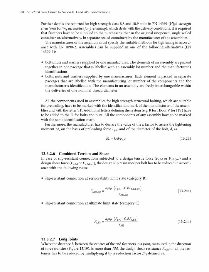
Further details are reported for high strength class 8.8 and 10.9 bolts in EN 14399 (High-strengthstructural bolting assemblies for preloading), which deals with the delivery conditions. It is requiredthat fasteners have to be supplied to the purchaser either in the original unopened, single sealedcontainer or, alternatively, in separate sealed containers by the manufacturer of the assemblies.
The manufacturer of the assembly must specify the suitable methods for tightening in accord-ance with EN 1090-2. Assemblies can be supplied in one of the following alternatives (EN14399-1):
• bolts, nuts and washers supplied by one manufacturer. The elements of an assembly are packedtogether in one package that is labelled with an assembly lot number and the manufacturer’sidentification;
• bolts, nuts and washers supplied by one manufacturer. Each element is packed in separatepackages that are labelled with the manufacturing lot number of the components and themanufacturer’s identification. The elements in an assembly are freely interchangeable withinthe deliveries of one nominal thread diameter.
All the components used in assemblies for high strength structural bolting, which are suitablefor preloading, have to be marked with the identification mark of the manufacturer of the assem-blies and with the letter ‘H’. Additional letters defining the system (e.g. R for HR or V for HV) haveto be added to the H for bolts and nuts. All the components of any assembly have to be markedwith the same identification mark.
Furthermore, the manufacturer has to declare the value of the k factor to assess the tighteningmoment Ms on the basis of preloading force Fp,C and of the diameter of the bolt, d, as
Ms = k d Fp,C 13 23
13.3.2.6 Combined Tension and ShearIn case of slip-resistant connections subjected to a design tensile force (Ft,Ed or Ft,Ed,ser) and adesign shear force (Fv,Ed or Fv,Ed,ser), the design slip resistance per bolt has to be reduced in accord-ance with the following rules:
• slip-resistant connection at serviceability limit state (category B):
Fs,Rd, ser =ksnμ Fp,C−0 8Ft,Ed, ser
γM3, ser13 24a
• slip-resistant connection at ultimate limit state (category C):
Fs,Rd =ksnμ Fp,C−0 8Ft,Ed
γM313 24b
13.3.2.7 Long JointsWhere the distance Lj between the centres of the end fasteners in a joint, measured in the directionof force transfer (Figure 13.19), is more than 15d, the design shear resistance Fv,Rd of all the fas-teners has to be reduced by multiplying it by a reduction factor βLf defined as:
368 Structural Steel Design to Eurocode 3 and AISC Specifications

βLf = 1−Lj −15 d
200d13 25
with the limitation βLf ≤ 1.0 and βLf ≥ 0.75.
13.4 Bolted Connection Design in Accordance with the US Approach
Bolts are treated in AISC 360-10, Section J.3 mainly, and in the RCSC Specification for StructuralJoints Using High-Strength Bolts, that is referred to by AISC 360-10.
13.4.1 US Practice for Fastener Assemblage
The two main US standard structural bolt types are ASTM A325 and ASTM A490. In particular:
• ASTMA325 bolts are available in diameters from½ to 1-½ in. (from 16 to 36mm,ASTMA325M)with a minimum tensile strength of 120 ksi (827MPa) for diameters of 1 in. (25.4 mm) andless and 105 ksi (724 MPa) for sizes over 1–1-½ in. (38.1 mm). They also come in two types.Type 1 is a medium carbon steel and can be galvanized; Type 3 is a weathering steel that offersatmospheric corrosion resistance. They have a fixed threaded length shorter than the total boltlength. But if nominal length is equal to or shorter than four times the nominal bolt diameterthen A325 bolts can be threaded full length.
• ASTM A490 bolts are available in diameters from ½ to 1-½ in. (from 16 to 36 mm, ASTMA490M) with aminimum tensile strength of 150 ksi (1034MPa) andmaximum tensile strengthof 170 ksi (1172MPa) for all diameters, and are offered in two types. Type 1 is alloy steel, andType 3 is a weathering steel that offers atmospheric corrosion resistance.
ASTM F1852 and ASTM F2280 bolts can be used in lieu, respectively, of ASTM A325 andASTM A490. They have the same mechanical and chemical characteristics and differ only fora splined end that extends beyond the threaded portion of the bolt. During installation, thissplined end is gripped by a specially designed wrench chuck and provides a mean for turningthe nut relative to the bolt, as discussed in the following.Structural bolts are specifically designed for use with heavy hex nuts. The nuts for structural
connections have to be conforming to ASTM A563 or ASTM A194 and the washers used forstructural connections to ASTM F436 specifications. This specification covers both flat circularand bevelled washers.
Lj
LjLj
F
F
F
F
Figure 13.19 Examples of long joints.
The Mechanical Fasteners 369

ASTM Specifications permit the galvanizing of ASTMA325 bolts, but ASTMA490 bolts shouldnot be galvanized or electroplated. The major problem with hot dip galvanizing and electroplatingA490 bolts is the potential hydrogen embrittlement. This scenario may occur when atomic hydro-gen is introduced during the pickling process that takes place prior to plating or hot dip galvan-izing process. In 2008, ASTM approved the use of zinc/aluminium protective coatings per ASTMF1136 for use on A490 structural bolts.
Both A325 and A490 are heavy hex bolts intended for structural usage and for connectingsteel profiles and/or plates, so they are not very long and their diameter is limited as indicatedabove. If different diameters and/or different length have to be used, reference can bemade to:
• ASTM A449 in lieu of ASTM A325 bolts. They range in diameter from ¼ to 3 in. (from 6.4to 76.2 mm) and are far more flexible in their configuration: they can be a headed bolt,a straight rod with threads or a bend bolt such as a right angle bend foundation bolt.From a material point of view, there are no relevant differences between A449 andA325 bolts.
• ASTM A354 grade BD in lieu of ASTM A490 bolts. A354 grade BD bolts are quenched andtempered alloy steel bolts, and are equal in strength to ASTM A490 bolts. They range indiameter from ¼ to 4 in. (from 6.4 to 102 mm) and can be used for anchor bolts andthreaded rods. A354 grade BC has a lower strength then Grade BD, closer to that of ASTMA325 bolts.
AISC 360-10 also allows the usage of ASTM A307 bolts. The ASTM A307 specification coverscarbon steel bolts and studs ranging from ¼ to 4 in. diameter (from 6.4 to 102 mm), with a min-imum tensile strength of 60 ksi (414MPa). There are three different steel grades (A, B and C),which denote configuration and application:
• Grade A is for headed bolts, threaded rods and bent bolts intended for general applications.• Grade B is for heavy hex bolts and studs intended for flanged joints in piping systems with cast
iron flange.• Grade C denotes non-headed anchor bolts, either bent or straight, intended for structural
anchorage purpose. Grade C has been now substituted by ASTM F1554 Grade 36, low carbon,36 ksi (248MPa) yield steel anchor bolts.
AISC 360-10 lists all bolt specifications into two groups according to their tensile strength:
• Group A (lower strength): ASTM A325, A325M, F1852, A354 Grade BC and A449;• Group B (higher strength): ASTM A490, A490M, F2280 and A354 Grade BD.
Bolts belonging to the same group have almost the same ultimate tensile strength:
ASTMA307 bolts are not grouped because their ultimate strength (60 ksi, 414MPa) is lower thanthe one of group A. As to the holes for bolts, AISC 360-10 individuates four types of holes:
Group A: 120 ksi (827MPa) minimum up to 1 in. diameter, 105 ksi (724MPa) for higher diameters (yieldingstrength: 92 ksi (634MPa) minimum up to 1 in. diameter, 81 ksi (558MPa) for higher diameters);
Group B: 150 ksi (1034MPa) minimum, 170 ksi (1172MPa) maximum (yielding strength: 130 ksi (896MPa)minimum).
370 Structural Steel Design to Eurocode 3 and AISC Specifications

• normal holes;• oversized holes;• short-slotted holes;• long-slotted holes.
The maximum allowed size for holes are listed in Tables 13.6a and 13.6b.Oversized holes are permitted in any or all plies of slip-critical connections, but they cannot be
used in bearing-type connections. Hardened washers have to be installed over oversized holes in anouter ply.Short-slotted holes are permitted in any or all plies of slip-critical or bearing-type connections.
The slots are permitted without regard to direction of loading in slip critical connections, but thelength has to be normal to the direction of the load in bearing-type connections. Washers have to beinstalled over short-slotted holes in an outer ply.Long-slotted holes are permitted in only one of the connected parts of either a slip critical or
bearing-type connection at an individual faying surface. Long-slotted holes are permitted withoutregard to direction of loading in slip-critical connections, but have to be normal to the direction ofload in bearing-type connections. Where long-slotted holes are used in an outer ply, plate washersor a continuous bar with standard holes, of a size sufficient to completely cover the slot after instal-lation, have to be provided.
Table 13.6b Nominal holes (dimensions in millimetres) (from Table J3.3M of AISC 360-10).
Bolt diameter,in. (mm)
Hole dimensions, mm (in.)
Standard(diameter)
Oversize(diameter) Short-slot (width × length) Long-slot (width × length)
M16 (0.630) 18 (0.709) 20 (0.787) 18 × 22 (0.709 × 0.866) 18 × 40 (0.709 × 1.575)M20 (0.787) 22 (0.866) 24 (0.945) 22 × 26 (0.866 × 1.024) 22 × 50 (0.866 × 1.969)M22 (0.866) 24 (0.945) 28 (1.102) 24 × 30 (0.945 × 1.181) 24 × 55 (0.945 × 2.165)M24 (0.945) 27 (1.063) 30 (1.181) 27 × 32 (1.063 × 1.260) 27 × 60 (1.063 × 2.362)M27 (1.06) 30 (1.181) 35 (1.378) 30 × 37 (1.181 × 1.457) 30 × 67 (1.181 × 2.638)M30 (1.18) 33 (1.299) 38 (1.496) 33 × 40 (1.299 × 1.575) 33 × 75 (1.299 × 2.953)≥ M36 (≥1.42) d + 3 (d +
0.118)d + 8 (d +0.315)
(d + 3) × (d + 10) ((d +0.118) × (d + 0.394))
(d + 3) × (2.5 × d) ((d +0.118) × (2.5 × d))
Table 13.6a Nominal holes (dimensions in inches) (from Table J3.3 of AISC 360-10).
Hole dimensions, in. (mm)
Bolt diameter,in. (mm)
Standard(diameter)
Oversize(diameter) Short-slot (width × length) Long-slot (width × length)
1/2 (12.7) 9/16 (14.3) 5/8 (7.9) 9/16 × 11/16 (14.3 × 17.5) 9/16 × 1–1/4 (14.3 × 331.8)5/8 (15.9) 11/16 (17.5) 13/16 (20.6) 11/16 × 7/8 (17.5 × 22.2) 11/16 × 1–9/16 (17.5 × 39.7)3/4 (19.1) 13/16 (20.6) 15/16 (23.8) 13/16 × 1 (20.6 × 25.4) 13/16 × 1–7/8 (20.6 × 47.6)7/8 (22.2) 15/16 (23.8) 1–1/16 (27.0) 15/16 × 1–1/8 (23.8 × 28.6) 15/16 × 2–3/16 (23.8 × 55.6)1 (25.4) 1–1/16 (27.0) 1–1/4 (31.8) 1–1/16 × 1–5/16 (27.0 × 33.3) 1–1/16 × 2–1/2 (27.0 × 63.5)≥1-1/8 (≥28.6) d + 1/16
(d + 1.6)d + 5/16(d + 7.9)
(d + 1/16) × (d + 3/8)((d + 1.6) × (d + 9.5))
(d + 1/16) × (2.5 × d)((d + 1.6) × (2.5 × d))
The Mechanical Fasteners 371

The distance between centres of standard, oversized or slotted holes should not be less than2–2/3 times the nominal diameter, d, of the fastener; a distance of 3d is preferred. The distancefrom the centre of a standard hole to an edge of a connected part in any direction should not beless than either the applicable value from Tables 13.7a and 13.7b.
The distance from the centre of an oversized or slotted hole to an edge of a connected partshould not be less than the one required for a standard hole to an edge of a connected part plusthe applicable increment, C2, from Tables 13.8a and 13.8b.
The maximum distance from the centre of any bolt to the nearest edge of parts in contact is12 times the thickness of the connected part under consideration, but cannot exceed 6 in.(150 mm). The longitudinal spacing of fasteners between elements consisting of a plate and ashape or two plates in continuous contact has to be as follows:
• for painted members or unpainted members not subject to corrosion, the spacing is limited to24 times the thickness of the thinner part or 12 in. (305 mm);
• for unpainted members of weathering steel subject to atmospheric corrosion, the spacing islimited to 14 times the thickness of the thinner part or 7 in. (180 mm).
According to the RCSC Specification and AISC 360-10, for structural applications there aregenerally three types of connections in which bolts are used: snug-tightened, pre-tensioned andslip critical connections.
Table 13.7b Minimum edge distance (a) from the centre of standard hole (b) to the edge of connected part(dimensions in millimetres) (from Table J3.4M of AISC 360-10).
Bolt diameter, mm (in.) Minimum edge distance, mm (in.)
16 (0.630) 22 (0.866)20 (0.787) 26 (1.024)22 (0.866) 28 (1.102)24 (0.945) 30 (1.181)27 (1.063) 34 (1.339)30 (1.181) 38 (1.496)36 (1.417) 46 (1.811)Over 36 1.25 × d
Table 13.7a Minimum edge distance (a) from the centre of standard hole (b) to the edge of connected part(dimensions in inches) (from Table J3.4 of AISC 360-10).
Bolt diameter, in. (mm) Minimum edge distance, in. (mm)
1/2 (12.7) 3/4 (19.1)5/8 (15.9) 7/8 (22.2)3/4 (19.1) 1 (25.4)7/8 (22.2) 1–1/8 (28.6)1 (25.4) 1–1/4 (31.75)1–1/8 (28.6) 1–1/21–1/4 (31.75) 1–5/8Over 1–1/4(Over 31.75)
1–1/4 × d
372 Structural Steel Design to Eurocode 3 and AISC Specifications
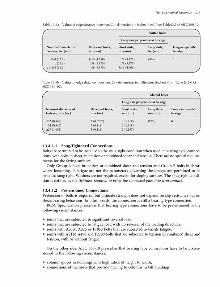
13.4.1.1 Snug-Tightened ConnectionsBolts are permitted to be installed to the snug-tight condition when used in bearing-type connec-tions, with bolts in shear, in tension or combined shear and tension. There are no special require-ments for the faying surfaces.Only Group A bolts in tension or combined shear and tension and Group B bolts in shear,
where loosening or fatigue are not the parameters governing the design, are permitted to beinstalled snug tight. Washers are not required, except for sloping surfaces. The snug-tight condi-tion is defined as the tightness required to bring the connected plies into firm contact.
13.4.1.2 Pretensioned ConnectionsPretension of bolts is required, but ultimate strength does not depend on slip resistance but onshear/bearing behaviour. In other words, the connection is still a bearing type connection.RCSC Specification prescribes that bearing type connections have to be pretensioned in the
following circumstances:
• joints that are subjected to significant reversal load;• joints that are subjected to fatigue load with no reversal of the loading direction;• joints with ASTM A325 or F1852 bolts that are subjected to tensile fatigue;• joints with ASTM A490 and F2280 bolts that are subjected to tension or combined shear and
tension, with or without fatigue.
On the other side, AISC 360-10 prescribes that bearing type connections have to be preten-sioned in the following circumstances:
• column splices in buildings with high ratios of height to width;• connections of members that provide bracing to columns in tall buildings;
Table 13.8a Values of edge distance increment C2 – dimensions in inches (mm) (from Table J3.5 of AISC 360-10).
Nominal diameter offastener, in. (mm)
Oversized holes,in. (mm)
Slotted holes
Long axis perpendicular to edge
Long axis parallelto edge
Short slots,in. (mm)
Long slots,in. (mm)
≤7/8 (22.2) 1/16 (1.588) 1/8 (3.175) (3/4)d 01 (25.4) 1/8 (3.175) 1/8 (3.175)
≥1–1/8 (28.6) 1/8 (3.175) 3/16 (4.763)
Table 13.8b Values of edge distance increment C2 – dimensions in millimetres (inches) (from Table J3.5M ofAISC 360-10).
Nominal diameter offastener, mm (in.)
Oversized holes,mm (in.)
Slotted holes
Long axis perpendicular to edge
Long axis parallelto edge
Short slots,mm (in.)
Long slots,mm (in.)
≤22 (0.866) 2 (0.0787) 3 (0.118) 0.75d 024 (0.945) 3 (0.118) 3 (0.118)
≥27 (1.063) 3 (0.118) 5 (0.197)
The Mechanical Fasteners 373

• various connections in buildings with cranes over 5-ton capacity;• connections for supports of running machinery and other sources of impact or stress reversal.
Bolts are to be pretensioned to tension values not less than those given in Tables 13.9a and13.9b. Such values are equal to 0.70 times the minimum tensile strength of the bolt.
13.4.1.3 Slip-Critical ConnectionsSlip resistance is required at the faying surfaces subjected to shear or combined shear and tension.Slip resistance has to be checked at either the factored-load level or service-load level, as a choice ofthe designer. RCSC Specification states that slip-critical joints are only required in the followingapplications involving shear or combined shear and tension:
• joints that are subjected to fatigue load with reversal of the loading direction;• joints that use oversized holes;• joints that use slotted holes, except those with applied load approximately normal (within
80–100 ) to the direction of the long dimension of the slot;• joints in which slip at the faying surfaces would be detrimental to the performance of the
structure.
Washers are not required in pretensioned joints and slip-critical joints, with the followingexceptions:
• ASTM F436 washers under both the bolt head and nut, when ASTM A490 bolts are preten-sioned in the connected material of a specified minimum yield strength less than 40 ksi(276MPa);
Table 13.9b Minimum bolt pretension (from Table J3.1M of AISC 360-10).
Bolt size, mm (in.) Group A (e.g. A325 bolts), kN (kips) Group B (e.g. A490 bolts), kN (kips)
M16 (0.630) 91 (20.5) 114 (25.6)M20 (0.787) 142 (31.9) 179 (40.2)M22 (0.866) 176 (39.6) 221 (49.7)M24 (0.945) 205 (46.1) 257 (57.8)M27 (1.06) 267 (60.0) 334 (75.1)M30 (1.18) 326 (73.3) 408 (91.7)M36 (1.42) 475 (106.8) 595 (133.8)
Table 13.9a Minimum bolt pretension (from Table J3.1 of AISC 360-10).
Bolt size, in. (mm) Group A (e.g. A325 bolts), kips (kN) Group B (e.g. A490 bolts), kips (kN)
1/2 (12.7) 12 (53.4) 15 (66.7)5/8 (15.9) 19 (84.5) 24 (106.8)3/4 (19.1) 28 (124.6) 35 (155.7)7/8 (22.2) 39 (173.5) 49 (218.0)1 (25.4) 51 (226.9) 64 (284.7)
1–1/8 (28.6) 56 (249.1) 80 (355.9)1–1/4 (31.8) 71 (315.8) 102 (453.7)1–3/8 (34.9) 85 (378.1) 121 (538.2)1–1/2 (38.1) 103 (458.2) 148 (658.3)
374 Structural Steel Design to Eurocode 3 and AISC Specifications

• an ASTM F436 washer under the turned element, when the calibrated wrench pretensioningmethod is used;
• an ASTM F436 washer under the nut as part of the fastener assembly, when the twist-off-typetension-control bolt pretensioning method is used;
• an ASTM F436 washer under the side (head or nut) that is turned, when the direct-tension-indicator pretensioning method is used;
• a washer or a continuous bar of sufficient size to completely cover the hole, when an oversizedor slotted hole occurs in an outer ply.
Bolts in slip-critical connections are pretensioned at the same values of bolts in pretensionedconnections as in Tables 13.9a and 13.9b.There are four methods of installation procedures admitted by the AISC to achieve the tension
required for the pretensioned bearing connections or the slip critical connections:
(1) Turn-of-Nut method;(2) Twist-Off-Type Tension-Control Bolt Pretensioning;(3) Direct Tension Indicating method (DTI);(4) Calibrated Wrench method.
For pretensioned joints and slip-critical joints, a tension calibrator has to be used before boltinstallation. A tension calibrator is a hydraulic device indicating the pretension that is developedin a bolt that is installed in it. A representative sample of no fewer than three complete fastenerassemblies of each combination of diameter, length, grade and lot to be used in the work has to bechecked at the site of installation in the tension calibrator to verify that the pretensioning methoddevelops a pretension equal to or greater than 1.05 times than the one specified in Tables 13.9aand 13.9b.A bolt tension calibrator is essential for:
(1) the pre-installation verification of the suitability of the fastener assembly, including the lubri-cation that is applied by the manufacturer;
(2) verifying the adequacy and the proper use of the specified pretensioning method;(3) determining the installation torque for the calibrated wrench pretensioning method. Actually
according to AISC 360-10 torque values determined from tables or from equations that claimto relate torque to pretension without verification shouldn’t be used. For the calibrated wrenchpretensioning method, installation procedures have to be calibrated on a daily basis.
(1) Turn-of-Nut Method: This method involves tightening the fastener to a low initial ‘snug tight’condition and then applying a prescribed amount of turn to develop the required preload. Theactual preload depends on how far the nut is turned. Special attention has to be paid when thismethod is used, in particular, it is important:(a) to snug the joint to bring the assembly into firm contact.(b) to inspect the joint to verify ‘snug tight’.(c) to match mark bearing face of the nut and end of the bolt with a single straight line.(d) to use a systematic approach that would involve the appropriate bolting pattern, apply the
required turns as given in the Table 13.10.(2) Twist-Off-Type Tension-Control Bolt Pretensioning: Tension control bolts use design features
that indirectly indicate tension. The most common is the twist-off bolt or tension control
The Mechanical Fasteners 375

(TC) bolt. An assembly tool holds this bolt from the nut end while an inner spindle on the toolgrips a spline section connected to the end of the bolt. An outer spindle on the tool turns thenut and tightens the fastener. When the designated torque has been reached, the spline snapsoff. This type of torque control system allows for quick inspection, if the spline is gone, intheory, the bolt has been properly tightened.
Twist-off-type tension-control bolt assemblies that meet the requirements of ASTM F1852and F2280 have to be used.
(3) Direct Tension Indicating Method (DTI): This method requites DTI washers according toASTM F959. The most common type of washer involves the use of hollow bumps on oneside of the washer. These bumps are flattened as the fastener is tightened. A feeler gaugeis used to measure the gap developed by the bumps. When the fastener has developed theproper tension, the feeler gauge will no longer fit in the gap. Some washer types fill the voidunder the bumps with coloured silicone that squirts out once the bumps are compressed,thereby indicating proper tension is reached (Figure 13.8). The pre-installation verificationprocedure illustrated previously has to be applied to demonstrate that, when the pretensionin the bolt reaches 1.05 times the one specified for installation, the gap is no less than pre-scribed by ASTM F959.
(4) Calibrated Wrench Method: Bolts are initially snug-tightened. Subsequently, the installationtorque determined in the pre-installation verification of the fastener assembly has to beapplied to all bolts in the joint. The scatter in the installed pretension can be significant withthis installation method. The relationship between torque and pretension is affected by manyfactors: the finish and tolerance on the bolt and nut threads, the lubrication, the shop or job-site conditions that contribute to dust and dirt or corrosion on the threads, the frictionbetween the turned element and the supporting surface, the variability of the air supplyparameters on impact wrenches, the condition, lubrication and power supply for the torquewrench. For these reasons RCSC Specification and AISC 360-10 put emphasis on dailywrench calibration activity and, as said before, it is not valid to use published values basedon a torque-tension relationship.
13.4.2 US Structural Verifications
Bolt structural verifications are addressed in AISC 360-10, chapter J3. Nominal strength of fas-teners has to be according to the values listed in Table 13.11.
The nominal tensile strength values in Table 13.11 are obtained from the equation:
Fnt = 0 75Fu 13 26
Table 13.10 Nut rotation from the snug-tight condition for turn-of-nutpretensioning.
Bolt length Rotation
≤4 db 1204 < db ≤ 8 1808 < db ≤ 12 240
db = bolt nominal diameter.
376 Structural Steel Design to Eurocode 3 and AISC Specifications

The factor of 0.75 accounts for the approximate ratio of the effective tension area of thethreaded portion of the bolt to the area of the shank of the bolt for common sizes. Thus in veri-fication formulas the gross (unthreaded) area has to be used.The values of nominal shear strength in Table 13.11 are obtained from the following equations:
(a) When threads are excluded from the shear planes:
Fnv = 0 563Fu 13 27
The factor 0.563 accounts for the effect of a shear/tension ratio of 0.625 and a 0.90 length reduc-tion factor, with joint lengths up to and including 38 in. (965 mm).(b) When threads are not excluded from the shear plane
Fnv = 0 450Fu 13 28
It is worth mentioning that the factor of 0.450 is 80% of 0.563, which accounts for the reducedarea of the threaded portion of the fastener when the threads are not excluded from theshear plane.In tension or compression long joints (i.e. with length longer than approximately 16 in. or
406 mm), the differential strain produces an uneven distribution of load between fasteners, thosenear the end taking a disproportionate part of the total load, so themaximum strength per fasteneris reduced. In this case, AISC 360-10 requires that the initial 0.90 factor should be replaced by 0.75when determining bolt shear strength for connections longer than 38 in. (965 mm). In lieu ofanother column of design values, the appropriate values are obtained by multiplying the tabulatedvalues by 0.75/0.90 = 0.833.
Table 13.11 Nominal strength of fasteners and threaded parts, ksi (MPa) (from Table J3.2 of AISC 360-10).
Description of fasteners
Nominal tensilestrength, Fnt,ksi (MPa)
Nominal shear strength inbearing type connections,
Fnv, ksi (MPa)
A307 bolts 45 (310) 27 (188)Group A (e.g. A325) bolts, when threads are not excludedfrom shear planes
90 (620) 54 (372)
Group A (e.g. A325) bolts, when threads are excluded fromshear planes
90 (620) 68 (457)
Group B (e.g. A490) bolts, when threads are not excludedfrom shear planes
113 (780) 68 (457)
Group B (e.g. A490) bolts, when threads are excluded fromshear planes
113 (780) 84 (579)
Threaded parts of anchor roads and threaded roads,according to ASTM F1554, whenthreads are not excluded from shear planes
0.75Fu 0.450Fu
Threaded parts of anchor roads and threaded roads,according to ASTM F1554, when threads are excludedfrom shear planes
0.75Fu 0.563Fu
The Mechanical Fasteners 377

13.4.2.1 Tensile or Shear Strength of Bolts
13.4.2.2 Combined Tension and Shear in Bearing-Type Connections
LRFD approach ASD approach
The design tensile strength ϕRn of a snug-tightened orpretensioned high-strength bolt subjected to combinedtension and shear, has to be greater or equal to the requiredtensile strength Tu.
ϕRn =ϕFntAb ≥Tu 13 33
The allowable tensile strength Rn/Ω of a snug-tightened orpretensioned high-strength bolt has to be greater or equalto the required tensile strength Ta:
Rn Ω= FntAb Ω≥Ta 13 34
Theavailable shear stressof theboltϕFnvhas tobe equalor to exceedthe required shear stress, frv:
ϕFnv ≥ frv 13 35
where ϕ= 0 75 and F nt is the nominal tensile stress(Table 13.11), modified to take into account the shear effects as:
Fnt = 1 3Fnt −FntϕFnv
frv ≤ Fnt
where Fnt and Fnv are the nominal tensile and the nominalshear stress (Table 13.11), respectively and frv is the requiredshear stress defined as:
frv =Vu Ab
where Ab is the nominal unthreaded bolt area and Vu is therequired shear strength.
The available shear stress of the bolt Fnv/Ω has to be equalor to exceed the required shear stress, frv:
Fnv Ω≥ frv 13 36
where Ω= 2 00 and F nt is the nominal tensile stress(Table 13.11), modified to take into account the sheareffects as:
Fnt = 1 3Fnt −ΩFntFnv
frv ≤ Fnt
where Fnt and Fnv are the nominal tensile and the nominalshear stress (Table 13.11), and frv is the required shear stressdefined as:
frv =Va Ab
where Ab is the nominal unthreaded bolt area and Va
is the required shear strength.
LRFD approach ASD approach
The design tensile strength ϕRn of a snug-tightened or pretensionedhigh-strength bolt has to be greater or equal to the requiredtensile strength Tu:
ϕRn =ϕFntAb ≥Tu 13 29
where ϕ= 0 75, Fnt is the nominal tensile stress (Table 13.11), Ab
is the nominal unthreaded bolt area and Tu is the required tensilestrength.
The allowable tensile strength Rn/Ω of a snug-tightened orpretensioned high-strength bolt has to be greater or equal tothe required tensile strength Ta:
Rn Ω= FntAb Ω≥Ta 13 30
where Ω= 2 00, Fnt is the nominal tensile stress(Table 13.11), Ab is the nominal unthreaded bolt area andTa is the required tensile strength.
The design shear strength ϕRn of a snug-tightened or pretensionedhigh-strength bolt has to be greater or equal to the required shearstrength Vu:
ϕRn =ϕFnvAb ≥Vu 13 31
whereϕ= 0 75, Fnv is the nominal shear stress (Table 13.11),Ab isthe nominal unthreaded bolt area and Vu is the required shearstrength for LRFD combinations.
The allowable shear strength Rn/Ω of a snug-tightened orpretensioned high-strength bolt has to be greater or equal tothe required shear strength Va:
Rn Ω= FnvAb Ω≥Va 13 32
where Ω= 2 00, Fnv is the nominal shear stress(Table 13.11), Ab is the nominal unthreaded bolt areaand Va is the required shear strength for ASDcombinations.
LRFD, load and resistance factor design and ASD, allowable strength design.
378 Structural Steel Design to Eurocode 3 and AISC Specifications

When the required stress, f, in either shear or tension, is less than or equal to 30%of the corresponding available stress, the effects of combined stresses need not to beinvestigated.
13.4.2.3 Slip-Critical Connections
As to the safety coefficients, it must be assumed:
The decrease of ϕ (and the increase of Ω) reflects the fact that consequences of exceeding sliplimit state become more severe from standard size holes through long-slotted holes.The available slip resistance has to be determined as follows:
Rn = μDuhf Tbnsksc 13 39
where Tb is the minimum fastener tension given in Tables 13.9a and 13.9b, Du = 1.13 is theratio of the mean installed bolt pretension to the specified minimum bolt pretension, ns isthe number of slip planes, μ is the mean slip coefficient (see later) and hf = 1 if elementsunder stress are connected directly by bolts or by means of one interposed filler(Figure 13.20).When fillers are more than one, it is assumed that hf = 0.85.Term ksc has to be assumed = 1 if there is no tension action applied to connection. If there is,
then it assumes the following values:
ksc = 1−Tu
DuTbnbLFRD 13 40a
ksc = 1−1 5Ta
DuTbnbASD 13 40b
LRFD ASD
The design slip resistance ϕRn of a pretensionedhigh-strength bolt in a slip-critical connectionhas to be greater or equal to the required shearstrength Vu:
ϕRn ≥Vu 13 37
The allowable slip resistance Rn/Ω of a pretensionedhigh-strength bolt in a slip-critical connectionhas to be greater or equal to the required shearstrength Va:
Rn Ω≥Va 13 38
ϕ= 1 00 or Ω = 1.50 for standard size and short-slotted holes perpendicular to the direction of the load;ϕ= 0 85 or Ω = 1.76 for oversized and short-slotted holes parallel to the direction of the load;ϕ= 0 70 or Ω = 2.14 for long-slotted holes.
The Mechanical Fasteners 379

where Ta and Tu are the required tension force using ASD and LRFD load combinations respect-ively, and nb is the number of bolts carrying the applied tension.
The mean slip coefficient μ is referred by AISC 360-10 and RCSC Specification to two kind offaying surfaces (classes A and B):
• μ = 0.30 for class A faying surfaces: uncoated clean mill scale steel surfaces, surfaces with classA coatings on blast-cleaned steel;
• μ = 0.50 for class B faying surfaces: uncoated blast-cleaned steel surfaces with class B coatingson blast-cleaned steel
• μ = 0.35 for class C surfaces: roughened hot-dip galvanized surfaces.
If faying surfaces have to be protected by a zinc primer coating, the coating has to be tested andqualified according to appendix A of RCSC Specification to determine if it can be classified asClass A or B, in order to assign a slip coefficient equal to 0.30 (if class A) or 0.50 (if class B).
The mean slip coefficient for clean hot-dip galvanized surfaces is in the order of 0.19, but can besignificantly improved by treatments such as hand wire brushing to the value of 0.35 as indicatedby RCSC Specification.
AISC 360-10 states that ‘Slip-critical connections have to be designed to prevent slip and for thelimit states of bearing-type connections’. This means that a slip-critical connection has to bedesigned to prevent slip at service load and AISC 360-10 design procedure guarantees this. Soat ultimate loads the connection can slip, then the Specifications requires verification of the con-nection for bearing and shear at ultimate loads.
In AISC 360-05 it was stated:
High-strength bolts in slip-critical connections are permitted to be designed to prevent slip eitheras a serviceability limit state or at the required strength limit state. The connection must also bechecked for shear strength in accordance with Sections J3.6 and J3.7 and bearing strength inaccordance with Sections J3.1 and J3.10 […]. Connections with standard holes or slots transverseto the direction of the load have to be designed for slip at serviceability limit state. Connectionswith oversized holes or slots parallel to the direction of the load have to be designed to prevent slipat the required strength level.
So the 2005 Code was slightly different: slip-critical connections could have been designed forpreventing slip at service loads or at ultimate loads. This was achieved by changing resistance andsafety factors:
Single filler plate Multiple filler plates
Figure 13.20 Single and multiple filler plates.
ϕ= 1 00; Ω = 1.50 For preventing slip at service loadsϕ= 0 85; Ω = 1.76 For preventing slip at ultimate loads
380 Structural Steel Design to Eurocode 3 and AISC Specifications

In AISC 360-10 more severe values for resistance and safety factors have been maintained foroversized and short-slotted holes parallel to the direction of the load. So 2010 Code allows fordesign of slip-critical connections with oversized loads for preventing slip at loads higher thanservice loads, even if not explicitly stated, because consequences of slip are worse with oversizedholes than with regular holes.
13.4.2.4 Bearing Strength at Bolt Holes
The nominal bearing strength Rn has to be determined as follows:
(a) for standard, oversized and short-slotted holes, if deformation at service loads is not a designconsideration:
Rn = 1 5lctFu ≤ 3 0dtFu 13 43
(b) for standard, oversized and short-slotted holes, if deformation at service loads is a designconsideration:
Rn = 1 2lctFu ≤ 2 4dtFu 13 44
(c) for a bolt in a connection with long-slotted holes with the slot perpendicular to the directionof force:
Rn = 1 0lctFu ≤ 2 0dtFu 13 45
where Fu is the specified minimum tensile strength of the connected material, d is the nominalbolt diameter, lc is the clear distance in the direction of the force between the edge of the holeand the edge of the adjacent hole or edge of the material and t is the thickness of connectedmaterial.
The use of oversized holes and short- and long-slotted holes parallel to the line of forceis restricted to slip-critical connections. Bearing-type connections can be used with standardholes only.Bearing resistance has to be checked for both bearing-type and slip-critical connections.The strength of a single bolt is the smaller between its shear strength and the bearing
strength at the bolt hole. The strength of a connection is the sum of the strengths of its individualbolts.
LRFD ASD
The design bearing strength ϕRn at a bolt hole has to begreater or equal to the required shear strength Vu:
ϕRn ≥Vu 13 41
where ϕ= 0 75.
The allowable bearing strength Rn/Ω at a bolt hole has tobe greater or equal to the required shear strength Va:
Rn Ω≥Va 13 42
where Ω = 2.00.
The Mechanical Fasteners 381

13.5 Connections with Rivets
Riveting techniques were used extensively until the first decades of the twentieth century(Figure 13.21) and they have now virtually disappeared in construction practice in favour ofbolted and welded connection techniques, which are cheaper nowadays.
Riveting is a method of connecting plates: ductile metal pins are inserted into holes andriveted to form a head at each end to prevent the joint from coming apart (Figure 13.22).Rivets were often used in the same way as ordinary structural bolts are currently used in shearand bearing and in tension joints. There is usually less slip in a riveted joint with respect to a bear-ing bolted joint because of the tendency for the rivet holes to be filled by the rivets when being hot-driven. Shop riveting was cheaper in the past than site riveting and for this reason shop-rivetingwas often combined with site-bolting. However, now this connection technique is used only insome historical refurbishments. The principal factor that delayed immediate acceptance of thebolts was the high cost of materials, including washers. Since then, because of the higher labourcosts together with the modern approach to designing connections requiring fewer bolts thanrivets, riveting is used only in some cases for historical buildings and bridges, owing to theirnon-competitive costs.
Figure 13.22 Riveting of the pin.
Figure 13.21 Example of a riveted joint in an historical bridge.
382 Structural Steel Design to Eurocode 3 and AISC Specifications

13.5.1 Design in Accordance with EU Practice
Criteria for the rivet verifications are reported in EN 1993-1-8 and are very similar tothose proposed for bolted connections. In particular, if A0 and fur identify the area of thehole and the ultimate strength of the pin, respectively, the following design resistance can beevaluated.
Shear: Design shear resistance is:
Fv,Rd =0 6 fur A0
γM213 46
Bearing: The same equations already introduced for bolted connections are proposed.Tension: Design tension resistance is:
Ft,Rd =0 6 fur A0
γM213 47
Shear and tension: The same equations for bolted connections are proposed.
13.5.2 Design in Accordance with US Practice
Rivets are not addressed any more either in AISC 360-10 or in RCSC Specification. Thesecond document indicates the ‘Guide to Design Criteria for Bolted and Riveted Joints SecondEdition’ (1987), as a reference document for rivets. Such a guide recognizes three structural rivetsteels:
• ASTM A502 grade 1, carbon rivet steel for general purposes;• ASTM A502 grade 2, carbon-manganese rivet steel suitable for use with high-strength carbon
and high strength low-alloy structural steels;• ASTM A502 grade 3, similar to grade 2 but with enhanced corrosion resistance.
The following design rules are taken from the ‘Guide to Design Criteria for Bolted and RivetedJoints, Second Edition’.
Tension: The tensile capacity Bu of a rivet is equal to the product of the rivet cross-sectional areaAb and its tensile strength σu. The cross section is generally taken as the undriven crosssection area of the rivet:
Bu =Abσu 13 48
A reasonable lower bound estimate of the rivet tensile capacity σu is 60 ksi (414 MPa) for A502grade 1 rivets and 80 ksi (552MPa) for A502 grade 2 or grade 3 rivets. Since ASTM specificationsdo not specify the tensile capacity, these values can be used.
Shear: The ratio of the shear strength τu to the tensile strength σu of a rivet was found to beindependent on the rivet grade, installation procedure, diameter and grip length.
Tests indicate the ratio to be about 0.75. Hence:
τu = 0 75σu 13 49
The Mechanical Fasteners 383

The shear resistance of a rivet is directly proportional to the available shear area and thenumber of critical shear planes. If a total of m critical shear planes pass through the rivet,the maximum shear resistance Su of the rivet is equal to:
Su = 0 75mAbσu 13 50
where Ab is the cross-section area of undriven rivet.Shear and tension: The following equation must be verified:
τ τu0 75
2
+ σ σu2 ≤ 1 13 51
where τ is the shear stress on the rivet shear plane, σ is the tensile stress of the rivet, τu is the shearstrength of the rivet and σu is the tensile strength of the rivet.
13.6 Worked Examples
Example E13.1 Verification of a Bearing Connection According to EC3
Verify, according to EC3, the connection in Figure E13.1.1 (all dimensions are in millimetres). It is a single lapbearing type joint with one shear plane. Ultimate design load, NSd, is 140 kN (31.5 kips). Bolts have a 16 mm(0.63 in.) diameter, class 8.8, not preloaded and the threaded portion of the shank is located in the bearinglength. Holes have 18 mm (0.709 in.) diameter. Plates to be connected by bolts are 150 mm (5.91 in.) wide and5 mm (0.197 in.) thick. The steel of the plates is S235.
ProcedureThe verification of this bearing type bolted connection goes through the following steps:
• check the positioning of the holes (spacing and end and edge distances);• evaluation of shear design force for each shear plane of each bolt (VEd);• evaluation of the design shear resistance for each shear plane (Fv.Rd);• evaluation of the design bearing resistance (Fb.Rd);• evaluation of design ultimate tensile resistance of the connected plate net cross-section at holes (Nu,Rd).
45
45
50 5070
60 150
Figure E13.1.1
384 Structural Steel Design to Eurocode 3 and AISC Specifications

Solution
• Check of positioning of the holes: with reference to EC3 prescriptions about spacing and edge distances ofholes (Table 13.4) we get:
p1 ≥ 2 2 d0 70 mm ≥ 2 2 18 = 39 6 mmp1 ≤min 14tmin;200 mm 70 mm ≤min 14 5;200 mm =70 0 mmp2 ≥ 2 4 d0 60 mm ≥ 2 4 18 = 43 2 mmp2 ≤min 14tmin;200 mm 60 mm ≤min 14 5;200 mm =70 0 mme1 ≥ 1 2 d0 50 mm ≥ 1 2 18 = 21 6 mme1 ≤ 40 mm+4tmin 50 mm ≤ 40 + 4 5 = 60 0 mme2 ≥ 1 2 d0 45 mm ≥ 1 2 18 = 21 6 mme2 ≤ 40 mm+4tmin 45 mm ≤ 40 + 4 5 = 60 0 mm
Design shear load for each bolt: Fv,Sd =NSd
4=1404
= 35 kN 7 87kips
• Design shear resistance per bolt (Eq. (13.16a)):
Fv,Rd =0 6 fub As
γM2=0 6 × 800 × 157
1 2510−3 = 60 3 kN 13 56 kips
Check:
FV ,Sd = 35kN ≤ FV ,Rd = 60 3 kN OK
• Design bearing resistance (Eqs. (13.18), (13.19a,b) and (13.20a,b))edge row bolt:
αb =mine13 d0
;fubfu;1.0 =min 0 926;1 123;2 222;1 = 0,926
k1 =min 2 8e2d0
−1 7;2 5 =min 5 3;2 5 = 2 5
Fb,Rd,ext =k1 αb fu d t
γM2=2 5 × 0 926 × 360 × 16 × 5
1 2510−3 = 53 3 kN 11 98 kips
internal row bolt:
αb =minp13 d0
−14;fubfu;1,0 =min 1 046;2 222;1 = 1 000
k1 =min 1 4p2d0
−1 7;2 5 =min 2 769;2 5 = 2 5
Fb,Rd, int =k1 αb fu d t
γM2=2 5 × 1 000 × 360 × 16 × 5
1 2510−3 = 57 6 kN 12 95 kips
Check:
Fv,Sd = 35kN≤min Fb,Rd, int ;Fb,Rd,ext =min 53 3;57 6 = 53 3kN= Fb,Rd,ext OK
• Plate design tensile resistance (Eqs. (5.3a) and (5.3b))Compute gross area, A
The Mechanical Fasteners 385

A= 5 × 150 = 750mm2 1 163 in 2
Compute net area, Anet
Anet = 5 × 150 −2 × 5 × 18 = 570mm2 0 884 in 2
Npl,Rd =A fyγM0
=750 × 235
1 0010−3 = 176 3 kN 39 6 kips
Nu,Rd = 0 9Anet fuγM2
=0 9 × 570 × 360
1 2510−3 = 147 7 kN 33 2 kips
Check:
NEd = 140 kN ≤min Npl,Rd ;Nu,Rd =min 176.3;147.7 = 147 7 kN OK
Example E13.2 Verification of a Bearing Connection According to AISC 360-10
Verify, according to AISC 360-10, the connection in Figure E13.2.1 (all dimensions are in inches). It is asingle lap bearing-type joint with one shear plane. The required shear strength for LRFD combinationsVu is 31.5 kips (140.1 kN). The required shear strength for ASD combinations Va is 21 kips (93.4 kN). Boltsare 5/8 in. (15.9 mm) in diameter, ASTM A325, not preloaded and the threaded portion of the shank islocated in the bearing length. Holes have a 11/16 in. (17.5 mm) diameter. Plates to be connected by boltsare 6 in. (152.4 mm) wide and 0.2 in. (5.1 mm) thick. The steel of the plates is ASTM A36: Fy = 36 ksi(248 MPa), Fu = 58 ksi (400MPa).
Check of positioning of the holesThe distance between centres of standard holes should not be less than 2–2/3 times the nominal diameter:
d = 5 8 in = 0 625 in 15 9 mm
min 2 4;2 7 d = 2 4 d = 2 4 0 625 = 3 8 > 2−2 3 OK
Check of design shear strengthMinimum edge distance from centre of standard hole to every edge of connected part (see Table 13.7a) for5/8 bolt: 7/8 in. = 0.875 in. (22.2 mm)
min 2;1 8 = 1 8 in > 0 875 in OK
Nominal shear strength of a bolt in bearing-type connection (see Table 13.11):
1.8
1.8
0.2
2 22.7
62.4
Figure E13.2.1
386 Structural Steel Design to Eurocode 3 and AISC Specifications

Fnv = 54 ksi 372 MPa
Nominal unthreaded bolt area Ab = 0 307 in 2 198 mm2
LRFD approach:Design shear strength of a bolt (1 shear plane):
ϕRn =ϕFnvAb = 0 75 × 54 × 0 307 = 12 43 kips 55 3 kN
Check of design bearing strengthDesign bearing strength at the bolt hole (deformation at service loads is not a design consideration):
edge row bolt:
ϕ 1 5lctFu = 0 75 × 1 5 × 2−0 5 × 11 16 × 0 2 × 58 = 21 61 kips
ϕ 3 0dtFu = 0 75 × 3 0 × 5 8 × 0 2 × 58 = 16 31 kips
ϕRn =min ϕ 1 5lctFu;ϕ 3 0dtFu =min 21 61;16 31 = 16 31 kips 72 6 kN
internal row bolt:
ϕ 1 5lctFu = 0 75 × 1 5 × 2 7− 11 16 × 0 2 × 58 = 26 26 kips
ϕ 3 0dtFu = 0 75 × 3 0 × 5 8 × 0 2 × 58 = 16 31 kips
ϕRn =min ϕ 1 5lctFu;ϕ 3 0dtFu =min 26 26;16 31 = 16 31 kips 72 6 kN
Design strength of a bolt (minimum between shear and bearing strength):
ϕRn =min 12 43;16 31 = 12 43 kips 55 3 kN
Design strength of the connection:
12 43 × 4 = 49 7 kips 221 kN >Vu = 31 5 kips 140 1 kN OK
ASD approach:Allowable shear strength Rn/Ω of a bolt:
Rn Ω= FnvAb Ω= 54 × 0 307 2 00 = 8 29 kips 36 9 kN
Design bearing strength at the bolt hole (deformation at service loads is not a design consideration):
edge row bolt:
1 5lctFu Ω= 1 5 × 2−0 5 × 11 16 × 0 2 × 58 2 00 = 14 41 kips 64 1 kN
3 0dtFu Ω= 3 0 × 5 8 × 0 2 × 58 2 00 = 10 88 kips 48 4 kN
Rn Ω=min 1 5lctFu Ω;3 0dtFu Ω =min 14 41;10 88 = 10 88 kips 48 4 kN
The Mechanical Fasteners 387

internal row bolt:
1 5lctFu Ω= 1 5 × 2 7− 11 16 × 0 2 × 58 2 00 = 17 51 kips 77 9 kN
3 0dtFu Ω= 3 0 × 5 8 × 0 2 × 58 2 00 = 10 88 kips 48 4 kN
Rn Ω=min 1 5lctFu Ω;3 0dtFu Ω =min 17 51;10 88 = 10 88 kips 48 4 kN
Design strength of a bolt (minimum between shear and bearing strength):
ϕRn =min 8 29;10 88 = 8 29 kips 36 9 kN
Design strength of the connection:
8 29 × 4 = 33 2 kips 147 7 kN >Va = 21 0 kips 93 4 kN OK
But the maximum tensile force that can be sustained by the connected elements depends on their tensileresistance.Connected elements tensile strengthRefer to Chapter 5 for comprehending formulas and symbols.
Tensile yielding in gross section:
Ag = 6 0 × 0 2 = 1 20 in 2 7 74 cm2
LFRD ϕAgFy = 0 90 × 1 20 × 36 = 38 9 kips 173 kN
ASD AgFy Ω= 1 20 × 36 1 67 = 25 9 kips 115 kN
Tensile rupture in net section:
Ae = 6 0 – 2 × 11 16 + 1 16 × 0 2 = 0 90 in 2 5 81 cm2
LFRD ϕAeFu = 0 75 × 0 90 × 58 = 39 2 kips 174 kN
ASD AeFu Ω= 0 90 × 58 2 00 = 26 1 kips 116 kN
Tensile strength:
LFRD min 38 9;39 2 = 38 9 kips 173 kN >Vu = 31 5 kips 140 1 kN OK
ASD min 25 9;26 1 = 25 9 kips 115 kN >Va = 21 0 kips 93 4 kN OK
So the connection is stronger than the connected plates.
Example E13.3 Evaluation of the Resistance of a Slip-Resistant Connection Subjectedto Shear Force According to EC3
Evaluate shear design resistance, according to EC3, of connection illustrated in Figure E13.3.1 (alldimensions are in millimetres). The connection is category C slip-resistant at an ultimate limit state(see Table 13.5). Bolts have a 20 mm (0.787 in.) diameter, class 10.9, preloaded. Holes have a 22 mm(0.866 in.) diameter. Each bolt has two friction surfaces. Elements to be connected and cover plates are
388 Structural Steel Design to Eurocode 3 and AISC Specifications

made of S235 steel. Friction surfaces are in class A (surfaces blasted with shot or grit with loose rustremoved, not pitted).
ProcedureConnection design resistance is computed with the following steps:
• check of positioning of the holes (spacing and end and edge distances);• evaluation of minimum bolt preloading force (Fp.C);• evaluation of design slip resistance at ultimate limit states (Fs,Rd);• evaluation of the design bearing resistance (Fb,Rd);• evaluation of design ultimate tensile resistance of cover plate net cross-section at holes (Fd,u,Rd);
Solution
• check of positioning of the holes: with reference to EC3 prescriptions about spacing and edge distances ofthe holes (Table 13.4) we get:
p1 ≥ 2 2 d0 50 mm≥ 2 2 22 = 48 4 mmp1 ≤min 14tmin;200 mm 50 mm≤min 14 8;200 mm = 112 0 mmp2 ≥ 2 4 d0 70 mm≥ 2 4 22 = 52 8 mmp2 ≤min 14tmin;200 mm 70 mm≤min 14 8;200 mm = 112 0 mme1 ≥ 1 2 d0 35 mm≥ 1 2 22 = 26 4 mme1 ≤ 40 mm+4tmin 35 mm≤ 40 + 4 8 = 72 0 mme2 ≥ 1 2 d0 35 mm≥ 1 2 22 = 26 4 mme2 ≤ 40 mm+4tmin 35 mm≤ 40 + 4 8 = 72 0 mm
• evaluation of minimum bolt preloading force (Eq. (13.22b))
Fp,C = 0 7 ftb As = 0 7 × 1000 × 245 10−3 = 171 5kN 38 56 kips
• For class A friction surfaces assume μ = 0.5 for computing design slip resistance (Eq. (13.22a)) and considertwo friction surfaces per bolt.
Fs Rd =ks n μ
γM3Fp C =
1 × 2 × 0 51 25
× 171 5 = 137 2kN 30 84 kips
Compute design slip resistance of the connection:
35
35
8
8
35 50 35 35
10
50 35
16
70 140
Figure E13.3.1
The Mechanical Fasteners 389

Fd,S,Rd = 4 Fs,Rd = 4 × 137 2 = 548 8kN 123 4 kips
• Design bearing resistance of each plate (Eqs. (13.18), (13.19a,b) and (13.20a,b))edge row bolt:
αb =mine13 d0
;fubfu
;1.0 =min 0 530; 2 778;1 = 0 530
k1 =min 2 8e2d0
−1 7;2 5 =min 2 755;2 5 = 2 5
Fb,Rd,ext =k1 αb fu d t
γM2=2 5 × 0 530 × 360 × 20 × 8
1 2510−3 = 61 05kN 13 73 kips
internal row bolt:
αb =minp13 d0
−14;fubfu;1 0 =min 0 508;2 778;1 = 0 508
k1 =min 1 4p2d0
−1 7;2 5 =min 2 755;2 5 = 2 5
Fb,Rd, int =k1 αb fu d t
γM2=2 5 × 0 508 × 360 × 20 × 8
1 2510−3 = 58 52kN 13 16 kips
Design bearing resistance of the connection (two plates, two edge holes and two internal holes foreach plate)
Fb,Rd = 2 × 2 × 61 05 + 2 × 58 52 = 478 28 kN 107 5 kips
• Cover plates design tensile resistance (Eqs. (5.3a) and (5.3b))Cover plate gross area,AA = 8 × 140 = 1120 mm2
Npl,Rd =A fyγM0
=1120 × 235
1 0010−3 = 263 2 kN 59 2 kips
Cover plate net area, Anet:
Anet = 8 × 140 −2 8 × 22 = 768mm2 1 19 in 2
Nu,Rd = 0 9Anet fuγM2
= 0 9 ×768 × 360
1 2510−3 = 199 1 kN 44 75 kips
Fd,u,Rd = 2 min Npl,Rd ;Nu,Rd = 2 min 263.2;199.1 = 2 × 199 1
= 398 2 kN 89 52 kips
Design shear resistance of the connection is the minimum between design slip resistance (548 kN), designbearing resistance (478.28 kN) and cover plates design tensile resistance (398.2 kN): so it is 398.2 kN.
390 Structural Steel Design to Eurocode 3 and AISC Specifications

Example E13.4 Evaluation of the Resistance of a Slip-Critical Connection Subjectedto Shear Force According to AISC 360-10
Evaluate shear design resistance, according to AISC 360-10, of connection illustrated in Figure E13.4.1 (alldimensions are in inches). The connection is slip-critical. Bolts have a 3/4 in. (19 mm) diameter, ASTM A490,preloaded. Holes have a 13/16 in. (20.6 mm) diameter. Each bolt has two friction surfaces. Elements to beconnected and cover plates are made of ASTM A36 steel: Fy = 36 ksi (248MPa), Fu = 58 ksi (400MPa).Friction surfaces are class B: uncoated blast-cleaned steel surfaces.
Check of positioning of the holesThe distance between centres of standard holes shouldn’t be less than 2–2/3 times the nominal diameter:
d = 3 4 in = 0 75 in 19 1 mm
min 2;2 7 d = 2 d = 2 0 75 = 2 67 > 2−2 3 = 2 667 OK
Minimum edge distance from centre of standard hole to every edge of connected cart (see Table 13.7a) for 3/4bolt: 1 in. (25.4 mm)
min 1 4;1 4 = 1 4 in > 1 in OK
Check of design slip resistanceMinimum bolt pretension (from Table 13.9a):
Tb = 35 kips 155 7 kN
For class B faying surfaces assume μ = 0.5 for computing bolt design slip resistance (Eq. (13.39)) and consider:two slip planes per bolt, one filler and no tension action applied to the connection.
Rn = μDuhf Tbnsksc = 0 5 × 1 13 × 1 × 35 × 2 × 1 = 39 55 kips 176 kN
1.4
2.7 5.5
1.4
0.350.7
0.35
1.4 1.4 1.4
0.4
1.42 2
Figure E13.4.1
The Mechanical Fasteners 391

Compute design slip resistance of the connection:LRFD (ϕ= 1 00):
4 ϕRn = 4 × 1 00 × 39 55 = 158 2 kps 703 7 kN
ASD (Ω = 1.50):
4 Rn 1 50 = 4 × 39 55 1 50 = 105 5 kips 469 3 kN
Check of design shear resistanceNominal shear strength of a bolt in bearing-type connection (A490 bolts when threads are excluded fromshear planes, see Table 13.11):
Fnv = 84 ksi 579 MPa
Nominal unthreaded bolt area Ab = 0 442 in 2 285 mm2
LRFD approach:Design shear strength of a bolt (two shear planes):
ϕRn =ϕFnvAb = 0 75 × 84 × 2 × 0 442 = 55 7 kips 247 8 kN
Design bearing strength at the bolt hole (deformation at service loads is a design consideration):
edge row bolt:
ϕ 1 2lctFu = 0 75 × 1 2 × 1 4−0 5 × 13 16 × 0 7 × 58 = 36 31 kips 161 5 kN
ϕ 2 4dtFu = 0 75 × 2 4 × 3 4 × 0 7 × 58 = 54 81 kips 243 8 kN
ϕRn =min ϕ 1 2lctFu;ϕ 2 4dtFu =min 36 31;54 81 = 36 31 kips 161 5 kN
internal row bolt:
ϕ 1 2lctFu = 0 75 × 1 2 × 2 0− 13 16 × 0 7 × 58 = 43 39 kips 193 kN
ϕ 2 4dtFu = 0 75 × 2 4 × 3 4 × 0 7 × 58 = 54 81 kips 243 8 kN
ϕRn =min ϕ 1 2lctFu;ϕ 2 4dtFu =min 43 39;54 81 = 43 39 kips 193 kN
Design strength for an edge bolt (minimum between shear and bearing strength):
ϕRn =min 55 7;43 39 = 43 39 kips 193 kN
Design strength for an internal bolt (minimum between shear and bearing strength):
ϕRn =min 55 7;36 31 = 36 31 kips 161 5 kN
Design strength of the connection:
36 31 × 2 + 43 39 × 2 = 159 4 kips 709 kN
392 Structural Steel Design to Eurocode 3 and AISC Specifications

ASD approach:Allowable shear strength of a bolt (two shear planes):
Rn Ω= FnvAb Ω= 84 × 2 × 0 442 2 00 = 37 12 kips 165 2 kN
Design bearing strength at the bolt hole (deformation at service loads is not a design consideration):
edge row bolt:
1 2lctFu Ω= 1 2 × 1 4−0 5 × 13 16 × 0 7 × 58 2 00 = 24 21 kips 48 4 kN
2 4dtFu Ω= 2 4 × 3 4 × 0 7 × 58 2 00 = 36 54 kips 162 5 kN
Rn Ω=min 1 2lctFu Ω;2 4dtFu Ω =min 24 21;36 54 = 24 21 kips 107 7 kN
internal row bolt:
1 2lctFu Ω= 1 2 × 2 0− 13 16 × 0 7 × 58 2 00 = 28 93 kips 128 7 kN
2 4dtFu Ω= 2 4 × 3 4 × 0 7 × 58 2 00 = 36 54 kips 162 5 kN
Rn Ω=min 1 2lctFu Ω;2 4dtFu Ω =min 28 93;36 54 = 28 93 kips 128 7 kN
Design strength for an edge bolt (minimum between shear and bearing strength):
Rn Ω=min 37 12;24 21 = 24 21 kips 107 7 kN
Design strength for an internal bolt (minimum between shear and bearing strength):
Rn Ω=min 37 12;28 93 = 28 93 kips 128 7 kN
Design strength of the connection:
24 21 × 2 + 28 93 × 2 = 106 3 kips 472 8 kN
Resistance of the connection.
LRFD approach:
Design slip resistance 158 2 kps 703 7 kNDesign shear and bearing resistance 159 4 kips 709 kN
ASD approach:
Design slip resistance 105 5 kps 469 3 kNDesign shear and bearing resistance 106 3 kips 472 8 kN
The design resistance of the connection is the minimum resistance between slip resistance and shear andbearing resistance. So in this case we have:
The Mechanical Fasteners 393

LRFD approach:
Design connection resistance 158 2 kps 703 7 kN
ASD approach:
Design connection resistance 105 5 kips 469,3 kN
Design connection resistance means that the connection does not slip at service loads and it does not fail forbearing or bolt shear at ultimate loads.But the maximum tensile force that can be sustained by the connected elements depends on their tensileresistance and on cover plates’ tensile resistance.Connected elements or cover plates tensile strengthRefer to Chapter 5 for comprehending formulas and symbols.Connected elements area is equal to cover plate area, so verify just connected elements.
Tensile yielding in gross section:
Ag = 5 5 × 0 7 = 3 85 in 2 24 8 cm2
LFRD ϕAgFy = 0 90 × 3 85 × 36 = 124 7 kips 555 kN
ASD AgFy Ω= 3 85 × 36 1 67 = 83 kips 369 kN
Tensile rupture in net section:
Ae = 5 5 – 2 × 13 16 + 1 16 × 0 7 = 2 63 in 2 17 cm2
LFRD ϕAeFu = 0 75 × 2 63 × 58 = 113 4 kips 509 kN
ASD AeFu Ω= 2 63 × 58 2 00 = 76 3 kips 339 kN
Tensile strength:
LFRD min 124 7;113 4 = 113 4 kips 509 kNASD min 83;76 3 = 76 3 kips 339 kN
So the connection is stronger than the connected plates.
394 Structural Steel Design to Eurocode 3 and AISC Specifications

CHAPTER 14
Welded Connections
14.1 Generalities on Welded Connections
Welding is an assembling process that allows us to permanently join two metallic elements caus-ing fusion of the adjoining parts. When comparing welded connections to bolted, nailed or rivetedones, it is apparent that the former are inherently monolithic and are at the same time stiffer andless complicated, allowing more freedom to the designer. These advantages are balanced by theneed of additional detailing and fabrication requirements, especially for that which concerns theassurance and verification of the quality of welded joints, in order to prevent potential partial lossof strength or stiffness, or possibly brittle fractures. This is the reason why the welding processshould always be performed by qualified welders. Additionally, in the presence of cyclic loads,fatigue design becomes particularly important, both when a large number of cycles is expected(>104) and when low-cycle fatigue is to be considered. In fact, the weld area, because of the stressconcentrations induced by both thermal effects and load path effects, is a critical location for theformation and propagation of cracks.In welded connections the connected elements are identified as base material, while the weld
material, when applicable, refers to the material that is added to the joint in its liquid state duringthe welding process. A classification of welding processes can be made from:
• autogenous processes: the base metal participates to the formation of the joint by fusion or crys-tallization with the weld metal, if present. The oldest autogenous welding process, in use forseveral millennia, is forge welding. In the Bronze Age, people would heat the base materialto a cherry red colour and pound it together until bonding occurred. Modern autogenous pro-cesses are typically characterized by a combined fusion of both base material and weld material.These processes are classified basing on the specific technique employed to attain sufficient heatinput, as well as on the basis of protecting the weld pool, which is the combination of fusedmaterials in the weld region during the welding process. The most common processes are: oxy-acetylene (oxyfuel) welding, arc welding with consumable or non-consumable electrodes, sub-merged arc welding (SAW), shielded metal arc welding (SMAW), gas metal arc welding(GMAW), also known as metal inert gas welding (MIG), metal active gas welding (MAG),gas tungsten arc welding (GTAW), also known as tungsten inert gas welding (TIG), and elec-troslag welding (ESW), used mostly for automatic applications for large welds.
Structural Steel Design to Eurocode 3 and AISC Specifications, First Edition. Claudio Bernuzzi and Benedetto Cordova.© 2016 John Wiley & Sons, Ltd. Published 2016 by John Wiley & Sons, Ltd.

• heterogeneous processes: in these processes, only the base material is the weld material used at atemperature lower than the melting temperature of the base material. A classic example is pro-vided by soldering or brazing processes.
As a consequence of the metallurgical phenomena (creation of the weld, solidification of theweld pool and thermal effects in the base material surrounding the weld region, known as heataffected zone –HAZ), there can be defects in the welded connection. These are classified intometallurgical and geometric defects.
Defects affect the proper strength performance of the welds; their potential presence must beascertained in order to avoid potentially dangerous conditions during service. Among the mostimportant metallurgical defects, there are:
• cracks: that is the typical discontinuities generated by tearing of the material (Figure 14.1),which can be classified into hot cracks or cold cracks. During the welding process, in the weld poolthere are impurities that segregate in preferential zones, and then solidify at lower temperatureswith respect to the base metal. This causes a loss of cohesion of the material, due to shrinkagestresses (which arise during the cooling process), causing in turns the formation of cracks. Theseare defined as hot cracks and are influenced by the carbon content, the presence of impurities inthe metal and by shrinkage effects of the weld. The cold cracks arise near or even after the con-clusion of the cooling process (even within 48 hours from the end of welding process), and are dueto the absorption of hydrogen during the formation of the weld pool by both base and weldmaterials;• lamellar tearing (Figure 14.2): a special family of cracks originated from tensile stresses can befound in the base material, perpendicular to the rolling direction of the material. The main causeof lamellar tearing can be identified in high shrinkage stresses developing during the cooling pro-cess, especially when the base material is characterized by large thickness and preventeddeformation;• inclusions: that is anomalous regions within the weld due to the presence in the weld pool of
materials other than the base and the weld metal. There can be solid inclusions (e.g. slag ortungsten) or gaseous inclusions (gas pockets created by gases trapped within the weld pool).
The most important geometric defects can be listed as follows:
• excess of weld metal: this defect takes place when an excessive amount of weld metal is depositedin the weld. This can have deleterious effects due to the potential discontinuities that can be
Figure 14.1 Cracks in welds.
396 Structural Steel Design to Eurocode 3 and AISC Specifications

created, which in turn can be dangerous for particular service conditions (e.g. fatigue, impactloads, low temperatures);
• lack of penetration (lack of fusion): this defect arises when there are regions in the joint area inwhich the weld pool has not reached the desired depth, thus creating discontinuities within thewelded connection (Figure 14.3a);
• lack of alignment: this defect is due to an improper alignment of the connected elements; thiscan cause a non-negligible change in the geometry of the joined parts (Figure 14.3b), thus cre-ating an eccentricity that is not accounted for during design.
In most instances, welded connections must be inspected in order to ascertain the presence ofdefects. In most situations, non-destructive tests (NDTs) are performed, which do not affect theproper performance of the joint in service. Among these testing techniques, there are: visualinspections, dye penetrant testing, magnetic particle testing, ultrasonic testing, testing with radi-ation imaging systems, radiographic testing and eddy current testing.In the following paragraph, a concise list of norms and specifications is provided, subdivided by
NDT technique used.
14.1.1 European Specifications
14.1.1.1 Visual Testing
• EN 1330-10: Non-destructive Testing – Terminology – Part 10: Terms Used In Visual Testing;• EN ISO 17637: Non-destructive testing of welds –Visual testing of fusion-welded joints.
14.1.1.2 Dye-Penetrant Testing
• EN 571-1: Non-destructive testing – Penetrant testing – Part 1: General principles;• EN ISO 3059: Non-destructive testing – Penetrant testing andmagnetic particle testing –View-
ing conditions;
(a) (b)
Figure 14.3 Weld defects: (a) lack of penetration and (b) lack of alignment.
Figure 14.2 Typical cases of lamellar tearing.
Welded Connections 397

• EN ISO 3452-2: Non-destructive testing – Penetrant testing – Part 2: Testing of penetrantmaterials;
• EN ISO 3452-3: Non-destructive testing – Penetrant testing – Part 3: Reference test blocks;• EN ISO 3452-4: Non-destructive testing – Penetrant testing – Part 4: Equipment;• EN ISO 3452-5: Non-destructive testing – Penetrant testing – Part 5: Penetrant testing at tem-
peratures higher than 50 C;• EN ISO 3452-5: Non-destructive testing – Penetrant testing – Part 5: Penetrant testing at tem-
peratures higher than 50 C;• EN ISO 3452-6: Non-destructive testing – Penetrant testing – Part 6: Penetrant testing at tem-
peratures lower than 10 C;• EN ISO 3452-6: Non-destructive testing – Penetrant testing – Part 6: Penetrant testing at tem-
peratures lower than 10 C;• EN ISO 12706: Non-destructive testing – Penetrant testing –Vocabulary;• EN ISO 23277: Non-destructive testing of welds – Penetrant testing of welds –Acceptance
levels;• EN ISO 10893-4: Non-destructive testing of steel tubes – Part 4: Liquid penetrant inspection of
seamless and welded steel tubes for the detection of surface imperfections.
14.1.1.3 Magnetic Particle Testing
• UNI EN 1330-7: Non-destructive testing – Terminology – Part 7: Terms used in magnetic par-ticle testing;
• EN ISO 3059: Non-destructive testing – Penetrant testing andmagnetic particle testing –View-ing conditions;
• EN ISO 9934-1: Non-destructive testing –Magnetic particle testing – Part 1: General principles;• EN ISO 9934-2: Non-destructive testing –Magnetic particle testing – Part 2: Detection media;• EN ISO 9934-3: Non-destructive testing –Magnetic particle testing – Part 3: Equipment;• EN ISO 17638: Non-destructive testing of welds –Magnetic particle testing;• EN ISO 23278: Non-destructive testing of welds –Magnetic particle testing of welds –Accept-
ance levels;• EN ISO 10893-1: Non-destructive testing of steel tubes – Part 1: Automated electromagnetic
testing of seamless and welded (except submerged arc-welded) steel tubes for the verificationof hydraulic leak tightness;
• EN ISO 10893-3: Non-destructive testing of steel tubes – Part 3: Automated full peripheral fluxleakage testing of seamless and welded (except submerged arc-welded) ferromagnetic steeltubes for the detection of longitudinal and/or transverse imperfections;
• EN ISO 10893-5: Non-destructive testing of steel tubes – Part 5: Magnetic particle inspection ofseamless and welded ferromagnetic steel tubes for the detection of surface imperfections.
14.1.1.4 Radiographic Testing
• EN 444: Non-destructive testing –General principles for radiographic examination of metallicmaterials by X- and gamma-rays;
• EN 1330-3: Non-destructive testing – Terminology – Part 3: Terms used in industrial radio-graphic testing;
• EN 1435: Non-destructive examination of welds – Radiographic examination of welded joints;• EN ISO 10893-6: Non-destructive testing of steel tubes – Part 6: Radiographic testing of the
weld seam of welded steel tubes for the detection of imperfections;
398 Structural Steel Design to Eurocode 3 and AISC Specifications

• EN ISO 17635: Non-destructive testing of welds –General rules for metallic materials;• EN 12517-1: Non-destructive testing of welds – Part 1: Evaluation of welded joints in steel,
nickel, titanium and their alloys by radiography –Acceptance levels;• EN 12517-2: Non-destructive testing of welds – Part 2: Evaluation of welded joints in alumin-
ium and its alloys by radiography –Acceptance levels;• EN 12681: Founding – Radiographic examination;• EN 13100-2: Non-destructive testing of welded joints in thermoplastics semi-finished prod-
ucts – Part 2: X-ray radiographic testing.
14.1.1.5 Ultrasonic Testing
• EN 583-1: Non-destructive testing –Ultrasonic examination – Part 1: General principles;• EN 1330-4:2010 Non-destructive testing – Terminology – Part 4: Terms used in ultrasonic testing;• EN ISO 11666: Non-destructive testing of welds –Ultrasonic testing –Acceptance levels;• EN ISO 23279: Non-destructive testing of welds –Ultrasonic testing – Characterization of indi-
cations in welds;• EN ISO 17640: Non-destructive testing of welds –Ultrasonic testing – Techniques, testing
levels and assessment;• EN ISO 10893-11: Non-destructive testing of steel tubes – Part 11: Automated ultrasonic test-
ing of the weld seam of welded steel tubes for the detection of longitudinal and/or transverseimperfections;
• EN ISO 10893-8: Non-destructive testing of steel tubes – Part 8: Automated ultrasonic testingof seamless and welded steel tubes for the detection of laminar imperfections;
• EN ISO 22825: Non-destructive testing of welds –Ultrasonic testing – Testing of welds in aus-tenitic steels and nickel-based alloys;
• EN ISO 7963: Non-destructive testing –Ultrasonic testing – Specification for calibration blockNo. 2.
14.1.1.6 Eddy Current Testing
• EN ISO 15549: Non-destructive testing – Eddy current testing –General principles;• EN ISO 12718: Non-destructive testing – Eddy current testing –Vocabulary;• EN 1711: Non-destructive examination of welds – Eddy current examination of welds by com-
plex plane analysis;• EN ISO 10893-1: Non-destructive testing of steel tubes – Part 1: Automated electromagnetic
testing of seamless and welded (except submerged arc-welded) steel tubes for the verificationof hydraulic leak tightness;
• EN ISO 10893-2: Non-destructive testing of steel tubes – Part 2: Automated eddy current test-ing of seamless and welded (except submerged arc-welded) steel tubes for the detection ofimperfections.
14.1.2 US Specifications
All structural steel welding requirements are contained in a document set forth by the AmericanWelding Society, AWS D1.1/D1.1M:2010 Structural Welding Code – Steel (2010). In particular,inspection requirements are outlined in Section 14.6 of that document.
Welded Connections 399

14.1.2.1 Visual Inspection
• AWS D1.1/D1.1M:2010 Section 6.9;• AWS B1.11:2000 Guide for the visual examination of welds.
14.1.2.2 Dye-Penetrant Testing
• AWS D1.1/D1.1M:2010 Section 6, Part C;• ASTM E165-09 Standard practice for liquid penetrant examination for general industry.
14.1.2.3 Magnetic Particle Testing
• AWS D1.1/D1.1M:2010 Section 6, Part C;• ASTM E709-08 Standard Guide for Magnetic Particle Testing.
14.1.2.4 Ultrasonic Testing
• AWS D1.1/D1.1M:2010 Section 6, Part F.
14.1.2.5 Radiation Imaging Systems
• AWS D1.1/D1/1M:2010 Section 6, Part G for radiation imaging systems;• ASTM E1000-98 Standard Guide for Radioscopy.
14.1.2.6 Radiographic Testing
• AWS D1.1/D1.1M:2010 Section 6 Part E;• ASTM E94-04 Standard Guide for Radiographic Examination;• ASTM E747-04 Standard Practice for Design, Manufacture and Material Grouping Classifica-
tion of Wire Image Quality Indicators (IQIs) Used for Radiology;• ASTM E1032-06 Standard Test Method for Radiographic Examination of Weldments.
14.1.3 Classification of Welded Joints
The load-resisting elements of a welded joint are the welds. Based on the relative position of theelements to be joined, there can be (Figure 14.4): butt joints, edge joints, corner joints, T-joints;L-joints (assimilated to corner joints in US practice), lap joints.
Based on the position of the weld and on the direction of the force to be transferred(Figure 14.5), there can be: longitudinal welds, transverse welds and inclined welds.
Finally, based on the type of weld, there can be: groove welds, fillet welds, slot welds and plugwelds. Each type of weld is characterized by its advantages and disadvantages. The vast majority ofwelds are fillet welds, due to their economy and ease of fabricating, both in the field and in a shop,followed by groove welds. Plug and slot welds are limited in applicability.
400 Structural Steel Design to Eurocode 3 and AISC Specifications

Groove welds can extend through the entire thickness of the joint, in which case they are calledcomplete joint penetration (CJP) welds, or they can extend only partially between the connectingmembers, in which case they are called partial joint penetration (PJP) welds. In bothcircumstances, groove welds require in most instances surface preparation of the connectingelements, which would affect the cost and the effectiveness of the weld. Some examples of surfacepreparations are shown in Figure 14.6. Fillet welds are obtained by depositing weld materialto create what is usually a 45 fillet along the weld line. Normally, no surface preparation suchas any of those shown in Figure 14.6 is necessary because the edge conditions resulting from shear-ing or flame cutting are usually acceptable for the fillet welding procedure. Plug and Slot welds aretypically used in combination with fillet welds, in situations where there is no sufficient room tofully develop a fillet weld; other applications include connecting overlapping plates to preventbuckling and construction welding to keep connected members temporarily in place.
14.2 Defects and Potential Problems in Welds
Several factors contribute to the overall quality of a weld, such as the type of electrode used for arcwelding, diameter of the electrode, amount of current used, configuration of the weld (horizontal,vertical, overhead), edge preparation, detailing of the weld, distortion of connected elements,
(a) (b)
(e) (f)
(d)(c)
Figure 14.4 Classification based on the relative position of the elements to be joined: (a) butt joint, (b) edge joint,(c) corner joint, (d) T-joint, (e) L-joint and (f ) lap joint.
(a) (b) (c)
Figure 14.5 Classification based on the location of the weld with respect to the force to be transferred:(a) longitudinal, (b) transverse and (c) inclined.
Welded Connections 401

heating of the connected elements and, in no small proportion, ability of the operator. Among themost common defects, there are: lack of fusion, lack of joint penetration, undercutting, slag inclu-sion, porosity and cracking.
Lack of fusion is due to a poor penetration of the weld into the base metal, typically due topoorly prepared surfaces (presence of mill scale, impurities or other coatings), to excessively rapidpasses of the electrode, preventing sufficient heating of the region or to an insufficient amount ofcurrent used for welding. Also, welding of two connecting members of considerably differentthicknesses can cause this defect, unless the thicker part is properly pre-heated, in order to avoidexcessive dispersion of heat through the larger member.
Lack of joint penetration, primarily affecting groove welds, takes place when the molten poolfails to penetrate for the whole depth of a groove, thus creating potential fracture initiation areas.The main causes for this defect relate to the choice of too large electrode, too little current or exces-sively fast welding passes. Lack of penetration can also be ascribed to a poor choice of weld detail(e.g. surface preparation) with respect to the welding process employed.
Undercutting of a weld happens when too large current is employed, thus digging out a trenchalong the direction of welding that remains unfilled. This is probably the easiest defect to visuallyidentify and is also the simplest to rectify.
Inclusion of slag represents a discontinuity within the solidified molten pool, which can be thepoint of initiation of a crack and at the same time takes away from the resisting cross-section of theweld. Slag usually would float to the surface of the molten pool, unless an excessively rapid coolingtraps it within. Overhead welds are particularly susceptible to this defect, as slag will float upwards.This defect, as well as the porosity defect, is not detectable by naked eye and thus ultrasonic orradiographic testing is needed to identify it.
Porosity is characterized by the presence of air or gas pockets that are trapped within the moltenpool during solidification. This defect is often due to excessively high currents or to the creation oftoo long an arc during the welding process.
Square with backing bar (CJP) Square without backing bar (CJP)
(a) (b)
Double bevel (CJP) Double-V (CJP)
(c) (d)
Single bevel with a land (CJP)Single bevel (CJP)
(e) (f)
Single-J (PJP)Single bevel (PJP)
(i) (j)
Double-J (CJP)Single-J (CJP)
(g) (h)
Figure 14.6 Examples of surface preparations for groove welds: (a–h) show CJP welds and (i–j) show PJP welds.
402 Structural Steel Design to Eurocode 3 and AISC Specifications

Finally, welds can develop cracks due to internal stresses arising during the cooling process.Cracks can be longitudinal or transverse to the weld line and they can also extend from the weldmetal into the base metal. The presence of impurities can cause a crack to form when the materialis still mostly molten (‘hot’ cracks); it’s important to maintain a heat distribution as uniform aspossible, also a slower cooling rate can help preventing these cracks. ‘Cold’ cracks are due to thepresence of hydrogen (a phenomenon that can be likened to the hydrogen embrittlement noticedin high strength fasteners) and are more likely when the weld has a high degree of restraint (i.e.boundary conditions that tend to prevent free shrinkage and reconfiguration of the material). Theuse of electrodes with low hydrogen content, paired with pre- and post-heating of the base mater-ial, can help preventing these cracks. Weld defects become of greatest concern when the weldedjoint is subject to repeated cycles of loading, as fatigue phenomena (both low- and high-cycle) cansubstantially reduce the capacity of the connection.
14.3 Stresses in Welded Joints
In order to calculate stresses in welded joints, it is useful to introduce the concept of an effectivearea, which is also called the effective throat area. The effective area is calculated as the effectivethroat dimension multiplied by the length of the weld. Depending on the type of weld, this effect-ive throat is calculated differently. For CJP groove welds, assuming that no defects are present, theeffective throat dimension can be taken as the thickness of the thinner of the connecting members.For example, in a butt joint with a CJP weld, in presence of a tensile force parallel to the longi-tudinal axis of the connected members (Figure 14.7), the state of stress can be considered equiva-lent to that of a continuous member with a cross-section calculated taking the thinner of the twoconnected members and multiplying it by the length of the weld.In fillet welds, the effective area is calculated multiplying the length of the fillet by an effective
throat dimension that is normally taken as the height of a triangle inscribed within the fillet itself(Figure 14.8). In current practice, the effective throat dimension can be taken as the height of thelargest isosceles triangle that can be inscribed within the fillet.For plug and slot welds, the effective area (typically resisting the external actions through shear-
ing stresses) is given by their nominal area contained in the shear plane, and usually correspond-ing to the effective diameter of the hole or slot dimensions filled by the weld.The stresses acting on the effective area can be conventionally indicated using the following
symbols (Figure 14.9):
• σ⊥, which represents the normal stress, acting perpendicularly to the effective area;• τ⊥, which represents the shearing stress in the plane of the effective area, perpendicular to the
longitudinal axis of the fillet;• τ//, which represents the shearing stress in the plane of the effective area, parallel to the lon-
gitudinal axis of the fillet;
M
N
Figure 14.7 Butt joint showing the distribution of tensile stresses through the cross-section.
Welded Connections 403

• σ//, which represents the normal stress perpendicular to the cross-section of the fillet. Thisstress value is usually neglected, with the notable exception of the case of fatigue checks.
In the following, some examples of typical situations are illustrated for which the relevant stressvalues are calculated. For the sake of simplicity, the assumption has been made that the stresses onthe effective throat area are uniformly distributed.
The effective throat dimension is indicated with a, whereas L, h or b are used, as appropriate, toindicate the length of the fillet. In order to simplify the calculation of the stresses to be used fordesign, the effective throat area can be rotated onto the horizontal or the vertical plane, dependingon whichever is most convenient.
14.3.1 Tension
In the case of a welded joint that is supposed to transmit a tensile force equal to F, the fillet weldscan be parallel to the direction of the force (longitudinal fillets), perpendicular to the force (trans-verse fillets) or inclined through a generic angle (inclined fillets).
Longitudinal fillet welds: With reference to Figure 14.10, if the fillets are parallel to the force (thereare a total of four fillets in the figure), the resulting stresses can be calculated directly based onthe effective throat area of each fillet in its actual location, or by rotating it onto the horizontal orvertical plane. Shearing stresses are of the τ// type, the amount of which is given by the followingexpression:
σ⊥σII
τII
τ⊥
Figure 14.9 State of stress in the effective throat area.
a
(d)
a
(e)
a
(f)
a
(a)
a
(b)
a
(c)
Figure 14.8 Effective throat dimension for various fillet shapes.
404 Structural Steel Design to Eurocode 3 and AISC Specifications

τ =F
4 L a14 1
Transverse fillet welds: With reference to Figure 14.11, if the (two) fillets are perpendicular to theforce, in order to calculate stresses directly on the effective throat area, inclined by 45 withrespect to the horizontal (x–z plane), the resulting stress components are:
σ⊥ =F
2 L a22
14 2a
τ =F
2 L a22
14 2b
In order to simplify the calculation of stresses, the effective throat area can be rotated onto thevertical plane (y–z plane) or onto the horizontal plane (x–z plane).
In the former case, the stresses that develop are perpendicular to the y axis (σ⊥) given by:
σ⊥ =F
2 L a14 3a
In the latter case, by rotating the effective throat area onto the x–z plane, stresses parallel tothe x–axis will develop (τ⊥):
τ⊥ =F
2 L a14 3b
Inclined fillets: In the case of two fillets placed obliquely with respect to the direction of the force, inthe effective throat area there will be two components of the force; one tangential to the lon-gitudinal axis of the weld (V = F cosθ) and one perpendicular to it (N = F sinθ), thus creating astate of stress that is more complicated with respect to the two previous cases.
y
y
F
L
x
x
aF
F/2
F/2
F/2
z
a
σ⊥
τ⊥
Figure 14.11 Plates connected with transverse fillet welds.
F
L F/2
F/2
a
Figure 14.10 Plates connected by longitudinal fillet welds.
Welded Connections 405

With reference to Figure 14.12, by rotating the effective throat area onto the horizontal plane,all associated stresses are contained within that plane. In particular, we have:
τ⊥ =F sinθ2 L a
14 4a
τ =F cosθ2 L a
14 4b
If the effective throat area is rotated onto the vertical plane, the state of stress instead becomes:
σ⊥ =F sinθ2 L a
14 5a
τ =F cosθ2 L a
14 5b
14.3.2 Shear and Flexure
The combination of shear and flexure is very common in welded joints for both residential andindustrial use. In the following, reference is made to a welded joint subject to an eccentric shearforce F, which generates a bending moment M equal to F Lb.
Longitudinal fillets: The total effective area (Figure 14.13) lies within the vertical plane and consistsof two rectangular surfaces, corresponding to the effective throat area of each fillet with throatdimension a and length h.
Rotating the effective throat areas onto the y–z plane, the following stresses develop, asso-ciated to shear (τ//) and flexure (σ⊥,max), respectively:
τ =F
2 a h14 6a
σ⊥,max =F LbW
=F Lb 3a h2
14 6b
a
F
F
N–
b
V
L
F/2
F/2
Figure 14.12 Welded connection with inclined fillets.
406 Structural Steel Design to Eurocode 3 and AISC Specifications

Transverse fillets: The total effective area (Figure 14.14) consists of two horizontal cross-sectionswith effective throat dimension a and length b. The distance between the centroids of the twofillets can be conservatively taken as h (whereas in reality it would be slightly larger than that).
By rotating the effective throat areas onto the y–z plane, the following stresses develop, asso-ciated to shear (τ⊥) and flexure (σ⊥,max), respectively:
τ⊥ =F
2 a b14 7a
σ⊥,max =F LbW
=F Lbb a h
14 7b
Combination of fillets: When connecting I-beams, it is common practice to use combinations oflongitudinal and transverse fillet welds (Figure 14.15). If the various parts of the joint have thesame stiffness, and the size of the fillet welds are appropriate with respect to the thickness of web
Lb
F
h
b
z
y
a
x
σ⊥
σ⊥
τ⊥
τ⊥
Figure 14.14 Joint in flexure with transverse fillet welds.
Lb
z
y
F
a
h x
Figure 14.13 Joint in flexure with longitudinal fillet welds.
Welded Connections 407

and flanges of the connecting element, the stress calculation can be performed similarly to thatpresented previously, considering the mechanical properties of an effective area consisting ofboth web fillets and flange fillets.
In everyday practice, it is commonplace to simplify calculations by assuming that the shearingforce is resisted entirely by the web fillets (fillets C in Figure 14.15), whereas the bending momentare resisted by the flange fillets (fillets A and B). By rotating the effective throat areas onto the y–zplane, the following stresses develop, associated with shear (τ//) and flexure (σ⊥,max), respectively:
τ =F
2 a3 L314 8a
σ⊥,max =F LbW
=F Lb
L1 a1 h1 + 2 L2 a2 h214 8b
14.3.3 Shear and Torsion
Due to the effect of eccentric actions on a welded joint, in which the line of application of the forceand the fillet welds are contained in the same plane, the joint can be subjected to a combination oftorsion and shear (Figure 14.16). In the following, reference is made to a joint subjected to a shearforce F and a torque equal to F e, in which e is the distance between the line of action of the forceand the centroid of the effective areas of the fillet welds.
Transverse fillets: For the case shown in Figure 14.16, in which two fillet welds are provided per-pendicular to the line of application of the force, the torsional couple is equilibrated by a coupleof forces developing within the fillets that can be estimated as:
H =F eh
14 9
Corresponding to the force H, a shearing stress τ// in the fillets develops, equal to:
τ =F e
h a L14 10
Lb
(a) (b)
F
zy
Fillet A
Fillet A
Fillet B
Fillet C
L2
L1
h1 h2 h3
a3
a2
tf
tw
a1
x
Figure 14.15 Combination of longitudinal and transverse fillet welds.
408 Structural Steel Design to Eurocode 3 and AISC Specifications

By rotating the effective throat area onto the horizontal plane, it is possible to calculate thestate of stress associated with the shear force F. In particular, the τ⊥ stresses are:
τ⊥ =F
2 L a14 11a
Alternatively, by rotating the effective throat area onto the vertical plane (perpendicular tothe page), the σ⊥ stresses associated with F are:
σ⊥ =F
2 L a14 11b
Longitudinal fillets: In the case shown in Figure 14.17, in which two longitudinal fillet welds areprovided, the torsional couple is equilibrated by a couple of forces of intensity, V, calculated as:
V =F ez
14 12
Similar to what was done before, by rotating the effective throat area onto the horizontalplane (or alternatively onto the vertical one), it is possible to calculate the associated state
a a
z
e
V VLh
F
Figure 14.17 Joint under torsion with longitudinal fillet welds.
Fa
h
L
H
H
e
a
Figure 14.16 Joint under torsion with transverse fillet welds.
Welded Connections 409

of stress. In particular, the shearing stress, τ ,1, associated with the force V developing as aresult of the applied torsion is:
τ ,1 =F e
z a L14 13
Corresponding to the applied force F, the resulting shearing stress τ//,2 is:
τ ,2 =F
2 a L14 14
The overall shearing stress τ// is obtained as the sum of the previous two components:
τ = τ ,1 + τ ,2 =Fa L
ez+12
14 15
Combination of fillets: When a joint is made using both transverse and longitudinal fillets, subjectto a force F applied with an eccentricity ewith respect to the centroid of the fillets (Figure 14.18),it is possible to assume that the total torque T (taking T = F e) is split into two contributions T1and T2, which are resisted by the transverse fillets (1) and by the longitudinal fillets (2), respect-ively.
If T1,max and T2,max represent the resistance developed by the pairs of fillets (1) and (2),respectively, the values for T1 and T2 can be calculated as follows:
T1 =TT1,max
T1,max +T2,max14 16a
T2 =TT2,max
T1,max +T2,max14 16b
It is possible to substitute terms T1,max and T2,max with the corresponding expressions involv-ing the strength of the individual fillets. When doing so, it should be noted that the filletstrength appears both at the numerator and at the denominator of the expressions, thus dem-onstrating that the distribution of resisting torques depends only on the geometric parametersof the weld. It is thus possible to calculate T1 and T2 as a sole function of the geometry of thefillet welds, as follows:
a2F
Fillet (1)
Fillet (2)
e
a1 L2
L1
L
h
Figure 14.18 Joint under torsion with transverse and longitudinal fillet welds.
410 Structural Steel Design to Eurocode 3 and AISC Specifications

T1 =TL L1 a1
L L1 a1 + h L2 a214 17a
T2 =Th L2 a2
L L1 a1 + h L2 a214 17b
The apportioned quote of torque acting on each fillet weld will generate a state of stress,which can be determined following that discussed previously for the transverse fillets(Figure 14.18) or the longitudinal fillets (Figure 14.19), as appropriate.
14.4 Design of Welded Joints
The basic approach that is employed in the design process consists of the transformation of themultidimensional state of stress found in a weld into an equivalent uniaxial state of stress, whichcan then be compared with a design reference value for the material and this can be appropriatelyreduced to account for the presence of defects or other considerations.The methods contained in various specifications have mostly an empirical origin and can be
traced back to the seminal work of Van den Eb (1952–1953) who performed experimental testswith the goal of defining the spatial domain for the resistance of fillet welds in terms of the stresscontributions σ⊥, τ⊥ and τ//.
14.4.1 Design According to the European Approach
The design strength of a complete penetration butt (CJP) joint and of a T-joint having an effectivethroat dimension no smaller than the thickness t of the stem of the T, and, in the case of a PJPconfiguration, having a thickness of the part that is not welded not larger of the smaller of t/5 and3mm, can be taken to be equal to the design strength of the weaker of the connecting members.This is true if the weld is placed using appropriate electrodes or weld metal that are characterizedby yielding and ultimate strengths that are not smaller than those of the base metal.The design strength of a partial penetration butt (PJP) joint is calculated in a similar way to a
fillet weld, using a measure of the penetration that is effectively reached for the effective throatdimension.
a
aa
a
Figure 14.19 Definition of effective throat dimension.
Welded Connections 411

For fillet welds, after Eurocode 3, the design strength per unit length Fw,Rd can be calculatedbased on either of the following methods:
• directional method;• simplified method.
The directional method requires the determination of the state of stress in the effective throatarea without rotations, and thus the stresses σ and τ are the normal and shear stresses in the planeof the effective throat area, respectively. This method requires checking the following limit states:
σ2⊥ + 3 τ2⊥ + τ2 ≤
fuβw γM2
14 18a
σ⊥ ≤0 9fuγM2
14 18b
where fu is the nominal tensile strength of the weakest element in the joint, γM2 is the partial safetyfactor and βw is an appropriate correlation coefficient as shown in Table 14.1.
The simplified method establishes that the design strength of a fillet weld should be taken, inde-pendently on the orientation of the weld, as:
Fw,Rd = fvw,d a 14 19
where a is the effective throat dimension (which, as mentioned before, is the height of the genericinscribed triangle, as in Figure 14.19) and fvw,d is the design shear strength of the weld, defined as:
fvw,d =fu
3 βw γM2
14 20
where fu is the nominal tensile strength of the weakest element of the joint, γM2 is the partial safetyfactor and βw is an appropriate correlation coefficient as listed in Table 14.1.
A commonly occurring configuration has a plate, or a flange of a beam, welded to an unstif-fened flange of an I-beam or other profile (Figure 14.20). In this case, an effective width beff is used,taken as the portion of the fillet weld that is effectively engaged in the joint.
Table 14.1 Design of welded joints.
Steel grade and reference provisionsCorrelationcoefficient βwEN 10025 EN 10210 EN 10219
S 235, S 235 W S 235 H S 235 H 0.8S 275, S 275 N/NL, S 275 M/ML S 275H, S 275NH/NLH S 275 H, S 275 NH/NLH, S 275 MH/
MLH0.85
S 355, S 355 N/NL, S 355 M/ML, S 355 W S 355H, S 355NH/NLH S 355 H, S 355 NH/NLH, S 355 MH/MLH
0.9
S 420 N/NL, S 420 M/ML S 420 MH/MLH 1.0S 460 N/NL, S 460 M/ML, S 460 Q/QL/QL1
S 460 NH/NLH S 460 NH/NLH, S 460 MH/MLH 1.0
412 Structural Steel Design to Eurocode 3 and AISC Specifications

In the case of a welded joint to an unstiffened I-section, the effective width beff is given by:
beff = tw + 2 s+ 7 k tf 14 21a
with:
k=tftp
fy, ffy,p
≤ 1 14 21b
in which fy is the yielding strength, t is the thickness and the subscripts p and f refer to the plate andthe flange of the profile, respectively.The term s is assumed to be equal to the fillet radius at the flange/web juncture (k-zone), and for
built-up sections is taken as 1.41 times (≈ 2) the effective throat dimension.In addition to the limit state checks for all members, the following condition must also be
verified:
beff ≥fy,pfu,p
bp 14 22
in which subscripts y and u refer to yielding and ultimate conditions, respectively, whereas sub-script p refers to the plate and bp is the length of the fillet weld.In the case of welded joints with other shape cross-sections, such as box or channel sections, if
the width of the connecting plate is similar to that of the flange, the effective width beff can beobtained as follows:
beff = 2tw + 5tf ≤ 2tw + 5ktf 14 23
Even when beff ≤ bp, the welds connecting the plate to the flange of the profile have to be sized sothat the design strength of the plate (calculated as b tp fy,p/γM0) can be transmitted, assuming auniform stress distribution.In lap splices, the design strength of a fillet weld must be reduced by means of a coefficient
βLw that accounts for the effects of non-uniform stress distribution along the length ofthe weld.
twtw
tp tp
tf
tfbeff
0.5 beff
0.5 beff
r
bp
Figure 14.20 Effective width in an unstiffened T-joint.
Welded Connections 413

In lap splices longer than 150a (where a is the effective throat dimension expressed in mm), thereduction factor βLw is assumed to be equal to βLw,1, which in turn is calculated as follows:
βLw,1 = 1 2−0 2Lj 150a ≤ 1 0 14 24
where Lj is the total length of the splice in the direction of transmitted force.For fillet welds longer than 1700 mm, which connect transverse stiffeners in built-up sections,
the reduction factor βLw can be taken to be equal to βLw,2 calculated as:
βLw, 2 = 1 1−Lw 17 with βLw,2 ≤ 1 0 and βLw,2 ≥ 0 6 14 25
where Lw is the weld length expressed in metres.
14.4.2 Design According to the US Practice
As discussed in the general section, ANSI/AISC 360-10 assigns an effective area for groove weldsequal to the length of the weld times the effective throat dimension. For a CJP weld, the effectivethroat dimension is equal to the thickness of the thinner of the connected parts. For a PJP weld, theeffective throat dimension is provided in Table 14.2 (from table AISC-J2.1), as a function of thesurface preparation (U- or J-groove, 45 or 60 bevel, 60 V-groove), of the welding position (flat,horizontal, vertical, or overhead), and of the welding process used (SMAW, GMAW, FCAW,SAW). In the case of SMAWwelding, for all welding positions and a 45 bevel, the effective throatdimension is to be taken as the depth of the groove minus 1/8-in. (3 mm). The same throat dimen-sion is also to be used for vertical and overhead welds using GMAW and FCAW (flux cored arcwelding) on a 45 bevel preparation. For all other cases, the effective throat dimension is given bythe actual groove depth.
The AISC Specification also allows the accounting for larger effective throat dimensions if thelarger values can be demonstrated experimentally, through a qualification procedure.
For the special category of flare groove welds, which occur when welding round bars, or formedprofiles (such as Hollow Structural Steel –HSS – sections) by completely filling the groove to forma flat surface, the Specification provides a mean to establish the effective throat dimension for flarewelds, as a function of the radius of the joint surface (see Table 14.3, from table AISC-J2.2). A notesuggests that in the case of HSS, a dimension equal to twice the thickness t of the shape can be usedin place of the radius.
Table 14.2 Effective throat of partial-joint-penetration groove welds (from Table J2.1 of AISC 360-10).
Welding process
Welding position F (flat),H (horizontal), V (vertical),OH (overhead)
Groove type(AWSD1.1/D1.M, Figure 3.3) Effective throat
Shielded metal arc (SMAW) All J or V groove 60 V depth of grooveGas metal arc (GMAW)Flux cored arc (FCAW)Submerged arc (SAW) F J or V groove 60 bevel or VGas metal arc (GMAW) F, H 45 bevel depth of grooveFlux cored arc (FCAW)Shielded metal arc (SMAW) All 45 bevel depth of grooveminus 1/8 in.
(3 mm)Gas metal arc (GMAW) V, OHFlux cored arc (FCAW)
414 Structural Steel Design to Eurocode 3 and AISC Specifications

For PJP groove welds, the minimum effective throat dimension has to be at least sufficient totransmit the calculated forces. Also, the Specification provides minimum effective throat dimen-sions for PJP welds, as a function of the material thickness of the smaller of the joined parts (seeTable 14.4, from table AISC-J2.3). The minimum throat dimensions range from 1/8 to 5/8-in.(3–16 mm), for plates of thicknesses from less than ¼-in. (6 mm) to over 6-in. (150 mm).For fillet welds, the Specification defines the effective area as the product of the effective throat
dimension of the weld times its effective length. As discussed in Section 14.1, the effectivethroat dimension is taken as the height of the triangle inscribed within the fillet. A larger valuecan be used for the effective throat dimension, extending inside the root of the weld, if weld pene-tration is consistently demonstrated through experimental testing using the same production pro-cess and procedure variables.The Specification also takes into consideration the case of fillet welds placed inside holes or
slots: in this case, the effective length of a fillet is measured along a line contained in the planeof the throat, and located at mid-length of the throat dimension. If fillets overlap, filling the holeor slot, the effective area cannot be larger than the nominal cross-sectional area of the hole or slotin the plane of the connected surfaces (faying surface).A fillet weld has to be of adequate size to carry the calculated forces, and it must follow the
minimum leg dimension requirements provided in Table 14.5 (from table AISC-J2.4), which con-tains theminimum leg size of a fillet weld as a function of thematerial thickness of the thinner partjoined. A single pass of the electrode must be used to deposit at least the prescribed minimumquantity of weld metal in the fillet. It is worth noting that these minimum leg sizes only applyto fillet welds used for strength and do not apply to fillet weld reinforcements, which are com-monly used to finish CJP or PJP groove welds, preventing potential surface defects.The Specification also prescribes maximum sizes for fillet welds: for connecting parts less than
¼-in. (6 mm) in thickness, the fillet cannot be thicker than the material; for connecting parts¼-in.-thick (6 mm) or thicker, the fillet cannot be thicker than the material minus 1/16-in.
Table 14.3 Effective weld throats of flare groove welds (from Table J2.2 ofAISC 360-10).
Welding process Flare bevel groove Flare V-groove
GMAW and FCAW-G (5/6)R (3/4)RSMAW and FCAW-S (5/16)R (5/8)RSAW (5/16)R (1/2)R
R = radius of joint surface (can be assumed to be 2 t for HSS).
Table 14.4 Minimum effective throat of partial-joint-penetration groove welds(from Table J2.3 of AISC 360-10).
Material thickness of thinnerpart joined, in. (mm)
Minimum effectivethroat, in. (mm)
To 1/4 (6) inclusive 1/8 (3)Over 1/4 (6) to 1/2 (13) 3/16 (5)Over 1/2 (13) to 3/4 (19) 1/4 (6)Over 3/4 (19) to 1-1/2 (38) 5/16 (8)Over 1-1/2 (38) to 2-1/4 (57) 3/8 (10)Over 2-1/4 (57) to 6 (150) 1/2 (13)Over 6 (150) 5/8 (16)
Welded Connections 415

(2 mm), unless the weld is specifically designated in the detail drawings to be built out to obtainfull-throat thickness.
In terms of length, the Specification requires the minimum length of a fillet weld designed forstrength to be at least equal to four times the nominal size of the weld leg. If the weld is shorterthan that, its effective length is taken as one-fourth of its actual length. A common case is theconnection of flat-bar tension members by means of pairs of longitudinal fillet welds: in this case,the Specification requires a minimum length equal to the perpendicular distance between the twofillets in the pair.
For an end-loaded fillet weld, that is a longitudinal fillet weld, parallel to the force, transferringforce to the end of a member, the distribution of stresses along the weld length is non-uniform,and difficult to evaluate. When the length of the end-loaded fillet is up to 100 times the size of thefillet weld leg, the effective length can be taken to be equal to the actual length. For lengthsabove 100 times the leg size, a factor that reduces the effective length of the weld must be used,given by:
β = 1 2−0 002 l w ≤ 1 0 14 26
where l is the actual length of the end-loaded weld and w is the size of the weld leg.Finally, if the weld is longer than 300 times the weld leg size, the effective length of the weld
should be taken as 180w.The Specification further deals with intermittent fillet welds, that is fillet welds that are not
placed continuously, but only along discrete lengths. The length of these fillet welds has to beat least 1–½-in. (38 mm), and in any case no less than four times the leg size of the weld.
For lap splice joints, the minimum amount of lap set by the Specification is five times the thick-ness of the thinner joined part, and it cannot be less than 1 in. (25 mm). Lap joints connectingmembers subjected to tension and using only transverse fillet welds to carry the force must bewelded along the end of both lapped parts, with the exception of the case in which the deformationof both parts is sufficiently restrained to prevent the opening of a gap at the splice at the max-imum load.
The Specification also covers the details of fillet weld termination. In the case of overlappingelements in which the edge of one connected part extends beyond the edge of another connectedpart that is subject to tensile stress, fillet welds will have to be terminated at a distance fromthat edge not smaller than the weld leg size. Other special cases are connections in whichflexibility of the outstanding elements is required, fillet welds joining transverse stiffeners to plategirders of thickness 3/4-in. (19 mm) or less and fillet welds placed on opposite sides of a com-mon plane.
The Specification requires the electrode choice for the weld to be in accordance with what spe-cified by AWS D1.1/D1.1M. Based on the grade and thickness of the base metal, and to some
Table 14.5 Minimum size of fillet welds (from Table J2.4 of AISC 360-10).
Material thickness of thinnerpart joined, in. (mm)
Minimum size of filletweld, in. (mm)
To 1/4 (6) inclusive 1/8 (3)Over 1/4 (6) to 1/2 (13) 3/16 (5)Over 1/2 (13) to 3/4 (19) 1/4 (6)Over 3/4 (19) 5/16 (8)
416 Structural Steel Design to Eurocode 3 and AISC Specifications

extent on the welding process, the nominal capacity of the electrode, indicated with FEXX, in whichXX usually corresponds to the strength in ksi, some common requirements are as follows:
• For grade A36 steels, up to 3/4-in. (19 mm) thick, use 60 or 70 ksi (414 or 483MPa) electrodes;• For grade A36 steels thicker than 3/4-in. (19 mm), A992 steels, A588 steels, A572-Gr.50 steels use
70 ksi (483MPa) electrodes;• For grade A913 steels, use 80 ksi (552MPa) filler material.
The complete requirements for matching filler metal are contained in AWS D1.1/D1.1M.
14.4.2.1 Design StrengthFor all types of welds, the design strength is defined as the lower value of the base metal strength,calculated according to the limit states of tensile rupture and shear rupture, and of the weld metalstrength, calculated for the limit state of rupture. For base metal, the nominal strength is given by:
Rn = FnBMABM 14 27
where FnBM is the nominal stress of the base metal and ABM is the cross-sectional area of the basemetal. Similarly, for the weld metal, the nominal strength is given by:
Rn = FnwAwe 14 28
where Fnw is the nominal stress of the weld and Awe is the effective area of the weld, calculated asdiscussed in the previous section.The Specification distinguishes various cases, based on the type of load and its direction with
respect to the weld axis and based on the type of weld being evaluated. All cases are summarized inTable 14.6 (from table AISC J2.5).For CJP groove welds, in the presence of a tension load normal to the axis of the weld, the
strength of the joint is controlled by the base metal, and a matching weld metal (filler metal) mustbe used, as discussed earlier. In the case of a compressive load normal to the axis of the weld, thejoint strength is once again controlled by the base metal and the Specification permits the use of afiller metal one strength level lower than the matching filler. In the case of a force parallel to theweld axis, the Specification does not require a weld check and the weld metal used can be the
Table 14.6 Available strength of welded joints, ksi (MPa) (from Table J2.5 – part 1 of AISC 360-10).
Complete-joint-penetration groove welds
Tension normal to weldaxis
Strength of the joint is controlled by thebase metal
Matching filler metal shall be used. For T- and Tensioncorner joints with backing left in place, notch toughfiller metal is required. See Section J2.6
Compression Normal toweld axis
Strength of the joint is controlled by thebase metal
Filler metal with a strength level equal to or one strengthlevel less than matching filler metal is permitted
Tension or compressionParallel to weld axis
Tension or compression in parts joinedparallel to a weld need not beconsidered in design of welds joiningthe parts
Filler metal with a strength level equal to or less thanmatching filler metal is permitted
Shear Strength of the joint is controlled by thebase metal
Matching filler metal by the base metal shall be used
Welded Connections 417

matching filler metal, or a lower strength filler. Finally, for the case of a shear force, the strength ofthe joint is controlled once again by the base metal, and the weld metal prescribed is the matchingfiller. These cases are summarized in the Table 14.6.
For PJP groove welds, for the case of tensile force normal to the weld axis, the base material shouldbe checked with Eq. (14.27) applying a resistance factor of 0.75, and the base material nominal stressshould be taken as the ultimatematerial strength Fu. The area to be used in Eq. (14.27) is the effectivenet area of the connecting part. In order to check the weld material, using Eq. (14.28), a resistancefactor of 0.80 is to be used. The weldmetal nominal stress is taken as 0.60 times the nominal capacityof the matching electrode used. The effective area to be used has been discussed in the previoussection.When considering a PJP connecting a column to a base plate, or connecting column splices,the Specification allows us to discount the effects of compressive stress in the design of the weld.
For connections in compression designed to bear members other than columns, the Specifica-tion requires us to check the base metal using a resistance factor of 0.90, a base metal stress equal tothe yielding stress of the base material Fy and an effective area equal to the gross area of the basemetal. For the weld metal check, the resistance factor to be used is 0.80, the weld metal stress is tobe taken equal to 0.60 times the nominal capacity of the electrode used and the effective area is theone discussed in the previous section for PJP welds.
For connections in compression of members that are not finished to bear, the base metal checksare the same as the previous case, while for the weld metal check a higher value of the nominalstress can be used, equal to 0.90 times the nominal capacity of the electrode used.
For the case of tension or compression parallel to the weld axis, as it was the case for CJP joints,the Specification allows to ignore the effects of that force in the design of the weld.
For the case of shear force, the base metal check uses a resistance factor of 1.0, a base metalnominal stress equal to 0.60 times the ultimate strength of the base metal Fu and an area equalto the effective net area in shear Anv of the base material. For the weld check, the resistance factorto be used is 0.75, the weld material nominal stress is to be taken as 0.60 times the nominal cap-acity of the electrode used and the effective area is the one discussed in the previous section for PJPwelds. Table 14.7 summarizes these requirements for PJP joints.
For fillet welds (including fillets in holes and slots) and skewed T-joints (Table 14.8), in the caseof shear force, the base metal check is once again made using a resistance factor of 0.75, a basemetal nominal stress equal to 0.60 times the ultimate strength of the base metal Fu and an areaequal to the effective net area in shear Anv of the base material. For the weld metal check, theresistance factor to be used is 0.75, the nominal weld stress is calculated as 0.60 times the nominalcapacity of the electrode used and the effective area is calculated following the approach discussedin the previous section for fillet welds.
In the case of compressive or tensile force parallel to the weld, as before, the Specification allowsthe designer to discount the effects of this force on the weld design.
As an alternative, for a linear weld group of fillet welds loaded through its centre of gravity, theavailable strength can also be calculated using a resistance factor of 0.75, and a nominal stress forthe weld equal to:
Fnw = 0 60FEXX 1 0 + 0 50sin1 5θ 14 29
where θ is the angle of loading measured from the longitudinal axis of the weld (i.e. 0 for a forceparallel to the weld, and 90 for a force perpendicular to the weld).
Also, for weld groups that are concentrically loaded and that consist of combinations of lon-gitudinal and transverse fillet welds, the Specification allows us to take the nominal stress for theweld equal to the greater of:
Rn =max Rnwl +Rnwt , 0 85Rnwl + 1 5Rnwt 14 30
418 Structural Steel Design to Eurocode 3 and AISC Specifications
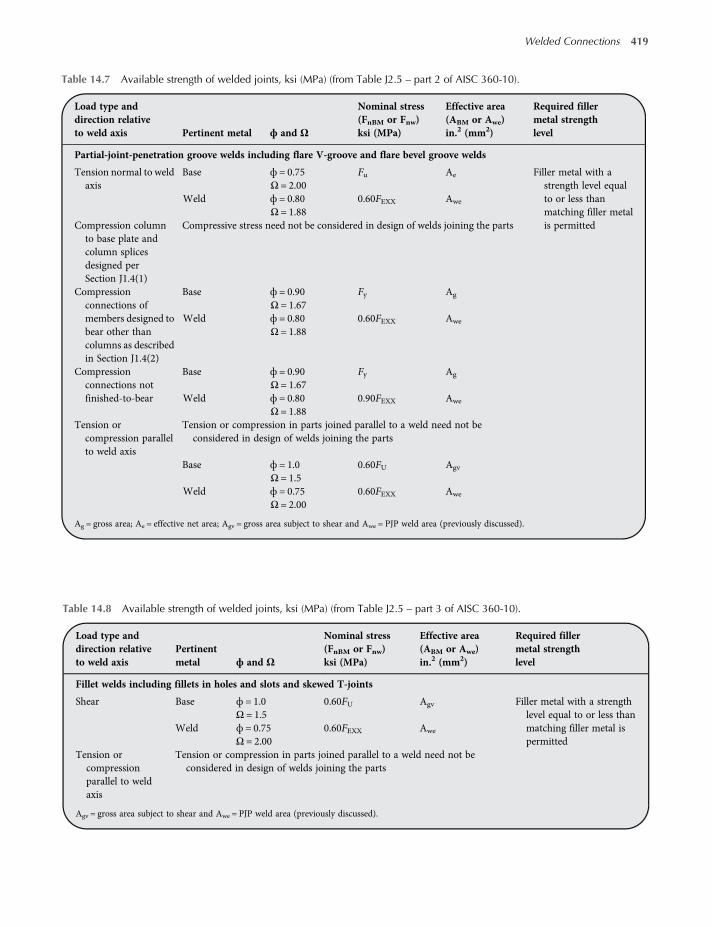
Table 14.7 Available strength of welded joints, ksi (MPa) (from Table J2.5 – part 2 of AISC 360-10).
Load type anddirection relativeto weld axis Pertinent metal ф and Ω
Nominal stress(FnBM or Fnw)ksi (MPa)
Effective area(ABM or Awe)in.2 (mm2)
Required fillermetal strengthlevel
Partial-joint-penetration groove welds including flare V-groove and flare bevel groove welds
Tension normal to weldaxis
Base ф = 0.75 Fu Ae Filler metal with astrength level equalto or less thanmatching filler metalis permitted
Ω = 2.00Weld ф = 0.80 0.60FEXX Awe
Ω = 1.88Compression columnto base plate andcolumn splicesdesigned perSection J1.4(1)
Compressive stress need not be considered in design of welds joining the parts
Compressionconnections ofmembers designed tobear other thancolumns as describedin Section J1.4(2)
Base ф = 0.90 Fy Ag
Ω = 1.67Weld ф = 0.80 0.60FEXX Awe
Ω = 1.88
Compressionconnections notfinished-to-bear
Base ф = 0.90 Fy Ag
Ω = 1.67Weld ф = 0.80 0.90FEXX Awe
Ω = 1.88Tension orcompression parallelto weld axis
Tension or compression in parts joined parallel to a weld need not beconsidered in design of welds joining the parts
Base ф = 1.0 0.60FU Agv
Ω = 1.5Weld ф = 0.75 0.60FEXX Awe
Ω = 2.00
Ag = gross area; Ae = effective net area; Agv = gross area subject to shear and Awe = PJP weld area (previously discussed).
Table 14.8 Available strength of welded joints, ksi (MPa) (from Table J2.5 – part 3 of AISC 360-10).
Load type anddirection relativeto weld axis
Pertinentmetal ф and Ω
Nominal stress(FnBM or Fnw)ksi (MPa)
Effective area(ABM or Awe)in.2 (mm2)
Required fillermetal strengthlevel
Fillet welds including fillets in holes and slots and skewed T-joints
Shear Base ф = 1.0 0.60FU Agv Filler metal with a strengthlevel equal to or less thanmatching filler metal ispermitted
Ω = 1.5Weld ф = 0.75 0.60FEXX Awe
Ω = 2.00Tension orcompressionparallel to weldaxis
Tension or compression in parts joined parallel to a weld need not beconsidered in design of welds joining the parts
Agv = gross area subject to shear and Awe = PJP weld area (previously discussed).
Welded Connections 419

where Rnwl is the total nominal strength of longitudinal fillet welds, as calculated above and Rnwt isthe total nominal strength of transverse fillet welds, calculated as described earlier, but not usingthe alternate method.
Finally, for plug and slot welds (Table 14.9), for the case of shear parallel to the faying surface onthe surface on which the effective area is calculated, the resistance factor to be used is 0.75, thenominal stress of the weld is taken as 0.60 times the nominal capacity of the electrode usedand the effective area is calculated following the considerations that were presented in the previoussection for plug and slot welds.
14.5 Joints with Mixed Typologies
Within a joint, it is good practice to avoid the usage of different joining methods, that is welds andbolts, or welds and rivets. Simultaneous use of multiple joining techniques is allowed, as long as atleast one of these is capable of carrying the whole force demand.
EC3 allows one exception to this rule: in slip critical joints, where slip is considered to be anultimate limit state (category C), the shearing force to be transmitted can be shared among pre-tensioned bolts and welds, as long as the fasteners are installed after the welds have been placed.
ANSI/AISC360-10 also allows an exception to this rule. Bolts installed in standard or short slotsholes (with the slot perpendicular to the direction of loading) are permitted to share load withlongitudinal fillet welds, with the limitation of taking the available strength of the bolts no greaterthan 50% of the available bearing strength in the connection. Also, in retrofits and modificationsof a bolted slip-critical connection, the additional welds can be sized to resist just the additionalloads, using the pre-tensioned bolts to resist their original design load.
14.6 Worked Examples
Example E14.1 Welded Connection According to EC3 for a Tension Member
Verify in accordance with EC3, the welded connection in Figure E14.1.1 between a plate 250 × 20mm (9.84 ×0.787 in.) in tension and a column flange, realized by one fillet weld orthogonal to the force axes.
Table 14.9 Available strength of welded joints, ksi (MPa) (from ACI 360-10, Table J2.5 – part 4).
Load type anddirection relativeto weld axis
Pertinentmetal ф and Ω
Nominal stress(FnBM or Fnw)ksi (MPa)
Effective area(ABM or Awe)in.2 (mm2)
Required filler metalstrength level
Plug and slot welds
Shear parallel tofaying surface onthe effective area
Base ф = 0.75 0.60FU Anv Filler metal with a strength levelequal to or less than matchingfiller metal is permitted
Ω = 2.00Weld ф = 0.75 0.60FEXX Awe
Ω = 2.00
Awe = PJP weld area (previously discussed) and Anv = net area subject to shear.
420 Structural Steel Design to Eurocode 3 and AISC Specifications

Applied tension force N= 900 kN 202 3 kips
Steel S275 fu = 430 N mm2 62 4 ksi
βw = 0 85
Fillet length l = 250 mm 9 84 in
Fillet side d = 20 mm 0 787 in
(1) EC3 directional methodCompute fillet throat dimension, a:
a= d 2 = 20 2 = 14mm 0 551 in
σ⊥ = τ⊥ =Nl a
22
=900 103
250 × 1422
= 181 8N mm2
The verification formulas are:
σ2⊥ + 3 τ2⊥ + τ2 = 181 82 + 3 × 181 82 + 02 = 363 6N mm2 ≤
≤fu
βw γM2=
4300 85 × 1 25
= 404 7N mm2 OK 52 7 ksi ≤ 58 7 ksi
σ⊥ = 181 8N mm2 ≤0 9fuγM2
=0 9 × 4301 25
= 309 6N mm2 OK 26 4 ksi ≤ 44 9 ksi
(2) Simplified EC3 methodThe verification formula is:
Fw,Ed ≤ Fw,Rd =fu a
3 βw γM2
Fw,Ed =N l = 900 103 250 = 3600N mm 20 56 kips in
Fw,Rd =fu a
3 βw γM2
=430 × 14
3 × 0 85 × 1 25= 3271N mm < 3600N mm
NOTVERIFIED 18 68 kips in < 20 56 kips in
As can be noted, in this case the EC3 simplified method is more conservative than the directional methodand the weld results are verified with the second method but not with the first one.
LN
Figure E14.1.1
Welded Connections 421

Example E14.2 Welded Connection According to EC3 for a Member in Bendingand Shear
Verify in accordance with the EC3 provisions, the welded connection between a UPN 240 profile in bending,connected to a gusset plate by two fillet welds of same length (Figure E14.2.1).
Applied load T = 90 kN 20 2 kips
Load eccentricity e = 600 mm 23 6 in
Steel S275 fu = 430 N mm2 62 4 ksi
βw = 0 85
Use two fillet welds of side length of 10 mm (0.394 in.) and length of 200 mm (7.87 in.) each.Forces acting on each fillet:
(a) Force parallel to fillet axes (h is profile depth):
T1 =T eh
=90 × 600240
= 225 kN 50 6 kips
(b) Force orthogonal to fillet axes:
T2 =T 2 = 90 2 = 45 kN 10 1 kips
(1) EC3 directional methodCompute fillet throat dimension, a:
a= d 2 = 10 2 = 7mm 0 276 in
σ⊥ = τ⊥ =T 2l a
22
=90 2 103
200 × 722
= 22 7N mm2 3 29 ksi
τ =T1
a l=225 103
7 × 200= 160 7N mm2 23 3 ksi
L
e
T
Te/h
Te/h
T/2
T/2
Figure E14.2.1
422 Structural Steel Design to Eurocode 3 and AISC Specifications

The verification formulas are:
σ2⊥ + 3 τ2⊥ + τ2 = 22 72 + 3 × 22 72 + 160 72 = 282N mm2
≤fu
βw γM2=
4300 85 × 1 25
= 404 7N mm2 OK 40 9 ksi ≤ 58 7 ksi
σ⊥ = 22 7N mm2 ≤0 9fuγM2
=0 9 × 4301 25
= 309 6N mm2 OK 3 29ksi ≤ 44 9 ksi
Stress rate 282 404 7 = 0 70
(2) Simplified EC3 methodThe verification formula is:
Fw,Ed ≤ Fw,Rd =fu a
3 βw γM2
Fw,Ed =T1
l
2
+T2
l
2
=225 103
200
2
+45 103
200
2
= 1147N mm 6 55 kips in
Fw,Rd =fu a
3 βw γM2
=430 × 7
3 × 0 85 × 1 25= 1636N mm > 1147N mm
OK 9 34 kips in > 6 55 kips in
Stress rate 1147 1636 = 0 70
As can be noted, stress rate is the same with both methods (= 0.70).
Welded Connections 423

CHAPTER 15
Connections
15.1 Introduction
The selection of the proper connections for mono-dimensional members is an extremely import-ant phase of each design. The choice of bolted connections, welded connections or connectionswith some components bolted and others welded has to be done considering not only the struc-tural performance but also economic factors associated with shop execution as well as site assem-blage, especially with reference to the costs of the manpower and of the impact on the buildingerection schedule. The use of either bolting or welding has certain advantages and disadvantages.Bolting requires either the punching or drilling of holes in all the plies of members to join. Asintroduced in Chapter 13, these holes may be standard size, oversized, short-slotted or long-slotted depending on the type of connection. It is not unusual to have one ply of material preparedwith a standard hole while another ply of the connection is prepared with a slotted hole in order toallow for easier and faster erection of the structural framing. However, the welding processrequires a greater level of skill than installing the bolts. Welding eliminates the need for punchingor drilling the plies of members to be connected to each other. It is preferable to avoid site weldingowing to the fact that shop welding guarantees a better quality level as well as higher structuralperformance.
Preliminary to the description of the most common type of connections, it should be noted thatthey can be distinguished in articulated connections and joints on the basis of the effects producedby the relative displacements between the members to be connected. All structures in fact move tosome extent and these movements may be permanent and irreversible or short-term and possiblyreversible. The effects can be non-negligible in terms of the behaviour of the structure, the per-formances of components and sub-systems during its lifetime. With reference to this aspect, it ispossible to distinguish in:
• articulated connections: which allow, under normal service conditions, relative movementsbetween the connected members in elastic range, without causing any plasticization of themas well as of the required devices (bolts, web, plate, angles, etc.). These connections can be dis-tinguished in pin joints, bearing joints or joints in synthetic material. Articulated connectionswere frequently used up to the beginning of this century: structural design strictly followed theelastic theory and the constraint conditions, on which calculations were based, were compliedwith as faithfully as possible. When plastic theory was developed and it became clear that eachequilibrated calculation model was in favour of safety, provided that localized failures and
Structural Steel Design to Eurocode 3 and AISC Specifications, First Edition. Claudio Bernuzzi and Benedetto Cordova.© 2016 John Wiley & Sons, Ltd. Published 2016 by John Wiley & Sons, Ltd.

buckling phenomena did not take place, the importance of constraint compliance with theirmodel was retrenched.
• joints: which do not allow any relative displacements in elastic range but provide the values ofdesign displacements or rotations via the spreading of plasticity. In this case, adequate ductilityof material is required associated with an appropriate choice of the connection details necessaryto avoid brittle failures and instability phenomena.
Furthermore, depending on the resistance of the connections, which has to be compared withthe one of the connected members, following types of connection can be distinguished:
• partial strength connection: if the connection is weaker than the connected members;• full strength connection: when failure occurs in one of the connected members, before than in
the connection.
The position of the connections depends, in some cases, on the internal forces and bendingmoment distribution on the members intended to connect. As an example, reference can be madeto the beam in Figure 15.1, which is supposed to have quite a long span, for example L = 20 m(65.6 ft), greater than the normal limit of transportability. If connections are supposed to belocated in the cross-sections (A), where no moment acts, they must be able to transfer only shearforce while, if it is preferable only a connection at the beammidspan (B), connection design has tobe developed considering the need to transfer the sole bending moments. In both cases, partialstrength connections should be used guaranteeing the transfer of the sole design shear (A) orof the sole design moment (B).
15.2 Articulated Connections
Nowadays, articulated connections are mainly used in truss members, typically for bridgesupports and for frames supporting machinery or moving equipment.The cost of making a pin joint is quite high because of themachining required for the pin and its
holes and also because of difficulties in assembly. Furthermore, pins are used in special architec-tural features where relative rotation occurs between the members being connected.
A A
A A
M)
T)
B
B
Figure 15.1 Example of cross-sections where locate intermediate partial-strength connections.
Connections 425

An aspect sometimes critical for connections is the required performance associated with thepractical realization of the kinematic mechanism considered in the design phase, especially withreference to the detailing associated with hinges and simple supports. As presented inSection 15.5.1, in addition to the checks for geometry and resistance, checks are also necessaryto verify the compatibility between the required displacement and the one guaranteed by thechosen detailing.
The movements of a structure are not in themselves detrimental. Problems may arise wheremovements are restrained, either by the way in which the structure is connected to the ground,or by surrounding elements such as claddings, adjacent buildings or other fixed or more rigiditems. If no adequate attention has been paid in the design phase to such movements and tothe associated forces and moments, it is possible that they will lead to, or contribute towards,deterioration in one or more elements. Deterioration in this context could range from crackingor disturbance of the finishes on a building to buckling or failure of primary structural elementsdue to large forces developed through inadvertent restraint. As an example, the portal frame inFigure 15.2 can be considered, which is characterized by a roof beam that is pinned to the columnat one end and simply supported at the other beam end.
A plate is attached at both beam ends, which has a hole to insert a pin to realize the connectionwith the column. In case of hinge restraints, coupled plates with a circular hole of equal diameterare attached to the column. In a similar way, in correspondence of the other beam end, connectionto the column is realized via coupled plates but has a slotted hole to allow for horizontal displace-ments. The slot should have an appropriate length in order to hamper the contact between the pinand the hole of the column plate, hence avoiding the transfer of horizontal forces to the verticalmember, which induces shear forces and bending moments on the column.
15.2.1 Pinned Connections
A pinned connection is generally composed of steel coupled plates (brackets) welded at the ends ofthe elements to be connected, suitably stiffened to contain the local effects related to the concen-tration of forces, and drilled to accommodate the pin, thereby allowing the kinematics expected inthe design phase (Figure 15.3).
Figure 15.2 Typical connection detail for a pinned simply supported beam.
426 Structural Steel Design to Eurocode 3 and AISC Specifications

The members to connect must be arranged so as to avoid any possible eccentricity in the trans-mission of the load and, at the same time, must be characterized by an adequate size to ensure thatthe force is transmitted via connection without any significant stress concentration. Furthermore,when the use conditions might lead to an accidental extraction of the pins, these must be blockedwith appropriate safety devices (plugs anti-release).Usually, shear force and bending moment acting on the pin are calculated assuming that the
brackets behave as simple supports and considering the reaction forces uniformly distributedalong the length of contact of each part.
15.2.2 Articulated Bearing Connections
Articulated bearing connections are frequently used as supports for bridges and can easily beobtained by means of a direct contact between the metal surfaces of the elements in the bondcompetitors. Usually, these connections can be divided in two types on the basis of the contactsurfaces:
• connections with contact between two surfaces of which at least one is curved: contact point canbe obtained via a ball bearing and linear contact is typically due to an interposed cylindricalround, which is presented in Figure 15.4a,b. Appropriate guides or wedges must be providedto control surface rolling and to transmit possible transverse forces;
• connections with concentrated contact between a plate and a plate with a knife (Figure 15.4c,d):which are frequently used for small span bridges and often for the supports of important cranerunway beams. Excessive contact pressure between the plates must be avoided in order not todeform the surfaces.
The evaluation of the state of stress is based on conventional Hertz formulas. Design is devel-oped considering, as limit for the strength the stress value flim, which has to be evaluated inaccordance with the considered Code of practice. This value is obtained from the tension limitstrength multiplied by a factor significantly greater than unity, accounting for the benefits asso-ciated with the tri-axial state of stress in correspondence of the joint, which has a beneficial con-finement effect.In cases of linear contact, that is contact due to a cylindrical hinge (cases a– d of Figure 15.5), it
is required that:
σ ≤ 4flim 15 1
0.5 FEd 0.5 FEd
FEd
dd0
Figure 15.3 Examples of pinned connections.
Connections 427

If cylindrical hinge has a length b, with reference to the symbols in Figure 15.5, assuming that Fis the transferred force, the design stress is evaluated as:
case (a) withr2r1
≥ 2:
σ = 0 18 E Fr2−r1r1 r2 b
15 2a
case (b):
σ =0 18 E F
r b15 2b
case (c):
σ =0 20 E F2r b
15 2c
(a) (b)
(d)(c)
Figure 15.4 Articulated bearing joints: contact between cylindrical (a) and spherical (b) surface, contact plate (c)and knife contact plate (d).
428 Structural Steel Design to Eurocode 3 and AISC Specifications

case (d) with term n identifying the number of the rollers:
σ =0 24 E Fn r b
15 2d
In case of punctual contact, that is contact due to a spherical hinge (cases e and f in Figure 15.5),it is required that:
σ ≤ 5 5flim 15 3
Design stress σ is evaluated as:
• in case (e) of Figure 15.5:
σ =0 06E2F r2−r1
2
r22 r21
315 4a
• in case (f ) of Figure 15.5:
σ =0 06E2F
r23
15 4b
15.3 Splices
As already introduced in Chapter 3, steel buildings have a skeleton frame, which is site-erected byconnecting mono-dimensional members. In addition to problems associated with the choice ofthe types of connections, also strictly depending on the connected members (secondary beam,girders, diagonal bracing, etc.) sometimes connections are necessary to realize a member of greatlength, splitting it into parts of a length suitable for transport by tracks (as already mentioned inSection 15.1). Typically, for columns in buildings as well as for trussed beams it can be convenientto site join single components via splice connections.There are many ways of making splices. For example, traditional cover plates may be used for
full load transfer or just for continuity; welds or bolts may be chosen as fasteners. Herein, referenceis made to the following types of splices, which are the most commonly used:
(a) (b) (c)
(d) (e)
r1 r2
r1r
r2
rr
(f )
Figure 15.5 Most common types of contact surfaces: linear contact via cylindrical pin (a–d) and via spherical ball(e) and (f).
Connections 429

• beam splices: for example connections between horizontal members, generally under bendingmoment and shear force;
• column splices: for example connections between vertical members, generally under compres-sion and shear forces and bending moment.
It should be noted that for these types of connections, as well as for all the other components,it is preferable to have shop welding instead of site welding in order to guarantee a betterquality of the product as well as to reduce the costs associated with the execution ofconnections.
15.3.1 Beam Splices
As for other types of connection, beam splices can be full or partial strength connections. In thelatter case, it can be convenient to place the joint in correspondence of zones interested by suitableinternal forces and moments, as already discussed with reference to the example of Figure 15.1.Some typical beam splices are illustrated in Figure 15.6:
(a) connection with extended end plate shop welded to beam end and site bolted;(b) connection with cover plates site bolted to beam flanges, to transfer the bending moment and/
or to the beam web to transfer the shear force;(c) connection with welded cover plates for the flanges and for the web. These plates can be site
welded at both beam ends or, more conveniently, shop welded at one beam end and sitewelded to the other beam;
(d) butt welded connection, which requires appropriate surface preparations (as discussed withreference to Figure 15.7).
It should be noted that the lacking of the appropriate thickness and/or width of the cover platesmakes the splice a partial strength connection.
(a) (b)
(c) (d)
Figure 15.6 Typical splice for beams.
430 Structural Steel Design to Eurocode 3 and AISC Specifications

15.3.2 Column Splices
Columns in framed systems are generally subjected to compression or to compression, shear andbending moments, hence resulting in predominant compression stresses. As a consequence, froma theoretical point of view, no splice connection is required, since the compression force istransferred by direct bearing. However, due to the presence of geometric imperfections (lackof straightness of the column) as well as of unavoidable erection eccentricities and to the fact thateven carefully machined surfaces will never assure full contact, column splices have necessarily tobe realized.Even when the column is subject to pure compression and full contact in bearing is assumed, all
the appropriate design verifications are necessary, as required by the Codes of practice. The loca-tion of the splice should be selected so that any adverse effect on column stability is avoided, that isthe distance of the connection from the floor level should be kept as low as possible. A limit of 0.25times the storey height is usually accepted. If this requirement cannot be fulfilled, account shouldbe taken of the bending moment due to deformations induced by member imperfections.
(a)
(d) (e) (f) (g)
(b) (c)
Machined
surfaces
Machined
ends
Figure 15.7 Examples of splice connections.
Connections 431

More significant values of the bending resistance may be required in splices when columns aresubject to primary bending moments, as in frame models assuming hinges at, or outside, the col-umn outer face, as shown in the discussion on joint modelling (see Section 15.5). In addition, incolumns acting as chords of cantilever bracing trusses, tensile forces may arise (uplift) in someload conditions(uplift), which are transmitted by splices.
Typical compression column splices suitable for use in simple frames are shown in Figure 15.7and in particular it is possible to recognize:
(a) splice connection with coupled cover plates site bolted to each column flange and to the col-umn web;
(b) splice connection with coupled cover plates site bolted to the sole column flanges;(c) splice connection with coupled cover plates site bolted to the column web and a single cover
plate per each column flange, site bolted to the outside faces of the column flanges in order toreduce the plan area occupied by the splice;
(d) splice connection with fillet welds and internal welded cover plates;(e) splice connection with light cover plates, which are bolted to the column flanges;(f) splice connection with an interposed plate, which is welded to both columns (generally shop
welded to one column and site welded to the other column);(g) splice connection with interposed plates shop welded to the column ends and site bolted to
each other.
When a bolted solution is adopted (a–c in Figure 15.7), forces are transmitted through thecover plates and distributed among the connecting plates in proportion to the stressresultant in the cross-sectional elements, for example for simple compression in proportionto the areas of the flanges and of the web. Differences in column flange thickness may be accom-modated by the use of packs. These may be positioned preferably on the outside faces of theflanges.
Splice connection types (d)–(g) rely on direct bearing. When the surfaces of the end cross-sections of the two column shapes are sawn and considered to be flat, and squareness betweenthese surfaces and the member axis is guaranteed, the axial force may be assumed to be trans-mitted by bearing. Both fillet welds (d) or light cover plates (e) are provided to resist possiblesecondary shear force and bending moment when the upper and lower columns differ in serialsize. Plates are flattened by presses in the range of thicknesses up to 50 mm (1.97 in.), andmachined by planning for thicknesses greater than 100 mm (3.94 in.). For intermediate thick-nesses either working process may be selected. In case of significant variation of cross-sectionaldimensions, as in the arrangement of type (f ), the plate must be checked for bending resistance.A possible conservative model assumes the plate as a cantilever of a height equal to the width andclamped to the upper column flange. The axial force, which is transmitted between the corres-ponding column flanges, is applied as an external load at the mean plane of the flange of the lowercolumn.
For larger differences in column size, a short vertical stiffener has to be located directly belowthe flange(s) of the upper column to directly assist in transferring the locally high force. If fullpenetration welding connections realize these splices, the verification of the welded connectionscan be omitted in most practical cases. Where the cross-section of the members connected viasplices vary considerably, a separating plate is required to realize the splice, the design of whichis more complex if subject to bending.
In Figure 15.8 some typical splice solutions are presented for sensible cross-section variations:
(a) A splice with a shop welded plate on the top of the lower column, which results very useful forthe direct positioning and the site welding of the upper column. Web stiffeners are always
432 Structural Steel Design to Eurocode 3 and AISC Specifications

required because they receive the load transmitted by the upper flange and transfer it to thelower web, which in turn redistributes it in the underlying part. Due to the differences betweencolumn axis, an additional bending moment also has to be transferred via the splice;
(b) A splice with longitudinal and transverse shop welded stiffeners at the top of the lower col-umn. The bottom end of the upper column is site welded to the plate. This splice is recom-mended when loads acting on the column are high and it is hence convenient to maintainthe longitudinal axis of the column coincident in order to avoid additional bendingmoments. A simplified model related to a stocky I-shaped section loaded by two concen-trated forces in correspondence of the flanges of the upper column can be adopted. Heightof the beam is the distance between the horizontal splice plates, which are considered thebeam flanges.
(c) A tapered splice. The size of the columns is different in this case too and the splice is tapered:at the end of each column a horizontal plate is welded and diagonal plates are placed to con-nect the column flanges. A design approach based on the use of the strut-and-tie model can beadopted, very similar to the one adopted for the design of isolated concrete stockyfoundations.
N(a)
(c)
(b)
M
eA
A
d
A A
M
M
N
N
Nf Nf
Nf
NfNf
Nf
Nf
Nf tgα
Nf tgα
α
Nf
tAw
α
W1W1
Nf,2Nf,1
W2W4 W2
W3
W3
twb
30°
Figure 15.8 Examples of column splice for columns with different cross-sections.
Connections 433

15.4 End Joints
Several types of end joints, for example joints connecting the end of elements with their longitu-dinal axis not parallel, can be considered, and in the following reference is made to:
• beam-to-column joints;• beam-to-beam joints;• bracing connections;• base-plate connections;• beam-to-concrete wall connections.
15.4.1 Beam-to-Column Connections
Beam-to-column joints canbe realizedbyconnecting thebeam flanges and/or thebeamweb,depend-ing on the required joint performance. In Figure 15.9 some common types of beam-to-columnjoints are presented, which refer to a beam attached to the column flange but can also be adoptedif the web column is considered. In particular, the following solutions are frequently adopted:
(a) web angle (cleat) connection: a couple of angles is site bolted to the beam web and to the col-umn flange;
(b) fin plate connection: a plate, parallel to column web, is shop welded to the column flange andsite bolted to the beamweb. This joint is also one of the few arrangements suitable for use withrectangular or square hollow section columns as no bolting to the column is necessary;
(c) header plate connection (partial depth end plate): a plate, parallel to the column flange, with adepth lower than theoneof theweb is shopwelded to thebeamweband site bolted to the column;
(d) flush end plate (full depth end plate): a plate having the depth of the beam and parallel to thecolumn flange, is shop welded both to the beam flanges and to the beamweb and site bolted tothe column. Furthermore, when high joint performance is required, it can be convenient toextend the plate beyond the tension flange of the beam in order to allow the positioning of anadditional bolt row external to the beam (extended end plate).
Both solutions (a) and (b) provide some allowance for tolerance (through the clearance in thebeam web holes) on member length. Type (b) connection permits beams to be lifted in from oneside. Furthermore, types (c) and (d) connections require a more strict control of the beam lengthand of the squareness of the cross-section at the end of the beam. The flush end plate scheme ofsolution (d) is sometimes preferred to the part depth end plate of solution (c) in order to reducethe chances of damage during transportation. Partial depth endplates should not normally be lessthan about 0.6 times the beam depth or the end torsional restraint to the beammay be reduced. Allthe presented types of connections can improved by adopting column panel stiffeners, in corres-pondence of the beam flange, which are necessary to avoid local weakness zone of the joint.
Additional joint solutions frequently used in steel structures practice are also proposed in thenext part of the chapter (Section 15.5) where joints are presented with reference to their guaran-teed performances.
15.4.2 Beam-to-Beam Connections
Floor decks in buildings are usually supported by grids of secondary beams and main girders.Most common types of these connections, which generally have a very limited degree of flexuralresistance, are reported in Figure 15.10, where it is possible to recognize:
434 Structural Steel Design to Eurocode 3 and AISC Specifications

(a) Web cleat bolted connection: angles are site bolted to the web of the secondary beam and of themain girder. It should be noted that the top flange of the secondary beam, which supports thefloor system, is located at a lower level than the corresponding one of the primary beam. Thissolution is convenient if the upper part of the girder can be embedded in the concrete floor orenclosed in partitions. Furthermore, it is good practice to place the angles as close as possibleto the upper flange of the girder in order to minimize cracking of the concrete floor slab due tothe beam rotation.
(a)
(b)
(c)
(d)
Figure 15.9 Typical examples of beam-to-column connections.
Connections 435

(b) Web cleated bolted-welded connection: angles are shop welded to the web of the secondarybeam and site bolted to the web of the main girder. As for the connection type (a), also inthis case the top flanges of the secondary beam and the girder are placed at different levels.
(c) Web cleated connection with coped secondary beam (single notched beam-to-beam connection):this solution, where angles can be bolted to the web of the beams or welded to the secondary
(a)
(b)
(c)
(d)
(e)
(f)
Figure 15.10 Examples of typical beam-to-beam connections.
436 Structural Steel Design to Eurocode 3 and AISC Specifications

beam and bolted to the main girders, differs from previous solutions (a) and (b) because inthis case, the beam and girder top flanges meet at the same level. The coped beam is thuslocally weakened and appropriate checks are required, as discussed next.
(d) Flush end plate connection: this connection is used when the same cross-section is adopted forsecondary beam andmain girder. Also in this case a coped beam is used as secondary memberbut both beam flanges are removed (double notched beam-to-beam connection). Flush endplate is shop welded to the web of the secondary beam and site bolted to the web of the maingirder.
(e) Stiffened flush end plate connection: a flush end plate is shop welded to the secondary beamand site bolted to a tee stiffener shop welded to the girder. This connection is in many casesvery expensive due to the costs associated with the shop welding techniques.
(f) Fin plate connection: this connection can be considered a variant to web angles connections.A single plate is shop welded to the primary beam end and site bolted to the secondary beam.A fin plate connection is particularly simple both to fabricate and to erect, but it requires care-ful design as it has to function as a hinge.
Connection types (d) and (e) possess some predictable stiffness and strength, but in routinedesign they are modelled as pins. In particular, there is a need to decide where the ‘hinge’ is locatedas explained in Section 15.5.1. Furthermore, it should be noted that types (a) and (c), which makeuse of web cleats bolted to both the girder and the beam, were extensively used in the past. Type (b)with the cleats bolted to the girder and welded to the beam, and types (d) and (e) where a flush endplate is adopted, may cause lack-of-fit during erection due to the dimensional tolerances.When a beam is coped, as in connection type (c) or (d), it should be verified that no failure
occurs at the beam section that has been weakened (block shear failure mechanism). Particularlyin these types of connection, it should be noted that the presence of bolt holes often weakens theholed component(s) of the member as well as the connection plate. Failure may occur locally thereby bearing or plate punching, or in an overall mode along a path whose position is determined bythe hole location and by the actions transferred by the plate, such as that considered in Chapter 5for tension members connected via staggered holes.Generally, if the plate proportions are appropriate to avoid instability, it results conservative for
the strength limit against general yield and satisfactory to design against local fracture, which isgenerally brittle.The actual failure stress distributions in bolted connection plates are both uncertain and com-
plicated. Plate sections may be subjected to simultaneous normal and shear stress, as in the case ofthe splice plates shown in Figure 15.11a,b. These may be designed conservatively against generalyield by using the shear and bending stresses determined by elastic analysis of the gross cross-section in the combined yield Von Mises criterion of Eqs. (1.1) and (1.3), and against fractureby using the stresses determined by elastic analyses of the net section.Furthermore, block failure may occur in some connection plates as shown in Figure 15.11c,d
and it may be assumed that the total resistance is provided partly by the tensile resistance acrossone section of the failure path, and partly by the shear resistance along another section of thefailure path. This assumption implies considerable redistribution from the elastic stress distribu-tion, which is likely to be very different from uniform.
15.4.3 Bracing Connections
Connections within the bracing members or between the bracing members and the main framingcomponents transfer generally forces between a number of differently oriented members.In Figure 15.12 typical connections for horizontal bracings (i.e. floor bracings and roofs bra-
cings) are proposed. As can be noted, diagonal elements are usually bolted to a plate fixed to the
Connections 437

primary beams. The location of these plates has to be defined considering the possible inter-ferences with structural and non-structural components. In absence of limitation due possibleinteractions with the slab as well as the roof, connections can be realized at the top flange level,as in solution (a) and (c) in Figure 15.12. Otherwise, different solutions have to be considered,attaching the plate to the beam or to the bottom flange of the beam. Usually, bracing membersare realized with slender profiles, owing to the fact that in service conditions, the floor slab directlytransfers horizontal forces to the vertical bracing systems. The removal of these bracings after theerection of the skeleton frame should result non-economical and for this reason, they are usuallyembedded in the concrete slab. Regarding vertical bracings, Figure 15.13 proposes typical detailsused for cross bracing and k-bracings.
In case of cross brace, type (a) connection attaches the bracing via a plate shop welded to thecolumn and bolted to the bracing (diagonal and horizontal) members. Type (b) is an internal bra-cing connection. In case of k-bracing connections, types (c) and (b) combine both functions bymaking the beams part of the bracing system.
With reference to the most common cross-bracing types that can be designed consideringactive both tension and compression members, diagonal members should be connected to eachother at the intersection point, as shown in Figure 15.14. This internal connection, realized inmany cases via one bolt, is usually enough to restraint efficiently the overall stability of the com-pression diagonal, reducing its effective length.
15.4.4 Column Bases
As for beam-to-column joints, column bases also have to be correctly classified in order to selectthe appropriate model to use in structural analysis. It is worth mentioning that the relationshipsbetween the moment and the rotation is significantly influenced by the level of the axial load act-ing at the base joint location, which increases significantly base joint performance in terms of bothrotational stiffness and moment resistance.
Bolt
forces
Bolt
forces
(a)
(c)
(b)
(d)
Bolt forces
Bolt
forces
Failure path
Failure
path
Plate
stresses
Plate stressesC
T
T
Figure 15.11 Stress distribution in bolted plates in shear and tension: (a) shear and bending, (b) tension andbending, (c) block tearing in plate and (d) block tearing in a coped beam.
438 Structural Steel Design to Eurocode 3 and AISC Specifications
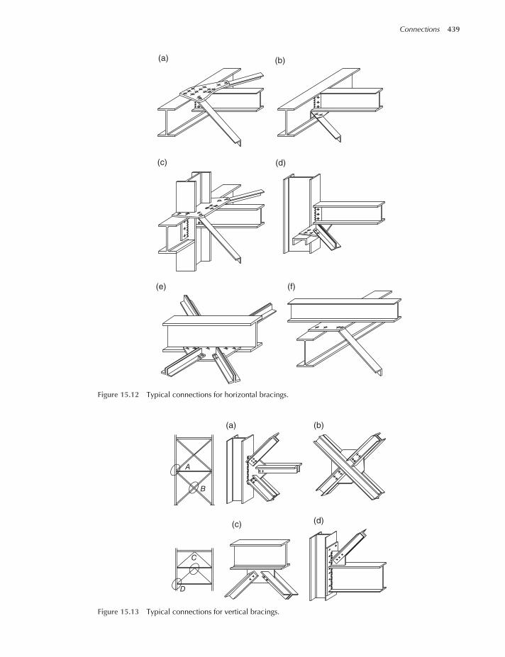
(a) (b)
(c) (d)
(e) (f)
Figure 15.12 Typical connections for horizontal bracings.
C
D
(c) (d)
A
B
(a) (b)
Figure 15.13 Typical connections for vertical bracings.
Connections 439

A column base connection always consists of a plate welded to the foot of the column andbolted down to the foundations (Figure 15.15). In a few cases, a second steel plate, usually ratherthicker, can be incorporated into the top of the foundation, helping both to locate the base of thecolumn accurately and in spreading the load into the weaker (concrete or masonry) foundationmaterial.
The plate is always attached to the column by means of shop fillet welds. However, if the col-umn carries only compression loads, direct bearing may be assumed into design, provided that thecontact surfaces are machined or can be considered to be flat. Machining is generally omittedwhen the transfer loads are relatively small. No verification of the welds is then required.
Baseplate connections in simple frames are typically subjected to the sole axial load; they aregenerally modelled as ideal pins, and are designed to transfer concentrated force (compression ortension). As it results from the base connections in Figure 15.15a,b anchor bolts are required onlyfor the erection phase, making possible to regulate the height of the column base. A combinationof axial and shear force acts on the column base, usually when the column is part of the bracingsystem (c). In tension connections, the baseplate thickness is often governed by the bendingmoments produced by the holding down bolts to transfer the acting load to foundation. In somecases, the use of stiffeners can be required (d), which significantly increases the fabrication contentand therefore the cost of the column base as compared with the cases (a) and (b).
With reference to concrete foundation in case of moderate tension forces, the bolts holdingdown are usually cast into the foundation (Figure 15.16).
Hooked anchor bolts allow clearance for their positioning and can contribute to transfer ten-sion force by friction between steel and concrete. As to the failure mode, owing to the importanceof a ductile failure mode with anchor bolt yielding, it is recommended to use an appropriate steelgrade in order to avoid brittle failure. Furthermore, when high tensile forces should be transferredto the foundation, which is frequent in high-rise and tall buildings, it is necessary to provideappropriate anchorage to the bolts. For example, threaded bolts may be used in conjunction withchannel sections embedded in the concrete (hammer head anchor bolts) as in Figure 15.17b orwith a washer plate as in Figure 15.16c.
In case of high shear forces, appropriate devices can be used in order to transfer these forces bycontact between the devices and the concrete. As an example, Figure 15.18 can be considered,which proposes:
solution (a) with a device obtained by shop welding at the bottom of the base plate a short length ofprofile identical to that of the column and filled in the concrete after the base plate positioning;
solution (b) with some appropriate stiffened plates shop welded to the bottom face of thebase-plate.
Figure 15.14 Example of cross bracing with an internal connection.
440 Structural Steel Design to Eurocode 3 and AISC Specifications
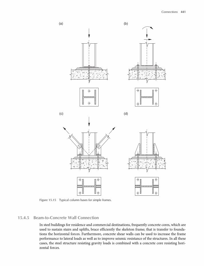
15.4.5 Beam-to-Concrete Wall Connection
In steel buildings for residence and commercial destinations, frequently concrete cores, which areused to sustain stairs and uplifts, brace efficiently the skeleton frame; that is transfer to founda-tions the horizontal forces. Furthermore, concrete shear walls can be used to increase the frameperformance to lateral loads as well as to improve seismic resistance of the structures. In all thesecases, the steel structure resisting gravity loads is combined with a concrete core resisting hori-zontal forces.
(a) (b)
(d)(c)
Figure 15.15 Typical column bases for simple frames.
Connections 441

N1
(a) (b) (c)
L
L1
L L
r r
aa a
r
Ø
N1 N1
Ø Ø
Figure 15.16 Examples of anchor bolts embedded in the concrete of foundation: simple anchor bolt (a) hookedanchor bolt (b) and anchor bolt with a washer plate (c).
LL
(b)(a)
45°
Figure 15.17 Typical solutions to anchor the foundation when bolts are in presence of high values of the tensionforce: hooked anchor bolts (a) and hammer head anchor bolts (b).
(a) (b)
Figure 15.18 Examples of appropriate device to transfer shear load via direct contact steel-concrete.
442 Structural Steel Design to Eurocode 3 and AISC Specifications

Particular attention must be paid to the connection systems between these two materials. Thetwo systems are built with dimensional tolerances of a different order of magnitude: millimetres incase of steel components and centimetres for concrete cores and walls. Special care is required toaccount for the relative sequence of erection of the concrete and steel components, the method ofconstruction of the core (influencing significantly concrete tolerances) and the feasibility of com-pensating for misalignments. Furthermore, it should be noted that the details in the concrete wallmust be suitably designed to disperse connection forces safely. In particular, joint detailing is espe-cially important when deep beams are required to transmit high vertical loads.The most common connections between steel beam and concrete cores (or concrete walls) are
illustrated in Figure 15.19. The connection of the steel beam can be made via different steel detailsand in particular:
(a) fin plate site welded to the adjustment tool and bolted to the beam web;(b) fin plate site welded to the steel plate encased in the concrete core and site welded to the
beam web;(c) fin plate site welded to the steel plate encased in the concrete core and site bolted to the
beam web;(d) rigid block and web angles site welded to the steel plate encased in the concrete core;(e) fin plate encased in the concrete core and site bolted to the beam web;(f) fin plate bolted via appropriate fasteners to the concrete core and to the beam web.
Connection type (a) with a pocket in the wall is convenient for simplicity of adjustment, butcomplex in terms of core erection: types from (b) to (f), where part of the connection is encased inthe core wall during concrete pouring, may be preferable.Reinforcing bars (rebars) and/or headed studs can also be used to anchor the connection in the
concrete components. Full penetration welds are preferred when rebars are connected directly to
V
(a)
(d) (e) (f)
(b) (c)
H
Figure 15.19 Examples of common beam-to-concrete wall connections.
Connections 443

the steel plate, so that eccentricity of the force with respect to the welds is avoided or significantlyreduced.
Checking of the various components within the connection should be conducted in a consistentmanner, ensuring that the principles of connection design, for example that the assumed distri-bution of forces satisfies equilibrium, are observed.
It could eventually occur that the tolerances associated with shop working as well as site assem-bling are not completely respected. As a consequence, problems could arise during the construc-tion phase, hampering a correct erection of the skeleton frame. Site attempts to assembly membersout of tolerances are very dangerous and have to be avoided. Figure 15.20a presents someexamples of typical steel beam-concrete wall connections via steel plate site bolted to the beam.Due to the excessive working tolerances in few cases it was not possible to assembly the beam inthe fin plate due to the non-correspondence of the holes. As a consequence normal holes of thinplate were site modified by slotting (Figure 15.20b) via oxyhydrogen flame but this technique hasto be absolutely avoided.
15.5 Joint Modelling
It can be noted that, although the terms connections and joints are often regarded as having thesame meaning, their definitions are slightly different:
• term connection identifies the location at which two or more elements meet. For design pur-poses it is the assembly of the basic components required to represent the behaviour during thetransfer of the relevant internal forces and moments through steel members. Term connectionidentifies a set of components such as plates, cleats, bolts and welds that actually join the mem-bers together. With reference to the Figure 15.21, connection is realized by top and seat anglesbolted to the beam and the column flanges;
• term joint identifies the zone where two or more members are interconnected. For design pur-poses it is the assembly of all the basic components required to represent the behaviour duringthe transfer of the relevant internal forces and moments between the connected members.
(a) (b)
Figure 15.20 Examples of beam-to-concrete wall connection (a) and site slots of the thin plate to assemble theconnection with geometrical tolerances that are too large (b).
444 Structural Steel Design to Eurocode 3 and AISC Specifications

A beam-to-column joint consists of a web panel and either one connection (single sided jointconfiguration) or two connections (double sided joint configuration).
Furthermore, the nodal zone is the zone where interactions among joints occur, that is whereone or more joints and connections are located. From a practical point of view, it is defined as thepoint at which the axes of two or more interconnected structural elements converge.It should be noted that nodes can be classified also on the basis of the number of the connected
beams. With reference to Figure 15.22, it is possible to identify a:
(a) one way node, where a sole beam is connected to the column;(b) two way node, where two beams are connected to the column;(c) three way node, where three beams are connected to the column;(d) four way node, where four beams are connected to the column.
Nodal zone
Connection
Joint
Figure 15.21 Terms and definitions.
(a) (c)
(b) (d)
Figure 15.22 Classification of the nodes on the basis of the connected members.
Connections 445

It is worth mentioning that all the approaches developed for the design of members cannot beused to design connections, owing to the fact that concentrate forces are transferred via zones oflimited extension. The approach to the description of the joint behaviour is still considerablycomplex. Construction forms typical of framed structures and, in particular, of multi-storeybuildings, allow for the introduction of practical assumptions, whereby the problem can bemade simpler. The state of deformation produced by beam-to-column joint interaction is byits own nature complex and involves significant local distortions. Being difficult to representit accurately for the purpose of frame analysis, it is, however, convenient to use a behaviourrepresentation in global terms and describe the stress state and the deformation of the beam-to-column joint with reference to the six components of the stress resultant (Nx, Ny, Nz, Mx, My,Mz) and the associated components of the overall deformation (δx, δy, δz, ϕx, ϕy, ϕz) shown inFigure 15.23.
The joint response to the force components corresponding to the two shear forces Ny and Nz,and the twisting actionMx, exhibits a negligible deformability when compared to that of the mem-bers, if these are, as is usual, made of open sections. Besides, as the axial deformation δx is insig-nificant in terms of structural response, joint behaviour may be represented by the in-plane andout-of-plane moment rotation relations (Mx–ϕx and My–ϕy, respectively). The stiffness of thefloors in their own planes is usually large enough in order that also the latter deformation com-ponent can be overlooked in the analysis. Ultimately, the joint response can be described throughthe sole equation governing its in-plane rotational behaviour. Experimental results show that theinteraction between the different stress components is modest. This relation, briefly referred to asthe moment-rotation relationship (M–ϕ), is assumed to express the joint performances.
All the components of the connection, as well as the part of the mono-dimensional connectedmembers, significantly influence the overall response of the beam-to-column joint. As anexample, if the one-way joint in Figure 15.24 is considered, its deformation can be consideredas the sum of the following distortion components:
• shear and bending deformation of the column web panel zone (b);• bending of the column flange (c). Furthermore, the compressed beam flange can be subjected to
local buckling at the joint location;• deformation of the connecting elements (d), that is plate and bolts.
My, 𝜙y
Mz, 𝜙z
Mx, 𝜙x
Nx, 𝛿xNy, 𝛿y
Nz, 𝛿z
y
x
z
Figure 15.23 Stress and deformations in a typical beam-to-column joint.
446 Structural Steel Design to Eurocode 3 and AISC Specifications

As to the characterization of the beam-to-column joint performance, as for other types of joint,reference has to be made to the relationship between the moment (M) at the beam end and therotation (Φ) in the plane of frame, which is considered as the relative rotation between the beamand the column (Figure 15.25), that is the one obtained as the difference between the beam (ϑb)and the column (ϑc) rotation. With reference to the typical moment–rotation (M–Φ) relationshipfor connection under monotonic loading presented in Figure 15.25, it can be noted that:
• initially, the response is approximately linear (elastic branch) and joint response is associatedwith the sole value of the rotational stiffness Ci, until the elastic bending moment Me isachieved. Experimental studies developed since last decades pointed out that in this phasehigher values of the rotational stiffness can be obtained preloading the bolts;
• in the post-elastic branch, joint response is characterized by a rotational stiffness Cred, signifi-cantly lower than the one of the elastic branch, mainly due to the local spread of plasticity in theconnection components as well as non-elastic phenomena. The end of this phase correspondsto the achievement of the plastic moment of the joint, Mp;
• eventually, an additional phase (strain-hardening branch), in which theM–Φ relationship has avery moderate slope with a low value of the associated rotational stiffness, Cp, until the loadcarrying capacity of the joint under flexure (Mu) is achieved.
Furthermore, it can be noted that the stiffness in the un-loading branches, Cunl, is practicallyconstant, independent on the level of bending moment reached in the loading phase.The ability to approximate at least the key parameters of the moment-rotation joint curve is an
essential prerequisite to allow for a safe design by using semi-continuous frame model. Mainly, inlast four decades several extensive studies have been developed on this topic all over the world inorder to develop suitable approaches to predict joint behaviour. Nowadays, the main tools avail-able for this purpose are;
• experimental tests;• mathematical expressions;• finite element models;• theoretical models.
Experimental tests on joint specimens allow for direct evaluation of the moment-rotation jointresponse with the limitation that the results are referred to the sole tested geometry and to the solecharacteristics of the materials composing the specimen. These tests are quite expensive andrequire very refined resources. As an example, in Figure 15.26 the specimen of a top-and-seatcleated connection with a very rigid column is presented together with some instruments ofthe measuring systems. Different inductive transducers need to be placed in order to capturethe different contributions to the connection rotation. In particular:
(a) (b) (c) (d) (e)
+ + =
Figure 15.24 A typical external beam-to-column joint and the main contribution to its response.
Connections 447

• transducers A to evaluate the overall joint rotation, ϕcn;• transducers B to evaluate the contribution due to bolt elongation, ϕb;• transducers C to evaluate the rotation due to the slip between the leg angle and the beam
flanges (ϕsl).
The contribution due to the angle rotation, ϕp, can be obtained by subtracting bolt and slipcontribution to the overall joint rotation, as:
ϕp =ϕcn−ϕb−ϕsl 15 5
Mathematical expressions used to predict joint response have the considerable advantage ofbeing extremely simple and immediately implementable in structural analysis programs; however,they fail to notice the changes in the behaviour of the same joint as a function of the geometricaland strength characteristics of the single components. Hence, their reliability does not appear fullysatisfactory, because they were calibrated basing on a necessarily small number of tests.
Finite element models are too complex by far to be adopted in design practice, despite havingthe advantage of allowing us to model joint geometry accurately. Moreover, a fewmodelling prob-lems, which are important to simulate the bolted joint behaviour and, in particular, those aspects
M
M
𝜙=𝜗b–𝜗c
Mu
Mp
MeCred
Ci
Cuni
Cp
𝜙e 𝜙p 𝜙u
𝜗c
𝜗b
𝜙
Figure 15.25 Typical moment-rotation (M–Φ) relationship for a beam-to-column joint.
M
𝜙s1𝜙p
𝜙b
𝜙cn
(a) (b)
A
A
B
BC
C
Figure 15.26 Moment-rotation determined via the experimental approach: (a) details of the measuring system forthe connection and contribution to joint rotation (b).
448 Structural Steel Design to Eurocode 3 and AISC Specifications

concerning the plate-bolt interaction and the contact between the plate elements, have not beencompletely solved so far. As an example, Figure 15.27 reports the mesh of the finite element modelof an extended end plate connection.Theoretical models, also identified in literature as physical-mechanical models, appear to be the
most suitable ones for using at a design stage, as they are simple enough and, at the same time,allow to clearly relate the characteristics of the joint overall response (or of one of its components)to the local mechanisms of behaviour. Besides, methods based on mechanical models possessgenerally a remarkable capability to adapt themselves to the wide range of node configurationsthat may occur in practice for the same type of connection. The model of the node can be con-ceived as a collection of models representative of the single parts brought together either in seriesor in parallel, thus recognizing that the overall behaviour is the result of the distortion of the singlecomponents. The most popular theoretical prediction method is the component approach: eachcomponent of the joint is simulated via an axial spring with an elastic-perfectly plastic behaviour,for which the elastic stiffness as well as the resistance is calculated via suitable equations based onthe geometry as well as on mechanical properties. These potential forces are converted to theactual forces by considering equilibrium and compatibility conditions. The moment capacityof the connection is then calculated making reference to the centre of compression.As an example, Figure 15.28 presents the spring system used to simulate the response of a typ-
ical external beam-to-column joint, realized by means of an extended end plate connection. As tothe key components necessary to reproduce adequately the connection response, reference hasbeen made at least to:
(1) column web panel in shear;(2) column web in compression;(3) beam flange in compression;(4) bolts in tension;
EP
(b)
(a)
+ + +
+ + +
IPE 300
Figure 15.27 The finite element model (a) to appraise the moment-rotation curve an extended end plateconnection (b).
Connections 449

(5) column web in tension;(6) flange column in bending;(7) end plate in bending.
Three zones can be distinguished, which differ from each other for the internal state of stress:part of the connection in tension (components 4–7), part of the connection in shear (component1) and part of the connection in compression (component 2 and 3).
15.5.1 Simple Connections
In steel design practice, the simple frame model is frequently adopted and hence beam-to-columnconnections must be designed to prevent the transmission of significant bending moments with avery limited rotational stiffness. Their purpose is to transfer the load from the supported membersinto the supporting members in such a way that essentially only direct forces are involved, forexample vertical shear in a beam-to-column or beam-to-beam connection, axial tension or com-pression in a lattice girder chord splice, column base or column splice connection. They may,therefore, only be used in situations where appropriate bracing systems are located, guaranteeingthat joints assumed to function as pins have adequate structural performances. Popular arrange-ments include lattice girders and bracing systems or connections between beams and columnsin rectangular frames in which lateral loadings are resisted by stiff systems of shear walls, coresor braced bays. Hinge connections can be realized using different connection details and inFigure 15.29 some of them are presented:
(a) fin plate connection: a thin plate is shop welded to the column and side bolted to the beamweb;(b) web cleat connection: a couple of angles is site bolted both to the web (or flange) of the column
and to the web of the beam;(c) flush end plate connection: a flush end plate is shop welded to the beam end and site bolted to
the column;(d) web and seat cleat connection: a couple of angles is site bolted to the beam web as in case (a)
but an additional seat angle is placed in correspondence of the bottom beam flange to facilitatethe bolting of the beam to the column. In some instances, an additional angle is bolted to thetop beam flange and to the column flange to provide restraints to lateral stability of the topflange of the beam;
(e) fin plate for the connection of tubular columns. A fin plate is shop welded to the columns andsite bolted to the beam, avoiding the direct connection to the columns via bolts;
(a) (b)
M
4765
1 2 3M
4765
1 2 3
Figure 15.28 The component approach: the undeformed (a) and the deformed (b) joint configuration.
450 Structural Steel Design to Eurocode 3 and AISC Specifications

(f) simple support to guarantee the beam continuity. Suitable stiffeners are necessary at the jointlocation in order to avoid premature failure due to the transfer of elevate reactions. The con-nection is obtained via a shop welded plate at the end of the column, which is site bolted tothe beam.
If connections are designed as hinges, at least two bolts must always be used. The use of a singlebolt, despite allowing a better match between the actual joint response and the hinged model con-sidered into design, is particularly sensitive to its possible defectiveness. In addition, it is not ableto transfer the limited value of bending moments resulting from the eccentricity associated withthe connection details. To better understand this aspect, the beam in Figure 15.30 can be con-sidered, which belongs to simple braced frames and, as a consequence, it can be designed as asimply supported beam. As to the model for structural analysis, reference should be made to threeschemes, differing in the position of their ideal hinges.
Scheme 1: it is assumed that the hinges are located at the intersection between the longitudinalaxes of beams and columns. The design of the beam is developed considering a beam span oflength L, slightly greater than the actual beam length (L − 2a), due to the presence of the col-umns. As to the connections, on the basis of the theoretical calculation model, they have to bedesigned in order to transfer, in addition to the shear end reaction (Ri) also a very modest valueof bending moment, due to the distance between the position of the ideal hinge and the one ofthe bolt rows. By defining with T and M the internal shear force and the bending moment,
(a) (b)
(d)
(f)
(c)
(e)
Figure 15.29 Examples of simple beam-to-column joints.
Connections 451
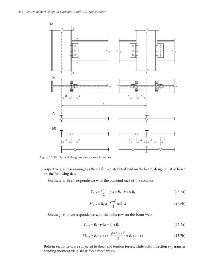
respectively, and assuming p as the uniform distributed load on the beam, design must be basedon the following data:
Section x–x, in correspondence with the outstand face of the column:
Tx−x =p L2
−p a=Ri−p a≈Ri 15 6a
Mx−x =Ri a−p a2
2≈Ri a 15 6b
Section y–y, in correspondence with the bolts row on the beam web:
Ty−y =Ri−p a+ e ≈Ri 15 7a
My−y =Ri a+ e −p a+ e 2
2≈Ri a+ e 15 7b
Bolts in section x–x are subjected to shear and tension forces, while bolts in section y–y transferbending moment via a shear force mechanism.
x
(a)
(b)
(d)
(c)
x
a e
L
a e aa ee
ae
y
y
Figure 15.30 Typical design modes for simple frames.
452 Structural Steel Design to Eurocode 3 and AISC Specifications

Scheme 2: it is assumed that hinges are located in correspondence of the angle legs connectedto the column flange (section x–x), that is reference is made to the actual beam span length(L − 2a), as shown in Figure 15.30c. It can be noted that:
Section x–x, which is in correspondence of the outstanding face of the column, is interestedby the sole shear force associated with the beam end reaction.Section y–y, which is in correspondence of the bolt row on the beam web, presents bolts sub-jected also to a shear force contribution due to bending moment acting on the section:
My−y =Ri e−p e2
2≈Ri e 15 8
In accordance with this scheme, columns are subjected to compression and bendingmoment dueto the hinge eccentricity, the value of which can be approximated, from the safe side, as Ri a.
Scheme 3: it is assumed (Figure 15.30d) that hinges are located in correspondence of the row ofthe bolts connected to the beam web (section y–y) and the beam span results reduced with ref-erence to one of the previous schemes.
Section x–x in correspondence of the outstanding face of the column a bending moment due tothe hinge eccentricity (Ri e) acting in addition to the shear force Ri.
Section y–y in correspondence of the bolts row on the beam web, which transfers a shearforce Ri.
Simple connections must be able to transfer only a very limited value of bending moment, inorder to guarantee the full compatibility between the structure and the design model. An adequaterotational capacity must be guaranteed by an appropriate selection of the connection details,which has to be properly taken into account when designing the beam. Table 15.1 is referredto some common design schemes for isolated beams and reports the values of the required rota-tion (determined neglecting the influence of the shear deformability) to be compared with therotational capacity of the connection.
Table 15.1 Value of the design rotation required for some common types of loaded beams.
A
L
B ΦA = ΦΒ A B
L
ΦA
pp L3
24 E Ip
p L3
48 E I
P
L/2 L/2
P L2
16 E IP
L/2 L/2
P L2
32 E I
P
L/3 L/3 L/3
P P L2
9 E IP
L/3 L/3 L/3
P P L2
18 E I
P P P
L/4 L/4 L/4 L/4
5 L2 P32 E I
P P P
L/4 L/4 L/4 L/4
5 L2 P64 E I
Connections 453

As bending moments developed in the joint, the bolts and the welds are subjected to tensionforces in addition to shear forces. Premature failure of those elements, which exhibit a brittle fail-ure and which are more heavily loaded in reality than in the calculation model, therefore has to bestrictly avoided. To enable rotation without increasing the bending moment that develops into thejoint too much, contact between the lower beam flange and the supporting member has to bestrictly avoided. So, it is imperative that the height hp of the plate is less than that of the supportedbeam web. If such a contact takes place, a compression force develops at the place of contact; it isequilibrated by tension forces in the bolts and a significant bending moment develops, as can benoted from Figure 15.31. The level of rotation at which the contact occurs is obviously dependenton the geometrical characteristics of the beam and of the header plate, but also on the actualdeformations of the joint components. A simple criterion that designers could apply, beforeany calculation, is to check whether the risk of contact may be disregarded. In particular, the fol-lowing rough assumptions are made:
• the supporting element remains un-deformed;• the centre of rotation of the beam is located in correspondence of the lower extremity of the
header plate.
On the basis of such assumptions, a safe estimation (i.e. a lower bound) of the joint limit rota-tion (ϕL) is:
ϕL =tphe
15 9
where tp is the thickness of the plate.In order to increase ϕL it is enough to reduce the distance hc; that is to weld the plate close to the
beam bottom flange. In this case, a joint has adequate ductility if failure is due to the plasticity onthe header plate, that is if this collapse occurs before failures of bolts as well as of the welding,which are typically brittle failure modes.
15.5.2 Rigid Joints
As previously introduced, if the rigid joint framemodel is adopted, no relative rotation is expectedbetween the beam and the column and the joint detailing has to be adequate to transfer the
hp
𝜙L
he
1
2Moment
(a) (b)
Rotation
tp
Figure 15.31 Header plate connection: (a) contact between the beam and the column flanges and (b) moment-rotation joint curve before the contact (zone 1) and after the contact (zone 2).
454 Structural Steel Design to Eurocode 3 and AISC Specifications
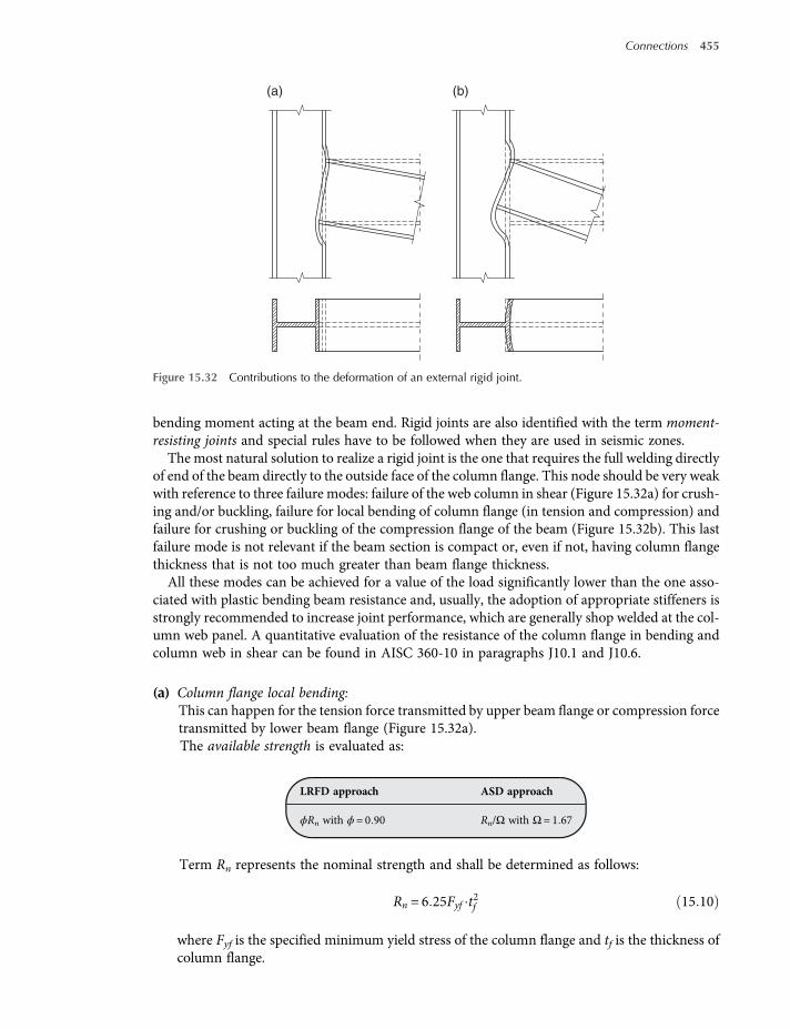
bending moment acting at the beam end. Rigid joints are also identified with the term moment-resisting joints and special rules have to be followed when they are used in seismic zones.The most natural solution to realize a rigid joint is the one that requires the full welding directly
of end of the beam directly to the outside face of the column flange. This node should be very weakwith reference to three failure modes: failure of the web column in shear (Figure 15.32a) for crush-ing and/or buckling, failure for local bending of column flange (in tension and compression) andfailure for crushing or buckling of the compression flange of the beam (Figure 15.32b). This lastfailure mode is not relevant if the beam section is compact or, even if not, having column flangethickness that is not too much greater than beam flange thickness.All these modes can be achieved for a value of the load significantly lower than the one asso-
ciated with plastic bending beam resistance and, usually, the adoption of appropriate stiffeners isstrongly recommended to increase joint performance, which are generally shop welded at the col-umn web panel. A quantitative evaluation of the resistance of the column flange in bending andcolumn web in shear can be found in AISC 360-10 in paragraphs J10.1 and J10.6.
(a) Column flange local bending:This can happen for the tension force transmitted by upper beam flange or compression forcetransmitted by lower beam flange (Figure 15.32a).The available strength is evaluated as:
LRFD approach ASD approach
ϕRn with ϕ= 0 90 Rn/Ω with Ω= 1 67
Term Rn represents the nominal strength and shall be determined as follows:
Rn = 6 25Fyf t2f 15 10
where Fyf is the specified minimum yield stress of the column flange and tf is the thickness ofcolumn flange.
(a) (b)
Figure 15.32 Contributions to the deformation of an external rigid joint.
Connections 455

(b) Column web panel zone shearThe column web area delimited by connected beam(s) (panel zone) is subjected to shearstress due to column shear and beam moments (Figure 15.33). This total web shear Ru
for load and resistance factor design (LRFD) or Ra for allowable stress design (ASD)can be evaluated, with reference to the LRFD forces, as:
LRFD approach ASD approach
Ru =Mu1
dm1+Mu2
dm2−Vu (15.11a)
whereMu1, Mu2 are factored moments and dm1, dm2 arethe distance between beam flange centroids.
Ra =Ma1
dm1+Ma2
dm2−Va (15.11b)
where Ma1, Ma2 are nominal moments and dm1, dm2
are the distance between beam flange centroids.
In order to avoid reinforcing web panel, adding stiffeners, for example the following expres-sions have to be satisfied:
LRFD approach ASD approach
Ru ≤ϕRn (15.12a)
where ϕRn (ϕ= 0 90) is the available strength of the webpanel zone for the shear failure mode.
Ra ≤Rn Ω (15.12a)
where Rn/Ω (Ω= 1 67) is the available strength of theweb panel zone for the shear failure mode.
Rn is the nominal strength and can be determined as follows (not considering web plasticresistance):
(1) for Pr ≤ 0.4 Pc:
Rn = 0 60Fy dc tw 15 13a
(2) for Pr > 0.4 Pc:
Rn = 0 60Fy dc tw 1 4−PrPc
15 13b
Story shear, Vu
A dm
1
A
dc
Vu
ΣRu
Mu2
Mu1
dm
2
Figure 15.33 Forces in the column panel zone.
456 Structural Steel Design to Eurocode 3 and AISC Specifications

where dc is the column depth, tw is the column web thickness, Pr is the requited axial strength(according to LRFD or ASD loading combinations), Pc = 0.60 Py and Py is the column axial yieldstrength (Py = FyAg).As an example, in Figure 15.34 typical common solutions for rigid beam-to-column joints are
presented. In particular, note the:
(a) fully welded connection of an external node at the roof level. Horizontal stiffeners are shopwelded to the column in correspondence of the bottom beam flange;
(b) bolted knee-connection of an external node at the roof level. Both ends of beam and columnare completed with shop welded stiffeners. Furthermore, the internal flange and the web ofthe column have been shop removed in order to allow a quick site assemblage via traditionalbolting technique;
(a) (b)
(c)
(e) (f)
(d)
Figure 15.34 Examples of typical rigid joints.
Connections 457

(c) knee-connection of an external node at the roof level with external end plate shop welded tothe member ends. In this case the diagonal cutting of the beam end is required;
(d) welded T-connection to join a floor beam to an external column. Stiffeners have been placedin correspondence of both the top and the bottom flange of the beam;
(e) bolted end plate connection to join a floor beam to the flange of an internal column;(f) bolted end plate connection to join a floor beam to the web of an internal column.
15.5.3 Semi-Rigid Joints
As previously introduced in Section 3.4, the models of hinged and rigid joints, which have beenextensively used in the past, have a quite limited application nowadays, owing to the need toaccount for the actual joint response. Classification in the past was mainly based on the connec-tion joint components, independent of the mechanical properties and this could lead, in somecases, to unsafe design. As an example, the results of a research carried out at the Universityof Trento (I) on beam-to-column joints are presented in Figure 15.35, where the non-dimensionalmoment-rotation curves, which have been evaluated with reference to a beam spam of 6m (19.7 ft),are presented for some of the tested joints. As to the joint classification in the figure, reference ismade to the EC3 criteria. It can be noted that EPBC and EPC connections, which are traditionally
(d)
EPBC–1 tp= 12 mm
EPBC–2 tp= 18 mm
tp
(e)
EPC–1
tp=18 mm
tp
TSC–1
tp=12 mm
(a)
tp
(b)
FPC–1
tp=12 mm
tp
(c)
FPC–2
tp=12 mm
tp
1.0
m
0.8
0.6
0.4
0.2
0.0 0.2 0.4 0.6 0.8 1.0 ϕ
Limiti EC3 per telai
Non controventati
Controventati
TSC
EPC
FPC–1
FPC–2
EPBC–1
EPBC–2
Figure 15.35 A typical moment-rotation joint curve classified according to EC3 criteria.
458 Structural Steel Design to Eurocode 3 and AISC Specifications
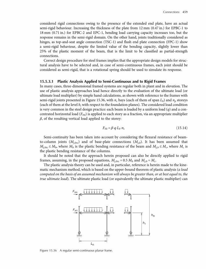
considered rigid connections owing to the presence of the extended end plate, have an actualsemi-rigid behaviour. Increasing the thickness of the plate from 12mm (0.47 in.) for EPBC-1 to18mm (0.71 in.) for EPBC-2 and EPC-1, bending load carrying capacity increases too, but theresponse remains in the semi-rigid domain. On the other hand, joints traditionally considered ashinges, as top-and-seat angle connection (TSC-1) and flush end plate connection (FPC-1) showa semi-rigid behaviour, despite the limited value of the bending capacity, slightly lower than25% of the plastic moment of the beam, that is the limit to be classified as partial-strengthconnections.Correct design procedure for steel frames implies that the appropriate design models for struc-
tural analysis have to be selected and, in case of semi-continuous frames, each joint should beconsidered as semi-rigid, that is a rotational spring should be used to simulate its response.
15.5.3.1 Plastic Analysis Applied to Semi-Continuous and to Rigid FramesIn many cases, three-dimensional framed systems are regular both in plant and in elevation. Theuse of plastic analysis approaches lead hence directly to the evaluation of the ultimate load (orultimate load multiplier) by simple hand calculations, as shown with reference to the frames withsemi-rigid joints presented in Figure 15.36, with nc bays (each of them of span Lb) and np storeys(each of them at the level hi with respect to the foundation planes). The considered load conditionis very common in the steel design practice: each beam is loaded by a uniform load (q) and a con-centrated horizontal load (FHi) is applied to each story as a fraction, via an appropriate multiplierβ, of the resulting vertical load applied to the storey:
FHi = β q Lb nc 15 14
Semi-continuity has been taken into account by considering the flexural resistance of beam-to-column joints (Mj,btc) and of base-plate connections (Mj,b). It has been assumed thatMj,btc ≤Mb, where Mb is the plastic bending resistance of the beam and Mj,b ≤Mc, where Mc isthe plastic bending resistance of the columns.It should be noted that the approach herein proposed can also be directly applied to rigid
frames, assuming, in the proposed equations, Mj,btc = 0.5Mb and Mj,b =Mc.The plastic analysis theory can be used and, in particular, reference is herein made to the kine-
matic mechanism method, which is based on the upper-bound theorem of plastic analysis (a loadcomputed on the basis of an assumed mechanism will always be greater than, or at best equal to, thetrue ultimate load). The ultimate plastic load (or equivalently the ultimate plastic multiplier) can
FHn
Lb
h1
hfn
FH1
Figure 15.36 A regular semi-continuous planar frame.
Connections 459

be evaluated directly on the basis of hand calculations. Defining qu as the uniform beam load asso-ciated with a full plastic mechanism (or equivalently αu) the ultimate load multiplier associated tothe reference uniform load qs (with qu = αu qs) we can obtain:
• Beam mechanism (Figure 15.37a):
qu =8 Mj,btc +Mb
L2b15 15a
αu =8 Mj,btc +Mb
qsL2b15 15b
• Panel mechanism (Figure 15.37b):
qu =2Mj,btc nc np +Mj,b nc + 1
β nc Lb
np
i= 1
hi
15 16a
αu =2Mj,btc nc np +Mj,b nc + 1
β nc Lb qs
np
i= 1
hi
15 16b
• Mixed mechanism (Figure 15.37c):
qu =Mj,btc nc np +Mj,b nc + 1 + 2 Mb nc np
β nc Lb
np
i= 1
hi + 0,25 nc np L2b
15 17a
FHn
(a) (b) (c)
FH1
ϑ ϑ ϑ ϑ ϑϑ
Lb
2ϑ 2ϑ
FH1 FH1
Lb Lb
FHn FHn
ϑ× hfn ϑ× hfn
ϑ× h1 ϑ× h1
Figure 15.37 Typical collapse mechanisms for regular semi-continuous frames: (a) beam mechanism, (b) panelmechanism and (c) mixed mechanism.
460 Structural Steel Design to Eurocode 3 and AISC Specifications

αu =Mj,btc nc np +Mj,b nc + 1 + 2 Mb nc np
qs β nc Lb
np
i= 1
hi + 0,25 nc np L2b
15 17b
As in case of hinged joints, for semi-rigid and rigid joints it is also necessary to guarantee anappropriate level of rotational capacity, owing to the fact that a complete plastic mechanism isgenerally activated only if relative rotations can occur at the plastic hinge locations.As an example of the importance of the rotational capacity of the plastic hinge, the isolated
beam with semi-rigid joints presented in Figure 15.38 can be considered. The static method toevaluate the ultimate load is applied, which is based on the lower-bound theorem of the plasticanalysis (a load computed on the basis of an assumed distribution of internal forces and bendingmoments with the applied loading and where member resistance is not exceeded is less than, or atbest equal to the true ultimate load). Joint bending resistance (Mpl,j) is supposed to be equal to halfof the one of the beam (Mpl,b), that is partial strength joints with Mpl,j =Mpl,b are used.As in the example of fixed-end beams (see Section 3.6.1) and also in case of semi-rigid joints, the
first two plastic hinges, which are at the joint location, are activated simultaneously for a uniformload pe evaluated as:
pe =12 Mpl, j
L2=6 Mpl,b
L215 18
Also in this case, the beam does not collapse and the additional load Δp (Figure 15.39) can beincreased until another plastic hinge is activated (Figure 15.40).
Apu
Mpl,j Mpl,j
C
L
B
Figure 15.38 Isolated beam with semi-rigid joints.
A C B
Mpl,j
MC,pe
MC,Δp
Mpl,j
pe
Δp
Figure 15.39 Activation of the plastic hinges at the beam ends.
Connections 461

This value of Δp corresponds to the formation of the third plastic hinge, which transforms thestructure in a mechanism and hence is named Δpu, obtained by the condition:
Mpl,b
4+Δpu L2
8=Mpl,b 15 19
It should be noted that it immediately evaluates the values of the rotation required to the joint toactivate the plastic mechanism Δϕu, which is:
Δϕu =Δpu L3
24 E I=
6Mpl,b
L2L3
24 E I=Mpl,b L3
4 E I=Mpl, j L3
8 E I15 20
It is of fundamental importance that the required rotation Δϕu can be reached by the selectedtype of semi-continuous joints avoiding brittle and premature failure.
15.6 Joint Standardization
In a typical braced multi-storey frame, joints represent about the 5% of total steel weight, but the30% or more of the cost of steel structure. Starting from this consideration, BCSA (British Con-structional Steelwork Association) and SCI (Steel Construction Institute) in the UK have devel-oped standard connections in the field of simple joints as well as moment connections.
Joint standardization reduces the number of connection types and promotes the use of standardcomponents for fittings: M20 8.8 bolts fully threaded whenever possible, with holes generally22 mm in diameter, punched or drilled, spaced at standard values, end plates and fin plates 10or 12 mm of thickness, and so on.
Using standardized components improves availability, leads to a material cost reduction andreduces time for buying, storage and handling. Furthermore, on the side of design, using stand-ardized joints guarantees that every joint has a good reliability because it has been computed inadvance by very skilled engineers.
BCSA standardization is available in the so called ‘green books’, several publications issued byBCSA and SCI (see the Bibliography in Appendix B). These standard joints have been computedaccording to EC3 (according to BS 5950 formerly) but, unfortunately, they use United Kingdom’sUB and UC profiles only, excluding European shapes such as the HE and IPE series.
In Table 15.2 an example of joint standardization is shown.A similar effort has been performed by AISC. In AISC Steel ConstructionManual, detailed pro-
cedures for any kind of joint are listed, with a lot of practical tables to help dimensioning the con-nections (Table 15.3).
Unfortunately analogous effort has not been performed up to now in developing EC3. TheCode states principles and rules, but no one has prepared construction manuals starting from it.
Joint standardization, especially for moment connections, is really important also for design ofsteel structures in seismic areas. Moment connections in frames designed for areas with high seis-micity actually have to exhibit two important properties:
A C B
Pu
Mpl,j Mpl,b Mpl,j
Figure 15.40 Collapse mechanism.
462 Structural Steel Design to Eurocode 3 and AISC Specifications

Table15
.2Excerptfrom
JointinSteelC
onstruction:
SimpleJointsto
Euroco
de3,
byBCSA
-SCI,Pu
blicationP3
58(201
1).
Beam
S275
Endplates
S275
Bolts
M20
8.8
Partial
depthendplates,ordinaryor
flow
drillbo
lts
200×12
OR150×10
mm
endplate
Beam
size
(VRd,beam)
Bolt
rows,n1
Un-notched
Singlenotch
Dou
blenotch
Fitting(endplate)
Fillet
weld
Min
supp
ort
thickn
ess
Tying
Shear
resist,
VRd(kN)
Critical
Check
Shear
resist,
VRd(kN)
Maxim
umlength,
l n(m
m)
Shear
resist,
VRd(kN)
Maxim
umlength,
l n(m
m)
Width,
b p(m
m)Thck,
t p(m
m)Heigh
t,h p
(mm)Gau
ge,
p 3(m
m)Leg,
s(m
m)
S275
S355
Resist,
NRd,u
(kN)
Critical
check
610×229×140
7902
4902
208
776
100
200
12500
140
84.8
4.2
554
11(1300kN
)6
776
4776
312
776
100
200
12430
140
84.9
4.2
477
11610×229×125
7819
4819
201
697
100
200
12500
140
84.4
3.8
548
11(1170kN
)6
705
4705
305
697
100
200
12430
140
84.4
3.9
471
11610×229×113
7764
4764
193
643
100
200
12500
140
84.1
3.6
544
11(1000kN
)6
657
4657
296
643
100
200
12430
140
84.1
3.6
468
11610×229×101
7750
4750
182
624
100
200
12500
140
84.0
3.5
525
11(1060kN
)6
645
4645
284
624
100
200
12430
140
84.0
3.5
462
11

(1) they must be more resistant than the beam they connect;(2) they must maintain the greater part of their moment resistance with node rotation prescribed
by Code, without showing brittle behaviour.
To achieve both targets it is necessary to test experimentally different typologies and verify theirbehaviour with special attention to their ductility. Calculations cannot guarantee the ductility of ajoint type: sometimes after changing just a detail a joint has shown amore ductile behaviour. AISChas tested few typologies of moment connections (prequalified connections) to be used in seismicframes and has developed a specific standard design procedure to use for them, which is containedin document AISC 358-10 ‘Prequalified Connections for Special and Intermediate Steel MomentFrames for Seismic Applications’. In the document, the scope is clearly declared:
The connections contained in this Standard are prequalified to meet the requirements in theAISC Seismic Provisions only when designed and constructed in accordance with the
Table 15.3 End plate connections according to the AISC Steel Construction Manual.
W44 Table 10-4 bolted/welded shear end-platevonnections
3 in./4 in. bolts12 rows
Bolt and end-plate available strength (kips)
ASTM design Thread condition Hole type End-plate thickness (in.)
1/4 5/16 3/8
ASD LRFD ASD LRFD ASD LRFD
A325/F1852 N — 197 295 246 369 254 382X — 197 295 246 369 295 443SC Class A STD 177 266 177 266 177 266
OVS 128 192 128 192 128 192SSLT 151 226 151 226 151 226
SC Class B STD 197 295 246 369 253 380OVS 183 274 183 274 183 274SSLT 195 293 215 323 215 323
A490 N — 197 295 246 369 295 443X — 197 295 246 369 295 443SC Class A STD 197 295 221 332 221 332
OVS 160 240 160 240 160 240SSLT 188 282 188 282 188 282
SC Class B STD 197 295 246 369 295 443OVS 196 294 229 343 229 343SSLT 195 293 244 366 269 403
Weld and beam available strength (kips) Support available70 ksi weld size (in.) Minimum beam web thickness (in.) Rn/Ω фRn Strength per inch
kips kips Thickness (kips/ft)ASD LRFD ASD LRFD
3/16 0.286 196 293 1400 2110¼ 0.381 260 3905/16 0.476 324 4863/8 0.571 387 581STD = standard holes N = threads included End-plate BeamOVS = oversized holes X = threads excluded Fy = 36 ksi Fy = 50 ksiSSLT = short-slotted holes transverse to
direction of loadSC = slip critical Fu = 58 ksi Fu = 65 ksi
464 Structural Steel Design to Eurocode 3 and AISC Specifications

requirements of this Standard. Nothing in this Standard shall preclude the use of connectiontypes contained herein outside the indicated limitations, nor the use of other connection types,when satisfactory evidence of qualification in accordance with the AISC Seismic Provisions arepresented to the authority having jurisdiction.
In other words, the engineer can adopt different connections, but he has to demonstrate that suchconnections meet AISC requirements and this is not an easy job.No similar prequalification of joints to be used for frames in seismic zones exists in Eurocode
3 up to now. So the choice of a joint that shows the correct behaviour under seismic actions is not astraightforward task.
Connections 465

CHAPTER 16
Built-Up Compression Members
16.1 Introduction
Individual members may be combined in a quite great variety of ways to produce a more efficientcompound cross-section member. The main advantage in the use of built-up members is thehigh value of the load-carrying capacity that can be achieved by combining suitably very slenderisolatedmembers. Furthermore, resistance can significantly exceed the sum of the axial resistancesof the component members, which can, as a result, be significantly limited by instability phenom-enon in the range of standard products.
16.2 Behaviour of Compound Struts
It can be noted that built-up compression members are composed by isolated members (chords)appropriately connected in a non-continuous way. For the sake of simplicity, chords can be com-pared with the flanges of I- or H-shaped hot-rolled profiles, the web of which, in built-up mem-bers, is realized by means of lacings, battens or plates. From a practical point of view, struts canbe classified on the basis of the distance between the centroids of the chords (h0) and of the radiusof gyration of the chord along the axis where the element is compounded (i1). In particular it ispossible to distinguish:
• strut with distant chords, if h0 > 6i1, such as laced struts and struts with batten plates, typicallyused as columns, that is to sustain vertical compression axial load;
• struts with close chords, if h0 < 3i1, such as buttoned struts (also named closely spaced built-upmembers), which are typically used for the chords of both trusses or for the struts in case ofelevated axial loads.
With reference to the type of connection between the chords, it is possible to distinguish:
• Laced members (Figure 16.1), where lacing members are interested by axial forces and eachchord can be considered as a simple strut, with a buckling length equal to the joint spacing.Shear deformability mainly depends on the axial deformability of the lattice members. Sometypical laces struts are presented in Figure 16.1c, which differ for the type of panel components.Most commonly used solutions are presented by N-type (a) and V-type laced panels (b) one,
Structural Steel Design to Eurocode 3 and AISC Specifications, First Edition. Claudio Bernuzzi and Benedetto Cordova.© 2016 John Wiley & Sons, Ltd. Published 2016 by John Wiley & Sons, Ltd.

where both diagonal and batten members can be subjected to compression or tension force.Solution (c) is obtained from (b) by inserting battens in order to reduce the effective lengthof the chord while solutions (d) and (e) present, in the same panel two laced members: oneunder tension and one under compression.
• Struts with batten plates (Figure 16.2), composed by chords rigidly connected by battenplates. Chords are compressed and bent, with a linear distribution of the bending moments nullat the middle of each panel. Moment distribution can be approximated with reference to theundeformed situation, while the vertical load buckling effects are considered balanced by equaland opposite axial, forces in the chords. These struts have a typical Vierendeel beam behaviour.
• Buttoned struts (Figure 16.3), in which the single chord is compressed and bent with a bendingmoment distribution that cannot be approximated as linear. In this case the overall lateral
d
(a) (b) (c)
(a) (b) (c) (d) (e)
Figure 16.1 Typical arrangements for laced struts (a), the associated design model (b) and types of lacingpanels (c).
d
(a) (b)
Figure 16.2 Typical arrangements for struts with batten plates (a) and the associated design model (b).
Built-Up Compression Members 467

bending contribution becomes significant if compared with the local one of the single chord sothat bending moment values must be computed with reference to the deformed configuration(second order analysis). Shear deformability depends mainly on the flexural deformability ofthe chords and on bolt slippage when bolted joints are used.
Load carrying capacity of built-up members is strictly influenced by several aspects, such asoverall and local response of members and connection behaviour.
Overall response of built-up members depends significantly on the deformability due to bend-ing and shear, which can significantly influence lateral deflection of the compound members forthe presence of initial geometrical imperfections. Bending deformability depends on the value ofthe moment of inertia of the compound struts while shear deformability is mainly affected by theperformances of lacings and battens and by the deformability of the connections.
Local behaviour of each chord and of the other strut components has to be verified in accord-ance with appropriate criteria as for isolated members.
Connections between the constituent members, which must be able to absorb any sliding actionbetween the profiles forming the cross-section can be characterized by a significant deformabilityable to increase significantly the overall and lateral deflection of the member and thus thedestabilizing effect of vertical loads increases, too. Furthermore, it should be noted that connec-tions represent a critical aspect of the compound struts, due to the fact that an excessive deform-ability decreases significantly the load carrying capacity. Two types of connections can bedistinguished:
• connection with static function if able to resist sliding force between the isolated members;• connection with kinematic function if able to prevent the buckling (local) of the isolated mem-
ber in the weakest direction.
d
(a) (b)
Figure 16.3 Typical arrangements for buttoned struts (a) and the associated design model (b).
468 Structural Steel Design to Eurocode 3 and AISC Specifications

As an example, the case presented in Figure 16.4 can be considered with connections resisting tosliding forces. The two angles behave as single isolated members for bending in direction y (aboutthe x-axis) and hence a connection with kinematic function can be adequate. Otherwise, whenbending in direction x (about the y-axis) is considered (a), the section must behave as a built-upmember (c) and hence a static function is required. If the angle legs are equal, there is no reasonfor statically connecting the two bars, when their buckling lengths are equal in both planes. Itmight be economical to connect the angles statically, but only if their legs are not equal or if buck-ling lengths in the two planes differ. However, a suitable composition can equalize the slendernessvalues in the two planes. For the same reason, it is always convenient to compose a section of twochannels when buckling lengths in the two planes are equal.Furthermore, it is worth mentioning that the influence of local behaviour on the overall per-
formance of a strut is difficult to quantify. It is preferable to ignore interaction between local andoverall response but, at the same time, to define dimensional limitations to built-up membergeometry that, if complied with, guarantees that the overall behaviour of the strut is practicallyindependent on local behaviour of any single chord.With reference to isolatedmembers, as previously introduced in Chapter 6, when shear deform-
ability is considered, the elastic critical load Ncr,id can be defined on the basis of the Eulerian load,Ncr, which is evaluated considering only the flexural contribution, as:
Ncr, id =Ncr
1 +χTG A
Ncr
=1
1Ncr
+χTG A
=π2 E A
λeq2 16 1
where χT is the shear factor of the cross-section of area A and E and G are the Young’s and theshear modulus, respectively.For isolated members, the equivalent slenderness, λeq, can be evaluated as:
λeq = λ2 +χT π2 E
G16 2
A similar approach can be adopted also in the design of strut members and slenderness λeqdepends strictly on the type of struts as well as on the panel geometry, as more clearly explainedin the following section.
y
x
y
(a)
(b)
(c)
x
N/2 N/2
N/2N/2
Figure 16.4 Examples of connections able to absorb slippage force.
Built-Up Compression Members 469

Recent design approaches for struts are based on a structural analysis accounting directly forsecond order effects. The model of a pinned-end strut is proposed, with a length L and an initialsinusoidal imperfection characterized by the maximum amplitude e0. As already considered forisolated compression member with geometrical imperfections, deflection of the midspan v due toan axial load N acting on the imperfect element can be approximated as:
v =e0
1−N
Ncr, id
16 3
where Ncr,id is the critical load of the strut, which can be expressed as a function of the elasticcritical load, Ncr, and of the panel shear stiffness, Sv, as:
Ncr, id =1
1Ncr
+1Sv
16 4
With reference to the midspan cross-section (Figure 16.5), the maximum bending moment Macting can be expressed, considering second order effects, as:
M =e0 N
1−N
Ncr, id
16 5
As a consequence, the maximum axial load on the chord, Nf, can be evaluated directly on thebasis of equilibrium equation as:
Nf =N2+Mh0
=N2
1 +
2 e0h0
1−N
Ncr, id
16 6
A very important aspect of built-up design regards the prevention of instability, which has to bedeveloped by taking adequately into account the presence of concentrated connections betweenthe chords. Two different buckling modes have to be explicitly considered into design:
N
N
N N/2
N/2
M/h0
M/h0
h0
M
M
Figure 16.5 Second order effects on the strut and axial load on the chords at the midspan.
470 Structural Steel Design to Eurocode 3 and AISC Specifications

• overall buckling mode, affecting built-up members in its whole length (Figure 16.6a) and sig-nificantly influenced by the loading condition as well as by the member end restraints;
• local buckling mode, affecting the chord between each panel (Figure 16.6b), with an effectivelength depending on the end panel restraints and a buckling mode depending on the chordcross-section geometry.
In addition to the checks on the components realizing the struts, load carrying capacity dependssignificantlyon the stability andhence theevaluationof the shear stiffness (Sv) of thepanel is requiredas preliminary to the verification. In the following, two common cases are considered as examples ofthe procedure to determine Sv. Several studies carried out in the past demonstrated that a designbased on these equations shows an adequate safety level if at least four panels form the strut.
16.2.1 Laced Compound Struts
The built-up laced column in Figure 16.7 is characterized by an equal N-type panel, the sheardeformability of which influences the overall compression response. With reference to each panel,shear displacements are due to lengthening of the diagonal lacing and to the shortening of thebatten.As to the first contribution, lacing length is Ld = a/sinϕ and tension force isNd = T/cosϕ. Elong-
ation Δ of the diagonal element can be evaluated as:
Δ = ε Ld =Nd
E AdLd 16 7
Lacing elongation can be re-written as:
Δ=T
cosϕ1
EAd
asenϕ
=TEAd
asenϕ cosϕ
16 8
(a) (b)
Figure 16.6 Typical failure modes for a battened column: (a) overall buckling and (b) local buckling of the chordbetween the panels.
Built-Up Compression Members 471

The corresponding lateral displacement δ1 of the panel, assuming that displacements are small, is:
δ1 =Δ
cosϕ=
TEAb
asenϕ cos2ϕ
16 9a
Shortening of the batten, subjected to the external horizontal force T (Figure 16.7c) is:
δ2 =TbEAb
16 9b
By the sum of δ1 and δ2, the total angular displacement produced by the horizontal force Tapplied to the panel, γ, is:
γ =δ1 + δ2
a=T
1EAdsenϕcos2ϕ
+b
aEAb16 10
As a consequence, shear stiffness, Sv, can be directly evaluated from the relationship γ =TSv,
hence resulting in:
1SV
=1
EAdsenϕcos2ϕ+
baEAb
16 11
On the basis of the previous Eq. (16.4), substituting the expression of the shear stiffness, it canbe obtained:
Ncr, id =1
1Ncr
+1
EAd cosϕsen2ϕ+
baEAb
16 12
Influence of the shear stiffness could be also taken into account considering Ncr, id =π2EIk2β,eqL
2and
introducing an appropriate effective length factor kβ,eq, defined as:
kβ,eq = 1 + π2EIL2
1EAdsenϕcos2ϕ
+b
aEAb16 13a
P
I
P
b
b
T T
Q
(a) (b) (c)
Q
γ1 γ1
δ1 δ2
ϕϕ ϕ
a a
b
a
Figure 16.7 Example of built-up laced member (a): deformed shape of the panel due to deformation of thediagonal (b) and of the batten (c).
472 Structural Steel Design to Eurocode 3 and AISC Specifications

Considering that cosϕ=bLd, sinϕ=
aLd, and using π2≈ 10, term kβ,eq can be alternatively
defined as:
kβ,eq = 1 + π2IL2
1b2a
L3dAd
+b3
Ad16 13b
In both Eqs. (16.12) and (16.13a), the function f(ϕ) = sinϕ cos2ϕ is contained, which assumesmaximum value approximately for ϕ = 35 . Moreover, if the angle ϕ ranges between 30 and 45the value of f(ϕ) is very similar to f(ϕ = 35 ), which guarantees the maximum efficiency of thebuilt-up lattice member.
16.2.2 Battened Compound Struts
In the case of a compound strut only made of batten plates, as the one in Figure 16.8a, the chordsare subjected to bending, shear and axial load while battens are mainly affected by shear and bend-ing moments. For these members, by using the same approach already adopted for lattice built-upmembers, reference has to be made to an internal panel, as the one delimited by the sectionsm–nand m1–n1.Shear stiffness of the panel can be evaluated on the basis of the horizontal displacements δ due
to the following contributions:
(1) flexural deformation of the chords (δF,cor) (as in Figure 16.8b);(2) flexural deformation of the batten (δF,cal) (as in Figure 16.8c);(3) shear deformation of the batten (δT,cal).
Battened members are internally, statically indeterminate structures but the evaluation ofinternal forces and moments is usually carried out by assuming that each panel is connected withthe other via hinges, considering that the deflection of the chords has a point of inflection at sec-tions m–n and m1–n1.
m
m1 n1
n
I
a
a /2
a /2
a2
a
2
a
2
a
T
δ1 δ1
2
2
(a) (b) (c)
T
2
T
2
T
2
Figure 16.8 Example of a built-up battenedmember (a): deformed panel shape due to the bending of the chords (b)and due to the bending of the batten (c).
Built-Up Compression Members 473

The total horizontal displacement δ due to a horizontal force, T, applied to the end of theconsidered panel can be obtained as:
δTOT = δF, cor + δF, cal + δT , cal 16 14
where subscripts F and T are related to the deformation associated with flexure and shear, respect-ively, while cor and cal are related to the chord and to the batten, respectively.
Flexure of the Chords Term δ1, which is related to the displacement of the end of one of thetwo chords, is evaluated considering a cantilever beam subjected to a lateral force equal to T/2:
δ=T2
a2
3 13EIcor
=Ta3
48EIcor16 15a
δF,cor = 2δ1 = 2Ta3
48EIcor=
Ta3
24EIcor16 15b
Flexure of the Batten The total displacement δ2 of the batten in bending is due to the rotation θat the chord-to-batten node associated with the bending moment. For each chord, each of the two
cantilever beams of length equal to a/2 are subjected to a moment ofT2
a2
and hence the total
moment at each end of the batten isTa2
(given by 2T2
a2
). As a consequence it is possible to
evaluate rotation and the associated displacement, respectively as:
θ =Ta2
13EIcal
b2=
Tab12EIcal
16 16a
δF,cal = 2θa2=
Ta2b12EIcal
16 16b
Shear Deformation of the Batten The displacement δT,cal due to the shear deformation of the
batten is evaluated with reference to the model of a beam under a constant shear load ofT ab.
Considering the shear strain γ =χTTabGAcal
, where χT is the shear factor of the batten, the associated
displacement is:
δT ,cal = 2γa2=
χTAcalG
Ta2
b16 17
Shear stiffness of the battened panel, SV, which depends on the values of these displacements,can be determined as:
1SV
=γTOTT
=δF,cor + δF,cal + δT ,cal
aT=
a2
24EIcor+
ab12EIcor
+χTa
bAcalG16 18
474 Structural Steel Design to Eurocode 3 and AISC Specifications

Finally, the elastic critical load for a battened struts with hinged ends,Ncr,id, can be expressed as:
Ncr, id =π2EIL2
1
1 + π2EIL2
a2
24EIcor+
a b12EIcal
+χT abAcalG
16 19
where I is the moment of inertia of the compound strut.Reference can be made to an appropriate effective length factor, kβ,eq, which for struts with bat-
tened plates is defined as:
kβ,eq = 1 + π2EIL2
a2
24EIcor+
ab12EIcal
+χTa
bAcalG16 20
Furthermore, neglecting the shear deformability of the battens, Eq. (16.20) simplifies to:
kβ,eq = 1 + π2EIL2
a2
24EIcor16 21
Alternatively, design can refer to the overall equivalent slenderness, λeq, defined as:
λeq =βeqL
r=
Lr
2
+ π2I
24Icor
a2
r216 22a
where L is the strut length and r is the radius of gyration, defined as r =I
2Acor.
Due toIr2
= 2Acor and Icor = Acor r2cor , Eq. (16.22a) can be re-written as:
λeq =βeqL
r=
Lr
2
+π2
12arcor
2
16 22b
It can be noted that the slenderness of the strut depends strictly on the overall slenderness of thechords rigidly connected (L/r) to each other in the compound member and on the local slender-ness of the isolated chords delimited by two contiguous battens (a/rcor).
16.3 Design in Accordance with the European Approach
EC3 in its general part 1-1 deals with the verification on compound struts. In particular, referenceis made to uniform built-up compression members with hinged ends that are laterally supported.For these struts, a bow imperfection e0 has to be considered, never lower than L/500, where L is thestrut length (e0≥ L/500). Furthermore, the elastic deformations of lacings or battenings can beconsidered due to a continuous (smeared) shear stiffness SV of the column. The proposedapproach for uniform built-up compression members can be applied if the lacings or battens com-pound consist of equal panels with parallel chords and the minimum number of panels in a mem-ber is three. If these assumptions are fulfilled, the structure is considered regular and it is hencepossible to smear the discrete structure to a continuum.
Built-Up Compression Members 475

It should be noted that the procedure can be applied also if chords are laced or battened them-selves in the perpendicular plane.
With reference to the symbols of Figure 16.9, if NEd and MEd are the design axial load and thedesign maximummoment in the middle of the built-up member considering second order effects,respectively, for a member with two identical chords their design force Nch,Ed is given by theexpression:
Nch,Ed = 0 5 NEd +MEd h0 Ach
2 Ieff16 23
where h0 is the distance between the centroids of chords,Ach is the cross-sectional area of one chordand Ieff is the effective moment of inertia of the built-up member and MEd can be obtained as:
MEd =NEd e0 +MI
Ed
1−NEd
Ncr−NEd
Sv
16 24
where term MIEd is the design value of the maximum moment (if present) in the middle of the
built-up member without second-order effects, Sv is the shear stiffness of the lacings or battenedpanel (Figure 16.9) and term Ncr is the effective critical force of the built-up member that is evalu-ated considering the sole flexural stiffness of the built-up column as:
Ncr =π2 E Ieff
L216 25
where E is the Young modulus, Ieff is the effective moment of inertia of the built-up member and Lis the effective length.
The checks for the elements connecting the chords to each other have to be performed for theend panel taking account of the shear force in the built-up member VEd, defined as:
VEd =π MEd
L16 26
(a) (b) (c)
NEd
NEd
L/2
L/2
a
h0 h0
h0
a
b
b
z
z
AchAch yy
e0
e0=L/500
Figure 16.9 Design model (a) for uniform built-up columns with lacings (b) and battenings (c).
476 Structural Steel Design to Eurocode 3 and AISC Specifications

16.3.1 Laced Compression Members
The chords and diagonal lacings subject to compression should be designed for buckling and sec-ondary moments may be neglected.The effective moment of inertia of laced built-up member, Ieff, is given by:
Ieff = 0 5 h20 Ach 16 27
where Ach is the cross-sectional area of one chord.As to constructional details, single lacing systems on opposite faces of the built-upmember with
two parallel laced planes should be corresponding systems as shown in Figure 16.10a, arranged sothat one is the shadow of the other. When the single lacing systems on opposite faces of a built-upmember with two parallel laced planes are mutually opposed in direction as shown inFigure 16.10b, the resulting torsional effects in the member should be taken into account. Further-more, tie panels should be provided at the ends of lacing systems, at points where the lacing isinterrupted and at joints with other members.The values of the shear stiffness for the most common cases are reported in Figure 16.11.
16.3.2 Battened Compression Members
The effective moment of inertia of battened built-up members is:
Ieff = 0 5 h20 Ach + 2 μ Ich 16 28
Chord
A
(a) (b)
B A B
chord
11
1 1
2 2
2 12
Lacing on face A Lacing on face B Lacing on face A Lacing on face B
2 1
1
2
2
1
2
Figure 16.10 Single lacing system on opposite faces of a built-up member with two parallel laced planes: (a)corresponding lacing system (recommended system) and (b) mutually opposed lacing system (not recommended).
Built-Up Compression Members 477

where Ich is the in plane moment of inertia of one chord and μ is the efficiency factor to be com-puted Table 16.1.
Batten plates as well as their connections have to be verified to the distribution of forces andbending moments presented in Figure 16.12, which are considered when applied on theplane panel.
The shear stiffness, Sv, is defined as:
Sv =24 E Ich
a2 1 +2 Ichn Ib
h0a
≤2 π2 E Ich
a216 29
where Ib is the in plane moment of inertia of one batten.
16.3.3 Closely Spaced Built-Up Members
Built-up compression members with chords in contact or closely spaced and connected, with ref-erence to Figure 16.14, through packing plates (a) or star battened angle members connected bypairs of battens in two perpendicular planes (b) should be checked for buckling as a single integralmember ignoring the effect of the shear stiffness (SV =∞), when the conditions in Table 16.2are met.
In the case of unequal-leg angles (Figure 16.13b), buckling about the y–y axis may be veri-fied with:
d d
d
Ad
Sv= Sv= Sv=2d3
nEAd ah02nEAd ah0
2nEAd ah02
Ad Ad
Av
h0 h0h0
d3 Ad h03
1+Av d
3d3
a
a
a
a
Figure 16.11 Shear stiffness of lacings of built-up members.
Table 16.1 Efficiency factor μ.
Criterion Efficiency factor μ
λ ≥ 150 μ = 075 < λ < 150 μ = 2–λ/75λ ≤ 75 μ = 1.0λ= L
0 5 h20 Ach + 2 Ich2 Ach
478 Structural Steel Design to Eurocode 3 and AISC Specifications
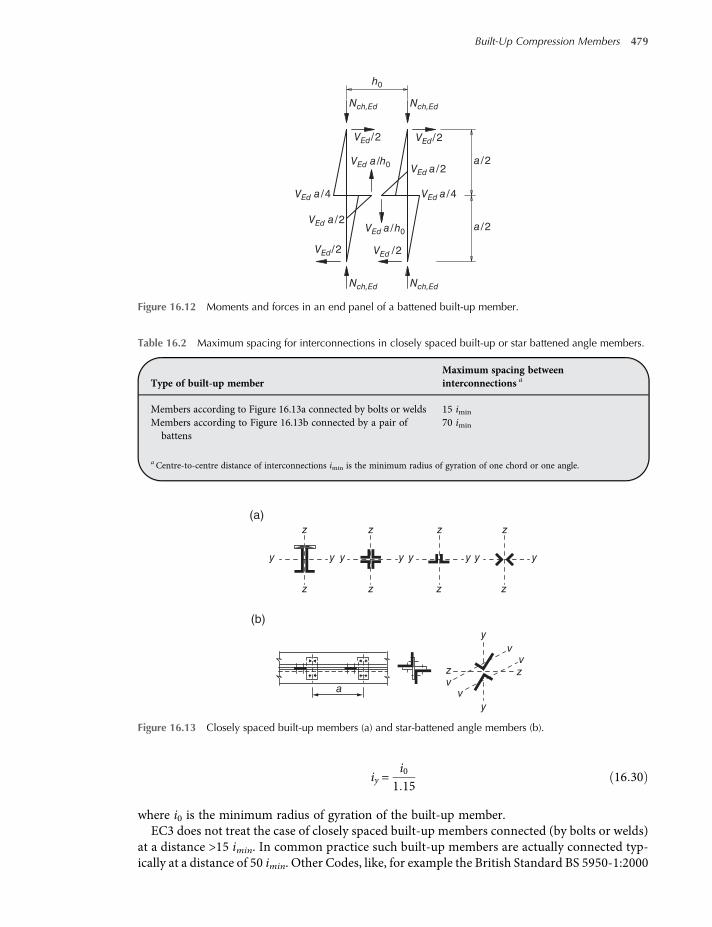
iy =i0
1 1516 30
where i0 is the minimum radius of gyration of the built-up member.EC3 does not treat the case of closely spaced built-up members connected (by bolts or welds)
at a distance >15 imin. In common practice such built-up members are actually connected typ-ically at a distance of 50 imin. Other Codes, like, for example the British Standard BS 5950-1:2000
h0
Nch,Ed
Nch,Ed Nch,Ed
Nch,Ed
VEd/2
VEd a/2
VEd a/4
VEd /2
VEd a/h0
VEd/2
VEd/2
VEd a /2
VEd a /4
VEd a /h0
a/2
a/2
Figure 16.12 Moments and forces in an end panel of a battened built-up member.
Table 16.2 Maximum spacing for interconnections in closely spaced built-up or star battened angle members.
Type of built-up memberMaximum spacing betweeninterconnections a
Members according to Figure 16.13a connected by bolts or welds 15 imin
Members according to Figure 16.13b connected by a pair ofbattens
70 imin
aCentre-to-centre distance of interconnections imin is the minimum radius of gyration of one chord or one angle.
z
z z z z
y y y y y y y
y
y
vv
vvzz
a
(a)
(b)
y
z z z
Figure 16.13 Closely spaced built-up members (a) and star-battened angle members (b).
Built-Up Compression Members 479

(no more used at the present), addressed such a case, prescribing how to design the built-upmember, which can be a single integral member provided that an equivalent slendernessλeq is used, computed as:
λeq = λ2m + λ2c 16 31
where λm is the slenderness of the whole member and λc is the slenderness of the single profile,computed using its minimum radius of gyration, using the distance between adjacent intercon-nections as length. Its value should not exceed 50.
It worth mentioning that some Codes, like the AISC 360-10 and the already mentioned BS5950, treat the case of laced and battened built-up compression members with the same previ-ously explained criteria of an equivalent (increased) slenderness, as shown in the nextparagraph.
16.4 Design in Accordance with the US Approach
Design according to the provisions for load and resistance factor design (LRFD) satisfies therequirements of AISC Specification when the design compressive strength ϕcPn of each structuralcomponent equals or exceeds the required compressive strength Pu determined on the basis ofthe LRFD load combinations. Design has to be performed in accordance with the followingequation:
Pu ≤ϕcPn 16 32
where ϕc is the compressive resistance factor ϕc = 0 90 and Pn represents the nominal compres-sive strength.
Design according to the provisions for allowable strength design (ASD) satisfies the require-ments of AISC Specification when the allowable compressive strength Pn/Ωc of each structuralcomponent equals or exceeds the required compressive strength Pa determined on the basis ofthe ASD load combinations. Design has to be performed in accordance with the followingequation:
Pa ≤ Pn Ωc 16 33
where Ωc is the compressive safety factor (Ωc = 1.67).The nominal compressive strength Pn is determined as:
Pn = FcrAg 16 34
AISC 360-10 specifications treat the case of built-up members composed of two shapes (angles,channels, etc.) either (i) closely spaced and interconnected by bolts or welds (Figure 16.13) or(ii) put at greater distance with at least one open side interconnected by perforated cover plates(Figure 16.14b) or lacing with tie plates (Figure 16.14a). The end connection has to be welded orconnected by means of pretensioned bolts. Intermediate connections can be bolted snug-tight orconnected with pretensioned bolts or welds. In the first case the effective length increases becauseof the greater shear deformability.
480 Structural Steel Design to Eurocode 3 and AISC Specifications
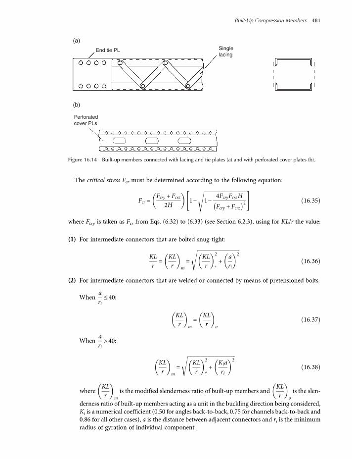
The critical stress Fcr must be determined according to the following equation:
Fcr =Fcry + Fcrz
2H1− 1−
4FcryFcrzH
Fcry + Fcrz2 16 35
where Fcry is taken as Fcr from Eqs. (6.32) to (6.33) (see Section 6.2.3), using for KL/r the value:
(1) For intermediate connectors that are bolted snug-tight:
KLr
=KLr m
=KLr
2
o+
ari
2
16 36
(2) For intermediate connectors that are welded or connected by means of pretensioned bolts:
Whenari≤ 40:
KLr m
=KLr o
16 37
Whenari> 40:
KLr m
=KLr
2
o+
Kiari
2
16 38
whereKLr m
is the modified slenderness ratio of built-up members andKLr o
is the slen-
derness ratio of built-up members acting as a unit in the buckling direction being considered,Ki is a numerical coefficient (0.50 for angles back-to-back, 0.75 for channels back-to-back and0.86 for all other cases), a is the distance between adjacent connectors and ri is the minimumradius of gyration of individual component.
End tie PL Single
lacing
Perforated
cover PLs
(a)
(b)
Figure 16.14 Built-up members connected with lacing and tie plates (a) and with perforated cover plates (b).
Built-Up Compression Members 481

16.5 Worked Examples
Example E16.1 Battened Built-Up Member according to EC3
Verify, according to EC3, a battened built-upmember composed of 2UPN240 as chords, connected by battensrealized with 340 × 150 × 12 plates (13.8 × 5.91 × 0.472 in.) put at a distance of a = 1200 mm (47 in.). Thedistance between centroids of 2 UPN is h0 = 355 mm (14 in.). The built-up member is 20 m (65.6 ft) long.The effective length in the plane of battens is 20 m. In the orthogonal plane the built-up member is restrainedso that flexural instability shall not be considered. The design axial load is 800 kN (180 kips).
Chords 2 UPN 240Steel S275 fy = 275MPa (40 ksi)Area of 1 chord Ach = 42.3 cm2 (6.56 in.2)Moment of inertia about the y–y axis Iy = 3599 cm4 (86.5 in.4)Moment of inertia about the z–z axis Iz = Ich = 274 cm4 (6.58 in.4)Radius of inertia about the y–y axis iy = 9.22 cm (3.63 in.)Radius of inertia about the z–z axis iz = 2.42 cm (0.953 in.)Distance between chord centroids h0 = 355mm (14 in.)Distance between battens a = 1200mm (47 in.)Battens 350 × 150 × 12 plate (13.8 × 5.91 × 0.472 in.)Built-up member length L = 2000 cm (65.6 ft)Design axial load NEd = 800 kN (180 kips)
Verify each chord instability between two battens:Moment of inertia of the whole member:
I1 = 0 5h20Ach + 2Ich = 0 5 × 35 52 × 42 3 + 2 × 274 = 27 202 cm4 654 in 4
Radius of inertia of the whole section:
i0 =I1
2Ach=
27 2022 × 42 3
= 17 93 cm 7 06 in
Critical length of built-up member in the plane containing battens:
λ=Lcri0
=200017 93
= 112; 75≤ λ≤ 150 then μ= 2−λ
75= 2−
11275
= 0 51
Effective moment of inertia:
Ieff = 0 5h20Ach + 2μIch = 0 5 × 35 52 × 42 3 + 2 × 0 51 × 274 = 26 934 cm4 647 in 4
Radius of inertia of the whole section computed using effective moment of inertia:
i0,eff =Ieff2Ach
=26 9342 × 42 3
= 17 84cm 7 02 in
Moment of inertia of batten: Ib =112
× 1 2 × 153 = 337 5 cm4 8 11 in 4
482 Structural Steel Design to Eurocode 3 and AISC Specifications

Shear stiffness:
Sv =24EIch
a2 1 +2IchnIb
hoa
=24 × 21 000 × 274
1202 × 1 +2 × 2742 × 337 5
×35 5120
= 7733 kN
≤2π2EIch
a2=2 × π2 × 21 000 × 274
1202= 7887 kN 1738 kips ≤ 1773 kips
Let’s consider: e0 =Lcr500
=2000500
= 4 cm 1 58 in (eccentricity).
Built-up member critical load:
Ncr = π2EIeff L2 = 3 142 × 21 000 × 26 934 20002 = 1396 kN 314 kips
Second order moment:
MEd =NEde0
1−NEd
Ncr−NEd
SV
=800 × 4
1−8001396
−8007733
=3200
1−0 573−0 103= 9892 kN cm 73 kip− ft
Maximum axial load in a chord considering second order effects:
Nch,Ed = 0 5NEd +MEdh0Ach
2Ieff= 0 5 × 800 +
9892 × 35 5 × 42 32 × 26 934
= 400 + 275 = 675 kN 151 7 kips
Verify a chord under compression loadNch,Ed, using the distance between chord as unbraced length and usingthe minimum radius of inertia.
λ1 = 93 9ε= 93 9235fy
= 93 9235275
= 86 8; λ=aiz=1202 42
= 50
λ= λ λ1 = 50 86 8 = 0 576; Φ= 0 5 1 + α λ−0 2 + λ2
= 0 5 × 1 + 0 49 × 0 576−0 2 + 0 5762 = 0 758
χ =1
Φ+ Φ2−λ2=
1
0 758 + 0 7582−0 5762= 0 800
Compute design compressive strength of a single chord Nch,Rd and compare it with maximum compressionload Nch,Ed.
Nch,Rd = χAchfyγM1
= 0 800 ×42 3 × 27 50
1 00= 931 kN > Nch,Ed = 675 kN OK
209 kips > 152 kips
(Stress ratio: 675/931 = 0.73).Verify the whole built-up member (two chords) for buckling in the plane of battensUse the already computed radius of inertia of the whole section, i0,eff.
Built-Up Compression Members 483

λ=Lcri0,eff
=200017 84
= 112; λ= λ λ1 = 112 86 8 = 1 29
Φ= 0 5 1 + α λ−0 2 + λ2
= 0 5 × 1 + 0 49 1 29−0 2 + 1 292 = 1 599
χ =1
Φ+ Φ2−λ2=
1
1 599 + 1 5992−1 292= 0 393
NRd = χ2AchfyγM1
= 0 393 ×2 × 42 3 × 27 50
1 00= 914 kN >NEd = 800 kN
Stress rate: 800/914 = 0.88.In this case, the verification of the whole built-up member for buckling on the length of 20 m is dominant
on the verification of a single chord for buckling on the distance between battens. In the verification of thewhole member the effective moment of inertia has been used.
Verify the whole built-up member (two chords) for buckling in the plane orthogonal to that of the battens.We hypothesize that built-up member is braced in this plane, so no check is needed.
Batten check:Shear and moment verification (see Figure 16.13). Max shear:
VEd = πMEd
L= 3 14 ×
98772000
= 15 5 kN 3 49 kips
Max shear and bending moment in the batten:
Vcal,Ed =VEd ah0
=15 5 × 120
35 5= 52 4 kN 11 8 kips
Mcal,Ed =VEd a2
=15 5 × 120
2= 930 kN cm 6 86 kip− ft
Shear area: Av = 15 × 1 2 = 18 cm2 2 79 in 2
Shear strength:
Vc,Rd =Vpl,Rd =Avfy3 γM0
=18 × 27 50
3 × 1 05= 272 2 kN 61 2 kips
Shear check: Vcal,Ed Vc,Rd = 52 4 272 2 = 0 19 < 1OKBeing shear stress ratio <0.50 resisting moment shall not be reduced:
Wcal,el =16× 1 2 × 152 = 45 cm3
Mc,Rd =Wcal,elfγM0
=45 × 27 50
1 00= 1238 kN cm > Mcal,Ed = 930 kN cm OK
9 13 kip− ft > 6 86 kip− ft
Chord verification:Check for compression and bending moment (Figure 16.13).
Maximum moment: Mch,Ed =VEd a4
=15 5 × 120
4= 465 kN cm 3 43kip− ft
Maximum axial load: Nch,Ed = 675 kN 152 kips .
484 Structural Steel Design to Eurocode 3 and AISC Specifications

(Near connections of the built-upmember the increment of axial load due to imperfection is actually minimaland axial load should be something more than 0.5NEd = 400 kN (90 kips). Here, to be on the safe side, use themaximum value.)
Ach = 42 3 cm2; Wpl,z = 75 7 cm3
Compression strength:
Npl,Rd =AchfyγM0
=42 3 × 27 50
1 00= 1163 kN 262 kips
Nch,Ed = 675 kN >hwtwfyγM0
=24−2 × 1 3 × 0 95 × 27 50
1 00= 559 kN 152 kips > 126 kips
Influence of axial load on bending strength shall be then considered.
a1 =Aweb
Ach=
24−2 × 1 3 × 0 9542 3
= 0 481
Mpl,z,Rd =Wpl,zfyγM0
=75 7 × 27 50
1 00= 2082 kN cm 15 4 kip− ft
MN ,z,Rd = 1−
NEd
Npl,Rd−a1
1−a1
2
Mpl,z,Rd = 1−
6751108
−0 481
1−0 481
2
× 2082 = 1955 kN cm
14 4 kip− ft
Check:
Nch,Ed
Npl,Rd+
Mch,Ed
MN ,z,Rd=
6751108
+4651955
= 0 61 + 0 24 = 0 85 < 1OK
Example E16.2 Battened Built-Up Member According to EC3
Verify, according to EC3, a battened built-up member composed of 2 UPN 240 as chords, like Example E16.1,but with battens put at a distance of a = 1800 mm (70.9 in.). The design axial load is 750 kN (169 kips). Allother parameters are equal to those in Example E16.1.
Chords 2 UPN 240Steel S275 fy = 275MPa (40 ksi)Area of 1 chord Ach = 42.3 cm2 (6.56 in.2)Moment of inertia about the y–y axis Iy = 3599 cm4 (86.5 in.4)Moment of inertia about the z–z axis Iz = Ich = 274 cm4 (6.58 in.4)Radius of inertia about the y–y axis iy = 9.22 cm (3.63 in.)Radius of inertia about the z–z axis iz = 2.42 cm (0.953 in.)Distance between chord centroids h0 = 355mm (14 in.)Distance between battens a = 1800 mm (70.9 in.)Battens 350 × 150 × 12 plate (13.8 × 5.91 × 0.472 in.)Built-up member length L = 2000 cm (65.6 ft)Design axial load NEd = 750 kN (169 kips)
Built-Up Compression Members 485

Verify each chord instability between two battens:Moment of inertia of the whole member:
I1 = 0 5h20Ach + 2Ich = 0 5 × 35 52 × 42 3 + 2 × 274 = 27 202 cm4 654 in 4
Radius of inertia of the whole section:
i0 =I1
2Ach=
27 2022 × 42 3
= 1793 cm 7 06 in
Critical length of built-up member in the plane containing battens:
λ=Lcri0
=200017 93
= 112; 75≤ λ≤ 150 then μ = 2−λ
75= 2−
11275
= 0 51
Effective moment of inertia:
Ieff = 0 5h20Ach + 2μIch = 0 5 × 35 52 × 42 3 + 2 × 0 51 × 274 = 26934 cm4 647 in 4
Radius of inertia of whole section computed using effective moment of inertia:
i0,eff =Ieff2Ach
=26 9342 × 42 3
= 17 84 cm 7 02 in
Moment of inertia of batten: Ib =112
× 1 2 × 153 = 337 5 cm4 8 11 in 4 .
Shear stiffness:
Sv =24EIch
a2 1 +2IchnIb
hoa
=24 × 21000 × 274
1802 × 1 +2 × 2742 × 337 5
×35 5180
= 3674 kN
≤2π2EIch
a2=2 × π2 × 21000 × 274
1802= 3506 kN;Assume Sv = 3506 kN 788 kips
Let’s consider: e0 =Lcr500
=2000500
= 4 cm 1 58 in (eccentricity).
Built-up member critical load:
Ncr = π2EIeff L2 = 3 142 × 21 000 × 26 934 20002 = 1396 kN 314 kips
Second order moment:
MEd =NEde0
1−NEd
Ncr−NEd
SV
=750 × 4
1−7501396
−7503506
= 12 056 kN cm 88 9 kip− ft
Maximum axial load in a chord considering second order effects:
Nch,Ed = 0 5NEd +MEdh0Ach
2Ieff= 0 5 × 750 +
12 056 × 35 5 × 42 32 × 26 934
= 375 + 336 = 711 kN 160 kips
486 Structural Steel Design to Eurocode 3 and AISC Specifications

Verify a chord under compression loadNch,Ed using as unbraced length the distance between chord and usingminimum radius of inertia.
λ1 = 93 9ε= 93 9235fy
= 93 9235275
= 86 8; λ=aiz=1802 42
= 74
λ= λ λ1 = 74 86 8 = 0 853; Φ= 0 5 1 + α λ−0 2 + λ2
= 0 5 × 1 + 0 49 × 0 853−0 2 + 0 8532 = 1 024
χ =1
Φ+ Φ2−λ2=
1
1 024 + 1 0242−0 8532= 0 629
Compute the design compressive strength of a single chord Nch,Rd and compare it with maximum compres-sion load Nch,Ed.
Nch,Rd = χAchfyγM1
= 0 629 ×42 3 × 27 50
1 00= 732 kN > Nch,Ed = 711 kNOK
Stress ratio 711 732 = 0,97
Verify the whole built-up member (two chords) for buckling in the plane of battens:Use the already computed radius of inertia of the whole section, i0.
λ=Lcri0,eff
=200017 84
= 112; λ= λ λ1 = 112 86 8 = 1 29
Φ= 0 5 1 + α λ−0 2 + λ2
= 0 5 × 1 + 0 49 1 29−0 2 + 1 292 = 1 599
χ =1
Φ+ Φ2−λ2=
1
1 599 + 1 5992−1 292= 0 393
NRd = χ2AchfyγM1
= 0 393 ×2 × 42 3 × 27 50
1 00= 914 kN >NEd = 750 kN
Stress ratio 750 914 = 0,82
In this case, different from Example E16.1, the verification of a single chord for buckling on the distancebetween battens is dominant on the verification of the whole built-up member for buckling on the lengthof 20 m.
Other verifications are equivalent to those in Example E16.1.In Table E16.2.1 a comparison between stress ratios, for Examples E16.1 and E16.2, is shown.
Table E16.2.1 Stress ratios for Examples E16.1 and E16.2.
ExampleChord local buckling(between two battens)
Built-up member global buckling(over the entire member length)
Dominantbuckling mode
E16.1 0.73 0.88 GlobalE16.2 0.97 0.82 Local
Built-Up Compression Members 487

It can be outlined that, by increasing batten distance from 1200 to 1800 mm, and as a consequenceincreasing slenderness of a single chord between two battens from 50 to 74, the dimensioning bucklingmode switches from the global buckling of the built-up member to the buckling of a chord betweentwo battens.
Example E16.3 Closely-Spaced Built-Up Member According to AISC
Compute according to AISC 360-10 the compressive strength of a closely-spaced built-up member composedby 2 L 4 × 4 × 3/8 (L102 × 102 × 9.5) as chords, 16 ft (4.88 m) length, connected at a distance of a = 39 in. (991mm). The separation between the two angles is 0.5 in. (12.7 mm). Effective length in the plane of connectors is16 ft. In the orthogonal plane the built-up member is restrained at the middle, so the effective length is 8 ft(K = 0.5).
Classify angle L 4 × 4 × 3/8(See Table 4.4a).
b t =43 8
= 10 7 < 0 45EFy
= 0 45 ×29 00036
= 12 8 The profile is non-slender
Slenderness in the plane orthogonal to connectors.
KLry
=0 5 × 16 12
1 23= 78
Slenderness in the plane of connectors.Radius of inertia of the whole section:
r = r2y + y + d 2 2 = 1 232 + 1 13 + 3 8 2 2 = 1 80 in 4,57 cm
This value has been here computed but it can be found in the AISC Manual Tables 1–15.
L 4 × 4 × 3/8 (from AISC Manual Tables 1–7)Steel ASTM A36 Fy = 36 ksi (248MPa)Area of 1 L As = 2.86 in.2 (18.5 cm2)Radius of inertia about the y–y axis ry = 1.23 in. (3.12 cm)Radius of inertia about the z–z axis ri = 0.779 in. (1.98 cm)Distance of centroid y = 1.13 in. (2.87 cm)Distance between connectors a = 39 in. (991mm.)
2 L 4 × 4 × 3/8 (from AISC Manual Tables 1–15)Area of 2 L As = 5.71 in.2 (37.0 cm2)Thickness of connectors d = 3/8 in. (9.5 mm)
r0 = 2.38 in. (6.05 cm)H = 0.843
488 Structural Steel Design to Eurocode 3 and AISC Specifications

(a) intermediate connectors are bolted snug-tight:
KLr m
=KLr
2
o
+ari
2
=1 × 16 121 80
2
+39
0 779
2
= 118 governs
(b) intermediate connectors are welded or connected by means of pretensioned bolts:
a ri = 39 0 779 = 50 > 40
KLr m
=KLr
2
o
+Kiari
2
=1 × 16 121 80
2
+0 5 × 390 779
2
= 110 governs
Fcrz =GJ
Agr0 2=11 200 × 2 × 0 141
5 71 × 2 382= 97 6 ksi 673MPa
(a) intermediate connectors are bolted snug-tight:
KLr m
= 118≤ 4 71EFy
= 4 7129 00036
= 134
Fe =π2EkLr
2 =3 142 × 29 000
1182= 20 6 ksi 142MPa
Fcry = 0 658FyFe Fy = 0 658
3620 6 × 36 = 17 3 ksi 119 2MPa
Fcr =Fcry + Fcrz
2H1− 1−
4FcryFcrzH
Fcry + Fcrz2 =
17 3 + 97 62 × 0 843
1− 1−4 × 17 3 × 97 6 × 0 843
17 3 + 97 6 2
= 16 8 ksi governs 115 8MPa
(b) intermediate connectors are welded or connected by means of pretensioned bolts:
KLr m
= 110≤ 4 71EFy
= 4 7129 00036
= 134
Fe =π2EkLr
2 =3 142 × 29 000
1102= 23 6 ksi 162 7MPa
Fcry = 0 658FyFe Fy = 0 658
3623 6 × 36 = 19 0 ksi 131MPa
Fcr =Fcry + Fcrz
2H1− 1−
4FcryFcrzH
Fcry + Fcrz2 =
19 0 + 97 62 × 0 843
1− 1−4 × 19 0 × 97 6 × 0 843
19 0 + 97 6 2
= 18 3 ksi governs 126 2MPa
Built-Up Compression Members 489

(a) intermediate connectors are bolted snug-tight:Design compressive strength:
ϕcFcrAs = 0 90 × 16 8 × 5 71 = 86 3 kips 384 kN
Allowable compressive strength:
FcrAs Ωc = 16 8 × 5 71 1 67 = 57 4 kips 255 kN
(b) intermediate connectors are welded or connected by means of pretensioned bolts:Design compressive strength:
ϕcFcrAs = 0 90 × 18 3 × 5 71 = 94 0 kips 418 kN
Allowable compressive strength:
FcrAs Ωc = 18 3 × 5 71 1 67 = 62 6 kips 278 kN
As can be seen, welded connectors or connected by means of pretensioned bolts instead of snug-tightbolts, allow us to increase the compressive strength of about 8–9%.
490 Structural Steel Design to Eurocode 3 and AISC Specifications

Appendix A
Conversion Factors
Toconvert To
Multiplyby To convert To
Multiplyby
Lengths in. mm 25.4 mm in. 0.0394ft m 0.3048 m ft 3.281
Areas in.2 mm2 645 mm2 in.2 0.00155in.2 cm2 6.45 cm2 in.2 0.155ft2 m2 0.093 m2 ft2 10.764
Forces lb N 4.448 N lb 0.225kips kN 4.448 kN kips 0.225
Moments kip-ft kNm 1.356 kNm kip-ft 0.0685Stresses psi N/m2 6895 N/m2 psi 0.0001450
ksi MPa(= N/mm2)
6.895 MPa(= N/mm2)
ksi 0.1450
Uniformloads
kip/ft kN/m 14.59 kN/m kip/ft 0.06852psf N/m2 47.88 N/m2 psf 0.02089kip/ft2 kN/m2 47.88 kN/m2 kip/ft2 0.02089
Temperature F C ( F − 32) × (5/9) = C —C F C × (9/5) + 32 = F —
Structural Steel Design to Eurocode 3 and AISC Specifications, First Edition. Claudio Bernuzzi and Benedetto Cordova.© 2016 John Wiley & Sons, Ltd. Published 2016 by John Wiley & Sons, Ltd.

Appendix B
References and Standards
B.1 Most Relevant Standards For European Design
The main standards for the design and construction of steel buildings are in the following listed inthe following groups:
Reference for structural design (see Section B.1.1);Reference for the materials and technical delivery conditions (see Section B.1.2);Reference for products and tolerances (see Section B.1.3);Reference for material tests (see Section B.1.4);Reference for mechanical fasteners (see Section B.1.5);Reference for welding (see Section B.1.6);Reference for protection (see Section B.1.7).
Codes and standards listed here are, in many cases, indicated with the year of issue, valid at thewriting phase of this book. Please refer to the updated version, if available.
B.1.1 Reference for Structural Design
• EN 1990 – Eurocode 0: Basis of structural design;• EN 1991 – Eurocode 1: Actions on structures;• EN 1992 – Eurocode 2: Design of concrete structures;• EN 1993 – Eurocode 3: Design of steel structures;• EN 1994 – Eurocode 4: Design of composite steel and concrete structures;• EN 1995 – Eurocode 5: Design of timber structures;• EN 1996 – Eurocode 6: Design of masonry structures;• EN 1997 – Eurocode 7: Geotechnical design;• EN 1998 – Eurocode 8: Design of structures for earthquake resistance;• EN 1999 – Eurocode 9: Design of aluminium structures.• EN 1993-1-1: Eurocode 3: Design of steel structures – Part 1-1: General rules and rules for
buildings;
Structural Steel Design to Eurocode 3 and AISC Specifications, First Edition. Claudio Bernuzzi and Benedetto Cordova.© 2016 John Wiley & Sons, Ltd. Published 2016 by John Wiley & Sons, Ltd.

• EN 1993-1-2: Eurocode 3: Design of steel structures – Part 1-2: General rules – Structural firedesign;
• EN 1993-1-3: Eurocode 3: Design of steel structures – Part 1-3: General rules – Supplementaryrules for cold-formed members and sheeting;
• EN 1993-1-4: Eurocode 3: Design of steel structures – Part 1-4: General rules – Supplementaryrules for stainless steels;
• EN 1993-1-5: Eurocode 3: Design of steel structures – Part 1-5: Plated structural elements;• EN 1993-1-6: Eurocode 3: Design of steel structures – Part 1-6: Strength and Stability of Shell
Structures;• EN 1993-1-7: Eurocode 3: Design of steel structures – Part 1-7: Plated structures subject to out
of plane loading;• EN 1993-1-8: Eurocode 3: Design of steel structures – Part 1-8: Design of joints;• EN 1993-1-9: Eurocode 3: Design of steel structures – Part 1-9: Fatigue;• EN 1993-1-10: Eurocode 3: Design of steel structures – Part 1-10: Material toughness and
through-thickness properties;• EN 1993-1-11: Eurocode 3: Design of steel structures – Part 1-11: Design of structures with
tension components;• EN 1993-1-12: Eurocode 3: Design of steel structures – Part 1-12: Additional rules for the
extension of EN 1993 up to steel grades S 700;• EN 1993-2: Eurocode 3: Design of steel structures – Part 2: Steel Bridges;• EN 1993-3-1: Eurocode 3: Design of steel structures – Part 3-1: Towers, masts and chimneys –
Towers and masts;• EN 1993-3-2: Eurocode 3: Design of steel structures – Part 3-2: Towers, masts and chimneys –
Chimneys;• EN 1993-4-1: Eurocode 3: Design of steel structures – Part 4-1: Silos;• EN 1993-4-2: Eurocode 3: Design of steel structures – Part 4-2: Tanks;• EN 1993-4-3: Eurocode 3: Design of steel structures – Part 4-3: Pipelines;• EN 1993-5: Eurocode 3: Design of steel structures – Part 5: Piling;• EN 1993-6: Eurocode 3: Design of steel structures – Part 6: Crane supporting structures.
B.1.2 Standards for Materials and Technical Delivery Conditions
EN ISO 643: Steels – Micrographic determination of the apparent grain size.EN 10025-1: Hot rolled products of structural steels – Part 1: General technical deliveryconditions.
EN 10025-2: Hot rolled products of structural steels – Part 2: Technical delivery conditions fornon-alloy structural steels.
EN 10025-3: Hot rolled products of structural steels – Part 3: Technical delivery conditions fornormalized/normalized rolled weldable fine grain structural steels.
EN 10025-4: Hot rolled products of structural steels – Part 4: Technical delivery conditions forthermomechanical rolled weldable fine grain structural steels.
EN 10025-5: Hot rolled products of structural steels – Part 5: Technical delivery conditions forstructural steels with improved atmospheric corrosion resistance.
EN 10025-6: Hot rolled products of structural steels – Part 6: Technical delivery conditions for flatproducts of high yield strength structural steels in the quenched and tempered condition.
EN 10027-1: Designation systems for steels – Part 1: Steel names.EN 10027-2: Designation systems for steels – Part 2: Numerical system.EN 10149-1: Hot-rolled flat products made of high yield strength steels for cold forming – Part 1:General delivery conditions.
Appendix B 493

EN 10149-2: Hot-rolled flat products made of high yield strength steels for cold forming – Part 2:Delivery conditions for thermomechanically rolled steels.
EN 10149-3: Hot-rolled flat products made of high yield strength steels for cold forming – Part 3:Delivery conditions for normalized or normalized rolled steels.
EN 10162: Cold rolled steel sections – Technical delivery conditions – Dimensional and cross-sectional tolerances.
EN 10164: Steel products with improved deformation properties perpendicular to the surface ofthe product – Technical delivery conditions.
EN 10268: Cold rolled steel flat products with high yield strength for cold forming – Technicaldelivery conditions.
• Hollow sectionsEN 10210-1: Hot finished structural hollow sections of non-alloy and fine grain steels – Part 1:Technical delivery conditions.
EN 10219-1: Cold formed welded structural hollow sections of non-alloy and fine grain steels –Part 1: Technical delivery conditions.
• Strip and flat productsEN 10346: Continuously hot-dip coated steel flat products – Technical delivery conditions.EN 10268: Cold rolled steel flat products with high yield strength for cold forming – Technicaldelivery conditions.
B.1.3 Products and Tolerances
EN 1090-1: Execution of steel structures and aluminium structures – Part 1: Requirements forconformity assessment of structural components.
EN 1090-2: Execution of steel structures and aluminium structures – Part 2: Technical require-ments for steel structures.
EN 10204: Metallic products – Types of inspection documents.EN 10024: Hot rolled taper flange I sections – Tolerances on shape and dimensions.EN 10034: Structural steel I and H sections – Tolerances on shape and dimensions.EN 10055: Hot rolled steel equal flange tees with radiused root and toes – Dimensions and tol-
erances on shape and dimensions.EN 10056-1: Structural steel equal and unequal leg angles – Part 1: Dimensions.EN 10056-2: Structural steel equal and unequal leg angles – Part 2: Tolerances on shape and
dimensions.EN 10058: Hot rolled flat steel bars for general purposes – Dimensions and tolerances on shape
and dimensions.EN 10059: Hot rolled square steel bars for general purposes –Dimensions and tolerances on shape
and dimensions.EN 10060: Hot rolled round steel bars for general purposes –Dimensions and tolerances on shape
and dimensions.EN 10061: Hot rolled hexagon steel bars for general purposes – Dimensions and tolerances on
shape and dimensions.EN 10279: Hot rolled steel channels – Tolerances on shape, dimensions and mass.
• Hollow sectionsEN 10219-2: Cold formed welded structural hollow sections of non-alloy and fine grain steels –Part 2: Tolerances, dimensions and sectional properties.
EN 10210-2: Hot finished structural hollow sections of non-alloy and fine grain steels – Part 2:Tolerances, dimensions and sectional properties.
494 Appendix B

EN 10278:2002: Dimensions and tolerances of bright steel products.• Flat products
EN 10278: Dimensions and tolerances of bright steel products.R-UNI EN 508-1.EN 508-1: Roofing products from metal sheet – Specification for self-supporting products ofsteel, aluminium or stainless steel sheet – Part 1: Steel
EN 10143: Continuously hot-dip coated steel sheet and strip – Tolerances on dimensionsand shape.
EN 14782: Self-supportingmetal sheet for roofing, external cladding and internal lining – Prod-uct specification and requirements.
EN 14509: Self-supporting double skin metal faced insulating panels – Factory made products –Specifications.
B.1.4 Material Tests
EN ISO 9015-1: Destructive tests on welds in metallic materials –Hardness testing – Part 1: Hard-ness test on arc welded joints.
EN ISO 6892-1: Metallic materials – Tensile testing – Part 1: Method of test at room temperature.EN ISO 7500-1: Metallic materials – Verification of static uniaxial testing machines – Part 1:Tension/compression testing machines – Verification and calibration of the force-measuringsystem.
EN ISO 376: Metallic materials – Calibration of force-proving instruments used for the verifica-tion of uniaxial testing machines.
EN ISO 9513: Metallic materials – Calibration of extensometers used in uniaxial testing.EN ISO 148-1: Metallic materials – Charpy pendulum impact test – Part 1: Test method.EN ISO 148-2: Metallic materials – Charpy pendulum impact test – Part 2: Verification of testingmachines.
EN ISO 148-3: Metallic materials – Charpy pendulum impact test – Part 3: Preparation and char-acterization of Charpy V-notch test pieces for indirect verification of pendulum impactmachines.
UNI EN ISO 18265: EN ISO 18265: Metallic materials -- Conversion of hardness values.
B.1.5 Mechanical Fasteners
EN ISO 898-1: Mechanical properties of fasteners made of carbon steel and alloy steel –Part 1: Bolts, screws and studs with specified property classes – Coarse thread and fine pitchthread.
EN ISO 898-5: Mechanical properties of fasteners made of carbon steel and alloy steel – Part 5: Setscrews and similar threaded fasteners not under tensile stresses.
EN ISO 898-6: Mechanical properties of fasteners – Part 6: Nuts with specified proof load values –Fine pitch thread.
EN ISO 1478: Tapping screws thread.EN ISO 1479: Hexagon head tapping screws.EN ISO 2702: Heat-treated steel tapping screws – Mechanical properties.EN ISO 4014: Hexagon head bolts – Product grades A and B.EN ISO 4016: Hexagon head bolts – Product grade CEN ISO 4017: Hexagon head screws – Product grades A and B.EN ISO 4018: Hexagon head screws – Product grade C.
Appendix B 495

EN ISO 7049: Cross-recessed pan head tapping screws.EN ISO 7089: Plain washers – Normal series – Product grade A.EN ISO 7090: Plain washers, chamfered – Normal series – Product grade A.EN ISO 7091: Plain washers – Normal series – Product grade C.EN ISO 10684: Fasteners – Hot dip galvanized coatings.EN 14399-1: High-strength structural bolting assemblies for preloading – Part 1: General
requirements.EN 14399-2: High-strength structural bolting assemblies for preloading – Part 2: Suitability test
for preloading.EN 14399-3: High-strength structural bolting assemblies for preloading – Part 3: System HR –
Hexagon bolt and nut assemblies.EN 14399-4: High-strength structural bolting assemblies for preloading – Part 4: System HV –
Hexagon bolt and nut assembliesEN 14399-5: High-strength structural bolting assemblies for preloading – Part 5: Plain washersEN 14399-6: High-strength structural bolting assemblies for preloading – Part 6: Plain chamfered
washers.EN 15048-1: Non-preloaded structural bolting assemblies – Part 1: General requirements.EN 15048-2: Non-preloaded structural bolting assemblies – Part 2: Suitability test.EN 20898-2: Mechanical properties of fasteners – Part 2: Nuts with specified proof load values –
Coarse thread.
B.1.6 Welding
B.1.6.1 Welding Processes
EN 1011-1: Welding – Recommendations for welding of metallic materials – Part 1: General guid-ance for arc welding.
EN 1011-2: Welding – Recommendations for welding of metallic materials – Part 2: Arc weldingof ferritic steels.
EN 1011-3: Welding – Recommendations for welding of metallic materials – Part 3: Arc weldingof stainless steels.
EN ISO 4063: Welding and allied processes – Nomenclature of processes and reference numbers.EN ISO 9692-1: Welding and allied processes – Recommendations for joint preparation – Part 1:
Manual metal-arc welding, gas-shielded metal-arc welding, gas welding, TIG welding and beamwelding of steels.
B.1.6.2 Welding Consumables
EN ISO 14171: Welding consumables – Solid wire electrodes, tubular cored electrodes andelectrode/flux combinations for submerged arc welding of non-alloy and fine grain steels –Classification.
B.1.7 Protection
EN ISO 12944-1: Paints and varnishes – Corrosion protection of steel structures by protectivepaint systems – Part 1: General introduction.
EN ISO 12944-2: Paints and varnishes – Corrosion protection of steel structures by protectivepaint systems – Part 2: Classification of environments.
496 Appendix B

EN ISO 12944-3: Paints and varnishes – Corrosion protection of steel structures by protectivepaint systems – Part 3: Design considerations.
EN ISO 12944-4: Paints and varnishes – Corrosion protection of steel structures byprotective paint systems – Part 4: Types of surface and surface preparation.
EN ISO 12944-5: Paints and varnishes – Corrosion protection of steel structures by protectivepaint systems – Part 5: Protective paint systems.
EN ISO 12944-6: Paints and varnishes – Corrosion protection of steel structures byprotective paint systems – Part 6: Laboratory performance test methods.
EN ISO 12944-7: Paints and varnishes – Corrosion protection of steel structures by protectivepaint systems – Part 7: Execution and supervision of paint work.
EN ISO 12944-8: Paints and varnishes – Corrosion protection of steel structures by protectivepaint systems – Part 8: Development of specifications for new work and maintenance.
EN ISO 8501-1: Preparation of steel substrates before application of paints and relatedproducts – Visual assessment of surface cleanliness – Part 1: Rust grades and preparationgrades of uncoated steel substrates and of steel substrates after overall removal of previouscoatings
EN ISO 8501-2: Preparation of steel substrates before application of paints and related products –Visual assessment of surface cleanliness – Part 2: Preparation grades of previously coated steelsubstrates after localized removal of previous coatings.
EN ISO 8501-3: Preparation of steel substrates before application of paints and related products –Visual assessment of surface cleanliness – Part 3: Preparation grades of welds, edges and otherareas with surface imperfections.
EN ISO 8501-4: Preparation of steel substrates before application of paints and related products –Visual assessment of surface cleanliness – Part 4: Initial surface conditions, preparation gradesand flash rust grades in connection with high-pressure water jetting.
EN ISO 8503-1: Preparation of steel substrates before application of paints and related products –Surface roughness characteristics of blast-cleaned steel substrates – Part 1: Specifications anddefinitions for ISO surface profile comparators for the assessment of abrasive blast-cleanedsurfaces.
EN ISO 8503-2: Preparation of steel substrates before application of paints and related products –Surface roughness characteristics of blast-cleaned steel substrates – Part 2: Method for thegrading of surface profile of abrasive blast-cleaned steel – Comparator procedure.
EN ISO 8503-3: Preparation of steel substrates before application of paints and related products– Surface roughness characteristics of blast-cleaned steel substrates – Part 3: Method for thecalibration of ISO surface profile comparators and for the determination of surface profile –Focusing microscope procedure.
EN ISO 8503-4: Preparation of steel substrates before application of paints and related products– Surface roughness characteristics of blast-cleaned steel substrates – Part 4: Method forthe calibration of ISO surface profile comparators and for the determination of surfaceprofile – Stylus instrument procedure.
EN ISO 8503-5: Preparation of steel substrates before application of paints and related products –Surface roughness characteristics of blast-cleaned steel substrates – Part 5: Replica tape methodfor the determination of the surface profile.
EN ISO 1461 : Hot dip galvanized coatings on fabricated iron and steel articles – Specificationsand test methods.
EN ISO 14713-1: Zinc coatings – Guidelines and recommendations for the protection againstcorrosion of iron and steel in structures – Part 1: General principles of design and corrosionresistance.
EN ISO 14713-2: Zinc coatings – Guidelines and recommendations for the protection againstcorrosion of iron and steel in structures – Part 2: Hot dip galvanizing.
Appendix B 497

B.2 Most Relevant Standards for United States Design
B.2.1 Reference for Structural Design
ANSI/AISC 360-10: Specification for Structural Steel BuildingsANSI/AISC 341-10: Seismic Provisions for Structural Steel BuildingsANSI/AISC 358-10: Prequalified Connections for Special and Intermediate Steel Moment Frames
for Seismic ApplicationsASCE/SEI 7-10: Minimum Design Loads for Buildings and Other Structures.ANSI/AISC 303-10: Code of Standard Practice for Steel Buildings and Bridges.Research Council on Structural Connections (RCSC) – Specification for Structural Joints Using
High-Strength Bolts.
B.2.2 Standards for Materials and Technical Delivery Conditions
ASTMA6/A6M – 14: Standard Specification for General Requirements for Rolled Structural SteelBars, Plates, Shapes and Sheet Piling.
ASTM A992/A992M – 11: Standard Specification for Structural Steel Shapes.ASTM A572/A572M-13a: Standard Specification for High-Strength Low-Alloy Columbium-
Vanadium Structural Steel.ASTM A913/A913M-14a: Standard Specification for High-Strength Low-Alloy Steel Shapes of
Structural Quality, Produced by Quenching and Self-Tempering Process (QST).ASTM A588/A588M-10 Standard Specification for High-Strength Low-Alloy Structural Steel, up
to 50 ksi (345 MPa) Minimum Yield Point, with Atmospheric Corrosion Resistance.ASTM A242/A242M-13: Standard Specification for High-Strength Low-Alloy Structural Steel.ASTM A36/A36M-12: Standard Specification for Carbon Structural Steel.ASTM A529/A529M-05: Standard Specification for High-Strength Carbon-Manganese Steel of
Structural Quality.
• Hollow sectionsASTM A500/A500M-13: Standard Specification for Cold-Formed Welded and Seamless Car-bon Steel Structural Tubing in Rounds and Shapes.
ASTM A501-07: Standard Specification for Hot-Formed Welded and Seamless Carbon SteelStructural Tubing.
ASTM A550-06: Standard Specification for Ferrocolumbium.ASTM A847/A847M-14: Standard Specification for Cold-Formed Welded and SeamlessHigh-Strength, Low-Alloy Structural Tubing with Improved Atmospheric CorrosionResistance.
ASTM A618/A618M-04: Standard Specification for Hot-Formed Welded and Seamless High-Strength Low-Alloy Structural Tubing.
ASTM A53/A53M-12: Standard Specification for Pipe, Steel, Black and Hot-Dipped, Zinc-Coated, Welded and Seamless.
• Strip and flat productsASTMA514/A514M-14: Standard Specification for High-Yield-Strength, Quenched and Tem-pered Alloy Steel Plate, Suitable for Welding.
ASTMA852/A852M – 01: Standard Specification for Quenched and Tempered Low Alloy Struc-tural Steel Plate with 70 ksi (485 MPa) Minimum Yield Strength to 4 in. (100 mm) Thick.
ASTM A606/A606M-09a: Standard Specification for Steel, Sheet and Strip, High-Strength,Low-Alloy, Hot-Rolled and Cold-Rolled, with Improved Atmospheric Corrosion Resistance.
498 Appendix B

ASTM A1011/A1011M-14: Standard Specification for Steel, Sheet and Strip, Hot-Rolled,Carbon, Structural, High-Strength Low-Alloy, High-Strength Low-Alloy with ImprovedFormability and Ultra-High Strength.
B.2.3 Material Tests
ASTM A673/A673M: standard specification for sampling procedure for impact testing of struc-tural steel.
B.2.4 Mechanical Fasteners
ASTM A307 – Standard Specification for Carbon Steel Bolts, Studs and Threaded Rod 60 000 PSITensile Strength
ASTM A325 – Standard Specification for Structural Bolts, Steel, Heat Treated, 120/105 ksiMinimum Tensile Strength
ASTM A325M – Standard Specification for Structural Bolts, Steel, Heat Treated 830 MPaMinimum Tensile Strength (Metric)
ASTM A354 – Standard Specification for Quenched and Tempered Alloy Steel Bolts, Studs andOther Externally Threaded Fasteners
ASTM A449 – Standard Specification for Hex Cap Screws, Bolts and Studs, Steel, Heat Treated,120/105/90 ksi Minimum Tensile Strength, General Use
ASTM A490 – Standard Specification for Structural Bolts, Alloy Steel, Heat Treated, 150 ksiMinimum Tensile Strength
ASTM A490M – Standard Specification for High-Strength Steel Bolts, Classes 10.9 and 10.9.3, forStructural Steel Joints (Metric)
ASTM F1852 – Standard Specification for “Twist Off” Type Tension Control Structural Bolt/Nut/Washer Assemblies, Steel, Heat Treated, 120/105 ksi Minimum Tensile Strength
ASTM F2280 – Standard Specification for “Twist Off” Type Tension Control Structural Bolt/Nut/Washer Assemblies, Steel, Heat Treated, 150 ksi Minimum Tensile Strength
ASTM F959 – Standard Specification for Compressible-Washer Type Direct Tension Indicatorsfor Use with Structural Fasteners
ASTM F436-11: Standard Specification for Hardened Steel Washers.ASTM F1136: Standard Specification for Zinc/Aluminium Corrosion Protective Coatings forFasteners
ASTM A563-07a: Standard Specification for Carbon and Alloy Steel Nuts.ASTM F1554-07ae1: Standard Specification for Anchor Bolts, Steel, 36, 55 and 105-ksi YieldStrength.
ASTM A502 – 03: Standard Specification for Rivets, Steel, Structural.
B.2.5 Welding
B.2.5.1 Welding Processes
Aws D1.1/D1.1m Structural Welding Code – Steel
B.2.5.2 Welding Consumables
AWS A5.1/A5.1M – Specification for Carbon Steel Electrodes for Shielded Metal Arc WeldingAWS A5.5 Low-Alloy Steel Electrodes for Shielded Metal Arc Welding
Appendix B 499

AWS A5.17/A5.17M – Specification for Carbon Steel Electrodes and Fluxes for Submerged ArcWelding
AWS A5.18 Carbon Steel Electrodes and Rods for Gas Shielded Arc WeldingAWS A5.20/A5.20M – Carbon Steel Electrodes for Flux Cored Arc Welding.AWS A5.23 Low-Alloy Steel Electrodes and Fluxes for Submerged Arc Welding.AWS A5.25 Carbon and Low-Alloy Steel Electrodes and Fluxes for Electroslag WeldingAWS A5.26 Carbon and Low-Alloy Steel Electrodes for Electrogas Welding.AWS A5.28 Low-Alloy Steel Electrodes and Rods for Gas Shielded Arc Welding.AWS A5.29 Low-Alloy Steel Electrodes for Flux Cored Arc Welding.AWS A5.32 Specification for Welding Shielding Gases.
B.2.6 Protection
SSPC SP2 – SSPC Surface Preparation Specification No. 2, Hand Tool Cleaning.SSPC SP6 – SSPC Surface Preparation Specification No. 6, Commercial Blast Cleaning.
B.3 Essential bibliography
In the following, the main references used are listed, on which this volume has been based.
AAVV (2005) Steel Designer’s Manual, (eds B. Davison and G.W. Owens), The Steel Construction Institute, BlackwellScience Ltd, Oxford, UK.
AAVV-ECCS (2006) Rules for Member Stability in EN 1993-1-1, Background Documentation and Design Guidelines, Euro-pean Convention for Constructional Steelwork.
AAVV-ECCS n. 123 (2008),Worked Examples According to EN 1993-1-3 Eurocode 3, Part 1-3, European Convention forConstructional Steelwork.
Ballio, G. and Mazzolani, F.M. (1983) Theory and Design of Steel Structuers, Taylor & Francis.Chen, W.F. (ed.) (1997) Handbook of Structural Engineering, CRC Press.Dowling, P.J., Harding, J.E. and Bjorhovde, R. (eds) (1992) Constructional Steel Design: an International Guide, Elsevier
Applied Science.Faella, C., Piluso V. and Rizzano, G. (2000), Structural Steel Semirigid Connections, CRC Press.Gardner, L. and Nethercot, D.A. (2005) Designers’ Guide to EN 1993-1-1 – Eurocode 3: Design of Steel Structures General
Rules and Rules for Buildings, Thomas Telford.Ghersi, A., Landolofo, R. and Mazzolani, F.M. (2002) Design of Metallic Cold-Formed Thin-Walled Members, Spon Press.Johansson, B., Maquoi, R., Sedlacek, G., Müller, C., and Beg D. (2007) Commentary andWorked Examples to EN 1993-1-5.
Plated Structural Elements. Joint Report Prepared under the JRC – ECCS cooperation agreement for the evolution ofEurocode 3 (programme of CEN / TC 250).
Rodhes, J. (1991) Design of Cold Formed Steel Members, Elsevier Applied Science.Sedlacek, G., Feldmann, M., Kühn, B., Tschickardt, D., Höhler, S., Müller, C., Hensen, W., Stranghöner, N., Dahl,
W., Langenberg, P., Münstermann, S., Brozetti, J., Raoul, J., Pope, R., and Bijlaard, F. (1993) Commentary andWorkedExamples to EN 1993-1-10. Material Toughness and Through Thickness Properties and other Toughness OrientedRules in EN 1993. Joint Report Prepared under the JRC – ECCS cooperation agreement for the evolution of Eurocode 3(programme of CEN/TC 250).
Simoes da Silva, L., Simoes, R., and Gervasio, H. (2010) Design of Steel Structure- Eurocode 3: Design of Steel Structures –Part 1-1- General Rules and Rules for Building, Ernst Sohn, A Wiley Company.
Trahair, N.S., Bradford, M.A., Nethercot, D.A. and Gardner, L. (2007) The Behaviour and Design of Steel Structures to EC3,Taylor & Francis Group.
In the following, a list of some websites is proposed that specialize in steel structures andfrom which free software is available.
http://www.access-steel.comhttp://www.bauforumstahl.de/
500 Appendix B

http://dicata.ing.unibs.it/gelfihttp://ceeserver.cee.cornell.edu/tp26http://www.ce.jhu.edu/bschaferhttp://www.constructalia.com/it_IT/tools/catherramientas.jsphttp://www.construiracier.fr/http://www.cticm.com/http://eurocodes.jrc.ec.europa.eu/home.phphttp://www.infosteel.be/http://www.ruukki.com/http://www.sbi.se/default_en.asphttp://www.steel-ncci.co.uk/http://www.steel-sci.org/http://www.steelconstruct.com
Appendix B 501

Index
Note: Pages number in italics and Bold denotes figures and tables
AISC 360–10bearing connection verification
bearing strength, 387–388hole positioning, 386shear strength, 386, 386tensile strength, 388
developmentflange cover plates, 145geometric properties, 145tensile rupture limit state, 146tensile strength, 144
single angle tension memberone side by bolts, 143standard hole, 143, 144tensile rupture limit state, 144tensile strength, 143
AISC approach, 37code defines, US standards, 118DAM, 323–327, 324–327, 328design for stability, 323vs. EC3
analysis methods, 321, 332first order analysis, 333
ELM, 327–329, 329FOM, 329–330, 330lateral deformability, 56second order analysis, 330–332torsion
non-HSS members, 267resisting torsional moment, 265restrained warping, 265, 266round and rectangular HSS, 266–267torsional stresses, 265
AISC Code of Standard Practice for SteelBuildings and Bridges, 89
AISC Commentary, 60AISC 360-10 Commentary of
Appendix 6, 89allowable compressive strength, 162allowable flexural strength, 242, 242
allowable strength design (ASD), 162, 174, 200, 203,317, 480
approximate second order analysis, 330DAM, 324–326FOM, 329gravity loads, 331
allowable stress design (ASD), 44, 47, 48, 56allowable tensile strength, 137allowable torsional strength, 266, 267alternative method 1 (AM1), flexure and axial force
interaction coefficients, 277, 278lateral flexural buckling, 275, 277moment distribution, 277relative slenderness, 275torsional deformation, 275, 276
alternative method 2 (AM2), flexure and axial forcecircular hollow cross-sections, 278equivalent uniform moment factors, 278, 280interaction coefficient, 278, 279rectangular hollow sections, 278torsional deformations, 278
American Iron and Steel Institute (AISI), 107American Society for Testing and Materials (ASTM
International), 7, 8, 9amplified sway moment method, 82–84, 83–84annealing, 13approximate second order analysis
beam-columns, 331bending direction, 331DAM/ELM, 330lateral/gravity loads, 331LRFD/ASD, 330, 331
arc welding, 395articulated bearing connections
contact surfacescommon types, 427, 428, 429cylindrical/spherical contact, 427, 428knife contact plate, 427, 428
Hertz formulas, 427metal surfaces, 427
Structural Steel Design to Eurocode 3 and AISC Specifications, First Edition. Claudio Bernuzzi and Benedetto Cordova.© 2016 John Wiley & Sons, Ltd. Published 2016 by John Wiley & Sons, Ltd.

articulated connectionsdeterioration, 426elastic theory, 424equilibrated calculation model, 424pin joint, 425, 426plastic theory, 424roof beam, 426, 426truss members, 425
ASD, see allowable strength design (ASD)autogenous processeswelding, 395
available axial strength, 283available lateral torsional strength, 283axial compression, 274, 285axial force, 148, 151, 157, 321axial load, 303, 307, 310and bending moments, 293–294, 297and flexure, classification of
major axis, 123–125minor axis, 126
axial strength, 291–292, 295
baseplate connections, 440battened compound strutsbatten flexure/plates, 473, 473, 474chord flexure, 474panel shear stiffness, 473shear deformation, 474–475
battened compression members, see also built-upcompression members
efficiency factor, 478, 478inertia, effective moment of, 477moments and forces, 478, 479
batten flexural deformation, 473, 473, 474batten shear deformation, 473beam-columnsdisplacement, 268EC3 formulas, 321
beam continuity, simple connections, 451beamsbraces, 89deformability, 176–177design rules for, 228–233dynamic effects, 178–179European design approach
resistance verifications, 186–190serviceability limit states, 184–185uniform members, buckling resistance of,
190–199height, 433mechanism, 460, 460slenderness, 177splices
butt welded connection, 430, 431full/partial strength connections, 430internal forces and moments, 425, 430
stability, 179–184US approach
flexural strength verification, 204–228
serviceability limit states, 199shear strength verification, 200–204
vertical deflections, 199, 199web, 311, 312
beam-to-beam connectionsfin plate, 437flexural resistance, 434, 436flush end plate, 437shear and tension, 437, 438stiffened flush end plate, 437stress distribution, 437, 438Von Mises criterion, 437web cleat bolted, 435web cleated bolted-welded, 436web cleated connection, coped secondary beam,
436–437beam-to-column joints, see also simple
connectionsbeamflanges, 434bolted connection resistance, 346, 346end joints, 434Europe-an approach, 57–59, 58–59finite element model, 346, 346flexural resistance, 459joint modelling, 61–63, 63, 445, 446panel stiffeners, 434rigid frame, 57, 57semi-continuous frame, 57, 57simple frame, 56–57, 57United States approach, 60, 60–61, 62web column, 434, 435
bearing, 383capacity, 311connection verification
AISC 360-10, 386, 386–388EC3, 384, 384–386slip-critical connection evaluation, 391,
391–394slip-resistant connection evaluation,
388–390, 389resistance, 363, 366
bendingand compression
strong axis, 112, 112–115, 113weak axis, 115, 115
deformability, 468moment distribution, 70, 70, 71moments, 151, 156, 179, 180, 268, 269, 307,
309, 310moment-shear resistance domain, 190, 190resistance, 186stiffness, 282stresses, 151test, 32, 32
biaxial bending, 179, 225, 226biaxial stress states, 2, 3bilinear interaction equations, 302bimoment, 250, 262, 264, 303, 307, 308block shear failure mechanism, 437
Index 503

bolted connectioninstalling of, 424punching/drilling holes, 424structural framing, 424
bolted connection resistancebeam-to-column joints, 346, 346brittle and buckling phenomena, 346design strength, 345stress, effective distribution of, 345uniform stress distribution, 347
bolts, see also bolted connection resistancefastener assemblages, 358–359metal pin, 345, 346
braced frames, 53, 284, 290, 328vs. no-sway frame, 53vs. unbraced frames, 51, 51
bracing connectionsflange level, 438, 439horizontal bracings, 437, 439internal cross, 438, 440vertical bracings, 438, 439
bracing systemimperfections
AISC provisions, 89–92EU provisions, 88–89
individuation of, 96–99Brinell Hardness Test, 32British Constructional Steelwork Association
(BCSA), 462brittle failure, 135Bronze age, 395buckling factor, 118buckling resistance assessment, 180, 315building and framed system, 50built-up compression members
battened, EC3, 477–478, 478, 479, 482–488, 487closely spaced, ASIC, 478–480, 479, 479, 481,
488–490compound struts, behaviour of, 466–471, 467–471
battened, 473, 473–475laced, 471–473, 472
European design approach, 475–476, 476laced compression members, 477, 477, 478load-carrying capacity, 466US design approach, 479, 480–481, 481
butt joints, 400, 401, 403, 403
calibrated wrench method, 375, 376cantilever, geometrical properties, 334capacity design, 108carbon equivalent value (CEV), 25carpentry steel, 1Cb coefficients, 209, 209centric axial force, 147characteristic combination, 46Charpy’s pendulum, 29–30, 30chord flexural deformation, 473, 473, 474chromium, 1circular cross-section, 245
circular shaft, 243CJP welds, see complete joint penetration
(CJP) weldsclass 4 sections, geometrical properties for, 115–118,
116, 117class 2 web method, 109, 110, 111close chords, strut, 466closely spaced built-up members
AISCbolted snug-tight, 490slenderness, 488
equivalent slenderness, 480lacing and tie plates, 478, 481spacing interconnections, 478, 479, 479
Code of Standard Practice for Steel Building andBridges, 325, 325
Codes of practice, column splices, 431cold cracks, 396, 396, 403cold-formed members, 309cold-formed profiles, 11, 12, 13, 134cold rolling, 11, 11collapse mechanisms, 204column bases
base joint performance, 438concrete foundation, 440, 442shear load transfer, 440, 442shop fillet welds, 440simple frames, 440, 441structural analysis, 438tension force, 440, 442
column braces, 89column splices, 430
bending resistance, 432Codes of practice, 431compression stresses, 431different cross-sections, 432, 433simple frames, 431, 432stocky I-shaped section, 433tapered splice, 433web stiffeners, 432
combination coefficients ψ, 44, 45combined shear and tension resistance,
365–366, 368compact elements, 76complete joint penetration (CJP) welds
design strength, 417European approach, 411groove welds, 401, 402stresses, 403US design practice, 414
compound struts, behaviour ofbatten plates, 467, 467buttoned struts, 467–468, 468connections, 468elastic critical load, 470isolated members (chords), 466laced members, 466, 467local buckling mode, 471, 471midspan chords, 470, 470
504 Index

overall buckling mode, 471, 471second order effects, 470, 470slippage force, 468, 469, 469
compression flange, 190, 198, 213, 215, 269, 282compression flange yielding, 204, 210, 215compression, flexure, shear and torsionaxial load, 307bimoment, influence of, 307, 308bi-symmetrical cross-section members, 303, 304centroid, 303DOF, 303European approach, 308–309finite element (FE) analysis, 303flexural-torsional buckling, 306geometric stiffness matrix, 304, 305moments of inertia, 305mono-symmetrical cross-section, 307, 307mono-symmetrical cross-section members,
304, 304normal stresses, 307sectorial area, distribution of, 307, 307shear centre, 303, 306uniform torsion, 306US approach, 309–310warping effects, 306, 307, 308
compression force, 274, 284compression, members ineffective length of, 166–171stability design, 148–166strength design, 147–148worked examples, 172–175
compute values, US vs. EC3 classificationapproaches, 128–133, 129, 130, 131
connectionsarticulated, 425–426articulated bearing, 427–429end joints
beam-to-beam, 434–437beam-to-column, 434beam-to-concrete wall, 441–444bracing, 437–438column bases, 438–441
joint modelling, 444–450rigid joints, 454–458semi-rigid, 458–462simple connections, 450–454
joint standardization, 462–465kinematic function, 468pinned, 426–427position of, 425resistance of, 425shear, 356, 358
bearing, 347–349, 348–349slip resistant connection, 349–354,
350–354shear and tension, 356, 358slippage force, 468, 469, 469splices
beam, 430–431
column, 431–433definition of, 429
static function, 468tension, 354–358, 355–356
constructional steel, 1Construction Products Regulation (CPR) No. 305/
2011, 7corner joints, 400, 401cracks, welds, 396, 396critical axial load, 269critical elastic buckling load, 321critical stress, 162–164cross-sectional shape, 148, 152, 154cross-section centroid, 148, 154, 306cross-section classification
distortion of, 107, 108European standards
compression or/and bending moment,110–115
geometrical properties, class 4 sections,115–118, 116, 117
internal or stiffened elements, 108local buckling, 107outstand (external) or unstiffened elements, 108overall buckling, 107US standards, 118–120, 119–120
cumulate density function (CDF), 37–38, 38
DAM, see direct analysis method (DAM)deformability, beam
deflection, 176load condition, 177shear distribution, 177
deformed configuration, 52degrees of freedom (DOFs), 303, 304, 306depth-to-width ratio, 247design approaches
European approach, 44–47, 45and structural reliability, 39–44, 40–43United States approach, 47, 47–48
design capacity, 158design compressive strength, 147, 480design for stability, 323design resistance, 186, 190, 235design rules
cross-section, 228, 229, 231displacement limit, 229, 230elastic modulus, 230, 233EU approach, 233–238floor beams, 233limit conditions, 229moment of inertia, 228steel grades, 229, 230, 232uniform load, 229, 232US approach, 239–242
design shear force, 189design strength, see also welding
available strength of, 417, 417CJP groove welds, 417, 418
Index 505

design strength, see also welding (cont’d)fillet welds, 418PJP groove welds, 418plug and slot welds, 420skewed T-joints, 418, 419tensile and shear rupture, 417welded joints, 418, 419
design stress, 428, 429design tensile strength, 137design torsional strength (LRFD), 266, 267deterioration, articulated connections, 426direct analysis method (DAM)
column out-of-plumbness, 325, 325design steps, 323LRFD/ASD, 324–326notional loads, 325, 326partial yielding, 326P-D effects, 323–325, 324residual stresses, 326second order analysis, 323stiffness reduction, 326summary of, 327, 328tb coefficient, 327, 327
direct tension indicator (DTI)bearing connections, 375compressible washers, 350, 351hollow bumps, 376washer, 351, 376
displacements, 303, 304distant chords, strut, 466distortion, 245distortional buckling, 107DOFs, see degrees of freedom (DOFs)doubly symmetrical compact I-shaped members
channels bentmajor axis, 206–209minor axis, 217–218
compact and non-compact webs, 210equal-leg single angle, 225–227slender flanges, 210–215slender webs, 215–217
DTI, see direct tension indicator (DTI)ductile failure, 135ductile failure mode, 440dye-penetrant testing, 397–398, 400dynamic effects
beam end restraints, 178damping, 179displacement, 178, 179frequency limit, 179serviceability limit state, 178, 179vibrations, 178
eccentric bracing system, 85, 85eccentricity, 453eddy current testing, 399edge joints, 400, 401effective area, 134, 136, 138, 403, 404effective beam stiffness, 167, 168
effective lengthEU approachcolumn stiffness, 167, 168concrete floor slabs, 169, 169continuous columns, distribution factor for,
168, 168effective beam stiffness, 167, 168non-sway frame, 166, 167, 168reduced beam stiffness, 167, 168sway frame, 166, 167, 169
flexural buckling, 166frames, members in, 166idealized conditions, 166US approachbeam-column connections, 171flexural stiffness, 169girder moment, 171isolated column, effective length factor,
169, 171sidesway inhibited frames, 169, 170sidesway uninhibited frames, 169, 170
effective length factor, 153, 164, 171effective length method (ELM)
braced frame systems, 328moment frame systems, 328second order analysis, 328summary of, 329, 329
effective net area, 138effective throat area, 403, 404effective width, 219elastic analysis, 53, 263, 264elastic analysis with bending moment
redistribution, 76–78elastic and plastic stress distribution, 212, 212elastic beam deflection, 176elastic branch, 447elastic buckling analysis, 181, 182elastic buckling stress, 163elastic critical buckling load, 285elastic critical buckling stress, 173, 175, 291,
295, 298elastic critical load, 148, 148. 151, 156elastic critical load multiplier, 53elastic design, 188–189elastic [K]E and geometric [K]G stiffness
matrices, 54elastic lateral-torsional buckling, 207, 225elastic method, 76elastic modulus, 178, 191, 217, 233elastic phase, 2, 3elastic section modulus, 186, 211, 215, 224elastic structural analysis, 280elastic torsional critical load, 154elasto-plastic method (EP), 76electric-resistance-welded (ERW), 203, 219electroslag welding (ESW), 395element slenderness, 152EN 1993-1-1, 108, 109, 110end fork conditions, 274
506 Index

end jointsbeam-to-beam connections
fin plate, 437flexural resistance, 434, 436flush end plate, 437shear and tension, 437, 438stiffened flush end plate, 437stress distribution, 437, 438Von Mises criterion, 437web cleat bolted, 435web cleated bolted-welded, 436web cleated connection with coped secondary
beam, 436–437beam-to-column joints
beamflanges, 434panel stiffeners, 434web column, 434, 435
beam-to-concrete wall connectionframe performance, 441reinforcing bars, 443schematic diagram of, 443, 443seismic resistance, 441thin plate site slots, 444, 444
bracing connectionsflange level, 438, 439horizontal bracings, 437, 439internal cross, 438, 440vertical bracings, 438, 439
column basesbase joint performance, 438concrete foundation, 440, 442shear load transfer, 440, 442shop fillet welds, 440simple frames, 440, 441structural analysis, 438tension force, 440, 442
definition of, 434ENV 1993-1-1, 184, 185, 319, 320equal-leg angle shape, 154, 154, 165equal-leg single anglebending moment, 225elastic lateral-torsional buckling, 226geometric axes of, 226non-compact legs, 227slender legs, 227toe
local buckling, 227maximum compression, 226maximum tension, 226
equivalent lateral force procedure, 80–82equivalent uniform moment factor (EUMF),
183, 184EU analysis design approach, 99–100Euler column, 148, 149Euler critical load, 157Eulerian load, 469EUMF, see equivalent uniform moment
factor (EUMF)Eurocode 3 (EC3), see also European approach
batten check, 484battened built-up member, 482bending and shear
stress rate, 423welded connections, 422, 422–423
inertia, effective moment of, 486plate design tensile resistance, 385procedure, 384shear and moment verification, 479, 484shear force, 388, 389stress ratios, 487tension member, 412welded connections, 420–421, 421
Eurocode 3 part 1-1 (EN 1993-1-1), 53European approach
angle in tensiondesign axial load, 140linear interpolation, 141standard holes, 140tensile rupture strength, 141
beam-column, 284–290built-up compression members
battened, 477–478, 478, 481design model, 476, 476elastic deformations, 475laced compression members, 477, 477, 478lacings or battened panel, 476, 476
compression, flexure, shear and torsionbeam-columns, 308local shear stress, 309
dye-penetrant testing, 397–398EC3-1, 320EC3-2a, 321EC3-2b
approximated second order analysis, 321FE buckling analysis, 322second order amplification factor, 322, 322
EC3-3, 322eddy current testing, 399effective length
column stiffness, 167, 168concrete floor slabs, 169, 169continuous columns, distribution factor for,
168, 168effective beam stiffness, 167, 168non-sway frame, 166, 167, 168reduced beam stiffness, 167, 168sway frame, 166, 167, 169
fastener assemblagesbolts, 358–359bolts and pins clearances, 362,
362–363, 363nuts, 359washers, 359–361, 360, 361, 361
frames analysis, 320, 321fusion-welded joints, 397lateral deformability, 53–56magnetic particle testing, 398material properties
Index 507

European approach (cont’d)Construction Products Regulation (CPR) No.
305/2011, 7hollow profiles, mechanical characteristics of, 4hot-rolled profiles, mechanical characteristics
of, 4nominal failure strength, 5nominal yielding strength values, 5non-alloyed steels, 6production process, 6structural steel design, 4thermo-mechanical rolling processes, 6yielding strength, 6
radiographic testing, 398–399resistance checks
axial force, 272bending resistance, 272bi-axial bending verification, 273, 274bolt fastener holes, 272, 273cross-section, 271, 272doubly symmetrical I-and H-shaped
sections, 272effective section modulus, 274hollow profiles, 273maximum longitudinal stress, 274moment resistance, 271plastic resistance, 272rectangular solid section, 272rectangular structural hollow sections, 273uniform compression, 274welded box sections, 273
resistance verificationsbending, 186, 189–190elastic design, 188–189plastic design, 187–188shear, 187, 189–190shear-torsion interaction, 189
second order analysis, 319serviceability limit states
deformability, 184–185vibrations, 185
stability checksalternative method 1 (AM1), 275–278alternative method 2 (AM2), 278–280beam-columns, 275bi-axial bending, 274general method, 280–281interaction factors, 275reduction factor, 275resistance, characteristic value for, 275, 275second order effects, 274single span members, 274torsional deformations, 274
stability designcoefficient c, 158, 161cold-formed sections, 158, 160design capacity, 158elastic critical load, 160flexural buckling, 161, 162
hot-rolled and built-up sections, 158, 159imperfection coefficient, values of, 158, 158relative slenderness, 161, 162torsional buckling, 161, 162
for steel design standards, 35–36, 44–47, 45structural verifications, 364bearing resistance, 363, 363, 366combined shear and tension resistance,
365–366, 368combined tension and shear, 368connections, categories of, 364, 364long joints, 368–369, 369shear resistance per shear plane, 365slip-resistant connection, 364, 367–368tension resistance, 365tension resistance/connection, 364, 365
tension chord, joint ofbeam flange, 141brittle collapse, 142plastic collapse, 142splice connection, trussed beam, 141
tension memberscapacity design approach, 135design axial force, 134linear interpolation, 136multi-linear line, 137reduction factors, 136, 136safety coefficient, 136sectional areas, 136, 137single angle, one leg, 135, 136staggered holes, fasteners, 136, 137staggered pitch, 137tensile load carrying capacity, 135tension resistance, cross-section, 135
torsionelastic analysis, 263, 264local buckling, 263plastic shear resistance, 265torsional moment, 264torsion members, 263St Venant torsion, 264, 265
ultrasonic testing, 399uniform members, buckling resistance ofgeneral approach, 191–192I-or H-shaped profiles, 192–199lateral-torsional buckling, 190, 191reduction factor, 191unrestrained beam, 191
visual testing, 397welded jointsCJP, 411directional method, 412, 412effective throat dimension, 413fillet welds, 414PJP, 411simplified method, 411, 412, 412T-joint, 412, 413uniform stress distribution, 413
European Committee for Standardization (CEN), 24
508 Index
European I beams (IPE), 72, 72European joint classification criteria, 59European standardscross-section classification
compression or/and bending moment,110–115
geometrical properties, class 4 sections,115–118, 116, 117
vs. US classification approaches, 127–133design procedure
buckling resistance, 315failure modes, 312, 312linear elastic buckling theory, 316patch loading types, 312, 313stiff loaded length, 314, 314transversal stiffeners, 313, 313, 315, 315web resistance, 312Young’s modulus, 313
European wide flange beams (HE), 72, 72extended end plate, 434external nodebolted end plate connection, 458bolted knee-connection, 457fully welded connection, 457knee-connection, 458welded T-connection, 458
fastener assemblagesEuropean design practice
bolts and pins clearances, 358–359, 362combined method, 360, 361, 361, 362end and edge distances, 361, 362, 362minimum free space, 360, 361nominal hole diameter, 362, 362nuts, 359snug-tight condition, 359steel painting, 359tightening process, 360torque method, 360washers/plate washers, 359
US approachASTM A325 bolts, 369, 370ASTM A490 bolts, 369, 370atmospheric corrosion, 372bolted connection design, 369edge distance values, 372, 373minimum edge distance, 372, 372nominal holes, 371pretensioned connections, 373–374slip-critical connections, 374, 374–376, 376snug-tightened connections, 373steel grades, 370tensile strength, 370
fillet welds, 401design strength, 418effective area, 403, 404European design approach, 414inclined, 405–406, 406stresses, 403, 404
US design practice, length, 415, 416finite element analysis, 280finite element (FE) buckling analysis, 53–54
EC3-2b, 322US and EC3 codes, 338
fin plate connectionbeam-to-column joints, 434beam web, 443tubular columns, 450web angles, 437
first order analysis method (FOM)DAM, 329horizontal and vertical loads, 322LRFD/ASD, 329summary of, 330, 330
first order elastic methods, 68fixed torsional restraint (FTR), 258, 259flange local buckling (FLB), 204, 217flexural buckling, 148, 162, 166, 172flexural buckling stress, 295, 298, 299flexural strength, 292–293, 296, 299
collapse mechanisms, 204doubly symmetrical compact I-shaped members
compact and non-compact webs, 210equal-leg single angle, 225–227major axis, channels bent, 206–209minor axis, channels bent, 217–218slender flanges, 210–215slender webs, 215–217
limit states, 204, 205, 206LRFD vs. ASD, 204plane of symmetry
double angles loaded, 222–224tees loaded, 220–222
rectangular bar and rounds, 227–228round HSS, 219–220single angles, 224square and rectangular HSS, 218–219unequal-leg single angle, 224–225unsymmetrical shapes, 228
flexural-torsional buckling, 148, 154, 162, 164,269, 287
flexure and axial forces, membersbeam-columns, 268beams, lateral buckling of, 270bending moments, 268, 269columns, axial buckling of, 270compression, 269, 271critical axial load, 269deformability, 268end ratio moment, 269, 270European approach, design
resistance checks, 271–274stability checks, 274–281
flexural buckling, 269, 269flexural torsional buckling, 269, 269instability phenomena, 268interaction domain, 271, 271plastic moment, 271
Index 509

flexure and axial forces, members (cont’d)resistance, 268squash load, 271stability, 269US approach, design
beam-column, 290–302forces and torsion, 281–283
flush end plate, see full depth end plateflush end plate connection (FPC-1), 450, 459FOM, see first order analysis method (FOM)force transfer mechanism, 134, 355, 355forming processes, bending and shear
consist, 11four way node, 445, 445frame analysis design approaches
AISCDAM, 323–327, 324–327, 328vs. EC3, 325, 332–333ELM, 327–329, 329FOM, 329–330, 330second order analysis, 330–332
European approachEC3-1, 320EC3-3, 322EC3-2a, 321EC3-2b, 321–322, 322
steel structure, 319, 320structural analysis, 333–336, 334–344, 339, 344
frame classification, 49framed systems
beam-to-column joint performanceEurope-an approach, 57–59, 58–59joint modelling, 61–63, 63rigid frame, 57, 57semi-continuous frame, 57, 57simple frame, 56–57, 57United States approach, 60, 60–61, 62
geometric imperfectionsEuropean approach, 63–67, 64, 64–67United States approach, 67–68
local imperfections and systemimperfections, 67
lateral deformabilityAISC procedure, 56cantilever beam, 52, 53European procedure, 53–56no-sway frame, 52sway frame, 52
simple framesbracing design, 85, 86bracing systems, 84, 85eccentric bracing system, 85, 85, 86K-bracing system, 85, 85, 86three-dimensional portal frame, 86X-cross bracing system, 84–85, 85
structural typology, 49frame horizontal limit displacement, 319frame stability, 49frequent combination, 46
full depth end plate, 434full strength connections
beam splices, 430beam-to-column connections, 434
full strength joint, 58fusion/crystallization, 395fusion lack, 402fusion-welded joints, 397
gas metal arc welding (GMAW), 395gas tungsten arc welding (GTAW), 395geometrical non-linearity, 68geometrical parameters, US vs. EC3 classification
approaches, 127, 127geometric imperfections, 22–23, 23–24
European approach, 63–67, 64, 64–67United States approach, 67–68local imperfections and system
imperfections, 67geometric stiffness matrix, 304, 305geometric welding defects
alignment, lack of, 397, 397cracks, 403joint penetration, lack of, 397, 397, 402porosity, 402slag inclusion, 402undercutting, 402weld metal, excess of, 396–397
girder moment, 171global buckling mode, 322global compression test, 27global/local imperfections, 320gravity loads, 331groove welds, 401, 402Guide to Design Criteria for Bolted and Riveted
Joints, Second Edition, 383gyration, effective radius of, 213, 216, 225
hardening branch, 27hardening phase, 2, 3hardness test, 32, 33header plate connection, 434hemi-symmetrical loading condition,
247, 248Hertz formulas, 427heterogeneous processes, welding, 396hinge eccentricity, 453hollow circular cold-formed profiles, 11, 12hollow closed cross-section, 246, 246hollow structural sections (HSS), 265, 266hooked anchor bolts, 440Hooke’s law, 249Horne’s method, 54, 55, 322, 338hot cracks, 396, 396, 403hot-rolled profiles, 134H-shaped hot-rolled profiles, 466HSS, see hollow structural sections (HSS)Huber–Hencky–Von Mises criterion, 2hydrogen, 1
510 Index

I-and H-shaped profilesbeams with end moments, 194, 195, 196buckling moment resistance, 198compression flange, 198elastic critical load, 193intermediate transverse load, coefficients, 194,
195, 196LTB verification of, 192mono-symmetrical cross-section, 193, 194relative slenderness, 193, 198, 199shear centre, 193, 197two axes of symmetry
beam flanges, 252flange boundary, 251Jourawsky’s approach, 252shear centre, 250stress distribution, 251torsional constant, 250w and Sw, distribution of, 251, 251
values, 194warping constant, 193, 197
I-beams, 407image quality indicators (IQIs), 400imperfection factor, 191, 191, 236imperfectionsgeometric imperfections, 22–23, 23–24mechanical imperfections, 19–22, 19–22
inclined fillets welds, 405–406, 406industrial revolution, 14inelastic analysis, 76inertia, effective moment of, 477initial imperfection, 151, 151in-plane instability, 283, 298, 300instability phenomena, 147, 148internal forces, 303, 304, 304internal or stiffened elements, 108International Organization for
Standardization (ISO), 24I-shaped hot-rolled profiles, 466I-shape profile, rolling process, 10, 11isolated members (chords), 466
jointclassification, 57material ductility, 425mixed typologies
ANSI/AISC360-10, 420EC3, 420
modellingbeam-to-column joint, 445–446, 447component approach, 449, 450elastic branch, 447experimental tests, 447–448, 448finite element models, 448–449, 449mathematical expressions, 448moment-rotation relationship, 446, 447, 448nodes, classification of, 445, 445post-elastic branch, 447rigid joints, 454–458, 455–457
semi-rigid joints, 458–462, 458–462simple connections, 450–454, 451–454, 453strain-hardening branch, 447stress and deformations, 446, 446terms and definitions, 444, 445theoretical models, 449, 450
plasticity, 425standardization
BCSA-SCI, 462, 463end plate connections, 462, 464green books, 462seismic frames, 464, 465standard components, 462steel structures design, 462
stiffness, 62
K-bracing system, 85, 85, 86kinematic mechanism method, 426, 459
laced compound strutsbuilt-up laced member, 471, 472, 473elongation, 471N-type panel, 471
laced compression members, 477, 477, 478lamellar tearing, 396, 397lap joints, 400, 401, 416lateral deformability
AISC procedure, 56cantilever beam, 52, 53European procedure, 53–56no-sway frame, 52sway frame, 52
lateral frame instability, deformed configuration,54, 55
lateral loads, 331lateral torsional buckling (LTB), 180, 190, 207, 213,
238, 282, 283, 285, 301curves, 191, 191, 192resistance, 280, 281
LFRD, see load and resistance factordesign (LFRD)
limit analysis theory, 346limit state design philosophy, 269limit states, 43, 204, 205, 206, 310linear elastic buckling theory, 316linear elastic constitutive law, 68linear interpolation, 136linear products, 15L-joints, 400, 401load and resistance factor design (LFRD), 47, 56,
162, 174, 200, 203, 317, 456, 457, 480approximate second order analysis, 330, 331vs. ASD approach, 204, 282, 310DAM, 324–326
load carrying capacity, 151, 152load conditions, 153, 153, 157local buckling mode, 107, 471, 471local elastic stiffness matrix, 303local imperfections, 67
Index 511

longitudinal fillet weldsshear and flexure, 406, 407shear and torsion, 409, 409–410tension, 404, 405
longitudinal imperfection, 23, 23long joints, 368–369, 369long-slotted holes, 371LTB, see lateral torsional buckling (LTB)
magnetic particle testing, 398, 400malleable iron, 14manganese, 1manpower cost, 424material ductility, joints, 425material properties, US vs. EC3 classification
approaches, 127–128maximum shear stress, 245, 247, 252mechanical fasteners
bearing connection verificationAISC 360-10, 386, 386–388EC3, 384, 384–386slip-critical connection evaluation, 391,
391–394slip-resistant connection evaluation,
388–390, 389bolted connection resistance, 345–347, 346definition of, 345, 346European design practice
fastener assemblages, 358–363, 360, 361, 361,362, 363
structural verifications, 363–369, 364, 369rivet connections, 382, 382–384shear connections, 356, 358
bearing, 347–349, 348–349slip resistant connection, 349–354, 350–354
tension connections, 354–358, 355–356US approach, bolted connection design
fastener assemblage, 351, 369–376,371–374, 376
structural verifications, 376–381, 377–379,380, 381
mechanical imperfections, 19–22, 19–22mechanical non-linearity, 68, 78–80mechanical tests
bending test, 32, 32hardness test, 32, 33stub column test, 27–29, 28, 29tensile testing, 25–27, 25–28toughness test, 29–32, 30, 31, 31
member imperfections, 23, 23member response, mixed torsion
bimoment, 261, 262boundary conditions, 259, 260, 262cantilever beam, 259, 260concentrated torsional load, 263, 263midspan, torque, 261, 261pure and warping torsion, distribution of, 261, 261rotation, 261, 262torsional restraints, 258, 259
torsion parameter, 259uniform torsional load, 263, 264warping moment, 260
members buckling lengths, 322Merchant–Rankine formula, 80metal active gas welding (MAG), 395metal inert gas welding (MIG), 395Metallic Materials Conversion of Hardness
Values, 32methods of analysis
elastic analysis with bending momentredistribution, 76–78
geometrical non-linearity, 68mechanical non-linearity, 68plasticity and instability, 68–74, 69–71, 72, 73–74European practice, 74–76, 75, 75US practice, 76
simplified analysis approachesamplified sway moment method, 82–84, 83–84equivalent lateral force procedure,
80–82, 81–82Merchant-Rankine formula, 80
structural analysis layout, 68midspan chords, 470, 470mixed mechanism, 460, 460moment frame systems, 328moment resistance, 438moment-rotation curve, 61mono-axial bending approach, 179mono-axial yielding stress, 2mono-dimensional elements, 15mono-dimensional members, 424, 429mono-symmetrical channel cross-sections
flexural shears, 252Jourawsky approach, 253parabolic distribution, 252sectorial area, 254, 254shear centre, 252, 253shear force, 252shear stress, 253
mono-symmetrical cross-section, 269
National Annex, 280, 313, 367NDTs, see non-destructive tests (NDTs)net reduction factor, 163nickel, 1nitrogen, 1nodal bracings, 90nodal column bracings, 90nodal lateral beam bracings, 92nodal torsional beam bracings, 92nodal zone joints, 445nominal compressive strength, 292, 296, 298nominal flexural strengths, 204, 206, 217, 283nominal shear strength, 200, 202, 240nominal torsional strength, 266noncompact elements, 76non-compact flanges, 210, 212, 216non-deformed configuration, 52
512 Index

non-destructive tests (NDTs)dye-penetrant testing, 397–398eddy current testing, 399magnetic particle testing, 398radiographic testing, 398–399ultrasonic testing, 399visual testing, 397
non-dimensional slenderness, 280, 281non-HSS members, 267non-slender elements, 76non-structural components, 438non-sway frame, 166, 167, 168non-uniform bending moment, 208non-uniform shear stress, 250non-uniform torsional moment, 243, 244, 249normalization, 13normal stresses, 247, 248, 248, 307, 310no-sway framevs. braced frame, 53vs. sway frames, 52
nutsfastener assemblages, 359hexagonal shape, 345, 346
one way node, 445, 445open cross-section, 246, 246out-of-plane effect, 244out-of-plane instability, 298outstand (external) or unstiffened elements, 108overall buckling mode, 471, 471oversized holes, 371oxyacetylene (oxyfuel) welding, 395oxygen, 1
pack-hardening, 13panel mechanism, 460, 460parabolic distribution, 247, 252parabolic interaction equation, 302partial depth end plate, see header plate connectionpartial joint penetration (PJP) weldsdesign strength, 418European approach, welded joints, 411groove welds, 401, 402US design practice, 415
partial safety factor, 148, 158, 186, 188partial strength connectionsbeam splices, 430cross-sections of, 425, 425
partial strength joints, 58P-D effects, 323–325, 324phosphorous, 1pinned connections, see also connectionsbending moment, 427definition of, 426, 427eccentricity, 427shear force, 427
pin or flexible joints, 58, 58planar frame model, 49, 50plane of symmetry
double angles loadedelastic section modulus, 224flange leg local buckling, 223flexural compression, 223limit states, 222Mn values, 224, 224web legs, 222, 223
tees loadedlateral torsional buckling, 221limit states, 220Mn values, 222, 222nominal flexural strength, 220non-compact flange, 221slender flange, 221yielding limit state, 220
plane products, 15plastic analysis, 53plastic beam moment, 70plastic design, 187–188plastic global analysis, 78plasticity and instability, 68–74, 69–71, 72, 73–74
European practice, 74–76, 75, 75US practice, 76
plastic method, 76plastic modulus, 191, 217, 218plastic moment, 207, 224, 241, 271, 292, 296, 299plastic phase, 2, 3plastic section modulus, 186plastic shear resistance, 187, 189plate washers, 359plug and slot welds, 401porosity, 402post-elastic branch, 447pretensioned connections, 373–374primary rolling, 10, 11probability density function (PDF), 37, 38, 41production processes, 10–13, 11–13proportionality slenderness, 150, 150, 162protrusion length, 358puddling furnace, 14punching shear resistance, 365pure torsional moment, 243, 260, 262pure torsion shear stresses, 245, 246
quasi-permanent combination, 46quasi-permanent values, 44quenching, 13quenching and tempering, 13
radiation imaging systems, 400radiographic testing, 398–400random variables, 37–39, 38–39rebars, see reinforcing barsrectangular bar and rounds, 227–228rectangular cross-section, 247, 252rectangular hollow square section (HSS), 203reduced beam stiffness, 167, 168reduction factors, 275, 281, 285re-entrant corners, 246
Index 513

reinforcing bars, 443relative bracings, 90relative column bracings, 90relative lateral beam bracings, 90–91relative slenderness, 161, 162, 172, 275, 278, 285required axial strength, 282required axial stress, 283required flexural strength, 282required flexural stresses, 283residual stresses, 152, 157resistance, 179restrained warping torsion, 267ribbed decking product, 16, 16, 18rigid-continuous frame models, 49rigid frame, 57rigid joints, 57, 58
column flange local bending, 455, 455–456column flange/web, 455column web panel zone shear
ASD, 456, 457common solutions, 457, 457external node, 457forces, 456, 456LRFD, 456, 457
deformation of, 455, 455moment-resisting joints, 455
rigorous second order analysis, 320rivet connections
EU design practice, 383historical bridge, 382, 382pin riveting, 382, 382US design practice, 383–384
Rockwell Hardness Test, 32rolling process, 10, 11rotational stiffness, 438round and rectangular HSS
LRFD vs. ASD, 266nominal torsional strength, 266
safety coefficient, 136safety index (SI) evaluation, 42, 336–340, 344St Venant’s theory, 69St Venant torsion, 264, 265, 267, 309, 310secondary rolling, 10second order approximate analysis, 100–106second order effects, 156, 274, 320, 324sectorial area, 248, 249, 249seismic design situations, combinations of
actions, 46semi-continuous frame models, 49, 57, 61, 62semi-probabilistic limit state approach, 43, 152semi-rigid joints, 58, 58, 63
correct design procedure, 459FPC-1, 459mechanical properties, 458moment-rotation joint curve, EC3 criteria,
458, 458plastic analysis
beam, bending resistance of, 459
collapse mechanism, 461, 462hinged, activation of, 461, 461isolated beam, 461, 461lower-bound theorem, 461semi-continuous planar frame, 459, 459,
460, 460three-dimensional framed systems, 459upper-bound theorem, 459
TSC-1, 459shear, 383
area, 188, 234, 240buckling, 188, 200deformability, 155, 157, 466, 468factor, 177force, 155lag factor, 138, 139, 140resistance, 187resistance per shear plane, 365stiffness, 471strain, 155and tension, 383, 384and tension connections, 356, 358
shear connectionsbearingbolted joints, 348, 348firm contact, 347hole deformation, 348, 349plasticity, 347, 348stress design approach, 347
failure of, 348, 349schematic diagram of, 347, 348shear force vs. relative displacement, 348slip resistantcombined method, 350DTI, 350, 351HRC tightening method, 350, 351inelastic settlements, 350pre-loaded joints, 349tightening, degree of, 348, 349, 350torque method, 350twisting moment, 349
shear stress, 309, 310flexure weldsfillets, combination of, 407–408, 408longitudinal fillets, 406, 407transverse fillets, 407, 407
torsion weldseccentric effect, 408effective throat dimension, 411, 411fillets, combination of, 410, 410–411longitudinal fillets, 409, 409–410, 411transverse fillets, 408–409, 409, 411
shear stress distribution, 245, 246shear-torsion interaction, 189shielded metal arc welding (SMAW), 395short-slotted holes, 371sidesway inhibited frames, 169, 170sidesway uninhibited frames, 169, 170silica, 1
514 Index

simple connectionsbeam continuity, 451beam-to-column joints, 450, 451bending moment, 452design modes, 452, 453fin plate, 450fin plate connection, tubular columns, 450header plate connection, 454, 454loaded beams, 453, 453shear force mechanism, 452simple frames, 451, 452web and seat cleat, 450web cleat, 450
simple-continuous frame models, 49simple framesbracing design, 85, 86bracing systems, 84, 85eccentric bracing system, 85, 85, 86K-bracing system, 85, 85, 86three-dimensional portal frame, 86X-cross bracing system, 84–85, 85
simple torsional restraint, 258, 259single angles, 224single notched beam-to-beam connection, see web
cleated connection with copedsecondary beam
slag inclusion, 402slender elements, 76slender flanges, 210, 212, 216slenderness ratio, 488slip-critical connections, see also fastener
assemblagesAISC 360-10 shear force, 391ASD approach, 393, 394connected elements, 394hole positioning, 391LRFD approach, 393, 394minimum bolt pretension, 374, 375shear/combined shear and tension, 374shear resistance, 392slip resistance, 374, 391, 392tension calibrator, 375washers, 374
slip critical joints, 420slippage force, 468, 469, 469slip-resistant connectionsassemblies, 368bolted connection, 350, 352bolts per line connection, 353, 353combined method, 350design pre-loading force, 367DTI, 350, 351eccentric shear, 354, 354EC3 shear force, 388, 389failure paths, 353, 353HRC tightening method, 350, 351inelastic settlements, 350plates, deformation capacity of, 352pre-loaded joints, 349
serviceability limit states, 364, 368shear and torsion, 353, 354stiff bolts and weak plates, 350, 351, 352stress distribution, 352, 353tightening, degree of, 348, 349, 350torque method, 350torsional moment, 354twisting moment, 349ultimate limit states, 364, 368
snug-tightened connections, 373sole pure torsion, 243, 261specified minimum tensile strength, 138specified minimum yield stress, 138splice joints, 416splices
axial force, 432beam, 430column, 430connection types, 432mono-dimensional members, 429
squash load, 271stability
bending moment, 151buckled shapes, 153, 153buckling resistance, 180, 181compression member, stability curve for, 152critical load, effect of shear
built-up compression members, 157elastic critical load, 156, 157elastic curvature equation, 156second order effects, 156shear deformations, 155, 155, 157transverse deflection, 155
cross-sectional shape, 152effective length, 149, 149, 152, 153elastic critical load, 148elastic critical moment, 180, 181, 183element slenderness, 152equal-leg angle shape, 154, 154Euler column, 148, 149EUMF, 183European approach
coefficient c, 158, 161cold-formed sections, 158, 160design capacity, 158elastic critical load, 160flexural buckling, 161, 162hot-rolled and built-up sections, 158, 159imperfection coefficient, values of, 158, 158relative slenderness, 161, 162torsional buckling, 161, 162
finite elements (FEs), 181flexural buckling, 148, 154generic cross-section, configuration of,
148, 148initial imperfection, 151, 151lateral torsional buckling, 179, 180load application point, 180load conditions, influence of, 153, 153
Index 515

stability (cont’d)load-transverse displacement relationship,
151, 151mid-length cross-section, 151, 151moment diagrams and values, 184, 184mono-symmetrical unequal flange I profiles, 181,
182, 183non-sway and sway frames, 152, 152proportionality slenderness, 150, 150shear centre, 180shear modulus, 154shell models, 181, 182squashing failure, 150steel grade, 152stress vs. slenderness, 150, 150torsional buckling, 148, 154torsional coefficient, 154US approach
ASD vs. LRFD, 162compressive strength, 162critical stress, 162generic doubly-symmetric members, 163particular generic doubly-symmetric members,
163–164single angles with b/t > 20, 165single angles with b/t ≤ 20, 165singly symmetrical members, 164T-shaped compression members, 165unsymmetrical members, 164
Wagner coefficient, 183warping coefficients, 154warping restraints, 183, 184
staggered pitch, 137static theorem, see limit analysis theorysteel-concrete composite floor system, 16, 17Steel Construction Institute (SCI), 462Steel-Conversion of Hardness Values to Tensile
Strength Values, 33steel design
European provisions, 35–36, 44–47, 45United States provisions, 37, 47, 47–48
steel framed systems, 49, see also framed systemssteel grade, 118, 152, 172steel material
carbon content, 1deformability of, 1European provisions, 4–7imperfections
geometric imperfections, 22–23, 23–24mechanical imperfections, 19–22, 19–22
iron–carbon alloys, 1mechanical tests
bending test, 32, 32hardness test, 32, 33stub column test, 27–29, 28, 29tensile testing, 25–27, 25–28toughness test, 29–32, 30, 31, 31
thermal treatments, 13United States provisions, 7–10
wrought iron, 1stiffened channel profile, 12, 13stiffened elements, 76, 118stiffeners, 311, 315, 315stiffness and resistance joint classification, 58strain-hardening branch, 447strength design
European approach, 147–148US approach, 148
stress, 307, 309design, 428, 429distribution, 243, 247, 248, 251, 352, 353tri-axial state, 427welded jointsbutt joint, 403, 403shear and flexure, 406–408, 407, 408shear and torsion, 408–411, 409–411tension, 404–406, 405, 406
stress-strain diagram, 27structural components, 438Structural Eurocode programme, 35structural reliability and design approaches,
39–44, 40–43structural steel, 1, 2structural system imperfections, 23, 23, 64structural typology, 49, 51–52, 51–52stub column test, 27–29, 28, 29submerged arc welding (SAW), 203, 395sulfur, 1sway frame, 166, 167, 169
vs. no-sway frames, 52symmetrical loading condition, 247, 248symmetric constitutive stress-strain law (σ–ε), 2, 107system imperfections, 67
tangential stress, 188tapered splice, 433tempering, 13, 14tensile design load, 134tensile rupture, 138tensile strength values, 33tensile testing, 25–27, 25–28tensile yielding, 138tension, 383
calibrator, 375connectionsangle legs, 356bending and shear, 356, 356bolt shank elongation, 355, 355design load, 356force distribution, 354, 356force transfer mechanism, 355, 355neutral axis, 357shear and torsion, 356, 356tensile force, 355, 355, 358
field actions, 201, 202resistance, 365zone, 186
tension control (TC) bolt, 375, 376
516 Index

tension flange yielding (TFY), 204, 214, 217tension membersconnection location, 134, 135design
European approach, 134–137US approach, 137–140
load carrying capacity, 134tension weldsinclined fillets, 405–406, 406longitudinal fillet, 404, 405tensile force, 404transverse fillet, 405, 405
TFY, see tension flange yielding (TFY)thermal treatments, 13thin-walled open cross-sections, 244, 246, 247three-dimensional framed system, 49, 50three way node, 445, 445T-joints, 400, 401, 411top-and-seat angle connection (TSC-1), 459torsionbeam-to-column rigid joint, 244, 245concepts of
I-and H-shaped profiles, 250–252mono-symmetrical channel cross-sections,
252–254warping constant, 255–258
cross-section, 243design
AISC procedure, 265–267European procedure, 263–265
mixed torsion, member response, 258–263out-of-plane effect, 244pure torsional moment, 243, 260, 262shear centre, 243, 244steel structures, 243warping restraints, 244, 245warping torsional moment, 243, 244
torsional buckling, 148, 154, 161, 162torsional deformations, 274, 276, 279, 287torsional moment, 304, 306, 309toughness test, 29–32, 30, 31, 31transition temperature, 30, 30transverse deflection, 155transverse fillet weldsshear and flexure, 407, 407shear and torsion, 408–409, 409tension, 405, 405
T-shaped compression members, 165tungsten inert gas welding (TIG), 395turn-of-nut method, 375, 376twisting moment, 349twist-off bolt, see tension control (TC) bolttwist-off-type tension-control bolt pretensioning,
375, 376two way node, 445, 445
ultimate limit states, 43, 45ultrasonic testing, 399, 400unequal-leg angles, 165
unequal-leg single anglebending moment, 224biaxial bending, 225βw values, 225, 225
uniaxial constitutive law, 2, 3uniaxial tensile test, 25uniform dead load, 233, 239uniform live load, 233, 239uniform torsional moment, 243, see also St Venant
torsionUnited States provisions
material propertiesASTM International, 7, 8, 9high-strength fasteners, 10hot-rolled structural steel shapes, 7–9, 8–9plate products, 9sheets, 10
for steel design, 37, 47, 47–48unstiffened elements, 76, 118unsymmetrical shapes, 228US and EC3 codes
cantilever properties, 334FE buckling analysis, 338Horne’s method, 338safety index evaluation, 336–340, 344top displacement, 335, 335
US approachbeam-column, 290–302bolted connection design
bearing strength, bolt holes, 381bearing-type connections, 378bolts, tensile/shear strength of, 378fastener assemblage, 369–373, 371–373pretensioned connections, 373–374slip-critical connections, 374, 374–376, 376,
379–381, 380snug-tightened connections, 373structural verifications, 376–377, 377
bolts or welds, 479, 480built-up compression members
design compressive strength, 480LRFD/ASD, 480
built-up members, 480, 481compression, flexure, shear and torsion
non-HSS members, 310round and rectangular HSS, 310
effective lengthbeam-column connections, 171flexural stiffness, 169girder moment, 171isolated column, effective length factor, 169, 171sidesway inhibited frames, 169, 170sidesway uninhibited frames, 169, 170
flexural strength verification, 204–228forces and torsion
flexure and axial force, 283flexure and compression, 281–282flexure and tension, 282single axis flexure and compression, 283
Index 517

US approach (cont’d)serviceability limit states
deformability, 199vibrations, 199
shear strength verificationbox-shaped members, 203Cv values, 200, 201design wall thickness, 203kv evaluation, 200, 201LRFD vs. ASD, 200nominal shear strength, 200, 202post buckling strength, 201–204rectangular hollow square section, 203shear yielding vs.shear buckling, 200–201
stability designASD vs. LRFD, 162compressive strength, 162critical stress, 162generic doubly-symmetric members, 163particular generic doubly-symmetric members,
163–164single angles with b/t ? 20, 165single angles with b/t £ 20, 165singly symmetrical members, 164T-shaped compression members, 165unsymmetrical members, 164
tension memberLRDF vs. ASD, 137shear lag factor, 138, 139, 140specified minimum tensile strength, 138specified minimum yield stress, 138
welded jointsCJP weld, 414effective weld throats, 414, 415fillet welds, length, 415, 416groove welds, 414, 415lap joints, 416partial-joint-penetration, 414, 414PJP welds, 415splice joints, 416
welding, 399–400US standards
ASD, 317available strength, 316–318cross-section classification, 118–120, 119–120LRFD, 317web compression buckling, 312, 318web local crippling, 312, 316web local yielding, 312, 316web sidesway buckling, 317, 317, 318
US structural verificationsbearing strength, bolt holes, 381bearing-type connections, 378bolts, tensile/shear strength, 378fasteners, nominal strength of, 376, 377nominal bearing strength, 381single bolt strength, 381slip-critical connections
ASD/LRFD, 380
bearing-type connections, 380minimum fastener tension, 374, 379oversized loads, 381single/multiple filler plates, 379, 380slip resistance, 379
tension/compression long joints, 377
variable-live load, 185Vickers Hardness Test, 32Vierendeel beam behaviour, 467visual inspection, 400visual testing, 397Von Mises criterion, 437
Wagner coefficient, 183warping coefficients, 154warping constant, 306
centroid, 255, 255cross-section nodes, 255, 256cross-sections, 255moments of inertia, 257mono-symmetrical cross-sections, 255, 256sectorial constants, 257shear centre, 255, 255torsional design, 255torsion constants, 258
warping end restraint, 181, 194warping restraints, 244, 245warping torsion, 247, 259, 264, 267, 306, 309, 310warping torsional moment, 243, 244washers, 345, 346, see also European design practice
combined method, 360, 361, 361, 362minimum free space, 360, 361plate washers, 359snug-tight condition, 359steel painting, 359tightening process, 360torque method, 360
web and seat cleat connection, 450web angle (cleat) connection, 434web buckling, 311, 312web cleat bolted connection, 435web cleat connection, 450web cleated bolted-welded connection, 436web cleated connection with coped secondary beam,
436–437web crippling, buckling phenomenon, 311, 312web crushing, 311, 312web failure, 311, 312web local buckling (WLB), 204, 218, 219web plastification factor, 211, 214web resistance, transverse forces
beams, 311–312, 311–312bearing capacity, 311European standards design procedure, 312–315,
312–316failure modes, 311, 312stiffeners, 311US standards design procedure, 316–318, 317, 318
518 Index

weldability characteristics, 25weld defects, 403, see also geometric
welding defectswelded connections, 424bending and shear, EC3, 422, 422–423defects and potential problems, 401–403design strength, 417, 417–420, 419, 420EC3 tension member, 420–421, 421European approach, 411–414, 412, 413European specifications
dye-penetrant testing, 397–398eddy current testing, 399magnetic particle testing, 398radiographic testing, 398–399ultrasonic testing, 399visual testing, 397
generalities, 395–397, 396, 397mixed joint typologies, 420shear and flexure, 406–408, 407, 408shear and torsion, 408–411, 409–411tension, 404–406, 405, 406US design practice, 414–416, 414–417US specifications, 399–400welded joints
classification of, 400–401, 401, 402design of, 411stresses, 403–404, 403–404
welded I-shaped beams, 210, 215welded jointsclassification
element relative position, 400, 401groove welds, 401, 402load-resisting elements, 400position of, 400, 401
design ofdesign strength, 417, 417–420, 419, 420European approach, 411–414, 412, 413stress contributions, 411US design practice, 414–416, 414–417
stressesbutt joint, 403, 403CJP groove welds, 403effective area, 403fillet welds, 403, 404shear and flexure, 406–408, 407, 408shear and torsion, 408–411, 409–411state of, 403, 404tension, 404–406, 405, 406
weldingautogenous processes, 395base material, 395cracks, 396, 396definition of, 395geometric defects, 396–397heterogeneous processes, 396inclusions, 396lamellar tearing, 396, 397metallurgical phenomena, 396NDTs, 397
width-to-thickness ratios, 76, 118, 246wrought iron, 1, 14
X-cross bracing system, 84–85, 85
yielding limit state, 204, 217, 218yield strength, 108Young’s modulus, 62, 149, 169, 313,
469, 476
Index 519

wiley end user license agreementGo to www.wiley.com/go/eula to access Wiley’s ebook EULA.
Related Documents