STRUCTURAL HEALTH MONITORING OF CABLE-STAYED BRIDGES

STRUCTURAL HEALTH MONITORING OF CABLE-STAYED

BRIDGES

by

Yumi Araki

B.Sc.E. (Civil Engineering), University of New Brunswick, 2016

A Thesis Submitted in Partial Fulfillment of

the Requirements for the Degree of

Master of Science in Engineering

in the Graduate Academic Unit of Civil Engineering

Supervisor: Kaveh Arjomandi, Ph.D., P.Eng., Department of Civil Engineering

Examining Board: Alan Lloyd., Ph.D., Department of Civil Engineering, Chair

Won Taek Oh, Ph.D., P.Eng., Department of Civil Engineering

Rickey Dubay, Ph.D., P.Eng., Department of Mechanical Engineering

This thesis is accepted by the Dean of Graduate Studies

THE UNIVERSITY OF NEW BRUNSWICK

April, 2018

© Yumi Araki, 2018

ii

ABSTRACT

In this thesis, topics relevant to structural health monitoring of bridges using ambient

vibration tests and operational modal analysis are discussed. First, a hybrid structural health

monitoring framework that involves various inspection and evaluation methods was

proposed for a more thorough analysis of the structure. This framework was then

implemented on a case-study cable-stayed bridge in New Brunswick, Canada to evaluate

its structural conditions. Using the proposed method, the stiffness of the main girders and

orthotropic deck as well as non-structural mass were determined. Areas that have

experienced structural changes or potential damage were successfully identified. Lastly,

the required monitoring time for ambient vibration testing of civil engineering structures

is investigated and an equation was developed to account for different excitation types and

total error values.

iii

ACKNOWLEDGEMENT

I would like to thank the following people:

My supervisor Dr. Kaveh Arjomandi for his guidance and continuously inspiring

me throughout my degree.

The administrative staff (Joyce Moore, MaryBeth Nicholson, Angela Stewart, and

Alisha Hanselpacker) and laboratory technicians (Andrew Sutherland, Min-Seop

Song, and Chris Forbes) at the Civil Engineering Department for their assistance.

The New Brunswick Department of Transportation and Infrastructure, the New

Brunswick Innovation Foundation, the Natural Science and Engineering Research

Council of Canada, and the Department of Civil Engineering at UNB for their

financial assistance.

My parents, Katsuyuki and Kazuko for their support and encouragement.

iv

Table of Contents

ABSTRACT ........................................................................................................................ ii

ACKNOWLEDGEMENT ................................................................................................. iii

Table of Contents ............................................................................................................... iv

List of Tables .................................................................................................................... vii

List of Figures .................................................................................................................. viii

1. Introduction ................................................................................................................. 1

1.1. Overview .............................................................................................................. 1

1.2. Thesis Structure .................................................................................................... 3

1.3. Contribution of the Candidate .............................................................................. 4

1.4. References ............................................................................................................ 4

2. Hybrid Structural Health Monitoring Approach for Condition Assessment of Cable-

Stayed Bridges. I: Methodology ......................................................................................... 6

2.1. Introduction .......................................................................................................... 7

2.2. Hybrid Monitoring Methodology ....................................................................... 12

2.3. Model Updating Based on Static Analysis ......................................................... 15

2.4. Model Updating Based on Dynamic Analysis ................................................... 17

2.4.1. Signal Processing ........................................................................................ 18

2.4.2. Cable Direct Vibration Test ........................................................................ 22

2.4.3. Operational Modal Analysis (OMA) .......................................................... 27

2.4.4. Automated Model Updating ....................................................................... 30

v

2.5. Conclusion .......................................................................................................... 32

2.6. Acknowledgement .............................................................................................. 32

2.7. References .......................................................................................................... 32

3. Hybrid Structural Health Monitoring Approach for Condition Assessment of Cable-

Stayed Bridges. II: Hawkshaw Bridge Case Study ........................................................... 38

3.1. Introduction ........................................................................................................ 39

3.2. Hawkshaw Bridge .............................................................................................. 41

3.3. Static Analysis .................................................................................................... 42

3.4. Direct Vibration Test of Cables ......................................................................... 44

3.5. Ambient Vibration Analysis .............................................................................. 47

3.5.1. Ambient Vibration Monitoring Field Tests ................................................ 48

3.5.2. Operational Modal Analysis (OMA) .......................................................... 51

3.5.3. Mode Shape Pairs ....................................................................................... 53

3.6. Model Updating.................................................................................................. 55

3.7. Conclusion .......................................................................................................... 59


3.9. Reference ........................................................................................................... 59

4. Monitoring Time Requirement in Operational Modal Tests .................................... 63

4.1. Introduction ........................................................................................................ 64

4.2. Theoretical Background ..................................................................................... 66

vi

4.3. Bias-Variance Error Trade-Off .......................................................................... 71

4.4. Excitation Distribution ....................................................................................... 73

4.5. Numerical Example with a SDOF System ......................................................... 76

4.6. Conclusion .......................................................................................................... 80


4.8. List of Symbols .................................................................................................. 81

4.9. References .......................................................................................................... 82

5. General Conclusions and Recommendations ............................................................ 85

5.1. General Conclusions .......................................................................................... 85

5.2. Recommendations .............................................................................................. 86

6. References ................................................................................................................. 87

Appendix A: Hawkshaw Bridge FE Modelling ................................................................ 94

Appendix B: Frequency Analyser ................................................................................... 103

Appendix C: Generation of a Signal with a Defined PSD .............................................. 107

Appendix D: Ambient Vibration Testing of the Hawkshaw Bridge ............................... 109

Appendix E: Vibration Testing of Scaled Cable-Stayed Bridge .................................... 118

Appendix F: Accelerometer Specifications and Accuracy of the Measurement ............ 127

CURRICULUM VITAE

vii

List of Tables

Table 3.1: Modelling parameters for FE model prior to model updating ........................ 48

Table 3.2. Effect of damping ratio on required monitoring time ..................................... 50

Table 3.3: Maximum and minimum allowable parameter changes ................................. 55

Table 3.4: Updated mode shape pairs .............................................................................. 58

Table 4.1: Summary of OMA case studies ...................................................................... 65

Table 4.2: Errors and monitoring time corresponding to 1.16% total error..................... 73

Table 4.3: Error values and their corresponding required monitoring time..................... 77

viii

List of Figures

Figure 2.1: Proposed framework for condition assessment of cable-stayed bridges using

hybrid SHM data ............................................................................................................... 15

Figure 2.2: Model Updating Based on Static Analysis (MUBSA) procedure ................. 17

Figure 2.3: Model Updating Based on Dynamic Analysis (MUBDA) procedure........... 18

Figure 2.4: Effect of low-pass filtering on spectral density estimate .............................. 21

Figure 2.5: Effect of segmenting on spectral density estimate ........................................ 22

Figure 2.6: Effect of cable tension on natural frequency ................................................. 24

Figure 2.7. Effect of section loss on cable tension ........................................................... 25

Figure 2.8: Effect of cable length on natural frequency-cable tension relationship ........ 26

Figure 3.1: Hawkshaw Bridge ......................................................................................... 41

Figure 3.2: Hawkshaw Bridge as-designed and surveyed deflection profile .................. 43

Figure 3.3: Vibration testing of the cables ....................................................................... 44

Figure 3.4: Estimated cable tension of the Hawkshaw Bridge ........................................ 46

Figure 3.5: Effect of temperature on the natural frequencies of the stay-cables ............. 47

Figure 3.6: Accelerometer mounted on the girder top flange .......................................... 49

Figure 3.7: Sensor configurations for vibration tests ....................................................... 49

Figure 3.8: Modal parameter extraction results ............................................................... 52

Figure 3.9: AutoMAC values for the captured mode shapes ........................................... 53

Figure 3.10: First four mode shape pairs ......................................................................... 54

Figure 3.11: Changes in Iz (%) ......................................................................................... 57

Figure 3.12: Changes in non-structural mass (%)............................................................ 57

Figure 4.1: Variance and bias errors ................................................................................ 68

ix

Figure 4.2: Effect of monitoring time on total error of PSD estimate (Bhalf = 0.002 Hz) 72

Figure 4.3: Effect of monitoring time on total error of PSD estimate (Bhalf = 0.4 Hz) .... 72

Figure 4.4: Optimal bias error for specified total error values for monitoring time ........ 75

Figure 4.5: Effect of 𝛼 on monitoring time ..................................................................... 77

Figure 4.6: Effect of specified total error on PSD estimate, white noise input ............... 78

Figure 4.7: Effect of specified total error on PSD estimate, normal PSD input (𝛼 = 0.5)

........................................................................................................................................... 79


........................................................................................................................................... 79

1

1. Introduction

1.1. Overview

Most of the bridges in operation around the world are at least a few decades old. These

aging structures have been subjected to structural changes that result from exposure to

damage and maintenance and repair programs implemented by the bridge owners.

Structural Health Monitoring (SHM) is referred to as a strategy for identifying damages,

and is implemented in the fields of civil, mechanical, and aerospace engineering (Farrar

and Worden 2007). Damage is defined as changes to material or geometric properties of

the system, and is identified through a following process: detecting, locating, identifying

the damage type, and evaluating the severity (Wenzel 2009). Damages that lead to

structural changes may or may not be visible, which makes it difficult to identify

problematic areas in the structures. Bridge owners have heavily relied on routine visual

inspections for detecting damage (Frangopol and Soliman 2016). However, visual

inspections are subjective and variability in results can be an issue for an accurate

evaluation of the structure (Phares et al. 2004), which makes it an unreliable method for

damage detection especially for damage that is not visual to the inspector.

For a more accurate and efficient damage identification, vibration-based evaluation

methods have been introduced to the civil engineering field. Operational Modal Analysis

(OMA) is a useful tool for SHM to analyse the dynamic properties of large systems that

are difficult to excite with a deterministic input signal (Brincker and Ventura 2015). Model

updating is the process of calibrating a finite element model so that a better agreement is

achieved between predicted response and experimental results (Mottershead and Friswell

2

1993). By conducting model updating with respect to dynamic response of the system

obtained from OMA, the modal parameters can be correlated to structural parameters,

allowing damage detection and quantification.

Ambient vibration testing, OMA, and model updating are well-established topics in the

academic field. However, there is little literature available for practical applications that

can be practically introduced into a SHM procedure to be implemented by bridge owners.

In practice, using multiple methods of evaluation is often preferred for condition

assessment of bridges in contrast to relying on just one method. By incorporating more

than one method, the structure is examined from a broader perspective, minimizing

uncertainties and inaccuracy associated with each individual method.

In this thesis, two topics related to vibration testing of cable-stayed bridges are addressed:

a) A framework for SHM for condition assessment of cable-stayed bridges is proposed.

The proposed framework incorporates data from various bridge evaluation and

inspection methods including OMA and model updating. This allows for a more in-

depth and accurate analysis of the bridge. Its application on a case-study bridge to

investigate the performance of the framework for SHM is also discussed in details.

This topic is split into two chapters: methodology (Chapter 2) and case study

(Chapter 3).

b) When designing the ambient vibration tests of the case-study bridge described in

Chapter 3, the author found out that there is scarcely any guidelines for the

calculation of required monitoring time for a given structure. Chapter 4 includes

the theoretical background of an equation suggested by ISO 4866:2010

(International Organization for Standardization 2010) and the development of a

3

new equation that can potentially replace the equation found in ISO 4866:2010 as

it removes some of the limitations of the equation.

Relevant background information is provided in the appendices. The details of the finite

element model of the case-study bridge and its analysis can be found in Appendix A.

Appendix B includes the derivation of a power spectral density estimate using a frequency

analyser. In Appendix C, the process for generation of time series from a known power

spectral density is presented. Conference papers on details of the ambient vibration testing

of the Hawkshaw Bridge and the study of a small-scale model presented at 2017

International Association for Bridge and Structural Engineering Symposium are also

included in Appendices D and E, respectively. Finally, a summary of the specifications of

the accelerometers used for the ambient vibration testing of the Hawkshaw Bridge and

accuracy of the measurement is included in Appendix F.

1.2. Thesis Structure

This thesis follows the article format, and three journal articles are included as Chapters 2,

3, and 4. Introductory and concluding chapters are also included.

In Chapter 2, the development of a hybrid SHM framework for the condition assessment

of cable-stayed bridges is discussed.

A practical application of the developed framework in Chapter 2 on a case-study cable-

stayed bridge in New Brunswick, Canada is presented in Chapter 3. Details of the structural

identification process is discussed. Studies included in Chapters 2 and 3 were submitted as

one manuscript to the Journal of Bridge Engineering.

4

Chapter 4 proposes an equation that includes the effect of input excitation spectral content

and the target accuracy for spectral density estimate. This article was submitted to the

Journal of Engineering Mechanics.

1.3. Contribution of the Candidate

The journal article prepared from studies presented in Chapters 2 and 3 was co-authored

by the author’s supervisor, Dr. Kaveh Arjomandi and Tracy MacDonald from the New

Brunswick Department of Transportation and Infrastructure. The article included in

Chapter 4 was co-authored by Dr. Arjomandi. For all of the articles, the field of research

was proposed by Dr. Arjomandi. For the article in Chapters 2 and 3, the candidate designed

and implemented the experimental and analysis procedure under the supervision of Dr.

Arjomandi. For the article included in Chapter 4, based on the proposed idea, the candidate

developed the analytical model, conducted the parametric studies, and analysed the data.

For all of the articles, the candidate prepared the manuscripts.

1.4. References

Brincker, R., and Ventura, C. E. (2015). Introduction to Operational Modal Analysis.

Introduction to Operational Modal Analysis.

Farrar, C. R., and Worden, K. (2007). “An introduction to structural health monitoring.”

Philosophical Transactions of the Royal Society of London A: Mathematical, Physical

and Engineering Sciences, 365(1851), 303–315.

5

Frangopol, D. M., and Soliman, M. (2016). “Life-cycle of structural systems: recent

achievements and future directions.” Structure and Infrastructure Engineering,

Taylor & Francis, 12(1), 1–20.

International Organization for Standardization. (2010). Mechanical vibration and shock -

Vibration of fixed structures - Guidelines for the measurements of vibrations and

evaluation of their effects on structures.

Mottershead, J. E., and Friswell, M. I. (1993). “Model Updating In Structural Dynamics:

A Survey.” Journal of Sound and Vibration, 167(2), 347–375.

Phares, B. M., Washer, G. A., Rolander, D. D., Graybeal, B. A., and Moore, M. (2004).

“Routine Highway Bridge Inspection Condition Documentation Accuracy and

Reliability.” Journal of Bridge Engineering, 9(4), 403–413.

Wenzel, H. (2009). Health Monitoring of Bridges. Health Monitoring of Bridges, Wiley.

6

2. Hybrid Structural Health Monitoring Approach for Condition

Assessment of Cable-Stayed Bridges. I: Methodology*

Abstract

This paper outlines a hybrid method of structural health monitoring for condition

assessment of cable-stayed bridges. The proposed method employs model updating based

on static and dynamic analyses. The structural identification accuracy is improved by pre-

calibrating the model according to the bridge static response prior to the automated model

updating based on the dynamic behaviour. Information from static response, global and

local vibration tests, visual inspections, traffic data, global positioning systems, and in-

depth cable inspections are incorporated in the assessment process. The signal processing

techniques and monitoring parameters to achieve an accurate identification is discussed in

detail. Stay cables in cable-stayed bridges are fracture critical elements that are susceptible

to damage over time. The structural integrity of these members are evaluated through a

hybrid method of visual inspections, direct vibration tests, bridge modal analysis, and

ultrasound tests. The proposed method is validated in a case-study that is outlined in

Chapter 3.

________________________________________________________________________

* Chapters 2 and 3 are submitted as the following manuscript to the Journal of Bridge

Engineering.

Araki, Y., Arjomandi, K., MacDonald, T. (2018). “Hybrid Structural Health Monitoring

Approach for Condition Assessment of Cable-Stayed Bridges.”

7

2.1. Introduction

Safety and reliability of bridge structures are major concerns for communities around the

world. Many in-service bridges were built several decades ago and are currently

experiencing major structural deterioration. Changes in community transportation needs

also demand continuous reassessment of the reliability of bridge structures to account for

the new demands. These factors have created a significant increase in demand for methods

to assess the reliability of existing structures and to forecast their remaining safe life-span.

Traditionally, bridge managers have heavily relied on routine visual inspections for

condition assessment and quality reassurance of their infrastructure (Frangopol and

Soliman 2016; Wenzel 2009). However, visual inspection methods suffer from significant

disadvantages; in addition to their qualitative nature, they are subjective and results may

vary depending on the inspector’s experience, which can lead to inconsistency and

inaccuracy (Phares et al. 2004). Recent advancements in sensing and communication

technologies have created valuable tools for identification of damages and assessment of

structural integrity using non-destructive techniques also known as Structural Health

Monitoring (SHM). SHM methods have recently been receiving significant attention for

civil engineering applications while they are widely used in the mechanical and aerospace

industries (Chang et al. 2003; Farrar and Worden 2007). SHM methods have significant

potential for supporting bridge administrators in their decision making process by

providing unprejudiced information about the bridge condition (Farhey 2005; Ko and Ni

2005). Adopting appropriate SHM techniques for bridge structures can potentially reduce

maintenance costs, increase safety, and prolong the overall service life (Jang and Spencer

8

2015). SHM is also effective in long-term applications with continuous monitoring such as

the Ting Kau Bridge project in Hong Kong (Ko et al. 2009).

Vibration-based monitoring (VBM) is a class of SHM that uses dynamic characteristics of

a structure to assess structural conditions (Brownjohn et al. 2011; Carden and Fanning

2004). Modal analysis is an effective VBM method that is classified into two major

categories: Experimental Modal Analysis (EMA) and Operational Modal Analysis (OMA).

Modal analysis is referred to the extraction of system modal properties using experimental

data (Ewins 2000). In EMA, both input excitation and response signals are recorded and

used to extract the vibration characteristics. On the other hand, in OMA, only the response

signal is used for the analysis. When implementing VBM on large infrastructure such as

bridges, it is often challenging to implement a deterministic mechanism to excite the entire

structure or to precisely record the ambient excitation forces. Therefore, it is convenient

and practical to use the structural vibration due to random ambient vibration sources such

as wind or traffic loads. OMA methods can be used for the analysis of these vibration

responses and for the evaluation of the vibrational characteristics of the structure

(Brownjohn et al. 2011).

Two main categories of OMA are the time domain and the frequency domain methods.

Commonly used time domain techniques are polyreference, Ibrahim time domain,

stochastic subspace identification, and eigensystem realization algorithm techniques.

Frequency domain methods are based on the analysis of spectral density matrices. Some

commonly used frequency domain techniques are frequency domain decomposition and

polyreference least square complex frequency domain (pLSCF) methods. These methods

each offer certain advantages and disadvantages and also vary in computational costs.

9

Discrepancies between the modal extraction results are expected when using different

OMA methods. Choosing the most suitable method for a specific application requires well

understanding of the limitations of each methods and experience of the evaluator

(Brownjohn et al. 2010). Development and validation of various OMA methods to improve

the reliability of assessments is ongoing in the research community (Agneni et al. 2010;

Brincker 2014; Deraemaeker et al. 2008; Peeters and De Roeck 2001). OMA can also be

used in condition monitoring of subsystems and individual elements, however the

challenge would be to first identify the critical subsystems.

Cables are critical structural elements in cable-stayed bridges. Cables can be inspected

through visual inspection or using more modern techniques such as acoustic or ultrasonic

methods. These modern technologies can provide an accurate evaluation of section loss

due to possible damage and corrosion. Dynamic tests using accelerometers or non-contact

sensors such as laser Doppler velocimeter and radar vibrometer can also be implemented

to determine tension forces in cables. Several previous case studies have proven the

effectiveness of these methods (Benedettini and Gentile 2011; Cunha et al. 2001; Ren et al.

2005).

Condition assessment of bridge structures using their response under static and quasi-static

loads is a common SHM application that is addressed in highway bridge codes such as the

Canadian Highway Bridge Design Code (Canadian Standards Association 2014) and the

AASHTO LRFD Bridge Design Specifications (American Association of State Highway

and Transportation Officials 2017). In these methods, deformations of a bridge structure

subjected to known static and quasi-static loads are used as inputs for evaluation of the

structural integrity. Measurements are often taken using displacement sensors such as

10

Linear Variable Differential Transformers (LVDT) and level sensors (Xu and Xia 2012).

However, for typical load capacity rating of bridges, long-term continuous monitoring is

not necessary. Therefore, remote sensing methods that offer a convenient sensor

installation procedure such as topographical survey, satellite imaging, and Global

Positioning System (GPS) are favourable. A typical Total Station Theodolite (TST) can

achieve a measurement accuracy of 1.5 mm or better. High accuracy GPS systems provide

a lower resolution which is reduced to 1 cm in the horizontal direction and 2 cm in the

vertical direction (Xu and Xia 2012; Yi et al. 2010).

SHM methods identify the static and dynamic behavioural characteristics of a structure.

These characteristic parameters (such as vibration modes) can be used for the evaluation

of the structural parameters such as member cross-section properties using model updating

methods. Model updating is the process of modification of a numerical model to achieve a

better agreement between numerical and experimental analysis results (Guggenberger

2009; Jaishi and Ren 2005). For example, dynamic model updating is used to achieve a

better agreement between modal properties of the numerical model and the in-situ

conditions captured in experiments through modification of the model parameters. As a

result, it can be used to detect, locate, and quantify the magnitude of changes in structural

properties within the structure. This can be ultimately used for determining the severity of

structural damage.

Model updating techniques can be categorized into manual and automated methods.

Schlune et al. 2009 suggest that manual refinement of the FE model be done prior to

automated parameter estimation as it improves accuracy in the initial model and therefore

improves the ultimate updated model accuracy. For the correlation of dynamic behaviour,

11

manual updating of a FE model is appropriate for systems where only a small number of

experimental modes are available and therefore the system is highly underdetermined

(Brincker and Ventura 2015). However, in the case of complicated structures where

matching higher modes is required, automated updating methods are preferred. Automated

methods are based on sensitivity-based updating techniques which take into account the

physical properties, and enables for a selection of sensitive parameters that have the most

impact on dynamic properties of the structure. Automated updating is an iterative process

that becomes a complex optimization problem in practical applications. In both manual and

automated model updating, engineering judgement plays a crucial role especially in the

selection of updating parameters, optimization objectives, and possible parameter ranges.

Most previous research explored the development and application of a specific SHM

method. It is evident that each of these methods provide certain levels of resolution in

structural identifications at local and global scales. In practical applications, for a

reasonable overall level of accuracy, it is inevitable to employ a combination of a variety

of methods. In this paper, a framework for implementing hybrid monitoring data in

condition assessment of cable-stayed bridges is outlined. The proposed framework

employs the information from topographic surveys, visual inspections, traffic counts,

ultrasonic tests of stay-cables, direct vibration monitoring of cables, and OMA of the

primary structure. A manual updating process is implemented in static model updating

followed by a sensitivity-based automated method for dynamic model updating. The

analysis techniques and signal processing methods to be employed to achieve reliable

results are discussed in detail. The proposed framework is applied to a case-study long-

span cable-stayed bridge in the province of New Brunswick in Canada. The details of the

12

case study and the efficiency of the proposed framework in the condition assessment of the

subject bridge are discussed in a companion paper.

2.2. Hybrid Monitoring Methodology

Individual inspection methods are limited in their accuracy and applicability in condition

assessment of structures. For example, they are powerful tools for identification of the

structural damage only if it is in an area that is accessible and visible to the inspector. They

are also relatively subjective and the inspector experience, effort, and judgement play a

significant role in the assessment accuracy. Another disadvantage of visual inspection

methods is their limitation in accurately quantifying damages. Visual inspection guidelines

suggest degrees of damage to be scaled into a limited number of categories; for example

the Ontario Structure Inspection Manual which is widely used in Canada categorizes

member conditions in four classes: excellent, good, fair, and poor (Ontario Ministry of

Transportation 2008). AASHTO (American Association of State Highway and

Transporatation Officials 2011) also defines four classes (good, fair, poor, and severe) of

damage for structural members. Verbal descriptions of defects falling into these categories

are provided in the guidelines. As a result of these approximations, visual inspections

naturally provide a lower resolution and quantification and less reliable assessment of

structural conditions. In the proposed framework in this paper, visual inspection data is

used for preliminary assessment of structural members showing visible damages.

Structural deformations during operation or static and quasi-static load testing conditions

can also be used to evaluate the structural performance. Such deformations can be

measured using sensors such as strain gauges and inclinometers. Remote sensing

techniques used in advanced topographical surveys can also be employed for measurement

13

of deformations. These methods can be more cost effective and convenient to conduct

especially in short-term monitoring. In the proposed framework, the structural

deformations due to quasi-static operational loads are used along with appropriate

structural static analysis and manual model updating. Using this approach, the overall

assessment accuracy can be improved by establishing a more accurate initial FE model that

is used in the next steps for dynamic analysis and automated model updating.

The proposed framework ultimately employs automated model updating using OMA

results to further calibrate the FE model to match the current dynamic properties of the

bridge. Ambient vibration tests are convenient to implement in bridges as they can be

performed on a bridge while it is open to traffic. These methods can be used to accurately

assess the local members’ conditions and the overall structural health if applied properly.

Stay cables in cable-stayed bridges are a fracture critical element and so they play a crucial

role by providing stability and integrity of the bridge. Cables are susceptible to corrosion

and tension loss over time and as a result of extreme events. Visual inspection methods

cannot always identify these defects and it is important to use an alternative monitoring

strategy for the assessment of the cables conditions. In the proposed framework, a process

including ultrasonic tests, direct vibration tests, and automated model updating using the

overall structural dynamic behaviour is implemented to accurately identify the integrity of

cables. Three important parameters of the cables are evaluated: cross-sectional area,

modulus of elasticity, and natural frequencies. Cross-sectional area of cables are

determined through ultrasonic evaluation. Direct vibration data of the cables provides

vibration characteristics of cables which can be used to evaluate tension forces within

cables. Modulus of elasticity is verified through analysis of the global vibration behaviour.

14

Visual inspection results are also considered in the analysis to supplement the analysis

especially for cables experiencing visible damages.

Figure 2.1 summarizes the proposed framework for evaluating the condition of cable-

stayed bridges using an integrated approach that combines static-analysis-based model

updating using topographical surveys, global and local vibration-based SHM, and more

traditional methods such as visual inspections. In this proposed solution, an initial static

FE model is created using as-built drawings of the bridge. Using manual updating, this

initial model is updated to better reflect the current status of the bridge. Information from

visual inspections, repair and maintenance history, traffic data, and topographical survey

data are used to update the model. Finally, output-only vibration tests are used to further

refine the accuracy of the model using automated model updating methods. Local vibration

and ultrasonic tests are used for the assessment of cables.

As can be seen in Figure 2.1, the proposed framework involves two main updating

processes: static model updating and dynamic model updating. The following sections

elaborate on each of these steps.

15

Figure 2.1: Proposed framework for condition assessment of cable-stayed bridges using

hybrid SHM data

2.3. Model Updating Based on Static Analysis

Model Updating Based on Dynamic Analysis (MUBDA) in large structural systems often

turns into a highly underdetermined optimization problem with a rather complex solution.

The solution to such a problem can result in significant inaccuracies where trivial local

optimization peaks are identified rather than actual structural conditions. As a result,

improving the initial model accuracy by performing Model Updating Based on Static

Analysis (MUBSA) prior to MUBDA becomes crucial for the success and accuracy of the

final assessment. This would be especially important for structural systems whose current

conditions are expected to be significantly different from their initial design condition.

Such a difference can be the result of aging, local and global structural damages, or

alterations in the structure during maintenance. Therefore, in this paper, a static manual

Initial

model

Dynamic model

updating

(automated)

Static model

updating

(manual)

Updated

model

Traffic

data

Topographic

survey

Visual

inspection

s

Cables

vibration tests

Operational

modal

analysis

Cables

ultrasonic tests

Repair and

maintenance

history

16

updating process is used to achieve an initial structural model that accurately represents the

in-service structure and to reduce the chance of falling into local computational traps.

In MUBSA, the primary structural system is modelled using design or as-built properties

of the bridge. This FE model provides a baseline for the ideal bridge structure intended in

the original design. Idealized boundary conditions and element properties along with the

additional weight of non-structural members are considered in this model. This model can

be further calibrated using the visual inspection data and maintenance history of the bridge.

Information such as pavement replacement, addition of non-structural components to the

bridge, and visually detectable damage within cables and supports can be used at this stage

to improve the accuracy of the FE model and to represent the current bridge condition.

Topographic survey data can also be used to update the general geometry of the bridge.

Finally, the static model can be updated using the measured deformation of the bridge

subjected to monitored traffic conditions. Several methods are available for capturing the

deformation profile, however if the bridge is under continuous stationary traffic load,

topographic surveys can provide information with reasonable accuracy. Model updating

methods can be used ultimately to minimize the deformation difference between the FE

model and the actual bridge through adjustment of the FE model. In this analysis,

monitored traffic data containing information about vehicle volume and type should be

used to estimate the operational live load for the static analysis. A schematic of MUBSA

procedure is presented in in Figure 2.2.

17

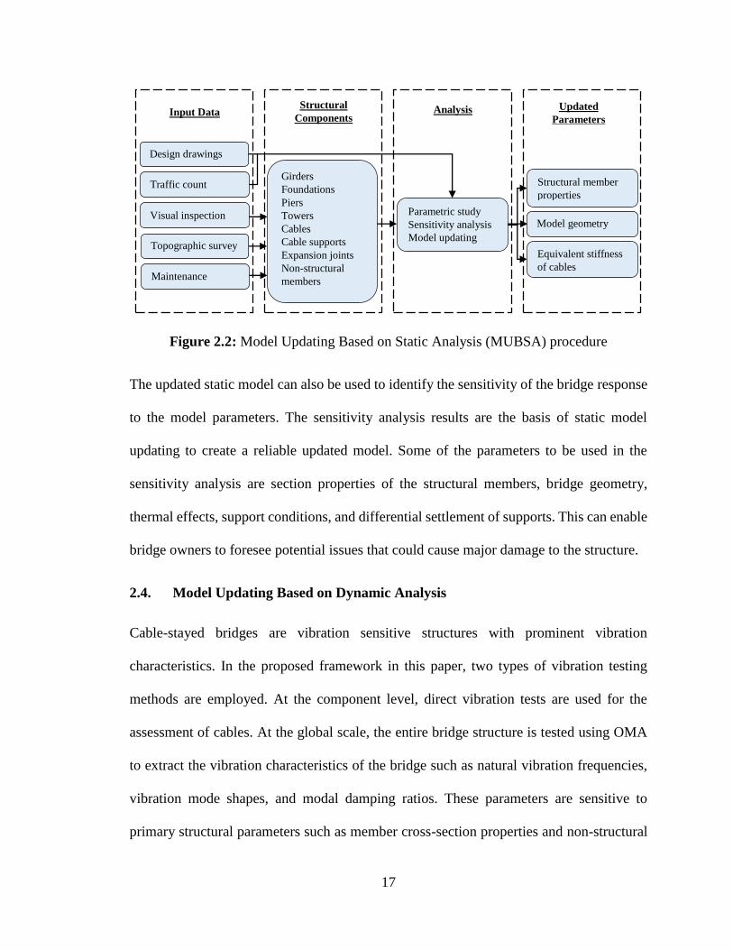
Figure 2.2: Model Updating Based on Static Analysis (MUBSA) procedure

The updated static model can also be used to identify the sensitivity of the bridge response

to the model parameters. The sensitivity analysis results are the basis of static model

updating to create a reliable updated model. Some of the parameters to be used in the

sensitivity analysis are section properties of the structural members, bridge geometry,

thermal effects, support conditions, and differential settlement of supports. This can enable

bridge owners to foresee potential issues that could cause major damage to the structure.

2.4. Model Updating Based on Dynamic Analysis

Cable-stayed bridges are vibration sensitive structures with prominent vibration

characteristics. In the proposed framework in this paper, two types of vibration testing

methods are employed. At the component level, direct vibration tests are used for the

assessment of cables. At the global scale, the entire bridge structure is tested using OMA

to extract the vibration characteristics of the bridge such as natural vibration frequencies,

vibration mode shapes, and modal damping ratios. These parameters are sensitive to

primary structural parameters such as member cross-section properties and non-structural

Input Data Structural

Components Analysis Updated

Parameters

Design drawings

Visual inspection

Traffic count

Topographic survey

Girders

Foundations

Piers

Towers

Cables

Cable supports

Expansion joints

Non-structural

members

Parametric study

Sensitivity analysis

Model updating

Model geometry

Equivalent stiffness

of cables

Structural member

properties

Maintenance

history

18

masses. The modal analysis results are ultimately used in combination with advanced

model updating techniques to develop an accurate and up-to-date numerical model of the

bridge structure.

Figure 2.3 illustrates the procedure for MUBDA and its major components. The following

sections outline the details of important components of MUBDA to ensure reliable results.

Figure 2.3: Model Updating Based on Dynamic Analysis (MUBDA) procedure

2.4.1. Signal Processing

The accuracy of the numerical models used for the condition assessment of a structure is

only as good as the quality of the collected vibration data. The collected signals must be

processed using three main techniques: detrending, band-pass filtering, and segmenting.

Pre-processing of the data is crucial for quality assurance of the collected information and

removal of unnecessary information that can introduce inaccuracies in the assessment

results. Additional signal pre-processing may be required for particular situations. The

ultimate objective is to achieve an accurate estimation of the correlation and spectral

density functions that are used for modal extraction.

Data Collection Structural

Components Analysis Updated

Parameters

Updated model

from MUBSA

Vibration testing of

cables

Ultrasonic test of

cables

Ambient vibration

testing

Primary structural

members

Stay cables

Primary structural

members Non-structural

mass

Signal processing

Cable vibration

analysis Operational modal

analysis

Sensitivity analysis

FE model updating

Structural member

properties

Non-structural mass

Support conditions

19

Detrending is removing specific trends from a signal to enable the analysis of the data

fluctuation without the trend. The most basic detrending that must be applied to vibration

data is the removal of mean, which eliminates the Direct Current (DC) offsets. If the signal

mean is a non-zero value, it results in a spike in the Power Spectral Density (PSD) which

can significantly influence the accuracy of OMA. Digital mean removal filters can be

expressed as:

𝑧𝑓(𝑛) = 𝑧(𝑛) −1

𝑁∑ 𝑧(𝑖)

𝑁

𝑖=1

(2.1)

where 𝑧𝑓(𝑛) is the discrete filtered signal, 𝑧(𝑛) is the unfiltered signal, and 𝑁 is the

number of data points.

Moving average is another detrending filter that can be used to remove short-term trends

from the vibration data. Equation (2.2) shows a typical short-term trend removal filter for

discrete signal processing.

𝑧𝑓(𝑛) = 𝑧(𝑛) −1

𝑘∑ 𝑧(𝑛 − 𝑖)

𝑘−1

𝑖=0

(2.2)

In this equation 𝑘 is the filter window size.

A band-pass filter can be applied to vibration data to remove the frequency range outside

the bandwidth of interest. A convenient method of applying band-pass filter is through FFT

filtering as shown in Equation (2.3).

𝑍𝑓(𝑛) = 𝑍(𝑛)𝑊(𝑛) (2.3)

In this equation, 𝑍𝑓(𝑛) is the filtered signal, 𝑍(𝑛) is the unfiltered signal, and 𝑊(𝑛) is the

band-pass filter, all in frequency domain.

20

The natural frequencies of large civil engineering structures are relatively low. Therefore,

low-pass filters are applied to isolate the frequencies of interests by removing components

of the higher frequency range. A preliminary FE modal analysis is necessary for the

selection of an appropriate cut-off frequency. This would allow for an improvement in

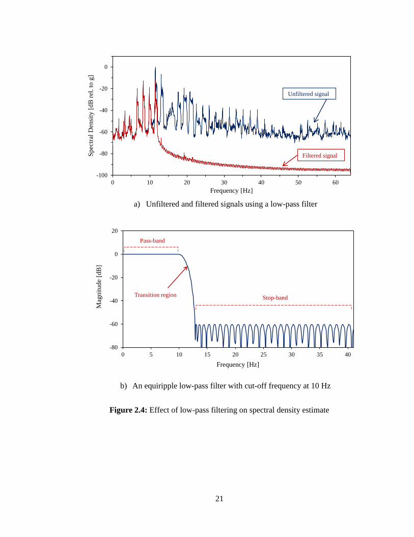
accuracy of the modal property estimates. The effect of a typical low-pass filter on the PSD

estimates of a typical vibration signal is illustrated in Figure 2.4(a). For this example, the

cut-off frequency is set at 10 Hz to remove the frequency content beyond 10 Hz. An

equiripple filter is a common filter in practical applications as an ideal filter with a sharp

cut-off yields a discontinuity in time-frequency transformations (Madisetti 2010). In this

filter, the transition region is defined to provide a smooth transition between pass-band and

stop-band (Figure 2.4(b)).

Segmenting is another pre-processing technique to ensure statistical reliability of the

estimation process. Hanning window with a 50% overlap is commonly applied to the

segmented signal in order to minimize leakage, which can be another issue during time-

frequqncy transformations. Leakage occurs from wrong assumption of signal periodicity.

Figure 2.5 presents the effect of segmenting on PSD estimation of a typical signal. The

variable (Ns) in this figure is the number of segments. As can be seen in the figure, proper

segmenting reduces the signal fluctuation while it maintains the dominant peaks. However,

a poor choice of number of segments results in coarse resolution of the peaks.

21

a) Unfiltered and filtered signals using a low-pass filter

b) An equiripple low-pass filter with cut-off frequency at 10 Hz

Figure 2.4: Effect of low-pass filtering on spectral density estimate

-100

-80

-60

-40

-20

0

0 10 20 30 40 50 60

Sp

ectr

al D

ensi

ty [

dB

rel

. to

g]

Frequency [Hz]

Unfiltered signal

Filtered signal

-80

-60

-40

-20

0

20

0 5 10 15 20 25 30 35 40

Mag

nit

ud

e [d

B]

Frequency [Hz]

Transition regionStop-band

Pass-band

22

Figure 2.5: Effect of segmenting on spectral density estimate

2.4.2. Cable Direct Vibration Test

Stay cables are critical structural members in cable-stayed bridges. The integrity of cables

can be assessed using several SHM techniques. In this paper, cables are evaluated in two

steps. In the first step, the ultrasound technique is used for the evaluation of the cables

cross-section area. In the second step, the cable tension is evaluated using their vibration

characteristics and the cable physical parameters identified from the first step. Natural

frequencies can be obtained from direct vibration measurements of cables. In this study,

Welch’s method is used to obtain PSD estimates to analyze the vibration data and to

determine the natural frequencies. Vibration signals are segmented with Hanning window

with a 50% overlap. Manual peak picking method is employed to identify cable natural

frequencies.

-100

-80

-60

-40

-20

0

0 1 2 3 4 5 6 7 8 9 10

Sp

ectr

al D

ensi

ty [

dB

rel

. to

g]

Frequency [Hz]

Ns = 1

Ns = 10

Ns = 100

23

Cable tension along with other cable parameters affect the measured natural vibraiton

frequencies (Caetano 2007). Equation (2.4) shows the relationship between the natural

frequencies, tension forces, and cable properties:

𝑓𝑛 =𝑛

2𝑙∙ √

𝐻

𝜇∙ [1 + 2√

𝐸𝑒𝑓𝑓𝐼

𝐻𝑙2+ (4 +

𝑛𝜋2

2)


𝐻𝑙2] (2.4)

where 𝑓𝑛 is the 𝑛 th natural frequency in Hz, 𝑙 is the horizontal length of the cable in m, 𝐻

is the horizontal component of the cable tension in N, 𝜇 is the cable mass per length in

kg/m, 𝐸𝑒𝑓𝑓 is the cable’s effective modulus of elasticity in N/m2, and 𝐼 is the moment of

inertia of the cable cross-section in m4.

Equation (2.4) is valid for cables with a small sag that are clamped on both ends. This

assumption is applicable to most cases where the cables are adequately pretensioned. 𝑓𝑛 in

Equation (2.4) can be calculated using direct vibration tests.

The modulus of elasticity for a specific type of cable can be found from manufacturer’s

documentation at the time of installation. However, cables’ effective elastic modulus to be

used in Equation (2.4) is influenced by the cable type and the magnitude of the cable sag.

For example, strand-cables have a reduced effective modulus of elasticity as a result of

twisting strands. Typical modulus of elasticity values for helical strands and locked-coil

strands are 170 and 180 GPa, respectively (Gimsing and Georgakis 2012). Sag in cables

also influence the effective modulus of elasticity. The relationship between existing stress

within the cable and cable sag and the effective modulus of elasticity is indeed nonlinear.

Equation (2.5) shows the effective modulus of elasticity for cable-stayed bridges if the

24

traffic load is small compared to dead load, which is generally true in most cases (Gimsing

and Georgakis 2012):

1

𝐸𝑒𝑓𝑓=

1

𝐸+

𝛾𝑐2𝑙2

12𝜎3 (2.5)

where 𝐸𝑒𝑓𝑓 is the effective modulus of elasticity, 𝐸 is the material modulus of elasticity

which includes the effect of cable type, 𝛾𝑐 is the specific weight of the cables, 𝑙 is the

horizontal length of the cable, and 𝜎 is the stress corresponding to the cable tension.

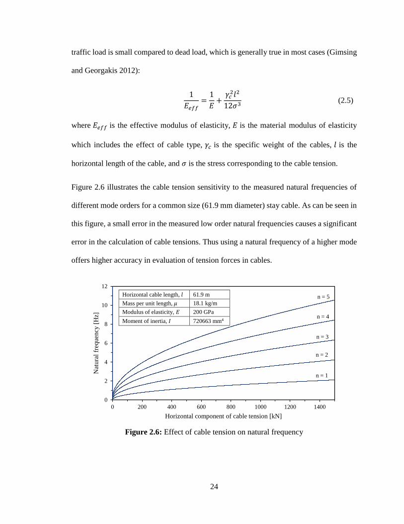
Figure 2.6 illustrates the cable tension sensitivity to the measured natural frequencies of

different mode orders for a common size (61.9 mm diameter) stay cable. As can be seen in

this figure, a small error in the measured low order natural frequencies causes a significant

error in the calculation of cable tensions. Thus using a natural frequency of a higher mode

offers higher accuracy in evaluation of tension forces in cables.

Figure 2.6: Effect of cable tension on natural frequency

0

2

4

6

8

10

12

0 200 400 600 800 1000 1200 1400

Nat

ura

l fr

equen

cy [

Hz]

Horizontal component of cable tension [kN]

n = 1

n = 2

n = 3

n = 4

n = 5Horizontal cable length, 𝑙 61.9 m

Mass per unit length, 𝜇 18.1 kg/m

Modulus of elasticity, 𝐸 200 GPa

Moment of inertia, 𝐼 720663 mm4

25

Damage in cables as a result of corrosion alternates the cable cross-section and potentially

mass per unit length. The effect of these parameters on the measured natural frequency is

significant and can influence the accuracy of the estimated cable tension. This is shown in

Figure 2.7 for the fifth order natural frequency of the cable in Figure 6. In this analysis, the

corroded cable mass per unit length is assumed to be proportional to the cable section loss

as can be estimated by:

𝜇′ = 𝜇0 (𝑑′

𝑑0)

2

(2.6)

where 𝜇0 and 𝑑0 are the mass per unit length and diameter of the undamaged cable and 𝜇′

and 𝑑′ are the updated parameters, respectively.

Figure 2.7: Effect of section loss on cable tension

As can be seen in Figure 2.7, small magnitudes of corrosion in cables introduce significant

errors on the assessed fifth mode natural vibration frequency. For example, at the measured

natural frequency of 6 Hz, a corrosion of 5% within the cable causes an error of 4.7% in

0

2

4

6

8

10

12

0 500 1000 1500

Nat

ura

l fr

equen

cy [

Hz]


Error

Section loss Error

20% 19.5%

15% 14.7%

10% 9.8%

5% 4.7%

0% 0%

26

the horizontal component of the assessed cable tension. Hence in order to achieve a high

accuracy in evaluating cables forces, it is critical to assess the cables cross-section using

high accuracy methods such as the ultrasound tests.

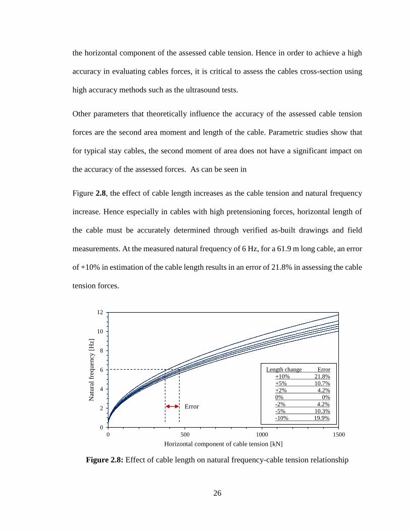
Other parameters that theoretically influence the accuracy of the assessed cable tension

forces are the second area moment and length of the cable. Parametric studies show that

for typical stay cables, the second moment of area does not have a significant impact on

the accuracy of the assessed forces. As can be seen in

Figure 2.8, the effect of cable length increases as the cable tension and natural frequency

increase. Hence especially in cables with high pretensioning forces, horizontal length of

the cable must be accurately determined through verified as-built drawings and field

measurements. At the measured natural frequency of 6 Hz, for a 61.9 m long cable, an error

of +10% in estimation of the cable length results in an error of 21.8% in assessing the cable

tension forces.

Figure 2.8: Effect of cable length on natural frequency-cable tension relationship

0

2

4

6

8

10

12

0 500 1000 1500

Nat

ura

l fr

equen

cy [

Hz]


Error

Length change Error

+10% 21.8%

+5% 10.7%

+2% 4.2%

0% 0%

-2% 4.2%

-5% 10.3% -10% 19.9%

27

Relaxation in cables subjected to sustained large tension forces is a common phenomenon

that must be considered in assessment of the structural integrity of cable-stayed bridges.

Relaxation is defined as permanent elongation of cables. Relaxation results in an increased

deflection of the bridge profile. As a rule of thumb, cable relaxation is significant and must

be considered for cables subjected to sustained loading greater than 50% of their ultimate

tensile strength (Gimsing and Georgakis 2012).

2.4.3. Operational Modal Analysis (OMA)

Global dynamic behaviour of cable-stayed bridges can be evaluated through vibration

monitoring of the girders. OMA methods use the bridge response to ambient sources of

vibration for modal identification of the bridge. The accuracy of the assessment relies on

careful planning and execution of the monitoring process. Choosing appropriate test

parameters such as sensor configuration, sampling frequency, and monitoring time is

crucial.

The number of sensors and their configuration must be chosen based on vibration modes

of interest. Sensor locations should be selected in order to avoid zero displacement nodes

in modes of interest and to capture locations with maximum vibration magnitudes for

improving the accuracy. Monitoring using a small number of sensors in a single setup

provides a coarse mesh which may not be sufficient to accurately capture global vibrational

behaviour. In these cases, roving OMA can be used to provide a better resolution. The

reference channels in roving OMA must be selected carefully as to avoid zero displacement

nodes in modes of interest.

Preliminary modal analysis of the bridge must be performed prior to field tests in order to

choose an appropriate sampling frequency. This exercise is to ensure that the vibration

28

frequency of all modes of interest are smaller than the Nyquist frequency. Vibration signals

must also be of sufficient length in order to allow OMA methods to capture vibration

characteristics. Two equations for the calculation of required monitoring time can be found

in the literature. These are to ensure that the captured vibration signals reserve adequate

information regarding the system behaviour. ISO 4866:2010 (International Organization

for Standardization 2010) suggests Equation (2.7) for the monitoring time:

𝑇𝑟𝑒𝑞 =200

𝜉𝑓𝑛 (2.7)

where 𝑇𝑟𝑒𝑞 is the required monitoring time, 𝜉 is the modal damping ratio, and 𝑓𝑛 is the

natural frequency of 𝑛th mode. This equation was developed to limit the statistical errors

of spectral density estimate. Brincker and Ventura (Brincker and Ventura 2015) suggest

Equation (2.8):


𝜉𝑓𝑚𝑖𝑛 (2.8)

where 𝑓𝑚𝑖𝑛 is the lowest frequency of interest. This equation is based on system memory

associated with autocorrelation function that corresponds to the lowest mode of interest.

These two equations can suggest a wide range for required monitoring time. In addition to

these two equations, structure availability for testing, monitoring equipment, and data

storage limitation can be limiting factors for selecting the monitoring time.

OMA methods are generally categorized into frequency and time domain techniques. Some

of the most common methods are the time-domain Poly-Reference (PR) and Frequency

Domain Decomposition (FDD). The PR method is not as intuitive as frequency domain

methods, and a thorough preparation is required for an accurate analysis. Disadvantages of

29

classical frequency domain methods are their incapability to identify closely-spaced modes

and a large number of plots for analysis (Brincker 2014). One of the more recently

developed methods that overcame these problems is poly-reference Least Squares

Complex Frequency (pLSCF) domain method (also known as polyMAX) where the PR

method is taken into the frequency domain. Other advantages of pLSCF method is that the

method is very stable and that a clear stabilization diagram can be constructed for a

graphical interpretation, allowing an automatic pole identification process (Dynamic

Design Solutions NV 2017a; Peeters et al. 2004). These advantages have made pLSCF one

of the most reliable and popular methods of OMA. The method is employed in the case

study described in the companion paper.

OMA identifies structural behaviour in the modal space. Modal Assurance Criterion

(MAC) values show the correlation magnitude of two modes as defined in Equation (2.9):

𝑀𝐴𝐶 =|𝜙𝑖

𝐻𝜙𝑗|2

(|𝜙𝑖𝐻𝜙𝑗|)(|𝜙𝑗

𝐻𝜙𝑖|)× 100 (2.9)

where 𝜙𝑖 and 𝜙𝑗 are two mode shape vectors. The MAC value approaches unity as the two

modes get closer to each other. MAC values are widely used in modal identification as well

as in model updating. MAC values can be calculated for a set of modes to determine the

correlation amongst themselves (autoMAC values), or can be used to correlate more than

one set of data to pick out modes that represent the same mode. AutoMAC values should

be calculated for the selection of appropriate modes for further analysis. Two modes with

MAC values close to one are categorized as highly correlated, however setting a MAC

limit for identical modes depends on the particular application.

30

2.4.4. Automated Model Updating

Model updating is the process of adjusting a numerical FE model to simulate a similar

response as the actual structure that is captured during field tests. The ultimate purpose of

model updating is to create an accurate numerical model of the structure at the current state.

Model updating based on vibration tests are performed by comparing the natural

frequencies and modes shapes between OMA results and the FE model. The natural

frequency values can be numerically compared while the mode shape pairs must be

correlated using the MAC values (Equation (2.9)). It is important to note that the order of

appearance of modes may be different in the numerical and test models due to initial

differences between structural parameters. Therefore care must be taken when creating

mode shape pairs. This is to ensure that the discrepancies between experiments and FE

analysis results are only because of errors in modeling assumptions and not non-legitimate

mode shape pairs.

Automated model updating achieves better correlation between the FE analysis and

experimental results through adjustments of identified parameters by the user. The first

step in model updating is to perform sensitivity analysis in order to determine the

parameters with significant effect on the global behaviour of the structure. These

parameters are selected as updating parameters in automated model updating. Allowable

parameter change is defined based on engineering judgement and visual inspection. Modal

characteristics of the FE model are selected as response parameters. The sensitivity

matrix, 𝑆 defines the relationship between updating parameters and response parameters,

as seen in Equation (2.10).

31

∆𝑅 = 𝑆 × ∆𝑃 (2.10)

Where ∆𝑅 and ∆𝑃 are vectors representing changes in the response and the updating

parameters, respectively. The difference between analytical and experimental results can

be minimized using mathematical methods such as the Bayesian estimation as shown in

Equation (2.11) (Dynamic Design Solutions NV 2017b).

𝑃𝑢 = 𝑃0 + 𝐺(−∆𝑅) (2.11)

Where 𝑃𝑢 is the updated parameter vector, 𝑃0 is the original updating parameter vector, and

𝐺 is the gain matrix that is computed from sensitivity matrix and confidence for both

updating and response parameters. These equations are all developed based on the

assumption that the bridge behaviour in operation can be modelled using a linear model

which is valid in most applications.

Target response for model updating is also chosen from test/field observations. The

selected parameters are updated so that the global behaviour of the model matches what is

observed on site. The automated model updating algorithms achieve the correlation by

minimizing the objective function matrix, which represents the difference between

experimental and numerical response parameters. Natural frequencies are often chosen as

the response parameter for objective function. Once model updating is complete, it is

important to look closely at the updated parameters after the analysis as some changes

suggested by the model may be unrealistic or not physically feasible. MAC values for the

updated mode shape pairs should also be checked for any irregular results.

32

2.5. Conclusion

In this first part of the companion papers, a hybrid SHM procedure for condition

assessment of cable-stayed bridges was proposed. The suggested procedure implements

both static and dynamic model updating. Model updating based on static analysis

incorporates initial design properties, topographic measurements, and visual inspection

data into the bridge assessment. Additionally, parametric studies may be performed to

further investigate the bridge static response to changes in structural properties and

environmental conditions. The conditions of the stay cables are extensively looked at

through direct dynamic tests, visual and ultrasonic inspections, static FE analysis, and

dynamic model updating. Finally, model updating based on dynamic analysis is performed

on the calibrated model to achieve correlation with dynamic behaviours captured from

ambient vibration tests. In Chapter 3, the proposed method is validated in a case-study

cable-stayed bridge in New Brunswick, Canada.

2.6. Acknowledgement

Authors would like to thank the Natural Sciences and Engineering Research Council of

Canada (NSERC), the New Brunswick Innovation Foundation (NBIF), the New Brunswick

Department of Transportation and Infrastructure (NBDTI), and the Department of Civil

Engineering at the University of New Brunswick for supporting this research.

2.7. References

Agneni, A., Balis Crema, L., and Coppotelli, G. (2010). “Output-only analysis of structures

with closely spaced poles.” Mechanical Systems and Signal Processing, 24(5), 1240–

1249.

33

American Association of State Highway and Transporatation Officials. (2011). The manual

for bridge evaluation. American Association of State Highway and Transportation

Officials, Washington, DC.

American Association of State Highway and Transportation Officials. (2017). AASHTO

LRFD Bridge Design Specifications. American Association of State Highway and

Transportation Officials, Washington, DC.

Benedettini, F., and Gentile, C. (2011). “Operational modal testing and FE model tuning

of a cable-stayed bridge.” Engineering Structures, 33(6), 2063–2073.

Brincker, R. (2014). “Some Elements of Operational Modal Analysis.” Shock and

Vibration, 2014, 1–11.



Brownjohn, J. M. W., Magalhaes, F., Caetano, E., and Cunha, A. (2010). “Ambient

vibration re-testing and operational modal analysis of the Humber Bridge.”

Engineering Structures, 32(8), 2003–2018.

Brownjohn, J. M. W., de Stefano, A., Xu, Y. L., Wenzel, H., and Aktan, A. E. (2011).

“Vibration-based monitoring of civil infrastructure: Challenges and successes.”

Journal of Civil Structural Health Monitoring, 1(3–4), 79–95.

Caetano, E. de S. (2007). Cable Vibrations in Cable-stayed Bridges. IABSE, Zurich,

Switzerland :

Canadian Standards Association. (2014). “Canadian highway bridge design code.”

34

Canadian Standards Association.

Carden, E. P., and Fanning, P. (2004). “Vibration Based Condition Monitoring: A Review.”

Structural Health Monitoring, 3(4), 355–377.

Chang, P. C., Flatau, A., and Liu, S. C. (2003). “Review paper: Health monitoring of civil

infrastructure.” Structural Health Monitoring, 2(3), 257–267.

Cunha, A., Caetano, E., and Delgado, R. (2001). “Dynamic Tests on Large Cable-Stayed

Bridge.” Journal of Bridge Engineering, 6(1), 54–62.

Deraemaeker, A., Reynders, E., De Roeck, G., and Kullaa, J. (2008). “Vibration-based

structural health monitoring using output-only measurements under changing

environment.” Mechanical Systems and Signal Processing, 22(1), 34–56.

Dynamic Design Solutions NV. (2017a). FEMtools Modal Parameter Extractor User’s

Guide. Leuven, Belgium.

Dynamic Design Solutions NV. (2017b). FEMtools Model Updating Theoretical Manual.

Leuven, Belgium.

Ewins, D. J. (2000). Modal testing : theory, practice, and application. Research Studies

Press, Baldock Hertfordshire England ;;Philadelphia PA.

Farhey, D. N. (2005). “Bridge Instrumentation and Monitoring for Structural Diagnostics.”





35




Gimsing, N. J., and Georgakis, C. T. (2012). Cable Supported Bridges : Concept and

Design. John Wiley & Sons.

Guggenberger, J. (2009). “Model Updating using Operational Data.” 4th European

Automotive Simulation Conference.




Jaishi, B., and Ren, W.-X. (2005). “Structural Finite Element Model Updating Using

Ambient Vibration Test Results.” Journal of Structural Engineering, 131(4), 617–

628.

Jang, S., and Spencer, B. F. J. (2015). “Structural Health Monitoring for Bridge Structures

using Smart Sensors.” Newmark Structural Engineering Laboratory. University of

Illinois at Urbana-Champaign, (May), 165.

Ko, J. M., and Ni, Y. Q. (2005). “Technology developments in structural health monitoring

of large-scale bridges.” Engineering Structures, 27(12 SPEC. ISS.), 1715–1725.

Ko, J. M., Ni, Y. Q., Zhou, H. F., Wang, J. Y., and Zhou, X. T. (2009). “Investigation

concerning structural health monitoring of an instrumented cable-stayed bridge.”

Structure and Infrastructure Engineering, 5(6), 497–513.

36

Madisetti, V. K. (2010). The Digital Signal Processing Handbook: Digital signal

processing fundamentals. CRC Press, Boca Raton, FL :

Ontario Ministry of Transportation. (2008). Ontario Structure Inspection Manual (OSIM).

Peeters, B., Auweraer, H. Van Der, Guillaume, P., and Leuridan, J. (2004). “The PolyMAX

frequency-domain method : a new standard for modal parameter estimation?” Shock

and Vibration, Hindawi Publishing Corporation, 11(3–4), 395–409.

Peeters, B., and De Roeck, G. (2001). “Stochastic System Identification for Operational

Modal Analysis: A Review.” Journal of Dynamic Systems, Measurement, and Control,

American Society of Mechanical Engineers, 123(4), 659–667.




Ren, W.-X., Peng, X.-L., and Lin, Y.-Q. (2005). “Experimental and analytical studies on

dynamic characteristics of a large span cable-stayed bridge.” Engineering Structures,

27(4), 535–548.

Schlune, H., Plos, M., and Gylltoft, K. (2009). “Improved bridge evaluation through finite

element model updating using static and dynamic measurements.” Engineering

Structures, 31, 1477–1485.


Xu, Y., and Xia, Y. (2012). Structural Health Monitoring of Long-span Suspension Bridges.

CRC Press.

37

Yi, T., Li, H., and Gu, M. (2010). “Recent research and applications of GPS based

technology for bridge health monitoring.” Science China Technological Sciences, SP

Science China Press, 53(10), 2597–2610.

38

3. Hybrid Structural Health Monitoring Approach for Condition

Assessment of Cable-Stayed Bridges. II: Hawkshaw Bridge Case

Study*

Abstract

This paper validates a proposed hybrid method for condition assessment of cable-stayed

bridges through a long-span bridge case study. The proposed method, explained in Chapter

2, incorporates data from various inspection, survey, and experimental results, aiming to

improve the accuracy of the assessment. The framework was applied to a case-study bridge

in New Brunswick, Canada. In this study, a wide range of information obtained from

original design drawings, visual inspection, cable inspection, traffic counts, Global

Positioning System (GPS) surveys, and global and local ambient vibration tests were

successfully incorporated. Model updating based on static and dynamic response of the

bridge was conducted. The conditions of stay-cables were examined with extra care, as

they are susceptible to long-term damage and their impact on the overall bridge condition

is significant. Structural health of primary structural members including stay-cables, bridge

girders, and the orthotropic steel deck were successfully identified by the application of the

outlined monitoring strategy to the bridge. Other structural parameters such as the bridge

overall weight and non-structural mass were also evaluated.

________________________________________________________________________

* Chapters 2 and 3 are submitted as the following manuscript to the Journal of Bridge

Engineering.

Araki, Y., Arjomandi, K., MacDonald, T. (2018). “Hybrid Structural Health Monitoring

Approach for Condition Assessment of Cable-Stayed Bridges.”

39

3.1. Introduction

Bridges function as important links in a transportation network. Many bridges in operation

worldwide are decades old and have experienced an increase in load demand as a result of

growth in traffic volume and development of heavier commercial trucks. Meanwhile, these

bridges are also experiencing structural deterioration and alteration due to aging, extreme

load conditions, and maintenance and improvements. These changes calls for a need for

accurate condition assessment of structural health and evaluation of remaining service life

of these bridges. Structural Health Monitoring (SHM) includes methods for evaluation of

the structural integrity using non-destructive measures. Compared to routine visual

inspections traditionally used for condition assessment of bridges, SHM provides a more

quantitative and less subjective information about structural health.

In Chapter 2, a hybrid approach for SHM and condition assessment of cable-stayed bridges

incorporating data from various methods is explained. In this method, a Finite Element

(FE) model of the bridge is calibrated to match the static and dynamic responses observed

in the field. This process is known as model updating. Static model updating is first

conducted based on initial design drawings, traffic data, visual inspection data, and

operational deflection shape obtained from topographic surveys. Employing static model

updating prior to the automated dynamic model updating, the overall assessment error is

reduced and the accuracy of the model updating process is improved (Schlune et al. 2009).

In addition to static response, the dynamic behaviour of the bridge is also examined. Modal

properties of the bridge is captured through Operational Modal Analysis (OMA). OMA

has been proven effective for modal parameter extraction in civil engineering applications

through various studies (Benedettini and Gentile 2011; Chang et al. 2001; Cunha et al.

40

2001; Ren et al. 2005; Wilson and Liu 1991). Local modal parameter extraction is also

found effective. A subsystem of a cable-stayed bridge and its analysis can be found in

Gentile and Martinez, Y. Cabrera 1997. Local vibration tests of cables are also common to

determine cable tension, as it is directly related to the natural frequencies of the cable.

Several case studies have proven the effectiveness of dynamic analysis for condition

assessment of the cables (Benedettini and Gentile 2011; Cunha et al. 2001; Ren et al. 2005).

Modal parameters obtained from OMA are set as reference response in automated model

updating. Using model updating, the modal parameters such as natural frequencies, mode

shapes, and damping ratios obtained from ambient vibration tests can be related to

structural parameters of the bridge. Previous model updating applications in civil

engineering structures can be found in Benedettini and Gentile (2011), Daniell and

Macdonald (2007), Macdonald and Daniell (2005), Wang et al. (2010), and Zhang et al.

(2001).

In this paper, a framework in condition assessment of cable-stayed bridges using a hybrid

monitoring approach is implemented to a case-study long-span cable-stayed bridge in the

province of New Brunswick in Canada. Details of the methodology can be found in Chapter

2. Information from topographic surveys, visual inspection data, ultrasonic tests of stay-

cables, direct vibration monitoring of cables, and OMA results of the primary structure is

incorporated to give an insight to the global health of the bridge as well as some important

local parameters. The analysis techniques and signal processing methods to be employed

for achieving reliable results are discussed in detail. The details of the case study and the

efficiency of the proposed framework in the condition assessment of the subject bridge are

discussed.

41

3.2. Hawkshaw Bridge

The Hawkshaw Bridge is a 332m long cable-stayed bridge that is located in Nackawic,

New Brunswick, Canada (Figure 3.1). This bridge was built in 1967.

a) Hawkshaw Bridge

b) Elevation view

Figure 3.1: Hawkshaw Bridge

The primary structural system of the bridge superstructure consists of two main girders

spaced at approximately 10 m centre-to-centre, floor beams, orthotropic deck, towers, and

stay-cables. A total of 48 stay-cables support the main girders in groups of six. The bridge

is located between a paper mill and the Trans-Canada Highway. As a result, the traffic

42

composition on the Hawkshaw Bridge includes a high number of commercial transport

trucks. The Hawkshaw Bridge shows excessive vibration during operation and has a visible

sag in the centre span. This has triggered multiple inspections on the bridge by New

Brunswick Department of Transportation and Infrastructure (NBDTI) including this study.

In this case study, the proposed hybrid SHM method described in Chapter 2 is applied to

the Hawkshaw Bridge. The fieldwork involved GPS surveying, traffic counting, and

vibration tests of the cables and the girders. Previous visual inspection and cable ultrasonic

inspection results were also incorporated in the analysis.

3.3. Static Analysis

A static model of the Hawkshaw Bridge was created using SAP2000. Using the original

design drawings, the as-designed cable tension forces were calculated. Tension forces in

the forestay and backstay cables as per the original design under the bridge dead load are

3952 kN and 4101 kN, respectively. The static model was also used for sensitivity analysis

of the bridge structure to the settlement of supports, ambient temperature changes, and

horizontal movement of piers.

Figure 3.2 shows the deformed shape of the bridge girder profile obtained from the original

design drawings and two sets of survey data. The design profile shows deflection under

design dead load and a third of live load. Those captured from the topographic surveys are

deflection profile under dead load and operational live load. It can be seen that the bridge

is experiencing larger deflection in comparison to the intended design.

43

Figure 3.2: Hawkshaw Bridge as-designed and surveyed deflection profile

The static model was also used to calculate the equivalent stiffness of the cable-tower

subsystem. The tower and forestay and backstay cables make up a subsystem that provides

support to the bridge deck system. This subsystem was replaced with springs at forestay

tie-down locations. It was found through the ultrasound tests that the cables cross-sectional

loss is negligible. Therefore, the cross-sectional area of the cables was assumed to be 13800

mm2 (2300 mm2 × 6 cables), as found in ASTM A586-04a (ASTM International 2015).

The modulus of elasticity was assumed to be 170 GPa for helical strands as found in

Gimsing and Georgakis (2012). Cable sag has an influence on the modulus of elasticity, as

shown in Equation (3.1):

1

𝐸𝑒𝑓𝑓=

1

𝐸+

𝛾𝑐2𝑙2

12𝜎3 (3.1)

where 𝐸𝑒𝑓𝑓 is the effective modulus of elasticity, 𝐸 is the material modulus of elasticity,

𝛾𝑐 is the cable specific weight, 𝑙 is the horizontal length of the cable, and 𝜎 is the cable

axial stress. From Equation (3.1), the effective modulus of elasticity was therefore

-0.1

-0.05

0

0.05

0.1

0.15

0.2

0.25

0 50 100 150 200 250 300

Def

lect

ion [

m]

Distance along bridge [m]

As-designed

July, 2016

June, 2014

44

calculated as 167.08 GPa for forestay and 168.10 GPa for backstay. Using the static model,

the equivalent vertical stiffness of cables are estimated to be 3.008×106 N/m.

3.4. Direct Vibration Test of Cables

Vibration behaviour of the cables was measured under ambient and manual excitations.

Vibration tests were conducted using tri-axial wireless MicroStrain G-Link LXRS

accelerometers. A wireless data aggregator was used to collect vibration data. The

accelerometers were securely attached to each cable using an in-house built mounting

system (Figure 3.3). The monitoring time was set at 5 minutes for ambient vibration and 2

minutes for manual excitation tests. The sampling frequency was 128 Hz.

Figure 3.3: Vibration testing of the cables

The diameter of each cable was measured with a digital caliper. An average difference of

0.64% was found compared to the design diameter of 61.9 mm. The discrepancies from

the design diameter were within the range of -0.36% to 3.72%.

45

Signal mean value was removed from the vibration measurements. A low-pass filter with

a cut-off frequency of 10 Hz was applied to the vibration signals. The cut-off frequency

was chosen based on the natural frequencies of the cables. Power Spectral Density (PSD)

estimates were calculated using Welch method with 10 segments and Hanning window

with an overlap of 50%. Natural frequencies were identified using manual peak picking

method.

Cable tension forces were calculated from natural frequencies using Equation (3.2):

𝑓𝑛 =𝑛

2𝑙∙ √

𝐻

𝜇∙ [1 + 2√


𝐻𝑙2+ (4 +

𝑛𝜋2

2)


𝐻𝑙2] (3.2)

where 𝑓𝑛 is the 𝑛 th natural frequency, 𝑙 is the horizontal length of the cable, 𝐻 is the

horizontal component of the cable tension, 𝜇 is the cable mass per length, 𝐸𝑒𝑓𝑓 is the

effective modulus of elasticity of the cables, and 𝐼 is the moment of inertia of the cable

cross-section. Minor section losses captured by ultrasonic inspections are accounted for in

the calculation of cable cross-sectional area and moment of inertia. Area loss less than 2%

was neglected in the analysis. Detailed specifications of the cables were not available,

therefore the moment of inertia of undamaged cables was calculated assuming that they are

solid throughout. Moment of inertia of the damaged cables 𝐼′ was estimated using Equation

(3.3).

𝐼′ = 𝐼0(1 − 𝑑𝐴)2 (3.3)

where 𝐼0 is the undamaged moment of inertia and 𝑑𝐴 is the cross-sectional area loss due to

damage. Cable tension forces were calculated with moduli of elasticity determined from

automated model updating results. The details of elastic modulus calculations are explained

46

in Section 3.6. Mass per unit length was assumed to be 18.57 kg/m. The calculated cable

tension under dead and operational live loads are summarized in Figure 3.4. Theoretically,

the cable tensions must be calibrated so that the towers are only subjected to axial forces.

However, as can be seen in Figure 4, a small horizontal force resulting from the cable forces

act at the top of the towers. Additionally, the cables on Nackawic side of each tower carry

slightly less tension than expected and in comparison to the cables on Fredericton side.

This can be an indication of the bridge small movement towards the Fredericton side.

a) Downstream

b) Upstream

Figure 3.4: Estimated cable tension of the Hawkshaw Bridge

The effect of thermal changes in the cable analysis results were also investigated by

measuring the vibration response of the south upstream backstay in two instances at

temperatures of 30.9 °C 28.8 °C. As can be seen in Figure 3.5, increased ambient

temperature results in an increase in the measured natural frequencies especially for higher

47

modes. This would consequently results in higher estimation of the cable forces which is

in agreement with engineering judgments.

Figure 3.5: Effect of temperature on the natural frequencies of the stay-cables

3.5. Ambient Vibration Analysis

An FE model of the bridge main girders, floor beams, and cable-tower equivalent

subsystem was created in SAP2000. The model was used for preliminary modal analysis

and as the basis for numerical model in FEMtools that is later used for model updating. A

summary of the model parameters can be found in Table 3.1.

1.0E-10

1.0E-08

1.0E-06

1.0E-04

1.0E-02

0 2 4 6 8 10

Sp

ectr

al D

ensi

ty [

g2/H

z]

Frequency [Hz]

T = 28.8 ˚C

T = 30.9 ˚C

48

Table 3.1: Modelling parameters for FE model prior to model updating

Component Parameter Value

Main girders Modulus of elasticity (steel) 200 GPa

Floor beams Modulus of elasticity (steel) 200 GPa

Cable-tower subsystem Spring stiffness 3008 kN/m

Bridge deck Non-structural mass 888 kg/m

Cable tie-down (forestay) Non-structural mass 13603 kg

The additional dead load from asphalt layer, steel guiderails, side curbs, and cable tie-down

supports were considered in the analysis. This model was created to accurately simulate

the vertical vibration behaviour of the structure. However, as the effects of the bridge

pavement and the continuity of the orthotropic steel deck are ignored, this model does not

accurately simulate the lateral and torsional modes. This limitation is accounted for in the

model updating process.

3.5.1. Ambient Vibration Monitoring Field Tests

Ambient vibration monitoring of the Hawkshaw Bridge was conducted in July 2016.

During these tests, one lane was closed while the other lane remained open to the daily

traffic. The lane closure was managed by the traffic control crew. The tests were conducted

using ten tri-axial wireless MicroStrain G-Link LXRS accelerometers. The sensors were

enclosed in weatherproof cases and were placed on top flanges of the main girders using

custom-built magnetic mounting plates (Figure 3.6). These plates were developed in-house

to provide a convenient method to securely mount the sensors on the steel girders.

49

Figure 3.6: Accelerometer mounted on the girder top flange

Two sensor configurations were tested. The exact location of the sensors were measured

using a high accuracy Global Position System (GPS) survey equipment. The preliminary

modal analysis results identified the first 10 vibration modes to be within 28 Hz. Therefore,

a sampling frequency of 64 Hz was selected to capture the target frequency range within

the Nyquist frequency. The preliminary modal analysis also showed the maximum

vibration magnitudes at the middle span. Therefore, two reference channels (one on each

girder) were located at the bridge mid-span. The sensor configurations are illustrated in

Figure 3.7.

a) Setup 1 sensor configuration

b) Setup 2 sensor configuration

Figure 3.7: Sensor configurations for vibration tests

50

The required monitoring time for the Hawkshaw Bridge was calculated using Equation

(3.4) obtained from ISO 4866:2010 (International Organization for Standardization 2010)

and Equation (3.5) developed by Brincker and Ventura (2015).


𝜉𝑓𝑛 (3.4)


𝜉𝑓𝑚𝑖𝑛 (3.5)

where 𝑇𝑟𝑒𝑞 is the required monitoring time in seconds, 𝜉 is the modal damping ratio, 𝑓𝑛 is

the natural frequency of 𝑛th mode, and 𝑓𝑚𝑖𝑛 is the lowest frequency of interest.

Accurate estimation of damping ratios in these equations are particularly challenging.

Table 3.2 shows the minimum required monitoring time using these equations for a range

of damping ratios. These values were estimated using the calculated fundamental

frequency of 0.5 Hz from the preliminary FE model.

Table 3.2. Effect of damping ratio on required monitoring time

Damping

Ratio

Monitoring Time [min]

Equation (3.4) Equation (3.5)

2% 333.33 16.67

5% 133.33 6.67

10% 66.67 3.33

In this case-study, the Hawkshaw Bridge was monitored for 158 minutes. The second setup

only lasted for 19 minutes due to sudden rain.

51

3.5.2. Operational Modal Analysis (OMA)

A moving average filter with a lag of 3840 points (equivalent to 60 seconds at 64 Hz) was

used for the two datasets to remove short-time trends as well as the mean. No band-pass

filter was applied since the frequency range of interest was close to the Nyquist frequency.

pLSCF method using FEMtools was used for modal parameter extraction and analysis of

the bridge deck vibration. Topographic survey data was used to develop a test mesh with

an accurate bridge girder profile. Only the main girders were defined in the test mesh.

Four parameters were adjusted for this analysis: blocksize, model order, and maximum and

minimum frequencies of interest. The blocksize is the lag that is considered in cross power

spectra calculations. For this analysis, the default number of 3072 (equivalent to 48 seconds

at 64 Hz) was used. The model order is the number of modes that are assumed to be present

in the frequency range. Care must be taken when choosing a model order as a small model

order can result in a failure for complete modal extraction and a large model number can

result in an extraction of noise modes. For this analysis, a model order of 200 was chosen.

The frequency range was 0 to 32 Hz to match the Nyquist frequency.

Partial modes were extracted from each test setup. The first five partial mode shapes along

with the corresponding natural frequencies and damping ratios from Setups 1 and 2 are

illustrated in Figure 3.8. Each test setup can only capture movements at the sensor locations.

The support locations automatically are assigned zero deformations. As can be seen in this

figure, the two setups have a good correlation in estimating the first mode shape, natural

frequency, and modal damping ratio. Antisymmetric modes were not well captured from

either of these two setups. This is because the reference channels were placed at the middle

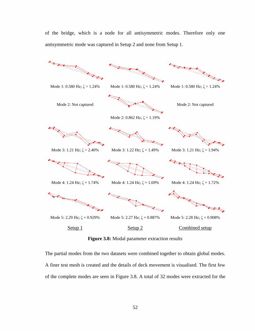
52

of the bridge, which is a node for all antisymmetric modes. Therefore only one

antisymmetric mode was captured in Setup 2 and none from Setup 1.

Mode 1: 0.580 Hz; ζ = 1.24% Mode 1: 0.580 Hz; ζ = 1.24% Mode 1: 0.580 Hz; ζ = 1.24%

Mode 2: Not captured

Mode 2: Not captured

Mode 2: 0.862 Hz; ζ = 1.19%




Setup 1 Setup 2 Combined setup

Figure 3.8: Modal parameter extraction results

The partial modes from the two datasets were combined together to obtain global modes.

A finer test mesh is created and the details of deck movement is visualised. The first few

of the complete modes are seen in Figure 3.8. A total of 32 modes were extracted for the

53

combined setup. The frequency tolerance for the difference between natural frequencies

from Setups 1 and 2 was set at 20%.

AutoMAC values for modes with vibration frequencies of less than 10 Hz are illustrated in

Figure 3.9. As can be seen in this figure, the captured modes can be interpreted as

distinctive physical modes.

a) Setup 1 b) Setup 2

Figure 3.9: AutoMAC values for the captured mode shapes

3.5.3. Mode Shape Pairs

Mode shape pairs are identified so that the reference response can be selected for model

updating. The FE and OMA modes that represent the same modes were selected as mode

shape pairs based on MAC values and natural frequencies. Figure 3.10 presents the first

four mode shapes and the natural frequencies from FE analysis and OMA, and the MAC

value of each pair for the two setups as well as the combined setup.

10

9

8

7

6

5

4

3

2

1

1 2 3 4 5 6 7 8 9 10 0

25

50

75

100

1 2 3 4 5 6 7 8 9 10

Mode

1

2

3

4

5

6

7

8

9

10

Mode

AutoMAC

0

25

50

75

100

0

25

50

75

100

10 20 30

EMA

20

40

60

80

100

120

140

160

FEA

Modal Assurance Criterion (MAC)

1 2 3 4 5 6 7 8 9 10 11 12

12

11

10

9

8

7

6

5 4

3

2

1

0

25

50

75

100

2 4 6 8 10 12

Mode

2

4

6

8

10

12

Mode

AutoMAC

0

25

50

75

100

2 4 6 8 10 12

Mode

2

4

6

8

10

12

Mode

AutoMAC

0

25

50

75

100

2 4 6 8 10 12

Mode

2

4

6

8

10

12

Mode

AutoMAC

54

a) Pair 1 (FEA Frequency: 0.609 Hz)

OMA Freq: 1.24 Hz

MAC: 86.8%

OMA Freq: 1.24 Hz

MAC: 90.6%

OMA Freq: 1.24 Hz

MAC: 87.0%

b) Pair 2 (FEA Frequency: 0.647 Hz)

OMA Freq: 0.580 Hz

MAC: 95.1% OMA Freq: 0.580 Hz


MAC: 91.8%

c) Pair 3 (FEA Frequency: 0.924 Hz)

No pair

No pair

OMA Freq: 0.862 Hz

MAC: 78.8%

d) Pair 4 (FEA Frequency: 1.24 Hz)

OMA Freq: 1.21 Hz


MAC: 94.8%

OMA Freq: 1.21 Hz

MAC: 94.3%

Setup 1 Setup 2 Combined

Figure 3.10: First four mode shape pairs

55

As can be seen from the figure, the MAC values are generally high, exceeding 85% for all

modes. The natural frequencies correlate well with an exception of the first torsional mode.

This mode shape pair has a frequency difference of 47%. Additionally, the order of

appearance is different for the FE analysis and OMA results (torsional mode appears after

first bending mode for OMA and before for FE analysis). This difference is because of the

fact that the torsional properties were not modelled accurately for the FE model. Hence

only the vertical modes were chosen as target response for model updating. For the

correlation of torsional modes, an appropriate FE model with proper torsional properties

must be created.

3.6. Model Updating

Sensitivity analysis was conducted on a 3D FE model. Three updating parameters were

selected from a sensitivity analysis based on the uncertainties in their values and their effect

on the overall vibration behaviour of the structure. These parameters are the cross-section

moment of inertia of the main girders and orthotropic deck in the strong axis, bridge deck

non-structural mass, and the equivalent cable-tower subsystem spring stiffness. The

permitted maximum and minimum changes for each parameter are summarized in Table

3.3.

Table 3.3: Maximum and minimum allowable parameter changes

Member Parameter Limits

Main girders and orthotropic

deck plate

Moment of inertia (strong axis) ±15%

Non-structural mass ±20%

Towers and cables Equivalent spring stiffness ±50%

The limit for the girders cross-section moment of inertia in the strong axis was set to be the

lowest. Based on the visual inspection results, the bridge girders were assessed with no

56

significant corrosion. Therefore the cross-section properties are less likely to have

experienced major degradation. Although no significant sources of mass change was

observed on the bridge, non-structural mass has a slightly higher limit than the moment of

inertia for its greater variability in estimation compared to the moment of inertia. The

modulus of elasticity was not known for the cables and deterioration was spotted in some

cables in 2016 which aligned with what was seen in ultrasonic inspection in 2009. Wrong

estimation of modulus or breakage in cable strands results directly in reduction of

equivalent spring stiffness. Additionally, the whole subsystem consisting of the tower and

cables was represented by the vertical spring stiffness. To allow these varying factors in

the analysis, the parameter was given the most flexibility.

For the reasons discussed in the previous section, the updating process was based only on

vertical modes. Target response was chosen from experimental modes that had a FE mode

pair with a MAC value higher than 70% and frequency difference of 20%.

The equivalent spring stiffness values experienced average reductions of 24.1%, 23.8%,

and 25.8% for Setups 1, 2, and the combined setup, respectively. With the overall average

reduced spring stiffness of 2494.4 kN/m, the updated moduli of elasticity for backstay and

forestay were determined to be 138.71 and 138.01 GPa, respectively. From Section 3.3,

the calculated theoretical effective moduli of elasticity were 168.10 and 167.08 GPa for

backstay and forestay cables, respectively. The % difference between theoretical and

experimental moduli of elasticity is -17.5% and -17.4% for backstay and forestay cables,

respectively.

57

Figure 3.11: Changes in Iz (%)

Figure 3.12: Changes in non-structural mass (%)

-4

-2

0

Setup 1

-8

-6

-4

-2

0

Setup 2

-4

-2

0

Combined

Setup

0

5

10

15

Setup 1

0

10

20

Setup 2

0

5

10

15

Combined

Setup

58

The changes in main girder moment of inertia and non-structural masses are shown in

Figure 3.11 and Figure 3.12. Trend-lines were calculated by averaging the values over 10

m intervals to show the trend in parameter changes. Overall, the results from the three

configurations are in agreement. It can be seen that all three setups yielded similar results.

Summarizing the results, the middle section of the bridge between the cable tie-down

locations is experiencing a reduction in stiffness and an increase in non-structural masses.

However, no significant degradation of the structure or apparent sources of additional mass

were observed from visual inspection.

The updated mode shape pairs are tabulated in Table 3.4. The torsional mode is noted T

and vertical modes are noted V. The numbers after the letters are the mode orders with

respect to that category (for example, first vertical mode is noted V1). With the updated

properties, some additional mode shape pairs were detected. This is evidence that the model

updating was successful in FE model calibration.

Table 3.4: Updated mode shape pairs

Mode

Setup 1 Setup 2 Combined Setup

OMA

Freq

[Hz]

FEA

Freq

[Hz]

%

Diff.

[%]

MAC

[%]

OMA

Freq

[Hz]

FEA

Freq

[Hz]

%

Diff.

[%]

MAC

[%]

OMA

Freq

[Hz]

FEA

Freq

[Hz]

%

Diff.

[%]

MAC

[%]

T1 1.24 0.556 -55.3 87.2 1.24 0.551 -55.7 90.7 1.24 0.556 -55.3 87.3

V1 0.580 0.590 1.62 95.1 0.580 0.584 0.69 92.8 0.580 0.590 1.62 91.5

V2 N/A 0.862 0.858 -0.42 78.8 N/A

V3 1.21 1.22 0.25 94.6 1.22 1.19 -1.82 94.8 1.21 1.22 0.17 94.6

V5 2.29 2.15 -6.05 67.5 N/A N/A

V7 3.31 3.32 0.16 92.8 N/A 3.31 3.32 0.23 75.2

V9 N/A 5.30 5.55 4.71 76.3 N/A

It can be seen from the table that the experimental and analytical natural frequencies

correlate well, with the greatest difference being 6.05%. The only exception is the first

59

torsional mode that was expected to show discrepancies, as explained previously. MAC

values are in a high range, mostly above 85%. Exceptions to these are the second vertical

mode from Setup 2, seventh vertical mode for Setup 1 and the combined setup, and the

ninth vertical mode for Setup 2.

3.7. Conclusion

A proposed hybrid SHM procedure for condition assessment of cable-stayed bridges was

applied to a case-study bridge. The condition of stay-cables, main girders, and non-

structural mass were accurately estimated. Field investigations such as visual inspections,

traffic data collection, topographic surveys, and ultrasonic tests were successfully

incorporated into the analysis. Current tension forces and effective modulus of elasticity of

the stay-cables were determined by integrating the information from inspections, local

vibration tests, FE static analysis results, and model updating results. Using model updating

techniques with respect to static and dynamic bridge responses, global condition of the

bridge was examined through parameter identification of main girder and orthotropic deck

stiffness and non-structural mass.


Authors would like to thank the Natural Sciences and Engineering Research Council of

Canada (NSERC), the New Brunswick Innovation Foundation (NBIF), the New Brunswick

Department of Transportation and Infrastructure (NBDTI), and the Department of Civil

Engineering at the University of New Brunswick for supporting this research.

3.9. Reference

ASTM International. (2015). “Standard Specification for Zinc-Coated Parallel and Helical

60

Steel Wire Structural Strand.” ASTM A586-04a(2014).







Chang, C. C., Chang, T. Y. P., and Zhang, Q. W. (2001). “Ambient Vibration of Long-

Span Cable-Stayed Bridge.” Journal of Bridge Engineering, 6(1), 46–53.



Daniell, W. E., and Macdonald, J. H. G. (2007). “Improved finite element modelling of a

cable-stayed bridge through systematic manual tuning.” Engineering Structures, 29,

358–371.




Leuven, Belgium.

Gentile, C., and Martinez, Y. Cabrera, F. (1997). “DYNAMIC INVESTIGATION OF A

REPAIRED CABLE-STAYED BRIDGE.” Earthquake Engineering & Structural

Dynamics, John Wiley & Sons, Ltd., 26(1), 41–59.

61



International Organization for Standardization. (2010). "Mechanical vibration and shock -


evaluation of their effects on structures." ISO 4866:2010.

Macdonald, J. H. G., and Daniell, W. E. (2005). “Variation of modal parameters of a cable-

stayed bridge identified from ambient vibration measurements and FE modelling.”







27(4), 535–548.



Structures, 31, 1477–1485.

Wang, H., Li, A., and Li, J. (2010). “Progressive finite element model calibration of a long-

span suspension bridge based on ambient vibration and static measurements.”


Wilson, J. C., and Liu, T. (1991). “Ambient vibration measurements on a cable-stayed

62

bridge.” Earthquake Engineering & Structural Dynamics, John Wiley & Sons, Ltd,

20(8), 723–747.

Zhang, Q. W., Chang, T. Y. P., and Chang, C. C. (2001). “Finite-Element Model Updating

for the Kap Shui Mun Cable-Stayed Bridge.” Journal of Bridge Engineering, 6(4),

285–293.

63

4. Monitoring Time Requirement in Operational Modal Tests*

Abstract

The selection of an appropriate monitoring time is critical in any ambient vibration test in

order to capture the system characteristics. In this paper, the limitations of the criteria

suggested by ISO 4866:2010 is discussed in detail. A new set of criteria is recommended

for monitoring time that encapsulates the effect of input excitation other than white noise

and error combinations for achieving the optimal required monitoring time for different

target overall errors. It is shown that even for the case of white noise, the new criteria is

able to obtain a spectral density estimate with the same level of accuracy as the commonly

used ISO 4866:2010 recommendation with a shorter monitoring time. Using the new

criteria, the optimum values for normalized bias and random errors are evaluated by

investigating their trade-off. The recommendations in this paper would allow one to select

an optimum monitoring time for excitations with spectral densities of normal distributions

that are often the reality. A series of numerical parametric studies were conducted to

validate the new recommendations.

________________________________________________________________________

* Araki, Y. and Arjomandi, K. “Monitoring Time Requirement in Operational Modal Tests.”

Submitted to the Journal of Engineering Mechanics.

64

4.1. Introduction

Monitoring time is an important experimental parameter that requires a careful selection

when conducting ambient vibration tests. Too short a data segment may not be an accurate

representation of the dynamic behaviour of the structure. Vibration data with an insufficient

length often results in identification errors (Brincker and Ventura 2015). Magalhães 2010

notes that the monitoring duration has a significant influence on the modal parameter

estimates, especially evident in the random error of modal damping ratio estimates. In

ambient vibration testing for modal analysis, it is important to select a monitoring time that

captures sufficient information about the structure. Some of the factors in selecting the

optimal sampling time are natural frequencies, modal damping ratios, signal-to-noise ratio,

and the identification algorithm. These factors are unique to the specific structure and make

it challenging to establish a universal rule for the selection of monitoring time that is

applicable to every structure.

For large civil infrastructures, the natural frequencies are often low, which demands a

longer monitoring time for obtaining system information from the vibration response. On

the other hand, memory reserve and data storage of the monitoring equipment can become

a limiting criterion for the monitoring time (Wilson and Liu 1991). However, with

improvement in technology, these limitations are becoming less of a concern. While some

of the practical measures such as those seen in Magalhães 2010 and Magalhães and Cunha

2011 used for the monitoring time selection work, they lack theoretical reasoning. Most of

the previous case studies of Operational Modal Analysis (OMA) in civil engineering

applications have chosen the monitoring time based on engineering judgement. Common

practice has been to preliminarily calculate the vibration modes using Finite Element (FE)

65

models, and to select the monitoring time based on engineering judgement and the natural

frequencies obtained. Table 4.1 summarizes some of OMA case studies for bridges and

their corresponding sampling duration.

Table 4.1: Summary of OMA case studies

Bridge Location Main

Span [m]

Fund.

Freq. [Hz]

Monitoring

Time [min]

Monitoring Time

Fund. Period

Vasco da Gama (Cunha

et al. 2001) Portugal 420 0.298 16 286.08

Quincy Bayview

(Wilson and Liu 1991) USA 274 0.37 10 222

Humber (Brownjohn et

al. 2010) UK 1410 0.056 15 (4 sets) 201.6

Hong Kong (Chang et

al. 2001) China 430 0.41 90 2214

Qingzhou (Ren et al.

2005) China 605 0.222 20 266.4

Hakucho Suspension

(Siringoringo and

Fujino 2008)

Japan 720 0.132 >12000 95040

Hawkshaw (Araki et al.

2018) Canada 218 0.580 158 16335

Aside from rule of thumb criteria that lack thorough theoretical reasoning, two main criteria

are available in the literature for the calculation of monitoring time. ISO 4866:2010

suggests its criterion based on limiting statistical errors in spectral density estimations. The

second method developed by Brincker and Ventura 2015 considers the time memory of the

autocorrelation function for a linear underdamped system. These two methods results in

very different required monitoring times for practical application.

In this paper, the fundamental theories for the development of the ISO 4866:2010

(International Organization for Standardization 2010) criteria is discussed. Some of the

limitations with regard to the input noise assumption and the selection of error combination

66

for the most optimal monitoring time are addressed. A new set of equations based on the

total error of Power Spectral Density (PSD) estimates are developed. Using the

recommended equations in this paper one can achieve the same level of accuracy as the

current criteria using shorter monitoring time. This paper also highlights the optimum

number of segments for PSD calculation. The recommendations in this paper would allow

one to select the optimum monitoring time for excitations with spectral densities of white

noise and normal distributions that are often the reality of vibration tests. Overall, the

recommended criteria are valid for a wide range of applications and is recommended to

replace the existing criteria in ISO 4866:2010. These criteria are examined through a series

of numerical parametric studies.

4.2. Theoretical Background

This section outlines the errors associated with the spectral density estimates in an ambient

vibration test. Additionally, the assumptions and limitations of the ISO 4866:2010 criteria

are discussed.

In OMA, the excitation is considered to be random. Using random vibration theories,

random signals can be expressed by correlation functions in the time domain or by spectral

density functions in the frequency domain. Autocorrelation function of a signal 𝑥(𝑡) is the

expected value of the product of a signal 𝑥(𝑡) with itself with a time lag, 𝜏, as can be seen

in Equation (4.1):

𝑅𝑥(𝜏) = 𝐸[𝑥(𝑡)𝑥(𝑡 + 𝜏)] (4.1)

Power Spectral Density (PSD) is defined as the Fourier transform of the autocorrelation

function:

67

𝑆𝑥(𝜔) =1

2𝜋∫ 𝑅𝑥(𝜏)𝑒−𝑖𝜔𝜏𝑑𝜏

∞

−∞

(4.2)

The area under the PSD curve is the square mean of the signal, which is proportional to the

power in the signal (Equation (4.3)).

𝐸[𝑥2] = ∫ 𝑆𝑥(𝜔)𝑑𝜔∞

−∞

(4.3)

Power spectral densities can be estimated using a frequency analyser. The frequency

analyser estimates PSD by applying narrow band filters. With respect to the frequency

variable in Hz, PSD estimate at a frequency is calculated using Equation (4.4):

��𝑦𝑓(𝑓0) =

𝐸[��]

𝐵𝑒 (4.4)

Where 𝑦𝑓(𝑡) is the filtered signal using a narrow band filter with a centre frequency of 𝑓0

and a filter bandwidth of 𝐵𝑒 and �� is an approximate time average of 𝑦𝑓2(𝑡). The PSD is

estimated by filtering a signal with narrow band filters with varying central frequencies.

A good estimation has good accuracy and precision (Oppenheim and Schafer 1975). The

error associated with the estimate of a variable 𝜙 can be expressed as a mean square error

that is comprised of two parts: the variance (𝜎2) and the square of the bias (𝑏2) of the

estimate.

𝐸 [(�� − 𝜙)2

] = 𝜎2[��] + 𝑏2[��] (4.5)

The bias error is the difference between the expected value of the estimates and their true,

while the variance error is a measure of concentration of the estimates around its mean

value. Figure 4.1 illustrated how the bias and variance errors affect the accuracy of PSD

estimates.

68

Figure 4.1: Variance and bias errors

Normalized bias error is bias error divided by the true value of the variable. Bias error of a

PSD estimate 𝑆𝑦 can be calculated by Equation (4.6) (Bendat and Piersol 1986):

𝑏[��𝑦(𝑓)] ≈𝐵𝑒

2

24𝑆𝑦

′′(𝑓) (4.6)

Under the assumption that the system acts as a SDOF system, the output spectral density

𝑆𝑦(𝑓) can be computed using Equation (4.7):

|𝑆𝑦(𝑓)| =1

𝑘2

𝑆𝑥

[1 − (𝑓 𝑓𝑛 ⁄ )2]2 + [2𝜉𝑓 𝑓𝑛⁄ ]2 (4.7)

Where 𝑆𝑥 is the spectral density of the input excitation force. For civil engineering

structures, damping ratios are small (typically less than 5% for long-span bridges without

mechanical damping systems), thus the following relation is valid in most cases:

2𝜉2 ≪ 1 (4.8)

Higher variance

𝑓

𝑆(𝑓)

𝑆(𝑓𝑖)

𝑓𝑖

𝐸[��(𝑓𝑖)]

Estimate

Actual

Bias error

Lower variance

69

Given that Equation (4.8) is held true, assuming a white noise input with a constant PSD

of 𝑆, at the damped frequency of the system, the second derivative of 𝑆𝑦 divided by 𝑆𝑦

becomes:

𝑆𝑦

′′(𝑓𝑑)

𝑆𝑦(𝑓𝑑)≈ −

8

𝐵ℎ𝑎𝑙𝑓2 (4.9)

Where 𝐵ℎ𝑎𝑙𝑓 is the half-power bandwidth in Hz. Therefore, the normalized bias error of

spectral density estimate at the damped frequency of the system 𝜀𝑏[��𝑦(𝑓𝑑)] can be

calculated using the following approximation (Oppenheim and Schafer 1975):

𝜀𝑏[��𝑦(𝑓𝑑)] ≈ −1

3(

𝐵𝑒

𝐵ℎ𝑎𝑙𝑓)

2

(4.10)

From this equation, it can be seen that when the input excitation is in the form of a white

noise, the peak is always underestimated, as indicated by the negative bias error.

The variance of an estimate of a variable 𝜙 is expressed as:

𝜎2[��] = 𝐸[��2] − 𝐸2[𝜙] (4.11)

Where 𝜎[��] is the standard deviation, also known as standard or random error. Normalized

standard error is the standard deviation divided by the true value.

For a signal with a total record length of 𝑇𝑟𝑒𝑞 = 𝑛𝑑𝑇, the normalized standard error is:

𝜀𝑟[��𝑦(𝑓)] = √2

2𝑛𝑑=

1

√𝑛𝑑

(4.12)

ISO 4866:2010 criterion recommends the required monitoring time by restricting the bias

and variance errors independently. These errors are introduced in the random vibration

70

analysis that leads to the determination of the required sample length for a response signal.

The recommendation in ISO 4866:2010 is based on three assumptions:

a) The recorded data is stationary;

b) The input excitation is white noise, and the system acts as a narrow band filter,

therefore the output signal is a narrow band process;

c) Bias error and variance error are restricted to 4% and 10%, respectively.

From Equation (4.10), the narrowband filter bandwidth is equal to the frequency resolution

of the sampled data, which is the reciprocal of the monitoring time. Therefore, rearranging

the equation, the sampling frequency can be expressed as follows:

𝑇 =1

√−12𝜉2𝑓𝑛2𝜀𝑏

(4.13)

With 𝑛𝑑 test datasets and a specified normalized bias error and normalized standard error,

the required monitoring time is:

𝑇𝑟𝑒𝑞 = 𝑛𝑑𝑇 =1

√−12𝜉2𝑓𝑛2𝜀𝑏𝜀𝑟

4 (4.14)

Substituting the error values from assumption c and rounding up the results, ISO 4866:2010

recommends the following requirement for monitoring time in ambient vibration tests:


𝜉𝑓𝑛 (4.15)

71

4.3. Bias-Variance Error Trade-Off

This section investigates the effect of varying normalized bias and variance errors on the

PSD estimates. The total normalized error, 𝐸𝑡𝑜𝑡 is defined as:

𝐸𝑡𝑜𝑡 =𝐸[(�� − 𝜙2)]

𝜙2= 𝜀𝑟

2 + 𝜀𝑏2 (4.16)

ISO 4866:2010 uses normalized random and variance errors of 4% and 10% which results

in a total error of 1.16%. However, this accuracy can only be maintained with 𝑛𝑑 of 100

that corresponds to the normalized random error of 10%. With different 𝑛𝑑 values, the

accuracy of the estimate can significantly change. The effect of monitoring time and

number of data segments on the accuracy of the PSD estimate for systems with a half-

power bandwidth of 0.002 Hz (𝑓𝑛 = 0.1 Hz, 𝜉 = 0.01) and 0.4 Hz (𝑓𝑛 = 2 Hz, 𝜉 = 0.1) can

be seen in Figure 4.2 and Figure 4.3, respectively.

As can be seen from the figure, to maintain a certain accuracy, a larger number of data

segments results in a longer required monitoring time. Additionally, for a number of

datasets available, the total error reaches a plateau after a certain monitoring time, with

little improvement in accuracy beyond that point. The normalized random (reflected in the

number of datasets) and bias error combinations and their corresponding monitoring times

that satisfy the total error of 1.16% for a system with a half-power bandwidth of 0.05 Hz

is tabulated in Table 4.2.

72

Figure 4.2: Effect of monitoring time on total error of PSD estimate (Bhalf = 0.002 Hz)

Figure 4.3: Effect of monitoring time on total error of PSD estimate (Bhalf = 0.4 Hz)

0.001

0.01

0.1

1

0 20000 40000 60000 80000 100000 120000 140000 160000 180000 200000

To

tal

Err

or,

Eto

t

Monitoring Time, Treq [sec]

Etot = 1.16%

Bhalf = 0.002 Hz

𝜉 = 0.01

fn = 0.1 Hz

0.001

0.01

0.1

1

0 500 1000 1500 2000 2500 3000

To

tal

Err

or,

Eto

t

Monitoring Time, Treq [sec]

Etot = 1.16%

Bhalf = 0.4 Hz

𝜉 = 0.1

fn = 2 Hz

nd = 10

nd = 50

nd = 100nd = 200

nd = 300

73

Table 4.2: Errors and monitoring time corresponding to 1.16% total error

nd 87 100 150 200 250 300

Normalized random error 0.1072 0.1000 0.0816 0.0707 0.0632 0.0577

Normalized bias error 0.0102 0.0400 0.0702 0.0812 0.0872 0.0909

Required monitoring time,

𝑇𝑟𝑒𝑞 [sec] 9900 5780 6540 8102 9777 11489

It can be seen from the table that increasing the number of datasets (hence reducing random

error) does not always result in an increase nor decrease in required monitoring time. The

same pattern is observed for normalized bias error; for a certain total error, there is an

optimal combination of the two errors. Therefore, it is misleading to consider the bias and

random errors separately when designing a vibration test. In the following section, a

generalized criteria for an optimum trade-off between bias and variance errors is developed.

4.4. Excitation Distribution

A main assumption in the development of the ISO 4866:2010 method discussed in Section

4.2 is that the input excitation is white noise, as noted in assumption b. However, theoretical

white noise is not achievable in practical modal analysis. In this section, the effect of input

excitations on the accuracy of the spectral density estimate with a different frequency

distribution will be investigated. A new set of equations are developed for PSD estimates

in case of non-white noise excitations.

Equation (4.9) was derived for a system subjected to an input excitation with a white noise

PSD. However, when the input PSD is not constant over the frequency range of interest,

the parameter 𝑆𝑦"/𝑆𝑦 varies with frequency. In this study, the effect of input excitation

with a frequency content that follows the shape of a normal distribution probability density

function (PDF) on PSD estimate errors and monitoring time is investigated. A spectral

74

density that has the shape of the PDF of a normally distributed signal is expressed as

follows:

𝑆𝑥(𝑓) =1

√2𝜋𝑒−(𝑓−𝑚)2 2𝜎2⁄ (4.17)

Where 𝑚 is the mean, 𝜎 is the standard deviation of the distribution. Substituting Equation

(4.17) into Equation (4.7) and removing negligible terms, a Taylor series approximation of

the parameter 𝑆𝑦"/𝑆𝑦 becomes:

𝑆𝑦

′′(𝑓𝑑)

𝑆𝑦(𝑓𝑑)≈

−2𝜎4 − 2𝑓𝑛3𝑚𝜉2 + 𝑓𝑛

2𝑚2𝜉2 + 3𝑓𝑛2𝜎2𝜉2 − 4𝑓𝑛𝑚𝜎2𝜉2 + 𝑓𝑛

4𝜉2

𝑓𝑛2𝜎4𝜉2

(4.18)

This equation approaches −8/𝐵ℎ𝑎𝑙𝑓2 , as seen in Equation (4.9), as 𝜎 approaches infinity.

To investigate the effect of excitation-system frequency ratio a new variable 𝛼 is

introduced:

𝛼 =𝑚

𝑓𝑛 (4.19)

Introducing 𝛼 into Equation (4.19) and removing negligible terms, Equation (4.18)

becomes:

𝑆𝑦"

𝑆𝑦≈

1

𝑓𝑛2𝜎4𝜉2

[(𝛼 − 1)2𝑓𝑛4𝜉2 + (−4𝛼 + 3)𝑓𝑛

2𝜎2𝜉2 − 2𝜎4] (4.20)

75

Substituting 𝑆𝑦"/𝑆𝑦 into Equation (4.6), the required monitoring time for the case of input

excitation with normally distributed frequency content can be calculated:

𝑇𝑟𝑒𝑞 = √|

(𝛼 − 1)2𝑓𝑛4𝜉2 + (−4𝛼 + 3)𝑓𝑛

2𝜎2𝜉2 − 2𝜎4

24𝜀𝑏𝜀𝑟4𝑓𝑛

2𝜎4𝜉2|

(4.21)

When the input excitation is normally distributed, bias error is not always negative.

Therefore, the absolute value of what is inside the square root is computed.

As discussed in the previous section, the selection of the error combination is crucial for

the optimal monitoring time. The plot of most efficient bias error values for specified total

errors is presented in Figure 4.4. As can be seen from the figure, ISO 4866:2010 criteria

can be improved by selecting a different normalized bias error for the specified total error

of 1.16%.

Figure 4.4: Optimal bias error for specified total error values for monitoring time

0

0.05

0.1

0.15

0 0.01 0.02 0.03 0.04 0.05

No

rmal

ized

Bia

s E

rro

r, ε

b

Total Error, Etot

ISO 4866:2010, nd = 100

nd = 108

Etot εb εr nd

0.5% 3.2% 6.3% 250

1% 4.5% 8.9% 125

1.16% 4.8% 9.6% 108

3% 7.7% 15.5% 42

5% 10.0% 20.0% 25

76

Upon selecting the normalized bias error for a target total error, the required monitoring

time can be computed for any system with an input excitation with a normally distributed

frequency content by substituting the error values into Equation (4.21). For example, for a

target total error of 1%, the normalized bias and random errors for the most optimal

monitoring time are 4.5% and 8.9%, respectively. Therefore, substituting these values, the

required monitoring time is:

𝑇𝑟𝑒𝑞(𝐸𝑡𝑜𝑡 = 0.01)

= 120.66√|(𝛼 − 1)2𝑓𝑛

4𝜉2 + (−4𝛼 + 3)𝑓𝑛2𝜎2𝜉2 − 2𝜎4

𝑓𝑛2𝜎4𝜉2

|

(4.22)

4.5. Numerical Example with a SDOF System

In this section, the effect of total error on spectral density estimation is investigated using

an idealised SDOF model with mass, stiffness, and damping ratio of 173293 kg, 171032.9

kN/m, and 8%. The natural frequency of the system is 5 Hz. The required monitoring time

calculated from ISO 4866:2010 (Equation (4.15)) is 500 seconds (361 seconds before

rounding). Input excitation signals were applied to the model using a MATLAB code in

order to obtain the vibrational response in the time domain method. Two noise signals were

applied to the model: a white noise and a signal with a frequency content shaped like a

normal distribution PDF. For the latter signal, the standard deviation of the frequency

content was specified as 1 Hz. Two 𝛼 values of 0.5 and 1.1 were tested; Figure 4.5 presents

how the required monitoring time for the system changes with respect to 𝛼. As can be seen

from this figure, the deviation between the required monitoring time for a white and normal

PSD input can be quite large. When the required time for white noise input is shorter, it

77

indicates that the target total error cannot be achieved using Equation (4.15), which can be

a significant source of error.

Figure 4.5: Effect of 𝛼 on monitoring time

The PSD of the system response with varying monitoring times that correspond to different

total error values was calculated using Welch method. The most optimal combination of

normalized bias and random errors was chosen for each total error value. The total error,

their corresponding normalized bias and random errors, and the required monitoring time

for each input excitation is tabulated in Table 4.3.

Table 4.3: Error values and their corresponding required monitoring time

𝐸𝑡𝑜𝑡 𝜀𝑏 𝜀𝑟

𝑇𝑟𝑒𝑞 [sec]

White Noise

Input

Normal Input

𝛼 = 0.5 𝛼 = 1.1

0.5% 3.2% 6.3% 1016 659 1062

1.16% 4.8% 9.6% 357 232 374

5% 10% 20% 57.1 37.0 59.6

0

500

1000

0 0.5 1 1.5 2 2.5 3

Mo

nit

ori

ng T

ime

[sec

]

α

𝜎 = 1 Hz

𝑓𝑛 = 5 Hz

𝜉 = 0.08

White input signal

Normal PSD input

78

The resulting PSD estimates are presented in Figure 4.6, Figure 4.7, and Figure 4.8. As can

be seen from the figures, with increasing error, the accuracy of PSD estimate decreases, as

expected.

It can be seen in Figure 4.7 that the peak of the PSD curves are not as defined as seen in

Figure 4.6 or Figure 4.8. This is because of the excitation power distribution. In this case,

the shape of the Frequency Response Function (FRF) is distorted significantly by the input

excitation PSD. This may make the peak identification more difficult depending on the

distortion severity.

Figure 4.6: Effect of specified total error on PSD estimate, white noise input

50

60

70

80

90

100

110

0 1 2 3 4 5 6 7

PS

D [

dB

rel

. to

m]

Frequency [Hz]

99

100

101

102

103

4.8 4.9 5 5.1 5.2

Theoretical

Etot = 0.5%

Etot = 1%

Etot = 5%

fn = 5 Hz

79



40

50

60

70

80

90

0 1 2 3 4 5 6 7

PS

D [

dB

rel

. to

m]

Frequency [Hz]

40

50

60

70

80

90

100

110

0 1 2 3 4 5 6 7

PS

D [

dB

rel

. to

m]

Frequency [Hz]

94

96

98

4.8 4.9 5 5.1 5.2

Theoretical

Etot = 0.5%

Etot = 1%

Etot = 5%

fn = 5 Hz

80

82

84

86

4.4 4.6 4.8 5 5.2

Theoretical

Etot = 0.5%

Etot = 1%

Etot = 5%

fn = 5 Hz

80

Comparing Figure 4.6 and Figure 4.7, when the frequency content of the input signal is

white, the monitoring time length affects the PSD estimate more than when the input noise

has a normal frequency content. While with a white noise input the PSD estimate fluctuates

around the true curve, in Figure 4.7 and Figure 4.8, it can be seen that the PSD can quite

accurately be estimated even with a total error of 5%. A benefit of the proposed criteria is

that the magnitude of the expected total error can be adjusted. This can reduce the

monitoring time significantly specially for systems with dominant modes; this is extremely

beneficial especially in ambient vibration testing of large structures. In these parametric

studies, the proposed equation was also successful in incorporating the effect of input

excitation and error values into the calculation of monitoring time requirement.

4.6. Conclusion

The monitoring time requirements for ambient vibration testing of civil engineering

structures was extensively investigated. Restriction of the error in the spectral density

estimates is the main objective in developing a criteria for the most optimal monitoring

time. A new set of criteria for the calculation of required monitoring time was developed

to include the effect of bias and random error trade-offs. Furthermore, the

recommendations in this paper incorporate the effect of the input excitation frequency

content when it follows the shape of a normal distribution. A parametric study was

conducted to examine the effect of monitoring time on PSD estimation and the validity of

the recommended criteria as a more general guideline for calculating monitoring time. The

results of the parametric studies showed that using the new criteria, the required monitoring

times can be successfully evaluated for systems with different input excitations.

81


Authors would like to acknowledge the Natural Sciences and Engineering Research

Council of Canada (NSERC), New Brunswick Innovation Foundation (NBIF), New

Brunswick Department of Transportation and Infrastructure (NBDTI), and Department of

Civil Engineering at the University of New Brunswick for their support for this research.

4.8. List of Symbols

𝑏 Bias error of an estimate

𝐵𝑒 Narrow band filter bandwidth in Hz

𝐵ℎ𝑎𝑙𝑓 Half-power bandwidth, equal to 2𝜉𝑓𝑛

𝐸 Expected value

𝐸𝑡𝑜𝑡 Total error

𝑓 Frequency variable [Hz]

𝑓𝑑 Damped frequency [Hz]

𝑓𝑛 Natural frequency [Hz]

𝑓𝑠 Sampling frequency [Hz]

𝑓0 Narrow band filter centre frequency [Hz]

𝐻(𝜔) Frequency response function

𝑚 Mean of input excitation in frequency domain

𝑛𝑑 Number of data segments

𝑅𝑥(𝜏) Autocorrelation function of signal 𝑥(𝑡)

𝑆𝑥′′(𝑓) Second derivative of 𝑆𝑥(𝑓) with respect to 𝜔

𝑆𝑥(𝑓) Spectral density of signal 𝑥(𝑡)

𝑡 Time variable

𝑇 Monitoring time per data segment

𝑇𝑟𝑒𝑞 Required sampling time in seconds

𝑢(𝑡) Displacement at time 𝑡

𝑢0 Initial displacement

82

𝑣0 Initial velocity

𝑥(𝑡) Input excitation signal

𝑦(𝑡) Output response signal

𝑦𝑓(𝑡) Filtered response signal

𝑧(𝜔0, ∆𝜔) True time average of 𝑦𝑓2(𝑡)

��(𝜔0, ∆𝜔) Approximate time average of 𝑦𝑓2(𝑡)

𝛼 Excitation mean frequency divided by system natural

frequency

∆𝜔 Narrow band filter bandwidth

𝜀𝑏 Normalized bias error

𝜀𝑟 Normalized standard error

𝜉 Damping ratio

𝜎 Standard deviation of a set of estimates, standard deviation

of input signal in frequency domain

𝜏 Time lag

𝜔 Angular frequency variable [rad/sec]

𝜔𝑑 Damped frequency [rad/sec]

𝜔𝑛 Natural frequency [rad/sec]

4.9. References

Araki, Y., Arjomandi, K., and MacDonald, T. (2018). “Hybrid structural health monitoring

approach for condition assessment of cable-stayed bridges.” Submitted to the Journal

of Bridge Engineering.

Bendat, J. S., and Piersol, A. G. (1986). Random data : analysis and measurement

procedures. Wiley, New York.

Brandt, A. (2011). Noise and vibration analysis : signal analysis and experimental

procedures. Wiley, Chichester; Hoboken, N.J. :

83








Chopra, A. K. (2012). Dynamics of structures: theory and applications to earthquake

engineering. Prentice Hall, Upper Saddle River N.J.

Clough, R. W., and Penzien, J. (2003). Dynamics of structures. McGraw-Hill, New York.






Magalhães, F. (2010). “Operational modal analysis for testing and monitoring of bridges

and special structures.” Doctor.

Magalhães, F., and Cunha, Á. (2011). “Explaining operational modal analysis with data

from an arch bridge.” Mechanical Systems and Signal Processing, 25(5), 1431–1450.

84

Newland, D. E. (2005). An Introduction to Random Vibrations, Spectral & Wavelet

Analysis. Dover Publications, Mineola N.Y.

Oppenheim, A. V., and Schafer, R. W. (1975). Digital signal processing. Prentice-Hall,

Englewood Cliffs N.J.



27(4), 535–548.

Siringoringo, D. M., and Fujino, Y. (2008). “System identification of suspension bridge

from ambient vibration response.” Engineering Structures, 30(2), 462–477.



20(8), 723–747.

85

5. General Conclusions and Recommendations

5.1. General Conclusions

In this thesis, three research topics that are related to dynamic analysis of cable-stayed

bridges are discussed. The topics are: 1) development of a hybrid SHM framework for

condition assessment of cable-stayed bridges that incorporates operational modal analysis

and other evaluation and inspection methods, 2) its application to a case-study cable-stayed

bridge, and 3) the development of an equation for calculating the required monitoring time

for ambient vibration testing of civil engineering structures. The summaries of conclusions

made regarding each topic are as follows:

a) The proposed framework for condition assessment of cable-stayed bridges

examines the global behaviour of the bridge of interest through various means of

evaluation. This article can be a guideline to incorporate vibration-based condition

assessment into a SHM process.

b) The framework described in Chapter 2 was implemented on a case-study bridge in

New Brunswick, Canada. Structural parameters such as girder and orthotropic deck

stiffness and non-structural masses were successfully identified, locating potential

damaged areas.

c) The requirement for monitoring time for ambient vibration testing of civil

engineering structures was studied. Limitations of ISO 4866:2010 (International

Organization for Standardization 2010) were addressed; the input excitation has to

be white and that the specified error cannot be modified. Additionally, the

monitoring time obtained from the equation is not optimal. A new equation was

developed to overcome these limiting criteria while optimizing the monitoring time.

86

Based on the numerical parametric studies, the proposed equation was able to

identify optimal monitoring times for varying accuracy margins.

5.2. Recommendations

Some recommendations are made for future research:

a) The SHM framework discussed in Chapters 2 involves manual static-analysis-

based model updating that relies on engineering judgement. Development of an

automated approach is recommended for a more systematic process.

b) The hybrid SHM method proposed in Chapter 2 is developed for long-span cable-

stayed bridges. It is recommended to develop methods that are designed for other

types of bridges.

c) The hybrid SHM framework was able to identify potential damaged areas, however,

no damage was observed in visual inspections. It is recommended that a detailed

inspection and evaluation be done to identify the source of reduced stiffness and

increased mass.

d) It is recommended that the proposed equation for required monitoring time

described in Chapter 4 be validated with experimental data obtained in a controlled

environment as a validation.

e) The proposed equation in Chapter 4 is only applicable to input excitation with a

frequency content that is either constant or follows a normal distributions. The

development of equations for input signals with other types of distribution would

be beneficial.

87

6. References

Agneni, A., Balis Crema, L., and Coppotelli, G. (2010). “Output-only analysis of structures

with closely spaced poles.” Mechanical Systems and Signal Processing, 24(5), 1240–

1249.

American Association of State Highway and Transporatation Officials. (2011). The manual

for bridge evaluation. American Association of State Highway and Transportation

Officials, Washington, DC.

American Association of State Highway and Transportation Officials. (2017). AASHTO

LRFD Bridge Design Specifications. American Association of State Highway and

Transportation Officials, Washington, DC.

Araki, Y., Arjomandi, K. (2018). “Hybrid structural health monitoring approach for

condition assessment of cable-stayed bridges.” Submitted to the Journal of Bridge

Engineering.

Araki, Y. and Arjomandi, K., and MacDonald, T. (2018). “Monitoring Time Requirement

in Operational Modal Tests.” Submitted to the Journal of Engineering Mechanics.

Araki, Y., Arjomandi, K., and Simpson, R. (2017). “Ambient Vibration Testing of the

Hawkshaw Bridge.” IABSE Symposium Vancouver 2017: Engineering the Future,

International Association for Bridge and Structural Engineering, 1965–1972.

ASTM International. (2015). “Standard Specification for Zinc-Coated Parallel and Helical

Steel Wire Structural Strand.” ASTM A586-04a(2014).

Bendat, J. S., and Piersol, A. G. (1986). Random data : analysis and measurement

88

procedures. Wiley, New York.



Brandt, A. (2011). Noise and vibration analysis : signal analysis and experimental

procedures. Wiley, Chichester; Hoboken, N.J.








Brownjohn, J. M. W., de Stefano, A., Xu, Y. L., Wenzel, H., and Aktan, A. E. (2011).

“Vibration-based monitoring of civil infrastructure: Challenges and successes.”

Journal of Civil Structural Health Monitoring, 1(3–4), 79–95.

Caetano, E. de S. (2007). Cable Vibrations in Cable-stayed Bridges. IABSE, Zurich,

Switzerland

Canadian Standards Association. (2014). “Canadian highway bridge design code.”

Canadian Standards Association.

Carden, E. P., and Fanning, P. (2004). “Vibration Based Condition Monitoring: A Review.”


89



Chang, P. C., Flatau, A., and Liu, S. C. (2003). “Review paper: Health monitoring of civil

infrastructure.” Structural Health Monitoring, 2(3), 257–267.

Chopra, A. K. (2012). Dynamics of structures: theory and applications to earthquake

engineering. Prentice Hall, Upper Saddle River N.J.

Clough, R. W., and Penzien, J. (2003). Dynamics of structures. McGraw-Hill, New York.



Daniell, W. E., and Macdonald, J. H. G. (2007). “Improved finite element modelling of a

cable-stayed bridge through systematic manual tuning.” Engineering Structures, 29,

358–371.

Deraemaeker, A., Reynders, E., De Roeck, G., and Kullaa, J. (2008). “Vibration-based

structural health monitoring using output-only measurements under changing

environment.” Mechanical Systems and Signal Processing, 22(1), 34–56.




Leuven, Belgium.

Ewins, D. J. (2000). Modal testing : theory, practice, and application. Research Studies

90

Press, Baldock Hertfordshire England; Philadelphia PA.

Farhey, D. N. (2005). “Bridge Instrumentation and Monitoring for Structural Diagnostics.”








Gentile, C., and Martinez, Y. Cabrera, F. (1997). “DYNAMIC INVESTIGATION OF A

REPAIRED CABLE-STAYED BRIDGE.” Earthquake Engineering & Structural

Dynamics, John Wiley & Sons, Ltd., 26(1), 41–59.



Guggenberger, J. (2009). “Model Updating using Operational Data.” 4th European

Automotive Simulation Conference.

International Organization for Standardization. (2010). "Mechanical vibration and shock -


evaluation of their effects on structures." ISO 4866:2010.

Jaishi, B., and Ren, W.-X. (2005). “Structural Finite Element Model Updating Using

Ambient Vibration Test Results.” Journal of Structural Engineering, 131(4), 617–

91

628.

Jang, S., and Spencer, B. F. J. (2015). “Structural Health Monitoring for Bridge Structures

using Smart Sensors.” Newmark Structural Engineering Laboratory. University of

Illinois at Urbana-Champaign, (May), 165.

Ko, J. M., and Ni, Y. Q. (2005). “Technology developments in structural health monitoring

of large-scale bridges.” Engineering Structures, 27(12 SPEC. ISS.), 1715–1725.

Ko, J. M., Ni, Y. Q., Zhou, H. F., Wang, J. Y., and Zhou, X. T. (2009). “Investigation

concerning structural health monitoring of an instrumented cable-stayed bridge.”

Structure and Infrastructure Engineering, 5(6), 497–513.

Macdonald, J. H. G., and Daniell, W. E. (2005). “Variation of modal parameters of a cable-

stayed bridge identified from ambient vibration measurements and FE modelling.”


Madisetti, V. K. (2010). The Digital Signal Processing Handbook: Digital signal

processing fundamentals. CRC Press, Boca Raton, FL :

Magalhães, F. (2010). “Operational modal analysis for testing and monitoring of bridges

and special structures.” Doctor.

Magalhães, F., and Cunha, Á. (2011). “Explaining operational modal analysis with data

from an arch bridge.” Mechanical Systems and Signal Processing, 25(5), 1431–1450.

Microstrain Sensing Systems (2015). G-Link - LXRS Wireless Accelerometer Node User

Manual. Williston, USA.

92

Mottershead, J. E., and Friswell, M. I. (1993). “Model Updating In Structural Dynamics:

A Survey.” Journal of Sound and Vibration, 167(2), 347–375.

Newland, D. E. (2005). An Introduction to Random Vibrations, Spectral & Wavelet

Analysis. Dover Publications, Mineola N.Y.

Ontario Ministry of Transportation. (2008). Ontario Structure Inspection Manual (OSIM).

Oppenheim, A. V., and Schafer, R. W. (1975). Digital signal processing. Prentice-Hall,

Englewood Cliffs N.J.

Padilha, D., Araki, Y., Arjomandi, K., and McGinn, J. (2017). “Vibration Testing of Scaled

Cable-Stayed Bridges.” IABSE Symposium Vancouver 2017: Engineering the Future,





Peeters, B., and De Roeck, G. (2001). “Stochastic System Identification for Operational

Modal Analysis: A Review.” Journal of Dynamic Systems, Measurement, and Control,

American Society of Mechanical Engineers, 123(4), 659–667.






93

27(4), 535–548.



Structures, 31, 1477–1485.

Siringoringo, D. M., and Fujino, Y. (2008). “System identification of suspension bridge

from ambient vibration response.” Engineering Structures, 30(2), 462–477.

Wang, H., Li, A., and Li, J. (2010). “Progressive finite element model calibration of a long-

span suspension bridge based on ambient vibration and static measurements.”





20(8), 723–747.

Xu, Y., and Xia, Y. (2012). Structural Health Monitoring of Long-span Suspension Bridges.

CRC Press.

Yi, T., Li, H., and Gu, M. (2010). “Recent research and applications of GPS based

technology for bridge health monitoring.” Science China Technological Sciences, SP

Science China Press, 53(10), 2597–2610.

Zhang, Q. W., Chang, T. Y. P., and Chang, C. C. (2001). “Finite-Element Model Updating

for the Kap Shui Mun Cable-Stayed Bridge.” Journal of Bridge Engineering, 6(4),

285–293.

94

Appendix A: Hawkshaw Bridge FE Modelling

95

In this section, the details of the Finite Element (FE) model of the Hawkshaw Bridge built

in SAP2000 is discussed. The Hawkshaw Bridge was designed in accordance with AISC

Design Manual for Orthotropic Steel Plate Deck Bridges (American Institute of Steel

Consctruction 1963). For the analysis of the global behaviour of the structure, System I is

used, for which the steel deck and longitudinal ribs act as a top flange for the main girders.

The effective width was assumed to be 5.03 m, which is a half of the girder spacing. The

design girder dimensions are summarized in Table A.1. A graphic representation of the

model girder sections is also presented in Figure A.1.

Figure A.1: Dimensions of girder sections, in mm (not to scale)

At the abutment and the cable tie-down locations, the supports were modelled as rollers

and the supports at the tower locations were modelled as a pin.

For this analysis, the design dead and live loads as specified in the design drawings

provided by NBDTI were used:

a) Dead load: 233.50 kN/m for steel superstructure and asphalt layer.

b) Live load: 116.75 kN/m, for H25-520 truck loading as specified in AASHO 1961.

The design dead load was converted into point loads applied along the deck.

96

Table A.1: Design girder sections and comparison with model

Location

Web

Thickness, tw

[mm]

Bottom Flange

Thickness, tf

[mm]

Design

Moment of

Inertia

[1011mm4]

Model Moment

of Inertia

[1011mm4]

0 to 1 (a) 25.4 25.4

1.21

1.43

0 to 1 (b) 19.05 25.4 1.32

0 to 1 (c) 12.7 25.4 1.20

1 to 2 9.525 25.4 1.21 1.14

2 to 3 9.525 31.75 1.37 1.29

3 to 4 9.525 31.75 1.37 1.29

4 to 5 12.7 31.75 1.45 1.35

5 to 6 12.7 63.5 2.14 2.00

6 to 7 12.7 76.2 2.39 2.20

7 to 8 12.7 76.2 2.14 2.20

8 to 9 12.7 63.5 1.42 2.00

9 to 10 12.7 31.75 1.37 1.35

10 to 11 9.525 31.75 1.21 1.29

11 to 12 9.525 25.4 1.21 1.14

12 to 13 9.525 31.75 1.37 1.29

13 to 14 9.525 38.1 1.53 1.44

14 to 15 12.7 38.1 1.62 1.50

15 to 16 25.4 57.15 2.03 2.05

16 to 17 25.4 57.15 1.53 2.05

17 to 18 9.525 38.1 1.53 1.44

18 to 19 9.525 38.1 1.53 1.44

19 to 20 9.525 63.5 1.53 1.95

20 to 21 9.525 76.2 2.10 2.17

21 to centreline 9.525 76.2 2.34 2.17

The shear and bending moment diagrams obtained from the design drawings and finite

element analyses are presented in Figure A.2 and Figure A.3. The values are in a good

agreement. The discrepancy in the last 30 m can be from the conversion of the distributed

load to point loads. The difference are the biggest at the tower location and at middle of

the bridge, 28.4% and 23.2%, respectively.

97

Figure A.2: Shear diagram comparison

Figure A.3: Moment diagram comparison

The cable tension force was determined from operational live load. For this part of the

analysis, only the deflection of one girder was analysed.

-1000

-500

0

500

1000

1500

0 20 40 60 80 100 120 140 160

Shea

r [k

N]


As designed

FE analysis

-15000

-10000

-5000

0

5000

10000

15000

0 20 40 60 80 100 120 140 160

Mo

men

t [k

N∙m

]


As designed

FE analysis

98

Figure A.4: Schematics for SAP2000 FE model of the Hawkshaw Bridge

The operational dead load was calculate from the weight of asphalt, steel curb and steel

guide rail. In the design drawings provided by NBDTI, the asphalt layer was designed as

57.15 mm thick. Previous structural evaluation report assumes 63.5 mm instead. Visual

inspection from 2016 showed that there has not been any additional overlay that could

significantly change the assumption for the dead load. The change in total dead load was

only 2.26%, therefore the increased 6.35 mm was not considered in the analysis.

Table A.2: Summary of traffic data obtained on June 28, 2017

Vehicle Type

Mass

[kg] Number

Rounded

up

Number

at a time

Mass

[kg]

Weight

[kN]

Cars 1627 9.5 10 0.95 1543 15

Pickup trucks 3629 3.33 4 0.38 1377 14

Loaded trucks 55300 3.5 4 0.38 20982 206

Unloaded trucks 8165 1.67 2 0.19 1549 15

Total 25451 250

Traffic count was conducted on the Hawskawh Bridge in 2016 during ambient vibration

testing of the girders. Only one lane was open to traffic when the traffic count was

conducted. The traffic was counted in 30 second intervals. The number of vehicles on the

bridge at a given moment was calculated assuming the vehicular speed of 30 km/hr. The

resulting operational live load is 249.69 kN (Table A.2), which was distributed equally

Tower Tower

Forestay supports

(zero deflection) Diagram not

to scale

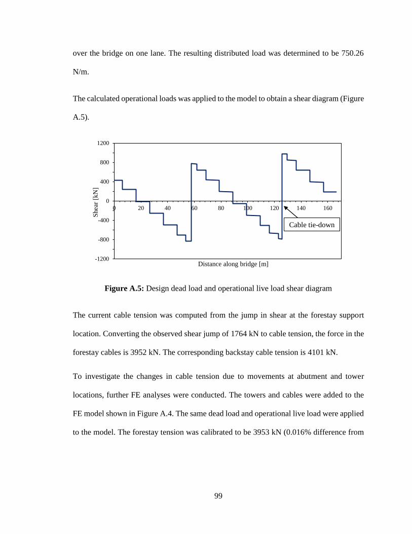
99

over the bridge on one lane. The resulting distributed load was determined to be 750.26

N/m.

The calculated operational loads was applied to the model to obtain a shear diagram (Figure

A.5).

Figure A.5: Design dead load and operational live load shear diagram

The current cable tension was computed from the jump in shear at the forestay support

location. Converting the observed shear jump of 1764 kN to cable tension, the force in the

forestay cables is 3952 kN. The corresponding backstay cable tension is 4101 kN.

To investigate the changes in cable tension due to movements at abutment and tower

locations, further FE analyses were conducted. The towers and cables were added to the

FE model shown in Figure A.4. The same dead load and operational live load were applied

to the model. The forestay tension was calibrated to be 3953 kN (0.016% difference from

-1200

-800

-400

0

400

800

1200

0 20 40 60 80 100 120 140 160

Shea

r [k

N]


Cable tie-down

100

analysis result), while the backstay percent difference was modelled as 4089 kN (0.289%

difference).

To allow horizontal movements at the abutment, the support was changed from a roller to

a pin. The resulting cable tension forces are seen in Table A.3.

Table A.3: Effect of movements at support locations

Location Movement Cable Tension [kN]

Direction Distance [mm] Forestay Backstay

N/A No Movement N/A 3953 4089

Abutment

Vertical +10 3949 4084

-10 3958 4094

Horizontal +10 3949 4084

-10 3979 4118

Tower

Vertical +10 3958 4094

-10 3949 4084

Horizontal +10 3943 4079

-10 3963 4059

The movements at abutment were computed using the girder profile from 2014 and 2016

topographic survey data. It was assumed that the footings have not settled at the tower

locations. According to the soil profile determined from the bore holes that were tested

prior to construction of the Hawkshaw Bridge, the abutment and the tower sit on layers of

till with gravel and sand. The soil at the abutment and tower locations on the Fredericton

side are layers of gravel, sand, and boulders sitting on bedrock. Following the assumption

that the towers are not susceptible to settlement, the deck elevation profile was recalculated

with reference elevation set at the towers.

101

Following the assumption that the towers are not susceptible to settlement, the deck

elevation profile was calculated with reference elevation set at the towers. The adjusted

profile is illustrated in Figure A.6 and Figure A.7.

Figure A.6: Adjusted elevation profile (Nackawic side)

Figure A.7: Adjusted elevation profile (Fredericton side)

-0.1

0

0.1

0.2

0.3

0 20 40 60 80 100 120 140 160

Def

lect

ion [

m]


Survey data from June, 2014

Survey data from July, 2016

-0.1

0

0.1

0.2

0.3

0 20 40 60 80 100 120 140 160

Def

lect

ion [

m]


Survey data from June, 2014

Survey data from July, 2016

102

These observed abutment movements were applied to the SAP2000 model. The abutment

movements applied and the resulting cable tension values are tabulated in Table A.4.

Table A.4: Effect of abutment movement, determined from survey data

Side Survey

Year

Movement

[mm]

Forestay

Cable

Tension

[kN]

% Diff.

Backstay

Cable

Tension

[kN]

% Diff.

Nackawic 2014 30 3967 0.34% 4105 0.39%

2016 29 3966 0.33% 4104 0.37%

Fredericton 2014 44 3973 0.51% 4113 0.58%

2016 63 3982 0.73% 4123 0.82%

It can be concluded that the effects of observed abutment movement on the cable tension

is minimal. Therefore, it was considered to be negligible in further analysis.

103

Appendix B: Frequency Analyser

104

In this section, the theoretical background for frequency analyser for Power Spectral

Density (PSD) approximation is discussed.

A frequency analyser is essentially a narrow band filter (Figure B.2) combined with an

r.m.s. meter (Figure B.1).

Figure B.1: Schematics of a frequency analyser

Figure B.2: Narrow band filter

The time average of ��(𝜔0, ∆𝜔) is calculated from output signal of the narrowband filter,

𝑦(𝑡):

��(𝜔0, ∆𝜔) =1

𝑇∫ 𝑦2(𝑡)𝑑𝑡

𝑇

0

(B.1)

The variable 𝑧 is a function of averaging time 𝑇 and the narrow band filter centre frequency

𝜔0 and bandwidth ∆𝜔.

𝑥(𝑡)

Output

response signal

Narrow

band filter Squaring Averaging

𝑦(𝑡) 𝑦2(𝑡) Output

meter

𝑧(𝑡)

0 −𝜔0 (𝑓0) 𝜔0 (𝑓0) 𝜔 (𝑓)

∆𝜔 (𝐵𝑒)

𝐻0

|𝐻𝑓(𝜔)|

105

𝐸[��] =1

𝑇∫ 𝐸[𝑦2]𝑑𝑡

𝑇

0

(B.2)

1

𝑇∫ 𝐸[𝑦2]𝑑𝑡

𝑇

0

= 𝐸[𝑦2] (B.3)

The output of the frequency analyser becomes closer to its true mean as 𝑇 approaches

infinity:

𝐸[𝑧] = lim𝑇→∞

𝐸[��] (B.4)

Assuming that 𝑦(𝑡) is stationary, the frequency response function, 𝐻(𝜔) relates the

spectral density of the signal and the filtered signal:

𝑆𝑦(𝜔) = |𝐻(𝜔)|2𝑆𝑥(𝜔) (B.5)

From Equation (B.4), since the square mean of a signal is equal to the area under the PSD

curve,

𝐸[𝑦2] = ∫ 𝑆𝑦(𝜔)𝑑𝜔∞

−∞

= ∫ |𝐻(𝜔)|2𝑆𝑥(𝜔)𝑑𝜔∞

−∞

(B.6)

When the narrow band bandwidth is very small,

𝐸[𝑦2] = 𝐸[𝑧] ≅ 2𝐻02∆𝜔𝑆𝑥(𝜔0) (B.7)

Rearranging Equation (B.7), it can be seen that one can approximate the spectral density

using a frequency analyzer with a known narrowband filter with a centre frequency of 𝜔0,

filter bandwidth of ∆𝜔, and filter magnitude of 𝐻0:

106

𝑆𝑥(𝜔0) ≅𝐸[��]

2𝐻02∆𝜔

(B.8a)

𝑆𝑦(𝜔0) ≅𝐸[��]

2∆𝜔 (B.8b)

Converting the angular frequency (rad/sec) to frequency (Hz) in Equation (B.8a) and to a

one-sided plot of the spectral density,

��𝑦(𝑓) =𝐸[��]

𝐵𝑒 (B.9)

^ indicates that it is an approximation of the variable. 𝑓 corresponds to 𝜔0 and 𝐵𝑒

corresponds to ∆𝜔:

𝑓 =𝜔0

2𝜋 (B.10a)

𝐵𝑒 =∆𝜔

2𝜋 (B.10b)

Therefore, the spectral density of a signal can be estimated from output of the frequency

analyser with a known narrowband filter bandwidth.

107

Appendix C: Generation of a Signal with a Defined PSD

108

In Chapter 4, it was necessary to generate a time history signal from a certain frequency

content for the numerical analysis. In this appendix, the procedure for such signal

generation is presented.

A signal in frequency domain contains two types of information: magnitude and phase.

They are associated with the real and imaginary components of the PSD, respectively.

Therefore, focusing only on the real part of the signal is not satisfactory for the calculation

of a time series. Phase information that is randomly distributed between 0 to 360 degrees

was introduced. The details of the process can be seen in Figure C.1.

Figure C.1: Flowchart for time series generation

When generating a signal from one-sided PSD, the PSD has to be made two-sided. In order

for the signal to be real, anti-symmetry has to be enforced by making the negative

frequency components complex conjugates of the positive components. Additionally, the

first components of the first and second halves of the PSD curves must be real.

Frequency content shape

𝑆(𝑓)

Amplitude, 𝐴(𝑓)

𝐴(𝑓) = √2𝑆(𝑓)

Phase information (random)

𝜙(𝑓)

Signal in frequency domain

𝑍(𝑓) = 𝐴(𝑓)𝑒𝑖𝜙(𝑓)

Signal in time domain

𝑧(𝑡)

Inverse fast Fourier Transform

109

Appendix D: Ambient Vibration Testing of the Hawkshaw Bridge

110

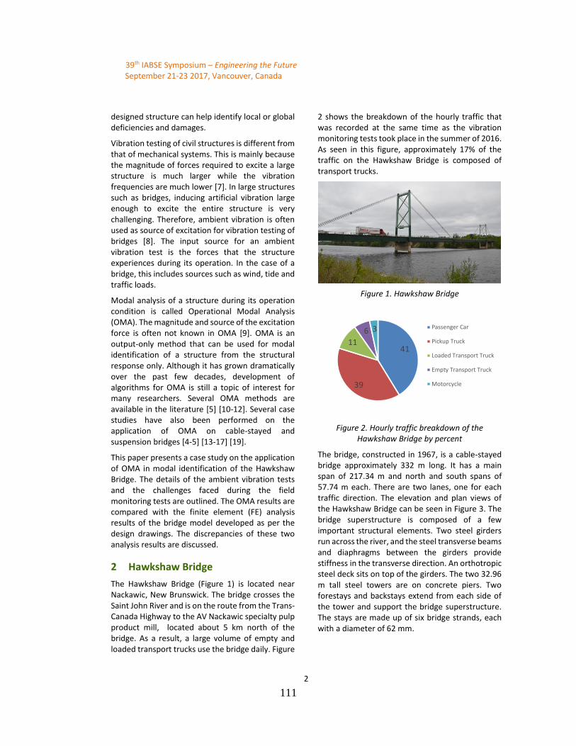
111

39th IABSE Symposium – Engineering the Future September 21-23 2017, Vancouver, Canada

2

designed structure can help identify local or global deficiencies and damages.

Vibration testing of civil structures is different from that of mechanical systems. This is mainly because the magnitude of forces required to excite a large structure is much larger while the vibration frequencies are much lower [7]. In large structures such as bridges, inducing artificial vibration large enough to excite the entire structure is very challenging. Therefore, ambient vibration is often used as source of excitation for vibration testing of bridges [8]. The input source for an ambient vibration test is the forces that the structure experiences during its operation. In the case of a bridge, this includes sources such as wind, tide and traffic loads.

Modal analysis of a structure during its operation condition is called Operational Modal Analysis (OMA). The magnitude and source of the excitation force is often not known in OMA [9]. OMA is an output-only method that can be used for modal identification of a structure from the structural response only. Although it has grown dramatically over the past few decades, development of algorithms for OMA is still a topic of interest for many researchers. Several OMA methods are available in the literature [5] [10-12]. Several case studies have also been performed on the application of OMA on cable-stayed and suspension bridges [4-5] [13-17] [19].

This paper presents a case study on the application of OMA in modal identification of the Hawkshaw Bridge. The details of the ambient vibration tests and the challenges faced during the field monitoring tests are outlined. The OMA results are compared with the finite element (FE) analysis results of the bridge model developed as per the design drawings. The discrepancies of these two analysis results are discussed.

2 Hawkshaw Bridge

The Hawkshaw Bridge (Figure 1) is located near Nackawic, New Brunswick. The bridge crosses the Saint John River and is on the route from the Trans-Canada Highway to the AV Nackawic specialty pulp product mill, located about 5 km north of the bridge. As a result, a large volume of empty and loaded transport trucks use the bridge daily. Figure

2 shows the breakdown of the hourly traffic that was recorded at the same time as the vibration monitoring tests took place in the summer of 2016. As seen in this figure, approximately 17% of the traffic on the Hawkshaw Bridge is composed of transport trucks.

Figure 1. Hawkshaw Bridge

Figure 2. Hourly traffic breakdown of the Hawkshaw Bridge by percent

The bridge, constructed in 1967, is a cable-stayed bridge approximately 332 m long. It has a main span of 217.34 m and north and south spans of 57.74 m each. There are two lanes, one for each traffic direction. The elevation and plan views of the Hawkshaw Bridge can be seen in Figure 3. The bridge superstructure is composed of a few important structural elements. Two steel girders run across the river, and the steel transverse beams and diaphragms between the girders provide stiffness in the transverse direction. An orthotropic steel deck sits on top of the girders. The two 32.96 m tall steel towers are on concrete piers. Two forestays and backstays extend from each side of the tower and support the bridge superstructure. The stays are made up of six bridge strands, each with a diameter of 62 mm.

41

39

11

6 3 Passenger Car

Pickup Truck

Loaded Transport Truck

Empty Transport Truck

Motorcycle

112


3

Figure 3. Elevation and plan views of the Hawkshaw Bridge with sensor locations

3 Ambient vibration tests

3.1 Equipment

LORD MicroStrain G-Link LXRS sensors were installed on the top flanges of the bridge girders. These sensors were used to capture acceleration in x, y and z directions. The acceleration data was wirelessly transmitted to the base station via LORD MicroStrain WSDA-1500-LXRS sensor data aggregator which was connected to a laptop computer.

3.2 Test setup

The base station and gateway were initially set up in an open space just off the bridge on the south side (Figure 4). However, due to wireless communication difficulties, they were relocated to the centre of the bridge. Ten wireless tri-axial accelerometer nodes were placed on the top flanges of the bridge girders, which were easily accessible (Figure 5). The sensor configuration and the node numbers are shown in Figure 3.

Figure 4. Original base station setup

3.3 Monitoring parameters

The sampling frequency was chosen as 64 Hz with ten tri-axial sensors, resulting in 30 channels. From a preliminary FE analysis, it was found out that the first modes of the Hawkshaw Bridge that were within the cumulative z direction Modal Mass Participation Ratio (MMPR) of 90% were below the natural frequency of 28 Hz. Therefore, taking Nyquist frequency considerations into account, the minimum sampling frequency requirement was calculated as 56 Hz. Furthermore, 64 Hz was the

113

114

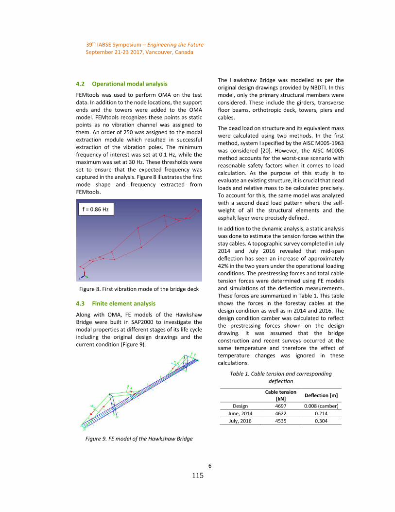
115


6

4.2 Operational modal analysis

FEMtools was used to perform OMA on the test data. In addition to the node locations, the support ends and the towers were added to the OMA model. FEMtools recognizes these points as static points as no vibration channel was assigned to them. An order of 250 was assigned to the modal extraction module which resulted in successful extraction of the vibration poles. The minimum frequency of interest was set at 0.1 Hz, while the maximum was set at 30 Hz. These thresholds were set to ensure that the expected frequency was captured in the analysis. Figure 8 illustrates the first mode shape and frequency extracted from FEMtools.

Figure 8. First vibration mode of the bridge deck

4.3 Finite element analysis

Along with OMA, FE models of the Hawkshaw Bridge were built in SAP2000 to investigate the modal properties at different stages of its life cycle including the original design drawings and the current condition (Figure 9).

Figure 9. FE model of the Hawkshaw Bridge

The Hawkshaw Bridge was modelled as per the original design drawings provided by NBDTI. In this model, only the primary structural members were considered. These include the girders, transverse floor beams, orthotropic deck, towers, piers and cables.

The dead load on structure and its equivalent mass were calculated using two methods. In the first method, system I specified by the AISC M005-1963 was considered [20]. However, the AISC M0005 method accounts for the worst-case scenario with reasonable safety factors when it comes to load calculation. As the purpose of this study is to evaluate an existing structure, it is crucial that dead loads and relative mass to be calculated precisely. To account for this, the same model was analyzed with a second dead load pattern where the self-weight of all the structural elements and the asphalt layer were precisely defined.

In addition to the dynamic analysis, a static analysis was done to estimate the tension forces within the stay cables. A topographic survey completed in July 2014 and July 2016 revealed that mid-span deflection has seen an increase of approximately 42% in the two years under the operational loading conditions. The prestressing forces and total cable tension forces were determined using FE models and simulations of the deflection measurements. These forces are summarized in Table 1. This table shows the forces in the forestay cables at the design condition as well as in 2014 and 2016. The design condition camber was calculated to reflect the prestressing forces shown on the design drawing. It was assumed that the bridge construction and recent surveys occurred at the same temperature and therefore the effect of temperature changes was ignored in these calculations.

Table 1. Cable tension and corresponding deflection

Cable tension

[kN] Deflection [m]

Design 4697 0.008 (camber)

June, 2014 4622 0.214

July, 2016 4535 0.304

f = 0.86 Hz

116


7

5 Results and discussion

Acquiring a healthy dataset representing the vibration behaviour of the Hawkshaw Bridge was challenging due to the difficulties discussed earlier in this paper. Four monitoring setups were tested. Using OMA, the first 10 natural frequencies and their mode shapes were evaluated using the most reliable set of data. The results of this analysis are shown in Table 2. This table also presents the modal analysis results using the FE method. As the source of ambient vibration was mainly traffic loads, only modes with significant vertical vibration were considered in this analysis.

Table 2. Comparison of natural frequencies (Hz)

OMA FEM

(AISC) FEM

(self-weight)

Mode Freq. [Hz]

Mode Freq. [Hz]

Mode Freq. [Hz]

1 0.86 2 0.47 2 0.48

2 1.21 3 0.49 3 0.50

3 1.25 4 0.60 4 0.62

4 1.48 5 0.73 5 0.74

5 2.42 6 0.83 6 0.86

6 2.82 7 0.92 7 0.93

7 3.05 8 1.06 10 1.10

8 3.30 9 1.18 11 1.23

9 3.33 10 1.23 12 1.24

10 3.70 11 1.25 13 1.34

As can be seen in Table 2, more number of modes were identified for the FE analyses than the OMA. In the case of the fundamental frequency, the OMA results yielded the highest value of the three. Further analysis is in progress to identify the parameters that effected such discrepancies. A key parameter is the ambient temperature that affects the bridge stiffness which consequently influences the governing vibration frequencies. The bridge receives direct sunlight, and therefore an increased temperature which causes elongation in the girders and cables. This can significantly influence the overall stiffness of the structure. Another key parameter is the effective mass of the structure. In general, a greater mass would result in a smaller natural frequency. Therefore, this could be an indication of overestimation of mass in the FE model. The two FE analyses show that the

overestimation of dead load for design did have an influence on the dynamic behaviour of the structure.

Extraction of modes in the x and y directions (longitudinal and transverse) using the OMA were particularly challenging. This is mainly due to the fact that the magnitude of excitations in the x and y directions were not large enough to excite the structure dominant modes. The maximum input magnitudes for x and y directions were approximately 0.15 and 0.3 G, respectively.

Furthermore, through studying the effect of sensor configurations, it was found that using five sensors along one side of the bridge does not provide enough degrees of freedom for such a large structure.

6 Conclusion

This paper presented the full-scale testing setup and post-processing of the data for the operation modal testing of the Hawkshaw Bridge. The experimental challenges such as the wireless communication issues, and the data acquisition bandwidth limitations were discussed.

The ambient vibration data were used for extraction of the governing natural frequencies and mode shapes using the OMA method. The results were compared with the FE modal analysis. The discrepancies between these results were discussed. Further investigations are in progress to study the effect of various governing parameters on the OMA results.

SHM as used in this full-scale testing project was a useful and reliable addition to visual inspection of the structural elements of the Hawkshaw Bridge. NBDTI intends to use the information gained from this project to help with future maintenance and repair goals.

7 Acknowledgement

The authors would like to thank the New Brunswick Department of Transportation and Infrastructure and the New Brunswick Innovation Foundation for their support of this research.

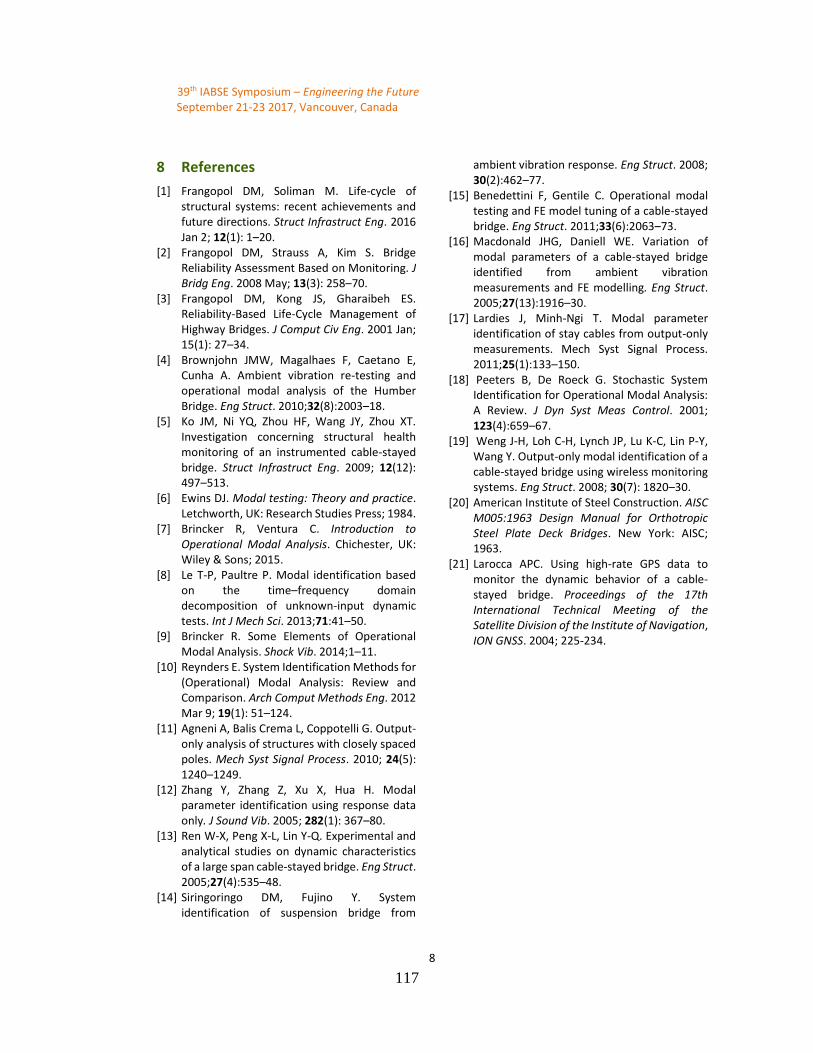
117


8

8 References

[1] Frangopol DM, Soliman M. Life-cycle of structural systems: recent achievements and future directions. Struct Infrastruct Eng. 2016 Jan 2; 12(1): 1–20.

[2] Frangopol DM, Strauss A, Kim S. Bridge Reliability Assessment Based on Monitoring. J Bridg Eng. 2008 May; 13(3): 258–70.

[3] Frangopol DM, Kong JS, Gharaibeh ES. Reliability-Based Life-Cycle Management of Highway Bridges. J Comput Civ Eng. 2001 Jan; 15(1): 27–34.

[4] Brownjohn JMW, Magalhaes F, Caetano E, Cunha A. Ambient vibration re-testing and operational modal analysis of the Humber Bridge. Eng Struct. 2010;32(8):2003–18.

[5] Ko JM, Ni YQ, Zhou HF, Wang JY, Zhou XT. Investigation concerning structural health monitoring of an instrumented cable-stayed bridge. Struct Infrastruct Eng. 2009; 12(12): 497–513.

[6] Ewins DJ. Modal testing: Theory and practice. Letchworth, UK: Research Studies Press; 1984.

[7] Brincker R, Ventura C. Introduction to Operational Modal Analysis. Chichester, UK: Wiley & Sons; 2015.

[8] Le T-P, Paultre P. Modal identification based on the time–frequency domain decomposition of unknown-input dynamic tests. Int J Mech Sci. 2013;71:41–50.

[9] Brincker R. Some Elements of Operational Modal Analysis. Shock Vib. 2014;1–11.

[10] Reynders E. System Identification Methods for (Operational) Modal Analysis: Review and Comparison. Arch Comput Methods Eng. 2012 Mar 9; 19(1): 51–124.

[11] Agneni A, Balis Crema L, Coppotelli G. Output-only analysis of structures with closely spaced poles. Mech Syst Signal Process. 2010; 24(5): 1240–1249.

[12] Zhang Y, Zhang Z, Xu X, Hua H. Modal parameter identification using response data only. J Sound Vib. 2005; 282(1): 367–80.

[13] Ren W-X, Peng X-L, Lin Y-Q. Experimental and analytical studies on dynamic characteristics of a large span cable-stayed bridge. Eng Struct. 2005;27(4):535–48.

[14] Siringoringo DM, Fujino Y. System identification of suspension bridge from

ambient vibration response. Eng Struct. 2008; 30(2):462–77.

[15] Benedettini F, Gentile C. Operational modal testing and FE model tuning of a cable-stayed bridge. Eng Struct. 2011;33(6):2063–73.

[16] Macdonald JHG, Daniell WE. Variation of modal parameters of a cable-stayed bridge identified from ambient vibration measurements and FE modelling. Eng Struct. 2005;27(13):1916–30.

[17] Lardies J, Minh-Ngi T. Modal parameter identification of stay cables from output-only measurements. Mech Syst Signal Process. 2011;25(1):133–150.

[18] Peeters B, De Roeck G. Stochastic System Identification for Operational Modal Analysis: A Review. J Dyn Syst Meas Control. 2001; 123(4):659–67.

[19] Weng J-H, Loh C-H, Lynch JP, Lu K-C, Lin P-Y, Wang Y. Output-only modal identification of a cable-stayed bridge using wireless monitoring systems. Eng Struct. 2008; 30(7): 1820–30.

[20] American Institute of Steel Construction. AISC M005:1963 Design Manual for Orthotropic Steel Plate Deck Bridges. New York: AISC; 1963.

[21] Larocca APC. Using high-rate GPS data to monitor the dynamic behavior of a cable-stayed bridge. Proceedings of the 17th International Technical Meeting of the Satellite Division of the Institute of Navigation, ION GNSS. 2004; 225-234.

118

Appendix E: Vibration Testing of Scaled Cable-Stayed Bridge*

________________________________________________________________________

* The primary author of this conference paper is Diego Padilha. Author of this thesis was

involved in the experimental tests and FE dynamic analysis of the scale model, as well as

manuscript preparation.

119

120


2

algorithm is still an interest of many researchers. In addition to theoretical developments, there is a significant demand for OMA applications. Several studies on the application of OMA in system identification of bridges [9-13] and the effectiveness of application of small-scale models in terms of modal analysis [2], [14-18] can be found in the literature.

This article describes results of an investigation conducted at the Smart Structures Research Group of the University of New Brunswick in collaboration with the New Brunswick Department of Transportation and Infrastructure. The development of a 1/75 elastic scale model of the Hawkshaw Bridge (Figure 1), its modal identification, and correlation of the results with the prototype structure are described. The correlation between the scale model and its prototype is confirmed using the OMA and the finite element (FE) analysis results. FE models of the scale model and the prototype structure were developed to ensure an accurate correlation between the two systems.

The numerical models were examined for both static and dynamic loading scenarios. Sensitivity analyses to account for the fabrication tolerances are also discussed. Random vibration sources were used to excite the model and the response was monitored using accelerometers. Correlation of the scale model response with the prototype response is discussed. An experimental parametric study was developed to investigate the effect of changes in the weight of the bridge deck and the cable tensions.

Figure 1. The Hawkshaw Bridge, NB, Canada

2 The Hawkshaw Bridge

The Hawkshaw Bridge is located near Nackawic, approximately 65 km west of Fredericton, New Brunswick, Canada. The bridge was constructed in 1967. It crosses the Saint John River, and it is a three-span cable-stayed bridge with an orthotropic steel deck. It has a length of approximately 332 m with the main span of 217.34 m and south and north spans of 57.73 m. The stay cables are connected to two steel towers supporting the orthotropic deck. Each tower carries 24 steel strands, which are divided into two sets of backstays and two sets of forestays. The stay cables are arranged in a form of a harp, which provides an aesthetically pleasant appearance and a decent vibration behaviour in long distance. Figure 2-a presents the layout of the Hawkshaw Bridge. The structure is symmetric about its centreline. A large volume of both empty and loaded logging trucks uses the facility each day along with passenger cars and pickup trucks. These trucks commute from a paper mill located about 5 km north of the bridge. The bridge is located on the route from the Trans-Canada Highway 2 to the paper mill.

3 Small-Scale Model

The physical model of the Hawkshaw Bridge was built in the Structural Engineering Laboratory of the University of New Brunswick. This model satisfies similitude requirements for the bending stiffness of the girders, towers and piers and the axial stiffness of the cable stays. The mass similitude accuracy of the stays was not considered for this case study since the primary focus was on the analysis of the deck behaviour on which the cable mass does not have a significant influence.

The design of the 1/75 small-scale model was performed strictly following the similitude theory to ensure similarity between two different systems [1]. The total length of the model is 4.43 m, which was calculated using the linear scale factor SL = 75. This scale factor was chosen based on the space available in the laboratory. The orthotropic deck, the steel box section towers, and the piers were replaced by solid cross-

121


3

sections with correctly scaled bending stiffness by scaling the moment of inertia about both strong and weak axes. The stay cable bundles of 6 on the prototype were modeled with a single 1.97 mm

diameter steel wire by properly scaling the cross-sectional area in the scale-model. Figure 2-b presents the overall layout of the small-scale model.

(a) Prototype

(b) 1/75 scale model

Figure 2. Layout of the prototype and 1/75 scale model of the Hawkshaw Bridge (All dimensions are in mm)

Aluminum alloy was used to build the model bridge deck, towers and piers. This material was chosen due to its lower modulus of elasticity

compared to steel used for the prototype. Therefore, the model is less stiff and requires less additional mass to represent the correct scaled

122


4

dead load for the model to achieve similarity. Table 1 presents the scale factors used to design the scale model.

Additional mass was added to the scale model deck to represent the scaled dead load of the structure. Small steel plates (127 mm x 50 mm x 20 mm) were attached to the deck using two bolts without passing through the deck to avoid any changes in the stiffness of the deck. A total of 85.7 kg was added throughout the bridge deck. Figure 3 shows the scale model including the added mass.

Table 1. Scale Factors of scale model

Designation Scale Factor

Length SL=Lp/Lm = 75

Modulus of Elasticity (Deck & Tower)

SE1=E1m/E1p=2.78

Modulus of Elasticity (Cables)

SE2=E2m/E2p=0.95

Area SA=SL2=(75)2

Inertia SI=SL4=(75)4

Force (Deck & Tower) SF1=SE1SL2=(2.78)(75)2

Force (Cables) SF2=SE2SL2=(0.95)(75)2

Time ST= SL1/2=(75)1/2

Frequency Sf= SL-1/2=(75)-1/2

Mass SM=SE1SL2=(2.78)(75)2

Figure 3. Scale model of the Hawkshaw Bridge

The elevations at the support locations and the cable tension are adjustable which allow for a realistic calibration of the model. Figure 4 shows the adjustable components.

Figure 4. Left: Backstay connection; Right: Forestay connection

3.1 Cable calibration

In order to calibrate the tension in the cables, the cable tension of the prototype structure was first scaled using equations (1) and (2), the subscripts p and m correspond to prototype and model, respectively

𝑆𝐹 =𝐹𝑝

𝐹𝑚 ; 𝑆𝐸 =

𝐸𝑝

𝐸𝑚 (1)

𝑆𝐹 = 𝑆𝐸𝑆𝐿2 (2)

Table 2 summarizes the parameters used to scale the tension of the cables in the model.

Table 2. Summary of cable forces

Element L

(m) SE SL

FP

(kN) Fm

(N)

Forestay 0.99 1 75 637.9 113.4

Backstay 0.89 1 75 674.5 119.9

Mersenne’s Law [19] shown in equation (3) was used to calculate the cable tension as a function of the cable’s fundamental vibration frequency. In this equation, f is the frequency in Hz, L is the length in metres, and μ is the mass per unit length in kg/m.

𝑓 =1

2𝐿√

𝑇

𝜇 (3)

The cable’s fundamental vibration frequency was measured using a smartphone built-in accelerometer. The smartphone was clamped on the top of the tower, and the cables were excited manually. The spectral content of the vibration was calculated in real time. The tensions in the cables were adjusted until the required dominant vibration frequencies were achieved for each wire.

123


5

The adopted calibration process is similar to how a guitar is tuned using a digital tuner. Table 3 shows parameters used to calibrate the tension of the wires.

Table 3. Summary of converted frequencies of scale model cables

Element L

(m)

μ (kg/m)

T

(N) f

(Hz)

Forestay 0.99 2.89E-02 113.41 31.43

Backstay 0.89 2.89E-02 119.9 36.00

Table 4. Design and as-built sections

Model Tower leg Deck Pier Cap Pier Column Pier Diaphragm

b (mm) h (mm) b (mm) h (mm) b (mm) h (mm) b (mm) h (mm) b (mm) h (mm)

1 9.5 9.5 76.2 15.8 15.8 15.8 12.7 12.7 12.7 25.4

2 7.7 8.5 53 14.5 15 15 12.7 12.7 12.7 25.4

Diff. (%) 18.9 10.5 30.4 8.2 5.1 5.1 0 0 0 0

3.2 Built versus designed scale model

A sensitivity analysis was performed using SAP2000 to account for section round-ups during fabrication. Two FE models were created based on the theoretical designed model and the manufactured model. Model 1 was developed with the sections slightly bigger than what was designed for, and Model 2 was developed strictly following the design calculations. Figure 5 shows the FE model of the 1/75 scale model of the Hawkshaw Bridge (Model 1). Table 4 shows the section dimensions and the difference between Model 1 and Model 2, where b and h are the width and thickness of each member, respectively.

Figure 5. SAP2000 FE Model of 1/75 scale model

A linear static analysis of the bridge models under their self-weight showed a discrepancy of about 13% for support reactions and mid-span deflections. Table 5 presents the results difference between the two models.

Table 5. SAP2000 linear static analysis results

Model 1 2 Discrep. (%)

Support Reaction (N) 45.01 38.8 13.80

Deflection MAX. (mm) 0.03 0.026 13.33

Dynamic analyses were also performed on the two models. The first five natural frequencies can be seen in Table 6. The natural frequencies from the two models present up to 21.2% difference and the mode shapes correlate well.

Table 6. SAP2000 dynamic analysis results

Mode Model 1

ω (Hz)

Model 2

ω (Hz)

Discrepancy

(%)

1 1.57 1.24 21.2

2 1.64 1.41 14.3

3 3.12 2.59 16.8

4 5.39 4.64 13.8

5 5.69 4.91 13.7

4 Vibration tests

The details of the vibration tests on the prototype bridge are discussed in [20].

Five LORD MicroStrain G-Link LXRS tri-axial accelerometer sensors were installed on the top of the deck to monitor the vibration of the scale model. The acceleration data was wirelessly transmitted to the base station via LORD MicroStrain WSDA-1500-LXRS sensor data aggregator which was connected to a laptop computer. The sensor layout can be seen in Figure 6.

As outlined in [20], the monitoring period for the prototype bridge was 148 minutes. Therefore, the minimum required time for the small-scale model tests was found to be approximately 14 min using the time scale factor of ST = (75)1/2 from Table 1.

124


6

128 Hz was chosen as the sampling rate. This was the maximum allowable sampling frequency with the used router bandwidth using five sensors. Table 7 shows the sampling parameters for the prototype and the scale model tests.

Table 7. Vibration monitoring parameters for the Hawkshaw Bridge and the scale model

Prototype Scale model

Sampling Freq. (Hz) 64 128

Number of Sensors 10 5

Test Duration (min) 148 20

Figure 6. Sensor layout for small-scale model tests (All dimensions are in mm)

Various types of random vibration sources were introduced to the model. These sources included impact loads from a hammer, vibration of a smartphone, and cyclic movement of a hand drill. These vibrations were applied on the deck, the cables, and the tower. Two configurations were tested to simulate different scenarios, which are described below:

Configuration 1: 100 % of the additional mass was added for this configuration. The cables were calibrated according to the as-built conditions in 1967. To ensure that the deck and piers are in contact, an additional weight of 500 g was added at the tower locations.

Configuration 2: This configuration is similar to Configuration 1, with properly scaled cable forces as of July 2016. In this configuration, the current cable tensions were calculated based on the static analysis results, so that the bridge deck elevation profile matches the survey data performed on the prototype structure in July 2016.

5 Results and discussion

The results from the laboratory tests were analysed using FEMtools, a software specialized in modal analysis. The results from OMA of the scaled model were compared with the OMA results of the prototype structure and FE analysis.

Table 8 presents the comparison between prototype OMA results, FE analysis results, and the scale model tests from Configurations 1 and 2. The natural frequencies for the scale model were scaled down using the scale factor for frequency, Sf from Table 1. For FE analysis results, only those that were included in the 90 % cumulative Z-direction Modal Mass Participation Ratio (MMPR) were included.

From Table, 8, it can be seen that the prototype structure generally had greater natural frequencies than the other three. This indicates that the actual structure is stiffer than what was assumed. Comparing Configurations 1 and 2, it can be seen that the cable calibration results in lower natural frequencies, from less stiffness of the overall structure.

The mode shapes were successfully extracted for the prototype structure and the small-scale model. A good correlation exists between the mode shapes. Further calibration of the models in order to reduce the discrepancy between the natural frequencies are currently under investigation by the authors.

Overall, a greater number of poles were extracted from the scale model tests. This is mainly due to the fact that a larger number of modes were excited with a larger magnitude in the laboratory tests. Further investigations are in progress to

125


7

provide more precise modal identification by accurate representation of mass, cable tension, boundary conditions, and slope of the model.

Table 8. Correlation between prototype and small-scale model

Prototype

Prototype FEM

Configuration 1 Configuration 2

Mode Natural

Freq. (Hz] Damping

(%) Natural

Freq. (Hz) Natural

Freq. (Hz) Damping

(%) Natural

Freq. (Hz) Damping

(%]

1 0.86 1.12 0.49 0.67 8.47 0.50 5.98

2 1.21 2.3 1.06 0.67 9.68 1.09 1.42

3 1.25 1.01 1.23 1.21 0.78 1.20 0.62

4 1.48 4.48 1.64 1.39 0.21 1.31 1.18

5 2.42 2.12 1.79 1.93 1.58 1.39 1.80

6 2.82 4.42 2.53 2.30 0.95 1.60 1.60

7 3.05 1.76 4.36 2.36 0.91 1.76 0.40

8 3.30 1.13 4.84 2.41 0.38 1.82 0.50

9 3.33 0.95 6.20 2.83 1.48 1.94 4.14

10 3.70 1.58 8.76 3.49 0.31 1.95 0.40

6 Conclusion

The development of a 1/75 scale model of the Hawkshaw Bridge was discussed. The experiments and analysis results show a good correlation between the design and as-built models. Dynamic test results were compared with the prototype OMA results. Further investigations and calibration of the scale model are in progress to achieve better correlation between the scale model and the prototype structure.

7 Acknowledgement

The authors would like to thank the New Brunswick Department of Transportation and Infrastructure and the New Brunswick Innovation Foundation for their financial support of this research.

8 References

[1] Harris HG, Sabnis GM. Structural Modeling and Experimental Techniques. Boca Raton: CRC Press; 1999.

[2] Shehadeh M, Shennawy Y, El-Gamal H. Similitude and scaling of large structural elements: case study. Alechandria Engineering Journal. 2015;54:147-154.

[3] Kline SJ, Radbill JR. Similitude and approximation theory. Journal of Applied Mechanics. 1996;33;238.

[4] Le T-P, Paultre P. Modal identification based on the time–frequency domain decomposition of unknown-input dynamic tests. Int J Mech Sci. 2013;71:41-50.

[5] Peeters B. and De Roeck G. Stochastic system identification for operational modal analysis: a review. Journal of Dynamic Systems, Measurement, and Control. 2001; 123(4): 659-667.

[6] Reynders E. System identification methods for (operational) modal analysis: review and comparison. Archives of Computational Methods in Engineering. 2012 Mar 9; 19(1): 51-124.

[7] Agneni A., Balis Crema L., and Coppotelli G. Output-only analysis of structures with closely spaced poles. Mechanical Systems and Signal Processing. 2010; 24(5): 1240-1249.

[8] Zhang Y., Zhang Z., Xu X., and Hua H. Modal parameter identification using response data only. Journal of Sound and Vibration. 2005; 282(1): 367-380.

126


8

[9] Ren W.-X., Peng X.-L., and Lin Y.-Q. Experimental and analytical studies on dynamic characteristics of a large span cable-stayed bridge. Engineering Structures. 2005; 27(4): 535-548.

[10] Siringoringo D.M., and Fujino Y. System identification of suspension bridge from ambient vibration response. Engineering Structures. 2008; 30(2):462-477.

[11] Benedettini F. and Gentile C. Operational modal testing and FE model tuning of a cable-stayed bridge. Engineering Structures. 2011; 33(6): 2063-2073.

[12] Wang H., Li A., and Li J. Progressive finite element model calibration of a long-span suspension bridge based on ambient vibration and static measurements. Engineering Structures. 2010; 32(9): 2546-2556.

[13] Deraemaeker A., Reynders E., De Roeck G., and Kullaa J. Vibration-based structural health monitoring using output-only measurements under changing environment. Mechanical Systems and Signal Processing. 2008; 22(1): 34-56.

[14] Caetano E, Cunha A, Taylor CA. Investigation of dynamic cable–deck interaction in a physical model of a cable‐stayed bridge. Part I: modal analysis. Earthquake Engineering & Structural Dynamics. 2000; 29:481–498.

[15] Caetano E, Cunha A, Taylor CA. Investigation of dynamic cable-deck interaction in a physical model of a cable-stayed bridge. Part II: seismic response. Earthquake Engineering & Structural Dynamics. 2000; 29:499–521.

[16] Xu Y-L, Xia Y. Testbed for Structural Health Monitoring of Long-Span Suspension Bridges. Journal of Bridge Engineering. 2011;

[17] Garevski M, Severn RT. Dynamic analysis of cable-stayed bridges by means of 3D analytical and physical modelling. 10th

World Conf. on Earthquake Engineering, Madrid. 1992.

[18] Irwin PA, Stoyanoff S, Xie J, Hunter M. Tacoma Narrows 50 years later— wind engineering investigations for parallel bridges. Bridge Structures. 2005;1:3-17.

[19] Rossing TD. “The Science of String Instruments”. New York: Springer; 2010

[20] Araki Y, Arjomandi K, Simpson R. Ambient vibration testing of the Hawkshaw Bridge. 39th International Association for Bridge and Structural Engineering (IABSE) Symposioum, Vancouver. 2017.

127

Appendix F: Accelerometer Specifications and Accuracy of the

Measurement

128

Table F.1 (retrieved from http://www.microstrain.com/wireless/g-link) summarizes the

specifications of the accelerometers mentioned in Chapter 3. Further details of the

sensors can be found in the accelerometer manual (Microstrain Sensing Systems).

Table F.1: Accelerometer specifications

http://www.microstrain.com/wireless/g-link

129

As can be seen from Table F.1, the wireless accelerometers can measure vibration with

an accuracy of up to 10 mG. The power spectral densities are estimated from the acquired

vibration data. With visual peak picking, the natural frequencies are determined to the

nearest 0.001 Hz. From Equation 2.4, observing the accuracy and significant figure of

each parameter, 4 significant digits were kept.

CURRICULUM VITAE

Candidate’s full name:

Yumi Araki

Universities attended:

University of New Brunswick, B.Sc.E. (Civil Engineering, Minor in Music), 2016

Publications:

Araki, Y., Arjomandi, K., and MacDonald, T. (2018). “Hybrid structural health

monitoring approach for condition assessment of cable-stayed bridges.” Submitted

to the Journal of Bridge Engineering (under review).

Araki, Y., and Arjomandi, K. (2018). “Monitoring time requirement in operational modal

tests.” Submitted to the Journal of Engineering Mechanics (under review).

Conference Presentations:

Araki, Y., Arjomandi, K., and Simpson, R. (2017). “Ambient Vibration Testing of the

Hawkshaw Bridge.” IABSE Symposium Vancouver 2017: Engineering the Future,


Padilha, D., Araki, Y., Arjomandi, K., and McGinn, J. (2017). “Vibration Testing of

Scaled Cable-Stayed Bridges.” IABSE Symposium Vancouver 2017: Engineering the

Future, International Association for Bridge and Structural Engineering, 1973–1980.

STRUCTURAL HEALTH MONITORING OF CABLE-STAYED BRIDGES

Documents