University of Nevada, Reno Structural Coefficients of High Polymer Modified Asphalt Mixes Based on Mechanistic-Empirical Analyses and Full-Scale Pavement Testing A dissertation submitted in partial fulfillment of the requirements for the degree of Doctor of Philosophy in Civil and Environmental Engineering by Jhony Habbouche Dr. Elie Y. Hajj / Dissertation Advisor Prof. Peter E. Sebaaly / Dissertation Co-advisor May, 2019

Welcome message from author
This document is posted to help you gain knowledge. Please leave a comment to let me know what you think about it! Share it to your friends and learn new things together.
Transcript
University of Nevada, Reno
Structural Coefficients of High Polymer Modified
Asphalt Mixes Based on Mechanistic-Empirical
Analyses and Full-Scale Pavement Testing
A dissertation submitted in partial
fulfillment of the requirements for the
degree of Doctor of Philosophy in Civil and
Environmental Engineering
by
Jhony Habbouche
Dr. Elie Y. Hajj / Dissertation Advisor
Prof. Peter E. Sebaaly / Dissertation Co-advisor
May, 2019

Copyright by Jhony Habbouche 2019 All Rights Reserved

THE GRADUATE SCHOOL
We recommend that the dissertation
prepared under our supervision by
Jhony Habbouche
entitled
Structural Coefficients of High Polymer Modified
Asphalt Mixes Based on Mechanistic-Empirical
Analyses and Full-Scale Pavement Testing
be accepted in partial fulfillment of the
requirements for the degree of
DOCTOR OF PHILOSOPHY
Elie Y. Hajj, Ph.D., Advisor
Peter E. Sebaaly, Ph.D., Co-advisor
Adam J.T. Hand, Ph.D., Committee Member
Raj V. Siddharthan, Ph.D., Committee Member
Ilya Zaliapin, Ph.D., Graduate School Representative
David W. Zeh, Ph.D., Dean, Graduate School
May, 2019

i
ABSTRACT
Asphalt concrete (AC) mixtures have been used as driving surfaces for flexibles pavements
since the early 1900s. With the increase of highway traffic volume and axle loads, the
introduction of modified asphalt binders provided transportation agencies an effective tool
to design balanced asphalt mixtures that can resist conflicting distresses such as permanent
deformation and fatigue cracking while maintaining good long-term durability (i.e.,
reduced moisture damage and aging). While polymer modified asphalt (PMA) mixtures,
with 2-3% polymer content, have shown improved long-term performance, it is also
believed that asphalt mixtures with high polymer (HP) content (i.e., >6% polymer content)
may offer additional advantages in flexible pavements subjected to heavy and slow-moving
traffic loads. The main objective of this study is to conduct an in-depth and comprehensive
evaluation of asphalt mixtures in the state of Florida with a high polymer (HP) modified
asphalt binder with approximately 7.5% Styrene-Butadiene-Styrene (SBS) polymer. The
study combines the following five major aspects: (1) Literature Review: information and
findings from the literature review on the performance of HP asphalt binders and mixtures
in the laboratory and in the field were collected. In addition, attempts to determine a
structural capacity for HP AC mixes using available data were executed. (2) Extensive
laboratory evaluation of HP asphalt binder and mixtures: PMA and HP asphalt binders
sampled from two different sources were evaluated in terms of long-term aging
susceptibility to observe and quantify the influence of binder modification on the oxidative
aging characteristics of these asphalt binders. Additionally, A total of 8 PMA and 8 HP AC

ii
mixes were manufactured and designed using PMA and HP asphalt binders and were
evaluated in terms of engineering properties (i.e., stiffness) and performance characteristics
(i.e., resistance to rutting, fatigue cracking, top-down cracking, and reflective cracking).
(3) Advanced mechanistic analysis under heavy moving loads using 3D-MOVE: the
developed properties and characteristics of PMA and HP mixtures were implemented in
the 3D-MOVE model to determine the responses and performance of PMA and HP
pavement sections under various loading conditions. Using the pavement responses from
3D-MOVE along with the performance models for the PMA and HP asphalt mixtures for
rutting in AC and fatigue cracking, structural coefficients of the HP modified asphalt
mixtures were determined using the fixed service life approach based on the fatigue
performance life and verified against other distress modes (i.e., AC and total rutting, top-
down cracking, and reflective cracking). (4) Full-scale pavement testing using PaveBox:
the 11 feet width by 11 feet depth by 7 feet height PaveBox served as a full-scale laboratory
tool to verify the structural coefficients developed and checked previously. (5) Advanced
numerical modeling of PaveBox using FLAC3D (Fast Lagragian Analysis of Continua
in 3-Dimensions): the three-dimensional explicit finite difference program was used to
provide an advanced analysis of sections built-in the full-scale PaveBox experiment.
The review of available literature led to the following findings and
recommendations:
• The reviewed laboratory studies indicated: a) Increasing the SBS polymer content
from 0, 3, 6, to 7.5% continues to improve the performance properties of the asphalt
binder and mixture, b) HP modification tends to slow down the oxidative aging of

iii
the asphalt binder, and c) HP asphalt binder should not be used to overcome the
negative impact of RAP on the resistance of the AC mixture to various types of
cracking.
• The reviewed field projects indicated: a) HP AC mixes have been used over a wide
range of applications from full depth AC layer to thin AC overlays under heavy
traffic, b) HP AC mixes did not show any construction related issues, c) while early
performance is encouraging, almost all HP field projects lack long-term
performance information.
• While several previous studies highlighted the positive impacts of the HP
modification of asphalt binders and mixtures, there is still a serious lack of
understanding on the structural value of the HP AC mix as expressed through the
structural coefficient for the AASHTO 1993 Guide. The attempt by the research
team to determine an aHP-AC based on the available information led to the conclusion
that empirically-based aHP-AC can underestimate the structural value of the HP AC
mix while determining the aHP-AC based on the mechanistic analysis of a singly
failure mode (i.e., fatigue cracking) may overestimate the structural value of the HP
AC mix.
The laboratory evaluation of PMA and AC mixes and the advanced mechanistic
analyses of PMA and HP flexible pavement structures led to the following findings and
recommendations:

iv
• Overall, HP AC mixes showed better engineering property and performance
characteristics when compared with the corresponding PMA control AC mixes
which can be credited to the high polymer modification of the asphalt binder (i.e.,
HP binder).
• The estimated initial fatigue-based structural coefficients ranged from 0.33 to 1.32.
Using advanced statistical analyses and considering all factors and their
interactions, an initial fatigue-based structural coefficient of 0.54 was determined
for HP AC mixes.
• The initial fatigue-based structural coefficient for HP AC mixes of 0.54 was
verified for the following distresses; rutting in AC layer, shoving in AC layer, total
rutting, top-down cracking, and reflective cracking. The verification process
concluded that the structural coefficient of 0.54 for HP AC mixes would lead to the
design of HP pavements that offer equal or better resistance to the various distresses
as the designed PMA pavements with the structural coefficient of 0.44. This
conclusion held valid for the design of both new and rehabilitation projects.
• Based on the data generated in the execution of the experimental plan and the
analyses presented, it was recommended that HP AC mixes be incorporated into
the current FDOT Flexible Pavement Design Manual with a structural coefficient
of 0.54.
v
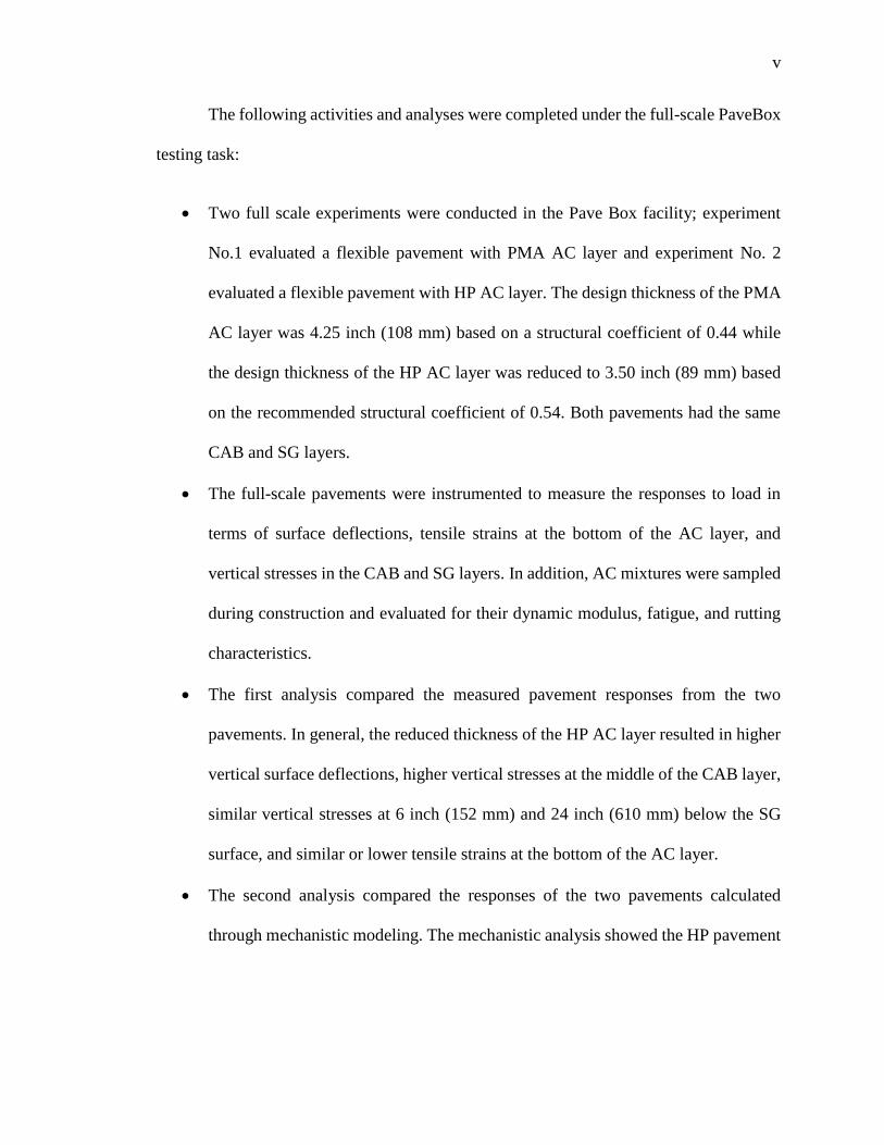
The following activities and analyses were completed under the full-scale PaveBox
testing task:
• Two full scale experiments were conducted in the Pave Box facility; experiment
No.1 evaluated a flexible pavement with PMA AC layer and experiment No. 2
evaluated a flexible pavement with HP AC layer. The design thickness of the PMA
AC layer was 4.25 inch (108 mm) based on a structural coefficient of 0.44 while
the design thickness of the HP AC layer was reduced to 3.50 inch (89 mm) based
on the recommended structural coefficient of 0.54. Both pavements had the same
CAB and SG layers.
• The full-scale pavements were instrumented to measure the responses to load in
terms of surface deflections, tensile strains at the bottom of the AC layer, and
vertical stresses in the CAB and SG layers. In addition, AC mixtures were sampled
during construction and evaluated for their dynamic modulus, fatigue, and rutting
characteristics.
• The first analysis compared the measured pavement responses from the two
pavements. In general, the reduced thickness of the HP AC layer resulted in higher
vertical surface deflections, higher vertical stresses at the middle of the CAB layer,
similar vertical stresses at 6 inch (152 mm) and 24 inch (610 mm) below the SG
surface, and similar or lower tensile strains at the bottom of the AC layer.
• The second analysis compared the responses of the two pavements calculated
through mechanistic modeling. The mechanistic analysis showed the HP pavement

vi
generated; better fatigue and rutting performance in the AC layer, higher rut depths
in the unbound layers but similar total rut depths.
In general, the overall results of the full-scale testing in the PaveBox supported the
aHP-AC selection of 0.54. A testing plan for the FDOT APT has been recommended to
further validate the recommended structural coefficient for HP AC mixes. The main thrust
of the APT plan is to identify unique cases where localized shear failure may occur in the
CAB layer under the reduced thickness of the HP AC layer.

vii
This dissertation is
dedicated to my mother
Mathilda, my father
Fares, my brother
Joseph, my sister Joyce,
and all my friends for all
their love, endless
support, and
encouragement. I praise
and thank the LORD for
each of them!

viii
ACKNOWLEDGMENTS
The completion of this doctoral dissertation was not possible without the support
of several people. With boundless love and appreciation, I would like to extend my heartfelt
gratitude and appreciation to the people who helped me to bring this research into reality.
I would like to express the deepest appreciation to my advisor Dr. Elie Y. Hajj who
has the attitude and the substance of a genius and leader. His expertise, consistent guidance,
time spend, and numerous advices helped me succeed during my journey at the Pavement
Engineering and Science (PES) program University of Nevada, Reno (UNR). I am also
very glad and thankful that I got to work with him on multiple other research projects that
made my background very diverse and gave me exposure to various challenging topics. I
appreciate him for giving me this opportunity.
I would also like to express my gratitude and truly gratefulness to my co-advisor
Professor Peter E. Sebaaly for his consistent guidance, encouragement, and unlimited
support as the director of the PES program.
I would like to express the deepest appreciation to Professor Raj V. Siddharthan for
his time, patience, knowledge, and continuous support.
I would like to express the deepest appreciation to Dr. Adam J. Hand and Dr. Ilya
Zaliapin for serving as members in my dissertation committee.

ix
I would like to express my heartfelt thanks to Dr. Nathaniel E. Morian and Eng.
Mr. Murugaiyah Piratheepan for guiding and helping me in order to make of this study a
well-done achievement.
My special thanks to all my colleagues and friends at PES program, CrossFit UNR,
Our Lady of Wisdom Newman Center, and Knight of Columbus for their encouragement
and moral support which made my stay and my studies at UNR more enjoyable.
Last, but certainly not least, I must acknowledge my family with tremendous and
deep thanks. Thank you dad, mum, brother, and sister, for all your support and
unconditional love! I love you! God bless!
x
TABLE OF CONTENTS
ABSTRACT ........................................................................................................................ I
ACKNOWLEDGMENTS ........................................................................................... VIII
TABLE OF CONTENTS ................................................................................................. X
LIST OF TABLES ...................................................................................................... XVII
LIST OF FIGURES .................................................................................................. XXIII
CHAPTER 1 INTRODUCTION ................................................................................1
1.1 BACKGROUND ................................................................................................1 1.2 AASHTO FLEXIBLE PAVEMENT DESIGN METHODOLOGY .............4
1.3 FDOT PAVEMENT DESIGN PRACTICE ....................................................8
1.4 PROBLEM STATEMENT ...............................................................................9 1.5 OBJECTIVES AND SCOPE ..........................................................................10 1.6 DISSERTATION OUTLINE ..........................................................................12
CHAPTER 2 REVIEW OF LITERATURE............................................................17
2.1 INTRODUCTION............................................................................................18 2.2 OBJECTIVE AND SCOPE ............................................................................22
2.3 LABORATORY EVALUATION OF HP MODIFIED ASPHALT
BINDERS AND MIXTURES ...................................................................................23 2.4 EVALUATION OF FIELD PROJECTS WITH HP AC MIXTURES ......33
2.5 PRELIMINARY ANALYSIS OF STRUCTURAL LAYER
COEFFICIENT FOR HP ASPHALT MIXTURES BASED ON EXISTING
STUDIES ....................................................................................................................35 2.8.1 NCAT Study ..............................................................................................37
2.8.1.1 Description ................................................................................................ 37 2.8.1.2 Approach 1: Determination of aHP-AC Based on Measured Rutting
Performance .......................................................................................................... 40 2.8.1.3 Approach 2: Determination of aHP-AC Based on FWD Data ..................... 42 2.8.1.4 Approach 3: Determination of aHP-AC Based on Loss in Serviceability .... 44
2.8.1.5 Approach 4: Determination of aHP-AC Based on Equivalent Distress Life
using 3D-Move Analysis ...................................................................................... 46 2.8.1.5.1 Input Parameters and Definition of Critical Points .......................... 49
2.8.1.5.2 Static Analysis .................................................................................... 52 2.8.1.5.3 Dynamic Analysis............................................................................... 53
2.8.2 NHDOT Study Auburn-Candia Resurfacing Study ..................................56 2.8.2.1 Description........................................................................................... 56 2.8.2.2 Approach 4: Determination of aHP-AC Based on Equivalent Distress
Life using 3D-Move Analysis. .............................................................................. 59 2.8.3 Summary of Analyses ...............................................................................62
2.6 SUMMARY OF FINDINGS AND RECOMMENDATIONS .....................64 2.7 ACKNOWLEDGEMENTS (AS MENTIONED IN THE PAPER) ............67 2.8 DISCLOSURE STATEMENT (AS MENTIONED IN THE PAPER) .......67

xi
2.9 FUNDING (AS MENTIONED IN THE PAPER) .........................................67
2.10 ORCID (AS MENTIONED IN THE PAPER) ...........................................68
2.11 REFERENCES ..............................................................................................68
CHAPTER 3 EXPERIMENTAL DESIGN AND TESTS DESCRIPTION .........69 3.1 EXPERIMENTAL DESIGN ..........................................................................69 3.2 MATERIALS ...................................................................................................72
3.2.1 Asphalt Binders ........................................................................................72
3.2.2 Aggregates ................................................................................................79 3.2.3 RAP Material............................................................................................87
3.3 DESCRIPTION OF TEST METHODS ........................................................91 3.3.1 Engineering Properties: Dynamic Modulus Test .....................................91 3.3.2 Performance Characteristics ...................................................................96
3.3.2.1 Rutting ................................................................................................. 96 3.3.2.2 Fatigue Cracking................................................................................ 100
3.3.2.3 Top-Down Cracking .......................................................................... 102 3.3.2.4 Reflective Cracking ........................................................................... 108
CHAPTER 4 MIX DESIGNS AND TEST RESULTS .........................................113 4.1 MIX DESIGNS ...............................................................................................113 4.2 PERFORMANCE TEST RESULTS AND ANALYSIS .............................122
4.2.1 Dynamic Modulus Test ...........................................................................123 4.2.2 Rutting ....................................................................................................132
4.2.3 Fatigue Cracking....................................................................................138 4.2.4 Top-Down Cracking ...............................................................................144 4.2.5 Reflective Cracking ................................................................................146
CHAPTER 5 FLEXIBLE PAVEMENT MODELING ........................................154
5.1 INPUTS FOR MECHANISTIC ANALYSIS ..............................................155 5.1.1 Dynamic Modulus Test ...........................................................................155 5.1.2 Braking Effect in Dynamic Analysis.......................................................156
5.1.3 Pavement Structures and Layers Properties ..........................................158 5.2 3D-MOVE MECHANISTIC ANALYSIS MODEL ...................................164 5.3 DESCRIPTION OF CRITICAL RESPONSES AND ANALYSIS
TEMPERATURES ..................................................................................................167
CHAPTER 6 DETERMINATION OF STRUCTURAL COEFFICIENT FOR
HP AC MIXES ............................................................................................................173 6.1 FATIGUE CRACKING PERFORMANCE LIFE .....................................175
6.2 INITIAL STRUCTURAL COEFFICIENT FOR HP AC MIXES............193 6.2.1 Introduction ............................................................................................193 6.2.2 Statistical Analyses of Structural Coefficients .......................................195
6.2.2.1 Evaluation of all data collected ......................................................... 195 6.2.2.2 Evaluation of Data based on Aggregate Sources: FL vs. GA ........... 200 6.2.2.3 Evaluation of Data based on NMAS: 9.5 vs. 12.5 mm ..................... 203 6.2.2.4 Summary ............................................................................................ 207
6.3 VERIFICATION FOR RUTTING PERFORMANCE ..............................210

xii
6.3.1 AC Rutting ..............................................................................................210
6.3.2 Total Rutting ...........................................................................................220
6.3.3 Verification of AC Shoving Performance ...............................................229 6.3.4 Verification of Top-Down Cracking Performance .................................234 6.3.5 Verification of Reflective Cracking Performance Life ...........................242 6.3.5.1 Reflective Cracking Model ................................................................ 243 6.3.5.2 Determination of fracture Parameters A and n .................................. 245
6.3.5.3 Reflective Cracking Mechanistic Analysis ........................................ 251 6.3.6 Summary of Mechanistic Analyses .........................................................259
CHAPTER 7 FULL-SCALE PAVEMENT TESTING ........................................261 7.1 INTRODUCTION..........................................................................................261
7.1.1 Background ............................................................................................261
7.1.2 Experimental Plan for Full-Scale Pavement Testing .............................264 7.2 ELEMENTS OF EXPERIMENTAL PROGRAM .....................................267
7.2.1 Description of PaveBox ..........................................................................267 7.2.2 Characteristics of SG Material ..............................................................269
7.2.2.1 Soil Classification .............................................................................. 269 7.2.2.2 Resilient Modulus .............................................................................. 271 7.2.3 Characteristics of Base Material ...........................................................276
7.2.4 Characteristics of AC Material ..............................................................279 7.2.4.1 Asphalt Binders ................................................................................. 280
7.2.4.2 Aggregates ......................................................................................... 282 7.2.4.3 Asphalt Mix Designs ......................................................................... 285 7.2.4.4 Performance Testing .......................................................................... 286
7.2.5 Pavement Structures ...............................................................................295
7.2.6 Data Acquisition System.........................................................................297 7.2.7 PaveBox Tests Preparation ....................................................................298 7.2.7.1 SG Deposition in the PaveBox .......................................................... 298
7.2.7.2 CAB Deposition in the PaveBox ....................................................... 300 7.2.7.3 AC Production and Deposition in PaveBox ...................................... 301
7.2.8 Loading Protocol and Instrumentation ..................................................304
7.2.8.1 Experiment No.1: PaveBox_PMA .................................................... 305 7.2.8.2 Experiment No.2: PaveBox_HP ........................................................ 311
7.2.9 Evaluation of Field Cores ......................................................................312 7.3 ANALYSIS OF MEASURED PAVEMENT RESPONSES .......................314
7.3.1 Preprocessing .........................................................................................315
7.3.2 Vertical Surface Deflections...................................................................319 7.3.3 Vertical Stresses in the Middle of the CAB Layers ................................325
7.3.4 Vertical Stresses in the SG Layers .........................................................330 7.3.5 Tensile Strains at the Bottom of AC Layers ...........................................336 7.3.6 Summary of Pavement Responses ..........................................................339
7.4 VERIFICATION OF STRUCTURAL COEFFICIENT USING FULL-
SCALE PAVEMENT TESTING............................................................................339
7.4.1 Introduction ............................................................................................339 7.4.2 Verification of aHP-AC Based on Fatigue Cracking .................................345
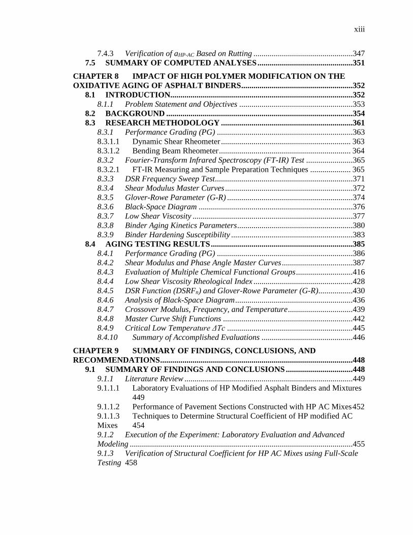
xiii
7.4.3 Verification of aHP-AC Based on Rutting .................................................347
7.5 SUMMARY OF COMPUTED ANALYSES ...............................................351
CHAPTER 8 IMPACT OF HIGH POLYMER MODIFICATION ON THE
OXIDATIVE AGING OF ASPHALT BINDERS .......................................................352 8.1 INTRODUCTION..........................................................................................352
8.1.1 Problem Statement and Objectives ........................................................353 8.2 BACKGROUND ............................................................................................354
8.3 RESEARCH METHODOLOGY .................................................................361 8.3.1 Performance Grading (PG) ...................................................................363 8.3.1.1 Dynamic Shear Rheometer ................................................................ 363 8.3.1.2 Bending Beam Rheometer ................................................................. 364 8.3.2 Fourier-Transform Infrared Spectroscopy (FT-IR) Test .......................365
8.3.2.1 FT-IR Measuring and Sample Preparation Techniques .................... 365 8.3.3 DSR Frequency Sweep Test....................................................................371
8.3.4 Shear Modulus Master Curves ...............................................................372 8.3.5 Glover-Rowe Parameter (G-R) ..............................................................374
8.3.6 Black-Space Diagram ............................................................................376 8.3.7 Low Shear Viscosity ...............................................................................377 8.3.8 Binder Aging Kinetics Parameters .........................................................380
8.3.9 Binder Hardening Susceptibility ............................................................383 8.4 AGING TESTING RESULTS ......................................................................385
8.4.1 Performance Grading (PG) ...................................................................386 8.4.2 Shear Modulus and Phase Angle Master Curves ...................................387 8.4.3 Evaluation of Multiple Chemical Functional Groups ............................416
8.4.4 Low Shear Viscosity Rheological Index .................................................428
8.4.5 DSR Function (DSRFn) and Glover-Rowe Parameter (G-R).................430 8.4.6 Analysis of Black-Space Diagram ..........................................................436 8.4.7 Crossover Modulus, Frequency, and Temperature ................................439
8.4.8 Master Curve Shift Functions ................................................................442 8.4.9 Critical Low Temperature ΔTc ..............................................................445
8.4.10 Summary of Accomplished Evaluations .............................................446
CHAPTER 9 SUMMARY OF FINDINGS, CONCLUSIONS, AND
RECOMMENDATIONS ...............................................................................................448 9.1 SUMMARY OF FINDINGS AND CONCLUSIONS .................................448
9.1.1 Literature Review ...................................................................................449 9.1.1.1 Laboratory Evaluations of HP Modified Asphalt Binders and Mixtures
449 9.1.1.2 Performance of Pavement Sections Constructed with HP AC Mixes 452
9.1.1.3 Techniques to Determine Structural Coefficient of HP modified AC
Mixes 454 9.1.2 Execution of the Experiment: Laboratory Evaluation and Advanced
Modeling ..............................................................................................................455 9.1.3 Verification of Structural Coefficient for HP AC Mixes using Full-Scale
Testing 458

xiv
9.2 APT IMPLEMENTATION PLAN ..............................................................460
9.2.1 Experimental Design ..............................................................................460
9.2.2 Instrumentation Plan ..............................................................................462 9.2.3 Pavement Design ....................................................................................463 9.2.4 Pavement Construction ..........................................................................465
CHAPTER 10 REFERENCES .................................................................................466
APPENDIX A EXTENDED LITERATURE REVIEW ...........................................485
A.1 INTRODUCTION..........................................................................................485 A.1.1 Background.................................................................................................485 A.1.2 AASHTO Flexible Design Methodology .....................................................487 A.1.3 FDOT Pavement Design Practice ..............................................................492 A.1.4 Problem Statement......................................................................................492
A.1.5 Objective and Scope ...................................................................................494 A.2 LABORATORY EVALUATION OF HP MODIFIED ASPHALT
BINDERS AND MIXTURES .................................................................................495 A.2.1 History of Polymer Modified Asphalt Binders ...........................................495
A.2.2 Laboratory Evaluation of Polymer Modified Asphalt Binders and Mixtures
in Florida .............................................................................................................499 A.2.2.1 Properties of Evaluated Asphalt Binders ............................................... 500
A.2.2.2 Properties of AC Mixtures ..................................................................... 503 A.2.2.3 APT Experiment: Design and Testing ................................................... 506
A.2.2.4 Conclusions and Implementation ........................................................... 509 A.2.3 Effect of Long-Term Aging on HP-Modified Asphalt Binders ...................510 A.2.4 Laboratory Evaluation of HP Binders in Poland: ORBITON HiMA .........513
A.2.4.1 Low Temperature Properties .................................................................. 514
A.2.4.2 Intermediate Temperature Properties ..................................................... 516 A.2.4.3 High Temperature Properties ................................................................. 518 A.2.5 Evaluation of Thin Overlay Mixes using HP Asphalt Binders ...................522
A.2.5.1 Experimental Plan and Pilot Specification............................................. 523 A.2.5.2 Test Results of Evaluated Binders and Mixtures ................................... 525
A.2.6 New Hampshire DOT Highways: 2011 Auburn-Candia Resurfacing .......532
A.2.6.1 Introduction and Testing Plan ................................................................ 532 A.2.6.2 Testing Description and Detailed Results .............................................. 533
A.3 FIELD HP AC MIXES PROJECTS WITH LIMITED PERFORMANCE
DATA ........................................................................................................................537 A.3.1 Introduction ................................................................................................537
A.3.2 High Polymer Modified Asphalt Mixture Trial in Mixture ........................539 A.3.3 Winning the Race Track Challenge using HP Mixes .................................539
A.3.4 Mill and AC Overlay on Normandale Road, City of Bloomington.............541 A.3.5 HP Modified Asphalt Mixtures on Busy Intersection in Georgia ...............542 A.3.6 High-Performance HP Overlays in New Hampshire and Vermont ...........543 A.3.7 HP Modified Overlay Mix on I-40 in Oklahoma ........................................544 A.3.8 HP Modified Thin Overlay Mix on I-5 in Oregon ......................................545
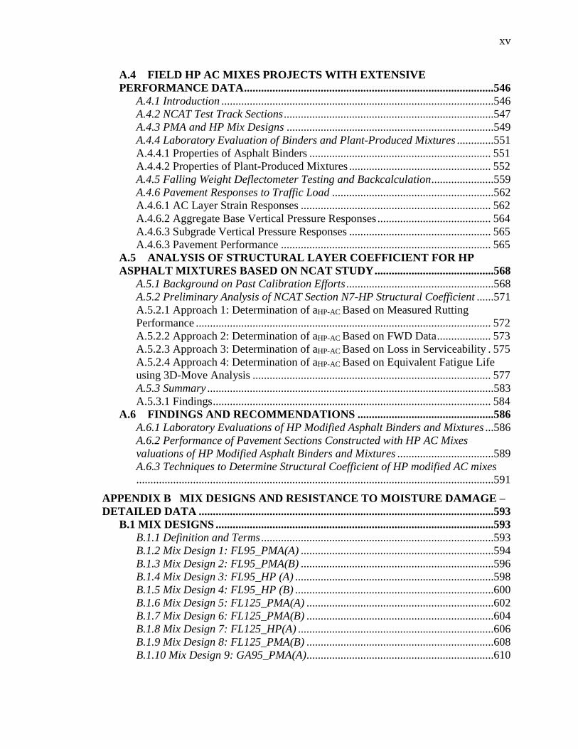
xv
A.4 FIELD HP AC MIXES PROJECTS WITH EXTENSIVE
PERFORMANCE DATA ........................................................................................546
A.4.1 Introduction ................................................................................................546 A.4.2 NCAT Test Track Sections ..........................................................................547 A.4.3 PMA and HP Mix Designs .........................................................................549 A.4.4 Laboratory Evaluation of Binders and Plant-Produced Mixtures .............551 A.4.4.1 Properties of Asphalt Binders ................................................................ 551
A.4.4.2 Properties of Plant-Produced Mixtures .................................................. 552 A.4.5 Falling Weight Deflectometer Testing and Backcalculation......................559 A.4.6 Pavement Responses to Traffic Load .........................................................562 A.4.6.1 AC Layer Strain Responses ................................................................... 562 A.4.6.2 Aggregate Base Vertical Pressure Responses ........................................ 564
A.4.6.3 Subgrade Vertical Pressure Responses .................................................. 565
A.4.6.3 Pavement Performance .......................................................................... 565 A.5 ANALYSIS OF STRUCTURAL LAYER COEFFICIENT FOR HP
ASPHALT MIXTURES BASED ON NCAT STUDY ..........................................568
A.5.1 Background on Past Calibration Efforts ....................................................568 A.5.2 Preliminary Analysis of NCAT Section N7-HP Structural Coefficient ......571 A.5.2.1 Approach 1: Determination of aHP-AC Based on Measured Rutting
Performance ........................................................................................................ 572 A.5.2.2 Approach 2: Determination of aHP-AC Based on FWD Data ................... 573
A.5.2.3 Approach 3: Determination of aHP-AC Based on Loss in Serviceability . 575 A.5.2.4 Approach 4: Determination of aHP-AC Based on Equivalent Fatigue Life
using 3D-Move Analysis .................................................................................... 577
A.5.3 Summary .....................................................................................................583
A.5.3.1 Findings .................................................................................................. 584 A.6 FINDINGS AND RECOMMENDATIONS ................................................586
A.6.1 Laboratory Evaluations of HP Modified Asphalt Binders and Mixtures ...586
A.6.2 Performance of Pavement Sections Constructed with HP AC Mixes
valuations of HP Modified Asphalt Binders and Mixtures ..................................589
A.6.3 Techniques to Determine Structural Coefficient of HP modified AC mixes
..............................................................................................................................591
APPENDIX B MIX DESIGNS AND RESISTANCE TO MOISTURE DAMAGE –
DETAILED DATA ........................................................................................................593 B.1 MIX DESIGNS ..................................................................................................593
B.1.1 Definition and Terms ..................................................................................593
B.1.2 Mix Design 1: FL95_PMA(A) ....................................................................594 B.1.3 Mix Design 2: FL95_PMA(B) ....................................................................596
B.1.4 Mix Design 3: FL95_HP (A) ......................................................................598 B.1.5 Mix Design 4: FL95_HP (B) ......................................................................600 B.1.6 Mix Design 5: FL125_PMA(A) ..................................................................602 B.1.7 Mix Design 6: FL125_PMA(B) ..................................................................604 B.1.8 Mix Design 7: FL125_HP(A) .....................................................................606
B.1.9 Mix Design 8: FL125_PMA(B) ..................................................................608 B.1.10 Mix Design 9: GA95_PMA(A)..................................................................610

xvi
B.1.11 Mix Design 10: GA95_PMA(B) ................................................................612
B.1.12 Mix Design 11: GA95_HP(A) ..................................................................614
B.1.13 Mix Design 12: GA95_HP(B) ..................................................................616 B.1.14 Mix Design 10: GA125_PMA(A) ..............................................................618 B.1.15 Mix Design 14: GA125_PMA(B) ..............................................................620 B.1.16 Mix Design 15: GA125_HP (A) ...............................................................622 B.1.17 Mix Design 16: GA125_HP(B) ................................................................624
B.1.18 Summary of Developed Mix Designs ........................................................626 B.2 RESISTANCE TO MOISTURE DAMAGE...................................................627
APPENDIX C DETAILED LABORATORY DATA ...............................................641 C.1 DYNAMIC MODULUS PROPERTY ............................................................641
C.1.1 Mix Design 1: FL95_PMA(A) ....................................................................641
C.1.2 Mix Design 2: FL95_PMA(B) ....................................................................643 C.1.3 Mix Design 3: FL95_HP(A) .......................................................................645
C.1.4 Mix Design 4: FL95_HP(B) .......................................................................647 C.1.5 Mix Design 5: FL125_PMA(A) ..................................................................649
C.1.6 Mix Design 6: FL125_PMA(B) ..................................................................651 C.1.7 Mix Design 7: FL125_HP(A) .....................................................................653 C.1.8 Mix Design 8: FL125_HP(B) .....................................................................655
C.1.9 Mix Design 9: GA95_PMA(A) ...................................................................657 C.1.10 Mix Design 10: GA95_PMA(B) ...............................................................659
C.1.11 Mix Design 11: GA95_HP(A) ..................................................................661 C.1.12 Mix Design 12: GA95_HP(B) ..................................................................663 C.1.13 Mix Design 13: GA125_PMA(A) .............................................................665
C.1.14 Mix Design 14: GA125_PMA(B) .............................................................667
C.1.15 Mix Design 15: GA125_HP(A) ................................................................669 C.1.16 Mix Design 1: GA125_HP(B) ..................................................................671 C.1.17. Dynamic Modulus and Phase Angle: Summary of All Mixes ................673
C.2 REPEATED TRIAXIAL LOAD (RLT) TEST - RUTTING ........................677 C.3 FLEXURAL BEAM FATIGUE TEST – FATIGUE CRACKING ..............685
APPENDIX D BOOTSTRAPPED FUNCTION FOR CONFIDENCE
INTERVALS OF MEAN STATISTIC IN R-PACKAGE .........................................717 D.1 ENTIRE DATA EVALUATED AS ONE GROUP ........................................717 D.2 ENTIRE DATA AGGREGATE SOURCES: FL VS. GA ............................719 D.3 ENTIRE DATA NMAS: 9.5 VS. 12.5 MM .....................................................723
APPENDIX E DAMAGED DYNAMIC MODULUS FOR PMA AC MIXES ......728
xvii
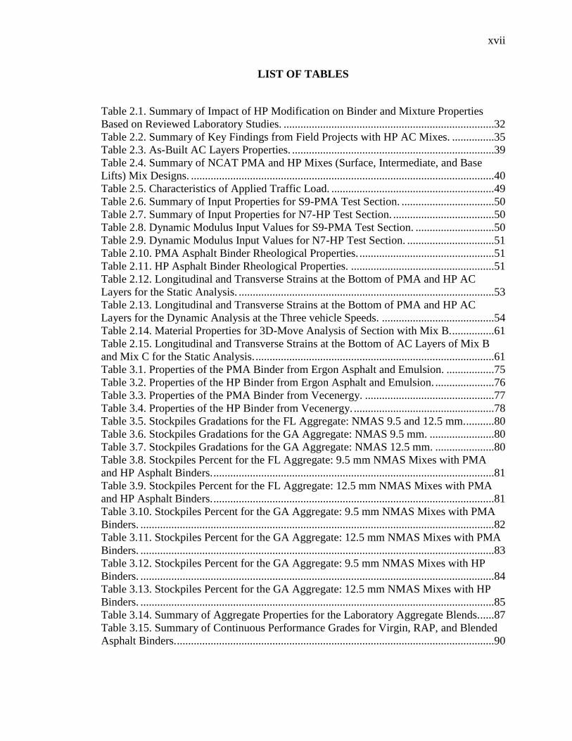
LIST OF TABLES
Table 2.1. Summary of Impact of HP Modification on Binder and Mixture Properties
Based on Reviewed Laboratory Studies. ...........................................................................32
Table 2.2. Summary of Key Findings from Field Projects with HP AC Mixes. ...............35
Table 2.3. As-Built AC Layers Properties. ........................................................................39
Table 2.4. Summary of NCAT PMA and HP Mixes (Surface, Intermediate, and Base
Lifts) Mix Designs. ............................................................................................................40
Table 2.5. Characteristics of Applied Traffic Load. ..........................................................49
Table 2.6. Summary of Input Properties for S9-PMA Test Section. .................................50
Table 2.7. Summary of Input Properties for N7-HP Test Section. ....................................50
Table 2.8. Dynamic Modulus Input Values for S9-PMA Test Section. ............................50
Table 2.9. Dynamic Modulus Input Values for N7-HP Test Section. ...............................51
Table 2.10. PMA Asphalt Binder Rheological Properties. ................................................51
Table 2.11. HP Asphalt Binder Rheological Properties. ...................................................51
Table 2.12. Longitudinal and Transverse Strains at the Bottom of PMA and HP AC
Layers for the Static Analysis. ...........................................................................................53
Table 2.13. Longitudinal and Transverse Strains at the Bottom of PMA and HP AC
Layers for the Dynamic Analysis at the Three vehicle Speeds. ........................................54
Table 2.14. Material Properties for 3D-Move Analysis of Section with Mix B. ...............61
Table 2.15. Longitudinal and Transverse Strains at the Bottom of AC Layers of Mix B
and Mix C for the Static Analysis. .....................................................................................61
Table 3.1. Properties of the PMA Binder from Ergon Asphalt and Emulsion. .................75
Table 3.2. Properties of the HP Binder from Ergon Asphalt and Emulsion. .....................76
Table 3.3. Properties of the PMA Binder from Vecenergy. ..............................................77
Table 3.4. Properties of the HP Binder from Vecenergy. ..................................................78
Table 3.5. Stockpiles Gradations for the FL Aggregate: NMAS 9.5 and 12.5 mm. ..........80
Table 3.6. Stockpiles Gradations for the GA Aggregate: NMAS 9.5 mm. .......................80
Table 3.7. Stockpiles Gradations for the GA Aggregate: NMAS 12.5 mm. .....................80
Table 3.8. Stockpiles Percent for the FL Aggregate: 9.5 mm NMAS Mixes with PMA
and HP Asphalt Binders. ....................................................................................................81
Table 3.9. Stockpiles Percent for the FL Aggregate: 12.5 mm NMAS Mixes with PMA
and HP Asphalt Binders. ....................................................................................................81
Table 3.10. Stockpiles Percent for the GA Aggregate: 9.5 mm NMAS Mixes with PMA
Binders. ..............................................................................................................................82
Table 3.11. Stockpiles Percent for the GA Aggregate: 12.5 mm NMAS Mixes with PMA
Binders. ..............................................................................................................................83
Table 3.12. Stockpiles Percent for the GA Aggregate: 9.5 mm NMAS Mixes with HP
Binders. ..............................................................................................................................84
Table 3.13. Stockpiles Percent for the GA Aggregate: 12.5 mm NMAS Mixes with HP
Binders. ..............................................................................................................................85
Table 3.14. Summary of Aggregate Properties for the Laboratory Aggregate Blends......87
Table 3.15. Summary of Continuous Performance Grades for Virgin, RAP, and Blended
Asphalt Binders. .................................................................................................................90
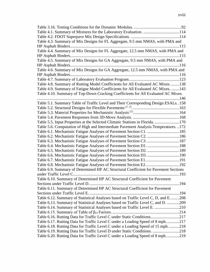
xviii
Table 3.16. Testing Conditions for the Dynamic Modulus. ..............................................92
Table 4.1. Summary of Mixtures for the Laboratory Evaluation. ...................................114
Table 4.2. FDOT Superpave Mix Design Specifications. ...............................................114
Table 4.3. Summary of Mix Designs for FL Aggregate, 9.5 mm NMAS, with PMA and
HP Asphalt Binders..........................................................................................................115
Table 4.4. Summary of Mix Designs for FL Aggregate, 12.5 mm NMAS, with PMA and
HP Asphalt Binders..........................................................................................................115
Table 4.5. Summary of Mix Designs for GA Aggregate, 9.5 mm NMAS, with PMA and
HP Asphalt Binders..........................................................................................................116
Table 4.6. Summary of Mix Designs for GA Aggregate, 12.5 mm NMAS, with PMA and
HP Asphalt Binders..........................................................................................................116
Table 4.7. Summary of Laboratory Evaluation Program. ................................................123
Table 4.8. Summary of Rutting Model Coefficients for All Evaluated AC Mixes. ........138
Table 4.9. Summary of Fatigue Model Coefficients for All Evaluated AC Mixes. ........143
Table 4.10. Summary of Top-Down Cracking Coefficients for All Evaluated AC Mixes.
..........................................................................................................................................146
Table 5.1. Summary Table of Traffic Level and Their Corresponding Design ESALs. .158
Table 5.2. Structural Designs for Flexible Pavements (1, 2). .............................................163
Table 5.3. Material Properties for Mechanistic Analysis (1). ............................................164
Table 5.4. Pavement Responses from 3D-Move Analysis. .............................................168
Table 5.5. Input Properties at the Selected Climatic Stations in Florida. ........................170
Table 5.6. Computation of High and Intermediate Pavement Analysis Temperatures. ..172
Table 6.1. Mechanistic Fatigue Analyses of Pavement Section C1. ...............................185
Table 6.2. Mechanistic Fatigue Analyses of Pavement Section C2. ...............................186
Table 6.3. Mechanistic Fatigue Analyses of Pavement Section C3. ...............................187
Table 6.4. Mechanistic Fatigue Analyses of Pavement Section D1. ...............................188
Table 6.5. Mechanistic Fatigue Analyses of Pavement Section D2. ...............................189
Table 6.6. Mechanistic Fatigue Analyses of Pavement Section D3. ...............................190
Table 6.7. Mechanistic Fatigue Analyses of Pavement Section E1. ................................191
Table 6.8. Mechanistic Fatigue Analyses of Pavement Section E2. ................................192
Table 6.9. Summary of Determined HP AC Structural Coefficient for Pavement Sections
under Traffic Level C.......................................................................................................193
Table 6.10. Summary of Determined HP AC Structural Coefficient for Pavement
Sections under Traffic Level D. .......................................................................................194
Table 6.11. Summary of Determined HP AC Structural Coefficient for Pavement
Sections under Traffic Level E. .......................................................................................194
Table 6.12. Summary of Statistical Analyses based on Traffic Level C, D, and E. ........208
Table 6.13. Summary of Statistical Analyses based on Traffic Level C, and D. ............209
Table 6.14. Summary of Statistical Analyses based on Traffic Level E. ........................210
Table 6.15. Summary of Table of βr3 Factors. .................................................................214
Table 6.16. Rutting Data for Traffic Level C under Static Conditions............................217
Table 6.17. Rutting Data for Traffic Level C under a Loading Speed of 8 mph. ............217
Table 6.18. Rutting Data for Traffic Level C under a Loading Speed of 15 mph. ..........218
Table 6.19. Rutting Data for Traffic Level D under Static Conditions. ..........................218
Table 6.20. Rutting Data for Traffic Level C under a Loading Speed of 8 mph. ............219
xix
Table 6.21. Rutting Data for Traffic Level C under a Loading Speed of 15 mph. ..........219
Table 6.22. Rutting Data for Traffic Level E under Static Conditions. ...........................219
Table 6.23. Rutting Data for Traffic Level E under a Loading Speed of 8 mph. ............220
Table 6.24. Rutting Data for Traffic Level E under a Loading Speed of 15 mph. ..........220
Table 6.25. Shoving Data for Pavement Section C1 under a Loading Speed of 15 mph.
..........................................................................................................................................232
Table 6.26. Shoving Data for Pavement Section C2 under a Loading Speed of 15 mph.
..........................................................................................................................................232
Table 6.27. Shoving Data for Pavement Section C3 under a Loading Speed of 15 mph.
..........................................................................................................................................233
Table 6.28. Shoving Data for Pavement Section D1 under a Loading Speed of 15 mph.
..........................................................................................................................................233
Table 6.29. Shoving Data for Pavement Section D2 under a Loading Speed of 15 mph.
..........................................................................................................................................233
Table 6.30. Shoving Data for Pavement Section D3 under a Loading Speed of 15 mph.
..........................................................................................................................................234
Table 6.31. Shoving Data for Pavement Section E1 under a Loading Speed of 15 mph.
..........................................................................................................................................234
Table 6.32. Shoving Data for Pavement Section E2 under a Loading Speed of 15 mph.
..........................................................................................................................................234
Table 6.33. Critical Tensile Stress at the Bottom of PMA AC Layer for all Pavement
Sections under Different Loading Speeds........................................................................236
Table 6.34. Critical Tensile Stress at the Bottom of HP AC Layer for all Pavement
Sections under Different Loading Speeds........................................................................237
Table 6.35. Energy ratio Linear Regression Models Function of Design Number of
ESALs for Different Reliability Levels. ..........................................................................238
Table 6.36. FDOT Preliminary Criteria for Top-Down Cracking. ..................................238
Table 6.37. ER Values of Top-Down Cracking in PMA Pavement Sections under
Different Loading Speeds. ...............................................................................................240
Table 6.38. ER Values of Top-Down Cracking in HP Pavement Sections under Different
Loading Speeds. ...............................................................................................................241
Table 6.39. Variation of ERHP-AC mix with respect to ERPMA-AC mix—ΔER (%) for mixes
FL95_PMA/HP(B) and GA95_PMA/HP(A). ..................................................................242
Table 6.40. Fracture Parameters A and n for 16 AC Mixes at 77°F (25°C). ...................251
Table 6.41. Structural Designs for Rehabilitated Flexible Pavements. ...........................252
Table 6.42. Undamaged and Damaged E* of existing PMA AC Layer at 77°F (25°C) and
33.3 Hz. ............................................................................................................................255
Table 6.43. Results of Reflective Cracking ME Analysis of Pavement Sections Designed
for Traffic Level C (i.e., R-C1, R-C2, and R-C3). ...........................................................258
Table 6.44. Results of Reflective Cracking ME Analysis of Pavement Sections Designed
for Traffic Level D (i.e., R-D1, R-D2, and R-D3). ..........................................................258
Table 6.45. Results of Reflective Cracking ME Analysis of Pavement Sections Designed
for Traffic Level E (i.e., R-E1, and R-E2). ......................................................................259
Table 7.1. Atterberg Limits of SG Material. ....................................................................270
Table 7.2. Calculated Parameters of SG Constitutive Models.........................................275

xx
Table 7.3. NDOT and FDOT Requirements for CAB Materials. ....................................278
Table 7.4. Properties of the PG76-22PMA Asphalt Binder Sampled from Vecenergy. .281
Table 7.5. Properties of the HP Asphalt Binder Sampled from Vecenergy. ...................282
Table 7.6. Gradations and JMF for the 12.5 mm NMAS PMA and HP AC Mixes. .......283
Table 7.7. NDOT and FDOT Aggregates Specifications for Bituminous Courses. ........284
Table 7.8. Summary of Mix Designs for 12.5 mm NMAS, Lockwood Aggregates, with
PMA and HP Asphalt Binders. ........................................................................................285
Table 7.9. Summary of Fatigue Model Coefficients for the Two Evaluated AC Mixes. 292
Table 7.10. Summary of Rutting Model Coefficients for Evaluated AC Mixes. ............295
Table 7.11. Pavement Sections for PMA and HP PaveBox Experiments. ......................296
Table 7.12. Loading Protocol for Experiment No.1 (PaveBox_PMA)............................306
Table 7.13. Details of Instrumentation Plan for Experiment No.1. .................................311
Table 7.14. Details of Instrumentation Plan for Experiment No.2. .................................312
Table 7.15. As-Constructed AC Layer Thickness and Air Voids. ...................................314
Table 7.16. Vertical Surface Deflections at Multiple Load Levels: Experiment No.1
(PaveBox_PMA). .............................................................................................................324
Table 7.17. Vertical Surface Deflections at Multiple Load Levels: Experiment No.2
(PaveBox_HP). ................................................................................................................324
Table 7.18. Vertical Stress Measurements in the Middle of the CAB Layer at Multiple
Load Levels: Experiment No. 1 (PaveBox_PMA). .........................................................329
Table 7.19. Vertical Stress Measurements in the Middle of the CAB Layer at Multiple
Load Levels: Experiment No. 2 (PaveBox_HP). .............................................................329
Table 7.20. Vertical Stress Measurements in the SG Layer at Multiple Load Levels:
Experiment No. 1 (PaveBox_PMA). ...............................................................................336
Table 7.21. Vertical Stress Measurements in the SG Layer at Multiple Load Levels:
Experiment No. 2 (PaveBox_HP). ...................................................................................336
Table 7.22. Strain Measurements at the Bottom of the PMA AC Layer at Multiple Load
Levels: Experiment No.1 (PaveBox_PMA). ...................................................................338
Table 7.23. Strain Measurements at the Bottom of the HP AC Layer at Multiple Load
Levels: Experiment No.2 (PaveBox_HP). .......................................................................338
Table 7.24. Backcalculated Moduli at Different Load Levels. ........................................341
Table 7.25. Fatigue Analysis of PMA and HP Pavement Structures at Different Load
Levels Using Measured Strains. ......................................................................................347
Table 7.26. Fatigue Analysis of PMA and HP Pavement Structures at Different Load
Levels Using 3D-Move Calculated Strains. .....................................................................347
Table 7.27. Moduli of Various Layers at 122°F (50°C). .................................................349
Table 7.28. Rutting Analysis of PMA and HP Pavement Structures at Different Load
Levels. ..............................................................................................................................350
Table 7.29. Percent Change in Rut Depths at Different Load Levels.(a) ..........................350
Table 8.1. Testing Matrix for Unaged/Aged Asphalt Binders. ........................................362
Table 8.2. Summary Table: Parameters of Interest. .........................................................362
Table 8.3. FT-IR Testing: Summary Table of Chemical Structural Source and
Corresponding Wave Numbers. .......................................................................................370
Table 8.4. DSR Frequency Sweep Test Conditions. ........................................................372
Table 8.5. Summary Table: Continuous Grade of Evaluated PMA and HP Binders. .....387

xxi
Table 8.6. FT-IR Absorbance Measurements: ERGON_PMA; Original, RTFO,
PAV20hrs, PAV40hrs, and PAV60hrs. ...........................................................................418
Table 8.7. FT-IR Absorbance Measurements: ERGON_PMA Aged @ 100°C for 6
Different Durations. .........................................................................................................418
Table 8.8. FT-IR Absorbance Measurements: ERGON_PMA Aged @ 85°C for 6
Different Durations. .........................................................................................................419
Table 8.9. FT-IR Absorbance Measurements: ERGON_PMA Aged @ 60°C for 6
Different Durations. .........................................................................................................419
Table 8.10. FT-IR Absorbance Measurements: ERGON_PMA Aged @ 50°C for 6
Different Durations. .........................................................................................................420
Table 8.11. FT-IR Absorbance Measurements: ERGON_HP; Original, RTFO,
PAV20hrs, PAV40hrs, and PAV60hrs. ...........................................................................420
Table 8.12. FT-IR Absorbance Measurements: ERGON_HP Aged @ 100°C for 6
Different Durations. .........................................................................................................421
Table 8.13. FT-IR Absorbance Measurements: ERGON_HP Aged @ 85°C for 6
Different Durations. .........................................................................................................421
Table 8.14. FT-IR Absorbance Measurements: ERGON_HP Aged @ 60°C for 6
Different Durations. .........................................................................................................422
Table 8.15. FT-IR Absorbance Measurements: ERGON_HP Aged @ 50°C for 6
Different Durations. .........................................................................................................422
Table 8.16. FT-IR Absorbance Measurements: VCNRJ_PMA; Original, RTFO,
PAV20hrs, PAV40hrs, and PAV60hrs. ...........................................................................423
Table 8.17. FT-IR Absorbance Measurements: VCNRJ_PMA Aged @ 100°C for 6
Different Durations. .........................................................................................................423
Table 8.18. FT-IR Absorbance Measurements: VCNRJ_PMA Aged @ 85°C for 6
Different Durations. .........................................................................................................424
Table 8.19. FT-IR Absorbance Measurements: VCNRJ_PMA Aged @ 60°C for 6
Different Durations. .........................................................................................................424
Table 8.20. FT-IR Absorbance Measurements: VCNRJ_PMA Aged @ 50°C for 6
Different Durations. .........................................................................................................425
Table 8.21. FT-IR Absorbance Measurements: VCNRJ_HP; Original, RTFO, PAV20hrs,
PAV40hrs, and PAV60hrs. ..............................................................................................425
Table 8.22. FT-IR Absorbance Measurements: VCNRJ_HP Aged @ 100°C for 6
Different Durations. .........................................................................................................426
Table 8.23. FT-IR Absorbance Measurements: VCNRJ_HP Aged @ 85°C for 6 Different
Durations. .........................................................................................................................426
Table 8.24. FT-IR Absorbance Measurements: VCNRJ_HP Aged @ 60°C for 6 Different
Durations. .........................................................................................................................427
Table 8.25. FT-IR Absorbance Measurements: VCNRJ_HP Aged @ 50°C for 6 Different
Durations. .........................................................................................................................427
Table 8.26. Evaluation Temperatures of DSRFn, and G-R Parameters for PMA and HP
Asphalt Binders. ...............................................................................................................431
Table 8.27. Summary Table of Critical Low Temperature Difference ΔTc. ...................446
Table 9.1. Summary of Laboratory of HP Binders and Mixtures. ...................................451
Table 9.2. Summary of Field Projects with HP AC Mixes. .............................................453

xxii
Table 9.3. Proposed APT Experiments. ...........................................................................462
xxiii
LIST OF FIGURES
Figure 1.1. Typical behavior of asphalt binders through pavement life. .............................3
Figure 1.2. AASHTO 1993 nomograph for designing flexible pavements (AASHTO
Guide, 1993). .......................................................................................................................5 Figure 1.3. Equation. AASHTO 1993 equation for designing flexible pavements. ............5 Figure 1.4. Equation. AASHTO 1993 equation for total structural number of a flexible
pavement structural for a given design traffic. ....................................................................7
Figure 1.5. Chart estimating structural coefficient of dense-graded asphalt concrete based
on the elastic (resilient) modulus after AASHTO 1993 (AASHTO Guide, 1993). .............8 Figure 2.1. Schematic of typical behavior of asphalt binders through pavement life. ......21 Figure 2.2. Comparison of Glover-Row (G-R) parameters for neat, PMA, and HP asphalt
binders in a black space diagram after (Zhu, 2015). ..........................................................26 Figure 2.3. Location of some HP field mixture projects in U.S.A. ...................................34 Figure 2.4. NCAT test track S9-PMA and N7-HP cross-sections design: materials and
layers thicknesses. ..............................................................................................................38 Figure 2.5. Aggregate gradations of PMA and HP mixes – NCAT test Track..................39
Figure 2.6. Rut depths measured at various levels of applied ESALs (Revised from Timm
et al., 2012). .......................................................................................................................41 Figure 2.7. Equation. HP structural coefficient function of PMA and HP layer
thicknesses. ........................................................................................................................41 Figure 2.8. Equation. Effective structural number from FWD data analysis. ...................43
Figure 2.9. Equation. Calculation of equivalent thickness using FWD backcalculated
modulus. .............................................................................................................................43
Figure 2.10. Equation. AASHTO 1993 equation for total structural number of a flexible
pavement structural for a given design traffic. ..................................................................44
Figure 2.11. Equation. PSI calculation based on IRI, rut depth, cracking, and patching. .44 Figure 2.12. Equation. AASHTO 1993 equation for designing flexible pavements. ........46 Figure 2.13. Fatigue characteristics of PMA-Base and HP-Base mixes at 68°F (20°C). ..47
Figure 2.14. Equation. Tensile strain function of number of loading cycles for PMA AC
mix at 68°F (20°C). ............................................................................................................47 Figure 2.15. Equation. Tensile strain function of number of loading cycles for HP AC
mix at 68°F (20°C). ............................................................................................................47 Figure 2.16. Sketch of PMA-pavement section. ................................................................52 Figure 2.17. Equation. HP structural coefficient function of HP AC mix based on fatigue
analysis. ..............................................................................................................................53
Figure 2.18. Longitudinal normal strain at P5 under dynamic loading at 8 mph for S9-
PMA and N7-HP. ...............................................................................................................55 Figure 2.19. Longitudinal normal strain at P5 under dynamic loading at 15 mph for S9-
PMA and N7-HP. ...............................................................................................................55 Figure 2.20. Aggregate gradations of NHDOT mixes A, B, and C. ..................................57 Figure 2.21. Fatigue characteristics of mixes A, B, and C at 59°F (15°C). .......................58 Figure 2.22. Equation. Tensile strain function of number of loading cycles for Mix A at
59°F (15°C). .......................................................................................................................58
xxiv
Figure 2.23. Equation. Tensile strain function of number of loading cycles for Mix B at
59°F (15°C). .......................................................................................................................59
Figure 2.24. Equation. Tensile strain function of number of loading cycles for Mix C at
59°F (15°C). .......................................................................................................................59 Figure 3.1. Flowchart of the experimental plan. ................................................................70 Figure 3.2. Steps followed to mix the liquid anti-strip with asphalt binder.......................74 Figure 3.3. JMF gradation for the FL aggregate: 9.5 mm NMAS mixes with PMA and HP
asphalt binders. ..................................................................................................................81 Figure 3.4. JMF gradation for the FL aggregate: 12.5 mm NMAS mixes with PMA and
HP asphalt binders. ............................................................................................................82 Figure 3.5. JMF gradation for the GA aggregate: 9.5 mm NMAS mixes with PMA
asphalt binders. ..................................................................................................................83
Figure 3.6. JMF gradation for the GA aggregate: 12.5 mm NMAS mixes with PMA
asphalt binders. ..................................................................................................................84 Figure 3.7. JMF gradation for the GA aggregate: 9.5 mm NMAS mixes with HP asphalt
binders. ...............................................................................................................................85
Figure 3.8. JMF gradation for the GA aggregate: 12.5 mm NMAS mixes with HP asphalt
binders. ...............................................................................................................................86 Figure 3.9. Blending chart process for SR-8_334 RAP stockpile with: (a) virgin binder A;
and (b) virgin binder B. ......................................................................................................90 Figure 3.10. Blending chart process for Crushed RAP stockpile with: (a) virgin binder A;
and (b) virgin binder B. ......................................................................................................91 Figure 3.11. Dynamic modulus master curve for FL95_PMA(A) AC mix. ......................93 Figure 3.12. Equation. E* non-symmetrical sigmoidal master curve model. ....................93
Figure 3.13. Equation. Actual and Reduced frequency function of shift factors. ..............93
Figure 3.14. Equation. Shift factors function of temperatures. ..........................................94 Figure 3.15. Equation. Phase angle function of E* and frequency. ...................................94 Figure 3.16. Equation. Phase angle master curve non-symmetrical model. ......................95
Figure 3.17. Phase angle master curve for FL95_PMA(A) AC mix. ................................95 Figure 3.18. RLT permanent deformation curve for FL95_PMA(B) mix at 122°F. .........97
Figure 3.19. Equation. Francken mathematical model: deformation vs. loading. .............98 Figure 3.20. Equation. MEPDG rutting regression model.................................................98 Figure 3.21. Equation. Thickness adjustment coefficient defined for rutting. ..................99
Figure 3.22. Equation. Regression constant defined for rutting. .......................................99 Figure 3.23. Equation. Regression constant defined for rutting. .......................................99 Figure 3.24. Equation. Rutting curves for FL95_PMA(B) AC mix. .................................99
Figure 3.25. Equation. Calculation of fatigue normalized modulus. ...............................100
Figure 3.26. NM curve for FL95_PMA(A) AC mix at 800 microstrain and 70°F (21.1°C).
..........................................................................................................................................101 Figure 3.27. Equation. MEPDG fatigue regression model. .............................................101 Figure 3.28. Fatigue curves for FL95_PMA(A) AC mix. ...............................................102 Figure 3.29. Equation. Creep compliance at time t. .........................................................104 Figure 3.30. Equation. Creep compliance correction factor at time t. .............................104
Figure 3.31. Equation. Creep compliance power law model. ..........................................104 Figure 3.32. Schematic representation of the mix creep compliance curve. ...................105

xxv
Figure 3.33. Equation. Tensile stress of tested specimen at time t. .................................105
Figure 3.34. Equation. Stress correction factor for the tested specimen..........................105
Figure 3.35. Equation. Poisson’s ratio. ............................................................................105 Figure 3.36. Equation. Tensile strain of tested specimen at time t. .................................106 Figure 3.37. Equation. Strain correction factor for the tested specimen..........................106 Figure 3.38. Schematic representation of mixture failure limits (FEf and DSCEf) . ........107 Figure 3.39. Equation. Elastic energy of tested specimen. ..............................................107
Figure 3.40. Equation. Elastic energy of tested specimen function of DSCEf and
DSCEmin. ..........................................................................................................................108 Figure 3.41. Equation. Calculation of parameter A using US units. ...............................108 Figure 3.42. Equation. Calculation of parameter A using SI units. .................................108 Figure 3.43. AMPT overlay test setup. ............................................................................110
Figure 3.44. Normalized load reduction curve for FL95_PMA(A) AC mix at a max
displacement of 0.025 inch (0.6350 mm) and a temperature of 77°F (25°C). .................110 Figure 3.45. Equation. Normalized crack driving force. .................................................111
Figure 3.46. Portion of hysteresis loop of the first loading cycle to calculate the critical
fracture energy of FL95_PMA(A) AC mix. ....................................................................111 Figure 3.47. Equation. Critical fracture energy. ..............................................................112 Figure 4.1. Asphalt binder contents of all PMA and HP AC mixes. ...............................117
Figure 4.2. Equation. Calculation of tensile strength TS. ................................................119 Figure 4.3. Un-conditioned tensile strength properties of evaluated mixes. ...................121
Figure 4.4. Moisture-conditioned tensile strength properties of evaluated mixes. ..........121 Figure 4.5. Tensile strength ratios of evaluated mixes. ...................................................122 Figure 4.6. E* master curves of FL95_PMA(A) and FL95_HP(A) at 68°F (20°C). .......125
Figure 4.7. E* master curves of FL95_PMA(B) and FL95_HP(B) at 68°F (20°C). .......126
Figure 4.8. E* master curves of FL125_PMA(A) and FL125_HP(A) at 68°F (20°C). ...126 Figure 4.9. E* master curves of FL125_PMA(B) and FL125_HP(B) at 68°F (20°C). ...127 Figure 4.10. E* master curves of GA95_PMA(A) and GA95_HP(A) at 68°F (20°C). ..127
Figure 4.11. E* master curves of GA95_PMA(B) and GA95_HP(B) at 68°F (20°C). ...128 Figure 4.12. E* master curves of GA125_PMA(A) and GA125_HP(A) at 68°F (20°C).
..........................................................................................................................................128 Figure 4.13. E* master curves of GA125_PMA(B) and GA125_HP(B) at 68°F (20°C).
..........................................................................................................................................129
Figure 4.14. E* master curves of all evaluated FL95 AC mixes at 68°F (20°C). ...........129 Figure 4.15. E* master curves of all evaluated FL125 AC mixes at 68°F (20°C). .........130 Figure 4.16. E* master curves of all evaluated GA95 AC mixes at 68°F (20°C). ..........130
Figure 4.17. E* master curves of all evaluated GA125 AC mixes at 68°F (20°C). ........131
Figure 4.18. E* values at 10 Hz and 77°F (25°C) of all evaluated AC mixes. ................131
Figure 4.19. E* values at 10 Hz and 122°F (50°C) of all evaluated AC mixes. ..............132 Figure 4.20. Rutting behavior of FL95 PMA and HP AC mixes at 122°F (50°C). .........135 Figure 4.21. Rutting behavior of FL125 PMA and HP AC mixes at 122°F (50°C). .......135 Figure 4.22. Rutting behavior of GA95 PMA and HP AC mixes at 122°F (50°C). ........136 Figure 4.23. Rutting behavior of GA125 PMA and HP AC mixes at 122°F (50°C). ......136
Figure 4.24. Rutting behavior of all evaluated FL95 & GA95 AC mixes at 122°F (50°C).
..........................................................................................................................................137

xxvi
Figure 4.25. Rutting behavior of all evaluated FL125 & GA125 AC mixes at 122°F
(50°C). ..............................................................................................................................137
Figure 4.26. Fatigue relationships of FL95 AC mixes at 77°F (25°C). ...........................141 Figure 4.27. Fatigue relationships of FL125 AC mixes at 77°F (25°C). .........................141 Figure 4.28. Fatigue relationships of GA95 AC mixes at 77°F (25°C). ..........................142 Figure 4.29. Fatigue relationships of GA125 AC mixes at 77°F (25°C). ........................142 Figure 4.30. Number of OT cycles to failure of all evaluated AC mixes at 77°F (25°C)
(Whiskers represent the 95% CI). ....................................................................................149 Figure 4.31. Critical fracture energy at the first OT cycle of all evaluated AC mixes at
77°F (25°C) (Whiskers represent the 95% CI). ...............................................................149 Figure 4.32. Critical propagation rate of all evaluated AC mixes at 77°F (25°C)
(Whiskers represent the 95% CI). ....................................................................................150
Figure 4.33. Cracking resistance of AC mixes: a sketch of the design interaction plot. .151
Figure 4.34. Cracking resistance interaction plot for FL PMA and HP AC mixes. ........152 Figure 4.35. Cracking resistance interaction plot for GA PMA and HP AC mixes. .......153
Figure 5.1. Flow chart of the mechanistic analysis approach. .........................................154
Figure 5.2. Applied loading: a) 3D configuration, and b) Plan illustration of a quarter
axle. ..................................................................................................................................156 Figure 5.3. Sketch a tractor-semi trailer truck considered for the determination of the
braking friction coefficient (Siddharthan et al., 2015). ....................................................157 Figure 5.4. Equation. Resilient modulus Mr function of LBR. ........................................160
Figure 5.5. Equation. Calculation of SN as per AASHTO guide design guide. ..............160 Figure 5.6. Equation. Calculation of total structural number. .........................................162 Figure 5.7. Equation. Calculation of required thickness of the AC layer. .......................162
Figure 5.8. Sketch of a newly constructed pavement section with the locations of the
selected response points. ..................................................................................................168 Figure 5.9. Equation. Calculation of effective intermediate temperature. .......................169 Figure 5.10. Equation. Calculation of effective high temperature. ..................................169
Figure 5.11. Schematic of load pulse frequency determination by MEPDG: a) single axle
load, and b) tandem axle. .................................................................................................171
Figure 5.12. Equation. Calculation of effective depth. ....................................................171 Figure 5.13. Equation. Calculation of time of loading. ...................................................171 Figure 6.1. Flowchart of the mechanistic analyses to determine an initial structural
coefficient for HP AC mixes in Florida. ..........................................................................174 Figure 6.2. Equation. Calculation of number of cycles to fatigue failure for PMA
pavement structures. ........................................................................................................176
Figure 6.3. Equation. Calculation of number of cycles to fatigue failure for HP pavement
structures. .........................................................................................................................176
Figure 6.4. Equation. Calculation of number of cycles to fatigue failure for HP pavement
structures using the service life approach. .......................................................................176 Figure 6.5. Equation. Calculation of critical tensile strain at the bottom of AC layer in a
HP pavement structure using service life approach. ........................................................176 Figure 6.6. Equation. Calculation of critical endurance limit tensile strain. ...................178
Figure 6.7. Equation. Calculation of the difference between the logs of the fatigue lives.
..........................................................................................................................................179
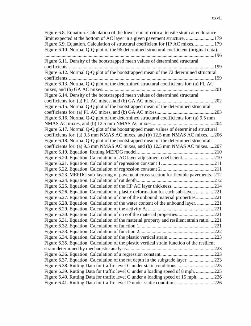
xxvii
Figure 6.8. Equation. Calculation of the lower end of critical tensile strain at endurance
limit expected at the bottom of AC layer in a given pavement structure. .......................179
Figure 6.9. Equation. Calculation of structural coefficient for HP AC mixes. ................179 Figure 6.10. Normal Q-Q plot of the 96 determined structural coefficient (original data).
..........................................................................................................................................196 Figure 6.11. Density of the bootstrapped mean values of determined structural
coefficients. ......................................................................................................................199
Figure 6.12. Normal Q-Q plot of the bootstrapped mean of the 72 determined structural
coefficients. ......................................................................................................................199 Figure 6.13. Normal Q-Q plot of the determined structural coefficients for: (a) FL AC
mixes, and (b) GA AC mixes. ..........................................................................................201 Figure 6.14. Density of the bootstrapped mean values of determined structural
coefficients for: (a) FL AC mixes, and (b) GA AC mixes...............................................202
Figure 6.15. Normal Q-Q plot of the bootstrapped mean of the determined structural
coefficients for: (a) FL AC mixes, and (b) GA AC mixes...............................................203
Figure 6.16. Normal Q-Q plot of the determined structural coefficients for: (a) 9.5 mm
NMAS AC mixes, and (b) 12.5 mm NMAS AC mixes...................................................204 Figure 6.17. Normal Q-Q plot of the bootstrapped mean values of determined structural
coefficients for: (a) 9.5 mm NMAS AC mixes, and (b) 12.5 mm NMAS AC mixes. ....206
Figure 6.18. Normal Q-Q plot of the bootstrapped mean of the determined structural
coefficients for: (a) 9.5 mm NMAS AC mixes, and (b) 12.5 mm NMAS AC mixes. ....207
Figure 6.19. Equation. Rutting MEPDG model. ..............................................................210 Figure 6.20. Equation. Calculation of AC layer adjustment coefficient. .........................210 Figure 6.21. Equation. Calculation of regression constant 1. ..........................................211
Figure 6.22. Equation. Calculation of regression constant 2. ..........................................211
Figure 6.23. MEPDG sub-layering of pavement cross-section for flexible pavements. .212 Figure 6.24. Equation. Calculation of rut depth...............................................................212 Figure 6.25. Equation. Calculation of the HP AC layer thickness. .................................214
Figure 6.26. Equation. Calculation of plastic deformation for each sub-layer. ...............221 Figure 6.27. Equation. Calculation of one of the unbound material properties. ..............221
Figure 6.28. Equation. Calculation of the water content of the unbound layer. ..............221 Figure 6.29. Equation. Calculation of the activity A. ......................................................221 Figure 6.30. Equation. Calculation of on eof the material properties. .............................221
Figure 6.31. Equation. Calculation of the material property and resilient strain ratio. ...221 Figure 6.32. Equation. Calculation of function 1.............................................................221 Figure 6.33. Equation. Calculation of function 2.............................................................222
Figure 6.34. Equation. Calculation of the plastic vertical strain. .....................................223
Figure 6.35. Equation. Calculation of the plastic vertical strain function of the resilient
strain determined by mechanistic analysis. ......................................................................223 Figure 6.36. Equation. Calculation of a regression constant. ..........................................223 Figure 6.37. Equation. Calculation of the rut depth in the subgrade layer. .....................223 Figure 6.38. Rutting Data for traffic level C under static conditions. .............................225 Figure 6.39. Rutting Data for traffic level C under a loading speed of 8 mph. ...............225
Figure 6.40. Rutting Data for traffic level C under a loading speed of 15 mph. .............226 Figure 6.41. Rutting Data for traffic level D under static conditions. .............................226

xxviii
Figure 6.42. Rutting Data for traffic level D under a loading speed of 8 mph. ...............227
Figure 6.43. Rutting Data for traffic level D under a loading speed of 15 mph. .............227
Figure 6.44. Rutting Data for traffic level E under static conditions. ..............................228 Figure 6.45. Rutting Data for traffic level E under a loading speed of 8 mph. ...............228 Figure 6.46. Rutting Data for traffic level E under a loading speed of 15 mph. .............229 Figure 6.47. Equation. Calculation of Rper. ......................................................................230 Figure 6.48. Equation. Calculation of the shoving criterion. ...........................................230
Figure 6.49. Comparison of critical tensile stress at the bottom of PMA and HP AC layer
for the same designed pavement structure and under the same loading speed. ...............238 Figure 6.50. Equation. Paris Law Model. ........................................................................244 Figure 6.51. Equation. Calculation of daily crack length. ...............................................244 Figure 6.52. Equation. Calculation of damage ratio. .......................................................244
Figure 6.53. Equation. Calculation of reflective cracking rate. .......................................245
Figure 6.54. Equation. Calculation of stress intensity factor. ..........................................245 Figure 6.55. Calculated SIF vs. crack length c for FL95_PMA(A) AC mix. ..................246
Figure 6.56. Equation. Calculation of normalized maximum load. .................................247
Figure 6.57. NM vs. c characteristics plot. ......................................................................247 Figure 6.58. NM vs. N plot for FL95_PMA(A) AC mix. ................................................248 Figure 6.59. c vs. N plot for FL95_PMA(A) AC mix. ....................................................249
Figure 6.60. Determination of A and n from crack length rate vs. N plot for
FL95_PMA(A) AC mix. ..................................................................................................250
Figure 6.61. Overall flowchart of the mechanistic analysis approach for reflective
cracking. ...........................................................................................................................253 Figure 6.62. Equation. Calculation of damaged dynamic modulus of existing AC layer.
..........................................................................................................................................254
Figure 6.63. Equation. Calculation of log of damaged dynamic modulus for existing AC
layer..................................................................................................................................254 Figure 6.64. RCR along time for pavement section R-C1: PMA/HP AC mix on top of
PMA AC layer. ................................................................................................................257 Figure 7.1. Flowchart of the verification of structural coefficient based on full-scale
pavement testing. .............................................................................................................266 Figure 7.2. Three-dimensional (3D) schematic of the PaveBox. .....................................268 Figure 7.3. Plan view and front and side elevations of the PaveBox...............................268
Figure 7.4. Gradation of SG material. ..............................................................................270 Figure 7.5. Equation. Calculation of group index. ...........................................................270 Figure 7.6. Moisture-density curve of the A-2-7(1) SG material. ...................................271
Figure 7.7. Preparation of MR test specimen: (a) cylindrical mold, (b) drill hammer, and
(c) scarifying tool. ............................................................................................................273
Figure 7.8. MR test specimen: (a) surrounded by latex membrane, (b) assembled in
triaxial cell, (c) before test, and (d) after quick shear test. ...............................................273 Figure 7.9. Calculation of MR: Theta model, hardening behavior. ..................................274 Figure 7.10. Calculation of MR: log-log model, softening behavior. ...............................274 Figure 7.11. Calculation of MR: Uzan model, hardening-softening behavior. .................274
Figure 7.12. Measured versus calculated SG MR using the Theta-model. .......................275 Figure 7.13. Measured versus calculated SG MR using the log-log model. .....................276

xxix
Figure 7.14. Measured versus calculated SG MR using the Uzan model. ........................276
Figure 7.15. Moisture-density curve of the CAB material. .............................................279
Figure 7.16. JMF gradation for the 12.5 mm NMAS PMA and HP AC mixes. ..............284 Figure 7.17. E* master curve of AC mixes at 68°F (20°C). ............................................287 Figure 7.18. Phase angle master curve of AC mixes at 68°F (20°C). .............................288 Figure 7.19. E* values at 10 Hz. ......................................................................................288 Figure 7.20. Beam fatigue data at three temperatures of PaveBox_PMA AC mix. ........291
Figure 7.21. Beam fatigue data at three temperatures of PaveBox_HP AC mix. ............291 Figure 7.22. Fatigue relationships of PaveBox_PMA and PaveBox_HP AC mixes at 77°F
(25°C). ..............................................................................................................................292 Figure 7.23. Rutting Curves for PaveBox_PMA AC mix. ..............................................293 Figure 7.24. Rutting Curves for PaveBox_HP AC mix. ..................................................294
Figure 7.25. Rutting behavior of PaveBox_PMA and PaveBox_HP AC mixes at 122°F
(50°C). ..............................................................................................................................295 Figure 7.26. Equation. Calculation of the HP AC layer thickness. .................................296
Figure 7.27. PMA and HP pavement sections in the PaveBox experiments. ..................297
Figure 7.28. SG deposition: (a) soil mixing in the mechanical mixer, and (b) placement of
moist soil in PaveBox. .....................................................................................................299 Figure 7.29. SG compaction in PaveBox: (a) vibratory plate compactor, (b) nuclear
density gauge measurements on top of compacted lift of SG soil, and (c) scarification of
the SG lift surface using a pickaxe to ensure bonding between compacted lifts. ............299
Figure 7.30. DCP test results for SG layer at two locations in PaveBox. ........................299 Figure 7.31. DCP test results for CAB layer at two locations in PaveBox......................300 Figure 7.32. Half-ton asphalt mixer used to mix and produce PMA and HP AC mixes for
PaveBox. ..........................................................................................................................302
Figure 7.33. Aggregate stockpiles organized and used to produce PMA and HP AC
mixes. ...............................................................................................................................302 Figure 7.34. Top view of the FWD loading plate used for dynamic loading. .................305
Figure 7.35. Plan view for PaveBox_PMA experiment No.1 at the AC surface. ............308 Figure 7.36. Section view for PaveBox_PMA experiment No.1 at the middle of CAB
layer..................................................................................................................................308 Figure 7.37. Section view for PaveBox_PMA experiment No.1 at 6 inch below the top of
SG. ...................................................................................................................................309
Figure 7.38. Section view for PaveBox_PMA experiment No.1 at 24 inch below the top
of SG. ...............................................................................................................................309 Figure 7.39. Cross section view for instrumentations in experiment No.1 PaveBox_PMA.
..........................................................................................................................................310
Figure 7.40. Completed full-scale PaveBox test setup for experiment No. 1. .................310
Figure 7.41. Diagram showing the locations of the cores sampled from both experiments.
..........................................................................................................................................313 Figure 7.42. (a) PMA AC core sample from experiment No. 1, and (b) HP AC core
sample from experiment No. 2.........................................................................................314 Figure 7.43. Preprocessed recordings by load cell at a target load level of 16,000 lb: (a)
PaveBox_PMA; and (b) PaveBox_HP. ...........................................................................317
xxx
Figure 7.44. Preprocessed recordings by LVDT L0 at a target load level of 16,000 lb: (a)
PaveBox_PMA; and (b) PaveBox_HP. ...........................................................................317
Figure 7.45. Preprocessed recordings by TEPC P7 at a target load level of 16,000 lb: (a)
PaveBox_PMA; and (b) PaveBox_HP. ...........................................................................318 Figure 7.46. Preprocessed recordings by strain gauge S1 at a target load level of 16,000
lb: (a) PaveBox_PMA; and (b) PaveBox_HP. .................................................................318 Figure 7.47. Measured vertical surface deflections as a function of applied surface loads
(experiment No. 1: PaveBox_PMA). ...............................................................................320 Figure 7.48. Measured vertical surface deflections as a function of applied surface loads
(experiment No. 2: PaveBox_HP). ..................................................................................320 Figure 7.49. Measured vertical surface deflections at the center of the loading plate (L0).
..........................................................................................................................................321
Figure 7.50. Measured vertical surface deflections at the center of the loading plate (L1).
..........................................................................................................................................321 Figure 7.51. Measured vertical surface deflections at the center of the loading plate (L2).
..........................................................................................................................................322
Figure 7.52. Measured vertical surface deflections at the center of the loading plate (L3).
..........................................................................................................................................322 Figure 7.53. Measured vertical surface deflections at the center of the loading plate (L4).
..........................................................................................................................................323 Figure 7.54. Measured vertical surface deflections at the center of the loading plate (L5).
..........................................................................................................................................323 Figure 7.55. Measured vertical surface deflections at the center of the loading plate (L6).
..........................................................................................................................................324
Figure 7.56. Measured vertical stresses as a function of applied surface loads (experiment
No. 1: PaveBox_PMA). ...................................................................................................326 Figure 7.57. Measured vertical stresses as a function of applied surface loads (experiment
No. 2: PaveBox_HP). .......................................................................................................327
Figure 7.58. Measured vertical stresses in the middle of the CAB layer and at the center
of the loading plate (P7). ..................................................................................................327
Figure 7.59. Measured vertical stresses in the middle of the CAB layer and at 12 inches
from the center of the loading plate (P8). ........................................................................328 Figure 7.60. Measured vertical stresses in the middle of the CAB layer and at 24 inches
from the center of the loading plate (P9). ........................................................................328 Figure 7.61. Measured vertical stresses in the middle of the CAB layer and at 36 inches
from the center of the loading plate (P10). ......................................................................329
Figure 7.62. Measured vertical stresses in the SG as a function of applied surface loads
(experiment No.1: PaveBox_PMA). ................................................................................332
Figure 7.63. Measured vertical stresses in the SG as a function of applied surface loads
(experiment No.2: PaveBox_HP). ...................................................................................332 Figure 7.64. Measured vertical stresses at 24 inches below the top of the SG and at the
center of the loading plate (P1). .......................................................................................333 Figure 7.65. Measured vertical stresses at 24 inches below the top of the SG and at a
radial distance of 12 inches from the center of the loading plate (P2). ...........................333

xxxi
Figure 7.66. Measured vertical stresses at 6 inches below the top of the SG and at the
center of the loading plate (P3). .......................................................................................334
Figure 7.67. Measured vertical stresses at 6 inches below the top of the SG and at a radial
distance of 12 inches from the center of the loading plate (P4).......................................334 Figure 7.68. Measured vertical stresses at 6 inches below the top of the SG and at a radial
distance of 24 inches from the center of the loading plate (P5).......................................335 Figure 7.69. Measured vertical stresses at 6 inches below the top of the SG and at a radial
distance of 48 inches from the center of the loading plate (P6).......................................335 Figure 7.70. Measured tensile strains at the bottom of the AC layer and at the center of
the loading plate (S1). ......................................................................................................337 Figure 7.71. Measured tensile strains at the bottom of the AC layer and at the center of
the loading plate (S2). ......................................................................................................338
Figure 7.72. Deflection basins at different load levels (experiment No.1: PaveBox_PMA).
..........................................................................................................................................340 Figure 7.73. Deflection basins at different load levels (experiment No.2: PaveBox_HP).
..........................................................................................................................................341
Figure 7.74. Comparison between measured and 3D-Move calculated surface deflections
(experiment No.1: PaveBox_PMA). ................................................................................343 Figure 7.75. Comparison between measured and 3D-Move calculated surface deflections
(experiment No.2: PaveBox_HP). ...................................................................................343 Figure 7.76. Comparison between measured and 3D-Move calculated strains at the
bottom of AC layer (experiment No.1: PaveBox_PMA).................................................344 Figure 7.77. Comparison between measured and 3D-Move calculated strains at the
bottom of AC layer (experiment No.2: PaveBox_HP). ...................................................344
Figure 7.78. Calculation: Fatigue MEPDG model for PaveBox_PMA AC Mix.............346
Figure 7.79. Calculation: Fatigue MEPDG model for PaveBox_HP AC Mix. ...............346 Figure 7.80. Calculation: Rutting MEPDG model for PaveBox_PMA AC Mix.............348 Figure 7.81. Calculation: Rutting MEPDG model for PaveBox_PMA AC Mix.............348
Figure 8.1. UNR Study: Comparison of G-R parameters for neat, PMA, and HP asphalt
binders in a black space diagram. ....................................................................................361
Figure 8.2. Absorbance spectrum using FT-IR for a given combination of HP and PMA
asphalt binder samples. ....................................................................................................371 Figure 8.3. Rhea package: example of binder master curve for a given PMA binder
combination (sampled from source B, and aged at 85°C for 15 days). ...........................373 Figure 8.4. Rhea package: example of binder master curve for a given HP binder
combination (sampled from source B, and aged at 85°C for 15 days). ...........................374
Figure 8.5. Equation. Calculation of Glover-Rowe parameter. .......................................374
Figure 8.6. Black Space of Glover-Rowe parameter at 15°C for PMA and HP asphalt
binders sampled from source A. ......................................................................................377 Figure 8.7. Rhea package: example of binder dynamic storage and loss viscosity curves
for a PMA binder sampled from source B, and aged at 85°C for 15 days. .....................378 Figure 8.8. Rhea package: example of binder dynamic storage and loss viscosity curves
for a HP binder sampled from source B, and aged at 85°C for 15 days. .........................379
Figure 8.9. Equation. Calculation of complex shear viscosity. .......................................379 Figure 8.10. Equation. Calculation of LSV percentage of difference. ............................379
xxxii
Figure 8.11. Equation. Calculation of dynamic viscosity using Cross model. ................380
Figure 8.12. Example of plot of oxidation kinetic measurements for: (a) ERGON_PMA,
and (b) ERGON_HP. 𝑟𝐶𝐴 = 𝐴𝑃𝛼𝑒 − 𝐸𝑎𝑅𝑇 ..................................................................381 Figure 8.13. Equation. Calculation of rate of carbonyl area, CA. ...................................382 Figure 8.14. Equation. Calculation of rate of carbonyl area, CA, function of fast and slow
rate of growth. ..................................................................................................................382 Figure 8.15. Example of fast and constant oxidation kinetic measurements and predicted
aging path for ERGON_PMA asphalt binder. .................................................................383 Figure 8.16. Equation. Calculation of LSV function of HS and CA. ..............................383 Figure 8.17. Equation. Calculation of HS function of G-R and CA. ...............................384 Figure 8.18. Hardening susceptibility of ERGON_PMA and ERGON_HP asphalt binders
for G-R parameter at 15°C and 0.005 rad/s. ....................................................................385
Figure 8.19. Shear modulus G* master curves at 60°C for Ergon_PMA_100°C. ...........392
Figure 8.20. Phase angle δ master curves at 60°C for Ergon_PMA_100°C. ...................392
Figure 8.21. Shear modulus G* master curves at 60°C for Ergon_PMA_85°C. .............393 Figure 8.22. Phase angle δ master curves at 60°C for Ergon_PMA_85°C. .....................393 Figure 8.23. Shear modulus G* master curves at 60°C for Ergon_PMA_60°C. .............394 Figure 8.24. Phase angle δ master curves at 60°C for Ergon_PMA_60°C. .....................394
Figure 8.25. Shear modulus G* master curves at 60°C for Ergon_PMA_50°C. .............395 Figure 8.26. Phase angle δ master curves at 60°C for Ergon_PMA_50°C. .....................395
Figure 8.27. Shear modulus G* master curves at 60°C for Ergon_HP_100°C. ..............396 Figure 8.28. Phase angle δ master curves at 60°C for Ergon_HP_100°C. ......................396 Figure 8.29. Shear modulus G* master curves at 60°C for Ergon_HP_85°C. ................397
Figure 8.30. Phase angle δ master curves at 60°C for Ergon_HP_85°C. ........................397 Figure 8.31. Shear modulus G* master curves at 60°C for Ergon_HP_60°C. ................398
Figure 8.32. Phase angle δ master curves at 60°C for Ergon_HP_60°C. ........................398 Figure 8.33. Shear modulus G* master curves at 60°C for Ergon_HP_50°C. ................399
Figure 8.34. Phase angle δ master curves at 60°C for Ergon_HP_50°C. ........................399 Figure 8.35. Shear modulus G* master curves at 60°C for Ergon_PMA aged for 15 days
at 100, 85, 60, and 50°C. ..................................................................................................400 Figure 8.36. Phase angle δ master curves at 60°C for Ergon_PMA aged for 15 days at
100, 85, 60, and 50°C. .....................................................................................................400
Figure 8.37. Shear modulus G* master curves at 60°C for Ergon_HP aged for 15 days at
100, 85, 60, and 50°C. .....................................................................................................401 Figure 8.38. Phase angle δ master curves at 60°C for Ergon_HP aged for 15 days at 100,
85, 60, and 50°C. .............................................................................................................401
Figure 8.39. Shear modulus G* master curves at 60°C for Ergon_PMA; Orginal, RTFO,
PAV20hrs, PAV40hrs, and PAV60hrs. ...........................................................................402
Figure 8.40. Phase angle δ master curves at 60°C for Ergon_PMA; Orginal, RTFO,
PAV20hrs, PAV40hrs, and PAV60hrs. ...........................................................................402 Figure 8.41. Shear modulus G* master curves at 60°C for Ergon_HP; Orginal, RTFO,
PAV20hrs, PAV40hrs, and PAV60hrs. ...........................................................................403 Figure 8.42. Phase angle δ master curves at 60°C for Ergon_HP; Orginal, RTFO,
PAV20hrs, PAV40hrs, and PAV60hrs. ...........................................................................403 Figure 8.43. Shear modulus G* master curves at 60°C for VCNRJ_PMA_100°C. ........404
xxxiii
Figure 8.44. Phase angle δ master curves at 60°C for VCNRJ _PMA_100°C. ...............404
Figure 8.45. Shear modulus G* master curves at 60°C for VCNRJ _PMA_85°C. .........405
Figure 8.46. Phase angle δ master curves at 60°C for VCNRJ _PMA_85°C. .................405 Figure 8.47. Shear modulus G* master curves at 60°C for VCNRJ _PMA_60°C. .........406 Figure 8.48. Phase angle δ master curves at 60°C for VCNRJ _PMA_60°C. .................406 Figure 8.49. Shear modulus G* master curves at 60°C for VCNRJ_PMA_50°C. ..........407 Figure 8.50. Phase angle δ master curves at 60°C for VCNRJ _PMA_50°C. .................407
Figure 8.51. Shear modulus G* master curves at 60°C for VCNRJ_HP_100°C. ...........408 Figure 8.52. Phase angle δ master curves at 60°C for VCNRJ_HP_100°C. ...................408 Figure 8.53. Shear modulus G* master curves at 60°C for VCNRJ_HP_85°C. .............409 Figure 8.54. Phase angle δ master curves at 60°C for VCNRJ_HP_85°C. .....................409 Figure 8.55. Shear modulus G* master curves at 60°C for VCNRJ_HP_60°C. .............410
Figure 8.56. Phase angle δ master curves at 60°C for VCNRJ_HP_60°C. .....................410
Figure 8.57. Shear modulus G* master curves at 60°C for VCNRJ_HP_50°C. .............411 Figure 8.58. Phase angle δ master curves at 60°C for VCNRJ_HP_50°C. .....................411
Figure 8.59. Shear modulus G* master curves at 60°C for VCNRJ_PMA aged for 15
days at 100, 85, 60, and 50°C. .........................................................................................412 Figure 8.60. Phase angle δ master curves at 60°C for VCNRJ_PMA aged for 15 days at
100, 85, 60, and 50°C. .....................................................................................................412
Figure 8.61. Shear modulus G* master curves at 60°C for VCNRJ_HP aged for 15 days
at 100, 85, 60, and 50°C. ..................................................................................................413
Figure 8.62. Phase angle δ master curves at 60°C for VCNRJ_HP aged for 15 days at
100, 85, 60, and 50°C. .....................................................................................................413 Figure 8.63. Shear modulus G* master curves at 60°C for VCNRJ_PMA; Orginal,
RTFO, PAV20hrs, PAV40hrs, and PAV60hrs. ...............................................................414
Figure 8.64. Phase angle δ master curves at 60°C for VCNRJ_PMA; Orginal, RTFO,
PAV20hrs, PAV40hrs, and PAV60hrs. ...........................................................................414 Figure 8.65. Shear modulus G* master curves at 60°C for VCNRJ_HP; Orginal, RTFO,
PAV20hrs, PAV40hrs, and PAV60hrs. ...........................................................................415 Figure 8.66. Phase angle δ master curves at 60°C for VCNRJ_HP; Orginal, RTFO,
PAV20hrs, PAV40hrs, and PAV60hrs. ...........................................................................415 Figure 8.67. Hardening susceptibility of ERGON_PMA, ERGON_HP, VCNRJ_PMA,
and VCNRJ_HP asphalt binders represented by Low Shear Viscosity (LSV). ...............429
Figure 8.68. Hardening susceptibility of ERGON_PMA, ERGON_HP, VCNRJ_PMA,
and VCNRJ_HP asphalt binders represented by DSRFn at 15°C. ..................................431 Figure 8.69. Hardening susceptibility of ERGON_PMA, ERGON_HP, VCNRJ_PMA,
and VCNRJ_HP asphalt binders represented by DSRFn at PG_Low+43°C. ..................432
Figure 8.70. Hardening susceptibility of ERGON_PMA, ERGON_HP, VCNRJ_PMA,
and VCNRJ_HP asphalt binders represented by DSRFn at PG_Mid. .............................432 Figure 8.71. Hardening susceptibility of ERGON_PMA, ERGON_HP, VCNRJ_PMA,
and VCNRJ_HP asphalt binders represented by DSRFn at Int_Temp. ...........................433 Figure 8.72. Hardening susceptibility of ERGON_PMA, ERGON_HP, VCNRJ_PMA,
and VCNRJ_HP asphalt binders represented by G-R at 15°C. .......................................434
Figure 8.73. Hardening susceptibility of ERGON_PMA, ERGON_HP, VCNRJ_PMA,
and VCNRJ_HP asphalt binders represented by G-R at PG_Low+43°C. .......................434

xxxiv
Figure 8.74. Hardening susceptibility of ERGON_PMA, ERGON_HP, VCNRJ_PMA,
and VCNRJ_HP asphalt binders represented by G-R at PG_Mid. ..................................435
Figure 8.75. Hardening susceptibility of ERGON_PMA, ERGON_HP, VCNRJ_PMA,
and VCNRJ_HP asphalt binders represented by G-R at Int_Temp. ................................435 Figure 8.76. Black space diagram of ERGON_PMA, ERGON_HP, VCNRJ_PMA, and
VCNRJ_HP asphalt binders at 15°C. ..............................................................................437 Figure 8.77. Black space diagram of ERGON_PMA, ERGON_HP, VCNRJ_PMA, and
VCNRJ_HP asphalt binders at PG_Low+43°C. ..............................................................437 Figure 8.78. Black space diagram of ERGON_PMA, ERGON_HP, VCNRJ_PMA, and
VCNRJ_HP asphalt binders at PG_Mid. .........................................................................438 Figure 8.79. Black space diagram of ERGON_PMA, ERGON_HP, VCNRJ_PMA, and
VCNRJ_HP asphalt binders at Int_Temp. .......................................................................438
Figure 8.80. Hardening susceptibility of ERGON_PMA, and VCNRJ_PMA asphalt
binders represented by Crossover Modulus and Crossover frequency @25°C. ..............440 Figure 8.81. Hardening susceptibility of ERGON_PMA, and VCNRJ_PMA asphalt
binders represented by Crossover Temperature @25°C. .................................................441
Figure 8.82. Analyses of crossover modulus and frequencies for Ergon_HP_100°C at
different aging durations. .................................................................................................441 Figure 8.83. Equation: WLF shifting relationship. ..........................................................442
Figure 8.84. Equation: Kaelble shifting relationship. ......................................................443 Figure 8.85. Master curve shift function parameter C1 function of oxidation. ................444
Figure 8.86. Master curve shift function parameter C2 function of oxidation. ................445 Figure 9.1. Mohr-Coulomb Failure and SSR. ..................................................................464
1
CHAPTER 1 INTRODUCTION
1.1 Background
Asphalt concrete (AC) mixtures have been used as driving surfaces for flexible pavements
since the early 1900s. As highway traffic increased in volumes, axle loads, and tire
pressures, the demand for high quality and durable AC mixtures became more critical. The
flexible pavement engineering community has kept up very well with these demands
through the introduction of new technologies for the manufacturing of asphalt binders and
mixtures, advanced pavement testing and evaluation techniques, and new construction
equipment. Typically, the resistance of AC mixtures to permanent deformation (rutting and
shoving) requires stiff asphalt binder and low asphalt binder content while its resistance to
cracking (fatigue, top-down, block, and thermal) requires flexible asphalt binder and higher
asphalt binder content. Specifically, the introduction of modified asphalt binders provided
transportation agencies the means to effectively design balanced asphalt mixtures that can
resist these conflicting distresses while maintaining a good long-term durability (i.e.,
reduced moisture damage and aging).
Figure 1.1 shows typical behavior of neat, modified, and ideal asphalt binders as a
function of anticipated temperatures over the life of the asphalt binder in the asphalt
mixture as part of the flexible pavement structure (IDOT, 2005). The typical behavior leads
to the following observations:
• A neat asphalt binder will be easier to produce and construct, however, it

2
may experience: a) rutting under high pavement temperatures due to its
softer behavior, b) fatigue cracking (bottom-up and top-down) at
intermediate temperatures due to its non-flexible behavior, and c) thermal
cracking at low pavement temperatures due to its brittle behavior.
• A modified asphalt binder will be generally more difficult to produce and
construct requiring higher temperatures, however, it may experience: a)
less rutting under high pavement temperatures due to its stronger
behavior, b) less fatigue cracking (bottom-up and top-down) at
intermediate pavement temperatures due to its flexible behavior, and c)
less thermal cracking at low pavement temperatures due to its more
ductile behavior.
• An ideal asphalt binder exhibits the most desirable behaviors and offers
excellent resistance to all three modes of distresses. Unfortunately, the
break in the behavior curve has proven to be impossible to achieve, and
therefore, the ideal binder does not currently exist.
Modified asphalt binders have been produced using a wide range of technologies
to modify the properties of the neat asphalt binder in order to accommodate the project-
specific load and climatic conditions. Throughout the past 50 years, asphalt binders have
been modified with polymers, ground tire rubber, chemicals (e.g., acid), recycled engine
oils, etc., to achieve the desired properties.
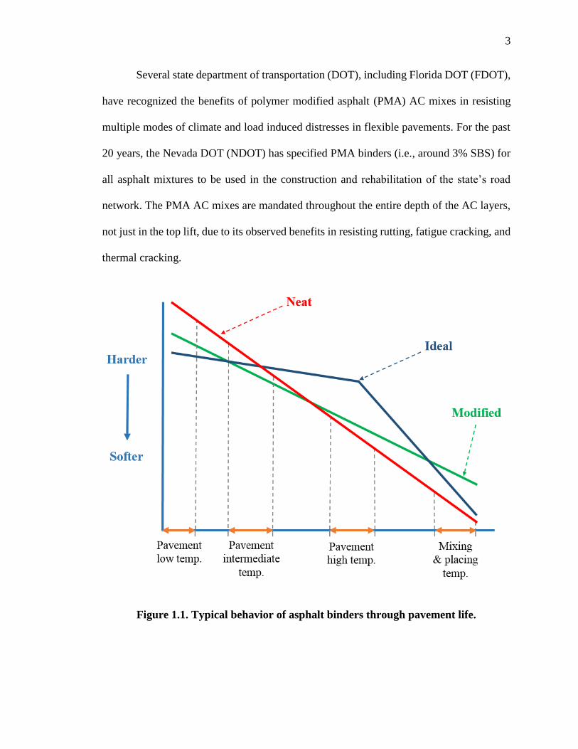
3
Several state department of transportation (DOT), including Florida DOT (FDOT),
have recognized the benefits of polymer modified asphalt (PMA) AC mixes in resisting
multiple modes of climate and load induced distresses in flexible pavements. For the past
20 years, the Nevada DOT (NDOT) has specified PMA binders (i.e., around 3% SBS) for
all asphalt mixtures to be used in the construction and rehabilitation of the state’s road
network. The PMA AC mixes are mandated throughout the entire depth of the AC layers,
not just in the top lift, due to its observed benefits in resisting rutting, fatigue cracking, and
thermal cracking.
Figure 1.1. Typical behavior of asphalt binders through pavement life.

4
1.2 AASHTO Flexible Pavement Design Methodology
The American Association of State Highway and Transportation Officials (AASHTO)
Guide for Design of Pavement Structures (AASHTO 1993 Guide) constitutes the primary
method used by FDOT for designing new and rehabilitated highway pavements. The
AASHTO 1993 Guide design method is based on information obtained at the AASHO
Road Test, which was performed from 1958 to 1960 near Ottawa, Illinois. The road test
was composed of six two-lane test loops, four large loops and two small ones, subjected to
truck traffic. The main objective of the road test was to determine the effect of different
axle loadings (i.e., configuration and load) on the performance and behavior of pavements.
The loaded trucks were mounted with bias-ply tires with inflation pressure of 70 psi (483
kPa). No super single tires, triple, or quad axles were utilized. The road test was only
subjected to a maximum of 2 million equivalent single axle loads (ESALs) (AASHTO
Guide, 1993).
The primary objective of the AASHO Road Test was to assess and evaluate the
pavement deterioration induced by traffic loads. The first pavement design guide, known
as AASHO Interim Guide for the Design of Rigid and Flexible Pavements was developed
using the AASHO Road Test results. Many versions were subsequently released including
the AASHTO 1993 Guide which is still used today by many transportation agencies
including FDOT. The overall approach of the AASHTO 1993 Guide is to design, both
flexible and rigid pavements, for a specified serviceability loss at the end of the design life
of the pavement. In the AASHTO design methodology, the monograph presented in Figure
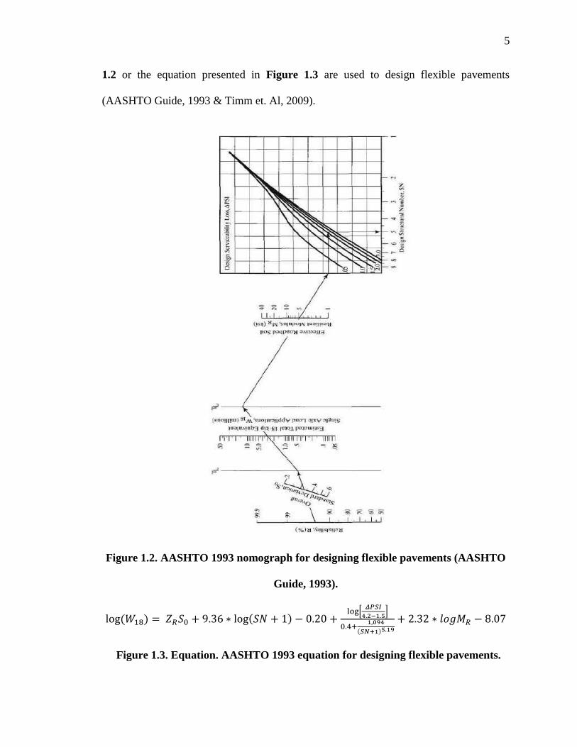
5
1.2 or the equation presented in Figure 1.3 are used to design flexible pavements
(AASHTO Guide, 1993 & Timm et. Al, 2009).
Figure 1.2. AASHTO 1993 nomograph for designing flexible pavements (AASHTO
Guide, 1993).
log (𝑊18) = 𝑍𝑅𝑆0 + 9.36 ∗ log(𝑆𝑁 + 1) − 0.20 +log[
𝛥𝑃𝑆𝐼
4.2−1.5]
0.4+1,094
(𝑆𝑁+1)5.19
+ 2.32 ∗ 𝑙𝑜𝑔𝑀𝑅 − 8.07
Figure 1.3. Equation. AASHTO 1993 equation for designing flexible pavements.
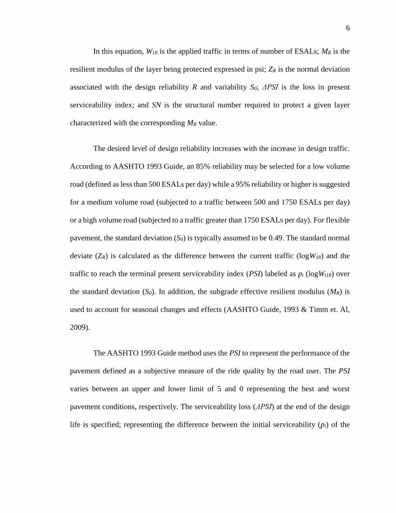
6
In this equation, W18 is the applied traffic in terms of number of ESALs; MR is the
resilient modulus of the layer being protected expressed in psi; ZR is the normal deviation
associated with the design reliability R and variability S0; ΔPSI is the loss in present
serviceability index; and SN is the structural number required to protect a given layer
characterized with the corresponding MR value.
The desired level of design reliability increases with the increase in design traffic.
According to AASHTO 1993 Guide, an 85% reliability may be selected for a low volume
road (defined as less than 500 ESALs per day) while a 95% reliability or higher is suggested
for a medium volume road (subjected to a traffic between 500 and 1750 ESALs per day)
or a high volume road (subjected to a traffic greater than 1750 ESALs per day). For flexible
pavement, the standard deviation (S0) is typically assumed to be 0.49. The standard normal
deviate (ZR) is calculated as the difference between the current traffic (logW18) and the
traffic to reach the terminal present serviceability index (PSI) labeled as pt (logWt18) over
the standard deviation (S0). In addition, the subgrade effective resilient modulus (MR) is
used to account for seasonal changes and effects (AASHTO Guide, 1993 & Timm et. Al,
2009).
The AASHTO 1993 Guide method uses the PSI to represent the performance of the
pavement defined as a subjective measure of the ride quality by the road user. The PSI
varies between an upper and lower limit of 5 and 0 representing the best and worst
pavement conditions, respectively. The serviceability loss (ΔPSI) at the end of the design
life is specified; representing the difference between the initial serviceability (pi) of the

7
pavement when opened to traffic and the terminal serviceability (pt) that the pavement is
expected to reach before rehabilitation, resurfacing, or reconstruction is required.
The empirical relationship among design traffic, pavement structure, and pavement
performance for flexible pavements is solved to determine the required structural capacity
of the pavement section, known as the structural number (SN). The total pavement SN is
defined as the summation of the layer thicknesses times the corresponding structural layers
and drainage coefficients as expressed in the equation presented in Figure 1.4.
𝑆𝑁 = ∑ 𝑎𝑖𝐷𝑖𝑚𝑖𝑖=1
Figure 1.4. Equation. AASHTO 1993 equation for total structural number of a
flexible pavement structural for a given design traffic.
In this equation, SN stands for the total structural number required for a given
design traffic; ai is the structural coefficient for the ith layer; Di is the thickness of the ith
layer expressed in inch; and mi is the drainage coefficient for the ith layer except for the AC
layer.
No direct method exists for establishing new structural coefficients as new AC
mixtures are created. The current structural coefficients were estimated based on many
factors including material stiffness, and compressive and/or tensile strength. Figure 1.5
shows a chart used to estimate the structural coefficient of dense-graded AC surface course
based on its elastic (resilient) modulus (EAC) at a temperature of 68°F (20°C) in accordance
with the AASHTO 1993 Guide (AASHTO Guide, 1993). These coefficients were

8
determined based on limited parameters used in the AASHO road test where a single type
subgrade soil, gravel base, and AC mix were considered. Furthermore, no advanced paving
materials including Superpave-designed AC mixes and polymer modified AC mixes were
used. Therefore, the relationship used to determine the AC structural coefficient may not
be valid for AC mixes currently used by FDOT and other state DOTs.
Figure 1.5. Chart estimating structural coefficient of dense-graded asphalt concrete
based on the elastic (resilient) modulus after AASHTO 1993 (AASHTO Guide,
1993).
1.3 FDOT Pavement Design Practice
FDOT recently updated and published a manual for designing flexible pavements in
Florida (September 2016) (FDOT Design Manual, 2016). This manual provides guidance
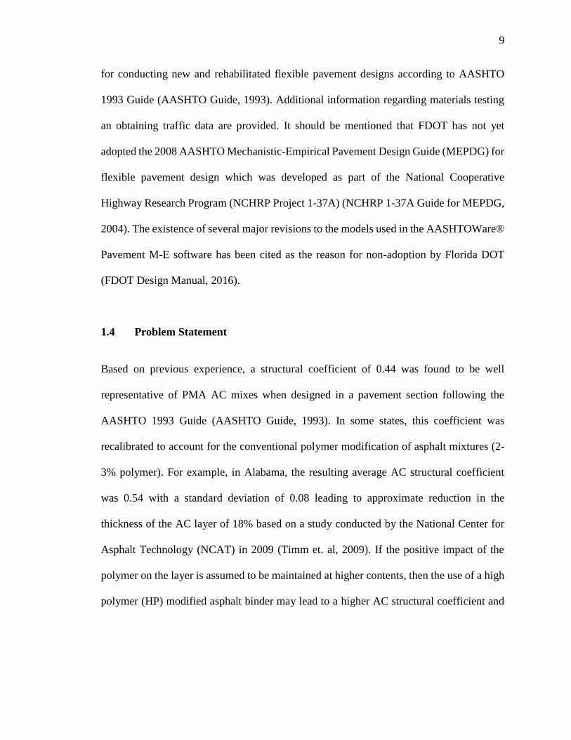
9
for conducting new and rehabilitated flexible pavement designs according to AASHTO
1993 Guide (AASHTO Guide, 1993). Additional information regarding materials testing
an obtaining traffic data are provided. It should be mentioned that FDOT has not yet
adopted the 2008 AASHTO Mechanistic-Empirical Pavement Design Guide (MEPDG) for
flexible pavement design which was developed as part of the National Cooperative
Highway Research Program (NCHRP Project 1-37A) (NCHRP 1-37A Guide for MEPDG,
2004). The existence of several major revisions to the models used in the AASHTOWare®
Pavement M-E software has been cited as the reason for non-adoption by Florida DOT
(FDOT Design Manual, 2016).
1.4 Problem Statement
Based on previous experience, a structural coefficient of 0.44 was found to be well
representative of PMA AC mixes when designed in a pavement section following the
AASHTO 1993 Guide (AASHTO Guide, 1993). In some states, this coefficient was
recalibrated to account for the conventional polymer modification of asphalt mixtures (2-
3% polymer). For example, in Alabama, the resulting average AC structural coefficient
was 0.54 with a standard deviation of 0.08 leading to approximate reduction in the
thickness of the AC layer of 18% based on a study conducted by the National Center for
Asphalt Technology (NCAT) in 2009 (Timm et. al, 2009). If the positive impact of the
polymer on the layer is assumed to be maintained at higher contents, then the use of a high
polymer (HP) modified asphalt binder may lead to a higher AC structural coefficient and

10
a reduced AC layer thickness for the same design traffic and serviceability design loss
(Timm et. al, 2009).
1.5 Objectives and Scope
The objective of this FDOT research study and this dissertation is to conduct an in-
depth and comprehensive evaluation of asphalt mixtures in the state of Florida with a HP
binder with approximately 7.5% Styrene-Butadiene-Styrene (SBS) polymer. The study
combines the following four major aspects:
• Extensive laboratory evaluation of HP asphalt binder and mixtures: PMA and
HP asphalt binders sampled from two different sources will be evaluated in terms
of long-term aging susceptibility to observe and quantify the influence of binder
modification on the oxidative aging characteristics of these asphalt binders.
Additionally, asphalt mixtures manufactured using local materials from multiple
sources in the State of Florida in terms of aggregate and asphalt binders (i.e., PMA,
and HP) will be designed following the FDOT Superpave mix design
specifications. These designed PMA and HP AC mixes will be evaluated in terms
of engineering properties (i.e., stiffness) and performance characteristics (i.e.,
resistance to rutting, fatigue cracking, top-down cracking, and reflective cracking).
• Advanced mechanistic analysis under heavy moving loads using 3D-MOVE: the
developed properties and characteristics of PMA and HP mixtures will be
implemented into an advanced flexible pavement modeling process called 3D-
Move model to determine the responses and performance of PMA and HP
11
pavement sections under various structural and loading conditions. Using the
pavement responses from 3D-Move along with the performance models for the
PMA and HP asphalt mixtures for fatigue cracking, rutting in AC layer, total rutting
in the pavement structural, top-down and reflective cracking, structural coefficients
of the HP modified asphalt mixtures will be determined using the fixed service life
approach. This section will lead to a preliminary structural coefficient of HP AC
mixes for use in the structural design of flexible pavements (New construction, and
rehabilitation).
• Full-Scale pavement testing using PaveBox: the 11 feet (335.3 cm) width by 11
feet (335.3 cm) depth by 7 feet (213.4 cm) height PaveBox will serve as a full-scale
laboratory tool to verify the structural coefficients developed and checked
previously.
• Advanced numerical modeling of PaveBox using FLAC3D (Fast Lagragian
Analysis of Continua in 3-Dimensions): the three-dimensional explicit finite
difference program will be used to provide an advanced analysis of sections built-
in the PaveBox experiment.
Consequently, a structural coefficient for asphalt mixes that contain HP asphalt
binder will be determined for the state of Florida. Moreover, a practical plan will be
developed to validate the recommended structural coefficient for HP AC mixes under the
FDOT Accelerated Pavement Testing (APT) facility. With this determination, the FDOT
12
Flexible Pavement design Manual may be modified to adopt the structural value for
mixtures containing this binder type.
1.6 Dissertation Outline
In this research, HP AC mixes are defined as asphalt mixtures manufactured using
asphalt binders modified with SBS at the approximate rate of 7.5% by weight of binder.
PMA AC mixes are defined as asphalt mixtures manufactured using asphalt binders
modified with SBS at the approximate rate of 3% by weight of binder. This document
constitutes a comprehensive dissertation and is the outcome of the FDOT comprehensive
research study (Grant BE321). This document is divided into multiple chapters that address
various key aspect of this study:
• Review of Literature: this section addresses the key aspects of HP modified
asphalt mixes and their performance in the laboratory and on existing field
projects. A general background on PMA asphalt binders and mixes evaluated
in the laboratory is provided. Information on actual demonstration field projects
with limited and extensive performance data accomplished using HP AC mixes
are also presented. In addition, a preliminary analysis of structural coefficient
for mixes manufactured using HP asphalt binders is provided. Finally,
conclusions and recommendations based on the review of literature are
provided. The outcome of this section (i.e., review of literature) is a peer-
reviewed paper titled “A Critical Review of High Polymer-Modified Asphalt
Binders and Mixtures”, submitted (May 16 2018), accepted (July 14 2018) and

13
published online (August 2nd 2018) in the International Journal of Pavement
Engineering (IJPE). Citation: Jhony Habbouche, Elie Y. Hajj, Peter E. Sebaaly
& Murugaiyah Piratheepan (2018) A critical review of high polymer-modified
asphalt binders and mixtures, International Journal of Pavement
Engineering, DOI: 10.1080/10298436.2018.1503273. This peer-reviewed
published paper constitutes Chapter 2. Additional information regarding the
literature review are available in details in Appendix A.
• Experimental Design and Tests Description: Chapter 3 presents the
experimental design for the development of structural coefficient for HP
modified AC mixes. The overall objectives of the experimental design is to
define the steps necessary to carry-out a laboratory evaluation to produce the
engineering properties and performance characteristics of the PMA and HP AC
mixes, define the process of incorporating the measured properties and
performance characteristics into a mechanistic approach / model to determine
an initial structural coefficient for HP AC mixes in Florida, and finally define
the process to validate and verify the determined structural coefficient via full-
scale testing (i.e., UNR PaveBox). Detailed information regarding the raw
materials sampled and used in this study (i.e., aggregates, asphalt binders, and
RAP) are also provided in this chapter. In addition, an informative description
of the performance test conducted for the completion of this study are also
provided in this chapter.

14
• Mix Designs and Tests Description: Chapter 4 presents in detail the mix
designs developed. In addition, it provides the analysis of all test results
generated from the performance evaluation of the laboratory AC mixes.
• Flexible Pavement Modeling: Chapter 5 aims to incorporate the measured
engineering property and performance characteristics of the evaluated PMA
and HP AC mixes into the mechanistic modeling of flexible pavement
responses to traffic loads. In addition, this chapter presents and defines several
input parameters to be selected and used in the mechanistic analysis, and
numerous output critical responses that can be determined accordingly.
• Determination of Structural Coefficient for HP AC Mixes: The objectives
of Chapter 6 are to determine the critical responses of the designed pavement
structures for the identified distresses of AC pavements including; fatigue
cracking, AC rutting, total rutting, top-down cracking, and reflective cracking
using the 3D-Move model, and to determine the structural coefficient for HP
AC mixes. First, the determined critical responses are used to estimate the
fatigue performance life of the designed pavement structures followed by the
development of the initial structural coefficient for HP AC mixes based on the
equal fatigue performance life approach. Finally, the fatigue-based initial
structural coefficients are verified for the other distress modes.
• Verification of Structural Coefficient for HP AC Mixes using Full-Scale
Pavement Testing: Chapter 7 presents in details the effort to verify the

15
structural coefficient determined through laboratory testing and computer
modeling in two instrumented full-scale asphalt pavements subjected to
stationary dynamic loadings.
• Impact of High Polymer Modification on the Oxidative Aging of Asphalt
Binders: The main objective of Chapter 8 is to assess the long-term aging
characteristics of conventional and highly modified asphalt binder in terms of
their rheological and chemical properties. An extended asphalt binder aging
experiment was generated and considered multiple combinations of PMA and
HP asphalt binders from different sources. Long-term oven aged asphalt binders
at multiple temperatures and multiple durations were evaluated using the
dynamic shear rheometer (DSR) for full master curve characterization. The
Fourier Transform Infrared Spectroscopy (FT-IR) was used for characterization
of chemical composition (e.g., carbonyl area growth, sulfoxide area growth, and
others). The evaluation initially considered the resistance to oxidation
specifically through measures of the early to fast-rate followed by the slower
constant-rate kinetics parameters resulting from multiple aging temperatures
and durations. An extensive rheological evaluation was then combined with the
kinetics parameters to consider the hardening susceptibility of the respective
asphalt binders utilizing multiple rheological indices to develop a wide
perspective of the overall binder behaviors. Finally, the two aspects were
combined to distinguish the overall influence of the high binder modification
processes.

16
• Summary of Findings, Conclusions, and Development of
Recommendations: APT Implementation Plan: Finally, conclusions and
recommendations based on the literature review, laboratory evaluation,
advanced mechanistic modeling, and full-scale testing are provided in Chapter
9. In addition, an implementation plan of the final recommended structural
coefficient for HP AC mixes using the APT setup at FDOT facilities is provided
in this chapter.
17
CHAPTER 2 REVIEW OF LITERATURE
This chapter addresses the key aspects of HP modified asphalt mixes and their performance
in the laboratory and on existing field projects. A general background on PMA asphalt
binders and mixes evaluated in the laboratory is provided. Information on actual
demonstration field projects with limited and extensive performance data accomplished
using HP AC mixes are also presented. In addition, a preliminary analysis of structural
coefficient for mixes manufactured using HP asphalt binders is provided. Finally
conclusions and recommendations based on the review of literature are provided. As
previously mentioned in Chapter 1 Section 1.6 “Dissertation Outline”, the outcome of this
section (i.e., review of literature) is a peer-reviewed paper titled “A Critical Review of High
Polymer-Modified Asphalt Binders and Mixtures”, submitted (May 16, 2018), accepted
(July 14, 2018) and published online (August 2nd, 2018) in the International Journal of
Pavement Engineering (IJPE). Citation: Jhony Habbouche, Elie Y. Hajj, Peter E. Sebaaly
& Murugaiyah Piratheepan (2018) A critical review of high polymer-modified asphalt
binders and mixtures, International Journal of Pavement
Engineering, DOI: 10.1080/10298436.2018.1503273. This peer-reviewed published paper
was revised in format to satisfy the dissertation guidelines manadated by the graduate
school at University of Nevada, Reno (UNR). Additional information regarding the
literature review are available in details in Appendix A.
The introduction of modified asphalt binders provided transportation agencies an
effective tool to design balanced mixtures that can resist conflicting distresses while
maintaining good long-term durability. While conventional polymer modified asphalt

18
(PMA) mixtures have shown improved long-term performance, it is also believed that
asphalt mixtures with high polymer (HP) content may offer additional advantages in
flexible pavements subjected to heavy and/or slow moving traffic loads. While no unique
and detailed handy guide that discusses the HP modification of binders and mixtures exists
at this time, and while asphalt industry is moving towards the use of much more durable
materials for a better long-term performance of newly constructed roads, this manuscript
summarizes the findings from the literature review on the performance of HP asphalt
binders and mixtures. The reviewed laboratory studies indicated that the increase in
polymer content continues to improve the performance properties of binders and mixtures.
The reviewed field projects showed encouraging early field performance without
exhibiting any construction related issues. In addition, this article presents attempts that
were explored to estimate a structural coefficient of HP mixes based on the available
information from literature. This analysis led to the conclusion that the designed HP
mixtures may lead up to 40% reduction in the asphalt layer thickness resulting in
considerable upfront cost-savings.
2.1 Introduction
Asphalt concrete (AC) mixtures have been used as driving services for flexible pavements
since the early 1900s. With the continuous increase in highway traffic volume, axle loads
and tyre pressures, the demand for high quality and durable AC mixtures became critical.
The flexible pavement engineering community has kept up very well with these demands
through the introduction of new technologies for the manufacturing of asphalt binders and
mixtures, advanced pavement testing and evaluation techniques, and new construction

19
equipment. Typically, the resistance of AC mixtures to permanent deformation (i.e. rutting
and shoving) requires stiff asphalt binder and low asphalt binder content while its resistance
to cracking (fatigue, top-down, block and thermal) requires flexible asphalt binder and
higher binder content. Specifically, the introduction of modified asphalt binders provided
transportation agencies the means to effectively design balanced asphalt mixtures that can
resist these conflicting distresses while maintaining a good long-term durability (i.e.
reduced moisture damage and aging susceptibility).
Figure 2.1 illustrates typical behaviour of neat, modified, and ideal asphalt binders
as a function of anticipated temperatures over the life of the asphalt binder in the asphalt
mixture as part of the pavement flexible structure (IDOT, 2005). The typical behavior leads
to the following observations:
• A neat asphalt binder will be easier to produce and construct, however, it
may experience: (a) rutting under high pavement temperature due to its
softer behaviour, (b) fatigue cracking (bottom-up and top-down) at
intermediate pavement temperatures due to its non-flexible behaviour and
(c) thermal cracking at low pavement temperatures due to its brittle
behavior.
• A modified asphalt binder will be generally more difficult to produce and
construct requiring higher temperatures, however, it may experience: (a)
less rutting under high pavement temperatures due to its stronger behaviour,
(b) less fatigue cracking (bottom-up and top-down) at intermediate

20
pavement temperatures and (c) less thermal cracking at low pavement
temperatures due to its more ductile behavior.
• An ideal asphalt binder exhibits the most desirable behaviors and offers
excellent resistance to all three modes of distresses. Unfortunately, the
break in the behavior curve has proven to be impossible to achieve, and
therefore, the ideal binder does not currently exist.
Modified asphalt binders have been produced using a wide range of technologies
to modify the properties of the neat asphalt binder to accommodate the project-specific
load and climatic conditions. Throughout the past 50 years, asphalt binders have been
modified with polymers, ground tyre rubber, chemicals (e.g. acid), recycled engine oils,
etc. to achieve the desired properties.
Several state departments of transportation (DOT), including Nevada and Florida
DOTs, have recognised the benefits of polymer-modified asphalt (PMA) mixes in resisting
multiple modes of climate and load induced distresses in flexible pavements. For the past
20 years, the Nevada DOT (NDOT) has specified PMA binders (i.e. around 3% SBS) for
all asphalt mixtures to be used in the construction and rehabilitation of the state’s road
network. The PMA AC mixes are mandated within the entire depth of the AC layers, not
just in the top lift, due to its observed benefits in resisting rutting, fatigue cracking and
thermal cracking.

21
Figure 2.1. Schematic of typical behavior of asphalt binders through pavement life.
From a structural design perspective and based on previous experiences, a layer
coefficient of 0.44 was found to be well representative of PMA AC mixes when designed
in a pavement section following the American Association for State Highway and
Transportation Officials (AASHTO) Guide for Design of Pavement Structures (AASHTO
Guide, 1993). In some states, this coefficient was recalibrated to account for the
conventional polymer modification of asphalt mixtures (2–3% polymer). For example, in
Alabama, the resulting average AC structural coefficient was changed to 0.54 with a
standard deviation of 0.08 leading to an approximate reduction in the thickness of the AC
layer of 18% based on a study conducted by the National Center for Asphalt Technology
(NCAT) in 2009 (Timm et al., 2009). If the positive impact of the polymer on the layer is
22
assumed to be maintained at higher contents, then the use of a higher polymer (HP)
modified asphalt binder may lead to a higher AC structural coefficient and a reduced AC
layer thickness for the same design traffic and serviceability design loss (Timm et al.,
2009).
2.2 Objective and Scope
This chapter constitutes a critical state-of-the-art review of HP asphalt binders and mixtures
evaluated in the laboratory and field. HP AC mixes are defined as asphalt mixtures
manufactured using asphalt binders modified with Styrene-Butadiene-Styrene (SBS) or
Styrene-Butadiene (SB) at the approximate rate of 7.5% by weight of the binder. PMA AC
mixes are defined as asphalt mixtures manufactured using asphalt binders modified with
SBS or SB at the approximate rate of 3% by weight of the binder. While no unique and
detailed handy guide that discusses the HP modification of asphalt binders and mixtures
exists at this time, and while asphalt industry is moving towards the use of much more
durable materials for a better long-term performance of newly constructed roads, this
manuscript summarises the information and findings from the literature review on the
performance of HP asphalt binders and mixtures. Two major objectives were targeted in
this review: (a) identify all current and previous studies that have been conducted to
evaluate the engineering properties and performance characteristics of HP asphalt binders
and HP AC mixes, and (b) determine a preliminary structural coefficient of HP AC mixes
for use in the structural design of flexible pavements.
The literature presented in this manuscript focused on three major areas of interest:
(a) laboratory evaluation of HP modified asphalt binders and mixtures, (b) performance of

23
pavement sections constructed with HP AC mixes and (c) techniques to determine the
structural coefficient of HP AC mixes. In addition, it documents studies that evaluated
asphalt binders and mixtures that were manufactured at multiple levels of modification but
do not fit the HP category as defined previously. These studies were incorporated in the
review only in cases where they represent the control materials since they offer insights on
the impact of the incremental increase in the polymer content on the properties of asphalt
binders and mixtures.
2.3 Laboratory Evaluation of HP Modified Asphalt Binders and Mixtures
Polymer modification of asphalt binder is not a new concept and has become progressively
more common over the past several decades. While several agencies utilise unmodified
asphalt binders many have increasingly become reliant upon PMA binders with a fair
portion of those located in climatic regions that experience significantly wider temperature
range conditions and a higher level of oxidation. Therefore, it is becoming ever more
important to characterise the benefits afforded with the polymer modification process. This
section includes six studies that evaluated the performance of HP asphalt binders and
mixtures in the laboratory.
The first experimental study was conducted by FDOT to assess the effect of
increasing the polymer content of asphalt binders in terms of resistance to rutting distress
(Greene et al., 2014). Three asphalt binders meeting the current FDOT specifications
(FDOT specifications, 2018) were evaluated in this study: a PG67-22 neat binder, PG76-
22PMA binder at 3% SBS content and a PG82-22PMA binder at 6% SBS content. All
asphalt binders were collected at the plant and laboratory tests such as dynamic shear
24
rheometer (DSR) (AASHTO T315, 2010), multiple stress creep recovery (MSCR) (ASTM
D7405, 2008) and binder fracture energy were conducted for analysis and characterisation
(Greene et al., 2014). In addition, AC mixtures were designed with 0.5-inch (12.5 mm)
nominal maximum aggregate size (NMAS) fine gradation using granite aggregate and the
three asphalt binders previously defined. The cracking resistance of the mixtures was
evaluated using the Superpave indirect tension test (IDT) (AASHTO, T322 2007). Finally,
similar AC mixes were evaluated in terms of resistance to rutting and fatigue cracking via
accelerated loading performed using the FDOT Heavy Vehicle Simulator (HVS) through
measuring the actual rut depth developed in the wheel path and the actual tensile strains at
the bottom of the AC layer, respectively. On one hand, the DSR results showed that the
PG82-22PMA binder exhibited the greatest stiffness, elasticity and rutting resistance, as
shown by its high G*, low δ and high G*/sin(δ), respectively. On the other hand, the MSCR
test results indicate that the two PMA binders exhibit greater viscoelastic behavior than the
neat binder shown by the higher recovery and lower non-recoverable creep compliance
values accompanied with a lower sensitivity to the stress level. Meanwhile, a greater
fracture energy was observed for the PG82-22PMA when compared with the PG76-
22PMA and PG67-22 binders indicating a better fracture resistance for AC mixes
manufactured with the PG82-22PMA binder. The IDT test results showed a minor
difference between the measured fracture energy values between the PG82-22 PMA and
PG76-22PMA AC mix; however, a 66% reduction in the creep rate was observed for the
PG82-22PMA AC mix as compared to the PG76-22PMA AC mix.

25
The HVS rutting performance showed that both polymer modified mixtures (i.e.
PG76-22PMA and PG82-22PMA) significantly out-performed the neat mix (i.e. PG67-22)
showing a rut depth reduction of 29% and 49% after 100,000 passes, respectively.
Meanwhile, the PG82-22PMA AC mix performed significantly better than the PG76-
22PMA in both measured rut depth (reduction of 28%) and shear area (reduction of 40%).
Additionally, the HVS fatigue performance showed significant reductions in measured
tensile strains at the bottom of AC layer for the two PMA AC mixes with the percent
reduction increasing with the higher polymer content (i.e. PG82-22PMA) (Greene et al.,
2014).
The second study was conducted at University of Nevada, Reno (UNR) to assess
the effect of HP content in improving the resistance of the asphalt binder to long-term
aging, and to observe and to quantify the influence of binder modification on the oxidative
aging characteristics of the evaluated asphalt binders (Zhu, 2015). An asphalt binder with
low susceptibility to long-term aging would significantly reduce the potential of the asphalt
mixture to all types of cracking including bottom-up fatigue, top-down fatigue, thermal,
reflective and block cracking. Three asphalt binders: neat, polymer modified with 3% SBS
(PMA) and highly polymer modified with 7.5% SBS (HP) were evaluated. The evaluated
asphalt binders were aged at different temperatures (i.e. 50, 60, and 85°C) and for different
durations (e.g. 0.5, 1, 15, 25, 60, 180 and 240 days) to measure the aging kinetics as a
function of time and temperature. The aged binders were then rheologically evaluated in
the DSR by determining the shear dynamic modulus (G*) and phase angle (δ) master
curves. Figure 2.2 shows the measured properties of the aged asphalt binders using the
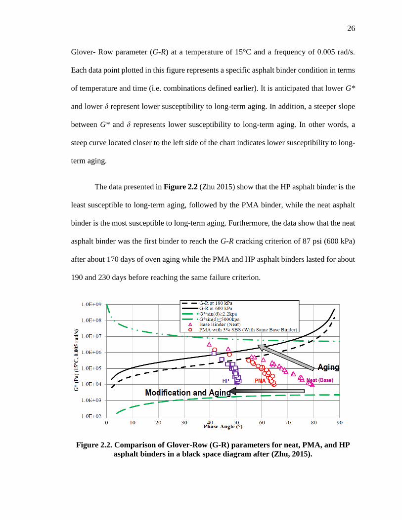
26
Glover- Row parameter (G-R) at a temperature of 15°C and a frequency of 0.005 rad/s.
Each data point plotted in this figure represents a specific asphalt binder condition in terms
of temperature and time (i.e. combinations defined earlier). It is anticipated that lower G*
and lower δ represent lower susceptibility to long-term aging. In addition, a steeper slope
between G* and δ represents lower susceptibility to long-term aging. In other words, a
steep curve located closer to the left side of the chart indicates lower susceptibility to long-
term aging.
The data presented in Figure 2.2 (Zhu 2015) show that the HP asphalt binder is the
least susceptible to long-term aging, followed by the PMA binder, while the neat asphalt
binder is the most susceptible to long-term aging. Furthermore, the data show that the neat
asphalt binder was the first binder to reach the G-R cracking criterion of 87 psi (600 kPa)
after about 170 days of oven aging while the PMA and HP asphalt binders lasted for about
190 and 230 days before reaching the same failure criterion.
Figure 2.2. Comparison of Glover-Row (G-R) parameters for neat, PMA, and HP
asphalt binders in a black space diagram after (Zhu, 2015).

27
The third study was conducted by researchers at ORLEN Asfalt in Poland. They
hypothesised that a crack can pass through a conventionally modified asphalt binder by
finding weak spots between the polymer network sections (Blazejowski et al., 2015).
Meanwhile, the crack passage through a highly modified asphalt binder is more difficult
because of the barrier formed by the polymer network. Limiting crack propagation in
asphalt mixtures remains a clear example illustrating the benefits of a continuous polymer
network acting in the asphalt binder and mixtures as an elastic reinforcement. In 2011, three
new HP asphalt binders were developed by these researchers: (a) ORBITON 25/55-80
HiMA designated to be used for typical asphalt base courses of long-life pavements (i.e.
perpetual) with slow traffic, (b) ORBITON 45/80-80 HiMA designated to be used for
wearing and binder courses of pavements subjected to very heavy loads and/or low
temperatures and (c) ORBITON 65/105-80 HiMA designed to be used for special
technologies such as stress absorbing membrane interlayers (SAMI), and emulsion
applications in slurry seals (Blazejowski et al., 2015). All three binders were modified with
7.5% SBS by weight of the binder. The properties of the three HP binders and AC mixes
were evaluated in the laboratory at the low temperature using the bending beam rheometer
(BBR) test by measuring the stiffness and coefficient of relaxation after 60 seconds (i.e.
S(60), and m) static load simulating the slow rate of thermal stresses (AASHTO T313,
2012), and thermal stress restrained specimen test (TSRST) by measuring the fracture
strength and fracture temperature (AASHTO TP10, 1993), respectively. Additionally, the
HP binders were evaluated at the intermediate temperature using the DSR test (i.e., G*sinδ)
(AASHTO T315, 2010). For the high temperature, the HP binders and AC mixes were
28
evaluated using the DSR (AASHTO T315, 2010) and MSCR (ASTM D7405, 2008) tests,
and the wheel tracker rutting test, respectively.
For the low temperature evaluation, the measured S(60) and m-value properties of
the evaluated binders show that the BBR critical low temperature continues to decrease as
the SBS content increases from 0%, 3%, to 7.5% except for the third HP binder designed
for use in Stress Absorbing Membrane Interlayer (SAMI) and slurry seals. In addition, the
TSRST fracture temperature of the evaluated AC mixes continues to decrease as the SBS
content increases from 0%, 3%, to 7.5%. These results clearly show the benefits of using
HP binders towards improving the resistance of AC mixes to thermal cracking. Meanwhile,
for the intermediate temperature, the measured G*sin(δ) properties of the evaluated asphalt
binders show that the DSR critical intermediate temperature continues to decrease as the
SBS content increases from 0%, 3%, to 7.5%. These results clearly show the increases
resistance of the HP binders to fatigue cracking. At the end for the high temperature, the
MSCR data showed increased rutting resistance of the evaluated binders as the SBS content
increases from 0%, 3%, to 7.5% (Blazejowski et al., 2015).
The fourth study consisted of evaluating high-performance thin overlay (HiPO)
mixtures manufactured using HP asphalt binders and reclaimed asphalt pavement (RAP).
HiPO was intended as a mean to extend the available funds for pavement preservation and
for essentially delaying the future need for pavement rehabilitation. Several distresses and
issues that shorten the service life of conventional overlays such as reflective cracking,
thermal cracking, fatigue cracking and rutting were addressed while developing the HiPO
mixtures specifications AASHTO Transportation System Preservation Technical Services
29
Program (AASHTO TSP2, 2012). Following the publication of the HiPO Specifications
(AASHTO TSP2, 2012), the New Hampshire (NH), Vermont (VT) and Minnesota (MN)
DOTs showed interest in using this specification for demonstration field projects. The main
interest in the HiPO specification is that it allows the use of RAP up to 25% by dry weight
of aggregate and an HP asphalt binder with 7.5% of SBS polymer, graded as PG76-34 or
PG82-28 (Mogawer et al., 2014). The experimental plan included work to develop a
Superpave mix design with an NMAS of 3/8-inch (9.5 mm) based on input from interested
DOTs following the pilot specification. The evaluations included performance tests to
evaluate the plant-produced mixtures collected from the field projects in terms of resistance
to reflective (Mogawer, 2014), thermal (AASHTO TP10, 1993) and fatigue cracking
(Mogawer et al., 2014) as well as rutting (Mogawer, 2014 & AASHTO T340, 2010).
Additional tests, not mandated as part of the specifications, were conducted such as
Hamburg wheel tracking device (HWTD) for further rutting evaluation as well as the
semicircular bending (SCB) test for further evaluation of resistance to cracking.
All evaluated mixtures exhibited an average overlay test (OT) cycles to failure
greater than the minimum required 300 cycles. However, the Vermont with RAP mix did
not exhibit cycles to failure within ± 10% of the number of cycles exhibited by the
corresponding mix without RAP indicating the need of assessing the applicability of using
24% RAP without changing the grade of the binder. For the thermal cracking properties,
the addition of RAP decreased the thermal cracking resistance of the VT mixture as
presented by the warmer thermal fracture temperature. In parallel, the results for the fatigue
cracking showed that the two mixtures with RAP (NH and VT) showed a similar number
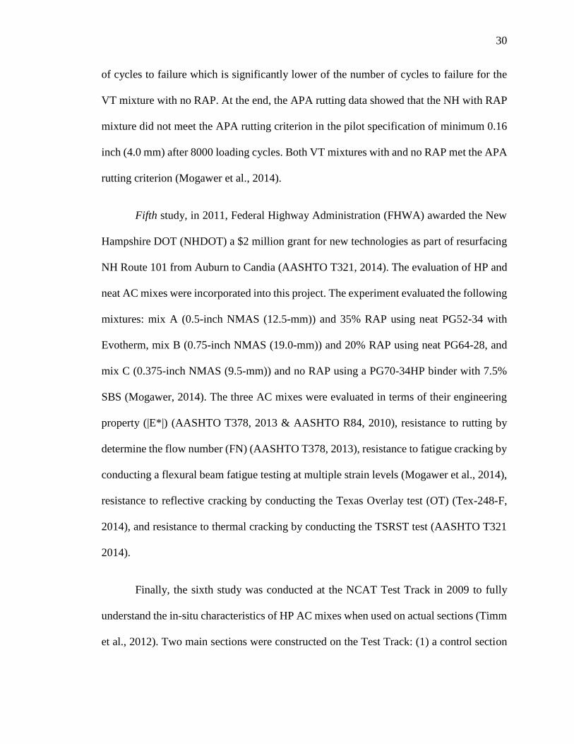
30
of cycles to failure which is significantly lower of the number of cycles to failure for the
VT mixture with no RAP. At the end, the APA rutting data showed that the NH with RAP
mixture did not meet the APA rutting criterion in the pilot specification of minimum 0.16
inch (4.0 mm) after 8000 loading cycles. Both VT mixtures with and no RAP met the APA
rutting criterion (Mogawer et al., 2014).
Fifth study, in 2011, Federal Highway Administration (FHWA) awarded the New
Hampshire DOT (NHDOT) a $2 million grant for new technologies as part of resurfacing
NH Route 101 from Auburn to Candia (AASHTO T321, 2014). The evaluation of HP and
neat AC mixes were incorporated into this project. The experiment evaluated the following
mixtures: mix A (0.5-inch NMAS (12.5-mm)) and 35% RAP using neat PG52-34 with
Evotherm, mix B (0.75-inch NMAS (19.0-mm)) and 20% RAP using neat PG64-28, and
mix C (0.375-inch NMAS (9.5-mm)) and no RAP using a PG70-34HP binder with 7.5%
SBS (Mogawer, 2014). The three AC mixes were evaluated in terms of their engineering
property (|E*|) (AASHTO T378, 2013 & AASHTO R84, 2010), resistance to rutting by
determine the flow number (FN) (AASHTO T378, 2013), resistance to fatigue cracking by
conducting a flexural beam fatigue testing at multiple strain levels (Mogawer et al., 2014),
resistance to reflective cracking by conducting the Texas Overlay test (OT) (Tex-248-F,
2014), and resistance to thermal cracking by conducting the TSRST test (AASHTO T321
2014).
Finally, the sixth study was conducted at the NCAT Test Track in 2009 to fully
understand the in-situ characteristics of HP AC mixes when used on actual sections (Timm
et al., 2012). Two main sections were constructed on the Test Track: (1) a control section
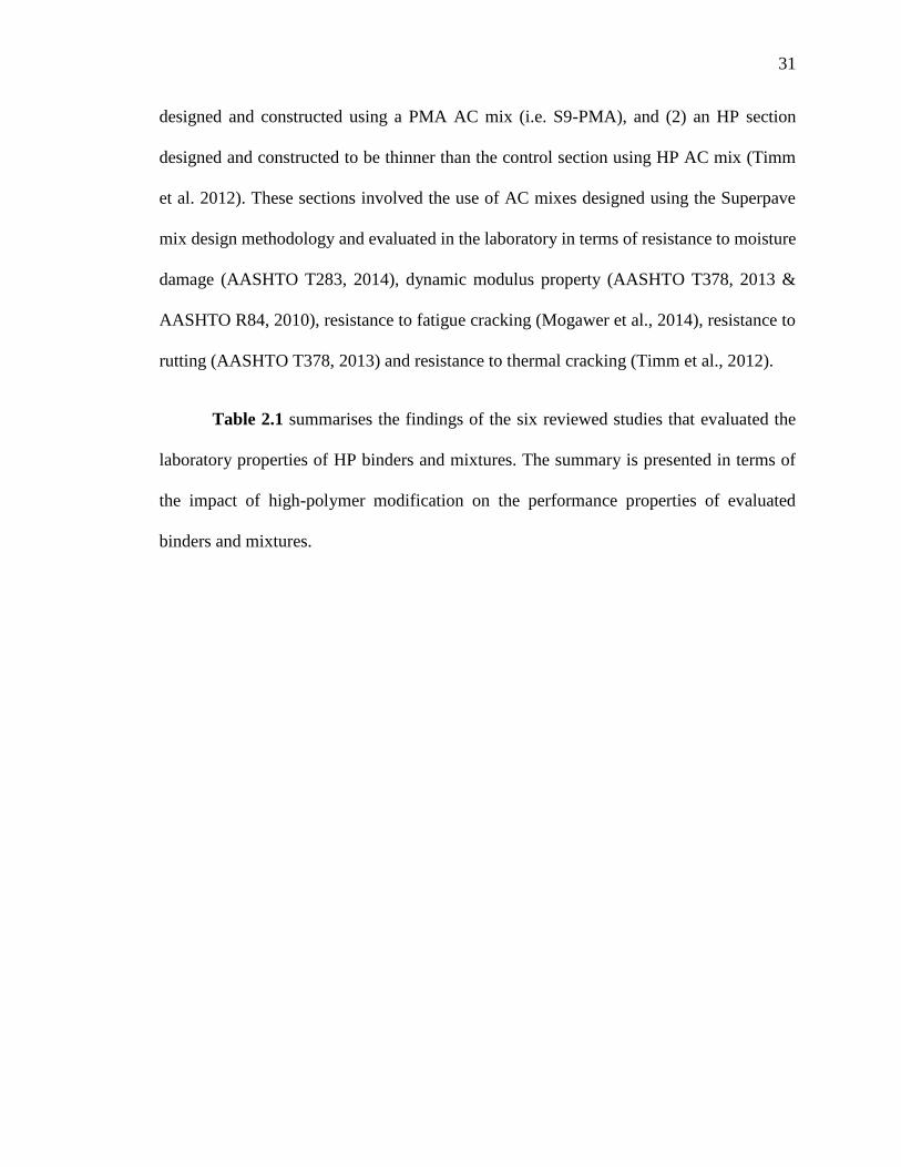
31
designed and constructed using a PMA AC mix (i.e. S9-PMA), and (2) an HP section
designed and constructed to be thinner than the control section using HP AC mix (Timm
et al. 2012). These sections involved the use of AC mixes designed using the Superpave
mix design methodology and evaluated in the laboratory in terms of resistance to moisture
damage (AASHTO T283, 2014), dynamic modulus property (AASHTO T378, 2013 &
AASHTO R84, 2010), resistance to fatigue cracking (Mogawer et al., 2014), resistance to
rutting (AASHTO T378, 2013) and resistance to thermal cracking (Timm et al., 2012).
Table 2.1 summarises the findings of the six reviewed studies that evaluated the
laboratory properties of HP binders and mixtures. The summary is presented in terms of
the impact of high-polymer modification on the performance properties of evaluated
binders and mixtures.
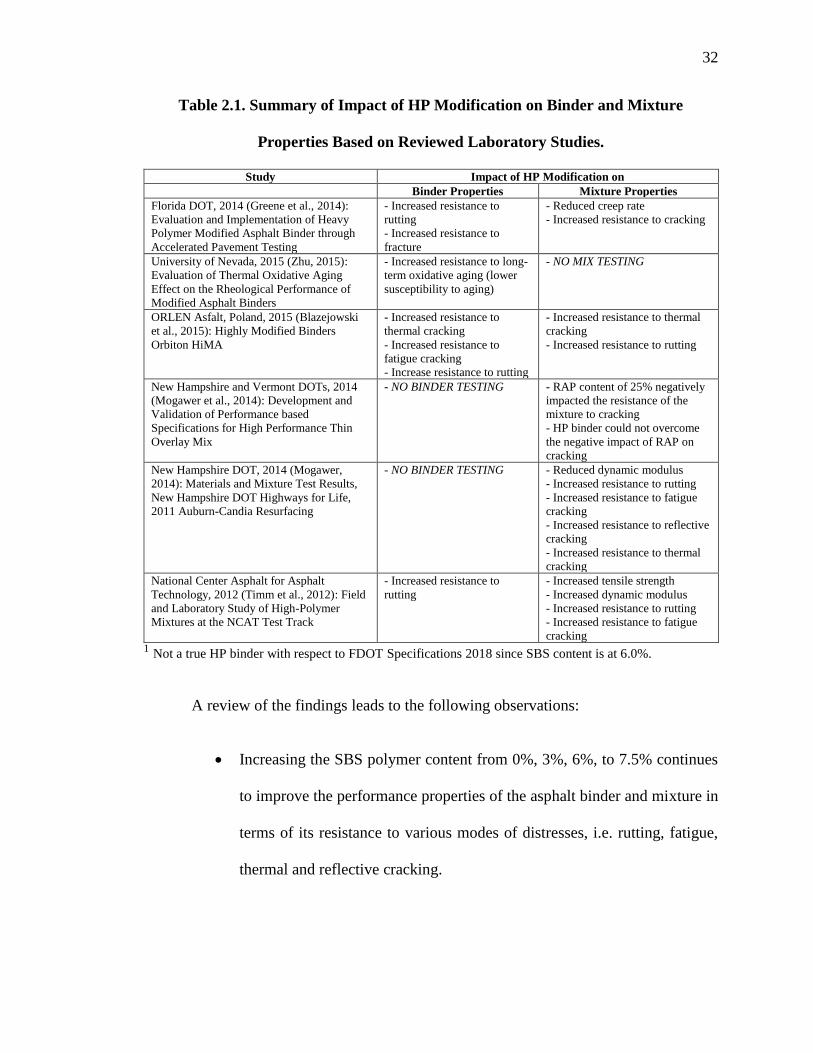
32
Table 2.1. Summary of Impact of HP Modification on Binder and Mixture
Properties Based on Reviewed Laboratory Studies.
Study Impact of HP Modification on
Binder Properties Mixture Properties
Florida DOT, 2014 (Greene et al., 2014):
Evaluation and Implementation of Heavy
Polymer Modified Asphalt Binder through
Accelerated Pavement Testing
- Increased resistance to
rutting
- Increased resistance to
fracture
- Reduced creep rate
- Increased resistance to cracking
University of Nevada, 2015 (Zhu, 2015):
Evaluation of Thermal Oxidative Aging
Effect on the Rheological Performance of
Modified Asphalt Binders
- Increased resistance to long-
term oxidative aging (lower
susceptibility to aging)
- NO MIX TESTING
ORLEN Asfalt, Poland, 2015 (Blazejowski
et al., 2015): Highly Modified Binders
Orbiton HiMA
- Increased resistance to
thermal cracking
- Increased resistance to
fatigue cracking
- Increase resistance to rutting
- Increased resistance to thermal
cracking
- Increased resistance to rutting
New Hampshire and Vermont DOTs, 2014
(Mogawer et al., 2014): Development and
Validation of Performance based
Specifications for High Performance Thin
Overlay Mix
- NO BINDER TESTING - RAP content of 25% negatively
impacted the resistance of the
mixture to cracking
- HP binder could not overcome
the negative impact of RAP on
cracking
New Hampshire DOT, 2014 (Mogawer,
2014): Materials and Mixture Test Results,
New Hampshire DOT Highways for Life,
2011 Auburn-Candia Resurfacing
- NO BINDER TESTING - Reduced dynamic modulus
- Increased resistance to rutting
- Increased resistance to fatigue
cracking
- Increased resistance to reflective
cracking
- Increased resistance to thermal
cracking
National Center Asphalt for Asphalt
Technology, 2012 (Timm et al., 2012): Field
and Laboratory Study of High-Polymer
Mixtures at the NCAT Test Track
- Increased resistance to
rutting
- Increased tensile strength
- Increased dynamic modulus
- Increased resistance to rutting
- Increased resistance to fatigue
cracking 1 Not a true HP binder with respect to FDOT Specifications 2018 since SBS content is at 6.0%.
A review of the findings leads to the following observations:
• Increasing the SBS polymer content from 0%, 3%, 6%, to 7.5% continues
to improve the performance properties of the asphalt binder and mixture in
terms of its resistance to various modes of distresses, i.e. rutting, fatigue,
thermal and reflective cracking.

33
• A unique feature of the HP modification has been identified as its ability to
slow down the oxidative aging of the asphalt binder. This feature is expected
to positively impact the resistance of the HP AC mix to various types of
cracking.
• The HP asphalt binder does not necessarily overcome any negative impact
the use of high RAP content can have on the resistance of the AC mixtures
to various types of cracking. The properties of the RAP binder should be
taken into consideration when designing HP AC mix with RAP content of
above 25% in order to optimise the benefits of the HP modification.
2.4 Evaluation of Field Projects with HP AC Mixtures
Several field demonstration projects were constructed in the United States of America
(USA), Canada, Southern America, Europe and Australia to evaluate the performance of
HP AC mixes. Figure 2.3 shows the locations of some of the projects on the U.S.A. map.
Table 2.2 summarizes the review of seven field HP AC mixes projects with limited and
extensive performance data in terms of description and key findings.
A review of the findings in Table 2.2 leads to the following observations:
• HP AC mixes have been used over a wide range of applications ranging
from full depth AC layer to thin AC overlays under heavy traffic on
interstates and slow-braking loads at intersections.
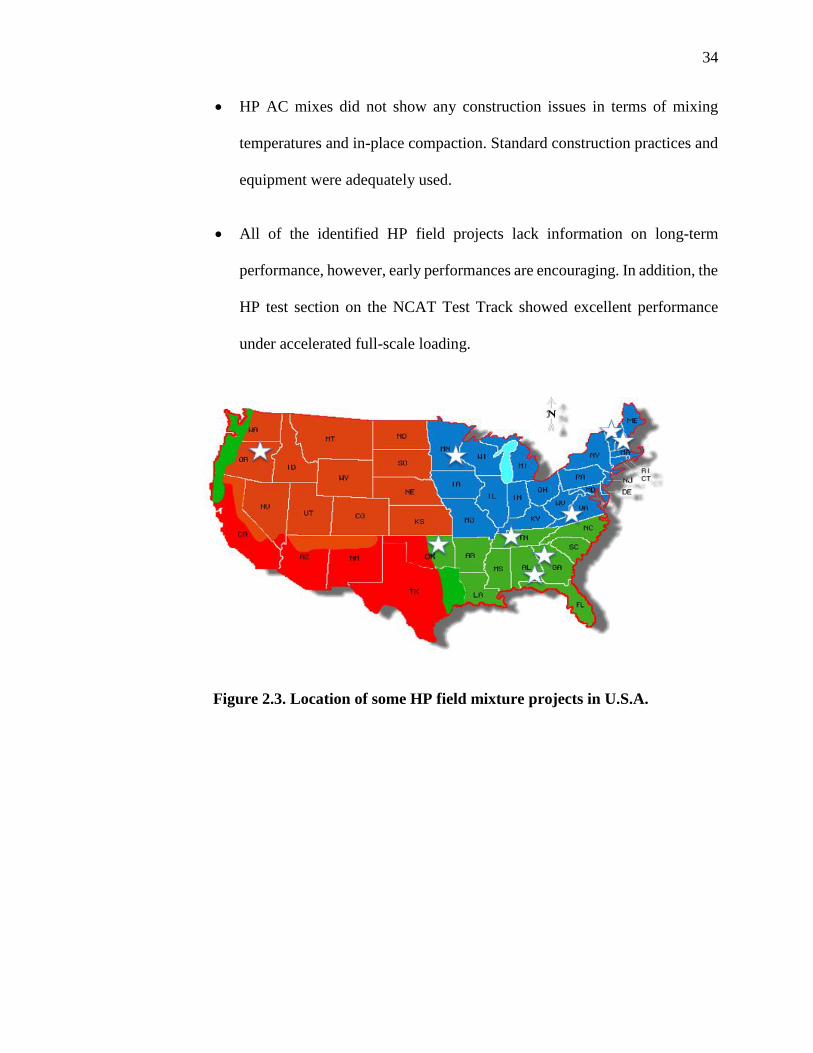
34
• HP AC mixes did not show any construction issues in terms of mixing
temperatures and in-place compaction. Standard construction practices and
equipment were adequately used.
• All of the identified HP field projects lack information on long-term
performance, however, early performances are encouraging. In addition, the
HP test section on the NCAT Test Track showed excellent performance
under accelerated full-scale loading.
Figure 2.3. Location of some HP field mixture projects in U.S.A.

35
Table 2.2. Summary of Key Findings from Field Projects with HP AC Mixes.
Location Project Description Key Findings
Brazil, 2011 (Smith,
2012)
- Mill and AC overlay on highway PR-092
- Traffic up to 4,200 heavy agricultural
trucks per day
- Good early performance
- Additional HP projects were constructed
on Dutra road which runs between Sao
Paulo and Rio de Janeiro
USA/ Advanced
Material Services
LLC, 2013
(Kuennen, 2015)
- Designing for Corvette Museum Race
Track in Bowling Green Nashville
- Raveling and bleeding are the main
concerns
- Evotherm WMA additive was used to
improve workability
- A potentially high performance AC mix
was delivered for the race track by using HP
asphalt binder
USA / City of
Bloomington, MN,
2012 (Fournier,
2013)
- Mill and AC overlay on Normandale
Road, City of Bloomington
- Subjected to heavy traffic due to its
location adjacent to the airport
- Two projects were constructed:
Normandale Service Road at 84th Street
and West 98th Street
- HP AC mix performed well and
constituted a good way to place more cost-
effective and durable asphalt pavements
with reduced thicknesses.
- HP AC mix offered possibility of building
pavement section on top of weak base and
subgrade layers
USA / Georgia DOT,
2010 (Fournier,
2010)
- Thin AC overlay at junction of Routes
138 and 155
- Pavement rutting and shoving were the
main concerns
- HP AC mix was observed to have similar
workability as regular PMA mix based on
general observations reported from the job
site
USA/NCAT Test
Track, 2009 (Timm
et al., 2012)
- HP test section designed with an AC layer
thickness 18% less than the AC layer
thickness of the PMA section
- HP section experienced lower rutting under
the entire loading cycle of 8.9 million
ESALs
- Both HP and PMA sections did not
experience any fatigue cracking under the
entire loading cycle of 8.9 million ESALs
USA / NHDOT and
VTDOT, 2014
(Mogawer et al.,
2014)
- New Hampshire project on Route 202,
AC overlay over existing AC pavement in
bad conditions without pre-treatment
- Vermont project on US-7, AC overlay
over existing AC pavement in bad
conditions with some pre-treatment
- Minimal reflective cracking on the New
Hampshire section containing RAP material
- No signs of environmental related cracking
and no evidence of rutting were observed
after 2 years of service
USA / Oklahoma
DOT, 2012
(Kuennen, 2012)
- Mill and overlay on I-40 west of
Oklahoma city
- HP AC mix had a low enough viscosity
making it workable and compactable when
used in the field
USA / Oregon DOT,
2012 (Fournier,
2012)
- Thin overlay mix on I-5 in Oregon
- Existing AC pavement had some wearing
ruts and raveling due to heavy trucks and
high traffic volumes
- No special plant adjustments were made to
accommodate the production of HP AC mix.
- No problems with viscosity were faced
during the paving of the HP mix
2.5 Preliminary Analysis of Structural Layer Coefficient for HP Asphalt Mixtures
Based on Existing Studies
Many factors may affect the determination of structural layer coefficients for new
asphalt mixtures that were not used at the AASHO Road Test (e.g. recycled material, PMA
and AC mixes). These factors include engineering properties, layer thickness, underlying

36
support, position in the pavement structure and stress state (Timm et al., 2009). The
objective of this section is to illustrate different potential approaches for the recalibration
of the structural layer coefficient of HP AC mixes using published data collected during
the NCAT study ‘Field and Laboratory Study of High-Polymer Mixtures at the NCAT Test
Track (Timm et al. 2012)’, and the NHDOT study ‘NHDOT Highways for Life Project:
2011 Auburn-Candia Resurfacing (AASHTO T321, 2014)’. It should be mentioned that no
efforts have been reported in both studies (Timm et al., 2012 & Mogawer, 2014) to
determine a structural coefficient for HP AC mixes to be used in pavement design of new
and rehabilitated flexible pavements. The following four approaches were explored in this
paper and a preliminary structural coefficient for HP AC mixes was determined
accordingly based on the engineering and performance properties reported in both studies
(Timm et al. 2012, & Mogawer, 2014):
• Approach 1: consists of using the fixed service life concept based on
measured rutting performance.
• Approach 2: consists of using the collected falling weight deflectometer
(FWD) data, method of equivalent thickness (MET) and estimation of
effective structural number (SNeff).
• Approach 3: consists of using the AASHTO 1993 Guide equation and
associated loss in serviceability index.
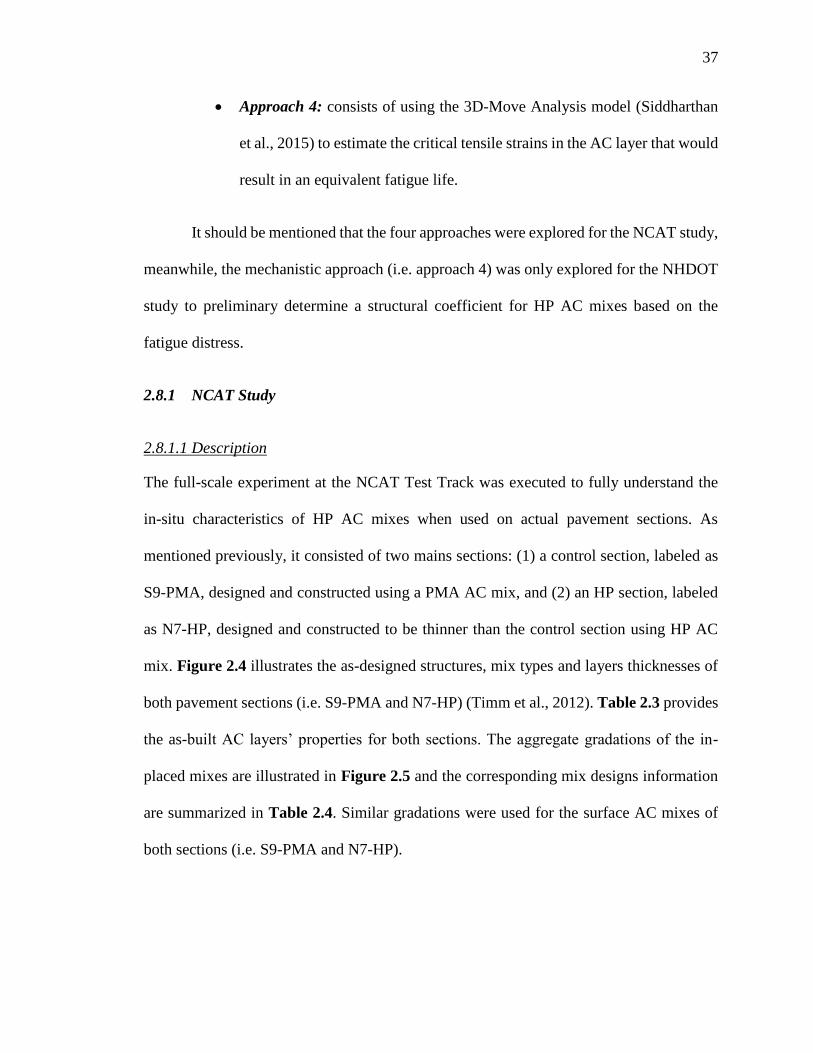
37
• Approach 4: consists of using the 3D-Move Analysis model (Siddharthan
et al., 2015) to estimate the critical tensile strains in the AC layer that would
result in an equivalent fatigue life.
It should be mentioned that the four approaches were explored for the NCAT study,
meanwhile, the mechanistic approach (i.e. approach 4) was only explored for the NHDOT
study to preliminary determine a structural coefficient for HP AC mixes based on the
fatigue distress.
2.8.1 NCAT Study
2.8.1.1 Description
The full-scale experiment at the NCAT Test Track was executed to fully understand the
in-situ characteristics of HP AC mixes when used on actual pavement sections. As
mentioned previously, it consisted of two mains sections: (1) a control section, labeled as
S9-PMA, designed and constructed using a PMA AC mix, and (2) an HP section, labeled
as N7-HP, designed and constructed to be thinner than the control section using HP AC
mix. Figure 2.4 illustrates the as-designed structures, mix types and layers thicknesses of
both pavement sections (i.e. S9-PMA and N7-HP) (Timm et al., 2012). Table 2.3 provides
the as-built AC layers’ properties for both sections. The aggregate gradations of the in-
placed mixes are illustrated in Figure 2.5 and the corresponding mix designs information
are summarized in Table 2.4. Similar gradations were used for the surface AC mixes of
both sections (i.e. S9-PMA and N7-HP).

38
These gradations were observed to be significantly finer when compared with the
aggregate gradation of the intermediate and base AC mixes. The PMA/HP intermediate
and HP base aggregate gradations were observed to be similar and slightly coarser than the
PMA base aggregate gradation. For both sections, the subgrade was classified as an
AASHTO A-4 metamorphic quartzite soil and compacted to target density and moisture
content. Direct measurements for the pavement structure responses to traffic loads were
made using strain gauges and pressure cells embedded at different locations and depths
within the pavement structure layers.
Figure 2.4. NCAT test track S9-PMA and N7-HP cross-sections design: materials
and layers thicknesses.

39
Table 2.3. As-Built AC Layers Properties.
Lift Surface Intermediate Base
Section S9-PMA N7-HP S9-PMA N7-HP S9-PMA N7-HP
Thickness, inch (mm) 1.2 (30) 1.0 (25) 2.8 (71) 2.1(53) 3.0 (76) 2.5 (64)
NMAS, inch (mm) 0.375 (9.5) 0.375
(9.5)
0.75
(19.0)
0.75
(19.0) 0.75 (19.0)
0.75
(19.0)
% polymer - SBS 2.8 7.5 2.8 7.5 0.0 7.5
Performance Grade 76-22 88-22 76-22 88-22 67-22 88-22
True PG Grade 81.7-24.7 93.5-26.4 78.6-25.5 93.5-26.4 69.5-26.0 93.5-26.4
Asphalt, % 6.1 6.3 4.4 4.6 4.7 4.6
Air voids, % 6.9 6.3 7.2 7.3 7.4 7.2
Plant Temperature,
°F (°C)
335
(168)
345
(174)
335
(168)
345
(174)
325
(163)
340
(171)
Paver Temperature,
°F (°C)
275
(135)
307
(153)
316
(158)
286
(141)
254
(123)
255
(124)
Compaction
Temperature, °F (°C)
264
(129)
297
(147)
273
(134)
247
(119)
243
(117)
240
(116)
Figure 2.5. Aggregate gradations of PMA and HP mixes – NCAT test Track.
25
.0 m
m1
inch
19
.0 m
m3
/4 i
nch
12
.5 m
m1
/2 i
nch
9.5
mm
3/8
inch
4.7
5 m
mN
o. 4
2.3
6 m
mN
o. 8
2.0
0 m
mN
o. 1
0
1.1
8 m
mN
o. 1
6
0.4
25
mm
No
. 4
00
.30
0 m
mN
o. 5
0
0.1
50
mm
No
. 1
00
0.0
75
mm
No
. 2
00
0.6
00
mm
No
. 3
0
0
10
20
30
40
50
60
70
80
90
100
Per
cen
t P
ass
ing
Sieve Size (0.45 Power)
PMA-Surface
HP-Surface
PMA/HP -
Intermediate

40
Table 2.4. Summary of NCAT PMA and HP Mixes (Surface, Intermediate, and Base
Lifts) Mix Designs.
Mix Type PMA HP
Lift ID Surface Intermediate Base Surface Intermediate
& Base
Asphalt PG Grade 76-22 76-22 67-22 88-22 88-22
% SBS Polymer 2.8 2.8 0.0 7.5 7.5
Design Air Voids, % 4.0 4.0 4.0 4.0 4.0
Optimum Binder Content
(by total weight of mix), % 5.8 4.7 4.6 5.9 4.6
Effective Binder (Pbe), % 5.1 4.1 4.1 5.3 4.2
Dust Proportion, DP 1.1 0.9 1.1 1.1 0.9
Maximum Specific
Gravity, Gmm 2.483 2.575 2.574 2.474 2.570
Voids in Mineral
Aggregate (VMA), % 15.8 13.9 13.9 16.2 14.0
Voids Filled with Asphalt
(VFA), % 75.0 71.0 71.0 75.0 72.0
2.8.1.2 Approach 1: Determination of aHP-AC Based on Measured Rutting Performance
As of June 27, 2011, approximately 8.9 million ESALs had been applied to test sections
N7-HP and S9-PMA. At that time, there was no cracking evident on either of the sections.
Weekly measurements of rut depths were collected and plotted (Refer to Figure 2.6).
Both sections showed rut depth values lower than 0.25 inch (6.4 mm) after 8.9
million ESALs indicating a high resistance to rutting. Referring to Figure 2.6, similar
rutting performance was observed on both sections up to an applied traffic of 3.5 million
ESALs. Based on the observed rutting performance of the AC layers, the structural
coefficient of the HP modified asphalt mix can be determined using the fixed service life
approach recommended in this paper/chapter. At the equivalent rutting performance of
approximately 0.12 inch (3 mm) after 3.5 million ESALs, the 5.75 inch (146 mm) AC layer
thickness for the HP pavement can be considered sufficient to achieve the same service life
as the corresponding 7.00 inch (178 mm) AC layer thickness for the PMA pavement. The

41
structural coefficient for the HP mix is then calculated as the ratio of the AC layer thickness
of the PMA pavement to the AC layer thickness of the HP pavement times 0.44, which is
the assumed structural layer coefficient for a typical PMA mix (Equation presented in
Figure 2.7). Accordingly, a structural coefficient of 0.54 is estimated for the HP mix based
on the equivalent rutting performance after a traffic loading of 3.5 million ESALs.
Figure 2.6. Rut depths measured at various levels of applied ESALs (Revised from
Timm et al., 2012).
𝑎𝐻𝑃−𝐴𝐶−𝑅𝑢𝑡 = (𝐴𝐶 𝑙𝑎𝑦𝑒𝑟 𝑡ℎ𝑖𝑐𝑘𝑛𝑒𝑠𝑠 𝑜𝑓 𝑃𝑀𝐴 𝑝𝑎𝑣𝑒𝑚𝑒𝑛𝑡 𝑓𝑜𝑟 𝑟𝑢𝑡𝑡𝑖𝑛𝑔 𝑖𝑛 𝐴𝐶
𝐴𝐶 𝑙𝑎𝑦𝑒𝑟 𝑡ℎ𝑖𝑐𝑘𝑛𝑒𝑠𝑠 𝑜𝑓 𝐻𝑃 𝑝𝑎𝑣𝑒𝑚𝑒𝑛𝑡 𝑓𝑜𝑟 𝑠𝑎𝑚𝑒 𝑟𝑢𝑡𝑡𝑖𝑛𝑔 𝑖𝑛 𝐴𝐶) ∗ 0.44
Figure 2.7. Equation. HP structural coefficient function of PMA and HP layer
thicknesses.

42
2.8.1.3 Approach 2: Determination of aHP-AC Based on FWD Data
FWD testing of S9-PMA and N7-HP Sections started in August 2009. The testing
was performed three times per month (on Mondays) for the S9-PMA section and on
alternating Mondays for the N7-HP section. Four different loads were applied three times
at each testing location at: 6000, 9000, 12,000 and 16,000 lb (2727, 4090, 5455 and 7273
kg) (Timm et al., 2012). In-situ pavement temperatures were recorded for each section
during FWD testing. The analysis of the FWD data, executed by NCAT researchers,
showed backcalculated moduli of 921,000 psi (6350 MPa), 2200 psi (15 MPa) and 27,800
psi (192 MPa) for the PMA AC, base and subgrade layers, respectively (Timm et al., 2012).
As recommended by the AASHTO 1993 Guide (AASHTO Guide, 1993), the
effective structural number (SNeff) can be calculated from the total thickness of the
pavement cross section above the subgrade and its effective modulus as expressed in the
equation in Figure 2.8. In addition, the MET is used to convert the top layers (i.e. AC and
base layers) into a half space with a subgrade modulus of Mr using the equation illustrated
in Figure 2.9. An equivalent layer thickness of 25.1 inch (637 mm) was calculated for the
PMA section. An effective modulus of the pavement cross section of 199,140 psi (1373
MPa) was then calculated using the equation presented in Figure 2.9 where D is equal to
the summation of the thickness of both the PMA AC and base layers (i.e. 13 inch).
Accordingly, an effective structural number of the PMA section was obtained using the
equation in Figure 2.8 (i.e. SNeff-PMA = 3.42). Therefore, the structural coefficient of the
PMA AC layer is calculated using the equation in Figure 2.9 and a value of 0.37 was
determined (i.e. aPMA-AC = 0.37).
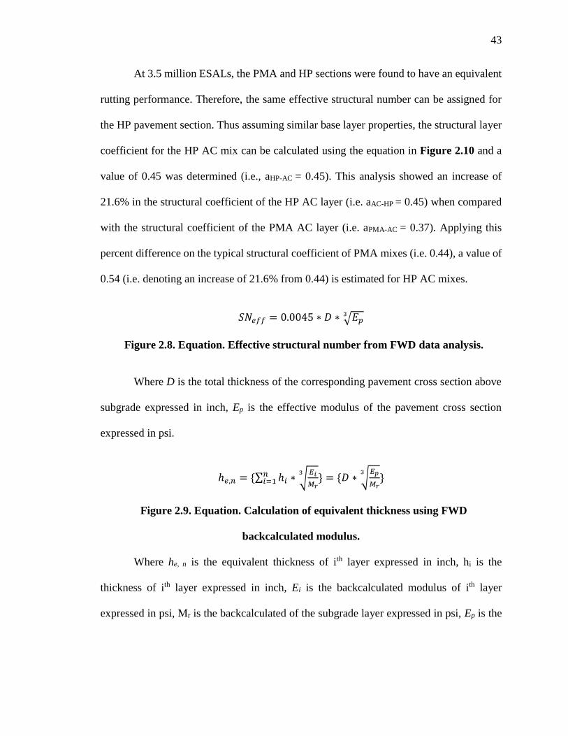
43
At 3.5 million ESALs, the PMA and HP sections were found to have an equivalent
rutting performance. Therefore, the same effective structural number can be assigned for
the HP pavement section. Thus assuming similar base layer properties, the structural layer
coefficient for the HP AC mix can be calculated using the equation in Figure 2.10 and a
value of 0.45 was determined (i.e., aHP-AC = 0.45). This analysis showed an increase of
21.6% in the structural coefficient of the HP AC layer (i.e. aAC-HP = 0.45) when compared
with the structural coefficient of the PMA AC layer (i.e. aPMA-AC = 0.37). Applying this
percent difference on the typical structural coefficient of PMA mixes (i.e. 0.44), a value of
0.54 (i.e. denoting an increase of 21.6% from 0.44) is estimated for HP AC mixes.
𝑆𝑁𝑒𝑓𝑓 = 0.0045 ∗ 𝐷 ∗ √𝐸𝑝3
Figure 2.8. Equation. Effective structural number from FWD data analysis.
Where D is the total thickness of the corresponding pavement cross section above
subgrade expressed in inch, Ep is the effective modulus of the pavement cross section
expressed in psi.
ℎ𝑒,𝑛 = {∑ ℎ𝑖 ∗ √𝐸𝑖
𝑀𝑟
3} = {𝐷 ∗ √
𝐸𝑝
𝑀𝑟
3}𝑛
𝑖=1
Figure 2.9. Equation. Calculation of equivalent thickness using FWD
backcalculated modulus.
Where he, n is the equivalent thickness of ith layer expressed in inch, hi is the
thickness of ith layer expressed in inch, Ei is the backcalculated modulus of ith layer
expressed in psi, Mr is the backcalculated of the subgrade layer expressed in psi, Ep is the

44
effective modulus of the pavement cross section expressed in psi, and D is the total
thickness of the pavement cross section in inch.
𝑆𝑁 = ∑ 𝑎𝑖𝐷𝑖𝑚𝑖𝑖=1
Figure 2.10. Equation. AASHTO 1993 equation for total structural number of a
flexible pavement structural for a given design traffic.
In this equation, SN stands for the total structural number required for a given
design traffic; ai is the structural coefficient for the ith layer; Di is the thickness of the ith
layer expressed in inch; and mi is the drainage coefficient for the ith layer except for the AC
layer.
2.8.1.4 Approach 3: Determination of aHP-AC Based on Loss in Serviceability
The PSI concept was developed during the AASHTO Road Test experiment to relate the
ride conditions of the road with the opinion of the user. The original PSI equation has been
modified throughout the years by State highway agencies to better describe local
conditions. The equation illustrated in Figure 2.11 shows the PSI equation for flexible
pavements (Sebaaly et al., 2003). It should be mentioned that there was no cracking (C)
and patching (P) reported on either of the sections after 8.9 million ESALs. Therefore, C
and P values in the equation of Figure 2.11 were considered equal to zero.
𝑃𝑆𝐼 = 5 ∗ 𝑒(−0.0041∗𝐼𝑅𝐼) − 1.38 ∗ 𝑅𝐷2 − 0.03 ∗ (𝐶 + 𝑃)0.5
Figure 2.11. Equation. PSI calculation based on IRI, rut depth, cracking, and
patching.

45
In this equation, PSI is the present serviceability index, IRI is the international
roughness index expressed in inch/mile, RD is the rut depth expressed in inch, C is the
cracking expressed ft2/1000ft2, and P is the patching expressed in ft2/1000ft2.
After 8.9 million ESAL, an average terminal serviceability value of 3.1 and 3.9 for
the PMA and HP pavement sections, respectively (pt-PMA = 3.1 and pt-HP = 3.9), were
estimated based on the IRI and rut depth data collected throughout the experiment.
Considering an initial serviceability of 4.2 (pi = 4.2) for both sections, the change in PSI
was found to be 1.1 and 0.3, respectively. A 50% reliability is considered for this analysis
because high reliabilities are used to artificially increase the predicted traffic to account for
uncertainty in the design process. Therefore, a normal deviate of zero value is then selected.
Solving for all input parameters in the AASHTO equation (i.e. equation in Figure 2.12),
the structural number of the PMA and HP pavement sections (SNPMA-AC and SNHP-AC) was
found to be 4.1 and 4.3, respectively. It should be mentioned that one-third of the
backcalculated moduli value of the subgrade layer was considered following the
recommendations from the AASHTO 1993 Guide procedure (AASHTO Guide, 1993).
Therefore, the corresponding structural coefficients of PMA and HP AC mixes were
calculate using the equation presented in and resulted in values of aPMA-AC = 0.46 and aHP-
AC = 0.60. This analysis showed an increase of 29.2% in the structural layer coefficient for
the HP AC layer when compared with the structural coefficient of the PMA AC layer.
Applying this percent difference on the recommended typical structural coefficient of PMA
mixes, a value of 0.57 can then be assumed for HP AC mixes (i.e. aHP-AC= 0.57).

46
log (𝑊18) = 𝑍𝑅𝑆0 + 9.36 ∗ log(𝑆𝑁 + 1) − 0.20 +log[
𝛥𝑃𝑆𝐼
4.2−1.5]
0.4+1,094
(𝑆𝑁+1)5.19
+ 2.32 ∗ 𝑙𝑜𝑔𝑀𝑅 − 8.07
Figure 2.12. Equation. AASHTO 1993 equation for designing flexible pavements.
In this equation, W18 is the applied traffic in terms of number of ESALs; MR is the
resilient modulus of the layer being protected expressed in psi; ZR is the normal deviation
associated with the design reliability R and variability S0; ΔPSI is the loss in present
serviceability index; and SN is the structural number required to protect a given layer
characterized with the corresponding MR value.
2.8.1.5 Approach 4: Determination of aHP-AC Based on Equivalent Distress Life using 3D-
Move Analysis
Field mixed laboratory compacted specimens of PMA and HP mixes were prepared and
evaluated in terms of their resistance to fatigue cracking at a temperature of 68°F (20°C)
using the flexural beam fatigue test in accordance with AASHTO T321 (Mogawer et al.,
2014). Figure 2.13 illustrates the fatigue relationships for PMA and HP AC mixes using
the power model as expressed in the equations presented in Figure 2.14 and Figure 2.15,
respectively. The following observations can be made:
• The HP AC mix showed significantly higher number of loading cycles to
failure when compared with the PMA AC mix.
• At a flexural strain level of 400 micro-strain (expected strain level at bottom
of AC), the average fatigue life of the HP AC mix was observed to be
approximately 33 times higher than the fatigue life of the PMA AC mix at
a temperature of 68° (20°C) (Timm and Peters-Davis, 2009).
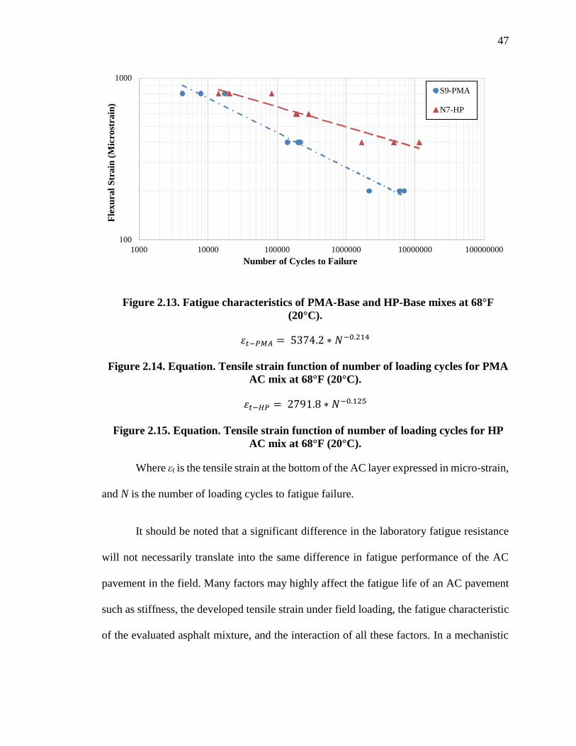
47
Figure 2.13. Fatigue characteristics of PMA-Base and HP-Base mixes at 68°F
(20°C).
휀𝑡−𝑃𝑀𝐴 = 5374.2 ∗ 𝑁−0.214
Figure 2.14. Equation. Tensile strain function of number of loading cycles for PMA
AC mix at 68°F (20°C).
휀𝑡−𝐻𝑃 = 2791.8 ∗ 𝑁−0.125
Figure 2.15. Equation. Tensile strain function of number of loading cycles for HP
AC mix at 68°F (20°C).
Where εt is the tensile strain at the bottom of the AC layer expressed in micro-strain,
and N is the number of loading cycles to fatigue failure.
It should be noted that a significant difference in the laboratory fatigue resistance
will not necessarily translate into the same difference in fatigue performance of the AC
pavement in the field. Many factors may highly affect the fatigue life of an AC pavement
such as stiffness, the developed tensile strain under field loading, the fatigue characteristic
of the evaluated asphalt mixture, and the interaction of all these factors. In a mechanistic
100
1000
1000 10000 100000 1000000 10000000 100000000
Fle
xu
ral
Str
ain
(M
icro
stra
in)
Number of Cycles to Failure
S9-PMA
N7-HP
48
pavement analysis, an AC layer with higher stiffness and lower laboratory fatigue life (in
a strain-controlled mode of loading) may experience lower tensile strain under field loading
and result in a longer pavement fatigue life. Therefore, a full mechanistic analysis would
be necessary to effectively evaluate the impact of HP binder on the fatigue performance of
the corresponding AC pavement.
Following the fixed service life approach for fatigue cracking recommended in this
paper, the required AC layer thickness for the HP pavement will be determined to achieve
the same service life in terms of a number of fatigue cycles to failure of the PMA pavement
section. For that, the 3D-Move software was used and two analyses were conducted: static
(i.e. stationary load), and dynamic (i.e. moving load). The 3D-Move analytical model
adopted here to undertake the pavement response computations uses a continuum-based
finite-layer approach. The 3D-Move analysis model can account for important pavement
response factors such as complex 3D contact stress distributions (normal and shear) of any
shape, vehicle speed and viscoelastic material characterisation for the AC layers. This
approach treats each pavement layer as a continuum and uses the Fourier transform
technique. Since rate-dependent material properties (viscoelastic) can be accommodated
by the approach, it is an ideal tool to model the behaviour of the AC layer and to study
pavement responses as a function of vehicle speed. Frequency-domain solutions are
adopted in 3D-Move Analysis, which enables the direct use of the frequency sweep test
data of AC mixture in the analysis. More information can be found in the literature
(Siddharthan et al., 2015).

49
2.8.1.5.1 Input Parameters and Definition of Critical Points
A single axle dual tire was explored in this paper and considered as traffic loading
on both sections (i.e. PMA and HP AC section) for both static and dynamic analyses. For
the dynamic analysis, a speed of 8, 15 and 60 mph (13, 24 and 97 km/h) was considered to
simulate the slow, intermediate and high speed of the loading trucks at the NCAT track,
respectively. Table 2.5 summarizes the input values for the applied traffic. Table 2.6 and
Table 2.7 summaries all the properties for the AC, base and subgrade layers from the PMA
and HP sections, respectively. Table 2.8 and Table 2.9 summaries the dynamic modulus
of the PMA and HP AC mixes, respectively. The RTFO properties for the PMA and HP
asphalt binders are summarized in Table 2.10 and Table 2.11, respectively. Figure 2.16
illustrates the PMA pavement section and the points of interest at the bottom of the PMA
AC layer (i.e. P1, P2, P3, P4, P5 and P6). It should be mentioned that the input information
were taken from the NCAT study, however, the mechanistic analysis, further discussion
and conclusions were explored in this effort.
Table 2.5. Characteristics of Applied Traffic Load.
Single Axle Dual Tires
Axle Load, lb (kN) 18,000 (80)
Tire Pressure, psi (kPa) 120 (827)
Dual Tires Spacing, inch (mm) 14 (356)
Tire Load, lb (kN) 4,500 (20)

50
Table 2.6. Summary of Input Properties for S9-PMA Test Section.
Pavement Layer Backcalculated Modulus Thickness, inch
(mm) Characterization
PMA Asphalt
Concrete
Static: 686,200 psi (4,731 MPa)
Dynamic: Dynamic Modulus of
PMA mix (Refer to Table 8)
7 (178) Linear Elastic /
Viscoelastic
Aggregate Base E = 2,200 psi (15 MPa) 6 (150) Linear Elastic
Subgrade E = 27,800 psi (192 MPa) Infinite Linear Elastic
Table 2.7. Summary of Input Properties for N7-HP Test Section.
Pavement Layer Backcalculated Modulus Thickness, inch Characterization
HP Asphalt
Concrete
Static: 541,500 psi (3,734 MPa)
Dynamic: Dynamic Modulus of
HP mix (Refer to Table 9)
To be
determined
Linear Elastic /
Viscoelastic
Aggregate Base E = 3,600 psi (25 MPa) 6 (150) Linear Elastic
Subgrade E = 33,000 psi (220 MPa) Infinite Linear Elastic
Table 2.8. Dynamic Modulus Input Values for S9-PMA Test Section.
E*, psi (MPa) Frequency (Hz)
Temperature,
°F (°C) 0.1 0.5 1 5 10 25
14 (-10) 2,186,700
(15,077)
2,419,500
(16,682)
2,506,000
(17,278)
2,676,400
(18,453)
2,737,700
(18,876)
2,808,700
(19,365)
40 (4) 1,295,700
(8,934)
1,621,400
(11,179)
1,757,500
(12,118)
2,052,200
(14,149)
2,167,400
(14,944)
2,307,300
(15,908)
70 (21) 458,600
(3,162)
686,200
(4,731)
802,000
(5,530)
1,102,400
(7,601)
1,240,800
(8,555)
1,426,800
(9,837)
100 (38) 128,600
(887)
208,700
(1,439)
256,700
(1,770)
406,900
(2,805)
490,100
(3,379)
617,700
(4,259)
130 (54) 43,900
(303)
66,300
(457)
80,300
(554)
128,600
(887)
158,400
(1,092)
208,800
(1,440)
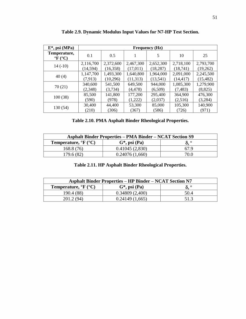
51
Table 2.9. Dynamic Modulus Input Values for N7-HP Test Section.
E*, psi (MPa) Frequency (Hz)
Temperature,
°F (°C) 0.1 0.5 1 5 10 25
14 (-10) 2,116,700
(14,594)
2,372,600
(16,358)
2,467,300
(17,011)
2,652,300
(18,287)
2,718,100
(18,741)
2,793,700
(19,262)
40 (4) 1,147,700
(7,913)
1,493,300
(10,296)
1,640,800
(11,313)
1,964,000
(13,541)
2,091,000
(14,417)
2,245,500
(15,482)
70 (21) 340,600
(2,348)
541,500
(3,734)
649,500
(4,478)
944,000
(6,509)
1,085,300
(7,483)
1,279,900
(8,825)
100 (38) 85,500
(590)
141,800
(978)
177,200
(1,222)
295,400
(2,037)
364,900
(2,516)
476,300
(3,284)
130 (54) 30,400
(210)
44,400
(306)
53,300
(367)
85,000
(586)
105,300
(726)
140,900
(971)
Table 2.10. PMA Asphalt Binder Rheological Properties.
Asphalt Binder Properties – PMA Binder – NCAT Section S9
Temperature, °F (°C) G*, psi (Pa) , °
168.8 (76) 0.41045 (2,830) 67.9
179.6 (82) 0.24076 (1,660) 70.0
Table 2.11. HP Asphalt Binder Rheological Properties.
Asphalt Binder Properties – HP Binder – NCAT Section N7
Temperature, °F (°C) G*, psi (Pa) , °
190.4 (88) 0.34809 (2,400) 50.4
201.2 (94) 0.24149 (1,665) 51.3
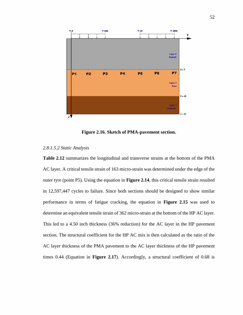
52
Figure 2.16. Sketch of PMA-pavement section.
2.8.1.5.2 Static Analysis
Table 2.12 summarizes the longitudinal and transverse strains at the bottom of the PMA
AC layer. A critical tensile strain of 163 micro-strain was determined under the edge of the
outer tyre (point P5). Using the equation in Figure 2.14, this critical tensile strain resulted
in 12,597,447 cycles to failure. Since both sections should be designed to show similar
performance in terms of fatigue cracking, the equation in Figure 2.15 was used to
determine an equivalent tensile strain of 362 micro-strain at the bottom of the HP AC layer.
This led to a 4.50 inch thickness (36% reduction) for the AC layer in the HP pavement
section. The structural coefficient for the HP AC mix is then calculated as the ratio of the
AC layer thickness of the PMA pavement to the AC layer thickness of the HP pavement
times 0.44 (Equation in Figure 2.17). Accordingly, a structural coefficient of 0.68 is
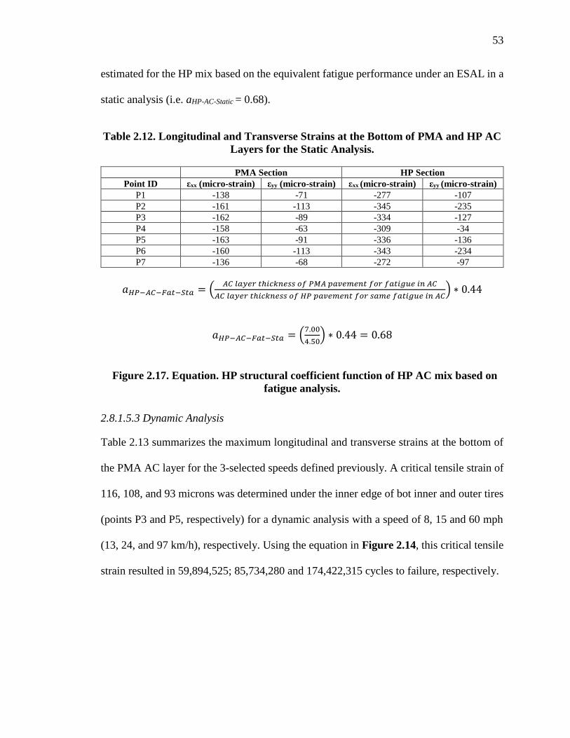
53
estimated for the HP mix based on the equivalent fatigue performance under an ESAL in a
static analysis (i.e. aHP-AC-Static = 0.68).
Table 2.12. Longitudinal and Transverse Strains at the Bottom of PMA and HP AC
Layers for the Static Analysis.
PMA Section HP Section
Point ID εxx (micro-strain) εyy (micro-strain) εxx (micro-strain) εyy (micro-strain)
P1 -138 -71 -277 -107
P2 -161 -113 -345 -235
P3 -162 -89 -334 -127
P4 -158 -63 -309 -34
P5 -163 -91 -336 -136
P6 -160 -113 -343 -234
P7 -136 -68 -272 -97
𝑎𝐻𝑃−𝐴𝐶−𝐹𝑎𝑡−𝑆𝑡𝑎 = (𝐴𝐶 𝑙𝑎𝑦𝑒𝑟 𝑡ℎ𝑖𝑐𝑘𝑛𝑒𝑠𝑠 𝑜𝑓 𝑃𝑀𝐴 𝑝𝑎𝑣𝑒𝑚𝑒𝑛𝑡 𝑓𝑜𝑟 𝑓𝑎𝑡𝑖𝑔𝑢𝑒 𝑖𝑛 𝐴𝐶
𝐴𝐶 𝑙𝑎𝑦𝑒𝑟 𝑡ℎ𝑖𝑐𝑘𝑛𝑒𝑠𝑠 𝑜𝑓 𝐻𝑃 𝑝𝑎𝑣𝑒𝑚𝑒𝑛𝑡 𝑓𝑜𝑟 𝑠𝑎𝑚𝑒 𝑓𝑎𝑡𝑖𝑔𝑢𝑒 𝑖𝑛 𝐴𝐶) ∗ 0.44
𝑎𝐻𝑃−𝐴𝐶−𝐹𝑎𝑡−𝑆𝑡𝑎 = (7.00
4.50) ∗ 0.44 = 0.68
Figure 2.17. Equation. HP structural coefficient function of HP AC mix based on
fatigue analysis.
2.8.1.5.3 Dynamic Analysis
Table 2.13 summarizes the maximum longitudinal and transverse strains at the bottom of
the PMA AC layer for the 3-selected speeds defined previously. A critical tensile strain of
116, 108, and 93 microns was determined under the inner edge of bot inner and outer tires
(points P3 and P5, respectively) for a dynamic analysis with a speed of 8, 15 and 60 mph
(13, 24, and 97 km/h), respectively. Using the equation in Figure 2.14, this critical tensile
strain resulted in 59,894,525; 85,734,280 and 174,422,315 cycles to failure, respectively.

54
Table 2.13. Longitudinal and Transverse Strains at the Bottom of PMA and HP AC
Layers for the Dynamic Analysis at the Three vehicle Speeds.
PMA Section HP Section
Speed (mph) 8
Point ID εxx (micro-strain) εyy (micro-strain) εxx (micro-strain) εyy (micro-strain)
P1 -100 -59 -223 -96
P2 -114 -90 -277 -215
P3 -116 -75 -272 -115
P4 -114 -64 -256 -73
P5 -116 -76 -275 -124
P6 -114 -89 -275 -214
P7 -100 -56 -22 -86
Speed (mph) 15
P1 -92 -54 -224 -93
P2 -106 -82 -275 -213
P3 -108 -69 -272 -111
P4 -106 -59 -250 -70
P5 -108 -71 -273 -119
P6 -106 -82 -277 -211
P7 -97 -52 -220 -83
Speed (mph) 60
P1 -80 -46 -209 -84
P2 -92 -70 -257 -192
P3 -93 -59 -248 -101
P4 -90 -50 -234 -65
P5 -93 -59 -254 -109
P6 -90 -69 -254 -191
P7 -80 -44 -205 -76
Since both sections should be designed to show a similar performance in terms of fatigue
cracking, the equation in Figure 2.15 was used to determine an equivalent tensile strain of
298, 285 and 261 microns at the bottom of the HP AC layer for the 3 speeds respectively.
This led to a 3.75 inch (95.25 mm), 3.50 inch (88.90 mm) and 3.25 inch (82.55 mm)
thickness (46%, 50% and 54% reduction, respectively) for AC layer in the HP pavement
section for a vehicle speed of 8, 15 and 60 mph (13, 24, and 97 km/h), respectively (Refer
Figure 9 and Figure 10). The structural coefficient for the HP AC mix is then calculated as
the ratio of the AC layer thickness of the PMA pavement to the AC layer thickness of the
HP pavement times 0.44 (Equation 5.9). Accordingly, a structural layer coefficient of 0.82,

55
0.88 and 0.94 is estimated for the HP mix based on the equivalent fatigue performance
under a single ESAL in a dynamic analysis at a speed of 8, 15 and 60 mph (13, 24, and 97
km/h), respectively.
Figure 2.18. Longitudinal normal strain at P5 under dynamic loading at 8 mph for
S9-PMA and N7-HP.
Figure 2.19. Longitudinal normal strain at P5 under dynamic loading at 15 mph
for S9-PMA and N7-HP.
-300
-250
-200
-150
-100
-50
0
50
100
0 0.2 0.4 0.6 0.8 1 1.2 1.4
Norm
al
Str
ain
X-X
(Mic
ro-S
tra
in)
Time (s)
S9-PMA
N7-HP
-300
-250
-200
-150
-100
-50
0
50
100
0 0.2 0.4 0.6 0.8 1 1.2 1.4
No
rma
l S
tra
in X
-X
(Mic
ro-S
train
)
Time (s)
S9-PMA
N7-HP

56
2.8.2 NHDOT Study Auburn-Candia Resurfacing Study
2.8.2.1 Description
In 2011, FHWA awarded the New Hampshire DOT (NHDOT) a $2 million grant for new
technologies as part of resurfacing NH Route 101 from Auburn to Candia. The evaluation
of HP and neat AC mixes were incorporated into this project. The experiment evaluated
the following mixtures (Mogawer, 2014):
• mix A: 0.5-inch (12.5-mm) NMAS and 35% RAP using neat PG52-34 with
Evotherm,
• mix B: 0.75-inch (19.0-mm) NMAS and 20% RAP using neat PG64-28,
and,
• mix C: 0.375-inch (9.5-mm) NMAS and no RAP using a PG70-34HP
binder with 7.5% SBS.
Figure 2.20 illustrates the aggregate gradation of the three evaluated mixtures. The
three mixtures were designed using the Superpave mix design methodology with 75 design
gyrations. The optimum asphalt binder content (OBC) for mixes A, B and C are 5.50%,
4.90% and 6.50%, respectively. The mixes were evaluated in terms of their engineering
property, and resistance to several modes of distresses (e.g. fatigue cracking). While
analyzing the data, it should be kept in mind that the HP mix (mix C), had a finer aggregate
gradation and a higher binder content when compared to the two mixes with high RAP
content (i.e. mix A and mix B).

57
Figure 2.20. Aggregate gradations of NHDOT mixes A, B, and C.
Dynamic modulus testing was performed for the three mixes (A, B and C) in accordance
with AASHTO T378 (AASHTO T378, 2013) and R84 (AASHTO R84, 2010). Mix B
exhibited the highest E* property (i.e. 2 times higher than E* of mix A), while mix C (HP)
exhibited the lowest modulus (i.e. 1.7 time lower than E* of mix A) indicating a softer
behavior of HP AC mixes under traffic loading.
The flexural beam fatigue testing was performed in accordance with AASHTO
T321 (AASHTO 321, 2014) to determine the fatigue characteristics of the three mixes.
Beams were trimmed from slabs compacted using the IPC Global Pressbox slab compactor.
In order to account for the relative locations of the various mixtures within the pavement
structure, mixes A and B were tested at strains of 250, 500 and 750 micro-strain while
higher strains of 750, 1000, 1,250 micro-strain were applied to test mix C. All tests were
conducted at a loading frequency of 10 Hz and a temperature of 59°F (15°C). The 50%
25
.0 m
m1
in
ch
19
.0 m
m3
/4 i
nch
12
.5 m
m1
/2 i
nch
9.5
mm
3/8
in
ch
4.7
5 m
mN
o. 4
2.3
6 m
mN
o. 8
2.0
0 m
mN
o. 1
0
1.1
8 m
mN
o. 1
6
0.4
25
mm
No
. 4
00
.30
0 m
mN
o. 5
0
0.1
50
mm
No
. 1
00
0.0
75
mm
No
. 2
00
0.6
00
mm
No
. 3
0
0
10
20
30
40
50
60
70
80
90
100P
erce
nt
Pass
ing
Sieve Size (0.45 Power)
High Polymer Mixture
0.5 inch (12.5 mm) + 35% RAP
0.75 inch (19.0 mm) + 20% RAP

58
reduction in initial beam stiffness (determined at cycle 50) was adopted as a failing
criterion. Figure 2.21 presents the beam fatigue results and the fatigue relationships of the
evaluated mixes are expressed in the equation presented in Figure 10, 11, and 12 for mix
A, B and C, respectively (AASHTO T321, 2014)). A considerably better fatigue
relationship was observed for the HP mix C when compared with mixes A and B. A
mechanistic analysis remains necessary to effectively evaluate the impact of HP binder on
the fatigue performance of the corresponding AC pavement.
Figure 2.21. Fatigue characteristics of mixes A, B, and C at 59°F (15°C).
휀𝑡−𝑀𝑖𝑥 𝐴 = 4,444.3 ∗ 𝑁−0.200
Figure 2.22. Equation. Tensile strain function of number of loading cycles for Mix
A at 59°F (15°C).
100
1000
10000
1,000 10,000 100,000 1,000,000 10,000,000
Fle
xu
ral
Str
ain
(M
icro
stra
in)
Number of Cycles to Failure
A: 0.5 inch (12.5 mm) + 35% RAP
B: 0.75 inch (19.0 mm) + 20% RAP
C: High Polymer Mixture

59
휀𝑡−𝑀𝑖𝑥 𝐵 = 18,681.1 ∗ 𝑁−0.285
Figure 2.23. Equation. Tensile strain function of number of loading cycles for Mix
B at 59°F (15°C).
휀𝑡−𝑀𝑖𝑥 𝐶 = 22,633.2 ∗ 𝑁−0.285
Figure 2.24. Equation. Tensile strain function of number of loading cycles for Mix
C at 59°F (15°C).
Where εt is the tensile strain at the bottom of the AC layer expressed in micro-strain,
and N is the number of loading cycles to failure.
The fourth approach, known as the mechanistic analysis approach, was explored in
here to determine a preliminary structural coefficient for HP AC mixes using the
engineering and performance characteristics reported previously by the NHDOT study.
Mix B was selected as a control mix and the service life approach in terms of fatigue
resistance was used to conduct the analysis. Because of the lack in some input information
(e.g. full master curve of the PMA and HP AC mixes, A-VTS parameters of the evaluated
asphalt binders), a static mechanistic analysis was only performed on mix B (considered
control mix) and mix C (HP).
2.8.2.2 Approach 4: Determination of aHP-AC Based on Equivalent Distress Life using 3D-
Move Analysis.
A trial pavement structure, designed in accordance with the flexible pavement design
manual of NHDOT (NHDOT, 2014), was selected to conduct the mechanistic analysis. For
mix B, the pavement structure consisted of 7.50 inch (191 mm) of AC (aAC-mix A = 0.38) on
top of a 12.00 inch (305 mm) crushed gravel (abase = 0.10) and a 12.00 inch (305 mm) of

60
gravel (asubbase = 0.07). For AC mix C, the base and subbase thickness and properties were
maintained the same, while the thickness of the AC layer was determined following the
matching fatigue performance life approach. A summary of the material properties for the
3D-Move analysis is provided in Table 2.14. A single axle dual tyre was applied as traffic
loading on the two sections (i.e. mix B and mix C) for the static 3D-Move analysis.
Table 2.15 summarises the longitudinal and transverse strains at the bottom of the
AC layer for the two evaluated sections (i.e. mix B and mix C). The same critical points
(i.e. P1, P2, P3, P4, P5, P6, and P7) selected for NCAT study are considered for the
evaluation of pavement responses (i.e. tensile strain) at the bottom of the AC layer of the
NHDOT designed section.
A critical tensile strain of 81 micro-strain was determined under the edge of the
outer tyre (point P5) for AC layer mix B. Using the equation in Figure 2.23, this critical
tensile strain resulted in 198,830,094 cycles to failure. Since the HP section (i.e. mix C)
should be designed for the same performance in terms of fatigue cracking, the equation
presented in Figure 2.24 was used to determine an equivalent tensile strain of 325 micro-
strain at the bottom of the AC layer mix C. This led to a 5.00 inch thickness (33% reduction)
for the AC layer in the HP pavement section (i.e. mix C). The structural coefficient for the
HP AC mix is then calculated as the ratio of the AC layer thickness of the PMA pavement
to the AC layer thickness of the HP pavement times 0.38. Accordingly, a structural
coefficient of 0.57 is estimated for the HP mix based on the equivalent fatigue performance
under an ESAL in a static analysis. It should be mentioned that many factors contributed
to the 33% reduction in AC layer thickness including (a) aggregate gradation (i.e. finer
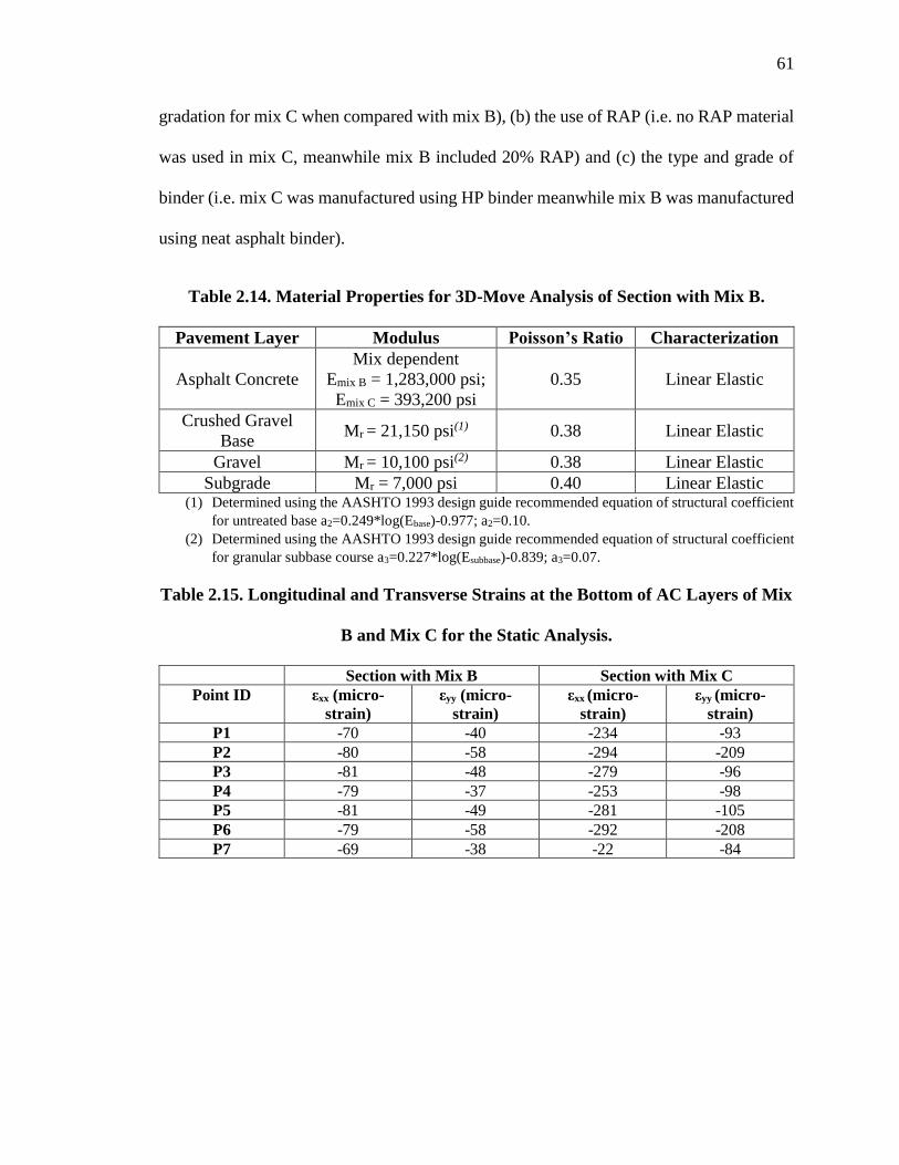
61
gradation for mix C when compared with mix B), (b) the use of RAP (i.e. no RAP material
was used in mix C, meanwhile mix B included 20% RAP) and (c) the type and grade of
binder (i.e. mix C was manufactured using HP binder meanwhile mix B was manufactured
using neat asphalt binder).
Table 2.14. Material Properties for 3D-Move Analysis of Section with Mix B.
Pavement Layer Modulus Poisson’s Ratio Characterization
Asphalt Concrete
Mix dependent
Emix B = 1,283,000 psi;
Emix C = 393,200 psi
0.35 Linear Elastic
Crushed Gravel
Base Mr = 21,150 psi(1) 0.38 Linear Elastic
Gravel Mr = 10,100 psi(2) 0.38 Linear Elastic
Subgrade Mr = 7,000 psi 0.40 Linear Elastic (1) Determined using the AASHTO 1993 design guide recommended equation of structural coefficient
for untreated base a2=0.249*log(Ebase)-0.977; a2=0.10.
(2) Determined using the AASHTO 1993 design guide recommended equation of structural coefficient
for granular subbase course a3=0.227*log(Esubbase)-0.839; a3=0.07.
Table 2.15. Longitudinal and Transverse Strains at the Bottom of AC Layers of Mix
B and Mix C for the Static Analysis.
Section with Mix B Section with Mix C
Point ID εxx (micro-
strain)
εyy (micro-
strain)
εxx (micro-
strain)
εyy (micro-
strain)
P1 -70 -40 -234 -93
P2 -80 -58 -294 -209
P3 -81 -48 -279 -96
P4 -79 -37 -253 -98
P5 -81 -49 -281 -105
P6 -79 -58 -292 -208
P7 -69 -38 -22 -84
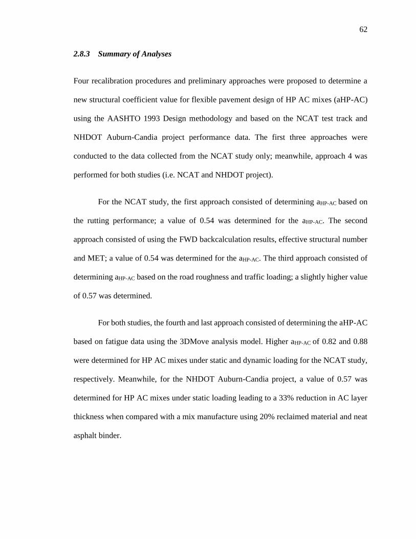
62
2.8.3 Summary of Analyses
Four recalibration procedures and preliminary approaches were proposed to determine a
new structural coefficient value for flexible pavement design of HP AC mixes (aHP-AC)
using the AASHTO 1993 Design methodology and based on the NCAT test track and
NHDOT Auburn-Candia project performance data. The first three approaches were
conducted to the data collected from the NCAT study only; meanwhile, approach 4 was
performed for both studies (i.e. NCAT and NHDOT project).
For the NCAT study, the first approach consisted of determining aHP-AC based on
the rutting performance; a value of 0.54 was determined for the aHP-AC. The second
approach consisted of using the FWD backcalculation results, effective structural number
and MET; a value of 0.54 was determined for the aHP-AC. The third approach consisted of
determining aHP-AC based on the road roughness and traffic loading; a slightly higher value
of 0.57 was determined.
For both studies, the fourth and last approach consisted of determining the aHP-AC
based on fatigue data using the 3DMove analysis model. Higher aHP-AC of 0.82 and 0.88
were determined for HP AC mixes under static and dynamic loading for the NCAT study,
respectively. Meanwhile, for the NHDOT Auburn-Candia project, a value of 0.57 was
determined for HP AC mixes under static loading leading to a 33% reduction in AC layer
thickness when compared with a mix manufacture using 20% reclaimed material and neat
asphalt binder.

63
The first three approaches for the determination of the structural coefficient of the
HP AC mix are all based on the AASHTO 1993 Guide concept with some slight variations
in the analysis. Therefore, it is reasonable to expect that similar coefficients will be
determined for the three approaches.
The fourth approach is based on the mechanistic analysis of the PMA and HP
structures and their anticipated fatigue life. This approach was investigated as part of this
effort to show that mechanistic-based layer coefficients may be different than the
empirically determined coefficients. However, the use of the available data from the NCAT
sections and NHDOT study for the mechanistic-based approach suffered from the
following limitations:
• Fatigue models for PMA and HP AC mixes were developed at a single
temperature which does not allow the incorporation of the modulus effect.
A true mechanistic analysis must incorporate the impact of AC mix
modulus on the calculation of tensile strains and the determination of the
fatigue life.
• No rutting models were developed for the PMA and HP AC mixes. The
rutting properties from the APA and FN represent the empirical behaviour
of the mixtures at a single temperature and do not incorporate the modulus
effect. A true mechanistic analysis must incorporate the impact of AC mix
modulus on the calculation of vertical strains and the determination of the
rutting life.

64
2.6 Summary of Findings and Recommendations
The objective of this literature review was to identify all currents and previous studies that
have been conducted to evaluate the performance of HP AC mixes. In this research, HP
AC mixes are defined as asphalt mixtures manufactured using asphalt binders modified
with SBS or SB polymers at the approximate rate of 7.5% by weight of the binder. The
findings of the literature review were presented with respect to the three areas of interest
that were defined in the scope of the review as (a) laboratory evaluations of HP modified
asphalt binders and mixtures, (b) performance of pavement sections constructed with HP
AC mixes and (c) techniques to determine structural coefficient of HP AC mixes.
For the evaluation of HP modified asphalt binders and mixtures in the laboratory,
the review identified several studies that evaluated the engineering properties and
performance characteristics of HP asphalt binders and mixtures. On the positive side, all
of the identified studies used the Superpave technology to evaluate the properties of the
binders and mixtures which makes the generated data highly applicable to the current
research on HP asphalt binders and mixtures. On the not so positive side, none of the
identified studies conducted a complete experimental design that can lead to the evaluation
of the performance of HP AC mixes with respect to all modes of distresses, i.e. rutting,
fatigue, thermal and reflective cracking. In addition, some of the studies did not incorporate
the evaluation of a control binder or mixture in order to clearly define the contribution of
the HP asphalt binder. Furthermore, some studies went directly into the evaluation of HP
mixtures without providing sufficient information on the properties of the HP binders used
in the manufacturing of the mixtures.

65
For the performance of HP AC mixes on the field, several projects were constructed
to evaluate the performance of HP modified asphalt mixtures as compiled in section III.
HP AC mixes have been used over a wide range of applications ranging from full depth
AC layer to thin AC overlays under heavy traffic on interstates and slow-braking loads at
intersections. HP AC mixes did not show any construction issues in terms of mixing
temperatures and in-place compaction. Standard construction practices and equipment
were adequately used. All of the identified HP field projects lack information on long-term
performance, however, early performances are encouraging. In addition, the HP test section
on the NCAT Test Track showed excellent performance under accelerated full-scale
loading. None of the available studies calculated the structural coefficient of HP AC mixes
(aHP-AC) mainly because of the unavailability of the required full performance
characterizations of the mixtures. In some cases, a hypothetical structural coefficient may
be identified as shown below:
• For the project in Brazil, the HP section replaced the standard section at a
45% reduction in the overall thickness indicating an aHP-AC that is 45%
higher than the corresponding structural coefficient for the composite
pavement (i.e. AC over cement-stabilized RAP).
• For the projects in Bloomington, MN and Oklahoma; the HP section
replaced the standard section at a 25% reduction in the thickness of the AC
layer indicating an aHP-AC that is 25% higher than the corresponding
structural coefficient for the standard AC mix.
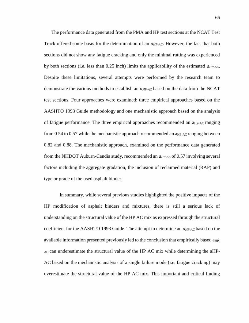
66
The performance data generated from the PMA and HP test sections at the NCAT Test
Track offered some basis for the determination of an aHP-AC. However, the fact that both
sections did not show any fatigue cracking and only the minimal rutting was experienced
by both sections (i.e. less than 0.25 inch) limits the applicability of the estimated aHP-AC.
Despite these limitations, several attempts were performed by the research team to
demonstrate the various methods to establish an aHP-AC based on the data from the NCAT
test sections. Four approaches were examined: three empirical approaches based on the
AASHTO 1993 Guide methodology and one mechanistic approach based on the analysis
of fatigue performance. The three empirical approaches recommended an aHP-AC ranging
from 0.54 to 0.57 while the mechanistic approach recommended an aHP-AC ranging between
0.82 and 0.88. The mechanistic approach, examined on the performance data generated
from the NHDOT Auburn-Candia study, recommended an aHP-AC of 0.57 involving several
factors including the aggregate gradation, the inclusion of reclaimed material (RAP) and
type or grade of the used asphalt binder.
In summary, while several previous studies highlighted the positive impacts of the
HP modification of asphalt binders and mixtures, there is still a serious lack of
understanding on the structural value of the HP AC mix as expressed through the structural
coefficient for the AASHTO 1993 Guide. The attempt to determine an aHP-AC based on the
available information presented previously led to the conclusion that empirically based aHP-
AC can underestimate the structural value of the HP AC mix while determining the aHP-
AC based on the mechanistic analysis of a single failure mode (i.e. fatigue cracking) may
overestimate the structural value of the HP AC mix. This important and critical finding

67
strongly supports the need of a full evaluation of the performance characteristics of the HP
AC mixes to determine the aHP-AC based on the mechanistic analysis of all possible critical
modes of failure. In addition, an extended asphalt binder aging experiment to assess the
long-term aging characteristics of conventional and highly modified asphalt binder in terms
of their rheological and chemical properties are needed. This experiment will need to
consider multiple combinations of PMA and HP asphalt binders from different sources.
Long-term oven aged asphalt binders at multiple temperatures and multiple durations will
need to be evaluated using the DSR for full master curve characterisation. The Fourier
Transform Infrared Spectroscopy (FT-IR) can be used for characterisation of chemical
composition (e.g. carbonyl area growth, sulfoxide area growth).
2.7 Acknowledgements (as mentioned in the paper)
The content of this study reflect the views of the authors, who are responsible for the facts
and the accuracy of the data presented herein. The contents of this manuscript do not
necessarily reflect the official views of policies of the sponsor at the time of publication.
2.8 Disclosure Statement (as mentioned in the paper)
No potential conflict of interest was reported by the author(s).
2.9 Funding (as mentioned in the paper)
The authors would like to acknowledge the Florida Department of Transportation (FDOT)
for sponsoring this research work [grant number Grant BE321].

68
2.10 ORCID (as mentioned in the paper)
Jhony Habbouche http://orcid.org/0000-0002-6216-3134, Elie Y. Hajj
http://orcid.org/0000-0001-8568-6360, and Murugaiyah Piratheepan http://orcid.org/0000-
0002-3302-4856.
2.11 References
The references will be added to the last chapter (Chapter 10) titled “References” to avoid
any possible redundancy.
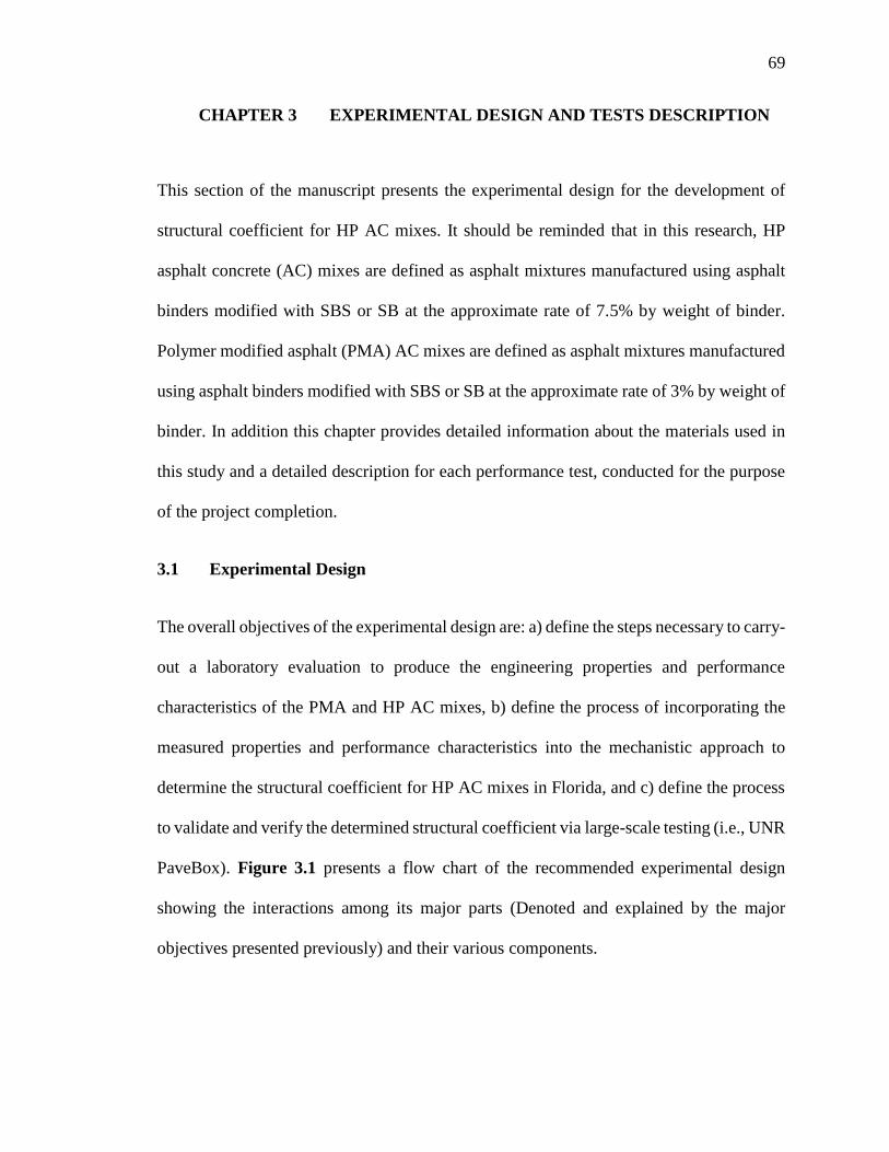
69
CHAPTER 3 EXPERIMENTAL DESIGN AND TESTS DESCRIPTION
This section of the manuscript presents the experimental design for the development of
structural coefficient for HP AC mixes. It should be reminded that in this research, HP
asphalt concrete (AC) mixes are defined as asphalt mixtures manufactured using asphalt
binders modified with SBS or SB at the approximate rate of 7.5% by weight of binder.
Polymer modified asphalt (PMA) AC mixes are defined as asphalt mixtures manufactured
using asphalt binders modified with SBS or SB at the approximate rate of 3% by weight of
binder. In addition this chapter provides detailed information about the materials used in
this study and a detailed description for each performance test, conducted for the purpose
of the project completion.
3.1 Experimental Design
The overall objectives of the experimental design are: a) define the steps necessary to carry-
out a laboratory evaluation to produce the engineering properties and performance
characteristics of the PMA and HP AC mixes, b) define the process of incorporating the
measured properties and performance characteristics into the mechanistic approach to
determine the structural coefficient for HP AC mixes in Florida, and c) define the process
to validate and verify the determined structural coefficient via large-scale testing (i.e., UNR
PaveBox). Figure 3.1 presents a flow chart of the recommended experimental design
showing the interactions among its major parts (Denoted and explained by the major
objectives presented previously) and their various components.
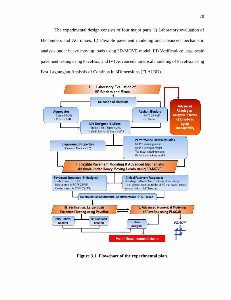
70
The experimental design consists of four major parts: I) Laboratory evaluation of
HP binders and AC mixes, II) Flexible pavement modeling and advanced mechanistic
analysis under heavy moving loads using 3D-MOVE model, III) Verification: large-scale
pavement testing using PaveBox, and IV) Advanced numerical modeling of PaveBox using
Fast Lagrangian Analysis of Continua in 3Dimensions (FLAC3D).
Figure 3.1. Flowchart of the experimental plan.

71
The objective of the laboratory evaluation (Part I) is to produce the necessary
engineering properties and performance characteristics of common PMA and HP AC mixes
used in Florida. These mixes are established following the FDOT Superpave mix design
specifications (FDOT Specifications, 2018) using two representative sources for
aggregates and asphalt binders.
The objective of the flexible pavement modeling (Part II) is to implement the
developed properties and characteristics into an advanced flexible pavement modeling
process to determine the responses and performance under various structural and loading
conditions. In addition, initial structural coefficients will be determined for the evaluated
HP AC mixes in Florida using the service life approach based on the performance life of
the PMA and HP AC pavement sections.
The objective of the full-scale pavement testing using PaveBox (Part III) is to verify
the structural coefficient developed and checked previously using a 11 feet (335.3 cm)
width by 11 feet (335.3 cm) depth by 7 feet (213.4 cm) height full-scale laboratory tool
called “PaveBox”.
The objective of the advanced numerical modeling of using FLAC3D (Part IV) is
to provide an advanced analysis of the sections built-in the PaveBox experiment using the
three-dimensional explicit finite difference program called FLAC3D.

72
3.2 Materials
This section involves the selection of the materials to be used in the fabrication of PMA
and HP AC mixes to be evaluated in the laboratory. Two sources of asphalt binders and
two sources of aggregates were recommended by the project panel as listed below:
• Asphalt binders: Ergon Asphalt and Emulsion of Jackson, MS, and Vecenergy of
Rivera Beach, FL.
• Aggregates: White Rock Quarries and Junction City Mining.
3.2.1 Asphalt Binders
Two asphalt binder Performance Grades (PG) were targeted from each source: PG76-
22PMA and HP Binder. The Ergon source was labeled as “A” and the Vecenergy source
was labeled as “B”. A total of ten 5-gallon buckets were obtained for each grade from each
source along with the corresponding anti-strip liquid agent. All four binders are modified
with SBS polymer which meets the polymer criterion of this research. The SBS contents
of the PMA binders are 3.2 and 3.0% by weight of binder for Ergon and Vecenergy,
respectively. The SBS contents of the HP binders are 7.6 and 8.0% by weight of binder for
Ergon and Vecenergy, respectively. The grade and source of the base binder and the SBS
content for each binder were provided by the suppliers (i.e., Ergon, and Vecenergy). The
SBS contents of all binders meet the criteria set forth in this research; i.e., PMA binder
approximately 3% and HP binder approximately 7.5% by weight of binder.

73
The liquid anti-strip was added in the laboratory to all sampled asphalt binders with
a dosage rate of 0.5% by weight of the binder. This process was accomplished gradually
throughout laboratory task to ensure good effectiveness of the liquid anti-strip when mixed
and stored with the asphalt binder.
Figure 3.2 summarizes the steps followed to mix and incorporate the liquid anti-
strip with the asphalt binder:
• Heat the asphalt binder sampled in 5-gallon buckets to the mixing temperature and
split it into one-gallon cans.
• Add the antistrip to the hot asphalt binder (dosage rate of 0.5% by weight of the
asphalt binder).
• Mix the anti-strip thoroughly using a mechanical stirrer so there is a moderate
visible recirculation for a minimum duration of 30 minutes. A heating membrane
was used to control the temperature and keep it as close as possible to the mixing
temperature throughout the mixing process.
• If desired, subdivide the asphalt binder into suitable portions for later use.

74
Figure 3.2. Steps followed to mix the liquid anti-strip with asphalt binder.
Table 3.1 to Table 3.4 summarize the properties of the four evaluated asphalt
binders with and without anti-strip agent. The Superpave PG system (AASHTO M320,
2014) was used to determine the continuous grades of the four binders to confirm their
PGs. All four binders met the corresponding FDOT Specifications 2018 (FDOT
Specifications, 2018) with the exception of the Ergon HP Binder without anti-strip agent
with a percent recovery of R3.2 = 89.5%, which is slightly lower than the minimum required
R3.2 of 90%. However, the same Ergon HP Binder with the anti-strip agent met the
specification with a R3.2 of 92.5%. Since all binders will be used with anti-strip agents, this
issue should not be of any concern to the research.
The measured binders’ data show a wide range in the measured properties of the
binders obtained from Ergon and Vecenergy at all levels of temperature and aging stages.
This will ensure a wide applicability of the research findings.

75
Table 3.1. Properties of the PMA Binder from Ergon Asphalt and Emulsion.
SUPERPAVE PG ASPHALT BINDER: ERGON PG76-22PMA
Test and
Method Conditions
Measurements FDOT Specification
2018
Minimum/Maximum
Value
Without Anti-
Strip Agent
With Anti-
Strip Agent
Source of base
binder
PG64-22
Exxon
PG64-22
Exxon --
Modifier Polymer SBS, 3.2% by
weight of binder
SBS, 3.2% by
weight of
binder
--
Additive Anti-Strip
Agent --
AD-here
LOF 65-00 EU,
0.5% by weight
of binder
--
Original Binder
Flash Point,
(AASHTO T48,
2006)
Cleveland
Open Cup 581°F 565°F Minimum 450°F
Rotational
Viscosity,
(AASHTO
T316, 2013)
275°F 1.553 Pa.s 1.504 Pa.s Maximum 3.000 Pa.s
Dynamic Shear
Rheometer,
(AASHTO
T315, 2012)
G*/sin 𝛿 @
76°C 1.38 kPa 1.35 kPa Minimum 1.00 kPa
Phase Angle,
𝛿 @ 76°C 65 degrees 66 degrees Maximum 75 degrees
Rolling Thin Film Oven (RTFO) Test Residues (AASHTO T240, 2013)
RTFO,
(AASHTO
T240, 2013)
Mass Change 0.17% 0.85% Maximum 1.00%
Multiple Stress
Creep Recovery
(AASHTO
M332, 2014)
Jnr, 3.2 @ 67°C 0.19 kPa-1 0.24 kPa-1 Maximum 1.00 kPa-1
Jnr,diff @ 67°C 1.6% 2.9% Maximum Jnr, diff =
75.0%
%R3.2 @ 67°C 84.1% 81.4%
%R3.2 ≥ 29.37(Jnr, 3.2)-
0.2633
≥ 45.2%
Pressure Aging Vessel Residue @ 100°C (AASHTO R28, 2012)
Dynamic Shear
Rheometer,
(AASHTO
T315, 2012)
G*sin 𝛿 @
26.5°C,
10 rad/sec
1,747 kPa 2,282 kPa Maximum 5000 kPa
Creep Stiffness,
(AASHTO
T313, 2012)
S (Stiffness)
@ -12°C, 60
sec.(a)
155.0 MPa 155.5 MPa Maximum 300.0 MPa
m-value @ -
12°C,
60 sec.(a)
0.336 0.355 Minimum 0.300
Continuous
Grade(b) -- PG76.4-24.7 PG75.7-26.5 --
(a) Testing temperature is 10°C warmer than the actual low PG.
(b) Continuous grade (AASHTO M320, 2014).

76
Table 3.2. Properties of the HP Binder from Ergon Asphalt and Emulsion.
SUPERPAVE PG ASPHALT BINDER: ERGON HP Binder
Test and
Method Conditions
Measurements FDOT Specification
2018
Minimum/Maximum
Value
Without Anti-
Strip Agent
With Anti-
Strip Agent
Source of base
binder --
PG52-28
Exxon/Imperial
PG52-28
Exxon/Imperial --
Modifier Polymer SBS, 7.6% by
weight of binder
SBS, 7.6% by
weight of
binder
--
Additive Anti-Strip
Agent --
AD-here
LOF 65-00 EU,
0.5% by weight
of binder
--
Original Binder
Flash Point,
(AASHTO T48,
2006)
Cleveland
Open Cup 536°F 549°F Minimum 450°F
Rotational
Viscosity,
(AASHTO T
316, 2013)
275°F 3.395 Pa.s 3.450 Pa.s Maximum 3.000 Pa.s(a)
Dynamic Shear
Rheometer,
(AASHTO
T315, 2012)
G*/sin 𝛿 @
76°C 4.62 kPa 4.53 kPa Minimum 1.00 kPa
Phase Angle,
𝛿 @ 76°C 47 degrees 49 degrees Maximum 65 degrees
Rolling Thin Film Oven (RTFO) Test Residues (AASHTO T240, 2013)
RTFO,
(AASHTO
T240, 2013)
Mass Change 0.28% 0.34% Maximum 1.00 %
Multiple Stress
Creep Recovery
(AASHTO
M332, 2014)
Jnr, 3.2 @ 76°C 0.08 kPa-1 0.06 kPa-1 Maximum 0.10 kPa-1
Jnr,diff @ 76°C 37.3 % 19.9 % --
%R3.2 @ 76°C 89.5 % 92.5 % %R3.2 ≥ 90.0 %
Pressure Aging Vessel Residue @ 100°C (AASHTO R28, 2012)
Dynamic Shear
Rheometer,
(AASHTO
T315, 2012)
G*sin 𝛿 @
26.5°C,
10 rad/sec
636 kPa 791 kPa Maximum 5000 kPa
Creep Stiffness,
(AASHTO
T313, 2012)
S (Stiffness)
@ -12°C, 60
sec.(b)
52.0 MPa 49.0 MPa Maximum 300 MPa
m-value @ -
12°C,
60 sec.(b)
0.413 0.418 Minimum 0.300
Continuous
Grade(c) -- PG93.5-33.5 PG93.5-34.6 --
(a) Binders with values higher than 3 Pa.s should be used with caution and only after consulting with the supplier
as to any special handling procedures, including pumping capabilities (FDOT Specifications, 2018).
(b) Testing temperature is 10°C warmer than the actual low PG.
(c) Continuous grade (AASHTO M320, 2014).
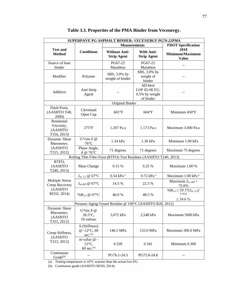
77
Table 3.3. Properties of the PMA Binder from Vecenergy.
SUPERPAVE PG ASPHALT BINDER: VECENERGY PG76-22PMA
Test and
Method Conditions
Measurements FDOT Specification
2018
Minimum/Maximum
Value
Without Anti-
Strip Agent
With Anti-
Strip Agent
Source of base
binder
PG67-22
Marathon
PG67-22
Marathon --
Modifier Polymer SBS, 3.0% by
weight of binder
SBS, 3.0% by
weight of
binder
--
Additive Anti-Strip
Agent --
AD-here
LOF 65-00 EU,
0.5% by weight
of binder
--
Original Binder
Flash Point,
(AASHTO T48,
2006)
Cleveland
Open Cup 601°F 604°F Minimum 450°F
Rotational
Viscosity,
(AASHTO
T316, 2013)
275°F 1.207 Pa.s 1.173 Pa.s Maximum 3.000 Pa.s
Dynamic Shear
Rheometer,
(AASHTO
T315, 2012)
G*/sin 𝛿 @
76°C 1.34 kPa 1.30 kPa Minimum 1.00 kPa
Phase Angle,
𝛿 @ 76°C 71 degrees 71 degrees Maximum 75 degrees
Rolling Thin Film Oven (RTFO) Test Residues (AASHTO T240, 2013)
RTFO,
(AASHTO
T240, 2013)
Mass Change 0.15 % 0.25 % Maximum 1.00 %
Multiple Stress
Creep Recovery
(AASHTO
M332, 2014)
Jnr, 3.2 @ 67°C 0.54 kPa-1 0.72 kPa-1 Maximum 1.00 kPa-1
Jnr,diff @ 67°C 14.5 % 22.3 % Maximum Jnr, diff =
75.0%
%R3.2 @ 67°C 46.0 % 48.5 %
%R3.2 ≥ 29.37(Jnr, 3.2)-
0.2633
≥ 34.6 %
Pressure Aging Vessel Residue @ 100°C (AASHTO R28, 2012)
Dynamic Shear
Rheometer,
(AASHTO
T315, 2012)
G*sin 𝛿 @
26.5°C,
10 rad/sec
3,072 kPa 2,548 kPa Maximum 5000 kPa
Creep Stiffness,
(AASHTO
T313, 2012)
S (Stiffness)
@ -12°C, 60
sec.(a)
146.5 MPa 155.0 MPa Maximum 300.0 MPa
m-value @ -
12°C,
60 sec.(a)
0.339 0.341 Minimum 0.300
Continuous
Grade(b) -- PG76.1-24.3 PG75.8-24.6 --
(a) Testing temperature is 10°C warmer than the actual low PG.
(b) Continuous grade (AASHTO M320, 2014).

78
Table 3.4. Properties of the HP Binder from Vecenergy.
SUPERPAVE PG ASPHALT BINDER: VECENERGY HP Binder
Test and
Method Conditions
Measurements FDOT Specification
2018
Minimum/Maximum
Value
Without Anti-
Strip Agent
With Anti-
Strip Agent
Source of base
binder --
PG52-28
Marathon
PG52-28
Marathon --
Modifier Polymer SBS, 8.0% by
weight of binder
SBS, 8.0% by
weight of
binder
--
Additive Anti-Strip
Agent --
AD-here
LOF 65-00 EU,
0.5% by weight
of binder
--
Original Binder
Flash Point,
(AASHTO T48,
2006)
Cleveland
Open Cup 606°F 597°F Minimum 450°F
Rotational
Viscosity,
(AASHTO T
316, 2013)
275°F 3.439 Pa.s 3.444 Pa.s Maximum 3.000 Pa.s(a)
Dynamic Shear
Rheometer,
(AASHTO
T315, 2012)
G*/sin 𝛿 @
76°C 4.83 kPa 4.72 kPa Minimum 1.00 kPa
Phase Angle,
𝛿 @ 76°C 38 degrees 36 degrees Maximum 65 degrees
Rolling Thin Film Oven (RTFO) Test Residues (AASHTO T240, 2013)
RTFO,
(AASHTO
T240, 2013)
Mass Change 0.12 % 0.18 % Maximum 1.00 %
Multiple Stress
Creep Recovery
(AASHTO
M332, 2014)
Jnr, 3.2 @ 76°C 0.02 kPa-1 0.02 kPa-1 Maximum 0.10 kPa-1
Jnr,diff @ 76°C 9.0 % 9.6 % --
%R3.2 @ 76°C 97.65 % 97.73 % %R3.2 ≥ 90.0 %
Pressure Aging Vessel Residue @ 100°C (AASHTO R28, 2012)
Dynamic Shear
Rheometer,
(AASHTO
T315, 2012)
G*sin 𝛿 @
26.5°C,
10 rad/sec
784 kPa 774 kPa Maximum 5000 kPa
Creep Stiffness,
(AASHTO
T313, 2012)
S (Stiffness)
@ -12°C, 60
sec.(b)
46.2 MPa 52.6 MPa Maximum 300 MPa
m-value @ -
12°C,
60 sec.(b)
0.433 0.443 Minimum 0.300
Continuous
Grade(c) -- PG99.7-30.0 PG98.5-30.1 --
(a) Binders with values higher than 3 Pa.s should be used with caution and only after consulting with the supplier
as to any special handling procedures, including pumping capabilities (FDOT Specifications, 2018).
(b) Testing temperature is 10°C warmer than the actual low PG.
(c) Continuous grade (AASHTO M320, 2014).

79
3.2.2 Aggregates
Two aggregates’ mineralogy were targeted in this study: Southeast Florida limestone and
Georgia Granite. The Southeast Florida limestone was obtained from White Rock Quarries
and labeled as “FL.” The Georgia Granite was obtained from Junction City Mining and
labeled as “GA.” Approximately six tons of aggregates were obtained from each source
along with the corresponding reclaimed asphalt pavement (RAP) materials.
Two aggregate gradations were evaluated from each aggregate source with
Nominal Maximum Aggregate Size (NMAS) of 9.5 mm and 12.5 mm. Gradation analyses
were conducted for all aggregate stockpiles and RAP materials (AASHTO T27, 2014 &
FM 1-T011, 2017). The stockpile labeled “Generated Dust” (i.e., FL P200 or GA P200)
was produced in the laboratory to generate passing No.200 (75-m) materials. This
stockpile was added to the Job Mix Formula (JMF) gradation to account for the dust
generated during the production of the AC mixes.
Table 3.5 presents the gradations of all the individual stockpiles sampled from the
FL source. Table 3.6 and Table 3.7 present the gradations of the stockpiles sampled from
the GA source and used for gradations with NMAS of 9.5 mm and 12.5 mm, respectively.
Table 3.8 to Table 3.13 coupled with Figure 3.3 to Figure 3.8 present the
stockpiles percent and JMF gradation for the various mixtures from the FL and GA
aggregate sources. RAP materials (i.e., milled materials stockpile) were only used with AC
mixtures manufactured using GA aggregates and PMA asphalt binders. It should be
mentioned that the percent of generated dust added to each mixture was established based

80
on the analysis of typical FDOT mix designs. In addition, it should be noted that the
recommended JMF gradations shown below were solely based on the blending of the
stockpiles from each aggregate source.
Table 3.5. Stockpiles Gradations for the FL Aggregate: NMAS 9.5 and 12.5 mm.
SIEVE SIZE Stockpile ID
S1A Stone C41 S1B Stone C51 Screenings F22 FL P200
1” (25.0 mm) 100.0 100.0 100.0 100.0
3/4” (19.00 mm) 99.6 100.0 100.0 100.0
1/2” (12.50 mm) 60.8 99.7 99.9 100.0
3/8” (9.50 mm) 12.1 91.4 99.8 100.0
No.4 (4.75 mm) 2.1 17.9 99.5 100.0
No.8 (2.36 mm) 2.0 6.3 90.5 100.0
No.16 (1.18 mm) 2.0 5.0 75.0 100.0
No.30 (0.600 mm) 1.9 4.4 60.7 100.0
No.50 (0.300 mm) 1.7 3.8 39.2 100.0
No.100 (0.150 mm) 1.4 2.8 9.1 100.0
No.200 (0.075 mm) 1.0 2.0 2.7 100.0
Table 3.6. Stockpiles Gradations for the GA Aggregate: NMAS 9.5 mm.
SIEVE SIZE
Stockpile ID
SR-8_334 S1B Stone
C53
Screenings
F22
Screenings
F23
Sand
334-MS
Sand
334-LS
GA
P200
3/4” (19.00 mm) 100.0 100.0 100.0 100.0 100.0 100.0 100.0
1/2” (12.50 mm) 97.8 100.0 100.0 100.0 100.0 100.0 100.0
3/8” (9.50 mm) 89.6 98.0 100.0 100.0 100.0 100.0 100.0
No.4 (4.75 mm) 55.7 35.0 98.0 98.0 100.0 100.0 100.0
No.8 (2.36 mm) 34.1 4.0 73.0 77.0 97.0 100.0 100.0
No.16 (1.18 mm) 25.3 3.0 47.0 53.0 78.0 100.0 100.0
No.30 (0.600 mm) 20.1 2.0 32.0 38.0 40.0 88.0 100.0
No.50 (0.300 mm) 13.9 1.0 21.0 29.0 13.0 43.0 100.0
No.100 (0.150 mm) 8.5 1.0 13.0 20.0 1.0 9.0 100.0
No.200 (0.075 mm) 4.8 1.0 5.5 15.0 1.0 4.0 100.0
Table 3.7. Stockpiles Gradations for the GA Aggregate: NMAS 12.5 mm.
SIEVE SIZE
Stockpile ID
Crushed
RAP
S1A
Stone
C47
S1B
Stone
C53
Screenings
F22
Screenings
F23
Sand
334-LS
Sand
F01
GA
P200
3/4” (19.00 mm) 100.0 100.0 100.0 100.0 100.0 100.0 100.0 100.0
1/2” (12.50 mm) 91.8 97.0 100.0 100.0 100.0 100.0 100.0 100.0
3/8” (9.50 mm) 85.5 60.0 98.0 100.0 100.0 100.0 100.0 100.0
No.4 (4.75 mm) 61.2 15.0 35.0 98.0 98.0 100.0 100.0 100.0
No.8 (2.36 mm) 44.7 4.0 4.0 73.0 77.0 100.0 100.0 100.0
No.16 (1.18 mm) 36.6 2.0 3.0 47.0 53.0 100.0 99.0 100.0
No.30 (0.600 mm) 29.1 1.0 2.0 32.0 38.0 88.0 87.0 100.0
No.50 (0.300 mm) 18.3 1.0 1.0 21.0 29.0 43.0 53.0 100.0
No.100 (0.150 mm) 8.1 1.0 1.0 13.0 20.0 9.0 17.0 100.0
No.200 (0.075 mm) 4.1 1.0 1.0 5.5 15.0 4.0 0.3 100.0

81
Table 3.8. Stockpiles Percent for the FL Aggregate: 9.5 mm NMAS Mixes with PMA
and HP Asphalt Binders.
Product
Description
Product
Code Producer Name Product Name
Plant/Pit
Number
Bin
Percentage
S1B Stone C51 White Rock Quarries S1B Stone 87339 44.25
Screenings F22 White Rock Quarries Screenings 87339 54.25
Generated
Dust -- -- FL P200 -- 1.50
Figure 3.3. JMF gradation for the FL aggregate: 9.5 mm NMAS mixes with PMA
and HP asphalt binders.
Table 3.9. Stockpiles Percent for the FL Aggregate: 12.5 mm NMAS Mixes with
PMA and HP Asphalt Binders.
Product
Description
Product
Code Producer Name
Product
Name
Plant/Pit
Number Bin Percentage
S1A Stone C41 White Rock
Quarries S1A Stone 87339 13.50
S1B Stone C51 White Rock
Quarries S1B Stone 87339 31.50
Screenings F22 White Rock
Quarries Screenings 87339 53.50
Generated Dust -- -- FL P200 -- 1.50
0
10
20
30
40
50
60
70
80
90
100
Per
cen
t P
ass
ing
Sieve Opening
Job Mix Formula
Max Line
SP9.5 FDOT Control Points
1 "
1/2
"
3/8
"
No
. 4
No
. 8
3/4
"
1 1
/2"
No
. 10
No
. 16
No
. 30
No
. 40
No
. 50
No
. 10
0N
o. 2
00
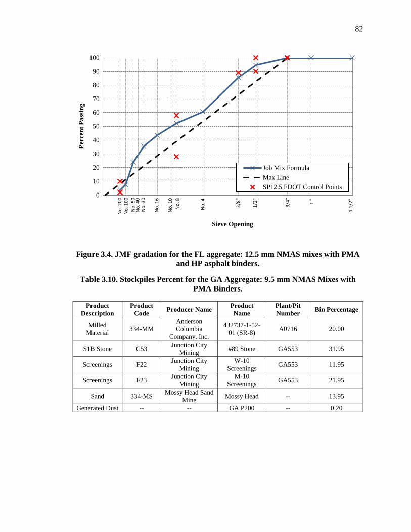
82
Figure 3.4. JMF gradation for the FL aggregate: 12.5 mm NMAS mixes with PMA
and HP asphalt binders.
Table 3.10. Stockpiles Percent for the GA Aggregate: 9.5 mm NMAS Mixes with
PMA Binders.
Product
Description
Product
Code Producer Name
Product
Name
Plant/Pit
Number Bin Percentage
Milled
Material 334-MM
Anderson
Columbia
Company. Inc.
432737-1-52-
01 (SR-8) A0716 20.00
S1B Stone C53 Junction City
Mining #89 Stone GA553 31.95
Screenings F22 Junction City
Mining
W-10
Screenings GA553 11.95
Screenings F23 Junction City
Mining
M-10
Screenings GA553 21.95
Sand 334-MS Mossy Head Sand
Mine Mossy Head -- 13.95
Generated Dust -- -- GA P200 -- 0.20
0
10
20
30
40
50
60
70
80
90
100
Per
cen
t P
ass
ing
Sieve Opening
Job Mix Formula
Max Line
SP12.5 FDOT Control Points
1 "
1/2
"
3/8
"
No
. 4
No
. 8
3/4
"
1 1
/2"
No
. 10
No
. 16
No
. 30
No
. 40
No
. 50
No
. 10
0N
o. 2
00

83
Figure 3.5. JMF gradation for the GA aggregate: 9.5 mm NMAS mixes with PMA
asphalt binders.
Table 3.11. Stockpiles Percent for the GA Aggregate: 12.5 mm NMAS Mixes with
PMA Binders.
Product
Description
Product
Code Producer Name
Product
Name
Plant/Pit
Number Bin Percentage
Crushed RAP 334-CR
Anderson
Columbia
Company
1-15 A0716 20.00
S1A Stone C47 Junction City
Mining #78 Stone GA553 22.95
S1B Stone C53 Junction City
Mining #89 Stone GA553 14.95
Screenings F22 Junction City
Mining
W-10
Screenings GA553 29.95
Sand F01 Vulcan Materials
Company Silica Sand 11057 11.95
Generated Dust -- -- GA P200 -- 0.20
0
10
20
30
40
50
60
70
80
90
100
Per
cen
t P
ass
ing
Sieve Opening
Job Mix Formula
Max Line
SP9.5 FDOT Control Points
1 "
1/2
"
3/8
"
No
. 4
No
. 8
3/4
"
1 1
/2"
No
. 10
No
. 16
No
. 30
No
. 40
No
. 50
No
. 10
0N
o. 2
00
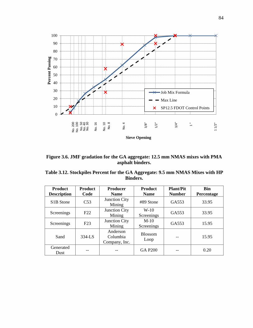
84
Figure 3.6. JMF gradation for the GA aggregate: 12.5 mm NMAS mixes with PMA
asphalt binders.
Table 3.12. Stockpiles Percent for the GA Aggregate: 9.5 mm NMAS Mixes with HP
Binders.
Product
Description
Product
Code
Producer
Name
Product
Name
Plant/Pit
Number
Bin
Percentage
S1B Stone C53 Junction City
Mining #89 Stone GA553 33.95
Screenings F22 Junction City
Mining
W-10
Screenings GA553 33.95
Screenings F23 Junction City
Mining
M-10
Screenings GA553 15.95
Sand 334-LS
Anderson
Columbia
Company, Inc.
Blossom
Loop -- 15.95
Generated
Dust -- -- GA P200 -- 0.20
0
10
20
30
40
50
60
70
80
90
100
Per
cen
t P
ass
ing
Sieve Opening
Job Mix Formula
Max Line
SP12.5 FDOT Control Points
1 "
1/2
"
3/8
"
No
. 4
No
. 8
3/4
"
1 1
/2"
No
. 10
No
. 16
No
. 30
No
. 40
No
. 50
No
. 10
0N
o. 2
00
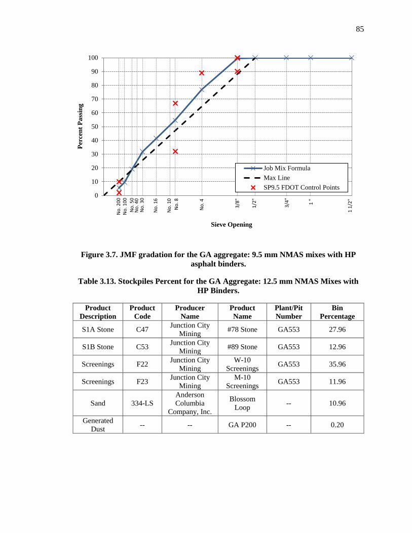
85
Figure 3.7. JMF gradation for the GA aggregate: 9.5 mm NMAS mixes with HP
asphalt binders.
Table 3.13. Stockpiles Percent for the GA Aggregate: 12.5 mm NMAS Mixes with
HP Binders.
Product
Description
Product
Code
Producer
Name
Product
Name
Plant/Pit
Number
Bin
Percentage
S1A Stone C47 Junction City
Mining #78 Stone GA553 27.96
S1B Stone C53 Junction City
Mining #89 Stone GA553 12.96
Screenings F22 Junction City
Mining
W-10
Screenings GA553 35.96
Screenings F23 Junction City
Mining
M-10
Screenings GA553 11.96
Sand 334-LS
Anderson
Columbia
Company, Inc.
Blossom
Loop -- 10.96
Generated
Dust -- -- GA P200 -- 0.20
0
10
20
30
40
50
60
70
80
90
100
Per
cen
t P
ass
ing
Sieve Opening
Job Mix Formula
Max Line
SP9.5 FDOT Control Points
1 "
1/2
"
3/8
"
No
. 4
No
. 8
3/4
"
1 1
/2"
No
. 10
No
. 16
No
. 30
No
. 40
No
. 50
No
. 10
0N
o. 2
00

86
Figure 3.8. JMF gradation for the GA aggregate: 12.5 mm NMAS mixes with HP
asphalt binders.
The following aggregate properties were measured on the recommended JMF
gradations and checked against the FDOT Specifications 2018 (FDOT Specifications,
2018):
• Coarse Aggregate Angularity (ASTM D5821, 2017)
• Fine Aggregate Angularity (AASHTO T304, 2017)
• Flat and Elongated Particles (ASTM D4791, 2017)
• Sand Equivalent (AASHTO T176, 2017)
Table 3.14 summarizes the properties of the aggregates sampled from the two
sources and measured on the recommended JMF gradations along with the corresponding
FDOT Specifications 2018 (FDOT Specifications, 2018). The “95” and “125” in the
0
10
20
30
40
50
60
70
80
90
100
Per
cen
t P
ass
ing
Sieve Opening
Job Mix Formula
Max Line
SP12.5 FDOT Control Points
1 "
1/2
"
3/8
"
No
. 4
No
. 8
3/4
"
1 1
/2"
No
. 10
No
. 16
No
. 30
No
. 40
No
. 50
No
. 10
0N
o. 2
00
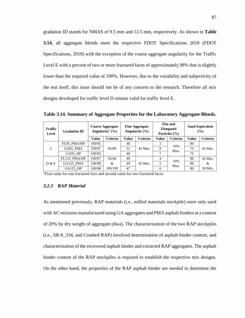
87
gradation ID stands for NMAS of 9.5 mm and 12.5 mm, respectively. As shown in Table
3.14, all aggregate blends meet the respective FDOT Specifications 2018 (FDOT
Specifications, 2018) with the exception of the coarse aggregate angularity for the Traffic
Level E with a percent of two or more fractured faces of approximately 98% that is slightly
lower than the required value of 100%. However, due to the variability and subjectivity of
the test itself, this issue should not be of any concern to the research. Therefore all mix
designs developed for traffic level D remain valid for traffic level E.
Table 3.14. Summary of Aggregate Properties for the Laboratory Aggregate Blends.
Traffic
Level Gradation ID
Coarse Aggregate
Angularity1 (%)
Fine Aggregate
Angularity (%)
Flat and
Elongated
Particles (%)
Sand Equivalent
(%)
Value Criteria Value Criteria Value Criteria Value Criteria
C
FL95_PMA/HP 100/92
85/80
48
45 Min.
2 10%
Max.
84
45 Min. GA95_PMA 100/97 51 8 75
GA95_HP 100/93 48 7 75
D & E
FL125_PMA/HP 100/97 95/90
&
100/100
49
45 Min.
4 10%
Max.
86 45 Min.
&
50 Min.
GA125_PMA 100/98 49 5 86
GA125_HP 100/98 47 6 80 1First value for one fractured face and second value for two fractured faces.
3.2.3 RAP Material
As mentioned previously, RAP materials (i.e., milled materials stockpile) were only used
with AC mixtures manufactured using GA aggregates and PMA asphalt binders at a content
of 20% by dry weight of aggregate (dwa). The characterization of the two RAP stockpiles
(i.e., SR-8_334, and Crushed RAP) involved determination of asphalt binder content, and
characterization of the recovered asphalt binder and extracted RAP aggregates. The asphalt
binder content of the RAP stockpiles is required to establish the respective mix designs.
On the other hand, the properties of the RAP asphalt binder are needed to determine the

88
properties of blended asphalt binder (i.e., combination of virgin and RAP asphalt binders)
using the blending chart approach.
The RAP materials were sampled, uniformly mixed, and then reduced to get
representative samples (AASHTO T2, 2015). The Centrifuge method with solvent of
trichloroethylene (TCE) was used for the extraction of the RAP asphalt binders. The
asphalt binder content of each RAP stockpile was determined in accordance with AASHTO
T164 (AASHTO T164, 2014). The recovered aggregates were then dried and evaluated in
terms of size distribution to be used in establishing the aggregate gradation of the resultant
mix design (i.e., virgin aggregates + RAP material) (AASHTO T27, 2014 & FM 1-T011,
2015). However, the extracted asphalt binder could not be further evaluated in terms of PG
grading (i.e., continuous grade) due to the potential high effect of TCE on the chemical and
rheological properties of the extracted asphalt binder. Therefore, the findings in terms of
asphalt binder contents of RAP stockpiles were only used for the establishment of
corresponding mix designs of AC mixes containing RAP material. Additional RAP asphalt
binders were extracted using a solvent of Toluene-Ethanol at 85/15 proportion. The
Toluene-Ethanol combination is anticipated to have lower impact on the chemical
properties of the extracted asphalt binder. FM 3-D5404 standard method (FM 3-D5404,
2000) was followed to recover the asphalt binder from the solvent solution using the
rotavapor apparatus. Finally, the Superpave PG system (AASHTO M320, 2014) was used
to determine the continuous grades of the two recovered RAP asphalt binders.
The RAP stockpile used with the GA PMA 9.5 mm mixes (i.e., SR8_334) had a
binder content of 5.63% by total weight of mix (twm). The RAP stockpile used with the
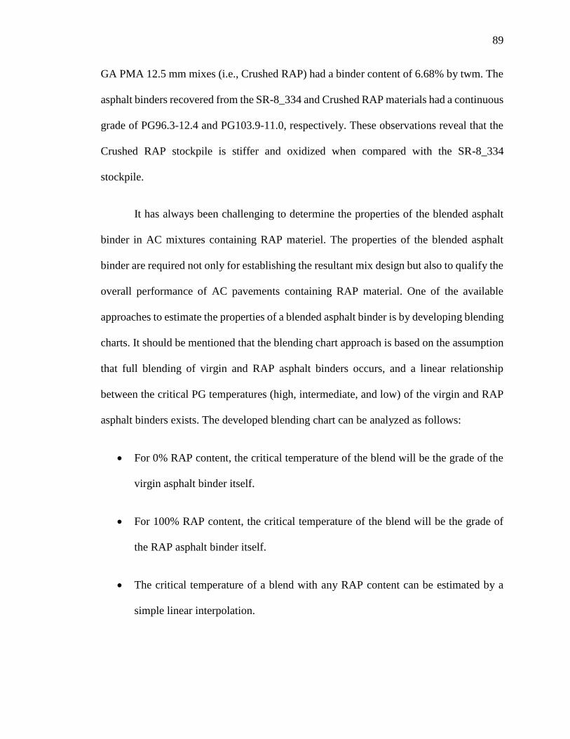
89
GA PMA 12.5 mm mixes (i.e., Crushed RAP) had a binder content of 6.68% by twm. The
asphalt binders recovered from the SR-8_334 and Crushed RAP materials had a continuous
grade of PG96.3-12.4 and PG103.9-11.0, respectively. These observations reveal that the
Crushed RAP stockpile is stiffer and oxidized when compared with the SR-8_334
stockpile.
It has always been challenging to determine the properties of the blended asphalt
binder in AC mixtures containing RAP materiel. The properties of the blended asphalt
binder are required not only for establishing the resultant mix design but also to qualify the
overall performance of AC pavements containing RAP material. One of the available
approaches to estimate the properties of a blended asphalt binder is by developing blending
charts. It should be mentioned that the blending chart approach is based on the assumption
that full blending of virgin and RAP asphalt binders occurs, and a linear relationship
between the critical PG temperatures (high, intermediate, and low) of the virgin and RAP
asphalt binders exists. The developed blending chart can be analyzed as follows:
• For 0% RAP content, the critical temperature of the blend will be the grade of the
virgin asphalt binder itself.
• For 100% RAP content, the critical temperature of the blend will be the grade of
the RAP asphalt binder itself.
• The critical temperature of a blend with any RAP content can be estimated by a
simple linear interpolation.
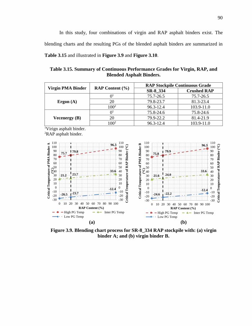
90
In this study, four combinations of virgin and RAP asphalt binders exist. The
blending charts and the resulting PGs of the blended asphalt binders are summarized in
Table 3.15 and illustrated in Figure 3.9 and Figure 3.10.
Table 3.15. Summary of Continuous Performance Grades for Virgin, RAP, and
Blended Asphalt Binders.
Virgin PMA Binder RAP Content (%) RAP Stockpile Continuous Grade
SR-8_334 Crushed RAP
Ergon (A)
01 75.7-26.5 75.7-26.5
20 79.8-23.7 81.3-23.4
1002 96.3-12.4 103.9-11.0
Vecenergy (B)
01 75.8-24.6 75.8-24.6
20 79.9-22.2 81.4-21.9
1002 96.3-12.4 103.9-11.0 1Virign asphalt binder. 2RAP asphalt binder.
(a) (b)
Figure 3.9. Blending chart process for SR-8_334 RAP stockpile with: (a) virgin
binder A; and (b) virgin binder B.
75.779.8
96.3
21.2 23.733.6
-26.5 -23.7
-12.4
-30
-20
-10
0
10
20
30
40
50
60
70
80
90
100
110
-30
-20
-10
0
10
20
30
40
50
60
70
80
90
100
110
0 10 20 30 40 50 60 70 80 90 100
Crit
ica
l T
em
pera
ture o
f R
AP
Bin
der (
°C)
Crit
ica
l T
em
pera
ture o
f P
MA
Bin
der A
(°C
)
RAP Content (%)
High PG Temp Inter PG Temp
Low PG Temp
75.879.9
96.3
21.6 24.033.6
-24.6 -22.2-12.4
-30
-20
-10
0
10
20
30
40
50
60
70
80
90
100
110
-30
-20
-10
0
10
20
30
40
50
60
70
80
90
100
110
0 10 20 30 40 50 60 70 80 90 100
Crit
ica
l T
em
pera
ture o
f R
AP
Bin
der (
°C)
Crit
ica
l T
em
pera
ture o
f P
MA
Bin
der B
(°C
)
RAP Content (%)
High PG Temp Inter PG Temp
Low PG Temp
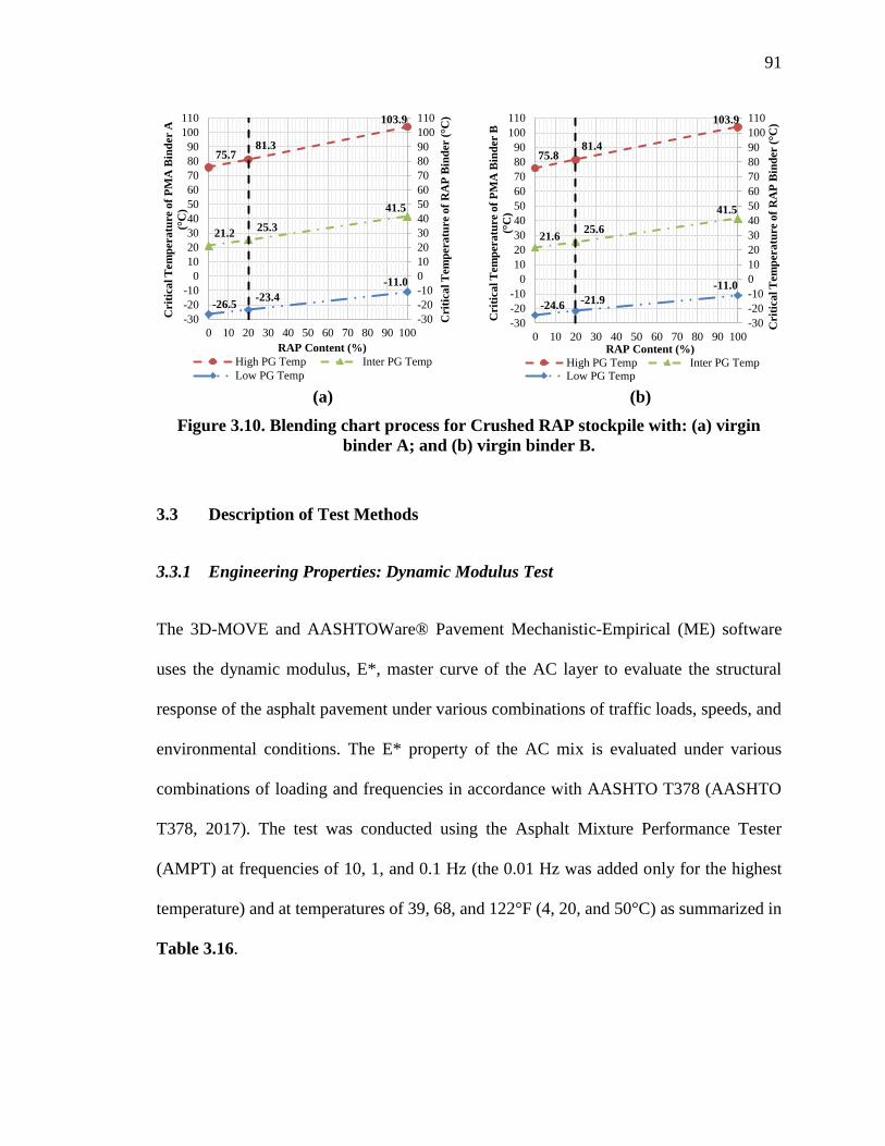
91
(a) (b)
Figure 3.10. Blending chart process for Crushed RAP stockpile with: (a) virgin
binder A; and (b) virgin binder B.
3.3 Description of Test Methods
3.3.1 Engineering Properties: Dynamic Modulus Test
The 3D-MOVE and AASHTOWare® Pavement Mechanistic-Empirical (ME) software
uses the dynamic modulus, E*, master curve of the AC layer to evaluate the structural
response of the asphalt pavement under various combinations of traffic loads, speeds, and
environmental conditions. The E* property of the AC mix is evaluated under various
combinations of loading and frequencies in accordance with AASHTO T378 (AASHTO
T378, 2017). The test was conducted using the Asphalt Mixture Performance Tester
(AMPT) at frequencies of 10, 1, and 0.1 Hz (the 0.01 Hz was added only for the highest
temperature) and at temperatures of 39, 68, and 122°F (4, 20, and 50°C) as summarized in
Table 3.16.
75.781.3
103.9
21.225.3
41.5
-26.5-23.4
-11.0
-30
-20
-10
0
10
20
30
40
50
60
70
80
90
100
110
-30
-20
-10
0
10
20
30
40
50
60
70
80
90
100
110
0 10 20 30 40 50 60 70 80 90 100
Crit
ica
l T
em
pera
ture o
f R
AP
Bin
der (
°C)
Crit
ica
l T
em
pera
ture o
f P
MA
Bin
der A
(°C
)
RAP Content (%)
High PG Temp Inter PG Temp
Low PG Temp
75.881.4
103.9
21.625.6
41.5
-24.6-21.9
-11.0
-30
-20
-10
0
10
20
30
40
50
60
70
80
90
100
110
-30
-20
-10
0
10
20
30
40
50
60
70
80
90
100
110
0 10 20 30 40 50 60 70 80 90 100
Crit
ica
l T
em
pera
ture o
f R
AP
Bin
der (
°C)
Crit
ica
l T
em
pera
ture o
f P
MA
Bin
der B
(°C
)
RAP Content (%)
High PG Temp Inter PG Temp
Low PG Temp
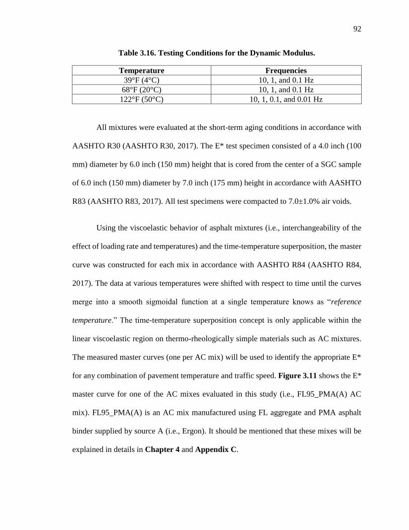
92
Table 3.16. Testing Conditions for the Dynamic Modulus.
Temperature Frequencies
39°F (4°C) 10, 1, and 0.1 Hz
68°F (20°C) 10, 1, and 0.1 Hz
122°F (50°C) 10, 1, 0.1, and 0.01 Hz
All mixtures were evaluated at the short-term aging conditions in accordance with
AASHTO R30 (AASHTO R30, 2017). The E* test specimen consisted of a 4.0 inch (100
mm) diameter by 6.0 inch (150 mm) height that is cored from the center of a SGC sample
of 6.0 inch (150 mm) diameter by 7.0 inch (175 mm) height in accordance with AASHTO
R83 (AASHTO R83, 2017). All test specimens were compacted to 7.0±1.0% air voids.
Using the viscoelastic behavior of asphalt mixtures (i.e., interchangeability of the
effect of loading rate and temperatures) and the time-temperature superposition, the master
curve was constructed for each mix in accordance with AASHTO R84 (AASHTO R84,
2017). The data at various temperatures were shifted with respect to time until the curves
merge into a smooth sigmoidal function at a single temperature knows as “reference
temperature.” The time-temperature superposition concept is only applicable within the
linear viscoelastic region on thermo-rheologically simple materials such as AC mixtures.
The measured master curves (one per AC mix) will be used to identify the appropriate E*
for any combination of pavement temperature and traffic speed. Figure 3.11 shows the E*
master curve for one of the AC mixes evaluated in this study (i.e., FL95_PMA(A) AC
mix). FL95_PMA(A) is an AC mix manufactured using FL aggregate and PMA asphalt
binder supplied by source A (i.e., Ergon). It should be mentioned that these mixes will be
explained in details in Chapter 4 and Appendix C.
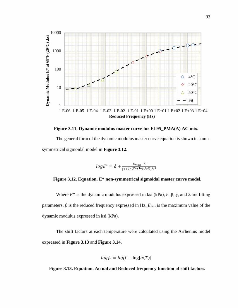
93
Figure 3.11. Dynamic modulus master curve for FL95_PMA(A) AC mix.
The general form of the dynamic modulus master curve equation is shown in a non-
symmetrical sigmoidal model in Figure 3.12.
𝑙𝑜𝑔𝐸∗ = 𝛿 +𝐸𝑚𝑎𝑥−𝛿
[1+𝜆𝑒(𝛽+𝛾 log(𝑓𝑟))]1/𝜆
Figure 3.12. Equation. E* non-symmetrical sigmoidal master curve model.
Where E* is the dynamic modulus expressed in ksi (kPa), δ, β, γ, and λ are fitting
parameters, fr is the reduced frequency expressed in Hz, Emax is the maximum value of the
dynamic modulus expressed in ksi (kPa).
The shift factors at each temperature were calculated using the Arrhenius model
expressed in Figure 3.13 and Figure 3.14.
𝑙𝑜𝑔𝑓𝑟 = 𝑙𝑜𝑔𝑓 + log [𝑎(𝑇)]
Figure 3.13. Equation. Actual and Reduced frequency function of shift factors.
1
10
100
1000
10000
1.E-06 1.E-05 1.E-04 1.E-03 1.E-02 1.E-01 1.E+00 1.E+01 1.E+02 1.E+03 1.E+04
Dy
na
mic
Mo
du
lus
E*
at
68
°F (
20°C
) ,k
si
Reduced Frequency (Hz)
4°C
20°C
50°C
Fit

94
Where fr is the reduced frequency expressed in Hz, f is the actual testing frequency
expressed in Hz, and a(T) is the shifting factor at temperature T.
log [𝑎(𝑇)] =𝛥𝐸𝑎
𝑅 ∗ 𝑙𝑛10(
1
𝑇−
1
𝑇𝑟)
Figure 3.14. Equation. Shift factors function of temperatures.
Where a(T) is the shifting factor at temperature T, ΔEa is the activation energy, T
is the testing temperature in degree Kelvin (°K), and Tr is the reference temperature in
degree kelvin (°K).
The master curve constitutes an effective method to predict the asphalt mixture E*
property beyond the testing conditions. In addition, the mechanical behavior of the asphalt
mixtures is highly influenced by the phase angle. This parameter affects the distribution of
the storage and loss moduli values known as elastic and viscous components of E*,
respectively. An approximate relation between the dynamic modulus and phase angle is
expressed in Figure 3.15.
δ (𝑤) ≈𝜋
2
𝑑 log (|𝐸∗|)
𝑑 log (𝑤)
Figure 3.15. Equation. Phase angle function of E* and frequency.
Where δ(w) is the phase angle expressed in degree (°), E* is the dynamic modulus
expressed in ksi (kPa), and w is the angular frequency expressed in rad/s.
By using Tr = 1/fr and w = 2πfr and by calculating the first derivative of E* with
respect to the angular frequency expressed in Figure 3.12, the modified phase angle model

95
in terms of reduced frequency at the reference temperature is expressed in Figure 3.16.
Figure 3.17 shows the phase angle, δ(w), master curve for one of the AC mixes evaluated
in this study.
𝛿(𝑤) = −𝑐 ∗𝜋
2∗ (𝐸𝑚𝑎𝑥 − 𝛿) ∗ 𝛾 ∗
𝑒(𝛽+𝛾 log(𝑓𝑟))
[1 + 𝜆𝑒(𝛽+𝛾 log(𝑓𝑟))][1+𝜆
𝜆]
Figure 3.16. Equation. Phase angle master curve non-symmetrical model.
Where δ(w) is the phase angle expressed in degree (°) at reference temperature Tr,
Emax is the maximum value of the dynamic modulus expressed in ksi (kPa), fr is the reduced
frequency expressed in Hz, and δ, β, γ, and λ are fitting parameters.
Figure 3.17. Phase angle master curve for FL95_PMA(A) AC mix.
0
5
10
15
20
25
30
35
40
1.E-08 1.E-06 1.E-04 1.E-02 1.E+00 1.E+02 1.E+04 1.E+06
Ph
ase
An
gle
at
68
°F (
20
°C),
deg
ree
Reduced Frequency (Hz)
4°C
20°C
50°C
Fit
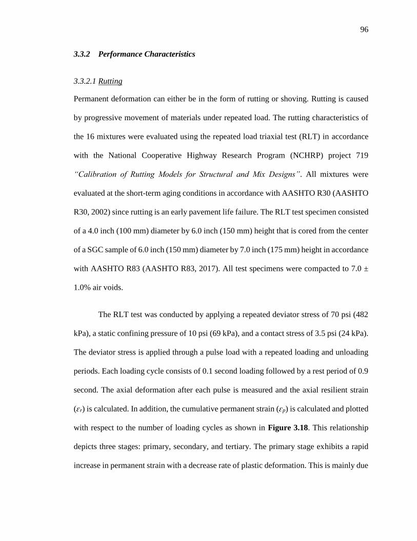
96
3.3.2 Performance Characteristics
3.3.2.1 Rutting
Permanent deformation can either be in the form of rutting or shoving. Rutting is caused
by progressive movement of materials under repeated load. The rutting characteristics of
the 16 mixtures were evaluated using the repeated load triaxial test (RLT) in accordance
with the National Cooperative Highway Research Program (NCHRP) project 719
“Calibration of Rutting Models for Structural and Mix Designs”. All mixtures were
evaluated at the short-term aging conditions in accordance with AASHTO R30 (AASHTO
R30, 2002) since rutting is an early pavement life failure. The RLT test specimen consisted
of a 4.0 inch (100 mm) diameter by 6.0 inch (150 mm) height that is cored from the center
of a SGC sample of 6.0 inch (150 mm) diameter by 7.0 inch (175 mm) height in accordance
with AASHTO R83 (AASHTO R83, 2017). All test specimens were compacted to 7.0 ±
1.0% air voids.
The RLT test was conducted by applying a repeated deviator stress of 70 psi (482
kPa), a static confining pressure of 10 psi (69 kPa), and a contact stress of 3.5 psi (24 kPa).
The deviator stress is applied through a pulse load with a repeated loading and unloading
periods. Each loading cycle consists of 0.1 second loading followed by a rest period of 0.9
second. The axial deformation after each pulse is measured and the axial resilient strain
(ԑr) is calculated. In addition, the cumulative permanent strain (ԑp) is calculated and plotted
with respect to the number of loading cycles as shown in Figure 3.18. This relationship
depicts three stages: primary, secondary, and tertiary. The primary stage exhibits a rapid
increase in permanent strain with a decrease rate of plastic deformation. This is mainly due

97
to a rearrangement of the mixture structure with an eventual concentration of stresses in
the contact surface between the loading plate and the sample due to small irregularities,
predominately associated with volumetric change (NCHRP Report 669, 2010). Previous
research has shown that densification is unlikely with pavements well compacted during
construction and its contribution is only at first working stage of asphalt pavement. The
secondary stage exhibits a constant rate of change of the permanent strain. Lower rate of
deformation during the secondary stage suggests a more stable mixture after initial
densification has been achieved, and the structure of the mix has finished its relocation due
to initial traffic compaction. The tertiary stage exhibits high rates of permanent strain
associated with plastic or shear deformation under no volume change (Pavement
Interactive, 2008 & NCHRP Project 719, 2012). This change is reached when the specimen
begins to deform significantly and individual aggregates composing the shape of the
mixture are moving past each other.
Figure 3.18. RLT permanent deformation curve for FL95_PMA(B) mix at 122°F.
0.0
1.0
2.0
3.0
4.0
5.0
0 500 1,000 1,500 2,000 2,500 3,000
Per
ma
nen
t S
train
, ԑp
(%
)
Number of Loading Cycles
Tertiary
Stage
Secondary
Stage
Primary
Stage

98
The Francken model, expressed in the equation shown in Figure 3.19, is used to
numerically model the permanent strain-loading cycle relationship. This well suited
mathematical model combines both a power model which characterizes the primary and
secondary stages, and an exponential model which fits the tertiary stage.
ԑ𝑝(𝑁) = 𝐴 ∗ 𝑁𝐵 + 𝐶 ∗ (𝑒𝐷∗𝑁 − 1)
Figure 3.19. Equation. Francken mathematical model: deformation vs. loading.
Where ԑ𝑝(𝑁) is the permanent axial strain expressed in inch / inch (or mm / mm),
N is the number of loading cycles, and A, B, C, and D are regression constants.
The RLT test was conducted at three different temperatures: 86, 104, and 122°F
(30, 40, and 50°C) for some AC mixes and 104, 122, and 140°F (40, 50, and 60°C) for
others. A rutting model for each mix was developed following the equation shown in
Figure 3.20 below. Figure 3.24 shows the rutting curves for an AC mix evaluated in this
study at the three testing temperatures.
ԑ𝑝
ԑ𝑟= 𝐾𝑧 ∗ 𝛽𝑟1 ∗ 10𝑘𝑟1 ∗ (𝑇)𝛽𝑟2∗𝑘𝑟2 ∗ (𝑁)𝛽𝑟3∗𝑘𝑟3
Figure 3.20. Equation. MEPDG rutting regression model.
Where ԑ𝑝 is the permanent axial strain expressed in inch / inch (or mm / mm), ԑ𝑟 is
the resilient axial strain expressed in inch / inch (or mm / mm), N is the number of loading
cycles, and T is the temperature of the asphalt mixture expressed in degree Fahrenheit (°F),
kr1, kr2, and kr3 are experimentally determined coefficients, βr1, βr2, and βr3 are laboratory-
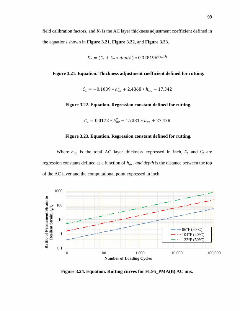
99
field calibration factors, and Kz is the AC layer thickness adjustment coefficient defined in
the equations shown in Figure 3.21, Figure 3.22, and Figure 3.23.
𝐾𝑧 = (𝐶1 + 𝐶2 ∗ 𝑑𝑒𝑝𝑡ℎ) ∗ 0.328196𝑑𝑒𝑝𝑡ℎ
Figure 3.21. Equation. Thickness adjustment coefficient defined for rutting.
𝐶1 = −0.1039 ∗ ℎ𝑎𝑐2 + 2.4868 ∗ ℎ𝑎𝑐 − 17.342
Figure 3.22. Equation. Regression constant defined for rutting.
𝐶2 = 0.0172 ∗ ℎ𝑎𝑐2 − 1.7331 ∗ ℎ𝑎𝑐 + 27.428
Figure 3.23. Equation. Regression constant defined for rutting.
Where ℎ𝑎𝑐 is the total AC layer thickness expressed in inch, 𝐶1 and 𝐶2 are
regression constants defined as a function of ℎ𝑎𝑐, and depth is the distance between the top
of the AC layer and the computational point expressed in inch.
Figure 3.24. Equation. Rutting curves for FL95_PMA(B) AC mix.
0.1
1
10
100
1000
10 100 1,000 10,000 100,000
Ratt
io o
f P
erm
an
ent
Str
ain
to
Res
ilen
t S
train
,ԑ p
/ԑr
Number of Loading Cycles
86°F (30°C)
104°F (40°C)
122°F (50°C)

100
3.3.2.2 Fatigue Cracking
Asphalt mixtures are expected to resist fatigue cracking after the first five years of their
service life when the asphalt binder becomes brittle due to long-term aging. Fatigue
cracking is typically caused by the repeated bending strains in the asphalt mix caused by
heavy loads during moderate weather conditions. In this study, the resistance of the
mixtures to fatigue cracking was evaluated using the flexural beam fatigue test according
to ASTM D7460 (ASTM D7460, 2010) and AASHTO T321 (AASHTO T321, 2017). The
mixtures for the fatigue test were short-term aged followed by long-term aging since
fatigue is a later pavement life distress. The 2×2×5 inch (51×51×381 mm) beam specimen
is subjected to a 4-point bending with free rotation and horizontal translation at all load and
reaction points. This produces a constant bending moment over the center portion of the
specimen.
The constant strain-controlled tests were conducted at different strain levels using
a repeated haversine load at a frequency of 10 Hz. Initial flexural stiffness is measured at
the 50th load cycle. The normalized modulus (NM) is calculated as expressed in the
equation shown in Figure 3.25 and plotted with respect to the number of loading cycles as
shown in Figure 3.26. Fatigue life or failure is defined as the number of cycles at which
the NM reaches its peak (i.e., maximum value).
𝑁𝑀 =𝑆𝑖 ∗ 𝑁𝑖
𝑆0 ∗ 𝑁0
Figure 3.25. Equation. Calculation of fatigue normalized modulus.
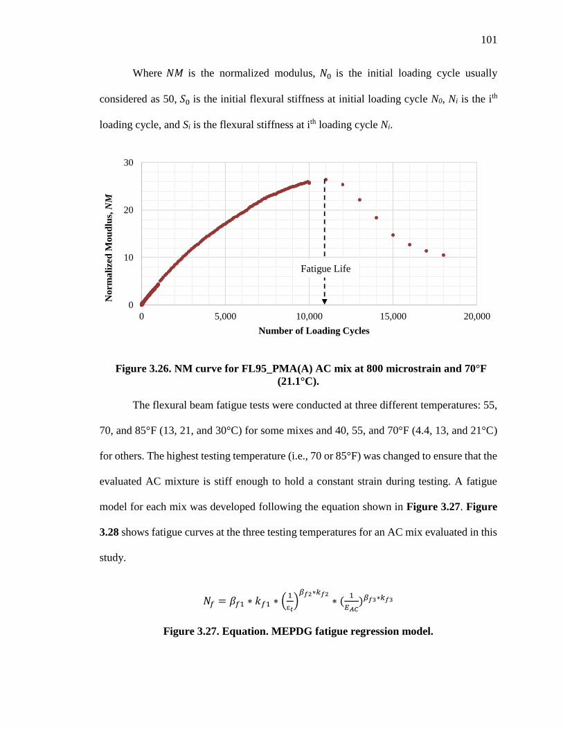
101
Where 𝑁𝑀 is the normalized modulus, 𝑁0 is the initial loading cycle usually
considered as 50, 𝑆0 is the initial flexural stiffness at initial loading cycle N0, Ni is the ith
loading cycle, and Si is the flexural stiffness at ith loading cycle Ni.
Figure 3.26. NM curve for FL95_PMA(A) AC mix at 800 microstrain and 70°F
(21.1°C).
The flexural beam fatigue tests were conducted at three different temperatures: 55,
70, and 85°F (13, 21, and 30°C) for some mixes and 40, 55, and 70°F (4.4, 13, and 21°C)
for others. The highest testing temperature (i.e., 70 or 85°F) was changed to ensure that the
evaluated AC mixture is stiff enough to hold a constant strain during testing. A fatigue
model for each mix was developed following the equation shown in Figure 3.27. Figure
3.28 shows fatigue curves at the three testing temperatures for an AC mix evaluated in this
study.
𝑁𝑓 = 𝛽𝑓1 ∗ 𝑘𝑓1 ∗ (1
ԑ𝑡)
𝛽𝑓2∗𝑘𝑓2
∗ (1
𝐸𝐴𝐶)𝛽𝑓3∗𝑘𝑓3
Figure 3.27. Equation. MEPDG fatigue regression model.
0
10
20
30
0 5,000 10,000 15,000 20,000
Norm
ali
zed
Mo
ud
lus,
NM
Number of Loading Cycles
Fatigue Life

102
Where Nf is the fatigue life expressed as number of load repetitions to fatigued
amage, ԑ𝑡 is the applied tensile strain expressed in inch / inch (or mm / mm), EAC is the
dynamic modulus od the asphalt mixture expressed in psi, kf1, kf2, and kf3 are experimentally
determined coefficients, and βf1, βf2, and βf3 are laboratory-field calibration factors.
Figure 3.28. Fatigue curves for FL95_PMA(A) AC mix.
3.3.2.3 Top-Down Cracking
Top-down cracking mechanism can be defined as the combination of several basic factors
including high surface horizontal tensile stresses at the tire-pavement interface, age
hardening of the asphalt binder resulting in high thermal stresses in the HMA, etc. In this
study, the resistance of the mixtures to top-down cracking was evaluated using the indirect
tension test jig mounted into the AMPT Pro machine in accordance with AASHTO T322
(AASHTO T322, 2007) and Appendix G of the NCHRP 9-57 study (NCHRP Project No.
9-57, 2016). The mixtures for the IDT test were short-term aged followed by long-term
100
1,000
10,000
1.E+04 1.E+05 1.E+06 1.E+07 1.E+08 1.E+09
Fle
xu
ral
Str
ain
(m
icro
stra
in)
Number of Cycles to Failure
55°F (13°C)
70°F (21°C)
85°F (30°C)

103
aging in accordance with AASHTO R30 (AASHTO R30, 2014) since top-down cracking
tends to occur after almost ~8 years of the pavement life in Florida.
The IDT test specimen consists of a 6.0 inch (150 mm) diameter by 1.5 inch (38
mm) height sample for an AC mix with a NMAS not exceeding ¾ inch (19 mm). The test
specimen is trimmed from the middle part of a SGC sample of 6.0 inch (150 mm) diameter
by 7.0 inch (175 mm) height. All test specimens were compacted to 7.0±1.0% air voids.
The top-down cracking evaluation of an AC mix consists of determining the tensile
creep compliance and the tensile failure limit by conducting the tensile creep and tensile
fracture tests, respectively. The tensile creep test is used to capture the permanent strain
associated with the time-dependent response of an asphalt mixture. The tensile creep
compliance parameters can be used to estimate the rate of damage accumulation of an
asphalt mixture subjected to repeated loads. On the other hand, the tensile fracture test is
used to determine the failure limit of an asphalt mixture. These material properties can be
used for estimating the fracture tolerance of the asphalt mixture. The energy ratio (ER) will
constitute the cracking performance comparison parameter and the controlling failure
criterion.
The tensile creep test applies a static step/ramp load of fixed magnitude rising from
the seating load (i.e., 10 lbf (50 N)) for a duration of 1,000 seconds. The magnitude of the
load is adjusted so that the horizontal deformation at 100 seconds is between 0.0010 and
0.0015 inch (0.0254 and 0.0038 mm) and the horizontal deformation at 1,000 seconds does
not exceed 0.0075 inches (0.0200 mm). The creep compliance (Dt) at each recording time,
t, is computed using the equation expressed in Figure 3.29. The creep compliance values

104
are fitted through a power-law as expressed in Figure 3.31 and used to determine the
mixture parameters D0, D1, and m-value as shown in Figure 3.32.
𝐷𝑡 =𝛥𝐻𝑡𝑟𝑖𝑚 𝑎𝑣𝑔,𝑡∗ℎ𝑎𝑣𝑔∗𝜙𝑎𝑣𝑔
𝑃𝑎𝑣𝑔∗𝐺𝐿∗ 𝐶𝑐𝑜𝑚𝑝𝑙𝑖𝑎𝑛𝑐𝑒,𝑡
Figure 3.29. Equation. Creep compliance at time t.
𝐶𝑐𝑜𝑚𝑝𝑙𝑖𝑎𝑛𝑐𝑒, 𝑡 = 0.6354 ∗𝛥𝑉𝑡𝑟𝑖𝑚 𝑎𝑣𝑔,𝑡
𝛥𝐻𝑡𝑟𝑖𝑚 𝑎𝑣𝑔,𝑡− 0.332
Figure 3.30. Equation. Creep compliance correction factor at time t.
𝐷(𝑡) = 𝐷0 + 𝐷1𝑡𝑚
Figure 3.31. Equation. Creep compliance power law model.
Where D(t) is the creep compliance at time t expressed in psi-1 (GPa-1), ΔHtrim avg, t
is the mean absolute horizontal deformation of all specimens in test group expressed in
inch (mm), havg is the average thickness of the specimen in the test group expressed in inch
(mm), Фavg is the average diameter of the specimen in the test group expressed in inch
(mm), Pavg is the average creep load of the specimen in the test group expressed in lbs. (N),
GL is the gage length equal to 1.5 inch (38 mm), Ccompliance is the creep compliance
correction factor at time t defined in the equation expressed in Figure 3.30, ΔVtrim avg, t is
the mean absolute vertical deformation of all specimens in test group expressed in inch
(mm), t recording time expressed in second, and D0, D1, m are the creep compliance
parameters.
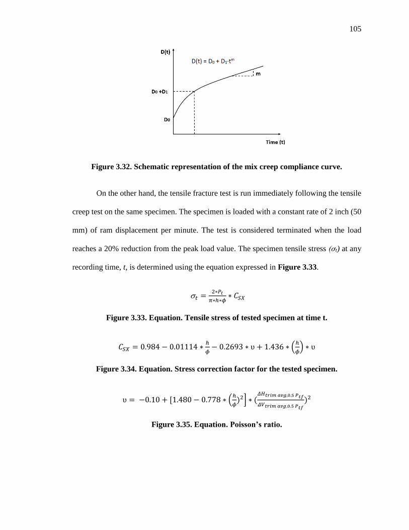
105
Figure 3.32. Schematic representation of the mix creep compliance curve.
On the other hand, the tensile fracture test is run immediately following the tensile
creep test on the same specimen. The specimen is loaded with a constant rate of 2 inch (50
mm) of ram displacement per minute. The test is considered terminated when the load
reaches a 20% reduction from the peak load value. The specimen tensile stress (ơt) at any
recording time, t, is determined using the equation expressed in Figure 3.33.
𝑡 =2∗𝑃𝑡
𝜋∗ℎ∗𝜙∗ 𝐶𝑆𝑋
Figure 3.33. Equation. Tensile stress of tested specimen at time t.
𝐶𝑆𝑋 = 0.984 − 0.01114 ∗ℎ
𝜙− 0.2693 ∗ ʋ + 1.436 ∗ (
ℎ
𝜙) ∗ ʋ
Figure 3.34. Equation. Stress correction factor for the tested specimen.
ʋ = −0.10 + [1.480 − 0.778 ∗ (ℎ
𝜙)2] ∗ (
𝛥𝐻𝑡𝑟𝑖𝑚 𝑎𝑣𝑔,0.5 𝑃𝑡𝑓
𝛥𝑉𝑡𝑟𝑖𝑚 𝑎𝑣𝑔,0.5 𝑃𝑡𝑓
)2
Figure 3.35. Equation. Poisson’s ratio.

106
Where σ(t) is the tensile stress of tested specimen at time t expressed in psi (Pa), Pt
is the load for the tested specimen at time t expressed in lbs. (N), h is the thickness of tested
specimen expressed in inch (mm), Ф is the diameter of tested specimen expressed in inch
(mm), CSX is the stress correction factor for the tested specimen defined in the equation
expressed in Figure 3.34, lbs. (N), υ is the Poisson’s ratio defined in the equation
expressed in Figure 3.35, and ΔHtrim avg, 0.5 Ptf and ΔVtrim avg, 0.5 Ptf are the normalized
absolute horizontal and vertical deformation at 50% of the peak load expressed in inch
(mm).
The specimen tensile strain (ԑt) at any recording time t is determined using the
equation expressed in Figure 3.36. The specimen failure strain is defined as tensile strain
at the instant of fracture (tf).
ԑ𝑡 =𝛥𝐻𝑛𝑜𝑟𝑚,𝑡
𝐺𝐿∗ 1.072 ∗ 𝐶𝐵𝑋
Figure 3.36. Equation. Tensile strain of tested specimen at time t.
𝐶𝐵𝑋 = 1.03 − 0.189 ∗ (ℎ
𝜙) − 0.081 ∗ ʋ + 0.089 ∗ (
ℎ
𝜙)2
Figure 3.37. Equation. Strain correction factor for the tested specimen.
Where ε(t) is the tensile strain of tested specimen at time t expressed in inch/inch
(mm/mm), GL is the gage length of 1.5 inch (38 mm), ΔHnorm,t is the normalized absolute
horizontal deformation of specimen at time t expressed in inch (mm), and CBX is the bulging
correction factor for the tested specimen defined in the equation expressed in Figure 3.37.
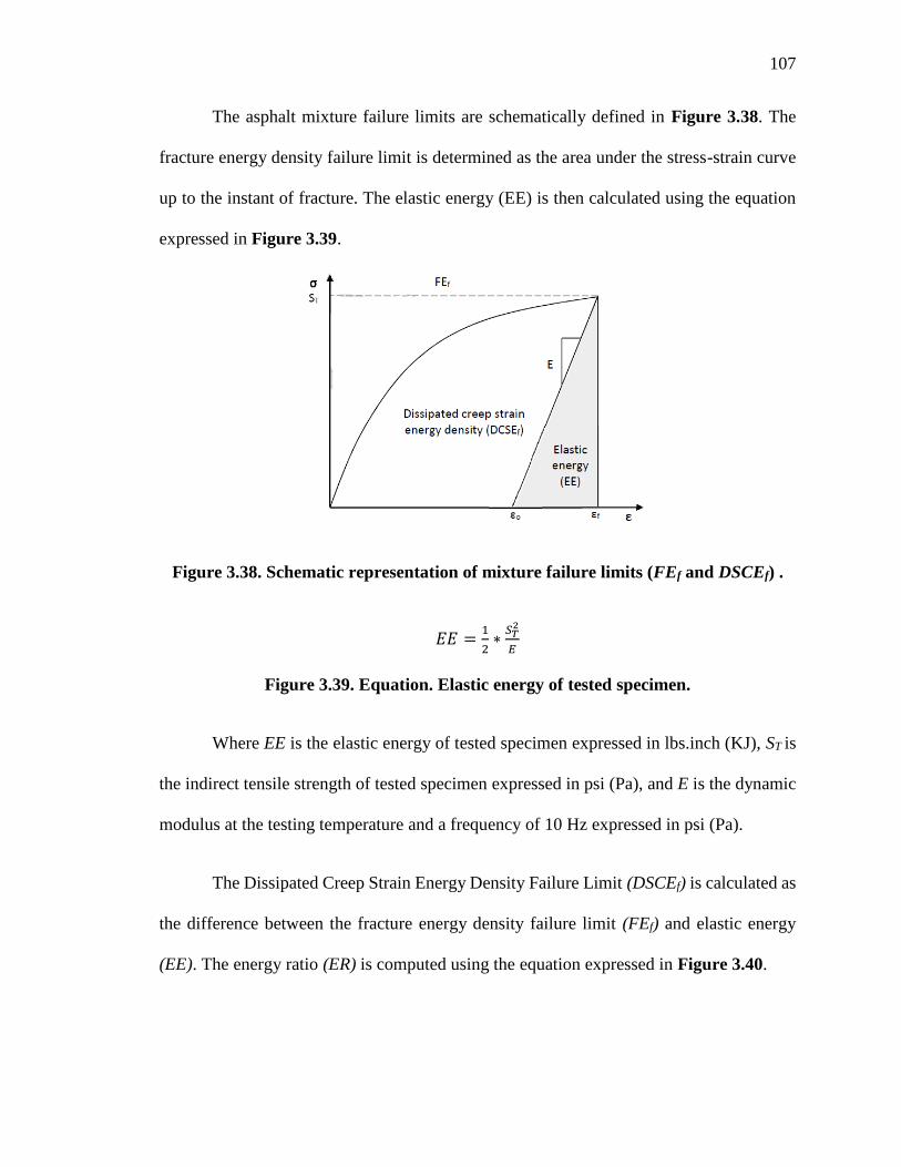
107
The asphalt mixture failure limits are schematically defined in Figure 3.38. The
fracture energy density failure limit is determined as the area under the stress-strain curve
up to the instant of fracture. The elastic energy (EE) is then calculated using the equation
expressed in Figure 3.39.
Figure 3.38. Schematic representation of mixture failure limits (FEf and DSCEf) .
𝐸𝐸 =1
2∗
𝑆𝑇2
𝐸
Figure 3.39. Equation. Elastic energy of tested specimen.
Where EE is the elastic energy of tested specimen expressed in lbs.inch (KJ), ST is
the indirect tensile strength of tested specimen expressed in psi (Pa), and E is the dynamic
modulus at the testing temperature and a frequency of 10 Hz expressed in psi (Pa).
The Dissipated Creep Strain Energy Density Failure Limit (DSCEf) is calculated as
the difference between the fracture energy density failure limit (FEf) and elastic energy
(EE). The energy ratio (ER) is computed using the equation expressed in Figure 3.40.

108
𝐸𝑅 = 𝐷𝑆𝐶𝐸𝑓
𝐷𝑆𝐶𝐸𝑚𝑖𝑛=
𝐷𝑆𝐶𝐸𝑓
𝑚2.98∗𝐷1𝐴
Figure 3.40. Equation. Elastic energy of tested specimen function of DSCEf and
DSCEmin.
Where A is the parameter that considers the tensile strength of the asphalt mixture
(ST) and the tensile stress (ơ) in the pavement structure determined in the advanced
pavement modeling section (Refer to the equation expressed in Figure 3.41). It should be
mentioned that the equation expressed in Figure 3.41 is valid for stress and strength
reported in psi, DSCEf in lbf-in/in3, D1 in psi-1, and A in psi-2. The equation expressed in
Figure 3.42 should replace the one expressed in Figure 3.41 for stress and strength
reported in MPa, DSCEf in kJ/m3, D1 in GPa-1, and A in MPa-2.
𝐴 = 1.42 ∗ 10−3 ∗(922.5−𝑆𝑇)
ơ3.1 + 1.70 ∗ 10−7
Figure 3.41. Equation. Calculation of parameter A using US units.
𝐴 = 8.64 ∗ 10−4 ∗(6.36−𝑆𝑇)
ơ3.1 + 3.57 ∗ 10−3
Figure 3.42. Equation. Calculation of parameter A using SI units.
3.3.2.4 Reflective Cracking
Reflective cracking is one of the primary forms of distresses in AC overlays of flexible and
rigid pavements. It affects ride quality and allows the penetration of water and debris into
the cracks which would accelerate the deterioration of the overlay and the underlying
pavement, thus leading to a reduction in pavement serviceability. The Texas overlay test
(OT) is used to evaluate the mixtures’ resistance to reflective cracking in accordance with
Tex-248-F procedure (Tex-248-F, 2017). The horizontal opening and closing of joints and

109
cracks that exist underneath a new AC overlay are specifically simulated. The Overlay test
jig was recently designed to increase the functionality of the AMPT machine by enabling
it to determine the susceptibility of asphalt mixtures to reflective cracking.
The OT specimens were only subjected to short-term aging. The OT specimen
consists of a 6 inch (150 mm) long by 3 inch (75 mm) wide and 1.5 inch (37.5 mm) thick
sample that is trimmed from a 6 inch (150 mm) diameter by 4.5 inch (115 mm) height SGC
sample compacted to 7.0±1.0% air voids. Once prepared, each sample is glued on two
metallic plates, well fixed on a mounting wide plate using epoxy. A photo of the overlay
test setup and a specimen ready for testing is shown in Figure 3.43.
The test is conducted in a controlled displacement mode until failure occurs at a
loading rate of one cycle per 10 seconds with a maximum displacement of 0.025 inch
(0.6350 mm) at 77±1°F (25±0.5°C). Each cycle consists of 5 seconds of loading and 5
seconds of unloading. The number of cycles to failure is defined as the number of cycles
to reach a 93% drop in initial load which is measured from the first opening cycle. If a 93%
reduction in initial load is not reached within a certain specified maximum number of
cycles, the test stops automatically. For this study, a total of 5,000 cycles is selected as a
maximum number of cycles for stopping the test. The crack driving force is recorded at
each loading cycle and a normalized load reduction curve is plotted as shown in Figure
3.44.

110
Figure 3.43. AMPT overlay test setup.
Figure 3.44. Normalized load reduction curve for FL95_PMA(A) AC mix at a max
displacement of 0.025 inch (0.6350 mm) and a temperature of 77°F (25°C).
A power function defined in the equation expressed in Figure 3.45 is used to fit the
load reduction curve function of the number of loading cycles to determine the crack
propagation rate (CPR) and the crack resistance index (CRI) (Garcia et al., 2016).
0
0.1
0.2
0.3
0.4
0.5
0.6
0.7
0.8
0.9
1
0 50 100 150 200 250 300
Cra
ck D
rivin
g N
orm
ali
zed
Load
Number of Loading Cycles

111
𝑁𝐿 = 𝑁𝐶𝑃𝑅 = 𝑁(0.0075∗𝐶𝑅𝐼−1)
Figure 3.45. Equation. Normalized crack driving force.
Where NL is the normalized crack driving force or load at each loading cycle
expressed in lb (kN), N is the loading cycles, CPR is the crack propagation rate, and CRI
is the crack resistance index.
The critical fracture energy (Gc) at the maximum peak load of the first loading
cycle is considered as the energy required to initiate crack. Figure 3.46 illustrates the crack
driving load function of the displacement of the first cycle. A negative load value indicates
a tension load while a positive one indicates compression. The area under the hysteresis
loop, limited for the tension phenomena (i.e., negative load), is considered essential to
compute the fracture parameters (i.e., critical fracture energy, CPR, and CRI) that
characterize the crack initiation stage of the OT. The critical fracture energy is calculated
using the equation expressed in Figure 3.47 (Garcia et al., 2016).
Figure 3.46. Portion of hysteresis loop of the first loading cycle to calculate the
critical fracture energy of FL95_PMA(A) AC mix.
112
𝐺𝑐 = 𝑊𝑐
𝑏∗ℎ
Figure 3.47. Equation. Critical fracture energy.
Where Gc is the critical fracture energy expressed in lb.-in./in.2 (kN-mm2), Wc is
the fracture area hatched in Figure 3.46 and expressed in lb.-in. (kN-mm), b is the
specimen width: 3 inch (76.2 mm), and h is the specimen height: 1.5 inch (38.1 mm).
The OT will also be used to determine the fracture properties of the evaluated
mixtures assuming that Mode I (opening mode) and Mode II (shearing mode) share the
same fracture mechanics properties (A and n). It should be mentioned that the first 100
cycles are only considered for fracture properties determination. The fracture parameters
(A and n) will be determined in accordance with the “Mechanistic-Empirical Asphalt
Overlay Thickness Design and Analysis System” (Zhou et al., 2008). The determined
fracture properties (A & n) will be used in the advanced dynamic modeling of flexible
pavements to predict crack propagation in AC overlays caused by both traffic loading and
thermal effects.

113
CHAPTER 4 MIX DESIGNS AND TEST RESULTS
As mentioned before, raw aggregate materials, collected from Southeast Florida (FL) and
Georgia Granite (GA), RAP material collected from GA, and highly and conventionally
polymer modified asphalt binders, PG76-22 and HP binder, were used to establish 16 AC
mix designs. This chapter presents in detail the mix designs developed. In addition, it
provides the analysis of all test results generated from the performance evaluation of the
laboratory AC mixes.
4.1 Mix Designs
In this research, 16 types of mixtures (refer to Table 4.1) were produced and evaluated in
the laboratory based on the following guidelines and recommendations:
• The NMAS 9.5 mm mixes should be designed for traffic level C and the NMAS
12.5 mm mixes should be designed for traffic level D.
• The FL aggregate source should not include RAP materials.
• The HP AC mixes should not include RAP materials.
• All binders should include an approved liquid anti-strip agent at the dosage rate of
0.5% by weight of binder.
As shown in Table 4.1, a total of 16 AC mixes were produced in the laboratory.
These mixtures were designed following the FDOT Superpave mix design methodology
(FDOT Specifications, 2018). The heated aggregates were mixed with various amount of
asphalt binder so that at least two were above and at least two were below the expected

114
optimum binder content (OBC) for each mixture. After the samples are mixed and
conditioned for 2 hours at the compaction temperature, the mixtures are compacted using
the Superpave gyratory compactor (SGC) for a certain number of gyrations based on the
NMAS and the targeted traffic level. The OBC for each mixture was determined by
identifying the maximum asphalt content which provides 4% air voids and meeting all the
applicable FDOT mix design specifications as summarized in Table 4.2.
Table 4.1. Summary of Mixtures for the Laboratory Evaluation.
Aggregate
Source
Gradation
NMAS
RAP
(%)
Ergon (A) Vecenergy (B)
PG76-22PMA HP Binder PG76-22PMA HP Binder
FL 9.5 mm 0 FL95_PMA FL95_HP FL95_PMA FL95_HP
12.5 mm 0 FL125_PMA FL125_HP FL125_PMA FL125_HP
GA
9.5 mm 0 – GA95_HP – GA95_HP
12.5 mm 0 – GA125_HP – GA125_HP
9.5 mm 20 GA95_PMA – GA95_PMA –
12.5 mm 20 GA125_PMA – GA125_PMA –
–Not applicable.
Table 4.2. FDOT Superpave Mix Design Specifications.
Aggregate
Source
Gradation
NMAS
Traffic
Level
FDOT Specifications 2018
Ninit1 Ndesign
2 Va3 VMA4 VFA5 DP6
FL 9.5mm C 7 75 4% ≥15% 65-75% 0.6-1.2
12.5mm D & E 8 100 4% ≥14% 65-75% 0.6-1.2
GA 9.5mm C 7 75 4% ≥15% 65-75% 0.6-1.2
12.5mm D & E 8 100 4% ≥14% 65-75% 0.6-1.2 1Ninit stands for initial number of gyrations. 2Ndesign stands for design number of gyrations. 3Va stands for air voids level. 4VMA stands for percentage of voids in mineral aggregate. 5VFA stands for percentage of voids filled with asphalt. 6DP stands for dust proportion
Table 4.3 to Table 4.6 summarize the mix design information for all AC mixes.
The abbreviations in the provided tables are defined as follows: twm stands for total weight
of mix, Gmm stands for theoretical maximum specific gravity of AC mixes, and Pbe stands

115
for percent of effective binder by volume. The details of the developed mix designs can be
found in Appendix B Section 1 (B.1).
Table 4.3. Summary of Mix Designs for FL Aggregate, 9.5 mm NMAS, with PMA
and HP Asphalt Binders.
Properties Mix Design ID
FL95_PMA(A) FL95_PMA(B) FL95_HP(A) FL95_HP(B)
Traffic Level (Ndesign) C (75) C (75) C (75) C (75)
OBC by twm (%) 6.2 6.2 5.9* 5.9*
RAP Binder Ratio, RBR 0.00 0.00 0.00 0.00
Gmm at OBC 2.368 2.362 2.356 2.370
Va (%) 4.0 4.0 3.7 4.3
VMA (%), Min. 15% 15.0 15.3 14.9 15.2
VFA (%), 65 – 75% 73.1 73.9 75.6 71.2
Pbe at OBC (%) 4.99 5.13 5.05 4.79
DP, 0.6 – 1.2 0.8 0.8 0.8 0.8 *An average OBC was selected between the two binder sources.
Table 4.4. Summary of Mix Designs for FL Aggregate, 12.5 mm NMAS, with PMA
and HP Asphalt Binders.
Properties Mix Design ID
FL125_PMA(A) FL125_PMA(B) FL125_HP(A) FL125_HP(B)
Traffic Level (Ndesign) D/E (100) D/E (100) D/E (100) D/E (100)
OBC by twm (%) 5.5* 5.5* 5.4 5.4
RAP Binder Ratio, RBR 0.00 0.00 0.00 0.00
Gmm at OBC 2.372 2.378 2.360 2.369
Va (%) 3.8 4.4 4.0 4.0
VMA (%), Min. 14% 13.9 14.0 14.2 13.9
VFA (%), 65 – 75% 72.4 69.2 71.9 71.2
Pbe at OBC (%) 4.49 4.38 4.60 4.44
DP, 0.6 – 1.2 0.8 0.8 0.8 0.8 * An average OBC was selected between the two binder sources.
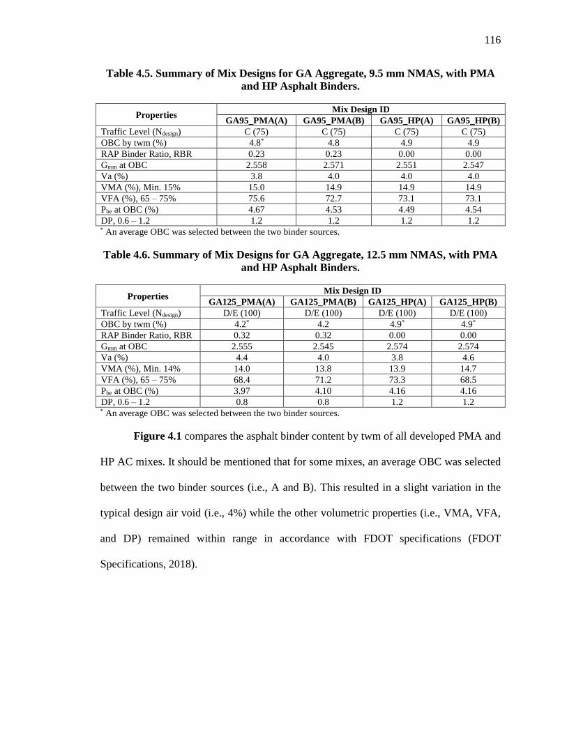
116
Table 4.5. Summary of Mix Designs for GA Aggregate, 9.5 mm NMAS, with PMA
and HP Asphalt Binders.
Properties Mix Design ID
GA95_PMA(A) GA95_PMA(B) GA95_HP(A) GA95_HP(B)
Traffic Level (Ndesign) C (75) C (75) C (75) C (75)
OBC by twm (%) 4.8* 4.8 4.9 4.9
RAP Binder Ratio, RBR 0.23 0.23 0.00 0.00
Gmm at OBC 2.558 2.571 2.551 2.547
Va (%) 3.8 4.0 4.0 4.0
VMA (%), Min. 15% 15.0 14.9 14.9 14.9
VFA (%), 65 – 75% 75.6 72.7 73.1 73.1
Pbe at OBC (%) 4.67 4.53 4.49 4.54
DP, 0.6 – 1.2 1.2 1.2 1.2 1.2 * An average OBC was selected between the two binder sources.
Table 4.6. Summary of Mix Designs for GA Aggregate, 12.5 mm NMAS, with PMA
and HP Asphalt Binders.
Properties Mix Design ID
GA125_PMA(A) GA125_PMA(B) GA125_HP(A) GA125_HP(B)
Traffic Level (Ndesign) D/E (100) D/E (100) D/E (100) D/E (100)
OBC by twm (%) 4.2* 4.2 4.9* 4.9*
RAP Binder Ratio, RBR 0.32 0.32 0.00 0.00
Gmm at OBC 2.555 2.545 2.574 2.574
Va (%) 4.4 4.0 3.8 4.6
VMA (%), Min. 14% 14.0 13.8 13.9 14.7
VFA (%), 65 – 75% 68.4 71.2 73.3 68.5
Pbe at OBC (%) 3.97 4.10 4.16 4.16
DP, 0.6 – 1.2 0.8 0.8 1.2 1.2 * An average OBC was selected between the two binder sources.
Figure 4.1 compares the asphalt binder content by twm of all developed PMA and
HP AC mixes. It should be mentioned that for some mixes, an average OBC was selected
between the two binder sources (i.e., A and B). This resulted in a slight variation in the
typical design air void (i.e., 4%) while the other volumetric properties (i.e., VMA, VFA,
and DP) remained within range in accordance with FDOT specifications (FDOT
Specifications, 2018).
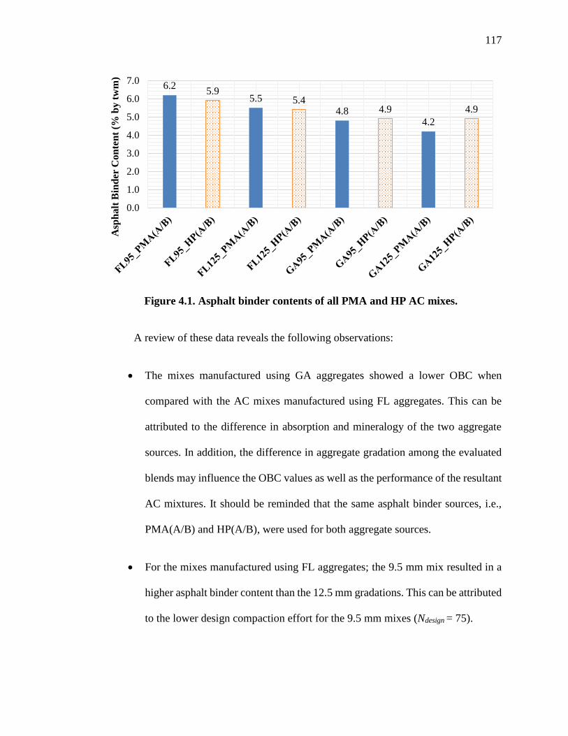
117
Figure 4.1. Asphalt binder contents of all PMA and HP AC mixes.
A review of these data reveals the following observations:
• The mixes manufactured using GA aggregates showed a lower OBC when
compared with the AC mixes manufactured using FL aggregates. This can be
attributed to the difference in absorption and mineralogy of the two aggregate
sources. In addition, the difference in aggregate gradation among the evaluated
blends may influence the OBC values as well as the performance of the resultant
AC mixtures. It should be reminded that the same asphalt binder sources, i.e.,
PMA(A/B) and HP(A/B), were used for both aggregate sources.
• For the mixes manufactured using FL aggregates; the 9.5 mm mix resulted in a
higher asphalt binder content than the 12.5 mm gradations. This can be attributed
to the lower design compaction effort for the 9.5 mm mixes (Ndesign = 75).
6.25.9
5.5 5.44.8 4.9
4.2
4.9
0.0
1.0
2.0
3.0
4.0
5.0
6.0
7.0
Asp
ha
lt B
ind
er C
on
ten
t (%
by
tw
m)

118
• For the mixes manufactured using FL aggregates; the 9.5 mm and 12.5 mm HP
mixes resulted in slightly lower binder contents than the 9.5 and 12.5 mm PMA
mixes. It should be mentioned that same aggregate gradation was maintained for
each of the 9.5 mm and 12.5 mm mixes when manufactured using PMA and HP
asphalt binders for the FL aggregate source.
• For the PMA mixes manufactured using GA aggregates; the 12.5 mm mixes
resulted in lower asphalt binder contents than the 9.5 mm mixes.
• The 9.5 and 12.5 mm HP mixes manufactured using GA aggregates resulted in
similar OBC (i.e., 4.9%) which is higher than the OBC observed for their
respective PMA control mixes. It should be mentioned that the 9.5 and 12.5 mm
HP using the GA aggregates do not contain any RAP materials because RAP is
not allowed in HP mixtures per FDOT specifications (FDOT Specifications,
2018).
In addition to the specifications listed in Table 4.2, all designed mixtures were
evaluated in terms of their resistance to moisture damage. Six to eight samples from each
mix were prepared at OBC and short-term aged for two hours at the compaction
temperature according to FM 1-T 283 (FM 1-T 283, 2018) and AASHTO T283 (AASHTO
T283, 2014). The aged samples were compacted in the Superpave Gyratory Compactor
(SGC) to a target air void of 7±1%. The compacted samples were then split into two sets
of 3-4 samples: one set was un-conditioned, and the other set was moisture-conditioned.
The samples in each set were selected to achieve similar average air voids. For the
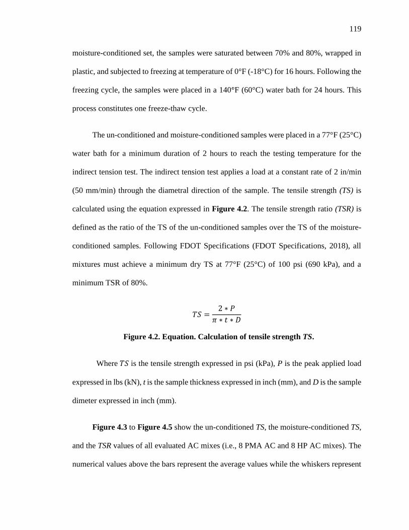
119
moisture-conditioned set, the samples were saturated between 70% and 80%, wrapped in
plastic, and subjected to freezing at temperature of 0°F (-18°C) for 16 hours. Following the
freezing cycle, the samples were placed in a 140°ۥF (60°C) water bath for 24 hours. This
process constitutes one freeze-thaw cycle.
The un-conditioned and moisture-conditioned samples were placed in a 77°F (25°C)
water bath for a minimum duration of 2 hours to reach the testing temperature for the
indirect tension test. The indirect tension test applies a load at a constant rate of 2 in/min
(50 mm/min) through the diametral direction of the sample. The tensile strength (TS) is
calculated using the equation expressed in Figure 4.2. The tensile strength ratio (TSR) is
defined as the ratio of the TS of the un-conditioned samples over the TS of the moisture-
conditioned samples. Following FDOT Specifications (FDOT Specifications, 2018), all
mixtures must achieve a minimum dry TS at 77°F (25°C) of 100 psi (690 kPa), and a
minimum TSR of 80%.
𝑇𝑆 =2 ∗ 𝑃
𝜋 ∗ 𝑡 ∗ 𝐷
Figure 4.2. Equation. Calculation of tensile strength TS.
Where 𝑇𝑆 is the tensile strength expressed in psi (kPa), P is the peak applied load
expressed in lbs (kN), t is the sample thickness expressed in inch (mm), and D is the sample
dimeter expressed in inch (mm).
Figure 4.3 to Figure 4.5 show the un-conditioned TS, the moisture-conditioned TS,
and the TSR values of all evaluated AC mixes (i.e., 8 PMA AC and 8 HP AC mixes). The
numerical values above the bars represent the average values while the whiskers represent

120
the 95% confidence interval (CI). An overlap in the CI’s indicates statistically similar
properties of the mixtures. A review of the provided data reveals the following
observations:
• Regardless of aggregate source (i.e., FL and GA) and asphalt binder type (i.e., PMA
and HP), all evaluated mixtures met the FDOT criteria in terms of minimum TS and
TSR for indicating a good resistance to moisture damage.
• Regardless of aggregate source, all HP mixes exhibited lower un-conditioned and
moisture-conditioned TS values when compared with their corresponding control
PMA AC mixes indicating a less stiff behavior of the HP mix at intermediate
temperature of 77°F (25°C).
• Regardless of aggregate source, the HP AC mixes manufactured with binder source
B exhibited slightly lower un-conditioned TS values when compared with HP AC
mixes manufactured using HP binder from source A. The same observation can be
made for the moisture-conditioned TS of all HP AC mixes except for the
FL125_HP(B) mix that exhibited slightly higher moisture-conditioned TS.
• The PMA AC mixes manufactured using GA aggregates exhibited significantly
higher un-conditioned and moisture-conditioned TS values than the PMA AC mixes
manufactured using FL aggregates. This can be attributed to the stiffening effect
from the RAP material used in the GA_PMA AC mixes.
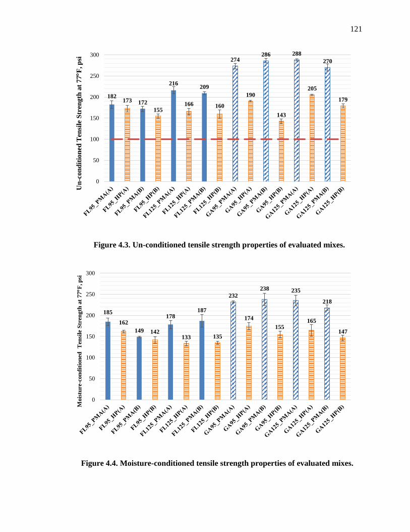
121
Figure 4.3. Un-conditioned tensile strength properties of evaluated mixes.
Figure 4.4. Moisture-conditioned tensile strength properties of evaluated mixes.
182173 172
155
216
166
209
160
274
190
286
143
288
205
270
179
0
50
100
150
200
250
300
Un
-co
nd
itio
ned
Ten
sile
Str
eng
th a
t 7
7F
, p
si
185
162
149 142
178
133
187
135
232
174
238
155
235
165
218
147
0
50
100
150
200
250
300
Mois
ture
-con
dit
ion
ed
Ten
sile
Str
eng
th a
t 7
7F
, p
si

122
Figure 4.5. Tensile strength ratios of evaluated mixes.
4.2 Performance Test Results and Analysis
The 16 designed mixtures (i.e., 8 PMA and 8 HP AC mixes) were evaluated at their
respective OBC for their engineering properties in terms of the dynamic modulus property
(E*), rutting characteristics in terms of resistance to permanent strains in triaxial testing,
fatigue cracking characteristics in terms of resistance to flexural bending strains, top-down
cracking characteristics in terms of resistance to tensile strains, and reflective cracking
characteristics in terms of resistance to crack propagation. Table 4.7 summarizes the
laboratory tests that were conducted to evaluate the engineering properties and
performance characteristics of the AC mixes listed in Table 4.1.
10094
8692
83 81
8985 85
91
83
100
82 80 81 82
0
10
20
30
40
50
60
70
80
90
100
Ten
sile
Str
eng
th R
ati
o, %

123
Table 4.7. Summary of Laboratory Evaluation Program.
Engineering
Property/
Distress
Mode
Standard Method/
Practice Measured Property
Laboratory
Conditioning
Number of
Replicates
Dynamic
Modulus
AASHTO T378
AASHTO R84 E* Master Curve Short-term oven aging 2
Rutting AASHTO R83 (εp/εr) vs. (Nr, T)
Rutting Model Short-term oven aging
2 per
temperature
Shoving1 NA2 NA2 NA2 NA2
Fatigue
Cracking
ASTM D7460
AASHTO T321
Nf vs. (εt, E)
Fatigue Model Long-term oven aging
Minimum of
3 strains per
temperature
Top-Down
Cracking
AASHTO T322
NCHRP 9-57 Appendix G DCSE, ER Long-term oven aging 2
Reflective
Cracking TxDOT Tex-248-F
Cycles to Failure
Fracture Parameters
(A, n)
Short-term oven aging 3
1will be evaluated through the mechanistic modeling of flexible pavements. 2Not applicable.
All the engineering properties and performance characteristics were evaluated at
the short-term aging condition except for the fatigue and top-down cracking since both are
considered to be long-term distresses. Short-term aging consisted of curing loose mixtures
at a temperature of 275°F (135°C) in a forced-draft laboratory oven for 4 hours prior to
compaction in accordance with AASHTO R30 (AASHTO R30, 2002). In the case of
fatigue and top-down cracking, the compacted specimens were long-term aged at a
temperature of 185°F (85°C) in a forced-draft oven for 5 days.
4.2.1 Dynamic Modulus Test
The E* property provides an indication on the overall quality of the asphalt mixture. The
magnitude of the E* depends on several properties of the mixture including; aggregate
properties, gradation, asphalt binder grade, mix volumetrics, and age. The magnitude of E*
also depends on temperature and rate of loading (i.e., frequency). Figure 4.6 to Figure
4.13 show the E* master curves of all 16 evaluated mixes constructed at a reference
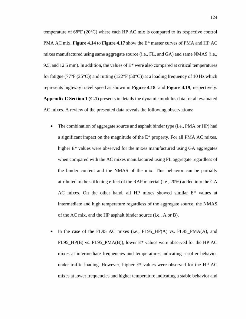
124
temperature of 68°F (20°C) where each HP AC mix is compared to its respective control
PMA AC mix. Figure 4.14 to Figure 4.17 show the E* master curves of PMA and HP AC
mixes manufactured using same aggregate source (i.e., FL, and GA) and same NMAS (i.e.,
9.5, and 12.5 mm). In addition, the values of E* were also compared at critical temperatures
for fatigue (77°F (25°C)) and rutting (122°F (50°C)) at a loading frequency of 10 Hz which
represents highway travel speed as shown in Figure 4.18 and Figure 4.19, respectively.
Appendix C Section 1 (C.1) presents in details the dynamic modulus data for all evaluated
AC mixes. A review of the presented data reveals the following observations:
• The combination of aggregate source and asphalt binder type (i.e., PMA or HP) had
a significant impact on the magnitude of the E* property. For all PMA AC mixes,
higher E* values were observed for the mixes manufactured using GA aggregates
when compared with the AC mixes manufactured using FL aggregate regardless of
the binder content and the NMAS of the mix. This behavior can be partially
attributed to the stiffening effect of the RAP material (i.e., 20%) added into the GA
AC mixes. On the other hand, all HP mixes showed similar E* values at
intermediate and high temperature regardless of the aggregate source, the NMAS
of the AC mix, and the HP asphalt binder source (i.e., A or B).
• In the case of the FL95 AC mixes (i.e., FL95_HP(A) vs. FL95_PMA(A), and
FL95_HP(B) vs. FL95_PMA(B)), lower E* values were observed for the HP AC
mixes at intermediate frequencies and temperatures indicating a softer behavior
under traffic loading. However, higher E* values were observed for the HP AC
mixes at lower frequencies and higher temperature indicating a stable behavior and

125
high rutting resistance under slow traffic loading.
• In the case of the FL125 AC mixes (i.e., FL125_HP(A) vs. FL125_PMA(A), and
FL125_HP(B) vs. FL125_PMA(B)), lower E* values were observed for the HP AC
mixes at intermediate frequency and temperature indicating a softer behavior under
traffic loading. On the other hand, slightly lower E* values were observed for the
HP AC mixes at much lower and higher frequencies simulating lower and higher
temperatures, respectively.
• In the case of the GA95 and GA125 AC mixes, significantly lower E* values were
observed for the HP mixes at all temperatures and frequencies when compared with
their corresponding GA PMA AC control mixes. This can be partially attributed to
the stiffer behavior of the GA PMA AC mixes containing 20% RAP.
Figure 4.6. E* master curves of FL95_PMA(A) and FL95_HP(A) at 68°F (20°C).
1
10
100
1,000
10,000
1.E-06 1.E-04 1.E-02 1.E+00 1.E+02 1.E+04 1.E+06
Dy
na
mic
Mo
du
lus
E* a
t 68
°F (
20
°C),
ksi
Reduced Frequency (Hz)
FL95_PMA(A)
FL95_HP(A)

126
Figure 4.7. E* master curves of FL95_PMA(B) and FL95_HP(B) at 68°F (20°C).
Figure 4.8. E* master curves of FL125_PMA(A) and FL125_HP(A) at 68°F (20°C).
1
10
100
1000
10000
1.E-06 1.E-04 1.E-02 1.E+00 1.E+02 1.E+04 1.E+06
Dy
na
mic
Mo
du
lus
E*
at
68
°F (
20
°C),
ksi
Reduced Frequency (Hz)
FL95_PMA(B)
FL95_HP(B)
1
10
100
1000
10000
1.E-06 1.E-04 1.E-02 1.E+00 1.E+02 1.E+04 1.E+06
Dy
na
mic
Mod
ulu
s E
* a
t 68
°F (
20
°C),
ksi
Reduced Frequency (Hz)
FL125_PMA(A)
FL125_HP(A)

127
Figure 4.9. E* master curves of FL125_PMA(B) and FL125_HP(B) at 68°F (20°C).
Figure 4.10. E* master curves of GA95_PMA(A) and GA95_HP(A) at 68°F (20°C).
1
10
100
1000
10000
1.E-06 1.E-04 1.E-02 1.E+00 1.E+02 1.E+04 1.E+06
Dy
na
mic
Mo
du
lus
E*
at
68
°F (
20
°C),
ksi
Reduced Frequency (Hz)
FL125_PMA(B)
FL125_HP(B)
1
10
100
1000
10000
1.E-06 1.E-04 1.E-02 1.E+00 1.E+02 1.E+04 1.E+06
Dy
na
mic
Mod
ulu
s E
* a
t 68
°F (
20
°C),
ksi
Reduced Frequency (Hz)
GA95_PMA(A)
GA95_HP(A)
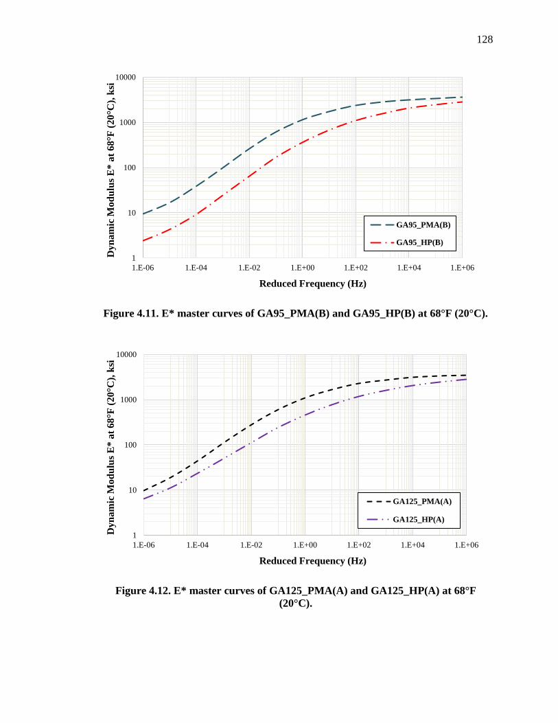
128
Figure 4.11. E* master curves of GA95_PMA(B) and GA95_HP(B) at 68°F (20°C).
Figure 4.12. E* master curves of GA125_PMA(A) and GA125_HP(A) at 68°F
(20°C).
1
10
100
1000
10000
1.E-06 1.E-04 1.E-02 1.E+00 1.E+02 1.E+04 1.E+06
Dy
na
mic
Mo
du
lus
E*
at
68
°F (
20
°C),
ksi
Reduced Frequency (Hz)
GA95_PMA(B)
GA95_HP(B)
1
10
100
1000
10000
1.E-06 1.E-04 1.E-02 1.E+00 1.E+02 1.E+04 1.E+06
Dy
na
mic
Mod
ulu
s E
* a
t 68
°F (
20
°C),
ksi
Reduced Frequency (Hz)
GA125_PMA(A)
GA125_HP(A)

129
Figure 4.13. E* master curves of GA125_PMA(B) and GA125_HP(B) at 68°F
(20°C).
Figure 4.14. E* master curves of all evaluated FL95 AC mixes at 68°F (20°C).
1
10
100
1000
10000
1.E-06 1.E-04 1.E-02 1.E+00 1.E+02 1.E+04 1.E+06
Dy
na
mic
Mo
du
lus
E*
at
68
°F (
20
°C),
ksi
Reduced Frequency (Hz)
GA125_PMA(B)
GA125_HP(B)
1
10
100
1000
10000
1.E-06 1.E-04 1.E-02 1.E+00 1.E+02 1.E+04 1.E+06
Dy
na
mic
Mo
du
lus
E* a
t 68
°F (
20
°C),
ksi
Reduced Frequency (Hz)
FL95_PMA(A)
FL95_PMA(B)
FL95_HP(A)
FL95_HP(B)

130
Figure 4.15. E* master curves of all evaluated FL125 AC mixes at 68°F (20°C).
Figure 4.16. E* master curves of all evaluated GA95 AC mixes at 68°F (20°C).
1
10
100
1000
10000
1.E-06 1.E-04 1.E-02 1.E+00 1.E+02 1.E+04 1.E+06
Dy
na
mic
Mo
du
lus
E*
at
68
°F (
20
°C),
ksi
Reduced Frequency (Hz)
FL125_PMA(A)
FL125_PMA(B)
FL125_HP(A)
FL125_HP(B)
1
10
100
1000
10000
1.E-06 1.E-04 1.E-02 1.E+00 1.E+02 1.E+04 1.E+06
Dy
na
mic
Mod
ulu
s E
* a
t 68
°F (
20
°C),
ksi
Reduced Frequency (Hz)
GA95_PMA(A)
GA95_PMA(B)
GA95_HP(A)
GA95_HP(B)

131
Figure 4.17. E* master curves of all evaluated GA125 AC mixes at 68°F (20°C).
Figure 4.18. E* values at 10 Hz and 77°F (25°C) of all evaluated AC mixes.
1
10
100
1000
10000
1.E-06 1.E-04 1.E-02 1.E+00 1.E+02 1.E+04 1.E+06
Dy
na
mic
Mo
du
lus
E*
at
68
°F (
20
°C),
ksi
Reduced Frequency (Hz)
GA125_PMA(A)
GA125_PMA(B)
GA125_HP(A)
GA125_HP(B)
678
477
716
386
751
446
819
479
1,225
485
1,393
488
1,329
567
1,412
532
0
200
400
600
800
1,000
1,200
1,400
1,600
Dy
na
mic
Mod
ulu
s at
77
°F (
25
°C)
an
d 1
0
Hz,
ksi

132
Figure 4.19. E* values at 10 Hz and 122°F (50°C) of all evaluated AC mixes.
4.2.2 Rutting
RLT test was used to evaluate the rutting behavior of the 16 AC mixes under repeated
loading. The permanent (εp) and resilient (εr) axial strains were measured during the RLT
test as a function of the number of loading repetitions. The resulting cumulative permanent
axial strain over the resilient strain (εp/εr) was plotted versus the number of load repetitions
(N) to determine the rutting behavior of the evaluated asphalt mixtures at each of the three
tested temperatures. The rutting relationship (εp/εr versus N) indicates the response of the
asphalt mixture to the repeated loading at high temperature. A lower relationship indicates
lower accumulated permanent strains with loading, thus predicting a better resistance to
rutting. Furthermore, a flatter curve indicates a lower susceptibility of the asphalt mixture
to repeated loading. Figure 4.20 to Figure 4.23 show the rutting relationships of the PMA
76 8090
52
109
69
118
49
171
54
221
59
217
80
242
65
0
50
100
150
200
250
300
Dy
na
mic
Mo
du
lus
at
12
2°F
(5
0°C
) a
nd
10
Hz,
ksi
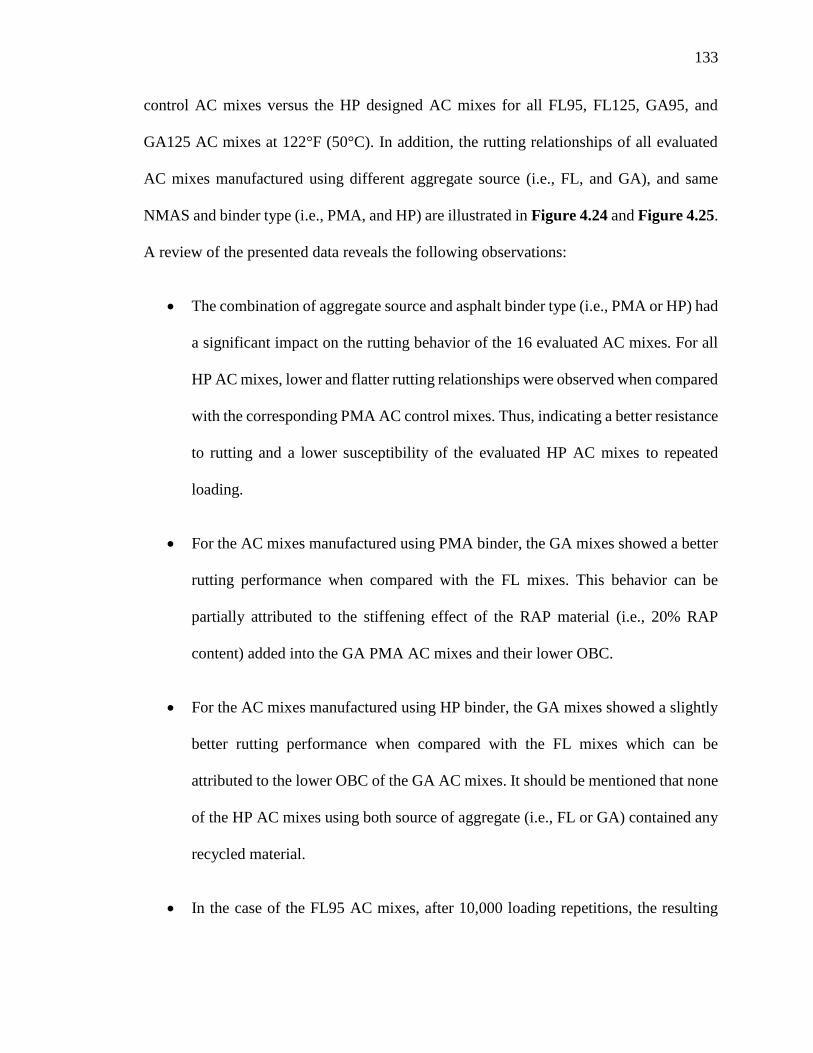
133
control AC mixes versus the HP designed AC mixes for all FL95, FL125, GA95, and
GA125 AC mixes at 122°F (50°C). In addition, the rutting relationships of all evaluated
AC mixes manufactured using different aggregate source (i.e., FL, and GA), and same
NMAS and binder type (i.e., PMA, and HP) are illustrated in Figure 4.24 and Figure 4.25.
A review of the presented data reveals the following observations:
• The combination of aggregate source and asphalt binder type (i.e., PMA or HP) had
a significant impact on the rutting behavior of the 16 evaluated AC mixes. For all
HP AC mixes, lower and flatter rutting relationships were observed when compared
with the corresponding PMA AC control mixes. Thus, indicating a better resistance
to rutting and a lower susceptibility of the evaluated HP AC mixes to repeated
loading.
• For the AC mixes manufactured using PMA binder, the GA mixes showed a better
rutting performance when compared with the FL mixes. This behavior can be
partially attributed to the stiffening effect of the RAP material (i.e., 20% RAP
content) added into the GA PMA AC mixes and their lower OBC.
• For the AC mixes manufactured using HP binder, the GA mixes showed a slightly
better rutting performance when compared with the FL mixes which can be
attributed to the lower OBC of the GA AC mixes. It should be mentioned that none
of the HP AC mixes using both source of aggregate (i.e., FL or GA) contained any
recycled material.
• In the case of the FL95 AC mixes, after 10,000 loading repetitions, the resulting

134
cumulative εp/εr of the FL95_PMA(A) and FL95_PMA(B) AC mixes were 6.2 and
18.9 times greater than the values of the FL95_HP(A) and FL95_HP(B) AC mixes,
respectively.
• In the case of the FL125 AC mixes, after 10,000 loading repetitions, the resulting
cumulative εp/εr of the FL125_PMA(A) and FL125_PMA(B) AC mixes were 8.6
and 5.6 times greater than the values of the FL125_HP(A) and FL125_HP(B) AC
mixes, respectively.
• In the case of the GA95 AC mixes, after 10,000 loading repetitions, the resulting
cumulative εp/εr of the GA95_PMA(A) and GA95_PMA(B) AC mixes were 2.6
and 2.7 times greater than the values of the GA95_HP(A) and GA95_HP(B) AC
mixes, respectively. These ratios are lower than the ones corresponding to the FL95
mixes mainly because of the stiffer behavior of GA95 PMA AC mixes containing
20% RAP.
• Similarly, in the case of the GA125 AC mixes, after 10,000 loading repetitions, the
resulting cumulative εp/εr of the GA125_PMA(A) and GA125_PMA(B) AC mixes
are 3.9 and 2.7 times greater than the values of the G125_HP(A) and GA125_HP(B)
AC mixes, respectively. These ratios remain lower than the ones corresponding to
the FL125 mixes given the stiffer behavior of the GA125 PMA AC mixes also
containing 20% RAP.
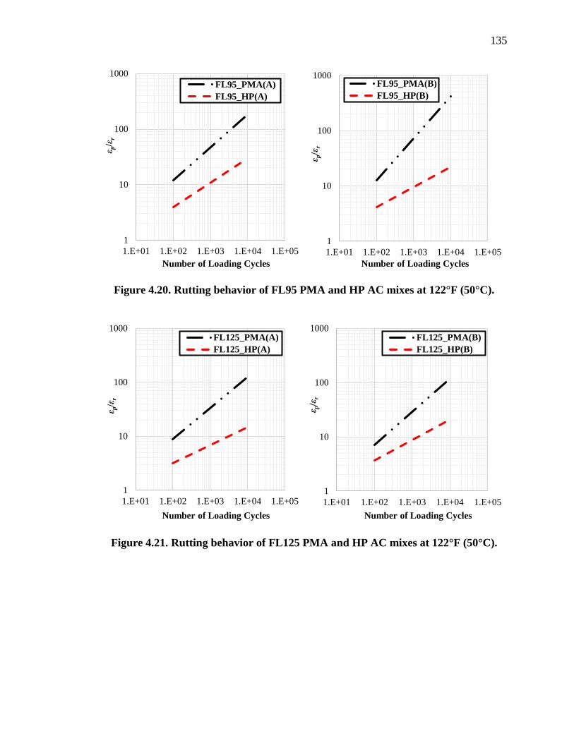
135
Figure 4.20. Rutting behavior of FL95 PMA and HP AC mixes at 122°F (50°C).
Figure 4.21. Rutting behavior of FL125 PMA and HP AC mixes at 122°F (50°C).
1
10
100
1000
1.E+01 1.E+02 1.E+03 1.E+04 1.E+05
ε p/ε
r
Number of Loading Cycles
FL95_PMA(A)
FL95_HP(A)
1
10
100
1000
1.E+01 1.E+02 1.E+03 1.E+04 1.E+05
ε p/ε
r
Number of Loading Cycles
FL95_PMA(B)
FL95_HP(B)
1
10
100
1000
1.E+01 1.E+02 1.E+03 1.E+04 1.E+05
ε p/ε
r
Number of Loading Cycles
FL125_PMA(A)
FL125_HP(A)
1
10
100
1000
1.E+01 1.E+02 1.E+03 1.E+04 1.E+05
ε p/ε
r
Number of Loading Cycles
FL125_PMA(B)
FL125_HP(B)

136
Figure 4.22. Rutting behavior of GA95 PMA and HP AC mixes at 122°F (50°C).
Figure 4.23. Rutting behavior of GA125 PMA and HP AC mixes at 122°F (50°C).
1
10
100
1000
1.E+01 1.E+02 1.E+03 1.E+04 1.E+05
ε p/ε
r
Number of Loading Cycles
GA95_PMA(A)
GA95_HP(A)
1
10
100
1000
1.E+01 1.E+02 1.E+03 1.E+04 1.E+05
ε p/ε
r
Number of Loading Cycles
GA95_PMA(B)
GA95_HP(B)
1
10
100
1000
1.E+01 1.E+02 1.E+03 1.E+04 1.E+05
ε p/ε
r
Number of Loading Cycles
GA125_PMA(A)
GA95_HP(A)
1
10
100
1000
1.E+01 1.E+02 1.E+03 1.E+04 1.E+05
εp/ε
r
Number of Loading Cycles
GA125_PMA(B)
GA95_HP(B)
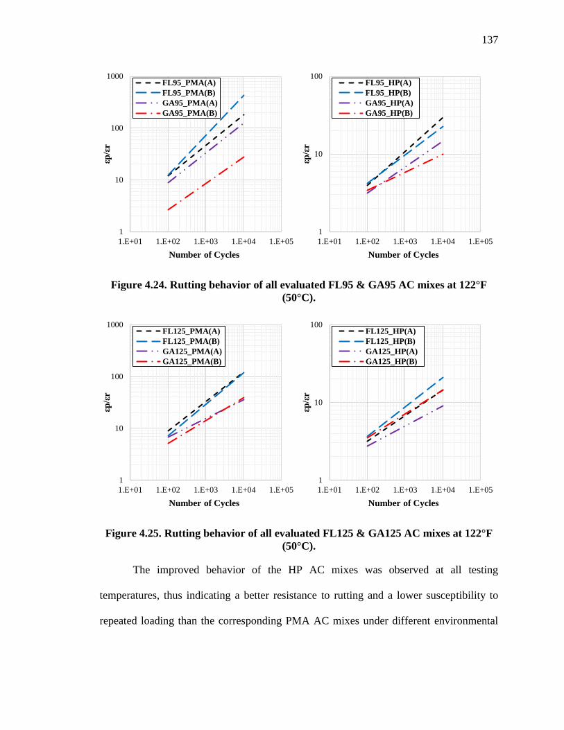
137
Figure 4.24. Rutting behavior of all evaluated FL95 & GA95 AC mixes at 122°F
(50°C).
Figure 4.25. Rutting behavior of all evaluated FL125 & GA125 AC mixes at 122°F
(50°C).
The improved behavior of the HP AC mixes was observed at all testing
temperatures, thus indicating a better resistance to rutting and a lower susceptibility to
repeated loading than the corresponding PMA AC mixes under different environmental
1
10
100
1000
1.E+01 1.E+02 1.E+03 1.E+04 1.E+05
εp/ε
r
Number of Cycles
FL95_PMA(A)
FL95_PMA(B)
GA95_PMA(A)
GA95_PMA(B)
1
10
100
1.E+01 1.E+02 1.E+03 1.E+04 1.E+05
εp/ε
r
Number of Cycles
FL95_HP(A)
FL95_HP(B)
GA95_HP(A)
GA95_HP(B)
1
10
100
1000
1.E+01 1.E+02 1.E+03 1.E+04 1.E+05
εp/ε
r
Number of Cycles
FL125_PMA(A)
FL125_PMA(B)
GA125_PMA(A)
GA125_PMA(B)
1
10
100
1.E+01 1.E+02 1.E+03 1.E+04 1.E+05
εp/ε
r
Number of Cycles
FL125_HP(A)
FL125_HP(B)
GA125_HP(A)
GA125_HP(B)

138
conditions. The noticeably better rutting relationship of the HP AC mixes (i.e., lower and
flatter curve) can be mainly attributed to the dominant behavior of the additional polymer.
Appendix C Section 2 (C.2) presents in detail the RLT test data for the 8 PMA and 8 HP
AC mixes. Table 4.8 summarizes the regression coefficients of the rutting models for the
evaluated AC mixes based on the approach recommended in AASHTO Mechanistic-
Empirical Pavement Design Guide (MEPDG).
Table 4.8. Summary of Rutting Model Coefficients for All Evaluated AC Mixes.
Mix ID Rutting Model Coefficients1
kr1 kf2 kf3
FL95_PMA(A) -12.4119 6.0735 0.4392
FL95_PMA(B) -15.4928 7.4574 0.5271
FL125_PMA(A) -14.2043 6.9175 0.4150
FL125_PMA(B) -10.7155 5.2287 0.4258
GA95_PMA(A) -18.8804 9.0534 0.3564
GA95_PMA(B) -13.7764 6.6140 0.3419
GA125_PMA(A) -11.4447 5.5212 0.3763
GA125_PMA(B) -21.5617 10.2064 0.4705
FL95_HP(A) -10.1818 4.8451 0.3992
FL95_HP(B) -6.1192 2.9910 0.2844
FL125_HP(A) -4.8104 2.4349 0.3113
FL125_HP(B) -12.8649 6.0716 0.3624
GA95_HP(A) -5.7850 2.6766 0.3280
GA95_HP(B) -6.3657 3.1349 0.2196
GA125_HP(A) -11.7157 5.5731 0.2401
GA125_HP(B) -9.0008 4.3241 0.2974 1 ԑ𝑝
ԑ𝑟= 𝐾𝑧 ∗ 𝛽𝑟1 ∗ 10𝑘𝑟1 ∗ (𝑇)𝛽𝑟2∗𝑘𝑟2 ∗ (𝑁)𝛽𝑟3∗𝑘𝑟3
4.2.3 Fatigue Cracking
The fatigue characteristics of the 16 AC mixes (i.e., 8 PMA and 8 HP AC mixes) were
evaluated using the flexural beam fatigue test in accordance with ASTM D7460 (ASTM
D7460, 2010) and AASHTO T321 (AASHTO T321, 2017) at three temperatures and
multiple strain levels. A fatigue curve at each testing temperature was developed for every

139
AC mix (i.e., PMA and HP AC mix) by fitting a power regression function between the
number of cycles to failure and the applied strain levels. Figure 4.26 to Figure 4.29 shows
the fatigue relationships for all evaluated AC mixes at 77°F (25°C). A higher and flatter
fatigue curve indicates a better resistance to fatigue cracking. A review of the presented
data reveals the following observations:
• The combination of aggregate source and asphalt binder type (i.e., PMA or HP) had
a significant impact on the fatigue behavior of the evaluated AC mixes. For all HP
AC mixes, better fatigue relationships were observed when compared with the
corresponding PMA AC control mixes at all strain levels and testing temperatures;
thus, indicating increased flexibility and resistance to fatigue cracking of the HP
AC mixes under different environmental conditions. The noticeably better fatigue
relationship for the HP AC mixes can be mainly attributed to the dominant behavior
of the additional polymer.
• For the AC mixes manufactured using PMA binder, the FL mixes showed a better
fatigue performance when compared with the GA mixes. This behavior can be
partially attributed to the stiffening effect of the RAP material added into the GA
PMA AC mixes and their lower OBC.
• For the AC mixes manufactured using HP binder, the FL mixes showed a slightly
better fatigue performance when compared with the GA mixes which can be
attributed to the higher OBC of the FL AC mixes. It should be mentioned that none
of the HP AC mixes using both source of aggregate (i.e., FL or GA) contained any
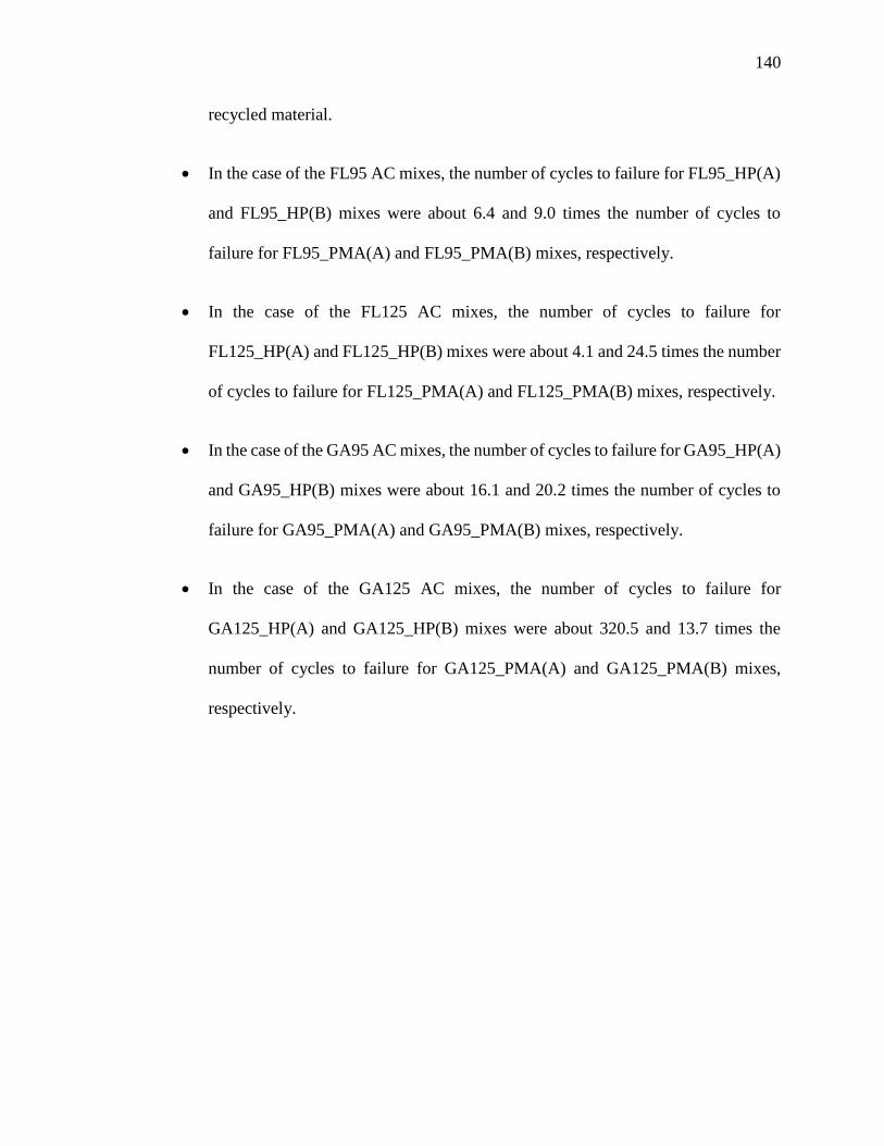
140
recycled material.
• In the case of the FL95 AC mixes, the number of cycles to failure for FL95_HP(A)
and FL95_HP(B) mixes were about 6.4 and 9.0 times the number of cycles to
failure for FL95_PMA(A) and FL95_PMA(B) mixes, respectively.
• In the case of the FL125 AC mixes, the number of cycles to failure for
FL125_HP(A) and FL125_HP(B) mixes were about 4.1 and 24.5 times the number
of cycles to failure for FL125_PMA(A) and FL125_PMA(B) mixes, respectively.
• In the case of the GA95 AC mixes, the number of cycles to failure for GA95_HP(A)
and GA95_HP(B) mixes were about 16.1 and 20.2 times the number of cycles to
failure for GA95_PMA(A) and GA95_PMA(B) mixes, respectively.
• In the case of the GA125 AC mixes, the number of cycles to failure for
GA125_HP(A) and GA125_HP(B) mixes were about 320.5 and 13.7 times the
number of cycles to failure for GA125_PMA(A) and GA125_PMA(B) mixes,
respectively.

141
Figure 4.26. Fatigue relationships of FL95 AC mixes at 77°F (25°C).
Figure 4.27. Fatigue relationships of FL125 AC mixes at 77°F (25°C).
10
100
1000
10000
1.E+03 1.E+05 1.E+07 1.E+09
Fle
xu
ral
Str
ain
Lev
el (
Mic
rost
rain
)
Number of Cycles to Failure
FL95_PMA(A)
FL95_HP(A)
10
100
1000
10000
1.E+03 1.E+05 1.E+07 1.E+09
Fle
xu
ral
Str
ain
Lev
el (
Mic
rost
rain
)
Number of Cycles to Failure
FL95_PMA(B)
FL95_HP(B)
10
100
1000
10000
1.E+03 1.E+05 1.E+07 1.E+09
Fle
xu
ral
Str
ain
Lev
el (
Mic
rost
rain
)
Number of Cycles to Failure
FL125_PMA(A)
FL125_HP(A)10
100
1000
10000
1.E+03 1.E+05 1.E+07 1.E+09
Fle
xu
ral
Str
ain
Lev
el (
Mic
rost
rain
)
Number of Cycles to Failure
FL125_PMA(B)
FL125_HP(B)

142
Figure 4.28. Fatigue relationships of GA95 AC mixes at 77°F (25°C).
Figure 4.29. Fatigue relationships of GA125 AC mixes at 77°F (25°C).
10
100
1000
10000
1.E+03 1.E+05 1.E+07 1.E+09
Fle
xu
ral
Str
ain
Lev
el (
Mic
rost
rain
)
Number of Cycles to Failure
GA95_PMA(A)
GA95_HP(A)
10
100
1000
10000
1.E+03 1.E+05 1.E+07 1.E+09
Fle
xu
ral
Str
ain
Lev
el (
Mic
rost
rain
)
Number of Cycles to Failure
GA95_PMA(B)
GA95_HP(B)
10
100
1000
10000
1.E+03 1.E+05 1.E+07 1.E+09
Fle
xu
ral
Str
ain
Lev
el (
Mic
ro-s
tra
in)
Number of Cycles to Failure
GA125_PMA(A)
GA125_HP(A)
10
100
1000
10000
1.E+03 1.E+05 1.E+07 1.E+09
Fle
xu
ral
Str
ain
Lev
el (
Mic
ro-s
tra
in)
Number of Cycles to Failure
GA125_PMA(B)
GA125_HP(B)
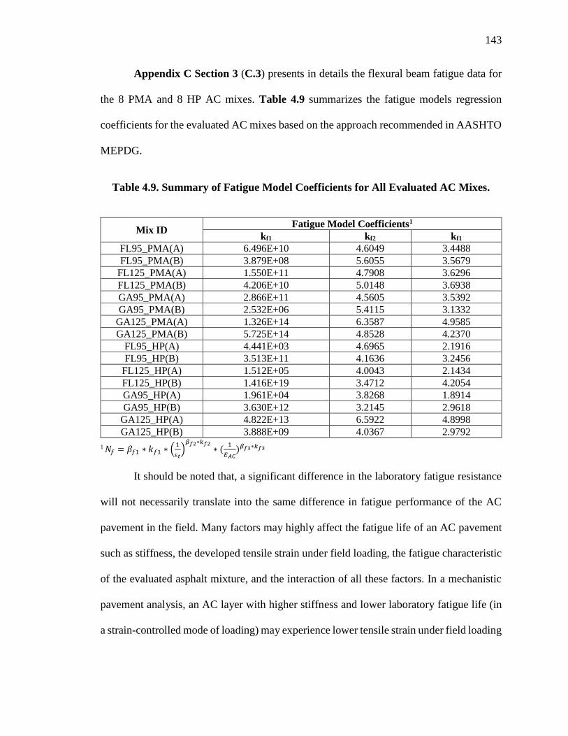
143
Appendix C Section 3 (C.3) presents in details the flexural beam fatigue data for
the 8 PMA and 8 HP AC mixes. Table 4.9 summarizes the fatigue models regression
coefficients for the evaluated AC mixes based on the approach recommended in AASHTO
MEPDG.
Table 4.9. Summary of Fatigue Model Coefficients for All Evaluated AC Mixes.
Mix ID Fatigue Model Coefficients1
kf1 kf2 kf1
FL95_PMA(A) 6.496E+10 4.6049 3.4488
FL95_PMA(B) 3.879E+08 5.6055 3.5679
FL125_PMA(A) 1.550E+11 4.7908 3.6296
FL125_PMA(B) 4.206E+10 5.0148 3.6938
GA95_PMA(A) 2.866E+11 4.5605 3.5392
GA95_PMA(B) 2.532E+06 5.4115 3.1332
GA125_PMA(A) 1.326E+14 6.3587 4.9585
GA125_PMA(B) 5.725E+14 4.8528 4.2370
FL95_HP(A) 4.441E+03 4.6965 2.1916
FL95_HP(B) 3.513E+11 4.1636 3.2456
FL125_HP(A) 1.512E+05 4.0043 2.1434
FL125_HP(B) 1.416E+19 3.4712 4.2054
GA95_HP(A) 1.961E+04 3.8268 1.8914
GA95_HP(B) 3.630E+12 3.2145 2.9618
GA125_HP(A) 4.822E+13 6.5922 4.8998
GA125_HP(B) 3.888E+09 4.0367 2.9792
1 𝑁𝑓 = 𝛽𝑓1 ∗ 𝑘𝑓1 ∗ (1
ԑ𝑡)
𝛽𝑓2∗𝑘𝑓2∗ (
1
𝐸𝐴𝐶)𝛽𝑓3∗𝑘𝑓3
It should be noted that, a significant difference in the laboratory fatigue resistance
will not necessarily translate into the same difference in fatigue performance of the AC
pavement in the field. Many factors may highly affect the fatigue life of an AC pavement
such as stiffness, the developed tensile strain under field loading, the fatigue characteristic
of the evaluated asphalt mixture, and the interaction of all these factors. In a mechanistic
pavement analysis, an AC layer with higher stiffness and lower laboratory fatigue life (in
a strain-controlled mode of loading) may experience lower tensile strain under field loading

144
and result in a longer pavement fatigue life. Therefore, a full mechanistic analysis would
be necessary to effectively evaluate the impact of HP binder on fatigue performance of the
corresponding AC pavement.
4.2.4 Top-Down Cracking
The resistance to top-down cracking of the 16 AC mixes (i.e., 8 PMA and 8 HP AC mixes)
were evaluated using the IDT test in accordance with AASHTO T312 (AASHTO T312,
2007) and Appendix G of the NCHRP 9-57 study (NCHRP 9-57, 2016) at 50°F (10°C).
The IDT test specimens were short-term aged followed by long-term aging (AASHTO
R30, 2002). The creep compliance parameters (i.e., D1, and m) of the 16 AC mixes were
determined using the tensile creep compliance test. In addition, the mixture failure strain
(εf) and the dissipated creep strain energy density failure limit (DSCEf) were determined
using the tensile fracture test. Table 4.10 summarizes top-down cracking properties for the
16 AC mixes. The following are some of the challenges that were faced as part of the test
which should be kept in mind when examining the test results.
• The Jig and associated instrumentations used for IDT testing which was mounted
into the AMPT Pro is still under verification and improvement by the equipment
supplier.
• The extensometers connected to the testing specimens were highly sensitive and
susceptible to bending with the increase in load amplitude.
• The IDT creep compliance test and tensile fracture test had to be conducted as two
separate tests for the software to properly record the required data.
145
• Some extensometers stopped working during testing of some test specimens. Thus,
some of the test results were based on one extensometer and/or one face of the test
specimen.
A review of the presented data in Table 4.10 reveals the following observations:
• The combination of aggregate source and asphalt binder type (i.e., PMA or HP) had
an impact on the test results of the evaluated AC mixes. A lower D1 is an indicator
of a lower creep stiffness for the evaluated AC mix. A higher m value is an indicator
of a higher susceptibility of the mix to creep as a function of time. For all HP AC
mixes, lower m values were observed when compared with the respective PMA AC
mixes.
• For the AC mixes manufactured using PMA binders, the FL mixes showed higher
D1 values when compared with the GA mixes. This behavior for the GA mixes can
be attributed to both, the lower OBC and the stiffening of the mix as a result of the
20% RAP addition.
• For the AC mixes manufactured using HP binders and for a given aggregate source
(i.e., FL, and GA), the mixes manufactured using asphalt binder from source (B)
showed a greater D1 value than the ones manufactured using asphalt binder from
source (A).

146
Table 4.10. Summary of Top-Down Cracking Coefficients for All Evaluated AC
Mixes.
Mix ID
Creep Compliance Parameters
E*1 (psi)
εf
(micro-
strain)
ST
(psi)
DSCEf
(lbf-in/in3) D1 (psi-1) m
FL95_PMA(A) 6.26E-07 0.4396 1,564,815 841 243.8 0.1279
FL95_PMA(B) 3.70E-07 0.5262 1,553,067 959 232.1 0.1459
FL95_HP(A) 3.41E-07 0.4376 1,129,991 796 165.5 0.0827
FL95_HP(B) 1.13E-06 0.4288 1,026,289 859 81.1 0.1542
FL125_PMA(A) 7.31E-08 0.6490 1,659,670 934 267.3 0.1689
FL125_PMA(B) 4.39E-07 0.4641 1,769,174 507 199.0 0.0667
FL125_HP(A) 9.45E-08 0.6349 1,070,090 723 185.7 0.0830
FL125_HP(B) 1.08E-06 0.4357 1,267,922 437 137.4 0.0342
GA95_PMA(A) 5.34E-08 0.7298 2,326,119 675 270.5 0.1235
GA95_PMA(B) 5.45E-08 0.6111 2,467,531 660 272.8 0.1293
GA95_HP(A) 9.24E-08 0.6601 1,309,838 1,112 204.1 0.1400
GA95_HP(B) 6.19E-07 0.4199 1,279,090 513 206.5 0.0593
GA125_PMA(A) 1.98E-08 0.7104 2,383,554 220 177.9 0.0184
GA125_PMA(B) 2.03E-09 1.0050 2,458,249 261 245.1 0.0274
GA125_HP(A) 2.80E-08 0.7681 1,318,540 933 225.6 0.1252
GA125_HP(B) 1.19E-06 0.3987 1,284,311 862 198.9 0.1033 1E* determined at testing temperature of 50°F (10°C) and a frequency of 10 Hz.
4.2.5 Reflective Cracking
The mixtures’ resistance to reflective cracking were evaluated in accordance with Tex-
248-F procedure using the AMPT machine (tex-248-F, 2017). Figure 4.30 shows the
number of cycles at 77°F (25°C) at which each evaluated AC mix reached 93% drop in
initial load. A higher number of OT cycles to failure indicates a better resistance to
reflective cracking. The numerical values above the bars represent the average values while
the whiskers represent the 95% CI. An overlap in the CI’s indicates statistically similar
properties of the mixtures.
In general, the combination of aggregate source and asphalt binder type (i.e., PMA
or HP) had a significant impact on the reflective cracking behavior of the evaluated AC

147
mixes. For all HP AC mixes, statistically similar or higher number of OT cycles to failure
were observed when compared with the respective PMA AC control mixes. Thus,
indicating an increased flexibility and resistance to reflective cracking of the HP AC mixes
under different environmental conditions. In addition, significantly higher number of OT
cycles to failure were observed for AC mixes manufactured using FL aggregate when
compared with the mixes manufactured using GA aggregates. Furthermore, GA mixes
manufactured using PMA binder exhibited very low number of OT cycles which can be
attributed to the observed increase in mixture stiffness with the use of 20% RAP.
The OT test data was further analysed to quantify the resistance of evaluated mixes
to cracking initiation and cracking propagation following Garcia et al. approach (Garcia et
al., 2016). The crack initiation is represented and evaluated using the critical fracture
energy (Gc), and the resistance to cracking during the propagation of the crack is evaluated
using the crack propagation rate (CPR). Figure 4.31 and Figure 4.32 show Gc and CPR of
all evaluated AC mixes, respectively. A greater Gc value indicates that the evaluated AC
mix is tough and requires high initial energy to initiate a crack. On the other hand, a greater
CPR value indicates that the evaluated AC mix is more susceptible to cracking (a fast crack
propagation indicates shorter reflective cracking live). The presented data reveal the
following observations:
• No consistent trends were observed for the generated Gc values of evaluated AC
mixes as a function of the aggregate mineralogy and asphalt binder type. For FL
aggregate, the PMA AC mixes showed statistically similar or greater Gc values
when compared with the respective HP mixes. For GA aggregate, the PMA AC
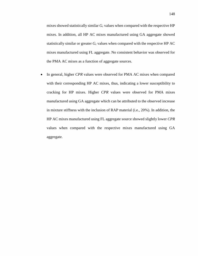
148
mixes showed statistically similar Gc values when compared with the respective HP
mixes. In addition, all HP AC mixes manufactured using GA aggregate showed
statistically similar or greater Gc values when compared with the respective HP AC
mixes manufactured using FL aggregate. No consistent behavior was observed for
the PMA AC mixes as a function of aggregate sources.
• In general, higher CPR values were observed for PMA AC mixes when compared
with their corresponding HP AC mixes, thus, indicating a lower susceptibility to
cracking for HP mixes. Higher CPR values were observed for PMA mixes
manufactured using GA aggregate which can be attributed to the observed increase
in mixture stiffness with the inclusion of RAP material (i.e., 20%). In addition, the
HP AC mixes manufactured using FL aggregate source showed slightly lower CPR
values when compared with the respective mixes manufactured using GA
aggregate.
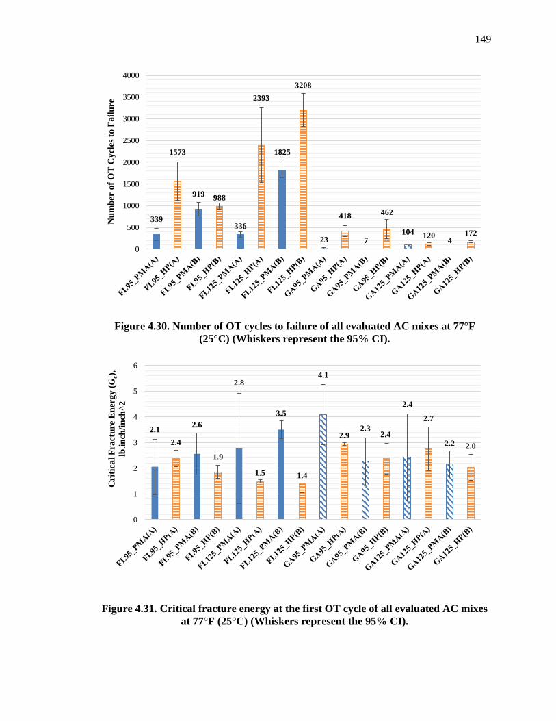
149
Figure 4.30. Number of OT cycles to failure of all evaluated AC mixes at 77°F
(25°C) (Whiskers represent the 95% CI).
Figure 4.31. Critical fracture energy at the first OT cycle of all evaluated AC mixes
at 77°F (25°C) (Whiskers represent the 95% CI).
339
1573
919988
336
2393
1825
3208
23
418
7
462
104 1204
172
0
500
1000
1500
2000
2500
3000
3500
4000
Nu
mb
er o
f O
T C
ycl
es t
o F
ail
ure
2.1
2.4
2.6
1.9
2.8
1.5
3.5
1.4
4.1
2.92.3
2.4
2.4
2.7
2.2 2.0
0
1
2
3
4
5
6
Cri
tica
l F
ract
ure
En
erg
y (
Gc)
,
lb.i
nch
/in
ch^
2

150
Figure 4.32. Critical propagation rate of all evaluated AC mixes at 77°F (25°C)
(Whiskers represent the 95% CI).
To better understand the cracking properties of all evaluated AC mixes, a design
interaction graph plotting Gc versus CPR was established. This interaction plot, illustrated
in Figure 4.33, includes the following four categories (Garcia et al., 2016):
• Tough-Crack Resistant: simulating a good resistance in both crack initiation (i.e.,
higher Gc values) and crack propagation (Flexible or Crack resistance) (i.e., lower
CPR values).
• Tough-Crack Susceptible: simulating a good resistance in crack initiation (i.e.,
higher Gc values) but susceptible to crack propagation (Brittle) (i.e., higher CPR
values).
• Soft-Crack Resistant: simulating softness and susceptibility to crack initiation (i.e.,
0.380.31 0.35 0.32
0.460.30 0.31 0.27
0.65
0.36
1.10
0.36
1.49
0.46
2.74
0.44
0.0
0.5
1.0
1.5
2.0
2.5
3.0
3.5
4.0
4.5
Cra
ck P
rop
ag
ati
on
Ra
te (
CP
R)
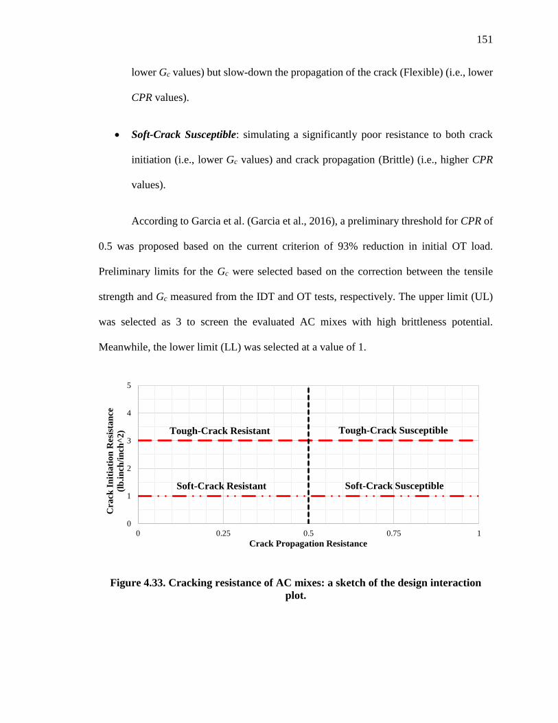
151
lower Gc values) but slow-down the propagation of the crack (Flexible) (i.e., lower
CPR values).
• Soft-Crack Susceptible: simulating a significantly poor resistance to both crack
initiation (i.e., lower Gc values) and crack propagation (Brittle) (i.e., higher CPR
values).
According to Garcia et al. (Garcia et al., 2016), a preliminary threshold for CPR of
0.5 was proposed based on the current criterion of 93% reduction in initial OT load.
Preliminary limits for the Gc were selected based on the correction between the tensile
strength and Gc measured from the IDT and OT tests, respectively. The upper limit (UL)
was selected as 3 to screen the evaluated AC mixes with high brittleness potential.
Meanwhile, the lower limit (LL) was selected at a value of 1.
Figure 4.33. Cracking resistance of AC mixes: a sketch of the design interaction
plot.
0
1
2
3
4
5
0 0.25 0.5 0.75 1
Cra
ck I
nit
iati
on
Res
ista
nce
(lb
.in
ch/i
nch
^2
)
Crack Propagation Resistance
Tough-Crack Resistant Tough-Crack Susceptible
Soft-Crack SusceptibleSoft-Crack Resistant

152
Figure 4.34 shows the cracking resistance interaction plot for all PMA and HP AC
mixes manufactured using FL aggregates. All FL AC mixes showed a CPR value lower
than 0.5 indicating a good cracking resistance. All FL mixes, except for FL125_PMA(B),
showed a CPR value between 1 and 3 indicating a good resistance to crack initiation.
FL125_PMA(B) mix was the only mix that showed tough-crack resistant mix.
Figure 4.35 shows the cracking resistance interaction plot for all PMA and HP AC
mixes manufactured with GA aggregates. All GA PMA AC mixes showed a CPR value
greater than 0.5 indicating a brittle behavior and a low resistance to crack propagation.
These mixes, except for GA95_PMA(A), showed Gc values between 1 and 3 indicating a
good resistance to crack initiation. On the other hand, all GA HP mixes show CPR values
lower than 0.5 and Gc values between 1 and 3 indicating soft-crack resistant mixes.
Figure 4.34. Cracking resistance interaction plot for FL PMA and HP AC mixes.
0
1
2
3
4
5
0.00 0.25 0.50 0.75 1.00 1.25 1.50 1.75 2.00 2.25 2.50 2.75
Cra
ck I
nit
iati
on
Res
ista
nce
(lb
.in
/in
^2)
Crack Propagation Resistance
FL95_PMA(A) FL95_HP(A) FL95_PMA(B) FL95_HP(B)FL125_PMA(A) FL125_HP(A) FL125_PMA(B) FL125_HP(B)CPR Limit LL UL
Soft-Crack Resistant
Tough-Crack Susceptible
Soft-Crack Susceptible
Tough-Crack Resistant

153
Figure 4.35. Cracking resistance interaction plot for GA PMA and HP AC mixes.
0
1
2
3
4
5
0.00 0.25 0.50 0.75 1.00 1.25 1.50 1.75 2.00 2.25 2.50 2.75
Cra
ck I
nit
iati
on
Res
ista
nce
(lb
.in
/in
^2
)
Crack Propagation Resistance
GA95_PMA(A) GA95_HP(A) GA95_PMA(B)
GA95_HP(B) GA125_PMA(A) GA125_HP(A)
GA125_PMA(B) GA125_HP(B) CPR Limit
Tough-Crack Resistant Tough-Crack Susceptible
Soft-Crack SusceptibleSoft-Crack Resistant
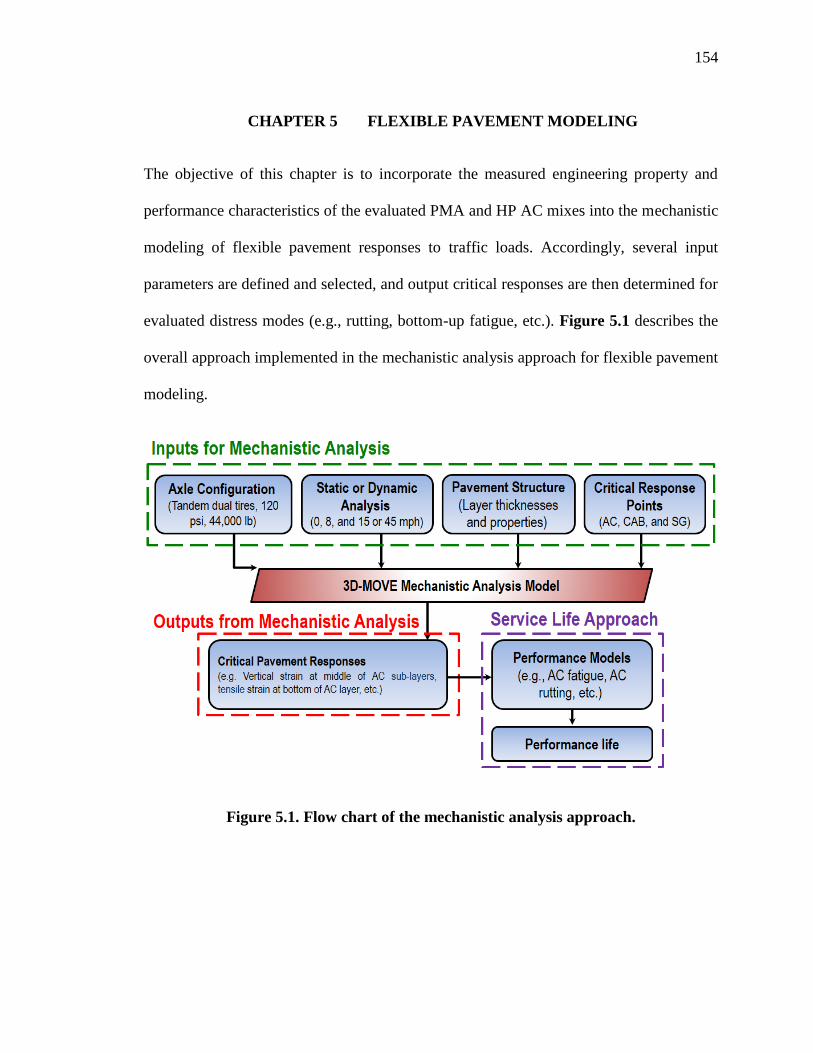
154
CHAPTER 5 FLEXIBLE PAVEMENT MODELING
The objective of this chapter is to incorporate the measured engineering property and
performance characteristics of the evaluated PMA and HP AC mixes into the mechanistic
modeling of flexible pavement responses to traffic loads. Accordingly, several input
parameters are defined and selected, and output critical responses are then determined for
evaluated distress modes (e.g., rutting, bottom-up fatigue, etc.). Figure 5.1 describes the
overall approach implemented in the mechanistic analysis approach for flexible pavement
modeling.
Figure 5.1. Flow chart of the mechanistic analysis approach.
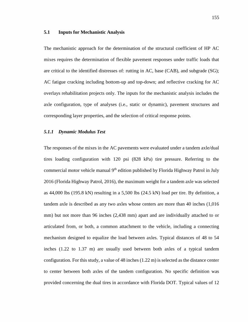
155
5.1 Inputs for Mechanistic Analysis
The mechanistic approach for the determination of the structural coefficient of HP AC
mixes requires the determination of flexible pavement responses under traffic loads that
are critical to the identified distresses of: rutting in AC, base (CAB), and subgrade (SG);
AC fatigue cracking including bottom-up and top-down; and reflective cracking for AC
overlays rehabilitation projects only. The inputs for the mechanistic analysis includes the
axle configuration, type of analyses (i.e., static or dynamic), pavement structures and
corresponding layer properties, and the selection of critical response points.
5.1.1 Dynamic Modulus Test
The responses of the mixes in the AC pavements were evaluated under a tandem axle/dual
tires loading configuration with 120 psi (828 kPa) tire pressure. Referring to the
commercial motor vehicle manual 9th edition published by Florida Highway Patrol in July
2016 (Florida Highway Patrol, 2016), the maximum weight for a tandem axle was selected
as 44,000 lbs (195.8 kN) resulting in a 5,500 lbs (24.5 kN) load per tire. By definition, a
tandem axle is described as any two axles whose centers are more than 40 inches (1,016
mm) but not more than 96 inches (2,438 mm) apart and are individually attached to or
articulated from, or both, a common attachment to the vehicle, including a connecting
mechanism designed to equalize the load between axles. Typical distances of 48 to 54
inches (1.22 to 1.37 m) are usually used between both axles of a typical tandem
configuration. For this study, a value of 48 inches (1.22 m) is selected as the distance center
to center between both axles of the tandem configuration. No specific definition was
provided concerning the dual tires in accordance with Florida DOT. Typical values of 12
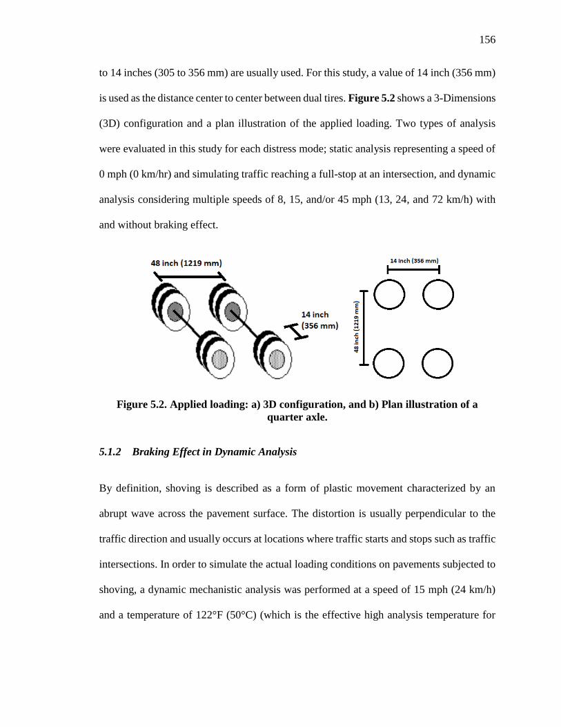
156
to 14 inches (305 to 356 mm) are usually used. For this study, a value of 14 inch (356 mm)
is used as the distance center to center between dual tires. Figure 5.2 shows a 3-Dimensions
(3D) configuration and a plan illustration of the applied loading. Two types of analysis
were evaluated in this study for each distress mode; static analysis representing a speed of
0 mph (0 km/hr) and simulating traffic reaching a full-stop at an intersection, and dynamic
analysis considering multiple speeds of 8, 15, and/or 45 mph (13, 24, and 72 km/h) with
and without braking effect.
Figure 5.2. Applied loading: a) 3D configuration, and b) Plan illustration of a
quarter axle.
5.1.2 Braking Effect in Dynamic Analysis
By definition, shoving is described as a form of plastic movement characterized by an
abrupt wave across the pavement surface. The distortion is usually perpendicular to the
traffic direction and usually occurs at locations where traffic starts and stops such as traffic
intersections. In order to simulate the actual loading conditions on pavements subjected to
shoving, a dynamic mechanistic analysis was performed at a speed of 15 mph (24 km/h)
and a temperature of 122°F (50°C) (which is the effective high analysis temperature for

157
rutting and shoving) under braking conditions. The user needs to specify a braking friction
coefficient (fBr) when specifying the axle/tire configuration. A braking friction coefficient
(fBr) of 0.623 was calculated considering a tractor-semi trailer truck on a sloped pavement
structure as illustrated in Figure 5.3 and based on the following assumptions (Siddharthan
et al., 2015):
• The vehicle speed at brake initiation is 40 mph (64 km/h) and the stopping distance
(SD) is 100 ft (30.48 m) with a pavement slope of 0 degree.
• The loading configuration consists of a tractor-semi trailer with a steering single
tires, driving dual tires, and trailer dual tires axle.
Figure 5.3. Sketch a tractor-semi trailer truck considered for the determination of
the braking friction coefficient (Siddharthan et al., 2015).
The tractor total weight, W1, is considered 16,000 lbs (71.2 kN) and the semitrailer
total weight W2 is considered 64,000 lbs. (284.7 kN) resulting in a gross weight of 80,000
lbs. (355.9 kN). It should be mentioned that the same configuration of tandem axle/dual
tires at the driving and trailer axle was considered as previously defined in Section 5.1.1.

158
5.1.3 Pavement Structures and Layers Properties
FDOT recently updated and published a manual for designing flexible pavements in
Florida (September 2016) (FDOT Design Manual, 2016). This manual provides guidance
for conducting new and rehabilitated flexible pavement designs according to the AASHTO
1993 Guide (AASHTO Guide, 1993). The accumulated 18-kip (80 kN) Equivalent Single
Axle Loads (ESALD) is the traffic load information used for pavement thickness design.
Table 5.1 summarizes the Traffic Levels for ESALD ranges for Superpave AC structural
courses (FDOT Design Manual, 2016). In this study, a design ESALD of 7, 20, and 40
million were considered for Traffic Levels C, D, and E, respectively.
Table 5.1. Summary Table of Traffic Level and Their Corresponding Design
ESALs.
ESALD (Million) Traffic Level
< 0.3 A
0.3 to < 3 B
3 to < 10 C
10 to < 30 D
>= 30 E
The following defines the general pavement layers in a flexible pavement system
in accordance with the FDOT Pavement Design Manual (2016) (FDOT Design Manual,
2016). The structural AC course is designed to distribute the traffic loadings to the base
course. Two types of structural AC courses, typically used by FDOT, were considered in
this study: a) structural course Type SP-9.5 which uses a 3/8 inch (9.5 mm) NMAS (i.e.,
FL95 and GA95 PMA and HP AC mixes) used for Traffic Level C, and b) structural course
Type SP-12.5 which uses a 1/2 inch (12.5 mm) NMAS (i.e., FL125 and GA125 PMA and
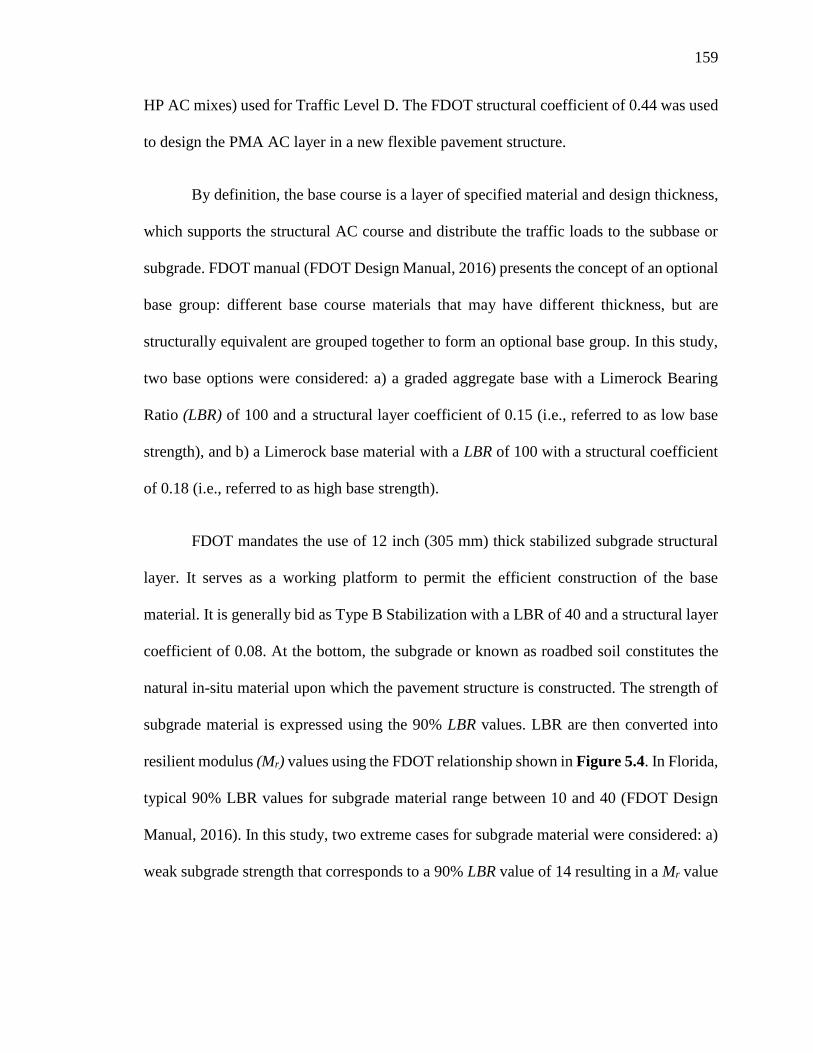
159
HP AC mixes) used for Traffic Level D. The FDOT structural coefficient of 0.44 was used
to design the PMA AC layer in a new flexible pavement structure.
By definition, the base course is a layer of specified material and design thickness,
which supports the structural AC course and distribute the traffic loads to the subbase or
subgrade. FDOT manual (FDOT Design Manual, 2016) presents the concept of an optional
base group: different base course materials that may have different thickness, but are
structurally equivalent are grouped together to form an optional base group. In this study,
two base options were considered: a) a graded aggregate base with a Limerock Bearing
Ratio (LBR) of 100 and a structural layer coefficient of 0.15 (i.e., referred to as low base
strength), and b) a Limerock base material with a LBR of 100 with a structural coefficient
of 0.18 (i.e., referred to as high base strength).
FDOT mandates the use of 12 inch (305 mm) thick stabilized subgrade structural
layer. It serves as a working platform to permit the efficient construction of the base
material. It is generally bid as Type B Stabilization with a LBR of 40 and a structural layer
coefficient of 0.08. At the bottom, the subgrade or known as roadbed soil constitutes the
natural in-situ material upon which the pavement structure is constructed. The strength of
subgrade material is expressed using the 90% LBR values. LBR are then converted into
resilient modulus (Mr) values using the FDOT relationship shown in Figure 5.4. In Florida,
typical 90% LBR values for subgrade material range between 10 and 40 (FDOT Design
Manual, 2016). In this study, two extreme cases for subgrade material were considered: a)
weak subgrade strength that corresponds to a 90% LBR value of 14 resulting in a Mr value
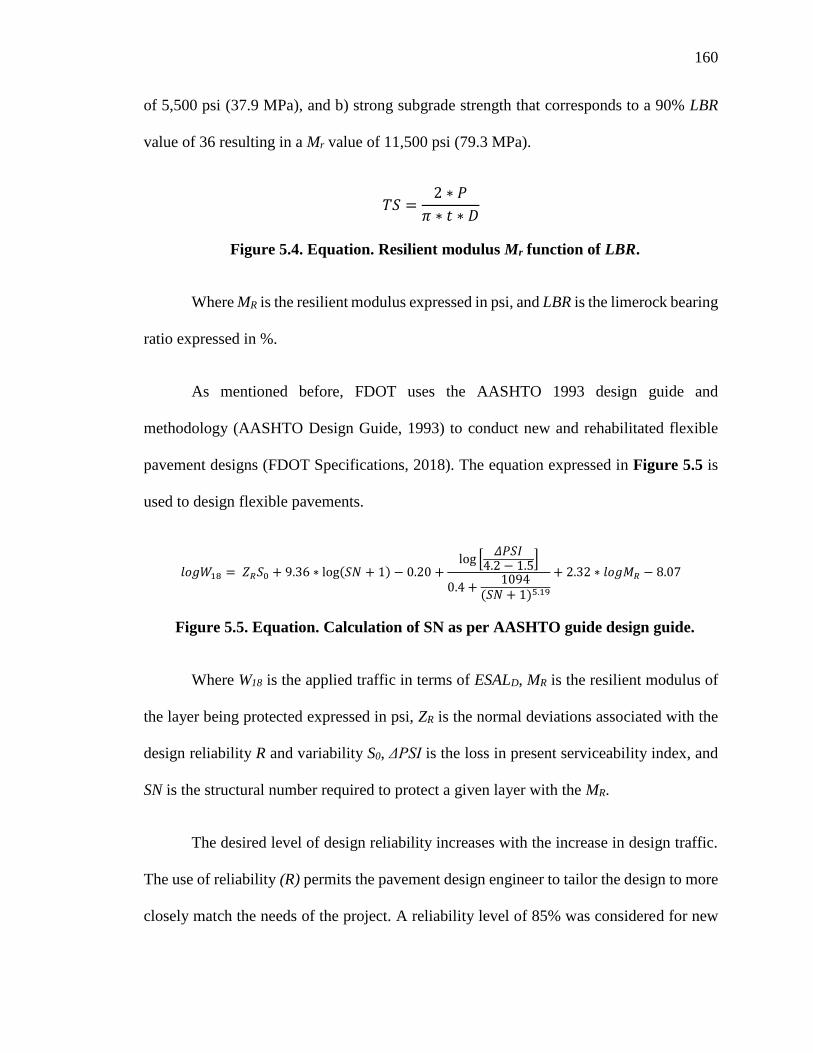
160
of 5,500 psi (37.9 MPa), and b) strong subgrade strength that corresponds to a 90% LBR
value of 36 resulting in a Mr value of 11,500 psi (79.3 MPa).
𝑇𝑆 =2 ∗ 𝑃
𝜋 ∗ 𝑡 ∗ 𝐷
Figure 5.4. Equation. Resilient modulus Mr function of LBR.
Where MR is the resilient modulus expressed in psi, and LBR is the limerock bearing
ratio expressed in %.
As mentioned before, FDOT uses the AASHTO 1993 design guide and
methodology (AASHTO Design Guide, 1993) to conduct new and rehabilitated flexible
pavement designs (FDOT Specifications, 2018). The equation expressed in Figure 5.5 is
used to design flexible pavements.
𝑙𝑜𝑔𝑊18 = 𝑍𝑅𝑆0 + 9.36 ∗ log(𝑆𝑁 + 1) − 0.20 +log [
𝛥𝑃𝑆𝐼4.2 − 1.5
]
0.4 +1094
(𝑆𝑁 + 1)5.19
+ 2.32 ∗ 𝑙𝑜𝑔𝑀𝑅 − 8.07
Figure 5.5. Equation. Calculation of SN as per AASHTO guide design guide.
Where W18 is the applied traffic in terms of ESALD, MR is the resilient modulus of
the layer being protected expressed in psi, ZR is the normal deviations associated with the
design reliability R and variability S0, ΔPSI is the loss in present serviceability index, and
SN is the structural number required to protect a given layer with the MR.
The desired level of design reliability increases with the increase in design traffic.
The use of reliability (R) permits the pavement design engineer to tailor the design to more
closely match the needs of the project. A reliability level of 85% was considered for new

161
construction projects; meanwhile a reliability level of 95% was considered for
rehabilitation projects. In this study and according to the FDOT design manual, a standard
deviation (S0) value of 0.45 is used in the design calculations to account for variability in
traffic load predictions and construction. The standard normal deviate (ZR) is calculated as
the difference between the current traffic (logW18) and the traffic to reach the terminal
present serviceability index (PSI) labeled as pt (logWt18) over the standard deviation (S0).
The AASHTO 1993 Guide method uses the PSI to represent the performance of the
pavement defined as a subjective measure of the ride quality by the road user. The PSI
varies between an upper and lower limit of 5 and 0 representing the best and worst
pavement conditions, respectively. The serviceability loss (PSI) at the end of the design
life is specified; representing the difference between the initial serviceability (pi) of the
pavement when opened to traffic and the terminal serviceability (pt) that the pavement is
expected to reach before rehabilitation, resurfacing, or reconstruction is required. A pi and
pt value of 4.2 and 2.5, respectively are considered in this study leading to a loss in
serviceability (ΔPSI) of 1.7.
The empirical relationship among design traffic, pavement structure, and pavement
performance for flexible pavements is solved to determine the required structural capacity
of the pavement section, known as the structural number (SN). The total pavement SN is
defined as the summation of the layer thicknesses times the corresponding structural layers
and drainage coefficients as expressed in the equation of Figure 5.6. For new construction
project, once the SN value is calculated using the equation defined in Figure 5.5 and having
the structural coefficient of the PMA AC layer and the thickness and structural coefficient

162
of the base and stabilized subgrade, the thickness of the PMA AC layer is determined using
the equation defined in Figure 5.6. For rehabilitation projects, the structural number of the
designed overlay (SN0) is calculated as the difference between the required structural
number (SNR) for a newly constructed pavement structure calculated using the equation
defined in Figure 5.5 and the structural number of the existing damaged pavement
structure after any milling (SNE). SNE is calculated using the reduced layer coefficients
taking into account the milling thickness of the existing pavement. In this study, the design
of AC overlays is based on existing pavement condition of “Fair”. For that, a reduced
structural coefficient of existing PMA AC mixes of 0.25 is used to compute SNE. It should
be mentioned that the structural coefficient of the base, and stabilized subgrade remain the
same as already used for the design of new pavement structures. The thickness of the
required structural overlay is then computed using the equation of Figure 5.7.
𝑆𝑁 = ∑ 𝑎𝑖𝐷𝑖𝑚𝑖
𝑖=1
Figure 5.6. Equation. Calculation of total structural number.
Where SN is the total structural number required for design traffic, ai is the
structural coefficient for the ith layer, Di is the thickness of the ith layer expressed in inch,
and mi is the drainage coefficient for the ith layer except the AC layer.
𝐷𝑂𝐿 = 𝑆𝑁𝑂𝐿/0.44
Figure 5.7. Equation. Calculation of required thickness of the AC layer.
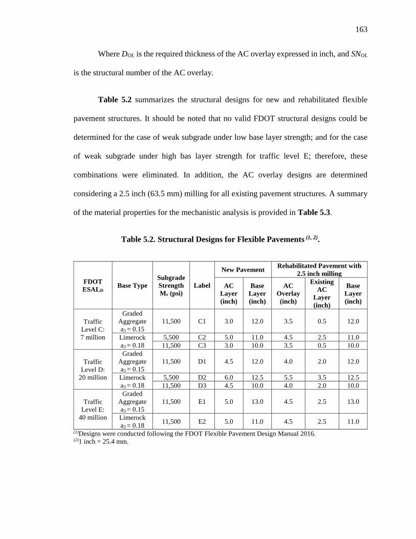
163
Where DOL is the required thickness of the AC overlay expressed in inch, and SNOL
is the structural number of the AC overlay.
Table 5.2 summarizes the structural designs for new and rehabilitated flexible
pavement structures. It should be noted that no valid FDOT structural designs could be
determined for the case of weak subgrade under low base layer strength; and for the case
of weak subgrade under high bas layer strength for traffic level E; therefore, these
combinations were eliminated. In addition, the AC overlay designs are determined
considering a 2.5 inch (63.5 mm) milling for all existing pavement structures. A summary
of the material properties for the mechanistic analysis is provided in Table 5.3.
Table 5.2. Structural Designs for Flexible Pavements (1, 2).
FDOT
ESALD Base Type
Subgrade
Strength
Mr (psi)
Label
New Pavement Rehabilitated Pavement with
2.5 inch milling
AC
Layer
(inch)
Base
Layer
(inch)
AC
Overlay
(inch)
Existing
AC
Layer
(inch)
Base
Layer
(inch)
Traffic
Level C:
7 million
Graded
Aggregate
a3 = 0.15
11,500 C1 3.0 12.0 3.5 0.5 12.0
Limerock
a3 = 0.18
5,500 C2 5.0 11.0 4.5 2.5 11.0
11,500 C3 3.0 10.0 3.5 0.5 10.0
Traffic
Level D:
20 million
Graded
Aggregate
a3 = 0.15
11,500 D1 4.5 12.0 4.0 2.0 12.0
Limerock
a3 = 0.18
5,500 D2 6.0 12.5 5.5 3.5 12.5
11,500 D3 4.5 10.0 4.0 2.0 10.0
Traffic
Level E:
40 million
Graded
Aggregate
a3 = 0.15
11,500 E1 5.0 13.0 4.5 2.5 13.0
Limerock
a3 = 0.18 11,500 E2 5.0 11.0 4.5 2.5 11.0
(1)Designs were conducted following the FDOT Flexible Pavement Design Manual 2016. (2)1 inch = 25.4 mm.
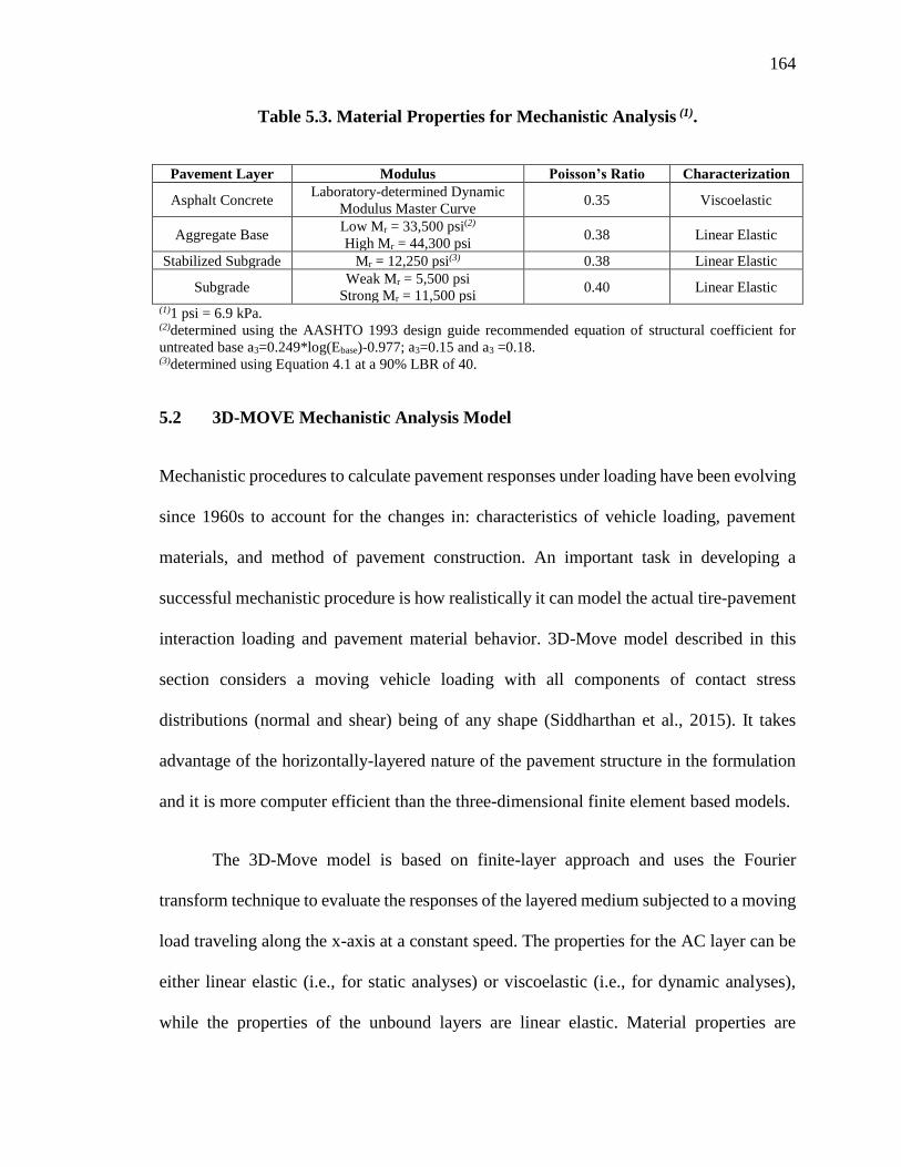
164
Table 5.3. Material Properties for Mechanistic Analysis (1).
Pavement Layer Modulus Poisson’s Ratio Characterization
Asphalt Concrete Laboratory-determined Dynamic
Modulus Master Curve 0.35 Viscoelastic
Aggregate Base Low Mr = 33,500 psi(2)
High Mr = 44,300 psi 0.38 Linear Elastic
Stabilized Subgrade Mr = 12,250 psi(3) 0.38 Linear Elastic
Subgrade Weak Mr = 5,500 psi
Strong Mr = 11,500 psi 0.40 Linear Elastic
(1)1 psi = 6.9 kPa. (2)determined using the AASHTO 1993 design guide recommended equation of structural coefficient for
untreated base a3=0.249*log(Ebase)-0.977; a3=0.15 and a3 =0.18. (3)determined using Equation 4.1 at a 90% LBR of 40.
5.2 3D-MOVE Mechanistic Analysis Model
Mechanistic procedures to calculate pavement responses under loading have been evolving
since 1960s to account for the changes in: characteristics of vehicle loading, pavement
materials, and method of pavement construction. An important task in developing a
successful mechanistic procedure is how realistically it can model the actual tire-pavement
interaction loading and pavement material behavior. 3D-Move model described in this
section considers a moving vehicle loading with all components of contact stress
distributions (normal and shear) being of any shape (Siddharthan et al., 2015). It takes
advantage of the horizontally-layered nature of the pavement structure in the formulation
and it is more computer efficient than the three-dimensional finite element based models.
The 3D-Move model is based on finite-layer approach and uses the Fourier
transform technique to evaluate the responses of the layered medium subjected to a moving
load traveling along the x-axis at a constant speed. The properties for the AC layer can be
either linear elastic (i.e., for static analyses) or viscoelastic (i.e., for dynamic analyses),
while the properties of the unbound layers are linear elastic. Material properties are
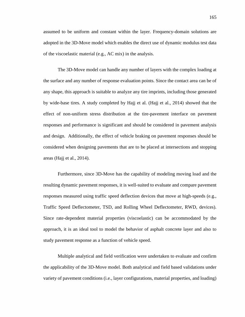
165
assumed to be uniform and constant within the layer. Frequency-domain solutions are
adopted in the 3D-Move model which enables the direct use of dynamic modulus test data
of the viscoelastic material (e.g., AC mix) in the analysis.
The 3D-Move model can handle any number of layers with the complex loading at
the surface and any number of response evaluation points. Since the contact area can be of
any shape, this approach is suitable to analyze any tire imprints, including those generated
by wide-base tires. A study completed by Hajj et al. (Hajj et al., 2014) showed that the
effect of non-uniform stress distribution at the tire-pavement interface on pavement
responses and performance is significant and should be considered in pavement analysis
and design. Additionally, the effect of vehicle braking on pavement responses should be
considered when designing pavements that are to be placed at intersections and stopping
areas (Hajj et al., 2014).
Furthermore, since 3D-Move has the capability of modeling moving load and the
resulting dynamic pavement responses, it is well-suited to evaluate and compare pavement
responses measured using traffic speed deflection devices that move at high-speeds (e.g.,
Traffic Speed Deflectometer, TSD, and Rolling Wheel Deflectometer, RWD, devices).
Since rate-dependent material properties (viscoelastic) can be accommodated by the
approach, it is an ideal tool to model the behavior of asphalt concrete layer and also to
study pavement response as a function of vehicle speed.
Multiple analytical and field verification were undertaken to evaluate and confirm
the applicability of the 3D-Move model. Both analytical and field based validations under
variety of pavement conditions (i.e., layer configurations, material properties, and loading)

166
demonstrated the applicability of the 3D-Move model relative to its consideration of
appropriate procedures to account for moving vehicle loading and pavement material
characterization (Nabizadeh et al., 2017).
The research team used the 3D-Move model in this research to determine pavement
critical responses and to estimate the structural layer coefficients of HP AC mixes due to
the following unique features:
• The speed of the load can be varied from 0 to 100 mph (0 to 161 km/h). This feature
becomes very critical as this research moves towards the validation phase under
Accelerated Pavement Test (APT) loading. The 3D-Move model has been
incorporated into a public domain software with highly efficient computational
speed which distinguishes it from the non-public domain commercial 3D Finite
Element software which have significantly longer computational time. FDOT will
be able to download and implement the public domain 3D-Move software to
analyze the PMA and HP AC pavements under APT loading. The variable speed
feature of the 3D-Move model will facilitate the implementation of the APT results
under low speed loading to highway loading at higher speeds.
• The pressure at the tire-pavement interface is non-uniform and can be applied in
the vertical and horizontal directions. The horizontal pressure is used to simulate
slow moving vehicles and braking on urban pavements, at intersections, and off-
ramps.
• The AC layer is modeled as a viscoelastic material where vehicle speed ad loading

167
frequency have a significant impact on flexible pavement response to loads. To
bring back the responses to the spatial and time domains, an inverse transformation
is needed. 3D-Move uses a two-dimensional Fourier transform because time, t, and
longitudinal direction, x, are interconnected due to the assumption that load moves
at constant speed. Therefore, for a specific response point, summations over
response contributions of waves corresponding to x-direction (longitudinal
direction towards which the load moves) and y-direction (horizontal direction
perpendicular to the travel direction) is performed to obtain the response(s) of
interest. In 3D-FAST formulation, however, since a general dynamic load is
modeled (which does not necessarily have constant moving speed) a three-
dimensional Fourier transform is applied, so summations are made over response
contributions of waves corresponding to x-, y-, and t-directions at a particular
location and time. if a similar 3D-Move iteration scheme is used in 3D-FAST, it
will be computationally time consuming, and if the response(s) are needed at
multiple locations within pavement structure, the runtime will be substantially high.
5.3 Description of Critical Responses and Analysis Temperatures
Table 5.4 summarizes the selected critical response types along with their locations within
the designed flexible pavement structures. These responses were computed at different
locations function of the type of analysis (i.e., static or dynamic) and at different depths
depending on the distress mode as illustrated in Figure 5.8.

168
Table 5.4. Pavement Responses from 3D-Move Analysis.
Distress
Mode
Pavement
Responses
Location within
Structure Performance Model
Analysis
Temperature
Fatigue
Cracking
Tensile
Strain (εt) Bottom of AC layer
MEPDG model from
laboratory evaluation
Effective
Intermediate
Pavement
Temperature (Teff-Int)
Rutting in
AC Layer
Vertical
Strain (εr) Middle of AC sub-layers
MEPDG model from
laboratory evaluation
Effective High
Pavement
Temperature (Teff-High)
Total
Rutting
Vertical
Strain (εr)
Middle of AC sub-layers,
Middle of base sub-layers,
and 6 inch into Subgrade
AASHTO M-E Design
Effective High
Pavement
Temperature (Teff-High)
Shoving Shear Strain
(γYZ) Top 0.5 inch of AC layer ---
Effective High
Pavement
Temperature (Teff-High)
Top-
Down
Cracking
Horizontal
Tensile
Stress (σt)
Top 0.5 inch of AC layer ---
Effective
Intermediate
Pavement
Temperature (Teff-Int)
Figure 5.8. Sketch of a newly constructed pavement section with the locations of the
selected response points.
The effective intermediate and high pavement temperatures were determined using

169
the equations defined in Figure 5.9 and Figure 5.10, respectively, in accordance with
National Corporation Highway Research Program (NCHRP 09-22) Report 704 “A
Performance-Related Specification for Hot-Mix Asphalt” (NCHRP 09-22, 2011). The
climatic stations in Gainesville and Marathon were selected to compute the effective
pavement temperatures for the mechanistic analysis. Table 5.5 summarizes all the
necessary climatic inputs for the equations in Figure 5.9 and Figure 5.10.
𝑇𝑒𝑓𝑓−𝐼𝑛𝑡 = −13.995 − 2.332(𝐹𝑟𝑒𝑞)0.5 + 1.006(𝑀𝐴𝐴𝑇) + 0.876(𝜎𝑀𝐴𝐴𝑇) − 1.186(𝑊𝑖𝑛𝑑)
+ 0.549(𝑆𝑢𝑛𝑠ℎ𝑖𝑛𝑒) + 0.071(𝑅𝑎𝑖𝑛)
Figure 5.9. Equation. Calculation of effective intermediate temperature.
𝑇𝑒𝑓𝑓−𝐻𝑖𝑔ℎ = 14.62 − 3.361𝐿𝑛(𝐹𝑟𝑒𝑞) − 10.940(𝑧) + 1.121(𝑀𝐴𝐴𝑇) + 1.718(𝜎𝑀𝐴𝐴𝑇)
− 0.431(𝑊𝑖𝑛𝑑) + 0.333(𝑆𝑢𝑛𝑠ℎ𝑖𝑛𝑒) + 0.08(𝑅𝑎𝑖𝑛)
Figure 5.10. Equation. Calculation of effective high temperature.
Where Teff-Int/High is the modified Witczak temperature expressed in °F, z is the
critical depth expressed in inch (considered as 1 inch (25.4 mm) from the top of the AC
layer), Freq is the loading frequency expressed in Hz, MAAT is the mean annual air
temperature expressed in °F, σMAAT is the standard deviation of the mean monthly air
temperature expressed in °F, Rain is the annual cumulative rainfall depth expressed in
inches, Sunshine is the mean annual percentage sunshine expressed in %, and Wind is the
man annual wind speed expressed in mph.

170
Table 5.5. Input Properties at the Selected Climatic Stations in Florida.
Property Location of the Selected Climatic Station
Gainesville Marathon
MAAT (°F) 68.1 78.1
σMAAT (°F) 9.7 6.0
Rain (inch) 45.9 34.0
Sunshine (%) 69.3 75.6
Wind (mph) 5.0 7.0
The MEPDG document (MEPDG Guide, 2004) recommends using a procedure
based on stress distributions to estimate the traffic-induced loading time and by that
determine the corresponding frequency at any depth of the pavement structure (i.e., AC,
base, stabilized subgrade, and subgrade). In order to calculate the effective duration at the
depth of interest, the MEPDG uses Odemark’s method of equivalent thickness to transform
the pavement structure into a single subgrade layer system, assuming that the stress
distribution is developed at 45 degrees in the equivalent layer system as illustrated in
Figure 5.11 and expressed in the equation defined in Figure 5.12. As presented in the
MEPDG, the time of loading of a haversine waveform in AC layer due to moving traffic
load is estimated using the equation of Figure 5.13. In the case of tandem axle
configuration, an overlap of the stress distribution may occur at deeper depths from the
surface; therefore, the effective length of the stress pulse (Leff) at these depths needs to be
adjusted to account for the overlapping.
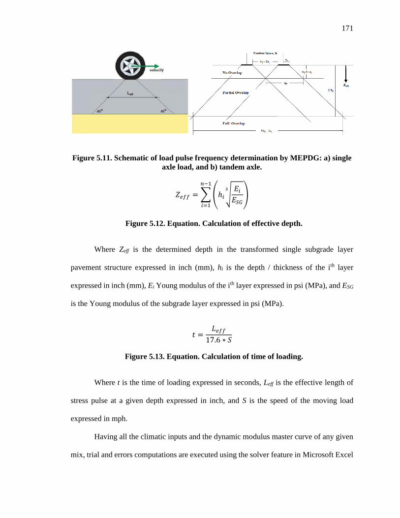
171
Figure 5.11. Schematic of load pulse frequency determination by MEPDG: a) single
axle load, and b) tandem axle.
𝑍𝑒𝑓𝑓 = ∑ (ℎ𝑖 √𝐸𝑖
𝐸𝑆𝐺
3
)
𝑛−1
𝑖=1
Figure 5.12. Equation. Calculation of effective depth.
Where Zeff is the determined depth in the transformed single subgrade layer
pavement structure expressed in inch (mm), hi is the depth / thickness of the ith layer
expressed in inch (mm), Ei Young modulus of the ith layer expressed in psi (MPa), and ESG
is the Young modulus of the subgrade layer expressed in psi (MPa).
𝑡 =𝐿𝑒𝑓𝑓
17.6 ∗ 𝑆
Figure 5.13. Equation. Calculation of time of loading.
Where t is the time of loading expressed in seconds, Leff is the effective length of
stress pulse at a given depth expressed in inch, and S is the speed of the moving load
expressed in mph.
Having all the climatic inputs and the dynamic modulus master curve of any given
mix, trial and errors computations are executed using the solver feature in Microsoft Excel

172
to determine the frequency at any given depth (in this case z = 1 inch (25.4 mm)), any given
speed, and any associated analysis temperature. Table 5.6 summarizes the determined high
and intermediate analysis temperatures at the two selected locations (i.e., Gainesville and
Marathon). The pavement analysis temperature for rutting and shoving evaluations in the
3D-Move model was selected as 122°F (50°C). However, the resistance to fatigue, top-
down, and reflective cracking was evaluated at an intermediate pavement analysis
temperature of 77°F (25°C).
Table 5.6. Computation of High and Intermediate Pavement Analysis
Temperatures.
Climatic Station in Gainesville
Target Distress and Location
Rutting at z = 1 inch
(25.4 mm)
Fatigue at z = 1 inch
(25.4 mm)
Mean Effective Temperature, °F (°C) 109.4 (43.0) 85.5 (29.7)
Standard Deviation (stdv), °F (°C) 2.2 (1.2) 4.0 (2.2)
Mean ± 2 stdv (95% CI) 113.8 (45.4) 77.5 (25.3)
Mean ± 3 stdv (99% CI) 116.0 946.7) 73.5 (23.1)
Climatic Station in Marathon
Target Distress and Location
Rutting at z = 1 inch
(25.4 mm)
Fatigue at z = 1 inch
(25.4 mm)
Mean Effective Temperature, ° (°C) 117.1 (47.3) 97.0 (36.1)
Standard Deviation (stdv), °F (°C) 3.0 (1.7) 5.0 (2.8)
Mean ± 2 stdv (95% CI) 123.1 (50.6) 87.0 (30.6)
Mean ± 3 stdv (99% CI) 126.1 (52.3) 82.0 (27.8)
173
CHAPTER 6 DETERMINATION OF STRUCTURAL COEFFICIENT
FOR HP AC MIXES
The objectives of this part of the research are; a) determine the critical responses of the
designed pavement structures for the identified distresses of AC pavements including;
fatigue cracking, AC rutting, total rutting, top-down cracking, and reflective cracking using
the 3D-Move model, and b) determine the structural coefficient for HP AC mixes. First,
the determined critical responses are used to estimate the fatigue performance life of the
designed pavement structures followed by the development of the initial structural
coefficient for HP AC mixes based on the equal fatigue performance life approach. Finally,
the fatigue-based initial structural coefficients are verified for the other modes of distress.
Figure 6.1 illustrates a step by step flowchart summary of these analyses.
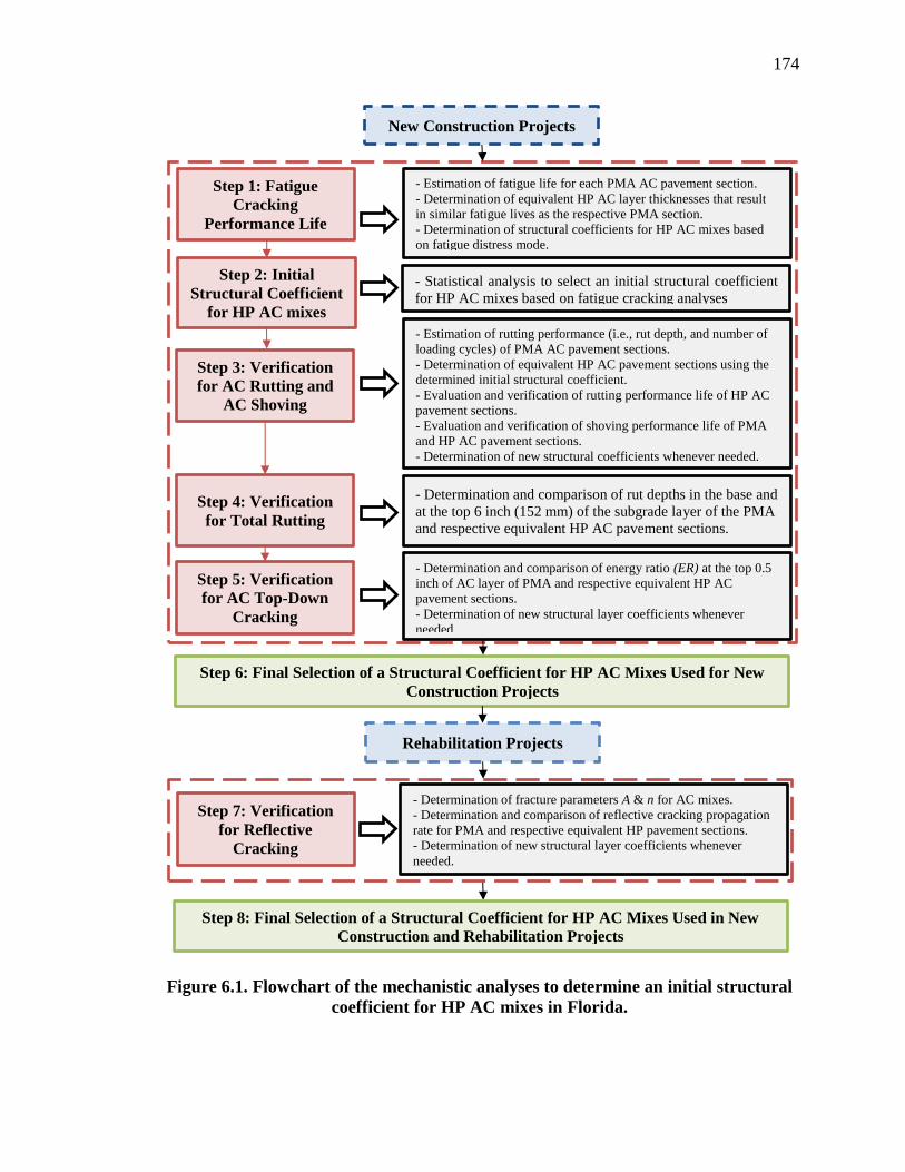
174
Figure 6.1. Flowchart of the mechanistic analyses to determine an initial structural
coefficient for HP AC mixes in Florida.
Step 1: Fatigue
Cracking
Performance Life
New Construction Projects
- Estimation of fatigue life for each PMA AC pavement section.
- Determination of equivalent HP AC layer thicknesses that result
in similar fatigue lives as the respective PMA section.
- Determination of structural coefficients for HP AC mixes based
on fatigue distress mode.
Step 2: Initial
Structural Coefficient
for HP AC mixes
based on Fatigue
Step 3: Verification
for AC Rutting and
AC Shoving
- Estimation of rutting performance (i.e., rut depth, and number of
loading cycles) of PMA AC pavement sections.
- Determination of equivalent HP AC pavement sections using the
determined initial structural coefficient.
- Evaluation and verification of rutting performance life of HP AC
pavement sections.
- Evaluation and verification of shoving performance life of PMA
and HP AC pavement sections.
- Determination of new structural coefficients whenever needed.
Step 4: Verification
for Total Rutting
- Determination and comparison of rut depths in the base and
at the top 6 inch (152 mm) of the subgrade layer of the PMA
and respective equivalent HP AC pavement sections.
Step 5: Verification
for AC Top-Down
Cracking
- Determination and comparison of energy ratio (ER) at the top 0.5
inch of AC layer of PMA and respective equivalent HP AC
pavement sections.
- Determination of new structural layer coefficients whenever
needed.
Step 6: Final Selection of a Structural Coefficient for HP AC Mixes Used for New
Construction Projects
Rehabilitation Projects
Step 7: Verification
for Reflective
Cracking
- Determination of fracture parameters A & n for AC mixes.
- Determination and comparison of reflective cracking propagation
rate for PMA and respective equivalent HP pavement sections.
- Determination of new structural layer coefficients whenever
needed.
Step 8: Final Selection of a Structural Coefficient for HP AC Mixes Used in New
Construction and Rehabilitation Projects
- Statistical analysis to select an initial structural coefficient
for HP AC mixes based on fatigue cracking analyses

175
6.1 Fatigue Cracking Performance Life
The fatigue characteristics of the 16 different AC mixes were evaluated using the flexural
beam fatigue test in accordance with AASHTO T321 (AASHTO T321, 2017) at three
temperatures and multiple strain levels. Using the fatigue models developed for each AC
PMA mix (Table 4.9) and the corresponding critical tensile strains (εt) determined from
the 3D-Move mechanistic analyses at the bottom of the AC layer, the number of cycles to
fatigue failure was determined for each new pavement section (Table 5.2). It should be
mentioned that the performance life of the PMA pavements was evaluated under stop-static
traffic—0 mph (0 km/h)—simulating full-stop trucks at intersections, slow traffic—8 mph
(13 km/h)—simulating the speed of the heavy vehicle simulator (HVS) at FDOT facilities
in Gainesville, and the fast-highway –45 mph (72 km/h)—traffic.
The dynamic modulus (E) term in the fatigue model was determined at the effective
intermediate temperature (i.e., 77° (25°C)) using the laboratory determined dynamic
modulus master curves (refer to Section 4.2.1). The frequency at which E was computed
was determined based on the MEPDG stress distribution concept using Odemark’s
equivalent thickness method explained previously in Section 5.3. The matching
performance life approach was then used to determine the required AC layer thickness for
the HP pavement sections as expressed in the equations defined in Figure 6.2 to Figure
6.4. The HP pavement sections were then determined in a way to achieve the same fatigue
service life (i.e., number of cycles to fatigue failure) as the corresponding PMA control
pavement sections. It should be recognized that the same fatigue performance life does not
translate into the same tensile strain value at the bottom of the AC layer. Using this

176
approach, the target tensile strain at the bottom of the AC HP layer can be determined as
expressed in the equation defined in Figure 6.5.
𝑁𝑓−𝑃𝑀𝐴 = 𝛽𝑓1 ∗ 𝑘𝑓1−𝑃𝑀𝐴 ∗ (1
ԑ𝑡−𝑃𝑀𝐴)
𝑘𝑓2−𝑃𝑀𝐴
∗ (1
𝐸𝐴𝐶−𝑃𝑀𝐴)𝑘𝑓3−𝑃𝑀𝐴
Figure 6.2. Equation. Calculation of number of cycles to fatigue failure for PMA
pavement structures.
𝑁𝑓−𝐻𝑃 = 𝛽𝑓1 ∗ 𝑘𝑓1−𝐻𝑃 ∗ (1
ԑ𝑡−𝐻𝑃)
𝑘𝑓2−𝐻𝑃
∗ (1
𝐸𝐴𝐶−𝐻𝑃)𝑘𝑓3−𝐻𝑃
Figure 6.3. Equation. Calculation of number of cycles to fatigue failure for HP
pavement structures.
𝑁𝑓−𝑃𝑀𝐴 = 𝑁𝑓−𝐻𝑃
Figure 6.4. Equation. Calculation of number of cycles to fatigue failure for HP
pavement structures using the service life approach.
ԑ𝑡−𝐻𝑃 = 10
(−1
𝑘𝑓2−𝐻𝑃)∗log [(
𝑘𝑓1−𝑃𝑀𝐴
𝑘𝑓1−𝐻𝑃)∗(
1ԑ𝑡−𝑃𝑀𝐴
)𝑘𝑓2−𝑃𝑀𝐴
∗((
1𝐸𝐴𝐶−𝑃𝑀𝐴
)𝑘𝑓3−𝑃𝑀𝐴
(1
𝐸𝐴𝐶−𝐻𝑃)
𝑘𝑓3−𝐻𝑃)]
Figure 6.5. Equation. Calculation of critical tensile strain at the bottom of AC layer
in a HP pavement structure using service life approach.
Where Nf-PMA and Nf-HP are the fatigue lives defined as the number of load
repetitions to fatigue damage for PMA and HP pavement sections, εt-PMA and εt-HP are the
applied tensile strain at the bottom of PMA and HP AC layers expressed in inch/inch (or
mm/mm), EAC-PMA and EAC-HP are defined as the dynamic modulus of PMA and HP AC
asphalt mixtures, respectively, and expressed in psi, kf1-PMA, kf2-PMA, kf3-PMA, kf1-HP, kf2-HP,
and kf3-HP are the experimentally determined coefficients for PMA and HP AC mixes, and
βf1-PMA, and βf1-HP are the mix-specific laboratory to field calibration factors (βf1-PMA
assumed to be equal to βf1-HP).

177
It should be mentioned that in this analysis mix-specific fatigue performance
models were used. Thus, the calibration parameters βf2-PMA, βf2-HP, βf3-PMA, and βf3-HP were
set equal to 1.
Previous research showed that there might be a level of stress or strain below which
no fatigue damage originating from the bottom of the AC layer occurs to the pavement
sections. This stress or strain has been termed as fatigue endurance limit (Prowell et al.,
2010). In other words, if a pavement is designed and constructed so that under repeated
traffic loads no damage occurs, then the pavement should last indefinitely without a
structural failure. Multiple approaches exist to estimate a fatigue endurance limit of an
evaluated mixture at a given temperature and loading frequency. The Strategic Highway
Research Program (SHRP) suggested that an AC mix laboratory fatigue life of 50 million
load cycles in a strain-controlled test is equivalent to 500 MSA in the field. Therefore, any
strain value which can result in a laboratory fatigue life of 50 million loading cycles can
be considered as the fatigue endurance limit. Due to the impracticality in conducting
laboratory fatigue test for 50 million cycles which would take more than 50 days per
specimen per temperature, multiple extrapolation techniques including exponential model,
power model, logarithmic model, single-stage Weibull function, and three stage Weibull
function can be used to predict high fatigue life under low fatigue strain (Prowell et al.,
2010). Using the fatigue relationships developed for the 16 evaluated AC mixes (i.e., 8
PMA and 8 HP), a tensile strain (εt-50 million cycles) at a given temperature and loading
frequency is estimated for 50 million loading cycles as expressed in the equation defined
in Figure 6.6.
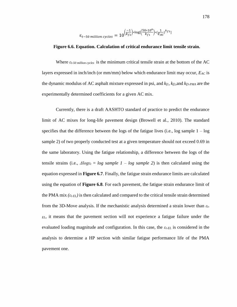
178
ԑ𝑡−50 𝑚𝑖𝑙𝑙𝑖𝑜𝑛 𝑐𝑦𝑐𝑙𝑒𝑠 = 10(
−1𝑘𝑓2
)∗log [(50∗106
𝑘𝑓1)∗(
1𝐸𝐴𝐶
)𝑘𝑓3]
Figure 6.6. Equation. Calculation of critical endurance limit tensile strain.
Where εt-50 million cycles is the minimum critical tensile strain at the bottom of the AC
layers expressed in inch/inch (or mm/mm) below which endurance limit may occur, EAC is
the dynamic modulus of AC asphalt mixture expressed in psi, and kf1, kf2,and kf3-PMA are the
experimentally determined coefficients for a given AC mix.
Currently, there is a draft AASHTO standard of practice to predict the endurance
limit of AC mixes for long-life pavement design (Browell et al., 2010). The standard
specifies that the difference between the logs of the fatigue lives (i.e., log sample 1 – log
sample 2) of two properly conducted test at a given temperature should not exceed 0.69 in
the same laboratory. Using the fatigue relationship, a difference between the logs of the
tensile strains (i.e., Δlogεt = log sample 1 – log sample 2) is then calculated using the
equation expressed in Figure 6.7. Finally, the fatigue strain endurance limits are calculated
using the equation of Figure 6.8. For each pavement, the fatigue strain endurance limit of
the PMA mix (εt-EL) is then calculated and compared to the critical tensile strain determined
from the 3D-Move analysis. If the mechanistic analysis determined a strain lower than εt-
EL, it means that the pavement section will not experience a fatigue failure under the
evaluated loading magnitude and configuration. In this case, the εt-EL is considered in the
analysis to determine a HP section with similar fatigue performance life of the PMA
pavement one.
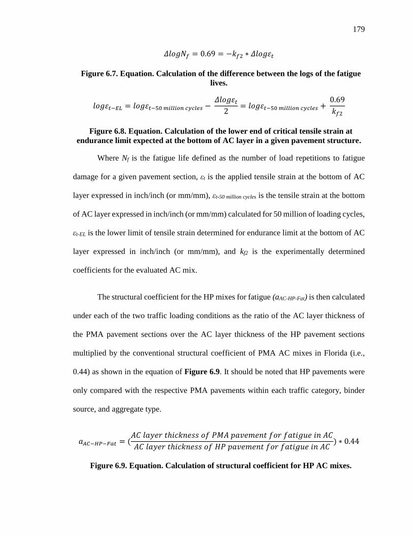
179
𝛥𝑙𝑜𝑔𝑁𝑓 = 0.69 = −𝑘𝑓2 ∗ 𝛥𝑙𝑜𝑔휀𝑡
Figure 6.7. Equation. Calculation of the difference between the logs of the fatigue
lives.
𝑙𝑜𝑔휀𝑡−𝐸𝐿 = 𝑙𝑜𝑔휀𝑡−50 𝑚𝑖𝑙𝑙𝑖𝑜𝑛 𝑐𝑦𝑐𝑙𝑒𝑠 − 𝛥𝑙𝑜𝑔휀𝑡
2= 𝑙𝑜𝑔휀𝑡−50 𝑚𝑖𝑙𝑙𝑖𝑜𝑛 𝑐𝑦𝑐𝑙𝑒𝑠 +
0.69
𝑘𝑓2
Figure 6.8. Equation. Calculation of the lower end of critical tensile strain at
endurance limit expected at the bottom of AC layer in a given pavement structure.
Where Nf is the fatigue life defined as the number of load repetitions to fatigue
damage for a given pavement section, εt is the applied tensile strain at the bottom of AC
layer expressed in inch/inch (or mm/mm), εt-50 million cycles is the tensile strain at the bottom
of AC layer expressed in inch/inch (or mm/mm) calculated for 50 million of loading cycles,
εt-EL is the lower limit of tensile strain determined for endurance limit at the bottom of AC
layer expressed in inch/inch (or mm/mm), and kf2 is the experimentally determined
coefficients for the evaluated AC mix.
The structural coefficient for the HP mixes for fatigue (aAC-HP-Fat) is then calculated
under each of the two traffic loading conditions as the ratio of the AC layer thickness of
the PMA pavement sections over the AC layer thickness of the HP pavement sections
multiplied by the conventional structural coefficient of PMA AC mixes in Florida (i.e.,
0.44) as shown in the equation of Figure 6.9. It should be noted that HP pavements were
only compared with the respective PMA pavements within each traffic category, binder
source, and aggregate type.
𝑎𝐴𝐶−𝐻𝑃−𝐹𝑎𝑡 = (𝐴𝐶 𝑙𝑎𝑦𝑒𝑟 𝑡ℎ𝑖𝑐𝑘𝑛𝑒𝑠𝑠 𝑜𝑓 𝑃𝑀𝐴 𝑝𝑎𝑣𝑒𝑚𝑒𝑛𝑡 𝑓𝑜𝑟 𝑓𝑎𝑡𝑖𝑔𝑢𝑒 𝑖𝑛 𝐴𝐶
𝐴𝐶 𝑙𝑎𝑦𝑒𝑟 𝑡ℎ𝑖𝑐𝑘𝑛𝑒𝑠𝑠 𝑜𝑓 𝐻𝑃 𝑝𝑎𝑣𝑒𝑚𝑒𝑛𝑡 𝑓𝑜𝑟 𝑓𝑎𝑡𝑖𝑔𝑢𝑒 𝑖𝑛 𝐴𝐶) ∗ 0.44
Figure 6.9. Equation. Calculation of structural coefficient for HP AC mixes.
180
Where 𝑎𝐴𝐶−𝐻𝑃−𝐹𝑎𝑡 is the structural coefficient for HP AC mixes determined based
on fatigue cracking performance.
Table 6.1 to Table 6.8 summarize the output of the fatigue mechanistic analyses
conducted at traffic levels C, D, and E. A review of the presented data reveals the following
observations:
• The combination of pavement structure (i.e., AC and base thickness), layer
properties, applied traffic, loading speed, and performance characteristics of the
evaluated mixes had an impact on the resultant structural coefficients for the
evaluated HP AC mixes. Values lower and higher than the PMA AC structural
coefficient (i.e., 0.44) were observed for the same pavement structure under the
same traffic depending on the evaluated mix and loading speed.
• For pavement section C1 (i.e., 3.00 inch (76 mm) PMA AC on top of 12.00 inch
(305 mm) low strength base and strong subgrade), the number of cycles to fatigue
failure decreased with the increase in loading speed for the evaluated 95 mm PMA
AC mixes except for GA95_PMA(B). The four evaluated mixes exhibited critical
tensile strains higher than their respective endurance limits irrespective of loading
speed. The resultant structural coefficient decreased with the increase of speed for
FL95_PMA(B) and GA95_PMA(B) mixes; while, an increasing and a constant
structural coefficient were observed for FL95_HP(A) and GA95_HP(A) mixes,
respectively.
181
• For pavement section C2 (i.e., 5.00 inch (127 mm) PMA AC on top of 11.00 inch
(279 mm) high strength base and weak subgrade), The three evaluated AC mixes
FL95_PMA(A), FL95_PMA(B), and GA95_PMA(B) exhibited critical tensile
strains lower than their respective endurance limit at the effective intermediate
temperature and analysis frequency irrespective of the loading speed. The number
of cycles to fatigue failure for GA95_PMA(A) AC mix under a loading speed of 8
mph was observed slightly higher than the one evaluated under a loading speed of
0 mph (0 km/h); much lower value was observed under a loading speed of 45 mph
(72 km/h). Constant resultant structural coefficient was determined for
FL95_HP(A) mix irrespective of the loading speed. High structural coefficient
values were observed for FL95_HP(B) mix. GA95_HP(A) mix shows an increase
in the structural coefficient with the increase of the speed, meanwhile the structural
coefficient for GA95_HP(B) mix decreases with the increase of the loading speed.
• For pavement section C3 (i.e., 3.00 inch (76 mm) PMA AC on top of 10.00 inch
(254 mm) high strength base and strong subgrade), all evaluated AC mixes showed
critical tensile strains at the bottom of the AC layer lower than their respective
endurance limit except for FL95_PMA(B) mix under static conditions regardless
of the evaluated mix, and loading speed. The number of cycles to fatigue failure
decreased with the increase of the speed for all evaluated PMA AC mixes except
for GA95_PMA(B) mix. Higher structural coefficient was observed under a
loading speed of 8 mph (13 km/h) for FL95_HP(A), and FL95_HP(B) mixes when
compared with the coefficients determined at 0 and 45 mph (0 and 72 km/h).

182
GA95_HP(A) AC mix shows a lower structural value under static conditions, and
the same coefficient at speed 8 and 45 mph (13 and 72 km/h). GA95_HP(B) AC
mix shows a decreasing HP structural coefficient with the increase of the loading
speed.
• For pavement section D1 (i.e., 4.50 inch (114 mm) PMA AC on top of 12.00 inch
(305 mm) low strength base and strong subgrade), all evaluated AC mixes showed
critical tensile strains at the bottom of the AC layer higher than their respective
endurance limit except for GA125_PMA(A) AC mix regardless of the evaluated
mix, and loading speed. In addition, the number of cycles to fatigue failure
decreased with the increase of the speed for all evaluated PMA AC mixes except
for GA125_PMA(A) mix. Similarly, all HP mixes except GA125_HP(A) mix
showed an increase in the structural coefficient with the increase of the loading
speed. GA125_HP(A) mix showed a similar structural coefficient under static
conditions and at speed of 8 mph (13 km/h); much higher when compared with the
one determined at a speed of 45 mph (72 km/h).
• For pavement section D2 (i.e., 6.00 inch (152 mm) PMA AC on top of 12.50 inch
(317 mm) high strength base and weak subgrade), all evaluated AC mixes showed
critical tensile strains at the bottom of the AC layer lower than their respective
endurance limit regardless of the evaluated mix, and loading speed. In addition, all
evaluated mixes showed a structural coefficient for HP mixes higher than 0.44 with
a maximum value of 1.32 for GA125_HP(A) mix and a minimum value of 0.46 for
FL125_HP(A) and GA125_HP(B) mixes. It should be mentioned that the AC layer
183
of pavement section D2 is the thickest among all the AC layers of the remaining
five PMA pavement sections.
• For pavement section D3 (i.e., 4.50 inch (114 mm) PMA AC on top of 10.00 inch
(254 mm) high strength base and strong subgrade), all evaluated PMA AC mixes
showed critical tensile strains at the bottom of the AC layer lower than their
endurance limit irrespective of the loading speed resulting in a number of cycles to
fatigue failure of around 110 million. On the other side, FL125_PMA(B) and
GA125_PMA(B) AC mixes showed a number of cycles to fatigue failure
decreasing with the increase of the loading speed. An increase in the determined
structural coefficient was observed with the increase of the loading speed for the
evaluated AC HP 125 mm mixes except for FL125_HP(B) mix.
• For pavement section E1 (i.e., 5.00 inch PMA AC on top of 13.00 inch low strength
base and strong subgrade), FL125_PMA(A) and GA125_PMA(B) AC mixes
showed a mechanistic critical tensile strain at the bottom of the AC layer lower than
the determined endurance limit regardless of the loading speed resulting in a
number of cycles to fatigue failure of around 110 million. FL125_HP(A) and
GA125_HP(B) AC mixes showed structural coefficient values for HP AC mixes
lower than 0.44. Meanwhile, higher values were observed for mixes GA125_HP(A)
and then FL125_HP(B).
• For pavement section E2 (i.e., 5.00 inch PMA AC on top of 11.00 inch high strength
base and strong subgrade), all PMA mixes showed a mechanistic critical tensile

184
strain at the bottom of the AC layer lower than the determined endurance limit
resulting in a number of cycles to fatigue failure of around 110 million except for
mixes FL125_PMA(B), GA125_PMA(A) and GA125_PMA(B) at a speed of 45
mph (72 km/h). The structural coefficients for FL125_HP(A) and GA125_HP(B)
were observed to be lower than 0.44 for mixes.

185
Table 6.1. Mechanistic Fatigue Analyses of Pavement Section C1.
PMA Mix ID Speed
(mph)
Thickness of
PMA Layer
(inch)
3D-MOVE
PMA Strain
(ms)
PMA
EL
(ms)
Cycles to
Failure
(million)
HP Mix ID Speed
(mph)
Equivalent
Max HP
Strain
HP
EL
(ms)
Thickness of
HP Layer
(inch)
SC of
AC HP
FL95_PMA(A)
0 3.00 473 346 26.1
FL95_HP(A)
0 541 398 2.75 0.48
8 3.00 333 210 13.3 8 445 283 2.25 0.59
45 3.00 273 152 7.5 45 403 226 1.75 0.75
FL95_PMA(B)
0 3.00 460 419 66.1
FL95_HP(B)
0 757 669 2.00 0.66
8 3.00 329 279 43.7 8 456 365 2.25 0.59
45 3.00 270 213 29.3 45 349 253 2.50 0.53
GA95_PMA(A)
0 3.00 352 198 8.1
GA95_HP(A)
0 537 270 3.00 0.44
8 3.00 248 130 5.8 8 406 188 3.00 0.44
45 3.00 207 97 3.6 45 359 147 3.00 0.44
GA95_PMA(B)
0 3.00 322 213 11.9
GA95_HP(B)
0 709 354 2.50 0.53
8 3.00 231 160 15.0 8 358 192 3.25 0.41
45 3.00 196 131 12.5 45 253 128 3.75 0.35

186
Table 6.2. Mechanistic Fatigue Analyses of Pavement Section C2.
PMA Mix ID Speed
(mph)
Thickness of
PMA Layer
(inch)
3D-MOVE
PMA Strain
(ms)
PMA
EL
(ms)
Cycles to
Failure
(million)
HP Mix ID Speed
(mph)
Equivalent
Max HP
Strain
HP
EL
(ms)
Thickness of
HP Layer
(inch)
SC of
AC HP
FL95_PMA(A)
0 5.00 285 346 110.1
FL95_HP(A)
0 398 398 3.75 0.59
8 5.00 203 239 110.5 8 306 306 3.75 0.59
45 5.00 166 169 110.6 45 248 248 3.75 0.59
FL95_PMA(B)
0 5.00 276 419 111.0
FL95_HP(B)
0 669 669 2.75 0.80
8 5.00 199 310 110.7 8 374 374 2.00 1.10
45 5.00 165 232 111.9 45 275 276 3.25 0.68
GA95_PMA(A)
0 5.00 206 198 92.4
GA95_HP(A)
0 284 270 6.00 0.37
8 5.00 150 146 98.7 8 214 208 5.25 0.42
45 5.00 125 107 54.3 45 191 158 4.75 0.46
GA95_PMA(B)
0 5.00 187 213 111.4
GA95_HP(B)
0 353 354 4.50 0.49
8 5.00 139 173 111.5 8 221 219 5.00 0.44
45 5.00 117 139 112.5 45 147 145 6.00 0.37

187
Table 6.3. Mechanistic Fatigue Analyses of Pavement Section C3.
PMA Mix ID Speed
(mph)
Thickness of
PMA Layer
(inch)
3D-MOVE
PMA Strain
(ms)
PMA
EL
(ms)
Cycles to
Failure
(million)
HP Mix ID Speed
(mph)
Equivalent
Max HP
Strain
HP
EL
(ms)
Thickness of
HP Layer
(inch)
SC of
AC HP
FL95_PMA(A)
0 3.00 396 346 59.3
FL95_HP(A)
0 454 398 2.50 0.53
8 3.00 293 210 24.1 8 390 282 2.00 0.66
45 3.00 244 152 12.6 45 365 230 2.75 0.48
FL95_PMA(B)
0 3.00 387 419 111.0
FL95_HP(B)
0 669 669 2.75 0.48
8 3.00 288 279 93.0 8 382 366 2.25 0.59
45 3.00 242 213 53.6 45 308 258 2.75 0.48
GA95_PMA(A)
0 3.00 310 198 14.5
GA95_HP(A)
0 460 270 2.50 0.53
8 3.00 225 130 9.1 8 349 181 2.25 0.59
45 3.00 189 97 5.4 45 313 142 2.25 0.59
GA95_PMA(B)
0 3.00 286 213 22.6
GA95_HP(B)
0 581 354 2.50 0.53
8 3.00 210 160 25.5 8 302 191 3.25 0.41
45 3.00 180 131 19.8 45 220 129 3.75 0.35

188
Table 6.4. Mechanistic Fatigue Analyses of Pavement Section D1.
PMA Mix ID Speed
(mph)
Thickness of
PMA Layer
(inch)
3D-MOVE
PMA Strain
(ms)
PMA
EL
(ms)
Cycles to
Failure
(million)
HP Mix ID Speed
(mph)
Equivalent
Max HP
Strain
HP
EL
(ms)
Thickness of
HP Layer
(inch)
SC of
AC HP
FL125_PMA(A)
0 4.50 333 308 76.5
FL125_H(A)
0 318 290 6.00 0.33
8 4.50 233 209 65.6 8 252 221 5.50 0.36
45 4.50 188 151 39.4 45 225 174 5.00 0.40
FL125_PMA(B)
0 4.50 320 272 49.5
FL125_HP(B)
0 987 783 2.50 0.79
8 4.50 224 187 45.0 8 384 296 3.00 0.66
45 4.50 180 137 28.1 45 253 170 3.75 0.53
GA125_PMA(A)
0 4.50 229 266 109.9
GA125_HP(A)
0 693 693 2.00 0.99
8 4.50 166 194 110.0 8 441 441 2.00 0.99
45 4.50 137 148 109.1 45 341 340 2.50 0.79
GA125_PMA(B)
0 4.50 219 191 57.6
GA125_HP(B)
0 344 293 5.50 0.36
8 4.50 159 135 50.8 8 233 192 5.25 0.38
45 4.50 132 101 29.5 45 187 135 5.00 0.40

189
Table 6.5. Mechanistic Fatigue Analyses of Pavement Section D2.
PMA Mix ID Speed
(mph)
Thickness of
PMA Layer
(inch)
3D-MOVE
PMA Strain
(ms)
PMA
EL
(ms)
Cycles to
Failure
(million)
HP Mix ID Speed
(mph)
Equivalent
Max HP
Strain
HP
EL
(ms)
Thickness of
HP Layer
(inch)
SC of
AC HP
FL125_PMA(A)
0 6.00 219 308 111.4
FL125_HP(A)
0 289 290 5.75 0.46
8 6.00 161 228 109.7 8 227 226 5.25 0.50
45 6.00 131 163 110.3 45 179 179 5.25 0.50
FL125_PMA(B)
0 6.00 210 272 111.0
FL125_HP(B)
0 782 783 3.00 0.88
8 6.00 155 203 111.0 8 312 311 2.75 0.96
45 6.00 128 147 109.8 45 188 188 4.25 0.62
GA125_PMA(A)
0 6.00 152 266 109.9
GA125_HP(A)
0 693 693 2.00 1.32
8 6.00 118 209 109.5 8 442 441 2.00 1.32
45 6.00 98 157 109.0 45 332 331 2.00 1.32
GA125_PMA(B)
0 6.00 145 191 111.6
GA125_HP(B)
0 292 293 5.50 0.48
8 6.00 114 147 111.0 8 201 201 5.25 0.50
45 6.00 96 107 112.0 45 143 143 5.75 0.46
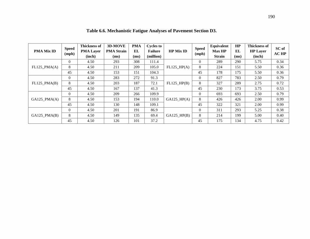
190
Table 6.6. Mechanistic Fatigue Analyses of Pavement Section D3.
PMA Mix ID Speed
(mph)
Thickness of
PMA Layer
(inch)
3D-MOVE
PMA Strain
(ms)
PMA
EL
(ms)
Cycles to
Failure
(million)
HP Mix ID Speed
(mph)
Equivalent
Max HP
Strain
HP
EL
(ms)
Thickness of
HP Layer
(inch)
SC of
AC HP
FL125_PMA(A)
0 4.50 293 308 111.4
FL125_HP(A)
0 289 290 5.75 0.34
8 4.50 211 209 105.0 8 224 151 5.50 0.36
45 4.50 153 151 104.3 45 178 175 5.50 0.36
FL125_PMA(B)
0 4.50 283 272 91.3
FL125_HP(B)
0 827 783 2.50 0.79
8 4.50 203 187 72.1 8 327 289 2.75 0.72
45 4.50 167 137 41.3 45 230 173 3.75 0.53
GA125_PMA(A)
0 4.50 209 266 109.9
GA125_HP(A)
0 693 693 2.50 0.79
8 4.50 153 194 110.0 8 426 426 2.00 0.99
45 4.50 130 148 109.1 45 322 321 2.00 0.99
GA125_PMA(B)
0 4.50 201 191 86.9
GA125_HP(B)
0 311 293 5.25 0.38
8 4.50 149 135 69.4 8 214 199 5.00 0.40
45 4.50 126 101 37.2 45 175 134 4.75 0.42

191
Table 6.7. Mechanistic Fatigue Analyses of Pavement Section E1.
PMA Mix ID Speed
(mph)
Thickness
of PMA
Layer
(inch)
3D-MOVE
PMA Strain
(ms)
PMA
EL
(ms)
Number of
Cycles to
Failure
(million)
HP Mix ID Speed
(mph)
Equivalent
Max HP
Strain
HP
EL
(ms)
Thickness of
HP Layer
(inch)
SC of
AC
HP
FL125_PMA(A)
0 5.00 300 308 111.4
FL125_HP(A)
0 289 290 6.50 0.34
8 5.00 210 212 111.8 8 224 224 6.25 0.35
45 5.00 167 154 75.1 45 194 176 5.75 0.38
FL125_PMA(B)
0 5.00 287 272 84.6
FL125_HP(B)
0 846 783 2.50 0.88
8 5.00 199 190 88.3 8 330 309 3.50 0.63
45 5.00 160 139 54.2 45 220 179 4.50 0.49
GA125_PMA(A)
0 5.00 203 266 109.9
GA125_HP(A)
0 693 693 2.25 0.98
8 5.00 146 197 109.3 8 427 179 2.00 1.10
45 5.00 122 149 112.6 45 329 330 2.50 0.88
GA125_PMA(B)
0 5.00 194 191 104.0
GA125_HP(B)
0 297 293 6.25 0.35
8 5.00 140 138 101.6 8 201 216 6.00 0.37
45 5.00 117 102 56.4 45 163 138 5.75 0.38
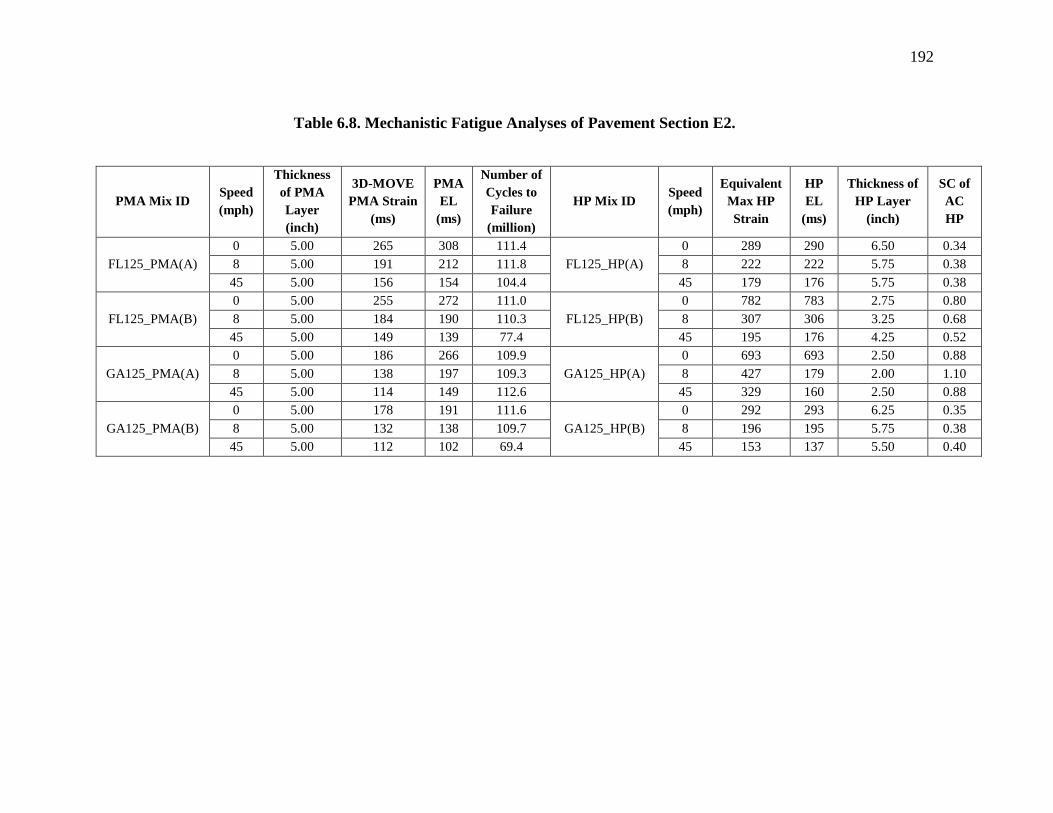
192
Table 6.8. Mechanistic Fatigue Analyses of Pavement Section E2.
PMA Mix ID Speed
(mph)
Thickness
of PMA
Layer
(inch)
3D-MOVE
PMA Strain
(ms)
PMA
EL
(ms)
Number of
Cycles to
Failure
(million)
HP Mix ID Speed
(mph)
Equivalent
Max HP
Strain
HP
EL
(ms)
Thickness of
HP Layer
(inch)
SC of
AC
HP
FL125_PMA(A)
0 5.00 265 308 111.4
FL125_HP(A)
0 289 290 6.50 0.34
8 5.00 191 212 111.8 8 222 222 5.75 0.38
45 5.00 156 154 104.4 45 179 176 5.75 0.38
FL125_PMA(B)
0 5.00 255 272 111.0
FL125_HP(B)
0 782 783 2.75 0.80
8 5.00 184 190 110.3 8 307 306 3.25 0.68
45 5.00 149 139 77.4 45 195 176 4.25 0.52
GA125_PMA(A)
0 5.00 186 266 109.9
GA125_HP(A)
0 693 693 2.50 0.88
8 5.00 138 197 109.3 8 427 179 2.00 1.10
45 5.00 114 149 112.6 45 329 160 2.50 0.88
GA125_PMA(B)
0 5.00 178 191 111.6
GA125_HP(B)
0 292 293 6.25 0.35
8 5.00 132 138 109.7 8 196 195 5.75 0.38
45 5.00 112 102 69.4 45 153 137 5.50 0.40

193
6.2 Initial Structural Coefficient for HP AC Mixes
6.2.1 Introduction
Multiple factors including applied traffic level, pavement structure, layer properties, and
performance characteristics of the evaluated PMA and HP AC mixes resulted in different
structural coefficients for HP AC mixes based on fatigue cracking analysis as summarized
in Table 6.9, Table 6.10, and Table 6.11. Some of these coefficients were observed lower
than 0.44 with a minimum value of 0.33 for FL125_HP(A) AC mix under static conditions
(i.e., at a full stop at an intersection) when evaluated in pavement section D1. On the other
hand, the highest value (i.e., 1.32) was observed for GA125_HP(A) AC mix at the three
considered loading speeds when evaluated in pavement section D2.
Table 6.9. Summary of Determined HP AC Structural Coefficient for Pavement
Sections under Traffic Level C.
Pavement
Section ID Speed (mph)
Mix / Binder ID
FL95 GA95
HP(A) HP(B) HP(A) HP(B)
C1
0 0.48 0.66 0.44 0.53
8 0.59 0.59 0.44 0.41
45 0.75 0.53 0.44 0.35
C2
0 0.59 0.80 0.37 0.49
8 0.59 1.10 0.42 0.44
45 0.59 0.68 0.46 0.37
C3
0 0.53 0.48 0.53 0.53
8 0.66 0.59 0.59 0.41
45 0.48 0.48 0.59 0.35

194
Table 6.10. Summary of Determined HP AC Structural Coefficient for Pavement
Sections under Traffic Level D.
Pavement
Section ID Speed (mph)
Mix / Binder ID
FL125 GA125
HP(A) HP(B) HP(A) HP(B)
D1
0 0.33 0.79 0.99 0.36
8 0.36 0.66 0.99 0.38
45 0.40 0.53 0.79 0.40
D2
0 0.46 0.88 1.32 0.48
8 0.50 0.96 1.32 0.50
45 0.50 0.62 1.32 0.46
D3
0 0.34 0.79 0.79 0.38
8 0.36 0.72 0.99 0.40
45 0.36 0.53 0.99 0.42
Table 6.11. Summary of Determined HP AC Structural Coefficient for Pavement
Sections under Traffic Level E.
Pavement
Section ID Speed (mph)
Mix / Binder ID
FL125 GA125
HP(A) HP(B) HP(A) HP(B)
E1
0 0.34 0.88 0.98 0.35
8 0.35 0.63 1.10 0.37
45 0.38 0.49 0.88 0.38
E2
0 0.34 0.80 0.88 0.35
8 0.38 0.68 1.10 0.38
45 0.38 0.52 0.88 0.40
Considering all these factors, a statistical analysis was needed to evaluate the
distribution of the structural coefficient for AC HP mixes determined under different
conditions. This analysis purpose was to determine a representative initial structural
coefficient for the evaluated cases. Thus, three major analyses were carried out: a) by
considering all 96 determined structural coefficients, b) after dissecting the data into two
separate groups based on the aggregate source (i.e., Limestone FL vs. Granite GA), and c)
after dissecting the data into two separate groups based on the NMAS (i.e., 9.5 mm vs. 12.5
mm). The following section describes the findings from all three statistical analyses.
195
6.2.2 Statistical Analyses of Structural Coefficients
6.2.2.1 Evaluation of all data collected
The statistical distribution of the determined 96 structural coefficients did not follow a
normal distribution. In statistics, a Q-Q plot (“Q” stands for quantile) is a probability plot
used to compare the probability distributions by plotting their quantiles against each other.
If the points in the Q-Q plot approximately lie on the equality line, the two distributions
that are being compared are considered similar. Moreover, if the points in the Q-Q plot lie
on a line but not necessarily the equality line, the two distributions are considered linearly
related. Figure 6.10 illustrates the sample versus theoretical quantiles (Q-Q plot) of the
statistical distribution representing the determined 96 structural coefficients. The
theoretical quantiles represent a perfect normal distribution. As shown in Figure 6.10, the
evaluated data set (i.e., 96 structural coefficient) is skewed from both sides and did not
follow a normal distribution.
In addition, multiple tests exist in statistics to evaluate the normality of a given
distribution. In this study, the Shapiro_Wilk test was used to evaluate and conform the non-
normality of the evaluated 96 structural coefficients. The p-value stands for the probability
of having an element lower than the W-value determined as output of the normality test. If
the determined p-value is less than the alpha level (i.e., selected allowable error), then the
null hypothesis that the data set is normally distributed is rejected. The observation of
having a p-value greater than the selected alpha level leads to the statement that the null
hypothesis that the data are normally distributed is accepted.

196
Figure 6.10. Normal Q-Q plot of the 96 determined structural coefficient (original
data).
For this study, the W- and p-values were determined as 0.85793 and 3.84E-08,
respectively. An alpha level of 0.05 (i.e. 5%) was selected. The determined p-value (i.e.,
3.84E-08) was observed to be significantly lower than 0.05 indicating that the 96 structural
coefficients data do not follow a normal distribution. Normality tests and verification were
implemented and multiple data transformations such as Box-Cox and multiple linear/non-
linear transformations were attempted to make the data set distribution normal. All these
attempts were unsuccessful and requested the need for a different methodology that can
deal with complicated data set and unknown statistic.
It should be noted that, the 96 cases evaluated in this study would not exist in
practice at all times throughout the pavement design life. These cases are dependent on

197
various factors such as traffic level, pavement structure, loading speed, AC mix property
and performance characteristics, and will not all occur at the same time. Furthermore,
different strengths of base and subgrade material, as well as different AC mixes (i.e.,
different asphalt binders and aggregate sources) not evaluated in this study may exist.
Therefore, a probabilistic type of analysis remains needed to effectively determine a
representative structural coefficient for HP AC mixes in Florida.
In statistics, bootstrapping is any test or metric that relies on random sampling with
replacement (Singh et al., 2008). It allows assigning measures of accuracy defined in terms
of bias, variance, confidence intervals, or prediction error to sample estimates. In this study,
the bootstrapped method is considered adequate for the analysis of the 96 structural
coefficients for HP AC mixes. It is used for estimating the distribution of mean statistic
without using normal theory. The bootstrapping algorithm for case resampling consists of
the following steps: a) data are resampled with replacement, and the size of the resample
must be equal to the size of the original set of data (i.e., 96 in this case); b) the statistic of
interest (i.e., in this case mean of the 96 determined structural coefficients for HP AC
mixes) is computed for the resampled data from step a; c) this scenario is repeated many
times to get a more precise estimate of the mean structural coefficient values. When the
sample size is insufficient for straightforward statistical inference, if the underlying
distribution is well-known, bootstrapping provides a way to account for the distortions
caused by the specific sample that may not be fully representative of the population (e.g.,
in this case having different strengths of base and subgrade material, as well as different
evaluated AC mixes).
198
In this study, the bootstrapping scenario was repeated 2,000 times to guarantee an
accurate convergence of the bootstrapped mean of the 96 determined structural
coefficients. Figure 6.11 illustrates the density distribution of the bootstrapped structural
coefficient mean. The convergence of the bootstrapped mean can be explained by the
observed bell-shape of the density curve. Moreover, a Q-Q plot of the bootstrapped data is
provided in Figure 6.12. As all the points fall approximately along the reference line, a
normal distribution can be assumed. In addition, the Shapiro_Wilk test was performed on
the bootstrapped data. A p-value of 0.66 (>0.05) was determined implying that the
distribution of the bootstrapped mean data of the 96 determined structural coefficients
combined is normal.
Finally, a bootstrapped structural coefficient mean value of 0.59 with a standard
error of 0.025 resulted from this analysis. Using the mean value minus two times the
standard error (corresponding to about 95% confidence interval), a value of 0.54 was
estimated for the structural coefficient of HP AC mixes based on fatigue analyses.
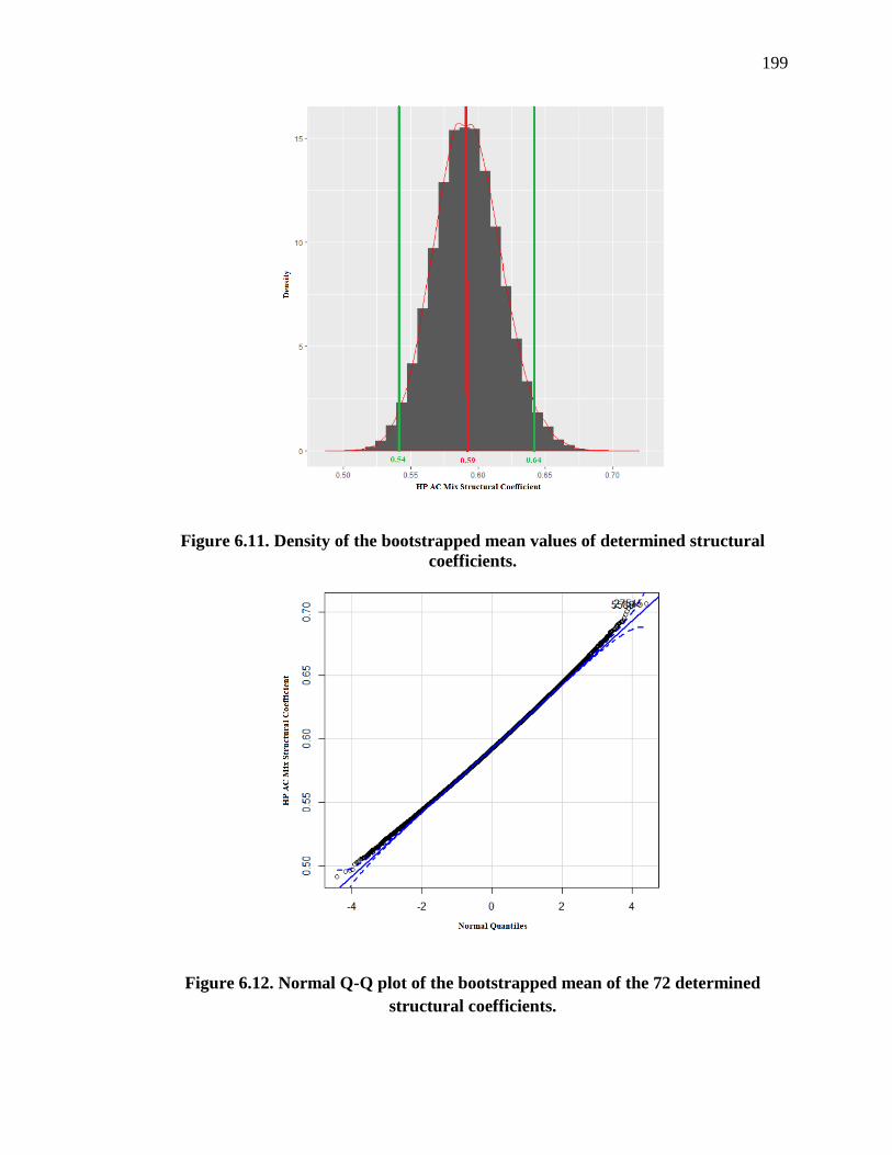
199
Figure 6.11. Density of the bootstrapped mean values of determined structural
coefficients.
Figure 6.12. Normal Q-Q plot of the bootstrapped mean of the 72 determined
structural coefficients.

200
6.2.2.2 Evaluation of Data based on Aggregate Sources: FL vs. GA
As mentioned before, two different aggregate sources were used in this study: Southeast
Florida limestone labeled “FL,” and Georgia Granite labeled “GA”. The use of different
aggregate source and mineralogy contributed to observed differences in the performance
evaluation of the designed PMA and HP AC mixes, which resulted in a wide range of HP
AC structural coefficients. Therefore, the 96 determined structural coefficients were
subdivided into two major data sets based on the aggregate sources with each set included
36 coefficients. Figure 6.13 illustrates the Q-Q plots of the HP structural coefficients
determined for FL and GA AC mixes. In the case of FL AC mixes, the structural
coefficients fell approximately along the reference line, thus indicating that the data set is
likely to have a normal distribution. However, the GA data set showed a skewed trend from
both sides and all the points fell approximately outside the reference line indicating a non-
normal distribution. The Shapiro_Wilk normality test performed on the FL data set showed
a p-value of 0.015 that is lower than the chosen alpha level of 0.05; thus, confirming the
non-normality of the evaluated data set. In parallel, the Shapiro_Wilk normality test
performed on the GA data set showed a p-value of 9.43E-07 that is significantly lower than
0.05, confirming the rejection of normality for the GA data set.

201
(a) (b)
Figure 6.13. Normal Q-Q plot of the determined structural coefficients for: (a) FL
AC mixes, and (b) GA AC mixes.
Similar to the analyses performed in Section 6.2.2.1, the bootstrapping scenario
was repeated 2,000 times on each data set separately to guarantee an accurate convergence
of their bootstrapped means. It should be noted that, while the FL data set followed a
normal distribution, bootstrapping was still applied for achieving a better estimate of the
mean structural coefficient while considering multiple scenarios that might be encountered
in practice. Figure 6.14 illustrates the density distribution of the bootstrapped structural
coefficient mean for each of the FL and GA data sets. The convergence of the bootstrapped
mean can be explained by the observed bell-shape of the density curve for each evaluated
data set. Moreover, a Q-Q plot of the bootstrapped mean for each data set is provided in
Figure 6.15. As all the points fall approximately along the reference line, a normal
distribution can be assumed for each of the evaluated data set. In addition, the
Shapiro_Wilk test was performed on the bootstrapped data. A p-value of 0.077 (>0.05) and
0.091 (>0.05) were determined for FL and GA data sets, respectively, confirming that the

202
data sets are normally distributed. As a result, a bootstrapped structural coefficient mean
value of 0.57 with a standard error of 0.025, and a bootstrapped structural coefficient mean
value of 0.53 with a standard error of 0.043 were determined for the FL and GA data sets,
respectively. Using the mean value minus two times the standard error (corresponding to
about 95% confidence interval), values of 0.52 and 0.61 were estimated for the structural
coefficient of HP AC mixes (based on fatigue analyses) from FL and GA aggregate
sources, respectively.
(a) (b)
Figure 6.14. Density of the bootstrapped mean values of determined structural
coefficients for: (a) FL AC mixes, and (b) GA AC mixes.

203
(a) (b)
Figure 6.15. Normal Q-Q plot of the bootstrapped mean of the determined
structural coefficients for: (a) FL AC mixes, and (b) GA AC mixes.
6.2.2.3 Evaluation of Data based on NMAS: 9.5 vs. 12.5 mm
As mentioned before, two aggregate gradations were evaluated from each aggregate source
with NMAS of 9.5 mm and 12.5 mm. The difference in NMAS contributed to some of the
differences in the performance evaluation of the designed PMA and HP AC mixes, which
resulted in a wide range of HP AC structural coefficients. Therefore, the 96 determined
structural coefficients were subdivided into two major data sets based on the NMAS with
each set included 36 coefficients.
Figure 6.16 illustrates the Q-Q plots of the HP structural coefficients determined
for 9.5 and 12.5 mm NMAS AC mixes. The majority of the structural coefficients of each
of the data sets (i.e., 9.5 and 12.5 mm NMAS) fell approximately outside the reference line
indicating that the data sets are not normally distributed. The Shapiro_Wilk normality test
performed on the 9.5 mm and 12.5 mm NMAS data sets showed p-values of 2.68E-4 and
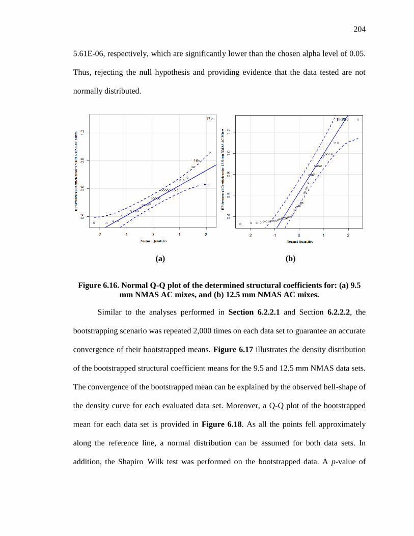
204
5.61E-06, respectively, which are significantly lower than the chosen alpha level of 0.05.
Thus, rejecting the null hypothesis and providing evidence that the data tested are not
normally distributed.
(a) (b)
Figure 6.16. Normal Q-Q plot of the determined structural coefficients for: (a) 9.5
mm NMAS AC mixes, and (b) 12.5 mm NMAS AC mixes.
Similar to the analyses performed in Section 6.2.2.1 and Section 6.2.2.2, the
bootstrapping scenario was repeated 2,000 times on each data set to guarantee an accurate
convergence of their bootstrapped means. Figure 6.17 illustrates the density distribution
of the bootstrapped structural coefficient means for the 9.5 and 12.5 mm NMAS data sets.
The convergence of the bootstrapped mean can be explained by the observed bell-shape of
the density curve for each evaluated data set. Moreover, a Q-Q plot of the bootstrapped
mean for each data set is provided in Figure 6.18. As all the points fell approximately
along the reference line, a normal distribution can be assumed for both data sets. In
addition, the Shapiro_Wilk test was performed on the bootstrapped data. A p-value of

205
0.062 (>0.05) and 0.242 (>0.05) were determined providing evidence that that each of the
data set tested is normally distributed. Resulting from these analyses, a bootstrapped
structural coefficient mean value of 0.58 with a standard error of 0.023 and a bootstrapped
structural coefficient mean value of 0.626 with a standard error of 0.037 that can be
attributed for the 9.5 and 12.5 NMAS data sets, respectively. Using the mean value minus
two times standard error (corresponding to about 95% confidence interval), values of 0.535
and 0.55 were estimated for the structural coefficient of HP AC mixes (based on fatigue
analyses) with 9.5 and 12.5 NMAS, respectively.
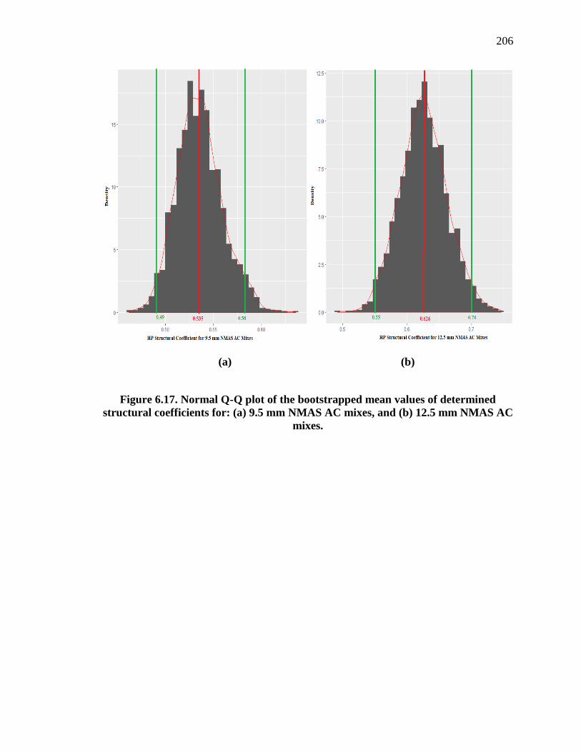
206
(a) (b)
Figure 6.17. Normal Q-Q plot of the bootstrapped mean values of determined
structural coefficients for: (a) 9.5 mm NMAS AC mixes, and (b) 12.5 mm NMAS AC
mixes.

207
(a) (b)
Figure 6.18. Normal Q-Q plot of the bootstrapped mean of the determined
structural coefficients for: (a) 9.5 mm NMAS AC mixes, and (b) 12.5 mm NMAS AC
mixes.
6.2.2.4 Summary
Based on the findings from the statistical analyses, the following observations can be made.
Table 6.12 summarizes the outcomes of the three statistical analyses.
• A bootstrapped structural coefficient mean value of 0.59 with a standard error of
0.025 resulted from the analysis of all determined 96 structural coefficients
combined as one set.
• After dissecting the data into two separate groups based on the aggregate source
(i.e., FL vs. GA), a bootstrapped structural coefficient mean value of 0.57 and 0.53
was obtained for FL and GA group, respectively. However, a higher standard error

208
of 0.043 was observed for the mixes with GA aggregates irrespective of aggregate
NMAS.
• After dissecting the data into two separate groups based on the NMAS (i.e., 9.5 mm
vs. 12.5 mm), the mixes with 12.5 mm NMAS had a higher bootstrapped structural
coefficient mean value than the mixes with 9.5 mm NMAS (0.626 vs. 0.58). The
mixes with 12.5 mm NMAS had also a higher standard error than the mixes with
9.5 mm NMAS (0.037 vs. 0.023).
Table 6.12. Summary of Statistical Analyses based on Traffic Level C, D, and E.
Analysis Description Factor Mean
(µ)
Standard
Error (SE)
µ–2*SE
(95% Confidence
Interval)
I
Considering all 96
determined structural
coefficients as one set.
All data
combined 0.59 0.025 0.54
II
After dissecting the data
into two separate groups
based on the aggregate
source (FL vs. GA).
FL aggregate
source 0.57 0.025 0.52
GA aggregate
source 0.53 0.043 0.45
III
After dissecting the data
into two separate groups
based on the NMAS (9.5
mm vs. 12.5 mm).
9.5 mm NMAS 0.58 0.023 0.535
12.5 mm NMAS 0.626 0.037 0.55
It should be mentioned that similar analyses were conducted considering the
determined structural coefficients for traffic level C and D only (the data for traffic level E
were excluded). Table 6.13 summarizes the outcome of these statistical analyses, again for
traffic level C, and D only. Comparing the 95% CI of the bootstrapped mean of both
analyses, Traffic Level C, D, and E vs. Traffic Level C and D only, it can be observed that
the addition of the determined structural coefficients for pavement structures subjected to
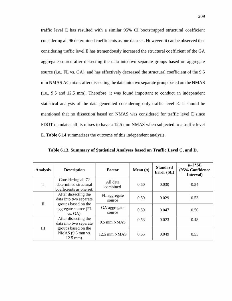
209
traffic level E has resulted with a similar 95% CI bootstrapped structural coefficient
considering all 96 determined coefficients as one data set. However, it can be observed that
considering traffic level E has tremendously increased the structural coefficient of the GA
aggregate source after dissecting the data into two separate groups based on aggregate
source (i.e., FL vs. GA), and has effectively decreased the structural coefficient of the 9.5
mm NMAS AC mixes after dissecting the data into two separate group based on the NMAS
(i.e., 9.5 and 12.5 mm). Therefore, it was found important to conduct an independent
statistical analysis of the data generated considering only traffic level E. it should be
mentioned that no dissection based on NMAS was considered for traffic level E since
FDOT mandates all its mixes to have a 12.5 mm NMAS when subjected to a traffic level
E. Table 6.14 summarizes the outcome of this independent analysis.
Table 6.13. Summary of Statistical Analyses based on Traffic Level C, and D.
Analysis Description Factor Mean (µ) Standard
Error (SE)
µ–2*SE
(95% Confidence
Interval)
I
Considering all 72
determined structural
coefficients as one set.
All data
combined 0.60 0.030 0.54
II
After dissecting the
data into two separate
groups based on the
aggregate source (FL
vs. GA).
FL aggregate
source 0.59 0.029 0.53
GA aggregate
source 0.59 0.047 0.50
III
After dissecting the
data into two separate
groups based on the
NMAS (9.5 mm vs.
12.5 mm).
9.5 mm NMAS 0.53
0.023
0.48
12.5 mm NMAS 0.65 0.049 0.55
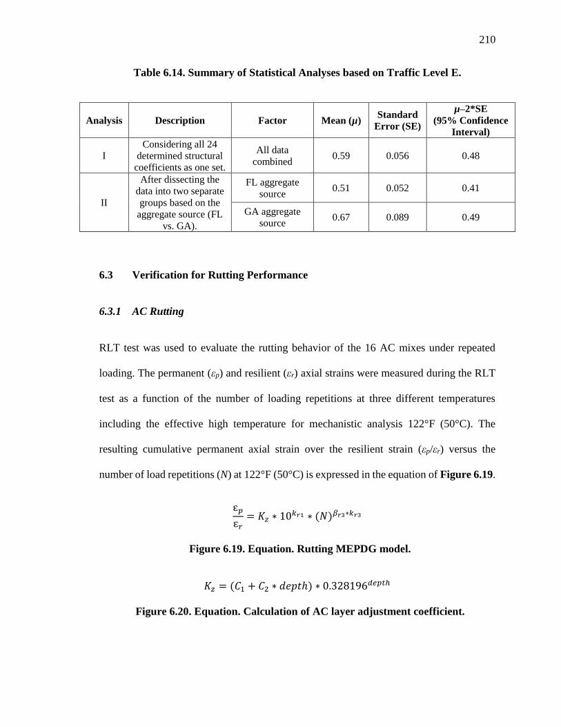
210
Table 6.14. Summary of Statistical Analyses based on Traffic Level E.
Analysis Description Factor Mean (µ) Standard
Error (SE)
µ–2*SE
(95% Confidence
Interval)
I
Considering all 24
determined structural
coefficients as one set.
All data
combined 0.59 0.056 0.48
II
After dissecting the
data into two separate
groups based on the
aggregate source (FL
vs. GA).
FL aggregate
source 0.51 0.052 0.41
GA aggregate
source 0.67 0.089 0.49
6.3 Verification for Rutting Performance
6.3.1 AC Rutting
RLT test was used to evaluate the rutting behavior of the 16 AC mixes under repeated
loading. The permanent (εp) and resilient (εr) axial strains were measured during the RLT
test as a function of the number of loading repetitions at three different temperatures
including the effective high temperature for mechanistic analysis 122°F (50°C). The
resulting cumulative permanent axial strain over the resilient strain (εp/εr) versus the
number of load repetitions (N) at 122°F (50°C) is expressed in the equation of Figure 6.19.
ԑ𝑝
ԑ𝑟= 𝐾𝑧 ∗ 10𝑘𝑟1 ∗ (𝑁)𝛽𝑟3∗𝑘𝑟3
Figure 6.19. Equation. Rutting MEPDG model.
𝐾𝑧 = (𝐶1 + 𝐶2 ∗ 𝑑𝑒𝑝𝑡ℎ) ∗ 0.328196𝑑𝑒𝑝𝑡ℎ
Figure 6.20. Equation. Calculation of AC layer adjustment coefficient.

211
𝐶1 = −0.1039 ∗ ℎ𝑎𝑐2 + 2.4868 ∗ ℎ𝑎𝑐 − 17.342
Figure 6.21. Equation. Calculation of regression constant 1.
𝐶2 = 0.0172 ∗ ℎ𝑎𝑐2 − 1.7331 ∗ ℎ𝑎𝑐 + 27.428
Figure 6.22. Equation. Calculation of regression constant 2.
Where ԑ𝑝 is the permanent axial strain expressed in inch/inch (mm/mm), ԑ𝑟 is the
resilient axial strain expressed in inch/inch (mm/mm), N is the number of loading cycles,
𝐾𝑍 is the AC layer thickness adjustment coefficient defined in the equation of Figure 6.20,
kr1 and kr3 are the experimentally determined coefficients, βr3 is the traffic loading
calibration factor, ℎ𝑎𝑐 is the total AC layer thickness expressed in inch, 𝐶1 and 𝐶2 are the
regression constants defined as a function of hac as expressed in the equation of Figure
6.21 and Figure 6.22, respectively, and depth is the distance between the top of the AC
layer and the computational point expressed in inch.
The MEPDG approach (MEPDG Guide, 2004) was followed to sub-divide each
layer of the pavement cross-section into sub-layers as illustrated in Figure 6.23. The
critical responses were then computed at the middle of each sub-layer. Using the rutting
model developed for each evaluated AC mix (i.e., PMA and HP) with the determined
resilient strain (εr) from 3D-Move mechanistic analyses, the permanent strain (εp) within
each AC sub-layer was calculated under three loading speeds 0, 8, and 15 mph (0, 13, and
24 km/h). It should be mentioned that for the 15 mph (24 km/h) dynamic case, a braking
friction coefficient (fBr) of 0.623 was considered for a tractor-semi trailer truck on a sloped
pavement structure as described previously in Section 5.1.2. The rut depth generated in the

212
AC layer is then determined for each pavement structure following the relationship of
Figure 6.24.
Figure 6.23. MEPDG sub-layering of pavement cross-section for flexible
pavements.
𝑅𝐷 = ∑ ԑ𝑝 ∗ ℎ𝐴𝐶𝑖
Figure 6.24. Equation. Calculation of rut depth.
Where 𝑅𝐷 is the rut depth generated in the AC layer expressed in inch (mm), ԑ𝑝 is
the permanent axial strain expressed in inch/inch (mm/mm), ℎ𝐴𝐶𝑖 is the thickness of the
AC sub-layer i expressed in inch (mm).
Preliminary traffic loading calibration factors βr3 (refer to Table 6.15) were
estimated for the purpose of this effort based on the following assumptions:
213
• The rut depth generated in the AC layer in a PMA designed pavement-cross section
was fixed to its maximum allowable value of 0.25 inch (6.4 mm).
• The number of loading cycles was determined function of the traffic level.
Referring to the AASHTO Guide 1993 (AASHTO Guide, 1993), one pass of a
tandem axle loaded with 44,000 lbs. (196 kN) on a pavement section characterized
with a structural number (SN) of 5.0 is equivalent to three equivalent single axle
load (ESAL). Therefore, for a traffic level C (i.e., 7 million ESALs), traffic level D
(i.e., 20 million ESALs), and traffic level E (i.e., 40 million ESALs), the number
of passes (N) is equal to 2.3, 6.7, and 13.3 million tandem axles passes, respectively.
Three factors were taken into consideration including the PMA AC mixes, traffic
level, and loading speed. An average βr3 factor was determined for each AC PMA mix at
a given traffic level (i.e., C, D, and E) under static conditions (i.e., 0 mph) as summarized
in Table 6.15. These factors were then used for the corresponding HP AC mixes (e.g.,
FL95_PMA(A) vs. FL95_HP(A)) at the same traffic level under all loading speeds (i.e.,0,
8, and 15 mph (0, 13, and 24 km/h)).

214
Table 6.15. Summary of Table of βr3 Factors.
Traffic
Level Section ID FL95_PMA(A) FL95_PMA(B) GA95_PMA(A) GA95_PMA(B)
C
C1 0.273355 0.295698 0.565351 0.615320
C2 0.257956 0.284580 0.544226 0.594831
C3 0.272963 0.267898 0.565633 0.615800
Average 0.268091 0.282725 0.558403 0.608651
Traffic
Level Section ID FL125_PMA(A) FL125_PMA(B) GA125_PMA(A) GA125_PMA(B)
D
D1 0.325921 0.349975 0.505013 0.511321
D2 0.329058 0.352872 0.508767 0.514225
D3 0.324395 0.348519 0.502157 0.508985
Average 0.326458 0.350455 0.505313 0.511510
Traffic
Level Section ID FL125_PMA(A) FL125_PMA(B) GA125_PMA(A) GA125_PMA(B)
E
E1 0.311459 0.334523 0.482181 0.488465
E2 0.312037 0.335076 0.483354 0.489455
Average 0.311748 0.334800 0.482767 0.488960
The initial structural coefficient of HP AC mixes determined based on the fatigue
performance life section (i.e., 0.54) was used to determine the thickness of the HP AC layer
in the various HP pavement structures (refer to the equation of Figure 6.25). It should be
mentioned that the base, stabilized subgrade, and subgrade layers were maintained the
same in both PMA and respective HP pavement structures.
ℎ𝐴𝐶−𝐻𝑃 =0.44
0.54∗ ℎ𝐴𝐶−𝑃𝑀𝐴
Figure 6.25. Equation. Calculation of the HP AC layer thickness.
Where ℎ𝐴𝐶−𝑃𝑀𝐴 is the thickness of the AC layer in PMA pavement section
expressed in inch (mm), and ℎ𝐴𝐶−𝐻𝑃 is the thickness of the AC layer in HP pavement
section expressed in inch (mm).

215
Table 6.16 to Table 6.24 summarize the rutting performance data of the AC layers
in the PMA and HP pavement sections. A review of the presented data reveals the following
observations:
• For traffic level C and under static conditions, all HP AC mixes except for
GA95_HP(B) showed lower AC rut depths (i.e., a 16 to 40 % decrease in AC rut
depths) when compared with their corresponding PMA AC layers. Thus, indicating
a better rutting performance for the HP AC mixes.
• For traffic level C and under dynamic loading (i.e., 8 and 15 mph (13, and 24
km/h)), all rut depths of HP AC mixes were observed to be lower than the respective
PMA AC mixes. Thus, indicating a better rutting performance for HP AC mixes.
• For traffic level D and under static conditions, all HP AC mixes except for the ones
manufactured using HP asphalt binder from source B showed lower AC rut depths
(i.e., a 32 to 52 % decrease in the rut depths) when compared with their
corresponding PMA AC layers.
• For traffic level D and under dynamic loading (i.e., 8 and 15 mph (13, and 24
km/h)), all rut depths of HP AC were observed to be lowered than the control PMA
ones.
• For traffic level E and under static conditions, all HP AC mixes except for the ones
manufactured using HP asphalt binder from source B showed lower AC rut depths

216
(i.e., a 32 to 52 % decrease in the rut depths) when compared with their
corresponding PMA AC layers.
• For traffic level E and under dynamic loading (i.e., 8 and 15 mph (13, and 24
km/h)), all rut depths of HP AC were observed to be lowered than the control PMA
ones.
It should be mentioned that for the case of AC mixes manufactured using HP
asphalt binders from source B, the rut depths generated in the AC layers were higher than
the ones generated in the corresponding PMA control ones and did not meet the criterion
of 0.25 inch (6.4 mm) as a maximum allowable rut depth in the AC layer. However, this
should not be of a concern since in reality, the design traffic will not be static (i.e., full
stop) during the entire design life of the pavement. The traffic would typically comprise
static and dynamic loading. It should also be noted that the static analysis considered in
this study used a modulus for the AC layer that was selected at a very low loading
frequency (i.e., 0.5 Hz) to represent heavy vehicles approaching a full stop condition at an
intersection. This resulted in a relatively low modulus for the AC layer ranging between
22,116 and 71,067 psi (152.5 and 490 MPa) for PMA AC mixes and between 14,524 and
33,269 psi (100 and 229 MPa) for HP AC mixes.

217
Table 6.16. Rutting Data for Traffic Level C under Static Conditions.
Section
ID PMA Mix ID
Rut Depths (inch) HP Mix ID
Rut Depths (inch)
AC Base Subgrade AC Base Subgrade
C1
FL95_PMA(A) 0.25 0.34 0.13 FL95_HP(A) 0.15 0.35 0.13
FL95_PMA(B) 0.25 0.33 0.13 FL95_HP(B) 0.17 0.36 0.13
GA95_PMA(A) 0.25 0.31 0.12 GA95_HP(A) 0.14 0.37 0.13
GA95_PMA(B) 0.25 0.30 0.12 GA95_HP(B) 0.20 0.37 0.13
C2
FL95_PMA(A) 0.25 0.19 0.16 FL95_HP(A) 0.17 0.21 0.16
FL95_PMA(B) 0.25 0.18 0.16 FL95_HP(B) 0.19 0.22 0.16
GA95_PMA(A) 0.25 0.17 0.15 GA95_HP(A) 0.16 0.22 0.16
GA95_PMA(B) 0.25 0.17 0.15 GA95_HP(B) 0.26 0.22 0.17
C3
FL95_PMA(A) 0.25 0.25 0.14 FL95_HP(A) 0.16 0.26 0.14
FL95_PMA(B) 0.25 0.25 0.14 FL95_HP(B) 0.11 0.26 0.14
GA95_PMA(A) 0.25 0.23 0.13 GA95_HP(A) 0.14 0.27 0.14
GA95_PMA(B) 0.25 0.23 0.13 GA95_HP(B) 0.21 0.27 0.14
Table 6.17. Rutting Data for Traffic Level C under a Loading Speed of 8 mph.
Section
ID PMA Mix ID
Rut Depths (inch) HP Mix ID
Rut Depths (inch)
AC Base Subgrade AC Base Subgrade
C1
FL95_PMA(A) 0.11 0.31 0.14 FL95_HP(A) 0.09 0.33 0.15
FL95_PMA(B) 0.10 0.30 0.14 FL95_HP(B) 0.10 0.35 0.15
GA95_PMA(A) 0.11 0.28 0.14 GA95_HP(A) 0.07 0.35 0.14
GA95_PMA(B) 0.11 0.26 0.14 GA95_HP(B) 0.09 0.35 0.15
C2
FL95_PMA(A) 0.12 0.19 0.16 FL95_HP(A) 0.10 0.19 0.18
FL95_PMA(B) 0.11 0.16 0.18 FL95_HP(B) 0.11 0.20 0.19
GA95_PMA(A) 0.11 0.15 0.17 GA95_HP(A) 0.08 0.20 0.19
GA95_PMA(B) 0.11 0.14 0.17 GA95_HP(B) 0.11 0.20 0.19
C3
FL95_PMA(A) 0.11 0.23 0.15 FL95_HP(A) 0.09 0.25 0.15
FL95_PMA(B) 0.10 0.22 0.15 FL95_HP(B) 0.10 0.26 0.15
GA95_PMA(A) 0.11 0.21 0.15 GA95_HP(A) 0.07 0.26 0.15
GA95_PMA(B) 0.10 0.20 0.14 GA95_HP(B) 0.09 0.25 0.15
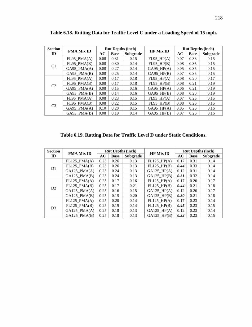
218
Table 6.18. Rutting Data for Traffic Level C under a Loading Speed of 15 mph.
Section
ID PMA Mix ID
Rut Depths (inch) HP Mix ID
Rut Depths (inch)
AC Base Subgrade AC Base Subgrade
C1
FL95_PMA(A) 0.08 0.31 0.15 FL95_HP(A) 0.07 0.33 0.15
FL95_PMA(B) 0.08 0.30 0.14 FL95_HP(B) 0.08 0.35 0.15
GA95_PMA(A) 0.08 0.27 0.14 GA95_HP(A) 0.05 0.35 0.15
GA95_PMA(B) 0.08 0.25 0.14 GA95_HP(B) 0.07 0.35 0.15
C2
FL95_PMA(A) 0.09 0.17 0.18 FL95_HP(A) 0.08 0.20 0.17
FL95_PMA(B) 0.08 0.17 0.18 FL95_HP(B) 0.08 0.21 0.19
GA95_PMA(A) 0.08 0.15 0.16 GA95_HP(A) 0.06 0.21 0.19
GA95_PMA(B) 0.08 0.14 0.16 GA95_HP(B) 0.08 0.20 0.19
C3
FL95_PMA(A) 0.08 0.23 0.15 FL95_HP(A) 0.07 0.25 0.15
FL95_PMA(B) 0.08 0.22 0.15 FL95_HP(B) 0.08 0.26 0.15
GA95_PMA(A) 0.10 0.20 0.15 GA95_HP(A) 0.05 0.26 0.16
GA95_PMA(B) 0.08 0.19 0.14 GA95_HP(B) 0.07 0.26 0.16
Table 6.19. Rutting Data for Traffic Level D under Static Conditions.
Section
ID PMA Mix ID
Rut Depths (inch) HP Mix ID
Rut Depths (inch)
AC Base Subgrade AC Base Subgrade
D1
FL125_PMA(A) 0.25 0.26 0.13 FL125_HP(A) 0.17 0.31 0.14
FL125_PMA(B) 0.25 0.26 0.13 FL125_HP(B) 0.44 0.33 0.14
GA125_PMA(A) 0.25 0.24 0.13 GA125_HP(A) 0.12 0.31 0.14
GA125_PMA(B) 0.25 0.24 0.13 GA125_HP(B) 0.31 0.32 0.14
D2
FL125_PMA(A) 0.25 0.17 0.16 FL125_HP(A) 0.17 0.20 0.17
FL125_PMA(B) 0.25 0.17 0.21 FL125_HP(B) 0.44 0.21 0.18
GA125_PMA(A) 0.25 0.16 0.15 GA125_HP(A) 0.12 0.20 0.17
GA125_PMA(B) 0.25 0.15 0.20 GA125_HP(B) 0.30 0.21 0.18
D3
FL125_PMA(A) 0.25 0.20 0.14 FL125_HP(A) 0.17 0.23 0.14
FL125_PMA(B) 0.25 0.19 0.14 FL125_HP(B) 0.45 0.23 0.15
GA125_PMA(A) 0.25 0.18 0.13 GA125_HP(A) 0.12 0.23 0.14
GA125_PMA(B) 0.25 0.18 0.13 GA125_HP(B) 0.32 0.23 0.15
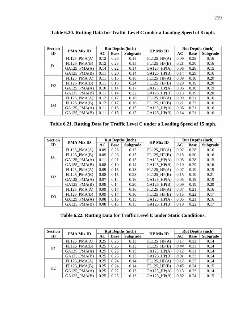
219
Table 6.20. Rutting Data for Traffic Level C under a Loading Speed of 8 mph.
Section
ID PMA Mix ID
Rut Depths (inch) HP Mix ID
Rut Depths (inch)
AC Base Subgrade AC Base Subgrade
D1
FL125_PMA(A) 0.12 0.23 0.15 FL125_HP(A) 0.09 0.28 0.16
FL125_PMA(B) 0.12 0.23 0.15 FL125_HP(B) 0.21 0.30 0.16
GA125_PMA(A) 0.14 0.22 0.14 GA125_HP(A) 0.06 0.28 0.15
GA125_PMA(B) 0.11 0.20 0.14 GA125_HP(B) 0.14 0.29 0.16
D2
FL125_PMA(A) 0.11 0.15 0.18 FL125_HP(A) 0.09 0.18 0.20
FL125_PMA(B) 0.11 0.15 0.24 FL125_HP(B) 0.20 0.19 0.20
GA125_PMA(A) 0.10 0.14 0.17 GA125_HP(A) 0.06 0.18 0.19
GA125_PMA(B) 0.11 0.14 0.22 GA125_HP(B) 0.13 0.19 0.20
D3
FL125_PMA(A) 0.12 0.17 0.16 FL125_HP(A) 0.09 0.21 0.16
FL125_PMA(B) 0.12 0.17 0.16 FL125_HP(B) 0.21 0.22 0.16
GA125_PMA(A) 0.11 0.15 0.15 GA125_HP(A) 0.06 0.21 0.16
GA125_PMA(B) 0.11 0.15 0.15 GA125_HP(B) 0.14 0.21 0.16
Table 6.21. Rutting Data for Traffic Level C under a Loading Speed of 15 mph.
Section
ID PMA Mix ID
Rut Depths (inch) HP Mix ID
Rut Depths (inch)
AC Base Subgrade AC Base Subgrade
D1
FL125_PMA(A) 0.09 0.23 0.15 FL125_HP(A) 0.07 0.28 0.16
FL125_PMA(B) 0.09 0.23 0.15 FL125_HP(B) 0.15 0.30 0.16
GA125_PMA(A) 0.11 0.21 0.15 GA125_HP(A) 0.05 0.28 0.15
GA125_PMA(B) 0.08 0.19 0.14 GA125_HP(B) 0.10 0.29 0.16
D2
FL125_PMA(A) 0.09 0.15 0.18 FL125_HP(A) 0.07 0.19 0.19
FL125_PMA(B) 0.08 0.15 0.23 FL125_HP(B) 0.15 0.19 0.21
GA125_PMA(A) 0.07 0.14 0.16 GA125_HP(A) 0.05 0.18 0.19
GA125_PMA(B) 0.08 0.14 0.20 GA125_HP(B) 0.09 0.19 0.20
D3
FL125_PMA(A) 0.09 0.17 0.16 FL125_HP(A) 0.07 0.21 0.16
FL125_PMA(B) 0.09 0.17 0.16 FL125_HP(B) 0.15 0.22 0.17
GA125_PMA(A) 0.08 0.15 0.15 GA125_HP(A) 0.05 0.21 0.16
GA125_PMA(B) 0.08 0.15 0.15 GA125_HP(B) 0.10 0.22 0.17
Table 6.22. Rutting Data for Traffic Level E under Static Conditions.
Section
ID PMA Mix ID
Rut Depths (inch) HP Mix ID
Rut Depths (inch)
AC Base Subgrade AC Base Subgrade
E1
FL125_PMA(A) 0.25 0.26 0.13 FL125_HP(A) 0.17 0.32 0.14
FL125_PMA(B) 0.25 0.26 0.13 FL125_HP(B) 0.44 0.33 0.14
GA125_PMA(A) 0.25 0.23 0.13 GA125_HP(A) 0.12 0.31 0.14
GA125_PMA(B) 0.25 0.23 0.13 GA125_HP(B) 0.31 0.33 0.14
E2
FL125_PMA(A) 0.25 0.24 0.14 FL125_HP(A) 0.17 0.23 0.14
FL125_PMA(B) 0.25 0.24 0.14 FL125_HP(B) 0.45 0.24 0.15
GA125_PMA(A) 0.25 0.22 0.13 GA125_HP(A) 0.13 0.23 0.14
GA125_PMA(B) 0.25 0.25 0.13 GA125_HP(B) 0.32 0.24 0.15
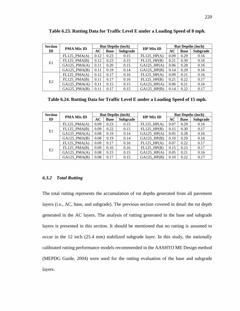
220
Table 6.23. Rutting Data for Traffic Level E under a Loading Speed of 8 mph.
Section
ID PMA Mix ID
Rut Depths (inch) HP Mix ID
Rut Depths (inch)
AC Base Subgrade AC Base Subgrade
E1
FL125_PMA(A) 0.12 0.23 0.15 FL125_HP(A) 0.09 0.29 0.16
FL125_PMA(B) 0.12 0.23 0.15 FL125_HP(B) 0.21 0.30 0.16
GA125_PMA(A) 0.11 0.20 0.15 GA125_HP(A) 0.06 0.28 0.16
GA125_PMA(B) 0.11 0.19 0.14 GA125_HP(B) 0.14 0.29 0.16
E2
FL125_PMA(A) 0.12 0.17 0.16 FL125_HP(A) 0.09 0.21 0.16
FL125_PMA(B) 0.11 0.17 0.16 FL125_HP(B) 0.21 0.22 0.17
GA125_PMA(A) 0.11 0.15 0.15 GA125_HP(A) 0.06 0.21 0.16
GA125_PMA(B) 0.11 0.17 0.15 GA125_HP(B) 0.14 0.22 0.17
Table 6.24. Rutting Data for Traffic Level E under a Loading Speed of 15 mph.
Section
ID PMA Mix ID
Rut Depths (inch) HP Mix ID
Rut Depths (inch)
AC Base Subgrade AC Base Subgrade
E1
FL125_PMA(A) 0.09 0.23 0.15 FL125_HP(A) 0.07 0.29 0.16
FL125_PMA(B) 0.09 0.22 0.15 FL125_HP(B) 0.15 0.30 0.17
GA125_PMA(A) 0.08 0.19 0.14 GA125_HP(A) 0.05 0.28 0.16
GA125_PMA(B) 0.08 0.19 0.14 GA125_HP(B) 0.10 0.29 0.16
E2
FL125_PMA(A) 0.09 0.17 0.16 FL125_HP(A) 0.07 0.22 0.17
FL125_PMA(B) 0.09 0.16 0.16 FL125_HP(B) 0.15 0.23 0.17
GA125_PMA(A) 0.08 0.15 0.15 GA125_HP(A) 0.05 0.21 0.16
GA125_PMA(B) 0.08 0.17 0.15 GA125_HP(B) 0.10 0.22 0.17
6.3.2 Total Rutting
The total rutting represents the accumulation of rut depths generated from all pavement
layers (i.e., AC, base, and subgrade). The previous section covered in detail the rut depth
generated in the AC layers. The analysis of rutting generated in the base and subgrade
layers is presented in this section. It should be mentioned that no rutting is assumed to
occur in the 12 inch (25.4 mm) stabilized subgrade layer. In this study, the nationally
calibrated rutting performance models recommended in the AASHTO ME Design method
(MEPDG Guide, 2004) were used for the rutting evaluation of the base and subgrade
layers.

221
The equation in Figure 6.26 to Figure 6.33 show the national field-calibrated
mathematical model and parameters used to calculate plastic vertical deformation within
the unbound pavement layers (i.e., base layer in this case).
𝛿𝐴(𝑁) = 𝛽1(휀0
휀𝑟)𝑒−(
𝜌𝑁
)𝛽
휀𝑣ℎ
Figure 6.26. Equation. Calculation of plastic deformation for each sub-layer.
𝐿𝑜𝑔𝛽 = −0.61119 − 0.017638(𝑊𝑐)
Figure 6.27. Equation. Calculation of one of the unbound material properties.
𝑊𝑐 = 51.712 ∗ [(𝑀𝑟
2555)1/0.64]𝐴
Figure 6.28. Equation. Calculation of the water content of the unbound layer.
𝐴 = −0.3586 ∗ 𝐺𝑊𝑇0.1192
Figure 6.29. Equation. Calculation of the activity A.
𝜌 = 109(𝐶0
(1 − (109)𝛽))
1𝛽
Figure 6.30. Equation. Calculation of on eof the material properties.
(휀0
휀𝑟) = [(0.15 ∗ 𝑒𝑥) + (20 ∗ 𝑒𝑦)]/2
Figure 6.31. Equation. Calculation of the material property and resilient strain
ratio.
𝑥 = 𝜌𝛽
Figure 6.32. Equation. Calculation of function 1.
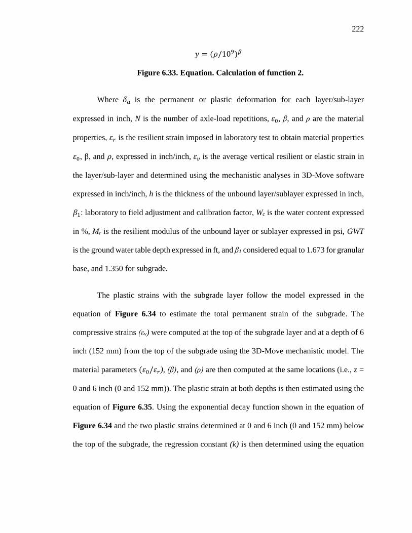
222
𝑦 = (𝜌/109)𝛽
Figure 6.33. Equation. Calculation of function 2.
Where 𝛿𝑎 is the permanent or plastic deformation for each layer/sub-layer
expressed in inch, N is the number of axle-load repetitions, 휀0, β, and ρ are the material
properties, 휀𝑟 is the resilient strain imposed in laboratory test to obtain material properties
휀0, β, and 𝜌, expressed in inch/inch, 휀𝑣 is the average vertical resilient or elastic strain in
the layer/sub-layer and determined using the mechanistic analyses in 3D-Move software
expressed in inch/inch, h is the thickness of the unbound layer/sublayer expressed in inch,
𝛽1: laboratory to field adjustment and calibration factor, Wc is the water content expressed
in %, Mr is the resilient modulus of the unbound layer or sublayer expressed in psi, GWT
is the ground water table depth expressed in ft, and β1 considered equal to 1.673 for granular
base, and 1.350 for subgrade.
The plastic strains with the subgrade layer follow the model expressed in the
equation of Figure 6.34 to estimate the total permanent strain of the subgrade. The
compressive strains (εv) were computed at the top of the subgrade layer and at a depth of 6
inch (152 mm) from the top of the subgrade using the 3D-Move mechanistic model. The
material parameters (휀0/휀𝑟), (β), and (ρ) are then computed at the same locations (i.e., z =
0 and 6 inch (0 and 152 mm)). The plastic strain at both depths is then estimated using the
equation of Figure 6.35. Using the exponential decay function shown in the equation of
Figure 6.34 and the two plastic strains determined at 0 and 6 inch (0 and 152 mm) below
the top of the subgrade, the regression constant (k) is then determined using the equation

223
of Figure 6.36. The total permanent deformation of the subgrade layer is then determined
using the equation defined in Figure 6.37.
휀𝑝(𝑧) = (휀𝑝,𝑧=0) ∗ 𝑒−𝑘∗𝑧
Figure 6.34. Equation. Calculation of the plastic vertical strain.
휀𝑝 = (휀0
휀𝑟)𝑒−(
𝜌𝑁
)𝛽
휀𝑣
Figure 6.35. Equation. Calculation of the plastic vertical strain function of the
resilient strain determined by mechanistic analysis.
𝑘 = (1
6) ∗ 𝐿𝑛(휀𝑝,𝑧=0/휀𝑝,𝑧=6)
Figure 6.36. Equation. Calculation of a regression constant.
𝑅𝐷𝑆𝐺 = ∫ 휀𝑝(𝑧)𝑑𝑧ℎ𝑏𝑒𝑑𝑟𝑜𝑐𝑘
0
= ( 1 − 𝑒−𝑘∗ℎ𝑏𝑒𝑑𝑟𝑜𝑐𝑘
𝑘) ∗ 휀𝑝,𝑧=0
Figure 6.37. Equation. Calculation of the rut depth in the subgrade layer.
Where 휀𝑝(𝑧) is the plastic vertical strain at depth z (measured from top of subgrade)
expressed in inch/inch, 휀𝑝,𝑧=0 is the plastic vertical strain at top of subgrade expressed in
inch/inch, k is the regression constant, 휀0 and β are the material properties, 휀𝑟 is the
resilient strain imposed in laboratory test to obtain material properties 휀0 , β, and 𝜌
expressed inch/inch, 휀𝑣 is the average vertical resilient or elastic strain in the layer/sub-
layer and determined using the mechanistic analyses in 3D-Move software expressed in
inch/inch, 𝑅𝐷𝑆𝐺 is the total plastic deformation of the subgrade layer expressed inch (mm),
ℎℎ𝑒𝑑𝑟𝑜𝑐𝑘 is the depth to bedrock from top of the subgrade expressed in inch (mm).

224
Table 6.16 to Table 6.24, and Figure 6.38 to Figure 6.46 summarize and illustrate
the rutting performance data of the base and subgrade layers for the PMA and HP pavement
sections. A review of the presented data reveals the following observations:
• Greater rut depths were generated in base layers of the HP pavement structures
when compared with the ones calculated in the PMA pavement structures. It should
be mentioned that thinner AC layers exist on top of the base layers in the HP
pavement structures when compared with the PMA ones leading to a stress
distribution of a higher magnitude into the base layer.
• Similar rut depths were observed in the subgrade layers of both PMA and HP
pavement structures under the same loading conditions (i.e., static vs. dynamic). It
should be mentioned that the pavement structures designed in accordance with
FDOT design manual (FDOT Design manual, 2016) are characterized by a thick
base, and 12 inch (305 mm) stabilized layer on top of the subgrade which may make
the subgrade insensitive to the decrease in the AC thickness.
• The total rutting criterion was limited to 0.75 inch (19 mm) for all the layers in the
evaluated structure. Since 0.25 inch (6.4 mm) is only allowed in the AC layer, a
value of 0.50 inch (12.5 mm) is only allowed as a total permanent deformation
generated in all unbound layers (i.e., in this case base, and subgrade). All evaluated
cases met this criterion indicating no excessive rutting in unbound materials over
the design life of the pavement when a structural coefficient value of 0.54 for HP
AC mixes is used.

225
Figure 6.38. Rutting Data for traffic level C under static conditions.
Figure 6.39. Rutting Data for traffic level C under a loading speed of 8 mph.
0.00
0.10
0.20
0.30
0.40
0.50
0.60
FL
95_P
MA
(A)
FL
95
_H
P(A
)
FL
95_P
MA
(B)
FL
95
_H
P(B
)
GA
95_P
MA
(A)
GA
95
_H
P(A
)
GA
95_P
MA
(B)
GA
95
_H
P(B
)
FL
95
_P
MA
(A)
FL
95
_H
P(A
)
FL
95
_P
MA
(B)
FL
95
_H
P(B
)
GA
95
_P
MA
(A)
GA
95
_H
P(A
)
GA
95
_P
MA
(B)
GA
95
_H
P(B
)
FL
95
_P
MA
(A)
FL
95
_H
P(A
)
FL
95
_P
MA
(B)
FL
95
_H
P(B
)
GA
95
_P
MA
(A)
GA
95
_H
P(A
)
GA
95
_P
MA
(B)
GA
95
_H
P(B
)
C1 C2 C3
Ru
t D
epth
s, i
nch
Subgrade Base Max Limit

226
Figure 6.40. Rutting Data for traffic level C under a loading speed of 15 mph.
Figure 6.41. Rutting Data for traffic level D under static conditions.
0.00
0.10
0.20
0.30
0.40
0.50
0.60
FL
95_P
MA
(A)
FL
95
_H
P(A
)
FL
95_P
MA
(B)
FL
95
_H
P(B
)
GA
95_P
MA
(A)
GA
95
_H
P(A
)
GA
95_P
MA
(B)
GA
95
_H
P(B
)
FL
95
_P
MA
(A)
FL
95
_H
P(A
)
FL
95
_P
MA
(B)
FL
95
_H
P(B
)
GA
95
_P
MA
(A)
GA
95
_H
P(A
)
GA
95
_P
MA
(B)
GA
95
_H
P(B
)
FL
95
_P
MA
(A)
FL
95
_H
P(A
)
FL
95
_P
MA
(B)
FL
95
_H
P(B
)
GA
95
_P
MA
(A)
GA
95
_H
P(A
)
GA
95
_P
MA
(B)
GA
95
_H
P(B
)
C1 C2 C3
Ru
t D
epth
s, i
nch
Subgrade Base Max Limit
0.00
0.10
0.20
0.30
0.40
0.50
0.60
FL
125_P
MA
(A)
FL
12
5_H
P(A
)
FL
125_P
MA
(B)
FL
12
5_H
P(B
)
GA
125_P
MA
(A)
GA
12
5_
HP
(A)
GA
125_P
MA
(B)
GA
12
5_
HP
(B)
FL
12
5_P
MA
(A)
FL
12
5_H
P(A
)
FL
12
5_P
MA
(B)
FL
12
5_H
P(B
)
GA
12
5_
PM
A(A
)
GA
12
5_
HP
(A)
GA
12
5_
PM
A(B
)
GA
12
5_
HP
(B)
FL
12
5_P
MA
(A)
FL
12
5_H
P(A
)
FL
12
5_P
MA
(B)
FL
12
5_H
P(B
)
GA
12
5_
PM
A(A
)
GA
12
5_
HP
(A)
GA
12
5_
PM
A(B
)
GA
12
5_
HP
(B)
D1 D2 D3
Ru
t D
epth
s, i
nch
Subgrade Base Max Limit

227
Figure 6.42. Rutting Data for traffic level D under a loading speed of 8 mph.
Figure 6.43. Rutting Data for traffic level D under a loading speed of 15 mph.
0.00
0.10
0.20
0.30
0.40
0.50
0.60
FL
125_P
MA
(A)
FL
12
5_H
P(A
)
FL
125_P
MA
(B)
FL
12
5_H
P(B
)
GA
125_P
MA
(A)
GA
12
5_
HP
(A)
GA
125_P
MA
(B)
GA
12
5_
HP
(B)
FL
12
5_P
MA
(A)
FL
12
5_H
P(A
)
FL
12
5_P
MA
(B)
FL
12
5_H
P(B
)
GA
12
5_
PM
A(A
)
GA
12
5_
HP
(A)
GA
12
5_
PM
A(B
)
GA
12
5_
HP
(B)
FL
12
5_P
MA
(A)
FL
12
5_H
P(A
)
FL
12
5_P
MA
(B)
FL
12
5_H
P(B
)
GA
12
5_
PM
A(A
)
GA
12
5_
HP
(A)
GA
12
5_
PM
A(B
)
GA
12
5_
HP
(B)
D1 D2 D3
Ru
t D
epth
s, i
nch
Subgrade Base Max Limit
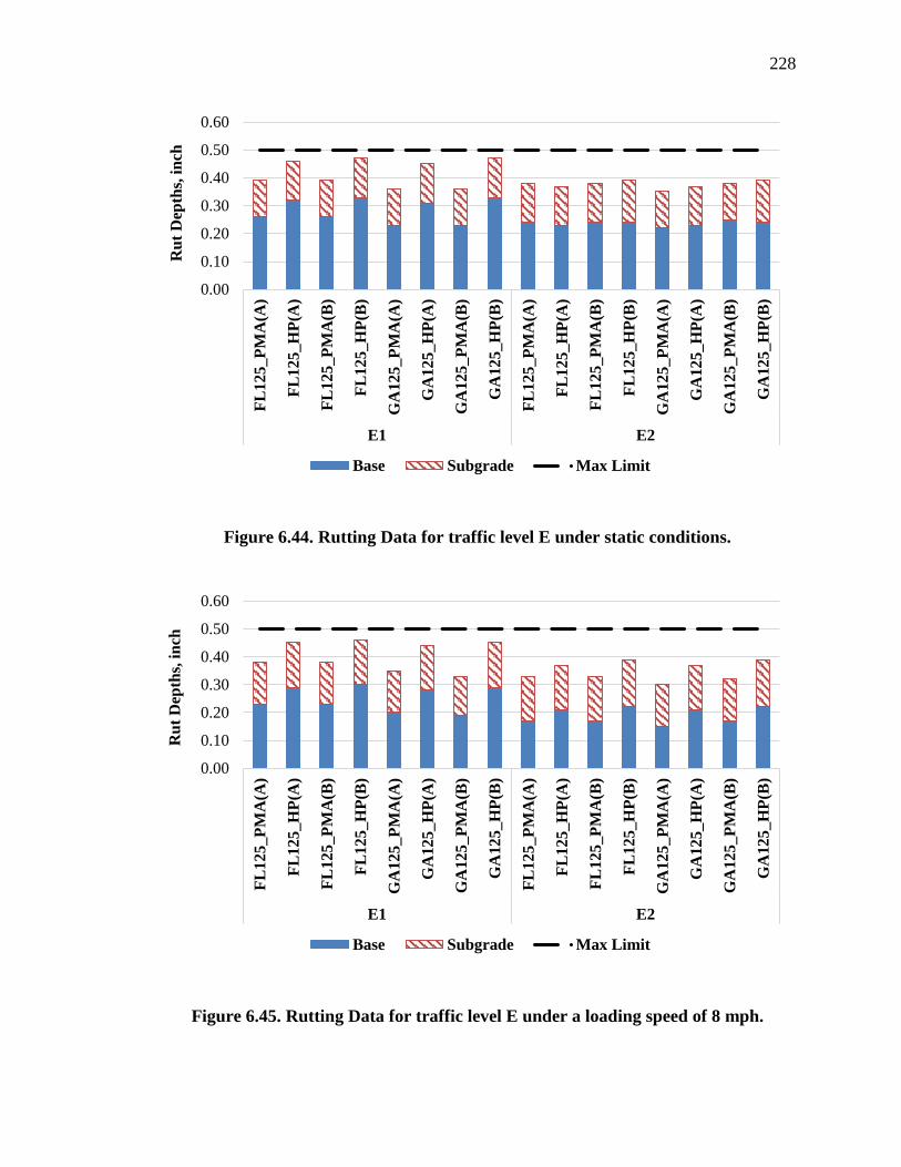
228
Figure 6.44. Rutting Data for traffic level E under static conditions.
Figure 6.45. Rutting Data for traffic level E under a loading speed of 8 mph.
0.00
0.10
0.20
0.30
0.40
0.50
0.60
FL
12
5_P
MA
(A)
FL
12
5_H
P(A
)
FL
12
5_P
MA
(B)
FL
12
5_H
P(B
)
GA
12
5_
PM
A(A
)
GA
12
5_
HP
(A)
GA
12
5_
PM
A(B
)
GA
12
5_
HP
(B)
FL
12
5_P
MA
(A)
FL
12
5_H
P(A
)
FL
12
5_P
MA
(B)
FL
12
5_H
P(B
)
GA
125_P
MA
(A)
GA
12
5_
HP
(A)
GA
12
5_
PM
A(B
)
GA
12
5_
HP
(B)
E1 E2
Ru
t D
epth
s, i
nch
Base Subgrade Max Limit

229
Figure 6.46. Rutting Data for traffic level E under a loading speed of 15 mph.
6.3.3 Verification of AC Shoving Performance
As mentioned earlier, shoving is a form of plastic movement that occurs at locations where
traffic starts and stops such as intersections (Pavement Interactive, 2008). Since HP AC
mixes can also be used at this type of locations, the fatigue-based initial structural
coefficient for HP AC mixes should be verified for shoving within the AC layer. While no
standard laboratory test exists to evaluate shoving in AC layer, the critical responses (e.g.,
shear strains and shear stresses) computed using the 3D-Move mechanistic analyses were
used to complete this verification check. It should be reminded that shoving was verified
by applying a braking friction coefficient (fBr) of 0.623 for the axle loading configuration
at a speed of 15 mph (km/h) and a temperature of 122°F (50°C). The selected analysis
temperature consists of the effective high analysis pavement temperature.
0.00
0.10
0.20
0.30
0.40
0.50
0.60
FL
12
5_P
MA
(A)
FL
12
5_H
P(A
)
FL
12
5_P
MA
(B)
FL
12
5_H
P(B
)
GA
12
5_
PM
A(A
)
GA
12
5_
HP
(A)
GA
12
5_
PM
A(B
)
GA
12
5_
HP
(B)
FL
12
5_P
MA
(A)
FL
12
5_H
P(A
)
FL
12
5_P
MA
(B)
FL
12
5_H
P(B
)
GA
125_P
MA
(A)
GA
12
5_
HP
(A)
GA
12
5_
PM
A(B
)
GA
12
5_
HP
(B)
E1 E2
Ru
t D
epth
s, i
nch
Base Subgrade Max Limit

230
The shoving analysis was completed by conducting a relative comparison between
the maximum shear strains determined from the mechanistic analysis within the top 0.50
inch (12.5 mm) of HP and PMA AC layers. Thus, a maximum allowable ratio between the
maximum shear strain in a HP AC layer and the maximum shear in a PMA AC layer was
developed. This maximum ratio between the estimated pavement responses was
implemented to verify that an acceptable resistance to shoving is achieved in the HP AC
mixes relative to their respective PMA AC mixes while giving due consideration to the
various mixtures’ properties. In this analysis, it was assumed that the resistance of the AC
mix to shoving is proportional to its resistance to rutting. Accordingly, the HP and PMA
mix specifics rutting relationships developed in the laboratory and provided in Table 4.8
were used to develop the maximum allowable ratio as a function of permanent axial strains.
The ratio between the maximum resilient axial strains of a HP and its respective PMA AC
mix, Rper (Equation of Figure 6.47), was related to an allowable ratio between their
corresponding shear strains using Hooke’s law for resilient responses. The established
shoving criterion for resilient shear strains ratio is shown in the equation of Figure 6.48.
𝑅𝑝𝑒𝑟 =ԑ𝑟−𝐻𝑃
ԑ𝑟−𝑃𝑀𝐴≤
ԑ𝑝−𝐻𝑃
ԑ𝑝−𝑃𝑀𝐴∗
𝑎𝐻𝑃
𝑎𝑃𝑀𝐴∗ 𝑁(𝛽𝑃𝑀𝐴∗𝑏𝑃𝑀𝐴−𝛽𝐻𝑃∗𝑏𝐻𝑃)
Figure 6.47. Equation. Calculation of Rper.
𝛾𝑥𝑧−𝐻𝑃
𝛾𝑥𝑧−𝑃𝑀𝐴≤ 𝑆ℎ𝑜𝑣𝑖𝑛𝑔 𝐶𝑟𝑖𝑡𝑒𝑟𝑖𝑜𝑛 = 𝑅𝑝𝑒𝑟 ∗
𝜏𝑥𝑧−𝐻𝑃
𝜏𝑥𝑧−𝑃𝑀𝐴∗
[𝜎𝑧−𝑃𝑀𝐴 − 𝜐 ∗ (𝜎𝑥−𝑃𝑀𝐴 + 𝜎𝑦−𝑃𝑀𝐴)]
[𝜎𝑧−𝐻𝑃 − 𝜐 ∗ (𝜎𝑥−𝐻𝑃 + 𝜎𝑦−𝐻𝑃)]
Figure 6.48. Equation. Calculation of the shoving criterion.

231
Where ԑ𝑝 is the permanent axial strain expressed in inch/inch (mm/mm),ԑ𝑟is the
resilient axial strain in the top 0.50 inch (12.5 mm) of AC layer expressed in inch/inch
(mm/mm), 𝑥𝑧
is the maximum resilient shear strain in the top 0.50 inch (12.5 mm) of AC
layer expressed in inch/inch (mm/mm), N is the number of loading cycles, a and b are the
experimentally determined coefficients, βr3 is the traffic loading calibration factor, σx, σy,
and σz are the normal stresses in the top 0.50 inch (12.5 mm) of AC layer determined using
3D-Move expressed in psi (Pa), τxz is the maximum shear stress in the top 0.50 inch (12.5
mm) of AC layer determined using 3D-Move expressed in psi (Pa), and υ is the Poisson’s
ratio.
Table 6.25 to Table 6.32 summarize the input stresses and strains used for the
shoving verification. The shoving resistance analysis leads to the following observations:
• No issues regarding the shoving distress (The equation of Figure 6.48 was verified)
are expected in the AC HP layer in pavement sections C1, C2, and C3 (i.e., traffic
level C).
• For traffic level D, the shoving criterion was met for all cases except for mix
GA125_HP(A) in pavement sections C2 and C3. It should me mentioned that the
corresponding control mix GA125_PMA(A) contains 20% of stiff RAP material
which may jeopardize the relative comparison between a HP AC mix where no
RAP material is allowed (as per FDOT specifications 2018 (FDOT Specifications,
2018) and its respective PMA AC mix. In addition, the degree of violations of the
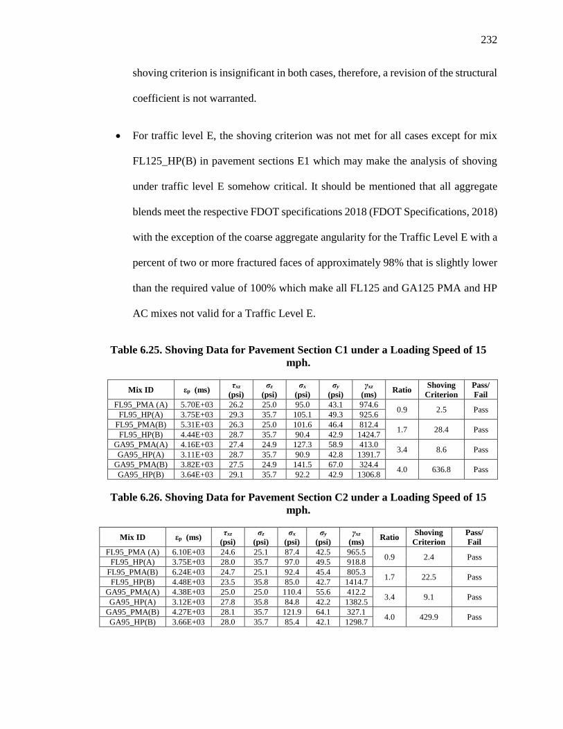
232
shoving criterion is insignificant in both cases, therefore, a revision of the structural
coefficient is not warranted.
• For traffic level E, the shoving criterion was not met for all cases except for mix
FL125_HP(B) in pavement sections E1 which may make the analysis of shoving
under traffic level E somehow critical. It should be mentioned that all aggregate
blends meet the respective FDOT specifications 2018 (FDOT Specifications, 2018)
with the exception of the coarse aggregate angularity for the Traffic Level E with a
percent of two or more fractured faces of approximately 98% that is slightly lower
than the required value of 100% which make all FL125 and GA125 PMA and HP
AC mixes not valid for a Traffic Level E.
Table 6.25. Shoving Data for Pavement Section C1 under a Loading Speed of 15
mph.
Mix ID εp (ms) τxz
(psi)
σz
(psi)
σx
(psi)
σy
(psi)
γxz
(ms) Ratio
Shoving
Criterion
Pass/
Fail
FL95_PMA (A) 5.70E+03 26.2 25.0 95.0 43.1 974.6 0.9 2.5 Pass
FL95_HP(A) 3.75E+03 29.3 35.7 105.1 49.3 925.6
FL95_PMA(B) 5.31E+03 26.3 25.0 101.6 46.4 812.4 1.7 28.4 Pass
FL95_HP(B) 4.44E+03 28.7 35.7 90.4 42.9 1424.7
GA95_PMA(A) 4.16E+03 27.4 24.9 127.3 58.9 413.0 3.4 8.6 Pass
GA95_HP(A) 3.11E+03 28.7 35.7 90.9 42.8 1391.7
GA95_PMA(B) 3.82E+03 27.5 24.9 141.5 67.0 324.4 4.0 636.8 Pass
GA95_HP(B) 3.64E+03 29.1 35.7 92.2 42.9 1306.8
Table 6.26. Shoving Data for Pavement Section C2 under a Loading Speed of 15
mph.
Mix ID εp (ms) τxz
(psi)
σz
(psi)
σx
(psi)
σy
(psi)
γxz
(ms) Ratio
Shoving
Criterion
Pass/
Fail
FL95_PMA (A) 6.10E+03 24.6 25.1 87.4 42.5 965.5 0.9 2.4 Pass
FL95_HP(A) 3.75E+03 28.0 35.7 97.0 49.5 918.8
FL95_PMA(B) 6.24E+03 24.7 25.1 92.4 45.4 805.3 1.7 22.5 Pass
FL95_HP(B) 4.48E+03 23.5 35.8 85.0 42.7 1414.7
GA95_PMA(A) 4.38E+03 25.0 25.0 110.4 55.6 412.2 3.4 9.1 Pass
GA95_HP(A) 3.12E+03 27.8 35.8 84.8 42.2 1382.5
GA95_PMA(B) 4.27E+03 28.1 35.7 121.9 64.1 327.1 4.0 429.9 Pass
GA95_HP(B) 3.66E+03 28.0 35.7 85.4 42.1 1298.7
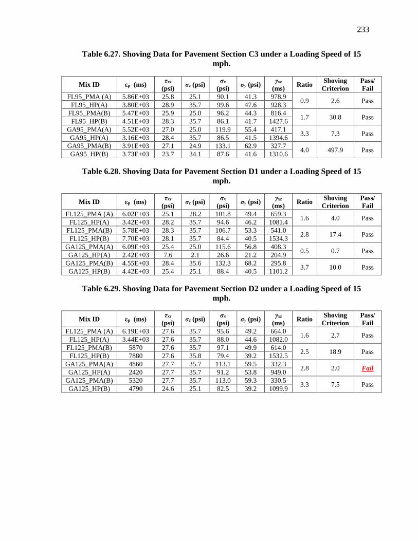
233
Table 6.27. Shoving Data for Pavement Section C3 under a Loading Speed of 15
mph.
Mix ID εp (ms) τxz
(psi) σz (psi)
σx
(psi) σy (psi)
γxz
(ms) Ratio
Shoving
Criterion
Pass/
Fail
FL95_PMA (A) 5.86E+03 25.8 25.1 90.1 41.3 978.9 0.9 2.6 Pass
FL95_HP(A) 3.80E+03 28.9 35.7 99.6 47.6 928.3
FL95_PMA(B) 5.47E+03 25.9 25.0 96.2 44.3 816.4 1.7 30.8 Pass
FL95_HP(B) 4.51E+03 28.3 35.7 86.1 41.7 1427.6
GA95_PMA(A) 5.52E+03 27.0 25.0 119.9 55.4 417.1 3.3 7.3 Pass
GA95_HP(A) 3.16E+03 28.4 35.7 86.5 41.5 1394.6
GA95_PMA(B) 3.91E+03 27.1 24.9 133.1 62.9 327.7 4.0 497.9 Pass
GA95_HP(B) 3.73E+03 23.7 34.1 87.6 41.6 1310.6
Table 6.28. Shoving Data for Pavement Section D1 under a Loading Speed of 15
mph.
Mix ID εp (ms) τxz
(psi) σz (psi)
σx
(psi) σy (psi)
γxz
(ms) Ratio
Shoving
Criterion
Pass/
Fail
FL125_PMA (A) 6.02E+03 25.1 28.2 101.8 49.4 659.3 1.6 4.0 Pass
FL125_HP(A) 3.42E+03 28.2 35.7 94.6 46.2 1081.4
FL125_PMA(B) 5.78E+03 28.3 35.7 106.7 53.3 541.0 2.8 17.4 Pass
FL125_HP(B) 7.70E+03 28.1 35.7 84.4 40.5 1534.3
GA125_PMA(A) 6.09E+03 25.4 25.0 115.6 56.8 408.3 0.5 0.7 Pass
GA125_HP(A) 2.42E+03 7.6 2.1 26.6 21.2 204.9
GA125_PMA(B) 4.55E+03 28.4 35.6 132.3 68.2 295.8 3.7 10.0 Pass
GA125_HP(B) 4.42E+03 25.4 25.1 88.4 40.5 1101.2
Table 6.29. Shoving Data for Pavement Section D2 under a Loading Speed of 15
mph.
Mix ID εp (ms) τxz
(psi) σz (psi)
σx
(psi) σy (psi)
γxz
(ms) Ratio
Shoving
Criterion
Pass/
Fail
FL125_PMA (A) 6.19E+03 27.6 35.7 95.6 49.2 664.0 1.6 2.7 Pass
FL125_HP(A) 3.44E+03 27.6 35.7 88.0 44.6 1082.0
FL125_PMA(B) 5870 27.6 35.7 97.1 49.9 614.0 2.5 18.9 Pass
FL125_HP(B) 7880 27.6 35.8 79.4 39.2 1532.5
GA125_PMA(A) 4860 27.7 35.7 113.1 59.5 332.3 2.8 2.0 Fail
GA125_HP(A) 2420 27.7 35.7 91.2 53.8 949.0
GA125_PMA(B) 5320 27.7 35.7 113.0 59.3 330.5 3.3 7.5 Pass
GA125_HP(B) 4790 24.6 25.1 82.5 39.2 1099.9
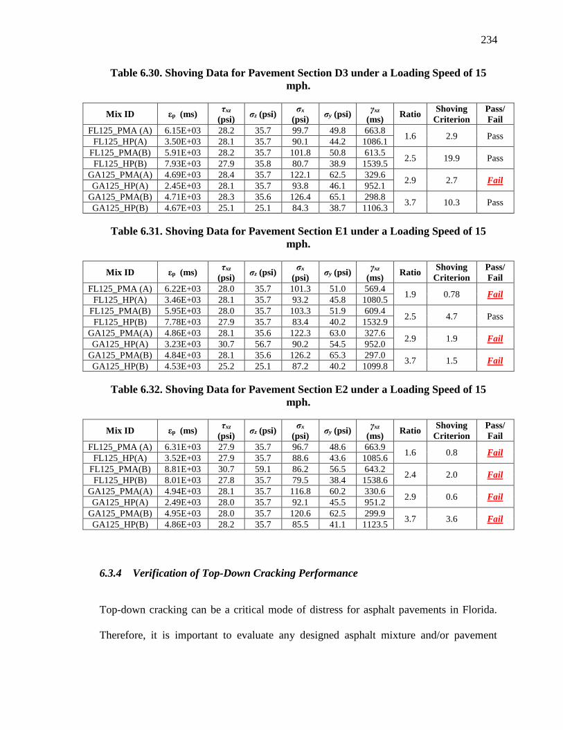
234
Table 6.30. Shoving Data for Pavement Section D3 under a Loading Speed of 15
mph.
Mix ID εp (ms) τxz
(psi) σz (psi)
σx
(psi) σy (psi)
γxz
(ms) Ratio
Shoving
Criterion
Pass/
Fail
FL125_PMA (A) 6.15E+03 28.2 35.7 99.7 49.8 663.8 1.6 2.9 Pass
FL125_HP(A) 3.50E+03 28.1 35.7 90.1 44.2 1086.1
FL125_PMA(B) 5.91E+03 28.2 35.7 101.8 50.8 613.5 2.5 19.9 Pass
FL125_HP(B) 7.93E+03 27.9 35.8 80.7 38.9 1539.5
GA125_PMA(A) 4.69E+03 28.4 35.7 122.1 62.5 329.6 2.9 2.7 Fail
GA125_HP(A) 2.45E+03 28.1 35.7 93.8 46.1 952.1
GA125_PMA(B) 4.71E+03 28.3 35.6 126.4 65.1 298.8 3.7 10.3 Pass
GA125_HP(B) 4.67E+03 25.1 25.1 84.3 38.7 1106.3
Table 6.31. Shoving Data for Pavement Section E1 under a Loading Speed of 15
mph.
Mix ID εp (ms) τxz
(psi) σz (psi)
σx
(psi) σy (psi)
γxz
(ms) Ratio
Shoving
Criterion
Pass/
Fail
FL125_PMA (A) 6.22E+03 28.0 35.7 101.3 51.0 569.4 1.9 0.78 Fail
FL125_HP(A) 3.46E+03 28.1 35.7 93.2 45.8 1080.5
FL125_PMA(B) 5.95E+03 28.0 35.7 103.3 51.9 609.4 2.5 4.7 Pass
FL125_HP(B) 7.78E+03 27.9 35.7 83.4 40.2 1532.9
GA125_PMA(A) 4.86E+03 28.1 35.6 122.3 63.0 327.6 2.9 1.9 Fail
GA125_HP(A) 3.23E+03 30.7 56.7 90.2 54.5 952.0
GA125_PMA(B) 4.84E+03 28.1 35.6 126.2 65.3 297.0 3.7 1.5 Fail
GA125_HP(B) 4.53E+03 25.2 25.1 87.2 40.2 1099.8
Table 6.32. Shoving Data for Pavement Section E2 under a Loading Speed of 15
mph.
Mix ID εp (ms) τxz
(psi) σz (psi)
σx
(psi) σy (psi)
γxz
(ms) Ratio
Shoving
Criterion
Pass/
Fail
FL125_PMA (A) 6.31E+03 27.9 35.7 96.7 48.6 663.9 1.6 0.8 Fail
FL125_HP(A) 3.52E+03 27.9 35.7 88.6 43.6 1085.6
FL125_PMA(B) 8.81E+03 30.7 59.1 86.2 56.5 643.2 2.4 2.0 Fail
FL125_HP(B) 8.01E+03 27.8 35.7 79.5 38.4 1538.6
GA125_PMA(A) 4.94E+03 28.1 35.7 116.8 60.2 330.6 2.9 0.6 Fail
GA125_HP(A) 2.49E+03 28.0 35.7 92.1 45.5 951.2
GA125_PMA(B) 4.95E+03 28.0 35.7 120.6 62.5 299.9 3.7 3.6 Fail
GA125_HP(B) 4.86E+03 28.2 35.7 85.5 41.1 1123.5
6.3.4 Verification of Top-Down Cracking Performance
Top-down cracking can be a critical mode of distress for asphalt pavements in Florida.
Therefore, it is important to evaluate any designed asphalt mixture and/or pavement

235
structure for its resistance to top-down cracking. The resistance to top-down cracking of
all 16 AC mixes were evaluated using the IDT test in accordance with AASHTO T312
(AASHTO T312, 2007) and Appendix G of the NCHRP 9-57 study (NCHRP 9-57, 2016)
at 50°F (10°C). Using the measured creep compliance and tensile strength, the threshold
dissipated creep strain energy (DSCEmin) and energy ratio (ER) were calculated using the
equation of Figure 3.40. The ER compares the failure DSCE (DSCEf) to DSCEmin. It
should be mentioned that DSCEmin takes into consideration the critical maximum tensile
stress developed in the AC layer of a designed pavement structure under traffic loading.
Table 6.33 and Table 6.34 summarize the critical tensile stress developed at the bottom of
the PMA and HP AC layers of all designed pavement structures under the evaluated traffic
speeds (i.e., 0, 8, and 45 mph), respectively.
The maximum tensile stress of the bottom of PMA AC layer ranged between 91.3
and 422.6 psi (0.63 and 2.91 MPa) for traffic level C, and between 51.1 and 278.8 psi (0.35
and 1.92 MPa) for traffic level D. The maximum tensile stress at the bottom of the HP AC
layer ranged between 50.6 and 315.7 psi (0.35 and 2.17 MPa) for traffic level C, and
between 55.4 and 234.4 psi (0.38 and 1.62 MPa) for traffic level D. Therefore, it can be
observed that the maximum tensile stress at the bottom of the HP AC layer was on average
20% lower than the stress determined at the bottom of the PMA AC layer as illustrated in
Figure 6.49. This indicates that the HP AC mixes have the potential to reduce top-down
cracking when compared with the PMA AC mixes evaluated in this research. (Analysis for
Traffic Level E).
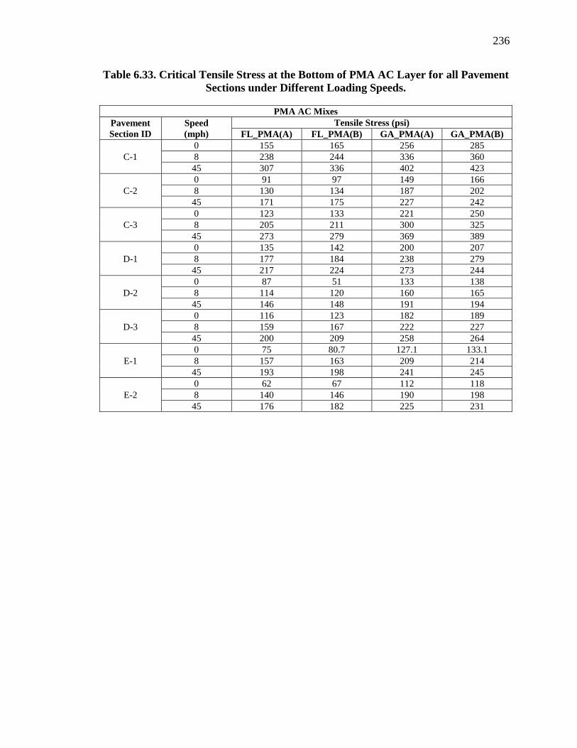
236
Table 6.33. Critical Tensile Stress at the Bottom of PMA AC Layer for all Pavement
Sections under Different Loading Speeds.
PMA AC Mixes
Pavement
Section ID
Speed
(mph)
Tensile Stress (psi)
FL_PMA(A) FL_PMA(B) GA_PMA(A) GA_PMA(B)
C-1
0 155 165 256 285
8 238 244 336 360
45 307 336 402 423
C-2
0 91 97 149 166
8 130 134 187 202
45 171 175 227 242
C-3
0 123 133 221 250
8 205 211 300 325
45 273 279 369 389
D-1
0 135 142 200 207
8 177 184 238 279
45 217 224 273 244
D-2
0 87 51 133 138
8 114 120 160 165
45 146 148 191 194
D-3
0 116 123 182 189
8 159 167 222 227
45 200 209 258 264
E-1
0 75 80.7 127.1 133.1
8 157 163 209 214
45 193 198 241 245
E-2
0 62 67 112 118
8 140 146 190 198
45 176 182 225 231

237
Table 6.34. Critical Tensile Stress at the Bottom of HP AC Layer for all Pavement
Sections under Different Loading Speeds.
HP AC Mixes
Pavement
Section ID Speed (mph)
Tensile Stress (psi)
FL_HP(A) FL_HP(B) GA_HP(A) GA_HP(B)
C-1
0 105 81 105 115
8 214 184 213 227
45 293 273 298 316
C-2
0 77 53 69 75
8 128 109 126 134
45 176 161 178 188
C-3
0 83 51 72 80
8 173 146 173 187
45 247 230 256 273
D-1
0 104 90 132 111
8 159 161 184 177
45 206 224 233 234
D-2
0 65 55 85 70
8 99 101 119 112
45 134 144 153 155
D-3
0 80 67 108 87
8 134 138 161 153
45 181 197 207 211
E-1
0 99 86 126 106
8 148 152 173 166
45 193 207 217 219
E-2
0 77 65 103 84
8 126 130 149 145
45 169 183 193 196
While no threshold limits have been set to assess the resistance to top-down
cracking of PMA and HP AC mixes in Florida, the criteria recommended in earlier FDOT
research at the University of Florida (Birgisson et al., 2006) were used for comparison
purposes. It should be mentioned that for the purpose of this study, the resistance to top-
down cracking of HP AC mixes were assessed relative to their respective PMA AC mixes
in order to verify the recommended structural coefficient for HP AC mixes. The optimum
ER (ERopt) for each traffic level was determined using ESALD and design reliability level

238
as summarized in Table 6.35. The FDOT criteria for top-down cracking for the PMA and
HP pavement structures at traffic levels C, D, and E are summarized in Table 6.36.
Figure 6.49. Comparison of critical tensile stress at the bottom of PMA and HP AC
layer for the same designed pavement structure and under the same loading speed.
Table 6.35. Energy ratio Linear Regression Models Function of Design Number of
ESALs for Different Reliability Levels.
Reliability (%) ER = f(ESALD in 10 millions)
99 ER = 0.4224*ESALD+0.9105
95 ER = 0.2957*ESALD+0.8496
90 ER = 0.2461*ESALD+0.8161
85 ER = 0.2191*ESALD+0.8017
80 ER = 0.1995*ESALD+0.7928
75 ER = 0.1832*ESALD+0.7809
70 ER = 0.1716*ESALD+0.7710
50 ER = 0.1331*ESALD+0.7470
Table 6.36. FDOT Preliminary Criteria for Top-Down Cracking.
Type of Design Reliability Traffic Level ERopt
New Construction 85%
C: 7 MESALs1 0.96
D: 20 MESALs 1.24
E: 40 MESALs 1.68 1M stands for million.
0
50
100
150
200
250
300
350
400
450
0 50 100 150 200 250 300 350 400 450
Cir
ticl
a T
ensi
le S
tres
s at
the
Bott
om
of
HP
AC
Layer
(p
si)
Critical Tensile Stress at the Bottom of PMA AC Layer (psi)
Equality Line

239
Table 6.37 and Table 6.38 summarizes the calculated energy ratio (ER) for all
evaluated PMA and HP AC mixes using the IDT test results along with the maximum
tensile stress (σmax) at the bottom of the AC layer determined from the mechanistic analysis
of the various pavement structures designed for traffic level C, level D, and level E. In
general, all calculated energy ratios were found within the range of the determined ERopt.
However, it should be mentioned that the ERopt values may not be applicable for top-down
cracking of lab produced PMA and HP AC mixes since they were developed based on aged
and damaged core samples collected approximately 12 years after construction.
The next step of the analysis was to apply the limitations specified in the Roque et
al. (2004) study (Roque et al., 2004) as stated below:
• Limitation 1: ER values for AC mixes with excessively low compliance rate (m-
values) are not considered reliable (relative to the change used in the calculation:
0.23 to 6.16E-03).
• Limitation 2: The ER concept should not be used to evaluate AC mixes
characterized by a DSCEf lower than 0.1053 lbf-in./in.3 (0.75 kJ/m3).
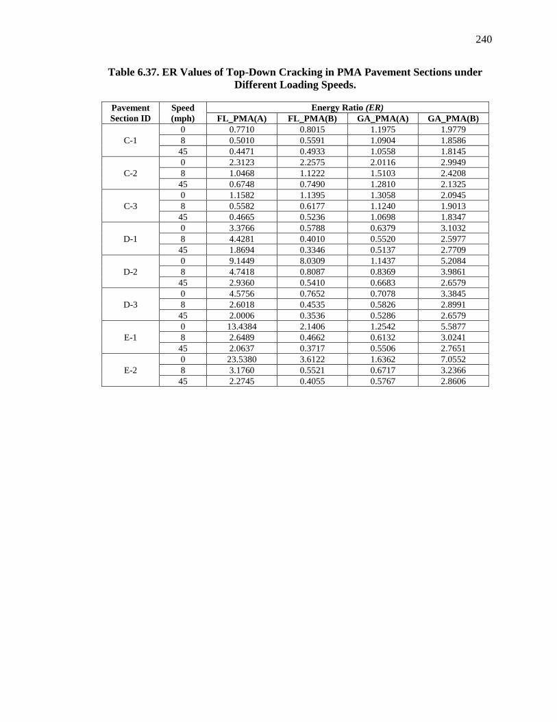
240
Table 6.37. ER Values of Top-Down Cracking in PMA Pavement Sections under
Different Loading Speeds.
Pavement
Section ID
Speed
(mph)
Energy Ratio (ER)
FL_PMA(A) FL_PMA(B) GA_PMA(A) GA_PMA(B)
C-1
0 0.7710 0.8015 1.1975 1.9779
8 0.5010 0.5591 1.0904 1.8586
45 0.4471 0.4933 1.0558 1.8145
C-2
0 2.3123 2.2575 2.0116 2.9949
8 1.0468 1.1222 1.5103 2.4208
45 0.6748 0.7490 1.2810 2.1325
C-3
0 1.1582 1.1395 1.3058 2.0945
8 0.5582 0.6177 1.1240 1.9013
45 0.4665 0.5236 1.0698 1.8347
D-1
0 3.3766 0.5788 0.6379 3.1032
8 4.4281 0.4010 0.5520 2.5977
45 1.8694 0.3346 0.5137 2.7709
D-2
0 9.1449 8.0309 1.1437 5.2084
8 4.7418 0.8087 0.8369 3.9861
45 2.9360 0.5410 0.6683 2.6579
D-3
0 4.5756 0.7652 0.7078 3.3845
8 2.6018 0.4535 0.5826 2.8991
45 2.0006 0.3536 0.5286 2.6579
E-1
0 13.4384 2.1406 1.2542 5.5877
8 2.6489 0.4662 0.6132 3.0241
45 2.0637 0.3717 0.5506 2.7651
E-2
0 23.5380 3.6122 1.6362 7.0552
8 3.1760 0.5521 0.6717 3.2366
45 2.2745 0.4055 0.5767 2.8606

241
Table 6.38. ER Values of Top-Down Cracking in HP Pavement Sections under
Different Loading Speeds.
Pavement
Section ID
Speed
(mph)
Energy Ratio (ER)
FL_HP(A) FL_HP(B) GA_HP(A) GA_HP(B)
C-1
0 2.1623 2.7140 3.8135 0.7462
8 2.0554 2.4172 3.7781 0.7316
45 0.5486 0.3387 1.0006 0.2387
C-2
0 4.5133 8.0612 11.5747 2.1423
8 1.3284 1.1449 2.5110 0.5362
45 0.7993 0.5449 1.4461 0.3286
C-3
0 3.6789 9.5806 10.2064 1.7874
8 0.8125 0.6405 1.4923 0.3308
45 0.5937 0.3742 1.0692 0.2513
D-1
0 2.5892 0.4378 4.2399 0.8604
8 1.1111 0.1243 2.5833 0.3768
45 0.8166 0.0859 2.1108 0.2899
D-2
0 8.9885 1.7174 11.5685 2.8079
8 2.8717 0.3226 5.2416 0.8362
45 0.9342 0.0966 2.3032 0.3133
D-3
0 5.0084 0.9854 6.5249 1.5616
8 1.4839 0.1608 3.0578 0.4586
45 0.9342 0.0966 2.3032 0.3133
E-1
0 2.8788 0.4855 4.6753 0.9556
8 1.2410 0.1359 2.7760 0.4099
45 0.8690 0.0916 2.2222 0.3046
E-2
0 5.5835 1.0811 7.2964 1.7424
8 1.6744 0.1826 3.4423 0.5050
45 1.0201 0.1045 2.4586 0.3367
Table 4.10 shows that all the PMA and HP AC mixes satisfied limitation 1
regarding the creep compliance rate by showing m-values within the acceptable range.
However, many of the AC mixes such as; FL95_HP(A), GA95_HP(B), FL125_HP(A),
FL125_PMA(B), FL125_HP(B), GA125_PMA(A), GA125_PMA(B), and GA125_HP(B)
failed limitation 2 with DSCEf values lower than 0.1053 lbf-in./in.3 (0.75 kJ/m3). Therefore,
the cases involving the use of these AC mixes were excluded from the mechanistic analysis
for top-down cracking.
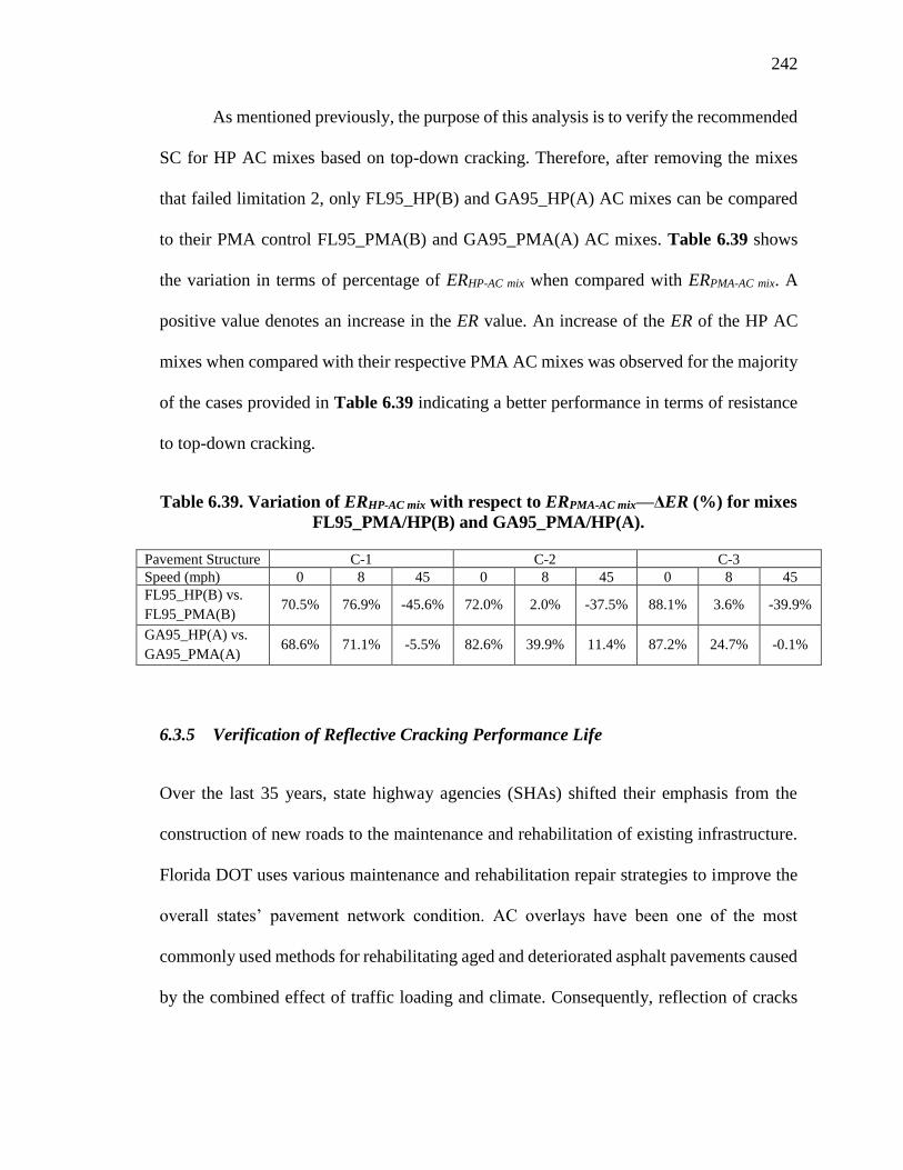
242
As mentioned previously, the purpose of this analysis is to verify the recommended
SC for HP AC mixes based on top-down cracking. Therefore, after removing the mixes
that failed limitation 2, only FL95_HP(B) and GA95_HP(A) AC mixes can be compared
to their PMA control FL95_PMA(B) and GA95_PMA(A) AC mixes. Table 6.39 shows
the variation in terms of percentage of ERHP-AC mix when compared with ERPMA-AC mix. A
positive value denotes an increase in the ER value. An increase of the ER of the HP AC
mixes when compared with their respective PMA AC mixes was observed for the majority
of the cases provided in Table 6.39 indicating a better performance in terms of resistance
to top-down cracking.
Table 6.39. Variation of ERHP-AC mix with respect to ERPMA-AC mix—ΔER (%) for mixes
FL95_PMA/HP(B) and GA95_PMA/HP(A).
Pavement Structure C-1 C-2 C-3
Speed (mph) 0 8 45 0 8 45 0 8 45
FL95_HP(B) vs.
FL95_PMA(B) 70.5% 76.9% -45.6% 72.0% 2.0% -37.5% 88.1% 3.6% -39.9%
GA95_HP(A) vs.
GA95_PMA(A) 68.6% 71.1% -5.5% 82.6% 39.9% 11.4% 87.2% 24.7% -0.1%
6.3.5 Verification of Reflective Cracking Performance Life
Over the last 35 years, state highway agencies (SHAs) shifted their emphasis from the
construction of new roads to the maintenance and rehabilitation of existing infrastructure.
Florida DOT uses various maintenance and rehabilitation repair strategies to improve the
overall states’ pavement network condition. AC overlays have been one of the most
commonly used methods for rehabilitating aged and deteriorated asphalt pavements caused
by the combined effect of traffic loading and climate. Consequently, reflection of cracks

243
from existing pavements becomes a major type of distress influencing the life of an AC
overlay and controlling its long-term performance. Once the AC overlay is cracked, it
allows moisture to penetrate into the mix and to the supporting layers promoting the
stripping of the asphalt binder from aggregates. It can also reduce the strength of the base
and subgrade materials, which would lead to the total failure of the flexible pavement
structure. Multiple factors can significantly influence the long-term performance of these
techniques including the specific conditions of the existing pavement and the combination
of materials, traffic, and environmental conditions under which the overlay has been
applied (Habbouche et al., 2017).
6.3.5.1 Reflective Cracking Model
The basic mechanism for reflective cracking is strain concentration in the AC overlay due
to the movement in the existing pavement at the vicinity of joints and/or cracks. In fact, the
majority of reflective cracking is caused by the combination of bending, shearing, and
thermal mechanisms resulting from traffic loads or daily and seasonal temperature changes.
The comprehensive ME asphalt overlay system developed by Texas Transportation
Institute (TTI) was used to evaluate the resistance to reflective cracking of PMA and HP
AC mixes when used in AC overlay rehabilitation projects (Zhou et al., 2008).
Various models have been developed to analyze and/or predict reflective cracking.
The TTI system consider the Paris’ law-based fracture mechanics model expressed in the
equation of Figure 6.50 for the evaluation of reflective cracking propagation (Zhou et al.,
2008). The use of Paris’ law for assessing the crack growth process in viscoelastic materials
such as AC mixtures, has been theoretically justified in multiple studies (Zhou et al., 2008).

244
This model requires the calculation of stress intensity factor (SIF) and the determination of
AC mixes fracture properties (i.e., A and n). These calculations have been recently
accomplished through the development of the SA-CrackPro program specifically tailored
for pavement SIF analysis and the Texas overlay test for the asphalt mixes fracture
properties (Zhou et al., 2008).
𝑑𝑐
𝑑𝑁= 𝐴 ∗ (𝑆𝐼𝐹)𝑛
Figure 6.50. Equation. Paris Law Model.
Where 𝑐 is the crack length expressed in inch (mm), 𝑁 is the number of loading
cycles, and 𝑆𝐼𝐹 is the stress intensity factor amplitude.
The recommended reflective cracking model includes three main components:
reflective crack propagation model expressed in the equation of Figure 6.51 based on
Paris’ law with the combination of bending, shearing, and thermal loading; reflective
cracking damage model expressed in the equation of Figure 6.52; and reflective cracking
amount model expressed in the equation of Figure 6.53 to describe the development of the
reflective cracking amount using a sigmoidal function (Zhou et al., 2008).
𝛥𝐶 = 𝑘1 ∗ 𝐴 ∗ (𝐾𝑏𝑒𝑛𝑑𝑖𝑔)𝑛 ∗ 𝛥𝑁𝑖 + 𝑘2 ∗ 𝐴 ∗ (𝐾𝑠ℎ𝑒𝑎𝑟𝑖𝑛𝑔)𝑛 ∗ 𝛥𝑁𝑖 + 𝑘3 ∗ 𝐴 ∗ (𝐾𝑡ℎ𝑒𝑟𝑚𝑎𝑙)𝑛 ∗ 𝛥𝑁𝑖
Figure 6.51. Equation. Calculation of daily crack length.
𝐷 = ∑ 𝛥𝐶/ℎ
Figure 6.52. Equation. Calculation of damage ratio.
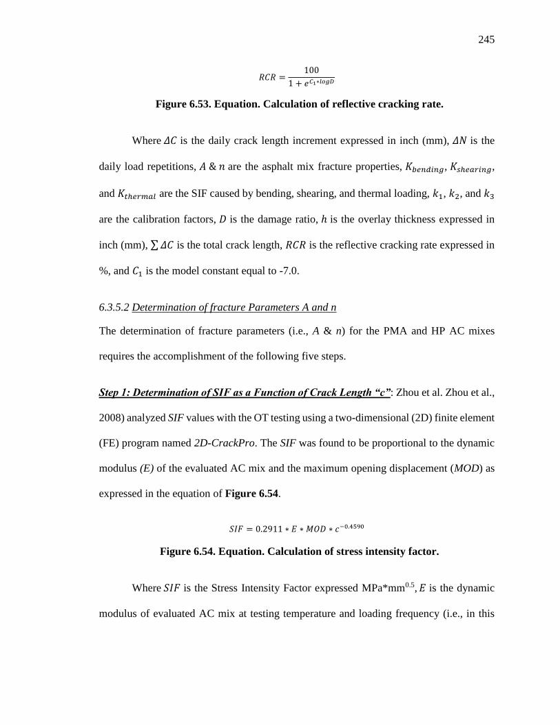
245
𝑅𝐶𝑅 =100
1 + 𝑒𝐶1∗𝑙𝑜𝑔𝐷
Figure 6.53. Equation. Calculation of reflective cracking rate.
Where 𝛥𝐶 is the daily crack length increment expressed in inch (mm), 𝛥𝑁 is the
daily load repetitions, 𝐴 & 𝑛 are the asphalt mix fracture properties, 𝐾𝑏𝑒𝑛𝑑𝑖𝑛𝑔, 𝐾𝑠ℎ𝑒𝑎𝑟𝑖𝑛𝑔,
and 𝐾𝑡ℎ𝑒𝑟𝑚𝑎𝑙 are the SIF caused by bending, shearing, and thermal loading, 𝑘1, 𝑘2, and 𝑘3
are the calibration factors, 𝐷 is the damage ratio, ℎ is the overlay thickness expressed in
inch (mm), ∑ 𝛥𝐶 is the total crack length, 𝑅𝐶𝑅 is the reflective cracking rate expressed in
%, and 𝐶1 is the model constant equal to -7.0.
6.3.5.2 Determination of fracture Parameters A and n
The determination of fracture parameters (i.e., A & n) for the PMA and HP AC mixes
requires the accomplishment of the following five steps.
Step 1: Determination of SIF as a Function of Crack Length “c”: Zhou et al. Zhou et al.,
2008) analyzed SIF values with the OT testing using a two-dimensional (2D) finite element
(FE) program named 2D-CrackPro. The SIF was found to be proportional to the dynamic
modulus (E) of the evaluated AC mix and the maximum opening displacement (MOD) as
expressed in the equation of Figure 6.54.
𝑆𝐼𝐹 = 0.2911 ∗ 𝐸 ∗ 𝑀𝑂𝐷 ∗ 𝑐−0.4590
Figure 6.54. Equation. Calculation of stress intensity factor.
Where 𝑆𝐼𝐹 is the Stress Intensity Factor expressed MPa*mm0.5, 𝐸 is the dynamic
modulus of evaluated AC mix at testing temperature and loading frequency (i.e., in this

246
case T=77°F (25°C) and f = 0.1 Hz) expressed in MPa, MOD is the maximum opening
displacement expressed in mm, 𝑐 is the crack length expressed in mm.
In this study, the equation of Figure 6.54 was implemented to determine the
relationship between SIF and c for all evaluated AC mixes. The dynamic modulus was
determined for each respective mix from the laboratory measured data at 77°F (25°C) and
loading frequency of 0.1 Hz (refer to Section 4.2.1 and Appendix C.1). Figure 6.55
illustrates, as an example, the calculated SIF versus c for FL95_PMA(A) mix. A modulus,
E, of 142,686 psi (984 MPa) and a MOD of 0.025 inch (0.6350 mm) were used. The data
in Figure 6.55 show a rapid decrease in SIF at low crack lengths indicating the importance
of the initial crack propagation stage to determine reasonable fracture parameters (i.e., A
& n).
Figure 6.55. Calculated SIF vs. crack length c for FL95_PMA(A) AC mix.
Step 2: Determination of normalized maximum load (NM) using OT test function of c:
In previous studies (Zhou et al., 2008 & Seo et al., 2004) different techniques (e.g., Digital
y = 181.85x-0.459
0
20
40
60
80
100
120
140
160
180
200
0 5 10 15 20 25
Str
ess
Inte
nsi
ty F
act
or,
SIF
(MP
A*m
m^
0.5
)
Crack Length, c (mm)
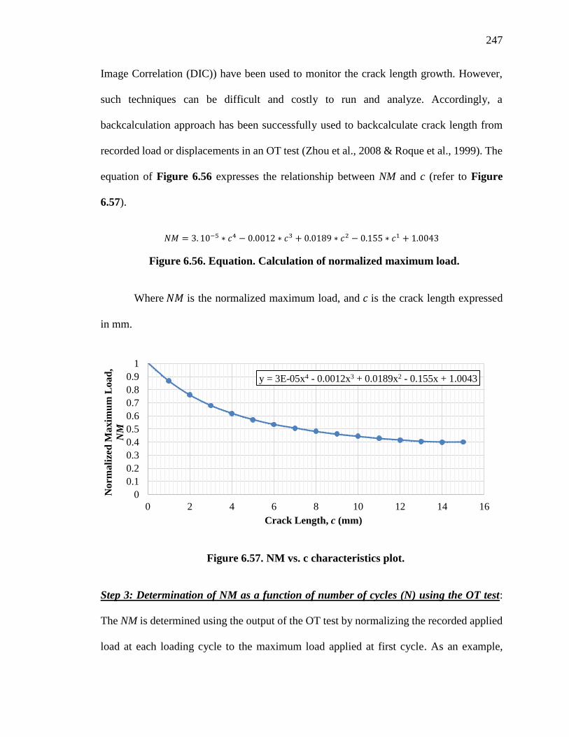
247
Image Correlation (DIC)) have been used to monitor the crack length growth. However,
such techniques can be difficult and costly to run and analyze. Accordingly, a
backcalculation approach has been successfully used to backcalculate crack length from
recorded load or displacements in an OT test (Zhou et al., 2008 & Roque et al., 1999). The
equation of Figure 6.56 expresses the relationship between NM and c (refer to Figure
6.57).
𝑁𝑀 = 3. 10−5 ∗ 𝑐4 − 0.0012 ∗ 𝑐3 + 0.0189 ∗ 𝑐2 − 0.155 ∗ 𝑐1 + 1.0043
Figure 6.56. Equation. Calculation of normalized maximum load.
Where 𝑁𝑀 is the normalized maximum load, and 𝑐 is the crack length expressed
in mm.
Figure 6.57. NM vs. c characteristics plot.
Step 3: Determination of NM as a function of number of cycles (N) using the OT test:
The NM is determined using the output of the OT test by normalizing the recorded applied
load at each loading cycle to the maximum load applied at first cycle. As an example,
y = 3E-05x4 - 0.0012x3 + 0.0189x2 - 0.155x + 1.0043
0
0.1
0.2
0.3
0.4
0.5
0.6
0.7
0.8
0.9
1
0 2 4 6 8 10 12 14 16
Norm
ali
zed
Maxim
um
Load
,
NM
Crack Length, c (mm)
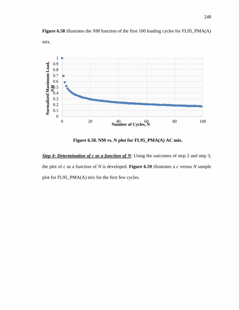
248
Figure 6.58 illustrates the NM function of the first 100 loading cycles for FL95_PMA(A)
mix.
Figure 6.58. NM vs. N plot for FL95_PMA(A) AC mix.
Step 4: Determination of c as a function of N: Using the outcomes of step 2 and step 3,
the plot of c as a function of N is developed. Figure 6.59 illustrates a c versus N sample
plot for FL95_PMA(A) mix for the first few cycles.
0
0.1
0.2
0.3
0.4
0.5
0.6
0.7
0.8
0.9
1
0 20 40 60 80 100
Norm
ali
zed
Ma
xim
um
Lo
ad
,
NM
Number of Cycles, N

249
Figure 6.59. c vs. N plot for FL95_PMA(A) AC mix.
Step 5: Determination of SIF function of N: Once c versus N is determined, SIF is
computed at each loading cycle as a function of c using the equation defined in Figure
6.60. The crack length variation rate (dc/dN) is then determined function of SIF. The
fracture parameters A and n are then determined as the corresponding intercept and slope
of dc/dN vs. N, respectively (Refer to Figure 6.54 for an example; A = 8.40E-02, and n =
6.77E-01).
0.0
2.0
4.0
6.0
8.0
10.0
12.0
14.0
16.0
18.0
0 1 2 3 4 5 6 7 8 9 10
Cra
ck L
eng
th, c
(mm
)
Number of Cycles, N
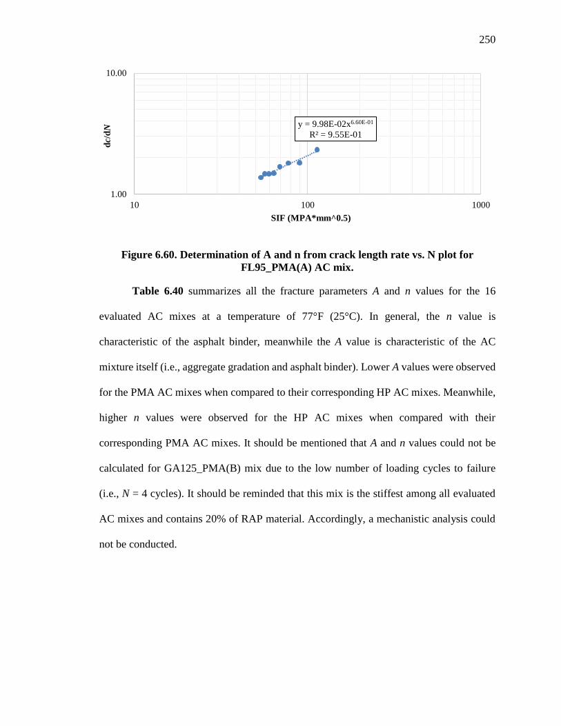
250
Figure 6.60. Determination of A and n from crack length rate vs. N plot for
FL95_PMA(A) AC mix.
Table 6.40 summarizes all the fracture parameters A and n values for the 16
evaluated AC mixes at a temperature of 77°F (25°C). In general, the n value is
characteristic of the asphalt binder, meanwhile the A value is characteristic of the AC
mixture itself (i.e., aggregate gradation and asphalt binder). Lower A values were observed
for the PMA AC mixes when compared to their corresponding HP AC mixes. Meanwhile,
higher n values were observed for the HP AC mixes when compared with their
corresponding PMA AC mixes. It should be mentioned that A and n values could not be
calculated for GA125_PMA(B) mix due to the low number of loading cycles to failure
(i.e., N = 4 cycles). It should be reminded that this mix is the stiffest among all evaluated
AC mixes and contains 20% of RAP material. Accordingly, a mechanistic analysis could
not be conducted.
y = 9.98E-02x6.60E-01
R² = 9.55E-01
1.00
10.00
10 100 1000
dc/
dN
SIF (MPA*mm^0.5)
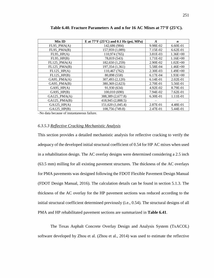
251
Table 6.40. Fracture Parameters A and n for 16 AC Mixes at 77°F (25°C).
Mix ID E at 77°F (25°C) and 0.1 Hz (psi, MPa) A n
FL95_PMA(A) 142,686 (984) 9.98E-02 6.60E-01
FL95_PMA(B) 157,959 (1,089) 7.15E-02 6.62E-01
FL95_HP(A) 110,974 (765) 3.81E-03 1.36E+00
FL95_HP(B) 78,819 (543) 1.71E-02 1.16E+00
FL125_PMA(A) 182,650 (1,259) 2.90E-02 1.02E+00
FL125_PMA(B) 197,354 (1,361) 5.58E-04 1.46E+00
FL125_HP(A) 110,467 (762) 2.30E-03 1.49E+00
FL125_HP(B) 80,898 (558) 6.17E-04 1.93E+00
GA95_PMA(A) 307,493 (2,120) 6.14E-01 2.02E-01
GA95_PMA(B) 380,369 (2,623) 2.70E-01 5.56E-01
GA95_HP(A) 91,930 (634) 4.92E-02 8.79E-01
GA95_HP(B) 100,010 (690) 7.94E-02 7.62E-01
GA125_PMA(A) 388,389 (2,677.8) 6.30E-01 1.11E-01
GA125_PMA(B) 418,945 (2,888.5) – –
GA125_HP(A) 151,620 (1,045.4) 2.87E-01 4.48E-01
GA125_HP(B) 108,756 (749.8) 2.47E-01 5.44E-01
–No data because of instantaneous failure.
6.3.5.3 Reflective Cracking Mechanistic Analysis
This section provides a detailed mechanistic analysis for reflective cracking to verify the
adequacy of the developed initial structural coefficient of 0.54 for HP AC mixes when used
in a rehabilitation design. The AC overlay designs were determined considering a 2.5 inch
(63.5 mm) milling for all existing pavement structures. The thickness of the AC overlays
for PMA pavements was designed following the FDOT Flexible Pavement Design Manual
(FDOT Design Manual, 2016). The calculation details can be found in section 5.1.3. The
thickness of the AC overlay for the HP pavement sections was reduced according to the
initial structural coefficient determined previously (i.e., 0.54). The structural designs of all
PMA and HP rehabilitated pavement sections are summarized in Table 6.41.
The Texas Asphalt Concrete Overlay Design and Analysis System (TxACOL)
software developed by Zhou et al. (Zhou et al., 2014) was used to estimate the reflective
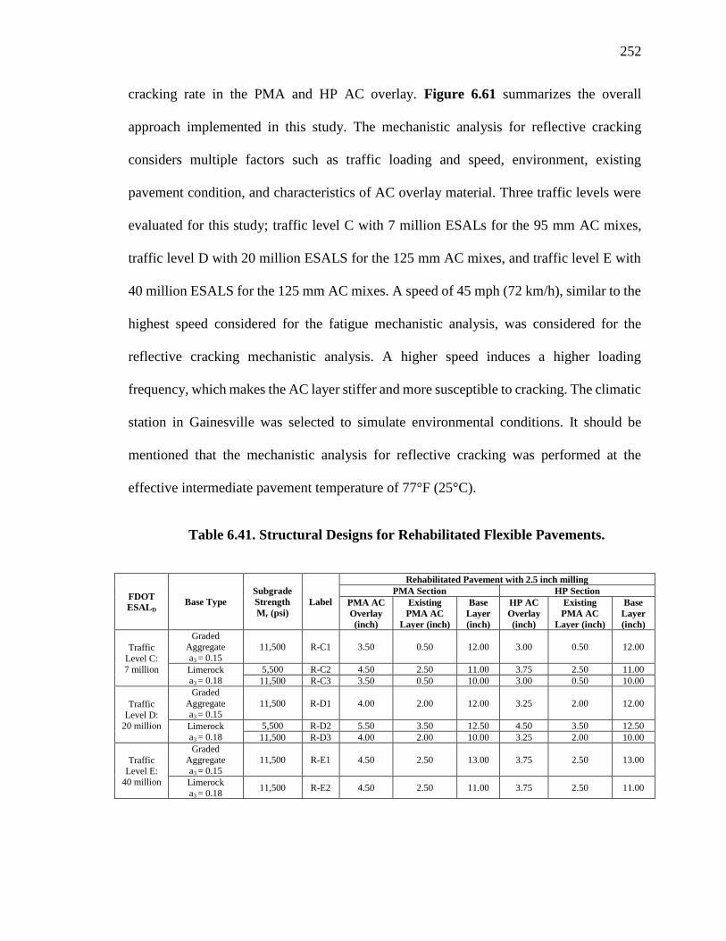
252
cracking rate in the PMA and HP AC overlay. Figure 6.61 summarizes the overall
approach implemented in this study. The mechanistic analysis for reflective cracking
considers multiple factors such as traffic loading and speed, environment, existing
pavement condition, and characteristics of AC overlay material. Three traffic levels were
evaluated for this study; traffic level C with 7 million ESALs for the 95 mm AC mixes,
traffic level D with 20 million ESALS for the 125 mm AC mixes, and traffic level E with
40 million ESALS for the 125 mm AC mixes. A speed of 45 mph (72 km/h), similar to the
highest speed considered for the fatigue mechanistic analysis, was considered for the
reflective cracking mechanistic analysis. A higher speed induces a higher loading
frequency, which makes the AC layer stiffer and more susceptible to cracking. The climatic
station in Gainesville was selected to simulate environmental conditions. It should be
mentioned that the mechanistic analysis for reflective cracking was performed at the
effective intermediate pavement temperature of 77°F (25°C).
Table 6.41. Structural Designs for Rehabilitated Flexible Pavements.
FDOT
ESALD Base Type
Subgrade
Strength
Mr (psi)
Label
Rehabilitated Pavement with 2.5 inch milling
PMA Section HP Section
PMA AC
Overlay
(inch)
Existing
PMA AC
Layer (inch)
Base
Layer
(inch)
HP AC
Overlay
(inch)
Existing
PMA AC
Layer (inch)
Base
Layer
(inch)
Traffic
Level C:
7 million
Graded
Aggregate
a3 = 0.15
11,500 R-C1 3.50 0.50 12.00 3.00 0.50 12.00
Limerock a3 = 0.18
5,500 R-C2 4.50 2.50 11.00 3.75 2.50 11.00
11,500 R-C3 3.50 0.50 10.00 3.00 0.50 10.00
Traffic
Level D: 20 million
Graded
Aggregate a3 = 0.15
11,500 R-D1 4.00 2.00 12.00 3.25 2.00 12.00
Limerock
a3 = 0.18
5,500 R-D2 5.50 3.50 12.50 4.50 3.50 12.50
11,500 R-D3 4.00 2.00 10.00 3.25 2.00 10.00
Traffic Level E:
40 million
Graded
Aggregate a3 = 0.15
11,500 R-E1 4.50 2.50 13.00 3.75 2.50 13.00
Limerock
a3 = 0.18 11,500 R-E2 4.50 2.50 11.00 3.75 2.50 11.00

253
Figure 6.61. Overall flowchart of the mechanistic analysis approach for reflective
cracking.
In order to simulate the deteriorated condition of an existing AC layer due to fatigue
cracking before rehabilitation, a reduction in the stiffness of the existing PMA AC layer
was applied. A damaged dynamic modulus master curve was calculated following the
approach used in AASHTOWare Pavement ME (MEPDG Guide, 2004). The undamaged
master curves of the evaluated PMA AC mixes, determined previously in Section 5.5.1
and Appendix C Section 1 (C.1), were used to determine the damaged master curve of the
existing AC layer after milling (equation of Figure 6.62) (MEPDG Guide, 2004). The
damage accumulation in the AC layer was estimated to be 0.6 representing a fair condition
of the existing AC layer over its service life (MEPDG Guide, 2004).

254
𝐸𝐴𝐶−𝑑𝑎𝑚𝑎𝑔𝑒𝑑 = 10𝛿 +𝐸𝐴𝐶−𝑢𝑛𝑑𝑎𝑚𝑎𝑔𝑒𝑑 − 10𝛿
1 + 𝑒−0.3+5∗𝑙𝑜𝑔𝑑𝐴𝐶
Figure 6.62. Equation. Calculation of damaged dynamic modulus of existing AC
layer.
log (𝐸𝐴𝐶−𝑢𝑛𝑑𝑎𝑚𝑎𝑔𝑒𝑑) = 𝛿 +𝛼
1 + 𝑒𝛽+𝛾[log(𝑡)−𝑐(log(𝜂)−log(𝜂𝑇𝑟))]
Figure 6.63. Equation. Calculation of log of damaged dynamic modulus for existing
AC layer.
Where 𝐸𝐴𝐶−𝑑𝑎𝑚𝑎𝑔𝑒𝑑 is the damaged dynamic modulus of existing AC layer
expressed in psi (MPa), 𝐸𝐴𝐶−𝑢𝑛𝑑𝑎𝑚𝑎𝑔𝑒𝑑 is the undamaged dynamic modulus of existing
AC layer expressed in psi (MPa), 𝛿 is the undamaged dynamic modulus master curve
fitting parameter, 𝑑𝐴𝐶 is the damage accumulation in AC from the bottom-up fatigue
cracking (assumed equal to 0.6), 𝑡 is the time of loading expressed in second, 𝜂 is the
viscosity of temperature of interest expressed in CPoise, 𝜂𝑇𝑟is the viscosity at reference
temperature expressed in CPoise, and 𝛼, 𝛽, 𝛿, 𝛾, 𝑎𝑛𝑑 𝑐 are mix specific fitting parameters.
It should be mentioned that all existing AC layers before rehabilitation were
assumed to be made of PMA AC mixes. Only the new AC overlay was considered either
as an undamaged PMA or HP AC mix. Appendix D Section 1 (D.1) presents in details the
damaged dynamic modulus data for all evaluated PMA AC mixes. Table 6.42 summarizes
the undamaged and damaged dynamic moduli determined at a temperature of 77° (25°C)
and a frequency of 33.3 Hz.
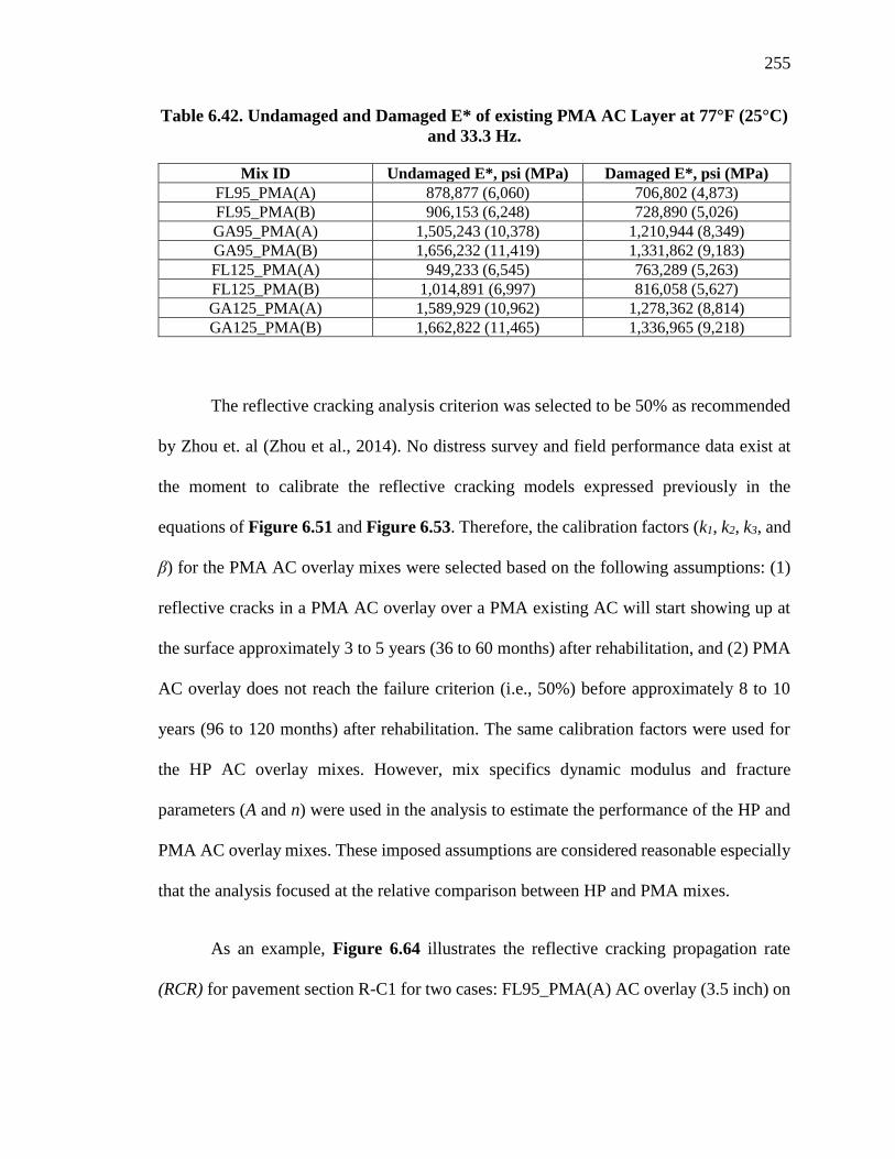
255
Table 6.42. Undamaged and Damaged E* of existing PMA AC Layer at 77°F (25°C)
and 33.3 Hz.
Mix ID Undamaged E*, psi (MPa) Damaged E*, psi (MPa)
FL95_PMA(A) 878,877 (6,060) 706,802 (4,873)
FL95_PMA(B) 906,153 (6,248) 728,890 (5,026)
GA95_PMA(A) 1,505,243 (10,378) 1,210,944 (8,349)
GA95_PMA(B) 1,656,232 (11,419) 1,331,862 (9,183)
FL125_PMA(A) 949,233 (6,545) 763,289 (5,263)
FL125_PMA(B) 1,014,891 (6,997) 816,058 (5,627)
GA125_PMA(A) 1,589,929 (10,962) 1,278,362 (8,814)
GA125_PMA(B) 1,662,822 (11,465) 1,336,965 (9,218)
The reflective cracking analysis criterion was selected to be 50% as recommended
by Zhou et. al (Zhou et al., 2014). No distress survey and field performance data exist at
the moment to calibrate the reflective cracking models expressed previously in the
equations of Figure 6.51 and Figure 6.53. Therefore, the calibration factors (k1, k2, k3, and
β) for the PMA AC overlay mixes were selected based on the following assumptions: (1)
reflective cracks in a PMA AC overlay over a PMA existing AC will start showing up at
the surface approximately 3 to 5 years (36 to 60 months) after rehabilitation, and (2) PMA
AC overlay does not reach the failure criterion (i.e., 50%) before approximately 8 to 10
years (96 to 120 months) after rehabilitation. The same calibration factors were used for
the HP AC overlay mixes. However, mix specifics dynamic modulus and fracture
parameters (A and n) were used in the analysis to estimate the performance of the HP and
PMA AC overlay mixes. These imposed assumptions are considered reasonable especially
that the analysis focused at the relative comparison between HP and PMA mixes.
As an example, Figure 6.64 illustrates the reflective cracking propagation rate
(RCR) for pavement section R-C1 for two cases: FL95_PMA(A) AC overlay (3.5 inch) on
256
top of an existing damaged FL95_PMA(A) AC layer (0.5 inch), and FL95_HP(A) AC
overlay (3.0 inch) on top of an existing damaged FL95_PMA(A) AC layer (0.5 inch).
Based on the data presented in Figure 6.64 the following observations can be made:
• For the case of the PMA AC overlay, the cracks started to reflect in the overlay
(i.e., RCR >0%) at an initial time (i.e., tinitial) of approximately 58 months (4.8 years)
after construction. The RCR reached its failure criterion (i.e., 50%) after 96 months
(8.0 years) (tRCR=50%) from construction. Thus it took 38 months (3.1 years) for the
PMA AC overlay to reach failure after initial cracking has occurred.
• For the case of HP AC overlay, the cracks started reflecting on top of the AC
overlay after 86 months (7.1 years) from construction. The RCR reached its failure
criterion after 137 months (11.4 years). Thus, it took 51 months (4.3 years) for the
HP AC overlay to reach failure after initial cracking has occurred.
• In summary, the illustrative example showed that, for the same traffic and
environmental conditions, a 3.0 inch of HP AC overlay is expected to perform
better than a 3.5 inch PMA AC overlay as demonstrated with the observed 41 month
delay in reaching failure criterion.
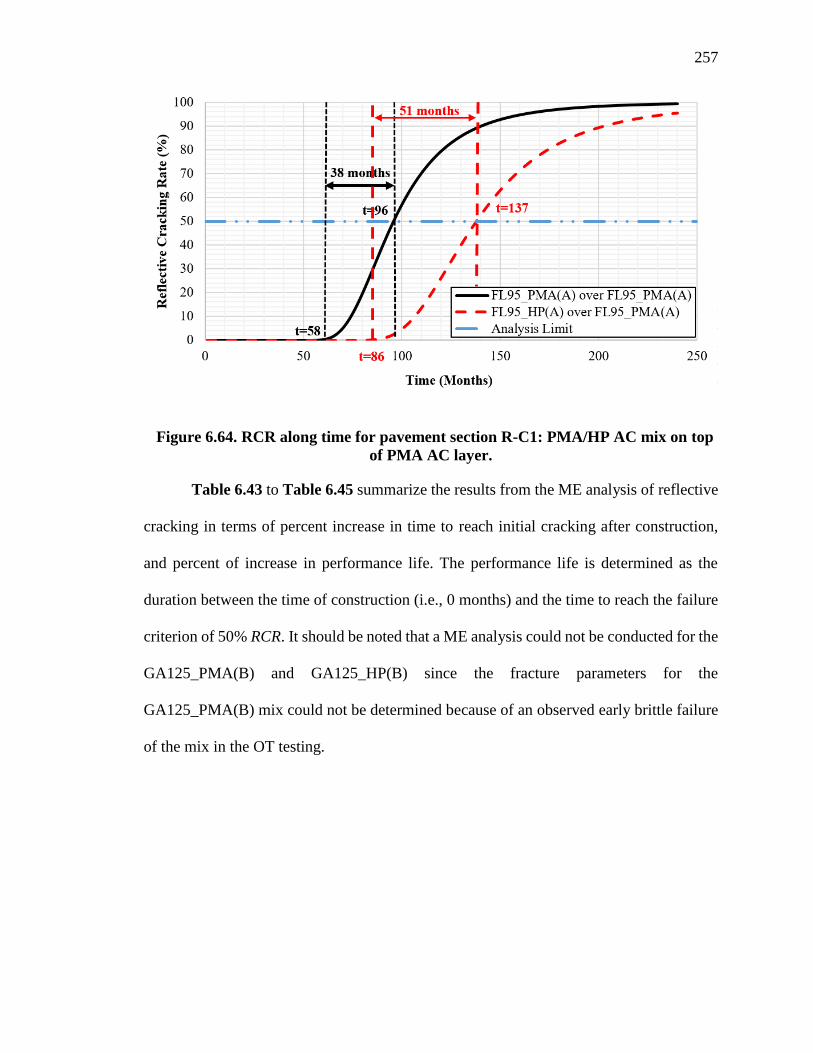
257
Figure 6.64. RCR along time for pavement section R-C1: PMA/HP AC mix on top
of PMA AC layer.
Table 6.43 to Table 6.45 summarize the results from the ME analysis of reflective
cracking in terms of percent increase in time to reach initial cracking after construction,
and percent of increase in performance life. The performance life is determined as the
duration between the time of construction (i.e., 0 months) and the time to reach the failure
criterion of 50% RCR. It should be noted that a ME analysis could not be conducted for the
GA125_PMA(B) and GA125_HP(B) since the fracture parameters for the
GA125_PMA(B) mix could not be determined because of an observed early brittle failure
of the mix in the OT testing.
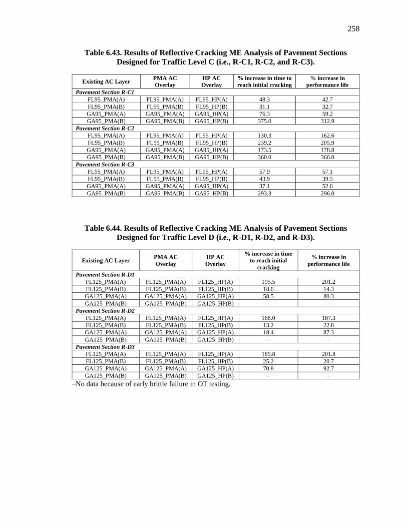
258
Table 6.43. Results of Reflective Cracking ME Analysis of Pavement Sections
Designed for Traffic Level C (i.e., R-C1, R-C2, and R-C3).
Existing AC Layer PMA AC
Overlay
HP AC
Overlay
% increase in time to
reach initial cracking
% increase in
performance life
Pavement Section R-C1
FL95_PMA(A) FL95_PMA(A) FL95_HP(A) 48.3 42.7
FL95_PMA(B) FL95_PMA(B) FL95_HP(B) 31.1 32.7
GA95_PMA(A) GA95_PMA(A) GA95_HP(A) 76.3 59.2
GA95_PMA(B) GA95_PMA(B) GA95_HP(B) 375.0 312.9
Pavement Section R-C2
FL95_PMA(A) FL95_PMA(A) FL95_HP(A) 130.3 162.6
FL95_PMA(B) FL95_PMA(B) FL95_HP(B) 239.2 205.9
GA95_PMA(A) GA95_PMA(A) GA95_HP(A) 173.5 178.8
GA95_PMA(B) GA95_PMA(B) GA95_HP(B) 360.0 366.0
Pavement Section R-C3
FL95_PMA(A) FL95_PMA(A) FL95_HP(A) 57.9 57.1
FL95_PMA(B) FL95_PMA(B) FL95_HP(B) 43.9 39.5
GA95_PMA(A) GA95_PMA(A) GA95_HP(A) 37.1 52.6
GA95_PMA(B) GA95_PMA(B) GA95_HP(B) 293.3 296.0
Table 6.44. Results of Reflective Cracking ME Analysis of Pavement Sections
Designed for Traffic Level D (i.e., R-D1, R-D2, and R-D3).
Existing AC Layer PMA AC
Overlay
HP AC
Overlay
% increase in time
to reach initial
cracking
% increase in
performance life
Pavement Section R-D1
FL125_PMA(A) FL125_PMA(A) FL125_HP(A) 195.5 201.2
FL125_PMA(B) FL125_PMA(B) FL125_HP(B) 18.6 14.3
GA125_PMA(A) GA125_PMA(A) GA125_HP(A) 58.5 80.3
GA125_PMA(B) GA125_PMA(B) GA125_HP(B) – –
Pavement Section R-D2
FL125_PMA(A) FL125_PMA(A) FL125_HP(A) 168.0 187.3
FL125_PMA(B) FL125_PMA(B) FL125_HP(B) 13.2 22.8
GA125_PMA(A) GA125_PMA(A) GA125_HP(A) 18.4 87.3
GA125_PMA(B) GA125_PMA(B) GA125_HP(B) – –
Pavement Section R-D3
FL125_PMA(A) FL125_PMA(A) FL125_HP(A) 189.8 201.8
FL125_PMA(B) FL125_PMA(B) FL125_HP(B) 25.2 20.7
GA125_PMA(A) GA125_PMA(A) GA125_HP(A) 70.8 92.7
GA125_PMA(B) GA125_PMA(B) GA125_HP(B) – –
–No data because of early brittle failure in OT testing.
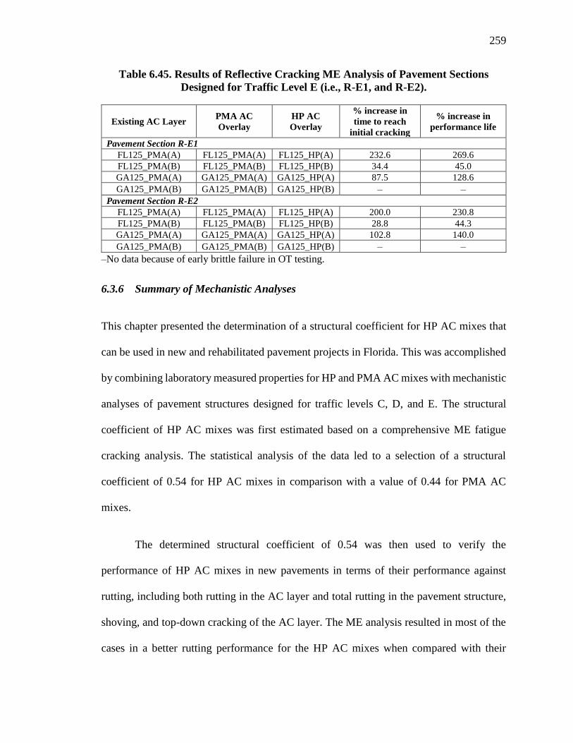
259
Table 6.45. Results of Reflective Cracking ME Analysis of Pavement Sections
Designed for Traffic Level E (i.e., R-E1, and R-E2).
Existing AC Layer PMA AC
Overlay
HP AC
Overlay
% increase in
time to reach
initial cracking
% increase in
performance life
Pavement Section R-E1
FL125_PMA(A) FL125_PMA(A) FL125_HP(A) 232.6 269.6
FL125_PMA(B) FL125_PMA(B) FL125_HP(B) 34.4 45.0
GA125_PMA(A) GA125_PMA(A) GA125_HP(A) 87.5 128.6
GA125_PMA(B) GA125_PMA(B) GA125_HP(B) – –
Pavement Section R-E2
FL125_PMA(A) FL125_PMA(A) FL125_HP(A) 200.0 230.8
FL125_PMA(B) FL125_PMA(B) FL125_HP(B) 28.8 44.3
GA125_PMA(A) GA125_PMA(A) GA125_HP(A) 102.8 140.0
GA125_PMA(B) GA125_PMA(B) GA125_HP(B) – –
–No data because of early brittle failure in OT testing.
6.3.6 Summary of Mechanistic Analyses
This chapter presented the determination of a structural coefficient for HP AC mixes that
can be used in new and rehabilitated pavement projects in Florida. This was accomplished
by combining laboratory measured properties for HP and PMA AC mixes with mechanistic
analyses of pavement structures designed for traffic levels C, D, and E. The structural
coefficient of HP AC mixes was first estimated based on a comprehensive ME fatigue
cracking analysis. The statistical analysis of the data led to a selection of a structural
coefficient of 0.54 for HP AC mixes in comparison with a value of 0.44 for PMA AC
mixes.
The determined structural coefficient of 0.54 was then used to verify the
performance of HP AC mixes in new pavements in terms of their performance against
rutting, including both rutting in the AC layer and total rutting in the pavement structure,
shoving, and top-down cracking of the AC layer. The ME analysis resulted in most of the
cases in a better rutting performance for the HP AC mixes when compared with their

260
respective PMA AC mixes. The rut depths determined in the unbound layers were observed
to be lower than the maximum allowable rut depth of 0.50 inch (12.6 mm) indicating an
acceptable performance for the HP pavement sections which had a thinner AC layer
thickness. The ME analysis for shoving in the AC layer showed, in general, acceptable
performance for the HP AC mixes. The top-down cracking analysis showed acceptable
performance for the HP AC mixes and exhibited ER values much greater than ERopt
irrespective of traffic level. In summary, the verification efforts supported the use of a
structural coefficient of 0.54 for HP AC mixes in new pavements.
In the case of rehabilitation projects, the adequacy of the selected structural
coefficient was verified for HP AC overlay mixes using a ME analysis for reflective
cracking. The analysis took into consideration the existing pavement condition in terms of
damaged modulus for the existing AC layer, mix-specific material properties, traffic
condition, and Florida climate. The HP AC overlay mixes resulted in an increase in both
time to reach initial cracking and performance life of the AC overlay. Thus, the structural
coefficient of 0.54 used to design the HP AC overlay is expected to result in an acceptable
or better performance when compared to the respective PMA AC overlay mix.
As an overall summary, the various analyses conducted in this chapter supported
the selection of a structural coefficient of 0.54 for HP AC mixes to be used in new
construction and rehabilitation designs in Florida.

261
CHAPTER 7 FULL-SCALE PAVEMENT TESTING
7.1 Introduction
7.1.1 Background
As part of the laboratory task, typical local materials from Florida were assessed and used
for the development of 16 AC mixes using PMA and HP asphalt binders (i.e., 8 PMA and
8 HP AC mixes) for new construction and rehabilitation projects. The mix designs were
conducted following the Superpave methodology to determine an optimal asphalt binder
content for each of the 16 evaluated mixes. Different OBC values were determined
depending on the aggregate source, aggregate gradation, asphalt binder type (i.e., PMA or
HP), and design traffic level. The viscoelastic properties of the 16 AC mixes were
evaluated using the dynamic modulus. The mixes were also evaluated in terms of their
resistance to rutting, fatigue cracking, top-down cracking, and reflective cracking. In
general, it was found that the combination of aggregate source and asphalt binder type (i.e.,
PMA or HP) impacted the performance characteristics of the evaluated AC mixes. A
structural coefficient for HP AC mixes from Florida was determined in the flexixble
pavement modeling part of this study. The following summarizes the main findings and
recommendations from the laboratory and advanced pavement modeling tasks (Habbouche
et al., 2018):
• Overall, HP AC mixes showed better performance characteristics when compared
with the corresponding PMA control AC mixes. The impact of the improvements
in engineering property and performance characteristics of the HP AC mixes were

262
evaluated through the mechanistic analysis of flexible pavements incorporating the
two types of mixtures.
• The critical responses determined using the 3D-Move (Siddharthan et al., 2015)
mechanistic model were used to evaluate the performance life of the designed
pavement structures for several targeted distresses including; fatigue cracking, AC
rutting, total rutting, top-down cracking, and reflective cracking. The critical
responses were computed and determined at different locations and at different
depths within the pavement structure depending on the distress mode. It should be
mentioned that two temperatures were considered for the mechanistic analysis:
77°F (25°C) simulating an intermediate temperature for cracking analyses, and
122°F (50°C) simulating a high temperature for rutting/showing analyses. These
two temperatures were determined using the corresponding critical climatic stations
in Florida (i.e., Gainesville and Marathon).
• An initial structural coefficient for HP AC mixes (aHP-AC) was determined based on
the fatigue performance life of the analyzed pavement structures. An equivalent HP
AC layer thickness that resulted in a similar fatigue life as the respective PMA
pavement section under static and dynamic loading conditions was determined.
Multiple factors including applied traffic level, pavement structure, and
performance characteristics of the evaluated PMA and HP AC mixes resulted in
different structural coefficients for HP AC mixes based on the fatigue cracking
analysis. The estimated initial fatigue-based structural coefficient ranged between
0.33 and 1.32. Using advanced statistical analyses and considering all factors and
263
their interactions, an initial fatigue-based structural coefficient of 0.54 was
determined for HP AC mixes.
• The initial fatigue-based aHP-AC of 0.54 was verified for the following distresses;
rutting and shoving in AC layer, total rutting, AC top-down cracking, and AC
reflective cracking. In all cases, the thickness of the HP AC layer was reduced based
on the fatigue-based structural coefficient of 0.54 and the resistance of the HP
pavement to the specific distress was evaluated and compared to the resistance of
its corresponding PMA pavement. The verification process concluded that the
structural coefficient of 0.54 for HP AC mixes would lead to the design of HP
pavements that offer equal or better resistance to the various evaluated distresses
than the designed PMA pavements with the structural coefficient of 0.44. This
conclusion held valid for the design of both new and rehabilitation projects.
Based on the data generated and the accompanied analyses, it was recommended
that HP AC mixes with a structural coefficient of 0.54 be evaluated in the Florida
Department of Transportation (FDOT) accelerated pavement testing (APT) facility. This
represents a 19% reduction in the thickness of the AC layer when using a HP AC mix in
place of a PMA AC mix while designing a flexible pavement under all similar conditions
of traffic, environment, and properties of base and subgrade (SG) layers.
Prior to full implementation in the APT experiment, the developed structural
coefficient for HP AC mixes of 0.54 was checked through full-scale laboratory testing of
asphalt pavements. The following section describes the executed experimental plan under
this task of the project. The main objective of this effort is to verify the structural coefficient

264
determined through laboratory testing and computer modeling in two instrumented full-
scale asphalt pavements subjected to stationary dynamic loadings.
7.1.2 Experimental Plan for Full-Scale Pavement Testing
Two experiments were conducted at the University of Nevada, Reno (UNR) full-scale
pavement testing facility. For each experiment, a pavement structure was built and tested
in the full-scale square box (PaveBox):
• Experiment No. 1 (referred to as PaveBox_PMA): pavement structure 1 consisted
of a PMA AC layer on top of a crushed aggregate base (CAB) and a SG.
• Experiment No. 2 (referred to as PaveBox_HP): pavement structure 2 consisted of
an HP AC layer with a reduced thickness on top of the same CAB and SG.
Both pavement structures were subjected to the same loading protocol. Dynamic
loads simulating the falling weight deflectometer (FWD) loading condition, were applied
at the surface of the pavement in the PaveBox for each experiment. The pavement surface
deflections along with critical pavement responses at different locations in the pavement
layers (i.e., stresses and strains) were monitored during testing through embedded
instrumentations. Linear variable differential transformers (LVDTs) were used to record
pavement surface deflections. Total earth pressure cells (TEPCs) were used to capture the
stresses induced in the CAB and SG due to surface loading. Strain gauges were attached to
the bottom of the AC layer to measure the load-induced tensile strains. At the end of each
PaveBox experiment, cores were cut from the AC layer for bulk specific gravity and air
voids measurements.
265
The main objective of this part of the study is to verify the structural coefficient for
HP AC mixes determined previously in Chapter 6. Thus, two major analyses were carried
out. Analysis I consisted of a comparison of measured pavement responses under dynamic
loadings, while analysis II verified the HP structural coefficient through mechanistic-
empirical analyses using service life approach. Figure 7.1 illustrates the flowchart of the
experimental plan for the verification of the recommended structural coefficient based on
full-scale pavement testing in the PaveBox.
The objectives of analysis I was to assess the impact of the reduced HP AC layer
thickness on the measured pavement responses under different levels of surface loads. This
was achieved through a direct comparison of the measured pavement responses collected
from both experiments (PMA and HP sections).
The objective of analysis II was to verify the structural coefficient for HP AC mixes
using the service life approach. PMA and HP AC mixes from both experiments were
collected and compacted in the laboratory. The compacted specimens were evaluated in
terms of engineering property (i.e., E*), and performance characteristics (i.e., resistance to
fatigue cracking and rutting). The measured properties and performance characteristics
were then implemented into an advanced flexible pavement modeling process to determine
the responses and performance at multiple loading levels.
Finally, the findings from analysis I and analysis II of the PaveBox experiments
were used to make any necessary modifications to the structural coefficient determined for
HP AC mixes in Florida using the laboratory and mechanistic analysis evaluations.

266
Figure 7.1. Flowchart of the verification of structural coefficient based on full-scale
pavement testing.
UNR PaveBox
Experiment No. 1 Pavement Structure 1
Control PMA Section
Experiment No. 2 Pavement Structure 2
HP Section
Dynamic Loading at Multiple Load Levels
Collect Pavement Responses Pavement Surface Deflections: δPMA and δHP
Strain at the bottom of AC layers: εPMA and εHP
Vertical stresses in CAB and SG layers: σPMA and σHP
Analysis I Comparison of Measured
Pavement Responses
Field Mixtures
Laboratory Compacted
(FMLC) Samples: Dynamic Modulus, E*
Resistance to Fatigue Cracking
Resistance to Rutting
Backcalculation
EPMA or HP, ECAB, and ESG
Mechanistic Analysis
using 3D-MOVE
Development of APT Implementation Plan
Analysis II Verification of Structural
Coefficient for HP AC Mixes
using Service Life Approach
Final Recommendations of a Structural Coefficient for HP AC Mixes

267
7.2 Elements of Experimental Program
A full-scale experimental program was carried out to verify the determined structural
coefficient for HP AC mixes. A total of two full-scale pavement structures were
constructed and subjected to dynamic loadings. This section summarizes the specific
characteristics of the two experiments including properties of the used materials,
construction techniques, and instrumentation plans.
7.2.1 Description of PaveBox
The PaveBox consisted of a square box with internal dimensions of 124 by 124 by 72 inch
(315 by 315 by 183 cm). The box is made of a steel base plate, H-shaped steel columns
infilled with 4- by 6 by 30 inch (102 by 152 by 762 mm) wood beams and braced at two
levels with steel beams and tension rods to act as lateral bracing system. Figure 7.2 and
Figure 7.3 show the drawings of the PaveBox.
The steel base plate is grouted to the laboratory floor, and 20 steel columns are
appropriately aligned and welded to the base plate. A total of 224 4- by 6- by 30-inch wood
beams (102 by 152 by 762 mm) are fitted between the columns. Polyvinyl chloride (PVC)
foam boards are used as filler between the gap inside the web of the columns and the wood
beams. A screw/nut fastening method is used to install the bracing system, which consisted
of eight steel beams and four tension rods.

268
Note: All dimensions are in inches.
Figure 7.2. Three-dimensional (3D) schematic of the PaveBox.
Figure 7.3. Plan view and front and side elevations of the PaveBox.
269
Since the experimental program included dynamic loading applied to a pavement
structure contained within the PaveBox, there was a concern about introducing
measurement errors in the data collected from the sensors due to the reflection of the waves
at the boundaries. A common technique to minimize such error is to install wave-absorbing
material on the inside walls of the PaveBox. Accordingly, the floor and the inner walls of
the PaveBox were covered by a fiberglass material (with paper-vapor-retarder side facing
inside) that is commercially available for use as insulation hajj et al., 2018). The PVC foam
boards acted as an additional wave absorber at the boundaries during the dynamic tests.
A plastic sheet was placed all around the inside of the completed PaveBox. This
sheet was intended to provide a frictionless boundary for vertical deformation similar to
what is expected in the field.
7.2.2 Characteristics of SG Material
The SG material in the PaveBox experiments was procured from a local source. The
following sections provide details of the SG material characterization.
7.2.2.1 Soil Classification
The results of sieve analysis test, undertaken in accordance with AASHTO T11 (AASHTO
T11, 2005) and AASHTO T27 (AASHTO T27, 2014) are shown in Figure 7.4. The
Atterberg limits were determined in accordance with AASHTO T89 (AASHTO T89, 2013)
and AASHTO T90 (AASHTO T90, 2016) and the results are summarized in Table 7.1.
The subgrade soil was classified as A-2-7 according to the AASHTO system (AASHTO
M145, 2017) and as clayey sand with gravel (group symbol: SC) according to the Unified
Soil Classification System (USCS) (ASTM D2487, 2011).

270
Figure 7.4. Gradation of SG material.
Table 7.1. Atterberg Limits of SG Material.
Atterberg Limits Value (%)
Liquid Limit 43
Plastic Limit 23
Plasticity Index 20
The quality of a soil as a highway SG material is typically estimated based on the
group index (GI). In general, the quality of performance of a soil as an SG material is
inversely proportional to the GI. The GI is calculated for A-2-7 material using the equation
of Figure 7.5, where P200 is the percentage passing through the number (No.) 200 sieve
and PI is plasticity index. A GI of 1 was calculated for the tested SG material, and the SG
was classified as A-2-7(1).
𝐺𝐼 = 0.01 ∗ (𝑃200 − 15)(𝑃𝐼 − 10)
Figure 7.5. Equation. Calculation of group index.
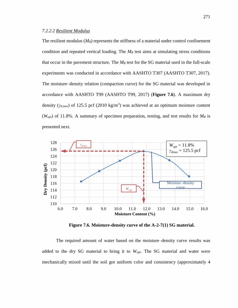
271
7.2.2.2 Resilient Modulus
The resilient modulus (MR) represents the stiffness of a material under control confinement
condition and repeated vertical loading. The MR test aims at simulating stress conditions
that occur in the pavement structure. The MR test for the SG material used in the full-scale
experiments was conducted in accordance with AASHTO T307 (AASHTO T307, 2017).
The moisture–density relation (compaction curve) for the SG material was developed in
accordance with AASHTO T99 (AASHTO T99, 2017) (Figure 7.6). A maximum dry
density (γd,max) of 125.5 pcf (2010 kg/m3) was achieved at an optimum moisture content
(Wopt) of 11.8%. A summary of specimen preparation, testing, and test results for MR is
presented next.
Figure 7.6. Moisture-density curve of the A-2-7(1) SG material.
The required amount of water based on the moisture–density curve results was
added to the dry SG material to bring it to Wopt. The SG material and water were
mechanically mixed until the soil got uniform color and consistency (approximately 4
110
112
114
116
118
120
122
124
126
128
6.0 7.0 8.0 9.0 10.0 11.0 12.0 13.0 14.0 15.0 16.0
Dry
Den
sity
(p
cf)
Moisture Content (%)
Wopt = 11.8%
γdmax = 125.5 pcf
Moisture–density
curve
γdmax
Wopt

272
minutes). The prepared soil was cured in sealed buckets with thick plastic covers for a
period of 16–24 hours.
After curing, soil specimens were fabricated to 12 inch (304.8 mm) in height and
6-inch (152.4 mm) diameter (Figure 7.7-a) cylinders. Figure 7.7-b shows a heavy duty
mechanical drill with a 6-inch (152.4 mm) cap employed for the purpose of compaction.
Each specimen was compacted in 15 lifts that resulted in a relative compaction of about
91%. It may be noted that the surface of each compacted lift was scarified to a depth about
1/8 inch (3.2 mm) to avoid de-bonding between the lifts (refer to Figure 7.7-c).
The test specimen surrounded by a latex membrane was secured with top and
bottom porous stone caps with moist paper filters placed in between porous stone and
specimen. The membrane was carefully sealed with caps by using ‘O’ rings (Figure 7.8-
a). The specimen assembly secured within the triaxial cell is shown in Figure 7.8-b. The
load sequences in accordance with AASHTO T307 (AASHTO T307, 2017) were applied.
Axial deformation and rebound of the specimen were monitored using LVDTs. The
resilient modulus for each sequence was calculated from the average of the last 5 loading
cycles of the applied 100 cycles. After completion of the MR test, the testing program was
continued with quick shear test. Figure 7.8-c and Figure 7.8-d display a SG specimen
before the resilient modulus test and after the quick shear test, respectively.

273
(a) (b) (c)
Figure 7.7. Preparation of MR test specimen: (a) cylindrical mold, (b) drill hammer,
and (c) scarifying tool.
(a) (b) (c) (d)
Figure 7.8. MR test specimen: (a) surrounded by latex membrane, (b) assembled in
triaxial cell, (c) before test, and (d) after quick shear test.
It is well accepted that an increase in MR resulting from an increase in bulk stress
(θ) is commonly referred to as “stress hardening” behavior. On the other hand, “stress
softening” behavior exhibits a decrease in the MR with an increase in deviator stress (σd).
Constitutive models are generally used to estimate MR of the material as a function of stress
state. Three constitutive models that represent hardening behavior (referred to as Theta
model or K-), softening behavior (referred to as log-log model or K-d), and hardening–

274
softening behavior (referred to as Uzan model) were considered to describe the behavior
of the tested SG material under the MR testing condition (Equations of Figure 7.9 through
Figure 7.11), where K is the regression constant of MR model. In these models, the
exponents of θ and σd (i.e., n and m) are expected to have a positive and a negative value,
respectively.
𝑀𝑅 = 𝐾𝜃𝑛
Figure 7.9. Calculation of MR: Theta model, hardening behavior.
𝑀𝑅 = 𝐾𝜎𝑑𝑚
Figure 7.10. Calculation of MR: log-log model, softening behavior.
𝑀𝑅 = 𝐾𝜃𝑛𝜎𝑑𝑚
Figure 7.11. Calculation of MR: Uzan model, hardening-softening behavior.
In order to identify the parameters of the models, the method of lest squares in
Microsoft® Excel™ Solver was employed. The calculated parameters for the evaluated
models are presented in Table 7.2. These parameters are for MR, , and d given in pounds
per square inch. Figure 7.12 through Figure 7.14 depict the comparison between the
measured and calculated MR using the constitutive models and associated model
parameters. It can be seen that the calculated MR using Uzan model that considers both
hardening and softening behavior, show the best agreement with the measured values. The
results of MR tests on the SG material revealed that the increase in σd at a constant confining
pressure resulted in the increase in MR value. The log-log model reflects the softening
characteristics of an unbound material. Such a model did not properly capture the behavior
of the tested SG material indicated by a positive value for the m parameter.
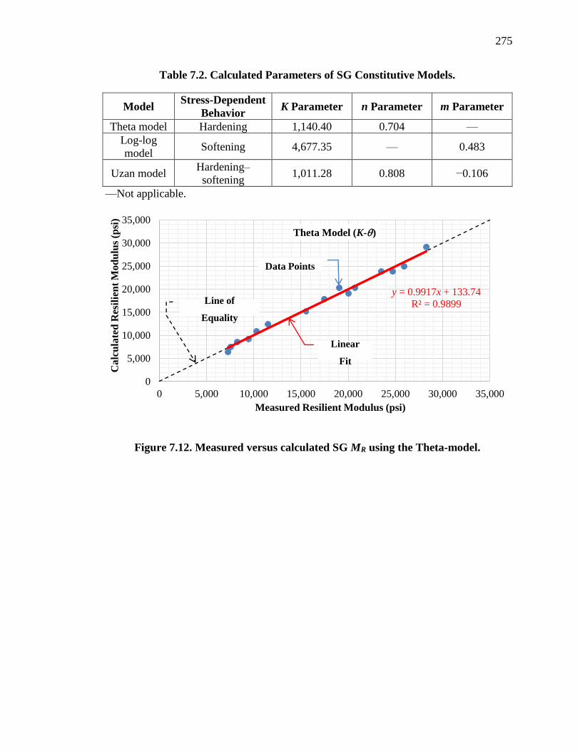
275
Table 7.2. Calculated Parameters of SG Constitutive Models.
Model Stress-Dependent
Behavior K Parameter n Parameter m Parameter
Theta model Hardening 1,140.40 0.704 —
Log-log
model Softening 4,677.35 — 0.483
Uzan model Hardening–
softening 1,011.28 0.808 −0.106
—Not applicable.
Figure 7.12. Measured versus calculated SG MR using the Theta-model.
y = 0.9917x + 133.74
R² = 0.9899
0
5,000
10,000
15,000
20,000
25,000
30,000
35,000
0 5,000 10,000 15,000 20,000 25,000 30,000 35,000
Calc
ula
ted
Res
ilie
nt
Mod
ulu
s (p
si)
Measured Resilient Modulus (psi)
Theta Model (K-)
Line of
Equality
Linear
Fit
Data Points

276
Figure 7.13. Measured versus calculated SG MR using the log-log model.
Figure 7.14. Measured versus calculated SG MR using the Uzan model.
7.2.3 Characteristics of Base Material
A typical local CAB layer was used in the full-scale PaveBox experiments. The CAB
material was selected following the NDOT materials’ specification for dense-graded CAB
y = 0.6424x + 5992.5
R² = 0.6581
0
5,000
10,000
15,000
20,000
25,000
30,000
35,000
0 5,000 10,000 15,000 20,000 25,000 30,000 35,000
Ca
lcu
late
d R
esil
ien
t M
od
ulu
s (p
si)
Measured Resilient Modulus (psi)
Log-Log Model (K-d)
Line of
Equality
Linear
FitData Points
y = 1.0025x - 52.909
R² = 0.9985
0
5,000
10,000
15,000
20,000
25,000
30,000
35,000
0 5,000 10,000 15,000 20,000 25,000 30,000 35,000
Calc
ula
ted
Res
ilie
nt
Mod
ulu
s (p
si)
Measured Resilient Modulus (psi)
Uzan Model
Line of
Equality
Linear
Fit
Data Points

277
(Type 2, Class B) (NDOT Silver Book, 2018). Table 7.3 summarizes the requirements for
the CAB material typically used in Nevada (i.e., Type 2, Class B base) in comparison to
the CAB used in Florida (i.e., Graded aggregate and Limerock bases). Overall, the
requirements for the CAB materials from NDOT and FDOT were comparable and the CAB
material used in the PaveBox experiments was considered acceptable for the purpose of
this task. A structural coefficient of 0.18 that is consistent with the value imposed by FDOT
for graded aggregate base was assumed for the CAB material used in the PaveBox (FDOT
Design Manual, 2016).
The CAB material used in both PaveBox experiments, was sampled from a local
supplier in northern Nevada in accordance with AASHTO T2 (AASHTO T2, 2015)
protocol. The sampled materials were blended and reduced to testing size following
AASHTO T248 (AASHTO T248, 2014), AASHTO T27 (AASHTO T27, 2014) and
AASHTO T180 (AASHTO T180, 2017) protocols were followed to determine the
gradation, γdmax, and Wopt. Figure 7.15 illustrates the moisture–density compaction curve
for the CAB material. The γdmax for the evaluated CAB material was 135.1 pcf (2164
kg/m3), maximum wet density was 147.0 pcf (2,354 kg/m3), and Wopt was 8.8%.

278
Table 7.3. NDOT and FDOT Requirements for CAB Materials.
Property
NDOT Type II,
Class B Base 0
FDOT Graded
Aggregate Base
Error! Reference
source not found.
FDOT Limerock
Base Error!
Reference source
not found.
Soundness Loss — 15% —
Percent of Carbonates — — ≥ 70%
PI 3 PI 15
(function of
percent passing
No. 200 sieve)
G1: PI 4 for
passing No. 40
material
Non-Plastic (NP)
Liquid Limit (LL) LL 35 G1: LL 25 for
passing No. 40
material
LL 35
Sand Equivalent (SE) — G2: SE 28 for
passing No.10
material
—
Lime Bearing Ratio
(LBR)
— LBR ≥ 100 LBR ≥ 100
R-Value R ≥ 70 — —
Gradation
Percent Passing Sieve:
3.5 inch (87.5 mm)
2 inch (50 mm)
1.5 inch (37.5 mm)
1 inch (25 mm)
0.75 inch (19 mm)
0.375 inch (9.5 mm)
No. 4 (4.75 mm)
No. 10 (2 mm)
No. 16 (1.18 mm)
No. 50 (0.3 mm)
No. 200 (0.075 mm)
100
100
100
80–100
—
—
30–65
—
15–40
—
2–12
100
100
95–100
—
65–90
45–75
35–60
25–45
—
5–25
0–10
≥ 97%
—
—
—
—
—
—
—
—
—
—

279
Figure 7.15. Moisture-density curve of the CAB material.
7.2.4 Characteristics of AC Material
This section summarizes the materials used in the fabrication of PMA and HP AC mixes
for the PaveBox experiments. The Superpave mix designs that were developed in
accordance with FDOT specifications 2018 (FDOT Specifications, 2018) are also
presented. The PMA and HP asphalt binders were sampled from Vecenergy of Rivera
Beach in Florida, while the aggregates were sampled from Lockwood pit; a common source
of aggregates in the greater Reno area. The AC mixes were produced on site using a half-
ton asphalt mixer. Loose mixtures were collected in five-gallon steel pails during
production for deposition in PaveBox. The produced mixtures were evaluated for their
engineering properties in terms of dynamic modulus (E*) master curve, fatigue cracking
characteristics in terms of resistance to flexural bending strains, and rutting characteristic
in terms of resistance to permanent strains in triaxial testing. In addition, field cores from
126
128
130
132
134
136
138
4 5 6 7 8 9 10 11 12
Dry
Den
sity
(p
cf)
Moisture Content (%)
Wopt = 8.8%
γdmax = 135.1 pcf
Moisture–density
curve
γdmax
Wopt
280
both experiments were collected after testing was completed for determination of as-
constructed density and thickness values.
7.2.4.1 Asphalt Binders
Two asphalt binders were used in this task: a PG76-22PMA and an HP Binder. A total of
fifteen 5-gallon buckets were obtained for each grade from the selected source. The PMA
and HP binders were reported to have 3.0%, and 8.0% SBS polymer by weight of binder,
respectively. Thus, meeting the definition set forth in this research for PMA and HP asphalt
binders. The grade and source of the base binder and the SBS content for each binder were
provided by the supplier. Table 7.4 and Table 7.5 summarize the properties of the sampled
PMA and HP asphalt binders, respectively. Both binders met the corresponding FDOT
specifications 2018 (FDOT Specifications, 2018).

281
Table 7.4. Properties of the PG76-22PMA Asphalt Binder Sampled from Vecenergy.
Test and Method Condition Measurement FDOT Specification
2018
Source of base binder — PG67-22 Marathon —
Modifier Polymer SBS, 3.0% by
weight of binder(a) —
Additive Anti-Strip Agent — —
Original Binder
Flash Point, AASHTO T48-
06
Cleveland Open
Cup 603°F 450°F Min.
Rotational Viscosity,
AASHTO T316-13 275°F 2.245 Pa.s 3.000 Pa.s Max.
Dynamic Shear Rheometer,
AASHTO T315-12
G*/sin 𝛿 at 76°C 1.21 kPa 1.00 kPa Min.
Phase Angle,
𝛿 at 76°C 74.0 degrees 75 degrees Max.
Rolling Thin Film Oven Test Residues (AASHTO T240-13)
Rolling Thin Film Oven,
AASHTO T240-13 Mass Change 0.32% 1.00% Max.
Multiple Stress Creep
Recovery AASHTO M332-
14
Jnr, 3.2 at 67°C 0.62 kPa-1 1.00 kPa-1 Max.
Jnr,diff at 67°C 19.8% —
%R3.2 at 67°C 54.3% %R3.2 ≥ 29.37(Jnr, 3.2)-0.2633
≥ 25.9%
Pressure Aging Vessel Residue @ 100°C (AASHTO R 28-12)
Dynamic Shear Rheometer,
AASHTO T315-12 G*sin 𝛿 at 26.5°C,
10 rad/sec. 3,155 kPa 5,000 kPa Max.
Creep Stiffness, AASHTO
T313-12
S (Stiffness) at
−12°C, 60 sec.(b) 148 MPa 300 MPa Max.
m-value at −12°C,
60 sec.(b) 0.328 0.300 Min.
—Not applicable. (a)%SBS was provided by the supplier. (b)Testing temperature is 10°C warmer than the actual low PG.

282
Table 7.5. Properties of the HP Asphalt Binder Sampled from Vecenergy.
Test and Method Condition Measurement FDOT Specification
2018
Source of base binder — PG58-28 Marathon —
Modifier Polymer SBS, 8.0% by
weight of binder(a) —
Additive Anti-Strip Agent — —
Original Binder
Flash Point, AASHTO T48-
06
Cleveland Open
Cup 604°F 450°F Min.
Rotational Viscosity,
AASHTO T316-13 275°F 3.401 Pa.s 3.000 Pa.s Max.(b)
Dynamic Shear Rheometer,
AASHTO T315-12
G*/sin 𝛿 at 76°C 2.28 kPa 1.00 kPa Max.
Phase Angle,
𝛿 at 76°C 47.1 degrees 65 degrees Max.
Rolling Thin Film Oven Test Residues (AASHTO T240-13)
Rolling Thin Film Oven,
AASHTO T240-13 Mass Change 0.67% 1.00% Max.
Multiple Stress Creep
Recovery AASHTO M332-
14
Jnr, 3.2 at 76°C 0.03 kPa-1 0.10 kPa-1 Max.
Jnr,diff at 76°C 8.6% —
%R3.2 at 76°C 97.5% %R3.2 ≥ 90.0%
Pressure Aging Vessel Residue @ 100°C (AASHTO R 28-12)
Dynamic Shear Rheometer,
AASHTO T315-12 G*sin 𝛿 at 26.5°C,
10 rad/sec. 1,150 kPa 5,000 kPa Max.
Creep Stiffness, AASHTO
T313-12
S (Stiffness) at
−12°C, 60 sec.(c) 85 MPa 300 MPa Max.
m-value at −12°C,
60 sec.(c) 0.389 0.300 Min.
—Not applicable. (a)%SBS was provided by the supplier. (b)Binders with values higher than 3 Pa.s should be used with caution and only after consulting
with the supplier as to any special handling procedures, including pumping capabilities (FDOT
Specifications, 2018) (c)Testing temperature is 10°C warmer than the actual low PG.
7.2.4.2 Aggregates
The aggregates were sampled from Lockwood pit in the northern part of Nevada. An
aggregate gradation with a Nominal Maximum Aggregate Size (NMAS) of 0.5 inch (12.5
mm) following FDOT specifications (FDOT Specifications, 2018) was targeted for the
experiment. It should be mentioned that the same gradation was targeted for both PMA and
HP AC mixes. Gradation analyses were conducted for all aggregate stockpiles. Table 7.6

283
presents the gradations of all the individual stockpiles. Figure 7.16 presents the aggregates
job mix formula (JMF) gradation for the AC mixes. It should be mentioned that no recycled
material was used in any of the AC mixes.
Table 7.7 summarizes the requirements for the aggregates typically used in Nevada
and Florida for AC mixes. Overall, the requirements for the aggregates from NDOT and
FDOT were comparable and the selected aggregates for the AC mixes used in the PaveBox
experiments was considered acceptable for the purpose of this task. A structural coefficient
of 0.44 that is consistent with the value imposed by FDOT was assumed for the PMA AC
mix used in the PaveBox (FDOT Design Manual, 2016).
Table 7.6. Gradations and JMF for the 12.5 mm NMAS PMA and HP AC Mixes.
Sieve Size
Percentage Passing
JMF
Gradation
0.75 inch
(19 mm)
AGG
Crushed
0.5 inch
(12.5 mm)
AGG
Crushed
0.375 inch
(9.5 mm)
AGG
Crushed
No. 4
(4.75 mm)
Crusher
Fines
Concrete
Sand
No. 4
(4.75 mm)
Natural
Fines
1.5 inch (37.5 mm) 100.0 100.0 100.0 100.0 100 100 100.0
1 inch (25 mm) 100.0 100.0 100.0 100.0 100 100 100.0
0.75 inch (19 mm) 100.0 100.0 100.0 100.0 100 100 100.0
0.5 inch (12.5 mm) 36.8 100.0 100.0 100.0 100 100 93.7
0.375 inch (9.5 mm) 5.5 55.3 100.0 100.0 100 100 85.2
No. 4 (4.75 mm) 1.1 0.9 21.2 98.0 99.3 99.6 65.7
No. 8 (2.36 mm) 0.9 0.8 1.3 64.4 90 98.7 51.9
No. 16 (1.18 mm) 0.8 0.7 0.7 40.4 62.2 96.5 38.8
No. 30 (0.6 mm) 0.8 0.6 0.5 26.8 39.8 84.1 28.3
No. 50 (0.3 mm) 0.7 0.6 0.5 19.6 19.7 45.6 16.2
No. 100 (0.15 mm) 0.7 0.5 0.4 15.4 7.5 11.7 7.5
No. 200 (0.075 mm) 0.7 0.5 0.4 12.6 4.1 3.2 4.8
Bin Percentages 10.0% 12.0% 15.0% 25.0% 24.0% 14.0% 100.0%

284
Figure 7.16. JMF gradation for the 12.5 mm NMAS PMA and HP AC mixes.
Table 7.7. NDOT and FDOT Aggregates Specifications for Bituminous Courses.
Property NDOT FDOT
Test Method Requirement Test Method Requirement
Fractured Faces Nev. T230 80% Min., 2
Fractures Min. ASTM D5821
95/90% for
Traffic Level D
Fine Aggregate Angularity — — AASHTO
T304 10% Max.
Flat and Elongated Particles — — ASTM D4791 10% Max.
PI Nev. T212 10 Max. — —
LL Nev. T210 35 Max. — —
Sand Equivalent — — AASHTO
T176 45% Min.
Absorption of Coarse
Aggregate Nev. T111 4% Max. — —
Percentage of Wear AASHTO T96 37% Max. FM 1-T096 45% Max.
Soundness (Coarse
Aggregate) (5 Cycles,
Sodium Sulfate)
AASHTO
T104 12% Max. Loss
AASHTO
T104 12% Max. Loss
Soundness (Fine Aggregate)
(5 Cycles, Sodium Sulfate)
AASHTO
T104 15% Max. Loss — —
Specific Gravity (Fine
Aggregate) Nev. T493 2.95 Max. — —
Specific Gravity (Coarse
Aggregate) Nev. T111 2.95 Max. — —
—Not applicable.
0
10
20
30
40
50
60
70
80
90
100
Per
cen
t P
ass
ing
Sieve Size
Job Mix Formula
Max Line
SP12.5 FDOT Control Points
1 i
nch
0.5
in
ch
0.3
75
in
ch
No.
4
No.
8
0.7
5 in
ch
1.5
in
ch
No.
10
No.
16
No.
30
No.
40
No.
50
No.
10
0N
o.
20
0
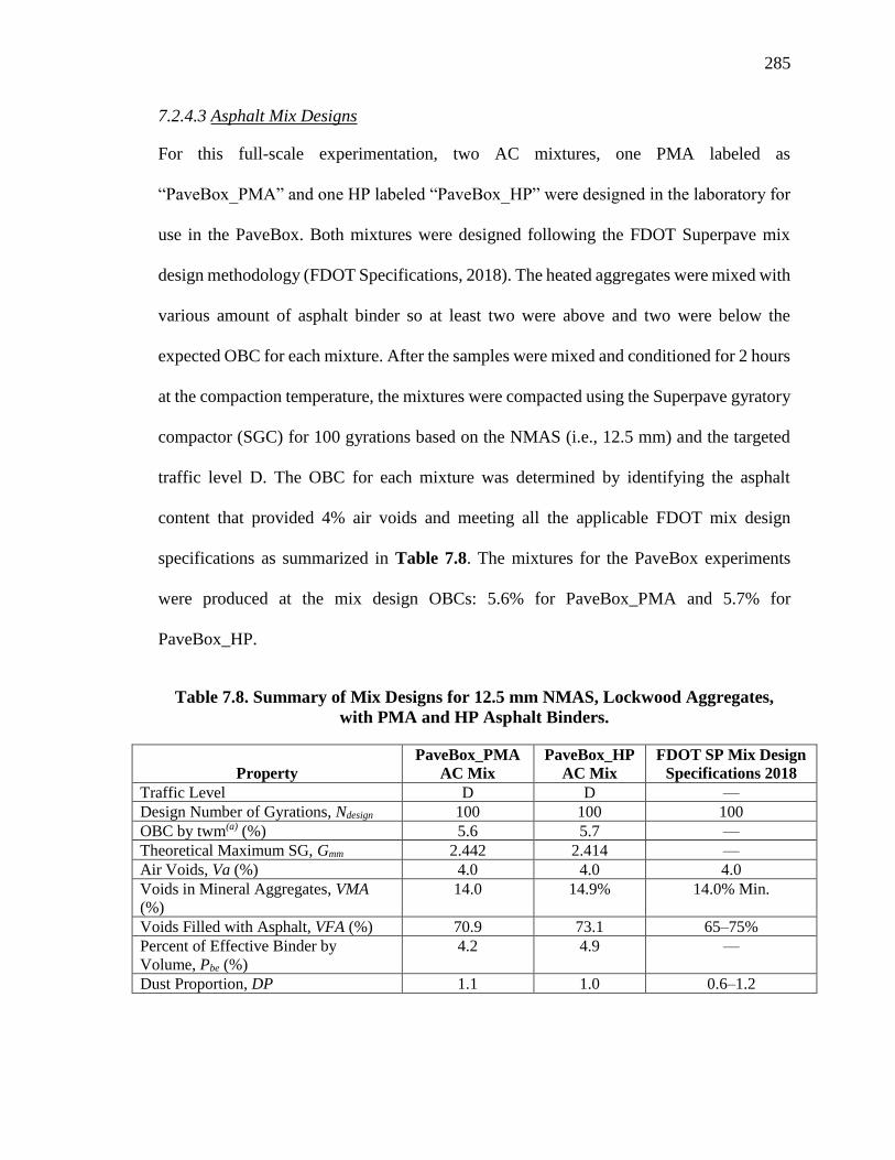
285
7.2.4.3 Asphalt Mix Designs
For this full-scale experimentation, two AC mixtures, one PMA labeled as
“PaveBox_PMA” and one HP labeled “PaveBox_HP” were designed in the laboratory for
use in the PaveBox. Both mixtures were designed following the FDOT Superpave mix
design methodology (FDOT Specifications, 2018). The heated aggregates were mixed with
various amount of asphalt binder so at least two were above and two were below the
expected OBC for each mixture. After the samples were mixed and conditioned for 2 hours
at the compaction temperature, the mixtures were compacted using the Superpave gyratory
compactor (SGC) for 100 gyrations based on the NMAS (i.e., 12.5 mm) and the targeted
traffic level D. The OBC for each mixture was determined by identifying the asphalt
content that provided 4% air voids and meeting all the applicable FDOT mix design
specifications as summarized in Table 7.8. The mixtures for the PaveBox experiments
were produced at the mix design OBCs: 5.6% for PaveBox_PMA and 5.7% for
PaveBox_HP.
Table 7.8. Summary of Mix Designs for 12.5 mm NMAS, Lockwood Aggregates,
with PMA and HP Asphalt Binders.
Property
PaveBox_PMA
AC Mix
PaveBox_HP
AC Mix
FDOT SP Mix Design
Specifications 2018
Traffic Level D D —
Design Number of Gyrations, Ndesign 100 100 100
OBC by twm(a) (%) 5.6 5.7 —
Theoretical Maximum SG, Gmm 2.442 2.414 —
Air Voids, Va (%) 4.0 4.0 4.0
Voids in Mineral Aggregates, VMA
(%)
14.0 14.9% 14.0% Min.
Voids Filled with Asphalt, VFA (%) 70.9 73.1 65–75%
Percent of Effective Binder by
Volume, Pbe (%)
4.2 4.9 —
Dust Proportion, DP 1.1 1.0 0.6–1.2
286
7.2.4.4 Performance Testing
Loose asphalt mixtures were collected from the outlet of the half-ton asphalt mixer during
production. The mixtures were evaluated for their engineering property in terms of E*, and
for performance characteristics in terms of their resistance to fatigue cracking and rutting.
The E* and rutting were evaluated at the short-term aging condition while fatigue cracking
was evaluated after long-term oven aging. Short-term aging consisted of reheating the loose
mixtures at the compaction temperature in a force-draft laboratory oven for three hours
prior to splitting, followed by an additional hour prior to compaction. In the case of the
fatigue cracking, the compacted specimens were long-term aged at a temperature of 185°F
(85°C) in a forced-draft oven for 5 days. It should be mentioned that test specimens were
compacted to an air void level similar to the as-constructed air voids of the AC layer in the
PaveBox. In-place density was determined using field cores sampled from each AC layer
after completing the experiment (refer to Section 7.2.9 for further details).
Fatigue and rutting testing were conducted at the respective effective intermediate
and high temperatures (i.e., 77°F (25°C) and 122°F (50°C), respectively) that were
determined for the state of Florida (refer to Section 5.3).
Dynamic Modulus
The E* property of each of the two AC mixes was determined in accordance with
AASHTO T378 (AASHTO T378, 2017). More information regarding this test can be found
in Section 3.3.1 of this manuscript. The E* provides an indication on the overall quality of
the AC mixture. The magnitude of E* depends on several properties of the mixture
including aggregate properties, gradation, asphalt binder grade, mix volumetrics, and mix
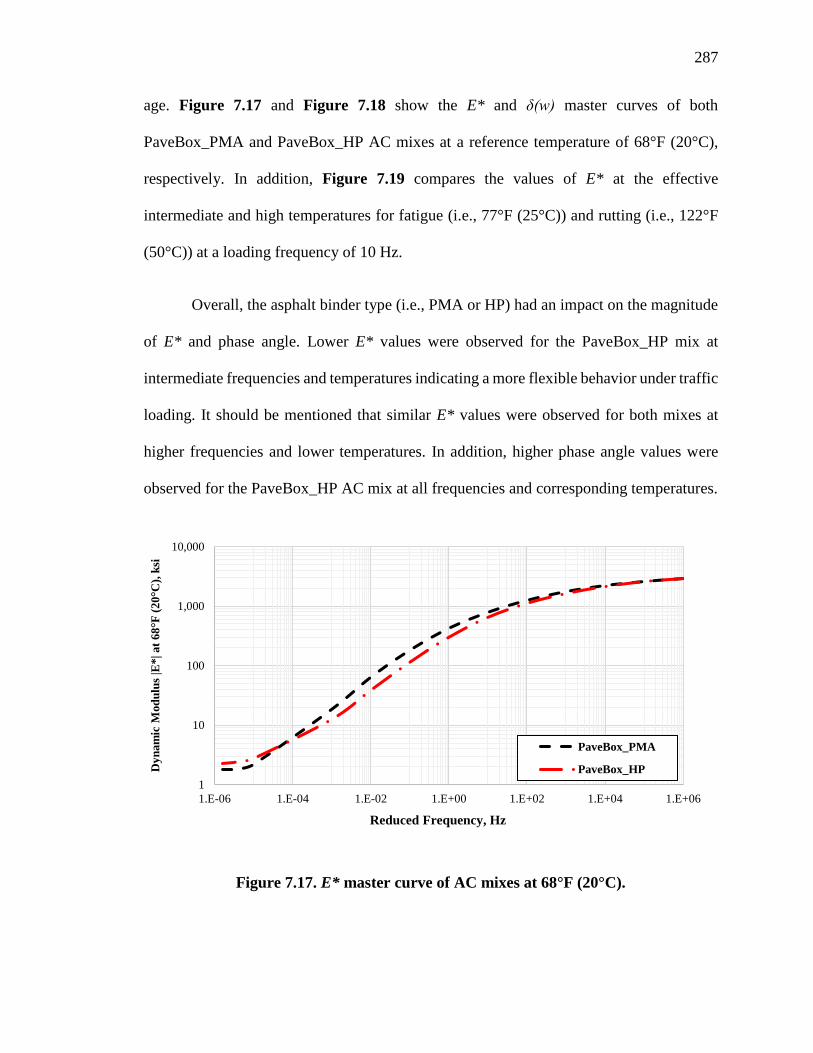
287
age. Figure 7.17 and Figure 7.18 show the E* and δ(w) master curves of both
PaveBox_PMA and PaveBox_HP AC mixes at a reference temperature of 68°F (20°C),
respectively. In addition, Figure 7.19 compares the values of E* at the effective
intermediate and high temperatures for fatigue (i.e., 77°F (25°C)) and rutting (i.e., 122°F
(50°C)) at a loading frequency of 10 Hz.
Overall, the asphalt binder type (i.e., PMA or HP) had an impact on the magnitude
of E* and phase angle. Lower E* values were observed for the PaveBox_HP mix at
intermediate frequencies and temperatures indicating a more flexible behavior under traffic
loading. It should be mentioned that similar E* values were observed for both mixes at
higher frequencies and lower temperatures. In addition, higher phase angle values were
observed for the PaveBox_HP AC mix at all frequencies and corresponding temperatures.
Figure 7.17. E* master curve of AC mixes at 68°F (20°C).
1
10
100
1,000
10,000
1.E-06 1.E-04 1.E-02 1.E+00 1.E+02 1.E+04 1.E+06
Dy
nam
ic M
od
ulu
s |E
*| at
68
°F (
20
°C),
ksi
Reduced Frequency, Hz
PaveBox_PMA
PaveBox_HP

288
Figure 7.18. Phase angle master curve of AC mixes at 68°F (20°C).
Figure 7.19. E* values at 10 Hz.
0
5
10
15
20
25
30
35
40
45
1.E-09 1.E-07 1.E-05 1.E-03 1.E-01 1.E+01 1.E+03 1.E+05 1.E+07
Ph
ase
An
gle
δ a
t 6
8°F
(2
0°C
), d
egre
e
Reduced Frequency, Hz
PaveBox_PMA
PaveBox_HP
585
448
7848
0
100
200
300
400
500
600
700
PaveBox_PMA PaveBox_HP PaveBox_PMA PaveBox_HP
At 77°F (25°C) At 122°F (50°C)
E*
at
10
Hz
(ksi
)

289
Fatigue Cracking
The fatigue characteristics of the two AC mixes were evaluated using the flexural beam
fatigue test according to AASHTO T321 (AASHTO T321, 2014) at three temperatures and
multiple strain levels. The mixtures for the fatigue test were short-term aged followed by
long-term oven aging since fatigue is a later pavement life distress. More information
regarding this test can be found in Section 3.3.2.2. The flexural beam fatigue tests were
conducted at 55, 70, and 85°F (13, 21, and 30°C) for the PaveBox_PMA AC mix and at
40, 55, and 70°F (4.4, 13, and 21°C) for the PaveBox_HP AC mix. The highest testing
temperature was adjusted to ensure the evaluated AC mix was stiff enough to hold a
constant strain during testing. A generalized fatigue model for each mix was developed
following the equation of Figure 3.27.
Figure 7.20 and Figure 7.21 show the fatigue relationships developed at all testing
temperatures for the PaveBox_PMA and PaveBox_HP AC mixes, respectively. In
addition, Figure 7.22 shows the fatigue relationships for the two evaluated AC mixes at
77°F (25°C). These relationships were interpolated using the measured data at the three
testing temperatures (i.e. 55, 70, and 85°F for PMA AC mix and 40, 55, and 70°F for HP
AC mix). A higher and flatter curve indicates a better resistance to fatigue cracking. The
asphalt binder type (i.e., PMA or HP) had a significant impact on the fatigue behavior of
the evaluated AC mixes. The PaveBox_HP AC mix showed better fatigue relationships
when compared with the PaveBox_PMA AC mix at all strain levels and testing
temperatures. Thus, indicating an increased flexibility and resistance to fatigue cracking
for the HP AC mix under different environmental conditions. For example, at 500 micro-
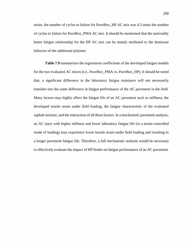
290
strain, the number of cycles to failure for PaveBox_HP AC mix was 4.5 times the number
of cycles to failure for PaveBox_PMA AC mix. It should be mentioned that the noticeably
better fatigue relationship for the HP AC mix can be mainly attributed to the dominant
behavior of the additional polymer.
Table 7.9 summarizes the regressions coefficients of the developed fatigue models
for the two evaluated AC mixes (i.e., PaveBox_PMA vs. PaveBox_HP). It should be noted
that, a significant difference in the laboratory fatigue resistance will not necessarily
translate into the same difference in fatigue performance of the AC pavement in the field.
Many factors may highly affect the fatigue life of an AC pavement such as stiffness, the
developed tensile strain under field loading, the fatigue characteristic of the evaluated
asphalt mixture, and the interaction of all these factors. In a mechanistic pavement analysis,
an AC layer with higher stiffness and lower laboratory fatigue life (in a strain-controlled
mode of loading) may experience lower tensile strain under field loading and resulting in
a longer pavement fatigue life. Therefore, a full mechanistic analysis would be necessary
to effectively evaluate the impact of HP binder on fatigue performance of an AC pavement.
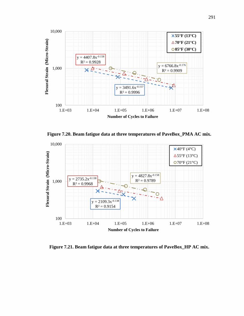
291
Figure 7.20. Beam fatigue data at three temperatures of PaveBox_PMA AC mix.
Figure 7.21. Beam fatigue data at three temperatures of PaveBox_HP AC mix.
y = 3491.6x-0.157
R² = 0.9996
y = 4407.8x-0.158
R² = 0.9928y = 6766.8x-0.176
R² = 0.9909
100
1,000
10,000
1.E+03 1.E+04 1.E+05 1.E+06 1.E+07 1.E+08
Fle
xu
ral
Str
ain
(M
icro
-Str
ain
)
Number of Cycles to Failure
55°F (13°C)
70°F (21°C)
85°F (30°C)
y = 2109.3x-0.138
R² = 0.9154
y = 2735.2x-0.138
R² = 0.9968
y = 4827.8x-0.158
R² = 0.9789
100
1,000
10,000
1.E+03 1.E+04 1.E+05 1.E+06 1.E+07 1.E+08
Fle
xu
ral
Str
ain
(M
icro
-Str
ain
)
Number of Cycles to Failure
40°F (4°C)
55°F (13°C)
70°F (21°C)

292
Figure 7.22. Fatigue relationships of PaveBox_PMA and PaveBox_HP AC mixes at
77°F (25°C).
Table 7.9. Summary of Fatigue Model Coefficients for the Two Evaluated AC
Mixes.
Mix ID
Fatigue Model Coefficients
kf1 kf2 kf3
PaveBox_PMA 1.1973E+01 6.2248E+00 2.6756E+00
PaveBox_HP 2.7552E+09 6.6407E+00 4.3438E+00
Rutting
The rutting characteristic of the two AC mixes were evaluated using the Repeated Load
Triaxial (RLT) setup (NCHRP Project 719, 2008). The RLT test was conducted at 104,
122, and 140°F (40, 50, and 60°C). A generalized rutting model for each of the two AC
mixes was developed following the equation of Figure 3.20.
Figure 7.23 and Figure 7.24 show the rutting curves for the evaluated
PaveBox_PMA and PaveBox_HP AC mixes at the three testing temperatures, respectively.
100
1,000
10,000
1.E+04 1.E+05 1.E+06 1.E+07 1.E+08 1.E+09
Fle
xu
ral
Str
ain
(M
icro
-Str
ain
)
Number of Cycles to failure
PaveBox_PMA
PaveBox_HP
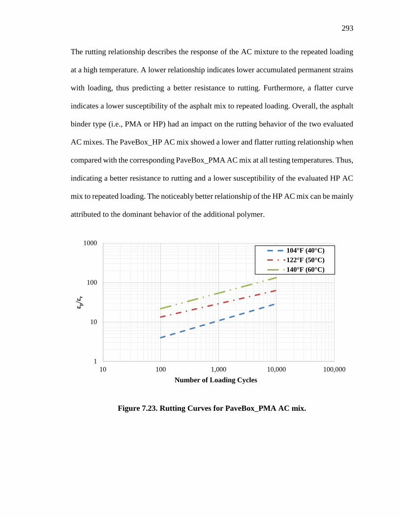
293
The rutting relationship describes the response of the AC mixture to the repeated loading
at a high temperature. A lower relationship indicates lower accumulated permanent strains
with loading, thus predicting a better resistance to rutting. Furthermore, a flatter curve
indicates a lower susceptibility of the asphalt mix to repeated loading. Overall, the asphalt
binder type (i.e., PMA or HP) had an impact on the rutting behavior of the two evaluated
AC mixes. The PaveBox_HP AC mix showed a lower and flatter rutting relationship when
compared with the corresponding PaveBox_PMA AC mix at all testing temperatures. Thus,
indicating a better resistance to rutting and a lower susceptibility of the evaluated HP AC
mix to repeated loading. The noticeably better relationship of the HP AC mix can be mainly
attributed to the dominant behavior of the additional polymer.
Figure 7.23. Rutting Curves for PaveBox_PMA AC mix.
1
10
100
1000
10 100 1,000 10,000 100,000
ε p/ε
r
Number of Loading Cycles
104°F (40°C)
122°F (50°C)
140°F (60°C)

294
Figure 7.24. Rutting Curves for PaveBox_HP AC mix.
Figure 7.25 shows the rutting relationship of the PaveBox_HP AC mix along with
the PaveBox_PMA AC mix at 122°F (50°C). For example, after 10,000 loading repetitions,
the resulting cumulative p/r of the PaveBox_PMA AC mix was about 2.2 times greater
than the value of the PaveBox_HP AC mix. Table 7.10 summarizes the regression
coefficients of the rutting models for the two evaluated AC mixes. It should be noted that,
a significant difference in the laboratory rutting resistance will not necessarily translate
into the same difference in rutting performance (i.e., rut depth) of the AC layer in the field.
Many factors may highly affect the rutting life of an AC pavement such as stiffness, the
developed compressive strain in each of the AC sub-layers under field loading, the rutting
characteristic of the evaluated asphalt mixture, and the interaction of all these factors.
Therefore, a full mechanistic analysis coupled with laboratory measured engineering and
1
10
100
1000
10 100 1,000 10,000 100,000
ε p/ε
r
Number of Loading Cycles
104°F (40°C)
122°F (50°C)
140°F (60°C)

295
performance properties would be necessary to quantify and effectively evaluate the impact
of HP binder on the rutting performance of the corresponding AC pavement.
Figure 7.25. Rutting behavior of PaveBox_PMA and PaveBox_HP AC mixes at
122°F (50°C).
Table 7.10. Summary of Rutting Model Coefficients for Evaluated AC Mixes.
Mix ID
Rutting Model Coefficients
kr1 kr2 kr3
PaveBox_PMA -10.8922 5.3491 0.3847
PaveBox_HP -11.0584 5.3505 0.3458
7.2.5 Pavement Structures
The FDOT flexible pavement design manual (FDOT Design Manual, 2016) was used to
design the PMA pavement structure for the PaveBox experiment. This manual provides
guidance for designing new and rehabilitated flexible pavements according to the
AASHTO 1993 Guide. More information regarding the procedure to design pavement
1
10
100
1000
10 100 1,000 10,000 100,000
ε p/ε
r
Number of Loading Cycles
PaveBox_PMA
PaveBox_HP
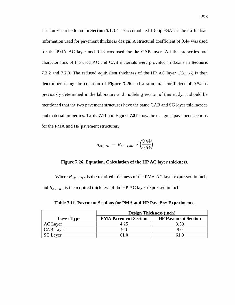
296
structures can be found in Section 5.1.3. The accumulated 18-kip ESAL is the traffic load
information used for pavement thickness design. A structural coefficient of 0.44 was used
for the PMA AC layer and 0.18 was used for the CAB layer. All the properties and
characteristics of the used AC and CAB materials were provided in details in Sections
7.2.2 and 7.2.3. The reduced equivalent thickness of the HP AC layer (HAC-HP) is then
determined using the equation of Figure 7.26 and a structural coefficient of 0.54 as
previously determined in the laboratory and modeling section of this study. It should be
mentioned that the two pavement structures have the same CAB and SG layer thicknesses
and material properties. Table 7.11 and Figure 7.27 show the designed pavement sections
for the PMA and HP pavement structures.
𝐻𝐴𝐶−𝐻𝑃 = 𝐻𝐴𝐶−𝑃𝑀𝐴 × (0.44
0.54)
Figure 7.26. Equation. Calculation of the HP AC layer thickness.
Where 𝐻𝐴𝐶−𝑃𝑀𝐴 is the required thickness of the PMA AC layer expressed in inch,
and 𝐻𝐴𝐶−𝐻𝑃 is the required thickness of the HP AC layer expressed in inch.
Table 7.11. Pavement Sections for PMA and HP PaveBox Experiments.
Layer Type
Design Thickness (inch)
PMA Pavement Section HP Pavement Section
AC Layer 4.25 3.50
CAB Layer 9.0 9.0
SG Layer 61.0 61.0

297
Figure 7.27. PMA and HP pavement sections in the PaveBox experiments.
7.2.6 Data Acquisition System
A National Instrument (NI) data acquisition system comprises of two 12 slot SCXI-1001
chassis populated with 18 NI SCXI-1320 conditioners were used to acquire the sensor data
in the full-scale PaveBox experiments. This 72 data channel system is capable of sampling
data at frequencies that range from 1 to 3,000 Hz. Such system is applicable for acquiring
data from a wide range of sensors including strain gauges, displacement transducers, load
cells, pressure cells, and accelerometers. Data from experiments involving dynamic
loading were acquired at 1,024 Hz to accommodate the requirements for double integration
algorithm for assessing the displacements. Data from experiments with static loading were
acquired at 32 Hz. Once the data was acquired, it was stored locally on the computer hard
drive in comma separated values (CSV) files that could be imported and utilized by most
software packages for data analysis.

298
7.2.7 PaveBox Tests Preparation
7.2.7.1 SG Deposition in the PaveBox
The goal was to place the SG material at 11% moisture content and at a 90% γd,max to a
depth of 61 inches (155 cm). The SG material was shoveled from the stockpile into five-
gallon buckets, placed in a concrete mixer, and mixed for less than a minute (10 to 30
seconds). The moist SG material was then transported and placed via a laboratory-
fabricated shoot and distributed within PaveBox area.
A gasoline-powered vibratory plate compactor was used to achieve the required in-
place compaction. Three to four passes lasting approximately 5 to 8 minutes each were
needed to arrive at a 4-inch (10.2 cm) compacted lift. Nuclear density gauge readings were
taken after each lift in the PaveBox, to confirm the required compaction had been reached
(90% of γd,max). Figure 7.28 and Figure 7.29 show the various construction stages of
placing the SG material into the PaveBox.
While nuclear density gauge was used to ensure the target density during the
placement of the SG lifts, dynamic cone penetrometer (DCP) testing was also used to assess
the density of the SG layer as a function of depth. Two DCP tests, at two different locations,
were conducted on the finished SG, after placement of all the SG lifts. Figure 7.30 shows
the readings of the two DCP tests. In general, the results indicated similar densities for the
SG layer in both locations.

299
(a) (b)
Figure 7.28. SG deposition: (a) soil mixing in the mechanical mixer, and (b)
placement of moist soil in PaveBox.
(a) (b) (c)
Figure 7.29. SG compaction in PaveBox: (a) vibratory plate compactor, (b) nuclear
density gauge measurements on top of compacted lift of SG soil, and (c) scarification
of the SG lift surface using a pickaxe to ensure bonding between compacted lifts.
Figure 7.30. DCP test results for SG layer at two locations in PaveBox.
0
1
2
3
4
5
6
0
300
600
900
1200
1500
1800
0 5 10 15 20
Cu
mu
lati
ve
Pen
etra
tion
(ft
)
Cu
mu
lati
ve
Pen
etra
tion
(m
m)
Number of Blows
DCP-1 SG
Layer
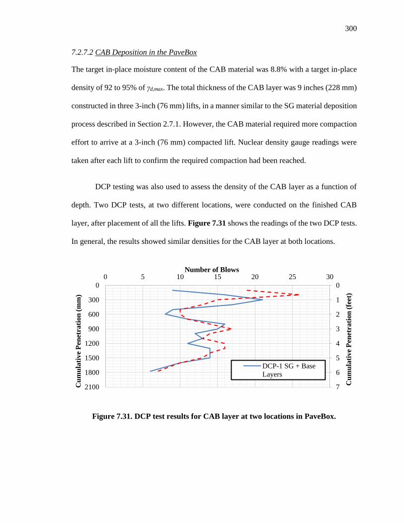
300
7.2.7.2 CAB Deposition in the PaveBox
The target in-place moisture content of the CAB material was 8.8% with a target in-place
density of 92 to 95% of γd,max. The total thickness of the CAB layer was 9 inches (228 mm)
constructed in three 3-inch (76 mm) lifts, in a manner similar to the SG material deposition
process described in Section 2.7.1. However, the CAB material required more compaction
effort to arrive at a 3-inch (76 mm) compacted lift. Nuclear density gauge readings were
taken after each lift to confirm the required compaction had been reached.
DCP testing was also used to assess the density of the CAB layer as a function of
depth. Two DCP tests, at two different locations, were conducted on the finished CAB
layer, after placement of all the lifts. Figure 7.31 shows the readings of the two DCP tests.
In general, the results showed similar densities for the CAB layer at both locations.
Figure 7.31. DCP test results for CAB layer at two locations in PaveBox.
0
1
2
3
4
5
6
7
0
300
600
900
1200
1500
1800
2100
0 5 10 15 20 25 30
Cu
mu
lati
ve
Pen
etra
tion
(fe
et)
Cu
mu
lati
ve
Pen
etra
tion
(m
m)
Number of Blows
DCP-1 SG + Base
Layers
301
7.2.7.3 AC Production and Deposition in PaveBox
Both the PMA and HP asphalt mixes for PaveBox experiments were mixed in a half-ton
asphalt mixer using asphalt binders sampled from Florida and local aggregates sampled
from Nevada. Figure 7.32 shows the asphalt mixer used to produce the AC mixes for the
PaveBox experiments. The aggregate stockpiles were sampled, brought to laboratory, and
organized into different bins as shown in Figure 7.33. The aggregates are proportioned out
of each bin onto a feeder belt according to the percentages given by the mix design. The
feeder belt transported the proportioned aggregates to the mixing pug mill. The aggregates
were heated in the pug mill at the mixing temperature for a minimum duration of 15
minutes. Approximate temperatures of 325°F (163°C) and 340°F (175°C) were used for
the PMA and HP AC mixes, respectively. After drying the aggregates, the heated liquid
asphalt binder was added into the pug mill on top of the heated aggregates. The mixing
process continued for an additional duration of 15 minutes to ensure uniformity and proper
coating of aggregates within the AC mix.
It should be mentioned that the moisture content of every stockpile was measured
prior to each experiment and proper adjustments were made for the amount of asphalt
binder to be added. The produced AC mix was discharged from the back of the asphalt
mixer in a big steel bucket mounted to the front of a forklift. The discharged AC mix was
then deposited into the PaveBox for compaction. The temperature of the discharged AC
mix was monitored during the entire production process and the mixing temperature was
adjusted to maintain the discharge temperatures as close as possible to 325°F (163°C) and
340°F (175°C) for the PMA and HP AC mixes, respectively. It should be mentioned that

302
the asphalt mixer has a maximum capacity of producing 1,000 lbs (453.6 kg) of ready AC
mix within a duration of 30 to 40 minutes. Thus, five batches of AC mixes were needed to
for each PaveBox experiment. This produced sufficient materials for both: constructing the
full AC layer in the PaveBox and for the laboratory performance evaluation.
Figure 7.32. Half-ton asphalt mixer used to mix and produce PMA and HP AC
mixes for PaveBox.
Figure 7.33. Aggregate stockpiles organized and used to produce PMA and HP AC
mixes.
303
The produced AC mix was placed in 1.0 to 1.5-inch (25 to 38 mm) lifts. The lifts
were compacted using a vibratory plate compactor to achieve a target in-place density of
92% to 96%. The produced AC mix was dumped directly into the PaveBox, spread
uniformly over the entire area, and leveled to a thickness of approximately 2.5 inch (63.5
mm) of uncompacted material. A vibratory plate was then used for compaction of the lift
by applying it around the perimeter of the PaveBox from the outside edge to the inside for
better compaction. Upon achieving an acceptable compaction on the first lift, the same
process was repeated for the second lift. A thin lift nuclear density gauge was used at
several locations around the surface of the box to measure the in-place density of the
compacted AC surface layer.
Loose AC mixtures were sampled into 5-gallon steel pails during placement of the
material in PaveBox. These materials were brought to the laboratory and were tested for
Gmm, E* property, and resistance to fatigue cracking and rutting. The results of the
laboratory evaluation of the produced AC mixes were presented in Section 7.2.4.4.
The loading of the pavement structure was conducted 5-7 days after the placement
of the AC layer. Cores were taken immediately after the completion of each of the
experiments. Cores were used to measure the as-constructed AC layer thickness and in-
place density. It should be noted that the laboratory specimens were compacted to a target
density similar to the as-constructed density.

304
7.2.8 Loading Protocol and Instrumentation
A hydraulic ram capable of delivering 60,000 lb (267 kN) was used to apply the dynamic
surface loads. The ram was modified by attaching a Moog-252 spool valve that can be
electronically controlled to provide the required flow to the ram to achieve the target
dynamic load with the target pulse duration. The system was connected to a hydraulic pump
along with accumulators to ensure adequate flow of hydraulic fluid necessary for the
repeated cycles of loading. The ram was mounted onto a stiff horizontal steel beam
connected between two vertical steel columns that comprised the reaction frame.
A computer running a real time operating system was connected to a National
Instrument (NI) 4-slot SCXI-1001 chassis populated with two NI SCXI-1320 conditioners
that were used to control the servo valve. A 100,000 lb (45 kN) interface pancake-type load
cell along with a string pot were attached to the ram, which in turn were electronically
connected to the controller. The controller design was a proportional-integral-derivative
(PID) controller. This control loop feedback mechanism was used to control the ram in
either force or displacement control mode depending on the mode selected for testing.
Careful calibration of the gain was essential to ensure the proper operation of the entire
loading system.
An FWD loading plate with 11.9 inch (300 mm) diameter (Figure 7.34) was used
to apply the dynamic loads on top of the pavement structure to better simulate actual tire
loading conditions. The ratio of the PaveBox dimensions to the diameter of the loading
plate was deemed sufficient to minimize the interference from the PaveBox boundaries.
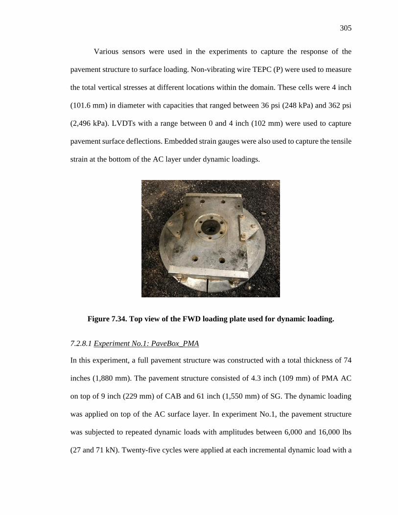
305
Various sensors were used in the experiments to capture the response of the
pavement structure to surface loading. Non-vibrating wire TEPC (P) were used to measure
the total vertical stresses at different locations within the domain. These cells were 4 inch
(101.6 mm) in diameter with capacities that ranged between 36 psi (248 kPa) and 362 psi
(2,496 kPa). LVDTs with a range between 0 and 4 inch (102 mm) were used to capture
pavement surface deflections. Embedded strain gauges were also used to capture the tensile
strain at the bottom of the AC layer under dynamic loadings.
Figure 7.34. Top view of the FWD loading plate used for dynamic loading.
7.2.8.1 Experiment No.1: PaveBox_PMA
In this experiment, a full pavement structure was constructed with a total thickness of 74
inches (1,880 mm). The pavement structure consisted of 4.3 inch (109 mm) of PMA AC
on top of 9 inch (229 mm) of CAB and 61 inch (1,550 mm) of SG. The dynamic loading
was applied on top of the AC surface layer. In experiment No.1, the pavement structure
was subjected to repeated dynamic loads with amplitudes between 6,000 and 16,000 lbs
(27 and 71 kN). Twenty-five cycles were applied at each incremental dynamic load with a

306
pulse duration of 0.1 sec followed by a rest period of 0.9 sec in each loading cycle. The
pavement structure was subjected to a series of four loading levels with a sequentially
higher load amplitudes. Table 7.12 summarizes the loading protocol for experiment No.1.
All loads were applied on the loading plate positioned directly at the top of the AC layer
and at the center of the PaveBox.
Table 7.12. Loading Protocol for Experiment No.1 (PaveBox_PMA).
Load Type
Target Load
Amplitude
(lb)
No. of
Loading
Cycles
Load Plate
Diameter
(inch)
Rest Period
Between
Load Levels
(min)
Dynamic load (0.1 sec. loading
+ 0.9 sec. rest period) 6,000 25
11.9 (FWD
loading plate) 2
Dynamic load (0.1 sec. loading
+ 0.9 sec. rest period) 9,000 25
11.9 (FWD
loading plate) 2
Dynamic load (0.1 sec. loading
+ 0.9 sec. rest period) 12,000 25
11.9 (FWD
loading plate) 2
Dynamic load (0.1 sec. loading
+ 0.9 sec. rest period) 16,000 25
11.9 (FWD
loading plate) 2
The instrumentation for the pavement structure consisted of surface LVDTs
installed diagonally to measure surface deflections at various radial distances of 0, 8, 12,
24, 36, 48, and 60 inch (0, 203, 305, 610, 914, 1,219, and 1,524 mm) from the center of the
load. The moving tips of the surface LVDTs rested on top of the AC layer. Figure 7.35
shows the drawing of the experiment No.1 setup (PaveBox_PMA) at the top of the AC
layer at an elevation (z) of 74 inches (188 cm) from the PaveBox floor. Ten 4-inch (101
mm) pressure cells were placed at three different locations: in the middle of the base—z =
65.5 inch (z = 166.4 cm), at 6 inch (15.2 cm) below the SG surface—z = 56.0 inch (z =
142.2 cm), and at 24 inches (61.0 cm) below the SG surface—z = 42 inch (z = 106.7 cm).
These cells were located directly under the center of the loading plate and diagonally at
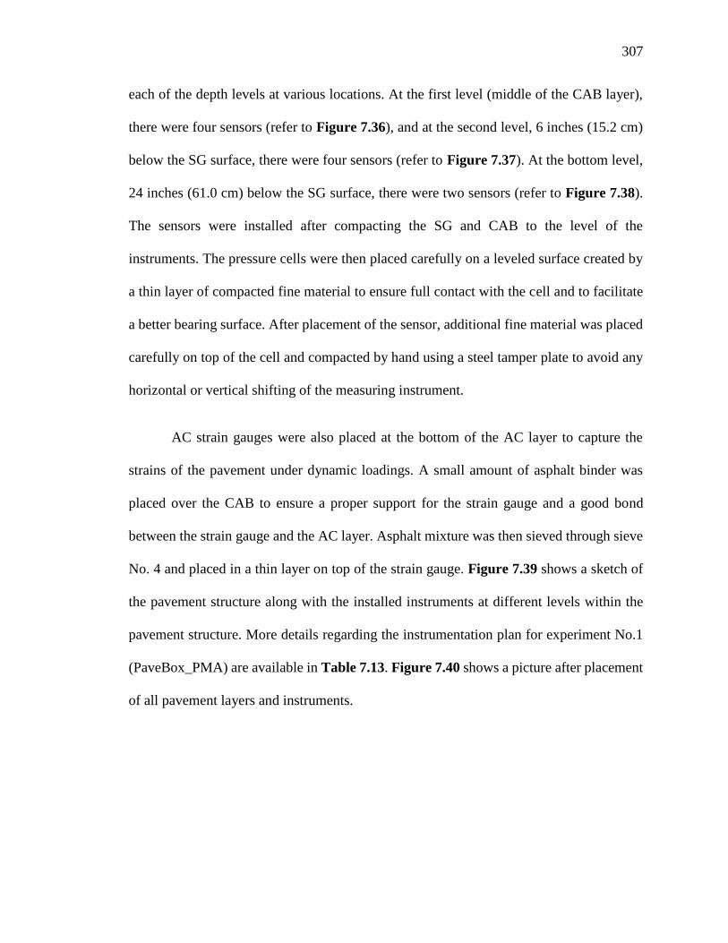
307
each of the depth levels at various locations. At the first level (middle of the CAB layer),
there were four sensors (refer to Figure 7.36), and at the second level, 6 inches (15.2 cm)
below the SG surface, there were four sensors (refer to Figure 7.37). At the bottom level,
24 inches (61.0 cm) below the SG surface, there were two sensors (refer to Figure 7.38).
The sensors were installed after compacting the SG and CAB to the level of the
instruments. The pressure cells were then placed carefully on a leveled surface created by
a thin layer of compacted fine material to ensure full contact with the cell and to facilitate
a better bearing surface. After placement of the sensor, additional fine material was placed
carefully on top of the cell and compacted by hand using a steel tamper plate to avoid any
horizontal or vertical shifting of the measuring instrument.
AC strain gauges were also placed at the bottom of the AC layer to capture the
strains of the pavement under dynamic loadings. A small amount of asphalt binder was
placed over the CAB to ensure a proper support for the strain gauge and a good bond
between the strain gauge and the AC layer. Asphalt mixture was then sieved through sieve
No. 4 and placed in a thin layer on top of the strain gauge. Figure 7.39 shows a sketch of
the pavement structure along with the installed instruments at different levels within the
pavement structure. More details regarding the instrumentation plan for experiment No.1
(PaveBox_PMA) are available in Table 7.13. Figure 7.40 shows a picture after placement
of all pavement layers and instruments.

308
Figure 7.35. Plan view for PaveBox_PMA experiment No.1 at the AC surface.
Figure 7.36. Section view for PaveBox_PMA experiment No.1 at the middle of CAB
layer.
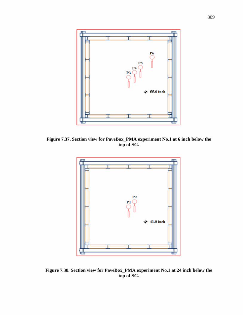
309
Figure 7.37. Section view for PaveBox_PMA experiment No.1 at 6 inch below the
top of SG.
Figure 7.38. Section view for PaveBox_PMA experiment No.1 at 24 inch below the
top of SG.
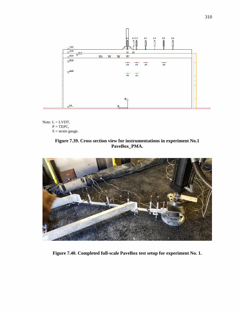
310
Note: L = LVDT.
P = TEPC,
S = strain gauge.
Figure 7.39. Cross section view for instrumentations in experiment No.1
PaveBox_PMA.
Figure 7.40. Completed full-scale PaveBox test setup for experiment No. 1.
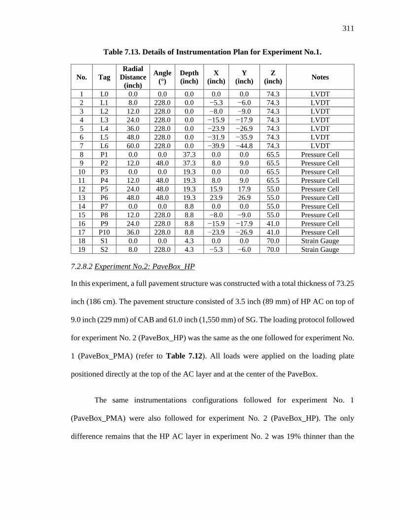
311
Table 7.13. Details of Instrumentation Plan for Experiment No.1.
No. Tag
Radial
Distance
(inch)
Angle
(°)
Depth
(inch)
X
(inch)
Y
(inch)
Z
(inch) Notes
1 L0 0.0 0.0 0.0 0.0 0.0 74.3 LVDT
2 L1 8.0 228.0 0.0 −5.3 −6.0 74.3 LVDT
3 L2 12.0 228.0 0.0 −8.0 −9.0 74.3 LVDT
4 L3 24.0 228.0 0.0 −15.9 −17.9 74.3 LVDT
5 L4 36.0 228.0 0.0 −23.9 −26.9 74.3 LVDT
6 L5 48.0 228.0 0.0 −31.9 −35.9 74.3 LVDT
7 L6 60.0 228.0 0.0 −39.9 −44.8 74.3 LVDT
8 P1 0.0 0.0 37.3 0.0 0.0 65.5 Pressure Cell
9 P2 12.0 48.0 37.3 8.0 9.0 65.5 Pressure Cell
10 P3 0.0 0.0 19.3 0.0 0.0 65.5 Pressure Cell
11 P4 12.0 48.0 19.3 8.0 9.0 65.5 Pressure Cell
12 P5 24.0 48.0 19.3 15.9 17.9 55.0 Pressure Cell
13 P6 48.0 48.0 19.3 23.9 26.9 55.0 Pressure Cell
14 P7 0.0 0.0 8.8 0.0 0.0 55.0 Pressure Cell
15 P8 12.0 228.0 8.8 −8.0 −9.0 55.0 Pressure Cell
16 P9 24.0 228.0 8.8 −15.9 −17.9 41.0 Pressure Cell
17 P10 36.0 228.0 8.8 −23.9 −26.9 41.0 Pressure Cell
18 S1 0.0 0.0 4.3 0.0 0.0 70.0 Strain Gauge
19 S2 8.0 228.0 4.3 −5.3 −6.0 70.0 Strain Gauge
7.2.8.2 Experiment No.2: PaveBox_HP
In this experiment, a full pavement structure was constructed with a total thickness of 73.25
inch (186 cm). The pavement structure consisted of 3.5 inch (89 mm) of HP AC on top of
9.0 inch (229 mm) of CAB and 61.0 inch (1,550 mm) of SG. The loading protocol followed
for experiment No. 2 (PaveBox_HP) was the same as the one followed for experiment No.
1 (PaveBox_PMA) (refer to Table 7.12). All loads were applied on the loading plate
positioned directly at the top of the AC layer and at the center of the PaveBox.
The same instrumentations configurations followed for experiment No. 1
(PaveBox_PMA) were also followed for experiment No. 2 (PaveBox_HP). The only
difference remains that the HP AC layer in experiment No. 2 was 19% thinner than the

312
PMA AC layer in experiment No. 1. More details regarding the instrumentation plan for
experiment No. 2 (PaveBox_HP) are available in Table 7.14.
Table 7.14. Details of Instrumentation Plan for Experiment No.2.
No. Tag
Radial
Distance
(inch)
Angle
(°)
Depth
(inch)
X
(inch)
Y
(inch)
Z
(inch) Notes
1 L0 0.0 0.0 0.0 0.0 0.0 73.5 LVDT
2 L1 8.0 228.0 0.0 −5.3 −6.0 73.5 LVDT
3 L2 12.0 228.0 0.0 −8.0 −9.0 73.5 LVDT
4 L3 24.0 228.0 0.0 −15.9 −17.9 73.5 LVDT
5 L4 36.0 228.0 0.0 −23.9 −26.9 73.5 LVDT
6 L5 48.0 228.0 0.0 −31.9 −35.9 73.5 LVDT
7 L6 60.0 228.0 0.0 −39.9 −44.8 73.5 LVDT
8 P1 0.0 0.0 36.5 0.0 0.0 65.5 Pressure Cell
9 P2 12.0 48.0 36.5 8.0 9.0 65.5 Pressure Cell
10 P3 0.0 0.0 18.5 0.0 0.0 65.5 Pressure Cell
11 P4 12.0 48.0 18.5 8.0 9.0 65.5 Pressure Cell
12 P5 24.0 48.0 18.5 15.9 17.9 55.0 Pressure Cell
13 P6 48.0 48.0 18.5 23.9 26.9 55.0 Pressure Cell
14 P7 0.0 0.0 8.0 0.0 0.0 55.0 Pressure Cell
15 P8 12.0 228.0 8.0 −8.0 −9.0 55.0 Pressure Cell
16 P9 24.0 228.0 8.0 −15.9 −17.9 41.0 Pressure Cell
17 P10 36.0 228.0 8.0 −23.9 −26.9 41.0 Pressure Cell
18 S1 0.0 0.0 3.5 0.0 0.0 70.0 Strain Gauge
19 S2 8.0 228.0 3.5 −5.3 −6.0 70.0 Strain Gauge
7.2.9 Evaluation of Field Cores
Field core samples from each experiment were collected after completing testing of the
pavement structures. Figure 7.41 shows the locations of the cores sampled from
experiments No. 1 and No. 2. As noticed, the cores were sampled from different locations
near and far from the loading area to account for all possible variabilities of the thickness
and in-place density of the corresponding AC layer. The core samples were used to measure
the as-constructed thickness and air voids of the PMA and HP AC layers. Figure 7.42
shows photos of core samples taken from the PMA and HP AC layers. The photos clearly

313
highlight the difference in the thickness of the AC layer between the two experiments
(PaveBox_PMA and PaveBox_HP). Table 7.15 summarizes the measured in-place
thicknesses and air voids for the various collected field core samples from each experiment.
For both experiments, the designed and as-constructed thicknesses were similar and
consistent throughout the entire AC layer. In addition, the in-place air voids for experiment
No.1 (PaveBox_PMA) and experiment No. 2 (PaveBox_HP) were within the desired air
voids levels of 8±1%. The HP AC layer showed a slightly lower air voids level when
compared with the PMA one.
Figure 7.41. Diagram showing the locations of the cores sampled from both
experiments.

314
Table 7.15. As-Constructed AC Layer Thickness and Air Voids.
AC Layer Type
As-Constructed Layer Thickness
(inch) As-Constructed Air Voids (%)
Average Target 95% Confidence
Interval Average
95% Confidence
Interval
PMA (Experiment No.
1) 4.30 4.25 0.19 8.1 1.3
HP (Experiment No. 2) 3.47 3.50 0.18 7.5 0.4
(a) (b)
Figure 7.42. (a) PMA AC core sample from experiment No. 1, and (b) HP AC core
sample from experiment No. 2.
7.3 Analysis of Measured Pavement Responses
This section of the manuscript summarizes the measured pavement responses from each of
the two PaveBox experiments. It also presents a comparison analysis for the measured
pavement responses in the PMA and HP pavement structures (referred to as analysis I in
Figure 7.1). First, the steps undertaken to preprocess the recordings from the various
instruments are presented. Then the analysis of the preprocessed data from the instruments
in the various pavement layers is presented and discussed.

315
7.3.1 Preprocessing
As mentioned earlier, the testing program for both experiments (i.e., experiment No. 1
PaveBox_PMA, and experiment No. 2 PaveBox_HP) involved a series of instruments. This
included LVDTs, pressure cells, and strain gauges to measure vertical displacements,
vertical stresses, and tensile strains at the installed locations, respectively.
The following preprocessing steps were undertaken for all recordings to identify
and separate the appropriate load-induced response signals from the recorded data:
• Selection of the five representative consecutive cycles of loading: these cycles are
selected after the application of the pulse load has been repeated many times (up to
about 20 cycles).
• Removal of the noise: subtracting the average of the recorded measurements prior
to the application of impulse load from all measurements.
Figure 7.43 through Figure 7.46 show, as an example, preprocessed measured
recordings at the center of the applied dynamic load of 16,000 lb for the load cell, the
surface LVDT, the TEPC in the middle of the CAB layer, and the strain gauge at the bottom
of the AC layer. By visually observing the data for 16,000 lb in Figure 7.43 to Figure 7.46,
it can be inferred that the reduced thickness of the HP AC layer resulted in an increase in
both, the center surface deflection and the vertical stress in the middle of the CAB layer.
However, a lower tensile strain at the bottom of the AC layer under 16,000 lb was observed
in the PaveBox_HP when compared to the PaveBox_PMA. Under the lower applied
surface load levels (i.e., 6,000 to 12,000 lb), the measured tensile strain at the bottom of

316
the HP AC layer was in general comparable to the corresponding strain measured at the
bottom of the PMA AC layer.
While similar characteristics were observed for the recorded signals from the load
cell, LVDTs, and TEPCs, the load-induced strain data recorded in the PaveBox_HP
exhibited a different shape than the one observed in the PaveBox_PMA. In particular, the
stain data recorded in the PaveBox_HP did not show a time strain recovery during the rest
(i.e., unloading) period of the surface dynamic load. This same behavior was observed
under all levels of surface load. It was also noted that the magnitude of the initial strain at
the beginning of the PaveBox_HP experiment and before the application of the loading
sequences was much higher than the one observed in the PaveBox_PMA experiment
(around 500 microstrain compared to 100 microstrain).
While the analysis focus was on the load-induced strain value (calculated as the
difference between the initial strain and the peak strain value), it was not clear if the
difference in the observed shape of the load-induced-strain is reflecting a true material
behavior or it is a result of the high initial strain value, or a combination of the
aforementioned. Thus, a certain degree of caution should be exercised when analyzing and
comparing the measured strain data from the two PaveBox experiments.
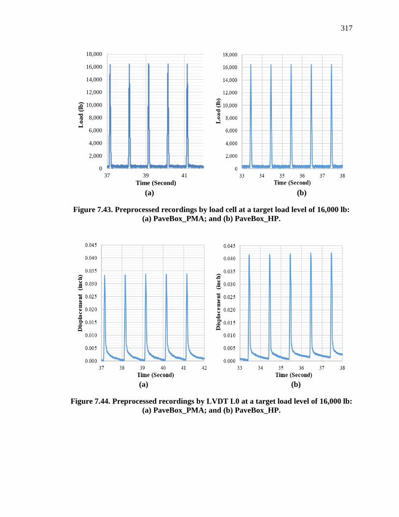
317
(a) (b)
Figure 7.43. Preprocessed recordings by load cell at a target load level of 16,000 lb:
(a) PaveBox_PMA; and (b) PaveBox_HP.
(a) (b)
Figure 7.44. Preprocessed recordings by LVDT L0 at a target load level of 16,000 lb:
(a) PaveBox_PMA; and (b) PaveBox_HP.
0
2,000
4,000
6,000
8,000
10,000
12,000
14,000
16,000
18,000
37 39 41
Lo
ad
(lb
)
Time (Second)

318
(a) (b)
Figure 7.45. Preprocessed recordings by TEPC P7 at a target load level of 16,000 lb:
(a) PaveBox_PMA; and (b) PaveBox_HP.
(a) (b)
Figure 7.46. Preprocessed recordings by strain gauge S1 at a target load level of
16,000 lb: (a) PaveBox_PMA; and (b) PaveBox_HP.
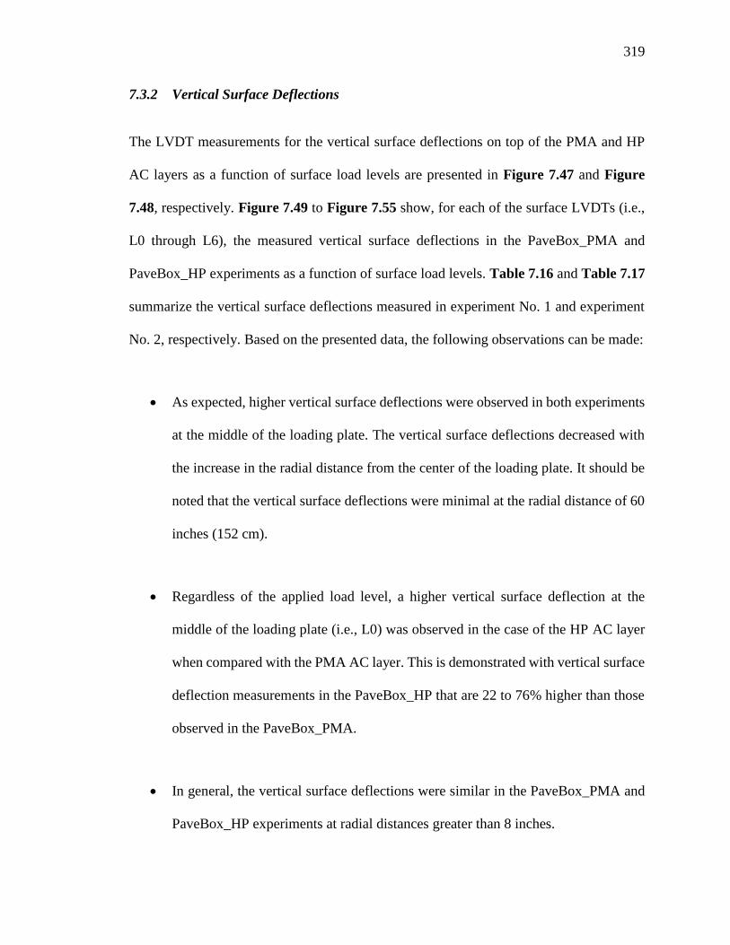
319
7.3.2 Vertical Surface Deflections
The LVDT measurements for the vertical surface deflections on top of the PMA and HP
AC layers as a function of surface load levels are presented in Figure 7.47 and Figure
7.48, respectively. Figure 7.49 to Figure 7.55 show, for each of the surface LVDTs (i.e.,
L0 through L6), the measured vertical surface deflections in the PaveBox_PMA and
PaveBox_HP experiments as a function of surface load levels. Table 7.16 and Table 7.17
summarize the vertical surface deflections measured in experiment No. 1 and experiment
No. 2, respectively. Based on the presented data, the following observations can be made:
• As expected, higher vertical surface deflections were observed in both experiments
at the middle of the loading plate. The vertical surface deflections decreased with
the increase in the radial distance from the center of the loading plate. It should be
noted that the vertical surface deflections were minimal at the radial distance of 60
inches (152 cm).
• Regardless of the applied load level, a higher vertical surface deflection at the
middle of the loading plate (i.e., L0) was observed in the case of the HP AC layer
when compared with the PMA AC layer. This is demonstrated with vertical surface
deflection measurements in the PaveBox_HP that are 22 to 76% higher than those
observed in the PaveBox_PMA.
• In general, the vertical surface deflections were similar in the PaveBox_PMA and
PaveBox_HP experiments at radial distances greater than 8 inches.

320
• Flatter deflection–load curves were observed at radial distances farther away from
the load indicating less sensitivity of the measured vertical deflections to the
magnitude of the applied surface load.
Figure 7.47. Measured vertical surface deflections as a function of applied surface
loads (experiment No. 1: PaveBox_PMA).
Figure 7.48. Measured vertical surface deflections as a function of applied surface
loads (experiment No. 2: PaveBox_HP).

321
Figure 7.49. Measured vertical surface deflections at the center of the loading plate
(L0).
Figure 7.50. Measured vertical surface deflections at the center of the loading plate
(L1).

322
Figure 7.51. Measured vertical surface deflections at the center of the loading plate
(L2).
Figure 7.52. Measured vertical surface deflections at the center of the loading plate
(L3).

323
Figure 7.53. Measured vertical surface deflections at the center of the loading plate
(L4).
Figure 7.54. Measured vertical surface deflections at the center of the loading plate
(L5).

324
Figure 7.55. Measured vertical surface deflections at the center of the loading plate
(L6).
Table 7.16. Vertical Surface Deflections at Multiple Load Levels: Experiment No.1
(PaveBox_PMA).
Target
Load
Level
(lb)
Average
Applied
Load (lb)
L0
(mils)
L1
(mils)
L2
(mils)
L3
(mils)
L4
(mils)
L5
(mils)
L6
(mils)
6,000 6,054 5.8 5.5 3.7 3.1 2.9 2.9 2.8
9,000 9,189 12.2 10.4 8.3 4.4 3.6 3.3 3.0
12,000 12,066 21.1 18.1 13.6 6.8 4.7 3.6 3.2
16,000 16,117 32.2 25.7 20.4 10.2 6.2 4.2 3.9
Table 7.17. Vertical Surface Deflections at Multiple Load Levels: Experiment No.2
(PaveBox_HP).
Target
Load
Level
(lb)
Average
Applied
Load (lb)
L0
(mils)
L1
(mils)
L2
(mils)
L3
(mils)
L4
(mils)
L5
(mils)
L6
(mils)
6,000 6,062 10.2 7.0 5.2 3.8 3.3 3.0 2.9
9,000 9,119 19.7 12.1 9.6 5.5 4.0 3.7 3.0
12,000 12,143 28.2 18.5 13.5 6.6 4.9 3.9 2.9
16,000 16,111 39.2 26.8 19.3 9.8 6.1 4.1 2.9

325
7.3.3 Vertical Stresses in the Middle of the CAB Layers
The TEPC measurements for the vertical stresses in the middle of the CAB layer in the
PaveBox_PMA and PaveBox_HP experiments as a function of surface load levels are
presented in Figure 7.56 and Figure 7.57, respectively. Figure 7.58 to Figure 7.61 show
the measured vertical stresses from each of the TEPCs (i.e., P7 through P10) in the
PaveBox_PMA and PaveBox_HP experiments as a function of surface load levels. Table
7.18 and Table 7.19 summarize the vertical stresses measured in experiment No. 1 and
experiment No. 2, respectively. Based on the presented data, the following observations
can be made:
• The highest vertical stresses in the middle of the CAB layer were observed under
the middle of the loading plate in each of the two experiments. The vertical stresses
decreased with the increase in radial distance from the center of the loading plate.
It should be noted that the vertical stresses were minimal at the radial distance of
36 inches (91.4 cm).
• Regardless of the surface loading level, higher vertical stresses under the middle of
the loading plate (i.e., P7) were observed in the PaveBox_HP experiment when
compared with the PaveBox_PMA experiment. This is demonstrated with vertical
stress measurements in the PaveBox_HP experiment that are 85 to 100% higher
than those observed in the PaveBox_PMA experiment.

326
• In general, the vertical stress measurements in the PaveBox_PMA experiment were
slightly higher than or similar to the respective measurements in the PaveBox_HP
experiment at radial distances greater than 8 inches (20.3 cm).
• Flatter stress–load curves were observed at radial distances farther away from the
load indicating less sensitivity of the measured vertical stresses to the magnitude of
the applied surface load.
Figure 7.56. Measured vertical stresses as a function of applied surface loads
(experiment No. 1: PaveBox_PMA).

327
Figure 7.57. Measured vertical stresses as a function of applied surface loads
(experiment No. 2: PaveBox_HP).
Figure 7.58. Measured vertical stresses in the middle of the CAB layer and at the
center of the loading plate (P7).

328
Figure 7.59. Measured vertical stresses in the middle of the CAB layer and at 12
inches from the center of the loading plate (P8).
Figure 7.60. Measured vertical stresses in the middle of the CAB layer and at 24
inches from the center of the loading plate (P9).
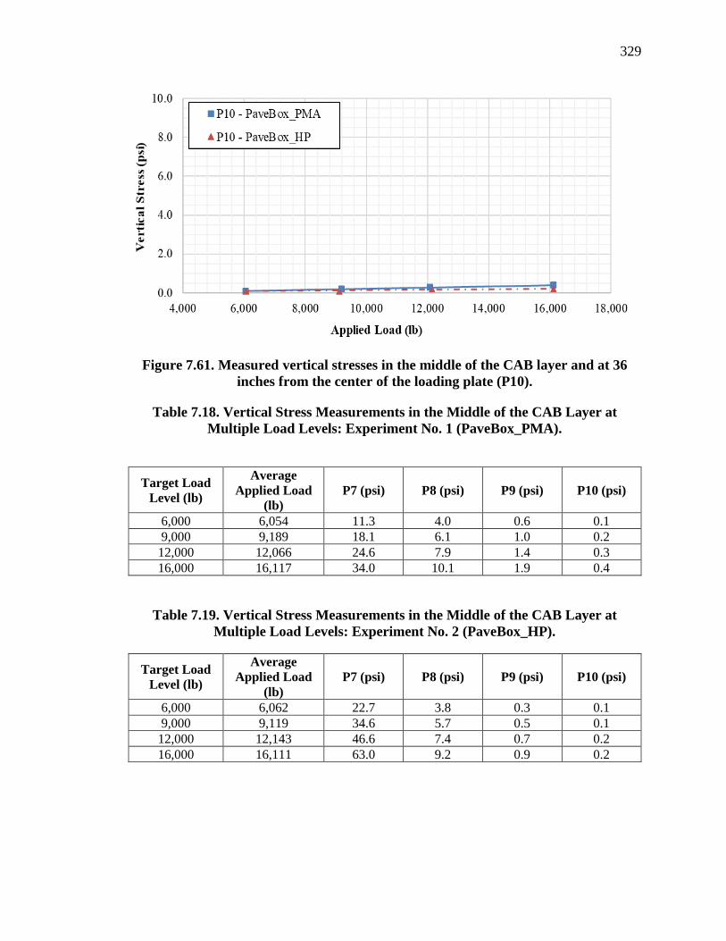
329
Figure 7.61. Measured vertical stresses in the middle of the CAB layer and at 36
inches from the center of the loading plate (P10).
Table 7.18. Vertical Stress Measurements in the Middle of the CAB Layer at
Multiple Load Levels: Experiment No. 1 (PaveBox_PMA).
Target Load
Level (lb)
Average
Applied Load
(lb)
P7 (psi) P8 (psi) P9 (psi) P10 (psi)
6,000 6,054 11.3 4.0 0.6 0.1
9,000 9,189 18.1 6.1 1.0 0.2
12,000 12,066 24.6 7.9 1.4 0.3
16,000 16,117 34.0 10.1 1.9 0.4
Table 7.19. Vertical Stress Measurements in the Middle of the CAB Layer at
Multiple Load Levels: Experiment No. 2 (PaveBox_HP).
Target Load
Level (lb)
Average
Applied Load
(lb)
P7 (psi) P8 (psi) P9 (psi) P10 (psi)
6,000 6,062 22.7 3.8 0.3 0.1
9,000 9,119 34.6 5.7 0.5 0.1
12,000 12,143 46.6 7.4 0.7 0.2
16,000 16,111 63.0 9.2 0.9 0.2

330
7.3.4 Vertical Stresses in the SG Layers
The TEPC measurements for the vertical stresses in the SG layer at 6 inches (152 mm) and
24 inches (610 mm) below the top of the SG as a function of surface load levels, are
presented in Figure 7.64 and Figure 7.65 for the PaveBox_PMA and PaveBox_HP
experiments, respectively. Figure 7.66 to Figure 7.69 show the measured vertical stresses
from each of the TEPC (i.e., P1 through P6) in the PaveBox_PMA and PaveBox_HP
experiments as a function of surface load levels. Table 7.20 and Table 7.21 summarize the
vertical stresses in experiment No. 1 and experiment No. 2, respectively. Based on the
presented data, the following observations can be made:
• Higher vertical stresses in the SG layer were observed under the center of the
loading plate. The vertical stresses in the SG layer decreased with the increase in
radial distance from the center of the loading plate. It should be noted that the
vertical stresses were minimal at the radial distance of 48 inch (1,220 mm) at a
distance of 6 inch (152 mm) below the SG surface.
• Regardless of the loading level, higher vertical stresses under the middle of the
loading plate (i.e., P3) was observed at a distance of 6 inch (152 mm) below the top
of the SG layer in the PaveBox_HP experiment when compared with the
PaveBox_PMA experiment. This is demonstrated with vertical stress
measurements in the PaveBox_HP experiment that are 43 to 46% higher than those
observed in the PaveBox_PMA experiment.

331
• Regardless of the loading level, higher vertical stresses under the middle of the
loading plate (i.e., P3) was observed at a distance of 24 inch (610 mm) below the
top of the SG layer in the PaveBox_HP experiment when compared with the
PaveBox_PMA experiment. This is demonstrated with vertical stress
measurements in the PaveBox_HP that are 20 to 30% higher than those observed
in the PaveBox_PMA.
• In general, the vertical stress measurements in the PaveBox_PMA experiment were
slightly higher than or similar to the respective measurements in the PaveBox_HP
experiment at both locations in the SG layer, i.e., 6 (152 mm) and 24 inch (610 mm)
below the top of the SG layer) and at any radial distance greater than 8 inches (203
mm).
• Flatter stress–load curves were observed at both evaluated depths in the SG layer
and at radial distances farther away from the load indicating less sensitivity of the
measured vertical stresses to the magnitude of the applied surface load.
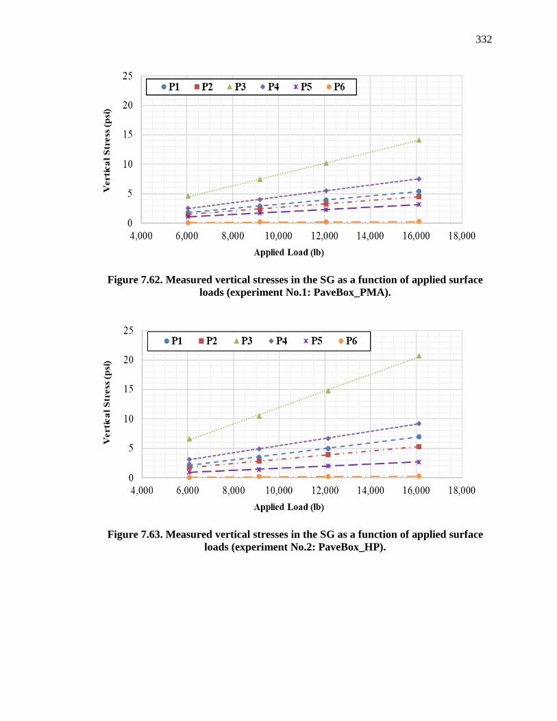
332
Figure 7.62. Measured vertical stresses in the SG as a function of applied surface
loads (experiment No.1: PaveBox_PMA).
Figure 7.63. Measured vertical stresses in the SG as a function of applied surface
loads (experiment No.2: PaveBox_HP).

333
Figure 7.64. Measured vertical stresses at 24 inches below the top of the SG and at
the center of the loading plate (P1).
Figure 7.65. Measured vertical stresses at 24 inches below the top of the SG and at a
radial distance of 12 inches from the center of the loading plate (P2).

334
Figure 7.66. Measured vertical stresses at 6 inches below the top of the SG and at
the center of the loading plate (P3).
Figure 7.67. Measured vertical stresses at 6 inches below the top of the SG and at a
radial distance of 12 inches from the center of the loading plate (P4).

335
Figure 7.68. Measured vertical stresses at 6 inches below the top of the SG and at a
radial distance of 24 inches from the center of the loading plate (P5).
Figure 7.69. Measured vertical stresses at 6 inches below the top of the SG and at a
radial distance of 48 inches from the center of the loading plate (P6).

336
Table 7.20. Vertical Stress Measurements in the SG Layer at Multiple Load Levels:
Experiment No. 1 (PaveBox_PMA).
Target Load
Level (lb)
Average
Applied Load
(lb)
P1
(psi)
P2
(psi)
P3
(psi)
P4
(psi)
P5
(psi)
P6
(psi)
6,000 6,054 1.8 1.5 4.6 2.5 1.1 0.1
9,000 9,189 2.9 2.4 7.4 4.0 1.7 0.2
12,000 12,066 3.9 3.3 10.2 5.5 2.3 0.2
16,000 16,117 5.4 4.5 14.1 7.5 3.2 0.3
Table 7.21. Vertical Stress Measurements in the SG Layer at Multiple Load Levels:
Experiment No. 2 (PaveBox_HP).
Target Load
Level (lb)
Average
Applied Load
(lb)
P1
(psi)
P2
(psi)
P3
(psi)
P4
(psi)
P5
(psi)
P6
(psi)
6,000 6,062 2.2 1.8 6.6 3.1 1.0 0.1
9,000 9,119 3.5 2.8 10.5 4.9 1.4 0.2
12,000 12,143 5.0 3.9 14.8 6.7 2.0 0.2
16,000 16,111 7.0 5.3 20.7 9.2 2.7 0.3
7.3.5 Tensile Strains at the Bottom of AC Layers
Figure 7.70 and Figure 7.71 show, respectively, the tensile strains measured by S1 and S2
at the bottom of the PMA (at a depth of 4.30 inches from the top of the pavement surface)
and HP (at a depth of 3.47 inches from the top of the pavement surface) AC layers as a
function of the surface load levels. S1 in both experiments is located under the center of
the loading plate while S2 is located at a radial distance of 8 inches from the center of the
loading plate. Table 7.22 and Table 7.23 summarize the tensile strains in experiment No.1
and experiment No.2, respectively. Based on the presented data, the following observations
can be made:
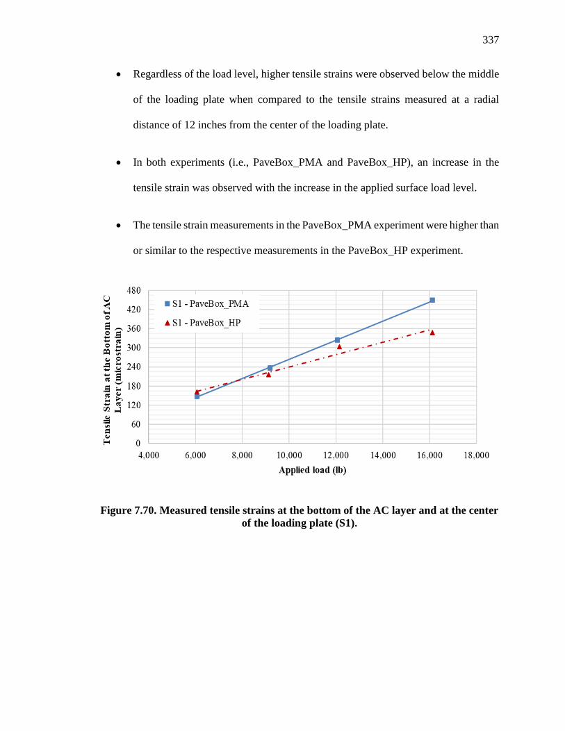
337
• Regardless of the load level, higher tensile strains were observed below the middle
of the loading plate when compared to the tensile strains measured at a radial
distance of 12 inches from the center of the loading plate.
• In both experiments (i.e., PaveBox_PMA and PaveBox_HP), an increase in the
tensile strain was observed with the increase in the applied surface load level.
• The tensile strain measurements in the PaveBox_PMA experiment were higher than
or similar to the respective measurements in the PaveBox_HP experiment.
Figure 7.70. Measured tensile strains at the bottom of the AC layer and at the center
of the loading plate (S1).

338
Figure 7.71. Measured tensile strains at the bottom of the AC layer and at the center
of the loading plate (S2).
Table 7.22. Strain Measurements at the Bottom of the PMA AC Layer at Multiple
Load Levels: Experiment No.1 (PaveBox_PMA).
Target Load Level (lb) Average Applied Load (lb) S1 (microstrain) S2 (microstrain)
6,000 6,054 147.6 48.4
9,000 9,189 236.6 65.2
12,000 12,066 324.4 82.8
16,000 16,117 448.8 102.2
Table 7.23. Strain Measurements at the Bottom of the HP AC Layer at Multiple
Load Levels: Experiment No.2 (PaveBox_HP).
Target Load Level (lb) Average Applied Load (lb) S1 (microstrain) S2 (microstrain)
6,000 6,062 161.0 34.7
9,000 9,119 216.2 48.2
12,000 12,143 303.8 61.4
16,000 16,111 348.0 71.5

339
7.3.6 Summary of Pavement Responses
The LVDT This chapter presented the results of the preprocessed recordings measured by
the embedded instrumentations in the PMA and HP pavement structures tested in the
PaveBox experiments. A comparison of the pavement responses from the two experiments
was conducted. In general, the reduced thickness of the HP AC layer resulted in the
following observations: a) higher vertical surface deflections under the center of the
loading plate, b) higher vertical stresses under the center of the loading plate at the middle
of the CAB layer, c) similar vertical stresses at 6 inch (152 mm) and 24 inch (610 mm)
below the SG surface, and d) similar or lower tensile strains at the bottom of the AC layer.
7.4 Verification of Structural Coefficient using Full-Scale Pavement Testing
This section presents the service life approach used to mechanistically verify the
applicability of the aHP-AC of 0.54 that was implemented in the full-scale pavement
experiments. An ME analysis was conducted using the backcalculated layers’ moduli in
conjunction with the laboratory developed performance models for the PMA and HP AC
mixtures used in the PaveBox (Section 7.2.4). The verification of the aHP-AC was conducted
based on AC fatigue cracking, AC rutting, and total pavement rutting. This effort is referred
to as analysis II in Figure 7.1.
7.4.1 Introduction
As described earlier, seven LVDTs were used at the surface of the AC layer to measure the
vertical deflections under four surface load levels. Figure 7.72 and Figure 7.73 illustrate
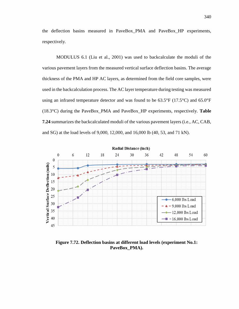
340
the deflection basins measured in PaveBox_PMA and PaveBox_HP experiments,
respectively.
MODULUS 6.1 (Liu et al., 2001) was used to backcalculate the moduli of the
various pavement layers from the measured vertical surface deflection basins. The average
thickness of the PMA and HP AC layers, as determined from the field core samples, were
used in the backcalculation process. The AC layer temperature during testing was measured
using an infrared temperature detector and was found to be 63.5°F (17.5°C) and 65.0°F
(18.3°C) during the PaveBox_PMA and PaveBox_HP experiments, respectively. Table
7.24 summarizes the backcalculated moduli of the various pavement layers (i.e., AC, CAB,
and SG) at the load levels of 9,000, 12,000, and 16,000 lb (40, 53, and 71 kN).
Figure 7.72. Deflection basins at different load levels (experiment No.1:
PaveBox_PMA).

341
Figure 7.73. Deflection basins at different load levels (experiment No.2:
PaveBox_HP).
Table 7.24. Backcalculated Moduli at Different Load Levels.
Experiment ID
Average AC
Temperature
(°F)
Average
Applied
Load
(lb)
Backcalculated
AC Modulus,
EAC (ksi)
Backcalculated
CAB Modulus,
ECAB (ksi)
Backcalculated
SG Modulus,
ESG (ksi)
PaveBox_PMA 63.5
9,189 555.0 39.2 11.1
12,066 524.2 40.8 14.8
16,117 553.9 25.9 14.7
PaveBox_HP 65.0
9,119 194.0 39.5 28.1
12,143 213.4 35.9 19.9
16,111 294.6 30.4 16.4
Based on the results of the backcalculation, the following observations can be made:
• Regardless of the applied load level, a higher EAC was observed for the PMA AC
layer when compared with the HP AC layer. This is demonstrated with an average
EAC for the PMA AC layer of 544 ksi (3,751 MPa) compared with 234 ksi (1,613
MPa) for the HP AC layer.
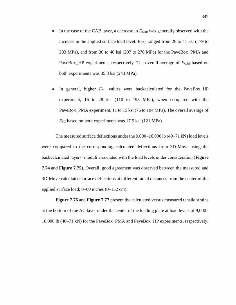
342
• In the case of the CAB layer, a decrease in ECAB was generally observed with the
increase in the applied surface load level. ECAB ranged from 26 to 41 ksi (179 to
283 MPa), and from 30 to 40 ksi (207 to 276 MPa) for the PaveBox_PMA and
PaveBox_HP experiments, respectively. The overall average of ECAB based on
both experiments was 35.3 ksi (243 MPa).
• In general, higher ESG values were backcalculated for the PaveBox_HP
experiment, 16 to 28 ksi (110 to 193 MPa), when compared with the
PaveBox_PMA experiment, 11 to 15 ksi (76 to 104 MPa). The overall average of
ESG based on both experiments was 17.5 ksi (121 MPa).
The measured surface deflections under the 9,000–16,000 lb (40–71 kN) load levels
were compared to the corresponding calculated deflections from 3D-Move using the
backcalculated layers’ moduli associated with the load levels under consideration (Figure
7.74 and Figure 7.75). Overall, good agreement was observed between the measured and
3D-Move calculated surface deflections at different radial distances from the center of the
applied surface load; 0–60 inches (0–152 cm).
Figure 7.76 and Figure 7.77 present the calculated versus measured tensile strains
at the bottom of the AC layer under the center of the loading plate at load levels of 9,000–
16,000 lb (40–71 kN) for the PaveBox_PMA and PaveBox_HP experiments, respectively.
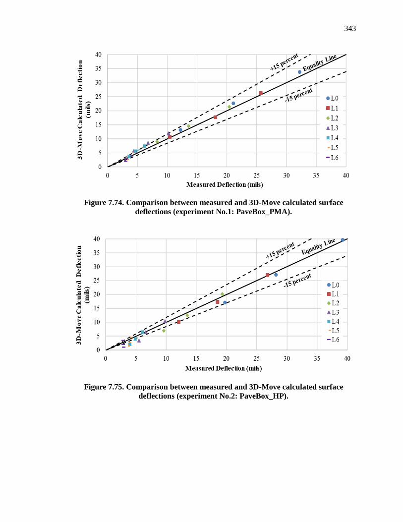
343
Figure 7.74. Comparison between measured and 3D-Move calculated surface
deflections (experiment No.1: PaveBox_PMA).
Figure 7.75. Comparison between measured and 3D-Move calculated surface
deflections (experiment No.2: PaveBox_HP).

344
Figure 7.76. Comparison between measured and 3D-Move calculated strains at the
bottom of AC layer (experiment No.1: PaveBox_PMA).
Figure 7.77. Comparison between measured and 3D-Move calculated strains at the
bottom of AC layer (experiment No.2: PaveBox_HP).
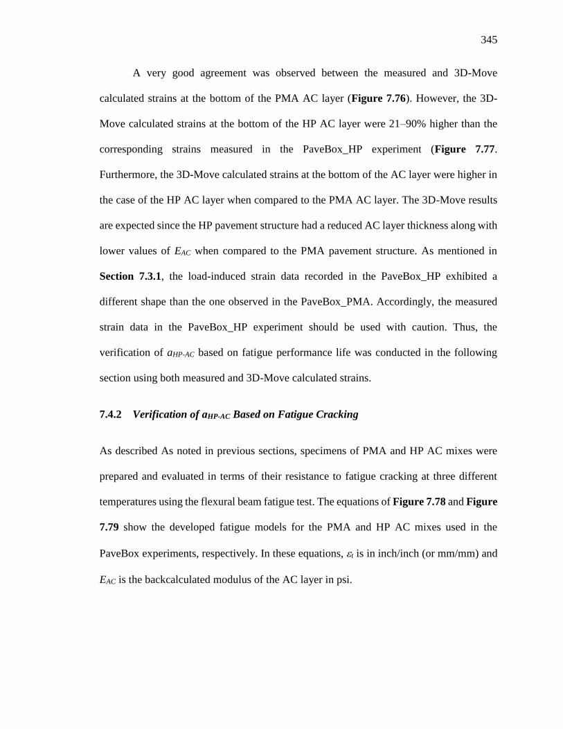
345
A very good agreement was observed between the measured and 3D-Move
calculated strains at the bottom of the PMA AC layer (Figure 7.76). However, the 3D-
Move calculated strains at the bottom of the HP AC layer were 21–90% higher than the
corresponding strains measured in the PaveBox_HP experiment (Figure 7.77.
Furthermore, the 3D-Move calculated strains at the bottom of the AC layer were higher in
the case of the HP AC layer when compared to the PMA AC layer. The 3D-Move results
are expected since the HP pavement structure had a reduced AC layer thickness along with
lower values of EAC when compared to the PMA pavement structure. As mentioned in
Section 7.3.1, the load-induced strain data recorded in the PaveBox_HP exhibited a
different shape than the one observed in the PaveBox_PMA. Accordingly, the measured
strain data in the PaveBox_HP experiment should be used with caution. Thus, the
verification of aHP-AC based on fatigue performance life was conducted in the following
section using both measured and 3D-Move calculated strains.
7.4.2 Verification of aHP-AC Based on Fatigue Cracking
As described As noted in previous sections, specimens of PMA and HP AC mixes were
prepared and evaluated in terms of their resistance to fatigue cracking at three different
temperatures using the flexural beam fatigue test. The equations of Figure 7.78 and Figure
7.79 show the developed fatigue models for the PMA and HP AC mixes used in the
PaveBox experiments, respectively. In these equations, t is in inch/inch (or mm/mm) and
EAC is the backcalculated modulus of the AC layer in psi.

346
𝑁𝑓 = (1.1973E + 01) (1
ԑ𝑡)
6.2248
(1
𝐸𝐴𝐶)
2.6756
Figure 7.78. Calculation: Fatigue MEPDG model for PaveBox_PMA AC Mix.
𝑁𝑓 = (2.7552E + 09) (1
ԑ𝑡)
6.6407
(1
𝐸𝐴𝐶)
4.3438
Figure 7.79. Calculation: Fatigue MEPDG model for PaveBox_HP AC Mix.
The measured strains in the PaveBox experiments were used to estimate Nf under
different load levels. Nf was also estimated using the 3D-Move calculated strains. Table
7.25 and Table 7.26 summarize the results of the fatigue analysis conducted using
measured and 3D-Move calculated strains, respectively. It should be kept in mind while
analyzing the data that the HP AC layer was 19% thinner than the PMA AC layer.
Regardless of the AC mix type, Nf decreased with the increase in the applied
surface load. Furthermore, higher Nf values were calculated for the HP AC layer when
compared to the PMA AC layer. The ratio of the HP to PMA fatigue lives ranged from
125–339 in the case of measured strains, and 2.7–17.4 in the case of 3D-Move calculated
strains. A lower ratio was observed at the target load level of 16,000 lb (71 kN) when
compared to 9,000 lb (40 kN).
In summary, the fatigue analysis of the two evaluated PMA and HP pavement
structures indicated an increase in the fatigue life of the HP AC layer when compared to
the PMA AC layer. The difference in AC layer fatigue life between the HP and PMA AC
mixes was highest at the lower load levels and decreased with the increase in load level.
Thus, the overall results of the fatigue analysis support the aHP-AC selection of 0.54.

347
Table 7.25. Fatigue Analysis of PMA and HP Pavement Structures at Different
Load Levels Using Measured Strains.
Target Load
Level (lbs) AC Mix ID
Measured
Tensile
Strain
(microstrain)
EAC (psi) Nf
(million)
Ratio of HP to
PMA fatigue
lives
9,000 PaveBox_PMA 236.6 555,000 190.5
339.1 PaveBox_HP 216.2 194,000 64,583.8
12,000 PaveBox_PMA 324.4 524,200 31.1
143.3 PaveBox_HP 303.8 213,400 4,459.4
16,000 PaveBox_PMA 448.8 553,900 3.6
125.3 PaveBox_HP 348.0 294,600 445.9
Table 7.26. Fatigue Analysis of PMA and HP Pavement Structures at Different
Load Levels Using 3D-Move Calculated Strains.
Target Load
Level (lbs) AC Mix ID
Measured
Tensile
Strain
(microstrain)
EAC (psi) Nf
(million)
Ratio of HP to
PMA fatigue
lives
9,000 PaveBox_PMA 235.2 555,000 197.6
17.4 PaveBox_HP 336.2 194,000 3,442.1
12,000 PaveBox_PMA 307.9 524,200 43.1
5.1 PaveBox_HP 478.1 213,400 219.5
16,000 PaveBox_PMA 482.8 553,900 2.3
2.7 PaveBox_HP 662.5 294,600 6.2
7.4.3 Verification of aHP-AC Based on Rutting
Since the PaveBox experiments were conducted at intermediate temperatures, the
verification of aHP-AC based on rutting was conducted using the 3D-Move generated
responses at the critical high temperature for Florida of 122°F (50°C). The verification was
conducted for rutting in the AC layer and in the unbound layers (i.e., CAB and SG).
As notes in previous sections (Section 7.2.4.4), specimens of PMA and HP AC
mixes were prepared and evaluated in terms of their resistance to rutting at three different
temperatures using the RLT test. The permanent (εp) and resilient (εr) axial strains were
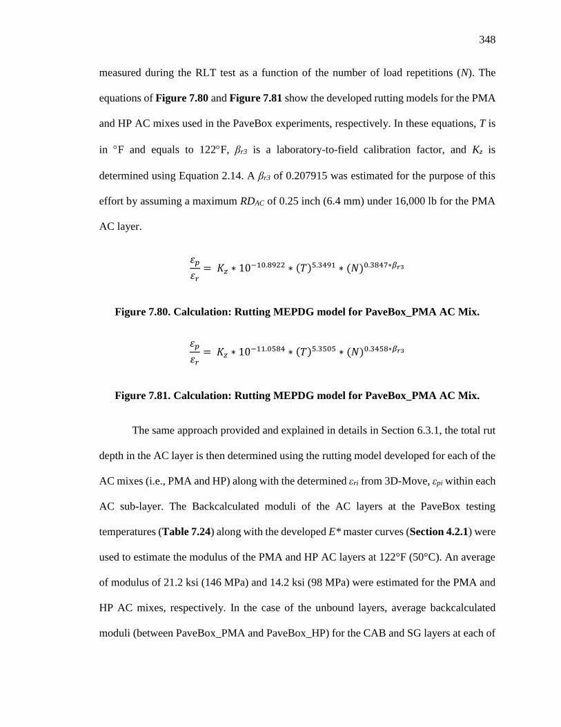
348
measured during the RLT test as a function of the number of load repetitions (N). The
equations of Figure 7.80 and Figure 7.81 show the developed rutting models for the PMA
and HP AC mixes used in the PaveBox experiments, respectively. In these equations, T is
in F and equals to 122F, βr3 is a laboratory-to-field calibration factor, and Kz is
determined using Equation 2.14. A βr3 of 0.207915 was estimated for the purpose of this
effort by assuming a maximum RDAC of 0.25 inch (6.4 mm) under 16,000 lb for the PMA
AC layer.
휀𝑝
휀𝑟= 𝐾𝑧 ∗ 10−10.8922 ∗ (𝑇)5.3491 ∗ (𝑁)0.3847∗𝛽𝑟3
Figure 7.80. Calculation: Rutting MEPDG model for PaveBox_PMA AC Mix.
휀𝑝
휀𝑟= 𝐾𝑧 ∗ 10−11.0584 ∗ (𝑇)5.3505 ∗ (𝑁)0.3458∗𝛽𝑟3
Figure 7.81. Calculation: Rutting MEPDG model for PaveBox_PMA AC Mix.
The same approach provided and explained in details in Section 6.3.1, the total rut
depth in the AC layer is then determined using the rutting model developed for each of the
AC mixes (i.e., PMA and HP) along with the determined εri from 3D-Move, εpi within each
AC sub-layer. The Backcalculated moduli of the AC layers at the PaveBox testing
temperatures (Table 7.24) along with the developed E* master curves (Section 4.2.1) were
used to estimate the modulus of the PMA and HP AC layers at 122°F (50°C). An average
of modulus of 21.2 ksi (146 MPa) and 14.2 ksi (98 MPa) were estimated for the PMA and
HP AC mixes, respectively. In the case of the unbound layers, average backcalculated
moduli (between PaveBox_PMA and PaveBox_HP) for the CAB and SG layers at each of

349
the loading levels were utilized in 3D-Move for the rutting analysis. Table 7.27
summarizes the moduli of the various layers used in the 3D-Move analysis.
Table 7.27. Moduli of Various Layers at 122°F (50°C).
Target Load Level
Load (lb)
Average PMA AC
Layer Modulus at
122F (Ksi)
Average HP AC
Layer Modulus at
122F (Ksi)
Average CAB
Layer Modulus
(Ksi)
Average SG Layer
Modulus (Ksi)
9,000 21.2 14.2 39.4 19.6
12,000 21.2 14.2 38.4 17.4
16,000 21.2 14.2 28.2 15.6
The rutting in the CAB and SG layers were also estimated using the nationally
calibrated rutting performance models recommended in the AASHTOWare® Pavement
ME software as explained in details in Section 6.3.2. Table 7.28 presents the calculated
rut depths for the AC, CAB, and SG layers. Table 7.29 summarizes the percent change in
the calculated rut depths of the HP pavement structure relative to the PMA pavement
structure at different load levels. In general, a decrease in the RDAC was determined for the
HP AC layer. The percent change in RDAC ranged between 12.0 and 17.6%. On the other
hand, an increase in RDCAB and RDSG was determined for the CAB and SG layers in the HP
pavement structure. The percent change in RDCAB was higher than that of RDSG and ranged
between 8.0 and 10.2%. The percent change in RDSG ranged between 4.5 and 9.4%.
Table 7.28 also summarizes the combined rut depth for the CAB and SG layers as
well as the total rut depth (i.e., summation of RDAC, RDCAB, and RDSG). While an increase
in the unbound material rut depth was observed, the total rut depth was found to be similar
for the PMA and HP pavement structures. In other words, the increase in the unbound
material rut depths was compensated by a decrease in the RDAC of the HP AC layer.
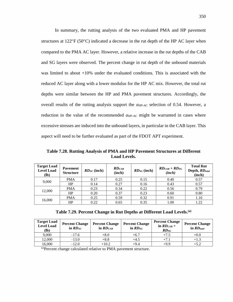
350
In summary, the rutting analysis of the two evaluated PMA and HP pavement
structures at 122F (50C) indicated a decrease in the rut depth of the HP AC layer when
compared to the PMA AC layer. However, a relative increase in the rut depths of the CAB
and SG layers were observed. The percent change in rut depth of the unbound materials
was limited to about +10% under the evaluated conditions. This is associated with the
reduced AC layer along with a lower modulus for the HP AC mix. However, the total rut
depths were similar between the HP and PMA pavement structures. Accordingly, the
overall results of the rutting analysis support the aHP-AC selection of 0.54. However, a
reduction in the value of the recommended aHP-AC might be warranted in cases where
excessive stresses are induced into the unbound layers, in particular in the CAB layer. This
aspect will need to be further evaluated as part of the FDOT APT experiment.
Table 7.28. Rutting Analysis of PMA and HP Pavement Structures at Different
Load Levels.
Target Load
Level Load
(lb)
Pavement
Structure RDAC (inch)
RDCAB
(inch) RDSG (inch)
RDCAB + RDSG
(inch)
Total Rut
Depth, RDtotal
(inch)
9,000 PMA 0.17 0.25 0.15 0.40 0.57
HP 0.14 0.27 0.16 0.43 0.57
12,000 PMA 0.23 0.34 0.22 0.56 0.79
HP 0.20 0.37 0.23 0.60 0.80
16,000 PMA 0.25 0.59 0.32 0.91 1.16
HP 0.22 0.65 0.35 1.00 1.22
Table 7.29. Percent Change in Rut Depths at Different Load Levels.(a)
Target Load
Level Load
(lb)
Percent Change
in RDAC
Percent Change
in RDCAB
Percent Change
in RDSG
Percent Change
in RDCAB +
RDSG
Percent Change
in RDtotal
9,000 –17.6 +8.0 +6.7 +7.5 +0.0
12,000 –13.0 +8.8 +4.5 +7.1 +1.3
16,000 –12.0 +10.2 +9.4 +9.9 +5.2 (a)Percent change calculated relative to PMA pavement structure.
351
7.5 Summary of Computed Analyses
The service life approach was used to mechanistically verify the applicability of the aHP-AC
of 0.54 that was implemented in the PaveBox experiments (referred to as analysis II in
Figure 7.1). An ME analysis was conducted using the backcalculated layers’ moduli in
conjunction with the laboratory-developed performance models for the PMA and HP AC
mixes. The ME analysis resulted in a better fatigue and rutting performance for the HP AC
layer when compared with the PMA AC layer. Higher rut depths were observed in the
unbound layers of the HP pavement structure, especially in the CAB layer. However,
similar total rut depths were determined for the PMA and HP pavement structures. In
general, the overall results of analysis II support the aHP-AC selection of 0.54. Though, a
reduction in the recommended value might be warranted if the load-induced stresses in the
unbound materials lead to permanent deformations that exceeds rut depth limits set by
FDOT.

352
CHAPTER 8 IMPACT OF HIGH POLYMER MODIFICATION ON THE
OXIDATIVE AGING OF ASPHALT BINDERS
8.1 Introduction
Asphalt binder aging constitutes an important factor that influences the performance life of
an asphalt pavement section. In the field, due to the asphalt binder aging, the surface of the
pavement section becomes brittle and may lose its stress relaxation capability resulting into
fatigue and thermal cracking due to the combined effects of traffic loading and climatic
conditions.
AC mixtures have been used as driving surfaces for flexible pavements since the
early 1900s. With the increase of highway traffic volume and axle loads, the introduction
of modified asphalt binders provided transportation agencies an effective tool to design
balanced asphalt mixtures that can resist conflicting distresses such as permanent
deformation and fatigue cracking while maintaining long-term durability (i.e., reduced
moisture damage and aging). Polymer modification of asphalt binders is not a new concept
and has been progressively more commonplace over the past several decades. While
several agencies utilize unmodified asphalts, many have increasingly become reliant upon
polymer modified asphalt binders with fair portion of those located in climatic regions that
experience significantly higher levels of oxidation, such as the western and south-western
of the U.S., for example. Many factors may have contributed to the accelerated aging in
these regions such as the elevated temperatures during the summer months, lack of an
extended hard freeze in the with months, and increased solar exposures, both temperature

353
and ultraviolet (UV) radiation, as a result of the reduced moisture and atmospheric
humidity levels.
Due to the increased levels of aging taking place in such locales where modified
asphalt binders are becoming more prevalent, it is becoming increasingly important to
characterize the benefits afforded with the polymer modification process. It is critical for
state highway agencies (SHAs) as well as other municipalities to be able to quantify the
benefits of modification in order to adequately utilize the dwindling transportation budgets
and to justify additional cost of the polymer. While PMA asphalt binders, with 2-3%
polymer content, have shown improved long-term performance (e.g., resistance to
oxidative aging), it is also believed that asphalt binders with high polymer content (known
as HP) (i.e., >6% polymer content) may offer additional advantages in flexible pavements
especially these subjected to heavy and low traffic loads, or extreme environmental
conditions.
8.1.1 Problem Statement and Objectives
While several previous studies highlighted the positive impacts of the HP modification of
asphalt binders and mixtures, there is still a serious lack of understanding on the impact of
high polymer modification on the oxidative aging of asphalt binders. The main objective
of this research section is to assess the long-term aging characteristics of conventional and
highly modified asphalt binder in terms of their rheological and chemical properties. An
extended asphalt binder aging experiment was generated and considered multiple
combinations of PMA and HP asphalt binders from different sources. Long-term oven aged
asphalt binders at multiple temperatures and multiple durations were evaluated using the

354
dynamic shear rheometer (DSR) for full master curve characterization. The Fourier
Transform Infrared Spectroscopy (FT-IR) was used for characterization of chemical
composition (e.g., carbonyl area growth, sulfoxide area growth). The evaluation initially
considered the resistance to oxidation specifically through measures of the early o fast-rate
followed by the slower constant-rate kinetics parameters resulting from multiple aging
temperatures and durations. An extensive rheological evaluation was then combined with
the kinetics parameters to consider the hardening susceptibility of the respective asphalt
binders utilizing multiple rheological indices to develop a wide perspective of the overall
binder behaviors. Finally, the two aspects were combined to distinguish the overall
influence of the high binder modification processes.
8.2 Background
In comparison to neat asphalt binders, the implemented modifiers have specific
enhancements to the physical properties and rheological performance of asphalt binders,
such as improving the ductility, expanding the relaxation spectra, and increasing the overall
strength. For instance, the triblock SBS, diblock SBR, and ethylene-vinyl acetate (EVA)
have been known to make asphalt binders more ductile at low temperature which increased
the resistance to thermal cracking and decreased the rutting potential at high temperatures
by stiffening the asphalt binders (Woo et al., 2007a, & b). In general, improvement in
asphalt binder ductility in conjunction with the improved elastic behavior due to polymer
modification can have a positive influence on the cracking resistance of asphalt mixtures
(Woo et al., 2007a; Airey, 2003; McDaniel et al., 2003; and Sebaaly et al., 2002). Previous
studies have shown the capability of polymer modifiers to lessen the deteriorative oxidative

355
age hardening effects (Lu et al., 1999; and Glover et al., 2005). Accordingly, more durable
asphalt pavements can be expected from the use of polymer modification (Glover et al.,
2005). Similar efforts to increase performance of asphalt binders and to capitalize on the
development of recycling technologies, the usage of waste materials in infrastructure
construction, namely the inclusion of tire rubber or ground tire rubber has earned a good
deal of attention from pavement researchers. Studies searching into the mechanism of these
modification techniques have indicated that the blending mechanism between the rubber
and neat asphalt binders is largely attributable to the penetration of the asphalt binder into
the polymer particles, specifically the styrene domain which tends to swell the rubber
particle (Navarro et al. 2010; Airey, 2004; and Bahl et al., 1993). This complex interaction
tends to create a strong link between the asphalt binder and the rubber, which may give rise
to significant changes in the behavior of the modified asphalt binder.
However, modified asphalt binders that are exposed to the same oxidation aging
procedures as a base asphalt binder have resulted in differing effects on the chemical and
physical properties of the aged asphalt binders. In the laboratory, the rolling thin fil oven
(RTFO) and the pressure aging vessel (PAV) aging processes have been established to
simulate plant mixing, lay-down, and long-term in-service durations of asphalt binders,
with validations of those efforts ongoing in the research fields. Photo or UV aging and
weathering have not seen the same level of standardization, but have also been investigated
by many researchers (Mouillet et al., 2008; Wu et al., 2010; and Lins et al., 2013). These
aging processes cause asphalt binders to become stiffer and more brittle, drastically
356
reducing the stress relaxation capabilities and adhesion strength between the asphalt
binders and aggregates.
Physical properties are often characterized through rheological performance
measures commonly used to study the effects of aging and oxidation of asphalt binders.
Evaluations of the influence of various modifiers, such as SBR, SBS, ground tire rubber
(GTR), on the oxidative aging and corresponding physical property changes indicated that
the modifiers have the potential to dramatically reduce oxidative aging rates and hardening
susceptibility parameters, though the benefits were found to be asphalt binder dependent
(Ruan et al., 2003). Furthermore, it was also concluded that the oxidative aging can result
in damage to the polymer network which then can significantly reduce the effectiveness of
the polymer on the ductility of the asphalt binder. Consequently, a significant reduction in
ductility improvement of selected SBS-modified asphalt binders has also been reported
(Woo et al., 2007b). Nevertheless, lower hardening susceptibility associated with lower
oxidation rate in SBS-modified asphalt binders in comparison with the corresponding base
binder has also been reported (Ruan et al., 2003).
As mentioned in previous chapters of this dissertation, SBS is a well-recognized
elastomer which has been commonly used in asphalt pavements. Remarkable strength and
elasticity of SBS-modified asphalt binders can be created from the physical cross-linking
of the molecules into a three dimensional network (Airey, 2003). Nonetheless, the degree
of SBS modification depends on the asphalt binder composition, SBS concentration and
structure, as well as binder-polymer compatibility (Lu et al., 1998; Lu et al., 1999; and
Airey, 2003). Others have investigated the aging characteristics of polymer modified

357
binders in porous asphalt pavements utilizing X-ray tomography, gel permeation
chromatography (GPC), FT-IR, and DSR measures (Lu et al., 2010). A general conclusion
indicated that the degradation of the polymer had occurred mainly during the production
and early in-service life of the pavement. However, the polymer did provide a benefit to
the hardening effect due to oxidation of the base asphalt binder to some extent and that the
base binder was an important component to obtain a durable modified asphalt binder.
Additional studies on oxidized polymer-modified asphalt binders by analyzing the
oxygen related chemical functionalities with FT-IR approach using attenuated total
reflectance (ATR) measures, determined that the polymer concentration remained constant
in the asphalt binder during an oxidation process thus refuting portions of the polymer
degradation complaint (Yut et al., 2011).
Rheological evaluations based upon master curve development can be a very useful
method to evaluate the influence of the oxidative aging on multiple physical characteristics
of asphalt binders. Correspondingly, black space diagrams, defined as complex modulus
versus phase angle, provides a robust evaluation methodology for the rheological
evaluation of asphalt binders. Recent work in the field of non-load related oxidation aging
induced cracking has utilized this evaluation technique to quantify the dramatically loss in
the relaxation properties of asphalt binders with the oxidative aging (Rowe, 2011).
A previous study was conducted at University of Nevada, Reno (UNR) to assess
the effect of high polymer content in improving the resistance of the asphalt binder to long-
term aging, and to observe and to quantify the influence of binder modification. On the
oxidative characteristics of the evaluated asphalt binders (Morian et al., 2015). An asphalt
358
binder with low susceptibility to long-term aging would significantly reduce the potential
of the asphalt mixture to all types of cracking including bottom-up fatigue, top-down
fatigue, thermal, reflective, and block cracking.
Three asphalt binders: neat, polymer modified with 3% SBS (PMA), and highly
polymer modified with 7.5% SBS (HP) were evaluated. The neat binder was used as the
base for the two polymer modified binders. The three evaluated asphalt binders were
subjected to long-term aging in forced draft ovens for various combinations of
temperatures (i.e., 50°C, 60°C, and 85°C) and aging durations (ranges from 0.5 days up to
240 days) to measure the aging kinetics as a function of time and temperature. Two
rheological parameters are usually utilized to describe the binder behavior at any
temperature and loading frequency: stiffness (shear complex modulus (G*) at high and
intermediate temperatures or asphalt binder stiffness (S) at low temperatures) and phase
angle (δ) at high and intermediate temperatures or m-value at low temperatures). As a result
of oxidative aging, the binder stiffness increases while the phase angle decreases (King et
al., 2012). Therefore, the aged binders were then rheologically evaluated in the DSR by
determining G* and phase angle master curves.
Figure 8.1 shows the measured properties of the aged asphalt binders using the
Glover-Row parameter (G-R) (defined in the following sections) at a temperature of 15°C
and a frequency of 0.005 rad/s. Each data point plotted in this figure represents a specific
asphalt binder condition in terms of temperature and time (i.e., combinations defined
earlier). It is anticipated that lower G* and lower δ represent lower susceptibility to long-
term aging. In addition, a steeper slope between G* and δ represents lower susceptibility
359
to long-term aging. In other words, a steep curve located closer to the left side of the chart
indicates lower susceptibility to long-term aging. The three evaluated binders start at
different locations in Black Space and each binder has a different rate of aging from the
lower right of the diagram to the upper left. In addition, Figure 8.1 shows a damage zone
where the brittle rheological behavior causes onset and significant cracking as defined by
the Glover-Rowe (G-R) parameter of 180 and 600 kPa, respectively. The G-R parameter
is a result of the relationship between G* and δ from the DSR test that has been traditionally
conducted at 15°C. The aforementioned cracking thresholds for the G-R parameter (i.e.,
180 and 600 kPa) are to correlate to ductility values of 5 cm and 3 cm that were reported
by Kandhal (Kandhal, 1977), respectively. It was originally defined by Ruan et al. (2003)
(Ruan et al., 2003) before it was reformulated for more practical use by Rowe (2011)
(Rowe, 2011) in a discussion by Anderson et al. (2011) as the Glover-Rowe (G-R)
parameter where all rheological properties are referenced at 0.005 rad/s and 15°C.
The data presented in Figure 8.1 show that the HP modified asphalt binder is the
least susceptible to long-term aging, followed by the PMA binder, while the neat asphalt
binder is the most susceptible to long-term aging. Furthermore, the data show that the neat
asphalt binder was the first binder to reach the GR cracking criterion of 600 kPa after about
170 days of oven aging while the PMA and HP modified asphalt binders lasted,
respectively, for about 190 and 230 days before reaching the same failure criterion.
Recently, a new binder parameter called ΔTc, has been introduced for evaluating
age related cracking potential. It is defined as the numerical difference between the low
continuous grade temperature determined from the BBR stiffness criterion (the temperature
360
TS where stiffness, S, equals 300 MPa) and the low continuous grade temperature
determined from the BBR m-value (the temperature Tm where m equals 0.300).The ΔTc
was first proposed by Anderson in 2011 to measure the ductility loss of aged asphalt binder
as part of a study examining relationships between asphalt binder properties and non-load
related cracking (the study focused on finding a parameter to explain block cracking in
airport pavements). . A negative value of ΔTc (TS-Tm) indicates the controlling role of the
relaxation properties of the binder at low temperature (i.e. m-controlled).
Anderson et al. (6) verified the satisfactory correlation of ΔTc with ductility and G-
R in several laboratory and field investigations. They also proposed that a value of -2.5°C
and -5°C for ΔTc would correlate to the same cracking thresholds discussed in G-R
parameter, i.e., onset and significant cracking, respectively.
From the construction point of view, oxidation stiffens the binders in asphalt
mixtures during refining, production, construction, and in-service, i.e., changing the
molecular structure of the binder through chemical reactions with oxygen. This
phenomenon reduces the binder phase angle and its stress relief capability. In fact, through
the chemical reactions, the oxygen atoms add to aliphatic carbon atoms attached to
aromatic rings to form functional groups called carbonyls and water via extraction of
hydrogen atoms. As a result, the ketones and organic acids are produced which are highly
polar with strong associations through Van der Waals forces with other active polar sites
in the binder. Suh reactions increase the apparent molecular weight and associated increase
in stiffness and are known as the predominant cause of binder embrittlement due to aging
(Pournoman, 2017).
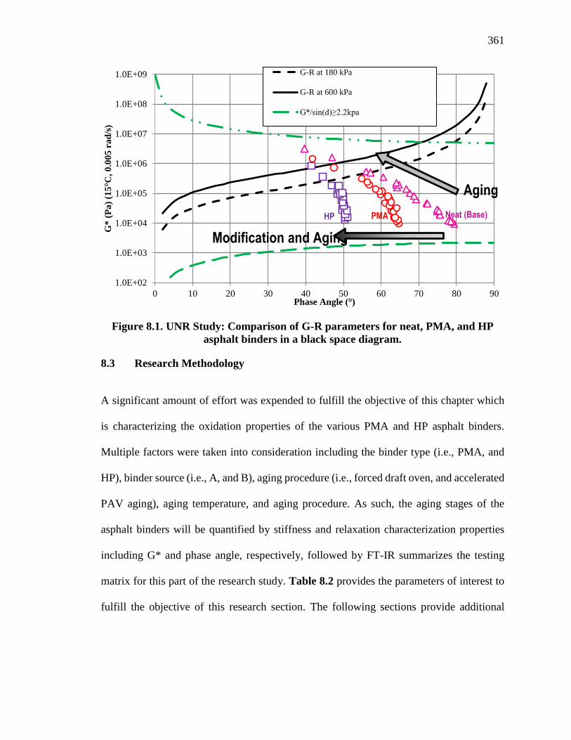
361
Figure 8.1. UNR Study: Comparison of G-R parameters for neat, PMA, and HP
asphalt binders in a black space diagram.
8.3 Research Methodology
A significant amount of effort was expended to fulfill the objective of this chapter which
is characterizing the oxidation properties of the various PMA and HP asphalt binders.
Multiple factors were taken into consideration including the binder type (i.e., PMA, and
HP), binder source (i.e., A, and B), aging procedure (i.e., forced draft oven, and accelerated
PAV aging), aging temperature, and aging procedure. As such, the aging stages of the
asphalt binders will be quantified by stiffness and relaxation characterization properties
including G* and phase angle, respectively, followed by FT-IR summarizes the testing
matrix for this part of the research study. Table 8.2 provides the parameters of interest to
fulfill the objective of this research section. The following sections provide additional
1.0E+02
1.0E+03
1.0E+04
1.0E+05
1.0E+06
1.0E+07
1.0E+08
1.0E+09
0 10 20 30 40 50 60 70 80 90
G*
(P
a)
(15
°C, 0
.00
5 r
ad
/s)
Phase Angle (°)
G-R at 180 kPa
G-R at 600 kPa
G*/sin(d)≥2.2kpa
Aging
Modification and Aging
PMA Neat (Base)HP
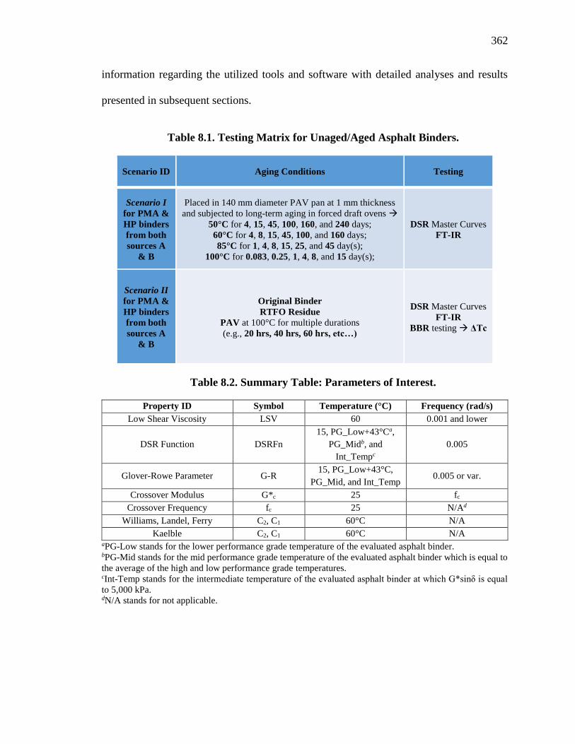
362
information regarding the utilized tools and software with detailed analyses and results
presented in subsequent sections.
Table 8.1. Testing Matrix for Unaged/Aged Asphalt Binders.
Scenario ID Aging Conditions Testing
Scenario I
for PMA &
HP binders
from both
sources A
& B
Placed in 140 mm diameter PAV pan at 1 mm thickness
and subjected to long-term aging in forced draft ovens →
50°C for 4, 15, 45, 100, 160, and 240 days;
60°C for 4, 8, 15, 45, 100, and 160 days;
85°C for 1, 4, 8, 15, 25, and 45 day(s);
100°C for 0.083, 0.25, 1, 4, 8, and 15 day(s);
DSR Master Curves
FT-IR
Scenario II
for PMA &
HP binders
from both
sources A
& B
Original Binder
RTFO Residue
PAV at 100°C for multiple durations
(e.g., 20 hrs, 40 hrs, 60 hrs, etc…)
DSR Master Curves
FT-IR
BBR testing → ΔTc
Table 8.2. Summary Table: Parameters of Interest.
Property ID Symbol Temperature (°C) Frequency (rad/s)
Low Shear Viscosity LSV 60 0.001 and lower
DSR Function DSRFn
15, PG_Low+43°Ca,
PG_Midb, and
Int_Tempc
0.005
Glover-Rowe Parameter G-R 15, PG_Low+43°C,
PG_Mid, and Int_Temp 0.005 or var.
Crossover Modulus G*c 25 fc
Crossover Frequency fc 25 N/Ad
Williams, Landel, Ferry C2, C1 60°C N/A
Kaelble C2, C1 60°C N/A aPG-Low stands for the lower performance grade temperature of the evaluated asphalt binder. bPG-Mid stands for the mid performance grade temperature of the evaluated asphalt binder which is equal to
the average of the high and low performance grade temperatures. cInt-Temp stands for the intermediate temperature of the evaluated asphalt binder at which G*sinδ is equal
to 5,000 kPa. dN/A stands for not applicable.
363
8.3.1 Performance Grading (PG)
The first step of an asphalt binder characterization consists of determining its true
continuous performance grade (PG). The performance grade of the virgin and extracted
asphalt binders was determined in accordance with AASHTO M320 (AASHTO M320,
2015). The high and low temperatures continuous grades for the material being evaluated
were determined following the DSR and BBR methodologies, respectively.
8.3.1.1 Dynamic Shear Rheometer
The AASHTO T315 method covers the determination of the dynamic shear modulus (G*)
and phase angle (δ) of asphalt binder when tested in dynamic (oscillatory) shear using
parallel plate test geometry. The method is intended to determine the linear viscoelastic
properties of unaged, short-term aged as per AASHTO T240 (known as RTFO residue),
and long-term aged asphalt binders (known as PAV residue; and as per AASHTO R28).
In this effort, test specimens were prepared as 1 mm thick by 25 mm in diameter
for unaged and RTFO aged binders or 2 mm thick by 8 mm in diameter for PAV aged
binders and formed between parallel metal plates. One of the parallel plates is oscillated
with respect to the other at 10 rad/sec strain controlled mode so that the measurements stay
in the linear viscoelastic behavior region. The final high and intermediate continuous PG
grades were determined utilizing the resulting parameters combining G* and δ for each
binder blend at corresponding aging level in accordance with the criteria specified in
AASHTO M320 (AASHTO M320, 2015).

364
8.3.1.2 Bending Beam Rheometer
The AASHTO T313 covers the determination of the flexural creep stiffness of asphalt
binders by means of a bending beam rheometer. In this effort, the material has been aged
through RTFO procedure (AASHTO T240) and through the PAV procedure (AASHTO
R28) to simulate the short and long-term aging condition of the material in the actual field
performance. The resultant long-term aged binder residues were poured in the bending
beam rheometer molds. The shaped beams were subjected to a constant static load of 980
± 50 mN magnitude for a duration of 240 seconds. It should be mentioned that the static
load is applied at the midpoint of the simply supported beam. The midpoint deflection is
recorded continuously; the maximum bending stress and strain at the midpoint of the beam
is then calculated from the standard dimensions of the beam (calibrated molds), the span
length, the deflection of the beam, and the load applied to the beam for multiple loading
times (i.e., 8, 15, 30, 60, 120, and 240 s). Subsequently, the stiffness of the beam for the
loading times specified above is then calculated as the ratio of the maximum stress over
the corresponding maximum strain at the same loading time identified previously. At the
end, the software provides the user with the calculated stiffness as well as the slope of the
logarithm of stiffness versus logarithm of time curve at the identified loading times. The
values reported for continuous grading purpose are the ones (i.e., S and m values) measured
/ calculated at loading time 60 seconds (i.e., S60s and m60s).
The BBR test is at least conducted at two different low temperatures to enable a
linear relationship between the stiffness and m-value with the corresponding testing
temperature. The temperatures at which the 300 MPa stiffness and m-value of 0.300 criteria

365
are met will be subtracted by 10°C due to the time-temperature superposition, reported as
the S-controlled and m-controlled continuous low-temperature grades, respectively. The
maximum of the two aforementioned temperatures is also reported as the low temperature
continuous grade.
8.3.2 Fourier-Transform Infrared Spectroscopy (FT-IR) Test
Fourier-Transform Infrared Spectroscopy, known as FT-IR, is a widely-used technique to
identify the material composition by identification of certain molecules or functional
groups and the concentration of those within a sample, here binder sample (Smith, 2011).
The fundamental theory of infrared spectroscopy is that infrared radiation passes into the
material, meanwhile some fractions of the radiation is absorbed, and the remaining
radiation is transmitted to the material or reflected by the material surface. Consideration
of the specific absorbed and reflected wavelength, the chemical components of the tested
specimen can be recognized. Detailed information regarding the FT-IR theoretical
background can be found elsewhere (Morian, 2014; and Zhu, 2015).
8.3.2.1 FT-IR Measuring and Sample Preparation Techniques
There are two primary categories of FT-IR sample preparation and measurement technique.
The first method is called “transmission testing” and involves with directly passing an IR
beam through the evaluated material sample before being read by any detector. The tested
sample in the transmission method is required to either be mixed with a transparent powder,
contained within an IR transparent cell, or made thin enough that the IR energy may pass
completely through it. The most common material being used as a powder or cell is
366
potassium bromide (KBr) which, as a drawback, will readily absorb moisture from the
atmosphere and could potentially dissolve.
The other method is generally known as reflectance testing, where the IR beam is
reflected or bounced off of the specimen surface then measured by the detector. One of the
common types of reflectance measurements is known as attenuated total reflectance (ATR)
in which the measurement is conducted by passing the IR beam through a crystal of high
refractive index on to the surface of the sample with a lower index. To avoid adding further
variability to the experiment by using the hydroscopic KBr, ATR spectrum of Nicolet 6700
manufactured by ThermoScientific Inc. was used in this study to get the infrared absorption
spectrum with binder samples with an ATR attachment.
As described, the ATR measuring technique was selected to conduct the FT-IR
spectroscopy on the binder samples. Several sample preparation methods have been tried
in previous studies (Pournoman, 2017) to generate a unique methodology applicable to all
various binder types, sources, and compositions. The finalized step-by-step methodology
with the Nicolet 6700 located in the University of Nevada, Reno asphalt binder laboratory
is summarized as follows:
1. Heat up 2 oz. of the evaluated asphalt binder at a selected high temperature for a
duration of 5 minutes. The heating temperature and duration can modified
accordingly (increased or decreased) based on the evaluated binder stiffness. In this
study, 300°C and 330°C were selected as heating temperatures for the PMA and
HP asphalt binders, respectively. The duration of 5 minutes was selected for all
evaluated asphalt binders (unaged and aged). It should be mentioned that the time-
367
temperature superposition concept remains applicable for special conditions to
avoid burning binders when heated at high temperatures.
2. Fully blend the heated asphalt binder sample.
3. Let the binder cool down for one minute to avoid damaging the crystal with heated
binder.
4. Use a sharp tool (i.e., clean sharp blade) to pick a small amount of asphalt binder
and place it on the FT-IR crystal.
5. Cover the collected asphalt binder sample with a small plastic sheet (i.e., plastic
glove) to avoid any possible sticking of the asphalt binder to device, and then apply
a slight pressure to fully cover the crystal with the binder, then remove the plastic
sheet to avoid any possible contamination of the sample spectra.
6. Collect the FT-IR spectrum for three times on the loaded sample; these spectra
constitute three measurements for the same evaluated sample.
7. Repeat step 3 to 6 for two more times on two additional samples collected from the
same binder heated in step one. These measurements will generate a total of 9
spectra; 3 measurements per evaluated binder sample.
8. Clean the binder sample mounted on the FT-IR device with isopropyl and wait for
the chemical to evaporate at least one minute before loading another binder sample
and before starting the next measurement.

368
Upon collecting at least three measurements per replicate for three replicates for a
total of 9 spectrums per binder combination, the average of at least 2 measurements were
used to determine multiple chemical components as summarized in Table 8.3 below and
explained as follows:
• The average carbonyl area (CA or C=O) is an indicator of oxygen absorption into
the binder by quantifying the growth of the carbonyl and functional groups. The
value of CA was determined by considering a baseline defined as the absorption
level at 1,523.489 and 1,820.473 cm-1. This value of CA was determined as the area
in arbitrary units, integrated between the average absorption spectra and the
determined baseline from 1,650.768 to 1,820.473 cm-1 wavenumbers and the
magnitude of the growth in CA in each aging level compared to the un-aged level
was utilized as an indication of aging (i.e. Cag).
• The Sulfoxide area (SO or S=O) is determined by considering a baseline defined
as the absorption level at 979.661 and 1,079.942 cm-1. This value of SO was
determined as the area in arbitrary units, integrated between the average absorption
spectra and the determined baseline from 979.661 to 1,079.942 cm-1 wavenumbers.
• The Polybutadiene Methylene area (PM) is determined by considering a baseline
defined as the absorption level at 1,394.282 and 1,486.848 cm-1. This value of PM
was determined as the area in arbitrary units, integrated between the average
absorption spectra and the determined baseline from 1,394.282 to 1,486.848 cm-1
wavenumbers.

369
• The Asphalt Peak area (AP) is determined by considering a baseline defined as
the absorption level at 1,355.712 and 1,394.282 cm-1. This value of AP was
determined as the area in arbitrary units, integrated between the average absorption
spectra and the determined baseline from 1,355.712 to 1,394.282 cm-1
wavenumbers.
• The Polybutadiene Trans Double Bond area (PTDBA) is determined by
considering a baseline defined as the absorption level at 925.664 and 981.590 cm-
1. This value of PTDBA was determined as the area in arbitrary units, integrated
between the average absorption spectra and the determined baseline from 925.664
to 981.590 cm-1 wavenumbers.
• The Polybutadiene Vinyl Double Bond area (PVDBA) is determined by
considering a baseline defined as the absorption level at 896.737 and 925.664 cm-
1. This value of PVDBA was determined as the area in arbitrary units, integrated
between the average absorption spectra and the determined baseline from 896.737
to 925.664 cm-1 wavenumbers.
• The Polybutadiene Cis Double Bond area (PCDBA) is determined by considering
a baseline defined as the absorption level at 711.604 and 734.746 cm-1. This value
of PCDBA was determined as the area in arbitrary units, integrated between the
average absorption spectra and the determined baseline from 711.604 to 734.746
cm-1 wavenumbers.
• The Polystyrene area (PA) is determined by considering a baseline defined as the
absorption level at 680.749 and 711.604 cm-1. This value of PA was determined as

370
the area in arbitrary units, integrated between the average absorption spectra and
the determined baseline from 680.749 to 711.604 cm-1 wavenumbers.
• A peak (P) was determined at wavenumber 1,492 cm-1 from 1,486.848 to 1,500.347
cm-1.
Figure 8.2 depicts the FT-IR spectra for PMA and HP binder samples. The PMA
and HP binders were sampled from source B (i.e., Vecenergy), and aged in a forced draft
oven at a temperature of 85°C for a duration of 15 days.
Table 8.3. FT-IR Testing: Summary Table of Chemical Structural Source and
Corresponding Wave Numbers.
Structural Source Wavenumber (cm-1)
Polystyrene 699 cm-1
Polybutadiene cis double bond 733 cm-1
Polybutadiene vinyl double bond 912 cm-1
Polybutadiene trans double bond 965 cm-1
Asphalt 1370 cm-1
Polybutadiene methylene 1450 cm-1
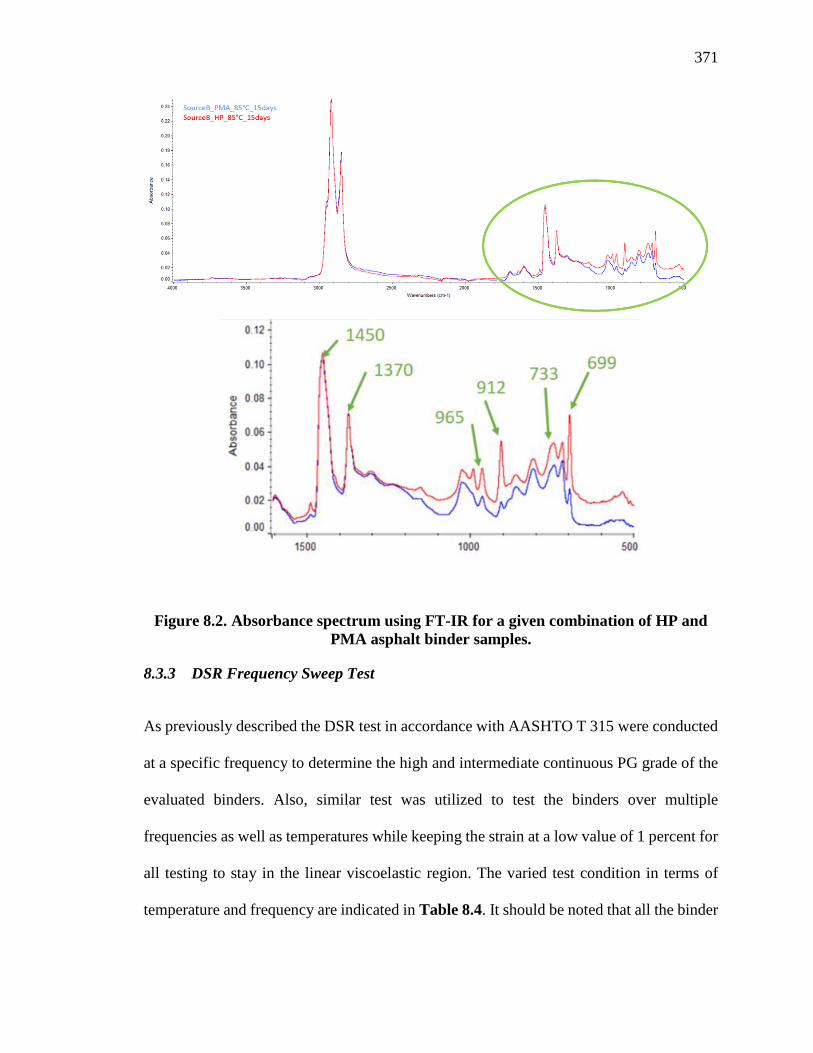
371
Figure 8.2. Absorbance spectrum using FT-IR for a given combination of HP and
PMA asphalt binder samples.
8.3.3 DSR Frequency Sweep Test
As previously described the DSR test in accordance with AASHTO T 315 were conducted
at a specific frequency to determine the high and intermediate continuous PG grade of the
evaluated binders. Also, similar test was utilized to test the binders over multiple
frequencies as well as temperatures while keeping the strain at a low value of 1 percent for
all testing to stay in the linear viscoelastic region. The varied test condition in terms of
temperature and frequency are indicated in Table 8.4. It should be noted that all the binder
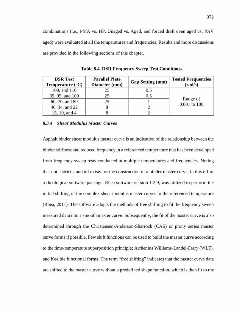
372
combinations (i.e., PMA vs. HP, Unaged vs. Aged, and forced draft oven aged vs. PAV
aged) were evaluated at all the temperatures and frequencies. Results and more discussions
are provided in the following sections of this chapter.
Table 8.4. DSR Frequency Sweep Test Conditions.
DSR Test
Temperature (°C)
Parallel Plate
Diameter (mm) Gap Setting (mm)
Tested Frequencies
(rad/s)
100, and 110 25 0.5
Range of
0.001 to 100
85, 95, and 100 25 0.5
60, 70, and 80 25 1
46, 34, and 22 8 2
15, 10, and 4 8 2
8.3.4 Shear Modulus Master Curves
Asphalt binder shear modulus master curve is an indication of the relationship between the
binder stiffness and reduced frequency in a referenced temperature that has been developed
from frequency sweep tests conducted at multiple temperatures and frequencies. Noting
that not a strict standard exists for the construction of a binder master curve, in this effort
a rheological software package, Rhea software version 1.2.9, was utilized to perform the
initial shifting of the complex shear modulus master curves to the referenced temperature
(Rhea, 2011). The software adopts the methods of free shifting to fit the frequency sweep
measured data into a smooth master curve. Subsequently, the fit of the master curve is also
determined through the Christensen-Anderson-Sharrock (CAS) or prony series master
curve forms if possible. Few shift functions can be used to build the master curve according
to the time-temperature superposition principle; Arrhenius Williams-Landel-Ferry (WLF),
and Kealble functional forms. The term “free shifting” indicates that the master curve data
are shifted to the master curve without a predefined shape function, which is then fit to the
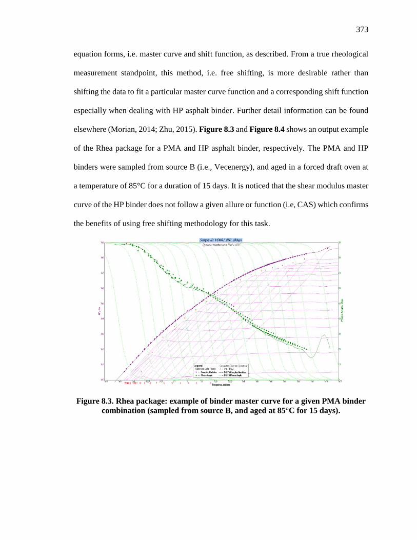
373
equation forms, i.e. master curve and shift function, as described. From a true rheological
measurement standpoint, this method, i.e. free shifting, is more desirable rather than
shifting the data to fit a particular master curve function and a corresponding shift function
especially when dealing with HP asphalt binder. Further detail information can be found
elsewhere (Morian, 2014; Zhu, 2015). Figure 8.3 and Figure 8.4 shows an output example
of the Rhea package for a PMA and HP asphalt binder, respectively. The PMA and HP
binders were sampled from source B (i.e., Vecenergy), and aged in a forced draft oven at
a temperature of 85°C for a duration of 15 days. It is noticed that the shear modulus master
curve of the HP binder does not follow a given allure or function (i.e, CAS) which confirms
the benefits of using free shifting methodology for this task.
Figure 8.3. Rhea package: example of binder master curve for a given PMA binder
combination (sampled from source B, and aged at 85°C for 15 days).
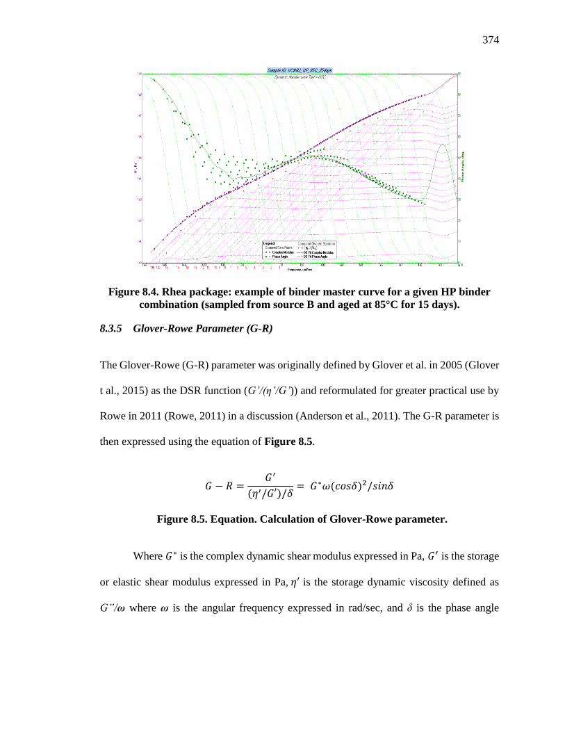
374
Figure 8.4. Rhea package: example of binder master curve for a given HP binder
combination (sampled from source B and aged at 85°C for 15 days).
8.3.5 Glover-Rowe Parameter (G-R)
The Glover-Rowe (G-R) parameter was originally defined by Glover et al. in 2005 (Glover
t al., 2015) as the DSR function (G’/(ƞ’/G’)) and reformulated for greater practical use by
Rowe in 2011 (Rowe, 2011) in a discussion (Anderson et al., 2011). The G-R parameter is
then expressed using the equation of Figure 8.5.
𝐺 − 𝑅 =𝐺′
(𝜂′/𝐺′)/𝛿= 𝐺∗𝜔(𝑐𝑜𝑠𝛿)2/𝑠𝑖𝑛𝛿
Figure 8.5. Equation. Calculation of Glover-Rowe parameter.
Where 𝐺∗ is the complex dynamic shear modulus expressed in Pa, 𝐺′ is the storage
or elastic shear modulus expressed in Pa, 𝜂′ is the storage dynamic viscosity defined as
G”/ω where ω is the angular frequency expressed in rad/sec, and δ is the phase angle

375
expressed in degree. It should be mentioned that all rheological properties are referenced
to 0.005 rad/s and 15°C.
These measures have been shown to correlate well with ductility; thus cracking
resistance as well as binder oxidation levels (Ruan et al., 2003). The G-R parameter
captures both rheological parameters needed to characterize binder viscoelastic behavior:
stiffness (G* at high and intermediate temperatures) and phase angle (δ at high and
intermediate temperatures)
However, there have also been limitations observed with the G-R parameter
measured in the DSR at intermediate temperatures, particularly when correlations were
attempted with modified binders (Glover et al., 2005). Traditionally, the DSRFn is reported
as a single point measurement at 15°C and a frequency of 0.005 rad/s (Ruan et al., 2003)
as is the corresponding G-R parameter (Rowe, 2011). It has been proposed that the original
DSRFn correlation to ductility measures (Kandhal, 1977) were based upon the
Pennsylvania climate using a PG 58-28 binder and thus have inherent assumptions. It has
been proposed that the original DSRFn and the subsequent G-R evaluation temperature of
15°C can appropriately be considered as either a constant offset of 43°C from the low
temperature PG grade labeled as PG_Low+43°C (King et al., 2012; King, 2013) or as the
midpoint of the PG binder grade labeled as PG_Mid (King, 2013). Both interpretations
yield the original 15°C evaluation temperature for the climate and materials used in the
early development of the DSRFn and G-R parameters, but will necessitate temperature
adjustment for many of the modified binders as well as binders not matching the original
PG58-28 grade. Further investigations have been conducted by other researchers to
376
evaluate the concept of equal stiffness through climate specific or material specific
temperatures at which the G-R parameter is evaluated (Hajj et al., 2016; Morian et al.,
2017). This evaluation was executed at the intermediate temperature labeled as Int_Temp
denoting the corresponding temperature at which G*sinδ is equal to 5,000 kPa.
8.3.6 Black-Space Diagram
The Glover-Rowe (G-R) parameter was originally defined by Glover et al. in 2005 (Glover
t al., 2015) as the Black space diagram is an indication of the, G*, versus phase angle, δ, at
a particular temperature and frequency. The specific temperature and frequency is selected
similar to those of the traditional Glover-Rowe parameter, i.e. 15°C and 0.005 rad/s,
respectively. Figure 8.6 shows the black space of Glover-Rowe parameter at 15°C for
PMA and HP binder source (i.e., Source B for this case). Each point in the black space
diagram represents an aging state and further aging moving the binder rheologically from
the lower right to the upper left of the diagram by increasing G* and decreasing δ. The
figure also shows a damage zone where cracking likely begins due to brittle rheological
behavior defined by G-R parameter between 180, onset of cracking, and 600 kPa,
significant cracking, that correlates to low ductility values of 5 to 3 cm, respectively. These
limits were previously related to surface raveling and cracking by Kandhal (Kandhal,
1977).
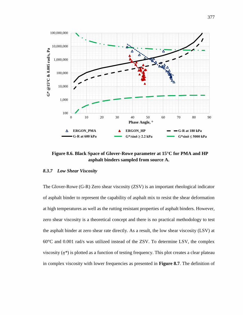
377
Figure 8.6. Black Space of Glover-Rowe parameter at 15°C for PMA and HP
asphalt binders sampled from source A.
8.3.7 Low Shear Viscosity
The Glover-Rowe (G-R) Zero shear viscosity (ZSV) is an important rheological indicator
of asphalt binder to represent the capability of asphalt mix to resist the shear deformation
at high temperatures as well as the rutting resistant properties of asphalt binders. However,
zero shear viscosity is a theoretical concept and there is no practical methodology to test
the asphalt binder at zero shear rate directly. As a result, the low shear viscosity (LSV) at
60°C and 0.001 rad/s was utilized instead of the ZSV. To determine LSV, the complex
viscosity (η*) is plotted as a function of testing frequency. This plot creates a clear plateau
in complex viscosity with lower frequencies as presented in Figure 8.7. The definition of
100
1,000
10,000
100,000
1,000,000
10,000,000
100,000,000
0 10 20 30 40 50 60 70 80 90
G*
@1
5°C
& 0
.00
5 r
ad
/s,
Pa
Phase Angle, °
ERGON_PMA ERGON_HP G-R at 180 kPa
G-R at 600 kPa G*/sinδ ≥ 2.2 kPa G*sinδ ≤ 5000 kPa
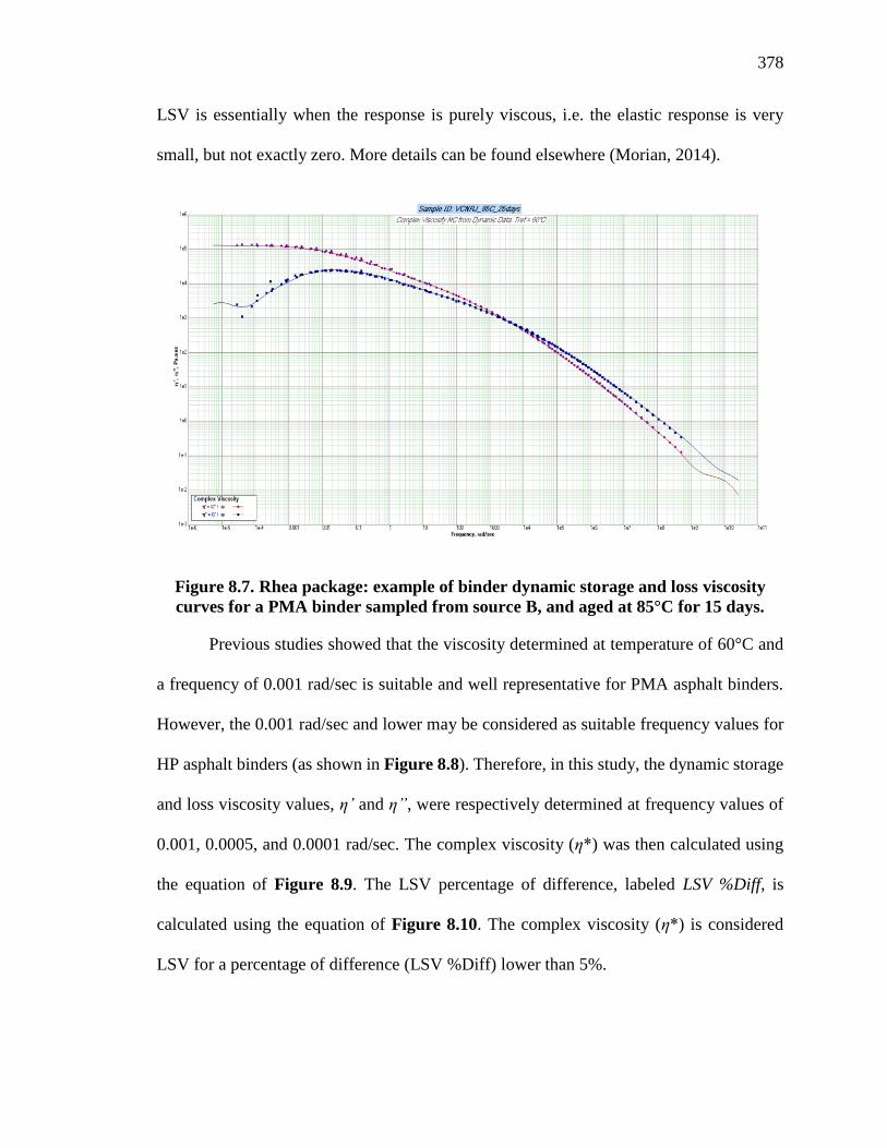
378
LSV is essentially when the response is purely viscous, i.e. the elastic response is very
small, but not exactly zero. More details can be found elsewhere (Morian, 2014).
Figure 8.7. Rhea package: example of binder dynamic storage and loss viscosity
curves for a PMA binder sampled from source B, and aged at 85°C for 15 days.
Previous studies showed that the viscosity determined at temperature of 60°C and
a frequency of 0.001 rad/sec is suitable and well representative for PMA asphalt binders.
However, the 0.001 rad/sec and lower may be considered as suitable frequency values for
HP asphalt binders (as shown in Figure 8.8). Therefore, in this study, the dynamic storage
and loss viscosity values, η’ and η”, were respectively determined at frequency values of
0.001, 0.0005, and 0.0001 rad/sec. The complex viscosity (η*) was then calculated using
the equation of Figure 8.9. The LSV percentage of difference, labeled LSV %Diff, is
calculated using the equation of Figure 8.10. The complex viscosity (η*) is considered
LSV for a percentage of difference (LSV %Diff) lower than 5%.

379
Figure 8.8. Rhea package: example of binder dynamic storage and loss viscosity
curves for a HP binder sampled from source B, and aged at 85°C for 15 days.
𝜂∗ = √𝜂′^2 + 𝜂′′^2
Figure 8.9. Equation. Calculation of complex shear viscosity.
𝐿𝑆𝑉 %𝐷𝑖𝑓𝑓 = 𝜂∗ − 𝜂′
𝜂∗∗ 100
Figure 8.10. Equation. Calculation of LSV percentage of difference.
Where 𝜂∗ is the complex shear viscosity expressed in Pa.s, 𝜂′ is the storage or
elastic shear viscosity expressed in Pa.s, and 𝜂′′ is the loss shear viscosity expressed in
Pa.s.
The Cross model (Cross, 1965) is a widely known model for ZSV measurement
and has the form expressed in the equation of Figure 8.11.
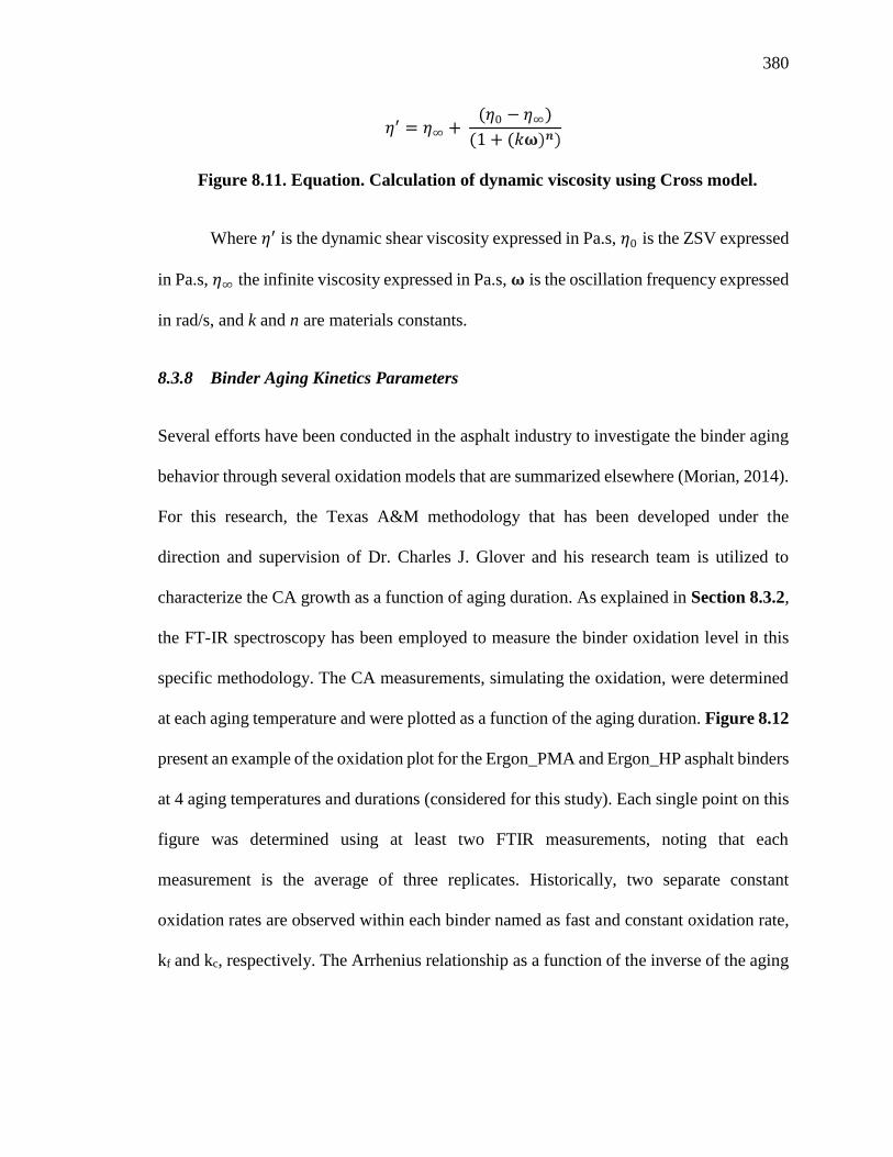
380
𝜂′ = 𝜂∞ + (𝜂0 − 𝜂∞)
(1 + (𝑘𝛚)𝒏)
Figure 8.11. Equation. Calculation of dynamic viscosity using Cross model.
Where 𝜂′ is the dynamic shear viscosity expressed in Pa.s, 𝜂0 is the ZSV expressed
in Pa.s, 𝜂∞ the infinite viscosity expressed in Pa.s, 𝛚 is the oscillation frequency expressed
in rad/s, and k and n are materials constants.
8.3.8 Binder Aging Kinetics Parameters
Several efforts have been conducted in the asphalt industry to investigate the binder aging
behavior through several oxidation models that are summarized elsewhere (Morian, 2014).
For this research, the Texas A&M methodology that has been developed under the
direction and supervision of Dr. Charles J. Glover and his research team is utilized to
characterize the CA growth as a function of aging duration. As explained in Section 8.3.2,
the FT-IR spectroscopy has been employed to measure the binder oxidation level in this
specific methodology. The CA measurements, simulating the oxidation, were determined
at each aging temperature and were plotted as a function of the aging duration. Figure 8.12
present an example of the oxidation plot for the Ergon_PMA and Ergon_HP asphalt binders
at 4 aging temperatures and durations (considered for this study). Each single point on this
figure was determined using at least two FTIR measurements, noting that each
measurement is the average of three replicates. Historically, two separate constant
oxidation rates are observed within each binder named as fast and constant oxidation rate,
kf and kc, respectively. The Arrhenius relationship as a function of the inverse of the aging

381
temperature and the gas constant R, expressed in the equation of Figure 8.13, is then
utilized to formulize the oxidation rates separately.
(a)
(b)
Figure 8.12. Example of plot of oxidation kinetic measurements for: (a)
ERGON_PMA, and (b) ERGON_HP.
0.0
0.1
0.2
0.3
0.4
0.5
0.6
0.7
0.8
0.9
0 50 100 150 200 250
CA
g,
Arb
itra
ry U
nit
s
Aging Duration (day)
ERGON_PMA_100°C
ERGON_PMA_85°C
ERGON_PMA_60°C
ERGON_PMA_50°C
0.0
0.1
0.2
0.3
0.4
0.5
0.6
0.7
0.8
0.9
0 50 100 150 200 250
CA
g,
Arb
itra
ry U
nit
s
Aging Duration (day)
ERGON_HP_100°C
ERGON_HP_85°C
ERGON_HP_60°C
ERGON_HP_50°C

382
𝑟𝐶𝐴 = 𝐴𝑃𝛼𝑒−𝐸𝑎𝑅𝑇
Figure 8.13. Equation. Calculation of rate of carbonyl area, CA.
Where 𝑟𝐶𝐴 is the rate of carbonyl area, CA, growth, either kf or kc; A is the pre-
exponential factor; P is the absolute oxygen pressure during oxidation expressed in atm; 𝛂
is the reaction order with respect to oxidation pressure; 𝐸𝑎 is the activation energy
expressed in J/mol; R is the ideal gas constant equal to 8.3144621 L/mol.°K; and T is the
temperature expressed in °K.
Finally, the two oxidation rates can be combined into one relationship describing
CA as function of aging time and duration, presented in the equation of Figure 8.14.
𝐶𝐴𝑔 = 𝑀 ∗ (1 − 𝑒−𝑘𝑓𝑡) + 𝑘𝑐𝑡
Figure 8.14. Equation. Calculation of rate of carbonyl area, CA, function of fast
and slow rate of growth.
Where 𝐶𝐴𝑔 is the carbonyl area growth, (CA-CA0); CA is the carbonyl area; 𝐶𝐴0
is the original or tank CA measurement; M is the initial jump, magnitude of fast rate
reaction in terms of CAg; kf is the fast rate of CA growth; kc is the slow or constant rate of
CA growth; and t is the time expressed in days.
As an example of the application of the equation of Figure 8.14 is shown in Figure
8.15, clearly representing the fast and constant oxidation phases as well as the predicted
aging path over different temperatures and multiple aging durations for Ergon_PMA
asphalt binder evaluated in this study.

383
Figure 8.15. Example of fast and constant oxidation kinetic measurements and
predicted aging path for ERGON_PMA asphalt binder.
8.3.9 Binder Hardening Susceptibility
One of the most significant parameters in characterizing the binder oxidation properties is
hardening susceptibility (HS) which originally relates the binder stiffness with aging.
Historically, the LSV and CA from the FT-IR measurements were utilized as an indication
of the binder stiffness and aging, respectively. The corresponding HS is a linear
relationship between the LSV and CA mathematically as defined by the equation of Figure
8.16.
𝑙𝑛 𝜂0∗ = 𝐻𝑆 ∗ 𝐶𝐴 + 𝑚
Figure 8.16. Equation. Calculation of LSV function of HS and CA.
0.0
0.1
0.2
0.3
0.4
0.5
0.6
0.7
0.8
0.9
0 50 100 150 200 250
CA
g,
Arb
itra
ry U
nit
s
Aging Duration (day)
ERGON_PMA_100°CERGON_PMA_85°CERGON_PMA_60°CERGON_PMA_50°CModeling ERGON_PMA_100°CModeling ERGON_PMA_85°CModeling ERGON_PMA_60°CModeling ERGON_PMA_50°C
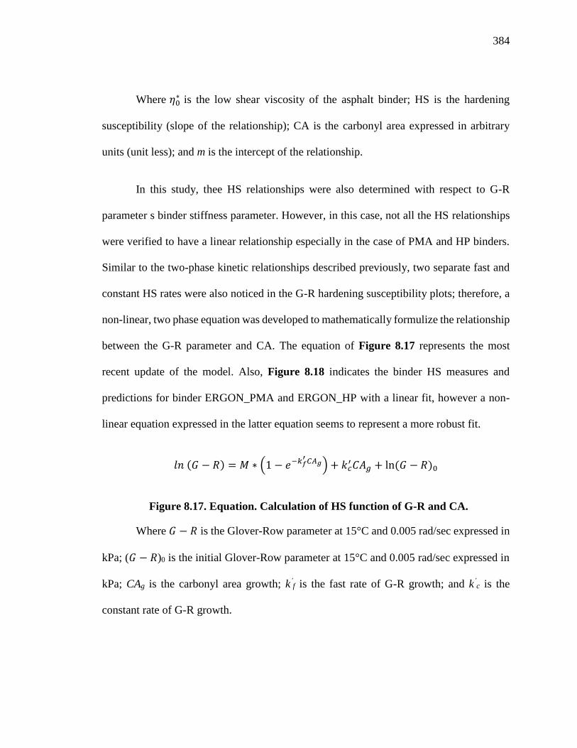
384
Where 𝜂0∗ is the low shear viscosity of the asphalt binder; HS is the hardening
susceptibility (slope of the relationship); CA is the carbonyl area expressed in arbitrary
units (unit less); and m is the intercept of the relationship.
In this study, thee HS relationships were also determined with respect to G-R
parameter s binder stiffness parameter. However, in this case, not all the HS relationships
were verified to have a linear relationship especially in the case of PMA and HP binders.
Similar to the two-phase kinetic relationships described previously, two separate fast and
constant HS rates were also noticed in the G-R hardening susceptibility plots; therefore, a
non-linear, two phase equation was developed to mathematically formulize the relationship
between the G-R parameter and CA. The equation of Figure 8.17 represents the most
recent update of the model. Also, Figure 8.18 indicates the binder HS measures and
predictions for binder ERGON_PMA and ERGON_HP with a linear fit, however a non-
linear equation expressed in the latter equation seems to represent a more robust fit.
𝑙𝑛 (𝐺 − 𝑅) = 𝑀 ∗ (1 − 𝑒−𝑘𝑓′ 𝐶𝐴𝑔) + 𝑘𝑐
′ 𝐶𝐴𝑔 + ln (𝐺 − 𝑅)0
Figure 8.17. Equation. Calculation of HS function of G-R and CA.
Where 𝐺 − 𝑅 is the Glover-Row parameter at 15°C and 0.005 rad/sec expressed in
kPa; (𝐺 − 𝑅)0 is the initial Glover-Row parameter at 15°C and 0.005 rad/sec expressed in
kPa; CAg is the carbonyl area growth; k’f is the fast rate of G-R growth; and k’
c is the
constant rate of G-R growth.

385
Figure 8.18. Hardening susceptibility of ERGON_PMA and ERGON_HP asphalt
binders for G-R parameter at 15°C and 0.005 rad/s.
8.4 Aging Testing Results
The test methodologies explained in Section 8.3, have been applied to the asphalt binder
materials defined in Section 3.2.1, through the described experimental plan in Table 8.1
and Table 8.2. The main objective of this section is to present the aging characteristics of
the various pre-determined binder blends, and, as a result, provide an evaluation of the
impact of high polymer modification considered in this study. The evaluated asphalt
binders were exposed to forced-draft oven aging and PAV aging protocols with multiple
temperatures and durations completed through the two scenarios (refer to Table 8.1).
First, the dynamic shear modulus (G*) master curves and rheological parameters
were determined using the DSR equipment. Second, the level of oxidation within each
y = 9,567.73e8.24x
R² = 0.89
y = 23,040.26e6.40x
R² = 0.92
100
1,000
10,000
100,000
1,000,000
10,000,000
100,000,000
0.000 0.100 0.200 0.300 0.400 0.500 0.600 0.700 0.800 0.900
G-R
@1
5°C
& 0
.00
5, P
a
CAg, Arbitrary Units
ERGON_PMA
ERGON_HP
Expon. (ERGON_PMA)
Expon. (ERGON_HP)
386
evaluated asphalt binder at a specific aging time and temperature were determined through
the FT-IR spectroscopy data. Ultimately, both results from both testing were combined to
establish the hardening susceptibility (HS) of the binder. The two methods of laboratory
aging (i.e., forced draft oven aging and PAV aging) have been compared at the end to
investigate the potential difference between these aging methods outcomes.
8.4.1 Performance Grading (PG)
The performance grade of the evaluated asphalt binders was determined in accordance with
AASHTO M320 (AASHTO M320, 2015). The high and low temperatures continuous
grades for the material being evaluated were determined following the DSR and BBR
methodologies, respectively. Table 8.5 summarizes the continuous grades, base binder,
polymer content, and percent recovery (%R) of the four evaluated asphalt binders (i.e.,
PMA and HP from source A and PMA and HP form source B). It should be mentioned that
NO liquid anti-strip was added to the evaluated asphalt binders only for this part of the
study (Binder aging experiments). The grade and source of the base binder and the SBS
content for each binder were provided by the suppliers (i.e., Ergon (Source A), and
Vecenergy (Source B)). The measured binders’ data show a wide range in the measured
properties of the binders obtained from Ergon and Vecenergy at all levels of temperature
and aging stages. This will ensure a wide applicability of the research findings.

387
Table 8.5. Summary Table: Continuous Grade of Evaluated PMA and HP Binders.
Binder Source
/ ID
Continuous Grade based on AASHTO M320
PMA HP
A
PG76.4-24.7
(Base Binder: PG64-22,
%SBS = 3.2% & %R = 84.1%)
PG93.5-33.5
(Base Binder: PG52-28,
%SBS = 7.6% & %R = 92.5%)
B
PG76.1-24.3
(Base Binder: PG67-22,
%SBS = 3.0% & %R = 46.0%)
PG99.7-30.0
(Base Binder: PG52-28,
%SBS = 8.0% & %R = 97.8%)
8.4.2 Shear Modulus and Phase Angle Master Curves
Asphalt binder shear modulus (G*) master curve is an indication of the relationship
between the binder stiffness and reduced frequency in a referenced temperature that has
been developed from frequency sweep tests conducted at multiple temperatures and
frequencies. Figure 8.19, Figure 8.21, Figure 8.23, and Figure 8.25 illustrates the G*
shear master curves at a reference temperature of 60°C for ERGON_PMA asphalt binder
aged in the forced-draft air oven at 100, 85, 60, and 50°C, respectively and for different
durations (i.e., 2 hours, 6 hours, 1 day… 240 days). Figure 8.20, Figure 8.22, Figure 8.24,
and Figure 8.26 illustrates the corresponding phase angle master curves (same reference
temperature) for ERGON_PMA asphalt binder at the same aging conditions (i.e.,
temperature, and duration). Figure 8.27, Figure 8.29, Figure 8.31, and Figure 8.33
illustrates the G* shear master curves at a reference temperature of 60°C for ERGON_HP
asphalt binder aged in the forced-draft air oven at 100, 85, 60, and 50°C, respectively and
for different durations (i.e., 2 hours, 6 hours, 1 day… 240 days). Figure 8.28, Figure 8.30,
Figure 8.32, and Figure 8.34 illustrates the corresponding phase angle master curves
(same reference temperature) for ERGON_HP asphalt binder at the same aging conditions
(i.e., temperature, and duration). Figure 8.35, and Figure 8.36 compares the G* and phase

388
angle master curves of ERGON_PMA asphalt binder aged for 15 days at different
temperatures (i.e., 100, 85, 60, and 50°C), respectively. Figure 8.37, and Figure 8.38
compares the G* and phase angle master curves of ERGON_HP asphalt binder aged for 15
days at different temperatures (i.e., 100, 85, 60, and 50°C), respectively. Figure 8.39, and
Figure 8.40 presents the G* and phase angle master curves of ERGON_PMA asphalt
binder, respectively, at unaged (i.e., original), short-term aged (i.e., RTFO), and accelerated
aging (i.e., PAV20hrs, PAV40hrs, and PAV60hrs) conditions. Similarly, Figure 8.41, and
Figure 8.42 presents the G* and phase angle master curves of ERGON_PMA asphalt
binder, respectively, at unaged (i.e., original), short-term aged (i.e., RTFO), and accelerated
aging (i.e., PAV20hrs, PAV40hrs, and PAV60hrs) conditions.
Figure 8.43, Figure 8.45, Figure 8.47, and Figure 8.49 illustrates the G* shear
master curves at a reference temperature of 60°C for VCNRJ_PMA asphalt binder aged in
the forced-draft air oven at 100, 85, 60, and 50°C, respectively and for different durations
(i.e., 2 hours, 6 hours, 1 day… 240 days). Figure 8.44, Figure 8.46, Figure 8.48, and
Figure 8.50 illustrates the corresponding phase angle master curves (same reference
temperature) for VCNRJ_PMA asphalt binder at the same aging conditions (i.e.,
temperature, and duration). Figure 8.51, Figure 8.53, Figure 8.55, and Figure 8.57
illustrates the G* shear master curves at a reference temperature of 60°C for VCNRJ_HP
asphalt binder aged in the forced-draft air oven at 100, 85, 60, and 50°C, respectively and
for different durations (i.e., 2 hours, 6 hours, 1 day… 240 days). Figure 8.52, Figure 8.54,
Figure 8.56, and Figure 8.58 illustrates the corresponding phase angle master curves
(same reference temperature) for VCNRJ_HP asphalt binder at the same aging conditions

389
(i.e., temperature, and duration). Figure 8.59, and Figure 8.60 compares the G* and phase
angle master curves of VCNRJ_PMA asphalt binder aged for 15 days at different
temperatures (i.e., 100, 85, 60, and 50°C), respectively. Figure 8.61, and Figure 8.62
compares the G* and phase angle master curves of VCNRJ_HP asphalt binder aged for 15
days at different temperatures (i.e., 100, 85, 60, and 50°C), respectively. Figure 8.63, and
Figure 8.64 presents the G* and phase angle master curves of VCNRJ_PMA asphalt
binder, respectively, at unaged (i.e., original), short-term aged (i.e., RTFO), and accelerated
aging (i.e., PAV20hrs, PAV40hrs, and PAV60hrs) conditions. Similarly, Figure 8.65, and
Figure 8.66 presents the G* and phase angle master curves of VCNRJ_PMA asphalt
binder, respectively, at unaged (i.e., original), short-term aged (i.e., RTFO), and accelerated
aging (i.e., PAV20hrs, PAV40hrs, and PAV60hrs) conditions.
The provided data lead to the following observations:
• Regardless of the asphalt binder type and PG, higher stiffness values were observed
with the increase of frequency values simulating lower temperatures and faster
traffic.
• Regardless of the asphalt binder type and PG, higher stiffness values were observed
with the increase of aging duration values simulating more oxidation of the asphalt
binder in the field.
• Regardless of the asphalt binder type and PG, higher stiffness values were observed
with the increase of aging temperature for the same aging duration values
simulating more potential oxidation of the asphalt binder in the field when
subjected to warmer climatic conditions and higher temperatures.
390
• The G* master curves of the evaluated HP asphalt binders showed a plateau at
intermediate temperature which can be credited to the effect of high polymer
modification. The stiffness increases with the increase of frequency; however, at
intermediate frequency values, the high polymer content takes over and start
decreasing the rate at which the stiffness is increasing. At higher frequencies
simulating lower temperatures and faster traffic, the binder stiffness starts picking
up again till it reaches the glassy modulus. It should be mentioned that regardless
of the aging temperature and aging durations, the same binder evaluated at different
aging combinations (i.e., temperature + duration) showed very close glassy
modulus. The plateau was seen less significant for higher aging temperatures and
longer aging durations. At that stage, the HP asphalt binder shows a similar G*
master curve allure but for sure with lower stiffness values simulating less stiff
behavior under traffic.
• Regardless of the asphalt binder type and PG, lower phase angle values were
observed with the increase of frequency values simulating more elastic behavior at
lower temperatures and under faster traffic.
• Regardless of the asphalt binder type and PG, lower phase angle values were
observed with the increase of aging duration values which can be due to the stiffer
behavior of the asphalt binder in the field.
• Regardless of the asphalt binder type and PG, lower phase angle values were
observed with the increase of aging temperature for the same aging durations.
• The phase angle master curves of the evaluated HP asphalt binders showed an
inverted N shape; at a higher frequencies, lower phase angle values were observed

391
simulating more elastic behavior for the asphalt binder at lower temperatures and
under faster traffic; with the decrease of the reduced frequency (warmer
temperatures and slower traffic), the phase angle values started increasing to reach
a peak value (right peak of the inverted N shape) at which the SBS polymer started
taking over and helped in decreasing the asphalt binder stiffness; the phase angle
values were observed decreasing again to reach a lower limit or a bottom sag (left
bottom peak of the inverted N shape) at which the asphalt binder phase angle starts
picking up simulating relative higher temperatures and slower traffic.
• Regardless of the aging temperatures and the evaluated HP asphalt binders, higher
right phase angle peak values (i.e., right peak of the inverted N shape) were
observed for shorter aging durations; meanwhile lower left low points (i.e., lower
phase angle sag values) (i.e., left trough of the inverted N shape) were observed for
shorter aging durations.
• Regardless of the aging durations and the evaluated HP asphalt binders, higher right
phase angle peak values (i.e., right peak of the inverted N shape) and higher left
phase angle sag values were observed for lower aging temperatures.
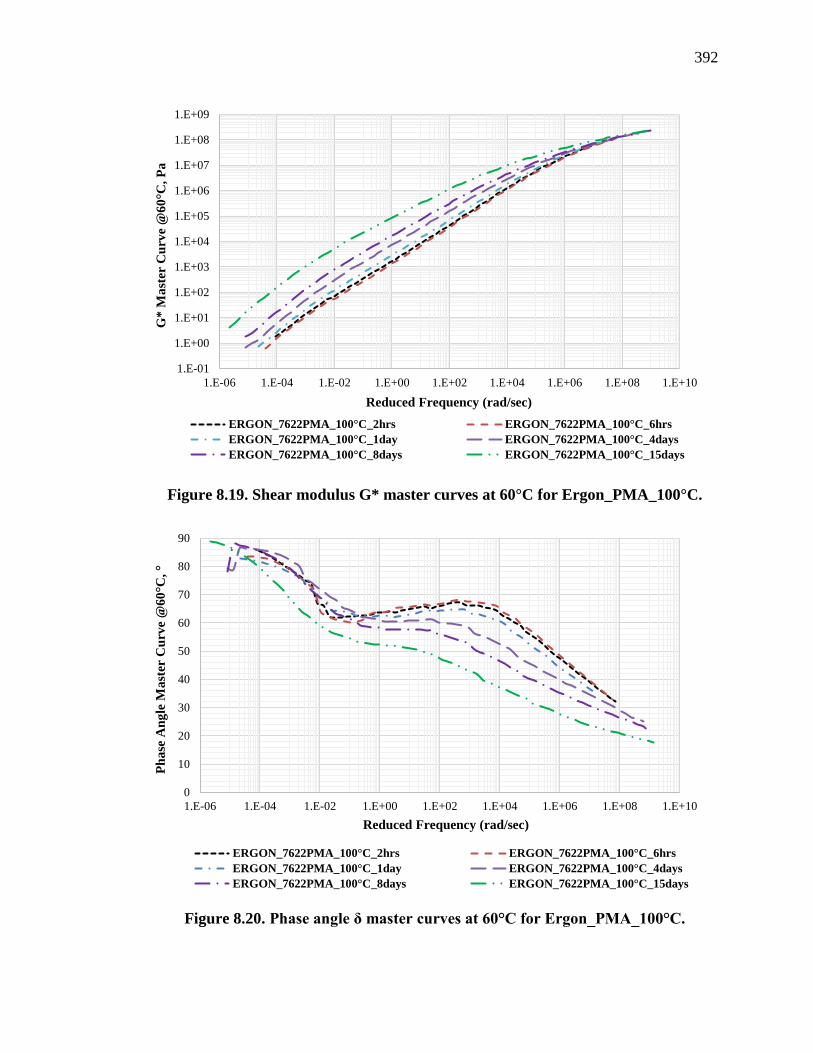
392
Figure 8.19. Shear modulus G* master curves at 60°C for Ergon_PMA_100°C.
Figure 8.20. Phase angle δ master curves at 60°C for Ergon_PMA_100°C.
1.E-01
1.E+00
1.E+01
1.E+02
1.E+03
1.E+04
1.E+05
1.E+06
1.E+07
1.E+08
1.E+09
1.E-06 1.E-04 1.E-02 1.E+00 1.E+02 1.E+04 1.E+06 1.E+08 1.E+10
G*
Ma
ster
Cu
rve
@6
0°C
, P
a
Reduced Frequency (rad/sec)
ERGON_7622PMA_100°C_2hrs ERGON_7622PMA_100°C_6hrs
ERGON_7622PMA_100°C_1day ERGON_7622PMA_100°C_4days
ERGON_7622PMA_100°C_8days ERGON_7622PMA_100°C_15days
0
10
20
30
40
50
60
70
80
90
1.E-06 1.E-04 1.E-02 1.E+00 1.E+02 1.E+04 1.E+06 1.E+08 1.E+10
Ph
ase
An
gle
Ma
ster
Cu
rve
@6
0°C
, °
Reduced Frequency (rad/sec)
ERGON_7622PMA_100°C_2hrs ERGON_7622PMA_100°C_6hrs
ERGON_7622PMA_100°C_1day ERGON_7622PMA_100°C_4days
ERGON_7622PMA_100°C_8days ERGON_7622PMA_100°C_15days

393
Figure 8.21. Shear modulus G* master curves at 60°C for Ergon_PMA_85°C.
Figure 8.22. Phase angle δ master curves at 60°C for Ergon_PMA_85°C.
1.E-01
1.E+00
1.E+01
1.E+02
1.E+03
1.E+04
1.E+05
1.E+06
1.E+07
1.E+08
1.E+09
1.E-06 1.E-04 1.E-02 1.E+00 1.E+02 1.E+04 1.E+06 1.E+08 1.E+10
G*
Ma
ster
Cu
rve
@6
0°C
, P
a
Reduced Frequency (rad/sec)
ERGON_7622PMA_85°C_1day ERGON_7622PMA_85°C_4days
ERGON_7622PMA_85°C_8days ERGON_7622PMA_85°C_15days
ERGON_7622PMA_85°C_25days ERGON_7622PMA_85°C_45days
0
10
20
30
40
50
60
70
80
90
1.E-06 1.E-04 1.E-02 1.E+00 1.E+02 1.E+04 1.E+06 1.E+08 1.E+10
Ph
ase
An
gle
ma
ster
Cu
rve
@6
0°C
, °
Reduced Frequency (rad/sec)
ERGON_7622PMA_85°C_1day ERGON_7622PMA_85°C_4days
ERGON_7622PMA_85°C_8days ERGON_7622PMA_85°C_15days
ERGON_7622PMA_85°C_25days ERGON_7622PMA_85°C_45days

394
Figure 8.23. Shear modulus G* master curves at 60°C for Ergon_PMA_60°C.
Figure 8.24. Phase angle δ master curves at 60°C for Ergon_PMA_60°C.
1.E-01
1.E+00
1.E+01
1.E+02
1.E+03
1.E+04
1.E+05
1.E+06
1.E+07
1.E+08
1.E+09
1.E-06 1.E-04 1.E-02 1.E+00 1.E+02 1.E+04 1.E+06 1.E+08 1.E+10
G*
Ma
ster
Cu
rve
@6
0°C
, P
a
Reduced Frequency (rad/sec)
ERGON_7622PMA_60°C_4days ERGON_7622PMA_60°C_8days
ERGON_7622PMA_60°C_15days ERGON_7622PMA_60°C_45days
ERGON_7622PMA_60°C_100days ERGON_7622PMA_60°C_160days
0
10
20
30
40
50
60
70
80
90
1.E-06 1.E-04 1.E-02 1.E+00 1.E+02 1.E+04 1.E+06 1.E+08 1.E+10
Ph
ase
An
gle
Ma
ster
Cu
rve
@6
0°C
, °
Reduced Frequency (rad/sec)
ERGON_7622PMA_60°C_4days ERGON_7622PMA_60°C_8days
ERGON_7622PMA_60°C_15days ERGON_7622PMA_60°C_45days
ERGON_7622PMA_60°C_100days ERGON_7622PMA_60°C_160days

395
Figure 8.25. Shear modulus G* master curves at 60°C for Ergon_PMA_50°C.
Figure 8.26. Phase angle δ master curves at 60°C for Ergon_PMA_50°C.
1.E-01
1.E+00
1.E+01
1.E+02
1.E+03
1.E+04
1.E+05
1.E+06
1.E+07
1.E+08
1.E+09
1.E-06 1.E-04 1.E-02 1.E+00 1.E+02 1.E+04 1.E+06 1.E+08 1.E+10
G*
Ma
ster
Cu
rve
@6
0°C
, P
a
Reduced Frequency (rad/sec)
ERGON_7622PMA_50°C_4days ERGON_7622PMA_50°C_15days
ERGON_7622PMA_50°C_45days ERGON_7622PMA_50°C_100days
ERGON_7622PMA_50°C_160days ERGON_7622PMA_50°C_240days
0
10
20
30
40
50
60
70
80
90
1.E-06 1.E-04 1.E-02 1.E+00 1.E+02 1.E+04 1.E+06 1.E+08 1.E+10
Ph
ase
An
gle
Ma
ster
Cu
rve
@6
0°C
, °
Reduced Frequency (rad/sec)
ERGON_7622PMA_50°C_4days ERGON_7622PMA_50°C_15days
ERGON_7622PMA_50°C_45days ERGON_7622PMA_50°C_100days
ERGON_7622PMA_50°C_160days ERGON_7622PMA_50°C_240days

396
Figure 8.27. Shear modulus G* master curves at 60°C for Ergon_HP_100°C.
Figure 8.28. Phase angle δ master curves at 60°C for Ergon_HP_100°C.
1.E+00
1.E+01
1.E+02
1.E+03
1.E+04
1.E+05
1.E+06
1.E+07
1.E+08
1.E+09
1.E-06 1.E-04 1.E-02 1.E+00 1.E+02 1.E+04 1.E+06 1.E+08 1.E+10
G*
Ma
ster
Cu
rve
@6
0°C
, P
a
Reduced Frequency (rad/sec)
ERGON_HP_100°C_2hrs ERGON_HP_100°C_6hrs ERGON_HP_100°C_1day
ERGON_HP_100°C_4days ERGON_HP_100°C_8days ERGON_HP_100°C_15days
0
10
20
30
40
50
60
70
80
90
1.E-06 1.E-04 1.E-02 1.E+00 1.E+02 1.E+04 1.E+06 1.E+08 1.E+10
Ph
ase
An
gle
Ma
ster
Cu
rve
@6
0°C
, °
Reduced Frequency (rad/sec)
ERGON_HP_100°C_2hrs ERGON_HP_100°C_6hrs ERGON_HP_100°C_1day
ERGON_HP_100°C_4days ERGON_HP_100°C_8days ERGON_HP_100°C_15days
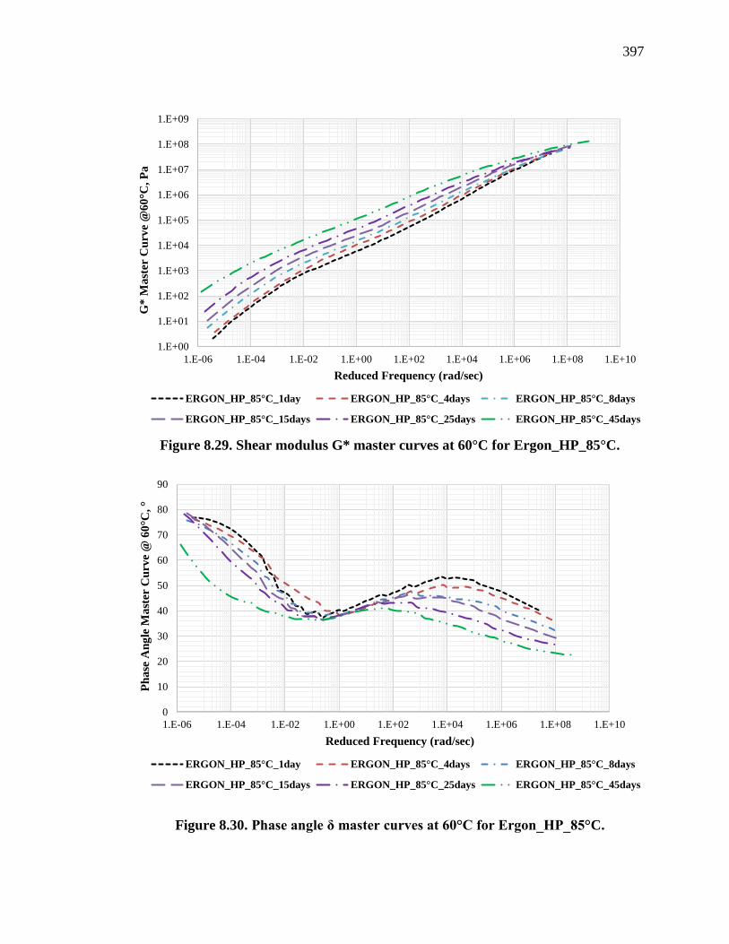
397
Figure 8.29. Shear modulus G* master curves at 60°C for Ergon_HP_85°C.
Figure 8.30. Phase angle δ master curves at 60°C for Ergon_HP_85°C.
1.E+00
1.E+01
1.E+02
1.E+03
1.E+04
1.E+05
1.E+06
1.E+07
1.E+08
1.E+09
1.E-06 1.E-04 1.E-02 1.E+00 1.E+02 1.E+04 1.E+06 1.E+08 1.E+10
G*
Ma
ster
Cu
rve
@6
0°C
, P
a
Reduced Frequency (rad/sec)
ERGON_HP_85°C_1day ERGON_HP_85°C_4days ERGON_HP_85°C_8days
ERGON_HP_85°C_15days ERGON_HP_85°C_25days ERGON_HP_85°C_45days
0
10
20
30
40
50
60
70
80
90
1.E-06 1.E-04 1.E-02 1.E+00 1.E+02 1.E+04 1.E+06 1.E+08 1.E+10
Ph
ase
An
gle
Ma
ster
Cu
rve
@ 6
0°C
, °
Reduced Frequency (rad/sec)
ERGON_HP_85°C_1day ERGON_HP_85°C_4days ERGON_HP_85°C_8days
ERGON_HP_85°C_15days ERGON_HP_85°C_25days ERGON_HP_85°C_45days

398
Figure 8.31. Shear modulus G* master curves at 60°C for Ergon_HP_60°C.
Figure 8.32. Phase angle δ master curves at 60°C for Ergon_HP_60°C.
1.E+00
1.E+01
1.E+02
1.E+03
1.E+04
1.E+05
1.E+06
1.E+07
1.E+08
1.E+09
1.E-06 1.E-04 1.E-02 1.E+00 1.E+02 1.E+04 1.E+06 1.E+08 1.E+10
G*
Ma
ster
Cu
rve
@ 6
0°C
, P
a
Reduced Frequency (rad/sec)
ERGON_HP_60°C_4days ERGON_HP_60°C_8days ERGON_HP_60°C_15days
ERGON_HP_60°C_45days ERGON_HP_60°C_100days ERGON_HP_60°C_160days
0
10
20
30
40
50
60
70
80
90
1.E-06 1.E-04 1.E-02 1.E+00 1.E+02 1.E+04 1.E+06 1.E+08
Ph
ase
An
gle
Ma
ster
Cu
rve
@ 6
0°C
, °
Reduced Frequency (rad/sec)
ERGON_HP_60°C_4days ERGON_HP_60°C_8days ERGON_HP_60°C_15days
ERGON_HP_60°C_45days ERGON_HP_60°C_100days ERGON_HP_60°C_160days

399
Figure 8.33. Shear modulus G* master curves at 60°C for Ergon_HP_50°C.
Figure 8.34. Phase angle δ master curves at 60°C for Ergon_HP_50°C.
1.E+00
1.E+01
1.E+02
1.E+03
1.E+04
1.E+05
1.E+06
1.E+07
1.E+08
1.E-06 1.E-04 1.E-02 1.E+00 1.E+02 1.E+04 1.E+06 1.E+08 1.E+10
G*
Ma
ster
Cu
rve
@ 6
0°C
, P
a
Reduced Frequency (rad/sec)
ERGON_HP_50°C_4days ERGON_HP_50°C_15days
ERGON_HP_50°C_45days ERGON_HP_50°C_100days
ERGON_HP_50°C_160days ERGON_HP_50°C_240days
0
10
20
30
40
50
60
70
80
90
1.E-06 1.E-04 1.E-02 1.E+00 1.E+02 1.E+04 1.E+06 1.E+08 1.E+10
Ph
ase
An
gle
Mss
ter C
urv
e @
60
°C, °
Reduced Frequency (rad/sec)
ERGON_HP_50°C_4days ERGON_HP_50°C_15days ERGON_HP_50°C_45days
ERGON_HP_50°C_100days ERGON_HP_50°C_160days ERGON_HP_50°C_240days
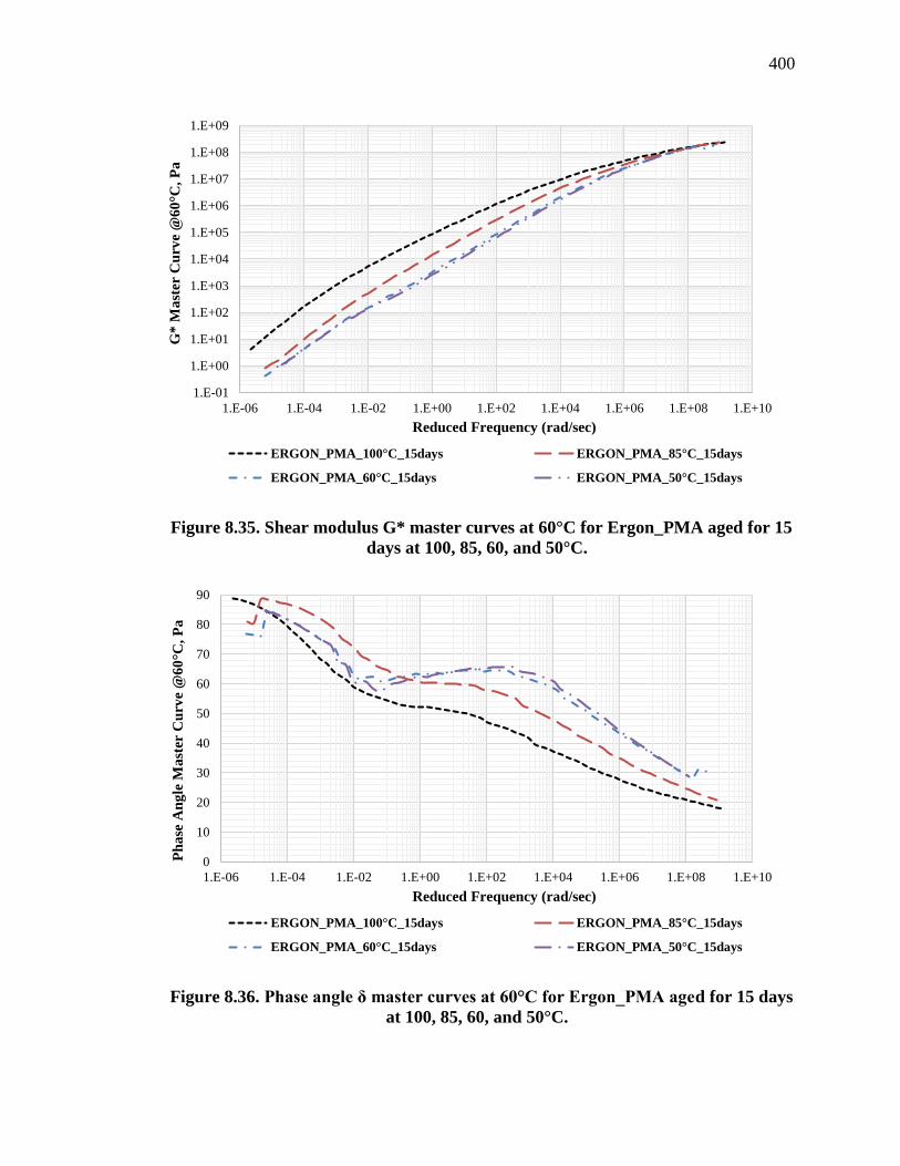
400
Figure 8.35. Shear modulus G* master curves at 60°C for Ergon_PMA aged for 15
days at 100, 85, 60, and 50°C.
Figure 8.36. Phase angle δ master curves at 60°C for Ergon_PMA aged for 15 days
at 100, 85, 60, and 50°C.
1.E-01
1.E+00
1.E+01
1.E+02
1.E+03
1.E+04
1.E+05
1.E+06
1.E+07
1.E+08
1.E+09
1.E-06 1.E-04 1.E-02 1.E+00 1.E+02 1.E+04 1.E+06 1.E+08 1.E+10
G*
Ma
ster
Cu
rve
@6
0°C
, P
a
Reduced Frequency (rad/sec)
ERGON_PMA_100°C_15days ERGON_PMA_85°C_15days
ERGON_PMA_60°C_15days ERGON_PMA_50°C_15days
0
10
20
30
40
50
60
70
80
90
1.E-06 1.E-04 1.E-02 1.E+00 1.E+02 1.E+04 1.E+06 1.E+08 1.E+10
Ph
ase
An
gle
Ma
ster
Cu
rve
@6
0°C
, P
a
Reduced Frequency (rad/sec)
ERGON_PMA_100°C_15days ERGON_PMA_85°C_15days
ERGON_PMA_60°C_15days ERGON_PMA_50°C_15days
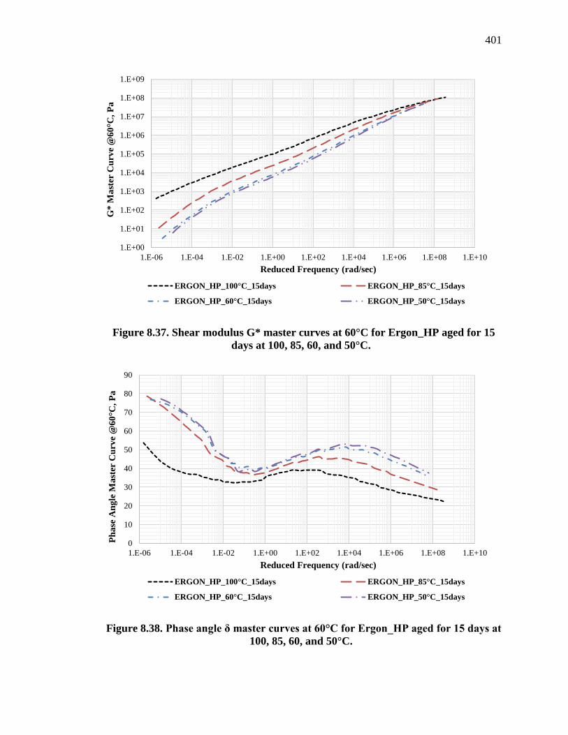
401
Figure 8.37. Shear modulus G* master curves at 60°C for Ergon_HP aged for 15
days at 100, 85, 60, and 50°C.
Figure 8.38. Phase angle δ master curves at 60°C for Ergon_HP aged for 15 days at
100, 85, 60, and 50°C.
1.E+00
1.E+01
1.E+02
1.E+03
1.E+04
1.E+05
1.E+06
1.E+07
1.E+08
1.E+09
1.E-06 1.E-04 1.E-02 1.E+00 1.E+02 1.E+04 1.E+06 1.E+08 1.E+10
G*
Ma
ster
Cu
rve
@6
0°C
, P
a
Reduced Frequency (rad/sec)
ERGON_HP_100°C_15days ERGON_HP_85°C_15days
ERGON_HP_60°C_15days ERGON_HP_50°C_15days
0
10
20
30
40
50
60
70
80
90
1.E-06 1.E-04 1.E-02 1.E+00 1.E+02 1.E+04 1.E+06 1.E+08 1.E+10
Ph
ase
An
gle
Ma
ster
Cu
rve
@6
0°C
, P
a
Reduced Frequency (rad/sec)
ERGON_HP_100°C_15days ERGON_HP_85°C_15days
ERGON_HP_60°C_15days ERGON_HP_50°C_15days
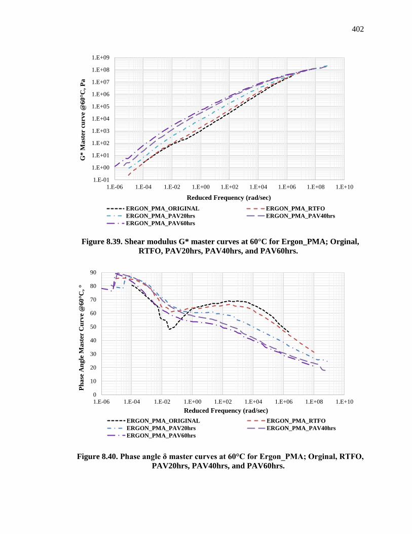
402
Figure 8.39. Shear modulus G* master curves at 60°C for Ergon_PMA; Orginal,
RTFO, PAV20hrs, PAV40hrs, and PAV60hrs.
Figure 8.40. Phase angle δ master curves at 60°C for Ergon_PMA; Orginal, RTFO,
PAV20hrs, PAV40hrs, and PAV60hrs.
1.E-01
1.E+00
1.E+01
1.E+02
1.E+03
1.E+04
1.E+05
1.E+06
1.E+07
1.E+08
1.E+09
1.E-06 1.E-04 1.E-02 1.E+00 1.E+02 1.E+04 1.E+06 1.E+08 1.E+10
G*
Ma
ster
cu
rve
@6
0°C
, P
a
Reduced Frequency (rad/sec)
ERGON_PMA_ORIGINAL ERGON_PMA_RTFO
ERGON_PMA_PAV20hrs ERGON_PMA_PAV40hrs
ERGON_PMA_PAV60hrs
0
10
20
30
40
50
60
70
80
90
1.E-06 1.E-04 1.E-02 1.E+00 1.E+02 1.E+04 1.E+06 1.E+08 1.E+10
Ph
ase
An
gle
Ma
ster
Cu
rve
@6
0°C
, °
Reduced Frequency (rad/sec)
ERGON_PMA_ORIGINAL ERGON_PMA_RTFO
ERGON_PMA_PAV20hrs ERGON_PMA_PAV40hrs
ERGON_PMA_PAV60hrs
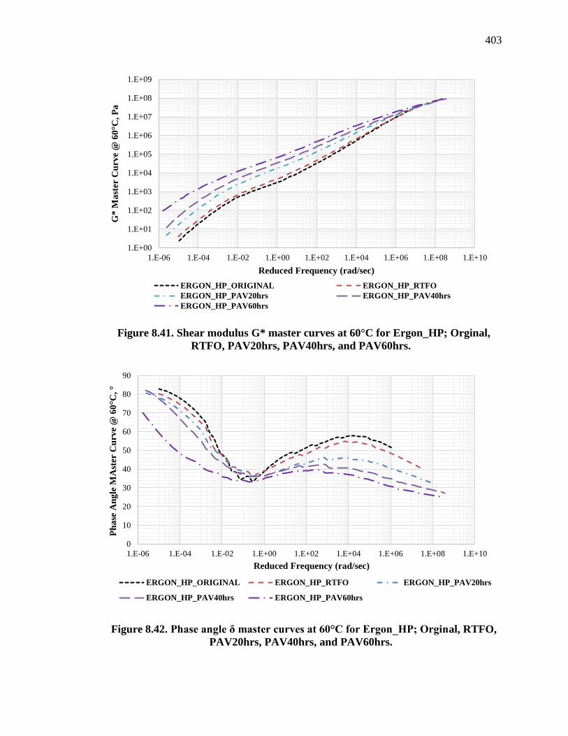
403
Figure 8.41. Shear modulus G* master curves at 60°C for Ergon_HP; Orginal,
RTFO, PAV20hrs, PAV40hrs, and PAV60hrs.
Figure 8.42. Phase angle δ master curves at 60°C for Ergon_HP; Orginal, RTFO,
PAV20hrs, PAV40hrs, and PAV60hrs.
1.E+00
1.E+01
1.E+02
1.E+03
1.E+04
1.E+05
1.E+06
1.E+07
1.E+08
1.E+09
1.E-06 1.E-04 1.E-02 1.E+00 1.E+02 1.E+04 1.E+06 1.E+08 1.E+10
G*
Ma
ster
Cu
rve
@ 6
0°C
, P
a
Reduced Frequency (rad/sec)
ERGON_HP_ORIGINAL ERGON_HP_RTFO
ERGON_HP_PAV20hrs ERGON_HP_PAV40hrs
ERGON_HP_PAV60hrs
0
10
20
30
40
50
60
70
80
90
1.E-06 1.E-04 1.E-02 1.E+00 1.E+02 1.E+04 1.E+06 1.E+08 1.E+10
Ph
ase
An
gle
MA
ster
Cu
rve
@ 6
0°C
, °
Reduced Frequency (rad/sec)
ERGON_HP_ORIGINAL ERGON_HP_RTFO ERGON_HP_PAV20hrs
ERGON_HP_PAV40hrs ERGON_HP_PAV60hrs

404
Figure 8.43. Shear modulus G* master curves at 60°C for VCNRJ_PMA_100°C.
Figure 8.44. Phase angle δ master curves at 60°C for VCNRJ _PMA_100°C.
1.E-02
1.E-01
1.E+00
1.E+01
1.E+02
1.E+03
1.E+04
1.E+05
1.E+06
1.E+07
1.E+08
1.E+09
1.E-06 1.E-04 1.E-02 1.E+00 1.E+02 1.E+04 1.E+06 1.E+08 1.E+10
G*
Ma
ster
Cu
rve
@6
0°C
, P
a
Reduced Frequency (rad/sec)
VCNRJ_7622PMA_100°C_2hrs VCNRJ_7622PMA_100°C_6hrs
VCNRJ_7622PMA_100°C_1day VCNRJ_7622PMA_100°C_4days
VCNRJ_7622PMA_100°C_8days VCNRJ_7622PMA_100°C_15days
0
10
20
30
40
50
60
70
80
90
1.E-06 1.E-04 1.E-02 1.E+00 1.E+02 1.E+04 1.E+06 1.E+08 1.E+10
Ph
ase
An
gle
Ma
ster
Cu
rve
@6
0°C
, °
Reduced Frequency (rad/sec)
VCNRJ_7622PMA_100°C_2hrs VCNRJ_7622PMA_100°C_6hrs
VCNRJ_7622PMA_100°C_1day VCNRJ_7622PMA_100°C_4days
VCNRJ_7622PMA_100°C_8days VCNRJ_7622PMA_100°C_15days

405
Figure 8.45. Shear modulus G* master curves at 60°C for VCNRJ _PMA_85°C.
Figure 8.46. Phase angle δ master curves at 60°C for VCNRJ _PMA_85°C.
1.E-01
1.E+00
1.E+01
1.E+02
1.E+03
1.E+04
1.E+05
1.E+06
1.E+07
1.E+08
1.E+09
1.E-06 1.E-04 1.E-02 1.E+00 1.E+02 1.E+04 1.E+06 1.E+08 1.E+10
Sh
ear
Mo
du
lus
Ma
ster
Cu
rve
@6
0°C
, P
a
Reduced Frequency (rad/sec)
VCNRJ_7622PMA_85°C_1day VCNRJ_7622PMA_85°C_4days
VCNRJ_7622PMA_100°C_8days VCNRJ_7622PMA_85°C_15days
VCNRJ_7622PMA_85°C_25days VCNRJ_7622PMA_85°C_45days
0
10
20
30
40
50
60
70
80
90
1.E-06 1.E-04 1.E-02 1.E+00 1.E+02 1.E+04 1.E+06 1.E+08 1.E+10
Ph
ase
An
gle
Ma
ster
Cu
rve
@6
0°C
, °
Reduced Frequency (rad/sec)
VCNRJ_7622PMA_85°C_1day VCNRJ_7622PMA_85°C_4days
VCNRJ_7622PMA_100°C_8days VCNRJ_7622PMA_85°C_15days
VCNRJ_7622PMA_85°C_25days VCNRJ_7622PMA_85°C_45days

406
Figure 8.47. Shear modulus G* master curves at 60°C for VCNRJ _PMA_60°C.
Figure 8.48. Phase angle δ master curves at 60°C for VCNRJ _PMA_60°C.
1.E-01
1.E+00
1.E+01
1.E+02
1.E+03
1.E+04
1.E+05
1.E+06
1.E+07
1.E+08
1.E+09
1.E-06 1.E-04 1.E-02 1.E+00 1.E+02 1.E+04 1.E+06 1.E+08 1.E+10
Sh
ear
Mo
du
lus
Ma
ster
Cu
rve
@6
0°C
, P
a
Reduced Frequency (rad/sec)
VCNRJ_7622PMA_60°C_4days VCNRJ_7622PMA_60°C_8days
VCNRJ_7622PMA_60°C_15days VCNRJ_7622PMA_60°C_45days
VCNRJ_7622PMA_60°C_100days VCNRJ_7622PMA_60°C_160days
0
10
20
30
40
50
60
70
80
90
1.E-06 1.E-04 1.E-02 1.E+00 1.E+02 1.E+04 1.E+06 1.E+08 1.E+10
Ph
ase
An
gle
Ma
str
Cu
rve
@6
0°C
, °
Reduced Frequency (rad/sec)
VCNRJ_7622PMA_60°C_4days VCNRJ_7622PMA_60°C_8days
VCNRJ_7622PMA_60°C_15days VCNRJ_7622PMA_60°C_45days
VCNRJ_7622PMA_60°C_100days VCNRJ_7622PMA_60°C_160days

407
Figure 8.49. Shear modulus G* master curves at 60°C for VCNRJ_PMA_50°C.
Figure 8.50. Phase angle δ master curves at 60°C for VCNRJ _PMA_50°C.
1.E-01
1.E+00
1.E+01
1.E+02
1.E+03
1.E+04
1.E+05
1.E+06
1.E+07
1.E+08
1.E+09
1.E-06 1.E-04 1.E-02 1.E+00 1.E+02 1.E+04 1.E+06 1.E+08 1.E+10
Sh
ear
Mo
du
lus
Ma
ster
Cu
rve
@6
0°C
, P
a
Reduced Frequency (rad/sec)
VCNRJ_7622PMA_50°C_4days VCNRJ_7622PMA_50°C_15days
VCNRJ_7622PMA_50°C_45days VCNRJ_7622PMA_50°C_100days
VCNRJ_7622PMA_50°C_160days VCNRJ_7622PMA_50°C_240days
0
10
20
30
40
50
60
70
80
90
1.E-06 1.E-04 1.E-02 1.E+00 1.E+02 1.E+04 1.E+06 1.E+08 1.E+10
Ph
ase
An
gle
Ma
ster
Cu
rve
@6
0°,
°
Reduced Frequency (rad/sec)
VCNRJ_7622PMA_50°C_4days VCNRJ_7622PMA_50°C_15days
VCNRJ_7622PMA_50°C_45days VCNRJ_7622PMA_50°C_100days
VCNRJ_7622PMA_50°C_160days VCNRJ_7622PMA_50°C_240days

408
Figure 8.51. Shear modulus G* master curves at 60°C for VCNRJ_HP_100°C.
Figure 8.52. Phase angle δ master curves at 60°C for VCNRJ_HP_100°C.
1.E+00
1.E+01
1.E+02
1.E+03
1.E+04
1.E+05
1.E+06
1.E+07
1.E+08
1.E+09
1.E-06 1.E-04 1.E-02 1.E+00 1.E+02 1.E+04 1.E+06 1.E+08
Sh
ear
Mo
du
lus
Ma
ster
Cu
rve,
Pa
Reduced Frequency (rad/sec)
VCNRJ_HP_100°C_2hrs VCNRJ_HP_100°C_6hrs
VCNRJ_HP_100°C_1day VCNRJ_HP_100°C_4days
VCNRJ_HP_100°C_8days VCNRJ_HP_100°C_15days
0
10
20
30
40
50
60
70
80
90
1.E-06 1.E-04 1.E-02 1.E+00 1.E+02 1.E+04 1.E+06 1.E+08
Ph
ase
An
gle
Ma
ster
Cu
rve.
°
Reduced Frequency (rad/sec)
VCNRJ_HP_100°C_2hrs VCNRJ_HP_100°C_6hrs
VCNRJ_HP_100°C_1day VCNRJ_HP_100°C_4days
VCNRJ_HP_100°C_8days VCNRJ_HP_100°C_15days
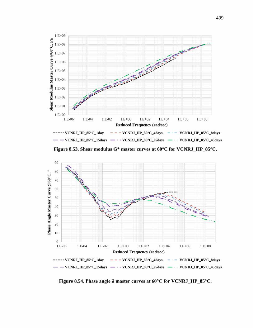
409
Figure 8.53. Shear modulus G* master curves at 60°C for VCNRJ_HP_85°C.
Figure 8.54. Phase angle δ master curves at 60°C for VCNRJ_HP_85°C.
1.E+00
1.E+01
1.E+02
1.E+03
1.E+04
1.E+05
1.E+06
1.E+07
1.E+08
1.E+09
1.E-06 1.E-04 1.E-02 1.E+00 1.E+02 1.E+04 1.E+06 1.E+08
Sh
ear
Mo
du
lus
Ma
ster
Cu
rve
@6
0°C
, P
a
Reduced Frequency (rad/sec)
VCNRJ_HP_85°C_1day VCNRJ_HP_85°C_4days VCNRJ_HP_85°C_8days
VCNRJ_HP_85°C_15days VCNRJ_HP_85°C_25days VCNRJ_HP_85°C_45days
0
10
20
30
40
50
60
70
80
90
1.E-06 1.E-04 1.E-02 1.E+00 1.E+02 1.E+04 1.E+06 1.E+08
Ph
ase
An
gle
Ma
ster
Cu
rve
@6
0°C
, °
Reduced Frequency (rad/sec)
VCNRJ_HP_85°C_1day VCNRJ_HP_85°C_4days VCNRJ_HP_85°C_8days
VCNRJ_HP_85°C_15days VCNRJ_HP_85°C_25days VCNRJ_HP_85°C_45days
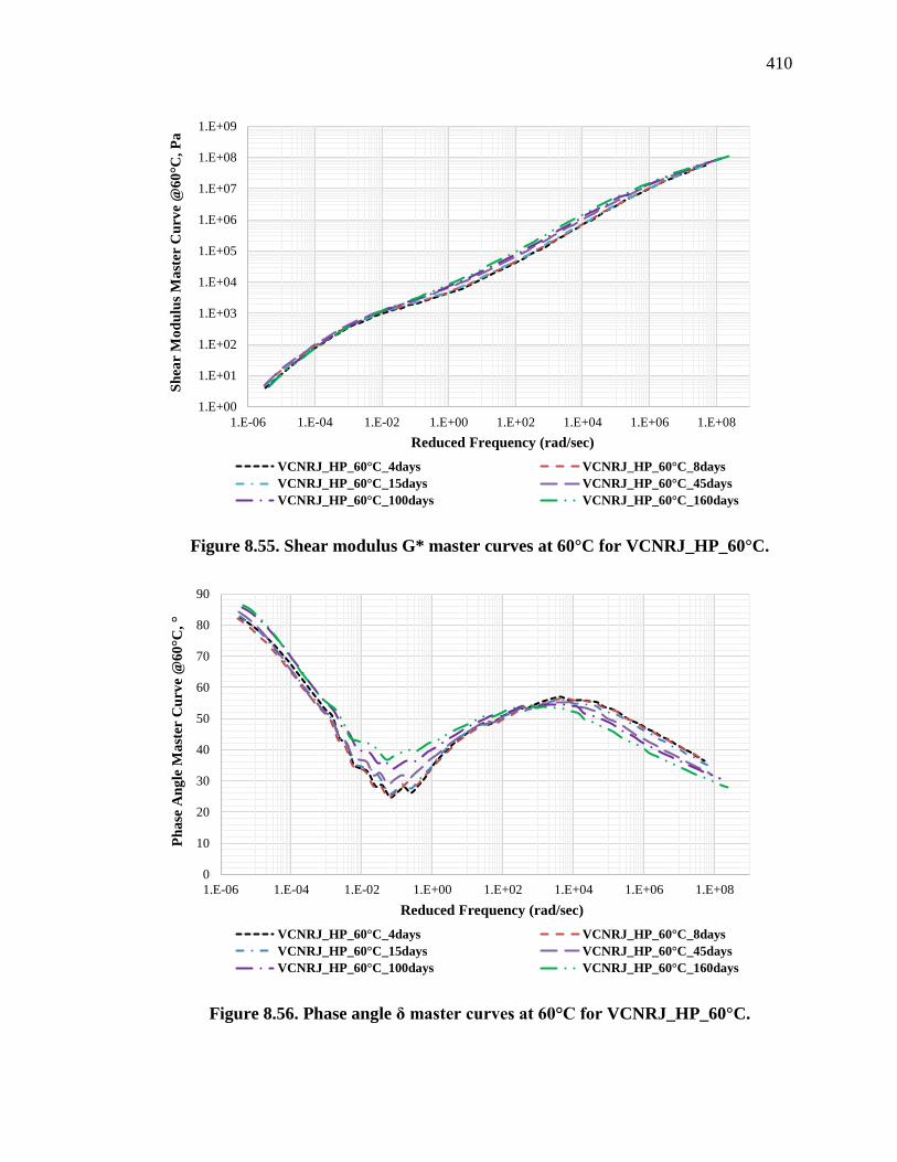
410
Figure 8.55. Shear modulus G* master curves at 60°C for VCNRJ_HP_60°C.
Figure 8.56. Phase angle δ master curves at 60°C for VCNRJ_HP_60°C.
1.E+00
1.E+01
1.E+02
1.E+03
1.E+04
1.E+05
1.E+06
1.E+07
1.E+08
1.E+09
1.E-06 1.E-04 1.E-02 1.E+00 1.E+02 1.E+04 1.E+06 1.E+08
Sh
ear
Mo
du
lus
Ma
ster
Cu
rve
@6
0°C
, P
a
Reduced Frequency (rad/sec)
VCNRJ_HP_60°C_4days VCNRJ_HP_60°C_8days
VCNRJ_HP_60°C_15days VCNRJ_HP_60°C_45days
VCNRJ_HP_60°C_100days VCNRJ_HP_60°C_160days
0
10
20
30
40
50
60
70
80
90
1.E-06 1.E-04 1.E-02 1.E+00 1.E+02 1.E+04 1.E+06 1.E+08
Ph
ase
An
gle
Ma
ster
Cu
rve
@6
0°C
, °
Reduced Frequency (rad/sec)
VCNRJ_HP_60°C_4days VCNRJ_HP_60°C_8days
VCNRJ_HP_60°C_15days VCNRJ_HP_60°C_45days
VCNRJ_HP_60°C_100days VCNRJ_HP_60°C_160days
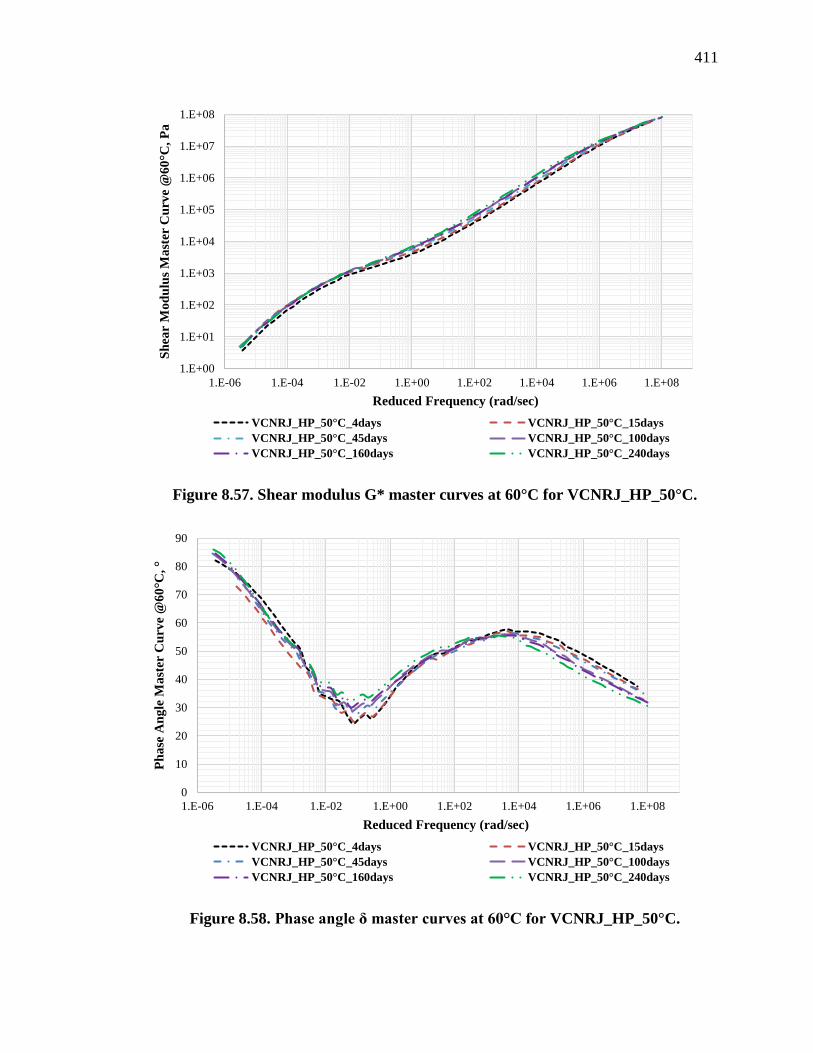
411
Figure 8.57. Shear modulus G* master curves at 60°C for VCNRJ_HP_50°C.
Figure 8.58. Phase angle δ master curves at 60°C for VCNRJ_HP_50°C.
1.E+00
1.E+01
1.E+02
1.E+03
1.E+04
1.E+05
1.E+06
1.E+07
1.E+08
1.E-06 1.E-04 1.E-02 1.E+00 1.E+02 1.E+04 1.E+06 1.E+08
Sh
ear
Mo
du
lus
Ma
ster
Cu
rve
@6
0°C
, P
a
Reduced Frequency (rad/sec)
VCNRJ_HP_50°C_4days VCNRJ_HP_50°C_15days
VCNRJ_HP_50°C_45days VCNRJ_HP_50°C_100days
VCNRJ_HP_50°C_160days VCNRJ_HP_50°C_240days
0
10
20
30
40
50
60
70
80
90
1.E-06 1.E-04 1.E-02 1.E+00 1.E+02 1.E+04 1.E+06 1.E+08
Ph
ase
An
gle
Ma
ster
Cu
rve
@6
0°C
, °
Reduced Frequency (rad/sec)
VCNRJ_HP_50°C_4days VCNRJ_HP_50°C_15days
VCNRJ_HP_50°C_45days VCNRJ_HP_50°C_100days
VCNRJ_HP_50°C_160days VCNRJ_HP_50°C_240days
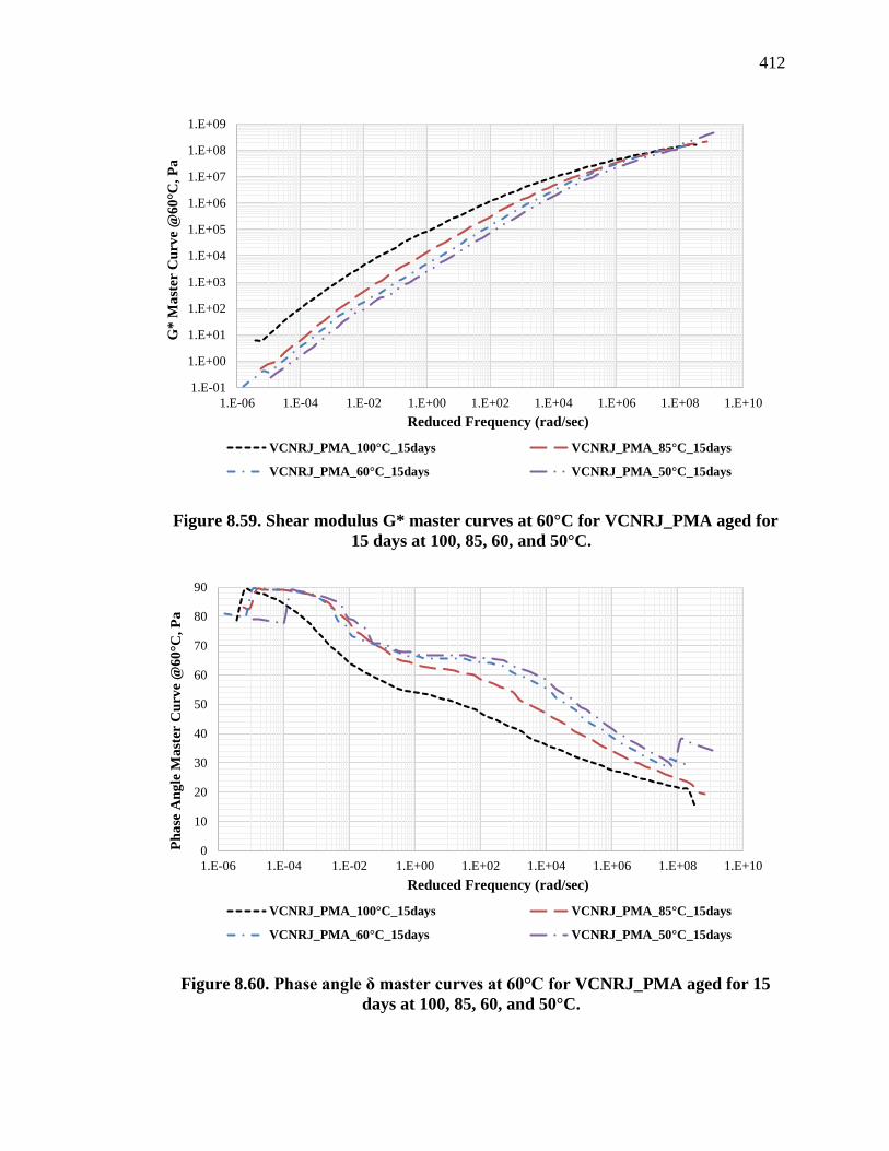
412
Figure 8.59. Shear modulus G* master curves at 60°C for VCNRJ_PMA aged for
15 days at 100, 85, 60, and 50°C.
Figure 8.60. Phase angle δ master curves at 60°C for VCNRJ_PMA aged for 15
days at 100, 85, 60, and 50°C.
1.E-01
1.E+00
1.E+01
1.E+02
1.E+03
1.E+04
1.E+05
1.E+06
1.E+07
1.E+08
1.E+09
1.E-06 1.E-04 1.E-02 1.E+00 1.E+02 1.E+04 1.E+06 1.E+08 1.E+10
G*
Ma
ster
Cu
rve
@6
0°C
, P
a
Reduced Frequency (rad/sec)
VCNRJ_PMA_100°C_15days VCNRJ_PMA_85°C_15days
VCNRJ_PMA_60°C_15days VCNRJ_PMA_50°C_15days
0
10
20
30
40
50
60
70
80
90
1.E-06 1.E-04 1.E-02 1.E+00 1.E+02 1.E+04 1.E+06 1.E+08 1.E+10
Ph
ase
An
gle
Ma
ster
Cu
rve
@6
0°C
, P
a
Reduced Frequency (rad/sec)
VCNRJ_PMA_100°C_15days VCNRJ_PMA_85°C_15days
VCNRJ_PMA_60°C_15days VCNRJ_PMA_50°C_15days

413
Figure 8.61. Shear modulus G* master curves at 60°C for VCNRJ_HP aged for 15
days at 100, 85, 60, and 50°C.
Figure 8.62. Phase angle δ master curves at 60°C for VCNRJ_HP aged for 15 days
at 100, 85, 60, and 50°C.
1.E+00
1.E+01
1.E+02
1.E+03
1.E+04
1.E+05
1.E+06
1.E+07
1.E+08
1.E-06 1.E-04 1.E-02 1.E+00 1.E+02 1.E+04 1.E+06 1.E+08
G*
Ma
ster
Cu
rve
@6
0°C
, P
a
Reduced Frequency (rad/sec)
VCNRJ_HP_100°C_15days VCNRJ_HP_85°C_15days
VCNRJ_HP_60°C_15days VCNRJ_HP_50°C_15days
0
10
20
30
40
50
60
70
80
90
1.E-06 1.E-04 1.E-02 1.E+00 1.E+02 1.E+04 1.E+06 1.E+08
Ph
ase
An
gle
Ma
ster
Cu
rve
@6
0°C
, P
a
Reduced Frequency (rad/sec)
VCNRJ_HP_100°C_15days VCNRJ_HP_85°C_15days
VCNRJ_HP_60°C_15days VCNRJ_HP_50°C_15days

414
Figure 8.63. Shear modulus G* master curves at 60°C for VCNRJ_PMA; Orginal,
RTFO, PAV20hrs, PAV40hrs, and PAV60hrs.
Figure 8.64. Phase angle δ master curves at 60°C for VCNRJ_PMA; Orginal,
RTFO, PAV20hrs, PAV40hrs, and PAV60hrs.
1.E-01
1.E+00
1.E+01
1.E+02
1.E+03
1.E+04
1.E+05
1.E+06
1.E+07
1.E+08
1.E+09
1.E-06 1.E-04 1.E-02 1.E+00 1.E+02 1.E+04 1.E+06 1.E+08 1.E+10
Sh
ear
Mo
du
lus
Ma
ster
Cu
rve
@6
0°C
, P
a
Reduced Frequency (rad/sec)
VCNRJ_PMA_ORIGINAL VCNRJ_PMA_RTFO
VCNRJ_PMA_PAV20hrs VCNRJ_PMA_PAV40hrs
VCNRJ_PMA_PAV60hrs
0
10
20
30
40
50
60
70
80
90
1.E-06 1.E-04 1.E-02 1.E+00 1.E+02 1.E+04 1.E+06 1.E+08 1.E+10
Ph
ase
An
gle
Ma
ster
Cu
rve
@6
0°C
, °
Reduced Frequency (rad/sec)
VCNRJ_PMA_ORIGINAL VCNRJ_PMA_RTFO
VCNRJ_PMA_PAV20hrs VCNRJ_PMA_PAV40hrs
VCNRJ_PMA_PAV60hrs

415
Figure 8.65. Shear modulus G* master curves at 60°C for VCNRJ_HP; Orginal,
RTFO, PAV20hrs, PAV40hrs, and PAV60hrs.
Figure 8.66. Phase angle δ master curves at 60°C for VCNRJ_HP; Orginal, RTFO,
PAV20hrs, PAV40hrs, and PAV60hrs.
1.E+00
1.E+01
1.E+02
1.E+03
1.E+04
1.E+05
1.E+06
1.E+07
1.E+08
1.E+09
1.E-06 1.E-04 1.E-02 1.E+00 1.E+02 1.E+04 1.E+06 1.E+08
Sh
ear
Mo
du
lus
Ma
ster
Cu
rve,
P
a
Reduced Frequency (rad/sec)
VCNRJ_HP_ORIGINAL VCNRJ_HP_RTFO VCNRJ_HP_PAV20hrs
VCNRJ_HP_PAV40hrs VCNRJ_HP_PAV60hrs
0
10
20
30
40
50
60
70
80
90
1.E-06 1.E-04 1.E-02 1.E+00 1.E+02 1.E+04 1.E+06 1.E+08
Ph
ase
An
gle
Ma
ster
Cu
rve
@6
0°C
, °
Reduced Frequency (rad/sec)
VCNRJ_HP_ORIGINAL VCNRJ_HP_RTFO VCNRJ_HP_PAV20hrs
VCNRJ_HP_PAV40hrs VCNRJ_HP_PAV60hrs

416
8.4.3 Evaluation of Multiple Chemical Functional Groups
After their respective aging durations, the asphalt binders were evaluated through FT-IR
spectroscopy measurements using ATR method. A minimum of two replicates FT-IR
spectra measurements were used to determine the average carbonyl area (CA), which is
again an indicator of the oxygen content of the binder by quantifying the carbonyl
functional group. It should be reminded that the CA is calculated as the area, expressed
in arbitrary units, between he IR absorption spectrum and the magnitude of the absorption
at 1,820 cm-1 used as baseline. This area is integrated from 1,650 to 1,820 cm-1
wavenumbers.
In this handout, a slight modification to the traditional methodology has been
utilized by focusing on the growth of the CA measurement rather than considering the CA
measurement outright. The carbonyl growth (CAg) is represented as the difference between
the CA at a given aging condition and the original CA measurement of the asphalt binder
otherwise known as CATank (simulated by the carbonyl of the asphalt binder evaluated at
the original unaged virgin state). By considering the CA measurements in this manner, any
influences of the magnitude of the CA measures on statistical significance determinations
will be nulled by CATank. Table 8.6, Table 8.7, Table 8.8, Table 8.9, and Table 8.10 show
the FT-IR measurements in terms of CA, CATank, and CAg measurements in addition to SO,
PM, AP, PTDBA, PVDBA, PCDBA, PA, and A ones (refer to Section 8.3.2.1 for the
definition and chemical significance of these parameters) for ERGON_PMA at its different
aging statuses (i.e., original, RTFO, PAV20hrs, PAV40hrs, and PAV60hrs, oven aged at
100°C, oven aged at 85°, oven aged at 60°C, and oven aged at 50°C). Table 8.11, Table
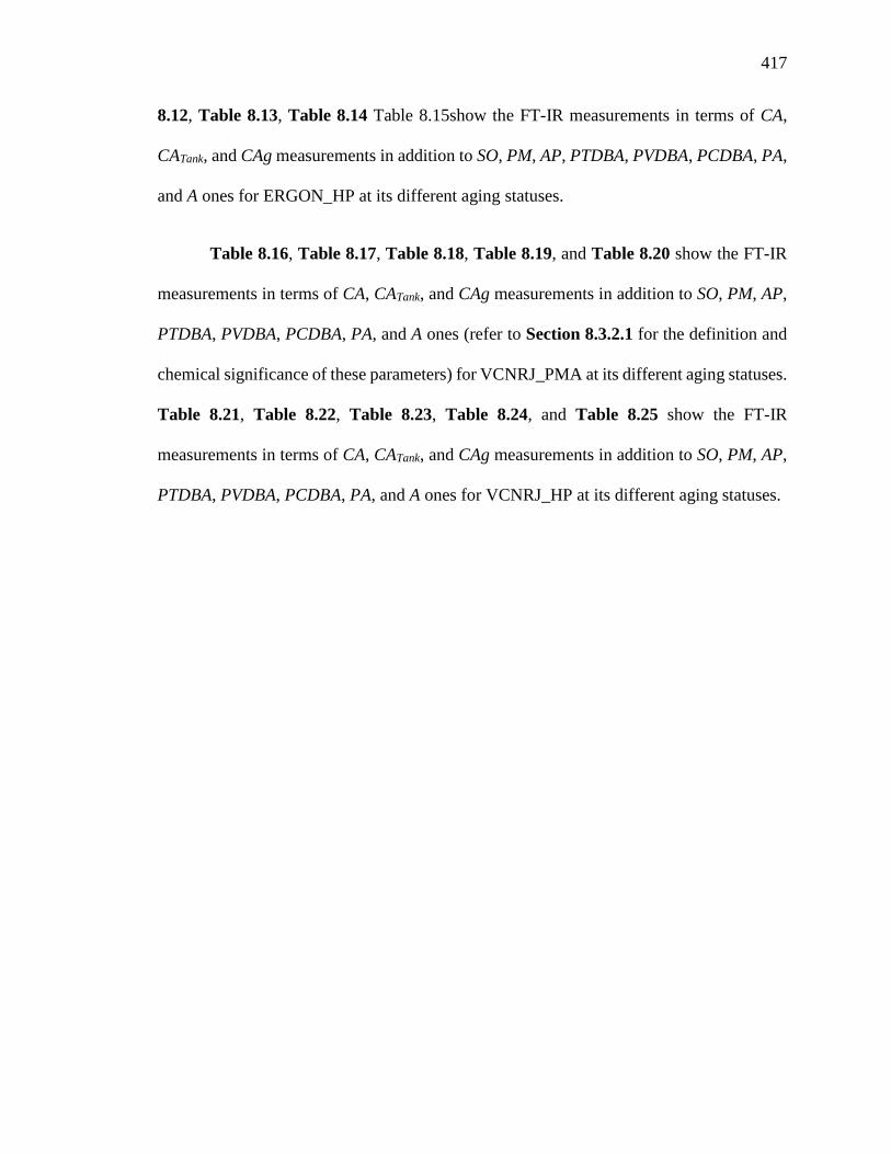
417
8.12, Table 8.13, Table 8.14 Table 8.15show the FT-IR measurements in terms of CA,
CATank, and CAg measurements in addition to SO, PM, AP, PTDBA, PVDBA, PCDBA, PA,
and A ones for ERGON_HP at its different aging statuses.
Table 8.16, Table 8.17, Table 8.18, Table 8.19, and Table 8.20 show the FT-IR
measurements in terms of CA, CATank, and CAg measurements in addition to SO, PM, AP,
PTDBA, PVDBA, PCDBA, PA, and A ones (refer to Section 8.3.2.1 for the definition and
chemical significance of these parameters) for VCNRJ_PMA at its different aging statuses.
Table 8.21, Table 8.22, Table 8.23, Table 8.24, and Table 8.25 show the FT-IR
measurements in terms of CA, CATank, and CAg measurements in addition to SO, PM, AP,
PTDBA, PVDBA, PCDBA, PA, and A ones for VCNRJ_HP at its different aging statuses.

418
Table 8.6. FT-IR Absorbance Measurements: ERGON_PMA; Original, RTFO, PAV20hrs, PAV40hrs, and PAV60hrs.
Binder ID Functional Group FT-IR Absorbance measurement (Arbitrary Units)
CA CATank CAg SO PM AP PTDBA PVDBA PCDBA PA P
Ergon_PMA_Original 0.000 0.000 0.000 0.000 2.984 0.651 0.264 0.000 0.166 0.116 0.014
Ergon_PMA_RTFO 0.058 0.000 0.058 0.009 3.080 0.634 0.246 0.000 0.167 0.116 0.014
Ergon_PMA_PAV20hrs 0.210 0.000 0.210 0.427 3.076 0.644 0.214 0.000 0.167 0.119 0.013
Ergon_PMA_PAV40hrs 0.573 0.000 0.573 0.721 2.971 0.633 0.181 0.000 0.161 0.117 0.015
Ergon_PMA_PAV60hrs 0.712 0.000 0.712 0.571 2.918 0.628 0.193 0.000 0.160 0.119 0.015
Table 8.7. FT-IR Absorbance Measurements: ERGON_PMA Aged @ 100°C for 6 Different Durations.
Binder ID Functional Group FT-IR Absorbance measurement (Arbitrary Units)
CA CATank CAg SO PM AP PTDBA PVDBA PCDBA PA P
Ergon_PMA_100°C_2hrs 0.047 0.000 0.047 0.001 2.958 0.651 0.253 0.000 0.164 0.118 0.100
Ergon_PMA_100°C_6hrs 0.036 0.000 0.036 0.071 3.114 0.653 0.245 0.000 0.169 0.118 0.013
Ergon_PMA_100°C_1day 0.083 0.000 0.083 0.198 3.071 0.644 0.230 0.000 0.166 0.121 0.014
Ergon_PMA_100°C_4days 0.234 0.000 0.234 0.506 3.059 0.648 0.202 0.000 0.165 0.117 0.014
Ergon_PMA_100°C_8days 0.423 0.000 0.423 0.664 3.040 0.654 0.192 0.000 0.162 0.117 0.012
Ergon_PMA_100°C_15days 0.597 0.000 0.597 0.780 2.858 0.570 0.159 0.000 0.148 0.108 0.011
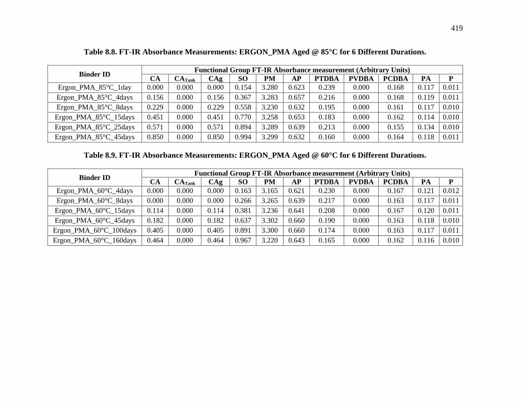
419
Table 8.8. FT-IR Absorbance Measurements: ERGON_PMA Aged @ 85°C for 6 Different Durations.
Binder ID Functional Group FT-IR Absorbance measurement (Arbitrary Units)
CA CATank CAg SO PM AP PTDBA PVDBA PCDBA PA P
Ergon_PMA_85°C_1day 0.000 0.000 0.000 0.154 3.280 0.623 0.239 0.000 0.168 0.117 0.011
Ergon_PMA_85°C_4days 0.156 0.000 0.156 0.367 3.283 0.657 0.216 0.000 0.168 0.119 0.011
Ergon_PMA_85°C_8days 0.229 0.000 0.229 0.558 3.230 0.632 0.195 0.000 0.161 0.117 0.010
Ergon_PMA_85°C_15days 0.451 0.000 0.451 0.770 3.258 0.653 0.183 0.000 0.162 0.114 0.010
Ergon_PMA_85°C_25days 0.571 0.000 0.571 0.894 3.289 0.639 0.213 0.000 0.155 0.134 0.010
Ergon_PMA_85°C_45days 0.850 0.000 0.850 0.994 3.299 0.632 0.160 0.000 0.164 0.118 0.011
Table 8.9. FT-IR Absorbance Measurements: ERGON_PMA Aged @ 60°C for 6 Different Durations.
Binder ID Functional Group FT-IR Absorbance measurement (Arbitrary Units)
CA CATank CAg SO PM AP PTDBA PVDBA PCDBA PA P
Ergon_PMA_60°C_4days 0.000 0.000 0.000 0.163 3.165 0.621 0.230 0.000 0.167 0.121 0.012
Ergon_PMA_60°C_8days 0.000 0.000 0.000 0.266 3.265 0.639 0.217 0.000 0.163 0.117 0.011
Ergon_PMA_60°C_15days 0.114 0.000 0.114 0.381 3.236 0.641 0.208 0.000 0.167 0.120 0.011
Ergon_PMA_60°C_45days 0.182 0.000 0.182 0.637 3.302 0.660 0.190 0.000 0.163 0.118 0.010
Ergon_PMA_60°C_100days 0.405 0.000 0.405 0.891 3.300 0.660 0.174 0.000 0.163 0.117 0.011
Ergon_PMA_60°C_160days 0.464 0.000 0.464 0.967 3.220 0.643 0.165 0.000 0.162 0.116 0.010

420
Table 8.10. FT-IR Absorbance Measurements: ERGON_PMA Aged @ 50°C for 6 Different Durations.
Binder ID Functional Group FT-IR Absorbance measurement (Arbitrary Units)
CA CATank CAg SO PM AP PTDBA PVDBA PCDBA PA P
Ergon_PMA_50°C_4days 0.000 0.000 0.000 0.102 3.003 0.613 0.237 0.000 0.164 0.117 0.016
Ergon_PMA_50°C_15days 0.065 0.000 0.065 0.249 3.040 0.605 0.218 0.000 0.166 0.120 0.014
Ergon_PMA_50°C_45days 0.170 0.000 0.170 0.457 3.128 0.648 0.193 0.000 0.157 0.114 0.012
Ergon_PMA_50°C_100days 0.230 0.000 0.230 0.644 3.212 0.656 0.191 0.000 0.168 0.121 0.011
Ergon_PMA_50°C_160days 0.328 0.000 0.328 0.756 3.069 0.653 0.176 0.000 0.163 0.116 0.013
Ergon_PMA_50°C_240days 0.381 0.000 0.381 0.869 3.055 0.653 0.164 0.000 0.159 0.115 0.012
Table 8.11. FT-IR Absorbance Measurements: ERGON_HP; Original, RTFO, PAV20hrs, PAV40hrs, and PAV60hrs.
Binder ID Functional Group FT-IR Absorbance measurement (Arbitrary Units)
CA CATank CAg SO PM AP PTDBA PVDBA PCDBA PA P
Ergon_HP_Original 0.000 0.000 0.000 0.000 2.857 0.620 0.228 0.342 0.124 0.340 0.028
Ergon_HP_RTFO 0.000 0.000 0.000 0.051 2.847 0.633 0.224 0.346 0.124 0.341 0.028
Ergon_HP_PAV20hrs 0.175 0.000 0.175 0.480 2.883 0.637 0.190 0.346 0.126 0.350 0.028
Ergon_HP_PAV40hrs 0.432 0.000 0.432 0.654 2.863 0.635 0.172 0.338 0.126 0.346 0.028
Ergon_HP_PAV60hrs 0.620 0.000 0.620 0.708 2.775 0.625 0.166 0.337 0.127 0.349 0.029

421
Table 8.12. FT-IR Absorbance Measurements: ERGON_HP Aged @ 100°C for 6 Different Durations.
Binder ID Functional Group FT-IR Absorbance measurement (Arbitrary Units)
CA CATank CAg SO PM AP PTDBA PVDBA PCDBA PA P
Ergon_HP_100°C_2hrs 0.000 0.000 0.000 0.046 3.049 0.637 0.220 0.353 0.127 0.351 0.025
Ergon_HP_100°C_6hrs 0.000 0.000 0.000 0.101 3.047 0.647 0.221 0.354 0.131 0.352 0.025
Ergon_HP_100°C_1day 0.036 0.000 0.036 0.238 3.037 0.643 0.201 0.354 0.129 0.355 0.025
Ergon_HP_100°C_4days 0.252 0.000 0.252 0.596 3.066 0.647 0.180 0.345 0.128 0.351 0.025
Ergon_HP_100°C_8days 0.326 0.000 0.326 0.638 2.906 0.623 0.173 0.332 0.129 0.339 0.025
Ergon_HP_100°C_15days 0.682 0.000 0.682 0.777 2.984 0.632 0.162 0.318 0.135 0.349 0.026
Table 8.13. FT-IR Absorbance Measurements: ERGON_HP Aged @ 85°C for 6 Different Durations.
Binder ID Functional Group FT-IR Absorbance measurement (Arbitrary Units)
CA CATank CAg SO PM AP PTDBA PVDBA PCDBA PA P
Ergon_HP_85°C_1day 0.000 0.000 0.000 0.169 2.943 0.637 0.213 0.351 0.131 0.351 0.027
Ergon_HP_85°C_4days 0.097 0.000 0.097 0.385 2.994 0.646 0.193 0.352 0.130 0.354 0.026
Ergon_HP_85°C_8days 0.160 0.000 0.160 0.567 3.084 0.644 0.179 0.348 0.127 0.351 0.024
Ergon_HP_85°C_15days 0.287 0.000 0.287 0.727 3.085 0.644 0.170 0.344 0.131 0.353 0.025
Ergon_HP_85°C_25days 0.442 0.000 0.442 0.773 3.110 0.645 0.168 0.339 0.131 0.353 0.024
Ergon_HP_85°C_45days 0.560 0.000 0.560 0.827 2.755 0.576 0.135 0.304 0.118 0.324 0.022

422
Table 8.14. FT-IR Absorbance Measurements: ERGON_HP Aged @ 60°C for 6 Different Durations.
Binder ID Functional Group FT-IR Absorbance measurement (Arbitrary Units)
CA CATank CAg SO PM AP PTDBA PVDBA PCDBA PA P
Ergon_HP_60°C_4days 0.000 0.000 0.000 0.197 3.031 0.639 0.208 0.354 0.132 0.354 0.027
Ergon_HP_60°C_8days 0.034 0.000 0.034 0.256 3.021 0.631 0.200 0.352 0.130 0.354 0.027
Ergon_HP_60°C_15days 0.099 0.000 0.099 0.368 2.985 0.649 0.194 0.354 0.131 0.356 0.027
Ergon_HP_60°C_45days 0.192 0.000 0.192 0.592 3.025 0.646 0.174 0.345 0.131 0.350 0.025
Ergon_HP_60°C_100days 0.280 0.000 0.280 0.768 2.923 0.642 0.161 0.346 0.129 0.357 0.027
Ergon_HP_60°C_160days 0.417 0.000 0.417 0.888 2.986 0.643 0.157 0.343 0.129 0.355 0.027
Table 8.15. FT-IR Absorbance Measurements: ERGON_HP Aged @ 50°C for 6 Different Durations.
Binder ID Functional Group FT-IR Absorbance measurement (Arbitrary Units)
CA CATank CAg SO PM AP PTDBA PVDBA PCDBA PA P
Ergon_HP_50°C_4days 0.000 0.000 0.000 0.127 3.083 0.634 0.213 0.354 0.129 0.355 0.024
Ergon_HP_50°C_15days 0.000 0.000 0.000 0.272 3.081 0.629 0.201 0.354 0.131 0.354 0.025
Ergon_HP_50°C_45days 0.126 0.000 0.126 0.411 3.005 0.633 0.181 0.332 0.125 0.338 0.023
Ergon_HP_50°C_100days 0.205 0.000 0.205 0.588 3.058 0.655 0.174 0.350 0.131 0.355 0.025
Ergon_HP_50°C_160days 0.243 0.000 0.243 0.690 3.056 0.655 0.167 0.350 0.131 0.356 0.026
Ergon_HP_50°C_240days 0.310 0.000 0.310 0.795 3.054 0.658 0.154 0.341 0.131 0.350 0.026

423
Table 8.16. FT-IR Absorbance Measurements: VCNRJ_PMA; Original, RTFO, PAV20hrs, PAV40hrs, and PAV60hrs.
Binder ID Functional Group FT-IR Absorbance measurement (Arbitrary Units)
CA CATank CAg SO PM AP PTDBA PVDBA PCDBA PA P
VCNRJ_PMA_Original 0.000 0.000 0.000 0.000 3.079 0.622 0.170 0.054 0.209 0.065 0.011
VCNRJ_PMA_RTFO 0.000 0.000 0.000 0.062 3.110 0.624 0.158 0.054 0.210 0.063 0.011
VCNRJ_PMA_PAV20hrs 0.207 0.000 0.207 0.489 3.077 0.615 0.124 0.050 0.204 0.062 0.012
VCNRJ_PMA_PAV40hrs 0.390 0.000 0.390 0.646 3.072 0.601 0.103 0.043 0.201 0.054 0.011
VCNRJ_PMA_PAV60hrs 0.696 0.000 0.696 0.617 3.040 0.610 0.113 0.047 0.203 0.055 0.010
Table 8.17. FT-IR Absorbance Measurements: VCNRJ_PMA Aged @ 100°C for 6 Different Durations.
Binder ID Functional Group FT-IR Absorbance measurement (Arbitrary Units)
CA CATank CAg SO PM AP PTDBA PVDBA PCDBA PA P
VCNRJ_PMA_100°C_2hrs 0.000 0.000 0.000 0.057 3.086 0.615 0.159 0.054 0.207 0.066 0.011
VCNRJ_PMA_100°C_6hrs 0.000 0.000 0.000 0.088 3.092 0.607 0.152 0.053 0.210 0.065 0.011
VCNRJ_PMA_100°C_1day 0.072 0.000 0.072 0.230 3.090 0.623 0.139 0.053 0.208 0.064 0.012
VCNRJ_PMA_100°C_4days 0.209 0.000 0.209 0.526 3.091 0.626 0.122 0.053 0.210 0.068 0.013
VCNRJ_PMA_100°C_8days 0.365 0.000 0.365 0.671 3.146 0.627 0.113 0.050 0.210 0.064 0.012
VCNRJ_PMA_100°C_15days 0.512 0.000 0.512 0.610 2.825 0.513 0.085 0.036 0.180 0.053 0.009

424
Table 8.18. FT-IR Absorbance Measurements: VCNRJ_PMA Aged @ 85°C for 6 Different Durations.
Binder ID Functional Group FT-IR Absorbance measurement (Arbitrary Units)
CA CATank CAg SO PM AP PTDBA PVDBA PCDBA PA P
VCNRJ_PMA_85°C_1day 0.000 0.000 0.000 0.154 3.049 0.593 0.147 0.053 0.207 0.064 0.011
VCNRJ_PMA_85°C_4days 0.064 0.000 0.064 0.407 3.132 0.624 0.125 0.050 0.206 0.063 0.010
VCNRJ_PMA_85°C_8days 0.216 0.000 0.216 0.554 3.058 0.628 0.114 0.052 0.204 0.069 0.011
VCNRJ_PMA_85°C_15days 0.315 0.000 0.315 0.723 3.106 0.630 0.109 0.049 0.208 0.066 0.011
VCNRJ_PMA_85°C_25days 0.535 0.000 0.535 0.795 3.043 0.622 0.100 0.047 0.207 0.065 0.012
VCNRJ_PMA_85°C_45days 0.885 0.000 0.885 0.857 3.219 0.620 0.080 0.042 0.201 0.061 0.009
Table 8.19. FT-IR Absorbance Measurements: VCNRJ_PMA Aged @ 60°C for 6 Different Durations.
Binder ID Functional Group FT-IR Absorbance measurement (Arbitrary Units)
CA CATank CAg SO PM AP PTDBA PVDBA PCDBA PA P
VCNRJ_PMA_60°C_4days 0.000 0.000 0.000 0.187 3.086 0.614 0.142 0.052 0.204 0.063 0.009
VCNRJ_PMA_60°C_8days 0.055 0.000 0.055 0.270 3.145 0.621 0.136 0.052 0.206 0.063 0.009
VCNRJ_PMA_60°C_15days 0.072 0.000 0.072 0.367 3.103 0.617 0.127 0.053 0.204 0.060 0.009
VCNRJ_PMA_60°C_45days 0.141 0.000 0.141 0.549 3.061 0.613 0.117 0.051 0.202 0.063 0.010
VCNRJ_PMA_60°C_100days 0.312 0.000 0.312 0.734 3.076 0.636 0.105 0.051 0.208 0.065 0.010
VCNRJ_PMA_60°C_160days 0.420 0.000 0.420 0.844 3.036 0.627 0.089 0.046 0.206 0.063 0.011

425
Table 8.20. FT-IR Absorbance Measurements: VCNRJ_PMA Aged @ 50°C for 6 Different Durations.
Binder ID Functional Group FT-IR Absorbance measurement (Arbitrary Units)
CA CATank CAg SO PM AP PTDBA PVDBA PCDBA PA P
VCNRJ_PMA_50°C_4days 0.000 0.000 0.000 0.131 3.064 0.610 0.149 0.055 0.208 0.064 0.010
VCNRJ_PMA_50°C_15days 0.021 0.000 0.021 0.275 3.134 0.628 0.131 0.054 0.209 0.063 0.100
VCNRJ_PMA_50°C_45days 0.076 0.000 0.076 0.435 3.123 0.626 0.121 0.053 0.207 0.063 0.010
VCNRJ_PMA_50°C_100days 0.171 0.000 0.171 0.603 3.177 0.631 0.110 0.051 0.202 0.062 0.009
VCNRJ_PMA_50°C_160days 0.203 0.000 0.203 0.632 3.187 0.629 0.109 0.051 0.207 0.065 0.008
VCNRJ_PMA_50°C_240days 0.289 0.000 0.289 0.777 3.125 0.629 0.100 0.050 0.203 0.063 0.008
Table 8.21. FT-IR Absorbance Measurements: VCNRJ_HP; Original, RTFO, PAV20hrs, PAV40hrs, and PAV60hrs.
Binder ID Functional Group FT-IR Absorbance measurement (Arbitrary Units)
CA CATank CAg SO PM AP PTDBA PVDBA PCDBA PA P
VCNRJ_HP_Original 0.000 0.000 0.000 0.000 2.729 0.565 0.249 0.354 0.192 0.350 0.030
VCNRJ_HP_RTFO 0.000 0.000 0.000 0.023 2.726 0.560 0.238 0.352 0.185 0.350 0.030
VCNRJ_HP_PAV20hrs 0.231 0.000 0.231 0.424 2.669 0.570 0.205 0.343 0.189 0.348 0.028
VCNRJ_HP_PAV40hrs 0.351 0.000 0.351 0.533 2.709 0.562 0.192 0.340 0.188 0.348 0.029
VCNRJ_HP_PAV60hrs 0.619 0.000 0.619 0.398 2.673 0.554 0.195 0.323 0.189 0.343 0.030

426
Table 8.22. FT-IR Absorbance Measurements: VCNRJ_HP Aged @ 100°C for 6 Different Durations.
Binder ID Functional Group FT-IR Absorbance measurement (Arbitrary Units)
CA CATank CAg SO PM AP PTDBA PVDBA PCDBA PA P
VCNRJ_HP_100°C_2hrs 0.000 0.000 0.000 0.077 2.873 0.561 0.237 0.351 0.189 0.347 0.028
VCNRJ_HP_100°C_6hrs 0.000 0.000 0.000 0.121 2.957 0.560 0.233 0.346 0.190 0.349 0.025
VCNRJ_HP_100°C_1day 0.046 0.000 0.046 0.220 2.991 0.573 0.225 0.349 0.195 0.347 0.026
VCNRJ_HP_100°C_4days 0.203 0.000 0.203 0.450 3.017 0.585 0.213 0.347 0.192 0.354 0.026
VCNRJ_HP_100°C_8days 0.363 0.000 0.363 0.536 3.008 0.581 0.203 0.338 0.193 0.355 0.026
VCNRJ_HP_100°C_15days 0.619 0.000 0.619 0.584 2.822 0.550 0.177 0.320 0.187 0.348 0.026
Table 8.23. FT-IR Absorbance Measurements: VCNRJ_HP Aged @ 85°C for 6 Different Durations.
Binder ID Functional Group FT-IR Absorbance measurement (Arbitrary Units)
CA CATank CAg SO PM AP PTDBA PVDBA PCDBA PA P
VCNRJ_HP_85°C_1day 0.000 0.000 0.000 0.132 2.692 0.559 0.232 0.355 0.190 0.353 0.025
VCNRJ_HP_85°C_4days 0.046 0.000 0.046 0.298 2.677 0.566 0.215 0.347 0.189 0.349 0.034
VCNRJ_HP_85°C_8days 0.110 0.000 0.110 0.445 2.796 0.576 0.206 0.348 0.190 0.355 0.031
VCNRJ_HP_85°C_15days 0.343 0.000 0.343 0.640 2.970 0.574 0.187 0.340 0.194 0.351 0.028
VCNRJ_HP_85°C_25days 0.465 0.000 0.465 0.603 2.818 0.573 0.188 0.335 0.189 0.350 0.030
VCNRJ_HP_85°C_45days 0.718 0.000 0.718 0.630 2.756 0.559 0.168 0.313 0.188 0.345 0.027

427
Table 8.24. FT-IR Absorbance Measurements: VCNRJ_HP Aged @ 60°C for 6 Different Durations.
Binder ID Functional Group FT-IR Absorbance measurement (Arbitrary Units)
CA CATank CAg SO PM AP PTDBA PVDBA PCDBA PA P
VCNRJ_HP_60°C_4days 0.000 0.000 0.000 0.130 2.709 0.553 0.235 0.349 0.193 0.351 0.030
VCNRJ_HP_60°C_8days 0.000 0.000 0.000 0.207 2.736 0.566 0.224 0.349 0.189 0.347 0.031
VCNRJ_HP_60°C_15days 0.033 0.000 0.033 0.279 2.761 0.568 0.220 0.347 0.191 0.348 0.031
VCNRJ_HP_60°C_45days 0.126 0.000 0.126 0.449 2.839 0.577 0.205 0.349 0.192 0.354 0.030
VCNRJ_HP_60°C_100days 0.204 0.000 0.204 0.577 2.759 0.569 0.193 0.340 0.189 0.350 0.030
VCNRJ_HP_60°C_160days 0.346 0.000 0.346 0.659 2.714 0.568 0.185 0.338 0.188 0.349 0.033
Table 8.25. FT-IR Absorbance Measurements: VCNRJ_HP Aged @ 50°C for 6 Different Durations.
Binder ID Functional Group FT-IR Absorbance measurement (Arbitrary Units)
CA CATank CAg SO PM AP PTDBA PVDBA PCDBA PA P
VCNRJ_HP_50°C_4days 0.000 0.000 0.000 0.111 2.733 0.568 0.231 0.351 0.191 0.345 0.031
VCNRJ_HP_50°C_15days 0.000 0.000 0.000 0.208 2.772 0.578 0.223 0.355 0.190 0.352 0.031
VCNRJ_HP_50°C_45days 0.014 0.000 0.014 0.320 2.742 0.571 0.213 0.350 0.190 0.349 0.031
VCNRJ_HP_50°C_100days 0.088 0.000 0.088 0.434 2.707 0.572 0.203 0.344 0.187 0.349 0.032
VCNRJ_HP_50°C_160days 0.128 0.000 0.128 0.521 2.724 0.571 0.201 0.347 0.189 0.350 0.031
VCNRJ_HP_50°C_240days 0.199 0.000 0.199 0.616 2.745 0.574 0.189 0.344 0.189 0.352 0.031

428
8.4.4 Low Shear Viscosity Rheological Index
Two replicate binders were tested on a DSR to determine the rheological parameters
utilized in this study. The first rheological parameters to be evaluated is the LSV of the
binders at their respective aging states. The value of LSV and CAg are combined to present
the HS parameters in a semi-log plot as shown in Figure 8.67. It should be mentioned that
the oxidation levels in this analysis were represented as the increase in the carbonyl
functional group or carbonyl growth labeled as CAg, from the original binder condition
(i.e., CATank). A consideration of the relative comparisons between the measured LSV
values of the evaluated binders (i.e., PMA vs. HP, ERGON vs. VCNRJ) generally indicated
a difference in the LSV values as a function of age. This finding is well known as the
hardening susceptibility (HS) and is typically understood to be binder specific. Further
general observations note that the overall CAg values differ with the same degree of aging.
It appears that the SBS high modification of the HP asphalt binder has led to an overall
increase in the magnitude of the oxidation growth due to the same oven aging conditions
of temperature and duration i.e., the x-axis exhibits a larger magnitude of oxidation with
the highly modified asphalt binder. This findings may not confirm with previous researchs,
however, it should be reminded that the HP binder and its control PMA asphalt binders
supplied from each source did not have the same base asphalt binder (i.e., PG52-28 for HP
vs. PG64-22 for PMA from ERGON, and PG52-28 for HP vs PG67-22 for PMA from
VCNRJ). The overall range of CAg was increased with the more modification for HP
binders as compared with the PMA ones. Essentially, the addition of the SBS polymer
dilutes the asphalt binder as whole since the SBS does not oxidize, at least not in carbonyl
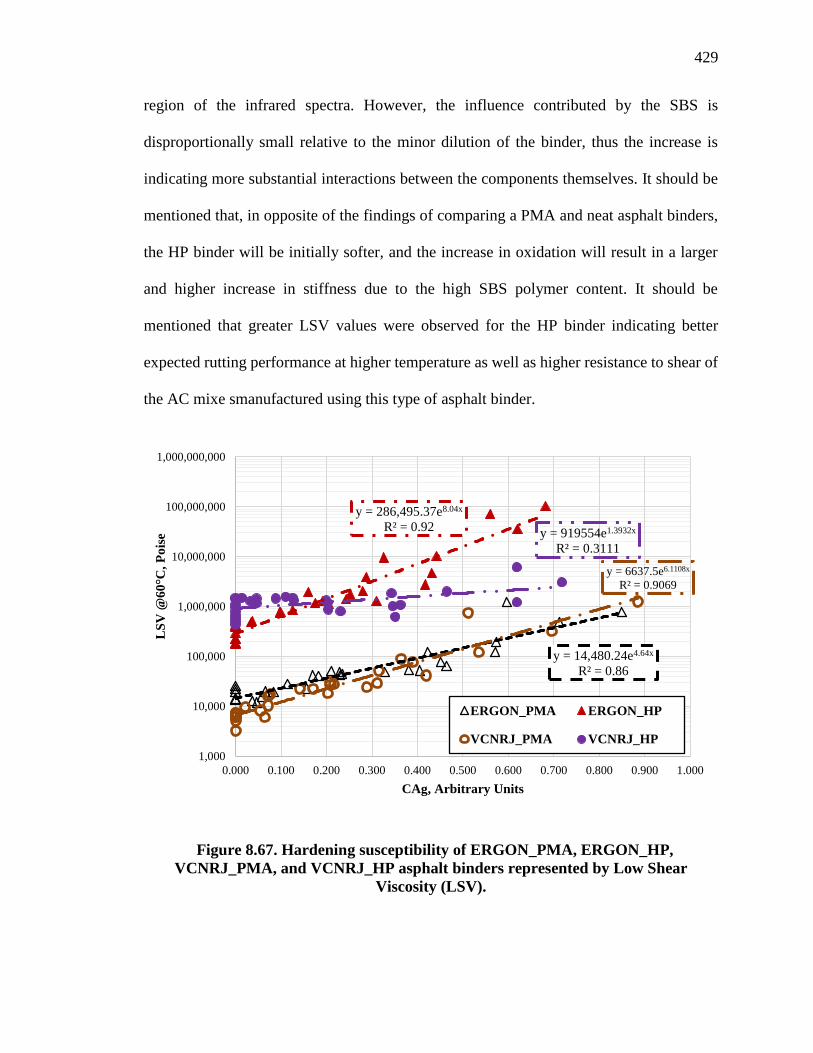
429
region of the infrared spectra. However, the influence contributed by the SBS is
disproportionally small relative to the minor dilution of the binder, thus the increase is
indicating more substantial interactions between the components themselves. It should be
mentioned that, in opposite of the findings of comparing a PMA and neat asphalt binders,
the HP binder will be initially softer, and the increase in oxidation will result in a larger
and higher increase in stiffness due to the high SBS polymer content. It should be
mentioned that greater LSV values were observed for the HP binder indicating better
expected rutting performance at higher temperature as well as higher resistance to shear of
the AC mixe smanufactured using this type of asphalt binder.
Figure 8.67. Hardening susceptibility of ERGON_PMA, ERGON_HP,
VCNRJ_PMA, and VCNRJ_HP asphalt binders represented by Low Shear
Viscosity (LSV).
y = 14,480.24e4.64x
R² = 0.86
y = 286,495.37e8.04x
R² = 0.92
y = 6637.5e6.1108x
R² = 0.9069
y = 919554e1.3932x
R² = 0.3111
1,000
10,000
100,000
1,000,000
10,000,000
100,000,000
1,000,000,000
0.000 0.100 0.200 0.300 0.400 0.500 0.600 0.700 0.800 0.900 1.000
LS
V @
60
°C,
Po
ise
CAg, Arbitrary Units
ERGON_PMA ERGON_HP
VCNRJ_PMA VCNRJ_HP

430
8.4.5 DSR Function (DSRFn) and Glover-Rowe Parameter (G-R)
Further oxidation studies have been conducted utilizing the rheological measure defined as
the DSR Function (DSRFn), which has later been represented as the Glover-Rowe
parameter (G-R). It should be mentioned that the mathematical functions of these
parameters were in detail presented in previous sections of this chapter. These measures
have shown to correlate well with ductility measures and thus cracking performance as
well as binder oxidation levels (Raun et al., 2003). However, there have also been certain
limitations observed, particularly when correlations were attempted with conventionally
and highly modified asphalt binders (Morian et al., 2013). Traditionally, the DSRFn is
reported as a single point measurement at 15°C and a frequency of 0.005 rad/s. To make
efficient use of the G* isotherms previously produced on the evaluated four asphalt binders
(i.e., 2 PMA vs. 2 HP), the DSRFn of the evaluated binders were converted and presented
at three temperatures in addition to 15°C, binder specific and related temperatures:
PG_Low + 43°C, PG_Mid, and Int_Temp. Table 8.26 summarizes the temperatures for
the four evaluated asphalt binders. Figure 8.68, Figure 8.69, Figure 8.70, and Figure 8.71
show the DSRFn of the four evaluated asphalt binders at 15°C, PG_Low+43°C, PG_Mid,
and Int_Temp, respectively.
Consideration of the DSRFn results indicated a different relative comparison
depending on the shifting temperatures. The HP binders showed a lower slope of the
DSRFn-CAg curve when compared with its corresponding control PMA binders for the
four evaluated temperatures. Although the DSRFn of polymer modified binders in general

431
was noted to not correlate particularly well with ductility (Glover et al., 2005), the measure
has been utilized to characterize the HS behavior of asphalt binder in sufficient fashion.
Table 8.26. Evaluation Temperatures of DSRFn, and G-R Parameters for PMA and
HP Asphalt Binders.
Binder ID Evaluation Temperature (°C)
PG_Low+43°C PG_Mid Int_Temp
ERGON_PMA 18.3 25.9 19.3
ERGON_HP 9.5 30.0 13.6
VCNRJ_PMA 18.7 25.9 22.9
VCNRJ_HP 13.0 34.0 13.7
Figure 8.68. Hardening susceptibility of ERGON_PMA, ERGON_HP,
VCNRJ_PMA, and VCNRJ_HP asphalt binders represented by DSRFn at 15°C.
y = 44.26e8.57x
R² = 0.83
y = 115.20e6.40x
R² = 0.92
y = 85.44e7.4378x
R² = 0.6323
y = 63.666e5.3702x
R² = 0.8502
1
10
100
1,000
10,000
100,000
1,000,000
0.000 0.100 0.200 0.300 0.400 0.500 0.600 0.700 0.800 0.900 1.000
DS
RF
n @
15
°C &
0.0
05
ra
d/s
CAg, Arbitrary Units
ERGON_PMA ERGON_HP
VCNRJ_PMA VCNRJ_HP

432
Figure 8.69. Hardening susceptibility of ERGON_PMA, ERGON_HP,
VCNRJ_PMA, and VCNRJ_HP asphalt binders represented by DSRFn at
PG_Low+43°C.
Figure 8.70. Hardening susceptibility of ERGON_PMA, ERGON_HP,
VCNRJ_PMA, and VCNRJ_HP asphalt binders represented by DSRFn at PG_Mid.
y = 23.12e7.76x
R² = 0.94
y = 234.40e6.87x
R² = 0.92
y = 37.622e7.4141x
R² = 0.6641
y = 76.088e6.0274x
R² = 0.8441
1
10
100
1,000
10,000
100,000
0.000 0.100 0.200 0.300 0.400 0.500 0.600 0.700 0.800 0.900 1.000
DS
RF
n @
PG
_L
ow
+4
3°C
& 0
.00
5 r
ad
/s
CAg, Arbitrary Units
ERGON_PMA ERGON_HP
VCNRJ_PMA VCNRJ_HP
y = 5.82e7.24x
R² = 0.94
y = 26.12e5.63x
R² = 0.92
y = 8.8093e7.1874x
R² = 0.6979
y = 70.843e5.8813x
R² = 0.8465
1
10
100
1,000
10,000
0.000 0.100 0.200 0.300 0.400 0.500 0.600 0.700 0.800 0.900 1.000
DS
RF
n @
PG
_M
id &
0.0
05
ra
d/s
CAg, Arbitrary Units
ERGON_PMA ERGON_HP
VCNRJ_PMA VCNRJ_HP

433
Figure 8.71. Hardening susceptibility of ERGON_PMA, ERGON_HP,
VCNRJ_PMA, and VCNRJ_HP asphalt binders represented by DSRFn at
Int_Temp.
Figure 8.72, Figure 8.73, Figure 8.74, and Figure 8.75 shows the G-R parameters
of the four evaluated asphalt binders at 15°C, PG_Low+43°C, PG_Mid, and Int_Temp,
respectively. Each data point plotted in these figures represents a specific asphalt binder
condition in terms of temperature and time (i.e. combinations defined earlier). Lower
slopes (i.e., HS) were observed for the HP asphalt binder when compared with its control
PMA asphalt binder indicating a lower change in stiffness for the same change in carbonyl
content (i.e., oxidation).
y = 19.04e7.70x
R² = 0.94
y = 135.05e6.54x
R² = 0.92
y = 15.478e7.2869x
R² = 0.6824y = 70.843e5.8813x
R² = 0.8465
1
10
100
1,000
10,000
100,000
0.000 0.100 0.200 0.300 0.400 0.500 0.600 0.700 0.800 0.900 1.000
DS
RF
n @
Int-
Tem
p &
0.0
05
ra
d/s
CAg, Arbitrary Units
ERGON_PMA ERGON_HP
VCNRJ_PMA VCNRJ_HP

434
Figure 8.72. Hardening susceptibility of ERGON_PMA, ERGON_HP,
VCNRJ_PMA, and VCNRJ_HP asphalt binders represented by G-R at 15°C.
Figure 8.73. Hardening susceptibility of ERGON_PMA, ERGON_HP,
VCNRJ_PMA, and VCNRJ_HP asphalt binders represented by G-R at
PG_Low+43°C.
y = 9,567.73e8.24x
R² = 0.89
y = 23,040.26e6.40x
R² = 0.92
y = 13546e7.9292x
R² = 0.7644
y = 12733e5.3702x
R² = 0.8502
100
1,000
10,000
100,000
1,000,000
10,000,000
100,000,000
0.000 0.100 0.200 0.300 0.400 0.500 0.600 0.700 0.800 0.900
G-R
@1
5°C
& 0
.00
5, P
a
CAg, Arbitrary Units
ERGON_PMA ERGON_HP
VCNRJ_PMA VCNRJ_HP
G-R = 600 kPa
G-R = 180 kPa
y = 4,820.92e7.97x
R² = 0.90
y = 46,880.11e6.87x
R² = 0.92
y = 5978.4e7.895x
R² = 0.7941
y = 15218e6.0274x
R² = 0.8441
100
1,000
10,000
100,000
1,000,000
10,000,000
0.000 0.100 0.200 0.300 0.400 0.500 0.600 0.700 0.800 0.900
G-R
@P
G_
Lo
w+
43
°C &
0.0
05
, P
a
CAg, Arbitrary Units
ERGON_PMA ERGON_HP
VCNRJ_PMA VCNRJ_HP
G-R = 600 kPa
G-R = 180 kPa

435
Figure 8.74. Hardening susceptibility of ERGON_PMA, ERGON_HP,
VCNRJ_PMA, and VCNRJ_HP asphalt binders represented by G-R at PG_Mid.
Figure 8.75. Hardening susceptibility of ERGON_PMA, ERGON_HP,
VCNRJ_PMA, and VCNRJ_HP asphalt binders represented by G-R at Int_Temp.
y = 1,243.89e7.57x
R² = 0.82
y = 5,214.34e5.62x
R² = 0.91
y = 1403.1e7.6576x
R² = 0.8296
y = 3520.3e3.617x
R² = 0.7005
100
1,000
10,000
100,000
1,000,000
10,000,000
0.000 0.100 0.200 0.300 0.400 0.500 0.600 0.700 0.800 0.900
G-R
@P
G_
Mid
& 0
.00
5, P
a
CAg, Arbitrary Units
ERGON_PMA ERGON_HP
VCNRJ_PMA VCNRJ_HP
G-R = 600 kPa
G-R = 180 kPa
y = 3,984.64e7.93x
R² = 0.89
y = 27,009.08e6.54x
R² = 0.92
y = 2464.1e7.7593x
R² = 0.8133
y = 14169e5.8813x
R² = 0.8465
100
1,000
10,000
100,000
1,000,000
10,000,000
0.000 0.100 0.200 0.300 0.400 0.500 0.600 0.700 0.800 0.900
G-R
@In
t_T
emp
& 0
.00
5, P
a
CAg, Arbitrary Units
ERGON_PMAERGON_HPVCNRJ_PMA
G-R = 600 kPa
G-R = 180 kPa
436
8.4.6 Analysis of Black-Space Diagram
Figure 8.76, Figure 8.77, Figure 8.78, and Figure 8.79 show the black space diagram of
the four evaluated asphalt binders at 15°C, PG_Low+43°C, PG_Mid, and Int_Temp,
respectively, with the G-R at 180 kPa, G-R at 600 kPa, G*/sinδ ≥ 2.2 kPa, and G*sinδ ≤
5,000 kPa. Each data point plotted in these figures represents a specific asphalt binder
condition in terms of temperature and time (i.e. combinations defined earlier).
It is anticipated that lower G* and lower δ represent lower susceptibility to long-
term aging. In addition, a steeper slope between G* and δ represents lower susceptibility
to long-term aging. In other words, a steep curve located closer to the left side of the chart
indicates lower susceptibility to long-term aging.
The data presented show that the HP asphalt binder (for example the Ergon one) is
less susceptible to long-term aging when compared with its control PMA asphalt binder
supplied from the same source at the four temperatures of evaluation. Furthermore, the data
show that the PMA binder was the first to reach the G-R cracking criterion of 600 kPa in
all cases.

437
Figure 8.76. Black space diagram of ERGON_PMA, ERGON_HP, VCNRJ_PMA,
and VCNRJ_HP asphalt binders at 15°C.
Figure 8.77. Black space diagram of ERGON_PMA, ERGON_HP, VCNRJ_PMA,
and VCNRJ_HP asphalt binders at PG_Low+43°C.
100
1,000
10,000
100,000
1,000,000
10,000,000
100,000,000
0 10 20 30 40 50 60 70 80 90
G*
@1
5°C
& 0
.00
5 r
ad
/s,
Pa
Phase Angle, °
ERGON_PMA ERGON_HP VCNRJ_PMAVCNRJ_HP G-R at 180 kPa G-R at 600 kPaG*/sinδ ≥ 2.2 kPa G*sinδ ≤ 5000 kPa
100
1,000
10,000
100,000
1,000,000
10,000,000
100,000,000
0 10 20 30 40 50 60 70 80 90
G*
@P
G_
Lo
w+
43
°C &
0.0
05
ra
d/s
, P
a
Phase Angle, °
ERGON_PMA ERGON_HP VCNRJ_PMAVCNRJ_HP G-R at 180 kPa G-R at 600 kPaG*/sinδ ≥ 2.2 kPa G*sinδ ≤ 5000 kPa

438
Figure 8.78. Black space diagram of ERGON_PMA, ERGON_HP, VCNRJ_PMA,
and VCNRJ_HP asphalt binders at PG_Mid.
Figure 8.79. Black space diagram of ERGON_PMA, ERGON_HP, VCNRJ_PMA,
and VCNRJ_HP asphalt binders at Int_Temp.
100
1,000
10,000
100,000
1,000,000
10,000,000
100,000,000
0 10 20 30 40 50 60 70 80 90
G*
@P
G_
Mid
& 0
.00
5 r
ad
/s,
Pa
Phase Angle, °
ERGON_PMA ERGON_HP VCNRJ_PMAVCNRJ_HP G-R at 180 kPa G-R at 600 kPaG*/sinδ ≥ 2.2 kPa G*sinδ ≤ 5000 kPa
100
1,000
10,000
100,000
1,000,000
10,000,000
100,000,000
0 10 20 30 40 50 60 70 80 90
G*
@In
t_T
emp
& 0
.00
5 r
ad
/s,
Pa
Phase Angle, °
ERGON_PMA ERGON_HP VCNRJ_PMAVCNRJ_HP G-R at 180 kPa G-R at 600 kPaG*/sinδ ≥ 2.2 kPa G*sinδ ≤ 5000 kPa

439
8.4.7 Crossover Modulus, Frequency, and Temperature
Figure 8.80 and Figure 8.81 show the hardening susceptibility of the PMA asphalt binders
(i.e., ERGON and VCNRJ) in terms of crossover modulus, crossover frequency, and
crossover temperature. Both PMA binders indicate reduction in the G*c as would be
expected with increased oxidation, noting the definition of G*c is based upon the phase
angle of 45°.Further consideration of the crossover frequency (fc), which is the shifted
frequency where G*c is determined (i.e., in this case at 25°C), likewise shows a reduction
with increased oxidation. Both of these observations generally indicate a stiffening and loss
of flexibility or viscous component with increased oxidation, i.e. shift of the master curves
to higher modulus values and lower frequencies for a given reference temperature.
When it comes to HP asphalt binders, with the inverted N-shape of the phase angle
master curves, possible crossover frequencies and corresponding G*c may exist at the same
reference temperature as illustrated in Figure 8.82. The data illustrated in this figure show
the possible existence of a low, intermediate, and high crossover frequencies and by that
corresponding G*c at a given reference temperature.

440
Figure 8.80. Hardening susceptibility of ERGON_PMA, and VCNRJ_PMA asphalt
binders represented by Crossover Modulus and Crossover frequency @25°C.
y = 21,319,477.36e-3.14x
R² = 0.90
y = 25,459,594.15e-3.85x
R² = 0.91
y = 837.57e-12.91x
R² = 0.94
y = 1,627.78e-14.14x
R² = 0.96
0.0
0.1
1.0
10.0
100.0
1,000.0
10,000.0
1,000,000
10,000,000
100,000,000
1,000,000,000
0.000 0.200 0.400 0.600 0.800 1.000
Cro
sso
ver
Fre
qu
ency
(fc
) @
25
°C,
rad
/s
Cro
sso
ver
Mo
du
lus
(G*
c) @
25
°C,
Pa
CAg, Arbitrary Units
ERGON_PMA Oven Aged, G*c
ERGON_PMA Orig - RTFO - PAVs, G*c
ERGON_PMA Oven Aged, fc
ERGON_PMA Orig - RTFO - PAVs, fc
Expon. (ERGON_PMA Oven Aged, G*c)
Expon. (ERGON_PMA Orig - RTFO - PAVs, G*c)
Expon. (ERGON_PMA Oven Aged, fc)
Expon. (ERGON_PMA Orig - RTFO - PAVs, fc)
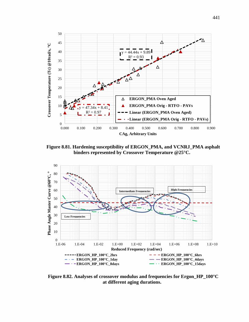
441
Figure 8.81. Hardening susceptibility of ERGON_PMA, and VCNRJ_PMA asphalt
binders represented by Crossover Temperature @25°C.
Figure 8.82. Analyses of crossover modulus and frequencies for Ergon_HP_100°C
at different aging durations.
y = 44.44x + 9.89
R² = 0.93
y = 47.34x + 8.41
R² = 0.97
0
5
10
15
20
25
30
35
40
45
50
0.000 0.100 0.200 0.300 0.400 0.500 0.600 0.700 0.800 0.900
Cro
sso
ver
Tem
per
atu
re (
Tc)
@1
0ra
d/s
, °C
CAg, Arbitrary Units
ERGON_PMA Oven Aged
ERGON_PMA Orig - RTFO - PAVs
Linear (ERGON_PMA Oven Aged)
Linear (ERGON_PMA Orig - RTFO - PAVs)
0
10
20
30
40
50
60
70
80
90
1.E-06 1.E-04 1.E-02 1.E+00 1.E+02 1.E+04 1.E+06 1.E+08 1.E+10
Ph
ase
An
gle
Ma
ster
Cu
rve
@6
0°C
, °
Reduced Frequency (rad/sec)
ERGON_HP_100°C_2hrs ERGON_HP_100°C_6hrs
ERGON_HP_100°C_1day ERGON_HP_100°C_4days
ERGON_HP_100°C_8days ERGON_HP_100°C_15days
Low Frequencies
Intermediate Frequencies High Frequencies

442
8.4.8 Master Curve Shift Functions
One of the more classic shift functions commonly used with rheological data is often
referenced by the original authors’ names William, Landel, and Ferry or the WLF equation
(Ruan, 2002). This function as depicted in the equation of Figure 8.83, has been commonly
used and is generally viewed as an empirical relationship.
𝒍𝒐𝒈𝒂𝑻 =−𝑪𝟏(𝑻 − 𝑻𝒈)
𝑪𝟐 + (𝑻 − 𝑻𝒈)
Figure 8.83. Equation: WLF shifting relationship.
Where 𝑎𝑇 is the shift factor as a function of temperature T, C1 and C2 are fitting
coefficients, T is the test temperature of interest expressed in °C, and Tg is the glassy
transition temperature often taken as the reference temperature expressed in °C.
However, the original WLF manuscript (Ruan, 2002) based upon polymer
materials, as well as others (Ferry, 1980) have suggested that the fitting parameters are
related to the fractional free volume of the molecular structure of the material at hand.
Recognizing that free molecular volume is not easy to measure, the parameters are typically
used as fitting coefficients. However, it has been suggested that C1 determines the location
fo the inflection point and the C2 parameter can be an indication of the temperature
susceptibility of a binder, which also increases with binder aging (Rowe, 2012 & Yusoff
et al., 2014).
As a result of often questionable shifting at lower temperatures with the WLF
function, a slight modification made by adding the absolute value of the temperature
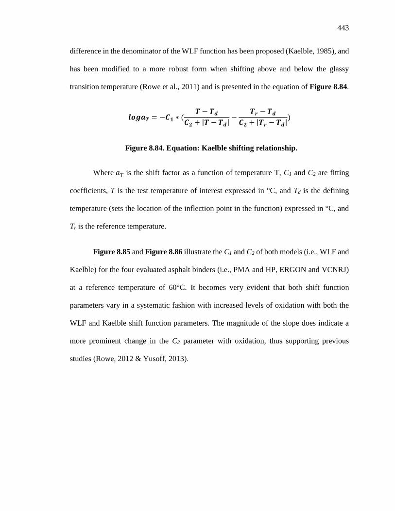
443
difference in the denominator of the WLF function has been proposed (Kaelble, 1985), and
has been modified to a more robust form when shifting above and below the glassy
transition temperature (Rowe et al., 2011) and is presented in the equation of Figure 8.84.
𝒍𝒐𝒈𝒂𝑻 = −𝑪𝟏 ∗ (𝑻 − 𝑻𝒅
𝑪𝟐 + |𝑻 − 𝑻𝒅|−
𝑻𝒓 − 𝑻𝒅
𝑪𝟐 + |𝑻𝒓 − 𝑻𝒅|)
Figure 8.84. Equation: Kaelble shifting relationship.
Where 𝑎𝑇 is the shift factor as a function of temperature T, C1 and C2 are fitting
coefficients, T is the test temperature of interest expressed in °C, and Td is the defining
temperature (sets the location of the inflection point in the function) expressed in °C, and
Tr is the reference temperature.
Figure 8.85 and Figure 8.86 illustrate the C1 and C2 of both models (i.e., WLF and
Kaelble) for the four evaluated asphalt binders (i.e., PMA and HP, ERGON and VCNRJ)
at a reference temperature of 60°C. It becomes very evident that both shift function
parameters vary in a systematic fashion with increased levels of oxidation with both the
WLF and Kaelble shift function parameters. The magnitude of the slope does indicate a
more prominent change in the C2 parameter with oxidation, thus supporting previous
studies (Rowe, 2012 & Yusoff, 2013).

444
Figure 8.85. Master curve shift function parameter C1 function of oxidation.
y = 8.61x + 12.10
R² = 0.66
y = 2.45x + 15.38
R² = 0.05
y = 5.80x + 18.04
R² = 0.45
y = 3.75x + 25.69
R² = 0.18
0
5
10
15
20
25
30
35
0.000 0.100 0.200 0.300 0.400 0.500 0.600 0.700 0.800 0.900
Ma
ster
Cu
rve
Sh
ift
Pa
ram
eter
, C
1
CAg, Arbitrary Units
ERGON_PMA, WLF ERGON_HP, WLF
ERGON_PMA, Kaeble ERGON_HP, Kaelble
Linear (ERGON_PMA, WLF) Linear (ERGON_HP, WLF)
Linear (ERGON_PMA, Kaeble) Linear (ERGON_HP, Kaelble)
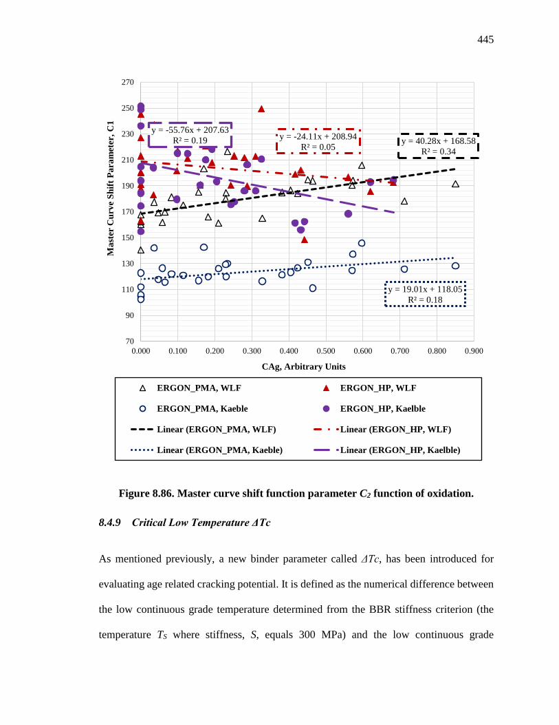
445
Figure 8.86. Master curve shift function parameter C2 function of oxidation.
8.4.9 Critical Low Temperature ΔTc
As mentioned previously, a new binder parameter called ΔTc, has been introduced for
evaluating age related cracking potential. It is defined as the numerical difference between
the low continuous grade temperature determined from the BBR stiffness criterion (the
temperature TS where stiffness, S, equals 300 MPa) and the low continuous grade
y = 40.28x + 168.58
R² = 0.34
y = -24.11x + 208.94
R² = 0.05
y = 19.01x + 118.05
R² = 0.18
y = -55.76x + 207.63
R² = 0.19
70
90
110
130
150
170
190
210
230
250
270
0.000 0.100 0.200 0.300 0.400 0.500 0.600 0.700 0.800 0.900
Ma
ster
Cu
rve
Sh
ift
Pa
ram
eter
, C
1
CAg, Arbitrary Units
ERGON_PMA, WLF ERGON_HP, WLF
ERGON_PMA, Kaeble ERGON_HP, Kaelble
Linear (ERGON_PMA, WLF) Linear (ERGON_HP, WLF)
Linear (ERGON_PMA, Kaeble) Linear (ERGON_HP, Kaelble)
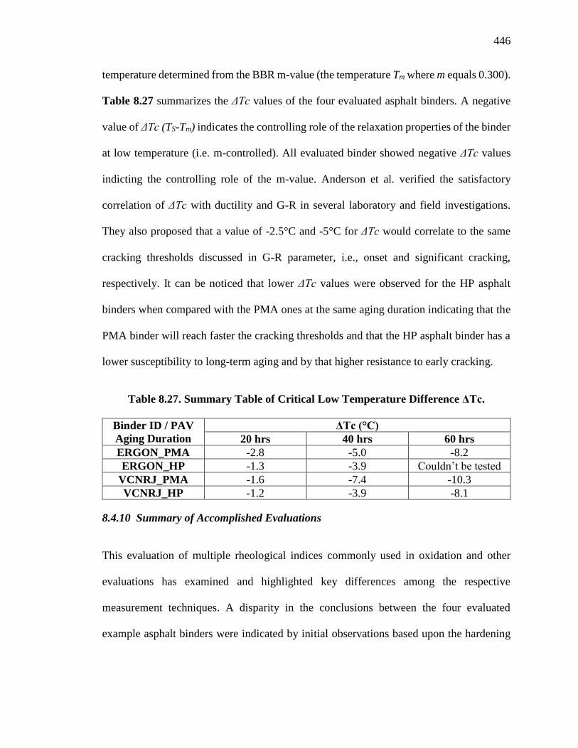
446
temperature determined from the BBR m-value (the temperature Tm where m equals 0.300).
Table 8.27 summarizes the ΔTc values of the four evaluated asphalt binders. A negative
value of ΔTc (TS-Tm) indicates the controlling role of the relaxation properties of the binder
at low temperature (i.e. m-controlled). All evaluated binder showed negative ΔTc values
indicting the controlling role of the m-value. Anderson et al. verified the satisfactory
correlation of ΔTc with ductility and G-R in several laboratory and field investigations.
They also proposed that a value of -2.5°C and -5°C for ΔTc would correlate to the same
cracking thresholds discussed in G-R parameter, i.e., onset and significant cracking,
respectively. It can be noticed that lower ΔTc values were observed for the HP asphalt
binders when compared with the PMA ones at the same aging duration indicating that the
PMA binder will reach faster the cracking thresholds and that the HP asphalt binder has a
lower susceptibility to long-term aging and by that higher resistance to early cracking.
Table 8.27. Summary Table of Critical Low Temperature Difference ΔTc.
Binder ID / PAV
Aging Duration
ΔTc (°C)
20 hrs 40 hrs 60 hrs
ERGON_PMA -2.8 -5.0 -8.2
ERGON_HP -1.3 -3.9 Couldn’t be tested
VCNRJ_PMA -1.6 -7.4 -10.3
VCNRJ_HP -1.2 -3.9 -8.1
8.4.10 Summary of Accomplished Evaluations
This evaluation of multiple rheological indices commonly used in oxidation and other
evaluations has examined and highlighted key differences among the respective
measurement techniques. A disparity in the conclusions between the four evaluated
example asphalt binders were indicated by initial observations based upon the hardening
447
characteristics, i.e., rheological indices as a function of oxidation represented as carbonyl
measures. The measures indicated a reduced susceptibility to aging indicated by a flatter
slope with respect to oxidation with the low shear viscosity measures. The index-oxidation
relationship was nearly identical for the Glover-Rowe parameter, i.e. DSRFn. The
magnitude of the discrepancy is further exemplified by the potential occurrence of multiple
crossover frequencies with their corresponding crossover modulus. These findings wee
additionally supported by the general reduced dependency of the shifting parameters of
both the WLF and Kaelble considerations for both PMA and HP binders. It should be
mentioned that higher percentage error was observed for the HP binder in comparison with
the PMA. The difference in low temperature controlled by S and m were also presented for
the four evaluated asphalt binders.
The potential for very different conclusions deduced from the same experience was
observed, solely depended upon the rheological measure being considered. While each
method presents its own merit and respective limitations, a single preferential method was
not really identified. However, the critical need for reliable and sound rheological measures
and data processing procedures was clearly demonstrated.
448
CHAPTER 9 SUMMARY OF FINDINGS, CONCLUSIONS, AND
RECOMMENDATIONS
The objective of this FDOT research study and this dissertation is to conduct an in-depth and
comprehensive evaluation of asphalt mixtures in the state of Florida manufactured with HP binder
that contains approximately 7.5% SBS polymer. This chapters presents a summary and
conclusions drawn based on the literature review, laboratory evaluation, advanced mechanistic
modeling, and full-scale testing conducted in this research study. In addition, an implementation
plan of the final recommended structural coefficient for HP AC mixes using the APT setup at
FDOT facilities is provided in this chapter.
9.1 Summary of Findings and Conclusions
The objective of this literature review was to identify all currents and previous studies that have
been conducted to evaluate the performance of HP AC mixes. In this research, HP AC mixes are
defined as asphalt mixtures manufactured using asphalt binders modified with SBS or SB polymers
at the approximate rate of 7.5% by weight of binder. The findings of the literature review will be
presented with respect to the three areas of interest that were defined in the Scope of the review
as: a) laboratory evaluations of HP modified asphalt binders and mixtures, b) performance of
pavement sections constructed with HP AC mixes, and c) techniques to determine structural
coefficient of HP AC mixes.
449
9.1.1 Literature Review
9.1.1.1 Laboratory Evaluations of HP Modified Asphalt Binders and Mixtures
The review identified several studies that evaluated the engineering properties and performance
characteristics of HP asphalt binders and mixtures. On the positive side, all of the identified studies
used the Superpave technology to evaluate the properties of the binders and mixtures which makes
the generated data highly applicable to the current research. On the not so positive side, none of
the identified studies conducted a complete experimental design that can lead to the evaluation of
the performance of HP AC mixes with respect to all modes of distresses, i.e., rutting, fatigue,
thermal, and reflective cracking. In addition, some of the studies did not incorporate the evaluation
of a control binder or mixture in order to clearly define the contribution of the HP asphalt binder.
Furthermore, some studies went directly into the evaluation of HP mixtures without providing
sufficient information on the properties of the HP binders used in the manufacturing of the
mixtures.
Table 9.1 summarizes the findings of the reviewed studies that evaluated the laboratory
properties of HP binders and mixtures. The summary is presented in terms of the impact of HP
modification on the performance properties of binders and mixtures. A review of the findings in
Table 9.1 leads to the following observations:
• Increasing the SBS polymer content from 0, 3, 6, to 7.5% continues to improve the
performance properties of the asphalt binder and mixture in terms of its resistance to the
various modes of distresses, i.e. rutting, fatigue, thermal, and reflective cracking.

450
• A unique feature of the HP modification has been identified as its ability to slow down the
oxidative aging of the asphalt binder. This feature is expected to positively impact the
resistance of the HP AC mix to the various types of cracking.
The HP asphalt binder should not be used to overcome the negative impact of RAP on the
resistance of the AC mixture to various types of cracking. The properties of the RAP binder should
be taken into consideration when designing HP AC mix with RAP content at or above 25% in
order to optimize the benefits of the HP modification.

451
Table 9.1. Summary of Laboratory of HP Binders and Mixtures.
Study Impact of High Polymer Modification
Binder Properties Mixture Properties
Florida DOT1: Evaluation and
Implementation of Heavy Polymer
Modified Asphalt Binder through
Accelerated Pavement Testing
- Increased resistance to
rutting
- Increased resistance to
fracture
- Reduced creep rate
- Increased resistance to
cracking
University of Nevada: Evaluation of
Thermal Oxidative Aging Effect on the
Rheological Performance of Modified
Asphalt Binders
- Increased resistance to
long-term oxidative aging -NO MIX TESTING
ORLEN Asfalt, Poland: Highly Modified
Binders Orbiton HiMA
- Increased resistance to
thermal cracking
- Increased resistance to
fatigue cracking
- Increase resistance to
rutting
- Increased resistance to
thermal cracking
- Increased resistance to
rutting
New Hampshire and Vermont DOTs:
Development and Validation of
Performance based Specifications for
High Performance Thin Overlay Mix
-NO BINDER TESTING
- RAP content of 25%
negatively impacted the
resistance of the mixture to
cracking
- HP binder could not
overcome the negative
impact of Rap on cracking
New Hampshire DOT: Materials and
Mixture Test Results, New Hampshire
DOT Highways for Life, 2011 Auburn-
Candia Resurfacing
-NO BINDER TESTING
- Reduced dynamic modulus
- Increased resistance to
rutting
- Increased resistance to
fatigue cracking
- Increased resistance to
reflective cracking
- Increased resistance to
thermal cracking
National Center Asphalt for Asphalt
Technology: Field and Laboratory Study
of High-Polymer Mixtures at the NCAT
Test Track
-Increased resistance to
rutting
- Increased tensile strength
- Increased dynamic
modulus
- Increased resistance to
rutting
- Increased resistance to
fatigue cracking 1 Not a true HP binder since SBS content at 6.0%

452
9.1.1.2 Performance of Pavement Sections Constructed with HP AC Mixes
The review Several field projects were constructed to evaluate the performance of HP modified
asphalt mixtures as compiled in Section 2.4. Table 9.2 summarizes the review of seven field HP
AC mixes projects with limited and extensive performance data. A review of the findings in Table
9.2 leads to the following observations:
• HP AC mixes have been used over a wide range of applications ranging from full depth
AC layer to thin AC overlays under heavy traffic on interstates and slow-braking loads at
intersections.
• HP AC mixes did not show any construction issues in terms of mixing temperatures and
in-place compaction. Standard construction practices and equipment were adequately used.
• All of the identified HP field projects lack information on long-term performance,
however, early performances are encouraging. In addition, the HP test section on the
NCAT Test Track showed excellent performance under accelerated full scale loading.

453
Table 9.2. Summary of Field Projects with HP AC Mixes.
Location Project Description Key Findings
Brazil, 2011
- Mill and AC overlay on highway
PR-092
- Traffic up to 4,200 heavy
agricultural trucks per day
- Good early performance
- Additional HP projects were constructed
on Dutra road which runs between Sao
Paulo and Rio de Janeiro
USA/ Advanced
Material Services
LLC, 2013
- Designing for Corvette Museum
Race Track in Bowling Green
Nashville
- Raveling and bleeding remain the
main concerns
- Evotherm WMA additive was
used to improve workability
- A potentially high performance AC mix
was delivered for the race track by using
HP asphalt binder
USA / City of
Bloomington,
MN, 2012
- Mill and AC overlay on
Normandale Road, City of
Bloomington
- Subjected to heavy traffic due to
its location adjacent to the airport
- Two projects were constructed:
Normandale Service Road at 84th
Street and West 98th Street
- HP AC mix performed well and
constituted a good way to place more cost-
effective and durable asphalt pavements
with reduced thicknesses.
- HP AC mix offered possibility of
building pavement section on top of weak
base and subgrade layers
USA / Georgia
DOT, 2010
- Thin AC overlay at junction of
Routes 138 and 155
- Pavement rutting and shoving
were the main concerns
- HP AC mix was observed to have similar
workability as regular PMA mix based on
general observations reported from the job
site
USA/NCAT Test
Track, 2009
- HP test section designed with an
AC layer thickness 18% less than
the AC layer thickness of the PMA
section
- HP section experienced lower rutting
under the entire loading cycle of 8.9
million ESALs
- Both HP and PMA sections did not
experience any fatigue cracking under the
entire loading cycle of 8.9 million ESALs
USA / NHDOT
and VTDOT, 2011
- New Hampshire project on Route
202, AC overlay over existing
pavement in bad conditions without
pre-treatment
- Vermont project on US-7, AC
overlay over existing pavement in
bad conditions with some pre-
treatment
- Minimal reflective cracking on the New
Hampshire section containing RAP
material
- No signs of environmental related
cracking and no evidence of rutting were
observed after 2 years of service
USA / Oklahoma
DOT, 2012
- Mill and overlay on I-40 west of
Oklahoma city
- HP AC mix had a low enough viscosity
making it workable and compactable when
used in the field
USA / Oregon
DOT, 2012
- Thin overlay mix on I-5 in Oregon
- Existing pavement had some
wearing ruts and raveling due to
heavy trucks and high traffic
volumes
- No special plant adjustments were made
to accommodate the production of HP AC
mix.
- No problems with viscosity were faced
during the paving of the HP mix
454
9.1.1.3 Techniques to Determine Structural Coefficient of HP modified AC Mixes
None of the available studies calculated the structural coefficient of HP AC mixes (aHP-AC) mainly
because of the unavailability of the required full performance characterizations of the mixtures. In
some cases, a hypothetical structural coefficient may be identified as shown below:
• For the project in Brazil; the HP section replaced the standard section at a 45% reduction
in the overall thickness indicating an aHP-AC that is 45% higher than the corresponding
structural coefficient for the composite pavement (i.e., AC over cement-stabilized RAP).
• For the projects in Bloomington, MN and Oklahoma; the HP section replaced the
standard section at a 25% reduction in the thickness of the AC layer indicating an aHP-AC
that is 25% higher than the corresponding structural coefficient for the standard AC mix.
The performance data generated from the PMA and HP test sections at the NCAT Test
Track offered some basis for the determination of an aHP-AC. However, the fact that both sections
did not show any fatigue cracking and only the minimal rutting was experienced by both sections
(i.e., less than 0.25 inch) limits the applicability of the estimated aHP-AC. Despite these limitations,
the research team attempted to demonstrate the various methods to establish an aHP-AC based on
the data from the NCAT test sections. Four approaches were examined; three empirical approaches
based on the AASHTO 1993 Guide methodology and one mechanistic approach based on the
analysis of fatigue performance. The three empirical approaches recommended an aHP-AC ranging
from 0.54 to 0.57 while the mechanistic approach recommended an aHP-AC ranging between 0.82
and 0.88.

455
In summary, while several previous studies highlighted the positive impacts of the HP
modification of asphalt binders and mixtures, there is still a serious lack of understanding on the
structural value of the HP AC mix as expressed through the structural coefficient for the AASHTO
1993 Guide. The attempt by the research team to determine an aHP-AC based on the available
information led to the conclusion that empirically-based aHP-AC can underestimate the structural
value of the HP AC mix while determining the aHP-AC based on the mechanistic analysis of a single
failure mode (i.e., fatigue cracking) may overestimate the structural value of the HP AC mix. This
important and critical finding strongly supports the approach implemented in this research where
the full evaluation of the performance characteristics of the HP AC mixes are conducted and the
aHP-AC is determined based on the mechanistic analysis of all possible critical modes of failure.
9.1.2 Execution of the Experiment: Laboratory Evaluation and Advanced Modeling
Locally available materials shipped from Florida were assessed and used for the development of
16 AC mixes using PMA and HP asphalt binders (i.e., 8 PMA and 8 HP AC mixes) for new
construction and rehabilitation projects. The mix designs were conducted following the Superpave
methodology to determine the optimal asphalt binder content (OBC) for each of the 16 evaluated
mixes. Various OBC values were determined depending on the aggregate source, aggregate
gradation, binder type (i.e., PMA or HP), binder source, and the possible use of any recycled
material (i.e., RAP). The 16 AC mixes were evaluated in terms of their resistance to moisture
damage, dynamic modulus, rutting, and multiple cracking distress modes (i.e., fatigue, top-down,
and reflective). In general, the combination of aggregate source and asphalt binder type (i.e., PMA
or HP) had significant impacts on the performance behavior of the evaluated AC mixes. The
456
following paragraphs summarizes the findings and recommendations from the laboratory
evaluation and advanced modelling of HP AC mixes produced for Florida:
• Overall, HP AC mixes showed better engineering property and performance characteristics
when compared with the corresponding PMA control AC mixes which can be credited to
the high polymer modification of the asphalt binder (i.e., HP binder). The true impact of
the improvements in engineering property and performance characteristics of the HP AC
mixes were evaluated through the mechanistic analysis of flexible pavements incorporating
the two types of mixtures.
• The critical responses determined using the 3D-Move mechanistic model were used to
evaluate the performance life of the designed pavement structures for several targeted
distresses including; fatigue cracking, AC rutting, total rutting, top-down cracking, and
reflective cracking. The critical responses were computed and determined at different
locations and at different depths within the structure depending on the distress mode. It
should be mentioned that two temperatures were considered for the mechanistic analysis:
77°F (25°C) simulating an intermediate temperature for cracking analyses, and 122°F
(50°C) simulating a high temperature for rutting/showing analyses. These temperatures
were determined using the corresponding critical climatic stations in Florida (i.e.,
Gainesville and Marathon).
• Initial structural coefficient for HP AC mixes was determined based on the fatigue
performance life of flexible pavements. An equivalent HP AC layer thickness was
determined which resulted in a similar fatigue life as the respective PMA pavement section
under static and dynamic loading conditions. Multiple factors including applied traffic
457
level, pavement structure, layers properties, and performance characteristics of the
evaluated PMA and HP AC mixes resulted in different structural coefficients for HP AC
mixes based on the fatigue cracking analysis. The estimated initial fatigue-based structural
coefficients ranged from 0.33 to 1.32. Using advanced statistical analyses and considering
all factors and their interactions, an initial fatigue-based structural coefficient of 0.54 was
determined for HP AC mixes.
• The initial fatigue-based structural coefficient for HP AC mixes of 0.54 was verified for
the following distresses; rutting in AC layer, shoving in AC layer, total rutting, top-down
cracking, and reflective cracking. In all cases, the thickness of the HP layer was reduced
based on the fatigue-based structural coefficient of 0.54 and the resistance of the HP
pavement to the specific distress was evaluated and compared to the resistance of its
corresponding PMA pavement. The verification process concluded that the structural
coefficient of 0.54 for HP AC mixes would lead to the design of HP pavements that offer
equal or better resistance to the various distresses as the designed PMA pavements with
the structural coefficient of 0.44. This conclusion held valid for the design of both new and
rehabilitation projects.
• Based on the data generated in this task and the analyses presented in this part of the
research herein, it is recommended that HP AC mixes be incorporated into the current
FDOT Flexible Pavement Design Manual with a structural coefficient of 0.54. This
represents a 23% reduction in the thickness of the AC layer when using a HP AC mix in
place of a PMA AC mix while designing a flexible pavement under all similar conditions
of traffic, environment, and properties of base and subgrade layers.

458
9.1.3 Verification of Structural Coefficient for HP AC Mixes using Full-Scale Testing
A verification of the recommended aHP-AC of 0.54 was conducted in this task using full-scale
pavement testing prior to the full implementation in the FDOT APT experiment. The experimental
plan comprised a PMA and an HP full-scale pavement structures that were fully instrumented and
subjected to stationary dynamic loads. The two pavement structures had identical CAB and SG
layers. The HP AC layer in the PaveBox_HP experiment was 19% thinner than the PMA AC layer
in the PaveBox_PMA experiment (3.50 versus 4.25 inches AC layer thickness). While FDOT
mandates the use of a 12 inch (305 mm) thick stabilized SG layer, only a typical SG layer was
used in the two PaveBox experiments. This was considered acceptable for the purpose of this task
that aimed for a relative comparison of responses between the PMA and HP pavement sections.
The two pavement structures were subjected to the same loading protocol. Dynamic loads
simulating FWD loading, were applied at the surface of the AC pavement. Pavement surface
deflections, vertical stresses, and strains at different depths and locations in the pavement layers
were monitored during testing through embedded instrumentations. LVDTs were used to record
surface pavement deflections. TEPC were used to capture the vertical stresses induced in the CAB
and SG layers due to surface loading. Strain gauges were attached to the bottom of the AC layer
to measure the load-induced strains. At the end of each experiment, cores were cut from the AC
layer for thickness and air voids measurements. Two major analyses were carried out in this task.
Analysis I consisted of a comparison of measured pavement responses under dynamic loadings,
while analysis II verified the aHP-AC of 0.54 using a ME approach of the tested pavement structures.
The following summarizes the findings and conclusions from the full-scale testing task:

459
• Overall, the HP AC mix showed better fatigue and rutting characteristics when compared
with the PMA AC mix. This was demonstrated with higher fatigue and lower rutting
relationships for the HP AC mix when compared with the PMA AC mix.
• A comparison of the measured pavement responses from the two experiments was
conducted. The reduced thickness of the HP AC layer resulted in the following
observations: a) higher vertical surface deflections under the center of the loading plate, b)
higher vertical stresses under the center of the loading plate at the middle of the CAB layer,
c) similar vertical stresses at 6 inch (152 mm) and 24 inch (610 mm) below the SG surface,
d) similar or lower tensile strains at the bottom of the AC layer, and d) comparable surface
deflections and vertical stresses in the CAB and SG layers at radial distances farther away
from the load, i.e. 8–60 inches (203–152 cm).
• An ME analysis was conducted using 3D-Move and the backcalculated layers’ moduli in
conjunction with the laboratory-developed performance models for the produced PMA and
HP AC mixes. The ME analysis with the reduced thickness of the HP AC layer resulted in
the following observations: a) better fatigue and rutting performance for the HP AC layer
when compared with the PMA AC layer, b) higher rut depths in the unbound layers of the
HP pavement structure, especially in the CAB layer, and c) similar total rut depths for the
PMA and HP pavement structures.
• In general, the results and findings from this task support the aHP-AC selection of 0.54. A
reduction in the recommended aHP-AC value might be warranted if the load-induced stresses
in the unbound materials (in the CAB layer in particular) lead to excessive permanent

460
deformations that exceeds the rut depth limits set by FDOT. This aspect requires further
evaluation in the FDOT APT experiment.
Based on these findings, an implementation plan was recommended for the APT
experiment at FDOT facility for the validation of the recommended aHP-AC selection of 0.54. The
recommended implementation plan is presented the following section.
9.2 APT Implementation Plan
This section of the manuscript presents recommendations for FDOT to validate the recommended
structural coefficient (aHP-AC of 0.54) through full scale testing under the APT facility. The main
concept of the validation plan is to evaluate the performance of flexible pavement sections
constructed with HP AC mixes at a reduced thickness of the AC layer relative to the performance
of control pavement sections. The plan was developed based on the findings from the performance
modeling of the flexible pavement sections and the full-scale pavement testing experiments
conducted in the PaveBox. The factors proposed in the APT implementation plan stems from those
that were considered in the previous tasks of this study (e.g., aggregate and asphalt binder sources,
NMAS, traffic level, etc.).
9.2.1 Experimental Design
The comparison of the performance of an HP pavement section with that of a PMA pavement
section is one of the main objectives of the recommended APT experiment. Table 9.3 summarizes
the recommended APT experiments. The following factors were identified for consideration in the
APT experimental plan:

461
• Asphalt binder type: a conventional PG76-22PMA and an HP asphalt binder from a
common supplier in Florida. Two candidate suppliers are Ergon Asphalt and Emulsion and
Vcenergy.
• Aggregate source: Southeast Florida limestone labeled as “FL,” and Georgia Granite
labeled as “GA.”
• Recycled asphalt pavement (RAP): a single source of RAP to be used with GA aggregates
and PMA asphalt binder at a rate of 20% following current FDOT standard of practice.
• Pavement structure: conventional pavement structures designed in accordance with the
FDOT design manual including a CAB layer and a 12 inch (305 mm) stabilized SG layer
on top of the existing SG. The CAB and SG layer will be the same across all pavement
sections.
• AC layer thickness: the thickness of the PMA AC layer will be designed using a structural
coefficient of 0.44. The thickness of the HP AC layer will be designed using the
recommended structural coefficient of 0.54 and a lower structural coefficient of 0.50. The
proposed structural coefficient of 0.50 is based on the results of the statistical analysis
conducted for the structural coefficients of AC mixes with GA aggregate source and 9.5
mm NMAS.
• Traffic Level: AC mixes with 9.5 and 12.5 mm NMAS designed for traffic levels C and D,
respectively, were considered in the statistical analysis. The NMAS contributed to some of
the differences in the performance evaluation of the designed PMA and HP AC mixes,

462
which resulted in a wide range of HP AC structural coefficients. Thus, AC mixes designed
for traffic levels C and D are recommended for the validation effort in the APT experiment.
• Pavement temperature: rutting was found to be most critical among the evaluated
distresses. Thus, testing during the hot seasons at the temperatures typically observed at
the APT facility is considered appropriate for the objectives of this experiment.
Table 9.3. Proposed APT Experiments.
Experiment
ID
Traffic
Level
Aggregate
Source Pavement Structure RAP (%)
HP1 C GA
Control PMA: aPMA-AC = 0.44
HP1A: aHP-AC = 0.54
HP1B: aHP-AC = 0.50
20
0
0
HP2 D FL Control PMA: aPMA-AC = 0.44
HP2A: aHP-AC = 0.54
0
0
9.2.2 Instrumentation Plan
The pavement test sections should be instrumented to provide a comprehensive picture of the
system response. Strain gauges should be installed at the bottom of the AC layers to provide the
strain history as a result of the surface loading. Strain gauges should be installed in the travel
direction and perpendicular to the travel direction to capture both the longitudinal and traverse
strains, respectively. TEPCs should be used to capture the stresses induced in the CAB and SG
layers due to loading. The TEPCs should be installed under the centerline of the load and at
different radial distances from the centerline of the load. Multi-depth deflectometers (MDD)
should be installed to measure elastic vertical deflections and permanent vertical deformations at
various depths within the pavement structure, relative to a reference depth located in the SG. Thus
allowing for the continuous monitoring of rutting under loading in the various pavement layers.
Thermocouples should be used to measure temperatures at various depths within the AC layer.

463
Time domain reflectometer can be used to monitor the changes in water content in the unbound
layers just outside the trafficked area during testing of the pavement sections.
9.2.3 Pavement Design
The pavement structures for the PMA control sections will need to be designed in accordance with
the FDOT manual for designing flexible pavements in Florida. The design thickness is based on a
tested Lime Bearing Ratio (LBR) of the SG, the type of CAB material to be used, and the design
traffic level. Consequently, the thickness of the AC layers in the HP pavement sections are reduced
based on the structural coefficients shown in Table 9.3.
A mechanistic analysis should be conducted for the designed pavement structures to
estimate the rutting level in the unbound layers, in particular the CAB layer. Based on this study,
it is anticipated that the load-induced vertical stresses in the CAB layer of the HP pavement
sections will be higher than the ones measured in the CAB layer of the PMA pavement structures.
It is suggested that a localized shear failure analysis be conducted prior to finalizing the pavement
structural designs to investigate the influence of the reduced HP AC layer on the rutting
performance of unbound layers. The analysis will consist of comparing the load-induced stress
level calculated at the middle of the CAB layer with the corresponding yield criterion of the
material. It should be noted that the localized shear failure analysis can only focus on the CAB
layer, since the12-inch stabilized layer will likely reduce the load-induced stresses in the SG layer.
Several failure criteria, such as Mohr–Coulomb, Drucker–Prager, Lade–Duncan, etc. have
been proposed for evaluating shear failure of unbound materials. The Mohr–Coulomb yield
criterion is one of the well-accepted criterion in soil plasticity that is determined using the shear
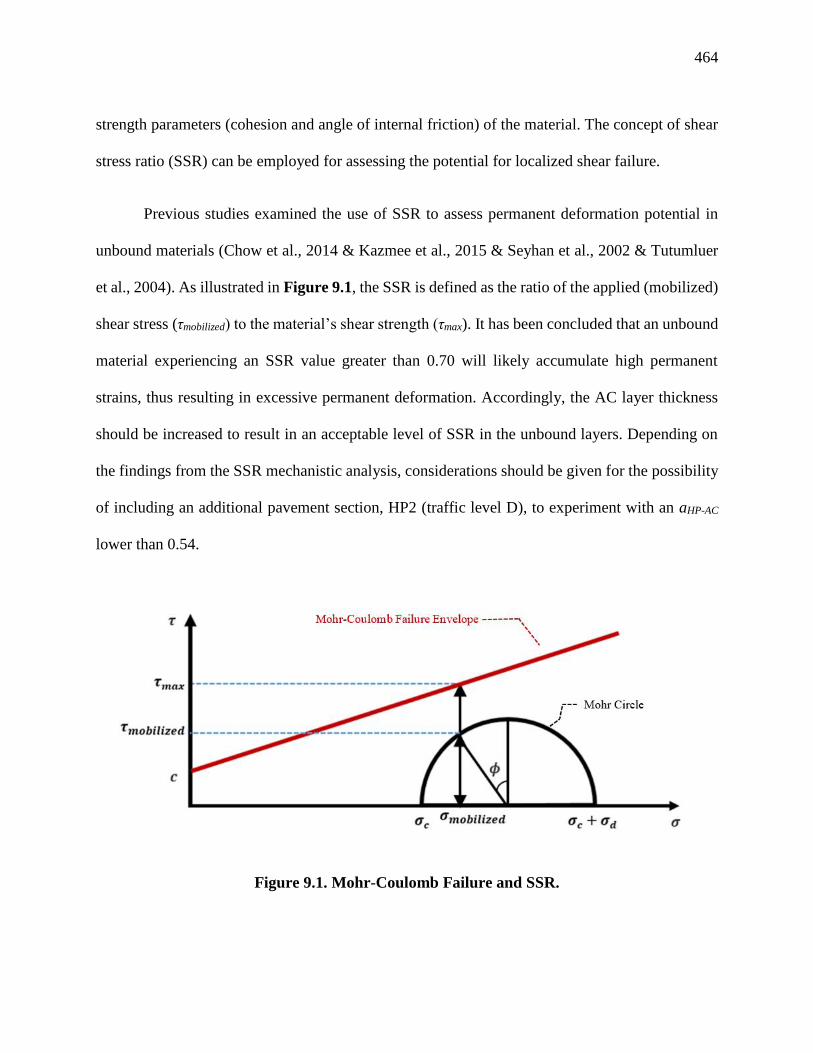
464
strength parameters (cohesion and angle of internal friction) of the material. The concept of shear
stress ratio (SSR) can be employed for assessing the potential for localized shear failure.
Previous studies examined the use of SSR to assess permanent deformation potential in
unbound materials (Chow et al., 2014 & Kazmee et al., 2015 & Seyhan et al., 2002 & Tutumluer
et al., 2004). As illustrated in Figure 9.1, the SSR is defined as the ratio of the applied (mobilized)
shear stress (τmobilized) to the material’s shear strength (τmax). It has been concluded that an unbound
material experiencing an SSR value greater than 0.70 will likely accumulate high permanent
strains, thus resulting in excessive permanent deformation. Accordingly, the AC layer thickness
should be increased to result in an acceptable level of SSR in the unbound layers. Depending on
the findings from the SSR mechanistic analysis, considerations should be given for the possibility
of including an additional pavement section, HP2 (traffic level D), to experiment with an aHP-AC
lower than 0.54.
Figure 9.1. Mohr-Coulomb Failure and SSR.

465
9.2.4 Pavement Construction
After accomplishing all needed structural designs and mechanistic analyses, the pavement
structures should be constructed in accordance with the FDOT specifications. Dynamic cone
penetrometer (DCP) and falling weight deflectometer (FWD) testing should be carried out
periodically on the individual layers during pavement construction to monitor the pavement
strength, modulus, and stiffening rate.
466
CHAPTER 10 REFERENCES
AASHTO. AASHTO Guide for Design of Pavement Structures, American Association of State
Highway and Transportation Officials, Washington, D.C., 1993.
AASHTO M145, Standard Specification for Classification of Soils and Soil-Aggregate Mixtures
for Highway Construction Purposes, American Association of State Highway and
Transportation Officials, Washington, D.C., 2017.
AASHTO M320, Standard Specification for Performance-Graded Asphalt Binder, American
Association of State Highway and Transportation Officials, 2014.
AASHTO M332, Standard Specification for Performance-Graded Asphalt Binder Using
Multiple Stress Creep Recovery (MSCR) Test, American Association of State Highway
and Transportation Officials, 2014.
AASHTO R28, Standard Practice for Accelerated Aging of Asphalt Binder Using a Pressurized
Aging Vessel (PAV), American Association of State Highway and Transportation Officials,
2012.
AASHTO R30, Standard Practice for Mixture Conditioning of Hot-Mix Asphalt (HMA), American
Association of State Highway and Transportation Officials, 2002.
AASHTO R83, Standard Practice for Preparation of Cylindrical Performance Test Specimens
Using the Superpave Gyratory Compactor (SGC), American Association of State Highway
and Transportation Officials, 2017.
AASHTO R84, Standard Practice for Developing Dynamic Modulus Master Curves for Hot Mix
Asphalt (HMA) Using the Asphalt Mixture Performance Tester (AMPT), American
Association of State Highway and Transportation Officials, Washington, D.C., 2010.

467
AASHTO TP10, Standard Test Method for Thermal Stress Restrained Specimen Tensile Strength,
American Association of State Highway and Transportation Officials, Washington, D.C.,
1993.
AASHTO T2, Standard Method of Test for Sampling of Aggregates, American Association of
State Highway and Transportation Officials, 1991-2015.
AASHTO T11-05, Standard Method of Test for Materials Finer Than 75-µm (No.200) Sieve in
Mineral Aggregates by Washing, American Association of State Highway and
Transportation Officials, Washington, D.C., 2005.
AASHTO T27-14, Standard method of Test for Sieve Analysis of Fine and Coarse Aggregates,
American Association of tate Highway and Transportation Officials, 2014.
AASHTO T48, Standard Method of Test for Flash and Fire Points by Cleveland Open Cup,
American Association of State Highway and Transportation Officials, 2006.
AASHTO T89-13, Standard Method of Test for Determining the Liquid Limit of Soils, American
Association of State Highway and Transportation Officials, Washington, D.C., 2013.
AASHTO T90-16, Standard Method of Test for Determining the Plastic Limit and Plasticity
Index of Soils, American Association of State Highway and Transportation Officials,
Washington, D.C., 2016.
AASHTO T99, Standard Method of Test for Moisture-Density Relations of Soils Using a 2.5-kg
(5.5-lb) Rammer and a 305-mm (12-inch) Drop, American Association of State Highway
and Transportation Officials, Washington, D.C., 2017.
AASHTO T164, Standard Method of Test for Quantitative Extraction of Asphalt Binder form Hot
Mix Asphalt (HMA), American Association of State Highway and Transportation Officials,
2014.
468
AASHTO T176, Standard Method of Test for Plastic Fines in Graded Aggregates and Soils by
Use of the Sand Equivalent Test, American Association of State Highway and
Transportation Officials, 2017.
AASHTO T180, Standard Method of Test for Moisture-Density Relations of Soils Using a 4.54-
kg (10-lb) Rammer and a 457-mm (18-inch) Drop, American Association of State
Highway and Transportation Officials, Washington, D.C., 2017.
AASHTO T240, Effect of Heat and Air on a Moving Film of Asphalt Binder (Rolling Thin-Film
Oven Test), American Association of State Highway and Transportation Officials, 2013.
AASHTO T248, Standard Method of Test for Reducing Samples of Aggregate to Testing Size,
American Association of State Highway and Transportation Officials, Washington, D.C.,
2014.
AASHTO T283, Standard Method of Test for Resistance of Compacted Asphalt Mixtures to
Moisture-Induced Damage, American Association of State Highway and Transportation
Officials, Washington, D.C., 2014.
AASHTO T304, Standard Method of Test for Uncompacted Void Content of Fine Aggregate,
American Association of State Highway and Transportation Officials, 2017.
AASHTO T307, Standard Method of Test for Determining the resilient Modulus of Soils and
Aggregate Materials, American Association of State Highway and Transportation
Officials, Washington, D.C., 2017.
AASHTO T313, Standard Method of test for Determining the Flexural Creep Stiffness of Asphalt
Binder Using the Bending Beam Rheometer (BBR), American Association of State
Highway and Transportation Officials, Washington, D.C., 2012.
469
AASHTO T315, Standard Method of Test for Determining the Rheological Properties of Asphalt
Binder Using a Dynamic Shear Rheometer (DSR), American Association of State Highway
and Transportation Officials, Washington, D.C., 2013.
AASHTO T316, Standard Method of Test for Viscosity Determination of Asphalt Binder Using
Rotational Viscometer, American Association of State Highway and Transportation
Officials, 2013.
AASHTO T321, Standard Method of Test for Determining the Fatigue Life of Compacted Asphalt
Mixtures Subjected to Repeated Flexural Bending, Association of State Highway and
Transportation Officials, Washington, D.C., 2014.
AASHTO T322, Standard Method of Test for Determining the Creep Compliance and Strength of
Hot-Mix Asphalt (HMA) Using the Indirect Tensile Test Device, American Association of
State Highway and Transportation Officials, Washington, D.C., 2013.
AASHTO T324, Standard Method of Test for Hamburg Wheel-Track Testing of Compacted Hot
Mix Asphalt (HMA), American Association of State Highway and Transportation Officials,
Washington, D.C., 2011.
AASHTO M332, Standard Specification for Performance-Graded Asphalt Binder Using Multiple
Stress Creep Recovery (MSCR) Test, American Association of State Highway and
Transportation Officials, 2014.
AASHTO T340, Standard Method of Test for Determining Rutting Susceptibility of Hot Mix
Asphalt (HMA) Using the Asphalt Pavement Analyzer (APA), American Association of
State Highway and Transportation Officials, Washington, D.C., 2010.

470
AASHTO T350, Standard Method of Test for Multiple Stress Creep Recovery (MSCR) Test of
Asphalt Binder Using a Dynamic Shear Rheometer (DSR), American Association of State
Highway and Transportation Officials, Washington, D.C., 2013.
AASHTO T378, Determining the Dynamic Modulus and Flow Number for Hot Mix Asphalt
(HMA) Using the Asphalt Mixture Performance Tester (AMPT), American Association of
State Highway and Transportation Officials, Washington, D.C., 2013.
Airey, G.D. “Rheological properties of styrene butadiene styrene polymer modified road
bitumens,” Fuel, Vol. 82, No. 14, pp. 1709–1719, 2003.
Airey, G.D., “Styrene butadiene styrene polymer modification of road bitumens,” Journal of
Material Science, Vol. 39, 2004, pp. 951–959.Araujo, M.F.A.S, V.F.C Lins, V.M.D Pasa,
L.F.M. Leite, “Weathering aging of modified asphalt binders,” Journal of Fuel Processing
Technology, Vol. 115, 2013, pp. 19-25.
Al-Omari B., and Darter M. I., Relationships between International Roughness Index and Present
Serviceability Rating, Transportation Research Record 1435, Transportation Research
Board, Washington, D. C., 1994.
American Association for State Highway and Transportation Officials (AASHTO) Transportation
System Preservation Technical Services Program (TSP2), Kraton Ultra-thin HMA / WMA
Overlay Study, http://www.tsp2.org/pavement/other-information/research-pavement/,
Accessed July 5th, 2012.
Anderson, D.A., D.W. Christensen, H.U. Bahia, R.N. Dongré, M.G. Sharma, C.E. Antle, and J.
Button, “Binder Characterization and Evaluation, Volume 3: Physical Characterization,”
SHRP Report A-369, Strategic Highway Research Board, National Research
Council,Washington, D.C., 1994.
471
Anderson, D.A., Y. Le Hir, J.P. Planche, D. Martin, “Zero Shear Viscosity of Asphalt Binders.”
In Transportation Research Record: Journal of the Transportation Research Board, No.
1810, Transportation Research Board of the National Academies, Washington D.C.,
2002, pp. 54-62.
ARA, Inc., ERES Consultants Division. Guide for Mechanistic-Empirical Design, Transportation
Research Board of the National Academies, National Cooperative Highway Research
Program NCHRP, Project 1-37A, Washington DC.
ASTM D4791, Standard Test Method for Flat Particles, Elongated Particles, or Flat and
Elongated Particles in Coarse Aggregate, American Society for Testing and Materials,
2017.
ASTM D5821, Standard Test Method for Determining the Percentage of Fractured Particles in
Coarse Aggregate, American Society for Testing and Materials, 2017.
ASTM D7460, Standard Test Method for Determining Fatigue Failure of Compacted Asphalt
Concrete Subjected to repeated Flexural Bending, American Society for Testing and
Materials, 2010.
Bahia H.U., Perdomo D., and Turner P., Applicability of Superpave Binder Testing Protocols to
Modified Binders, Transportation Research Record, 1997, 1586:16-23.
Bates R., and Worch R., Styrene-Butadiene Rubber Later Modified Asphalt, Engineering Brief No.
39, Federal Aviation Administration, Washington, DC, 1987.
http://www.faa.gov/arp/engineering/briefs/eb39.htm.
Becker y., Mendez M. P., and Rodriguez Y., Polymer Modified Asphalt, Vis Technol 2011, 9
(1):39-50.

472
Birgisson B., Wang J., and Roque R., Implementation of the Florida Cracking Model Into the
Mechanistic-Empirical Pavement Design, University of Florida, Florida Department of
Transportation (FDOT), UF No.: 0003932, Contract No.: BD-545 #20, December 2006.
Blazejowski K., Olszacki J., and Peciakowski H., Highly Modified Binders Orbiton HiMA,
ORLEN Asfalt, Application Guide, Version 1e, Poland, 2015.
Chow, L.C., Mishra, D., and Tutumluer, E. (2014), Framework for Development of an Improved
Unbound Aggregate Base Rutting Model for Mechanistic–Empirical Pavement Design,
Transportation Research Record, 2401, pp. 11–21, Transportation Research Board,
Washington, DC.
Christensen, D.W. and D.A. Anderson, “Interpretation of Dynamic Mechanical Test Data for
Paving Grade Asphalt Cements,” Asphalt Paving Technology, Journal of the Association
of Asphalt Paving Technologists, Vol. 61, 1992a, pp. 67-116.
Christensen, D.W. and D.A. Anderson, “Chemical-Physical Property Relationships for Asphalt
Cements and the Dispersed Polar Fluid Model,” Proceedings 204th American Chemical
Society National Meeting, Washington, D.C., Vol. 37, No. 3-4, 1992b, pp. 1279-1291.
Coree B.J., and White T.D., The Synthesis of Mixture Strength Parameters Applied to the
Determination of AASHTO Layer Coefficient Distributions, Asphalt Pavement
Technology, vol. 58, 1989.
D’Angelo J., New High-Temperature Binder Specifications Using Multistress Creep and
Recovery, Transportation Research Circular, Development in Asphalt Binder
Specifications, No E-C147, pp.1-13, 2010.
Ferry, J.D., Viscoelastic Properties of Polymers, Third Edition, John Wiley & Sons, Inc., Hoboken,
New Jersey, 1980.

473
Florida Department of Transportation (FDOT). Flexible Pavement Design Manual, FDOT Office
of Design, Pavement Management Section, September 2016.
Florida Department of Transportation (FDOT), Standard Specifications for Road and Bridge
Construction, January 2018.
Florida Highway Patrol, Commercial Motor Vehicle Manual, Office of Commercial Vehicle
Enforcement. Ninth edition, July 2016.
FM 1-T011, Florida Method of Test for Materials Finer Than 75µm (No. 200) Sieve in Mineral
Aggregate by Washing, Florida Department of Transportation, State Materials Office,
January 2015.
FM 1-T 283, Florida Method of Test for Resistance of Compacted Bituminous Mixture to
Moisture-Induced Damage, Florida Department of Transportation, State Materials Office,
February 2018
FM 3-D5404, Florida Method of Test for Recovery of Asphalt From Solution Using The Rotavapor
Apparatus, Florida Department of Transportation, State Materials Office, September 2000.
Fournier P., Georgia DOT Chooses Highly Modified Asphalt for Busy Intersection, Dixie
Contactor Edition, Volume 84, Number 10, October 2010,
kraton.com/products/hima/documents/DXC%20Oct2010_feature2%20(2).pdf.
Fournier P., New Pavement Technologies Tried in Twin Cities, Asphalt Review, Roads, published
by the Australian Asphalt Pavement Association, Volume 103, Number 4, April 2013.
Fournier P., Oregon Tries Advanced Pavement Overlay, Asphalt Review, Roads, Pacific Builder
and Engineer, Volume 118, Number 8, August 2012.
Garcia V., Miramontes A., Garibay J., Abdallah I. , and Nazarian S., Improved Overlay Tester for
Fatigue Cracking Resistance of Asphalt Mixtures, Center for Transportation Infrastructure

474
Systems, The University of Texas at El Paso, Research performed in cooperation with
Texas Department of Transportation (TxDOT), Report No. TxDOT 0-6815-1, June 2016.
Glover, C.J., R.R. Davison, C.H. Domke, Y. Ruan, P. Juristyarini, D.B. Knorr, and S.H. Jung.
“Development of a New Method for Assessing Asphalt Binder Durability with Field
Validation,” Report No. FHWA/TX-05/1872-2. Texas Transportation Institute, College
Station, Texas, 2005.
Greene J., Chun S., and Choubane B., Evaluation and Implementation of a Heavy Polymer
Modified Asphalt Binder Through Accelerated Pavement Testing, Florida Department of
Transportation, State Materials Office, Research Report Number FL/DOT/SMO/14-564,
February 2014.
Guide for Mechanistic-Empirical Design of New and Rehabilitated Pavement Structures, Part 3.
Design Analysis, Chapter 3. Design of New and Reconstructed Flexible Pavements,
National Cooperative Highway research Program, Transportation Research Board,
National research Council, Prepared by ARA, Champaign, march 2004.
Habbouche J., Hajj E.Y., Morian N. E., Sebaaly P.E., and Piratheepan M., Reflective Cracking
Relief Interlayer for Asphalt Pavement Rehabilitation: From Development to
Demonstration, Road Materials and Pavement Design, 18:sup4, 30-57, DOI:
10.1080/14680629.2017.1389080.
Habbouche J., Hajj E. Y., and Sebaaly P. E., Structural Coefficient for High Polymer Modified
Asphalt Mixes in Florida – Task 3: Execution of the Experiment, WRSC-UNR-FDOT-
BE321-Task-3, Florida Department of Transportation (FDOT), Western Regional
Superpave Center (WRSC), Pavement Engineering and Science Program (PES),
University of Nevada Reno (UNR), November 6, 2018.

475
Hajj E. Y., Siddharthan R. V., Nabizadeh H., Elfass S., Nimeri M., Kazemi S. F., batioja-Alvarez
D. D., and Piratheepan M., Analysis Procedures for Evaluating Superheavy Load
Movement on Flexible Pavements, Volume I: Final Report, Report No. FHWA-HRT-18-
049, Federal Highway Administration, Washington D.C., 2018.
Hajj E.Y., Thushanthan P., Sebaaly P., and Siddharthan R., Influence of Tire-Pavement Stress
Distribution, Shape, and Braking on Performance Predictions for Asphalt Pavement,
Transportation Research Board, Transportation research Record, Print ISSN 0361-1981,
Washington D.C., 2014.
Hossain M., Habib A., and LaTorella T.M., Structural Layer Coefficients of Crumb-Rubber
Modified Asphalt Concrete Mixtures, Transportation Research Record 1583,
Transportation Research Board, Washington, D.C., 1997.
Illinois Department of Transportation (IDOT). Polymer-Modified Hot Mix Asphalt, Bureau of
Materials and Physical Research, Pavement Technology Advisory, Design, Construction
and Materials, PTA-B5, 2005.
Jacobs M. M. J., Crack Growth in Asphaltic Mixes, Ph.D. Dissertation, Delft University of
Technology, Road Railroad Research Laboratory, The Netherlands, 1995.
Kaelble, D.H. “Computer-Aided Design of Polymers and Composites,” Marcel Dekker, New
York, 1985, pp. 145-147.
Kandhal, P.S. ASTM STP 628: Low-Temperature Properties of Bituminous Materials and
Compacted Bituminous Paving Mixtures. American Society for Testing and Materials,
Philadelphia, PA, pp. 95-106, 1977.

476
Kazmee, H. and Tutumluer, E. (2015), Evaluation of Aggregate Subgrade Materials Used as
Pavement Subgrade/Granular Subbase, Report No. FHWA-ICT-15-013, Federal Highway
Administration, Washington, DC.
Kuennen T., Oklahoma Anticipates I-40 Performance Gain with HMA, www.theasphaltpro.com,
Asphalt Pro, June/July 2012, p.38-43.
Kuennen T., Winning the Race Track Challenge, Asphalt Pavement Magazine, Published by the
National Asphalt Pavement Association, Volume 20, Number 6, November/December
2015, p.18-23.
Lau, C.K., K.M. Lunsford, C.J. Glover, R.R. Davison, and J.A. Bullin. “Reaction Rates and
Hardening Susceptibilities as Determined from POV Aging of Asphalts,” In Transportation
Research Record: Journal of the Transportation Research Board, No. 1342, Transportation
Research Board of the National Academies, Washington D.C., 1992, pp. 50-57.
Liu, M., M.A. Ferry, R.R. Davison, C.J. Glover, and J.A. Bullin. “Oxygen Uptake as Correlated
to Carbonyl Growth in Aged Asphalts and Asphalt Corbett Fractions,” Industrial &
Engineering Chemistry Product Research and Development, Vol. 37, 1998.
Liu, W., and T. Scullion. Modulus 6.0 for Windows: User’s Manual. FHWA/TX-05/0-1869-2.
Texas Transportation Institute, the Texas A&M University System, Federal Highway
Administration, Texas, 2001.
Lu, X., and U. Isacsson. “Chemical and Rheological Evaluation of Ageing Properties of SBS
Polymer Modified Bitumens,” Fuel, Vol. 77, No. 9, 1998, pp. 961–972.
Lu, X., and U. Isacsson. “Chemical and Rheological Characteristics of Styrene-Butadiene
Styrene Polymer-Modified Bitumens,” In Transportation Research Record: Journal of the
477
Transportation Research Board, No. 1661, Transportation Research Board of the National
Academies, Washington, D.C., pp. 83–92, 1999.
Lu, X., B Sandman, P. Redelius, “Aging characteristics of polymer modified binders in porous
pavements,” International Society of Asphalt Pavements, 11th International Conference
on Asphalt Pavements, Nagoya, Aichi, Japan, Aug. 2010.
Mohammed L.N. et al., Investigation of the Use of Recycled Polymer Modified Asphalt Binder in
Asphalt Concrete Pavements (with discussion and closure), Journal of the Association of
Asphalt Paving Technologists, 2003, 72:551-94.
Mogawer W. S., Austerman A. J., Kluttz R., and Mohammad L. N., Development and Validation
of Performance Based Specifications for High Performance Thin Overlay Mix,
Transportation research Board, Transportation Research Circular, Number E-C189, Page
52-68, October 2014.
Mogawer W. S., Material and Mixture Test Results, New Hampshire DOT Highways for Life
Project, 2011 Auburn-Candia Resurfacing, University of Massachusetts, Highway
Sustainability Research Center (HRSC), April 11th, 2014.
Morian, N. E., Hajj, E.Y., and Sebaaly, P.E., “Significance of Mixture Parameters on Binder
Aging in HMA Mixtures,” Transportation Research Record, No. 2370, Vol. 1, 2013, pp.
116-127.Morian, N. E., “Influence of Mixture Characteristics on the Oxidative Aging of
Asphalt Binders,” Ph.D. Dissertation, University of Nevada, Reno, UMI Number:
3626103, ProQuest UMI Dissertation Publishing, Ann Arbor, MI, May, 2014.
Morian, N., C. Zhu, and E. Y. Hajj. “Rheological Indices: Phenomenological Aspects of Asphalt
Binder Aging Evaluations,” In Press, Transportation Research Record: Journal of the

478
Transportation Research Board, Transportation Research Board of the National
Academies, Washington, D.C., 2015.
Mouillet V, F. Farcas, and S. Besson, “Ageing by UV radiation of an elastomer modified
bitumen,” Fuel, Vol. 87, 2008, pp. 2408-2419.
Nabizadeh H. S., Development of a Comprehensive Analysis Approach for Evaluating
Superheavy Load Movement on Flexible Pavements, Dissertation for fulfillment of
doctorate degree, Civil and Environmental Engineering, University of Nevada Reno
(UNR), December 2017.
Navarro F.J, P. Partal, F.J. Martínez-Boza, and C. Gallegos, “Novel recycled
polyethylene/ground tire rubber/bitumen blends for use in roofing applications: Thermo-
mechanical properties,” Polymer Testing, Vol. 29, 2010, pp. 588–595.
NCHRP Project No. 09-22, A Performance-Related Specification for Hot-Mixed Asphalt, National
Cooperative Highway research Program, Transportation research Board, NCHRP Report
704, Washington D.C., 2011.
NCHRP Project No. 09-57, Experimental Design for Field Validation of Laboratory Tests to
Assess Cracking Resistance of Asphalt Mixture, National Cooperative Highway Research
Program and Transportation Research Board of the National Academies, April 2016.
NCHRP Report 669, Model for Predicting Reflection Cracking of Hot-mix Asphalt Overlays,
National Cooperative Highway Research Program and Transportation Research Board of
the National Academies.
NCHRP Report 719, Calibration of Rutting Models for Structural and Mix Design, National
Cooperative Highway Research Program, a Synthesis of Highway Practice, Transportation
Research Board, National Research Council.
479
NDOT, Standard Specifications for Road and Bridge Construction, Nevada Department of
Transportation, Carson City, Nevada, July 6, 2018.
Newcomb D., Limit the Strain at the Bottom of an Asphalt Pavement, and What Do You Get? A
Perpetual Pavement, Hot Mix Asphalt Technology, 2003, 8(6): 30-2.
Partl M. N., and Newman J. K., Flexural Beam Fatigue Properties of Airfield Asphalt mixtures
Containing Styrene-Butadiene Based Polymer Modifiers, In: Proceedings of the Sixth
International Rile, Symposium, Zurich, Switzerland, 2003. P. 357-63.
Pavement Interactive, Rutting, Flexible Pavement Distress, Pavement Distresses, Pavement
Management, May 6, 2008.
Pournoman. S., Oxidative Aging of Binders with High Recycled Asphalt Materials, Thesis
submitted in partial fulfillment of the requirements for the degree of Master of Science in
Civil and Environmental Engineering, University of Nevada, Reno, May 2019.
Prowell B.D., Brown E. R., Aderson R. M., Daniel J.S., Quintus H. V, Shen S., Carpenter S.H.,
Bhattacharjee S., and Maghsoodloo S., Validating the Fatigue Endurance Limit for Hot
Mix Asphalt, National Cooperative Highway research Program, Transportation research
Board, NCHRP Report 646, Washington D.C., 2010.
Rhea, Rheology Analysis Software, version 1.2.9 Abatech, Inc., Blooming Glen, PA, 2014.Rowe,
G.M., M.J. Sharrock, M.G. Bouldin, R.N. Dongré, “Advanced Techniques to Develop
Asphalt Master Curves from the Bending Beam Rheometer,” Petroleum and Coal, Vol. 43,
No. 1, 2001
Roque R., Birgisson B., Drakos C., and Dietrich B., Development and Field Evaluation of Energy-
Based Criteria for Top-Down Cracking Performance of Hot Mix Asphalt, Journal of the
Association of Asphalt Paving Technologists, Vol. 73, pp. 229-260, 2004.
480
Roque R., Birgisson B., Tia M., Kim B., and Cui Z., Guidelines for the Use of Modifiers in
Superpave Mixtures: Executive Summary, and Volume 1 of 3 volumes, Evaluation of SBS
Modifier, State Job 9905279., Florida Department of Transportation, Tallahassee, FL,
2004.
Roque R., Niu T., Lopp G., and Zou J., Development of a Binder Fracture Test to Determine
Fracture Energy, Florida Department of Transportation, Contract BDK75 977-27,
Tallahassee, FL., 2012.
Roque R., Zhang Z., and Sankar B., Determination of Crack Growth Rate Parameters of
Asphalt Mixtures Using the Supeprave IDT, Journal of the Association of Asphalt Paving
Technologists, Vol. 68, pp. 404-433, 1999.
Rowe, G.M. Prepared discussion following: Anderson, R.M., G.N. King, D.I. Hanson, and P.B.
Blankenship, “Evaluation of the Relationship between Asphalt Binder Properties and
Non-Load Related Cracking,” Asphalt Paving Technology, Journal of the Association of
Asphalt Paving Technologists, Vol. 80, 2011, pp. 615-663.
Rowe, G.M. and M.J. Sharrock. “Alternate Shift Factor Relationship for Describing the
Temperature Dependency of the Viscoelastic Behavior of Asphalt Materials,” In
Transportation Research Record: Journal of the Transportation Research Board, No.
2207, Transportation Research Board of the National Academies, Washington D.C.,
2011.
Rowe, G.M., “Interrelationships in Rheological Parameters,” Presented at the 51st Petersen
Asphalt Research Conference, Western Research Institute, Laramie, Wyoming, July 14-
16, 2014a.
481
Rowe, G.M., “Assessment of Parameters for Asphalt Cracking Using Linear Visco-Elastic
Properties,” Presented at the Pavement Performance Prediction (P3) Symposium,
Western Research Institute, Laramie, Wyoming, July 17, 2014b.
Ruan, Y.H., R.R. Davison, C.J. Glover, “Oxidation and viscosity hardening of polymer-modified
asphalts,” Energy & Fuels, Vol. 17, 2003, pp. 991-998.Ruan, Y., R.R. Davison, and C.J.
Glover. “An Investigation of Asphalt Durability: Relationships between Ductility and
Rheological Properties for Unmodified Asphalts,” Petroleum Science and Technology,
Vol. 21, Issue 1&2, Marcel Drekker, Inc., New York, NY. pp. 231-254, 2003.
Sargand S.M., Kim S.S., Performance Evaluation of Polymer Modified and Unmodified
Superpave Mixes, In: Second International Symposium on Maintenance and
Rehabilitation of Pavements and Technological Control, Auburn, AL, 2001.
Sebaaly, P.E., A. Lake, and J. Epps. “Evaluation of Low-Temperature Properties of HMA
Mixtures,” Journal of Transportation Engineering, Vol. 128, No. 6, pp. 578-586, 2002.
Sebaaly P.E., Bazi G.M., and Vivekanathan Y., Evaluation of New Pavement Technologies in
Nevada, University of Nevada, 2003.
Seo Y., Kim Y., Schapery, Witczak M., and Bonaquist R., A Study of Crack-Tip Deformation and
Crack Growth in Asphalt Concrete Using Fracture Mechanics, Journal of the Association
of Asphalt Paving Technologists, Vol. 73, pp. 200-228, 2004.
Seyhan, U. and Tutumluer, E. (2002), Anisotropic Modular Ratios as Unbound Aggregate
Performance Indicators, Journal of Materials in Civil Engineering, 14(5), pp. 409–416,
American Society of Civil Engineers, Reston, VA.
482
Siddharthan R.V., Hajj E.Y., Sebaaly P.E., and Nitharsan R., Formulation and Application of 3D-
Move: A dynamic Pavement Analysis Program, Report FHWA-RD-WRSC-UNR-201506,
Western Regional Superpave Center, University of Nevada, Reno, June 2015.
Singh K., and Xie M., Bootstrap: A Statistical Method, Rutgers University, 2008.
Smith K., Kraton’s HiMA Trials in Brazil, Asphalt Paving, Reproduced by kind permission of
World Highways, Route One Publishing, September 2012.
Terrel R, Walter J. Modified Asphalt Pavement Materials: The European Experience, Journal of
Association of Asphalt Pavement Technologists (AAPT), 1986, 55:482.
Tex-248-F, Overlay Test, Test Procedure for Texas Department of Transportation, Austin, TX,
2014.
Thompson DC. Hoiberg AJ, editor. Bituminous Materials: Asphalt Tars and Pitches, Robert
Krieger Publishing Co.; 1979.
Timm D.H., and K. Peters-Davis, Recalibration of the Asphalt Layer Coefficient, Report No. 09-
03, National Center for Asphalt Technology, Auburn University, August 2009.
Timm D. H., Design, Construction, and Instrumentation of the 2006 test Track Structural Study,
Report No. 09-01, National Center for Asphalt Technology, Auburn University, February
2009.
Timm D.H., Robbins M.M., Willis J.R., Tran N., and Taylor A., Field and Laboratory Study of
High-Polymer Mixtures at the NCAT Test Track, Interim Report, Report No. 12-08,
National Center for Asphalt Technology, Auburn University, August 2012.
Tutumluer, E., Kim, I.T., and Santoni, R.L. (2004), Modulus Anisotropy and Shear Stability of
Geofiber-Stabilized Sands, Transportation Research Record, 1874, pp. 125–135,
Transportation Research Board, Washington, DC.
483
Van Wyk A., Yoder E.J., and Wood L.E., Determination of Structural Equivalency Factors for
Recycled Layers by Using Field Data, Transportation Research Record 898,
Transportation Research Board, Washington, D.C., 1983.
Woo, W.J., E. Ofori-Abebresse, A. Chowdhury, J. Hilbrich, Z. Kraus, A. Epps Martin, and C.J.
Glover. “Polymer Modified Asphalt Durability in Pavements,” Report No. FHWA/TX-
07/0-4688-1. Texas Transportation Institute, College Station, Texas, 2007a.
Woo, J.W., J.M. Hilbrich, and C.J. Glover. “Loss of Polymer-Modified Binder Durability with
Oxidative Aging: Base Binder Stiffening Versus Polymer Degradation,” In
Transportation Research Record: Journal of the Transportation Research Board, No.
1998, Transportation Research Board of the National Academies, Washington, D.C., pp.
38–46, 2007b.
Wu, P.S, L. Pang G. Liu, P.J. Zhu, “Laboratory study on ultraviolet radiation aging of bitumen,”
Journal of Materials in Civil Engineering, Vol. 22, 2010, pp. 767-772.
Yildirim. Y. polymer Modified Asphalt Binders, Construction and Building Materials,
ELSEVIER, September 2005.
Yut, I., A. Zofka, “Attenuated Total Reflection (ATR) Fourier Transform Infrared (FT-IR)
Spectroscopy of Oxidized Polymer-Modified Bitumens,” Applied Spectroscopy, Vol. 65,
No. 7, 2011.
Zhou F., Hu S., Hu X., and Scullion T., Mechanistic-Empirical Asphalt Overlay Thickness Design
and Analysis System, Texas Transportation Institute (TTI), Texas Department of
Transportation, Technical Report 0-5123-3, August 2008.
Zhu. C., Evaluation of Thermal Oxidative Aging Effect on the Rheological Performance of
Modified Asphalt Binders, Thesis submitted in partial fulfillment of the requirements for

484
the degree of Master of Science in Civil and Environmental Engineering, University of
Nevada, Reno, December 2015.

485
APPENDIX A EXTENDED LITERATURE REVIEW
A.1 Introduction
A.1.1 Background
Asphalt concrete (AC) mixtures have been used as driving surfaces for flexible pavements since
the early 1900s. As highway traffic increased in volumes, axle loads, and tire pressures, the
demand for high quality and durable AC mixtures became more critical. The flexible pavement
engineering community has kept up very well with these demands through the introduction of new
technologies for the manufacturing of asphalt binders and mixtures, advanced pavement testing
and evaluation techniques, and new construction equipment. Typically, the resistance of AC
mixtures to permanent deformation (rutting and shoving) requires stiff asphalt binder and low
asphalt binder content while its resistance to cracking (fatigue, top-down, block, and thermal)
requires flexible asphalt binder and higher asphalt binder content. Specifically, the introduction of
modified asphalt binders provided transportation agencies the means to effectively design balanced
asphalt mixtures that can resist these conflicting distresses while maintaining a good long-term
durability (i.e., reduced moisture damage and aging).
Figure A.1 shows typical behavior of neat, modified, and ideal asphalt binders as a
function of anticipated temperatures over the life of the asphalt binder in the asphalt mixture as
part of the flexible pavement structure (IDOT, 2005). The typical behavior leads to the following
observations:
• A neat asphalt binder will be easier to produce and construct, however, it may experience:
a) rutting under high pavement temperatures due to its softer behavior, b) fatigue cracking

486
(bottom-up and top-down) at intermediate pavement temperatures due to its non-flexible
behavior, and c) thermal cracking at low pavement temperatures due to its brittle behavior.
• A modified asphalt binder will be generally more difficult to produce and construct
requiring higher temperatures, however, it may experience: a) less rutting under high
pavement temperatures due to its stronger behavior, b) less fatigue cracking (bottom-up
and top-down) at intermediate pavement temperatures due to its flexible behavior, and c)
less thermal cracking at low pavement temperatures due to its more ductile behavior.
• An ideal asphalt binder exhibits the most desirable behaviors and offers excellent resistance
to all three modes of distresses. Unfortunately, the break in the behavior curve has proven
to be impossible to achieve, and therefore, the ideal binder does not currently exist.
Modified asphalt binders have been produced using a wide range of technologies to modify
the properties of the neat asphalt binder in order to accommodate the project-specific load and
climatic conditions. Throughout the past 50 years, asphalt binders have been modified with
polymers, ground tire rubber, chemicals (e.g., acid), recycled engine oils, etc., to achieve the
desired properties.
Several state department of transportation (DOT), including Florida DOT (FDOT), have
recognized the benefits of polymer modified asphalt (PMA) AC mixes in resisting multiple modes
of climate and load induced distresses in flexible pavements. For the past 20 years, the Nevada
DOT (NDOT) has specified PMA binders (i.e., around 3% SBS) for all asphalt mixtures to be used
in the construction and rehabilitation of the state’s road network. The PMA AC mixes are
mandated throughout the entire depth of the AC layers, not just in the top lift, due to its observed
benefits in resisting rutting, fatigue cracking, and thermal cracking.
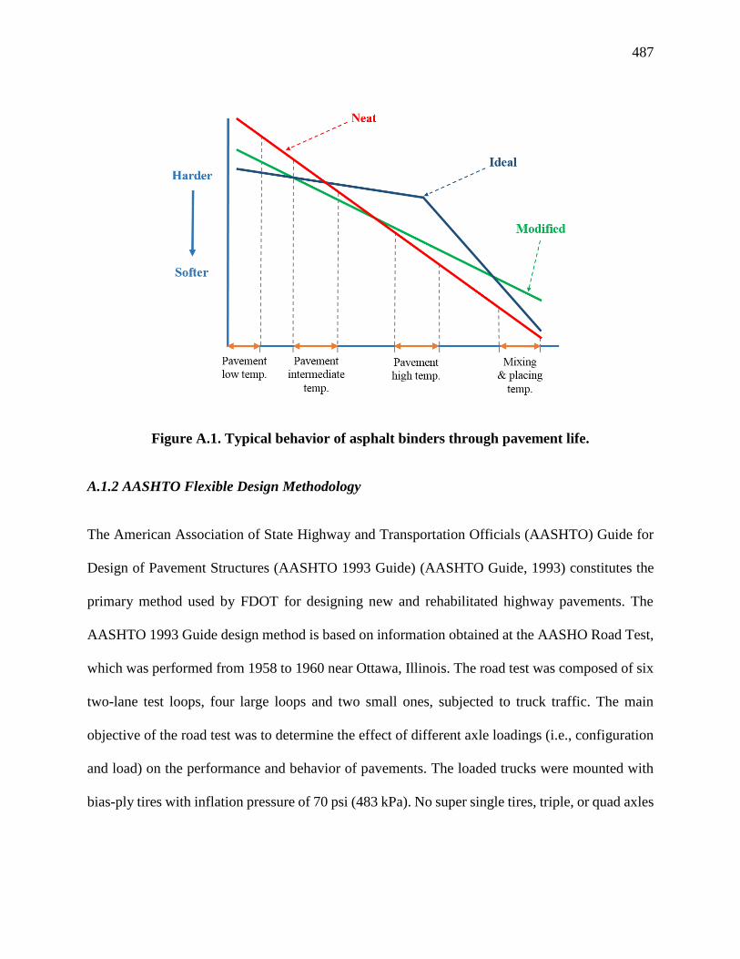
487
Figure A.1. Typical behavior of asphalt binders through pavement life.
A.1.2 AASHTO Flexible Design Methodology
The American Association of State Highway and Transportation Officials (AASHTO) Guide for
Design of Pavement Structures (AASHTO 1993 Guide) (AASHTO Guide, 1993) constitutes the
primary method used by FDOT for designing new and rehabilitated highway pavements. The
AASHTO 1993 Guide design method is based on information obtained at the AASHO Road Test,
which was performed from 1958 to 1960 near Ottawa, Illinois. The road test was composed of six
two-lane test loops, four large loops and two small ones, subjected to truck traffic. The main
objective of the road test was to determine the effect of different axle loadings (i.e., configuration
and load) on the performance and behavior of pavements. The loaded trucks were mounted with
bias-ply tires with inflation pressure of 70 psi (483 kPa). No super single tires, triple, or quad axles
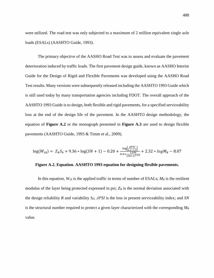
488
were utilized. The road test was only subjected to a maximum of 2 million equivalent single axle
loads (ESALs) (AASHTO Guide, 1993).
The primary objective of the AASHO Road Test was to assess and evaluate the pavement
deterioration induced by traffic loads. The first pavement design guide, known as AASHO Interim
Guide for the Design of Rigid and Flexible Pavements was developed using the AASHO Road
Test results. Many versions were subsequently released including the AASHTO 1993 Guide which
is still used today by many transportation agencies including FDOT. The overall approach of the
AASHTO 1993 Guide is to design, both flexible and rigid pavements, for a specified serviceability
loss at the end of the design life of the pavement. In the AASHTO design methodology, the
equation of Figure A.2 or the monograph presented in Figure A.3 are used to design flexible
pavements (AASHTO Guide, 1993 & Timm et al., 2009).
log (𝑊18) = 𝑍𝑅𝑆0 + 9.36 ∗ log(𝑆𝑁 + 1) − 0.20 +log[
𝛥𝑃𝑆𝐼
4.2−1.5]
0.4+1,094
(𝑆𝑁+1)5.19
+ 2.32 ∗ 𝑙𝑜𝑔𝑀𝑅 − 8.07
Figure A.2. Equation. AASHTO 1993 equation for designing flexible pavements.
In this equation, W18 is the applied traffic in terms of number of ESALs; MR is the resilient
modulus of the layer being protected expressed in psi; ZR is the normal deviation associated with
the design reliability R and variability S0; ΔPSI is the loss in present serviceability index; and SN
is the structural number required to protect a given layer characterized with the corresponding MR
value.

489
Figure A.3. AASHTO 1993 Nomograph for designing flexible pavements.
The desired level of design reliability increases with the increase in design traffic.
According to AASHTO 1993 Guide, an 85% reliability may be selected for a low volume road
(defined as less than 500 ESALs per day) while a 95% reliability or higher is suggested for a
medium volume road (subjected to a traffic between 500 and 1750 ESALs per day) or a high
volume road (subjected to a traffic greater than 1750 ESALs per day). For flexible pavement, the
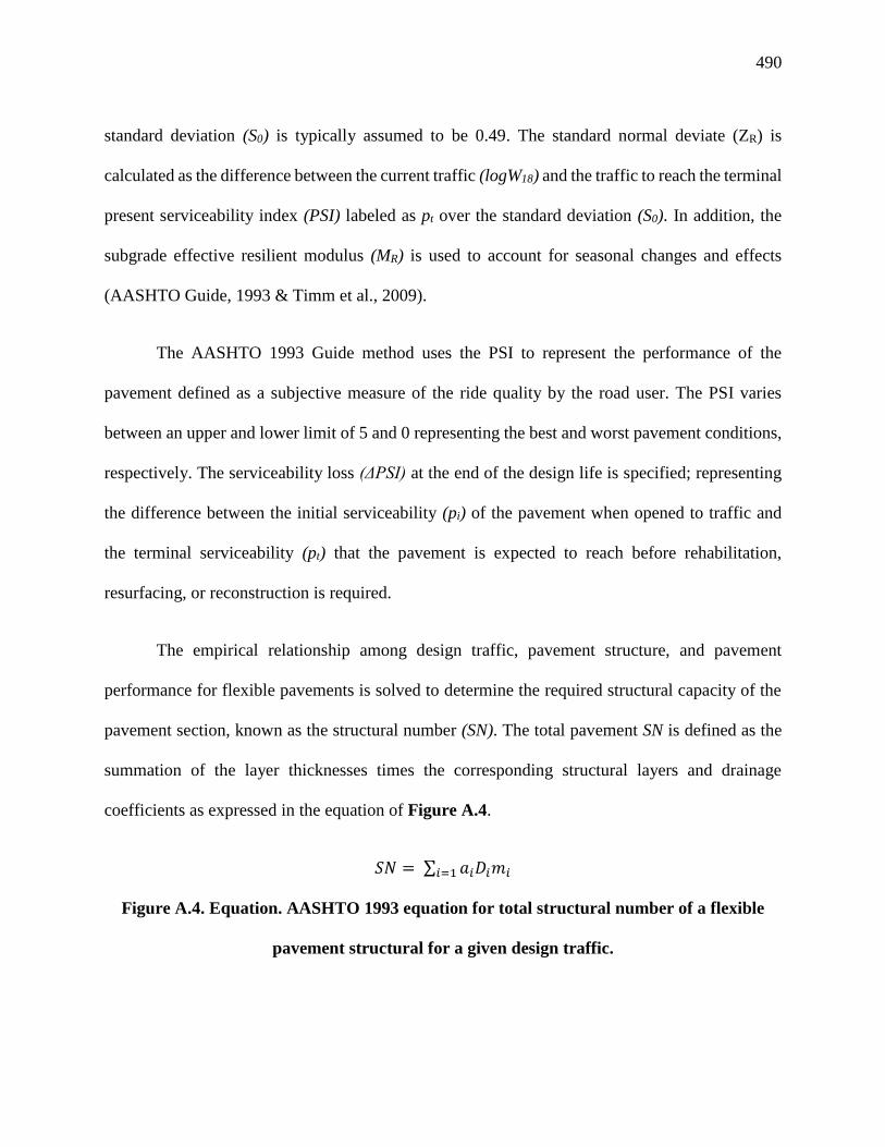
490
standard deviation (S0) is typically assumed to be 0.49. The standard normal deviate (ZR) is
calculated as the difference between the current traffic (logW18) and the traffic to reach the terminal
present serviceability index (PSI) labeled as pt over the standard deviation (S0). In addition, the
subgrade effective resilient modulus (MR) is used to account for seasonal changes and effects
(AASHTO Guide, 1993 & Timm et al., 2009).
The AASHTO 1993 Guide method uses the PSI to represent the performance of the
pavement defined as a subjective measure of the ride quality by the road user. The PSI varies
between an upper and lower limit of 5 and 0 representing the best and worst pavement conditions,
respectively. The serviceability loss (ΔPSI) at the end of the design life is specified; representing
the difference between the initial serviceability (pi) of the pavement when opened to traffic and
the terminal serviceability (pt) that the pavement is expected to reach before rehabilitation,
resurfacing, or reconstruction is required.
The empirical relationship among design traffic, pavement structure, and pavement
performance for flexible pavements is solved to determine the required structural capacity of the
pavement section, known as the structural number (SN). The total pavement SN is defined as the
summation of the layer thicknesses times the corresponding structural layers and drainage
coefficients as expressed in the equation of Figure A.4.
𝑆𝑁 = ∑ 𝑎𝑖𝐷𝑖𝑚𝑖𝑖=1
Figure A.4. Equation. AASHTO 1993 equation for total structural number of a flexible
pavement structural for a given design traffic.

491
In this equation, SN stands for the total structural number required for a given design traffic;
ai is the structural coefficient for the ith layer; Di is the thickness of the ith layer expressed in inch;
and mi is the drainage coefficient for the ith layer except for the AC layer.
No direct method exists for establishing new structural coefficients as new AC mixtures
are created. The current structural coefficients were estimated based on many factors including
material stiffness, and compressive and/or tensile strength. Figure A.5 shows a chart used to
estimate the structural coefficient of dense-graded AC surface course based on its elastic (resilient)
modulus (EAC) at a temperature of 68°F (20°C) in accordance with the AASHTO 1993 Guide
(AASHTO Guide, 1993). These coefficients were determined based on limited parameters used in
the AASHO road test where a single type subgrade soil, gravel base, and AC mix were considered.
Furthermore, no advanced paving materials including Superpave-designed AC mixes and polymer
modified AC mixes were used. Therefore, the relationship used to determine the AC structural
coefficient may not be valid for AC mixes currently used by FDOT and other state DOTs.
Figure A.5. Chart estimating structural coefficient of dense-graded asphalt concrete based
on the elastic (resilient) modulus after AASHTO 1993.
492
A.1.3 FDOT Pavement Design Practice
FDOT recently updated and published a manual for designing flexible pavements in Florida
(September 2016) (FDOT Design Manual, 2016). This manual provides guidance for conducting
new and rehabilitated flexible pavement designs according to the AASHTO 1993 Guide.
Additional information regarding materials testing and obtaining traffic data are provided. It
should be mentioned that FDOT has not yet adopted the 2008 AASHTO Mechanistic-Empirical
Pavement Design Guide (MEPDG) for flexible pavement design which was developed as part of
the National Cooperative Highway Research Program (NCHRP Project 1-37A) (MEPDG Guide,
2004). The existence of several major revisions to the models used in the AASHTOWare®
Pavement M-E software has been cited as the reason for non-adoption by Florida DOT (Timm et
al., 2009).
A.1.4 Problem Statement
Based on previous experience, a structural coefficient of 0.44 was found to be well representative
of PMA AC mixes when designed in a pavement section following the AASHTO 1993 Guide. In
some states, this coefficient was recalibrated to account for the conventional polymer modification
of asphalt mixtures (2-3% polymer). For example, in Alabama, the resulting average AC structural
coefficient was 0.54 with a standard deviation of 0.08 leading to approximate reduction in the
thickness of the AC layer of 18% based on a study conducted by the National Center for Asphalt
Technology (NCAT) in 2009 (Timm et al., 2009). If the positive impact of the polymer on the
layer is assumed to be maintained at higher contents, then the use of a high polymer (HP) modified
asphalt binder may lead to a higher AC structural coefficient and a reduced AC layer thickness for
the same design traffic and serviceability design loss (Timm et al., 2009).

493
Consequently, the objective of this FDOT research study is to determine the structural
coefficient for asphalt mixes that contain a HP modified binder (specified by FDOT as HP binder
and containing approximately 7.5% polymer). With this determination, the FDOT Flexible
Pavement Design Manual may be modified to adopt the structural value for mixtures containing
this binder type. For this purpose, the major tasks to be carried out in this research are:
• Conduct an extensive review of literature by compiling information about HP AC mixes,
their evaluation in the laboratory, their implementation on actual existing demonstration
field projects, and their performance all around the United States, Central America, and
Europe.
• Establish mix designs for PMA and HP AC mixes following the FDOT Superpave mix
design specifications using representative local materials from multiple sources in the state
of Florida.
• Evaluate the engineering properties and performance characteristics of the designed PMA
and HP AC mixes, and implement the developed properties and characteristics into an
advanced flexible pavement modeling process to determine the responses and performance
under various structural and loading conditions. This task will lead to preliminary
structural coefficients for HP AC mixes.
• Verify the structural coefficients assigned to the HP modified asphalt mixtures, developed
and checked in the previous tasks for various type of distresses using a full-scale laboratory
testing of asphalt pavement structures (e.g., Pave-Box).

494
• Develop a practical plan to validate the recommended structural coefficient for HP AC
mixes under the FDOT Accelerated Pavement Testing (APT) facility.
A.1.5 Objective and Scope
In this research, HP AC mixes are defined as asphalt mixtures manufactured using asphalt binders
modified with Styrene-Butadiene-Styrene (SBS) or Styrene-Butadiene (SB) at the approximate
rate of 7.5% by weight of binder. PMA AC mixes are defined as asphalt mixtures manufactured
using asphalt binders modified with SBS or SB at the approximate rate of 3% by weight of binder.
The literature review conducted in this research had two objectives: a) identify and review all
current and previous studies that have been conducted to evaluate the engineering properties and
performance characteristics of HP asphalt binders and HP AC mixes, and b) identify and assess
methods used to determine the structural coefficient of HP AC mixes for use in the structural
design of flexible pavements.
The literature review presented in this report covers studies that evaluated HP asphalt
binders and HP AC mixes. In addition, the report documents studies that evaluated asphalt binders
and mixtures that were manufactured at multiple levels of polymer modification but do not fit the
HP category as defined in this research. These studies were incorporated in the review since they
offer insights on the impact of the incremental increase in the polymer content on the properties of
asphalt binders and mixtures.
The literature review focused on three major areas of interest: a) laboratory evaluations of
HP modified asphalt binders and mixtures, b) performance of pavement sections constructed with
HP AC mixes, and c) techniques to determine the structural coefficient of HP AC mixes. It should

495
be noted that evaluations of PMA binders and PMA AC mixes have been included only in cases
where they represent the control materials.
A.2 Laboratory Evaluation of HP Modified Asphalt Binders and Mixtures
Polymer modification of asphalt binders is not a new concept and has become progressively more
common over the past several decades. While several agencies utilize unmodified asphalt binders,
many have increasingly become reliant upon polymer modified asphalt binders with a fair portion
of those located in climatic regions that experience significantly wider temperature range
conditions and higher levels of oxidation. Therefore, it is becoming ever more important to
characterize the benefits afforded with the polymer modification process. The objectives of this
chapter are to: a) present an overall background on the history of asphalt binder modification using
polymers, and b) provide some detailed information about recent laboratory studies that evaluated
the performance of HP asphalt binders and mixtures.
A.2.1 History of Polymer Modified Asphalt Binders
The increase in traffic volume and axle loads coupled with reduced budgets of public agencies
required better performance from the designed pavement structure. The modification of asphalt
binders was identified as a suitable solution to provide the improved performance (Zhu, 2015).
The processes providing the modification of asphalt binders using natural and synthetic polymers
were patented as early as 1843 in Europe (Yildirim, 2005 & Thompson et al., 1979). The
significantly higher costs of the early polymer modified asphalt binders limited their use in the
United States till mid-1980s when newer and less expensive polymers were developed (Terrel et
al., 1986). A survey conducted in 1997, indicated that 47 out of 50 states allowed the use of

496
modified asphalt binders and some DOTs (35 out of 47) confirmed that their use is quickly
increasing (Bahia et al., 1997). At that time, many research teams around the world focused on
evaluating the benefits to pavement performance attributed to the use of polymer modified asphalt
binders. A study done for Ohio DOT (OHDOT) showed that AC mixtures manufactured using
modified asphalt binders performed much better in terms of resistance to fatigue cracking and
permanent deformation when compared with mixtures manufactured using neat asphalt binders
(Sargand et al., 2001). A significantly higher viscosity was observed for modified asphalt binders
at 140°F (60°C) in accordance with a study done in Nevada in 2003 (Sebaaly et al., 2003). In a
2003 study discussing the concept of hot mix asphalt (HMA) perpetual pavements, Newcomb
claimed the benefit of using a modified asphalt mixture in the bottom lift of the AC layer in
increasing the fatigue life of the pavement structure (Newcomb, 2003). Consequently, agencies
estimated an addition of four to six years of life for a pavement structure when constructed using
a modified asphalt binder.
A 2003 study by the US Army Corps of Engineers showed that the type of modifier may
affect the performance of the asphalt binder in resisting multiple distresses such as rutting, fatigue,
thermal cracking, and moisture damage (Part et al., 2003). In comparison to neat asphalt binders,
modifiers typically invoke specific enhancements to the physical properties and rheological
performance of asphalt binders, such as improving the ductility, expanding the relaxation spectra,
and increasing its overall strength. For example, ductility and resistance to rutting can be improved
by the use of natural rubber in asphalt binder despite its problems with compatibility and
decomposition (Becker et al., 2011). The use of tire rubber improved the resistance to rutting and
reflective cracking but still required high mixing temperatures and long digestion times to prevent
the separation of the modified asphalt binder (Becker et al., 2011). Meanwhile, the addition of

497
Styrene-Butadiene-Rubber modifier (SBR) to asphalt binders helped in improving the low-
temperature ductility, elastic recovering as well as the cohesive and adhesive properties of the
binder (Becker et al., 2011). Within the past 20 years, the SBS modifier replaced the SBR because
of its wider compatibility and greater tensile strength property (Bates et al., 1987). In general,
improvement in asphalt binder ductility in conjunction with the improved elastic behavior due to
polymer modification can have a positive influence on the cracking resistance of asphalt mixtures.
Previous studies have shown the capability of polymer modifiers to lessen the deteriorative
oxidative age hardening effects (Roque et al., 2004). Accordingly, more durable asphalt pavements
can be expected from the use of polymer modified AC mixtures.
Currently, SBS is a well-recognized elastomer which is commonly used in asphalt mixtures
due to its elasticity and ability to be recycled. Asphalt binders modified with SBS polymers have
shown improved performance at low temperatures when compared to un-modified binders and
binders modified with chemically reactive polymers (e.g., Polyphosphoric Acid…). In 2003,
Mohammed et al. evaluated the possibility of recycling SBS modified asphalt mixtures as part of
the pavement rehabilitation process (Mohammed et al., 2003). Cores were sampled from US61 in
Louisiana and the eight-year-old SBS modified binder was extracted and recovered. The recovered
polymer modified asphalt binder was blended with virgin binder and evaluated at different range
of temperatures. The blend was found to be much stiffer than anticipated at both low and high
temperatures with a higher rutting resistance and a lower fatigue resistance. A 2004 FDOT study
showed the use of SBS polymer in asphalt binder was able to reduce the rate of micro-damage
accumulation and therefore benefited cracking resistance (Roque et al., 2004). However, it was
found that there is no effect for using SBS on healing or aging characteristics of the asphalt
mixture.
498
The most commonly used polymer modified asphalt binders limit the SBS content to
around 3% due to cost and construction issues. Recent studies showed that these issues can be
overcome by modifying the conventional structure of the SBS polymer to produce a modified
asphalt binder with increased durability and reduced costs. In 2010, researchers at Delft University
developed a new SBS polymer structure that allowed the use of SBS at levels of 7 – 8% by weight
of asphalt binder (Fournier, 2010).
Figure A.6 illustrates a typical polymer modified asphalt binder with 2.5% polymer where
the polymer is not in continuous phase (Timm et al, 2012). Increasing the polymer content up to
7.5% changes the structure from asphalt binder with a dispersed swollen polymer phase to a
swollen polymer with a dispersed asphalt binder phase. At this stage, the HP asphalt binder is more
like an asphalt-modified rubber rather than a rubber-modified asphalt where the rubber makes the
continuous phase in the structure. The phase reversal achieved by the addition of high polymer
content produces a more elastic asphalt binder with improved resistance to permanent
deformations (i.e., rutting and shoving) and cracking (i.e., fatigue, thermal, and reflective).
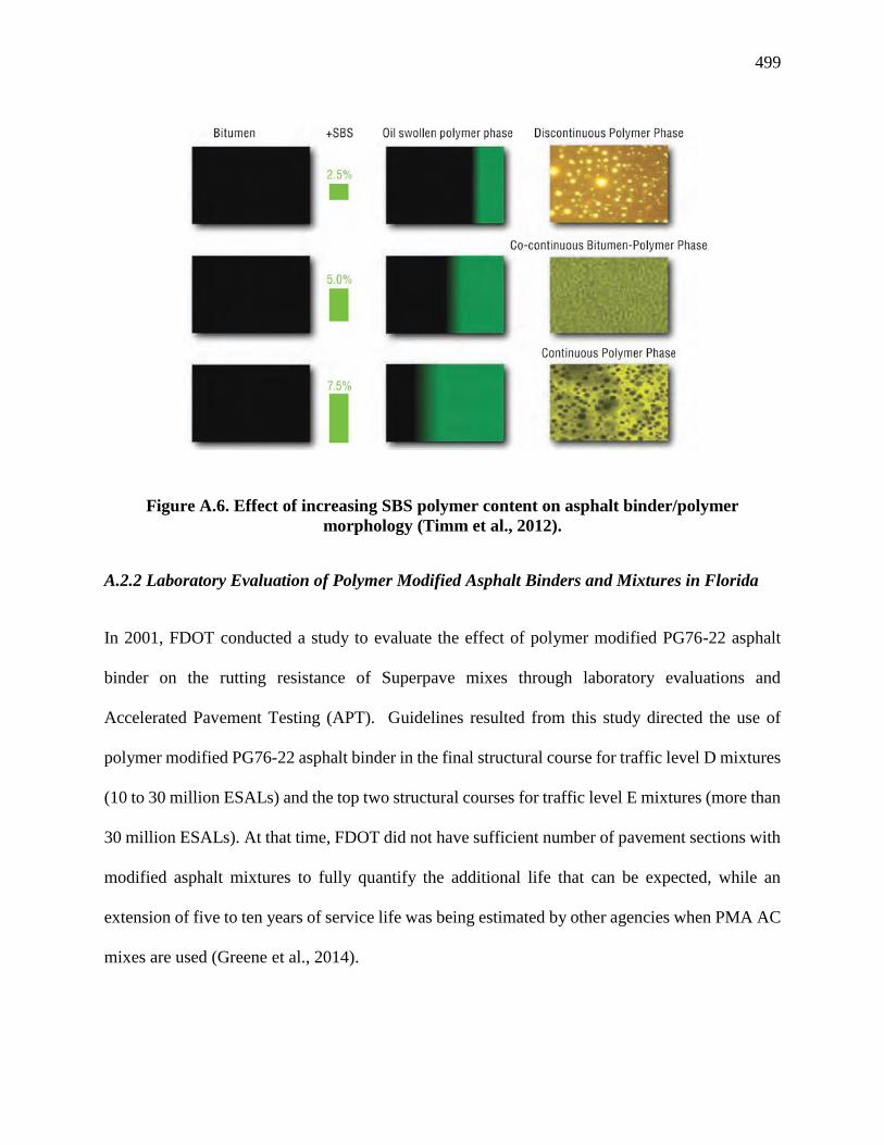
499
Figure A.6. Effect of increasing SBS polymer content on asphalt binder/polymer
morphology (Timm et al., 2012).
A.2.2 Laboratory Evaluation of Polymer Modified Asphalt Binders and Mixtures in Florida
In 2001, FDOT conducted a study to evaluate the effect of polymer modified PG76-22 asphalt
binder on the rutting resistance of Superpave mixes through laboratory evaluations and
Accelerated Pavement Testing (APT). Guidelines resulted from this study directed the use of
polymer modified PG76-22 asphalt binder in the final structural course for traffic level D mixtures
(10 to 30 million ESALs) and the top two structural courses for traffic level E mixtures (more than
30 million ESALs). At that time, FDOT did not have sufficient number of pavement sections with
modified asphalt mixtures to fully quantify the additional life that can be expected, while an
extension of five to ten years of service life was being estimated by other agencies when PMA AC
mixes are used (Greene et al., 2014).

500
Within the past five years, FDOT attempted to increase the rutting resistance of asphalt
mixtures by increasing the polymer content of asphalt binders resulting in a grade of PG82-
22PMA. The cost of the PG82-22PMA, in 2014, was approximately $100 and $250 per liquid
metric ton more expensive than the PG76-22PMA and the neat PG67-22 asphalt binder,
respectively. Therefore, such investment requires the assessment and quantification of additional
benefits provided by the use of PG82-22PMA. In response, an extensive study was conducted to
evaluate the performance of PG82-22PMA mixtures in terms of rutting and fatigue resistance in
the laboratory and under APT loading (Greene et al., 2014).
It should be noted that the PG82-22PMA asphalt binder and mixture evaluated in the FDOT
study contained 6% SBS polymer by weight of binder. Therefore, the PG82-22PMA does not meet
the requirement of a HP binder as defined in this current study (i.e., approximate SBS content of
7.5% by weight of binder). As discussed in the scope of the literature review, the FDOT study was
included since it offers an insight on the impact of incrementally increasing the SBS content from
0, 3, to 6% by weight of binder.
A.2.2.1 Properties of Evaluated Asphalt Binders
Three asphalt binders meeting the current FDOT specifications were evaluated in this study: a
PG67-22 neat binder, a PG76-22PMA binder at 3% SBS content, and a PG82-22PMA binder at
6% SBS content. All asphalt binders were collected at the plant and laboratory tests such as
dynamic shear rheometer (DSR), multiple stress creep recovery (MSCR), and binder fracture
energy were conducted for analysis and characterization (Greene et al., 2014).

501
Dynamic Shear Rheometer
The DSR is used to characterize the viscous and elastic behavior of asphalt binders at high to
intermediate pavement temperatures (part of the in-service pavement temperature range) via
measuring the complex modulus (G*) and phase angle () (AASHTO T315, 2013). This
characterization is used in the Superpave Performance Grade (PG) asphalt binder specification.
DSR tests were performed on original asphalt binders at the high temperature of each selected
binder grade (i.e. 67, 76, and 82°C). Figure A.7 presents the DSR properties of the three evaluated
binders. The results showed that the PG82-22PMA binder exhibited the greatest stiffness,
elasticity, and rutting resistance, as shown by its high G*, low 𝛿, and high G*/sin(𝛿), respectively.
It should be mentioned that FDOT specifies a minimum G*/sin(𝛿) of 1.0 kPa and a maximum
phase angle () of 75° and 65° for PG76-22PMA and PG82-22PMA asphalt binders, respectively.
Figure A.7. DSR properties of PG67-22, PG76-22PMA, and PG82-22PMA binders (Greene
et al., 2014).
Multiple Stress Creep Recovery
The MSCR test provides additional properties on the asphalt binder at high pavement temperature
to assess its resistance to rutting under the expected traffic level. The test consists of applying a
stress level of 0.1 kPa or 3.2 kPa for ten consecutive cycles. Each cycle consists of a creep period
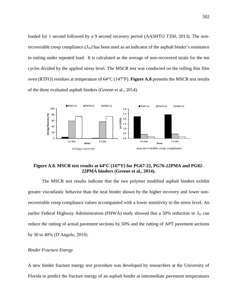
502
loaded for 1 second followed by a 9 second recovery period (AASHTO T350, 2013). The non-
recoverable creep compliance (Jnr) has been used as an indicator of the asphalt binder’s resistance
to rutting under repeated load. It is calculated as the average of non-recovered strain for the ten
cycles divided by the applied stress level. The MSCR test was conducted on the rolling thin film
oven (RTFO) residues at temperature of 64°C (147°F). Figure A.8 presents the MSCR test results
of the three evaluated asphalt binders (Greene et al., 2014).
Figure A.8. MSCR test results at 64C (147F) for PG67-22, PG76-22PMA and PG82-
22PMA binders (Greene et al., 2014).
The MSCR test results indicate that the two polymer modified asphalt binders exhibit
greater viscoelastic behavior than the neat binder shown by the higher recovery and lower non-
recoverable creep compliance values accompanied with a lower sensitivity to the stress level. An
earlier Federal Highway Administration (FHWA) study showed that a 50% reduction in Jnr can
reduce the rutting of actual pavement sections by 50% and the rutting of APT pavement sections
by 30 to 40% (D’Angelo, 2010).
Binder Fracture Energy
A new binder fracture energy test procedure was developed by researchers at the University of
Florida to predict the fracture energy of an asphalt binder at intermediate pavement temperatures

503
(Roque et al., 2012). It was shown that this fracture energy constitutes a fundamental property of
the asphalt binder independent of the testing temperature and the loading rate. The test consists of
applying a direct tensile stress on a binder specimen at relatively high loading rate (0.4-3.9
inch/min (10-100 mm/min)) and measures the stress versus strain curve. The average true stress
versus strain curve is calculated on the central cross-sectional area of the specimen where fracture
initiates and propagates. Fracture energy is calculated as the surface underneath the stress-strain
curve from the beginning of the test to the highest stress level representing the point of initial
fracture. The test was conducted at a temperature of 50°F (10°C) on RTFO residues subjected to
long-term aging in the pressure aging vessel (PAV). A greater fracture energy was observed for
the PG82-22PMA when compared with the PG76-22PMA and PG67-22 binders (Figure A.9)
indicating a better fracture resistance for AC mixes manufactured with the PG82-22PMA binder
(Greene et al., 2014).
Figure A.9. Binder fracture energy test results for PG67-22, PG76-22PMA, and PG82-
22PMA binders (Greene et al., 2014).
A.2.2.2 Properties of AC Mixtures
The AC mixtures were designed with 0.5-inch (12.5 mm) nominal maximum aggregate size
(NMAS) fine gradation using granite aggregate. The optimum asphalt binder contents were
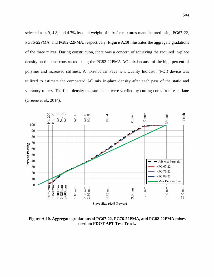
504
selected as 4.9, 4.8, and 4.7% by total weight of mix for mixtures manufactured using PG67-22,
PG76-22PMA, and PG82-22PMA, respectively. Figure A.10 illustrates the aggregate gradations
of the three mixes. During construction, there was a concern of achieving the required in-place
density on the lane constructed using the PG82-22PMA AC mix because of the high percent of
polymer and increased stiffness. A non-nuclear Pavement Quality Indicator (PQI) device was
utilized to estimate the compacted AC mix in-place density after each pass of the static and
vibratory rollers. The final density measurements were verified by cutting cores from each lane
(Greene et al., 2014).
Figure A.10. Aggregate gradations of PG67-22, PG76-22PMA, and PG82-22PMA mixes
used on FDOT APT Test Track.
25
.0 m
m1
inch
19
.0 m
m3
/4 i
nch
12
.5 m
m1
/2 i
nch
9.5
mm
3/8
inch
4.7
5 m
mN
o. 4
2.3
6 m
mN
o. 8
2.0
0 m
mN
o. 1
0
1.1
8 m
mN
o. 1
6
0.4
25
mm
No
. 4
00
.30
0 m
mN
o. 5
0
0.1
50
mm
No
. 1
00
0.0
75
mm
No
. 2
00
0.6
00
mm
No
. 3
0
0
10
20
30
40
50
60
70
80
90
100
Per
cen
t P
ass
ing
Sieve Size (0.45 Power)
Job Mix Formula
PG 67-22
PG 76-22
PG 82-22
Max Density Line

505
Superpave Indirect Tension
The cracking resistance of the mixtures was evaluated using the Superpave indirect tension test
(IDT) (AASHTO T322). The test was conducted only on cores from the PG76-22PMA and PG82-
22PMA sections at a temperature of 50°F (10°C) due to time limitations. The IDT applies a
diametral creep load on a 6 inch (150 mm) diameter by 2.5 inch (64 mm) height sample to measure
the creep compliance followed by the tensile strength. Using the measured creep compliance and
tensile strength, the dissipated creep strain energy (DCSE) and energy ratio (ER) are calculated
and used to assess the resistance of the evaluated asphalt mixture to top-down cracking. Figure
A.11 shows the measured properties from the IDT in terms of fracture energy, creep rate, and
energy ratio. These plots lead to the following observations:
• Slightly lower fracture energy was observed for the PG82-22PMA AC mix when compared
with the PG76-22PMA AC mix. However, this minor difference in the measured fracture
energy values may be due to the variability in the IDT test.
• A 66% reduction in the creep rate was observed for the PG82-22PMA AC mix as compared
to the PG76-22PMA AC mix.
• Relatively higher energy ratio was exhibited by the PG82-22PMA AC mix indicating a
better cracking resistance when compared with the PG76-22PMA AC mix.

506
Figure A.11. IDT fracture properties for PG76-22PMA and PG82-22PMA asphalt mixtures
(Greene et al., 2014).
A.2.2.3 APT Experiment: Design and Testing
In general, APT consists of applying repetitive full scale wheel loads to a pavement structure to
simulate in-service loading conditions. The accelerated loading was performed using the FDOT
Heavy Vehicle Simulator (HVS), electrically powered, mobile, and fully automated. The overall
experiment evaluated the rutting and fatigue performance of the different mixtures (Greene et al.,
2014).
For the evaluation of rutting resistance, the AC layers of the existing three test lanes were
milled to a depth of 4 inch (102 mm) leaving 1 inch (25 mm) of the existing AC layer in-place.
The milled 4 inch (102 mm) AC mix was replaced by the PMA and neat asphalt mixtures as shown
in Figure A.12-a. The mix designs were classified as Superpave fine-graded mixes manufactured
using granite material with 5.1% asphalt binder content by total weight of mix. For rutting
evaluation, the pavement test track lanes were heated to 122°F (50°C) and trafficked with a 9,000
pounds (4,082 Kg) load on dual tires with inflation pressure of 100 psi (690 kPa). Laser profiles
were used to measure rut depths at various intervals of the HVS loading (Greene et al., 2014).
For the evaluation of fatigue resistance, additional two test lanes were constructed
consisting of two 1.5 inch (38 mm) lifts of the same PMA Superpave fine-graded AC mixes placed

507
directly on the granular base layer (Refer to Figure A.12-b). The water table was raised to the
bottom of the base to weaken the pavement structure. Longitudinal strains under dual tires load of
12,000 pounds (5,443 Kg) with inflation pressure of 110 psi (758 kPa) were measured by strain
gauges installed at the bottom of the 3 inch (76 mm) AC layer (Greene et al., 2014).
The rutting performance of the various mixes were evaluated through measuring the actual
rut depth developed in the wheel path and by estimating the shear area at the edge of the rut relative
to the area of wheel path. Figure A.13 illustrates the rut profiles (i.e., progression of rut depths)
of the three test lanes as well as the transverse rut profiles after 100,000 passes. Table A.1
summarizes the rutting and shear area values of the various sections under the HVS loading. The
data in Figure A.13 and Table A.1 indicate that both polymer modified mixtures (i.e., PG76-
22PMA, and PG82-22PMA) significantly out-performed the neat mix (i.e., PG67-22) showing a
rut depth reduction of 29% and 49% after 100,000 passes, respectively. Meanwhile the PG82-
22PMA AC mix performed significantly better than the PG76-22PMA in both measured rut depth
(reduction of 28%) and shear area (reduction of 40%) (Greene et al., 2014).
In the fatigue resistance evaluation, FDOT researchers reported significant reductions in
measured tensile strains at the bottom of AC layer for the two PMA AC mixes with the percent
reduction increasing with the higher polymer content (i.e., PG82-22PMA). In addition, the
predicted fatigue life of the PG82-22PMA AC mix was seven times higher than the fatigue life of
the PG76-22PMA AC mix. On the other hand, the predicted fatigue lives of the two polymer
modified mixes were more than 20 times higher than the predicted fatigue life of the neat PG67-
22 mix (Greene et al, 2014).
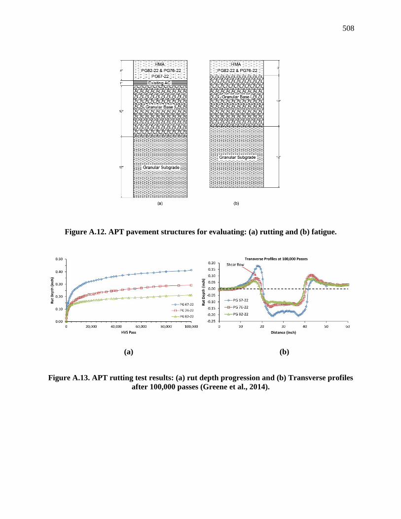
508
Figure A.12. APT pavement structures for evaluating: (a) rutting and (b) fatigue.
(a) (b)
Figure A.13. APT rutting test results: (a) rut depth progression and (b) Transverse profiles
after 100,000 passes (Greene et al., 2014).

509
Table A.1. Summary of the Rutting Performance of the APT Sections (Greene et al., 2014).
Pass
Number
PG67-22 PG76-22PMA PG82-22PMA
Rut, inch
(mm)
Shear
Area/ WP
Area
Rut, inch
(mm)
Shear Area/
WP Area
Rut, inch
(mm)
Shear
Area/ WP
Area
100 0.06
(1.52) 0.21
0.03
(0.76) 0.44
0.06
(1.52) 0.23
5,000 0.24
(6.10) 0.60
0.16
(4.06) 0.50
0.14
(3.56) 0.28
10,000 0.28
(7.11) 0.63
0.19
(4.83) 0.52
0.15
(3.81) 0.20
20,000 0.32
(8.13) 0.61
0.22
(5.59) 0.49
0.17
(4.32) 0.30
100,000 0.41
(10.41) 0.72
0.29
(7.37) 0.45
0.21
(5.34) 0.27
A.2.2.4 Conclusions and Implementation
The data presented in this FDOT research on the laboratory evaluations of the asphalt binders and
mixtures and the APT evaluations indicated that the incremental addition of the SBS polymer from
0, 3, to 6% by weight of binder significantly improved the resistance of the materials to rutting and
fatigue. Under all the evaluations, the data showed that the addition of 3% SBS improved the
performance of the binder and mix relative to the 0% SBS while the addition of 6% SBS improved
the performance of the binder and mix relative to the 3% SBS at a significantly higher rate. These
observations lead to the belief that increasing the SBS content to the HP level of 7.5% would
continue to improve the performance of the asphalt binder and mix.
Based on the findings of this study, FDOT allowed the use of the PG82-22PMA binder by
increasing the mix compaction temperature from 331°F (166°C) to 340°F (171°C) along with a
decrease of the phase angle criterion in the binder specification from 75° to 65°. FDOT
implemented the PG82-22PMA in two resurfacing projects during 2012: (a) SR 60 in Hillsborough

510
County, and (b) the mainline pavement in Nassau County on SR 200. The latest comments received
from FDOT personnel indicated that both projects are still showing good performance in terms of
smoothness, rutting, and fatigue resistance (Greene et al., 2014).
A.2.3 Effect of Long-Term Aging on HP-Modified Asphalt Binders
In addition to improving the resistance of the AC mixtures to rutting and cracking, the high
polymer content may improve the resistance of the asphalt binder to long-term aging. An asphalt
binder with low susceptibility to long-term aging would significantly reduce the potential of the
asphalt mixture to all types of cracking: bottom-up fatigue, top-down fatigue, thermal, reflective,
and block. This phenomenon was evaluated in a recent research study by the Pavement
Engineering and Science (PES) Program at University of Nevada, Reno (UNR) where the long-
term aging susceptibility of three asphalt binders: neat, polymer modified with 3% SBS (PMA),
and highly polymer modified with 7.5% SBS (HP) were evaluated (Zhu, 2015 & Morian et al.,
2015). The main objective of the study was to observe and quantify the influence of binder
modification on the oxidative aging characteristics of asphalt binders.
The neat binder was used as the base for the two polymer modified binders. The evaluated
asphalt binders were aged to measure the aging kinetics as a function of time and temperature
when the binders were exposed to free-atmospheric air. The three asphalt binders were placed in
5.5 inch (140 mm) diameter PAV pan at 0.04 inch (1 mm) film thickness and subjected to long-
term aging in forced draft ovens for various combinations of temperatures and aging durations as
follows:
• 122°F (50°C) for 4, 8, 15, 30, 60, 120, 180, and 240 days;
• 140°F (60°C) for 2, 4, 8, 15, 30, 60, 100, and 160 days; and

511
• 185°F (85°C) for 0.5, 1, 2, 4, 8, 15, 25, and 40 days.
Rheological evaluations based upon master curve development can be a very useful method
to evaluate the influence of oxidative aging on multiple physical characteristics of asphalt binders.
The rheological indices utilized in this study were derived from the developed dynamic shear
modulus master curve utilizing the time-temperature superposition principle to predict properties
at the temperature and frequency combinations. Two asphalt binder replicates were tested in the
DSR to determine the rheological parameters by conducting isothermal frequency sweeps at
different temperatures ranging from 230°F (110°C) to 28.4°F (-2°C). The isotherms were then
shifted into master curves of dynamic shear modulus (G*) and phase angle () utilizing the Rhea
software package. Correspondingly, black space diagrams, defined as shear modulus versus phase
angle plot, provides a robust evaluation methodology for the rheological evaluation of asphalt
binders. The aging susceptibility of the asphalt binders were evaluated using the Glover-Row (G-
R) parameter defined as function of G* and the corresponding as indicated in Equation A.1.
𝐺 − 𝑅 = 𝐺∗𝑐𝑜𝑠2𝛿
sin 𝛿 [Equation. A.1]
Where;
G*: dynamic shear modulus; and
𝛿: phase angle
Figure A.14 shows the measured properties of the aged binders plotted on the G-R
parameter scale. Each data point plotted in this figure represents a specific asphalt binder condition
in terms of temperature and time as defined earlier. It is anticipated that lower G* and lower δ
represent lower susceptibility to long-term aging. In addition, a steeper slope between G* and δ
represents lower susceptibility to long-term aging. In other words, a steep curve located closer to

512
the left side of the chart indicates lower susceptibility to long-term aging. The data presented in
Figure A.14 show that the HP asphalt binder is the least susceptible to long-term aging, followed
by the PMA binder, while the neat asphalt binder is the most susceptible to long-term aging.
Furthermore, the data show that the neat asphalt binder was the first binder to reach the G-R
cracking criterion of 87 psi (600 kPa) after about 170 days of oven aging while the PMA and HP
asphalt binders lasted for about 190 and 230 days before reaching the same failure criterion.
The advantages of the SBS polymer modification have been fairly distinct, consistent and
directly evident as outcome of this study. In summary, the addition of SBS polymer in well
formulated and consistently blended materials do provide clear benefits to the overall performance
of asphalt binders and corresponding mixtures in terms of longevity and aging resistance.
Figure A.14. Comparison of Glover-Rowe (G-R) parameters for neat, PMA, and HP
asphalt binders in a black space diagram.
1.0E+02
1.0E+03
1.0E+04
1.0E+05
1.0E+06
1.0E+07
1.0E+08
1.0E+09
0 10 20 30 40 50 60 70 80 90
G*
(P
a)
(15
°C, 0
.00
5 r
ad
/s)
Phase Angle (°)
G-R at 180 kPaG-R at 600 kPaG*/sin(d)≥2.2kpaG*sin(d)≤5000kpaBase Binder (Neat)PMA with 3% SBS (With Same Base Binder)HP with 7.5% SBS (With Same Base Binder)
Aging
Modification and Aging
PMA Neat (Base)HP
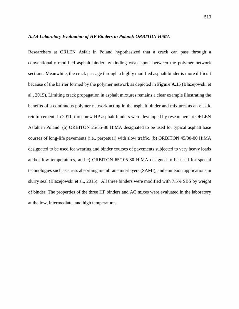
513
A.2.4 Laboratory Evaluation of HP Binders in Poland: ORBITON HiMA
Researchers at ORLEN Asfalt in Poland hypothesized that a crack can pass through a
conventionally modified asphalt binder by finding weak spots between the polymer network
sections. Meanwhile, the crack passage through a highly modified asphalt binder is more difficult
because of the barrier formed by the polymer network as depicted in Figure A.15 (Blazejowski et
al., 2015). Limiting crack propagation in asphalt mixtures remains a clear example illustrating the
benefits of a continuous polymer network acting in the asphalt binder and mixtures as an elastic
reinforcement. In 2011, three new HP asphalt binders were developed by researchers at ORLEN
Asfalt in Poland: (a) ORBITON 25/55-80 HiMA designated to be used for typical asphalt base
courses of long-life pavements (i.e., perpetual) with slow traffic, (b) ORBITON 45/80-80 HiMA
designated to be used for wearing and binder courses of pavements subjected to very heavy loads
and/or low temperatures, and c) ORBITON 65/105-80 HiMA designed to be used for special
technologies such as stress absorbing membrane interlayers (SAMI), and emulsion applications in
slurry seal (Blazejowski et al., 2015). All three binders were modified with 7.5% SBS by weight
of binder. The properties of the three HP binders and AC mixes were evaluated in the laboratory
at the low, intermediate, and high temperatures.
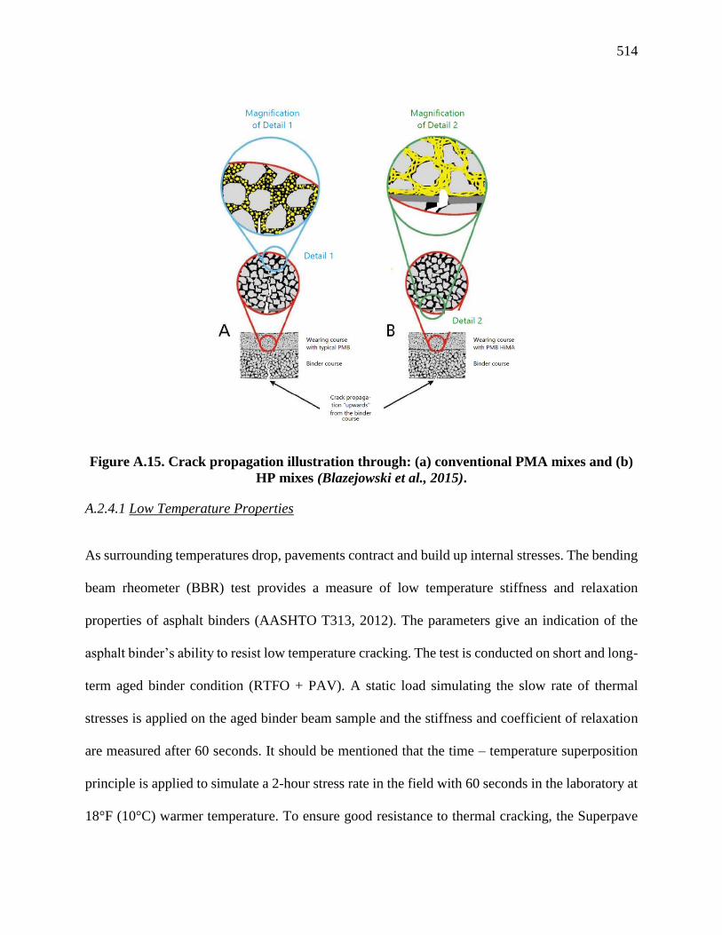
514
Figure A.15. Crack propagation illustration through: (a) conventional PMA mixes and (b)
HP mixes (Blazejowski et al., 2015).
A.2.4.1 Low Temperature Properties
As surrounding temperatures drop, pavements contract and build up internal stresses. The bending
beam rheometer (BBR) test provides a measure of low temperature stiffness and relaxation
properties of asphalt binders (AASHTO T313, 2012). The parameters give an indication of the
asphalt binder’s ability to resist low temperature cracking. The test is conducted on short and long-
term aged binder condition (RTFO + PAV). A static load simulating the slow rate of thermal
stresses is applied on the aged binder beam sample and the stiffness and coefficient of relaxation
are measured after 60 seconds. It should be mentioned that the time – temperature superposition
principle is applied to simulate a 2-hour stress rate in the field with 60 seconds in the laboratory at
18°F (10°C) warmer temperature. To ensure good resistance to thermal cracking, the Superpave

515
PG system requires the long-term aged asphalt binder to maintain a creep stiffness (S) below 300
MPa and an m-value above 0.300.
As indicated earlier, the HiMA binders contained 7.5% SBS while the neat asphalt binders
contained 0% SBS. The SBS content of the PMA binders could not be verified from the literature,
however, it is believed to be approximately 3%.
In addition to testing the binders in the BBR, mixtures manufactured using neat,
conventional PMA, and HP binders were evaluated in terms of thermal cracking resistance using
the thermal stress restrained specimen test (TSRST) (AASHTO TP10, 1993). The test measures
the tensile stress in a restrained AC specimen as it is cooled at a constant rate. As the temperature
drops, the specimen is restrained from contracting thus inducing tensile stresses. The fracture
strength and the fracture temperature are measured as part of this test. Figure A.16 parts a and b
present the data of the low temperature evaluations on the neat, two PMA, and HP binders from
the BBR and the corresponding mixes from the TSRST. It should be noted that the evaluated
binders and mixes were originally labeled as follows: a) the neat binders and mixes were labeled
by their Pen Grade, b) the conventional PMA binders and mixes were labeled with a “PMB”
extension, and c) the HP binders and mixtures were labeled with a “HiMA” extension. The data in
Figure A.16 are grouped into three parts where each part compares the properties of the
corresponding neat, two PMA, and HP binders and mixtures. The data in Figure A.16-a are
presented in terms of the temperatures at which the S(60) and m-value Superpave PG criteria are
met while the data in Figure A.16-b are presented in terms of the TSRST fracture temperature. It
should be noted that the lower the critical temperature of the S(60) and m-value the more resistant

516
the binder is to thermal cracking. The lower the TSRST fracture temperature the more resistant is
the asphalt mix to thermal carking.
The measured S(60) and m-value properties of the neat, two PMA, and HP binders show
that the BBR critical low temperatures continue to decrease as the SBS content increases from 0,
3, to 7.5% except for the third HP binder designed for use in SAMI and slurry seals. In addition,
the TSRST fracture temperature of the neat, two PMA, and HP mixtures continues to decrease as
the SBS content increases from 0, 3, to 7.5%. These results clearly show the benefits of using HP
binders towards improving the resistance of AC mixes to thermal cracking.
A.2.4.2 Intermediate Temperature Properties
The asphalt binders were evaluated in terms of their resistance to fatigue cracking using the DSR
test according to the Superpave PG system (AASHTO T315, 2013). The long-term aged asphalt
binder (RTFO + PAV) is tested in the DSR at a frequency of 10 rad/sec and the G* and δ are
measured. To ensure good resistance to fatigue cracking, the Superpave PG system requires the
long-term aged binder to maintain a G*sin(δ) less than 5,000 kPa. Figure A.17 presents the data
of the intermediate temperature evaluations on the neat, two PMA, and HP binders from the DSR.
The data in Figure A.17 are presented in terms of the temperatures at which the G*sin(δ)
Superpave PG criterion is met. It should be noted that the lower the temperature of the G*sin(δ)
the more resistant the binder to fatigue cracking. The measured G*sin(δ) properties of the neat,
two PMA, and HP binders show that the DSR critical intermediate temperature continues to
decrease as the SBS content increases from 0, 3, to 7.5%. These results clearly show the increased
resistance of the HP binders to fatigue cracking.

517
(a)
(b)
Figure A.16. Low temperature properties for neat, PMA, and HP asphalt binders and
mixtures (Bazejowski et al., 2015).

518
Figure A.17. Intermediate temperature properties for neat, PMA, and HP asphalt binders
(Bazejowski et al., 2015).
A.2.4.3 High Temperature Properties
The asphalt binders were evaluated in terms of their resistance to rutting using the DSR test
according to the Superpave PG system (AASHTO T315, 2013). Testing was conducted on original
binders prior to aging and on short-term aged residues (i.e., RTFO aged). To ensure good resistance
to rutting, the Superpave system requires a G*/sin(δ) higher than 1.00 and 2.20 kPa for original
un-aged and short-term aged binders, respectively. Figure A.18 presents the data of the high
temperature evaluations on the neat, two PMA, and HP binders from the DSR. The data in Figure
A.19 are presented in terms of the temperatures at which the G*/sin(δ) Superpave PG criteria are
met for the original and short-term aged binders. It should be noted that the higher the temperature
of the G*/sin(δ) the more resistant the binder to rutting. The measured G*/sin(𝛿) properties of the

519
neat, two PMA, and HP binders show the DSR critical temperatures continue to increase as the
SBS content increases from 0, 3, to 7.5%. These results clearly show the increased resistance of
the HP binders to rutting.
To further assess the rutting resistance of the binders, the MSCR test was performed at
temperatures of 147 and 158°F (64 and 70°C). The MSCR test measures the creep compliance (Jnr)
and the average percent recovery (R) of the binder at two stress levels (i.e., 0.1 kPa and 3.2 kPa).
Figure A.20 presents the Jnr and R properties of the neat, two PMA, and HP binders at the two
testing temperatures. The lower the Jnr and the higher the R the more resistant the binder will be to
rutting. The data in Figure A.20 show the HP binders plotted at the upper right hand corner of the
graph indicating lower Jnr and higher R properties than the neat and PMA binders at both
temperatures. In addition, the PMA binders also showed lower Jnr and higher R properties than the
neat binders at both temperatures. Again, the MSCR data show increased rutting resistance of the
binders as the SBS content increases from 0, 3, to 7.5%.
In addition to binder testing, mixtures manufactured with neat, two PMA, and HP binders
were evaluated for rutting resistance by applying 10,000 cycles using a small wheel tracker at a
temperature of 140°F (60°C). Figure A.21 presents the measured rut depths of the various
mixtures. Lower rut depths were observed for mixtures manufactured using the HP asphalt binders.
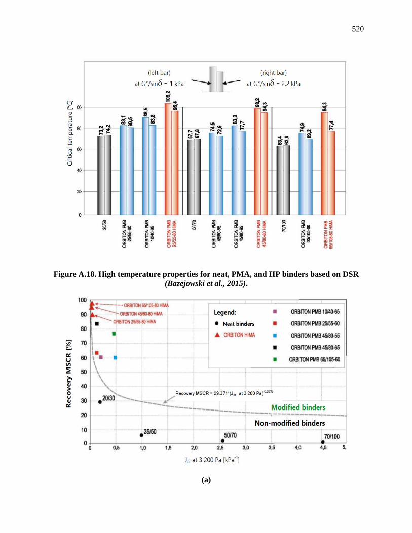
520
Figure A.18. High temperature properties for neat, PMA, and HP binders based on DSR
(Bazejowski et al., 2015).
(a)

521
(b)
Figure A.19. High temperature properties for neat, PMA, and HP binders based on the
MSCR test at (a) 64°C, and (b) 70°C (Bazejowski et al., 2015).
Figure A.20. High temperature properties for neat, PMA, and HP mixtures (Bazejowski et
al., 2015).

522
In summary, this study showed the positive impact of increasing the SBS content of asphalt
binders on the performance of asphalt binders and mixtures in terms of resisting the three
categories of asphalt pavement distresses: thermal cracking, fatigue cracking, and rutting.
A.2.5 Evaluation of Thin Overlay Mixes using HP Asphalt Binders
Over the last 35 years, the focus of state DOTs changed from the construction of new roads to
maintenance and rehabilitation of existing infrastructure by using several pavement preservation
techniques. These techniques are defined as a set of cost-effective practices designed to extend
pavement life, improve safety, and save public funds. Thin asphalt concrete overlay (thickness ≤
1.5 inch (38 mm)) is considered a preservation treatment for AC pavements. State DOTs in the
Northeast Pavement Preservation Partnership (NEPPP), the Pennsylvania Asphalt Pavement
Association (PAPA), academia, and industry, developed a pilot specification for high-performance
thin overlay (HiPO) mixtures manufactured using HP asphalt binders and reclaimed asphalt
pavement (RAP). HiPO was intended as a mean to extend the available funds for pavement
preservation and for essentially delaying future need for pavement rehabilitation. Several
distresses and issues that shorten the service life of conventional overlays such as reflective
cracking, thermal cracking, fatigue cracking, and rutting were addressed while developing the
HiPO mixtures specifications. In 2012, the pilot specification was published by the National Center
for Pavement Preservation (NCPP) and was posted on the AASHTO Transportation System
Preservation Technical Services Program (TSP2) website (AASHTO TSP2, 2012). Following the
publication of the HiPO Specifications, the New Hampshire (NH), Vermont (VT), and Minnesota
(MN) DOTs showed interest in using this specification for demonstration field projects. The main
interest in the HiPO specification is that it allows the use of RAP up to 25% by dry weight of

523
aggregate and a HP asphalt binder with 7.5 % of SBS polymer, graded as PG76-34 or PG82-28
(Mogawer et al., 2014).
A.2.5.1 Experimental Plan and Pilot Specification
The experimental plan, illustrated in Figure A.21, included work to develop a Superpave mix
design with a NMAS of 3/8-inch (9.5 mm) based on input from interested DOTs following the
pilot specification summarized in Table A.2. It should be mentioned that the Minnesota mixture
did not meet the NMAS for a HiPO mixture and was excluded from further evaluations. The
evaluations included performance tests to evaluate the plant-produced mixtures collected from the
field projects in terms of resistance to reflective, thermal, and fatigue cracking as well as rutting.
Additional tests, not mandated as part of the specifications, were conducted such as Hamburg
wheel tracking device (HWTD) for further rutting evaluation as well as the semicircular bending
(SCB) test for further evaluation of resistance to cracking.

524
Figure A.21. Experimental plan for evaluating HiPO mixtures (Mogawer et al., 2014).
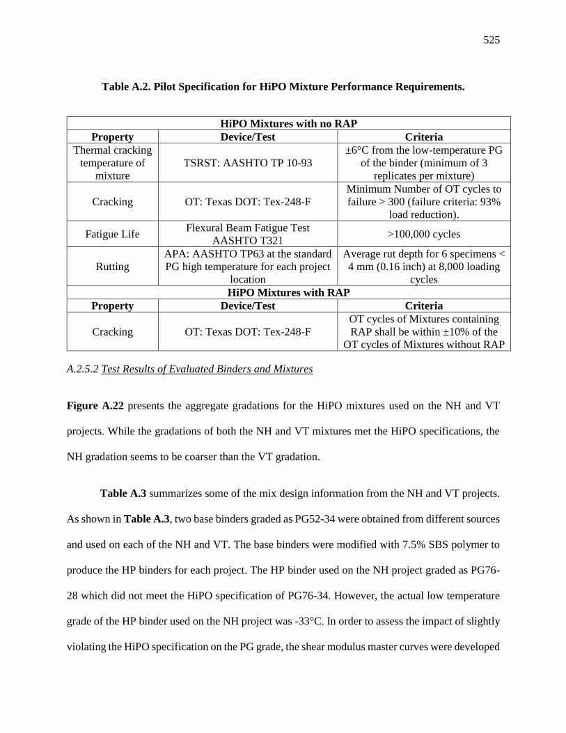
525
Table A.2. Pilot Specification for HiPO Mixture Performance Requirements.
HiPO Mixtures with no RAP
Property Device/Test Criteria
Thermal cracking
temperature of
mixture
TSRST: AASHTO TP 10-93
±6°C from the low-temperature PG
of the binder (minimum of 3
replicates per mixture)
Cracking OT: Texas DOT: Tex-248-F
Minimum Number of OT cycles to
failure > 300 (failure criteria: 93%
load reduction).
Fatigue Life Flexural Beam Fatigue Test
AASHTO T321 >100,000 cycles
Rutting
APA: AASHTO TP63 at the standard
PG high temperature for each project
location
Average rut depth for 6 specimens <
4 mm (0.16 inch) at 8,000 loading
cycles
HiPO Mixtures with RAP
Property Device/Test Criteria
Cracking OT: Texas DOT: Tex-248-F
OT cycles of Mixtures containing
RAP shall be within ±10% of the
OT cycles of Mixtures without RAP
A.2.5.2 Test Results of Evaluated Binders and Mixtures
Figure A.22 presents the aggregate gradations for the HiPO mixtures used on the NH and VT
projects. While the gradations of both the NH and VT mixtures met the HiPO specifications, the
NH gradation seems to be coarser than the VT gradation.
Table A.3 summarizes some of the mix design information from the NH and VT projects.
As shown in Table A.3, two base binders graded as PG52-34 were obtained from different sources
and used on each of the NH and VT. The base binders were modified with 7.5% SBS polymer to
produce the HP binders for each project. The HP binder used on the NH project graded as PG76-
28 which did not meet the HiPO specification of PG76-34. However, the actual low temperature
grade of the HP binder used on the NH project was -33°C. In order to assess the impact of slightly
violating the HiPO specification on the PG grade, the shear modulus master curves were developed

526
for the HP binders from the two projects. The Christensen-Anderson model (CAM) presented in
Equation A.2 was used to develop the shear modulus master curves of the HP binders as illustrated
in Figure A.23.
𝐺∗(𝜔) = 𝐺𝑔[1 + (𝜔𝑐
𝜔𝑟)
log 2
𝑅 ]−𝑅
log 2 [Equation. A.2]
Where;
𝐺∗(𝜔): complex shear modulus (kPa);
Gg: glass modulus assumed equal to 106 (kPa);
𝜔𝑟: reduced frequency at the defining temperature (rad/s);
𝜔𝑐: cross over frequency at the defining temperature (rad/s);
𝜔: loading frequency (rad/s); and
R: rheological index.
It was found that the shear modulus master curves of the two HP binders shown in Error!
Reference source not found. are very similar indicating that the overall rheological properties of
the two HP binders are close. Therefore, it was concluded that the slight difference in the low
temperature grade should not influence the overall performance of the two binders.
The available mix design information did not contain any reference on the use of an anti-strip
additive in both mixtures, therefore, it can be reasonably assumed that no such additive was used.
The optimum binder content of the NH mixture violated the HiPO mix specification by 0.2%. The
impact of this minor violation will be taken into consideration when comparing the performance
properties of the two mixtures.
The properties of the RAP materials used in the two mixtures were not documented in the
available literature from this study. However, the available information provided the optimum
binder content and the virgin binder content for each mixture as shown in Table A.3. Using this
information, the research team calculated the RAP binder contents as presented in Table A.3. This

527
calculation showed the binder content of the RAP material used in the VT mixture to be 0.2%
higher than the binder content of the RAP material used in the NH mixture.
Figure A.22. HiPO mixtures gradations for New Hampshire and Vermont projects.
25
.0 m
m1
inch
19
.0 m
m3
/4 i
nch
12
.5 m
m1
/2 i
nch
9.5
mm
3/8
inch
4.7
5 m
mN
o. 4
2.3
6 m
mN
o. 8
2.0
0 m
mN
o. 1
0
1.1
8 m
mN
o. 1
6
0.4
25
mm
No
. 4
00
.30
0 m
mN
o. 5
0
0.1
50
mm
No
. 1
00
0.0
75
mm
No
. 2
00
0.6
00
mm
No
. 3
0
0
10
20
30
40
50
60
70
80
90
100
Per
cen
t P
ass
ing
Sieve Size (0.45 Power)
Pilot Specification
New Hampshire HiPO with RAP
Vermont HiPO No RAP
Vermont HiPO with RAP
Max Density Curve
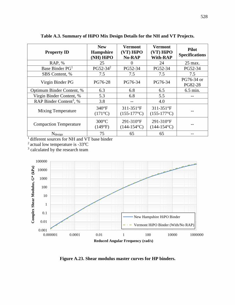
528
Table A.3. Summary of HiPO Mix Design Details for the NH and VT Projects.
Property ID
New
Hampshire
(NH) HiPO
Vermont
(VT) HiPO
No-RAP
Vermont
(VT) HiPO
With-RAP
Pilot
Specifications
RAP, % 25 0 24 25 max.
Base Binder PG1 PG52-342 PG52-34 PG52-34 PG52-34
SBS Content, % 7.5 7.5 7.5 7.5
Virgin Binder PG PG76-28 PG76-34 PG76-34 PG76-34 or
PG82-28
Optimum Binder Content, % 6.3 6.8 6.5 6.5 min.
Virgin Binder Content, % 5.3 6.8 5.5 --
RAP Binder Content3, % 3.8 -- 4.0
Mixing Temperature 340°F
(171°C)
311-351°F
(155-177°C)
311-351°F
(155-177°C) --
Compaction Temperature 300°C
(149°F)
291-310°F
(144-154°C)
291-310°F
(144-154°C) --
Ndesign 75 65 65 -- 1 different sources for NH and VT base binder 2 actual low temperature is -33oC 3 calculated by the research team
Figure A.23. Shear modulus master curves for HP binders.
0.001
0.01
0.1
1
10
100
1000
10000
100000
0.000001 0.0001 0.01 1 100 10000 1000000
Co
mp
lex S
hea
r M
od
ulu
s, G
* (
kP
a)
Reduced Angular Frequency (rad/s)
New Hampshire HiPO Binder
Vermont HiPO Binder (With/No RAP)
529
Reflective Cracking Properties
The Texas Overlay Test (OT) was used to evaluate the resistance of the HiPO AC mixtures to
reflective cracking (Tex-248-F, 2014). The testing was conducted at a temperature of 59°F (15°C)
on specimens compacted to an air void level of 7.0±1.0%. The test specimens consisted of 6.0 inch
(150 mm) long by 3.0 inch (75 mm) wide and 1.5 inch (38 mm) thick sample trimmed from a 6.0
inch (150 mm) diameter by 4.5 inch (115 mm) height sample prepared in the Superpave Gyratory
Compactor (SGC). The maximum displacement (i.e., joint opening) was selected as 0.025 inch
(0.635 mm). The test was stopped after 2,000 loading cycles if a 93% drop in initial load, measured
from the first opening cycle, was not reached. Table A.4 summarizes the results from the various
mixture performance tests. All evaluated mixtures exhibited an average OT cycles to failure
greater than the minimum required 300 cycles. However, the Vermont with RAP mix did not
exhibit cycles to failure within ±10% of the number of cycles exhibited by the corresponding mix
without RAP indicating the need of assessing the applicability of using 24% RAP without
changing the grade of the virgin binder.
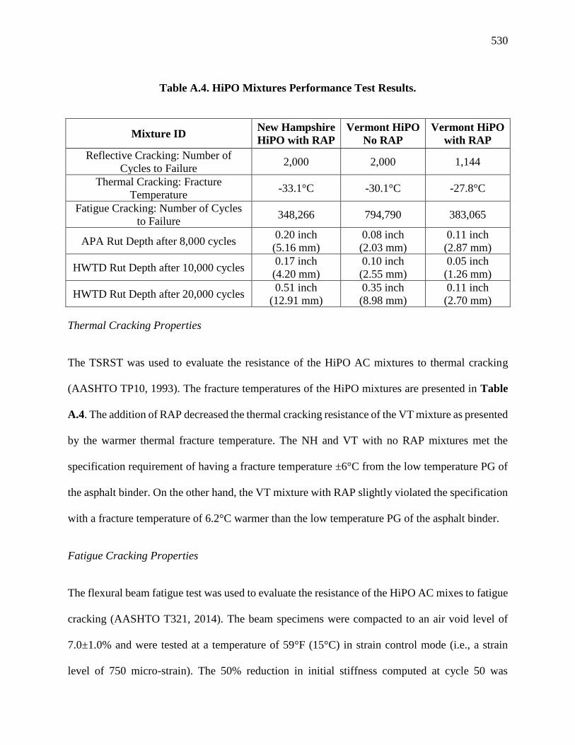
530
Table A.4. HiPO Mixtures Performance Test Results.
Mixture ID New Hampshire
HiPO with RAP
Vermont HiPO
No RAP
Vermont HiPO
with RAP
Reflective Cracking: Number of
Cycles to Failure 2,000 2,000 1,144
Thermal Cracking: Fracture
Temperature -33.1°C -30.1°C -27.8°C
Fatigue Cracking: Number of Cycles
to Failure 348,266 794,790 383,065
APA Rut Depth after 8,000 cycles 0.20 inch
(5.16 mm)
0.08 inch
(2.03 mm)
0.11 inch
(2.87 mm)
HWTD Rut Depth after 10,000 cycles 0.17 inch
(4.20 mm)
0.10 inch
(2.55 mm)
0.05 inch
(1.26 mm)
HWTD Rut Depth after 20,000 cycles 0.51 inch
(12.91 mm)
0.35 inch
(8.98 mm)
0.11 inch
(2.70 mm)
Thermal Cracking Properties
The TSRST was used to evaluate the resistance of the HiPO AC mixtures to thermal cracking
(AASHTO TP10, 1993). The fracture temperatures of the HiPO mixtures are presented in Table
A.4. The addition of RAP decreased the thermal cracking resistance of the VT mixture as presented
by the warmer thermal fracture temperature. The NH and VT with no RAP mixtures met the
specification requirement of having a fracture temperature ±6°C from the low temperature PG of
the asphalt binder. On the other hand, the VT mixture with RAP slightly violated the specification
with a fracture temperature of 6.2°C warmer than the low temperature PG of the asphalt binder.
Fatigue Cracking Properties
The flexural beam fatigue test was used to evaluate the resistance of the HiPO AC mixes to fatigue
cracking (AASHTO T321, 2014). The beam specimens were compacted to an air void level of
7.0±1.0% and were tested at a temperature of 59°F (15°C) in strain control mode (i.e., a strain
level of 750 micro-strain). The 50% reduction in initial stiffness computed at cycle 50 was

531
considered as a failure criterion. The results of the fatigue cracking are summarized in Table A.4.
The two mixtures with RAP (NH and VT) showed similar numbers of cycles to failure which is
significantly lower than the number of cycles to failure for the VT mixture with no RAP. This data
further questions the applicability of using RAP without changing the PG of the virgin binder.
Rutting Properties
The asphalt pavement analyzer (APA) was used to evaluate the rutting resistance of the HiPO AC
mixtures. The maximum high pavement temperature that mixtures may experience in the field was
estimated to be 140°F (60°C). The APA rutting data are presented in Table A.4. The NH with
RAP mixture did not meet the APA rutting criterion in the pilot specification of minimum 0.16
inch (4.0 mm) after 8,000 loading cycles. Both VT mixtures with and no RAP met the APA rutting
criterion.
Additional rutting evaluations were conducted in the HWT (AASHTO T324, 2011). The
specimens, compacted to an air void level of 7.0±1.0%, were soaked for 30 minutes in a heated
water bath at a temperature of 122°F (50°C) prior to testing. A continuous loading was applied to
the submerged samples using a steel wheel. The HWTD rutting data are presented in Table A.4.
The HWTD rutting data on the VT mixtures followed the expected trend where the addition of
24% RAP decreased the rut depth of the HiPO AC mixtures.
In summary, this study showed that HP binders can be used to design HiPO AC mixtures
with and without RAP as per the pilot specifications for thin AC overlays to be used as a
preservation treatment. However, the following observations were made from the measured
mixtures properties:

532
• The use of 24-25% RAP without changing the PG of the virgin binder can have a negative
impact on the resistance of the mixture to thermal and fatigue cracking. This impact was
more obvious on the VT mixtures since both with and no RAP mixtures were evaluated.
• Even though the available literature from this study did not include information on the
properties of the RAP materials used in each mix, the analysis of the performance data
leads to the conclusion that the RAP material used in the NH mix is softer than the RAP
material used in the VT mix. This is supported by the higher thermal fracture temperature
and higher rutting observed in the APA and HWTD for the NH mix with RAP.
• One significant observation from this study is that the use of HP binder will improve the
performance of the AC mixtures BUT will not make up for the deficiencies associated
with the percent and properties of RAP materials used in the mixtures. Therefore, agencies
should still assess the impact of these two important parameters on the performance of
the AC mix even with the use of HP binders.
The NH and VT HiPO mixtures were applied on field sections presented in Section A.3.
A.2.6 New Hampshire DOT Highways: 2011 Auburn-Candia Resurfacing
A.2.6.1 Introduction and Testing Plan
In 2011, FHWA awarded the New Hampshire DOT (NHDOT) a $2 million grant for new
technologies as part of resurfacing NH Route 101 from Auburn to Candia. The evaluation of HP
and neat AC mixes were incorporated into this project. The experiment evaluated the following
mixtures: mix A (0.5-inch NMAS (12.5-mm)) and 35% RAP using neat PG52-34 with Evotherm,

533
mix B (0.75-inch NMAS (19.0-mm)) and 20% RAP using neat PG64-28, and mix C (0.375-inch
NMAS (9.5-mm)) and no RAP using a PG70-34HP binder with 7.5% SBS (Mogawer et al., 2014).
This study was incorporated into the literature review to examine the ability of the HP binder to
produce an AC mix with comparable properties to other AC mixes from the same aggregate source
with higher NMAS and RAP contents.
A.2.6.2 Testing Description and Detailed Results
Aggregate Gradation and Mix Designs
Figure A.24 illustrates the aggregate gradation of the three evaluated mixtures. The three mixtures
were designed using the Superpave mix design methodology with 75 design gyrations. The
optimum asphalt binder content for mixes A, B, and C are 5.50%, 4.90%, and 6.50%, respectively.
Figure A.24. Aggregate gradations of NHDOT mixes A, B, and C.
25
.0 m
m1
in
ch
19
.0 m
m3
/4 i
nch
12
.5 m
m1
/2 i
nch
9.5
mm
3/8
in
ch
4.7
5 m
mN
o. 4
2.3
6 m
mN
o. 8
2.0
0 m
mN
o. 1
0
1.1
8 m
mN
o. 1
6
0.4
25
mm
No
. 4
00
.30
0 m
mN
o. 5
0
0.1
50
mm
No
. 1
00
0.0
75
mm
No
. 2
00
0.6
00
mm
No
. 3
0
0
10
20
30
40
50
60
70
80
90
100
Per
cen
t P
ass
ing
Sieve Size (0.45 Power)
High Polymer Mixture
0.5 inch (12.5 mm) + 35% RAP
0.75 inch (19.0 mm) + 20% RAP
534
Engineering Properties
The Dynamic modulus (E*) represents the engineering property of the AC mix and provides an
indication on its overall quality. Dynamic modulus testing was performed for the three mixes (A,
B, and C) in accordance with AASHTO T378 (AASHTO T378, 2013) and R84 (AASHTO R84,
2010). Mix B exhibited the highest E* property while mix C (HP) exhibited the lowest modulus.
This indicates that the HP binder was unable to overcome the impact of RAP, higher NMAS with
coarser gradation, and higher optimum binder content on the E* property of the AC mix.
Rutting Properties
The AMPT machine was used to determine the flow number (FN) of the three mixes (A, B, and
C) according to AASHTO T378 (AASHTO T378, 2013). The testing temperature was 122°F
(50°C) selected as the design high temperature at 50% reliability as determined using the long-
term pavement performance bind (LTPPBind) software version 3.1. This temperature was
computed at a depth of 0.80 inch (20 mm) below the pavement surface. The Francken model was
used to determine the tertiary flow. The highest FN was measured on the HP mix C at 346 followed
by mix B at 237 and mix A at 128 cycles. This indicates that the HP binder was able to overcome
the impact of RAP, higher NMAS with coarser gradation, and higher OBC on the FN property and
produced an HP AC mix that is more resistant to rutting.
Cracking Properties
Fatigue Cracking: Flexural beam fatigue testing was performed in accordance with AASHTO
T321 (AASHTO T321, 2014) to determine the fatigue characteristics of the three mixes. Beams
were trimmed from slabs compacted using the IPC Global Pressbox slab compactor. In order to

535
account for the relative locations of the various mixtures within the pavement structure, mixes A
and B were tested at strains of 250, 500, and 750 micro-strain while higher strains of 750, 1000,
1,250 micro-strain were applied to test mix C. All tests were conducted at a loading frequency of
10Hz and a temperature of 59°F (15°C). The 50% reduction in initial beam stiffness (determined
at cycle 50) was adopted as a failing criterion. Figure A.25 presents the beam fatigue results and
fatigue relationship of the evaluated mixes (Mogawer et al., 2014). A considerably better fatigue
relationship was observed for the HP mix C when compared with mixes A and B.
Figure A.25. Fatigue characteristics of mixes A, B, and C at 59°F (15°C).
It should be noted that, a significant difference in the laboratory fatigue resistance will not
necessarily translate to the same difference in fatigue performance in the field. Many factors may
highly affect the fatigue life of an asphalt pavement such as stiffness, tensile strain under field
loading, the fatigue characteristic of the asphalt mixture, pavement structure, and the interaction
of all these factors. In a mechanistic pavement analysis, an AC layer with a higher stiffness will
100
1000
10000
1,000 10,000 100,000 1,000,000 10,000,000
Fle
xu
ral
Str
ain
(M
icro
stra
in)
Number of Cycles to Failure
A: 0.5 inch (12.5 mm) + 35% RAP
B: 0.75 inch (19.0 mm) + 20% RAP
C: High Polymer Mixture

536
show a lower laboratory fatigue life in a strain-controlled mode of loading, on the other hand, it
will produce a lower tensile strain under field loading which may result in a longer fatigue life in
the field. Therefore, a full mechanistic analysis would be necessary to effectively evaluate the
impact of HP mixes on the fatigue performance of AC pavements.
Reflective Cracking: The Texas OT was used to evaluate the mixtures’ resistance to reflective
cracking in accordance with Tex-248-F (Tex-248-F, 2014) procedure at a testing temperature of
50°F (10°C). Failure was defined as the number of cycles to reach a 93% drop in initial load which
is measured from the first opening cycle. The best performance was observed for the HP mix C
with a number of cycles to failure of 968. Mixes A and B showed much lower resistance to
reflective cracking with similar number of cycles to failures of 18 and 17, respectively (Mogawer
et al., 2014).
Thermal Cracking: The TSRST was used to evaluate the resistance of the mixes to thermal
cracking (AASHTO TP10, 1993). The thermal fracture temperatures were observed to be -26, -22,
and -37°C for mixes A, B, and C, respectively. The lowest fracture temperature was observed for
the HP mix C followed by mix A while mix B showed the warmest fracture temperature. It should
be noted that only the HP mix C exhibited a fracture temperature lower than the low temperature
PG of the binder. Mixes A and B exhibited fracture temperatures that are significantly warmer
than the low temperature PG of their respective binder.
In summary, it should be recognized that the presence of RAP in mixes A and B and the
higher optimum binder content of mix C contributed to the increase in its resistance to all three
modes of cracking: fatigue, reflective and thermal. However, the fatigue life of the HP mix C at
750 micro-strain is over 600 times the fatigue life of mixes A and B, the reflective cracking life of
537
the HP mix is 54 times the reflective cracking life of mixes A and B, and the thermal fracture
temperature is 11 - 15°C lower than the thermal fracture temperature of mixes A and B. It is
believed that a significant portion of this large increase in the resistance of the HP mix C to fatigue,
reflective, and thermal cracking can be attributed to the properties of the HP binder. In addition to
exhibiting a superior resistance to all modes of cracking, the HP mix C also exhibited higher
resistance to rutting than mixes A and B with RAP.
A.3 Field HP AC Mixes Projects with Limited Performance Data
A.3.1 Introduction
Several field demonstration projects were constructed to evaluate the performance of HP AC mixes
as summarized in Table A.5. Figure A.26 shows the locations of some of the projects on the U.S.A
map. This chapter presents the available information from some of the identified projects in terms
design, testing, construction, and the up to date field performance of the HP AC mixes. The field
projects presented in this chapter have very limited information concerning their long-term
performance. Test sections on the NCAT Test Track with extensive field performance data will be
presented in Section A.4.
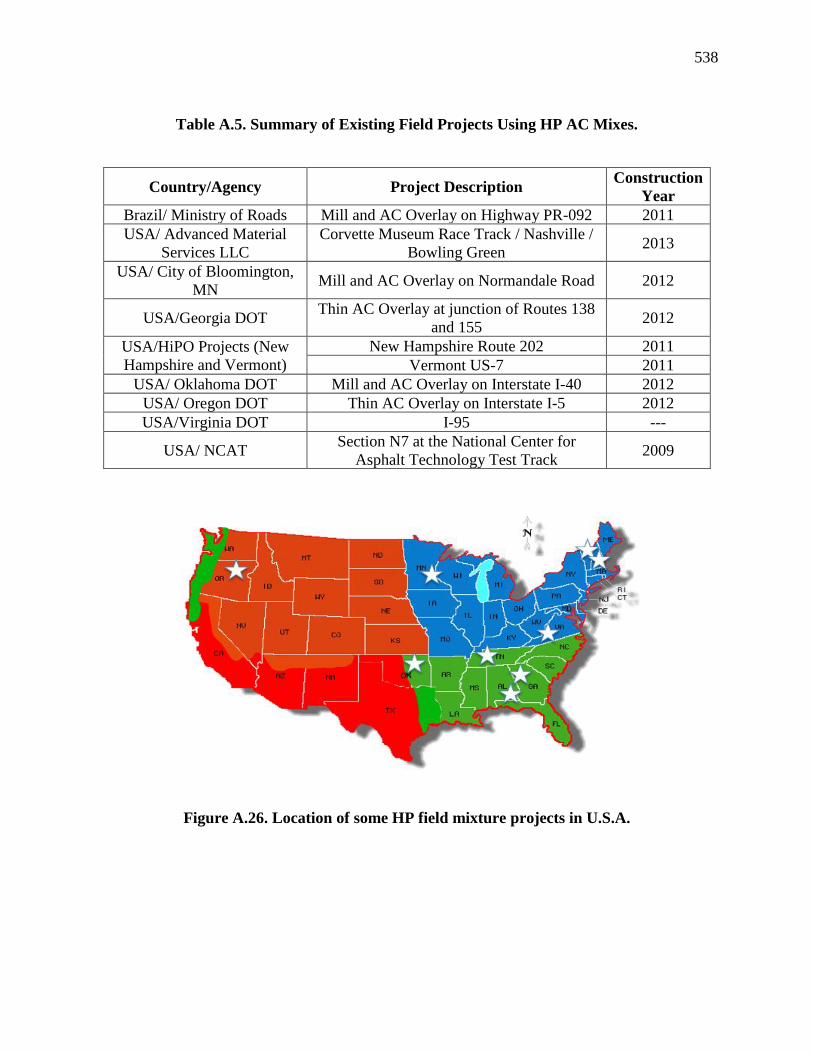
538
Table A.5. Summary of Existing Field Projects Using HP AC Mixes.
Country/Agency Project Description Construction
Year
Brazil/ Ministry of Roads Mill and AC Overlay on Highway PR-092 2011
USA/ Advanced Material
Services LLC
Corvette Museum Race Track / Nashville /
Bowling Green 2013
USA/ City of Bloomington,
MN Mill and AC Overlay on Normandale Road 2012
USA/Georgia DOT Thin AC Overlay at junction of Routes 138
and 155 2012
USA/HiPO Projects (New
Hampshire and Vermont)
New Hampshire Route 202 2011
Vermont US-7 2011
USA/ Oklahoma DOT Mill and AC Overlay on Interstate I-40 2012
USA/ Oregon DOT Thin AC Overlay on Interstate I-5 2012
USA/Virginia DOT I-95 ---
USA/ NCAT Section N7 at the National Center for
Asphalt Technology Test Track 2009
Figure A.26. Location of some HP field mixture projects in U.S.A.

539
A.3.2 High Polymer Modified Asphalt Mixture Trial in Mixture
The first HP AC mix trial in Brazil was constructed in 2011 on a small test section located on
Highway PR-092 in the state of Paraná (Smith, 2012). PR-092 is known to be one of the most
important and busiest roads in Parana State carrying approximately 1,800 vehicles and 4,200 heavy
agricultural trucks per day. The HP binder was modified with 7.5% SBS by weight of binder. The
standard pavement structure proposed by the Parana State DOT consisted of a 12 inch (305 mm)
total thickness: 7.9 inch (200 mm) base course of cement-treated RAP, 1 inch (25 mm) Stress
Absorbing Membrane Interlayer (SAMI), 1.6 inch (40 mm) binder course, and 1.6 inch (40 mm)
PMA wearing course. The HP AC trial alternative consisted of 6.5 inch (165 mm) of dense-graded
HMA reflecting a 46% reduction in the total structural section. Even-though this project does not
include any performance properties on the HP binder, mixture, and field section, its value to the
literature review remains through its hypothetical increase in the structural coefficient for the HP
AC mix. Since the overall structural section was reduced by 46%, it can be concluded that the
structural coefficient of the HP AC mix can be 46% higher than the structural coefficient of the
combination of standard AC mix and cement-treated RAP base.
A.3.3 Winning the Race Track Challenge using HP Mixes
The National Corvette Museum Motorsports Park in Bowling Green, Kentucky has one of the
high-performance tracks that attract professional and talented drivers to push their limits and fine-
tune their machines. The facility has two circuits featuring technical turns with straightaways and
elevation changes: a 2-mile (3.2-km) with 13-turn high-speed west course and a 1-mile (1.6-km)
with 10-turn east course. Designing asphalt mixes for race tracks significantly differ from
designing mixes for highway pavements. On a race track, raveling and bleeding remain the main

540
concerns. The project required more than 58,000 tons of AC mix, including 20,000 tons of mix
optimized for the track surface. The HP binder was modified with 7.5% SBS and graded as PG82-
22. The HP AC mix was designed following the Marshall Mix design methodology (75-blow)
(Kuennen, 2012).
The Evotherm warm-mix asphalt additive was added to improve the HP AC mix
workability which was expected to be stiff and difficult to compact. An important key point of the
HP asphalt binder remains its softening point. It is defined as the temperature at which the asphalt
binder changes phase from a semi-solid to a more viscous liquid leading to the migration of the
fines to the surface due to the effect of extremely hot tires. For the race track, the minimum required
softening point is 180°F (82°C) necessitating the use of polymers. The mixture was manufactured
using an aggregate gradation that provides an optimum macro-texture accompanied with
minimizing the damage induced from lateral shear forces of fast tires. Silica-rich limestone from
the Fort Payne formation in Springfield, TN was selected as the best and most cost-effective
material to enhance friction and skid-resistance on the race track. Pavement macro-texture remains
a driving consideration for race tracks operating under wet or dry conditions, rain or shine, such
as for National Corvette Museum Motorsports Park (Kuennen, 2012).
The pavement structure consisted of an 8.5 inch (216 mm) dense-graded layer of aggregate
base followed by a 5 inch (127 mm) PG64-22 asphalt base course and two 1.5 inch (38 mm) lifts
of the HP AC mix serving as the wearing course layer. The value of this project to the literature is
that it shows the various applications where HP binders have been successfully used in the US.

541
A.3.4 Mill and AC Overlay on Normandale Road, City of Bloomington
In 2012, the City of Bloomington, MN, constructed two projects with HP AC mixes to overcome
the effects of weak water-saturated bases and subgrades as well as the heavy traffic that comes
with its prime location south of Minneapolis and St. Paul, adjacent to the international airport and
the sprawling Mall of America within its limits (Fournier, 2013).
The first project was located on Normandale Service Road at 84th Street. It consisted of
milling 6 inch (150 mm) of the existing AC layer and replacing it with three 2 inch (51 mm) HP
mix lifts of 3/8-inch (9.5 mm) NMAS. The constructed section was 400 ft (122 m) long and 25 ft
(7.6 m) wide, part of a larger reconstruction project in the area. Both the base and subgrade layers
were characterized as soft and wet materials (Fournier, 2013).
The second project was located on West 98th Street from Logan Ave. South to Penn Ave.
South involving the use of HP and conventional PMA mixes (i.e., PG58-28). The HP section was
designed with a 25% thinner overlay layer compared to the conventional overlay. The reduction
in overlay thickness was meant to overcome the increase in costs, while still reducing reflective
and thermal cracking known as major issues in Minnesota, and achieving better durability
(Fournier, 2013).
The HP binder for both projects included 7.5% SBS. The HP mixes were expected to help
the city place more cost-effective and durable asphalt pavements resulting with reduced pavement
thicknesses, and/or built pavement section on top of questionable existing base and subgrade
layers. The HP mixes consisted of a 0.375-inch (9.5-mm) NMAS containing 6% of HP asphalt

542
binder by total weight of mix. The mix was foamed at 300°F (149°C), placed at a temperature of
265°F (130°C), and compacted to a density of 92% verified by cores.
The value of this project to the literature review is two folds: a) it represents a situation
where the HP AC mix is used to overcome the effect of weak base and subgrade which represents
a scenario identified in the FDOT project statement, and b) a hypothetical structural coefficient
can be estimated from the 25% reduction in the thickness of the HP AC layer.
A.3.5 HP Modified Asphalt Mixtures on Busy Intersection in Georgia
In 2010, Georgia DOT (GDOT) decided to evaluate a HP AC mix designed for better pavement
durability and higher resistance to rutting and shoving at the junction of two busy state highways
(Routes 138 and 155) in Stockbridge, Henry County. The main concern of the GDOT was rutting
and shoving at the intersection especially with the huge increase of braking actions induced by
heavy trucks (Fournier, 2010).
Due to the traffic level at the evaluated intersection, GDOT specified a Superpave mix
design with a PG76-22 asphalt binder modified with a 7.5% SBS. The actual binder met the
requirements of PG82-28. The granite aggregate gradation was characterized as dense with 0.5
inch (12.5 mm) NMAS. The work on site consisted of milling 1.5 inch (38 mm) of the existing
AC layer and replacing it with the HP modified mix at 7% in-place air voids (Fournier, 2010).
Based on general observations reported from the job site, the HP modified mix had similar
workability as the regular SBS modified mix (Fournier, 2010).
543
A.3.6 High-Performance HP Overlays in New Hampshire and Vermont
The NEPPP pilot performance-based HiPO overlay mixtures presented in Chapter II were
implemented on two demonstration projects located in New Hampshire and Vermont. The first
project, located in New Hampshire, placed 1,500 tons of HP mixes with 25% RAP material on
Route 202 in Rochester at a 1.0 inch (25 mm) thickness overlay for a 1.75-mile (2.7-km) length.
The existing pavement was in bad conditions and no milling was done prior to the placement of
the HiPO overlay. A conventional New Hampshire DOT mixture was placed on an adjacent section
for comparison purposes (Mogawer et al., 2014).
In summer 2011, the Vermont DOT placed a HiPO mixture on two 1-mile (1.6 km) sections
on US-7 in Danby, VT. One of the mixes did not contain RAP, while the other mix had 24% RAP.
The existing pavement was rated as fair to good after 14 years of service with some isolated areas
of permanent deformation, some transverse cracking, and some shrinkage cracking. Surface
preparation preceded the overlay placement included spot filling of permanent deformation areas,
crack sealing along the length of the project, patching of cracks and potholes. Some milling was
performed at transition areas and across bridges (Mogawer et al., 2014).
In terms of field performance of the HiPO mixes placed on the two demonstration projects;
minimal reflective cracking was observed on the New Hampshire section including RAP (25% of
cracking that has returned) which can be due to the lack of surface preparation since the existing
pavement was in poor conditions. No reflective cracking was observed on the Vermont section.
Additionally, after 2 years of service, no signs of environmental related cracking nor rutting have
been observed on all sections (Mogawer et al., 2014).

544
A.3.7 HP Modified Overlay Mix on I-40 in Oklahoma
The project consisted of a 2-mile (3.2-km) mill-and-overlay on I-40 at the eastern end of Caddo
County west of Oklahoma City. The objective of using a HP AC mix for the overlay was to
increase durability, possibly reduce the thickness of the AC layer, and allow the DOT to complete
a larger resurfacing program with the same amount of funds. Three different AC mixes were
manufactured using a HP modified asphalt binder graded as PG76-28E. The “E” stands for
“extremely high grade” based on the MSCR test with a minimum of 95% recovery at a stress level
of 3.2 kPa. The HP modified asphalt binder contained 7.5% SBS. An improvement in overall
performance, resistance to raveling, reduced fatigue cracking and rutting were expected by the
Oklahoma DOT (ODOT) based on the findings from the National Center for Asphalt Technology’s
(NCAT) Test Track study (Kuennen, 2012).
The project consisted of milling 5 inch (127 mm) from the existing AC surface and placing
the HP AC overlay at 8 inch (200 mm) thick which was expected to perform equivalent to a
conventional 10.5 inch (267 mm) PMA overlay. The 8 inch (200 mm) HP AC overlay was
constructed as follows: an intermediate 1.5 inch (38 mm) rich layer of 0.375-inch (9.5-mm) NMAS
running at binder content of 5.6 to 5.8% followed by two lifts of 2.5 inch (64 mm) Oklahoma S3
base coarse with a 0.75 inch (19 mm) NMAS and capped with a 1.5 inch (38 mm) lift of Oklahoma
S5 mixture with a 0.375-inch (9.5-mm) NMAS. A 0.75 inch (19 mm) open-graded friction course
(OGFC) was placed on top to provide high friction and good drainability to eliminate hydroplaning
and truck tire spray. The purpose of having a HP modified rich mixture at the bottom is to increase
resistance to reflective cracking from the existing AC layer. It was reported that the produced HP
AC mix for this project was highly workable at a temperature of 325°F (163°C).

545
Even-though this project does not offer information on the properties of the HP binder and
AC mix, its value to the literature review will be in two folds; a) a hypothetical structural
coefficient can be determined based on the relative thicknesses of the HP and PMA layers, and b)
the long-term performance of the section will be valuable if it can be obtained by the research
team.
A.3.8 HP Modified Thin Overlay Mix on I-5 in Oregon
This demonstration project consisted of a 2 mile (3.2 km) segment on the northbound lanes of I-5
near Medford, OR. The project was part of a nationwide demonstration program involving thin
pavement overlays incorporating HP asphalt binders. The mix design was produced based on the
specifications developed by the NEPPP for the HiPO overlay mix presented in Chapter II. The
objective of using the HiPO asphalt mix on this project was to evaluate the thin overlay pavement
preservation option under heavy traffic (Fournier, 2013).
The PMA binders contained 3% SBS while the HP binder contained 7.5% SBS and both
binders were graded as PG70-22ER. The “ER” extension stands for passing the Oregon DOT
(ODOT) specification on the minimum Elastic Recovery (ER) of 50% per AASHTO T301. The
major difference between the two binders is the ER value; the PMA binder had an ER of 64%
while the HP binder had an ER of 89%. The PMA and HiPO mixes were produced with identical
aggregate gradations and volumetric properties. The mixes were manufactured using 0.375-inch
(9.5-mm) NMAS aggregate with 6.4% asphalt binder by total weight of mix and 20% RAP. It
should be mentioned that no special plant adjustments were reported to accommodate the
production of the HiPO mix.
546
The existing pavement on I-5 had a 0.75 inch (19 mm) OGFC mostly deteriorated due to
wear and raveling. Historically, 2 inch (51 mm) of the existing pavement would be milled and
replaced with a new AC mix followed by an OGFC. In this project, ODOT decided to micro-mill
1 inch (25 mm) and replace with the new AC mix. Two 1-mile (1.6-km) travel-lanes were milled
to 1 inch (25 mm) and replaced with the HiPO mix followed by a 1-mile section of the same two
travel-lanes milled and replaced with ODOT’s 0.375-inch (9.5-mm) NMAS dense-graded PMA
mix at the same thickness. Prior to paving of the travel lanes, ODOT required the contractor to
place the HiPO mix on the shoulder to check its workability and appearance. A latex-modified
asphalt tack coat, CRS-2Ph, was used to ensure a strong bond between the existing pavement and
the overlay. No problems were reported during the production, laydown, and compaction of the
PMA and HiPO mixes, except the CRS-2Ph was switched to CSS-1h traditional tack coat on the
second and final shift of paving to cut down on clumping (Fournier, 2013).
Even-though this project does not offer information on the properties of the HP binder and
mixture, its value to the literature review will be in the long-term performance of the HiPO thin
overlay under heavy traffic if it can be obtained by the research team.
A.4 Field HP AC Mixes Projects with Extensive Performance Data
A.4.1 Introduction
As presented earlier, several studies have shown that HP AC mixes have the potential to improve
the resistance to cracking and rutting with a potential reduction in the AC layer thickness when
compared to PMA AC mixes. While the laboratory evaluations done on HP asphalt binders and
AC mixes were promising, it remains necessary to fully understand and evaluate the performance
547
and in-situ characteristics of the HP AC mixes on actual field projects. For this purpose, a full-
scale experiment was conducted at the National Center for Asphalt Technology (NCAT) Test
Track in 2009. This chapter documents some detailed information about the work done and
presents the findings from the full-scale experiment.
A.4.2 NCAT Test Track Sections
The full-scale experiment at the NCAT Test Track was sponsored by Kraton Performance
Polymers LLC to fully understand the in-situ characteristics of HP AC mixes when used on actual
pavement sections. It consisted of two mains sections: (1) a control section, labeled as S9-PMA,
designed and constructed using a PMA AC mix, and (2) a HP section, labeled as N7-HP, designed
and constructed to be thinner than the control section using HP AC mix. The section labeling is a
combination of a letter and a number: N and S denotes North and South, respectively, meanwhile
the digit represents the section number (1 through 13 on each tangent). Figure A.27 illustrates the
as-designed structures, mix types, and layers thicknesses of both pavement sections (i.e., S9-PMA
and N7-HP) (Timm et al., 2012).
Random longitudinal (RL) stations were established at different locations within and
between wheel paths throughout each section prior to construction. These locations played a major
role during construction. They constituted the locations of nuclear density testing, and survey
points for thickness. They also served as locations for falling weight deflectometer (FWD) testing
and determination of transverse profile. For both sections, the subgrade was classified as an
AASHTO A-4(0) metamorphic quartzite soil and compacted to target density and moisture
content. The average dry unit weights of the subgrade material for section S9-PMA and N7-HP
were 123.4 and 121.8 lb/ft3 (1,977 and 1,951 kg/m3) with a moisture content of 9.2% and 9.4%,

548
respectively. The aggregate base was a crushed granite material placed at 6 inch (150 mm) thick.
The average dry unit weights of the aggregate base material for section S9-PMA and N7-HP were
140.2 and 140.6 lb/ft3 (2,246 and 2,252 kg/m3) with a moisture content of 5.0 and 4.1%,
respectively. Direct measurements for the pavement structure responses to traffic loads were made
using strain gauges and pressure cells embedded at different locations and depths within the
pavement structure layers. Table A.6 summarizes the as-built AC layer properties for the two
sections(Timm et al., 2012).
Figure A.27. NCAT Test Track S9-PMA and N7-HP cross-sections design: materials and
layers thicknesses (Timm et al., 2012).

549
Table A.6. As-Built AC Layers Properties.
Lift Surface Intermediate Base
Section S9-
PMA
N7-
HP S9-PMA N7-HP S9-PMA N7-HP
Thickness, inch
(mm) 1.2 (30)
1.0
(25) 2.8 (71) 2.1(53) 3.0 (76) 2.5 (64)
NMAS, inch (mm) 0.375
(9.5)
0.375
(9.5)
0.75
(19.0)
0.75
(19.0)
0.75
(19.0)
0.75
(19.0)
% polymer - SBS 2.8 7.5 2.8 7.5 0.0 7.5
Performance Grade 76-22 88-22 76-22 88-22 67-22 88-22
Asphalt, % 6.1 6.3 4.4 4.6 4.7 4.6
Air voids, % 6.9 6.3 7.2 7.3 7.4 7.2
Plant Temperature,
°F (°C)
335
(168)
345
(174)
335
(168)
345
(174)
325
(163)
340
(171)
Paver Temperature,
°F (°C)
275
(135)
307
(153)
316
(158)
286
(141)
254
(123)
255
(124)
Compaction
Temperature, °F
(°C)
264
(129)
297
(147)
273
(134)
247
(119)
243
(117)
240
(116)
A.4.3 PMA and HP Mix Designs
All AC mixes were designed using the Superpave mix design methodology with 80 design
gyrations. Table A.7 and Figure A.28 present the aggregate gradation of each lift of the AC layer
for both sections. The optimum binder content was determined at 4% air voids and satisfying all
volumetric properties criteria. Table A.8 summarizes the mix design information for the different
lifts (i.e., surface, intermediate, and base) for both PMA and HP AC mixes. Similar volumetric
properties were observed for the PMA and HP AC mixes despite the large difference in the binder
PG resulting from the additional polymer in the HP binder (Timm et al., 2012).

550
Table A.7. Aggregate Gradations of PMA and HP Mixes - NCAT Test Track.
Sieve Size Surface Layer Mixes
Intermediate
Layer Mixes Base Layer Mixes
PMA HP PMA & HP PMA HP
1 inch (25.0 mm) 100 100 100 100 100
0.75 inch (19.0
mm) 100 100 93 93 93
0.5 inch (12.5 mm) 100 100 82 84 82
0.375 inch (9.5
mm) 100 100 71 73 71
No. 4 (4.75 mm) 78 77 52 55 52
No. 8 (2.36 mm) 60 60 45 47 45
No. 16 (1.18 mm) 46 45 35 36 35
No. 30 (0.6 mm) 31 31 24 25 24
No. 50 (0.3 mm) 16 16 12 14 12
No. 100 (0.15 mm) 10 9 7 8 7
No. 200 (0.075
mm) 5.8 5.7 3.9 4.6 3.9
Figure A.28. Aggregate gradations of PMA and HP mixes - NCAT Test Track.
25
.0 m
m1
inch
19
.0 m
m3
/4 i
nch
12
.5 m
m1
/2 i
nch
9.5
mm
3/8
inch
4.7
5 m
mN
o. 4
2.3
6 m
mN
o. 8
2.0
0 m
mN
o. 1
0
1.1
8 m
mN
o. 1
6
0.4
25
mm
No
. 4
00
.30
0 m
mN
o. 5
0
0.1
50
mm
No
. 1
00
0.0
75
mm
No
. 2
00
0.6
00
mm
No
. 3
0
0
10
20
30
40
50
60
70
80
90
100
Per
cen
t P
ass
ing
Sieve Size (0.45 Power)
PMA-Surface
HP-Surface
PMA/HP - Intermediate
PMA-Base
HP-Base

551
Table A.8. Summary of NCAT PMA and HP Mixes (Surface, Intermediate, and Base Lifts)
Mix Designs.
Mix Type PMA HP
Lift ID Surface Intermediate Base Surface Intermediate
& Base
Asphalt PG Grade 76-22 76-22 67-22 88-22 88-22
% SBS Polymer 2.8 2.8 0.0 7.5 7.5
Design Air Voids, % 4.0 4.0 4.0 4.0 4.0
Optimum Binder Content (by
total weight of mix), % 5.8 4.7 4.6 5.9 4.6
Effective Binder (Pbe), % 5.1 4.1 4.1 5.3 4.2
Dust Proportion, DP 1.1 0.9 1.1 1.1 0.9
Maximum Specific Gravity,
Gmm 2.483 2.575 2.574 2.474 2.570
Voids in Mineral Aggregate
(VMA), % 15.8 13.9 13.9 16.2 14.0
Voids Filled with Asphalt
(VFA), % 75.0 71.0 71.0 75.0 72.0
A.4.4 Laboratory Evaluation of Binders and Plant-Produced Mixtures
Loose mixtures were collected in five-gallon pails during production and were brought back to the
NCAT laboratory for further evaluation. Corresponding asphalt binders used during production
were all sampled at the plant and brought back to the laboratory.
A.4.4.1 Properties of Asphalt Binders
All asphalt binders were sampled at the plant except for the PG76-22 used in the surface mixture
lift of section S9-PMA which was replaced by the extracted and recovered binder from the field
mixture. AASHTO M320-10 was followed to test and grade all binders. It should be mentioned
that the HP binder used for the surface lift in section N7-HP had a similar workability and
compactability as of the PG76-22 binder in the laboratory and on field. In addition, the MSCR test
was used to determine the PG of all asphalt binders in accordance with AASHTO MP 19-10. Table
A.9 summarizes all the PG’s and MSCR results.
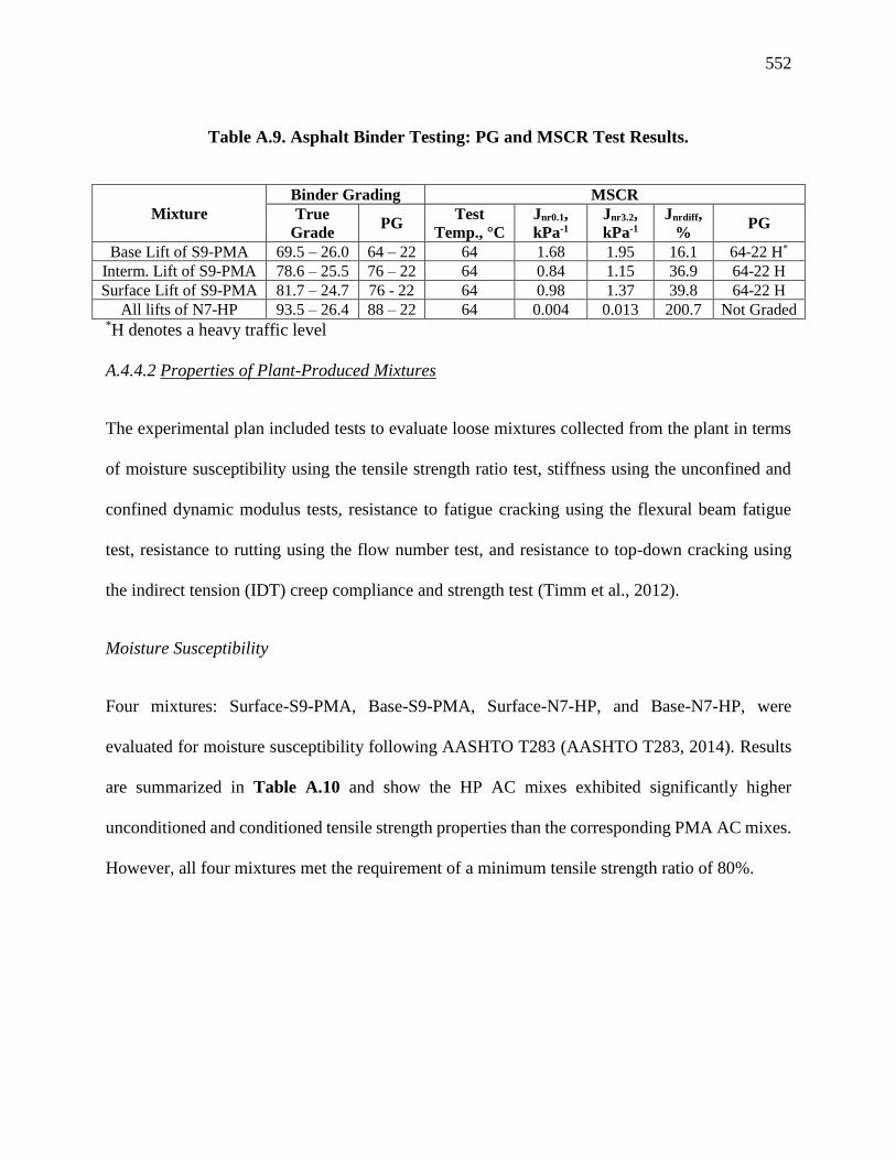
552
Table A.9. Asphalt Binder Testing: PG and MSCR Test Results.
Mixture
Binder Grading MSCR
True
Grade PG
Test
Temp., °C
Jnr0.1,
kPa-1
Jnr3.2,
kPa-1
Jnrdiff,
% PG
Base Lift of S9-PMA 69.5 – 26.0 64 – 22 64 1.68 1.95 16.1 64-22 H*
Interm. Lift of S9-PMA 78.6 – 25.5 76 – 22 64 0.84 1.15 36.9 64-22 H
Surface Lift of S9-PMA 81.7 – 24.7 76 - 22 64 0.98 1.37 39.8 64-22 H
All lifts of N7-HP 93.5 – 26.4 88 – 22 64 0.004 0.013 200.7 Not Graded *H denotes a heavy traffic level
A.4.4.2 Properties of Plant-Produced Mixtures
The experimental plan included tests to evaluate loose mixtures collected from the plant in terms
of moisture susceptibility using the tensile strength ratio test, stiffness using the unconfined and
confined dynamic modulus tests, resistance to fatigue cracking using the flexural beam fatigue
test, resistance to rutting using the flow number test, and resistance to top-down cracking using
the indirect tension (IDT) creep compliance and strength test (Timm et al., 2012).
Moisture Susceptibility
Four mixtures: Surface-S9-PMA, Base-S9-PMA, Surface-N7-HP, and Base-N7-HP, were
evaluated for moisture susceptibility following AASHTO T283 (AASHTO T283, 2014). Results
are summarized in Table A.10 and show the HP AC mixes exhibited significantly higher
unconditioned and conditioned tensile strength properties than the corresponding PMA AC mixes.
However, all four mixtures met the requirement of a minimum tensile strength ratio of 80%.

553
Table A.10. Summary of Moisture Susceptibility Properties of the PMA and HP Mixtures.
Mixture Treatment Tensile Strength,
psi (kPa)
Tensile Strength
Ratio, TSR, %
Surface-S9-PMA Conditioned 137.2 (946)
94 Unconditioned 145.4 (1,003)
Base-S9-PMA Conditioned 116.2 (801)
86 Unconditioned 134.6 (928)
Surface-N7-HP Conditioned 197.1 (1,359)
89 Unconditioned 222.1 (1,531)
Base-N7-HP Conditioned 208.4 (1,437)
88 Unconditioned 237.6 (1,638)
Dynamic Modulus Property
Dynamic modulus (E*) testing was performed on each of the plant-produced mix placed on the
sections S9-PMA and N7-HP in accordance with AASHTO T378 (AASHTO T378, 2013) and
AASHTO R84 (AASHTO R84, 2010). The E* property provides an indication of the stiffness and
the overall quality of the asphalt mixture. All measured data had a coefficient of variation (COV)
lower than 13% indicating good repeatability of the results. The testing was done unconfined and
with a 20 psi (138 kPa) confinement pressure on all evaluated mixtures. Figure A.29 and Figure
A.30 illustrate the unconfined and confined E* master curves for all the evaluated mixtures,
respectively. Examination of the E* master curves leads to the following observations:
• For both confined and unconfined testing conditions, the dynamic modulus values reported
for the HP AC mixes are higher than for the PMA AC mixes indicating a stiffer mix.
• No impact was observed on the ranking of PMA and HP AC mixes in terms of dynamic
modulus with the addition of confinement. However, higher values for both mixes were
reported under the confinement condition which was conventionally expected.

554
• All AC mixes, PMA and HP, for each confinement condition (i.e., unconfined and
confined) exhibit similar dynamic modulus at a low temperature and high frequency (i.e.,
upper right end of the master curve).
Overall, it can be noticed that the high polymer content of the HP AC mixes had a much
greater impact on the measured E* values for the surface course when compared with the
intermediate and base course layers. The confinement had significant effects on the E* values
especially at the lowest reduced frequencies (i.e., below 1 Hz).
Figure A.29. Unconfined dynamic modulus master curves.
1
10
100
1000
10000
0.000001 0.0001 0.01 1 100 10000 1000000
Un
con
fin
ed D
yn
am
ic M
od
ulu
s at
68°F
(20°C
), k
si
Reduced Frequency (Hz)
PMA-Surface
HP-Surface
PMA-Intermediate
PMA-Base
HP-Intermediate/base
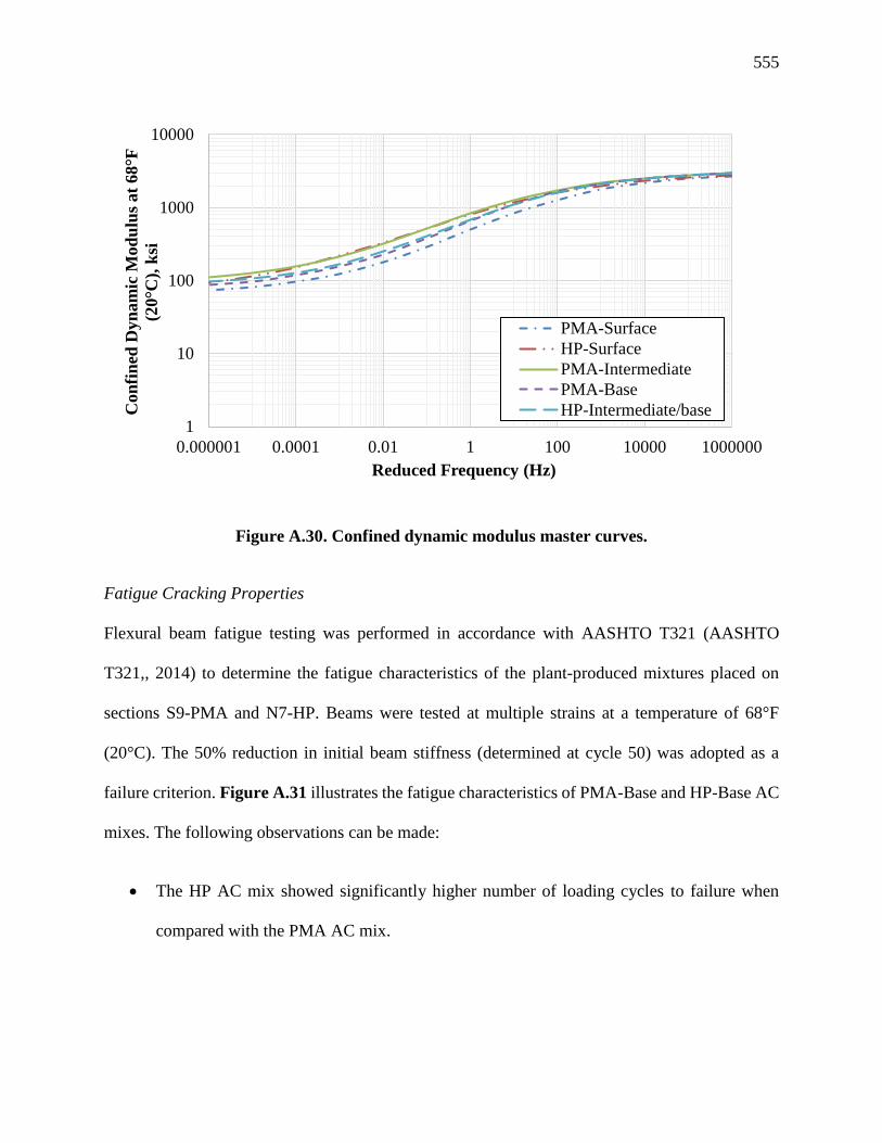
555
Figure A.30. Confined dynamic modulus master curves.
Fatigue Cracking Properties
Flexural beam fatigue testing was performed in accordance with AASHTO T321 (AASHTO
T321,, 2014) to determine the fatigue characteristics of the plant-produced mixtures placed on
sections S9-PMA and N7-HP. Beams were tested at multiple strains at a temperature of 68°F
(20°C). The 50% reduction in initial beam stiffness (determined at cycle 50) was adopted as a
failure criterion. Figure A.31 illustrates the fatigue characteristics of PMA-Base and HP-Base AC
mixes. The following observations can be made:
• The HP AC mix showed significantly higher number of loading cycles to failure when
compared with the PMA AC mix.
1
10
100
1000
10000
0.000001 0.0001 0.01 1 100 10000 1000000
Con
fin
ed D
yn
am
ic M
od
ulu
s at
68
°F
(20°C
), k
si
Reduced Frequency (Hz)
PMA-Surface
HP-Surface
PMA-Intermediate
PMA-Base
HP-Intermediate/base

556
• At a flexural strain level of 400 micro-strain (expected strain level at bottom of AC), the
average fatigue life of the HP AC mix was observed to be approximately 33 times higher
than the fatigue life of the PMA AC mix at a temperature of 68°F (20°C) (Tim et al., 2012).
Figure A.31. Fatigue characteristics of PMA-Base and HP-Base mixes at 68°F (20°C).
Rutting Properties
Asphalt Pavement Analyzer (APA) Results: The APA was used to evaluate the rutting
susceptibility of the PMA and HP AC mixes. The testing was performed according to AASHTO
T340 (AASHTO T340, 2010) at a temperature of 147.2°F (64°C). All tested samples were
subjected to a pressure of 100 psi (690 kPa) for 8,000 cycles.
Table A.11 summarizes the measured APA test results. Based on previous experience from
sections on the NCAT test track, a mix with an average APA rut depth less than 0.21 inch (5.5
mm) should be able to withstand at least 10 million EASLs. Therefore, the evaluated mixes are
100
1000
1000 10000 100000 1000000 10000000 100000000
Fle
xu
ral
Str
ain
(M
icro
stra
in)
Number of Cycles to Failure
S9-PMA
N7-HP

557
not expected to fail in terms of rutting. The APA data of rut depth versus loading cycles were fitted
with a power function to determine the secondary stage rutting rate. The HP-surface AC mix
showed the lowest secondary stage rutting rate followed by the HP-base AC mix. Combining the
fatigue cracking data with the APA data indicates the possibility of designing a highly flexible HP
pavement structure with high rut resistance (Timm et al., 2009).
Table A.11. APA Testing Results of PMA/HP Surface/Base AC Mixes.
Mixture ID
Average Rut
Depth, inch
(mm)
Standard Deviation
(SDV), inch (mm) COV, %
Rate of Secondary
Rutting, inch/cycle
(mm/cycle)
PMA-Surface 3.07
(78.0)
0.58
(14.7) 19
0.000140
(0.003556)
PMA-Base 4.15
(105.4)
1.33
(33.8) 32
0.000116
(0.002946)
HP-Surface 0.62
(15.7)
0.32
(8.1) 52
0.0000267
(0.000678)
HP-Base 0.86
(21.8)
0.20
(5.1) 23
0.0000280
(0.000711)
Flow Number Properties: The FN property of the PMA/HP Surface/Base AC mixes were measured
according to AASHTO T378 (AASHTO T378, 2013). The testing temperature was 139°F (59.5°C)
selected as the design high pavement temperature at 50% reliability determined using the long-
term pavement performance bind (LTPPBind) software version 3.1 at a depth of 0.80 inch (20
mm) below the pavement surface. The Francken model was used to determine the on-set of the
tertiary flow, i.e. FN. A higher FN value indicates a high resistance to rutting. As shown in Figure
A.32, the best rutting resistance was observed for the HP AC mixes especially the surface mix.
The HP AC mixes exhibited FN values that are approximately 6 times greater than the FN of the
PMA AC mixes.
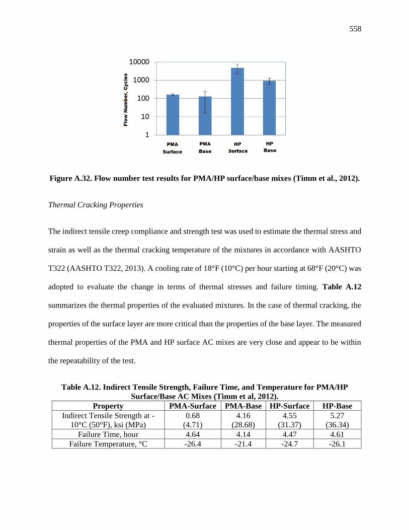
558
Figure A.32. Flow number test results for PMA/HP surface/base mixes (Timm et al., 2012).
Thermal Cracking Properties
The indirect tensile creep compliance and strength test was used to estimate the thermal stress and
strain as well as the thermal cracking temperature of the mixtures in accordance with AASHTO
T322 (AASHTO T322, 2013). A cooling rate of 18°F (10°C) per hour starting at 68°F (20°C) was
adopted to evaluate the change in terms of thermal stresses and failure timing. Table A.12
summarizes the thermal properties of the evaluated mixtures. In the case of thermal cracking, the
properties of the surface layer are more critical than the properties of the base layer. The measured
thermal properties of the PMA and HP surface AC mixes are very close and appear to be within
the repeatability of the test.
Table A.12. Indirect Tensile Strength, Failure Time, and Temperature for PMA/HP
Surface/Base AC Mixes (Timm et al, 2012).
Property PMA-Surface PMA-Base HP-Surface HP-Base
Indirect Tensile Strength at -
10°C (50°F), ksi (MPa)
0.68
(4.71)
4.16
(28.68)
4.55
(31.37)
5.27
(36.34)
Failure Time, hour 4.64 4.14 4.47 4.61
Failure Temperature, °C -26.4 -21.4 -24.7 -26.1
559
A.4.5 Falling Weight Deflectometer Testing and Backcalculation
FWD testing of S9-PMA and N7-HP Sections started in August 2009. The testing was performed
three times per month (on Mondays) for the S9-PMA section and on alternating Mondays for the
N7-HP section. The testing was done at the same location of the random longitudinal stations
already established prior to construction using a Dynatest Model 8000 FWD. A circular load plate
of 11.8 inch (300 mm) diameter was used to conduct the FWD testing. Nine geophones were used
to measure the deflections at the pavement surface. The geophones were spaced at; 0, 8, 12, 18,
24, 36, 48, 60, and 72 inch (0, 203, 305, 457, 610, 914, 1219, 1524, and 1829 mm) from the center
of the load. Four different loads were applied three times at each testing location at: 6000, 9000,
12000, and 16000 lb (2727, 4090, 5455, and 7273 kg) (Timm et al., 2009). In-situ pavement
temperatures were recorded for each section during FWD testing.
NCAT researchers used the EVERCALC 5.0 software to backcalculate the layers moduli
of the three-layer pavement section (AC over aggregate base and subgrade) from the measured
FWD deflection data. The layer thicknesses were selected based on surveys at each offset and
random location. Figure A.33 to Figure A.35 present the backcalculated moduli for the AC,
granular base, and subgrade layers at the 9000 lb (4090 kg) load level, respectively.

560
Figure A.33. Backcalculated AC modulus of sections N7-HP and S9-PMA (Timm et al.,
2012).
Figure A.34. Backcalculated granular base modulus of sections N7-HP and S9-PMA (Timm
et al., 2012).

561
Figure A.35. Backcalculated subgrade modulus of sections N7-HP and S9-PMA (Timm et
al., 2012).
A review of the backcalculated moduli data presented in Figures A.33 to A.35 reveals the
following observations:
• The variation in the backcalculated AC moduli clearly reveals the seasonal effects on the
AC layer’s stiffness.
• Relatively low backcalculated moduli for the granular base layer were observed for both
sections. The researchers indicated that these values were consistent with findings from
previous laboratory triaxial resilient modulus testing conducted at NCAT.
• Relatively high backcalculated moduli values for the subgrade layer were observed for both
sections when compared with the backcalculated moduli for the granular base layer
indicating the presence of strong subgrade material underneath both pavement sections
(N7-HP and S9-PMA).
562
A.4.6 Pavement Responses to Traffic Load
As mentioned earlier, strain gauges and pressure cells were installed to measure strains and stresses
at various locations and depths. Four primary measured pavement responses were collected: a)
longitudinal strain at the bottom of the AC layer, b) transverse strain at the bottom of the AC layer,
c) vertical stress in the aggregate base layer, and d) vertical stress in the subgrade layer. Weekly
data were collected since traffic began on August 28, 2009. The following paragraphs summarize
the response data collected during the period between August 28, 2009 and June 9, 2011 (Timm
et al., 2012).
A.4.6.1 AC Layer Strain Responses
Longitudinal Strains
Table A.13 summarizes the measured longitudinal strains at the bottom of the AC layer under a
single axle load at three temperatures of 50, 68, and 110°F (10, 20, and 44°C). Similar strains were
observed on sections S9-PMA and N7-HP at the two lower temperatures. However, at the higher
temperature, a lower longitudinal strain was measured on the N7-HP section when compared with
strain on the S9-PMA section. The variability expressed by the standard deviation and COV was
more than double for the N7-HP section when compared with S9-PMA. It should be mentioned
that the AC layer in section S9-PMA is 1.25 inch (32 mm) thicker than the one in section N7-HP
indicating that the increase in the HP mix modulus at the high temperature, caused by the higher
polymer content, was enough to overcome the thickness advantage held by S9-PMA section.

563
Table A.13. Longitudinal Strain Measured at the Bottom of the AC Layer.
Section ID Temperature,
°F (°C)
Longitudinal Strain
(micro-strain)
Standard Deviation
(micro-strain) COV (%)
S9-PMA
50 (10) 225 44
20 68 (20) 350 69
110 (44) 979 192
N7-HP
50 (10) 225 101
45 68 (20) 337 152
110 (44) 862 388
Transverse Strains
Table A.14 summarizes the measured transverse strains at the bottom of the AC layer under a
single axle load at three temperatures of 50, 68, and 110°F (10, 20, and 44°C). The transverse
strains were observed to be lower than the measured longitudinal strains at the three corresponding
temperatures. Less variability was observed with the measured transverse strains. At the two lower
temperatures, higher strains were measured at N7-HP when compared with S9-PMA. At 110°F
(44°C), the measured strains changed order where the S9-PMA showed higher values. This can be
attributed to the interaction between layer thickness and modulus value.
Table A.14. Transverse Strain Measured at the Bottom of the AC Layer.
Section ID Temperature,
°F (°C)
Transverse Strain
(micro-strain)
Standard Deviation
(micro-strain) COV (%)
S9-PMA
50 (10) 145 10
7 68 (20) 221 16
110 (44) 590 42
N7-HP
50 (10) 184 48
26 68 (20) 256 67
110 (44) 559 147
Since fatigue cracking is controlled by the highest tensile strain at the bottom of the AC layer, the
contribution of the HP mix towards the magnitude of the longitudinal strains is more critical. Using
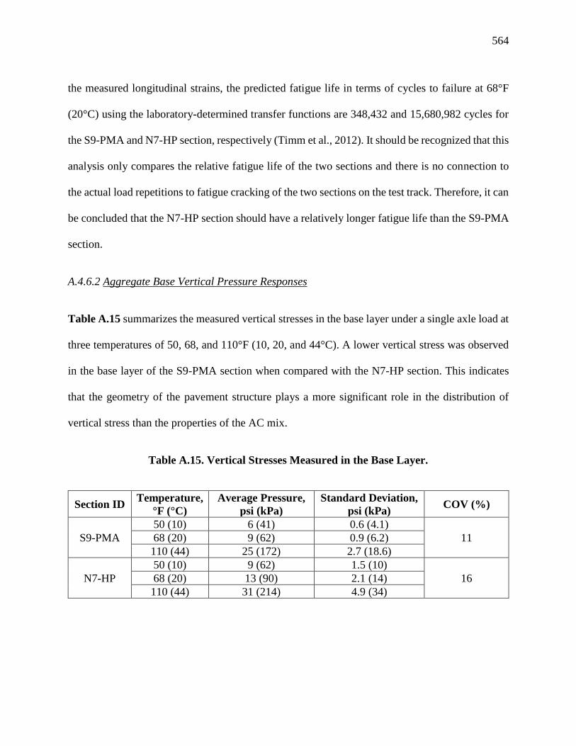
564
the measured longitudinal strains, the predicted fatigue life in terms of cycles to failure at 68°F
(20°C) using the laboratory-determined transfer functions are 348,432 and 15,680,982 cycles for
the S9-PMA and N7-HP section, respectively (Timm et al., 2012). It should be recognized that this
analysis only compares the relative fatigue life of the two sections and there is no connection to
the actual load repetitions to fatigue cracking of the two sections on the test track. Therefore, it can
be concluded that the N7-HP section should have a relatively longer fatigue life than the S9-PMA
section.
A.4.6.2 Aggregate Base Vertical Pressure Responses
Table A.15 summarizes the measured vertical stresses in the base layer under a single axle load at
three temperatures of 50, 68, and 110°F (10, 20, and 44°C). A lower vertical stress was observed
in the base layer of the S9-PMA section when compared with the N7-HP section. This indicates
that the geometry of the pavement structure plays a more significant role in the distribution of
vertical stress than the properties of the AC mix.
Table A.15. Vertical Stresses Measured in the Base Layer.
Section ID Temperature,
°F (°C)
Average Pressure,
psi (kPa)
Standard Deviation,
psi (kPa) COV (%)
S9-PMA
50 (10) 6 (41) 0.6 (4.1)
11 68 (20) 9 (62) 0.9 (6.2)
110 (44) 25 (172) 2.7 (18.6)
N7-HP
50 (10) 9 (62) 1.5 (10)
16 68 (20) 13 (90) 2.1 (14)
110 (44) 31 (214) 4.9 (34)

565
A.4.6.3 Subgrade Vertical Pressure Responses
Table A.16 summarizes the measured vertical stresses in the subgrade under a single axle load at
three temperatures of 50, 68, and 110°F (10, 20, and 44°C). Slightly higher pressures were
measured at the N7-HP section when compared with the S9-PMA section. This indicates that the
geometry of the pavement structure plays a more significant role in the distribution of vertical
stress than the properties of the AC mix but to a lesser extent at deeper locations.
Table A.16. Vertical Stresses Measured in the Subgrade Layer.
Section ID Temperature,
°F (°C)
Average Pressure ,
psi (kPa)
Standard Deviation,
psi (kPa) COV (%)
S9-PMA
50 (10) 5 (34) 0.4 (2.8)
9 68 (20) 7 (48) 0.6 (4.1)
110 (44) 17 (117) 1.4 (9.6)
N7-HP
50 (10) 8 (55) 0.8 (5.5)
10 68 (20) 10 (69) 1.0 (6.9)
110 (44) 17 (117) 1.7 (11.7)
A.4.6.3 Pavement Performance
Approximately nine million ESALs were applied to the test sections (S9-PMA and N7-HP) as of
June 27, 2011 while pavement performance was weekly monitored. Figure A.36 illustrates the
weekly measurements of rut depths for both sections. The rutting performance of the two sections
remained close until approximately 3.5 million ESALs after which the observed rutting in the S9-
PMA section started to significantly increase relative to rutting in the N7-HP section. Since the rut
depths in both sections are relatively low (i.e., less than 0.25 inch (6.4 mm)), it can be assumed
that the rutting is generated in the total AC layer (i.e., surface and base). Therefore, the rutting
properties of the PMA and HP mixes presented in Table A.11 and Figure A.36 can be used to
explain the relative rutting performance of the two sections as follows:

566
• The measured APA rut depths (Table A.11) of the PMA AC mixes are significantly higher
than the rut depths of the HP AC mixes. This indicates that the PMA section will experience
overall higher rutting than the HP section under traffic loads as shown in Figure A.36.
• The measured APA rates of secondary rutting (Table A.11) of the PMA AC mixes are
significantly higher than the APA rates of secondary rutting of the HP AC mixes. This
indicates that after a certain level of traffic loading the PMA AC mixes will experience
more progressive rutting than the HP AC mixes as shown in Figure A.36.
• The flow numbers (Figure A.36) of the PMA AC mixes are significantly lower than the
flow numbers of the HP mixes indicating that the PMA AC mixes will experience tertiary
flow much earlier than the HP mixes.
• The combination of the APA and FN data clearly shows that the PMA AC mixes will
experience higher rutting than the HP AC mixes at a relatively lower number of load
repetitions. In the absence of fully calibrated rutting models for the two mixes, it is believed
that the combination of climatic conditions at the initial loading stage, pavement structure,
and rutting characteristics of the two mixes has led to the clear separation in the rutting
performance of the two sections at approximately 3.5 million ESALs as shown in Figure
A.36.
Additionally, weekly roughness measurement (IRI) were collected on both sections as
illustrated in Figure A.37. The collected data revealed that section N7-HP was constructed at a
much rougher level than section S9-PMA. However, the N7-HP section was able to maintain its
construction level of roughness throughout the entire loading cycle. It should be noted that: a)
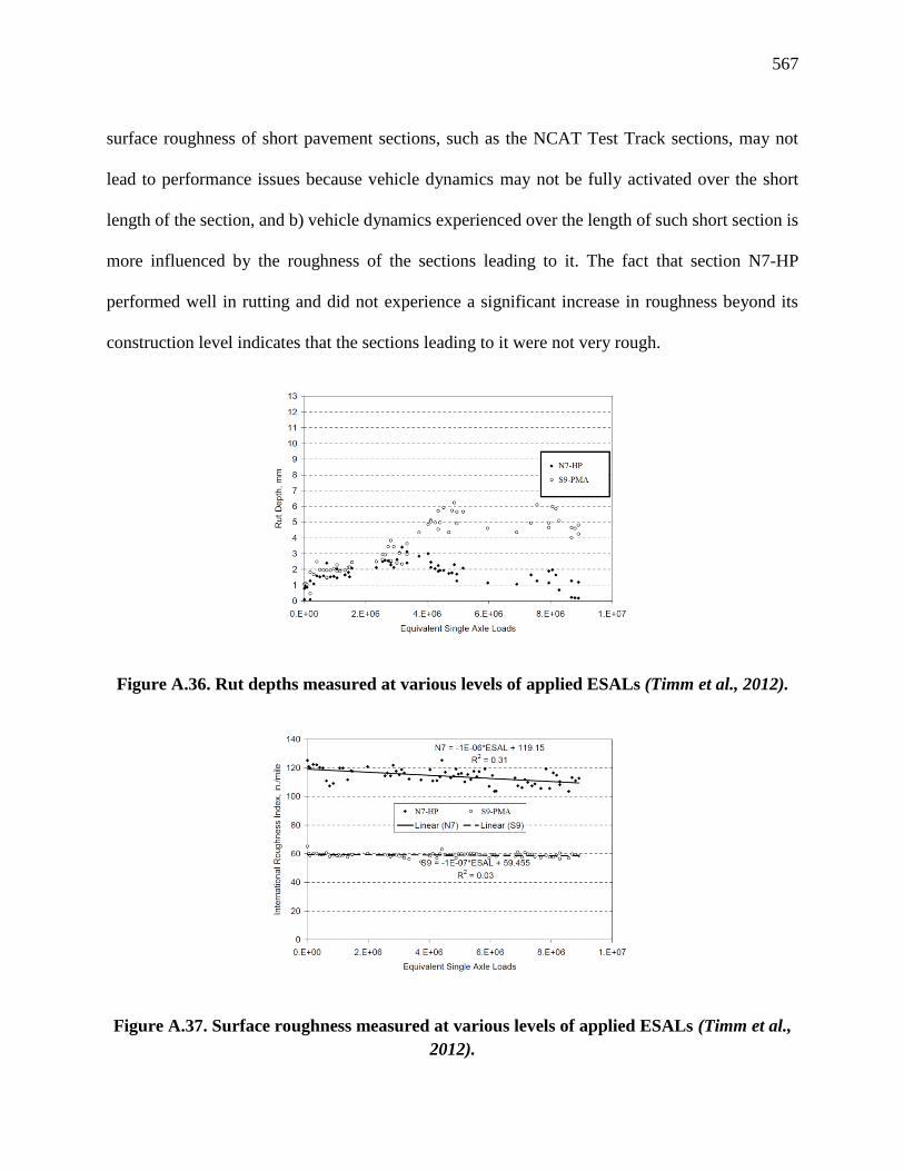
567
surface roughness of short pavement sections, such as the NCAT Test Track sections, may not
lead to performance issues because vehicle dynamics may not be fully activated over the short
length of the section, and b) vehicle dynamics experienced over the length of such short section is
more influenced by the roughness of the sections leading to it. The fact that section N7-HP
performed well in rutting and did not experience a significant increase in roughness beyond its
construction level indicates that the sections leading to it were not very rough.
Figure A.36. Rut depths measured at various levels of applied ESALs (Timm et al., 2012).
Figure A.37. Surface roughness measured at various levels of applied ESALs (Timm et al.,
2012).

568
A.5 Analysis of Structural Layer Coefficient for HP Asphalt Mixtures Based on NCAT
Study
Based on previous experience, a structural coefficient of 0.44 was found to be representative of
PMA AC mixes when designed in pavement sections for the state of Florida following the Flexible
Pavement Design Manual. In some other states, this structural coefficient was recalibrated to
account for the conventional polymer modification of asphalt mixtures (2-3% polymer). If the
positive impact of the polymer is assumed to be proportionally maintained at higher contents, then
the use of a HP asphalt binder (7.5% polymer) can potentially lead to a higher AC structural
coefficient (aHP-AC) and a reduced AC layer thickness for the same design traffic and serviceability
loss (Timm et al., 2009). The objective of this chapter is to illustrate several potential approaches
to recalibrate the structural coefficient using the laboratory and field performance of HP AC mixes
used in the experimental section N7-HP at the NCAT test track.
A.5.1 Background on Past Calibration Efforts
As mentioned in the previous chapters, many factors may affect the determination of structural
layer coefficients for new asphalt mixtures that were not used at the AASHO Road Test (e.g.,
recycled material, PMA and HP AC mixes). These factors include engineering properties, layer
thickness, underlying support, position in the pavement structure, and stress state. Many studies
have been conducted to determine these structural coefficients (Timm et al., 2009).
For AC mixes containing recycled materials, Van Wyk et al. (Van Wyk et al., 1983)
compared the deflection basins generated by non-destructive testing to theoretical deflection basins
using BISTRO, a layered elastic software program. The pavement cross section was selected so
569
the deflection basins matched adequately. Pavement responses such as tensile strains at the bottom
of the AC layer, compressive strains at the top of subgrade, and surface deflections were computed
on two similar pavement sections, one conventional and the other including RAP with similar
design life. The structural number (SN), the thickness and quality of base and subbase material, as
well as the type of subgrade were maintained the same for both sections making the structural
coefficient of the AC mix with RAP the only variable parameter. The structural number is a direct
measure of the layer’s thicknesses and their corresponding structural coefficients. It should be
mentioned that this method accounts for the distress criteria (i.e., rutting and fatigue cracking) that
constitutes the shortest pavement life.
Hossain et al. used FWD test data to determine the structural layer coefficient of crumb-
rubber modified (CRM) mixes for Kansas DOT (KDOT) (Hossain et al., 1997). The layer
conditions were then determined from the effective structural number calculated using
backcalculated moduli, layer thicknesses and Equation A.3 recommended by the AASHTO 1993
Guide. High variability in the structural layer coefficients was observed from this study.
𝑆𝑁𝑒𝑓𝑓 = 0.0045 ∗ 𝐷 ∗ √𝐸𝑝3 [Equation. A.3]
Where;
D: total thickness of the corresponding pavement cross section above the subgrade (inch); and
Ep: effective modulus of the pavement cross section (psi).
In 2009, Timm et al. used the performance of 11 test sections of neat and PMA AC mixes built on
the NCAT Test Track between 2003 and 2006 as summarized in Figure A.38 to establish the
structural coefficient for PMA AC mixes for the Alabama DOT as described below:

570
• The performance of the test sections were converted into PSI using the relationship
developed by Al-Omari and Darter (49) shown below:
𝑃𝑆𝐼 = 5 ∗ 𝑒(−0.0038∗𝐼𝑅𝐼) [Equation. A.4]
• Using the calculated PSI, the terminal serviceability (pt) and the change in PSI (ΔPSI) was
determined for each section.
• Using the ΔPSI, the resilient modulus property of the subgrade, and traffic in ESALs, the
equivalent SN for each section was determined.
• Finally, the structural coefficient for each PMA section was determined using its
equivalent SN and the thickness of the various layers including the PMA AC layer.
• The determined structural coefficients for the PMA AC mixes had an average value of
0.54 and a standard deviation of 0.08.

571
Figure A.38. NCAT Test Track structural sections (Timm et al., 2012).
A.5.2 Preliminary Analysis of NCAT Section N7-HP Structural Coefficient
The objective of this section is to illustrate different potential approaches for the recalibration of
the structural layer coefficient of HP AC mixes using published data collected during the NCAT
study; Field and Laboratory Study of High-Polymer Mixtures at the NCAT Test Track (Timm et
al., 2012). The following four approaches were explored as part of this chapter and a preliminary
structural coefficient for the HP AC mix was determined accordingly.
• Approach 1: consists of determining a structural coefficient for the HP AC mix using the
fixed service life concept based on measured rutting performance.
572
• Approach 2: consists of determining a structural coefficient for the HP AC mix using
collected FWD data, method of equivalent thickness (MET), and estimation of effective
structural number (SNeff).
• Approach 3: consists of determining a structural coefficient for the HP AC mix using the
AASHTO 1993 Guide equation and associated loss in serviceability index.
• Approach 4: consists of determining a structural coefficient for the HP AC mix based on
equivalent fatigue life using the 3D-Move Analysis model.
Two pavement sections, a PMA and a HP, were considered as part of these analyses. The
PMA section consisted of a 7 inch (178 mm) thick AC layer while the AC layer thickness of the
HP section was determined according to each of the examined approaches. Both sections had a 6
inch (150 mm) CAB layer placed on top of the same subgrade. A structural coefficient (a2) and a
draining coefficient (m2) of 0.14 and 1.0 were assumed for the base layer, respectively.
In each approach, a percent difference between the estimated structural coefficients of the
PMA AC and HP AC mixes used on the NCAT track will be calculated. This percent difference
will be applied to the 0.44 structural coefficient for the PMA AC mix to estimate that of HP AC
mix from Florida.
A.5.2.1 Approach 1: Determination of aHP-AC Based on Measured Rutting Performance
As of June 27, 2011, approximately 8.9 million ESALs had been applied to test sections N7-HP
and S9-PMA. At that time, there was no cracking evident on either of the sections. Weekly
measurements of rut depths were collected and plotted (Refer to Figure A.36). Both sections

573
showed rut depth values lower than 0.25 inch (6.4 mm) after 8.9 million ESALs indicating a high
resistance to rutting. Referring to Figure A.36, similar rutting performance was observed on both
sections up to an applied traffic of 3.5 million ESALs. Based on the observed rutting performance
of the AC layers, the structural coefficient of the HP modified asphalt mix can be determined using
the fixed service life approach. At the equivalent rutting performance of approximately 0.12 inch
(3 mm) after 3.5 million ESALs, the 5.75 inch (146 mm) AC layer thickness for the HP pavement
can be considered sufficient to achieve the same service life as the corresponding 7.00 inch (178
mm) AC layer thickness for the PMA pavement. The structural coefficient for the HP mix is then
calculated as the ratio of the AC layer thickness of the PMA pavement to the AC layer thickness
of the HP pavement times 0.44 which is the assumed structural layer coefficient of the PMA mix
according to FDOT (Equation 5.3). Accordingly, a structural coefficient of 0.54 is estimated for
the HP mix based on the equivalent rutting performance after a traffic loading of 3.5 million
ESALs.
𝑎𝐻𝑃−𝐴𝐶−𝑅𝑢𝑡 = (𝐴𝐶 𝑙𝑎𝑦𝑒𝑟 𝑡ℎ𝑖𝑐𝑘𝑛𝑒𝑠𝑠 𝑜𝑓 𝑃𝑀𝐴 𝑝𝑎𝑣𝑒𝑚𝑒𝑛𝑡 𝑓𝑜𝑟 𝑟𝑢𝑡𝑡𝑖𝑛𝑔 𝑖𝑛 𝐴𝐶
𝐴𝐶 𝑙𝑎𝑦𝑒𝑟 𝑡ℎ𝑖𝑐𝑘𝑛𝑒𝑠𝑠 𝑜𝑓 𝐻𝑃 𝑝𝑎𝑣𝑒𝑚𝑒𝑛𝑡 𝑓𝑜𝑟 𝑠𝑎𝑚𝑒 𝑟𝑢𝑡𝑡𝑖𝑛𝑔 𝑖𝑛 𝐴𝐶) ∗ 0.44 [Equation. A.5]
A.5.2.2 Approach 2: Determination of aHP-AC Based on FWD Data
As recommended by the AASHTO 1993 Guide, the effective structural number can be calculated
from the total thickness of the pavement cross section above the subgrade and its effective modulus
(refer to Equation A.1). The analysis of the FWD data showed backcalculated moduli of 921,000
psi (6,350 MPa), 2,200 psi (15 MPa), and 27,800 psi (192 MPa) for the PMA AC, base, and
subgrade layers, respectively (Timm et al., 2012). The method of equivalent thickness (MET) is
574
used to convert the top layers (i.e., AC and base layers) into a half space with a subgrade modulus
of Mr using Equation A.6.
ℎ𝑒,𝑛 = {∑ ℎ𝑖 ∗ √𝐸𝑖
𝑀𝑅
3} = {𝐷 ∗ √
𝐸𝑝
𝑀𝑅
3}𝑛
𝑖=1 [Equation. A.6]
Where;
he,n: equivalent thickness of ith layer (inch);
hi: thickness of ith layer (inch);
Ei: backcalculated modulus of ith layer (psi);
MR: backcalculated modulus of the subgrade layer (psi);
Ep: effective modulus of the pavement cross section (psi); and
D: total thickness of the pavement cross section (inch).
Therefore, the equivalent layer thickness for the PMA section is calculated using Equation
A.7 as follows:
ℎ𝑒,𝑛 = ℎ𝑃𝑀𝐴−𝐴𝐶 ∗ √𝐸𝐴𝐶
𝑀𝑅
3+ ℎ𝑏𝑎𝑠𝑒 ∗ √
𝐸𝑏𝑎𝑠𝑒
𝑀𝑅
3
= 7 ∗ √921,000
27,800
3+ 6 ∗ √
2,200
27,800
3= 25.1 𝑖𝑛𝑐ℎ (637 mm) [Equation. A.7]
The effective modulus of the pavement cross section can be then calculated using Equation
5.6 where D is equal to the summation of the thickness of both the PMA AC and base layers (i.e.,
13 inch).
𝐸𝑝 = 𝑀𝑅 ∗ (ℎ𝑒,𝑛
𝐷)3 = 27,800 ∗ (
25.1
13)3 = 199,140 𝑝𝑠𝑖 (1,373 MPa) [Equation. A.8]
Accordingly, using Equation A.1, the effective structural number of the PMA section is
calculated as follows.
𝑆𝑁𝑒𝑓𝑓−𝑃𝑀𝐴 = 0.0045 ∗ 𝐷 ∗ √𝐸𝑝3 = 0.0045 ∗ 13 ∗ √199140
3= 3.42 [Equation. A.9]
575
Therefore, using Equation A.2, the structural coefficient of the PMA AC layer is calculated as
follows and a value of 0.37 was determined (i.e., aPMA-AC = 0.37).
𝑆𝑁𝑒𝑓𝑓−𝑃𝑀𝐴 = 𝑎𝑃𝑀𝐴−𝐴𝐶 ∗ ℎ𝑃𝑀𝐴−𝐴𝐶 + 𝑎𝑏𝑎𝑠𝑒 ∗ ℎ𝑏𝑎𝑠𝑒 ∗ 𝑚𝑏𝑎𝑠𝑒
3.42 = 𝑎𝑃𝑀𝐴−𝐴𝐶 ∗ 7 + 0.14 ∗ 6 ∗ 1 [Equation. A.9]
At 3.5 million EASLs, the PMA and HP sections were found to have an equivalent rutting
performance. Therefore, the same effective structural number can be assigned for the HP pavement
section. Thus assuming similar base layer properties, the structural layer coefficient for the HP AC
mix can be calculated using Equation A.2 and a value of 0.45 was determined (i.e., aHP-AC = 0.45).
𝑆𝑁𝐻𝑃−𝐴𝐶 = 𝑎𝐻𝑃−𝐴𝐶 ∗ ℎ𝐻𝑃−𝐴𝐶 + 𝑎𝑏𝑎𝑠𝑒 ∗ ℎ𝑏𝑎𝑠𝑒 ∗ 𝑚𝑏𝑎𝑠𝑒
3.42 = 𝑎𝐻𝑃−𝐴𝐶 ∗ 5.75 + 0.14 ∗ 6 ∗ 1 [Equation. A.10]
This analysis showed an increase of 21.6% in the structural coefficient of the HP AC layer
(i.e., aAC-HP = 0.45) when compared with the structural coefficient of the PMA AC layer (i.e., aPMA-
AC = 0.37). Applying this percent difference on the recommended structural coefficient of PMA
mixes in Florida, a value of 0.54 (i.e., denoting an increase of 21.6% from 0.44) is estimated for a
FDOT HP AC mix.
A.5.2.3 Approach 3: Determination of aHP-AC Based on Loss in Serviceability
The PSI concept was developed during the AASHTO Road Test experiment to relate the ride
conditions of the road with the opinion of the user. The original PSI equation has been modified
throughout the years by State highway agencies to better describe local conditions. Equation A.11
shows the PSI equation for flexible pavements Error! Reference source not found.. As mentioned

576
before, there was no cracking and patching reported on either of the sections after 8.9 million
ESALs. Therefore, C and P values in Equation A.11 were considered equal to zero.
𝑃𝑆𝐼 = 5 ∗ 𝑒(−0.0041∗𝐼𝑅𝐼) − 1.38 ∗ 𝑅𝐷2 − 0.03 ∗ (𝐶 + 𝑃)0.5 [Equation. A.11]
Where;
PSI: present serviceability index;
IRI: international roughness index (inch/mile);
RD: rut depth (inch);
C: cracking (ft2/1000ft2); and
P: patching (ft2/1000ft2).
After 8.9 million ESAL, average terminal serviceability values of 3.1 and 3.9 were
calculated for the PMA and HP pavement sections, respectively (pt-PMA=3.1, and pt-HP=3.9).
Considering an initial serviceability of 4.2 (pi=4.2) for both sections, the change in PSI was found
to be 1.1 and 0.3, respectively. A 50% reliability is considered for this analysis because high
reliabilities are used to artificially increase the predicted traffic to account for uncertainty in the
design process. Therefore, a normal deviate of zero value is then selected. Solving for all input
parameters in Equation 1.1, the structural number of the PMA and HP pavement sections (SNPMA-
AC and SNHP-AC) was found to be 4.1 and 4.3, respectively. It should be mentioned that one-third
of the backcalculated moduli value of the subgrade layer was considered following the
recommendations from the AASHTO 1993 Guide procedure. Therefore, the corresponding
structural coefficients of PMA and HP AC mixes were calculated using Equations 5.11 and 5.12
and resulted in values of aPMA-AC = 0.46 and aHP-AC = 0.60. This analysis showed an increase of
29.2% in the structural layer coefficient for the HP AC layer when compared with the structural
coefficient of the PMA AC layer. Applying this percent difference on the recommended structural
coefficient of PMA mixes in Florida, a value of 0.57 can then be assumed for FDOT HP AC mixes
(i.e. aHP-AC = 0.57).
577
𝑆𝑁𝑃𝑀𝐴−𝐴𝐶 = 𝑎𝑃𝑀𝐴−𝐴𝐶 ∗ ℎ𝑃𝑀𝐴−𝐴𝐶 + 𝑎𝑏𝑎𝑠𝑒 ∗ ℎ𝑏𝑎𝑠𝑒 ∗ 𝑚𝑏𝑎𝑠𝑒
4.1 = 𝑎𝑃𝑀𝐴−𝐴𝐶 ∗ 7 + 0.14 ∗ 6 ∗ 1 → 𝑎𝑃𝑀𝐴−𝐴𝐶 = 0.46 [Equation A.12]
𝑆𝑁𝐻𝑃−𝐴𝐶 = 𝑎𝐻𝑃−𝐴𝐶 ∗ ℎ𝐻𝑃−𝐴𝐶 + 𝑎𝑏𝑎𝑠𝑒 ∗ ℎ𝑏𝑎𝑠𝑒 ∗ 𝑚𝑏𝑎𝑠𝑒
4.3 = 𝑎𝐻𝑃−𝐴𝐶 ∗ 5.75 + 0.14 ∗ 6 ∗ 1 → 𝑎𝐻𝑃−𝐴𝐶 = 0.60 [Equation A.13]
A.5.2.4 Approach 4: Determination of aHP-AC Based on Equivalent Fatigue Life using 3D-Move
Analysis
As noted in previous sections, field mixed laboratory compacted specimens of PMA and HP mixes
were prepared and evaluated in terms of their resistance to fatigue cracking at a temperature of
68°F (20°C) using the flexural beam fatigue test. Equation A.14 and A.15 show the fatigue
relationship for PMA and HP mixes using the power model, respectively.
휀𝑡−𝑃𝑀𝐴 = 5374.2 ∗ 𝑁−0.214 [Equation. A.14]
휀𝑡−𝐻𝑃 = 2791.8 ∗ 𝑁−0.125 [Equation. A.15]
Where;
휀t: tensile strain at the bottom of the AC layer (micro-strain); and
N: Number of cycles to failure.
As shown previously, the predicted fatigue life in terms of cycles to failure at 68°F (20°C)
using the laboratory-determined transfer function is expected to be 348,432 and 15,680,982 cycles
for the S9-PMA and N7-HP sections, respectively. Following the fixed service life approach for
fatigue cracking, the required AC layer thickness for the HP pavement will be determined to
achieve the same service life in terms of number of fatigue cycles to failure of the PMA pavement

578
section. For that, the 3D-Move software was used and two analyses were conducted: static (i.e.,
stationary load), and dynamic (i.e., moving load).
The 3D-Move analytical model adopted here to undertake the pavement response
computations uses a continuum-based finite-layer approach. The 3D-Move analysis model can
account for important pavement response factors such as complex 3D contact stress distributions
(normal and shear) of any shape, vehicle speed, and viscoelastic material characterization for the
AC layers. This approach treats each pavement layer as a continuum and uses the Fourier transform
technique. Since rate-dependent material properties (viscoelastic) can be accommodated by the
approach, it is an ideal tool to model the behavior of AC layer and also to study pavement responses
as a function of vehicle speed. Frequency-domain solutions are adopted in 3D-Move Analysis,
which enables the direct use of the frequency sweep test data of AC mixture in the analysis. More
information can be found in literature.
Input Parameters and Definition of Critical Points
A single axle dual tires was applied as traffic loading on both sections for both static and dynamic
analyses. For the dynamic analysis, a speed of 45 mph (72 km/h) was considered to simulate the
speed of the loading trucks at the NCAT track.
Table A.17 summarizes the input values for the applied traffic. Table A.18 and Table
A.19 summarize all the properties for the AC, base and subgrade layers from the PMA and HP
sections, respectively. Table A.20 and Table A.21 summarize the dynamic modulus of the PMA
and HP AC mixes, respectively. The RTFO properties for the PMA and HP asphalt binders are
summarized in Table A.22 and Table A.23, respectively. Figure A.39 illustrates the PMA

579
pavement section and the points of interest at the bottom of the PMA AC layer (i.e., P1, P2, P3,
P4, P5, and P6).
Table A.17. Characteristics of Applied Traffic Load.
Single Axle Dual Tires
Axle Load, lb (kN) 18,000 (80)
Tire Pressure, psi (kPa) 120 (827)
Dual Tires Spacing, inch (mm) 14 (356 mm)
Tire Load, lb (kN) 4,500 (20)
Table A.18. Summary of Input Properties for S9-PMA Test Section.
Pavement Layer Backcalculated Modulus Thickness, inch
(mm) Characterization
PMA Asphalt
Concrete
Static: 921,000 psi (6,350 MPa)
Dynamic: Dynamic Modulus of
PMA mix (Refer to Table 17)
7 (178) Viscoelastic
Aggregate Base E = 2,200 psi (15 MPa) 6 (150) Linear Elastic
Subgrade E = 27,800 psi (192 MPa) Infinite Linear Elastic
Table A.19. Summary of Input Properties for N7-HP Test Section.
Pavement Layer Backcalculated Modulus Thickness, inch Characterization
HP Asphalt
Concrete
Static: 882,000 psi (6,081 MPa)
Dynamic: Dynamic Modulus of
HP mix (Refer to Table 18)
To be
determined Viscoelastic
Aggregate Base E = 3,600 psi (25 MPa) 6 (150) Linear Elastic
Subgrade E = 33,000 psi (220 MPa) Infinite Linear Elastic

580
Table A.20. Dynamic Modulus Input Values for S9-PMA AC Mix.
E*, psi (MPa) Frequency (Hz)
Temperature, °F
(°C) 0.1 0.5 1 5 10 25
14 (-10) 2,186,700
(15,077)
2,419,500
(16,682)
2,506,000
(17,278)
2,676,400
(18,453)
2,737,700
(18,876)
2,808,700
(19,365)
40 (4) 1,295,700
(8,934)
1,621,400
(11,179)
1,757,500
(12,118)
2,052,200
(14,149)
2,167,400
(14,944)
2,307,300
(15,908)
70 (21) 458,600
(3,162)
686,200
(4,731)
802,000
(5,530)
1,102,400
(7,601)
1,240,800
(8,555)
1,426,800
(9,837)
100 (38) 128,600
(887)
208,700
(1,439)
256,700
(1,770)
406,900
(2,805)
490,100
(3,379)
617,700
(4,259)
130 (54) 43,900
(303)
66,300
(457)
80,300
(554)
128,600
(887)
158,400
(1,092)
208,800
(1,440)
Table A.21. Dynamic Modulus Input Values for N7-HP AC Mix.
E*, psi (MPa) Frequency (Hz)
Temperature, °F
(°C)
0.1 0.5 1 5 10 25
14 (-10) 2,116,700
(14,594)
2,372,600
(16,358)
2,467,300
(17,011)
2,652,300
(18,287)
2,718,100
(18,741)
2,793,700
(19,262)
40 (4) 1,147,700
(7,913)
1,493,300
(10,296)
1,640,800
(11,313)
1,964,000
(13,541)
2,091,000
(14,417)
2,245,500
(15,482)
70 (21) 340,600
(2,348)
541,500
(3,734)
649,500
(4,478)
944,000
(6,509)
1,085,300
(7,483)
1,279,900
(8,825)
100 (38) 85,500
(590)
141,800
(978)
177,200
(1,222)
295,400
(2,037)
364,900
(2,516)
476,300
(3,284)
130 (54) 30,400
(210)
44,400
(306)
53,300
(367)
85,000
(586)
105,300
(726)
140,900
(971)
Table A.22. PMA Asphalt Binder Rheological Properties.
Asphalt Binder Properties – PMA Binder – NCAT Section S9
Temperature, °F (°C) G*, psi (Pa) , °
168.8 (76) 0.41045 (2,830) 67.9
179.6 (82) 0.24076 (1,660) 70.0
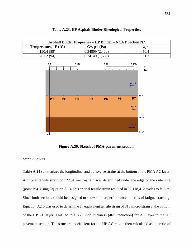
581
Table A.23. HP Asphalt Binder Rheological Properties.
Asphalt Binder Properties – HP Binder – NCAT Section N7
Temperature, °F (°C) G*, psi (Pa) , °
190.4 (88) 0.34809 (2,400) 50.4
201.2 (94) 0.24149 (1,665) 51.3
Figure A.39. Sketch of PMA-pavement section.
Static Analysis
Table A.24 summarizes the longitudinal and transverse strains at the bottom of the PMA AC layer.
A critical tensile strain of 127.51 micro-strain was determined under the edge of the outer tire
(point P5). Using Equation A.14, this critical tensile strain resulted in 39,118,412 cycles to failure.
Since both sections should be designed to show similar performance in terms of fatigue cracking,
Equation A.15 was used to determine an equivalent tensile strain of 313 micro-strain at the bottom
of the HP AC layer. This led to a 3.75 inch thickness (46% reduction) for AC layer in the HP
pavement section. The structural coefficient for the HP AC mix is then calculated as the ratio of
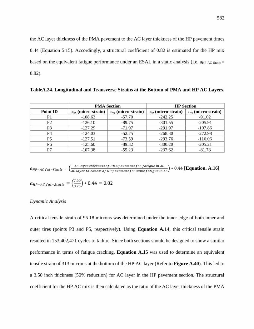
582
the AC layer thickness of the PMA pavement to the AC layer thickness of the HP pavement times
0.44 (Equation 5.15). Accordingly, a structural coefficient of 0.82 is estimated for the HP mix
based on the equivalent fatigue performance under an ESAL in a static analysis (i.e. aHP-AC-Static =
0.82).
TableA.24. Longitudinal and Transverse Strains at the Bottom of PMA and HP AC Layers.
PMA Section HP Section
Point ID εxx (micro-strain) εyy (micro-strain) εxx (micro-strain) εyy (micro-strain)
P1 -108.63 -57.70 -242.25 -91.02
P2 -126.10 -89.75 -301.55 -205.91
P3 -127.29 -71.97 -291.97 -107.86
P4 -124.03 -52.75 -268.30 -272.98
P5 -127.51 -73.59 -293.76 -116.06
P6 -125.60 -89.32 -300.20 -205.21
P7 -107.38 -55.23 -237.62 -81.78
𝑎𝐻𝑃−𝐴𝐶 𝑓𝑎𝑡−𝑆𝑡𝑎𝑡𝑖𝑐 = (𝐴𝐶 𝑙𝑎𝑦𝑒𝑟 𝑡ℎ𝑖𝑐𝑘𝑛𝑒𝑠𝑠 𝑜𝑓 𝑃𝑀𝐴 𝑝𝑎𝑣𝑒𝑚𝑒𝑛𝑡 𝑓𝑜𝑟 𝑓𝑎𝑡𝑖𝑔𝑢𝑒 𝑖𝑛 𝐴𝐶
𝐴𝐶 𝑙𝑎𝑦𝑒𝑟 𝑡ℎ𝑖𝑐𝑘𝑛𝑒𝑠𝑠 𝑜𝑓 𝐻𝑃 𝑝𝑎𝑣𝑒𝑚𝑒𝑛𝑡 𝑓𝑜𝑟 𝑠𝑎𝑚𝑒 𝑓𝑎𝑡𝑖𝑔𝑢𝑒 𝑖𝑛 𝐴𝐶) ∗ 0.44 [Equation. A.16]
𝑎𝐻𝑃−𝐴𝐶 𝑓𝑎𝑡−𝑆𝑡𝑎𝑡𝑖𝑐 = (7.00
3.75) ∗ 0.44 = 0.82
Dynamic Analysis
A critical tensile strain of 95.18 microns was determined under the inner edge of both inner and
outer tires (points P3 and P5, respectively). Using Equation A.14, this critical tensile strain
resulted in 153,402,471 cycles to failure. Since both sections should be designed to show a similar
performance in terms of fatigue cracking, Equation A.15 was used to determine an equivalent
tensile strain of 313 microns at the bottom of the HP AC layer (Refer to Figure A.40). This led to
a 3.50 inch thickness (50% reduction) for AC layer in the HP pavement section. The structural
coefficient for the HP AC mix is then calculated as the ratio of the AC layer thickness of the PMA
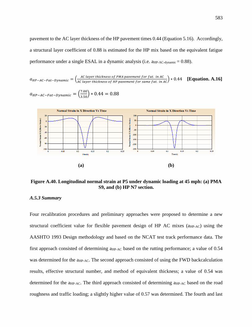
583
pavement to the AC layer thickness of the HP pavement times 0.44 (Equation 5.16). Accordingly,
a structural layer coefficient of 0.88 is estimated for the HP mix based on the equivalent fatigue
performance under a single ESAL in a dynamic analysis (i.e. aHP-AC-dynamic = 0.88).
𝑎𝐻𝑃−𝐴𝐶−𝐹𝑎𝑡−𝐷𝑦𝑛𝑎𝑚𝑖𝑐 = (𝐴𝐶 𝑙𝑎𝑦𝑒𝑟 𝑡ℎ𝑖𝑐𝑘𝑛𝑒𝑠𝑠 𝑜𝑓 𝑃𝑀𝐴 𝑝𝑎𝑣𝑒𝑚𝑒𝑛𝑡 𝑓𝑜𝑟 𝑓𝑎𝑡. 𝑖𝑛 𝐴𝐶
𝐴𝐶 𝑙𝑎𝑦𝑒𝑟 𝑡ℎ𝑖𝑐𝑘𝑛𝑒𝑠𝑠 𝑜𝑓 𝐻𝑃 𝑝𝑎𝑣𝑒𝑚𝑒𝑛𝑡 𝑓𝑜𝑟 𝑠𝑎𝑚𝑒 𝑓𝑎𝑡. 𝑖𝑛 𝐴𝐶) ∗ 0.44 [Equation. A.16]
𝑎𝐻𝑃−𝐴𝐶−𝐹𝑎𝑡−𝐷𝑦𝑛𝑎𝑚𝑖𝑐 = (7.00
3.50) ∗ 0.44 = 0.88
(a) (b)
Figure A.40. Longitudinal normal strain at P5 under dynamic loading at 45 mph: (a) PMA
S9, and (b) HP N7 section.
A.5.3 Summary
Four recalibration procedures and preliminary approaches were proposed to determine a new
structural coefficient value for flexible pavement design of HP AC mixes (aHP-AC) using the
AASHTO 1993 Design methodology and based on the NCAT test track performance data. The
first approach consisted of determining aHP-AC based on the rutting performance; a value of 0.54
was determined for the aHP-AC. The second approach consisted of using the FWD backcalculation
results, effective structural number, and method of equivalent thickness; a value of 0.54 was
determined for the aHP-AC. The third approach consisted of determining aHP-AC based on the road
roughness and traffic loading; a slightly higher value of 0.57 was determined. The fourth and last
584
approach consisted of determining the aHP-AC based on fatigue data using the 3D-Move Analysis
model; higher aHP-AC of 0.82 and 0.88 were determined for HP AC mixes under static and dynamic
loading, respectively.
A.5.3.1 Findings
The first three approaches for the determination of the structural coefficient of the HP AC mix are
all based on the AASHTO 1993 Guide concept with some slight variations in the analysis.
Therefore, it is reasonable to expect that similar coefficients will be determined for the three
approaches.
The fourth approach is based on the mechanistic analysis of the PMA and HP structures
and their anticipated fatigue life. The research team wanted to present this approach to show that
mechanistic-based layer coefficients maybe significantly different than the empirically determined
coefficients. However, the use of the available data from the NCAT sections for the mechanistic-
based approach suffered from the following serious limitations:
1- Fatigue models for PMA and HP AC mixes were developed at a single temperature which
does not allow the incorporation of the modulus effect. A true mechanistic analysis must
incorporate the impact of AC mix modulus on the calculation of tensile strains and the
determination of the fatigue life.
2- No rutting models were developed for the PMA and HP AC mixes. The rutting properties
from the APA and FN represent the empirical behavior of the mixtures at a single
temperature and do not incorporate the modulus effect. A true mechanistic analysis must

585
incorporate the impact of AC mix modulus on the calculation of vertical strains and the
determination of the rutting life.
The large difference between the coefficients determined by the empirical approaches (1-
3) and the mechanistic approach (4) should not jeopardize the applicability of the 3D-Move model
for the following reasons:
1- The fact that neither sections at the NCAT Test Track showed any fatigue cracking after
8.9 million ESALs indicates that the fatigue-based structural coefficients would be high
which is consistent with approach 4.
2- The current research will conduct fatigue and rutting testing at multiple temperatures which
will allow the development of fatigue and rutting models that incorporate the impact of the
modulus on the performance of the mixtures which is critical for a full mechanistic
analysis.
3- The current research will determine the structural coefficients based on multiple distress
modes of: fatigue, rutting in AC, and total rutting and check their validity with other
distresses of: top-down cracking, reflective cracking, and shoving.
4- The 3D-Move model has been validated through several studies to provide the same
pavement analysis as the linear elastic model used in the AASHTO M-E Design when
applied at static conditions (i.e. zero speed). The additional benefit of the 3D-Move model
is that it incorporates vehicle speed and braking stresses.

586
A.6 Findings and Recommendations
The objective of this literature review was to identify all currents and previous studies that have
been conducted to evaluate the performance of HP AC mixes. In this research, HP AC mixes are
defined as asphalt mixtures manufactured using asphalt binders modified with SBS or SB polymers
at the approximate rate of 7.5% by weight of binder. The findings of the literature review will be
presented with respect to the three areas of interest that were defined in the Scope of the review
as: a) laboratory evaluations of HP modified asphalt binders and mixtures, b) performance of
pavement sections constructed with HP AC mixes, and c) techniques to determine structural
coefficient of HP AC mixes.
A.6.1 Laboratory Evaluations of HP Modified Asphalt Binders and Mixtures
The review identified several studies that evaluated the engineering properties and performance
characteristics of HP asphalt binders and mixtures. On the positive side, all of the identified studies
used the Superpave technology to evaluate the properties of the binders and mixtures which makes
the generated data highly applicable to the current research. On the not so positive side, none of
the identified studies conducted a complete experimental design that can lead to the evaluation of
the performance of HP AC mixes with respect to all modes of distresses, i.e., rutting, fatigue,
thermal, and reflective cracking. In addition, some of the studies did not incorporate the evaluation
of a control binder or mixture in order to clearly define the contribution of the HP asphalt binder.
Furthermore, some studies went directly into the evaluation of HP mixtures without providing
sufficient information on the properties of the HP binders used in the manufacturing of the
mixtures.
587
Table A.25 summarizes the findings of the reviewed studies that evaluated the laboratory
properties of HP binders and mixtures. The summary is presented in terms of the impact of HP
modification on the performance properties of binders and mixtures. A review of the findings in
Table A.25 leads to the following observations:
• Increasing the SBS polymer content from 0, 3, 6, to 7.5% continues to improve the
performance properties of the asphalt binder and mixture in terms of its resistance to the
various modes of distresses, i.e. rutting, fatigue, thermal, and reflective cracking.
• A unique feature of the HP modification has been identified as its ability to slow down the
oxidative aging of the asphalt binder. This feature is expected to positively impact the
resistance of the HP AC mix to the various types of cracking.
• The HP asphalt binder should not be used to overcome the negative impact of RAP on the
resistance of the AC mixture to various types of cracking. The properties of the RAP binder
should be taken into consideration when designing HP AC mix with RAP content at or
above 25% in order to optimize the benefits of the HP modification.
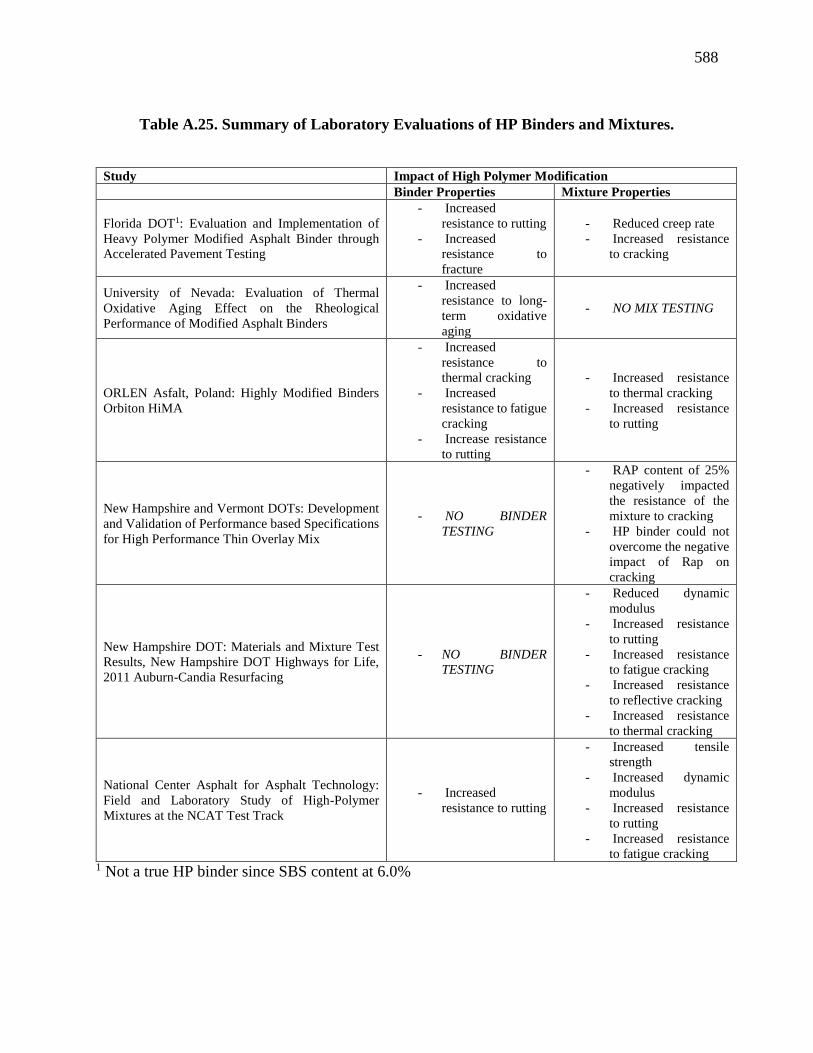
588
Table A.25. Summary of Laboratory Evaluations of HP Binders and Mixtures.
Study Impact of High Polymer Modification
Binder Properties Mixture Properties
Florida DOT1: Evaluation and Implementation of
Heavy Polymer Modified Asphalt Binder through
Accelerated Pavement Testing
- Increased
resistance to rutting
- Increased
resistance to
fracture
- Reduced creep rate
- Increased resistance
to cracking
University of Nevada: Evaluation of Thermal
Oxidative Aging Effect on the Rheological
Performance of Modified Asphalt Binders
- Increased
resistance to long-
term oxidative
aging
- NO MIX TESTING
ORLEN Asfalt, Poland: Highly Modified Binders
Orbiton HiMA
- Increased
resistance to
thermal cracking
- Increased
resistance to fatigue
cracking
- Increase resistance
to rutting
- Increased resistance
to thermal cracking
- Increased resistance
to rutting
New Hampshire and Vermont DOTs: Development
and Validation of Performance based Specifications
for High Performance Thin Overlay Mix
- NO BINDER
TESTING
- RAP content of 25%
negatively impacted
the resistance of the
mixture to cracking
- HP binder could not
overcome the negative
impact of Rap on
cracking
New Hampshire DOT: Materials and Mixture Test
Results, New Hampshire DOT Highways for Life,
2011 Auburn-Candia Resurfacing
- NO BINDER
TESTING
- Reduced dynamic
modulus
- Increased resistance
to rutting
- Increased resistance
to fatigue cracking
- Increased resistance
to reflective cracking
- Increased resistance
to thermal cracking
National Center Asphalt for Asphalt Technology:
Field and Laboratory Study of High-Polymer
Mixtures at the NCAT Test Track
- Increased
resistance to rutting
- Increased tensile
strength
- Increased dynamic
modulus
- Increased resistance
to rutting
- Increased resistance
to fatigue cracking 1 Not a true HP binder since SBS content at 6.0%
589
A.6.2 Performance of Pavement Sections Constructed with HP AC Mixes valuations of HP
Modified Asphalt Binders and Mixtures
Several field projects were constructed to evaluate the performance of HP modified asphalt
mixtures as compiled in Sections A.3 and A.4. Table A.26 summarizes the review of seven field
HP AC mixes projects with limited and extensive performance data. A review of the findings in
Table 26 leads to the following observations:
• HP AC mixes have been used over a wide range of applications ranging from full depth
AC layer to thin AC overlays under heavy traffic on interstates and slow-braking loads at
intersections.
• HP AC mixes did not show any construction issues in terms of mixing temperatures and
in-place compaction. Standard construction practices and equipment were adequately used.
• All of the identified HP field projects lack information on long-term performance,
however, early performances are encouraging. In addition, the HP test section on the
NCAT Test Track showed excellent performance under accelerated full scale loading.
• It is recommended that the research team attempts to obtain long-term field performance
from the field projects in Georgia, New Hampshire, Vermont, Oklahoma, and Oregon.
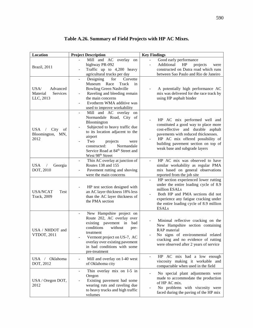
590
Table A.26. Summary of Field Projects with HP AC Mixes.
Location Project Description Key Findings
Brazil, 2011
- Mill and AC overlay on
highway PR-092
- Traffic up to 4,200 heavy
agricultural trucks per day
- Good early performance
- Additional HP projects were
constructed on Dutra road which runs
between Sao Paulo and Rio de Janeiro
USA/ Advanced
Material Services
LLC, 2013
- Designing for Corvette
Museum Race Track in
Bowling Green Nashville
- Raveling and bleeding remain
the main concerns
- Evotherm WMA additive was
used to improve workability
- A potentially high performance AC
mix was delivered for the race track by
using HP asphalt binder
USA / City of
Bloomington, MN,
2012
- Mill and AC overlay on
Normandale Road, City of
Bloomington
- Subjected to heavy traffic due
to its location adjacent to the
airport
- Two projects were
constructed: Normandale
Service Road at 84th Street and
West 98th Street
- HP AC mix performed well and
constituted a good way to place more
cost-effective and durable asphalt
pavements with reduced thicknesses.
- HP AC mix offered possibility of
building pavement section on top of
weak base and subgrade layers
USA / Georgia
DOT, 2010
- Thin AC overlay at junction of
Routes 138 and 155
- Pavement rutting and shoving
were the main concerns
- HP AC mix was observed to have
similar workability as regular PMA
mix based on general observations
reported from the job site
USA/NCAT Test
Track, 2009
- HP test section designed with
an AC layer thickness 18% less
than the AC layer thickness of
the PMA section
- HP section experienced lower rutting
under the entire loading cycle of 8.9
million ESALs
- Both HP and PMA sections did not
experience any fatigue cracking under
the entire loading cycle of 8.9 million
ESALs
USA / NHDOT and
VTDOT, 2011
- New Hampshire project on
Route 202, AC overlay over
existing pavement in bad
conditions without pre-
treatment
- Vermont project on US-7, AC
overlay over existing pavement
in bad conditions with some
pre-treatment
- Minimal reflective cracking on the
New Hampshire section containing
RAP material
- No signs of environmental related
cracking and no evidence of rutting
were observed after 2 years of service
USA / Oklahoma
DOT, 2012
- Mill and overlay on I-40 west
of Oklahoma city
- HP AC mix had a low enough
viscosity making it workable and
compactable when used in the field
USA / Oregon DOT,
2012
- Thin overlay mix on I-5 in
Oregon
- Existing pavement had some
wearing ruts and raveling due
to heavy trucks and high traffic
volumes
- No special plant adjustments were
made to accommodate the production
of HP AC mix.
- No problems with viscosity were
faced during the paving of the HP mix

591
A.6.3 Techniques to Determine Structural Coefficient of HP modified AC mixes
None of the available studies calculated the structural coefficient of HP AC mixes (aHP-AC) mainly
because of the unavailability of the required full performance characterizations of the mixtures. In
some cases, a hypothetical structural coefficient may be identified as shown below:
• For the project in Brazil; the HP section replaced the standard section at a 45% reduction
in the overall thickness indicating an aHP-AC that is 45% higher than the corresponding
structural coefficient for the composite pavement (i.e., AC over cement-stabilized RAP).
• For the projects in Bloomington, MN and Oklahoma; the HP section replaced the
standard section at a 25% reduction in the thickness of the AC layer indicating an aHP-AC
that is 25% higher than the corresponding structural coefficient for the standard AC mix.
The performance data generated from the PMA and HP test sections at the NCAT Test
Track offered some basis for the determination of an aHP-AC. However, the fact that both sections
did not show any fatigue cracking and only the minimal rutting was experienced by both sections
(i.e., less than 0.25 inch) limits the applicability of the estimated aHP-AC. Despite these limitations,
the research team attempted to demonstrate the various methods to establish an aHP-AC based on
the data from the NCAT test sections. Four approaches were examined; three empirical approaches
based on the AASHTO 1993 Guide methodology and one mechanistic approach based on the
analysis of fatigue performance. The three empirical approaches recommended an aHP-AC ranging
from 0.54 to 0.57 while the mechanistic approach recommended an aHP-AC ranging between 0.82
and 0.88.
592
In summary, while several previous studies highlighted the positive impacts of the HP
modification of asphalt binders and mixtures, there is still a serious lack of understanding on the
structural value of the HP AC mix as expressed through the structural coefficient for the AASHTO
1993 Guide. The attempt by the research team to determine an aHP-AC based on the available
information led to the conclusion that empirically-based aHP-AC can underestimate the structural
value of the HP AC mix while determining the aHP-AC based on the mechanistic analysis of a single
failure mode (i.e., fatigue cracking) may overestimate the structural value of the HP AC mix. This
important and critical finding strongly supports the approach implemented in this research where
the full evaluation of the performance characteristics of the HP AC mixes are conducted and the
aHP-AC is determined based on the mechanistic analysis of all possible critical modes of failure.

593
APPENDIX B MIX DESIGNS AND RESISTANCE TO MOISTURE DAMAGE –
DETAILED DATA
B.1 Mix Designs
B.1.1 Definition and Terms
Mix Design IDs:
• “FL”: White Rock Quarries, Southeast Florida.
• “GA”: Junction City Mining, Georgia Granite.
• “95” and “125”: NMAS of 9.5 mm and 12.5 mm, respectively.
• “PMA”: polymer modified asphalt binder (modified with SBS at the approximate rate of 3% by weight of binder).
• “HP”: high polymer modified asphalt binder (modified with SBS at the approximate rate of 7.5% by weight of binder).
• “(A)”: binder from Ergon Asphalt and Emulsion.
• “(B)”: binder from Vecenergy.

594
B.1.2 Mix Design 1: FL95_PMA(A)
Type of Mix: Fine SP-9.5
Intended Use of Mix: Structural
Design Traffic Level: C
Gyrations @ Ndes: 75
Product
Description Product Code
Producer
Name Product Name
Plant/Pit
Number
Bin Percentage
(%)
S1B Stone C51 White Rock
Quarries S1B Stone 87339 44.25
Screenings F22 White Rock
Quarries Screenings 87339 54.25
Generated Dust -- -- FL P200 -- 1.50
PERCENTAGE BY WEIGHT TOTAL AGGREGATE PASSING SIEVES
Blend 44.25% 54.25% 1.50% Job Mix
Formula
Control
Points Stockpile ID S1B Stone C51 Screenings F22 FL P200
SIE
VE
SIZ
E
3/4” (19.00 mm) 100.0 100.0 100.0 100.0
1/2” (12.50 mm) 99.7 99.9 100.0 99.8 100
3/8” (9.50 mm) 91.4 99.8 100.0 96.1 90 – 100
No.4 (4.75 mm) 17.9 99.5 100.0 63.4 ≤ 90
No.8 (2.36 mm) 6.3 90.5 100.0 53.4 32 – 67
No.16 (1.18 mm) 5.0 75.0 100.0 44.4
No.30 (0.600 mm) 4.4 60.7 100.0 36.4
No.50 (0.300 mm) 3.8 39.2 100.0 24.4
No.100 (0.150 mm) 2.8 9.1 100.0 7.7
No.200 (0.075 mm) 2.0 2.7 100.0 3.8 2 – 10
Gsb 2.510
AGGREGATE GRADATION CURVE
0
10
20
30
40
50
60
70
80
90
100
Per
cen
t P
ass
ing
Sieve Opening
Job Mix Formula
Max Line
SP9.5 FDOT Control Points
1 "
1/2
"
3/8
"
No
. 4
No
. 8
3/4
" 1
1/2
"
No
. 10
No
. 16
No
. 30
No
. 40
No
. 50
No
. 10
0
No
. 20
0

595
HOT MIX DESIGN DATA
Pb (%) Gmb @ Ndes Gmm Va (%) VMA (%) VFA (%) Pbe (%) DP = P0.075/Pbe
5.0 2.245 2.407 6.8 15.1 55.1 3.8 1.0
5.5 2.262 2.391 5.4 14.8 63.9 4.3 0.9
6.0 2.269 2.374 4.4 15.1 70.5 4.8 0.8
6.5 2.279 2.358 3.3 15.1 78.0 5.3 0.7
Selected Optimum Total Binder Content (OBC): 6.2 %
RAP Total Binder Content: No RAP was used
RAP Binder Ratio (RBR) at OBC: 0.00
VA at OBC: 4.0%
VMA at OBC: 15.0%
VFA at OBC: 73.1%
DP at OBC: 0.8%
Mixing Temperature: 325°F (163°C)
Compaction Temperature: 310°F (155°C)
Additives: Antistrip 0.5%
0.0%
1.0%
2.0%
3.0%
4.0%
5.0%
6.0%
7.0%
8.0%
4.5% 5.0% 5.5% 6.0% 6.5% 7.0%
% A
ir V
oid
s
% Asphalt Binder
4%
8%
12%
16%
20%
24%
4.5% 5.0% 5.5% 6.0% 6.5% 7.0%
% V
MA
% Asphalt Binder
0%
20%
40%
60%
80%
100%
4.5% 5.0% 5.5% 6.0% 6.5% 7.0%
% V
FA
% Asphalt Binder
0.0
0.2
0.4
0.6
0.8
1.0
1.2
1.4
4.5% 5.0% 5.5% 6.0% 6.5% 7.0%
Du
st P
rop
ort
ion
% Asphalt Binder
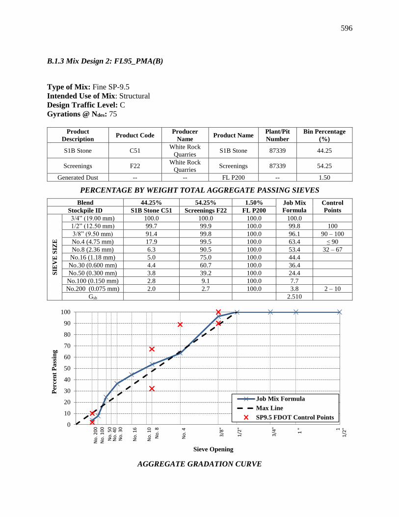
596
B.1.3 Mix Design 2: FL95_PMA(B)
Type of Mix: Fine SP-9.5
Intended Use of Mix: Structural
Design Traffic Level: C
Gyrations @ Ndes: 75
Product
Description Product Code
Producer
Name Product Name
Plant/Pit
Number
Bin Percentage
(%)
S1B Stone C51 White Rock
Quarries S1B Stone 87339 44.25
Screenings F22 White Rock
Quarries Screenings 87339 54.25
Generated Dust -- -- FL P200 -- 1.50
PERCENTAGE BY WEIGHT TOTAL AGGREGATE PASSING SIEVES
Blend 44.25% 54.25% 1.50% Job Mix
Formula
Control
Points Stockpile ID S1B Stone C51 Screenings F22 FL P200
SIE
VE
SIZ
E
3/4” (19.00 mm) 100.0 100.0 100.0 100.0
1/2” (12.50 mm) 99.7 99.9 100.0 99.8 100
3/8” (9.50 mm) 91.4 99.8 100.0 96.1 90 – 100
No.4 (4.75 mm) 17.9 99.5 100.0 63.4 ≤ 90
No.8 (2.36 mm) 6.3 90.5 100.0 53.4 32 – 67
No.16 (1.18 mm) 5.0 75.0 100.0 44.4
No.30 (0.600 mm) 4.4 60.7 100.0 36.4
No.50 (0.300 mm) 3.8 39.2 100.0 24.4
No.100 (0.150 mm) 2.8 9.1 100.0 7.7
No.200 (0.075 mm) 2.0 2.7 100.0 3.8 2 – 10
Gsb 2.510
AGGREGATE GRADATION CURVE
0
10
20
30
40
50
60
70
80
90
100
Per
cen
t P
ass
ing
Sieve Opening
Job Mix Formula
Max Line
SP9.5 FDOT Control Points
1 "
1/2
"
3/8
"
No
. 4
No
. 8
3/4
" 1
1/2
"
No
. 10
No
. 16
No
. 30
No
. 40
No
. 50
No
. 10
0
No
. 20
0

597
HOT MIX DESIGN DATA
Pb (%) Gmb @ Ndes Gmm Va (%) VMA (%) VFA (%) Pbe (%) DP = P0.075/Pbe
5.5 2.241 2.385 6.0 15.6 61.5 4.4 0.9
6.0 2.255 2.368 4.8 15.5 69.4 4.9 0.8
6.5 2.284 2.352 2.9 14.9 80.6 5.4 0.7
7.0 2.303 2.336 1.4 14.7 90.5 5.9 0.6
Selected Optimum Total Binder Content (OBC): 6.2 %
RAP Total Binder Content: No RAP was used
RAP Binder Ratio (RBR) at OBC: 0.00
VA at OBC: 4.0%
VMA at OBC: 15.3%
VFA at OBC: 73.9%
DP at OBC: 0.8%
Mixing Temperature: 325°F (163°C)
Compaction Temperature: 310°F (155°C)
Additives: Antistrip 0.5%
0.0%
1.0%
2.0%
3.0%
4.0%
5.0%
6.0%
7.0%
5.0% 5.5% 6.0% 6.5% 7.0% 7.5%
% A
ir V
oid
s
% Asphalt Binder
4%
8%
12%
16%
20%
24%
5.0% 5.5% 6.0% 6.5% 7.0% 7.5%
% V
MA
% Asphalt Binder
0%
20%
40%
60%
80%
100%
5.0% 5.5% 6.0% 6.5% 7.0% 7.5%
% V
FA
% Asphalt Binder
0.0
0.2
0.4
0.6
0.8
1.0
1.2
1.4
5.0% 5.5% 6.0% 6.5% 7.0% 7.5%
Du
st P
rop
ort
ion
% Asphalt Binder

598
B.1.4 Mix Design 3: FL95_HP (A)
Type of Mix: Fine SP-9.5
Intended Use of Mix: Structural
Design Traffic Level: C
Gyrations @ Ndes: 75
Product
Description Product Code
Producer
Name Product Name
Plant/Pit
Number
Bin Percentage
(%)
S1B Stone C51 White Rock
Quarries S1B Stone 87339 44.25
Screenings F22 White Rock
Quarries Screenings 87339 54.25
Generated Dust -- -- FL P200 -- 1.50
PERCENTAGE BY WEIGHT TOTAL AGGREGATE PASSING SIEVES
Blend 44.25% 54.25% 1.50% Job Mix
Formula
Control
Points Stockpile ID S1B Stone C51 Screenings F22 FL P200
SIE
VE
SIZ
E
3/4” (19.00 mm) 100.0 100.0 100.0 100.0
1/2” (12.50 mm) 99.7 99.9 100.0 99.8 100
3/8” (9.50 mm) 91.4 99.8 100.0 96.1 90 – 100
No.4 (4.75 mm) 17.9 99.5 100.0 63.4 ≤ 90
No.8 (2.36 mm) 6.3 90.5 100.0 53.4 32 – 67
No.16 (1.18 mm) 5.0 75.0 100.0 44.4
No.30 (0.600 mm) 4.4 60.7 100.0 36.4
No.50 (0.300 mm) 3.8 39.2 100.0 24.4
No.100 (0.150 mm) 2.8 9.1 100.0 7.7
No.200 (0.075 mm) 2.0 2.7 100.0 3.8 2 – 10
Gsb 2.510
AGGREGATE GRADATION CURVE
0
10
20
30
40
50
60
70
80
90
100
Per
cen
t P
ass
ing
Sieve Opening
Job Mix Formula
Max Line
SP9.5 FDOT Control Points
1 "
1/2
"
3/8
"
No
. 4
No
. 8
3/4
" 1
1/2
"
No
. 10
No
. 16
No
. 30
No
. 40
No
. 50
No
. 10
0
No
. 20
0

599
HOT MIX DESIGN DATA
Pb (%) Gmb @ Ndes Gmm Va (%) VMA (%) VFA (%) Pbe (%) DP = P0.075/Pbe
5.0 2.242 2.386 6.0 15.2 60.2 4.1 0.9
5.5 2.256 2.369 4.8 15.1 68.3 4.6 0.8
6.0 2.275 2.353 3.3 14.8 77.6 5.1 0.7
6.5 2.290 2.337 2.0 14.7 86.5 5.7 0.7
Selected Optimum Total Binder Content (OBC): 5.8 %
RAP Total Binder Content: No RAP was used
RAP Binder Ratio (RBR) at OBC: 0.00
VA at OBC: 4.0%
VMA at OBC: 14.9%
VFA at OBC: 73.2%
DP at OBC: 0.8%
Mixing Temperature: 340°F (171°C)
Compaction Temperature: 325°F (163°C)
Additives: Antistrip 0.5%
0.0%
1.0%
2.0%
3.0%
4.0%
5.0%
6.0%
7.0%
4.5% 5.0% 5.5% 6.0% 6.5% 7.0%
% A
ir V
oid
s
% Asphalt Binder
4%
8%
12%
16%
20%
24%
4.5% 5.0% 5.5% 6.0% 6.5% 7.0%
% V
MA
% Asphalt Binder
0%
20%
40%
60%
80%
100%
4.5% 5.0% 5.5% 6.0% 6.5% 7.0%
% V
FA
% Asphalt Binder
0.0
0.2
0.4
0.6
0.8
1.0
1.2
1.4
4.5% 5.0% 5.5% 6.0% 6.5% 7.0%
Du
st P
rop
ort
ion
% Asphalt Binder

600
B.1.5 Mix Design 4: FL95_HP (B)
Type of Mix: Fine SP-9.5
Intended Use of Mix: Structural
Design Traffic Level: C
Gyrations @ Ndes: 75
Product
Description Product Code
Producer
Name Product Name
Plant/Pit
Number
Bin Percentage
(%)
S1B Stone C51 White Rock
Quarries S1B Stone 87339 44.25
Screenings F22 White Rock
Quarries Screenings 87339 54.25
Generated Dust -- -- FL P200 -- 1.50
PERCENTAGE BY WEIGHT TOTAL AGGREGATE PASSING SIEVES
Blend 44.25% 54.25% 1.50% Job Mix
Formula
Control
Points Stockpile ID S1B Stone C51 Screenings F22 FL P200
SIE
VE
SIZ
E
3/4” (19.00 mm) 100.0 100.0 100.0 100.0
1/2” (12.50 mm) 99.7 99.9 100.0 99.8 100
3/8” (9.50 mm) 91.4 99.8 100.0 96.1 90 – 100
No.4 (4.75 mm) 17.9 99.5 100.0 63.4 ≤ 90
No.8 (2.36 mm) 6.3 90.5 100.0 53.4 32 – 67
No.16 (1.18 mm) 5.0 75.0 100.0 44.4
No.30 (0.600 mm) 4.4 60.7 100.0 36.4
No.50 (0.300 mm) 3.8 39.2 100.0 24.4
No.100 (0.150 mm) 2.8 9.1 100.0 7.7
No.200 (0.075 mm) 2.0 2.7 100.0 3.8 2 – 10
Gsb 2.510
AGGREGATE GRADATION CURVE
0
10
20
30
40
50
60
70
80
90
100
Per
cen
t P
ass
ing
Sieve Opening
Job Mix Formula
Max Line
SP9.5 FDOT Control Points
1 "
1/2
"
3/8
"
No
. 4
No
. 8
3/4
" 1
1/2
"
No
. 10
No
. 16
No
. 30
No
. 40
No
. 50
No
. 10
0
No
. 20
0

601
HOT MIX DESIGN DATA
Pb (%) Gmb @ Ndes Gmm Va (%) VMA (%) VFA (%) Pbe (%) DP = P0.075/Pbe
5.5 2.237 2.383 6.2 15.8 61.0 4.4 0.9
6.0 2.279 2.367 3.7 14.7 74.7 4.9 0.8
6.5 2.288 2.350 2.6 14.8 82.3 5.4 0.7
7.0 2.306 2.334 1.2 14.6 92.0 5.9 0.7
Selected Optimum Total Binder Content (OBC): 6.0 %
RAP Total Binder Content: No RAP was used
RAP Binder Ratio (RBR) at OBC: 0.00
VA at OBC: 4.0%
VMA at OBC: 15.1%
VFA at OBC: 73.3%
DP at OBC: 0.8%
Mixing Temperature: 340°F (171°C)
Compaction Temperature: 325°F (163°C)
Additives: Antistrip 0.5%
0.0%
1.0%
2.0%
3.0%
4.0%
5.0%
6.0%
7.0%
5.0% 5.5% 6.0% 6.5% 7.0% 7.5%
% A
ir V
oid
s
% Asphalt Binder
4%
8%
12%
16%
20%
24%
5.0% 5.5% 6.0% 6.5% 7.0% 7.5%
%V
MA
.
% Asphalt Binder
0%
20%
40%
60%
80%
100%
5.0% 5.5% 6.0% 6.5% 7.0% 7.5%
%V
FA
% Asphalt Binder
0.0
0.2
0.4
0.6
0.8
1.0
1.2
1.4
5.0% 5.5% 6.0% 6.5% 7.0% 7.5%
Du
st P
rop
ort
ion
% Asphalt Binder

602
B.1.6 Mix Design 5: FL125_PMA(A)
Type of Mix: Fine SP-12.5
Intended Use of Mix: Structural
Design Traffic Level: D/E
Gyrations @ Ndes: 100
Product
Description Product Code
Producer
Name Product Name
Plant/Pit
Number
Bin Percentage
(%)
S1A Stone C41 White Rock
Quarries S1A Stone 87339 13.50
S1B Stone C51 White Rock
Quarries S1B Stone 87339 31.50
Screenings F22 White Rock
Quarries Screenings 87339 53.50
Generated Dust -- -- FL P200 -- 1.50
PERCENTAGE BY WEIGHT TOTAL AGGREGATE PASSING SIEVES
Blend 13.50% 31.50% 53.50% 1.50% Job Mix
Formula
Control
Points Stockpile ID S1A Stone
C41
S1B Stone
C51
Screenings
F22 FL P200
SIE
VE
SIZ
E
1” (25.0 mm) 100.0 100.0 100.0 100.0 100.0
3/4” (19.00 mm) 99.6 100.0 100.0 100.0 99.9 100
1/2” (12.50 mm) 60.8 99.7 99.9 100.0 94.6 90 – 100
3/8” (9.50 mm) 12.1 91.4 99.8 100.0 85.3 ≤ 90
No.4 (4.75 mm) 2.1 17.9 99.5 100.0 60.7
No.8 (2.36 mm) 2.0 6.3 90.5 100.0 52.2 28 – 58
No.16 (1.18 mm) 2.0 5.0 75.0 100.0 43.5
No.30 (0.600 mm) 1.9 4.4 60.7 100.0 35.6
No.50 (0.300 mm) 1.7 3.8 39.2 100.0 23.9
No.100 (0.150 mm) 1.4 2.8 9.1 100.0 7.4
No.200 (0.075 mm) 1.0 2.0 2.7 100.0 3.7 2 – 10
Gsb 2.499
AGGREGATE GRADATION CURVE
0
10
20
30
40
50
60
70
80
90
100
Per
cen
t P
ass
ing
Sieve Opening
Job Mix Formula
Max Line
SP12.5 FDOT Control Points
1 "
1/2
"
3/8
"
No
. 4
No
. 8
3/4
" 1
1/2
"
No
. 1
0
No
. 1
6
No
. 30
No
. 40
No
. 5
0
No
. 10
0
No
. 20
0
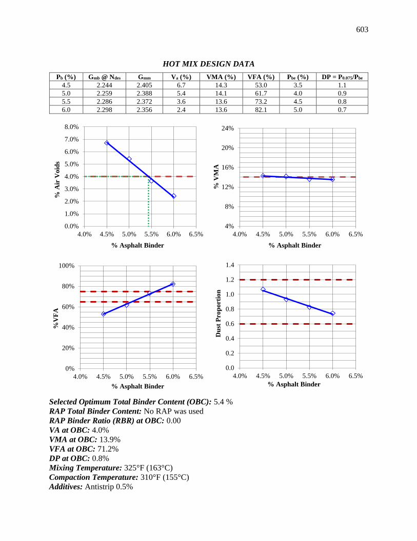
603
HOT MIX DESIGN DATA
Pb (%) Gmb @ Ndes Gmm Va (%) VMA (%) VFA (%) Pbe (%) DP = P0.075/Pbe
4.5 2.244 2.405 6.7 14.3 53.0 3.5 1.1
5.0 2.259 2.388 5.4 14.1 61.7 4.0 0.9
5.5 2.286 2.372 3.6 13.6 73.2 4.5 0.8
6.0 2.298 2.356 2.4 13.6 82.1 5.0 0.7
Selected Optimum Total Binder Content (OBC): 5.4 %
RAP Total Binder Content: No RAP was used
RAP Binder Ratio (RBR) at OBC: 0.00
VA at OBC: 4.0%
VMA at OBC: 13.9%
VFA at OBC: 71.2%
DP at OBC: 0.8%
Mixing Temperature: 325°F (163°C)
Compaction Temperature: 310°F (155°C)
Additives: Antistrip 0.5%
0.0%
1.0%
2.0%
3.0%
4.0%
5.0%
6.0%
7.0%
8.0%
4.0% 4.5% 5.0% 5.5% 6.0% 6.5%
% A
ir V
oid
s
% Asphalt Binder
4%
8%
12%
16%
20%
24%
4.0% 4.5% 5.0% 5.5% 6.0% 6.5%
% V
MA
% Asphalt Binder
0%
20%
40%
60%
80%
100%
4.0% 4.5% 5.0% 5.5% 6.0% 6.5%
%V
FA
% Asphalt Binder
0.0
0.2
0.4
0.6
0.8
1.0
1.2
1.4
4.0% 4.5% 5.0% 5.5% 6.0% 6.5%
Du
st P
rop
ort
ion
% Asphalt Binder
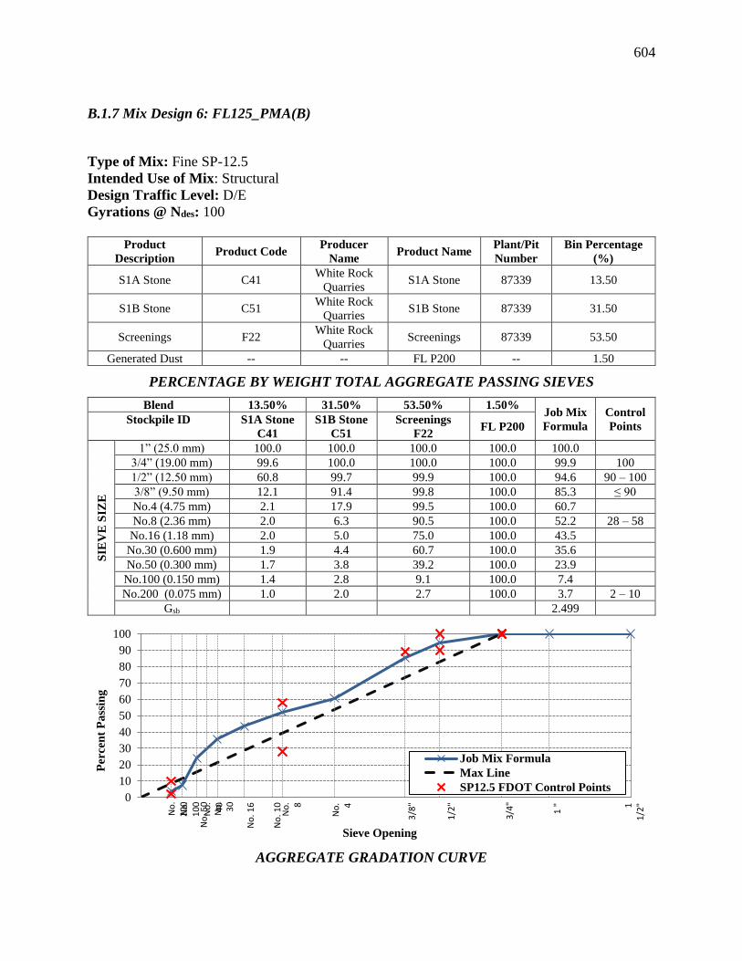
604
B.1.7 Mix Design 6: FL125_PMA(B)
Type of Mix: Fine SP-12.5
Intended Use of Mix: Structural
Design Traffic Level: D/E
Gyrations @ Ndes: 100
Product
Description Product Code
Producer
Name Product Name
Plant/Pit
Number
Bin Percentage
(%)
S1A Stone C41 White Rock
Quarries S1A Stone 87339 13.50
S1B Stone C51 White Rock
Quarries S1B Stone 87339 31.50
Screenings F22 White Rock
Quarries Screenings 87339 53.50
Generated Dust -- -- FL P200 -- 1.50
PERCENTAGE BY WEIGHT TOTAL AGGREGATE PASSING SIEVES
Blend 13.50% 31.50% 53.50% 1.50% Job Mix
Formula
Control
Points Stockpile ID S1A Stone
C41
S1B Stone
C51
Screenings
F22 FL P200
SIE
VE
SIZ
E
1” (25.0 mm) 100.0 100.0 100.0 100.0 100.0
3/4” (19.00 mm) 99.6 100.0 100.0 100.0 99.9 100
1/2” (12.50 mm) 60.8 99.7 99.9 100.0 94.6 90 – 100
3/8” (9.50 mm) 12.1 91.4 99.8 100.0 85.3 ≤ 90
No.4 (4.75 mm) 2.1 17.9 99.5 100.0 60.7
No.8 (2.36 mm) 2.0 6.3 90.5 100.0 52.2 28 – 58
No.16 (1.18 mm) 2.0 5.0 75.0 100.0 43.5
No.30 (0.600 mm) 1.9 4.4 60.7 100.0 35.6
No.50 (0.300 mm) 1.7 3.8 39.2 100.0 23.9
No.100 (0.150 mm) 1.4 2.8 9.1 100.0 7.4
No.200 (0.075 mm) 1.0 2.0 2.7 100.0 3.7 2 – 10
Gsb 2.499
AGGREGATE GRADATION CURVE
0
10
20
30
40
50
60
70
80
90
100
Per
cen
t P
ass
ing
Sieve Opening
Job Mix Formula
Max Line
SP12.5 FDOT Control Points
1 "
1/2
"
3/8
"
No
. 4
No
. 8
3/4
" 1
1/2
"
No
. 10
No
. 16
No
. 3
0
No
. 4
0
No
. 50
No
. 1
00
No
. 2
00

605
HOT MIX DESIGN DATA
Pb (%) Gmb @ Ndes Gmm Va (%) VMA (%) VFA (%) Pbe (%) DP = P0.075/Pbe
5.0 2.255 2.394 5.8 14.3 59.4 3.9 1.0
5.5 2.275 2.378 4.3 14.0 69.0 4.4 0.8
6.0 2.290 2.361 3.0 13.9 78.3 4.9 0.8
6.5 2.299 2.345 2.0 14.0 86.0 5.4 0.7
Selected Optimum Total Binder Content (OBC): 5.7 %
RAP Total Binder Content: No RAP was used
RAP Binder Ratio (RBR) at OBC: 0.00
VA at OBC: 4.0%
VMA at OBC: 13.9%
VFA at OBC: 72.2%
DP at OBC: 0.8%
Mixing Temperature: 325°F (163°C)
Compaction Temperature: 310°F (155°C)
Additives: Antistrip 0.5%
0.0%
1.0%
2.0%
3.0%
4.0%
5.0%
6.0%
7.0%
4.5% 5.0% 5.5% 6.0% 6.5% 7.0%
% A
ir V
oid
s
% Asphalt Binder
4%
8%
12%
16%
20%
24%
4.5% 5.0% 5.5% 6.0% 6.5% 7.0%
% V
MA
% Asphalt Binder
0%
20%
40%
60%
80%
100%
4.5% 5.0% 5.5% 6.0% 6.5% 7.0%
%V
FA
% Asphalt Binder
0.0
0.2
0.4
0.6
0.8
1.0
1.2
1.4
4.5% 5.5% 6.5%
Du
st P
rop
ort
ion
% Asphalt Binder
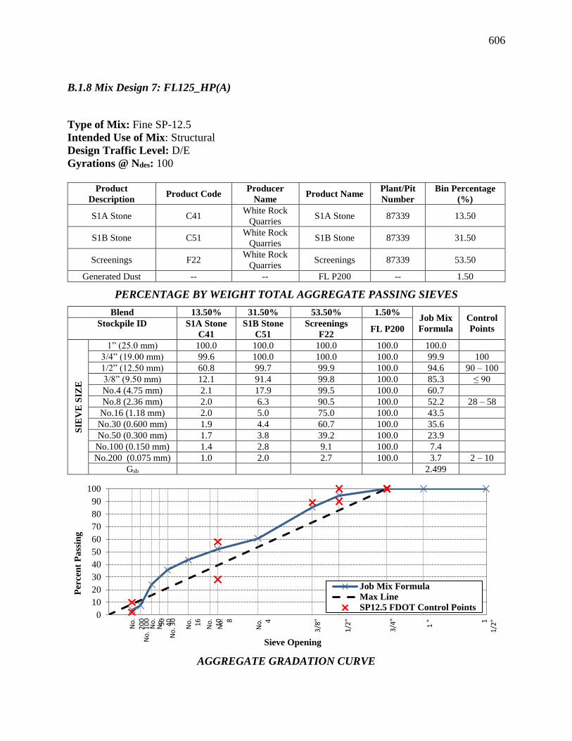
606
B.1.8 Mix Design 7: FL125_HP(A)
Type of Mix: Fine SP-12.5
Intended Use of Mix: Structural
Design Traffic Level: D/E
Gyrations @ Ndes: 100
Product
Description Product Code
Producer
Name Product Name
Plant/Pit
Number
Bin Percentage
(%)
S1A Stone C41 White Rock
Quarries S1A Stone 87339 13.50
S1B Stone C51 White Rock
Quarries S1B Stone 87339 31.50
Screenings F22 White Rock
Quarries Screenings 87339 53.50
Generated Dust -- -- FL P200 -- 1.50
PERCENTAGE BY WEIGHT TOTAL AGGREGATE PASSING SIEVES
Blend 13.50% 31.50% 53.50% 1.50% Job Mix
Formula
Control
Points Stockpile ID S1A Stone
C41
S1B Stone
C51
Screenings
F22 FL P200
SIE
VE
SIZ
E
1” (25.0 mm) 100.0 100.0 100.0 100.0 100.0
3/4” (19.00 mm) 99.6 100.0 100.0 100.0 99.9 100
1/2” (12.50 mm) 60.8 99.7 99.9 100.0 94.6 90 – 100
3/8” (9.50 mm) 12.1 91.4 99.8 100.0 85.3 ≤ 90
No.4 (4.75 mm) 2.1 17.9 99.5 100.0 60.7
No.8 (2.36 mm) 2.0 6.3 90.5 100.0 52.2 28 – 58
No.16 (1.18 mm) 2.0 5.0 75.0 100.0 43.5
No.30 (0.600 mm) 1.9 4.4 60.7 100.0 35.6
No.50 (0.300 mm) 1.7 3.8 39.2 100.0 23.9
No.100 (0.150 mm) 1.4 2.8 9.1 100.0 7.4
No.200 (0.075 mm) 1.0 2.0 2.7 100.0 3.7 2 – 10
Gsb 2.499
AGGREGATE GRADATION CURVE
0
10
20
30
40
50
60
70
80
90
100
Per
cen
t P
ass
ing
Sieve Opening
Job Mix Formula
Max Line
SP12.5 FDOT Control Points
1 "
1/2
"
3/8
"
No
. 4
No
. 8
3/4
" 1
1/2
"
No
. 1
0
No
. 1
6
No
. 30
No
. 4
0
No
. 5
0
No
. 10
0
No
. 2
00
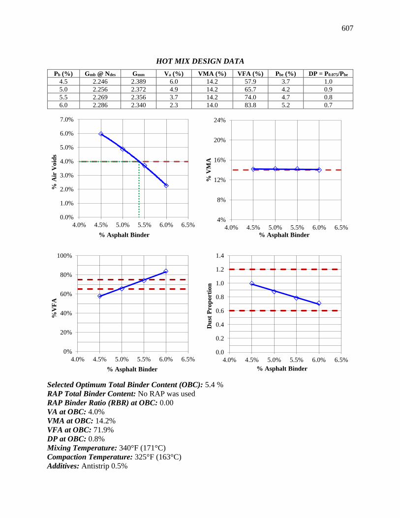
607
HOT MIX DESIGN DATA
Pb (%) Gmb @ Ndes Gmm Va (%) VMA (%) VFA (%) Pbe (%) DP = P0.075/Pbe
4.5 2.246 2.389 6.0 14.2 57.9 3.7 1.0
5.0 2.256 2.372 4.9 14.2 65.7 4.2 0.9
5.5 2.269 2.356 3.7 14.2 74.0 4.7 0.8
6.0 2.286 2.340 2.3 14.0 83.8 5.2 0.7
Selected Optimum Total Binder Content (OBC): 5.4 %
RAP Total Binder Content: No RAP was used
RAP Binder Ratio (RBR) at OBC: 0.00
VA at OBC: 4.0%
VMA at OBC: 14.2%
VFA at OBC: 71.9%
DP at OBC: 0.8%
Mixing Temperature: 340°F (171°C)
Compaction Temperature: 325°F (163°C)
Additives: Antistrip 0.5%
0.0%
1.0%
2.0%
3.0%
4.0%
5.0%
6.0%
7.0%
4.0% 4.5% 5.0% 5.5% 6.0% 6.5%
% A
ir V
oid
s
% Asphalt Binder
4%
8%
12%
16%
20%
24%
4.0% 4.5% 5.0% 5.5% 6.0% 6.5%
% V
MA
% Asphalt Binder
0%
20%
40%
60%
80%
100%
4.0% 4.5% 5.0% 5.5% 6.0% 6.5%
%V
FA
% Asphalt Binder
0.0
0.2
0.4
0.6
0.8
1.0
1.2
1.4
4.0% 4.5% 5.0% 5.5% 6.0% 6.5%
Du
st P
rop
ort
ion
% Asphalt Binder

608
B.1.9 Mix Design 8: FL125_PMA(B)
Type of Mix: Fine SP-12.5
Intended Use of Mix: Structural
Design Traffic Level: D/E
Gyrations @ Ndes: 100
Product
Description Product Code
Producer
Name Product Name
Plant/Pit
Number
Bin Percentage
(%)
S1A Stone C41 White Rock
Quarries S1A Stone 87339 13.50
S1B Stone C51 White Rock
Quarries S1B Stone 87339 31.50
Screenings F22 White Rock
Quarries Screenings 87339 53.50
Generated Dust -- -- FL P200 -- 1.50
PERCENTAGE BY WEIGHT TOTAL AGGREGATE PASSING SIEVES
Blend 13.50% 31.50% 53.50% 1.50% Job Mix
Formula
Control
Points Stockpile ID S1A Stone
C41
S1B Stone
C51
Screenings
F22 FL P200
SIE
VE
SIZ
E
1” (25.0 mm) 100.0 100.0 100.0 100.0 100.0
3/4” (19.00 mm) 99.6 100.0 100.0 100.0 99.9 100
1/2” (12.50 mm) 60.8 99.7 99.9 100.0 94.6 90 – 100
3/8” (9.50 mm) 12.1 91.4 99.8 100.0 85.3 ≤ 90
No.4 (4.75 mm) 2.1 17.9 99.5 100.0 60.7
No.8 (2.36 mm) 2.0 6.3 90.5 100.0 52.2 28 – 58
No.16 (1.18 mm) 2.0 5.0 75.0 100.0 43.5
No.30 (0.600 mm) 1.9 4.4 60.7 100.0 35.6
No.50 (0.300 mm) 1.7 3.8 39.2 100.0 23.9
No.100 (0.150 mm) 1.4 2.8 9.1 100.0 7.4
No.200 (0.075 mm) 1.0 2.0 2.7 100.0 3.7 2 – 10
Gsb 2.499
AGGREGATE GRADATION CURVE
0
10
20
30
40
50
60
70
80
90
100
Per
cen
t P
ass
ing
Sieve Opening
Job Mix FormulaMax LineSP12.5 FDOT Control Points
1 "
1/2
"
3/8
"
No
. 4
No
. 8
3/4
" 1
1/2
"
No
. 1
0
No
. 1
6
No
. 3
0
No
. 4
0
No
. 5
0
No
. 1
00
No
. 2
00

609
HOT MIX DESIGN DATA
Pb (%) Gmb @ Ndes Gmm Va (%) VMA (%) VFA (%) Pbe (%) DP = P0.075/Pbe
4.5 2.254 2.400 6.1 13.9 56.2 3.5 1.1
5.0 2.266 2.383 4.9 13.9 64.8 4.0 0.9
5.5 2.275 2.366 3.8 14.0 72.6 4.5 0.8
6.0 2.296 2.349 2.3 13.6 83.3 5.0 0.7
Selected Optimum Total Binder Content (OBC): 5.4 %
RAP Total Binder Content: No RAP was used
RAP Binder Ratio (RBR) at OBC: 0.00
VA at OBC: 4.0%
VMA at OBC: 13.9%
VFA at OBC: 71.2%
DP at OBC: 0.8%
Mixing Temperature: 340°F (171°C)
Compaction Temperature: 325°F (163°C)
Additives: Antistrip 0.5%
0.0%
1.0%
2.0%
3.0%
4.0%
5.0%
6.0%
7.0%
4.0% 4.5% 5.0% 5.5% 6.0% 6.5%
% A
ir V
oid
s
% Asphalt Binder
4%
8%
12%
16%
20%
24%
4.0% 4.5% 5.0% 5.5% 6.0% 6.5%
% V
MA
% Asphalt Binder
0%
20%
40%
60%
80%
100%
4.0% 4.5% 5.0% 5.5% 6.0% 6.5%
%V
FA
% Asphalt Binder
0.0
0.2
0.4
0.6
0.8
1.0
1.2
1.4
4.0% 4.5% 5.0% 5.5% 6.0% 6.5%
Du
st P
rop
ort
ion
% Asphalt Binder
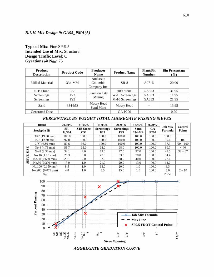
610
B.1.10 Mix Design 9: GA95_PMA(A)
Type of Mix: Fine SP-9.5
Intended Use of Mix: Structural
Design Traffic Level: C
Gyrations @ Ndes: 75
Product
Description Product Code
Producer
Name Product Name
Plant/Pit
Number
Bin Percentage
(%)
Milled Material 334-MM
Anderson
Columbia
Company Inc.
SR-8 A0716 20.00
S1B Stone C53 Junction City
Mining
#89 Stone GA553 31.95
Screenings F22 W-10 Screenings GA553 11.95
Screenings F23 M-10 Screenings GA553 21.95
Sand 334-MS Mossy Head
Sand Mine Mossy Head -- 13.95
Generated Dust -- -- GA P200 -- 0.20
PERCENTAGE BY WEIGHT TOTAL AGGREGATE PASSING SIEVES
Blend 20.00% 31.95% 11.95% 21.95% 13.95% 0.20% Job Mix
Formula
Control
Points Stockpile ID SR-
8_334
S1B Stone
C53
Screenings
F22
Screenings
F23
Sand
334-MS
GA
P200
SIE
VE
SIZ
E
3/4” (19.00 mm) 100.0 100.0 100.0 100.0 100.0 100.0 100.0
1/2” (12.50 mm) 97.8 100.0 100.0 100.0 100.0 100.0 99.6 100
3/8” (9.50 mm) 89.6 98.0 100.0 100.0 100.0 100.0 97.3 90 – 100
No.4 (4.75 mm) 55.7 35.0 98.0 98.0 100.0 100.0 69.7 ≤ 90
No.8 (2.36 mm) 34.1 4.0 73.0 77.0 97.0 100.0 47.5 32 – 67
No.16 (1.18 mm) 25.3 3.0 47.0 53.0 78.0 100.0 34.4
No.30 (0.600 mm) 20.1 2.0 32.0 38.0 40.0 100.0 22.6
No.50 (0.300 mm) 13.9 1.0 21.0 29.0 13.0 100.0 14.0
No.100 (0.150 mm) 8.5 1.0 13.0 20.0 1.0 100.0 8.3
No.200 (0.075 mm) 4.8 1.0 5.5 15.0 1.0 100.0 5.6 2 – 10
Gsb 2.759
AGGREGATE GRADATION CURVE
0
10
20
30
40
50
60
70
80
90
100
Per
cen
t P
ass
ing
Sieve Opening
Job Mix Formula
Max Line
SP9.5 FDOT Control Points
1 "
1/2
"
3/8
"
No
. 4
No
. 8
3/4
"
1 1
/2"
No
. 10
No
. 16
No
. 30
No
. 40
No
. 5
0
No
. 1
00
No
. 2
00
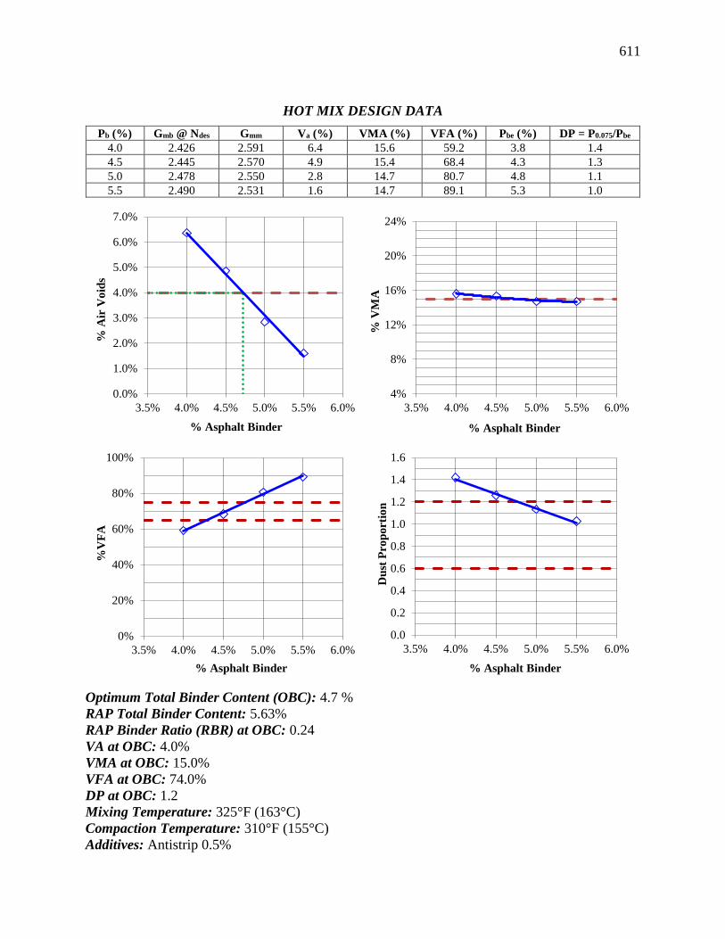
611
HOT MIX DESIGN DATA
Pb (%) Gmb @ Ndes Gmm Va (%) VMA (%) VFA (%) Pbe (%) DP = P0.075/Pbe
4.0 2.426 2.591 6.4 15.6 59.2 3.8 1.4
4.5 2.445 2.570 4.9 15.4 68.4 4.3 1.3
5.0 2.478 2.550 2.8 14.7 80.7 4.8 1.1
5.5 2.490 2.531 1.6 14.7 89.1 5.3 1.0
Optimum Total Binder Content (OBC): 4.7 %
RAP Total Binder Content: 5.63%
RAP Binder Ratio (RBR) at OBC: 0.24
VA at OBC: 4.0%
VMA at OBC: 15.0%
VFA at OBC: 74.0%
DP at OBC: 1.2
Mixing Temperature: 325°F (163°C)
Compaction Temperature: 310°F (155°C)
Additives: Antistrip 0.5%
0.0%
1.0%
2.0%
3.0%
4.0%
5.0%
6.0%
7.0%
3.5% 4.0% 4.5% 5.0% 5.5% 6.0%
% A
ir V
oid
s
% Asphalt Binder
4%
8%
12%
16%
20%
24%
3.5% 4.0% 4.5% 5.0% 5.5% 6.0%
% V
MA
% Asphalt Binder
0%
20%
40%
60%
80%
100%
3.5% 4.0% 4.5% 5.0% 5.5% 6.0%
%V
FA
% Asphalt Binder
0.0
0.2
0.4
0.6
0.8
1.0
1.2
1.4
1.6
3.5% 4.0% 4.5% 5.0% 5.5% 6.0%
Du
st P
rop
ort
ion
% Asphalt Binder

612
B.1.11 Mix Design 10: GA95_PMA(B)
Type of Mix: Fine SP-9.5
Intended Use of Mix: Structural
Design Traffic Level: C
Gyrations @ Ndes: 75
Product
Description Product Code
Producer
Name Product Name
Plant/Pit
Number
Bin Percentage
(%)
Milled Material 334-MM
Anderson
Columbia
Company Inc.
SR-8 A0716 20.00
S1B Stone C53 Junction City
Mining
#89 Stone GA553 31.95
Screenings F22 W-10 Screenings GA553 11.95
Screenings F23 M-10 Screenings GA553 21.95
Sand 334-MS Mossy Head
Sand Mine Mossy Head -- 13.95
Generated Dust -- -- GA P200 -- 0.20
PERCENTAGE BY WEIGHT TOTAL AGGREGATE PASSING SIEVES
Blend 20.00% 31.95% 11.95% 21.95% 13.95% 0.20% Job Mix
Formula
Control
Points Stockpile ID SR-
8_334
S1B Stone
C53
Screenings
F22
Screenings
F23
Sand
334-MS
GA
P200
SIE
VE
SIZ
E
3/4” (19.00 mm) 100.0 100.0 100.0 100.0 100.0 100.0 100.0
1/2” (12.50 mm) 97.8 100.0 100.0 100.0 100.0 100.0 99.6 100
3/8” (9.50 mm) 89.6 98.0 100.0 100.0 100.0 100.0 97.3 90 – 100
No.4 (4.75 mm) 55.7 35.0 98.0 98.0 100.0 100.0 69.7 ≤ 90
No.8 (2.36 mm) 34.1 4.0 73.0 77.0 97.0 100.0 47.5 32 – 67
No.16 (1.18 mm) 25.3 3.0 47.0 53.0 78.0 100.0 34.4
No.30 (0.600 mm) 20.1 2.0 32.0 38.0 40.0 100.0 22.6
No.50 (0.300 mm) 13.9 1.0 21.0 29.0 13.0 100.0 14.0
No.100 (0.150 mm) 8.5 1.0 13.0 20.0 1.0 100.0 8.3
No.200 (0.075 mm) 4.8 1.0 5.5 15.0 1.0 100.0 5.6 2 – 10
Gsb 2.759
AGGREGATE GRADATION CURVE
0
10
20
30
40
50
60
70
80
90
100
Per
cen
t P
ass
ing
Sieve Opening
Job Mix Formula
Max Line
SP9.5 FDOT Control Points
1 "
1/2
"
3/8
"
No
. 4
No
. 8
3/4
"
1 1
/2"
No
. 10
No
. 16
No
. 30
No
. 40
No
. 5
0
No
. 10
0N
o. 2
00
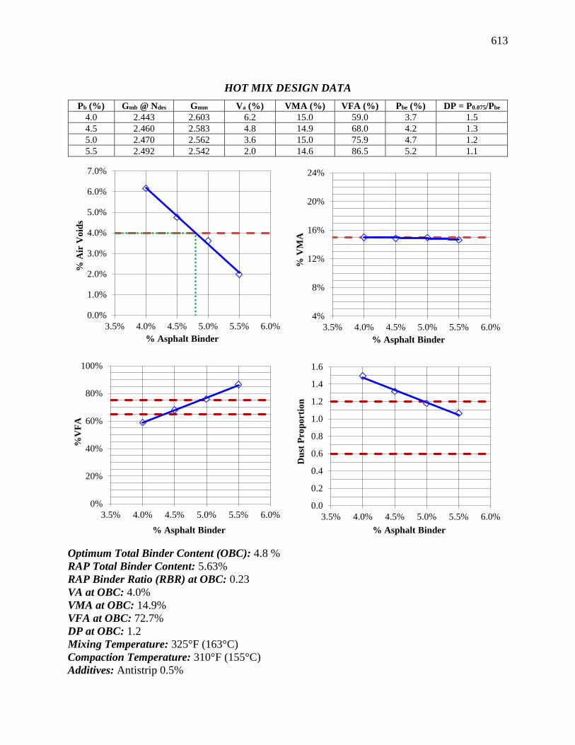
613
HOT MIX DESIGN DATA
Pb (%) Gmb @ Ndes Gmm Va (%) VMA (%) VFA (%) Pbe (%) DP = P0.075/Pbe
4.0 2.443 2.603 6.2 15.0 59.0 3.7 1.5
4.5 2.460 2.583 4.8 14.9 68.0 4.2 1.3
5.0 2.470 2.562 3.6 15.0 75.9 4.7 1.2
5.5 2.492 2.542 2.0 14.6 86.5 5.2 1.1
Optimum Total Binder Content (OBC): 4.8 %
RAP Total Binder Content: 5.63%
RAP Binder Ratio (RBR) at OBC: 0.23
VA at OBC: 4.0%
VMA at OBC: 14.9%
VFA at OBC: 72.7%
DP at OBC: 1.2
Mixing Temperature: 325°F (163°C)
Compaction Temperature: 310°F (155°C)
Additives: Antistrip 0.5%
0.0%
1.0%
2.0%
3.0%
4.0%
5.0%
6.0%
7.0%
3.5% 4.0% 4.5% 5.0% 5.5% 6.0%
% A
ir V
oid
s
% Asphalt Binder
4%
8%
12%
16%
20%
24%
3.5% 4.0% 4.5% 5.0% 5.5% 6.0%
% V
MA
% Asphalt Binder
0%
20%
40%
60%
80%
100%
3.5% 4.0% 4.5% 5.0% 5.5% 6.0%
%V
FA
% Asphalt Binder
0.0
0.2
0.4
0.6
0.8
1.0
1.2
1.4
1.6
3.5% 4.0% 4.5% 5.0% 5.5% 6.0%
Du
st P
rop
ort
ion
% Asphalt Binder
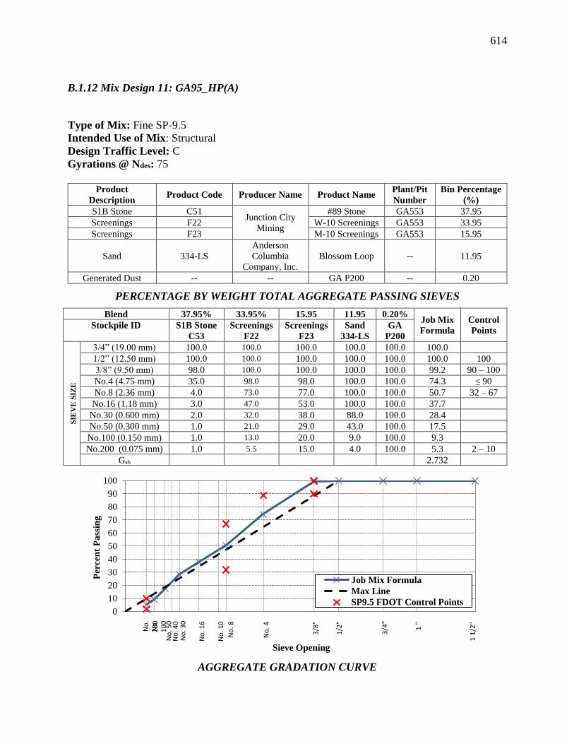
614
B.1.12 Mix Design 11: GA95_HP(A)
Type of Mix: Fine SP-9.5
Intended Use of Mix: Structural
Design Traffic Level: C
Gyrations @ Ndes: 75
Product
Description Product Code Producer Name Product Name
Plant/Pit
Number
Bin Percentage
(%)
S1B Stone C51 Junction City
Mining
#89 Stone GA553 37.95
Screenings F22 W-10 Screenings GA553 33.95
Screenings F23 M-10 Screenings GA553 15.95
Sand 334-LS
Anderson
Columbia
Company, Inc.
Blossom Loop -- 11.95
Generated Dust -- -- GA P200 -- 0.20
PERCENTAGE BY WEIGHT TOTAL AGGREGATE PASSING SIEVES
Blend 37.95% 33.95% 15.95 11.95 0.20% Job Mix
Formula
Control
Points Stockpile ID S1B Stone
C53
Screenings
F22
Screenings
F23
Sand
334-LS
GA
P200
SIE
VE
SIZ
E
3/4” (19.00 mm) 100.0 100.0 100.0 100.0 100.0 100.0
1/2” (12.50 mm) 100.0 100.0 100.0 100.0 100.0 100.0 100
3/8” (9.50 mm) 98.0 100.0 100.0 100.0 100.0 99.2 90 – 100
No.4 (4.75 mm) 35.0 98.0 98.0 100.0 100.0 74.3 ≤ 90
No.8 (2.36 mm) 4.0 73.0 77.0 100.0 100.0 50.7 32 – 67
No.16 (1.18 mm) 3.0 47.0 53.0 100.0 100.0 37.7
No.30 (0.600 mm) 2.0 32.0 38.0 88.0 100.0 28.4
No.50 (0.300 mm) 1.0 21.0 29.0 43.0 100.0 17.5
No.100 (0.150 mm) 1.0 13.0 20.0 9.0 100.0 9.3
No.200 (0.075 mm) 1.0 5.5 15.0 4.0 100.0 5.3 2 – 10
Gsb 2.732
AGGREGATE GRADATION CURVE
0
10
20
30
40
50
60
70
80
90
100
Per
cen
t P
ass
ing
Sieve Opening
Job Mix Formula
Max Line
SP9.5 FDOT Control Points
1 "
1/2
"
3/8
"
No
. 4
No
. 8
3/4
"
1 1
/2"
No
. 10
No
. 16
No
. 30
No
. 40
No
. 50
No
. 1
00
No
. 2
00
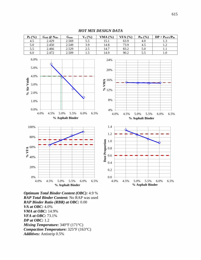
615
HOT MIX DESIGN DATA
Pb (%) Gmb @ Ndes Gmm Va (%) VMA (%) VFA (%) Pbe (%) DP = P0.075/Pbe
4.5 2.429 2.569 5.5 15.1 63.9 4.0 1.3
5.0 2.450 2.549 3.9 14.8 73.9 4.5 1.2
5.5 2.466 2.529 2.5 14.7 83.2 5.0 1.1
6.0 2.472 2.509 1.5 14.9 90.2 5.5 1.0
Optimum Total Binder Content (OBC): 4.9 %
RAP Total Binder Content: No RAP was used
RAP Binder Ratio (RBR) at OBC: 0.00
VA at OBC: 4.0%
VMA at OBC: 14.9%
VFA at OBC: 73.1%
DP at OBC: 1.2
Mixing Temperature: 340°F (171°C)
Compaction Temperature: 325°F (163°C)
Additives: Antistrip 0.5%
0.0%
1.0%
2.0%
3.0%
4.0%
5.0%
6.0%
4.0% 4.5% 5.0% 5.5% 6.0% 6.5%
% A
ir V
oid
s
% Asphalt Binder
4%
8%
12%
16%
20%
24%
4.0% 4.5% 5.0% 5.5% 6.0% 6.5%
% V
MA
% Asphalt Binder
0%
20%
40%
60%
80%
100%
4.0% 4.5% 5.0% 5.5% 6.0% 6.5%
% V
FA
% Asphalt Binder
0.0
0.2
0.4
0.6
0.8
1.0
1.2
1.4
4.0% 4.5% 5.0% 5.5% 6.0% 6.5%
Du
st P
rop
ort
ion
% Asphalt Binder

616
B.1.13 Mix Design 12: GA95_HP(B)
Type of Mix: Fine SP-9.5
Intended Use of Mix: Structural
Design Traffic Level: C
Gyrations @ Ndes: 75
Product
Description Product Code Producer Name Product Name
Plant/Pit
Number
Bin Percentage
(%)
S1B Stone C51 Junction City
Mining
#89 Stone GA553 37.95
Screenings F22 W-10 Screenings GA553 33.95
Screenings F23 M-10 Screenings GA553 15.95
Sand 334-LS
Anderson
Columbia
Company, Inc.
Blossom Loop -- 11.95
Generated Dust -- -- GA P200 -- 0.20
PERCENTAGE BY WEIGHT TOTAL AGGREGATE PASSING SIEVES
Blend 37.95% 33.95% 15.95 11.95 0.20% Job Mix
Formula
Control
Points Stockpile ID S1B Stone
C53
Screenings
F22
Screenings
F23
Sand
334-LS
GA
P200
SIE
VE
SIZ
E
3/4” (19.00 mm) 100.0 100.0 100.0 100.0 100.0 100.0
1/2” (12.50 mm) 100.0 100.0 100.0 100.0 100.0 100.0 100
3/8” (9.50 mm) 98.0 100.0 100.0 100.0 100.0 99.2 90 – 100
No.4 (4.75 mm) 35.0 98.0 98.0 100.0 100.0 74.3 ≤ 90
No.8 (2.36 mm) 4.0 73.0 77.0 100.0 100.0 50.7 32 – 67
No.16 (1.18 mm) 3.0 47.0 53.0 100.0 100.0 37.7
No.30 (0.600 mm) 2.0 32.0 38.0 88.0 100.0 28.4
No.50 (0.300 mm) 1.0 21.0 29.0 43.0 100.0 17.5
No.100 (0.150 mm) 1.0 13.0 20.0 9.0 100.0 9.3
No.200 (0.075 mm) 1.0 5.5 15.0 4.0 100.0 5.3 2 – 10
Gsb 2.732
AGGREGATE GRADATION CURVE
0
10
20
30
40
50
60
70
80
90
100
Per
cen
t P
ass
ing
Sieve Opening
Job Mix FormulaMax LineSP9.5 FDOT Control Points
1 "
1/2
"
3/8
"
No
. 4
No
. 8
3/4
"
1 1
/2"
No
. 10
No
. 16
No
. 30
No
. 40
No
. 50
No
. 1
00
No
. 2
00
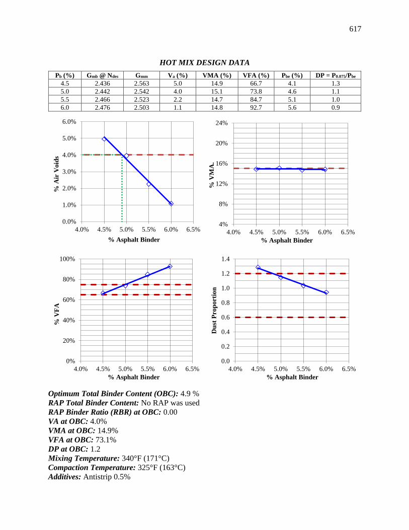
617
HOT MIX DESIGN DATA
Pb (%) Gmb @ Ndes Gmm Va (%) VMA (%) VFA (%) Pbe (%) DP = P0.075/Pbe
4.5 2.436 2.563 5.0 14.9 66.7 4.1 1.3
5.0 2.442 2.542 4.0 15.1 73.8 4.6 1.1
5.5 2.466 2.523 2.2 14.7 84.7 5.1 1.0
6.0 2.476 2.503 1.1 14.8 92.7 5.6 0.9
Optimum Total Binder Content (OBC): 4.9 %
RAP Total Binder Content: No RAP was used
RAP Binder Ratio (RBR) at OBC: 0.00
VA at OBC: 4.0%
VMA at OBC: 14.9%
VFA at OBC: 73.1%
DP at OBC: 1.2
Mixing Temperature: 340°F (171°C)
Compaction Temperature: 325°F (163°C)
Additives: Antistrip 0.5%
0.0%
1.0%
2.0%
3.0%
4.0%
5.0%
6.0%
4.0% 4.5% 5.0% 5.5% 6.0% 6.5%
% A
ir V
oid
s
% Asphalt Binder
4%
8%
12%
16%
20%
24%
4.0% 4.5% 5.0% 5.5% 6.0% 6.5%
% V
MA
.
% Asphalt Binder
0%
20%
40%
60%
80%
100%
4.0% 4.5% 5.0% 5.5% 6.0% 6.5%
% V
FA
% Asphalt Binder
0.0
0.2
0.4
0.6
0.8
1.0
1.2
1.4
4.0% 4.5% 5.0% 5.5% 6.0% 6.5%
Du
st P
rop
ort
ion
% Asphalt Binder
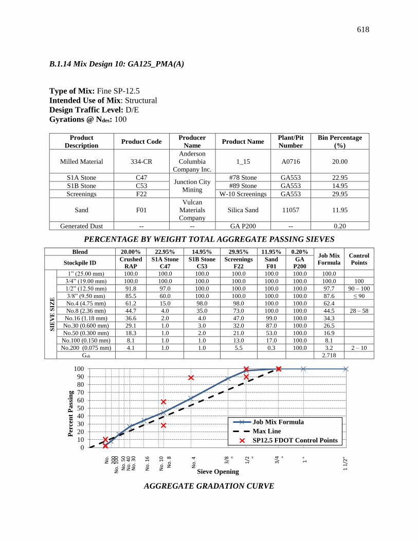
618
B.1.14 Mix Design 10: GA125_PMA(A)
Type of Mix: Fine SP-12.5
Intended Use of Mix: Structural
Design Traffic Level: D/E
Gyrations @ Ndes: 100
Product
Description Product Code
Producer
Name Product Name
Plant/Pit
Number
Bin Percentage
(%)
Milled Material 334-CR
Anderson
Columbia
Company Inc.
1_15 A0716 20.00
S1A Stone C47 Junction City
Mining
#78 Stone GA553 22.95
S1B Stone C53 #89 Stone GA553 14.95
Screenings F22 W-10 Screenings GA553 29.95
Sand F01
Vulcan
Materials
Company
Silica Sand 11057 11.95
Generated Dust -- -- GA P200 -- 0.20
PERCENTAGE BY WEIGHT TOTAL AGGREGATE PASSING SIEVES
Blend 20.00% 22.95% 14.95% 29.95% 11.95% 0.20% Job Mix
Formula
Control
Points Stockpile ID Crushed
RAP
S1A Stone
C47
S1B Stone
C53
Screenings
F22
Sand
F01
GA
P200
SIE
VE
SIZ
E
1” (25.00 mm) 100.0 100.0 100.0 100.0 100.0 100.0 100.0
3/4” (19.00 mm) 100.0 100.0 100.0 100.0 100.0 100.0 100.0 100
1/2” (12.50 mm) 91.8 97.0 100.0 100.0 100.0 100.0 97.7 90 – 100
3/8” (9.50 mm) 85.5 60.0 100.0 100.0 100.0 100.0 87.6 ≤ 90
No.4 (4.75 mm) 61.2 15.0 98.0 98.0 100.0 100.0 62.4
No.8 (2.36 mm) 44.7 4.0 35.0 73.0 100.0 100.0 44.5 28 – 58
No.16 (1.18 mm) 36.6 2.0 4.0 47.0 99.0 100.0 34.3
No.30 (0.600 mm) 29.1 1.0 3.0 32.0 87.0 100.0 26.5
No.50 (0.300 mm) 18.3 1.0 2.0 21.0 53.0 100.0 16.9
No.100 (0.150 mm) 8.1 1.0 1.0 13.0 17.0 100.0 8.1
No.200 (0.075 mm) 4.1 1.0 1.0 5.5 0.3 100.0 3.2 2 – 10
Gsb 2.718
AGGREGATE GRADATION CURVE
0
10
20
30
40
50
60
70
80
90
100
Per
cen
t P
ass
ing
Sieve Opening
Job Mix Formula
Max Line
SP12.5 FDOT Control Points
1 "
1/2 "
3/8 "
No
. 4
No
. 8 3/4 "
1 1
/2"
No
. 10
No
. 16
No
. 30
No
. 40
No
. 50
No
. 10
0
No
. 2
00

619
HOT MIX DESIGN DATA
Pb (%) Gmb @ Ndes Gmm Va (%) VMA (%) VFA (%) Pbe (%) DP = P0.075/Pbe
4.0 2.425 2.563 5.4 14.4 62.5 3.8 0.9
4.5 2.463 2.543 3.1 13.5 76.8 4.3 0.8
5.0 2.475 2.523 1.9 13.5 86.0 4.8 0.7
5.5 2.485 2.503 0.7 13.6 94.5 5.3 0.6
Optimum Total Binder Content (OBC): 4.3 %
RAP Total Binder Content: 6.68%
RAP Binder Ratio (RBR) at OBC: 0.31
VA at OBC: 4.0%
VMA at OBC: 13.9%
VFA at OBC: 71.3%
DP at OBC: 0.8
Mixing Temperature: 325°F (163°C)
Compaction Temperature: 310°F (155°C)
Additives: Antistrip 0.5%
0.0%
1.0%
2.0%
3.0%
4.0%
5.0%
6.0%
3.5% 4.0% 4.5% 5.0% 5.5% 6.0%
% A
ir V
oid
s
% Asphalt Binder
4%
8%
12%
16%
20%
24%
3.5% 4.0% 4.5% 5.0% 5.5% 6.0%
% V
MA
% Asphalt Binder
0%
20%
40%
60%
80%
100%
3.5% 4.0% 4.5% 5.0% 5.5% 6.0%
% V
FA
% Asphalt Binder
0.0
0.2
0.4
0.6
0.8
1.0
1.2
1.4
3.5% 4.0% 4.5% 5.0% 5.5% 6.0%
Du
st P
rop
ort
ion
% Asphalt Binder

620
B.1.15 Mix Design 14: GA125_PMA(B)
Type of Mix: Fine SP-12.5
Intended Use of Mix: Structural
Design Traffic Level: D/E
Gyrations @ Ndes: 100
Product
Description Product Code
Producer
Name Product Name
Plant/Pit
Number
Bin Percentage
(%)
Milled Material 334-CR
Anderson
Columbia
Company Inc.
1_15 A0716 20.00
S1A Stone C47 Junction City
Mining
#78 Stone GA553 22.95
S1B Stone C53 #89 Stone GA553 14.95
Screenings F22 W-10 Screenings GA553 29.95
Sand F01
Vulcan
Materials
Company
Silica Sand 11057 11.95
Generated Dust -- -- GA P200 -- 0.20
PERCENTAGE BY WEIGHT TOTAL AGGREGATE PASSING SIEVES
Blend 20.00% 22.95% 14.95% 29.95% 11.95% 0.20% Job Mix
Formula
Control
Points Stockpile ID Crushed
RAP
S1A Stone
C47
S1B Stone
C53
Screenings
F22
Sand
F01
GA
P200
SIE
VE
SIZ
E
1” (25.00 mm) 100.0 100.0 100.0 100.0 100.0 100.0 100.0
3/4” (19.00 mm) 100.0 100.0 100.0 100.0 100.0 100.0 100.0 100
1/2” (12.50 mm) 91.8 97.0 100.0 100.0 100.0 100.0 97.7 90 – 100
3/8” (9.50 mm) 85.5 60.0 100.0 100.0 100.0 100.0 87.6 ≤ 90
No.4 (4.75 mm) 61.2 15.0 98.0 98.0 100.0 100.0 62.4
No.8 (2.36 mm) 44.7 4.0 35.0 73.0 100.0 100.0 44.5 28 – 58
No.16 (1.18 mm) 36.6 2.0 4.0 47.0 99.0 100.0 34.3
No.30 (0.600 mm) 29.1 1.0 3.0 32.0 87.0 100.0 26.5
No.50 (0.300 mm) 18.3 1.0 2.0 21.0 53.0 100.0 16.9
No.100 (0.150 mm) 8.1 1.0 1.0 13.0 17.0 100.0 8.1
No.200 (0.075 mm) 4.1 1.0 1.0 5.5 0.3 100.0 3.2 2 – 10
Gsb 2.718
AGGREGATE GRADATION CURVE
0
10
20
30
40
50
60
70
80
90
100
Per
cen
t P
ass
ing
Sieve Opening
Job Mix Formula
Max Line
SP12.5 FDOT Control Points
1 "
1/2 "
3/8 "
No
. 4
No
. 8 3/4 "
1 1
/2"
No
. 10
No
. 16
No
. 30
No
. 40
No
. 50
No
. 10
0
No
. 2
00
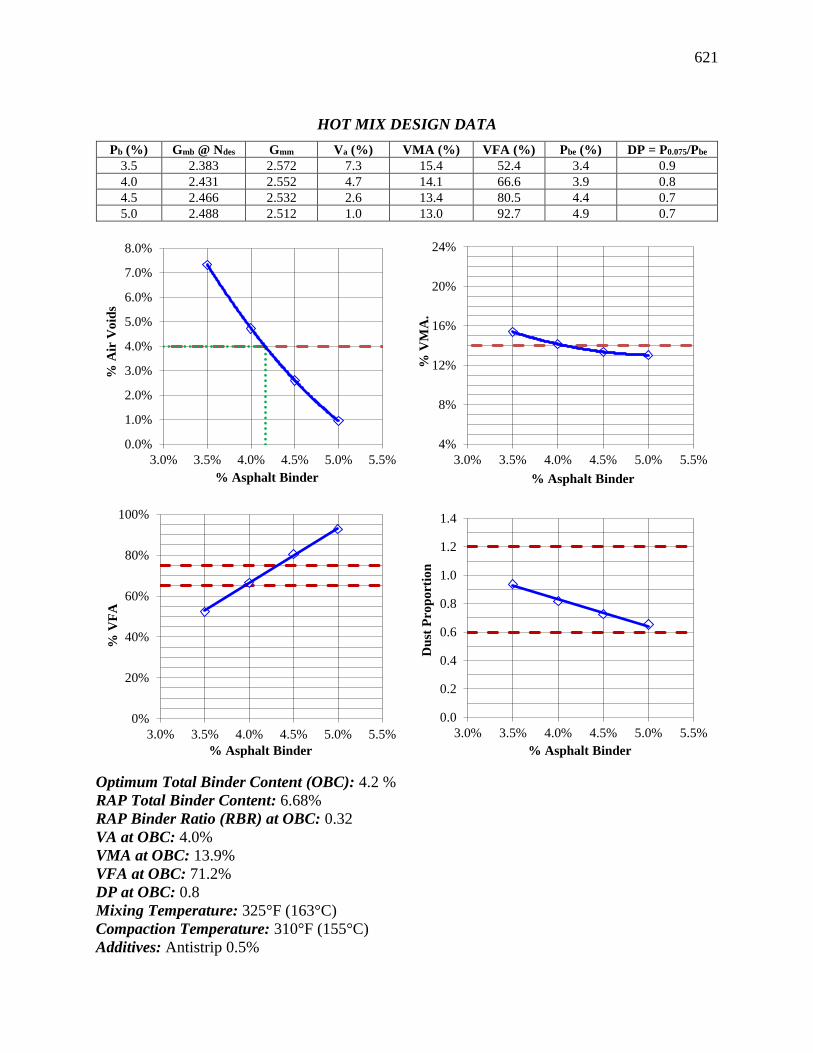
621
HOT MIX DESIGN DATA
Pb (%) Gmb @ Ndes Gmm Va (%) VMA (%) VFA (%) Pbe (%) DP = P0.075/Pbe
3.5 2.383 2.572 7.3 15.4 52.4 3.4 0.9
4.0 2.431 2.552 4.7 14.1 66.6 3.9 0.8
4.5 2.466 2.532 2.6 13.4 80.5 4.4 0.7
5.0 2.488 2.512 1.0 13.0 92.7 4.9 0.7
Optimum Total Binder Content (OBC): 4.2 %
RAP Total Binder Content: 6.68%
RAP Binder Ratio (RBR) at OBC: 0.32
VA at OBC: 4.0%
VMA at OBC: 13.9%
VFA at OBC: 71.2%
DP at OBC: 0.8
Mixing Temperature: 325°F (163°C)
Compaction Temperature: 310°F (155°C)
Additives: Antistrip 0.5%
0.0%
1.0%
2.0%
3.0%
4.0%
5.0%
6.0%
7.0%
8.0%
3.0% 3.5% 4.0% 4.5% 5.0% 5.5%
% A
ir V
oid
s
% Asphalt Binder
4%
8%
12%
16%
20%
24%
3.0% 3.5% 4.0% 4.5% 5.0% 5.5%
% V
MA
.
% Asphalt Binder
0%
20%
40%
60%
80%
100%
3.0% 3.5% 4.0% 4.5% 5.0% 5.5%
% V
FA
% Asphalt Binder
0.0
0.2
0.4
0.6
0.8
1.0
1.2
1.4
3.0% 3.5% 4.0% 4.5% 5.0% 5.5%
Du
st P
rop
ort
ion
% Asphalt Binder

622
B.1.16 Mix Design 15: GA125_HP (A)
Type of Mix: Fine SP-12.5
Intended Use of Mix: Structural
Design Traffic Level: D/E
Gyrations @ Ndes: 100
Product
Description Product Code Producer Name Product Name
Plant/Pit
Number
Bin Percentage
(%)
S1A Stone C47
Junction City
Mining
#78 Stone GA553 27.96
S1B Stone C51 #89 Stone GA553 12.96
Screenings F22 W-10 Screenings GA553 35.96
Screenings F23 M-10 Screenings GA553 11.96
Sand 334-LS
Anderson
Columbia
Company, Inc.
Blossom Loop -- 10.96
Generated Dust -- -- GA P200 -- 0.20
PERCENTAGE BY WEIGHT TOTAL AGGREGATE PASSING SIEVES
Blend 27.96% 12.96% 35.96% 11.96% 10.96% 0.20% Job Mix
Formula
Control
Points Stockpile ID S1A Stone
C47
S1B Stone
C53
Screenings
F22
Screenings
F23
Sand
334-LS
GA
P200
1” (25.00 mm) 100.0 100.0 100.0 100.0 100.0 100.0 100.0
SIE
VE
SIZ
E
3/4” (19.00 mm) 100.0 100.0 100.0 100.0 100.0 100.0 100.0 100
1/2” (12.50 mm) 97.0 100.0 100.0 100.0 100.0 100.0 99.2 90 – 100
3/8” (9.50 mm) 60.0 98.0 100.0 100.0 100.0 100.0 88.6 ≤ 90
No.4 (4.75 mm) 15.0 35.0 98.0 98.0 100.0 100.0 66.9
No.8 (2.36 mm) 4.0 4.0 73.0 77.0 100.0 100.0 48.3 28 – 58
No.16 (1.18 mm) 2.0 3.0 47.0 53.0 100.0 100.0 35.3
No.30 (0.600 mm) 1.0 2.0 32.0 38.0 88.0 100.0 26.4
No.50 (0.300 mm) 1.0 1.0 21.0 29.0 43.0 100.0 16.3
No.100 (0.150 mm) 1.0 1.0 13.0 20.0 9.0 100.0 8.7
No.200 (0.075 mm) 1.0 1.0 5.5 15.0 4.0 100.0 4.8 2 – 10
Gsb 2.736
AGGREGATE GRADATION CURVE
0
10
20
30
40
50
60
70
80
90
100
Per
cen
t P
ass
ing
Sieve Opening
Job Mix Formula
Max Line
SP12.5 FDOT Control Points
1 "
1/2
"
3/8
"
No
. 4
No
. 8
3/4
"
1 1
/2"
No
. 10
No
. 16
No
. 30
No
. 40
No
. 50
No
. 1
00
No
. 20
0

623
HOT MIX DESIGN DATA
Pb (%) Gmb @ Ndes Gmm Va (%) VMA (%) VFA (%) Pbe (%) DP = P0.075/Pbe
4.0 2.447 2.612 6.3 14.1 55.4 3.3 1.5
4.5 2.466 2.591 4.8 13.9 65.4 3.8 1.3
5.0 2.482 2.570 3.4 13.8 75.2 4.3 1.1
5.5 2.497 2.550 2.1 13.8 84.9 4.8 1.0
Optimum Total Binder Content (OBC): 4.8 %
RAP Total Binder Content: No Rap was used
RAP Binder Ratio (RBR) at OBC: 0.00
VA at OBC: 4.0%
VMA at OBC: 13.9%
VFA at OBC: 71.4%
DP at OBC: 1.2
Mixing Temperature: 340°F (171°C)
Compaction Temperature: 325°F (163°C)
Additives: Antistrip 0.5%
0.0%
1.0%
2.0%
3.0%
4.0%
5.0%
6.0%
7.0%
3.5% 4.0% 4.5% 5.0% 5.5% 6.0%
% A
ir V
oid
s
% Asphalt Binder
4%
8%
12%
16%
20%
24%
3.5% 4.0% 4.5% 5.0% 5.5% 6.0%
% V
MA
% Asphalt Binder
0%
20%
40%
60%
80%
100%
3.5% 4.0% 4.5% 5.0% 5.5% 6.0%
% V
FA
% Asphalt Binder
0.0
0.2
0.4
0.6
0.8
1.0
1.2
1.4
3.5% 4.5% 5.5%
Du
st P
rop
ort
ion
% Asphalt Binder

624
B.1.17 Mix Design 16: GA125_HP(B)
Type of Mix: Fine SP-12.5
Intended Use of Mix: Structural
Design Traffic Level: D/E
Gyrations @ Ndes: 100
Product
Description Product Code Producer Name Product Name
Plant/Pit
Number
Bin Percentage
(%)
S1A Stone C47
Junction City
Mining
#78 Stone GA553 27.96
S1B Stone C51 #89 Stone GA553 12.96
Screenings F22 W-10 Screenings GA553 35.96
Screenings F23 M-10 Screenings GA553 11.96
Sand 334-LS
Anderson
Columbia
Company, Inc.
Blossom Loop -- 10.96
Generated Dust -- -- GA P200 -- 0.20
PERCENTAGE BY WEIGHT TOTAL AGGREGATE PASSING SIEVES
Blend 27.96% 12.96% 35.96% 11.96% 10.96% 0.20% Job Mix
Formula
Control
Points Stockpile ID S1A Stone
C47
S1B Stone
C53
Screenings
F22
Screenings
F23
Sand
334-LS
GA
P200
1” (25.00 mm) 100.0 100.0 100.0 100.0 100.0 100.0 100.0
SIE
VE
SIZ
E
3/4” (19.00 mm) 100.0 100.0 100.0 100.0 100.0 100.0 100.0 100
1/2” (12.50 mm) 97.0 100.0 100.0 100.0 100.0 100.0 99.2 90 – 100
3/8” (9.50 mm) 60.0 98.0 100.0 100.0 100.0 100.0 88.6 ≤ 90
No.4 (4.75 mm) 15.0 35.0 98.0 98.0 100.0 100.0 66.9
No.8 (2.36 mm) 4.0 4.0 73.0 77.0 100.0 100.0 48.3 28 – 58
No.16 (1.18 mm) 2.0 3.0 47.0 53.0 100.0 100.0 35.3
No.30 (0.600 mm) 1.0 2.0 32.0 38.0 88.0 100.0 26.4
No.50 (0.300 mm) 1.0 1.0 21.0 29.0 43.0 100.0 16.3
No.100 (0.150 mm) 1.0 1.0 13.0 20.0 9.0 100.0 8.7
No.200 (0.075 mm) 1.0 1.0 6.0 15.0 4.0 100.0 4.8 2 – 10
Gsb 2.736
AGGREGATE GRADATION CURVE
0
10
20
30
40
50
60
70
80
90
100
Per
cen
t P
ass
ing
Sieve Opening
Job Mix FormulaMax LineSP12.5 FDOT Control Points
1 "
1/2
"
3/8
"
No
. 4
No
. 8
3/4
"
1 1
/2"
No
. 10
No
. 16
No
. 30
No
. 40
No
. 50
No
. 1
00
No
. 2
00

625
HOT MIX DESIGN DATA
Pb (%) Gmb @ Ndes Gmm Va (%) VMA (%) VFA (%) Pbe (%) DP = P0.075/Pbe
4.5 2.436 2.591 6.0 15.0 60.0 3.8 1.3
5.0 2.461 2.570 4.2 14.5 70.9 4.3 1.1
5.5 2.481 2.550 2.7 14.3 81.2 4.8 1.0
6.0 2.504 2.529 1.0 14.0 92.7 5.3 0.9
Optimum Total Binder Content (OBC): 5.1 %
RAP Total Binder Content: No Rap was used
RAP Binder Ratio (RBR) at OBC: 0.00
VA at OBC: 4.0%
VMA at OBC: 14.5%
VFA at OBC: 72.5%
DP at OBC: 1.1
Mixing Temperature: 340°F (171°C)
Compaction Temperature: 325°F (163°C)
Additives: Antistrip 0.5%
0.0%
1.0%
2.0%
3.0%
4.0%
5.0%
6.0%
7.0%
4.0% 4.5% 5.0% 5.5% 6.0% 6.5%
% A
ir V
oid
s
% Asphalt Binder
4%
8%
12%
16%
20%
24%
4.0% 4.5% 5.0% 5.5% 6.0% 6.5%
% V
MA
% Asphalt Binder
0%
20%
40%
60%
80%
100%
4.0% 4.5% 5.0% 5.5% 6.0% 6.5%
% V
FA
% Asphalt Binder
0.0
0.2
0.4
0.6
0.8
1.0
1.2
1.4
4.0% 4.5% 5.0% 5.5% 6.0% 6.5%
Du
st P
rop
ort
ion
% Asphalt Binder

626
B.1.18 Summary of Developed Mix Designs
Table B.1. Summary of Mix Designs for FL Aggregate 9.5 mm NMAS with PMA and HP
Asphalt Binders.
Mix Design ID FL95_PMA(A) FL95_PMA(B) FL95_HP(A) FL95_HP(B)
Traffic Level (Ndesign) C (75) C (75) C (75) C (75)
OBC by twm, % 6.2 6.2 5.9* 5.9*
RAP Binder Ratio, RBR 0.00 0.00 0.00 0.00
Gmm at OBC 2.368 2.362 2.356 2.370
Va, % 4.0 4.0 3.7 4.3
VMA, % (min 15%) 15.0 15.3 14.9 15.2
VFA, % (65 – 75%) 73.1 73.9 75.6 71.2
Pbe at OBC, % 4.99 5.13 5.05 4.79
DP ( 0.6 – 1.2) 0.8 0.8 0.8 0.8 * The recommended OBC is slightly different from the true OBC in order to achieve a consistent mix design for the
two binder sources.
Table B.2. Summary of Mix Designs for FL Aggregate 12.5 mm NMAS with PMA and HP
Asphalt Binders.
Mix Design ID FL125_PMA(A) FL125_PMA(B) FL125_HP(A) FL125_HP(B)
Traffic Level (Ndesign) D/E (100) D/E (100) D/E (100) D/E (100)
OBC by twm1, % 5.5* 5.5* 5.4 5.4
RAP Binder Ratio, RBR 0.00 0.00 0.00 0.00
Gmm2 at OBC 2.372 2.378 2.360 2.369
Va, % 3.8 4.4 4.0 4.0
VMA, % (min 15%) 13.9 14.0 14.2 13.9
VFA, % (65 – 75%) 72.4 69.2 71.9 71.2
Pbe3 at OBC, % 4.49 4.38 4.60 4.44
DP ( 0.6 – 1.2) 0.8 0.8 0.8 0.8 * The recommended OBC is slightly different from the true OBC in order to achieve a consistent mix design for the
two binder sources.
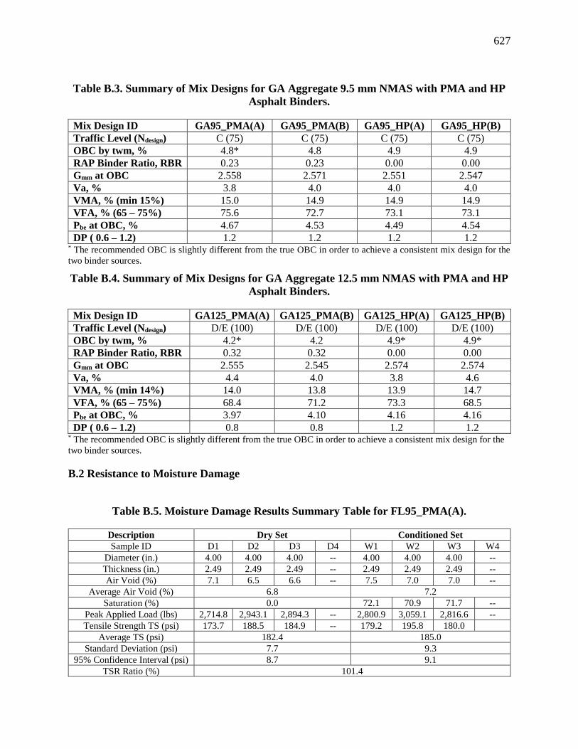
627
Table B.3. Summary of Mix Designs for GA Aggregate 9.5 mm NMAS with PMA and HP
Asphalt Binders.
Mix Design ID GA95_PMA(A) GA95_PMA(B) GA95_HP(A) GA95_HP(B)
Traffic Level (Ndesign) C (75) C (75) C (75) C (75)
OBC by twm, % 4.8* 4.8 4.9 4.9
RAP Binder Ratio, RBR 0.23 0.23 0.00 0.00
Gmm at OBC 2.558 2.571 2.551 2.547
Va, % 3.8 4.0 4.0 4.0
VMA, % (min 15%) 15.0 14.9 14.9 14.9
VFA, % (65 – 75%) 75.6 72.7 73.1 73.1
Pbe at OBC, % 4.67 4.53 4.49 4.54
DP ( 0.6 – 1.2) 1.2 1.2 1.2 1.2 * The recommended OBC is slightly different from the true OBC in order to achieve a consistent mix design for the
two binder sources.
Table B.4. Summary of Mix Designs for GA Aggregate 12.5 mm NMAS with PMA and HP
Asphalt Binders.
Mix Design ID GA125_PMA(A) GA125_PMA(B) GA125_HP(A) GA125_HP(B)
Traffic Level (Ndesign) D/E (100) D/E (100) D/E (100) D/E (100)
OBC by twm, % 4.2* 4.2 4.9* 4.9*
RAP Binder Ratio, RBR 0.32 0.32 0.00 0.00
Gmm at OBC 2.555 2.545 2.574 2.574
Va, % 4.4 4.0 3.8 4.6
VMA, % (min 14%) 14.0 13.8 13.9 14.7
VFA, % (65 – 75%) 68.4 71.2 73.3 68.5
Pbe at OBC, % 3.97 4.10 4.16 4.16
DP ( 0.6 – 1.2) 0.8 0.8 1.2 1.2 * The recommended OBC is slightly different from the true OBC in order to achieve a consistent mix design for the
two binder sources.
B.2 Resistance to Moisture Damage
Table B.5. Moisture Damage Results Summary Table for FL95_PMA(A).
Description Dry Set Conditioned Set
Sample ID D1 D2 D3 D4 W1 W2 W3 W4
Diameter (in.) 4.00 4.00 4.00 -- 4.00 4.00 4.00 --
Thickness (in.) 2.49 2.49 2.49 -- 2.49 2.49 2.49 --
Air Void (%) 7.1 6.5 6.6 -- 7.5 7.0 7.0 --
Average Air Void (%) 6.8 7.2
Saturation (%) 0.0 72.1 70.9 71.7 --
Peak Applied Load (lbs) 2,714.8 2,943.1 2,894.3 -- 2,800.9 3,059.1 2,816.6 --
Tensile Strength TS (psi) 173.7 188.5 184.9 -- 179.2 195.8 180.0
Average TS (psi) 182.4 185.0
Standard Deviation (psi) 7.7 9.3
95% Confidence Interval (psi) 8.7 9.1
TSR Ratio (%) 101.4
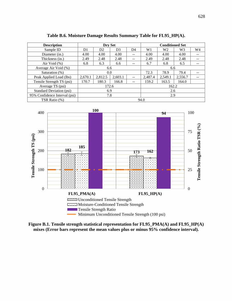
628
Table B.6. Moisture Damage Results Summary Table for FL95_HP(A).
Description Dry Set Conditioned Set
Sample ID D1 D2 D3 D4 W1 W2 W3 W4
Diameter (in.) 4.00 4.00 4.00 -- 4.00 4.00 4.00 --
Thickness (in.) 2.49 2.48 2.48 -- 2.49 2.48 2.48 --
Air Void (%) 6.8 6.3 6.6 -- 6.7 6.8 6.5 --
Average Air Void (%) 6.6 6.6
Saturation (%) 0.0 72.3 78.9 79.4 --
Peak Applied Load (lbs) 2,670.1 2,812.5 2,603.1 -- 2,487.4 2,549.1 2,556.7 --
Tensile Strength TS (psi) 170.7 180.3 166.8 -- 159.2 163.5 164.0
Average TS (psi) 172.6 162.2
Standard Deviation (psi) 6.9 2.6
95% Confidence Interval (psi) 7.8 2.9
TSR Ratio (%) 94.0
Figure B.1. Tensile strength statistical representation for FL95_PMA(A) and FL95_HP(A)
mixes (Error bars represent the mean values plus or minus 95% confidence interval).
182 173
185162
10094
0
25
50
75
100
0
100
200
300
400
FL95_PMA(A) FL95_HP(A)
Ten
sile
Str
ength
Rati
o T
SR
(%
)
Ten
sile
Str
ength
TS
(p
si)
Unconditioned Tensile Strength
Moisture-Conditioned Tensile Strength
Tensile Strength Ratio
Minimum Unconditioned Tensile Strength (100 psi)

629
Table B.7. Moisture Damage Results Summary Table for FL95_PMA(B).
Description Dry Set Conditioned Set
Sample ID D1 D2 D3 D4 W1 W2 W3 W4
Diameter (in.) 4.00 4.00 4.00 -- 4.00 4.00 4.00 --
Thickness (in.) 2.49 2.48 2.49 -- 2.48 2.48 2.48 --
Air Void (%) 7.2 6.6 7.0 -- 7.5 7.0 7.0 --
Average Air Void (%) 6.9 7.2
Saturation (%) 0.0 76.7 71.9 78.7 --
Peak Applied Load (lbs) 2,665.7 2,607.8 2,807.4 -- 2,338.1 2,296.1 2,330.6 --
Tensile Strength TS (psi) 170.6 167.1 179.3 -- 150.3 147.3 149.5
Average TS (psi) 172.3 149.0
Standard Deviation (psi) 6.2 1.5
95% Confidence Interval (psi) 6.1 1.7
TSR Ratio (%) 86.5
Table B.8. Moisture Damage Results Summary Table for FL95_HP(B).
Description Dry Set Conditioned Set
Sample ID D1 D2 D3 D4 W1 W2 W3 W4
Diameter (in.) 4.00 4.00 4.00 -- 4.00 4.00 4.00 --
Thickness (in.) 2.40 2.49 2.49 -- 2.48 2.48 2.48 --
Air Void (%) 6.9 6.3 6.7 -- 7.9 7.3 7.6 --
Average Air Void (%) 6.6 7.6
Saturation (%) 0.0 77.5 70.8 72.6 --
Peak Applied Load (lbs) 2,338.3 2,516.5 2,384.4 -- 2,193.8 2,323.5 2,106.6 --
Tensile Strength TS (psi) 150.1 161.1 152.7 -- 141.0 149.2 135.1
Average TS (psi) 154.6 141.8
Standard Deviation (psi) 5.8 7.1
95% Confidence Interval (psi) 5.7 8.0
TSR Ratio (%) 91.7

630
Figure B.2. Tensile strength statistical representation for FL95_PMA(B) and FL95_HP(B)
mixes (Error bars represent the mean values plus or minus 95% confidence interval).
Table B.9. Moisture Damage Results Summary Table for FL125_PMA(A).
Description Dry Set Conditioned Set
Sample ID D1 D2 D3 D4 W1 W2 W3 W4
Diameter (in.) 4.00 4.00 4.00 -- 4.00 4.00 4.00 4.00
Thickness (in.) 2.49 2.49 2.49 -- 2.50 2.49 2.50 2.49
Air Void (%) 6.5 6.7 6.6 -- 6.3 6.5 6.3 6.5
Average Air Void (%) 6.6 6.4
Saturation (%) 0.0 72.2 77.5 79.1 79.3
Peak Applied Load (lbs) 3,418.0 3,506.4 3,210.1 -- 2,914.4 2,657.6 2,669.2 2,931.5
Tensile Strength TS (psi) 218.4 224.3 205.4 -- 185.8 169.8 170.2 187.6
Average TS (psi) 216.0 178.4
Standard Deviation (psi) 9.7 9.6
95% Confidence Interval (psi) 8.5 9.5
TSR Ratio (%) 82.6
172155149 142
8692
0
25
50
75
100
0
100
200
300
400
FL95_PMA(B) FL95_HP(B)
Ten
sile
Str
eng
th R
ati
o T
SR
(%
)
Ten
sile
Str
eng
th T
S (
psi
)
Unconditioned Tensile Strength
Moisture-Conditioned Tensile Strength
Tensile Strength Ratio
Minimum Unconditioned Tensile Strength (100 psi)

631
Table B.10. Moisture Damage Results Summary Table for FL125_HP(A).
Description Dry Set Conditioned Set
Sample ID D1 D2 D3 D4 W1 W2 W3 W4
Diameter (in.) 4.00 4.00 4.00 -- 4.00 4.00 4.00 4.00
Thickness (in.) 2.48 2.49 2.49 -- 2.49 2.48 2.48 2.48
Air Void (%) 6.7 6.2 6.5 -- 6.6 6.8 6.3 6.6
Average Air Void (%) 6.4 6.6
Saturation (%) 0.0 78.0 76.2 79.6 70.9
Peak Applied Load (lbs) 2,479.1 2,721.2 2,560.9 -- 2,022.1 2,006.2 2,121.1 2,173.1
Tensile Strength TS (psi) 158.8 174.1 163.8 -- 129.5 128.5 136.0 139.7
Average TS (psi) 165.6 133.4
Standard Deviation (psi) 7.8 5.3
95% Confidence Interval (psi) 7.6 5.2
TSR Ratio (%) 80.6
Figure B.3. Tensile strength statistical representation for FL125_PMA(A) and
FL125_HP(A) mixes (Error bars represent the mean values plus or minus 95% confidence
interval).
216
166178
133
83 81
0
25
50
75
100
0
100
200
300
400
FL125_PMA(A) FL125_HP(A)
Ten
sile
Str
ength
Rati
o T
SR
(%
)
Ten
sile
Str
ength
TS
(p
si)
Unconditioned Tensile Strength
Moisture-Conditioned Tensile Strength
Tensile Strength Ratio
Minimum Unconditioned Tensile Strength (100 psi)

632
Table B.11. Moisture Damage Results Summary Table for FL125_PMA(B).
Description Dry Set Conditioned Set
Sample ID D1 D2 D3 D4 W1 W2 W3 W4
Diameter (in.) 4.00 4.00 4.00 -- 4.00 4.00 4.00 --
Thickness (in.) 2.49 2.49 2.49 -- 2.48 2.48 2.48 --
Air Void (%) 6.7 6.5 7.0 -- 6.4 6.6 6.5 --
Average Air Void (%) 6.7 6.5
Saturation (%) 0.0 79.5 78.1 74.3 --
Peak Applied Load (lbs) 3,332.6 3,204.3 3,294.7 -- 2,915.9 2,710.7 3,118.0 --
Tensile Strength TS (psi) 212.7 204.5 210.2 -- 186.9 173.8 199.7
Average TS (psi) 209.1 186.8
Standard Deviation (psi) 4.2 13.0
95% Confidence Interval (psi) 4.1 14.7
TSR Ratio (%) 89.3
Table B.12. Moisture Damage Results Summary Table for FL125_HP(B).
Description Dry Set Conditioned Set
Sample ID D1 D2 D3 D4 W1 W2 W3 W4
Diameter (in.) 4.00 4.00 4.00 -- 4.00 4.00 4.00 4.00
Thickness (in.) 2.48 2.49 2.48 -- 2.48 2.48 2.48 2.48
Air Void (%) 6.7 6.6 6.6 -- 6.7 6.8 6.6 6.6
Average Air Void (%) 6.6 6.7
Saturation (%) 0.0 78.0 79.4 79.1 73.8
Peak Applied Load (lbs) 2,342.4 2,669.7 2,459.2 -- 2,113.0 2,098.3 2,039.8 2,165.6
Tensile Strength TS (psi) 150.0 170.8 157.6 -- 135.4 134.5 130.9 138.9
Average TS (psi) 159.5 134.9
Standard Deviation (psi) 10.5 3.3
95% Confidence Interval (psi) 10.3 3.2
TSR Ratio (%) 84.6

633
Figure B.4. Tensile strength statistical representation for FL125_PMA(B) and
FL125_HP(B) mixes (Error bars represent the mean values plus or minus 95% confidence
interval).
Table B.13. Moisture Damage Results Summary Table for GA95_PMA(A).
Description Dry Set Conditioned Set
Sample ID D1 D2 D3 D4 W1 W2 W3 W4
Diameter (in.) 4.00 4.00 4.00 -- 4.00 4.00 4.00 4.00
Thickness (in.) 2.50 2.49 2.49 -- 2.49 2.49 2.49 2.50
Air Void (%) 7.0 6.0 6.2 -- 6.6 6.2 6.5 6.9
Average Air Void (%) 6.4 6.6
Saturation (%) 0.0 70.3 76.7 70.6 77.9
Peak Applied Load (lbs) 4,229.8 4,410.5 4,220.3 -- 3,611.9 3,598.9 3,669.3 3,643.6
Tensile Strength TS (psi) 268.9 282.2 269.7 -- 230.8 230.0 234.8 232.4
Average TS (psi) 273.6 232.0
Standard Deviation (psi) 7.4 2.1
95% Confidence Interval (psi) 6.5 2.1
TSR Ratio (%) 84.8
209
160
187
135
8985
0
25
50
75
100
0
100
200
300
400
FL125_PMA(B) FL125_HP(B)
Ten
sile
Str
eng
th R
ati
o T
SR
(%
)
Ten
sile
Str
eng
th T
S (
psi
)
Unconditioned Tensile Strength
Moisture-Conditioned Tensile Strength
Tensile Strength Ratio
Minimum Unconditioned Tensile Strength (100 psi)

634
Table B.14. Moisture Damage Results Summary Table for GA95_HP(A).
Description Dry Set Conditioned Set
Sample ID D1 D2 D3 D4 W1 W2 W3 W4
Diameter (in.) 4.00 4.00 4.00 -- 4.00 4.00 4.00 --
Thickness (in.) 2.49 2.49 2.49 -- 2.48 2.49 2.48 --
Air Void (%) 7.0 7.0 6.8 -- 7.0 7.1 7.0 --
Average Air Void (%) 6.9 7.0
Saturation (%) 0.0 73.6 79.0 76.6 --
Peak Applied Load (lbs) 2,975.0 3,006.5 2,940.5 -- 2,821.0 2,745.8 2,589.0 --
Tensile Strength TS (psi) 190.2 192.1 188.2 -- 180.7 175.5 166.0
Average TS (psi) 190.2 174.0
Standard Deviation (psi) 2.0 7.5
95% Confidence Interval (psi) 1.9 8.4
TSR Ratio (%) 91.5
Figure B.5. Tensile strength statistical representation for GA95_PMA(A) and GA95_HP(A)
mixes (Error bars represent the mean values plus or minus 95% confidence interval).
274
190
232
174
85
92
0
25
50
75
100
0
100
200
300
400
GA95_PMA(A) GA95_HP(A)
Ten
sile
Str
ength
Rati
o T
SR
(%
)
Ten
sile
Str
ength
TS
(p
si)
Unconditioned Tensile Strength
Moisture-Conditioned Tensile Strength
Tensile Strength Ratio
Minimum Unconditioned Tensile Strength (100 psi)

635
Table B.15. Moisture Damage Results Summary Table for GA95_PMA(B).
Description Dry Set Conditioned Set
Sample ID D1 D2 D3 D4 W1 W2 W3 W4
Diameter (in.) 4.00 4.00 4.00 -- 4.00 4.00 4.00 --
Thickness (in.) 2.49 2.49 2.49 -- 2.50 2.49 2.49 --
Air Void (%) 6.4 6.7 6.7 -- 6.3 6.9 6.7 --
Average Air Void (%) 6.6 6.6
Saturation (%) 0.0 71.1 70.4 70.6 --
Peak Applied Load (lbs) 4,504.9 4,548.2 4,375.4 -- 3,754.1 3,527.9 3,910.8 --
Tensile Strength TS (psi) 287.9 290.9 279.2 -- 239.1 225.1 249.9
Average TS (psi) 286.0 238.1
Standard Deviation (psi) 6.1 12.5
95% Confidence Interval (psi) 5.3 14.1
TSR Ratio (%) 83.2
Table B.16. Moisture Damage Results Summary Table for GA95_HP(B).
Description Dry Set Conditioned Set
Sample ID D1 D2 D3 D4 W1 W2 W3 W4
Diameter (in.) 4.00 4.00 4.00 -- 4.00 4.00 4.00 4.00
Thickness (in.) 2.47 2.47 2.48 -- 2.49 2.48 2.48 2.48
Air Void (%) 6.0 6.1 6.1 -- 7.1 7.1 7.0 7.0
Average Air Void (%) 6.1 7.0
Saturation (%) 0.0 74.8 74.9 77.0 75.4
Peak Applied Load (lbs) 2,108.6 2,216.1 2,316.0 -- 2,539.3 2,306.0 2,312.3 2,481.5
Tensile Strength TS (psi) 135.9 143.0 148.9 -- 162.6 147.7 148.3 159.5
Average TS (psi) 142.6 154.5
Standard Deviation (psi) 6.5 7.6
95% Confidence Interval (psi) 5.7 7.5
TSR Ratio (%) 108.3

636
Figure B.6. Tensile strength statistical representation for GA95_PMA(B) and GA95_HP(B)
mixes (Error bars represent the mean values plus or minus 95% confidence interval).
Table B.17. Moisture Damage Results Summary Table for GA125_PMA(A).
Description Dry Set Conditioned Set
Sample ID D1 D2 D3 D4 W1 W2 W3 W4
Diameter (in.) 4.00 4.00 4.00 -- 4.00 4.00 4.00 --
Thickness (in.) 2.49 2.49 2.49 -- 2.50 2.50 2.49 --
Air Void (%) 6.6 6.7 6.7 -- 7.0 6.9 6.6 --
Average Air Void (%) 6.7 6.8
Saturation (%) 0.0 76.3 73.2 78.5 --
Peak Applied Load (lbs) 4,532.8 4,511.5 4,463.4 -- 3,879.8 3,636.7 3,538.6 --
Tensile Strength TS (psi) 290.0 288.6 285.3 -- 247.3 231.9 225.9
Average TS (psi) 288.0 235.0
Standard Deviation (psi) 2.4 11.1
95% Confidence Interval (psi) 2.7 12.5
TSR Ratio (%) 81.6
286
143
238
155
83
100
0
25
50
75
100
0
100
200
300
400
FL95_PMA(B) FL95_HP(B)
Ten
sile
Str
eng
th R
ati
o T
SR
(%
)
Ten
sile
Str
eng
th T
S (
psi
)
Unconditioned Tensile Strength
Moisture-Conditioned Tensile Strength
Tensile Strength Ratio
Minimum Unconditioned Tensile Strength (100 psi)
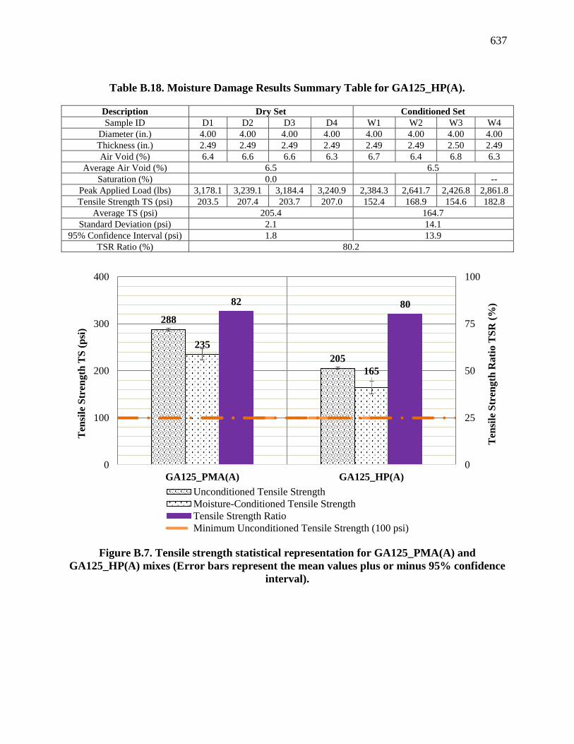
637
Table B.18. Moisture Damage Results Summary Table for GA125_HP(A).
Description Dry Set Conditioned Set
Sample ID D1 D2 D3 D4 W1 W2 W3 W4
Diameter (in.) 4.00 4.00 4.00 4.00 4.00 4.00 4.00 4.00
Thickness (in.) 2.49 2.49 2.49 2.49 2.49 2.49 2.50 2.49
Air Void (%) 6.4 6.6 6.6 6.3 6.7 6.4 6.8 6.3
Average Air Void (%) 6.5 6.5
Saturation (%) 0.0 --
Peak Applied Load (lbs) 3,178.1 3,239.1 3,184.4 3,240.9 2,384.3 2,641.7 2,426.8 2,861.8
Tensile Strength TS (psi) 203.5 207.4 203.7 207.0 152.4 168.9 154.6 182.8
Average TS (psi) 205.4 164.7
Standard Deviation (psi) 2.1 14.1
95% Confidence Interval (psi) 1.8 13.9
TSR Ratio (%) 80.2
Figure B.7. Tensile strength statistical representation for GA125_PMA(A) and
GA125_HP(A) mixes (Error bars represent the mean values plus or minus 95% confidence
interval).
288
205
235
165
82 80
0
25
50
75
100
0
100
200
300
400
GA125_PMA(A) GA125_HP(A)
Ten
sile
Str
ength
Rati
o T
SR
(%
)
Ten
sile
Str
ength
TS
(p
si)
Unconditioned Tensile Strength
Moisture-Conditioned Tensile Strength
Tensile Strength Ratio
Minimum Unconditioned Tensile Strength (100 psi)
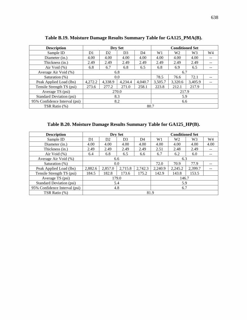
638
Table B.19. Moisture Damage Results Summary Table for GA125_PMA(B).
Description Dry Set Conditioned Set
Sample ID D1 D2 D3 D4 W1 W2 W3 W4
Diameter (in.) 4.00 4.00 4.00 4.00 4.00 4.00 4.00 --
Thickness (in.) 2.49 2.49 2.49 2.49 2.49 2.49 2.49 --
Air Void (%) 6.8 6.7 6.8 6.5 6.8 6.9 6.5 --
Average Air Void (%) 6.8 6.7
Saturation (%) 0.0 78.5 76.6 72.1 --
Peak Applied Load (lbs) 4,272.2 4,338.9 4,234.4 4,040.7 3,505.7 3,320.6 3,405.9 --
Tensile Strength TS (psi) 273.6 277.2 271.0 258.1 223.8 212.1 217.9
Average TS (psi) 270.0 217.9
Standard Deviation (psi) 8.3 5.9
95% Confidence Interval (psi) 8.2 6.6
TSR Ratio (%) 80.7
Table B.20. Moisture Damage Results Summary Table for GA125_HP(B).
Description Dry Set Conditioned Set
Sample ID D1 D2 D3 D4 W1 W2 W3 W4
Diameter (in.) 4.00 4.00 4.00 4.00 4.00 4.00 4.00 4.00
Thickness (in.) 2.49 2.49 2.49 2.49 2.51 2.48 2.49 --
Air Void (%) 6.4 6.8 6.5 6.6 6.7 6.2 6.0 --
Average Air Void (%) 6.6 6.3
Saturation (%) 0.0 72.0 70.9 77.9 --
Peak Applied Load (lbs) 2,882.6 2,857.0 2,715.8 2,742.3 2,240.9 2,245.2 2,399.7 --
Tensile Strength TS (psi) 184.5 182.8 173.6 175.2 142.9 143.8 153.5
Average TS (psi) 179.0 146.7
Standard Deviation (psi) 5.4 5.9
95% Confidence Interval (psi) 4.8 6.7
TSR Ratio (%) 81.9

639
Figure B.8. Tensile strength statistical representation for GA125_PMA(B) and
GA125_HP(B) mixes (Error bars represent the mean values plus or minus 95% confidence
interval).
270
179
218
147
81 82
0
25
50
75
100
0
100
200
300
400
GA125_PMA(B) GA125_HP(B)
Ten
sile
Str
eng
th R
ati
o T
SR
(%
)
Ten
sile
Str
eng
th T
S (
psi
)
Unconditioned Tensile Strength
Moisture-Conditioned Tensile Strength
Tensile Strength Ratio
Minimum Unconditioned Tensile Strength (100 psi)

640
Figure B.9. Tensile strength representation of the 16 evaluated mixes.
0
50
100
150
200
250
300
0 50 100 150 200 250 300Mo
istu
re-C
on
dit
ion
ed T
ensi
le S
tren
gth
(p
si)
Unconditioned Tensile Strength (psi)
FL95_PMA(A) FL95_HP(A)
FL95_PMA(B) FL95_HP(B)
FL125_PMA(A) FL125_HP(A)
FL125_PMA(B) FL125_HP(B)
GA95_PMA(A) GA95_HP(A)
GA95_PMA(B) GA95_HP(B)
GA125_PMA(A) GA125_HP(A)
GA125_PMA(B) GA125_HP(B)
Tensile Strength Ratio = 110% Tensile Strength Ratio = 100%
Tensile Strength Ratio = 90% Tensile Strength Ratio = 80%

641
APPENDIX C DETAILED LABORATORY DATA
C.1 Dynamic Modulus Property
C.1.1 Mix Design 1: FL95_PMA(A)
Figure C.1. Dynamic modulus of FL95_PMA(A) mixture at 68°F (20°C).
Figure C.2. Phase angle of FL95_PMA(A) mixture at 68°F (20°C).
1
10
100
1000
10000
1.E-06 1.E-05 1.E-04 1.E-03 1.E-02 1.E-01 1.E+00 1.E+01 1.E+02 1.E+03 1.E+04
Dyn
am
ic M
od
ulu
s E
* a
t 6
8°F
(2
0°C
)
,ksi
Reduced Frequency (Hz)
4°C
20°C
50°C
Fit
0
5
10
15
20
25
30
35
40
1.E-08 1.E-06 1.E-04 1.E-02 1.E+00 1.E+02 1.E+04 1.E+06
Ph
ase
An
gle
at
68
°F (
20
°C),
deg
ree
Reduced Frequency (Hz)
4°C
20°C
50°C
Fit

642
Figure C.3. Log (a[T]) of FL95_PMA(A) mixture.
Table C.1. Dynamic Modulus Input Values for FL95_PMA(A) AC mix.
E*, psi (MPa) Frequency (Hz)
Temperature, °F
(°C) 0.1 0.5 1 5 10 25
14 (-10) 1,945,719
(13,415)
2,281,477
(15,730)
2,414,749
(16,649)
2,693,661
(18,572)
2,800,138
(19,306)
2,928,378
(20,190)
40 (4) 913,337
(6,297)
1,260,750
(8,693)
1,417,852
(9,776)
1,784,068
(12,301)
1,937,760
(13,360)
2,133,436
(14,710)
70 (21) 215,122
(1,483)
380,913
(2,626)
474,418
(3,271)
741,742
(5,114)
876,002
(6,040)
1,067,179
(7,358)
100 (38) 36,183
(249)
71,889
(496)
96,715
(667)
186,944
(1,289)
243,401
(1,678)
337,210
(2,325)
130 (54) 10,484
(72)
15,779
(109)
19,893
(137)
37,266
(257)
49,970
(345)
74,116
(511)
Table C.2. Phase Angle Input Values for FL95_PMA(A) AC mix.
Phase Angle, ° Frequency (Hz)
Temperature, °F (°C) 0.1 0.5 1 5 10 25
14 (-10) 8.0 6.3 5.7 4.5 4.0 3.5
40 (4) 18.8 15.6 14.3 11.6 10.5 9.3
70 (21) 33.1 30.1 28.7 25.1 23.6 21.5
100 (38) 35.8 36.6 36.6 35.8 35.1 33.9
130 (54) 27.1 30.3 31.6 34.1 35.0 35.9
2.008
0.000
-3.229
-4
-3
-2
-1
0
1
2
3
0 10 20 30 40 50 60
Lo
g(a
[T])
Temperature (°C)
log[𝑎(𝑇)] =195,267.6261
𝑅 ∗ 𝑙𝑛10(
1
𝑇−
1
20)

643
C.1.2 Mix Design 2: FL95_PMA(B)
Figure C.4. Dynamic modulus of FL95_PMA(B) mixture at 68°F (20°C).
Figure C.5. Phase angle of FL95_PMA(B) mixture at 68°F (20°C).
1
10
100
1000
10000
1.E-06 1.E-05 1.E-04 1.E-03 1.E-02 1.E-01 1.E+00 1.E+01 1.E+02 1.E+03 1.E+04
Dyn
am
ic M
od
ulu
s E
* a
t 6
8°F
(2
0°C
),
ksi
Reduced Frequency (Hz)
4°C
20°C
50°C
Fit
0
5
10
15
20
25
30
35
40
1.E-08 1.E-06 1.E-04 1.E-02 1.E+00 1.E+02 1.E+04 1.E+06
Ph
ase
An
gle
at
68
°F (
20
°C),
deg
ree
Reduced Frequency (Hz)
4°C
20°C
50°C
Fit
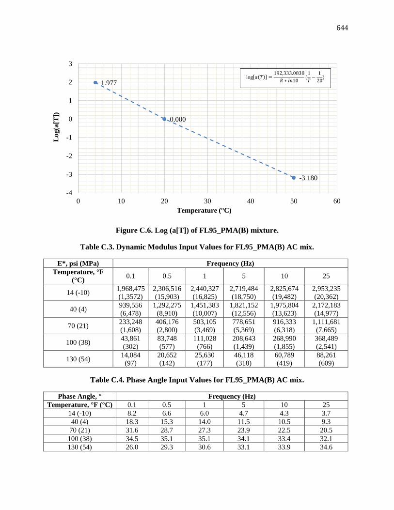
644
Figure C.6. Log (a[T]) of FL95_PMA(B) mixture.
Table C.3. Dynamic Modulus Input Values for FL95_PMA(B) AC mix.
E*, psi (MPa) Frequency (Hz)
Temperature, °F
(°C) 0.1 0.5 1 5 10 25
14 (-10) 1,968,475
(1,3572)
2,306,516
(15,903)
2,440,327
(16,825)
2,719,484
(18,750)
2,825,674
(19,482)
2,953,235
(20,362)
40 (4) 939,556
(6,478)
1,292,275
(8,910)
1,451,383
(10,007)
1,821,152
(12,556)
1,975,804
(13,623)
2,172,183
(14,977)
70 (21) 233,248
(1,608)
406,176
(2,800)
503,105
(3,469)
778,651
(5,369)
916,333
(6,318)
1,111,681
(7,665)
100 (38) 43,861
(302)
83,748
(577)
111,028
(766)
208,643
(1,439)
268,990
(1,855)
368,489
(2,541)
130 (54) 14,084
(97)
20,652
(142)
25,630
(177)
46,118
(318)
60,789
(419)
88,261
(609)
Table C.4. Phase Angle Input Values for FL95_PMA(B) AC mix.
Phase Angle, ° Frequency (Hz)
Temperature, °F (°C) 0.1 0.5 1 5 10 25
14 (-10) 8.2 6.6 6.0 4.7 4.3 3.7
40 (4) 18.3 15.3 14.0 11.5 10.5 9.3
70 (21) 31.6 28.7 27.3 23.9 22.5 20.5
100 (38) 34.5 35.1 35.1 34.1 33.4 32.1
130 (54) 26.0 29.3 30.6 33.1 33.9 34.6
1.977
0.000
-3.180
-4
-3
-2
-1
0
1
2
3
0 10 20 30 40 50 60
Lo
g(a
[T])
Temperature (°C)
log 𝑎 𝑇 =192,333.0838
𝑅 ∗ 𝑙𝑛10(
1
𝑇−
1
20)

645
C.1.3 Mix Design 3: FL95_HP(A)
Figure C.7. Dynamic modulus of FL95_HP(A) mixture at 68°F (20°C).
Figure C.8. Phase angle of FL95_HP(A) mixture at 68°F (20°C).
1
10
100
1000
10000
1.E-06 1.E-05 1.E-04 1.E-03 1.E-02 1.E-01 1.E+00 1.E+01 1.E+02 1.E+03 1.E+04
Dyn
am
ic M
od
ulu
s E
* a
t 6
8°F
(2
0°C
),
ksi
Reduced Frequency (Hz)
4°C
20°C
50°C
Fit
0
5
10
15
20
25
30
35
1.E-08 1.E-06 1.E-04 1.E-02 1.E+00 1.E+02 1.E+04 1.E+06
Ph
ase
An
gle
at
68°F
(2
0°C
), d
egre
e
Reduced Frequency (Hz)
4°C
20°C
50°C
Fit

646
Figure C.9. Log (a[T]) of FL95_HP(A) mixture.
Table C.5. Dynamic Modulus Input Values for FL95_HP(A) AC mix.
E*, psi (MPa) Frequency (Hz)
Temperature, °F
(°C) 0.1 0.5 1 5 10 25
14 (-10) 1,369,389
(9,445)
1,713,661
(11,815)
1,859,930
(12,824)
2,185,025
(15,065)
2,316,221
(15,970)
2,479,723
(17,097)
40 (4) 577,508
(3,982)
843,612
(5,816)
973,676
(6,713)
1,300,520
(8,967)
1,447,680
(9,981)
1,643,773
(11,333)
70 (21) 153,206
(1,056)
260,189
(1,794)
322,797
(2,226)
511,678
(3,528)
612,121
(4,220)
761,546
(5,251)
100 (38) 43,213
(298)
70,748
(488)
89,002
(614)
153,519
(1,058)
193,600
(1,335)
260,689
(1,797)
130 (54) 21,229
(146)
27,313
(188)
31,684
(218)
48,553
(335)
60,016
(414)
80,795
(557)
Table C.6. Phase Angle Input Values for FL95_HP(A) AC mix.
Phase Angle, ° Frequency (Hz)
Temperature, °F (°C) 0.1 0.5 1 5 10 25
14 (-10) 12.1 10.2 9.5 8.0 7.4 6.7
40 (4) 21.1 18.5 17.4 15.0 14.1 12.9
70 (21) 30.7 28.7 27.7 25.2 24.1 22.5
100 (38) 30.6 32.0 32.2 32.0 31.6 30.8
130 (54) 19.6 23.9 25.6 28.9 30.0 31.1
1.834
0.000
-2.949
-4
-3
-2
-1
0
1
2
3
0 10 20 30 40 50 60
Lo
g(a
[T])
Temperature (°C)
log 𝑎 𝑇 =178,363.1841
𝑅 ∗ 𝑙𝑛10(
1
𝑇−
1
20)
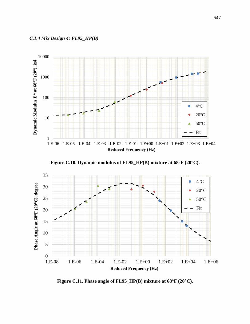
647
C.1.4 Mix Design 4: FL95_HP(B)
Figure C.10. Dynamic modulus of FL95_HP(B) mixture at 68°F (20°C).
Figure C.11. Phase angle of FL95_HP(B) mixture at 68°F (20°C).
1
10
100
1000
10000
1.E-06 1.E-05 1.E-04 1.E-03 1.E-02 1.E-01 1.E+00 1.E+01 1.E+02 1.E+03 1.E+04
Dyn
am
ic M
od
ulu
s E
* a
t 6
8°F
(2
0°)
, k
si
Reduced Frequency (Hz)
4°C
20°C
50°C
Fit
0
5
10
15
20
25
30
35
1.E-08 1.E-06 1.E-04 1.E-02 1.E+00 1.E+02 1.E+04 1.E+06
Ph
ase
An
gle
at
68
°F (
20
°C),
deg
ree
Reduced Frequency (Hz)
4°C
20°C
50°C
Fit

648
Figure C.12. Log (a[T]) of FL95_HP(B) mixture.
Table C.7. Dynamic Modulus Input Values for FL95_HP(B) AC mix.
E*, psi (MPa) Frequency (Hz)
Temperature, °F
(°C) 0.1 0.5 1 5 10 25
14 (-10) 1,306,229
(9,006)
1,654,600
(11,408)
1,803,591
(12,435)
2,135,925
(14,727)
2,270,390
(15,654)
2,438,154
(16,810)
40 (4) 501,085
(3,455)
755,584
(5,210)
882,424
(6,084)
1,206,398
(8,138)
1,354,233
(9,337)
1,552,750
(10,706)
70 (21) 112,803
(778)
200,603
(1,383)
253,952
(1,751)
421,058
(2,903)
512,821
(3,536)
652,211
(4,497)
100 (38) 28,721
(198)
47,326
(326)
60,172
(415)
107,784
(743)
138,677
(956)
192,088
(1,324)
130 (54) 15,055
(104)
18,309
(126)
20,831
(144)
31,148
(215)
38,472
(265)
52,186
(360)
Table C.8. Phase Angle Input Values for FL95_HP(B) AC mix.
Phase Angle, ° Frequency (Hz)
Temperature, °F (°C) 0.1 0.5 1 5 10 25
14 (-10) 13.3 10.6 9.6 7.4 6.7 5.7
40 (4) 24.7 21.5 20.0 16.7 15.3 13.6
70 (21) 31.5 30.7 30.1 28.1 27.0 25.3
100 (38) 28.6 30.2 30.7 31.5 31.6 31.4
130 (54) 22.4 24.6 25.6 27.7 28.5 29.5
1.895
0.000
-3.048
-4
-3
-2
-1
0
1
2
3
0 10 20 30 40 50 60
Log(a
[T])
Temperature (°C)
log 𝑎 𝑇 =184,332.4996
𝑅 ∗ 𝑙𝑛10(
1
𝑇−
1
20)

649
C.1.5 Mix Design 5: FL125_PMA(A)
Figure C.13. Dynamic modulus of FL125_PMA(A) mixture at 68°F (20°C).
Figure C.14. Phase angle of FL125_PMA(A) mixture at 68°F (20°C).
1
10
100
1000
10000
1.E-06 1.E-05 1.E-04 1.E-03 1.E-02 1.E-01 1.E+00 1.E+01 1.E+02 1.E+03 1.E+04
Dyn
am
ic M
od
ulu
s E
* a
t 6
8°F
(2
0°C
), k
si
Reduced Frequency (Hz)
4°C
20°C
50°C
Fit
0
5
10
15
20
25
30
35
40
1.E-08 1.E-06 1.E-04 1.E-02 1.E+00 1.E+02 1.E+04 1.E+06
Ph
ase
An
gle
at
68°F
(2
0°C
), d
egre
e
Reduced Frequency (Hz)
4°C
20°C
50°C
Fit

650
Figure C.15. Log (a[T]) of FL125_PMA(A) mixture.
Table C.9. Dynamic Modulus Input Values for FL125_PMA(A) AC mix.
E*, psi (MPa) Frequency (Hz)
Temperature, °F
(°C) 0.1 0.5 1 5 10 25
14 (-10) 2,034,061
(14,024)
2,379,316
(16,405)
2,515,240
(17,342)
2,796,650
(19,282)
2,902,693
(20,013)
3,029,132
(20,885)
40 (4) 979,275
(6,752)
1,339,161
(9,233)
1,502,075
(10,356)
1,881,278
(12,971)
2,039,802
(14,064)
2,240,711
(15,449)
70 (21) 261,138
(1,800)
437,430
(3,016)
535,501
(3,692)
814,254
(5,641)
953,967
(6,577)
1,152,829
(7,948)
100 (38) 56,112
(387)
102,308
(705)
132,262
(912)
235,127
(1,621)
297,143
(2,049)
398,332
(2,746)
130 (54) 15,344
(106)
25,727
(177)
32,709
(226)
58,714
(405)
76,037
(524)
107,068
(738)
Table C.10. Phase Angle Input Values for FL125_PMA(A) AC mix.
Phase Angle, ° Frequency (Hz)
Temperature, °F (°C) 0.1 0.5 1 5 10 25
14 (-10) 8.4 6.6 6.0 4.7 4.2 3.6
40 (4) 18.6 15.4 14.1 11.4 10.4 9.1
70 (21) 31.7 28.8 27.4 23.9 22.4 20.4
100 (38) 33.7 34.7 34.7 33.9 33.2 31.9
130 (54) 24.3 27.9 29.4 32.2 33.2 34.1
1.981
0.000
-3.186
-4
-3
-2
-1
0
1
2
3
0 10 20 30 40 50 60
Lo
g(a
[T])
Temperature (°C)
log 𝑎 𝑇 =192,662.7110
𝑅 ∗ 𝑙𝑛10(
1
𝑇−
1
20)
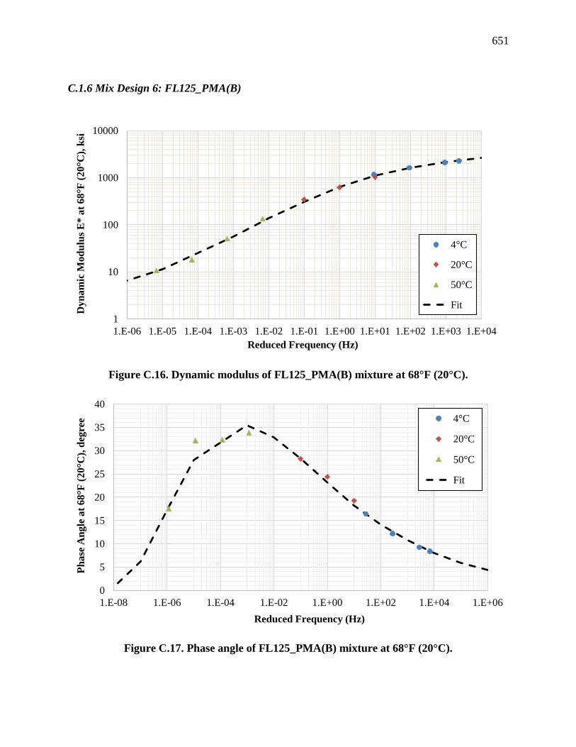
651
C.1.6 Mix Design 6: FL125_PMA(B)
Figure C.16. Dynamic modulus of FL125_PMA(B) mixture at 68°F (20°C).
Figure C.17. Phase angle of FL125_PMA(B) mixture at 68°F (20°C).
1
10
100
1000
10000
1.E-06 1.E-05 1.E-04 1.E-03 1.E-02 1.E-01 1.E+00 1.E+01 1.E+02 1.E+03 1.E+04
Dyn
am
ic M
od
ulu
s E
* a
t 6
8°F
(2
0°C
), k
si
Reduced Frequency (Hz)
4°C
20°C
50°C
Fit
0
5
10
15
20
25
30
35
40
1.E-08 1.E-06 1.E-04 1.E-02 1.E+00 1.E+02 1.E+04 1.E+06
Ph
ase
An
gle
at
68°F
(2
0°C
), d
egre
e
Reduced Frequency (Hz)
4°C
20°C
50°C
Fit

652
Figure C.18. Log (a[T]) of FL125_PMA(B) mixture.
Table C.11. Dynamic Modulus Input Values for FL125_PMA(B) AC mix.
E*, psi (MPa) Frequency (Hz)
Temperature, °F
(°C) 0.1 0.5 1 5 10 25
14 (-10) 2,141,540
(14,765)
2,485,273
(17,135)
2,618,831
(18,056)
2,892,034
(19,940)
2,993,772
(20,641)
3,114,157
(21,471)
40 (4) 1,057,697
(7,293)
1,436,157
(9,902)
1,605,099
(11,067)
1,992,677
(13,739)
2,152,370
(14,840)
2,352,778
(16,222)
70 (21) 283,594
(1,955)
477,553
(3,293)
584,798
(4,032)
886,518
(6,112)
1,035,945
(7,413)
1,246,573
(8,595)
100 (38) 58,832
(406)
109,489
(755)
142,600
(983)
256,744
(1,770)
325,541
(2,245)
437,447
(3,016)
130 (54) 15,396
(106)
26,344
(182)
33,819
(233)
62,104
(428)
81,172
(560)
115,560
(797)
Table C.12. Phase Angle Input Values for FL125_PMA(B) AC mix.
Phase Angle, ° Frequency (Hz)
Temperature, °F (°C) 0.1 0.5 1 5 10 25
14 (-10) 8.4 6.9 6.3 5.1 4.6 4.1
40 (4) 16.7 13.9 12.8 10.5 9.6 8.6
70 (21) 29.1 25.5 24.0 20.5 19.0 17.2
100 (38) 35.5 35.0 34.3 31.7 30.3 28.4
130 (54) 23.4 30.0 32.1 35.0 35.5 35.4
1.971
0.000
-3.170
-4
-3
-2
-1
0
1
2
3
0 10 20 30 40 50 60
Lo
g(a
[T])
Temperature (°C)
log 𝑎 𝑇 =191,720.3272
𝑅 ∗ 𝑙𝑛10(
1
𝑇−
1
20)

653
C.1.7 Mix Design 7: FL125_HP(A)
Figure C.19. Dynamic modulus of FL125_HP(A) mixture at 68°F (20°C).
Figure C.20. Phase angle of FL125_HP(A) mixture at 68°F (20°C).
1
10
100
1000
10000
1.E-06 1.E-04 1.E-02 1.E+00 1.E+02 1.E+04
Dyn
am
ic M
od
ulu
s E
* a
t 6
8°F
(2
0°C
), k
si
Reduced Frequency (Hz)
4°C
20°C
50°C
Fit
0
5
10
15
20
25
30
35
1.E-08 1.E-06 1.E-04 1.E-02 1.E+00 1.E+02 1.E+04 1.E+06
Ph
ase
An
gle
at
68
°F (
20
°C),
deg
ree
Reduced Frequency (Hz)
4°C
20°C
50°C
Fit

654
Figure C.21. Log (a[T]) of FL125_HP(A) mixture.
Table C.13. Dynamic Modulus Input Values for FL125_HP(A) AC mix.
E*, psi (MPa) Frequency (Hz)
Temperature, °F
(°C) 0.1 0.5 1 5 10 25
14 (-10) 1,366,334
(9,421)
1,681,304
(11,592)
1,815,860
(12,520)
2,117,573
(14,600)
2,240,777
(15,450)
2,395,836
(16,519)
40 (4) 585,609
(4,038)
830,066
(5,723)
948,295
(6,538)
1,244,655
(8,582)
1,378,478
(9,504)
1,557,779
(10,741)
70 (21) 155,026
(1,069)
256,842
(1,771)
314,643
(2,169)
485,048
(3,344)
574,369
(3,960)
706,587
(4,872)
100 (38) 37,199
(256)
64,710
(446)
82,224
(567)
141,734
(977)
177,584
(1,224)
236,501
(1,631)
130 (54) 11,750
(81)
18,549
(128)
23,014
(159)
39,180
(270)
49,691
(343)
68,223
(470)
Table C.14. Phase Angle Input Values for FL125_HP(A) AC mix.
Phase Angle, ° Frequency (Hz)
Temperature, °F (°C) 0.1 0.5 1 5 10 25
14 (-10) 12.7 11.0 10.3 8.8 8.2 7.5
40 (4) 20.9 18.4 17.4 15.2 14.3 13.1
70 (21) 30.4 28.1 27.0 24.4 23.3 21.8
100 (38) 32.5 33.2 33.1 32.1 31.4 30.2
130 (54) 20.5 26.2 28.2 31.4 32.3 33.0
1.965
0.000
-3.160
-4
-3
-2
-1
0
1
2
3
0 10 20 30 40 50 60
Lo
g(a
[T])
Temperature (°C)
log 𝑎 𝑇 =191,108.4878
𝑅 ∗ 𝑙𝑛10(
1
𝑇−
1
20)

655
C.1.8 Mix Design 8: FL125_HP(B)
Figure C.22. Dynamic modulus of FL125_HP(B) mixture at 68°F (20°C).
Figure C.23. Phase angle of FL125_HP(B) mixture at 68°F (20°C).
1
10
100
1000
10000
1.E-06 1.E-05 1.E-04 1.E-03 1.E-02 1.E-01 1.E+00 1.E+01 1.E+02 1.E+03 1.E+04
Dyn
am
ic M
od
ulu
s E
* a
t 6
8°F
(2
0°C
), k
si
Reduced Frequency (Hz)
4°C
20°C
50°C
Fit
0
5
10
15
20
25
30
35
40
1.E-08 1.E-06 1.E-04 1.E-02 1.E+00 1.E+02 1.E+04 1.E+06
Ph
ase
An
gle
at
68
°F (
20
°C),
deg
ree
Reduced Frequency (Hz)
Fit
4°C
20°C
50°C

656
Figure C.24. Log (a[T]) of FL125_HP(A) mixture.
Table C.15. Dynamic Modulus Input Values for FL125_HP(B) AC mix.
E*, psi (MPa) Frequency (Hz)
Temperature, °F
(°C) 0.1 0.5 1 5 10 25
14 (-10) 1,584,600
(10,925)
1,967,828
(13,568)
2,125,421
(14,654)
2,463,470
(16,985)
2,594,957
(17,892)
2,754,689
(18,993)
40 (4) 621,763
(4,287)
940,140
(6,482)
1,094,550
(7,547)
1,475,754
(10,175)
1,643,469
(11,331)
1,862,650
(12,843)
70 (21) 123,313
(850)
236,420
(1,630)
305,886
(2,109)
522,761
(3,604)
640,382
(4,415)
816,358
(5,629)
100 (38) 21,871
(151)
43,149
(297)
58,497
(403)
117,876
(813)
157,523
(1,086)
226,964
(1,565)
130 (54) 6,930
(48)
10,643
(73)
13,377
(92)
24,732
(171)
33,086
(228)
49,262
(340)
Table C.16. Phase Angle Input Values for FL125_HP(B) AC mix.
Phase Angle, ° Frequency (Hz)
Temperature, °F (°C) 0.1 0.5 1 5 10 25
14 (-10) 14.5 12.4 11.5 9.8 9.1 8.3
40 (4) 22.2 19.3 18.1 15.5 14.5 13.2
70 (21) 31.5 28.4 27.0 23.8 22.4 20.7
100 (38) 35.8 35.2 34.5 32.0 30.7 29.0
130 (54) 25.3 32.6 34.3 35.9 35.8 35.1
1.887
0.000
-3.034
-4
-3
-2
-1
0
1
2
3
0 10 20 30 40 50 60
Log(a
[T])
Temperature (°C)
log 𝑎 𝑇 =183,492.2351
𝑅 ∗ 𝑙𝑛10(
1
𝑇−
1
20)

657
C.1.9 Mix Design 9: GA95_PMA(A)
Figure C.25. Dynamic modulus of GA95_PMA(A) mixture at 68°F (20°C).
Figure C.26. Phase angle of GA95_PMA(A) mixture at 68°F (20°C).
1
10
100
1000
10000
1.E-06 1.E-05 1.E-04 1.E-03 1.E-02 1.E-01 1.E+00 1.E+01 1.E+02 1.E+03 1.E+04
Dyn
am
ic M
od
ulu
s E
* a
t 6
8°F
(2
0°C
), k
si
Reduced Frequency (Hz)
4°C
20°C
50°C
Fit
0
5
10
15
20
25
30
35
40
1.E-08 1.E-06 1.E-04 1.E-02 1.E+00 1.E+02 1.E+04 1.E+06
Ph
ase
An
gle
at
68
°F (
20
°C),
deg
ree
Reduced Frequency (Hz)
Fit
4°C
20°C
50°C
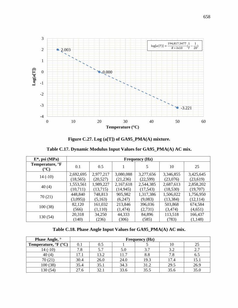
658
Figure C.27. Log (a[T]) of GA95_PMA(A) mixture.
Table C.17. Dynamic Modulus Input Values for GA95_PMA(A) AC mix.
E*, psi (MPa) Frequency (Hz)
Temperature, °F
(°C) 0.1 0.5 1 5 10 25
14 (-10) 2,692,695
(18,565)
2,977,217
(20,527)
3,080,088
(21,236)
3,277,656
(22,599)
3,346,855
(23,076)
3,425,645
(23,619)
40 (4) 1,553,561
(10,711)
1,989,227
(13,715)
2,167,618
(14,945)
2,544,385
(17,543)
2,687,613
(18,530)
2,858,202
(19,707)
70 (21) 448,840
(3,095))
748,813
(5,163)
905,982
(6,247)
1,317,386
(9,083)
1,506,022
(13,384)
1,756,950
(12,114)
100 (38) 82,120
(566)
161,032
(1,110)
213,846
(1,474)
396,036
(2,731)
503,868
(3,474)
674,584
(4,651)
130 (54) 20,318
(140)
34,250
(236)
44,333
(306)
84,896
(585)
113,518
(783)
166,437
(1,148)
Table C.18. Phase Angle Input Values for GA95_PMA(A) AC mix.
Phase Angle, ° Frequency (Hz)
Temperature, °F (°C) 0.1 0.5 1 5 10 25
14 (-10) 7.8 5.7 5.0 3.7 3.2 2.7
40 (4) 17.1 13.2 11.7 8.8 7.8 6.5
70 (21) 30.4 26.0 24.0 19.3 17.4 15.1
100 (38) 35.4 35.1 34.3 31.2 29.5 26.9
130 (54) 27.6 32.1 33.6 35.5 35.6 35.0
2.003
0.000
-3.221
-4
-3
-2
-1
0
1
2
3
0 10 20 30 40 50 60
Lo
g(a
[T])
Temperature (°C)
log 𝑎 𝑇 =194,817.3477
𝑅 ∗ 𝑙𝑛10(
1
𝑇−
1
20)

659
C.1.10 Mix Design 10: GA95_PMA(B)
Figure C.28. Dynamic modulus of GA95_PMA(B) mixture at 68°F (20°C).
Figure C.29. Phase angle of GA95_PMA(B) mixture at 68°F (20°C).
1
10
100
1000
10000
1.E-06 1.E-05 1.E-04 1.E-03 1.E-02 1.E-01 1.E+00 1.E+01 1.E+02 1.E+03 1.E+04
Dyn
am
ic M
od
ulu
s E
* a
t 6
8°F
(2
0°C
), k
si
Reduced Frequency (Hz)
4°C
20°C
50°C
Fit
0
5
10
15
20
25
30
35
40
1.E-08 1.E-06 1.E-04 1.E-02 1.E+00 1.E+02 1.E+04 1.E+06
Ph
ase
An
gle
at
68
°F (
20
°C),
deg
ree
Reduced Frequency (Hz)
Fit
4°C
20°C
50°C
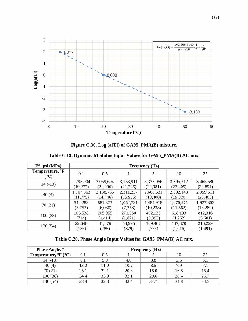
660
Figure C.30. Log (a[T]) of GA95_PMA(B) mixture.
Table C.19. Dynamic Modulus Input Values for GA95_PMA(B) AC mix.
E*, psi (MPa) Frequency (Hz)
Temperature, °F
(°C) 0.1 0.5 1 5 10 25
14 (-10) 2,795,904
(19,277)
3,059,694
(21,096)
3,153,911
(21,745)
3,333,056
(22,981)
3,395,212
(23,409)
3,465,580
(23,894)
40 (4) 1,707,863
(11,775)
2,138,755
(14,746)
2,311,237
(15,935)
2,668,631
(18,400)
2,802,143
(19,320)
2,959,511
(20,405)
70 (21) 544,283
(3,753)
881,873
(6,080)
1,052,731
(7,258)
1,484,918
(10,238)
1,676,971
(11,562)
1,927,363
(13,289)
100 (38) 103,538
(714)
205,055
(1,414)
271,360
(1,871)
492,135
(3,393)
618,193
(4,262)
812,316
(5,601)
130 (54) 22,648
(156)
41,376
(285)
54,995
(379)
109,467
(755)
147,370
(1,016)
216,229
(1,491)
Table C.20. Phase Angle Input Values for GA95_PMA(B) AC mix.
Phase Angle, ° Frequency (Hz)
Temperature, °F (°C) 0.1 0.5 1 5 10 25
14 (-10) 6.1 5.0 4.6 3.8 3.5 3.1
40 (4) 13.0 11.0 10.2 8.5 7.9 7.1
70 (21) 25.1 22.1 20.8 18.0 16.8 15.4
100 (38) 34.4 33.0 32.1 29.6 28.4 26.7
130 (54) 28.8 32.3 33.4 34.7 34.8 34.5
1.977
0.000
-3.180
-4
-3
-2
-1
0
1
2
3
0 10 20 30 40 50 60
Lo
g(a
[T])
Temperature (°C)
log 𝑎 𝑇 =192,308.6140
𝑅 ∗ 𝑙𝑛10(
1
𝑇−
1
20)

661
C.1.11 Mix Design 11: GA95_HP(A)
Figure C.28. Dynamic modulus of GA95_HP(A) mixture at 68°F (20°C).
Figure C.29. Phase angle of GA95_HP(A) mixture at 68°F (20°C).
1
10
100
1000
10000
1.E-06 1.E-05 1.E-04 1.E-03 1.E-02 1.E-01 1.E+00 1.E+01 1.E+02 1.E+03 1.E+04
Dyn
am
ic M
od
ulu
s E
* a
t 6
8°F
(2
0°C
), k
si
Reduced Frequency (Hz)
4°C
20°C
50°C
Fit
0
5
10
15
20
25
30
35
40
1.E-08 1.E-06 1.E-04 1.E-02 1.E+00 1.E+02 1.E+04 1.E+06
Ph
ase
An
gle
at
68
°F (
20
°C),
deg
ree
Reduced Frequency (Hz)
4°C
20°C
50°C
Fit
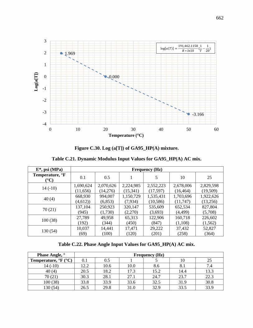
662
Figure C.30. Log (a[T]) of GA95_HP(A) mixture.
Table C.21. Dynamic Modulus Input Values for GA95_HP(A) AC mix.
E*, psi (MPa) Frequency (Hz)
Temperature, °F
(°C) 0.1 0.5 1 5 10 25
14 (-10) 1,690,624
(11,656)
2,070,626
(14,276)
2,224,985
(15,341)
2,552,223
(17,597)
2,678,006
(16,464)
2,829,598
(19,509)
40 (4) 668,930
(4,612))
994,007
(6,853)
1,150,729
(7,934)
1,535,431
(10,586)
1,703,696
(11,747)
1,922,626
(13,256)
70 (21) 137,104
(945)
250,923
(1,730)
320,147
(2,270)
535,609
(3,693)
652,534
(4,499)
827,804
(5,708)
100 (38) 27,789
(192)
49,958
(344)
65,313
(450)
122,906
(847)
160,718
(1,108)
226,602
(1,562)
130 (54) 10,037
(69)
14,441
(100)
17,471
(120)
29,222
(201)
37,432
(258)
52,827
(364)
Table C.22. Phase Angle Input Values for GA95_HP(A) AC mix.
Phase Angle, ° Frequency (Hz)
Temperature, °F (°C) 0.1 0.5 1 5 10 25
14 (-10) 12.2 10.6 10.0 8.6 8.1 7.4
40 (4) 20.5 18.2 17.3 15.2 14.4 13.3
70 (21) 30.3 28.1 27.1 24.7 23.7 22.3
100 (38) 33.8 33.9 33.6 32.5 31.9 30.8
130 (54) 26.5 29.8 31.0 32.9 33.5 33.9
1.969
0.000
-3.166
-4
-3
-2
-1
0
1
2
3
0 10 20 30 40 50 60
Lo
g(a
[T])
Temperature (°C)
log 𝑎 𝑇 =191,462.1158
𝑅 ∗ 𝑙𝑛10(
1
𝑇−
1
20)

663
C.1.12 Mix Design 12: GA95_HP(B)
Figure C.31. Dynamic modulus of GA95_HP(B) mixture at 68°F (20°C).
Figure C.32. Phase angle of GA95_HP(B) mixture at 68°F (20°C).
1
10
100
1000
10000
1.E-06 1.E-05 1.E-04 1.E-03 1.E-02 1.E-01 1.E+00 1.E+01 1.E+02 1.E+03 1.E+04
Dyn
am
ic M
od
ulu
s E
* a
t 6
8°F
(2
0°C
), k
si
Reduced Frequency (Hz)
4°C
20°C
50°C
Fit
0
5
10
15
20
25
30
35
40
1.E-08 1.E-06 1.E-04 1.E-02 1.E+00 1.E+02 1.E+04 1.E+06
Ph
ase
An
gle
at
68
°F (
20°C
), d
egre
e
Reduced Frequency (Hz)
4°C
20°C
50°C
Fit

664
Figure C.33. Log (a[T]) of GA95_HP(B) mixture.
Table C.23. Dynamic Modulus Input Values for GA95_HP(B) AC mix.
E*, psi (MPa) Frequency (Hz)
Temperature, °F
(°C) 0.1 0.5 1 5 10 25
14 (-10) 1,488,799
(10,265)
1,820,909
(12,555)
1,959,715
(13,512)
2,264,236
(15,611)
2,385,901
(16,450)
2,536,789
(17,491)
40 (4) 636,248
(4,387)
914,601
(6,306)
1,047,226
(7,220)
1,373,178
(9,468)
1,517,226
(10,461)
1,707,143
(11,770)
70 (21) 148,419
(1,023)
264,866
(1,826)
332,137
(2,290)
531,347
(3,664)
635,330
(4,380)
787,998
(5,433)
100 (38) 26,422
(182)
53,209
(367)
71,475
(493)
137,184
(946)
178,291
(1,229)
247,064
(1,703)
130 (54) 5,962
(41)
10,920
(75)
14,520
(100)
29,007
(200)
39,253
(271)
58,327
(402)
Table C.24. Phase Angle Input Values for GA95_HP(B) AC mix.
Phase Angle, ° Frequency (Hz)
Temperature, °F (°C) 0.1 0.5 1 5 10 25
14 (-10) 12.5 10.7 10.0 8.5 8.0 7.3
40 (4) 21.0 18.4 17.3 15.0 14.1 12.9
70 (21) 31.7 29.0 27.8 24.9 23.6 22.0
100 (38) 35.6 35.8 35.4 33.9 32.9 31.6
130 (54) 23.5 29.6 31.6 34.7 35.4 35.9
1.933
0.000
-3.108
-4
-3
-2
-1
0
1
2
3
0 10 20 30 40 50 60
Lo
g(a
[T])
Temperature (°C)
log 𝑎 𝑇 =187,987.8055
𝑅 ∗ 𝑙𝑛10(
1
𝑇−
1
20)
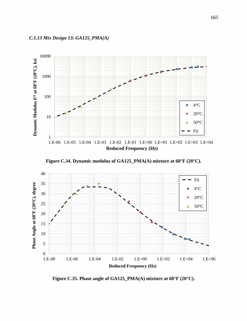
665
C.1.13 Mix Design 13: GA125_PMA(A)
Figure C.34. Dynamic modulus of GA125_PMA(A) mixture at 68°F (20°C).
Figure C.35. Phase angle of GA125_PMA(A) mixture at 68°F (20°C).
1
10
100
1000
10000
1.E-06 1.E-05 1.E-04 1.E-03 1.E-02 1.E-01 1.E+00 1.E+01 1.E+02 1.E+03 1.E+04
Dyn
am
ic M
od
ulu
s E
* a
t 6
8°F
(2
0°C
), k
si
Reduced Frequency (Hz)
4°C
20°C
50°C
Fit
0
5
10
15
20
25
30
35
40
1.E-08 1.E-06 1.E-04 1.E-02 1.E+00 1.E+02 1.E+04 1.E+06
Ph
ase
An
gle
at
68
°F (
20
°C),
deg
ree
Reduced Frequency (Hz)
Fit
4°C
20°C
50°C

666
Figure C.36. Log (a[T]) of GA125_PMA(A) mixture.
Table C.25. Dynamic Modulus Input Values for GA125_PMA(A) AC mix.
E*, psi (MPa) Frequency (Hz)
Temperature, °F
(°C) 0.1 0.5 1 5 10 25
14 (-10) 2,746,066
(18,933)
3,008,320
(20,742)
3,103,855
(21,400)
3,289,111
(22,678)
3,354,753
(23,130)
3,430,140
(23,650)
40 (4) 1,670,986
(11,521)
2,078,579
(14,331)
2,243,960
(15,472)
2,592,518
(17,875)
2,725,300
(18,790)
2,884,070
(19,885)
70 (21) 548,681
(3,783)
863,507
(5,954)
1,021,688
(7,044)
1,422,703
(9,809)
1,602,401
(11,048)
1,838,950
(12,679)
100 (38) 109,815
(757)
209,566
(1,445)
272,763
(1,881)
478,047
(3,296)
593,518
(4,092)
770,501
(5,312)
130 (54) 23,397
(161)
42,975
(296)
56,801
(392)
110,124
(759)
146,099
(1,007)
210,123
(1,449)
Table C.26. Phase Angle Input Values for GA125_PMA(A) AC mix.
Phase Angle, ° Frequency (Hz)
Temperature, °F (°C) 0.1 0.5 1 5 10 25
14 (-10) 6.0 4.9 4.5 3.6 3.3 3.0
40 (4) 13.4 11.2 10.3 8.5 7.8 7.0
70 (21) 26.1 22.9 21.5 18.4 17.2 15.6
100 (38) 34.6 33.5 32.7 30.3 29.0 27.3
130 (54) 27.5 31.3 32.5 34.3 34.6 34.6
2.041
0.000
-3.282
-4
-3
-2
-1
0
1
2
3
0 10 20 30 40 50 60
Lo
g(a
[T])
Temperature (°C)
log 𝑎 𝑇 =198,524.5646
𝑅 ∗ 𝑙𝑛10(
1
𝑇−
1
20)
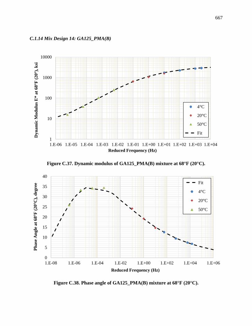
667
C.1.14 Mix Design 14: GA125_PMA(B)
Figure C.37. Dynamic modulus of GA125_PMA(B) mixture at 68°F (20°C).
Figure C.38. Phase angle of GA125_PMA(B) mixture at 68°F (20°C).
1
10
100
1000
10000
1.E-06 1.E-05 1.E-04 1.E-03 1.E-02 1.E-01 1.E+00 1.E+01 1.E+02 1.E+03 1.E+04
Dyn
am
ic M
od
ulu
s E
* a
t 6
8°F
(2
0°)
, k
si
Reduced Frequency (Hz)
4°C
20°C
50°C
Fit
0
5
10
15
20
25
30
35
40
1.E-08 1.E-06 1.E-04 1.E-02 1.E+00 1.E+02 1.E+04 1.E+06
Ph
ase
An
gle
at
68
°F (
20°C
), d
egre
e
Reduced Frequency (Hz)
Fit
4°C
20°C
50°C
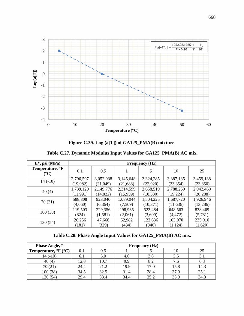
668
Figure C.39. Log (a[T]) of GA125_PMA(B) mixture.
Table C.27. Dynamic Modulus Input Values for GA125_PMA(B) AC mix.
E*, psi (MPa) Frequency (Hz)
Temperature, °F
(°C) 0.1 0.5 1 5 10 25
14 (-10) 2,796,597
(19,982)
3,052,938
(21,049)
3,145,648
(21,688)
3,324,285
(22,920)
3,387,185
(23,354)
3,459,138
(23,850)
40 (4) 1,739,120
(11,991)
2,149,776
(14,822)
2,314,599
(15,959)
2,658,519
(18,330)
2,788,269
(19,224)
2,942,460
(20,288)
70 (21) 588,808
(4,060)
923,040
(6,364)
1,089,044
(7,509)
1,504,225
(10,371)
1,687,720
(11.636)
1,926,946
(13,286)
100 (38) 119,503
(824)
229,356
(1,581)
298,935
(2,061)
523,484
(3,609)
648,563
(4,472)
838,469
(5,781)
130 (54) 26,256
(181)
47,668
(329)
62,982
(434)
122,636
(846)
163,070
(1,124)
235,010
(1,620)
Table C.28. Phase Angle Input Values for GA125_PMA(B) AC mix.
Phase Angle, ° Frequency (Hz)
Temperature, °F (°C) 0.1 0.5 1 5 10 25
14 (-10) 6.1 5.0 4.6 3.8 3.5 3.1
40 (4) 12.8 10.7 9.9 8.2 7.6 6.8
70 (21) 24.4 21.2 19.9 17.0 15.8 14.3
100 (38) 34.5 32.5 31.4 28.4 27.0 25.1
130 (54) 29.4 33.4 34.4 35.2 35.0 34.3
-4
-3
-2
-1
0
1
2
3
0 10 20 30 40 50 60
Lo
g(a
[T])
Temperature (°C)
log 𝑎 𝑇 =195,698.1765
𝑅 ∗ 𝑙𝑛10(
1
𝑇−
1
20)
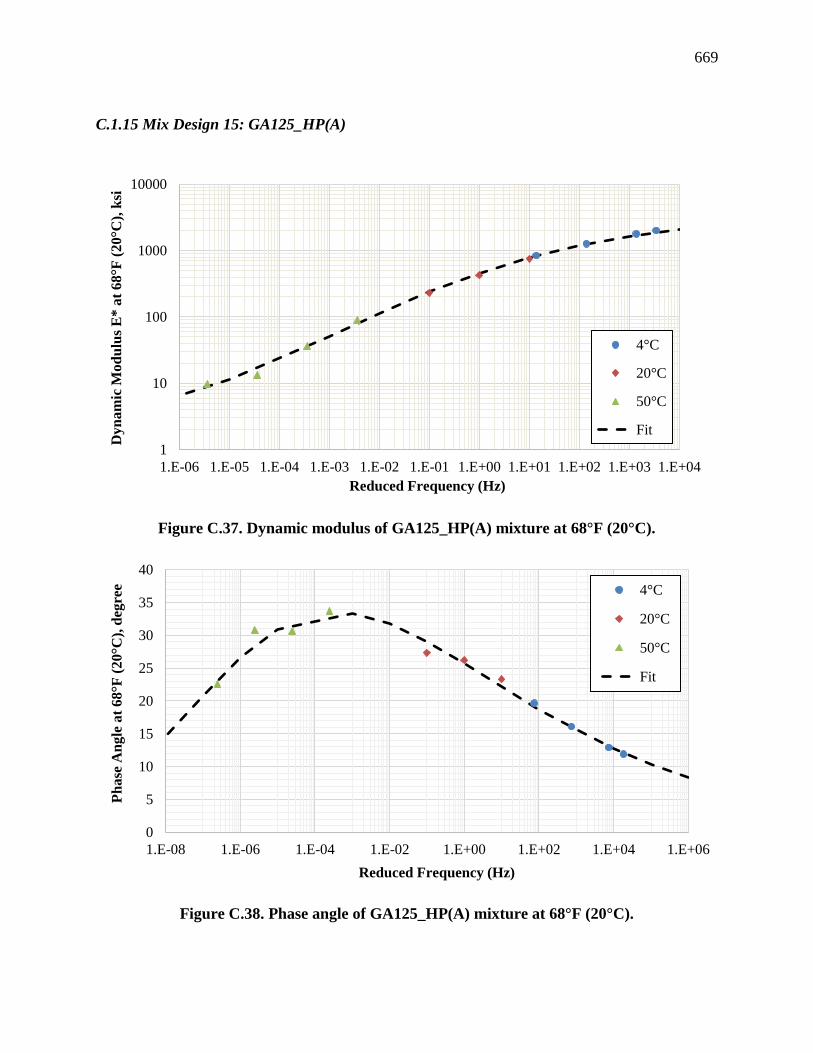
669
C.1.15 Mix Design 15: GA125_HP(A)
Figure C.37. Dynamic modulus of GA125_HP(A) mixture at 68°F (20°C).
Figure C.38. Phase angle of GA125_HP(A) mixture at 68°F (20°C).
1
10
100
1000
10000
1.E-06 1.E-05 1.E-04 1.E-03 1.E-02 1.E-01 1.E+00 1.E+01 1.E+02 1.E+03 1.E+04
Dyn
am
ic M
od
ulu
s E
* a
t 6
8°F
(2
0°C
), k
si
Reduced Frequency (Hz)
4°C
20°C
50°C
Fit
0
5
10
15
20
25
30
35
40
1.E-08 1.E-06 1.E-04 1.E-02 1.E+00 1.E+02 1.E+04 1.E+06
Ph
ase
An
gle
at
68
°F (
20
°C),
deg
ree
Reduced Frequency (Hz)
4°C
20°C
50°C
Fit
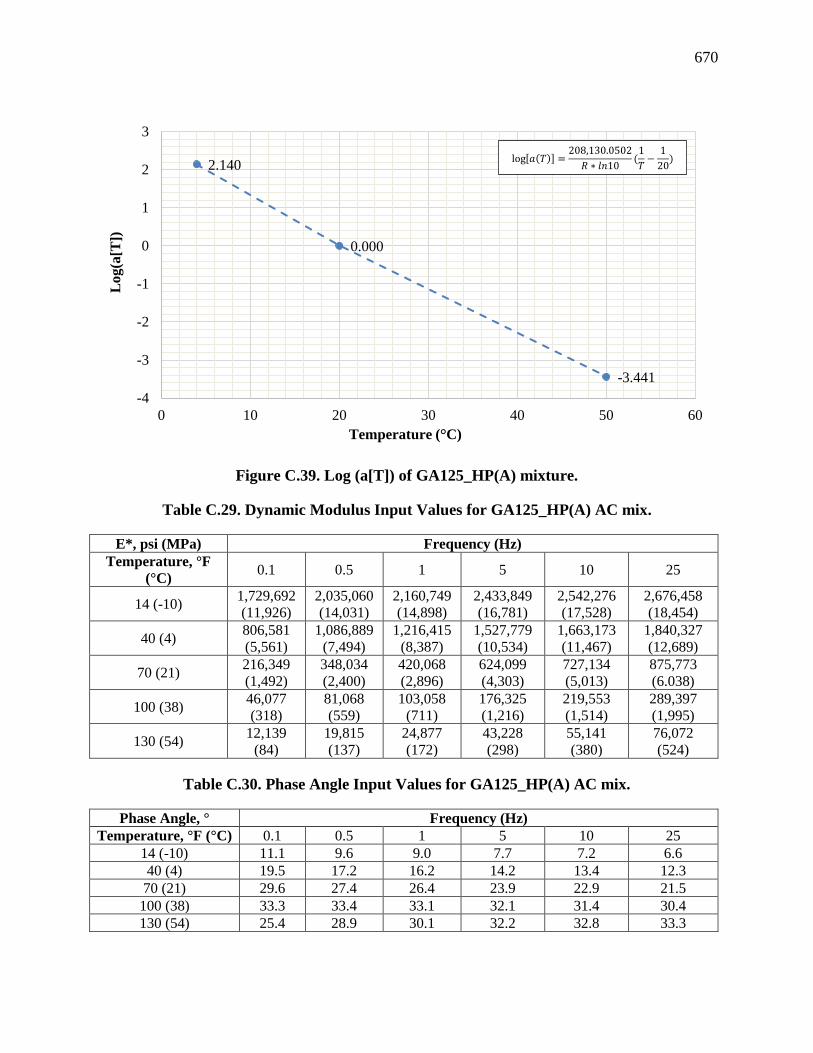
670
Figure C.39. Log (a[T]) of GA125_HP(A) mixture.
Table C.29. Dynamic Modulus Input Values for GA125_HP(A) AC mix.
E*, psi (MPa) Frequency (Hz)
Temperature, °F
(°C) 0.1 0.5 1 5 10 25
14 (-10) 1,729,692
(11,926)
2,035,060
(14,031)
2,160,749
(14,898)
2,433,849
(16,781)
2,542,276
(17,528)
2,676,458
(18,454)
40 (4) 806,581
(5,561)
1,086,889
(7,494)
1,216,415
(8,387)
1,527,779
(10,534)
1,663,173
(11,467)
1,840,327
(12,689)
70 (21) 216,349
(1,492)
348,034
(2,400)
420,068
(2,896)
624,099
(4,303)
727,134
(5,013)
875,773
(6.038)
100 (38) 46,077
(318)
81,068
(559)
103,058
(711)
176,325
(1,216)
219,553
(1,514)
289,397
(1,995)
130 (54) 12,139
(84)
19,815
(137)
24,877
(172)
43,228
(298)
55,141
(380)
76,072
(524)
Table C.30. Phase Angle Input Values for GA125_HP(A) AC mix.
Phase Angle, ° Frequency (Hz)
Temperature, °F (°C) 0.1 0.5 1 5 10 25
14 (-10) 11.1 9.6 9.0 7.7 7.2 6.6
40 (4) 19.5 17.2 16.2 14.2 13.4 12.3
70 (21) 29.6 27.4 26.4 23.9 22.9 21.5
100 (38) 33.3 33.4 33.1 32.1 31.4 30.4
130 (54) 25.4 28.9 30.1 32.2 32.8 33.3
2.140
0.000
-3.441
-4
-3
-2
-1
0
1
2
3
0 10 20 30 40 50 60
Lo
g(a
[T])
Temperature (°C)
log 𝑎 𝑇 =208,130.0502
𝑅 ∗ 𝑙𝑛10(
1
𝑇−
1
20)

671
C.1.16 Mix Design 1: GA125_HP(B)
Figure C.37. Dynamic modulus of GA125_HP(B) mixture at 68°F (20°C).
Figure C.38. Phase angle of GA125_HP(B) mixture at 68°F (20°C).
1
10
100
1000
10000
1.E-06 1.E-05 1.E-04 1.E-03 1.E-02 1.E-01 1.E+00 1.E+01 1.E+02 1.E+03 1.E+04
Dyn
am
ic M
od
ulu
s E
* a
t 6
8°F
(2
0°C
), k
si
Reduced Frequency (Hz)
4°C
20°C
50°C
Fit
0
5
10
15
20
25
30
35
40
1.E-08 1.E-06 1.E-04 1.E-02 1.E+00 1.E+02 1.E+04 1.E+06
Ph
ase
An
gle
at
68°F
(2
0°C
), d
egre
e
Reduced Frequency (Hz)
Fit
4°C
20°C
50°C
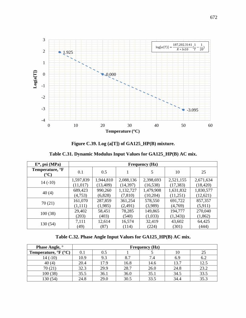
672
Figure C.39. Log (a[T]) of GA125_HP(B) mixture.
Table C.31. Dynamic Modulus Input Values for GA125_HP(B) AC mix.
E*, psi (MPa) Frequency (Hz)
Temperature, °F
(°C) 0.1 0.5 1 5 10 25
14 (-10) 1,597,839
(11,017)
1,944,810
(13,409)
2,088,136
(14,397)
2,398,693
(16,538)
2,521,155
(17,383)
2,671,634
(18,420)
40 (4) 689,423
(4,753)
990,260
(6,828)
1,132,727
(7,810)
1,479,908
(10,204)
1,631,832
(11,251)
1,830,577
(12,621)
70 (21) 161,070
(1,111)
287,859
(1,985)
361,254
(2,491)
578,550
(3,989)
691,722
(4,769)
857,357
(5,911)
100 (38) 29,402
(203)
58,451
(403)
78,285
(540)
149,865
(1,033)
194,777
(1,343))
270,040
(1,862)
130 (54) 7,111
(49)
12,614
(87)
16,574
(114)
32,419
(224)
43,602
(301)
64,425
(444)
Table C.32. Phase Angle Input Values for GA125_HP(B) AC mix.
Phase Angle, ° Frequency (Hz)
Temperature, °F (°C) 0.1 0.5 1 5 10 25
14 (-10) 10.9 9.3 8.7 7.4 6.9 6.2
40 (4) 20.4 17.9 16.8 14.6 13.7 12.5
70 (21) 32.3 29.9 28.7 26.0 24.8 23.2
100 (38) 35.5 36.1 36.0 35.1 34.5 33.5
130 (54) 24.8 29.0 30.5 33.5 34.4 35.3
1.925
0.000
-3.095
-4
-3
-2
-1
0
1
2
3
0 10 20 30 40 50 60
Lo
g(a
[T])
Temperature (°C)
log 𝑎 𝑇 =187,202.3141
𝑅 ∗ 𝑙𝑛10(
1
𝑇−
1
20)

673
C.1.17. Dynamic Modulus and Phase Angle: Summary of All Mixes
Figure C.40. Dynamic modulus master curves of FL95_PMA(A), FL95_PMA(B),
FL95_HP(A), and FL95_HP(B) mixes at 68°F (20°C).
Figure C.41. Phase angle master curves of FL95_PMA(A), FL95_PMA(B), FL95_HP(A),
and FL95_HP(B) mixes at 68°F (20°C).
1
10
100
1000
10000
1.E-06 1.E-04 1.E-02 1.E+00 1.E+02 1.E+04 1.E+06
Dyn
am
ic M
od
ulu
s E
* a
t 6
8°F
(2
0°C
), k
si
Reduced Frequency (Hz)
FL95_PMA(A)
FL95_PMA(B)
FL95_HP(A)
FL95_HP(B)
0
5
10
15
20
25
30
35
40
1.E-08 1.E-06 1.E-04 1.E-02 1.E+00 1.E+02 1.E+04 1.E+06
Ph
ase
An
gle
at
68
°F (
20
°C),
deg
ree
Reduced Frequency (Hz)
FL95_PMA(A)
FL95_PMA(B)
FL95_HP(A)
FL95_HP(B)

674
Figure C.42. Dynamic modulus master curves of FL125_PMA(A), FL125_PMA(B),
FL125_HP(A), and FL125_HP(B) mixes at 68°F (20°C).
Figure C.43. Phase angle master curves of FL125_PMA(A), FL125_PMA(B),
FL125_HP(A), and FL125_HP(B) mixes at 68°F (20°C).
1
10
100
1000
10000
1.E-06 1.E-04 1.E-02 1.E+00 1.E+02 1.E+04 1.E+06
Dyn
am
ic M
od
ulu
s E
* a
t 6
8°F
(2
0°C
), k
si
Reduced Frequency (Hz)
FL125_PMA(A)
FL125_PMA(B)
FL125_HP(A)
FL125_HP(B)
0
5
10
15
20
25
30
35
40
1.E-08 1.E-06 1.E-04 1.E-02 1.E+00 1.E+02 1.E+04 1.E+06
Ph
ase
An
gle
at
68
°F (
20
°C),
deg
ree
Reduced Frequency (Hz)
FL125_PMA(A)
FL125_PMA(B)
FL125_HP(A)
FL125_HP(B)

675
Figure C.44. Dynamic modulus master curves of GA95_PMA(A), GA95_PMA(B),
GA95_HP(A), and GA95_HP(B) mixes at 68°F (20°C).
Figure C.45. Phase angle master curves of GA95_PMA(A), GA95_PMA(B), GA95_HP(A),
and GA95_HP(B) mixes at 68°F (20°C).
1
10
100
1000
10000
1.E-06 1.E-04 1.E-02 1.E+00 1.E+02 1.E+04 1.E+06
Dyn
am
ic M
od
ulu
s E
* a
t 6
8°F
(2
0°C
), k
si
Reduced Frequency (Hz)
GA95_PMA(A)
GA95_PMA(B)
GA95_HP(A)
GA95_HP(B)
0
5
10
15
20
25
30
35
40
1.E-08 1.E-06 1.E-04 1.E-02 1.E+00 1.E+02 1.E+04 1.E+06
Ph
ase
An
gle
at
68
°F (
20
°C),
deg
ree
Reduced Frequency (Hz)
GA95_PMA(A)
GA95_PMA(B)
GA95_HP(A)
GA95_HP(B)
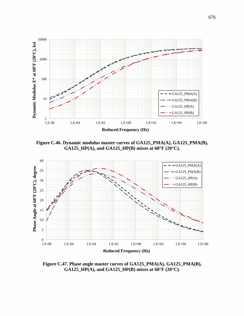
676
Figure C.46. Dynamic modulus master curves of GA125_PMA(A), GA125_PMA(B),
GA125_HP(A), and GA125_HP(B) mixes at 68°F (20°C).
Figure C.47. Phase angle master curves of GA125_PMA(A), GA125_PMA(B),
GA125_HP(A), and GA125_HP(B) mixes at 68°F (20°C).
1
10
100
1000
10000
1.E-06 1.E-04 1.E-02 1.E+00 1.E+02 1.E+04 1.E+06
Dyn
am
ic M
od
ulu
s E
* a
t 6
8°F
(2
0°C
), k
si
Reduced Frequency (Hz)
GA125_PMA(A)
GA125_PMA(B)
GA125_HP(A)
GA125_HP(B)
0
5
10
15
20
25
30
35
40
1.E-08 1.E-06 1.E-04 1.E-02 1.E+00 1.E+02 1.E+04 1.E+06
Ph
ase
An
gle
at
68
°F (
20
°C),
deg
ree
Reduced Frequency (Hz)
GA125_PMA(A)
GA125_PMA(B)
GA125_HP(A)
GA125_HP(B)

677
C.2 Repeated Triaxial Load (RLT) Test - Rutting
Figure C.48. Rutting raw and modeled data of FL95_PMA(A) at 86, 104, and 122°F (30, 40,
and 50°C).
Figure C.49. Rutting raw and modeled data of FL95_PMA(B) at 86, 104, and 122°F (30, 40,
and 50°C).
1
10
100
1000
100 1,000 10,000 100,000 1,000,000
εp/ε
r
Number of CyclesRaw Data @ 86°F (30°C) Modeled Data @86°F (30°C)Raw Data at 104°F (40°C) Modeled Data @104°F (40°C)Raw Data @ 122°F (50°C) Modeled Data @122°F (50°C)
1
10
100
1000
100 1,000 10,000 100,000 1,000,000
εp/ε
r
Number of CyclesRaw Data @86°F (30°C) Modeled Data @86°F (30°C)Raw Data @104°F (40°C) Modeled Data @104°F (40°C)Raw Data @122°F (50°C) Modeled Data @122°F (50°C)
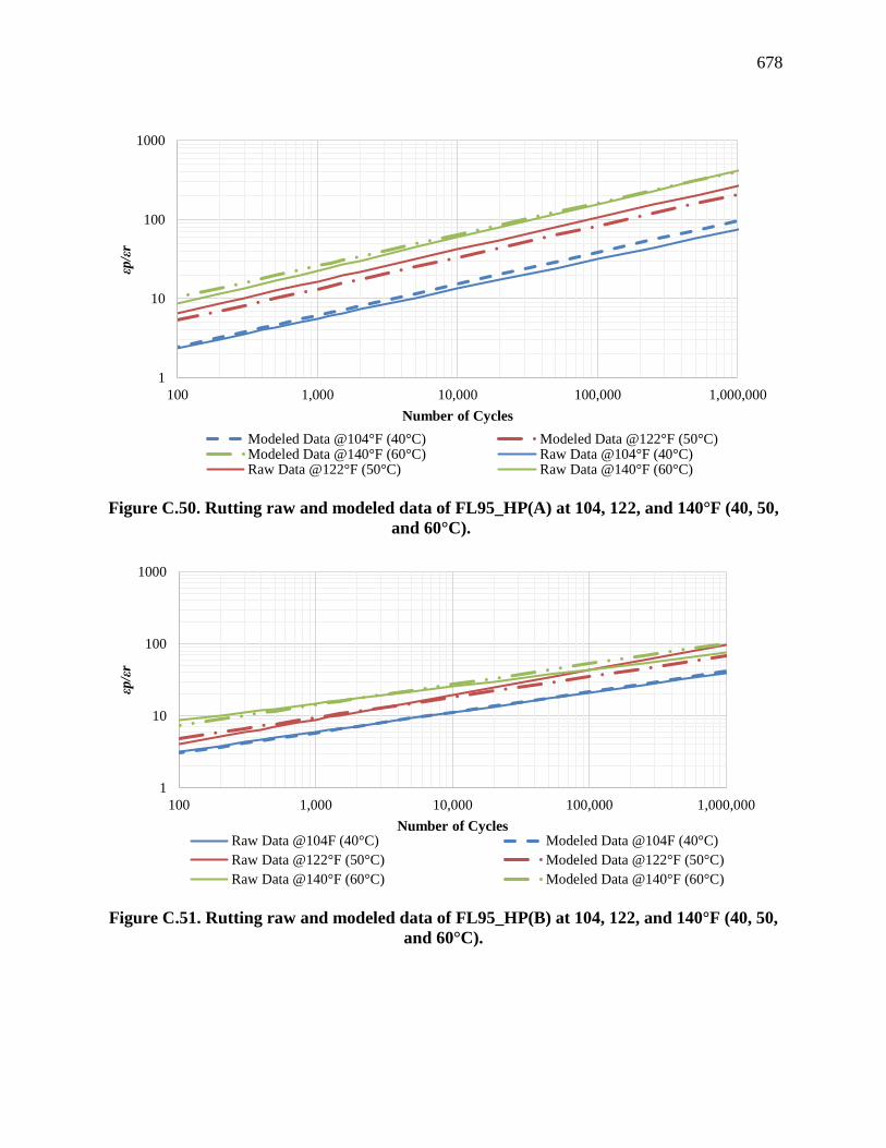
678
Figure C.50. Rutting raw and modeled data of FL95_HP(A) at 104, 122, and 140°F (40, 50,
and 60°C).
Figure C.51. Rutting raw and modeled data of FL95_HP(B) at 104, 122, and 140°F (40, 50,
and 60°C).
1
10
100
1000
100 1,000 10,000 100,000 1,000,000
εp/ε
r
Number of Cycles
Modeled Data @104°F (40°C) Modeled Data @122°F (50°C)Modeled Data @140°F (60°C) Raw Data @104°F (40°C)Raw Data @122°F (50°C) Raw Data @140°F (60°C)
1
10
100
1000
100 1,000 10,000 100,000 1,000,000
εp/ε
r
Number of CyclesRaw Data @104F (40°C) Modeled Data @104F (40°C)
Raw Data @122°F (50°C) Modeled Data @122°F (50°C)
Raw Data @140°F (60°C) Modeled Data @140°F (60°C)

679
Figure C.52. Rutting raw and modeled data of FL125_PMA(A) at 86, 104, and 122°F (30,
40, and 50°C).
Figure C.53. Rutting raw and modeled data of FL125_PMA(B) at 86, 104, and 122°F (30,
40, and 50°C).
1
10
100
1000
100 1,000 10,000 100,000 1,000,000
εp/ε
r
Number of CyclesRaw Data @86°F (30°C) Modeled @86°F (30°C)
Raw Data @104°F (40°C) Modeled @104°F (40°C)
Raw Data @144°F (50°C) Modeled @144°F (50°C)
1
10
100
1000
100 1,000 10,000 100,000 1,000,000
εp/ε
r
Number of Cycles
Raw Data @86°F (30°C) Modeled Data @86°F (30°C)Raw Data @102°F (40°C) Modeled Data @102°F (40°C)Raw Data @122°F (50°C) Modeled Data @122°F (50°C)

680
Figure C.54. Rutting raw and modeled data of FL125_HP(A) at 104, 122, and 140°F (40,
50, and 60°C).
Figure C.55. Rutting raw and modeled data of FL125_HP(B) at 104, 122, and 140°F (40, 50,
and 60°C).
1
10
100
1000
100 1,000 10,000 100,000 1,000,000
εp/ε
r
Number of CyclesRaw Data @86°F (30°C) Modeled Data @86°F (30°C)Raw Data @104°F (40°C) Modeled Data @104°F (40°C)Raw Data @122°F (50°C) Modeled Data @122°F (50°C)
1
10
100
1000
100 1,000 10,000 100,000 1,000,000
εp/ε
r
Number of Cycles
Raw Data @104°F (40°C) Modeled Data @104°F (40°C)Raw Data @122°F (50°C) Modeled Data @122°F (50°C)Raw Data @140°F (60°C) Modeled Data @140°F (60°C)

681
Figure C.56. Rutting raw and modeled data of GA95_PMA(A) at 104, 122, and 140°F (40,
50, and 60°C).
Figure C.57. Rutting raw and modeled data of GA95_PMA(B) at 104, 122, and 140°F (40,
50, and 60°C).
1
10
100
1000
100 1,000 10,000 100,000 1,000,000
εp/ε
r
Number of Cycles
Raw Data @104°F (40°C) Modeled Data @104°F (40°C)Raw Data @122°F (50°C) Modeled Data @122°F (50°C)Raw Data @140°F (60°C) Modeled Data @140°F (60°C)
1
10
100
1000
100 1,000 10,000 100,000 1,000,000
εp/ε
r
Number of Cycles
Raw Data @104°F (40°C) Modeled Data @104°F (40°C)Raw Data @122°F (50°C) Modeled Data @122°F (50°C)Raw Data @140°F (60°C) Modeled Data @140°F (60°C)

682
Figure C.58. Rutting raw and modeled data of GA95_HP(A) at 104, 122, and 140°F (40, 50,
and 60°C).
Figure C.59. Rutting raw and modeled data of GA95_HP(B) at 104, 122, and 140°F (40, 50,
and 60°C).
1
10
100
1000
100 1,000 10,000 100,000 1,000,000
εp/ε
r
Number of Cycles
Raw Data @104°F (40°C) Modeled Data @104°F (40°C)
Raw Data @122°F (50°C) Modeled Data @122°F (50°C)
Raw Data @140°F (60°C) Modeled Data @140°F (60°C)
1
10
100
1000
100 1,000 10,000 100,000 1,000,000
εp/ε
r
Number of Cycles
Raw Data @104°F (40°C) Modeled Data @104°F (40°C)Raw Data @122°F (50°C) Modeled Data @122°F (50°C)Raw Data @140°F (60°C) Modeled Data @140°F (60°C)

683
Figure C.60. Rutting raw and modeled data of GA125_PMA(A) at 104, 122, and 140°F (40,
50, and 60°C).
Figure C.61. Rutting raw and modeled data of GA125_PMA(B) at 104, 122, and 140°F (40,
50, and 60°C).
1
10
100
1000
100 1,000 10,000 100,000 1,000,000
εp/ε
r
Number of Cycles
Raw Data @104°F (40°C) Modeled Data @104°F (40°C)
Raw Data @122°F (50°C) Modeled Data @122°F (50°C)
1
10
100
1000
100 1,000 10,000 100,000 1,000,000
εp/ε
r
Number of CyclesRaw Data @104°F (40°C) Modeled Data @104°F (40°C)Raw Data @122°F (50°C) Modeled Data @122°F (50°C)Raw Data @140°F (60°C) Modeled Data @140°F (60°C)
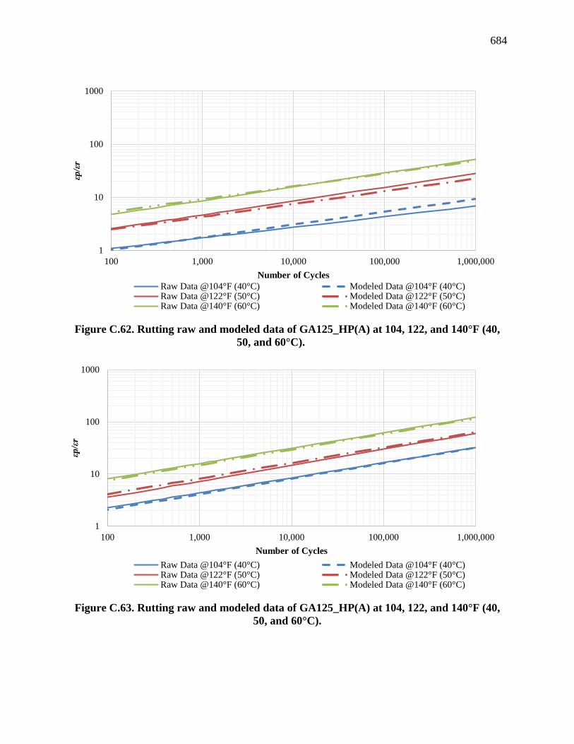
684
Figure C.62. Rutting raw and modeled data of GA125_HP(A) at 104, 122, and 140°F (40,
50, and 60°C).
Figure C.63. Rutting raw and modeled data of GA125_HP(A) at 104, 122, and 140°F (40,
50, and 60°C).
1
10
100
1000
100 1,000 10,000 100,000 1,000,000
εp/ε
r
Number of Cycles
Raw Data @104°F (40°C) Modeled Data @104°F (40°C)Raw Data @122°F (50°C) Modeled Data @122°F (50°C)Raw Data @140°F (60°C) Modeled Data @140°F (60°C)
1
10
100
1000
100 1,000 10,000 100,000 1,000,000
εp/ε
r
Number of Cycles
Raw Data @104°F (40°C) Modeled Data @104°F (40°C)Raw Data @122°F (50°C) Modeled Data @122°F (50°C)Raw Data @140°F (60°C) Modeled Data @140°F (60°C)

685
C.3 Flexural Beam Fatigue Test – Fatigue Cracking
Figure C.64. Beam fatigue raw data of FL95_PMA(A) at 55, 70, ad 85°F (13, 20, and 30°C).
y = 3535.5x-0.173
R² = 0.9794
y = 6276.4x-0.194
R² = 0.791
y = 12124x-0.218
R² = 0.9838
100
1000
10000
1.E+03 1.E+04 1.E+05 1.E+06
Fle
xu
ral
Str
ain
(M
icro
ns)
Number of Cycles to Failure
55°F (13°C)
70°F (21°C)
85°F (30°C)

686
Table C.33. Summary of Beam Fatigue Data for FL95_PMA(A) AC mix.
Sample
ID
Air
Voids
Level
(%)
Testing
Temp,
°F (°C)
Dynamic
Modulus E*,
psi (MPa)a
Initial Flexural
Stiffness S0, psi
(MPa)
Initial
Dissipated
Energy E0,
J/m3
Flexural
Strain Level
(micro-strain)
Number
of Cycles
to Failure
S1 6.7 55
(13)
1,380,800
(9,520)
1,207,004
(8,322) 1,385 397 277,237
S2 7.3 55
(13)
1,380,800
(9,520)
1,166,829
(8,045) 2,999 610 32,000
S3 7.6 55
(13)
1,380,800
(9,520)
1,045,287
(7,207) 3,472 697 8,500
S4 6.4 55
(13)
1,380,800
(9,520)
982,196
(6,772) 5,665 790 6,600
S5 7.3 70
(21)
876,600
(6,044)
699,952
(4,826) 1,406 498 162,104
S6 6.7 70
(21)
876,600
(6,044)
678,922
(4,681) 1,258 499 352,494
S7 6.3 70
(21)
876,600
(6,044)
548,533
(3,782) 3,441 801 120,000
S8 7.3 70
(21)
876,600
(6,044)
586,098
(4,041) 7,163 802 59,000
S9 7.2 70
(21)
876,600
(6,044)
585,517
(4,037) 7,163 1,006 16,000
S10 7.2 70
(21)
876,600
(6,044)
663,403
(4,574) 7,307 1,007 7,400
S11 7.3 85
(30)
490,000
(3,378)
312,556
(2,155) 3,215 804 263,000
S12 6.3 85
(30)
490,000
(3,378)
315,312
(2,174) 3,617 901 159,000
S13 7.5 85
(30)
490,000
(3,378)
249,610
(1,721) 3,675 998 83,000
S14 8 85
(30)
490,000
(3,378)
230,030
(1,586) 3,215 1193 45,658
a Dynamic Modulus E* is determined at the testing temperature and a frequency of 10 Hz
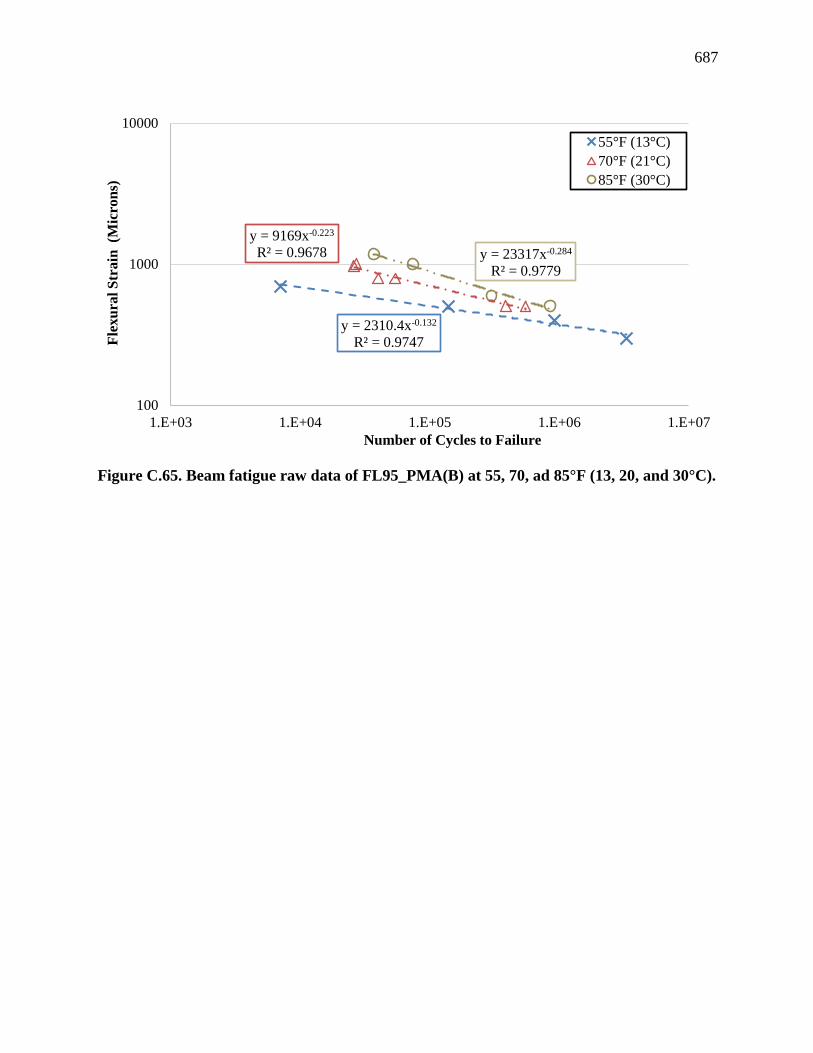
687
Figure C.65. Beam fatigue raw data of FL95_PMA(B) at 55, 70, ad 85°F (13, 20, and 30°C).
y = 2310.4x-0.132
R² = 0.9747
y = 9169x-0.223
R² = 0.9678 y = 23317x-0.284
R² = 0.9779
100
1000
10000
1.E+03 1.E+04 1.E+05 1.E+06 1.E+07
Fle
xu
ral
Str
ain
(M
icro
ns)
Number of Cycles to Failure
55°F (13°C)
70°F (21°C)
85°F (30°C)

688
Table C.34. Summary of Beam Fatigue Data for FL95_PMA(B) AC mix.
Sample
ID
Air
Voids
Level
(%)
Testing
Temp,
°F (°C)
Dynamic
Modulus E*,
psi (MPa)a
Initial Flexural
Stiffness S0, psi
(MPa)
Initial
Dissipated
Energy E0,
J/m3
Flexural
Strain Level
(micro-strain)
Number
of Cycles
to Failure
S1 7.7 55
(13)
1,422,400
(9,807)
1,216,867
(8,390) 661 298 3,300,000
S2 7.9 55
(13)
1,422,400
(9,807)
1,048,898
(7,225) 1,274 400 917,000
S3 7.7 55
(13)
1,422,400
(9,807)
1,001,921
(6,908) 1,871 499 140,000
S4 7.8 55
(13)
1,422,400
(9,807)
981,180
(6,765) 3,580 696 7,000
S5 7.6 70
(21)
916,900
(6,322)
636,281
(4,387) 1,554 499 551,000
S6 7.6 70
(21)
916,900
(6,322)
771,746
(5,321) 1,942 504 386,000
S7 7.6 70
(21)
916,900
(6,322)
476,159
(3,283) 4,486 789 40,000
S8 8 70
(21)
916,900
(6,322)
507,052
(3,496) 9,096 792 54,000
S9 7.6 70
(21)
916,900
(6,322)
475,144
(3,276) 5,495 971 26,000
S10 7.8 70
(21)
916,900
(6,322)
444,541
(3,065) 4,017 1005 27,000
S11 8 85
(30)
524,300
(3,615)
285,289
(1,967) 3,252 998 74,000
S12 8.1 85
(30)
524,300
(3,615)
271,511
(1,872) 4,053 1,180 46,000
a Dynamic Modulus E* is determined at the testing temperature and a frequency of 10 Hz
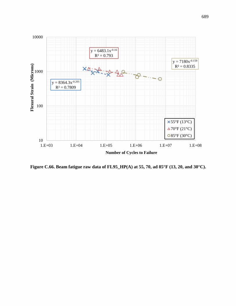
689
Figure C.66. Beam fatigue raw data of FL95_HP(A) at 55, 70, ad 85°F (13, 20, and 30°C).
y = 8364.3x-0.201
R² = 0.7809
y = 6483.1x-0.16
R² = 0.793
y = 7180x-0.159
R² = 0.8335
10
100
1000
10000
1.E+03 1.E+04 1.E+05 1.E+06 1.E+07 1.E+08
Fle
xu
ral
Str
ain
(M
icro
ns)
Number of Cycles to Failure
55°F (13°C)
70°F (21°C)
85°F (30°C)
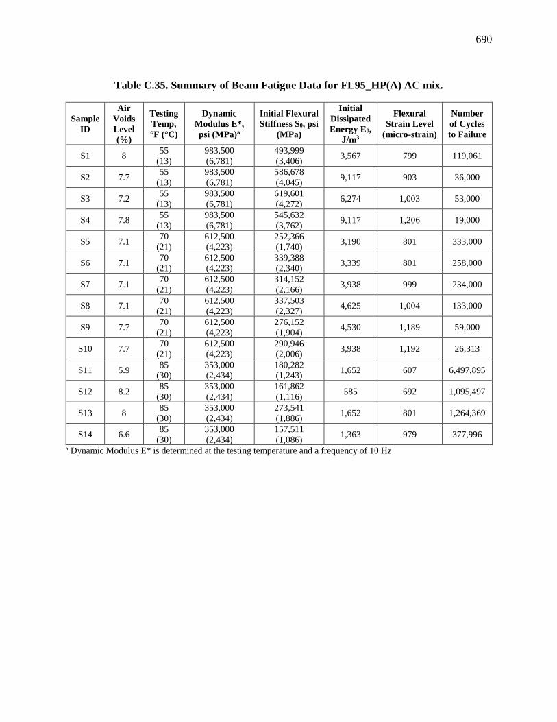
690
Table C.35. Summary of Beam Fatigue Data for FL95_HP(A) AC mix.
Sample
ID
Air
Voids
Level
(%)
Testing
Temp,
°F (°C)
Dynamic
Modulus E*,
psi (MPa)a
Initial Flexural
Stiffness S0, psi
(MPa)
Initial
Dissipated
Energy E0,
J/m3
Flexural
Strain Level
(micro-strain)
Number
of Cycles
to Failure
S1 8 55
(13)
983,500
(6,781)
493,999
(3,406) 3,567 799 119,061
S2 7.7 55
(13)
983,500
(6,781)
586,678
(4,045) 9,117 903 36,000
S3 7.2 55
(13)
983,500
(6,781)
619,601
(4,272) 6,274 1,003 53,000
S4 7.8 55
(13)
983,500
(6,781)
545,632
(3,762) 9,117 1,206 19,000
S5 7.1 70
(21)
612,500
(4,223)
252,366
(1,740) 3,190 801 333,000
S6 7.1 70
(21)
612,500
(4,223)
339,388
(2,340) 3,339 801 258,000
S7 7.1 70
(21)
612,500
(4,223)
314,152
(2,166) 3,938 999 234,000
S8 7.1 70
(21)
612,500
(4,223)
337,503
(2,327) 4,625 1,004 133,000
S9 7.7 70
(21)
612,500
(4,223)
276,152
(1,904) 4,530 1,189 59,000
S10 7.7 70
(21)
612,500
(4,223)
290,946
(2,006) 3,938 1,192 26,313
S11 5.9 85
(30)
353,000
(2,434)
180,282
(1,243) 1,652 607 6,497,895
S12 8.2 85
(30)
353,000
(2,434)
161,862
(1,116) 585 692 1,095,497
S13 8 85
(30)
353,000
(2,434)
273,541
(1,886) 1,652 801 1,264,369
S14 6.6 85
(30)
353,000
(2,434)
157,511
(1,086) 1,363 979 377,996
a Dynamic Modulus E* is determined at the testing temperature and a frequency of 10 Hz

691
Figure C.67. Beam fatigue raw data of FL95_HP(B) at 40, 55, ad 70°F (4, 13, and 20°C).
y = 8265.4x-0.225
R² = 0.9622
y = 7193.4x-0.183
R² = 0.5882 y = 15630x-0.217
R² = 0.9107
10
100
1000
10000
1.E+03 1.E+04 1.E+05 1.E+06 1.E+07 1.E+08
Fle
xu
ral
Str
ain
(M
icro
ns)
Number of Cycles to Failure
40°F (4°C)
55°F (13°C)
70°F (21°C)

692
Table C.36. Summary of Beam Fatigue Data for FL95_HP(B) AC mix.
Sample
ID
Air
Voids
Level
(%)
Testing
Temp,
°F (°C)
Dynamic
Modulus E*,
psi (MPa)a
Initial Flexural
Stiffness S0, psi
(MPa)
Initial
Dissipated
Energy E0,
J/m3
Flexural
Strain Level
(micro-strain)
Number
of Cycles
to Failure
S1 7.6 40
(4)
1,357,000
(9356)
1,100,836
(7,590) 862 400 759,651
S2 7.5 40
(4)
1,357,000
(9356)
1,259,073
(8,681) 2,059 550 130,000
S3 7.6 40
(4)
1,357,000
(9356)
985,967
(6,798) 4,014 701 71,000
S4 7.4 55
(13)
877,800
(6,052)
531,853
(3,667) 4,371 802 182,000
S5 7.1 55
(13)
877,800
(6,052)
636,281
(4,387) 9,487 849 44,000
S6 7.6 55
(13)
877,800
(6,052)
498,930
(3,440) 5,643 1,003 71,000
S7 7.6 55
(13)
877,800
(6,052)
440,625
(3,038) 9,487 1,252 25,000
S8 8 70
(21)
513,200
(3538)
258,022
(1,779) 1578 746 928,000
S9 7.2 70
(21)
513,200
(3538)
249,175
(1,718) 1813 750 988,000
S10 8 70
(21)
513,200
(3538)
304,144
(2,097) 4061 976 531,000
S11 8 70
(21)
513,200
(3538)
220,893
(1,523) 2453 994 373,000
S12 7.8 70
(21)
513,200
(3538)
215,381
(1,485) 2453 1,248 163,000
S13 7.8 70
(21)
513,200
(3538)
213,640
(1,473) 4325 1,296 68,000
a Dynamic Modulus E* is determined at the testing temperature and a frequency of 10 Hz

693
Figure C.68. Beam fatigue raw data of FL125_PMA(A) at 55, 70, ad 85°F (13, 20, and
30°C).
y = 3037.3x-0.171
R² = 0.9483
y = 4484.6x-0.173
R² = 0.959y = 50777x-0.351
R² = 0.9946
10
100
1000
10000
1.E+03 1.E+04 1.E+05 1.E+06 1.E+07 1.E+08
Fle
xu
ral
Str
ain
(M
icro
ns)
Number of Cycles to Failure
55°F (12°C)
70°F (21°C)
85°F (30°C)

694
Table C.37. Summary of Beam Fatigue Data for FL125_PMA(A) AC mix.
Sample
ID
Air
Voids
Level
(%)
Testing
Temp,
°F (°C)
Dynamic
Modulus E*,
psi (MPa)a
Initial Flexural
Stiffness S0, psi
(MPa)
Initial
Dissipated
Energy E0,
J/m3
Flexural
Strain Level
(micro-strain)
Number
of Cycles
to Failure
S1 7.2 55
(13)
1,471,400
(10,145)
1,184,233
(8,165) 1,294 400 118,000
S2 7.5 55
(13)
1,471,400
(10,145)
1,264,584
(8,719) 1,663 488 57,000
S3 8 55
(13)
1,471,400
(10,145)
986,982
(6,805) 1,663 602 8,900
S4 7.5 55
(13)
1,471,400
(10,145)
1,386,271
(9,558) 5,058 695 7,200
S5 7 70
(21)
954,600
(6,582)
774,066
(5,337) 1,602 498 312,000
S6 7.9 70
(21)
954,600
(6,582)
703,578
(4,851) 2,793 500 384,000
S7 7.9 70
(21)
954,600
(6,582)
681,967
(4,702) 2,793 696 27,000
S8 8 70
(21)
954,600
(6,582)
615,105
(4,241) 2,802 697 54,000
S9 8 70
(21)
954,600
(6,582)
581,021
(4,006) 4,168 893 13,000
S10 7.7 70
(21)
954,600
(6,582)
627,578
(4,327) 6,416 906 14,000
S11 7.6 85
(30)
556,300
(3836)
267,015
(1,841) 1864 602 317,000
S12 7.8 85
(30)
556,300
(3836)
284,854
(1,964) 3874 697 191,000
S13 7.9 85
(30)
556,300
(3836)
231,625
(1,597) 3398 812 133,000
S14 7.3 85
(30)
556,300
(3836)
277,167
(1,911) 3874 905 101,000
S15 8.1 31700 556,300
(3836)
245,114
(1,690) 3618 1,002 71,000
a Dynamic Modulus E* is determined at the testing temperature and a frequency of 10 Hz

695
Figure C.69. Beam fatigue raw data of FL125_PMA(B) at 55, 70, ad 85°F (13, 20, and
30°C).
y = 2349.5x-0.16
R² = 0.9099
y = 4438.1x-0.193
R² = 0.8872y = 8208x-0.21
R² = 0.9833
10
100
1000
10000
1.E+03 1.E+04 1.E+05 1.E+06 1.E+07 1.E+08
Fle
xu
ral
Str
ain
(M
icro
ns)
Number of Cycles to Failure
55°F (12°C)
70°F (21°C)
85°F (30°C)

696
Table C.38. Summary of Beam Fatigue Data for FL125_PMA(B) AC mix.
Sample
ID
Air
Voids
Level
(%)
Testing
Temp,
°F (°C)
Dynamic
Modulus E*,
psi (MPa)a
Initial Flexural
Stiffness S0, psi
(MPa)
Initial
Dissipated
Energy E0,
J/m3
Flexural
Strain Level
(micro-strain)
Number
of Cycles
to Failure
S1 7.4 55
(13)
1,576,300
(10,868)
1,141,012
(7,867) 1,212 295 232,000
S2 7.6 55
(13)
1,576,300
(10,868)
1,215,416
(8,380) 365 298 713,000
S3 7.5 55
(13)
1,576,300
(10,868)
1,096,050
(7,557) 710 390 49,000
S4 8 55
(13)
1,576,300
(10,868)
891,402
(6,146) 1,212 493 13,000
S5 7.5 55
(13)
1,576,300
(10,868)
966,967
(6,666) 2,712 595 10,001
S6 8 70
(21)
1,036,600
(7,147)
574,930
(3,964) 365 347 524,000
S7 7.4 70
(21)
1,036,600
(7,147)
771,891
(5,322) 796 353 345,000
S8 7.8 70
(21)
1,036,600
(7,147)
666,593
(4,596) 2,377 491 58,000
S9 8 70
(21)
1,036,600
(7,147)
590,739
(4,073) 1,213 509 135,000
S10 7.5 70
(21)
1,036,600
(7,147)
607,853
(4,191) 2,377 692 10,001
S11 7.6 70
(21)
1,036,600
(7,147)
627,578
(4,327) 2,550 693 32,000
S12 7.8 85
(30)
609,300
(4,201)
368,976
(2,544) 3,350 597 239,000
S13 8.3 85
(30)
609,300
(4,201)
330,831
(2,281) 1,407 693 148,000
S14 7.3 85
(30)
609,300
(4,201)
350,701
(2,418) 3,350 795 72,000
S15 8.3 85
(30)
609,300
(4,201)
321,404
(2,216) 2,696 892 37,000
a Dynamic Modulus E* is determined at the testing temperature and a frequency of 10 Hz
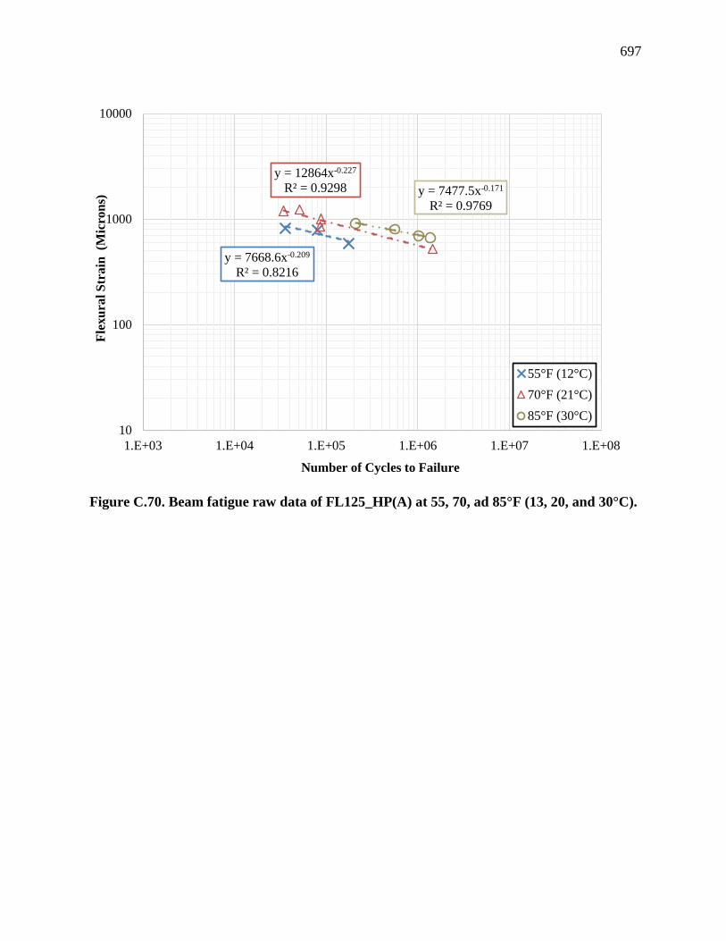
697
Figure C.70. Beam fatigue raw data of FL125_HP(A) at 55, 70, ad 85°F (13, 20, and 30°C).
y = 7668.6x-0.209
R² = 0.8216
y = 12864x-0.227
R² = 0.9298 y = 7477.5x-0.171
R² = 0.9769
10
100
1000
10000
1.E+03 1.E+04 1.E+05 1.E+06 1.E+07 1.E+08
Fle
xu
ral
Str
ain
(M
icro
ns)
Number of Cycles to Failure
55°F (12°C)
70°F (21°C)
85°F (30°C)

698
Table C.39. Summary of Beam Fatigue Data for FL125_HP(A) AC mix.
Sample
ID
Air
Voids
Level
(%)
Testing
Temp,
°F (°C)
Dynamic
Modulus E*,
psi (MPa)a
Initial Flexural
Stiffness S0, psi
(MPa)
Initial
Dissipated
Energy E0,
J/m3
Flexural
Strain Level
(micro-strain)
Number
of Cycles
to Failure
S1 7.8 55
(13)
929,100
(6,406)
811,341
(5,594) 1,516 588 177,000
S2 7.8 55
(13)
929,100
(6,406)
679,937
(4,688) 1,516 792 81,000
S3 7.8 55
(13)
929,100
(6,406)
588,273
(4,056) 2,423 821 36,000
S4 7.6 70
(21)
574,800
(3,963)
332,717
(2,294) 2,476 525 1,448,169
S5 7.4 70
(21)
574,800
(3,963)
354,182
(2,442) 3,172 848 86,000
S6 7.6 70
(21)
574,800
(3,963)
302,404
(2,085) 3,804 1,000 88,000
S7 7.3 70
(21)
574,800
(3,963)
313,572
(2,162) 5,504 1,195 34,000
S8 7.3 70
(21)
574,800
(3,963)
336,778
(2,322) 3,172 1,230 51,000
S9 7.8 85
(30)
328,700
(2,266)
213,496
(1,472) 628 664 1,367,721
S10 7.7 85
(30)
328,700
(2,266)
186,229
(1,284) 744 696 1,024,926
S11 7.7 85
(30)
328,700
(2,266)
198,992
(1,372) 1,446 806 558,104
S12 7.7 85
(30)
328,700
(2,266)
181,297
(1,250) 628 909 209,592
a Dynamic Modulus E* is determined at the testing temperature and a frequency of 10 Hz
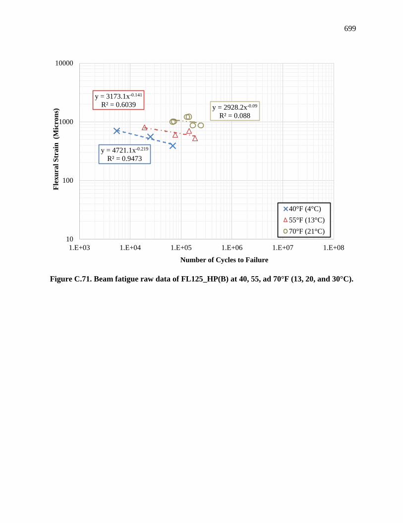
699
Figure C.71. Beam fatigue raw data of FL125_HP(B) at 40, 55, ad 70°F (13, 20, and 30°C).
y = 4721.1x-0.219
R² = 0.9473
y = 3173.1x-0.141
R² = 0.6039 y = 2928.2x-0.09
R² = 0.088
10
100
1000
10000
1.E+03 1.E+04 1.E+05 1.E+06 1.E+07 1.E+08
Fle
xu
ral
Str
ain
(M
icro
ns)
Number of Cycles to Failure
40°F (4°C)
55°F (13°C)
70°F (21°C)

700
Table C.40. Summary of Beam Fatigue Data for FL125_HP(B) AC mix.
Sample
ID
Air
Voids
Level
(%)
Testing
Temp,
°F (°C)
Dynamic
Modulus E*,
psi (MPa)a
Initial Flexural
Stiffness S0, psi
(MPa)
Initial
Dissipated
Energy E0,
J/m3
Flexural
Strain Level
(micro-strain)
Number
of Cycles
to Failure
S1 7.7 40
(4)
1,643,800
(11,334)
1,336,088
(9,212) 756 362 69,000
S2 7.7 40
(4)
1,643,800
(11,334)
1,004,386
(6,925) 1,957 553 25,000
S3 7.7 40
(4)
1,643,800
(11,334)
921,280
(6,352) 3,127 695 5,400
S4 7.4 55
(13)
1,091,400
(7,525)
634,395
(4,374) 1,357 524 188,000
S5 6.8 55
(13)
1,091,400
(7,525)
847,601
(5,844) 2,363 598 77,000
S6 7.7 55
(13)
1,091,400
(7,525)
561,441
(3,871) 2,809 699 143,000
S7 8.2 55
(13)
1,091,400
(7,525)
607,998
(4,192) 2,363 802 19,000
S8 7.9 70
(21)
640,900
(4,419)
294,610
(1,721) 2,676 867 169,000
S9 7.8 70
(21)
640,900
(4,419)
296,457
(2,044) 3,262 869 244,000
S10 7.3 70
(21)
640,900
(4,419)
336,052
(2,317) 4,221 999 68,000
S11 8.7 70
(21)
640,900
(4,419)
221,473
(1,527) 3,262 1,014 72,000
S12 7.8 70
(21)
640,900
(4,419)
202,473
(1,396) 5,160 1,210 130,000
S13 7.8 70
(21)
640,900
(4,419)
222,778
(1,536) 6,241 1,218 142,000
a Dynamic Modulus E* is determined at the testing temperature and a frequency of 10 Hz
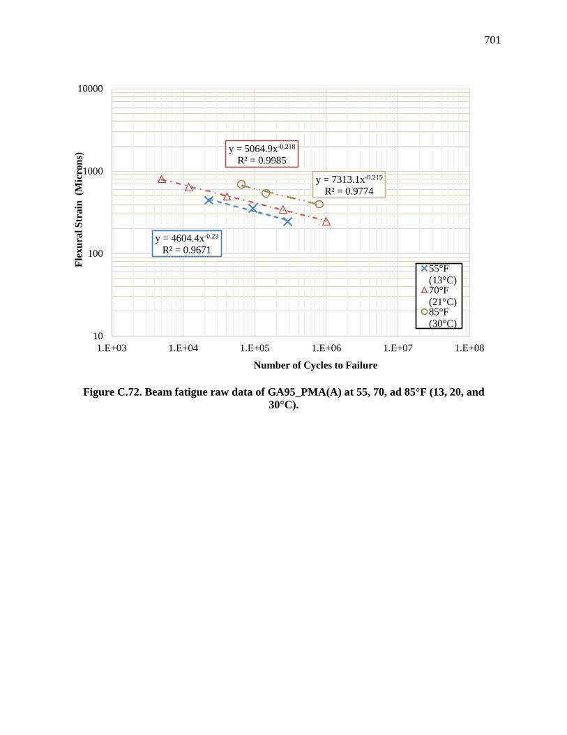
701
Figure C.72. Beam fatigue raw data of GA95_PMA(A) at 55, 70, ad 85°F (13, 20, and
30°C).
y = 4604.4x-0.23
R² = 0.9671
y = 5064.9x-0.218
R² = 0.9985
y = 7313.1x-0.215
R² = 0.9774
10
100
1000
10000
1.E+03 1.E+04 1.E+05 1.E+06 1.E+07 1.E+08
Fle
xu
ral
Str
ain
(M
icro
ns)
Number of Cycles to Failure
55°F
(13°C)70°F
(21°C)85°F
(30°C)

702
Table C.41. Summary of Beam Fatigue Data for GA95_PMA(A) AC mix.
Sample
ID
Air
Voids
Level
(%)
Testing
Temp,
°F (°C)
Dynamic
Modulus E*,
psi (MPa)a
Initial Flexural
Stiffness S0, psi
(MPa)
Initial
Dissipated
Energy E0,
J/m3
Flexural
Strain Level
(micro-strain)
Number
of Cycles
to Failure
S1 7 55
(13)
2,128,000
(14,672)
2,265,635
(15,621) 476 246 287,000
S2 7 55
(13)
2,128,000
(14,672)
1,801,369
(12,420) 1,307 350 94,000
S3 7.9 55
(13)
2,128,000
(14,672)
1,933,353
(13,330) 1,898 443 23,000
S4 7.9 70
(21)
1,506,800
(10,389)
1,291,126
(8,902) 228 247 1,000,000
S5 8.1 70
(21)
1,506,800
(10,389)
1,274,882
(8,790) 2,858 345 249,000
S6 7.7 70
(21)
1,506,800
(10,389)
1,156,821
(7,976) 1,692 492 41,000
S7 8 70
(21)
1,506,800
(10,389)
1,059,356
(7,304) 2,858 643 12,000
S8 6.9 70
(21)
1,506,800
(10,389)
1,209,615
(8,340) 7,322 805 5,000
S9 7.5 85
(30)
932,700
(6,431)
743,754
(5,128) 948 397 801,000
S10 7.6 85
(30)
932,700
(6,431)
689,074
(4,751) 1,661 541 142,000
S11 7.7 85
(30)
932,700
(6,431)
683,853
(4,717) 2,887 694 65,000
a Dynamic Modulus E* is determined at the testing temperature and a frequency of 10 Hz

703
Figure C.73. Beam fatigue raw data of GA95_PMA(B) at 55, 70, ad 85°F (13, 20, and 30°C)
y = 2907.2x-0.181
R² = 0.992
y = 3344.6x-0.17
R² = 0.9864
y = 7020.4x-0.218
R² = 0.9122
10
100
1000
10000
1.E+03 1.E+04 1.E+05 1.E+06 1.E+07 1.E+08
Fle
xu
ral
Str
ain
(M
icro
ns)
Number of Cycles to Failure
55°F (13°C)
70°F (21°C)
85°F (30°C)

704
Table C.42. Summary of Beam Fatigue Data for GA95_PMA(B) AC mix.
Sample
ID
Air
Voids
Level
(%)
Testing
Temp,
°F (°C)
Dynamic
Modulus E*,
psi (MPa)a
Initial Flexural
Stiffness S0, psi
(MPa)
Initial
Dissipated
Energy E0,
J/m3
Flexural
Strain Level
(micro-strain)
Number
of Cycles
to Failure
S1 7.9 55
(13)
2,280,800
(15,725)
1,775,262
(12,240) 459 249 737,000
S2 7.9 55
(13)
2,280,800
(15,725)
1,862,720
(12,843) 1,402 349 145,000
S3 8 55
(13)
2,280,800
(15,725)
1,832,407
(12,634) 2,333 449 28,000
S4 8.1 70
(21)
1,677,800
(11,568)
1,180,462
(8,139) 392 248 5,813,780
S5 7.9 70
(21)
1,677,800
(11,568)
1,293,447
(8,918) 3,290 347 409,000
S6 7.9 70
(21)
1,677,800
(11,568)
994,379
(8,656) 1,690 493 59,000
S7 7.7 70
(21)
1,677,800
(11,568)
1,114,760
(7,686) 3,290 649 21,000
S8 7.5 70
(21)
1,677,800
(11,568)
1,074,295
(7,407) 8,233 808 4,600
S9 7.9 85
(30)
1,088,700
(7,506)
580,731
(4,004) 789 394 585,000
S10 7.9 85
(30)
1,088,700
(7,506)
610,754
(4,211) 1,753 539 85,000
S11 7.7 85
(30)
1,088,700
(7,506)
581,456
(4,009) 2,742 697 56,000
a Dynamic Modulus E* is determined at the testing temperature and a frequency of 10 Hz

705
Figure C.74. Beam fatigue raw data of GA95_HP(A) at 40, 55, ad 70°F (4, 13, and 21°C).
y = 10094x-0.255
R² = 0.9843
y = 9529.3x-0.231
R² = 0.9855y = 13085x-0.238
R² = 0.8528
10
100
1000
10000
1.E+03 1.E+04 1.E+05 1.E+06 1.E+07 1.E+08
Fle
xu
ral
Str
ain
(M
icro
ns)
Number of Cycles to Failure
40°F 55°F
70°F
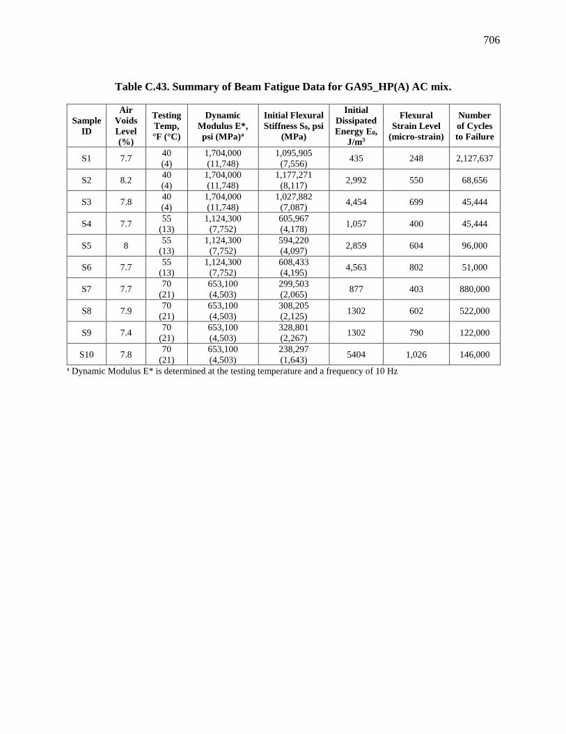
706
Table C.43. Summary of Beam Fatigue Data for GA95_HP(A) AC mix.
Sample
ID
Air
Voids
Level
(%)
Testing
Temp,
°F (°C)
Dynamic
Modulus E*,
psi (MPa)a
Initial Flexural
Stiffness S0, psi
(MPa)
Initial
Dissipated
Energy E0,
J/m3
Flexural
Strain Level
(micro-strain)
Number
of Cycles
to Failure
S1 7.7 40
(4)
1,704,000
(11,748)
1,095,905
(7,556) 435 248 2,127,637
S2 8.2 40
(4)
1,704,000
(11,748)
1,177,271
(8,117) 2,992 550 68,656
S3 7.8 40
(4)
1,704,000
(11,748)
1,027,882
(7,087) 4,454 699 45,444
S4 7.7 55
(13)
1,124,300
(7,752)
605,967
(4,178) 1,057 400 45,444
S5 8 55
(13)
1,124,300
(7,752)
594,220
(4,097) 2,859 604 96,000
S6 7.7 55
(13)
1,124,300
(7,752)
608,433
(4,195) 4,563 802 51,000
S7 7.7 70
(21)
653,100
(4,503)
299,503
(2,065) 877 403 880,000
S8 7.9 70
(21)
653,100
(4,503)
308,205
(2,125) 1302 602 522,000
S9 7.4 70
(21)
653,100
(4,503)
328,801
(2,267) 1302 790 122,000
S10 7.8 70
(21)
653,100
(4,503)
238,297
(1,643) 5404 1,026 146,000
a Dynamic Modulus E* is determined at the testing temperature and a frequency of 10 Hz

707
Figure C.75. Beam fatigue raw data of GA95_HP(B) at 40, 55, ad 70°F (4, 13, and 21°C).
y = 20146x-0.326
R² = 0.9558
y = 70940x-0.417
R² = 0.9508y = 14926x-0.235
R² = 0.9316
10
100
1000
10000
1.E+03 1.E+04 1.E+05 1.E+06 1.E+07 1.E+08
Fle
xu
ral
Str
ain
(M
icro
ns)
Number of Cycles to Failure
40°F
55°F
70°F

708
Table C.44. Summary of Beam Fatigue Data for GA95_HP(B) AC mix.
Sample
ID
Air
Voids
Level
(%)
Testing
Temp,
°F (°C)
Dynamic
Modulus E*,
psi (MPa)a
Initial Flexural
Stiffness S0, psi
(MPa)
Initial
Dissipated
Energy E0,
J/m3
Flexural
Strain Level
(micro-strain)
Number
of Cycles
to Failure
S1 7.4 40
(4)
1,517,500
(10,463)
1,177,561
(8,119) 1,344 393 155,000
S2 7.2 40
(4)
1,517,500
(10,463)
1,119,256
(7,717) 2,659 541 82,000
S3 7.7 40
(4)
1,517,500
(10,463)
998,005
(6,881) 4,266 699 28,000
S4 7.7 55
(13)
1,033,400
(7,125)
813,807
(5,611) 1,792 493 155,000
S5 7.7 55
(13)
1,033,400
(7,125)
620,181
(4,276) 1,804 623 73,000
S6 7.7 55
(13)
1,033,400
(7,125)
519,525
(3,582) 3,689 802 51,000
S7 7.6 70
(21)
635,800
(4,384)
299,938
(2,068) 1,479 599 840,000
S8 7.9 70
(21)
635,800
(4,384)
311,106
(2,145) 2,114 789 280,000
S9 7.6 70
(21)
635,800
(4,384)
325,320
(2,243) 3,458 984 69,000
S10 7.3 70
(21)
635,800
(4,384)
261,213
(1,801) 2,114 1,193 68,000
a Dynamic Modulus E* is determined at the testing temperature and a frequency of 10 Hz

709
Figure C.76. Beam fatigue raw data of GA125_PMA(A) at 55, 70, ad 85°F (13, 20, and
30°C).
y = 1245.8x-0.121
R² = 0.9924
y = 2656.2x-0.164
R² = 0.9879y = 3219.2x-0.154
R² = 0.959
100
1000
10000
1.E+03 1.E+04 1.E+05 1.E+06 1.E+07
Fle
xu
ral
Str
ain
(M
icro
ns)
Number of Cycles to Failure
55°F (13°C)
70°F (21°C)
85°F (30°C)
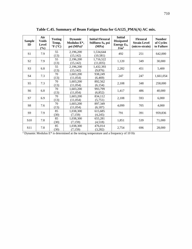
710
Table C.45. Summary of Beam Fatigue Data for GA125_PMA(A) AC mix.
Sample
ID
Air
Voids
Level
(%)
Testing
Temp,
°F (°C)
Dynamic
Modulus E*,
psi (MPa)a
Initial Flexural
Stiffness S0, psi
(MPa)
Initial
Dissipated
Energy E0,
J/m3
Flexural
Strain Level
(micro-strain)
Number
of Cycles
to Failure
S1 7.9 55
(13)
2,196,200
(15,142)
1,534,644
(10,581) 492 251 642,000
S2 7.9 55
(13)
2,196,200
(15,142)
1,716,522
(11,835) 1,120 349 30,000
S3 6.8 55
(13)
2,196,200
(15,142)
1,432,393
(9,876) 2,282 451 5,400
S4 7.3 70
(13)
1,603,200
(11,054)
938,249
(6,469) 247 247 1,661,054
S5 7.3 70
(13)
1,603,200
(11,054)
892,562
(6,154) 2,108 348 258,000
S6 6.8 70
(13)
1,603,200
(11,054)
993,799
(6,852) 1,417 486 40,000
S7 6.9 70
(13)
1,603,200
(11,054)
834,112
(5,751) 2,108 593 6,000
S8 7.6 70
(13)
1,603,200
(11,054)
897,349
(6,187) 4,099 705 4,000
S9 7.9 85
(30)
1,038,300
(7,159)
615,685
(4,245) 791 391 959,836
S10 7.8 85
(30)
1,038,300
(7,159)
655,281
(4,518) 1,851 539 71,000
S11 7.8 85
(30)
1,038,300
(7,159)
476,014
(3,282) 2,754 696 28,000
a Dynamic Modulus E* is determined at the testing temperature and a frequency of 10 Hz
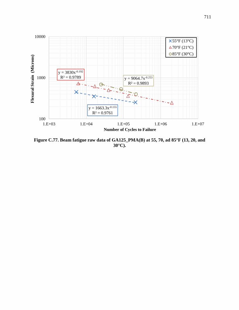
711
Figure C.77. Beam fatigue raw data of GA125_PMA(B) at 55, 70, ad 85°F (13, 20, and
30°C).
y = 1663.3x-0.155
R² = 0.9761
y = 3830x-0.192
R² = 0.9789 y = 9064.7x-0.253
R² = 0.9893
100
1000
10000
1.E+03 1.E+04 1.E+05 1.E+06 1.E+07
Fle
xu
ral
Str
ain
(M
icro
ns)
Number of Cycles to Failure
55°F (13°C)
70°F (21°C)
85°F (30°C)

712
Table C.46. Summary of Beam Fatigue Data for GA125_PMA(B) AC mix.
Sample
ID
Air
Voids
Level
(%)
Testing
Temp,
°F (°C)
Dynamic
Modulus E*,
psi (MPa)a
Initial Flexural
Stiffness S0, psi
(MPa)
Initial
Dissipated
Energy E0,
J/m3
Flexural
Strain Level
(micro-strain)
Number
of Cycles
to Failure
S1 7.8 55
(13)
2,275,500
(15,689)
1,483,301
(10,227) 442 251 211,000
S2 7.8 55
(13)
2,275,500
(15,689)
2,140,612
(14,759) 1,188 351 16,000
S3 7.8 55
(13)
2,275,500
(15,689)
1,222,233
(8,427) 1,811 454 5,400
S4 8.5 70
(13)
1,688,500
(11,642)
896,043
(6,178) 326 248 1,993,970
S5 7.9 70
(13)
1,688,500
(11,642)
901,845
(6,218) 2,267 358 133,000
S6 7.9 70
(13)
1,688,500
(11,642)
782,334
(5,394) 1,026 503 40,000
S7 7.7 70
(13)
1,688,500
(11,642)
791,906
(5,460) 2,267 620 17,000
S8 7.5 70
(13)
1,688,500
(11,642)
893,287
(6,159) 3,400 724 6,100
S9 8.1 85
(30)
1,114,300
(7,683)
655,426
(4,519) 1,140 398 217,000
S10 7.9 85
(30)
1,114,300
(7,683)
623,372
(4,298) 1,196 530 86,000
S11 8.3 85
(30)
1,114,300
(7,683)
527,502
(3,637) 2,260 691 25,000
a Dynamic Modulus E* is determined at the testing temperature and a frequency of 10 Hz
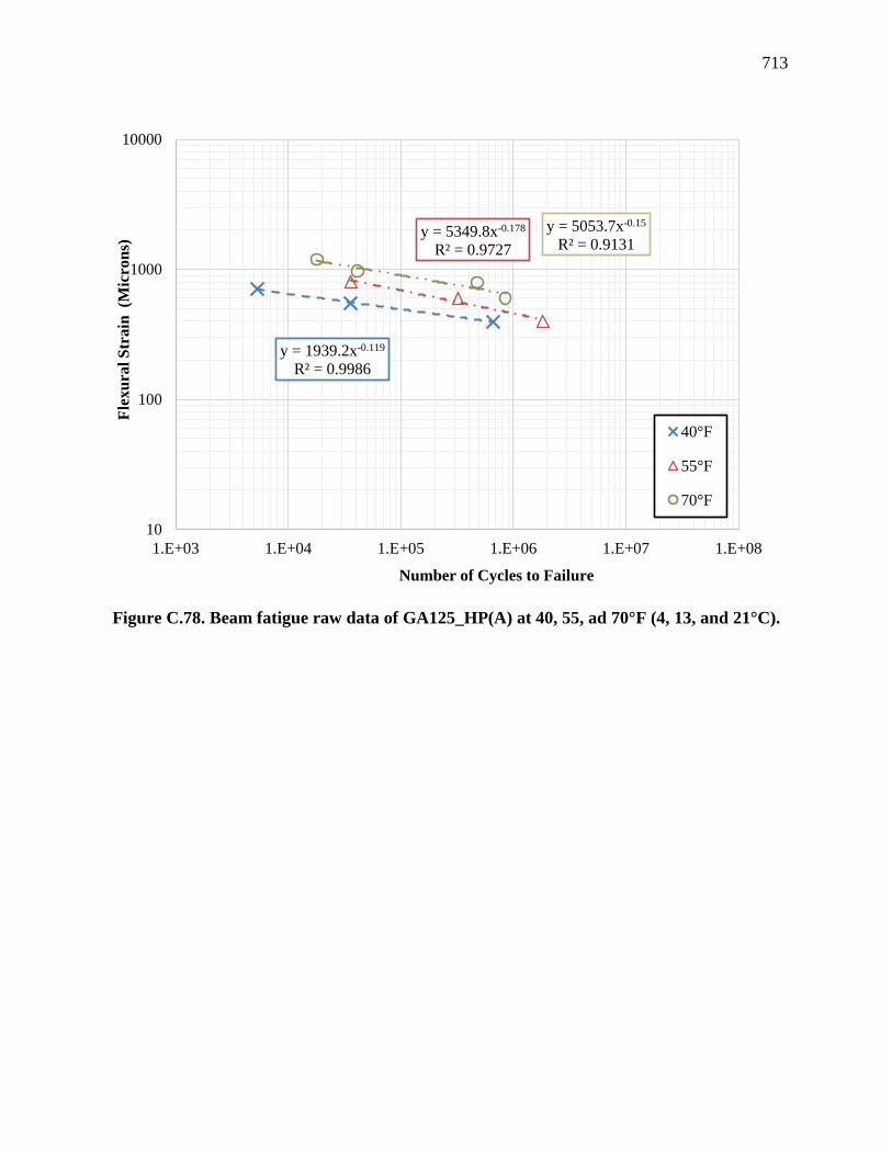
713
Figure C.78. Beam fatigue raw data of GA125_HP(A) at 40, 55, ad 70°F (4, 13, and 21°C).
y = 1939.2x-0.119
R² = 0.9986
y = 5349.8x-0.178
R² = 0.9727
y = 5053.7x-0.15
R² = 0.9131
10
100
1000
10000
1.E+03 1.E+04 1.E+05 1.E+06 1.E+07 1.E+08
Fle
xu
ral
Str
ain
(M
icro
ns)
Number of Cycles to Failure
40°F
55°F
70°F

714
Table C.47. Summary of Beam Fatigue Data for GA125_HP(A) AC mix.
Sample
ID
Air
Voids
Level
(%)
Testing
Temp,
°F (°C)
Dynamic
Modulus E*,
psi (MPa)a
Initial Flexural
Stiffness S0, psi
(MPa)
Initial
Dissipated
Energy E0,
J/m3
Flexural
Strain Level
(micro-strain)
Number
of Cycles
to Failure
S1 6.9 40
(4)
1,663,500
(11,469)
1,268,790
(8,748) 1,254 396 666,000
S2 6.9 40
(4)
1,663,500
(11,469)
1,374,958
(9,480) 3,420 551 36,000
S3 7.1 40
(4)
1,663,500
(11,469)
1,289,095
(8,888) 5,659 706 5,300
S4 7.2 55
(13)
1,155,200
(7,965)
734,906
(5,067) 1,165 397 1,826,578
S5 7.2 55
(13)
1,155,200
(7,965)
747,960
(5,157) 2,977 600 324,000
S6 6.9 55
(13)
1,155,200
(7,965)
904,310
(6,235) 6,087 804 36,000
S7 7.7 70
(21)
727,600
(5,017)
406,541
(2,803) 4881 603 845,000
S8 6.9 70
(21)
727,600
(5,017)
512,777
(2,846) 2699 796 474,000
S9 7.4 70
(21)
727,600
(5,017)
398,274
(2,746) 4881 975 41,000
S10 7.6 70
(21)
727,600
(5,017)
362,159
(2,497) 5743 1195 18,000
a Dynamic Modulus E* is determined at the testing temperature and a frequency of 10 Hz

715
Figure C.79. Beam fatigue raw data of GA125_HP(B) at 40, 55, ad 70°F (4, 13, and 21°C).
y = 4197.1x-0.209
R² = 0.9755
y = 7912.4x-0.244
R² = 0.9801 y = 13230x-0.259
R² = 0.999
10
100
1000
10000
1.E+03 1.E+04 1.E+05 1.E+06 1.E+07 1.E+08
Fle
xu
ral
Str
ain
(M
icro
ns)
Number of Cycles to Failure
40°F
55°F
70°F

716
Table C.48. Summary of Beam Fatigue Data for GA125_HP(B) AC mix.
Sample
ID
Air
Voids
Level
(%)
Testing
Temp,
°F (°C)
Dynamic
Modulus E*,
psi (MPa)a
Initial Flexural
Stiffness S0, psi
(MPa)
Initial
Dissipated
Energy E0,
J/m3
Flexural
Strain Level
(micro-strain)
Number
of Cycles
to Failure
S1 7.5 40
(4)
1,632,100
(11,253)
1,732,911
(11,948) 1,481 396 89,000
S2 7.4 40
(4)
1,632,100
(11,253)
1,445,156
(9,964) 3,104 549 13,000
S3 7.5 40
(4)
1,632,100
(11,253)
1,450,087
(9,998) 6,169 735 5,000
S4 7.7 55
(13)
1,120,000
(7,722)
991,768
(6,838) 1,403 302 535,051
S5 6.5 55
(13)
1,120,000
(7,722)
853,692
(5,886) 2,671 595 48,937
S6 7.2 55
(13)
1,120,000
(7,722)
947,096
(6,530) 2,808 596 48,000
S7 7.5 55
(13)
1,120,000
(7,722)
825,700
(5,693) 5,659 804 9,100
S8 6.5 70
(21)
692,200
(4,773)
700,387
(4,829) 646 394 731,798
S9 6 70
(21)
692,200
(4,773)
393,632
(2,714) 4,464 609 154,955
S10 6.5 70
(21)
692,200
(4,773)
403,785
(2,784) 6,920 1,212 9,800
a Dynamic Modulus E* is determined at the testing temperature and a frequency of 10 Hz
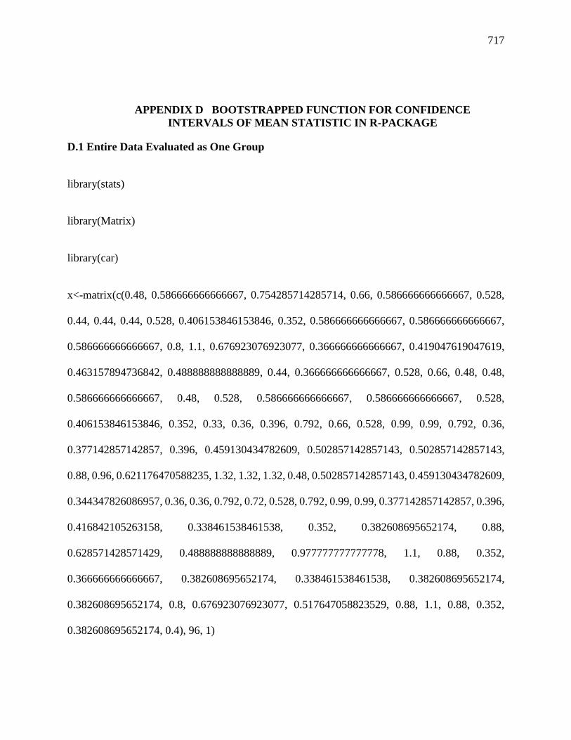
717
APPENDIX D BOOTSTRAPPED FUNCTION FOR CONFIDENCE
INTERVALS OF MEAN STATISTIC IN R-PACKAGE
D.1 Entire Data Evaluated as One Group
library(stats)
library(Matrix)
library(car)
x<-matrix(c(0.48, 0.586666666666667, 0.754285714285714, 0.66, 0.586666666666667, 0.528,
0.44, 0.44, 0.44, 0.528, 0.406153846153846, 0.352, 0.586666666666667, 0.586666666666667,
0.586666666666667, 0.8, 1.1, 0.676923076923077, 0.366666666666667, 0.419047619047619,
0.463157894736842, 0.488888888888889, 0.44, 0.366666666666667, 0.528, 0.66, 0.48, 0.48,
0.586666666666667, 0.48, 0.528, 0.586666666666667, 0.586666666666667, 0.528,
0.406153846153846, 0.352, 0.33, 0.36, 0.396, 0.792, 0.66, 0.528, 0.99, 0.99, 0.792, 0.36,
0.377142857142857, 0.396, 0.459130434782609, 0.502857142857143, 0.502857142857143,
0.88, 0.96, 0.621176470588235, 1.32, 1.32, 1.32, 0.48, 0.502857142857143, 0.459130434782609,
0.344347826086957, 0.36, 0.36, 0.792, 0.72, 0.528, 0.792, 0.99, 0.99, 0.377142857142857, 0.396,
0.416842105263158, 0.338461538461538, 0.352, 0.382608695652174, 0.88,
0.628571428571429, 0.488888888888889, 0.977777777777778, 1.1, 0.88, 0.352,
0.366666666666667, 0.382608695652174, 0.338461538461538, 0.382608695652174,
0.382608695652174, 0.8, 0.676923076923077, 0.517647058823529, 0.88, 1.1, 0.88, 0.352,
0.382608695652174, 0.4), 96, 1)

718
x
qqPlot(x)
shapiro.test(x)
boot.mean = function(x,B,binwidth=NULL) {
n = length(x)
boot.samples = matrix( sample(x,size=n*B,replace=TRUE), B, n)
boot.statistics = apply(boot.samples,1,mean)
se = sd(boot.statistics)
require(ggplot2)
if ( is.null(binwidth) )
binwidth = diff(range(boot.statistics))/30
p = ggplot(data.frame(x=boot.statistics),aes(x=x)) +
geom_histogram(aes(y=..density..),binwidth=binwidth) + geom_density(color="red")
plot(p)
interval = mean(x) + c(-1,1)*0*se
print( interval )

719
return( list(boot.statistics = boot.statistics, interval=interval, se=se, plot=p) )}
out= with( data.frame(x), boot.mean(x, B=2000))
y<-out$'boot.statistics'
qqPlot(y)
shapiro.test(y)
D.2 Entire Data Aggregate Sources: FL vs. GA
Source FL:
library(stats)
library(Matrix)
library(car)
xFL<-matrix(c(0.48, 0.586666666666667, 0.754285714285714, 0.66, 0.586666666666667,
0.528, 0.586666666666667, 0.586666666666667, 0.586666666666667, 0.8, 1.1,
0.676923076923077, 0.528, 0.66, 0.48, 0.48, 0.586666666666667, 0.48, 0.33, 0.36, 0.396, 0.792,
0.66, 0.528, 0.459130434782609, 0.502857142857143, 0.502857142857143, 0.88, 0.96,
0.621176470588235, 0.344347826086957, 0.36, 0.36, 0.792, 0.72, 0.528, 0.338461538461538,
0.352, 0.382608695652174, 0.88, 0.628571428571429, 0.488888888888889,
0.338461538461538, 0.382608695652174, 0.382608695652174, 0.8, 0.676923076923077,
0.517647058823529), 48, 1)

720
xFL
qqPlot(xFL)
shapiro.test(xFL)
boot.mean = function(x,B,binwidth=NULL) {
n = length(x)
boot.samples = matrix( sample(x,size=n*B,replace=TRUE), B, n)
boot.statistics = apply(boot.samples,1,mean)
se = sd(boot.statistics)
require(ggplot2)
if ( is.null(binwidth) )
binwidth = diff(range(boot.statistics))/30
p = ggplot(data.frame(x=boot.statistics),aes(x=x)) +
geom_histogram(aes(y=..density..),binwidth=binwidth) + geom_density(color="red")
plot(p)
interval = mean(x) + c(-1,1)*2*se
print( interval )

721
return( list(boot.statistics = boot.statistics, interval=interval, se=se, plot=p) )}
out= with( data.frame(xFL), boot.mean(xFL, B=2000))
yFL<-out$'boot.statistics'
qqPlot(yFL)
shapiro.test(yFL)
Source GA:
library(stats)
library(Matrix)
library(car)
xGA<-matrix(c(0.44, 0.44, 0.44, 0.528, 0.406153846153846, 0.352, 0.366666666666667,
0.419047619047619, 0.463157894736842, 0.488888888888889, 0.44, 0.366666666666667,
0.528, 0.586666666666667, 0.586666666666667, 0.528, 0.406153846153846, 0.352, 0.99, 0.99,
0.792, 0.36, 0.377142857142857, 0.396, 1.32, 1.32, 1.32, 0.48, 0.502857142857143,
0.459130434782609, 0.792, 0.99, 0.99, 0.377142857142857, 0.396, 0.416842105263158,
0.977777777777778, 1.1, 0.88, 0.352, 0.366666666666667, 0.382608695652174, 0.88, 1.1, 0.88,
0.352, 0.382608695652174, 0.4), 48, 1)
xGA
qqPlot(xGA)

722
shapiro.test(xGA)
boot.mean = function(x,B,binwidth=NULL) {
n = length(x)
boot.samples = matrix( sample(x,size=n*B,replace=TRUE), B, n)
boot.statistics = apply(boot.samples,1,mean)
se = sd(boot.statistics)
require(ggplot2)
if ( is.null(binwidth) )
binwidth = diff(range(boot.statistics))/30
p = ggplot(data.frame(x=boot.statistics),aes(x=x)) +
geom_histogram(aes(y=..density..),binwidth=binwidth) + geom_density(color="red")
plot(p)
interval = mean(x) + c(-1,1)*2*se
print( interval )
return( list(boot.statistics = boot.statistics, interval=interval, se=se, plot=p) )}

723
out= with( data.frame(xGA), boot.mean(xGA, B=2000))
yGA<-out$'boot.statistics'
qqPlot(yGA)
shapiro.test(yGA)
D.3 Entire Data NMAS: 9.5 vs. 12.5 mm
NMAS 9.5 mm
library(stats)
library(Matrix)
library(car)
xN9<-matrix(c( 0.48, 0.586666666666667, 0.754285714285714, 0.66, 0.586666666666667,
0.528, 0.44, 0.44, 0.44, 0.528, 0.406153846153846, 0.352, 0.586666666666667,
0.586666666666667, 0.586666666666667, 0.8, 1.1, 0.676923076923077, 0.366666666666667,
0.419047619047619, 0.463157894736842, 0.488888888888889, 0.44, 0.366666666666667,
0.528, 0.66, 0.48, 0.48, 0.586666666666667, 0.48, 0.528, 0.586666666666667,
0.586666666666667, 0.528, 0.406153846153846, 0.352), 36, 1)
xN9

724
qqPlot(xN9)
shapiro.test(xN9)
boot.mean = function(x,B,binwidth=NULL) {
n = length(x)
boot.samples = matrix( sample(x,size=n*B,replace=TRUE), B, n)
boot.statistics = apply(boot.samples,1,mean)
se = sd(boot.statistics)
require(ggplot2)
if ( is.null(binwidth) )
binwidth = diff(range(boot.statistics))/30
p = ggplot(data.frame(x=boot.statistics),aes(x=x)) +
geom_histogram(aes(y=..density..),binwidth=binwidth) + geom_density(color="red")
plot(p)
interval = mean(x) + c(-1,1)*2*se
print( interval )
return( list(boot.statistics = boot.statistics, interval=interval, se=se, plot=p) )}
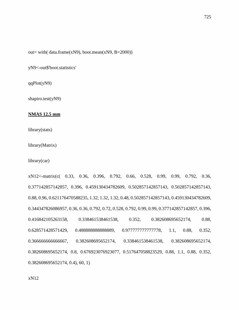
725
out= with( data.frame(xN9), boot.mean(xN9, B=2000))
yN9<-out$'boot.statistics'
qqPlot(yN9)
shapiro.test(yN9)
NMAS 12.5 mm
library(stats)
library(Matrix)
library(car)
xN12<-matrix(c( 0.33, 0.36, 0.396, 0.792, 0.66, 0.528, 0.99, 0.99, 0.792, 0.36,
0.377142857142857, 0.396, 0.459130434782609, 0.502857142857143, 0.502857142857143,
0.88, 0.96, 0.621176470588235, 1.32, 1.32, 1.32, 0.48, 0.502857142857143, 0.459130434782609,
0.344347826086957, 0.36, 0.36, 0.792, 0.72, 0.528, 0.792, 0.99, 0.99, 0.377142857142857, 0.396,
0.416842105263158, 0.338461538461538, 0.352, 0.382608695652174, 0.88,
0.628571428571429, 0.488888888888889, 0.977777777777778, 1.1, 0.88, 0.352,
0.366666666666667, 0.382608695652174, 0.338461538461538, 0.382608695652174,
0.382608695652174, 0.8, 0.676923076923077, 0.517647058823529, 0.88, 1.1, 0.88, 0.352,
0.382608695652174, 0.4), 60, 1)
xN12

726
qqPlot(xN12)
shapiro.test(xN12)
boot.mean = function(x,B,binwidth=NULL) {
n = length(x)
boot.samples = matrix( sample(x,size=n*B,replace=TRUE), B, n)
boot.statistics = apply(boot.samples,1,mean)
se = sd(boot.statistics)
require(ggplot2)
if ( is.null(binwidth) )
binwidth = diff(range(boot.statistics))/30
p = ggplot(data.frame(x=boot.statistics),aes(x=x)) +
geom_histogram(aes(y=..density..),binwidth=binwidth) + geom_density(color="red")
plot(p)
interval = mean(x) + c(-1,1)*2*se
print( interval )
return( list(boot.statistics = boot.statistics, interval=interval, se=se, plot=p) )}

727
out= with( data.frame(xN12), boot.mean(xN12, B=2000))
yN12<-out$'boot.statistics'
qqPlot(yN12)
shapiro.test(yN12)
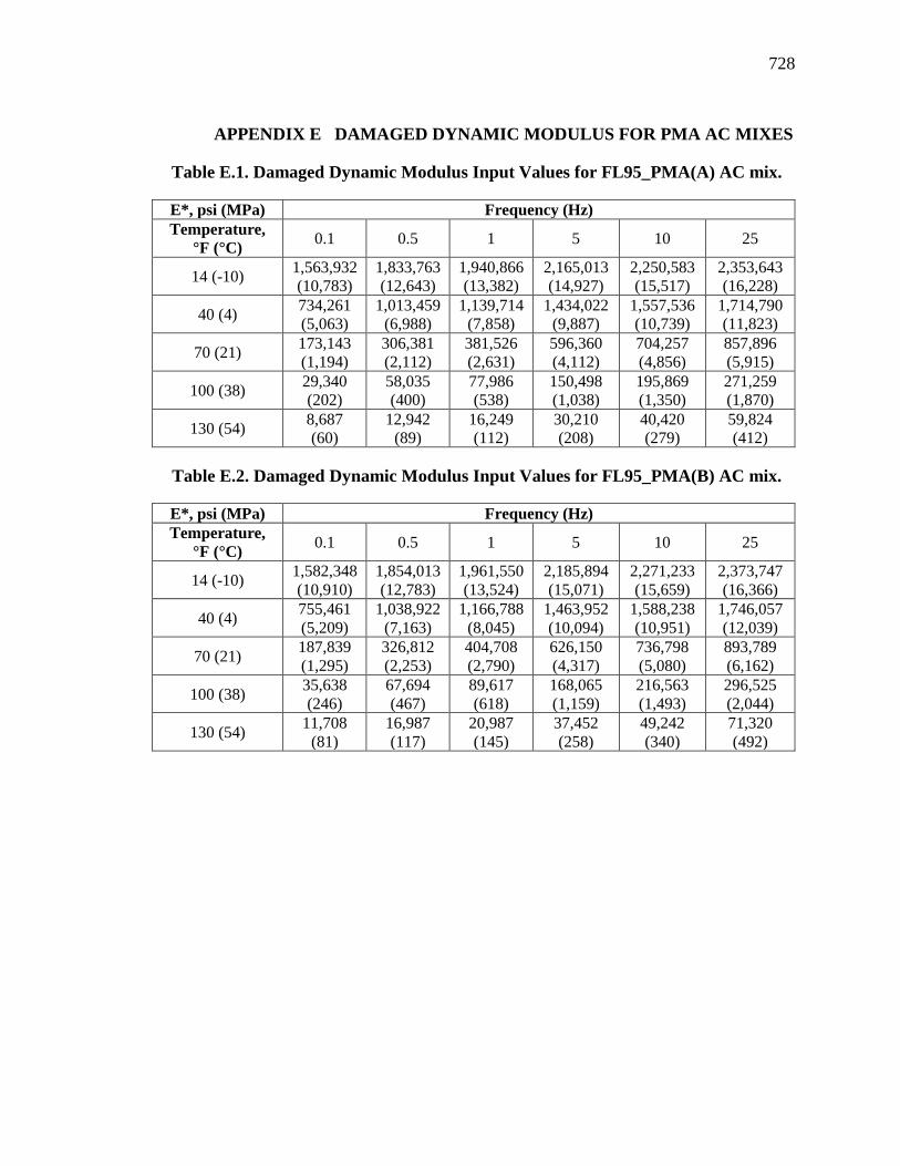
728
APPENDIX E DAMAGED DYNAMIC MODULUS FOR PMA AC MIXES
Table E.1. Damaged Dynamic Modulus Input Values for FL95_PMA(A) AC mix.
E*, psi (MPa) Frequency (Hz)
Temperature,
°F (°C) 0.1 0.5 1 5 10 25
14 (-10) 1,563,932
(10,783)
1,833,763
(12,643)
1,940,866
(13,382)
2,165,013
(14,927)
2,250,583
(15,517)
2,353,643
(16,228)
40 (4) 734,261
(5,063)
1,013,459
(6,988)
1,139,714
(7,858)
1,434,022
(9,887)
1,557,536
(10,739)
1,714,790
(11,823)
70 (21) 173,143
(1,194)
306,381
(2,112)
381,526
(2,631)
596,360
(4,112)
704,257
(4,856)
857,896
(5,915)
100 (38) 29,340
(202)
58,035
(400)
77,986
(538)
150,498
(1,038)
195,869
(1,350)
271,259
(1,870)
130 (54) 8,687
(60)
12,942
(89)
16,249
(112)
30,210
(208)
40,420
(279)
59,824
(412)
Table E.2. Damaged Dynamic Modulus Input Values for FL95_PMA(B) AC mix.
E*, psi (MPa) Frequency (Hz)
Temperature,
°F (°C) 0.1 0.5 1 5 10 25
14 (-10) 1,582,348
(10,910)
1,854,013
(12,783)
1,961,550
(13,524)
2,185,894
(15,071)
2,271,233
(15,659)
2,373,747
(16,366)
40 (4) 755,461
(5,209)
1,038,922
(7,163)
1,166,788
(8,045)
1,463,952
(10,094)
1,588,238
(10,951)
1,746,057
(12,039)
70 (21) 187,839
(1,295)
326,812
(2,253)
404,708
(2,790)
626,150
(4,317)
736,798
(5,080)
893,789
(6,162)
100 (38) 35,638
(246)
67,694
(467)
89,617
(618)
168,065
(1,159)
216,563
(1,493)
296,525
(2,044)
130 (54) 11,708
(81)
16,987
(117)
20,987
(145)
37,452
(258)
49,242
(340)
71,320
(492)

729
Table E.3. Damaged Dynamic Modulus Input Values for FL125_PMA(A) AC mix.
E*, psi (MPa) Frequency (Hz)
Temperature,
°F (°C) 0.1 0.5 1 5 10 25
14 (-10) 1,634,910
(11,272)
1,912,373
(13,185)
2,021,608
(13,938)
2,247,762
(15,498)
2,332,983
(16,085)
2,434,595
(16,786)
40 (4) 787,235
(5,428)
1,076,456
(7,422)
1,207,381
(8,325)
1,512,126
(10,426)
1,639,524
(11,304)
1,800,984
(12,417)
70 (21) 210,107
(1,449)
351,783
(2,425)
430,597
(2,969)
654,617
(4,513)
766,896
(5,289)
926,711
(6,389)
100 (38) 45,338
(313)
82,464
(569)
106,536
(735)
189,203
(1,305)
239,042
(1,648)
320,362
(2,209)
130 (54) 12,575
(87)
20,920
(144)
26,530
(183)
47,429
(327)
61,351
(424)
86,289
(595)
Table E.4. Damaged Dynamic Modulus Input Values for FL125_PMA(B) AC mix.
E*, psi (MPa) Frequency (Hz)
Temperature,
°F (°C) 0.1 0.5 1 5 10 25
14 (-10) 1,721,246
(11,868)
1,997,485
(13,772)
2,104,819
(14,512)
2,324,378
(16,026)
2,406,139
(16,590)
2,502,886
(17,257)
40 (4) 850,219
(5,862)
1,154,367
(7,959)
1,290,137
(8,895)
1,601,612
(11,043)
1,729,949
(11,928)
1,891,006
(13,038)
70 (21) 228,114
(1,573)
383,988
(2,648)
470,175
(3,242)
712,651
(4,914)
832,738
(5,742)
1,002,008
(6,909)
100 (38) 47,484
(327)
88,195
(608)
114,804
(792)
206,536
(1424)
261,824
(1,805)
351,757
(2,425)
130 (54) 12,577
(87)
21,376
(147)
27,383
(189)
50,114
(346)
65,438
(451)
93,073
(642)

730
Table E.5. Damaged Dynamic Modulus Input Values for GA95_PMA(A) AC mix.
E*, psi (MPa) Frequency (Hz)
Temperature,
°F (°C) 0.1 0.5 1 5 10 25
14 (-10) 2,164,493
(14,924)
2,393,148
(16,500)
2,475,820
(17,070)
2,634,595
(18,165)
2,690,207
(18,548)
2,753,527
(18,985)
40 (4) 1,249,033
(8,612)
1,599,154
(11,026)
1,742,517
(12,014)
2,045,304
(14,102)
2,160,409
(14,895)
2,297,503
(15,841)
70 (21) 361,227
(2,491)
602,299
(4,153)
728,608
(5,024)
1,059,231
(7,303)
1,210,828
(8,348)
1,412,485
(9,739)
100 (38) 66,514
(459)
129,931
(896)
172,375
(1188)
318,791
(2,198)
405,450
(2,795)
542,646
(3,741)
130 (54) 16,846
(116)
28,043
(193)
36,147
(249)
68,745
(474)
91,747
(633)
134,275
(926)
Table E.6. Damaged Dynamic Modulus Input Values for GA95_PMA(B) AC mix.
E*, psi (MPa) Frequency (Hz)
Temperature,
°F (°C) 0.1 0.5 1 5 10 25
14 (-10) 2,247,243
(15,494)
2,459,237
(16,956)
2,534,953
(17,478)
2,678,923
(18,471)
2,728,874
(18,815)
2,785,426
(19,205)
40 (4) 1,372,842
(9,465)
1,719,127
(11,853)
1,857,742
(12,809)
2,144,960
(14,785)
2,252,257
(15,529)
2,378,725
(16,401)
70 (21) 437,735
(3,018)
709,038
(4,889)
846,348
(5,835)
1,193,673
(8,230)
1,348,016
(9,294)
1,549,243
(10,682)
100 (38) 83,532
(576)
165,116
(1,138)
218,402
(1,506)
395,826
(2,729)
497,133
(3,428)
653,139
(4,503)
130 (54) 18,525
(128)
33,576
(231)
44,521
(307)
88,297
(609)
118,757
(819)
174,095
(1,200)
Table E.7. Damaged Dynamic Modulus Input Values for GA125_PMA(A) AC mix.
E*, psi (MPa) Frequency (Hz)
Temperature,
°F (°C) 0.1 0.5 1 5 10 25
14 (-10) 2,207,116
(15,218)
2,417,875
(16,671)
2,494,652
(17,200)
2,643,532
(18,227)
2,696,285
(18,590)
2,756,870
(19,008)
40 (4) 1,343,131
(9,261)
1,670,692
(11,519)
1,803,600
(12,435)
2,083,717
(14,367)
2,190,427
(15,102)
2,318,022
(15,982)
70 (21) 441,195
(3,042)
694,204
(4,786)
821,325
(5,663)
1,143,599
(7,885)
1,288,013
(8,881)
1,478,115
(10,191)
100 (38) 88,502
(610)
168,666
(1,163)
219,454
(1,513)
384,429
(2,651)
477,228
(3,290)
619,459
(4,271)
130 (54) 19,052
(131)
34,786
(240)
45,896
(316)
88,750
(612)
117,661
(811)
169,113
(1,166)
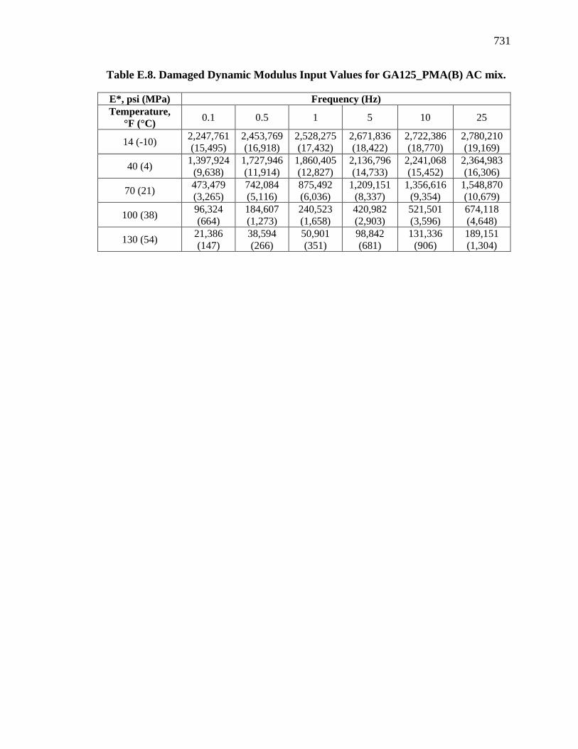
731
Table E.8. Damaged Dynamic Modulus Input Values for GA125_PMA(B) AC mix.
E*, psi (MPa) Frequency (Hz)
Temperature,
°F (°C) 0.1 0.5 1 5 10 25
14 (-10) 2,247,761
(15,495)
2,453,769
(16,918)
2,528,275
(17,432)
2,671,836
(18,422)
2,722,386
(18,770)
2,780,210
(19,169)
40 (4) 1,397,924
(9,638)
1,727,946
(11,914)
1,860,405
(12,827)
2,136,796
(14,733)
2,241,068
(15,452)
2,364,983
(16,306)
70 (21) 473,479
(3,265)
742,084
(5,116)
875,492
(6,036)
1,209,151
(8,337)
1,356,616
(9,354)
1,548,870
(10,679)
100 (38) 96,324
(664)
184,607
(1,273)
240,523
(1,658)
420,982
(2,903)
521,501
(3,596)
674,118
(4,648)
130 (54) 21,386
(147)
38,594
(266)
50,901
(351)
98,842
(681)
131,336
(906)
189,151
(1,304)
Related Documents

![ASPHALT CONCRETE [Types] - KSU Facultyfac.ksu.edu.sa/sites/default/files/AC-1-LabTYPESDISTRESS.pdf · ASPHALT CONCRETE [Types] Introduction ... Sand Asphalt Mix Sand asphalt mixes](https://static.cupdf.com/doc/110x72/5b72d5437f8b9a674d8d5d0c/asphalt-concrete-types-ksu-asphalt-concrete-types-introduction-sand.jpg)