Structural Changes in the Transmission Mechanism of Monetary Policy in Mexico: A Non-linear VAR Approach * Alejandro Gaytan González ♣ [email protected] Jesus R. Gonzalez-Garcia ♦ [email protected] April, 2006 Working Paper 2006-06 Dirección General de Investigación Económica Banco de México * We thank Daniel Chiquiar, Manuel Ramos-Francia and Alberto Torres for very helpful comments and Edgar Hernández and Lorenzo Bernal for excellent research assistance. The opinions in this paper correspond to the authors and do not necessarily reflect the point of view of Banco de México or the IMF. ♣ Dirección General de Investigación Económica, Banco de México. ♦ Statistics Department, International Monetary Fund.

Welcome message from author
This document is posted to help you gain knowledge. Please leave a comment to let me know what you think about it! Share it to your friends and learn new things together.
Transcript
Structural Changes in the Transmission Mechanism of
Monetary Policy in Mexico: A Non-linear VAR Approach *
Alejandro Gaytan González ♣ [email protected]
Jesus R. Gonzalez-Garcia ♦
April, 2006 Working Paper 2006-06
Dirección General de Investigación Económica Banco de México
* We thank Daniel Chiquiar, Manuel Ramos-Francia and Alberto Torres for very helpful comments and
Edgar Hernández and Lorenzo Bernal for excellent research assistance. The opinions in this paper correspond to the authors and do not necessarily reflect the point of view of Banco de México or the IMF.
♣ Dirección General de Investigación Económica, Banco de México. ♦ Statistics Department, International Monetary Fund.


Structural Changes in the Transmission Mechanism of
Monetary Policy in Mexico: A Non-linear VAR Approach
Alejandro Gaytan
Jesus R. Gonzalez-Garcia
April, 2006 Working Paper 2006-06
Dirección General de Investigación Económica Banco de México
Abstract. In this paper we present a first approach to the study of the transformation in the transmission mechanism of monetary policy that has taken place in Mexico in recent years. For this purpose, we use a non-linear VAR model that allows for regime shifts. The comparison of the different regimes identified leads to the following main findings: a) there was a major structural change in the transmission mechanism around January 2001, date that coincides with the formal adoption of the inflation targeting framework; b) after this change, fluctuations in the real exchange rate have had smaller effects on the process of price formation, the formation of inflation expectations and the nominal interest rate; c) also, there have been stronger reactions of the nominal interest rate to increases in the output gap and the rate of inflation; and d) the movements of the nominal interest rate have a more effective influence on the real exchange rate and the rate of inflation. JEL: E52, E58 and F33. Keywords: monetary policy, Mexico, monetary transmission mechanism, non-linear models.

Resumen. Este documento de trabajo presenta un primer acercamiento al estudio de las transformaciones que han tenido lugar en el mecanismo de transmisión de la política monetaria en México en años recientes. Para este fin, se utiliza un modelo no lineal de vectores autorregresivos que permite cambios de régimen. La comparación de los diferentes regímenes identificados sugiere los siguientes resultados principales: a) se observó un importante cambio estructural en el mecanismo de transmisión alrededor de enero de 2001, fecha que coincide con la adopción formal del esquema de objetivos de inflación; b) después de este cambio, las fluctuaciones del tipo de cambio real han tenido un efecto menor sobre los procesos de formación de precios y de expectativas de inflación y sobre la tasa de interés nominal; c) adicionalmente, se ha incrementado la reacción de la tasa de interés nominal ante incrementos en la brecha del producto y la tasa de inflación; y d) los movimientos en la tasa de interés nominal tienen una influencia más efectiva sobre el tipo de cambio real y la tasa de inflación.

1 Introduction
After the currency and financial crisis of 1995, monetary policy in México has been devoted
to pursue the objective of long-run price stability, which has resulted in a major change in
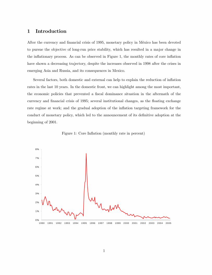
the inflationary process. As can be observed in Figure 1, the monthly rates of core inflation
have shown a decreasing trajectory, despite the increases observed in 1998 after the crises in
emerging Asia and Russia, and its consequences in Mexico.
Several factors, both domestic and external can help to explain the reduction of inflation
rates in the last 10 years. In the domestic front, we can highlight among the most important,
the economic policies that prevented a fiscal dominance situation in the aftermath of the
currency and financial crisis of 1995; several institutional changes, as the floating exchange
rate regime at work; and the gradual adoption of the inflation targeting framework for the
conduct of monetary policy, which led to the announcement of its definitive adoption at the
beginning of 2001.
Figure 1: Core Inflation (monthly rate in percent)
0%
1%
2%
3%
4%
5%
6%
7%
8%
1990 1991 1992 1993 1994 1995 1996 1997 1998 1999 2000 2001 2002 2003 2004 2005
1
In this paper we present a first approach to the study of one aspect of the changes in
the inflationary process in Mexico, namely, the identification by means of empirical methods
of the changes that have occurred in the transmission mechanism of monetary policy. This
exploration sheds light on the underlying causes of the success observed in the reduction
of inflation in recent years and the role played by the profound changes observed in the
implementation of monetary policy.
To identify possible changes in the transmission mechanism of monetary policy we use
a Markov-switching vector autoregressive (MS-VAR) methodology in order to determine the
dates of the structural changes and to study how the dynamic relationships of the main macro-
economic variables have changed over time. First, we estimate a linear vector autoregression
(VAR) model including the following endogenous variables: the real exchange rate, the output
gap, the rate of inflation, the expected rate of inflation and the nominal interest rate. After
showing that the linear estimation shows considerable parameter instability, we estimate an
MS-VAR that allows for changes in the parameters over time. The non-linear estimation with
regime shifts allows an endogenous identification of different regimes over time according to
the changes in the parameters of the model, without the need for priors about the dates of the
changes, their direction or magnitude. Finally, in order to characterize the changes that have
occurred in the transmission mechanism of monetary policy, we assume a simple recursive
structure of the model to identify structural shocks and present a comparison of the impulse
response functions and the variance decomposition corresponding to different regimes.
The results of the exercise with regime shifts suggest the following changes in the trans-
mission mechanism of monetary policy in recent years. There seems to be a major structural
break in the transmission mechanism at the beginning of 2001, date that coincides with the
formal adoption of the inflation targeting framework. After this change, fluctuations in the
real exchange rate have had smaller effects on the process of price formation and on inflation
expectations. The nominal interest rate has also shown a milder reaction to real depreciations.
In addition, there is evidence of a stronger reaction of the nominal interest rate to demand
pressures, measured by the output gap, and the inflation rate. Finally, the results suggest
a stronger response of the real exchange rate and the rate of inflation to movements in the
interest rate.
2

The paper is organized as follows. In section 2, we discuss the model estimated. In section
3, we present the unit root tests for the series included in the model in order to examine
the possible presence of unit roots. Section 4, presents the estimation of the VAR model in a
linear framework and the analysis of its stability properties. In section 5 we estimate the VAR
allowing for regime shifts. These shifts will allow us to identify the changes in the transmission
mechanism by comparing the impulse response functions and variance decomposition obtained
from the different regimes, assuming a recursive structure of the model. Section 6 summarizes
the results and presents the conclusions.
2 The Monetary Transmission Mechanism and the Estimated
Model
Since the work of Sims (1980) VAR models have been the most widely used empirical method-
ology to study the transmission mechanism of monetary policy,1 mainly because VARs provide
a systematic way to capture rich dynamic structures and co-movements between different time
series without restricting for a specific functional form.
The use of VARs for the study of the monetary transmission mechanism requires some
identifying assumptions to allow for contemporaneous co-movement between the endogenous
variables and to isolate the different shocks to be able, for example, to distinguish between
a monetary shock from a simple “surprise” movement in the monetary variable.2 The sim-
plest form of identification assumptions is to assume a recursive structure of the economy in
which the first variable responds only to lagged values of all endogenous variables, the second
responds to the same lagged values and the contemporaneous value of the first variable, and
so on. In this case, the last variable of the system responds to lags and the contemporaneous
realization of all the other endogenous variables. Other approaches derive the identification
from different assumptions about the timing of responses of variables or from theoretical mod-
1See for example Bernanke and Blinder (1997), Clarida and Gertler (1997) and Leeper, Sims and Zha (1996).2A VAR with k endogenous variables requires k(k-1) identifying assumptions. A common assumption is to
orthogonalize the innovations so that an innovation or shock in one equation of the system is uncorrelated with
the innovations in other equations. These restrictions provide half on the identifying assumptions for a just
identified VAR. About the identification assumptions in VAR models see Christiano et.al. (2000).
3
els. VAR models identified in this way are termed structural vector autoregression (SVAR)
models. The identification assumptions may be determined by the short run relations between
the variables (e.g. Bernanke and Mihov 1998) or may come in the form of long run restric-
tions based on theoretical grounds (e.g. a vertical Phillips curve in the long run, as in Quah
and Vahey 1995). In addition, a recent stream of literature on SVAR models, uses minimal
restrictions about the signs and shapes of the responses of the variables to shocks that are
also derived from a theoretical model (Uhlig 2005, Canova and de Nicolo 2002).
There are some important criticisms to the use of VAR models to study the monetary
transmission mechanism: First, there is the question of what is really captured by an identified
shock. This problem becomes evident when small changes in the identification assumptions or
in the set of endogenous variables included imply important differences in the impulse response
functions of a given variable to a specific structural shock. The most common example of this
problem is the “price puzzle” of monetary policy: a predicted increase in inflation following a
monetary tightening. The main explanation of this puzzle (Sims 1992) is that when monetary
policy is forward looking, and the VAR model has as a poor account of inflation expectations,
an increase in the nominal interest rate coming from inflation expectations may end up being
attributed to a policy shock.3
A second criticism is related to the stability and linearity of VAR models. There are
two main issues concerning these problems when the VAR methodology is used to study an
economy that has experienced periods of instability and policy changes. First, there may be
important policy regime changes, as changes in the monetary policy rule over time, and if
these changes affect the process of expectation formation, the coefficients of the model will
change vis-à-vis the rule. In addition, in some emerging economies financial crises episodes
may imply an increase in the variance of shocks, exceptional responses of monetary policy
and, in some cases, the abandonment of previous monetary policy rules. These are some
reasons why linear VAR estimations for countries like Mexico usually have severe difficulties
in delivering reasonable results.
The third criticism is related with the structural restrictions used for identification. Recur-3Sims and Zha (1995) show that including variables like commodity prices, which contain information about
inflationary pressures, helps to solve the price puzzle.
4
sive and short run restrictions depend on particular timing assumptions: if these assumptions
are not accurate because of misspecification or because they do not hold over the frequency
of the data used for the estimation, the identified “structure” may be just summarizing cor-
relations in the data. Several studies have shown that frequently used short run and long
run restrictions are not free of problems to identify the structural parameters.4 However, as
Sims (1982) has pointed out, the results may still be empirically relevant as they can uncover
the regularities present in the data. Also Christiano et. al. (2000) have shown that with
a recursive identification, the response of blocks of variables to a shock outside the block is
invariant to the recursive ordering inside the block.
The VAR approach has also been criticized because of its limitations to identify the sys-
tematic part of monetary policy, leaving just a reaction function in surprises (Clarida 2001).
The alternative approach is to estimate directly structural models using GMM or maximum
likelihood techniques. However, although such an approach may be more fruitful in providing
a coherent framework to answer important policy questions, it is model dependent. In con-
trast, the VAR approach can encompass a large set of different models. In addition, the VAR
approach has shown a clear advantage in fitting the data.
In this paper we take the simplest set of identification restrictions, a recursive structure,
as a first approximation to the study of the transmission mechanism of monetary policy in
Mexico,5 and try to overcome some of the potential problems of the VAR approach in the
following way: 1) we include inflationary expectations as an endogenous variable of the VAR
and control for inflation in primary good prices to avoid the so called price puzzle; and 2) we
allow for changes in parameters and heteroscedastic innovations by using a VAR model with
regime shifts.
The set of endogenous variables included in the VAR is consistent with the micro-founded
small open economy models of Svensson (2000) and Galí and Monacelli (2002).6 The endoge-
4See Canova and Pina (1999) and Cooley and Dweyer (1998).5An interesting alternative is to obtain a structural identification using sign and shape restrictions as pro-
posed in Uhlig (2005).6The system of equations derived in Galí and Monacelli (2002) are: (i) an uncovered interest rate parity
condition for the real exchange rate; (ii) a forward looking Phillips curve for domestic inflation; (iii) a forward
looking IS curve for the output gap; and (iv) a central bank loss function derived from the utility function of
5
nous variables included in the model, ordered according to the recursive structure adopted,
are the following: the real exchange rate, the output gap, the rate of inflation, the expected
rate of inflation,7 and the nominal interest rate. The recursive structure assumed is similar
to the one used by Christiano, Eichenbaum and Evans (2000) (EEC henceforth).8 Those
authors ordered output, prices and commodity prices before the federal funds rate, which is
considered the monetary policy instrument. In EEC, they treat a closed economy, hence,
there is no real exchange rate. The identification assumptions used in this paper imply that
the contemporaneous values of all variables different to the nominal interest rate belong to
the information set of the monetary authorities, and that these variables does not respond
to contemporaneous realizations of monetary policy shocks. These assumptions about the
information set of the central bank may remain controversial. However, we considered that
the central bank has very frequent information about the evolution of prices, expectations and
indicators of economic activity. With respect to the real exchange rate, it is assumed that it
does not react on impact to any of the variables of the system.
In addition to the endogenous variables mentioned, we include some exogenous variables:
(i) the foreign (US) rate of inflation, to control for imported inflation; (ii) an indicator of
foreign economic activity, as an exogenous source of variation of the domestic output gap;
(iii) the rate of growth of the oil price; and an indicator of inflation of international primary
goods.9
a representative consumer.7The series of the expected rate of inflation was obtained from the monthly survey conducted by Banco de
México for the period May 1997 to February 2005. Unfortunately, there is no alternative source of information
about inflation expectations before May 1997. Thus, for the rest of the sample (November 1991 to April 1997)
the series was constructed as the dynamic forecast of a GMM estimation, which is shown in Appendix A.8 In addition EEC include total reserves, non borrowed reserves and a monetary aggregate.9The definitions of the variables used and their sources are shown in Appendix B.
6
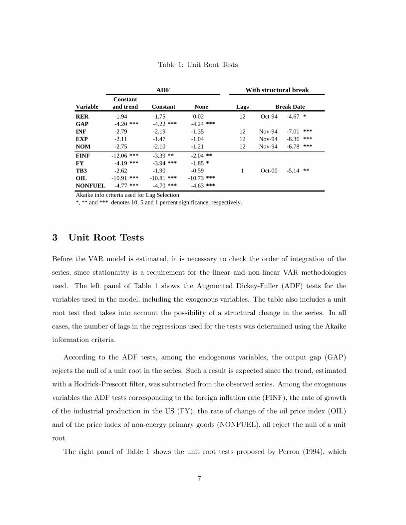
Table 1: Unit Root Tests
Variable LagsRER -1.94 -1.75 0.02 12 Oct-94 -4.67 *GAP -4.20 *** -4.22 *** -4.24 ***INF -2.79 -2.19 -1.35 12 Nov-94 -7.01 ***EXP -2.11 -1.47 -1.04 12 Nov-94 -8.36 ***NOM -2.75 -2.10 -1.21 12 Nov-94 -6.78 ***FINF -12.06 *** -3.39 ** -2.04 **FY -4.19 *** -3.94 *** -1.85 *TB3 -2.62 -1.90 -0.59 1 Oct-00 -5.14 **OIL -10.91 *** -10.81 *** -10.73 ***NONFUEL -4.77 *** -4.70 *** -4.63 ***Akaike info criteria used for Lag Selection*, ** and *** denotes 10, 5 and 1 percent significance, respectively.
ADF With structural break
Break DateConstantand trend Constant None
3 Unit Root Tests
Before the VAR model is estimated, it is necessary to check the order of integration of the
series, since stationarity is a requirement for the linear and non-linear VAR methodologies
used. The left panel of Table 1 shows the Augmented Dickey-Fuller (ADF) tests for the
variables used in the model, including the exogenous variables. The table also includes a unit
root test that takes into account the possibility of a structural change in the series. In all
cases, the number of lags in the regressions used for the tests was determined using the Akaike
information criteria.
According to the ADF tests, among the endogenous variables, the output gap (GAP)
rejects the null of a unit root in the series. Such a result is expected since the trend, estimated
with a Hodrick-Prescott filter, was subtracted from the observed series. Among the exogenous
variables the ADF tests corresponding to the foreign inflation rate (FINF), the rate of growth
of the industrial production in the US (FY), the rate of change of the oil price index (OIL)
and of the price index of non-energy primary goods (NONFUEL), all reject the null of a unit
root.
The right panel of Table 1 shows the unit root tests proposed by Perron (1994), which
7

take into account the possibility of a structural change in the series. In these tests the null
hypothesis postulates a unit root in the series and the alternative the case of a stationary
process with an exogenous change in its level. The results of the tests show that the series
of the real exchange rate (RER), the inflation rate (INF), inflation expectations (EXP) and
the nominal exchange rate (NOM) can be considered stationary variables if a once and for all
change in level is taken into account. In all cases, the estimated breaks are located just before
the currency crisis that erupted in December 1994. Also, the tests show that the series of the
US three-month Treasury bill rate (TB3) can be considered a stationary series with a change
in level in October 2000.
Once the order of integration of the series has been determined, in the following section
we present the estimation of a reduced form linear VAR model and analyze the stability of its
parameters over time in order to look for evidence suggesting structural changes.
4 Reduced Form Linear VAR
The initial estimation of the reduced form linear VAR includes twelve lags of the endogenous
variables, and the contemporaneous observations and two lags of the exogenous variables.
The data set used for the estimation starts in November 1991 and ends in February 2005.
After the initial estimation, the model was reduced following the testing procedure explained
in Brüggemann, Krolzig and Lütkepohl (2003) and Brüggemann and Lütkepohl (2001).10
This procedure involves testing zero restrictions on individual coefficients in each of the five
equations of the reduced form VAR. Specifically, at each step of the procedure used in this
paper a single regressor was eliminated if the p-value corresponding to its t-statistic was higher
than 0.10. Then, the reduced model was estimated and a new regressor was eliminated. The
process stopped when all coefficients showed a significance level below 0.10 and then a joint
test for all zero restrictions was applied.
10Brüggemann, Krolzig and Lütkepohl (2003) compare the testing procedure for model reduction used in this
paper with the general-to-specific reduction approach implemented in PcGets. Using Monte Carlo experiments,
the authors found that both approaches are similar in terms of recovering the “true” model and the accuracy
of the impulse response functions obtained. However, the multiple path approach used by PcGets seems to be
superior when the different approaches are evaluated in terms of the accuracy of forecasts.
8
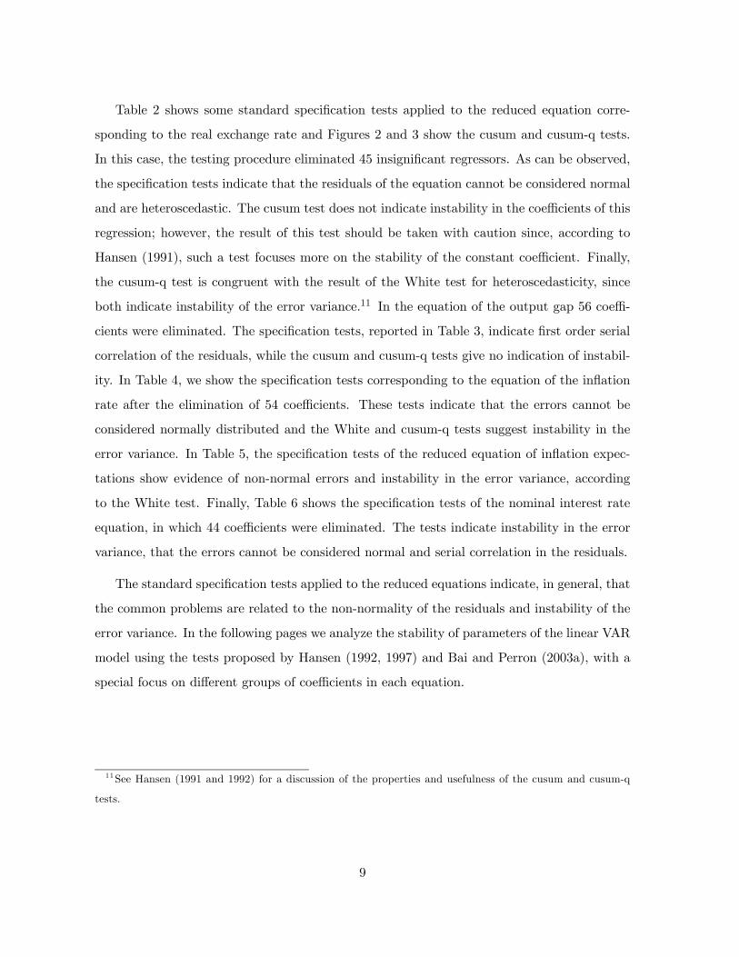
Table 2 shows some standard specification tests applied to the reduced equation corre-
sponding to the real exchange rate and Figures 2 and 3 show the cusum and cusum-q tests.
In this case, the testing procedure eliminated 45 insignificant regressors. As can be observed,
the specification tests indicate that the residuals of the equation cannot be considered normal
and are heteroscedastic. The cusum test does not indicate instability in the coefficients of this
regression; however, the result of this test should be taken with caution since, according to
Hansen (1991), such a test focuses more on the stability of the constant coefficient. Finally,
the cusum-q test is congruent with the result of the White test for heteroscedasticity, since
both indicate instability of the error variance.11 In the equation of the output gap 56 coeffi-
cients were eliminated. The specification tests, reported in Table 3, indicate first order serial
correlation of the residuals, while the cusum and cusum-q tests give no indication of instabil-
ity. In Table 4, we show the specification tests corresponding to the equation of the inflation
rate after the elimination of 54 coefficients. These tests indicate that the errors cannot be
considered normally distributed and the White and cusum-q tests suggest instability in the
error variance. In Table 5, the specification tests of the reduced equation of inflation expec-
tations show evidence of non-normal errors and instability in the error variance, according
to the White test. Finally, Table 6 shows the specification tests of the nominal interest rate
equation, in which 44 coefficients were eliminated. The tests indicate instability in the error
variance, that the errors cannot be considered normal and serial correlation in the residuals.
The standard specification tests applied to the reduced equations indicate, in general, that
the common problems are related to the non-normality of the residuals and instability of the
error variance. In the following pages we analyze the stability of parameters of the linear VAR
model using the tests proposed by Hansen (1992, 1997) and Bai and Perron (2003a), with a
special focus on different groups of coefficients in each equation.
11See Hansen (1991 and 1992) for a discussion of the properties and usefulness of the cusum and cusum-q
tests.
9

Table 2:
Diagnostic tests Statistic p-valueR2 0.9745R2 Adjusted 0.9680F (45 constraints on general model) 0.4357 0.9983Jarque-Bera 641.9186 0.0000LM(1) 0.0659 0.7979LM(12) 0.8664 0.5830ARCH(1) 0.1625 0.6875White Heteroskedasticity Test 5.0341 0.0000
Equation: Real Exchange Rate (RER)
Figure 2: RER Equation, CUSUM Test
-4 0
-3 0
-2 0
-1 0
0
1 0
2 0
3 0
4 0
9 5 9 6 9 7 9 8 9 9 0 0 0 1 0 2 0 3 0 4
Figure 3: RER Equation, CUSUM-Q Test
-0 .2
0 .0
0 .2
0 .4
0 .6
0 .8
1 .0
1 .2
9 5 9 6 9 7 9 8 9 9 0 0 0 1 0 2 0 3 0 4

Table 3:
Diagnostic tests Statistic p-valueR2 0.9207R2 Adjusted 0.9089F (56 constraints on general model) 0.4676 0.9982Jarque-Bera 0.9272 0.6290LM(1) 3.2249 0.0749LM(12) 1.2481 0.2593ARCH(1) 2.1267 0.1469White Heteroskedasticity Test 0.7354 0.8644
Equation: Output Gap (GAP)
Figure 4: GAP Equation, CUSUM Test
-4 0
-3 0
-2 0
-1 0
0
1 0
2 0
3 0
4 0
9 5 9 6 9 7 9 8 9 9 0 0 0 1 0 2 0 3 0 4
Figure 5: GAP Equation, CUSUM-Q Test
-0 .2
0 .0
0 .2
0 .4
0 .6
0 .8
1 .0
1 .2
9 5 9 6 9 7 9 8 9 9 0 0 0 1 0 2 0 3 0 4

Table 4:
Diagnostic tests Statistic p-valueR2 0.9637R2 Adjusted 0.9577F (54 constraints on general model) 0.4190 0.9995Jarque-Bera 693.3582 0.0000LM(1) 0.0105 0.9186LM(12) 1.0590 0.4013ARCH(1) 1.1360 0.2883White Heteroskedasticity Test 3.3956 0.0000
Equation: Inflation (INF)
Figure 6: INF Equation, CUSUM Test
-4 0
-3 0
-2 0
-1 0
0
1 0
2 0
3 0
4 0
9 5 9 6 9 7 9 8 9 9 0 0 0 1 0 2 0 3 0 4
Figure 7: INF Equation, CUSUM-Q Test
-0 .2
0 .0
0 .2
0 .4
0 .6
0 .8
1 .0
1 .2
9 5 9 6 9 7 9 8 9 9 0 0 0 1 0 2 0 3 0 4

Table 5:
Diagnostic tests Statistic p-valueR2 0.9604R2 Adjusted 0.9494F (43 constraints on general model) 0.3803 0.9995Jarque-Bera 3581.0220 0.0000LM(1) 0.0282 0.8670LM(12) 0.6783 0.7687ARCH(1) 0.0301 0.8625White Heteroskedasticity Test 4.2306 0.0000
Equation: Inflation Expectations (EXP)
Figure 8: EXP Equation, CUSUM Test
-4 0
-3 0
-2 0
-1 0
0
1 0
2 0
3 0
4 0
9 6 9 7 9 8 9 9 0 0 0 1 0 2 0 3 0 4
Figure 9: EXP Equation, CUSUM-Q Test
-0 .2
0 .0
0 .2
0 .4
0 .6
0 .8
1 .0
1 .2
9 6 9 7 9 8 9 9 0 0 0 1 0 2 0 3 0 4
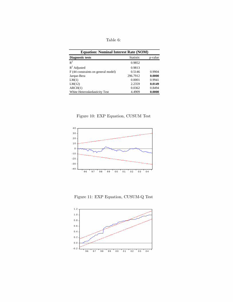
Table 6:
Diagnostic tests Statistic p-valueR2 0.9852R2 Adjusted 0.9813F (44 constraints on general model) 0.5146 0.9904Jarque-Bera 296.7912 0.0000LM(1) 0.0001 0.9941LM(12) 2.2359 0.0149ARCH(1) 0.0362 0.8494White Heteroskedasticity Test 4.4909 0.0000
Equation: Nominal Interest Rate (NOM)
Figure 10: EXP Equation, CUSUM Test
-4 0
-3 0
-2 0
-1 0
0
1 0
2 0
3 0
4 0
9 6 9 7 9 8 9 9 0 0 0 1 0 2 0 3 0 4
Figure 11: EXP Equation, CUSUM-Q Test
-0 .2
0 .0
0 .2
0 .4
0 .6
0 .8
1 .0
1 .2
9 6 9 7 9 8 9 9 0 0 0 1 0 2 0 3 0 4
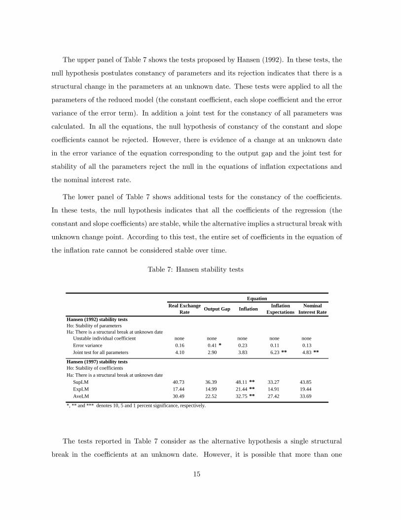
The upper panel of Table 7 shows the tests proposed by Hansen (1992). In these tests, the
null hypothesis postulates constancy of parameters and its rejection indicates that there is a
structural change in the parameters at an unknown date. These tests were applied to all the
parameters of the reduced model (the constant coefficient, each slope coefficient and the error
variance of the error term). In addition a joint test for the constancy of all parameters was
calculated. In all the equations, the null hypothesis of constancy of the constant and slope
coefficients cannot be rejected. However, there is evidence of a change at an unknown date
in the error variance of the equation corresponding to the output gap and the joint test for
stability of all the parameters reject the null in the equations of inflation expectations and
the nominal interest rate.
The lower panel of Table 7 shows additional tests for the constancy of the coefficients.
In these tests, the null hypothesis indicates that all the coefficients of the regression (the
constant and slope coefficients) are stable, while the alternative implies a structural break with
unknown change point. According to this test, the entire set of coefficients in the equation of
the inflation rate cannot be considered stable over time.
Table 7: Hansen stability tests
Hansen (1992) stability testsHo: Stability of parametersHa: There is a structural break at unknown date Unstable individual coefficient none none none none none Error variance 0.16 0.41 * 0.23 0.11 0.13 Joint test for all parameters 4.10 2.90 3.83 6.23 ** 4.83 **
Hansen (1997) stability testsHo: Stability of coefficientsHa: There is a structural break at unknown date SupLM 40.73 36.39 48.11 ** 33.27 43.85 ExpLM 17.44 14.99 21.44 ** 14.91 19.44 AveLM 30.49 22.52 32.75 ** 27.42 33.69
*, ** and *** denotes 10, 5 and 1 percent significance, respectively.
EquationReal Exchange
Rate Output Gap Inflation Inflation Expectations
Nominal Interest Rate
The tests reported in Table 7 consider as the alternative hypothesis a single structural
break in the coefficients at an unknown date. However, it is possible that more than one
15

structural break may have occurred in the coefficients of the linear VAR model. Hence, we
also present tests that allow for multiple breaks in the coefficients, with special focus on partial
structural break tests applied to different groups of coefficients, as explained below.
Table 8 presents the results of two tests proposed by Bai and Perron (2003), the UDmax
andWDmax. In these tests the null indicates the absence of structural breaks, and its rejection
the presence of an unknown number of breaks for a given maximum number of possible breaks.
In this paper, we allowed for a maximum number of three possible structural breaks. This
limit was determined by the size of the sample and the large number of parameters to be
estimated in each equation. Using these tests we examined the stability of different subsets of
coefficients. Specifically, in each equation we tested the stability of the groups of coefficients
corresponding to the lags of each endogenous variable, as well as those associated with the
exogenous variables and the constant. These tests by groups of variables are important because
we are interested in the dynamic response of each endogenous variable to innovations in the
other variables.
As can be observed in Table 8, the only equation that does not show evidence of structural
breaks in any group of parameters is the output gap equation. For the equation of the
real exchange rate both the UDmax and WDmax tests suggest instability of the coefficients
associated with its own lags, the lags of the output gap and those corresponding to the nominal
interest rate. The tests for the inflation equation indicate instability in the coefficients of the
real exchange rate and the output gap, and the WDmax test indicates in addition instability
in the coefficients of inflation expectations. The equation of inflation expectations shows
instability in the coefficients of the real exchange rate, the output gap, the rate of inflation
and the nominal interest rate. Finally, both tests indicate instability in the coefficients of the
nominal interest rate equation corresponding to the real exchange rate, the rate of inflation and
the exogenous variables. Only the WDmax test suggest additional instability of the coefficients
associated with the lags of the output gap and the own lags of the nominal interest rate. In
summary, the UDmax and WDmax tests show clear evidence of instability of the groups of
coefficients in the equations of the linear VAR.
16
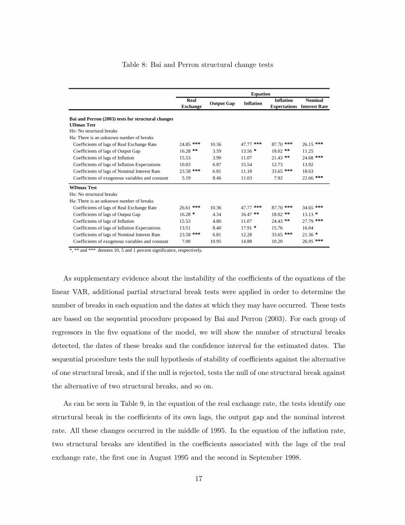
Table 8: Bai and Perron structural change tests
Bai and Perron (2003) tests for structural changesUDmax TestHo: No structural breaksHa: There is an unknown number of breaks Coefficients of lags of Real Exchange Rate 24.85 *** 10.36 47.77 *** 87.70 *** 26.15 *** Coefficients of lags of Output Gap 16.28 ** 3.59 13.56 * 18.02 ** 11.25 Coefficients of lags of Inflation 15.53 3.90 11.07 21.43 ** 24.68 *** Coefficients of lags of Inflation Expectations 10.03 6.87 15.54 12.73 13.92 Coefficients of lags of Nominal Interest Rate 23.58 *** 6.81 11.18 33.65 *** 18.63 Coefficients of exogenous variables and constant 5.19 8.46 11.03 7.92 22.66 ***
WDmax TestHo: No structural breaksHa: There is an unknown number of breaks Coefficients of lags of Real Exchange Rate 26.61 *** 10.36 47.77 *** 87.70 *** 34.65 *** Coefficients of lags of Output Gap 16.28 * 4.34 16.47 ** 18.02 ** 13.13 * Coefficients of lags of Inflation 15.53 4.80 11.07 24.43 ** 27.79 *** Coefficients of lags of Inflation Expectations 13.51 8.40 17.91 * 15.76 16.04 Coefficients of lags of Nominal Interest Rate 23.58 *** 6.81 12.28 33.65 *** 21.36 * Coefficients of exogenous variables and constant 7.00 10.95 14.88 10.20 26.95 ***
Equation
*, ** and *** denotes 10, 5 and 1 percent significance, respectively.
Real Exchange Output Gap Inflation Inflation
ExpectationsNominal
Interest Rate
As supplementary evidence about the instability of the coefficients of the equations of the
linear VAR, additional partial structural break tests were applied in order to determine the
number of breaks in each equation and the dates at which they may have occurred. These tests
are based on the sequential procedure proposed by Bai and Perron (2003). For each group of
regressors in the five equations of the model, we will show the number of structural breaks
detected, the dates of these breaks and the confidence interval for the estimated dates. The
sequential procedure tests the null hypothesis of stability of coefficients against the alternative
of one structural break, and if the null is rejected, tests the null of one structural break against
the alternative of two structural breaks, and so on.
As can be seen in Table 9, in the equation of the real exchange rate, the tests identify one
structural break in the coefficients of its own lags, the output gap and the nominal interest
rate. All these changes occurred in the middle of 1995. In the equation of the inflation rate,
two structural breaks are identified in the coefficients associated with the lags of the real
exchange rate, the first one in August 1995 and the second in September 1998.
17
Additionally, there is one structural break in the coefficients associated with the output
gap in September 1998. The equation of inflation expectations shows three breaks in the
coefficients associated with the real exchange rate (in June 1995, September 1998 and February
2001), and there are also two structural breaks in the coefficients corresponding to the lags
of the output gap (June 1995 and May 1998). In addition, the coefficients of the lags of the
inflation rate show one structural break (October 2001), and those corresponding to the lags of
the nominal interest rate show one break (August 1995). Finally, the equation of the nominal
interest rate presents structural breaks in the coefficients of the real exchange rate (October
1995), the lags of the inflation rate (June 1998), its owns lags (July 1995), and the coefficients
associated to the exogenous variables (June 1999).
The estimated dates of the structural breaks in the coefficients of the reduced form VAR
are far from showing coincidence. Nevertheless, they may suggest the possible dates of the
changes in the monetary transmission mechanism. As can be observed in Figure 12, the dates
of the structural breaks in the coefficients are concentrated in the middle of 1995, the year of
the currency and financial crisis, and during 1998, a year marked by considerable instability in
the Mexican economy as a result of the negative effects of the financial crises in East Asia and
Russia. There are also two break dates in 2001, February and October 2001. These results
suggest that we may expect to find structural breaks in the transmission mechanism in 1995,
1998 and 2001.
18
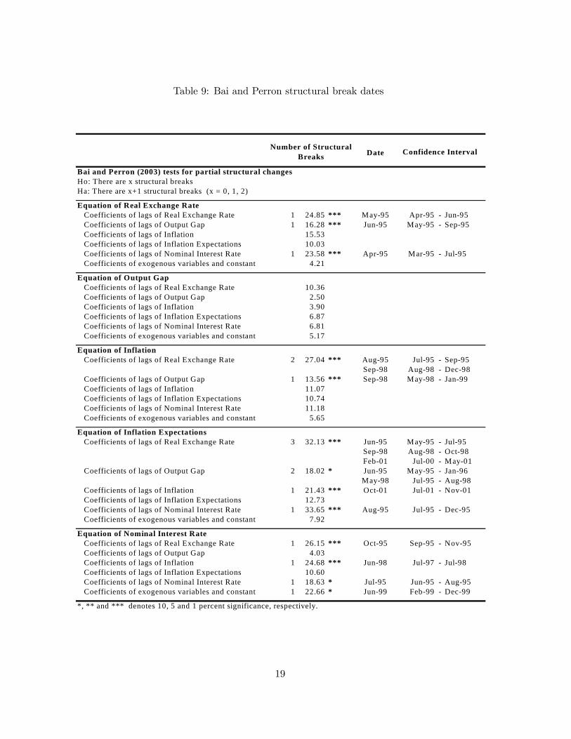
Table 9: Bai and Perron structural break dates
Date
Bai and Perron (2003) tests for partial structural changesHo: There are x structural breaksHa: There are x+1 structural breaks (x = 0, 1, 2)
Equation of Real Exchange Rate Coefficients of lags of Real Exchange Rate 1 24.85 *** May-95 Apr-95 - Jun-95 Coefficients of lags of Output Gap 1 16.28 *** Jun-95 May-95 - Sep-95 Coefficients of lags of Inflation 15.53 Coefficients of lags of Inflation Expectations 10.03 Coefficients of lags of Nominal Interest Rate 1 23.58 *** Apr-95 Mar-95 - Jul-95 Coefficients of exogenous variables and constant 4.21
Equation of Output Gap Coefficients of lags of Real Exchange Rate 10.36 Coefficients of lags of Output Gap 2.50 Coefficients of lags of Inflation 3.90 Coefficients of lags of Inflation Expectations 6.87 Coefficients of lags of Nominal Interest Rate 6.81 Coefficients of exogenous variables and constant 5.17
Equation of Inflation Coefficients of lags of Real Exchange Rate 2 27.04 *** Aug-95 Jul-95 - Sep-95
Sep-98 Aug-98 - Dec-98 Coefficients of lags of Output Gap 1 13.56 *** Sep-98 May-98 - Jan-99 Coefficients of lags of Inflation 11.07 Coefficients of lags of Inflation Expectations 10.74 Coefficients of lags of Nominal Interest Rate 11.18 Coefficients of exogenous variables and constant 5.65
Equation of Inflation Expectations Coefficients of lags of Real Exchange Rate 3 32.13 *** Jun-95 May-95 - Jul-95
Sep-98 Aug-98 - Oct-98Feb-01 Jul-00 - May-01
Coefficients of lags of Output Gap 2 18.02 * Jun-95 May-95 - Jan-96May-98 Jul-95 - Aug-98
Coefficients of lags of Inflation 1 21.43 *** Oct-01 Jul-01 - Nov-01 Coefficients of lags of Inflation Expectations 12.73 Coefficients of lags of Nominal Interest Rate 1 33.65 *** Aug-95 Jul-95 - Dec-95 Coefficients of exogenous variables and constant 7.92
Equation of Nominal Interest Rate Coefficients of lags of Real Exchange Rate 1 26.15 *** Oct-95 Sep-95 - Nov-95 Coefficients of lags of Output Gap 4.03 Coefficients of lags of Inflation 1 24.68 *** Jun-98 Jul-97 - Jul-98 Coefficients of lags of Inflation Expectations 10.60 Coefficients of lags of Nominal Interest Rate 1 18.63 * Jul-95 Jun-95 - Aug-95 Coefficients of exogenous variables and constant 1 22.66 * Jun-99 Feb-99 - Dec-99
*, ** and *** denotes 10, 5 and 1 percent significance, respectively.
Confidence IntervalNumber of Structural Breaks
19

Figure 12: Bai and Perron dates of breaks
Nov
-92
Mar
-93
Jul-9
3
Nov
-93
Mar
-94
Jul-9
4
Nov
-94
Mar
-95
Jul-9
5
Nov
-95
Mar
-96
Jul-9
6
Nov
-96
Mar
-97
Jul-9
7
Nov
-97
Mar
-98
Jul-9
8
Nov
-98
Mar
-99
Jul-9
9
Nov
-99
Mar
-00
Jul-0
0
Nov
-00
Mar
-01
Jul-0
1
Nov
-01
Mar
-02
Jul-0
2
Nov
-02
Mar
-03
Jul-0
3
Nov
-03
Mar
-04
Jul-0
4
Nov
-04
The results of the tests shown provide evidence about the instability of the linear VAR
model estimated. However, the identified break dates are specific to each equation and do not
consider the breaks in the system that is approximated by the VAR. In the next section, we
adopt a flexible estimation strategy that allows an appropriate modeling and identification of
the structural changes in the entire system.
5 Reduced Form Non-linear VAR
In this section, we apply a non-linear estimation methodology aimed at the identification of
the structural changes in the parameters of the reduced form VAR. After the identification of
the dates of structural changes, we will compare the impulse response functions to structural
shocks and the variance decomposition corresponding to different regimes, assuming a recur-
sive structure of the model, in order to assess the changes in the transmission mechanism.
20
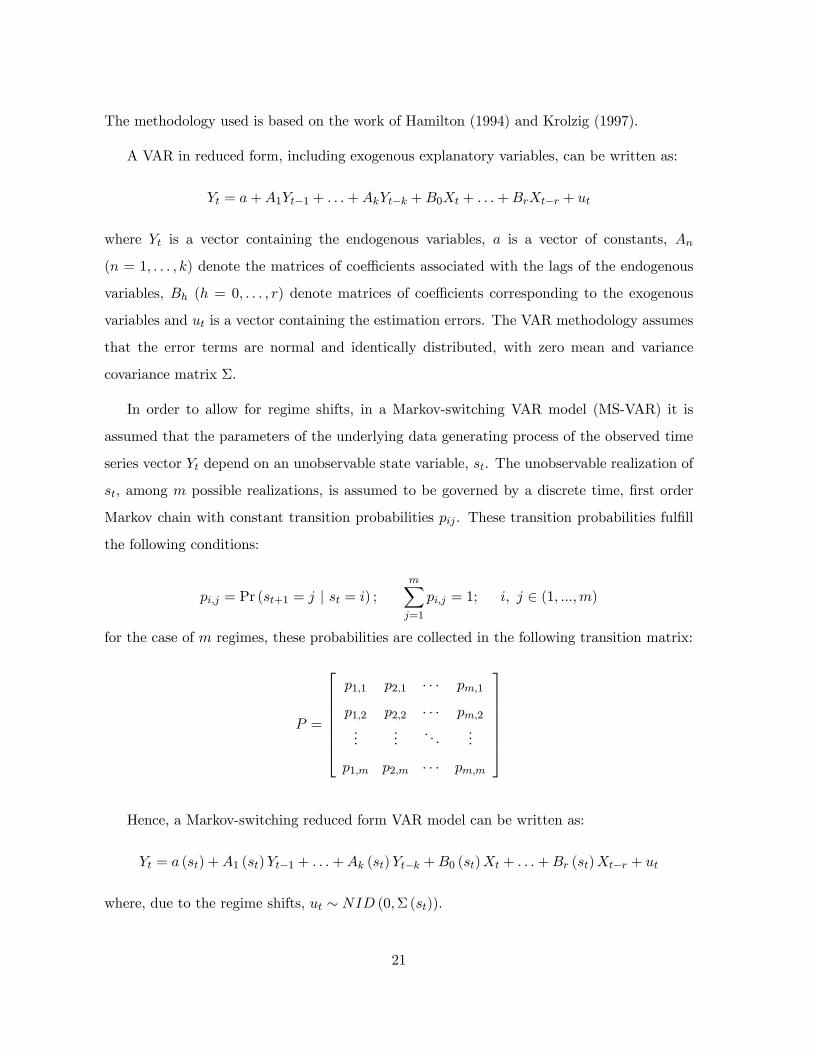
The methodology used is based on the work of Hamilton (1994) and Krolzig (1997).
A VAR in reduced form, including exogenous explanatory variables, can be written as:
Yt = a+A1Yt−1 + . . .+AkYt−k +B0Xt + . . .+BrXt−r + ut
where Yt is a vector containing the endogenous variables, a is a vector of constants, An
(n = 1, . . . , k) denote the matrices of coefficients associated with the lags of the endogenous
variables, Bh (h = 0, . . . , r) denote matrices of coefficients corresponding to the exogenous
variables and ut is a vector containing the estimation errors. The VAR methodology assumes
that the error terms are normal and identically distributed, with zero mean and variance
covariance matrix Σ.
In order to allow for regime shifts, in a Markov-switching VAR model (MS-VAR) it is
assumed that the parameters of the underlying data generating process of the observed time
series vector Yt depend on an unobservable state variable, st. The unobservable realization of
st, among m possible realizations, is assumed to be governed by a discrete time, first order
Markov chain with constant transition probabilities pij . These transition probabilities fulfill
the following conditions:
pi,j = Pr (st+1 = j | st = i) ;mXj=1
pi,j = 1; i, j ∈ (1, ...,m)
for the case of m regimes, these probabilities are collected in the following transition matrix:
P =
⎡⎢⎢⎢⎢⎢⎢⎣p1,1 p2,1 · · · pm,1
p1,2 p2,2 · · · pm,2
......
. . ....
p1,m p2,m · · · pm,m
⎤⎥⎥⎥⎥⎥⎥⎦
Hence, a Markov-switching reduced form VAR model can be written as:
Yt = a (st) +A1 (st)Yt−1 + . . .+Ak (st)Yt−k +B0 (st)Xt + . . .+Br (st)Xt−r + ut
where, due to the regime shifts, ut ∼ NID (0,Σ (st)).
21

It is worth noting that, as in the tests for structural breaks presented in the preceding
section, we do not need any assumption about the dates of the regime shifts or the type of
changes in the parameters of the reduced form VAR. The dates of the shifts will be inferred
from a series of probabilities indicating which regime prevails in any given date of the sample.12
The MS-VAR model was estimated using the same effective sample used in the estimation of
the linear model, that is, from November 1992 to February 2005. In this model the different
regimes imply changes over time in the constant coefficient, the coefficients of the lagged
endogenous variables and the exogenous variables, and the variance covariance matrix of the
residuals.
The small size of the sample (148 effective observations) imposes limitations in the number
of parameters that can be estimated, given that allowing for regime shifts increases very
rapidly the number of parameters to be estimated. With the sample used, an MS-VAR with
four regimes can be estimated including a maximum of three lags of the endogenous variables
and five exogenous regressors. On the other hand, if we consider three regimes and three lags
of the endogenous variables, we can include thirteen exogenous regressors. We considered
that allowing dynamic effects of the exogenous variables was important to obtain a better
identification of the transmission mechanism in each regime, which is approximated by means
of the reduced form VAR corresponding to that regime and the assumptions used to identify
structural shocks. Thus, we estimated an MS-VAR with three regimes and, as a result, it was
necessary to make a selection of the exogenous regressors to be included.
In the case of the rate of growth of the industrial production in the U.S. (FY), the rate
of interest of the three-month US Treasury bill (TB3) and the rate of change of the oil price
index (OIL), we included the contemporaneous values and up to two lags, since we considered
these variables the most important exogenous variables affecting the endogenous variables in
the system. In the case of the rate of inflation in the US (FINF) and the rate of growth of
12The MS-VAR methodology has as a by-product of the expectation maximization algorithm used to maxi-
mize the likelihood function, two series of probabilities for the entire sample. The smoothed probabilities are
calculated using the information of the entire data set, while the filter probabilities are estimated using infor-
mation contained only in the period before any given date for which the probabilities are estimated. Hence, the
series of smoothed probabilities is preferred as indicator of which regime prevails at each date in the sample.
22

the price index of non-energy commodities (NONFUEL), we included only lags one and two
because we considered that the transmission of price movements may involve some delay.
The model described above was tested against alternative models in order to check the
specification used. First, we performed tests to determine the number of regimes. The results
of these tests, shown in the upper panel of Table 10, suggest that the model with three regimes
is preferred to an estimation with only two regimes and to a linear model.13 On the other
hand, the model estimated was also compared with three nested models in which the following
restrictions were imposed: a) the constant coefficients do not change across regimes; b) the
slope coefficients are constant across regimes; and c) the variance covariance matrix of the
residuals is constant across regimes. These hypotheses were rejected using standard likelihood
ratio tests, as can be observed in the lower panel of Table 10. Hence, we maintained the model
with three regimes and shifts in all parameters.
The model was then reduced by eliminating from the system the regressors that resulted
non-significant using the following testing procedure. In the first step, likelihood ratio tests
were computed under the null of zero coefficients for each of the regressors in the system. Based
on these results, the first lag of the rate of inflation of the price index of non-energy primary
goods (NONFUEL(-1)) was eliminated, since the null was not rejected. Then, a reduced
model was estimated and likelihood ratio tests were computed again for each regressor. In
this second (and final) step, the second lag of the external rate of inflation (FINF(-2)) was
eliminated. Table 11 shows the tests described and the joint test for the restriction implied
by the elimination of both variables.
Figure 13 shows the series of smoothed probabilities obtained from the estimation of the
reduced model. As can be observed, the periods corresponding to the currency crisis of 1995
and the turbulence observed in the Mexican economy in the second half of 1998 are identified
13The tests used are non-standard likelihood ratio tests because of the problem of nuisance parameters,
which means that some parameters of the unrestricted model are not identified under the null hypothesis
tested. Basically, these tests are calculated as a correction on the p-value of standard likelihood ratio tests.
Specifically, the relevant p-value of the test is calculated as the sum of the standard p-value of a likelihood ratio
test with n restrictions (the number of parameters that disappear under the null) and the following expression:
2hn2£ehΓ
¡n2
¢¤, where Γ (·) represents the gamma function and h is the difference between the values of the log
of the likelihood functions of the unrestricted and restricted models. See Krolzig (1997).
23

Table 10: MS-VAR tests on regimes and nested models
Null hypothesis Number of restrictions p-value
Two regimes 164 0.000
One regime 326 0.000
In the model with three regimes:
Constancy of the constant coefficient 10 0.000
Constancy of slope coefficients 280 0.000
Constancy of variance covariance matrix 30 0.000
by regime 3. On the other hand, regime 2 includes the period after the currency crisis and
up to February 2001 (excluding the months corresponding to Regime 3 in 1998) and the year
1994. Finally, regime 1 is clearly prevalent since the beginning of 2001 and, according to the
series of probabilities, it was present also before 1994.
Given that the periods before and after the currency crisis of 1994 are qualitatively differ-
ent, because of the change in the exchange rate regime, among other reasons, we estimated
the reduced MS-VAR model with three regimes using as few observations as possible from
the period before the currency crisis, in order to obtain a better identification of the regimes
Table 11: Model reduction
Reduction of the MS-VAR Number of restrictions p-value
1st step: NONFUEL(-1) 15 0.719
2nd step: FINF(-2) 15 0.214
Joint test 30 0.442
24
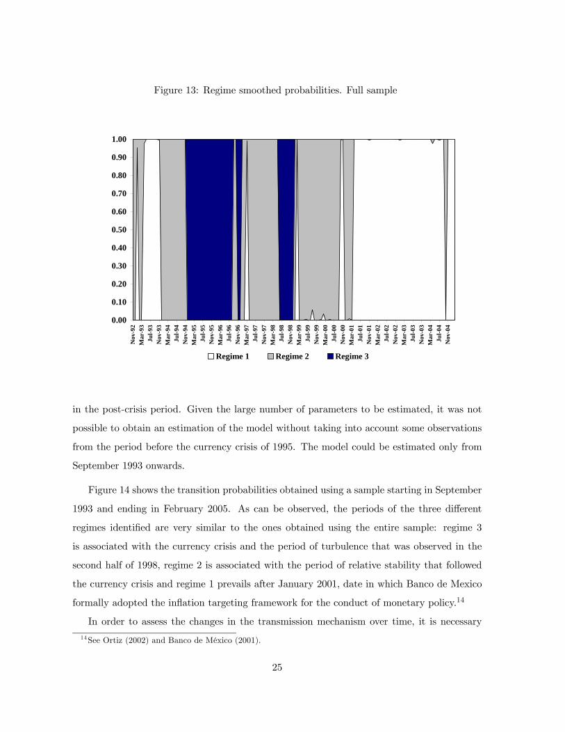
Figure 13: Regime smoothed probabilities. Full sample
0.00
0.10
0.20
0.30
0.40
0.50
0.60
0.70
0.80
0.90
1.00N
ov-9
2M
ar-9
3Ju
l-93
Nov
-93
Mar
-94
Jul-9
4N
ov-9
4M
ar-9
5Ju
l-95
Nov
-95
Mar
-96
Jul-9
6N
ov-9
6M
ar-9
7Ju
l-97
Nov
-97
Mar
-98
Jul-9
8N
ov-9
8M
ar-9
9Ju
l-99
Nov
-99
Mar
-00
Jul-0
0N
ov-0
0M
ar-0
1Ju
l-01
Nov
-01
Mar
-02
Jul-0
2N
ov-0
2M
ar-0
3Ju
l-03
Nov
-03
Mar
-04
Jul-0
4N
ov-0
4
Regime 1 Regime 2 Regime 3
in the post-crisis period. Given the large number of parameters to be estimated, it was not
possible to obtain an estimation of the model without taking into account some observations
from the period before the currency crisis of 1995. The model could be estimated only from
September 1993 onwards.
Figure 14 shows the transition probabilities obtained using a sample starting in September
1993 and ending in February 2005. As can be observed, the periods of the three different
regimes identified are very similar to the ones obtained using the entire sample: regime 3
is associated with the currency crisis and the period of turbulence that was observed in the
second half of 1998, regime 2 is associated with the period of relative stability that followed
the currency crisis and regime 1 prevails after January 2001, date in which Banco de Mexico
formally adopted the inflation targeting framework for the conduct of monetary policy.14
In order to assess the changes in the transmission mechanism over time, it is necessary
14See Ortiz (2002) and Banco de México (2001).
25

Figure 14: Regime smoothed probabilities. Reduced sample
0.00
0.10
0.20
0.30
0.40
0.50
0.60
0.70
0.80
0.90
1.00Se
p-93
Jan-
94M
ay-9
4Se
p-94
Jan-
95M
ay-9
5Se
p-95
Jan-
96M
ay-9
6Se
p-96
Jan-
97M
ay-9
7Se
p-97
Jan-
98M
ay-9
8Se
p-98
Jan-
99M
ay-9
9Se
p-99
Jan-
00M
ay-0
0Se
p-00
Jan-
01M
ay-0
1Se
p-01
Jan-
02M
ay-0
2Se
p-02
Jan-
03M
ay-0
3Se
p-03
Jan-
04M
ay-0
4Se
p-04
Jan-
05
Regime 1 Regime 2 Regime 3
to make some assumptions about the structure of the model that will allow the identification
of the structural shocks in the system and obtain meaningful impulse response functions and
variance decompositions. In what follows, we will assume a recursive structure for the model
with the following order of the endogenous variables: the real exchange rate, the output gap,
the rate of inflation, the inflation expectations and the nominal interest rate. The implicit
assumptions about this particular ordering were discussed in section 2.
The first way we use to assess the changes in the transmission mechanism is based on the
comparison of the impulse response functions of the regimes identified. In this comparison, we
omit the impulse response functions corresponding to regime 3, corresponding to the periods
of the currency crisis of 1995 and turbulence of 1998, given that they are very unstable. Hence,
we will compare the impulse response functions corresponding to regimes 1 and 2, which are
associated mainly with the period that followed the currency crisis and the adoption of the
inflation targeting framework.
26

Figures 15 and 16 present the impulse response functions corresponding to regimes 1 (black
line) and 2 (grey line) using the recursive order of the endogenous variables described above.
The rows of these figures show the response of each variable, in a five-year time horizon, to
a structural shock in one of the variables in the system. Figure 15 shows the response of the
variables to a one standard deviation shock in each regime, while in figure 16 the shocks are
normalized to one percentage point. The comparison of the impulse response functions of the
different regimes will focus on the graphs in Figure 15, which take into account the change in
the distribution of the structural shocks across regimes. The conclusions obtained apply also
to the response functions shown in Figure 16.
In the first row of Figure 15, we can observe that the effects of a shock in the real ex-
change rate on both the rate of inflation and inflation expectations have been considerably
smaller after 2001. Consistent with these reduced effects on the inflation rate and inflation
expectations, the reaction of the nominal interest rate is also smaller when compared with the
reaction observed in the previous period. This would suggest that, after the adoption of the
inflation targeting framework, the process of price formation and the formation of inflation
expectations pay less attention to the fluctuations in the real exchange rate and, hence, the
nominal interest rate has also a milder reaction to those shocks.15
In the second row of Figure 15, we can notice that since 2001 there is an increase in the
response of the inflation rate and inflation expectations to output gap shocks. The response
of the interest rate is stronger and more persistent in the face of those shocks. In addition, the
third row shows that both inflation expectations and the interest rate have stronger and more
persistent reactions to a shock in the rate of inflation. The above suggests that nowadays
the processes of formation of both price and inflation expectations pay less attention to the
movements in the real exchange rate and more to those of the output gap and inflation,
and consequently the reaction of the nominal interest rate is more heavily influenced by these
shocks and less by movements in the real exchange rate. All this is consistent with the inflation
targeting framework and the floating exchange rate regime at work.
15 It its worth noting that in regime 2 some responses of the variables have signs differing from the predictions
of theory, in particular: (i) a real depreciation has a negative effect on the output gap; and (ii) an increase in
the output gap reduces inflation, inflationary expectations and the interes rate.
27

Figure 15: Response functions to a one standard deviation shock
28

Figure 16: Response functions to a one percentage point shock
29
In the last row of Figure 15, we can observe that, after the adoption of the inflation
targeting framework, a shock in the nominal interest rate generates a larger real appreciation
than in the previous regime. Also, increases in the nominal interest rate have been more
effective to produce a faster and stronger reduction of the inflation rate since 2001. This
is so, even when such an increase is able to generate a reduction of the output gap only
after six months. This result suggest that there has been not only a change in the reaction
of the interest rate, with a stronger response to demand pressures and inflation, but that
the increases in the interest rate have become more effective in reducing inflation after the
adoption of the inflation targeting framework.
Another useful tool to assess the changes in the transmission mechanism that can be
obtained from the non-linear VAR estimated, consists in comparing the changes in the variance
decomposition of the different regimes.16 Table 12 shows the variance decomposition of regimes
1 and 2 considering forecast horizons of one (upper panel) and five years (lower panel). The
comparison will focus on a five year horizon since, as can be observed, the results for a one
year horizon are qualitatively the same.
As can be seen in the second column of the lower panel of Table 12, before the adoption
of inflation targeting, the shocks in the real exchange rate explained most of the variance
of the rest of the variables, and these shares have decreased considerably after 2001 for all
variables. In particular, the proportion of the variance of inflation explained by the real
exchange rate decreased from 53 to 4 percent. In a similar way, the shares of the variance
of inflation expectations and the interest rate explained by the real exchange rate decreased
from 59 to 15 percent and from 57 to 14 percent, respectively. After the adoption of inflation
targeting, the actual rate of inflation becomes, in relative terms, a more important determinant
in the process of formation of inflation expectations and the response of the interest rate. In
particular, the explanatory power of inflation increased from 4 to 57 percent for the case of
inflation expectations and from 4 to 31 percent for the nominal interest rate. That means
that inflation surprises have become a more important determinant than real exchange rate
surprises. On the other hand, in the last column of Table 12 we observe that the relative
16The variance decomposition determines the relative explanatory power of the structural innovations for
different time horizons and thus determine the sources of movements of the variables.
30

importance of the interest rate as a source of fluctuations in the rest of the variables has
increased since 2001. In this case, the share of the variance of the real exchange rate explained
by shocks in the nominal interest rate increased from 4 to 31 percent, the one corresponding
to the output gap from 2 to 9 percent and the ones corresponding to the inflation rate and
inflation expectations from 3 to 11 and 9 percent, respectively.
The comparison suggests similar conclusions to the ones obtained before. After the adop-
tion of inflation targeting, the shocks in the real exchange rate have much less influence on
the rest of the variables in the system, while shocks in the inflation rate have more impor-
tant effects on the behavior of inflation expectations and the nominal interest rate. On the
other hand, movements of the nominal interest rate are more effective than before to induce
fluctuations in the real exchange rate, the output gap and the rate of inflation.
31
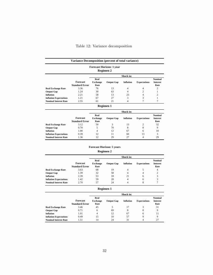
Table 12: Variance decomposition
Forecast Standard Error
Real Exchange
RateOutput Gap Inflation Expectations
Nominal Interest
RateReal Exchange Rate 3.36 76 13 4 4 2Output Gap 1.24 30 63 4 2 1Inflation 2.21 58 13 23 4 2Inflation Expectations 1.21 67 27 3 3 1Nominal Interest Rate 2.55 61 21 4 7 7
Forecast Standard Error
Real Exchange
RateOutput Gap Inflation Expectations
Nominal Interest
RateReal Exchange Rate 3.12 50 3 13 2 32Output Gap 0.70 5 70 8 8 9Inflation 1.00 4 12 67 6 10Inflation Expectations 0.39 12 11 60 13 3Nominal Interest Rate 1.36 12 29 27 4 29
Forecast Standard Error
Real Exchange
RateOutput Gap Inflation Expectations
Nominal Interest
RateReal Exchange Rate 3.63 68 19 4 5 4Output Gap 1.39 32 58 4 4 2Inflation 2.39 53 18 21 6 3Inflation Expectations 1.42 59 28 4 6 3Nominal Interest Rate 2.70 57 24 4 8 7
Forecast Standard Error
Real Exchange
RateOutput Gap Inflation Expectations
Nominal Interest
RateReal Exchange Rate 3.46 45 5 17 3 31Output Gap 0.71 6 69 8 8 9Inflation 1.01 4 12 67 6 11Inflation Expectations 0.49 15 10 57 9 9Nominal Interest Rate 1.51 14 24 31 4 27
Shock in:
Variance Decomposition (percent of total variance)
Shock in:
Regimen 2
Forecast Horizon: 1 yearRegimen 2
Regimen 1
Shock in:
Regimen 1
Shock in:
Forecast Horizon: 5 years
32

6 Conclusions
This paper presents a first approach to the study of the changes that have taken place in the
transmission mechanism of monetary policy in Mexico using a linear VAR model, structural
break tests, and a non-linear VAR methodology that is appropriate for modeling regime shifts.
First, we estimated a linear reduced form VAR and studied the stability of its parameters
over time using an ample set of structural change tests. These tests led to the conclusion that
the linear VAR model is subject to a considerable degree of parameter instability over time.
To overcome this problem and be able to model appropriately the structural changes in the
transmission mechanism, we adopted an estimation method that allows for changes over time
in all the coefficients of the VAR, as well as heteroscedastic errors.
Based on the estimation of a MS-VAR that allows regime shifts without the need of
assumptions about the dates of the shifts, and assuming a recursive structure of the system,
we compared the impulse response functions and variance decomposition corresponding to
different regimes. This allowed us to characterize the structural changes that have occurred
in recent years.
The results suggest that there was a major structural change in the transmission mech-
anism of monetary policy around the beginning of 2001, the date of formal adoption of the
inflation targeting framework for the conduct of monetary policy. This structural change
implied a less important role of the fluctuations of the real exchange rate in the process of
price formation and in the formation of inflation expectations, as well as a milder effect on
the nominal interest rate. Also, the adoption of the inflation targeting framework involved
a stronger reaction of the nominal interest rate due to increases in the output gap and the
inflation rate. In addition, we found that after the structural change, movements of the nom-
inal interest rate have had a stronger effect on the real exchange rate, and have become more
effective in changing the trajectory of inflation.
This study should be considered a first step on a broader research agenda aimed at analyz-
ing the transmission mechanism of monetary policy in Mexico. However, even if the estimated
model has some drawbacks inherent to the VAR approach in general, and the recursive iden-
tification of structural shocks in particular, it serves the purpose of shedding light about the
33
dates of the changes in the transmission mechanism and its characterization. A next step
in the research agenda, would imply using alternative identification assumptions, based on
more solid theoretical grounds, to estimate structural vector autoregression models (SVAR).
In particular, the immediate next step seems to involve using a set of sign restrictions for the
impulse response functions derived form a theoretical small open economy model, as in the
work of Canova and de Nicolo (2002) and Uhlig (2005).
References
[1] Bai, J. & Perron, P. (1998). "Estimating and Testing Linear Models with Multiple Struc-
tural Changes". Econometrica, 66 (1), 47-78.
[2] –––––- (2003a). "Computation and Analysis of Multiple Structural Change Mod-
els". Journal of Applied Econometrics, 18 (1), 1-22.
[3] –––––- (2003b). Critical Values for Multiple Structural Change Tests. Econometrics
Journal, 6 (1), 72-78.
[4] Banco de México (2001). "Informe sobre la Inflación: Octubre-Diciembre 2000", Banco
de México.
[5] Bernanke, B. S. & Blinder A. (1992). "The Federal Funds Rate and the Channels of
Monetary Transmission". American Economic Review, 82 (4), 901-921.
[6] Bernanke, B. S. & Mihov, I. (1998). "Measuring Monetary Policy". Quarterly Journal of
Economics, 113 (3), 869-902.
[7] Boivin, J. & Giannoni, M. (2002a). "Assessing Changes in the Monetary Transmission
Mechanism: A VAR Approach". Economic Policy Review, 8 (1), 97—111.
[8] –––––- (2002b). "Has Monetary Policy Become Less Powerful?" Staff Report No.
144, Federal Reserve Bank of New York.
[9] Brüggemann, R. & Lütkepohl, H. (2001). "Lag Selection in Subset VAR Models with an
Application to a U.S. Monetary System". In R. Friedmann, L. Knüppel and H. Lütkepohl
34

(Eds.), Econometric Studies — A Festschrift in Honor of Joachim Frohn, pp. 107-128. LIT,
Münster.
[10] Brüggemann, R., Lütkepohl, H., & Krolzig, H. (2003). "Comparison of Model Reduction
Methods for VAR Processes". Unpublished manuscript, Economics Department, Oxford
University.
[11] Canova, F. & De Nicolo, G. (1998). "Did You Know that Monetary Shocks Matter for
Output and Inflation Cycle? Evidence from the G-7". CEPR Working Paper, No.2028.
[12] –––––- (2002). "Monetary Disturbances Matter for Business Fluctuations in the
G-7". Journal of Monetary Economics, 49 (6), 1131-1159.
[13] Canova, F. & Pina, J. (1999). "Monetary Misspecification in VAR Models". CEPRWork-
ing Paper, No.2333.
[14] Clarida, R. (2001). "The Empirics of Monetary Policy Rules in Open Economies". Inter-
national Journal of Finance and Economics, 6 (4), pp.315-23.
[15] Clarida, R. & Gertler, M. (1997). "How the Bundesbank Conducts Monetary Policy".
In C. D. Romer and D. H. Romer (Eds.), Reducing Inflation: Motivation and Strategy.
NBER. Studies of Business Cycles, 30, Chicago.
[16] Clarida, R., Gali, J. & Gertler, M. (2001). "Optimal Monetary Policy in Open versus
Closed Economies: An Integrated Approach". The American Economic Review, 91 (2),
248-252.
[17] Choi, K., Jung, C. & Shambora, W. (2003) "Macroeconomic Effects of Inflation Targeting
Policy in New Zealand". Economics Bulletin, 5 (17), 1-6.
[18] Christiano, L., M. Eichenbaum and C. Evans (2000). "Monetary Policy Shocks: What
Have We Learned and to What End?" in Taylor and Woodford, Handbook of Macroeco-
nomics.
[19] Cooley, T. & Dwyer, M. (1998). "Business Cycle Analysis Without Much Theory A Look
at Structural VARs". Journal of Econometrics, 83 (1-2), 57-88.
35
[20] Cooley, T & Leroy, S. (1985). "Atheoretical Macroeconomics: A Critique". Journal of
Monetary Economics, 16 (3), 283-308.
[21] Faust, J. & Leeper, E. (1997). "When Do Long-Run Identifying Restrictions Give Reliable
Results?" Journal of Business and Economic Statistics, 15 (3), 345-353.
[22] Francis, N. & Owyang, M.T. (2004). "Monetary Policy in a Markov-Switching VECM:
Implications for the Cost of Disinflation and the Price Puzzle". Working Paper 2003-
001D. Federal Reserve Bank of St. Louis.
[23] Gali, J. & Monacelli, T. (2002). "Monetary Policy and Exchange Rate Volatility in a
Small Open Economy". NBER, Working Paper no. 8905.
[24] Gottschalk, J. (2001). "An Introduction into the SVAR Methodology: Identification,
Interpretation and Limitations of SVAR Models". University of Kiel Working Paper No.
1072.
[25] Hamilton, J. D. (1994). Time Series Analysis. Princeton University Press, New Jersey.
[26] Hansen, B. E. (1990). "Lagrange Multiplier Tests for Parameter Instability in Non-Linear
Models". Unpublished manuscript, University of Rochester.
[27] –––––- (1991). "A Comparison of Tests for Parameter Stability: An Examination
of Asymptotic Local Power". Unpublished manuscript, University of Rochester.
[28] –––––- (1992). "Testing for Parameter Instability in Linear Models". Journal of
Policy Modeling, 14 (4), 517-533.
[29] –––––- (1997). "Approximate Asymptotic P Values for Structural-Change Tests".
Journal of Business & Economic Statistics, 15 (1), 60-67.
[30] Hendry, D. F. & Krolzig, H.-M. (2003). "The Properties of Automatic Gets Modelling".
Unpublished manuscript, Economics Department, Oxford University.
[31] Krolzig, H.-M. (1997). Markov-Switching Vector Autoregressions. Modelling, Statistical
Inference and Application to Business Cycle Analysis. Springer,Berlin.
36

[32] –––––- (2003). "General-to-Specific Model Selection Procedures for Structural Vec-
tor Autoregressions". Unpublished manuscript, Economics Department, Oxford Univer-
sity.
[33] Leeper, E., Sims, C. & Zha, T. (1996). "What does Monetary Policy Do?". Brookings
Papers on Economic Activity, 2, 1-78.
[34] Martínez, L., Sánchez, O. & Werner, A. (2001). "Consideraciones sobre la Conducción
de la Política Monetaria y el Mecanismo de Transmisión en México". Banco de México
Research Document 2001-2.
[35] Ortiz, G. (2002). "Inflación y Política Monetaria en México", presentation of La Inflación
en México (2 volumes), Gaceta de Economía, ITAM, México, 9-16.
[36] Perron, P. (1994). "Trend, Unit Root and Structural Change in Macroeconomic Time Se-
ries". In B.B. Rao (Ed.), Cointegration for the Applied Economist, Chapter 4. St.Martin’s
Press, New York.
[37] Quah, D. & Vahey, S. (1995). "Measuring Core Inflation". Economic Journal, 105, 1130-
1144.
[38] Sims, C. (1980). "Macroeconomics and Reality". Econometrica, 48 (1), 1-48.
[39] –––––- (1982). "Policy Analysis with Econometric Models". Brookings Papers on
Economic Activity, 1, 107-152.
[40] –––––- (1992). "Interpreting the Macroeconomic Time Series Facts: The Effects of
Monetary Policy". European Economic Review, 36 (5), 975-1000.
[41] Svensson, L.E.O. (2000). "Open-economy inflation targeting". Journal of International
Economics 50 (1), 155-184.
[42] Uhlig, H. (2005). "What Are The Effects of Monetary Policy on Output? Results from
an Agnostic Identification Procedure". Journal of Monetary Economics, 52 (2), 381-419.
37

A Inflation expectations
The expected rate of inflation from the monthly survey conducted by Banco de México is available
from May 1997, and there is no alternative source of information about this variable before that date.
In this appendix we present the equation used to complete the series of the expected rate of inflation
for the period November 1991 - April 1997. The series was constructed as a dynamic forecast of the
following GMM equation:
πet = α1 + α2πet−1 + α3π
et−2 + α4π
at + α5immt + α6dept + α7Dt ∗ dept
where, πet is the rate of inflation expectations, πat the annual rate of inflation, imm the money market
rate and dept the rate of nominal depreciation. The list of instruments include lags of the following
variables: inflation expectations, annual inflation, the money market rate, nominal depreciation and
manufacturing wages (w). The lags used as instruments are shown in Table A1. To account for the
effect of nominal depreciation on inflation expectations we included a dummy variable (Dt) interacted
with nominal depreciation. This dummy variable Dt takes the value of 1 if nominal depreciation
exceeds the 12-month moving average plus two standard deviations. The result of the estimation is
shown in the following table:
Table A1
Method: GMMSample: 1997:09 a 2005:01
Coefficient Std. Error
0.0677 0.06220.5772 *** 0.10820.1922 ** 0.08490.0882 *** 0.02630.0576 *** 0.01150.1006 *** 0.03780.2508 *** 0.0754
R2 0.9941*** Denotes 1 percent significance.** Denotes 5 percent significance.
1α
2α
3α
4α
5α
6α
7α
Instrument list: ∆πet−2, πet−3, π
et−4, ∆π
at−1, π
at−2, π
at−3,
∆immt−1,∆immt−2, immt−3, immt−4,
dept−1, dept−2,∆wt−1, wt−2, wt−3
38
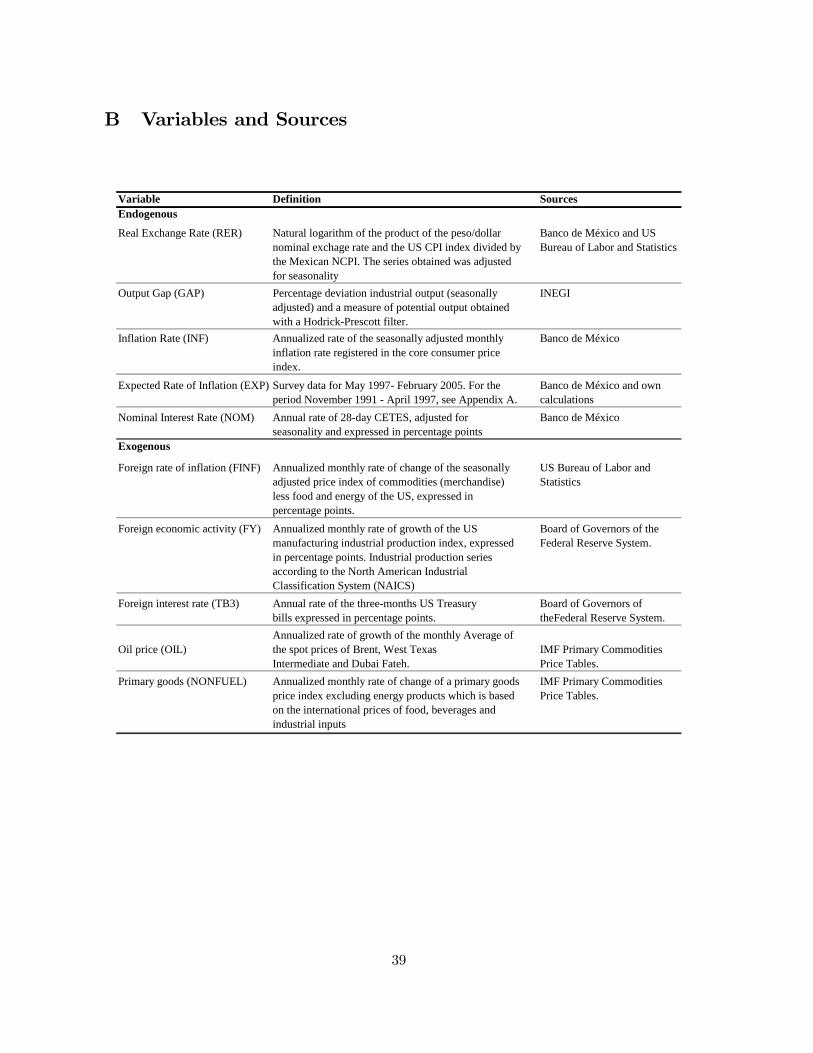
B Variables and Sources
Variable Definition SourcesEndogenous
Real Exchange Rate (RER) Natural logarithm of the product of the peso/dollarnominal exchage rate and the US CPI index divided by the Mexican NCPI. The series obtained was adjusted for seasonality
Banco de México and USBureau of Labor and Statistics
Output Gap (GAP) Percentage deviation industrial output (seasonally adjusted) and a measure of potential output obtained with a Hodrick-Prescott filter.
INEGI
Inflation Rate (INF) Annualized rate of the seasonally adjusted monthlyinflation rate registered in the core consumer price index.
Banco de México
Expected Rate of Inflation (EXP) Survey data for May 1997- February 2005. For the period November 1991 - April 1997, see Appendix A.
Banco de México and own calculations
Nominal Interest Rate (NOM) Annual rate of 28-day CETES, adjusted for seasonality and expressed in percentage points
Banco de México
Exogenous
Foreign rate of inflation (FINF) Annualized monthly rate of change of the seasonally adjusted price index of commodities (merchandise) less food and energy of the US, expressed in percentage points.
US Bureau of Labor and Statistics
Foreign economic activity (FY) Annualized monthly rate of growth of the USmanufacturing industrial production index, expressed in percentage points. Industrial production series according to the North American Industrial Classification System (NAICS)
Board of Governors of the Federal Reserve System.
Foreign interest rate (TB3) Annual rate of the three-months US Treasury bills expressed in percentage points.
Board of Governors of theFederal Reserve System.
Oil price (OIL)Annualized rate of growth of the monthly Average of the spot prices of Brent, West TexasIntermediate and Dubai Fateh.
IMF Primary CommoditiesPrice Tables.
Primary goods (NONFUEL) Annualized monthly rate of change of a primary goodsprice index excluding energy products which is based on the international prices of food, beverages and industrial inputs
IMF Primary CommoditiesPrice Tables.
39
Related Documents