Structural Approaches to Vector Autoregressions · in empirical macroeconomics and finance. The VAR is a reduced.form time series model of the economy that is estimated by ordinary

John W. Keating

John W. Keating, assistantprofessor, Department of Economics,Washington University in St. Louis, was a visiting scholar atthe Federal Reserve Bank of St. Louis while this paper waswritten. Richard L Jako provided research assistance.

Structural Approaches toVector Autoregressions

ciait HE VECTOR AUTOREGRESSION (VAR)

model of Sims (1980) has become a popular toolin empirical macroeconomics and finance. TheVAR is a reduced.form time series model of theeconomy that is estimated by ordinary leastsquares.1 Initial interest in VARs arose becauseof the inability of economists to agree on theeconomy’s true structure. VAR users thoughtthat important dynamic characteristics of theeconomy could be revealed by these modelswithout imposing structural restrictions from aparticular economic theory.

Impulse response functions and variancedecompositions, the hallmark of VAR analysis,illustrate the dynamic characteristics of empiricalmodels. These dynamic indicators were initiallyobtained by a mechanical technique that somebelieved was unrelated to economic theory.2Cooley and LeRoy (1985), however, argued thatthis method, which is often described as atheo~retical, actually implies a particular economicstructure that is difficult to reconcile with eco-nomic theory.

This criticism led to the development of a“structural” VAR approach by Bernanke (1986),Blanchard and Watson (1986) and Sims (1986).This technique allows the researcher to use eco-nomic theory to transform the reduced-form

VAR model into a system of structural equations.The parameters are estimated by imposing con-temporaneous structural restrictions. The crucialdifference between atheoretical and structuralVARs is that the latter yield impulse responsesand variance decompositions that can be givenstructural interpretations.

An alternative structural VAR method, developedby Shapiro and Watson (1988) and Blanchard andQuah (1989), utilizes long-run restrictions toidentify the economic structure from the reducedform. Such models have long-run characteristicsthat are consistent with the theoretical restric-tions used to identify parameters. Moreover,they often exhibit sensible short-run propertiesas well.

For these reasons, many economists believe thatstructural VARs may unlock economic informationembedded in the reduced-form time series model.This paper serves as an introduction to thisdeveloping literature. The VAR model is shownto be a reduced-form for a linear simultaneousequations model. The contemporaneous andlong-run approaches to identifying structuralparameters are developed. Finally, estimatesof contemporaneous and long-run structuralVAR models using a common set of macro-economic variables are presented. These models

‘A VAR can be derived for a subset of the variables from alinear structural model. Furthermore, it is a linear approxi-mation to any nonlinear structural model. The accuracy ofthe VAR approximation will depend on the features of thenonlinear structure.

2A Choleski decomposition of the covariance matrix for theVAR residuals.

SEPTEMBEP,/OCTOBEFI 1992

are intended to provide a comparison betweencontemporaneous and long-run structural VARmodeling strategies. The implications of theempirical results are also discussed.

The standard, linear, simultaneous equationsmodel is a useful starting point for understandingthe structural VAR approach. A simultaneousequations system models the dynamic relation-ship between endogenous and exogenous vari-ables. A vector representation of this system is

(1) Ax1 = C(L)x1, + Dz1,

where x1 is a vector of endogenous variablesand z1 is a vector of exogenous variables. Theelements of the square matrix, A, are the struc-tural parameters on the contemporaneous en-dogenous variables and C(L) is a kth degreematrix polynomial in the la~operator L, that is,C(L)=Co+CIL+CZL2+...+CkL, where all of the Cmatrices are square. The matrix D measures thecontemporaneous response of endogenous varia-bles to the exogenous variables.~In theory,some exogenous variables are observable whileothers are not. Observable exogenous variablestypically do not appear in VARs because Sims(1980) argued forcefully against exogeneity.Hence, the vector z is assumed to consist of un-observable variables, which are interpreted asdisturbances to the structural equations, and x1and z1 are vectors with length equal to the num-ber of structural equations in the model.~

A reduced-form for this system is

(2) x1 = A”C(L) x1, + A~Dz1.

A panicular structural specification for the “er-ror term” z is required to obtain a VARrepresentation. Two alternative, commonly used

and attractive assumptions are that shocks haveeither temporary or permanent effects. If shockshave temporary effects, z1 equals s,, a seriallyuncorrelated vector (vector white noise).~That is,

(3) z1 = E~.

Alternatively, z can be modeled as a unit rootprocess, that is,

(4) z1 — z1, =

Equation 4 imphes that z equals the sum of allpast and present realizations of E. Hence, shocksto z are permanent. The assumptions in equations3 and 4 are not as restrictive as they might ap-pear. If these shock processes were specified asgeneral autoregressions, the VARs would haveadditional lags. The procedures to identify struc-tural parameters, however, would be unaffected.

Under the assumption that exogenous shockshave only temporary effects, equation 2 can berewritten as,

(5) x1 = /3(L); , + e1,

where /3(L) = A~C(L)and e1 = A”Dç. Theequation system in 5 is a VAR representation ofthe structural model because the last term inthis expression is serially uncorrelated and eachvariable is a function of lagged values of all thevariables.6 The VAR coefficient matrix, /3(L), is anonlinear function of the contemporaneous andthe dynamic structural parameters.

If the shocks have permanent effects, the VARmodel is obtained by applying the first differenceoperator (A = 1— L) to equation 2 and insertingequation 4 into the resulting expression, to obtain

(6) Ax, = /3(L)Ax1, + e1,

with /3(L) and e1 previously defined.

This is a common VAR specification because manymacroeconomic time series appear to have aunit root.7 Because of the low power of tests

~Thismodel can accommodate lags of z; this feature is omitted,however, to simplify the discussion.

if observable exogenous variables exist, they are includedas explanatory variables in the VAR.

5The individual elements in a vector white noise process, intheory, may be contemporaneously correlated. In structuralVAR practice, they are typically assumed to be independent.

6The last term represents linear combinations of seriallyuncorrelated shocks, and these are serially uncorrelated aswell. See any textbook covering the basics of time seriesanalysis for a proof of this result.

‘This model can also be written in levels form:

x1

=[AC(L) + I]x,_1 —A1C(L) x1_2 + A1DE1.

Sims, Stock and Watson (1990) show that this reduced formis consistently estimated by OLS, but hypothesis tests mayhave non-standard distributions because the series haveunit roots.

39

for unit roots, their existence is controversial.VARs can accommodate either side of the de-bate, however.8

The VAR is a general dynamic specificationbecause each variable is a function of laggedvalues of all the variables. This generality, how-ever, comes at a cost. Because each equationhas many lags of each variable, the set of varia-bles must not be too large. Otherwise, the mod-el would exhaust the available data? If allshocks have unit roots, equation B is estimated.If all shocks are stationary, equation 5 is used.b0If some shocks have temporary effects whileothers have permanent effects, the empiricalmodel must account for this.

Recently, Blanchard and Quah (1989) have es-timated a VAR model where some variableswere assumed to be stationary while others hadunit roots. Alternatively, ICing, Plosser, Stockand Watson (1991) use a cointegrated model,where all the variables are difference stationarybut some linear combinations of the variablesare stationary. The stationary linear combinationsare constructed by cointegration regressions priorto VAR estimation. They impose the cointegrationconstraints using the vector error-correctionmodel of Engle and Granger (1987). Sometimesunit-root tests combined with theory suggest thecoefficients for stationary linear combinations.Shapiro and Watson (1988), for example, presentevidence that the nominal interest rate and in-flation each have a unit root while the differ-ence between these two variables is stationary.They impose the cointegration constraint byselecting this noisy proxy for the real rate ofinterest as a variable for the model.

Unrestricted versions of the VAR model (andthe error-correction model) are estimated by or-dinary least squares (OLS) because Zeliner(1962) proved that OLS estimates of such a sys-tem are consistent and efficient if eachequation has precisely the same set of explanatoryvariables. If the underlying structural modelprovides a set of over-identifying restrictions onthe reduced form, however, OLS is no longeroptimal.” The simultaneous equations system in

a contemporaneous structural VAR, however,generally does not impose restrictions on thereduced form.

An alternative approach of Doan, Littermanand Sims (1984) estimates the VAR in levels witha Bayesian prior placed on the hypothesis thateach time series has a unit root. The BayesianVAR model permits more lags by imposingrestrictions on the VAR coefficients, reducingthe number of estimated parameters (calledhyper-parameters). The reduction in parameterscontributes to the Bayesian model’s propensityto yield superior out-of-sample forecasts comparedwith unrestricted VARs with symmetric lagstructure,

rp2~/’fJ21%Jp~flR4,29j.2i)jt12/S’171iUC~

‘L1JR.A1..~VAR 9/flfl9L1~

9~

It is clear from equations 5 and 6 that, if thecontemporaneous parameters in A and D wereknown, the dynamic structure represented bythe parameters in C(L) could be calculated fromthe estimated VAR coefficients, that is, C(L) =

A/3(L). Furthermore, the structural shocks, E,,

could be derived from the estimated residuals,that is, ç = D - ‘Ae,. Because the coefficients inA and D are unknown, identification of structuralparameters is achieved by imposing theoreticalrestrictions to reduce the number of unknownstructural parameters to be less than or equalto the number of estimated parameters of thevariance-covariance matrix of the VAR residuals.Specifically, the covariance matrix for the residuals,

~ from either equation 5 or equation 6 is

(7) 1 =E{e,eJ = A’DE~s/JDA2= A’DX,DA’,

where E is the unconditional expectations operator,and I is the covariance matrix for the shocks.

An OLS estimate of the VAR provides an estimateof Xe that can be used with equation 7 to obtainestimates of A, D and I~.The contemporaneousstructural approach imposes restrictions onthese three matrices. There are n2 elements in A,

8 Alternatively, the unit root could result from parameters inthe dynamic structural model.

o The lag structure of a VAR can be shown to represent vari-ous sources of economic dynamics. Structural models withrational expectations predict restrictions on the VAR model.Dynamics in these models are often motivated by the costsof adiustment to desired or equilibrium positions. The lagstructure of the VAR can also be motivated by dynamicprocesses for structural disturbances.

1OVAR lag length is often selected by statistical criteria suchas the modified likelihood ratio test of Sims (1980).

hA two-step structural VAR estimator will generally not beefficient if there are structural restrictions for C(L) since thisimplies restrictions on /3(L). For example, Sargent (1979)derives restrictions on VAR coefficients from a particularmodel of the term structure of interest rates under rationalexpectations. The full structural system is estimated bymaximum likelihood.

n2 elements in D, and n(n+ 1)12 unique elementsin I,, but only n(n + 1)/2 unique elements in 1,,.The maximum number of structural parametersis equal to the number of unique elements in I~.Thus, a structural model will not be identified un-less at least Zn2 restrictions are imposed on A,D and I.

Often these restrictions are exclusion restrictions;of course, that need not be the case. Typically,I, is specified as a diagonal matrix because theprimitive structural disturbances are assumed tooriginate from independent sources. The remainingparameters are identified by imposing additionalrestrictions on A and D. The main diagonal ele-ments of A are set to unity because each structuralequation is normalized on a particular endogenousvariable. The main diagonal for D has this samespecification since each equation has a structuralshock. These normalizations provide 2n restric-tions. Identification requires at least 3n(n — 1)12 ad-ditional restrictions based on economic theory.Alternatively, the restrictions may be based onthe contemporaneous information assumedavailable to particular economic agents followingSims (1986). Keating (1990) and West (1990) ex-tend this approach by showing how rational ex-pectations restrictions can be imposed in thecontemporaneous structural VAR framework.Except for Bernanke (1986) and Blanchard(1989), existing models typically have not at-tempted to identify the structural parametersin D- Hence, D is usually taken to be the identitymatrix, leaving at least n(n — 1)/2 additional iden-tifying restrictions to be imposed on A.

A two-step procedure is used to estimatestructural VAR models. First, the reduced-formVAR, with enough lags of each variable toeliminate serial correlation from the residuals, isestimated with OLS. Next, a sufficient numberof restrictions is imposed on A, D and I~toidentify these parameters. This paper obtainsthe parameters in equation 7 with an algorithmfor solving a nonlinear system of equations.Blanchard and Quah (1989) use this approach toestimate a structural VAR model.” Standarderrors for the parameters, the impulse responsesand the variance decompositions are calculated

using the Monte Carlo approach of Runkle(1987), which simulates the VAR model togenerate distributions for these results.”

The identification technique used in this paperis adequate for a model in which the number ofparameters is equal to the number of uniqueelements in I~•Alternative methods are neededto estimate a model with fewer parameters.Bernanke (1986) uses the method-of-momentsapproach of Hapsen (1982) to estimate theparameters in equation 7 and obtain standarderrors. Sims (1986) estimates the system ofsimultaneous equations for the residualsin equation 5 using maximum likelihood.”Blanchard and Watson (1986) also estimate thesystem of equations for residuals; however, theyemploy a sequential instrumental variables tech-nique in which estimated structural shocks areused as instruments in all subsequent equa-tions.15

The following four-equation contemporaneousstructural VAR model is used to illustrate a par-ticular set of such identifying restrictions. Theresiduals from a VAR consisting of the price lev-el (p), output (y), the interest rate (r) and money(m) are used in the model. This model is used inthe empirical work which follows. Equation 8provides three restrictions by assuming that theprice level is predetermined, except thatproducers can respond immediately to aggre-gate supply shocks. Equation 9 is a reduced-form IS equation that models output as afunction of all the variables in the model. Thisapproach was taken instead of explicitly model-ing expected future inflation to calculate thereal interest rate and explicitly modeling theterm structure of interest rates to tie the short-term rate in the model with the long-term ratepredicted by theory. The IS disturbance is alsoa factor in the output equation. The money sup-ply function in equation 10 allows the Fed toadjust short-term interest rates to changes inthe money stock. Two restrictions are obtainedfrom assuming that the Fed does not immediatelyobserve aggregate measures of output and price.The last equation is a short-run money demandfunction specifying nominal money holdings as

“Their model is identified by long-run restrictions.“The actual residuals are randomly sampled, and the sampled

residuals are used as shocks to the estimated VAR. Afterthe artificial series are generated, they are used to performthe same structural VAR analysis. After 200 replications ofthe model, standard errors were calculated for the parameterestimates, the impulse responses and the variance decom-positions.

‘~lncontrast to the typical simultaneous equations model,this approach has no observable exogenous variables.

‘5This technique requires a structural model for which thereare no estimated parameters in the first equation, the secondequation has one parameter, the third has two parameters,etc. While the recursive model fits this description, thistechnique can estimate a much broader set of models.

a function of nominal GNP and the interest rate.This specification is motivated by a buffer stocktheory where short-run money holdings rise inproportion to nominal income, yielding the finalrestriction for a just-identified model. Eachequation includes a structural disturbance.

(8) e~= £7’

(9) e~= A1e~+ A2eç + A3e~°+

(10) ef = A4e7’ + r”

(11) er = AJe~+ eV) + A,e~+ ErStandard VAR tools are employed after the

structural parameters are estimated. Impulse re-sponse functions and variance decompositionfunctions conveniently summarize the dynamicresponse of the variables to the shocks, whichis known as the moving average representation(MAR). The MAR for the VAR is obtained byapplying simple algebra to a function of the lagoperator. Take the VAR model for x:

x1 = /3(L), +

and subtract /3(L) from both sides of thisequation:

— fl(L)x1_, = e,.

Then factor terms in x, using the lag operator,

[I — /3(L)L]; = e1.

Multiply both sides of this equation by the in-verse of [I—f3(L)L]:

x1 =[I — /3(L)Lf’e1.

Insert the expression from equation 5 for e1 intothis last equation:

(12) x, = [I — /3(L)L f’A’Ds, =

where 0(L) =

and each 0, is an n x n matrix of parametersfrom the structural model. Equation 12 impliesthat the response of ~ to c, is 0

r Hence, thesequence of 0~from i=O,1,2 illustrates the

dynamic response of the variables to the shocks.If the variables in x are stationary, then the im-pulse responses must approach zero as i be-comes large.

Variance decompositions allocate each variable’sforecast error variance to the individual shocks.These statistics measure the quantitative effectthat the shocks have on the variables. If E, x, isthe expected value of x, based on all informationavailable at time t—j, the forecast error is:

— E,~x,= 9~

since the information at time t — j includes all £

occurring at or before time t — j and the condition-al expectation of future E is zero because theshocks are serially uncorrelated. The forecasterror variances for the individual series are thediagonal elements in the following matrix:

E(x, — E1~x,)(x1 — E,~) =

If 0~,is the (v,s) element in 0, and a, is thestandard deviation for disturbance s (s = 1 n),the j-steps-ahead forecast variance of the v-thvariable is easy to calculate:

i—I

E(x,~— E,~x~1)2= ~ ~9, o v = 1, 2,..., n

The variance decomposition function (VDF)writes the j-steps-ahead percentage of forecasterror variance for variable v atributable to thek-th shock:

i..1

~(13) VDF(v,k,j) = x 100.

~i~o s~1

The same analysis can be used to derive theMAR for the VAR model in equation 6.

(14) Ax1 =

where 0(L) =[T—/3(L)Lf’A’D. The response ofx, rather than the change in x, is frequently ofgreater interest to economists. These impulseresponses can be generated recursively by as-suming that all the elements of e at time zeroand earlier are equal to zero.1°For example,

‘elf the pre-sample is nonzero, its effects are lumped to-gether with x0 which represents the initial conditions.

42

= x0 + LONG.~RL.uvSEITRL.JCTURAL VARMODELS

and

= x, +60E, + O,E,.

Inserting the expression for x, into the x2 equa-tion yields:

= x, +90E

2+ (00 + O,)E,.

Repeating this operation for all x up to x,, yieldsthe following:

= x0 + 05e, + ( 0,~+ 0,)c,~,+ ... +

This result is equivalently written as

(15) x1 = x0 + I(L)E~ = x0 + L r.E~.,

where r~= Li—U

(?~~0,)c,.

The response of x÷toE, is I~.Since the differencedspecification assumes that Ax is stationary, the 0.matrix goes to zero as j gets large. This impliesthat 1 converges to the sum of coefficients in0(L). Restrictions on this sum of coefficients areused to identify long-run structural VAR models.The variance decompositions for this model areidentical to equation 13 except that 0 is replacedby r.

In contrast to the atheoretical VAR modelsdeveloped by Sims (1980), the structural approachyields impulse responses and variance decom-positions that are derived using parametersfrom an explicit economic model.17 Findingdynamic patterns consistent with the structuralmodel used for identification would provideevidence in support of the theoretical model.Otherwise, the theory is invalid or the empiricalmodel is somehow misspecified.

Shapiro and Watson (1988) and Blanchard andQuah (1989) developed the alternative approachof imposing identifying restrictions on long-runmultipliers for structural shocks. An advantageis that these models do not impose contem-poraneous restrictions, but they allow the datato determine short-run dynamics based condi-tionally on a particular long-run model.18

If each shock has a permanent effect on atleast one of the variables and if cointegrationdoes not exist for the variables in x, the VARin equation 6 can be estimated.” The impulseresponse function for x in equation 15 showsthat the long-run effect of E converges to thesum of coefficients in 0(L). It is obvious fromthe definition of 0(L) that replacing L by oneyields the sum of coefficients. Hence, this sumis conveniently written as 0(1), and this matrixis used to parameterize long-run restrictions.The relationship between parameters of thestructural MAR, contemporaneous structuralparameters and VAR lag coefficients is given by

(16) 0(L)=[I—/3(L)Lf’A’D.

The long-run multipliers are obtained by replacingL in equation 16 with unity.

Setting L equal to unity, solving equation 16for A’D and inserting the result into equation7 yields

(17) [I —/3(1)] L [I — fi(i)f’’ =

where the matrix /3(1) is the sum of VAR coeffi-cients.

This equation can be used to identify theparameters in 0(1) and )L~.A minimal set ofrestrictions on the long-run response of macro-economic variables to structural disturbances isused to identify long-run structural VAR models.Estimates of the matrices on the left side of

“The relationship between structural and atheoretical VARsis addressed in the shaded insert at right.

‘8For example, agents may temporarily be away from long-run equilibrium positions or monetary policy may be non-neutral in the short run.

“Unit-root tests and cointegration tests support this assump-tion for the time series used in this paper. See Keating(1992) for this evidence.

The Relationship between Atheoretical andStructural VAR Approaches

Atheoretical VAR practitioners separate theresiduals into orthogonal shocks by calculatinga Choleski decomposition of the covariancematrix for the residuals. This decompositionis obtained by finding the unique lowertriangular matrix A that solves the followingequation:

= U’.

This statistical decomposition depends on thesequence in which variables are ordered in x.The residuals’ covariance matrix from a VARordered by output, the interest rate, moneyand the price level yields a Choleski decom-position that is algebraically equivalent toestimating the following four equations byordinary least squares:

e~=

e~= R,e~’+e’7= R2e~+ 113 er + 142e~= R4e1 + R5e7 + R0e” +

Hence, each is shock is uncorrelated withthe other shocks by construction. This systemimplies that the first variable responds to itsown exogenous shock, the second variableresponds to the first variable plus an exogenousshock to the second variable, and so on. Inpractice, atheoretical VAR studies report resultsfrom various orderings. The total number ofpossible orderings of the system is n!, a number

that increases rapidly with n.’ Investigatorssometimes note that certain properties of themodel are insensitive to alternative orderings.Results sensitive to VAR orderings are difficultto interpret, especially if a recursive economicstructure is implausible.

This atheoretical approach has been criticizedby Cooley and LeRoy (1985). First, if the Choleskitechnique is in fact atheoretical, then theestimated shocks are not structural and willgenerally be linear combinations of the structuraldisturbances.z In this case, standard VARanalysis is difficult to interpret because theimpulse responses and variance decompositionsfor the Choleski shocks will be compllcatedfunctions of the dynamic effects of all thestructural disturbances. The second pointattacks the claim that Choleski decompositionsare atheoretical. The Choleski ordering canbe interpreted as a recursive contemporaneousstructural model. Unfortunately, most economictheories do not imply recursive contemporaneoussystems. Such criticisms of the atheoreticalapproach inspired structural approaches toVAR modeling. If therory predicts a con-temporaneous recursive economic structure,a particular Choleski factorization of thecovariance matrix for the residuals is appro-priate. But a researcher using the structuralapproach would not experiement withvarious orderings, unless these specificationswere predicted by alternative theories.

‘For example 3! = 6 but 6! = 720ZThis result is easy to prove. The Choleski decompositionyields a system in which e = Rv but the true structuralmodel is e1 — A1D~,imp’ying that the shocks from theCholeski decomposition are linear combinations of thestructural distrubances; v = R ‘A

equation 17 are obtained directly from theunconstrained VAR.20 0(1) has n2 elements andE, has n(n+ 1)/2 unique elements. The n(n + 1)/2unique elements in the symmetric matrix on theleft side of equation 17 is the number of param-eters in a just-identified modeL2’ Thus, at leastn’ identifying restrictions must be applied to0(1) and E~.The elements of the main diagonalfor 0(1) can each be set equal to one, analogouslyto the normalization used in the contempo-raneous model. If each element of £ is assumedto be independent) then E1 is diagonal. Hence)n(n — 1)12 additional restrictions are needed for00) to identify the model.

Several alternative approaches for obtainingthe structural parameters have been developed.Shapiro and Watson (1988) impose the long-runzero restrictions on 00) by estimating thesimultaneous equations model with particularexplanatory variables differenced one additionaltime. King, Plosser, Stock and Watson (1991)impose long-run restrictions using the vectorerror-correction model with some of the long-run features of the model chosen by cointegrationregressions. Gali (1992) combines contemporaneousrestrictions with long-run restrictions to identifya structural model. In the empirical section, weuse the approach developed by Blanchard andQuah (1989).

Equations 18 through 21 present the long-runidentifying restrictions used in the empiricalexample.” The time subscripts are omittedbecause the restrictions pertain to long-runbehavior. Three restrictions come from equation18, which specifies that aggregate supply shocksare the sole source of permanent movements inoutput.” Two more restrictions are obtainedfrom the long-run IS or spending balanceequation, 19, which specifies the interest rate asa function of output and the IS shock.” Notethe coefficient 5, should be negative. The finalrestriction comes from the money demand

function, 20, which sets real money equal to anincreasing function of output, a decreasingfunction of the interest rate, and a moneydemand shock. Equation 21 allows the supply ofmoney to respond to all variables in the modeland a money supply shock.”

‘S(18) y = E

(19) r = S,y + E

(20) m—p = S,y + S,r + £m,l

(21) m = S4y + S,r + 56(m—p) + E

The examples from the previous two sectionsare estimated to illustrate the long-run andcontemporaneous identification methods. Bothmodels use real GNP to measure output, theGNP deflator for the price level, Ml as ameasure of the stock of money, and the threemonth Treasury bill rate determined in thesecondary market as the interest rate. The dataare first-differenced. Statistical tests suggest thatthis transformation makes the data stationary.”The first step is to estimate the reduced-formVAR model. The estimated variance-covariancematrix from the reduced form is used to obtainthe second-stage structural estimates. Four lagsare used for the VAR model and the sample-period is from the first quarter of 1959 to thethird quarter of 1991.

;1I;d~rLnt)h s/r~z:,tr~r~I1s•i~t.oI

Table ii reports the parameter estimates forthe long-run model in equations 18 through 21.The first four parameters are standard deviationsfor the structural shocks, and each of these

20The Bayesian approach is not employed since a unit root isrequired to be certain that shocks have permanent effects.

2lAn over-identified long-run model will imply restrictions onthe reduced-form coefficients.

22This is a simplified version of the model in Keating (1992).

231f interest rates affect capital accumulation, then IS shocksmay permanently affect output and the restrictions in equation19 may not be appropriate. If this is the only misspecificationof the model, actual money supply and money demandshocks will be identified but the empirical aggregate supplyand IS shocks will be mixtures of these real structuraldisturbances.

24Technically, the IS equation should use the real interestrate, an unobservable variable. However, if permanentmovements in the nominal rate and the real rate are identical,this specification is legitimate. This would be true, forexample, if the Fisher equation held and if inflation followeda stationary time series process.

2’Thus, 9(1) is:r 0 00

—5, 1 0 01 0

L5~—S5 ~6 1‘6For empirical evidence, see the unit-root tests in Keating

(1992).

Table 1Estimates for the Long-Run Model

Parameter Standard error.0144’ .0041

05 .0092’ .0028.0149’ .0031

0ms .0172’ .0042

— .1171 .3068~2 .8722’ .4219S3 —2.276 - .708354 —1.411 - .577855 1.569 1.02055 9048’ 3842

NOTE. An asterisk (‘) indicates significance at the 5percent level.

estimates is significantly different I nm zero.The coefficient in the IS equation, S~,is negativeas hypothesized, but insignificantly different fromzero. Each parameter in the money demandfunction is statistically significant and has thesign predicted by economic theory. The coefficienton real GNP, 5,, is not statistically different fromone. Parameters for the money supply equationcan be interpreted as a policy reaction functionin which the Fed reduces money if output risesbut increases money if interest rates rise. Thislast effect is not statistically significant. Theincrease in money in response to an increase in realmoney may reflect the fact that the Fed has typicallysmoothed interest rate fluctuations in the post-war period, so that a money demand shock thatraises real money will be accommodated by acomparable increase in nominal money.

The impulse responses for the long-run modelare shown in figures 1 through 4. Point estimatesand 90 percent confidence intervals are graphedfor the variables. If the long-run parameterestimates are consistent with the theoreticalmodel, the asymptotic properties of the impulseresponses must also be consistent with thetheory. Economic restrictions are not imposedon the dynamic properties of the model. Theempirical aggregate supply shock raises outputand real money and lowers the interest rate,the price level and nominal money. The realspending shock raises output only temporarilybecause of the restriction that aggregate supplyshocks are the only factor in long-run outputmovements. The interest rate and the pricelevel rise, while the nominal and real measuresof money decline after each variable initiallyrises by a small amount. The money demand

shock has a strong positive effect on nominaland real money. The other effects are relativelyweak, with prices falling, output temporarilyfalling and the interest rate temporarily rising.Money and the price level both rise in responseto an increase in the money supply, which alsocauses a temporary decline in the interest rateand a temporary increase in output and realmoney. The impulse response functions provideevidence that the shocks affect each variable astheory predicts.

The variance decompositions in table 2 showthe average amount of the variance of eachvariable attributable to each shock. Standarderrors for these estimates are in parentheses.The output variance due to the supply shockone quarter in the future is only 17 percent.Eight quarters in the future, however, theestimate becomes nearly half of output’svariance and, at 48 quarters, 90 percent of thevariance of output is attributed to supply shocks.Variability in the price level is dominated byaggregate supply shocks, particularly in theshort run. The other shocks have temporaryoutput effects. This long-run feature is obtainedbecause the model forces aggregate supply shocksto explain all permanent output movements. Short-run output movements are dominated by realspending shocks. This shock explains most ofthe interest rate variance and the variance ofreal money in the long run. The money supplyshock has a gradual effect on output that peaksat 13 percent of the variance two years in thefuture. This shock accounts for a large portionof the short-run variance of the interest rateand the long-run movement in nominal money.The money demand shock has virtually no effecton output, interest rates or prices. Many theoriespredict that money demand shocks will nothave much effect on these variables if the Feduses the interest rate as its operating target.Money demand shocks have strong effects onnominal money and real money. In general, theresults for this model are consistent with mosteconomists’ views about economic behavior,although some might be surprised by therelatively small effect on output of moneysupply disturbances.

(]onte:nporaneous structural .Mta.lcl

The parameter estimates for the contemporane-ous model in equations 8 through 11 are reportedin table 3. The coefficients in the reduced-form IS equation are all negative. The negative

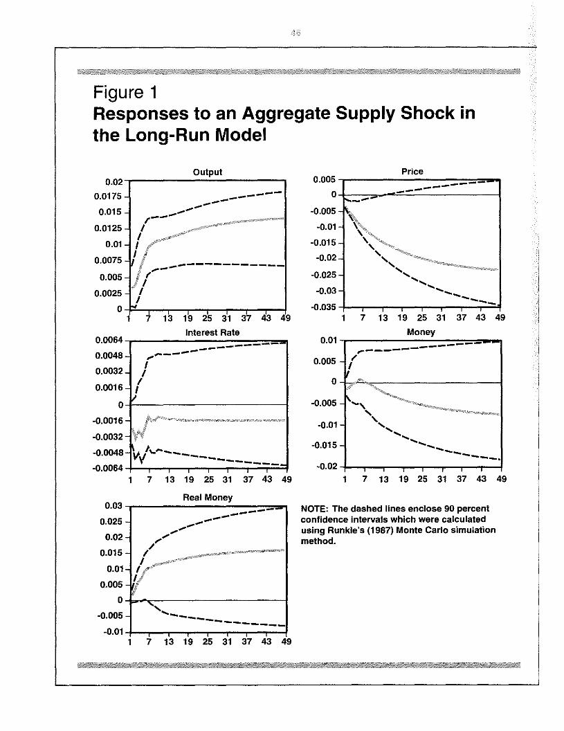
Figure 1Responses to an Aggregate Supply Shock inthe Long-Run Model

Output PriceO-02 0S05 - ____________________________

nfl-ic 0—,JaJ - ,..

0015 - -0.005 -

I — —

0.0125- I -0.01- \xI

001- i -0015-

04)075 - I 1 -0.02-j~e — ‘N

0-005 - ~ I -0025 - s.,,jI

0.0025 - / -0.03-I —. .—.

0-~ -0.035-1 7 13 19 25 31 37 43 49 1 7 13 19 25 31 37 43 49

Interest Rate Money0.0064- 0.01

00048-- r 0.0050.0032 - /

0.0016- 0

0- “ -0.005A ff1 C - r -001

-0.0032- -

-0.0048- ~ -0.015-0.0064- -0.02

1 7 13 19 25 31 37 43 49 1 7 13 19 25 31 37 43 49

Real Money0.03 - - NOTE: The dashed lines enclose 90 percent

0.025 - .—- confidence intervals which were calculatedusing Runkle’s (1987) Monte Carlo simulation

- 7 method.

0-015- /II0-01-

0.005 -

0 -

-0.005-

-0.01- I I

1 7 13 19 25 31 37 43 49

47

Figure 2Responses to a Real Spending Shock in theLong-Run Model

Output0.012

0.01

0-008

0.006

0.004

0.002

0

-04)02

0.012—

— — —4-———

0.01- —

0008- (704)06- j

// I.s.%

0004- ‘- —

0.002- I

1 7 13 19 25 31 37 43 49

Real Money0_005 -

•1~

0-

-0.005 - “ —

-0,01-

-0.015-

002 -

-0025 - s.— —

— — —

-0.03 _________________

0.025

0.02

0.015

0.01

0.005

0

-0.005

0.01

0-005-

0-

-0.005 -

-0.01-

-0.015 -

Price

Money

— •5 —— — — — —

I’

~.

‘S‘S

-04)2 I I I I

1 7 13 19 25 31 37 43 49

NOTE: The dashed lines enclose 90 percentconfidence intervals which were calculatedusing Runkles (1987) Monte Carlosimulation method.

1 7 13 19 25 31 37 43Interest Rate

49 1 7 13 19 25 31 37 43 49

I 1 I

1 7 13 19 25 31 37 43 49

B

Figure 3Responses to a Money Demand Shock in theLong-Run Model

I I I I I

1 7 13 19 25 31 37 43 49

Interest Rate

,—.1~

I

IP~>

It ,—

Price0006 — -

— ——0-004 - ——0.002 -

0-~

-0.002 -

-0004 -

-0.006 - N,,-04)08 -

-0.01

0.0225

0.02 -

0.0175 -

0.015 -

0.0125 -

0.01 -

0.0075 -

0.005-

04)025 -

— I I I

1 7 13 19 25 31 37 43 49

Money

0~~~

— —— —0 I I I I I I

1 7 13 19 25 31 37 43 49

NOTE: The dashed linesenclose 90 percentconfidence Intervals which were calculatedusing Runkle’s (1987) Monte Carlo simulationmethod.

Output0.0036 -

0.0024 -

0.0012 -

0-

-0.0012 -

-0.0024 -

-0.0036-

-0.0048 -

11I’I’

— — —--— — — —

4 ~L~e ——~,

IVa?

0-0045

0.0036

00018

0.0009

0

-0.0009

-0.0018

-0.00271 7 13 19 25 31 37 43

Real Money0.018 -

0.0162 -

0.0144 -

0.0126-

0.0108-

0.009-

04)072 -

0-0054-

I-I flflQC -

17I I I I I I

13 19 25 31 37 43 49

Figure 4Responses to a Money Supply Shock in theLong-Run Model

00175

0,015 -

0.0125-

0.01-

0.0075-

0.005-

0.0025 -

0-

-0.0025-

04)175-

0.015 -

0.0125-

0.01-

0.0075 -

0~005-

0.0025-

0-

-0.0025 -

Price

——

——~2-~

,//14

/147II/ / ——

~-/-,

I I I I I I

7 13 19 25 31 37 43 49

Money

I-1~I,

4U

I ———r

I I I I I I I

7 13 19 25 31 37 43 49

NOTE: The dashed lines enclose 90 percentconfidence intervals which were calculatedusing Runkle’s (1987) Monte Carlosimulation method.

Output

fl hOARInterest Rate

0.0032-

0.0016-

0-

£I’I ~“I ‘S’II,

I

/ — — —7 —/

4j4

-00016-

-0.0032-

-00048-

-0.0064-1

I I I I I

7 13 19 25 31 37 43 4

Real Money

Table 2Variance Decompositions for the Long-Run Model

Aggregate Real Money MoneyQuarter(s) supply spending demand supply

variable ahead shock shock shock shock

Output1 17(24) 76(24) 1 ( 8) 7(16)2 16(23) 78(24) 1(8) 5(14)4 24(25) 65(24) 0 ( 6) 11(14)8 45(23) 42(19) 0(4) 13(11)

16 67(15) 24(13) 0(2) 9(7)32 84(8) 11(7) 0(1) 5(3)48 90(5) 7(5) 0(1) 3(2)

Interest Rate1 13 (13) 49 (25) 1 ( 8) 37 (23)2 14(13) 57(23) 1(7) 27(19)4 13(11) 71(15) 3(5) 13(9)8 8(10) 84(12) 2(3) 6(6)

16 5(11) 91(12) 1(2) 3(4)32 4(13) 94(13) 1(1) 1(2)48 4(14) 95(14) 0(1) 1(1)

Real Money7(11) 2(10) 90(17) 2(11)

2 12(14) 3(8) 73(18) 12(14)4 18 (17) 8 (12) 59 (19) 14 (14)8 26(19) 24(17) 4108) 9(10)

16 25 (19) 38 (20) 33 (18) 4 ( 5)32 26 (21) 44 (21) 29 (19) 2 ( 3)48 27 (22) 45 (21) 28 (19) 1 (1)

Money1 6(10) 5(14) 73(22) 15(20)2 3(9) 2(10) 63(22) 32(21)4 1(9) 3(11) 59(23) 38(22)8 0 (10) 10(15) 50 (21) 40 (21)

16 1(11) 14(17) 46(20) 39(20)32 4(13) 11(17) 41(19) 44(20)48 6 (15) 9 (17) 39 (19) 46 (20)

PrIce1 73 (27) 2 (12) 9 (13) 16 (23)2 78(27) 404) 500) 12(21)4 77(28) 7(16) 2(8) 13(21)8 69 (28) 15 (19) 1 ( 7) 16 (20)

16 60(27) 20(21) 0(7) 20(19)32 55 (27) 22 (21) 0 ( 7) 23 (19)48 54 (27) 22 (22) 0 ( 7) 24 (19)

NOTE: Standard errors are fl parentheses

Table 3Estimates for the ContemporaneousModel

Parameter Standard error‘~as 0036’ .00030~ .0086 0027ems 0087 04190

md 0087 .0324A —.1164 3255A2 0469 4122A3 3327 .6539A4 1.030 8302A5 5632 2.098A0 9397 5.737

NOTE: An asterisk ( ) indicates signthcance atthe 5 percentlevel

coefficient on money would be unexpected in astructural IS equation; however, these estimatesare reduced-form coefficients, not structural pa-rameters. The coefficient on money in theinterest rate equation is positive. This supportsthe view that the central bank attempts tostabilize money gr-owth by raising interest rates.In the money demand equation, the coefficienton nommal spending is roughly one-half 1 andthe interest rate coefficient is almost — 1.0.Hence, the parameter estimates in this structuralmodel are consistent with economic theory.Unfortunately, each of these structural para-meters is statistically’ insignificant.

Figures 5 through S plot the impulse responses.In contrast to the long-run model, the aggregatesupply equation is normalized on the pricelevel. Hence, an aggregate supply shock raisesthe price level and reduces output. The aggre-gate supply shock has this expected effect onprices and output. Real money also decreases.The adverse supply shock has a weak positiveeffect on money and the interest rate. The ISshock raises prices, output and the interest rate.Real and nominal money initially increase,although both subsequently fall. The moneysupply equation is normalized on the interestrate so a reduction in the supply of money raiseinterest rates. This shock raises the interest rateand causes a decline in nominal money, realmoney and the price level. Surprisingly, outputrises briefly before it begins to decline. Themoney demand shock causes the interest rate,nominal and real money to increase whileoutput falls- The rising price level is inconsistent

with theory, although this effect is notstatistically significant. In contrast with the long-run model, there are a few unusual features inthe impulse responses for the contemporaneousspecification. Most of the dynamic patterns,however, are consistent with the structuralmodel.

The variance decompositions for the con-temporaneous model are shown in table 4.Many features of this table are comparable tothe long-run model’s results. For example, theaggregate supply shock gradually explains mostof output’s variability, is the most importantshock for the price level and is never animportant source of interest rate movements.The IS shock is the most important source ofshort-run output movement, and it explainsmost of the long-run variance of the interestrate. Some results, however, are considerablydifferent compared with the results fi-om thelong-run model. The money demand shock hasits greatest effect on output in the long run.This shock explains a large amount of the short-run variance of the interest rate but virtuallynone of the long-run variance of real ornominal money balances. The money supplyshock has essentially no effect on output, whileaccounting for a large amount of the variancein real money, even in the long run, and noneof the variance of prices. These results areinconsistent with most macroeconomic theories.

This paper outlines the basic theory behindstructural VAR models and estimates two modelsusing a standard set of macroeconomic data.The results for the two specifications are oftensimilar. The long-run structural VAR model inthis paper generally provides empirical resultsthat are consistent with the structural model.Some of the variance decompositions and theimpulse responses for the contemporaneousmodel were inconsistent with standard macro-economic theory. ‘I’hese inconsistencies pertainto the effects of money supply and moneydemand disturbances. Another result is thatstructural parameters in the long-run model aremore precisely estimated than parameters in thecontemporaneous model. Wherever a significantdiscrepancy exists between the two models, themodel with long-run restrictions yields sensibleresults, while the results from the contemporaneousmodel are inconsistent with standard economictheories.

Figure 5Responses to an Aggregate Supply Shock inthe Contemporaneous Model

Output

I.—’

— — — —

0.0025-

0-

-0,0025 -

-0.005 -

-0.0075 -

-0.01-

-0.0125-

-0.015 -

-0.0175

0.0075-

0.005-

0.0025-

0-

-0.0025-

-0.005

0.005

0

-0.005 -

-0,01-

-0.015-

-0.02-

-0,025 -

-0.03-

— I I

1 7 13 19 25 31 37 43 4

Interest Rate

‘-I-

I I I I I

1 7 13 19 25 31 37 43 49

Real Money

...

—— — — —

1

0.02

0.015-

0.01 -

0.005 -

-0.005 -

-0-atI I I I I

1 7 13 19 25 31 37 43 49

NOTE: The dashed lines enclose 90 percentconfidence intervals which were calculatedusing Runkle’s (1987) Monte Carlosimulation method.

——

Price

— — —

—— —

p

Money

— — ———0~~

~0

,,

0

S.—--— —

4.-

I I I I I

7 13 19 25 31 37 43 49

Figure 6Responses to a Real Spending Shock in theContemporaneous Model

Output

I I I I I

1 7 13 19 25 31 37 43 49

Interest Rate

I I I I I

1 7 13 19 25 31 37 43 49

Real Money

I I I I I I

7 13 19 25 31 37 43 49

0.02

0.015

0.01

0,005

0

-0.005

0.016-

0.012 -

0.008 -

0.004-

0-

-0.004 -

-0.008’

-0.012-

Price

‘-I- —— ——r — — —

-~\______ __

¼*5

*5*5

*5S..

1

NOTE: The dashed lines enclose 90 percentconfidence intervals which were calculatedusing Runkle’s (1987) Monte Carlosimulation method.

i’~S.

~ ‘ -

‘S.’

7 13 19 25 31

Money

0.015-

0.0125-

0.01-

0.0075-

0.005-

0.0025 -

0-

-0.0025-

0.0112 -

00096-

0.008 -

0.0064-

00048-

0.0032 -

0.0016 -

0-

-0.0016-

0.006-

0.003-

0-

-0.003 -

-0.006 -

-0.009 -

-0.012 -

-0.015-

-0.018-

-0.021-

It—

II ~/1’Iiii

*5*5

1

Figure 7Responses to a Money Supply Shock in theContemporaneous Model

0~005-

04)025-

0-

-0.0025 -

-0.005 -

-0,0075-

0.009-

0.0072-

0.0054-

0.0036-

00018-

0-

-0.0018-

-04)036

0.005

0

-0.005-

-0.01-

-0,015 -

-0.02-

-0.025 -

-0,03 -

Output

I I I I I

7 13 19 25 31 37 43 4

Interest Rate

A —

7’——V

S

I I’.I,I

I I I I I I I I

1 7 13 19 25 31 37 43 49

Real Money

¼—S.—————

*5~5

Price

I—

——

1~

‘S.4%~~~_—— — —

0.0105-

0,007-

0.0035 -

0-

-0.0035 -

-0.007-

-0.0105-

-0.014

—-

,4’

—— —— — — — *

3 1 113

0.

I I

19 25 31 37 43 4

Money

0

-0.005

-0.01

-0.015‘

-0.02-

-0025-

-0.03

S.-S.-.

— —— —

+ I I I I I I

1 13 19 25 31 37 43 49

NOTE: The dashed lines enclose 90 percentconfidence intervals which were calculatedusing Runkles (1987) Monte Carlosimulation method.

I I I I I I I

7 13 19 25 31 37 43 49

Figure 8Responses to a Money Demand Shock in theContemporaneous Model

Output Price0.002- 0.0125-

0— 0.01—00075- ——

-0.002- -

0.005 -

-0004- /0,0025- •~‘~ /

-0006-\ ___________________0--~~,~

-0.008 * \ -0.0025 -

—— —4——’.—-

0.01 Li’ -0.005-

-0.012- I I I I I I I ~0,0075 I I I

1 7 13 19 25 31 37 43 49 1 7 13 19 25 31 37 43 49

Interest Rate Money0.01- 0018-

I nn’ic~ —0.0075- 1% .

0.012- ‘

0005 1 *

- 0009 I00025- 0006 /

0- 0.003’

-0,0025- I-- O~0~ j

1 7 13 19 25 31 37 43 49 1 7 13 19 25 31 37 43 49

Real Money0.02- NOTE: The dashed lines enclose 90 percent

— confidence intervals which were calculated0.015- using Runkle’s (1987) Monte Carlo

simulation method,0.01- r’

/0.005-

~

-0.005-‘.4-. —— — —

-0,01- I I

1 7 13 19 25 31 37 43 49

Table 4Variance Decompositions for the Contemporaneous Model

Quarter(s)Aggregatesupply

Realspending

Moneydemand

Moneysupply

Variable ahead shock shock shock shock

Output

248

163248

I ( 2)1(3)3(5)

12(10)28(16)47 (21)55(23)

94(16)93(16)91(15)73(19)51(20)31(21)23(22)

4(14)3(13)5(13)

13(14)19(14)20 (14)20(14)

2(4)3(5)1(3)2( 5)2 ( 7)2 ( 9)2(10)

Interest Rate1248

163248

2 ( 2)4 ( 4)

10 ( 7)8(6)8 ( 7)8(10)8(11)

12(12)17(13)38 (15)56(18)63(20)67(22)88(22)

37(28)34(24)27 (18)19(16)12(15)9(14)8(14)

49(31)44(30)25 (23)17(20)16(20)16(20)15(20)

Real Money1248

163248

19 ( 7)18(8)24(11)3403)38(16)42 (20)45(21)

11(14)5(11)2(8)4(7)

10(10)14 (12)15(12)

36(21)16(18)6(16)204)1(15)0 (15)0(16)

34(22)60(20)68(19)6109)51(21)44 (23)40(24)

Money1248

163246

2( 2)1(2)0(2)0(3)1(6)4(10)7(13)

14(15)702)300)1(9)101)1(11)0(11)

44(24)23(22)13(21)

7(20)6(20)7(20)7(20)

41(31)68(27)83(26)92(25)92(25)89(25)86(25)

Price1248

163248

100(0)98(2)95(4)89(7)8400)8201)81(12)

0(0)0(1)2(2)6(6)

12(8)14(9)1500)

0(0)2(1)3(3)4(5)4(6)3(7)3( 7)

0(0)0(1)0(2)0(5)0(7)1 ( 9)1 ( 9)

NOTE: Standard errors are in parentheses.

These comparisons between contemporaneousand long-run specifications may not generalizeto all structural VAR applications, but they sug-gest that long-run structural VARs may yieldtheoretically predicted results more frequentlythan VAR5 identified with short-run restrictions.This result is not surprising. One reason is thateconomic theories may often have similar long-run properties but different short-run features.For example, while output movenìents are drivensolely by aggregate supply shocks in a typicali-cal business cycle model, supply shocks will ac-count for permanent output movements inKeynesian models, hut every shock may havesonic cyclical effect. In addition, long-run struc-tural VAR models may provide superiorresults because they typically do not imposecontemporaneous exclusion restrictions. Keating(1990) shows that contemporaneous zero”restrictions may be inappropriate in an environ-ment with forward-looking agents who have ra-tional expectations. The intuition behind thisresult is that any observable contemporaneousvariable may provide information about futureevents. One implication from that paper is thatdifferent short-run restrictions can be obtainedfrom alternative assumptions about available in-formation. Further research should investigateother examples of contemporaneous and long-run structural VAR models to determine whetherthe superior performance of this paper’s long-runmodel is a special case or a more general result.

Bernanke, Ben S. “Alternative Explanations of the Money-Income Correlation,” Carnegie-Rochester Conference Serieson Public Policy (Autumn 1986), pp. 49-100.

Blanchard, Olivier Jean. “A Traditional Interpretation of Mac-roeconomic Fluctuations,” American Economic Review (De-cember 1989), pp. 1146-64.

Blanchard, Olivier Jean, and Danny Ouah. “The Dynamic Ef-fects of Aggregate Demand and Supply Disturbances,”American Economic Review (September 1989), pp. 655-73.

Blanchard, Olivier Jean. and Mark W. Watson. “Are BusinessCycles All Alike?” in Robert J. Gordon, ed., The AmericanBusiness Cyc/e (University of Chicago Press, 1986).

Cooley, Thomas F., and Stephen F. LeRoy. “AtheoreticalMacroeconomics: A Critique,” Journal of Monetary Eco-nomics (November 1985), pp. 283-308.

Dickey, David A., and Wayne A. Fuller. “Distribution of theEstimators for Autoregressive Time Series With a UnitRoot,” Journal of the American Statistical Association(June 1979), pp. 427-31.

Doan, Thomas, Robert B. Litterman, and Christopher Sims.“Forecasting and Conditional Proiection Using RealisticPrior Distributions,” Econometric Review (Vol. 3, No. I, 1984),pp. I-IOU.

Engle, Robert F., and C, W. J. Granger. “Co-Integration andError Correction: Representation, Estimation, and Testing,”Econometrica (March 1987), pp. 251-76.

Fuller, Wayne A. Introduction to Statistical Time Series (WileyPress, 1976).

Gall, Jordi. “How Well Does the lS-LM Model Fit PostwarU.S. Data,” Quarterly Journal of Economics (May 1992),pp. 709-38.

Hansen, Lars Peter. “Large Sample Properties of GeneralizedMethod of Moments Estimators,” Econometrica (July 1982),pp. 1029-54.

Keating, John W. “Postwar Business Cycles in a NaturalRate Model,” revised version of Washington UniversityWorking Paper #159 (St. Louis, MO, July 1992).

_______- “Identifying VAR Models under Rational Expecta-tions,” Journal of Monetary Economics (June 1990), pp.453-76.

Keating, John W., and John V. Nye. “Permanent and TransitoryShocks in Real Output: Estimates from Nineteenth Centuryand Postwar Economies,” Washington University WorkingPaper #160 (St. Louis, MO, July 12, 1991).

King, Robert G., Charles I. Plosser, James H. Stock, andMark W. Watson. “Stochastic Trends and Economic Fluc-tuations,” American Economic Review (September 1991),pp. 819-40.

Nelson, Charles R., and Charles I, Plosser. “Trends andRandom Walks in Macroeconomic Time Series: Some Evi-dence and Implications,” Journal of Monetary Economics(September 1982), pp. 139-62.

Runkle, David E. “Vector Autoregressions and Reality,”Journal of Business and Economic Statistics (October 1987),pp. 437-42.

Sargent, Thomas J. “A Note on Maximum Likelihood Estimationof the Rational Expectations Model of the Term Structure,”Journal of Monetary Economics (January 1979), pp.133-43.

Schwert, G. William, “Effects of Model Specification on Testsfor Unit Roots in Macroeconomic Data,” Journal of MonetaryEconomics (July 1987), pp. 73-104.

Shapiro, Matthew D., and Mark W, Watson. “Sources ofBusiness Cycle Fluctuations,” in Stanley Fischer, ed,,NBER Macroeconomics Annual 1988 (MIT Press, 1988),pp. 111-48.

Sims, Christopher A. “Are Forecasting Models Usable forPolicy Analysis?” Federal Reserve Bank of MinneapolisQuarterly Review (Winter 1986), pp. 2-16.

“Macroeconomics and Reality,” Econometrica(January 1960), pp. 1-46.

Sims, Christopher A., James H. Stock, and Mark W. Watson,“Inference in Linear Time Series Models with Some UnitRoots,” Econometrica (January 1990), pp. 113-44.

Stock, James H., and Mark W. Watson. “A Simple Estimatorof Cointegrating Vectors in Higher Order Integrated Systems,”Federal Reserve Bank of Chicago Working Paper WP-91-4,(February 1991).

______ - “Testing for Common Trends,” Journal of theAmerican Statistical Association (December 1988), pp. 1097-107.

“Variable Trends in Economic Time Series,” Journalof Economic Perspectives (Summer 1988), pp. 147-74.

West, Kenneth D. “The Sources of Fluctuations in AggregateInventories and GNP,” Quarterly Journal of Economics(November 1990), pp. 939-71.

Zellner, Arnold. “An Efficient Method of Estimating Seeming-ly Unrelated Regressions and Tests for Aggregation Bias,”Journal of the American Statistical Association (June 1962),pp. 348-68.

SEPTEMBER/OCTOBER 1592