STRESSOR RESPONSE MODEL FOR THE SEAGRASSES, Halodule ...

Final Report for Technical Assistance for an Ecological Evaluation of the Southwest Florida Feasibility Study

STRESSOR RESPONSE MODEL FOR THE SEAGRASSES, Halodule wrightii and Thalassia testudinum

By Frank J. Mazzotti, Leonard G. Pearlstine, Robert Chamberlain, Tomma Barnes, Kevin Chartier, and Donald DeAngelis

Joint Ecosystem Modeling Laboratory

Technical Report

FINAL REPORT

for

Technical Assistance for an Ecological Evaluation of the

Southwest Florida Feasibility Study

STRESSOR RESPONSE MODELS FOR THE SEAGRASSES, Halodule wrightii and Thalassia testudinum

Prepared By:

Frank J. Mazzotti1, Leonard G. Pearlstine1, Robert Chamberlain 2, Tomma Barnes3, Kevin Chartier1, and Donald DeAngelis4

1University of Florida

Ft. Lauderdale Research and Education Center 3205 College Ave Davie, FL 33314 (954) 577-6304

2South Florida Water Management District

3301 Gun Club Road West Palm Beach, FL 33406

3Post, Buckley, Schuh and Jernigan

3501 North Causeway Blvd., Suite 725 Metairie, LA 70001

(504) 862-1481

4United States Geological Survey University of Miami, Dept. of Biology

1301 Memorial Dr. RM 215 Coral Gables, FL 33146

Prepared For: South Florida Water Management District

Fort Myers Service Center 2301 McGregor Blvd. Fort Myers, FL 33901

United States Geological Survey

1301 Memorial Dr. RM 215 Coral Gables, FL 33146

(305) 284-3974

May 2007

ii

University of Florida

This report should be cited as:

Mazzotti, F.J., Pearlstine, L.G., Chamberlain, R., Barnes, T., Chartier, K., and DeAngelis, D. 2007, Stressor response models for Seagrasses, Halodule wrightii and Thalassia testudnium. JEM Technical Report. Final report to the South Florida Water Management District and the U.S..Geological Survey. University of Florida, Florida Lauderdale Research and Education Center, Fort Lauderdale, Florida, 19 pages.

Any use of trade, firm, or product names is for descriptive purposes only and does not imply endorsement by the University of Florida.

Although this report is in the public domain, permission must be secured from the individual copyright owners to reproduce any copyrighted material contained within this report.

iii

Contents Introduction......................................................................................................................................1

Southwest Florida Feasibility Study.............................................................................................1 C43 West Reservoir......................................................................................................................1

Forcasting Models............................................................................................................................1 Habitat Suitability Indices ............................................................................................................2

Ecology of the Seagrass ...................................................................................................................2 HSI for Seagrass ..............................................................................................................................9 References Cited ............................................................................................................................17

Figures Figure 1. Caloosahatchee Estuary SAV monitoring stations..........................................................4 Figure 2. Time series density of seagrass .......................................................................................5 Figure 3. Seagrass coverage at two locations in San Carlos Bay ...................................................6 Figure 4. HSI value for seagrass response to salinity ..................................................................10 Figure 5. HSI value for seagrass response to light. ......................................................................11 Figure 6. Average Monthly Photosynthetic Active Radiation (PAR). .........................................12 Figure 7. Light attenuation vs. Salinity in seagrass areas.............................................................13 Figure 8. Light attenuation regions...............................................................................................18 Figure 9. HSI value for Seagrass response to temperature. ..........................................................14 Figure10. Estimated water temperature in the Caloosahatchee Estuary .......................................15

Tables Table 1. Habitat requirements for the seagrass, Halodule and Thalassia. ....................................7 Table 2. Changes to the HSI model’s spatial boundaries and post-processing routines................9

iv

STRESSOR RESPONSE MODEL FOR THE SEAGRASSES, Halodule wrightii and Thalassia testudinum

By Frank J. Mazzotti, Leonard G. Pearlstine, Robert Chamberlain, Tomma Barnes, Kevin Chartier, and Donald DeAngelis

Introduction A key component in adaptive management of Comprehensive Everglades Restoration Plan (CERP) projects is evaluating alternative management plans. Regional hydrological and ecological models will be applied to evaluate restoration alternatives and the results will be applied to modify management actions.

Southwest Florida Feasibility Study

The Southwest Florida Feasibility Study (SWFFS) is a component of the Comprehensive Everglades Restoration Plan (CERP). The SWFFS is an independent but integrated implementation plan for CERP projects and was initiated in recognition that there were additional water resource issues (needs, problems, and opportunities) within Southwest Florida that were not being addressed directly by CERP. The SWFFS identifies, evaluates, and compares alternatives that address those additional water resource issues in Southwest Florida. An adaptive assessment strategy is being developed that will create a system-wide monitoring program to measure and interpret ecosystem responses. The SWFFS provides an essential framework to address the health and sustainability of aquatic systems. This includes a focus on water quantity and quality, flood protection, and ecological integrity.

C43 West Reservoir The purpose of the C43 Basin Storage Reservoir project is to improve the timing, quantity, and quality of freshwater flows to the Caloosahatchee River estuary. The project includes an above-ground reservoir with a total storage capacity of approximately (170,000 acre-feet) and will be located in the C-43 Basin in Hendry, Glades, or Lee Counties. The initial design of the reservoir assumed 8094 hectares (20,000 acres) with water levels fluctuating up to 2.4 meters (8 feet) above grade. The final size, depth and configuration of this facility will be determined through more detailed planning and design.

Forecasting Models Forecasting models bring together research and monitoring to ecosystems of Southwest Florida and place them into an adaptive management framework for the evaluation of alternative plans. There are two principle ways to structure adaptive management: (1) passive, by which policy

1

decisions are made based on a forecasting model and the model is revised as monitoring data become available, and (2) active, by which management activities are implemented through statistically valid experimental design to better understand how and why natural systems respond to management (Wilhere 2002).

In an integrated approach that includes both passive and active-adaptive management, a forecasting model simulates system response and is validated by monitoring programs to measure actual system response. Monitoring can then provide information for passive-adaptive management for recalibration of the forecasting model. Directed research, driven by model uncertainties, is an active-adaptive management strategy for learning and the reduction of uncertainties in the model.

The forecasting models for the C-43 West Reservoir Project and the Southwest Florida Feasibility Study consist of a set of stressor response (habitat suitability) models for individual species. These stressor response models have been developed principally with literature, expert knowledge, and currently available field data.

Habitat Suitability Indices Habitat Suitability Indices (HSI) models were developed with each stressor variable portrayed spatially and temporally across systems of the study area at scales appropriate to the organism or community being portrayed. The HSI models have been incorporated into a GIS to portray responses spatially and temporally to facilitate policy decisions. That is, the model describes a response surface of habitat suitability values that vary spatially according to stressor levels throughout the estuary and temporally according to temporal patterns in stressor variables. Much of the temporal variation is a result of temporal cycling of important stressor inputs, such as water temperature and salinity. Temporal change for other important variables may not be cyclical, such as rising sea level and increasing land use and fresh water demands in the region. Areas predicted to be suitable and those predicted to be less suitable or disturbed should be targeted for additional sampling as part of the model validation and adaptive management process.

Species selected for modeling (focal species) are ecologically, recreationally or economically important and have a well established linkage to stressors of management interest. They may also make good focal species because they engage the public in caring about the outcome of restoration projects. The habitat suitability models (HSI) were developed by choosing specific life stages of each species with the most limited, restricted, or tightest range of suitable conditions, to capture the highest sensitivities of the organisms to the environmental changes associated with the planned restoration activities. Values used in the models are listed in Table 1.

The models calculate habitat suitability monthly as the weighted geometric mean of the environmental variables identified as important for each model. Because the geometric mean is derived from the product of the variables rather than the sum (as in the arithmetic mean) and has the appropriate property that if any of the individual variables are unsuitable for species success (i.e., the value of the variable is zero) then the entire index goes to zero.

Ecology of Seagrasses Beds of submerged aquatic vegetation (SAV) are important to the ecology of shallow estuarine and marine environments. These beds provide habitat for many benthic and pelagic organisms,

2

function as nurseries for juveniles and other early life stages, stabilize sediments, improve water quality, and can form the basis of a detrital food web (Kemp et al. 1984; Fonseca and Fisher 1986; Carter et al. 1988; Killgore et al. 1989; Lubber et al. 1990). Because of the importance of these beds, estuarine restoration initiatives often focus on SAV (Batiuk et al. 1992; Johansson and Greening 2000; Virnstein and Morris 2000). SAV are commonly monitored to gauge the health of estuarine systems, (Tomasko et al. 1996) and their environmental requirements can form the basis for water quality goals (Dennison et al. 1993; Stevenson et al. 1993).

In the Caloosahatchee Estuary, field and laboratory research has been conducted by the South Florida Water Management District (SFWMD, associated contractors, and non-government organizations over a wide range of flows and salinities. This information, along with the results from researchers in other systems, is used to estimate maximum freshwater inflow limits and associated water quality requirements to protect and restore Halodule wrightii (shoal grass) and Thalassia testudinum (turtle grass).

McNulty et al. (1972) and Harris et al. (1983) mapped SAV in the lower estuary upstream of Shell Point, as well as throughout the outer embayments. Halodule is the only seagrass species consistently located upstream of Shell Point (Figure 1: Stations 5 and 6) until it mixes downstream with Thalassia and other less common species in San Carlos Bay (Stations 7 and 8) and Pine Island Sound (Stations 9 and 10). Halodule has a wide salinity tolerance (McMahan 1968). It does not survive below 3.5 ppt and prefers salinity as high as 44 ppt (Zieman and Zieman 1989). This wide tolerance is probably why it is the only true seagrass species encountered upstream of Shell Point. Monitoring results (Figure 2a) indicate that, of all areas where Halodule is present, the lowest biomass is found upstream, where salinity is more diluted and most variable (Chamberlain et al 1995, Chamberlain and Doering 1998b, Doering et al. 2002). The greatest biomass occurs when salinity is above 20 ppt. Figure 2a also depicts seasonal growth patterns that can be influenced by high freshwater inflow that cause decreasing salinity (as occurred in the Water Year 2006) due to tropical storms during 2004 and 2005.

Literature summarized by Zieman and Zieman (1989) indicates that the optimum salinity range for Thalassia is 24-35 ppt. The maximum photosynthetic activity of Thalassia occurs in euhaline seawater and decreases proportionately with decreasing salinity. Thalassia does not grow in areas with salinity normally below 17 ppt and will suffer significant leaf loss when exposed to lower salinity. Thalassia does not exist upstream of Shell Point where salinity during the SFWMD study was more variable. Recent monitoring results (Figure 2b) also depict a declining density below normal at the end of WY 2006 from discharge related to tropical storms during 2004 and 2005.

Comparison of map coverage by Harris et al. (1983) determined substantial loss in seagrass during the mid-later 20th century. This loss was in part due to changes in freshwater flow patterns (salinity variability), physical alteration in the estuary and watershed, as well as changes in water management practices (Chamberlain and Doering 1998a). Harris et al. (1983) reported that the greatest loss appeared to be from deeper beds, which indicates that a change in water clarity has occurred, in part probably due to the increased freshwater inflow reaching the downstream beds and associated decreased water quality (i.e., increased water color).

In general, as flows increase, the water quality constituents (primarily color) that inhibit light penetration also increase. Therefore, as light attenuation increases, the depth at which the seagrass can survive decreases. SFWMD monitoring data indicates that average monthly flows

3

from S-79 that exceed 4,000 cfs are associated with light penetration below that necessary to support plants at 1 m depth in San Carlos Bay. Lower mean monthly discharges that approach 3,000 cfs are associated with the same problem for Halodule upstream of Shell Point. At deeper depths (e.g., 1.5m) plant coverage is considerably more sensitive to the freshwater inflow (Figure 3).

Figure 1. Caloosahatchee Estuary SAV monitoring stations for Vallisneria americana is found at stations 1-3, Halodule wrightii at stations 5-10, Thalassia testudinum at stations 8-10. Based on the literature identified in Table 1, along with SFWMD laboratory and field research, the HSI curve in Figure 4 was formulated to represent relative Halodule and Thalassia response to salinity values generated during model runs.

Although there are species-specific variations, generally speaking, SAV distributions are limited by four environmental factors: light, salinity, temperature, and nutrients (Dennison et al. 1993, Kemp et al. 2004). In the Caloosahatchee, as indicated above, studies have documented that SAV distribution and subsequently its functionality, is strongly related to limits on their physiological response to salinity and light. Except at the distribution margins, plant location in the estuary generally depends on salinity, while growth characteristics controlling plant height and depth strongly relates to light attenuation within salinity tolerant zones. The average daily bottom light (ADBL) required by SAV, which helps determine the depth to which plants exist, is measured in the photosynthetic active radiation (PAR) spectrum of 400-700 nanometers during the entire 24 hour day (not just daylight or peak light periods). ADBL for shoal grass can be divided into stressed environments like in Iona Cove, and more desirable areas as in San Carlos Bay (as evidenced in the results of Dunton 1994 and 1996 from Texas). Dunton and Tomasko (1991) and Dunton (1996) also determined light requirements during winter and summer seasons. Based primarily on their results, the minimum range of ADBL in Iona Cove is

2estimated to be about 50-60 micro-Einsteins (uE = micromoles/m /sec) and saturation is 220-

4

300uE, depending on the season . In San Carlos Bay, the minimum and saturation levels of ADBL equates to about, 75-100uE, and 225-325uE, respectively.

Halodule at Stations 5, 6, 7, and 8 January 2004 - May 2006

Date

1/1/04 5/1/04 9/1/04 1/1/05 5/1/05 9/1/05 1/1/06 5/1/06

Shoo

ts/m

2

0

200

400

600

800

1000

1200

Station 5Station 6Station 7 Station 8

a.

WY2006

Date1/1/04 5/1/04 9/1/04 1/1/05 5/1/05 9/1/05 1/1/06 5/1/06

Shoo

ts/m

2

0

50

100

150

200

250

300

350

Station 7Station 8

Thallasia at Station 7 and Station 8 January 2004 - May 2006

WY2006

b.

Figure 2. Time series density of seagrass: (a.) Halodule wrightii; and (b) alassia testudinum (turtle

ted Th

grass) in the Caloosahatchee Estuary and San Carlos Bay, with the time period of a Water Year indica(WY: May 1 –April 30). Data collected by the Sanibel-Captiva Conservation Foundation.

5

Hydroacoustic Sampled Seagrass % Coverage at 1.5 m

Figure 3. Seagrass coverage at two locations downstream of the Caloosahatchee River (a. Site 7; and b. Site 9-in Figure 1) compared to 60-day average freshwater inflow from S-79 prior to sampling. These estimates can be put on a relative HSI scale from 0 to 1 as reflected in Figure 5. However, this scale better reflects the quality of habitat (e.g. plant growth potential and health), not the amount of coverage (acres), which is one of the HSI modeling objectives. For example, a HSI =1.0 or 0.5 both represent an area with plant coverage that is sustainable between months. To address this issue, a “50% Approach” was adopted, whereby a single linear line from the minimum ADBL during the winter in Iona Cove to the PAR level of 150uE is used that represents 50% of saturation during the summer growing season in San Carlos Bay (Figure 5).

a. Reach 3B

0 1000 2000 3000 4000 5000 6000 7000 8000 9000 10000

Seag

rass

% C

over

0

10

20

30

40

50

60

70

80

90

100

b. R

60-d Freshwater Flow from S-79 (cfs)

each 4A

0 1000 2000 3000 4000 5000 6000 7000 8000 9000 10000

Seag

rass

% C

over

Northern San Carlos Bay

Chino Island- Lower Pine Island Sound

0

10

20

30

40

50

60

70

80

90

100

6

Table 1. Habitat Requirements for the Seagrasses, Halodule and Thalassia. The following table summarizes S-79 inflow criteria (mean monthly cubic feet per second), important salinity ranges, and water quality requirements for the protection and support of Halodule and Thalassia in the Caloosahatchee Estuary. Variable Estuary Area Value Source Halodule and Thalassia

Throughout their range

Light to 1m: 1) Min. 20-25% of Subsurface irradiance 2) Minimum attenuation Coef -1.5 3) Most important during warm growing season 4) Recovery goal: Deeper, 2m? 5) Optimal Productivity at 300 mE

Kenworthy and Haunert 1991 Tomasko and Hall 1999 Dixon and Leverone 1995 Herzka and Dunton 1997 Fong et al. 1997

Halodule Throughout its

range Salinity: 1) 3.5ppt - minimum tolerance; duration of tolerance 1-2 months; Recovery 1 year (following winter and spring) of preferred salinity 2) Prefers > 20ppt, below which productivity declines 3) Optimum, seawater ~ 35ppt 4) Location requirements – long term average salinity >20ppt, std. dev. < 10ppt

Zieman and Zieman 1989 McMahan 1968 Chamberlain and Doering 1998b Chamberlain (Pers. field/lab obs) 2004

Temperature:

1) Greatest productivity during March – September (Possibly a magnitude more biomass in shallow areas of Area 6) 2) Optimum 22-26oC

Chamberlain (Pers. field/lab obs/analysis) 2004 Fong et al. 1997

Area 5 Flow (to achieve above

salinity and light limits): 1) Max < 3,000 cfs 2) Preferred < 1000 cfs 3) Optimum < 500 cfs

Chamberlain and Doering 1998b Doering et al. 2002

Thalassia Throughout its

range Salinity: 1) ~ 6ppt - minimum tolerance; duration tolerance 1-2 months; Recovery 1 year (following winter and spring) of preferred salinity;

Chamberlain and Doering 1998b Doering and Chamberlain 2000 Doering et al. 2002 Zieman and Zieman 1989 Zieman et al 1999 Chamberlain (Pers. field/lab obs/analysis) 2004

7

Mortality when 0 ppt for > 3 weeks – no recovery 2) Prefers > 20ppt, < 17ppt productivity declines 3) Optimum, 24-35ppt 4) Location requirements – long term average salinity >20-25ppt, std. dev. < 5ppt

Temperature:

1) Greatest productivity during March – September 2) Optimum when ~ 30oC 3) Decreased productivity @ < 20 oC 4) Stressful when water temp < 15 oC (winter) 5) Mortality - month>36oC

Chamberlain (Pers. field/lab obs/analysis) 2004 Dawes et al. 1997 Koch and Erskine 2001 Miller 2000

Halodule and Thalassia

Area 6 Flow (to achieve above salinity and light limits): 1) Max 4,500 cfs 2) Preferred < 2,500 cfs 3) Optimum < 1,000 cfs

Chamberlain and Doering 1998b Chamberlain 1995 Doering et al. 2002

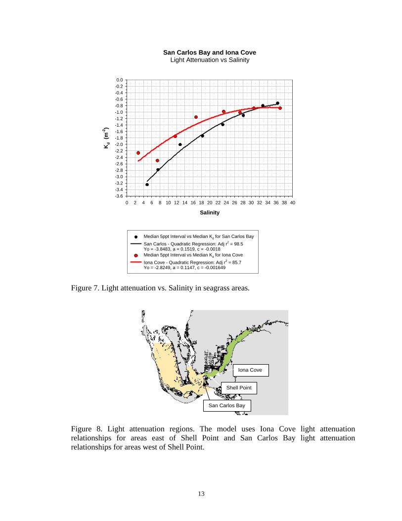
The formula for calculating ADBL is based on the Lambert-Beer equation, which requires knowing: (1) surface incident light in the PAR spectral range; (2) water column light attenuation (K); and (3) depth. Average monthly incident PAR for the Caloosahatchee is depicted in Figure 6 and was calculated from a daily average PAR dataset, recorded by a continuous sensor during 1998-2004, located in the nearby Estero Bay Watershed. Light attenuation was calculated based on the curvilinear relationships of salinity and simultaneous light attenuations measurements (Figure 7) at stations upstream and downstream of Shell Point (Figure 8). Depth was determined from bathymetry surveys of the Caloosahatchee Estuary and the resulting information supplied in a GIS data file that matched the grid cell points of the model.

Seasonal patterns are an indication of the influence and importance of temperature on seagrass, with the best growth occurring between the 22 and 30oC range. In addition, temperature will affect photosynthesis by altering the rate of biochemical reactions of photosynthesis. Therefore, ecological models of seagrass include temperature as a variable governing seagrass growth predictions (Fong et al. (1887). Based on these literature results and those identified in Table 1, a HSI temperature curve was developed (Figure 9) that indicates the relative importance and input value to the HSI model, as per the estimated daily average (ambient) temperature (Figure 10).

8

HSI for the Seagrass, Halodule wrightii and Thalassia testudinum HSI Variables and Summary Formula

Habitat suitability for the combined grasses Halodule wrightii and Thalassia testudinum is calculated monthly as a geometric mean: HSI = (Previousw * Salinityw * Temperaturew * LightAvailabilityw) Where w = the weight for each variable and the sum of w = 1. In the accepted model, each of the variables has been weighed equally, so w = 0.25. Previous "Previous" variable included because current month’s HSI score should depend on the how well the grass was doing last month (previous score). In the model application, Previous = previous_month_HSI score + 0.05, (not to exceed 1.0), in order to allow for

growth from month to month, if other conditions are suitable.

Table 2. Changes to HSI model’s spatial boundaries (A and B) and post-processing routines (C) for adjusting the final HSI ecological model scores to better reflect long-term impacts of severe reduction in seagrass coverage due to low HSI scores of environmental variables (salinity, light and temperature in above model formula).

Routine Model output criteria Model score adjustment A. Apply new masks for the three areas of

the estuary (Pine Island, San Carlos Bay, and Iona Cove

Consider them separately and evaluate the spread across them

B. Establish a lower depth threshold of 5 ft and 7ft in San Carlos Bay and Pine Island Sound

Model areas > depth thresholds are not scored

C. If HSI score < 0.1 for one month, Than HSI = 0.1 for remainder of season Adjustments were agreed to by ecological benefits sub-team (6/14/06)

HSI Curves and Application (for determining HSI variable input values) Salinity HSI Calculation – Values based on the literature identified in Table 1, along with SFWMD laboratory and field research, which resulted in the curvilinear relationship between HSI values and salinity depicted below in Figure 4. Data Source - Freshwater inflows are estimated for S-79 and from the tidal basin using hydrologic models. Flows are generated for each base-case and proposed alternative.

9

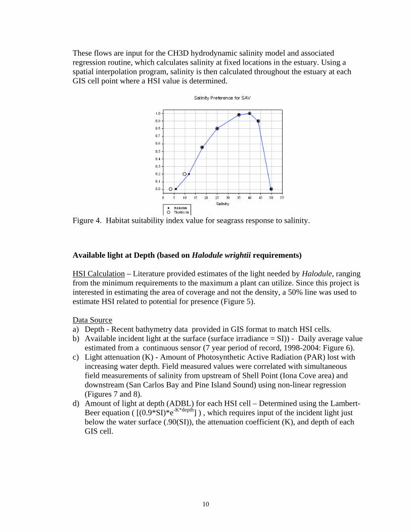
These flows are input for the CH3D hydrodynamic salinity model and associated regression routine, which calculates salinity at fixed locations in the estuary. Using a spatial interpolation program, salinity is then calculated throughout the estuary at each GIS cell point where a HSI value is determined.

Figure 4. Habitat suitability index value for seagrass response to salinity.

Available light at Depth (based on Halodule wrightii requirements) HSI Calculation – Literature provided estimates of the light needed by Halodule, ranging from the minimum requirements to the maximum a plant can utilize. Since this project is interested in estimating the area of coverage and not the density, a 50% line was used to estimate HSI related to potential for presence (Figure 5). Data Source a) Depth - Recent bathymetry data provided in GIS format to match HSI cells. b) Available incident light at the surface (surface irradiance = SI)) - Daily average value

estimated from a continuous sensor (7 year period of record, 1998-2004: Figure 6). c) Light attenuation (K) - Amount of Photosynthetic Active Radiation (PAR) lost with

increasing water depth. Field measured values were correlated with simultaneous field measurements of salinity from upstream of Shell Point (Iona Cove area) and downstream (San Carlos Bay and Pine Island Sound) using non-linear regression (Figures 7 and 8).

d) Amount of light at depth (ADBL) for each HSI cell – Determined using the Lambert-Beer equation ( [(0.9*SI)*e-K*depth] ) , which requires input of the incident light just below the water surface (.90(SI)), the attenuation coefficient (K), and depth of each GIS cell.

10

Light vs HSI for Halodule wrightii P (rate)

PAR (~400-700 nm @ umol m-2 sec-1)

25 50 75 100 125 150 175 200 225 250 275 300 325 350

HS

I Val

ue (P

hoto

synt

hetic

rate

)

0.0

0.1

0.2

0.3

0.4

0.5

0.6

0.7

0.8

0.9

1.0

PAR vs. HSI value for P during Winter in Iona CovePAR vs HSI Value for P during

50% Line

Summer in Iona CovePAR vs. HSI value for P during Winter in San Carlos bay/Pine Island SoundPAR vs. HSI value for P during Summer in San Carlos bay/Pine Island SoundMin Ic PAR to 50% HSI from above Curves (all seasons and all areas)

Figure 5. Habitat suitability index value for seagrass response to light. HSI values represent the relative amount of average daily light required by Halodule wrightii. The 50% line was used in the model to indicate relative light vs. plant’s need to maintain presence

11

Available Light at the Surface

Average Monthly PAR

0

100

200

300

400

500

600

Jan Feb Mar Apr May Jun Jul Aug Sep Oct Nov Dec

Month (1998-2004)

Ave

rage

Inci

dent

PA

R

Average PAR

Figure 6. Average Monthly Photosynthetic Active Radiation (PAR)

12

San Carlos Bay and Iona Cove Light Attenuation vs Salinity

Salinity

0 2 4 6 8 10 12 14 16 18 20 22 24 26 28 30 32 34 36 38 40

Kd

(m-2

)

-3.6-3.4-3.2-3.0-2.8-2.6-2.4-2.2-2.0-1.8-1.6-1.4-1.2-1.0-0.8-0.6-0.4-0.20.0

Median 5ppt Interval vs Median Kd for San Carlos Bay San Carlos - Quadratic Regression: Adj r2 = 98.5Yo = -3.8483, a = 0.1519, c = -0.0018Median 5ppt Interval vs Median Kd for Iona CoveIona Cove - Quadratic Regression: Adj r2 = 85.7Yo = -2.8249, a = 0.1147, c = -0.001649

Figure 7. Light attenuation vs. Salinity in seagrass areas.

Iona Cove

Shell Point

San Carlos Bay

Figure 8. Light attenuation regions. The model uses Iona Cove light attenuation relationships for areas east of Shell Point and San Carlos Bay light attenuation relationships for areas west of Shell Point.

13

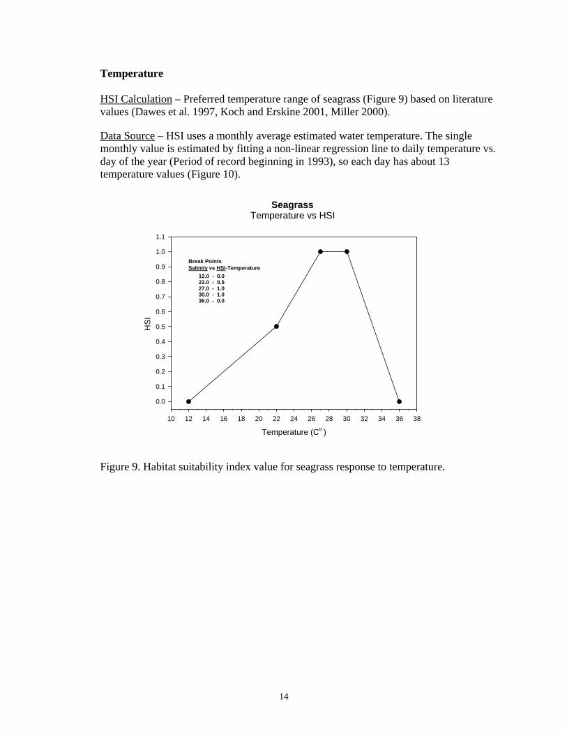
Temperature HSI Calculation – Preferred temperature range of seagrass (Figure 9) based on literature values (Dawes et al. 1997, Koch and Erskine 2001, Miller 2000).

Data Source – HSI uses a monthly average estimated water temperature. The single monthly value is estimated by fitting a non-linear regression line to daily temperature vs. day of the year (Period of record beginning in 1993), so each day has about 13 temperature values (Figure 10).

SeagrassTemperature vs HSI

Temperature (Co )

10 12 14 16 18 20 22 24 26 28 30 32 34 36 38

HS

I

0.0

0.1

0.2

0.3

0.4

0.5

0.6

0.7

0.8

0.9

1.0

1.1

12.0 - 0.022.0 - 0.527.0 - 1.030.0 - 1.036.0 - 0.0

Salinity vs HSI-TemperatureBreak Points

Figure 9. Habitat suitability index value for seagrass response to temperature.

14

Day of Year

0 30 60 90 120 150 180 210 240 270 300 330 360

Tem

pera

ture

(o C)

1617181920212223242526272829303132

Figure 10. Estimated water temperature in the Caloosahatchee Estuary adjacent to seagrass area.

References Cited

15

Batiuk, R.A., R.J. Orth, K.A. Moore, W.C. Dennison, J.C. Stevenson, L.W. Staver, V. Carter, N.B. Rybicki, R.E. Hickman, S. Kollar, S. Bieber, and P. Heasly 1992. Chesapeake Bay submerged aquatic vegetation habitat requirements and restoration targets: A technical synthesis. Chesapeake Bay Program CBP/TRS 83/92 186 pp. Bulthuis, D.A. 1987. Effects of temperature on photosynthesis and growth of seagrass. Aquatic Botany 27: 27-40 Carter, V., J.W. Barko, G.L. Godshalk, and N.B. Rybicki. 1988. Effects of submerged macrophytes on water quality in tidal Potomic River. Maryland. Journal of Freshwater Ecology 4:493-501. Chamberlain (Pers. field/lab obs/analysis) 2004 Chamberlain, R.H., D.E. Haunert, P.H. Doering, K.M. Haunert, and J.M. Otero. 1995. Preliminary estimate of optimum freshwater inflow to the Caloosahatchee Estuary, Florida. Technical report, South Florida Water Management District, West Palm Beach, Florida. Chamberlain, R. H. 1995. Impacts from freshwater inflow on seagrass in the Caloosahatchee Estuary. Poster Presentation, 13th Biennial Conference of the Estuarine Research Federation. Chamberlain, R. H. and P.H. Doering. 1998a. Freshwater inflow to the Caloosahatchee Estuary and the resource-based method for evaluation, p. 81-90. In S.F. Treat (ed.), Proceedings of the 1997 Charlotte Harbor Public Conference and Technical Symposium. South Florida Water Management District and Charlotte Harbor National Estuary Program, Technical Report No. 98-02. Washington, D.C. Chamberlain, R. H. and P.H. Doering. 1998b. Preliminary estimate of optimum freshwater inflow to the Caloosahatchee Estuary: A resource-based approach, p. 121-130. In S.F. Treat (ed.), Proceedings of the 1997 Charlotte Harbor Public Conference and Technical Symposium. South Florida Water Management District and Charlotte Harbor National Estuary Program, Technical Report No. 98-02. Washington, D.C. Dennison, W.C., R.J. Orth, K.A. Moore, J.C. Stevenson, V. Carter, S. Kollar, P. W. Bergstrom and R.A. Batiuk. 1993. Assessing water quality with submersed aquatic vegetation. Bioscience 43(2):86-94. Doering, P.H. and R.H. Chamberlain. 2000. Experimental studies on the salinity tolerance of Turtle Grass, Thalassia testudinum, p. 81-98. In S.A. Bortone (ed.), Seagrasses: Monitoring, Ecology, Physiology, and Management. CRC Press LLC, Boca Raton, Florida, 318 pp. Doering, P. H., R. H. Chamberlain, and D.E. Haunert. 2002. Using submerged aquatic vegetation to establish minimum and maximum freshwater inflows to the Caloosahatchee Estuary, Florida. Estuaries 25 (1343-1354).

16

Dixon, L.K. and J.R. Leverone. 1995. Light requirements of Thalassia testudinum in Tampa Bay, Florida. Final report to the Surface Water Improvement and Management Department, Southwest Florida Water Management District, Tampa. Dunton, K. H. 1994. Seasonal growth and biomass of the subtropical seagrass Halodule wrightii in relation to continuous measurements of underwater irradiance. Marine Biology 120:479-489. Dunton, K. H. 1996. Photosynthetic production and biomass of the subtropical seagrass Halodule wrightii along an estuarine gradient. Estuaries 19-2B:436-447. Dunton, K. H., and D. A. Tomasko. 1991. The seasonal variation in the photosynthetic performance of Halodule wrightii measured in situ in Laguna Madre Texas. In W. J. Kenworthy and D.E. Haunert (eds.), The Light Requirements of Seagrass: Proceedings of a Workshop to Examine the Capability of Water Quality Criteria, Standards and Monitoring Programs to Protect Seagrasses, National Oceanic and Atmospheric Administration Technical Memorandum NMFS-SEFC-287. Beaufort, North Carolina. Fong, P., M.E. Jacobson, M. C. Mescher, D. Lirman, and M. C. Harwell. 1997. Investigating the management potential of a seagrass model through sensitivity analysis and experiments. Ecol. App. 7: 300-315. Fonseca, M.S. and J.S. Fisher. 1986. A comparison of canopy friction and sediment movement between four species of seagrass and with reference to their ecology and restoration. Marine Ecological Progress Series 29: 15-22.

Harris, B.A., K.D. Haddad, K.A. Steidinger, and J.A. Huff. 1983. Assessment of Fisheries Habitat: Charlotte Harbor and Lake Worth, Florida. Florida Department of Natural Resources, Bureau of Marine Research, St. Petersburg, Florida. 211 pp.

Herzka, S.Z. and K.H. Dunton. 1997. Seasonal photosynthetic patterns of the seagrass Thalassia testuninum in the western Gulf of Mexico. Marine Ecological Process Series 152: 103-117. Johansson, J.O.R. and H.S. Greening. 2000. Seagrass restoration in Tampa Bay: A resource based approach to estuarine management, p 279-294. In S.A. Bortone (ed.). Seagrasses: Monitoring, Ecology, Physiology, and Management. CRC Press, Boca Raton, Florida. Kenworthy, W. J. and D.E. Haunert. 1991. The light requirements of seagrass: Proceedings of a workshop to examine the capability of water quality criteria, standards and monitoring programs to protect seagrasses. National Oceanic and Atmospheric Administration Technical Memorandum NMFS-SEFC-287. Beaufort, North Carolina. Kemp, W.M., W.R. Boynton, R.R. Twilley, J.C. Stevenson, and L.G. Ward. 1984. Influence of submersed vascular plants on ecological processes in upper Chesapeake Bay, p. 367-394. In V.S. Kennedy (ed.). The Estuary as a Filter. Academic Press, New York.

17

Kemp, W.M., R. Batiyk, R. Bartleson, P. Bergstrom, V. Carter, C. Gallegos, W. Hunley, L. Karrh, E.W. Koch, J.M. Landwehr, K.A. More, L. Murrey, M. Naylor, N.B. Rybicki, J.C. Stevenson, and D.J. Wilcox. 2004. Habitat requirements for submerged aquatic vegetation in Chesapeake Bay: Water quality, light regime, and physical-chemical factors. Estuaries 27: 363-377. Killgore, K.J., R.P. Morgan, II, and N.B. Rybicki.1989. Distribution and abundance of fishes associated with submersed aquatic plants in the Potomic River. North American Journal of Fisheries Management 9:101-111. Koch, M. S. and J.M. Erskine. 2001. Sulfide as a phytotoxin to the tropical seagrass, Thalassia testudinum with high salinity and temperature. Journal of Experimental Marine Biology and Ecology 266: 81-95. Lubbers, L., W.R. Boynton, and W.M. Kemp. 1990. Variations in structure of estuarine fish communities in relation to abundance of submersed vascular plants. Marine Ecological Progress Series 65: 1-14. McNulty, J.K., W.N. Lindall, J.E. Sykes. 1972. Cooperative Gulf of Mexico estuarine inventory and study, Florida: Phase 1, area description. NOAA Technical Rep. NMFS Circ-368. McMahan, C.A. 1968. Biomass and salinity tolerance of shoal-grass and manatee grass on lower Laguna Madre, Texas. Journal of Wildlife Management 32: 501-506. Stevenson, J.C., L.W. Staver, and K.W.Staver.1993. Water quality associated with survival of submersed aquatic vegetation along an estuarine gradient. Estuaries 16: 346-361. Tomasko, D.A., C.J. Dawes, and M.O. Hall. 1996. The effects of anthropogenic enrichment on turtle grass (Thalassia testudinum) in Sarasota Bay, Florida. Estuaries 19: 448-456. Tomasko, D.A. and M.O. Hall. 1999. Productivity and biomass of the seagrass Thalassia testudinum along a gradient of freshwater influence in Charlotte harbor, Florida. Estuaries 22 (3A): 592-602. Virnstein, R.W. and L.J. Morris.2000. Setting seagrass targets for the Indian River Lagoon, Florida, p. 211-218. In S.A. Bortone (ed.). Seagrasses: Monitoring, Ecology, Physiology, and Management. CRC Press, Boca Raton, Florida. Wilhere, G.F. 2002. Adaptive management in habitat conservation plans. Conservation Biol. 16(1): 20-29.

Zieman, J.C. and R.T. Zieman 1989. The ecology of the seagrass meadows of the west coast of Florida: a community profile. U.S. Fish and Wildl. Serv. Biol. Rep. 85(7.25). 155 pp.

18

Zieman, J.C., J.W. Fourqurean, and T.A. Frankovich. 1999. Seagrass die-off in Florida Bay: Long-term trends in abundance and growth of turtle grass, Thalassia testudinum. Estuaries 22:460-470.

19