Editor: Prof. Dr.-Ing. habil. Heinz Konietzky Layout: Angela Griebsch TU Bergakademie Freiberg, Institut für Geotechnik, Gustav-Zeuner-Straße 1, 09599 Freiberg [email protected] Stress and deformation tensor Author: Prof. Dr.-Ing. habil. Heinz Konietzky (TU Bergakademie Freiberg, Geotechnical In- stitute) 1 Stress and Deformation Tensor ........................................................................... 2 Introduction.................................................................................................... 2 Preliminary note to tensors ............................................................................ 2 Particular tensors........................................................................................... 3 Typical tensor operations .............................................................................. 4 Stress tensor ................................................................................................. 6 Deformation tensor ...................................................................................... 20 Compatibility condition................................................................................. 26 Equilibrium conditions.................................................................................. 27

Welcome message from author
This document is posted to help you gain knowledge. Please leave a comment to let me know what you think about it! Share it to your friends and learn new things together.
Transcript
Editor: Prof. Dr.-Ing. habil. Heinz Konietzky Layout: Angela Griebsch
TU Bergakademie Freiberg, Institut für Geotechnik, Gustav-Zeuner-Straße 1, 09599 Freiberg [email protected]
Stress and deformation tensor Author: Prof. Dr.-Ing. habil. Heinz Konietzky (TU Bergakademie Freiberg, Geotechnical In-
stitute)
1 Stress and Deformation Tensor ........................................................................... 2
Introduction .................................................................................................... 2
Preliminary note to tensors ............................................................................ 2
Particular tensors ........................................................................................... 3
Typical tensor operations .............................................................................. 4
Stress tensor ................................................................................................. 6
Deformation tensor ...................................................................................... 20
Compatibility condition ................................................................................. 26
Equilibrium conditions .................................................................................. 27

Stress and deformation tensor
Only for private and internal use! Updated: 25 August 2017
page 2 of 28
1 Stress and deformation tensor
Introduction
Geomechanical calculations have to consider the following 3 fundamental relations:
Equilibrium conditions
Compatibility conditions
Constitutive laws
The coupling between the stresses and deformations is performed by the constitutive laws (material laws) as indicated by Figure 1. Stresses and Deformations are given by second-order tensors. The constitutive law is given by a fourth-oder tensor. The scheme in Figure 1 illustrates the interaction of the individual components, which are explained in more detail within the next chapters.
inner + outer Forces FI, FA
Displacements ui
Equilibrium
conditions
Compatibility
conditions
Stresses
ij
Constitutive laws Deformations
ij
Fig.1: Geomechanical calculation scheme
Preliminary note to tensors
In simplified terms tensors can be considered as special multi-dimensional matrices, which have certain characteristics. For geomechanics the transformation characteristics are of special importance (tensor algebra).
Stress and deformation tensor
Only for private and internal use! Updated: 25 August 2017
page 3 of 28
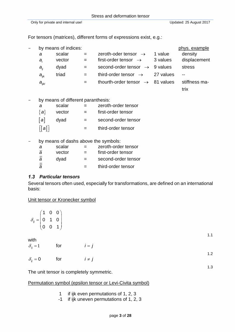
For tensors (matrices), different forms of expressions exist, e.g.: - by means of indices: phys. example
a scalar = zeroth-oder tensor 1 value density
ia vector = first-order tensor 3 values displacement
ija dyad = second-order tensor 9 values stress
ijka triad = third-order tensor 27 values --
ijkla = thourth-order tensor 81 values stiffness ma-
trix - by means of different paranthesis:
a scalar = zeroth-order tensor
a vector = first-order tensor
a dyad = second-order tensor
a = third-order tensor
- by means of dashs above the symbols:
a scalar = zeroth-order tensor
a vector = first-order tensor
a dyad = second-order tensor
a = third-order tensor
Particular tensors
Several tensors often used, especially for transformations, are defined on an international basis: Unit tensor or Kronecker symbol
1 0 0
0 1 0
0 0 1
ij
1.1
with
1 ij for i j
1.2
0ij for i j
1.3
The unit tensor is completely symmetric. Permutation symbol (epsilon tensor or Levi-Civita symbol) 1 if ijk even permutations of 1, 2, 3
-1 if ijk uneven permutations of 1, 2, 3
Stress and deformation tensor
Only for private and internal use! Updated: 25 August 2017
page 4 of 28
ijk =
0 if at least 2 indices are equal (no permutation)
even permutation = composition of even number of two-part cycles 312
Example: 123 321 123 even permutation (2 cycles) 231
The -tensor is completely antisymmetric (skew-symmetric).
123 = 231 = 312 = -321 = -132 = -213 = 1
1.4
all other elements are zero ! Zero tensor all elements are zero:
ija
0 0 0
0 0 0
0 0 0
1.5
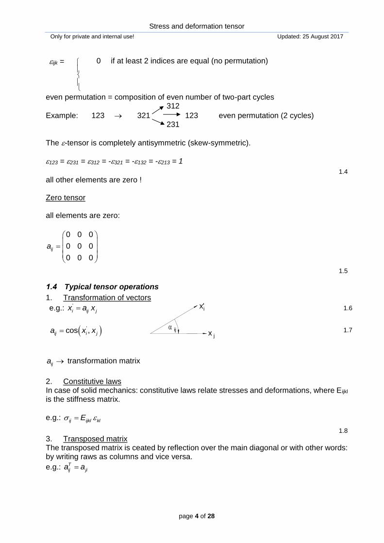
Typical tensor operations
1. Transformation of vectors
e.g.: i ij jx a x'
x'i
x j
ij
1.6
'cos ,ij i ja x x
1.7
ija transformation matrix
2. Constitutive laws In case of solid mechanics: constitutive laws relate stresses and deformations, where Eijkl is the stiffness matrix.
e.g.: ij ijkl klE
1.8
3. Transposed matrix The transposed matrix is ceated by reflection over the main diagonal or with other words: by writing raws as columns and vice versa.
e.g.: T
ij jia a
Stress and deformation tensor
Only for private and internal use! Updated: 25 August 2017
page 5 of 28
1
11 12 13 11 21 31
21 22 23 12 22 32
31 32 33 11 23 33
a a a a a a
a a a a a a
a a a a a a
1.9
4. Invertible matrix The product of a matrix and the corresponding invertible matrix results in the unit matrix (all diagonal elements = 1).
e.g.: 1
ij ij ija a
1.10
5. Determinant of matrix
1 2 3 11 22 33 21 32 13 31 12 23 11 32 23 12 21 33 13 22 31ij rst r s ta a a a a a a a a a a a a a a a a a a a a a
1.11
6. Vector product
The vector product j ka b can be written as:
i ijk j kc e a b
1.12
7. „Replacement rule“
e.g.: i ik ka a ik = Kronecker symbol
change of indices: from k to i
or e.g: total effektiv
ij ij ij p
1.13
8. Derivations (differential quotient – comma convention)
e.g.: ,
ii j
j
uu
x
1.14
9. Einstein’s summation convention (summation over equal indices)
e.g.: 11 22 33iia a a a
1.15
10. Addition rule Summation tensor (only tensors of equal format can be added or subtracted)
e.g.: 1... 1... 1...i in i in i ina b s
1.16
e.g.: i i ia b s
1.17
11. Product rule Product tensor (all elements of the left factor of order m are multiplied under consideration of the se-quence with all elements of the right factors of order n, that means the multiplication of a
Stress and deformation tensor
Only for private and internal use! Updated: 25 August 2017
page 6 of 28
tensors of order m with a tensor of order n results in a tensor of order (m + n). Please note: the product of two tensors is as a general rule not commutative!
e.g. 1... 1... 1... 1...i in j jm i in j jm
i j ij
a b p
a b p
1.18
12. Contraction Contraction occurs either when a pair of literal indices of the tensor are set equal to each
other and summed over or if during the multiplication of two tensors of order n 2 one index of the left factor is equal to the right factor. In both cases the rank of the final tensor is reduced by two.
e.g. ij j i
ijk jq ikq
a b c
a b c
1.19
or iik ka b 1.20
or by using the Kronecker symbol
ij ijk Ka b 1.21
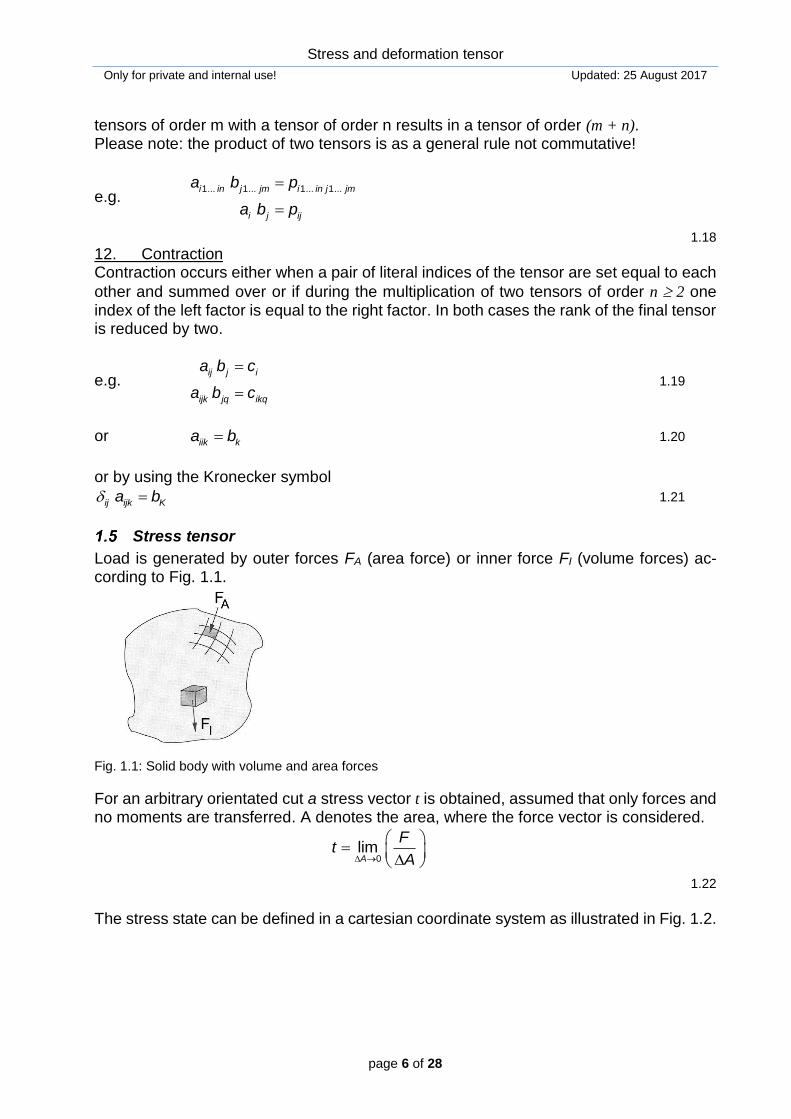
Stress tensor
Load is generated by outer forces FA (area force) or inner force FI (volume forces) ac-cording to Fig. 1.1.
Fig. 1.1: Solid body with volume and area forces
For an arbitrary orientated cut a stress vector t is obtained, assumed that only forces and no moments are transferred. A denotes the area, where the force vector is considered.
0limA
Ft
A
1.22
The stress state can be defined in a cartesian coordinate system as illustrated in Fig. 1.2.
Stress and deformation tensor
Only for private and internal use! Updated: 25 August 2017
page 7 of 28
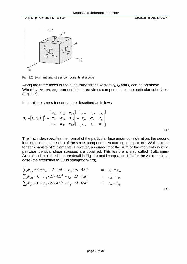
Fig. 1.2: 3-dimentional stress components at a cube
Along the three faces of the cube three stress vectors t1, t2 and t3 can be obtained:
Whereby {i1, i2, i3} represent the three stress components on the particular cube faces (Fig. 1.2). In detail the stress tensor can be described as follows:
11 12 13
1 2 3 21 22 23
31 32 33
, ,
xx xy xzT
ij yx yy yz
zx zy zz
t t t
1.23
The first index specifies the normal of the particular face under consideration, the second index the impact direction of the stress component. According to equation 1.23 the stress tensor consists of 9 elements. However, assumed that the sum of the moments is zero, pairwise identical shear stresses are obtained. This feature is also called ‘Boltzmann-Axiom’ and explained in more detail in Fig. 1.3 and by equation 1.24 for the 2-dimensional case (the extension to 3D is straightforward).
2 2
2 2
2 2
0 4 4
0 4 4
0 4 4
xy xy yx xy yx
xz xz zx xz zx
yz yz zy yz zy
M l l l l
M l l l l
M l l l l
1.24

Stress and deformation tensor
Only for private and internal use! Updated: 25 August 2017
page 8 of 28
yy
xx
yy
xx
yx
xy
xy
yx
l
Fig. 1.3: Equilibrium considerations for a volume element (2D, x-y-plane)
From eq.1.24 it follows, that the stress tensor is symmetric, that means:
ij ji or T
1.25
Therefore, the number of stress values is reduced from 9 to 6 (three pairwise identical shear stresses meaning no rotations). The relationship between stress vector and stress tensor is obtained on the basis of the equilibrium conditions in direction of the coordinates xi (Fig. 1.4):
cos ,i in n x ,
1.26
d di iA n A ,
1.27
where ni is the unit normal vector.
Fig. 1.4: Orientation of stress tensor and stress vector
1 11 1 21 2 31 3
2 12 1 22 2 32 3
3 13 1 23 2 33 3
t dA dA dA dA
t dA dA dA dA
t dA dA dA dA
1.28
Stress and deformation tensor
Only for private and internal use! Updated: 25 August 2017
page 9 of 28
Using (1.26) and (1.27) equation 1.28 can be simplified as follows:
1 11 1 21 2 31 3
2 12 1 22 2 32 3
3 13 1 23 2 33 3
t n n n
t n n n
t n n n
.
1.29
Equation 1.29 can be rewritten in tensor form as follows:
i ji j ij j
T
t n n
n n
.
1.30
Equation 1.30 documents the equality of pairwise shear stresses. The so defined second-order stress tensor is called ‚Cauchy stress tensor‘ or „true“ stress tensor or ‘Euler stress
tensor’. The Cauchy stress tensor ij relates the current force vector to the current (de-formed) area element.
i ji jdF dA
1.31
Fi: current force vector
Aj: current area element with d dj jA n A
Alternatively, the current force vector Fi can be related to the original area A° (that means before any deformation!). Such a stress tensor is called ‚Nominal stress tensor‘, ‘La-grange stress tensor’ or ‘First Piola-Kirchhoff tensor’ Tij:
d di ji jF T A
1.32
The stress tensor can be decomposed into normal and shear components (n: normal vector; m: tangential vector) as illustrated by Fig. 1.5:
n i i i ij jn t n n
1.33
or
n i i i ij jm t m n
1.34
In detail, equations 1.33 and 1.34 can also be written as:
1 11 1 1 12 2 1 13 3
2 21 1 2 22 2 2 23 3
3 31 1 3 32 2 3 33 3
n n n n n n n
n n n n n n
n n n n n n
1.35

Stress and deformation tensor
Only for private and internal use! Updated: 25 August 2017
page 10 of 28
From equation 1.35 follows for instance:
1
0
0
n
11n and
0
0
1
n
33n .
For the shear stress follows:
1 11 1 1 12 2 1 13 3
2 21 1 2 22 2 2 23 3
3 31 1 3 32 2 3 33 3
n m n m n m n
m n m n m n
m n m n m n
.
1.36
From equation 1.36 follows for instance:
1
0
0
n
;
0
1
0
m
21n
0
0
1
n
;
0
1
0
m
23n
If n i ji jm n , than:
1
0
0
n
;
0
1
0
m
12n
n
m
t
.
n
m
Fig. 1.5: Decomposition of stress vector t into normal and shear stress component

Stress and deformation tensor
Only for private and internal use! Updated: 25 August 2017
page 11 of 28
Thereby, it always holds: ni ni = 1 and mi mi = 1
Now we consider specific directions, where only normal stresses exist, but no shear
stress . For such a constellation it holds:
ti = ij nj and ti = ij nj,
1.37
where nj characterizes the principal stress directions. Equalization of both expressions in 1.37 yields:
ij nj = ij nj or (ij - ij ) nj = 0.
1.38
Equation 1.37 describes an eigenvalue problem with eigenvalues und nj. The non-trivial solution is obtained if the coefficient determinant of equation 1.38 vanishes:
det 0ij ij ,
1.39
or
11 12 13
12 22 23
13 23 33
0
.
1.40
The solution of equation 1.40 is a characteristic equation of third order:
3 2
1 2 3 0I I I ,
1.41
where the following holds:
1 11 22 33KK ij ijI ,
1.42
11 13 22 2311 12
2
31 33 32 3321 22
2 2 2
11 22 22 33 11 33 12 23 31
1
2ii jj ij jiI
,
1.43
3
2 2 2
11 22 33 11 23 22 13 33 12 12 23 31
1 1 3det
3 2 2
2
ij ii jj KK ij jK Ki ij ji KKI
.
1.44
Stress and deformation tensor
Only for private and internal use! Updated: 25 August 2017
page 12 of 28
The values I1, I2, I3 are called ‚main invariants‘ (I1: first main invariant, I2: second main invariant, I3: third main invariant) of the stress tensor, that means that they are independ-ent of the coordinate systems (independent of translations or rotations of the reference system). Besides these main invariants there are the so called ‚basic invariants‘, which can be considered as a special subset of the main invariants. They are defined as follows:
1 1
2
2 1 2
3
3 1 1 2 3
1 1
2 2
1 1
3 3
kk
ij ji
ij jk ki
J I
J I I
J I I I I
.
1.45
Besides the cartesian representation it is also possible to find a formulation in form of the principal stresses:
1 1 2 3I ,
1.46
2 1 2 2 3 1 3I ,
1.47
3 1 2 3I .
1.48
An interesting decomposition of the stress tensor is possible, if a mean normal stress is defined as follows:
0 11 22 33
1 1
3 3KK .
1.49
0 is also called „hydrostatic stress state“ or ‘mean stress’ or ‘spherical stress’. Based on these definitions the stress tensor can be written as:
0ij ij ijs
1.50
In terms of matrix notation this means:
11 12 13 0 11 0 12 13
21 22 23 0 21 22 0 23
31 32 33 0 31 32 33 0
0 11 12 13
0 21 22 23
0 31 32 33
0 0
0 0
0 0
0 0
0 0
0 0
s s s
s s s
s s s
,
1.51
where sij is referred as deviatoric stress part.
Stress and deformation tensor
Only for private and internal use! Updated: 25 August 2017
page 13 of 28
For the spherical tensor as well as for the stress deviator invariants can be defined. The main invariants for the spherical tensor are given as follows:
2 3
1 0 2 0 3 0
33
2I I I
1.52
The corresponding basic invariants are:
2 3
1 0 2 0 3 0
33
2J J J
1.53
For the deviatoric part the main invariants are:
1 11 0 22 0 33 0 0D
kkI s
1.54
2
2 2 2
11 0 22 0 22 0 33 0 11 0 33 0 12 23 31
1
2
D
ii jj ij jiI s s s s
1.55
3 det
1 1 3
3 2 2
D
ij
ii jj kk ij jk ki ij ji kk
I s
s s s s s s s s s
1.56
The basic invariants for the deviatoric part are:
1 0D
kkJ s
1.57
2 2 2 2 2 2
2 11 0 22 0 33 0 12 23 31
2 2 2 2 2 2
11 22 22 33 33 11 12 23 31
2 2 2
1 2 2 3 3 1
1 12 2 2
2 2
1
6
1
6
D
ij jiJ s s
1.58
3 1 0 2 0 3 0
1
3
D
ij jk kiJ s s s
1.59
Quite often stress components are defined, which are related to the octahedral plane. The octahedral plane is equally inclined to the principal stress directions (hydrostatic axis). The principal stresses act along the x1, x2 and x3 direction:

Stress and deformation tensor
Only for private and internal use! Updated: 25 August 2017
page 14 of 28
1
2
3
0 0
0 0
0 0
ij
x1
x2
x3
2
3
1
t j
nj
1
2
3
1arccos 54,7
3
1 2 3, , jt
Fig. 1.6: Representation of octahedral stresses
The stress vector tj is defined by the three principal stress components 1, 2 and 3. Regarding the normal on the octahedral plane the stress vector tj has the following carte-sian components:
N
i ij jt n 1
3jn .
1.60
The projection and summation of the components on the vektor nj (hydrostatic axis) pro-vides the octahedral normal stress:
31 21 2 3 0
1 1
33 3 3 3OCT
.
1.61
The octahedral normal stress is equivalent to mean stress (Equation 1.49). The subtrac-tion of the octahedral normal stresses from the principal stresses leads to the deviatoric stresses:
1 1 0
2 2 0
3 3 0
s
s
s
1.62
Stress and deformation tensor
Only for private and internal use! Updated: 25 August 2017
page 15 of 28
These deviatoric stresses can also be referred to the octahedral plane and given as Car-tesian components:
31 21 2 3
3 3 3
s s s ss st t t .
1.63
The addition of vectors leads to the octahedral shear stresses:
2 2 2
1 2 3
22 2
31 2
2 2 2
1 2 3
2
3 3 3
1
3
2 1
3 3
OCT
D
ij ij
t t t
ss s
s s s
J s s
.
1.64
Another very popular quantity is the so-called ‚von-Mises equivalent stress‘ F. This stress
value is based on a strength criterion, which relates the yield stress F to the stress devi-ator:
2
20 3 D
FJ .
1.65
This implies that:
2 2 2
2 1 2 2 3 1 3
3 13
2 2
D
F ij ijJ s s
1.66
and
22 2
3 3OCT F F .
1.67
Principal stresses and principal stress directions: The stress tensor as a symmetric linear operator has the characteristic, that it can be diagonalised. That means, there are three orientations (directions) perpendicular to each other in space, where the corresponding normal stresses reach extreme values (principal stresses or principal normal stresses) and the shear stresses vanish. In this case, only the trace of the tensors has non-vanishing values:
Stress and deformation tensor
Only for private and internal use! Updated: 25 August 2017
page 16 of 28
1
2
3
0 0
0 0
0 0
ij
.
1.68
The stress vectors on these specific surface areas coincide with the directions of the normal vectors of these surface areas. Therefore, the stress vectors have only one non-vanishing component. Thus, for the stress vector at the considered surface area it holds:
i it n
and
1 1 1 1
2 2 2 2
3 3 3 3
t n l
t n m
t n n
.
1.69
The normal vector , ,in l m n describes the principal normal stress directions. For the
unit vector the following holds in general:
32 2 2 2
1
1i
i
n l m n
,
1.70
squaring equation 1. yields:
2 2 2
1 1
2 2 2
2 2
2 2 2
3 3
t l
t m
t n
1.71
and 2
2 1
2
1
22 2
2
2
22 3
2
3
tl
tm
tn
.
1.72

Stress and deformation tensor
Only for private and internal use! Updated: 25 August 2017
page 17 of 28
The addition of the equations 1.72 under consideration of equation 1.70 gives:
22 2
31 2
2 2 2
1 2 3
1
tt t.
1.73
Equation 1.73 describes an ellipsoid, that means the values 1, 2 and 3 represent the half-axes of the ellipsoid (Fig. 1.7). The surface of the ellipsoid represents all possible stress vectors. If two principal stresses are equal, a spheroid is coming up. If all principal stresses are equal (isotropic stress state) a sphere is coming up.
Fig. 1.7: Prinzipal stress ellipsoid
In geomechanics, especially in soil mechanics, descriptions on the basis of the deviatoric stress plane, see Fig. 1.8, are very common.
Fig. 1.8: Decomposition of the stress state into hydrostatic and deviatoric part, where the stress vector t
defines the stress point T
1
3
2
t
h
s
Hydrostatische Achse
12
3
const.Deviatorebene
1 2 3
T (1 2 3
3
3arccos

Stress and deformation tensor
Only for private and internal use! Updated: 25 August 2017
page 18 of 28
1 2 3 1
3 3
3 3h
1.74
2 2 2
1 2 3 22 Ds s s s J
1.75
On the deviatoric plane it holds:
1 2 3 const.
1.76
The deviatoric plane through the coordinate system is also called π-plane (fig. 1.9).
Fig. 1.9: Illustration of Lode angle θ in the -plane
It holds:
3
3
22
3 3cos 3
2
D
D
J
J
and
1.77
D
3
3D 22
J1 3 3arccos
3 2(J )
.
1.78
'1
'2
'3
T

Stress and deformation tensor
Only for private and internal use! Updated: 25 August 2017
page 19 of 28
Fig. 1.10: Illustration of Lode angle in the principal stress space
In geotechnical engineering the follwoing two modified invariants are often used: Roscoe invariants p und q as well as Lode angle θ. Thereby, it holds:
1
1
3 p ,
1.79
23 Dq J and
1.80
3
3
22
1 3 3arccos
3 2( )
D
D
J
J
.
1.81
For the conventional triaxial test the following expressions (eq. 1.82-1.84) can be de-duced:
1 3
1( 2 )
3p ,
1.82
1 3q and
1.83
2
1 3 1 2 3
1arccos (3 6 ) 3 6
3s s s s s .
1.84
Stress and deformation tensor
Only for private and internal use! Updated: 25 August 2017
page 20 of 28
Deformation tensor
For the coordinates of a point at the initial and final deformed state the following inverse
relations exist: o
ji ix x x
and o o
i i jx x x
.
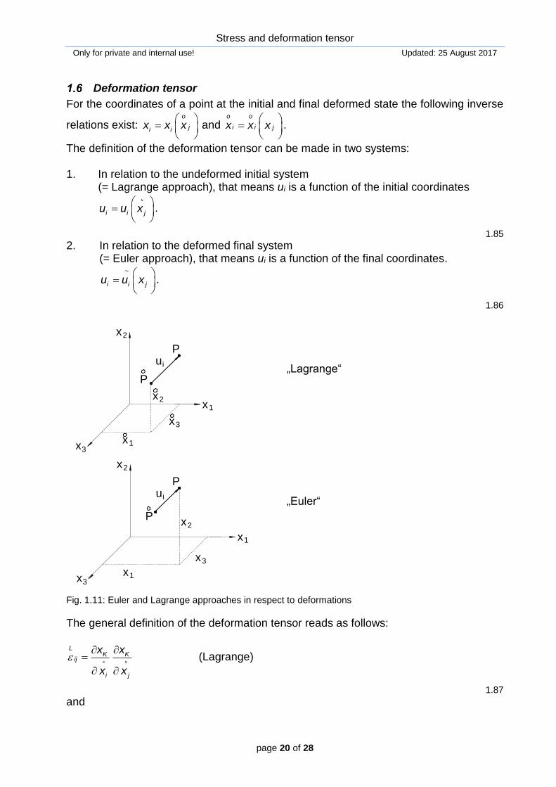
The definition of the deformation tensor can be made in two systems: 1. In relation to the undeformed initial system
(= Lagrange approach), that means ui is a function of the initial coordinates
i i ju u x
.
1.85
2. In relation to the deformed final system (= Euler approach), that means ui is a function of the final coordinates.
~
i i ju u x
.
1.86
x
x
x
2
1
3
x2
x3
x1
ui
P
P
„Lagrange“
x
x
x
2
1
3
x2
x3
x1
ui
P
P
„Euler“
Fig. 1.11: Euler and Lagrange approaches in respect to deformations
The general definition of the deformation tensor reads as follows: L
K Kij
i j
x x
x x
(Lagrange)
1.87
and
Stress and deformation tensor
Only for private and internal use! Updated: 25 August 2017
page 21 of 28
j
K
i
KE
ijx
x
x
x
(Euler).
1.88
With the help of the gradient tensors (= displacement gradients) i
j
u
x
and i
j
u
x
, respec-
tively, the deformation tensor can be defined as follows: „Lagrange“:
i i i ix x u x
with i iij
jj
x u
x x
and
1.89
Li i
jK ij ij
j K
jK i ijK
j K j K
u u
x x
uu u u
x x x x
,
1.90
„Euler“:
i i jx x u x with i i
ij
j j
ux
x x
and
1.91
Ei i iK
jK jK
K j j K
u u uu
x x x u.
1.92
Stress and deformation tensor
Only for private and internal use! Updated: 25 August 2017
page 22 of 28
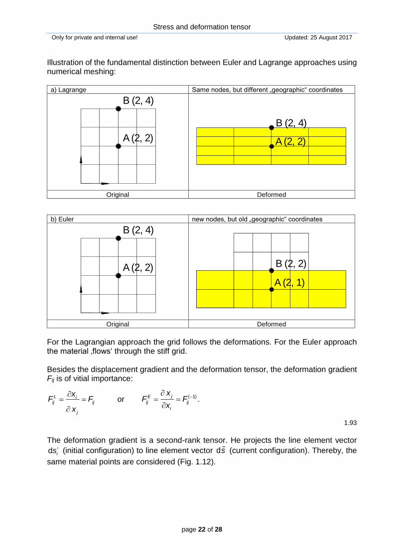
Illustration of the fundamental distinction between Euler and Lagrange approaches using numerical meshing:
a) Lagrange Same nodes, but different „geographic“ coordinates
A (2, 2)
B (2, 4)
B (2, 4)
A (2, 2)
Original Deformed
b) Euler new nodes, but old „geographic“ coordinates
A (2, 2)
B (2, 4)
B (2, 2)
A (2, 1)
Original Deformed
For the Lagrangian approach the grid follows the deformations. For the Euler approach the material ‚flows‘ through the stiff grid. Besides the displacement gradient and the deformation tensor, the deformation gradient Fij is of vitial importance:
L iij ij
j
xF F
x
or ( 1)jE
ij ij
i
xF F
x
.
1.93
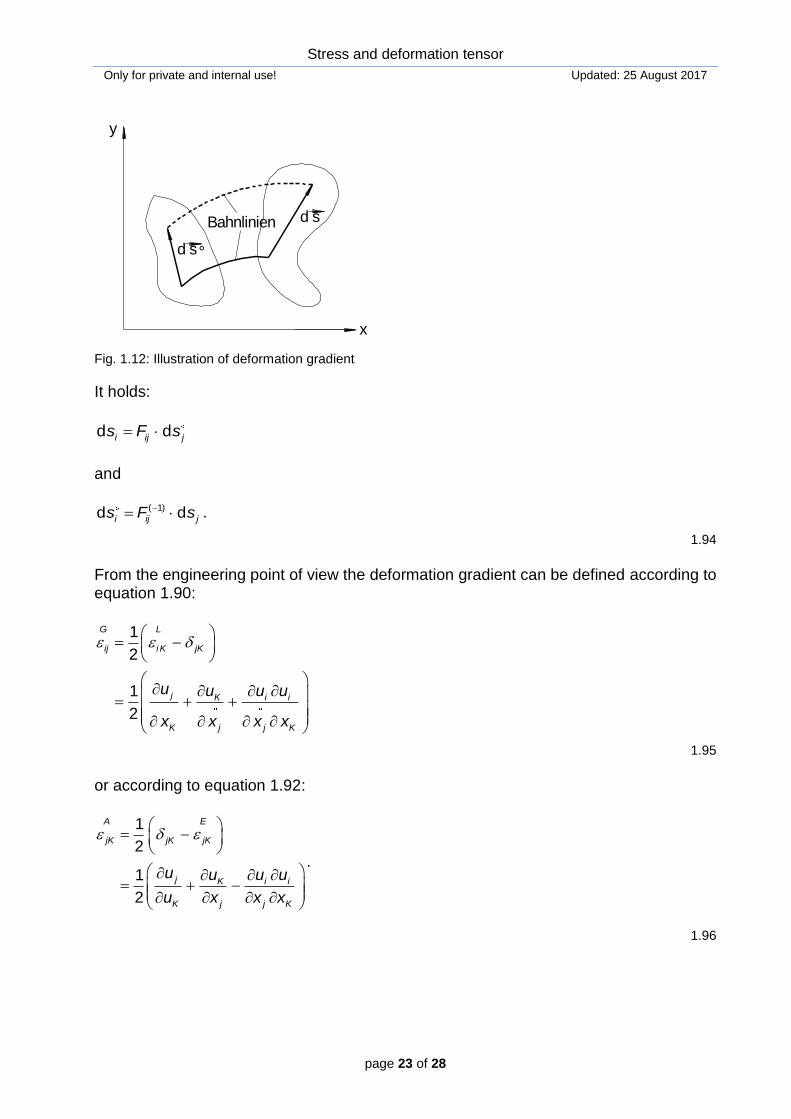
The deformation gradient is a second-rank tensor. He projects the line element vector
d is (initial configuration) to line element vector ds (current configuration). Thereby, the
same material points are considered (Fig. 1.12).
Stress and deformation tensor
Only for private and internal use! Updated: 25 August 2017
page 23 of 28
y
x
Bahnlinien d s
d s°
Fig. 1.12: Illustration of deformation gradient
It holds:
d di ij js F s
and
( 1)d di ij js F s .
1.94
From the engineering point of view the deformation gradient can be defined according to equation 1.90:
1
2
1
2
G L
ij i K jK
j K i i
K j j K
u u u u
x x x x
1.95
or according to equation 1.92:
1
2
1
2
A E
jK jK jK
j K i i
K j j K
u u u u
u x x x
.
1.96

Stress and deformation tensor
Only for private and internal use! Updated: 25 August 2017
page 24 of 28
Expression 1.95 is called ‘Green deformation tensor’, the expression 1.96 is called ‘Al-mansi deformation tensor’. In the engineering praxis the Green deformation tensor is pre-ferred. Moreover, most often the quadratic term is neglected under the assumption, that
1i
j
u
x
. Thus, for small deformation, the distinction between Langrangian and Eulerian
approaches disappears and the simplified deformation tensor is given as:
1
2
jiij
j i
uu
x x
.
1.97
The deformation tensor according to equation 1.97 can be extended to include rotations:
, , , ,
1 1
2 2ij i j j i i j j i
ij ij
Deformations Rotations
u u u u
e w
.
1.98
Fig. 1.13: Illustration of rotation and deformation (2D)
It holds:
12 13 12 21
21 23 13 31
31 32 23 32
0
0 with
0
ij
w w w w
w w w w w
w w w w
and
1.99
11 12 13 12 21
21 22 23 13 31
31 32 33 23 32
withij
e e e e e
e e e e e e
e e e e e
.
1.100
Stress and deformation tensor
Only for private and internal use! Updated: 25 August 2017
page 25 of 28
Thus, the deformation tensor can be written as:
11 12 12 13 13
21 21 22 23 23
31 31 32 32 33
ij
e e w e w
e w e e w
e w e w e
,
1.101
with
1
2ij ij jie and
1for
2ij ij jiw i j .
1.102
eij is called deformation tensor, wij is called rotation tensor. It holds:
1 for i j
2ij ije ,
1.103
Where ij are shear strain components and e11, e22 and e33 are direct strain components (elongations or shortenings).
The volumetric strain v is given by the following expression:
11 22 33
d
dv KK
V
V
.
1.104
The mean direct strain (elongation or shortening) 0 is given by:
0
1 1
3 3KK v .
1.105
In most cases rotations are neglected and it holds:
11 12 13
21 22 23
31 32 33
ij
e e e
e e e
e e e
with
12 21
23 32
13 31
e e
e e
e e
.
1.106
In complete analogy to the stress tensor invariants can be defined also for the deformation tensor, e.g.:
1 11 22 33I e e e ,
1.107
2 11 22 22 33 11 33I e e e e e e and
1.108
3 11 22 33I e e e .
Stress and deformation tensor
Only for private and internal use! Updated: 25 August 2017
page 26 of 28
1.109
Compatibility condition
From expression 1.110 the strain components can be obtained in a unique manner. Oth-erwise, the displacements can not be obtained in a unique manner based on given strains only. The compatibility conditions (= conditions of integrability) are necessary additional requirements to deduce displacements on the basis of given strain components by inte-gration. The consideration of the compatibility conditions guarantees that strains lead to a ‘correct’ displacement field and the continuum is not disturbed. Starting point is the deformation tensor:
, ,
1
2ij i j j iu u .
1.110
Second derivatives of equation 1.110 with corresponding index permutations give the following four expressions:
, , ,
, , ,
, , ,
, , ,
1
2
1
2
1
2
1
2
ij kl i jkl j ikl
kl ij k lij l kij
ik jl i kjl k ijl
jl ik j lik l jik
u u
u u
u u
u u
.
1.111
Due to the fact that the sequence of differentation is arbitrary, through addition and sub-traction of the expressions 1.111 the following expression is obtained:
, , , , 0ij kl kl ij ik jl jl ik
1.112
From expression 1.112 the 6 compatibility conditions can be deduced under the condition
for i jij ji as follows:
11, 22 22,11 12,12
22, 33 33, 22 23, 23
33,11 11, 33 13,13
11, 23 23,11 13, 21 12, 31
22, 31 31, 22 21, 32 23,12
33,12 12, 33 32,13 31, 23
2 0
2 0
2 0
0
0
0
.
1.113
Stress and deformation tensor
Only for private and internal use! Updated: 25 August 2017
page 27 of 28
First equation in 1.113 can exemplary also be written as:
2 22
2 22
yy xyxx
y x x y
.
1.114
Under plain strain conditions all strain components and derivations in respect to the third direction in space vanish, that means only equation 1.114 is left over. Equation 1.114 indicates, that the second derivations of the direct strains and the second derivations of the angular distortions have to be in due proportion. The above used term strain is the so called ‚technical strain‘ or ‘Cauchy strain’ in contrast to the so called ‘logarithmic strain’ or ‘Hencky strain’. Only for small deformations both expressions (Equations 1.115 and 1.116) provide nearly the same value:
Technical strain: l
l
,
1.115
Logarithmic strain: lnl
l
.
1.116
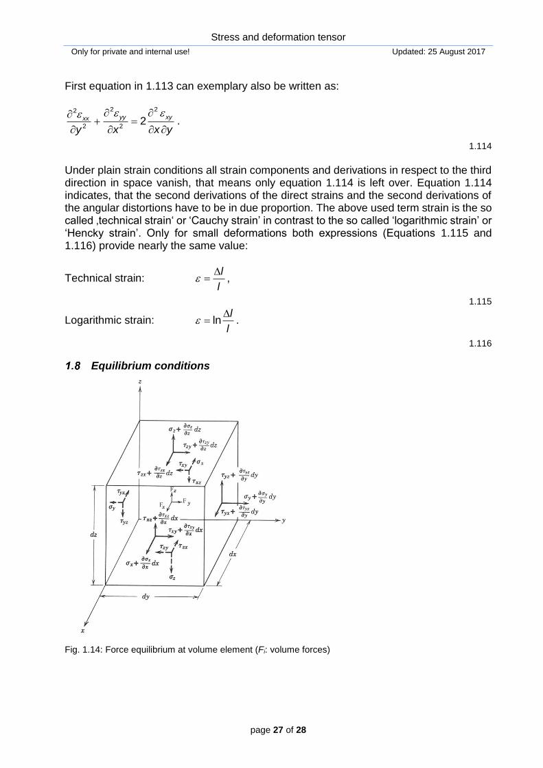
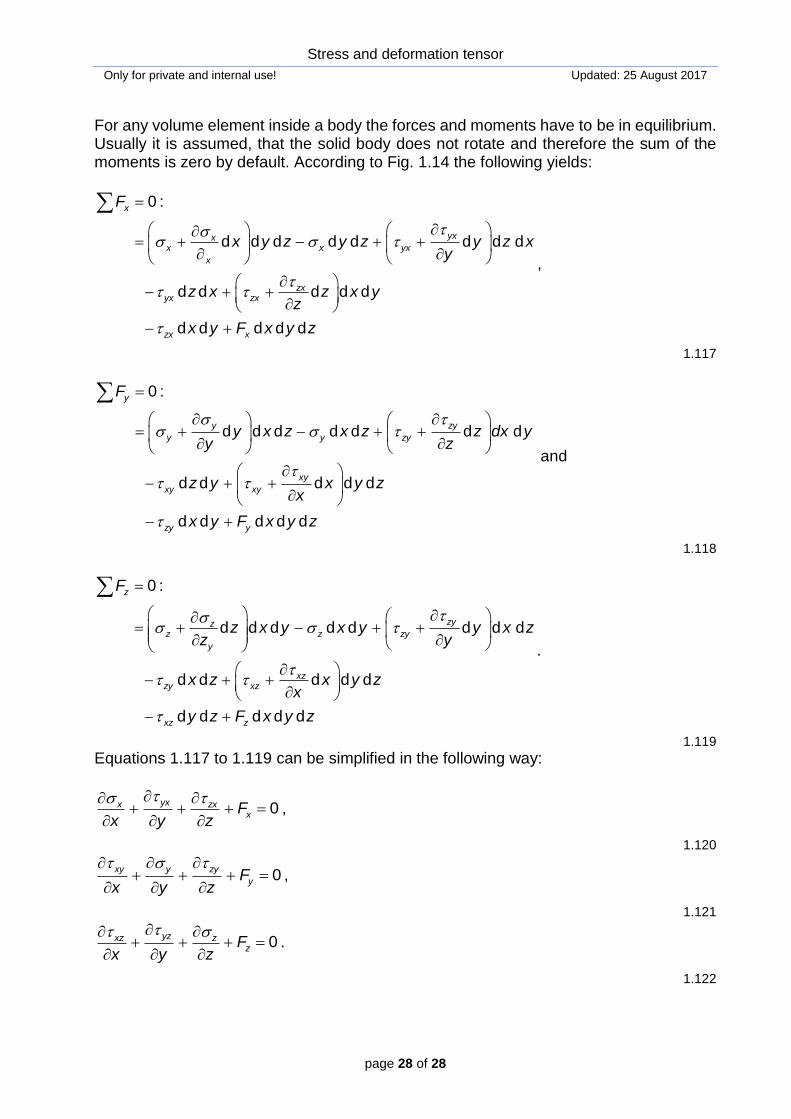
Equilibrium conditions
Fig. 1.14: Force equilibrium at volume element (Fi: volume forces)
Stress and deformation tensor
Only for private and internal use! Updated: 25 August 2017
page 28 of 28
For any volume element inside a body the forces and moments have to be in equilibrium. Usually it is assumed, that the solid body does not rotate and therefore the sum of the moments is zero by default. According to Fig. 1.14 the following yields:
0 :
d d d d d d d d
d d d d d
d d d d d
x
yxxx x yx
x
zxyx zx
zx x
F
x y z y z y z xy
z x z x yz
x y F x y z
,
1.117
0 :
d d d d d d d
d d d d d
d d d d d
y
y zy
y y zy
xy
xy xy
zy y
F
y x z x z z dx yy z
z y x y zx
x y F x y z
and
1.118
0 :
d d d d d d d d
d d d d d
d d d d d
z
zyzz z zy
y
xzzy xz
xz z
F
z x y x y y x zz y
x z x y zx
y z F x y z
.
1.119
Equations 1.117 to 1.119 can be simplified in the following way:
0yxx zx
xFx y z
,
1.120
0xy y zy
yFx y z
,
1.121
0yzxz z
zFx y z
.
1.122
Related Documents