Streamflow simulation: A nonparametric approach

Streamflow simulation: A nonparametric approach

Ashish Sharma,1 David G. Tarboton, and Upmanu LallUtah Water Research Laboratory, Utah State University, Logan

Abstract. In this paper kernel estimates of the joint and conditional probability densityfunctions are used to generate synthetic streamflow sequences. Streamflow is assumed tobe a Markov process with time dependence characterized by a multivariate probabilitydensity function. Kernel methods are used to estimate this multivariate density function.Simulation proceeds by sequentially resampling from the conditional density functionderived from the kernel estimate of the underlying multivariate probability densityfunction. This is a nonparametric method for the synthesis of streamflow that is data-driven and avoids prior assumptions as to the form of dependence (e.g., linear ornonlinear) and the form of the probability density functions (e.g., Gaussian). We show,using synthetic examples with known underlying models, that the nonparametric methodpresented is more flexible than the conventional models used in stochastic hydrology andis capable of reproducing both linear and nonlinear dependence. The effectiveness of thismodel is illustrated through its application to simulation of monthly streamflow from theBeaver River in Utah.

1. Introduction

A goal of stochastic hydrology is to generate syntheticstreamflow sequences that are statistically similar to observedstreamflow sequences. Statistical similarity implies sequencesthat have statistics and dependence properties similar to thoseof the historical record. These sequences represent plausiblefuture streamflow scenarios under the assumption that thefuture will be similar to the past. In this paper we present anonparametric approach for the generation of syntheticstreamflow sequences. This approach is appropriate for thesimulation of stationary unregulated streamflow inputs that areneeded in simulation studies to analyze alternative designs,operation policies, and rules for water resources systems. Theutility of this approach relative to conventional parametricmethods is demonstrated through applications to monthlystreamflow from the Beaver River, near Beaver, Utah, and tosamples generated from linear and nonlinear models withknown statistical attributes.Consider a time series {X1, X2, z z z , Xt, z z z } where Xt

represents streamflow quantities at time t. In practice, thedependence structure of streamflow sequences is often as-sumed to be Markovian, that is, dependent on only a finite setof prior values. With this assumption, Bras and Rodroguez-Iturbe [1985] note that stochastic streamflow models are anexercise in conditional probability. An order p model simulatesXt on the basis of the previous values, that is, Xt21, Xt22, z z z ,Xt2p. This requires that a d 5 p 1 1 dimensional jointprobability distribution be specified. Simulation can proceedfrom the conditional density function, defined as

f~XtuXt21, Xt22, z z z , Xt2p!

5f~Xt, Xt21, Xt22, z z z , Xt2p!

E f~Xt, Xt21, Xt22, z z z , Xt2p! dXt

(1)

Traditional parametric models specify (1) through assumeddistributions. Here, it is suggested that streamflow may insteadbe directly modeled from empirical, data-driven estimates ofthe joint and conditional density functions given in (1). Non-parametric estimates of these density functions are developeddirectly from the historical data. A method is considered non-parametric if it can reproduce a broad class of possible under-lying density functions [Scott, 1992, p. 44]. Nonparametricmethods for density estimation strive to approximate the un-derlying density locally using data from a small neighborhoodof the point of estimate [Lall, 1995]. They impose only weakassumptions, such as continuity of the target function, ratherthan a priori specification or choice of a particular parametricprobability distribution (Gaussian, lognormal, etc.). A perusalof the statistical literature shows that nonparametric statisticalestimation, using splines, kernel functions, nearest neighbormethods and orthogonal series methods, is an active area, withmajor developments still unfolding. Silverman [1986] and Scott[1992] provide good introductory texts. Applications of non-parametric methods in hydrology are reviewed by Lall [1995].Our model is based on a nonparametric kernel density esti-

mate of the p 1 1 dimensional density function f(Xt ,Xt21, z z z , Xt2p), which is then used in (1) to estimate theconditional density function that forms the basis for generationof synthetic streamflow series. This is called a nonparametricorder p , or NPp, model. It has the following advantages:1. Statistical attributes of the data are automatically hon-

ored since one works with a smoothed empirical frequencydistribution based directly on the historical data. Such at-tributes include nonlinear dependence and inhomogeneity(i.e., statistical properties that vary by streamflow state).2. The somewhat tenuous issue of choosing between dif-

ferent models for the probability distribution is sidestepped.3. Considerations related to the above two points lead to a

procedure that is easy to use and is able to automatically model

1Now at Department of Water Engineering, School of Civil Engi-neering, University of New South Wales, Sydney, Australia.

Copyright 1997 by the American Geophysical Union.

Paper number 96WR02839.0043-1397/97/96WR-02839$09.00

WATER RESOURCES RESEARCH, VOL. 33, NO. 2, PAGES 291–308, FEBRUARY 1997

291

the distributional and dependence characteristics of the histor-ical time series. Use of such a procedure should result inimproved decisions for reservoir operation and design.We shall first review some of the traditional approaches,

noting their shortcomings and motivating the need for thenonparametric approach. Kernel density estimation is re-viewed next. We then describe the NPp model and illustrate itsuse with synthetic data from a linear autoregressive (AR1)model and a self-exciting threshold autoregressive (SETAR)model [Tong, 1990, section 3.3.1.1]. These tests demonstratethe effectiveness of the NPp approach in representing bothlinear and nonlinear systems, without prior specification of themodel equations. An application of our model to simulatemonthly streamflow from the Beaver River, near Beaver, Utah,is then presented and results are compared to those from anAR1 model with marginal densities chosen from the best fittingof four commonly used probability density functions.

2. BackgroundAnnual and monthly streamflow has been modeled exten-

sively using autoregressive moving average (ARMA) typemodels [Bras and Rodriguez-Iturbe, 1985; Salas et al., 1980;Pegram et al., 1980; Loucks et al., 1981; Stedinger et al., 1985b;Stedinger and Vogel, 1984; McLeod et al., 1977; Hipel et al.,1977; Yevjevich, 1972]. The early Thomas-Fiering model[Thomas and Fiering, 1962; Fiering, 1967; Beard, 1967], an au-toregressive lag 1 model with seasonally varying coefficients, isa good example of this approach.

~Xt, j 2 mj! 5 r js j

s j21~Xt, j21 2 mj21! 1 s j~1 2 r j

2!1/ 2Wt, j (2)

where Xt, j is the seasonal streamflow at year t and season(month) j, r j is the lag 1 correlation coefficient between sea-sons j and j 2 1, mj is the mean streamflow in season j , s j isthe standard deviation of flow in season j, and Wt, j is anindependent random variable with mean 0 and variance 1. Byallowing the noise term Wt, j to be from a skewed distribution[Lettenmaier and Burges, 1977; Todini, 1980], streamflow froma skewed distribution can be approximated. Thus this modelreproduces the mean, variance, and correlations betweenmonthly streamflows and approximates the skewness. Theseare the variables traditionally considered as most important bystochastic hydrologists. As written, this model applies only to asingle site; however, it is illustrative of a very general class ofARMAmodels for single sites and in a multivariate context formultiple sites or seasons that have been developed and appliedextensively in hydrology over the years and described at lengthin texts on the subject [e.g., Salas et al., 1980; Loucks et al.,1981; Bras and Rodriguez-Iturbe, 1985].Such models can be viewed as special cases of a general

multivariate ARMA( p, q) model:

Xt11 5 Oj50

p

AjXt2j 1 Oj50

q

BjWt2j 1 U (3)

where Xt is a vector of the variables of interest, includingannual and seasonal flows at all sites; Aj and Bj are coefficientmatrices; U is a vector of coefficients, and Wt is a vector ofindependent random innovations. The first term represents anautoregressive component, and the second term represents amoving average component. In all but the simplest univariate

models it is impractical to assume anything but a Gaussiandistribution for theWt. This is equivalent to the assumption ofa multivariate Gaussian distribution for the time series depen-dence structure. The ARMA model is then defined throughthe estimation of the parameters Aj, Bj, U and the modelorder ( p , q). To account for the fact that the real streamflowsare not Gaussian, the flows are often first transformed to aGaussian distribution and then the transformed variables areused with (3) [Stedinger, 1981; Stedinger and Taylor, 1982; Ste-dinger et al., 1985a]. Reproducing moments in the originalcoordinates may then be difficult.The general linear model depicted by (3) is a special case of

the conditional density function of (1). This multivariate Gaus-sian structure with transformed marginal distributions (denot-ed MGTM here) has with few exceptions [Yakowitz, 1985;Smith, 1991, 1992; Lall and Sharma, 1996] underlain practicallyall stochastic hydrology to date. The Lall and Sharma work isvery similar in spirit to this work, though its approach is that ofa nearest neighbor bootstrap rather than kernel density esti-mation. We believe that both are good alternatives that need tobe considered for streamflow simulation.The preceding discussion reveals the basic structure of cur-

rent time series estimation methods and hints at their re-stricted view of the possibilities of variation in hydrologicaltime series. The main reasons for the prevalence of linearARMA models for hydrologic time series analysis may be thefollowing: (1) the framework has been well developed in thestatistical literature for stationary processes; (2) the techniquesare well understood and taught; and (3) software for multivar-iate analysis has been developed by a number of people, isreadily available, and does not pose a severe computationalburden [Salas, 1993].Some drawbacks of the MGTM approach are the following:1. Only a limited degree of heterogeneity in the statistical

dependence structure is admitted through the normalizingtransform. The dependence of variance of streamflow onstreamflow magnitude is often noted. There is evidence insome streamflow data that correlations are different dependingon whether flows are low or high. We give an example of thisin section 6 using state-dependent correlation statistics definedin Appendix A. In an MGTM model the correlation structureis fixed regardless of flow magnitude. Among others, Yevjevich[1972] has argued for the systematic identification of nonsta-tionarities in the mean of the time series (e.g., jumps, periodi-cities) and their removal to yield a stationary time series thatcan be analyzed by standard methods. However, such featuresmay be part of the underlying dynamics and important tomodel behavior (e.g., to a drought regime) that may be relatedto threshold dependent processes.2. The MGTM models impose a time reversible structure.

The joint distributions of (Xt, Xt11, z z z , Xt1m) and of (Xt,Xt21, z z z , Xt2m) are identical. Tong [1990, p. 9] shows anexample of daily streamflow that is not time reversible andargues that the dynamics of physical processes is time irreversible.3. The choice of a distribution for Wt or of an appropriate

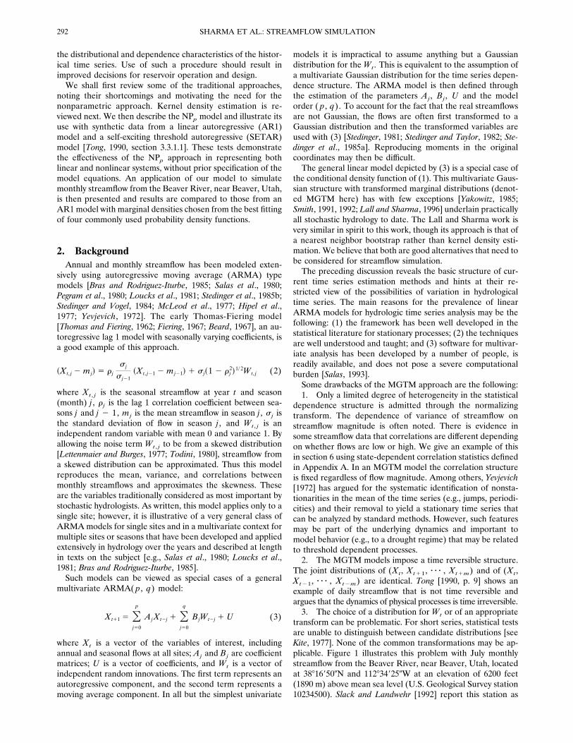
transform can be problematic. For short series, statistical testsare unable to distinguish between candidate distributions [seeKite, 1977]. None of the common transformations may be ap-plicable. Figure 1 illustrates this problem with July monthlystreamflow from the Beaver River, near Beaver, Utah, locatedat 388169500N and 1128349250W at an elevation of 6200 feet(1890 m) above mean sea level (U.S. Geological Survey station10234500). Slack and Landwehr [1992] report this station as

SHARMA ET AL.: STREAMFLOW SIMULATION292

unregulated and free from other anthropogenic effects. Thefigure shows the histogram of monthly flow, with four com-monly used distributions fitted to the data. The histogram hasbimodality that cannot be reproduced by any of the distribu-tions commonly used. This figure also shows a kernel densityestimate. Note that this is effectively a smoothing of the histo-gram. The following Filliben correlation statistics [Grygier andStedinger, 1990] test the goodness of fit for each distribution inFigure 1: kernel density estimate, 0.998; normal, 0.963; lognor-mal, 0.979; three-parameter lognormal, 0.982; and gamma,0.985. The Filliben correlation statistic is the correlation be-tween empirical quantiles from a plotting position and fitteddistribution quantiles corresponding to the data values. For aperfect fit the Filliben correlation statistic should be 1, and it isby construction a value that lies close to 1. The relative depar-ture from 1 provides a measure of the relative goodness of fitbetween the different distributions. By this measure the non-parametric density estimate fits better than any of these com-monly used parametric choices. A x2 test [Benjamin and Cor-nell, 1970, p. 460] rejected at the 95% level the hypothesis thatthis histogram was from a normal distribution. However, the x2

test would not reject any of the other distributions, includingthe nonparametric density estimate, which is typical of theinability to distinguish between candidate distributions.4. The synthetic traces generated by MGTM replicate the

first few (2 or 3) moments of the underlying dependence struc-ture. Consequently, the generated series may bear little resem-blance to the observed series in terms of persistence andthreshold crossings, factors that are of interest to hydrologists.The ARMA models also are incapable of displaying suddenbursts or jumps, a feature that may often be observed during anotherwise prolonged drought.5. Salas and Smith [1981] and Salas et al. [1980] discussed

physical justifications for ARMA models and showed that alinear control system representation of basin processes canlead to ARMA models of streamflow. However, other factors

emerge when one considers the relationship of streamflow tosome causative factors. For instance, in snow-fed basins thestreamflow response during snowmelt months is a thresholdresponse to temperature. The dynamics of soil moisture ishysteretic and nonlinear. The dynamics of vegetative consump-tive use and retention of water is also quite different during wetand dry periods and as a function of temperature. Runoffgeneration mechanisms during protracted wet or dry periodswill consequently be different. While these comments havemore direct bearing on streamflow at timescales shorter than amonth or a year, they are relevant for the longer timescales inthat they influence the variance of the streamflow at thesetimescales.6. Despite the fact that nearly 30 years have elapsed since

the classical time series (AR) models were introduced to prac-ticing hydrologists, acceptance and application of these modelsfor drought analysis and reservoir operation by practitionershas been limited. They often prefer to base their decisions onthe historical record (or a resampled proxy thereof). Kendalland Dracup [1991] note that the index sequential method,which is basically a sequential resampling of the historicalrecord, appears to be the procedure of choice in many watermanagement agencies, including the California Department ofWater Resources, U.S. Bureau of Reclamation, Los AngelesDepartment of Water, and the Metropolitan Water District ofSouthern California. This is practiced in spite of the recogni-tion that history is unlikely to repeat itself and that the recordis perhaps woefully short.In summary, while the MGTM ARMA framework is indeed

useful in certain contexts, a more flexible time series analysismethod capable of reproducing additional features of hydro-logic data is needed. The success of linear ARMA models withsome hydrologic data sets may be fortuitous and a conse-quence of short records. The technical issues are nonlinearity,nonstationarity, and inhomogeneity in the underlying depen-dence structure. Parametric nonlinear models [Bendat and

Figure 1. Histogram and probability density estimates of July monthly streamflow (in cubic feet per second;1 foot3 s21 is equal to 28.317 L s21) in the Beaver River near Beaver, Utah. The dots on the x axis denote theindividual data points.

293SHARMA ET AL.: STREAMFLOW SIMULATION

Piersol, 1986; Tong, 1990] can be used in place of the linearARMAmodels to model nonlinear time series. The use of suchmodels, however, still requires specification of the form ofnonlinear dependence, something which may be difficult to doin practice. From a practitioner’s perspective the key issues arereproducibility of observed data characteristics, simplicity, anddependability. The nonparametric techniques proposed hereavoid the difficult model specification issues associated withparametric linear or nonlinear models. They amount to resa-mpling from the original data, with perturbations, and repro-duce directly the characteristics of the original data in a simpleand dependable way.

3. Kernel Density EstimationKernel density estimation entails a weighted moving average

of the empirical frequency distribution of the data. Most non-parametric density estimators can be expressed as kernel den-sity estimation methods [Scott, 1992, p. 125.]. In this paper weuse multivariate kernel density estimators with Gaussian ker-nels and bandwidth selected using least squares cross-validation (LSCV) [e.g., Scott, 1992, p. 160]. This bandwidthselection method is one from among the many available meth-ods. Our methodology is intended to be generic and shouldwork with any bandwidth and kernel density estimationmethod. This section reviews kernel density estimation first ina univariate and then in a multivariate setting and gives detailsof the LSCV procedure for estimating bandwidth. For a reviewof hydrologic applications of kernel density and distributionfunction estimators, readers are referred to work by Lall[1995]; Silverman [1986] and Scott [1992] provide good intro-ductory texts.A univariate kernel probability density estimator is written

f~ x! 5 Oi51

n 1nh KS x 2 xi

h D (4)

where there are n sample data xi. K( ) is a kernel functionthat must integrate to 1, and h is a parameter called thebandwidth that defines the locale over which the empiricalfrequency distribution is averaged. There are many possiblekernel functions given in texts such as those by Silverman[1986] and Scott [1992]. The Gaussian kernel function, a pop-ular and practical choice, is used here:

K~ x! 51

~2p!1/ 2exp ~2x2/ 2! (5)

The density estimate in (4) is formed by summing kernels withbandwidth h centered at each observation xi. This is similar tothe construction of a histogram where individual observationscontribute to the density by placing a rectangular box (analo-gous to the kernel function) in the prespecified bin the obser-vation lies in. The histogram is discrete and sensitive to theposition and size of each bin. By using smooth kernel functions,the kernel density estimate in (4) is smooth and continuous.A multivariate extension of (4) and (5) for a vector x in d

dimensions can be written as

f~x! 51n O

i51

n 1~2p!d/ 2 det ~H!1/ 2

z exp S2~x 2 x i!TH21~x 2 x i!

2 D (6)

where n is the number of observed vectors xi and H is abandwidth matrix that must be from the class of symmetricpositive definite d 3 d matrices [Wand and Jones, 1994]. Theabove density estimate is formed by summing Gaussian kernelswith a covariance matrix H, centered at each observation xi. Auseful specification of the bandwidth matrix H is

H 5 l2S (7)

Here, S is the sample covariance matrix of the data and l2

prescribes the bandwidth relative to this estimate of scale.These are parameters of the model that are estimated from thedata. The procedure of scaling the bandwidth matrix propor-tional to the covariance matrix (equation (7)) is called “spher-ing” [Fukunaga, 1972] and ensures that all kernels are orientedalong the principal components of the covariance matrix.Silverman [1986, pp. 70–72] cites results indicating that suf-

ficient conditions for convergence of the kernel density esti-mate to an underlying density function under broad conditionsmet by any kernel that is a usable probability density function,are that as n 3 ` , h 3 0 and nh 3 ` . This also applies tol in the multivariate context. However, the rate of convergencedepends on how h or l is chosen. Methods for choosing thebandwidth are based on evaluation of factors such as bias,E{ f(x) 2 f(x)}; variance, Var{ f(x)}; mean square error(MSE); integrated square error (ISE); and mean integratedsquare error (MISE) of the estimate:

MSE5 E$@ f~x! 2 f~x!#2%

5 $E@ f~x! 2 f~x!#%2 1 Var $ f~x!% (8)

ISE5 E5d

~ f~x! 2 f~x!!2 dx (9)

MISE5 EE5d

~ f~x! 2 f~x!!2 dx (10)

A small value of the bandwidth (h or l) can result in a densityestimate that appears “rough,” and has a high variance. On theother hand, too high an h results in an “over smoothed” den-sity estimate with modes and asymmetries smoothed out. Suchan estimate has low variance but is more biased with respect tothe underlying density. This bias-variance trade-off [Silverman,1986, section 3.3.1] plays an important role in choice of h.Taylor series expansion of the one-dimensional density es-

timate in (4) can be used to show that the asymptotic meanintegrated square error (AMISE) is [Silverman, 1986, p. 40;Sain et al., 1994]

AMISE~h! <R~K!

nh 114

sK4 h4R~ f 0! (11)

where R[ g( x)] 5 *g( x)2 dx for any function g( x) (eitherK( x) or f0( x)), f0 is the second derivative, and sK

2 5 *u2K(u)du . This can be generalized to higher dimensions.One choice for the bandwidth is one that directly minimizes

(11) if the true distribution were known. This value is known asthe AMISE optimal bandwidth for that distribution. For aGaussian distribution with Gaussian kernel functions (estima-tor defined by (6) and (7)) Silverman [1986, pp. 86–87] givesthis bandwidth as

l 5 S 4d 1 2D

1/~d14!

n21/~d14! (12)

In the univariate case (d 5 1) this reduces to h 5 1.06sn21/5


where s is an estimate of the standard deviation (Silverman ad-vocates a robust estimate) of the data. An upper bound on band-width can be obtained by minimizing R( f0) over a class of prob-ability densities. This leads to the optimal bandwidth for thesmoothest possible density function. Scott [1992, p. 181] citesresults showing that this upper bound (1# d# 10) is 1.08 to 1.12times the l in (12).Data-driven methods have been developed to estimate the

bandwidth when the underlying distribution is not known.They minimize estimates of ISE, MISE, or AMISE formedonly from the data. LSCV [Silverman, 1986, pp. 48–52] is onesuch method, based on the fact that the integrated square error(equation (9)) can be expanded as

ISE5 R@ f~x!# 2 2E f~x! f~x! dx 1 R@ f~x!# (13)

The first term may be directly evaluated. The second term maybe recognized as E[ f(X)] and estimated using leave one outcross validation. The last term, R( f(x)), is independent of thebandwidth and does not need to be considered. The LSCVmethod in one dimension chooses the bandwidth, h, to mini-mize the following LSCV score, comprising the first two termsin (13):

LSCV~h! 51n2h O

i51

n Oj51

n

K ~2!S xi 2 xjh D

22n O

i51

n Oj51jÞ1

n 1nh KS xi 2 xj

h D (14)

Here, K(2) denotes the convolution of the kernel function withitself (for example, if K is the standard Gaussian kernel, thenK(2) will be the Gaussian density with variance 2).On the basis of results by Sain et al. [1994] and Adamowski

and Feluch [1991] the generalization of the LSCV score tohigher dimensions with multivariate Gaussian kernel functionsand a symmetric positive definite bandwidth matrix H as spec-ified by, for example, (7) is

LSCV(H)

5

1 1 ~1/n!Oi51

n OjÞi

@exp ~2Lij/4! 2 2d/ 211 exp ~2Lij/ 2!#

~2p1/ 2!dn det ~H!1/ 2

(15)

where

Lij 5 ~x i 2 x j!TH21~x i 2 x j! (16)

We use numerical minimization of (15) over the single param-eter l with bandwidth matrix from (7) to estimate all thenecessary probability density functions. We recognize thatLSCV bandwidth estimation is occasionally degenerate, so onthe basis of suggestions by Silverman [1986, p. 52] and theupper bound given by Scott [1992, p. 181], we restrict oursearch to the range l/4 to 1.1l.

4. Nonparametric Order p Markov StreamflowModel, NPpTo keep the presentation simple, the equations will be pre-

sented for a lag 1 (order p 5 1) model. The formulae pre-

sented are readily extended to include higher-order lags. Con-sideration of higher-order models raises the issue ofdetermination of the correct order p . This is deferred to futurework. Here results are presented for the simplest case (NP1)analogous to the simple AR1 model. In the form presentedbelow, the model can be applied to simulate stationary se-quences such as annual flows. Section 6 describes how appli-cation of the model to pairs of sequential months is used tosimulate seasonally nonstationary (e.g., monthly) streamflowsequences.The joint distribution of Xt and its prior value Xt21 is esti-

mated using (6) on the basis of n observed data vectors xi. Fora time series x0, x1, x2, z z z , xn, the data vector xi has ele-ments ( xi, xi21), where 1 # i # n . Hence x1 5 ( x1, x0),x2 5 ( x2, x1), z z z , xn 5 ( xn, xn21). These are a series ofordered pairs. There is one less ordered pair than the length ofthe time series. The conditional density (equation (1)) is writ-ten as

f~XtuXt21! 5f~Xt, Xt21!

E f~Xt, Xt21! dXt

5f~Xt, Xt21!fm~Xt21!

(17)

where fm(Xt21) is the marginal density of Xt21. Now applyingthe estimator in (6), the joint density estimate is obtained as

f~Xt, Xt21! 51n O

i51

n 12pl2 det ~S!1/ 2

z exp S2H F Xt 2 xiXt21 2 xi21G

T

S21F Xt 2 xiXt21 2 xi21GY2l2J D (18)

Note that each observation contributes to this density estimatedepending on the distance of the observation ( xi, xi21) to thepoint (Xt, Xt21), the bandwidth l, and the sample covariancematrix S of (Xt, Xt21). The bandwidth l is obtained by min-imizing the LSCV score function (equation (15)).Denote the terms in the covariance matrix:

S 5 F S11S21 S12S22G (19)

Then for a given Xt21, (18) substituted in (17) reduces to asum of Gaussian kernels dependent on a single variable Xt:

f~XtuXt21! 5 Oi51

n 1~2pl2S9!1/ 2

wi exp S2~Xt 2 bi!2

2l2S9 D (20)

where

wi 5 exp S2~Xt21 2 xi21!2

2l2S22DYO

j51

n

exp S2~Xt21 2 xj21!2

2l2S22D

(21a)

S9 5 S11 2S122

S22(21b)

bi 5 xi 1 ~Xt21 2 xi21!S12S22

(21c)

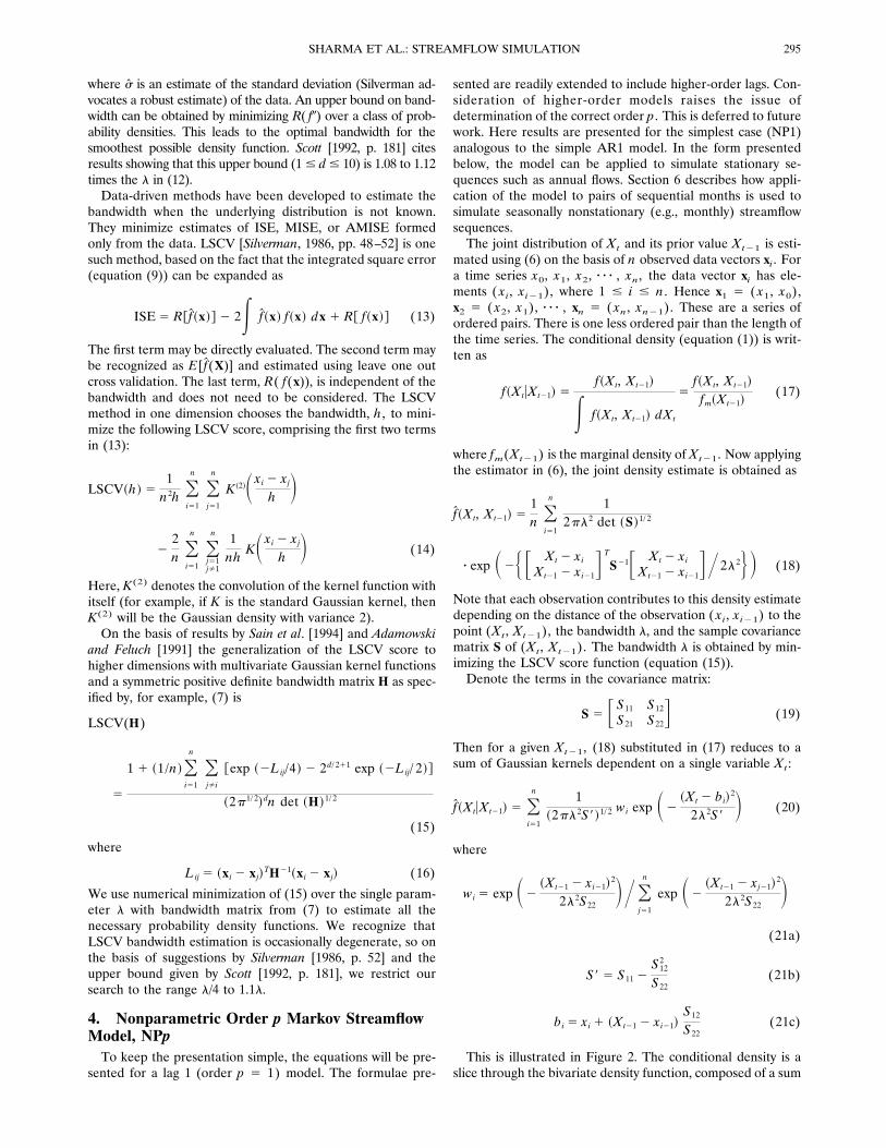
This is illustrated in Figure 2. The conditional density is aslice through the bivariate density function, composed of a sum


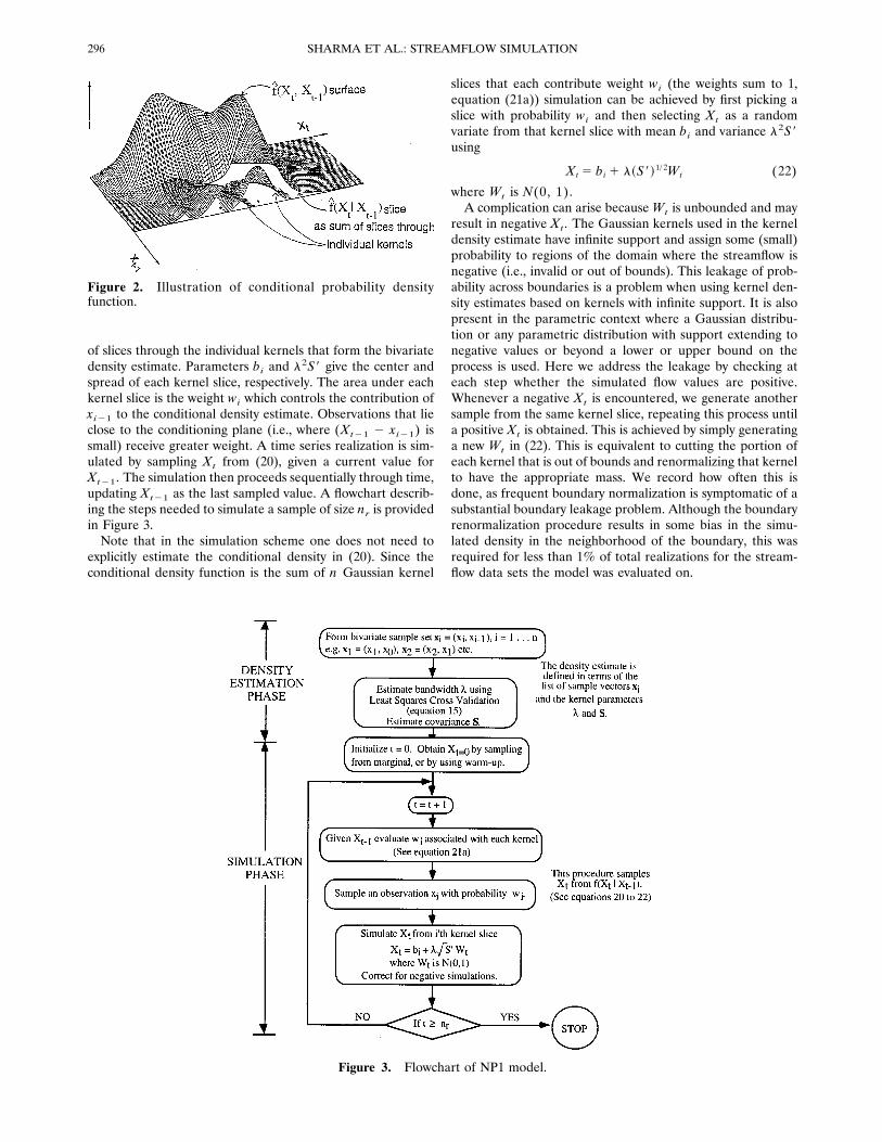
of slices through the individual kernels that form the bivariatedensity estimate. Parameters bi and l2S9 give the center andspread of each kernel slice, respectively. The area under eachkernel slice is the weight wi which controls the contribution ofxi21 to the conditional density estimate. Observations that lieclose to the conditioning plane (i.e., where (Xt21 2 xi21) issmall) receive greater weight. A time series realization is sim-ulated by sampling Xt from (20), given a current value forXt21. The simulation then proceeds sequentially through time,updating Xt21 as the last sampled value. A flowchart describ-ing the steps needed to simulate a sample of size nr is providedin Figure 3.Note that in the simulation scheme one does not need to

explicitly estimate the conditional density in (20). Since theconditional density function is the sum of n Gaussian kernel

slices that each contribute weight wi (the weights sum to 1,equation (21a)) simulation can be achieved by first picking aslice with probability wi and then selecting Xt as a randomvariate from that kernel slice with mean bi and variance l2S9using

Xt 5 bi 1 l~S9!1/ 2Wt (22)

where Wt is N(0, 1).A complication can arise because Wt is unbounded and may

result in negative Xt. The Gaussian kernels used in the kerneldensity estimate have infinite support and assign some (small)probability to regions of the domain where the streamflow isnegative (i.e., invalid or out of bounds). This leakage of prob-ability across boundaries is a problem when using kernel den-sity estimates based on kernels with infinite support. It is alsopresent in the parametric context where a Gaussian distribu-tion or any parametric distribution with support extending tonegative values or beyond a lower or upper bound on theprocess is used. Here we address the leakage by checking ateach step whether the simulated flow values are positive.Whenever a negative Xt is encountered, we generate anothersample from the same kernel slice, repeating this process untila positive Xt is obtained. This is achieved by simply generatinga new Wt in (22). This is equivalent to cutting the portion ofeach kernel that is out of bounds and renormalizing that kernelto have the appropriate mass. We record how often this isdone, as frequent boundary normalization is symptomatic of asubstantial boundary leakage problem. Although the boundaryrenormalization procedure results in some bias in the simu-lated density in the neighborhood of the boundary, this wasrequired for less than 1% of total realizations for the stream-flow data sets the model was evaluated on.

Figure 2. Illustration of conditional probability densityfunction.

Figure 3. Flowchart of NP1 model.


There are two alternatives for initializing the nonparametricsimulation procedure. The first is to sample Xt at t 5 0 fromthe appropriate marginal distribution, which is a univariatekernel density function given by (4) with bandwidth h 5l(S11)

1/ 2. Each prior data point contributes equal weight(1/n) to this kernel estimate. Therefore the initial variate maybe obtained by picking one of the prior values xi21 at randomwith probability 1/n and then using

Xt 5 xi21 1 l~S11!1/ 2Wt (23)

where Wt is N(0, 1).The second initialization alternative is to specify Xt at t 5 0

arbitrarily (e.g., equal to the mean) and provide a suitably long“warm-up” period, discarding the first several values simulatedto avoid any initialization bias.The nonparametric simulation model has been presented

from the perspective of formally estimating the underlyingprobability density function and then sampling from it. How-ever, when viewed operationally one sees that it has close tiesto the bootstrap [Efron, 1979; Efron and Tibishirani, 1993]. Infact, it is a smoothed bootstrap. Each kernel slice that contrib-utes weight wi is centered over a prior data pair ( xi, xi21), sopicking a kernel slice amounts to picking a prior data pair withprobability wi. The bootstrap is a statistical method that in-volves resampling the original data (with replacement) that hasapplications in estimation of confidence intervals and quanti-fication of parameter uncertainty [Hardle and Bowman, 1988;Woo, 1989; Tasker, 1987; Zucchini and Adamson, 1989]. Theclassic bootstrap assumes data are independent and identicallydistributed and resamples from each prior data point withequal probability. The nearest neighbor bootstrap method pre-sented by Lall and Sharma [1996] was designed for bootstrap-ping dependent data. It is similar to the approach here in thata data pair nearby to the conditioning vector is picked, and itssuccessor is chosen as the simulated data value. However, ituses a conditional probability density represented by a discretekernel which is based on the assumption of a local Poissondistribution in the neighborhood of the conditioning vector.The nearest neighbor bootstrap also differs in that there is noperturbation of the selected point. Consequently, it only re-produces streamflow values that have been observed. The ap-proach presented here amounts to picking a prior data pair ( xi,xi21) that is nearby, that is, xi21 near to the conditioning valueXt21, according to weights based on Gaussian kernels, thenthrough (22), adding a perturbation. The perturbations in ourapproach serve to smooth over the gaps between data points inthe density estimate and provide alternative streamflow real-izations that are different but are stochastically similar to thehistorical record.Simulations from this nonparametric approach retain the

marginal and joint density structure of the historical time seriesincluding nonlinearities and state dependence. One can alsoanalytically calculate the marginal distribution and the valuesof the NP1 model mean, standard deviation, skewness, and lag1 correlation from the kernel density estimate (equation (18)).These are given in Appendix B and compared in the resultsbelow to sample statistics from the historical data.

5. Testing With Synthetic DataIn order to evaluate the ability of our model to recover

structure from known linear and nonlinear parametric models,

we conducted tests using two synthetic models. The purpose ofthese experiments was to verify the performance of the NP1model where the true model is known. The first model usedwas a linear autoregressive order 1 (AR1) model of the typecommonly used to model streamflow. The second was a self-exciting threshold autoregressive (SETAR) model [Tong,1990]. A two-level Monte Carlo experiment was used in bothcases: (1) generate 100 level 1 sample records of length 80 fromthe true model (AR1 or SETAR); and (2) for each samplerecord, generate 100 level 2 realizations, each of length 80,from the NP1 model.Note that we refer to the 100 samples first generated as level

1 samples. These are representative of the observed data. Werefer to the 10,000 realizations generated (100 NP1 realiza-tions from each of the 100 level 1 sample records) as level 2realizations. These are representative of what our model wouldsimulate given the level 1 sample records and were used toevaluate how well the NP1 model reproduces statistics of thesamples it is based on as well as the underlying populationstatistics. Since all realizations are the same length as therecord from which they are generated, the 100 realizationsfrom each record provide estimates of the natural samplingvariability associated with that record length. Statistics such asthe mean, standard deviation, lag 1 correlation, and skewnesswere estimated, as well as marginal and joint kernel densityestimates from the sample records and realizations.Box plots are used for the graphical comparisons. These

consist of a box that extends over the interquartile range of thequantity being plotted, estimated from the 100 realizations.The line in the center of this box is the median, and whiskersextend to the 5% and 95% quantiles of the compared statistic.

5.1. Tests With AR1 Data

The AR1 model used was

Xt 5 0.5 Xt21 1 0.866 Wt (24)

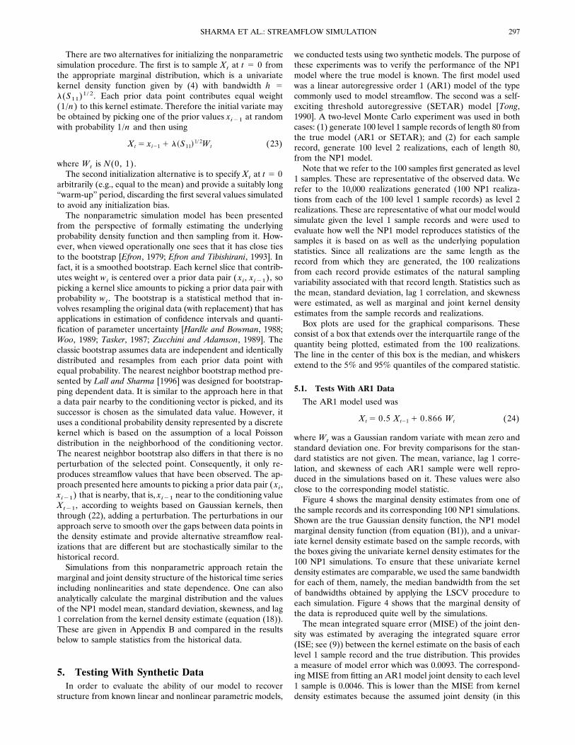
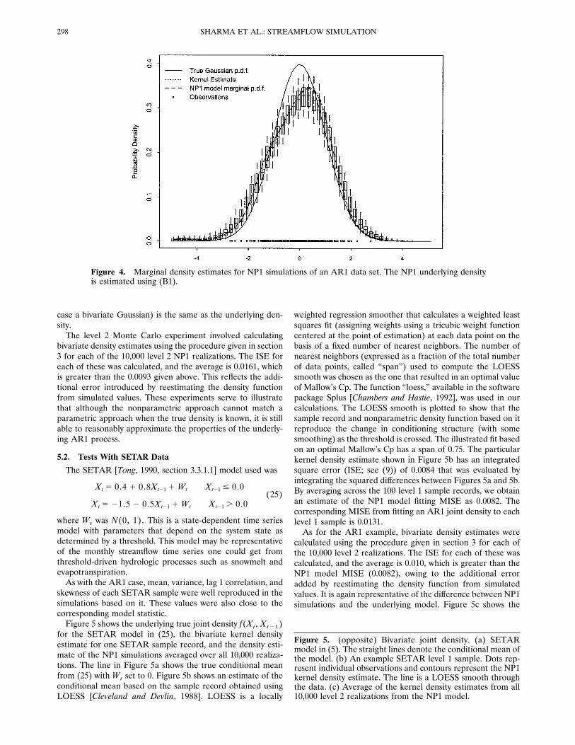
where Wt was a Gaussian random variate with mean zero andstandard deviation one. For brevity comparisons for the stan-dard statistics are not given. The mean, variance, lag 1 corre-lation, and skewness of each AR1 sample were well repro-duced in the simulations based on it. These values were alsoclose to the corresponding model statistic.Figure 4 shows the marginal density estimates from one of

the sample records and its corresponding 100 NP1 simulations.Shown are the true Gaussian density function, the NP1 modelmarginal density function (from equation (B1)), and a univar-iate kernel density estimate based on the sample records, withthe boxes giving the univariate kernel density estimates for the100 NP1 simulations. To ensure that these univariate kerneldensity estimates are comparable, we used the same bandwidthfor each of them, namely, the median bandwidth from the setof bandwidths obtained by applying the LSCV procedure toeach simulation. Figure 4 shows that the marginal density ofthe data is reproduced quite well by the simulations.The mean integrated square error (MISE) of the joint den-

sity was estimated by averaging the integrated square error(ISE; see (9)) between the kernel estimate on the basis of eachlevel 1 sample record and the true distribution. This providesa measure of model error which was 0.0093. The correspond-ing MISE from fitting an AR1 model joint density to each level1 sample is 0.0046. This is lower than the MISE from kerneldensity estimates because the assumed joint density (in this


case a bivariate Gaussian) is the same as the underlying den-sity.The level 2 Monte Carlo experiment involved calculating

bivariate density estimates using the procedure given in section3 for each of the 10,000 level 2 NP1 realizations. The ISE foreach of these was calculated, and the average is 0.0161, whichis greater than the 0.0093 given above. This reflects the addi-tional error introduced by reestimating the density functionfrom simulated values. These experiments serve to illustratethat although the nonparametric approach cannot match aparametric approach when the true density is known, it is stillable to reasonably approximate the properties of the underly-ing AR1 process.

5.2. Tests With SETAR Data

The SETAR [Tong, 1990, section 3.3.1.1] model used was

Xt 5 0.4 1 0.8Xt21 1 Wt Xt21 # 0.0(25)

Xt 5 21.5 2 0.5Xt21 1 Wt Xt21 . 0.0

where Wt was N(0, 1). This is a state-dependent time seriesmodel with parameters that depend on the system state asdetermined by a threshold. This model may be representativeof the monthly streamflow time series one could get fromthreshold-driven hydrologic processes such as snowmelt andevapotranspiration.As with the AR1 case, mean, variance, lag 1 correlation, and

skewness of each SETAR sample were well reproduced in thesimulations based on it. These values were also close to thecorresponding model statistic.Figure 5 shows the underlying true joint density f(Xt, Xt21)

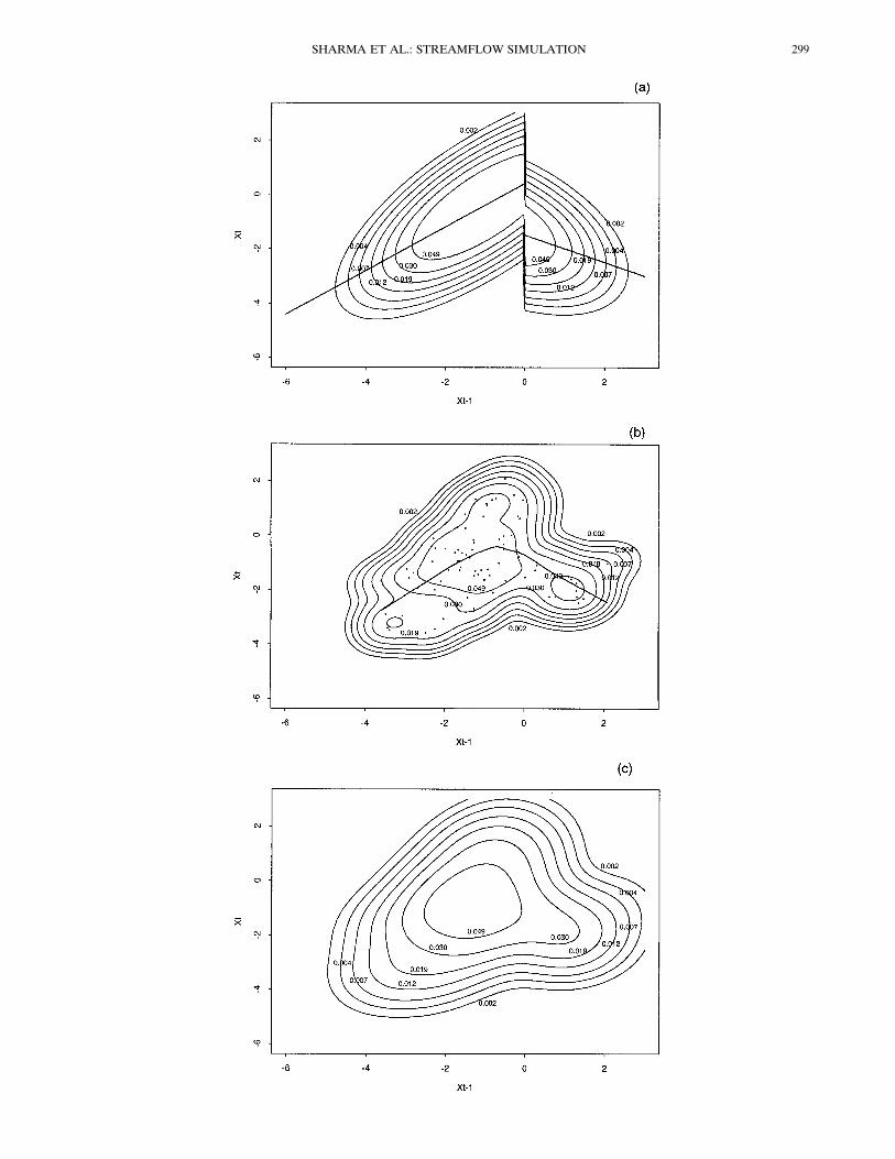
for the SETAR model in (25), the bivariate kernel densityestimate for one SETAR sample record, and the density esti-mate of the NP1 simulations averaged over all 10,000 realiza-tions. The line in Figure 5a shows the true conditional meanfrom (25) with Wt set to 0. Figure 5b shows an estimate of theconditional mean based on the sample record obtained usingLOESS [Cleveland and Devlin, 1988]. LOESS is a locally

weighted regression smoother that calculates a weighted leastsquares fit (assigning weights using a tricubic weight functioncentered at the point of estimation) at each data point on thebasis of a fixed number of nearest neighbors. The number ofnearest neighbors (expressed as a fraction of the total numberof data points, called “span”) used to compute the LOESSsmooth was chosen as the one that resulted in an optimal valueof Mallow’s Cp. The function “loess,” available in the softwarepackage Splus [Chambers and Hastie, 1992], was used in ourcalculations. The LOESS smooth is plotted to show that thesample record and nonparametric density function based on itreproduce the change in conditioning structure (with somesmoothing) as the threshold is crossed. The illustrated fit basedon an optimal Mallow’s Cp has a span of 0.75. The particularkernel density estimate shown in Figure 5b has an integratedsquare error (ISE; see (9)) of 0.0084 that was evaluated byintegrating the squared differences between Figures 5a and 5b.By averaging across the 100 level 1 sample records, we obtainan estimate of the NP1 model fitting MISE as 0.0082. Thecorresponding MISE from fitting an AR1 joint density to eachlevel 1 sample is 0.0131.As for the AR1 example, bivariate density estimates were

calculated using the procedure given in section 3 for each ofthe 10,000 level 2 realizations. The ISE for each of these wascalculated, and the average is 0.010, which is greater than theNP1 model MISE (0.0082), owing to the additional erroradded by reestimating the density function from simulatedvalues. It is again representative of the difference between NP1simulations and the underlying model. Figure 5c shows the

Figure 4. Marginal density estimates for NP1 simulations of an AR1 data set. The NP1 underlying densityis estimated using (B1).

Figure 5. (opposite) Bivariate joint density. (a) SETARmodel in (5). The straight lines denote the conditional mean ofthe model. (b) An example SETAR level 1 sample. Dots rep-resent individual observations and contours represent the NP1kernel density estimate. The line is a LOESS smooth throughthe data. (c) Average of the kernel density estimates from all10,000 level 2 realizations from the NP1 model.



average density function estimated from the 10,000 realiza-tions. This captures the essential nonlinearity of the SETARmodel despite smoothing over the discontinuity. No modelfrom the MGTM class of models is able to reproduce sampleswhich exhibit such nonlinear structure. A bivariate normaldistribution with the true mean and covariance of the model in(25), that is, without fitting errors, has an ISE relative to Figure5a of 0.0119, larger than that obtained from the NP1 model fitswith 80 data points. Asymptotically, the NP1 kernel densityestimate will converge to the underlying SETAR model ex-actly, that is, with no fitting errors. This reiterates the pointthat model mis-specification, for example, by selection of thebivariate normal distribution, precludes a model from conver-gence to whatever the underlying distribution may be.Table 1 shows the state dependent correlation statistics (de-

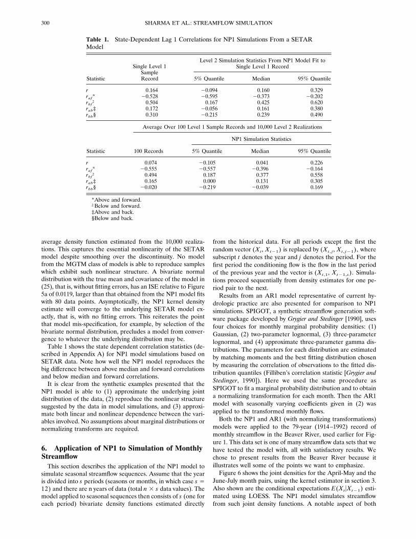
scribed in Appendix A) for NP1 model simulations based onSETAR data. Note how well the NP1 model reproduces thebig difference between above median and forward correlationsand below median and forward correlations.It is clear from the synthetic examples presented that the

NP1 model is able to (1) approximate the underlying jointdistribution of the data, (2) reproduce the nonlinear structuresuggested by the data in model simulations, and (3) approxi-mate both linear and nonlinear dependence between the vari-ables involved. No assumptions about marginal distributions ornormalizing transforms are required.

6. Application of NP1 to Simulation of MonthlyStreamflowThis section describes the application of the NP1 model to

simulate seasonal streamflow sequences. Assume that the yearis divided into s periods (seasons or months, in which case s 512) and there are n years of data (total n 3 s data values). Themodel applied to seasonal sequences then consists of s (one foreach period) bivariate density functions estimated directly

from the historical data. For all periods except the first therandom vector (Xt, Xt21) is replaced by (Xt, j, Xt, j21), wheresubscript t denotes the year and j denotes the period. For thefirst period the conditioning flow is the flow in the last periodof the previous year and the vector is (Xt,1, Xt21,s). Simula-tions proceed sequentially from density estimates for one pe-riod pair to the next.Results from an AR1 model representative of current hy-

drologic practice are also presented for comparison to NP1simulations. SPIGOT, a synthetic streamflow generation soft-ware package developed by Grygier and Stedinger [1990], usesfour choices for monthly marginal probability densities: (1)Gaussian, (2) two-parameter lognormal, (3) three-parameterlognormal, and (4) approximate three-parameter gamma dis-tributions. The parameters for each distribution are estimatedby matching moments and the best fitting distribution chosenby measuring the correlation of observations to the fitted dis-tribution quantiles (Filliben’s correlation statistic [Grygier andStedinger, 1990]). Here we used the same procedure asSPIGOT to fit a marginal probability distribution and to obtaina normalizing transformation for each month. Then the AR1model with seasonally varying coefficients given in (2) wasapplied to the transformed monthly flows.Both the NP1 and AR1 (with normalizing transformations)

models were applied to the 79-year (1914–1992) record ofmonthly streamflow in the Beaver River, used earlier for Fig-ure 1. This data set is one of many streamflow data sets that wehave tested the model with, all with satisfactory results. Wechose to present results from the Beaver River because itillustrates well some of the points we want to emphasize.Figure 6 shows the joint densities for the April-May and the

June-July month pairs, using the kernel estimator in section 3.Also shown are the conditional expectations E(XtuXt21) esti-mated using LOESS. The NP1 model simulates streamflowfrom such joint density functions. A notable aspect of both

Table 1. State-Dependent Lag 1 Correlations for NP1 Simulations From a SETARModel

Statistic

Single Level 1SampleRecord

Level 2 Simulation Statistics From NP1 Model Fit toSingle Level 1 Record

5% Quantile Median 95% Quantile

r 0.164 20.094 0.160 0.329raf* 20.528 20.595 20.373 20.202rbf† 0.504 0.167 0.425 0.620rab‡ 0.172 20.056 0.161 0.380rbb§ 0.310 20.215 0.239 0.490

Statistic

Average Over 100 Level 1 Sample Records and 10,000 Level 2 Realizations

100 Records

NP1 Simulation Statistics

5% Quantile Median 95% Quantile

r 0.074 20.105 0.041 0.226raf* 20.555 20.557 20.396 20.164rbf† 0.494 0.187 0.377 0.558rab‡ 0.165 0.000 0.131 0.305rbb§ 20.020 20.219 20.039 0.169

*Above and forward.†Below and forward.‡Above and back.§Below and back.


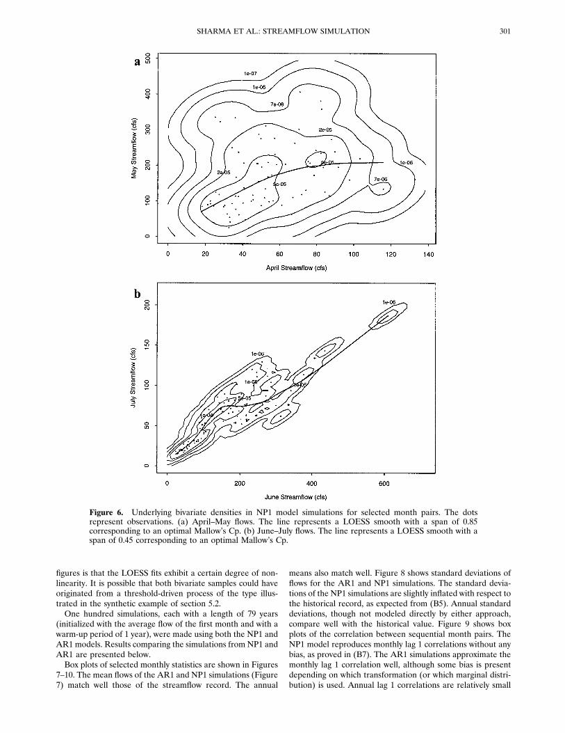
figures is that the LOESS fits exhibit a certain degree of non-linearity. It is possible that both bivariate samples could haveoriginated from a threshold-driven process of the type illus-trated in the synthetic example of section 5.2.One hundred simulations, each with a length of 79 years

(initialized with the average flow of the first month and with awarm-up period of 1 year), were made using both the NP1 andAR1 models. Results comparing the simulations from NP1 andAR1 are presented below.Box plots of selected monthly statistics are shown in Figures

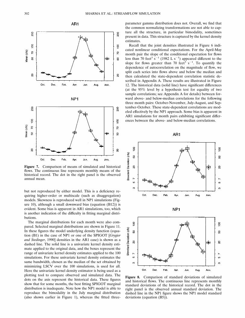
7–10. The mean flows of the AR1 and NP1 simulations (Figure7) match well those of the streamflow record. The annual

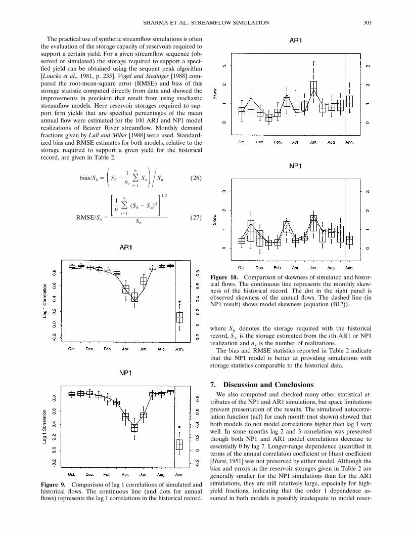
means also match well. Figure 8 shows standard deviations offlows for the AR1 and NP1 simulations. The standard devia-tions of the NP1 simulations are slightly inflated with respect tothe historical record, as expected from (B5). Annual standarddeviations, though not modeled directly by either approach,compare well with the historical value. Figure 9 shows boxplots of the correlation between sequential month pairs. TheNP1 model reproduces monthly lag 1 correlations without anybias, as proved in (B7). The AR1 simulations approximate themonthly lag 1 correlation well, although some bias is presentdepending on which transformation (or which marginal distri-bution) is used. Annual lag 1 correlations are relatively small

Figure 6. Underlying bivariate densities in NP1 model simulations for selected month pairs. The dotsrepresent observations. (a) April–May flows. The line represents a LOESS smooth with a span of 0.85corresponding to an optimal Mallow’s Cp. (b) June–July flows. The line represents a LOESS smooth with aspan of 0.45 corresponding to an optimal Mallow’s Cp.


but not reproduced by either model. This is a deficiency re-quiring higher-order or multiscale (such as disaggregation)models. Skewness is reproduced well in NP1 simulations (Fig-ure 10), although a small downward bias (equation (B12)) isevident. Some bias is apparent in AR1 simulations, too, whichis another indication of the difficulty in fitting marginal distri-butions.The marginal distributions for each month were also com-

pared. Selected marginal distributions are shown in Figure 11.In these figures the model underlying density function (equa-tion (B1) in the case of NP1 or one of the SPIGOT [Grygierand Stedinger, 1990] densities in the AR1 case) is shown as adashed line. The solid line is a univariate kernel density esti-mate applied to the original data, and the boxes represent therange of univariate kernel density estimates applied to the 100simulations. For these univariate kernel density estimates thesame bandwidth, chosen as the median of the set obtained byminimizing LSCV over the 100 simulations, is used for all.Here the univariate kernel density estimator is being used as aplotting tool to compare observed and simulated data. Thedots on the axis represent the historical data. These figuresshow that for some months, the best fitting SPIGOT marginaldistribution is inadequate. Note how the NP1 model is able toreproduce the bimodality in the July marginal distribution(also shown earlier in Figure 1), whereas the fitted three-

parameter gamma distribution does not. Overall, we find thatthe common normalizing transformations are not able to cap-ture all the structure, in particular bimodality, sometimespresent in data. This structure is captured by the kernel densityestimates.Recall that the joint densities illustrated in Figure 6 indi-

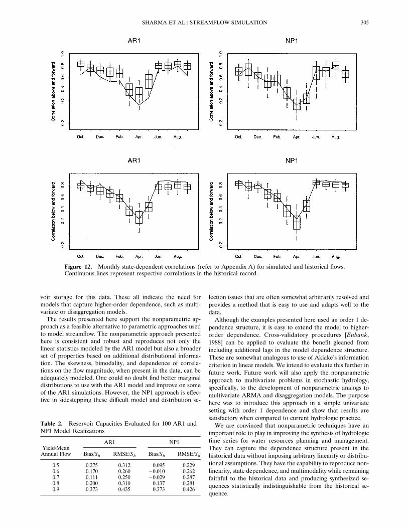
cated nonlinear conditional expectations. For the April-Maymonth pair the slope of the conditional expectation for flowsless than 70 feet3 s21 (1982 L s21) appeared different to theslope for flows greater than 70 feet3 s21. To quantify thedependence of autocorrelation on the magnitude of flow, wesplit each series into flows above and below the median andthen calculated the state-dependent correlation statistic de-scribed in Appendix A. These results are illustrated in Figure12. The historical data (solid line) have significant differences(at the 95% level by a hypothesis test for equality of twosample correlations; see Appendix A for details) between for-ward above- and below-median correlations for the followingthree month pairs: October-November, July-August, and Sep-tember-October. These state-dependent correlations are mod-eled effectively by the NP1 approach. Some bias is apparent inAR1 simulations for month pairs exhibiting significant differ-ences between the above- and below-median correlations.

Figure 8. Comparison of standard deviations of simulatedand historical flows. The continuous line represents monthlystandard deviations of the historical record. The dot in theright panel is the observed annual standard deviation. Thedashed line in the NP1 figure shows the NP1 model standarddeviations (equation (B5)).

Figure 7. Comparison of means of simulated and historicalflows. The continuous line represents monthly means of thehistorical record. The dot in the right panel is the observedannual mean.


The practical use of synthetic streamflow simulations is oftenthe evaluation of the storage capacity of reservoirs required tosupport a certain yield. For a given streamflow sequence (ob-served or simulated) the storage required to support a speci-fied yield can be obtained using the sequent peak algorithm[Loucks et al., 1981, p. 235]. Vogel and Stedinger [1988] com-pared the root-mean-square error (RMSE) and bias of thisstorage statistic computed directly from data and showed theimprovements in precision that result from using stochasticstreamflow models. Here reservoir storages required to sup-port firm yields that are specified percentages of the meanannual flow were estimated for the 100 AR1 and NP1 modelrealizations of Beaver River streamflow. Monthly demandfractions given by Lall and Miller [1988] were used. Standard-ized bias and RMSE estimates for both models, relative to thestorage required to support a given yield for the historicalrecord, are given in Table 2.

bias/Sh 5 S Sh 21nr

Oi51

nr

SsiDYSh (26)

RMSE/Sh 5

F 1n Oi51

nr

~Sh 2 Ssj!2G 1/ 2

Sh(27)

where Sh denotes the storage required with the historicalrecord, Ssi is the storage estimated from the ith AR1 or NP1realization and nr is the number of realizations.The bias and RMSE statistics reported in Table 2 indicate

that the NP1 model is better at providing simulations withstorage statistics comparable to the historical data.

7. Discussion and ConclusionsWe also computed and checked many other statistical at-

tributes of the NP1 and AR1 simulations, but space limitationsprevent presentation of the results. The simulated autocorre-lation function (acf) for each month (not shown) showed thatboth models do not model correlations higher than lag 1 verywell. In some months lag 2 and 3 correlation was preservedthough both NP1 and AR1 model correlations decrease toessentially 0 by lag 7. Longer-range dependence quantified interms of the annual correlation coefficient or Hurst coefficient[Hurst, 1951] was not preserved by either model. Although thebias and errors in the reservoir storages given in Table 2 aregenerally smaller for the NP1 simulations than for the AR1simulations, they are still relatively large, especially for high-yield fractions, indicating that the order 1 dependence as-sumed in both models is possibly inadequate to model reser-

Figure 9. Comparison of lag 1 correlations of simulated andhistorical flows. The continuous line (and dots for annualflows) represents the lag 1 correlations in the historical record.

Figure 10. Comparison of skewness of simulated and histor-ical flows. The continuous line represents the monthly skew-ness of the historical record. The dot in the right panel isobserved skewness of the annual flows. The dashed line (inNP1 result) shows model skewness (equation (B12)).


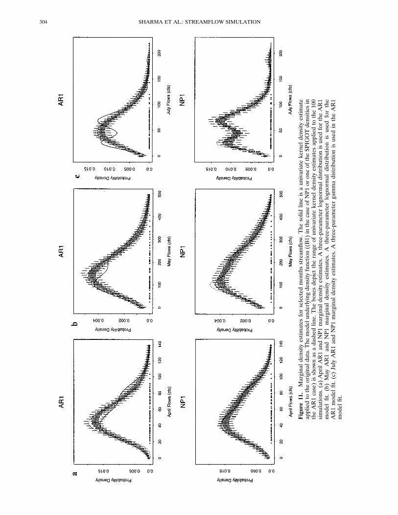
Figure11.Marginaldensityestimatesforselectedmonthsstreamflow.Thesolidlineisaunivariatekerneldensityestimate

appliedtotheoriginaldata.Themodelunderlyingdensityfunction((B1)inthecaseofNP1oroneoftheSPIGOTdensitiesin

theAR1case)isshownasadashedline.Theboxesdepicttherangeofunivariatekerneldensityestimatesappliedtothe100

simulations.(a)AprilAR1andNP1marginaldensityestimates.Athree-parameterlognormaldistributionisusedfortheAR1

modelfit.(b)MayAR1andNP1marginaldensityestimates.Athree-parameterlognormaldistributionisusedforthe

AR1modelfit.(c)JulyAR1andNP1marginaldensityestimates.A

three-parametergammadistributionisusedintheAR1

modelfit.


voir storage for this data. These all indicate the need formodels that capture higher-order dependence, such as multi-variate or disaggregation models.The results presented here support the nonparametric ap-

proach as a feasible alternative to parametric approaches usedto model streamflow. The nonparametric approach presentedhere is consistent and robust and reproduces not only thelinear statistics modeled by the AR1 model but also a broaderset of properties based on additional distributional informa-tion. The skewness, bimodality, and dependence of correla-tions on the flow magnitude, when present in the data, can beadequately modeled. One could no doubt find better marginaldistributions to use with the AR1 model and improve on someof the AR1 simulations. However, the NP1 approach is effec-tive in sidestepping these difficult model and distribution se-

lection issues that are often somewhat arbitrarily resolved andprovides a method that is easy to use and adapts well to thedata.Although the examples presented here used an order 1 de-

pendence structure, it is easy to extend the model to higher-order dependence. Cross-validatory procedures [Eubank,1988] can be applied to evaluate the benefit gleaned fromincluding additional lags in the model dependence structure.These are somewhat analogous to use of Akiake’s informationcriterion in linear models. We intend to evaluate this further infuture work. Future work will also apply the nonparametricapproach to multivariate problems in stochastic hydrology,specifically, to the development of nonparametric analogs tomultivariate ARMA and disaggregation models. The purposehere was to introduce this approach in a simple univariatesetting with order 1 dependence and show that results aresatisfactory when compared to current hydrologic practice.We are convinced that nonparametric techniques have an

important role to play in improving the synthesis of hydrologictime series for water resources planning and management.They can capture the dependence structure present in thehistorical data without imposing arbitrary linearity or distribu-tional assumptions. They have the capability to reproduce non-linearity, state dependence, and multimodality while remainingfaithful to the historical data and producing synthesized se-quences statistically indistinguishable from the historical se-quence.

Figure 12. Monthly state-dependent correlations (refer to Appendix A) for simulated and historical flows.Continuous lines represent respective correlations in the historical record.

Table 2. Reservoir Capacities Evaluated for 100 AR1 andNP1 Model Realizations

Yield/MeanAnnual Flow

AR1 NP1

Bias/Sh RMSE/Sh Bias/Sh RMSE/Sh

0.5 0.275 0.312 0.095 0.2290.6 0.170 0.260 20.010 0.2620.7 0.111 0.250 20.029 0.2870.8 0.200 0.310 0.137 0.2810.9 0.373 0.435 0.373 0.426


Appendix A: State-Dependent CorrelationCoefficients

This appendix describes the measures we used to quantifynonlinear dependence in data. The usual estimator of lag 1correlation is

r 51

~n 2 1!sx2 Ot51

n21

~ xt 2 x!~ xt11 2 x! (A1)

where x and sx2 are the mean and variance of xt, t 5 1, z z z , n .

1. Forward, above median correlation (raf) is defined asthe correlation between above median flows and flows in thesubsequent time step. This is calculated by replacing the sumover all t in the expression above by the sum over those t forwhich xt is greater than the median flow xmedian, replacing thesx2 by the product of the standard deviations of the abovemedian flows and flows one time step ahead of above medianflows, replacing x by the mean of the above median and onetime step ahead of above median flows, and adjusting n ac-cordingly.2. Forward, below median correlation (rbf) is the correla-

tion between all below median flows and the flow in the sub-sequent time steps, calculated in a similar manner with the sumover those t for which xt , xmedian.3. Backward, above median correlation (rab) is the corre-

lation between above median flows and the preceding timestep’s flow, calculated in a similar manner with the sum overthose t for which xt11 . xmedian.4. Backward, below median correlation (rbb) is the corre-

lation between below median flows and the preceding timestep’s flow, calculated in a similar manner with the sum overthose t for which xt11 , xmedian.For a linear Gaussian process the above and below pair of

correlations in either the forward or backward direction shouldbe the same. Differences indicate nonlinearity or state depen-dence in the dependence structure. To test the significance ofdifferences between sample correlation coefficients r1 and r2,the following test from Kendall and Stuart [1979, p. 315] wasused. The test is based on the transformation of the correlationcoefficient r as

z 512 log S 1 1 r

1 2 rD (A2)

The quantity z1 2 z2 is closely normally distributed with zeromean and variance 1/(n1 2 3) 1 1/(n2 2 3), where n1 andn2 are the sample sizes, under the null hypothesis that z1 andz2 are calculated from sample correlation coefficients frompopulations with the same correlation coefficient. Thereforethe significance test compares ( z1 2 z2)/[1/(n1 2 3) 11/(n2 2 3)]1/ 2 to the standard normal distribution. This testis approximate unless the samples are from independent biva-riate normal populations. In section 6 we used this test toinvestigate the significance of the difference between raf (5 r1)and rbf (5 r2). Sets of above and below median flows areeffectively censored samples, inconsistent with the indepen-dence assumptions. Nevertheless, an approximate measure ofwhether these quantities are significantly different can be ob-tained by use of this test.

Appendix B: Derivation of Model StatisticsWe derive here the expected values of selected statistics of

the NP1 model. These depend on the observed data xi, kernelparameters l and S, and the Gaussian kernel function.

Marginal Distribution of XtThe marginal density of Xt (denoted fm(Xt)) is estimated as

fm~Xt! 5 E f~Xt, Xt21! dXt21 51n O

i51

n

fG~Xt 2 xi, l2S11!

(B1)

where

fG~Xt 2 xi, l2S11! 51

~2pl2S11!1/ 2exp S2

~Xt 2 xi!2

2l2S11D (B2)

denotes a Gaussian density function with mean xi and variancel2S11. This follows from (6) with H from (7) and S expressedas (19). Equation (6) is the sum of n multivariate Gaussians,each of which when integrated over Xt21 results in the uni-variate Gaussian given above. This marginal distribution isused to calculate model mean, covariance, and skewness.

Mean m* of XtThis can be evaluated using the marginal distribution in

(B1). Since each kernel is symmetric and centered at a datapoint, the NP1 model mean (m9) is the sample mean:

m9 5 E@Xt# 5 E Xt fm~Xt! dXt 51n O

i51

n

xi (B3)

Standard Deviation of XtThe variance under the NP1 model can be written as

s92 5 E@~Xt 2 m9!2# 5 E ~Xt 2 m9!2fm~Xt! dt (B4)

where the expectation is over the marginal distribution, (B1).Since fm(Xt) from (B1) is a sum of Gaussian probability den-sity functions (pdf’s) with individual means xi, and variancesl2S11 and the xi have sample variance S11, we get

s92 5 S11~1 1 l2! (B5)

Note the inflation in the underlying variance by the factor(1 1 l2).

Lag 1 Correlation

The lag 1 correlation (r91) under the NP1 model is expressedas the ratio

r91 5E@~Xt 2 m9!~Xt21 2 m9!#

s92(B6)

where expectation is over the joint density estimate in (6). Thisexpression simplifies to

r91 5~1 1 l!2S12

~1 1 l2!~S11S22!1/ 25 r (B7)

where r denotes the sample lag 1 correlation:


r 5S12

~S11S22!1/ 2(B8)

Skewness

The coefficient of skewness (g9) under the NP1 model isdefined as the ratio

g9 5E@~Xt 2 m9!3#

s935

E ~Xt 2 m9!3fm~Xt! dt

s93(B9)

where the expectation is over the marginal distribution in (B1).By integrating over the marginal distribution, the numeratorcan be evaluated as

E@~Xt 2 m9!3# 51n O

i51

n

xi3 1 3l2S11

1n O

i51

n

xi 2 3m9l2S11

2 3m91n O

i51

n

xi2 1 3m92

1n O

i51

n

xi 2 m93 (B10)

Now recognizing (B3), the second and third terms cancel, andthis is equivalent to

E@~Xt 2 m9!3# 51n O

i51

n

~ xi 2 m9!3 (B11)

The expression for g9 then becomes

g9 5

~1/n!Oi51

n

~ xi 2 m9!3

s935

g~1 1 l2!3/ 2

(B12)

where g is the skewness estimator

g 5

~1/n!Oi51

n

~ xi 2 m9!3

S113/ 2 (B13)

and S11 is the sample variance. The decrease in skewness isdue to the inflation of variance by (B5). The results derivedhere do not account for the cut and normalize boundary cor-rections applied.

Acknowledgments. This research was supported by the U.S. Geo-logical Survey (USGS), Department of the Interior, under USGSaward 1434-92-G-2265. The views and conclusions contained in thisdocument are those of the authors and should not be interpreted asnecessarily representing the official policies, either expressed or im-plied, of the U.S. Government. We thank Jery Stedinger, DennisLettenmaier, and three anonymous reviewers for insightful commentswhich have improved this work.

ReferencesAdamowski, K., and W. Feluch, Application of nonparametric regres-sion to groundwater level prediction, Can. J. Civ. Eng., 18, 600–606,1991.

Beard, L. R., Monthly Streamflow Simulation, Hydrol. Eng. Cent., U.S.Corps of Eng., Washington, D. C., 1967.

Bendat, J. S., and A. G. Piersol, Random Data: Analysis and Measure-ment Procedures, 2nd ed., John Wiley, New York, 1986.

Benjamin, J. R., and C. A. Cornell, Probability, Statistics, and Decisionfor Civil Engineers, McGraw-Hill, New York, 1970.

Bras, R. L., and I. Rodriguez-Iturbe, Random Functions and Hydrology,Addison-Wesley, Reading, Mass., 1985.

Chambers, J. M., and T. J. Hastie, Statistical Models in S, Wadsworthand Brooks/Cole, Pacific Grove, Calif., 1992.

Cleveland, W. S., and S. J. Devlin, Locally weighted regression: Anapproach to regression by local fitting, J. Am. Stat. Assoc., 83(403),596–610, 1988.

Efron, B., Bootstrap methods: Another look at the jackknife, Ann.Stat., 7, 1–26, 1979.

Efron, B., and R. Tibishirani, An Introduction to the Bootstrap, Chap-man and Hall, New York, 1993.

Eubank, R. L., Spline Smoothing and Non-Parametric Regression, Mar-cel-Dekker, New York, 1988.

Fiering, M. B., Streamflow Synthesis, Harvard Univ. Press, Cambridge,Mass., 1967.

Fukunaga, K., Introduction to Statistical Pattern Recognition, Academic,San Diego, Calif., 1972.

Grygier, J. C., and J. R. Stedinger, Spigot, A synthetic streamflowgeneration package, technical description, version 2.5, School of Civ.and Environ. Eng., Cornell Univ., Ithaca, N. Y., 1990.

Hardle, W., and A. W. Bowman, Bootstrapping in nonparametricregression: Local adaptive smoothing and confidence bands, J. Am.Stat. Assoc., 83(401), 102–110, 1988.

Hipel, K. W., A. I. Mcleod, and W. C. Lennox, Advances in Box-Jenkins modeling, 1, Model construction, Water Resour. Res., 13(3),567–575, 1977.

Hurst, H. E., Long-term storage capacity of reservoirs, Trans. Am. Soc.Civ. Eng., 116, 770–799, 1951.

Kendall, D. R., and J. A. Dracup, A comparison of index-sequentialand AR(1) generated hydrologic sequences, J. Hydrol., 122, 335–352,1991.

Kendall, M., and A. Stuart, The Advanced Theory of Statistics, vol. 2,Inference and Relationship, Macmillan, New York, 1979.

Kite, G. W., Frequency and Risk Analysis in Hydrology, Water Resour.Publ., Fort Collins, Colo., 1977.

Lall, U., Recent advances in nonparametric function estimation: Hy-draulic applications, U.S. Natl. Rep. Int. Union Geod. Geophys. 1991–1994, Rev. Geophys., 33, 1093, 1995.

Lall, U., and C. W. Miller, An optimization model for screening mul-tipurpose reservoir systems, Water Resour. Res., 24(7), 953–968,1988.

Lall, U., and A. Sharma, A nearest neighbor bootstrap for time seriesresampling, Water Resour. Res., 32(3), 679–693, 1996.

Lettenmaier, D. P., and S. J. Burges, An operational approach topreserving skew in hydrologic models of long-term persistence, Wa-ter Resour. Res., 13(2), 281–290, 1977.

Loucks, D. P., J. R. Stedinger, and D. A. Haith,Water Resource SystemsPlanning and Analysis, Prentice-Hall, Englewood Cliffs, N. J., 1981.

McLeod, A. I., K. W. Hipel, and W. C. Lennox, Advances in Box-Jenkins modeling, 2, Applications, Water Resour. Res., 13(3), 577–585, 1977.

Pegram, G. G. S., J. D. Salas, D. C. Boes, and V. Yevjevich, StochasticProperties of Water Storage, Colo. State Univ., Fort Collins, 1980.

Sain, S. R., K. A. Baggerly, and D. W. Scott, Cross-validation ofmultivariate densities, J. Am. Stat. Assoc., 89(427), 807–817, 1994.

Salas, J. D., Analysis and modeling of hydrologic time series, in Hand-book of Hydrology, edited by D. R. Maidment, McGraw-Hill, NewYork, 1993.

Salas, J. D., and R. A. Smith, Physical basis of stochastic models ofannual flows, Water Resour. Res., 17(2), 428–430, 1981.

Salas, J. D., J. W. Delleur, V. Yevjevich, and W. L. Lane, AppliedModeling of Hydrologic Time Series, Water Resour. Publ., Littleton,Colo., 1980.

Scott, D. W., Multivariate Density Estimation, Theory, Practice, andVisualization, John Wiley, New York, 1992.

Silverman, B. W., Density Estimation for Statistics and Data Analysis,Chapman and Hall, New York, 1986.

Slack, J. R., and J. M. Landwehr, Hydro-climate data network: A U.S.Geological Survey streamflow data set for the United States for thestudy of climate variations, 1874–1988, U.S. Geol. Surv. Open FileRep. 92-129, 1992.

Smith, J. A., Long-range streamflow forecasting using nonparametricregression, Water Resour. Bull., 27(1), 39–46, 1991.


Smith, L. A., Identification and prediction of low dimensional dynam-ics, Physica D, 58, 50–76, 1992.

Stedinger, J. R., Estimating correlations in multivariate streamflowmodels, Water Resour. Res., 17(1), 200–208, 1981.

Stedinger, J. R., and M. R. Taylor, Synthetic streamflow generation, 1,Model verification and validation, Water Resour. Res., 18(4), 909–918, 1982.

Stedinger, J. R., and R. M. Vogel, Disaggregation procedures forgenerating serially correlated flow vectors, Water Resour. Res.,20(11), 47–56, 1984.

Stedinger, J. R., D. P. Lettenmaier, and R. M. Vogel, MultisiteARMA(1,1) and disaggregation models for annual streamflow gen-eration, Water Resour. Res., 21(4), 497–509, 1985a.

Stedinger, J. R., D. Pei, and T. A. Cohn, A condensed disaggregationmodel for incorporating parameter uncertainty into monthly reser-voir simulations, Water Resour. Res., 21(5), 665–675, 1985b.

Tasker, G. D., Comparison of methods for estimating low flow char-acteristics of streams, Water Resour. Bull., 23(6), 1077–1083, 1987.

Thomas, H. A., and M. B. Fiering, Mathematical synthesis of stream-flow sequences for the analysis of river basins by simulation, inDesign of Water Resource Systems, edited by A. Maass et al., pp.459–493, Harvard Univ. Press, Cambridge, Mass., 1962.

Todini, J., The preservation of skewness in linear disaggregationschemes, J. Hydrol., 47, 199–214, 1980.

Tong, H., Nonlinear Time Series Analysis: A Dynamical Systems Per-spective, Academic, San Diego, Calif., 1990.

Vogel, R. M., and J. R. Stedinger, The value of stochastic streamflowmodels in overyear reservoir design applications,Water Resour. Res.,24(9), 1483–1490, 1988.

Wand, M. P., and M. C. Jones, Multivariate plug-in bandwidth selec-tion, Comput. Stat., 9, 97–116, 1994.

Woo, M. K., Confidence intervals of optimal risk-based hydraulic de-sign parameters, Can. Water Resour. J., 14(1), 10–16, 1989.

Yakowitz, S., Nonparametric density estimation, prediction, and re-gression for markov sequences, J. Am. Stat. Assoc., 80(389), 215–221,1985.

Yevjevich, V. M., Stochastic Processes in Hydrology, Water Resour.Publ., Fort Collins, Colo., 1972.

Zucchini, W., and P. T. Adamson, Bootstrap confidence intervals fordesign storms from exceedance series, Hydrol. Sci. J., 34(1), 41–48,1989.

U. Lall and D. G. Tarboton, Utah Water Research Laboratory,Utah State University, Logan, UT 84322-4110. (e-mail:[email protected])A. Sharma, Department of Water Engineering, School of Civil En-

gineering, University of New South Wales, Sydney 2052, Australia.

(Received October 16, 1995; revised August 12, 1996;accepted September 18, 1996.)


Streamflow simulation: A nonparametric approach

Documents