Streamflow recession analysis using water height - HAL-Insu

HAL Id: insu-02874661https://hal-insu.archives-ouvertes.fr/insu-02874661

Submitted on 13 Aug 2021

HAL is a multi-disciplinary open accessarchive for the deposit and dissemination of sci-entific research documents, whether they are pub-lished or not. The documents may come fromteaching and research institutions in France orabroad, or from public or private research centers.

L’archive ouverte pluridisciplinaire HAL, estdestinée au dépôt et à la diffusion de documentsscientifiques de niveau recherche, publiés ou non,émanant des établissements d’enseignement et derecherche français ou étrangers, des laboratoirespublics ou privés.

Copyright

Streamflow recession analysis using water heightElizabeth Jachens, Clément Roques, D. Rupp, J. Selker

To cite this version:Elizabeth Jachens, Clément Roques, D. Rupp, J. Selker. Streamflow recession analysis us-ing water height. Water Resources Research, American Geophysical Union, 2020, 56 (6),�10.1029/2020WR027091�. �insu-02874661�

Streamflow Recession Analysis Using Water HeightE. R. Jachens1 , C. Roques2,3 , D. E. Rupp4 , and J. S. Selker1

1Department of Biological and Ecological Engineering, Oregon State University, Corvallis, OR, USA, 2Department ofEarth Sciences, ETH Zürich, Zurich, Switzerland, 3Géosciences Rennes, University of Rennes 1, Rennes, France, 4OregonClimate Change Research Institute, College of Earth, Oceanic and Atmospheric Sciences, Oregon State University,Corvallis, OR, USA

Abstract Recession analysis is widely used for characterizing aquifer and basin properties based on thefalling limb of the hydrograph. However, recession analysis using streamflow discharge requires arelationship (the rating curve) between simultaneous measurements of water height, h, and discharge, Q,across a wide range of flows, which is expensive to obtain, and changes in time. We leverage the relationshipbetween h and Q (typical power law) to perform recession analysis using h directly, thus permittingidentification of transient flow regimes, where only h is available. Recession analysis evaluates the rate ofchange in discharge, −dQ/dt, as a function of discharge, Q, in a bilogarithmic plot where the slope, b,contains information about aquifer characteristics. While values of b are not conserved when replacing Qwith h, we find that the variability in values of b within and between events is captured in recession analysisfor bothQ and h. For example, when considering individual recessions from a large number of watersheds, achange from a smaller b at high discharge/stage to a larger b at lower discharge/stage occurs in mostwatersheds and suggests a transition to a more long‐lasting, and less drought‐sensitive, baseflow regime.With the advent of low‐cost reliable pressure loggers, as well as satellites that provide global reporting ofriver stage, recession analysis using water height expands the number of river systems where recessionanalysis can be conducted and provides the potential for insights into the variability of watershed drainagecharacteristics without the need for a discharge record.

1. Introduction

The understanding of streamflow dynamics is fundamental for water resources management, flood predic-tion, sediment transport, and drought assessment. The establishment of accurate hydrographs is critical butis expensive to obtain. Though measuring continuous water height has become easy using automatic pres-sure transducers, estimating discharge requires a local rating curve constructed from field‐collected dis-charges measurements paired with concurrent water height measurements over the range of flows ofinterest, typically covering peak to baseflow discharges. These extreme discharges are cause for uncertaintiesin a rating curve due to their low frequency of occurrence, safety concerns at high discharges, and instru-ment precision impeding the collection of reliable estimates at low discharges (Kiang et al., 2018).Extrapolation of a rating curve to include extreme events compromises the validity of the hydrograph(Lang et al., 2010). Additionally, a rating curve is no longer valid if the stream undergoes channel changes,a common consequence of high flows (U.S. Department of Agriculture‐National Resources ConservationService (USDA‐NRCS), 2012).

The falling limb of a hydrograph is an expression of the processes controlling groundwater discharge to astream. Recession analysis (RA) employs characteristics of this receding limb to quantify hydraulic proper-ties of the source aquifer. The falling limb of the hydrograph is often described by a power law:

−dQdt

¼ a · Qb (1)

where Q is streamflow (m3/s) and a and b are constants (Brutsaert & Nieber, 1977; Troch et al., 2013).Parameters a and b are often estimated by fitting Equation 1 on recession data in bilogarithmic space,where log(a) is the intercept and b is the slope (Brutsaert & Nieber, 1977; Kirchner, 2009; Roqueset al., 2017; Rupp & Selker, 2006a).

Both theory (e.g., Bogaart et al., 2013; Brutsaert & Nieber, 1977; Rupp & Selker, 2006b) and observations(e.g., Clark et al., 2009; Mutzner et al., 2013; Rupp & Selker, 2006a; Tashie et al., 2020) show that the

©2020. American Geophysical Union.All Rights Reserved.

RESEARCH ARTICLE10.1029/2020WR027091

Key Points:• Using water height in place of

discharge for recession analysispreserves general characteristics ofthe recession curve

• An analytical expression equatingthe power law exponents of waterheight and discharge is given whenthe rating curve is a power law

• The ratio of power law exponents forindividual recessions at high andlow water heights can identify atransition in streamflow regimes

Supporting Information:• Supporting Information S1

Correspondence to:E. R. Jachens,[email protected]

Citation:Jachens, E. R., Roques, C., Rupp, D. E.,& Selker, J. S. (2020). Streamflowrecession analysis using water height.Water Resources Research, 56,e2020WR027091. https://doi.org/10.1029/2020WR027091

Received 9 JAN 2020Accepted 3 JUN 2020Accepted article online 8 JUN 2020

JACHENS ET AL. 1 of 9

parameter b is not typically constant over a recession. Commonly evoked hydraulic theory—relying onanalytical solutions to the Boussinesq equation for drainage to a fully penetrating channel from an idea-lized, initially fully saturated, and unconfined horizontal aquifer—predicts values of b = 3 for early‐time(higher Q) transitioning to b = 1.5 or 1 for late‐time (lower Q) recession (Brutsaert & Nieber, 1977).However, because of the complexity of natural watersheds, RA performed on streamflow data revealsstrong variability in b values beyond the simple bilogarithmically linear representation of Equation 1for high and low flows (e.g., Biswal & Marani, 2014; Dralle et al., 2015; McMillan et al., 2011;Mutzner et al., 2013; Ploum et al., 2019; Shaw & Riha, 2012; Tashie et al., 2019; Wang, 2011). Thevariability in recession parameters can reveal information about the complexities in watershed response.The shape of the RA plot, which includes any breaks in slope (i.e., changes in b) as well as other pattersthat can be identified in individual or collective/cloud of recession events, illustrates the “structuraldecay of flow.”

The parameter b reflects the rate of change in the rate of streamflow recession: A higher value of b (for b > 1)indicates that the rate of decline decreases more quickly. When considering drought resilience, comparing bvalues for high and low flows can be used to identify a change in hydraulic regime and using b values at lowflows to indicate a watershed's sensitivity to climate change. Where b increases as Q decreases, streamflowbecomes more stable, or sustained, at low flows and may indicate watersheds that are less sensitive todrought (Berghuijs et al., 2016; Jachens et al., 2020). In this case, b values are larger at low flows than at highflows. As noted, observations reveal large variability in recession behavior, including cases where b is largerat lower Q than at higher Q (e.g., Clark et al., 2009; Mutzner et al., 2013; Rupp & Selker, 2006a), inconsistentthe aforementioned hydraulic theory. Recent studies have suggested that such cases are common (Jachenset al., 2020; Tashie et al., 2020). In contrast, if b decreases as Q decreases, this indicates that streamflow ismore stable, or sustained, at high flows while streamflow declines at a faster rate at low flows. In this case,the smaller b values at low flows could indicate that streamflow in the watershed could be sensitive todrought and vulnerable to climate change. By comparing b values at different ranges of Q (i.e., high andlow flows), we can say something about which regime is more sustained and thus the vulnerability todrought. Comparing b at high and low flows, then, may provide a useful metric to characterize watershedssensitivity to drought.

This paper aims to demonstrate the reliability and utility of performing RA on measured water height reces-sion analysis directly (hereafter referred to as WHRA) in order to estimate the ratio of b from high to lowflows and describe the structural decay of streamflow recession without introducing error through the defi-nition and uncertainty of a rating curve. Using WHRA can leverage water height data that are more widelyavailable with the advent of low‐cost reliable pressure loggers, as well as satellites that provide global report-ing of river stage. We first present the mathematical framework to compare RA andWHRA.We then test themethodology on two real‐data watersheds, one with larger b values at high flows compared to low flows andthe other with larger b values at low flows compared to high flows. Finally, we test the universality of thismethodology on a batch of 37 Swiss watersheds.

2. Methods

Here we describe a method for analyzing recession hydrographs using water height instead of discharge rate,leveraging the power law rating curve equation. Rating curves employ a variety of mathematical formsincluding power law, linear, parabolic, exponential, or a compound segment fit (Kennedy, 1984;Lovellford, 2013).

The power law equation for rating curves is standard (Clarke, 1999; Degagnea et al., 1996; Phillips &Eaton, 2009; Reitan & Petersen‐Øverleir, 2004) and is consistent with the form of discharge resistance equa-tions such as Manning's and Chezy's (Herschy, 1993; Kennedy, 1984):

Q ¼ c · hm (2)

where h is water height (m) and c and m are constants. The transformation of Equation 1 for WHRA plotssubstitutes the right‐hand side of Equation 2 for discharge, resulting in an expression that is a function ofwater height:

10.1029/2020WR027091Water Resources Research

JACHENS ET AL. 2 of 9

−dQdt

¼ −ddt

c · hmð Þ (3)

−dQdt

¼ c ·m · hm−1 ·−dhdt

(4)

Thus, −dQ/dt versus Q can be expressed in terms of h for the WHRA axes using Equations 2 and 4 as

c ·m · hm−1 ·−dhdt

� �versus c · hm½ � (5)

The fitting coefficient c appears on both axes in Equation 5, and thus, the mathematical simplification holdstrue for bilogarithmic space:

m · hm−1 ·−dhdt

� �versus hm½ � (6)

Equation 6 can be simplified for the special case of m = 1 and thus Q = h from Equation 1:

ln−dhdt

� �versus ln h½ � (7)

Values ofm in the literature for power law rating curves tend to be close to 2 or 3 but can range from 1 to 10(Fenton & Keller, 2001; Nathanson et al., 2012; Phillips & Eaton, 2009; Reitan &Petersen‐Øverleir, 2004, 2008). For simplicity of the calculations, including preserving the axis form fromRA, and because no m values are known, the following analysis uses m = 1. However, we later show thatour analysis of the observed streamflow recessions is not very sensitive the assumed value ofm and assumingm = 1 does not affect the results of this analysis or decrease the generality of the results.

The slope of the WHRA plot can be related to the slope of the RA plot by substituting Equations 2 and 4 intothe slope calculation as shown in the following equation and simplification:

bRA ¼ln

−dQ2

dt

� �− ln

−dQ1

dt

� �

ln Q2ð Þ − ln Q1ð Þ ¼ln c ·m · h2

m−1 ·−dh2dt

� �− ln c ·m · h1

m−1 ·−dh1dt

� �

ln c · h2mð Þ − ln c · h1

mð Þ (8)

bRA ¼ m − 1þ bWHRA

m(9)

where bRA is b estimated with RA plot ln−dQdt

� �versus ln Q½ � and bWHRA is b estimated from WHRA plot

ln−dhdt

� �versus ln h½ � from Equation 7.

To identify a change in recession behavior between high (h) and low (l) flows, we define the ratio of b,Rb = bh/bl. For a rating curve taking the form of a power law (Equation 2), the ratio of b values during highand low flows, Rb, is as follows:

Rb ¼b RA;hð Þb RA;lð Þ

¼m − 1þ bWHRA;h

m − 1þ bWHRA;l(10)

where the subscripts h and l indicate high‐flow and low‐flow regimes\periods of the recession,respectively.

We classified recessions as either high‐ or low‐flow events based on whether the portion of the recession isgreater than or less than the median streamflow of all records. Events that span the median streamflow areclassified as high flow events. We calculated a representative value of Rb per watershed as the ratio of themedian bh to the median bl.

10.1029/2020WR027091Water Resources Research

JACHENS ET AL. 3 of 9

We tested the methodology by first analyzing in detail data from two watersheds from the U.S. GeologicalSurvey (USGS) database for which both water height and discharge measurements were available for at least10 years: West Conewago Creek near Manchester, PA (USGS Station# 01574000) and the South Fork of theMcKenzie River, OR (USGS Station# 14159200). West Conewango Creek is located in in the northeasternUnited States and has a watershed area of 1,321 km2. The South Fork of the McKenzie River is located inthe northwestern United States and has a watershed area of 414 km2. We then performed similar analysison a batch of streamflow time series in order to evaluate the validity of WHRA across different watershedcharacteristics. For this purpose, we selected watersheds across Switzerland where 30 years of both waterheight and stream discharge data were freely and readily available (Federal Office for the Environment(FOEN), 2019). We have considered watersheds with limited influence by extended lakes and anthropogenicregulations that could bias the analysis. These leads to the selection of 37 watersheds spanning diverse cli-mate, geomorphological settings and watershed sizes (from 1 to 1,856 km2).

For the Swiss watershed data set, daily average discharge data is given in m3/s and water height is given inmeters above mean sea level. Since there were no published datums or rating curves, we fit power law ratingcurves, whichminimized the root mean square error for water height vs. discharge in log‐log space. The opti-mized datum was subtracted from the watershed's water height data to represent the effective water depththat was used for the final rating curve. The watersheds all have rating curve root‐mean‐square logarithmicerror (RMSLE) below 0.25 [−], which indicates a rating curve without multiple segments that has not chan-ged significantly over time making.

When performing RA, care must be taken when computing the time derivative at low flow to reduce discre-tization error (Rupp & Selker, 2006a). Here the exponential time step method was used (Roques et al., 2017).Additionally, mean daily data (discharge or water height) was calculated from the 15 min USGS data tofurther reduce noise. The beginning of the recession was defined as 1 day after the peak in discharge toexclude the potential influence of overland flow. Based on the uncertainty analysis by Dralle et al. (2017)on recession event selection, we only included recession events with duration >5 days of decreasing flow.The end of the recession was defined to be the minimum discharge or height prior to an increase. The sen-sitivity of recession parameters to the precise hydrograph recession definition was found to be low, consis-tent with previous studies (Dralle et al., 2017). For the slope of the individual recessions, individualestimates of a and b are based on direct linear fitting using least squares regression in bilogarithms spaceand the median of all values are used to describe the variation in watershed behavior.

3. Results and Discussion3.1. Case Study: West Conewago Creek, PA

West Conewago Creek has published data for discharge and water height starting in October of 2007. TheUSGS provisional rating curve for West Conewago Creek is best fit by a power law rating curve withc = 16.4 (m2/s) and m = 3.4 (R2 = 0.96) based on Equation 2 (USGS, 2018). A total of 244 recession eventswas identified.

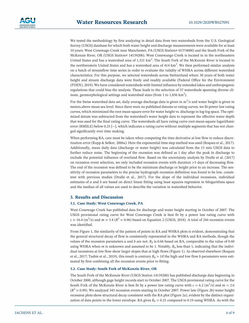
From Figure 1, the similarity of the pattern of points in RA and WHRA plots is evident, demonstrating thatthe general structural decay of flow is consistently represented in the WHRA and RA methods, though thevalues of the recession parameters a and b are not. Rb is 0.66 based on RA, comparable to the value of 0.60using WHRA when m is unknown and assumed to be 1. Notably, Rb less than 1, indicating that the indivi-dual recessions at low flow show larger slopes that at high flows (Figure 1). As observed elsewhere (Roqueset al., 2017; Tashie et al., 2019), this result is contrary Rb > 1if the high and low flow b parameters were esti-mated by first combining all the recession events prior to fitting.

3.2. Case Study: South Fork of McKenzie River, OR

The South Fork of the McKenzie River (USGS Station 14159200) has published discharge data beginning inOctober 2000, although gage height records start in October 2007. The USGS provisional rating curve for theSouth Fork of the McKenzie River is best fit by a power law rating curve with c = 6.2 (m2/s) and m = 2.6(R2 = 0.99). We analyzed 345 recession events starting in October 2007. Power law (Figure 2b) water heightrecession plots show structural decay consistent with the RA plot (Figure 2a), evident by the distinct organi-zation of data points in the lower envelope. RA gives Rb = 0.21 compared to 0.19 using WHRA. As with the

10.1029/2020WR027091Water Resources Research

JACHENS ET AL. 4 of 9

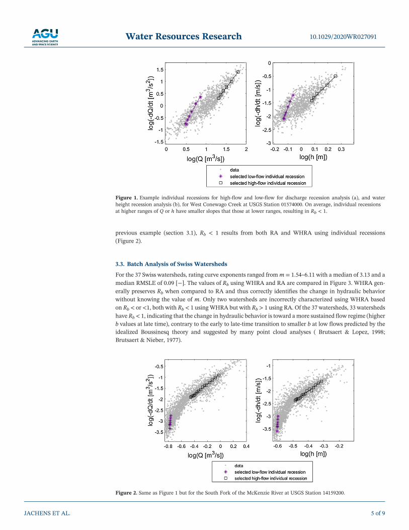
previous example (section 3.1), Rb < 1 results from both RA and WHRA using individual recessions(Figure 2).

3.3. Batch Analysis of Swiss Watersheds

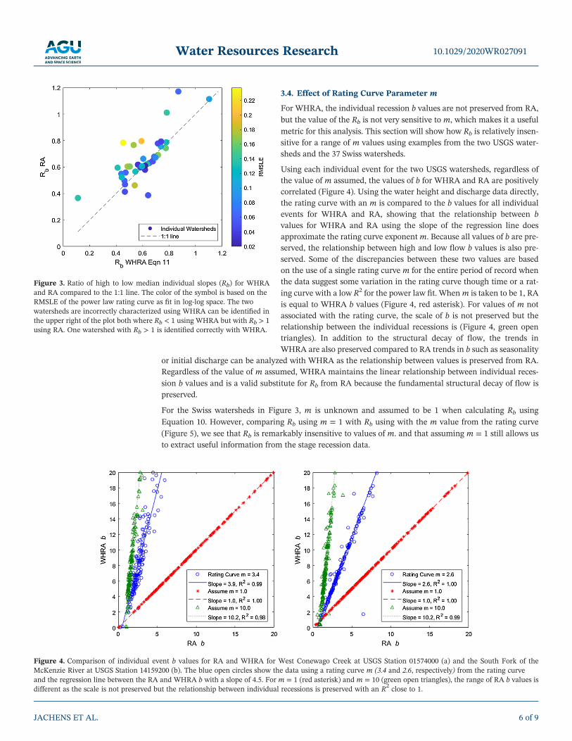
For the 37 Swiss watersheds, rating curve exponents ranged fromm = 1.54–6.11 with a median of 3.13 and amedian RMSLE of 0.09 [−]. The values of Rb using WHRA and RA are compared in Figure 3. WHRA gen-erally preserves Rb when compared to RA and thus correctly identifies the change in hydraulic behaviorwithout knowing the value of m. Only two watersheds are incorrectly characterized using WHRA basedon Rb < or <1, both with Rb < 1 usingWHRA but with Rb > 1 using RA. Of the 37 watersheds, 33 watershedshave Rb< 1, indicating that the change in hydraulic behavior is toward a more sustained flow regime (higherb values at late time), contrary to the early to late‐time transition to smaller b at low flows predicted by theidealized Boussinesq theory and suggested by many point cloud analyses ( Brutsaert & Lopez, 1998;Brutsaert & Nieber, 1977).

Figure 1. Example individual recessions for high‐flow and low‐flow for discharge recession analysis (a), and waterheight recession analysis (b), for West Conewago Creek at USGS Station 01574000. On average, individual recessionsat higher ranges of Q or h have smaller slopes that those at lower ranges, resulting in Rb < 1.

Figure 2. Same as Figure 1 but for the South Fork of the McKenzie River at USGS Station 14159200.

10.1029/2020WR027091Water Resources Research

JACHENS ET AL. 5 of 9

3.4. Effect of Rating Curve Parameter m

For WHRA, the individual recession b values are not preserved from RA,but the value of the Rb is not very sensitive to m, which makes it a usefulmetric for this analysis. This section will show how Rb is relatively insen-sitive for a range of m values using examples from the two USGS water-sheds and the 37 Swiss watersheds.

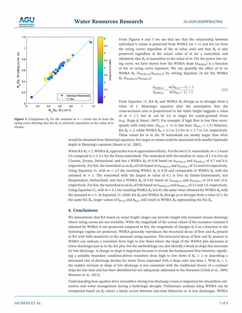
Using each individual event for the two USGS watersheds, regardless ofthe value of m assumed, the values of b for WHRA and RA are positivelycorrelated (Figure 4). Using the water height and discharge data directly,the rating curve with an m is compared to the b values for all individualevents for WHRA and RA, showing that the relationship between bvalues for WHRA and RA using the slope of the regression line doesapproximate the rating curve exponentm. Because all values of b are pre-served, the relationship between high and low flow b values is also pre-served. Some of the discrepancies between these two values are basedon the use of a single rating curve m for the entire period of record whenthe data suggest some variation in the rating curve though time or a rat-ing curve with a low R2 for the power law fit. Whenm is taken to be 1, RAis equal to WHRA b values (Figure 4, red asterisk). For values of m notassociated with the rating curve, the scale of b is not preserved but therelationship between the individual recessions is (Figure 4, green opentriangles). In addition to the structural decay of flow, the trends inWHRA are also preserved compared to RA trends in b such as seasonality

or initial discharge can be analyzed with WHRA as the relationship between values is preserved from RA.Regardless of the value of m assumed, WHRA maintains the linear relationship between individual reces-sion b values and is a valid substitute for Rb from RA because the fundamental structural decay of flow ispreserved.

For the Swiss watersheds in Figure 3, m is unknown and assumed to be 1 when calculating Rb usingEquation 10. However, comparing Rb using m = 1 with Rb using with the m value from the rating curve(Figure 5), we see that Rb is remarkably insensitive to values of m. and that assuming m = 1 still allows usto extract useful information from the stage recession data.

Figure 3. Ratio of high to low median individual slopes (Rb) for WHRAand RA compared to the 1:1 line. The color of the symbol is based on theRMSLE of the power law rating curve as fit in log‐log space. The twowatersheds are incorrectly characterized using WHRA can be identified inthe upper right of the plot both where Rb < 1 using WHRA but with Rb > 1using RA. One watershed with Rb > 1 is identified correctly with WHRA.

Figure 4. Comparison of individual event b values for RA and WHRA for West Conewago Creek at USGS Station 01574000 (a) and the South Fork of theMcKenzie River at USGS Station 14159200 (b). The blue open circles show the data using a rating curve m (3.4 and 2.6, respectively) from the rating curveand the regression line between the RA and WHRA b with a slope of 4.5. For m = 1 (red asterisk) and m = 10 (green open triangles), the range of RA b values isdifferent as the scale is not preserved but the relationship between individual recessions is preserved with an R2 close to 1.

10.1029/2020WR027091Water Resources Research

JACHENS ET AL. 6 of 9

From Figures 4 and 5 we see that see that the relationship betweenindividual b values is preserved from WHRA (m = 1) and RA (m fromthe rating curve) regardless of the m value used and that Rb is alsopreserved regardless of the actual value of m for a watershed, andultimately that Rb is insensitive to the value of m. For the power law rat-ing curve, we have shown how the WHRA slope (bWHRA) is a functionof the m rating curve exponent. We can quantify the effect of m onWHRA Rb (bWHRA,h/bWHRA,l) by solving Equation 10 for the WHRARb (bWHRA,h/bWHRA,l):

bWHRA;h

bWHRA;l¼ m bRA;h − 1

� �þ 1

m bRAl − 1ð Þ þ 1(11)

From Equation 11, RA Rb and WHRA Rb diverge as m diverges from avalue of 1. Manning's equation plus the assumption that thecross‐sectional area is proportional to the water height suggests a valueof m = 1.7, but m can be 2.0 or larger for coarse‐grained rivers(e.g., Rupp & Smart, 2007). For example, if high flow to low flow corre-sponds with early‐time (bRA,h = 3) to late‐time (bRA,l = 1.5) behavior,RA Rb = 2, while WHRA Rb = 2.3 or 2.5 for m = 1.7 or 2.0, respectively.These values for m in the 39 watersheds are mostly larger than what

would be obtained fromManning's equation, but largerm values could be associated with smaller hydraulicdepth in Manning's equation (Smart et al., 2002).

When RA Rb= 2,WHRA Rb approaches 4 asm approaches infinity. For the twoU.S. watersheds,m= 2.4 and2.6 compared to 1.5–6.1 for the Swiss watersheds. The watershed with the smallest m value of 1.5 is Ova daCluozza, Zernez, Switzerland, and has a WHRA Rb of 0.56 based on bWHRA,h and bWHRA,l of 4.7 and 8.4,respectively. For RA, the watershed as an Rb of 0.60 based on bWHRA,h and bWHRA,l of 3.6 and 6.0 respectively.Using Equation 11, with m = 2.5 the resulting WHRA Rb is 0.58 and comparable to WHRA Rb with theassumed m = 1. The watershed with the largest m value of 6.1 is Ova da Emme‐Emmenmatt, nurHauptstation, Switzerland, and has a WHRA Rb of 0.45 based on bWHRA,h and bWHRA,l of 10.6 and 23.6,respectively. For RA, the watershed as an Rb of 0.60 based on bWHRA,h and bWHRA,l of 2.2 and 3.9, respectively.Using Equation 11, withm= 6.1 the resulting WHRA Rb is 0.45, the same value obtained for WHRA Rbwiththe assumedm = 1. In Equation 11, while RA Rb and WHRA Rb diverge asm diverges from a value of 1, forthe same RA Rb, larger values of bRA,h and bRA,l will result in WHRA Rb approaching the RA Rb.

4. Conclusions

We demonstrate that RA based on water height (stage) can provide insight into transient stream dischargewhere rating curves are not available. While the magnitude of the actual values of the recession constant bobtained by WHRA is not preserved compared to RA, the magnitude of changes in b as a function in thehydrologic regime are preserved. WHRA generally reproduces the structural decay of flow and Rb presentin RA with little sensitivity to the assumed rating equation. The structural decay of flow and Rb present inWHRA can indicate a transition from high to low flows where the slope of the WHRA plot decreases atlower discharges just as in the RA plot, but the methodology can also identify a break in slope that increasesfor low discharge. A change in slope is important because it reveals the fundamental flow behavior, signify-ing a possible boundary condition‐driven transition from high to low flows if Rb > 1 or describing adecreased rate of discharge decline for lower flows expressed with a slope ratio less than 1. With Rb > 1,the sudden increase in slope at low discharge is not consistent with the traditional theory of a constantslope for late time and has been identified but not adequately addressed in the literature (Clark et al., 2009;Mutzner et al., 2013).

Understanding how aquifers drive streamflow during low discharge events is important for streamflow esti-mation and water management during a hydrologic drought. Preliminary analysis using WHRA can beinterpreted based on Rb where a break occurs between late‐time behaviors or at low discharges. WHRA

Figure 5. Comparison Rb for the assumed m = 1 versus the m from therating curve showing that the Rb is relatively insensitive to the value of mchosen.

10.1029/2020WR027091Water Resources Research

JACHENS ET AL. 7 of 9

can provide insight into relative watershed characteristics at different flow regimes in basins where dedi-cated fieldwork for discharge measurements to create rating curves is not feasible.

Data Availability Statement

The data sets used in this paper are freely available from the USGS website for the watersheds in the UnitedStated and at http://www.hydroshare.org/resource/58801283d02c4dbcac876bfa86749082 for the watershedsfrom the Federal Office for the Environment (FOEN), Bern, Switzerland. Respective codes can be obtainedfrom the corresponding author.

Conflict of Interest

The authors declare that they have no conflict of interest.

ReferencesBerghuijs, W. R., Hartmann, A., & Woods, R. A. (2016). Streamflow sensitivity to water storage changes across Europe. Geophysical

Research Letters, 43, 1980–1987. https://doi.org/10.1002/2016GL067927Biswal, B., & Marani, M. (2014). “Universal” recession curves and their geomorphological interpretation. Advances in Water Resources, 65,

34–42. https://doi.org/10.1016/j.advwatres.2014.01.004Bogaart, P. W., Rupp, D. E., Selker, J. S., & van der Velde, Y. (2013). Late‐time drainage from a sloping Boussinesq aquifer.Water Resources

Research, 49, 7498–7507. https://doi.org/10.1002/2013WR013780Brutsaert, W., & Lopez, J. P. (1998). Basin‐scale geohydrologic drought flow features of riparian aquifers in the southern Great Plains.Water

Resources Research, 34(2), 233–240. https://doi.org/10.1029/97WR03068Brutsaert, W., & Nieber, J. L. (1977). Regionalized drought flow hydrographs from a mature glaciated plateau. Water Resources Research,

13(3), 637–643. https://doi.org/10.1029/WR013i003p00637Clark, M. P., Rupp, D. E., Woods, R. A., Tromp‐van Meerveld, H. J., Peters, N. E., & Freer, J. E. (2009). Consistency between hydrological

models and field observations: Linking processes at the hillslope scale to hydrological responses at the watershed scale. HydrologicalProcesses, 23(2), 311–319. https://doi.org/10.1002/hyp.7154

Clarke, R. T. (1999). Technical note: Uncertainty in the estimation of mean annual flood due to rating‐curve indefinition. Journal ofHydrology, 222, 185–190.

Degagnea, M. P. J., Douglas, G. G., Hudson, H. R., & Simonovic, S. P. (1996). A decision support system for the analysis and use ofstage‐discharge rating curves. Journal of Hydrology, 184(3‐4), 225–241. https://doi.org/10.1016/0022-1694(95)02973-7

Dralle, D., Karst, N., & Thompson, S. E. (2015). a, b careful: The challenge of scale invariance for comparative analyses in power lawmodelsof the streamflow recession. Geophysical Research Letters, 42, 9285–9293. https://doi.org/10.1002/2015GL066007

Dralle, D. N., Karst, N. J., Charalampous, K., Veenstra, A., & Thompson, S. E. (2017). Event‐scale power law recession analysis: Quantifyingmethodological uncertainty. Hydrology and Earth System Sciences, 21(1), 65–81. https://doi.org/10.5194/hess-21-65-2017

Fenton, J. D., & Keller, R. J. (2001). The calculation of streamflow from measurements of stage. Cooperative Research Centre forCatchment Hydrology, (report 01/6), 84. Retrieved from http://www.catchment.crc.org.au/pdfs/technical200106.pdf

Federal Office for the Environment (FOEN). (2019). Retrieved from https://www.hydrodaten.admin.ch/en/current‐situation‐table‐dis-charge‐and‐water‐levels.htmlww.bafu.admin.ch/bafu/en/home.html

Herschy, R. (1993). The stage‐discharge relation. Flow Measurement and Instrumentation, 4(1), 11–15. Retrieved from. https://doi.org/10.1016/0955-5986(93)90005-4

Jachens, E. R., Rupp, D. E., Roques, C., & Selker, J. S. (2020). Recession analysis revisited: Impacts of climate on parameter estimation.Hydrology and Earth System Sciences, 24(3), 1159–1170. https://doi.org/10.5194/hess-24-1159-2020

Kennedy, E. J. (1984). Discharge ratings at gaging stations: Techniques of water‐resource investigations of the United States GeologicalSurvey. https://doi.org/10.1016/0022-1694(70)90079-X

Kiang, J. E., Gazoorian, C., McMillan, H., Coxon, G., Le Coz, J., Westerberg, I. K., et al. (2018). A comparison of methods for streamflowuncertainty estimation. Water Resources Research, 54, 7149–7176. https://doi.org/10.1029/2018WR022708

Kirchner, J. W. (2009). Catchments as simple dynamical systems: Catchment characterization, rainfall‐runoff modeling, and doinghydrology backward. Water Resources Research, 45, W02429. https://doi.org/10.1029/2008WR006912

Lang, M., Pobanz, K., Renard, B., Renouf, E., & Sauquet, E. (2010). Extrapolation of rating curves by hydraulic modelling, with applicationto flood frequency analysis. Hydrological Sciences Journal–Journal des Sciences Hydrologiques, 55(6), 883–898. https://doi.org/10.1080/02626667.2010.504186

Lovellford, R. (2013). Variation in the timing of Coho Salmon (Oncorhynchus kisutch) migration and spawning relative to river dischargeand temperature. Master of Science Thesis in Water Resources Science at Oregon State University.

McMillan, H. K., Clark, M. P., Bowden, W. B., Duncan, M., & Woods, R. A. (2011). Hydrological field data from a modeller's perspective:Part 1. Diagnostic tests for model structure. Hydrological Processes, 25(4), 511–522. https://doi.org/10.1002/hyp.7841

Mutzner, R., Bertuzzo, E., Tarolli, P., Weijs, S. V., Nicotina, L., Ceola, S., et al. (2013). Geomorphic signatures on Brutsaert base flowrecession analysis. Water Resources Research, 49, 5462–5472. https://doi.org/10.1002/wrcr.20417

Nathanson, M., Kean, J. W., Grabs, T. J., Seibert, J., Laudon, H., & Lyon, S. W. (2012). Modelling rating curves using remotely sensedLiDAR data. Hydrological Processes, 26(9), 1427–1434. https://doi.org/10.1002/hyp.9225

Phillips, J. C., & Eaton, B. C. (2009). Detecting the timing of morphologic change using stage‐discharge regressions: A case study at FishtrapCreek, British Columbia, Canada. Canadian Water Resources Journal, 34(3), 285–300. https://doi.org/10.4296/cwrj3403285

Ploum, S. W., Lyon, S. W., Teuling, A. J., Laudon, H., & van der Velde, Y. (2019). Soil frost effects on streamflow recessions in a sub‐arcticcatchment. Hydrological Processes, 33(9), 1304–1316. https://doi.org/10.1002/hyp.13401

Reitan, T., & Petersen‐Øverleir, A. (2004). Estimating the discharge rating curve by nonlinear regression ‐ The frequentist approach,(2). Retrieved from http://www.nve.no/Global/Publikasjoner/Publikasjoner%5Cn2004/Report%5Cn2004/Trykkefil%5Cnreport%5Cn6‐04.pdf

10.1029/2020WR027091Water Resources Research

JACHENS ET AL. 8 of 9

Reitan, T., & Petersen‐Øverleir, A. (2008). Bayesian power‐law regression with a location parameter, with applications for construction ofdischarge rating curves. Stochastic Environmental Research and Risk Assessment, 22(3), 351–365. https://doi.org/10.1007/s00477-007-0119-0

Roques, C., Rupp, D. E., & Selker, J. S. (2017). Improved streamflow recession parameter estimation with attention to calculation of−dQ/dt. Advances in Water Resources, 108, 29–43. https://doi.org/10.1016/j.advwatres.2017.07.013

Rupp, D. E., & Selker, J. S. (2006a). Information, artifacts, and noise in dQ/dt − Q recession analysis. Advances in Water Resources, 29(2),154–160. https://doi.org/10.1016/j.advwatres.2005.03.019

Rupp, D. E., & Selker, J. S. (2006b). On the use of the Boussinesq equation for interpreting recession hydrographs from sloping aquifers.Water Resources Research, 42, W12421. https://doi.org/10.1029/2006WR005080

Rupp, D. E., & Smart, G. M. (2007). Comment on “Flow resistance equations without explicit estimation of the resistance coefficient forcoarse‐grained rivers” by Raul Lopez, Javier Barragan, andM. Angels Colomer. Journal of Hydrology, 346(3–4), 174–178. https://doi.org/10.1016/j.jhydrol.2007.08.024

Shaw, S. B., & Riha, S. J. (2012). Examining individual recession events instead of a data cloud: Using a modified interpretation ofdQ/dt − Q streamflow recession in glaciated watersheds to better inform models of low flow. Journal of Hydrology, 434‐435, 46–54.https://doi.org/10.1016/j.jhydrol.2012.02.034

Smart, G. M., Duncan, M. J., & Walsh, J. M. (2002). Relatively rough flow resistance equations. Journal of Hydraulic Engineering, 128(6),568–578. https://doi.org/10.1061/(ASCE)0733-9429(2002)128:6(568)

Tashie, A., Pavelsky, T., & Band, L. E. (2020). An empirical reevaluation of streamflow recession analysis at the continental scale. WaterResources Research, 56, e2019WR025448. https://doi.org/10.1029/2019WR025448

Tashie, A., Scaife, C. I., & Band, L. E. (2019). Transpiration and subsurface controls of streamflow recession characteristics. HydrologicalProcesses, 33(19), 2561–2575. https://doi.org/10.1002/hyp.13530

Troch, P. A., Berne, A., Bogaart, P., Harman, C., Hilberts, A. G. J., Lyon, S. W., et al. (2013). The importance of hydraulic groundwatertheory in catchment hydrology: The legacy of Wilfried Brutsaert and Jean‐Yves Parlange. Water Resources Research, 49, 5099–5116.https://doi.org/10.1002/wrcr.20407

U.S. Department of Agriculture‐National Resources Conservation Service (USDA‐NRCS). (2012). National Engineering Handbook, Part630, Chapter 14: Stage Discharge Relations. Part 630 Hydrology National Engineering Handbook, (April).

USGS. (2018). WaterWatch: Customized Rating Curve Builder. Retrieved September 10, 2019, from https://waterwatch.usgs.gov/?id=mkrcWang, D. (2011). On the base flow recession at the Panola Mountain Research Watershed, Georgia, United States. Water Resources

Research, 47, W03527. https://doi.org/10.1029/2010WR009910

10.1029/2020WR027091Water Resources Research

JACHENS ET AL. 9 of 9