Stream Runtime Verification A Tutorial C´ esar S´ anchez IMDEA Software Institute, Spain Martin Leucker, Daniel Thoma, Torben Sheffel, Malte Schmitz and A. Schramm (et al.) Ben D’Angelo, Henny B. Sipma, Sriram Sankaranarayanan, Zohar Manna Bernd Finkbeiner, Peter Faymonville, Hazem Torfah (et al.) Felipe Gorostiaga Laura Bozzelli RV’18 Tutorials Cyprus 10 November, 2018

Welcome message from author
This document is posted to help you gain knowledge. Please leave a comment to let me know what you think about it! Share it to your friends and learn new things together.
Transcript
1/72
Stream Runtime VerificationA Tutorial
Cesar Sanchez
IMDEA Software Institute, Spain
Martin Leucker, Daniel Thoma, Torben Sheffel, Malte Schmitz and A. Schramm (et al.)
Ben D’Angelo, Henny B. Sipma, Sriram Sankaranarayanan, Zohar Manna
Bernd Finkbeiner, Peter Faymonville, Hazem Torfah (et al.)
Felipe Gorostiaga Laura Bozzelli
RV’18 Tutorials Cyprus 10 November, 2018

2/72
Introduction
3/72
Introduction
To express rich monitors easily
Main goal of Stream Runtime Verification:

3/72
Introduction

3/72
Introduction

3/72
Introduction

3/72
Introduction

3/72
Introduction

3/72
Introduction

3/72
Introduction
3/72
Introduction

3/72
Introduction
To express rich monitors easily
Main goal of Stream Runtime Verification:

3/72
Introduction
I Expressive: extend monitoring to computing richeroutcomes (beyond YES/NO)
I User friendly: engineers use (and prefer) the language
Temporal Logics (and calculi, regular expressions, etc) tend tobe cumbersome in practice for engineers
To express rich monitors easily
Main goal of Stream Runtime Verification:
I for outline runtime verification
I both online and offline
I non intrusively

4/72
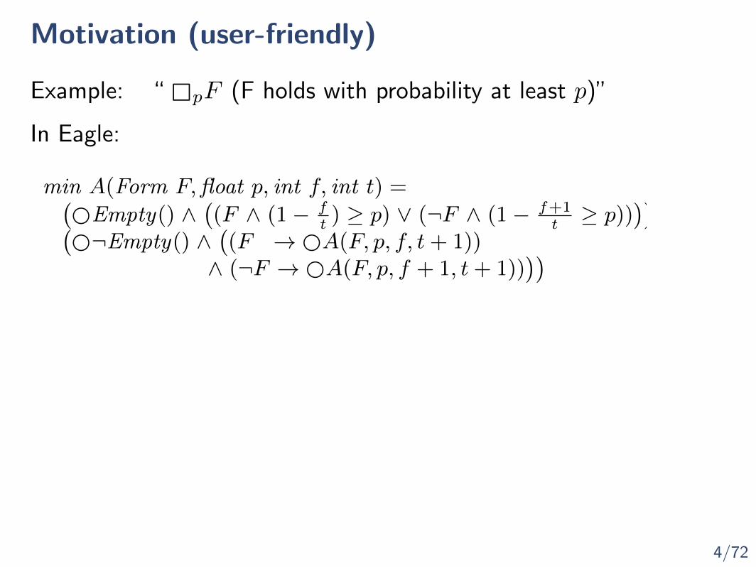
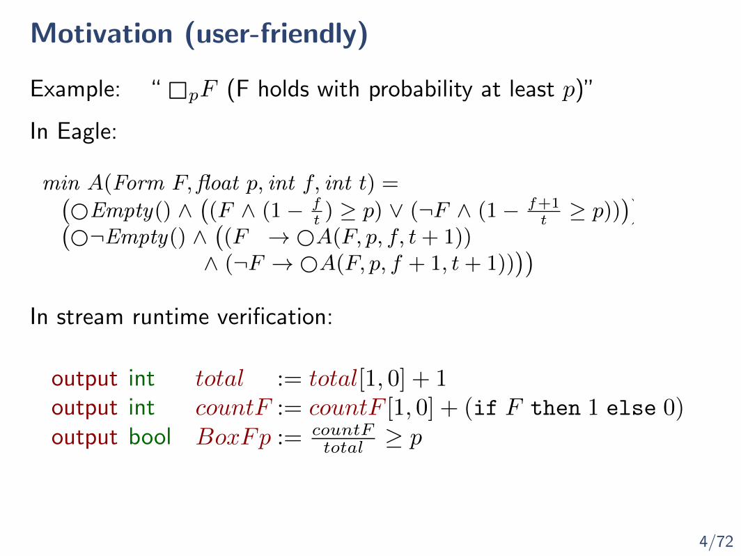
Motivation (user-friendly)
Example: “ pF (F holds with probability at least p)”
4/72
Motivation (user-friendly)
Example: “ pF (F holds with probability at least p)”
min A(Form F,float p, int f, int t) =(Empty() ∧
((F ∧ (1− f
t) ≥ p) ∨ (¬F ∧ (1− f+1
t≥ p))
))∨(
¬Empty() ∧((F → A(F, p, f, t+ 1))∧ (¬F → A(F, p, f + 1, t+ 1))
))
In Eagle:
4/72
Motivation (user-friendly)
Example: “ pF (F holds with probability at least p)”
min A(Form F,float p, int f, int t) =(Empty() ∧
((F ∧ (1− f
t) ≥ p) ∨ (¬F ∧ (1− f+1
t≥ p))
))∨(
¬Empty() ∧((F → A(F, p, f, t+ 1))∧ (¬F → A(F, p, f + 1, t+ 1))
))In stream runtime verification:
output int total := total[1, 0] + 1output int countF := countF [1, 0] + (if F then 1 else 0)output bool BoxFp := countF
total ≥ p
In Eagle:

4/72
Motivation (user-friendly)
Example: “ pF (F holds with probability at least p)”
min A(Form F,float p, int f, int t) =(Empty() ∧
((F ∧ (1− f
t) ≥ p) ∨ (¬F ∧ (1− f+1
t≥ p))
))∨(
¬Empty() ∧((F → A(F, p, f, t+ 1))∧ (¬F → A(F, p, f + 1, t+ 1))
))
In Eagle:
In stream runtime verification:
output int total := ffold(+, toint(true))output int countF := ffold(+, toint(F ))output bool BoxFp := countF
total ≥ p

4/72
Motivation (user-friendly)
Example: “ pF (F holds with probability at least p)”
min A(Form F,float p, int f, int t) =(Empty() ∧
((F ∧ (1− f
t) ≥ p) ∨ (¬F ∧ (1− f+1
t≥ p))
))∨(
¬Empty() ∧((F → A(F, p, f, t+ 1))∧ (¬F → A(F, p, f + 1, t+ 1))
))
In Eagle:
In stream runtime verification:
output int total := fcount(true)output int countF := fcount(F )output bool BoxFp := countF
total ≥ p

5/72
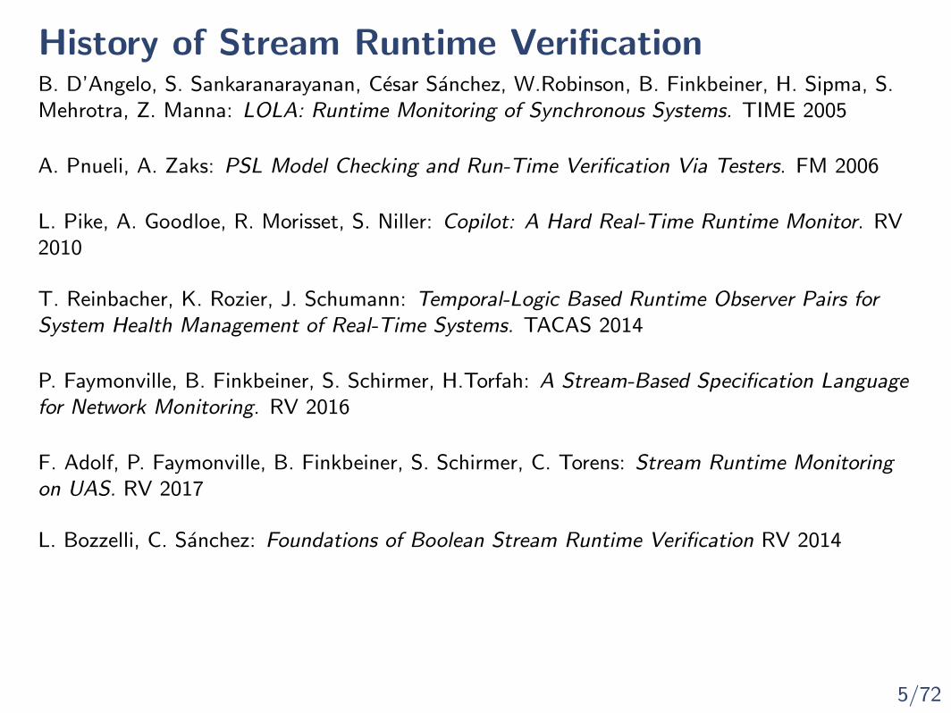
History of Stream Runtime VerificationB. D’Angelo, S. Sankaranarayanan, Cesar Sanchez, W.Robinson, B. Finkbeiner, H. Sipma, S.Mehrotra, Z. Manna: LOLA: Runtime Monitoring of Synchronous Systems. TIME 2005
A. Pnueli, A. Zaks: PSL Model Checking and Run-Time Verification Via Testers. FM 2006
P. Faymonville, B. Finkbeiner, S. Schirmer, H.Torfah: A Stream-Based Specification Languagefor Network Monitoring. RV 2016
F. Adolf, P. Faymonville, B. Finkbeiner, S. Schirmer, C. Torens: Stream Runtime Monitoringon UAS. RV 2017
L. Bozzelli, C. Sanchez: Foundations of Boolean Stream Runtime Verification RV 2014
M. Leucker, C. Sanchez, T.Scheffel, M. Schmitz, A. Schramm: TeSSLa: Runtime Verificationof Non-synchronized Real-Time Streams. SAC 2018
L. Pike, A. Goodloe, R. Morisset, S. Niller: Copilot: A Hard Real-Time Runtime Monitor. RV2010
T. Reinbacher, K. Rozier, J. Schumann: Temporal-Logic Based Runtime Observer Pairs forSystem Health Management of Real-Time Systems. TACAS 2014
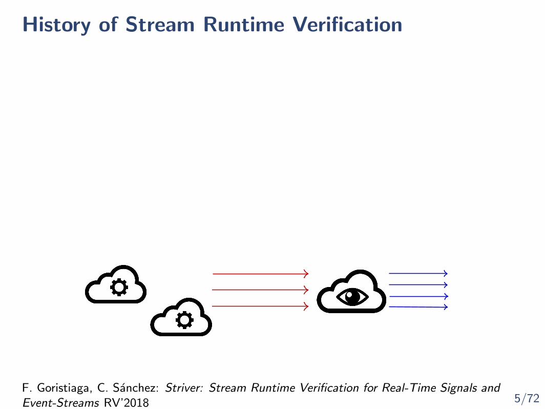
F. Goristiaga, C. Sanchez: Striver: Stream Runtime Verification for Real-Time Signals andEvent-Streams RV’2018

5/72
History of Stream Runtime VerificationB. D’Angelo, S. Sankaranarayanan, Cesar Sanchez, W.Robinson, B. Finkbeiner, H. Sipma, S.Mehrotra, Z. Manna: LOLA: Runtime Monitoring of Synchronous Systems. TIME 2005

5/72
History of Stream Runtime VerificationB. D’Angelo, S. Sankaranarayanan, Cesar Sanchez, W.Robinson, B. Finkbeiner, H. Sipma, S.Mehrotra, Z. Manna: LOLA: Runtime Monitoring of Synchronous Systems. TIME 2005
A. Pnueli, A. Zaks: PSL Model Checking and Run-Time Verification Via Testers. FM 2006
LTL
PSL

5/72
History of Stream Runtime VerificationB. D’Angelo, S. Sankaranarayanan, Cesar Sanchez, W.Robinson, B. Finkbeiner, H. Sipma, S.Mehrotra, Z. Manna: LOLA: Runtime Monitoring of Synchronous Systems. TIME 2005
A. Pnueli, A. Zaks: PSL Model Checking and Run-Time Verification Via Testers. FM 2006
L. Pike, A. Goodloe, R. Morisset, S. Niller: Copilot: A Hard Real-Time Runtime Monitor. RV2010
T. Reinbacher, K. Rozier, J. Schumann: Temporal-Logic Based Runtime Observer Pairs forSystem Health Management of Real-Time Systems. TACAS 2014

5/72
History of Stream Runtime VerificationB. D’Angelo, S. Sankaranarayanan, Cesar Sanchez, W.Robinson, B. Finkbeiner, H. Sipma, S.Mehrotra, Z. Manna: LOLA: Runtime Monitoring of Synchronous Systems. TIME 2005
A. Pnueli, A. Zaks: PSL Model Checking and Run-Time Verification Via Testers. FM 2006
P. Faymonville, B. Finkbeiner, S. Schirmer, H.Torfah: A Stream-Based Specification Languagefor Network Monitoring. RV 2016
F. Adolf, P. Faymonville, B. Finkbeiner, S. Schirmer, C. Torens: Stream Runtime Monitoringon UAS. RV 2017
L. Pike, A. Goodloe, R. Morisset, S. Niller: Copilot: A Hard Real-Time Runtime Monitor. RV2010
T. Reinbacher, K. Rozier, J. Schumann: Temporal-Logic Based Runtime Observer Pairs forSystem Health Management of Real-Time Systems. TACAS 2014
5/72
History of Stream Runtime VerificationB. D’Angelo, S. Sankaranarayanan, Cesar Sanchez, W.Robinson, B. Finkbeiner, H. Sipma, S.Mehrotra, Z. Manna: LOLA: Runtime Monitoring of Synchronous Systems. TIME 2005
A. Pnueli, A. Zaks: PSL Model Checking and Run-Time Verification Via Testers. FM 2006
P. Faymonville, B. Finkbeiner, S. Schirmer, H.Torfah: A Stream-Based Specification Languagefor Network Monitoring. RV 2016
F. Adolf, P. Faymonville, B. Finkbeiner, S. Schirmer, C. Torens: Stream Runtime Monitoringon UAS. RV 2017
L. Bozzelli, C. Sanchez: Foundations of Boolean Stream Runtime Verification RV 2014
L. Pike, A. Goodloe, R. Morisset, S. Niller: Copilot: A Hard Real-Time Runtime Monitor. RV2010
T. Reinbacher, K. Rozier, J. Schumann: Temporal-Logic Based Runtime Observer Pairs forSystem Health Management of Real-Time Systems. TACAS 2014

5/72
History of Stream Runtime VerificationB. D’Angelo, S. Sankaranarayanan, Cesar Sanchez, W.Robinson, B. Finkbeiner, H. Sipma, S.Mehrotra, Z. Manna: LOLA: Runtime Monitoring of Synchronous Systems. TIME 2005
A. Pnueli, A. Zaks: PSL Model Checking and Run-Time Verification Via Testers. FM 2006
P. Faymonville, B. Finkbeiner, S. Schirmer, H.Torfah: A Stream-Based Specification Languagefor Network Monitoring. RV 2016
F. Adolf, P. Faymonville, B. Finkbeiner, S. Schirmer, C. Torens: Stream Runtime Monitoringon UAS. RV 2017
L. Bozzelli, C. Sanchez: Foundations of Boolean Stream Runtime Verification RV 2014
M. Leucker, C. Sanchez, T.Scheffel, M. Schmitz, A. Schramm: TeSSLa: Runtime Verificationof Non-synchronized Real-Time Streams. SAC 2018
L. Pike, A. Goodloe, R. Morisset, S. Niller: Copilot: A Hard Real-Time Runtime Monitor. RV2010
T. Reinbacher, K. Rozier, J. Schumann: Temporal-Logic Based Runtime Observer Pairs forSystem Health Management of Real-Time Systems. TACAS 2014
Mϕ
5/72
History of Stream Runtime VerificationB. D’Angelo, S. Sankaranarayanan, Cesar Sanchez, W.Robinson, B. Finkbeiner, H. Sipma, S.Mehrotra, Z. Manna: LOLA: Runtime Monitoring of Synchronous Systems. TIME 2005
A. Pnueli, A. Zaks: PSL Model Checking and Run-Time Verification Via Testers. FM 2006
P. Faymonville, B. Finkbeiner, S. Schirmer, H.Torfah: A Stream-Based Specification Languagefor Network Monitoring. RV 2016
F. Adolf, P. Faymonville, B. Finkbeiner, S. Schirmer, C. Torens: Stream Runtime Monitoringon UAS. RV 2017
L. Bozzelli, C. Sanchez: Foundations of Boolean Stream Runtime Verification RV 2014
M. Leucker, C. Sanchez, T.Scheffel, M. Schmitz, A. Schramm: TeSSLa: Runtime Verificationof Non-synchronized Real-Time Streams. SAC 2018
L. Pike, A. Goodloe, R. Morisset, S. Niller: Copilot: A Hard Real-Time Runtime Monitor. RV2010
T. Reinbacher, K. Rozier, J. Schumann: Temporal-Logic Based Runtime Observer Pairs forSystem Health Management of Real-Time Systems. TACAS 2014
F. Goristiaga, C. Sanchez: Striver: Stream Runtime Verification for Real-Time Signals andEvent-Streams RV’2018

6/72
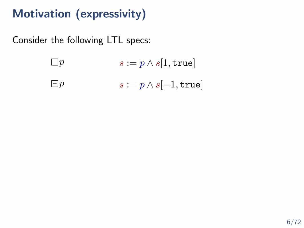
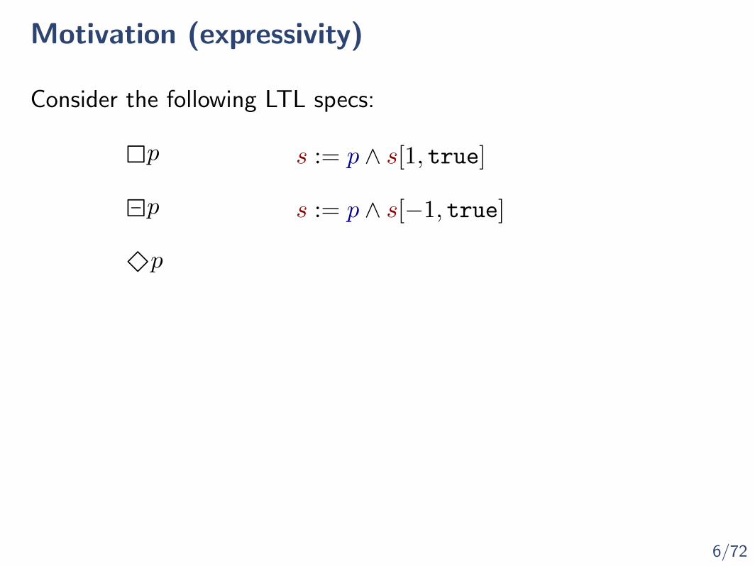
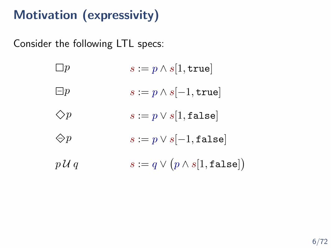
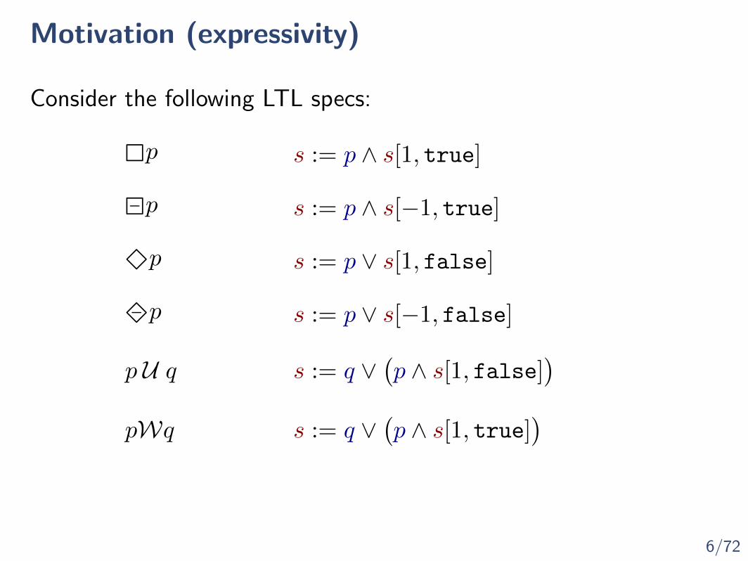
Motivation (expressivity)
p
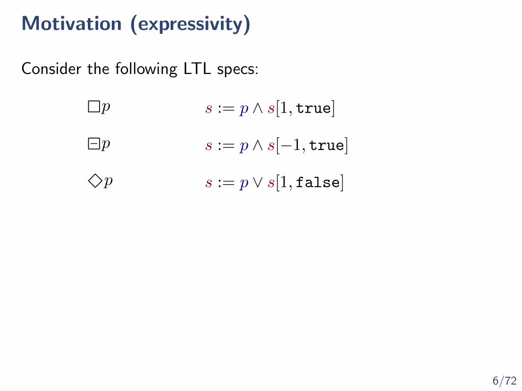
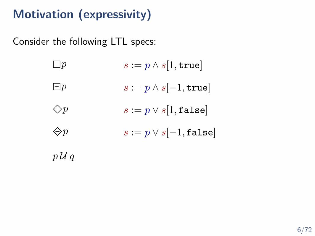
Consider the following LTL specs:

6/72
Motivation (expressivity)
p s := p ∧ s[1, true]
Consider the following LTL specs:

6/72
Motivation (expressivity)
p
p
s := p ∧ s[1, true]
Consider the following LTL specs:
6/72
Motivation (expressivity)
p
p
s := p ∧ s[1, true]
s := p ∧ s[−1, true]
Consider the following LTL specs:
6/72
Motivation (expressivity)
p
p
p
s := p ∧ s[1, true]
s := p ∧ s[−1, true]
Consider the following LTL specs:
6/72
Motivation (expressivity)
p
p
p
s := p ∧ s[1, true]
s := p ∧ s[−1, true]
s := p ∨ s[1, false]
Consider the following LTL specs:

6/72
Motivation (expressivity)
p
p
p
p
s := p ∧ s[1, true]
s := p ∧ s[−1, true]
s := p ∨ s[1, false]
Consider the following LTL specs:

6/72
Motivation (expressivity)
p
p
p
p
s := p ∧ s[1, true]
s := p ∧ s[−1, true]
s := p ∨ s[1, false]
s := p ∨ s[−1, false]
Consider the following LTL specs:
6/72
Motivation (expressivity)
p
p
p
p
p U q
s := p ∧ s[1, true]
s := p ∧ s[−1, true]
s := p ∨ s[1, false]
s := p ∨ s[−1, false]
Consider the following LTL specs:
6/72
Motivation (expressivity)
p
p
p
p
p U q
s := p ∧ s[1, true]
s := p ∧ s[−1, true]
s := p ∨ s[1, false]
s := p ∨ s[−1, false]
s := q ∨(p ∧ s[1, false]
)
Consider the following LTL specs:

6/72
Motivation (expressivity)
p
p
p
p
p U q
pWq
s := p ∧ s[1, true]
s := p ∧ s[−1, true]
s := p ∨ s[1, false]
s := p ∨ s[−1, false]
s := q ∨(p ∧ s[1, false]
)
Consider the following LTL specs:
6/72
Motivation (expressivity)
p
p
p
p
p U q
pWq
s := p ∧ s[1, true]
s := p ∧ s[−1, true]
s := p ∨ s[1, false]
s := p ∨ s[−1, false]
s := q ∨(p ∧ s[1, false]
)s := q ∨
(p ∧ s[1, true]
)
Consider the following LTL specs:

6/72
Motivation (expressivity)
p
p
p
p
p U q
pWq
s := p ∧ s[1, true]
s := p ∧ s[−1, true]
s := p ∨ s[1, false]
s := p ∨ s[−1, false]
s := q ∨(p ∧ s[1, false]
)s := q ∨
(p ∧ s[1, true]
)
Consider the following LTL specs:
p s := p[1, false]

6/72
Motivation (expressivity)
p
p
p
p
p U q
pWq
s := p ∧ s[1, true]
s := p ∧ s[−1, true]
s := p ∨ s[1, false]
s := p ∨ s[−1, false]
s := q ∨(p ∧ s[1, false]
)s := q ∨
(p ∧ s[1, true]
)
Consider the following LTL specs:
p s := p[1, false]
Why restrict to Booleans?

7/72
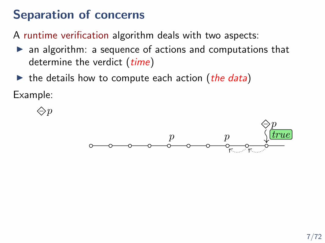
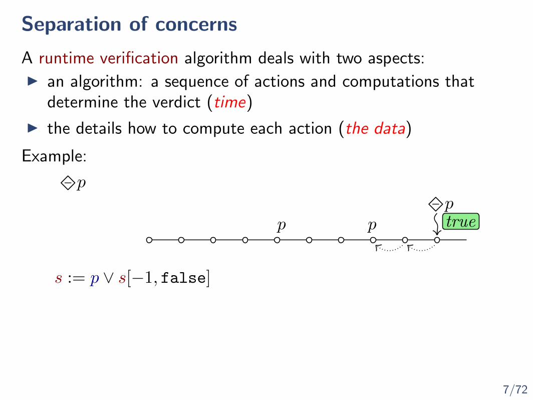
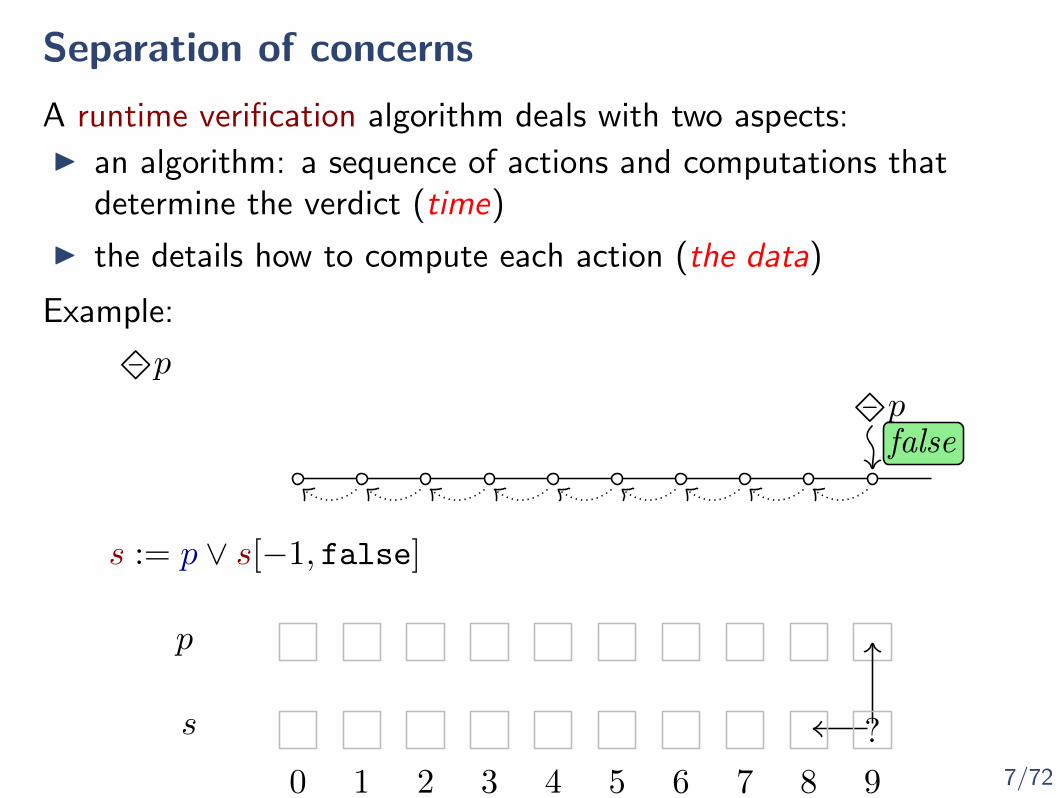
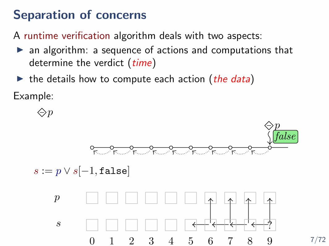
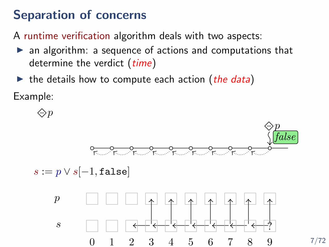
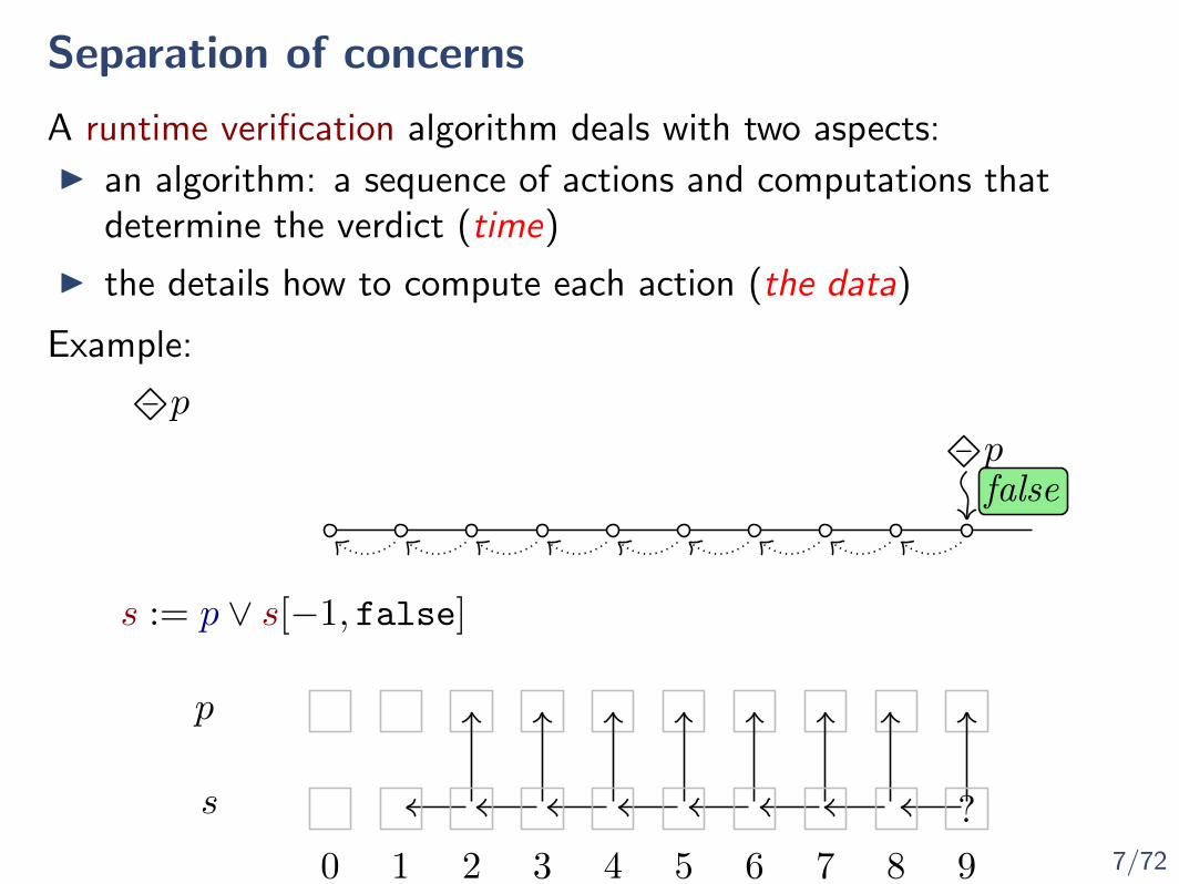
Separation of concerns
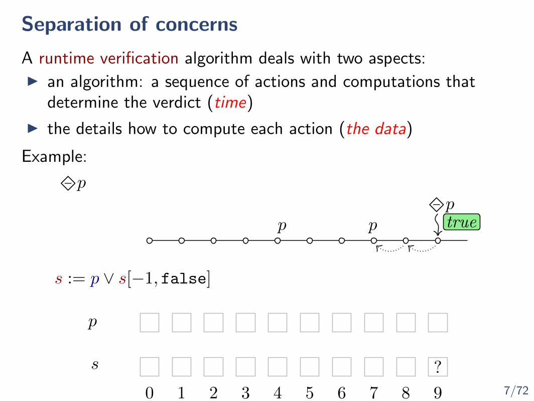
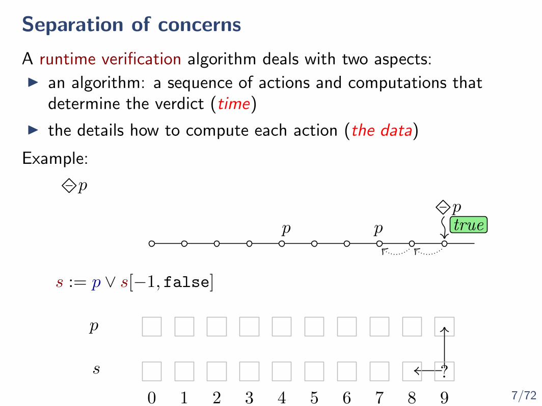
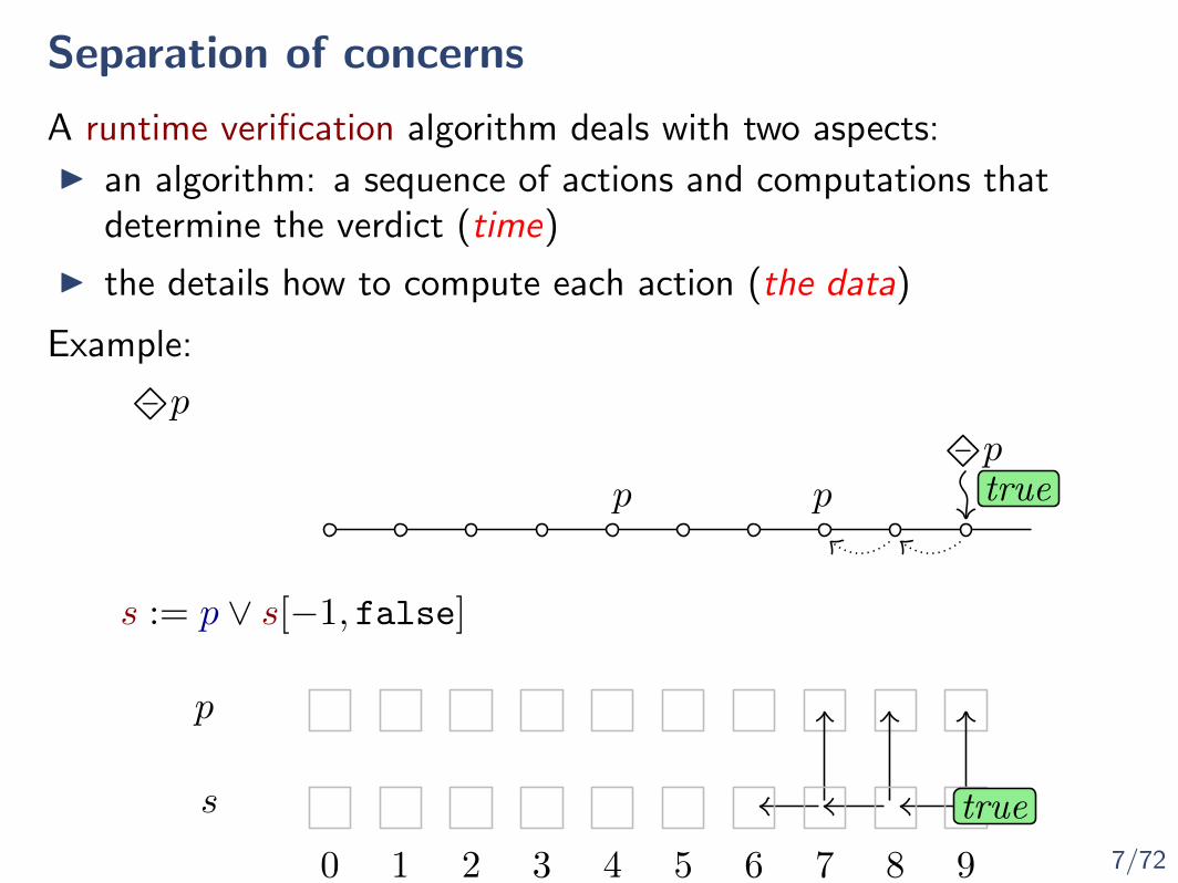
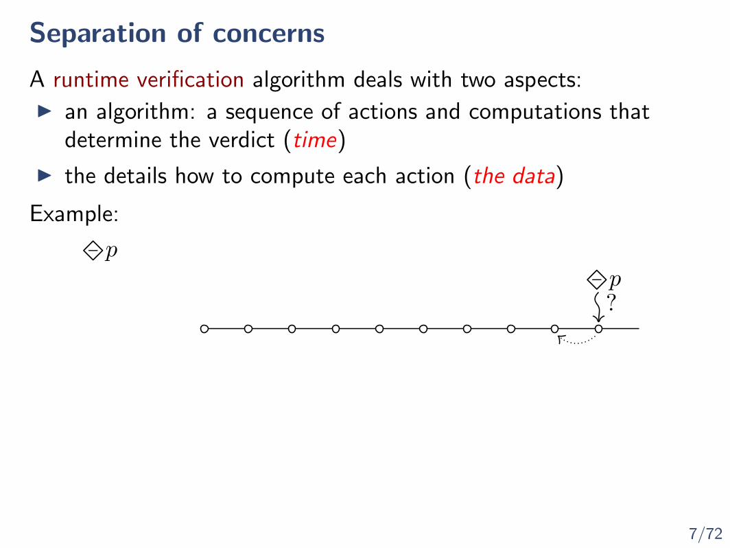
I an algorithm: a sequence of actions and computations thatdetermine the verdict (time)
Example:
A runtime verification algorithm deals with two aspects:
I the details how to compute each action (the data)

7/72
Separation of concerns
I an algorithm: a sequence of actions and computations thatdetermine the verdict (time)
Example:
pp
?
A runtime verification algorithm deals with two aspects:
I the details how to compute each action (the data)

7/72
Separation of concerns
I an algorithm: a sequence of actions and computations thatdetermine the verdict (time)
Example:
p
p pp
?
A runtime verification algorithm deals with two aspects:
I the details how to compute each action (the data)

7/72
Separation of concerns
I an algorithm: a sequence of actions and computations thatdetermine the verdict (time)
Example:
p
p pp
?
A runtime verification algorithm deals with two aspects:
I the details how to compute each action (the data)

7/72
Separation of concerns
I an algorithm: a sequence of actions and computations thatdetermine the verdict (time)
Example:
p
p pp
?
A runtime verification algorithm deals with two aspects:
I the details how to compute each action (the data)
7/72
Separation of concerns
I an algorithm: a sequence of actions and computations thatdetermine the verdict (time)
Example:
p
p pp
?
A runtime verification algorithm deals with two aspects:
I the details how to compute each action (the data)
true
7/72
Separation of concerns
I an algorithm: a sequence of actions and computations thatdetermine the verdict (time)
Example:
p
s := p ∨ s[−1, false]
p pp
?
A runtime verification algorithm deals with two aspects:
I the details how to compute each action (the data)
true
7/72
Separation of concerns
I an algorithm: a sequence of actions and computations thatdetermine the verdict (time)
Example:
p
s := p ∨ s[−1, false]
p pp
?
s
p
0 1 2 3 4 5 6 7 8 9
?
A runtime verification algorithm deals with two aspects:
I the details how to compute each action (the data)
true
7/72
Separation of concerns
I an algorithm: a sequence of actions and computations thatdetermine the verdict (time)
Example:
p
s := p ∨ s[−1, false]
p pp
?
s
p
0 1 2 3 4 5 6 7 8 9
?
A runtime verification algorithm deals with two aspects:
I the details how to compute each action (the data)
true

7/72
Separation of concerns
I an algorithm: a sequence of actions and computations thatdetermine the verdict (time)
Example:
p
s := p ∨ s[−1, false]
p pp
?
s
p
0 1 2 3 4 5 6 7 8 9
?
A runtime verification algorithm deals with two aspects:
I the details how to compute each action (the data)
true
7/72
Separation of concerns
I an algorithm: a sequence of actions and computations thatdetermine the verdict (time)
Example:
p
s := p ∨ s[−1, false]
p pp
?
s
p
0 1 2 3 4 5 6 7 8 9
?
A runtime verification algorithm deals with two aspects:
I the details how to compute each action (the data)
true
true

7/72
Separation of concerns
I an algorithm: a sequence of actions and computations thatdetermine the verdict (time)
Example:
pp
?
A runtime verification algorithm deals with two aspects:
I the details how to compute each action (the data)
7/72
Separation of concerns
I an algorithm: a sequence of actions and computations thatdetermine the verdict (time)
Example:
pp
?
A runtime verification algorithm deals with two aspects:
I the details how to compute each action (the data)

7/72
Separation of concerns
I an algorithm: a sequence of actions and computations thatdetermine the verdict (time)
Example:
pp
?
A runtime verification algorithm deals with two aspects:
I the details how to compute each action (the data)

7/72
Separation of concerns
I an algorithm: a sequence of actions and computations thatdetermine the verdict (time)
Example:
pp
?
A runtime verification algorithm deals with two aspects:
I the details how to compute each action (the data)

7/72
Separation of concerns
I an algorithm: a sequence of actions and computations thatdetermine the verdict (time)
Example:
pp
?
A runtime verification algorithm deals with two aspects:
I the details how to compute each action (the data)

7/72
Separation of concerns
I an algorithm: a sequence of actions and computations thatdetermine the verdict (time)
Example:
pp
?
A runtime verification algorithm deals with two aspects:
I the details how to compute each action (the data)

7/72
Separation of concerns
I an algorithm: a sequence of actions and computations thatdetermine the verdict (time)
Example:
pp
?
A runtime verification algorithm deals with two aspects:
I the details how to compute each action (the data)

7/72
Separation of concerns
I an algorithm: a sequence of actions and computations thatdetermine the verdict (time)
Example:
pp
?
A runtime verification algorithm deals with two aspects:
I the details how to compute each action (the data)

7/72
Separation of concerns
I an algorithm: a sequence of actions and computations thatdetermine the verdict (time)
Example:
pp
?
A runtime verification algorithm deals with two aspects:
I the details how to compute each action (the data)

7/72
Separation of concerns
I an algorithm: a sequence of actions and computations thatdetermine the verdict (time)
Example:
pp
?
A runtime verification algorithm deals with two aspects:
I the details how to compute each action (the data)

7/72
Separation of concerns
I an algorithm: a sequence of actions and computations thatdetermine the verdict (time)
Example:
pp
?
A runtime verification algorithm deals with two aspects:
I the details how to compute each action (the data)
false

7/72
Separation of concerns
I an algorithm: a sequence of actions and computations thatdetermine the verdict (time)
Example:
p
s := p ∨ s[−1, false]
p?
A runtime verification algorithm deals with two aspects:
I the details how to compute each action (the data)
false
7/72
Separation of concerns
I an algorithm: a sequence of actions and computations thatdetermine the verdict (time)
Example:
p
s := p ∨ s[−1, false]
p?
s
p
0 1 2 3 4 5 6 7 8 9
?
A runtime verification algorithm deals with two aspects:
I the details how to compute each action (the data)
false

7/72
Separation of concerns
I an algorithm: a sequence of actions and computations thatdetermine the verdict (time)
Example:
p
s := p ∨ s[−1, false]
p?
s
p
0 1 2 3 4 5 6 7 8 9
?
A runtime verification algorithm deals with two aspects:
I the details how to compute each action (the data)
false

7/72
Separation of concerns
I an algorithm: a sequence of actions and computations thatdetermine the verdict (time)
Example:
p
s := p ∨ s[−1, false]
p?
s
p
0 1 2 3 4 5 6 7 8 9
?
A runtime verification algorithm deals with two aspects:
I the details how to compute each action (the data)
false
7/72
Separation of concerns
I an algorithm: a sequence of actions and computations thatdetermine the verdict (time)
Example:
p
s := p ∨ s[−1, false]
p?
s
p
0 1 2 3 4 5 6 7 8 9
?
A runtime verification algorithm deals with two aspects:
I the details how to compute each action (the data)
false

7/72
Separation of concerns
I an algorithm: a sequence of actions and computations thatdetermine the verdict (time)
Example:
p
s := p ∨ s[−1, false]
p?
s
p
0 1 2 3 4 5 6 7 8 9
?
A runtime verification algorithm deals with two aspects:
I the details how to compute each action (the data)
false

7/72
Separation of concerns
I an algorithm: a sequence of actions and computations thatdetermine the verdict (time)
Example:
p
s := p ∨ s[−1, false]
p?
s
p
0 1 2 3 4 5 6 7 8 9
?
A runtime verification algorithm deals with two aspects:
I the details how to compute each action (the data)
false
7/72
Separation of concerns
I an algorithm: a sequence of actions and computations thatdetermine the verdict (time)
Example:
p
s := p ∨ s[−1, false]
p?
s
p
0 1 2 3 4 5 6 7 8 9
?
A runtime verification algorithm deals with two aspects:
I the details how to compute each action (the data)
false
7/72
Separation of concerns
I an algorithm: a sequence of actions and computations thatdetermine the verdict (time)
Example:
p
s := p ∨ s[−1, false]
p?
s
p
0 1 2 3 4 5 6 7 8 9
?
A runtime verification algorithm deals with two aspects:
I the details how to compute each action (the data)
false

7/72
Separation of concerns
I an algorithm: a sequence of actions and computations thatdetermine the verdict (time)
Example:
p
s := p ∨ s[−1, false]
p?
s
p
0 1 2 3 4 5 6 7 8 9
?
A runtime verification algorithm deals with two aspects:
I the details how to compute each action (the data)
false

7/72
Separation of concerns
I an algorithm: a sequence of actions and computations thatdetermine the verdict (time)
Example:
p
s := p ∨ s[−1, false]
p?
s
p
0 1 2 3 4 5 6 7 8 9
?
A runtime verification algorithm deals with two aspects:
I the details how to compute each action (the data)
false
false
8/72
Domains
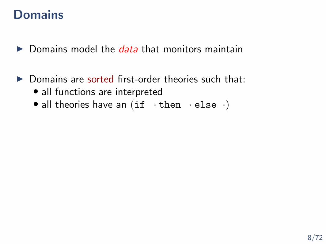
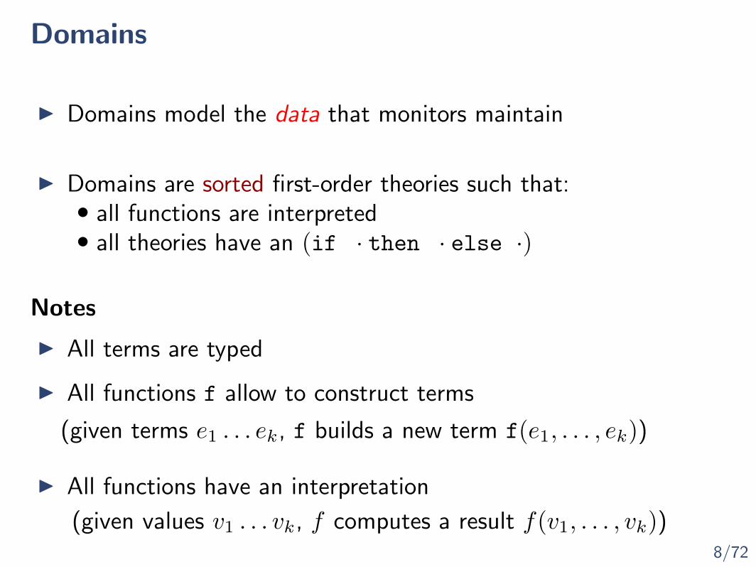
I Domains model the data that monitors maintain
I Domains are sorted first-order theories such that:• all functions are interpreted• all theories have an (if · then · else ·)
8/72
Domains
I Domains model the data that monitors maintain
I Domains are sorted first-order theories such that:• all functions are interpreted• all theories have an (if · then · else ·)
I All terms are typed
Notes
I All functions f allow to construct terms
I All functions have an interpretation
(given terms e1 . . . ek, f builds a new term f(e1, . . . , ek))
(given values v1 . . . vk, f computes a result f(v1, . . . , vk))

9/72
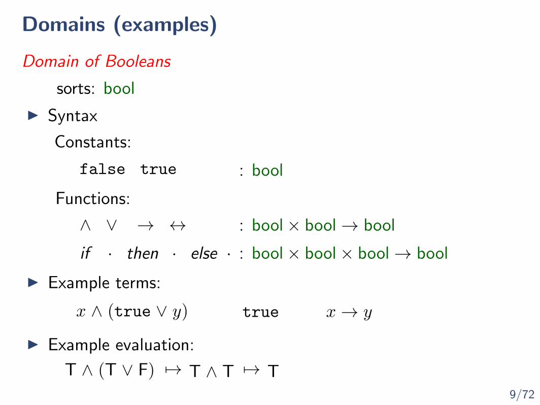
Domains (examples)
sorts: bool
Constants:
Domain of Booleans
Functions:
false true : bool
if · then · else · : bool× bool× bool→ bool
∧ ∨ → ↔ : bool× bool→ bool
I Syntax
9/72
Domains (examples)
sorts: bool
Constants:
Domain of Booleans
Functions:
false true : bool
if · then · else · : bool× bool× bool→ bool
∧ ∨ → ↔ : bool× bool→ bool
I Syntax
I Example terms:
x ∧ (true ∨ y) true x→ y
I Example evaluation:
T ∧ (T ∨ F) 7→ T ∧ T 7→ T

9/72
Domains (examples)
sorts: bool3
Constants:
Domain of Booleans 3
Functions:
if · then · else · : bool× bool3× bool3→ bool3
∧ ∨ → ↔ : bool3× bool3→ bool3
I Syntax
I Example terms:
x ∧ (true ∨ y) true x→ y
I Example evaluation:
T ∧ (? ∨ F) 7→ T ∧ ? 7→ ?
false true ? : bool3
? ∨ x
T
F
?

9/72
Domains (examples)
sorts: bool4
Constants:
Domain of Booleans 4
Functions:
if · then · else · : bool× bool4× bool4→ bool4
∧ ∨ → ↔ : bool4× bool4→ bool4
I Syntax
I Example terms:
x ∧ (>p ∨ y) true x→ y
I Example evaluation:
T ∧ (>p ∨ F) 7→ T ∧ >p7→ >p
false true >p ⊥p : bool4
⊥p ∨ x
T
F
>p
⊥p

9/72
Domains (examples)
sorts: bool, int
Constants:
Functions:
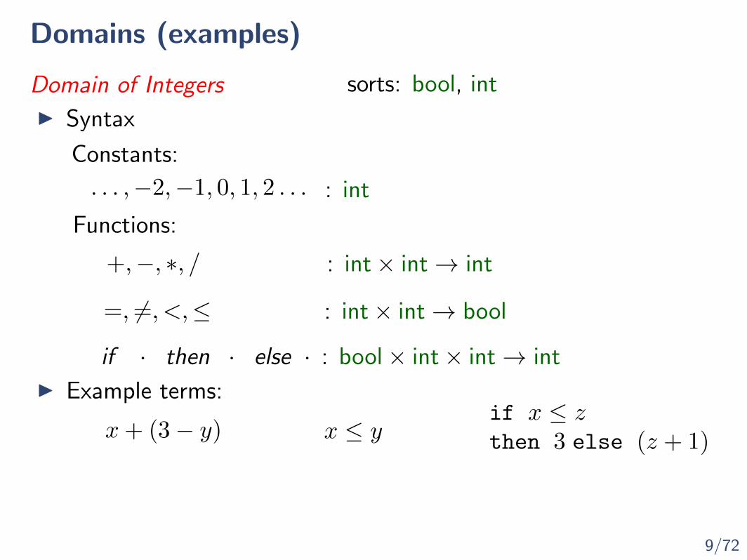
. . . ,−2,−1, 0, 1, 2 . . . : int
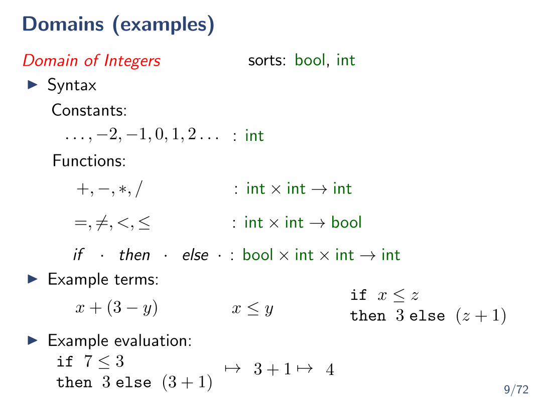
Domain of Integers
I Syntax
if · then · else · : bool× int× int→ int
=, 6=, <,≤ : int× int→ bool
: int× int→ int+,−, ∗, /
9/72
Domains (examples)
sorts: bool, int
Constants:
Functions:
. . . ,−2,−1, 0, 1, 2 . . . : int
I Example terms:
x+ (3− y) x ≤ yif x ≤ zthen 3 else (z + 1)
Domain of Integers
I Syntax
if · then · else · : bool× int× int→ int
=, 6=, <,≤ : int× int→ bool
: int× int→ int+,−, ∗, /
9/72
Domains (examples)
sorts: bool, int
Constants:
Functions:
. . . ,−2,−1, 0, 1, 2 . . . : int
I Example terms:
I Example evaluation:
x+ (3− y) x ≤ yif x ≤ zthen 3 else (z + 1)
7→ 3 + 1if 7 ≤ 3then 3 else (3 + 1)
7→ 4
Domain of Integers
I Syntax
if · then · else · : bool× int× int→ int
=, 6=, <,≤ : int× int→ bool
: int× int→ int+,−, ∗, /

9/72
Domains (examples)
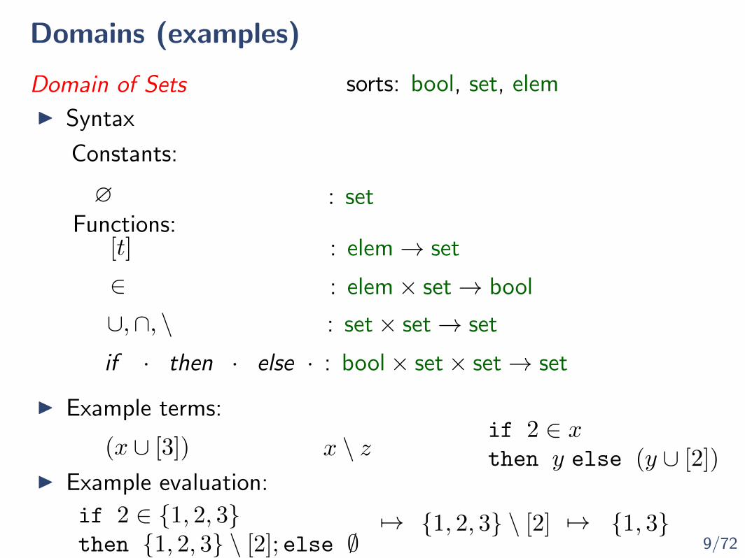
sorts: bool, set, elem
∅ : set
Domain of Sets
[t] : elem→ set
∪,∩, \ : set× set→ set
if · then · else · : bool× set× set→ set
Constants:
Functions:
I Syntax
∈ : elem× set→ bool

9/72
Domains (examples)
sorts: bool, set, elem
∅ : set
Domain of Sets
[t] : elem→ set
∪,∩, \ : set× set→ set
if · then · else · : bool× set× set→ set
I Example terms:
(x ∪ [3]) x \ zif 2 ∈ xthen y else (y ∪ [2])
Constants:
Functions:
I Syntax
∈ : elem× set→ bool
9/72
Domains (examples)
sorts: bool, set, elem
∅ : set
Domain of Sets
[t] : elem→ set
∪,∩, \ : set× set→ set
if · then · else · : bool× set× set→ set
I Example terms:
I Example evaluation:
(x ∪ [3]) x \ zif 2 ∈ xthen y else (y ∪ [2])
7→ {1, 2, 3} \ [2]if 2 ∈ {1, 2, 3}then {1, 2, 3} \ [2]; else ∅
7→ {1, 3}
Constants:
Functions:
I Syntax
∈ : elem× set→ bool
10/72
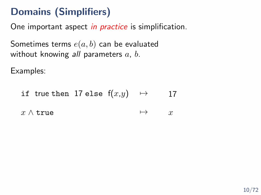
Domains (Simplifiers)
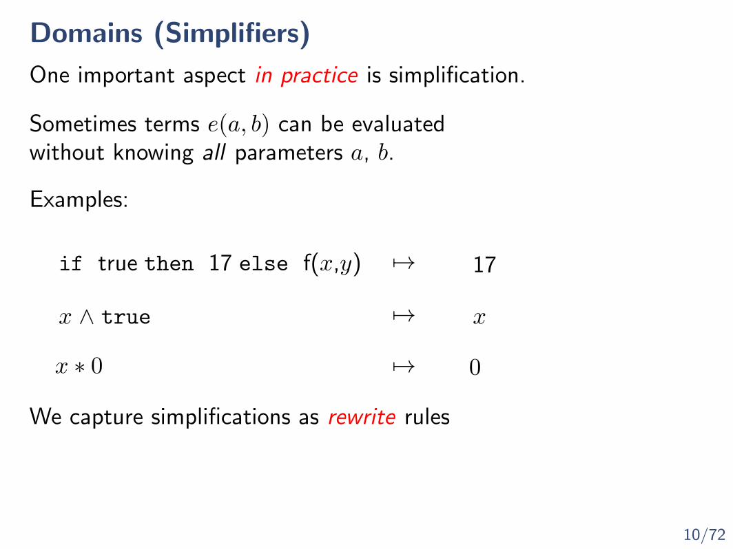
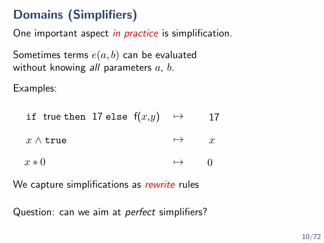
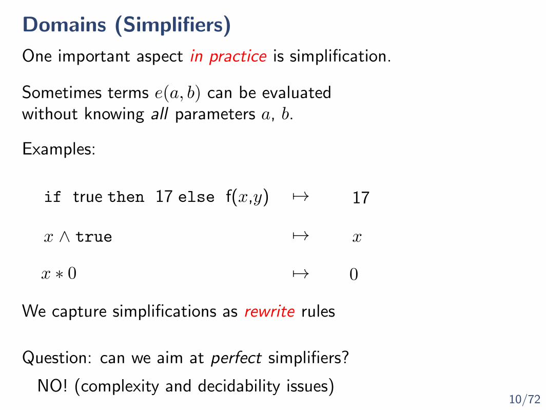
One important aspect in practice is simplification.
Sometimes terms e(a, b) can be evaluatedwithout knowing all parameters a, b.

10/72
Domains (Simplifiers)
One important aspect in practice is simplification.
Sometimes terms e(a, b) can be evaluatedwithout knowing all parameters a, b.
Examples:

10/72
Domains (Simplifiers)
One important aspect in practice is simplification.
Sometimes terms e(a, b) can be evaluatedwithout knowing all parameters a, b.
Examples:
if true then 17 else f(x,y) 7→ 17
10/72
Domains (Simplifiers)
One important aspect in practice is simplification.
Sometimes terms e(a, b) can be evaluatedwithout knowing all parameters a, b.
Examples:
x ∧ true 7→ x
if true then 17 else f(x,y) 7→ 17

10/72
Domains (Simplifiers)
One important aspect in practice is simplification.
Sometimes terms e(a, b) can be evaluatedwithout knowing all parameters a, b.
Examples:
x ∗ 0 7→ 0
x ∧ true 7→ x
if true then 17 else f(x,y) 7→ 17
10/72
Domains (Simplifiers)
One important aspect in practice is simplification.
Sometimes terms e(a, b) can be evaluatedwithout knowing all parameters a, b.
Examples:
We capture simplifications as rewrite rules
x ∗ 0 7→ 0
x ∧ true 7→ x
if true then 17 else f(x,y) 7→ 17
10/72
Domains (Simplifiers)
One important aspect in practice is simplification.
Sometimes terms e(a, b) can be evaluatedwithout knowing all parameters a, b.
Examples:
We capture simplifications as rewrite rules
Question: can we aim at perfect simplifiers?
x ∗ 0 7→ 0
NO! (complexity and decidability issues)
x ∧ true 7→ x
if true then 17 else f(x,y) 7→ 17

11/72
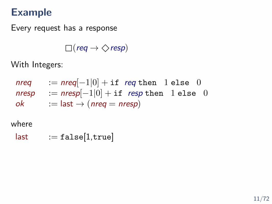
Example
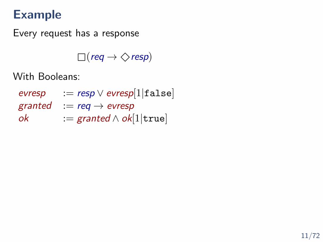
Every request has a response

11/72
Example
Every request has a response
(req→resp)
11/72
Example
Every request has a response
(req→resp)
evresp := resp ∨ evresp[1|false]granted := req→ evrespok := granted ∧ ok[1|true]
With Booleans:
11/72
Example
Every request has a response
(req→resp)
nreq := nreq[−1|0] + if req then 1 else 0nresp := nresp[−1|0] + if resp then 1 else 0ok := last→ (nreq = nresp)
With Integers:
where
last := false[1,true]
11/72
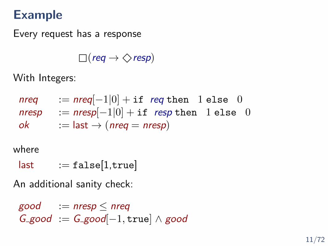
Example
Every request has a response
(req→resp)
nreq := nreq[−1|0] + if req then 1 else 0nresp := nresp[−1|0] + if resp then 1 else 0ok := last→ (nreq = nresp)
With Integers:
good := nresp ≤ nreqG good := G good[−1, true] ∧ good
An additional sanity check:
where
last := false[1,true]
11/72
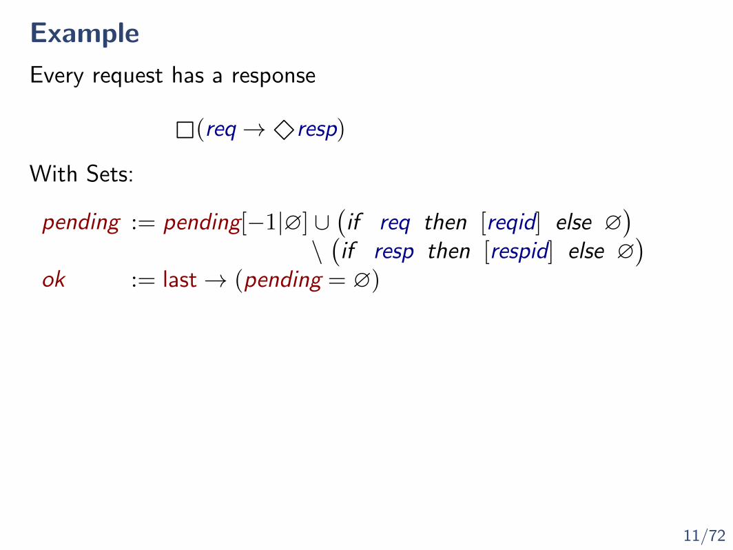
Example
Every request has a response
(req→resp)
pending := pending[−1|∅] ∪(if req then [reqid] else ∅
)\(if resp then [respid] else ∅
)ok := last→ (pending = ∅)
With Sets:
12/72
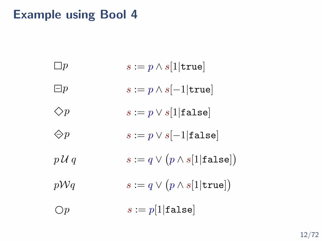
Example using Bool 4
p
p
p
p
p U q
pWq
s := p ∧ s[1|true]
s := p ∧ s[−1|true]
s := p ∨ s[1|false]
s := p ∨ s[−1|false]
s := q ∨(p ∧ s[1|false]
)s := q ∨
(p ∧ s[1|true]
)p s := p[1|false]

12/72
Example using Bool 4
p
p
p
p
p U q
pWq
s := p ∧ s[1|⊥p]
s := p ∧ s[−1|true]
s := p ∨ s[1|>p]
s := p ∨ s[−1|false]
s := q ∨(p ∧ s[1|⊥p]
)s := q ∨
(p ∧ s[1|>p]
)p s := p[1|false]
13/72
Stream Runtime VerificationSyntax
14/72
Stream Runtime Verification syntax
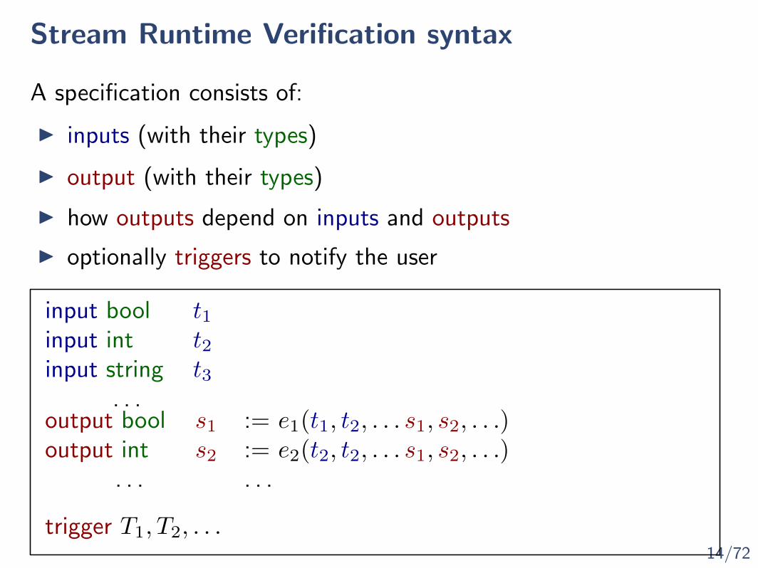
A specification consists of:

14/72
Stream Runtime Verification syntax
A specification consists of:
input bool t1input int t2input string t3
. . .
I inputs (with their types)
14/72
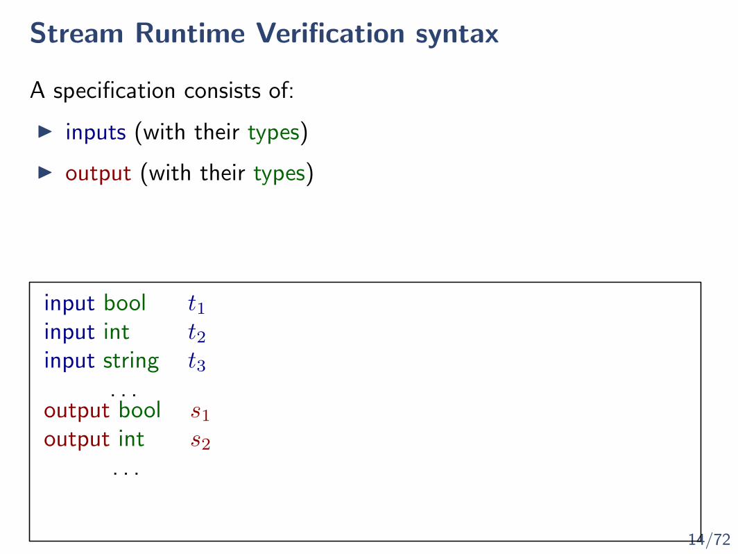
Stream Runtime Verification syntax
A specification consists of:
input bool t1input int t2input string t3
. . .output bool s1
output int s2
. . .
I inputs (with their types)
I output (with their types)
14/72
Stream Runtime Verification syntax
A specification consists of:
input bool t1input int t2input string t3
. . .output bool s1
output int s2
. . .
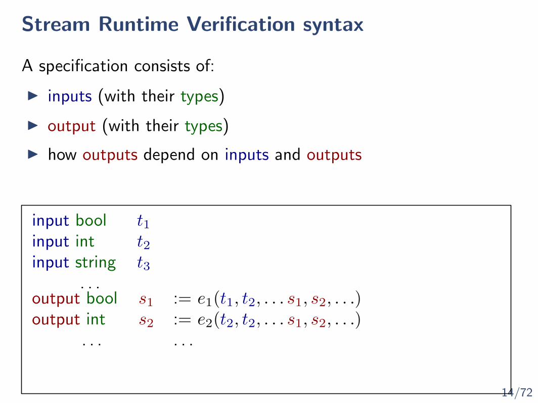
I inputs (with their types)
I output (with their types)
I how outputs depend on inputs and outputs
:= e1(t1, t2, . . . s1, s2, . . .):= e2(t2, t2, . . . s1, s2, . . .). . .
14/72
Stream Runtime Verification syntax
A specification consists of:
input bool t1input int t2input string t3
. . .output bool s1
output int s2
. . .
I inputs (with their types)
I output (with their types)
I how outputs depend on inputs and outputs
:= e1(t1, t2, . . . s1, s2, . . .):= e2(t2, t2, . . . s1, s2, . . .). . .
I optionally triggers to notify the user
trigger T1, T2, . . .

15/72
Stream Runtime Verification syntax
A specification consists of:
input bool t1input int t2input string t3
. . .output bool s1
output int s2
. . .
I inputs (with their types)
I output (with their types)
I how outputs depend on inputs and outputs
:= e1(t1, t2, . . . s1, s2, . . .):= e2(t2, t2, . . . s1, s2, . . .). . .
I optionally triggers to notify the user
trigger T1, T2, . . .
independent stream variables
dependent stream variables
defining equations
16/72
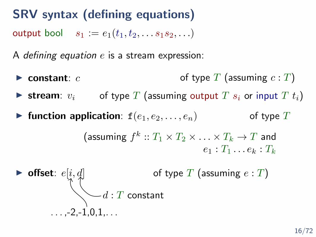
SRV syntax (defining equations)
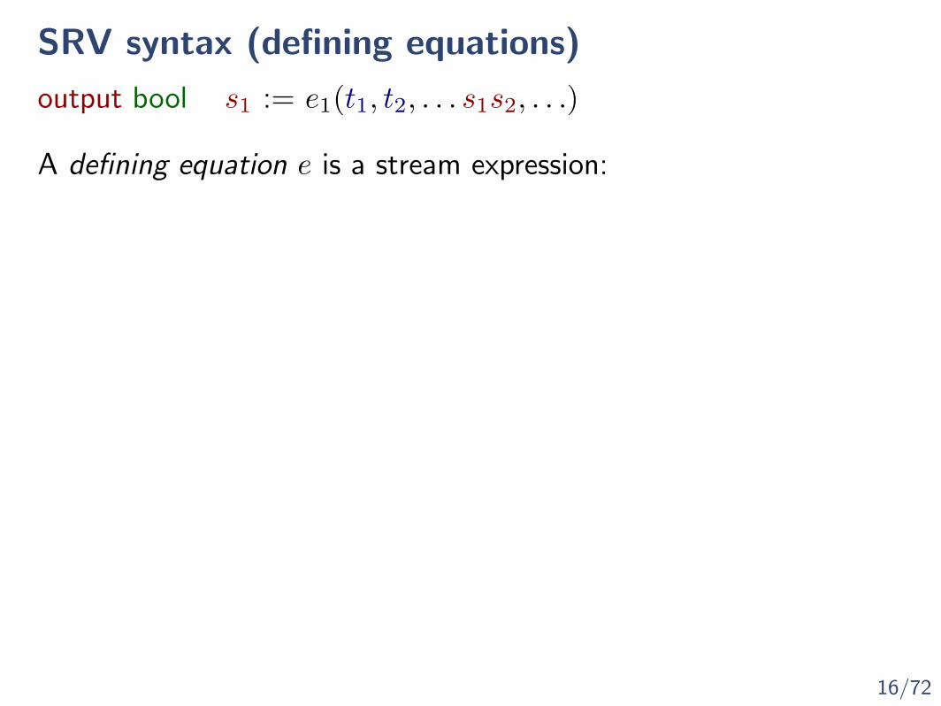
output bool s1 := e1(t1, t2, . . . s1s2, . . .)
A defining equation e is a stream expression:
16/72
SRV syntax (defining equations)
output bool s1 := e1(t1, t2, . . . s1s2, . . .)
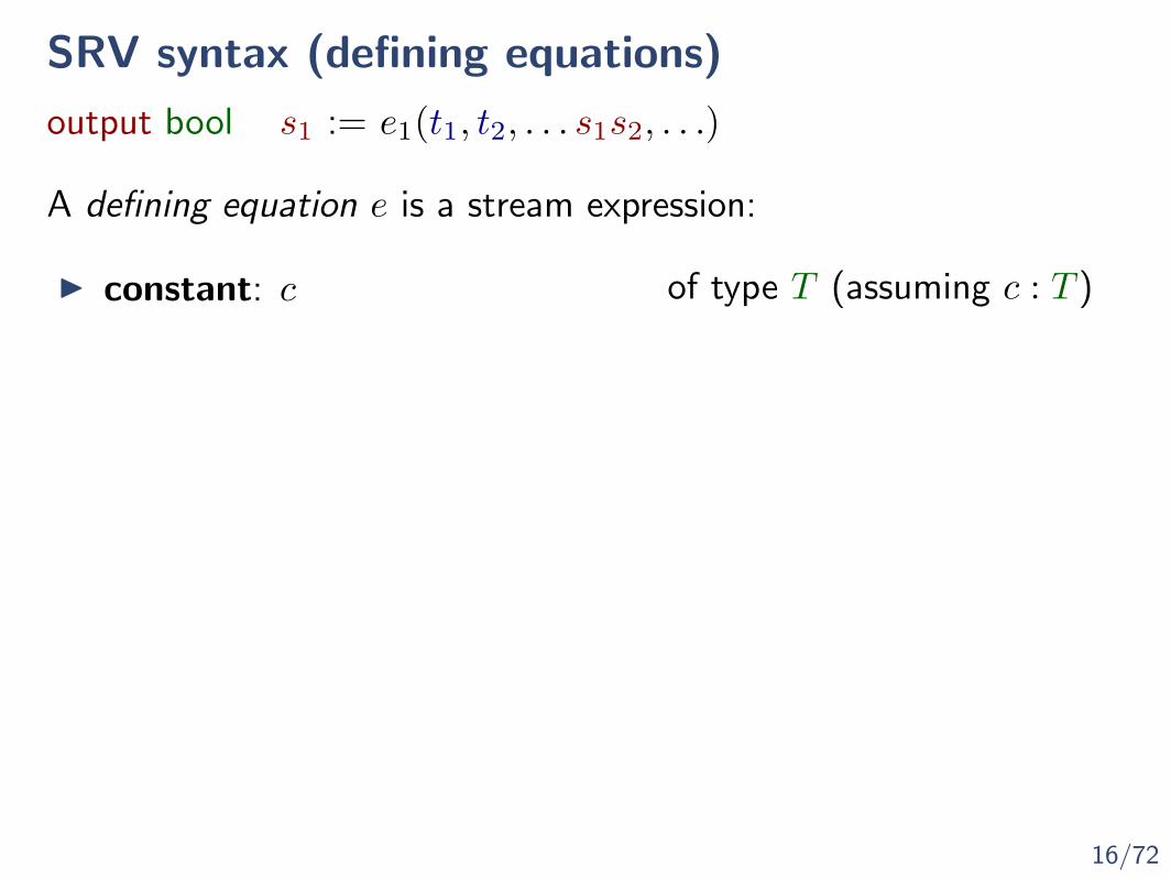
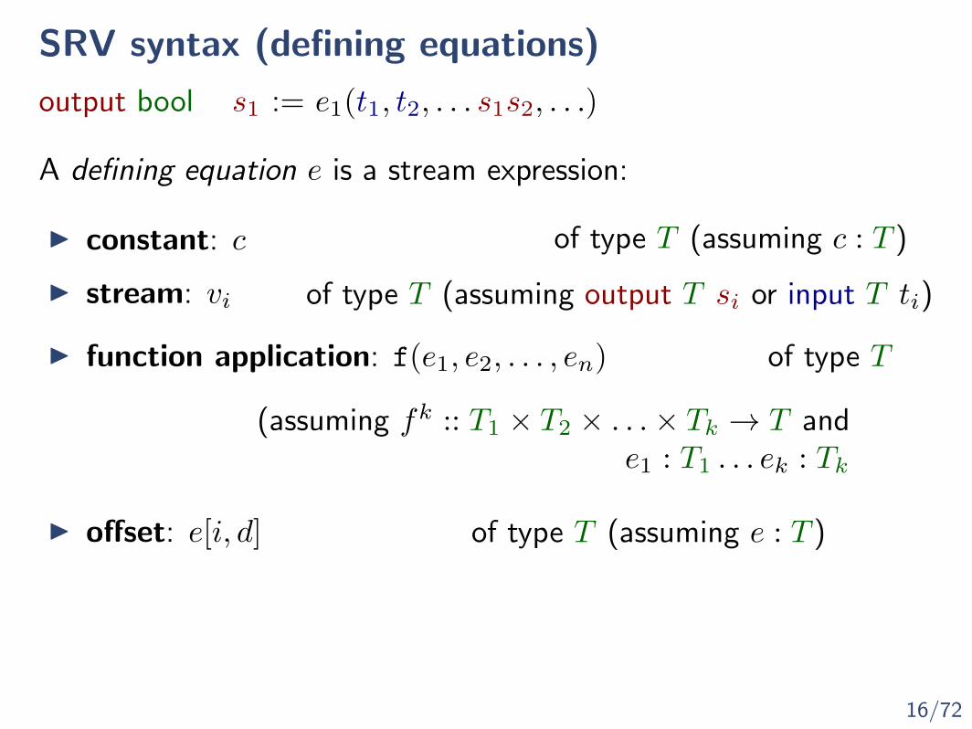
A defining equation e is a stream expression:
I constant: c of type T (assuming c : T )

16/72
SRV syntax (defining equations)
output bool s1 := e1(t1, t2, . . . s1s2, . . .)
A defining equation e is a stream expression:
I constant: c
I stream: vi
of type T (assuming c : T )
of type T (assuming output T si or input T ti)

16/72
SRV syntax (defining equations)
output bool s1 := e1(t1, t2, . . . s1s2, . . .)
A defining equation e is a stream expression:
I constant: c
I stream: vi
of type T (assuming c : T )
of type T (assuming output T si or input T ti)
I function application: f(e1, e2, . . . , en)
(assuming fk :: T1 × T2 × . . .× Tk → T ande1 : T1 . . . ek : Tk
of type T
I offset: e[i, d] of type T (assuming e : T )
. . . ,-2,-1,0,1,. . .
d : T constant

17/72
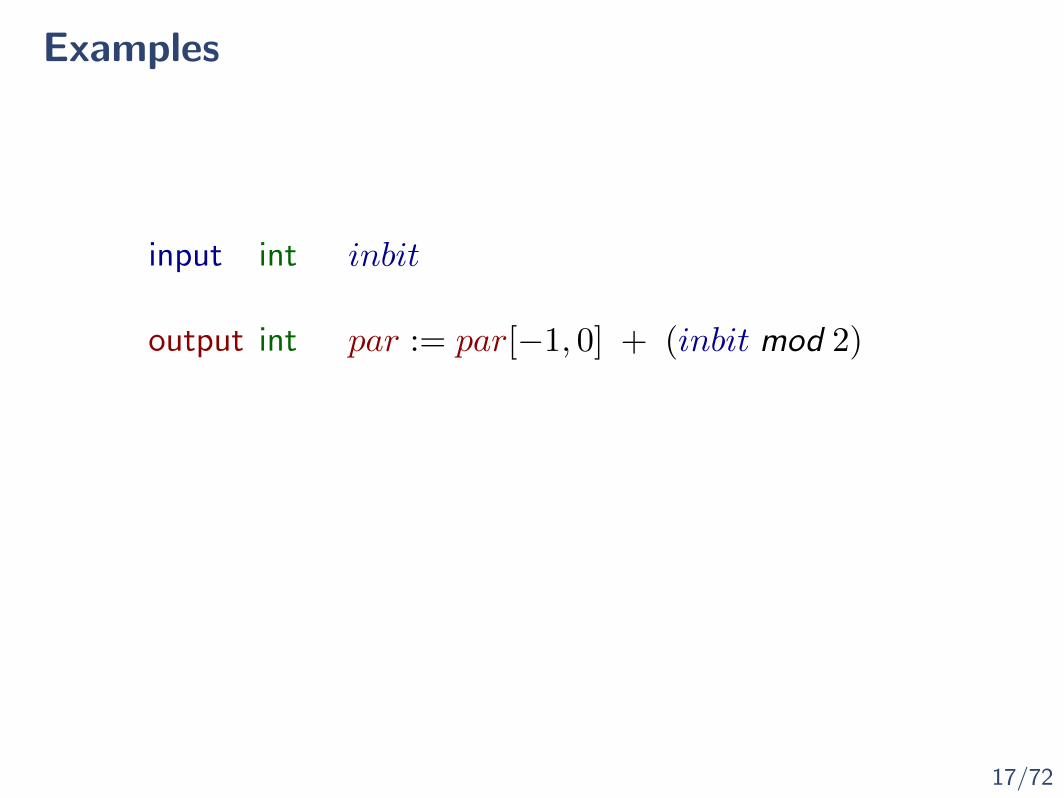
Examples
output bool ok := true

17/72
Examples
input int h
output int height := h

17/72
Examples
output bool resp := ok ∧ (n ≥ 0)
input int ninput bool ok

17/72
Examples
input int n
output int m := (n2 + 7) mod 16

17/72
Examples
output int resp := if cond then nelse n+ 1
input int ninput bool cond
17/72
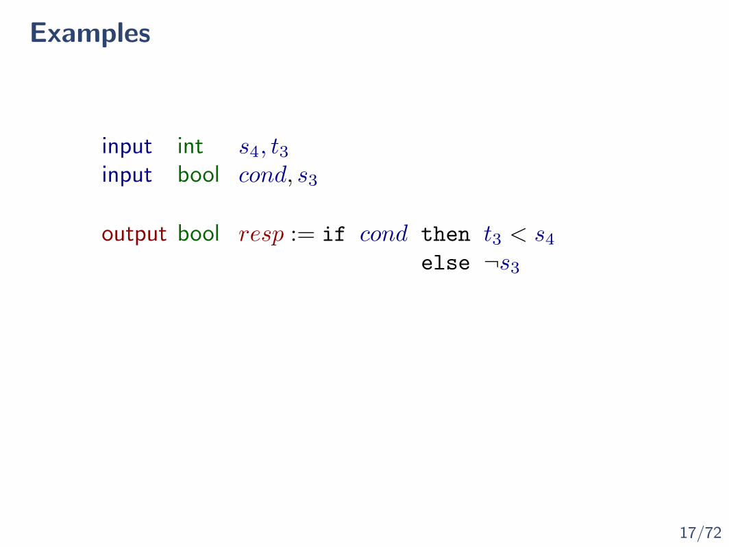
Examples
output bool resp := if cond then t3 < s4
else ¬s3
input int s4, t3input bool cond, s3
17/72
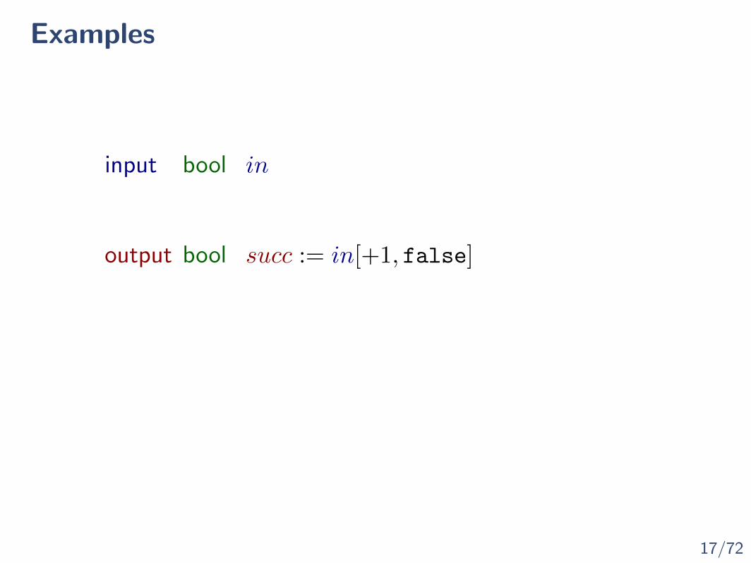
Examples
output bool succ := in[+1, false]
input bool in
17/72
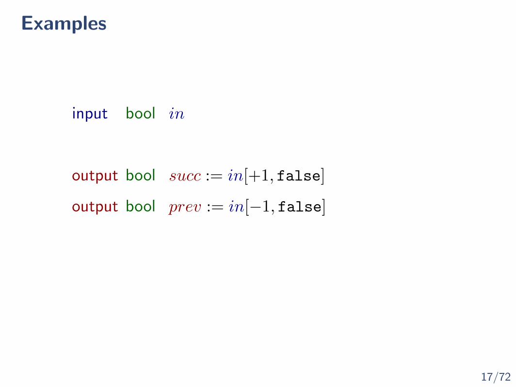
Examples
output bool succ := in[+1, false]
input bool in
output bool prev := in[−1, false]
17/72
Examples
input int inbit
output int par := par[−1, 0] + (inbit mod 2)

17/72
Examples
input bool req, resp
output bool ok := resp ∨ (¬req ∧ ok[+1, false])
18/72
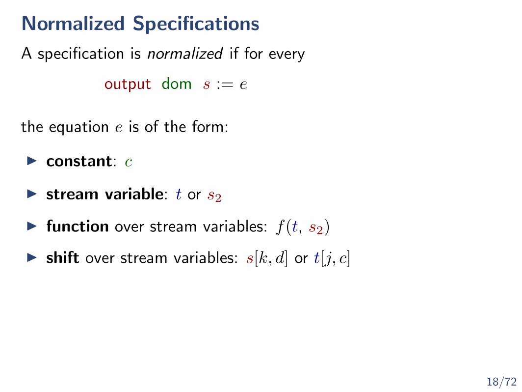
Normalized Specifications
A specification is normalized if for every
output dom s := e
the equation e is of the form:
I constant: c
I stream variable: t or s2
I function over stream variables: f(t, s2)
I shift over stream variables: s[k, d] or t[j, c]
18/72
Normalized Specifications
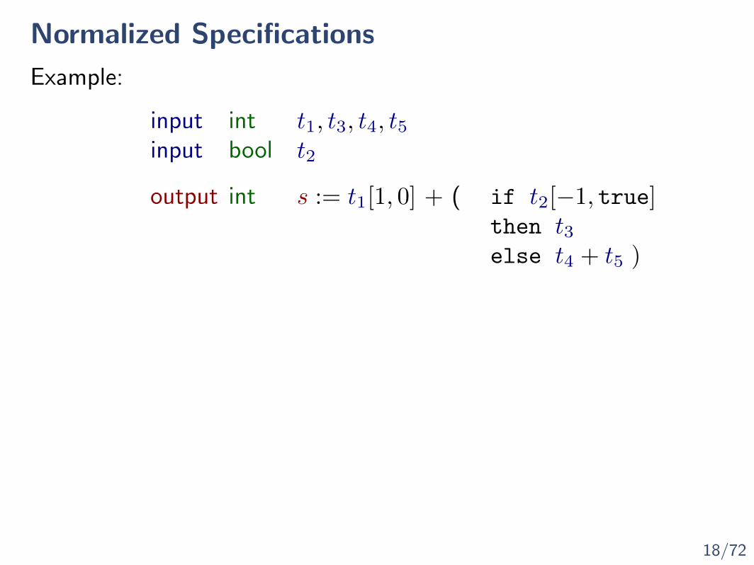
Example:
input int t1, t3, t4, t5input bool t2
output int s := t1[1, 0] + ( if t2[−1, true]then t3else t4 + t5 )

18/72
Normalized Specifications
Example:
input int t1, t3, t4, t5input bool t2
output int s := t1[1, 0] + ( if t2[−1, true]then t3else t4 + t5 )
can be normalized to:
output int s := s1 + s2
output int s1 := t1[1, 0]output int s2 := if s3 then t3 else s4
output bool s3 := t2[−1, true]output int s4 := t4 + t5

19/72
Stream Runtime VerificationSemantics

20/72
Semantics (intention)
Spec ϕ

20/72
Semantics (intention)
Spec ϕ
Lola compiler
monitor Mϕ
static time

20/72
Semantics (intention)
τ1τ2τ3τ4
Spec ϕ
Lola compiler
monitor Mϕ
σ1σ2σ3σ4
Intention: Mϕ is a “function” from inputs to outputs
static time
runtime
21/72
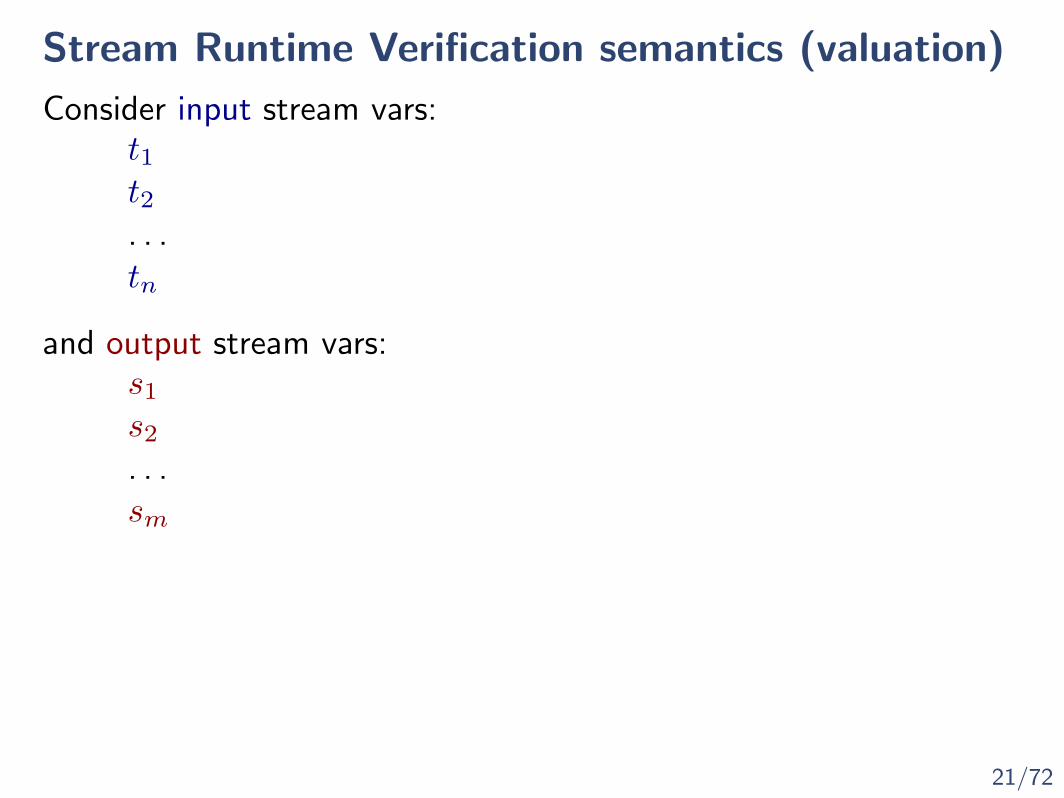
Stream Runtime Verification semantics (valuation)
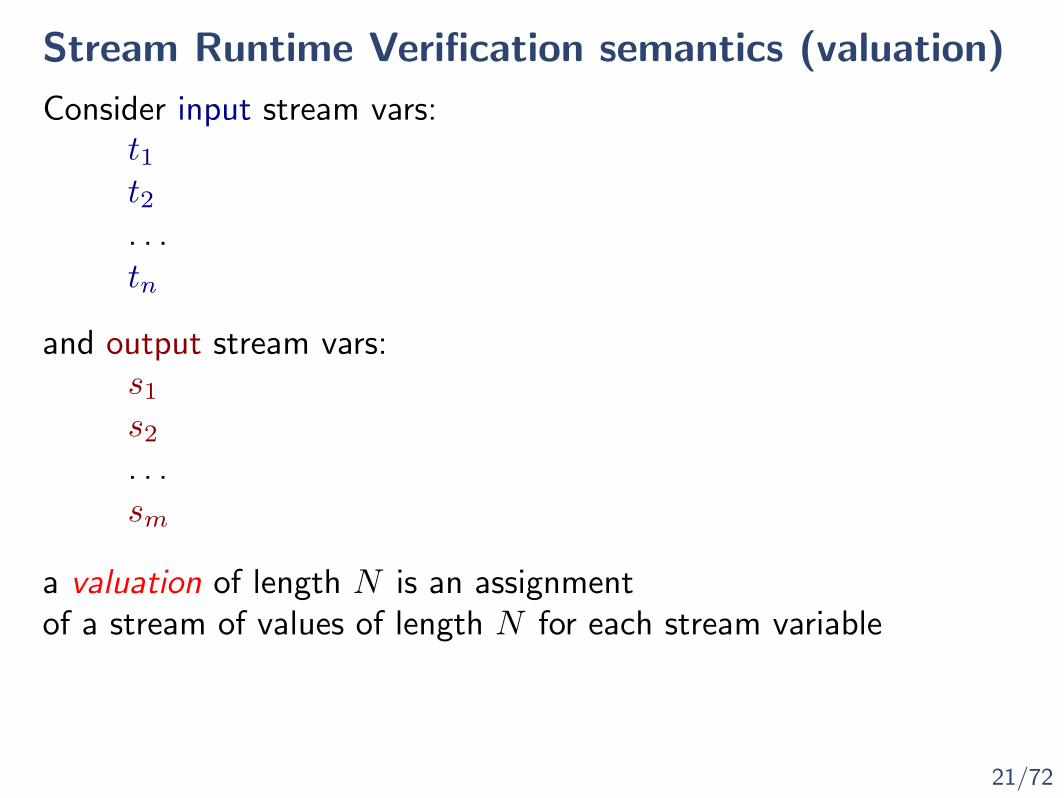
Consider input stream vars:
and output stream vars:
t1t2. . .tn
s1
s2
sm
. . .
21/72
Stream Runtime Verification semantics (valuation)
Consider input stream vars:
and output stream vars:
t1t2. . .tn
s1
s2
sm
. . .
a valuation of length N is an assignmentof a stream of values of length N for each stream variable
21/72
Stream Runtime Verification semantics (valuation)
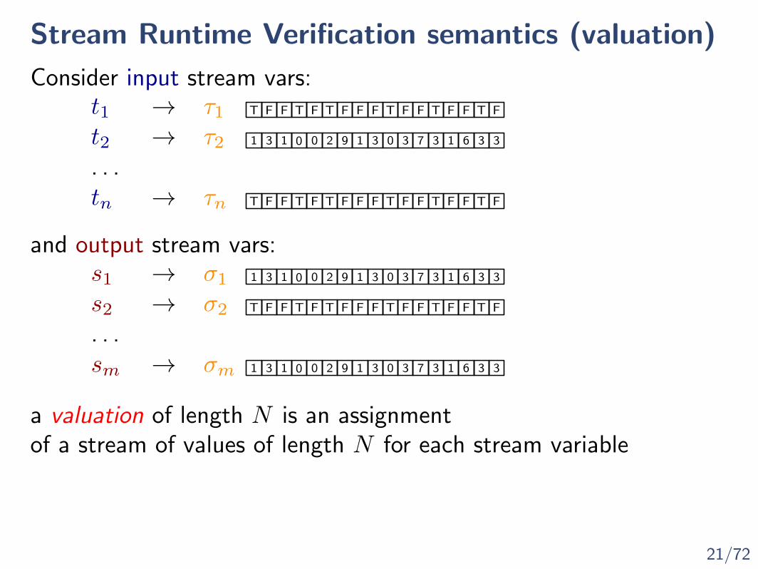
Consider input stream vars:
and output stream vars:
t1t2. . .tn
s1
s2
sm
. . .
a valuation of length N is an assignmentof a stream of values of length N for each stream variable
→ τ1→ τ2
→ τn
→ σ1
→ σ2
→ σm
T T T T T TF F F F F F F F F F F
1 1 1 13 2 33 30 0 9 0 7 3 6 3
T T T T T TF F F F F F F F F F F
T T T T T TF F F F F F F F F F F
1 1 1 13 2 33 30 0 9 0 7 3 6 3
1 1 1 13 2 33 30 0 9 0 7 3 6 3

21/72
Stream Runtime Verification semantics (valuation)
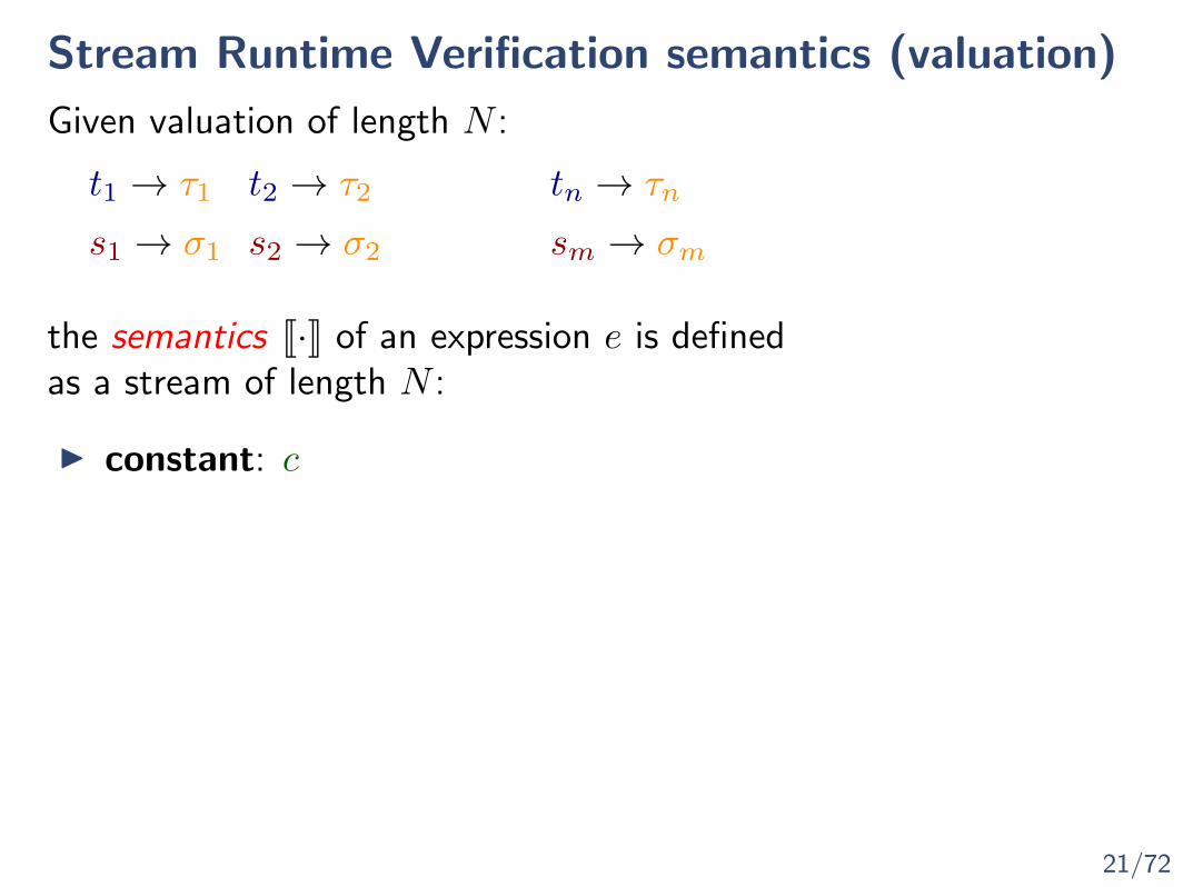
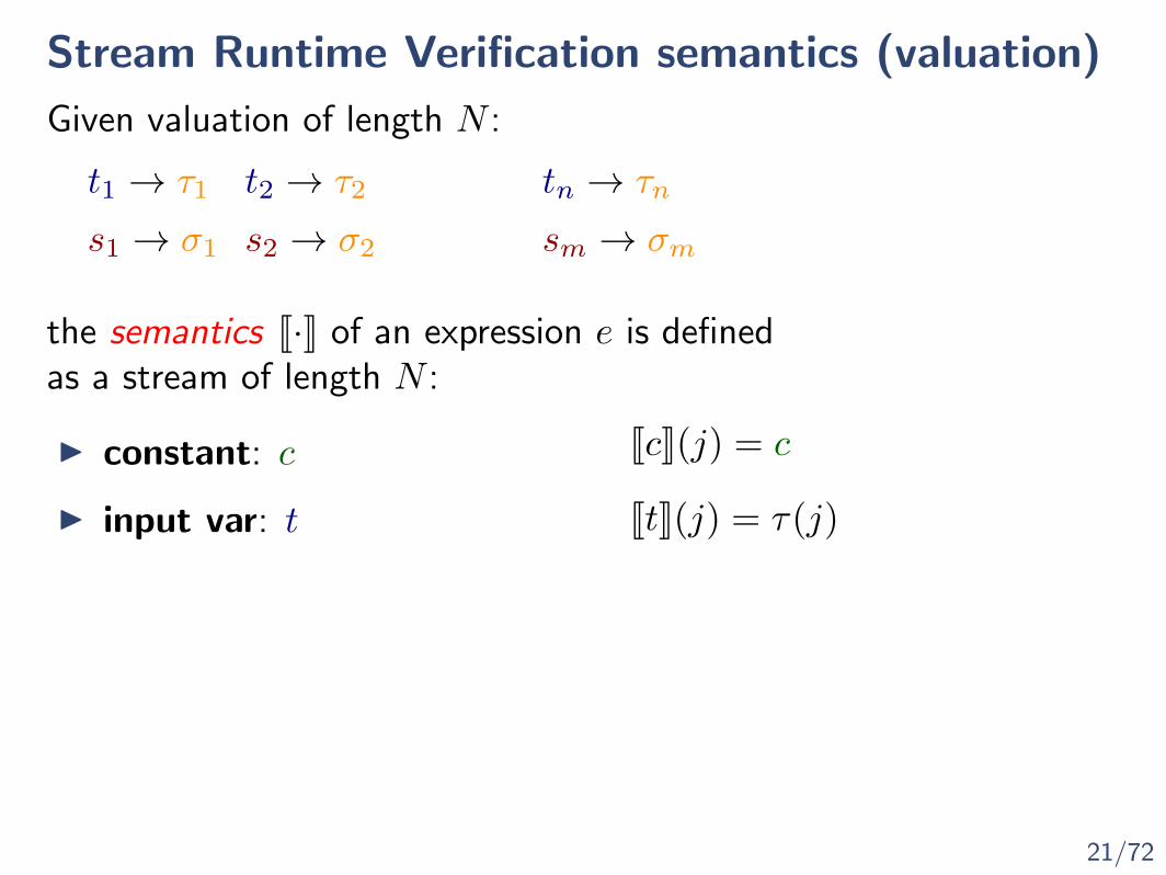
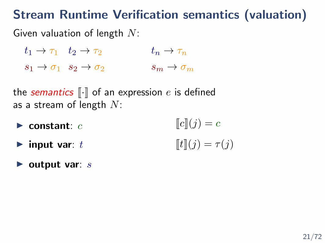
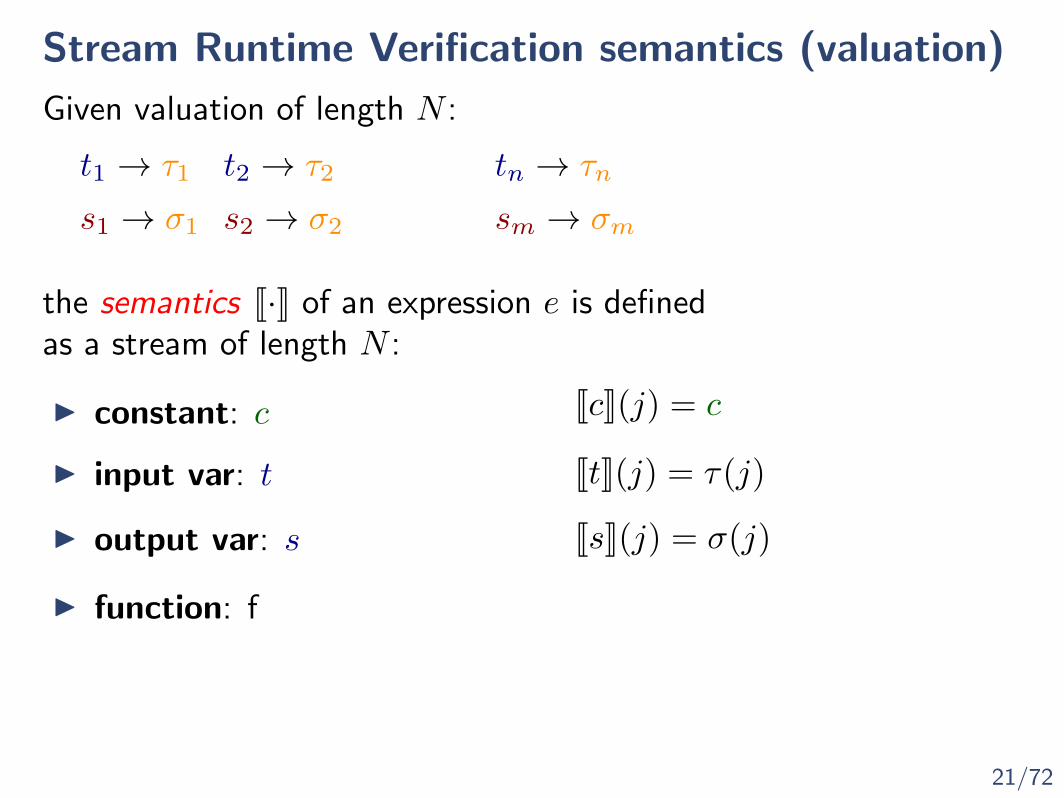
Given valuation of length N :
t1 → τ1 t2 → τ2 tn → τn
s1 → σ1 s2 → σ2 sm → σm
the semantics J·K of an expression e is definedas a stream of length N :
21/72
Stream Runtime Verification semantics (valuation)
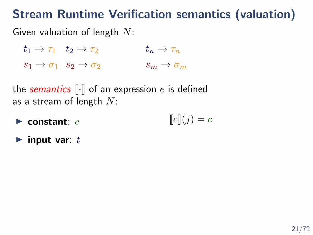
Given valuation of length N :
t1 → τ1 t2 → τ2 tn → τn
s1 → σ1 s2 → σ2 sm → σm
the semantics J·K of an expression e is definedas a stream of length N :
I constant: c

21/72
Stream Runtime Verification semantics (valuation)
Given valuation of length N :
t1 → τ1 t2 → τ2 tn → τn
s1 → σ1 s2 → σ2 sm → σm
the semantics J·K of an expression e is definedas a stream of length N :
I constant: c JcK(j) = c
21/72
Stream Runtime Verification semantics (valuation)
Given valuation of length N :
t1 → τ1 t2 → τ2 tn → τn
s1 → σ1 s2 → σ2 sm → σm
the semantics J·K of an expression e is definedas a stream of length N :
I constant: c
I input var: t
JcK(j) = c
21/72
Stream Runtime Verification semantics (valuation)
Given valuation of length N :
t1 → τ1 t2 → τ2 tn → τn
s1 → σ1 s2 → σ2 sm → σm
the semantics J·K of an expression e is definedas a stream of length N :
I constant: c
I input var: t
JcK(j) = c
JtK(j) = τ(j)
21/72
Stream Runtime Verification semantics (valuation)
Given valuation of length N :
t1 → τ1 t2 → τ2 tn → τn
s1 → σ1 s2 → σ2 sm → σm
the semantics J·K of an expression e is definedas a stream of length N :
I constant: c
I input var: t
JcK(j) = c
JtK(j) = τ(j)
I output var: s

21/72
Stream Runtime Verification semantics (valuation)
Given valuation of length N :
t1 → τ1 t2 → τ2 tn → τn
s1 → σ1 s2 → σ2 sm → σm
the semantics J·K of an expression e is definedas a stream of length N :
I constant: c
I input var: t
JcK(j) = c
JtK(j) = τ(j)
I output var: s JsK(j) = σ(j)
21/72
Stream Runtime Verification semantics (valuation)
Given valuation of length N :
t1 → τ1 t2 → τ2 tn → τn
s1 → σ1 s2 → σ2 sm → σm
the semantics J·K of an expression e is definedas a stream of length N :
I constant: c
I input var: t
I function: f
JcK(j) = c
JtK(j) = τ(j)
I output var: s JsK(j) = σ(j)
Jf(e1, . . . , ek)K(j) = f(Je1K(j), . . . , JekK(j))

21/72
Stream Runtime Verification semantics (valuation)
Given valuation of length N :
t1 → τ1 t2 → τ2 tn → τn
s1 → σ1 s2 → σ2 sm → σm
the semantics J·K of an expression e is definedas a stream of length N :
I constant: c
I input var: t
I function: f
I shift s[k, d](j)
JcK(j) = c
JtK(j) = τ(j)
I output var: s JsK(j) = σ(j)
Jf(e1, . . . , ek)K(j) = f(Je1K(j), . . . , JekK(j))
Js[k, d]K(j) =
{σ(j + k) if 1 ≤ j + k ≤ Nd otherwise
22/72
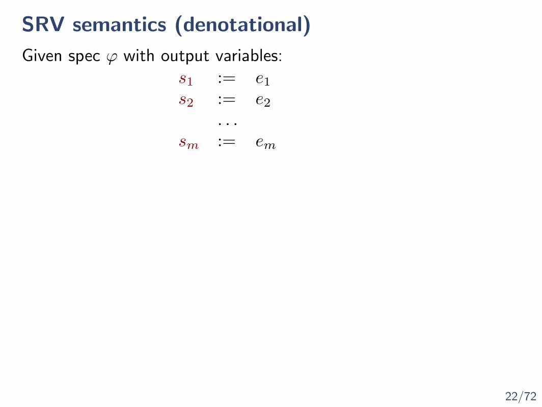
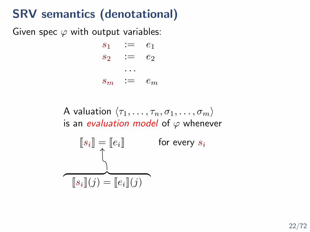
SRV semantics (denotational)
Given spec ϕ with output variables:s1 := e1
s2 := e2
. . .sm := em

22/72
SRV semantics (denotational)
Given spec ϕ with output variables:s1 := e1
s2 := e2
. . .sm := em
JsiK = JeiK for every si
A valuation 〈τ1, . . . , τn, σ1, . . . , σm〉is an evaluation model of ϕ whenever
22/72
SRV semantics (denotational)
Given spec ϕ with output variables:s1 := e1
s2 := e2
. . .sm := em
JsiK = JeiK for every si
A valuation 〈τ1, . . . , τn, σ1, . . . , σm〉is an evaluation model of ϕ whenever
︷ ︸︸ ︷JsiK(j) = JeiK(j)

22/72
SRV semantics (denotational)
Given spec ϕ with output variables:s1 := e1
s2 := e2
. . .sm := em
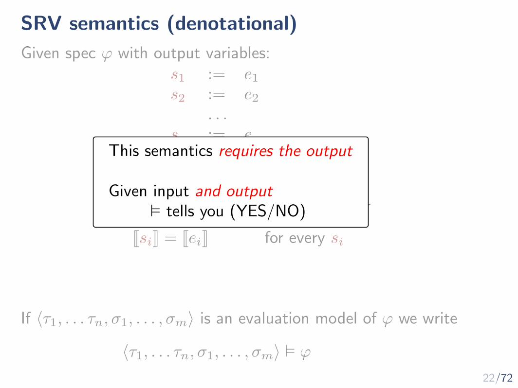
If 〈τ1, . . . τn, σ1, . . . , σm〉 is an evaluation model of ϕ we write
JsiK = JeiK for every si
A valuation 〈τ1, . . . , τn, σ1, . . . , σm〉is an evaluation model of ϕ whenever
〈τ1, . . . τn, σ1, . . . , σm〉 � ϕ
22/72
SRV semantics (denotational)
Given spec ϕ with output variables:s1 := e1
s2 := e2
. . .sm := em
If 〈τ1, . . . τn, σ1, . . . , σm〉 is an evaluation model of ϕ we write
JsiK = JeiK for every si
A valuation 〈τ1, . . . , τn, σ1, . . . , σm〉is an evaluation model of ϕ whenever
〈τ1, . . . τn, σ1, . . . , σm〉 � ϕ
This semantics requires the output
Given input and output� tells you (YES/NO)
23/72
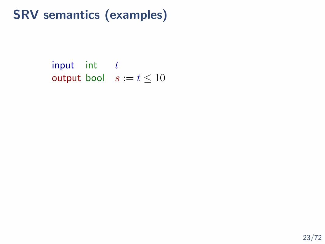
SRV semantics (examples)
input int toutput bool s := t ≤ 10

23/72
SRV semantics (examples)
input int toutput bool s := t ≤ 10
For τ : 1 2 3 4 5 6 7 8 9 10 11 12
σ : T T T T T T T T T F FT
〈τ , σ〉 � ϕ

23/72
SRV semantics (examples)
input int toutput bool s := t ≤ 10
For τ : 1 2 3 4 5 6 7 8 9 10 11 12
σ : T T T T T T T T T F FT
〈τ , σ〉 � ϕ
In fact, σ is the only output for τ
23/72
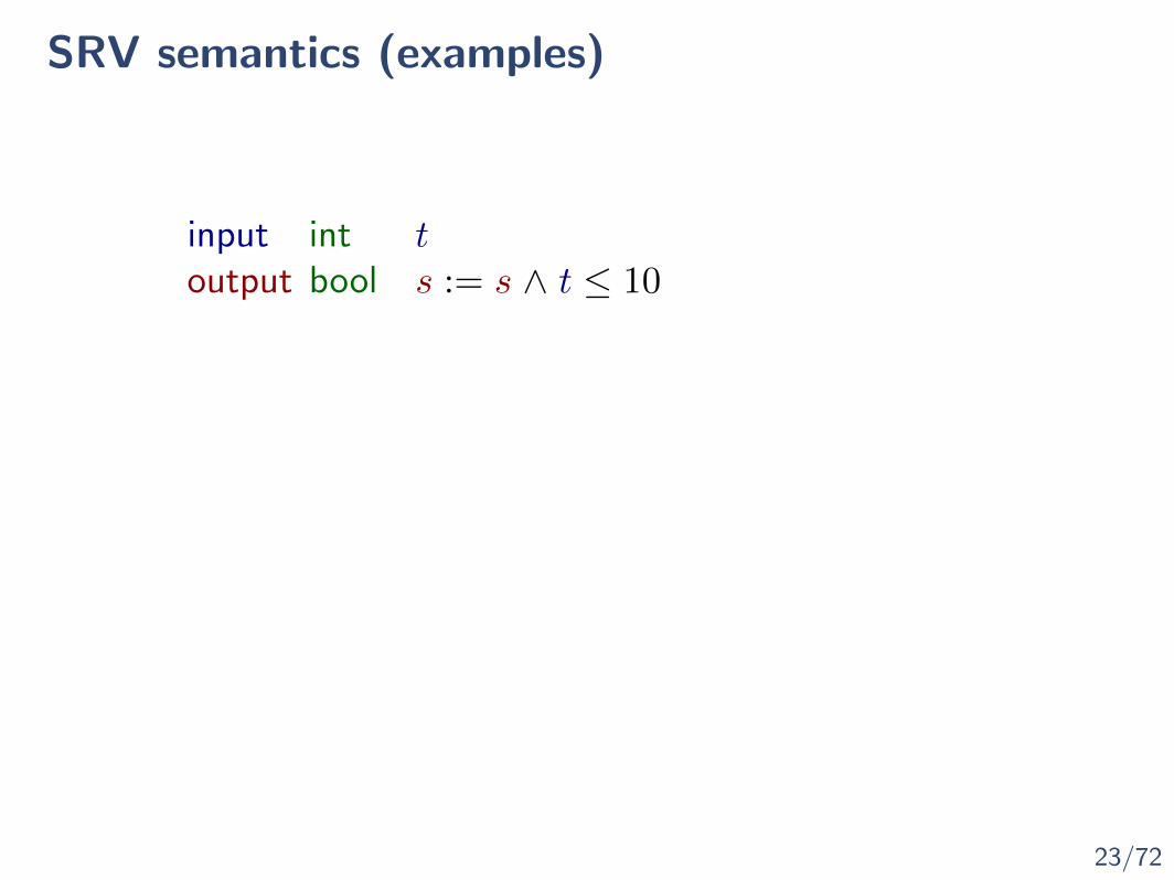
SRV semantics (examples)
input int toutput bool s := s ∧ t ≤ 10

23/72
SRV semantics (examples)
input int toutput bool s := s ∧ t ≤ 10
For τ : 1 2 3 4 5 6 7 8 9 10 11 12
σ : T T T T T T T T T F FT
〈τ , σ〉 � ϕ

23/72
SRV semantics (examples)
input int toutput bool s := s ∧ t ≤ 10
For τ : 1 2 3 4 5 6 7 8 9 10 11 12
σ : T T T T T T T T T F FT
〈τ , σ〉 � ϕ
σ′ : F FF FF FF F F F F F
〈τ , σ′〉 � ϕ
BUT
23/72
SRV semantics (examples)
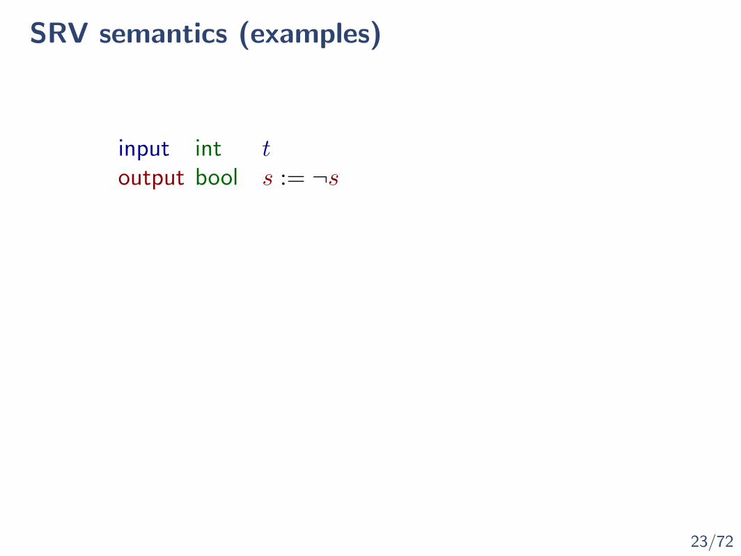
input int toutput bool s := ¬s

23/72
SRV semantics (examples)
input int toutput bool s := ¬s
For τ : 1 2 3 4 5 6 7 8 9 10 11 12
〈τ , σ〉 � ϕ
There is no σ with

24/72
Well-defined specifications
24/72
Well-defined specifications
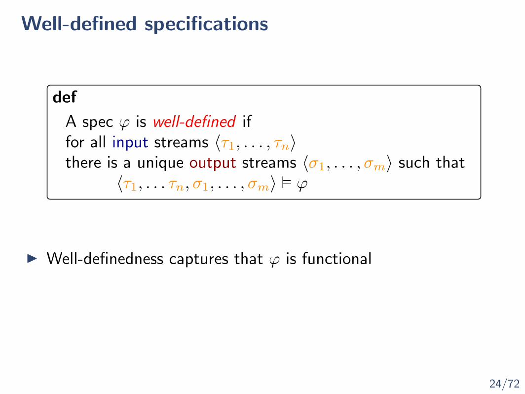
I Well-definedness captures that ϕ is functional
A spec ϕ is well-defined iffor all input streams 〈τ1, . . . , τn〉there is a unique output streams 〈σ1, . . . , σm〉 such that
〈τ1, . . . τn, σ1, . . . , σm〉 � ϕ
def

24/72
Well-defined specifications
I Well-definedness captures that ϕ is functional
I . . . but it is a semantic condition
(hard or even impossible to check)
A spec ϕ is well-defined iffor all input streams 〈τ1, . . . , τn〉there is a unique output streams 〈σ1, . . . , σm〉 such that
〈τ1, . . . τn, σ1, . . . , σm〉 � ϕ
def

25/72
Dependency graph
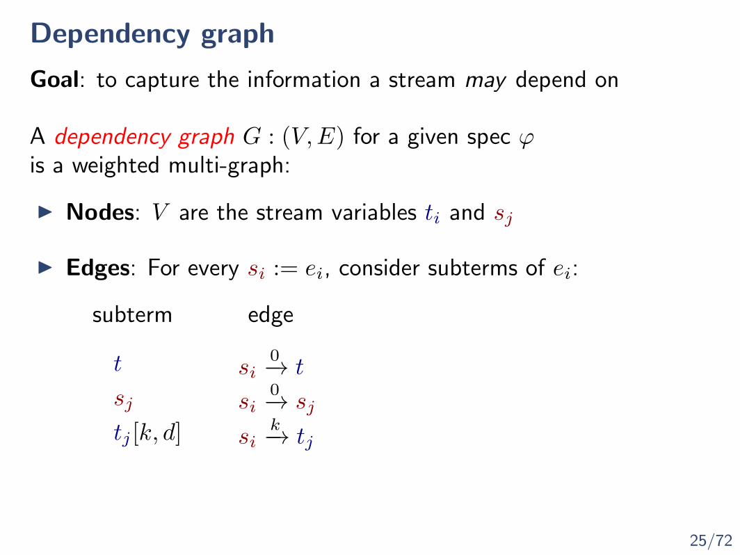
Goal: to capture the information a stream may depend on
25/72
Dependency graph
A dependency graph G : (V,E) for a given spec ϕis a weighted multi-graph:
Goal: to capture the information a stream may depend on
25/72
Dependency graph
A dependency graph G : (V,E) for a given spec ϕis a weighted multi-graph:
I Nodes: V are the stream variables ti and sj
Goal: to capture the information a stream may depend on

25/72
Dependency graph
A dependency graph G : (V,E) for a given spec ϕis a weighted multi-graph:
I Nodes: V are the stream variables ti and sj
I Edges: For every si := ei, consider subterms of ei:
subterm edge
Goal: to capture the information a stream may depend on

25/72
Dependency graph
A dependency graph G : (V,E) for a given spec ϕis a weighted multi-graph:
I Nodes: V are the stream variables ti and sj
I Edges: For every si := ei, consider subterms of ei:
t si0−→ t
subterm edge
Goal: to capture the information a stream may depend on

25/72
Dependency graph
A dependency graph G : (V,E) for a given spec ϕis a weighted multi-graph:
I Nodes: V are the stream variables ti and sj
I Edges: For every si := ei, consider subterms of ei:
t si0−→ t
sj si0−→ sj
subterm edge
Goal: to capture the information a stream may depend on
25/72
Dependency graph
A dependency graph G : (V,E) for a given spec ϕis a weighted multi-graph:
I Nodes: V are the stream variables ti and sj
I Edges: For every si := ei, consider subterms of ei:
t si0−→ t
sj si0−→ sj
tj [k, d] sik−→ tj
subterm edge
Goal: to capture the information a stream may depend on

25/72
Dependency graph
A dependency graph G : (V,E) for a given spec ϕis a weighted multi-graph:
I Nodes: V are the stream variables ti and sj
I Edges: For every si := ei, consider subterms of ei:
t si0−→ t
sj si0−→ sj
sj [k, d] sik−→ sj
tj [k, d] sik−→ tj
subterm edge
Goal: to capture the information a stream may depend on
26/72
Dependency graph (examples)
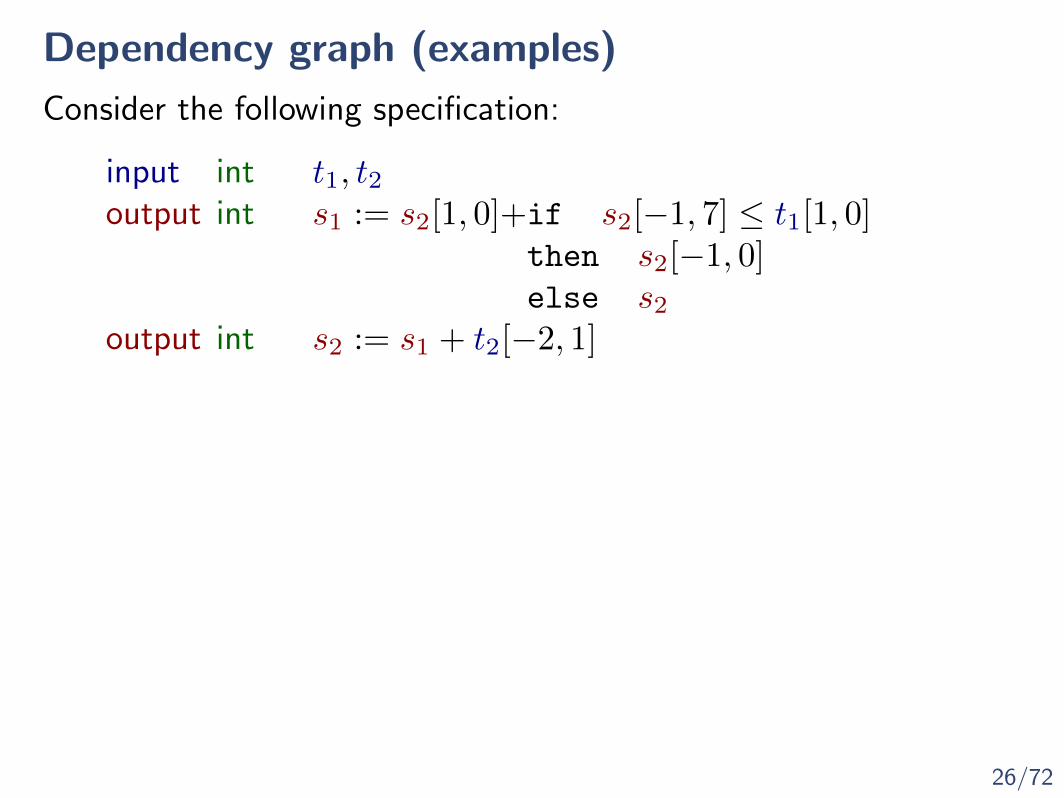
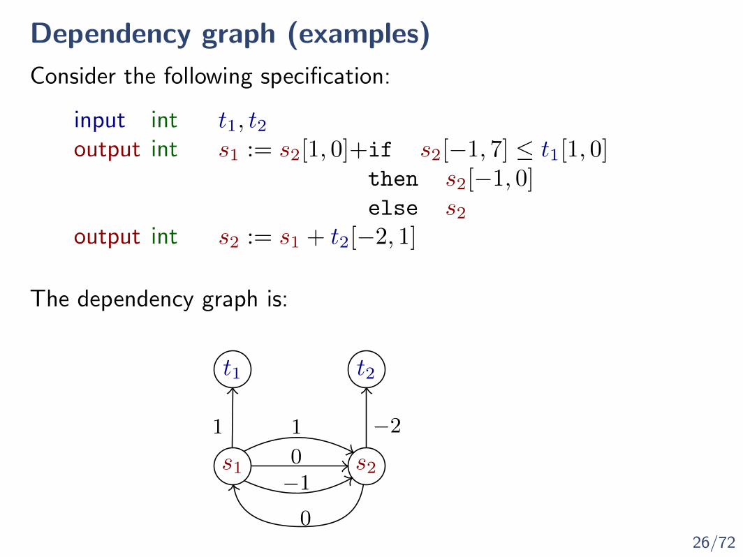
Consider the following specification:
input int t1, t2output int s1 := s2[1, 0]+if s2[−1, 7] ≤ t1[1, 0]
then s2[−1, 0]else s2
output int s2 := s1 + t2[−2, 1]
26/72
Dependency graph (examples)
Consider the following specification:
input int t1, t2output int s1 := s2[1, 0]+if s2[−1, 7] ≤ t1[1, 0]
then s2[−1, 0]else s2
output int s2 := s1 + t2[−2, 1]
The dependency graph is:
t1 t2
s1 s2
1
0
1
−10
−2

27/72
Well-formed specifications
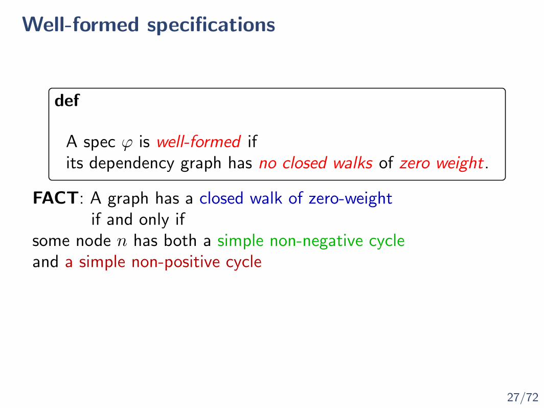
def
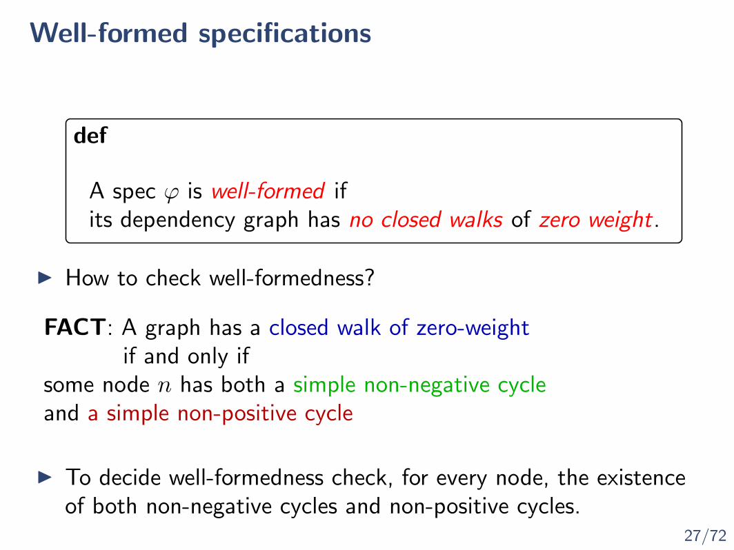
A spec ϕ is well-formed ifits dependency graph has no closed walks of zero weight.

27/72
Well-formed specifications
I How to check well-formedness?
def
A spec ϕ is well-formed ifits dependency graph has no closed walks of zero weight.

27/72
Well-formed specifications
I How to check well-formedness?
def
A spec ϕ is well-formed ifits dependency graph has no closed walks of zero weight.
FACT: A graph has a closed walk of zero-weightif and only if
some node n has both a simple non-negative cycleand a simple non-positive cycle
27/72
Well-formed specifications
I How to check well-formedness?
def
A spec ϕ is well-formed ifits dependency graph has no closed walks of zero weight.
FACT: A graph has a closed walk of zero-weightif and only if
some node n has both a simple non-negative cycleand a simple non-positive cycle
I To decide well-formedness check, for every node, the existenceof both non-negative cycles and non-positive cycles.
27/72
Well-formed specifications
def
A spec ϕ is well-formed ifits dependency graph has no closed walks of zero weight.
FACT: A graph has a closed walk of zero-weightif and only if
some node n has both a simple non-negative cycleand a simple non-positive cycle

27/72
Well-formed specifications
def
A spec ϕ is well-formed ifits dependency graph has no closed walks of zero weight.
FACT: A graph has a closed walk of zero-weightif and only if
some node n has both a simple non-negative cycleand a simple non-positive cycle
FACT: Let G be dependency graph of a well-formed spec andlet S be a strongly connected component of G. Then, eitherI all the simple cycles in S are strictly positive orI all the simple cycles in S are strictly negative

28/72
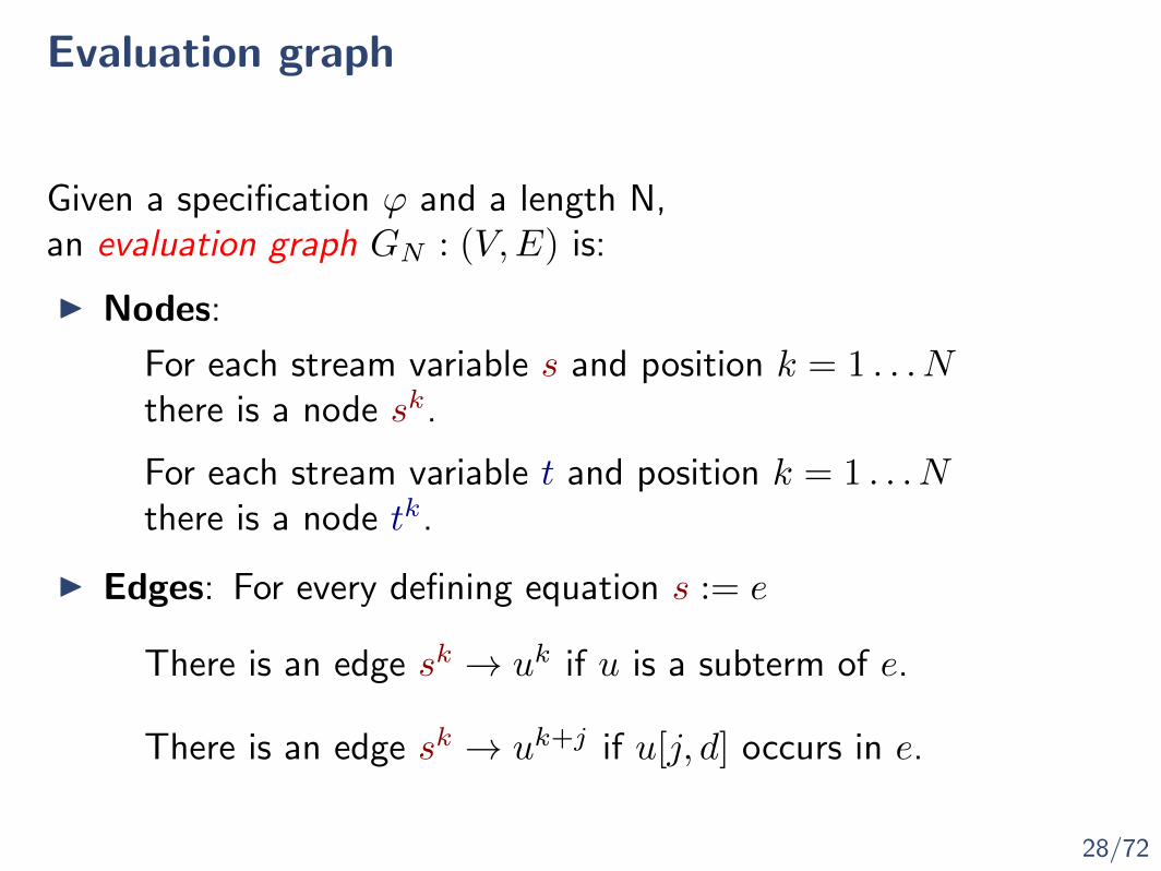
Evaluation graph
Given a specification ϕ and a length N,an evaluation graph GN : (V,E) is:

28/72
Evaluation graph
Given a specification ϕ and a length N,an evaluation graph GN : (V,E) is:
I Nodes:
I Edges:
28/72
Evaluation graph
Given a specification ϕ and a length N,an evaluation graph GN : (V,E) is:
I Nodes:
I Edges:
For each stream variable t and position k = 1 . . . Nthere is a node tk.
For each stream variable s and position k = 1 . . . Nthere is a node sk.
28/72
Evaluation graph
Given a specification ϕ and a length N,an evaluation graph GN : (V,E) is:
I Nodes:
I Edges:
For each stream variable t and position k = 1 . . . Nthere is a node tk.
For each stream variable s and position k = 1 . . . Nthere is a node sk.
There is an edge sk → uk if u is a subterm of e.
There is an edge sk → uk+j if u[j, d] occurs in e.
For every defining equation s := e
29/72
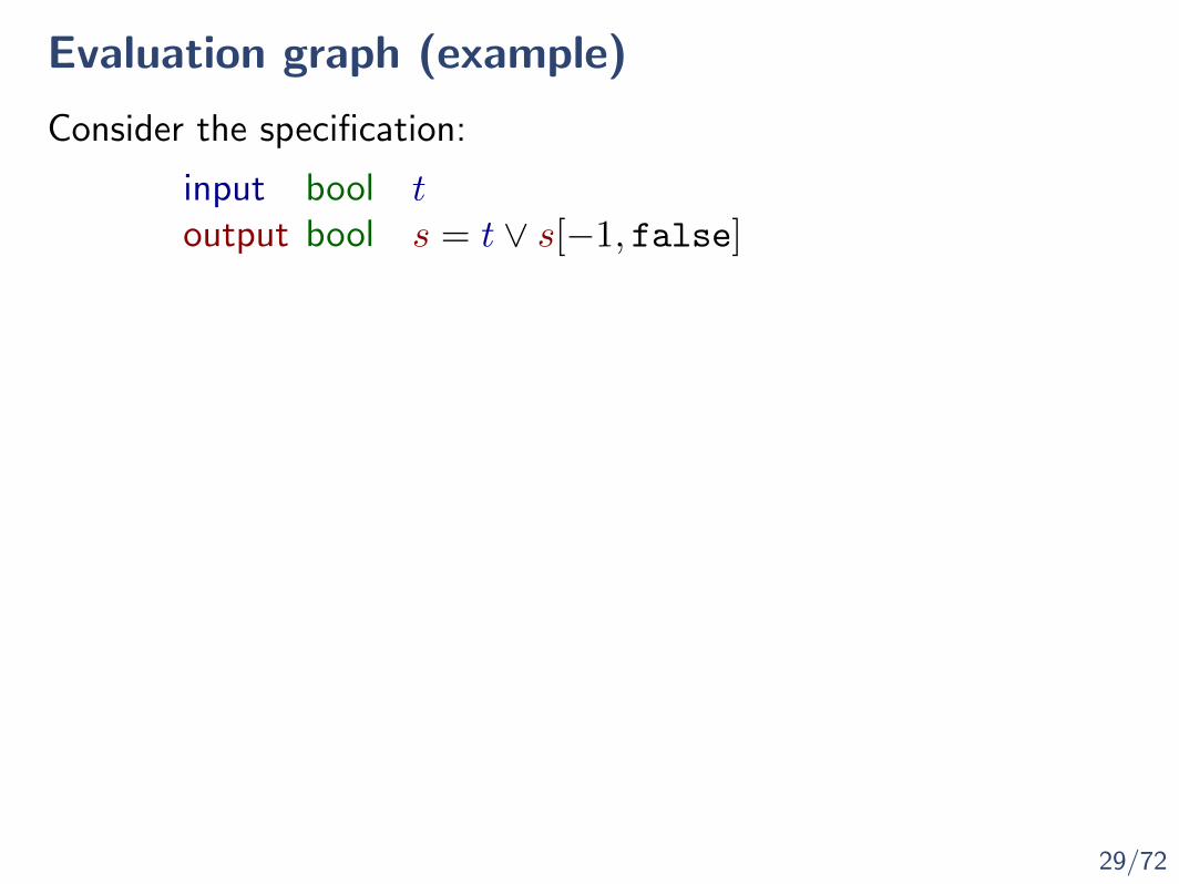
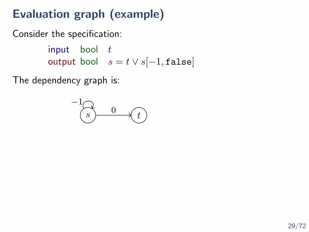
Evaluation graph (example)
input bool toutput bool s = t ∨ s[−1, false]
Consider the specification:
29/72
Evaluation graph (example)
input bool toutput bool s = t ∨ s[−1, false]
Consider the specification:
The dependency graph is:
s t0
−1
29/72
Evaluation graph (example)
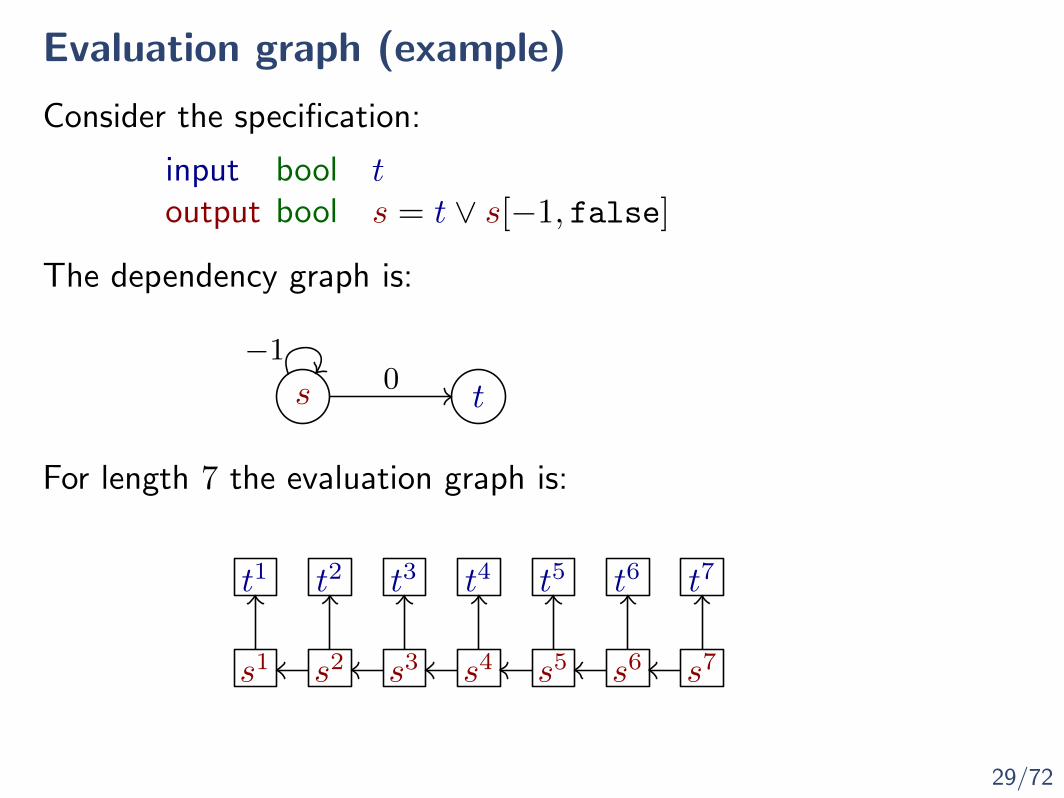
input bool toutput bool s = t ∨ s[−1, false]
s1 s2 s3 s4 s5 s6 s7
Consider the specification:
The dependency graph is:
s t0
−1
t1 t2 t3 t4 t5 t6 t7
For length 7 the evaluation graph is:
30/72
Evaluation graph and dependency graph
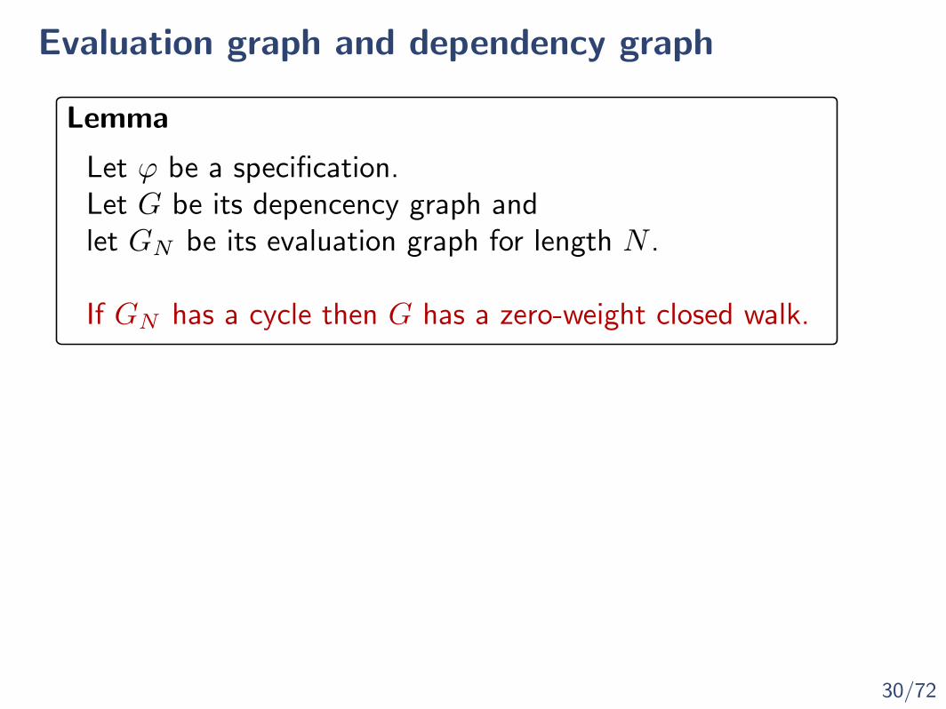
Lemma
Let ϕ be a specification.Let G be its depencency graph andlet GN be its evaluation graph for length N .
If GN has a cycle then G has a zero-weight closed walk.
30/72
Evaluation graph and dependency graph
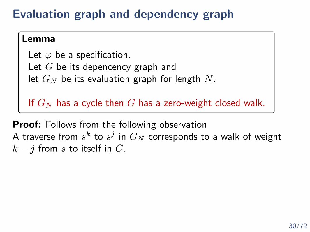
Proof: Follows from the following observationA traverse from sk to sj in GN corresponds to a walk of weightk − j from s to itself in G.
Lemma
Let ϕ be a specification.Let G be its depencency graph andlet GN be its evaluation graph for length N .
If GN has a cycle then G has a zero-weight closed walk.

30/72
Evaluation graph and dependency graph
Corollary
If G is well-formed, then for every N , GN has no cycles.
Lemma
Let ϕ be a specification.Let G be its depencency graph andlet GN be its evaluation graph for length N .
If GN has a cycle then G has a zero-weight closed walk.

31/72
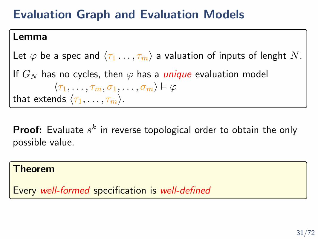
Evaluation Graph and Evaluation Models
Let ϕ be a spec and 〈τ1 . . . , τm〉 a valuation of inputs of lenght N .
If GN has no cycles, then ϕ has a unique evaluation model〈τ1, . . . , τm, σ1, . . . , σm〉 � ϕ
that extends 〈τ1, . . . , τm〉.
Lemma
31/72
Evaluation Graph and Evaluation Models
Let ϕ be a spec and 〈τ1 . . . , τm〉 a valuation of inputs of lenght N .
If GN has no cycles, then ϕ has a unique evaluation model〈τ1, . . . , τm, σ1, . . . , σm〉 � ϕ
that extends 〈τ1, . . . , τm〉.
Lemma
Proof: Evaluate sk in reverse topological order to obtain the onlypossible value.
Theorem
Every well-formed specification is well-defined
32/72
Wellformed and welldefined
Theorem
Every well-formed specification is well-defined

32/72
Wellformed and welldefined
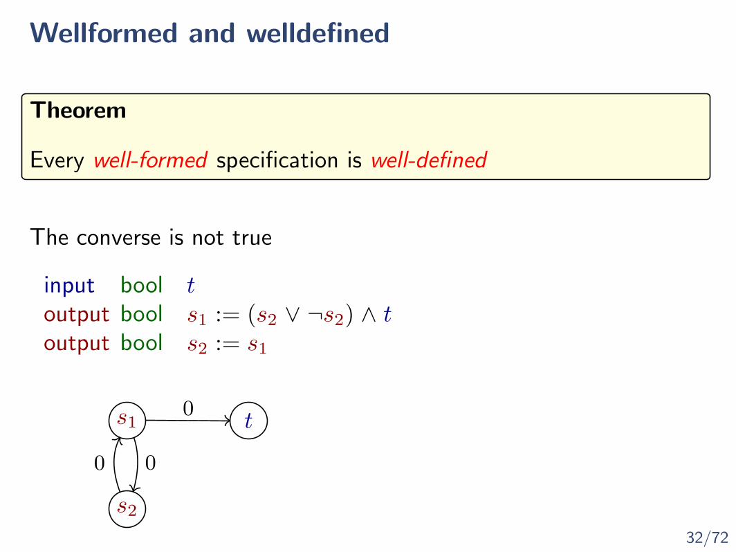
Theorem
Every well-formed specification is well-defined
The converse is not true

32/72
Wellformed and welldefined
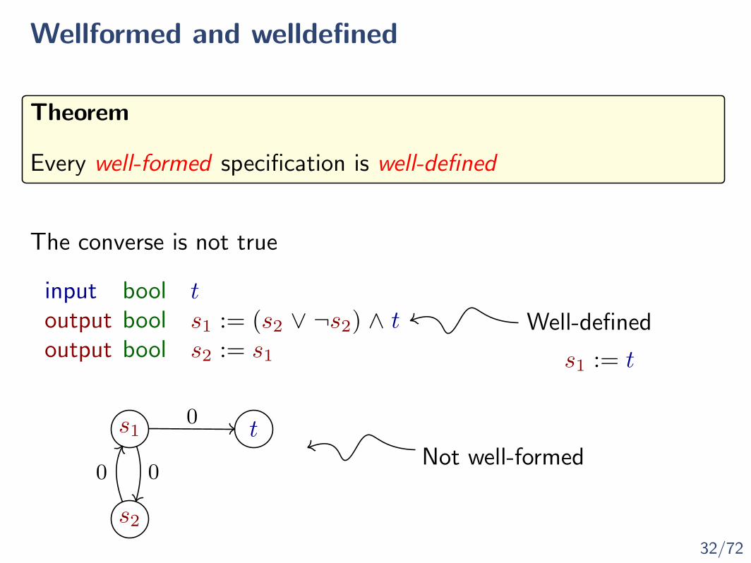
Theorem
Every well-formed specification is well-defined
The converse is not true
input bool toutput bool s1 := (s2 ∨ ¬s2) ∧ toutput bool s2 := s1
32/72
Wellformed and welldefined
Theorem
Every well-formed specification is well-defined
The converse is not true
input bool toutput bool s1 := (s2 ∨ ¬s2) ∧ toutput bool s2 := s1
s1 t0
s2
0 0
32/72
Wellformed and welldefined
Theorem
Every well-formed specification is well-defined
The converse is not true
input bool toutput bool s1 := (s2 ∨ ¬s2) ∧ toutput bool s2 := s1
s1 t0
s2
0 0
Well-defined
Not well-formed
s1 := t

33/72
Operational SemanticsOnline Runtime Verification

34/72
Operational semantics
The denotational semantics (well-definedness)only guarantee a single output per input.
. . . but how to compute this output?

35/72
Online algorithm
The algorithm will work on position variables ski
At position k, the algorithm will instantiatesi := ei into ski = eki , where
I ck → c
I f(a1, . . . , aj)k = f(ak1 , . . . , a
kj )
I si[j, d]k =
{d if j + k < 1
sj+ki
∣∣∣d
otherwise

36/72
Online algorithm
The algorithm maintains two storages:
I R: resolved equations {. . . tkj = c . . . ski = c′ . . .}
I U : unresolved equations {. . . ski = g . . .}
All position variables ski with known values are in R.
Position variables ski whose values are notcompletely determined yet are in U .
Initially: R is empty, U is empty

37/72
Online algorithm
At every step k:
1. add tki = τki to R for every input
2. add ski = ek to U for every dependent stream si
3. Repeat
substitute slj ← c in every eq in U if slj = c ∈ R,
apply functions f(c1, . . . , ck) if all arguments are constants
apply simplifiers
Until U does not change
if some eq in U becomes sli = c move to R

38/72
Online algorithm
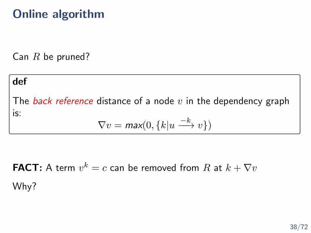
Can R be pruned?

38/72
Online algorithm
Can R be pruned?
def
The back reference distance of a node v in the dependency graphis:
∇v = max(0, {k|u −k−−→ v})
38/72
Online algorithm
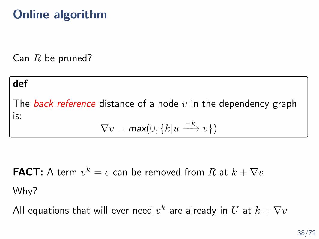
Can R be pruned?
def
The back reference distance of a node v in the dependency graphis:
∇v = max(0, {k|u −k−−→ v})
FACT: A term vk = c can be removed from R at k +∇v
Why?
38/72
Online algorithm
Can R be pruned?
def
The back reference distance of a node v in the dependency graphis:
∇v = max(0, {k|u −k−−→ v})
FACT: A term vk = c can be removed from R at k +∇v
All equations that will ever need vk are already in U at k +∇v
Why?

39/72
Online algorithm (example)
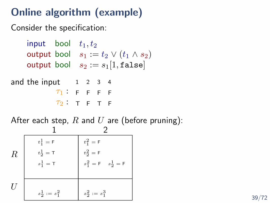
input bool t1, t2output bool s1 := t2 ∨ (t1 ∧ s2)output bool s2 := s1[1, false]
τ1 :1 2 3 4
Consider the specification:
and the input
τ2 :F F F F
T F T F

39/72
Online algorithm (example)
input bool t1, t2output bool s1 := t2 ∨ (t1 ∧ s2)output bool s2 := s1[1, false]
τ1 :1 2 3 4
Consider the specification:
and the input
τ2 :F F F F
T F T F
After each step, R and U are (before pruning):
R
U

39/72
Online algorithm (example)
input bool t1, t2output bool s1 := t2 ∨ (t1 ∧ s2)output bool s2 := s1[1, false]
τ1 :1 2 3 4
Consider the specification:
and the input
τ2 :F F F F
T F T F
After each step, R and U are (before pruning):
t11 = F
t12 = T
s11 = T
s12 := s21
R
U
1
39/72
Online algorithm (example)
input bool t1, t2output bool s1 := t2 ∨ (t1 ∧ s2)output bool s2 := s1[1, false]
τ1 :1 2 3 4
Consider the specification:
and the input
τ2 :F F F F
T F T F
After each step, R and U are (before pruning):
t11 = F
t12 = T
s11 = T
s12 := s21
R
U
1t21 = F
t22 = F
s21 = F
s22 := s31
2
s12 = F
t31 = F
t32 = T
3
s22 := s31
s31 := s32
s32 := s41

39/72
Online algorithm (example)
input bool t1, t2output bool s1 := t2 ∨ (t1 ∧ s2)output bool s2 := s1[1, false]
τ1 :1 2 3 4
Consider the specification:
and the input
τ2 :F F F F
T F T F
After each step, R and U are (before pruning):
t11 = F
t12 = T
s11 = T
s12 := s21
R
U
1t21 = F
t22 = F
s21 = F
s22 := s31
2
s12 = F
t31 = F
t32 = T
t41 = F
t42 = F
s42 = F
s41 = F
3 4s32 = F
s31 = F
s22 = F
s22 := s31
s31 := s32
s32 := s41

40/72
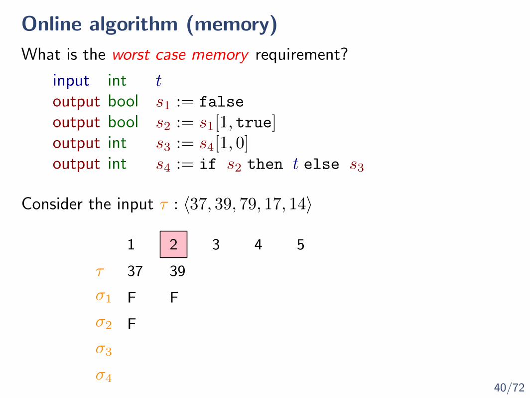
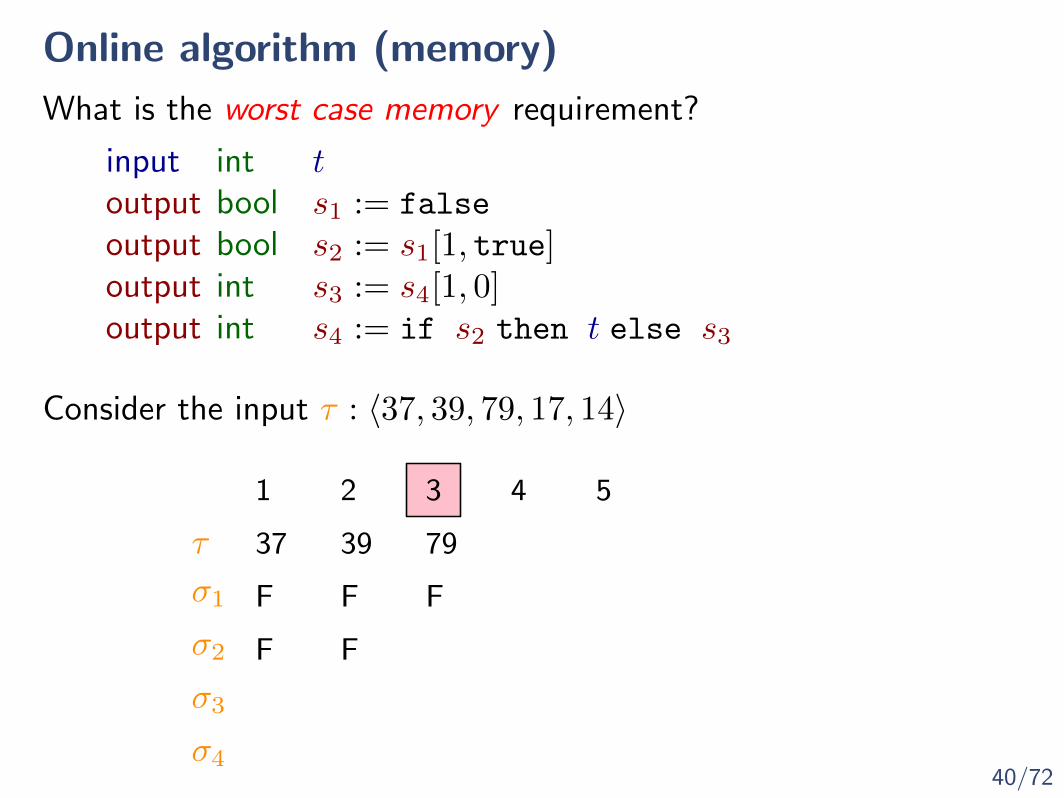
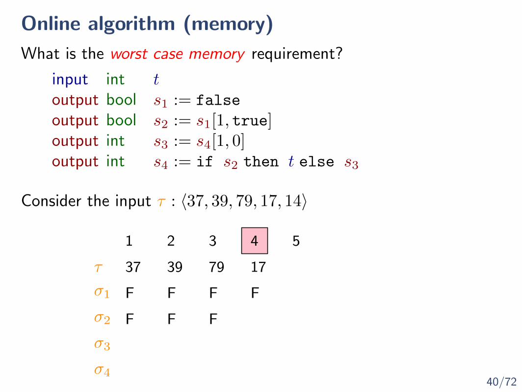
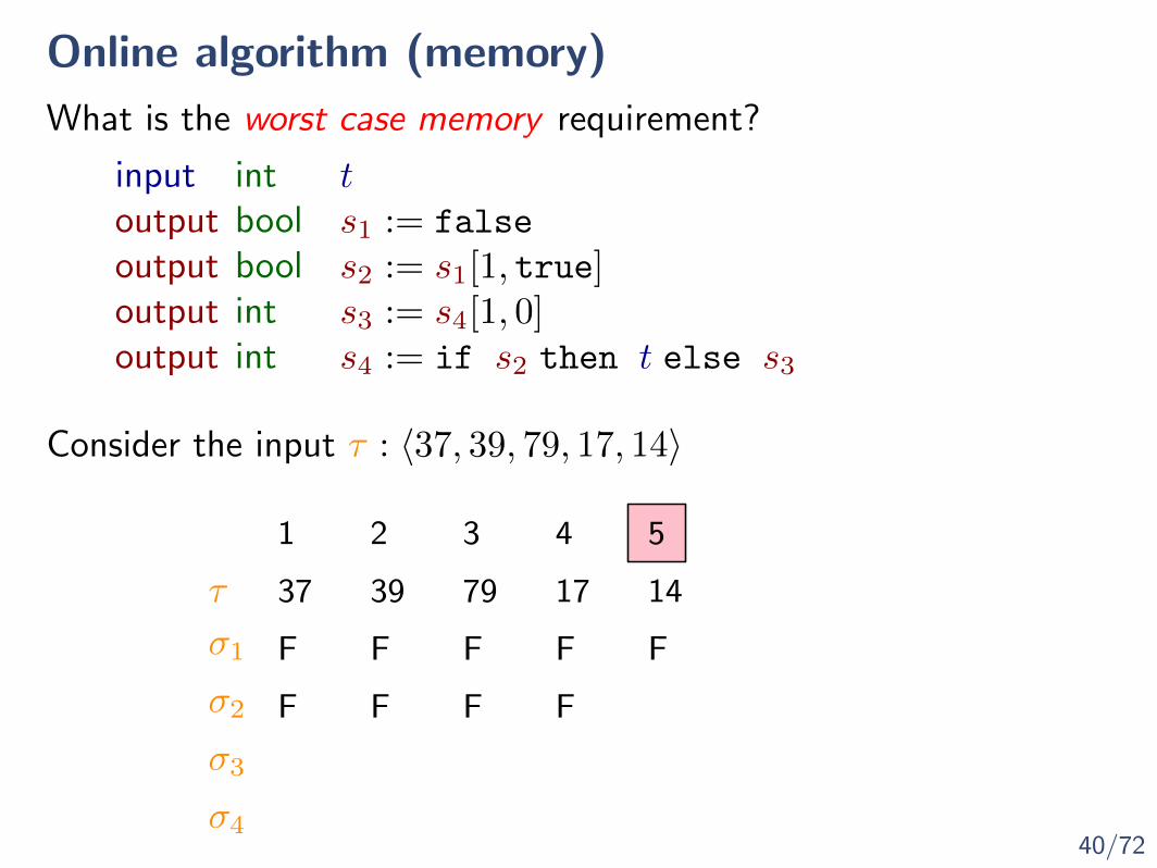
Online algorithm (memory)
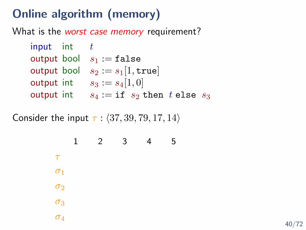
What is the worst case memory requirement?

40/72
Online algorithm (memory)
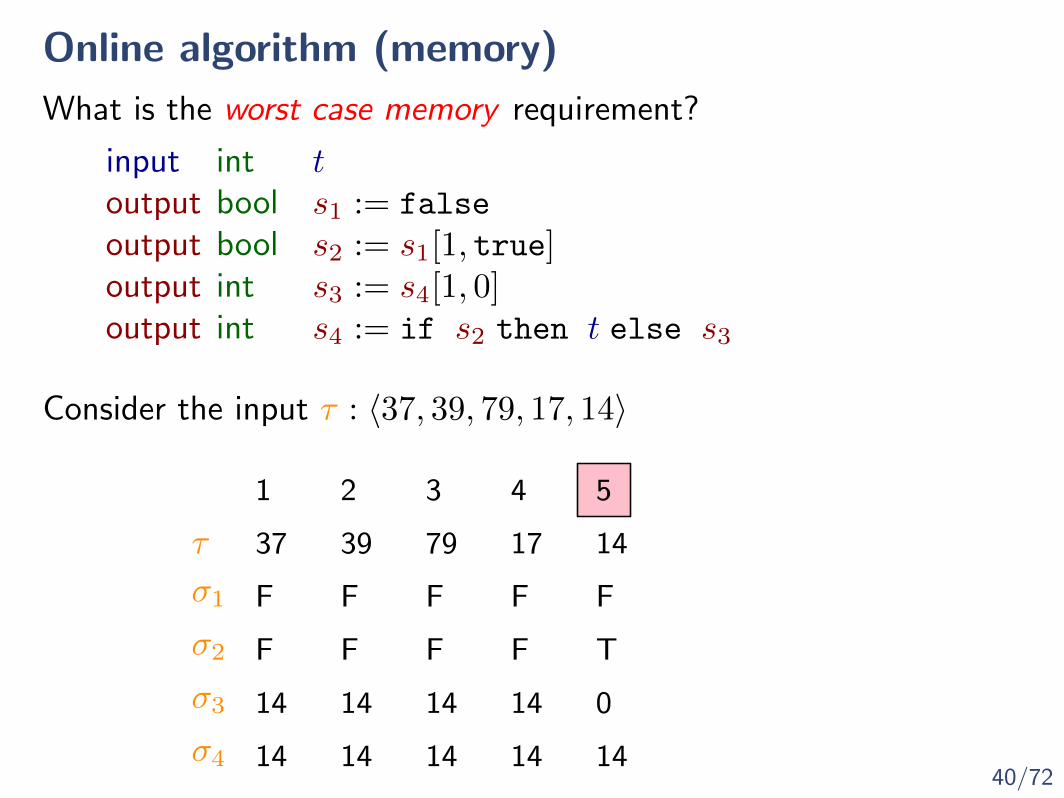
What is the worst case memory requirement?
input int toutput bool s1 := false
output bool s2 := s1[1, true]output int s3 := s4[1, 0]output int s4 := if s2 then t else s3
Consider the input τ : 〈37, 39, 79, 17, 14〉
40/72
Online algorithm (memory)
1
What is the worst case memory requirement?
input int toutput bool s1 := false
output bool s2 := s1[1, true]output int s3 := s4[1, 0]output int s4 := if s2 then t else s3
Consider the input τ : 〈37, 39, 79, 17, 14〉
τ
σ1
σ2
σ3
σ4
2 4 53

40/72
Online algorithm (memory)
1
What is the worst case memory requirement?
input int toutput bool s1 := false
output bool s2 := s1[1, true]output int s3 := s4[1, 0]output int s4 := if s2 then t else s3
Consider the input τ : 〈37, 39, 79, 17, 14〉
37
F
τ
σ1
σ2
σ3
σ4
2 4 53
40/72
Online algorithm (memory)
1
What is the worst case memory requirement?
input int toutput bool s1 := false
output bool s2 := s1[1, true]output int s3 := s4[1, 0]output int s4 := if s2 then t else s3
Consider the input τ : 〈37, 39, 79, 17, 14〉
37 39
F F
F
τ
σ1
σ2
σ3
σ4
2 4 53
40/72
Online algorithm (memory)
1
What is the worst case memory requirement?
input int toutput bool s1 := false
output bool s2 := s1[1, true]output int s3 := s4[1, 0]output int s4 := if s2 then t else s3
Consider the input τ : 〈37, 39, 79, 17, 14〉
37 39 79
F F
F F
F
τ
σ1
σ2
σ3
σ4
2 4 53
40/72
Online algorithm (memory)
1
What is the worst case memory requirement?
input int toutput bool s1 := false
output bool s2 := s1[1, true]output int s3 := s4[1, 0]output int s4 := if s2 then t else s3
Consider the input τ : 〈37, 39, 79, 17, 14〉
37 39 79 17
F F F
F F F
F
τ
σ1
σ2
σ3
σ4
2 4 53
40/72
Online algorithm (memory)
1
What is the worst case memory requirement?
input int toutput bool s1 := false
output bool s2 := s1[1, true]output int s3 := s4[1, 0]output int s4 := if s2 then t else s3
Consider the input τ : 〈37, 39, 79, 17, 14〉
37 39 79 17 14
F F F F
F F F F
F
τ
σ1
σ2
σ3
σ4
2 4 53
40/72
Online algorithm (memory)
1
What is the worst case memory requirement?
input int toutput bool s1 := false
output bool s2 := s1[1, true]output int s3 := s4[1, 0]output int s4 := if s2 then t else s3
Consider the input τ : 〈37, 39, 79, 17, 14〉
37 39 79 17 14
F F F F
F F F F T
14 14 14 14 0
14
F
14 14 14 14
τ
σ1
σ2
σ3
σ4
2 4 53
Memory required is linear in the size of the trace
41/72
Online algorithm (memory)
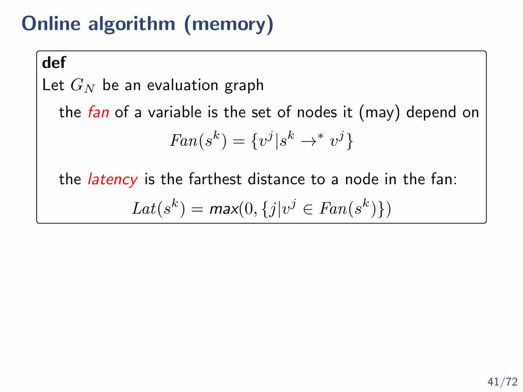
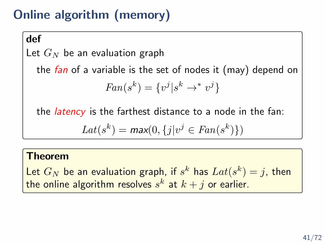
Let GN be an evaluation graph
Fan(sk) = {vj |sk →∗ vj}the fan of a variable is the set of nodes it (may) depend on
the latency is the farthest distance to a node in the fan:
Lat(sk) = max(0, {j|vj ∈ Fan(sk)})
def
41/72
Online algorithm (memory)
Theorem
Let GN be an evaluation graph, if sk has Lat(sk) = j, thenthe online algorithm resolves sk at k + j or earlier.
Let GN be an evaluation graph
Fan(sk) = {vj |sk →∗ vj}the fan of a variable is the set of nodes it (may) depend on
the latency is the farthest distance to a node in the fan:
Lat(sk) = max(0, {j|vj ∈ Fan(sk)})
def

42/72
Efficient monitorability
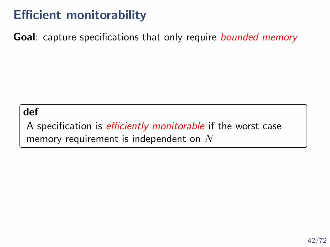
Goal: capture specifications that only require bounded memory
42/72
Efficient monitorability
Goal: capture specifications that only require bounded memory
A specification is efficiently monitorable if the worst casememory requirement is independent on N
def

43/72
Efficient monitorability (example)
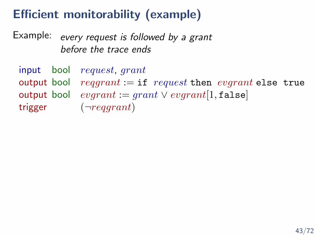
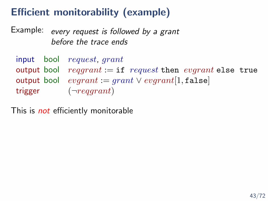
Example: every request is followed by a grantbefore the trace ends
43/72
Efficient monitorability (example)
Example: every request is followed by a grantbefore the trace ends
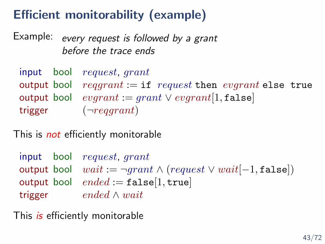
input bool request, grantoutput bool reqgrant := if request then evgrant else true
output bool evgrant := grant ∨ evgrant[1, false]trigger (¬reqgrant)
43/72
Efficient monitorability (example)
Example: every request is followed by a grantbefore the trace ends
input bool request, grantoutput bool reqgrant := if request then evgrant else true
output bool evgrant := grant ∨ evgrant[1, false]trigger (¬reqgrant)
This is not efficiently monitorable

43/72
Efficient monitorability (example)
Example: every request is followed by a grantbefore the trace ends
input bool request, grantoutput bool reqgrant := if request then evgrant else true
output bool evgrant := grant ∨ evgrant[1, false]trigger (¬reqgrant)
This is not efficiently monitorable
input bool request, grantoutput bool wait := ¬grant ∧ (request ∨ wait[−1, false])output bool ended := false[1, true]trigger ended ∧ wait
This is efficiently monitorable
44/72
Efficiently Monitorable
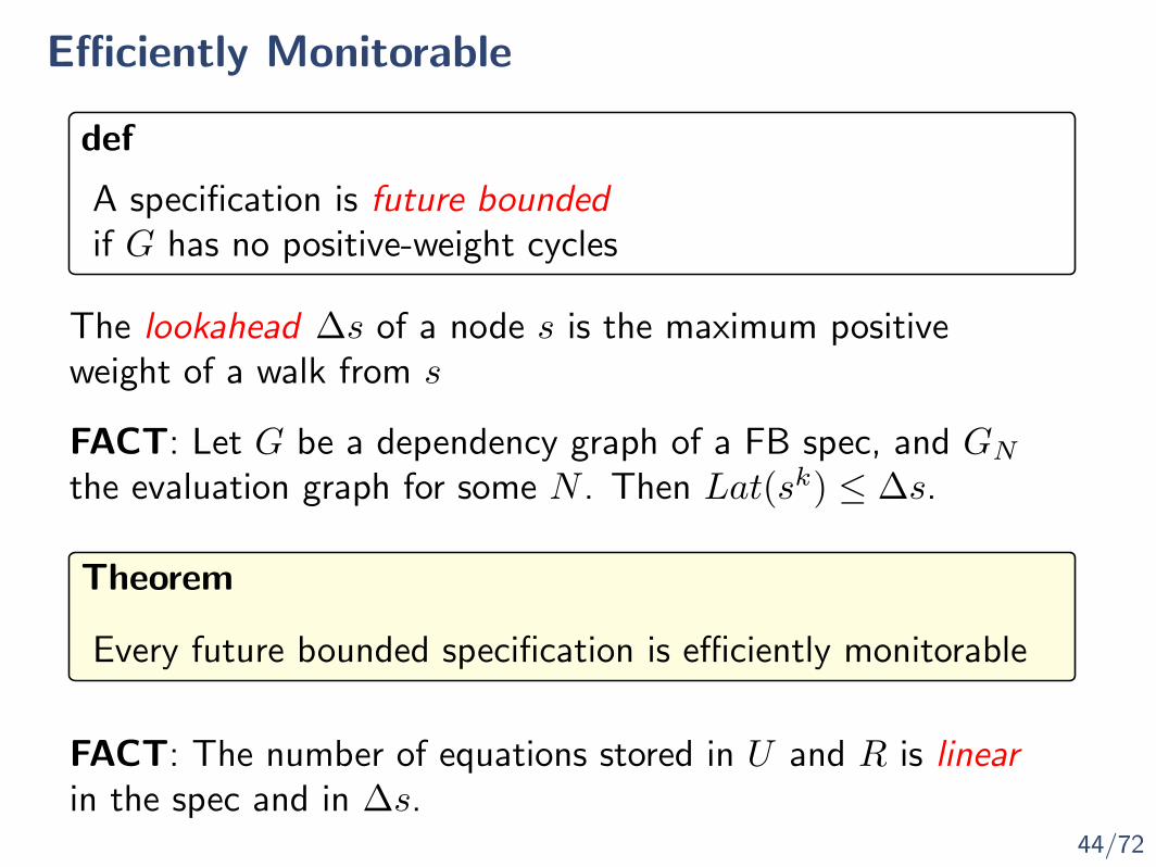
A specification is future boundedif G has no positive-weight cycles
def
Every future bounded specification is efficiently monitorable
Theorem
The lookahead ∆s of a node s is the maximum positiveweight of a walk from s
FACT: Let G be a dependency graph of a FB spec, and GNthe evaluation graph for some N . Then Lat(sk) ≤ ∆s.
FACT: The number of equations stored in U and R is linearin the spec and in ∆s.
45/72
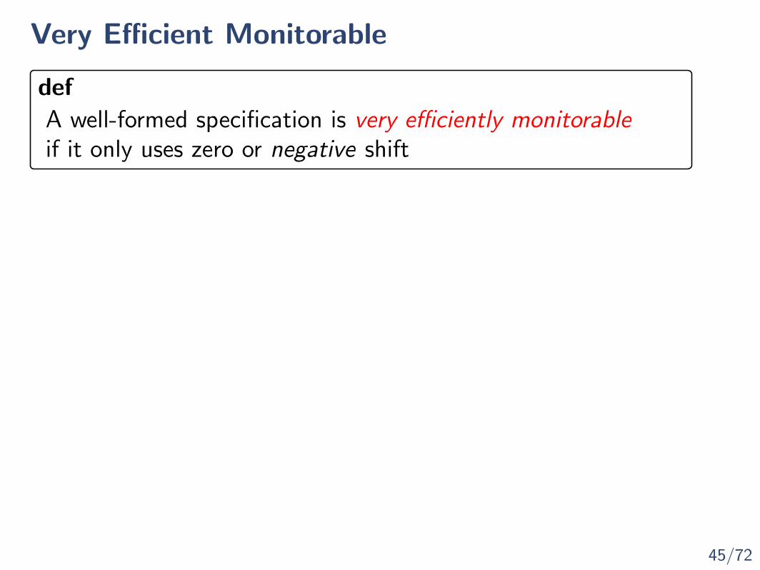
Very Efficient Monitorable
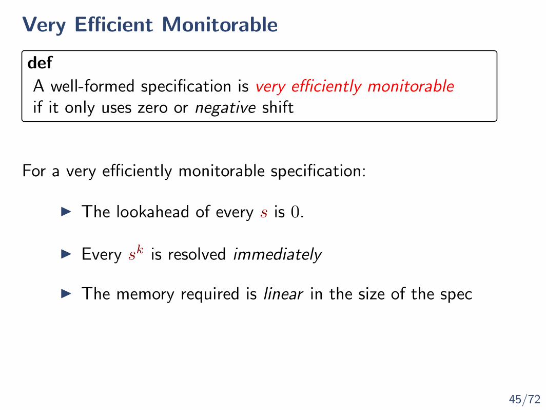
A well-formed specification is very efficiently monitorableif it only uses zero or negative shift
def
45/72
Very Efficient Monitorable
For a very efficiently monitorable specification:
I The lookahead of every s is 0.
I Every sk is resolved immediately
I The memory required is linear in the size of the spec
A well-formed specification is very efficiently monitorableif it only uses zero or negative shift
def
46/72
Operational SemanticsOffline Runtime Verification
47/72
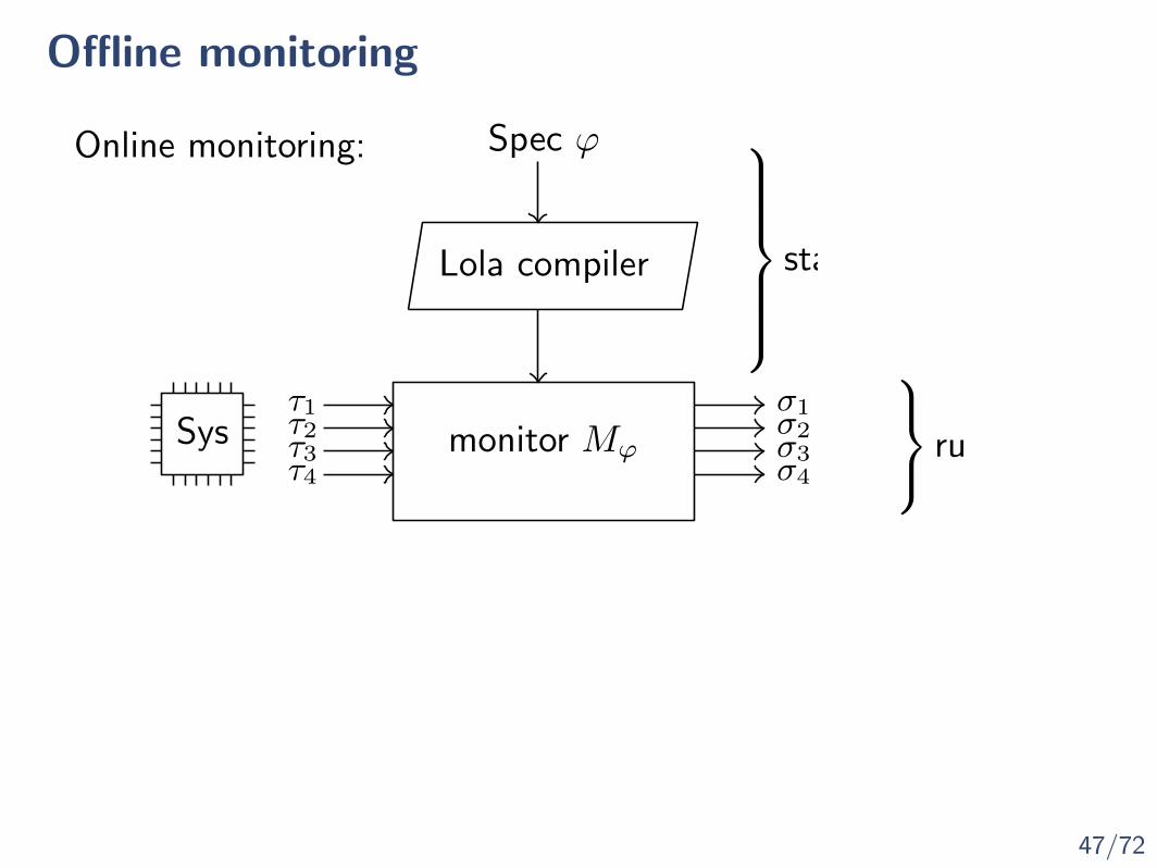
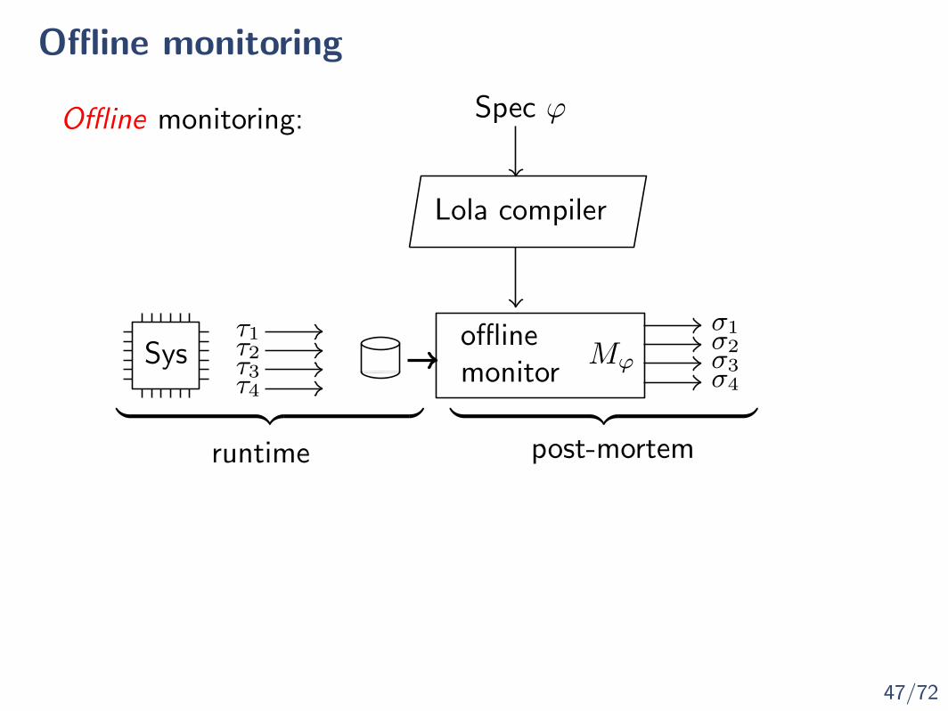
Offline monitoring
τ1τ2τ3τ4
Spec ϕ
Lola compiler
static time
monitor Mϕ
σ1σ2σ3σ4
runtime
Online monitoring:
Sys

47/72
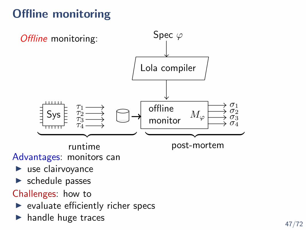
Offline monitoring
Offline monitoring:
τ1τ2τ3τ4
Sys︸ ︷︷ ︸runtime
47/72
Offline monitoring
Offline monitoring:
τ1τ2τ3τ4
Spec ϕ
Lola compiler
offlinemonitor
Mϕ
σ1σ2σ3σ4︸ ︷︷ ︸
post-mortem
Sys︸ ︷︷ ︸runtime

47/72
Offline monitoring
Offline monitoring:
τ1τ2τ3τ4
Spec ϕ
Lola compiler
offlinemonitor
Mϕ
σ1σ2σ3σ4︸ ︷︷ ︸
post-mortem
Sys︸ ︷︷ ︸runtime
Advantages: monitors canI use clairvoyanceI schedule passes
47/72
Offline monitoring
Offline monitoring:
τ1τ2τ3τ4
Spec ϕ
Lola compiler
offlinemonitor
Mϕ
σ1σ2σ3σ4︸ ︷︷ ︸
post-mortem
Sys︸ ︷︷ ︸runtime
Advantages: monitors canI use clairvoyanceI schedule passes
Challenges: how toI evaluate efficiently richer specsI handle huge traces

48/72
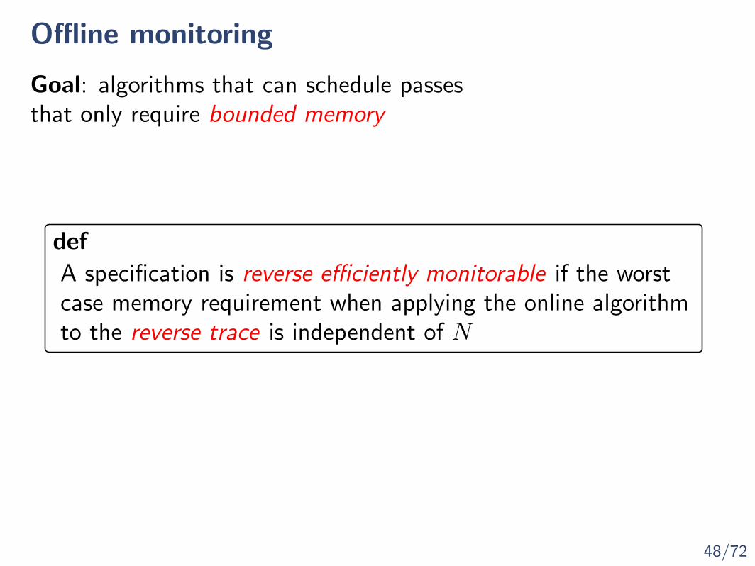
Offline monitoring
Goal: algorithms that can schedule passesthat only require bounded memory
48/72
Offline monitoring
Goal: algorithms that can schedule passesthat only require bounded memory
A specification is reverse efficiently monitorable if the worstcase memory requirement when applying the online algorithmto the reverse trace is independent of N
def
49/72
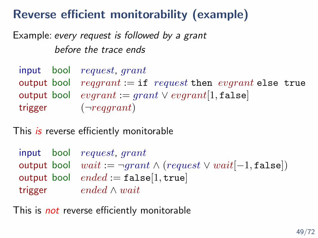
Reverse efficient monitorability (example)
Example: every request is followed by a grant
before the trace ends

49/72
Reverse efficient monitorability (example)
Example: every request is followed by a grant
input bool request, grantoutput bool reqgrant := if request then evgrant else true
output bool evgrant := grant ∨ evgrant[1, false]trigger (¬reqgrant)
before the trace ends

49/72
Reverse efficient monitorability (example)
Example: every request is followed by a grant
input bool request, grantoutput bool reqgrant := if request then evgrant else true
output bool evgrant := grant ∨ evgrant[1, false]trigger (¬reqgrant)
This is reverse efficiently monitorable
input bool request, grantoutput bool wait := ¬grant ∧ (request ∨ wait[−1, false])output bool ended := false[1, true]trigger ended ∧ wait
before the trace ends
49/72
Reverse efficient monitorability (example)
Example: every request is followed by a grant
input bool request, grantoutput bool reqgrant := if request then evgrant else true
output bool evgrant := grant ∨ evgrant[1, false]trigger (¬reqgrant)
This is reverse efficiently monitorable
input bool request, grantoutput bool wait := ¬grant ∧ (request ∨ wait[−1, false])output bool ended := false[1, true]trigger ended ∧ wait
This is not reverse efficiently monitorable
before the trace ends
50/72
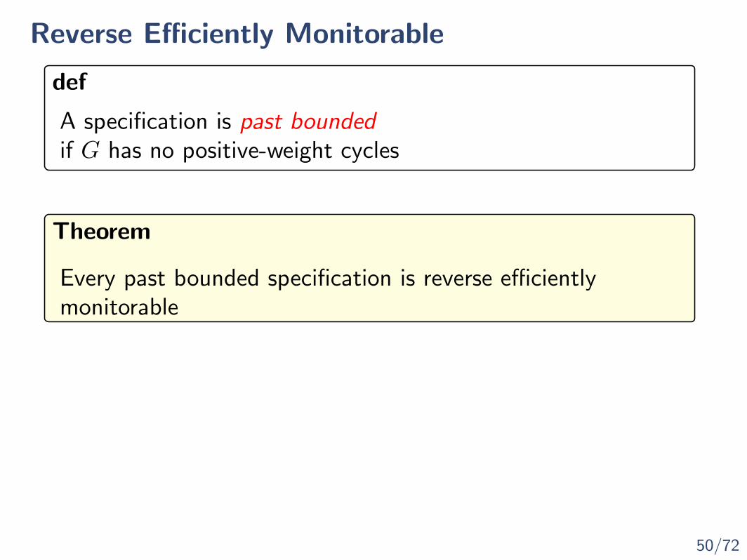
Reverse Efficiently Monitorable
A specification is past boundedif G has no positive-weight cycles
def
Every past bounded specification is reverse efficientlymonitorable
Theorem

51/72
Partition Graph
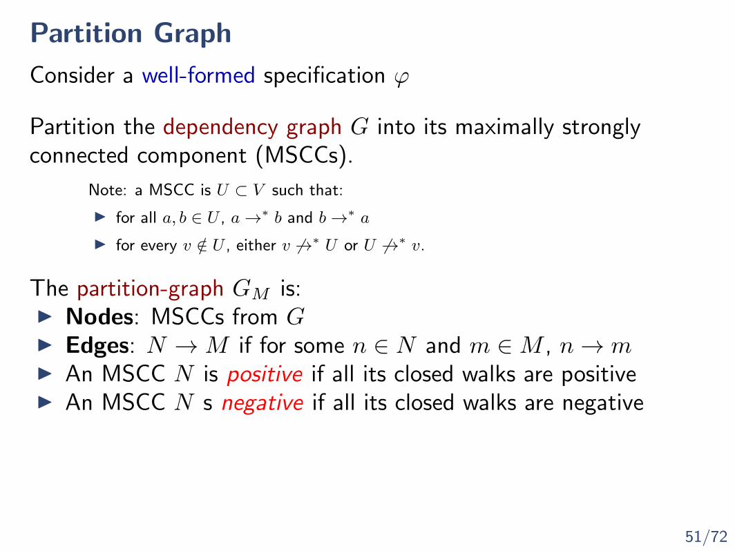
Consider a well-formed specification ϕ
Partition the dependency graph G into its maximally stronglyconnected component (MSCCs).

51/72
Partition Graph
Consider a well-formed specification ϕ
Partition the dependency graph G into its maximally stronglyconnected component (MSCCs).
Note: a MSCC is U ⊂ V such that:
I for all a, b ∈ U , a→∗ b and b→∗ a
I for every v /∈ U , either v 6→∗ U or U 6→∗ v.
51/72
Partition Graph
Consider a well-formed specification ϕ
Partition the dependency graph G into its maximally stronglyconnected component (MSCCs).
Note: a MSCC is U ⊂ V such that:
I for all a, b ∈ U , a→∗ b and b→∗ a
I for every v /∈ U , either v 6→∗ U or U 6→∗ v.
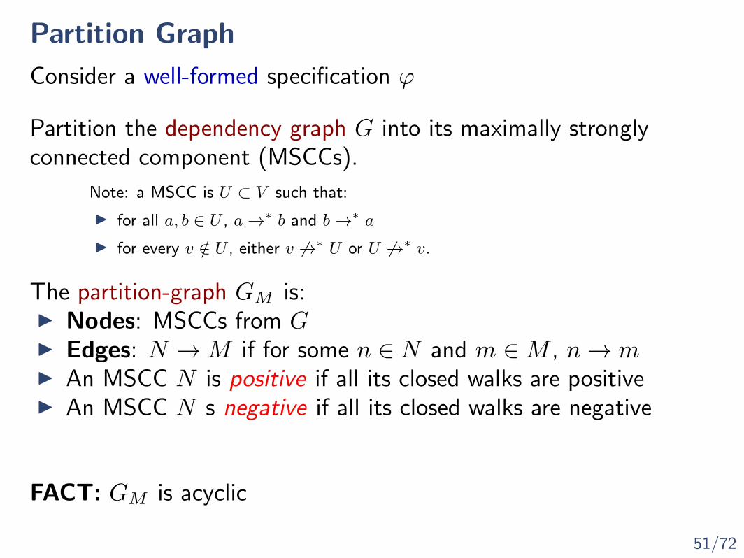
The partition-graph GM is:I Nodes: MSCCs from GI Edges: N →M if for some n ∈ N and m ∈M , n→ mI An MSCC N is positive if all its closed walks are positiveI An MSCC N s negative if all its closed walks are negative
51/72
Partition Graph
Consider a well-formed specification ϕ
Partition the dependency graph G into its maximally stronglyconnected component (MSCCs).
Note: a MSCC is U ⊂ V such that:
I for all a, b ∈ U , a→∗ b and b→∗ a
I for every v /∈ U , either v 6→∗ U or U 6→∗ v.
The partition-graph GM is:I Nodes: MSCCs from GI Edges: N →M if for some n ∈ N and m ∈M , n→ mI An MSCC N is positive if all its closed walks are positiveI An MSCC N s negative if all its closed walks are negative
FACT: GM is acyclic
52/72
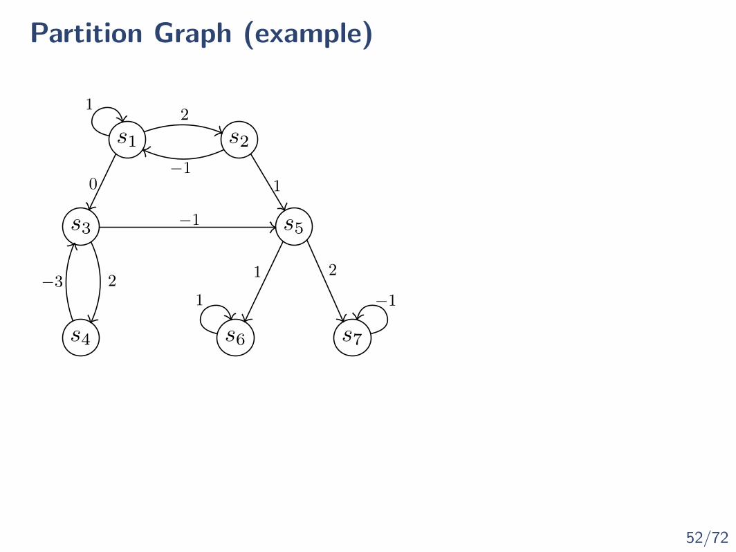
Partition Graph (example)
s1
s3 s5
s7s6s4
2
−1
1
1
1 2
−1
0
−3 21 −1
s2

52/72
Partition Graph (example)
s1
s3 s5
s7s6s4
2
−1
1
1
1 2
−1
0
−3 21 −1
s2

52/72
Partition Graph (example)
s1
s3 s5
s7s6s4
2
−1
1
1
1 2
−1
0
−3 21 −1
s2
M1
M2 M3
M4 M5

52/72
Partition Graph (example)
s1
s3 s5
s7s6s4
2
−1
1
1
1 2
−1
0
−3 21 −1
M2 M3
M1s2
M4 M5
M1
M2 M3
M4 M5

52/72
Partition Graph (example)
s1
s3 s5
s7s6s4
2
−1
1
1
1 2
−1
0
−3 21 −1
M2 M3
M1s2
M4 M5
–+
–
+

52/72
Partition Graph (example)
s1
s3 s5
s7s6s4
2
−1
1
1
1 2
−1
0
−3 21 −1
M2 M3
M1s2
M4 M5
–+
–
+
The processing order of a node in GM is defined as:I p(M) = 0 if M is a – leaf.I p(M) = 1 if M is a + leaf.I Other nodes:p(M) = max{1 + p(N)|M →∗ N, and M and N switch}
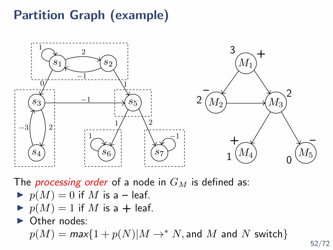
52/72
Partition Graph (example)
s1
s3 s5
s7s6s4
2
−1
1
1
1 2
−1
0
−3 21 −1
M2 M3
M1s2
M4 M5
–+
–
+
The processing order of a node in GM is defined as:I p(M) = 0 if M is a – leaf.I p(M) = 1 if M is a + leaf.I Other nodes:p(M) = max{1 + p(N)|M →∗ N, and M and N switch}
01
22
3
53/72
Offline Monitoring Algorithm
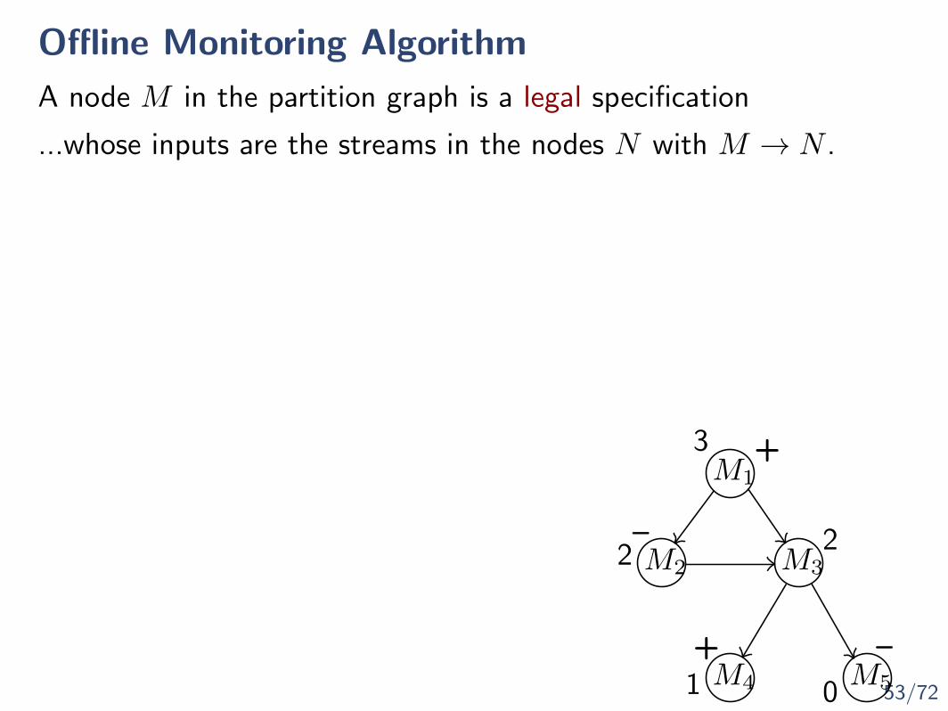
A node M in the partition graph is a legal specification
...whose inputs are the streams in the nodes N with M → N .
M2 M3
M1
M4 M5
–+
–
+
01
22
3

53/72
Offline Monitoring Algorithm
A node M in the partition graph is a legal specification
...whose inputs are the streams in the nodes N with M → N .
Offline algorithm
For i = 0 to max(p(M)), with increment 2:
1. Apply online algorithm forward to specs M with p(M) = i
2. Apply online algorithm backwards to specs M with p(M) = i+ 1
M2 M3
M1
M4 M5
–+
–
+
01
22
3s1
s3 s5
s7s6s4
2
−1
1
1
1 2
−10
−3 21 −1
s2

54/72
Boolean SRVTheoretical Results

55/72
Main Idea
BSRV NFA

55/72
Main Idea
BSRV NFA
exp
1

56/72
BSRV as Language Recognizers
I Given SPEC ϕ:
L(ϕ) := {τ | (τ , σ) � ϕ for some σ}

56/72
BSRV as Language Recognizers
I Given SPEC ϕ:
L(ϕ) := {τ | (τ , σ) � ϕ for some σ}
output bool y := if E then y else ¬y
E :=(first→ (x ∧ y)
)∧(
y → ¬y[+1|false])∧(
¬y → (x[+1|true] ∧ y[+1|true]))
I Example:

56/72
BSRV as Language Recognizers
I Given SPEC ϕ:
L(ϕ) := {τ | (τ , σ) � ϕ for some σ}
output bool y := if E then y else ¬y
E :=(first→ (x ∧ y)
)∧(
y → ¬y[+1|false])∧(
¬y → (x[+1|true] ∧ y[+1|true]))
I The language L(ϕ):
{input x holds at odd positions}
I Example:

57/72
From BSRV to NFA
Forward distance f : maximum k in t[k|d]Backwards distance b : maximum k in t[−k|d]
I Given ϕ we build an NFA over 2X :

57/72
From BSRV to NFA
Forward distance f : maximum k in t[k|d]Backwards distance b : maximum k in t[−k|d]
I Given ϕ we build an NFA over 2X :
input stream variables

57/72
From BSRV to NFA
Forward distance f : maximum k in t[k|d]Backwards distance b : maximum k in t[−k|d]
I Given ϕ we build an NFA over 2X :
I The states are built from A = 2X∪Y and A⊥ = A ∪ ⊥
input stream variables
output stream variables
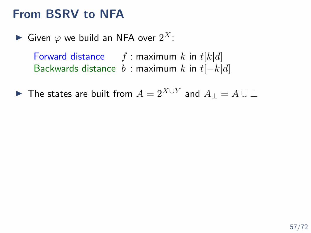
57/72
From BSRV to NFA
Forward distance f : maximum k in t[k|d]Backwards distance b : maximum k in t[−k|d]
I Given ϕ we build an NFA over 2X :
I The states are built from A = 2X∪Y and A⊥ = A ∪ ⊥
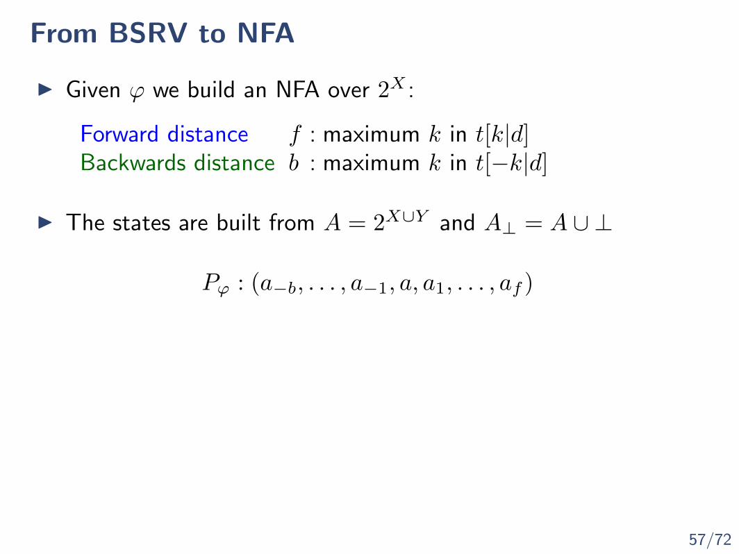
57/72
From BSRV to NFA
Forward distance f : maximum k in t[k|d]Backwards distance b : maximum k in t[−k|d]
I Given ϕ we build an NFA over 2X :
I The states are built from A = 2X∪Y and A⊥ = A ∪ ⊥
Pϕ : (a−b, . . . , a−1, a, a1, . . . , af )

57/72
From BSRV to NFA
Forward distance f : maximum k in t[k|d]Backwards distance b : maximum k in t[−k|d]
I Given ϕ we build an NFA over 2X :
I The states are built from A = 2X∪Y and A⊥ = A ∪ ⊥
Pϕ : (a−b, . . . , a−1, a, a1, . . . , af )
history look-aheadcurrent

57/72
From BSRV to NFA
Forward distance f : maximum k in t[k|d]Backwards distance b : maximum k in t[−k|d]
I Given ϕ we build an NFA over 2X :
I The states are built from A = 2X∪Y and A⊥ = A ∪ ⊥
Pϕ : (a−b, . . . , a−1, a, a1, . . . , af )

57/72
From BSRV to NFA
Forward distance f : maximum k in t[k|d]Backwards distance b : maximum k in t[−k|d]
I Given ϕ we build an NFA over 2X :
I The states are built from A = 2X∪Y and A⊥ = A ∪ ⊥
Pϕ : (a−b, . . . , a−1, a, a1, . . . , af )
I States: Q = {p ∈ Pϕ | for every output s, Js, pK = Je, pK }
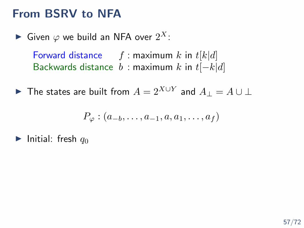
57/72
From BSRV to NFA
Forward distance f : maximum k in t[k|d]Backwards distance b : maximum k in t[−k|d]
I Given ϕ we build an NFA over 2X :
I The states are built from A = 2X∪Y and A⊥ = A ∪ ⊥
Pϕ : (a−b, . . . , a−1, a, a1, . . . , af )
I Initial: fresh q0
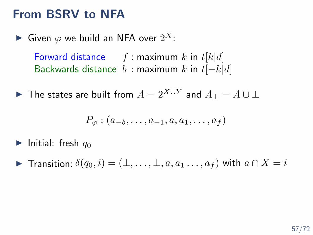
57/72
From BSRV to NFA
Forward distance f : maximum k in t[k|d]Backwards distance b : maximum k in t[−k|d]
I Given ϕ we build an NFA over 2X :
I The states are built from A = 2X∪Y and A⊥ = A ∪ ⊥
Pϕ : (a−b, . . . , a−1, a, a1, . . . , af )
I Initial: fresh q0
I Transition: δ(q0, i) = (⊥, . . . ,⊥, a, a1 . . . , af ) with a ∩X = i
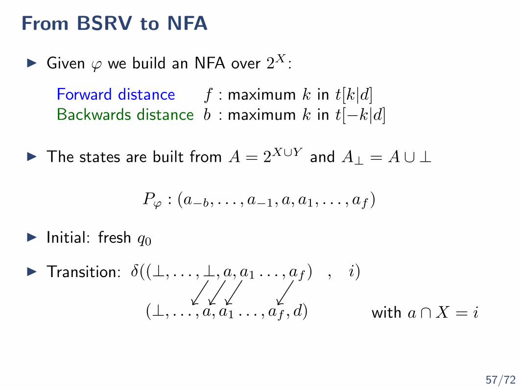
57/72
From BSRV to NFA
Forward distance f : maximum k in t[k|d]Backwards distance b : maximum k in t[−k|d]
I Given ϕ we build an NFA over 2X :
I The states are built from A = 2X∪Y and A⊥ = A ∪ ⊥
Pϕ : (a−b, . . . , a−1, a, a1, . . . , af )
I Initial: fresh q0
δ((⊥, . . . ,⊥, a, a1 . . . , af ) , i)I Transition:
(⊥, . . . , a, a1 . . . , af , d) with a ∩X = i
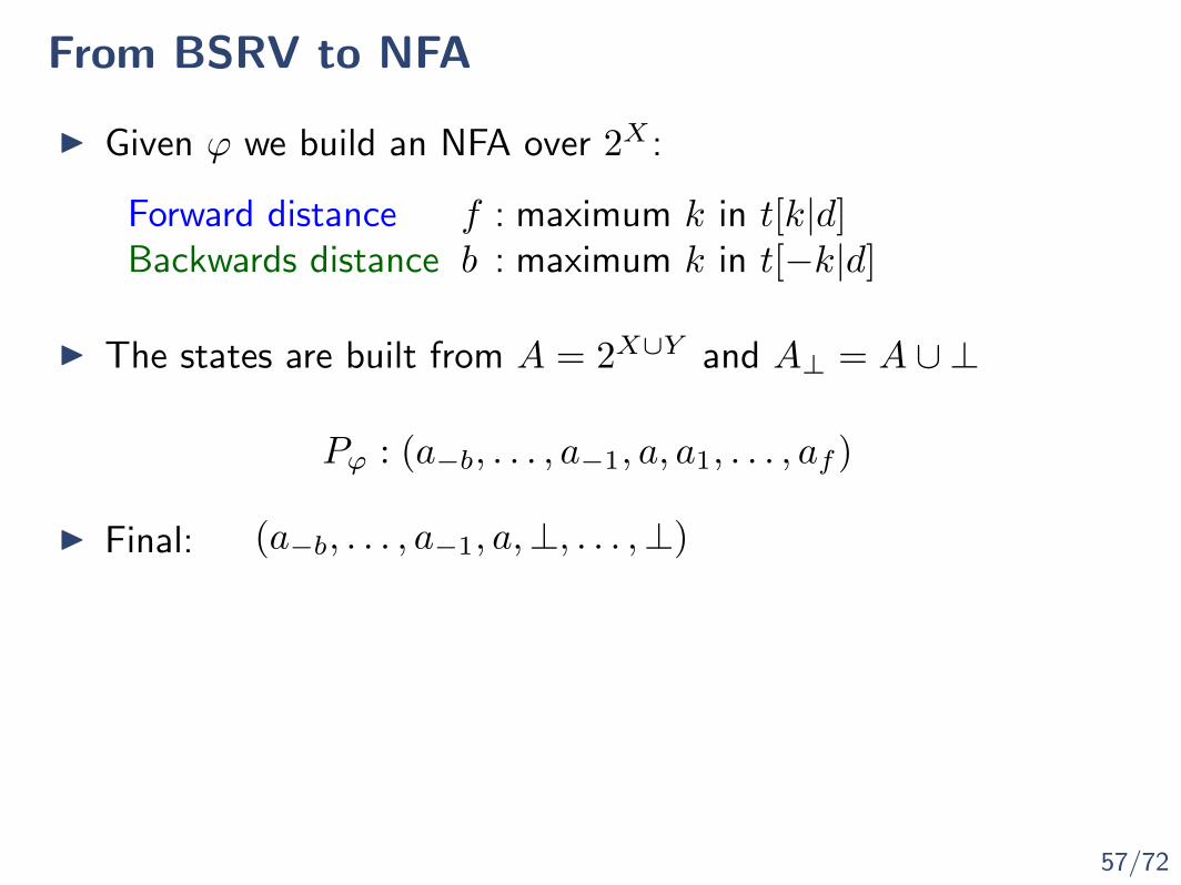
57/72
From BSRV to NFA
Forward distance f : maximum k in t[k|d]Backwards distance b : maximum k in t[−k|d]
I Given ϕ we build an NFA over 2X :
I The states are built from A = 2X∪Y and A⊥ = A ∪ ⊥
Pϕ : (a−b, . . . , a−1, a, a1, . . . , af )
I Final: (a−b, . . . , a−1, a,⊥, . . . ,⊥)
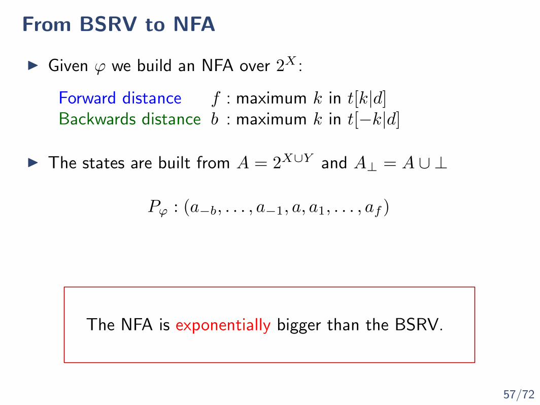
57/72
From BSRV to NFA
Forward distance f : maximum k in t[k|d]Backwards distance b : maximum k in t[−k|d]
I Given ϕ we build an NFA over 2X :
I The states are built from A = 2X∪Y and A⊥ = A ∪ ⊥
Pϕ : (a−b, . . . , a−1, a, a1, . . . , af )
The NFA is exponentially bigger than the BSRV.

58/72
From LTL to BSRV
I Is the (BSRV to NFA) translation tight?
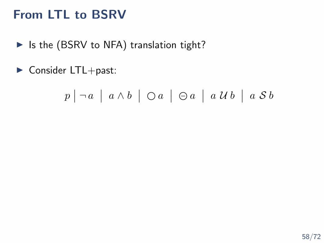
58/72
From LTL to BSRV
I Is the (BSRV to NFA) translation tight?
I Consider LTL+past:
p∣∣ ¬ a ∣∣ a ∧ b ∣∣ a
∣∣ a∣∣ a U b ∣∣ a S b

58/72
From LTL to BSRV
I Is the (BSRV to NFA) translation tight?
I Consider LTL+past:
p∣∣ ¬ a ∣∣ a ∧ b ∣∣ a
∣∣ a∣∣ a U b ∣∣ a S b
I Given ψ, the output streams are Y = SF (ψ) ∪ {init}
init : first → (yψ ∨ ¬init)yp : py¬a : ¬ yaya∨b : ya ∨ ybya : ya[+1|false]ya : ya[−1|false]yaUb : yb ∨ (¬last ∧ ya ∧ yaUb[+1|true])yaSb : yb ∨ (¬first ∧ ya ∧ yaSb[−1|true])

58/72
From LTL to BSRV
I Is the (BSRV to NFA) translation tight?
I Consider LTL+past:
p∣∣ ¬ a ∣∣ a ∧ b ∣∣ a
∣∣ a∣∣ a U b ∣∣ a S b
BSRV is exponentially more succint than NFA.
I LTL+past is exponentially more succinct than NFA [LMS’02]

59/72
From NFA to BSRV
I Start from A : 〈Σ, Q, q0, δ, F 〉 Create:
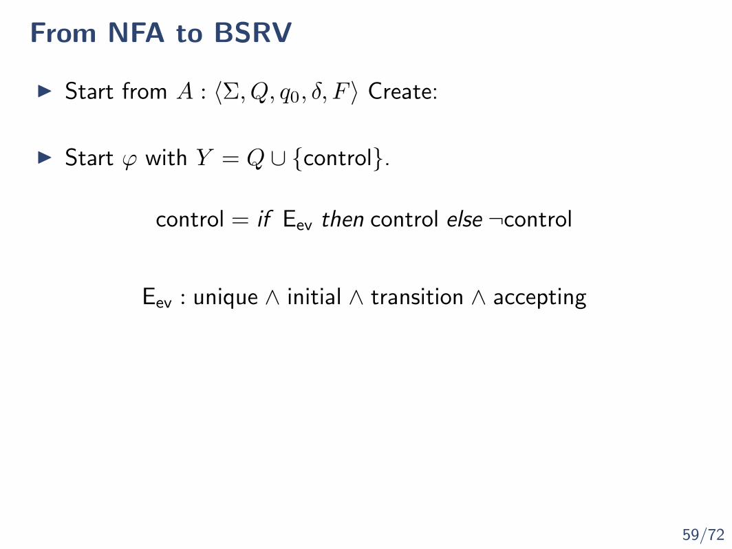
59/72
From NFA to BSRV
I Start from A : 〈Σ, Q, q0, δ, F 〉 Create:
control = if Eev then control else ¬control
I Start ϕ with Y = Q ∪ {control}.
Eev : unique ∧ initial ∧ transition ∧ accepting
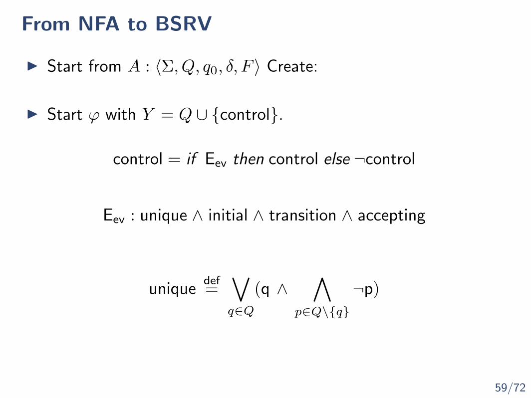
59/72
From NFA to BSRV
I Start from A : 〈Σ, Q, q0, δ, F 〉 Create:
control = if Eev then control else ¬control
I Start ϕ with Y = Q ∪ {control}.
Eev : unique ∧ initial ∧ transition ∧ accepting
uniquedef=∨q∈Q
(q ∧∧
p∈Q\{q}
¬p)
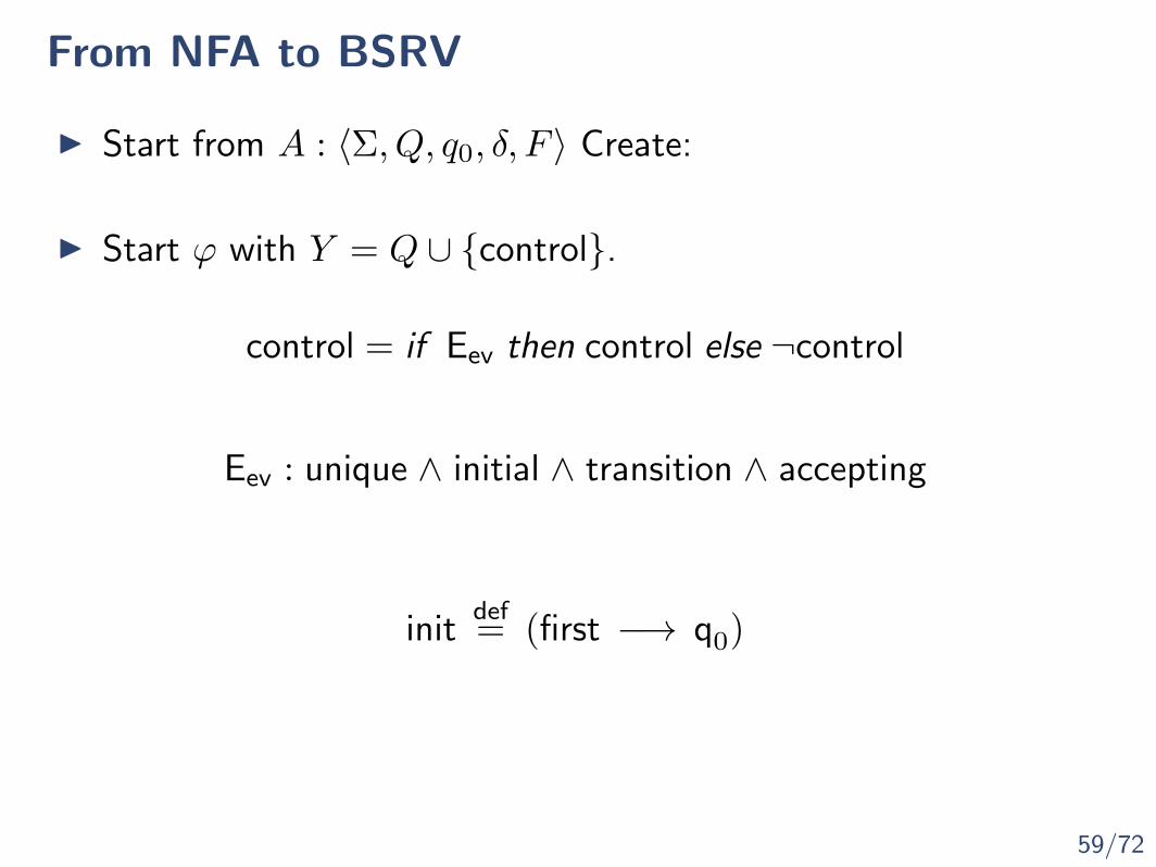
59/72
From NFA to BSRV
I Start from A : 〈Σ, Q, q0, δ, F 〉 Create:
control = if Eev then control else ¬control
I Start ϕ with Y = Q ∪ {control}.
Eev : unique ∧ initial ∧ transition ∧ accepting
initdef= (first −→ q0)
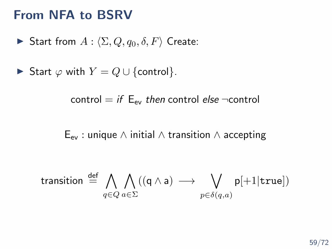
59/72
From NFA to BSRV
I Start from A : 〈Σ, Q, q0, δ, F 〉 Create:
control = if Eev then control else ¬control
I Start ϕ with Y = Q ∪ {control}.
Eev : unique ∧ initial ∧ transition ∧ accepting
transitiondef=∧q∈Q
∧a∈Σ
((q ∧ a) −→∨
p∈δ(q,a)
p[+1|true])
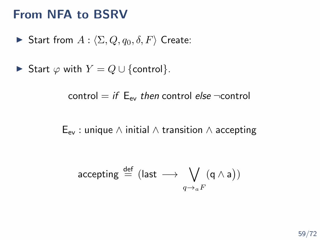
59/72
From NFA to BSRV
I Start from A : 〈Σ, Q, q0, δ, F 〉 Create:
control = if Eev then control else ¬control
I Start ϕ with Y = Q ∪ {control}.
Eev : unique ∧ initial ∧ transition ∧ accepting
acceptingdef= (last −→
∨q→aF
(q ∧ a))

59/72
From NFA to BSRV
I Start from A : 〈Σ, Q, q0, δ, F 〉 Create:
control = if Eev then control else ¬control
I Start ϕ with Y = Q ∪ {control}.
Eev : unique ∧ initial ∧ transition ∧ accepting
The translation from NFA to BSRV is linear.

60/72
Main results (Expressivity)
Theorem: BSRV as recognizers capture the set of all regularlanguages

60/72
Main results (Expressivity)
Theorem: BSRV as recognizers capture the set of all regularlanguages
Theorem: BSRV are closed under union, concatenation andKleene star
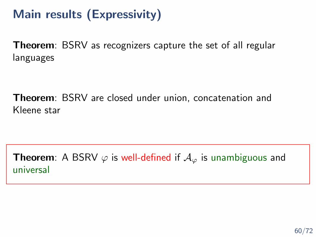
60/72
Main results (Expressivity)
Theorem: BSRV as recognizers capture the set of all regularlanguages
Theorem: BSRV are closed under union, concatenation andKleene star
Theorem: A BSRV ϕ is well-defined if Aϕ is unambiguous anduniversal
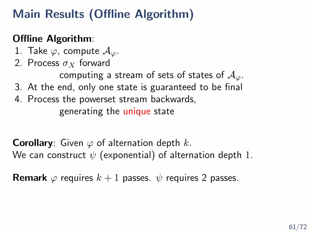
61/72
Main Results (Offline Algorithm)
Offline Algorithm:1. Take ϕ, compute Aϕ.2. Process σX forward
computing a stream of sets of states of Aϕ.3. At the end, only one state is guaranteed to be final4. Process the powerset stream backwards,
generating the unique state
Corollary: Given ϕ of alternation depth k.We can construct ψ (exponential) of alternation depth 1.
Remark ϕ requires k + 1 passes. ψ requires 2 passes.

62/72
Decision Problems
under-defined PSPACE-completewell-defined EXPTIME PSPACE-hardover-defined EXPSPACE-completesemantic equivalence EXPSPACE-completelanguage emptyness PSPACE-completelanguage universality,equivalence, inclusion
EXPSPACE-complete
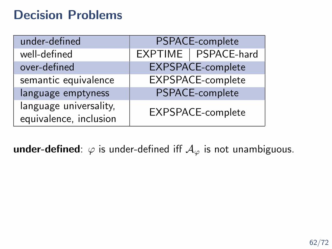
62/72
Decision Problems
under-defined PSPACE-completewell-defined EXPTIME PSPACE-hardover-defined EXPSPACE-completesemantic equivalence EXPSPACE-completelanguage emptyness PSPACE-completelanguage universality,equivalence, inclusion
EXPSPACE-complete
under-defined: ϕ is under-defined iff Aϕ is not unambiguous.
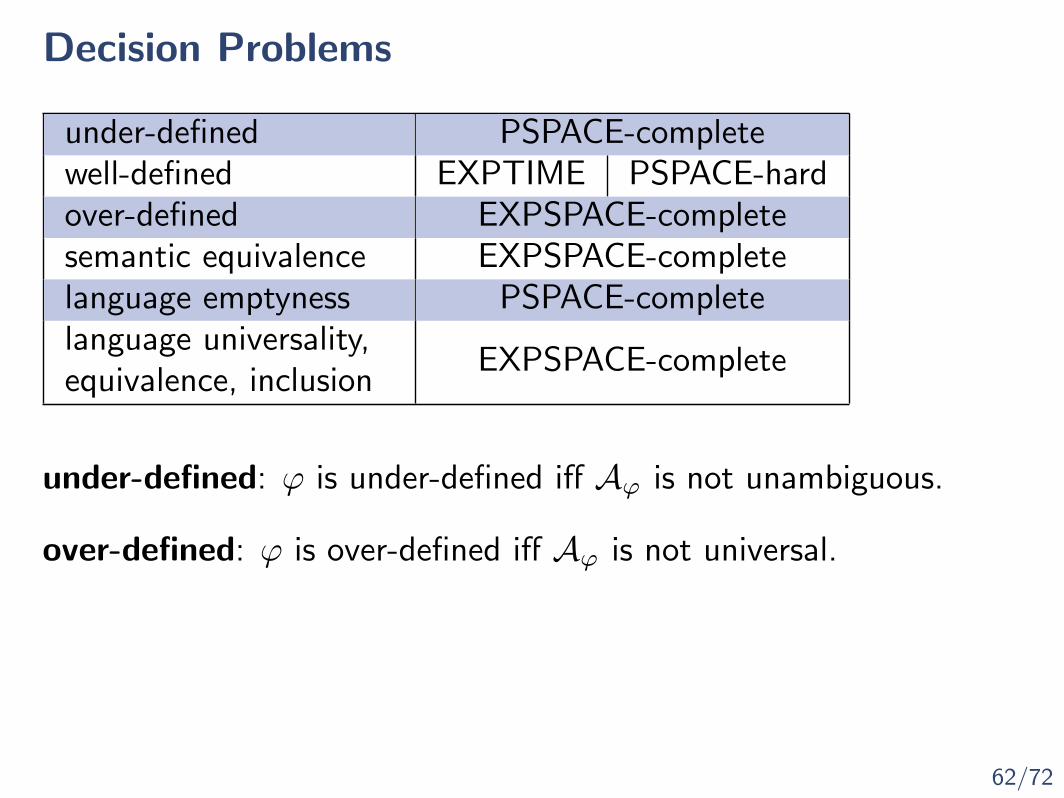
over-defined: ϕ is over-defined iff Aϕ is not universal.
well-defined: checking universality of unamiguous is PTIMEchecking unamiguous is PSPACE

63/72
Extensions
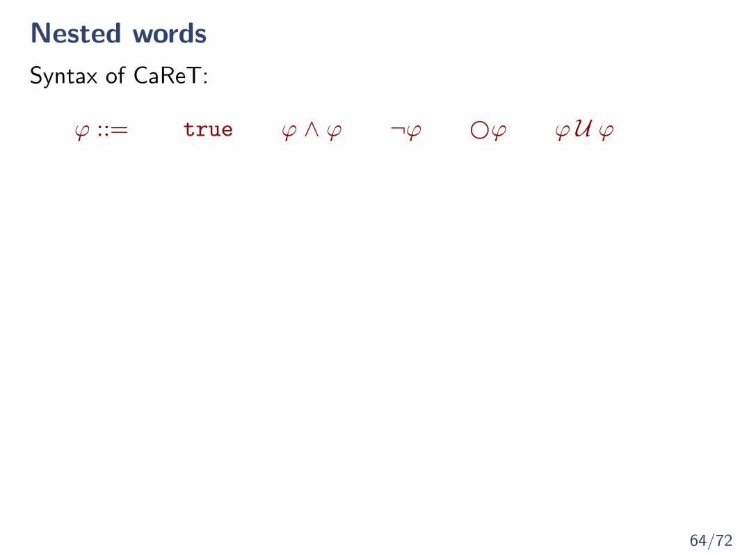
64/72
Nested words
Syntax of CaReT:
ϕ ::= true ϕ ∧ ϕ ¬ϕ ϕ ϕ U ϕ
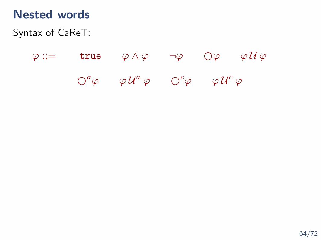
64/72
Nested words
Syntax of CaReT:
ϕ ::= true ϕ ∧ ϕ ¬ϕ ϕ ϕ U ϕ
aϕ ϕ Ua ϕ cϕ ϕ Uc ϕ

64/72
Nested words
Syntax of CaReT:
ϕ ::= true ϕ ∧ ϕ ¬ϕ ϕ ϕ U ϕ
aϕ ϕ Ua ϕ cϕ ϕ Uc ϕ
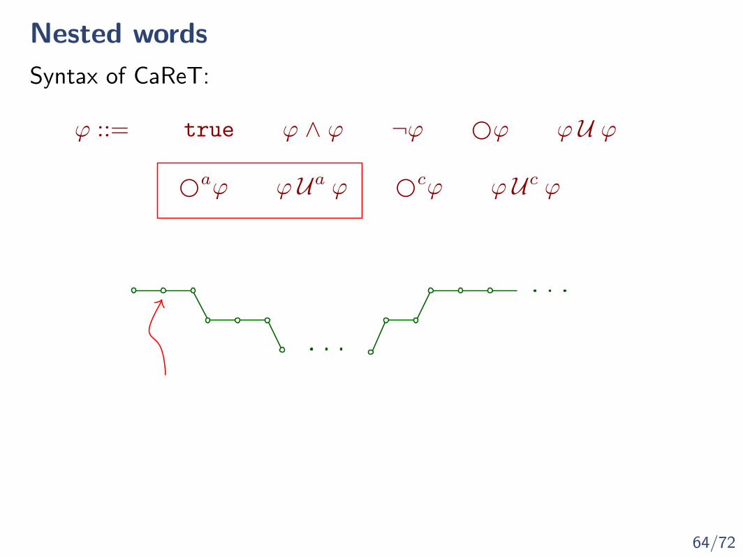
64/72
Nested words
Syntax of CaReT:
ϕ ::= true ϕ ∧ ϕ ¬ϕ ϕ ϕ U ϕ
aϕ ϕ Ua ϕ cϕ ϕ Uc ϕ
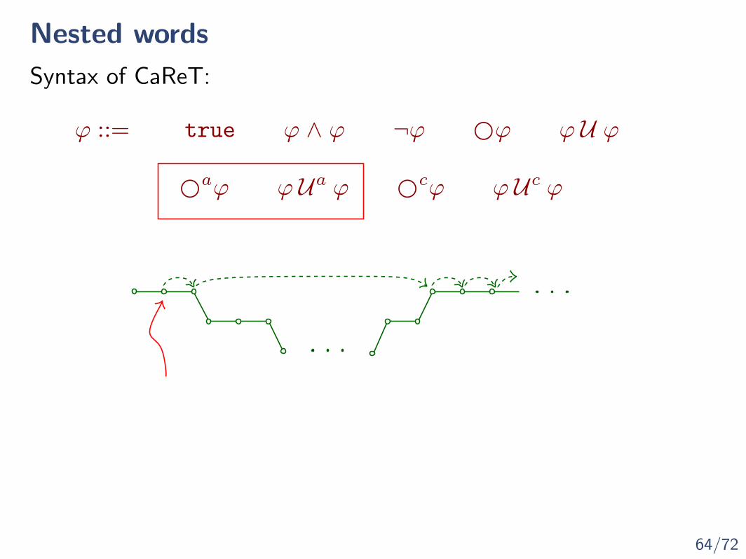
64/72
Nested words
Syntax of CaReT:
ϕ ::= true ϕ ∧ ϕ ¬ϕ ϕ ϕ U ϕ
aϕ ϕ Ua ϕ cϕ ϕ Uc ϕ
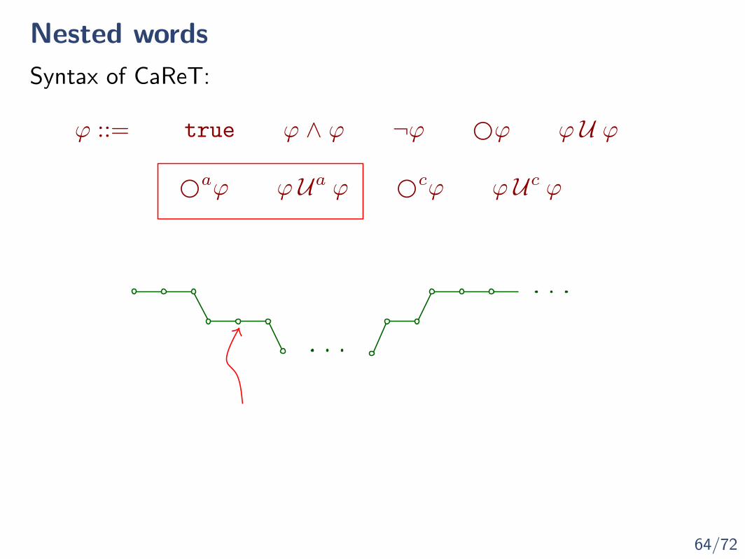
64/72
Nested words
Syntax of CaReT:
ϕ ::= true ϕ ∧ ϕ ¬ϕ ϕ ϕ U ϕ
aϕ ϕ Ua ϕ cϕ ϕ Uc ϕ
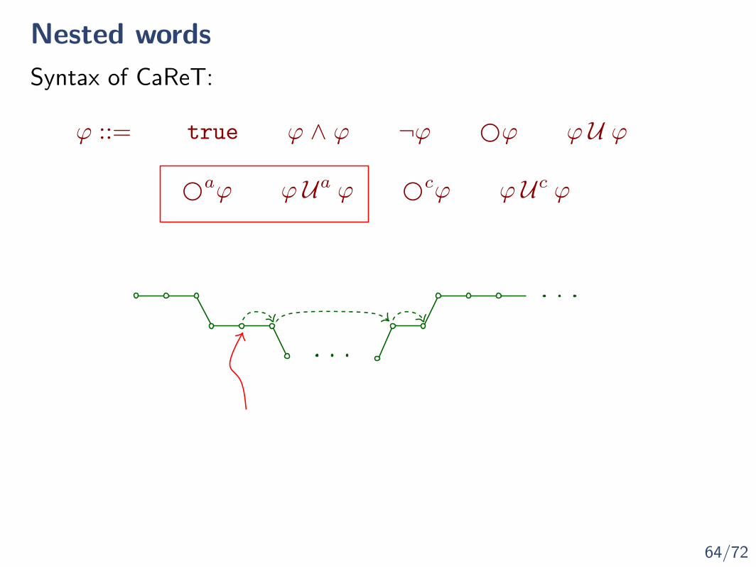
64/72
Nested words
Syntax of CaReT:
ϕ ::= true ϕ ∧ ϕ ¬ϕ ϕ ϕ U ϕ
aϕ ϕ Ua ϕ cϕ ϕ Uc ϕ
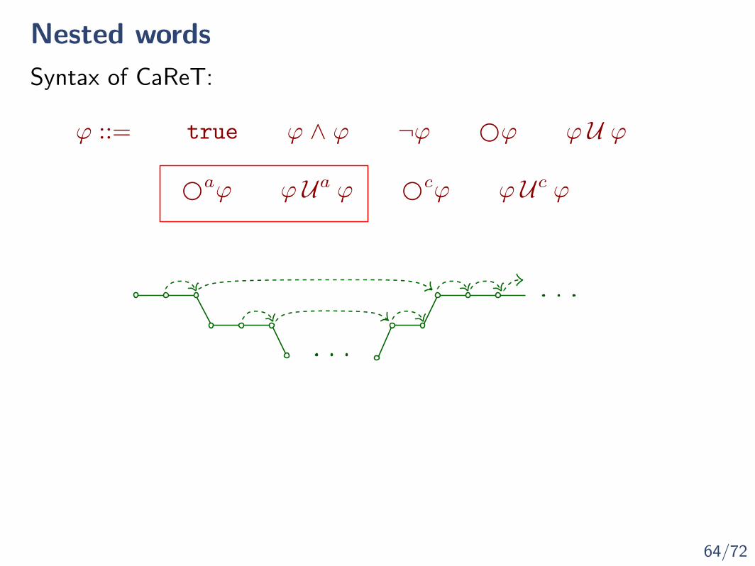
64/72
Nested words
Syntax of CaReT:
ϕ ::= true ϕ ∧ ϕ ¬ϕ ϕ ϕ U ϕ
aϕ ϕ Ua ϕ cϕ ϕ Uc ϕ
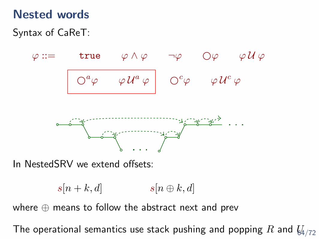
64/72
Nested words
Syntax of CaReT:
ϕ ::= true ϕ ∧ ϕ ¬ϕ ϕ ϕ U ϕ
aϕ ϕ Ua ϕ cϕ ϕ Uc ϕ
In NestedSRV we extend offsets:
s[n+ k, d] s[n⊕ k, d]
where ⊕ means to follow the abstract next and prev
The operational semantics use stack pushing and popping R and U
65/72
Parametrized SRV
I Lola2.0 extends SRV with parametrization
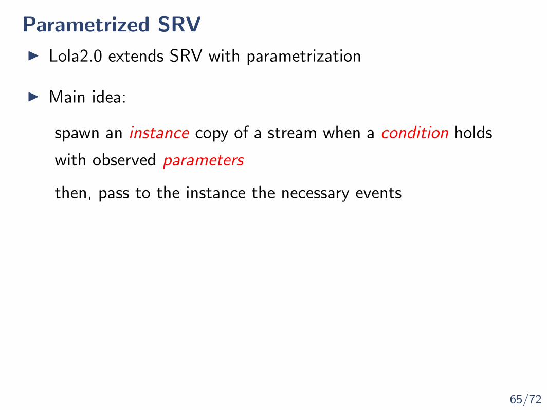
65/72
Parametrized SRV
I Lola2.0 extends SRV with parametrization
I Main idea:
spawn an instance copy of a stream when a condition holds
with observed parameters
then, pass to the instance the necessary events
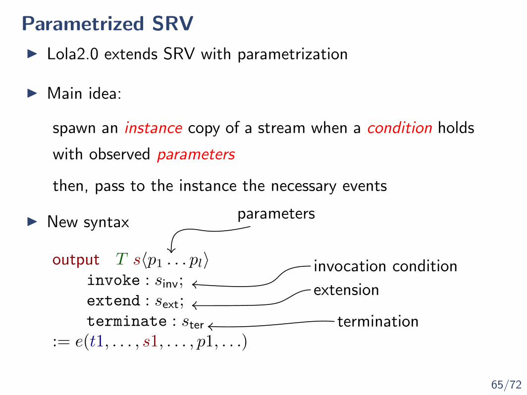
65/72
Parametrized SRV
I Lola2.0 extends SRV with parametrization
I Main idea:
spawn an instance copy of a stream when a condition holds
with observed parameters
then, pass to the instance the necessary events
I New syntax
output T s〈p1 . . . pl〉invoke : sinv;extend : sext;terminate : ster
:= e(t1, . . . , s1, . . . , p1, . . .)
parameters
invocation condition
extension
termination
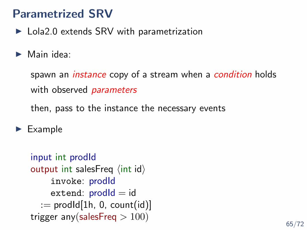
65/72
Parametrized SRV
I Lola2.0 extends SRV with parametrization
I Main idea:
spawn an instance copy of a stream when a condition holds
with observed parameters
then, pass to the instance the necessary events
I Example
input int prodIdoutput int salesFreq 〈int id〉
invoke: prodIdextend: prodId = id
:= prodId[1h, 0, count(id)]trigger any(salesFreq > 100)
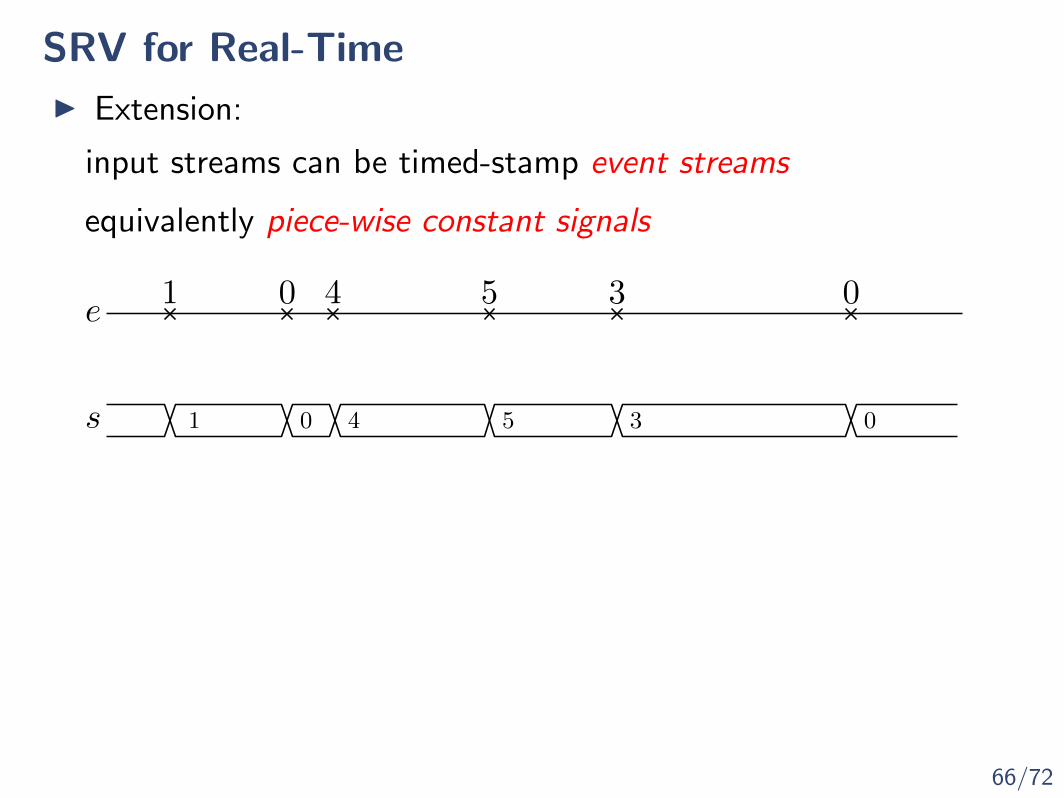
66/72
SRV for Real-Time
I Extension:
input streams can be timed-stamp event streams
equivalently piece-wise constant signals
e
s
1 0 4 5 3 0
1 0 4 5 3 0

66/72
SRV for Real-Time
I Extension:
input streams can be timed-stamp event streams
equivalently piece-wise constant signals
e
s
1 0 4 5 3 0
1 0 4 5 3 0
I Target application: observation of timed-asynchronous systems
• multi-core hardware (non-intrusive, FPGA)• RV for cloud monitoring
I The synchronous notion of time is relaxed:Asynchronous Stream Runtime Verification
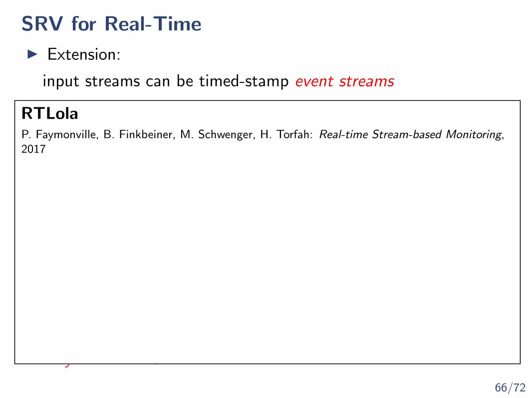
P. Faymonville, B. Finkbeiner, M. Schwenger, H. Torfah: Real-time Stream-based Monitoring,2017
RTLola
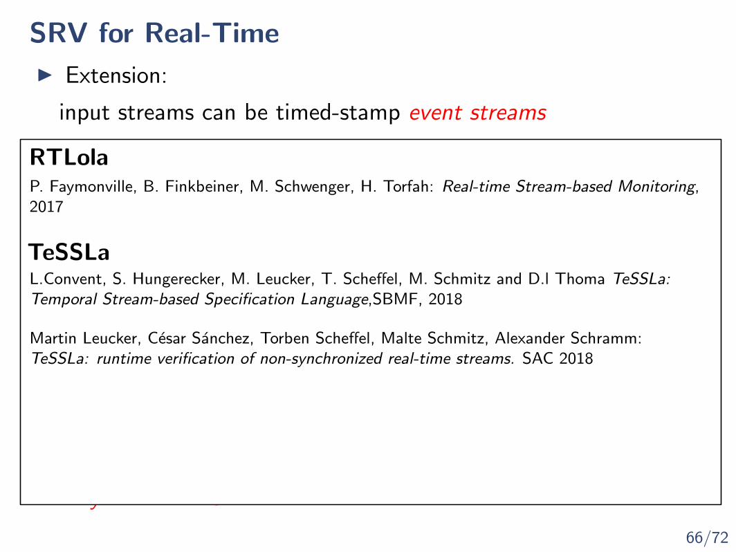
66/72
SRV for Real-Time
I Extension:
input streams can be timed-stamp event streams
equivalently piece-wise constant signals
e
s
1 0 4 5 3 0
1 0 4 5 3 0
I Target application: observation of timed-asynchronous systems
• multi-core hardware (non-intrusive, FPGA)• RV for cloud monitoring
I The synchronous notion of time is relaxed:Asynchronous Stream Runtime Verification
L.Convent, S. Hungerecker, M. Leucker, T. Scheffel, M. Schmitz and D.l Thoma TeSSLa:Temporal Stream-based Specification Language,SBMF, 2018
Martin Leucker, Cesar Sanchez, Torben Scheffel, Malte Schmitz, Alexander Schramm:TeSSLa: runtime verification of non-synchronized real-time streams. SAC 2018
P. Faymonville, B. Finkbeiner, M. Schwenger, H. Torfah: Real-time Stream-based Monitoring,2017
RTLola
TeSSLa
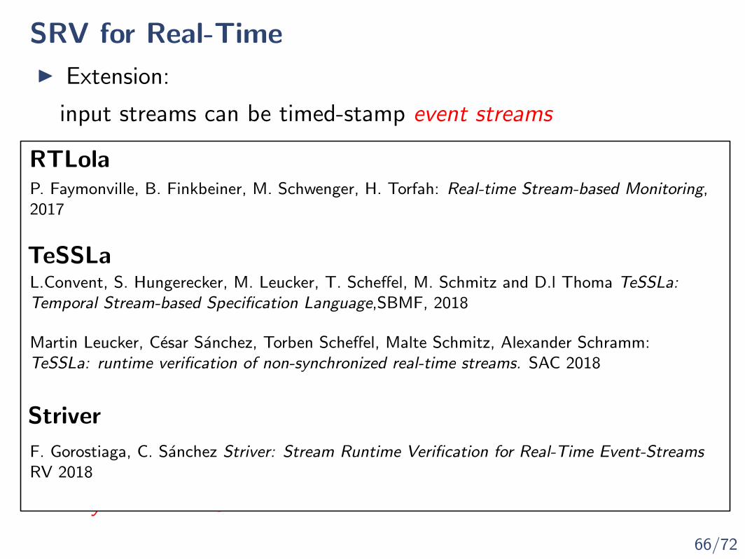
66/72
SRV for Real-Time
I Extension:
input streams can be timed-stamp event streams
equivalently piece-wise constant signals
e
s
1 0 4 5 3 0
1 0 4 5 3 0
I Target application: observation of timed-asynchronous systems
• multi-core hardware (non-intrusive, FPGA)• RV for cloud monitoring
I The synchronous notion of time is relaxed:Asynchronous Stream Runtime Verification
L.Convent, S. Hungerecker, M. Leucker, T. Scheffel, M. Schmitz and D.l Thoma TeSSLa:Temporal Stream-based Specification Language,SBMF, 2018
Martin Leucker, Cesar Sanchez, Torben Scheffel, Malte Schmitz, Alexander Schramm:TeSSLa: runtime verification of non-synchronized real-time streams. SAC 2018
P. Faymonville, B. Finkbeiner, M. Schwenger, H. Torfah: Real-time Stream-based Monitoring,2017
F. Gorostiaga, C. Sanchez Striver: Stream Runtime Verification for Real-Time Event-StreamsRV 2018
RTLola
TeSSLa
Striver

67/72
SRV for Real-Time (RTLola)
I Idea: Slice the time in windows
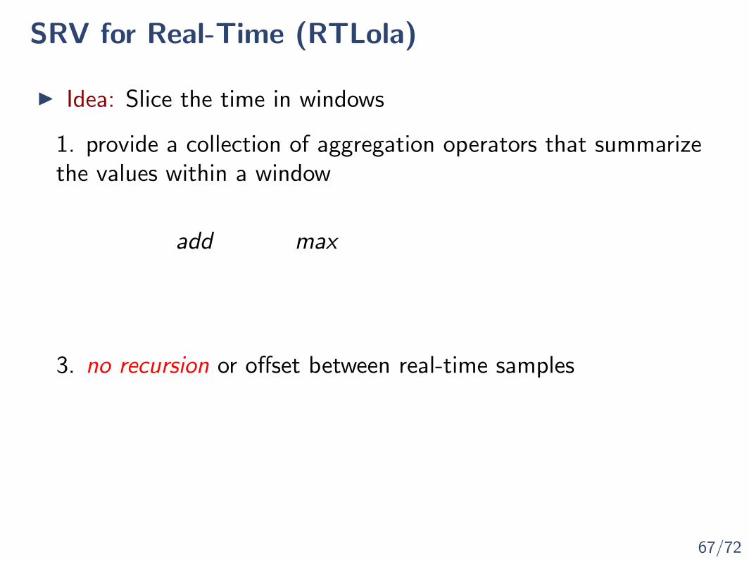
67/72
SRV for Real-Time (RTLola)
I Idea: Slice the time in windows
1. provide a collection of aggregation operators that summarizethe values within a window
add max
3. no recursion or offset between real-time samples
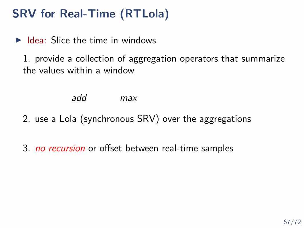
67/72
SRV for Real-Time (RTLola)
I Idea: Slice the time in windows
1. provide a collection of aggregation operators that summarizethe values within a window
add max
3. no recursion or offset between real-time samples
2. use a Lola (synchronous SRV) over the aggregations
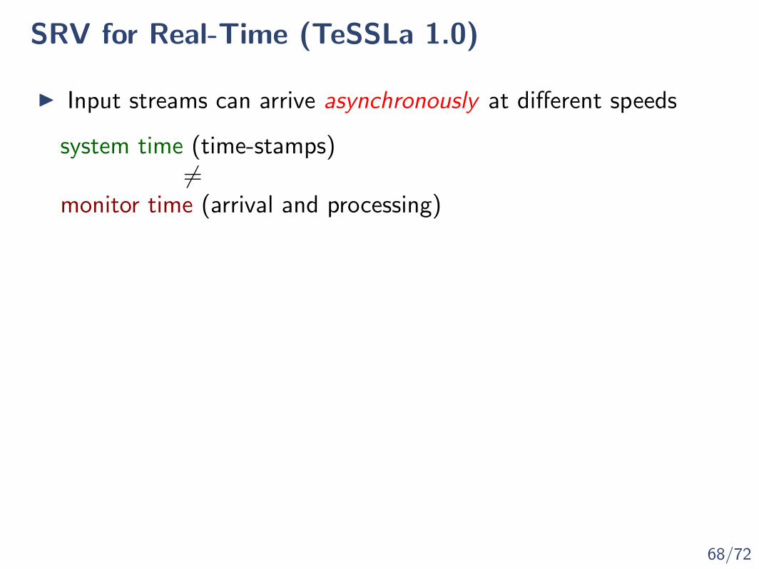
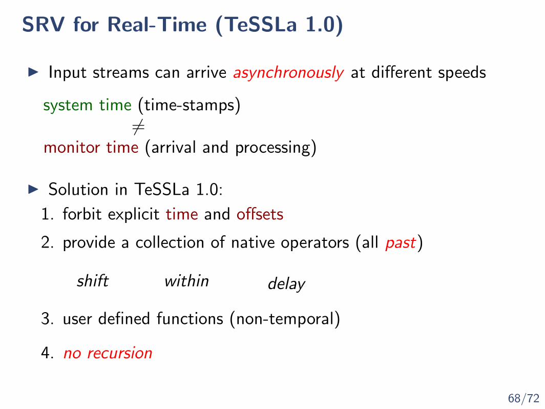
68/72
SRV for Real-Time (TeSSLa 1.0)
I Input streams can arrive asynchronously at different speeds
system time (time-stamps)6=
monitor time (arrival and processing)
I Solution in TeSSLa 1.0:
1. forbit explicit time and offsets
2. provide a collection of native operators (all past)
shift within delay
3. user defined functions (non-temporal)
4. no recursion
Deprecated
Superseded by TeSSLa 2.0

69/72
SRV for Real-Time (TeSSLa 2.0)
https://www.isp.uni-luebeck.de/tessla
I Provided temporal building blocks
default last delayLast time lift
I Provides controlled recursion
I (all past temporal operators)
I Evaluation is guaranteed to be finite state (FPGA)
70/72
SRV for Real-Time (Striver)
I Main idea: keep time explicit

70/72
SRV for Real-Time (Striver)
I Main idea: keep time explicit
I Generalize s[−1] by the previous event in a stream time of s
I Defining equations
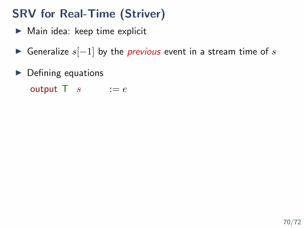
70/72
SRV for Real-Time (Striver)
I Main idea: keep time explicit
I Generalize s[−1] by the previous event in a stream time of s
I Defining equations
output T s := e
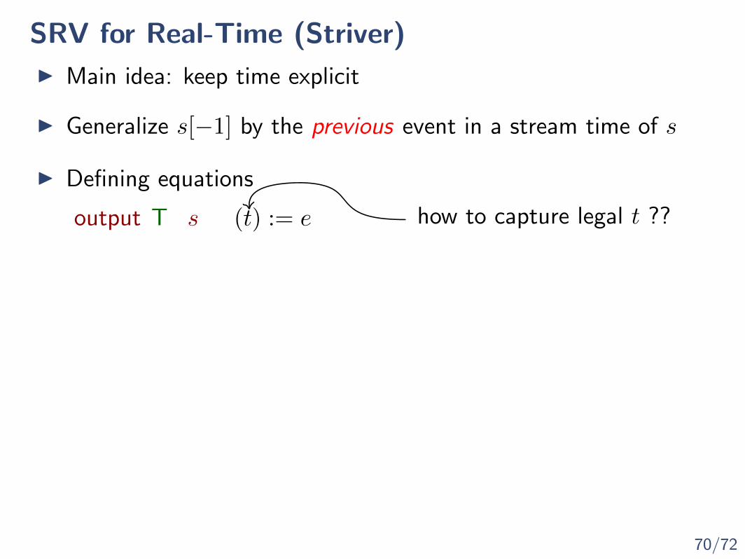
70/72
SRV for Real-Time (Striver)
I Main idea: keep time explicit
I Generalize s[−1] by the previous event in a stream time of s
I Defining equations
how to capture legal t ??output T s (t) := e

70/72
SRV for Real-Time (Striver)
I Main idea: keep time explicit
I Generalize s[−1] by the previous event in a stream time of s
I Defining equations
output T s.ticks := αs.val(t) := e

70/72
SRV for Real-Time (Striver)
I Main idea: keep time explicit
I Generalize s[−1] by the previous event in a stream time of s
I Defining equations
• Ticking expressions
α ::= {c} | v.ticks | α ∪ α | delay(w)
output T s.ticks := αs.val(t) := e

70/72
SRV for Real-Time (Striver)
I Main idea: keep time explicit
I Generalize s[−1] by the previous event in a stream time of s
I Defining equations
• Ticking expressions
• Value expressions
α ::= {c} | v.ticks | α ∪ α | delay(w)
output T s.ticks := αs.val(t) := e
e ::= d | x(τx) | f(e, . . . e) | τ ′

70/72
SRV for Real-Time (Striver)
I Main idea: keep time explicit
I Generalize s[−1] by the previous event in a stream time of s
I Defining equations
• Ticking expressions
• Value expressions
• Offset expressions
α ::= {c} | v.ticks | α ∪ α | delay(w)
output T s.ticks := αs.val(t) := e
e ::= d | x(τx) | f(e, . . . e) | τ ′
τx ::= x.prevEq τ ′ | x.prev τ ′
τ ′ ::= t | τz

71/72
Striver (examples)
I x : default(s,v)
input T soutput T x.ticks := s.ticks ∪ {0}
x.val(t) := if t = 0 then v else s(t)

71/72
Striver (examples)
I x : default(s,v)
input T soutput T x.ticks := s.ticks ∪ {0}
x.val(t) := if t = 0 then v else s(t)
I x : time(s)
input T soutput time x.ticks := s.ticks
x.val(t) := t
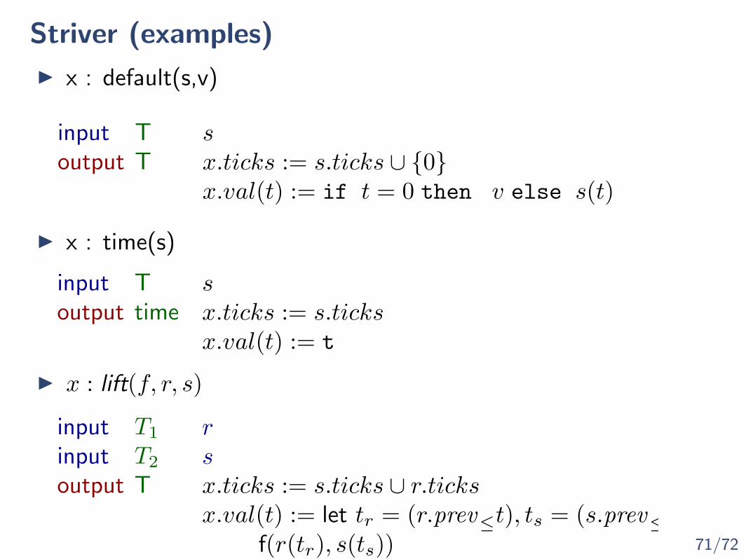
71/72
Striver (examples)
I x : default(s,v)
input T soutput T x.ticks := s.ticks ∪ {0}
x.val(t) := if t = 0 then v else s(t)
I x : time(s)
input T soutput time x.ticks := s.ticks
x.val(t) := t
I x : lift(f, r, s)
input T1 rinput T2 soutput T x.ticks := s.ticks ∪ r.ticks
x.val(t) := let tr = (r.prev≤t), ts = (s.prev≤t) inf(r(tr), s(ts))
72/72
Conclusions
I Stream RV specify behaviors as dependencies between streams
I SRV generalizes monitoring algs to the collection of statistics
I Well-formed specifications guarantee semantics
I Efficiently monitorability guarantee finite state monitors
I Offline monitors can be scheduled to (finite state) passes
I Current directions: generalizing SRV to• asynchronous time• real time• decentralized monitoring• distributed time• monitoring under uncertainty
Related Documents