Stratospheric Dehydration, Residence Time, and Age-of-Air Inferred ...

Stratospheric Dehydration, Residence Time, and Age-of-Air

Inferred from the SDW Forward Trajectory Model – An Intercomparison of using MERRA, ERA interim, JRA55, and CFSR

Oct. 19, 2016SPARC RIP

Tao Wang (JPL, former aggie)

Andrew Dessler (Texas A&M Univ.)

Mark Schoeberl (STC Corp.)

Motivation

1/24

ContributetoS-RIP

• Running forward (TRAJ3D by Ken Bowman)straightforward; longer (16 years) integration period.

(Schoeberl et al., 2003 JGR)

these are backward integrations, Figure 1b shows tropicalparcels descending relative to those in Figure 1a. In aforward integration the parcels would be rising in responseto tropical heating.)[24] The two diabatic simulations, using assimilated

winds from UKMO and the FVDAS, show parcels rapidlymoving to middle latitudes after 50 days. The diabaticdistributions are generally similar even after 200 daysalthough the FVDAS integration is beginning to show anupward plume in the north polar region not seen in theUKMO case. In contrast, the UKMO and FVDAS kine-matic integrations show large vertical dispersion of parcelsafter 50 days; some parcels have already moved into thetroposphere and have been removed from the model. Strik-ingly, the FVGCM kinematic integration shows almost nomeridional or vertical dispersion after 50 days and thedistribution is still confined to middle and low latitudes

after 200 days, while the four DAS experiments havemoved parcels to the polar regions.[25] In order to quantify the initial dispersion of parcels

from the tropics, we have computed the decay rate for thenumber of parcels in the tropics during the first six monthsof the integration. This short period insures that the parcelcount is representative of the initial dispersion and notcontaminated by parcels recirculated from midlatitudes. Ofcourse, the calculation includes the effects of both verticaland horizontal dispersion. The decay rates a (in years!1) fornumber of parcels between 15!S and 15!N in the lowerstratosphere for the first five experiments shown in Table 1are as follows (the experiment labeling in Figure 2 is used):UKM D., 3.7; UKM K., 5.2; FVDAS D., 2.2; FVDAS K.,4.2; FVGCM, 0.35. The data is least-squares fit to theexponential form exp(!at). The rates reflect the impressiongiven in Figure 1. Higher values of a mean more rapid

Figure 1. The distribution of parcels 50 days (part a) and 200 days (part b) after the beginning of theback trajectory calculation (Dt = !50, !200 days). The lower thin white lines show the zonal meanaltitude of the tropopause, the upper thin white line shows the zonal mean altitude of the 380K isentrope.The short thin vertical gray line segment at 20 km in each figure over the equator shows the initialposition of the parcels. Grayscale indicates zonal mean temperature. Parcels are shown as white dots. Thefar left panel shows the results using the UKMO DAS wind fields, diabatic trajectories (UKM D.). Thenext panel (left to right) uses the same wind fields, but is a kinematic trajectory calculation UKM K.).The third panel uses the FVDAS wind fields and diabatic trajectories (FVDAS D.). The fourth panel usesthe FVDAS with kinematic trajectory calculation (FVDAS K.). The fifth panel shows the kinematictrajectory calculation using the FVGCM (FVGCM K.). The percent of parcels remaining in thestratosphere at the time are indicated in each panel.

SCHOEBERL ET AL.: LOWER STRATOSPHERIC AGE SPECTRA ACL 5 - 5

these are backward integrations, Figure 1b shows tropicalparcels descending relative to those in Figure 1a. In aforward integration the parcels would be rising in responseto tropical heating.)[24] The two diabatic simulations, using assimilated

winds from UKMO and the FVDAS, show parcels rapidlymoving to middle latitudes after 50 days. The diabaticdistributions are generally similar even after 200 daysalthough the FVDAS integration is beginning to show anupward plume in the north polar region not seen in theUKMO case. In contrast, the UKMO and FVDAS kine-matic integrations show large vertical dispersion of parcelsafter 50 days; some parcels have already moved into thetroposphere and have been removed from the model. Strik-ingly, the FVGCM kinematic integration shows almost nomeridional or vertical dispersion after 50 days and thedistribution is still confined to middle and low latitudes

after 200 days, while the four DAS experiments havemoved parcels to the polar regions.[25] In order to quantify the initial dispersion of parcels

from the tropics, we have computed the decay rate for thenumber of parcels in the tropics during the first six monthsof the integration. This short period insures that the parcelcount is representative of the initial dispersion and notcontaminated by parcels recirculated from midlatitudes. Ofcourse, the calculation includes the effects of both verticaland horizontal dispersion. The decay rates a (in years!1) fornumber of parcels between 15!S and 15!N in the lowerstratosphere for the first five experiments shown in Table 1are as follows (the experiment labeling in Figure 2 is used):UKM D., 3.7; UKM K., 5.2; FVDAS D., 2.2; FVDAS K.,4.2; FVGCM, 0.35. The data is least-squares fit to theexponential form exp(!at). The rates reflect the impressiongiven in Figure 1. Higher values of a mean more rapid

Figure 1. The distribution of parcels 50 days (part a) and 200 days (part b) after the beginning of theback trajectory calculation (Dt = !50, !200 days). The lower thin white lines show the zonal meanaltitude of the tropopause, the upper thin white line shows the zonal mean altitude of the 380K isentrope.The short thin vertical gray line segment at 20 km in each figure over the equator shows the initialposition of the parcels. Grayscale indicates zonal mean temperature. Parcels are shown as white dots. Thefar left panel shows the results using the UKMO DAS wind fields, diabatic trajectories (UKM D.). Thenext panel (left to right) uses the same wind fields, but is a kinematic trajectory calculation UKM K.).The third panel uses the FVDAS wind fields and diabatic trajectories (FVDAS D.). The fourth panel usesthe FVDAS with kinematic trajectory calculation (FVDAS K.). The fifth panel shows the kinematictrajectory calculation using the FVGCM (FVGCM K.). The percent of parcels remaining in thestratosphere at the time are indicated in each panel.

SCHOEBERL ET AL.: LOWER STRATOSPHERIC AGE SPECTRA ACL 5 - 5

10

20

30

Height(km)

Diabatic run: realistic upwelling

vertical motion = dθ/dt

Kinematic run vertical motion = dP/dt

• Domain-filling: statistically robust

• Diabatic Run (vertical coordinate θ)

The S-D-W Forward Trajectory MODEL

50-days integration

2/24

Parcels are thinned out by a factor of 3

3yrs

The concept of domain filling

Pressure(h

Pa)

2/24

Endingpoint

Startingpoint Atmost16years

u Along each parcel’s integration path, we record:location, T, H2O, dehydration events,age …

u Parcels travelled below 345 K (~10km) and above 1800-K (~40km) are removed.

This model has been used to study:• Dehydration/H2O (Schoeberl and Dessler, 2011; Schoeberl et al., 2012, 2013; Wang et al., 2015);

• Transport of O3/CO (by using chemical prod/loss rates, Wang et al., 2014);• Age spectrum (Schoeberl and Dessler, 2011; Schoeberl et al., 2012; Ray et al., 2014);• Cloud Formation (Schoeberl et al., 2014, 2016);• Water vapor feedback (Dessler et al., 2013);• Water vapor long-term variability (Dessler et al., 2014) & future projection (Dessler et al., 2015);• Indian/North American monsoon (Zhang et al., 2016; Schwartz et al., in progress; Randel et al., in progress);• MJO (Wright et al., in progress);• Convective influences (Su et al., in progress) ;… 3/24

!

!52

Figure 3.5. Water vapor tape recorder signal averaged over 15o N-S from August 2004 to December 2009. The black contours are MLS H2O overlaid in each panel to emphasize the comparison in propagation of this signal.

Fig. 3.5 shows that all model runs driven by different reanalyses did a good job

reproducing the tape recorder up to ~10 hPa (~30 km). Apparently, the ERAi run shows a

drier stratospheric entry level of H2O, due to the cold temperature bias displayed in Fig.

3.4b. CFSR on the other hand, shows wetter air of 0.7-1.4 ppmv due to its warm bias

(Fig. 3.4c). The MLS H2O contours are overlaid in each panel to compare the vertical

propagation of the tape recorder signal. It is obvious that ERAi run creates a faster

transport than the MERRA and CFSR runs, caused by the larger diabatic heating in the

ERAi datasets.

The different transport time scales hinted at from three reanalyses are more

clearly shown in Fig. 3.6, which compares the diabatic heating rates and thus the vertical

Traj.MERRA

Traj.ERAi Traj.CFSR

MLS

4/24

1970 1980 1990 2000 2010Time

-1.0

0.0

1.0

2.0

H2O

Ano

m. (

ppm

v)

1970 1980 1990 2000 2010

83 hPa

Time Series: lon[0,360],lat[-18,0,0,18],,vert[100,31],time[1960.042,2013.958],X00: monthly_gridded_H2O_lon360_monCat_2004-2013.nc; X01: 140415_B_s100_i370_mthd_inj1sav3_MERwindT_day_dhAll_fdhm-un_newT_since80_var1_monCat_1980-2013.nc; X02: 120916_sat100_init370_ERAi_6hr_15yr_addGPH_var1_monCat_1980-2013.nc; X03: 150101_s100_i370_mthd_inj1sav3_JRA55windT_day_dhAll_fdhm-un_var1_monCat_1958-2013

MLS MERRA ERAi JRA55

Traj.MERRA Traj.ERAi Traj.JRA55 MLS

Entry level (83-hPa) Water Vapor Anomaly, comparing to MLS

4/24

1960 1970 1980 1990 2000 2010 Time

-75

-60

-45

-75

-60

-45

68

0.6

0.9

1.2

1.5

1.8

2.1

2.4

O3 (

ppm

v)

-75

-60

-45

MLS

-75

-60

-45

83

TRAJ_MERak

0.6

0.9

1.2

1.5

1.8

2.1

2.4

O3 (

ppm

v)

Lon-Lat: lon[0,360],lat[-90,-60,-60,-40],,vert[150,10],time[2005.042,2011.958],X00: grid_mon_mlsO3_noICE_noNeg_noSpike_lon360_monCat_2004-2011.nc; X01: 130721_s100_i370_mthd_MER_day_Wac_P-L_allPacl_Long_O3forcing_lifetime_fineV_3isob_mlsAK_monCat_2005-2011_100-1.nc;

-75

-60

-45

-75

-60

-45

68

0.6

0.9

1.2

1.5

1.8

2.1

2.4

O3 (

ppm

v)

-75

-60

-45

MLS

-75

-60

-45

83

TRAJ_MERak

0.6

0.9

1.2

1.5

1.8

2.1

2.4

O3 (

ppm

v)


-75

-60

-45

-75

-60

-45

68

0.6

0.9

1.2

1.5

1.8

2.1

2.4

O3 (

ppm

v)

-75

-60

-45

MLS

-75

-60

-45

83

TRAJ_ERAiak

0.6

0.9

1.2

1.5

1.8

2.1

2.4

O3 (

ppm

v)

Lon-Lat: lon[0,360],lat[-90,-60,-60,-40],,vert[150,10],time[2005.042,2011.958],X00: grid_mon_mlsO3_noICE_noNeg_noSpike_lon360_monCat_2004-2011.nc; X01: 130725_s100_i370_mthd_ERAi_day_Wac_P-L_allPacl_Long_O3forcing_lifetime_fineV_3isob_mlsAK_monCat_2005-2011_100-1.nc;

Polar O3 at 68 hPa (~18 km)MLS Traj.MERRA Traj.ERAi

SEP

-75

-60

-45

-75

-60

-45

68

0.6

0.9

1.2

1.5

1.8

2.1

2.4

O3 (

ppm

v)

-75

-60

-45

MLS

-75

-60

-45

83

TRAJ_MERak

0.6

0.9

1.2

1.5

1.8

2.1

2.4

O3 (

ppm

v)


5/24

30

45

6075

30

45

6075

68

0.9

1.7

2.1

2.4

2.6

2.9

O3 (

ppm

v)

30

45

6075

MLS

30

45

6075

83

TRAJ_ERAiak

0.9

1.7

2.1

2.4

2.6

2.9

O3 (

ppm

v)

Lon-Lat: lon[0,360],lat[30,60,60,90],,vert[150,10],time[2005.042,2011.958],X00: grid_mon_mlsO3_noICE_noNeg_noSpike_lon360_monCat_2004-2011.nc; X01: 130725_s100_i370_mthd_ERAi_day_Wac_P-L_allPacl_Long_O3forcing_lifetime_fineV_3isob_mlsAK_monCat_2005-2011_100-1.nc;

30

45

6075

30

45

6075

68

0.9

1.7

2.1

2.4

2.6

2.9

O3 (

ppm

v)

30

45

6075

MLS

30

45

6075

83

TRAJ_MERak

0.9

1.7

2.1

2.4

2.6

2.9

O3 (

ppm

v)

Lon-Lat: lon[0,360],lat[30,60,60,90],,vert[150,10],time[2005.042,2011.958],X00: grid_mon_mlsO3_noICE_noNeg_noSpike_lon360_monCat_2004-2011.nc; X01: 130721_s100_i370_mthd_MER_day_Wac_P-L_allPacl_Long_O3forcing_lifetime_fineV_3isob_mlsAK_monCat_2005-2011_100-1.nc;

30

45

6075

30

45

6075

68

0.9

1.7

2.1

2.4

2.6

2.9

O3 (

ppm

v)

30

45

6075

MLS

30

45

6075

83

TRAJ_ERAiak

0.9

1.7

2.1

2.4

2.6

2.9

O3 (

ppm

v)

Lon-Lat: lon[0,360],lat[30,60,60,90],,vert[150,10],time[2005.042,2011.958],X00: grid_mon_mlsO3_noICE_noNeg_noSpike_lon360_monCat_2004-2011.nc; X01: 130725_s100_i370_mthd_ERAi_day_Wac_P-L_allPacl_Long_O3forcing_lifetime_fineV_3isob_mlsAK_monCat_2005-2011_100-1.nc;

DJF

30

4560

75

30

4560

75

30

4560

75

83

0.6

1.2

1.6

1.8

2.0

2.3

O3 (

ppm

v)

30

4560

75

24PVU

MLS

30

4560

75

24PVU

WACCM

30

4560

75

24PVU

68

TRAJ_MER

0.9

1.7

2.1

2.4

2.6

2.9

O3 (

ppm

v)

Lon-Lat: lon[0,360],lat[30,60,60,90],,vert[150,10],time[2005.042,2011.958],X00: monthly_gridded_mlsO3_noICE_monCat_2004-2011.nc; X01: WAC_nugByMER_allChem_interp2mls_mygrid_3cord_200501-201112_aver_isob2.nc; X02: 130721_s100_i370_mthd_MER_day_Wac_P-L_allPacl_Long_O3forcing_lifetime_var1_monCat_2005-2011.nc;

Wangetal.,ACP,2014

1.Dehydration

/Final Dehydration

6/24

-30-20-10

0102030

00

Latit

ude

(O )

2.53

3.5

3.53.5

4 4 4 4 4

45

DJF

-30-20-10

0102030

00

Latit

ude

(O )

33.5

3.5

3.5

4

4

4

4 4.5

4.55

5 5

66

MAM

-30-20-10

0102030

00

Latit

ude

(O )

4.5

55

5

5.5

5.5

5.5

5.56

6 6

6

66

6.5

7

778

JJA

0 60 120 180 240 300Longitude (O )

-30-20-10

0102030

00

Latit

ude

(O )

44.5

4.5

5

5

5

5

55.5

5.5

5.5

66

6 6

66

7

SON

1 883 4423101801744035602

FDP Events (#)

0 60 120 180 240 300Longitude (O )

-30-20-10

0102030

00

Latit

ude

(O )

3.5

4

4

4

4.5

4.5 4.5

4.5

5

55

5

5

55.5

6

6.578

ALL

1 1164129664183171741168570

FDP Events (#)

-30-20-10

0102030

00

Latit

ude

(O )

2.533.5

3.5

3.5

4

4

44 4

4

444

4.55

DJF

-30-20-10

0102030

00

Latit

ude

(O )

33.5

3.5

4

4

4

4

4.5

4.5

5

5

55 66 6

7

MAM

-30-20-10

0102030

00

Latit

ude

(O )

4.5

55.5

5.5

5.5

5.5

6

6

6

6 6

6

6.5

7

7 78

JJA

0 60 120 180 240 300Longitude (O )

-30-20-10

0102030

00

Latit

ude

(O )

44.5

4.5

5

5

5

5 5

5.55.5 5.56

6

66

7

SON

1 594 351878271511442113

FDP Events (#)

0 60 120 180 240 300Longitude (O )

-30-20-10

0102030

00

Latit

ude

(O )

3.54 4

4.54.5

4.5

5

5 5 5 5555

5.55.5

6

66.57

ALL

1 1418146143573365878166805

FDP Events (#)

-30-20-10

0102030

00

Latit

ude

(O )

2.53

3

3

33

3.5

3.5

4 4

4

DJF

-30-20-10

0102030

00

Latit

ude

(O )

33.5

3.5

3.5

4

4

4

44

4

4.55

MAM

-30-20-10

0102030

00

Latit

ude

(O )

44.55

55

5 5 5

5

5

5.5

5.5 5.56 6

66 6

6.5

6.5

7

7

8

8

JJA

0 60 120 180 240 300Longitude (O )

-30-20-10

0102030

00

Latit

ude

(O )

3.54

4

4.5

4.5

5

5

5

5

5 55

5.5

5.56 6

SON

7 10385379111851707536203

FDP Events (#)

0 60 120 180 240 300Longitude (O )

-30-20-10

0102030

00

Latit

ude

(O )

33.5

3.5

4

4

4

4.5 4.5 4.5

4.5

4.54.5

5

5

555.567

ALL

1 1447150294272365210125754

FDP Events (#)

Traj.MERRA

Traj.ERAi

Traj.JRA55

12

34

56

78

9101112Climatological Months

-90 -60 -30 0 30 60 90

Latitude

2 4505

10185

16568

32205

206528

MDP Events (#)

min max20% 40% 60% 80%

Normalized FDP Frequency

Horizontally, no big differences…

2007-2013 annual average

White contour lines: dehydration H2O

Where dehydration occurs…

7/24

Traj.MERRA

Traj.ERAi

Traj.JRA55

1 2 3 4 5 6 7 8 9 10 11 12Climatological Months

110

100

90

80

70

60

Pressu

re (hP

a)

6

975

12830

129654

389058

1077606

FDP E

vents (

#)


110

100

90

80

70

60

Pressu

re (hP

a)

6

833

18619

157185

459032

1033875

FDP E

vents (

#)


110

100

90

80

70

60

Pressu

re (hP

a)

4

691

15585

114692

415905

1145624

FDP E

vents (

#)

J F M A M J J A S O N DClimatological Months

60

70

80

90

100

110

Pres

sure

(hPa

)

60

70

80

90

100

110

Pres

sure

(hPa

)

60

70

80

90

100

110

Pres

sure

(hPa

)

12

34

56

78


-90 -60 -30 0 30 60 90

Latitude

2 4505

10185

16568

32205

206528

MDP Events (#)

min max20% 40% 60% 80%


Vertically…

2007-2013 annual average

8/24

110

100

90

80

70

60

Cold

Poi

nt P

ress

ure

(hPa

)

0 20 40 60 80 100Fraction (%)

0 20 40 60 80 100Fraction (%)

DJF

110

100

90

80

70

60

Cold

Poi

nt P

ress

ure

(hPa

)

0 20 40 60 80 100Fraction (%)

0 20 40 60 80 100Fraction (%)

MAM

110

100

90

80

70

60

Cold

Poi

nt P

ress

ure

(hPa

)

0 20 40 60 80 100Fraction (%)

0 20 40 60 80 100Fraction (%)

JJA

110

100

90

80

70

60

Cold

Poi

nt P

ress

ure

(hPa

)

0 20 40 60 80 100Fraction (%)

0 20 40 60 80 100Fraction (%)

SON

110

100

90

80

70

60

Cold

Poi

nt P

ress

ure

(hPa

)

0 20 40 60 80 100Fraction (%)

0 20 40 60 80 100Fraction (%)

ALL

MER

110

100

90

80

70

60

Cold

Poi

nt P

ress

ure

(hPa

)

0 20 40 60 80 100Fraction (%)

0 20 40 60 80 100Fraction (%)

DJF

110

100

90

80

70

60

Cold

Poi

nt P

ress

ure

(hPa

)

0 20 40 60 80 100Fraction (%)

0 20 40 60 80 100Fraction (%)

MAM

110

100

90

80

70

60

Cold

Poi

nt P

ress

ure

(hPa

)

0 20 40 60 80 100Fraction (%)

0 20 40 60 80 100Fraction (%)

JJA

110

100

90

80

70

60

Cold

Poi

nt P

ress

ure

(hPa

)

0 20 40 60 80 100Fraction (%)

0 20 40 60 80 100Fraction (%)

SON

110

100

90

80

70

60

Cold

Poi

nt P

ress

ure

(hPa

)

0 20 40 60 80 100Fraction (%)

0 20 40 60 80 100Fraction (%)

ALL

MER

110

100

90

80

70

60

Cold

Poi

nt P

ress

ure

(hPa

)0 20 40 60 80 100

Fraction (%)

0 20 40 60 80 100Fraction (%)

DJF

110

100

90

80

70

60

Cold

Poi

nt P

ress

ure

(hPa

)

0 20 40 60 80 100Fraction (%)

0 20 40 60 80 100Fraction (%)

MAM

110

100

90

80

70

60

Cold

Poi

nt P

ress

ure

(hPa

)

0 20 40 60 80 100Fraction (%)

0 20 40 60 80 100Fraction (%)

JJA

110

100

90

80

70

60

Cold

Poi

nt P

ress

ure

(hPa

)

0 20 40 60 80 100Fraction (%)

0 20 40 60 80 100Fraction (%)

SON

110

100

90

80

70

60

Cold

Poi

nt P

ress

ure

(hPa

)

0 20 40 60 80 100Fraction (%)

0 20 40 60 80 100Fraction (%)

ALL

MER

110

100

90

80

70

60

Cold

Poi

nt P

ress

ure

(hPa

)

0 20 40 60 80 100Fraction (%)

0 20 40 60 80 100Fraction (%)

DJF

110

100

90

80

70

60

Cold

Poi

nt P

ress

ure

(hPa

)

0 20 40 60 80 100Fraction (%)

0 20 40 60 80 100Fraction (%)

MAM

110

100

90

80

70

60

Cold

Poi

nt P

ress

ure

(hPa

)

0 20 40 60 80 100Fraction (%)

0 20 40 60 80 100Fraction (%)

JJA

110

100

90

80

70

60

Cold

Poi

nt P

ress

ure

(hPa

)

0 20 40 60 80 100Fraction (%)

0 20 40 60 80 100Fraction (%)

SON

110

100

90

80

70

60

Cold

Poi

nt P

ress

ure

(hPa

)0 20 40 60 80 100

Fraction (%)

0 20 40 60 80 100Fraction (%)

ALL

MER


110

100

90

80

70

60

Pressu

re (hP

a)

6

975

12830

129654

389058

1077606

FDP E

vents (

#)

J F M A M J J A S O N D

Traj.MERRA

MERRA-T

6070

80

90

100110

Pres

sure

(hPa

)

12

34

56

78


-90 -60 -30 0 30 60 90

Latitude

2 4505

10185

16568

32205

206528

MDP Events (#)

min max20% 40% 60% 80%


100.5hPa

85.4hPa

72.6hPa

Wangetal.,ACP,2015 9/24

110

100

90

80

70

60

Cold

Poi

nt P

ress

ure

(hPa

)

0 20 40 60 80 100Fraction (%)

0 20 40 60 80 100Fraction (%)

DJF

110

100

90

80

70

60

Cold

Poi

nt P

ress

ure

(hPa

)

0 20 40 60 80 100Fraction (%)

0 20 40 60 80 100Fraction (%)

MAM

110

100

90

80

70

60

Cold

Poi

nt P

ress

ure

(hPa

)

0 20 40 60 80 100Fraction (%)

0 20 40 60 80 100Fraction (%)

JJA

110

100

90

80

70

60

Cold

Poi

nt P

ress

ure

(hPa

)

0 20 40 60 80 100Fraction (%)

0 20 40 60 80 100Fraction (%)

SON

110

100

90

80

70

60

Cold

Poi

nt P

ress

ure

(hPa

)

0 20 40 60 80 100Fraction (%)

0 20 40 60 80 100Fraction (%)

ALL

MERERAi

110

100

90

80

70

60

Cold

Poi

nt P

ress

ure

(hPa

)

0 20 40 60 80 100Fraction (%)

0 20 40 60 80 100Fraction (%)

DJF

110

100

90

80

70

60

Cold

Poi

nt P

ress

ure

(hPa

)

0 20 40 60 80 100Fraction (%)

0 20 40 60 80 100Fraction (%)

MAM

110

100

90

80

70

60

Cold

Poi

nt P

ress

ure

(hPa

)

0 20 40 60 80 100Fraction (%)

0 20 40 60 80 100Fraction (%)

JJA

110

100

90

80

70

60

Cold

Poi

nt P

ress

ure

(hPa

)

0 20 40 60 80 100Fraction (%)

0 20 40 60 80 100Fraction (%)

SON

110

100

90

80

70

60

Cold

Poi

nt P

ress

ure

(hPa

)

0 20 40 60 80 100Fraction (%)

0 20 40 60 80 100Fraction (%)

ALL

MERERAi

110

100

90

80

70

60

Cold

Poi

nt P

ress

ure

(hPa

)0 20 40 60 80 100

Fraction (%)

0 20 40 60 80 100Fraction (%)

DJF

110

100

90

80

70

60

Cold

Poi

nt P

ress

ure

(hPa

)

0 20 40 60 80 100Fraction (%)

0 20 40 60 80 100Fraction (%)

MAM

110

100

90

80

70

60

Cold

Poi

nt P

ress

ure

(hPa

)

0 20 40 60 80 100Fraction (%)

0 20 40 60 80 100Fraction (%)

JJA

110

100

90

80

70

60

Cold

Poi

nt P

ress

ure

(hPa

)

0 20 40 60 80 100Fraction (%)

0 20 40 60 80 100Fraction (%)

SON

110

100

90

80

70

60

Cold

Poi

nt P

ress

ure

(hPa

)

0 20 40 60 80 100Fraction (%)

0 20 40 60 80 100Fraction (%)

ALL

MERERAi

110

100

90

80

70

60

Cold

Poi

nt P

ress

ure

(hPa

)

0 20 40 60 80 100Fraction (%)

0 20 40 60 80 100Fraction (%)

DJF

110

100

90

80

70

60

Cold

Poi

nt P

ress

ure

(hPa

)

0 20 40 60 80 100Fraction (%)

0 20 40 60 80 100Fraction (%)

MAM

110

100

90

80

70

60

Cold

Poi

nt P

ress

ure

(hPa

)

0 20 40 60 80 100Fraction (%)

0 20 40 60 80 100Fraction (%)

JJA

110

100

90

80

70

60

Cold

Poi

nt P

ress

ure

(hPa

)

0 20 40 60 80 100Fraction (%)

0 20 40 60 80 100Fraction (%)

SON

110

100

90

80

70

60

Cold

Poi

nt P

ress

ure

(hPa

)0 20 40 60 80 100

Fraction (%)

0 20 40 60 80 100Fraction (%)

ALL

MERERAi


110

100

90

80

70

60

Pressu

re (hP

a)

6

975

12830

129654

389058

1077606

FDP E

vents (

#)


110

100

90

80

70

60

Pressu

re (hP

a)

4

691

15585

114692

415905

1145624

FDP E

vents (

#)

J F M A M J J A S O N D J F M A M J J A S O N D

Traj.MERRA Traj.ERAi

MERRA-TERAi-T

6070

80

90

100110

Pres

sure

(hPa

)

12

34

56

78


-90 -60 -30 0 30 60 90

Latitude

2 4505

10185

16568

32205

206528

MDP Events (#)

min max20% 40% 60% 80%


100.5hPa

85.4hPa

72.6hPa79.2hPa

95.7hPa

6070

80

90

100110

Pres

sure

(hPa

)


110

100

90

80

70

60

Cold

Poi

nt P

ress

ure

(hPa

)

0 20 40 60 80 100Fraction (%)

0 20 40 60 80 100Fraction (%)

DJF

110

100

90

80

70

60

Cold

Poi

nt P

ress

ure

(hPa

)

0 20 40 60 80 100Fraction (%)

0 20 40 60 80 100Fraction (%)

MAM

110

100

90

80

70

60

Cold

Poi

nt P

ress

ure

(hPa

)

0 20 40 60 80 100Fraction (%)

0 20 40 60 80 100Fraction (%)

JJA

110

100

90

80

70

60

Cold

Poi

nt P

ress

ure

(hPa

)

0 20 40 60 80 100Fraction (%)

0 20 40 60 80 100Fraction (%)

SON

110

100

90

80

70

60

Cold

Poi

nt P

ress

ure

(hPa

)

0 20 40 60 80 100Fraction (%)

0 20 40 60 80 100Fraction (%)

ALL

MERERAiGPS

110

100

90

80

70

60

Cold

Poi

nt P

ress

ure

(hPa

)

0 20 40 60 80 100Fraction (%)

0 20 40 60 80 100Fraction (%)

DJF

110

100

90

80

70

60

Cold

Poi

nt P

ress

ure

(hPa

)

0 20 40 60 80 100Fraction (%)

0 20 40 60 80 100Fraction (%)

MAM

110

100

90

80

70

60

Cold

Poi

nt P

ress

ure

(hPa

)

0 20 40 60 80 100Fraction (%)

0 20 40 60 80 100Fraction (%)

JJA

110

100

90

80

70

60

Cold

Poi

nt P

ress

ure

(hPa

)

0 20 40 60 80 100Fraction (%)

0 20 40 60 80 100Fraction (%)

SON

110

100

90

80

70

60

Cold

Poi

nt P

ress

ure

(hPa

)

0 20 40 60 80 100Fraction (%)

0 20 40 60 80 100Fraction (%)

ALL

MERERAiGPS

110

100

90

80

70

60

Cold

Poi

nt P

ress

ure

(hPa

)0 20 40 60 80 100

Fraction (%)

0 20 40 60 80 100Fraction (%)

DJF

110

100

90

80

70

60

Cold

Poi

nt P

ress

ure

(hPa

)

0 20 40 60 80 100Fraction (%)

0 20 40 60 80 100Fraction (%)

MAM

110

100

90

80

70

60

Cold

Poi

nt P

ress

ure

(hPa

)

0 20 40 60 80 100Fraction (%)

0 20 40 60 80 100Fraction (%)

JJA

110

100

90

80

70

60

Cold

Poi

nt P

ress

ure

(hPa

)

0 20 40 60 80 100Fraction (%)

0 20 40 60 80 100Fraction (%)

SON

110

100

90

80

70

60

Cold

Poi

nt P

ress

ure

(hPa

)

0 20 40 60 80 100Fraction (%)

0 20 40 60 80 100Fraction (%)

ALL

MERERAiGPS

110

100

90

80

70

60

Cold

Poi

nt P

ress

ure

(hPa

)

0 20 40 60 80 100Fraction (%)

0 20 40 60 80 100Fraction (%)

DJF

110

100

90

80

70

60

Cold

Poi

nt P

ress

ure

(hPa

)

0 20 40 60 80 100Fraction (%)

0 20 40 60 80 100Fraction (%)

MAM

110

100

90

80

70

60

Cold

Poi

nt P

ress

ure

(hPa

)

0 20 40 60 80 100Fraction (%)

0 20 40 60 80 100Fraction (%)

JJA

110

100

90

80

70

60

Cold

Poi

nt P

ress

ure

(hPa

)

0 20 40 60 80 100Fraction (%)

0 20 40 60 80 100Fraction (%)

SON

110

100

90

80

70

60

Cold

Poi

nt P

ress

ure

(hPa

)0 20 40 60 80 100

Fraction (%)

0 20 40 60 80 100Fraction (%)

ALL

MERERAiGPS

MERRA-TERAi-TGPS-T

100.5hPa

85.4hPa

72.6hPa79.2hPa

95.7hPa


110

100

90

80

70

60

Pressu

re (hP

a)

6

975

12830

129654

389058

1077606

FDP E

vents (

#)


Traj.MERRA6070

80

90

100110

Pres

sure

(hPa

)

12

34

56

78


-90 -60 -30 0 30 60 90

Latitude

2 4505

10185

16568

32205

206528

MDP Events (#)

min max20% 40% 60% 80%



110

100

90

80

70

60

Pressu

re (hP

a)

1

957

17226

129115

470123

797415

FDP E

vents (

#)


Traj.GPS6070

80

90

100110

Pres

sure

(hPa

)



Wangetal.,ACP,2015

3524 T. Wang et al.: Impact of temperature vertical structure on stratospheric H2O simulation

MLS traj.MER-T traj.GPS-T traj.MER-Twave

2007 2008 2009 2010 2011 2012 2013Time

-1.0

-0.5

0.0

0.5

1.0

H2O

Ano

m. (

ppm

v) 100 hPa

-1.0

-0.5

0.0

0.5

1.0

H2O

Ano

m. (

ppm

v)

2007 2008 2009 2010 2011 2012 2013

83 hPa

Time Series: lon[0,360],lat[-18,0,0,18],,vert[100,31],time[2007.042,2013.958],X00: monthly_gridded_H2O_lon360_monCat_2004-2013.nc; X01: 140415_s100_i370_mthd_inj1sav3_MERwindT_day_dhAll_fdhm-un_fineV_3isob_mlsAK_monCat_2006-2013.nc; X02: 140416_s100_i370_mthd_inj1sav3_MERwindTwave_day_dhAll_fdhm-un_fineV_3isob_mlsAK_monCat_2006-2013.nc; X03: 140417_s100_i370_mthd_inj1sav3_MERwind-GPST_day

MLS traj.MER-T.AK traj.GPS-T.AK traj.MER-Twave.AK

2007 2008 2009 2010 2011 2012 2013Time

-1.0

-0.5

0.0

0.5

1.0

H2O

Ano

m. (

ppm

v) 100 hPa

-1.0

-0.5

0.0

0.5

1.0

H2O

Ano

m. (

ppm

v)

2007 2008 2009 2010 2011 2012 2013

83 hPa



Weighted%by%AK%

MER-CPT GPS-CPT MER-CPTwave

2007 2008 2009 2010 2011 2012 2013Time

-2.0

-1.0

0.0

1.0

2.0

Col

d Po

int T

Ano

m. (

K)

2007 2008 2009 2010 2011 2012 2013

Time Series: lon[0,360],lat[-18,0,0,18],,time[2007.042,2013.958],X00: GPS_xtropo_day2mon_2007-2013.nc; X01: MER_xtropo_day2mon_1979-2013.nc; X02: MER_Norminal_wv_xtropo_day2mon_2007-2013.nc;

GPS MER MER-wv

2007 2008 2009 2010 2011 2012 2013Time

-1.0

-0.5

0.0

0.5

1.0

H2O

Ano

m. (

ppm

v) 100 hPa

-1.0

-0.5

0.0

0.5

1.0H

2O A

nom

. (pp

mv)

2007 2008 2009 2010 2011 2012 2013

83 hPa


MLS traj.MER-T.AK traj.MER-Twave.AKtraj.GPS-T.AK

2007 2008 2009 2010 2011 2012 2013Time

-2.0

-1.0

0.0

1.0

2.0

Col

d Po

int T

Ano

m. (

K)

2007 2008 2009 2010 2011 2012 2013


GPS MER MER-wva) 83-hPa H2O Anomaly

b) Cold-Point Tropopause Anomaly

Figure 8. (a) Trajectory simulated H2O anomalies compared with the MLS observations; and (b) cold-point temperature anomalies fromthree temperature data sets. All time series are averaged over the deep tropics (18� N–18� S). All trajectory results in panel a are weightedby the MLS averaging kernels for fair comparison.

ences become smaller. Thus we conclude that using GPS-Tand MER-Twave decreases simulated stratospheric H2O byan average of⇠ 0.11 and 0.28 ppmv, respectively, accountingfor ⇠ 2.5 and 7% changes given typical stratospheric H2Oabundances of ⇠ 4 ppmv.It is important to point out that, despite these differences

in the absolute value of H2O, there is virtually no differencein the anomalies (residual from the average annual cycle).In Fig. 8a, we compare the time series of H2O anomaliesat 83 hPa from the three different trajectory runs weightedby the MLS averaging kernels to the MLS H2O observa-tions. Note that the interannual variations of approximately±0.5 ppmv in H2O are in good agreement with the interan-nual changes of about±1K in cold-point tropopause temper-atures (Fig. 8b) for all three different runs, further support-ing that the stratospheric entry level of H2O and cold-pointtropopause temperature are strongly coupled (e.g., Randel etal., 2004, 2006; Randel and Jensen, 2013). We also comparedtraj.MER-T and traj.MER-Twave over a longer period (1985–2013), and it shows almost no differences in interannual vari-ability either. Clearly, for studying the interannual variabilityof H2O, MERRA temperatures in coarse vertical resolutionare as good as temperatures at finer vertical resolution.

4 Summary

The dehydration of air entering the stratosphere largely de-pends on the cold-point temperature around the tropopause.This may not be represented accurately by reanalyses due totheir relatively coarse vertical resolution that reports coarsertemperature vertical structure. To investigate the impactsof this, we compare trajectory results from using standardMERRA temperatures at coarse model levels (traj.MER-T)to those using GPS temperatures in higher vertical resolution(traj.GPS-T) and those using adjusted MERRA temperatureswith finer vertical structures induced by waves (traj.MER-Twave).Driven by the same MERRA circulation, with a 100%

saturation assumption we find that on average traj.GPS-Tdries the stratospheric H2O prediction by ⇠ 0.1 ppmv andtraj.MER-Twave dries it by ⇠ 0.2–0.3 ppmv (Fig. 7a–b), ac-counting for at most⇠ 2.5% and 7.5% of changes given typ-ical stratospheric H2O abundances of⇠ 4 ppmv, respectively.However, despite the differences in H2O abundances, the in-terannual variability (residual from the mean annual cycle)exhibits virtually no differences due to the strong couplingbetween the interannual changes of stratospheric H2O andtropical cold-point tropopause temperatures (Fig. 8). There-fore, in terms of studying the interannual changes of strato-spheric H2O, we argue that reanalysis temperatures are moreuseful due to their long-term availability.

Atmos. Chem. Phys., 15, 3517–3526, 2015 www.atmos-chem-phys.net/15/3517/2015/



2007 2008 2009 2010 2011 2012 2013Time

-1.0

-0.5

0.0

0.5

1.0

H2O

Ano

m. (

ppm

v) 100 hPa

-1.0

-0.5

0.0

0.5

1.0

H2O

Ano

m. (

ppm

v)

2007 2008 2009 2010 2011 2012 2013

83 hPa



2007 2008 2009 2010 2011 2012 2013Time

-1.0

-0.5

0.0

0.5

1.0

H2O

Ano

m. (

ppm

v) 100 hPa

-1.0

-0.5

0.0

0.5

1.0

H2O

Ano

m. (

ppm

v)

2007 2008 2009 2010 2011 2012 2013

83 hPa



Weighted%by%AK%


2007 2008 2009 2010 2011 2012 2013Time

-2.0

-1.0

0.0

1.0

2.0Co

ld P

oint

T A

nom

. (K

)

2007 2008 2009 2010 2011 2012 2013


GPS MER MER-wv

2007 2008 2009 2010 2011 2012 2013Time

-1.0

-0.5

0.0

0.5

1.0

H2O

Ano

m. (

ppm

v) 100 hPa

-1.0

-0.5

0.0

0.5

1.0

H2O

Ano

m. (

ppm

v)

2007 2008 2009 2010 2011 2012 2013

83 hPa



2007 2008 2009 2010 2011 2012 2013Time

-2.0

-1.0

0.0

1.0

2.0Co

ld P

oint

T A

nom

. (K

)

2007 2008 2009 2010 2011 2012 2013







4 Summary




10/24

Wangetal.,ACP,2015



2007 2008 2009 2010 2011 2012 2013Time

-1.0

-0.5

0.0

0.5

1.0

H2O

Ano

m. (

ppm

v) 100 hPa

-1.0

-0.5

0.0

0.5

1.0

H2O

Ano

m. (

ppm

v)

2007 2008 2009 2010 2011 2012 2013

83 hPa



2007 2008 2009 2010 2011 2012 2013Time

-1.0

-0.5

0.0

0.5

1.0

H2O

Ano

m. (

ppm

v) 100 hPa

-1.0

-0.5

0.0

0.5

1.0

H2O

Ano

m. (

ppm

v)

2007 2008 2009 2010 2011 2012 2013

83 hPa



Weighted%by%AK%


2007 2008 2009 2010 2011 2012 2013Time

-2.0

-1.0

0.0

1.0

2.0

Col

d Po

int T

Ano

m. (

K)

2007 2008 2009 2010 2011 2012 2013


GPS MER MER-wv

2007 2008 2009 2010 2011 2012 2013Time

-1.0

-0.5

0.0

0.5

1.0

H2O

Ano

m. (

ppm

v) 100 hPa

-1.0

-0.5

0.0

0.5

1.0H

2O A

nom

. (pp

mv)

2007 2008 2009 2010 2011 2012 2013

83 hPa



2007 2008 2009 2010 2011 2012 2013Time

-2.0

-1.0

0.0

1.0

2.0

Col

d Po

int T

Ano

m. (

K)

2007 2008 2009 2010 2011 2012 2013







4 Summary






2007 2008 2009 2010 2011 2012 2013Time

-1.0

-0.5

0.0

0.5

1.0

H2O

Ano

m. (

ppm

v) 100 hPa

-1.0

-0.5

0.0

0.5

1.0

H2O

Ano

m. (

ppm

v)

2007 2008 2009 2010 2011 2012 2013

83 hPa



2007 2008 2009 2010 2011 2012 2013Time

-1.0

-0.5

0.0

0.5

1.0

H2O

Ano

m. (

ppm

v) 100 hPa

-1.0

-0.5

0.0

0.5

1.0

H2O

Ano

m. (

ppm

v)

2007 2008 2009 2010 2011 2012 2013

83 hPa



Weighted%by%AK%


2007 2008 2009 2010 2011 2012 2013Time

-2.0

-1.0

0.0

1.0

2.0Co

ld P

oint

T A

nom

. (K

)

2007 2008 2009 2010 2011 2012 2013


GPS MER MER-wv

2007 2008 2009 2010 2011 2012 2013Time

-1.0

-0.5

0.0

0.5

1.0

H2O

Ano

m. (

ppm

v) 100 hPa

-1.0

-0.5

0.0

0.5

1.0

H2O

Ano

m. (

ppm

v)

2007 2008 2009 2010 2011 2012 2013

83 hPa



2007 2008 2009 2010 2011 2012 2013Time

-2.0

-1.0

0.0

1.0

2.0Co

ld P

oint

T A

nom

. (K

)

2007 2008 2009 2010 2011 2012 2013







4 Summary






2007 2008 2009 2010 2011 2012 2013Time

-1.0

-0.5

0.0

0.5

1.0

H2O

Ano

m. (

ppm

v) 100 hPa

-1.0

-0.5

0.0

0.5

1.0H

2O A

nom

. (pp

mv)

2007 2008 2009 2010 2011 2012 2013

83 hPa



2007 2008 2009 2010 2011 2012 2013Time

-1.0

-0.5

0.0

0.5

1.0

H2O

Ano

m. (

ppm

v) 100 hPa

-1.0

-0.5

0.0

0.5

1.0H

2O A

nom

. (pp

mv)

2007 2008 2009 2010 2011 2012 2013

83 hPa



Weighted%by%AK%


2007 2008 2009 2010 2011 2012 2013Time

-2.0

-1.0

0.0

1.0

2.0

Col

d Po

int T

Ano

m. (

K)

2007 2008 2009 2010 2011 2012 2013


GPS MER MER-wv

2007 2008 2009 2010 2011 2012 2013Time

-1.0

-0.5

0.0

0.5

1.0

H2O

Ano

m. (

ppm

v) 100 hPa

-1.0

-0.5

0.0

0.5

1.0H

2O A

nom

. (pp

mv)

2007 2008 2009 2010 2011 2012 2013

83 hPa



2007 2008 2009 2010 2011 2012 2013Time

-2.0

-1.0

0.0

1.0

2.0

Cold

Poi

nt T

Ano

m. (

K)

2007 2008 2009 2010 2011 2012 2013







4 Summary




ThevariabilityofH2OislargelycontrolledbythevariabilityofCPT,althoughintermsofCPTmagnitudetherecouldexistsomedifferencesacrossdifferentreanalyses. 10/24

Our Definition: Average time it takes for parcels to cross a given height for the very first time.(different from chemical residence time or life time)

370-K

380-K

400-K

420-K

500-K

1800-K...

2.ResidenceTime

Top of TTL

CPT

11/24

! = Δ!!"/!" =

Δ!!"#" ∙ (!!!)

!!/!" ≈ Δ!!!"! ∙ (1~14 !"# 1000~0.1 ℎ!")

Tropical:Lat.[-30,30]

-0.2 -0.1 0.0 0.1 0.2 0.3 0.4 0.5Heating Rates (K/s)

355360365370375380385390395400420440

00

θ (K

)

355360365370375380385390395400420440

θ (K

)

Global

-0.2 -0.1 0.0 0.1 0.2 0.3 0.4 0.5Heating Rates (K/s)

355360365370375380385390395400420440

00

θ (K

)

355360365370375380385390395400420440

θ (K

)

N.Mid.Lat.[30,60]

-0.2 -0.1 0.0 0.1 0.2 0.3 0.4 0.5Heating Rates (K/s)

355360365370375380385390395400420440

00

θ (K

)

355360365370375380385390395400420440

θ (K

)

N.Polar.[60,90]

-0.2 -0.1 0.0 0.1 0.2 0.3 0.4 0.5Heating Rates (K/s)

355360365370375380385390395400420440

00

θ (K

)

355360365370375380385390395400420440

θ (K

)

S.Mid.Lat.[-60,-30]

-0.2 -0.1 0.0 0.1 0.2 0.3 0.4 0.5Heating Rates (K/s)

355360365370375380385390395400420440

00

θ (K

)

355360365370375380385390395400420440

θ (K

)

S.Polar.[-60,-90]

-0.2 -0.1 0.0 0.1 0.2 0.3 0.4 0.5Heating Rates (K/s)

355360365370375380385390395400420440

00

θ (K

)

355360365370375380385390395400420440

θ (K

)

Vertical Profile:lon[0,360],lat[-90,90],vert[355,450],time[1980.042,2013.958],X00: MER_day2mon_Q_1979-2013.nc; X01: ERAi_day2mon_Q_1979-2013.nc; X02: JRA55_day2mon_dtdttot_1958-2013.nc; X03: CFSR_day2mon_Q_1979-2010.nc;

MERRA ERAi JRA55 CFSR

ERAi total heating rates is much larger than the others in the TTL

Residence times inferred from the trajectory model are largely depending on the heating rates used.


-0.2 -0.1 0.0 0.1 0.2 0.3 0.4 0.5Heating Rates (K/s)

355360365370375380385390395400420440

00

θ (K

)

355360365370375380385390395400420440

θ (K

)Global

-0.2 -0.1 0.0 0.1 0.2 0.3 0.4 0.5Heating Rates (K/s)

355360365370375380385390395400420440

00

θ (K

)

355360365370375380385390395400420440

θ (K

)

N.Mid.Lat.[30,60]

-0.2 -0.1 0.0 0.1 0.2 0.3 0.4 0.5Heating Rates (K/s)

355360365370375380385390395400420440

00

θ (K

)

355360365370375380385390395400420440

θ (K

)

N.Polar.[60,90]

-0.2 -0.1 0.0 0.1 0.2 0.3 0.4 0.5Heating Rates (K/s)

355360365370375380385390395400420440

00

θ (K

)

355360365370375380385390395400420440

θ (K

)

S.Mid.Lat.[-60,-30]

-0.2 -0.1 0.0 0.1 0.2 0.3 0.4 0.5Heating Rates (K/s)

355360365370375380385390395400420440

00

θ (K

)

355360365370375380385390395400420440

θ (K

)

S.Polar.[-60,-90]

-0.2 -0.1 0.0 0.1 0.2 0.3 0.4 0.5Heating Rates (K/s)

355360365370375380385390395400420440

00

θ (K

)

355360365370375380385390395400420440

θ (K

)



MERRAERAiJRA55CFSR

12/24

19.518.818.417.917.617.216.716.215.915.415.011.5

Appr

oxim

ate

Alt (

km)

(1980-2013 ave)

Traj.ERAiTraj.JRA55Traj.CFSRTraj.MERRA

17d 25d 24d 25d

2.1 mon2.7 mon 3.3 mon 3.4 mon

32d 47d 46d 47d

46d 67d 70d 71d

63d 88d 97d 98d

80d 108d 125d 127d

29d42d46d46d

~ 38d(Kruger et al., 2009 ACP, NH

wintertime)

13/24


0 30 60 90 120 150 180 210residence time (days)

380

390

400

410

420

430

440

450

00

θ (K

)

380

390

400

410

420

430

440

450

θ (K

)

Global


380

390

400

410

420

430

440

450

00

θ (K

)

380

390

400

410

420

430

440

450θ

(K)

N.Mid.Lat.[30,60]


380

390

400

410

420

430

440

450

00

θ (K

)

380

390

400

410

420

430

440

450

θ (K

)

N.Polar.[60,90]


380

390

400

410

420

430

440

450

00

θ (K

)

380

390

400

410

420

430

440

450

θ (K

)

S.Mid.Lat.[-60,-30]


380

390

400

410

420

430

440

450

00

θ (K

)

380

390

400

410

420

430

440

450

θ (K

)

S.Polar.[-60,-90]


380

390

400

410

420

430

440

450

00

θ (K

)

380

390

400

410

420

430

440

450

θ (K

)

Vertical Profile:lon[0,360],lat[-90,90],vert[380,450],time[1980.042,2000.958],X00: residence_time_161015_mthd_MERRA_grid3D_mon_1979-2014.nc; X01: residence_time_161011_mthd_ERAi_grid3D_mon_1979-2014.nc; X02: residence_time_161009_mthd_JRA55_grid3D_mon_1958-2013.nc; X03: residence_time_161017_mthd_CFSR_grid3D_mon_1979-2010.nc;


Appr

oxim

ate

Alt (

km)

20.0

19.5

19.1

18.8

18.6

18.4

17.6

16.7

(1980-2013 ave)

14/24


0 180 360 540 720 900 1080residence time (days)

380400420440460480500600700800900

1000

00

θ (K

)

3804004204404604805006007008009001000

00

θ (K

)

Global


380400420440460480500600700800900

1000

00

θ (K

)

3804004204404604805006007008009001000

00

θ (K

)

N.Mid.Lat.[30,60]


380400420440460480500600700800900

1000

00

θ (K

)

3804004204404604805006007008009001000

00

θ (K

)

N.Polar.[60,90]


380400420440460480500600700800900

1000

00

θ (K

)

3804004204404604805006007008009001000

00

θ (K

)

S.Mid.Lat.[-60,-30]


380400420440460480500600700800900

1000

00

θ (K

)

3804004204404604805006007008009001000

00

θ (K

)

S.Polar.[-60,-90]


380400420440460480500600700800900

1000

00

θ (K

)

3804004204404604805006007008009001000

00

θ (K

)

Vertical Profile:lon[0,360],lat[-90,90],vert[380,1000],time[1980.042,2000.958],X00: residence_time_161015_mthd_MERRA_grid3D_mon_1979-2014.nc; X01: residence_time_161011_mthd_ERAi_grid3D_mon_1979-2014.nc; X02: residence_time_161009_mthd_JRA55_grid3D_mon_1980-2013.nc; X03: residence_time_161017_mthd_CFSR_grid3D_mon_1979-2010.nc;


Traj.MERRATraj.ERAiTraj.JRA55Traj.CFSR

Appr

oxim

ate

Alt (

km)

35.233.831.429.025.521.921.321.019.518.818.416.7

1 10 100 1000Residence Time @ 420K (days)

0

3

6

9

12

15

H 2O

(ppm

v)


0

3

6

9

12

15

H 2O

(ppm

v)

0.000 0.000 0.001 0.010 0.020 0.030 0.050 0.070 0.100 0.300 0.500 0.700 1.000

Norm

alize

d Fr

eque

ncy

(%)

Traj.MERRA

@380K

@420K


0

3

6

9

12

15

H 2O

(ppm

v)


0

3

6

9

12

15

H 2O

(ppm

v)

0.000 0.000 0.001 0.010 0.020 0.030 0.050 0.070 0.100 0.300 0.500 0.700 1.000

Norm

alize

d Fr

eque

ncy

(%)

Traj.ERAi

ERAi:• Faster transport;• Lower H2O.

@380K

@420K


0

3

6

9

12

15H 2

O (p

pmv)


0

3

6

9

12

15

H 2O

(ppm

v)

0.000 0.000 0.001 0.010 0.020 0.030 0.050 0.070 0.100 0.300 0.500 0.700 1.000

Norm

alize

d Fr

eque

ncy

(%)

Not sufficiently dehydrated : <1%

Ascending too slow: <2%

14/24

Traj.MERRA

DJF JJA

Residence Time @380-K (1980-2013 ave)

White contour lines: heating rates

0 60 120 180 240 300 360Lon. (O )

-60

-30

0

30

60

Lat.

(O )

-0.4-0.3

-0.1

-0.1

0.1

0.1

0.3

0.3

0.4

0.4

0 60 120 180 240 300 360Lon. (O )

-0.4

-0.3

-0.3

-0.1

-0.1

0.1

0.1

0.3

0.3

0.4

0.40.5

0 60 120 180 240 300 360Lon. (O )

-0.4-0.3

-0.1

-0.1

0.1

0.1

0.3

0.3

0.4

0.4

0 60 120 180 240 300 360Lon. (O )

-0.4

-0.3

-0.3

-0.1

-0.1

0.1

0.1

0.3

0.3

0.3

0.4

380

-60

-30

0

30

60

Lat.

(O )

-0.5

-0.4-0.3

-0.1

-0.1

0.1

0.1

0.3

0.3

-0.4-0.3

-0.1

-0.1

0.1

0.1

0.3

0.3

0.4

0.4

0.5

0.5

0.5

-0.5

-0.4-0.3

-0.1

-0.1

0.1

0.1

0.3

0.3

-0.4-0.3

-0.1

-0.1

0.1

0.1

0.3

0.3

0.3 400

-60

-30

0

30

60

Lat.

(O )

-0.5

-0.4-0.3

-0.1

-0.1

0.1

0.1

0.30.3

0.3

0.3

MERRA

-0.5-0.4-0.3

-0.1

-0.1

0.1

0.1

0.3

0.3

0.4

0.4

0.4

0.5

0.5

0.50.5

ERAi

-0.5

-0.4-0.3

-0.1

-0.1

0.1

0.1

0.30.3

0.3

0.3

JRA55

-0.4-0.3

-0.1

-0.1

0.1

0.1

0.3

0.3 0.3

420

CFSR

binFrac:[ 0.000, 0.050, 0.100, 0.150, 0.300, 0.650, 0.900, 1.000,], Lon-Lat: lon[0,360],lat[-60,0,0,60],,vert[380,450],time[1980.042,2013.958],X00: residence_time_161008_mthd_MERRA_grid3D_mon_1979-2014.nc; X01: residence_time_161011_mthd_ERAi_grid3D_mon_1979-2014.nc; X02: residence_time_161009_mthd_JRA55_noH2O_grid3D_mon_1958-2013.nc; X03: residence_time_161017_mthd_CFSR_noH2O_grid3D_mon_1979-2010.nc;

12 18 20 22 24 26 30 36 180

residence time (days)0 60 120 180 240 300 360

Lon. (O )

-60

-30

0

30

60

Lat.

(O )

-0.4-0.3-0.1

-0.1

0.1

0.1

0.3

0.30.4

0.4

0 60 120 180 240 300 360Lon. (O )

-0.3

-0.3

-0.1

-0.1

0.1

0.1

0.3

0.3

0.4

0.4

0.4

0.5

0.5

0 60 120 180 240 300 360Lon. (O )

-0.4-0.3-0.1

-0.1

0.1

0.1

0.3

0.30.4

0.4

0 60 120 180 240 300 360Lon. (O )

-0.4 -0.3-0.1

-0.1

0.1

0.1

0.3

0.30.4

380

-60

-30

0

30

60

Lat.

(O )

-0.3-0.1

-0.1

0.1

0.1

0.3

0.3

0.3

0.3

0.4

-0.3-0.1

-0.1

0.1

0.1

0.3

0.3

0.4

0.40.40.5

0.5

-0.3-0.1

-0.1

0.1

0.1

0.3

0.3

0.3

0.3

0.4

-0.3-0.1

-0.1

0.1

0.1

0.3

0.3

0.3

0.3

0.4

400

-60

-30

0

30

60

Lat.

(O )

-0.3-0.3

-0.3-0.1

-0.1

0.1

0.1

0.1

0.3

0.4

MERRA

-0.3-0.3

-0.1

-0.1

0.1

0.1

0.3

0.3

0.3

0.4

0.4

0.4

0.4

0.5

ERAi

-0.3-0.3

-0.3-0.1

-0.1

0.1

0.1

0.1

0.3

0.4

JRA55

-0.3-0.1

-0.1

0.1

0.1

0.1

0.3

0.30.4

420

CFSR


12 18 20 22 24 26 30 36 180

residence time (days)0 60 120 180 240 300 360Lon. (O )

-60

-30

0

30

60

Lat.

(O )

-0.4-0.3

-0.1

-0.1

0.1

0.1

0.3

0.3

0.4

0.4

0 60 120 180 240 300 360Lon. (O )

-0.4

-0.3

-0.3

-0.1

-0.1

0.1

0.1

0.3

0.30.

40.40.5

0 60 120 180 240 300 360Lon. (O )

-0.4-0.3

-0.1

-0.1

0.1

0.1

0.3

0.3

0.4

0.4

0 60 120 180 240 300 360Lon. (O )

-0.4

-0.3

-0.3

-0.1

-0.1

0.1

0.1

0.3

0.3

0.3

0.4

380

-60

-30

0

30

60

Lat.

(O )

-0.5

-0.4-0.3

-0.1

-0.1

0.1

0.1

0.3

0.3

-0.4-0.3

-0.1

-0.1

0.1

0.1

0.3

0.3

0.4

0.4

0.5

0.5

0.5

-0.5

-0.4-0.3

-0.1

-0.1

0.1

0.1

0.30.3

-0.4-0.3

-0.1

-0.1

0.1

0.1

0.3

0.3

0.3 400

-60

-30

0

30

60

Lat.

(O )

-0.5

-0.4-0.3

-0.1

-0.1

0.1

0.1

0.30.3

0.3

0.3

MERRA

-0.5-0.4-0.3

-0.1

-0.1

0.1

0.1

0.3

0.3

0.4

0.4

0.4

0.5

0.5

0.50.5

ERAi

-0.5

-0.4-0.3

-0.1

-0.1

0.1

0.1

0.30.3

0.3

0.3

JRA55

-0.4-0.3

-0.1

-0.1

0.1

0.1

0.3

0.3 0.3

420

CFSR


12 18 20 22 24 26 30 36 180

residence time (days)Residence Time (days)

15/24

1985 1990 1995 2000 2005 2010Time

20222426283032

Res

iden

ce T

ime

(day

s)

-0.36-0.34-0.32-0.30-0.28

Hea

ting

Rat

es (K

/s)x

(-1)

Residence Time Anom. relation

-4 -2 0 2 4 6 8 Residence Time (days)

-0.06-0.04-0.020.000.020.04

Hea

ting

Rat

es (K

/s)

R2 = 0.254y = -0.00x +/- 0.00

380 K

1985 1990 1995 2000 2005 2010Time

-20246

Res

iden

ce T

ime

(day

s)

-0.020.000.020.04

Hea

ting

Rat

es (K

/s)x

(-1)

Time Series: lon[0,360],lat[-30,0,0,30],,vert[380,450],time[1980.042,2013.958],X00: residence_time_161008_mthd_MERRA_grid3D_mon_1979-2014.nc; X01: MER_day2mon_Q_1979-2013.nc;

Residence Time relation

15 20 25 30 35 Residence Time (days)

0.240.260.280.300.320.340.360.38

Hea

ting

Rat

es (K

/s)

380 KResidence Time Anom. relation


-0.06-0.04-0.020.000.020.04

Hea

ting

Rat

es (K

/s)

380 K


residence time@380-K vs. Q@380-K

R = -0.51

TropicalAve.

380-K: the most direct influence from heating ratesAnomaly

AnomalyTraj.MERRA

Traj.MERRA

16/24

0 60 120 180 240 300 360Lon. (O )

-60

-30

0

30

60

Lat.

(O )

0 60 120 180 240 300 360Lon. (O )

0 60 120 180 240 300 360Lon. (O )

0 60 120 180 240 300 360Lon. (O )

380

-60

-30

0

30

60La

t. (O )

400

-60

-30

0

30

60

Lat.

(O )

MERRA

ERAi

JRA55

420

CFSR


12 18 20 22 24 26 30 36 180

residence time (days)

Traj.MERRA Traj.ERAi Traj.JRA55 Traj.CFSRDJF

JJA

Residence Time @ 380-K (1980-2013 ave)

0 60 120 180 240 300 360Lon. (O )

-60

-30

0

30

60

Lat.

(O )

0 60 120 180 240 300 360Lon. (O )

0 60 120 180 240 300 360Lon. (O )

0 60 120 180 240 300 360Lon. (O )

380

-60

-30

0

30

60

Lat.

(O )

400

-60

-30

0

30

60La

t. (O )

MERRA

ERAi

JRA55

420

CFSR


12 18 20 22 24 26 30 36 180

residence time (days)

17/24

1960 1965 1970 1975 1980 1985 1990 1995 2000 2005 2010Time

-40.-20.

0.20.40.

resi

denc

e tim

e An

om. (

days

) 1960 1965 1970 1975 1980 1985 1990 1995 2000 2005 2010

420 K

Time Series: lon[0,360],lat[-30,0,0,30],,vert[380,1500],time[1960.042,2013.958],X00: residence_time_161015_mthd_MERRA_grid3D_mon_1979-2014.nc; X01: residence_time_161009_mthd_JRA55_grid3D_mon_1958-2013.nc;

MERRA JRA55

Traj.MERRATraj.JRA55

Residence Time Anomaly (remove annual cycle in 2000-2010)

R=0.87

19/24

Age-of-Air:Averagetimeittakestotransportanairparcelfromitsentrypoint(370-K)toagivenlocationinthestratosphere

3.Age-of-Air

20/24

parcel ages @380K

0 60E 120E 180 120W 60W 080S

40S

EQ

40N

80Nresidence time @380K

0 60E 120E 180 120W 60W 080S

40S

EQ

40N

80N

12

15

18

19

20

21

22

23

24

25

26

28

30

33

36

108

180

age

of a

ir (d

ays)

10 100duration (days)

0

1

2

3

4

5

frequ

ency

(%)


0

20

40

60

80

100

cum

ulat

ive

frequ

ency

(%)

A.allparcelages@380K B.residencetime@380K

1999/09/12

21/24

-60 -30 0 30 60Lat. (O )

100.068.146.431.621.514.710.0

Pres

(hPa

)

1.02.03.0 4.0

4.0

5.0

-60 -30 0 30 60Lat. (O )

1.0 2.0 3.0

4.04.

0

-60 -30 0 30 60Lat. (O )

1.0 2.03.0

3.0

-60 -30 0 30 60Lat. (O )

1.02.03.0

3.0

16182124262932

Appr

ox. A

lt. (k

m)

ALL

100.068.146.431.621.514.710.0

Pres

(hPa

)

1.02.03.0 4.0

4.0

1.02.0 3.0

4.0

4.0

1.0 2.03.0

3.0

4.0

1.0 2.03.0

3.0

16182124262932

Appr

ox. A

lt. (k

m)

SON

100.068.146.431.621.514.710.0

Pres

(hPa

)

1.02.0 3.04.0

4.0 5.0

5.0

1.0 2.0 3.0

4.0

4.0

1.0 2.03.0

3.04.0

1.0 2.03.0

3.0

16182124262932

Appr

ox. A

lt. (k

m)

JJA

100.068.146.431.621.514.710.0

Pres

(hPa

)

1.0 2.03.0 4.0

4.0

1.0 2.0 3.0

4.04.0

1.02.0

3.0

3.0

1.0 2.03.0

3.0

16182124262932

Appr

ox. A

lt. (k

m)

MAM

100.068.146.431.621.514.710.0

Pres

(hPa

)

1.02.03.0 4.0

4.0

5.0

MERRA

1.0 2.03.0

4.0

ERAi

1.02.0 3.0

3.0

JRA55

1.02.0 3.0

3.0

16182124262932

Appr

ox. A

lt. (k

m)

DJF

CFSR

binFrac:[ 0.000, 0.050, 0.150, 0.300, 0.650, 0.950, 1.000,], Latitude-Vertical:lon[0,360],lat[-90,90],vert[100,10],time[2000.042,2013.958],X00: 140415_B_s100_i370_mthd_inj1sav3_MERwindT_day_dhAll_fdhm-un_newT_since80_var1_monCat_1980-2013.nc; X01: 120916_sat100_init370_ERAi_6hr_15yr_addGPH_var1_monCat_1980-2013.nc; X02: 150101_s100_i370_mthd_inj1sav3_JRA55windT_day_dhAll_fdhm-un_var1_monCat_1958-2013.nc; X03: 110906_noCnv_NCEP_UVQT_var1_monCat_1980-2010.nc;

0.0 1.0 2.0 3.0 4.0 5.0

age-of-air (years)

Traj.MERRA Traj.ERAi Traj.JRA55 Traj.CFSRAnnual Average of Age-of-Air (2000–2010)

-60 -30 0 30 60Lat. (O )

100.068.146.431.621.514.710.0

Pres

(hPa

) -1.2-1.0

-0.8

-0.8

-0.8

-0.5

-60 -30 0 30 60Lat. (O )

-1.5

-1.5-1.2-1.0-0.8

-0.5-60 -30 0 30 60

Lat. (O )

-1.5

-1.2-1.0 -0.8 -0.5

-60 -30 0 30 60Lat. (O )

16182124262932

Appr

ox. A

lt. (k

m)

ALL

100.068.146.431.621.514.710.0

Pres

(hPa

) -1.2

-1.0

-1.0

-0.8

-0.8

-0.5-0.2

-1.5

-1.5-1.5

-1.5-1.2 -1.0-0.8-0.5

-1.5

-1.5-1.5

-1.2

-1.2

-1.0-0.8-0.5

16182124262932

Appr

ox. A

lt. (k

m)

DJF

100.068.146.431.621.514.710.0

Pres

(hPa

)

-1.2

-1.0

-1.0-1.0

-0.8

-0.8

-0.5 -0.2

-1.5

-1.5-1.5 -1.5

-1.2-1.0-0.8 -0.5

-1.5

-1.5-1.2-1.0-0.8

16182124262932

Appr

ox. A

lt. (k

m)

MAM

100.068.146.431.621.514.710.0

Pres

(hPa

)

-1.2-1.0

-0.8 -0

.8

-0.5

-0.5

-1.5

-1.5

-1.2

-1.2

-1.0-0.8 -0.5

-1.5

-1.2-1.0

-0.8-0.5

16182124262932

Appr

ox. A

lt. (k

m)

JJA

100.068.146.431.621.514.710.0

Pres

(hPa

) -1.2

-1.0

-1.0

-0.8

-0.8

-0.5

-0.5

-0.2

ERAi-MERRA

-1.5

-1.5

-1.2

-1.0-0.8 -0.5

JRA55-MERRA

-1.5

-1.2

-1.0 -0.8-0.5

CFSR-MERRA

16182124262932

Appr

ox. A

lt. (k

m)

SON

MERRA-MERRA

], Diff plot: Latitude-Vertical:lon[0,360],lat[-90,90],vert[100,10],time[2000.042,2010.958],X00: 140415_B_s100_i370_mthd_inj1sav3_MERwindT_day_dhAll_fdhm-un_newT_since80_var1_monCat_1980-2013.nc; X01: 120916_sat100_init370_ERAi_6hr_15yr_addGPH_var1_monCat_1980-2013.nc; X02: 150101_s100_i370_mthd_inj1sav3_JRA55windT_day_dhAll_fdhm-un_var1_monCat_1958-2013.nc; X03: 110906_noCnv_NCEP_UVQT_var1_monCat_1980-2010.nc;

-2.0 -1.5 -1.2 -1.0 -0.8 -0.5 -0.2 0.0 0.2 0.5 0.8 1.0 1.2 1.5 2.0

age-of-air (years)-60 -30 0 30 60

Lat. (O )

100.068.146.431.621.514.710.0

Pres

(hPa

)

-60 -30 0 30 60Lat. (O )

-60 -30 0 30 60Lat. (O )

-60 -30 0 30 60Lat. (O )

16182124262932

Appr

ox. A

lt. (k

m)

ALL

100.0

68.146.431.621.514.710.0

Pres

(hPa

)

16182124262932

Appr

ox. A

lt. (k

m)

DJF

100.0

68.146.431.621.514.710.0

Pres

(hPa

)

16182124262932

Appr

ox. A

lt. (k

m)

MAM

100.0

68.146.431.621.514.710.0

Pres

(hPa

)

16182124262932

Appr

ox. A

lt. (k

m)

JJA

100.0

68.146.431.621.514.710.0

Pres

(hPa

)

ERAi-MERRA

JRA55-MERRA

CFSR-MERRA

16182124262932

Appr

ox. A

lt. (k

m)

SON

MERRA-MERRA

], Diff plot: Latitude-Vertical:lon[0,360],lat[-90,90],vert[100,10],time[2000.042,2010.958],X00: 140415_B_s100_i370_mthd_inj1sav3_MERwindT_day_dhAll_fdhm-un_newT_since80_var1_monCat_1980-2013.nc; X01: 120916_sat100_init370_ERAi_6hr_15yr_addGPH_var1_monCat_1980-2013.nc; X02: 150101_s100_i370_mthd_inj1sav3_JRA55windT_day_dhAll_fdhm-un_var1_monCat_1958-2013.nc; X03: 110906_noCnv_NCEP_UVQT_var1_monCat_1980-2010.nc;

-2.0 -1.5 -1.2 -1.0 -0.8 -0.5 -0.2 0.0 0.2 0.5 0.8 1.0 1.2 1.5 2.0

age-of-air (years)

Traj.(ERAi–MERRA) Traj.(JRA55–MERRA) Traj.(CFSR–MERRA)

Summary

• Trajectory is a useful tool to (indirectly) validate and quantify differences reanalyses;

• Vertical structures of dehydration show large differences due to differences in CPT; but the interannual variability of CPT are basically the same, so as H2O predicted;

• Residence time is anti-correlated with vertical upwelling. ERA interim has the strongest upwelling, resulting ~2 months of residence time within the TTL since passing the tropopause; MERRA, JRA55, and CFSR indicates of at least 3 months;

• Using ERAi, JRA55, and CFSR produces much younger air than using MERRA. In mid-latitude the 4-5 years old air is close to what observed fom SF6 and CO2 (personal communication with Eric Ray)

23/24

References

Schoeberl,M.R.,A.R.Douglass,Z.Zhu,andS.Pawson (2003),Acomparisonofthelowerstratosphericagespectraderivedfromageneralcirculationmodelandtwodataassimilationsystems,J.Geophys.Res.,108,4113,doi:10.1029/2002JD002652,D3.

Krüger,K.,Tegtmeier,S.,andRex,M.:VariabilityofresidencetimeintheTropicalTropopauseLayerduringNorthernHemispherewinter,Atmos.Chem.Phys.,9,6717-6725,doi:10.5194/acp-9-6717-2009,2009.

Schoeberl,M.R.,andA.E.Dessler,Dehydrationofthestratosphere,Atmos.Chem.Phys.,11,doi:10.5194/acp-11-8433-2011,8433-8446,2011.

Schoeberl,M.R.,A.E.Dessler,T.Wang:Simulationofstratosphericwatervaporandtrendsusingthreereanalyses,Atmos.Chem.Phys.,12,6475-6487,doi:10.5194/acp-12-6475-2012,2012.

Schoeberl,M.R.,Dessler,A.E.,andWang,T.,Modelinguppertroposphericandlowerstratosphericwatervaporanomalies,Atmos.Chem.Phys.,13,7783-7793,doi:10.5194/acp-13-7783-2013,2013.

Dessler,A.E.,M.R.Schoeberl,T.Wang,S.M.Davis,andK.H.Rosenlof,Stratosphericwatervaporfeedback,Proc.Natl.Acad.Sci.,110,18,087-18,091,doi:10.1073/pnas.1310344110,2013.

Wang,T.,W.J.Randel,A.E.Dessler,M.R.Schoeberl,andD.E.Kinnison,Trajectorymodelsimulationsofozone(O3)andcarbonmonoxide(CO)inthelowerstratosphere,Atmos.Chem.Phys.,14,7135-7147,doi:10.5194/acp-14-7135-2014,2014.

Dessler,A.E.,M.R.Schoeberl,T.Wang,S.M.Davis,K.H.Rosenlof,andJ.-P.Vernier,Variationsofstratosphericwatervaporoverthepastthreedecades,J.Geophys.Res.,119,doi:10.1002/2014JD021712,2014.

Schoeberl,M.R.,Dessler,A.E.,Wang,T.,Avery,M.A,Jensen,E.:CloudFormation,Convection,andStratosphericDehydration,EarthandSpaceScience,DOI:10.1002/2014EA000014,2014.Ray,E.A.,Moore,F.L,Rosenlof,K.H,Davis,S.M.,Sweeney,C.,Tans,P.,Wang,T.,Elkins,J.W.,Bönisch,H.,Engel,A.,Sugawara,S.,T.

Nakazawa andS.Aoki(2014),ImprovingstratospherictransporttrendanalysisbasedonSF6andCO2measurements,J.Geophys.Res.,doi:10.1002/2014JD021802.

Wang,T.,A.E.Dessler,M.R.Schoeberl,W.J.Randel,andJ.-E.Kim,Theimpactoftemperatureverticalstructureontrajectorymodelingofstratosphericwatervapor,Atmos.Chem.Phys.,15,3517-3526,doi:10.5194/acp-15-3517-2015,2015.

Dessler,A.E.,H.Ye,T.Wang,M.R.Schoeberl,L.D.Oman,A.R.Douglass,A.H.Butler,K.H.Rosenlof,S.M.Davis,andR.W.Portmann(2016),Transportoficeintothestratosphereandthehumidificationofthestratosphereoverthe21stcentury,Geophys.Res.Lett.,43,2323–2329,doi:10.1002/2016GL067991.

Schoeberl,M.,A.Dessler,H.Ye,T.Wang,M.Avery,andE.Jensen(2016),Theimpactofgravitywavesandcloudnucleationthresholdonstratosphericwaterandtropicaltroposphericcloudfraction,EarthandSpaceScience,3,doi:10.1002/2016EA000180.

Zhang,K.,Fu,R.,Wang,T.,andLiu,Y.:ImpactofgeographicvariationsoftheconvectiveanddehydrationcenteronstratosphericwatervaporovertheAsianmonsoonregion,Atmos.Chem.Phys.,16,7825-7835,doi:10.5194/acp-16-7825-2016,2016.

24/24

ExtraSlides

22/24

1965 1970 1975 1980 1985 1990 1995 2000 2005 2010Time

-50.

0.

50.

age-

of-a

ir An

om. (

days

)

1965 1970 1975 1980 1985 1990 1995 2000 2005 2010

100 hPa

Time Series: lon[0,360],lat[-15,0,0,15],,vert[100,10],time[1965.042,2013.958],X00: 140415_B_s100_i370_mthd_inj1sav3_MERwindT_day_dhAll_fdhm-un_newT_since80_var1_monCat_1980-2013.nc; X01: 120916_sat100_init370_ERAi_6hr_15yr_addGX02: 150101_s100_i370_mthd_inj1sav3_JRA55windT_day_dhAll_fdhm-un_var1_monCat_1958-2013.nc; X03: 110906_noCnv_NCEP_UVQT_var1_monCat_1980-2010.nc;



parcel ages @380K

0 60E 120E 180 120W 60W 080S

40S

EQ

40N


0 60E 120E 180 120W 60W 080S

40S

EQ

40N

80N

12

15

18

19

20

21

22

23

24

25

26

28

30

33

36

108

180

age

of a

ir (d

ays)


0

1

2

3

4

5

frequ

ency

(%)


0

20

40

60

80

100cu

mul

ativ

e fre

quen

cy (%

)

parcel ages @380K

0 60E 120E 180 120W 60W 080S

40S

EQ

40N


0 60E 120E 180 120W 60W 080S

40S

EQ

40N

80N

12

15

18

19

20

21

22

23

24

25

26

28

30

33

36

108

180

age

of a

ir (d

ays)


0

1

2

3

4

5

frequ

ency

(%)


0

20

40

60

80

100

cum

ulat

ive

frequ

ency

(%)

A.allparcelages@380K B.residencetime@380K

1999/09/12

allparcelages@380K

residencetime@380K

! = Δ!!"/!" =

Δ!!"#" ∙ (!!!)

!!/!" ≈ Δ!!!"! ∙ (1~14 !"# 1000~0.1 ℎ!")

1~14 for 1000~0.1 hPa

2 4 6 8 10 12 14coefficients

0.1

1.0

10.0

100.0

1000.0

Pres

sure

(hPa

)

Traj.MERRA Traj.ERAi Traj.JRA55 Traj.CFSR

-60 -30 0 30 60Lat. (O )

380410440470500650800950

e (K

)

-60 -30 0 30 60Lat. (O )

-60 -30 0 30 60Lat. (O )

-60 -30 0 30 60Lat. (O )

ALL

380410440470500650800950

e (K

)

DJF

380410440470500650800950

e (K

)

MAM

380410440470500650800950

e (K

)

JJA

380410440470500650800950

e (K

)

MERRA

ERAi

JRA55

SON

CFSR

binFrac:[ 0.000, 0.050, 0.100, 0.150, 0.300, 0.650, 0.900, 1.000,], Latitude-Vertical:lon[0,360],lat[-60,0,0,60],,vert[380,1000],time[1980.042,2013.958],X00: residence_time_161008_mthd_MERRA_grid3D_mon_1979-2014.nc; X01: residence_time_161011_mthd_ERAi_grid3D_mon_1979-2014.nc; X02: residence_time_161009_mthd_JRA55_noH2O_grid3D_mon_1958-2013.nc; X03: residence_time_161017_mthd_CFSR_noH2O_grid3D_mon_1979-2010.nc;

0.00 2.50 4.50 7.00 9.00 12.50

normalized freq. (%)

H2O amount JUST before crossing the 380-K isentrope(January, 2000-2010 average)


0.0 0.1 0.2 0.3 0.4 0.5 0.6 0.7Heating Rates (K/s)

380385390395400420440460480500550600650700750800

1000

00

θ (K

)

3803853903954004204404604805005506006507007508001000

θ (K

)

Global

0.0 0.1 0.2 0.3 0.4 0.5 0.6 0.7Heating Rates (K/s)

380385390395400420440460480500550600650700750800

1000

00

θ (K

)

3803853903954004204404604805005506006507007508001000

θ (K

)

N.Mid.Lat.[30,60]

0.0 0.1 0.2 0.3 0.4 0.5 0.6 0.7Heating Rates (K/s)

380385390395400420440460480500550600650700750800

1000

00

θ (K

)

3803853903954004204404604805005506006507007508001000

θ (K

)

N.Polar.[60,90]

0.0 0.1 0.2 0.3 0.4 0.5 0.6 0.7Heating Rates (K/s)

380385390395400420440460480500550600650700750800

1000

00

θ (K

)

3803853903954004204404604805005506006507007508001000

θ (K

)

S.Mid.Lat.[-60,-30]

0.0 0.1 0.2 0.3 0.4 0.5 0.6 0.7Heating Rates (K/s)

380385390395400420440460480500550600650700750800

1000

00

θ (K

)

3803853903954004204404604805005506006507007508001000

θ (K

)

S.Polar.[-60,-90]

0.0 0.1 0.2 0.3 0.4 0.5 0.6 0.7Heating Rates (K/s)

380385390395400420440460480500550600650700750800

1000

00

θ (K

)

3803853903954004204404604805005506006507007508001000

θ (K

)



MERRAERAiJRA55CFSR

1985 1990 1995 2000 2005 2010Time

20222426283032

Res

iden

ce T

ime

(day

s)

-0.36-0.34-0.32-0.30-0.28

Hea

ting

Rat

es (K

/s)x

(-1)



-0.06-0.04-0.020.000.020.04

Hea

ting

Rat

es (K

/s)

R2 = 0.254y = -0.00x +/- 0.00

380 K

1985 1990 1995 2000 2005 2010Time

-20246

Res

iden

ce T

ime

(day

s)

-0.020.000.020.04

Hea

ting

Rat

es (K

/s)x

(-1)




0.240.260.280.300.320.340.360.38

Hea

ting

Rat

es (K

/s)



-0.06-0.04-0.020.000.020.04

Hea

ting

Rat

es (K

/s)

380 K



R = -0.72

TropicalAve.

380-K: the most prominent influence directly from heating rates

1970 1980 1990 2000 2010Time

-2.0

0.0

2.0

4.0

Col

d-Po

int T

Ano

m. (

K)

1970 1980 1990 2000 2010

Time Series: lon[0,360],lat[-18,0,0,18],,time[1960.042,2013.958],X00: MER_xtropo_day2mon_1979-2013.nc; X01: ERAi_xtropo_day2mon_1979-2013.nc; X02: JRA55_xtropo_day2mon_1958-2013.nc;

MERRA ERAi JRA55

1970 1980 1990 2000 2010Time

-1.0

0.0

1.0

2.0

H2O

Ano

m. (

ppm

v)1970 1980 1990 2000 2010

83 hPa

Time Series: lon[0,360],lat[-18,0,0,18],,vert[100,31],time[1960.042,2013.958],X00: monthly_gridded_H2O_lon360_monCat_2004-2013.nc; X01: 140415_B_s100_i370_mthd_inj1sav3_MERwindT_day_dhAll_fdhm-un_newT_since80_var1_monCat_1980-2013.nc; X02: 120916_sat100_init370_ERAi_6hr_15yr_addGPH_var1_monCat_1980-2013.nc; X03: 150101_s100_i370_mthd_inj1sav3_JRA55windT_day_dhAll_fdhm-un_var1_monCat_1958-2013

MLS MERRA ERAi JRA55

Traj.MERRA Traj.ERAi Traj.JRA55 MLS

CPT-MERRA CPT-ERAi CPT-JRA55

a) 83-hPa Water Vapor Anomaly

b) Cold-Point Temperature Anomaly

5/29


JJA


White contour lines: heating rates


JJA



15.

20.

25.

30. 380 K


-3.-2.-1.0.1.2. 380 K

40.

50.

60.

70.

80.

resid

ence

tim

e (d

ays) 400 K

-8.-6.-4.-2.0.2.4.

resid

ence

tim

e An

om. (

days

)

400 K

80.

100.

120.

140.

JAN FEB MAR APR MAY JUN JUL AUG SEP OCT NOV DEC

420 K

-20.

-10.

0.

10.

JAN FEB MAR APR MAY JUN JUL AUG SEP OCT NOV DEC

420 K

Time Series: lon[0,360],lat[-30,0,0,30],,vert[380,450],time[1980.042,2000.958],X00: residence_time_161015_mthd_MERRA_grid3D_mon_1979-2014.nc; X01: residence_time_161011_mthd_ERAi_grid3D_mon_1979-2014.nc; X02: residence_time_161009_mthd_JRA55_grid3D_mon_1980-2013.nc; X03: residence_time_161017_mthd_CFSR_grid3D_mon_1979-2010.nc;



(1980-2013 Tropical Ave.)

2 ~ 3 months

16/25

1985 1990 1995 2000 2005 2010Time

20222426283032

Res

iden

ce T

ime

(day

s)

-0.36-0.34-0.32-0.30-0.28

Hea

ting

Rat

es (K

/s)x

(-1)



-0.06-0.04-0.020.000.020.04

Hea

ting

Rat

es (K

/s)

R2 = 0.254y = -0.00x +/- 0.00

380 K

1985 1990 1995 2000 2005 2010Time

-20246

Res

iden

ce T

ime

(day

s)

-0.020.000.020.04

Hea

ting

Rat

es (K

/s)x

(-1)




0.240.260.280.300.320.340.360.38

Hea

ting

Rat

es (K

/s)



-0.06-0.04-0.020.000.020.04

Hea

ting

Rat

es (K

/s)

380 K



R = -0.72

TropicalAve.

380-K: the most prominent influence directly from heating rates

1960 1965 1970 1975 1980 1985 1990 1995 2000 2005 2010Time

-5.

0.

5.

10. 380 K

-10.0.

10.20.

resid

ence

tim

e An

om. (

days

)

400 K

-20.0.

20.40.60.1960 1965 1970 1975 1980 1985 1990 1995 2000 2005 2010

420 K

Time Series: lon[0,360],lat[-30,0,0,30],,vert[380,1000],time[1960.042,2013.958],X00: residence_time_161008_mthd_MERRA_grid3D_mon_1980-2014.nc; X01: residence_time_161011_mthd_ERAi_grid3D_mon_1980-2014.nc; X02: residence_time_161009_mthd_JRA55_noH2O_grid3D_mon_1958-2013.nc; X03: residence_time_161017_mthd_CFSR_noH2O_grid3D_mon_1980-2010.nc;


Traj.MERRA Traj.ERAiTraj.JRA55 Traj.CFSR

20002001200220032004200520062007200820092010201120122013Time

0.1

0.2

0.3

0.4 100 hPa

20002001200220032004200520062007200820092010201120122013Time

-0.1

0.0

0.1

0.1 100 hPa0.5

1.0

1.5

2.0

2.5

age-

of-a

ir (y

ears

) 56 hPa

-0.5

0.0

0.5

age-

of-a

ir An

om. (

year

s)

56 hPa

2.53.03.54.04.55.0

20002001200220032004200520062007200820092010201120122013

10 hPa

-0.5

0.0

0.5

1.0

20002001200220032004200520062007200820092010201120122013

10 hPa

Time Series: lon[0,360],lat[-15,0,0,15],,vert[100,10],time[2000.042,2013.958],X00: 140415_B_s100_i370_mthd_inj1sav3_MERwindT_day_dhAll_fdhm-un_newT_since80_var1_monCat_1980-2013.nc; X01: 120916_sat100_init370_ERAi_6hr_15yr_addGX02: 150101_s100_i370_mthd_inj1sav3_JRA55windT_day_dhAll_fdhm-un_var1_monCat_1958-2013.nc; X03: 110906_noCnv_NCEP_UVQT_var1_monCat_1980-2010.nc;


2000 2002 2004 2006 2008 2010 2012Time


Tropical (18o N–S) Time Series (2000 – 2013)

Traj.MERRAresidencetimeat380K

Mostofthemonlyneeds~15days

Frequency of Parcels Entered the 380-K

Traj.MERRA Traj.ERAi Traj.JRA55 Traj.CFSR

Normalized Frequency (%)

DJF

JJA

-60 -30 0 30 60Lat. (O )

380410440470500650800950

12001500

θ (K)

MERRA

-60 -30 0 30 60Lat. (O )

ERAi

-60 -30 0 30 60Lat. (O )

JRA55

-60 -30 0 30 60Lat. (O )

ALL

CFSR

binFrac:[ 0.000, 0.050, 0.100, 0.150, 0.300, 0.650, 0.900, 1.000,], Latitude-Vertical:lon[0,360],lat[-60,0,0,60],,vert[380,1500],time[1980.042,2000.958],X00: residence_time_161015_mthd_MERRA_grid3D_mon_1979-2014.nc; X01: residence_time_161011_mthd_ERAi_grid3D_mon_1979-2014.nc; X02: residence_time_161009_mthd_JRA55_grid3D_mon_1980-2013.nc; X03: residence_time_161017_mthd_CFSR_grid3D_mon_1979-2010.nc;

0.00 2.50 4.50 7.00 9.00 12.50

freq. (%)

-60 -30 0 30 60Lat. (O )

380410440470500650800950

12001500

θ (K

)

MERRA

-60 -30 0 30 60Lat. (O )

ERAi

-60 -30 0 30 60Lat. (O )

JRA55

-60 -30 0 30 60Lat. (O )

ALL

CFSR

binFrac:[ 0.000, 0.050, 0.100, 0.150, 0.300, 0.650, 0.900, 1.000,], Latitude-Vertical:lon[0,360],lat[-60,0,0,60],,vert[380,1500],time[1980.042,2000.958],X00: residence_time_161015_mthd_MERRA_grid3D_mon_1979-2014.nc; X01: residence_time_161011_mthd_ERAi_grid3D_mon_1979-2014.nc; X02: residence_time_161009_mthd_JRA55_grid3D_mon_1980-2013.nc; X03: residence_time_161017_mthd_CFSR_grid3D_mon_1979-2010.nc;

0.00 2.50 4.50 7.00 9.00 12.50

freq. (%)Normalized Frequency (%)

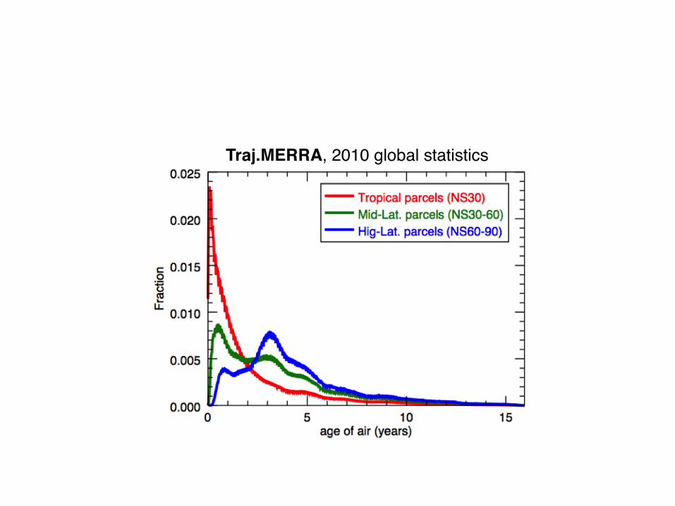
Traj.MERRA, 2010 global statistics

[-15,0],[0,15]

0.00 1.00 2.00 3.00 4.00 5.00age-of-air (years)

16

19

22

25

29

32

Appr

ox. A

lt (k

m)

100.082.568.156.246.438.331.626.121.517.814.712.110.0

Pres

(hPa

)

Global

0.00 1.00 2.00 3.00 4.00 5.00age-of-air (years)

16

19

22

25

29

32

Appr

ox. A

lt (k

m)

100.082.568.156.246.438.331.626.121.517.814.712.110.0

Pres

(hPa

)

N.Mid.Lat.[30,60]

0.00 1.00 2.00 3.00 4.00 5.00age-of-air (years)

16

19

22

25

29

32

Appr

ox. A

lt (k

m)

100.082.568.156.246.438.331.626.121.517.814.712.110.0

Pres

(hPa

)

N.Polar.[60,90]

0.00 1.00 2.00 3.00 4.00 5.00age-of-air (years)

16

19

22

25

29

32

Appr

ox. A

lt (k

m)

100.082.568.156.246.438.331.626.121.517.814.712.110.0

Pres

(hPa

)

S.Mid.Lat.[-60,-30]

0.00 1.00 2.00 3.00 4.00 5.00age-of-air (years)

16

19

22

25

29

32

Appr

ox. A

lt (k

m)

100.082.568.156.246.438.331.626.121.517.814.712.110.0

Pres

(hPa

)

S.Polar.[-60,-90]

0.00 1.00 2.00 3.00 4.00 5.00age-of-air (years)

16

19

22

25

29

32

Appr

ox. A

lt (k

m)

100.082.568.156.246.438.331.626.121.517.814.712.110.0

Pres

(hPa

)

Vertical Profile:lon[0,360],lat[-90,90],vert[100,10],time[2000.042,2013.958],X00: 140415_B_s100_i370_mthd_inj1sav3_MERwindT_day_dhAll_fdhm-un_newT_since80_var1_monCat_1980-2013.nc; X01: 120916_sat100_init370_ERAi_6hr_15yr_addGX02: 150101_s100_i370_mthd_inj1sav3_JRA55windT_day_dhAll_fdhm-un_var1_monCat_1958-2013.nc; X03: 110906_noCnv_NCEP_UVQT_var1_monCat_2004-2010.nc;


[-15,0],[0,15]

0.00 1.00 2.00 3.00 4.00 5.00age-of-air (years)

16

19

22

25

29

32

Appr

ox. A

lt (k

m)

100.082.568.156.246.438.331.626.121.517.814.712.110.0

Pres

(hPa

)

Global

0.00 1.00 2.00 3.00 4.00 5.00age-of-air (years)

16

19

22

25

29

32

Appr

ox. A

lt (k

m)

100.082.568.156.246.438.331.626.121.517.814.712.110.0

Pres

(hPa

)

N.Mid.Lat.[30,60]

0.00 1.00 2.00 3.00 4.00 5.00age-of-air (years)

16

19

22

25

29

32

Appr

ox. A

lt (k

m)

100.082.568.156.246.438.331.626.121.517.814.712.110.0

Pres

(hPa

)

N.Polar.[60,90]

0.00 1.00 2.00 3.00 4.00 5.00age-of-air (years)

16

19

22

25

29

32

Appr

ox. A

lt (k

m)

100.082.568.156.246.438.331.626.121.517.814.712.110.0

Pres

(hPa

)

S.Mid.Lat.[-60,-30]

0.00 1.00 2.00 3.00 4.00 5.00age-of-air (years)

16

19

22

25

29

32

Appr

ox. A

lt (k

m)

100.082.568.156.246.438.331.626.121.517.814.712.110.0

Pres

(hPa

)

S.Polar.[-60,-90]

0.00 1.00 2.00 3.00 4.00 5.00age-of-air (years)

16

19

22

25

29

32

Appr

ox. A

lt (k

m)

100.082.568.156.246.438.331.626.121.517.814.712.110.0

Pres

(hPa

)



[-15,0],[0,15]

0.00 1.00 2.00 3.00 4.00 5.00age-of-air (years)

16

19

22

25

29

32

Appr

ox. A

lt (k

m)

100.082.568.156.246.438.331.626.121.517.814.712.110.0

Pres

(hPa

)

Global

0.00 1.00 2.00 3.00 4.00 5.00age-of-air (years)

16

19

22

25

29

32

Appr

ox. A

lt (k

m)

100.082.568.156.246.438.331.626.121.517.814.712.110.0

Pres

(hPa

)

N.Mid.Lat.[30,60]

0.00 1.00 2.00 3.00 4.00 5.00age-of-air (years)

16

19

22

25

29

32

Appr

ox. A

lt (k

m)

100.082.568.156.246.438.331.626.121.517.814.712.110.0

Pres

(hPa

)N.Polar.[60,90]

0.00 1.00 2.00 3.00 4.00 5.00age-of-air (years)

16

19

22

25

29

32

Appr

ox. A

lt (k

m)

100.082.568.156.246.438.331.626.121.517.814.712.110.0

Pres

(hPa

)

S.Mid.Lat.[-60,-30]

0.00 1.00 2.00 3.00 4.00 5.00age-of-air (years)

16

19

22

25

29

32

Appr

ox. A

lt (k

m)

100.082.568.156.246.438.331.626.121.517.814.712.110.0

Pres

(hPa

)

S.Polar.[-60,-90]

0.00 1.00 2.00 3.00 4.00 5.00age-of-air (years)

16

19

22

25

29

32

Appr

ox. A

lt (k

m)

100.082.568.156.246.438.331.626.121.517.814.712.110.0

Pres

(hPa

)



Traj.ERAiTraj.JRA55Traj.CFSRTraj.MERRA

26/29

1960 1965 1970 1975 1980 1985 1990 1995 2000 2005 2010Time

100.068.146.431.621.514.710.0

Pres

(hPa

)

16182124262932

Appr

ox. A

lt. (k

m)

CFSR

100.0

68.146.431.621.514.710.0

Pres

(hPa

)

16182124262932

Appr

ox. A

lt. (k

m)

MER

RA

100.0

68.146.431.621.514.710.0

Pres

(hPa

)

16182124262932

Appr

ox. A

lt. (k

m)

ERAi

100.0

68.146.431.621.514.710.0

Pres

(hPa

)

16182124262932

Appr

ox. A

lt. (k

m)

JRA55

ALLbinFrac:[ 0.000, 0.050, 0.150, 0.300, 0.650, 0.950, 1.000,], Time-Vertical: lon[0,360],lat[-15,0,0,15],,vert[100,10],time[1960.042,2013.958],X00: 110906_noCnv_NCEP_UVQT_var1_monCat_1980-2010.nc; X01: 140415_B_s100_i370_mthd_inj1sav3_MERwindT_day_dhAll_fdhm-un_newT_since80_var1_monCat_1980-2013.nc; X02: 120916_sat100_init370_ERAi_6hr_15yr_addGPH_var1_monCat_1980-2013.nc; X03: 150101_s100_i370_mthd_inj1sav3_JRA55windT_day_dhAll_fdhm-un_var1_monCat_1958-2013.nc;

-1.0 -0.5 0.0 0.5 1.0

age-of-air Anom. (years)

15o N–Saverageanomaly(removingannualcycle2000–2009)Traj.JRA55

Traj.ERAi

Traj.MERRA

Traj.CFSR

27/29

-60 -30 0 30 60Lat. (O )

316.2

215.4

146.8

100.0

68.1

46.4

31.6

Pres

(hPa

)

e=340Ke=340K

e=500K

e=380K

e=355K

e=440K

200

210

210

210

220

220

230 240 -2PVU

10

13

16

18

21

24

Appr

ox. A

lt. (k

m)

MLS

ALL

23456781015305080120150200

H2O

(ppm

v)

Latitude-Vertical:lon[0,360],lat[-90,90],vert[315,30],time[2005.042,2011.958],X00: monthly_gridded_H2O_lon360_monCat_2004-2012.nc;

-60 -30 0 30 60Lat. (O )

316.2

215.4

146.8

100.0

68.1

46.4

31.6Pr

es (h

Pa)

e=340Ke=340K

e=500K

e=380K

e=355K

e=440K

200

210

210

210

220

220

230

240 -2PVU

10

13

16

18

21

24

App

rox.

Alt.

(km

)

MLS

ALL

23456781015305080120150200

H2O

(ppm

v)


-60 -30 0 30 60Lat. (O )

316.2

215.4

146.8

100.0

68.1

46.4

31.6Pr

es (

hPa)

e=340Ke=340K

e=500K

e=380K

e=355K

e=440K

200

210

210

210

220

220

230

240 -2PVU

10

13

16

18

21

24

App

rox.

Alt.

(km

)

ML

SALL

234567810121518305080150

H2O

(pp

mv)


-60 -30 0 30 60Lat. (O )

316.2

215.4

146.8

100.0

68.1

46.4

31.6

Pres

(hPa

)

e=340Ke=340K

e=500K

e=380K

e=355K

e=440K

200

210

210

210

220

220

230

240 -2PVU

10

13

16

18

21

24

App

rox.

Alt.

(km

)

MLS

ALL

234567810121518305080150

H2O

(ppm

v)


H2O

con

cent

ratio

n (p

pmv)

3/40

Pres

sure

(hPa

)

Tropical 30o N–S [H2O] (ppmv)

MLS

2005 2006 2007 2008 2009 100.0

68.1

46.4

31.6

21.5

14.7

MLS

2005 2006 2007 2008 2009 16.0

18.0

20.0

22.0

24.0

26.0

28.0

30.0

2005 2006 2007 2008 2009 100.0

68.1

46.4

31.6

21.5

14.7

MERRA

2005 2006 2007 2008 2009 16.0

18.0

20.0

22.0

24.0

26.0

28.0

30.0

2005 2006 2007 2008 2009 100.0

68.1

46.4

31.6

21.5

14.7

ERAi

isob (hPa)

2005 2006 2007 2008 2009 16.0

18.0

20.0

22.0

24.0

26.0

28.0

30.0isoh (km)

Water Vapor Concentration (ppmv)

2.00 3.00 3.50 4.00 4.50 5.00 6.50

2005 2006 2007 2008 2009 100.0

68.1

46.4

31.6

21.5

14.7

MLS

2005 2006 2007 2008 2009 16.0

18.0

20.0

22.0

24.0

26.0

28.0

30.0

2005 2006 2007 2008 2009 100.0

68.1

46.4

31.6

21.5

14.7

MERRA

2005 2006 2007 2008 2009 16.0

18.0

20.0

22.0

24.0

26.0

28.0

30.0

2005 2006 2007 2008 2009 100.0

68.1

46.4

31.6

21.5

14.7

ERAi

isob (hPa)

2005 2006 2007 2008 2009 16.0

18.0

20.0

22.0

24.0

26.0

28.0

30.0isoh (km)


2.00 3.00 3.50 4.00 4.50 5.00 6.50

Time

H2O “tape-recorder”

~ 16 km

~ 28 km

Brewer, QJRMS, 1949

~ 16 km

~ 28 km

1/29

Pres

sure

(hPa

)

2005 2006 2007 2008 2009 100.0

68.1

46.4

31.6

21.5

14.7

MLS

2005 2006 2007 2008 2009 16.0

18.0

20.0

22.0

24.0

26.0

28.0

30.0

2005 2006 2007 2008 2009 100.0

68.1

46.4

31.6

21.5

14.7

MERRA

2005 2006 2007 2008 2009 16.0

18.0

20.0

22.0

24.0

26.0

28.0

30.0

2005 2006 2007 2008 2009 100.0

68.1

46.4

31.6

21.5

14.7

ERAi

isob (hPa)

2005 2006 2007 2008 2009 16.0

18.0

20.0

22.0

24.0

26.0

28.0

30.0isoh (km)


2.00 3.00 3.50 4.00 4.50 5.00 6.50

2005 2006 2007 2008 2009 100.0

68.1

46.4

31.6

21.5

14.7

MLS

2005 2006 2007 2008 2009 16.0

18.0

20.0

22.0

24.0

26.0

28.0

30.0

2005 2006 2007 2008 2009 100.0

68.1

46.4

31.6

21.5

14.7

MERRA

2005 2006 2007 2008 2009 16.0

18.0

20.0

22.0

24.0

26.0

28.0

30.0

2005 2006 2007 2008 2009 100.0

68.1

46.4

31.6

21.5

14.7

ERAi

isob (hPa)

2005 2006 2007 2008 2009 16.0

18.0

20.0

22.0

24.0

26.0

28.0

30.0isoh (km)


2.00 3.00 3.50 4.00 4.50 5.00 6.50

Time

TRAJ.

2005 2006 2007 2008 2009 100.0

68.1

46.4

31.6

21.5

14.7

MLS

2005 2006 2007 2008 2009 16.0

18.0

20.0

22.0

24.0

26.0

28.0

30.0

2005 2006 2007 2008 2009 100.0

68.1

46.4

31.6

21.5

14.7

MERRA

2005 2006 2007 2008 2009 16.0

18.0

20.0

22.0

24.0

26.0

28.0

30.0

2005 2006 2007 2008 2009 100.0

68.1

46.4

31.6

21.5

14.7

ERAi

isob (hPa)

2005 2006 2007 2008 2009 16.0

18.0

20.0

22.0

24.0

26.0

28.0

30.0isoh (km)


2.00 3.00 3.50 4.00 4.50 5.00 6.50

Pres

sure

(hPa

)

Time

~ 16 km

~ 28 km H2O “tape-recorder”

Our Model

Tropical 30o N–S [H2O] (ppmv)

MLS

2/29

-60 -30 0 30 60Lat. (O )

380410440470500650800950

e (K

)

-60 -30 0 30 60Lat. (O )

-60 -30 0 30 60Lat. (O )

-60 -30 0 30 60Lat. (O )

ALL

380410440470500650800950

e (K

)

DJF

380410440470500650800950

e (K

)

MAM

380410440470500650800950

e (K

)

JJA

380410440470500650800950

e (K

)

MERRA

ERAi

JRA55

SON

CFSR

binFrac:[ 0.000, 0.050, 0.100, 0.150, 0.300, 0.650, 0.900, 1.000,], Latitude-Vertical:lon[0,360],lat[-60,0,0,60],,vert[380,1000],time[1980.042,2013.958],X00: residence_time_161008_mthd_MERRA_grid3D_mon_1979-2014.nc; X01: residence_time_161011_mthd_ERAi_grid3D_mon_1979-2014.nc; X02: residence_time_161009_mthd_JRA55_noH2O_grid3D_mon_1958-2013.nc; X03: residence_time_161017_mthd_CFSR_noH2O_grid3D_mon_1979-2010.nc;

0.00 2.50 4.50 7.00 9.00 12.50

normalized freq. (%)

Stratospheric Dehydration, Residence Time, and Age-of-Air Inferred ...

Documents