Strategies for Computing Minimal Free Resolutions

Article No. sy980221J. Symbolic Computation (1998) 26, 409–431

Strategies for Computing Minimal Free Resolutions†

ROBERTO LA SCALA‡¶ AND MICHAEL STILLMAN§‖

‡Dipartimento di Matematica, Universita di Bari, Italy§Department of Mathematics, Cornell University, U.S.A.

In the present paper we study algorithms based on the theory of Grobner bases forcomputing free resolutions of modules over polynomial rings. We propose a techniquewhich consists in the application of special selection strategies to the Schreyer algorithm.The resulting algorithm is efficient and, in the graded case, allows a straightforwardminimalization algorithm. These techniques generalize to factor rings, skew commutativerings, and some non-commutative rings. Finally, the proposed approach is comparedwith other algorithms by means of an implementation developed in the new systemMacaulay2.

c© 1998 Academic Press

1. Introduction

One of the most important computations in algebraic geometry or commutative algebrathat a computer algebra system should provide is the computation of finite free reso-lutions of ideals and modules. Resolutions are used as an aid to understand the subtlenature of modules and are also a basis of further computations, such as computing sheafcohomology, local cohomology, Ext, Tor, etc. Modern methods for calculating free reso-lutions derive from the theory of Grobner bases. These methods were introduced at theend of the 1970s by Richman (1974); Spear (1977); Schreyer (1980) and have survived incomputer algebra systems up to now. However, the problem with these algorithms is thatmany computations of interest for researchers were out of range. This is giving impulseto authors such as Capani et al. (1997), Siebert (1996) and ourselves to develop decisiveimprovements of the resolution techniques.

Resolution algorithms based on Grobner bases can be divided essentially into two types.The first type is based on computing the syzygy module on a minimal set of generators.The second type, initially used by Frank Schreyer, is based on computing the syzygymodule on a Grobner basis. In both cases, using induced term orderings leads to a largeimprovement in the sizes of the Grobner bases involved. Which of these two methods isbest depends in part on the specific input ideal or module. However, we have found thatfor problems of interest, the Schreyer technique, together with the improvements that wesuggest, on the average outperforms the other methods.

†This research was performed with the contribution of MURST, and M. Stillman would like to thankthe NSF for partial support during the preparation of this manuscript.¶E-mail: [email protected]‖E-mail: [email protected]

0747–7171/98/100409 + 23 30.00/0 c© 1998 Academic Press

410 Roberto La Scala and Michael Stillman

The syzygies of the Schreyer resolution are usually computed level by level. (i.e., firstsyzygies first, then second syzygies, etc.) In this way just one syzygy is obtained by any S-polynomial reduction. Our improvement of the Schreyer algorithm is based essentially onthe remark that we can use global strategies instead for the selection of the S-polynomialswhich allow the computation of couples of syzygies from single reductions. This resultsnot only in an optimization of the calculation of the Schreyer resolution but also ofits minimalization. It can be proved in fact that with respect to suitable strategies aminimal resolution corresponds exactly to the syzygies traced by S-polynomial reductionsto zero. It follows that using our technique the Betti numbers are derived by the Schreyerresolution with no additional computations.

An important feature of the proposed algorithms is that they can be easily extended.In the present paper we explain how to generalize them to factor rings and show thatthe resolution procedure can be applied to non- graded ideals and modules. We describean implementation, and some of the choices one has when computing a resolution. Wesuggest some optimizations that we have found to be useful. Finally, we compare thesealgorithms with other algorithms, using a suite of examples. These tests are performedusing an installation developed in the new system Macaulay2 (Grayson and Stillman,1993–1998).

2. Preliminaries

In this section, we define our notation regarding Grobner bases. Since the algorithmswe describe also work over a factor ring R of a polynomial ring S, we also describe ournotation regarding Grobner bases in this setting. Without too much more difficulty, onecould extend these definitions to more general situations, e.g. (factor rings of) skew-commutative polynomial rings, Weyl algebras, and non- commutative polynomial rings.The algorithms given in this paper would work, with small modifications, in these moregeneral settings.

Let S = K[x1, . . . , xn] be a polynomial ring over the field K, endowed with a termorder > that we fix once and for all.

A power product (or monomial of S) is an element

t = xα11 · · ·xαnn ∈ S,

where α1, . . . , αn are non-negative integers.Any non-zero element f ∈ S may be written uniquely as the sum

f = c1 ·m1 + · · ·+ ck ·mk,

where 0 6= ci ∈ K, mi monomials, and m1 > m2 > · · · > mk. We define:

lc(f) = c1, the leading coefficient ,lm(f) = m1, the leading monomial .

For any set G ⊂ S, we let in(G) denote the K-vector space spanned by the monomials{lm(f) : f ∈ G}. If J ⊂ S is an ideal, then in(J) ⊂ S is the monomial ideal generatedby the lead terms of J .

Let R = S/J be a factor ring of S. We may extend the above notions to this situation.Let N ⊂ S be the K-vector space spanned by the set of standard monomials of R, that

Strategies for Computing Minimal Free Resolutions 411

is, the set of monomials of S not in in(J). Any element f ∈ R may be uniquely writtenas the image of an element g ∈ N , and we set lc(f) = lc(g) and lm(f) = lm(g) ∈ N .

For any set G ⊂ R, let in(G) denote the K-vector space generated by the lead mono-mials {lm(f) : f ∈ G}. Thus, N = in(R), and in(S) = N ⊕ in(J), as K-vector spaces.

Let F be a free module over R, and let F be the free S-module with the same rank asF and corresponding basis. A monomial of F is by definition any element

m = t · e,where t ∈ N is a standard monomial and e is any element of the canonical basis of F .

A term order on F is a total order on the monomials of F such that:

(i) if m < n, then t ·m < t · n;(ii) if s < t, then s · e < t · e

for all m,n monomials of F , s, t power products in S, and e any basis element of F .Fix a term order on F . Then, any element f ∈ F may be written uniquely (as the

image of an element) in the form:

f = c1 ·m1 + · · ·+ ck ·mk,

where 0 6= ci ∈ K, mi monomials, and m1 > m2 > . . . > mk. If m1 = t ·e, for the moduleelement f we define:

lc(f) = c1, the leading coefficient ,lm(f) = m1, the leading monomial ,lpp(f) = t, the leading power product .

As usual, for any G ⊂ F , we denote by in(G) ⊂ F the K-vector space generated by{lm(f) : f ∈ G}.

We say that {g1, . . . , gs} ⊂ I ⊂ F is a Grobner basis of the R-module I, if {lm(g1), . . .,lm(gs)} generates in(I), that is, every monomial in in(I) is divisible by some lm(gi). TheGrobner basis is called auto-reduced if every lead monomial lm(gi) divides no monomialoccuring in any gj , other than itself. The Grobner basis is called irredundant if in(I) isminimally generated by {lm(g1), . . . , lm(gs)}, which in turn means that this set generatesin(I), and no lead term lm(gi) divides any lm(gj), for j 6= i.

3. The Schreyer Resolution and Its Frame

Throughout this section, R = S/J is a factor ring of the polynomial ring S, andM = F0/I is an R-module, where F0 is a free module. If both M and R are graded, thenall of our sequences of modules, and resolutions will be graded as well.

Consider a sequence of R-homomorphisms:

Φ : · · · −→ Flϕl−→ Fl−1

ϕl−1−→ · · · ϕ2−→ F1ϕ1−→ F0

where each Fi is a free R-module with a given (canonical) basis Ei. Let Ci = ϕi(Ei) bethe image of the given basis, and define the level of an element f in Ci to be lev(f) = i.Note that Φ is not necessarily a complex.

Definition 3.1. Let τ = {τi} be a sequence of term orderings τi on the Fi. We call τ aterm ordering on Φ if it satisfies the following compatibility relationship:


s · e1 < t · e2 whenever s · lmϕi(e1) < t · lmϕi(e2),

where e1 and e2 are elements of Ei.

Definition 3.2. Given a Φ as above, and a term ordering on Φ, define the initial termsof Φ, in(Φ), to be the sequence of (graded) R-homomorphisms:

Ξ = in(Φ) : · · · −→ Flξl−→ Fl−1

ξl−1−→ · · · ξ2−→ F1ξ1−→ F0

where ξi(e) = lmϕi(e), for all e in Ei. That is, in(Φ) consists of the leading monomialsof the columns of (each matrix of) Φ.

Notice that a term ordering on Φ is also a term ordering for Ξ. The converse holds, iffor this order, Ξ = in(Φ).

Definition 3.3. A Schreyer resolution of an R-module M = F0/I is an exact sequence:

Φ : · · · → Flϕl−→ Fl−1

ϕl−1−→ · · · ϕ2−→ F1ϕ1−→ F0

together with a term ordering on Φ, such that:

(i) coker(ϕ1) = M ;(ii) ϕi(Ei) forms an irredundant Grobner basis of image(ϕi) (for all i where Fi 6= 0);

Our plan in the next section is to give an algorithm that computes a Schreyer resolution.A useful way of picturing this resolution is by its “frame”.

Definition 3.4. A Schreyer frame of M = F0/I is a sequence of (graded) R-homomor-phisms:

Ξ : · · · → Flξl−→ Fl−1

ξl−1−→ · · · ξ2−→ F1ξ1−→ F0

where each column is a monomial, and a term ordering on Ξ such that:

(i) ξ1(E1) is a minimal set of generators for in(I);(ii) ξi(Ei) is a minimal set of generators for in(ker ξi−1) (i ≥ 2).

If Φ is a Schreyer resolution, then in(Φ) is a Schreyer frame. The reason we introducethis concept is because one can compute a Schreyer frame first, and then “fill it in” toform a Schreyer resolution.

Let Ξ be a Schreyer frame. It is useful to introduce the following notation. Given i,and a basis element e ∈ Ei−1, we put:

Bi = ξi(Ei);Ei(e) = {ε ∈ Ei : ξi(ε) = s · e, for some power product s}.

Thus Ei(e) consists of those basis elements that map to multiples of e. Note that this setcan be empty.

The following lemma is the basis of our algorithm to compute a Schreyer frame. Letξi : Fi → Fi−1 be a map of free R-modules, such that each element ξi(ε) is a monomial,for all ε ∈ ξi. Suppose that ξi is endowed with a term ordering.


Lemma 3.5. Given the above setup, we have that in(ker ξi) is minimally generated by⋃e∈Ei−1

r⋃j=2

mingens ((in(J), t1, . . . , tj−1) : tj) · εj

where for each e in the outer union, if Ei(e) = {ε1, . . . , εr} then ξi(εj) = tj · e, andmingens defines the subset of the minimal generators of the considered monomial idealwhich do not lie in in(J).

Proof. Let∑j gj ·mj = 0 where mj are minimal generators of in(image ξi) and gj are

standard polynomials of S. Let sk·εk be the leading monomial of the corresponding syzygywith sk = lm(gk). For cancelling sk ·mk in the sum there are exactly two possibilities:

sk ·mk = sh ·mh for some h,sk · tk belongs to in(J),

where mk = tk · e.

This lemma immediately translates into an algorithm to compute a Schreyer frame (orall possible frames) given in(J) and in(I).

Proposition 3.6. If Ξ is a Schreyer frame for M , then there exists a Schreyer resolutionΦ such that Ξ = in(Φ).

Proof. With respect to the term ordering assigned on the free module F0, any irredun-dant Grobner basis C1 of the submodule I ⊂ F0 satisfies in(C1) = B1. Note now that forany monomial m ∈ B2, there exists an element g in C1 = ϕ1(E1) such that:

m = t · ε,where t is a standard power product, ε ∈ E1 and ϕ1(ε) = g. By definition, the setC2 = ϕ2(E2) is formed by the syzygies traced by the reductions to zero of the elementst · g as m varies in B2. Since the term ordering of F1 satisfies the condition of Definition3.1, we have:

in(ker ξ1) = in(kerϕ1).It follows that C2 is an irredundant Grobner basis of ker(ϕ1) and in(C2) = B2. Iteratingfor all the levels i, we get a Schreyer resolution Φ such that Ξ = in(Φ).

Note that this is essentially Schreyer’s original proof that the syzygy module is con-structed from a Grobner basis computation. The resolution Φ produced in the aboveproposition is not quite unique, given the Schreyer frame Ξ. One could make it uniqueby requiring that each ϕi(Ei) forms an auto-reduced Grobner basis.

Proposition 3.7. If Φ is a complex of free S-modules, with a term ordering, such thatin(Φ) is a Schreyer frame of M , then Φ is a free resolution of M .

Proof. Clear.

The following proposition explains how a term ordering can be assigned on a frame.


Proposition 3.8. Let Ξ : · · · −→ Flξl−→ Fl−1

ξl−1−→ · · · ξ2−→ F1ξ1−→ F0 be a sequence

of homomorphisms where each column is a monomial. To give a term ordering on Ξ isequivalent to give a term ordering on F0 and place total orders on the sets Ei(e) 6= ∅, forevery i ≥ 1 and e ∈ Ei−1.

Proof. By induction on the level i, the term ordering on the free module Fi can bedefined as follows. For any s, t power products, ε1, ε2 ∈ Ei, m = ξi(ε1), n = ξi(ε2), we put:

s · ε1 < t · ε2 iff s ·m < t · n, ors ·m = t · n and ε1 < ε2 w.r.t. the order on Ei(e),with m,n multiples of e ∈ Ei−1.2

Example 3.9. Let K be a field of any characteristic and let the polynomial ring S =K[x0, . . . , x5] be endowed by the term ordering DegRevLex. Consider the graded moduleM = S/I, where the monomial ideal I is the face ideal of a triangulation of the realprojective plane (first introduced by Reisner (1976)).

I = 〈 x2x4x5, x0x4x5, x2x3x5, x1x3x5, x0x1x5,x1x3x4, x0x3x4, x1x2x4, x0x2x3, x0x1x2 〉.

Then, a Schreyer frame Ξ for M is given by the bases:

B1 = { x2x4x5, x0x4x5, x2x3x5, x1x3x5, x0x1x5, x1x3x4, x0x3x4, x1x2x4,x0x2x3, x0x1x2 };

B2 = { x4e3, x5e6, x5e7, x5e8, x2e2, x4e5, x2e4, x5e9, x3e5, x5e10, x3e8,x4e9, x1e7, x4e10, x3e10, x0x4e4 };

B3 = { x5e11, x5e12, x4e9, x5e13, x5e14, x5e15, x4e15, x2e16 };

B4 = { x5e7 }.

For simplifying the notation, we have used the same letters ej for indicating the elementsof the canonical bases of the free modules F1 = S10, F2 = S16, F3 = S8. The termordering on Ξ is defined for any level i in the usual way:

s · ej < t · ek iff s ·mj < t ·mk, ors ·mj = t ·mk and j < k,

where s, t are power products, ej , ek are elements of Ei s.t. ξi(ej) = mj , ξi(ek) = mk.

4. The Algorithms

An algorithm for computing Schreyer resolutions has been found independently byRichman (1974); Spear (1977); Schreyer (1980). In this section we propose a new versionof that algorithm which improves both the computation of the Schreyer resolution, andits minimalization (in the graded case). In the graded case, minimalization can be a time-consuming process. The algorithm presented here allows a nice, efficient algorithm forcomputing a minimal resolution, and the graded Betti numbers of the minimal resolutionare produced with no extra work.


Let M = F0/I be an R-module, let C1 be an irredundant Grobner basis of I, and letΞ be a Schreyer frame of M . The following algorithm takes these data and produces aSchreyer resolution Φ of M , such that in(Φ) = Ξ. Of course we assume these sequences aretruncated when they are infinite. The main idea here is very simple: process the s-pairsin such a way that the higher-level elements are processed first. If an element reduces toa non-zero value (which is possible since we do not yet have all of the elements of theGrobner basis), then we get two elements for the price of one: we get the syzygy, and weget a Grobner basis element at the previous level. We show that the Betti numbers are aby-product of this computation and we can minimalize Φ very easily. Note that we couldmodify this algorithm to compute the Grobner basis on the fly. The difficulty is thatwe need then to compute the Schreyer frame on the fly as well, and the correspondingalgorithm is somewhat harder to describe.

For this algorithm, let the variable B be the union of the sets B1, . . . ,Bl initializedas the monomial bases of Ξ. We call the elements of B the S-polynomials. The outputconsists of the Grobner bases C1, . . . , Cl of Φ together with the sets of minimal syzygiesH1, . . . ,Hl, Hi ⊂ Ci.

Algorithm 4.1. Resolution[C1]

Ci,Hi:= ∅ (1 ≤ i ≤ l )while B 6= ∅ dom:= minBB:= B \ {m}i:= lev(m)if i = 1 theng:= the element of C1 s.t. lm(g) = mC1:= C1 ∪ {g}H1:= H1 ∪ {g}

else(f, g):= Reduce[m, Ci−1]Ci:= Ci ∪ {g}if f 6= 0 thenCi−1:= Ci−1 ∪ {f}B:= B \ {lm(f)} removing one S-polynomial for free!!

elseHi:= Hi ∪ {g}

return Ci,Hi (1 ≤ i ≤ l )

The function min concerns the selection strategies we use for the algorithm. By defi-nition, a strategy of Resolution is any total ordering of the set B = B1 ∪ . . . ∪ Bl s.t. ifone of the following conditions holds:

(i) deg(m)− lev(m) ≤ deg(n)− lev(n) and lev(m) < lev(n);(ii) deg(m) < deg(n) and lev(m) = lev(n);(iii) deg(m) = deg(n) and lev(m) > lev(n);

then m < n, for all m,n ∈ B. Note that such strategies are easily defined. For instance,a class of them is obtained by putting:


m < n iff deg(m) < deg(n), or deg(m) = deg(n) and lev(m) > lev(n).

We call these strategies DRLv (Degree Reverse Level). Another natural class of strategiesis SDLv (Slanted Degree Level):

m < n iff deg(m)− lev(m) < deg(n)− lev(n), ordeg(m)− lev(m) = deg(n)− lev(n) and lev(m) < lev(n).

The function Reduce in the algorithm Resolution is a simplification procedure whichreturns both the reductum and the corresponding syzygy. We may either reduce untilthe lead term cannot be simplified, or we can reduce until all terms cannot be simplified.(When we discuss implementations, the first variant will be algorithm A0, and the secondvariant, A1):

Procedure 4.2. Reduce[t · ε, Ci−1]

f:= t · k, where ϕi−1(ε) = kg:= t · εwhile f 6= 0 and lm(f) ∈ in〈Ci−1〉 dochoose h ∈ Ci−1 s.t. lm(h) | lm(f) (at first iteration h

not allowed to be f)

f:= f − lc(f) lpp(f)lc(h) lpp(h) h

g:= g − lc(f) lpp(f)lc(h) lpp(h) e, where ϕi−1(e) = h

if f 6= 0 theng:= g − e, where ϕi−1(e) = f

return f, g

Procedure 4.3. ReduceAll[t · ε, Ci−1]

f:= t · k, where ϕi−1(ε) = kg:= t · εr:= 0while f 6= 0 do

if lm(f) ∈ in〈Ci−1〉 thenchoose h ∈ Ci−1 s.t. lm(h) | lm(f) (at first iteration h

not allowed to be f)

f:= f − lc(f) lpp(f)lc(h) lpp(h) h

g:= g − lc(f) lpp(f)lc(h) lpp(h) e, where ϕi−1(e) = h

elser:= r + lm(f)f:= f − lm(f)

if r 6= 0 theng:= g − e, where ϕi−1(e) = r

return r, g

To prove the correctness of the proposed algorithm, we start with the following:


Proposition 4.4. The resolution Φ computed by Resolution is a Schreyer one.

Proof. By induction on i, we suppose that at termination the set Ci is an irredundantGrobner basis of the module kerϕi−1. By the definition of Resolution we have imme-diately that Bi+1 ⊂ in(Ci+1) i.e. Ci+1 is a Grobner basis of kerϕi. We have to prove nowthat Ci+1 is an irredundant Grobner basis, that is:

Bi+1 = in(Ci+1).

Let f ∈ Ci+1 be an element obtained at some step of the algorithm Resolution by amonomial m ∈ B. We claim that lm(f) ∈ Bi+1. If m ∈ Bi+1 the claim follows immediatelysince lm(f) = m. Suppose now that m ∈ Bi+2, i.e. f is the reductum of an S-polynomial.Denote by g any element of Ci+1 computed at a previous step. By definition of thereductum we have that lm(g) does not divide lm(f). Moreover, by induction we cansuppose that lm(g) ∈ Bi+1. Therefore, lm(g) is not a proper multiple of lm(f) since Bi+1

is the minimal monomial basis of in(kerϕi). We conclude that the claim is true.

From this point on we assume that the module M is graded. Note that for any level i,the elements of Ci \Hi are non-minimal elements of the basis Ci. By eliminating them, anew graded free resolution of M :

Ψ : · · · → Gqψq−→ Gq−1

ψq−1−→ · · · ψ2−→ G1ψ1−→ F0 → M → 0

is clearly defined with rk(Gi) ≤ rk(Fi), where possibly Gi = 0 even if Fi 6= 0. Denoteby Di the image of the basis of free module Gi through the map ψi (i ≥ 1). We have agraded epimorphism of complexes Φ θ→ Ψ:

. . . → Fq → . . . → F1 → F0 → Mθq ↓ θ1 ↓ ↓

. . . → Gq → . . . → G1 → F0 → M

such that θi−1(Hi) = Di and H1 = D1. For i > 1, denote by Ki the subset of Ci ofthe syzygies traced by S-polynomials which reduce to non-zero elements. Let g be anelement of Ki obtained at any step of the procedure Resolution and denote by f thecorresponding S-polynomial reductum. Note that the component corresponding to f iszero for the elements of Ki computed in the previous steps, and is equal to −1 ∈ K forthe syzygy g. Therefore, Ki is a free basis of the kernel of the projection defined by θi−1

of the module ker(ϕi−1) onto ker(ψi−1).For the algorithm Resolution we have the following important result:

Proposition 4.5. The resolution Ψ is a minimal resolution of the graded module M .

Proof. By the conditions (ii) and (iii), any element f of the basis C1 is added byResolution to H1 = D1 only if f is not reducible to zero w.r.t. to the partial Grobnerbasis of the elements of degree ≤ deg(f). Therefore, D1 is a minimal basis of the moduleI = image(ϕ1).

We have to prove now that D2, . . . ,Dq define a minimal resolution of kerψ1. Initially,we show that any element of Hi is not a linear combination over the ring S of otherelements of Ci. Then, we prove that Di = θi−1(Hi) is a minimal basis of the modulekerψi−1.


Let f ∈ Ci,deg(f) = d. Suppose that f is not a minimal element of the basis Ci. Then,there is g ∈ Ci+1 a syzygy of degree d s.t. its component corresponding to f is differentfrom zero. We claim that f, g are obtained in the algorithm Resolution by the samemonomial of Bi+1.

Let m,n be the monomials of the Schreyer frame which create f, g respectively. Notethat m,n have the same degree d, but lev(m) ≤ lev(n). Since the syzygy g has a non-zero component corresponding to f , we have clearly that the monomial m cannot beselected in the algorithm after n. On the other hand, by the strategy condition (iii) ofResolution, we have that m cannot be selected before n. Therefore, the elements f, gare created simultaneously by a monomial m = n of the level i+ 1. We deduce that anyelement of Hi is minimal in the basis Ci.

By contradiction, we suppose now thatDi is not a minimal basis of the module kerψi−1,i.e. there exist f ′ ∈ Di, g′ ∈ kerψi s.t. deg(f ′) = deg(g′) and g′ has the componentcorresponding to f ′ different from zero. Therefore, by definition of θ, there are f ∈Hi, g ∈ kerϕi of the same degree s.t. g has a non- zero component corresponding to f .This contradicts the minimality of the elements of Hi.2

Note that from the above result it follows that the graded Betti numbers of M areobtained by the algorithm Resolution with no additional computations. They are simplythe number of elements of the sets Hi in each degree. Moreover, for obtaining a minimalresolution of the module M it is sufficient to transform each Hi, i > 1 in Di by meansof the homomorphism θi−1. The following simple algorithm implements θi−1.

Denote by Ki the subsets of Bi of the monomials corresponding to S-polynomials whichreduce to non-zero elements in Resolution. Moreover, assume that Ki is endowed bythe converse ordering w.r.t. the selection strategy.

Algorithm 4.6. Minimalize[Hi]

for m ∈ Ki do(f, g):= resp. the reductum and the syzygy obtained by mfor h ∈ Hi dohe:= the component of h corresponding to e ∈ Ei−1, ϕi−1(e) = fh:= h+ he · gh:= Strip[h]

return Hi

The subprocedure Strip is defined as follows:

Procedure 4.7. Strip[h]

for m ∈ Ki−1 dog:= the syzygy of Ci−1 obtained by mhe:= the component of h corresponding to e ∈ Ei−1, ϕi−1(e) = gh:= h− he · e

return h

The correctness of Minimalize is based on the remark that if the syzygy g ∈ Ci is com-


puted at any step of the procedure Resolution, then the components of g correspondingto the elements of Ci−1 obtained in the next steps are clearly all zero. Note that ourminimalization of the Schreyer resolution is much easier than the “classical” one sincewe know a priori which syzygies give rise to a minimal resolution.

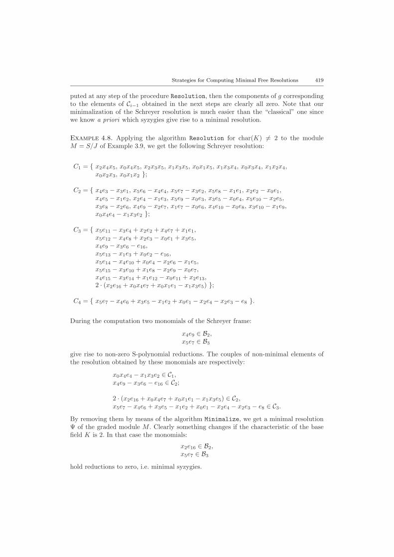
Example 4.8. Applying the algorithm Resolution for char(K) 6= 2 to the moduleM = S/J of Example 3.9, we get the following Schreyer resolution:

C1 = { x2x4x5, x0x4x5, x2x3x5, x1x3x5, x0x1x5, x1x3x4, x0x3x4, x1x2x4,x0x2x3, x0x1x2 };

C2 = { x4e3 − x3e1, x5e6 − x4e4, x5e7 − x3e2, x5e8 − x1e1, x2e2 − x0e1,x4e5 − x1e2, x2e4 − x1e3, x5e9 − x0e3, x3e5 − x0e4, x5e10 − x2e5,x3e8 − x2e6, x4e9 − x2e7, x1e7 − x0e6, x4e10 − x0e8, x3e10 − x1e9,x0x4e4 − x1x3e2 };

C3 = { x5e11 − x3e4 + x2e2 + x4e7 + x1e1,x5e12 − x4e8 + x2e3 − x0e1 + x3e5,x4e9 − x3e6 − e16,x5e13 − x1e3 + x0e2 − e16,x5e14 − x4e10 + x0e4 − x2e6 − x1e5,x5e15 − x3e10 + x1e8 − x2e9 − x0e7,x4e15 − x3e14 + x1e12 − x0e11 + x2e13,2 · (x2e16 + x0x4e7 + x0x1e1 − x1x3e5) };

C4 = { x5e7 − x4e6 + x3e5 − x1e2 + x0e1 − x2e4 − x2e3 − e8 }.

During the computation two monomials of the Schreyer frame:

x4e9 ∈ B2,x5e7 ∈ B3

give rise to non-zero S-polynomial reductions. The couples of non-minimal elements ofthe resolution obtained by these monomials are respectively:

x0x4e4 − x1x3e2 ∈ C1,x4e9 − x3e6 − e16 ∈ C2;

2 · (x2e16 + x0x4e7 + x0x1e1 − x1x3e5) ∈ C2,x5e7 − x4e6 + x3e5 − x1e2 + x0e1 − x2e4 − x2e3 − e8 ∈ C3.

By removing them by means of the algorithm Minimalize, we get a minimal resolutionΨ of the graded module M . Clearly something changes if the characteristic of the basefield K is 2. In that case the monomials:

x2e16 ∈ B2,x5e7 ∈ B3

hold reductions to zero, i.e. minimal syzygies.


5. Implementation

In this section we examine some of the choices that need to be made by an implementa-tion and propose some optimizations. After discussing these choices and implementationissues, we describe four variants of our algorithm: A0, A1, A1-H, and B, as well as twoother algorithms, M and MH. In the next section, we give examples of resolution compu-tations using these algorithms and variants, to evaluate their relative usefulness, at leastfor these examples.

With the notation of Section 4, let M = F0/I be an R-module, and let

Ξ : Flξl−→ Fl−1

ξl−1−→ · · · ξ2−→ F1ξ1−→ F0

be a Schreyer frame of the module M . For all i, we have defined:

Ei = the canonical basis of Fi;Ei(e) = {ε ∈ Ei : ξi(ε) = s · e, for some power product s};Bi = ξi(Ei), the S-polynomials to reduce in level i;

where e is any element in Ei−1.It is also useful to define, for ε ∈ Ei, the total monomial and total power product of ε:If ε ∈ E0, set total(ε) := ε and totalpp(ε) := 1. If i ≥ 1, and ε ∈ Ei, set total(ε) :=

s · total(e) and totalpp(ε) := s · totalpp(e), where ξi(ε) = s · e.

5.1. implementation issues

We discuss the main issues that an implementation must address.

Compute the Grobner basis first, or on the fly?

If the input module M is not graded, then a Grobner basis must be computed first. If Mis graded, then one can either precompute the Grobner basis of I, or compute it during thecomputation of the resolution. The advantage to computing it along with the resolutionis that one does not duplicate any effort this way. The advantages of precomputing theGrobner basis include: the time required is small compared to the computation of theentire resolution; the algorithm is much easier to describe and implement; and certainother optimizations are made possible by having the entire frame available.

Algorithms A0, A1, and A1-H all precompute the Grobner basis, while Algorithm Bcomputes it on the fly.

The choice of the induced term orders

Induced term orders is the single most important optimization to use for computingresolutions. For the algorithms presented here, it is necessary for the correctness of thealgorithm. For other algorithms (e.g. M and MH presented below), it is essential forobtaining a reasonable performance from the algorithm.

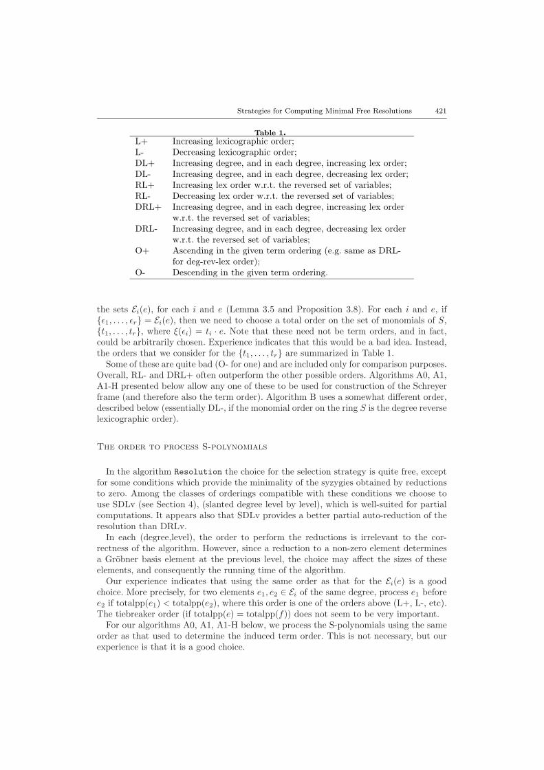
However, there is a lot of leeway in choosing an induced term order.This choice determines the Schreyer frame, and so it is important to choose the order so

that the frame is as small as possible. During the algorithm for construction of the frame,the frame (and therefore the term order) is determined by the choice of total orders on


Table 1.L+ Increasing lexicographic order;L- Decreasing lexicographic order;DL+ Increasing degree, and in each degree, increasing lex order;DL- Increasing degree, and in each degree, decreasing lex order;RL+ Increasing lex order w.r.t. the reversed set of variables;RL- Decreasing lex order w.r.t. the reversed set of variables;DRL+ Increasing degree, and in each degree, increasing lex order

w.r.t. the reversed set of variables;DRL- Increasing degree, and in each degree, decreasing lex order

w.r.t. the reversed set of variables;O+ Ascending in the given term ordering (e.g. same as DRL-

for deg-rev-lex order);O- Descending in the given term ordering.

the sets Ei(e), for each i and e (Lemma 3.5 and Proposition 3.8). For each i and e, if{ε1, . . . , εr} = Ei(e), then we need to choose a total order on the set of monomials of S,{t1, . . . , tr}, where ξ(εi) = ti · e. Note that these need not be term orders, and in fact,could be arbitrarily chosen. Experience indicates that this would be a bad idea. Instead,the orders that we consider for the {t1, . . . , tr} are summarized in Table 1.

Some of these are quite bad (O- for one) and are included only for comparison purposes.Overall, RL- and DRL+ often outperform the other possible orders. Algorithms A0, A1,A1-H presented below allow any one of these to be used for construction of the Schreyerframe (and therefore also the term order). Algorithm B uses a somewhat different order,described below (essentially DL-, if the monomial order on the ring S is the degree reverselexicographic order).

The order to process S-polynomials

In the algorithm Resolution the choice for the selection strategy is quite free, exceptfor some conditions which provide the minimality of the syzygies obtained by reductionsto zero. Among the classes of orderings compatible with these conditions we choose touse SDLv (see Section 4), (slanted degree level by level), which is well-suited for partialcomputations. It appears also that SDLv provides a better partial auto-reduction of theresolution than DRLv.

In each (degree,level), the order to perform the reductions is irrelevant to the cor-rectness of the algorithm. However, since a reduction to a non-zero element determinesa Grobner basis element at the previous level, the choice may affect the sizes of theseelements, and consequently the running time of the algorithm.

Our experience indicates that using the same order as that for the Ei(e) is a goodchoice. More precisely, for two elements e1, e2 ∈ Ei of the same degree, process e1 beforee2 if totalpp(e1) < totalpp(e2), where this order is one of the orders above (L+, L-, etc).The tiebreaker order (if totalpp(e) = totalpp(f)) does not seem to be very important.

For our algorithms A0, A1, A1-H below, we process the S-polynomials using the sameorder as that used to determine the induced term order. This is not necessary, but ourexperience is that it is a good choice.


The amount of auto-reduction

While performing a single reduction, we may use the Reduce, or the ReduceAll algo-rithm. The first stops once the lead term cannot be simplified, and the latter stops onceno term can be simplified. This second approach often leads to partially “auto-reduced”Grobner bases. One could also continue, making each Grobner basis totally auto-reduced.In some examples, this gives a dramatic improvement, since the size of the basis will of-ten be much smaller. The difficulties include the fact that minimalization is conceivablymuch more time consuming, as is modifying the elements so far obtained.

We have not yet implemented minimalization for this full auto- reduction, but initialtime tests indicate that full auto-reduction would be quite useful in certain cases. Wewill report on these techniques in a later paper.

Algorithms A0 and B use no auto-reduction (i.e. Reduce), while algorithms A1 andA1-H use ReduceAll.

Reduction strategy

While performing a single reduction, if there are several possible divisors of the leadterm, which one should we choose? Our choice (in Algorithms A0,A1,A1-H) is to choosethe element which is least, in the monomial order. This is necessary if partial auto-reduction is desired. In general, it is often the case that only one element of the basisdivides the given monomial (especially further back in the resolution). It would be niceto use this fact in some optimization.

Representation of monomials and the induced monomial order

Given a monomial m = t · e ∈ Fi, how should we represent m, in order to allow for thefast computation of the induced monomial order? We have chosen to represent m as thepair (totalpp(m), e), instead of using the pair (t, e). This complicates general arithmetic,but speeds up the comparison times. We have not done time comparisons between thetwo approaches, but we expect that the added complications of using the first techniqueleads to better performance of the algorithm.

Consider a heap based approach for performing reductions

If we are reducing a very large polynomial, and in each iteration, we add in smallpolynomials, then we are essentially performing an insertion sort. If we use an analogof a heap sort, reduction times are often drastically reduced. See Yan (1998) for details.Our algorithm A1-H uses this approach.

Allow for partial computation

This is just a reminder to implementors that allowing for partial computation (e.g.computing to a certain (slanted) degree, or a certain level) is essential, since one oftenonly cares about part of the resolution, e.g. the (slanted) linear part, or, in the caseR = S/I, because the entire resolution often cannot be computed since the resolution isinfinite.


Miscellaneous optimizations

Before performing the reductions of the S-polynomials, one may compute the resolutionof the monomial module F0/ in(I). The regularity of F0/I is no larger than the regularityof this monomial module. Therefore one may avoid processing all S-polynomials in highenough (slanted) degree. Furthermore, the computation of the resolution of F0/ in(I)involves very little extra work.

Another optimization is that, since we compute a Grobner basis anyway, it is quitesimple to check whether we have a complete intersection. If so, simply return the Koszulcomplex (or, in the module case, the Eagon–Northcott complex) of the original genera-tors. These optimizations are not used in the algorithms A0, A1, A1-H, B, M, MH, sincethis decision rightly belongs in a higher level routine.

Finally, the Schreyer frame will sometimes be longer than the minimal resolution.One can postpone computing certain (degree,level)’s (possibly forever, if we are onlycomputing up to a specific slanted degree). See Example 6.4 for a specific case of this.This speeds up some partial computations quite a lot. (Our algorithms A0, A1, A1-Huse this optimization.)

5.2. Algorithms

We now summarize the algorithms and variants that we test in the next section.

• Algorithm A0. This is the algorithm Resolution described in this paper. Firstwe compute a Grobner basis of I, and then its Schreyer frame. We then processthe elements in any way s.t. in a given degree, we process elements of higher levelfirst. For example, processing elements by increasing slanted degree is the methodwe have implemented in Macaulay2. In this algorithm, the order in which pairsare reduced in each (degree, level) is important. Heuristically, we have found thatusing the same order as that used to compute the frame (up to computing degreeby degree) is best most of the time. The reduction of an element stops once a leadterm is obtained where the corresponding Grobner basis element at the previouslevel has not been computed. This tends to not give auto-reduced Grobner bases,but is very effective in many examples.• Algorithm A1. This is a variant of algorithm A0, where we use the simplification

procedure ReduceAll.• Algorithm A1-H. We have also implemented a heap based reduction algorithm

for algorithm A1. See Yan (1998) for a description of the technique (the authorcalls them “geobuckets”). This often improves performance by a modest amount,although the improvement for computing Grobner bases in general can be dramatic.• Algorithm B. This is essentially algorithm A0, with the following differences. The

Grobner basis of I is computed “on the fly”, as is the Schreyer frame. This meansthat the Grobner basis computation of I is not duplicated. On the down side, itmeans that the ordering we use to construct the frame must be essentially degreeby degree based, which we have found not to be optimal in many cases. Also, thecoding of this algorithm is sufficiently more complicated that it is much harder tochange the algorithm for testing purposes. Thus, we cannot change the frame order,we do not have heap based reduction, and we do not have the ReduceAll routineimplemented. If we did, one could expect corresponding increases in performance.


The term ordering used to compute the frame, as well as process elements, is DO+that is increasing degree, and in each degree, ascending in the given term ordering.• Algorithm M. Compute a minimal generating set of syzygies on the minimal

generating set of the input module I, and then compute a minimal generating setof syzygies of those elements, and continue until done. At each step, use an inducedterm ordering. Also, compute minimal generators while computing the syzygies, tonot duplicate effort.

This was the method used in the original Macaulay program, except that wedid not use induced orders for the term ordering. The savings obtained from usinginduced orders is dramatic.• Algorithm MH. Same as M, except compute Hilbert functions so that at each

level, degree, one knows exactly the sum of the numbers of Grobner basis elementsand minimal syzygies at that step. The Hilbert functions take some time to com-pute, but the savings can be dramatic. Both algorithms M and MH are describedin more detail in Capani et al. (1997).

6. Examples and Timings

For each example, we describe the ideal I ⊂ R, and give the minimal Betti numbersand a table of statistics for computing the resolution of R/I. In the case that randompolynomials are required, the exact same ideal is used for each algorithm variant.

For each example, the table of statistics has the following information. The columnFrame represents the size of the Schreyer frame in terms of total number of monomialsw.r.t. the different choices of the ordering. Each Res is the size of the Schreyer resolution(total number of monomials in all the Grobner bases) for the algorithms correspondingto the previous columns. For any algorithm we give the computing time w.r.t. to thedifferent frame orderings.

All the times are reported in seconds. The tests are performed with a NEC Versa6200MX laptop, running Linux 2.0.29, 128 MB RAM, and a 166 MHz Pentium processor.Times run on a Pentium Pro 200 Mhz Linux box tend to run roughly 2.5 to 3 times fasterthan on this Pentium processor. The version of Macaulay2 that we use is 0.8.30. All ofthe examples and benchmarks used here are included in the Macaulay2 distribution.

Example 6.1. [3 × 3 commuting matrices] I ⊂ R = Z32003[xi,j , yi,j , 1 ≤ i, j ≤ 3] isthe ideal generated by the entries of the 3× 3 matrix XY − Y X, where X = (xi,j) andY = (yi,j). This is an ideal minimally generated by eight quadrics in 18 variables.

Although this is a simple example, we have included it since it is one of our favorites,and it illustrates some of the pitfalls in implementing resolution algorithms.

Note that, even in this simple case, there are orders for which the algorithm hasextremely poor performance. Using the orders O- or L- for computing the Schreyer frameleads to enormous frames, and consequently to very large resolutions. From now one, wewill not include either of these two orders in our tests.

Note also that the partially auto-reduced resolution for each choice of order is largerthan the size of the resolution when computed using Algorithm A0. The timings are onlyaccurate up to about 10% or 15% (the previous time that the algorithm MH was run,the time required was 1.1 s).

This is an example where full auto-reduction gives larger resolutions, in terms of num-bers of monomials. Almost all of the current algorithms now compute this quite rapidly.


Order Frame A0 Res A1 A1-H ResL+ 674 0.99 20658 1.13 1.01 23283RL+ 742 1.1 22753 1.68 1.44 25475DL+ 682 0.99 20755 1.14 1. 23320DL- 774 1.4 24175 1.69 1.5 29275DRL+ 742 1.1 22790 1.66 1.41 25112DRL- 650 0.97 19214 1.13 0.97 20945O+ 650 0.97 19214 1.09 0.96 20945RL- 1208 1.71 38762 3.29 2.7 72571L- 1722 1.93 66493 10.72 6.48 213865O- 2806 2.21 93842 59.19 20.67 578646

Algorithm B time 1.3Algorithm M time 1.2Algorithm MH time 0.92

The minimal Betti numbers of R/I:

Total 1 8 33 60 61 32 50: 1 - - - - - -1: - 8 2 - - - -2: - - 31 32 3 - -3: - - - 28 58 32 44: - - - - - - 1

Example 6.2. [Gr(2,7)] I ⊂ R = Z31991[x1, . . . , x21] is the ideal of the grassmannianof 2-planes in affine 7-space, in its Plucker embedding. I is minimally generated by 35quadrics. I is also generated by the 4 × 4 Pfaffians of a generic 7 × 7 skew symmetricmatrix.

Order Frame A0 Res A1 A1-H ResL+ 9402 32.47 344575 26.44 22.22 284530RL+ 9814 37.44 390317 25.88 22.15 297173DL+ 9402 35.15 355338 29.16 23.34 303188DL- 9814 38.04 411158 27.32 22.71 307689DRL+ 9814 40.96 411438 27.55 22.4 307689DRL- 9402 36.02 355292 29.09 23.2 303188O+ 9402 33.83 355292 27.99 22.79 303188RL- 9402 36.08 348923 25.87 21.32 278994



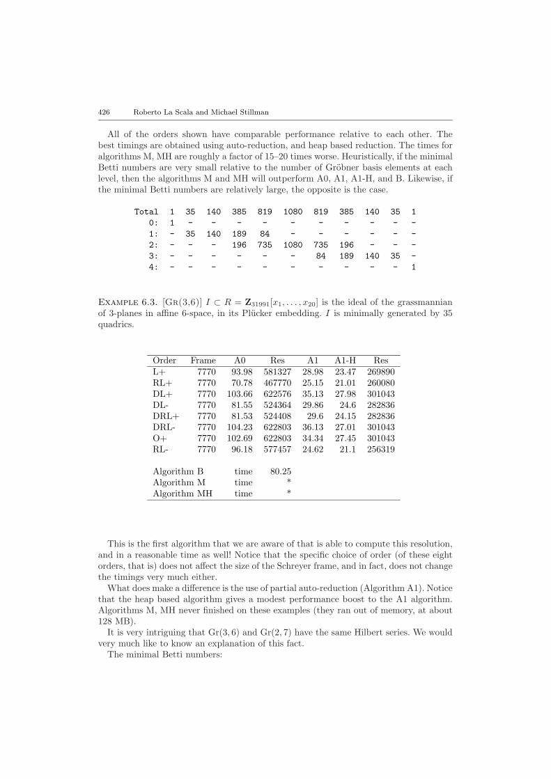
All of the orders shown have comparable performance relative to each other. Thebest timings are obtained using auto-reduction, and heap based reduction. The times foralgorithms M, MH are roughly a factor of 15–20 times worse. Heuristically, if the minimalBetti numbers are very small relative to the number of Grobner basis elements at eachlevel, then the algorithms M and MH will outperform A0, A1, A1-H, and B. Likewise, ifthe minimal Betti numbers are relatively large, the opposite is the case.

Total 1 35 140 385 819 1080 819 385 140 35 10: 1 - - - - - - - - - -1: - 35 140 189 84 - - - - - -2: - - - 196 735 1080 735 196 - - -3: - - - - - - 84 189 140 35 -4: - - - - - - - - - - 1

Example 6.3. [Gr(3,6)] I ⊂ R = Z31991[x1, . . . , x20] is the ideal of the grassmannianof 3-planes in affine 6-space, in its Plucker embedding. I is minimally generated by 35quadrics.


Algorithm B time 80.25Algorithm M time *Algorithm MH time *

This is the first algorithm that we are aware of that is able to compute this resolution,and in a reasonable time as well! Notice that the specific choice of order (of these eightorders, that is) does not affect the size of the Schreyer frame, and in fact, does not changethe timings very much either.

What does make a difference is the use of partial auto-reduction (Algorithm A1). Noticethat the heap based algorithm gives a modest performance boost to the A1 algorithm.Algorithms M, MH never finished on these examples (they ran out of memory, at about128 MB).

It is very intriguing that Gr(3, 6) and Gr(2, 7) have the same Hilbert series. We wouldvery much like to know an explanation of this fact.

The minimal Betti numbers:


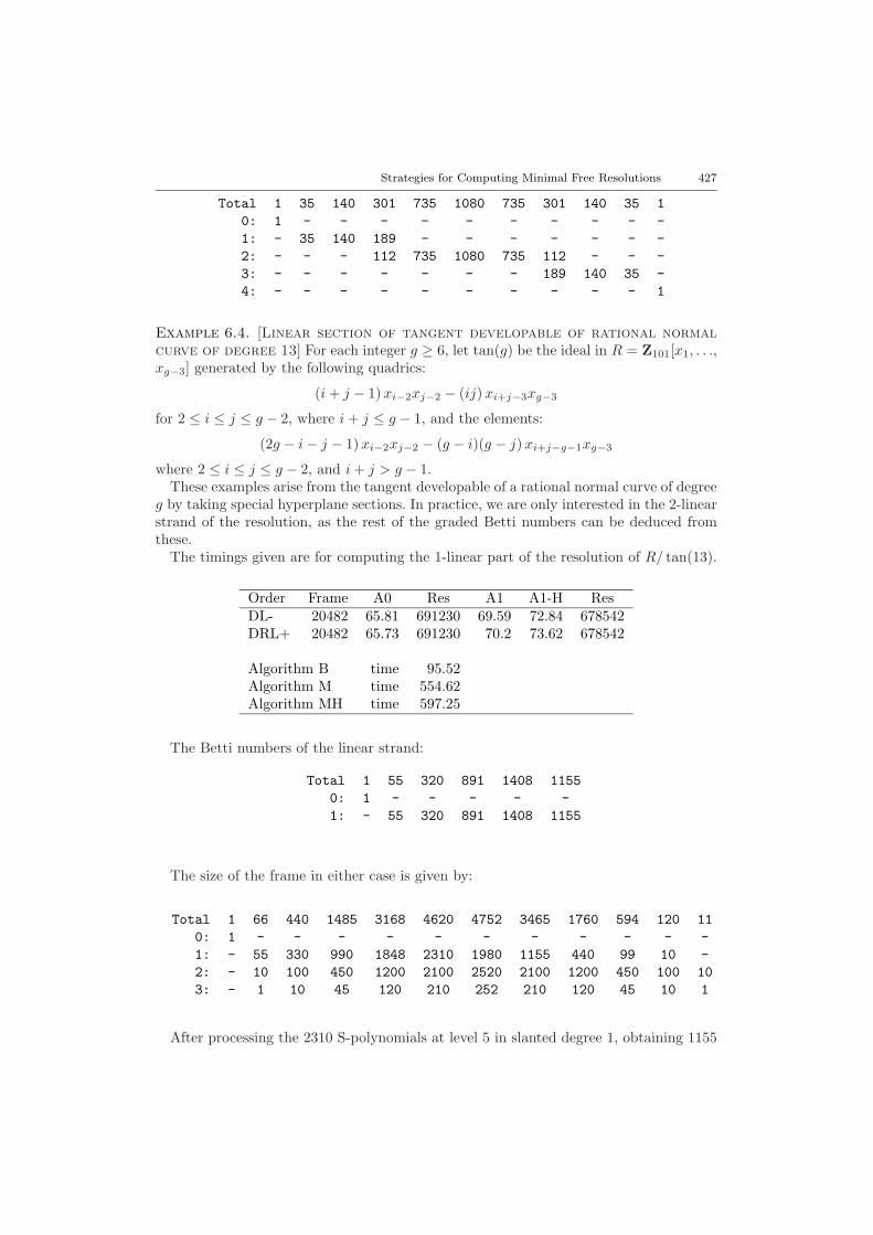
Total 1 35 140 301 735 1080 735 301 140 35 10: 1 - - - - - - - - - -1: - 35 140 189 - - - - - - -2: - - - 112 735 1080 735 112 - - -3: - - - - - - - 189 140 35 -4: - - - - - - - - - - 1

Example 6.4. [Linear section of tangent developable of rational normalcurve of degree 13] For each integer g ≥ 6, let tan(g) be the ideal in R = Z101[x1, . . .,xg−3] generated by the following quadrics:

(i+ j − 1)xi−2xj−2 − (ij)xi+j−3xg−3

for 2 ≤ i ≤ j ≤ g − 2, where i+ j ≤ g − 1, and the elements:

(2g − i− j − 1)xi−2xj−2 − (g − i)(g − j)xi+j−g−1xg−3

where 2 ≤ i ≤ j ≤ g − 2, and i+ j > g − 1.These examples arise from the tangent developable of a rational normal curve of degree

g by taking special hyperplane sections. In practice, we are only interested in the 2-linearstrand of the resolution, as the rest of the graded Betti numbers can be deduced fromthese.

The timings given are for computing the 1-linear part of the resolution of R/ tan(13).

Order Frame A0 Res A1 A1-H ResDL- 20482 65.81 691230 69.59 72.84 678542DRL+ 20482 65.73 691230 70.2 73.62 678542


The Betti numbers of the linear strand:

Total 1 55 320 891 1408 11550: 1 - - - - -1: - 55 320 891 1408 1155

The size of the frame in either case is given by:

Total 1 66 440 1485 3168 4620 4752 3465 1760 594 120 110: 1 - - - - - - - - - - -1: - 55 330 990 1848 2310 1980 1155 440 99 10 -2: - 10 100 450 1200 2100 2520 2100 1200 450 100 103: - 1 10 45 120 210 252 210 120 45 10 1

After processing the 2310 S-polynomials at level 5 in slanted degree 1, obtaining 1155


minimal syzygies, the 1980 S-polynomials at level 6 in slanted degree 1 all give non-minimal syzygies. Thus the remaining S-polynomials in slanted degree 1 need never bereduced since we are only interested in the linear strand.

Example 6.5. [Gor(8,3)] Given a homogeneous polynomial f of degree d in R =Z101[x1, . . . , xn], define the ideal:

If = {g ∈ R : g(∂/∂x1, . . . , ∂/∂xn) · f = 0}.For a random f of degree d, in R denote the ideal If by gor(n, d).

The timings given are for computing the graded Betti numbers of R/gor(8, 3).


Algorithm B time 617.13Algorithm M time *Algorithm MH time *

The issue here is auto-reduction. Full auto-reduction would be the best, compared tothese other algorithms, but we do not yet have a complete implementation. AlgorithmsM, MH never finished on these examples.

The minimal Betti numbers:

Total 1 28 105 162 168 162 105 28 10: 1 - - - - - - - -1: - 28 105 162 84 - - - -2: - - - - 84 162 105 28 -3: - - - - - - - - 1

Example 6.6. [Jac(4,5)] Given a random homogeneous polynomial f of degree 4 inR = Z101[x1, . . . , x5], let jac(f) be the ideal in R = R/f generated by the five partialderivatives of f .

The timings given are for computing the Betti numbers of R/jac(f) through F4.

Order Frame A0 Res A1 A1-H ResDL- 1032 1374.95 561913 1284.13 800.12 574837DRL+ 1032 1541.7 561913 1550.02 980.57 574837Algorithm B time 1325.8Algorithm M time 9.03


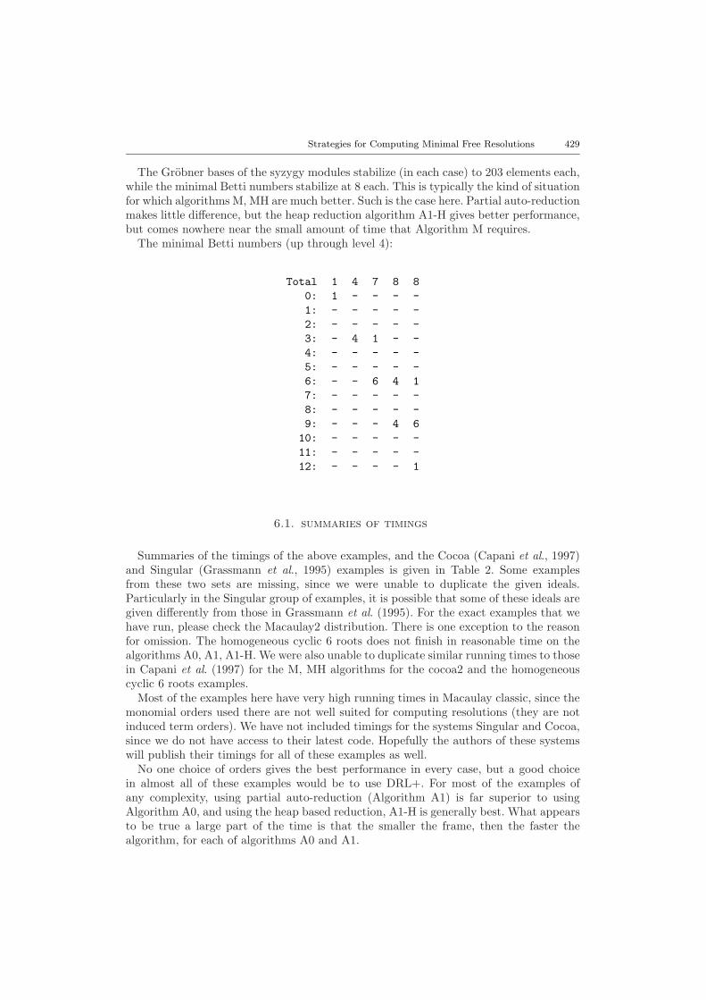
The Grobner bases of the syzygy modules stabilize (in each case) to 203 elements each,while the minimal Betti numbers stabilize at 8 each. This is typically the kind of situationfor which algorithms M, MH are much better. Such is the case here. Partial auto-reductionmakes little difference, but the heap reduction algorithm A1-H gives better performance,but comes nowhere near the small amount of time that Algorithm M requires.

The minimal Betti numbers (up through level 4):

Total 1 4 7 8 80: 1 - - - -1: - - - - -2: - - - - -3: - 4 1 - -4: - - - - -5: - - - - -6: - - 6 4 17: - - - - -8: - - - - -9: - - - 4 610: - - - - -11: - - - - -12: - - - - 1

6.1. summaries of timings

Summaries of the timings of the above examples, and the Cocoa (Capani et al., 1997)and Singular (Grassmann et al., 1995) examples is given in Table 2. Some examplesfrom these two sets are missing, since we were unable to duplicate the given ideals.Particularly in the Singular group of examples, it is possible that some of these ideals aregiven differently from those in Grassmann et al. (1995). For the exact examples that wehave run, please check the Macaulay2 distribution. There is one exception to the reasonfor omission. The homogeneous cyclic 6 roots does not finish in reasonable time on thealgorithms A0, A1, A1-H. We were also unable to duplicate similar running times to thosein Capani et al. (1997) for the M, MH algorithms for the cocoa2 and the homogeneouscyclic 6 roots examples.

Most of the examples here have very high running times in Macaulay classic, since themonomial orders used there are not well suited for computing resolutions (they are notinduced term orders). We have not included timings for the systems Singular and Cocoa,since we do not have access to their latest code. Hopefully the authors of these systemswill publish their timings for all of these examples as well.

No one choice of orders gives the best performance in every case, but a good choicein almost all of these examples would be to use DRL+. For most of the examples ofany complexity, using partial auto-reduction (Algorithm A1) is far superior to usingAlgorithm A0, and using the heap based reduction, A1-H is generally best. What appearsto be true a large part of the time is that the smaller the frame, then the faster thealgorithm, for each of algorithms A0 and A1.


Table 2.Best Example MH A0[DRL+] A1-H[DRL+] BB cocoa1 1.11 0.43 0.45 0.28A1 cocoa2 922.42 19.63 7.37 22.14A1,B,A0 cocoa3 1.81 1.02 0.98 0.99MH cocoa4 0.2 0.4 0.35 0.64A1 cocoa5 5.56 3.34 2.96 3.09MH,B cocoa6 1.00 1.22 1.21 1.1B cocoa8 3.42 1.28 1.27 1.07

A1 gr27 316.19 40.96 22.71 34.6A1 gr36 * 81.53 24.15 80.25A1 gor83 * 612.36 571.62 617.13A1 tandev13 597.25 65.73 73.62 95.52MH jac45 9.03 1541.7 980.57 1325.8

A0 singular3 2.71 1.16 1.4 0.5B singular4 19.74 8.74 9.8 4.84B singular5 5.34 1.21 1.8 0.96MH singular7 1.26 3.19 2.8 16.15B singular8 1.02 0.26 0.22 0.16MH singular9 16.12 39.68 33.35 38.3MH singular10 0.42 1.42 1.39 1.8MH singular11 44.66 245.02 245.69 281.93A1 singular12 35.04 6.29 4.63 6.79MH singular13 5.87 13.53 13.41 3.92A1 singular14 0.98 0.27 0.24 0.41B,A01 singular19 3.2 0.64 0.65 0.61B singular20 126.77 101.3 98.52 94.15

Similarly, no one choice of algorithm always gives the best performance. However, wewere able to obtain resolutions (e.g. Gr(3, 6)) that we have been unable to obtain usingany other algorithm or theoretical result.

References

——Capani, A., De Dominicis, G., Niesi, G., Robbiano, L. (1997). Computing minimal finite free resolutions,J. Pure Appl. Algebra, 117–118, 105–117.

——Grassmann, H., Greuel, G.M., Martin, B., Neumann, W., Pfister, G., Pohl, W., Schonemann, H., Siebert,T. (1995). Standard bases, syzygies, and their implementation in SINGULAR, Preprint 251, Uni-versity of Kaiserslautern.

——Grayson, D., Stillman, M. (1993–1998). Macaulay2: a system for computation in algebraic geometry andcommutative algebra, http://www.math.uiuc.edu/Macaulay2, computer software.

——La Scala, R. (1994). An algorithm for complexes, Proceedings of ISSAC 94, pp. 264–268. Oxford, ACMPress.

——La Scala, R. (1996). Un approccio computazionale alle risoluzioni libere minimali, PhD Thesis, Universityof Bari.

——Moller, H. M., Mora, T., Traverso, C. (1992). Grobner bases computation using syzygies, Proceedings ofISSAC 92, pp. 320–328, Oxford, ACM Press.

——Reisner, G. (1976). Cohen–Macaulay quotients of polynomial rings. Adv. Math., 21, 30–49.——Richman, F. (1974). Constructive aspects of noetherian rings, Proc. Amer. Math. Soc., 44, 436–441.


——Schreyer, F.O. (1980). Die Berechnung von Syzygien mit dem verallgemeinerten Weierstrass’schen Divi-sionssatz, Diplomarbeit, Hamburg.

——Siebert, T. (1996). On strategies and implementations for computations of free resolutions, Preprint 8,University of Kaiserslautern.

——Spear, D. (1977). A constructive approach to commutative ring theory, Proceedings of 1977 MACSYMAUsers’ Conference, pp. 369–376. NASA CP-2012.

——Yan, T. (1998). The geobucket data structure for polynomials, J. Symb. Comput., 25, 285–293.

Originally received 25 July 1997Accepted 22 October 1997

Strategies for Computing Minimal Free Resolutions

Documents