University of New Orleans ScholarWorks@UNO Department of Economics and Finance Working Papers, 1991-2006 Department of Economics and Finance 1-1-2004 Strategic trading against retail investors with disposition effects Jouahn Nam Pace University Jun Wang Baruch College Ge Zhang University of New Orleans Follow this and additional works at: hp://scholarworks.uno.edu/econ_wp is Working Paper is brought to you for free and open access by the Department of Economics and Finance at ScholarWorks@UNO. It has been accepted for inclusion in Department of Economics and Finance Working Papers, 1991-2006 by an authorized administrator of ScholarWorks@UNO. For more information, please contact [email protected]. Recommended Citation Nam, Jouahn; Wang, Jun; and Zhang, Ge, "Strategic trading against retail investors with disposition effects" (2004). Department of Economics and Finance Working Papers, 1991-2006. Paper 23. hp://scholarworks.uno.edu/econ_wp/23

Welcome message from author
This document is posted to help you gain knowledge. Please leave a comment to let me know what you think about it! Share it to your friends and learn new things together.
Transcript

University of New OrleansScholarWorks@UNODepartment of Economics and Finance WorkingPapers, 1991-2006 Department of Economics and Finance
1-1-2004
Strategic trading against retail investors withdisposition effectsJouahn NamPace University
Jun WangBaruch College
Ge ZhangUniversity of New Orleans
Follow this and additional works at: http://scholarworks.uno.edu/econ_wp
This Working Paper is brought to you for free and open access by the Department of Economics and Finance at ScholarWorks@UNO. It has beenaccepted for inclusion in Department of Economics and Finance Working Papers, 1991-2006 by an authorized administrator of [email protected] more information, please contact [email protected].
Recommended CitationNam, Jouahn; Wang, Jun; and Zhang, Ge, "Strategic trading against retail investors with disposition effects" (2004). Department ofEconomics and Finance Working Papers, 1991-2006. Paper 23.http://scholarworks.uno.edu/econ_wp/23

Strategic Trading against Retail Investors with
Disposition Effects
Jouahn Nam, Jun Wang and Ge Zhang∗
Abstract
In this paper, we study a model incorporating the retail trader’s reluctance to sell into
losses. We show that in this setup the informed trader always buys the asset when he
receives a favorable signal. However, when the informed trader receives an unfavorable
signal, he may not always sell the asset if the signal is moderately bad and the retail trader
is reluctant to realize losses. Hence the good news travels faster than the bad news and
the asset price exhibits steady climbs with sharp and sudden drops.
Keywords: Disposition effect, retail investors, strategic trading.
JEL classification: G10.
∗Nam is from Lubin School of Business, Pace University, New York, NY, 10038. phone: (212) 346-
1818, email: [email protected]. Wang is from Department of Economics and Finance, Baruch College, One
Bernard Baruch Way, Box B10-225 New York, NY 10010 phone: (646) 312-3507, fax: (646) 312-3451, email:
jun [email protected]. Zhang is from Department of Economics and Finance, College of Business Admin-
istration, University of New Orleans, New Orleans, LA 70148. Tel: (504) 280-6096, email: [email protected].
We would like to thank John Graham and Pete Kyle for many helpful comments. All errors are ours.

Strategic Trading against Retail Investors with Disposition Effects
Abstract
In this paper, we study a model incorporating the retail trader’s reluctance to sell into
losses. We show that in this setup the informed trader always buys the asset when he
receives a favorable signal. However, when the informed trader receives an unfavorable
signal, he may not always sell the asset if the signal is moderately bad and the retail trader
is reluctant to realize losses. Hence the good news travels faster than the bad news and
the asset price exhibits steady climbs with sharp and sudden drops.
Keywords: Disposition effect, retail investors, strategic trading.
JEL classification: G10.

1 Introduction
In the past several years, the Internet has transformed the way many individual investors invest
their money. Using the Internet, the individual investors have gained easy access to real time
stock quote and market information. The low transaction costs offered by the online brokerage
firms enable more investors to trade on their own with minimal cost. The following paragraph
is an excerpt from the SEC filing document about the second quarter 2000 of E*Trade Group,
one of the largest online brokerage firms catering to individual investors.
Brokerage transactions for the second quarter of fiscal 2000 totaled 14.2 million,
or an average of 226,100 transactions per day. This is an increase of 220% over
the average daily brokerage transaction volume of 70,200 in the prior year.
Note that the year over year growth of transaction volume is over 200%. This boom of online
stock trading is evidence that retail investors are playing an increasingly important role in the
market. Especially in the trading of internet stocks, while many professional traders shy away
from some extremely volatile stocks, retail investors play a dominant role in the trading of
these stocks.
In most of the microstructure literature, retail investors are usually treated as noise traders
and they are assumed to provide market liquidity by submitting orders of random sizes. How-
ever, there is evidence suggesting that the trading activities of retail investors are not com-
pletely random. Several regularities of their trading activities exist. One of the predominant
regularities of the retail investors’ trading behavior is the reluctance to sell assets below their
purchase price, or “losers”. This effect is called disposition effect. The reason for such reluc-
tance is more related to psychology than to economics. As selling into losses is like admitting
a prior mistake, people have a natural tendency to avoid such action. Odean (1998) provides
evidence that individual investors tend to sell winners too early and hold losers too long. In
2
several laboratory studies, people become more risk averse after prior losses and less risk
averse after prior gains (See Thaler and Johnson 1990, Gertner 1993). Barberis, Huang, and
Santos (2001) incorporate reluctance to sell into losses in the representative agent’s utility
function and study the implication for asset dynamics.
In this paper, we provide a model to study the effect of retail investors’ reluctance to sell
into losses on the trading strategies of informed traders. We show that when the market is
dominated by retail investors who are unwilling to realize losses, informed traders may not
trade as aggressively with bad signals as they would in a market made up with regular noise
traders. When informed traders receive good signals, they simply act on the signals and buy
shares. The price increases following their trade but the rise in price does not affect the trading
behavior of retail investors. When informed traders receive bad signals, they have to consider
two effects from selling shares. Selling shares always drags down the price but not to the full
extent of bad signals informed traders receive. When informed traders sell shares in the early
period, they capture the profit of selling right away. However, the price decrease makes retail
traders reluctant to sell in the later period. This effect reduces the liquidity in the later period
and reduces the trading profit of informed traders in the future. When the initial signal is
moderately bad, the loss in trading profit from lost liquidity outweighs the early trading gain.
Thus informed traders are less aggressive in trading on bad news.
Because informed traders are more likely to refrain from selling after receiving bad infor-
mation, bad news will travel slowly in these markets. In contrast, good news is not held back
by informed traders. When firms are in the early growth stage, information is quite noisy.
Then informed traders sell only when the early information is really bad but they buy when
the news is marginally good. Hence in these markets, good news travel faster than bad news.
In this case we provide one explanation on the assumption made by Hong, Lim, and Stein
(2000). As for the price patterns, these markets are likely to have long steady climbs with
sharp drops because the informed trader chooses to refrain from selling until the last possible
3

minute. Because the volume during the increase consists of trading volume contributed by
informed traders and retail investors, and retail investors are reluctant to sell if the price drops,
the volume during the price increase is likely to be higher than the volume during the price
drop.
This paper is related to many studies that attempt to explain asset dynamics using behavior
models, for example, Barberis, Shleifer and Vishny (1998), Danial, Hirshleifer and Subrah-
manyam (1998), Hong and Stein (1999), etc. We study how one common behavior bias,
reluctance to sell losses, can effect the asset price dynamics.
The paper is organized as follows: Section 2 describes the model and Section 3 shows
equilibria in this model. Section 4 provides some discussions. Section 5 concludes the paper.
2 Model setup
Consider a two period economy with one traded asset. This asset generates a dividend at
the end of period 2 and the dividend can be one of the two values,D or 0, (D > 0). At the
beginning of the first period, the market consensus is that the probability of dividend beingD
is δ0. The market consists of one trader and one market maker. In each period, the trader can
buy one unit of the asset, sell one unit of the asset, or not trade. The trader is an informed
trader with probabilityµ and a retail trader with probability1−µ.1 One can also consider this
model as one market maker dealing with many traders. In each period, one of the traders is
selected randomly to trade. In this case,µ represents the percentage of informed traders and
1−µ is the percentage of noise traders.
1Easley, O’Hara and Srinivas (1998) adopts a similar structure to study in which market informed traders
trade, equity market or derivative market.
4

Before submitting an order in each period, the informed trader observes a signal. In period
1, the signal indicates the asset is in one of two states,H or L. In stateH, the probability of a
positive dividend isδH and in stateL, the probability of a positive dividend isδL. We assume
that δH > δ0 > δL. Ex ante, the probability of stateH occurring isβ and the probability of
stateL occurring is1−β. In period 2, the informed trader observes the dividend value before
he submits an order. The informed trader is risk neutral and he attempts to maximize his
expected trading profit in both periods. Assuming the discount factor of the informed trader is
1, maximizing the expected trading profit in both periods is equivalent to maximizing the sum
of the two-period trading profit. In addition, The state is revealed to the market maker at the
end of period 1 and the dividend of the asset is revealed at the end of period 2.2
The retail trader trades for liquidity or hedging reasons. In period 1, he issues a buy order
with probability λ and a sell order with probabilityγ, (λ > 0, γ > 0, λ + γ < 1). To capture
the reluctance of retail investors to sell into losses, we assume that in period 2 the retail trader
issues a buy order with the same probabilityλ but a sell order with probabilityαγ. If the
period 1 price of the asset does not decrease,α = 1, otherwise,α≤ 1. Thisα is a coefficient
to model the retail trader’s willingness to sell into losses. As the retail trader only observes
asset prices, thisα depends only on the price history of the asset.
The market maker is risk neutral and competitive.3 He does not know whether the trader is
an informed trader or a retail trader, but he knows the probabilityµ that a trader is an informed
trader. He does not observe the signal the informed traders observes in period 1. Instead, he
knows the distribution of the two states. In each period, the market maker sets the price of
the asset after he observes the trade order, but before any information is revealed. Because
2If the state is not revealed in the market at the end of period 1, the main results of this model still hold
although the derivation is more complicated. See discussion in Section 4.3Like most of the works in this area, the role of the market maker here is to set the market price of the asset.
One can consider there are many market makers competing against each other for the order flow and this is
consistent with the practice at NYSE and NASDAQ.
5

the market maker is risk-neutral and competitive, he sets the price of the asset equal to the
expected value of the asset. This trading setup is similar to Glosten and Milgrom (1985) and
is widely used in the microstructure literature. Figure 1 sketches the timeline of this model
and Table 1 lists the parameters described above.
3 Equilibria
We concentrate on perfect Bayesian equilibria of this game. First define the following nota-
tion: x is the trading choice of the trader and it can take three values,b, buy one unit of asset,
s, sell one unit of asset, and,n, not trade. In order to accommodate mixed strategy, we define
Πt = (πbt ,πn
t ,πst ), t ∈ {1,2} as the probability weights at timet that the informed trader assigns
to the three available trading strategies in the equilibrium. If the informed trader adopts a pure
strategy, then he assigns a probability weight of 1 to the strategy he selects and 0 to other
strategies. The informed trader needs to select a strategy for all the possible states, therefore
his strategy space is then{Π1(δH),Π1(δL),Π2(1),Π2(0)}, whereΠt(δ) is his timet strategy
given his private information about the probability of high dividend state,δ.
For the market maker, letω1(x1) be his belief of the informed trader’s strategy in period
1 given orderx1. Let ω2(x1,x2,δ) be his belief of the informed trader’s strategy in period 2
given the trader’s order ofx1 in period 1 andx2 in period 2, and the revealed probability of
the high dividend state,δ. Let p1(x1) be the period 1 price of the asset given trader’s orderx1.
Let p2(x1,x2,δ) be the period 2 price of the asset given the trader’s order ofx1 in period 1 and
x2 in period 2, and the revealed probability of the high dividend state,δ. Note that since the
state is revealed at the end of period 1, the order of the informed trader in period 1 does not
affect how the market maker prices the asset in period 2 directly. But it has an indirect effect.
The trading order may depress the price in period 1 and hence cause the retail trader to be less
6

willing to sell in period 2. The market maker takes this effect into account when valuing the
asset in period 2.
Because the retail trader is not strategic in his trading decision, we define the equilibrium
based on the strategies and beliefs of the informed trader and market maker.
Definition. A Perfect Bayesian Equilibriumis a triple consisting of informed trader strate-
gies,{Π1(δH),Π1(δL),Π2(1),Π2(0)}; market maker pricing strategies,{p1(x1), p2(x1,x2,δ)};and beliefs,{ω1(x1),ω2(x1,x2,δ)} such that
• (sequential rationality — informed trader) Any strategy at time 1 (time 2) to which the
informed trader assigns a positive probability weight maximizes his payoff from time 1
(time 2) given the trading strategy and belief of the market maker.
• (perfect competition — market maker) The pricing strategy of the market maker ensures
that he earns zero expected profit given his belief.
• (belief consistency) The market maker’s belief is consistent with the informed trader’s
strategy whenever possible.
3.1 Equilibrium strategies in period 2
We first determine the trading strategy of the informed trader and the pricing strategy of the
market maker in period 2. The informed trader observes the dividend of the asset. Suppose the
informed trader follows the strategy to issue a buy order when he observes the dividend to beD
and to issue a sell order when he observes the dividend to be 0. Belief consistency requires that
the market maker expect the trading strategy of the informed trader. When the market maker
observes a buy order, he knows that the order comes from either an informed trader who knows
that the dividend isD or a retail trader who does not have any new information. If the buy
order comes from an informed trader, the dividend of the asset must beD. The probability
7

of such event is the probability of an informed traderµ multiplied by the probability of high
dividend,δ, which is revealed at the end of period 1. If the order is from a retail trader, there is
no information content of the trade. The value of the asset is determined by the revealed state,
δD. The probability of such event is the probability of a retail trader(1−µ) multiplied by the
probability of a retail trader issuing a buy orderλ. Hence the market maker sets the period 2
price of the asset given a buy order as
p2(x1,b,δ) =µδD +(1−µ)λ(δD)
µδ +(1−µ)λ. (1)
If the trade is a sell order, the market maker expects that with unconditional probability
µ(1− δ) the order comes from an informed trader who observes the dividend is 0. With
unconditional probability(1−µ)αγ, the order is from a retail trader and no more information
is extracted. In this case, the market maker sets the period 2 price of the asset given a sell
order as
p2(x1,s,δ) =(1−µ)αγ(δD)
µ(1−δ)+(1−µ)αγ. (2)
Note that because of the presence of retail trader, the market maker will never price the asset
outside the range of[0,D]. Hence it is always optimal for the informed trader to issue a buy
order when he observes the dividend to beD and to issue a sell order when he observes the
dividend to be 0. Any other strategy is not optimal to the informed trader. Hence the above
strategies and beliefs constitute an equilibrium for period 2.
Lemma 1. In period 2, the informed trader plays the pure strategy of issuing a buy order when
he observes the dividend to beD and a sell order when he observes the dividend to be 0. The
market maker holds the belief that the informed trader play such a strategy and selects the
pricing functions as in Equations (1) and (2).
8
3.2 Equilibrium strategies in period 1
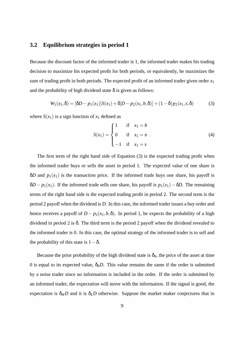
Because the discount factor of the informed trader is 1, the informed trader makes his trading
decision to maximize his expected profit for both periods, or equivalently, he maximizes the
sum of trading profit in both periods. The expected profit of an informed trader given orderx1
and the probability of high dividend stateδ is given as follows:
W1(x1,δ) = [δD− p1(x1)]S(x1)+ δ[D− p2(x1,b,δ)]+(1−δ)p2(x1,s,δ) (3)
whereS(x1) is a sign function ofx1 defined as
S(x1) =
1 if x1 = b
0 if x1 = n
−1 if x1 = s
. (4)
The first term of the right hand side of Equation (3) is the expected trading profit when
the informed trader buys or sells the asset in period 1. The expected value of one share is
δD and p1(x1) is the transaction price. If the informed trade buys one share, his payoff is
δD− p1(x1). If the informed trade sells one share, his payoff isp1(x1)− δD. The remaining
terms of the right hand side is the expected trading profit in period 2. The second term is the
period 2 payoff when the dividend isD. In this case, the informed trader issues a buy order and
hence receives a payoff ofD− p2(x1,b,δ). In period 1, he expects the probability of a high
dividend in period 2 isδ. The third term is the period 2 payoff when the dividend revealed to
the informed trader is 0. In this case, the optimal strategy of the informed trader is to sell and
the probability of this state is1−δ.
Because the prior probability of the high dividend state isδ0, the price of the asset at time
0 is equal to its expected value,δ0D. This value remains the same if the order is submitted
by a noise trader since no information is included in the order. If the order is submitted by
an informed trader, the expectation will move with the information. If the signal is good, the
expectation isδHD and it isδLD otherwise. Suppose the market maker conjectures that in
9

period 1, the informed trader will buy the asset if he observes a good signal,δH , and sell the
asset if he encounters a bad signal,δL. The bid and ask prices in period 1 are then determined
as follows:
p1(b) =µβδHD +(1−µ)λδ0D
µβ +(1−µ)λ. (5)
p1(s) =µ(1−β)δLD +(1−µ)γδ0D
µ(1−β)+(1−µ)γ. (6)
Note that a buy order always increases the price of the asset and a sell order always decreases
the price. Because the order contains the noisy signal of the informed trader, the market
maker always adjust the price based on the order flow. However, this adjustment is not to
the full extent reflected by the signal received by the informed trader, so the informed trader
still finds it profitable to issue the trade order under normal circumstances. As shown by the
following results, the informed trader finds it optimal to buy if he observes a good signal,δH ,
and sell otherwise. Thus the market maker’s conjecture is consistent and the prices specified
in equations (5) and (6) are the market prices in period 1.
The trading strategy of the informed trader in period 1 is the focus of this model. When
the informed trader observes a good signal, issuing a buy order is always the optimal strategy.
Since the signal is revealed at the end of period 1 and a buy order will only drive the price up,
the period 2 payoff to the informed trader is the same if he buys one unit in period 1 as it is if
he does not trade. Buying in period 1 has the additional advantage of owning one unit which
is priced under the expected value given the good signal. Hence we have the following result:
Lemma 2. In period 1, when the informed trader observes a good signal, he trades on this
signal immediately and issues a buy order. That is, ifδ = δH , maxx1 W1(x1,δH) = W1(b,δH).
When the informed trader observes a bad signal, things are more interesting. If the retail
trader is not reluctant to sell into losses, the informed trader always issue a sell order in period
1. Just like the case of receiving a good signal, the payoff of the informed trader in period 2 is
the same because the signal is revealed at the end of period 1. A sell order in period 1 has the
10

extra payoff of selling one unit above its intrinsic value. Hence the strategy of issuing a sell
order after observing a bad signal strictly dominates the other two alternatives.
Lemma 3. In period 1, when the informed trader observes a bad signal and the retail trader
is not reluctant to sell into losses, the informed trader trades on this signal immediately and
issues a sell order. That is, ifδ = δL andα = 1, maxx1 W1(x1,δL) = W1(s,δL).
Thus, as a base case for comparison, we have established the equilibrium when the retail
trader shows no disposition effect.
Proposition 1. When the retail trader shows no disposition effect, there is one unique equilib-
rium where the informed trader always issue a buy order when he receives a good signal and
a sell order when he receives a bad signal.
Proof. Consider the following equilibrium: the strategy of the informed trader is specified as
Π1(δH) = (1,0,0), Π1(δL) = (0,0,1), Π2(1) = (1,0,0), Π2(0) = (0,0,1); the market maker
believes that the informed trader follows this strategy and his pricing strategy is specified by
Equations (1), (2), (5), and (6), whereα = 1. From Lemmas 1, 2, and 3, we know that these
strategies and beliefs constitute an equilibrium.
We prove the uniqueness of this equilibrium by contradiction. Suppose there exists another
equilibrium where the informed trader follows a different strategy. Suppose the informed
trader does not buy after observing a good signal. Becauseλ is positive, the price set by the
market maker will be always less than the value perceived by the informed trader (δHD in
period 1 andD in period 2). In this case, a buy order generates positive payoff to the informed
trader while a sell order generates negative payoff and no-trade incurs zero payoff. Therefore,
the only optimal strategy for the informed trader is to buy after observing a good signal. This
conclusion contradicts the initial assumption. On the other hand, suppose the informed trader
does not sell after observing a bad signal. Becauseγ is positive, the price set by the market
maker will be always greater than the value perceived by the informed trader (δLD in period
11
1 and0 in period 2). In addition, because the retail trader does not have any disposition effect
(α = 1), the trading in period 1 has no effect on the trading in period 2. In this case, a sell
order generates positive payoff to the informed trader and is the optimal pure strategy for the
informed trader. This conclusion again contradicts the assumption. Thus we have proved the
uniqueness of the equilibrium.
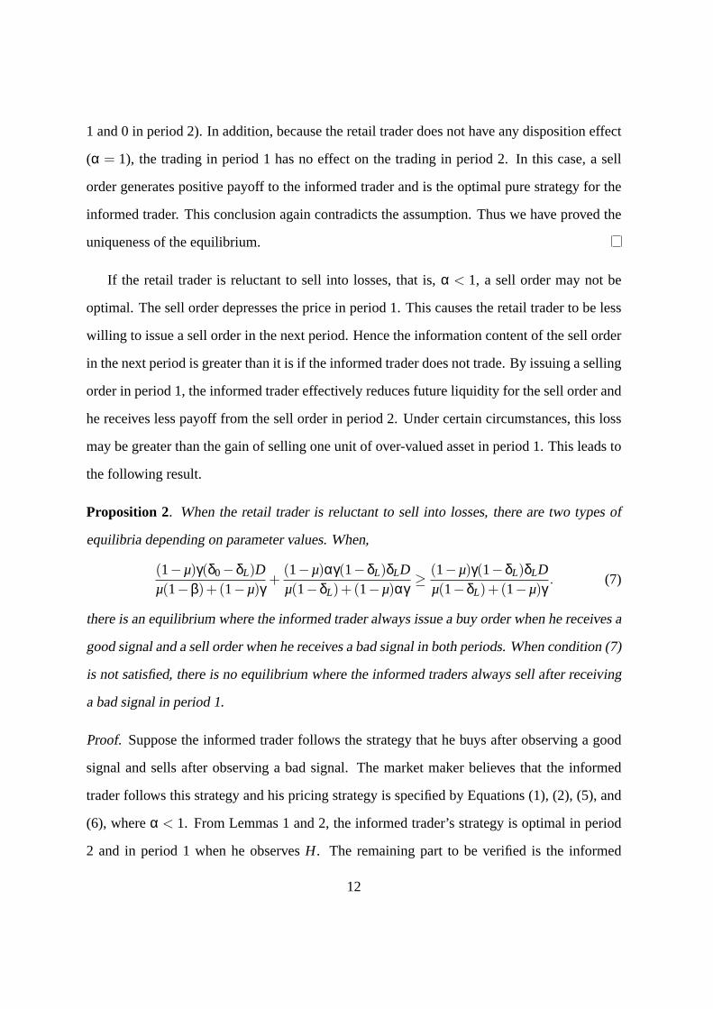
If the retail trader is reluctant to sell into losses, that is,α < 1, a sell order may not be
optimal. The sell order depresses the price in period 1. This causes the retail trader to be less
willing to issue a sell order in the next period. Hence the information content of the sell order
in the next period is greater than it is if the informed trader does not trade. By issuing a selling
order in period 1, the informed trader effectively reduces future liquidity for the sell order and
he receives less payoff from the sell order in period 2. Under certain circumstances, this loss
may be greater than the gain of selling one unit of over-valued asset in period 1. This leads to
the following result.
Proposition 2. When the retail trader is reluctant to sell into losses, there are two types of
equilibria depending on parameter values. When,
(1−µ)γ(δ0−δL)Dµ(1−β)+(1−µ)γ
+(1−µ)αγ(1−δL)δLDµ(1−δL)+(1−µ)αγ
≥ (1−µ)γ(1−δL)δLDµ(1−δL)+(1−µ)γ
. (7)
there is an equilibrium where the informed trader always issue a buy order when he receives a
good signal and a sell order when he receives a bad signal in both periods. When condition (7)
is not satisfied, there is no equilibrium where the informed traders always sell after receiving
a bad signal in period 1.
Proof. Suppose the informed trader follows the strategy that he buys after observing a good
signal and sells after observing a bad signal. The market maker believes that the informed
trader follows this strategy and his pricing strategy is specified by Equations (1), (2), (5), and
(6), whereα < 1. From Lemmas 1 and 2, the informed trader’s strategy is optimal in period
2 and in period 1 when he observesH. The remaining part to be verified is the informed
12
trader’s strategy in period when he observesL. In this case, neither a buy order or no-trade
leads to a lower price at time 1. Neither strategy triggers any reluctance to sell in period 2
and the expected payoff from the second period is the same. However, a buy order incurs a
loss in period 1 because he observesL and no-trade generates zero payoff in period 1. Thus
no-trade dominates a buy order. Now we only need to compare no-trade and a sell order
after the informed trader observesL. The payoff after a sell order isW1(s,δL) and the payoff
after no-trade isW1(n,δL). For informed trader to prefer a sell order, it must be the case that
W1(s,δL) ≥W1(n,δL). Simplifying this condition leads to (7). Thus we have shown the first
part of the proposition. To prove the second part, we use contradiction. Suppose there is an
equilibrium that the informed trader always issues a sell order after observingL and condition
(7) does not hold. In this case, informed trader plays the pure strategy of a sell order. Based
on the definition of the equilibrium, the informed trader receives higher payoff from a sell
order than any other alternatives (including no-trade). That is,W1(s,δL) >W1(n,δL). This
contradicts the assumption that condition (7) does not hold.
Note that the first term on the left hand side of (7) is the payoff to the informed trader from
selling a unit of overpriced asset in period 1. The second term is the expected payoff of period
2 in the low dividend state when the informed trader needs to sell. The right hand side is the
informed trader’s expected payoff of period 2 in the low dividend state if he does not trade in
period 1. The expected payoff in the high dividend state in period 2 is the same no matter the
informed trader sells the asset in period 1 or not. Hence it does not affect the informed trader’s
decision to sell in period 1.
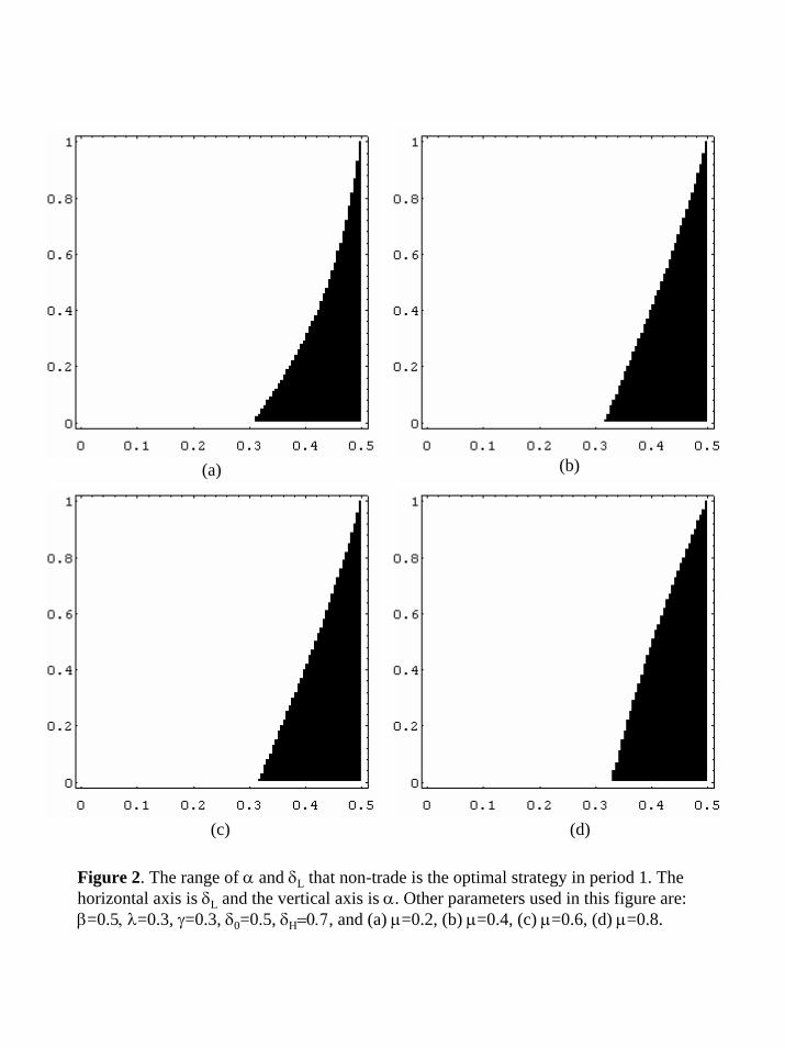
Figure 2 illustrates the combination ofα andδL where the informed trader does not trade
fully on his information in period 1. As can be seen from Figure 2, whenδL is close toδ0,
i.e., the signal is moderately bad, the informed trader does not trade on this signal because
the gain of trading in period 1 is minimal while the loss from lowering the liquidity in the
future period is much larger. On the other hand, whenα decreases from 1 to 0, that is, the
13

retail trader becomes more reluctant to sell into losses, the range ofδL in which no trade in
period 1 is optimal increases. This result is not surprising as the retail trader’s reluctance to
sell into losses makes the period 1 sell order more unfavorable. Hence no trade occurs for a
wider range ofδL values.
If the signal is really bad, that is,δL is close to 0, selling in period 1 is always the optimal
strategy for the informed trader, no matter whatα is. Low δL has two effects on the selling
order. First, the profit of selling over-valued asset is higher whenδL is low. Second, sinceδL is
revealed at the end of period 1, the bid price that market maker sets in period 2 is proportional
to δL. Hence the gain from not trading in period 1 and not reducing future market liquidity
is proportional toδL as well. This gain can not offset the large trading profit from selling in
period 1 when the signal is really bad. Figure 2 also shows the non-trading range varies for
different level ofµ. The higher theµ is, the bigger the size of non-trading area. This may
seem counter-intuitive since a highµ is an indication of high percentage of informed traders
in the market. A close examination of condition (7) reveals the logic. The key is that the
market maker has perfect knowledge ofµ. Thus, the higher theµ is, the smaller the trading
profit to the informed trader of selling a unit in period 1. That is why the size of non-trading
area increases withµ. In the limit case ofµ very close to 0, the market maker does not adjust
price if he sees an incoming sell order. Hence selling in period 1 is always optimal because
the expected profit of period 2 is the same while selling in period 1 brings the informed trader
an additional profit of(δ0−δL)D.
When condition (7) holds, the informed trader has no incentive to issue a sell order when
he observes a bad signal and the market maker expects him to sell. However, if the market
maker expects the informed trader to select no-trade strategy and treats all sell order from
retail trader, he will not change price after a sell order in period 1. Then the informed trader
finds sell order attractive. Thus there is no equilibrium where either no-trade or sell is played
14

by the informed trader as a pure strategy. We can find an equilibrium where the informed
trader plays a mixed strategy between no-trade and sell order.
Proposition 3. Suppose the retail trader is reluctant to sell into losses. When condition (7)
does not hold, there is an equilibrium where the informed trader buy after receiving a good
signal in both periods, sell after a bad signal in period 2, and plays a mixed strategy between
no-trade and sell after a bad signal in period 1.
Proof. Consider the following equilibrium: the strategy of the informed trader is specified
as Π1(δH) = (1,0,0), Π1(δL) = (0,1− πs1,π
s1), Π2(1) = (1,0,0), Π2(0) = (0,0,1), where
0< πs1 < 1. The market maker believes that the informed trader follows this strategy and his
pricing strategy is specified by Equations (1), and (5) for buy orders. For sell order, the market
maker sets the bid price in period 1 as
p1(s)′ =µπs
1(1−β)δLD +(1−µ)γδ0D
µπs1(1−β)+(1−µ)γ
, (8)
and Equation (2) withα< 1 after a sell order andα = 1 after a no trade. The informed trader’s
payoff after a sell order is
W1(s,δL)′ = [p1(s)′−δLD])+ δL[D− p2(s,b,δL)]+(1−δL)p2(s,s,δL). (9)
His payoff after no-trade is
W1(n,δL)′ = δL[D− p2(n,b,δL)]+ (1−δL)p2(n,s,δL). (10)
If πs1 = 1, W1(n,δL)′ > W1(s,δL)′, and if πs
1 = 0, W1(n,δL)′ < W1(s,δL)′. Because both
W1(s,δL)′ andW1(n,δL)′ are continuous with respect toπs1, there always exists aπs∗
1 such
thatW1(s,δL)′ = W1(n,δL)′. It is easy to verify that a buy order after observingL is dominated
by no-trade and all the other strategies of the informed trader are optimal. Thus we have a
mixed-strategy equilibrium where the informed trader, after observingL, issues a sell order
with probabilityπs∗1 and does not trade with probability1−πs∗
1 .
15

4 Discussions
4.1 Robustness of the results
Note that not revealing the signal to the market maker at the end of period 1 does not change
the results qualitatively. If the signal in period 1 is not revealed, the market maker needs to
update the reference price as well as the probability distribution based on the order in period
1. A buy order increases the period 1 price of the asset and tilts the distribution toward high
dividend state. With no liquidity change, the informed trader still finds it profitable to buy
when having a good signal. Similarly, a sell order decreases the period 1 price of the asset
and tilts the distribution toward low dividend state. If the retail trader is reluctant to sell into
losses after the price drops, the liquidity of the next period may dry up and future sell orders
are likely to depress the price even further. This effect can be so big that the informed trader
may hold the bad news without any trading.
The key result that the informed trader would trade less aggressively with bad news when
the retail investors are reluctant to sell losses does not depend on the specific trading model
here.
4.2 Empirical predictions
We can derive several empirical implications from this model. First of all, as the buy order is
never held back by the informed trader, the asset price rises in period 1 and again in period 2.
When the bad signal is received, the informed trader may not always trade on this information
as shown above. If the informed trader does not trade in period 1, the price stays the same in
period 1, and it is likely to drop in period 2. Hence the price pattern leading to a loss is flat in
period 1 and sharp drops in period 2. If the informed trader sells in period 1, the price drops
16

in period 1. Retail traders become reluctant to sell in period 2, and any new sell order from
the informed trader brings down the price substantially since liquidity is reduced. The price
pattern in this case is a small drop followed by a significant drop. Hence, markets where retail
investors dominate are likely to have long steady climb with sharp drops.
Secondly, the volume during price increase consists of trading volume contributed by the
informed trader and the retail investor. When the informed trader observes a bad signal, he
may refrain from trading immediately and reducing trading volume leading to price drop. In
addition, if the informed trader sells after a bad signal, the price drop leads to retail investors’
reluctance to sell, again depressing trading volume. Overall, the volume during the price
increase is likely to be higher than the volume during the price drop.
Finally, the more retail traders there are in a market, informed traders can better hide their
trades in general. However, after an initial price drop, the retail traders become reluctant to
sell into losses, there is a significant loss of liquidity in this case. During such times, the sell
orders from informed traders quickly depress the market price. Thus more retail traders in a
market leads to less liquidity and severe price drops during extreme market downturns.
5 Conclusion
In this paper, we construct a model incorporating the retail trader’s reluctance to sell into
losses. We show that in this setup the informed trader always buys the asset when he receives
favorable signal. However, when the informed trader receives unfavorable signal, he may
not sell the asset if the signal is moderately bad and the retail trader is reluctant to realize
losses. From this model, we can derive the following empirical implications: 1) The asset
price exhibits steady climbs with sharp and sudden drops; 2) The volume during the price
17

increase is higher than the volume during the price drop; 3) More retail traders in a market
leads to less liquidity and severe price drops during extreme market downturns.
Future research can be extended in several ways. It will be interesting to incorporate
learning in the model. In the current setup, the informed has perfect knowledge about the retail
investors who are reluctant to sell losses. If the informed trader is trading with some standard
noise traders and some retail investors, then the informed is uncertain whether a price decrease
will reduce the future liquidity and by how much. Studying the informed trader’s learning and
strategic trading activities in this context is quite interesting. Previous works such as Foster
and Viswanathan (1994), Hong and Rady (2000), Gervais and Odean (1999) may provide
directions on how to proceed. It will also be interesting to test the predictions empirically.
Given the recent surge of retail investors in the stock market, a study of their trading behavior
on the overall market is very important.
18
6 References
Andersen, T.G., and T. Bollerslev, 1998, DM-Dollar volatility: Intraday activity patterns,
macroeconomic announcements, and longer-run dependencies,Journal of Finance, 53, 219-
265.
Barberis, N., M. Huang, and T. Santos, 2001, Prospect theory and asset prices,Quarterly
Journal of Economics116, 1-53.
Barberis, N., A. Shleifer, and R. Vishny, 1998, A Model of investor sentiment,Journal of
Financial Economics49, 307-343.
Conrad, J., A. Hameed, and C.M. Niden, 1992, Volume and autocovariances in short-horizon
individual security returns,Journal of Finance49, 1305-1329.
Daniel, K.D., D. Hirshleifer, and A. Subrahmanyam, 1998, A theory of overconfidence, self-
attrition and security market under- and over-reactions,Journal of Finance52, 1-33.
Easley, D., M. O’hara, and P.S. Srinivas, 1998, Option volume and stock prices: Evidence on
where informed traders trade,Journal of Finance, 431-465.
Foster, F. D., and S. Viswanathan, 1994, Strategic trading with asymmetrically informed
traders and long-lived information,Journal of Financial and Quantitative Analysis, 499-519.
Gertner, R., 1993, Game shows and economic behavior: Risk taking on card shark,Quarterly
Journal of Economics, 507-521.
Gervais, S., and T. Odean, 1999, Learning to be overconfident, working paper, Wharton
School.
Glosten, Lawrence R. and Paul Milgrom 1985, Bid, ask, and transaction prices in a specialist
market with heterogeneously informed traders,Journal of Financial Economics14, 71-100.
19

Hong, H., and J. C. Stein, 1999, A unified theory of underreaction, momentum trading and
overreaction in asset markets,Journal of Finance, 2143-2184.
Hong, H., T. Lim, and J. C. Stein, 2000, Bad news travels slowly: Size, analyst coverage, and
the profitability of momentum strategies.Journal of Finance, 265-296.
Hong, H., and S. Rady, 2000, Strategic trading and learning about liquidity, working paper,
Stanford University.
Kyle, A., 1985, Continuous auctions and insider trading,Econometrica, 53, 1315-1335.
Lo, A. and A.C. MacKinlay, 1990, An econometric analysis of nonsynchronous trading,Jour-
nal of Econometrics45, 181-211.
Llorente, G., R. Michaely, G. Saar, and J. Wang, 2000, Dynamic volume-return relation of
individual stocks, working paper, MIT.
Odean, T., 1998, Are investors reluctant to realize their losses?Journal of Finance, 1775-1798.
Thaler, R. H., and E. Johnson, 1990, Gambling with the house money and trying to break
even: The effects of prior outcomes on risky choice,Management Science, 643-660.
20

Table 1. Parameters used in the model.
Parameter Definitionδ the probability of the dividend being Dδ0 the consensus probability of D at time 0δH the probability of state H that informed traders learns in period 1δL the probability of state L that informed traders learns in period 1β the probability of state H occurring in period 1µ the probability that an informed trader is submitting an orderλ the probability that the retail trader issues a buy order in either periodγ the probability that the retail trader issues a sell order in period 1α the coefficient modeling the retail trader’s reluctance to sell losses
21

Period 1 Period 2
10 2
The consensus is δ0 for D.
Informed trader observes the signal (H or L).
Informed trader issues a trading order
Market maker sets prices (p1).
Signal is revealed.
Informed trader observes the signal (D or 0).
Market maker sets prices (p2).
Informed trader issues a trading order
Signal is revealed.
Figure 1, Time line of the model.
(b)(a)
(c) (d)
Figure 2. The range of α and δL that non-trade is the optimal strategy in period 1. The horizontal axis is δL and the vertical axis is α. Other parameters used in this figure are:β=0.5, λ=0.3, γ=0.3, δ0=0.5, δΗ=0.7, and (a) µ=0.2, (b) µ=0.4, (c) µ=0.6, (d) µ=0.8.
Related Documents