Strategic Market Games with a Finite Horizon and Incomplete

Strategic Market Games with a Finite Horizon and Incomplete

Markets

Gaël Giraud and Sonia Weyers∗

February 9, 2003

Abstract

We study a strategic market game associated to an intertemporal economy with a finite hori-

zon and incomplete markets. We demonstrate that generically, for any finite number of players,

every sequentially strictly individually rational and default-free stream of allocations can be

approximated by a full subgame-perfect equilibrium. As a consequence, imperfect competition

may Pareto-dominate perfect competition when markets are incomplete. Moreover — and this

contrasts with the main message conveyed by the market games literature — there exists a large

open set of initial endowments for which full subgame-perfect equilibria do not converge to η-

efficient allocations when the number of players tends to infinity. Finally, strategic speculative

bubbles may survive at full subgame-perfect equilibria.

Keywords: Strategic Market Games, Folk Theorem, Incomplete Markets, Bubbles

JEL Classification Codes: C72, D43, D52.

Addresses: Gaël Giraud, BETA UMR-7522 CNRS, 61, avenue de la Forêt Noire, 67000

Strasbourg, France; Sonia Weyers, INSEAD, Boulevard de Constance, 77305 Fontainebleau

Cedex, France.

∗We thank Tim Van Zandt for his comments. All errors remain ours. Comments to [email protected] [email protected].

1 Introduction

It is widely acknowledged that a sensible model of resource allocation, over time and with uncer-

tainty, must include two components: (1) commodities that are allocated on a system of sequential

spot markets, and (2) a sequential system of incomplete financial markets through which income

is redistributed among investors. The general equilibrium model with incomplete markets (GEI)

offers a convenient framework for the analysis of the main issues at hand: existence and multiplicity

of equilibria, efficiency, persistence of speculative bubbles, and impact of market incompleteness

on welfare, prices, and consumption.1 However, this model neglects the fact that prices should be

derived endogenously from the strategic interaction of investors. To take account of this requires a

more detailed modeling of the way in which transactions occur.

There is now an extensive literature on strategic market games whose equilibria provide a rig-

orous foundation for the “invisible hand” (see Dubey (1994) for a survey). Prominent in this

approach is the strategic market game model (see Shapley & Shubik (1977), Postelwaite & Schmei-

dler (1978)); here agents are assumed to send quantity-setting strategies to trading posts, where

prices form so as to equalize supply and demand on each market.

In such models, phenomena related to imperfect competition are known to prevail: strategic

equilibria are typically inefficient (Dubey & Rogawski (1990)), arbitrage opportunities may occur at

equilibrium (Koutsougeras (2000)), the market structure matters (Weyers (1999)), and sunspots are

compatible with the completeness of markets (Peck & Shell (1991)). Nevertheless, in the absence

of uncertainty and as the number of players grows to infinity, “nice” or “full” Nash equilibria

are known to converge to (almost) efficient allocations (Dubey & Shubik (1978), Postlewaite &

Schmeidler (1978)). This enables us to consider the invisible hand as a limit case of imperfect

competition. To date, however, there is no extension of the basic strategic market game to an

1See Magill & Quinzii (1996) for an extensive account of these various topics.

1

intertemporal economy with finitely many players and intrinsic uncertainty.

The main aim of the present paper is to start filling this gap. We construct a strategic market

game with fiat money, that is associated to a finite-horizon economy with incomplete markets. Our

main assumption is that there is nontrivial monitoring as the game unfolds: players can condition

their present actions on the prices previously prevailing in the economy. However, players do not

observe details of the transactions or how the prices are formed. The assets in our model are

long-lived nominal securities. These securities yield dividends over two or more periods and can

be retraded at each date after their issue. Traders are concerned with future resale values of the

security in addition to its dividend streams, unlike the case with short-lived securities.2

Our results are threefold and bring good and bad news both. The first result is that, generically,

all the “default-free” and “sequentially strictly individually rational” allocations can be approxi-

mated arbitrarily closely by “full” subgame-perfect equilibria. Clearly, this result is akin to a

perfect Folk theorem with imperfect monitoring, and we will show how it differs from a simple

application of already known results. The terms in quotation marks will be defined with care in

the body of the paper. For the moment, it suffices to note that this result implies that a nonempty

subset of constrained (second-best) efficient allocations can be approximated by means of strategic

equilibria.3

By contrast, it is well known that, generically, every competitive equilibrium of such a finite-

horizon GEI economy is not second-best efficient (Geanakoplos & Polemarchakis (1986), Citanna,

Kajii & Villanacci (1998)).4 As a result, imperfect competition under certain circumstances may

2These yield a positive dividend for only one period after they are issued. Hence they can only be traded once.3An allocation is constrained efficient if it is efficient given the incompleteness of the asset markets, as in Geanako-

plos & Polemarchakis (1986).4 In fact, the cited papers prove the generic constrained inefficiency of competitive equilibria for numeraire assets,

not for purely financial ones. However, it is well known that fixing the price level of commodities in each state isequivalent to transforming financial securities into real assets that deliver a numeraire commodity in each state (see,e.g., Geanakoplos & Mas-Colell (1989)). Hence, the negative results proven in these other papers are easily importedinto our framework.

2

yield subgame-perfect equilibrium allocations that Pareto-dominate the competitive equilibria of

the corresponding GEI economy.

One by-product of our first result is an existence proof for full subgame-perfect equilibria for

finite-horizon economies with incomplete markets. Regarding the notion of genericity used in this

paper, let us specify that by “generic” we mean “for a dense and open subset of initial endowments,

and given any fixed asset return structure”. This is less demanding than many existence results for

competitive equilibria in GEI economies (see, e.g., Duffie & Shafer (1985)), which are stated for a

generic set of asset return structures in addition to initial endowments.

Our second result concerns the relationship between strategic market games and their com-

petitive counterpart. Postlewaite & Schmeidler (1978) examine this question for the static game

with fiat money and show that, for any η > 0, the “full” Nash equilibria5 converge to η-efficient

allocations of the underlying economy as the number of agents grows to infinity. The intuitively

appealing analogue of this convergence result in our context would be that “full” subgame-perfect

equilibria converge to η-efficient allocations as the number of players tends to infinity. Roughly

speaking, we show that this convergence fails if the horizon is long enough compared to the num-

ber of agents,6 players are sufficiently patient, and initial endowments are not already η-efficient.

More precisely: even when markets are complete, there exists a nonempty and open subset of the

set of feasible allocations that (a) can be approximated by “full” subgame-perfect equilibria and

(b) do not converge to an η-efficient allocation as individual market power vanishes — provided

endowments belong to an open subset not contained in the closure of the η-efficient allocations (see

Theorem 2).

Our third result concerns the link between the fundamental value of an asset and its price. In a

5Loosely speaking, these are equilibria at which all trading posts are open and active.6Of course, this needs to be made precise. Indeed, two simultaneous limits are taken (with respect to the number

of agents and the horizon), and the order in which they are taken matters. For the indeterminacy result obtained inthis paper, the horizon tends to infinity first. See Section 6 for more on this issue.

3

perfectly competitive finite-horizon economy, the fundamental value of financial contracts (i.e., the

discounted value of their dividend stream) is always equal, at equilibrium, to their exchange price,

so that speculative bubbles cannot arise.7 We show by means of an example that, in our finite-

horizon model with strategic investors, the price of a security may be different from its fundamental

value — even if asset markets are complete, and regardless of the (finite) number of agents.

Though the main result of this paper looks like a Folk theorem, we stress that it does not follow

from usual Folk theorems. There are several reasons for this. First, the intertemporal market game

we are analyzing is not a repeated game. Wealth can be transmitted across periods and states of

Nature (through financial securities), so that a player’s action at a given date influences not only

his current payoff but also the set of future available actions. Hence, the game we study is formally

a stochastic game with a continuum of actions at each date, a continuum of transition states, and

incomplete (but symmetric) information. To the best of our knowledge, nothing like a perfect Folk

theorem is available for games of this type.

Second, even if there were no assets to trade in any period, our game would still not be a repeated

game because the underlying economy is not assumed to be stationary. This is the second reason

why our results cannot be deduced from standard ones. As a consequence, we do not compare

the strategic outcomes of our intertemporal game with outcomes of any one-shot game (as is done

for Folk theorems) but rather with a subset of the feasible allocations of the whole intertemporal

economy.

Third, our horizon is finite and the terminal date can be assumed to be common knowledge.8

Even in proper repeated games, this feature is known to induce some interiority restrictions9 in

7See Magill & Quinzii (1996, section 21) for a proof.8Recall from Neyman (1999) that even an exponentially small departure from common knowledge on the number

of repetitions of a one-shot game enables the approximation of any feasible and individually rational outcome of thatgame by a subgame-perfect equilibrium.

9See Benoit & Krishna (1985) for details and the repeated Prisoner’s Dilemma for a counterexample.

4

order for anything akin to a perfect Folk theorem to hold. Thus, at the very least we show that

our intertemporal market game generically satisfies this kind of interiority restriction.

Finally, standard Folk theorems rely on the min-max point of each player as a threat in case a

deviation is observed. Our proof does not. Indeed, in a strategic market game, a trader’s min-max

point is no-trade and, by confining ourselves to full subgame-perfect equilibria, we explicitly avoid

the no-trade equilibrium when constructing a punishing phase. Moreover, for the min-max threat

to have real bite, players must be able to identify the perpetrator of any detected deviation. This

is impossible in our model, as players observe only aggregate quantities.

The paper is structured as follows. Section 2 contains the description of the model — that is,

the stochastic GEI economy and the game. Section 3 contains our first theorem: for any number

of players and whenever endowments are not η-efficient, all the “default-free” and “sequentially

individually rational” allocations can generically be sustained as full subgame-perfect equilibria.

Section 4 contains our second theorem; it states that, generically, “full” subgame-perfect equilibria

do not converge to η-efficient allocations. The discussion of speculative bubbles follows in Section

5, and Section 6 concludes. The appendix contains all the proofs.

2 The Model

2.1 The Stochastic GEI Economy

We consider a class of pure exchange economies with finite horizon, finitely many uncertain states

of nature, and incomplete markets of purely financial assets.

5

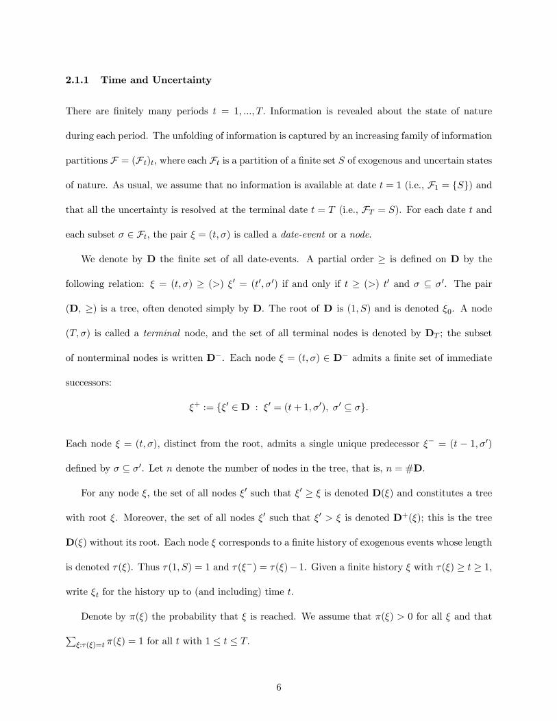
2.1.1 Time and Uncertainty

There are finitely many periods t = 1, ..., T. Information is revealed about the state of nature

during each period. The unfolding of information is captured by an increasing family of information

partitions F = (F t)t, where each Ft is a partition of a finite set S of exogenous and uncertain states

of nature. As usual, we assume that no information is available at date t = 1 (i.e., F1 = S) and

that all the uncertainty is resolved at the terminal date t = T (i.e., FT = S). For each date t and

each subset σ ∈ Ft, the pair ξ = (t,σ) is called a date-event or a node.

We denote by D the finite set of all date-events. A partial order ≥ is defined on D by the

following relation: ξ = (t,σ) ≥ (>) ξ0 = (t0,σ0) if and only if t ≥ (>) t0 and σ ⊆ σ0. The pair

(D, ≥) is a tree, often denoted simply by D. The root of D is (1, S) and is denoted ξ0. A node

(T,σ) is called a terminal node, and the set of all terminal nodes is denoted by DT ; the subset

of nonterminal nodes is written D−. Each node ξ = (t,σ) ∈ D− admits a finite set of immediate

successors:

ξ+ := ξ0 ∈ D : ξ0 = (t+ 1,σ0), σ0 ⊆ σ.

Each node ξ = (t,σ), distinct from the root, admits a single unique predecessor ξ− = (t − 1,σ0)

defined by σ ⊆ σ0. Let n denote the number of nodes in the tree, that is, n = #D.

For any node ξ, the set of all nodes ξ0 such that ξ0 ≥ ξ is denoted D(ξ) and constitutes a tree

with root ξ. Moreover, the set of all nodes ξ0 such that ξ0 > ξ is denoted D+(ξ); this is the tree

D(ξ) without its root. Each node ξ corresponds to a finite history of exogenous events whose length

is denoted τ(ξ). Thus τ(1, S) = 1 and τ(ξ−) = τ(ξ)− 1. Given a finite history ξ with τ(ξ) ≥ t ≥ 1,

write ξt for the history up to (and including) time t.

Denote by π(ξ) the probability that ξ is reached. We assume that π(ξ) > 0 for all ξ and thatPξ:τ(ξ)=t π(ξ) = 1 for all t with 1 ≤ t ≤ T.

6

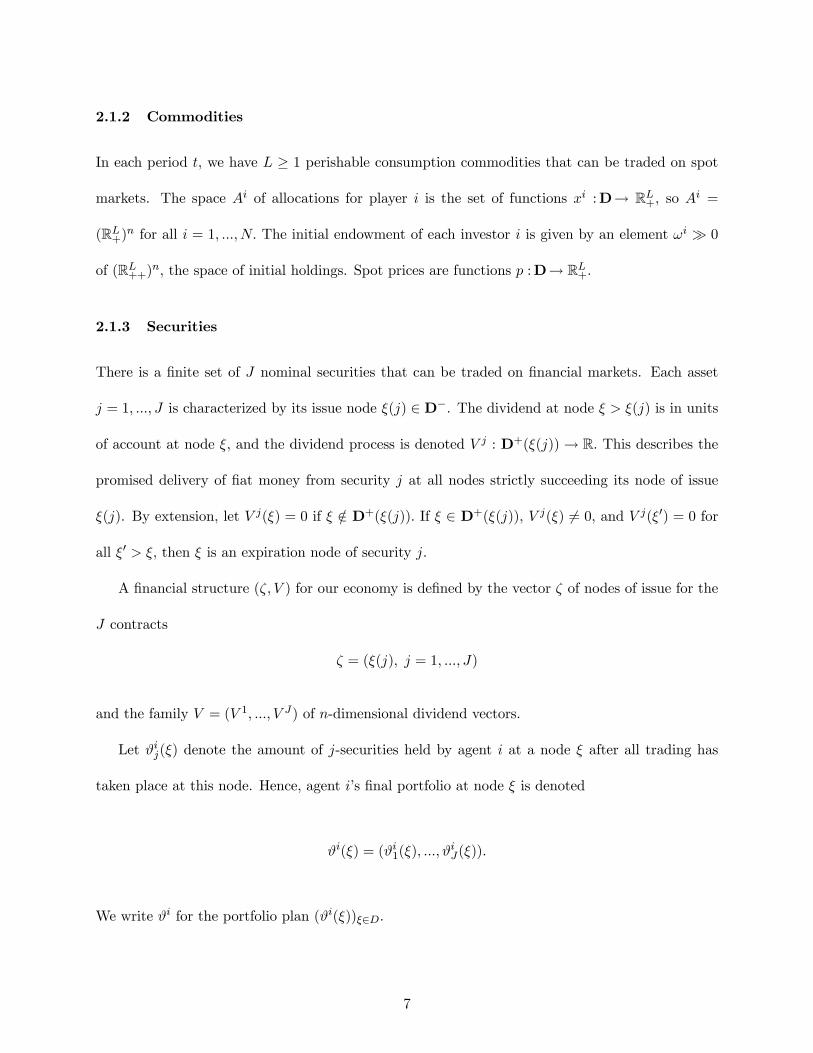
2.1.2 Commodities

In each period t, we have L ≥ 1 perishable consumption commodities that can be traded on spot

markets. The space Ai of allocations for player i is the set of functions xi :D→ RL+, so Ai =

(RL+)n for all i = 1, ..., N. The initial endowment of each investor i is given by an element ωi À 0

of (RL++)n, the space of initial holdings. Spot prices are functions p :D→ RL+.

2.1.3 Securities

There is a finite set of J nominal securities that can be traded on financial markets. Each asset

j = 1, ..., J is characterized by its issue node ξ(j) ∈ D−. The dividend at node ξ > ξ(j) is in units

of account at node ξ, and the dividend process is denoted V j : D+(ξ(j))→ R. This describes the

promised delivery of fiat money from security j at all nodes strictly succeeding its node of issue

ξ(j). By extension, let V j(ξ) = 0 if ξ /∈ D+(ξ(j)). If ξ ∈ D+(ξ(j)), V j(ξ) 6= 0, and V j(ξ0) = 0 for

all ξ0 > ξ, then ξ is an expiration node of security j.

A financial structure (ζ, V ) for our economy is defined by the vector ζ of nodes of issue for the

J contracts

ζ = (ξ(j), j = 1, ..., J)

and the family V = (V 1, ..., V J) of n-dimensional dividend vectors.

Let ϑij(ξ) denote the amount of j-securities held by agent i at a node ξ after all trading has

taken place at this node. Hence, agent i’s final portfolio at node ξ is denoted

ϑi(ξ) = (ϑi1(ξ), ...,ϑiJ(ξ)).

We write ϑi for the portfolio plan (ϑi(ξ))ξ∈D.

7

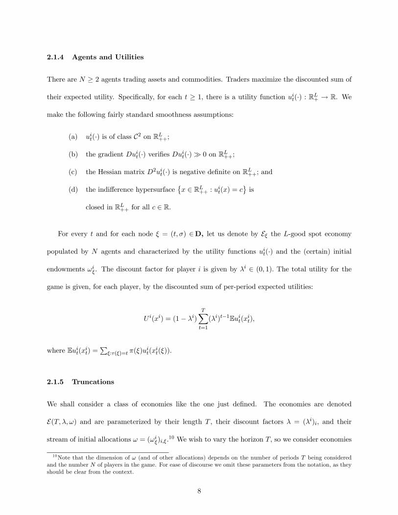
2.1.4 Agents and Utilities

There are N ≥ 2 agents trading assets and commodities. Traders maximize the discounted sum of

their expected utility. Specifically, for each t ≥ 1, there is a utility function uit(·) : RL+ → R. We

make the following fairly standard smoothness assumptions:

(a) uit(·) is of class C2 on RL++;

(b) the gradient Duit(·) verifies Duit(·)À 0 on RL++;

(c) the Hessian matrix D2uit(·) is negative definite on RL++; and

(d) the indifference hypersurface©x ∈ RL++ : uit(x) = c

ªis

closed in RL++ for all c ∈ R.

For every t and for each node ξ = (t,σ) ∈D, let us denote by Eξ the L-good spot economy

populated by N agents and characterized by the utility functions uit(·) and the (certain) initial

endowments ωiξ. The discount factor for player i is given by λi ∈ (0, 1). The total utility for the

game is given, for each player, by the discounted sum of per-period expected utilities:

U i(xi) = (1− λi)TXt=1

(λi)t−1Euit(xit),

where Euit(xit) =P

ξ:τ(ξ)=t π(ξ)uit(x

it(ξ)).

2.1.5 Truncations

We shall consider a class of economies like the one just defined. The economies are denoted

E(T,λ,ω) and are parameterized by their length T , their discount factors λ = (λi)i, and their

stream of initial allocations ω = (ωiξ)i,ξ.10 We wish to vary the horizon T, so we consider economies

10Note that the dimension of ω (and of other allocations) depends on the number of periods T being consideredand the number N of players in the game. For ease of discourse we omit these parameters from the notation, as theyshould be clear from the context.

8

E(T,λ,ω) as truncations of an infinite-horizon economy E∞(λ,ω).

We consider only economies E∞(λ,ω) that become stationary after some number of periods.

That is, we assume there exists some integer τ > 0 such that uit(·) = uit0(·) for all t, t0 ≥ τ .

Moreover, for every pair of nodes ξ = (t,σ) and ξ0 = (t0,σ0) ∈ D with t, t0 ≥ τ , we have ωiξ = ωiξ0 for

every agent i. This simplifying assumption will prevent cumbersome situations in which individual

utilities may become increasingly flat with time or in which initial endowments may “explode” with

time, so that any reward or punishment late enough in the time horizon would become ineffective.

Let BS(D) denote the set of initial allocations for E∞(λ,ω). By the stationarity assumption on

E∞(λ,ω), it follows that BS(D) is the set of bounded functions on D that become stationary after

time τ .

Given E∞(λ,ω), denote by E∞T (λ,ω) the truncated economy of length T . This economy has the

same set of agents (with their discount factors and utility functions) as E∞(λ,ω) but is derived from

it by considering only its first T periods; hence E(T,λ,ω) = E∞T (λ,ω). Similarly, if Ω is some subset

of BS(D), we denote by ΩT the set of allocations that are truncations to time T of an allocation

in Ω. This is also the corresponding set of initial allocations for the truncated economy. When we

consider the number N of agents as a parameter that can vary, we use the notations E∞(λ,ω;N),

E∞T (λ,ω;N), and E(T,λ,ω;N) as well as Ω(N) and ΩT (N).

2.2 The Game

For any T, let GT be the game associated with the truncated economy E∞T (λ,ω) of length T . If

N is considered as a parameter that may vary, we will use the notation GT (N). At each node,

a Postlewaite & Schmeidler market game with fiat money determines the allocation of goods. In

addition, there are asset markets that link the periods.

9

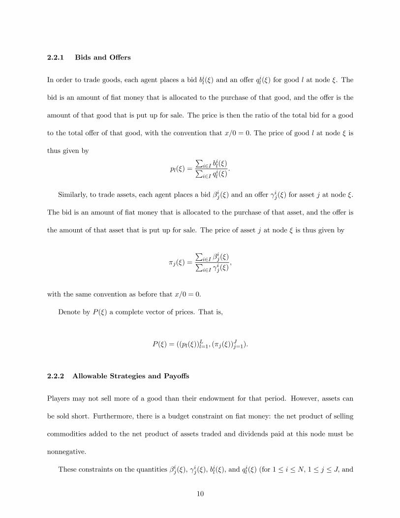
2.2.1 Bids and Offers

In order to trade goods, each agent places a bid bil(ξ) and an offer qil(ξ) for good l at node ξ. The

bid is an amount of fiat money that is allocated to the purchase of that good, and the offer is the

amount of that good that is put up for sale. The price is then the ratio of the total bid for a good

to the total offer of that good, with the convention that x/0 = 0. The price of good l at node ξ is

thus given by

pl(ξ) =

Pi∈I b

il(ξ)P

i∈I qil(ξ).

Similarly, to trade assets, each agent places a bid βij(ξ) and an offer γij(ξ) for asset j at node ξ.

The bid is an amount of fiat money that is allocated to the purchase of that asset, and the offer is

the amount of that asset that is put up for sale. The price of asset j at node ξ is thus given by

πj(ξ) =

Pi∈I β

ij(ξ)P

i∈I γij(ξ)

,

with the same convention as before that x/0 = 0.

Denote by P (ξ) a complete vector of prices. That is,

P (ξ) = ((pl(ξ))Ll=1, (πj(ξ))

Jj=1).

2.2.2 Allowable Strategies and Payoffs

Players may not sell more of a good than their endowment for that period. However, assets can

be sold short. Furthermore, there is a budget constraint on fiat money: the net product of selling

commodities added to the net product of assets traded and dividends paid at this node must be

nonnegative.

These constraints on the quantities βij(ξ), γij(ξ), b

il(ξ), and q

il(ξ) (for 1 ≤ i ≤ N, 1 ≤ j ≤ J, and

10

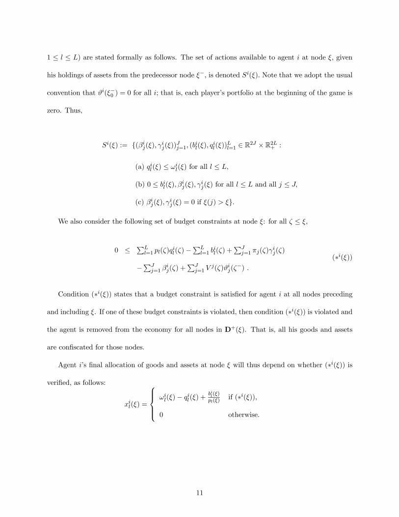
1 ≤ l ≤ L) are stated formally as follows. The set of actions available to agent i at node ξ, given

his holdings of assets from the predecessor node ξ−, is denoted Si(ξ). Note that we adopt the usual

convention that ϑi(ξ−0 ) = 0 for all i; that is, each player’s portfolio at the beginning of the game is

zero. Thus,

Si(ξ) := (βij(ξ), γij(ξ))Jj=1, (bil(ξ), qil(ξ))Ll=1 ∈ R2J ×R2L+ :

(a) qil(ξ) ≤ ωil(ξ) for all l ≤ L,

(b) 0 ≤ bil(ξ),βij(ξ), γij(ξ) for all l ≤ L and all j ≤ J,

(c) βij(ξ), γij(ξ) = 0 if ξ(j) > ξ.

We also consider the following set of budget constraints at node ξ: for all ζ ≤ ξ,

0 ≤ PLl=1 pl(ζ)q

il(ζ)−

PLl=1 b

il(ζ) +

PJj=1 πj(ζ)γ

ij(ζ)

−PJj=1 β

ij(ζ) +

PJj=1 V

j(ζ)ϑij(ζ−) .

(∗i(ξ))

Condition (∗i(ξ)) states that a budget constraint is satisfied for agent i at all nodes preceding

and including ξ. If one of these budget constraints is violated, then condition (∗i(ξ)) is violated and

the agent is removed from the economy for all nodes in D+(ξ). That is, all his goods and assets

are confiscated for those nodes.

Agent i’s final allocation of goods and assets at node ξ will thus depend on whether (∗i(ξ)) is

verified, as follows:

xil(ξ) =

ωil(ξ)− qil(ξ) + bil(ξ)

pl(ξ)if (∗i(ξ)),

0 otherwise.

11

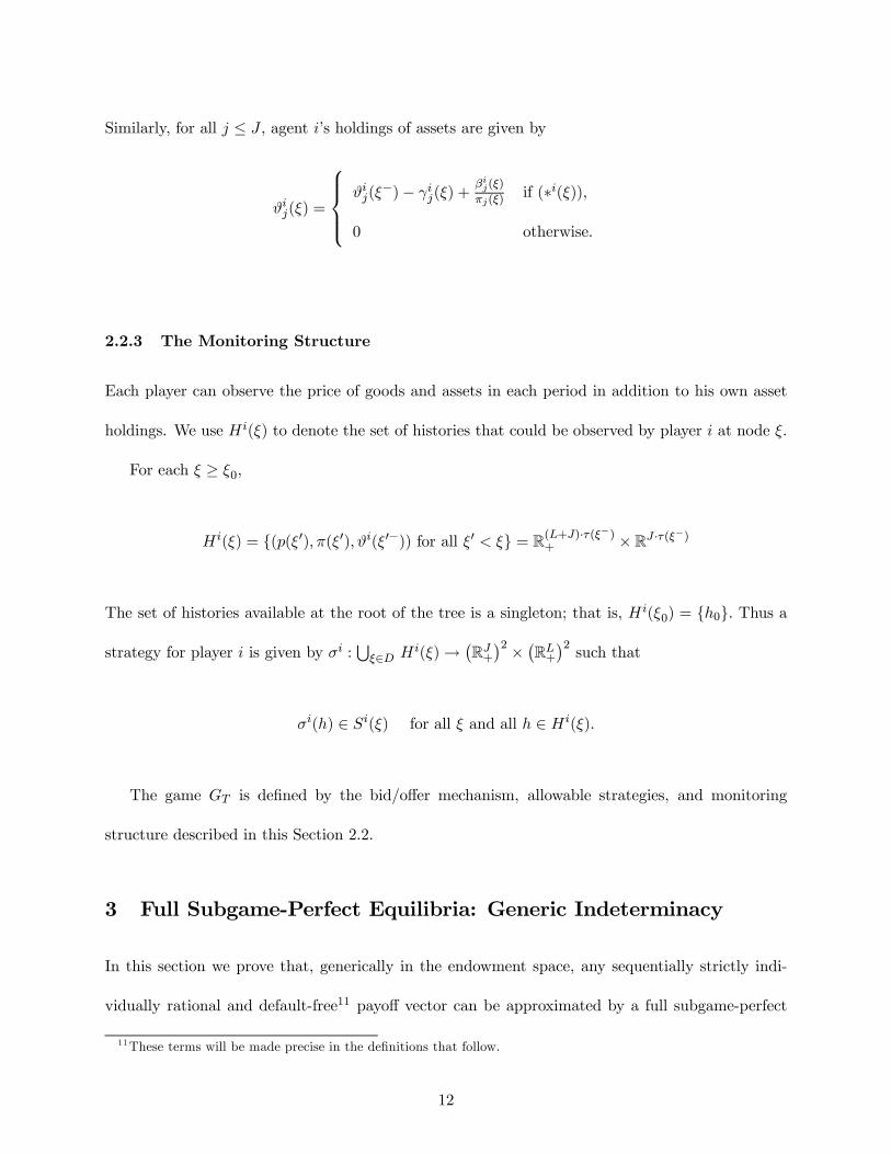
Similarly, for all j ≤ J , agent i’s holdings of assets are given by

ϑij(ξ) =

ϑij(ξ

−)− γij(ξ) +βij(ξ)

πj(ξ)if (∗i(ξ)),

0 otherwise.

2.2.3 The Monitoring Structure

Each player can observe the price of goods and assets in each period in addition to his own asset

holdings. We use Hi(ξ) to denote the set of histories that could be observed by player i at node ξ.

For each ξ ≥ ξ0,

Hi(ξ) = (p(ξ0),π(ξ0),ϑi(ξ0−)) for all ξ0 < ξ = R(L+J)·τ(ξ−)+ ×RJ ·τ(ξ−)

The set of histories available at the root of the tree is a singleton; that is, Hi(ξ0) = h0. Thus a

strategy for player i is given by σi :S

ξ∈D Hi(ξ)→ ¡

RJ+¢2 × ¡RL+¢2 such that

σi(h) ∈ Si(ξ) for all ξ and all h ∈ Hi(ξ).

The game GT is defined by the bid/offer mechanism, allowable strategies, and monitoring

structure described in this Section 2.2.

3 Full Subgame-Perfect Equilibria: Generic Indeterminacy

In this section we prove that, generically in the endowment space, any sequentially strictly indi-

vidually rational and default-free11 payoff vector can be approximated by a full subgame-perfect

11These terms will be made precise in the definitions that follow.

12

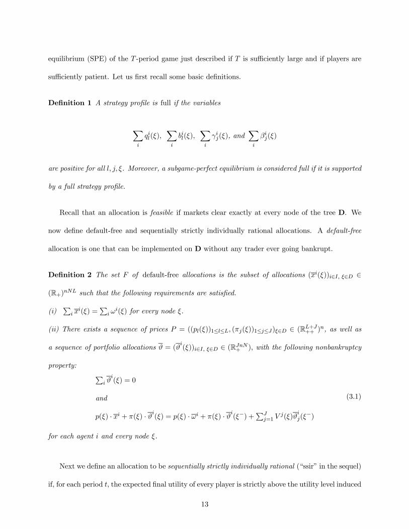
equilibrium (SPE) of the T -period game just described if T is sufficiently large and if players are

sufficiently patient. Let us first recall some basic definitions.

Definition 1 A strategy profile is full if the variables

Xi

qil(ξ),Xi

bil(ξ),Xi

γij(ξ), andXi

βij(ξ)

are positive for all l, j, ξ. Moreover, a subgame-perfect equilibrium is considered full if it is supported

by a full strategy profile.

Recall that an allocation is feasible if markets clear exactly at every node of the tree D. We

now define default-free and sequentially strictly individually rational allocations. A default-free

allocation is one that can be implemented on D without any trader ever going bankrupt.

Definition 2 The set F of default-free allocations is the subset of allocations (xi(ξ))i∈I, ξ∈D ∈

(R+)nNL such that the following requirements are satisfied.

(i)Pi xi(ξ) =

Pi ω

i(ξ) for every node ξ.

(ii) There exists a sequence of prices P = ((pl(ξ))1≤l≤L, (πj(ξ))1≤j≤J)ξ∈D ∈ (RL+J++ )n, as well as

a sequence of portfolio allocations ϑ = (ϑi(ξ))i∈I, ξ∈D ∈ (RJnN+ ), with the following nonbankruptcy

property: Pi ϑi(ξ) = 0

and

p(ξ) · xi + π(ξ) · ϑi(ξ) = p(ξ) · ωi + π(ξ) · ϑi(ξ−) +PJj=1 V

j(ξ)ϑij(ξ

−)

(3.1)

for each agent i and every node ξ.

Next we define an allocation to be sequentially strictly individually rational (“ssir” in the sequel)

if, for each period t, the expected final utility of every player is strictly above the utility level induced

13

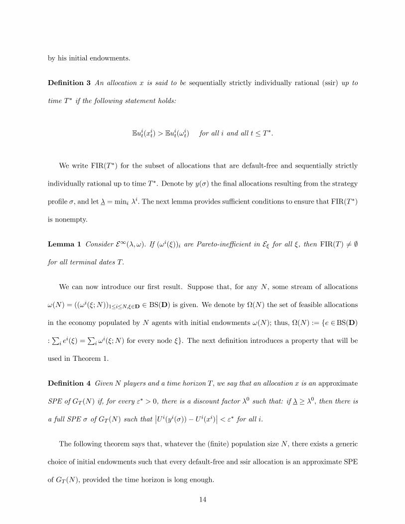
by his initial endowments.

Definition 3 An allocation x is said to be sequentially strictly individually rational (ssir) up to

time T ∗ if the following statement holds:

Euit(xit) > Euit(ωit) for all i and all t ≤ T ∗.

We write FIR(T ∗) for the subset of allocations that are default-free and sequentially strictly

individually rational up to time T ∗. Denote by y(σ) the final allocations resulting from the strategy

profile σ, and let λ = mini λi. The next lemma provides sufficient conditions to ensure that FIR(T ∗)

is nonempty.

Lemma 1 Consider E∞(λ,ω). If (ωi(ξ))i are Pareto-inefficient in Eξ for all ξ, then FIR(T ) 6= ∅

for all terminal dates T.

We can now introduce our first result. Suppose that, for any N , some stream of allocations

ω(N) = ((ωi(ξ;N))1≤i≤N,ξ∈D ∈ BS(D) is given. We denote by Ω(N) the set of feasible allocations

in the economy populated by N agents with initial endowments ω(N); thus, Ω(N) := e ∈BS(D)

:Pi ei(ξ) =

Pi ω

i(ξ;N) for every node ξ. The next definition introduces a property that will be

used in Theorem 1.

Definition 4 Given N players and a time horizon T, we say that an allocation x is an approximate

SPE of GT (N) if, for every ε∗ > 0, there is a discount factor λ0 such that: if λ ≥ λ0, then there is

a full SPE σ of GT (N) such that¯U i(yi(σ))− U i(xi)¯ < ε∗ for all i.

The following theorem says that, whatever the (finite) population size N , there exists a generic

choice of initial endowments such that every default-free and ssir allocation is an approximate SPE

of GT (N), provided the time horizon is long enough.

14

Theorem 1 For any N, there exist an open and dense subset Ω∗(N) of the space Ω(N) and some

integer T 0(N) such that, for every horizon T ≥ T 0(N): if initial endowments ω belong to Ω∗T (N),

then every x ∈FIR(T − T 0(N)) is an approximate SPE of GT (N).

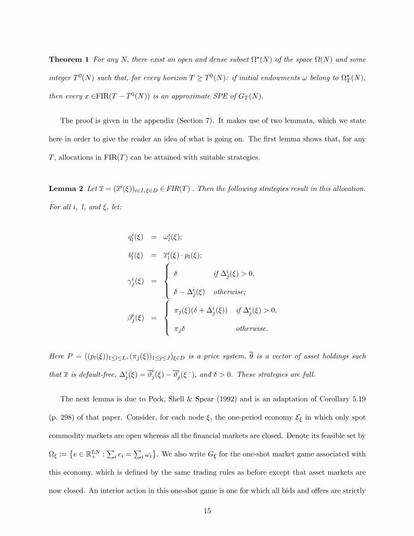
The proof is given in the appendix (Section 7). It makes use of two lemmata, which we state

here in order to give the reader an idea of what is going on. The first lemma shows that, for any

T , allocations in FIR(T ) can be attained with suitable strategies.

Lemma 2 Let x = (xi(ξ))i∈I, ξ∈D ∈FIR(T ) . Then the following strategies result in this allocation.

For all i, l, and ξ, let:

qil(ξ) = ωil(ξ);

bil(ξ) = xil(ξ) · pl(ξ);

γij(ξ) =

δ if ∆ij(ξ) > 0,

δ −∆ij(ξ) otherwise;

βij(ξ) =

πj(ξ)(δ +∆

ij(ξ)) if ∆ij(ξ) > 0,

πjδ otherwise.

Here P = ((pl(ξ))1≤l≤L, (πj(ξ))1≤j≤J)ξ∈D is a price system, θ is a vector of asset holdings such

that x is default-free, ∆ij(ξ) = ϑij(ξ)− ϑ

ij(ξ

−), and δ > 0. These strategies are full.

The next lemma is due to Peck, Shell & Spear (1992) and is an adaptation of Corollary 5.19

(p. 298) of that paper. Consider, for each node ξ, the one-period economy Eξ in which only spot

commodity markets are open whereas all the financial markets are closed. Denote its feasible set by

Ωξ :=©e ∈ RLN+ :

Pi ei =

Pi ωiª. We also write Gξ for the one-shot market game associated with

this economy, which is defined by the same trading rules as before except that asset markets are

now closed. An interior action in this one-shot game is one for which all bids and offers are strictly

15

positive. Consequently, an interior Nash equilibrium is a Nash equilibrium (NE) with interior

actions. Note that a strategy profile is full if it has interior actions at every node.

Lemma 3 (after Peck, Shell & Spear (1992)) Under our maintained assumptions, for each node ξ

there exists an open and dense subset Ω∗ξ of initial allocations of the economy Eξ such that the set

of interior NE allocations of the one-shot game Gξ is a smooth submanifold of dimension L(N −1)

of the set of feasible allocations.

The proof of Theorem 1 consists of defining a punishment strategy if a deviation is observed from

the “specified correct way to play” as well as a reward phase at the end of play. The equilibrium

path that is followed as long as nobody deviated achieves a given allocation that is default-free and

ssir; this is possible owing to Lemma 1. During the reward phase, one-shot Nash equilibria are

played of the game defined by the spot consumption goods markets and considering the securities

markets closed. This is what introduces the approximation.

In order to provide incentives for players to punish deviators, the equilibrium plan prescribes to

shift from one sequence of rewarding Nash equilibria to another (strictly dominated) one in the event

that a player fails to punish. This requires finding a sequence of Pareto-ranked Nash equilibria of the

game defined by the spot consumption goods markets and considering the securities markets closed.

However, we restrict ourselves to full subgame-perfect equilibria and so the securities markets are

never actually closed, because there is always a positive contribution to each side of each market.

Thus it must be checked, even in the reward phase, that no player would gain an advantage by

deviating multiple times in such a way as to capture and then use resources from the asset markets.

Remark 3.1. Theorem 1 provides, as a by-product, an existence proof for full subgame-perfect

equilibria in the presence of incomplete markets. Also, since it is easy to construct economies

with default-free and ssir allocations that are first-best efficient, Theorem 1 shows that imperfect

competition may overcome the (generic) second-best inefficiency of perfectly competitive equilibria.

16

Finally, Theorem 1 gives an insight into the degree of indeterminacy of full SPE allocations.12 As

such, it echoes and reinforces results from Geanakoplos & Mas-Colell (1989). They show that, in a

smooth two-period economy with S states of nature, if the asset return matrix has full rank and if

N > J then there is a generic subset of initial endowments such that the manifold of competitive

equilibria is of dimension S − 1. This holds for any number of missing assets and for every finite

number of agents. Our result implies that the indeterminacy of the set of full subgame-perfect

equilibria is typically even larger, since FIR(T ) has the same dimension as the space of feasible

allocations itself.

Remark 3.2 If we were to consider the same intertemporal game but with a continuum of

players, then Dubey & Kaneko’s (1984) “anti-Folk theorem” would imply that, as long as indi-

vidual deviations cannot be observed, players would play as if there were no monitoring. As a

consequence, our Theorem 1 would no longer hold.13 Thus, our paper suggests that there is a

discontinuity between the asymptotic strategic market game and its oceanic counterparts. More-

over, price manipulation seems to be necessary in order to outperform the (generically inefficient)

competitive equilibria with incomplete markets.

Remark 3.3 The reason we avoided an infinite-horizon setting is that the finite horizon allows

us to circumvent the problems raised by Ponzi schemes (see Magill & Quinzii (1994)). On the

other hand, we treat both the length of the horizon and the discount factor as parameters, thus

circumventing the usual counterintuitive backward phenomena.

12Notice that a partial converse inclusion can be easily shown: every full SPE must induce a feasible allocation.Moreover, as this final allocation is individually rational, it must also be default-free. However, it need not be ssir,in general.13See Kaneko (1982) for a first statement of the anti-Folk theorem. See also Dubey & Kaneko (1985) for an

extension of the anti-Folk theorem to the case of finitely many players, where small deviations cannot be observed.

17

4 A Nonconvergence Result

Postlewaite & Schmeidler (1978) show that: if the number of traders is large enough, and if the

aggregate endowment is large enough relative to the number of traders, and if each individual

trader’s endowment is small enough, then any full NE is η-efficient.

In this section, we deduce a nonconvergence result from Theorem 1. We show that, for a large

open set of initial endowments that does not contain the closure of the subset of η-efficient allo-

cations, Postlewaite and Schmeidler’s convergence result cannot be extended to our intertemporal

setup. To set the stage, we now recall definitions and the approximate efficiency theorem from

Postlewaite & Schmeidler (1978).14

Definition 5 For η > 0, a feasible allocation x is η-efficient if there does not exist any allocation

(a) that Pareto-dominates x and is feasible in any fictitious economy with the same utility functions

as the original ones and (b) in which the aggregate initial endowment vector is at most (1−η)Pi ωi,

where ωi are the initial allocations in the original economy.

Note that the set of η-efficient allocations is an open subset of the feasible set. For the sake of

completeness, we now recall the classical result obtained by Postlewaite & Schmeidler (1978) for a

one-period economy.

Approximate Efficiency Theorem (Postlewaite & Schmeidler (1978)) For any positive numbers

α,β, η, any allocation resulting from a full NE in an economy (ωi, ui)1≤i≤N is η-efficient, where

ωi < β · (1, ..., 1) for all i = 1, ..., N, Pi ωi > N · α · (1, ..., 1), and N > 16Lβ/αη2.

In the next theorem, we show two things. First, we make the easy observation that, if initial

allocations are η-efficient, then FIR(T ) is included in the set of η-efficient allocations, which we

14 It is worth noting that the definition of feasibility used by Postlewaite & Schmeidler (1978) requires only thatdemand not exceed supply, whereas we require that markets clear.

18

denote Γη. Second, if initial allocations are not in the closure Γη of the set of η-efficient allocations,

then there is an open set of allocations that are in FIR(T ) and that are not η-efficient.

Theorem 2 For any population size N, there exists an open and dense subset Ωη(N) of the space

Ω(N) with the following property. For any horizon T :

• if ω ∈ Ωη

T (N) ∩ Γη then FIR(T ) ⊆ Γη; and

• if ω ∈ Ωη

T (N)\Γη then FIR(T )\Γη contains a full-dimensional nonempty open subset.

Corollary 1 If the horizon is sufficiently long and players are sufficiently patient, then there is

a full-dimensional subset of feasible allocations that can be approximated by full subgame-perfect

equilibria and that are not in the closure of the set of η-efficient allocations. Hence Postlewaite and

Schmeidler’s approximate convergence theorem cannot be extended to our setup.

This follows from Theorem 1 and the second part of Theorem 2 after observing that FIR(T ) ⊂

FIR(T − T 0(N)).

Remark 4.1. Our preceding results are “only” generic, and there are two reasons for that.

The most obvious one is that we need the set of one-shot NE allocations of the stage-games of

the last R periods to be full-dimensional. In some sense, this is the analogue, in our general

equilibrium framework, of the full-dimensionality requirement that was found by Benoit & Krishna

(1985) to be a necessary condition for anything akin to a perfect Folk theorem to hold in finitely

repeated games. But there is a second reason: when the number N of agents grows, we need to

consider economies with new, additional initial endowments. It is perfectly possible — even though

we started with an economy whose initial endowments were inefficient — that adding new agents

makes the resulting initial allocations Pareto-optimal (or, at least, η-efficient).15 Clearly, however,

15To see this, think of an economy with a large number of traders and a Pareto-optimal allocation that does notbelong to the core. This economy may be viewed as being obtained from a smaller one that is made of a subgroupof agents whose initial endowments were not efficient.

19

the problem disappears if one slightly perturbs the new initial endowments that have just been

added. This is where the generic choice of initial endowments enters the picture for the second

time.

5 Strategic Speculative Bubbles

In a finite-horizon, perfectly competitive, stochastic GEI economy, if a security ceases to yield any

dividend then its equilibrium price is zero, because its capital value is exclusively attributable to

its dividend stream. Here it is easy to see, given Theorem 2, that a security can have a positive

price even if it yields no dividend.

Consider an economy of any length with any number of players. As neither of these will vary

in this section, we drop the corresponding notation. Now consider a security j that yields a zero

dividend in any period. Suppose that players coordinate on an equilibrium path where each trader

must put fixed, positive bids and supplies for this dummy asset:

βij(ξ) = βj(ξ) > 0,

γij(ξ) = γj(ξ) > 0.

Thus, for any ξ, i, j we have

πj(ξ) =βj(ξ)

γj(ξ)> 0,

ϑij(ξ) = ϑij(ξ−),

βij(ξ) = πj(ξ)γij(ξ).

Hence this asset has a nonzero price along the equilibrium path even though there will be no net

20

trade of it. Moreover, the trading of this asset does not affect the budget constraint.

Therefore, given any SPE allocation x∗ of any game defined without security j, one can add the

dummy asset j and complete the equilibrium strategies accordingly. By virtue of Theorem 2, x∗ is

still an SPE allocation of the modified game that includes security j. The capital value of j along

such a subgame-perfect path can only arise from a (strategic) speculative bubble on the security.

As a consequence, the linear pricing rule (or, equivalently, the no-arbitrage opportunity as-

sumption, or still equivalently the martingale property of prices) does not necessarily hold at a

full SPE of our financial trading game, even though the (finite) number of agents may be cho-

sen to be arbitrarily large. This may seem reminiscent of the findings by Koutsougeras (2000).

There is, however, a sharp distinction between his result and ours: Koutsougeras (2000) builds

one particular example of a static game, where identical objects of trade can be given different

prices at equilibrium. Moreover, in his model the apparent arbitrage opportunity disappears as the

number of agents tends to infinity. What we have just shown is that, for every economy, there is

a generic choice of endowments such that there exist full subgame-perfect equilibria that exhibit

arbitrage opportunities, provided the horizon of the economy is sufficiently large and its traders are

sufficiently patient. And these arbitrage opportunities do not vanish as the population becomes

large.

6 Concluding Remarks

Perhaps the most important implication of the present work is that it leads to reconsidering the

efficiency of the “invisible hand” for intertemporal economies. Indeed, we show in this paper that

the effect of price manipulation may be much different in a dynamic setting than in a static one. In

particular, the convergence of strategic equilibria toward (almost) efficient allocations — as players’

influence on prices becomes negligible — fails when truly dynamic behavior is taken into account

21

(when markets are incomplete, this may be fortunate!). This remark prompts five issues.

1. It sheds new light on questions that were recently reactivated by Levine & Zame (1999). They

consider a model with a single consumption good and no aggregate risk in which the incompleteness

of markets is circumvented by intertemporal consumption smoothing. As the traders’ lives tend to

infinity and the traders become infinitely patient, every competitive allocation converges to perfect

risk sharing with constant average consumption. Our indeterminacy results suggest that the positive

result of Levine and Zame rests on vulnerable grounds. Indeed, when the general equilibrium model

with perfect competition is viewed as a shortcut for the limit of a strategic market game, then such

conclusions can not always be drawn. Indeed, in such a game, associated to a generic economy

there always exist full subgame-perfect equilibria that remain far from perfect risk sharing.

More generally, the main argument (in the macroeconomic literature) in favor of the “permanent

income hypothesis” is that, when investors are patient, they can borrow in bad times and save in

good ones. This argument fails in our framework because such behavior may be prohibited along

the equilibrium path. Indeed, since players are nonnegligible, they can affect prices by smoothing

their consumption stream. Because prices are observed, this individual impact will be noticed and

may induce retaliation. Hence it may happen that no player wishes to smoothen his consumption

across time, however patient he may be, for fear of being punished.

2. Our results put into question the shortcut described in Chapter 7 of Debreu’s (1959) Theory of

Value, according to which a complete set of contingent markets open at time 0 would be enough, in

theory, to enable investors to make optimal decisions in an intertemporal economy. For this shortcut

to work, two related things are required. One is the equivalence between a market structure with

a complete set of contingent markets (on the one hand) and a market structure with spot markets

and intertemporal trades through a complete set of securities (on the other). The second is the

implicit assumption of competitive equilibrium theory that, in the intertemporal model, players

22

do not reconsider — as time passes — the decisions they made at the beginning of time. These

two requirements are satisfied when markets are competitive or if players cannot observe market

behavior as time passes. If, on the contrary, players can observe the (spot and financial) market

behavior and have the opportunity to revise their strategies accordingly, as they do in this paper,

then the equivalence between contingent markets and financial ones fails even when markets are

complete. This nonequivalence echoes the result already obtained in Weyers (1999) for two-period

economies. There, it was proven that a complete set of contingent claims does not yield the same

set of Nash equilibria as the outcomes induced by a complete set of financial securities. Here, the

property that market structure matters in strategic games is extended to the more general setting

of intertemporal incomplete markets.

3. We have shown that, when markets are incomplete, imperfect competition may perform

better than perfectly competitive markets. Unfortunately, however, we do not prove that it must

do so. Indeed, there are many subgame-perfect equilibria of the sufficiently long game that are not

(constrained) efficient, and these may be Pareto-dominated by perfectly competitive equilibria. The

second open question, then, is whether it is possible to restrict the set of subgame-perfect equilibria

to those that yield second-best outcomes. This question is addressed, and answered positively, in

Giraud & Stahn (2001) but for a different mechanism than the one used in this paper, a different

strategic solution concept, and only for two-period economies.

4. We make one proviso: as already stated, what drives the results obtained in this paper is that,

given a certain number of agents or types, we first take a sufficiently large horizon and then let the

number of agents or types increase. At first glance, it seems that reversing the order of both limits

should drastically change the results. Indeed, a basic step of our argument is the indeterminacy

of static Nash equilibria, which enables us to construct reward and punishment strategies in the

last periods of play. As a consequence, taking first a given horizon length and a sufficiently large

23

population — and only then letting the horizon length increase — might change the qualitative results

obtained in this paper. This inquiry is left for further research.

5. One main restriction of the present work is that we only consider purely financial assets,

primarily because this enables us to build on Postlewaite & Schmeidler’s (1978) strategic market

game with fiat money. Indeed, this latter specification has the advantage that the convergence

of strategic equilibria toward η-efficient allocations obtains much more easily than with Shapley

& Shubik’s (1977) formulation, where an additional condition in terms of numéraire liquidity is

needed. This provides an additional strength to our negative result: in this paper, the failure of

convergence cannot be attributed to some lack of liquidity. On the other hand, an extension of our

results to the setting of real assets would not be problematic, provided that those securities are still

traded within a strategic framework with fiat money.

However, what is problematic — and this may look paradoxical at first glance — is the treatment

of the following apparently simpler case. Suppose that traders face a finite-horizon economy with

no uncertainty, trade within a numéraire framework à la Shapley & Shubik (1977) or Dubey &

Shubik (1978), and simply transfer wealth across periods thanks to the (storable) numéraire. In

this situation, it is not clear how to define a reward phase at the end of every play. In fact,

precluding backward induction phenomena would require players to play some interior SPE for a

number of periods, which would serve as reward periods, at the end of the game. The difficulty is

that, even for two-period games, the existence of an SPE with nontrivial monitoring in a strategic

market game is an open question. We leave this, together with the extension of the present work

to the numéraire framework, for further research.

24

7 Appendix

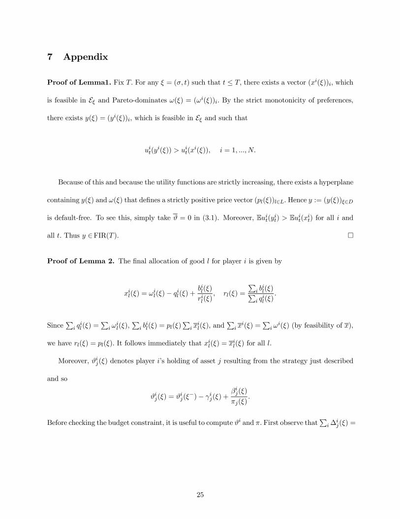
Proof of Lemma1. Fix T. For any ξ = (σ, t) such that t ≤ T, there exists a vector (xi(ξ))i, which

is feasible in Eξ and Pareto-dominates ω(ξ) = (ωi(ξ))i. By the strict monotonicity of preferences,

there exists y(ξ) = (yi(ξ))i, which is feasible in Eξ and such that

uit(yi(ξ)) > uit(x

i(ξ)), i = 1, ..., N.

Because of this and because the utility functions are strictly increasing, there exists a hyperplane

containing y(ξ) and ω(ξ) that defines a strictly positive price vector (pl(ξ))l∈L. Hence y := (y(ξ))ξ∈D

is default-free. To see this, simply take ϑ = 0 in (3.1). Moreover, Euit(yit) > Euit(xit) for all i and

all t. Thus y ∈FIR(T ). ¤

Proof of Lemma 2. The final allocation of good l for player i is given by

xil(ξ) = ωil(ξ)− qil(ξ) +bil(ξ)

ril(ξ), rl(ξ) =

Pi bil(ξ)P

i qil(ξ)

.

SincePi qil(ξ) =

Pi ω

il(ξ),

Pi bil(ξ) = pl(ξ)

Pi xil(ξ), and

Pi xi(ξ) =

Pi ω

i(ξ) (by feasibility of x),

we have rl(ξ) = pl(ξ). It follows immediately that xil(ξ) = xil(ξ) for all l.

Moreover, ϑij(ξ) denotes player i’s holding of asset j resulting from the strategy just described

and so

ϑij(ξ) = ϑij(ξ−)− γij(ξ) +

βij(ξ)

πj(ξ).

Before checking the budget constraint, it is useful to compute ϑi and π. First observe thatPi∆

ij(ξ) =

25

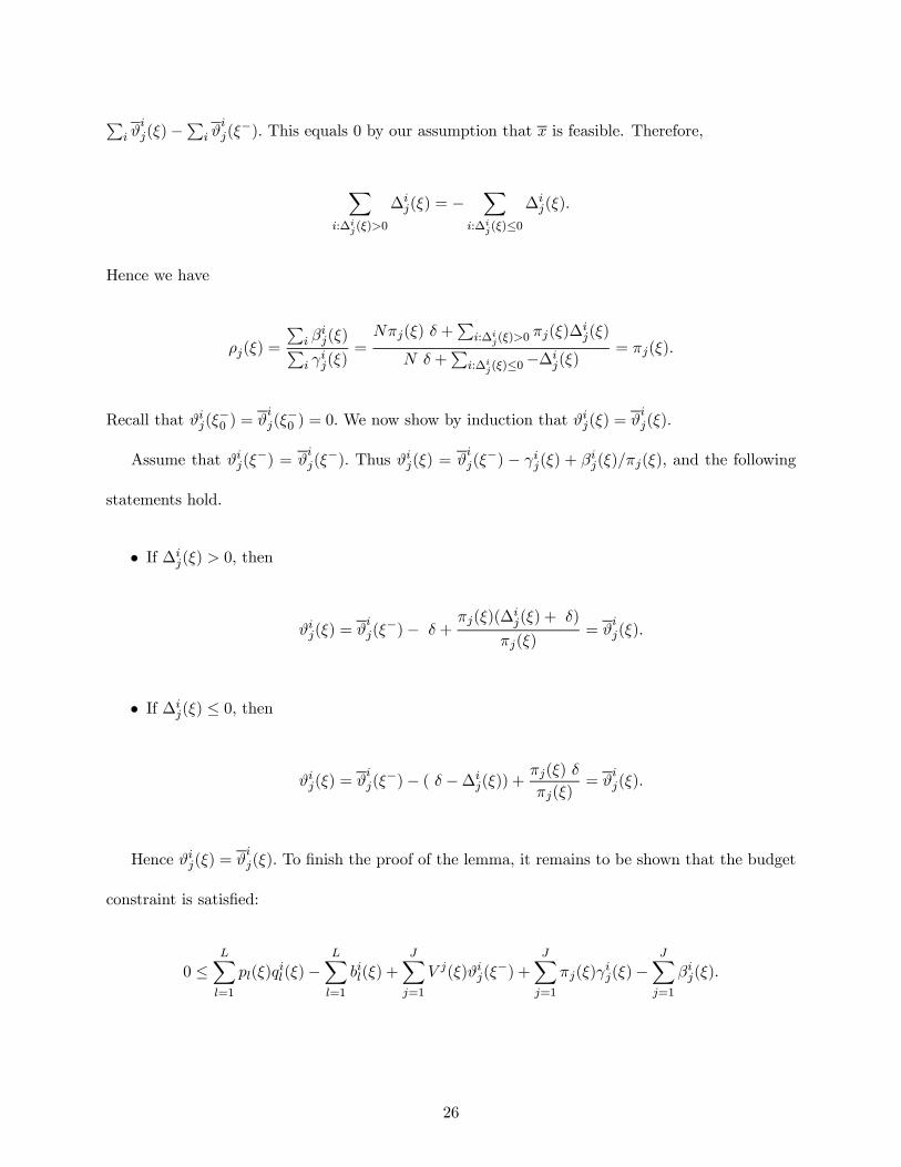
Pi ϑij(ξ)−

Pi ϑij(ξ

−). This equals 0 by our assumption that x is feasible. Therefore,

Xi:∆i

j(ξ)>0

∆ij(ξ) = −X

i:∆ij(ξ)≤0

∆ij(ξ).

Hence we have

ρj(ξ) =

Pi βij(ξ)P

i γij(ξ)

=Nπj(ξ) δ +

Pi:∆i

j(ξ)>0πj(ξ)∆

ij(ξ)

N δ +Pi:∆i

j(ξ)≤0−∆ij(ξ)

= πj(ξ).

Recall that ϑij(ξ−0 ) = ϑ

ij(ξ

−0 ) = 0. We now show by induction that ϑ

ij(ξ) = ϑ

ij(ξ).

Assume that ϑij(ξ−) = ϑ

ij(ξ

−). Thus ϑij(ξ) = ϑij(ξ

−) − γij(ξ) + βij(ξ)/πj(ξ), and the following

statements hold.

• If ∆ij(ξ) > 0, then

ϑij(ξ) = ϑij(ξ

−)− δ +πj(ξ)(∆

ij(ξ) + δ)

πj(ξ)= ϑ

ij(ξ).

• If ∆ij(ξ) ≤ 0, then

ϑij(ξ) = ϑij(ξ

−)− ( δ −∆ij(ξ)) +πj(ξ) δ

πj(ξ)= ϑ

ij(ξ).

Hence ϑij(ξ) = ϑij(ξ). To finish the proof of the lemma, it remains to be shown that the budget

constraint is satisfied:

0 ≤LXl=1

pl(ξ)qil(ξ)−

LXl=1

bil(ξ) +JXj=1

V j(ξ)ϑij(ξ−) +

JXj=1

πj(ξ)γij(ξ)−

JXj=1

βij(ξ).

26

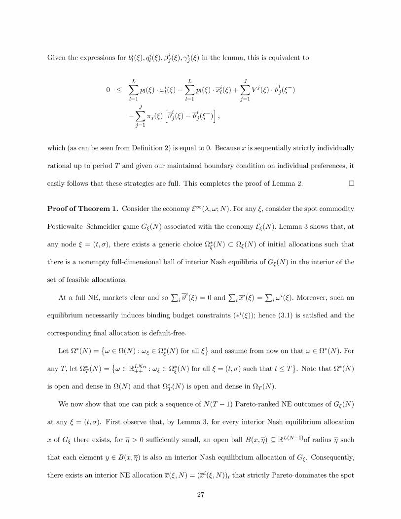
Given the expressions for bil(ξ), qil(ξ),β

ij(ξ), γ

ij(ξ) in the lemma, this is equivalent to

0 ≤LXl=1

pl(ξ) · ωil(ξ)−LXl=1

pl(ξ) · xil(ξ) +JXj=1

V j(ξ) · ϑij(ξ−)

−JXj=1

πj(ξ)hϑij(ξ)− ϑ

ij(ξ

−)i,

which (as can be seen from Definition 2) is equal to 0. Because x is sequentially strictly individually

rational up to period T and given our maintained boundary condition on individual preferences, it

easily follows that these strategies are full. This completes the proof of Lemma 2. ¤

Proof of Theorem 1. Consider the economy E∞(λ,ω;N). For any ξ, consider the spot commodity

Postlewaite—Schmeidler game Gξ(N) associated with the economy Eξ(N). Lemma 3 shows that, at

any node ξ = (t,σ), there exists a generic choice Ω∗ξ(N) ⊂ Ωξ(N) of initial allocations such that

there is a nonempty full-dimensional ball of interior Nash equilibria of Gξ(N) in the interior of the

set of feasible allocations.

At a full NE, markets clear and soPi ϑi(ξ) = 0 and

Pi xi(ξ) =

Pi ω

i(ξ). Moreover, such an

equilibrium necessarily induces binding budget constraints (∗i(ξ)); hence (3.1) is satisfied and the

corresponding final allocation is default-free.

Let Ω∗(N) =©ω ∈ Ω(N) : ωξ ∈ Ω∗ξ(N) for all ξ

ªand assume from now on that ω ∈ Ω∗(N). For

any T, let Ω∗T (N) =©ω ∈ RLNn++ : ωξ ∈ Ω∗ξ(N) for all ξ = (t,σ) such that t ≤ T

ª. Note that Ω∗(N)

is open and dense in Ω(N) and that Ω∗T (N) is open and dense in ΩT (N).

We now show that one can pick a sequence of N(T − 1) Pareto-ranked NE outcomes of Gξ(N)

at any ξ = (t,σ). First observe that, by Lemma 3, for every interior Nash equilibrium allocation

x of Gξ there exists, for η > 0 sufficiently small, an open ball B(x, η) ⊆ RL(N−1)of radius η such

that each element y ∈ B(x, η) is also an interior Nash equilibrium allocation of Gξ. Consequently,

there exists an interior NE allocation x(ξ, N) = (xi(ξ, N))i that strictly Pareto-dominates the spot

27

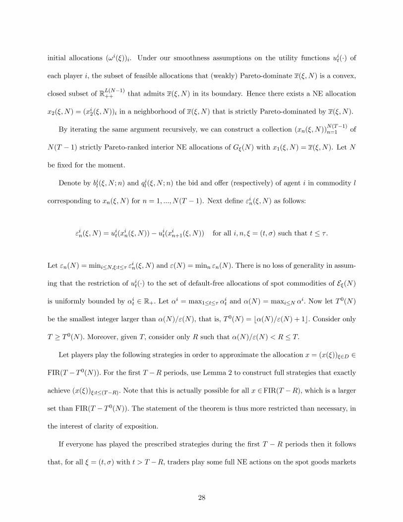
initial allocations (ωi(ξ))i. Under our smoothness assumptions on the utility functions uit(·) of

each player i, the subset of feasible allocations that (weakly) Pareto-dominate x(ξ, N) is a convex,

closed subset of RL(N−1)++ that admits x(ξ, N) in its boundary. Hence there exists a NE allocation

x2(ξ, N) = (xi2(ξ, N))i in a neighborhood of x(ξ, N) that is strictly Pareto-dominated by x(ξ, N).

By iterating the same argument recursively, we can construct a collection (xn(ξ, N))N(T−1)n=1 of

N(T − 1) strictly Pareto-ranked interior NE allocations of Gξ(N) with x1(ξ, N) = x(ξ, N). Let N

be fixed for the moment.

Denote by bil(ξ, N ;n) and qil(ξ,N ;n) the bid and offer (respectively) of agent i in commodity l

corresponding to xn(ξ, N) for n = 1, ..., N(T − 1). Next define εin(ξ, N) as follows:

εin(ξ, N) = uit(x

in(ξ, N))− uit(xin+1(ξ, N)) for all i, n, ξ = (t,σ) such that t ≤ τ .

Let εn(N) = mini≤N,ξ:t≤τ εin(ξ, N) and ε(N) = minn εn(N). There is no loss of generality in assum-

ing that the restriction of uit(·) to the set of default-free allocations of spot commodities of Eξ(N)

is uniformly bounded by αit ∈ R+. Let αi = max1≤t≤τ αit and α(N) = maxi≤N αi. Now let T 0(N)

be the smallest integer larger than α(N)/ε(N), that is, T 0(N) = bα(N)/ε(N) + 1c. Consider only

T ≥ T 0(N). Moreover, given T, consider only R such that α(N)/ε(N) < R ≤ T.

Let players play the following strategies in order to approximate the allocation x = (x(ξ))ξ∈D ∈

FIR(T −T 0(N)). For the first T −R periods, use Lemma 2 to construct full strategies that exactly

achieve (x(ξ))ξ:t≤(T−R). Note that this is actually possible for all x ∈FIR(T −R), which is a larger

set than FIR(T − T 0(N)). The statement of the theorem is thus more restricted than necessary, in

the interest of clarity of exposition.

If everyone has played the prescribed strategies during the first T − R periods then it follows

that, for all ξ = (t,σ) with t > T −R, traders play some full NE actions on the spot goods markets

28

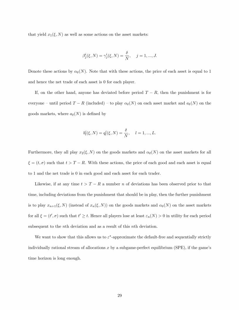
that yield x1(ξ,N) as well as some actions on the asset markets:

βij(ξ, N) = γij(ξ, N) =δ

N, j = 1, ..., J.

Denote these actions by αδ(N). Note that with these actions, the price of each asset is equal to 1

and hence the net trade of each asset is 0 for each player.

If, on the other hand, anyone has deviated before period T − R, then the punishment is for

everyone — until period T −R (included) — to play αδ(N) on each asset market and aδ(N) on the

goods markets, where aδ(N) is defined by

bil(ξ, N) = qil(ξ, N) =

δ

N, l = 1, ..., L.

Furthermore, they all play x2(ξ, N) on the goods markets and αδ(N) on the asset markets for all

ξ = (t,σ) such that t > T −R. With these actions, the price of each good and each asset is equal

to 1 and the net trade is 0 in each good and each asset for each trader.

Likewise, if at any time t > T − R a number n of deviations has been observed prior to that

time, including deviations from the punishment that should be in play, then the further punishment

is to play xn+1(ξ,N) (instead of xn(ξ, N)) on the goods markets and αδ(N) on the asset markets

for all ξ = (t0,σ) such that t0 ≥ t. Hence all players lose at least εn(N) > 0 in utility for each period

subsequent to the nth deviation and as a result of this nth deviation.

We want to show that this allows us to ε∗-approximate the default-free and sequentially strictly

individually rational stream of allocations x by a subgame-perfect equilibrium (SPE), if the game’s

time horizon is long enough.

29

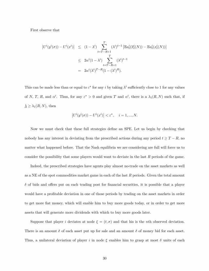
First observe that

¯U i(yi(σ))− U i(xi)¯ ≤ (1− λi)

TXt=T−R+1

(λi)t−1¯Euit(xit(N))− Euit(xit(N))

¯≤ 2αi(1− λi)

TXt=T−R+1

(λi)t−1

= 2αi(λi)T−R(1− (λi)R).

This can be made less than or equal to ε∗ for any i by taking λi sufficiently close to 1 for any values

of N, T, R, and αi. Thus, for any ε∗ > 0 and given T and αi, there is a λ1(R,N) such that, if

λ ≥ λ1(R,N), then ¯U i(yi(σ))− U i(xi)¯ < ε∗, i = 1, ...,N.

Now we must check that these full strategies define an SPE. Let us begin by checking that

nobody has any interest in deviating from the prescribed actions during any period t ≥ T −R, no

matter what happened before. That the Nash equilibria we are considering are full will force us to

consider the possibility that some players would want to deviate in the last R periods of the game.

Indeed, the prescribed strategies have agents play almost no-trade on the asset markets as well

as a NE of the spot commodities market game in each of the last R periods. Given the total amount

δ of bids and offers put on each trading post for financial securities, it is possible that a player

would have a profitable deviation in one of those periods by trading on the asset markets in order

to get more fiat money, which will enable him to buy more goods today, or in order to get more

assets that will generate more dividends with which to buy more goods later.

Suppose that player i deviates at node ξ = (t,σ) and that his is the nth observed deviation.

There is an amount δ of each asset put up for sale and an amount δ of money bid for each asset.

Thus, a unilateral deviation of player i in node ξ enables him to grasp at most δ units of each

30

financial asset and Jδ units of fiat money.

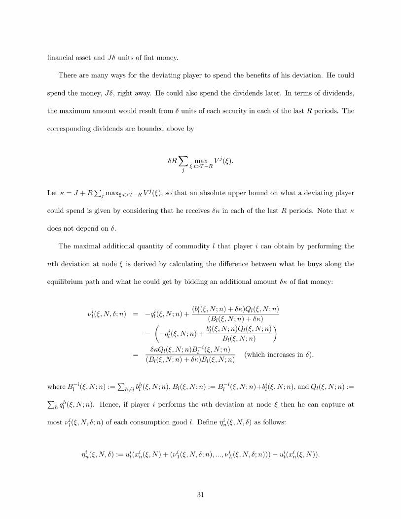
There are many ways for the deviating player to spend the benefits of his deviation. He could

spend the money, Jδ, right away. He could also spend the dividends later. In terms of dividends,

the maximum amount would result from δ units of each security in each of the last R periods. The

corresponding dividends are bounded above by

δRXj

maxξ:t>T−R

V j(ξ).

Let κ = J +RPjmaxξ:t>T−R V

j(ξ), so that an absolute upper bound on what a deviating player

could spend is given by considering that he receives δκ in each of the last R periods. Note that κ

does not depend on δ.

The maximal additional quantity of commodity l that player i can obtain by performing the

nth deviation at node ξ is derived by calculating the difference between what he buys along the

equilibrium path and what he could get by bidding an additional amount δκ of fiat money:

νil(ξ, N, δ;n) = −qil(ξ, N ;n) +(bil(ξ, N ;n) + δκ)Ql(ξ, N ;n)

(Bl(ξ, N ;n) + δκ)

−µ−qil(ξ, N ;n) +

bil(ξ, N ;n)Ql(ξ,N ;n)

Bl(ξ, N ;n)

¶=

δκQl(ξ, N ;n)B−il (ξ, N ;n)

(Bl(ξ, N ;n) + δκ)Bl(ξ,N ;n)(which increases in δ),

where B−il (ξ,N ;n) :=Ph6=i b

hl (ξ, N ;n), Bl(ξ, N ;n) := B

−il (ξ, N ;n)+b

il(ξ, N ;n), and Ql(ξ, N ;n) :=P

h qhl (ξ, N ;n). Hence, if player i performs the nth deviation at node ξ then he can capture at

most νil(ξ, N, δ;n) of each consumption good l. Define ηin(ξ, N, δ) as follows:

ηin(ξ,N, δ) := uit(x

in(ξ, N) + (ν

i1(ξ, N, δ;n), ..., ν

iL(ξ, N, δ;n)))− uit(xin(ξ, N)).

31

Thus, player i gains at most ηin(ξ, N, δ) at node ξ and loses εin(ξ

0) at each successor node ξ0 ≥ ξ.

Given that there are a finite number of players and a finite number of nodes, let

η(N, δ) = maxξ,i,n

ηin(ξ, N, δ),

and recall that εn(N) = mini≤N,ξ:t≤τ εin(ξ, N) and ε(N) = minn εn(N).

Now, in order to derive a certainly overstated upper bound on the benefits of deviating, we

calculate the maximum benefit the deviating player could gain if he were to bid the maximum

possible amount of money on every commodity and in every period. Thus the actual benefit di

that player i gets from deviating is less thanPTs=t(λ

i)s−1η(N, δ). His loss li from deviating in period

t is felt every period after period t, and li ≥ ε(N)(PTs=t+1(λ

i)s−1).

By continuity of each stage-utility function, and since the νil(ξ, N, δ;n) are increasing in δ, there

exists a δ0(N, t) sufficiently small that

di ≤TXs=t

(λi)s−1η(N, δ0(N, t)) < ε(N)

ÃTX

s=t+1

(λi)s−1!≤ li.

Let

δ0(N) = minT−R≤t≤T

δ0(N, t).

When δ is smaller than δ0(N), this form of deviation cannot be profitable for any player at any

period t after T −R.

The finite collection of N(T − 1) Pareto-ranked interior NE allocations associated with each

node ξ is sufficient for the preceding punishment strategy to have real bite (i.e., to dissuade any

player from deviating from the equilibrium path). Indeed, at any nonterminal node of the tree,

at most N(T − 2) deviations have already occurred. This completes the proof of the fact that no

32

player will wish to deviate during any of the last R periods.16

Suppose now that player i is considering a deviation in a period t ≤ T − R. From periods t

until T − R included, the maximum amount of spot commodity available will be δ. We already

know from previous reasoning that no player will find it profitable to deviate after period T − R

no matter how many deviations have already occurred. Therefore, the maximum possible gain for

player i is given by

di = (1− λi)

((λi)t−1(αi − ui(xit(ξ))) +

T−RXs=t+1

(λi)s−1(Euis(ωis + δ1)−Euis(xis))),

where ξ is the node at which player i deviated in period t and 1 is the unit vector of length L. On

the other hand, the minimal loss to player i from performing the nth deviation is

hi = (1− λi)TX

s=T−R+1(λi)sεn(N).

By continuity of the utility functions we have, for δ small enough (say, δ ≤ δ1(N)), that di ≤

(1− λ)λt−iαi. Moreover, hi ≥ ε(N)R(1− λi)(λi)T .

Thus, if di ≤ (1−λi)(λi)t−1αi < ε(N)R(1−λi)(λi)T ≤ hi, then player i will not find it profitable

to deviate:

(1− λi)(λi)t−1αi < εiR(1− λi)(λi)T

⇐⇒ (λi)t−1αi < εiR(λi)T

⇐= α(N) < ε(N)R(λi)T

⇐⇒ (λi)T > α(N)ε(N)R

The right-hand side of the last inequality must be less than 1 in order to make sense, but this is

imposed by our assumption on R.

16Recall that we require (without loss of generality) that there be no assets to be traded in the last period.

33

Therefore, for any T we can find R and λ2(R,N) such that (λ2(R,N))T > α(N)/ε(N)R.

If λ ≥ λ2(R,N), then hi ≥ di for all i and no player finds it profitable to deviate in any period

t ≤ T−R. Hence the proposed full strategy profile is subgame-perfect. Recall that α(N)/ε(N)R < 1

by assumption on R and let λ0(R,N, ε∗) = maxλ1(R,N, ε∗),λ2(R,N). Now, for any ε∗, if λ

≥ λ0(R,N, ε∗) then the proposed strategy profile is a full SPE that ε∗-approximates x.

This completes the proof of Theorem 1. ¤

Proof of Theorem 2. To prove the first part, suppose that ω is η-efficient. Take x ∈FIR(T ). If

x is not η-efficient, then there exists z := (zi)i such that

U i(zi) ≥ U i(xi),Xi

zi ≤ (1− η)Xi

xi = (1− η)Xi

ωi.

As x is ssir, it follows that U i(xi) > U i(ωi). Hence U i(zi) > U i(ωi) andPi zi ≤ (1 − η)

Pi ω

i,

which contradicts the fact that ω is η-efficient.

To prove the second part of the theorem, let Ωη(N) be the subset of Ω∗(N) (as defined in the

proof of Theorem 1) that contains only initial allocations that are Pareto-inefficient at every node.

Thus Ωη(N) is open and dense in Ω(N).

Take y = (yi)i that strictly Pareto-dominates ω, as in the proof of Lemma 1, and let yk :=

1ky +

k−1k ω. It is easily seen that

yk ∈ FIR(T ) for all k and yk → ω.

Because ω /∈ Γη, there exists a k0 such that, for every k > k0, yk /∈ Γη.

Because preferences are strictly concave, uit(yik(ξ)) > u

it(ω

i(ξ)). Hence, for all ξ, yk(ξ) is in the

34

interior of the set of individually rational and feasible allocations of Eξ(N):

IRξ =

(x(ξ) ∈ RL+ : uit(xi(ξ)) ≥ uit(ωi(ξ)) and

Xi

xi(ξ) =Xi

ωi(ξ)

).

Preferences are strictly monotonic, so for every feasible allocation m(ξ) belonging to some neigh-

borhood of yk(ξ) there is a hyperplane through m(ξ) and ω(ξ) whose orthogonal direction defines

a strictly positive price vector. It follows that there exists a ν(ξ) > 0 such that n(ξ) ∈ IRξ for all

n(ξ) ∈ B(yk(ξ), ν(ξ)).

Let B =Q

ξ∈D B(yk(ξ), ν(ξ)). Then n is ssir and default-free for all n ∈ B. Thus B ⊆FIR(T )

and is full-dimensional. For maxξ ν(ξ) sufficiently small, B ∩ Γη = ∅. ¤

8 Bibliography

Benoit, J.-P. & V. Krishna, “Finitely Repeated Games”, Econometrica 53(4) (1985), 905—922.

Citanna, A., Kajii, A. & A. Villanacci, “Constrained Suboptimality in Incomplete Markets: A

General Approach and Two Applications”, Economic Theory 11(3) (1998), 495—521.

Debreu, G., Theory of Value (1959), Wiley, New York.

Dubey, P., “Market Games: A Survey of Recent Results”, in: J.-F. Mertens & S. Sorin (Eds.),

Game-Theoretic Methods in General Equilibrium Theory (1994), Kluwer, Dortrecht, pp. 209—224.

Dubey, P. & M. Kaneko, “Information Patterns and Nash Equilibrium in Extensive Games I”,

Mathematical Social Sciences 8 (1984), 111—139.

35

Dubey, P. & M. Kaneko, “Information Patterns and Nash Equilibrium in Extensive Games II”,

Mathematical Social Sciences 10 (1984), 247—262.

Dubey, P. & J.-D. Rogawski, “Inefficiency of Smooth Market Mechanisms”, Journal of Mathemat-

ical Economics 19(3) (1990), 285—304.

Dubey, P. & M. Shubik, “The Noncooperative Equilibria of a Closed Trading Economy with Market

Supply and Bidding Strategies”, Journal of Economic Theory 17 (1978), 1—20.

Duffie, D. &W. Shafer, “Equilibrium in Incomplete Markets I: A Basic Model of Generic Existence”,

Journal of Mathematical Economics 14 (1985), 285—300.

Geanakoplos, J. & A. Mas-Colell, “Real Indeterminacy with Financial Assets”, Journal of Economic

Theory 47(1) (1989), 22—28.

Geanakoplos, J. & H. Polemarchakis, “Existence, Regularity and Constrained Suboptimality of

Competitive Allocations When the Asset Market is Incomplete”, in: W. P. Heller, R. M. Ross & B.

A. Starrett (Eds.), Uncertainty, Information, and Communication: Essays in Honor of Kenneth

Arrow, vol. 3 (1986), Cambridge University Press, Cambridge, pp. 67—97.

Giraud, G. & H. Stahn, “Efficiency and Imperfect Competition with Incomplete Markets”, mimeo,

(2001).

36

Kaneko, M., “Some Remarks on the Folk Theorem in Game Theory”, Mathematical Social Sciences

3 (1982), 281—290.

Koutsougeras, L., “A Remark on the Number of Trading Posts in Strategic Market Games”, mimeo,

(2000).

Levine, D. & W. Zame, “Risk Sharing and Market Incompleteness”, in: P.J.J. Herrings, A.J.J.

Talman and G. Van der Laan (Eds.), The Theory of Markets (2000), North-Holland, Amsterdam,

pp. 217—228.

Magill, M. & M. Quinzii, “Infinite Horizon Incomplete Markets”, Econometrica 62 (1994), 853—880.

Magill, M. & M. Quinzii, Theory of Incomplete Markets (1996), MIT Press, Cambridge, MA.

Neyman, A. “Cooperation in Repeated Games When the Number of Stages is not Common Knowl-

edge”, Econometrica 67(1) (1999), 45—64.

Peck, J. & K. Shell, “Market Uncertainty: Correlated and Sunspot Equilibria in Imperfectly Com-

petitive Economies”, Review of Economic Studies 58 (1991), 1011—1029.

Peck, J., K. Shell & S. Spear, “The Market Game: Existence and Structure of Equilibrium”, Journal

of Mathematical Economics 21 (1992), 271—299.

37

Postlewaite, A. & D. Schmeidler, “Approximate Efficiency of non-Walrasian Nash Equilibria”,

Econometrica 46 (1978), 127—135.

Shapley, L. & M. Shubik, “Trade Using One Commodity as a Means of Payment”, Journal of

Political Economy 85 (1977), 937—968.

Weyers, S. “Uncertainty and Insurance in Strategic Market Games”, Economic Theory 14 (1999),

181—201.

38