source: https://doi.org/10.7892/boris.85659 | downloaded: 2.1.2022 Strategic Default, Debt Structure, and Stock Returns Philip Valta y Journal of Financial and Quantitative Analysis, forthcoming Abstract This paper theoretically and empirically investigates how the debt structure and the strategic interaction between shareholders and debt holders in the event of default a/ect expected stock returns. The model predicts that expected stock returns are higher for rms that face high debt renegotiation di¢ culties and that have a large fraction of secured or convertible debt. Using a large sample of publicly traded US rms between 1985 and 2012, the paper presents new evidence on the link between debt structure and stock returns that is supportive of the models predictions. Keywords: Debt Structure, Debt Renegotiation, Stock Returns JEL Classication : G13, G32, G33 I thank Jerome Detemple, Darrell Du¢ e, Laurent FrØsard, Amit Goyal, Alexandre Jeanneret, Diego Liechti, Erwan Morellec, Clemens Otto, Aurelie Sannajust, Enrique Schroth, Norman Schürho/, an anony- mous referee, Paul Malatesta (the Editor), and seminar and conference participants at the University of Lausanne, the 2007 Swiss Doctoral Workshop in Gerzensee, the 2008 European FMA Meetings, and the 2008 EFMA Meetings for valuable comments and suggestions. Access to the UCLA-LoPucki Research Data- base is gratefully acknowledged. y HEC Paris. Address: 1, rue de la Liberation, 78350 Jouy-en-Josas, France. Email: [email protected]. Phone: +33 1 39 67 97 42. Fax: +33 1 39 67 70 85. Web: www.hec.fr/valta.

Welcome message from author
This document is posted to help you gain knowledge. Please leave a comment to let me know what you think about it! Share it to your friends and learn new things together.
Transcript

source: https://doi.org/10.7892/boris.85659 | downloaded: 2.1.2022
Strategic Default, Debt Structure, and Stock Returns�
Philip Valtay
Journal of Financial and Quantitative Analysis, forthcoming
Abstract
This paper theoretically and empirically investigates how the debt structure
and the strategic interaction between shareholders and debt holders in the event
of default a¤ect expected stock returns. The model predicts that expected stock
returns are higher for �rms that face high debt renegotiation di¢ culties and
that have a large fraction of secured or convertible debt. Using a large sample of
publicly traded US �rms between 1985 and 2012, the paper presents new evidence
on the link between debt structure and stock returns that is supportive of the
model�s predictions.
Keywords: Debt Structure, Debt Renegotiation, Stock Returns
JEL Classi�cation: G13, G32, G33
�I thank Jerome Detemple, Darrell Du¢ e, Laurent Frésard, Amit Goyal, Alexandre Jeanneret, DiegoLiechti, Erwan Morellec, Clemens Otto, Aurelie Sannajust, Enrique Schroth, Norman Schürho¤, an anony-mous referee, Paul Malatesta (the Editor), and seminar and conference participants at the University ofLausanne, the 2007 Swiss Doctoral Workshop in Gerzensee, the 2008 European FMA Meetings, and the2008 EFMA Meetings for valuable comments and suggestions. Access to the UCLA-LoPucki Research Data-base is gratefully acknowledged.
yHEC Paris. Address: 1, rue de la Liberation, 78350 Jouy-en-Josas, France. Email: [email protected]. Phone:+33 1 39 67 97 42. Fax: +33 1 39 67 70 85. Web: www.hec.fr/valta.

I Introduction
A �rm typically defaults when shareholders are unable to make contractual payments to
debt holders. Shareholders can, however, also have incentives to strategically induce de-
fault because they can sometimes recover a substantial fraction of �rm value even though
they are residual claimants. Recent papers explicitly consider this strategic default incen-
tive and analyze the implications for the cross-section of stock returns (Garlappi, Shu, and
Yan (2008); Garlappi and Yan (2011); Hackbarth, Haselmann, and Schoenherr (2013)), eq-
uity risk (Favara, Schroth, and Valta (2012)), and yield spreads (Davydenko and Strebulaev
(2007)). While these papers provide important insights on the pricing implications of strate-
gic default, they remain silent on how the heterogeneity of �rms�debt structure a¤ects �rms�
default incentives. Speci�cally, corporate debt often includes security provisions and conver-
sion rights that can signi�cantly alter shareholders�incentives to default.1 In this paper I
address this issue by investigating how such covenants a¤ect shareholders�default incentives
and expected stock returns.
Shareholders have decision rights regarding the �rm�s policy choices and make operating
decisions. To the extent that these operating decisions a¤ect the risk of a �rm�s cash �ow,
these decisions should impact a �rm�s equilibrium rate of return. One important such decision
is whether or not to pay interest on debt and to make debt repayments. If shareholders
decide not to honor the debt contract even though they could, they default strategically.
Shareholders will, however, only default strategically if they are better o¤in default than they
would be if the �rm remains a going concern. Therefore, depending on the amount of cash
�ow that shareholders expect to receive in default, they will decide to default strategically
or not.2 Since debt structure and the possibility to renegotiate debt contracts directly a¤ect
1The recent papers by Rauh and Su� (2010) or Colla, Ippolitto, and Li (2013) provide evidence on the
heterogeneity of �rms�debt structure.
2A number of empirical papers provide evidence that shareholders receive a considerable fraction of �rm
value upon default. Early contributions include Gilson, John, and Lang (1990), Franks and Torous (1989),
1

this decision to default, these characteristics should also impact �rms�equilibrium rate of
return.
To shed new light on the relation between debt structure and stock returns, I extend
a contingent claims model by introducing secured and convertible debt. The model also
allows for the renegotiation of debt contracts between shareholders and debt holders and
hence permits to analyze the role of debt structure and renegotiation frictions on expected
stock returns. The predictions of the model regarding renegotiation frictions and expected
stock returns are consistent with the available empirical evidence (Favara, Schroth, and Valta
(2012)). In addition, the model generates new predictions on the relation between secured
and convertible debt and expected stock returns. More speci�cally, the model predicts that
expected stock returns are higher for �rms that have a greater fraction of secured or convert-
ible debt. Intuitively, a large fraction of secured debt reduces the ability of shareholders to
extract �rm value from debt holders in renegotiation. As a result, the strategic default option
becomes less valuable, and equity risk and expected stock returns increase. For convertible
debt, the intuition is as follows. Because payments to convertible debt holders increase with
a higher fraction of convertible debt, and debt holders delay the decision to convert, share-
holders have to pay the higher coupon for a longer time. Moreover, shareholders face the risk
of having to share their upside with convertible debt holders in case debt holders exercise
their option to convert their claim into existing shareholders�equity. Consequently, equity
risk and expected stock returns increase.
To test the model�s predictions, I form a large sample of publicly traded US �rms for the
period 1985 to 2012. I then test the predictions using the Fama and MacBeth (1973) method
and a portfolio analysis. Overall, the data are consistent with the model�s predictions. First,
using the normalized number of institutional shareholders as a proxy for renegotiation fric-
tions, I �nd that average stock returns are increasing with renegotiation frictions, consistent
with recent evidence by Favara, Schroth, and Valta (2012). As predicted by the model,
and Asquish, Gertner, and Scharfstein (1994).
2

this e¤ect is stronger for �rms closer to the renegotiation threshold. Intuitively, when it
becomes more di¢ cult to renegotiate the debt contract, the strategic default option becomes
less valuable. As a result, shareholders will require a higher return. Second, average stock
returns are increasing with the fraction of �rms�secured debt. This e¤ect is also stronger
for �rms closer to the renegotiation threshold, as predicted by the model. Finally, I �nd
supporting evidence for the prediction that stock returns are increasing with the fraction of
�rms�convertible debt.
To provide further support for these results, I subject the main �ndings to a number
of robustness checks. First, I address a possible endogeneity bias regarding secured and
convertible debt. Second, I use an alternative proxy for renegotiation frictions. Third, I
investigate average returns around Chapter 11 �lings. Finally, I examine whether the results
hold with alternative proxies for �nancial distress. Overall, the main results are robust to
these additional tests.
This paper makes two contributions to the literature. First, while prior research o¤ers
important insights on the implications of bargaining in default, liquidation costs, and renego-
tiation frictions for stock returns and equity risk of �rms with a simple capital structure (e.g.,
Garlappi, Shu, and Yan (2008); Garlappi and Yan (2011); Favara, Schroth, and Valta (2012);
Hackbarth, Haselmann, and Schoenherr (2013)), this paper analyzes the pricing implications
of more complex capital structures, including secured and convertible debt. Speci�cally, this
study investigates how the type of debt a¤ects expected stock returns and shows that the
allocation of property rights implicit in debt covenants is important for the pricing of equity.
Second, this paper continues a line of research that generally investigates how strategic
default incentives a¤ect corporate choices and asset prices. This research relates strategic
default to optimal debt structure (Berglöf and von Thadden (1994); Bolton and Scharfstein
(1996); Hackbarth, Hennessy, and Leland (2007)), multiple creditors (Hege and Mella-Barral
(2005)), credit spreads (Anderson and Sundaresan (1996)), dividend policy (Fan and Sun-
daresan (2000)), and debt and equity valuation (Mella-Barral and Perraudin (1997); Davy-
3

denko and Strebulaev (2007); Garlappi, Shu, and Yan (2008); Garlappi and Yan (2011);
Favara, Schroth, and Valta (2012); Hackbarth, Haselmann, and Schoenherr (2013); Zhang
(2012)). In establishing a link between a �rm�s debt structure, debt renegotiation, and stock
returns, this paper highlights the importance of breaking up �rms�debt structure and pro-
poses one speci�c channel relating debt structure to equity risk and expected stock returns.
The paper proceeds as follows. Section II presents the model and derives empirical
predictions. Section III discusses the data and descriptive statistics. Section IV presents the
main results. Section V contains robustness checks. Section VI concludes.
II Model and Predictions
Corporate debt often includes features such as conversion rights or debt covenants that secure
part of the debt (see, e.g., Mikkelson (1981); Leeth and Scott (1989); Rauh and Su� (2010);
Colla, Ippolito, and Li (2013)). This paper extends the contingent claims model of Fan and
Sundaresan (2000) to account for this evidence, and derives testable implications on how
these features relate to expected stock returns.
A Model Setup
Investment policy is �xed and managers act in shareholders�best interest. Assets are traded
continuously in arbitrage free markets. The term structure is �at with risk-free rate r at
which investors can borrow and lend. Cash �ows from operations, X, are independent
of capital structure choices and evolve according to a geometric Brownian motion with a
constant growth rate �P > 0 and a constant volatility �, so that
dXt = �PXtdt+ �XtdB
Pt ; (1)
4

where BPt is a standard Brownian motion under the physical measure P.3
The �rm pays taxes � 2 [0; 1] on corporate income and therefore has an incentive to issue
debt. Shareholders have the option to default strategically on the �rm�s debt obligation,
and will do so if the cash �ow falls below an endogenous default (renegotiation) threshold,
XB. In default, a fraction � 2 [0; 1] of asset value is lost as a frictional cost. Because liqui-
dation is costly, there exists a surplus associated with renegotiation, in which shareholders
get a fraction � 2 [0; 1] of the renegotiation surplus through Nash bargaining.4 As such,
shareholders can extract rents from debt holders in renegotiation.5
Finally, to account for renegotiation frictions, I follow Davydenko and Strebulaev (2007)
and assume that debt renegotiations fail with probability q.6 In the case of failure, the �rm
is liquidated and priority rules are enforced. Debt holders receive (1 � �) of the value of
the unlevered �rm in default, and shareholders receive nothing. As such, the parameter
q measures the likelihood of a failure of an out-of-court workout, or the possibility that a
Chapter 11 reorganization is converted into a liquidation procedure according to Chapter 7.
3Under the risk-neutral measure, Q, the evolution of the cash �ow process, Xt; is
dXt = �QXtdt+ �XtdB
Qt ;
where �Q is the risk-adjusted drift, and BQt is a Brownian motion under the risk-neutral measure Q.
4Introducing proportional renegotiation costs does not change the qualitative results as long as liquidation
costs are larger than renegotiation costs. Intuitively, renegotiation costs simply reduce the cash �ow that is
shared between shareholders and debt holders in renegotiation.
5Because debt holders give up some �rm value to shareholders in renegotiation, this situation represents a
deviation from the absolute priority rule; a fact which has been empirically documented (early contributions
include Gilson, John, and Lang (1990), Franks and Torous (1989), and Asquith, Gertner, and Scharfstein
(1994)).
6See Francois and Morellec (2004) for alternative specifcations to incorporate such frictions.
5

B Straight Debt
This section considers the case of a �rm with outstanding equity and straight debt. Debt
payments consist of a perpetual constant coupon payment, c. Shareholders choose the rene-
gotiation threshold, XB, that maximizes the value of equity, taking into account the an-
ticipated renegotiation outcome. This optimization problem of the shareholders yields the
following Proposition (see the Appendix for details).
Proposition 1: Assume that the cash �ow process evolves according to equation 1. When
shareholders choose the value-maximizing renegotiation threshold, XB, the value of equity
under the risk-neutral pricing measure is
E(X) = (1� �)"�
X
r � �Q �c
r
�+
�c
r
1
1� �
��X
XB
��#;
the endogenous renegotiation threshold, XB, is,
XB =r � �Qr
�
�� 1c
1� (1� q)��;
and � is
� =
�1
2� �
Q
�2
��
s�1
2� �
Q
�2
�2+2r
�2< 0:
Proposition 1 shows that the equity value in square brackets consists of two parts. The
�rst part is the after-tax present value of cash �ows to shareholders ignoring the option to
default strategically. The second term captures the after-tax present value of the option to
default. This option has positive value for shareholders. The term (X=XB)� is the risk-
neutral probability of strategic default and renegotiation.
The goal of this paper is to understand the implications of renegotiation frictions and of
di¤erent types of debt for expected stock returns. In this model, the instantaneous expected
6

return is a linear function of the equity beta, �E, and given by
ER = r + ��E; (2)
where � = �P ��Q denotes the constant risk premium associated with the cash �ow process
X [see, for instance, Garlappi and Yan (2011)]. If the cash �ow shock is perfectly correlated
with market risk, � corresponds to the market risk premium and �E is the market beta.
More generally, however, the equity beta, �E, corresponds to the elasticity of the equity
value with respect to the cash �ow shock, X,
�E =@E
@X
X
E= 1 +
(1� �) cr
E�(1� �) c
r
E
�X
XB
��: (3)
In equation 3, the equity beta consists of three terms. The �rst term is the �rm�s cash �ow
beta normalized to one. The second term measures the e¤ect of �nancial leverage on equity
risk. Holding everything else constant, a higher �nancial leverage increases the equity beta.
The third term captures the equity�s option value to default. This option�s value increases
with shareholders�ability to extract rents at the expense of creditors in renegotiation. Hence,
a higher value of the default option lowers the equity beta, ceteris paribus.
I �rst address the question how renegotiation frictions a¤ect expected stock returns.
Di¤erentiating ER with respect to q yields
@ER
@q> 0;
implying that more renegotiation frictions are associated with higher expected returns. The
intuition for this result is as follows. If renegotiation is di¢ cult and likely to fail, chances
increase that the �rm is liquidated and the absolute priority rule followed. As a result,
shareholders expect to extract less �rm value at the expense of debt holders in renegotiation,
leading to a decrease in the equity value (@E=@q < 0). Consequently, shareholders have less
7

incentives to default strategically and will delay their strategic default decision (@XB=@q <
0). As such, renegotiation frictions make shareholders�default option less valuable. As a
result, the equity beta and expected stock returns increase. Note that this prediction holds
unconditionally of the �rm�s distance to strategic default and renegotiation. However, since
the main economic e¤ect operates through the renegotiation threshold, the model implies
that the e¤ect should be stronger for �rms closer to the renegotiation threshold.
Prediction 1. Firms facing higher renegotiation frictions have higher expected stock re-
turns. This e¤ect is stronger for �rms closer to the renegotiation threshold.
C Secured Debt
Secured debt represents a large part of corporate debt and has received considerable attention
in the literature. It has been argued that secured debt can increase �rm value by limiting
possible legal claims in bankruptcy (Scott (1977; 1979)) and that it reduces administrative
and enforcement costs, prevents asset substitution, and alleviates the underinvestment prob-
lem (Smith and Warner (1979); Johnson and Stulz (1985)). Moreover, Morellec (2001) shows
that pledging part of the �rm�s assets as collateral to the debt contract by issuing secured
debt increases �rm value.
The wide use of secured debt has also been empirically documented. Barclay and Smith
(1995), for instance, document that on average one third of �rms�debt is secured. Leeth and
Scott (1989) report for a sample of small business loans that about sixty percent of the loans
are secured by some type of collateral, and Houston and James (1996) �nd that about 30
percent of debt is secured. Despite the fact that �rms hold a considerable fraction of secured
debt, existing models remain silent on the implications of security provisions for equity risk
and expected stock returns. However, the proportion of secured debt is likely to be an
important determinant of what shareholders can expect to recover in debt renegotiations.
In this section, I therefore consider the case of a �rm with outstanding equity, straight debt,
and secured debt to address this question.
8

When debt is secured, debt holders require the �rm to pledge a part of the �rm�s assets
as collateral. Shareholders cannot sell the collateral or increase its risk without agreement
of debt holders. Suppose that debt holders secure part of their debt with existing assets
as a collateral. The contract speci�es that in renegotiation, debt holders get a fraction
� 2 [0; 1] of the unlevered �rm value for sure, while they negotiate over the residual value with
shareholders. In such a setup, the amount of collateral naturally relates to the proportion
of secured debt. The higher the collateral speci�ed by �, the greater the �rm�s fraction of
secured debt.
Denote by XS the endogenous renegotiation threshold in the presence of secured debt.
Suppose furthermore that other frictions make renegotiations di¢ cult. Since shareholders
have no claim on the assets that are used as collateral for the secured debt, the expected
value of equity in renegotiation is reduced by the fraction of the �rm�s secured assets. Com-
pared with the straight debt case, shareholders receive a smaller cash �ow (by (1� �)) in
renegotiation, all else equal.
As in the previous section, shareholders�objective is to choose the renegotiation threshold,
XS, that maximizes the value of equity. Solving the optimization problem yields Proposition
2.
Proposition 2: Assume that the cash �ow process evolves according to equation 1.
When a �rm has secured debt outstanding, and shareholders choose the value-maximizing
renegotiation threshold, XS, the value of equity under the risk-neutral pricing measure is
ES(X) = (1� �)"�
X
r � �Q �c
r
�+
�c
r
1
1� �
��X
XS
��#;
and the endogenous renegotiation threshold, XS; is
XS =r � �Qr
�
�� 1c
1� (1� q)�� (1� �) :
9

Moreover, the expected return is given by
ERS = r + ��SE = r + �
1 +
(1� �) cr
ES�(1� �) c
r
ES
�X
XS
��!:
Note that the equity value, the equity beta, and expected stock returns are the same as in
the previous section. The only di¤erence comes from the renegotiation threshold, XS, that
now contains the additional component (1��) in the denominator. As such, the proportion
of secured debt a¤ects equity risk and expected stock returns only through the renegotiation
threshold XS:
Speci�cally, if a larger proportion of debt is secured, shareholders will be able to extract
less from debt holders in a potential renegotiation. As a result, the expected equity value
in renegotiation is smaller (@E=@� < 0), and shareholders will wait longer before they
default strategically (@XS=@� < 0). Hence, a higher fraction of secured debt reduces the
ability of shareholders to extract �rm value from debt holders in renegotiation and decreases
the value of the strategic default option. As a result, the equity beta and expected stock
returns increase with the fraction of secured debt (@ERS=@� > 0). This prediction holds
unconditionally of the �rm�s distance to strategic default and renegotiation. However, similar
to renegotiation frictions, the model implies that the e¤ect should be stronger for �rms closer
to the renegotiation threshold.
Prediction 2. Firms with a larger proportion of secured debt have higher expected stock
returns. This e¤ect is stronger for �rms closer to the renegotiation threshold.
D Convertible Debt
Corporate debt routinely incorporates conversion options, and �rms with capital structures
that include convertible debt claims represent a broad spectrum of �rm size and industries
(Mikkelson (1981)). There are numerous theoretical explanations for the use of convertible
debt, including, among others, information asymmetry problems (Stein (1992)), agency costs
10

(Jensen and Meckling (1976)), or the need for sequential-�nancing (Mayers (1998)).
A standard approach for valuing convertible debt is to decompose the convertible debt
value into an investment and option component (Ingersoll (1977)). The idea behind this
decomposition is that both components can be priced separately, such that the investment
component is typically obtained as the value of straight debt of an appropriate benchmark
�rm. This practical approach, however, assumes that the conversion strategy does not a¤ect
the default strategy. Since the goal of this paper is to analyze the economic mechanism of
shareholders�choice to default strategically, the interaction between debt holders�conversion
strategy and shareholders�default strategy must be considered. In this section I analyze the
implications of this interaction for expected stock returns and extend the straight debt model
by adding convertible debt to the capital structure.
Consider a �rm with outstanding equity, perpetual straight debt with coupon, cs, and
perpetual convertible debt with coupon, cc; as long as the �rm�s cash �ow is above the rene-
gotiation threshold and no conversion takes place. I assume for simplicity that straight and
convertible debt have the same priority. This assumption is not critical for the subsequent
analysis, and other types of seniority could be incorporated leading to qualitatively similar
results (Lyandres and Zhdanov (2013)). Moreover, I assume that there is no call provision,
that the whole debt issue is converted at the same point in time, and that in renegotiations,
the holders of convertible and straight debt are negotiating side by side against shareholders.
In this setup, shareholders will default strategically if the �rm�s cash �ow, X, hits the
endogenous renegotiation threshold, XD. On the other hand, debt holders will convert their
claim into a fraction of equity if the �rm�s cash �ow crosses the conversion threshold XC .
Hence, to determine the equity value, lower and upper boundary conditions are needed.
The lower value-matching condition for the value of equity in renegotiation is identical
to the case of straight debt, because convertible and straight debt holders are negotiating
side by side against shareholders, and therefore the expected value in renegotiations for
shareholders remains unchanged (see the Appendix). Alternatively, if the cash �ow crosses
11

the conversion threshold, convertible debt holders loose their coupon claim, and the �rm
becomes a levered �rm with straight debt only. Existing shareholders receive (1� ) of the
equity value after conversion, namely (1 � )E 0 (XC) = (1 � ) (v0(XC)�D0(XC)), where
E 0 (XC) is the equity value at the conversion threshold right after conversion has taken place
(with equity and only straight debt outstanding), v0(XC) is the value of the �rm right after
conversion, and D0(XC) is the value of straight debt right after conversion.
The proportion of convertible debt as a function of the two coupons cc and cs is de�ned
as ' = cc=(cs + cc). In this setting, the expected recovery of convertible debt holders in
liquidation and renegotiation is ['q (1� �) + ' (1� q) (1� ��)] [XD=(r � �)] (1� �) (value-
matching condition). Upon conversion, convertible debt holders obtain a fraction of the
value of equity at the conversion threshold right after conversion, E 0 (XC).
Shareholders choose the renegotiation threshold, XD, that maximizes the value of equity,
taking into account the anticipated renegotiation outcome and convertible debt holders�
optimal conversion strategy. Solving the optimization problem yields Proposition 3 (see the
Appendix).
Proposition 3: Assume that the cash �ow process evolves according to equation 1.
A �rm has convertible and straight debt outstanding, shareholders choose the equity value-
maximizing renegotiation threshold, XD, and convertible debt holders choose the debt value-
maximizing conversion threshold, XC . For XD < X < XC , the value of equity under the
risk-neutral pricing measure is given by
EC(X) = (1� �)�
X
r � �Q �(cs+ cc)
r
�+AR (1� �)
�XD
r � �Q ((1� q)�� � 1) +(cs+ cc)
r
�+AC
�(1� )E 0 (XC)� (1� �)
�XC
r � � �(cs+ cc)
r
��;
12

where AR and AC are
AR =
�X
XD
��2 �X�1��2 �X�1��2C
��X�1��2D �X�1��2
C
� ;AC =
�X
XC
��2 �X�1��2 �X�1��2D
��X�1��2C �X�1��2
D
� ;and �1 and �2
�2 =
�1
2� �
Q
�2
��
s�1
2� �
Q
�2
�2+2r
�2< 0
�1 =
�1
2� �
Q
�2
�+
s�1
2� �
Q
�2
�2+2r
�2> 0:
The value of equity consists of three parts. The �rst row represents the after-tax present
value of cash �ows to shareholders ignoring the shareholders�option to default strategically
and convertible debt holders�option to convert. The AR-term in the second row corresponds
to the present value of a claim (barrier option) that pays one unit at a future point in time
when the cash �ow X crosses the constant renegotiation threshold XD without crossing the
constant conversion threshold XC before. Since the expression in parentheses following the
AR-term is positive, the overall second row is positive and corresponds to the after-tax value
of the option to default strategically. Accordingly, the AC -term in the third row represents
the present value of a claim that pays one unit only if X crosses the conversion threshold XC
and no renegotiation has occurred. Since the expression in parentheses following the AC -
term is negative, the third row is overall negative and captures the value loss to shareholders
due to debt holders�option to convert their claim into equity.
As in the previous sections, the equity beta is de�ned as the elasticity of the equity value
with respect to the cash �ow shock. Hence, the equity beta and expected stock returns are
13

given by
�CE =@EC
@X
X
EC=
266664(1� �) 1
r��Q
+@AR@X
(1� �)�
XDr��Q ((1� q)�� � 1) +
(cs+cc)r
�+@AC
@X
�(1� )E 0 (XC)� (1� �)
�XCr��Q �
(cs+cc)r
��377775� X
EC
and
ER = r + ��CE;
where@AR
@X=
�X
XD
��2 1X
��1X
�1��2 � �2X�1��2C
��X�1��2D �X�1��2
C
�and
@AC
@X=
�X
XC
��2 1X
��1X
�1��2 � �2X�1��2D
��X�1��2C �X�1��2
D
� :
In the equity beta expression, the terms @AR=@X and @AC=@X are the sensitivities of the
barrier options with respect to the cash �ow shock, X, and are interpreted similarly to the
delta of an option. Since the AR�term represents a put option, its derivative with respect
to X is negative. Conversely, the @AC=@X�term is positive like the delta of a plain vanilla
call option. Overall, the second row captures the e¤ect of shareholders� strategic default
option on the equity beta. Accordingly, the third row measures the e¤ect of debt holders�
option to convert their claim into equity on the equity beta.
As noted by Hennessy and Tserlukevich (2008), endowing debt holders with an option
to convert their debt into equity results in additional strategic interdependence between
shareholders and debt holders. The optimal renegotiation and conversion barriers result
from a Nash equilibrium between shareholders and convertible debt holders. Shareholders
choose the equity value maximizing renegotiation strategy given their beliefs about the debt
holders�conversion strategy. Accordingly, debt holders select an optimal conversion strategy
to maximize the convertible debt value given their beliefs about shareholders�renegotiation
strategy.
14

These restrictions are expressed by the two smooth-pasting conditions
@E
@X
����X=XD
= (1� q) ��(1=(r � �Q)) (1� �)
and@DC
@X
����X=XC
= @E 0 (XC)
@XC
I obtain the optimal renegotiation and conversion thresholds by jointly solving the two
smooth-pasting conditions numerically. I solve for these thresholds using the following base-
line assumptions: � = 5%, = 0:1; r = 6%, �Q = 2%; cs = 5; � = 30%; q = 0:5; � = 0:5 and
� = 0:35: In this base case environment, renegotiation fails half of the time, shareholders and
debt holders have the same amount of bargaining power, and debt holders receive 10% of
shareholders�equity at conversion ( = 0:1). I have veri�ed that the results are not sensitive
to the choice of these parameter values.
Figure 1 shows how the optimal renegotiation and conversion thresholds vary with the
proportion of convertible debt. Interestingly, the renegotiation threshold increases with a
higher fraction of convertible debt '. The main intuition for this result is that a higher
proportion of convertible debt increases the value of convertible debt at the expense of
the existing shareholders. As a result, shareholders have incentives to default strategically
earlier, implying a higher renegotiation threshold. Similarly, the conversion threshold also
increases with the fraction of convertible debt. The reason for this e¤ect is that convertible
debt holders receive larger cash �ows in the form of coupon payments and hence have fewer
incentives to convert and forgo these payments.
< Insert Figures 1 and 2 about here >
Figure 2 displays comparative statics for the equity value and the equity beta for varying
proportions of convertible debt '. While the strategic default mechanism from the previ-
ous sections is still working in the presence of convertible debt, there is now an additional
15

subtle interaction between shareholders�and convertible debt holders�optimal decisions. In
particular, shareholders will default strategically if they believe that they are better o¤ in
renegotiation than if the �rm continues its operations. Simultaneously, shareholders have to
guess debt holders�optimal conversion strategy. This interaction between shareholders and
convertible debt holders has the following implications for the e¤ect of a higher fraction of
convertible debt on the equity value and the equity beta. First, the equity value decreases
with the proportion of convertible debt ': The intuition for this e¤ect is that convertible debt
becomes more valuable as the proportion of convertible debt increases. This value increase
of convertible debt comes at the expense of existing shareholders, implying a decrease in the
equity value.
Second, an increasing fraction of convertible debt also represents a risk for shareholders�
cash �ows. Speci�cally, since payments to convertible debt holders increase with a higher ',
and debt holders delay the decision to convert, shareholders have to pay the higher coupon
for a longer time. Moreover, shareholders face the risk of having to share their upside with
convertible debt holders in case debt holders exercise their option to convert their claim into
existing shareholders�equity. As a result, the equity beta and hence expected stock returns
increase.
Prediction 3. Firms with a larger proportion of convertible debt have higher expected stock
returns.
III Data and Descriptive Statistics
This section describes the variables used in the analysis and presents descriptive statistics.
A Secured and Convertible debt
Secured and convertible debt are directly observable in the Compustat database. Hence,
secured debt is the proportion of secured debt (dm) to total debt (dlc+dltt), and convertible
16

debt is the proportion of convertible debt (cvd) to total debt.
B Renegotiation frictions
Renegotiation frictions are related to how easily debt renegotiations are carried out. Debt
renegotiations are especially di¢ cult when they involve many parties with diverse interests
(Bolton and Scharfstein (1996); Hege and Mella-Barral (2005)). Bolton and Scharfstein
(1996) argue, for instance, that dispersed public debt makes debt more di¢ cult to renego-
tiate because of free-rider problems. Moreover, Bris, Welch, and Zhu (2006) �nd that the
time that a Chapter 11 �rm needs to con�rm a reorganization plan is positively and sig-
ni�cantly related to the number of creditors. Much like the dispersion of debt holders, the
dispersion of shareholders also hinder renegotiation due to coordination problems. To cap-
ture this idea, I follow Davydenko and Strebulaev (2007) and use the number of institutional
shareholders as a proxy for renegotiation frictions. More speci�cally, I use the normalized
number of shareholders (Shareholders), de�ned as the logarithm of the number of di¤erent
institutional shareholders divided by the logarithm of the market value of the �rm�s equity.7
In a robustness test, I use a Her�ndahl index based on the proportion of ownership by each
institutional investor as an alternative proxy for renegotiation frictions.
C Distance from the Renegotiation Threshold
The model predicts that the e¤ects of renegotiation frictions and secured debt on expected
stock returns are stronger for �rms close to the renegotiation threshold. Following the
literature on bankruptcy prediction, I use Altman�s (1968) Z-score to identify �rms close to
the renegotiation threshold. I calculate the Z-score for every �rm-month observation. Next,
I pool all observations and split the sample into quartiles based on the Z-score. Accordingly,
the group of �rms in the lowest Z-score quartile contains �rms close to the renegotiation7Favara, Schroth, and Valta (2012) use an international cross-section of �rms and measure renegotiation
frictions with bankruptcy code data at the country level.
17

threshold, and the group of �rms in the highest Z-score quartile contains �rms far away from
the renegotiation threshold.8 For robustness, and to provide further support for the results,
I redo part of the analysis using two alternative measures of distress. The �rst measure is the
probability of bankruptcy based on Zmijewski�s (1984) multiple choice analysis. The second
proxy is the default probability estimate constructed along the lines of Vassalou and Xing
(2004) and Bharath and Shumway (2008). The results using these two alternative measures
of distress generally support those I obtain using the Z-score.
D Data
The sample is based on a panel of US �rms over the period 1985 to 2012. Monthly stock
market data come from the Center for Research in Security Prices (CRSP), annual �nancial
statement data are from Standard & Poor�s Compustat, and institutional ownership data
come from the Thomson Financial Ownership Database.
The sample includes all �rms listed on the NYSE, AMEX, and NASDAQwith share codes
10 and 11 that are contained in the intersection of the CRSP monthly returns �le and the
Compustat industrial annual �le. To ensure that the accounting variables are known before
the returns they are used to explain, I match the accounting data for all �scal year-ends in
calendar year t�1 with the returns for July of year t to June of year t+1 (Fama and French
(1992)).
Size is CRSP market equity. Book equity is total assets (at) minus total liabilities
(dlc+dltt). The book-to-market ratio is calculated by dividing book equity by Compus-
tat market equity, which is Compustat stock price (prcc_f) times shares outstanding at
8Splitting the sample in four groups is admittedly arbitrary. This choice, however, tries to balance two
o¤setting concerns. On the one hand, I wish to capture �rms with a Z-score low enough to identify �rms that
are close to the renegotiation threshold. On the other hand, making too many groups reduces the sample
signi�cantly and makes the portfolio construction unreliable. Choosing four groups strikes a balance between
the two concerns. Although the results in the paper are presented with splits into four groups, in unreported
tables I replicate most �ndings using more or less groups, and the results are qualitatively similar.
18

�scal year end (csho). Leverage is the ratio of book liabilities (total assets (at) minus book
equity) to total market value of the �rm. Momentum is the �rm�s past 12-month average
return, skipping the most recent month.
I exclude �nancial �rms (SIC codes between 6000 and 6999) and regulated �rms (SIC
codes above 9000). Moreover, a �rm must have information on the book value of assets, the
market value of equity, momentum, total debt (dlc+dltt), secured debt (dm), convertible
debt (cvd), and institutional ownership to be included in the sample. I also require that the
sample contains at least 12 monthly observations per �rm. Finally, I winsorize all variables
at the one percent level in each tail to reduce the impact of outliers. Table 1 contains a
summary and the de�nitions of the variables used in the empirical analysis.
< Insert Table 1 about here >
E Descriptive Statistics
The �nal sample consists of 638,593 �rm-month observations. Table 2 contains summary
statistics for the main variables.
< Insert Table 2 about here >
The mean return is positive with 0.96 percent and the median return is zero. This
indicates a positively skewed distribution of stock returns, which is consistent with empirical
�ndings. On average, �rms have 90 institutional shareholders, with a median value of 38.
The average amount of secured debt held by �rms is 36 percent, which is consistent with the
number reported by Barclay and Smith (1995). On average, �rms have 7 percent convertible
debt outstanding, and 42 percent of �rms�total debt is maturing within three years (short-
term debt). The average return over the past twelve months is 1.25 percent.
Since the type of debt �nancing plays an important role in this paper, Table 3 presents
summary statistics by sub-samples based on whether or not �rms have secured or convertible
debt outstanding.
19

< Insert Table 3 about here >
Panel A contains descriptive statistics for �rms without secured debt, and Panel B for
�rms with a positive amount of secured debt. Firms with no secured debt tend to be larger,
have a higher Z-score, a lower default probability, and a lower book-to-market ratio.
Panel C and Panel D contain the same statistics for convertible debt. Firms without any
convertible debt are smaller, and they have a higher Z-score and a lower default probability.
The book-to-market ratio is slightly higher for �rms without convertible debt outstanding.
IV Results
A Fama and MacBeth Analysis
To examine the relation between renegotiation frictions, debt structure, and stock returns,
I perform a regression analysis using the Fama and MacBeth (1973) method.9 In each
estimation, I control for �rm characteristics that are known to a¤ect stock returns. These
characteristics include the size of a �rm, the book-to-market ratio, and momentum returns
(see Fama and French (1992); Carhart (1997)). Table 4 presents the estimation results.
< Insert Table 4 about here >
Panel A of Table 4 presents the coe¢ cient estimates for the full sample, absolute values of
t-statistics in parentheses, and in brackets the changes in average monthly returns when the
independent variable increases by one standard deviation. The model predicts that �rms that
face high renegotiation frictions have higher expected returns. The sign for the coe¢ cient
of renegotiation frictions should therefore be positive. Using the proxy Shareholders for
renegotiation frictions, the estimate in column 1 of Table 4 supports this prediction. The
coe¢ cient of Shareholders has a value of 0.984 and is statistically signi�cant at the one
9I also estimate pooled regressions with monthly dummy variables and obtain very similar results.
20

percent level. This �nding corroborates the �ndings of Favara, Schroth, and Valta (2012)
using a di¤erent sample and an alternative, �rm-speci�c proxy for renegotiation frictions.
A similar result holds for secured debt. In column 2, the coe¢ cient of Secured is positive
and statistically signi�cant. Adding Shareholders (column 3) does not change the coe¢ cient
nor the signi�cance. This result supports the model�s prediction that �rms with a higher
proportion of secured debt have higher returns. The results in Panel A of Table 4 also support
the model�s third prediction regarding convertible debt.10 The coe¢ cient of Convertible is
positive and statistically signi�cant in columns 4 to 6, indicating that �rms with a higher
proportion of convertible debt earn, on average, higher stock returns.
While the e¤ects are statistically signi�cant for all variables of interest, the economic
impact is rather moderate for the full sample. An increase of one standard deviation in the
variable Shareholders increases average stock returns by 17 basis points per month. Similarly,
increasing the fraction of secured debt by one standard deviation leads, on average, to a 5-6
basis points increase in monthly stock returns. Finally, increasing the fraction of convertible
debt by one standard deviation increases average stock returns by 14 basis points per month.
Regarding the control variables, the book-to-market ratio has a strong positive e¤ect
on stock returns, re�ecting the value premium. Momentum is also positive and signi�cant,
while size is only weakly related to stock returns.
The model further predicts that the e¤ects of renegotiation frictions and secured debt
are stronger for �rms close to the renegotiation threshold. To investigate this additional
prediction, I reestimate the speci�cation in columns 1, 2, and 3 for �rms in the lowest and
highest Z-score quartile, respectively. Panel B of Table 4 presents the results for both groups
of �rms.10Since a large proportion of �rms reports zero convertible debt, I include a dummy variable equal to one
if a �rm has convertible debt outstanding, and zero otherwise. I do this to isolate the e¤ect of a higher
proportion of convertible debt on stock returns (as predicted by the model).
21

Columns 1 through 3 of Panel B present the results for �rms close to the renegotiation
threshold. Notably, the coe¢ cient of Shareholders is positive with a value of 1.136 and is
statistically signi�cant. Compared to the full sample estimate, the coe¢ cient is larger. In
particular, the economic signi�cance increases to 24 basis points per month. Similarly, the
coe¢ cient of Secured is also positive and signi�cant. Notably, the economic signi�cance
doubles to 11 basis points per month.
Columns 4 through 6 show results for �rms farther away from the renegotiation thresh-
old. The coe¢ cient of Shareholders is much smaller and barely statistically signi�cant. The
economic signi�cance also decreases to 10 basis points per month. The coe¢ cient of Secured
is also smaller and becomes statistically insigni�cant. These results support the prediction
that the e¤ects of renegotiation frictions and secured debt on stock returns are stronger for
�rms close to the renegotiation threshold. Taken together, the analysis in this section pro-
vides evidence that renegotiation frictions and the debt structure are systematically related
to stock returns.
B Factor Model Regressions
In this section, I investigate the relation between renegotiation frictions, debt structure, and
stock returns by computing abnormal returns (alphas) from factor models. These models
are the Fama and French (1993) thee-factor model including the market return, the size, and
book-to-market factor, the four-factor model including the Carhart (1997) momentum factor,
and the �ve-factor model including the Pastor and Stambaugh (2003) liquidity factor.11
To compute these abnormal returns, I sort stocks, at the beginning of each calendar
month, into �ve quantiles based on either the proxy for renegotiation frictions, the proportion
of secured debt, or the proportion of convertible debt. For each quantile, I then compute
the alpha as the intercept on a regression of monthly excess returns (over the risk-free rate)
on explanatory variables that include the monthly returns from the Fama and French (1993)
11I thank Kenneth French for providing the data on factor-mimicking portfolios in his data library.
22

mimicking portfolios, the Carhart (1997) momentum factor, and the Pastor and Stambaugh
(2003) liquidity factor. I compute these alphas using all the individual stocks by quantile.
Alternatively, I collapse the data at the monthly frequency and compute equal-weighted or
value-weighted returns for each quantile. These equal- or value-weighted returns are then in
turn regressed on the factor mimicking portfolios. I also compute the di¤erence in alphas
between the highest and lowest quantile as a zero-cost long-short (L/S) portfolio.
Table 5 reports the results for the portfolio analysis. Panel A contains the results for
Shareholders as a proxy renegotiation frictions for �rms in the lowest and highest Z-score
quartile, respectively. The model predicts that �rms that face high renegotiation frictions
have higher expected returns. The average return should thus increase from quantile 1
(lowest renegotiation frictions) to quantile 5 (highest renegotiation frictions). Moreover, this
e¤ect should be stronger for �rms close to the renegotiation threshold. The results in Panel
A of Table 5 support this prediction. In particular, in the upper part of Panel A, which
contains �rms in the lowest Z-score quartile, the monthly excess return (column 1) increases
from 0.31% in the �rst quantile to 1.13% in the �fth quantile. A simple strategy that holds
the �rms in the highest quantile and sells short the �rms in the lowest quantile (L/S) yields
a return of 82 basis points per months (t=7.64) or roughly 9.8 percentage points per year.
This result remains una¤ected by the inclusion of well known factors. In all columns, the
strategy of going long the �fth quantile and selling short the �rms in the lowest quantile
yields positive and signi�cant alphas between 59 (three-factor alpha) and 74 basis points
(equal-weighted portfolio �ve-factor alpha) per month.
The lower part of Panel A reports excess returns and alphas from the same models but
for �rms in the highest Z-score quartile. The results show that a portfolio that holds the
�rms in the highest quantile and sells short the �rms in the lowest quantile still yields a
positive abnormal return. However, the numbers are economically much smaller compared
to those where �rms are close to the renegotiation threshold. For instance, the L/S �ve-
factor alpha portfolio yields an abnormal return of 71 basis points per month for distressed
23

�rms, while the same strategy only yields 35 basis points per month for �rms farther away
from the renegotiation threshold. Moreover, for the equal and value-weighted portfolio, the
L/S strategy does not yield statistically signi�cant alphas for �rms farther away from the
renegotiation threshold.
< Insert Table 5 about here >
A similar result holds for secured debt. In the upper part of Panel B, the alpha of the
�fth quantile is positive and statistically signi�cant in four out of six cases. Similarly, the
strategy of holding the �rms in the �fth quantile and shorting the �rms in the lowest quantile
yields abnormal returns between 20 and 38 basis per month. By contrast, the alpha of the
�fth quantile for �rms with a high Z-score is often negative and/or statistically insigni�cant
(lower part of Panel B).
Panel C shows the results for convertible debt. Since the model predicts an unconditional
relation between the proportion of convertible debt and expected stock returns, Panel C
presents the results for the full sample. In all speci�cations, the alpha is larger for the �fth
quantile compared to the �rst quantile. Importantly, the alpha of �rms in the �fth quantile
is positive and signi�cant in all cases. Moreover, the strategy of going long the �rms in the
�fth quantile and short the �rms in the �rst quantile yields abnormal returns between 32
and 68 basis points per month. These numbers are statistically signi�cant and economically
large.
C Discussion
So far, the analysis has shown that the variables Shareholders, Secured, and Convertible a¤ect
stock returns even after taking into account other factors (size, book-to-market ratio, and
momentum). The reason put forth in this paper why these variables are relevant in explaining
stock returns is that they capture a speci�c dimension of a �rm�s exposure to risk factors.
From the model we know that this dimension relates to the strategic behavior of shareholders
24

in default, and their possibilities to extract rents from creditors. This dimension becomes
most relevant for �rms close to the default threshold, and it seems that this e¤ect is not
correctly measured by the other variables accounting for the cross-section of expected stock
returns. Thus, the e¤ect explored in this paper does not necessarily identify a new priced
factor, but rather points to an important economic mechanism that relates renegotiation
frictions, debt structure, and strategic default to stock returns.
V Robustness and Further Evidence
This section contains robustness checks to further support the main results.
A Instrumental Variables Estimation
A potential concern with the inference so far is that the proportion of secured and convertible
debt could be endogenously determined. In this section, I address this issue by using an
instrumental variable regression. I use instruments for secured and convertible debt that are
likely to meet the relevance and exclusion restrictions.12 The relevance restriction requires
that the instrument has a clear e¤ect on the endogenous variables (secured or convertible
debt). The exclusion restriction requires that the instrument should be uncorrelated with
any other determinants of the dependent variable in the second stage (stock returns). In
other words, and in the context of this paper, the instrument has no e¤ect on stock returns
other than indirectly through the �rst stage channel, i.e. through its e¤ect on secured or
convertible debt.
My �rst instrument for secured and convertible debt is a dummy variable equal to one
for utility industries (four-digit SIC between 4900 and 4999), and zero otherwise. Recent
research suggests that collateral is a �rst-order determinant of capital structure (see, e.g.,
Rampini and Viswanathan (2013)). Since utility �rms typically have valuable tangible assets
12See, for instance, Angrist and Pischke (2009) for a discussion of these restrictions.
25

that can serve as collateral and increase the �rm�s debt capacity, the utility industry dummy
is likely to be signi�cantly related to debt capacity and hence to the �rm�s ability to raise
secured or convertible debt. Furthermore, I do not expect the utility industry dummy to be
systematically related to stock returns other than through its e¤ect on debt capacity and
capital structure. As a result, the exclusion restriction is likely to be satis�ed.
The second instrument for secured debt is the one year lagged secured debt. Indeed,
the lag of secured debt should capture systematic di¤erences in the level of secured debt
and is likely to be positively related to the level of secured debt in the next year. At the
same time, there is no reason to believe that the lagged accounting value of secured debt has
a systematic e¤ect on contemporaneous stock returns other than through its e¤ect on the
contemporaneous level of secured debt.
For convertible debt, I also use the utility industry dummy and the one year lagged
proportion of convertible debt as instruments. Because the convertible debt regression in-
cludes the additional dummy variable dconv, which equals one if the �rm has convertible
debt outstanding, and zero otherwise, I add a third instrumental variable to have an overi-
denti�ed system. Speci�cally, I use as an instrument a dummy variable equal to one if the
�rm has a credit rating, and zero otherwise. Indeed, research suggests that the presence of
a credit rating is positively and signi�cantly related to �nancial leverage (Faulkender and
Petersen (2006)). Furthermore, it seems implausible that the presence of a credit rating
would systematically impact stock returns other than through its impact on the �rm�s level
of debt.
Table 6 reports the �rst and second stage estimation results of these instrumental vari-
able regressions for secured and convertible debt. The results con�rm the �ndings of the
previous sections. The coe¢ cient of secured debt is signi�cantly positive for �rms close to
the renegotiation threshold (column 2). The coe¢ cient is also signi�cantly larger compared
to the Fama and MacBeth estimates (the coe¢ cient increases from 0.002 to 0.005). Further-
more, the results from the �rst stage regression suggest that the instruments are signi�cantly
26

related to the proportion of secured debt. Finally, the p-value from a test of overidentifying
restrictions shows that the joint null hypothesis that the instruments are valid cannot be
rejected. Noteworthy, and as expected, the coe¢ cient of Secured is not signi�cantly di¤erent
from zero for �rms in the highest Z-score quartile (column 4).
< Insert Table 6 about here >
The coe¢ cient estimates for convertible debt are also positive and statistically signi�cant
(column 7), supporting the results of the Fama and MacBeth (1973) estimations and the
portfolio analysis. Also, the p-value of the test of overidentifying restrictions is above the
critical level to reject instrument validity. Overall, the results using instrumental variable
regressions provide further support for the model�s predictions and the main results.
B Alternative Proxy for Renegotiation Frictions
This section explores the relation between an alternative proxy for renegotiation frictions
and stock returns. Speci�cally, I compute a Her�ndahl index (HHI) based on the equity
ownership by each institutional investor. This measure should take into account the voting
power di¤erences among institutional shareholders. It has a high value when institutional
ownership is concentrated, and a low value when there are many institutional investors with
relatively small ownership stakes. Admittedly, debt renegotiation will be easier with a more
concentrated ownership structure, as coordination among relatively few large shareholders
is easier than among many small shareholders (see also Davydenko and Strebulaev (2007)).
Hence, low values of the Her�ndahl index should be related to high renegotiation frictions,
and vice versa.
To construct the proxy, I extract the proportion of shares held by every institutional
investor in each quarter from the Thomson Financial Ownership database, and then compute
the HHI for every �rm in my sample. Since these voting power di¤erences are more important
for �rms with a higher fraction of institutional ownership, the tests in this section only
27

consider �rms with at least 15% of shares held by institutional investors. The results are
robust to variations in this cuto¤ level.
< Insert Table 7 about here >
I sort stocks into �ve quantiles based on this HHI, and then estimate abnormal returns
from factor models. Table 7 presents the abnormal returns from these estimations for �rms
in the lowest and highest Z-score quartile, respectively. The results largely con�rm the
results from the previous sections. Notably, the alphas are signi�cantly higher in the lowest
quantile (high renegotiation frictions) compared to the highest quantile (low renegotiation
frictions). For instance, in column 1, the alpha from a four-factor model is 52 basis points
per month and statistically signi�cant in the lowest quantile, while the alpha is 10 basis
points (insigni�cant) in the highest quantile. As a result, the strategy of going long the
stocks in the lowest quantile and selling short the �rms in the highest quantile yields a
positive and signi�cant alpha of 42 basis points per month. This result becomes slightly
weaker for the equal and value-weighted portfolio abnormal returns. The return di¤erence
between highest and lowest quantile drops to around 30 basis points and looses statistical
signi�cance. However, the alphas in the lowest HHI quantile are positive and signi�cant
across all factor models. By contrast, the results are much weaker for �rms farther away
from the renegotiation threshold. In particular, the return di¤erence of a long-short portfolio
is economically smaller and statistically not signi�cant.
C Renegotiation Frictions Around Chapter 11 �lings
To provide further supporting evidence of the e¤ect of renegotiation frictions on distressed
stock returns, I collect data on actual Chapter 11 �lings from the LoPucki Bankruptcy
Research Database.13 The LoPucki Database provides information on each bankrupt �rm,
such as which chapter was �led, whether or not the �ling was voluntary, the length of the
13This database can be obtained through http://lopucki.law.ucla.edu/request_download.htm.
28

procedure, etc. I match this data with my sample of �rms and identify 417 Chapter 11
�lings. For each �rm, I keep observations from a maximum of �ve years before and three
years after Chapter 11 �ling, and sort �rms into two groups based on the median time
spent in bankruptcy. Next, I split the sample at the median based on the main proxy for
renegotiation frictions, Shareholders. I then estimate �ve-factor models and investigate the
return premium for �rms with high relative to low renegotiation frictions.14 Table 8 reports
the results.
< Insert Table 8 about here >
The �rst pattern to note from Table 8 is that abnormal returns are negative for all groups.
This �nding is consistent with the fact that �rms around bankruptcy �lings experience
important value losses. Furthermore, it turns out that the abnormal returns on the L/S
portfolio are positive and economically large, ranging from 15 basis points to 3.74 percentage
points. This result suggests that �rms with higher renegotiation frictions (Shareholders is
above the median) earn reliably higher returns around Chapter 11 �lings. Thus, it seems
that shareholders of �rms that expect renegotiations to be more di¢ cult demand higher
distress premia. Interestingly, the length of the bankruptcy procedure does not seem to have
an important e¤ect on this result. Overall, the tests in this section further support the view
that renegotiation frictions are relevant determinants of distress premia in the cross-section
of stocks.14Balwin and Mason (1983) investigate the dynamics of the equity beta around the bankruptcy of one
particular �rm and �nd evidence consistent with deviations from the absolute priority rule. Similary, Hack-
barth, Haselmann, and Schoerherr (2013) analyze the distress return premium for �rms with and without
absolute priority deviations deviations and �nd evidence consistent with the view that shareholders�recovery
and bargaining in default are important factors in explaining distress return premia.
29

D Alternative Measures of Distress
In an additional robustness test, I use two alternative measures for �rms�distance to the
renegotiation threshold. The �rst proxy is based on Zmijewski�s (1984) probit model for
predicting bankruptcy.15 I construct two groups of �rms based on the median Zmijewski
score. Firms with a score above the median are considered to be closer to the renegotiation
threshold, and �rms with a score below the median are considered to be farther away from
the renegotiation threshold. Panel A of Table 9 reports abnormal returns from �ve factor
models for quantiles based on Shareholders and Secured.
< Insert Table 9 about here >
The results in Panel A of Table 9 show that, for Shareholders, abnormal returns are
economically larger for �rms closer to the renegotiation threshold. For instance, while the
value-weighed L/S portfolio yields an abnormal return of 40 basis points for �rms with a
Zmijewski score above the median, the abnormal return of the same portfolio for �rms with
a score below the median is only 28 basis points. The results for secured debt are slightly
weaker, but still support the idea that the e¤ect is larger for �rms closer to the renegotiation
threshold.
The second additional measure is a default probability estimate, constructed along the
lines of Bharath and Shumway (2008). As before, I make two groups of �rms based on the
below- and above-median probability of default. Panel B of Table 9 presents the results.
The results are broadly consistent with the results in Panel A, again with slightly weaker
results for secured debt. Taken together, these results suggest that the main �ndings of this
paper are not very sensitive to a speci�c measure of �nancial distress.
15The probability of default based on the Zmijewski model is
N��4:3� 4:5
�NetIncomeTotalAssets
�+ 5:7
�TotalLiabilitiesTotalAssets
�� 0:004
�CurrentAssets
CurrentLiabilities
��; where N is the standard cu-
mulative normal distribution function.
30

E Short- and Long-Term Debt
So far, the evidence in this paper suggests that the proportions of secured and convertible
debt are positively related to average stock returns. As such, the paper�s focus was on
speci�c types of debt. However, another natural dimension of debt structure to investigate is
the split between short- and long-term debt. Indeed, theoretical research (see, e.g., Gertner
and Scharfstein (1991), or Berglöf and von Thadden (1994)) suggests that the presence of
short-term debt makes debt renegotiation more di¢ cult, because short-term lenders have
little incentives to forgive debt when the concessions accrue to subordinated long-term debt
holders. Thus, recent empirical research uses the �rm�s proportion of short-term debt as
a proxy for renegotiation frictions and relates it to the pricing of debt and equity (see
Davydenko and Strebulaev (2007) and Zhang (2012)).
To investigate the relation between short-term debt and stock returns in the context of
this paper�s research design, I follow these papers and compute each �rm�s short-term debt
as debt maturing within three years divided by total debt. Next, each calendar month, for
�rms with a low and high Z-score respectively, I sort stocks into �ve quantiles based on the
�rm�s short-term debt. I then estimate factor models to compute abnormal returns. Table
10 shows the results.
< Insert Table 10 about here >
Interestingly, for �rms located in the lowest Z-score quartile, the abnormal returns for
�rms with the highest proportion of short-term debt (quantile 5) are signi�cantly higher
compared to the abnormal returns of �rms with the lowest proportion of short-term debt
(quantile 1). For instance, for the value-weighted portfolio, the abnormal return is -29 basis
points per months for the lowest short-term debt quantile, and +29 basis points per months
for the highest short-term debt quantile. As a result, the L/S strategy yields an economically
large abnormal return of 58 basis per month. For �rms in the highest Z-score quartile, the
di¤erences in abnormal returns between the lowest and highest short-term debt quantile are
31

much smaller in magnitude and not systematically di¤erent from zero. Hence, the results
in this section somewhat mirror the results using Shareholders or the HHI as a proxy for
renegotiation frictions. Therefore, and as suggested by the literature, the proportion of
short-term debt could be used as an additional proxy for frictions in the debt renegotiation
process.
VI Conclusion
This paper analyzes whether renegotiation frictions and the �rm�s debt structure a¤ect
expected stock returns. In the model, shareholders can act strategically to induce default and
recover a substantial fraction of �rm value in renegotiation. The model generates predictions
on the relation between renegotiation frictions, secured and convertible debt, and stock
returns. In particular, the model predicts that �rms that face more renegotiation frictions,
and that have a greater fraction of secured debt or convertible debt, have higher expected
stock returns.
Using a large sample of publicly traded US �rms between 1985 and 2012, I �nd strong
support for the model�s predictions. Moreover, the main results are robust to a possible
endogeneity bias and to alternative measures of renegotiation frictions and distress. Overall,
these new results highlight an important link between debt structure and stock returns, and
suggest that the allocation of property rights implicit in debt covenants is an important
determinant of stock returns.
One dimension of �rms�debt structure not explored in this paper is the �rms�proportion
of public to total debt. Hence, a potential avenue for further research is to explore how
the proportion of public to total debt relates to stock returns, either through the channel
proposed in this paper, or through another mechanism. I leave this question for future
research.
32

Appendix: Derivation
Straight debt.Given the dynamics of the cash �ow shock, X, in equation 1, the after-tax cash �ow to
shareholders is � (Xt) = (Xt � c) (1� �). In equilibrium, this after-tax cash �ow plus theexpected change in the value of equity, � (Xt) + dE, must be equal to the risk free return.
Applying Itô�s lemma, the value of equity, E(X), satis�es the following ordinary di¤erential
equation (ODE)1
2�2X2EXX + �
QXEX + (1� �) (X � c) = rE;
where EX and EXX are the �rst and second derivatives of the equity value with respect to
the cash �ow X. The ODE is solved subject to the value-matching, smooth-pasting, and
no-bubbles condition:
limX#XB
E(X) = (1� q)�� XB
r � �Q (1� �) ;
limX#XB
EX(X) = (1� q)��1
r � �Q (1� �) ;
limX"1
E(X)=X � 1:
The general solution to the ODE is
E (X) = AX�1 +BX� + (1� �)�
X
r � �Q �c
r
�,
where �1 and � are given by
�1 =
�1
2� �
Q
�2
�+
s�1
2� �
Q
�2
�2+2r
�2> 0;
� =
�1
2� �
Q
�2
��
s�1
2� �
Q
�2
�2+2r
�2< 0:
The last boundary condition implies that A = 0. Using the value-matching condition in
combination with the general solution yields
B =
�(1� q)�� XB
r � � (1� �)� (1� �)�
XB
r � �Q �c
r
���1
XB
��:
Replacing B into the general solution, solving for the endogenous renegotiation threshold,
XB, and simplifying yields the expression for equity value, E(X), in Proposition 1.
33

Using the same techniques, the value of debt is given by
D (X) =c
r
"1�
�X
XB
��#+
�(1� (1� q)��� �q) XB
r � �Q (1� �)��
X
XB
��:
Applying Itô�s Lemma to the value of equity and dividing by Et yields
dEtEt
=1
Et
��QXt
@E
@X+1
2�2XX
2t EXX
�dt+ �
@E
@X
Xt
EtdBt;
where the term @E@X
XtEtcorresponds to the equity beta, �E, in equation 3. Next, taking the
derivative of the equity beta, �E, with respect to q, yields
@�E@q
=@�E@E
@E
@q= �(1� �)
E2| {z }�
@E
@q|{z}�
> 0;
where �E can be rewritten as
�E =(1� �)E
+ �;
and
= X=�r � �Q
�� �(X=
�r � �Q
�� c=r) > 0:
Because the expected return, ER, is a linear function of the equity beta, it follows that
@ER=@q > 0:
Secured Debt.The value of equity satis�es the same ODE as in the straight debt case. The value-
matching, smooth-pasting, and no-bubbles conditions are given by
limX#XB
ES(X) = (1� q)�� (1� �) XB
r � �Q (1� �) ;
limX#XB
ESX(X) = (1� q)�� (1� �)1
r � �Q (1� �) :
limX"1
ES(X)=X � 1.
Using the same form of general solution in combination with the value-matching and smooth-
pasting conditions, algebraic derivations yield the expressions for the equity value, ES, and
the renegotiation threshold, XS, in Proposition 2. The debt value is given by
34

DS (X) =c
r
"1�
�X
XS
��#+
�(1� (1� q)�� (1� �)� �q (1� �)) XS
r � �Q (1� �)��
X
XS
��:
Convertible Debt.The value of equity satis�es the same di¤erential equation as in the straight and secured
debt case. The lower and upper boundary conditions to price equity in the presence of
convertible debt are as follows:
limX#XB
E(X) = (1� q)�� XD
r � �Q (1� �) ;
limX#XB
EX(X) = (1� q)��1
r � �Q (1� �) ;
limX"XC
E(V ) = (1� )E 0(XC):
Using the �rst and third boundary condition and same form of general solution as in the
straight debt case, algebraic manipulation yields the value of equity in Proposition 3.
The boundary conditions for pricing convertible debt are:
limX#XB
DC(X) = [' (1� q) (1� ��) + 'q (1� �)] XD
r � �Q (1� �) ;
limX"XC
DC(X) = E 0(XC);
limX"XC
DCX(X) =
@E 0(XC)
@XC
:
Similarly, using conditions one and three and the general solution to the di¤erential equation
yields the following value of convertible debt, DC (X),
DC(X) =cc
r+ AR
�(1� (1� q)�� � q�)' XD
r � �Q (1� �)�cc
r
�+AC
� E 0(XC)�
cc
r
�;
where AR and AC are given in Proposition 3.
35

0 0.1 0.2 0.3 0.4 0.51.6
1.8
2
2.2
2.4
2.6
2.8
3
3.2
3.4
3.6
Ren
egot
iatio
n th
resh
old
Proportion of convertible to total debt0 0.1 0.2 0.3 0.4 0.5
0
20
40
60
80
100
120
140
160
180
Con
vers
ion
thre
shol
d
Proportion of convertible to total debt
Figure 1: This �gure shows the renegotiation and conversionthresholds for various proportions of convertible debt to to-tal debt '. The model�s parameters are set to � = 0:35; r =0:06; �Q = 0:02; � = 0:02; � = 0:3; X = 10; = 0:5; q = 0:5; � =0:5; � = 0:05:
0 0.1 0.2 0.3 0.4 0.570
75
80
85
90
95
100
105
Equ
ity v
alue
Proportion of convertible to total debt0 0.1 0.2 0.3 0.4 0.5
0.086
0.088
0.09
0.092
0.094
0.096
0.098
0.1
Exp
ecte
d re
turn
Proportion of convertible to total debt
Figure 2: This �gure shows the value of equity and the ex-pected stock return for various proportions of convertible debtto total debt '. The model�s parameters are set to � = 0:35; r =0:06; �Q = 0:02; � = 0:02; � = 0:3; X = 10; = 0:5; q = 0:5; � =0:5; � = 0:05:
36

Table1:De�nitionofvariables
Thistabledescribesthevariablesusedintheempiricalanalysis.CRSP
istheUniversityofChicago�s
CenterforResearchinSecurityPricesdatabase.TFOwnershipistheThomsonFinancialOwnership
Dataofquarterlyinstitutionalstockholdingstakenfrom
SECforms13F.FISDistheFixedIncome
SecuritiesDatabaseprovidedbyMergent.CompustatisStandard&Poor�sCompustatdatabase.
Variable
Factor
Variabledescription
Datasource
Frictions
Shareholders
Log(Numberofinstitutionalshareholders)/log(Market
equity)
TFOwner&Compu-
stat
Frictions
1-HHI
Her�ndahlindexcomputedusingthepercentageofown-
ershipbyeachinstitutionalinvestor
TFOwner
Secureddebt
Secureddebt
Secureddebtdividedbytotaldebt
Compustat
Convertibledebt
Convertibledebt
Convertibledebtdividedbytotaldebt
Compustat
Short-term
debt
Short-term
debt
Proportionoftotaldebtmaturingwithinthreeyears
Compustat
Control
Size
Log(Marketvalueofequity)
CRSP
Control
Book-to-market
Log((Totalassets-totaldebt)/Marketvalueofequity)Compustat
Control
Momentum
Averagestockreturnoverthepast12month,skipping
themostrecentmonth
CRSP
Distress
Zscore
1.2*WCap./TA+1.4*RetEarn/TA+3.3*EBIT/TA+
0.6*ME/TL+Sales/TA
CRSP
&Compustat
Distress
Zmijewskiscore
N(-4.3-4.5*NetIncome/TA+5.7*Totalliab/TA-
0.004*CurrAssets/CurrLiab)
Compustat
Distress
Defaultprobability
Defaultprobabilityestimatefrom
astructuralmodelfol-
lowingBharathandShumway(2008)
CRSP
&Compustat
37

Table 2: Descriptive statistics
This table reports summary statistics for the variables in the sample. The sam-ple period is 1985 to 2012. Return is the monthly stock return, Shareholdersis the normalized number of institutional shareholders, HHI is the Her�ndahl-Hirschman index measuring the ownership concentration of institutional in-vestors, Short-term debt is the proportion of total debt maturing within threeyears, Secured debt is the proportion of secured to total debt, Convertible debtis the proportion of convertible to total debt, Size is the logarithm of the marketvalue of equity, Book-to-market is the book-to-market ratio, Momentum is theaverage stock return over the past 12 month, Zscore is Altman�s (1968) Zscore,Zmijewski score is the Default probability based on Zmijewski (1984), and defaultprobability is a default probability estimate from a structural model. Please referto Table 1 for a de�nition of the variables.
Mean 25% Median 75% Std. Dev. N
Return (%) 0:96 �7:35 0:00 7:97 15:70 638; 593Nb. of shareholders 90:05 12:00 38:00 113:00 140:40 638; 593Shareholders 0:67 0:62 0:68 0:75 0:18 638; 593HHI 0:02 0:00 0:01 0:03 0:02 638; 593Secured debt 0:36 0:00 0:21 0:72 0:38 638; 593Convertible debt 0:07 0:00 0:00 0:00 0:22 638; 593Short-term debt 0:42 0:10 0:32 0:74 0:35 537; 589Size 5:24 3:72 5:14 6:67 2:05 638; 593Book-to-market 1:19 0:49 0:84 1:41 1:33 638; 593Momentum (%) 1:25 �1:43 1:05 3:58 4:90 638; 593Zscore 4:22 2:02 3:27 5:01 5:86 620; 827Zmijewski score 0:20 0:01 0:07 0:29 0:28 621; 349Default probability 0:24 0:00 0:08 0:44 0:29 638; 593
38

Table 3: Descriptive statistics by subsamples
This table reports summary statistics for �rms with and without secured andconvertible debt, respectively. The sample period is 1985 to 2012. Return is themonthly stock return, Total assets is total book assets, Book-to-market is thebook-to-market ratio, Zscore is Altman�s (1968) Zscore, and Default probabilityis a default probability estimate from a structural model. Please refer to Table 1for a de�nition of the variables.
Panel A: Firms with no secured debt
Mean 25% Median 75% Std. Dev. N
Return (%) 0:96 �6:49 0:25 7:41 14:46 165; 682Total assets 1; 924:78 82:22 371:71 1; 436:18 4; 659:64 165; 682Book-to-market 1:00 0:44 0:74 1:19 1:09 165; 682Zscore 4:50 2:41 3:70 5:48 5:90 161; 589Default probability 0:20 0:00 0:02 0:41 0:26 165; 682
Panel B: Firms with secured debt
Return (%) 0:96 �7:69 0:00 8:21 16:12 472; 911Total assets 1; 221:27 45:28 155:37 650:54 3; 792:26 472; 911Book-to-market 1:25 0:50 0:88 1:49 1:39 472; 911Zscore 4:12 1:89 3:11 4:82 5:84 459; 238Default probability 0:25 0:00 0:10 0:46 0:30 472; 911
Panel C: Firms with no convertible debt
Return (%) 1:00 �7:27 0:00 7:94 15:63 542; 784Total assets 1; 289:35 47:22 166:11 717:44 3; 879:60 542; 784Book-to-market 1:19 0:49 0:85 1:41 1:33 542; 784Zscore 4:52 2:16 3:44 5:26 6:02 528; 142Default probability 0:22 0:00 0:05 0:42 0:28 542; 784
Panel D: Firms with convertible debt
Return (%) 0:74 �7:82 0:00 8:15 16:08 95; 809Total assets 2; 052:18 96:18 428:97 1; 562:78 4; 837:55 95; 809Book-to-market 1:15 0:45 0:82 1:39 1:29 95; 809Zscore 2:53 1:43 2:45 3:63 4:43 92; 685Default probability 0:33 0:00 0:32 0:55 0:31 95; 809
39

Table 4: Fama and MacBeth analysis
This table presents estimates from Fama and MacBeth (1973) regressions.The dependent variable is the monthly stock return. Shareholders is thenormalized number of institutional shareholders, Secured is the proportionof secured to total debt, Convertible is the proportion of convertible to totaldebt, and dconv is a dummy equal to one if the �rm has convertible debtoutstanding, and zero otherwise. The sample period is 1985 to 2012. Pleaserefer to Table 1 for a de�nition of the variables. Panel A presents results forthe full sample. In Panel B, columns 1 through 3 show results for �rms inthe lowest Z-score quartile, and columns 4 through 6 show results for �rmsin the highest Z-score quartile. Newey and West (1987) t-statistics adjustedfor autocorrelation for up to six lags are reported in parentheses below thecoe¢ cient estimates. The numbers in brackets are the changes in averagemonthly returns when the independent variable increases by one standarddeviation. Coe¢ cients marked ***, **, and * are signi�cant at the 1%, 5%,and 10% signi�cance level, respectively.
Panel A: Full sample
(1) (2) (3) (4) (5) (6)
Shareholders 0:984��� 0:981��� 0:978��� 0:971���
(0:298) (0:298) (0:294) (0:294)[0:17] [0:17] [0:17] [0:17]
Secured 0:001�� 0:001�� 0:002��
(0:001) (0:001) (0:001)[0:05] [0:05] [0:06]
Convertible 0:007��� 0:006�� 0:006���
(0:002) (0:002) (0:002)[0:14] [0:13] [0:14]
dconv �0:522����0:492����0:500���(0:116) (0:116) (0:116)
Size 0:073 0:091� 0:081� 0:090� 0:080� 0:089�
(0:046) (0:047) (0:047) (0:047) (0:047) (0:047)Log(book-to-market) 0:316��� 0:360��� 0:318��� 0:373��� 0:329��� 0:333���
(0:108) (0:105) (0:108) (0:102) (0:105) (0:105)Momentum 0:062��� 0:064��� 0:061��� 0:064��� 0:061��� 0:060���
(0:020) (0:020) (0:020) (0:020) (0:020) (0:020)Constant �0:140 0:393 �0:231 0:474 �0:142 �0:239
(0:455) (0:499) (0:450) (0:500) (0:456) (0:449)
Observations 638,593 638,593 638,593 638,593 638,593 638,593R2 0:03 0:03 0:03 0:03 0:03 0:03Number of months 324 324 324 324 324 324
40

Table 4: continued
Panel B: Firms in the lowest or highest Z-score quartile
Lowest Z-score quartile Highest Z-score quartile
(1) (2) (3) (4) (5) (6)
Shareholders 1:136��� 1:163��� 0:684� 0:677�
(0:410) (0:407) (0:409) (0:411)[0:24] [0:25] [0:09] [0:10]
Secured 0:002� 0:003�� �0:001 �0:001(0:001) (0:001) (0:001) (0:001)[0:09] [0:11] [0:02] [0:03]
Size 0:025 0:043 0:035 0:132��� 0:157��� 0:128���
(0:062) (0:060) (0:064) (0:049) (0:046) (0:048)Log(book-to-market) 0:222�� 0:264�� 0:210� 0:514��� 0:546��� 0:506���
(0:109) (0:104) (0:109) (0:145) (0:141) (0:143)Momentum 0:073��� 0:075��� 0:072��� 0:054�� 0:060�� 0:056��
(0:019) (0:019) (0:019) (0:027) (0:027) (0:027)Constant �0:230 0:389 �0:411 �0:079 0:247 �0:023
(0:527) (0:603) (0:534) (0:509) (0:449) (0:501)
Observations 155,229 155,229 155,229 155,200 155,200 155,200R2 0:04 0:04 0:04 0:04 0:04 0:05Number of months 324 324 324 324 324 324
41

Table 5: Abnormal returns from factor models
This table reports calendar time portfolio abnormal returns. At the beginning of everycalendar month, stocks are sorted into �ve quantiles based on Shareholders, Secured,or Convertible. For secured and convertible debt, �rms are grouped conditional thata �rm has secured or convertible debt outstanding, respectively. XRet is the returnin excess of the risk free rate. Alpha is the intercept on a regression of monthly excessreturns on explanatory variables, that include the monthly returns from Fama andFrench (1993) mimicking portfolios, the Carhart (1997) momentum factor, and thePastor and Stambaugh (2003) liquidity factor. These alphas are computed using allindividual stocks by quantile, or using equal- and value-weighted monthly portfolioreturns by quantile. L/S is the alpha of a zero-cost portfolio of �rms that holds the�rms in the highest quantile and sells short the �rms in the lowest quantile. N/monthis either the average number of observations per quantile or the number of monthswith portfolio returns. The sample period is 1985 to 2012. Please refer to Table 1 fora de�nition of the variables. t-statistics are shown below the coe¢ cient estimates.
Panel A: Shareholders as a proxy for renegotiation frictionsLowest Z-score quartile
Individual stocks EW-Portfolio VW-PortfolioQuantile XRet 3-factor � 4-factor � 5-factor � 5-factor � 5-factor �1 0:31% �0:35% �0:21% �0:28% �0:29% �0:34%(low) (2:93) (3:36) (1:98) (2:71) (1:41) (1:48)2 0:70% �0:03% 0:13% 0:06% 0:01% 0:27%
(7:54)) (0:35) (1:50) (0:63) (0:03) (1:68)3 0:79% �0:02% 0:12% 0:06% �0:01% 0:03%
(8:46) (0:24) (1:39) (0:64) (0:03) (0:18)4 0:75% �0:14% �0:01% �0:06% �0:04% �0:11%
(7:32)) (1:53) (0:05) (0:63) (0:33) (0:60)5 1:13% 0:24% 0:46% 0:42% 0:45% 0:30%(high) (9:19) (2:01) (3:83) (3:45) (1:78) (1:27)L/S 0:82% 0:59% 0:67% 0:71% 0:74% 0:64%
(7:64) (5:64) (6:29) (6:62) (2:27) (1:95)N/months 30,980 30,980 30,980 30,980 324 324
Highest Z-score quartile1 �0:06% �0:50% �0:22% �0:23% �0:13% 0:18%(low) (0:67) (5:37) (2:40) (2:39) (0:79) (0:88)2 0:25% �0:23% �0:01% �0:02% 0:04% 0:24%
(2:98) (2:96) (0:05) (0:22) (0:40) (1:91)3 0:55% 0:05% 0:21% 0:23% 0:21% 0:47%
(6:77) (0:63) (2:78) (3:01) (2:14) (3:85)4 0:55% �0:02% 0:13% 0:14% 0:08% 0:13%
(6:68) (0:31) (1:76) (1:78) (0:71) (0:95)5 0:54% �0:06% 0:12% 0:12% 0:13% 0:36%(high) (6:05) (0:68) (1:45) (1:45) (0:99) (2:49)L/S 0:60% 0:44% 0:35% 0:35% 0:26% 0:18%
(6:14) (4:76) (3:69) (3:67) (1:23) (0:73)N/months 31,090 31,090 31,090 31,090 324 324
42

Table 5: continued
Panel B: Proportion of secured debtLowest Z-score quartile
Individual stocks EW-Portfolio VW-PortfolioQuantile XRet 3-factor � 4-factor � 5-factor � 5-factor � 5-factor �1 0:65% �0:11% 0:04% �0:04% �0:17% 0:15%(low) (5:84) (1:06) (0:39) (0:35) (1:05) (0:86)2 0:72% �0:06% 0:13% 0:07% 0:11% 0:02%
(6:10)) (0:54) (1:16) (0:62) (0:64) (0:11)3 0:67% �0:15% 0:03% �0:04% �0:08% 0:15%
(5:65) (1:41) (0:24) (0:38) (0:48) (0:68)4 0:74% �0:02% 0:15% 0:11% 0:06% �0:03%
(6:34) (0:19) (1:33) (1:01) (0:33) (0:13)5 0:98% 0:14% 0:27% 0:19% 0:21% 0:35%(high) (8:43) (1:24) (2:40) (1:68) (1:13) (1:70)L/S 0:33% 0:25% 0:23% 0:23% 0:38% 0:20%
(2:88) (2:35) (2:12) (2:10) (1:55) (0:72)N/months 25,150 25,150 25,150 25,150 324 324
Highest Z-score quartile1 0:50% 0:05% 0:21% 0:20% 0:20% 0:26%(low) (5:18) (0:55) (2:30) (2:20) (1:85) (2:02)2 0:40% �0:07% 0:19% 0:19% 0:17% 0:14%
(3:60) (0:71) (1:83) (1:80) (1:35) (0:73)3 0:21% �0:31% �0:09% �0:07% �0:09 0:23%
(1:78) (2:89) (0:9) (0:69) (0:63) (1:09)4 0:25% �0:22% 0:02% 0:01% 0:04% 0:25%
(2:23) (2:10) (0:16) (0:09) (0:30) (1:20)5 0:23% �0:32% �0:16% �0:13% �0:08% 0:46%(high) (2:19) (3:31) (1:64) (1:38) (0:66) (2:26)L/S �0:28% �0:37% �0:37% �0:34% �0:28% 0:20%
(2:83) (4:08) (4:04) (3:65) (1:72) (0:87)N/months 21,292 21,292 21,292 21,292 324 324
43

Table 5: continued
Panel C: Proportion of convertible debtFull sample
Individual stocks EW-Portfolio VW-PortfolioQuantile XRet 3-factor � 4-factor � 5-factor � 5-factor � 5-factor �1 0:52% �0:26% �0:12% �0:14% �0:14% 0:07%(low) (4:66) (2:49) (1:09) (1:28) (0:96) (0:49)2 0:32% �0:41% �0:24% �0:30% �0:30% �0:18%
(2:86) (3:93) (2:31) (2:80) (2:01) (1:04)3 0:31% �0:40% �0:24% �0:29% �0:21% �0:14%
(2:69) (3:68) (2:19) (2:63) (1:45) (0:75)4 0:31% �0:34% �0:14% �0:21% �0:21% 0:23%
(2:60) (3:10) (1:23) (1:85) (1:28) (1:15)5 0:72% 0:06% 0:29% 0:32% 0:34% 0:75%(high) (5:88) (0:54) (2:54) (2:78) (1:93) (3:20)L/S 0:20% 0:32% 0:40% 0:45% 0:48% 0:68%
(1:73) (3:02) (3:74) (4:18) (2:10) (2:43)N/months 19,034 19,034 19,034 19,034 324 324
44

Table 6: Instrumental variable regressionst
This table presents the �rst and second stage estimates from instrumental vari-able regressions. The dependent variable in columns 2, 4, and 7 is the monthlystock return. Shareholders is the normalized number of institutional shareholders,Secured is the proportion of secured to total debt, Convertible is the proportionof convertible to total debt, and dconv is a dummy equal to one if the �rm hasconvertible debt, zero otherwise. The sample period is 1985 to 2012. Please referto Table 1 for a de�nition of the variables. The instruments for secured debt area utility industry dummy and one year lagged secured debt. The instrumentsfor convertible debt are a utility industry dummy, one year lagged convertibledebt, and the presence of a credit rating. The Sargan chi2-statistic of overiden-tifying restrictions and its p-values are presented at the bottom of the table. Allspeci�cations include monthly dummies. Robust standard errors are reported inparentheses below the coe¢ cient estimates. Coe¢ cients marked ***, **, and *are signi�cant at the 1%, 5%, and 10% signi�cance level, respectively.
1. Z-score quartile 4. Z-score quartile Full sample(1) (2) (3) (4) (5) (6) (7)
1. stage 2. stage 1. stage 2. stage 1. stage 1. stage 2. stageSecured Secured Convertible dconv
Secured 0:005��� �0:001(0:002) (0:001)
Convertible 0:042���
(0:009)dconv �3:223���
(0:654)
Shareholders �2:888��� 1:167��� 0:023 0:114 3:309��� 0:005�� 0:821���
(0:339) (0:228) (0:550) (0:303) (0:131) (0:003) (0:140)Size �0:919��� 0:084��� �1:551��� 0:150��� �0:283��� �0:003��� 0:106���
(0:036) (0:024) (0:043) (0:024) (0:013) (0:001) (0:014)Log(book-to-market) 1:376��� 0:282��� �0:248�� 0:591��� �1:467��� 0:009��� 0:477���
(0:076) (0:051) (0:107) (0:059) (0:027) (0:001) (0:038)Momentum 0:037��� 0:067��� 0:151��� 0:012 �0:009�� �0:001��� 0:047���
(0:012) (0:008) (0:017) (0:009) (0:004) (0:000) (0:005)Utility dummy 0:895��� �2:303�� �0:165 0:062���
(0:322) (1:170) (0:149) (0:003)Lagged Secured 0:711��� 0:733���
(0:002) (0:002)Lagged Convertible 0:801��� 0:011���
(0:001) (0:000)Credit rating 2:180��� 0:110���
(0:054) (0:001)
Monthly dummies yes yes yes yes yes yes yesObservations 139,860 139,860 127,829 127,829 503,374 503,374 503,374Adjusted R2 0:54 0:13 0:58 0:17 0:64 0:46 0:14
Sargan chi2-statistic 0:37 0:43 2:12p-value (chi2) 0:55 0:51 0:15
45

Table7:Alternativeproxyforrenegotiation
frictions
Thistablereportscalendartimeportfolioabnormalreturns.Atthebeginningofeverycalendarmonth,stocks
aresortedinto�vequantilesbasedontheHHImeasuringinstitutionalownershipconcentration.Alphaisthe
interceptonaregressionofmonthlyexcessreturnsonexplanatoryvariables,thatincludethemonthlyreturns
from
FamaandFrench(1993)mimickingportfolios,theCarhart(1997)momentumfactor,andthePastorand
Stambaugh(2003)liquidityfactor.Thesealphasarecomputedusingallindividualstocksbyquantile,orusing
equal-andvalue-weightedmonthlyportfolioreturnsbyquantile.L/Sisthealphaofazero-costportfolioof�rms
thatholdsthe�rmsinthehighestquantileandsellsshortthe�rmsinthelowestquantile.N/monthiseitherthe
averagenumberofobservationsperquantileorthenumberofmonthswithportfolioreturns.Thesampleperiod
is1985to2012.PleaserefertoTable1forade�nitionofthevariables.t-statisticsareshownbelowthecoe¢cient
estimates.
LowestZ-scorequartile
HighestZ-scorequartile
Individualstocks
EW-Portfolio
VW-Portfolio
Individualstocks
EW-Portfolio
VW-Portfolio
Quantile
4-factor�
5-factor�
5-factor�
5-factor�
4-factor�
5-factor�
5-factor�
5-factor�
10:52%
0:44%
0:41%
0:45%
0:29%
0:29%
0:36%
0:49%
(low)
(4:55)
(3:82)
(2:33)
(1:88)
(3:25)
(3:27)
(3:33)
(3:97)
20:36%
0:28%
0:17%
�0:02%
0:07%
0:05%
0:09%
0:31%
(3:19)
(2:44)
(1:06)
(0:11)
(0:85)
(0:63)
(0:81)
(2:32)
30:03%
�0:04%
�0:02%
0:06%
0:12%
0:13%
0:14%
0:20%
(0:27)
(0:39)
(0:13)
(0:30)
(1:39)
(1:50)
(1:21)
(1:33)
40:11%
0:03%
0:11%
0:07%
0:18%
0:19%
0:15%
0:32%
(1:09)
(0:25)
(0:67)
(0:35)
(2:16)
(2:22)
(1:29)
(2:00)
50:10%
0:04%
0:15%
0:13%
0:13%
0:15%
0:14%
0:50%
(high)
(0:94)
(0:40)
(0:93)
(0:69)
(1:55)
(1:72)
(1:26)
(3:11)
L/S
�0:42%
�0:40%
�0:26%
�0:32%
�0:16%
�0:14%
�0:22%
0:01%
(3:65)
(3:43)
(1:10)
(1:04)
(1:77)
(1:63)
(1:39)
(0:06)
N/months
20,878
20,878
324
324
24,991
24,991
324
324
46

Table 8: Renegotiation frictions and distress premia around Chapter 11 �lings
This table reports calendar time abnormal returns for �rms that �led for Chapter 11.For a maximum of �ve years before to three years after the �ling, stocks are sorted,at the beginning of every calendar month, into two groups based on the median timea �rm has spent in Chapter 11. In addition, each of these two groups is split into twogroups based on the median of Shareholders. Alpha is the intercept on a regressionof monthly excess returns on explanatory variables, that include the monthly returnsfrom Fama and French (1993) mimicking portfolios, the Carhart (1997) momentumfactor, and the Pastor and Stambaugh (2003) liquidity factor. These alphas arecomputed using all individual stocks by quantile, or using equal- and value-weightedmonthly portfolio returns by quantile. L/S is the alpha of a zero-cost portfolio of�rms that holds the �rms in the highest quantile and sells short the �rms in thelowest quantile. N/month is either the average number of observations per quantileor the number of months with portfolio returns. The sample period is 1985 to 2012.Please refer to Table 1 for a de�nition of the variables. t-statistics are shown belowthe coe¢ cient estimates.
Long bankruptcies Short bankruptciesInd. stocks EW-Portf. VW-Portf. Ind. stocks EW-Portf. VW-Portf.5-factor � 5-factor � 5-factor � 5-factor � 5-factor � 5-factor �
Below median �3:36% �4:21% �6:40% �3:73% �4:87% �4:83%(10:96) (3:32) (4:05) (11:05) (4:09) (2:74)
Above median �2:82% �2:72% �3:47% �3:58% �2:56% �1:09%(9:16) (2:39) (2:62) (10:84) (3:20) (0:95)
L/S 0:53% 1:49% 2:93% 0:15% 2:31% 3:74%(1:74) (0:87) (1:42) (0:43) (1:65) (1:78)
N/months 3,660 97 97 3,645 97 97
47

Table 9: Alternative proxies for distress
This table reports calendar time portfolio abnormal returns from a 5-factor � model.At the beginning of every calendar month, stocks are sorted into �ve quantiles basedon Shareholders or Secured. For secured debt, �rms are grouped conditional that a�rm has secured debt outstanding. The 5-factor � is the intercept on a regressionof monthly excess returns on explanatory variables, that include the monthly returnsfrom Fama and French (1993) mimicking portfolios, the Carhart (1997) momentumfactor, and the Pastor and Stambaugh (2003) liquidity factor. These alphas arecomputed using all individual stocks by quantile, or using equal- and value-weightedmonthly portfolio returns by quantile. L/S is the alpha of a zero-cost portfolio of�rms that holds the �rms in the highest quantile and sells short the �rms in thelowest quantile. N/month is either the average number of observations per quantileor the number of months with portfolio returns. The sample period is 1985 to 2012.Please refer to Table 1 for a de�nition of the variables. t-statistics are shown belowthe coe¢ cient estimates.
Panel A: Zmijewski scoreShareholders
Above median Zmijewski score Below median Zmijewski scoreQuantile Ind. stocks EW-Portf. VW-Portf. Ind. stocks EW-Portf. VW-Portf.1 �0:25% �0:30% �0:09% 0:06% 0:06% 0:10%(low) (3:52) (1:76) (0:48) (1:04) (0:38) (0:61)5 0:32% 0:28% 0:31% 0:39% 0:46% 0:38%(high) (4:19) (1:51) (1:94) (6:27) (3:65) (2:29)L/S 0:57% 0:58% 0:40% 0:33% 0:40% 0:28%
(8:02) (2:30) (1:67) (5:22) (2:07) (1:36)N/months 62,070 324 324 62010 324 324
SecuredAbove median Zmijewski score Below median Zmijewski score
Quantile Ind. stocks EW-Portf. VW-Portf. Ind. stocks EW-Portf. VW-Portf.1 0:11% 0:03% 0:28% 0:14% 0:14% 0:24%(low) (1:65) (0:35) (2:66) (2:28) (1:56) (2:25)5 0:20% 0:13% 0:43% 0:14% 0:14% 0:37%(high) (2:57) (0:90) (2:44) (1:92) (1:18) (2:08)L/S 0:09% 0:10% 0:15% 0:00% 0:00% 0:13%
(1:31) (0:54) (0:71) (0:01) (0:04) (0:61)N/months 48,380 324 324 43,388 ] 324 324
48

Table 9: continued
Panel B: Default probabilityShareholders
Above median Default Probability Below median Default ProbabilityQuantile Ind. stocks EW-Portf. VW-Portf. Ind. stocks EW-Portf. VW-Portf.1 �0:19% �0:18% �0:21% 0:01% �0:02% �0:07%(low) (3:55) (1:10) (1:08) (0:11) (0:11) (0:44)5 0:27% 0:29% 0:46% 0:44% 0:44% 0:33%(high) (3:55) (1:65) (2:84) (7:00) (3:43) (2:37)L/S 0:46% 0:47% 0:66% 0:43% 0:46% 0:40%
(6:68) (1:96) (2:65) (6:82) (2:37) (1:95)N/months 62,270 324 324 62,340 324 324
SecuredAbove median Default Probability Below median Default Probability
Quantile Ind. stocks EW-Portf. VW-Portf. Ind. stocks EW-Portf. VW-Portf.1 �0:04% �0:09% 0:20% 0:10% 0:06% 0:26%(low) (0:58) (0:71) (1:51) (1:69) (0:56) (2:19)5 0:02% 0:09% 0:35% 0:24% 0:16% 0:47%(high) (0:31) (0:59) (2:19) (3:55) (1:44) (2:48)L/S 0:06% 0:18% 0:15% 0:14% 0:10% 0:21%
(0:93) (0:91) (0:72) (2:48) (0:68) (0:92)N/months 48,330 324 324 43,860 324 324
49

Table10:Short-term
debtandaveragestockreturns
Thistablereportscalendartimeportfolioabnormalreturns.Atthebeginningofeverycalendarmonth,stocks
aresortedinto�vequantilesbasedontheproportionofshort-termdebt.Alphaistheinterceptonaregressionof
monthlyexcessreturnsonexplanatoryvariables,thatincludethemonthlyreturnsfrom
FamaandFrench(1993)
mimickingportfolios,theCarhart(1997)momentumfactor,andthePastorandStambaugh(2003)liquidityfactor.
Thesealphasarecomputedusingallindividualstocksbyquantile,orusingequal-andvalue-weightedmonthly
portfolioreturnsbyquantile.L/Sisthealphaofazero-costportfolioof�rmsthatholdsthe�rmsinthehighest
quantileandsellsshortthe�rmsinthelowestquantile.N/monthiseithertheaveragenumberofobservations
perquantileorthenumberofmonthswithportfolioreturns.Thesampleperiodis1985to2012.Pleasereferto
Table1forade�nitionofthevariables.t-statisticsareshownbelowthecoe¢cientestimates.
LowestZ-scorequartile
HighestZ-scorequartile
Individualstocks
EW-Portfolio
VW-Portfolio
Individualstocks
EW-Portfolio
VW-Portfolio
Quantile
4-factor�
5-factor�
5-factor�
5-factor�
4-factor�
5-factor�
5-factor�
5-factor�
1�0:04%
�0:12%
�0:27%
�0:29%
0:02%
0:01%
�0:14%
0:18%
(low)
(0:39)
(1:16)
(1:29)
(1:25)
(0:28)
(0:17)
(0:82)
(0:85)
20:11%
0:02%
�0:06%
0:19%
0:09%
0:08%
0:05%
0:24%
(1:17)
(0:24)
(0:38)
(1:21)
(1:09)
(1:02)
(0:42)
(1:92)
30:05%
0:01%
�0:01%
0:02%
0:03%
0:01%
0:21%
0:46%
(0:53)
(0:07)
(0:05)
(0:16)
(0:41)
(0:16)
(2:13)
(3:84)
40:27%
0:21%
�0:04%
�0:10%
0:10%
0:08%
0:08%
0:12%
(2:36)
(1:85)
(0:28)
(0:57)
(1:25)
(0:96)
(0:75)
(0:94)
50:27%
0:19%
0:45%
0:29%
�0:01%
0:06%
0:13%
0:38%
(high)
(2:14)
(1:49)
(1:76)
(1:26)
(0:08)
(0:39)
(0:98)
(2:58)
L/S
0:31%
0:31%
0:72%
0:58%
�0:03%
0:05%
0:27%
0:20%
(2:93)
(2:93)
(2:18)
(1:77)
(0:29)
(0:35)
(1:24)
(0:80)
N/months
25,880
25,880
324
324
25,680
25,680
324
324
50

References
Altman, E.. "Financial Ratios, Discriminant Analysis and the Prediction of Corporate
Bankruptcy." Journal of Finance, 23 (1968), 589-609.
Anderson, R., and S. Sundaresan. "The Design and Valuation of Debt Contracts." Review
of Financial Studies, 9 (1996), 37-68.
Angrist, J., and J.-S. Pischke. "Mostly Harmless Econometrics: An Empiricist�s Compan-
ion." Princeton University Press (2009).
Asquith, P., R. Gertner, and D. Scharfstein. "Anatomy of Financial Distress: An Examina-
tion of Junk-Bond Issues." Quarterly Journal of Economics, 109 (1994), 625-658.
Baldwin, C., and S. Mason. "The Priority Structure of Corporate Liabilities." Journal of
Finance, 50 (1995), 899-917.
Barclay, M., and C. Smith. "The Priority Structure of Corporate Liabilities." Journal of
Finance, 50 (1995), 899-917.
Bharath, S., and T. Shumway. "Forecasting Default with the Merton Distance to Default
Model." Review of Financial Studies, 21 (2008), 1339-1369.
Berglof, E., and E. von Thadden. "Short-term versus long-term interests: Capital structure
with multiple investors." Quarterly Journal of Economics, 109 (1994), 1055-1084.
Bolton, P., and D. Scharfstein. "Optimal Debt Structure and the Number of Creditors."
Journal of Political Economy, 104 (1996), 1-25.
Bris, A., I. Welch, and N. Zhu. "The Costs of Bankruptcy: Chapter 7 Liquidation versus
Chapter 11 Reorganization." Journal of Finance, 61 (2006), 1253-1303.
Carhart, M.. "On the Persistence in Mutual Fund Performance." Journal of Finance, 52
(1997), 57-82.
Colla, P., F. Ippolito, and K. Li. "Debt Specialization." Journal of Finance, 68 (2013),
2117-2141.
51
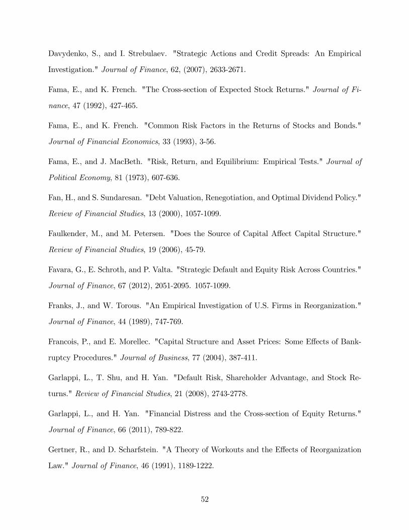
Davydenko, S., and I. Strebulaev. "Strategic Actions and Credit Spreads: An Empirical
Investigation." Journal of Finance, 62, (2007), 2633-2671.
Fama, E., and K. French. "The Cross-section of Expected Stock Returns." Journal of Fi-
nance, 47 (1992), 427-465.
Fama, E., and K. French. "Common Risk Factors in the Returns of Stocks and Bonds."
Journal of Financial Economics, 33 (1993), 3-56.
Fama, E., and J. MacBeth. "Risk, Return, and Equilibrium: Empirical Tests." Journal of
Political Economy, 81 (1973), 607-636.
Fan, H., and S. Sundaresan. "Debt Valuation, Renegotiation, and Optimal Dividend Policy."
Review of Financial Studies, 13 (2000), 1057-1099.
Faulkender, M., and M. Petersen. "Does the Source of Capital A¤ect Capital Structure."
Review of Financial Studies, 19 (2006), 45-79.
Favara, G., E. Schroth, and P. Valta. "Strategic Default and Equity Risk Across Countries."
Journal of Finance, 67 (2012), 2051-2095. 1057-1099.
Franks, J., and W. Torous. "An Empirical Investigation of U.S. Firms in Reorganization."
Journal of Finance, 44 (1989), 747-769.
Francois, P., and E. Morellec. "Capital Structure and Asset Prices: Some E¤ects of Bank-
ruptcy Procedures." Journal of Business, 77 (2004), 387-411.
Garlappi, L., T. Shu, and H. Yan. "Default Risk, Shareholder Advantage, and Stock Re-
turns." Review of Financial Studies, 21 (2008), 2743-2778.
Garlappi, L., and H. Yan. "Financial Distress and the Cross-section of Equity Returns."
Journal of Finance, 66 (2011), 789-822.
Gertner, R., and D. Scharfstein. "A Theory of Workouts and the E¤ects of Reorganization
Law." Journal of Finance, 46 (1991), 1189-1222.
52

Gilson, S., K. John, and L. Lang. "Troubled Debt Restructuring: An Empirical Study of
Private Reorganization of Firms in Default." Journal of Financial Economics, 27 (1990),
315-353.
Hackbarth, D., R. Haselmann, and D. Schoenherr. "Distress Risk, Stock Returns, and the
1978 Bankruptcy Reform Act." Working paper (2013), Boston University.
Hackbarth, D., C. Hennessy, and H. Leland. "Can the Trade-O¤ Theory Explain Debt
Structure?" Review of Financial Studies, 20 (2007), 1389-1428.
Hege, U., and P. Mella-Barral. "Repeated Dilution of Di¤usely Held Debt." Journal of
Business, 78 (2005), 737-786.
Hennessy, C., and Y. Tserlukevich. "Taxation, Agency Con�icts, and the Choice Between
Callable and Convertible Debt." Journal of Economic Theory, 143 (2008), 374-404.
Houston, J., and C. James. "Bank Information Monopolies and the Mix of Private and
Public Debt Claims." Journal of Finance, 51 (1996), 1863-1889.
Ingersoll, J.. "A Contingent-Claims Valuation of Convertible Securities." Journal of Finan-
cial Economics, 4 (1977), 289-321.
Jensen, M., and W. Meckling. "Theory of the Firm: Managerial Behavior, Agency Costs,
and Capital Structure." Journal of Financial Economics, 3 (1976), 305-360.
Johnson, H., and R. Stulz. "An Analysis of Secured Debt." Journal of Financial Economics,
14 (1985), 501-521.
Leeth, J., and J. Scott. "The Incidence of Secured Debt: Evidence from the Small Business
Community." Journal of Financial and Quantitative Analysis, 24 (1989), 379-394.
Lyandres, E., and A. Zhdanov. "Convertible Debt and Investment Timing." Journal of
Corporate Finance, forthcoming (2013).
Mayers, D.. "Why Firms Issue Convertible Bonds: The Matching of Financial and Real
Investment Options." Journal of Financial Economics, 47 (1998), 83-102.
53

Mella-Barral, P., andW. Perraudin. "Strategic Debt Service." Journal of Finance, 52 (1997),
531-556.
Mikkelson, W.. "Convertible Debt and Security Returns." Journal of Financial Economics,
9 (1981), 237-264.
Morellec, E.. "Asset Liquidity, Capital Structure, and Secured Debt." Journal of Financial
Economics, 61 (2001), 173-206.
Newey, W., and K. West. "A Simple, Positive Semi-De�nite, Heteroskedasticity and Auto-
correlation Consistent Covariance Matrix." Econometrica, 55 (1987), 703-708.
Pastor, L., and R. Stambaugh. "Liquidity Risk and Expected Stock Returns." Journal of
Political Economy, 111 (2003), 642-685.
Rampini, A., and S. Viswanathan. "Collateral and Capital Structure." Journal of Financial
Economics, 109 (2013), 466-492.
Rauh, J., and A. Su�. "Capital Structure and Debt Structure." Review of Financial Studies,
12 (2010), 4242-4280.
Scott, J.. "Bankruptcy, Secured Debt, and Optimal Capital Structure." Journal of Finance,
32 (1977), 1-19.
Scott, J.. "Bankruptcy, Secured Debt, and Optimal Capital Structure: Reply." Journal of
Finance, 34 (1979), 253-260.
Smith, C., and J. Warner. "On Financial Contracting: An Analysis of Bond Covenants."
Journal of Financial Economics, 7 (1979), 117-161.
Stein, J.. "Convertible Bonds as Backdoor Financing." Journal of Financial Economics, 32
(1992), 3-21.
Vassalou, M., and Y. Xing. "Default Risk in Equity Returns." Journal of Finance, 59 (2004),
831-868.
54

Zhang, A.. "Distress Risk Premia in Expected Stock and Bond Returns." Journal of Banking
and Finance, 36 (2012), 225-238.
Zmijewski, M.. "Methological Issues Related to the Estimation of Financial Distress Predic-
tion Models." Journal of Accounting Research, 22 (1984), 59-82.
55
Related Documents