Strange baryon production in heavy ion collisions

arX

iv:h

ep-p

h/95

0725

0v2

7 J

ul 1

995

Strange Baryon Production

in Heavy Ion Collisions

by

A. Capella, A. Kaidalov*, A. Kouider Akil, C. Merino, J. Tran Thanh Van

Laboratoire de Physique Theorique et Hautes Energies **Universite de Paris XI, batiment 211, 91405 Orsay Cedex, France

Abstract

The rapidity distribution of Λ and Λ produced in nucleus-nucleus collisions

at CERN energies is studied in the framework of an independent string model -

with quark-antiquark as well as diquark-antidiquark pairs in the nucleon sea. It is

shown that, besides the Λ-Λ pair production resulting from the fragmentation of

sea diquarks, final state interactions of co-moving secondaries π +N → K + Λ and

π + N → K + Λ are needed in order to reproduce the data. Predictions for Pb-Pb

collisions are presented.

LPTHE Orsay 95-41

June 1995

* Present address : ITEP, B. Cheremushkinskaya ulitsa 25, 117 259 Moscow,Russia** Laboratoire associe au Centre National de la Recherche Scientifique - URA

D0063

2

1. Introduction

A substantial increase in the ratio of strange over non-strange particles between

proton-proton and central nucleus-nucleus collisions has been observed experimen-

tally both at CERN and AGS [1]. Such an increase was expected as a consequence

of quark gluon plasma (QGP) formation due to an increase of the strange quark

production rate in the deconfined phase [2]. However, as in the case of other possible

signals of QGP, one has to check whether such a phenomenon is typical of a central

nucleus-nucleus collision or, on the contrary, it is already present in proton-nucleus

interactions *. Unfortunately, the experimental situation is not conclusive. While

in the data from the NA35 collaboration strangeness is enhanced between pp and

pS, the effect is not seen when taking an average over three different nuclear targets

[4]. However, two other experimental facts indicate that strangeness enhancement

is not only present in central nucleus-nucleus collisions. Indeed in pp collisions, the

ratio K/π increases both with increasing energy and with increasing multiplicity [5].

Also the ratio Λ/p in pp collisions increases from 0.26 at√s = 20 GeV [6] to 0.39

at√s = 1 800 GeV [7]. Furthermore, results from the NA36 collaboration [8] show

a large strangeness enhancement between peripheral and average nucleus-nucleus

collisions.

Actually, it has been emphasized [9-11] that strangeness enhancement is ex-

pected to occur in independent string models such as the Dual Parton Model (DPM)

[9] and the Quark Gluon String Model (QGSM) [12]. Indeed, the average number

* For instance, in the case of J/ψ suppression, R. Salmeron, followed by many

other authors, has shown that the effect could be explained by extrapolation of the

corresponding hadron-nucleus data [3].

3

of collisions per participant nucleon increases between pp and pA as well as be-

tween pA and central AB collisions. The resulting extra particles are produced in

the fragmentation of strings involving sea constituents at their ends. Since strange

sea quarks are present in the nucleon sea, the ratio of strange over non-strange

secondaries will also increase. The value of this increase depends on the ratio

S =2(s+ s)

u+ d+ u+ d

in the nucleon sea. We shall use a value of S in the range 0.4 to 0.5, consistent

both with strangeness suppression in string fragmentation at the highest available

energies [7] and with conventional parton distributions for DIS [13]. In order to

explain the observed enhancement of Λ and Λ, two approaches have been proposed.

In DPM, diquark-antidiquark pairs have been introduced in the nucleon sea - with

the same ratio, relative to quark-antiquark pairs, as in the string breaking process

[10, 11]. The second approach is string fusion [14, 15]. However, both mechanisms

have a common caveat, namely, they lead to the same increase in absolute value of

strange baryons and antibaryons - while experimentally the excess of Λ’s is much

larger than that of Λ’s.

In the present work we solve this problem by introducing final state interactions

of co-moving pions and nucleons which increase the number of produced Λ’s via

the binary interactions π + N → K + Λ (K∗ + Λ, ...). This is a fundamental

mechanism in hadron gas models [2] and has been incorporated into some Monte

Carlo codes [12, 15, 16]. Clearly, such an interaction is very efficient in producing

Λ’s - since the density of both pions and nucleons is high as compared to that of

Λ’s. Actually, it was shown in Ref. [11], that using the experimentally measured

pion and nucleon densities in central SS collisions, together with the cross-section

4

of the above reaction (which is about 1.5 mb at the maximum near threshold),

one precisely obtains the missing number of Λ’s. Obviously, the conjugate reaction

π + N → K + Λ (K∗ + Λ) will also produce some extra Λ but the absolute yield is

much smaller than the one of Λ’s due to the smallness of the N density as compared

to that of N ’s.

In this paper we compute, in the framework described above, the rapidity

distributions of Λ and Λ in SS and Pb-Pb collisions. A substantial increase of the

ratios Λ/π− and Λ/π− (70 % and 50 %, respectively) is predicted between SS and

Pb-Pb.

Extra evidence for the necessity of a final state interaction is obtained from

baryon stopping. The rapidity distribution of proton minus antiproton in central

SS collisions, computed in independent string models, has a dip at y∗ ∼ 0 which

is much more pronounced that the one observed experimentally [17] - while the

corresponding distributions both in pp and in peripheral SS collisions are well re-

produced. In other words, the stopping power in the model is too small as compared

to experiment and rescattering of the produced baryon is required in order to in-

crease it [12] [15].

The plan of the paper is as follows : in Section 2 we give the general formulae

of DPM for nucleus-nucleus collisions in the presence of diquark-antidiquark pairs

in the nucleon sea and compute the rapidity distributions of Λ and Λ in pp and SS

collisions without final state interactions. In Section 3, we introduce the final state

interactions and give the modified Λ and Λ rapidity distributions in SS collisions

as well as the model predictions for Pb-Pb collisions. The rapidity distribution

of pions and protons in pp, SS and Pb-Pb collisions are also given. A list of

5

average multiplicities for pions, kaons, baryons and antibaryons without and with

final state interactions is given in Table 1. Section 4 contains some final remarks

and conclusions. In Appendix 1 we give the momentum distribution functions and

fragmentation functions used in this work, as well as the formulae for the hadronic

spectra of the individual strings.

2. The Model

In DPM and QGSM, the dominant contribution to multiparticle production in

pp collisions is a two string production - the two strings being stretched between

the valence diquark of a proton and a valence quark of the other proton, and vice-

versa. In fact, in this paper we shall restrict ourselves to this component (see

Section 4 for a discussion on this approximation). Therefore we have exactly two

strings per inelastic collision. When the number of inelastic collisions experienced

by a nucleon in a nuclear collision is larger than one, the extra strings (two per

each extra collision) have sea quark constituents at the end corresponding to the

multiply wounded nucleon. As explained in the Introduction, since strange sea

quarks are present in the nucleon sea, the ratio of strange over non-strange particles

will increase. One can object, however, that if the fraction S of strange quarks

(defined in the Introduction) is the same as in the string breaking process, then the

strings with sea quarks at their ends will produce the same strange over non-strange

ratio as in the string breaking process - with no net strangeness enhancement. While

true at asymptotic energies, this is not the case at present ones. For instance, let us

consider the K−/π− ratio. In NN collisions at 200 GeV/c, the experimental value

of this ratio is about 0.05. Since the values of S we consider are much larger, it is

clear that the ratio K−/π− will increase. Another example is the ratio Λ/p which,

6

as discussed in the Introduction, reaches a value close to 0.4 at Fermilab [7]. In the

following we shall use the value S = 0.5. However, taking S = 0.4 changes very

little our results [11].

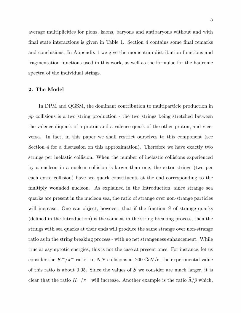
The general formulae for the single particle inclusive rapidity distribution in

nucleus-nucleus collisions is the following [9] :

dNAB

dy=

1

σAB

∑

nA,nB,n

σnA,nB ,n

{

θ(nB − nA)[

nA

(

NqqA

v−qB

v

µA,µB(y) +N

qA

v−qqB

v

µA,µB(y))

+

(nB − nA)(

NqA

s−qB

v

µA,µB(y) +N

qA

s−qqB

v

µA,µB

)

+ (n− nB)(

NqA

s−qB

s

µA,µB(y) +N

qA

s−qB

s

µA,µB(y))]

+sym (nA ↔ nB)} . (2.1)

Here σABnA,nb,n is the cross-section for n inelastic nucleon-nucleon collisions involving

nA and nB participating nucleons, σAB =∑

nA,nB ,nσn,nA,nB

is the inelastic nucleus-

nucleus cross-section, and µA = n/nA, µB = n/nB. N(y) are the inclusive spectra

of each individual string. Note that the total number of strings in Eq. (2.1) is 2n

(two for each nucleon-nucleon collision).

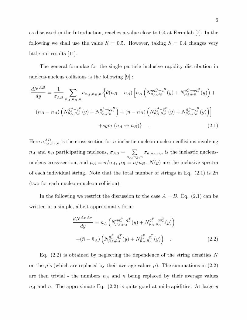
In the following we restrict the discussion to the case A = B. Eq. (2.1) can be

written in a simple, albeit approximate, form

dNAP AT

dy= nA

(

NqqP

v−qT

v

µA,µA(y) +N

qP

v−qqT

v

µA,µA(y))

+(n− nA)(

NqP

s−qT

s

µA,µA(y) +N

qP

s−qT

s

µA,µA(y))

. (2.2)

Eq. (2.2) is obtained by neglecting the dependence of the string densities N

on the µ’s (which are replaced by their average values µ). The summations in (2.2)

are then trivial - the numbers nA and n being replaced by their average values

nA and n. The approximate Eq. (2.2) is quite good at mid-rapidities. At large y

7

it becomes worse. However, in the rapidity region where the baryon densities are

sizeable (y∗ ≤ 2.5), the errors involved are 5 to 10 %.

In Eqs. (2.1) and (2.2) only qs-qs pairs in the nucleon sea are considered. As

discussed in the Introduction, we now assume that qqs-qqs pairs are also present with

relative fraction α. The modification in Eqs. (2.1) and (2.2) are straightforward.

Eq. (2.2) is changed into :

dNAP AT

dy= nA

(

NqqP

v−qT

v

µA,µA(y) +N

qP

v−qqT

v

µA,µA(y))

+ (n− nA)[

(1 − 2α)(

NqP

s−qT

s

µA,µA(y)

+NqP

s−qT

s

µA,µA(y))

+ α(

NqqP

s−qT

s

µA,µA(y) +N

qqP

s−qT

s

µA,µA(y) +N

qP

s−qqT

s

µA,µA(y) +N

qP

s−qqT

s

µA,µA(y))]

.

(2.3)

In the following, we compute the rapidity distributions of Λ and Λ in nucleus-

nucleus collisions using Eq. (2.3). The rapidity distributions of the individual

strings are obtained by convoluting momentum distribution functions and fragmen-

tation functions. All relevant formulae (including absolute normalization) are given

in Appendix 1.

In numerical calculations we use the value α = 0.1 taken from JETSET [18]. (A

somewhat smaller value, α = 0.07, is obtained in FRITIOF [16] and in BAMJET

[19]). The values of nA and n are obtained in the optical approximation of the

Glauber model, with Saxon-Woods profiles, for impact parameter |b| ≤ 1 fm. We

get in SS collisions : nA = 31, n = 55 and in Pb-Pb collisions nA = 192, n = 676.

Before giving the numerical results, let us make some remarks concerning

Eq. (2.3). Its first two terms are the same as in NN collisions - except for the

value of µA - which is 1 for NN , 2 for central SS and 4.5 for central Pb-Pb. The

8

third and fourth terms give negligeably small contributions to baryon-antibaryon

production due to the large, (mΛ +mΛ)2, thresholds in the short qs-qs strings. The

remaining terms contain the contribution of sea diquarks and produce Λ and Λ by

pairs. Detailed formulae for the rapidity distributions of baryons and antibaryons

resulting from the various terms of Eq. (2.3) are given in Appendix 1.

In Fig. 1 we give the Feynman x distributions of Λ and Λ in pp collisions.

They are obtained from the first two terms of Eq. (2.3) (i.e. from the sum of

the contributions of the two qq-q valence-valence strings) with µA = 1. As shown

previously in Ref. [20], the agreement with available data is quite good. Note that

the shape of the fragmentation functions is determined from Regge intercepts (see

Ref. [20] and Appendix 1).

The corresponding rapidity distributions in central SS collisions are given in

Figs. 2 and 3. We see that the yields of both Λ and Λ are smaller than the data. The

Λ yield, in particular, is considerably smaller than the experimental one. There-

fore, we need a mechanism to produce extra Λ’s. As already mentioned in the

Introduction this can be achieved by a final state interaction of co-moving secon-

daries π +N → K + Λ (K∗ + Λ, ...). A smaller number of Λ will also be produced

via π + N → K + Λ (K∗ + Λ, ...). In the next section we discuss in detail these

final state interactions.

3. The Final State Interaction of Secondaries

In independent string models, it is assumed that secondaries produced in dif-

ferent strings are independent from each other. Introducing a final state interaction

of secondaries represents a departure from the independent string picture. In fact,

9

it corresponds to the simplest form of string interaction. It should be stressed that

it is not known how to treat quantitatively such an interaction. Here we adopt

the formalism introduced in Ref. [21]. Note that, at moderate energies, such a

treatment of string interaction can be justified in the framework of Reggeon Field

Theory [22].

Let us consider the number of Λ’s produced by unit of space time volume d4x

resulting from the interaction π +N → K + Λ (K∗ + Λ, ...). One has [21]

dNΛ

d4x=< σ > ρπ(x) ρp(x) (3.1)

where ρ(x) are space-time dependent particle densities and < σ > is the interaction

cross-section - properly averaged over the momentum distributions of the colliding

particles. We take < σ >= 1.5 mb which is the value of π− + p → K0 + Λ/Σ0 at

its maximum near threshold. Beyond the threshold these two-body cross-sections

decrease rapidly but quasi two-body interactions convert this sharp decrease into a

mild increase.

We use cylindrical space-time variables : the longitudinal proper time is τ =√t2 − z2 and the space-time rapidity y = 1

2ℓn[

t+zt−z

]

. In these variables d4x =

τ dτ dy d2s, where ~s is the transverse coordinate and d2s an element of transverse

area. As customary, we assume boost invariance - i.e. that the space-densities ρi(x)

are independent of y - and assume, furthermore, that the dilution in time of the

density is mainly due to longitudinal motion. With this two assumptions we have

[21] :

ρi(τ, y, ~s) = ρi(τ, ~s)τ0τ

. (3.2)

10

Using (3.2) it is trivial to integrate Eq. (3.1) on the variable τ . One gets

dNΛ

dy=

∫

d2sdNπ

dy d2s

dNp

dy d2s3 < σ > ℓn [(τ + τ0)/τ0] (3.3)

where τ0 is the formation proper time and τ the time during which the final in-

teraction takes place. We take τ0 = 1 fm and τ = 3 fm - based on interferometry

measurements which indicate a very short time of particle emission and a freeze out

time τ0 + τ ∼ 4 fm [23]. The factor 3 results from the product of three pion times

two nucleon species, divided by a factor 2 - which is due to the fact that one out of

two πN combinations have a negligeably small cross-section. For instance among

the π±p combinations only π−p has to be considered.

Let us now explain how to compute dNi/dy d2s in Eq. (3.3). The formulae

given in Section 2 (see for instance Eq. (2.3)) give the expression of dN/dy - which is

the result of integrating dN/dy d2s over d2s. Actually, the only dependence on ~s is

in the average values nA, nB and n. In the Glauber model, these average quantities

are known as a function of ~b and ~s. In the optical approximation one has

n(~b,~s) =ABσ

σABTA(~b− ~s) TB(~s) , (3.4)

and

nA(~b,~s) =A

σABTA(~b− ~s) σNA(~s) (3.5)

where

σNA(~s) = 1 − (1 − σ TA(~s))A

.

Here σ is the nucleon-nucleon inelastic cross-section and TA(~b) the nuclear profile -

for which we use the standard Saxon-Woods expression. Clearly, when computing

11

the r.h.s. of Eq. (3.3) one has to perform the products n2(~b,~s), n2A(~b,~s), nA(b, ~s)

n(b, ~s) and integrate them over both d2s and d2b. It is easy to see that such integrals

of products are smaller than the product of integrals dNπ/dy times dNp/dy and

that the ratio of the former over the latter is roughly proportional to R−2A ∼ A−2/3.

Therefore, the number of Λ’s resulting from the final state interaction, will increase

quite fast with increasing A. Indeed, at mid-rapidities, the product dNπ/dy times

dNp/dy increases withA approximately as A8/3 and thus the number of Λ’s increases

approximately as A2.

In order to compute the rapidity distributions of Λ resulting from the final

state interaction (3.1) one has to compute first the densities of pions and protons.

This has been done using the formulae in Appendix 1.

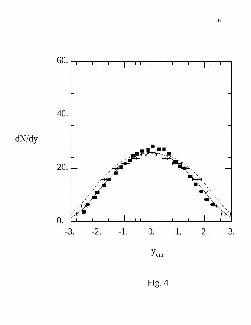
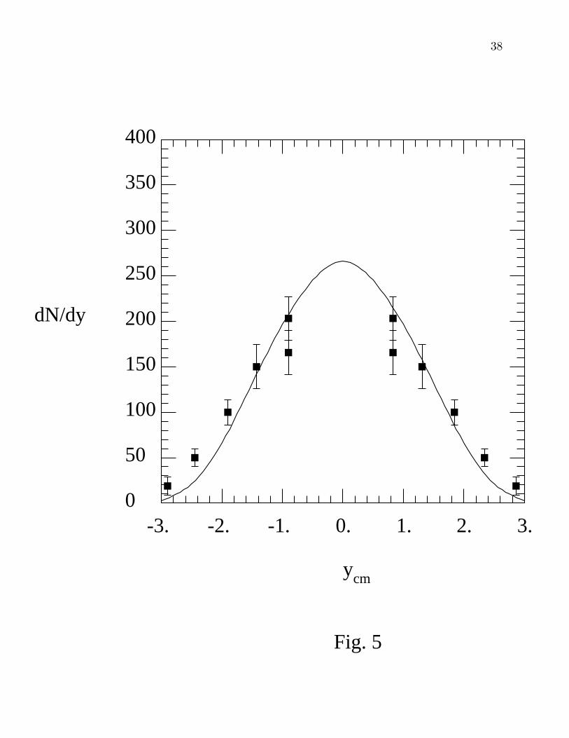
The rapidity distributions of h− in NN , SS and Pb-Pb collisions are given

in Figs. 4 and 5. The agreement with experiment is reasonable. Note that, due

to the two string approximation in NN , the rapidity distribution tends to be too

broad. Indeed, the contribution of the qs-qs strings, although small at 200 GeV/c,

is concentrated at mid-rapidities. This is partly compensated by choosing steeper

diquark fragmentation functions (see Appendix 1). In any case, our aim here is

not to get the best possible description of h− distributions, but only to have a

reasonable form of dNπ−/dy in order to use it in Eq. (3.1). Following Ref. 4, we

have taken dNπ−/dy = 0.93 dNh−/dy.

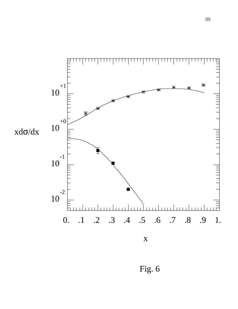
The Feynman x distributions of proton and antiprotons in pp collisions are given

in Fig. 6. The agreement with data is quite good. Note that diffractive dissociation,

which produces a peak near x = 1 in the p distribution has not been included in

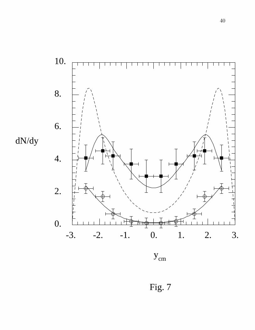
the model. The corresponding results for peripheral and central SS collisions are

12

given in Fig. 7. Actually, both the data and the theoretical curves correspond to

the difference p− p. The shape of the rapidity distribution is well reproduced in the

model for peripheral collisions but not for central ones. In the latter case, the shape

of the experimental distribution is much flatter than the theoretical one. Note,

however, that the average multiplicity is the same for the two distributions. This

disagreement between an independent string model prediction and experiment is

very significant and we are going to discuss it in some detail. First of all, in DPM

the stopping power is entirely controlled by the momentum distribution functions.

More precisely, when the average number of collisions per nucleon increases (i.e.

when µA in Eq. (2.3) increases), the maximum of the proton spectrum is shifted to

smaller rapidities (see Fig. 2 of Ref. [24]). This effect is seen in Fig. 7. However,

in central SS collisions µA ∼ 2 and, therefore, the effect is small. Moreover, the

decrease of the proton spectrum between its maximum and y∗ ∼ 0 is very steep even

for a large number of inelastic collisions. Thus, the dramatic flattening of the proton

rapidity distribution between peripheral and central SS collisions in Fig. 7 cannot

be reproduced in the model, and, as discussed in the Introduction, rescattering of

the produced nucleons is needed.

We can now compute the rapidity distribution of Λ resulting from the final

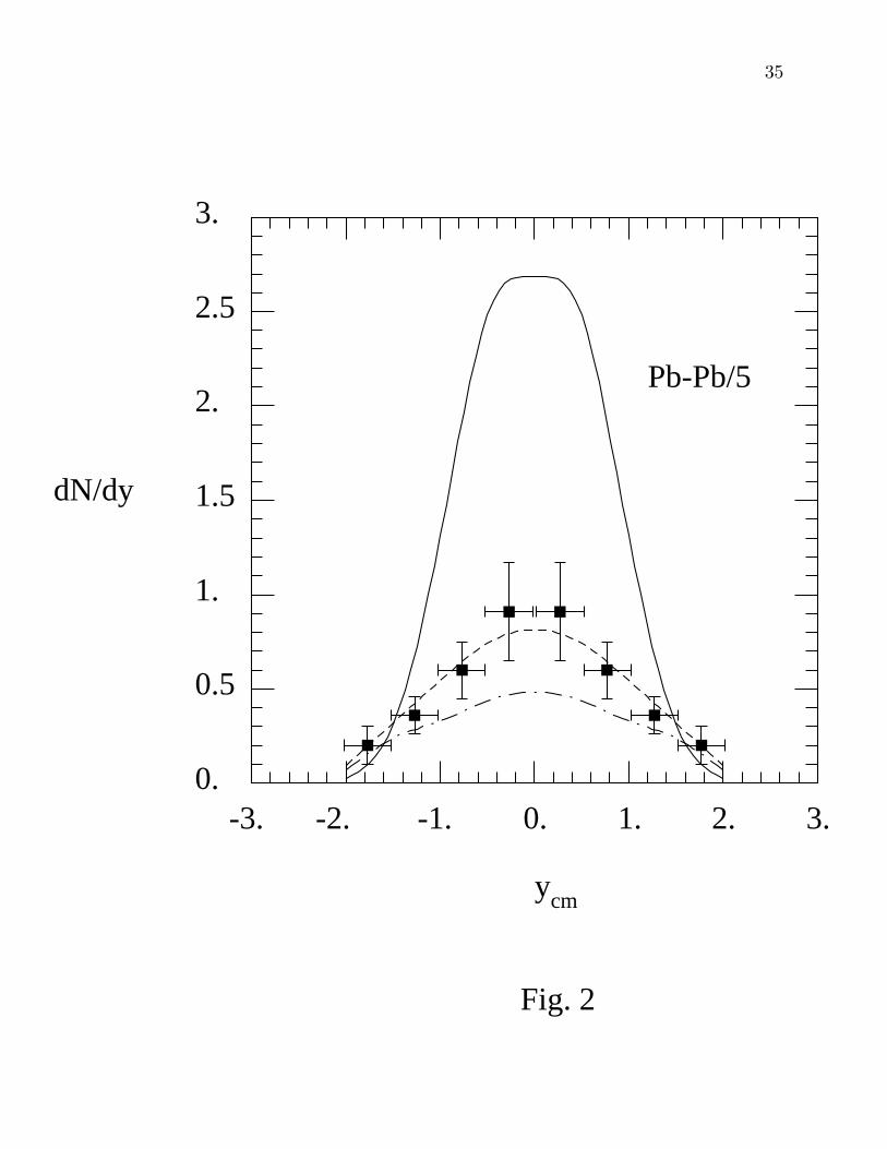
state interaction π + N → K + Λ (K∗ + Λ, ...). The results are shown in Fig. 2.

The agreement with experiment is quite good.

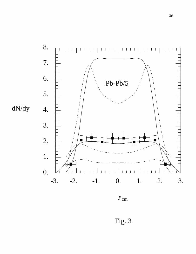
The corresponding results for Λ production, including the effect of the final

state interaction π + N → K + Λ (K∗ + Λ, ...), are given in Fig. 3 (dashed line).

We see that the final state interaction has produced a substantial increase of the

Λ yield, which is now in qualitative agreement with experiment. We conclude that

13

the main features of Λ and Λ production in central SS collisions can be understood

in the scenario presented in this paper.

We turn next to central Pb-Pb collisions at 160 GeV/c per nucleon. In this

case the rate of strange baryon production from the final state interactions is

very high at mid-rapidities due to the large value of the pion density and one

can not ignore any longer the crossed reactions π + Λ → K + N and π + Λ →

K + N . Indeed, it turns out that, at mid-rapidities, equilibrium between strange

and non strange baryons is reached before the freeze out time τ0 + τ (assumed to

be the same as in central SS collisions). When this equilibrium is reached one has

< n >p + < n >n= 1.6 < n >Λ (where 0.6 < n >Λ takes into account the Σ±

baryons) and the strange baryon multiplicity does not increase any longer. The

predictions for the rapidity distribution of Λ and Λ in central Pb-Pb are shown in

Figs. 2 and 3 (upper lines scaled down by a factor 5).

A close look at Fig. 3 shows that the computed Λ distribution in SS collisions

has a shallow dip at y∗ = 0 which is not seen in the data. Probably this is related to

the lack of baryon stopping discussed above and requires further rescattering of the

produced Λ’s. In order to have a rough estimate of the effect of the baryon rescat-

tering, we have introduced some extra stopping in the proton spectrum (without

changing the proton average multiplicity) by shifting it by ∆y = 0.5. The modified

p − p rapidity distribution is shown in Fig. 7 (full upper line). Using such shifted

proton distributions in Eq. (3.3), we obtain a flatter Λ distribution both in SS and

Pb-Pb collisions (full lines in Fig. 3), which for SS collisions is in good agreement

with experiment.

Finally, the average multiplicities of pions, kaons, protons lambdas and anti

14

lambdas in SS and Pb-Pb collisions are given in Table 1. (A discussion of cascades

and omega production in the present framework can be found in Refs. 10, 11). We

observe that the ratio Λ/h− (Λ/h−) increase by about 50 % (70 %) between SS

and Pb-Pb collisions.

4. Conclusions

We have studied meson and baryon strangeness enhancement in an independent

string model with quark-antiquark and diquark-antidiquark pairs in the nucleon sea.

The expe rimental data have forced us to depart from string independence and to

introduce a final state interaction of co-moving secondaries. The necessity of final

state rescattering also follows from the study of the shape of the proton rapidity

distribution in central SS collisions. Final state interactions are the simplest forms

of string interaction - which is a first step in order to drive the system toward

equilibrium. Using all these ingredients, we have obtained a reasonable agreement

with experiment. We feel that a more accurate description is not possible in the

present state of the art.

The present model has many uncertainties that we want to discuss briefly.

Apart from the poor knowledge of the parameter S and α, there is an uncertainty

resulting from the hadronization of short strings and, in particular, of strings in-

volving sea diquarks (see Appendix 1). Furthermore, the introduction of final state

interactions rises a lot of questions. Not only a rigourous treatment of the final

state interaction does not exist, but, moreover, we can not be sure that other re-

actions (for most of which the cross-sections are not even known) do not affect

our results. (In particular we have neglected annihilation reactions of nucleons and

antilambdas or antinucleons and lambdas which have a very large cross-section at

15

threshold. However, this cross-section drops very fast after the threshold and the

corresponding value of < σ > in Eqs. (3.1), (3.3) is not known). Despite all these

drawbacks, the effects discussed in the present work are important and cannot be

ignored in strangeness enhancement studies.

A characteristic feature of the model presented here is that it predicts a contin-

uous strangeness enhancement, not only from proton-proton to proton-nucleus and

to average (i.e. minimum-bias) nucleus-nucleus collisions, but also in proton-proton

when energy or event multiplicity is increased. Of course to get this latter effect it is

necessary to give up the two string approximation in pp collisions. This assumption

is of no consequence for the results presented here, provided a good description of

pp data is achieved [25]. Indeed the results for nucleus-nucleus collisions are deter-

mined by the input in pp (or rather NN) collisions. However, when multistrings

are introduced, one obtains [26] an increase of the ratio K/π in pp collision when

increasing either the energy or the event multiplicity, as observed experimentally.

Moreover, the increase with energy [7] of the ratio Λ/p, can also be understood in

this way. Note, however, that the contribution to strangeness enhancement result-

ing from the final state interaction (which is very important for Λ production) is

most effective in central nucleus-nucleus collisions where the densities of secondaries

are very large.

In conclusion, the study of strangeness enhancement is a very active field. This

is clear from the large number of recent work on the subject [1]. Actually, during

the latest stages of the present work [27] many interesting papers on this subject

have appeared in the literature [28-31]. Some of them give also predictions for Pb-

Pb collisions. The theoretical ideas in these papers and their predictions are, in

16

general, quite different from ours. Forthcoming results with a lead beam at CERN

will certainly trigger more activity and give new insight into this very interesting

field. Predictions for RHIC and LHC energies are also needed.

Acknowledgements :

We would like to thank A. Krzywicki for useful discussions. We also thank J.

Ranft for an ongoing collaboration on this subject.

One of the authors (C. M.) has benefitted of a EEC postdoctoral project ER-

BCHBI CT 930 547.

This work has been done with the help of an INTAS contract 93-0079.

17

Appendix 1

Hadron Spectra of Individual String

Both in DPM and QGSM the hadron spectra of the individual strings are given

by a convolution of structure functions and fragmentation functions. In DPM, one

has for the rapidity density N qq−q(y, s) of hadron h in, say, a diquark-quark string :

N qq−qµ1,µ2

(y, s) =

∫ 1

0

dx1

∫ 1

0

dx2 ρqqµ1

(x1) ρqµ2

(x2)

dN qq−q

dy(y − ∆, sstr.) θ(sstr. − sthr.) . (A.1)

Here ρqqµ1

and ρqµ2

are the momentum distribution functions of diquark and quark

which depend on the light cone momentum fractions x1 and x2. The index µ1

(µ2) denotes the number of inelastic collisions suffered by the nucleon to which the

diquark (quark) belongs. The squared invariant mass of the string is sstr = x1x2s

and ∆ = 1/2 log[x1/x2] is the rapidity distance between the C. of M. of the string

and the overall C. of M. At fixed values of x1 and x2 the string hadronization is

just given in terms of qq and q fragmentation functions :

dN qq−q

dy(y − ∆, sstr.) =

Ghqq(y) for y ≥ ∆

Ghq (y) for y ≤ ∆

(A.2)

where G(y) are fragmentation functions (see below). Of course dN qqv−qv/dy = 0

for y outside the rapidity interval determined by the string endpoints. Note the

presence of a threshold θ-function in Eq. (A.2). The value of sthr corresponds to

the squared mass of the lightest system that can be produced in association with

the triggered hadron h*.

* For instance for a qqv-qv string fragmenting into a Λ we have sthr = (mΛ +

18

An important feature of DPM and QGSM is the fact that the structure function

is determined in terms of Regge intercepts. In DPM, the structure function in the

presence of 2k such constituents is given by [9] :

ρk(x1 · · ·x2k) = C2k x−1/21 x−1

2 · · ·x−12k−1x

3/22k δ

(

1 −2k∑

i=1

xi

)

. (A.3)

The index 1 refers to the valence quark and the index 2k to the diquark. All other

indices refer to sea quarks and antiquarks. The constant C2k is obtained from the

normalization of ρ2k to unity. The structure function of each individual constituent,

which appears in Eq. (A.1), is obtained by integrating (A.3) over the variables of

all other constituents. (In actual calculations the singular factor x−1 is replaced by

x−1 with x = (x2 + µ2/s)1/2, and µ = 0.1 GeV ; varying µ between 0.05 and 0.3

produces only minor changes in our results).

In QGSM the formulae are somewhat different [7]. The diquark and quark

fragment independently from each other and the threshold resulting from the θ-

function in (A.1) is not present. Moreover in Eq. (A.3) sea quarks are assumed

to have, at present energies, a x−1/2 behaviour at x ∼ 0 - the same as for valence

quarks. In this case the integration of ρ in (A.3) over all variables except one can

be performed analytically. One gets

ρq2k(x) = Cq

2k x−0.5(1 − x)2k+1/2

ρqq2k(x) = Cqq

2k x1.5(1 − x)2k−3/2 . (A.3′)

mK)2. For that of a us-d string we have sthr = m2Λ. Likewise for pion (kaon)

production in a ud (sd) string we have sthr = µ2π(m2

K) - where µπ is the pion

transverse mass.

19

The coefficients C are determined (analytically) from the normalization to unity of

ρ(x). Note that the x−1 behaviour in DPM strongly reduces the probability of a

sea quark to cross to the opposite hemisphere (as compared to an x−1 behaviour,

which corresponds to a flat distribution in rapidity). As a consequence, the results

obtained in DPM and QGSM are quite similar - at least at the energies considered

here.

In the first DPM papers, fragmentation functions were just derived from a fit to

pp (or e+e−) data. An important break through was achieved when it was realized

that, not only momentum distribution functions, but also fragmentation functions

could be derived in terms of Regge intercepts [7]. In this way the predictivity of

the model was greatly increased. Indeed, it has been possible to predict the shape

of the rapidity distributions of π, K, p, Λ, etc in pp collisions - with absolute rates

as the only free parameters.

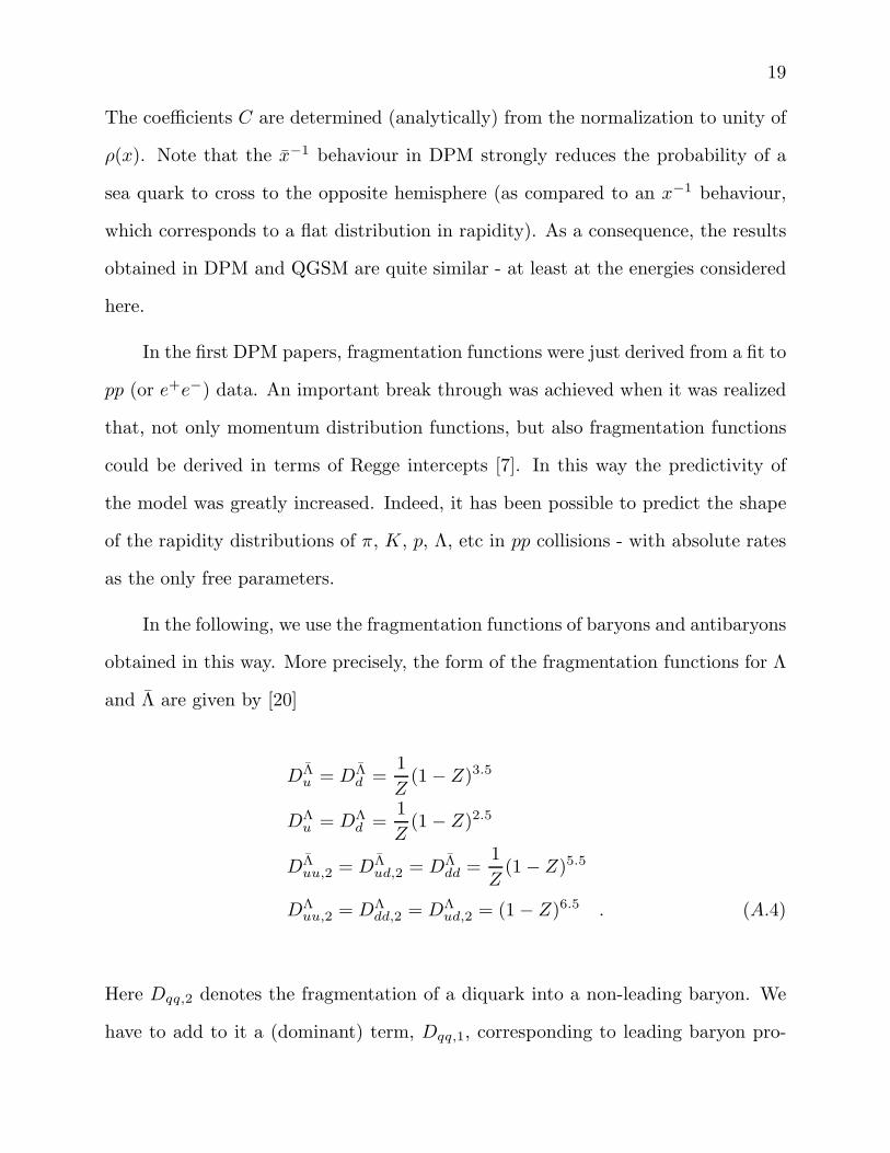
In the following, we use the fragmentation functions of baryons and antibaryons

obtained in this way. More precisely, the form of the fragmentation functions for Λ

and Λ are given by [20]

DΛu = DΛ

d =1

Z(1 − Z)3.5

DΛu = DΛ

d =1

Z(1 − Z)2.5

DΛuu,2 = DΛ

ud,2 = DΛdd =

1

Z(1 − Z)5.5

DΛuu,2 = DΛ

dd,2 = DΛud,2 = (1 − Z)6.5 . (A.4)

Here Dqq,2 denotes the fragmentation of a diquark into a non-leading baryon. We

have to add to it a (dominant) term, Dqq,1, corresponding to leading baryon pro-

20

duction, given by

DΛuu,1 = DΛ

dd,1 =1

ZZ1.5(1 − Z)1.5 ; DΛ

ud,1 =1

ZZ1.5(1 − Z)0.5 . (A.5)

Turning to p and p production, we have [20]

Dpu = Dp

d =1

Z(1 − Z)3

Dpu =

1

Z(1 − Z)2 ; Dp

d =1

Z(1 − Z)2

[

1

3+

2

3(1 − Z)

]

Dpdd,2 = Dp

uu,2 = Dpud,2 =

1

Z(1 − Z)5

Dpdd,2 = Dp

uu,2 = Dpud,2 =

1

Z(1 − Z)6 (A.6)

and, for the leading proton,

Dpud,1 =

1

ZZ1.5(1 − Z)0 ; Dp

uu,1 =1

Z(1 − Z)0 . (A.7)

Finally for neutron production we have

Dnu = Dp

d ; Dnd = Dp

u , Dnuu,2 = Dp

uu,2 ,

Dnud,1(2) = Dp

ud,1(2) , Dnuu,1 =

2

3ZZ1.5(1 − Z)1 . (A.8)

The values of all powers of Z and 1 − Z in Eqs. (A.4)-(A.8) are determined in

terms of Regge intercepts*. For example, the power 0 of 1 − Z in Eq. (A.7) is

given by −αR(0) + λ where αR(0) = 0.5 is the dominant reggeon intercept and

* The only factors which are not determined in this way are the factor [1/3 +

2/3(1−Z)] in Eq. (A.6) and the factor 2/3 in Eq. (A.8). These factors have a trivial

origin. For instance the factor in (A.6) results from the fact that the fragmentation

of u and d quarks into a proton is the same at Z → 0. However, at Z → 1 the

21

λ = 2α′p2⊥

≃ 0.5 is common to all fragmentation functions and results from the

integration over transverse momentum. In the case of Λ production DΛud,1 has a

softer Z → 1 behaviour, with a power −αφ(0)+λ = 0.5, which explains the different

shape of Λ and p (non-diffractive) rapidity distributions (see Figs. 1 and 6). Of

course, there are some numerical uncertainties in the determination of these powers

- in particular in the power of Z in the leading baryon fragmentation function. The

value 1.5 used above has been chosen, within the theoretically allowed range, in

order to obtain the best description of the pp data in the DPM formalism.

The only remaining point is to define the functions Gqq and Gq in the r.h.s. of

Eq. (A.2), in terms of the fragmentation functions defined above. This is done in the

following way. Let us consider first the production of antibaryons and non-leading

baryons. In this case we have

Ghqq,2(y) = ah Z+ Dh

qq,2(Z+) Z− Dhq (Z−) , for y ≥ ∆

Ghq,2(y) = ah Z− Dh

q (Z−) Z+ Dhqq,2(Z+) , for y ≤ ∆ . (A.9)

Here Z+ and Z− are the light cone momentum fractions defined as Z+ = exp(ystr−

ystrMAX), Z− = exp(−ystr − ystr

MAX), where ystr = y − ∆ and ystrMAX is the maximal

rapidity that a hadron h can have in the string (for fixed values of the momentum

fractions x1 and x2 of the string ends). Note that for a string with a very large in-

fragmentation of a u-quark is three times larger since the three combinations u(ud),

u(du) and u(uu) are possible. (The later will give a ∆++ which will often decay into

a proton). On the contrary, for the fragmentation of a d quark the only possible

combination is d(uu). Likewise, the fragmentation of a diquark uu into a leading

neutron is only possible through diquark breaking and has a probability of 2/3 as

compared to the corresponding one for a ud diquark.

22

variant mass Z− ∼ 0 for y ≥ ∆ and therefore Ghqq,2(y) ∼ ah Z+ Dh

qq(Z+). Likewise,

for y ≤ ∆, Z+ ∼ 0 and Ghq,2(y) ∼ ah Z− Dh

q (Z−).

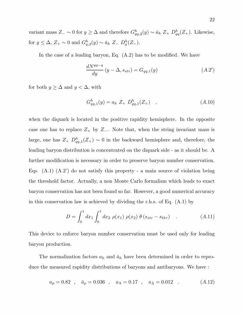
In the case of a leading baryon, Eq. (A.2) has to be modified. We have

dN qq−q

dy(y − ∆, sstr) = Gqq,1(y) (A.2′)

for both y ≥ ∆ and y < ∆, with

Ghqq,1(y) = ah Z+ Dh

qq,1(Z+) , (A.10)

when the diquark is located in the positive rapidity hemisphere. In the opposite

case one has to replace Z+ by Z−. Note that, when the string invariant mass is

large, one has Z+ Dhqq,1(Z+) ∼ 0 in the backward hemisphere and, therefore, the

leading baryon distribution is concentrated on the diquark side - as it should be. A

further modification is necessary in order to preserve baryon number conservation.

Eqs. (A.1) (A.2’) do not satisfy this property - a main source of violation being

the threshold factor. Actually, a non Monte Carlo formalism which leads to exact

baryon conservation has not been found so far. However, a good numerical accuracy

in this conservation law is achieved by dividing the r.h.s. of Eq. (A.1) by

D =

∫ 1

0

dx1

∫ 1

0

dx2 ρ(x1) ρ(x2) θ (sstr − sthr) . (A.11)

This device to enforce baryon number conservation must be used only for leading

baryon production.

The normalization factors ah and ah have been determined in order to repro-

duce the measured rapidity distributions of baryons and antibaryons. We have :

ap = 0.82 , ap = 0.036 , aΛ = 0.17 , aΛ = 0.012 . (A.12)

23

Note that the same normalization constant a is used for antibaryons and for non-

leading baryons.

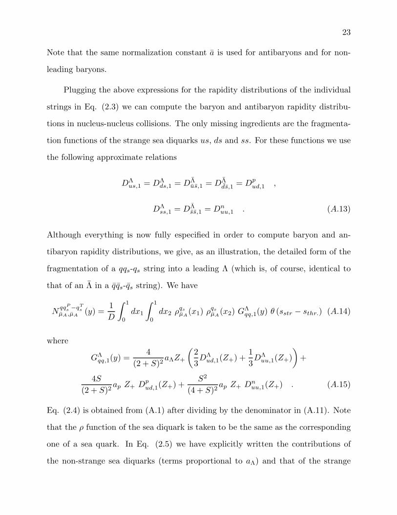
Plugging the above expressions for the rapidity distributions of the individual

strings in Eq. (2.3) we can compute the baryon and antibaryon rapidity distribu-

tions in nucleus-nucleus collisions. The only missing ingredients are the fragmenta-

tion functions of the strange sea diquarks us, ds and ss. For these functions we use

the following approximate relations

DΛus,1 = DΛ

ds,1 = DΛus,1 = DΛ

ds,1 = Dpud,1 ,

DΛss,1 = DΛ

ss,1 = Dnuu,1 . (A.13)

Although everything is now fully especified in order to compute baryon and an-

tibaryon rapidity distributions, we give, as an illustration, the detailed form of the

fragmentation of a qqs-qs string into a leading Λ (which is, of course, identical to

that of an Λ in a qqs-qs string). We have

NqqP

s−qT

s

µA,µA(y) =

1

D

∫ 1

0

dx1

∫ 1

0

dx2 ρqs

µA(x1) ρ

qs

µA(x2) G

Λqq,1(y) θ (sstr − sthr.) (A.14)

where

GΛqq,1(y) =

4

(2 + S)2aΛZ+

(

2

3DΛ

ud,1(Z+) +1

3DΛ

uu,1(Z+)

)

+

4S

(2 + S)2ap Z+ Dp

ud,1(Z+) +S2

(4 + S)2ap Z+ Dn

uu,1(Z+) . (A.15)

Eq. (2.4) is obtained from (A.1) after dividing by the denominator in (A.11). Note

that the ρ function of the sea diquark is taken to be the same as the corresponding

one of a sea quark. In Eq. (2.5) we have explicitly written the contributions of

the non-strange sea diquarks (terms proportional to aΛ) and that of the strange

24

sea diquarks (terms proportional to ap). The contribution of the non-strange sea

diquarks (uu, dd, ud and du) is proportional to 4/(2 + S)2. That of the diquarks

containing one strange quark (us, ds, su and sd) is proportional to 4S/(2 + S)2,

and that of the diquark ss to S2/(2 + S)2. For the fragmentation functions of the

strange sea diquarks we have used Eqs. (A.13).

Note that for the baryon production in strings containing sea diquarks we have

used the same prescription as for valence diquarks, namely we have divided by

the denominator D (see Eqs. (A.11) and (A.14)) - although, in this case, this is

not required by baryon number conservation since baryons are produced by pairs.

Without dividing by D the production of Λ and Λ from sea diquark strings would

have been substantially smaller. Actually, we regard the hadronization of the sea

diquark strings as the main source of uncertainty in this approach.

Turning next to the production of p and p, we have to replace in Eq. (A.14),

GΛqq,1 by

Gpqq,1(y) =

4

(2 + S)2ap

[

2

3Dp

ud,1(Z+) +1

6Dp

uu,1(Z+) +1

6Dp

dd,1(Z+)

]

. (A.16)

In this case, the contribution coming from the fragmentation of strings containing

strange sea diquarks turns out to be very small and has been neglected.

In order to compute the final state interaction of secondaries (pions and nu-

cleons) introduced in Section 3, we also need the rapidity distribution of h−. In

this case the contribution of the q-q strings is not negligeable and has the effect of

narrowing the rapidity distribution. For our present purpose, however, it is enough

to consider the two valence strings, provided the fragmentation function of valence

quark and diquark are chosen in such a way as to reproduce the NN → h− dis-

tribution. As expected from the absence of q-q strings, the diquark fragmentation

25

functions have to be softer than expected from Regge arguments. (Of course this

drawback disappears when multistrings are introduced [32]). We take

Gπ−

ud (y) = ah−(1 − Z)4 ; Gπ−

uu = ah−(1 − Z)5 Gπ−

dd = ah−(1 − Z)4 (A.17)

where

Z = |2µπ sinh(y − ∆)/√sstr| ,

and µπ is the transverse pion mass. The normalization, chosen to reproduce the

rapidity plateau height inNN collisions, is ah− = 0.59. For the quark fragmentation

functions we take the ones introduced in Refs. [33], namely

Gh−

d (y) =ah−

1.35(1 + Z) F (Z)

Gh+

d (y) =ah−

1.35(1 − Z) F (Z) (A.18)

where

F (Z) =1.3(1 − Z)2 + 0.05

1 − 0.5Z.

Actually, in computing the h− rapidity distribution in AA collisions, we have

used Eq. (2.2), i.e. the expression without sea diquarks. More precisely, we take

dNAP AT

h−

dy= nA

(

NqqP

v−qT

v

µA,µA(y) +N

qP

v−qqT

v

µA,µA(y))

+

(n− nA)2

2 + S

(

NqP

s−qT

s

µA,µA(y) +N

qP

s−qT

s

µA,µA(y))

(A.19)

In Eq. (A.19) we only consider the contribution of the non-strange sea strings. Of

course some pions are also produced in strange sea ones. However their contribution

is small and roughly compensates the loss of pions resulting from the introduction

26

of sea diquark strings (see Section 2), where pion production is smaller than in qs-qs

strings.

Finally, to compute the kaon multiplicities (Table 1), we have used the exper-

imental values in NN collisions [6] and have assumed 11] that the fragmentation

s → K+ (s → K−) is equal to u → π+ (d → π−). This is, of course, justified only

at the first string break-up. However, due to the small momentum fraction carried

by the sea quark the probability of further break-ups in the rapidity hemisphere of

the sea quark is negligeably small.

27

References

[1] See Proceedings of S’95 Conference, Tucson, January 1995.

[2] B. Koch, B. Muller and J. Rafelski, Phys. Rep. 142 (1986) 167.

[3] R. Salmeron, Nucl. Phys. A566 (1994) 199c.

[4] NA35 Collaboration : T. Alber et al., Z. Phys. C64 (1994) 195.

[5] E755 Collaboration : N. N. Biswas, Proceedings XXI International Symposium

on Multiparticle Dynamics, World Scientific (1992).

[6] M. Gazdzicki and Ole Hansen, Nucl. Phys. A528 (1991) 754.

[7] E765 Collaboration : T. Alexopoulos et al., Phys. Rev. D46 (1992) 2773.

[8] NA36 Collaboration : J. M. Nelson, Nucl. Phys. A566 (1994) 217c.

[9] A. Capella, U. Sukhatme, C. I. Tan and J. Tran Thanh Van, Phys. Rep. 236

(1994) 225.

[10] J. Ranft, A. Capella, J. Tran Thanh Van, Phys. Lett. B320 (1994) 346 ;

H. J. Mohring, J. Ranft, A. Capella, J. Tran Thanh Van, Phys. Rev. D47

(1993) 4146 (the calculations in these papers are based on the DPMJET and

DTNUC codes).

[11] A. Capella, Orsay preprint LPTHE 94-113.

[12] QGSM : A. Kaidalov, Phys. Lett. B117 (1982) 459 ; A. Kaidalov and K. A.

Ter-Martirosyan, Phys. Lett. B117 (1982) 247. For the corresponding Monte

Carlo code see N. S. Amelin et al., Phys. Rev. C47 (1993) 2299 ; N. S. Amelin

et al, Nucl. Phys. A544 (1992) 463c.

28

[13] A.D. Martin, R. G. Roberts and W. J. Stirling, preprint RAL-94-005 (DTP/94/3).

[14] N. Armesto, M.A. Braun, E.G. Ferreiro and C. Pajares, University of Santiago

de Compostela, preprint US-FT/16-94. References to earlier papers on string

fusion can be found in G. Gustafson, Nucl. Phys. A566 (1994) 233c.

[15] RQMD : H. Sorge, R. Matiello, A. von Kectz, H. Stocker and W. Greiner, Z.

Phys. C47 (1990) 629 ; H. Sorge, M. Berenguer, H. Stocker and W. Greiner,

Phys. Lett. B289 (1992) 6 ; Th. Schonfeld et al, Nucl. Phys. A544 (1992)

439c.

[16] FRITIOF : B. Andersson, G. Gustafson and B. Nilsson-Almquist, Nucl . Phys.

B 281 (1987) 289 ; B. Nilsson-Almquist, E. Stenlund, Comp. Phys. Comm.

43 (1987) 387. In this code the enhancement of Λ and Λ is essentially due to

the final state interaction (B. Andersson, private communication).

[17] NA35 Collaboration : H. Strobele et al., Nucl. Phys. A525 (1991) 59c.

[18] JETSET : T. Sjostrand, CERN Report CERN-TH 6488/92, 1992.

[19] BAMJET : S. Ritter, Comput. Phys. Commun. 31 (1984) 393.

J. Ranft and S. Ritter, Acta Phys. Pol. B11 (1980) 259.

[20] A. B. Kaidalov and O. I. Piskunova, Z. Phys. C30 (1986) 141.

[21] P. Koch, U. Heinz and J. Pitsut, Phys. Lett. B243 (1990) 149.

[22] K. G. Boreskov, A. B. Kaidalov, S. M. Kiselev and N. Ya Smorodinskaya, Sov.

J. Nucl. Phys. 53 (1991) 356.

[23] NA35 Collaboration : G. Roland, Nucl. Phys. A566 (1994) 527c ; D. Ferenc,

Proceedings XXIX Rencontres de Moriond (1994) ed. J. Tran Thanh Van ;

29

NA44 collaboration : T.J. Humanic, Nucl. Phys. A566 (1994) 115c ; S.

Panday, Proceedings Rencontres de Moriond, ibid.

[24] A. Capella, J. A. Casado, C. Pajares, A. V. Ramallo and J. Tran Thanh Van,

Z. Phys. C33 (1987) 541.

[25] For Monte Carlo analysis of strangeness enhancement in the present approach,

including multistrings in pp collisions, see J. Ranft, A. Capella and J. Tran

Thnah Van, in preparation.

[26] J. Ranft, preprint LNF 94/035 P.

[27] A short description of the results of the present work was given in A. Capella

et al., Proceedings XXX Rencontres de Moriond, Les Arcs (France), 1995,

presented by C. Merino.

[28] T. S. Biro, P. Levai and J. Zimanyi, preprint RIPNP, Budapest (1995) and Ref.

1.

[29] P. Levai and Xin-Nian Wang, preprint RIPNP, Budapest and Ref. 1.

[30] C. Slotta, J. Sollfrank and U. Heinz preprint TPR-95-04.

[31] K. Kadija, N. Schmitz and P. Seyboth, MPI-PhE/95-07.

[32] A. B. Kaidalov and O. I. Piskunova, Sov. J. Nucl. Phys. 41 (1985) 816.

[33] A. Capella and J. Tran Thanh Van, Z. Phys. C10 (1981) 249.

[34] NA35 Collaboration : D. Rohrich, Nucl. Phys. A566 (1994) 35c.

[35] NA35 Collaboration : T. Alber et al., Proceedings XXX Rencontres de Moriond,

Les Arcs, France (1995).

[36] A. E. Brenner et al., Phys. Rev. D26 (1982) 1497.

30

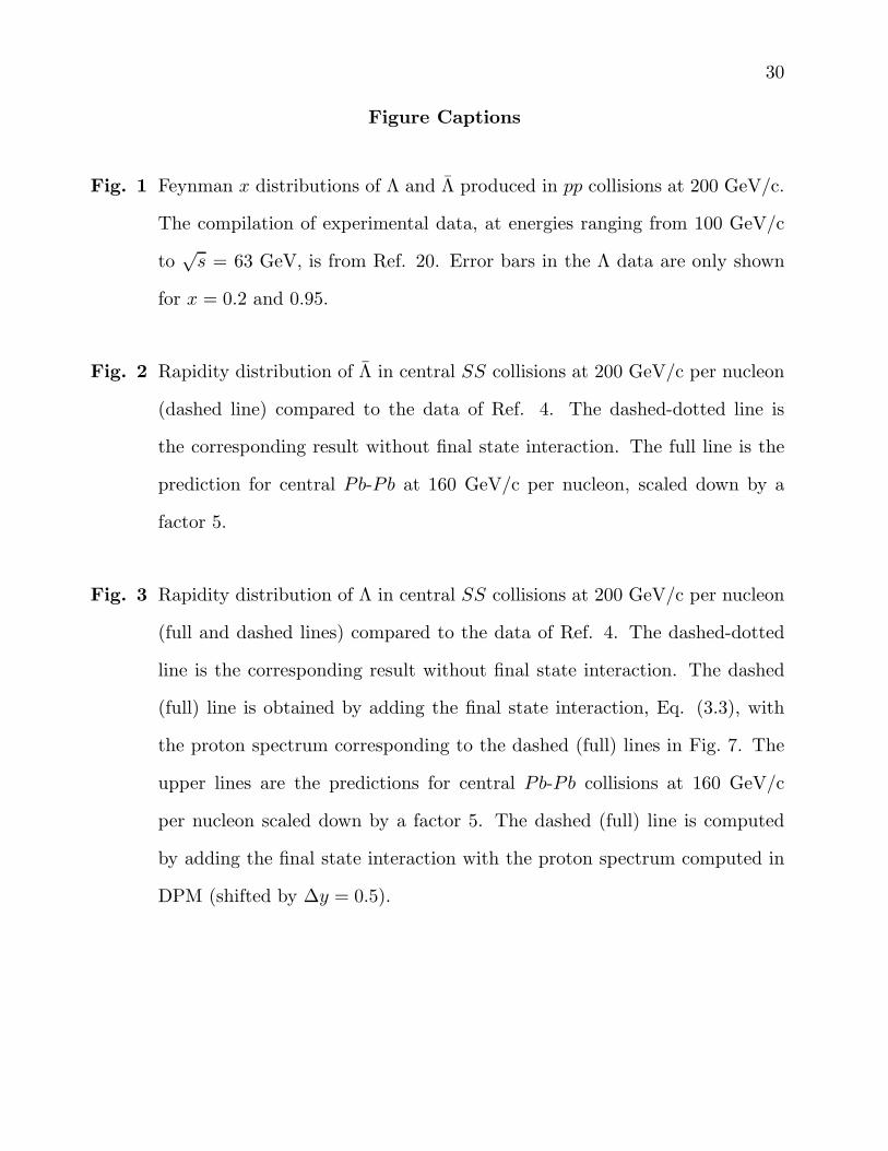
Figure Captions

Fig. 1 Feynman x distributions of Λ and Λ produced in pp collisions at 200 GeV/c.

The compilation of experimental data, at energies ranging from 100 GeV/c

to√s = 63 GeV, is from Ref. 20. Error bars in the Λ data are only shown

for x = 0.2 and 0.95.

Fig. 2 Rapidity distribution of Λ in central SS collisions at 200 GeV/c per nucleon

(dashed line) compared to the data of Ref. 4. The dashed-dotted line is

the corresponding result without final state interaction. The full line is the

prediction for central Pb-Pb at 160 GeV/c per nucleon, scaled down by a

factor 5.

Fig. 3 Rapidity distribution of Λ in central SS collisions at 200 GeV/c per nucleon

(full and dashed lines) compared to the data of Ref. 4. The dashed-dotted

line is the corresponding result without final state interaction. The dashed

(full) line is obtained by adding the final state interaction, Eq. (3.3), with

the proton spectrum corresponding to the dashed (full) lines in Fig. 7. The

upper lines are the predictions for central Pb-Pb collisions at 160 GeV/c

per nucleon scaled down by a factor 5. The dashed (full) line is computed

by adding the final state interaction with the proton spectrum computed in

DPM (shifted by ∆y = 0.5).

31

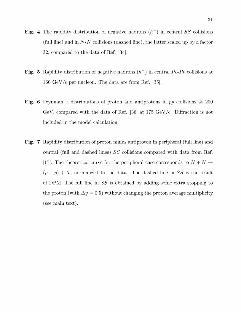
Fig. 4 The rapidity distribution of negative hadrons (h−) in central SS collisions

(full line) and in N -N collisions (dashed line), the latter scaled up by a factor

32, compared to the data of Ref. [34].

Fig. 5 Rapidity distribution of negative hadrons (h−) in central Pb-Pb collisions at

160 GeV/c per nucleon. The data are from Ref. [35].

Fig. 6 Feynman x distributions of proton and antiprotons in pp collisions at 200

GeV, compared with the data of Ref. [36] at 175 GeV/c. Diffraction is not

included in the model calculation.

Fig. 7 Rapidity distribution of proton minus antiproton in peripheral (full line) and

central (full and dashed lines) SS collisions compared with data from Ref.

[17]. The theoretical curve for the peripheral case corresponds to N +N →

(p − p) + X, normalized to the data. The dashed line in SS is the result

of DPM. The full line in SS is obtained by adding some extra stopping to

the proton (with ∆y = 0.5) without changing the proton average multiplicity

(see main text).

32

NN NN SS SS SS Pb-Pb Pb-Pb

experiment [6] DPM DPM + f.s.i experiment [4] DPM DPM + f.s.i.

h

�

3.29 3.22 � 0.06 95 98 � 3 798

�

�

3.06 3.06 � 0.08 88 91 � 3 742

K

�

0.17 0.17 � 0.05 7.0 7.4 6.9 � 0.4 72 76.

K

+

0.24 0.24 � 0.05 8.4 11.2 (10.6) 12.4 � 0.4 80 127.5 (120.0)

K

s

0

0.20 0.20 � 0.02 7.6 9.2 (8.9) 10.5 � 1.7 75 101 (97.)

p 0.97 0.99 � 0.15 24 19.5 (20.6) | 194

�

118 (130)

�p 0.05 0.05 � 0.02 2.3 1.7 | 30 23

� 0.12 0.096 � 0.010 3.7 9.3 (8.0) 9.4 � 1 36 131 (116)

�

� 0.014 0.013 � 0.004 1.3 2.1 2.2 � 0.4 18 27

Table 1

33

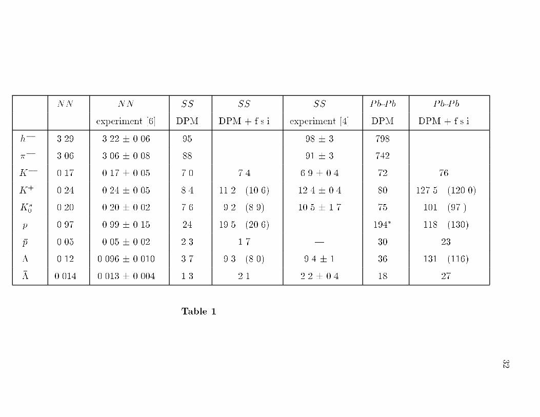
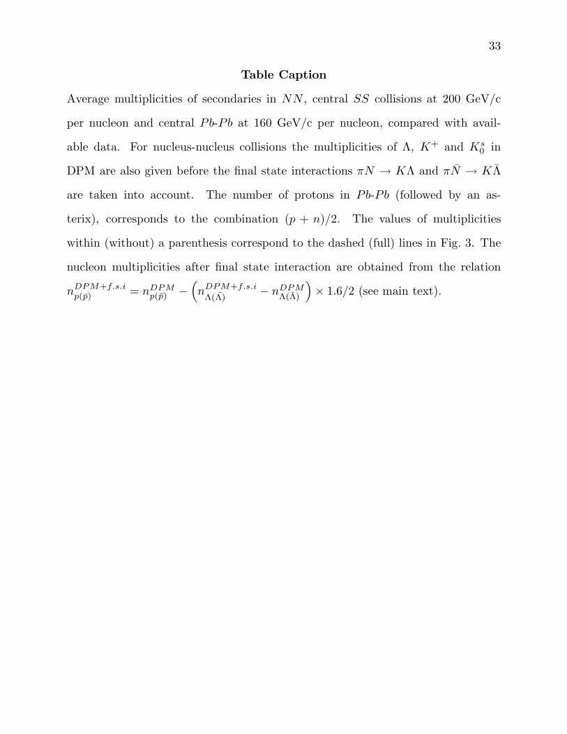
Table Caption

Average multiplicities of secondaries in NN , central SS collisions at 200 GeV/c

per nucleon and central Pb-Pb at 160 GeV/c per nucleon, compared with avail-

able data. For nucleus-nucleus collisions the multiplicities of Λ, K+ and Ks0 in

DPM are also given before the final state interactions πN → KΛ and πN → KΛ

are taken into account. The number of protons in Pb-Pb (followed by an as-

terix), corresponds to the combination (p + n)/2. The values of multiplicities

within (without) a parenthesis correspond to the dashed (full) lines in Fig. 3. The

nucleon multiplicities after final state interaction are obtained from the relation

nDPM+f.s.ip(p) = nDPM

p(p) −(

nDPM+f.s.i

Λ(Λ)− nDPM

Λ(Λ)

)

× 1.6/2 (see main text).

34

0. .1 .2 .3 .4 .5 .6 .7 .8 .9 1.10

-3

10-2

10-1

10+0

(x/π)dσ/dx

|x|

Fig. 1

35

-3. -2. -1. 0. 1. 2. 3.0.

0.5

1.

1.5

2.

2.5

3.

dN/dy

ycm

Pb-Pb/5

Fig. 2

36

-3. -2. -1. 0. 1. 2. 3.0.

1.

2.

3.

4.

5.

6.

7.

8.

dN/dy

ycm

Pb-Pb/5

Fig. 3

37

-3. -2. -1. 0. 1. 2. 3.0.

20.

40.

60.

dN/dy

Fig. 4

ycm

38

-3. -2. -1. 0. 1. 2. 3.0

50

100

150

200

250

300

350

400

dN/dy

Fig. 5

ycm

39

0. .1 .2 .3 .4 .5 .6 .7 .8 .9 1.

10-2

10-1

10+0

10+1

xdσ/dx

x

Fig. 6

40

-3. -2. -1. 0. 1. 2. 3.0.

2.

4.

6.

8.

10.

dN/dy

Fig. 7

ycm