STRAIN MEASUREMENT OF COMPOSITE MATERIALS USING …

STRAIN MEASUREMENT OF COMPOSITE MATERIALS USING FIBRE OPTIC SENSORS

By

Peter Andrew Caskey Furlong

A thesis submitted to

The Faculty of Graduate Studies and Research

in partial fulfilment of

the degree requirements of

Master of Applied Science in Mechanical Engineering

Ottawa-Carleton Institute for

Mechanical and Aerospace Engineering

Department of Mechanical and Aerospace Engineering

Carleton University

Ottawa, Ontario, Canada

May 2007

© Copyright

2007 - Peter Andrew Caskey Furlong

R eproduced with perm ission of the copyright owner. Further reproduction prohibited without perm ission.

Library and Archives Canada

Bibliotheque et Archives Canada

Published Heritage Branch

395 Wellington Street Ottawa ON K1A 0N4 Canada

Your file Votre reference ISBN: 978-0-494-26987-9 Our file Notre reference ISBN: 978-0-494-26987-9

Direction du Patrimoine de I'edition

395, rue Wellington Ottawa ON K1A 0N4 Canada

NOTICE:The author has granted a nonexclusive license allowing Library and Archives Canada to reproduce, publish, archive, preserve, conserve, communicate to the public by telecommunication or on the Internet, loan, distribute and sell theses worldwide, for commercial or noncommercial purposes, in microform, paper, electronic and/or any other formats.

AVIS:L'auteur a accorde une licence non exclusive permettant a la Bibliotheque et Archives Canada de reproduire, publier, archiver, sauvegarder, conserver, transmettre au public par telecommunication ou par I'lnternet, preter, distribuer et vendre des theses partout dans le monde, a des fins commerciales ou autres, sur support microforme, papier, electronique et/ou autres formats.

The author retains copyright ownership and moral rights in this thesis. Neither the thesis nor substantial extracts from it may be printed or otherwise reproduced without the author's permission.

L'auteur conserve la propriete du droit d'auteur et des droits moraux qui protege cette these.Ni la these ni des extraits substantiels de celle-ci ne doivent etre imprimes ou autrement reproduits sans son autorisation.

In compliance with the Canadian Privacy Act some supporting forms may have been removed from this thesis.

While these forms may be included in the document page count, their removal does not represent any loss of content from the thesis.

Conformement a la loi canadienne sur la protection de la vie privee, quelques formulaires secondaires ont ete enleves de cette these.

Bien que ces formulaires aient inclus dans la pagination, il n'y aura aucun contenu manquant.

i * i

CanadaR eproduced with perm ission of the copyright owner. Further reproduction prohibited without perm ission.

The undersigned recommend to

the Faculty of Graduate Studies and Research

acceptance of the thesis

Strain Measurement of Composite Materials Using Fibre Optic Sensors

Submitted by Peter Andrew Caskey Furlong

in partial fulfilment of the requirements for the degree of

Master of Applied Science in Mechanical Engineering

Dr. Choon-Lai Tan, Thesis Supervisor

Dr. Fred Nitzsche, Thesis Co-Supervisor

Dr. Jonathan Beddoes, Chair, Department of Mechanical and Aerospace Engineering

Carleton University

2007


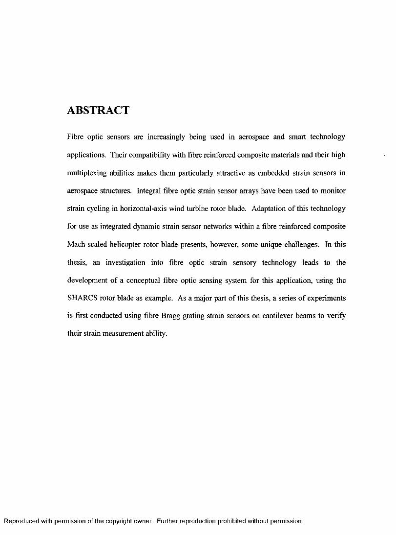
ABSTRACT

Fibre optic sensors are increasingly being used in aerospace and smart technology

applications. Their compatibility with fibre reinforced composite materials and their high

multiplexing abilities makes them particularly attractive as embedded strain sensors in

aerospace structures. Integral fibre optic strain sensor arrays have been used to monitor

strain cycling in horizontal-axis wind turbine rotor blade. Adaptation of this technology

for use as integrated dynamic strain sensor networks within a fibre reinforced composite

Mach scaled helicopter rotor blade presents, however, some unique challenges. In this

thesis, an investigation into fibre optic strain sensory technology leads to the

development of a conceptual fibre optic sensing system for this application, using the

SHARCS rotor blade as example. As a major part of this thesis, a series of experiments

is first conducted using fibre Bragg grating strain sensors on cantilever beams to verify

their strain measurement ability.


I would like to dedicate this thesis to my father.

iv


ACKNOWLEDGEMENTS

I would like express my gratitude to my thesis supervisor, Dr. Tan, for his wisdom,

guidance and patience throughout my entire graduate studies experience. I would also

like to thank Dr. Nitzsche for introducing me to the SHARCS research project. I would

like to thank Dr. Jacques Albert as well for graciously providing me with access to the

necessary optical equipment which enabled me to carry out my experimental

investigations. I wish also to thank Albane Laronch for fabricating and providing me

with sensors, and for helping me to master the art of fusion splicing. Thanks are also due

to Alex Proctor and Kevin Sangster for their guidance and assistance in the machine shop

while fabricating my experimental test apparatus, specimens, and material test coupons. I

thank Calvin Rans for assisting me with the tensile testing of the fibreglass material

coupons. Finally I would like to thank Iain Johnston, Miriam Lyon, and the rest o f the

Carleton Triathlon Club organization for providing me with an essential outlet from my

academic work; it’s been a pleasure training and competing with you during my time

here.

v


TABLE OF CONTENTS

Abstract iii

Acknowledgements v

Table of Contents vi

List of Tables xi

List of Figures xii

Nomenclature xvi

Chapter 1: Introduction 1

Chapter 2: Fibre Optic Strain Sensors 5

2.0 Introduction.................................................................................................................... 5

2.1 Fibre Optic Sensory Technology.................................................................................. 5

2.1.1 Advantages of Fibre Optic Sensors........................................................................6

2.1.2 Fibre Optic Sensory Systems................................................................................. 6

2.1.3 Sources.....................................................................................................................7

2.1.4 Detectors................................................................................................................. 7

2.1.5 Sensor Types........................................................................................................... 8

2.1.6 Fibre Types............................................................................................................. 9

2.1.7 Optical Strain Sensors.............................................................................................9

2.1.8 Fibre Bragg Gratings (FBG) as Strain Sensors................................................... 12

2.2 Review of Basic Fibre Optic Theory.......................................................................... 13

vi


2.2.1 The Nature of Light..............................................................................................14

2.2.2 Electromagnetic Waves...................................................................................... 15

2.2.3 Absorption of Light in Silica Glass.....................................................................15

2.2.4 Guiding Light within the Optical Fibre...............................................................17

2.2.5 Propagation of Guided Light............................................................................... 18

2.3 Bragg Gratings............................................................................................................. 19

2.3.1 How Bragg Gratings are Written into Optical Fibre.......................................... 20

2.3.2 Bragg Wavelength of a Grating...........................................................................21

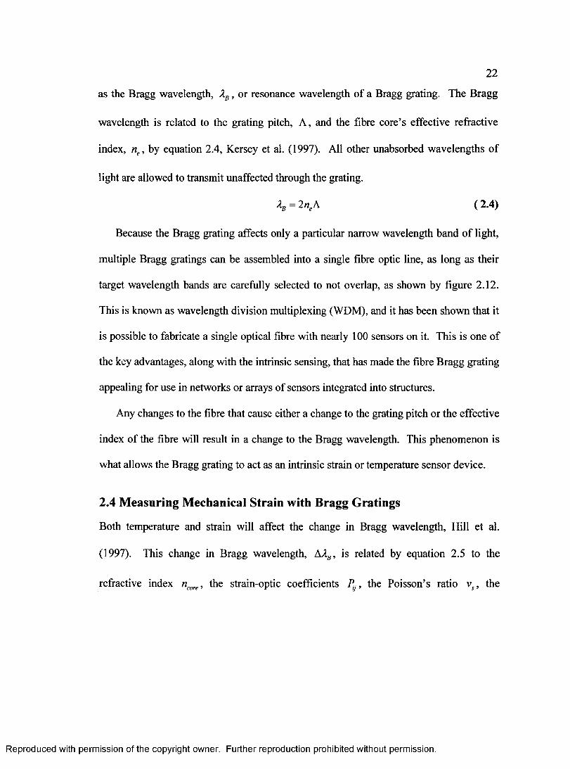
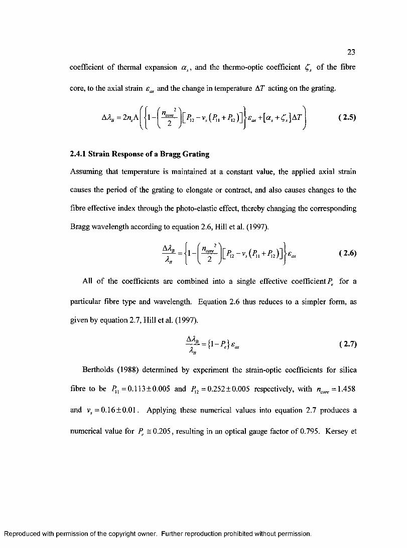
2.4 Measuring Mechanical Strain with Bragg Gratings....................................................22

2.4.1 Strain Response of a Bragg Grating.................................................................... 23

2.4.2 Thermal Response of a Bragg Grating................................................................ 24

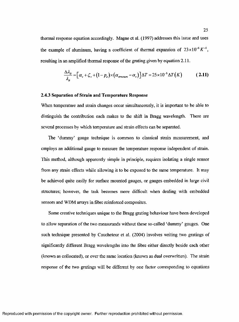
2.4.3 Separation of Strain and Temperature Response................................................25

2.4.4 Non-Uniform Strains and Gradients................................................................... 26

2.4.5 Components of Strain.......................................................................................... 27

2.5 Concluding Remarks....................................................................................................27

Chapter 3: Experimental Setup 36

3.0 Introduction.................................................................................................................. 36

3.1 Equipment Setup and Integration................................................................................36

3.1.1 Optical Equipment................................................................................................37

3.1.2 Electrical Resistance Strain Gauge Equipment...................................................38

3.1.3 Mechanical Equipment........................................................................................ 41

3.2 Specimen Geometry and Constraints..........................................................................42

3.2.1 Aluminum Specimen Geometry and Constraints...............................................42

3.2.2 Fibreglass Specimen Geometry and Constraints................................................43

3.3 Applied Loads..............................................................................................................44

3.3.1 Aluminum Specimen........................................................................................... 46

3.3.2 Fibreglass Specimen............................................................................................ 46

3.4 Material Properties of Specimens...............................................................................47

3.4.1 Aluminum Properties..........................................................................................50vii


3.4.2 Fibreglass Properties..........................................................................................50

3.5 Cantilever Beam Theoretical Solutions..................................................................... 53

3.5.1 Bending of a Hollow Rectangular Cantilever Beam.......................................... 53

3.5.2 Torsion of a Thin-Walled Hollow Rectangular Section.................................... 54

3.5.3 Mohr’s Circle of Strains....................................................................................... 55

3.6 Strain Gauge Rosette Measurements..........................................................................56

3.6.1 Installation of Electrical Resistance Gauges.......................................................58



3.7 Concluding Remarks................................................................................................... 61

Chapter 4: FBG Sensor Testing and Results 88

4.0 Introduction.................................................................................................................. 88

4.1 Sensor Installation........................................................................................................88

4.2 Sensor Properties and Optical Signals....................................................................... 92

4.3 Collection and Processing of Optical Signal Data.....................................................93

4.4 Sensor Experimental Results...................................................................................... 95



4.5 Discussion of Results and Errors................................................................................99

4.5.1 Data Collection and Processing...........................................................................99

4.5.2 Thermal Effects...................................................................................................100

4.5.3 Position and Alignment...................................................................................... 100

4.5.4 Summary of Experimental Errors......................................................................101

4.6 Transverse Sensitivity of FBG Sensors....................................................................102

4.6.1 Transverse Sensitivity Behaviour Observed in Experimental Results 104

4.6.2 Transverse Sensitivity of Embedded Sensors in a Laminate............................ 107

4.7 Applying FBG Sensors to Thin Shell Laminates................................................... 111

4.8 Concluding Remarks..................................................................................................112

viii


Chapter 5: A Proposed FBG Sensor System for SHARCS 132

5.0 Introduction...............................................................................................................132

5.1 System Design Objectives and Basic Requirements............................................. 133

5.1.1 Measurement Range........................................................................................... 134

5.1.2 Measurement Speed........................................................................................... 136

5.1.3 Measurement Resolution................................................................................... 137

5.1.4 Structural Geometry............................................................................................137

5.1.5 Weight Restriction..............................................................................................138

5.1.6 Structural Intrusiveness...................................................................................... 138

5.1.7 Summary of Design Requirements................................................................... 138

5.2 Sensor Network.........................................................................................................139

5.2.1 Dynamic Strain Monitoring Sensors................................................................. 139

5.2.2 Vibration Monitoring Sensors............................................................................140

5.2.3 Structural Health Monitoring Sensors.............................................................. 141

5.2.4 Combining all Sensors into a Single Network..................................................142

5.3 Structural Integration............................................................................................... 143

5.3.1 Sensor Failure.....................................................................................................143

5.3.2 Host Failure......................................................................................................... 144

5.3.3 Routing of Optical Fibre in the SHARCS Rotor..............................................145

5.4 Data Acquisition.......................................................................................................148

5.4.1 Transmitting and Receiving Optical Signals....................................................148

5.4.2 Optical Circuit Components.............................................................................. 149

5.4.3 SHARCS Sensory System Concept...................................................................152

5.5 System Calibration................................................................................................... 154

5.5.1 Sensor Transverse Sensitivity............................................................................155

5.5.2 Wavelength Dependence of Fused Couplers/Splitters......................................155

5.5.3 Temperature Response of a LPG.......................................................................156

5.6 Concluding Remarks................................................................................................ 156

Chapter 6: Conclusions 163ix


6.1 Recommendations for Future Work 164

x


LIST OF TABLES

Table 2.1 Types of fibre optic sensors..................................................................................28

Table 2.2 Typical categories of the electromagnetic spectrum........................................... 28

Table 3.1 Aluminum specimen applied loads.......................................................................62

Table 3.2 Fibreglass specimen applied loads........................................................................62

Table 3.3 Specimen material properties................................................................................63

Table 3.4 Test specimen electrical resistance gauge rosette information...........................63

Table 3.5 Principal strains on the aluminum specimen measured by the top rosette........64

Table 3.6 Principal strains on the aluminum specimen measured by the bottom rosette. 64

Table 3.7 Principal strains on the fibreglass specimen in poor agreement.........................65

Table 3.8 Principal strains on the fibreglass specimen in good agreement........................65

Table 4.1 Typical properties of experimental materials used in FBG experiments 113

Table 4.2 Fibre Bragg grating sensor information..............................................................113

Table 4.3 Sample of raw optical data.................................................................................. 114

Table 4.4 FBG sensor measurements on the aluminum beam...........................................114

Table 4.5 FBG sensor measurements on the fibreglass beam...........................................115

Table 5.1 Lamina material properties used for SHARCS rotor - Mikjaniec (2006)...... 157

Table 5.2 Lamina stiffness matrix coefficients...................................................................157

Table 5.3 Approximate extension stiffness matrices of SHARCS rotor.......................... 158

Table 5.4 Sensitivity coefficients for embedded FBG sensor in lamina........................... 158

xi


LIST OF FIGURES

Figure 1.1 SHARCS rotor blade and sub-systems - Mikjaniec (2006)................................. 4

Figure 1.2 Wind turbine with fibre optic sensors - Schroeder et al. (2006).........................4

Figure 2.1 Typical optical circuit using a tuneable laser source......................................... 29

Figure 2.2 Typical optical circuit using a broadband source.............................................. 29

Figure 2.3 Propagation of an electromagnetic wave............................................................ 30

Figure 2.4 Interaction of light with a substance................................................................... 30

Figure 2.5 Signal attenuation of silica optical fibre - Hecht (2006)................................... 31

Figure 2.6 Reflection, refraction and critical angle for total internal reflection................ 31

Figure 2.7 Typical cross-section of a step-indexed multi-mode silica optical fibre..........32

Figure 2.8 Different acceptable propagation paths of guided rays in an optical fibre 32

Figure 2.9 Modal representation of guided light in an optical fibre................................... 33

Figure 2.10 Phase mask fabrication technique - Hill et al. (1997)..................................... 33

Figure 2.11 Fibre Bragg grating............................................................................................ 34

Figure 2.12 Wavelength division multiplexed array of Bragg grating sensors................ 34

Figure 2.13 Variation of thermo-optic coefficient for silica fibre - Hill et al. (1997).......35

Figure 3.1 Optical interrogation circuit................................................................................66

Figure 3.2 Optical signal sample of a fibre Bragg grating...................................................66

Figure 3.3 Wire grid type electrical resistance strain gauge................................................67

Figure 3.4 Wheatstone bridge circuit.................................................................................... 67

Figure 3.5 Single gauge in quarter bridge configuration.....................................................68

Figure 3.6 Portable strain indicator and switch and balance units...................................... 68

Figure 3.7 Steel support frame...............................................................................................69

Figure 3.8 Steel support plate................................................................................................69

Figure 3.9 Aluminum section: geometric properties........................................................... 70

xii


Figure 3.10 Fibreglass section: geometric properties..........................................................70

Figure 3.11 Fibreglass beam: fixtures and constraints.........................................................71

Figure 3.12 Resolving applied loads.....................................................................................71

Figure 3.13 Material test coupon geometry of the fibreglass used..................................... 72

Figure 3.14 Axial stress versus axial strain plot for fibreglass test coupon........................72

Figure 3.15 Strain coordinate transformation relationship and Mohr’s circle....................73

Figure 3.16 Principal strain orientation and Mohr’s circle..................................................73

Figure 3.17 Typical electrical resistance strain gauge rosette configurations................... 74

Figure 3.18 Construction of Mohr's circle using a rectangular strain gauge rosette 74

Figure 3.19 Bending strains measured by the top rosette for upright aluminum beam.... 75

Figure 3.20 Combined bending and torsion strains measured by the top rosette for upright

aluminum beam...................................................................................................................... 75

Figure 3.21 Principal angles measured by the top rosette for upright aluminum beam ... 76

Figure 3.22 Bending strains measured by the top rosette for inverted aluminum beam .. 76

Figure 3.23 Combined bending and torsion strains measured by the top rosette for

inverted aluminum beam........................................................................................................77

Figure 3.24 Principal angles measured by the top rosette for inverted aluminum beam.. 77

Figure 3.25 Bending strains measured by the bottom rosette for upright aluminum beam

................................................................................................................................................. 78

Figure 3.26 Combined bending and torsion strains measured by the bottom rosette for

upright aluminum beam.........................................................................................................78

Figure 3.27 Principal angles measured by the bottom rosette for upright aluminum beam

................................................................................................................................................. 79

Figure 3.28 Bending strains measured by the bottom rosette for inverted aluminum beam

................................................................................................................................................. 79

Figure 3.29 Combined bending and torsion strains measured by the bottom rosette for

inverted aluminum beam........................................................................................................80

Figure 3.30 Principal angles measured by the bottom rosette for inverted aluminum beam

80

xiii


Figure 3.31 Bending strains in poor agreement for upright fibreglass beam......................81

Figure 3.32 Combined bending and torsion strains in poor agreement for upright

fibreglass beam ...................................................................................................................... 81

Figure 3.33 a = 0 degree direction axial strains in poor agreement for fibreglass beam.. 82

Figure 3.34 a = 45 degree direction axial strains in poor agreement for fibreglass beam 82

Figure 3.35 a = 90 degree direction axial strains in poor agreement for fibreglass beam 83

Figure 3.36 a = 0 degree direction axial strains in good agreement for fibreglass beam. 83

Figure 3.37 a = 45 degree direction axial strains in good agreement for fibreglass beam84

Figure 3.38 a = 90 degree direction axial strains in good agreement for fibreglass beam 84

Figure 3.39 Bending strains in good agreement for upright fibreglass beam.....................85

Figure 3.40 Combined bending and torsion strains in good agreement for upright

fibreglass beam...................................................................................................................... 85

Figure 3.41 Principal angles in good agreement for upright fibreglass beam....................86

Figure 3.42 Bending strains in good agreement for inverted fibreglass beam ...................86

Figure 3.43 Combined bending and torsion strains in good agreement for inverted

fibreglass beam ...................................................................................................................... 87

Figure 3.44 Principal angles in good agreement for inverted fibreglass beam...................87

Figure 4.1 Installation of a FBG using different adhesives............................................... 116

Figure 4.2 Optical signal change of tilted FBG #1 during installation............................. 116

Figure 4.3 Optical signal of FBG #1 after installation....................................................... 117







Figure 4.10 Optical signal of FBG #8 after installation.................................................... 120

Figure 4.11 FBG reflection signals aligned using maximum insertion loss..................... 121

Figure 4.12 FBG reflection signals aligned using centre wavelength.............................. 121

xiv


Figure 4.13 Shift of FBG #4 optical signal due to applied strain......................................122

Figure 4.14 Error in FBG strain readings due to thermal sensitivity................................ 122

Figure 4.15 Bending results for axial strain on FBG #1.................................................... 123

Figure 4.16 Combined bending and torsion results for axial strain on FBG # 1 ...............123


Figure 4.18 Combined bending and torsion results for axial strain on FBG #2 ...............124




Figure 4.22 Combined bending and torsion results for axial strain on FBG # 4 .............. 126








Figure 4.30 Combined bending and torsion results for axial strain on FBG #8 ...............130

Figure 4.31 Transverse stresses acting on the FBG sensors due to adhesive...................131

Figure 4.32 FBG sensors embedded in a unidirectional laminate, Fan et al. (2004)..... 131

Figure 5.1 Laminate lay-up for the root of SHARCS rotor - Mikjaniec (2006)............ 159

Figure 5.2 Laminate lay-up for the blade of SHARCS rotor - Mikjaniec (2006)........... 159

Figure 5.3 Sensor placement and optical fibre routing for SHARCS rotor......................160

Figure 5.4 Long period grating transmission signal - Bhatia (1999).............................. 161

Figure 5.5 Basic LPG interrogation circuit for a FBG sensor...........................................161

Figure 5.6 Conceptual data acquisition system for SHARCS...........................................162

xv


NOMENCLATURE

b,, b0 width of the interior and outer walls of the cross-section

c speed of light in a vacuum

ht, hg height of the interior and outer walls of the cross-section

kopl transverse sensitivity coefficient

kEl coefficient relating the elastic influence of a lamina on a sensor

lk length of the kth lamina

ne effective refractive index of the fibre core

nt refractive index of the i th medium

rbend bending radius of an optical fibre

rLE radius of the leading edge of a rotor blade cross-section

tk thickness of the kth lamina

t thickness of the top surface wall of the beam

v( speed of light in the / th medium

x position in the x axis direction

ya , y, position on the outer and interior surfaces in the y axis direction

z position in the z axis direction

xvi


Axy area of the cross-section in the x - y plane

AU,AU, A22 coefficients of the laminate extension stiffness matrix

CW centre wavelength of an optical signal

Et Young’s modulus for the i th direction

F axial applied axial force on cross-section of rotor

Fa , Ft axial and transverse strain sensitivity factors

Fapt FBG gauge factor coefficient

Gj shear modulus‘ij’

Ix second moment of area of cross-section about the x axis

Kul, K23l coefficients relating the direct strains of a lamina in plane stress

L length

M x, Tz moment about the x axis and torque about the z axis

Pi force applied in the i th direction

Pj strain-optic coefficients of the fibre core

Pe effective strain-optic coefficient of the fibre core

R radius

AR change in electrical resistance

AT change in temperature

matrix regarding transfer of strain from the adhesive to the FBG

AV change in voltage across Wheatstone bridge

xvii


coefficient of thermal expansion of the sensor fibre core

£ n relative permittivity of the / th medium

£u strain component ‘ij’

4 apparent strain component ‘ij’

4 Bragg resonance wavelength

AAg change in Bragg resonance wavelength

Ar ,A l wavelengths at threshold value of an optical signal

M n relative permeability of the i th medium

Vf ’ Vs Poisson’s ratio of the optical fibre

o, angular orientation ‘i’

p̂ath angle of the lamina or optical fibre path to the rotor blade axis

^ U ^ T0 direct and shear stress components ‘ij’

C thermo-optic coefficient of the sensor fibre core

A grating pitch or spacing

ACRONYMS

CLLIPS Carleton Laboratory for Laser Induced Photonic Structures

FBG Fibre Bragg Grating

FORJ Fibre Optic Rotary Joint

LED Light Emitting Diode

xviii


LPG Long Period Grating

OTF Optical Tuneable Filter

PD Photo-Diode

SHARCS Smart Hybrid Active Rotor Control System

SLD Super Luminescent Diode

WDC Wavelength Dependant Coupler


CHAPTER 1: INTRODUCTION

Fibre optic sensors are finding increasingly more applications in aerospace and smart

technology applications, from structural health monitoring to pressure, strain and

temperature measurements. Their ability to be highly multiplexed into sensor arrays and

their compatibility with fibre reinforced composite materials makes them highly

attractive to experimental researchers as embedded sensors in aerospace structures.

An active area of research in the Department of Mechanical and Aerospace

Engineering at Carleton University is the application of smart technology systems to

controlling helicopter rotor blade structural dynamics. The Smart Hybrid Active Rotor

Control System (SHARCS) was developed in order to simultaneously reduce vibration

and noise by actively controlling three integrated smart sub-systems in a single rotor

blade. The three smart sub-systems which make up SHARCS are the smart-spring, the

anhedral tip and the trailing edge flap, as shown in figure 1.1.

One step in the development of SHARCS is experimental wind tunnel testing of its

sub-systems using a one meter long fibre reinforced composite Mach scaled rotor blade,

the preliminary design of which was carried out by Mikjaniec (2006); it is hereby referred

to as the SHARCS rotor blade. The performance of SHARCS can be evaluated by

dynamically monitoring the structural deformation and vibration behaviour of the rotor


2

blade during wind tunnel testing. To this end, it is proposed that a distributed network of

fibre optic strain sensors, embedded within its fibre reinforced composite structure be

employed, thereby allowing simultaneous monitoring of the real-time strains at multiple

locations. Systems have been developed for real-time load monitoring of horizontal-axis

wind-turbine rotor blades, such as the system presented by Schroeder et al. (2006) for the

wind-turbine shown in figure 1.2. This system collects the strain amplitude history of the

rotor blade, which is useful in assessment of its fatigue life and continuing evaluation of

its structural integrity. To adapt a similar fibre optic sensing system for use in a Mach

scaled helicopter rotor blade, with the additional sensing ability to measure dynamic

vibration amplitudes, presents a number of challenges. The rotor blade geometry is

smaller, requiring a more compact system; its rotational speed is higher, requiring a faster

data acquisition speed; its structure is more fragile, requiring a less intrusive sensor

network; and the strain amplitudes associated with structural vibrations are significantly

smaller in magnitude, requiring a more sensitive strain sensor.

The objective of this thesis is to investigate the feasibility of using fiber optic sensory

technology specifically for use in the SHARCS rotor blade sensing application. The

organization of this thesis will be as follows. The next Chapter will present a literature

review of fibre optic strain sensor technology and devices, in which the most appropriate

sensors for SHARCS are selected; the theoretical relationship which enables them to

measure strain is also presented. Chapter 3 will present an experimental apparatus which

will be used for testing the fibre optic strain sensors, which consists of two cantilever test

specimens that are calibrated by use of conventional electrical resistance gauges. Chapter


4 presents the experimental test results of the fibre optic strain sensors, and examines the

agreement of the experimental measurements with the theoretical optical behaviour of the

sensors. Chapter 5 presents an overview of the fibre optic strain sensing system design

requirements based on the SHARCS rotor blade preliminary design. The associated

challenges are discussed and a conceptual system capable of meeting the requirements is

presented. The final conclusions from this work and recommendations for future work

are then presented in Chapter 6.


4

Trailing Edge Flap Andhedral Tip

Smart Spring

Figure 1.1 SHARCS rotor blade and sub-systems - Mikjaniec (2006)

Figure 1.2 Wind turbine with fibre optic sensors - Schroeder et al. (2006)


5

CHAPTER 2. FIBRE OPTIC STRAIN SENSORS

2.0 Introduction

A “fibre optic strain sensor” is a device which employs the use of fibre optics to measure

mechanical strain. It is a part of a much larger family of “fibre optic sensors” of which

there are many device types and measurands. This Chapter provides a brief background

on fibre optic sensory technology, with particular focus on strain measurement devices.

The focus is further concentrated on some of the research work that has been done on the

development of fibre Bragg gratings as strain sensors. To this end, a basic review of fibre

optic theory is also provided in this Chapter to serve as background for understanding

how fibre Bragg gratings work.

2.1 Fibre Optic Sensory Technology

Fibre optic sensory technology is still in its adolescence; it has emerged out of the fibre

optic revolution that occurred in the telecommunications industry through the 1970s and

1980s. The tremendous consumer demand in telecommunications has since continued to

drive the development of fibre optic technology at an incredible rate. Udd (1991) has

shown that this high-paced development has led to a drastic reduction in the cost

associated with fibre optic equipment, a significant increase in component quality,


6

variety, and availability. All of these factors combined show an exceptional market trend

for fibre optics to strongly set foot in the sensory industry.

2.1.1 Advantages of Fibre Optic Sensors

Udd (1991) describes many of the advantages associated with fibre optic sensors over

conventional methods. They include their immunity to electromagnetic interference,

high-temperature performance, vibration and shock resistance, chemical resistance,

compact size, light weight, high sensitivity, high accuracy, high speed potential, low

signal loss over large distances, and ability to be highly multiplexed into large networks.

For these and other reasons, it is believed that fibre optic sensors show great potential for

replacing the majority of environmental sensory equipment in use; in some cases, they

even show potential for creation of new sensors that could produce such quality of

measurement that other sensory devices simply could not compare.

2.1.2 Fibre Optic Sensory Systems

A typical fibre optic sensory system consists of four major elements; the source, the

optical fibre, the sensor, and the detector. The combination of these elements can vary

significantly depending on the desired accuracy of measurement, and the required speed

of data acquisition. The most noticeable difference between systems is the type of source

used, and typically falls into one of two categories; a tuneable laser source, or a

broadband light source. Gomall (2003) shows the basic optical circuit diagrams for these

two different system styles, as outlined in figures 2.1 and 2.2 respectively.


7

2.1.3 Sources

A tuneable laser source provides a single wavelength of light as the optical input, and can

be ‘tuned’, or swept through a range of wavelengths. A broadband light source simply

provides many wavelengths of light simultaneously and continuously as the optical input.

It relies entirely on the optical spectrum analyzer for determining both power and

wavelength of the optical sensor output signals. Tuneable laser sources are typically

more expensive and bulky, but provide higher measurement accuracy, and are thus more

suited to laboratory testing and characterization of the optical sensor devices through

controlled experiments. Broadband light sources are more compact and rugged, and thus

offer a more portable system for doing field measurements during practical application of

the sensor technology.

2.1.4 Detectors

Tuneable laser sources are typically combined with two detector components; a power

meter and a wavelength measurement feedback device. The feedback device, which

might be packaged directly with the laser source itself, provides improved wavelength

accuracy while sweeping. The power of the output signal is measured by a power meter,

independent of wavelength, making for a fairly simple detection system.

Broadband light sources are typically combined with optical spectrum analyzers,

which according to Agilent Technologies (1996), typically fall into one of three

categories, namely diffraction-grating-based, Fabry-Perot interferometer-based or

Michelson interferometer-based. Of these three, Gomall (2003) claims the Michelson


8

interferometer-based analyzers usually offer the highest accuracy of wavelength

measurement.

Alternative spectrum analysis techniques are continuously being sought and

developed for specific sensing applications. These alternatives would provide cheaper,

more compact, higher speed, more accurate, or simpler methods for detection, thereby

better meeting the exact needs for data acquisition of the system. Examples of such

systems are (a) the one suggested by Kang et al. (1998), which uses a tilted fibre Bragg

grating mounted on a piezo-ceramic stretching element to act as a tuneable filter for

interrogating another sensor, and (b) the one suggested by Simpson et al. (2004), which

uses a low-cost charge-coupled device linear array to measure the radiation modes exiting

a tilted fibre Bragg grating, allowing for high accuracy interrogation of multiple sensors.

When combined with the already compact nature of broadband light sources and the

sensor devices themselves, these alternatives could lead to affordable optical sensing

systems with the ability to be fully integrated into the sensing environment or structure.

2.1.5 Sensor Types

While the selection of source and detector components is extremely important to

achieving the desired speed and accuracy of the system, it is the sensors themselves that

must be most carefully selected to match the desired measurands. Table 2.1 lists a

variety of sensor types and some of the measurands that Udd (1991) associates with each.

Optical sensors can be classified as either extrinsic or intrinsic. For the extrinsic type,

the sensing takes place outside of the fibre, which is used solely as a conduit to transport

light signals to and from the sensor device. For the intrinsic sensors, also known as all-


9

fibre sensors, the sensing takes place within the fibre itself. Intrinsic sensors have created

a large wake of research because of their simple all-fibre design, allowing them to be

easily combined with fibre reinforced composite structures.

2.1.6 Fibre Types

Intrinsic sensors can be created in a large variety of optical fibre materials and types. The

most commonly used optical material is silica glass fibre because of its abundant use in

telecommunications applications. It typically has additives, known as dopants, such as

germanium to enhance the optical properties of the base silica fibre. Silica fibre is

commercially available in many varieties, such as single-mode, multi-mode, step or

graded index profiles, high birefringence or polarization preserving. The most commonly

used varieties are the step-index multi-mode and step-index single-mode. There are other

more exotic optical materials that have been researched for sensor use, for example, Xiao

et al. (2003), and Grobnic et al. (2004) suggest the use of single-crystal sapphire devices

for taking strain measurements under high temperature conditions where the doped silica-

based sensors cannot maintain consistent optical properties.

2.1.7 Optical Strain Sensors

Civil engineers have applied fibre optic strain sensors to large concrete structures like

buildings, bridges and some roadways for monitoring deflections, strains, and thermal

expansion for some time, Gomall et al. (2003). Many of these devices offered several

advantages; they include the ability of the optical fibres to be highly multiplexed, and be

distributed easily over large distances with low signal loss. An example of the type of


10

instrument designed for civil engineering applications is an extensometer that uses an

internal fibre Bragg grating as a strain measurement device.

The large scale of civil structures has allowed embedment of fibre optic cable and

sensors with minimal intrusiveness and negligible effects on the overall integrity and

behaviour of the structure. However, the same may not be true for use in smaller and

thinner composite structures that are typical of the aerospace and many mechanical

engineering applications. The embedment of the optical fibre and sensing devices can

have a significant effect on the behaviour of the final structure. For intrinsic devices, it

would only be necessary to determine the effects of embedding the optical fibre into a

composite structure, thereby reducing the complexity of the problem to modeling a

simple continuous fibre as an inclusion.

Some work has been done by mechanical and aerospace engineers to address the

mechanical performance of composite structures with these embedded all-fibre sensors.

Eaton et al. (1995) examined by using finite element analysis the induced stress and

strain concentrations in both the optical fibre, and the surrounding composite laminate

structure due to embedment at several relative fibre orientations. Surgeon et al. (2001)

performed some experimental work that examined the influence of an embedded optical

fibre on fatigue damage progress in carbon fibre reinforced polymers. Skontorp (2002)

investigated the embedment of optical fibre at structural details with inherent stress

concentrations, and concluded that the presence of the optical fibre, when oriented in the

primary direction of the laminate’s fibre, did not significantly affect the structural

integrity of the laminate, or initiate its failure. Shivakumar et al. (2004) investigated


11

experimentally the failure modes and effects of composite laminate coupons with an

embedded optical fibre at different orientations. Later, Shivakumar et al. (2005) used

finite element models of the same test coupons to predict the stress concentrations, and

the failure of those specimens due to the inclusion of the optical fibre. This work

continues in parallel to the development and refinement of the intrinsic strain sensors

themselves.

Of the intrinsic fibre optic strain sensors listed in Table 2.1, there are three of

particular interest; the Brillouin scattering, the interferometric type, and the fibre Bragg

grating type sensors. The Brillouin scattering sensors are distributed sensors that take

advantage of Rayleigh scattering, and time domain refractometry to create a fully

distributed sensor over the length of the fibre, capable of measuring strain and

temperature. Alahbabi et al. (2004), have shown development of this sensor technology

to distributed sensing over distances of 6.3 km, with spatial resolution near 1.3m, strain

resolution of 80 micro-strain, and temperature resolution of 3 degrees centigrade. These

sensors show tremendous potential for distributed sensing, but currently do not present

sufficient resolution when compared to the interferometric and fibre Bragg grating point

strain sensors. Although many of the interferometric strain sensors are capable o f being

intrinsically designed, Udd (1991) suggests that most are typically applied in an extrinsic

form; thereby making them less suitable for integration into a fibre reinforced composite

structure. It is for these reasons the fibre Bragg grating was selected as the optical strain

sensor device with the greatest current ability for taking multiple high resolution point


12

strain measurements within a composite aerospace structure, such as a helicopter rotor

blade.

2.1.8 Fibre Bragg Gratings (FBG) as Strain Sensors

Much research has been done on the difficulties and applications of fibre Bragg gratings

as strain sensors to the mechanical and aerospace sectors. Friebele et al. (1999) have

presented an overview of the challenges and current solutions for embedding fibre Bragg

grating sensors into spacecraft structures; tackling issues from composite fabrication

techniques, ingress and egress of optical fibre, suitable source and spectral analysis

components, to meeting qualification requirements for space flight.

Some research has focused on the coatings of these optical sensors. Pak (1992)

examined the longitudinal shear transfer for an embedded sensor in composite materials,

and concluded that a bare fibre (uncoated) would present better shear transfer than a

coated fibre, unless the coating was stiffer than the core material. Uncoated optical fibre

is quite fragile, and work has been done by Hadjiprocopiou et al. (1996) to optimize

suitable coatings for these sensors and at the same time minimize stress concentration

effects in the structure in which they are embedded. Coated optical fibre behaves more

predictably when guiding light because the exact refractive index of the material

surrounding the core is known. A bare fibre, when mounted, is surrounded by the epoxy,

or the matrix material, which might have an unknown refractive index, or one that is

inconsistent. According to Green et al. (2000), these coatings will affect both the local

stress concentration of the fibre in the host material, and the strain measurement

accuracy. Because of the fragile nature of bare optical fibre, ingress and egress methods


13

have been developed by Kang et al. (2000) to protect the fibre from fracture at these

points when dealing with sensors embedded in composite structures.

The foundation for using fibre Bragg gratings as strain sensors was laid by Bertholds

et al. (1988) with the determination of the individual strain-optic coefficients for optical

fibre. Since then, many researchers have applied these values in order to predict the

behaviour of Bragg gratings under various strain conditions, and apply them to various

engineering situations. Tian and Tao (2001) successfully showed by experiment the

application of fibre Bragg gratings to determining torsional deformation of cylindrical

shafts. Kim et al. (2004) successfully showed experimentally a method for determining

the deflected shape of a simple beam model employing multiple fibre Bragg grating

strain sensors.

2.2 Review of Basic Fibre Optic Theory

In what follows below in this Chapter, a brief review of the basics of fibre optic theory is

given. Some insight into how fibre Bragg gratings function as intrinsic mechanical strain

sensor devices for the body to which they are mounted or embedded will also be

provided. “Fibre optic” generally refers to the guided transmission of light through a

transparent fibre material. To understand how this fibre is able to guide light, it is

essential to understand the fundamentals of “optics”, the branch of physics that describes

the behaviour and properties of light.


14

2.2.1 The Nature of Light

There has been much debate throughout history over the exact nature of light, and to this

day it is still not fully understood. Light was originally thought to be composed of

particles, however in the 1800’s Thomas Young showed through his famous double-slit

experiments that light definitely exhibited wave characteristics. Further research led

James Maxwell to the conclusion that light was in fact a component of the

electromagnetic wave spectrum. This theory held until the 1900’s when light interaction

with materials known as semi-conductors could not be explained by the electromagnetic

wave theory. This interaction, known as the photoelectric effect, was unexplained until

the emergence of quantum physics. In quantum physics, energy is given a particle form,

known as quanta, and when specifically dealing with light energy, these particles are

referred to as photons. With quantum physics, much of the debate between the particle

and wave nature of light has since been reconciled, Ghatak (1998).

When dealing with the propagation of light through any medium, it is treated as a

continuum, and thus the electromagnetic (EM) wave theory is applied. The quantum

physics theory is more useful when dealing with sources and detectors of light, which

involves the interaction of photons with semiconductors, NEETS (2006). Since any fibre

optic sensing system involves sources of light, propagation of light through a fibre optic

medium, and the detection of light, both theories would need to be examined in order to

formulate a complete understanding of the system. However, the scope will be limited to

presenting EM wave theory only since it is critical to understanding how Bragg gratings

function.


15

2.2.2 Electromagnetic Waves

All electromagnetic waves have perpendicular electric and magnetic fields that oscillate

in phase with each other and are also perpendicular to the direction of the wave

propagation, as shown in figure 2.3. “Light” commonly refers to the visible, infra-red

(IR) and ultra-violet (UV) wavelengths of the electromagnetic wave spectrum. Table 2.2

shows some of the common wavelength-divided categories of electromagnetic wave

spectrum.

When light encounters a substance, it is reflected, refracted, absorbed or transmitted

as shown in figure 2.4. It is convenient when dealing with these interactions to think of

the propagating light wave as a “ray”, or simply a straight line that is travelling along the

axis of the wave’s propagation as previously shown in figure 2.3. Light rays that are not

refracted, transmitted, or reflected when they encounter a substance are absorbed. A

substance through which almost all wavelengths of light can be transmitted is said to be

transparent. There is no known substance that is perfectly transparent to all wavelengths

of light; some wavelengths will always be absorbed. Silica glass is considered to be a

highly transparent substance and thus is used as the core material in the majority of

optical fibre. It is however not transparent to all wavelengths of light, and is thereby

limited to operating within a certain range of the electromagnetic spectrum that is not

absorbed.

2.2.3 Absorption of Light in Silica Glass

The wavelengths of light that are absorbed by silica glass are governed by quantum

physics theory, the chemical makeup of the material and its crystalline atomic structure.


16

A significant portion of the ultraviolet spectrum is absorbed because of its interaction

with electrons, causing them to excite to higher energy states. Similarly, the infra-red

spectrum is absorbed because of its interaction with the vibratory motion of the silicon-

oxygen atomic bonds in the silica glass, NEETS (2006). These are considered intrinsic

absorptions; they are inherent to the basic chemical structure of silica glass and cannot be

avoided. Intrinsic absorption limits the useful spectral range of silica glass fibre between

700nm and 1600nm, NEETS (2006).

Besides these intrinsic absorptions, there are two other mechanisms which cause

signal strength losses, extrinsic absorption and scattering. Extrinsic absorption is caused

by the impurities contained within the silica fibre. The most common impurity is the

hydroxyl ion (-OH), which appears as a result of water being present in the

manufacturing process of the silica fibre, and causes three absorption peaks within the

700nm to 1600nm range. Scattering is caused by light interacting with localised density

fluctuations within the silica fibre; this results in the light being partially redirected in all

directions. It is one of the primary sources of signal loss in silica optical fibre, with

increasing severity towards the ultra-violet range; it is also the basis for Brillouin

scattering distributed sensors.

All these forms of signal loss combined limit the operating spectral window for any

system using silica glass fibre from approximately 700nm to 1600nm, and avoiding the

wavelength bands associated with the hydroxyl absorption as shown by Hecht (2006) in

figure 2.5. After considering absorption of light, and the possibility of scattering, the


17

remainder of light within the spectral operating window should transmit through the silica

fibre with very low loss to the signal strength.

2.2.4 Guiding Light within the Optical Fibre

The transmitted light must now be guided within the silica fibre along the fibre axis

without being lost to the exterior. This is achieved by taking advantage of the refraction

and reflection of light when it encounters a boundary between two media.

When a ray of light travels in a medium other than vacuum, its rate of propagation is

reduced. The ratio of the speed in a vacuum, c , to the speed in the medium, v,, is known

as the refractive index, nt , of the material and is related to the relative permittivity, s ri,

and relative permeability, firi, of the medium according to equation 2.1.

A ray that propagates into a medium with a higher refractive index changes angular

orientation according to equation 2.2, known as Snell’s Law, in order to accommodate

the slower rate of wave propagation in the new medium. A ray traveling in reverse

would go through an exact opposite angular change, following the same path. This re

orientation of the ray is known as refraction, and is depicted in figure 2.6.

A special case can occur when a ray attempts to change into a faster medium at a

large angle. Should the angle be such that according to Snell’s Law the refracted angle

would be 90 degrees, the ray would travel along the boundary of the two media. This is

( 2.1)

«, sin (6\) = n2 sin (92) ( 2.2)


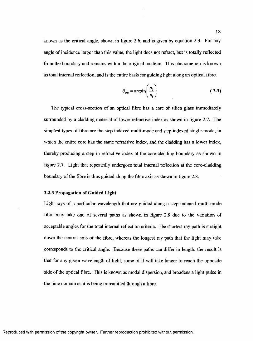
known as the critical angle, shown in figure 2.6, and is given by equation 2.3. For any

angle of incidence larger than this value, the light does not refract, but is totally reflected

as total internal reflection, and is the entire basis for guiding light along an optical fibre.

The typical cross-section of an optical fibre has a core of silica glass immediately

simplest types of fibre are the step indexed multi-mode and step indexed single-mode, in

which the entire core has the same refractive index, and the cladding has a lower index,

thereby producing a step in refractive index at the core-cladding boundary as shown in

figure 2.7. Light that repeatedly undergoes total internal reflection at the core-cladding

boundary of the fibre is thus guided along the fibre axis as shown in figure 2.8.

2.2.5 Propagation of Guided Light

Light rays of a particular wavelength that are guided along a step indexed multi-mode

fibre may take one of several paths as shown in figure 2.8 due to the variation of

acceptable angles for the total internal reflection criteria. The shortest ray path is straight

down the central axis of the fibre, whereas the longest ray path that the light may take

corresponds to the critical angle. Because these paths can differ in length, the result is

that for any given wavelength of light, some of it will take longer to reach the opposite

side of the optical fibre. This is known as modal dispersion, and broadens a light pulse in

the time domain as it is being transmitted through a fibre.

from the boundary and remains within the original medium. This phenomenon is known

arcsm (2.3)

surrounded by a cladding material of lower refractive index as shown in figure 2.7. The


19

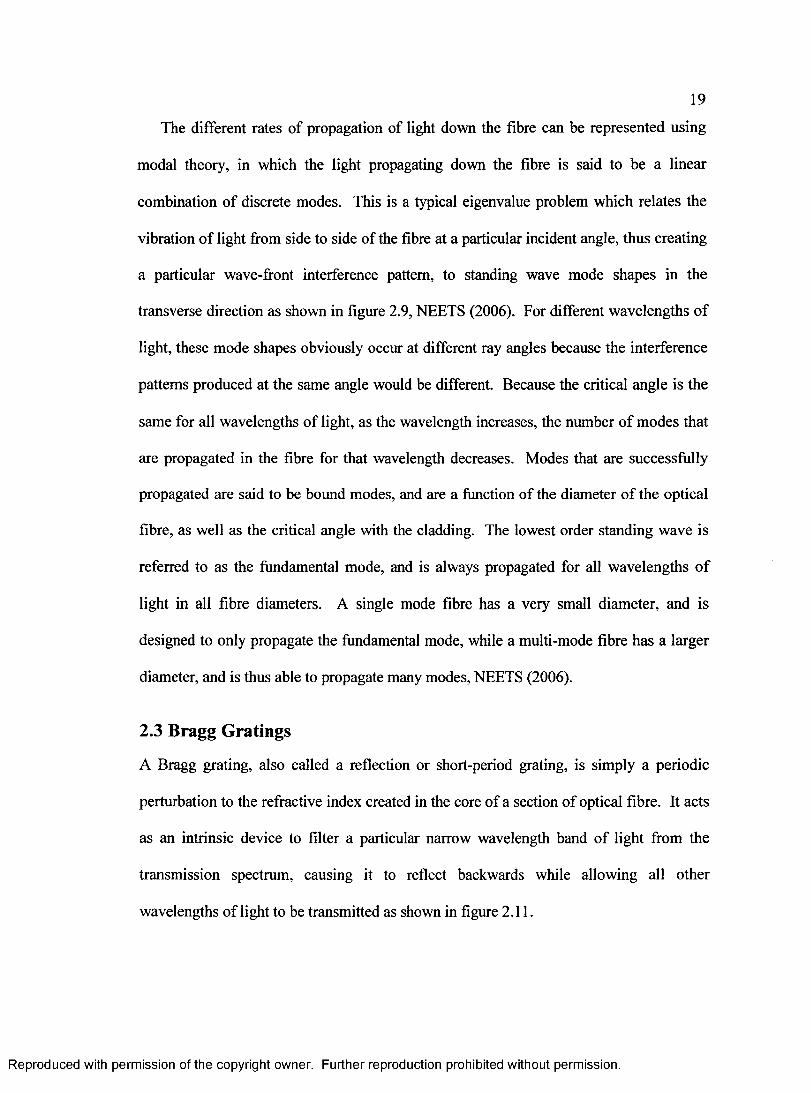
The different rates of propagation of light down the fibre can be represented using

modal theory, in which the light propagating down the fibre is said to be a linear

combination of discrete modes. This is a typical eigenvalue problem which relates the

vibration of light from side to side of the fibre at a particular incident angle, thus creating

a particular wave-front interference pattern, to standing wave mode shapes in the

transverse direction as shown in figure 2.9, NEETS (2006). For different wavelengths of

light, these mode shapes obviously occur at different ray angles because the interference

patterns produced at the same angle would be different. Because the critical angle is the

same for all wavelengths of light, as the wavelength increases, the number of modes that

are propagated in the fibre for that wavelength decreases. Modes that are successfully

propagated are said to be bound modes, and are a function of the diameter of the optical

fibre, as well as the critical angle with the cladding. The lowest order standing wave is

referred to as the fundamental mode, and is always propagated for all wavelengths of

light in all fibre diameters. A single mode fibre has a very small diameter, and is

designed to only propagate the fundamental mode, while a multi-mode fibre has a larger

diameter, and is thus able to propagate many modes, NEETS (2006).

2.3 Bragg Gratings

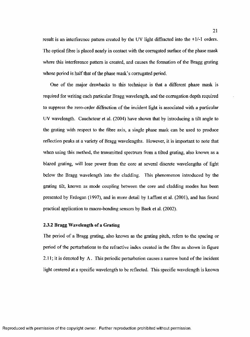
A Bragg grating, also called a reflection or short-period grating, is simply a periodic

perturbation to the refractive index created in the core of a section of optical fibre. It acts

as an intrinsic device to filter a particular narrow wavelength band of light from the

transmission spectrum, causing it to reflect backwards while allowing all other

wavelengths of light to be transmitted as shown in figure 2.11.


20

2.3.1 How Bragg Gratings are Written into Optical Fibre

Bragg gratings are formed by exposing the core of a photosensitive fibre to an intense

optical interference pattern. According to Atkins (1996), this photosensitivity can be

improved for any germano-silicate fibre by using a high temperature hydrogen treatment.

Bragg gratings were first formed in optical fibre by the internal writing technique by

Hill et al. (1978). They found that by creating a strong standing wave pattern of light

within a germania-doped silica fibre, a grating pattern would gradually form along the

full length of the fibre due to the migration of dopant particles within the fibre core. The

formation of these gratings is a diffusion process driven by the interference pattern of

light. When exposed to elevated temperatures, the dopant particles will diffuse out of the

grating pattern into the fibre core. The grating is thus only semi-stable and will naturally

degrade and fade over time. Meltz et al. (1989) showed that by controlling the

intersecting angle of two ultraviolet beams through the side of the fibre, Bragg gratings

could be created to reflect any desired wavelength of light. This method is known as the

transverse holographic method.

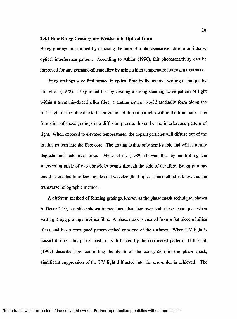
A different method of forming gratings, known as the phase mask technique, shown

in figure 2.10, has since shown tremendous advantage over both these techniques when

writing Bragg gratings in silica fibre. A phase mask is created from a flat piece o f silica

glass, and has a corrugated pattern etched onto one of the surfaces. When UV light is

passed through this phase mask, it is diffracted by the corrugated pattern. Hill et al.

(1997) describe how controlling the depth of the corrugation in the phase mask,

significant suppression of the UV light diffracted into the zero-order is achieved. The


21

result is an interference pattern created by the UV light diffracted into the +1/-1 orders.

The optical fibre is placed nearly in contact with the corrugated surface of the phase mask

where this interference pattern is created, and causes the formation of the Bragg grating

whose period is half that of the phase mask’s corrugated period.

One of the major drawbacks to this technique is that a different phase mask is

required for writing each particular Bragg wavelength, and the corrugation depth required

to suppress the zero-order diffraction of the incident light is associated with a particular

UV wavelength. Caucheteur et al. (2004) have shown that by introducing a tilt angle to

the grating with respect to the fibre axis, a single phase mask can be used to produce

reflection peaks at a variety of Bragg wavelengths. However, it is important to note that

when using this method, the transmitted spectrum from a tilted grating, also known as a

blazed grating, will lose power from the core at several discrete wavelengths of light

below the Bragg wavelength into the cladding. This phenomenon introduced by the

grating tilt, known as mode coupling between the core and cladding modes has been

presented by Erdogan (1997), and in more detail by Laffont et al. (2001), and has found

practical application to macro-bending sensors by Baek et al. (2002).

2.3.2 Bragg Wavelength of a Grating

The period of a Bragg grating, also known as the grating pitch, refers to the spacing or

period of the perturbations to the refractive index created in the fibre as shown in figure

2.11; it is denoted by A . This periodic perturbation causes a narrow band of the incident

light centered at a specific wavelength to be reflected. This specific wavelength is known


22

as the Bragg wavelength, AB, or resonance wavelength of a Bragg grating. The Bragg

wavelength is related to the grating pitch, A, and the fibre core’s effective refractive

index, ne, by equation 2.4, Kersey et al. (1997). All other unabsorbed wavelengths of

light are allowed to transmit unaffected through the grating.

As = 2neA ( 2.4)

Because the Bragg grating affects only a particular narrow wavelength band of light,

multiple Bragg gratings can be assembled into a single fibre optic line, as long as their

target wavelength bands are carefully selected to not overlap, as shown by figure 2.12.

This is known as wavelength division multiplexing (WDM), and it has been shown that it

is possible to fabricate a single optical fibre with nearly 100 sensors on it. This is one of

the key advantages, along with the intrinsic sensing, that has made the fibre Bragg grating

appealing for use in networks or arrays of sensors integrated into structures.

Any changes to the fibre that cause either a change to the grating pitch or the effective

index of the fibre will result in a change to the Bragg wavelength. This phenomenon is

what allows the Bragg grating to act as an intrinsic strain or temperature sensor device.

2.4 Measuring Mechanical Strain with Bragg Gratings

Both temperature and strain will affect the change in Bragg wavelength, Hill et al.

(1997). This change in Bragg wavelength, AAB, is related by equation 2.5 to the

refractive index ncore, the strain-optic coefficients Py , the Poisson’s ratio vs, the


23

coefficient of thermal expansion a s, and the thermo-optic coefficient C,s of the fibre

core, to the axial strain em and the change in temperature AT acting on the grating.

A AB = 2neA({ ( 2 \n

I 1-core

2u \ J

[ ^ - v . « , + ^ ) ] k + K + C ] A r (2.5)

2.4.1 Strain Response of a Bragg Grating

Assuming that temperature is maintained at a constant value, the applied axial strain

causes the period of the grating to elongate or contract, and also causes changes to the

fibre effective index through the photo-elastic effect, thereby changing the corresponding

Bragg wavelength according to equation 2.6, Hill et al. (1997).

= 1-

( 2 \ ncore

v 2 ,[ ^ 1 2 Vj (^ 1 1 "*"̂ 12)] [ £ a. (2.6)

All of the coefficients are combined into a single effective coefficient/^ for a

particular fibre type and wavelength. Equation 2.6 thus reduces to a simpler form, as

given by equation 2.7, Hill et al. (1997).

A/L= { i- p , ) ‘ (2.7)

Bertholds (1988) determined by experiment the strain-optic coefficients for silica

fibre to be Pn = 0.113 ±0.005 and Pn = 0.252 ±0.005 respectively, with ncore= 1.458

and vs = 0.16 ± 0.01. Applying these numerical values into equation 2.7 produces a

numerical value for Pe = 0.205, resulting in an optical gauge factor of 0.795. Kersey et


24

al. (1997) have reported a similar equation as shown by equation 2.8, but with a gauge

factor of 0.78.

2.4.2 Thermal Response of a Bragg Grating

Assuming that strain is maintained at a constant value, the applied temperature change

causes the thermal expansion of the fibre material, and a change to the fibre effective

index, resulting in a change in the Bragg wavelength according to equation 2.9. The

coefficient of thermal expansion and thermo-optic coefficient at room temperature are

given by Magne et al. (1997) to be 5x l0“7^ -1 and 7xlO“6A'~1 respectively. Applying

these numerical values, the thermal sensitivity of a Bragg grating is given by equation

However, Hill et al. (1997) found the values for the thermo-optic coefficient to be

slightly non-linear over the temperature range as shown by figure 2.13, and would need

to be adjusted accordingly when changing temperature ranges. It is also important to

note that when a Bragg grating is mounted onto a structure, the difference in thermal

expansion coefficients of that structure to that of silica glass fibre may result in an

additional axial strain component acting on the gauge, and would change this reduced

ax ( 2.8)

2 . 10.

(2.9)

^ = 7.5x1 O'6 AT (K)AB

( 2.10)


25

thermal response equation accordingly. Magne et al. (1997) addresses this issue and uses

the example of aluminum, having a coefficient of thermal expansion of 23xl(T6 AT1,

resulting in an amplified thermal response of the grating given by equation 2.11.

^ = [ a , + C + ( l - f t ) > = ( a „ » - « . ) ] A J ’ = 25xlO'‘ A r ( i f ) (2.11)a b

2.4.3 Separation of Strain and Temperature Response

When temperature and strain changes occur simultaneously, it is important to be able to

distinguish the contribution each makes to the shift in Bragg wavelength. There are

several processes by which temperature and strain effects can be separated.

The ‘dummy’ gauge technique is common to classical strain measurement, and

employs an additional gauge to measure the temperature response independent of strain.

This method, although apparently simple in principle, requires isolating a single sensor

from any strain effects while allowing it to be exposed to the same temperature. It may

be achieved quite easily for surface mounted gauges, or gauges embedded in large civil

structures; however, the task becomes more difficult when dealing with embedded

sensors and WDM arrays in fibre reinforced composites.

Some creative techniques unique to the Bragg grating behaviour have been developed

to allow separation of the two measurands without these so-called ‘dummy’ gauges. One

such technique presented by Caucheteur et al. (2004) involves writing two gratings of

significantly different Bragg wavelengths into the fibre either directly beside each other

(known as collocated), or over the same location (known as dual overwritten). The strain

response of the two gratings will be different by one factor corresponding to equations


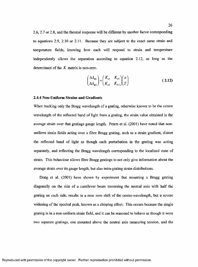
26

2.6,2.7 or 2.8, and the thermal response will be different by another factor corresponding

to equations 2.9, 2.10 or 2.11. Because they are subject to the exact same strain and

temperature fields, knowing how each will respond to strain and temperature

independently allows the separation according to equation 2.12, as long as the

determinant of the K matrix is non-zero.

'aV X i Kn ) V

^AAB2/ I * * k T2)

2.4.4 Non-Uniform Strains and Gradients

When tracking only the Bragg wavelength of a grating, otherwise known to be the centre

wavelength of the reflected band of light from a grating, the strain value obtained is the

average strain over that gratings gauge length. Peters et al. (2001) have noted that non-

uniform strain fields acting over a fibre Bragg grating, such as a strain gradient, distort

the reflected band of light as though each perturbation in the grating was acting

separately, and reflecting the Bragg wavelength corresponding to the localized state of

strain. This behaviour allows fibre Bragg gratings to not only give information about the

average strain over its gauge length, but also intra-grating strain distributions.

Dong et al. (2001) have shown by experiment that mounting a Bragg grating

diagonally on the side of a cantilever beam traversing the neutral axis with half the

grating on each side, results in a near zero shift of the centre-wavelength, but a severe

widening of the spectral peak, known as a chirping effect. This occurs because the single

grating is in a non-uniform strain field, and it can be reasoned to behave as though it were

two separate gratings, one mounted above the neutral axis measuring tension, and the


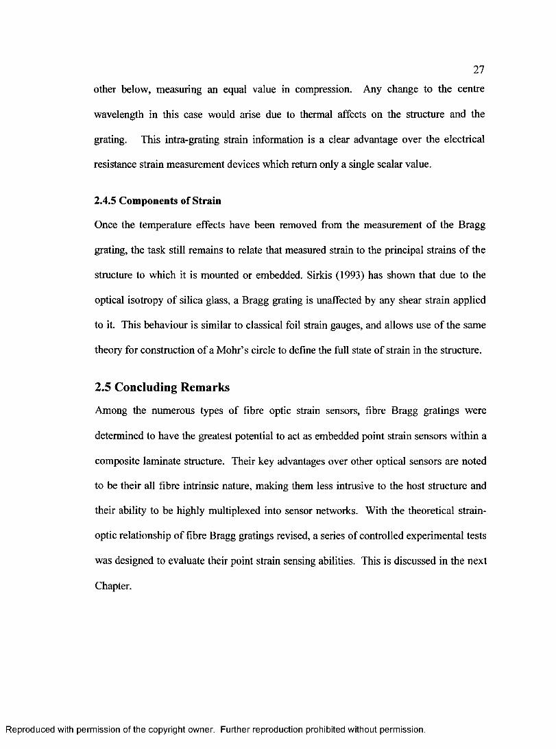
27

other below, measuring an equal value in compression. Any change to the centre

wavelength in this case would arise due to thermal affects on the structure and the

grating. This intra-grating strain information is a clear advantage over the electrical

resistance strain measurement devices which return only a single scalar value.

2.4.5 Components of Strain

Once the temperature effects have been removed from the measurement of the Bragg

grating, the task still remains to relate that measured strain to the principal strains of the

structure to which it is mounted or embedded. Sirkis (1993) has shown that due to the

optical isotropy of silica glass, a Bragg grating is unaffected by any shear strain applied

to it. This behaviour is similar to classical foil strain gauges, and allows use of the same

theory for construction of a Mohr’s circle to define the full state of strain in the structure.

2.5 Concluding Remarks

Among the numerous types of fibre optic strain sensors, fibre Bragg gratings were

determined to have the greatest potential to act as embedded point strain sensors within a

composite laminate structure. Their key advantages over other optical sensors are noted

to be their all fibre intrinsic nature, making them less intrusive to the host structure and

their ability to be highly multiplexed into sensor networks. With the theoretical strain-

optic relationship of fibre Bragg gratings revised, a series of controlled experimental tests

was designed to evaluate their point strain sensing abilities. This is discussed in the next

Chapter.


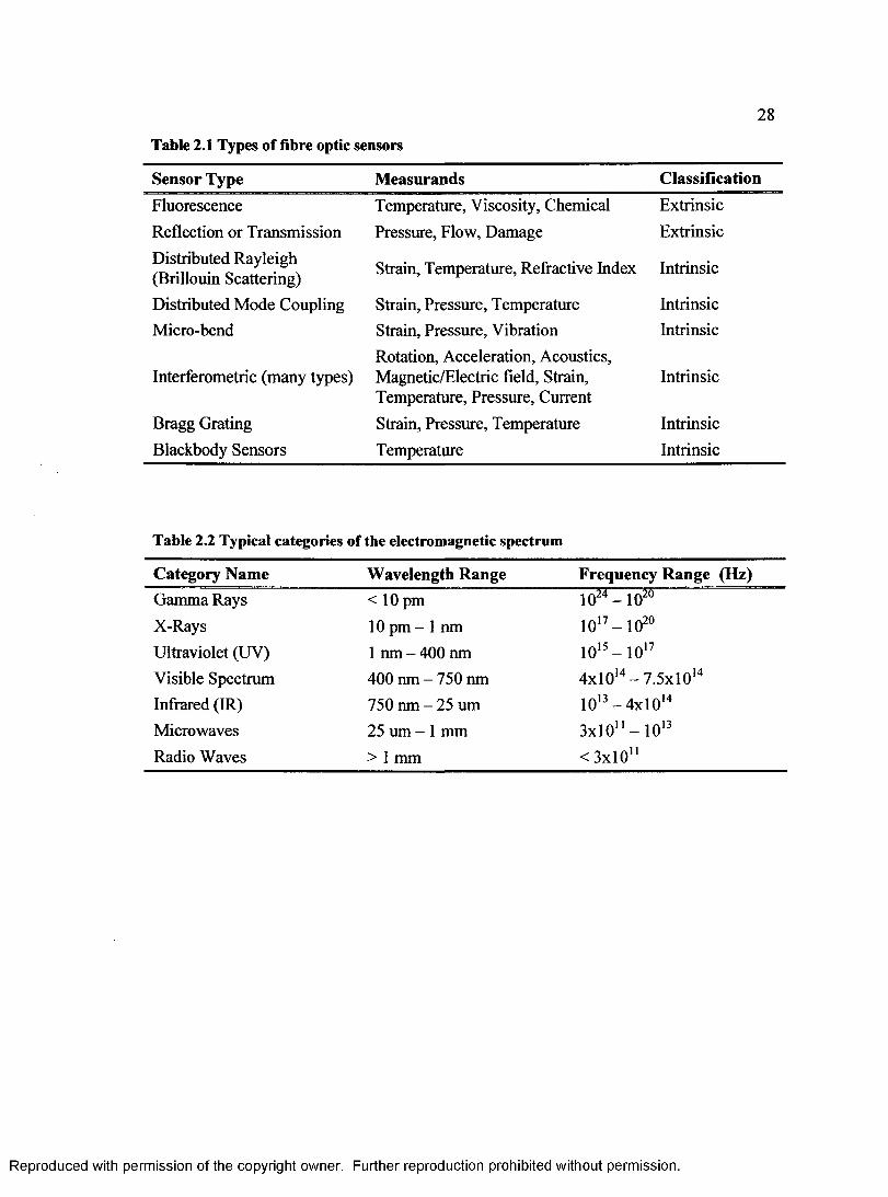
28

Table 2.1 Types of fibre optic sensors

Sensor Type Measurands ClassificationFluorescence Temperature, Viscosity, Chemical ExtrinsicReflection or Transmission Pressure, Flow, Damage ExtrinsicDistributed Rayleigh (Brillouin Scattering) Strain, Temperature, Refractive Index Intrinsic

Distributed Mode Coupling Strain, Pressure, Temperature IntrinsicMicro-bend Strain, Pressure, Vibration

Rotation, Acceleration, Acoustics,Intrinsic

Interferometric (many types) Magnetic/Electric field, Strain, Temperature, Pressure, Current

Intrinsic

Bragg Grating Strain, Pressure, Temperature IntrinsicBlackbody Sensors Temperature Intrinsic

Table 2.2 Typical categories of the electromagnetic spectrum

Category Name Wavelength Range Frequency Range (Hz)Gamma Rays < 10 pm 1024- 102°X-Rays 10 pm - 1 nm -j I sl oUltraviolet (UV) 1 nm - 400 nm 1015- 1 0 17Visible Spectrum 400 nm - 750 nm 4xl014-7 .5 x l0 14Infrared (IR) 750 nm - 25 um 1013- 4 x1014Microwaves 25 um - 1 mm 3xl0n - 10BRadio Waves > 1 mm <3x10"


29

Input Signal Input Signal (""(J")

Optical Fibre

Circulator

ReflectedSignal

ReflectedSignalFeedback Bragg

GratingS en so rOptical

Signal Transm ited S ignal __ *

Transm itedSignal — ( U )

OpticalPower Meter

Tuneable Laser Source

Laser W avelength M easurem ent

Fibre

Figure 2.1 Typical optical circuit using a tuneable laser source

Input Signal Input Signal

Optical Fibre Reflected

SignalReflectedSignal Bragg

GratingS en so r

Transm ited Signal *__ *

Transm ited Signal *— £21

Optical

CirculatorB roadband Light Source

Optical Spectrum Analyzer

Fibre

Figure 2.2 Typical optical circuit using a broadband source


30

Wavelength

ElectricField

Figure 2.3 Propagation of an electromagnetic wave

Reflected Ray

Incident Light Rays

(also transm itted}

Transm itted Ray

Figure 2.4 Interaction of light with a substance


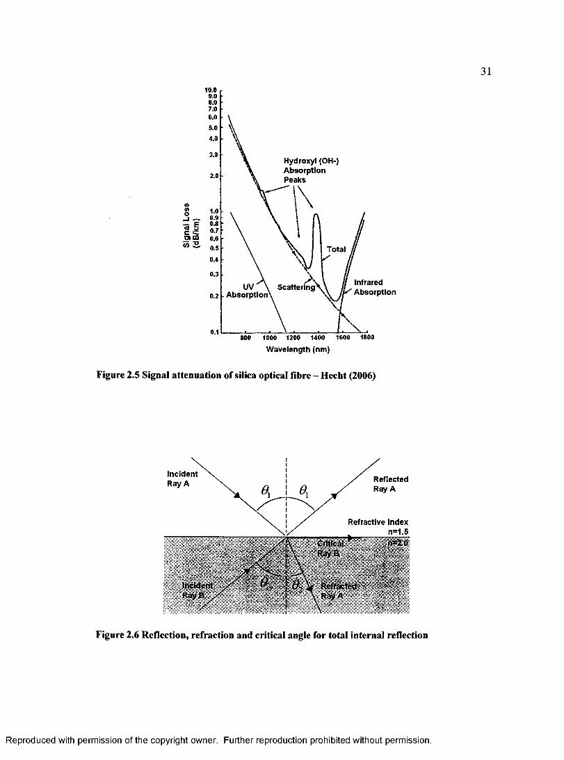
3110.0

9.0 ■

7.0 ■6.0 ■

5.0 •

4.0 ■

3.0Hydroxyl (OH-)A bsorptionPeaks2.0

1.0 0.9 0.8 0.7

O) CO 0.6 0.5 Total0.4

0.3InfraredA bsorption

ScatteringVUV \ . A bsorption0.2

0.1800 1000 1200 1400 1600 1800

W avelength (nm)

Figure 2.5 Signal attenuation of silica optical fibre - Hecht (2006)

Incident Ray A Reflected

Ray A

Refractive Index n=1.5n=2.0Critical

Ray B

IncidentR ayB

Refracted Ray A

Figure 2.6 Reflection, refraction and critical angle for total internal reflection


32

Cladding Material

Silica Core

Refractive Index

Figure 2.7 Typical cross-section of a step-indexed multi-mode silica optical fibre

C ladding

Silica Core

Figure 2.8 Different acceptable propagation paths of guided rays in an optical fibre


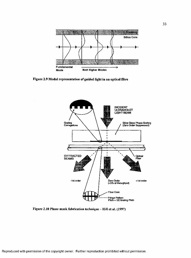
Fundam ental --------------------------------------- =>Mode Next Higher M odes

Figure 2.9 Modal representation of guided light in an optical fibre

Grating Corrugations

DIFFRACTED BEAMS

INCIDENT ULTRAVIOLET LIGHT BEAM

Silica Glass Phase Grating (Zero Order Suppressed)

Zero Order (<5% of throughput)

1st order ■•■1st order

Fringe PatternPitch = 1/2 Grating Pitch

Figure 2.10 Phase mask fabrication technique - Hill et al. (1997)


34

Input Signal Reflected Signal Transm itted Signal

Silica CoreInput Signal

Transm itted SignalReflected Signal

Refractive Index of Silica Core

Perturbation to Refractive Index

Normal Refractive Index of Core

Figure 2.11 Fibre Bragg grating

/ i j Reflected / L Reflected ^ Reflected

—i 11111 n rm— —i 1111111 r m— —i ihim rm—0C0^ „ T ransm ission

Signal < ------------- ■«------------- -4---------------

+ -^2 /lh / o + A3 XSignal

3̂

Reflection S ignals

Input Signal Total Reflection Signal Total Transm itted S ignal

Figure 2.12 Wavelength division multiplexed array of Bragg grating sensors


35

14

Wavelengthshift,

nm

X = 15S6 nm7.2 x 10'VC

0 100 200 300 400 500 600 700 800 900Temperature, C

Figure 2.13 Variation of thermo-optic coefficient for silica fibre - Hill et al. (1997)


36

CHAPTER 3: EXPERIMENTAL SETUP

3.0 Introduction

In order to test fibre Bragg gratings as point strain sensors experimentally, they must be

mounted onto a structure and have a predictable strain field applied to them. To this end,

a simple experimental apparatus with a cantilever beam capable of producing a range of

repeatable and predictable strain fields is employed. A detailed description of the test

apparatus, the optical circuit used for interrogating the fibre Bragg gratings and the use of

conventional electrical resistance strain gauge rosettes is given in this Chapter. Two

cantilever test beams are employed; one is an extruded aluminum beam and the other, a

pultruded fibreglass beam. Analytical solutions are then presented for the strains acting

on each specimen where the FBG sensors will be mounted. Finally, the analytical

solutions are further verified with use of electrical resistance strain gauge rosettes.

3.1 Equipment Setup and Integration

The complete experimental setup involves three distinct sets of equipment integrated into

a single experiment; optical, electrical, and mechanical. The optical equipment refers to

the fibre Bragg gratings and the optical circuit devices required for their interrogation.

The electrical equipment refers to the electrical resistance strain gauge rosettes and the


37

electrical circuit devices required for their interrogation. The mechanical equipment

refers to the support frame, the applied loads, and the cantilever test specimens.

3.1.1 Optical Equipment

The optical equipment used for interrogating fibre Bragg gratings during this work was

only available for use in the Carleton Laboratory for Laser Induced Photonic Structures

(CLLIPS), hereby referred to as the CLLIPS laboratory, in the Department of Electronics,

Carleton University, because it is shared by multiple research projects. This required that

all the mechanical equipment, and electrical resistance strain gauge equipment be

relocated to the CLLIPS laboratory in order to perform the experimental tests.

The optical circuit used to interrogate a single fibre Bragg grating is shown in figure

3.1, and is similar to the tuneable laser source circuit. Most of the components in the

circuit shown in figure 3.1 are a part of the SWS-OMNI system made by JDS

UNIPHASE. The figure shows the optical connection of the components; the SWS-

OMNI system is also connected to a PC and is controlled by the SWS-OMNI 2 (version

10.0) software. The SWS-OMNI system is capable of sweeping the electromagnetic

spectrum from 1519.5 ww to 1634ww at a speed of 4Qnm/s with an absolute wavelength

resolution of 2pm, and dynamic range of 70dB. When measuring transmitted or

reflected signals, the software normalizes the measured signal against a reference signal

from the optical source. This results in measuring the relative loss in signal power, and

thus corrects for any variations of intensity between wavelengths due to the source itself.

The exact values for optical signal power loss through the individual circuit

components and connections are of little consequence because the parameter of interest is


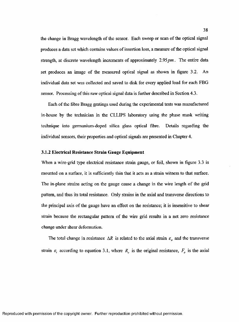
38

the change in Bragg wavelength of the sensor. Each sweep or scan of the optical signal

produces a data set which contains values of insertion loss, a measure of the optical signal

strength, at discrete wavelength increments of approximately 2.95p m . The entire data

set produces an image of the measured optical signal as shown in figure 3.2. An

individual data set was collected and saved to disk for every applied load for each FBG

sensor. Processing of this raw optical signal data is further described in Section 4.3.

Each of the fibre Bragg gratings used during the experimental tests was manufactured

in-house by the technician in the CLLIPS laboratory using the phase mask writing

technique into germanium-doped silica glass optical fibre. Details regarding the

individual sensors, their properties and optical signals are presented in Chapter 4.

3.1.2 Electrical Resistance Strain Gauge Equipment

When a wire-grid type electrical resistance strain gauge, or foil, shown in figure 3.3 is

mounted on a surface, it is sufficiently thin that it acts as a strain witness to that surface.

The in-plane strains acting on the gauge cause a change in the wire length of the grid

pattern, and thus its total resistance. Only strains in the axial and transverse directions to

the principal axis of the gauge have an effect on the resistance; it is insensitive to shear

strain because the rectangular pattern of the wire grid results in a net zero resistance

change under shear deformation.

The total change in resistance AR is related to the axial strain sa and the transverse

strain st according to equation 3.1, where Ra is the original resistance, Fa is the axial


39

strain sensitivity factor and Ft is transverse strain sensitivity factor of the gauge, Hetenyi

(1950).

A/?= r = Fas a + Ftet (3.1)K o

When interrogating a single strain gauge, it is not possible to separate the axial and

transverse strain components, unless the relationship between the two is already known,

such as the Poisson contraction that occurs during simple axial tension. It is convenient

therefore to define an ‘apparent strain’ s ' as shown in equation 3.2, that is related to the

resistance change of the gauge by what is known as the gauge factor F , Hetenyi (1950).

, AR 1 1 ks = - s -------------- (3.2)

R .F " ( 1 + t ) '(1 + *)

The gauge factor is related to the axial and transverse strain sensitivity factors by

equation 3.3 and a correction factor k is also defined according to equation 3.4, which is

known as the transverse sensitivity of the gauge, Hetenyi (1950).

F = Fa + F, (3.3)

k = %- (3.4)Fa

When multiple gauge measurements are taken simultaneously at different

orientations, this correction factor can be applied to the ‘apparent’ strains to separate the

strain components, as long as Fa * F t . Section 3.6 describes in further detail the

separation of the strain components by using multiple strain gauges.


40

The gauge factor and transverse sensitivity parameters are typically provided by the

gauge manufacturer. Equation 3.1 can also be represented using the gauge factor and

transverse sensitivity parameters instead of the axial and transverse strain sensitivity

factors.

AR F Fk~d~ = S°T\— T\ + g> T i (3 ,1)K 0 + V V + k)

The change in resistance is measured by using a quarter Wheatstone bridge circuit; an

electrical circuit containing four balanced resistors, one of which is the strain gauge as

shown in figure 3.4. When the resistances in the circuit are balanced, the voltage across

the centre of the Wheatstone bridge is zero; changes in the resistance of the strain gauge

cause changes in this voltage which is measured using a highly accurate voltage

measurement device. The voltage change AV is related to the resistance change of the

gauge by equation 3.5, where V0 is the voltage applied to the circuit and Fb is the bridge

factor; for a quarter Wheatstone bridge circuit Fb = 0.25 .

= F , ( 3.5)Va b Ra

The strain gauge is connected to the quarter Wheatstone bridge circuit using a three

lead wire configuration as shown in figure 3.5. Thermal effects can cause the resistances

of these lead wires to change; however, if all the lead wires are of equal length and gauge

thickness, and thus resistance, and they are exposed to the same environment, each would

exhibit approximately the same change in resistance. The three wire configuration takes

advantage of this situation by connecting the third wire into the opposing arm of the


41

bridge circuit, thus restoring the balance of the circuit should any change in lead wire

resistance occur.

The voltage source applied to the circuit, the voltage measurement device, and the

other three resistors in the Wheatstone bridge circuit, known as completion resistors, are

internal components to a strain gauge indicator unit shown in figure 3.5. This unit also

possesses a variable resistance, which is used to balance the bridge circuit to a measured

voltage of zero. The unit allows input of the gauge factor and consequently calculates the

apparent strain directly from the measured voltage, which is displayed digitally in micro

strain. A single indicator unit can easily be used to interrogate multiple strain gauges by

employing a switch and balance unit, to which each gauge is connected and balanced

individually in the three wire configuration. A portable strain indicator unit and a

portable switch and balance unit, shown in figure 3.6, were employed to carry out the

experimental electrical resistance strain gauge measurements as will be described in

Section 3.6.

3.1.3 Mechanical Equipment

As an experimental strain apparatus, the cantilever beam offers many advantages. It is

simple in design, affordable, and if designed properly, the same support apparatus can be

used for a variety of test specimens and loading conditions. The steel support frame

shown in figure 3.7 was used to support the cantilever beam specimens. A steel support

plate was fabricated as shown in figure 3.8 which allows different specimens to be

mounted at a range of angular orientations relative to the frame.


42

Two different cantilever test specimens were fabricated to mount onto this test frame;

one made of a hollow rectangular aluminum extrusion, and the other, made of a hollow

rectangular fibreglass pultrusion. The geometry and constraints, application of loads, and

material properties are presented below.

3.2 Specimen Geometry and Constraints

A hollow rectangular cross-section was chosen for both test specimen designs because

the geometry is simple, approximate theoretical solutions to bending and torsion for this

geometry are known, and it has flat surfaces ideal for attaching multiple adjacent sensors.

Manufacturers typically provide geometric dimensions for their fabricated extrusion and

pultrusion cross-sections. For each of the cross-sections used, these dimensions were

verified using a set of Vernier calipers.

3.2.1 Aluminum Specimen Geometry and Constraints

The aluminum cantilever beam has a hollow rectangular cross-section with an exterior

height of hQ - 50.8 mm, an exterior width of b0 = 25.4 mm and a uniform wall thickness

on all sides of / = 3.048 mm as shown in figure 3.9. The length of the beam from the

free end to the fixed end is L - 812.8 mm. Another geometric property of interest is the

second moment of area lx. For a hollow rectangular section, Ix is given by equation 3.6,

where ht and bt are the inner height and inner width of the rectangular cross section

respectfully; the calculated value of Ix for this section is given in figure 3.9.

i J J t J J t (3.6)' 12 12


43

Another geometric property of interest is the average enclosed area of the hollow

cross section Axy, which is used in the theoretical solution for the torsion induced shear

stresses of Section 3.5.2. For a hollow rectangular section Axy is given by equation 3.7,

where Aa is the area enclosed by the outer surfaces and Aj is the area enclosed by the

inner surfaces; the calculated value of Axy for this section is given in figure 3.9.

^=A±4.=U±M. (3.7)2 2

The fixed end of the cantilever beam was welded to a circular aluminum base plate,

which was mounted onto the steel support plate shown in figure 3.8 by four steel bolts.

The free end of the aluminum beam was welded closed using a small rectangular

aluminum plate that matched the exterior dimensions of the cross section. Holes were

later drilled into this plate, and tapped with threads to allow application of bending and

torsional loads on the cantilever beam.

3.2.2 Fibreglass Specimen Geometry and Constraints

The fibreglass cantilever beam has a hollow rectangular cross-section with an exterior

height of h0 = 101.6 mm, an exterior width of b0 = 50.8 mm, a vertical wall thickness of

ty =3.175 mm, and a horizontal wall thickness of tx = 6.350 mm as shown in figure 3.9.

The length of the beam from the free end to the fixed end is L = 749.3 mm. Values for

the second moment of area and the average enclosed area of this cross section are

calculated using equations 3.6 and 3.7, respectively, and are given in figure 3.10.


44

Fibreglass can not be welded; the cross-section was therefore clamped to a specially

fabricated support structure at the fixed end to be as rigid as possible. Figure 3.11 shows

the assembly of this support structure. A steel block was machined to fit tightly inside

the fixed end of the cantilever beam and was then welded onto a large circular steel base

plate, which was mounted onto the steel support plate shown in figure 3.8 by four steel

bolts. Holes were drilled and tapped with threads into the steel plug, to which rectangular

steel plates would be fastened using steel bolts, thereby clamping the walls of the cross-

section on all sides as shown in figure 3.11. The free end of the fibreglass beam has a

similar steel plug clamped into it as shown in figure 3.11. Holes were drilled into the

face of this steel plug and tapped with threads to allow application of bending and

torsional loads onto the cantilever beam.

3.3 Applied Loads

Static loads are applied at the free end of the cantilever specimens by suspending masses

of known values from a hanger. The applied forces at the free end of the beams are a

result of adding sequential masses to the hanger. The masses were individually weighed

and converted into gravitational forces.

Transverse forces applied through the shear centre of the cross-section produce no

torsion and only bending of the cantilever beam. The shear centre for a rectangular

section coincides with the intersection of the two planes of symmetry, at the centre o f the

section. A hole was drilled and tapped with threads at the shear centre location on the

plate at the free end of each specimen; loads will be applied through this point to produce

pure bending.


45

During the fabrication of the specimens, particular care was taken to ensure that the

cross section remained oriented as precisely as possible in the vertical direction. This

would ensure that the default loading through the shear centre would produce bending in

only the vertical plane.

A load that is applied at a lateral distance from the shear centre can be resolved into a

transverse load of the same value acting through the shear centre with the addition of a

torsional moment about the elastic axis of the section. Application of loads at

incremental lateral distances from the shear centre is achieved by attaching a horizontal

torsion bar to the plate at the free end of each specimen as shown in figure 3.12. These

torsion bars have evenly spaced holes from which the masses are suspended.

It should be noted that the torsional moment will cause a varying angular deflection

of the cross section along the beam length. The transverse load components will thus

vary along the beam length, causing some skew bending out of the vertical plane. The

resulting lateral deflection of the beam will in turn cause the torsional moment to vary

along the beam axis. This effect is known as coupling, and can have a pronounced effect

on the beam if the bending or torsional deflections are appreciably large. As long as the

deflections are small, coupling effects such as these can be considered negligible; thereby

allowing the bending moments, torsion moments, and axial forces acting on the beam to

be considered linearly independent of each other. Figure 3.12 shows how the loads are

applied to the test specimens and resolved assuming this linear independence. By

inverting the beams, or reversing the torsion bars, additional loads can be applied to the

beams that have identical magnitudes of bending and torsion, but different signs.


46

3.3.1 Aluminum Specimen

Table 3.1 lists the transverse force increments that are applied at the free end of the

aluminum cantilever beam. The bending moments M x acting on the beam will increase

linearly with distance z from the free end according to equation 3.8, where Py is the

applied transverse force.

M x =Pyz (3.8)

The position z of each electrical resistance gauge is listed in Table 3.4. The torsional

moments Tz that accompany the transverse forces are determined by equation 3.9, where

x is the lateral distance from the shear centre to where the force Py is applied at the free

end.

Tz =Pyx (3.9)

The torsional moments are listed in Table 3.1 for all the applied forces and all the

lateral positions xi of the aluminum beam indicated in figure 3.9.

3.3.2 Fibreglass Specimen

Table 3.2 shows the transverse force increments that are applied at the free end of the

fibreglass cantilever beam. The corresponding bending and torsional moments again are

given by equations 3.8 and 3.9, respectively; the position z of each electrical resistance

gauge is listed in Table 3.5.


47

The torsional moments that accompany the transverse forces are determined by

equation 3.9. The torsional moments are listed in Table 3.2 for all the applied forces and

all the lateral positions x, of the fibreglass beam indicated in figure 3.10.

3.4 Material Properties of Specimens

The materials used for construction of the cantilever test specimens, aluminum extrusion

and fibreglass pultrusion, are considered to be linearly elastic materials. The fibreglass

pultrusion is a polyester/glass composite; polyester is a polymeric material, which can

exhibit non-linear visco-elastic behaviour at high temperatures. As long as the

temperature remains well below the glass transition temperature of the polyester, it will

behave similar to glass; the response will for all practical purposes be linear until ultimate

failure of the material.

A fully anisotropic linearly elastic material requires 21 independent material

constants to complete the stiffness and compliance matrices. An orthotropic material

requires only 9 independent material constants because it has no coupling between the

shear and direct components of stresses and strains. The coefficients of the compliance

matrix for an orthotropic material are related to the 9 independent material constants of

equation 3.10, see e.g. Tuttle (2004), such that — = — = -JL. s where EiE z E y Ez Ex Ey Ex

denotes the Young’s modulus in the i-th axis, vy refers to the Poisson’s ratio in the i-j

plane, and the numerical average, or tensor shear strain s is related to the engineering

shear strain by syx = yyx/2 .


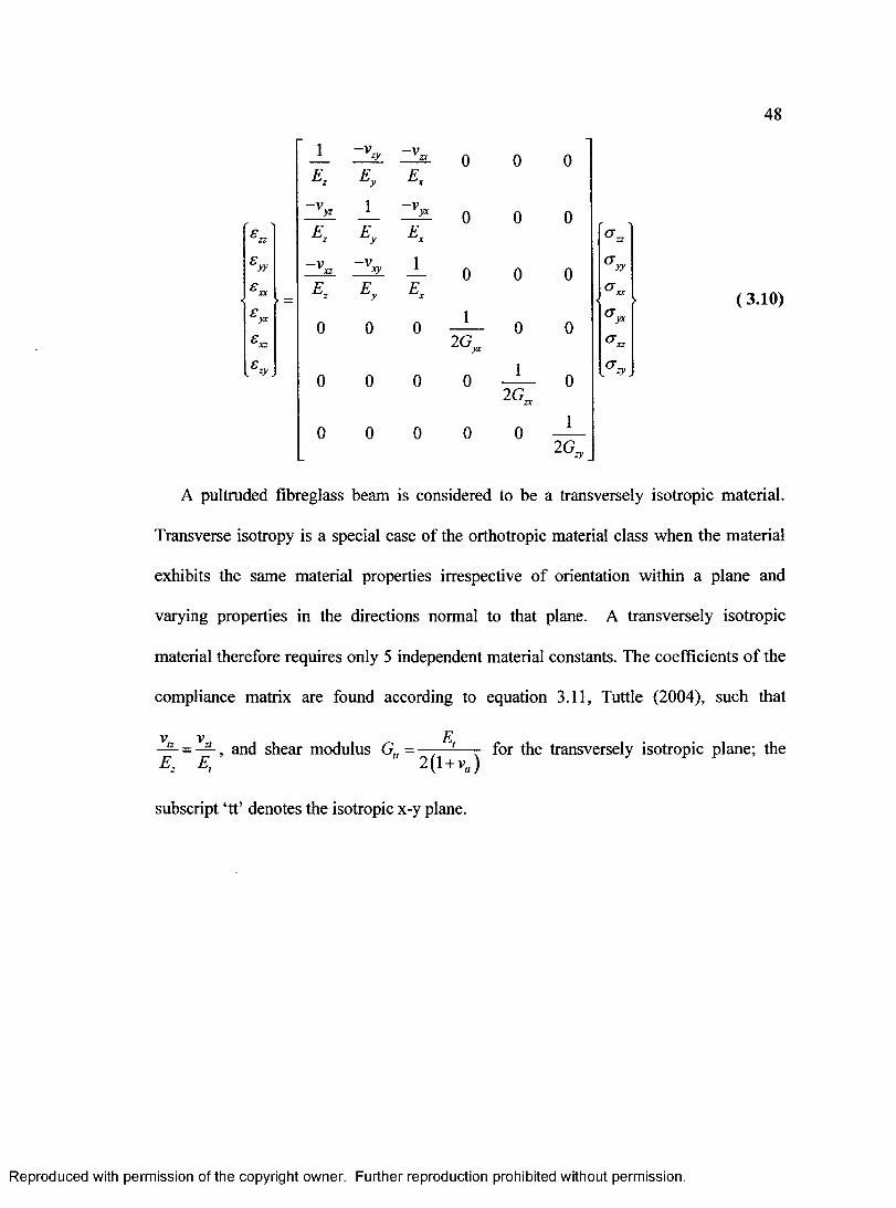
48

i

E y

- Vzc

Ex0 0 0

- v*E ,

1

Ey" v *

Ex0 0 0 ■>

£ yy ~ V xz

Ez~ v >y

Ey

1

Ex0 0 0

«

aX X

>

0 0 01

0 0S *z 2 Gy* O-xz

0 0 0 01

02 ^

0 0 0 0 01

2 G , _

A pultruded fibreglass beam is considered to be a transversely isotropic material.

Transverse isotropy is a special case of the orthotropic material class when the material

exhibits the same material properties irrespective of orientation within a plane and

varying properties in the directions normal to that plane. A transversely isotropic

material therefore requires only 5 independent material constants. The coefficients of the

compliance matrix are found according to equation 3.11, Tuttle (2004), such that

v v E— = — , and shear modulus G„ = —— — - for the transversely isotropic plane; theE z E , 2 (1 + v« )

subscript ‘tt’ denotes the isotropic x-y plane.


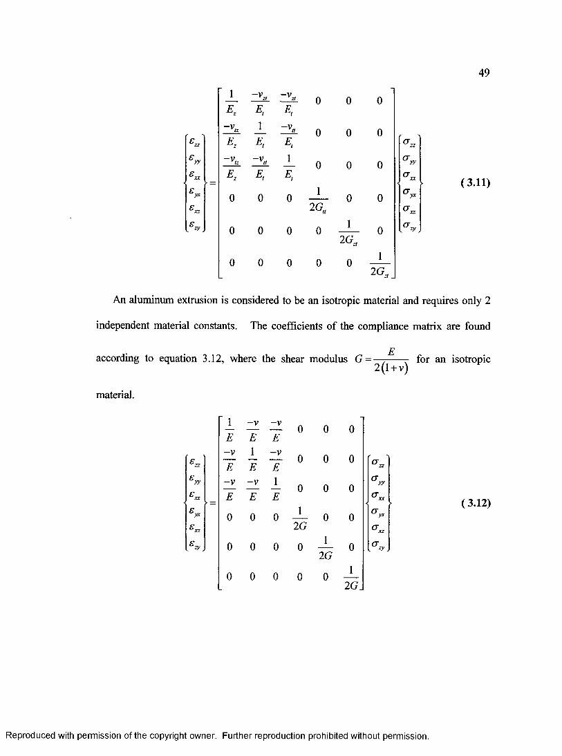
49

1Ez

-v*E,

~ V zt

Et0 0 0

V" v rz

Ez1

E, E,0 0 0

CTzz

£ xx

~ V ,z

Ez~v„E,

1

E,0 0 0

<a XX

>

0 0 01

0 0O’zz

0 0 0 0 1 02G-

0 0 0 0 0 1

An aluminum extrusion is considered to be an isotropic material and requires only 2

independent material constants. The coefficients of the compliance matrix are found

according to equation 3.12, where the shear modulus G = for an isotropic

material.

■ 1 E

-v~E

-v~E

0 0 0

'

eu-V

~E1E

-v~E

0 0 0 O’zzs y y

£ xx<

-v~E

-v~E

1E

0 0 0*

£ z z

0 0 0 12 G

0 0O'zz

. V 0 0 0 01

2G0

0 0 0 0 0 12 G.


50

3.4.1 Aluminum Properties

The aluminum material used for the cantilever beam is 6063-T5 extrusion. The required

material constants for this aluminum are listed by the Mat-Web (2007) as E = 68.9 GPa

and v = 0.33. The yield strength of this aluminum is listed as a Y =145 MPa; all applied

loads were verified to produce direct stresses in the beam well below this value or

permanent deformation of the cantilever specimen will occur.

The material properties listed in Table 3.3 were verified by employing electrical

resistance strain gauge rosettes on the cantilever specimen as will be discussed in Section

3.6. After verifying the geometry of the specimen and the applied load values, the strains

measured by the gauges are shown to agree with the theoretical solutions for bending and

torsion of Section 3.5, thus indicating that the material constants are indeed as quoted by

Mat-Web (2007).

3.4.2 Fibreglass Properties

The fibreglass pultrusion used for the cantilever beam was manufactured by Bedford

Reinforced Plastics Inc. The material constants quoted by the manufacturer are listed in

Table 3.3. The material constant v„ was however not provided and was assumed to be

0.3, by comparison to similar polyester fibreglass pultruded materials. These constants

had been experimentally determined from several samples by the manufacturer; they

should be verified however, because as noted by Mottram (2004), the values provided are

not always true, and often have significant deviations from the real properties. Similar to

the aluminum specimen, the material constants of the fibreglass cantilever beam can be


verified by employing electrical resistance strain gauge rosettes. After verifying the

geometry of the specimen and the applied load values, the strains measured by the gauges

were found to disagree significantly with the corresponding theoretical solutions for

bending and torsion; this will be further discussed in Section 3.6.

In order to resolve this discrepancy, additional experimental tests were done. The

simplest was uni-axial tension of a flat specimen of the fibreglass pultrusion material.

Several rectangular test coupons were fabricated from the walls of the fibreglass beam

with the geometry as shown in figure 3.13 with the fibre direction being parallel to the

coupon length. During this test, the strain gauges can also be tested to determine if they

are properly measuring the true strain on the fibreglass specimens. The strain gauges

were mounted as shown in figure 3.13, one aligned with the fibre direction and the other

orthogonal to it.

The test coupons were monotonically loaded in simple tension using a hydraulic

powered material testing system (MTS). The MTS machine has a calibrated load cell

capable of accurately measuring the applied tensile force Pz on the specimen during the

loading cycle. The tensile stress is calculated using equation 3.13, where A is the

cross-sectional area of the test coupon.

<7„=-S- (3.13)K

During the loading cycle, a linear variable displacement transducer (LVDT)

extensometer simultaneously measured the displacement along the axis of loading

between two points on the coupon surface. The initial distance between these points is


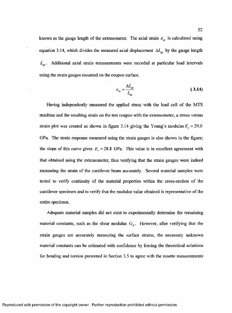
52

known as the gauge length of the extensometer. The axial strain e„ is calculated using

equation 3.14, which divides the measured axial displacement A b y the gauge length

. Additional axial strain measurements were recorded at particular load intervals

using the strain gauges mounted on the coupon surface.

e * = - T - <3*14)gz

Having independently measured the applied stress with the load cell of the MTS

machine and the resulting strain on the test coupon with the extensometer, a stress versus

strain plot was created as shown in figure 3.14 giving the Young’s modulus E, =29.0

GPa. The strain response measured using the strain gauges is also shown in the figure;

the slope of this curve gives Ez = 28.8 GPa. This value is in excellent agreement with

that obtained using the extensometer, thus verifying that the strain gauges were indeed

measuring the strain of the cantilever beam accurately. Several material samples were

tested to verify continuity of the material properties within the cross-section of the

cantilever specimen and to verify that the modulus value obtained is representative of the

entire specimen.

Adequate material samples did not exist to experimentally determine the remaining

material constants, such as the shear modulus Gzt. However, after verifying that the

strain gauges are accurately measuring the surface strains, the necessary unknown

material constants can be estimated with confidence by forcing the theoretical solutions

for bending and torsion presented in Section 3.5 to agree with the rosette measurements


53

obtained by experiment in Section 3.6. The material constants derived in this semi-

empirical method are listed in Table 3.3 as Ez = 30.2 GPa, Gzt - 4.1 GPa, and

= 0.25 . The other Poisson’s ratio vtt = 0.3 was assumed, and had no effect on the

theoretical solution for this beam. The elastic modulus Ez = 30.2 GPa estimated using

the semi-empirical method in the fibre axis direction agrees within 2% of the modulus

Ez = 28.8 GPa as determined by the MTS experiment, thereby suggesting that the

approach gave an acceptable level of accuracy for estimating the necessary material

constants.

3.5 Cantilever Beam Theoretical Solutions

Analytical solutions derived from simple beam and torsion theory can be used to predict

the stresses acting on each cantilever specimen and the resulting strains, using the values

o f the various parameters given in the previous sections. The solutions for combined

bending and torsion loads can be obtained by simple superposition of the solution of the

individual load cases.

3.5.1 Bending of a Hollow Rectangular Cantilever Beam

A transverse load applied at the free end of the cantilever beam that passes through the

shear centre and the vertical principal axis of the hollow rectangular cross section results

in simple bending of the beam in the vertical plane. This axial stress distribution in the

beam due to pure bending is given by equation 3.15, Roark (1975), where Ix is the

second moment of area of the cross section about the x axis, Mx is the bending moment


54

acting on that section at position z about the x axis, and y0 is the position on the

exterior surface of the cross section measured from the neutral axis of the beam in the y

direction.

M v<ru = — f e - (3.15)

X

In bending, the shear stress rzy at the top and bottom surfaces of the hollow

rectangular cross section is zero, and can thus be ignored for any strain gauges or FBG

sensors mounted on those surfaces.

3.5.2 Torsion of a Thin-Walled Hollow Rectangular Section

For a hollow thin-walled rectangular section under torsion, the average shear stress tXz

on the top surface near the middle of the wall can be found using equation 3.16, Roark

(1975), where Axy is the average of the area enclosed by the inner surfaces and the area

enclosed by the outer surfaces given by equation 3.7, T, is the applied torsional moment

about the elastic axis, and t is the thickness of the top wall.

T,2 A x y t

( 3.16)

For a thin wall, the shear stress on the inner and outer walls will be very close, and is

therefore assumed to be constant across the wall thickness. For slightly thicker walls, the

stress will vary in an approximately linear distribution across the thickness of the wall

with proportion to the distance from the elastic axis of the section. Knowing the average

shear stress in the wall, equation 3.17 can be used to determine an approximate shear


55

stress Tao on the exterior surface of the wall, where ya and y, are the positions on the

outer and inner surfaces of the wall respectively; they are measured from the neutral axis

in the y direction.

(3-17)

3.5.3 Mohr’s Circle of Strains

The strains at a particular point are related to the applied stresses through Hooke’s Law

as described in Section 3.4. Rotating the coordinate axes of the strain field by an angle 9

causes the components of strain to transform according to equations 3.18,3.19 and 3.20.

sx, = +g‘ + ———̂-cos 29 + e sin 29 ( 3.18)

ez, = £x+Sz _£*— cos 29 — sin 29 (3.19)

., = - ——— sin 29 + er, cos 29 (3.20)2

Mohr’s circle, shown in figure 3.15, is a graphical representation of this strain

coordinate transformation. The centre C and radius R of the Mohr’s circle are given by

equations 3.21 and 3.22 respectively.

C = ̂ (3.21)

R = . ' g x - Q 2


56

The orientation of the principal planes where the shear strain components are zero is

denoted by 6P as shown in figure 3.16 and can easily be shown to be as given by

equation 3.23.

The principal strains, sPX and sp2, are thus related by equations 3.24 and 3.25 to the

centre and radius of the circle respectively.

The maximum shear strain sxzmsx occurs at an orientation 6 = 45° from the principal

orientation as shown in figure 3.16 and is related to the radius by equation 3.26.

*— = * (3-26)

With the Mohr’s circle, it is possible to determine the components of the strain field

at any arbitrary orientation. This is convenient for determining the individual

components of strain acting on a strain gauge that is mounted at a particular orientation.

3.6 Strain Gauge Rosette Measurements

An electrical resistance strain gauge rosette, shown in figure 3.17, is a set of individual

electrical resistance strain gauges that are oriented differently, but packaged together onto

a single bondable strip, on which the orientations of the gauges relative to each other are

known. Rosettes are a convenient way of using the strain gauges to experimentally

measure the full state of strain at a given location.

(3.23)

£■̂>1 — C + R (3.24)

sP2 = C - R ( 3.25)


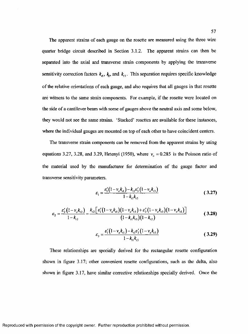
57

The apparent strains of each gauge on the rosette are measured using the three wire

quarter bridge circuit described in Section 3.1.2. The apparent strains can then be

separated into the axial and transverse strain components by applying the transverse

sensitivity correction factors kn, and kti. This separation requires specific knowledge

of the relative orientations of each gauge, and also requires that all gauges in that rosette

are witness to the same strain components. For example, if the rosette were located on

the side o f a cantilever beam with some of gauges above the neutral axis and some below,

they would not see the same strains. ‘Stacked’ rosettes are available for these instances,

where the individual gauges are mounted on top of each other to have coincident centers.

The transverse strain components can be removed from the apparent strains by using

equations 3.27, 3.28, and 3.29, Hetenyi (1950), where v0 =0.285 is the Poisson ratio of

the material used by the manufacturer for determination of the gauge factor and

transverse sensitivity parameters.

= £;(i-v,*„)-y;(i-v,,*„) (3.27)1 - k k1 Kn K, 3

_ e' (l - vBkn ) kn [s[ (1 - vDkn )(1 - vak,3 ) + ̂ (1 - vak,3 ) (1 - v0kn )]

2 " l - * ,2 ■ (l-*„* ,3) ( l - * ,2) ( • }

£j = ( 3 .29)l - k nkl3

These relationships are specially derived for the rectangular rosette configuration

shown in figure 3.17; other convenient rosette configurations, such as the delta, also

shown in figure 3.17, have similar corrective relationships specially derived. Once the


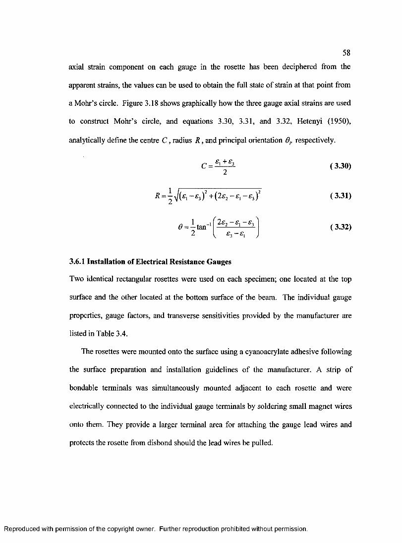
58

axial strain component on each gauge in the rosette has been deciphered from the

to construct Mohr’s circle, and equations 3.30, 3.31, and 3.32, Hetenyi (1950),

analytically define the centre C , radius R , and principal orientation 0P respectively.

3.6.1 Installation of Electrical Resistance Gauges

Two identical rectangular rosettes were used on each specimen; one located at the top

surface and the other located at the bottom surface of the beam. The individual gauge

properties, gauge factors, and transverse sensitivities provided by the manufacturer are

listed in Table 3.4.

The rosettes were mounted onto the surface using a cyanoacrylate adhesive following

the surface preparation and installation guidelines of the manufacturer. A strip of

bondable terminals was simultaneously mounted adjacent to each rosette and were

electrically connected to the individual gauge terminals by soldering small magnet wires

onto them. They provide a larger terminal area for attaching the gauge lead wires and

protects the rosette from disbond should the lead wires be pulled.

apparent strains, the values can be used to obtain the full state of strain at that point from

a Mohr’s circle. Figure 3.18 shows graphically how the three gauge axial strains are used

( 3.30)

( 3.31)

( 3.32)


59

To verify that no damage was caused to the gauges during installation, the electrical

resistance value of each gauge was verified using a multi-meter. The rosette positions

were then measured from the location of applied loads as listed in Table 3.4. It was

difficult to align the rosette so that one gauge lies perfectly along the principal axis of the

beam. The misalignment can be calculated from experimental measurement as the

principal angle during pure bending. The constant angular offset between theoretical and

experimental lines shown in the principal angle plot of figure 3.21 is the true spatial

orientation of the rosette with respect to the principal axes of the beam. This value is

calculated for each rosette and is listed in Table 3.4.


The apparent strain was converted to the true strain along the axis of each gauge using the

manufacturer gauge properties of Table 3.4. Using the Mohr’s strain circle analysis, the

principal strains, maximum shear strains, and principal angles were obtained for each

rosette and compared to the corresponding theoretical values for the aluminum test

specimen. These results are graphically and numerically presented for bending and

combined bending and torsion in figures 3.19 - 3.30 and Tables 3.5 - 3.6, where figures

3.19 - 3.24 and Table 3.5 correspond to the top surface rosette, and figures 3.25 - 3.30

and Table 3.6 correspond to the bottom surface rosette.

The principal strains measured by the top surface rosette agree within 2% of

theoretical values over the tested range, whereas the measurements obtained by the

bottom surface rosette agree slightly less, but still within 3%. The excellent agreement

with theoretical values verifies that the test specimen behaviour follows the analytical


60

solutions and that the material constants of the specimen listed by Mat-Web (2007), as

shown in Table 3.3 and described in Section 3.4.2 are accurate.


The same analysis of the principal strains, maximum shear strains and principal angles

was carried out for the fibreglass specimen as was described for the aluminum specimen.

Figures 3.31 - 3.32 and Table 3.8 show that there is significant disagreement between the

measured and theoretical values when using the material constants provided by the

manufacturer. Additional material testing was therefore carried out as described in

Section 3.4.3 to resolve this disagreement. The material testing verified that the rosettes

measured accurately the surface strains of the fibreglass specimen, and that the material

constants were significantly different from those given by the manufacturer.

Knowing that the rosettes were correctly measuring the strains, the remaining

material constants necessary for completion of the analytical solution were estimated by

forcing the theoretical values to agree with the rosette measurements. Figures 3.33 - 3.35

show the original disagreement in the axial strain components measured by the rosettes in

the a = 0 degree, a = 45 degree and a = 90 degree directions, respectively. Figures 3.36 -

3.38 show the final agreement of the a = 0 degree, a = 45 degree, and a = 90 degree axial

strain components after the corrections on the material constants.

Repeating the analysis of the principal strains using the new estimated material

constants listed in Table 3.3, figures 3.39 - 3.44 and Table 3.9 show the agreement of the

principal strains measured by the top surface rosette with the theoretical values. The

principal strains were forced to agree within 2% over the tested range in order to have a


61

similar accuracy as the aluminum theoretical solution. A similar analysis was repeated

using the rosette on the bottom surface of the fibreglass cantilever specimen; the results

were not significantly different, and are therefore not presented here.


The experimental results of Section 3.6 using the electrical resistance strain gauge

rosettes have shown that the theoretical solutions of Section 3.5 accurately predicted the

strain fields present at the top and bottom surfaces of both the aluminum and fibreglass

cantilever beams. The apparatus is now ready for fibre Bragg grating sensors to be

experimentally tested, whose measurements can then be compared to theoretical solutions

and those obtained using conventional electrical resistance gauges.


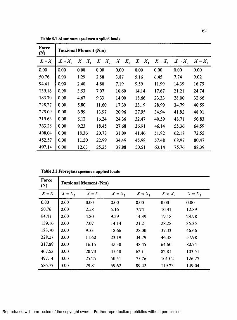
Table 3.1 Aluminum specimen applied loads

62

Force(N) Torsional Moment (Nm)

X = X, II II>5 II ii II>5 X"II II>5 ii

0.00 0.00 0.00 0.00 0.00 0.00 0.00 0.00 0.0050.76 0.00 1.29 2.58 3.87 5.16 6.45 7.74 9.0294.41 0.00 2.40 4.80 7.19 9.59 11.99 14.39 16.79139.16 0.00 3.53 7.07 10.60 14.14 17.67 21.21 24.74183.70 0.00 4.67 9.33 14.00 18.66 23.33 28.00 32.66228.27 0.00 5.80 11.60 17.39 23.19 28.99 34.79 40.59275.09 0.00 6.99 13.97 20.96 27.95 34.94 41.92 48.91319.63 0.00 8.12 16.24 24.36 32.47 40.59 48.71 56.83363.28 0.00 9.23 18.45 27.68 36.91 46.14 55.36 64.59408.04 0.00 10.36 20.73 31.09 41.46 51.82 62.18 72.55452.57 0.00 11.50 22.99 34.49 45.98 57.48 68.97 80.47497.14 0.00 12.63 25.25 37.88 50.51 63.14 75.76 88.39

Table 3.2 Fibreglass specimen applied loads

Force(N) Torsional Moment (Nm)

*rH H II>5 ii II I I II>5

0.00 0.00 0.00 0.00 0.00 0.00 0.0050.76 0.00 2.58 5.16 7.74 10.31 12.8994.41 0.00 4.80 9.59 14.39 19.18 23.98139.16 0.00 7.07 14.14 21.21 28.28 35.35183.70 0.00 9.33 18.66 28.00 37.33 46.66228.27 0.00 11.60 23.19 34.79 46.38 57.98317.89 0.00 16.15 32.30 48.45 64.60 80.74407.52 0.00 20.70 41.40 62.11 82.81 103.51497.14 0.00 25.25 50.51 75.76 101.02 126.27586.77 0.00 29.81 59.62 89.42 119.23 149.04


63

Table 33 Specimen material properties

Elastic Constant AI6063-T5(Mat-Web)

FibreglassManufacturer

FibreglassEmpirical

Ex 68.95 GPa 19.3 GPa 30.2 GPa

E, 68.95 GPa 5.5 GPa N/A

vu 0.33 0.28 0.25

v„ 0.33 0.28 N/A

Gu 25.92 GPa 3.1 GPa N/A

Gu 25.92 GPa 3.1 GPa 4.1 GPa

CTEl 23.4 fim /n fC 8.0 fim /n fC N/A

CTE, 23.4 nmlm°C 30.0 N/A

Table 3.4 Test specimen electrical resistance gauge rosette information

Beam Gauge RosetteSurface

z(mm)

Orientation(Degrees)

GaugeFactor

TransverseSensitivity

Resistance(Ohm)

Al. 1 Top 661.7 -1.32 + 0 2.08 0.013 120Al. 2 Top 661.7 -1.32 + 45 2.11 0.009 120Al. 3 Top 661.7 -1.32 + 90 2.08 0.013 120Al. 4 Bottom 661.7 -2.25 + 0 2.08 0.013 120Al. 5 Bottom 661.7 -2 .25-45 2.11 0.009 120Al. 6 Bottom 661.7 -2 .25-90 2.08 0.013 120

Fg- 1 Top 655.6 3.95 + 0 2.08 0.013 120

Fg- 2 Top 655.6 3.95+45 2.11 0.009 120

Fg. 3 Top 655.6 3.95 + 90 2.08 0.013 120

Fg- 4 Bottom 655.6 1.27 + 0 2.08 0.013 120

Fg- 5 Bottom 655.6 1.27 + 45 2.11 0.009 120

Fg. 6 Bottom 655.6 1.27 + 90 2.08 0.013 120


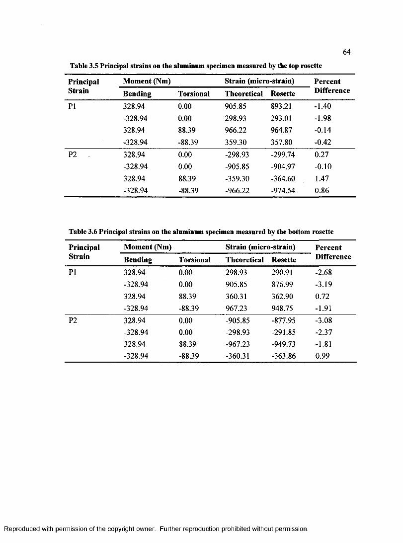
64

Table 3.5 Principal strains on the aluminum specimen measured by the top rosette

Principal Moment (Nm) Strain (micro-strain) PercentStrain Bending Torsional Theoretical Rosette Difference

PI 328.94 0.00 905.85 893.21 -1.40-328.94 0.00 298.93 293.01 -1.98328.94 88.39 966.22 964.87 -0.14-328.94 -88.39 359.30 357.80 -0.42

P2 328.94 0.00 -298.93 -299.74 0.27-328.94 0.00 -905.85 -904.97 -0.10328.94 88.39 -359.30 -364.60 1.47-328.94 -88.39 -966.22 -974.54 0.86

Table 3.6 Principal strains on the aluminum specimen measured by the bottom rosette


PI 328.94 0.00 298.93 290.91 -2.68-328.94 0.00 905.85 876.99 -3.19328.94 88.39 360.31 362.90 0.72-328.94 -88.39 967.23 948.75 -1.91

P2 328.94 0.00 -905.85 -877.95 -3.08-328.94 0.00 -298.93 -291.85 -2.37328.94 88.39 -967.23 -949.73 -1.81-328.94 -88.39 -360.31 -363.86 0.99


65

Table 3.7 Principal strains on the fibreglass specimen in poor agreement


PI 384.71 0.00 551.14 351.90 -36.15-384.71 0.00 154.32 89.45 -42.03384.71 144.38 754.00 546.96 -27.46-384.71 -144.38 357.18 249.53 -30.14

P2 384.71 0.00 -154.32 -90.04 -41.65-384.71 0.00 -551.14 -353.26 -35.90384.71 144.38 -357.18 -236.72 -33.72-384.71 -144.38 -754.00 -561.69 -25.51

Table 3.8 Principal strains on the fibreglass specimen in good agreement


PI 384.71 0.00 352.70 352.02 -0.19-384.71 0.00 89.78 89.48 -0.33384.71 144.38 523.87 547.11 4.44-384.71 -144.38 260.95 249.57 -4.36

P2 384.71 0.00 -89.78 -90.07 0.33-384.71 0.00 -352.70 -353.38 0.19384.71 144.38 -260.95 -236.76 -9.27-384.71 -144.38 -523.87 -561.84 7.25


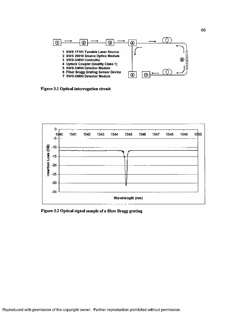
66

©

SWS 17101 Tunable Laser Source SWS 20010 Source Optics Module SWS-OMNI Controller Opteck Coupler (Quality C lass 1) SWS-OMNI Detector Module

6 Fiber Bragg Grating S ensor Device7 SWS-OMNI Detector Module

m .

r©

« D J j

Figure 3.1 Optical interrogation circuit

1---------1---------1-------- 1---------1---------1---------1---------1---------1------15(40 1541 1542 1543 1544 1545 1546 1547 1548 1549 15fe0

g -10

M8 -15

o -20 € a>8 -25

-30

-35

I f

W a v e len g th (nm)

Figure 3.2 Optical signal sample of a fibre Bragg grating


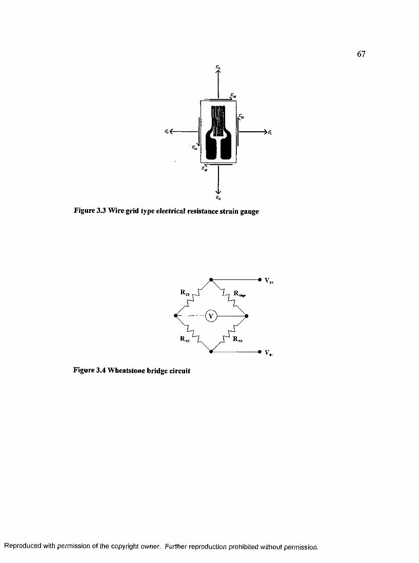
Figure 3.3 Wire grid type electrical resistance strain gauge

* V,

Figure 3.4 Wheatstone bridge circuit


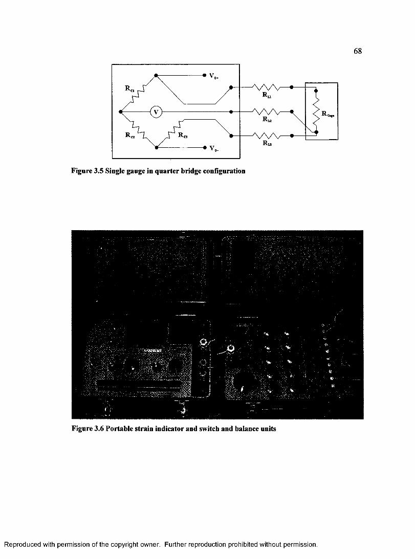
68

* v,

■L3

* V,

Figure 3.5 Single gauge in quarter bridge configuration

Figure 3.6 Portable strain indicator and switch and balance units


69

Figure 3.7 Steel support frame

Figure 3.8 Steel support plate


70

b = 2S.40 mm h = 50.80 mm t = 3.048 mm L = 812.8 mm

I„= 133772 mm A = 1076.64 mm

h

x0 = 0.000 mm x, = 25.40 mm x, = 50.80 mm x, = 76.20 mm

x 4= 101.6 mm x5 = 127.0 mm x 6= 152.4 mm x, = 177.8 mm

Figure 3.9 Aluminum section: geometric properties

f t ,

t,

b = 50.80 mm h = 101.6 mm 11 = 6.350 mm tj = 3.175 mm L = 749.3 mm

I„= 1837270 mm4 jj A = 4556.44 mm

x 0= 0.000 mm x , = 50.80 mm x ,= 101.6 mm

i j = 152.4 mm x 4 = 203.2 mm x, = 254.0 mm

Figure 3.10 Fibreglass section: geometric properties


71

Fibreglass Beam

Steel Block & Steel Base PlateSteel Plug

for Free EndSteel / Clamps

Steel Torsion Bar

Figure 3.11 Fibreglass beam: fixtures and constraints

Figure 3.12 Resolving applied loads


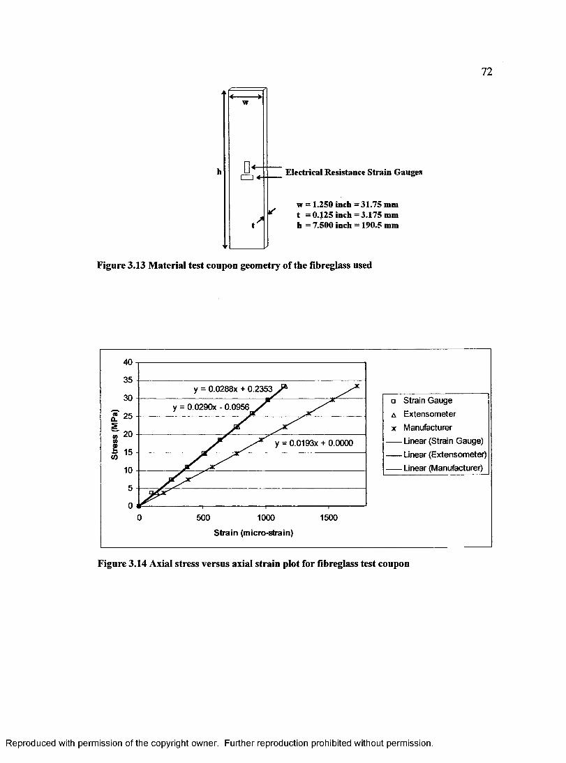
72

h Electrical Resistance Strain Gauges

w = 1.250 inch = 31.75 mm t =0.125 inch =3.175 mm h = 7.500 inch = 190.5 mm

Figure 3.13 Material test coupon geometry of the fibreglass used

40

35y = 0.0288X + 0.2353

30y = 0.0290x - 0.0956

25

20y = 0.0193x + 0.0000

15

10

5

00 500 1000 1500

S tra in (m icro-strain)

□ Strain G auge

a Extensom eter

x Manufacturer

Linear (Strain Gauge)

— Linear (Extensom eter)

Linear (Manufacturer)

Figure 3.14 Axial stress versus axial strain plot for fibreglass test coupon


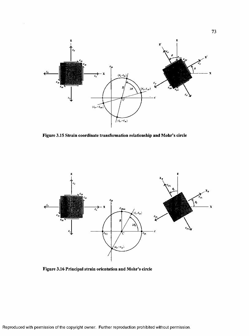
73

Figure 3.15 Strain coordinate transformation relationship and Mohr’s circle

Figure 3.16 Principal strain orientation and Mohr’s circle


Rectangular Rosette Delta Rosette0,2=45“

Gj Gi

p .. = 60°

p.,=120°

Figure 3.17 Typical electrical resistance strain gauge rosette configurations

c =

d = £ . - C

Figure 3.18 Construction of Mohr's circle using a rectangular strain gauge rosette


75

1000

800

600

400 oI . 200c

sto200 250 300 3:>0

-200

-400

B end ing M om ent (Nm)

■e— Theoretical Principal 1

-a — Theoretical Principal 2

-o— Theoretical Max S h ear

-x— Experimental Principal 1

Experimental Principal 2

-i— Experimental Max S hear

Figure 3.19 Bending strains measured by the top rosette for upright aluminum beam

1200

1000

„ 800 c| 600

40001 200c

«P2

2m -200

-400

-600

T orsional M om ent (Nm)

- a —Theoretical Principal 1

- a — Theoretical Principal 2

Theoretical Max S hear

-x — Experimental Principal 1

-x — Experimental Principal 2

- t— Experimental Max S hear

Figure 3.20 Combined bending and torsion strains measured by the top rosette for upright aluminum beam


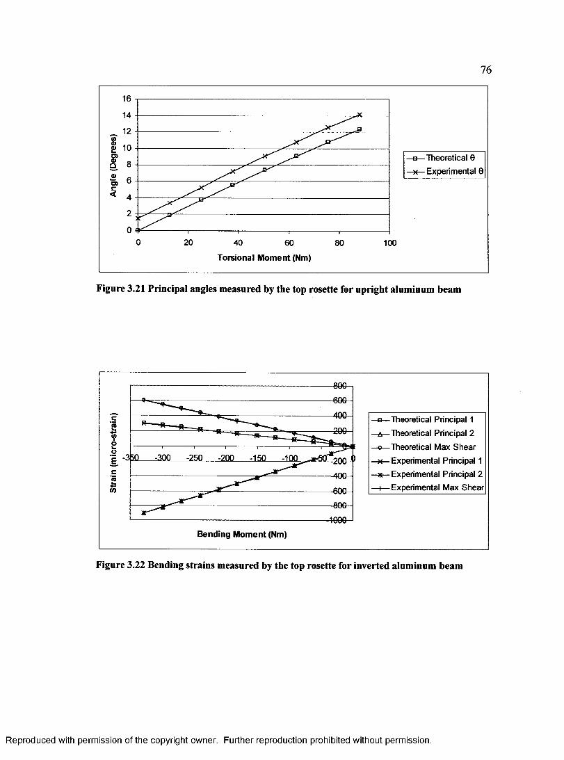
76

<0a>OJ0)Q

O)c<

16

14

12

10

8

6

4

2

00 20 40 60 80 100

—e— Theoretical 0

-x — Experimental 0


Figure 3.21 Principal angles measured by the top rosette for upright aluminum beam

6 0 0

6 0 0

4 0 0

600

p -350 -300 -250 -200 -150 -100

4 0 0

-6 0 0

-8 0 0

4000

B end ing M om en t (Nm)

e — Theoretical Principal 1

Theoretical Principal 2

-©— Theoretical Max S h ear



h— Experimental Max S hear

Figure 3.22 Bending strains measured by the top rosette for inverted aluminum beam


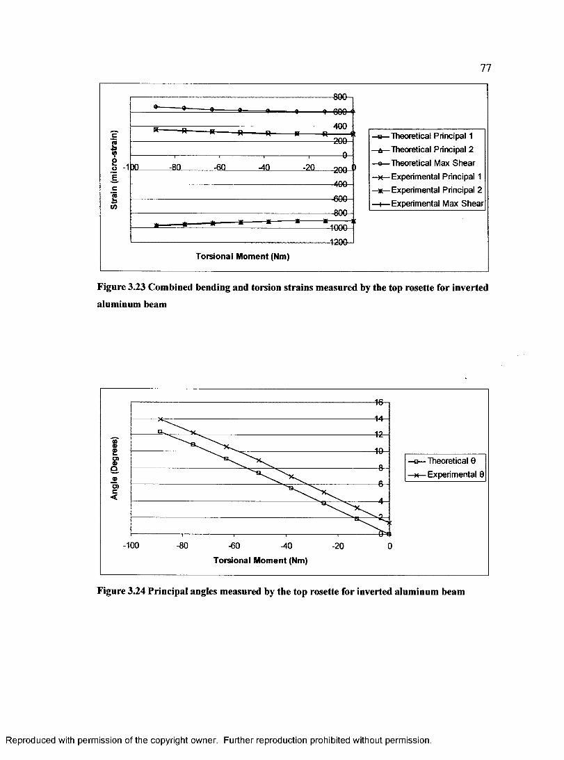
77

80fr■y-600-^— 4 0 0 -

2Q&

1 -an ^2a -20&

400-

-60&

-soa

Torsional M oment (Nm)

—b— Theoretical Principal 1

—a — Theoretical Principal 2

—e— Theoretical Max S h ear

—x— Experimental Principal 1

—*— Experimental Principal 2

—i— Experimental Max S hear

Figure 3.23 Combined bending and torsion strains measured by the top rosette for inverted aluminum beam

v><u£o><0o

<3)c<

-100 -80 -60 4 0 -20 0

Torsional M om ent (Nm)

—b— Theoretical 0

—x — Experimental 0

Figure 3.24 Principal angles measured by the top rosette for inverted aluminum beam


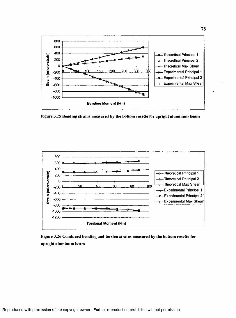
78

800

600

~ 400

3 200«PS 001 -200c3to -600

100___ 150___ 200___ 250___ 300___ 3 i0

-400

-800

-1000B end ing M om en t (Nm)

■e— Theoretical Principal 1

-a—Theoretical Principal 2

-©— Theoretical Max S hear




Figure 3.25 Bending strains measured by the bottom rosette for upright aluminum beam

800

600

400

2000

2CL 40. TOO

-600

-800

-1000-1200

T orsional M om en t (Nm)

■b—Theoretical Principal 1

-a — Theoretical Principal 2

-©— Theoretical Max S hear


-*— Experimental Principal 2


Figure 3.26 Combined bending and torsion strains measured by the bottom rosette for upright aluminum beam


79

18

16

14

1210

864

20

0 20 40 60 80 100


-b— Theoretical 0

•*— Experim ental 0

Figure 3.27 Principal angles measured by the bottom rosette for upright aluminum beam


—a— Theoretical Principal 1

a Theoretical Principal 2

—e— Theoretical Max S h ear

— Experimental Principal 1

—*— Experimental Principal 2

—i— Experimental Max S h ear

Figure 3.28 Bending strains measured by the bottom rosette for inverted aluminum beam


80

800cs<pooE

=9=gQQ=*i

— 4 0 0 -

200c

-80 -60 4 0 -20<n ■200

400

-600


—s — Theoretical Principal 1


—©— Theoretical Max S h ear



—i— Experimental Max S h ear

Figure 3.29 Combined bending and torsion strains measured by the bottom rosette for inverted aluminum beam

M©O)©Q©O)c<

-100 -80 -60 4 0 -20 0T orsional M om ent (Nm)

■e— Theoretical 0

Experimental 0

Figure 3.30 Principal angles measured by the bottom rosette for inverted aluminum beam


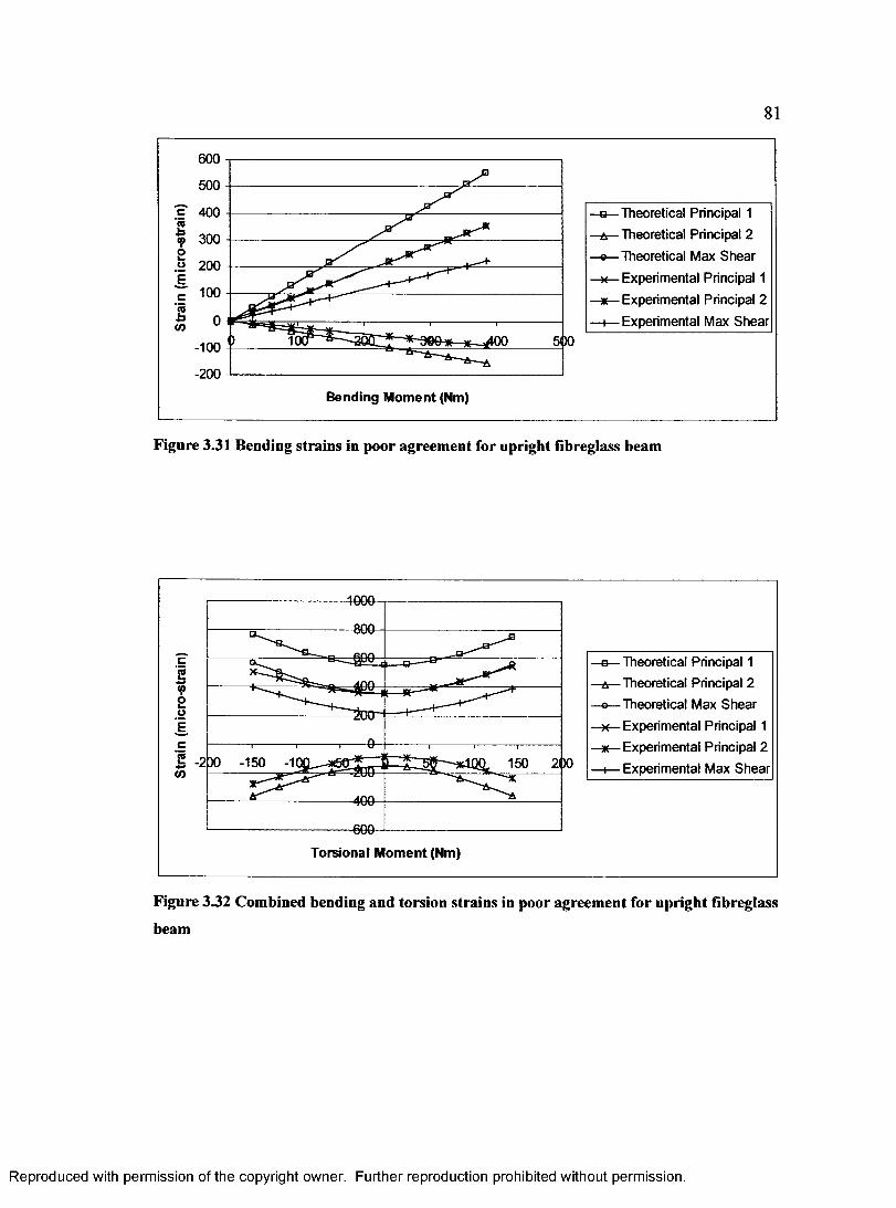
81

600

500

400

300

200

100

500-100

-200B end ing M om en t (Nm)


Theoretical Principal 2

—©— Theoretical Max S hear

—* — Experimental Principal 1



Figure 3.31 Bending strains in poor agreement for upright fibreglass beam

--------------------------------- 4Q0Q—

©no

.... 600

.*00'— ^ ^

(--------

o

X) -150 150 2l--------- >1''__-zUO—

100

-----------------------------------6 0 0 -








Figure 3.32 Combined bending and torsion strains in poor agreement for upright fibreglass beam


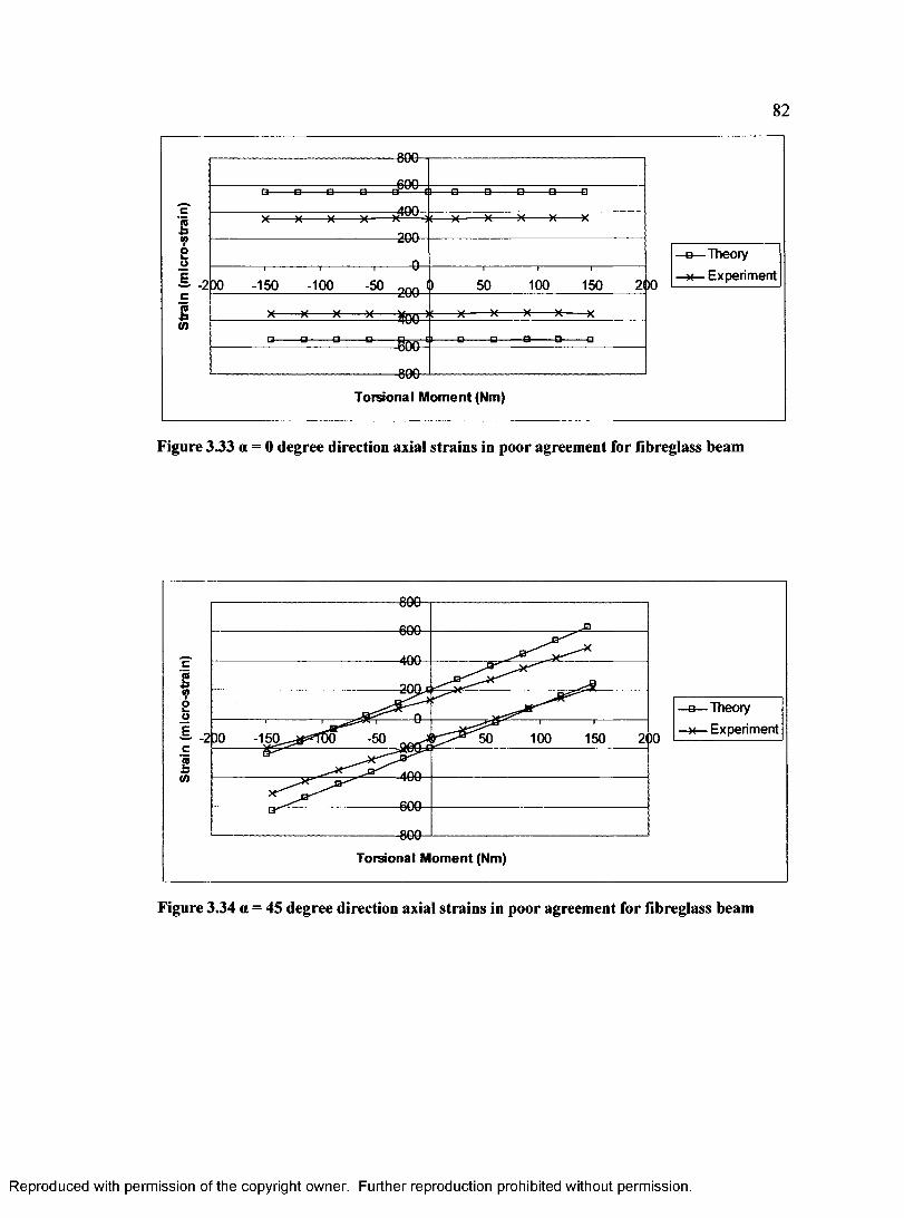
82

c

3 0 08oE 100 200-150 -100 -50 150c1(0

800—1------------------


□ Theory

— Experiment

Figure 3.33 a = 0 degree direction axial strains in poor agreement for fibreglass beam

000

000

4 0 0cs<poL.o _

-2 DO c —sCO —

-150 -50 100 150 200

4 0 0

•600

800—1------------------


-a— Theory

-x — Experiment

Figure 3.34 a = 45 degree direction axial strains in poor agreement for fibreglass beam


83

500

csoE 21)0-150 -100 -50 100 150csto

b150

-200-J-------------T orsional M om ent (Nm)

—a— Theory

—x — Experiment

Figure 335 a = 90 degree direction axial strains in poor agreement for fibreglass beam

400

500500cs

«p2oE -150 -100 100 200-50 150cIto 500

500

--------- 400-J----------------


-a— Theory

-x — Experim ent

Figure 336 a = 0 degree direction axial strains in good agreement for fibreglass beam


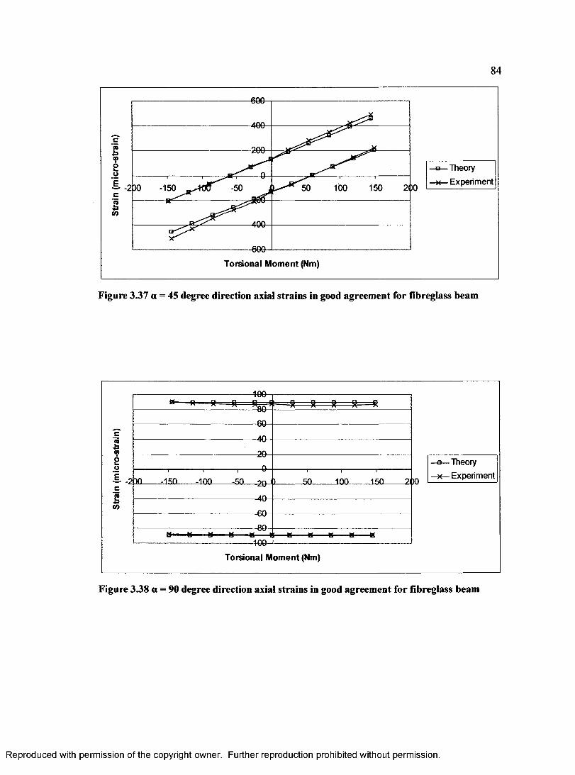
84

£00

400c£<ps

509

uI -150 -50 100 150 200c£CO

400

-600—'----------------Torsional M om en t (Nm)

-a— Theory

- x — Experiment

Figure 3.37 a = 45 degree direction axial strains in good agreement for fibreglass beam

c£o01 too 150 200c£CO

106—1----------------T orsional M om ent (Nm)

-q— Theory

Experiment

Figure 3.38 a = 90 degree direction axial strains in good agreement for fibreglass beam


85

400350300250200150100500

-50-100-150

4Q&

Bending M om ent (Nm)




—k — Experimental Principal 1



Figure 339 Bending strains in good agreement for upright fibreglass beam



—a—Theoretical Principal 2





Figure 3.40 Combined bending and torsion strains in good agreement for upright fibreglass beam


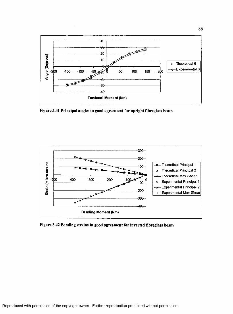
86

o>

-150 -100 -50 100 150 21)0o>


■a— Theoretical 0

Experimental 0

Figure 3.41 Principal angles in good agreement for upright fibreglass beam

-3G&

20&

= -5 t̂oo -300 -200

■2G&

-30&

40&Bending M om ent (Nm)




—x — Experimental Principal 1



Figure 3.42 Bending strains in good agreement for inverted fibreglass beam


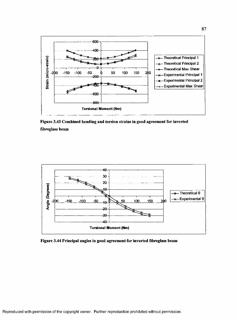
87

■b «P o.2 -2 E. cS ■**

CO

-600-

DO -150 -100 -50t-------- r*

50 100 150 200- 200-

--------- i ----£

-600-

-8 0 0 -


-b—"Theoretical Principal 1

- a— Theoretical Principal 2

-o— Theoretical Max S h ear



-h— Experimental Max S h ear

Figure 3.43 Combined bending and torsion strains in good agreement for inverted

fibreglass beam

o>

100 150-150 -100 -50 21)0o>

T o rs io n al M om en t (Nm)

-a — Theoretical 9

-x — Experim ental 0

Figure 3.44 Principal angles in good agreement for inverted fibreglass beam


88

CHAPTER 4: FBG SENSOR TESTING AND RESULTS

4.0 Introduction

The cantilever beam specimens validated in Chapter 3 were used to experimentally test

FBG sensors. The experimental tests that were carried out using these sensors are

described in this Chapter. A range of practical issues are addressed; they include sensor

installation, data collection and processing, identifying potential sources of error and

establishing quantitative estimates of their influence on the FBG strain measurement

results. The FBG measured strains are then graphically and numerically compared with

the theoretical and rosette measured axial strains for each sensor in its particular

orientation. A discussion of the experimental results and errors is then presented, placing

particular focus on the influence of transverse strain components in FBG sensor

measurements and the interaction of FBG sensors with the adhesive. To this end,

projections are made for the expected strain-optic behaviour of FBG sensors embedded

within thin fibre reinforced laminate shell structures.

4.1 Sensor Installation

Each sensor was written into its own optical fibre using the phase mask technique as

described in Section 2.3.1 and was installed on the test specimen surface using an


89

adhesive. The cladding was stripped away from the fibre during the writing process,

leaving the sensor bare. The adhesive will thus act as a cladding to the sensor, and must

exhibit the appropriate optical and mechanical properties to prevent the loss of optical

signal and provide adequate adhesion.

To prevent loss of optical signal, the refractive index of the adhesive must be lower

than that of the fibre, however, refractive indices are not values typically published by

adhesive manufacturers. Specialty coatings with known refractive indices could be used

to re-coat the bare sensors prior to adhesion. However this would likely reduce the

transfer of strain into the sensor as was suggested by Pak (1992). It was noted by Lin et

al. (2005) that the adhesive layer between the sensor and specimen will behave similar to

a coating and affect the transfer of strain into the sensor. No coatings were applied to

sensors during these experiments.

The first adhesive used was a two part room temperature curing epoxy/hardener

(LePage Regular Epoxy 11); epoxy is typical of the material used as the matrix in fibre

reinforced composite laminate structures. The second adhesive used was a one part room

temperature curing cyanoacrylate adhesive (Loctite Super Glue Brush-on) and is typical

of the adhesive used for installation of strain gauges on test specimens. Neither

manufacturer was able to provide mechanical properties for their adhesives, however

values listed in Table 4.1 were estimated based on comparable adhesive products and the

values measured by Olivier et al. (1992) using the nano-indendation technique for

determining the modulus of thin coatings.


90

The installation technique and procedure must be consistent for the mounting of each

sensor. Geometric deviations such as adhesive thickness and curvature of the fibre may

produce inconsistencies between sensor readings. Minimizing the thickness of adhesive

between the sensor and specimen surface improves the transfer of strain to the sensor as

confirmed by Lin et al. (2005). The bare sensors were therefore installed in direct contact

with the specimen surfaces, and adhesive applied around them.

To prevent the sensor from taking a curved path while the adhesive cured, a slight

tension was applied to the fibre using pieces of adhesive tape. The epoxy/hardener took

several hours to fully cure at room temperature, during which the tape slowly released

tension on the fibre, and resulted in an arc-shaped path. Additional constraints were

therefore applied as shown in figure 4.1 by clamping a rubber pad with a channel cut into

it over the sensor to hold it in alignment while the adhesive cured; a release film was used

to prevent the rubber pad from adhering to the specimen. The cured epoxy/hardener

adhesive surrounding the sensor was minimal, coating only the upper and side surfaces

and filleting the lower section of the sensor to the test specimen as shown in figure 4.1.

The cyanoacrylate adhesive cured within minutes and required no additional constraints

to keep the sensors in alignment. The cured cyanoacrylate adhesive surrounding the

sensor formed a slightly convex shape as shown in figure 4.1.

Tensions and contact pressures applied during curing of the adhesive leave residual

strains in the sensor, which cause a permanent distortion of the Bragg peak in its optical

signal. Sensors embedded in a composite structure would be exposed to vacuum or

autoclave pressures and temperatures while curing and may result in significant signal


91

distortion. The Bragg peaks of sensors may also reduce in strength during the cure cycle

of a laminate if using a high temperature adhesive. This is because exposure to elevated

temperatures increases diffusion rates, and would thereby cause the Bragg grating pattern

to fade because its original formation was due to a diffusion based process. A new

generation of Bragg gratings, known as surface relief Bragg gratings, are under

investigation by Smith et al. (2006) where the grating is physically etched into the core of

the fibre, making the sensors stable when exposed to high temperatures. As long as the

distorted and faded optical signal contains a noticeable and measurable Bragg peak,

residual strain and temperature exposure effects during the installation process can be

neglected. This is because additional applied strain will be superimposed over the

residual strain, thereby shifting the distorted optical signal according to the same strain-

optic relationship as an undisturbed sensor.

Each sensor was connected to the optical circuit during installation to examine

distortion and changes of the optical signal. Figure 4.2 shows the optical signal o f a tilted

FBG sensor measured in transmission before and after installation. The noticeable

changes are a wavelength shift of all the peaks caused by the applied tension, and

changes in wavelengths and strengths of the other peaks, which correspond to a change in

the power coupling behaviour of the tilted gratings to radiation modes; the changes seen

in these peaks are due to the refractive index change from air to adhesive surrounding the

sensor core.


92

4.2 Sensor Properties and Optical Signals

Eight FBG sensors were experimentally tested in total; two sensors on the aluminum

beam and six sensors on the fibreglass beam. Each sensor was adhesively bonded onto

either the top or bottom surface of the specimen at approximate orientations of 0, 45, or

90 degrees. The specific location and orientation of each sensor was measured after

installation and is listed in Table 4.2 along with the type of adhesive used.

The eight sensors were not identical in design, resulting in a range of optical signals,

but all contained a noticeable and measurable Bragg peak. Some sensors had dual

overwritten gratings, some had tilted gratings, and some were typical planar gratings.

They should, in theory, all reflect a Bragg peak corresponding to their grating pitch along

the centreline of the fibre, and should all respond equally to applied strains. Some

sensors were measured using the transmission spectrum, while others were measured

using the reflection spectrum or both. The final optical signals, after distortions caused

during installation, are shown in figures 4.3 - 4.10 for sensors 1 -8 respectively.

The mechanical and optical properties of an FBG sensor are essentially the same as

the optical fibre they are written in. All experimentally tested sensors were written in

germanium-doped silica glass optical fibre which, according to Prabhugoud and Peters

(2006), has the mechanical and optical properties as listed in Table 4.1. The diameter of

the multi-mode fibre was measured using micrometers to be approximately \25/j.m.


93

4.3 Collection and Processing of Optical Signal Data

Due to the absolute resolution of the SWS-OMNI system, the wavelength accuracy of

any given data set is inherently ±2p m , equating to a high strain resolution of ±1,6ps for

a 1550wn FBG. Table 4.3 shows a typical set of the raw optical signal data that was

collected for each load and there exists a Bragg peak. The wavelength at which the

minimum insertion loss value occurs was not consistently located within the peak. The

tip of the peak flattens as shown in figure 4.11, allowing the minimum to be located

randomly among several adjacent points. This random signal error can be reduced by

applying a simple computational algorithm to each data set and consistently determine a

centre wavelength for the Bragg peak as described below.

The peak is generally located by finding the minimum insertion loss of the signal and

applying any offset may be required if the minimum value is not located in the Bragg

peak as is typical of a tilted grating shown in figure 4.3. The wavelengths where the

optical signal intersects a designated power threshold on each side of the peak such as

those shown in figure 4.12 are calculated by linearly interpolating within the

corresponding measurement interval. The centre wavelength of the peak is computed as

given by equation 4.1, where AR and AL are the wavelengths at threshold, Carson (2006).

( An + A, )C W = ^ ( 4.1)

2

The threshold is typically set at 3dB above the minimum insertion loss, but can be set

to any value intersecting the optical signal peak where it is consistently clear. The centre

wavelength for each sensor at no load is listed in Table 4.2 and shown graphically in the


94

optical signal plots of figures 4.3 to 4.10. The improvement to signal alignment using

this method is shown by figure 4.12 and corresponds to a reduction in random error by

approximately ±12pm for transmission and ±20pm for reflection signals, or ±10/is and

±16he respectively for a 1550n/w FBG sensor.

The shift of centre wavelength shown in figure 4.13 is calculated for each applied

load by referencing the centre wavelength of a zero load data set. Due to thermal

sensitivity of FBG sensors, the centre wavelength may vary slightly over time. Zero load

data sets were therefore recorded immediately prior to any series of sensor measurements

to be used as the corresponding centre wavelength reference. An additional zero load set

was recorded at the end of each series to observe any change in ambient temperature that

may have occurred. The ‘false’ strain reading indicated by the zero load set at the end of

a measurement series would equate to a change in ambient temperature as shown in

figure 4.14. This figure equates thermal and strain induced centre wavelength shifts o f a

1550nm sensor and accounts for thermal expansion of the test specimen using the

appropriate coefficients of thermal expansion as listed in Table 3.3. This method does

not eliminate the effects of localized random temperature fluctuations, which would

introduce random errors into the observed strain measurements proportional to their

magnitudes as shown by figure 4.14. A temperature discrimination technique was not

deemed necessary during these experiments because of the relatively stable thermal

environment in the CLLIPS laboratory.


95

4.4 Sensor Experimental Results

Having calculated the shift of centre wavelength for each applied load, it can be

converted into an apparent strain using equation 2.7 with an optical gauge factor of 0.795,

as derived in Chapter 2. The apparent strain of each FBG sensor is compared to the

theoretical and rosette measured strain components of the test specimen that are acting in

the axial orientation of the sensor. This comparison is presented graphically for each

sensor by two figures; the first figure compares strain values for applied bending loads,

while the second figure compares strain values for application of combined bending and

torsion at constant bending load values; figures 4.15 - 4.30 thus correspond to FBG 1 - 8

sequentially in pairs. Tables 4.4 and 4.5 present a numerical comparison of these strain

values at maximum and minimum applied load combinations.


FBG 1 and FBG 2 were installed on the aluminum test specimen using epoxy/hardener

adhesive at the locations indicated in Table 4.2. Both sensors were of the tilted grating

type. Their optical signals, as shown in figures 4.3 and 4.4, were measured in

transmission.

The apparent strain measured by FBG 1 is in agreement within 2% and a difference

of 13 micro-strain of the theoretical axial strain component as shown in Table 4.4. The

range of axial strain applied to this sensor was approximately -900fie to +900u s ,

corresponding to an approximate Bragg wavelength shift of -1.1 lww to +1.11 nm. The

measured response of FBG 1 to applied bending loads was linear as shown in figure 4.15,


96

and because it was oriented at approximately 1.75 degrees, its measured response to

applied torsional loads was negligible as shown in figure 4.16.



range of axial strain applied to this sensor was approximately -630 jj.e to +630/ie ,

corresponding to an approximate Bragg wavelength shift of -0.775nm to +0.775n m .

The measured response of FBG 2 to applied bending loads was linear as shown in figure

4.17, and because it was oriented at approximately -42 degrees, its measured response to

applied torsional loads was also linear as shown in figure 4.18.


FBG 3, FBG 4, and FBG 5 were installed on the fibreglass test specimen using

epoxy/hardener adhesive at the locations indicated in Table 4.2. FBG 3 had dual Bragg

peaks in its optical signal and was measured in reflection as shown in figure 4.5, whereas

FBG 4 and FBG 5 had only single Bragg peaks in their optical signals and were measured

in transmission as shown in figures 4.6 and 4.7 respectively. FBG 6, FBG 7, and FBG 8

were installed on the fibreglass test specimen using cyanoacrylate adhesive at the

locations described in Table 4.2. All three sensors had single Bragg peaks and were

measured in both transmission and reflection as shown in figures 4.8 - 4.10.



range of axial strain applied to this sensor was approximately -335pis to +335^ ie ,


97

corresponding to an approximate Bragg wavelength shift of -0.437nm to +0.437nm.


4.19, and because it was oriented slightly off the beam axis at approximately -6 degrees,

its measured response to applied torsional loads was very small, but still linear as shown

in figure 4.20.



range of axial strain applied to this sensor was approximately -450/us to +250jue,

corresponding to an approximate Bragg wavelength shift of -0.553ww to +0.307nm.


4.21, and because it was oriented at approximately 49 degrees, its measured response to




range of axial strain applied to this sensor was approximately -90 /is to +90f ie ,

corresponding to an approximate Bragg wavelength shift of -O.llOww to +0.11 Onm.


4.23, and because it was oriented at approximately 89.5 degrees, its measured response to




range of axial strain applied to this sensor was approximately -350 fjs to +350fj.e,


98

corresponding to an approximate Bragg wavelength shift of -0.433ww to +0.433nm .






range of axial strain applied to this sensor was approximately -410/is to +410/ie,

corresponding to an approximate Bragg wavelength shift of -0.511 nm to +0.511nm.






range of axial strain applied to this sensor was approximately -100/is to +100/ is ,

corresponding to an approximate Bragg wavelength shift of -0.124n/w to +0.124w/w.


4.29, and because it was oriented at approximately 89.5 degrees, its measured response to


The strain range achieved using the fibreglass specimen was lower than originally

planned due to a larger than desired thickness of the top and bottom surface walls. In

addition, the elastic modulus of the material was found to be significantly higher than the

published value.


99

4.5 Discussion of Results and Errors

Each FBG sensor was shown in Section 4.4 to respond linearly in proportion to bending

and torsional loads as was expected for their measured orientations. For the most part,

there was reasonable numerical agreement between the apparent strain and the theoretical

axial strain component; thus showing that equation 2.7 predicts with reasonable accuracy

the strain induced wavelength shift of an FBG adhered to a structure. However, during

the last set of experiments, using FBG 6, FBG 7, FBG 8 and the cyanoacrylate adhesive,

there was a noticeable difference in the agreement of the strain results as shown in Table

4.5. The source of this error was believed to be an increased transverse sensitivity of the

FBG sensors due to use of the cyanoacrylate adhesive. Before examining this issue, a

brief review of other possible sources of error is in order to establish some quantitative

estimates of their contribution to the total disagreement. Error quantities estimated will

be those typical of a 1550nm centre wavelength FBG sensor.

4.5.1 Data Collection and Processing

Processing the data sets using the centre wavelength algorithm described in section 4.3

was found to reduce signal alignment errors to within approximately ±0.5pm and can

account for an error of approximately ± 0 A p e. The SWS-OMNI system resolution of

±2pm can account for a strain error of approximately ±1.6p s within any data set no

matter how accurately it is processed. Data collection and processing can thus account

for a total strain error of approximately +2.Ope.


100

4.5.2 Thermal Effects

Changes to ambient temperatures were observed by calculating the centre wavelength

shifts between the zero load data sets recorded at the beginning and end of each

measurement series. The greatest shift observed among all series was approximately

5pm and according to equation 2.7 can account for a maximum strain error of

approximately ±4.1 fxe. Figure 4.14 shows that depending on which test specimen the

sensor is installed, this error equates to no more than an ambient temperature change of

±0.4 °C during any series of data measurements. Localized temperature fluctuations

would not be able to account for any noticeable and consistent deviation of the data series

trend from theory, as this would imply a consistent source of error. By observing a data

series consisting entirely of zero load sets, it was found that the localized temperature

fluctuations can be slightly larger than the measured ambient temperature changes, and

would thus increase the error by approximately ±1.5//£. Thermal effects during these

experiments are therefore estimated to account for a total strain error of approximately

±5.6h e , showing that the CLLIPS laboratory environment was thermally stable within

an approximate range of ±0.55°C .

4.5.3 Position and Alignment

The position of each sensor was confirmed to be accurate within ±1.0mm as listed in

Table 4.2 by measuring their relative position to the rosettes using a set of Vernier

calipers. The resulting strain error is at most ±0.16%, corresponding to an extremely

small error of ±0.6//f, ±0.8/us, and ±0.2fis for FBG 6, FBG 7, and FBG 8 respectively.


101

A slight misalignment of a sensor from its orientation as listed in Table 4.2 could account

for strain values to consistently measure above or below the theoretically predicted values

during bending; however, this would cause an increased disagreement between the

measured values observed during combined bending and torsion. By varying the

measured orientations of a sensor, an improvement of approximately ±2.0/js could be

observed before other values would exceed this disagreement. The error due to

misalignment is also bound by Mohr’s circle and cannot account for a sensor measuring

strain values exceeding the limits established by the principal strains as was the case with

FBG 8 shown in figures 4.29 and 4.30.

4.5.4 Summary of Experimental Errors

By combining the strain error estimates, an average strain error of approximately

± 10.5/iff was estimated, primarily attributed to thermal sources. This magnitude is close

and consistent with the deviations of FBG sensors 1 - 5 noted in Tables 4.4 and 4.5.

After accounting for this error, the remaining unaccounted for errors of FBG 6, FBG 7

and FBG 8 are approximately -4.5% , +2.3% and +9.9% respectively. The error of

sensor 7 is acceptably low considering the theoretical solution agreed less with the rosette

measurements during combined bending and torsion. The error of sensor 6 may have

been caused by bond degradation, thus reading consistently lower than the theoretical

value. The error of sensor 8 however can only be attributed to an increased transverse

sensitivity in the sensors caused by the use of cyanoacrylate adhesive. A quick review of


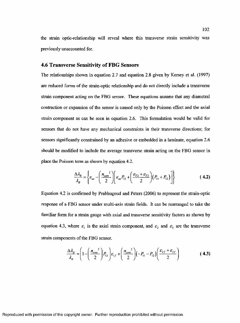
102

the strain optic-relationship will reveal where this transverse strain sensitivity was

previously unaccounted for.

4.6 Transverse Sensitivity of FBG Sensors

The relationships shown in equation 2.7 and equation 2.8 given by Kersey et al. (1997)

are reduced forms of the strain-optic relationship and do not directly include a transverse

strain component acting on the FBG sensor. These equations assume that any diametral

contraction or expansion of the sensor is caused only by the Poisson effect and the axial

strain component as can be seen in equation 2.6. This formulation would be valid for

sensors that do not have any mechanical constraints in their transverse directions; for

sensors significantly constrained by an adhesive or embedded in a laminate, equation 2.6

should be modified to include the average transverse strain acting on the FBG sensor in

place the Poisson term as shown by equation 4.2.

M b( i \ n*core &Y2 (4.2)

Equation 4.2 is confirmed by Prabhugoud and Peters (2006) to represent the strain-optic

response of a FBG sensor under multi-axis strain fields. It can be rearranged to take the

familiar form for a strain gauge with axial and transverse sensitivity factors as shown by

equation 4.3, where £] is the axial strain component, and e2 and f 3 are the transverse

strain components of the FBG sensor.

1 - £ \ f + {-P u-P n)r £ + £ '2 / 3/ (4.3)


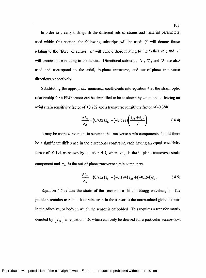
103

In order to clearly distinguish the different sets of strains and material parameters

used within this section, the following subscripts will be used: ‘f will denote those

relating to the ‘fibre’ or sensor; ‘a ’ will denote those relating to the ‘adhesive’; and 7 ’

will denote those relating to the lamina. Directional subscripts 7 ‘2 ’, and ‘3 ’ are also

used and correspond to the axial, in-plane transverse, and out-of-plane transverse

directions respectively.

Substituting the appropriate numerical coefficients into equation 4.3, the strain optic

relationship for a FBG sensor can be simplified to be as shown by equation 4.4 having an

axial strain sensitivity factor of +0.732 and a transverse sensitivity factor of -0.388.

A An /„ „ ___n\ ( ̂ 2/ ^3/

Ab= (0.732) s]f + (-0.388) (4.4)

It may be more convenient to separate the transverse strain components should there

be a significant difference in the directional constraint, each having an equal sensitivity

factor of -0.194 as shown by equation 4.5, where s2f is the in-plane transverse strain

component and e3f is the out-of-plane transverse strain component.

A/L js_= (0.732) exf + (-0.194) e2f + (-0.194) e3f ( 4.5)

Equation 4.5 relates the strain of the sensor to a shift in Bragg wavelength. The

problem remains to relate the strains seen in the sensor to the unrestrained global strains

in the adhesive, or body in which the sensor is embedded. This requires a transfer matrix

denoted by [7}a] in equation 4.6, which can only be derived for a particular sensor-host


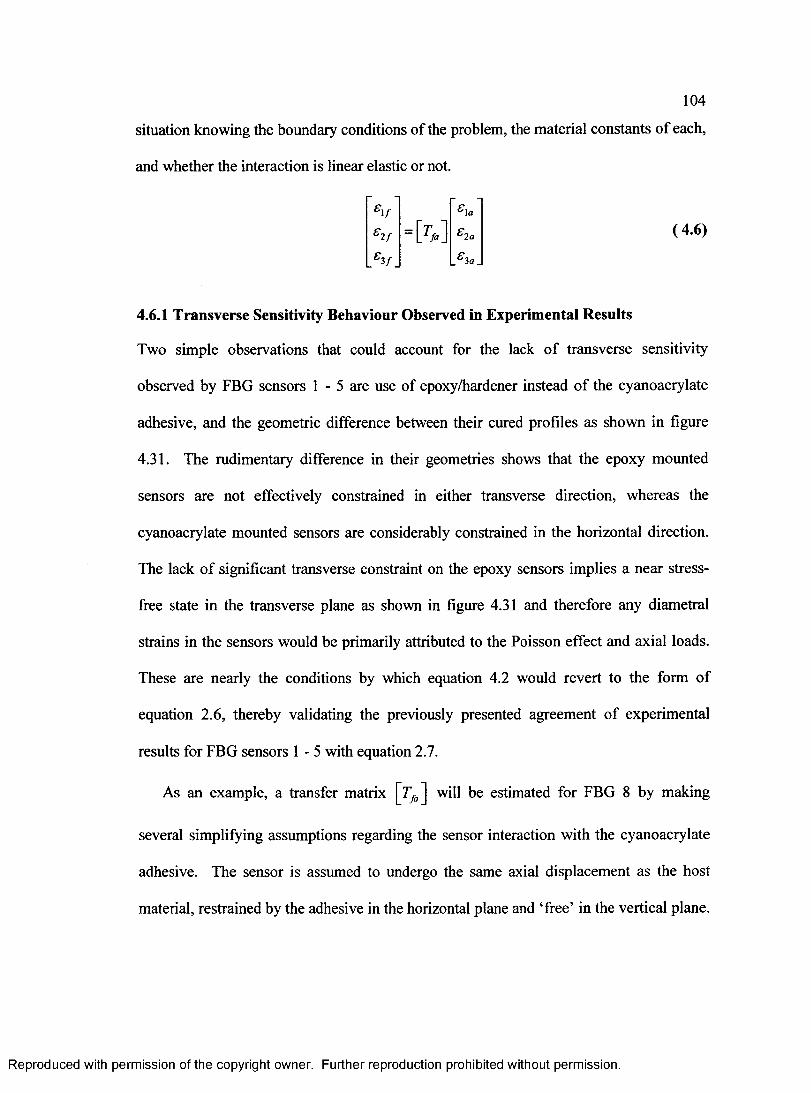
104

situation knowing the boundary conditions of the problem, the material constants of each,

and whether the interaction is linear elastic or not.

*1 / ’ *!«"

S 2 f *2 a

_*3 a.

4.6.1 Transverse Sensitivity Behaviour Observed in Experimental Results

Two simple observations that could account for the lack of transverse sensitivity

observed by FBG sensors 1 - 5 are use of epoxy/hardener instead of the cyanoacrylate

adhesive, and the geometric difference between their cured profiles as shown in figure

4.31. The rudimentary difference in their geometries shows that the epoxy mounted

sensors are not effectively constrained in either transverse direction, whereas the

cyanoacrylate mounted sensors are considerably constrained in the horizontal direction.

The lack of significant transverse constraint on the epoxy sensors implies a near stress-

free state in the transverse plane as shown in figure 4.31 and therefore any diametral

strains in the sensors would be primarily attributed to the Poisson effect and axial loads.

These are nearly the conditions by which equation 4.2 would revert to the form of

equation 2.6, thereby validating the previously presented agreement of experimental

results for FBG sensors 1 -5 with equation 2.7.

As an example, a transfer matrix J will be estimated for FBG 8 by making

several simplifying assumptions regarding the sensor interaction with the cyanoacrylate

adhesive. The sensor is assumed to undergo the same axial displacement as the host

material, restrained by the adhesive in the horizontal plane and ‘free’ in the vertical plane.


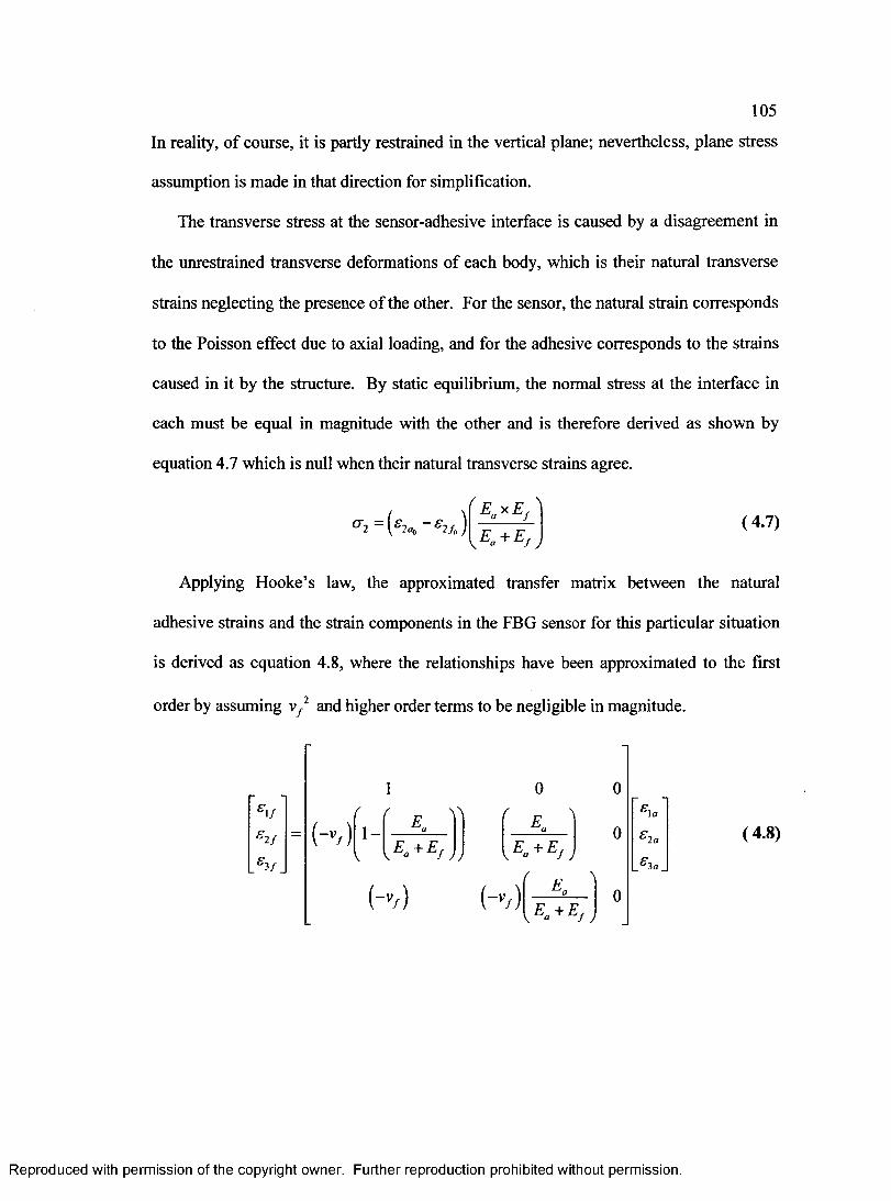
105

In reality, of course, it is partly restrained in the vertical plane; nevertheless, plane stress

assumption is made in that direction for simplification.

The transverse stress at the sensor-adhesive interface is caused by a disagreement in

the unrestrained transverse deformations of each body, which is their natural transverse

strains neglecting the presence of the other. For the sensor, the natural strain corresponds

to the Poisson effect due to axial loading, and for the adhesive corresponds to the strains

caused in it by the structure. By static equilibrium, the normal stress at the interface in

each must be equal in magnitude with the other and is therefore derived as shown by

equation 4.7 which is null when their natural transverse strains agree.

° 2 ~ (^2«d € 2 f0 )' Eg*Ef '

K E ° + E f J

(4.7)

Applying Hooke’s law, the approximated transfer matrix between the natural

adhesive strains and the strain components in the FBG sensor for this particular situation

is derived as equation 4.8, where the relationships have been approximated to the first

order by assuming vf 2 and higher order terms to be negligible in magnitude.

'i/' 2 /

' 3 /

K )f r w

i -Ea + E f

\ a f j j

K )

E + E

K ) E + Ef J

'2 a

'3 a

(4.8)


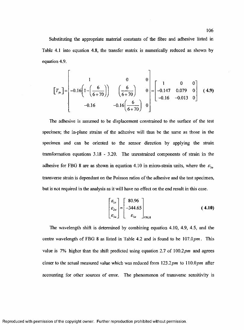
106

Substituting the appropriate material constants of the fibre and adhesive listed in

Table 4.1 into equation 4.8, the transfer matrix is numerically reduced as shown by

equation 4.9.

1

-0.16 1 - 6 )]/

1 6 + 70 J , V

0

6

-0.16 -0.16

6 + 70 )

' 66 + 70.

1 0 0-0.147 0.079 0-0.16 -0.013 0

(4.9)

The adhesive is assumed to be displacement constrained to the surface of the test

specimen; the in-plane strains of the adhesive will thus be the same as those in the

specimen and can be oriented to the sensor direction by applying the strain

transformation equations 3.18 - 3.20. The unrestrained components of strain in the

adhesive for FBG 8 are as shown in equation 4.10 in micro-strain units, where the e3a

transverse strain is dependant on the Poisson ratios of the adhesive and the test specimen,

but is not required in the analysis as it will have no effect on the end result in this case.

(4.10)

F B G 8

X , " ‘ 80.96 "

S 2 a- -344.65

. £ 1 a . * 3 a

The wavelength shift is determined by combining equation 4.10, 4.9, 4.5, and the

centre wavelength of FBG 8 as listed in Table 4.2 and is found to be \ 07.0pm . This

value is 7% higher than the shift predicted using equation 2.7 of 100.2pm and agrees

closer to the actual measured value which was reduced from 123.2pm to 110.0pm after

accounting for other sources of error. The phenomenon of transverse sensitivity is


107

therefore shown to be a logical explanation for the experimentally observed

measurements of FBG 8 being consistently higher than the theoretical and rosette values.

4.6.2 Transverse Sensitivity of Embedded Sensors in a Laminate

When embedding sensors into a laminate, the transverse interaction of the sensor with the

host material is considerably more complex than the example presented in Section 4.6.1.

Although the experimental work carried out in this study did not include laminates, it is

nevertheless useful to discuss briefly this issue here. A sensor at an angled orientation to

laminate fibres would form a small resin pocket around it as shown in figure 4.32, whose

size, shape and symmetry are dependant on the relative orientations of the sensor to the

adjacent laminae. These defects pose a significant structural threat to thinner laminates;

in contrast, Skontorp (2002) showed that a sensor installed in parallel with the

unidirectional fibres caused almost negligible detriment. The variable boundary

conditions of these resin pockets surrounding the sensor in the transverse plane and along

its axis make it difficult to accurately predict the interaction of the sensor with the host

material. This issue will not be further addressed here; it could be more effectively

investigated using numerical methods, such as the boundary element or finite element

methods.

By considering the simpler case when a sensor is installed in parallel with

unidirectional fibres of a laminate, an estimate of the transverse interaction between a

FBG sensor and a lamina of properties similar to the laminate can be made. The estimate

assumes the lamina is transversely isotropic; that the sensor is completely and elastically

bound within the lamina; that the sensor undergoes the same axial strain as the lamina;


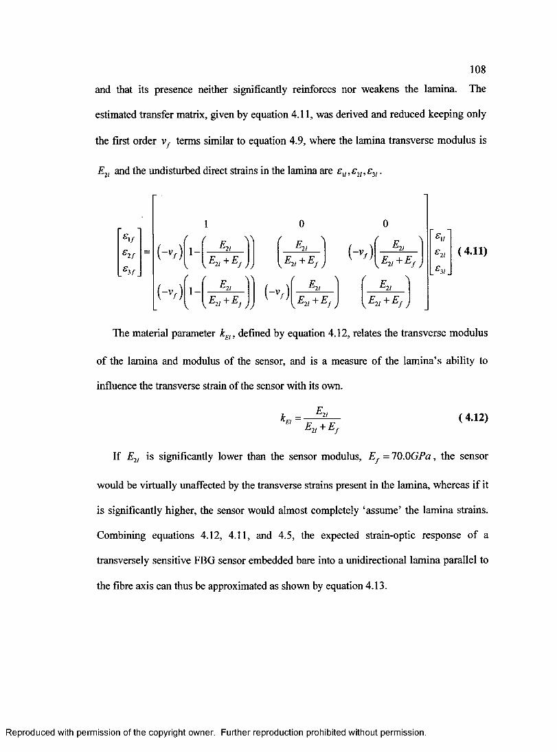
108

and that its presence neither significantly reinforces nor weakens the lamina. The

estimated transfer matrix, given by equation 4.11, was derived and reduced keeping only

the first order vf terms similar to equation 4.9, where the lamina transverse modulus is

E2l and the undisturbed direct strains in the lamina are su,s2l,s 2l.

'if' i f H )

K )

1 - '2I\ En + E f ) )

"2/E 2 , + E f J

K ) '21V E 21 + E f J

1 -Ej, + E f

\ 21 f JK ) '2 1

F + F\ 21 f

'2 1

V E t- i + E f

' 2 1 ( 4.11)

The material parameter kEI, defined by equation 4.12, relates the transverse modulus

of the lamina and modulus of the sensor, and is a measure of the lamina’s ability to

influence the transverse strain of the sensor with its own.

F- 21

K E1 ~ 'E n + Ef

( 4.12)

If E2I is significantly lower than the sensor modulus, Ef = lO.OGPa, the sensor

would be virtually unaffected by the transverse strains present in the lamina, whereas if it

is significantly higher, the sensor would almost completely ‘assume’ the lamina strains.

Combining equations 4.12, 4.11, and 4.5, the expected strain-optic response of a

transversely sensitive FBG sensor embedded bare into a unidirectional lamina parallel to

the fibre axis can thus be approximated as shown by equation 4.13.


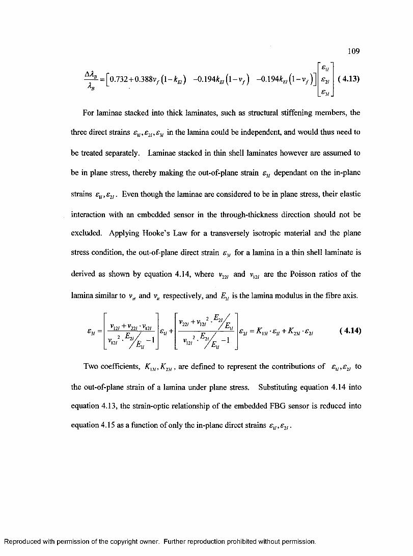
109

A / L= [o.732 +0.388V, ( l - * H) -0.194Jtf l( l - v / ) -0 .194^/ ( l - v / )] '21 ( 4.13)

For laminae stacked into thick laminates, such as structural stiffening members, the

three direct strains su,s2l,s3l in the lamina could be independent, and would thus need to

be treated separately. Laminae stacked in thin shell laminates however are assumed to

be in plane stress, thereby making the out-of-plane strain s3l dependant on the in-plane

strains £v,£2l • Even though the laminae are considered to be in plane stress, their elastic

interaction with an embedded sensor in the through-thickness direction should not be

excluded. Applying Hooke’s Law for a transversely isotropic material and the plane

stress condition, the out-of-plane direct strain sv for a lamina in a thin shell laminate is

derived as shown by equation 4.14, where v22/ and v12/ are the Poisson ratios of the

lamina similar to vz, and v„ respectively, and Eu is the lamina modulus in the fibre axis.

e 3l =v m + v 22i - v n i

v 2 . ^ 21/ _ j12/ A,£v +

V221 +V12 /2 ^21/'I I

v 2 .^21/ _1 vm / E]j 1S21 ~ KuI ' Sv + ^ 23/ ' S2I ( 4.14)

Two coefficients, Kul,K n l , are defined to represent the contributions o f su,s 2, to

the out-of-plane strain of a lamina under plane stress. Substituting equation 4.14 into

equation 4.13, the strain-optic relationship of the embedded FBG sensor is reduced into

equation 4.15 as a function of only the in-plane direct strains su,s2l.


110

A1 [0.732 + 0.388 • v, (1 - kB ) - 0.194 • kB (l - v, ) ■ Ki3] ■ sv(4.15)

h +[-0.194.tH( l - » / )-0.194-tB( l -v / ).JCa ].ffJ1

This equation is of the familiar form presented for electrical resistance strain gauges

o f equation 3.1, where the axial strain sensitivity factor is given by equation 4.16, the

transverse strain sensitivity factor is given by equation 4.17.

Fa = [o.732 + 0.388 • vf (l - kB ) - 0.194 • kB, (l - vf ) • Kl3 ] (4.16)

Ff =[-0.194-*£/( l - v / ) -0 .1 9 4 ^ H( l - v / ) - ^ 23] (4.17)

An ‘optical’ gauge factor Fopt and transverse sensitivity correction factor kopl can be

defined by equations 4.18 and 4.19 respectively.

Fv =0.732 + 0.38*.v/ ( l - * H)-0.194-*H( l -v / )[l + Jt„+tf!J] (4.18)

t [ - 0 .1 9 4 t„ ( l - v J ) [ H - ^ ] ] ( 4 J 9 )

op> [0 .7 3 2 + 0 .3 8 8 • vf (1 - ka ) - 0.194

This allows FBG measurements to be taken as single ‘apparent’ strains, which can be

separated into the true strain components by using equation 4.20 and knowing the ratio of

s 2t l e1/ '•> or alternatively, employing multiple sensors at different orientations and relating

their strains by the strain transformation equations 3.18 - 3.20, similar to a rosette

analysis.

C = A/l* 1 = gi/ / 1 ** > (4.20)m (l + * „ ) (l + *w )


I l l

4.7 Applying FBG Sensors to Thin Shell Laminates

Thin shell laminates are considered to be in a state of plane stress, and as such, according

to Hooke’s law, only three of the six strain components will be independent, the two in

plane direct strains £,, ex, and the in-plane shear strain sa . Unless the principal strain

orientations are known, three FBG sensor measurements would be needed at a single

point in order to characterize the full state of strain in the laminate, each at a different

orientation that is known relative to the others.

The simplest solution to this problem would be to deploy three FBG sensors at

different levels in the laminate, each at a different orientation. This, however, gives rise

to a potential problem. As it was suggested in Section 4.6.2, orienting FBG sensors

differently between laminae results in different and difficult to predict sensitivity factors

which need to be known for every gauge in order to relate their measurements in a rosette

configuration. A simple solution to this problem is to completely embed each FBG

sensor into a unidirectional lamina, which are then be oriented in at least three different

directions within the laminate thickness. By making the centres of each FBG sensor in

the differently oriented laminae coincident through the thickness, the result is to have

effectively created a ‘stacked’ FBG rosette, ensuring that each sensor is measuring the

same strain field. To consistently embed sensors into unidirectional laminae, the FBG

could be sandwiched between two laminae of equal thickness, creating a thicker lamina.

The relationships presented in Section 4.6.2 could be used to estimate the sensor

sensitivity factors; these estimates could be further calibrated and corrected to their true

values by performing a series of simple laminate coupon tests with embedded sensors.


112


The experimental tests successfully demonstrated the ability of FBG sensors to measure

with high numerical accuracy the strains in the test specimens, even over small ranges.

Temperature effects were suspected to be the primary contributor to strain measurement

errors, which could be eliminated by the use of a temperature discriminating system or

sensor. During the final set of tests, an increased transverse sensitivity was observed in

the FBG measurements, and was later attributed to the elastic interaction of the sensor

and its host material. When embedding FBG sensors in fibre reinforced laminates, they

should be installed parallel to the fibre axis direction in order to exhibit more consistent

sensitivity factors, and to pose less threat to the structural integrity o f the host. Having

verified their strain measurement ability and challenges, it remains to determine how

FBG sensors can be efficiently networked and integrated into the SHARCS rotor design,

and meaningful data extracted from them.


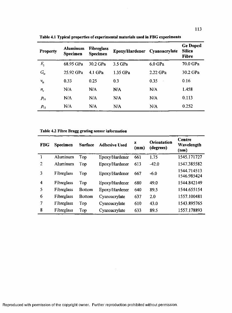
113

Table 4.1 Typical properties of experimental materials used in FBG experiments

Property AluminumSpecimen

FibreglassSpecimen Epoxy/Hardener Cyanoacrylate

Ge DopedSilicaFibre

68.95 GPa 30.2 GPa 3.5 GPa 6.0 GPa 70.0 GPa

Gu 25.92 GPa 4.1 GPa 1.35 GPa 2.22 GPa 30.2 GPa

vi« 0.33 0.25 0.3 0.35 0.16

ne N/A N/A N/A N/A 1.458

Pn N/A N/A N/A N/A 0.113

Pn N/A N/A N/A N/A 0.252

Table 4.2 Fibre Bragg grating sensor information

FBG Specimen Surface Adhesive Used z(mm)

Orientation(degrees)

CentreWavelength(nm)

1 Aluminum Top Epoxy/Hardener 661 1.75 1545.1717272 Aluminum Top Epoxy/Hardener 613 -42.0 1547.385582

3 Fibreglass Top Epoxy/Hardener 667 -6.0 1544.7145131546.985424

4 Fibreglass Top Epoxy/Hardener 680 49.0 1544.8421495 Fibreglass Bottom Epoxy/Hardener 640 89.5 1544.6551546 Fibreglass Bottom Cyanoacrylate 637 2.0 1557.1004817 Fibreglass Top Cyanoacrylate 610 43.0 1543.8957658 Fibreglass Top Cyanoacrylate 633 89.5 1557.178893


114

Table 4.3 Sample of raw optical data

Wavelength(nm)

Transmission Reflection

Insertion Loss Group Delay Insertion Loss Group Delay(Db) (s) (Db) (s)

1543.800894 -7.227310 502.99365 -28.24890 1850.518331543.803859 -7.251820 505.05346 -29.54755 1850.516031543.806823 -7.368600 507.48857 -28.94098 1852.407221543.809788 -7.620670 512.60985 -25.61900 1986.759311543.812752 -8.014170 507.93015 -21.69442 2143.853511543.815717 -8.542950 506.78431 -19.32384 2078.264271543.818682 -9.182540 499.76033 -17.81734 2140.330001543.821646 -9.920610 495.55047 -16.73932 2176.737261543.824611 -10.67103 493.37699 -15.92085 2186.363201543.827576 -11.45869 483.34894 -15.37974 2201.205841543.830540 -12.27095 480.48622 -14.95571 2212.331891543.833505 -13.04050 475.09788 -14.64231 2217.332021543.836470 -13.79808 474.90916 -14.38424 2220.582681543.839434 -14.53107 474.96822 -14.24284 2226.00144

Table 4.4 FBG sensor measurements on the aluminum beam

FBG Moment (Nm) Strain Values (micro-strain) FBG to TheoryBending Torsional Theoretical Rosette FBG Diff. % Diff.

1 328.63 0.00 903.86 889.80 911.53 7.67 0.85-328.63 0.00 -903.86 -903.74 -898.80 5.06 -0.56328.63 88.39 887.86 883.20 900.47 12.61 1.42-328.63 -88.39 -887.86 -893.74 -899.16 -11.3 1.27

2 304.95 0.00 339.70 332.57 336.47 -3.23 -0.95-304.95 0.00 -339.70 -341.96 -352.86 -13.16 3.87304.95 88.39 641.28 644.49 628.97 -12.31 -1.92-304.95 -88.39 -641.28 -651.60 -638.00 3.28 -0.51


Table 4.5 FBG sensor measurements on the fibreglass beam

115

FBGMoment (Nm) Strain Values (micro-strain) FBG to Theory

Bending Torsional Theoretical Rosette FBG Diff. % Diff.

3 391.69 0.00 354.19 354.16 351.06 -3.13 -0.88-391.69 0.00 -354.19 -354.70 -348.43 5.76 -1.62152.38 -57.98 110.24 111.20 104.08 -6.16 -5.58-152.38 57.98 -110.24 -110.06 -113.75 -3.51 3.18

4 399.14 0.00 104.45 103.82 106.36 1.91 1.83-399.14 0.00 -104.45 -104.74 -103.92 0.53 -0.51399.14 59.62 241.94 242.53 241.76 -0.18 -0.08-399.14 -149.04 -448.18 -445.44 -451.82 -3.64 0.81

5 375.39 0.00 87.57 86.30 90.22 2.65 3.03-375.39 0.00 -87.57 -84.80 -82.88 4.69 -5.36146.04 -57.98 31.85 31.35 31.61 -0.24 -0.75-146.04 57.98 -31.85 -30.57 -33.61 -1.76 5.52

6 373.99 0.00 -342.36 -342.35 -316.62 25.74 -7.52-373.99 0.00 342.36 342.85 333.84 -8.52 -2.49373.99 -149.04 -365.05 -361.54 -350.71 14.34 -3.93-373.99 149.04 365.05 363.63 346.03 -19.02 -5.21

7 358.16 0.00 136.76 136.30 135.29 -1.47 -1.07-358.16 0.00 -136.76 -137.06 -142.50 -5.74 4.20358.16 -149.04 447.46 437.31 466.39 18.93 4.23-358.16 149.04 -447.46 -432.39 -468.44 -20.98 4.69

8 371.20 0.00 -86.59 -85.33 -104.75 -18.16 20.97-371.20 0.00 86.59 83.85 99.90 13.31 15.36371.20 -149.04 -80.96 -79.68 -97.44 -16.48 20.36-371.20 149.04 80.96 77.71 99.50 18.54 22.90


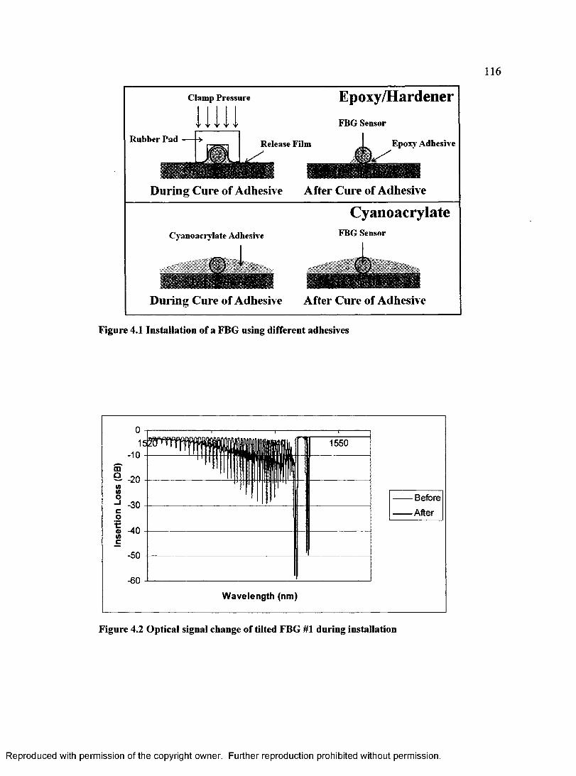
c

Rubber P a d ----

4 *rf 1During 1

lamp Pressi

|f « II

Dure of i

*re Epoxy/HardenerFBG Sensor

Release F i l m ^ ^ ^ ^ ^ ^ ^ ^ ^ E ^ ^ A d h e s i v e

Adhesive After Cure of Adhesive

CyanoacrylateCyanoacrylate Adhesive FBG Sensor

During Cure of Adhesive After Cure of Adhesive

Figure 4.1 Installation of a FBG using different adhesives

1550-10

too_i -30 c o

® -40<oc-50

-60W a v e le n g th (nm )

Figure 4.2 Optical signal change of tilted FBG #1 during installation


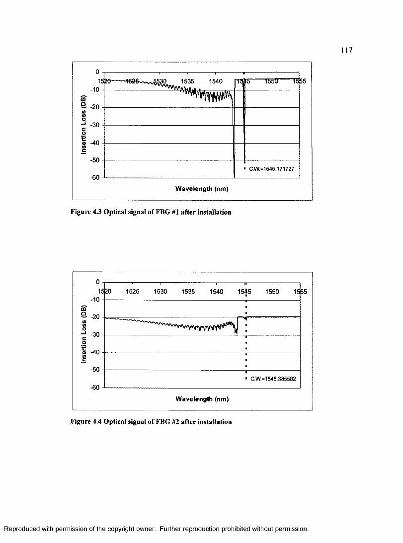
117

1535 1540 rrajte T55U1 TC55-10

-20

-30

^0

-50■ C.W.=1545.171727

-60

W a v e le n g th (nm )

Figure 4.3 Optical signal of FBG #1 after installation

15451520 1525 1530 1535 1540 1550 1555-10

-20

-30

-40

-50C.W.=1545.385582

-60




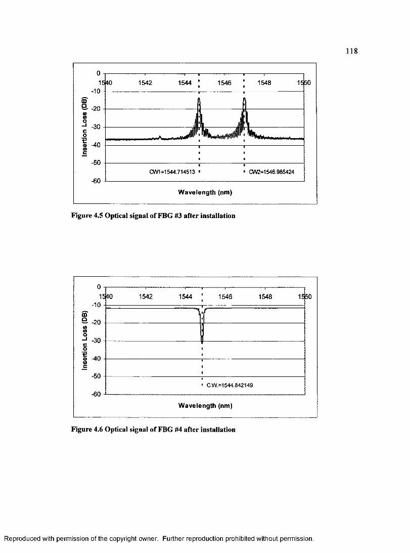
118

15501540 1542 1544 1546 1548-10

-20

-30

-40

-50CW1 =1544.714513 CW2=1546.985424

-60



1540-10

mS- -20coCOo—1 -30

1542 1544 1546 1548 1550

r ~

o -40 co

-50

-60C.W.=1544.842149




119

1540-10

m° -20 w (0 o

-30o€®(0c

-40

-50

-60

1542 1544 vr 1546 1548 1550

C.W.=1544.655154



1550___1552 . 1554„ . J 5 5 6 ‘ 1558___ 1560___1562. , 1564-10

-20

-30

-40

-50C.W =1557.100481

-60




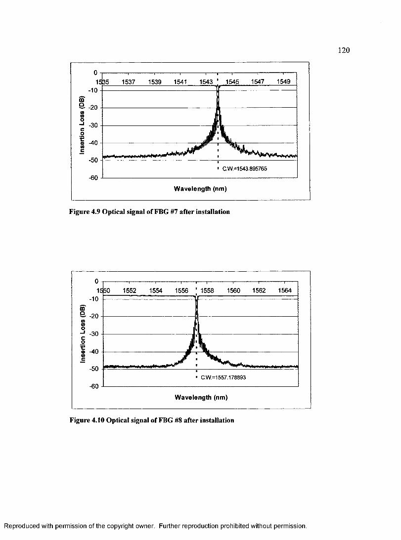
120

1545 1547 154915431535 1537 1539 1541-10

-20

- 1 -30

1̂0

-50C.W =1543.895765

-60



1550 1552 1560 1562 15641554 1556 ’ 1558-10

-20

- 1 -30

-40

-50C.W.=1557.178893

-60




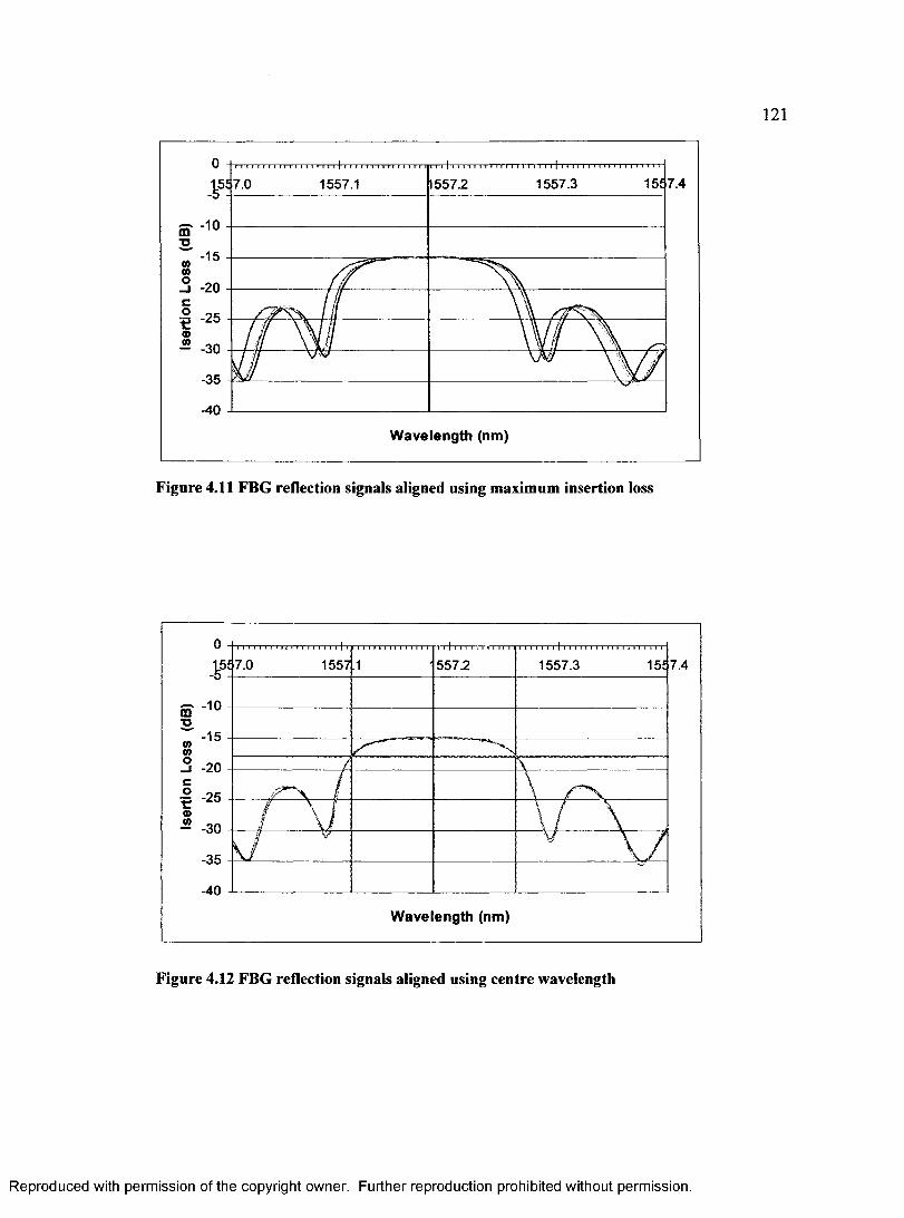
121

15f 7.41557.37.0 1557.1 1557.2

-10

-15

-20

-25

-30

-35

-40

W a v e len g th (nm )

Figure 4.11 FBG reflection signals aligned using maximum insertion loss

7.0 1557 1557.3 15£ 7.4557.2

-10■o

-15

-25

-30

-35

-40

W a v e len g th (nm )

Figure 4.12 FBG reflection signals aligned using centre wavelength


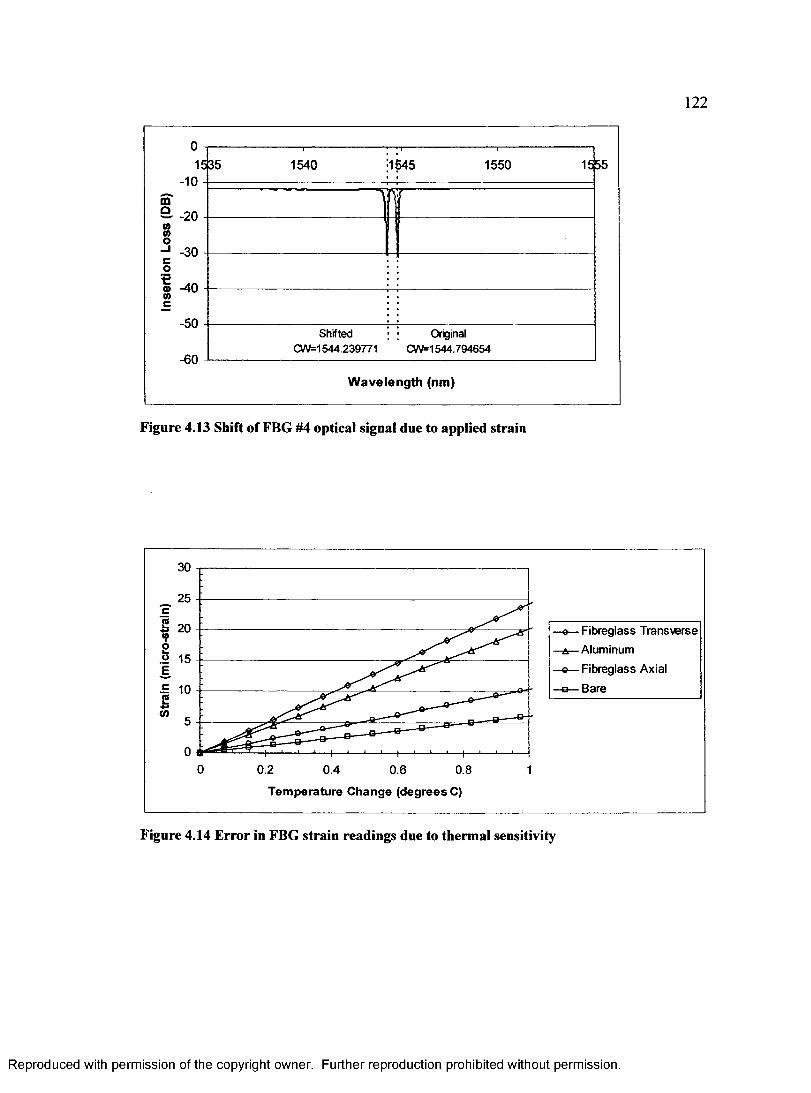
122

15451535 15551540 1550-10

-20

-30

-40

-50Shifted

CW=1544.239771Original

CW=1544.794654-60


Figure 4.13 Shift of FBG #4 optical signal due to applied strain

30

25

20

15

10

5

00 0.2 0.4 0.6 0.8 1

T e m p e ra tu re C h a n g e (d e g re e s C)

—0 -- Fibreglass Transverse

—A—-Aluminum

—e—-Fibreg lass Axial

—B—-B are

Figure 4.14 Error in FBG strain readings due to thermal sensitivity


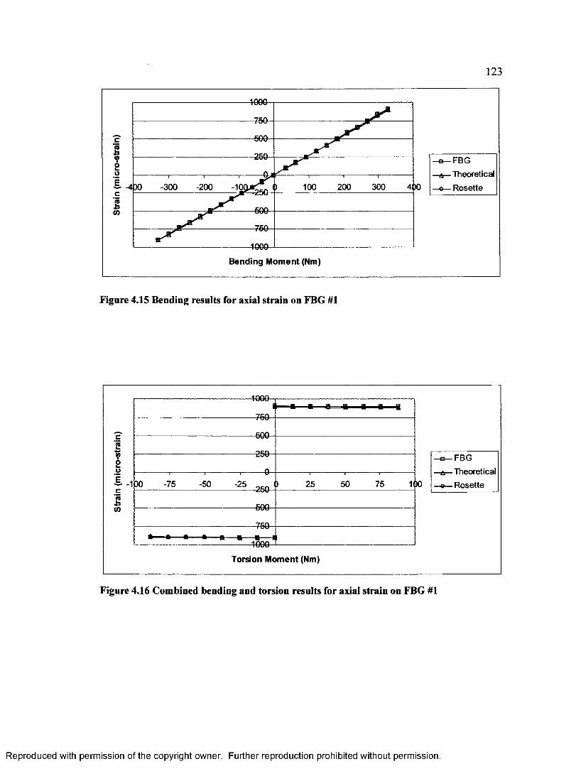
123

J§aSQac

<?so _~ -430 c —S» —

-300 200 300 400-200 100-25&

soa

•750-

-1000 J---------------B ending M om ent (Nm)

—B—-FB G

—A—-Theoretical

—©— R osette

Figure 4.15 Bending results for axial strain on FBG #1

jsam a

am

1 -75 -50 -25 75 100•250

-soa

75&

1000-1--------------Torsion M om ent (Nm)

—B--FB G

—A—-Theoretical

—e—- R osette

Figure 4.16 Combined bending and torsion results for axial strain on FBG #1


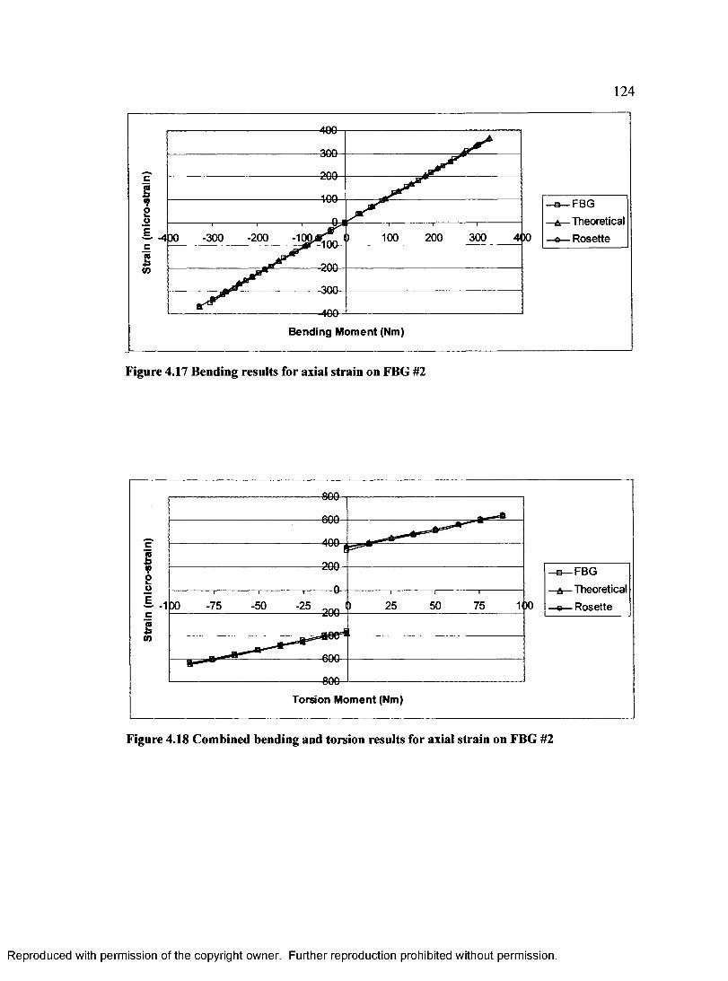
124

4 0 0

000

5 0 0cS<Poo _— 4 3 0 c —sCO —

300 4 )0-200 100 200-300

-209

-300

400—1-----------------


—B—-FB G

—A—-Theoretical

—e—- R osette


-800

€00

4 0 0

500

1001 -50 -25-75 ■200

-600

800—1----------------

Torsion M om ent (Nm)

—B- -FB G

—A—-Theoretical

—e—- R osette



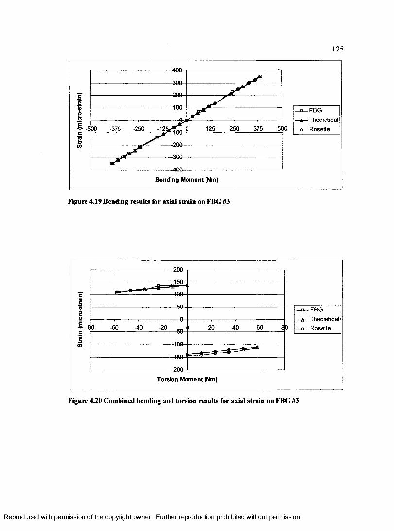
125

4 0 0

OQOoooc

«P — 8o _

-5X1 c —

375 51X)-375 -250 - 12! 125 250

£tO -200

-300

400—I-----------------


O' -FB G

—A--Theoretical

—e—- R osette


4 0 0c£v80 _~ 40C —

1to -

-60 -20 404 0

4 0 0

200—1---------------T orsion M om ent (Nm)

□ -FB G

—A—-Theoretical

—e—- R osette



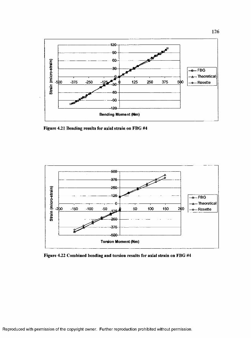
126

£«ps01c£(O

---------------------------------------------429-r

S '---- " - - ...... C7U "

fin

^0

O Iyi " i i530 -375 -250 - 1 2 V * * i) 125 250 375 5

fin-dm w* * * oo

90-------------------------------------- =i20_

—B--FB G

—A—-Theoretical

—e - - R osette

Bending M om ent (Nm)


5 0 9

250c

4 2 5<PS01 -150 -100 100 150 200-50c

•250

-375

500-I--------------


—B--FB G

—A—-Theoretical

—e—- R osette



127

C --s<p —so _— -5 DOc —sto —

250-375 -250 -121 125 375

-------- 400- ---------------B end ing M om ent (Nm)

—B--FB G

—A--Theoretical

- R osette


-60

40

c —s«p -o&_o _— -JO c —s <0 —

-60 -40 -20

60—*----------------


—B—-FB G

—A—-Theoretical

—e—- R osette



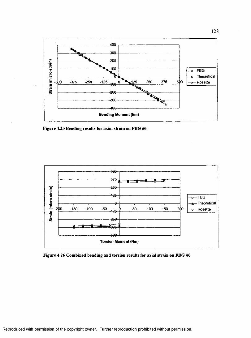
128

4 0 0

-300-

200

<PS01 250 375-375 -250 -125 125c£CO ■200

■300

4 0 0 -“-----------------


■ - o - -FB G

—A--Theoretical

—e - - R osette


-500

070

050c

420<Pok.o _~ -200 2i X)-150 -100 -50 100 150420_c■SCO 250

5 0 0 -“----------------

T orsion M om ent (Nm)

—B—-FB G

—A—-Theoretical

—o—- R osette



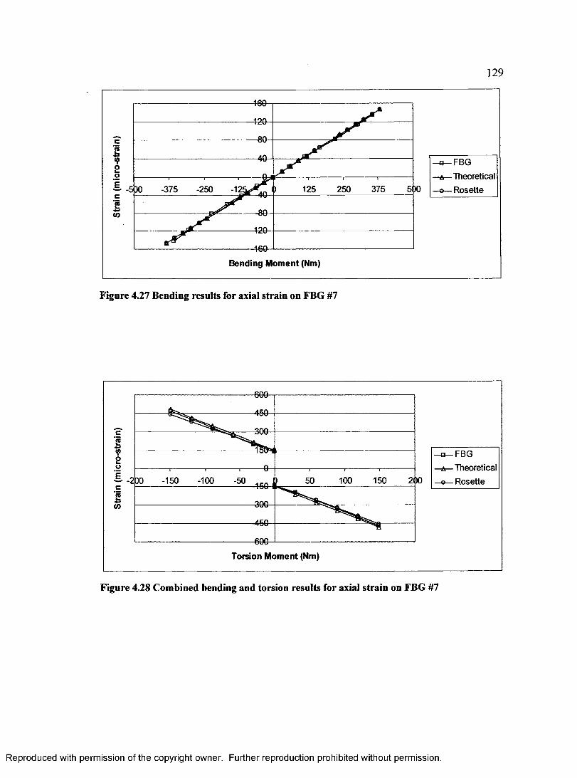
129

4 6 0

420

c

«pso _— -530 c —

375 500-375 -250 - 12! 125 250

2(0

460—1-------------B ending M om ent (Nm)

-a — FBG

- a — Theoretical

-©— R osette


ann

Stra

in

(mic

ro-s

trai

n)

fb

4 5 n

± oaa— ^ 3 0 0

)0

i— - - ----------------------------------------------itxrH i---------------- . . . . . .... .- a — FBG

30 -150 -100 -50 ) 50 100 150 2I —« — R osette

onn■OUv

4 50

ann




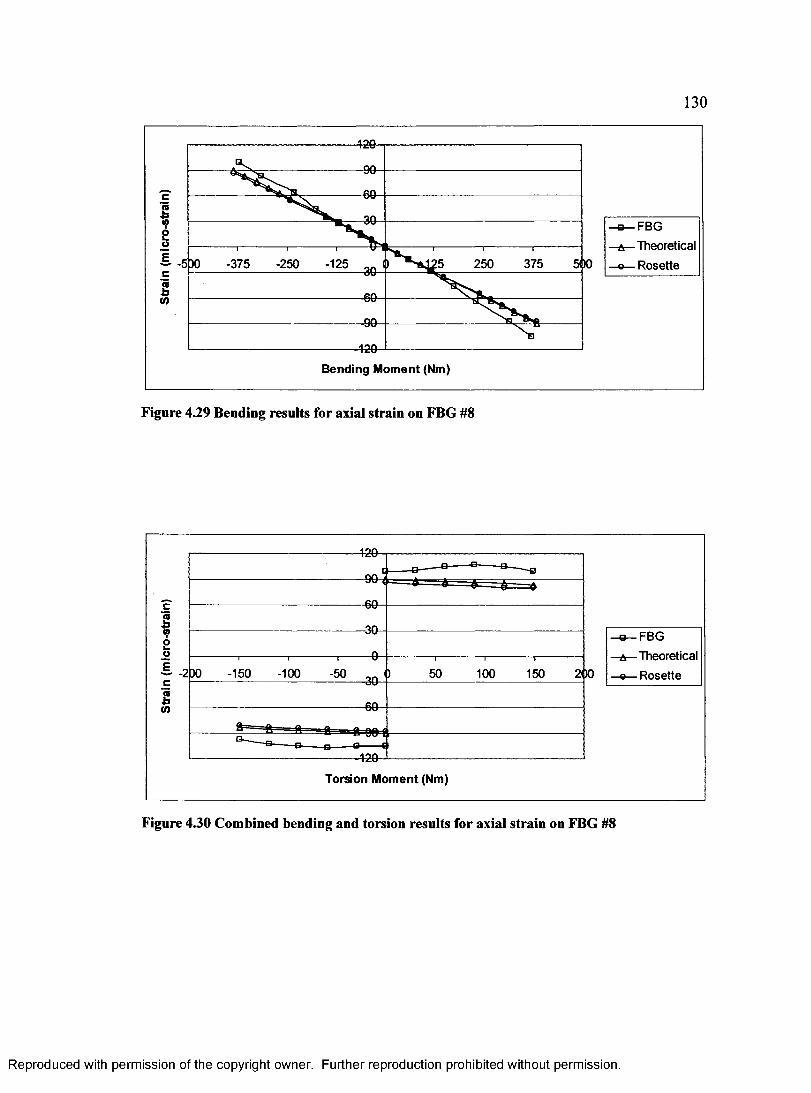
130

c3«psoE -375 -250 -125 250 375 9 )0

120-I--------------B ending M om ent (Nm)

—B--FB G

—A--Theoretical

—e—- R osette


cs

oE -150 200-100 -50 100 150chco -6fr

420-J----------------


—B--FB G

—A--Theoretical

—©—- R osette



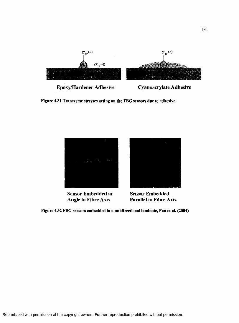
Epoxy/Hardener Adhesive Cyanoacrylate Adhesive

Figure 4.31 Transverse stresses acting on the FBG sensors due to adhesive

Sensor Embedded at Sensor EmbeddedAngle to Fibre Axis Parallel to Fibre Axis

Figure 432 FBG sensors embedded in a unidirectional laminate, Fan et al. (2004)


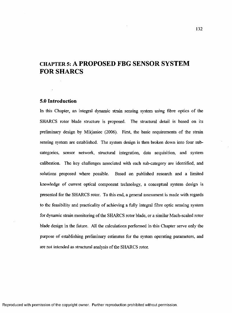
132

CHAPTER 5: A PROPOSED FBG SENSOR SYSTEM FOR SHARCS

5.0 Introduction

In this Chapter, an integral dynamic strain sensing system using fibre optics of the

SHARCS rotor blade structure is proposed. The structural detail is based on its

preliminary design by Mikjaniec (2006). First, the basic requirements of the strain

sensing system are established. The system design is then broken down into four sub

categories, sensor network, structural integration, data acquisition, and system

calibration. The key challenges associated with each sub-category are identified, and

solutions proposed where possible. Based on published research and a limited

knowledge of current optical component technology, a conceptual system design is

presented for the SHARCS rotor. To this end, a general assessment is made with regards

to the feasibility and practicality of achieving a fully integral fibre optic sensing system

for dynamic strain monitoring of the SHARCS rotor blade, or a similar Mach-scaled rotor

blade design in the future. All the calculations performed in this Chapter serve only the

purpose of establishing preliminary estimates for the system operating parameters, and

are not intended as structural analysis of the SHARCS rotor.


133

5.1 System Design Objectives and Basic Requirements

The basic system design requirements can be established by examining the desired

system performance and the constraints placed on the system by the SHARCS rotor

design. The sensory system has three major performance objectives as listed below.

System performance objectives:

1. dynamic strain monitoring

2. structural vibration monitoring

3. structural health monitoring

In order to achieve integration, the sensory system must conform to the constraints

imposed on it by the SHARCS rotor design, which can be summarized into three major

areas as listed below.

System constraints:

1. confined to structural geometry

2. restricted system weight

3. minimal structural intrusiveness

Based on the preliminary SHARCS rotor design presented by Mikjaniec (2006),

system operating parameters such as measurement range, speed and resolution will be

estimated, followed by a brief look at the system constraints.


134

5.1.1 Measurement Range

The system should be able to measure strains from zero to maximum rotational speed of

the rotor. Estimating the largest strains in the structure during these two extreme load

cases will establish a target measurement range for the system. The loads and cross-

sectional properties used in these estimates are those determined by Mikjaniec (2006).

The maximum strains when stationary are due to static bending moments in the

flapping plane, and are related to the axial strain by equation 5.1.

• Root M - -22.5Nm y - ±4.5mm E l = 47.3Nm2

The maximum tensile and compressive strains during static bending at zero rotation

are estimated to be 12140/if and ±2922f i s , in the root and blade respectively.

The largest strains during maximum rotation are due to centrifugal forces on the

cross-section, and bending moments in the flapping plane.

• Root F = 1500N M = 0.50Nm

• Blade F = 74007V M = 0.92Nm

The axial strain due to extension is related to the centrifugal force by equation 5.2,

Mikjaniec (2006), where the subscript k denotes the properties of an individual lamina in

the cross-section.

• Blade M = -20.0 Nm y = ±4.5 mm E l = 30.8Nm

F F ( 5.2)


135

Using the material properties of Table 5.1 and approximating the cross-sectional areas

of each laminate (tk -lk) as flat plates from leading to trailing edge, the products of area

and stiffness matrix coefficients were estimated as shown in Table 5.2. The maximum

tensile strains due to extension are thereby estimated to be +650/us and +835//S in the

root and blade respectively. The maximum tensile and compressive strains due to

bending are found using equation 5.1 to be ±47.6//f and ±134he for the root and blade

respectively, and can be superimposed over the extension strains.

The axial strain range in the root is +2140 /us to +602A/us and -2140 he to

+691.6fie on the top and bottom surfaces respectively, and in the blade +2922he to

+10\fis and -2922fie to +969he for the top and bottom respectively. Torsion of the

section will add shear strain components to these values, but is not included in this

preliminary estimate.

The required system range for axial strains is estimated to be -5000i+e to +1000//&,

for a total range of 4000he . If a portion of the blade at the free end was supported prior

to rotation and during early spin-up, the strains due to static bending would be

significantly lower. This would allow the strain measurement range of the system to be

much smaller. Considering an unsupported rotor for now, the range should be increased

to, say, 6000he to allow for measuring higher strains during vibration of the structure,

and account for the uncalculated lead/lag bending and torsion strains on the section.


136

5.1.2 Measurement Speed

To properly characterize dynamic variations of strain, several sample measurements must

be obtained over the course of one vibration cycle, which are assumed to be sinusoidal in

form. The sampling rate of the system will limit its ability to recognize structural

vibrations of higher frequencies; the system must therefore operate at a minimum speed

relative to the structural dynamics of the SHARCS rotor in order to be effective in

monitoring structural vibrations. The key natural elastic frequencies of the structure are

calculated by Mikjaniec (2006) as listed below in cycles per revolution (per rev) and also

in cycles per second (Hz) at the operating speed of the rotor which is 150 rad / 5.

Natural Elastic Frequencies:

• 1st Flapping 2.55 per rev 60.9 Hz

• 2nd Flapping 4.53 per rev 108 Hz

• 1st Lead/Lag 5.33 per rev 127 Hz

• 1st Torsion 5.82 per rev 139 Hz

Assuming that a sampling rate of 6 per cycle is the minimum to adequately recognize

a sinusoidal form, the system would have to operate at a speed of no less than 834 Hz. A

slightly higher sampling rate would improve the systems ability to characterize vibrations

of the rotor within this frequency range, and also increase the detectable frequency range

of the system. The minimum target operating speed of the system, for a sampling rate of

between 7 and 11 per cycle, is 1.0 kHz to 1.5 kHz.


137

5.1.3 Measurement Resolution

In order to monitor dynamic strain variations, the system must be able to distinctly

recognize a small change in strain; the smallest measurable change is the system

resolution. The system should be able to characterize structural vibrations, which may

have very small amplitudes relative to the large axial strain components in the rotor.

Based on the experimental results, a target of 5 micro-strain resolution appears to be

attainable for the system, which includes the improvement attributed to separation of

temperature from the measurements and compensation for transverse sensitivity.

5.1.4 Structural Geometry

The sensor network and installation will be confined to the defined geometry of the rotor

structure. The laminate and structural geometries of the root and blade sections of the

rotor are defined by Mikjaniec (2006) as shown in figures 5.1 and 5.2. The outer

geometry is a NACA0012 airfoil 75.3 mm in chord length; the laminate is built inward

from this surface and consists of S-glass/Epoxy and IM6/Epoxy unidirectional pre

impregnated laminae, the material properties of which are listed in Table 5.1. Behind the

leading edge laminate, a ballast of lead is used to balance the centre of gravity to Va chord

position, and the remainder of the internal cavity is filled with a low density foam core

material. The root section is assumed to be adhesively bonded onto a titanium

mandrel/support-arm, whose geometry is not clearly defined by Mikjaniec (2006), but

will be assumed to partially match the inner perimeter of the laminate at the root section

near the ’A-chord position.


138

5.1.5 Weight Restriction

To achieve a Lock number of 3.7, Mikjaniec (2006) established the target total weight of

the SHARCS rotor blade, including all smart-systems, to be 536 g. The structure and

ballast designed by Mikjaniec (2006) have a total weight of 400 g, leaving 136 g for all

other systems. As this weight is mostly needed for the smart-systems being installed in

the rotor blade, the total weight of the sensor system should be very small. A maximum

target weight will be set at 25 g for sensor system components installed in the rotor itself.

5.1.6 Structural Intrusiveness

The embedding of sensors in the laminate should not disrupt the lay-up by creating voids

or stress concentrations. The effects on the host structure can be minimized by

embedding sensors in unidirectional laminae having a fibre direction in the sensor

orientation. The diameter of sensor should be smaller than the thickness of the lamina, so

that it will not locally compromise the lamina strength.

5.1.7 Summary of Design Requirements

In summary, the target design requirements are as listed below.

Range 6000//S

Speed 1.0 kHz to 1.5 kHz

Resolution 5 fis

Weight 25 g

Structure compatible with geometry and non-intrusive


139

5.2 Sensor Network

The sensor network should be designed such that the sensors are located to achieve each

of the performance objectives, while minimizing the total number of sensors needed.

5.2.1 Dynamic Strain Monitoring Sensors

As was suggested in Section 4.7, for characterizing accurately the full state of strain at a

given point, the ideal placement of sensors into the laminate is to be ‘stacked’ in

unidirectional lamina of three different orientations at the location of interest. Although

the loads are higher at the root of the rotor, the strains in the blade section are slightly

higher due to the thinner laminate structure. The laminate in the blade section contains

three unidirectional lamina orientations, 0°, +45°, and -45°, between chord position

0.00mm and 21.6mm and between S\Amm and 60.7mm as shown in figure 5.2. The

appropriate place to locate embedded strain sensors is therefore in the blade section

beyond rotor position 0226 (Sta. 0226), and between the leading edge and chord position

2\.6mm or between chord positions 51.4mm and 60.1mm as shown in figure 5.3.

Additional sets of sensors can be located within the root section and farther along the

blade section in order to provide a more complete distribution of the strains within the

whole rotor structure, although these strains will be lower in magnitude. Temperature

effects can be separated from the strain measurements by using a dual-overwritten grating

among the three sensors at each location.


140

5.2.2 Vibration Monitoring Sensors

To monitor vibrations in the structure, sensors need to be able to detect the amplitude of

the vibrations, as well as the vibration mode. Dyllong and Kreuder (1999) showed that

accurate reconstruction of the mode shapes with their amplitudes, up to the 3rd mode can

be achieved using a cubic-spline interpolation technique and at least five ‘well-placed’

non-uniformly spaced sensors along the length of the structure. For accurate

reconstruction of only the 1st and 2nd mode shapes, 3 or 4 sensors, respectively, would

suffice.

The vibration modes of interest are those corresponding to the natural elastic

frequencies given by Mikjaniec (2006); the 1st modes of torsion and lead/lag, and the 1st

and 2nd modes of flapping. In order to apply the technique presented by Dyllong and

Kreuder (1999), the strain measurements used for interpolation must be dependant only

on the vibration mode being examined. The modes must therefore be separated from

each other and separated from the steady state strains in the rotor.

Flapping and lead/lag are both bending modes of the rotor section, and produce most

noticeably variations in the axial strain. They can be separated from each other and the

axial extension of the blade by using four axial strain sensors in a given cross-sectional

plane. They would be located on opposing sides of the flapping neutral axis in pairs,

each pair at a significantly different distance from the lead/lag neutral axis as shown in

figure 5.3. Axial sensors are unaffected by shear strain, thereby making them insensitive

to any torsional vibrations. Four sets of axial sensors, in groups of four, would be


141

required to accurately reconstruct the 1st lead/lag and the 1st and 2nd flapping mode shapes

and amplitudes.

Torsion of the section can be separated from axial extension and bending vibrations

by using a pair of sensors at the same location that are oriented at opposing angles to each

other, not oriented in the axial direction, as in the case of +45° and -45° sensors. Any

axial or transverse strain applied to this pair due to bending or extension of the section

will cause each sensor to measure the same value. Torsion produces shear strain in the

section, which causes each sensor to measure differently from the other due to their

opposing angles. There is some distributed shear strain caused by bending, however,

since the amount due to bending is known, it allows the remainder to be attributed only to

torsion. Three pairs of sensors would be required to accurately reconstruct the 1st torsion

mode shape and amplitude, and they should be located where the bending of the section

can be determined so as to remove the bending shear from the measurements.

According to Dyllong and Kreuder (1999), the sensors must be ‘well-placed’,

meaning that an idea of the expected mode shapes is needed prior to deciding their

specific locations. Predicting the mode shapes of the rotor can be achieved using FEM

modeling and examining the eigenvector which corresponds to each vibration mode.

5.2.3 Structural Health Monitoring Sensors

To monitor structural health, a history of the strain at a given location can be kept in a

data log. If the strain begins to change from its typical value, this would indicate the

onset of fatigue damage to the structure in the vicinity of the sensor. Sensors for


142

structural health monitoring should be placed near locations of stress concentration in the

laminate, such as changes in laminate thickness, ply drop-off and pick-up locations, and

attachment points of smart-system devices.

5.2.4 Combining all Sensors into a Single Network

Considering all the sensor locations described to achieve each objective, the total number

of sensors can be minimized for the system by having each sensor in the network

contribute to multiple objectives. Figure 5.3 shows a final reduced network with 28

sensors in total; 16 axial strain sensors, four sensors at +45° and four sensors at -45°,

and four over-written sensors at -45° to separate temperature effects from the strain

measurements.

The 16 axial sensors are able to characterize the 1st and 2nd flapping modes and the 1st

lead/lag mode, while the four pairs of ±45° sensors are able to characterize the 1st torsion

mode. There are four locations where the full state of strain can be monitored,

independent of temperature effects, one located at each cross-sectional plane, two located

on the upper surface, and two located on the lower surface of the rotor. Structural health

of the rotor can be monitored by viewing the strain history of any sensor in the network.

The sensors are located at four different cross-sectional planes, each plane having

seven sensors; four axial, one at +45°, one at -45°, and one over-written at -45°. The

exact location of each plane should be determined using the ‘well-placed’ locations

described by Dyllong and Kreuder (1999) for interpolation of vibration mode shapes, and

the locations of largest strains in the structure. The placement of each sensor in the


143

laminate and the routing of optical fibre to and from each sensor, as shown in figure 5.3,

will be addressed along with other structural integration concerns in the next Section.

5.3 Structural Integration

The sensor network should be integrated into the rotor while minimizing the risk of

failure to the host structure, the sensors, and the optical fibre network.

5.3.1 Sensor Failure

The sensor must be able to withstand the tensile and compressive strains seen in the host

material; if the sensor fails before the host material, the sensor would cease to provide

useful information. Because FBG sensors are made of silica glass, which is brittle, their

failure stress is governed by the probability of a random critical sized flaw in the

crystalline structure of the glass. Gougeon et al. (2004) performed dynamic fatigue

testing of bare and coated silica fibres to investigate the effects of exposure to humidity.

They explain that presence of moisture at the surface of a fibre reduces its failure strength

and fatigue life by breaking down the silicon-oxygen bonds at crack tips and accelerating

sub-critical crack growth. They found by experiment that the mean failure stress of

coated and bare silica fibre to be lower at room temperature and 50% relative humidity

than in a dry environment. The lowest mean failure stress values they reported were

A.lAGPa and 8.54GPa for coated and bare fibre respectively. It is assumed that the

properties found by Gougeon et al. (2004) are representative of the typical strength of

silica glass optical fibre, and thus the strength of FBG sensors. Compared to the tensile

strengths and material properties of S-glass/Epoxy and IM6/Epoxy unidirectional lamina,


144

as listed in Table 5.1, the sensor is stronger than both, and would not fail prior to the

failure of the host material under the same axial strain.

5.3.2 Host Failure

If the sensor is small compared to the lamina thickness, its presence will have little effect

on the strength of the host structure. The laminae thickness used in the lay-up of the

SHARCS structure given by Mikjaniec (2006), as shown in figures 5.1 and 5.2, are

approximately 0.500mm for the axial oriented S-glass/Epoxy laminae and 0.065mm for

the ±45° oriented IM6/Epoxy laminae.

The typical diameter of multi-mode optical fibre is 0.125mm with cladding, and

between 0.050mm and 0.0625mm bare, whereas single-mode optical fibre is 0.125mm

with cladding, and between 0.008mm and 0.010mm bare. Kojima et al. (2004) have

developed a small diameter optical fibre specifically for use as embedded sensors in

composite materials, having a core diameter of 0.0065mm, and with cladding and a

polyimide coating, a total diameter of 0.040mm. Cladding can be chemically stripped

from the silica core by immersion in hot sulphuric acid, a process which was shown by

Matthewson et al. (1997) to have little effect on the strength of the fibre. Bare single

mode fibre is extremely fragile, and thus difficult to handle without breaking; applying a

thin coating to the fibre may provide sufficient reinforcement to allow light handling.

The S-glass laminae are sufficiently thicker than the diameter of multi-mode and

single mode fibre, allowing either to be used as embedded sensors. The IM6 laminae are

nearly 8 times thinner than the S-glass, and would only allow use of bare single-mode


145

sensors with a thin coating without creating a significant structural flaw. If this cannot be

achieved due to fibre handling, alternatives are to embed the ±45° sensors between axial

laminae, thus creating resin pockets, or install them on the interior laminate surface.

5.3.3 Routing of Optical Fibre in the SHARCS Rotor

The same failure concerns described in Sections 5.3.1 and 5.3.2 apply to the optical fibre

used as a conduit to and from the sensor. By taking the most efficient route to each

sensor, the amount of optical fibre embedded in the host can be minimized, keeping the

weight low, and its structural presence minimal.

The most efficient path for routing optical fibre to the axial sensors is a straight line

along the axis of the rotor passing through each sensor. The optical fibre for these

sensors can be embedded and routed directly to each sensor location within the laminae

because the fibre diameter is small compared to the thickness of the S-glass laminae.

The most efficient path for routing optical fibre to the ±45° sensors is a helical-like

path around the perimeter of the cross-section while translating down the rotor axis. This

would require the optical fibre to turn the leading edge of the cross-section, and the

trailing edge, which could be accomplished if a trailing edge wedge, or spar was

incorporated into the laminate design. Glaesemann and Castilone (2002) examined the

mechanical reliability of bent optical fibre, and list the smallest allowable fibre bend

radius as 5m m , with increasing reliability for larger radii and lower stress levels; a

general minimum fibre bend radius of 5mm will therefore be assumed. The external

radius of the NACA0012 profile at the leading edge of the SHARCS rotor is


146

approximately \.2mm. For a helical path at either ±45°, the radius o f the helical

curvature, and thus the bend radius of the fibre, is found to be approximately 2.4mm by

equation 5.3, which was derived to relate the helical path angle to the radius o f the

leading edge, Weisstein (2003).

rb e n d = r L E - ( l + t a a 2 0 p * h ) ( 5*3)

The radius at the mid-plane of each lamina will also be smaller than the radius of the

outer NACA0012 profile, optical fibre at +45° can thus not safely turn the leading edge

of the rotor. Using equation 5.3, the leading edge radius would have to be approximately

2.5mm, or the fibre angle would have to be less than ±29° for the fibre to safely turn the

leading edge. Unless the laminate was redesigned with ±29° lamina orientations, each

±45° sensor must therefore be installed on its own optical fibre in the network, and the

optical fibre must be routed to the sensor location taking a path outside the lamina and

then enter the lamina prior to the sensor.

Routing the optical fibre between laminae would disturb the laminate and create

locations of structural weakness and must be avoided. The SHARCS laminate is built on

foam core, as shown in figures 5.1 and 5.2, leaving access to the ±45° laminae edges

directly from the foam core between chord positions 30.6mm and 44.6m m . This allows

the optical fibre to be safely routed below, or depressed into, the foam surface as shown

in figure 5.3, without significantly affecting the laminate. The optical fibre would travel

down the axis of the rotor, and then turn to the appropriate orientation and enter the

lamina at chord position 30.6m m . The turn radius of the fibre in the foam, and thus the


147

fibre bend radius, should be as generous as possible, as Wang et al. (2005) showed that

bend radii less than 12mm create additional macro-bending loss in single-mode fibre.

As was suggested in Section 5.3.2, the thickness of the IM6 laminae at ±45° is so

thin that it would only allow bare single-mode optical fibre with a thin coating to be

embedded into it. Because the optical fibre will be routed to the sensor location through

the foam, the cladding does not need to be removed from the entire optical fibre, only the

end section of the fibre containing the sensor which will be embedded in the lamina.

Even though the sensor will still be quite fragile, this makes handling and installation of

the ±45° fibre more manageable.

Although it is desired to monitor the complete state of strain at the locations with high

stresses, embedding sensors into the laminate at those locations may weaken it and cause

failure, especially when considering the extremely thin IM6 lamina. The bottom surface

of the blade section, immediately beyond the root section of the rotor is under the highest

tensile loads at maximum rotation, and the highest compressive loads when stationary. It

is therefore decided, on the side of caution, to install the ±45° sensors on the upper

surface for the two most inboard cross-sections, and to balance the number of optical

fibres routed in the laminate on each surface, the +45° sensors are located on the bottom

surface for the two outboard cross-sections. Also, because the ±45° sensors are each on

their own optical fibre, it is more convenient for data acquisition to use them as the

temperature discriminating dual over-written gratings.

There are 12 optical fibres in the sensor network of each rotor blade, and can all

originate from a common fibre optic ribbon cable bonded to the titanium mandrel/support


148

arm. The fibres can then separate from each other, fan out around the titanium mandrel,

and then enter into the laminae or the foam core at their respective entry points.

5.4 Data Acquisition

Data acquisition deals with the part of the system concerning the transmission and receipt

of optical signals, and how the system actually interrogates the sensor network.

5.4.1 Transmitting and Receiving Optical Signals

Having integrated a sensor network into the structure, an optical signal must be sent to

and retrieved from each sensor. This requires a continuous optical wave guide, or optical

fibre path from the source, to the sensor, and then back to the detector. This creates a

challenge for using fibre optic sensors in a rotor blade because the sensors are located in a

rotating frame of reference. There are two possible solutions to this problem, use a fibre

optic rotary joint (FORJ) to allow rotating optical fibres to maintain an optical path with

non-rotating fibres, or to have the source and detector units rotating with the rotor blade.

Commercially available FORJ devices, such as those manufactured by Schleifring

Ltd., are capable of rotational speeds up to 2000 rpm for a single fibre FORJ, but only up

to speeds of 100 rpm for a multi-fibre FORJ. As there are several optical fibres used in

the network of each blade, and four blades, a multi-channel device would be needed; it is

not possible to use many single FORJ devices because the optical fibres would tangle

around each other. The rotor speed is 1433 rpm, thus current FORJ technology can not

solve the problem. The source and detector units must therefore rotate with the rotor

blades at 1433 rpm, requiring some form of structural integration with the rotor hub.


149

This will be the greatest challenge of the entire system design, as the system resolution,

range, and speed are all highly dependant on the source and detector units.

5.4.2 Optical Circuit Components

Conventional optical sources and detectors, such as tuneable lasers and spectrum

analyzers are not capable of meeting the speed requirement, and are also too bulky to be

mounted onto or rotated with the rotor structure. Ling et al. (2006) demonstrated a

simple, fairly compact passive interrogation scheme for measuring dynamic strains of a

FBG sensor using a super luminescent diode (SLD) as a source, and passing the signal

through an optical tuneable filter (OTF). The OTF causes optical signal loss proportional

to the wavelength of light, therefore as the centre wavelength of the FBG shifts, the

optical power measured by the detector will shift proportionally. Dyllong and Kreuder

(1999) demonstrated a similar system using a broadband light source and a wavelength

dependant coupler (WDC) which performs a similar function to the OTF. Zhang et al.

(1998) also demonstrated a similar system, but using a long period grating (LPG), in

place of the OTF and WDC. A LPG causes loss to the optical transmission signal over a

fairly wide band as shown in figure 5.4. If the reflected signal of a FBG sensor was

transmitted through a stable LPG, the power loss to the Bragg peak would be

proportional to its centre wavelength. Zhang et al. (1998) splits the reflected signal from

the FBG sensor into two, applies the LPG to only one of the signals, and measures each

signal using its own photo-detector. The ratio of power measured by the detector behind

the LPG to the power measured by the unaffected detector indicates the centre

wavelength position of the Bragg peak. This accounts for wavelength dependant power


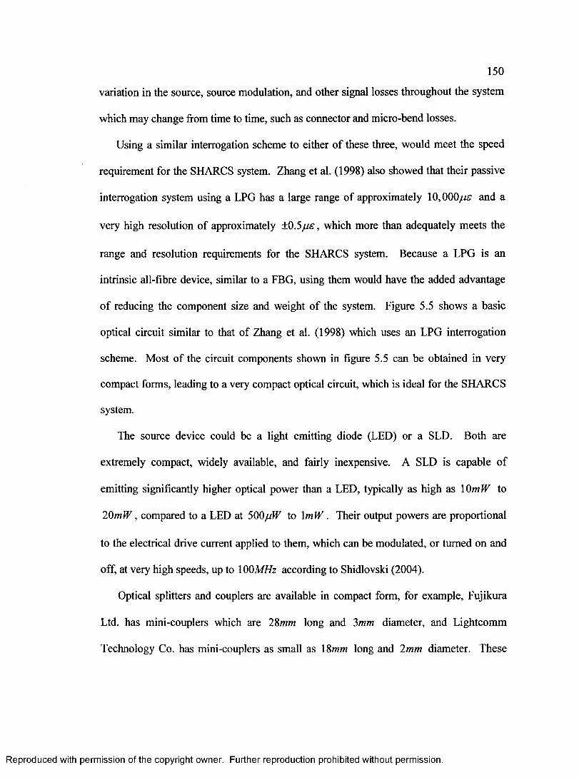
150

variation in the source, source modulation, and other signal losses throughout the system

which may change from time to time, such as connector and micro-bend losses.

Using a similar interrogation scheme to either of these three, would meet the speed

requirement for the SHARCS system. Zhang et al. (1998) also showed that their passive

interrogation system using a LPG has a large range of approximately 10,000//£ and a

very high resolution of approximately ±0.5j j s , which more than adequately meets the

range and resolution requirements for the SHARCS system. Because a LPG is an

intrinsic all-fibre device, similar to a FBG, using them would have the added advantage

of reducing the component size and weight of the system. Figure 5.5 shows a basic

optical circuit similar to that of Zhang et al. (1998) which uses an LPG interrogation

scheme. Most of the circuit components shown in figure 5.5 can be obtained in very

compact forms, leading to a very compact optical circuit, which is ideal for the SHARCS

system.

The source device could be a light emitting diode (LED) or a SLD. Both are

extremely compact, widely available, and fairly inexpensive. A SLD is capable of

emitting significantly higher optical power than a LED, typically as high as \0mW to

20m W , compared to a LED at 500/jW to 1 m W . Their output powers are proportional

to the electrical drive current applied to them, which can be modulated, or turned on and

off, at very high speeds, up to 100MHz according to Shidlovski (2004).

Optical splitters and couplers are available in compact form, for example, Fujikura

Ltd. has mini-couplers which are 28mm long and 3mm diameter, and Lightcomm

Technology Co. has mini-couplers as small as 18mm long and 2mm diameter. These


151

devices are fused-couplers, and can be built to divide the input signal in any proportion,

evenly or unevenly into to any number of outputs; the optical power is divided among the

outputs, and some optical power is lost due to excess losses in the coupler.

There are several options available for compact detectors, among which photo-diodes

(PD) appear to be the most appropriate choice for the SHARCS system. Godfrey (1998)

compares the characteristics of many different photo-detector devices, and thereby

provides a basis for selecting the most appropriate device for a given system design.

Godfrey (1998) describes the typical characteristics of a PD as small, lightweight, low

cost, rugged, very sensitive with the ability to measure from the pW to the mW range of

optical power, high linearity, able to detect a broad range of wavelengths, stable, and can

be easily packaged and customized at a fairly low cost to suit any design.

By using these compact components to replace those of figure 5.5, the same passive

interrogation circuit as Zhang et al. (1998) would be achieved, but in a miniaturized form.

The basic optical circuit would require a pair of PD detectors, one LED or SLD source,

one LPG filter, and two mini-splitters for interrogation of a single FBG sensor. Applying

this circuit design to the SHARCS system for each sensor would however result in 28

LED sources, 28 LPG filters, 56 mini-splitters and 56 PD detectors for each of the four

rotor blades. By sharing sources and detectors among sensors, and combining splitters,

the total number of components in the system can be significantly reduced. The result is

a more complex system architecture, but one that is overall more efficient in use of

system resources, size, and weight. The next section describes a conceptual design for


152

the data acquisition system of the SHARCS sensory system, which uses the passive LPG

interrogation technique and as few components as possible.

5.4.3 SHARCS Sensory System Concept

Some trade-offs can be made to the system performance in order to reduce the number of

required components. For example, by intermittently interrogating one out of every four

sensors, only 14 PD detectors would be needed, at the penalty of reducing the system

speed below one quarter its maximum. This can be achieved using four sources, where

each is filtered to generate only a spectral window corresponding to one out of four

sensors. Because LED and SLD sources can be modulated at speeds up to 100 MHz, this

allows each of the four sensors to be interrogated in rapid succession using the same set

of detectors. Even at one quarter its maximum speed, the system is still more than

capable of fulfilling the SHARCS speed requirement.

Figure 5.6 shows a conceptual system using the LPG passive interrogation technique

to monitor all 28 sensors in the SHARCS network, while significantly reducing the

number of required components. The system shares four common sources, each filtered

to generate a different spectral window, which are then modulated so that only one source

is active at any given time. The 28 sensors are divided into four groups, each group

corresponds to one of the four cross-sectional planes shown in figure 5.3, and all seven

sensors of that group have centre wavelengths which correspond to the same spectral

window of one of the four sources. Thus, when any given source is active, only the seven

sensors from the corresponding cross-sectional plane will generate an optical response.

All seven sensors of a given group are simultaneously and continuously monitored by


153

seven pairs of detectors, where each detector pair corresponds to one sensor in the group.

The 14 detectors are common to all four groups, leaving control of which sensors are

active at any time to the source modulation. One of the two detectors in each pair is

located behind a series of LPG filters that correspond with the four spectral windows of

the sources and sensors. The four spectral windows are spaced so that they correspond

only to a linear portion of the LPG transmission signal, as shown in figure 5.4.. Because

the transmission peak of a LPG has a rise on one side and a fall on the other, as shown in

figure 5.4, a single LPG can be used for two or more spectral windows. Therefore, one

or two LPG filters may be sufficient for all four spectral windows. Should multiple LPG

filters be used, their signals should not interfere with the linear regions of the other filters.

A special consideration must be given to the dual-overwritten sensors which are used to

separate temperature from the strain measurements, as both sensors are in the same fibre

and need to be interrogated simultaneously. This is only achievable using two sets of

detectors in parallel, and filtering out the optical response of the unwanted sensor prior to

each detector.

This system uses the passive interrogation technique on the detector side, while the

only actively controlled devices in the system are the sources which are modulated. This

allows some flexibility in system operation; one source can remain constantly active to

continuously monitor a single cross-sectional plane, two sources can be modulated at any

desired frequency, or they can all be modulated as desired. Optical signals from a given

source can only be split so many times before the power at the detector is insufficient

after all the system power losses. This system concept allows modifications as needed, to


154

add additional sources, detectors or sensors, and compensate for the actual performance

of each system component to power losses.

5.5 System Calibration

If the system was completely closed and integrated into the SHARCS rotor, it would be

very difficult to monitor its performance and ensure it is accurately measuring the strains.

A source may fail, a detector may cease to work properly, or a sensor itself may fail or

debond. It is therefore essential for the continuing operation and accuracy of the system

that it be able to be calibrated from time to time with relative ease.

The simplest method to achieve this is to make the entire system modular, and easily

separable. Figure 5.6 shows that the conceptual system is separated into three modules,

the source module, the detector module, and the sensor module. Only the sensor module

is integrated into the SHARCS rotor, and consists of the sensors and the optical fibre

routed to each sensor location. All the optical fibres originate from a fibre optic ribbon

cable on the titanium support arm, which can be terminated with a multiple fibre

connector, such as the MT, MTP, MPO-type connectors. This type of connector is very

compact, and allows for all 12 optical fibres to be simultaneously connected and

disconnected easily and quickly to other devices with a matching connector. The detector

and source module can be fitted with the same type of connectors, thereby allowing each

module to be easily separated and calibrated individually using other optical sources,

detectors, and spectrum analyzers, or replaced if needed.


155

There are three other areas of concern regarding system calibration and performance,

namely, transverse sensitivity of the sensors, wavelength dependence of fused

couplers/splitters, and influence of temperature on the transmission spectrum of a LPG.

5.5.1 Sensor Transverse Sensitivity

As described in Section 4.6.2, the elastic interaction of the sensor with the host lamina

can affect its transverse sensitivity. The material coefficients kEI,K w ,K 23l for each

lamina used in the SHARCS structure are listed in Table 5.4. These values are used to

approximate the axial and transverse sensitivity factors Fa,Ft and the corresponding

optical gauge factor and transverse sensitivity Fopt, kopl of an embedded FBG sensor,

following the example of Section 4.6.3, and are listed in Table 5.4. The transverse

sensitivity for an embedded FBG sensor is estimated to be -1.6% and -2.0% for the S-

glass and IM6 lamina respectively. These values can be verified by laminate tensile test

coupons made of the respective lamina materials and tested in an MTS machine while

simultaneously measuring the optical response of embedded FBG sensors.

5.5.2 Wavelength Dependence of Fused Couplers/Splitters

The power splitting ratio of a fused coupler is typically wavelength dependant. As the

wavelength of the FBG shifts, the change in power splitting ratio of the last coupler

before the detector pair would cause a ‘false’ strain indication for that sensor. The

wavelength variation of the coupler is typically provided by the manufacturer and can be

easily verified by testing it with a wavelength tuneable source. This effect can then be

accounted for in the measurements of each sensor.


156

5.5.3 Temperature Response of a LPG

Bhatia (1999) showed in figure 5.4, that the transmission spectrum of a LPG shifts in

wavelength with temperature changes. This would cause the interrogation system to

indicate a ‘false’ sensor strain. A simple solution is to use an internal temperature sensor

circuit in the detector unit, as shown in figure 5.6, using the same passive interrogation

technique and a LPG, to determine the temperature in the detector. Output from this

circuit can then be used to compensate for the temperature shifts of the other LPG

devices in the system. An external connector is included so this circuit can be calibrated.


Based on the SHARCS preliminary structural design by Mikjaniec (2006), a basic set of

system design requirements was established for an integral dynamic strain sensing system

using fibre optics. A preliminary sensor network was established which would meet the

multiple sensing objectives; it consists of 28 embedded FBG sensors using 12 single

mode optical fibres. Based on the high-speed dynamic FBG interrogation techniques

developed by several researchers and available miniature optical components, a

conceptual data acquisition system was presented which should be able to meet all the

system requirements and performance objectives. A fully integral fibre optic sensing

system for dynamic strain monitoring of the SHARCS rotor blade thus appears to be

attainable using fairly inexpensive devices. It would, however, require detailed design

and calibration. It remains to determine the ideal locations of the sensors, which requires

a reasonably accurate prediction of the expected strain components and deflection shapes

of the rotor blade; this could be achieved using finite element modeling.


157

Table 5.1 Lamina material properties used for SHARCS rotor - Mikjaniec (2006)

Property S-glass / Epoxy IM6 Carbon Fibre / Epoxy

v/ 0.5 0.66

P (g le n ? ) 2.00 1.60

£, (GPa) 43 203

E2 (GPa) 8.9 11.2

Gn (GPa) 4.5 8.4

vn 0.27 0.32

FlT (M Pa) 1280 3500

F2T (M Pa) 49 56

Fk (M Pa) 690 1540

F2C (M Pa) 158 150

F6 (M Pa) 69 98

Table 5.2 Lamina stiffness matrix coefficients

Coefficient (GPa) S-glass / Epoxy IM6 Carbon Fibre / Epoxy

Orientation 0 0 +45°

©yn1

Qn 45.55 206.65 95.98 95.98

Qn 12.30 66.13 79.18 79.18

Qn 9.43 11.40 95.98 95.98

0,6 0 0 48.81 -48.81

026 0 0 48.81 -48.81

066 4.5 8.4 50.30 50.30


158

Table 5.3 Approximate extension stiffness matrices of SHARCS rotor

Stiffness Coefficient & Area Product Root Laminate Blade Laminate

E ' . ' . K ) , ( GPa • mm2 = AMO’)*=1

7821 5798

!> * •/* ( 4 2)t (GPa-mm2 = N -\0 i )i= l

4003 3457

(GPa-mm* = N -103)*=1

4321 3902

(GPa mm7 = N -10’ )*= 1

0 (balanced) 0 (balanced)

Z ' . - ' . K ) , (GPa-mm2 = AMO’ ) 0 (balanced) 0 (balanced)

(G P a-m m '= N -10! )£ = 1

2222 2022

Table 5.4 Sensitivity coefficients for embedded FBG sensor in lamina

Coefficient S-glass / Epoxy IM6 Carbon Fibre / Epoxy

k E l 0.113 0.138

* . 3 -0..356 -0.418

* 2 3 -0.320 -0.307

Fa 0.7936 0.7949

F, -0.0125 -0.0156

Fop, 0.7811 0.7793

KP, -0.01575 -0.019625


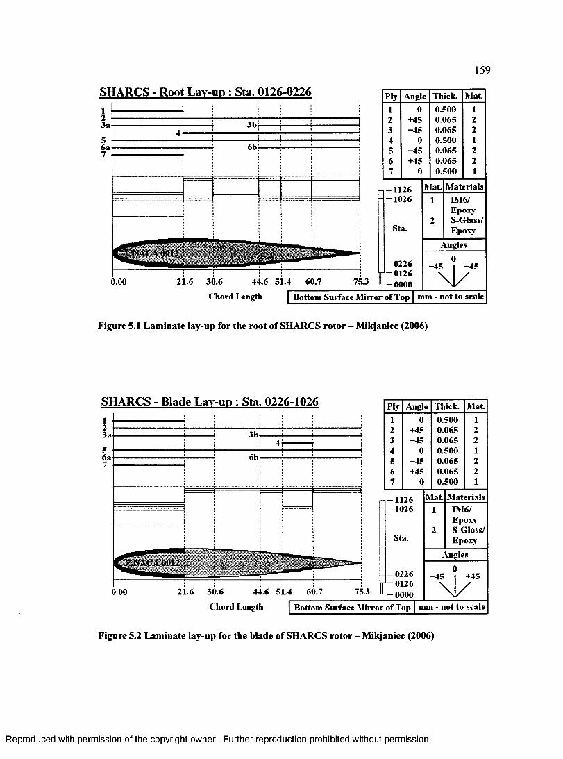
159

SHARCS - Root Lay-up : Sta. 0126-0226

fitfNACA 0012

Ply Angle Thick. M at

1 0 0.500 12 +45 0.065 23 -45 0.065 24 0 0.500 15 -4 5 0.065 26 +45 0.065 27 0 0.500 1

0.00

-1 1 2 6-1 0 2 6

Sta.

-0 2 2 6-0 1 2 6-000021.6 30.6 44.6 51.4 60.7 75-3

Chord Length Bottom Surface Mirror of Top | mm - not to scale

Mat. MaterialsEVI6/EpoxyS-Glass/Epoxy

Angles

0-4 5 I +45

N /

Figure 5.1 Laminate lay-up for the root of SHARCS rotor - Mikjaniec (2006)

SHARCS - Blade Lay-up : Sta. 0226-1026

NAC'A 0012

Ply Angle Thick. Mat.1 0 0.500 12 +45 0.065 23 -45 0.065 24 0 0.500 15 -45 0.065 26 +45 0.065 27 0 0.500 1

0.00 30.6 44.6 51.4

Chord Length

-1 1 2 6-1 0 2 6

Sta.

-0 2 2 6-0 1 2 6-0000

Bottom Surface Mirror of Top mm - not to scale

Mat. MaterialsIM6/EpoxyS-Glass/Epoxy

Angles

0-4 5 | +45

\ 1 /

Figure 5.2 Laminate lay-up for the blade of SHARCS rotor - Mikjaniec (2006)


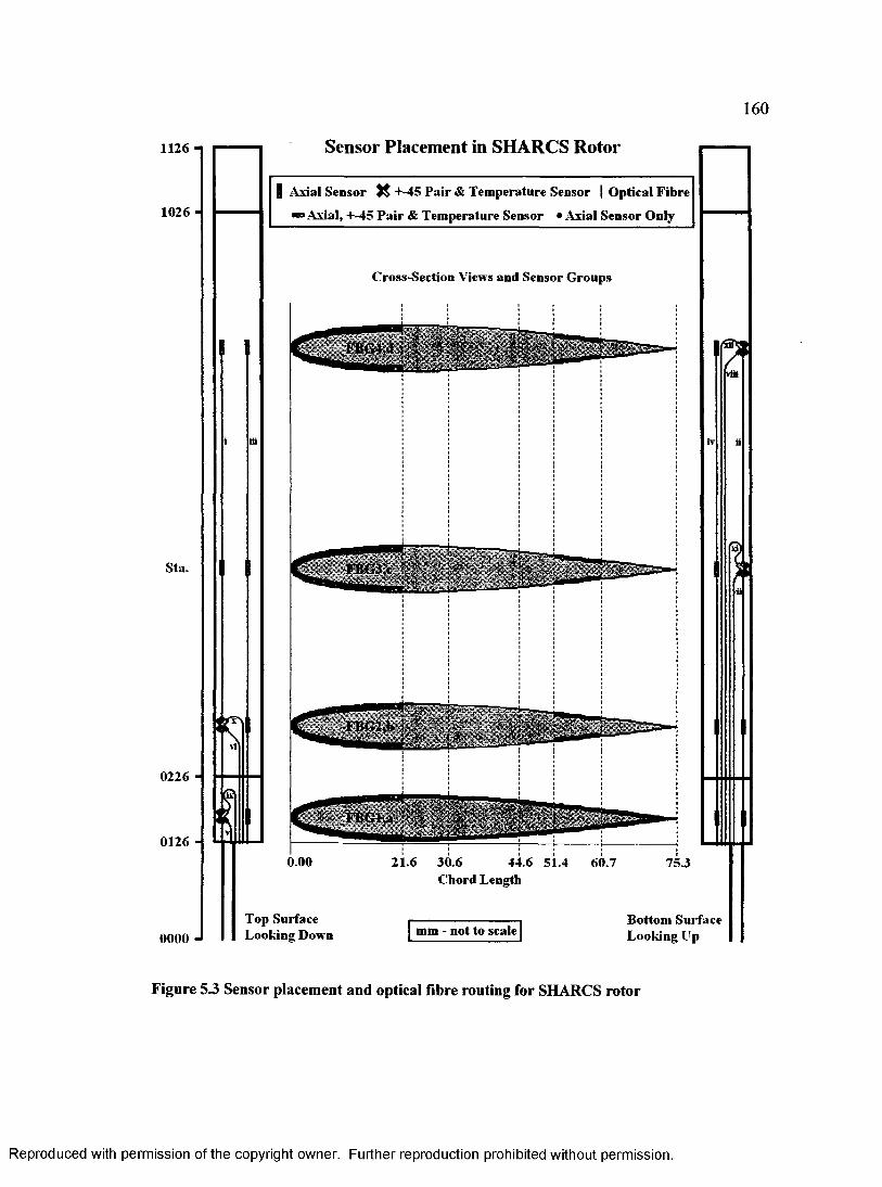
160

H 26 n

1026

Sta.

i n

0226 -

0126 -

Sensor Placement in SHARCS Rotor

| Axial Sensor t t +-45 Pair & Temperature Sensor | Optical Fibre

• Axial, +-45 Pair & Temperature Sensor • Axial Sensor Only

0.00

Cross-Section Views and Sensor Groups

FBG4

. , i >rwmm

FBG2,b ; ■nil

TBGi.a i ■;>; - iijp

21.6 30.6 44.6 51.4 60.7Chord Length

75.3

0000 -JTop Surface Looking Down mm - not to scale

Bottom Surface Looking Up

Figure 5.3 Sensor placement and optical fibre routing for SHARCS rotor


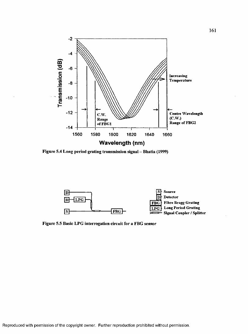
161

QQ■oco5> o (0 -8

E(0c -102i -

-12 Centre Wavelength (C.W.)Range of FBG2

C.W. Range of FBG1

-141560 1580 1600 1620 1640 1660

Wavelength (nm)Figure 5.4 Long period grating transmission signal - Bhatia (1999)

■ Source■ Detector■ Fibre Bragg Grating - Long Period Grating ' Signal Coupler / Splitter

Figure 5.5 Basic LPG interrogation circuit for a FBG sensor


0-

[d |— | l p gl p g J-^i

FBG -

FBGLPG

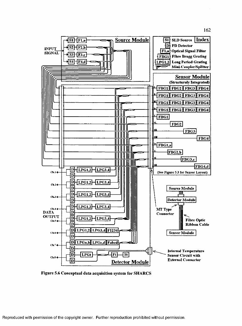
162

INPUT_SIGNAL

-4sTHfm

->fS 2 |- [FLb

SLD Source I n d e x PD Detector

Source Module

Optical Signal Filter Fibre Bragg Grating Long Period Grating Mini-Coupler/Splitter

S3HF3,cl FBG1- F4,d LPG1,2

Sensor Module(Structuraly Integrated)

M FBG1 | | f BG2 H FBG3 H FBG4

H FBG1 [Tf BG2 H FBG3 H FBG4

FBG1 FBG2H FBG3H FBG4

FBG2| FBG3HFBG4FBG1

H f b g i

FBG4

“ FBGl,a

FBG4)dd H l p g u H lpg3,4

(See Figure 5.3 for Sensor Layout)C h .l 4

Dj-j LPG1,2}—| LPG3,4CTl2 «

Source Module

BDJ-| LPG1,2|—| LPG3.4Ch.3 4

Detector Module

MT Type Connector

LPG3,4Ch. 4 4

DATAOUTPUT

Ch-5 4DJ-| LPG1,2[—| LPG3,4 Fibre Optic

Ribbon Cable

P || LPGl^H LPG3,4Hf 1234Sensor ModuleCH.6 4

DH LPGa,bH LPGc,dHFabcd

D LPGt

Detector ModuleCh.8 4

Internal Temperature Sensor Circuit with External Connector

Figure 5.6 Conceptual data acquisition system for SHARCS


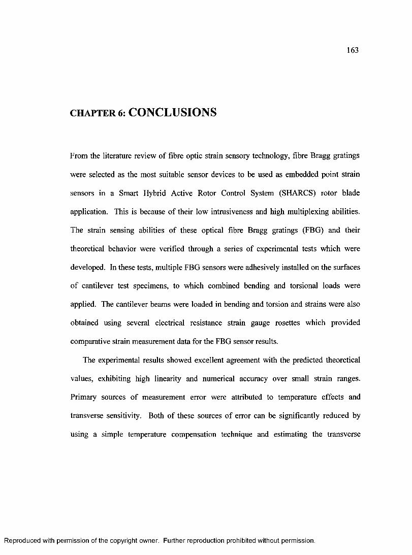
163

CHAPTER 6: CONCLUSIONS

From the literature review of fibre optic strain sensory technology, fibre Bragg gratings

were selected as the most suitable sensor devices to be used as embedded point strain

sensors in a Smart Hybrid Active Rotor Control System (SHARCS) rotor blade

application. This is because of their low intrusiveness and high multiplexing abilities.

The strain sensing abilities of these optical fibre Bragg gratings (FBG) and their

theoretical behavior were verified through a series of experimental tests which were

developed. In these tests, multiple FBG sensors were adhesively installed on the surfaces

of cantilever test specimens, to which combined bending and torsional loads were

applied. The cantilever beams were loaded in bending and torsion and strains were also

obtained using several electrical resistance strain gauge rosettes which provided

comparative strain measurement data for the FBG sensor results.

The experimental results showed excellent agreement with the predicted theoretical

values, exhibiting high linearity and numerical accuracy over small strain ranges.

Primary sources of measurement error were attributed to temperature effects and

transverse sensitivity. Both of these sources of error can be significantly reduced by

using a simple temperature compensation technique and estimating the transverse


164

sensitivities of the FBG sensors, which are based on the elastic interaction of the sensor

with the surrounding host materials. This was demonstrated in the present work.

A conceptual dynamic strain sensing system and sensor network was presented for

the SHARCS rotor blade application. It was based on a preliminary structural design of

the rotor blade by Mikjaniec (2006). It follows the techniques employed by several

researchers, the use of available compact optical components to meet a basic set of

system design requirements. In a more detailed design of the system as a next step, it is

suggested that a finite element analysis of the SHARCS rotor blade be performed to

establish more accurately the limiting strains in order to determine the appropriate FBG

system requirements.

6.1 Recommendations for Future Work

In continuing research on the topic of fibre optic strain sensors embedded in composite

materials and to fully realize an integral dynamic fibre optic strain sensing system within

a mach scaled helicopter rotor blade, such as that proposed in Chapter 5 of this work,

there are several areas of research which should be addressed in more detail.

A boundary element or finite element study could be used to investigate the effect of

the resin pocket geometry on the transverse sensitivity of embedded FBG sensors. This

parametric study would serve as support for the theoretical optical response of FBG

sensors embedded in laminate structures.

A finite element model analysis of the rotor blade would establish more accurately

the system design requirements, and assist with sensor placement within the structure.

The finite element model would also serve as a link between the measured strains and the


165

loads acting on the rotor blade, accounting for coupling effects due to the anisotropy of

laminate lay-up and coupling caused by the structural dynamics and large deflections of

the rotor blade.

Integration of the sensor module within the rotor blade structure requires addressing

several practical issues, such as ingress/egress of the optical fibre into the laminate, the

routing of optical fibre to the sensing locations, the details of manufacturing and

assembly with regards to the laminate lay-up, temperature exposure and fading of the

FBG sensors during the cure cycle of the laminate, and application of any specialized

coatings which may required. These issues would be addressed through a series of

practical investigations, which could also include laminate coupon testing with embedded

FBG sensors to assess their measurement repeatability and any fatigue of the sensors.

Finally, assembly and calibration of the source and detector modules would require as

a first step proof of concept testing of the basic interrogation circuit, shown in figure 5.5,

using the compact components described in Chapter 5. After testing the basic

interrogation circuit, more complex circuit concepts can be built and tested, leading to the

final verification and testing of the source and detector module concepts illustrated in

figure 5.6.


166

References

Agilent Technologies (1996), “Optical Spectrum Analysis”. Application Note 1550-4,

Santa Clara, California, USA

Alahbabi, M.N., Lawrence, N.P., Cho, Y.T., and Newson, T.P. (2004). “High spatial

resolution microwave detection system for Brillouin-based distributed temperature and

strain sensors”. Measurement Science and Technology. 15, pp. 1539-1543

ANSYS, version 10.0 Help File, 2006

Atkins, R.M. (1996). Photosensitivity in Optical Fibers, Lucent Technologies-Bell

Laboratories, Murray Hill, New Jersey, USA.

Baek, S., Jeong, Y., and Lee, B. (2002). “Characteristics of short-period blazed fiber

Bragg gratings for use as macro-bending sensors”. Applied Optics. 41, pp. 631-636

Bertholds, A., and Dandliker, R. (1988). “Determination of the Individual Strain-Optic

Coefficients in Single-Mode Optical Fibers”. Journal o f Lightwave Technology. 6, pp.

17-20

Bhatia, V. (1999). “Applications of long-period gratings to single and multi-parameter

sensing”. Optics Express. 4, pp. 457-466

Carson, M. (2006). “Characterizing polarization-dependant wavelength in AWGs and

PLCs”. Application Note 155, EXFO Electro-Optical Engineering Inc.


167

Caucheteur, C., Lhomme, F., Maakaroun, F., Chah, K., Blondel, M., and Megret, P.

(2004). “Simultaneous strain and temperature sensor using superimposed tilted Bragg

gratings”. Proceedings Symposium IEEE/LEOS Benelux Chapter, pp. 219-222

Chen, X., Zhou, K., Zhang, L., and Bennion, I. (2005). “Optical Chemosensor Based on

Etched Titled Bragg Grating Structures in Multimode Fiber”. IEEE Photonics

Technology Letters. 17, pp. 864-866

Dong, X., Meng, H., Liu, Z., Kai, G., and Dong, X. (2001). “Bend measurement with

chirp of fiber Bragg grating”. Smart Materials and Structures. 10, pp. 1111-1113

Dyllong, E., Kreuder, A. (1999). “Optimal reconstruction of mode shapes using

nonuniform strain sensor spacing”. Proceedings o f the 1999IEEE/ASME International

Conference on Advanced Intelligent Mechatronics

Eaton, N.C., Drew, R.R., and Geiger, H (1995). “Finite element stress and strain analysis

in composites with embedded optical fiber sensors”. Smart Materials and Structures. 4,

pp. 114-117

Erdogan, T. (1997). “Fiber Grating Spectra”. Journal o f Lightwave Technology. 15, pp.

1277-1294

Fan, Y., and Kahrizi, M. (2004). “Applicability of an Optimized Fiber Optic Smart

Structure”. Proceedings o f the 2004 IEEE International Conference on MEMS, NANO

and Smart Systems (ICMENS’04)

Friebel, E.J., Askins, C.G., Bosse, A.B., Kersey, A.D., Patrick, H.J., Pogue, W.R.,

Putnam, M.A., Simon, W.R., Tasker, F.A., Vincent, W.S., and Vohra, S.T.(1999).


168

“Optical fiber sensors for spacecraft applications”. Smart Materials and Structures. 8,

pp.813-838

Ghatak, A., and Thyagarajan, K.(1998). Introduction to Fiber Optics, Cambridge

University Press, Cambridge, United Kingdom.

Giles, C. R. (1997). “Lightwave Applications of Fiber Bragg Gratings”. Journal o f

Lightwave Technology. 15, pp. 1391-1404

Glaesemann, S., and Castilone, R.J. (2002). “The mechanical reliability of Coming

optical fiber in bending”. White paper: WP3690, Coming Inc., New York, USA.

Godfrey, L. (1998). “Choosing the detector for your unique light sensing application”.

PerkinElmer Inc.

Gomall, W., and Amarel, T. (2003). Applications and techniques for fiber Bragg grating

sensor measurements, EXFO, Burleigh Products Group, Victor, New York, USA.

Green, A.K., Zaidman, M., Shafir, E., Tur, M., and Gali, S. (2000). “Infrastructure

development for incorporating fibre-optic sensors in composite materials”. Smart

Materials and Structures. 9, pp.316-321

Grobnic, D., Mihailov, S.J., Smelser, C.W., and Ding, H. (2004). “Sapphire fibre Bragg

grating sensor made using femtosecond laser radiation for ultrahigh temperature

applications”. IEEE Photonics Technology Letters, 16, pp. 2505-2507

Grossman, B.G., and Huang, L.T. (1998). “Fiber optic sensor array for multi-dimensional

strain measurement”. Smart Materials and Structures. 7, pp. 159-165


169

Gougeon, N., Poulain, M., and Abdi, R. El (2004). “Evolution of strength silica optical

fibers under various moisture conditions”. Optical Materials. 27, pp. 75-79

Hadjiprocopiou, M., Reed, G.T., Hollaway, L.,and Thome, A.M. (1996). “Optimization

of fibre coating properties for fiber optic smart structures”. Smart Materials and

Structures. 5, pp.441-448

Hecht, J. (2006). Understanding Fiber Optics, Prentice Hall, New Jersey, USA

Hetenyi, M. (1950). Handbook o f Experimental Stress Analysis, John Wiley & Sons, Inc.,

New York, USA

Hill, K.O., Fujii, Y., Johnson, D.C., and Kawasaki, B.S. (1978). “Photosensitivity in

optical fiber waveguides: Application to reflection filter fabrication”. Applied Physics

Letters. 32, pp. 647-49

Hill, K.O. and Meltz, G. (1997). “Fiber Bragg Grating Technology Fundamentals and

Overview”. Journal o f Lightwave Technology. 15, pp. 1263-1276

Kalamkarov, A.L., Georgiades, A.V., MacDonald, D.O., and Fitzgerald, S.B. (2000).

“Pultruded fibre reinforced polymer reinforcements with embedded fibre optic sensors”.

Canadian Journal o f Civil Engineering. 27, pp. 972-984

Kang, H.K., Park, J.W., Ryu, C.Y., Hong, C.S., and Kim, C.G. (2000). “Development of

fibre optic ingress/egress methods for smart composite structures”. Smart Materials and

Structures. 9, pp. 149-156


170

Kang, S.C., Kim, S.Y., Lee, S.B., Kwon, S.W., Choi, S.S., and Lee, B.H. (1998).

“Temperature-Independent Strain Sensor System Using a Tilted Fiber Bragg Grating

Demodulator”. IEEE Photonics Technology Letters. 10, pp. 1461-1463

Kersey, A.D., Davis, M.A., Patrick, H.J., LeBlanc, M., Koo, K.P., Askins, C.G., Putnam,

M.A., and Friebele, J. (1997). “Fiber Grating Sensors”. Journal o f Lightwave

Technology. 15, pp. 1442-1463

Kim, N.-S., and Cho, N.-S. (2004). “Estimating Deflection of a Simple Beam Model

Using Fiber Optic Bragg-grating Sensors”. Experimental Mechanics. 44, pp. 433-439

Kojima, S., Komatsuzaki, S., Kurosawa, Y., and Hongo, A. (2004). “Embedding type

strain sensors using small-diameter fiber Bragg grating to composite laminate structures”.

Hitachi Cable Review No. 23 (August 2004), Advanced Technology Laboratories,

Hitachi Cable, Ltd., Japan

Laffont, G., and Ferdinand, P.(2001). “Tilted short-period fibre-Bragg-grating-induced

coupling to cladding modes for accurate refractometry”. Measurement Science and

Technology. 12, pp. 765-770

Lau, K.T., Yuan, L., and Zhou, L.M. (2001). “Thermal effects on an embedded grating

sensor in and FRP structure”. Smart Materials and Structures. 10, pp. 705-717

Lin, Y.B., Chang, K.C., Chem, J.C., and Wang, L.A. (2005). “Packaging Methods of

Fiber-Bragg Grating Sensors in Civil Structure Applications”. IEEE Sensors Journal. 5,

pp.419-424


171

Ling, H.-Y., Lau, K.-T., Cheng, L., and Jin, W. (2006). “Viability of using an embedded

FBG sensor in a composite structure for dynamic strain measurement”. Measurement. 39,

pp. 328-334

Magne, S., Rougeault, S., Vilela, M., and Ferdinand, P. (1997). “State-of-strain

evaluation with fiber Bragg grating rosettes: application to discrimination between strain

and temperature effects in fiber sensors”. Applied Optics. 36, pp. 9437-9447

Mall, S., Dosedel, S.B., and Holl, M.W. (1996). “The performance of graphite-epoxy

composite with embedded optical fibers under compression”. Smart Materials and

Structures. 5, pp. 209-215

Matthewson, M.J., Kurkjian, C.R., and Hamblin, J.R. (1997). “Acid stripping of fused

silica optical fibers without strength degradation”. Journal o f Lightwave Technology. 15,

pp. 490-497

Mat-Web (2007). Online material properties data-base www.matweb.com

Meltz, G., Morey, W.W., and Glenn, W.H.(1989). “Formation of Bragg gratings in

optical fibers by a transverse holographic method”. Optics Letters. 14, pp. 823-825

Mikjaniec, T. (2006). “The Preliminary Design of the SHARCS Rotor Blade”. M.A.Sc.

Thesis, Department of Mechanical and Aerospace Engineering, Carleton University,

Ottawa, Ontario

Mottram, J.T.(2004). “Shear Modulus of Standard Pultruded Fiber Reinforced Plastic

Material”. Journal o f Composites for Construction. 8, pp. 141-147


http://www.matweb.com

172

NEETS (2006). “Introduction to Fibre Optics”. NEETS Module 24, Integrated

Publishing, Port Richey, Florida, USA

Oliver, W.C., Pharr, G.M. (1992). “An Improved Technique for Determining Hardness

and Elastic Modulus Using Load and Displacement Sensing Indentation Experiments”.

Journal o f Materials Research. 7, pp. 1564-1583

Pak, Y.E. (1992). “Longitudinal shear transfer in fiber optic sensors”. Smart Materials

and Structures. 1, pp. 57-62

Peters, K., Studer, M., Botsis, J., Iocco, A., Limberger, H., and Salathe, R.(2001).

“Embedded Optical Fiber Bragg Grating Sensor in a Nonuniform Strain Field:

Measurements and Simulations”. Experimental Mechanics. 41, pp. 19-28

Prabhugoud, M., Peters, K. (2006). “Finite element model for embedded fiber Bragg

grating sensor”. Smart Materials an Structures. 15, pp. 550-562

Riley, W.F., Sturges, L.D., and Morris, D.H. (1995). Statics and Mechanics o f Materials,

John Wiley & Sons Inc., New York, USA

Rourk, R.J. (1975). Formulas for Stress and Strain, McGraw Hill, Inc., New York, USA

Shidlovski, V. (2004). “Superluminescent diodes. Short overview of device operation

principles and performance parameters.” SuperlumDiodes Ltd., Moscow, Russia

Shivakumar, K., and Emmanwori, L. (2004). “Mechanics of failure of composite

laminates with an embedded fiber optic sensor”. Journal o f Composite Materials. 38, pp.

669-680


173

Shivakumar, K., and Bhargava, A. (2005). “Failure mechanics of a composite laminate

embedded with a fiber optic sensor”. Journal o f Composite Materials. 39, pp. 777-798

Shroeder, K., Ecke, W., Apitz, J., Lembke, E., and Lenschow, G. (2006). “A fibre Bragg

grating sensor system monitors operational load in a wind turbine rotor blade”.

Measurement Science Technology. 17, pp. 1167-1172

Simpson, A.G., Zhou, K., Zhang, L., Everall, L., and Bennion, I. (2004). “Optical sensor

interrogation with a blazed fiber Bragg grating and a charge-coupled device linear array”.

Applied Optics. 43, pp. 33-40

Sirkis, J.S.(1993). “Optical and mechanical isotropies in embedded fiber optic sensors”.

Smart Materials and Structures. 2, pp. 255-259

Skontorp, A. (2002). “Composites with embedded optical fibers at structural details with

inherent stress concentrations”. Journal o f Composite Materials. 36, pp. 2501-2515

Smith, K.H., Ipson, B.L., Loweder, T.L., Hawkins, A.R., Selfridge, R.H., and Schultz,

S.M. (2006). “Surface-relief fiber Bragg gratings for sensing applications”. Applied

Optics. 45, pp. 1669-1675

Stewart, A., Carman, G., and Richards, L. (2003). “Nondestructive Evaluation Technique

Utilizing Embedded Thermal Fiber Optic Sensors”. Journal o f Composite Materials. 37,

pp. 2197-2206

Surgeon, M., and Weavers, M. (2001). “The influence of embedded optical fibres on the

fatiqgue damage progress in quasi-isotropic CFRP laminates”. Journal o f Composite

Materials. 35, pp.931 -940


174

Tian, X.G., and Tao, X.M.(2001). “Torsion Measurement Using Fiber Bragg Grating

Sensors”. Experimental Mechanics. 41, pp.248-253

Tuttle, M.E. (2004). Structural Analysis o f Polymeric Composite Materials, Marcel

Dekker, Inc., New York, USA

Udd, E., (1991), Fiber Optic Sensors, An Introduction for Engineers and Scientists, John

Wiley & Sons, Inc., New York, USA.

Wang, Q., Farrell, G., and Freir, T. (2005). “Theoretical and experimental investigations

of macro-bend losses for standard single mode fibers”. Optics Express. 13, pp. 4476-4484

Weisstein, E.W. (2003). “Helix”. Mathworld - a Wolfram Web Resource.

Xiao, H., Deng, J., Pickrell, G., May, R.G., and Wang, A. (2003). “Single-Crystal

Sapphire Fiber-Based Strain Sensor for High-Temperature Applications”. Journal o f

Lightwave Technology. 21, pp. 2276 - 2283

Zhang, L., Fallon, R., Everall, L.A., Williams, J.A.R., and Bennion, I. (1998). “Large-

Dynamic-Range and High-Resolution from a Strain Sensing System using Long-Period

Grating Interrogating FBG Strain Sensor”. ECOC’98. 20-24 September 1998, Madrid,

Spain


STRAIN MEASUREMENT OF COMPOSITE MATERIALS USING …

Documents