Stopping rules for utility functions and the St. Petersburg gamble

ELSEVIER Applied Mathematics and Computation 98 (1999) 279-291

A~LIED MATHEMATIC5

AND COM ~LITATIION

Stopping rules for utility functions and the St. Petersburg gamble

Moshe Dror, Bruce C. Hartman * MIS Department, College of Business, University of Arizona, Tucson, AZ 85721, USA

Abstract

We study, using the St. Petersburg paradox, the risk attitudes expressed by utility functions without the normal continuity and differentiability assumptions. We model the repeated St. Petersburg lottery with two parameters, starting wealth and return ratio, as a stochastic process with a simple control mechanism and the objective of maximizing utility of the outcome. A stopping function expresses the earliest stopping stage; a finite value resolves the paradox. This new approach can measure the risk at- titude of discontinuous utilities in only a finite horizon repetition of the lottery, opening the door to new usefulness of the utility concept in modeling. As an Example we give an application to behavior of persons receiving entitlements towards additional income from working. © 1999 Elsevier Science Inc. All rights reserved.

Keywords." Decision analysis; Risk analysis; Utility lheory

I, In troduct ion

Utility functions are supposed to measure an individual 's happiness with levels o f wealth; they try to capture the behavior o f individuals who make choices about money. One can tell f rom the utility function the att i tude o f its owner toward risk - aversion, love, or neither. What real valued functions o f money can qualify as utilities?

Classical theory tells us that utilities must be cont inuous and differentiable, sometimes twice. These characteristics make the functions convenient to handle in computat ions , and models based on such functions have produced useful

* Corresponding author. E-mail: [email protected].

0096-3003/99/$ -. ~e¢ front matter © 1999 Elsevier Science Inc. All rights reserved. PII: S0096-3003(97) 10169-2

280 M. Dror, B.C Hartman / Appl. Math. Comput. 98 (1999)279-291

results - in consumer microeconomics, finance, and decision analysis, for ex- ample (see any micro textbook such as Varian, 1992). To produce such func- tions, the foundations of this theory have a rich axiomatic structure. The axiom systems make statements about preference orderings among certain outcomes and lotteries, which are states with two possible outcomes, with probabilities p and 1 - p of occurring. The probability p could be 1 (certainty) or zero, so lotteries include the case of certain and impossible outcomes. The utility of a lottery is assumed to be the expected value of the utilities of the possible outcomes. A standard theory of utility, which we assume, requires calculation of expected values of simple two-choice lotteries as the convex combination of the utility of the choices with weights the probabilities.

Discontinuous functions let us model decision-making under risk in a broader class of situations. Many of these situations are of managerial im- portance. We give one real application to attitudes of people receiving an en- titlement in the light of the US Tax Code for 1995. The familiar notion of utility, so extended, promotes significant understanding for the manager, and helps to show what might be done to remedy the situation.

We want to find a way to characterize for discontinuous candidate utility functions the attitude toward risk they capture. Such a technique provides an alternate way to derive results like the classical ones for this broader class of utility functions.

It is natural to approach this problem from the standpoint of the St. Pe- tersburg game, described in Section 2, which is played using such a lottery. The paradox induced by applying expected value calculations to the value of the game led in the 1700s to the initial description and debate of the utility concept.

We formulate the game as a control program, for which the optimal policy is a stopping function f . Such a stopping function provides an alternative to normal axiomatic developments. The theory of risk can be extended to broader classes of utility functions, because f c a n be determined with no differentiability or continuity demands, based on a sequence of finite stages. To our knowledge, such an analysis of utility in the light of the paradox has not appeared in the literature.

2. St. Petersburg game

A fair coin will be tossed repeatedly in independent tosses until a tail occurs. You begin the game with a starting stake of $ x0/> 1. After each toss you are offered a bet on the outcome of the following lottery. You may end the game and keep your winnings from the previous tosses of the coin, or stake all you have on the next toss of the coin. If a head comes up, the stake will be mul- tiplied by a return ratio B > 2. If a tail is thrown you will lose the entire stake.

M. Dror, B.C. Hartman / Appl. Math. Comput. 98 (1999) 279-291 281

The coin is fair, so the expected pay-off of the game at coin toss k + 1 is (1/2)Bx~ + (1/2)0 = (B/2)xk, where xk denotes the original stake plus the winnings after k throws. Based solely on the expected value of the lottery, when B > 2 you would bet your stake each time until a tail is thrown. Clearly a tail will be thrown eventually, and with probability 1 you are sure to lose your original stake. This dilemma is known in the literature as the St. Pe- tersburg paradox and dates back at least to Bernoulli (1738). For interesting discussions of the St. Petersburg paradox see Samuelson, 1977 and Lopes, 1981.

The version of the above game is equivalent to a classical statement (see, for instance, Samuelson, 1977). There, Peter runs the game, and Paul is offered a bet in which the prize is B ~r if no tail occurs by the Nth toss, and nothing otherwise. Paul may quit after each toss. The question asked is what is the most Paul would pay for the opportunity to play this game for N tosses. Viewed in a finite horizon, Paul should always be willing to choose a larger N, and pay a larger sum for the opportunity. A paradox occurs, since it is unlikely that Paul would opt for a very large N and pay a large sum for the chance.

Let U(x) be a real-valued utility function expressing for the participant the utility value of state x. Certain utilities avoid the paradox that occurs when U is linear, that one should play until the entire stake is lost. Standard derivations of this result use Pratt's theorem (see Arrow, 1970, or Pratt, 1964), which re- quires the differentiability of a utility function. In this paper we present a simple stochastic control model for our version of the St. Petersburg lottery. With some utilities, the optimal control policy is a stopping rule - it tells the player to stop betting at some stage. One can use these stopping rules to compare risk attitudes represented by different utilities.

We can characterize the risk attitude of a utility individually, or compare a parametrized family of utilities. For an individual utility U we use as the characterization the stopping function fu(x0, B) of the starting wealth x0 and return ratio B, which gives the smallest stage at which the player should stop. Its range is the extended natural numbers including ~ ; it is independent of any parameters of the utility under consideration. The smaller the value of f for a given x0 and B, the greater the risk aversion there. This criterion for risk at- titude is two-dimensional, differing for users at both starting wealths and re- turn ratios.

We use the stopping stage to compare utilities in a parametrized family, providing more generality at the expense of higher dimensionality of the cri- terion. Now the stopping stage f(x0, B, a) is a function of x0, B, and the pa- rameters (in the vector ~) of the family under consideration. Utilities in a parametrized family could express risk attitudes which differ not only by x0 and B, but by values of the parameters.

282 M. Dror, B.C. Hartman / Appl. Math. Comput. 98 (1999) 279-291

3. The game as a control problem

To set up the control problem for the St. Petersburg game, we define at the kth turn the possible states xk = Bkxo and 0. There are two possible control actions uk E {0, 1}; the payoff ratio at the turn is a random disturbance ek ~ {B, 0} with uniform probabilities of ½. The system evolves according to the state equation

xk+l = xk + (e~ - 1)UkXk = Xk[1 4- e~uk -- uk]. (1)

Given an initial value x0, the optimization problem is to determine an admis- sible control law ~z specifying the uk that maximizes the utility functional

J~(xo) = lkimEe k { U(xk))

subject to the system constraint. This is an infinite horizon problem in which we seek tf , the stage of the game at which we stop, which maximizes E{ U(x 9) }. If tf = ~ then the game is never stopped; we have the St. Petersburg paradox for this U.

As an example, formulate the St. Petersburg gamble with utility U(x) = x as a finite horizon problem with no more than N coin tosses. If we play for N steps, JN(XN) = XN; for each k,

/ B',~N-k Jk(xk)=maxEe~Jk+'(Xk-~l)=xkmax{l'B/Z}~,k 0,, -~ ) Xk;

and Jo(xo) = (B/2)Uxo. Observe that for B ~< 2 the player should stop at once; f ( x o , B ) = 0. For B > 2 the optimal policy for any N is to toss; f ( xo , B) = ~ . This policy is clearly optimal independently of the horizon N, so that when N --* cx~, we should choose to play. The player with this utility prefers the risk of the lottery.

Selection of a different utility function may eliminate the paradox. One could obtain a similar effect by "discounting" the future value of money (which requires a time sequence); or by changing the size of the bet at each turn. In the example above, the player bets his entire holdings at face value. If he is allowed to reduce his bet at each turn in exchange for a similarly reduced reward, a different optimal rule recommending stopping might emerge.

4. Comparing utilities

What interests us here are these questions: 1. Are there discontinuous utilities U, as well as continuous ones, such that the

game's optimal control policy results in a finite stopping point f ( xo , B) for some B and x0?

M. Dror. B.C Hartman / Appl. Math. Comput. 98 (1999) 279-291 283

2. Can we compare discontinuous utilities (and continuous ones) parametrized by some c~ by comparing stopping functions f(Xo, B, a) over the range of val- ues of xo,B, and a? If U is the family of functions bounded above by the parameter ~ = M, then

for any B and x0 we should not play beyond that utility amount, fu(xo, B, M) is the number of the first stage for which the expected utility value exceeds M. The members of this simple but uninteresting single parameter family all have finite f; each is guaranteed a finite stopping rule.

The following fact (Arrow, 1970; Pratt, 1964; Fishburn, 1988) states an equivalence between several ways of comparing twice differentiable utility functions as to their ability to resolve the paradox. Let R,(x) = -u"(x)/u'(x) denote the absolute risk aversion at x of the utility function u. Let the initial stake x0 in a gamble be divided into amounts y0 for a risky investment and z0 for a riskless one; let B be the expected return rate of the risky investment which exceeds that of the riskless one.

Fact 1. The following are equivalent for any two utility functions U and V which are twice differentiable.

1. There exists an increasing, concave function g such that for all x, V(x) = g(U(x)).

2. Rv(x) >1 Ru(x) for all x. 3. Maximizing expected utility V(x) requires dividing xo so that the riskless

investment z v is no smaller than the riskless amount z~ invested to maximize expected utility U(x); z~" >t z~'.

Point 3 may be restated as

Fact 2. 4. Suppose that for the St. Petersburg gamble defined by Xo and B, the stopping

point fv(x0, B) maximizing U is finite. Then to maximize V we will stop no later; fz(x0, B) <~ fv(xo, B). I f no finite stopping rule exists for V, then none can exist for U; fv(xo,B) = oo.

For a particular utility, a finite value f(x0, B) of the stopping function for some gamble defined by (x0, B) means that there is a strategy for that number of plays which can be carried out indefinitely. Such a strategy is equivalent to convergence of the finite horizon model to the infinite; to existence of a finite expectation; or to existence of a sequence of prices for each turn of the game for which the player will stop.

The question is therefore one of modeling the lottery appropriately so that stopping conditions make sense as measures of risk aversion of utility func- tions. Since one cannot actually play an infinite horizon game, it is desirable to evaluate utility functions based on their finite horizon performance. Our model

284 M. Dror, B. C Hartman I Appl. Math. Comput. 98 (1999) 279-291

assesses utilities based on behavior in a finite set of states, which could in principle be observed, rather than on limit behavior, which cannot.

5. HARA utility functions

The class of HARA (Hyperbolic Absolute Risk Aversion) utilities pro- vides important examples for applications. It includes utilities with absolute or relative risk aversions decreasing, increasing, or constant, reflecting risk atti- tudes often assumed for real decision makers. It consists of real unbounded functions U, twice continuously differentiable, which satisfy the differential equation

- U'(x)/U"(x) = a + hr, Vx, (2)

where ~ = (a, b), a, b/> 0 are scalar parameters. The left-hand side is the re- ciprocal of the absolute risk aversion of U at x. Three general forms satisfy the differential equation.

V ( x ) = - e -x/a , ~ = ( a , 0 ) , a > 0 , (3)

U(x) = In (a + x), ~ --: (a, 1), (4)

1 U(x)=-~--~_l(a+bx) ' - l /b , ~ = ( a , b ) , b-~0,1 . (5)

Merton (1971) and Bertsekas (1987) discuss HARA utilities in the context of dynamic portfolio analysis. The optimal policy n multiplicatively separates the effect of the starting stake x0 from that of the random rate of return ek and its probability distribution. For the St. Petersburg game, the optimal policy at period k is myopic - the gambler plays (invests all in a risky venture) for one period, and subsequently does not play (invests exclusively in the safe alter- native).

We can obtain the classical results on risk attitude for these functions without using the twice differentiable nature of U, and considering only what happens under finite repetition of the game. In this section we write the ob- jective function of the control problem for forms (3)-(5), and present the re- sulting stopping functions f ( xo ,B , ~) in Table 1. The derivations for Eqs. (4) and (5) are presented in Appendix A. Note that for B ~< 2 we should always stop, so in what follows, we restrict attention to the cases B > 2.

For exponential utilities (3), the objective for stage k E {0 , . . . ,N} is

Jk(xk) = min [exp [--xk/a], exp [(--xk/a)(B/2)N-x]],

where the left term of the minimization occurs for uk = 0, or stop, and the right-hand term occurs for uk = 1, or bet. For a > 0, the player should never stop playing, since the right-hand term is always larger; f (xo ,B , (a, 0)) = o~.

M. Dror, B.C Hartman I Appl. Math. Comput. 98 (1999) 279-291 285

Table 1 Dependence of stopping functions for HARA utilities on parameters ~, initial wealths x0, and return ratios B > 2 (q, t,K are defined in appendix)

HARA class U, c~ f(x0, B, a) Parameters

Eq. (3) Exponential - e -~/a, = zc, a > 0 = (a, 0)

Eq. (4) Logarithm In (x + a), a = 0 = (a, 1) a > B~/4(B- 1)

a<~B2/4(B- 1) b ¢ 2 Eq. (5) Power ~ (a + bx) Ib-li/b,

= 0 = 0 = q No closed form

~ = (a,b), = 0 B>~4, a > 0 b ¢ 0 , 1 = t B < 4 ,

K(B,t)<~a/xo, and a/xo <K(B, t+ 1)

For logarithmic utility functions (4), the objective at the kth stage is

Jk(xk) = max [ln (xk + a), In a~/2(Bxk + a) l /2 , . . . , In al/2(BJxk+a) 1/2j,

. . . , In al/2(BN-kXk + a)l/2N-k],

and

Jo(xo)=max[ ln(xo+a) ,max[ lna t /2 (BJxo+a) l /2J]] .

When a = 0, we should always stop, since the term In(x0 + a),x0/> 1, domi- nates; f (xo ,B, (0, 1)) = 0. This is the solution of the St. Petersburg paradox originally offered by Bernoulli, who suggested the log function as an appro- priate measure of humans' evaluation of money. See the appendix for an analysis of the case a > 0.

The power utility function (5) with b # 0, 1 has objective

1 F 1 1 max [(a + Jk(xk) .---- b - ,2N_k (a + BU-kbxk) (b-tl/b bxk)(b-l)/b

2 u-k - 1 ] -+ -~-~ a(b-1)/b , ..I

Jo(Xo) ~-- b~max[ (a -~ bxo)(b-l)/b,l (a-~-BNbxo)(b-])/b-Jf-~N l a(b-l)/b ] .

For B > 2 and general b the stopping condition is a transcendental equation which must be solved numerically for the first stopping point t depending on a. When b = 2, (b - 1)/b = ½, and we have the family parametrized by e = (a, 2) of square-root utility functions considered by Cramer (see Samuelson, 1977).

286 M. Dror, B.C. Hartman / Appl. Math. Comput. 98 (1999) 279-291

For these functions an analytical solution exists. This family is rich enough to generate a stopping point at any desired stage. Simply choose a appropriately.

Fact 3. Let the rate of return of the St. Petersburg gamble be B > 2, and the initial stake be xo > O. Then for any arbitrarily large stage t, there is a power utility function of the form given by Eq. (5) with ~ = (a, 2) such that it is optimal to play for turns 1 , . . . , t - 1 and stop at turn t.

6. Example 1

As an example of the use of our method for noncontinuous, nondifferen- tiable utilities, consider the function below with k a positive integer.

U(x) = { x 2 k < x < 2 k + l , inx 2 k - l~<x~<2k. (6)

This represents a world in which amounts whose integer part is even are better than amounts whose integer part is odd. (Perhaps it is better for those who pay with $2 bills.) This utility function is monotonic a.e., indeed differentiable a.e., but is not concave.

Note that if monotonicity fails on a set of points which is dense in a set of positive measure, then monotonicity no longer need imply differentiability (Dror and Hartman, 1993).

We consider only two cases. For x0 = 1, B --- 5, we should always stop, and f (1 ,5 ) = 0 from Table 1; for our winnings will always lie where U is loga- rithmic with a = 0.

On the other hand, for x0 = 5/2, B = 5 no stopping point exists, since the utility after N plays is (5/2) N+I . Since 5 k - 1 mod 4, the winnings are always an integer plus ~, and are in the interval above an even integer but below the next odd one. The subsequent utility will be linear, not logarithmic, and f ( 5 / 2 , 5) = cx>.

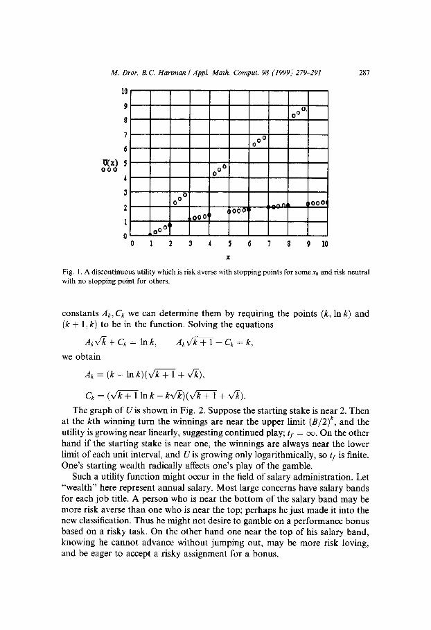
This utility function, shown in Fig. 1, cannot be classified as to risk aversion by tests of differentiability. However the function f(x0, B) can specify its risk behavior.

7. Example 2

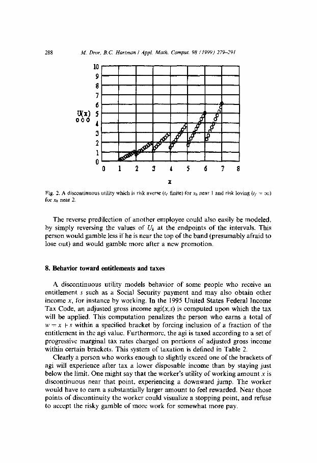
Here the utility function is defined as follows: let U(x) = Uk(x) on the in- terval [k,k+ 1), where Uk(x)= AkV/£+ Ck; and Ck and Ak are defined below. The Uk are chosen so that Uk(k) = l n k and Uk(k+ 1) = k. This means that near the lower endpoints of the intervals, U grows like In x, whereas near the upper endpoints of the intervals U grows like x. Since each function Uk has two

M. Dror, B.C. Hartman / Appl. Math. Comput. 98 (1999) 279-291 287

10

9 ooO. I 8

U(x) o o o

o o0

o o °

o 00 o o o too01 ' ' -

iO00 (

000' 0 1 2 3 ,I. 5 6 7 8 9 10

Fig. 1. A discontinuous utility which is risk averse with stopping points for some x0 and risk neutral with no stopping point for others.

constants Ak, Ck we can determine them by requiring the points (k, In k) and (k + 1, k) to be in the function. Solving the equations

A~ v ~ + Ck = ln k, A~ v ~ + l + Ck = k,

we obtain

A~ = ( k - Ink)( k , f k T 1 + v~),

Ck = ( k v ~ 1 In k - kv~)(v /k + 1 + v~).

The graph of U is shown in Fig. 2. Suppose the starting stake is near 2. Then at the kth winning turn the winnings are near the upper limit (B/2) k, and the utility is growing near linearly, suggesting continued play; t I = ~ . On the other hand if the starting stake is near one, the winnings are always near the lower limit of each unit interval, and U is growing only logarithmically, so tf is finite. One's starting wealth radically affects one's play of the gamble.

Such a utility function might occur in the field of salary administration. Let "wealth" here represent annual salary. Most large concerns have salary bands for each job title. A person who is near the bottom of the salary band may be more risk averse than one who is near the top; perhaps he just made it into the new classification. Thus he might not desire to gamble on a performance bonus based on a risky task. On the other hand one near the top of his salary band, knowing he cannot advance without jumping out, may be more risk loving, and be eager to accept a risky assignment for a bonus.

IIII

M. Dror, B .C Hartman / Appl. Math. Comput. 98 (1999) 279-291

tr(x) 0 0 0

10

9

8 7

6

4 :3

2

1 0

288

,¢

¢

r

0 1 2 3 l 5 6 7 8

Fig. 2. A discontinuous utility which is risk averse (t s finite) for x0 near 1 and risk loving (tf = ~ ) for x0 near 2.

The reverse predilection of another employee could also easily be modeled, by simply reversing the values of Uk at the endpoints of the intervals. This person would gamble less if he is near the top of the band (presumably afraid to lose out) and would gamble more after a new promotion.

8. Behavior toward entitlements and taxes

A discontinuous utility models behavior of some people who receive an entitlement s such as a Social Security payment and may also obtain other income x, for instance by working. In the 1995 United States Federal Income Tax Code, an adjusted gross income agi(x,s) is computed upon which the tax will be applied. This computation penalizes the person who earns a total of w = x + s within a specified bracket by forcing inclusion of a fraction of the entitlement in the agi value. Furthermore, the agi is taxed according to a set of progressive marginal tax rates charged on portions of adjusted gross income within certain brackets. This system of taxation is defined in Table 2.

Clearly a person who works enough to slightly exceed one of the brackets of agi will experience after tax a lower disposable income than by staying just below the limit. One might say that the worker's utility of working amount x is discontinuous near that point, experiencing a downward jump. The worker would have to earn a substantially larger amount to feel rewarded. Near those points of discontinuity the worker could visualize a stopping point, and refuse to accept the risky gamble of more work for somewhat more pay.

M. Dror, B. CI Hartman / Appl. Math. Comput. 98 (1999) 279-291 289

Table 2 SSI and Federal income tax brackets and rates for couple married filing jointly, US Tax Code, 1995

Entitlement schedule Tax rate schedule

Earnings x Fraction ofs AGI Marginal tax rate

$0-32,000 0.0 $0-39,000 0.15 $32,001-44,000 0.5 $39,001-94,250 0.28 $44,001 -up 0.85 $94,251 - 143,600 0.31

$143,601-256,500 0.36 $256,501-up 0.396

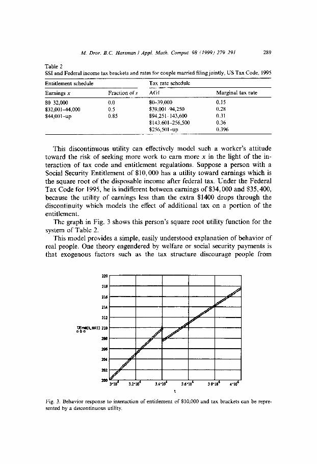
This discontinuous utility can effectively model such a worker's attitude toward the risk of seeking more work to earn more x in the light of the in- teraction of tax code and entitlement regulations. Suppose a person with a Social Security Entitlement of $10,000 has a utility toward earnings which is the square root of the disposable income after federal tax. Under the Federal Tax Code for 1995, he is indifferent between earnings of $34,000 and $35,400, because the utility of earnings less than the extra $1400 drops through the discontinuity which models the effect of additional tax on a portion of the entitlement.

The graph in Fig. 3 shows this person's square root utility function for the system of Table 2.

This model provides a simple, easily understood explanation of behavior of real people. One theory engendered by welfare or social security payments is that exogenous factors such as the tax structure discourage people from

2~

218

216

214

212

2~

20~

2O4

2O2

200

f f 3"10

j z J J f

t

Fig. 3. Behavior response to interaction of entitlement of $10,000 and tax brackets can be repre- sented by a discontinuous utility.

290 M. Dror, B.C. Hartman / Appl. Math. Comput. 98 (1999) 279-291

working. With this form of utility one's attitude toward work becomes simply rational economic behavior. Note that this utility is uniformly increasing al- most everywhere; one could measure the risk attitude at other income values without detecting that the person would not accept a job at a certain pay range. We could question the person in general and get the response that work was desired; that would be rational over most of the utility domain. A change in behavior might easily be accomplished by altering the externalities that affect the utility.

9. Conclusion

Stopping rules for real-valued functions representing utility can characterize them as to risk aversion without using any continuity or differentiability as- sumptions, by considering only behavior in the finite horizon. The appropriate measure of risk attitude is the stopping function f, which expresses the earliest stopping stage in a St. Petersburg lottery as a function of the starting wealth and the return ratio of the gamble. To classify a family of candidate utility functions, the parameters of the family may be included as arguments o f f This stopping function provides a multi-dimensional risk attitude criterion. It forms the basis for a comparison of risk attitude when the notion of utility is extended to such nondifferentiable functions.

Our examples show that our new approach to risk assessment might allow a different and potentially more general model of risk attitude. We also analyzed a practical example involving entitlements like Social Security payments, based on the 1995 US Federal Tax Code. A discontinuous utility of earnings from labor is useful in explaining individual behavior toward additional earnings when combined with the entitlement payment and the Tax Code. Such useful alternate utility models might apply in such areas as salary administration or quantity discounting, areas of significant managerial relevance.

Appendix A. Stopping points for HARA functions

Here we include brief derivations of the results presented in Table 1. We restrict attention to the cases B > 2.

(a) Logarithmic utility (4): The objective is

Jo(xo) = max [ln (Xo + a), lna'/2(BJXo + a)l/2J].

When a > 0, since In is monotonic the optimum occurs at

q = arg max[(BJx0 + a)1/2~]. Y

M. Dror, B.C Hartman I Appl. Math. Comput. 98 (1999) 279-291 291

The first s topping point q occurs if (Bqxo+a)l/2q>/ (Bq+lx0 q-a) l/2q+~ or (Bqxo + a) 2 >~ Bq+lxo + a. Let y~ = Bqxo, then (yq + a) 2 >~ Byq + a. The dis- cr iminant o f this quadrat ic equat ion in yq is A = B 2 - 4 a B + 4 a . For a > B2/4(B - 1) is negative, and noyq satisfies the equationf(xo, B, (a, 1)) = 0.

For a < B2/4(B - 1), the roots are yq = (B - 2a) /2 ± A/2 and q is a stop- ping point if yq is positive and outside the interval whose endpoints are the roots. For instance when B = 3, A ~> 0 for a ~< 9, a n d f i s a s topping point when yq = Bqxo is outside the interval (½ (3 - 2a) - ½ x~- - - 8a, ½ (3 - 2a )+ ½ v/-ff--- 8aa). For given x0 and B, q, the value o f f , can be calculated based on a.

(b) Power utility (5) with b = 2. The objective is

b S - ] - m a x l [ (a+bxo)Ib-ll/~',l(a'oU~-~; x(b-lt/b" 2N - 1 (b_l)/b ] Jo(xo) = ~- o v~oj ~ - ~ . ] .

We should stop at the first t such that

21(a + 2x0) 1/2 >1 (a + 2Btxo) 1/2 + (2' - 1)a 1/2.

Algebraic reduct ion yields the s topping condit ion a/xo >~ K(B, t), where

1 1 (2 t - (B/2)')2 (a.1) K(B' t )==-2( I_2- 0 ( B , _ 2 t)

K(B,t) is positive and strictly decreases with t for B < 4; K is 0 when B = 4; and K is always negative when B > 4. So for B 7> 4, any a gives t = 0; if B < 4, a player who will stop at turn t has utility with a/xo in the closed-open interval [K(B, t), K(B, t + 1)); such a parameter choice will produce t = f(x0, B, (a, 2)) as the smallest s topping stage.

References

Arrow, K., 1970. Essays in the Theory of Risk Bearing. Markham, Chicago. Bernoulli, D., 1738. Exposition of new theory on the measurement of risk. English translation:

Econometrica 22 (1954) 23-36. Bertsekas, D.P., 1987. Dynamic Programming: Deterministic and Stochastic Models. Prentice-

Hall, Englewood Cliffs, NJ. Dror, M., Hartman, B.C., 1993. A note on when monotonicity implies differentiability a.e. Internat.

J. Math. Edu. Sci. Technol. 24 (6), 92~926. Fishburn, P., 1988. Nonlinear Preference and Utility Theory. Johns Hopkins University Press,

Baltimore, MD. Lopes, L.L., 1981. Notes, comments, and new findings: decision making in the short run. J. Exp.

Psychol. 7 (5), 377-385. Merton, R.C., 1971. Optimum consumption and portfolio rules in a continuous-time model. J.

Econom. Theory 3, 373413. Pratt, J.W., 1964. Risk aversion in the small and in the large. Econometrica 32, 122-136. Samuelson, P., 1977. St. Petersburg paradoxes: defanged, dissected, and historically described. J.

Econom. Literature 15, 24-55. Varian, H.R., 1992. Microeconomic Analysis, Third ed., W.W. Norton, New York.