STOCK MOVEMENT PREDICTION WITH DEEP LEARNING ...

STOCK MOVEMENT PREDICTION WITH DEEP LEARNING,FINANCE TWEETS SENTIMENT, TECHNICAL INDICATORS,

AND CANDLESTICK CHARTING

by

Yichuan Xu

Submitted in partial fulfillment of the requirementsfor the degree of Master of Computer Science

at

Dalhousie UniversityHalifax, Nova Scotia

February 2020

© Copyright by Yichuan Xu, 2020

Table of Contents

List of Tables . . . . . . . . . . . . . . . . . . . . . . . . . . . . . . . . . . . v

List of Figures . . . . . . . . . . . . . . . . . . . . . . . . . . . . . . . . . . vi

Abstract . . . . . . . . . . . . . . . . . . . . . . . . . . . . . . . . . . . . . . viii

List of Abbreviations Used . . . . . . . . . . . . . . . . . . . . . . . . . . ix

Acknowledgements . . . . . . . . . . . . . . . . . . . . . . . . . . . . . . . x

Chapter 1 Introduction . . . . . . . . . . . . . . . . . . . . . . . . . . 1

1.1 Motivation . . . . . . . . . . . . . . . . . . . . . . . . . . . . . . . . . 1

1.2 Research Problem Formulation . . . . . . . . . . . . . . . . . . . . . 3

1.3 Contributions . . . . . . . . . . . . . . . . . . . . . . . . . . . . . . . 4

1.4 Outline . . . . . . . . . . . . . . . . . . . . . . . . . . . . . . . . . . . 4

Chapter 2 Background and Related Work . . . . . . . . . . . . . . . 6

2.1 Efficient Market Hypothesis . . . . . . . . . . . . . . . . . . . . . . . 6

2.2 Trading Techniques . . . . . . . . . . . . . . . . . . . . . . . . . . . . 7

2.3 Sentiment Analysis in Stock Market . . . . . . . . . . . . . . . . . . . 9

2.4 Machine Learning and Deep Learning . . . . . . . . . . . . . . . . . . 10

2.5 Convolutional Neural Network (CNN) . . . . . . . . . . . . . . . . . . 12

2.6 Long Short-Term Memory (LSTM) . . . . . . . . . . . . . . . . . . . 14

2.7 Deep Learning in Finance . . . . . . . . . . . . . . . . . . . . . . . . 16

2.8 Candlestick Charting . . . . . . . . . . . . . . . . . . . . . . . . . . . 17

2.9 Experiment Design . . . . . . . . . . . . . . . . . . . . . . . . . . . . 17

Chapter 3 Experiment on Daily News dataset . . . . . . . . . . . . 20

3.1 Data Source . . . . . . . . . . . . . . . . . . . . . . . . . . . . . . . . 20

3.2 Rationale of Modeling . . . . . . . . . . . . . . . . . . . . . . . . . . 20

ii

3.3 Results . . . . . . . . . . . . . . . . . . . . . . . . . . . . . . . . . . . 26

Chapter 4 Experiment on StockTwits Dataset . . . . . . . . . . . . 27

4.1 Rationale of Modeling . . . . . . . . . . . . . . . . . . . . . . . . . . 27

4.2 Instruments . . . . . . . . . . . . . . . . . . . . . . . . . . . . . . . . 284.2.1 StockTwits . . . . . . . . . . . . . . . . . . . . . . . . . . . . 284.2.2 MS SQL Server . . . . . . . . . . . . . . . . . . . . . . . . . . 284.2.3 Visual Studio . . . . . . . . . . . . . . . . . . . . . . . . . . . 284.2.4 Ta-lib . . . . . . . . . . . . . . . . . . . . . . . . . . . . . . . 29

4.3 Data Analysis . . . . . . . . . . . . . . . . . . . . . . . . . . . . . . . 294.3.1 Finance Tweets . . . . . . . . . . . . . . . . . . . . . . . . . . 294.3.2 Stock Market Data . . . . . . . . . . . . . . . . . . . . . . . . 31

4.4 Technical Indicators . . . . . . . . . . . . . . . . . . . . . . . . . . . . 31

4.5 Sentiment Analysis . . . . . . . . . . . . . . . . . . . . . . . . . . . . 34

4.6 Collective Sentiment . . . . . . . . . . . . . . . . . . . . . . . . . . . 35

4.7 Evaluation . . . . . . . . . . . . . . . . . . . . . . . . . . . . . . . . . 36

4.8 Empirical Results . . . . . . . . . . . . . . . . . . . . . . . . . . . . . 37

Chapter 5 Analysis of Candlestick Pattern . . . . . . . . . . . . . . 41

5.1 Introduction . . . . . . . . . . . . . . . . . . . . . . . . . . . . . . . . 41

5.2 Background and Related Work . . . . . . . . . . . . . . . . . . . . . . 425.2.1 Construction Of The Candle Line . . . . . . . . . . . . . . . . 425.2.2 Real Body and Shadows . . . . . . . . . . . . . . . . . . . . . 435.2.3 Doji . . . . . . . . . . . . . . . . . . . . . . . . . . . . . . . . 455.2.4 Dark Cloud Cover . . . . . . . . . . . . . . . . . . . . . . . . 465.2.5 Harami . . . . . . . . . . . . . . . . . . . . . . . . . . . . . . 475.2.6 Window . . . . . . . . . . . . . . . . . . . . . . . . . . . . . . 485.2.7 Evening Star . . . . . . . . . . . . . . . . . . . . . . . . . . . 505.2.8 Morning Star . . . . . . . . . . . . . . . . . . . . . . . . . . . 515.2.9 Example in Real World . . . . . . . . . . . . . . . . . . . . . . 51

5.3 Data Analysis . . . . . . . . . . . . . . . . . . . . . . . . . . . . . . . 54

5.4 Rational of Modeling . . . . . . . . . . . . . . . . . . . . . . . . . . . 57

5.5 Result and Analysis . . . . . . . . . . . . . . . . . . . . . . . . . . . . 58

iii

Chapter 6 Conclusion and Future Research . . . . . . . . . . . . . . 60

6.1 Forthcoming Research . . . . . . . . . . . . . . . . . . . . . . . . . . 61

Bibliography . . . . . . . . . . . . . . . . . . . . . . . . . . . . . . . . . . . 62

iv

List of Tables

3.1 Test cases in first experiment . . . . . . . . . . . . . . . . . . . 21

3.2 Experiment Results . . . . . . . . . . . . . . . . . . . . . . . . 26

4.1 List of collected companies . . . . . . . . . . . . . . . . . . . . 32

4.2 Examples of technical indicators . . . . . . . . . . . . . . . . . 32

4.3 Test cases for second experiment . . . . . . . . . . . . . . . . . 36

4.4 Result for MSFT . . . . . . . . . . . . . . . . . . . . . . . . . . 37

4.5 Result for XPO . . . . . . . . . . . . . . . . . . . . . . . . . . 38

4.6 Result for AMD . . . . . . . . . . . . . . . . . . . . . . . . . . 38

4.7 Result on Aggregate dataset . . . . . . . . . . . . . . . . . . . 39

4.8 Results for Attention-based LSTM . . . . . . . . . . . . . . . . 39

5.1 Analysis of harami in AMD . . . . . . . . . . . . . . . . . . . . 58

5.2 Analysis of harami in Google . . . . . . . . . . . . . . . . . . . 58

5.3 Analysis of harami in Microsoft . . . . . . . . . . . . . . . . . . 58

v

List of Figures

2.1 AMD Yearly Chart . . . . . . . . . . . . . . . . . . . . . . . . 8

2.2 Multilayer Perceptron . . . . . . . . . . . . . . . . . . . . . . . 11

2.3 Convolutional Layer . . . . . . . . . . . . . . . . . . . . . . . 13

2.4 Pooling Layer . . . . . . . . . . . . . . . . . . . . . . . . . . . 14

2.5 LSTM cell . . . . . . . . . . . . . . . . . . . . . . . . . . . . . 15

2.6 Candlestick Charting . . . . . . . . . . . . . . . . . . . . . . . 18

3.1 Experiment design on News dataset . . . . . . . . . . . . . . . 22

3.2 GloVe . . . . . . . . . . . . . . . . . . . . . . . . . . . . . . . 23

3.3 CNN-LSTM . . . . . . . . . . . . . . . . . . . . . . . . . . . . 24

3.4 Architecture of first experiment . . . . . . . . . . . . . . . . . 25

4.1 StockTwits Raw Data . . . . . . . . . . . . . . . . . . . . . . 29

4.2 StockTwits Data Schema . . . . . . . . . . . . . . . . . . . . . 30

4.3 Relative strength index . . . . . . . . . . . . . . . . . . . . . . 33

4.4 Accuracy results for individual stock dataset . . . . . . . . . . 40

4.5 MCC results for individual stock dataset . . . . . . . . . . . . 40

5.1 Candlestick body . . . . . . . . . . . . . . . . . . . . . . . . . 43

5.2 Long candle breakout . . . . . . . . . . . . . . . . . . . . . . . 44

5.3 Examples of Doji . . . . . . . . . . . . . . . . . . . . . . . . . 45

5.4 Gravestone doji . . . . . . . . . . . . . . . . . . . . . . . . . . 46

5.5 Single Candle Pattern . . . . . . . . . . . . . . . . . . . . . . 47

5.6 Variations of dark cloud cover [1] . . . . . . . . . . . . . . . . 47

5.7 Harami . . . . . . . . . . . . . . . . . . . . . . . . . . . . . . . 48

5.8 Window . . . . . . . . . . . . . . . . . . . . . . . . . . . . . . 48

vi

5.9 Alibaba from 12/2018 to 2/2019 [2] . . . . . . . . . . . . . . . 49

5.10 Evening star . . . . . . . . . . . . . . . . . . . . . . . . . . . . 50

5.11 Collapsing doji star . . . . . . . . . . . . . . . . . . . . . . . . 50

5.12 Morning star . . . . . . . . . . . . . . . . . . . . . . . . . . . 51

5.13 iQIYI (1) . . . . . . . . . . . . . . . . . . . . . . . . . . . . . 52

5.14 iQIYI (2) . . . . . . . . . . . . . . . . . . . . . . . . . . . . . 53

5.15 iQIYI (3) . . . . . . . . . . . . . . . . . . . . . . . . . . . . . 54

5.16 Bearish Harami . . . . . . . . . . . . . . . . . . . . . . . . . . 56

5.17 Bullish Harami . . . . . . . . . . . . . . . . . . . . . . . . . . 56

5.18 CNN model in third experiment . . . . . . . . . . . . . . . . . 57

5.19 CNN Learning Curve in third experiment . . . . . . . . . . . . 59

vii

Abstract

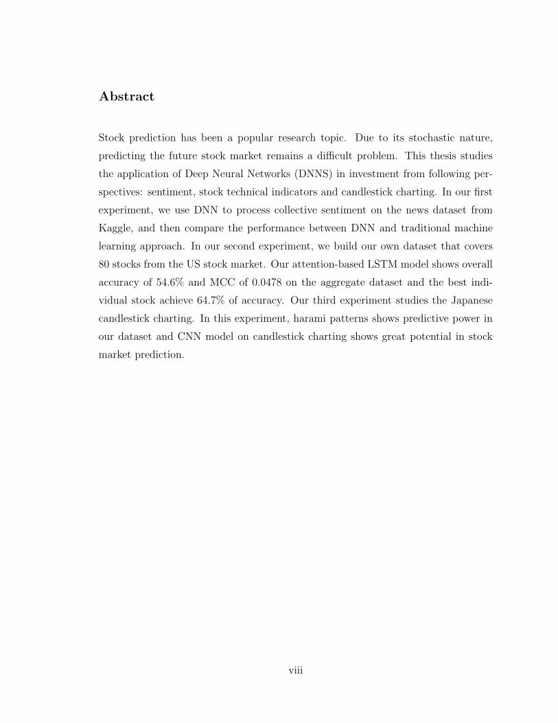
Stock prediction has been a popular research topic. Due to its stochastic nature,

predicting the future stock market remains a difficult problem. This thesis studies

the application of Deep Neural Networks (DNNS) in investment from following per-

spectives: sentiment, stock technical indicators and candlestick charting. In our first

experiment, we use DNN to process collective sentiment on the news dataset from

Kaggle, and then compare the performance between DNN and traditional machine

learning approach. In our second experiment, we build our own dataset that covers

80 stocks from the US stock market. Our attention-based LSTM model shows overall

accuracy of 54.6% and MCC of 0.0478 on the aggregate dataset and the best indi-

vidual stock achieve 64.7% of accuracy. Our third experiment studies the Japanese

candlestick charting. In this experiment, harami patterns shows predictive power in

our dataset and CNN model on candlestick charting shows great potential in stock

market prediction.

viii

List of Abbreviations Used

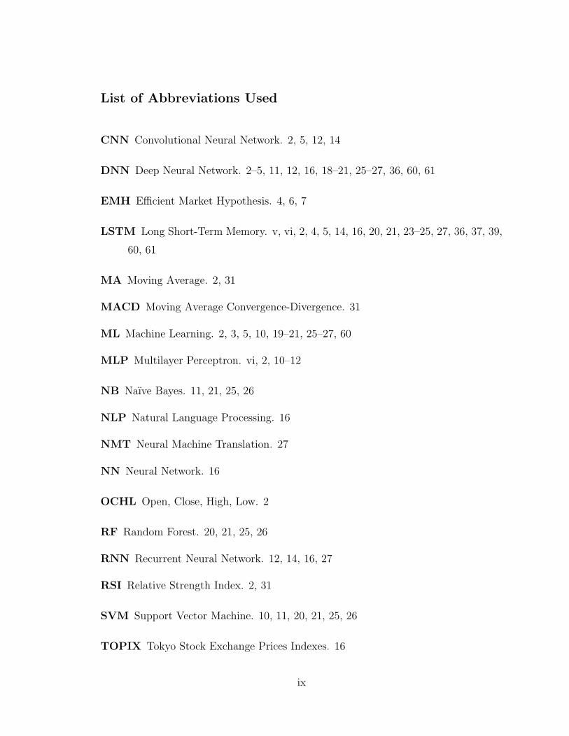
CNN Convolutional Neural Network. 2, 5, 12, 14

DNN Deep Neural Network. 2–5, 11, 12, 16, 18–21, 25–27, 36, 60, 61

EMH Efficient Market Hypothesis. 4, 6, 7

LSTM Long Short-Term Memory. v, vi, 2, 4, 5, 14, 16, 20, 21, 23–25, 27, 36, 37, 39,

60, 61

MA Moving Average. 2, 31

MACD Moving Average Convergence-Divergence. 31

ML Machine Learning. 2, 3, 5, 10, 19–21, 25–27, 60

MLP Multilayer Perceptron. vi, 2, 10–12

NB Naıve Bayes. 11, 21, 25, 26

NLP Natural Language Processing. 16

NMT Neural Machine Translation. 27

NN Neural Network. 16

OCHL Open, Close, High, Low. 2

RF Random Forest. 20, 21, 25, 26

RNN Recurrent Neural Network. 12, 14, 16, 27

RSI Relative Strength Index. 2, 31

SVM Support Vector Machine. 10, 11, 20, 21, 25, 26

TOPIX Tokyo Stock Exchange Prices Indexes. 16

ix

Acknowledgements

This research was supported by an NSERC grant at the Dalhousie University. We

also appreciate the help from StockTwits for the access to finance tweets on their

platform.

x

Chapter 1

Introduction

1.1 Motivation

Despite the rapid development in world’s economy and technology, the passion and

enthusiasm for stock market has never diminished. Over the past hundred years,

successful investors have published lots of books to share the taste of success in

investment; researchers have published countless papers in stock market and try to

figure out a way to make consistent profit from stock market. While much effort was

put into the stock market, being able to predict the future stock market movement

and make consistent profit is still a dream. Because the reality is discouraging: in

a long run, 70% percent of investors lose money; 20% can break even and only 10%

investors are able to make profit [3].

Although the development of technology does not change the fact most investors

are losing money, it has changed how investors acquire and share information. Over

the past few decades, the way how investors trade stocks have shifted from reading

outdated newspaper and placing orders through telephone, to now reading the latest

news from every corner of this planet and trading at real time from anywhere in the

world. The difference has effectively led to a dramatic change in decision making

regarding investment since the faster to acquire information, the faster to react and

trade at a better price. The amount of information has grown in almost an exponen-

tial manner [4] and part of that can be ascribed to the thriving social media. Social

platforms like Facebook and Twitter are becoming a major source where most people

get and share information. The popularity in social media has attracted many re-

searches in social media sentiment [5]. The significant event recently is in September

of 2019, JPMorgan Chase released the Volfefe Index to reflect the volatility in stock

market sentiment for US Treasury bonds due to the influence of tweets by President

Donald Trump [6]. Since 2016, when the 45th President of the United States of Amer-

ica, Donald Trump, was elected, his tweets on national and international affairs have

1

2

influenced the stock market to a very large scale. The name Volfefe is taken from one

of his tweets that contains a typo ’covfefe’. This thesis is inspired by the influence of

social media and state-of-the-art technology and find out if there is some correlation

between sentiment, technical indicators and stock market movement.

With the development in Deep Neural Network in recent years, there have been

many very successful applications, for instance, autonomous driving, disease diagno-

sis etc. With the huge number of data in finance related sectors, applying DNN to

investment field has shown great potential as well. Aside from basic stock market

indicators like Open, Close, High, Low (OCHL) and volume, other technical indica-

tors including moMoving Average (MA), Relative Strength Index (RSI) and other

indicators are drawing greater attention regarding feature engineering in more and

more financial prediction models.

Much effort has been made to take advantage of the data boom and seek an ap-

proach to generate consistent revenue and profit. There are numerous research work

regarding stock movement prediction using sentiment analysis with traditional meth-

ods [5, 7]. Nevertheless, the recent progress made in Machine Learning (ML) have

motivated many researchers and brought different perspectives into this field. In the

past three decades, there has been a thriving evolution of artificial intelligence from

Multilayer Perceptron [8] to DNN, like Convolutional Neural Network (CNN) [9] and

Long Short-Term Memory (LSTM). Bollen et al. [5] used twitter sentiment for stock

movement prediction; Chen et al. [10] used LSTM and basic stock market data includ-

ing OCHL data in the stock market prediction and found improvement over tradition

methods. Nelson et al. [11] experimented on LSTM and stock technical indicators

derived from OCHL, which outperforms tradition methods with few exceptions.

However, each coin has two sides. While the study on twitter sentiment shows

the correlation between twitter sentiment and stock movement [5], only 3.6% news

and 8.7% pass-along values makes the Twitter data less convincing compared with

over 40% of the tweets are pointless babble based on the data gathered by Pear

Analytics [12]. In other words, in this enormous amount of data on Twitter, most of

them are irrelevant to our study and may create waste of time and resource. To reduce

the impact of irrelevant information on stock market prediction, we use another data

source from StockTwits to replace Twitter. More details about this data source will

3

be covered in Chapter 4 .

Aside from finance tweets and stock technical indicators, we are inspired by

the famous Japanese candlestick charting. Steven Nison wrote many books about

Japanese candlestick charting. One of his books is the famous Beyond candlesticks:

New Japanese charting techniques revealed, which introduces and explains candlestick

charting and patterns. This book is the cornerstone of our research into the candle-

stick charting. In our third experiment, we analyze some famous candlestick patterns

and build a DNN model that uses these candlestick charting as our data source.

1.2 Research Problem Formulation

While there are many research studying the stock market movement using public

sentiment [5, 13, 12] and technical analysis [14, 15, 11, 16], quite few published re-

search studies the combination of public sentiment and technical analysis (there may

be many research done but not publicly available). In thesis, the stock movement

prediction is to predict the future up or down of the stocks, in comparison with the

prediction of the price at market close.

During our initial research there are few challenges. Our first challenge is the

dataset. While the stock history data are publicly available, the source for text data

that can reflect public sentiment are rarely accessible.

Our second challenge is to explore the chemistry between sentiment analysis and

technical analysis. Since there are not much work publicly available regarding the

combination of sentiment analysis and technical analysis, it is interesting to see if this

combination could improve the accuracy of stock movement prediction. Last but not

least, many published works study the Japanese candlestick charting [17, 18, 19, 20],

but the conclusion from these researches are controversial. With the development

of deep learning approach, we think it is worthwhile to study this problem from a

different perspective.

The goal of this thesis includes the following:

• create and use the available data to study the correlation between sentiment

analysis, technical analysis and future stock market movement

• compare the performance with DNN models and traditional ML models

4

• if the dataset needs improvement, make adjustment to the dataset or build a

new dataset

• study the DNN model on the dataset and make optimization on top of it

• experiment if DNN model performs well for aggregate stock dataset or varies

on individual stock

• analyze candlestick charting and experiment working with DNN model

1.3 Contributions

The main contribution of this thesis are as follows:

• a new stock trend prediction model on attention-based LSTM trained on a

dataset including stock history, finance tweets sentiment and technical indica-

tors;

• a comparison of finance tweets posted during different periods of time in a

trading day;

• evaluation of the model under different test cases: after-hour finance tweets and

weighted on maximum followers giving best predictive power; and

• test result that resembles Gaussian Distribution in individual stock dataset

brings new interesting topics.

• part of our work regarding stock prediction on sentiment analysis and deep

learning is accepted by the 3rd International Workshop on Big Data for Finan-

cial News and Data at IEEE Bigdata conference in 2019.

1.4 Outline

The remainder of this thesis is organized as follows: Chapter 2 presents an overview

of related work and background study in stock market, deep learning and problem

formulation. More precisely, we will introduce some fundamental knowledge including

Efficient Market Hypothesis, basic trading techniques, the use of sentiment analysis

5

in stock market, Machine Learning algorithms, CNN, LSTM, candlestick charting

introduction and the experiment design for this thesis.

In Chapter 3, we conduct an experiment using news dataset and stock history

data to compare the performance among Deep Neural Network (DNN) model and

traditional Machine Learning (ML) models regarding sentiment analysis and future

stock market movement prediction. As we realize the restrictions of this dataset,

there is no further work on this dataset and we decide to build an improved dataset,

which is covered in chapter 4.

In Chapter 4, we take the reflection from last experiment on news dataset and build

a new configurable dataset for future stock market movement prediction. This piece

of work was accepted by the 3rd International Workshop on Big Data for Financial

News and Data. In this chapter, we build a software to generate dataset with different

configurations including the choice of posted time of finance tweets and methods

regarding how to calculate the collective sentiment score, from raw data that includes

stock history price, finance tweets with sentiment and technical indicators. We also

experiment on attention-based LSTM model to predict future stock price movement.

In Chapter 5, we have a detailed research into Japanese candlestick charting and

some technical patterns. By analyzing some famous and classic patterns, we get some

positive feedback through real-life investment. With the controversial quantitative

definition on these patters, we analyze the predictive power of harami pattern on

three stocks in our dataset. We also explore the application of Convolutional Neural

Network on candlestick charting images to predict future stock market movement.

The conclusion and future research of this thesis are presented in Chapter 6.

Chapter 2

Background and Related Work

2.1 Efficient Market Hypothesis

Efficient Market Hypothesis (EMH) states that market prices reflect all available

information. This implies that “beating the market” consistently based on history

data is virtually impossible since market prices should only react to new information.

According to the EMH, the stock market is priced fairly, and it is impossible for

investors to purchase stocks at undervalued price and sell stocks at overvalued price.

Theoretically, no expert selection nor any system can outperform the overall market,

and the only way to gain higher profit is to make riskier investment. Efficient Market

Hypothesis was developed by Engene Fama in 1960s, whose work was followed up by

many famous economists [21]. Engene Fama conducted the test based on the three

forms of efficient market: weak-form efficiency, semi-strong-form efficiency and strong-

form efficiency. Weak form refers to the information set that is just historical prices.

The result of weak form test implies that the trading strategies using historical share

prices or other historical data will not guarantee excess return in the long run. Semi-

strong form is the information set that is obviously publicly available (e.g., annual

report, stock splits, etc). The conclusion from the semi-strong form test implies

that share prices adjust to publicly available new information very rapidly and in an

unbiased fashion. In strong-form efficient market, all available information is fully

reflected in prices which means no individual could gain excess profit than others

because he has monopolistic access to some information.

EMH required that investors have rational expectations. This does not mean in-

vestors have to be rational: it allows that the new information would make some

investors overreact and some underreact, but the reactions are considered to be ran-

dom and falls under normal distribution pattern. However, with the fast development

made in technology and internet, especially with the prevalence of social media, the

question remains to be answered whether this assumption still holds up as the public

6

7

sentiment can now spread faster than anyone’s imagination.

Besides, as much as EMH prevails, the debate about the validity of EMH has

never stopped. Ramon [22] find stock market exhibits chaos which is a nonlinear

in deterministic process and it only appears random because it can not be easily

expressed. While neural network is capable of learning nonlinear, chaotic system, it

may be possible to outperform traditional approaches.

2.2 Trading Techniques

Without doubt the best way to trade stocks are buying stocks at a low price and

selling at a high price, but the reality is often not the case as people wish for. Being

able to prediction the future stock price is the goal all investors and researchers are

trying to achieve. Overall, the stock price prediction methods can be put into two

general categories: Fundamental analysis (FA) and technical analysis (TA). FA is

focused on the intrinsic value of a stock by looking at the economic factors, such as

revenues, debt, growth rate, etc. FA takes a broader view of a company and consid-

ers long term perspective. They believe the return takes time to realize its intrinsic

value. Technical Analysis, on the other hand, concentrates on stock price and tools

that were derived from stock price. Due to the sensitivity over the history data,

TA is usually considered as an approach for short-term to mid-term investment. In-

vestors use technical indicators to help predicting trend of a stock or index. Common

technical indicators include moving average (MA), relative strength index (RSI) and

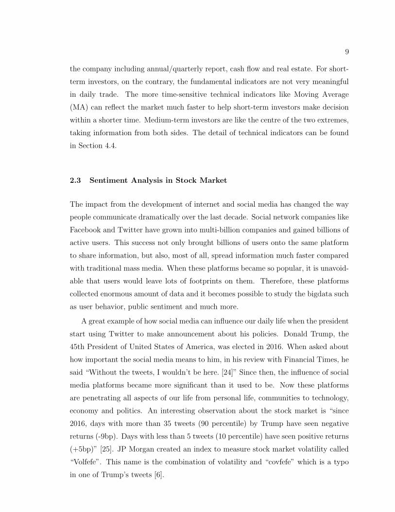
moving average convergence/divergence (MACD). Following is an example of apply-

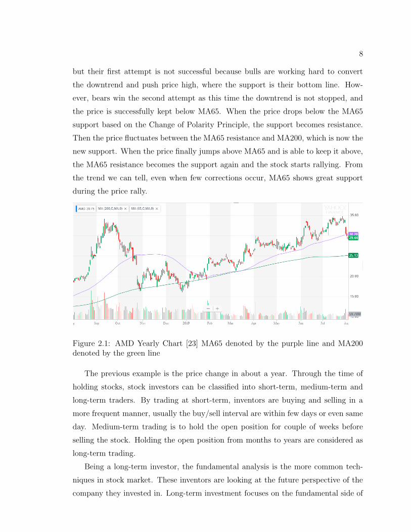
ing technical indicators. As illustrated in Figure 2.1, the purple line and green line

are MA65 and MA200 respectively. Generally, these lines are acting as support or

resistance during price fluctuation. The support, as the name suggests, is to support

the stock price from going lower, whereas resistance is to hold the price from going

higher. These trend lines can be the MA lines, a specific price level etc. According to

the Change of Polarity Principle, support becomes resistance when price drops below

support. Similarly, the resistance becomes support when price breaks resistance. In

Figure 2.1, the stock price moves upward to its peak level and then starts to pull

back. When price reaches the support of MA65 line it bounces back a little bit before

it can drop further. In other word, the bears try to pull the price into a downtrend,

8

but their first attempt is not successful because bulls are working hard to convert

the downtrend and push price high, where the support is their bottom line. How-

ever, bears win the second attempt as this time the downtrend is not stopped, and

the price is successfully kept below MA65. When the price drops below the MA65

support based on the Change of Polarity Principle, the support becomes resistance.

Then the price fluctuates between the MA65 resistance and MA200, which is now the

new support. When the price finally jumps above MA65 and is able to keep it above,

the MA65 resistance becomes the support again and the stock starts rallying. From

the trend we can tell, even when few corrections occur, MA65 shows great support

during the price rally.

Figure 2.1: AMD Yearly Chart [23] MA65 denoted by the purple line and MA200denoted by the green line

The previous example is the price change in about a year. Through the time of

holding stocks, stock investors can be classified into short-term, medium-term and

long-term traders. By trading at short-term, inventors are buying and selling in a

more frequent manner, usually the buy/sell interval are within few days or even same

day. Medium-term trading is to hold the open position for couple of weeks before

selling the stock. Holding the open position from months to years are considered as

long-term trading.

Being a long-term investor, the fundamental analysis is the more common tech-

niques in stock market. These inventors are looking at the future perspective of the

company they invested in. Long-term investment focuses on the fundamental side of

9

the company including annual/quarterly report, cash flow and real estate. For short-

term investors, on the contrary, the fundamental indicators are not very meaningful

in daily trade. The more time-sensitive technical indicators like Moving Average

(MA) can reflect the market much faster to help short-term investors make decision

within a shorter time. Medium-term investors are like the centre of the two extremes,

taking information from both sides. The detail of technical indicators can be found

in Section 4.4.

2.3 Sentiment Analysis in Stock Market

The impact from the development of internet and social media has changed the way

people communicate dramatically over the last decade. Social network companies like

Facebook and Twitter have grown into multi-billion companies and gained billions of

active users. This success not only brought billions of users onto the same platform

to share information, but also, most of all, spread information much faster compared

with traditional mass media. When these platforms became so popular, it is unavoid-

able that users would leave lots of footprints on them. Therefore, these platforms

collected enormous amount of data and it becomes possible to study the bigdata such

as user behavior, public sentiment and much more.

A great example of how social media can influence our daily life when the president

start using Twitter to make announcement about his policies. Donald Trump, the

45th President of United States of America, was elected in 2016. When asked about

how important the social media means to him, in his review with Financial Times, he

said “Without the tweets, I wouldn’t be here. [24]” Since then, the influence of social

media platforms became more significant than it used to be. Now these platforms

are penetrating all aspects of our life from personal life, communities to technology,

economy and politics. An interesting observation about the stock market is “since

2016, days with more than 35 tweets (90 percentile) by Trump have seen negative

returns (-9bp). Days with less than 5 tweets (10 percentile) have seen positive returns

(+5bp)” [25]. JP Morgan created an index to measure stock market volatility called

“Volfefe”. This name is the combination of volatility and “covfefe” which is a typo

in one of Trump’s tweets [6].

10

Early research shows using Twitter mood to predict the stock market provides en-

hancement compared with non-sentiment methods [5]. Johan et al. [5] build Google-

Profile of Mood States (GPOMS) that categorizes the tweet sentiment into six dif-

ferent emotions. They observe the sentiment “Calm” and “Happiness” has better

predictive power than general levels of OptionFinder. Later work by Si et al. [26]

and Pagolu et al. [27] also found correlation between public sentiments in tweets and

stock future movement.

As mentioned in Section 1.1, the problem of using Twitter as the data source is

due to the fact that Twitter is a general social network platform, its information come

from all different sources. 3.6% news and 8.7% pass-along values may contain useful

information while 40% of the tweets are pointless babble, not to mention the fake or

misleading information that are widespread on Twitter. Hence, it remains a question

whether Twitter is a reliable source for financial market.

2.4 Machine Learning and Deep Learning

Machine learning is the study of statistical models that we use computers to process

tasks without user instructions. Typical Machine Learning methods include super-

vised learning, unsupervised learning and reinforcement learning. Famous Machine

Learning algorithms includes Support Vector Machine, decision trees, Multilayer Per-

ceptron etc.

Supervised learning algorithms build the model with dataset that contains both

features and labels. In other words, each training record has at least one associated

label. Supervised learning algorithms include classification and regression. Classifica-

tion model is used to predict discrete result or limited set of values, which is applicable

to this thesis. For example, given the length of hair and body weight, predict the

gender between male and female. Regression model, on the other hand, is to predict

a range of continuous values. To show the difference between classification model and

regression model, a good example is to predict the weather. If the goal is to predict

the whether it is sunny or cloudy, this is the classification model. On the other side,

if the goal is to predict the temperature for tomorrow, it is a regression model.

In classification algorithms, two main types of model includes generative model

11

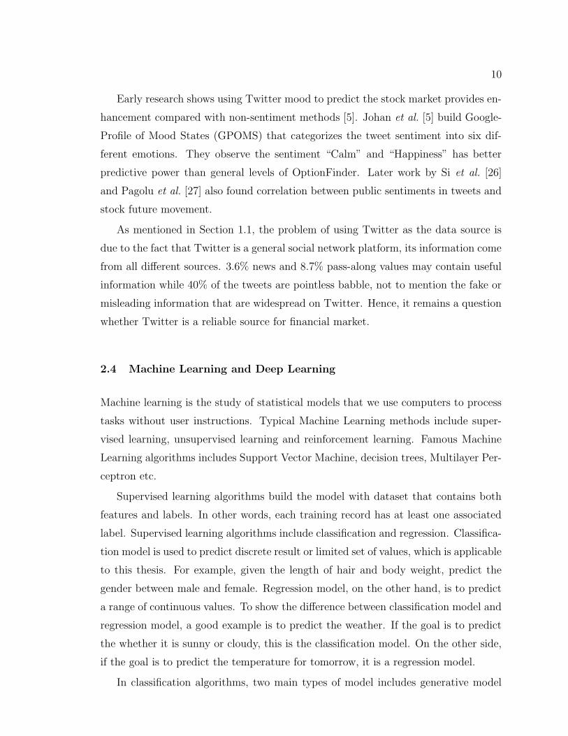
Figure 2.2: An Multilayer Perceptron consists of at least three layers: an input layer,a hidden layer and an output layer.

and discriminative model. Generative models learn the joint probability distribu-

tion p(x, y), while discriminative model learns the conditional probability distribution

p(y|x). Famous generative classifiers include Naıve Bayes, Markov random fields and

Hidden Markov Models; famous discriminative classifiers include Logistic regression,

Support Vector Machine and traditional neural networks.

Multilayer Perceptron (MLP) is the first step before entering the world of Deep

Neural Network. An MLP has at least three layers of nodes including an input layer,

a hidden layer and an output layer. Except for the input layer, each node acts like

a neuron that uses a nonlinear activation function. By adding more hidden layers,

the network gets deeper and more complicated. While all the neurons are connected

between two adjacent layers, this type of network with more hidden layers are also

called Feed-Forward Neural Network. In the example of MLP (Figure 2.2), given the

input size x = 3, the number of neurons at hidden layer h = 4 and output layer o = 1,

the total number of parameter is 3 × 4 + 4 × 1 + (4 + 1) = 21, where (4 + 1) is the

bias term for hidden layer and output layer.

Before we bring the formulation, here are the general definition of terms:

• x: input vector

• y: label

• ω[k]: the weight matrices for the ith node at layer k

• b[k]: the bias vector for the ith node at layer k

12

• z: the sum of dot production and bias

• σ: non-linear activation function

• α[k]: the activation vector for the ith node at layer k

• o: the output

Based on the example in Figure 2.2, to calculate the activation of hidden layer:

z[1] = w[1] · x+ b[1] (2.1)

α[1] = σ(z) (2.2)

The output of hidden layer:

z[2] = w[2] · α[1] + b[2] (2.3)

o = α[2] = σ(z[2]) (2.4)

The loss function is used to measure the difference between the labels and predic-

tions, in our example we use L2 loss function:

L =n∑

i=1

(yi − oi)2 (2.5)

Since the goal is minimize the loss L, we apply back propagation by using chain

rule:∂L

∂ω(k)=

∂L

∂α[k]

∂α[k]

∂z[k]∂z[k]

∂ω[k](2.6)

This way we are able to adjust the weight for each node and optimize the neural

network. MLP paved the path for Deep Neural Networks such as Convolutional

Neural Network (CNN), Recurrent Neural Network (RNN).

2.5 Convolutional Neural Network (CNN)

While feed-forward neural networks perform well in many tasks, when it gets deeper

and have more hidden layers, the number of parameters to train increase significantly

as the neurons in adjacent layers are fully connected. CNN, however, has a different

13

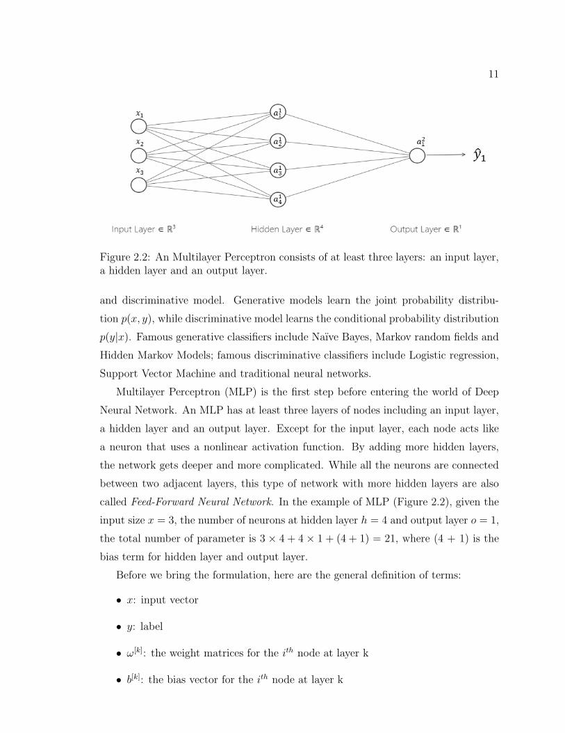
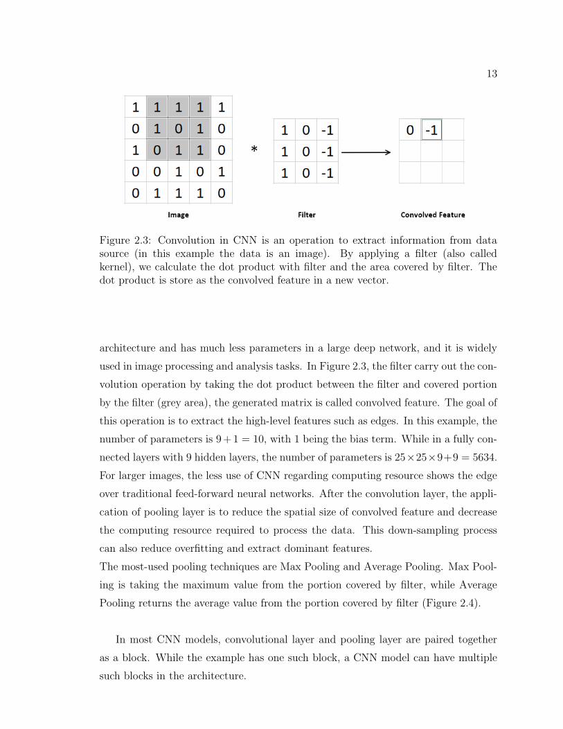
Figure 2.3: Convolution in CNN is an operation to extract information from datasource (in this example the data is an image). By applying a filter (also calledkernel), we calculate the dot product with filter and the area covered by filter. Thedot product is store as the convolved feature in a new vector.

architecture and has much less parameters in a large deep network, and it is widely

used in image processing and analysis tasks. In Figure 2.3, the filter carry out the con-

volution operation by taking the dot product between the filter and covered portion

by the filter (grey area), the generated matrix is called convolved feature. The goal of

this operation is to extract the high-level features such as edges. In this example, the

number of parameters is 9 + 1 = 10, with 1 being the bias term. While in a fully con-

nected layers with 9 hidden layers, the number of parameters is 25×25×9+9 = 5634.

For larger images, the less use of CNN regarding computing resource shows the edge

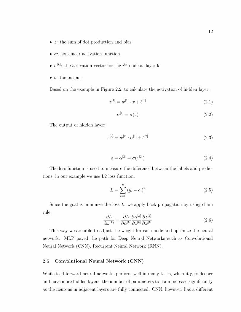
over traditional feed-forward neural networks. After the convolution layer, the appli-

cation of pooling layer is to reduce the spatial size of convolved feature and decrease

the computing resource required to process the data. This down-sampling process

can also reduce overfitting and extract dominant features.

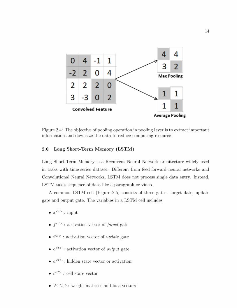
The most-used pooling techniques are Max Pooling and Average Pooling. Max Pool-

ing is taking the maximum value from the portion covered by filter, while Average

Pooling returns the average value from the portion covered by filter (Figure 2.4).

In most CNN models, convolutional layer and pooling layer are paired together

as a block. While the example has one such block, a CNN model can have multiple

such blocks in the architecture.

14

Figure 2.4: The objective of pooling operation in pooling layer is to extract importantinformation and downsize the data to reduce computing resource

2.6 Long Short-Term Memory (LSTM)

Long Short-Term Memory is a Recurrent Neural Network architecture widely used

in tasks with time-series dataset. Different from feed-forward neural networks and

Convolutional Neural Networks, LSTM does not process single data entry. Instead,

LSTM takes sequence of data like a paragraph or video.

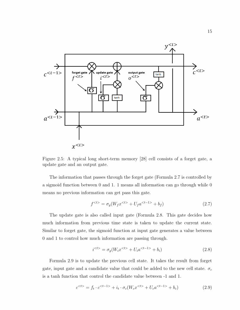
A common LSTM cell (Figure 2.5) consists of three gates: forget date, update

gate and output gate. The variables in a LSTM cell includes:

• x<t> : input

• f<t> : activation vector of forget gate

• i<t> : activation vector of update gate

• o<t> : activation vector of output gate

• a<t> : hidden state vector or activation

• c<t> : cell state vector

• W,U, b : weight matrices and bias vectors

15

Figure 2.5: A typical long short-term memory [28] cell consists of a forget gate, aupdate gate and an output gate.

The information that passes through the forget gate (Formula 2.7 is controlled by

a sigmoid function between 0 and 1. 1 means all information can go through while 0

means no previous information can get pass this gate.

f<t> = σg(Wfx<t> + Ufa

<t−1> + bf ) (2.7)

The update gate is also called input gate (Formula 2.8. This gate decides how

much information from previous time state is taken to update the current state.

Similar to forget gate, the sigmoid function at input gate generates a value between

0 and 1 to control how much information are passing through.

i<t> = σg(Wix<t> + Uia

<t−1> + bi) (2.8)

Formula 2.9 is to update the previous cell state. It takes the result from forget

gate, input gate and a candidate value that could be added to the new cell state. σc

is a tanh function that control the candidate value between -1 and 1.

c<t> = ft · c<t−1> + it · σc(Wcx<t> + Uca

<t−1> + bc) (2.9)

16

The output gate controls how much information from the hidden layers passes to

compute the output activation Formula 2.10.

o<t> = σg(Wox<t> + Uoa

<t−1> + bo) (2.10)

Lastly, the hidden state vector (Formula 2.11 is also known as the output vector

of the LSTM unit.

a<t> = o<t> · σh(c<t>) (2.11)

Similar to other DNN architectures, LSTM model uses the gradient descent and

backpropagation through time to train the parameters W, U and b.

2.7 Deep Learning in Finance

In finance sector, researchers have put a lot effort in the application of Deep Neu-

ral Network. As early as 1990s, Kimoto [29] already used modular neural network

to analyse the Tokyo Stock Exchange and its internal representation. Their predic-

tion system on Tokyo Stock Exchange Prices Indexes (TOPIX) achieved accurate

prediction and the simulation on trading showed considerable profit. The system

provides buy and sell signal to help investors make trading decisions. Later work

from Mizuno et al. [30] also applied NN model but they included technical analysis

and feature engineering. Although their model did help making selling decision to

minimize the loss. However, it did not make higher profit in buying decisions. When

social media became popular, Bollen et al. [5] used proposed sentiment algorithms and

combined with neural network for stock movement prediction. Their research shows

the correlation between the market and certain emotion like calmness and happiness.

Recurrent Neural Networks (RNNS) were applied in many time-series data prob-

lems like speech recognition, Natural Language Processing (NLP). However, problems

like vanishing gradient [31] and exploding gradient [32] make it very difficult to train

RNN models on large time steps. The appearance of LSTM solved many tasks that

were not solvable by previous learning algorithms for RNNS [33] by introducing a

‘memory cell’ that can memorize information in its cells for a long period of time.

17

2.8 Candlestick Charting

Japanese Candlestick chart was developed as early as 1700s in japan to help predict

rice price. In Nison’s book, he brought this tool to western readers and explained how

candlestick patterns are capable of predicting stock market movement [34]. However,

the lack of research in this tool has brought many controversial voices questioning

whether this tool really works.

Horton [35] examined Japanese candlestick of technical analysis for 349 stock

and concluded that patterns like stars, crows, or doji does not help predicting stock

market movement. Marshal [18] took Dow Jones Industrial Average (DJIA) data

from 1992 to 2002 and found that candlestick technical analysis is not profitable in

US stock market. In his later work [36] he tested candlestick patterns in the Japanese

equity market over the 1975–2004 period and found strong evidence that candlestick

technical analysis is not profitable on large stocks in the Japanese equity market.

On the other hand, Fock et al. [37] studied the predictive power of candlestick pat-

terns and found the combination of candlestick patterns together with other technical

indicators was able to get higher returns. Following this research, Chen et al. [20]

shows that pair of bullish and bearish harami, and the pattern of homing pigeon shows

best forecasting power for both medium-market-cap and large-market-cap stocks in

eight pattern from their results. Based on this insight, we worked on dataset in our

framework and found some interesting observations.

As mentioned above, candlestick charting was originally used to predict the trend

of rice price [34], but Charles H. Dow introduced this tool in his Dow theory in the

late 1800s [38]. Currently we just need to know that a candlestick bar consists of a

wide bar and vertical line that pierces the bar vertically. The detailed introduction

of candlestick charting is in our third experiment (Section 5.2).

2.9 Experiment Design

The work from Bollen et al. [5], Nelson et al. [11] and Nison et al. [34] use different

approach to predict future stock market movement. Bollen et al.’s research collect

Twitter data and calculate the ratio of positive and negative ratio of daily tweets and

use traditional fuzzy neural network for stock prediction. Nelson et al. combines the

18

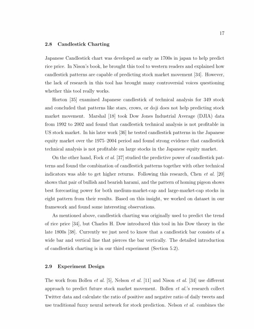
Figure 2.6: The top and bottom of the line are the highest and lowest price respec-tively, where top and bottom of the bar in white (or green) are close and open priceand in black (or red) vice versa

state-of-the-art Deep Neural Network and stock technical indicators. This experiment

shows that DNN model is capable to learn from the large training data and there is

great potential in this field. Nison et al.’s analysis on the famous Japanese Candle-

stick brings a new way to analyze the stock market that is different from traditional

technical analysis. Though in his research there is no theoretical evidence to describe

the relationship between candlestick charting and US stock market, the examples he

uses for every pattern and theory of candlestick charting are intriguing and inspiring.

Chen et al. [20] explore the predictive power of candlestick chart in Chinese stock

market and their conclusion shows that bullish harami pattern, bearish harami pat-

tern, and the pattern of homing pigeon always provide the best forecasting power for

both medium-market-value and large-market value stocks. These researches inspired

for this thesis to explore the possibility of combining social media sentiment, stock

technical indicators and candlestick pattern together.

Due to the awareness of privacy protection, data now becomes the crude oil in our

economy and gets harder to acquire, especially for DNN projects that requires large

amount of data. For this reason, a reliable data source is difficult to find and even

with the data it takes lots of time to analyze and process. In our thesis, as the goal is

to explore how we can apply DNN, technical indicators and candlestick charting in the

stock market. Our thesis consists of three gradual experiment. The first experiment

is to find an existing and mature dataset that is available publicly, and train our

models based on top of that. Based on this principle, we adopted the dataset from

Kaggle that contains stock price data and news from reddit. During data analysis and

feature engineering, though few issues with this dataset are found, it is a good start

19

to measure the performance of DNN models and other traditional ML approaches;

By reflecting on our first experiment, we build the configurable datasets in our second

experiment and benchmark on different configurations regarding the time sensitivity

of the finance tweets. The new dataset is based on a much larger data source that

we collected from Yahoo Finance and StockTwits. Our third experiment focuses on

candlestick charting and application of DNN on candlestick charting. The goal is

to explore the correlation between candlestick charting in form of images and stock

movement.

Chapter 3

Experiment on Daily News dataset

In this first experiment, in order to compare the performance among DNN models

and traditional methods, we use an existing dataset from Kaggle to conduct this ex-

periment. There are many previous works on stock market prediction, while multiple

Machine Learning approaches are applied including Support Vector Machine (SVM),

Random Forest, LSTM etc. In this experiment, we will compare the performance

among these approaches, and explore a way to analyze the sentiment from news data.

3.1 Data Source

Kaggle, as mentioned above, is the source of news and stock data for this experiment.

Kaggle is an open platform for data scientists and Machine Learning enthusiasts,

currently owned by Google LLC. It is a web-based platform where users can upload

and publish datasets and work with other Machine Learning engineers or enthusiasts

or join competitions on solving data science challenges.

The dataset we use is “Daily News for Stock Market Prediction” by Aaron7sun [39].

This dataset includes news data and stock data ranging from 2008-06-08 to 2016-07-

01. In terms of news, they are collected from Reddit world news channel. The data

includes 25 top news for each date where the news is ranked from top to bottom

based on their popularity. The stock data is the DJIA index acquired from Yahoo

Finance including OCHL and volume.

3.2 Rationale of Modeling

At this stage, there are few goals we want to achieve:

• analyze the news sentiment from the news dataset

• build DNN model and traditional ML models that uses combined dataset in-

cluding news sentiment and stock data

20

21

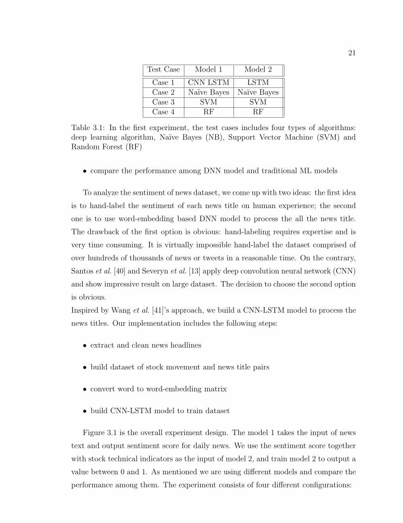
Test Case Model 1 Model 2

Case 1 CNN LSTM LSTMCase 2 Naıve Bayes Naıve BayesCase 3 SVM SVMCase 4 RF RF

Table 3.1: In the first experiment, the test cases includes four types of algorithms:deep learning algorithm, Naıve Bayes (NB), Support Vector Machine (SVM) andRandom Forest (RF)

• compare the performance among DNN model and traditional ML models

To analyze the sentiment of news dataset, we come up with two ideas: the first idea

is to hand-label the sentiment of each news title on human experience; the second

one is to use word-embedding based DNN model to process the all the news title.

The drawback of the first option is obvious: hand-labeling requires expertise and is

very time consuming. It is virtually impossible hand-label the dataset comprised of

over hundreds of thousands of news or tweets in a reasonable time. On the contrary,

Santos et al. [40] and Severyn et al. [13] apply deep convolution neural network (CNN)

and show impressive result on large dataset. The decision to choose the second option

is obvious.

Inspired by Wang et al. [41]’s approach, we build a CNN-LSTM model to process the

news titles. Our implementation includes the following steps:

• extract and clean news headlines

• build dataset of stock movement and news title pairs

• convert word to word-embedding matrix

• build CNN-LSTM model to train dataset

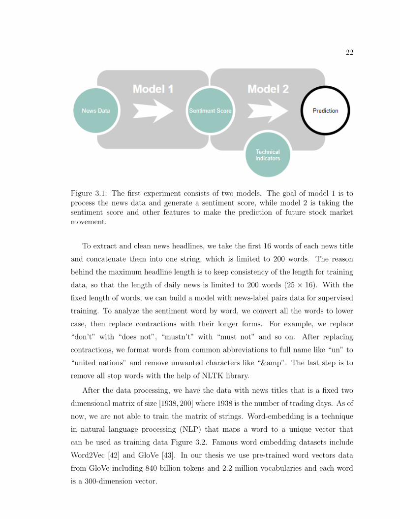
Figure 3.1 is the overall experiment design. The model 1 takes the input of news

text and output sentiment score for daily news. We use the sentiment score together

with stock technical indicators as the input of model 2, and train model 2 to output a

value between 0 and 1. As mentioned we are using different models and compare the

performance among them. The experiment consists of four different configurations:

22

Figure 3.1: The first experiment consists of two models. The goal of model 1 is toprocess the news data and generate a sentiment score, while model 2 is taking thesentiment score and other features to make the prediction of future stock marketmovement.

To extract and clean news headlines, we take the first 16 words of each news title

and concatenate them into one string, which is limited to 200 words. The reason

behind the maximum headline length is to keep consistency of the length for training

data, so that the length of daily news is limited to 200 words (25 × 16). With the

fixed length of words, we can build a model with news-label pairs data for supervised

training. To analyze the sentiment word by word, we convert all the words to lower

case, then replace contractions with their longer forms. For example, we replace

“don’t” with “does not”, “mustn’t” with “must not” and so on. After replacing

contractions, we format words from common abbreviations to full name like “un” to

“united nations” and remove unwanted characters like “&amp”. The last step is to

remove all stop words with the help of NLTK library.

After the data processing, we have the data with news titles that is a fixed two

dimensional matrix of size [1938, 200] where 1938 is the number of trading days. As of

now, we are not able to train the matrix of strings. Word-embedding is a technique

in natural language processing (NLP) that maps a word to a unique vector that

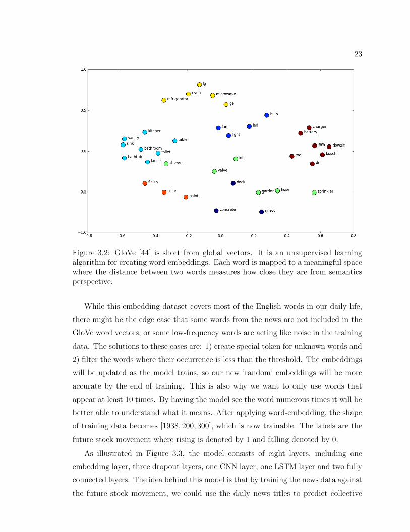
can be used as training data Figure 3.2. Famous word embedding datasets include

Word2Vec [42] and GloVe [43]. In our thesis we use pre-trained word vectors data

from GloVe including 840 billion tokens and 2.2 million vocabularies and each word

is a 300-dimension vector.

23

Figure 3.2: GloVe [44] is short from global vectors. It is an unsupervised learningalgorithm for creating word embeddings. Each word is mapped to a meaningful spacewhere the distance between two words measures how close they are from semanticsperspective.

While this embedding dataset covers most of the English words in our daily life,

there might be the edge case that some words from the news are not included in the

GloVe word vectors, or some low-frequency words are acting like noise in the training

data. The solutions to these cases are: 1) create special token for unknown words and

2) filter the words where their occurrence is less than the threshold. The embeddings

will be updated as the model trains, so our new ’random’ embeddings will be more

accurate by the end of training. This is also why we want to only use words that

appear at least 10 times. By having the model see the word numerous times it will be

better able to understand what it means. After applying word-embedding, the shape

of training data becomes [1938, 200, 300], which is now trainable. The labels are the

future stock movement where rising is denoted by 1 and falling denoted by 0.

As illustrated in Figure 3.3, the model consists of eight layers, including one

embedding layer, three dropout layers, one CNN layer, one LSTM layer and two fully

connected layers. The idea behind this model is that by training the news data against

the future stock movement, we could use the daily news titles to predict collective

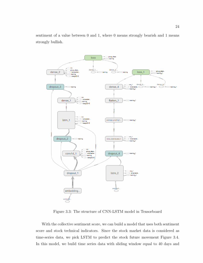
24

sentiment of a value between 0 and 1, where 0 means strongly bearish and 1 means

strongly bullish.

Figure 3.3: The structure of CNN-LSTM model in Tensorboard

With the collective sentiment score, we can build a model that uses both sentiment

score and stock technical indicators. Since the stock market data is considered as

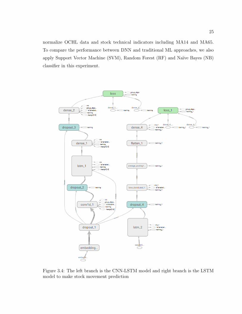
time-series data, we pick LSTM to predict the stock future movement Figure 3.4.

In this model, we build time series data with sliding window equal to 40 days and

25

normalize OCHL data and stock technical indicators including MA14 and MA65.

To compare the performance between DNN and traditional ML approaches, we also

apply Support Vector Machine (SVM), Random Forest (RF) and Naıve Bayes (NB)

classifier in this experiment.

Figure 3.4: The left branch is the CNN-LSTM model and right branch is the LSTMmodel to make stock movement prediction

26

Test Case Model 1 Model 2

DNN 51.20% 53.73%NB 52.84% 41.03%

SVM 45.37% 46.52%RF 52.85% 46.16%

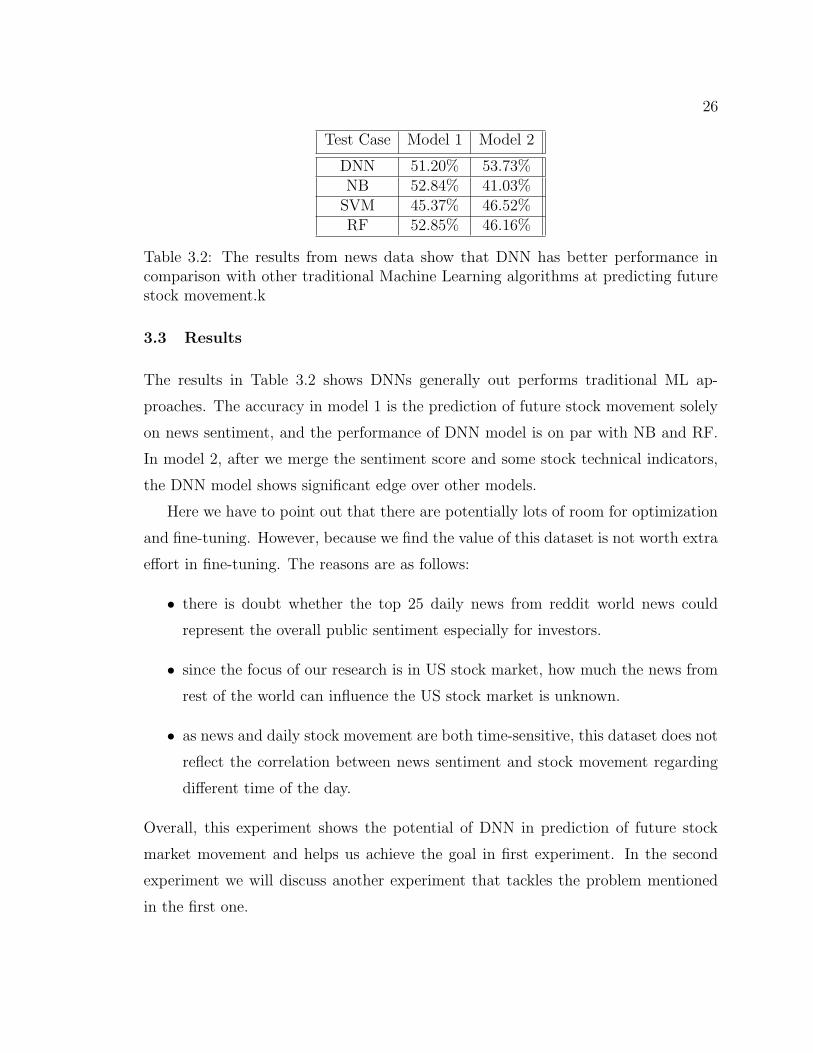
Table 3.2: The results from news data show that DNN has better performance incomparison with other traditional Machine Learning algorithms at predicting futurestock movement.k

3.3 Results

The results in Table 3.2 shows DNNs generally out performs traditional ML ap-

proaches. The accuracy in model 1 is the prediction of future stock movement solely

on news sentiment, and the performance of DNN model is on par with NB and RF.

In model 2, after we merge the sentiment score and some stock technical indicators,

the DNN model shows significant edge over other models.

Here we have to point out that there are potentially lots of room for optimization

and fine-tuning. However, because we find the value of this dataset is not worth extra

effort in fine-tuning. The reasons are as follows:

• there is doubt whether the top 25 daily news from reddit world news could

represent the overall public sentiment especially for investors.

• since the focus of our research is in US stock market, how much the news from

rest of the world can influence the US stock market is unknown.

• as news and daily stock movement are both time-sensitive, this dataset does not

reflect the correlation between news sentiment and stock movement regarding

different time of the day.

Overall, this experiment shows the potential of DNN in prediction of future stock

market movement and helps us achieve the goal in first experiment. In the second

experiment we will discuss another experiment that tackles the problem mentioned

in the first one.

Chapter 4

Experiment on StockTwits Dataset

4.1 Rationale of Modeling

In Kaggle dataset experiment, DNN models outperform traditional ML models over-

all. However, the following restrictions requires us to build a better dataset. First,

the US stock market opens at 9:30 am Eastern Time and closes at 4:30 pm Eastern

Time, the missing information about time on the news makes it less reliable compared

with more time-sensitive social media platform. Secondly, the top news collected from

Reddit World News Channel (/r/worldnews) does not guarantee authenticity, so there

are questions whether it can represent the public sentiment especially in the finance

sector. Besides, DNN models generally perform better with larger dataset. Building a

larger dataset with more detailed data may help improving the performance of DNN

models.

With DNN drawing much more attention in the past few years, CNN based

method [45] and LSTM based models [28, 16] are able to take the advantage larger

datasets from text (e.g., news and twitter) and history stock price to produce better

results.

Following the intuition in news experiment, instead of using text as input for this

model, we use OCHL data, collective sentiment score and technical indicators to feed

the neural network. Furthermore, we want to explore the answers to the questions

that are mentioned in our first experiment.

The application of Attention [46] in NLP is one of the most exciting breakthroughs

in the past few years. In NLP especially Neural Machine Translation (NMT), the

performance of conventional RNN tend to diminish as the length of input sequence

increases, while attention model could maintain a relatively stable performance. The

attention layer does a ‘re-scan’ of the input and extract useful information that has

more connection to the target.

27

28

4.2 Instruments

4.2.1 StockTwits

StockTwits is a social media platform for investors, traders and enthusiasts to share

ideas about investment insight and experience. As the name suggests, StockTwits is

similar to Twitter in many ways in terms of post mechanism, user subscription and

share mechanism. However, the difference makes it unique to Twitter and attracted

many users from all over the world. Unlike Twitter that suits people from all walks

of life, StockTwits is built to focus on stock market and users are mostly interested

in investing and trading in the stock market. Twitter is a very good source of public

information, but the focus on finance makes StockTwits the choice for our thesis.

4.2.2 MS SQL Server

SQL Server is a relational database management system developed by Microsoft. This

software is used to store all data collected from StockTwits in one place. The size of

database after migration goes up to 150 gigabytes and just the finance tweets alone

has over 100 millions items. SQL Server provides the stable running environment for

queries in this project. Note that as SQL Sever Express version only support database

of the size up to 10 gigabytes, we use SQL Server Enterprise version in our project.

4.2.3 Visual Studio

Visual Studio 2019 is an Integrated Development Environment by Microsoft. This

software is used for several purpose. First of all, each line of the monthly back from

StockTwits is a JSON object, we build a software that maps all the JSON object

into a class variable that can be then stored in a relational database. Secondly,

due to the large size of the raw data (over 150 gigabytes), appropriate process on

handling this much data is required to run on a personal computer that has limited

computing resources. Thirdly, to create a dataset that is usable for our project,

feature engineering will be necessary on the huge database. Hence, optimization on

queries is crucial to be time efficient.

29

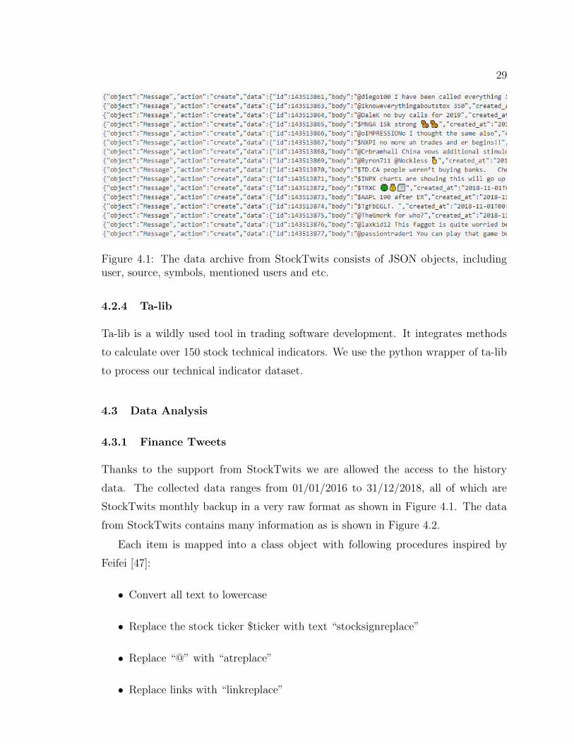
Figure 4.1: The data archive from StockTwits consists of JSON objects, includinguser, source, symbols, mentioned users and etc.

4.2.4 Ta-lib

Ta-lib is a wildly used tool in trading software development. It integrates methods

to calculate over 150 stock technical indicators. We use the python wrapper of ta-lib

to process our technical indicator dataset.

4.3 Data Analysis

4.3.1 Finance Tweets

Thanks to the support from StockTwits we are allowed the access to the history

data. The collected data ranges from 01/01/2016 to 31/12/2018, all of which are

StockTwits monthly backup in a very raw format as shown in Figure 4.1. The data

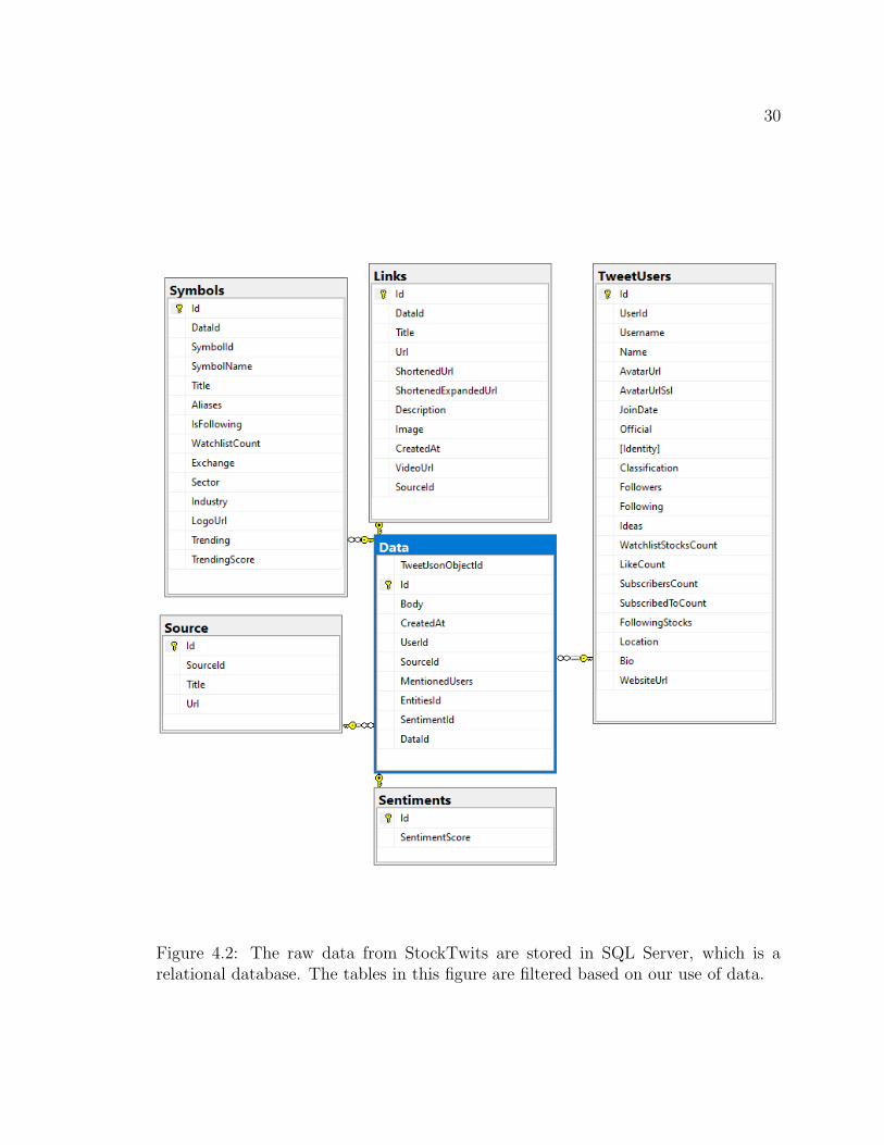
from StockTwits contains many information as is shown in Figure 4.2.

Each item is mapped into a class object with following procedures inspired by

Feifei [47]:

• Convert all text to lowercase

• Replace the stock ticker $ticker with text “stocksignreplace”

• Replace “@” with “atreplace”

• Replace links with “linkreplace”

30

Figure 4.2: The raw data from StockTwits are stored in SQL Server, which is arelational database. The tables in this figure are filtered based on our use of data.

31

During feature engineering, we find that StockTwits does not have consistent fi-

nance tweets backup until 11/05/2017. For some stocks no finance tweet was recorded

on certain days including tech giants like Microsoft and Amazon. Also, StockTwits

started collecting sentiment score since 05/10/2017, which will be covered in detail

in later sections. To prevent data inconsistency, the queries on finance tweets collect

from 01/11/2017 when collected finance tweets and sentiment score become consis-

tent.

4.3.2 Stock Market Data

The stock data is acquired from Yahoo Finance from 11 industries: Basic Materials,

Communication Services, Consumer Cyclical, Consumer Defensive, Energy, Financial

Services, Health care, Industries, Real Estate, Technology and Utilities1. We collect

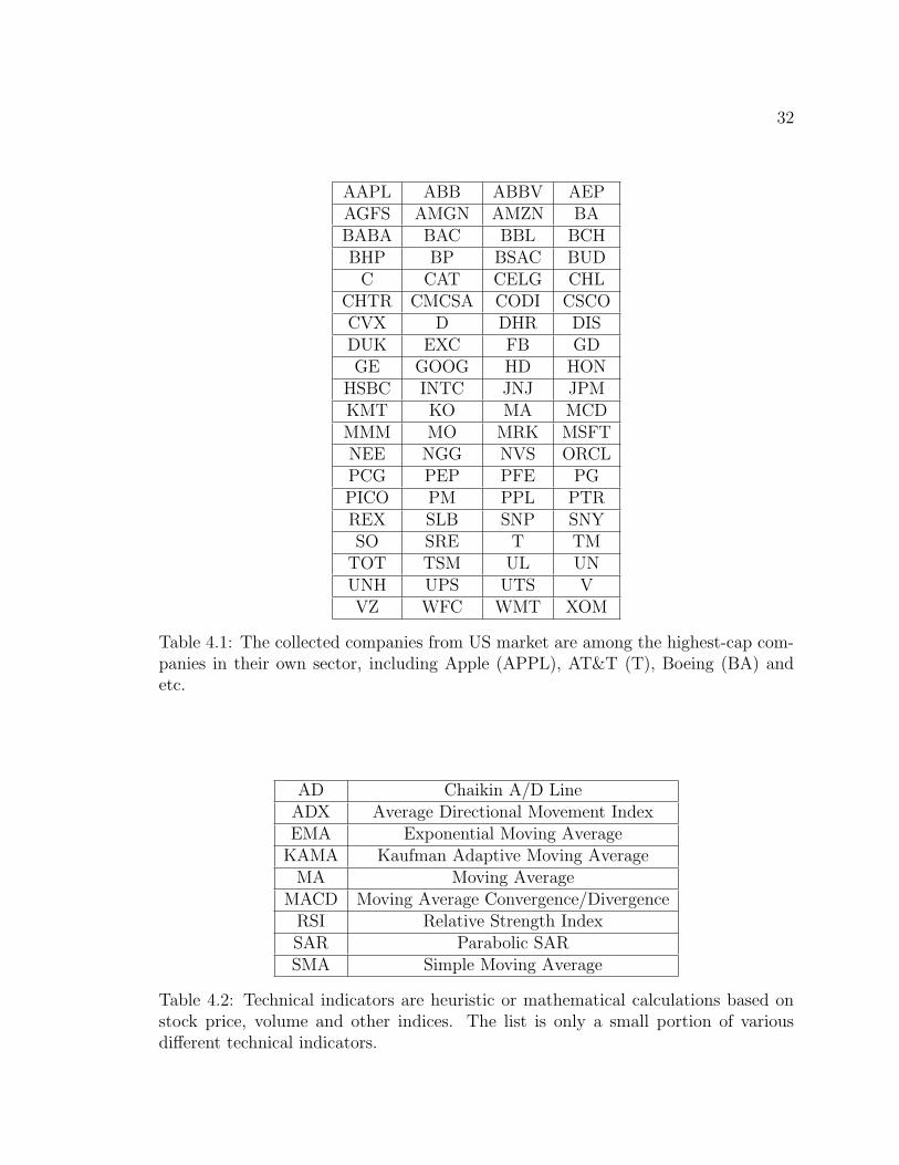
80 stocks in total from each sector (see full list in Table 4.1. All stocks are top-market-

cap companies within its own sector, including Apple (AAPL), Amazon (AMZN), T

(AT&T) and so on. We collect history data of these stocks from 01/01/2016 to

31/12/2018 and the daily price includes Open, Close, High, Low and Volume.

4.4 Technical Indicators

In the first experiment we use few technical indicators with brief explanation. In

this section we are going to give a more detailed introduction of technical indica-

tors. Technical Indicators are usually heuristic or mathematical calculation based on

the price, volume and other measurement by traders who follow technical analysis.

Common technical indicators include Moving Average (MA), Relative Strength Index

(RSI) and Moving Average Convergence-Divergence (MACD). People have created

many technical indicators and table 4.2 show few of them.

Moving Average (MA) is a widely used indicator in technical analysis that helps

smooth out price action by filtering out the ”noise” from random short-term price

fluctuations [48]. While there are Simple Moving Average and many other MA vari-

ants, MA usually refers to Simple Moving Average and in this paper we will use MA

to refer to Simple Moving Average.

1https://finance.yahoo.com/industries

32

AAPL ABB ABBV AEPAGFS AMGN AMZN BABABA BAC BBL BCHBHP BP BSAC BUD

C CAT CELG CHLCHTR CMCSA CODI CSCOCVX D DHR DISDUK EXC FB GDGE GOOG HD HON

HSBC INTC JNJ JPMKMT KO MA MCDMMM MO MRK MSFTNEE NGG NVS ORCLPCG PEP PFE PGPICO PM PPL PTRREX SLB SNP SNYSO SRE T TM

TOT TSM UL UNUNH UPS UTS VVZ WFC WMT XOM

Table 4.1: The collected companies from US market are among the highest-cap com-panies in their own sector, including Apple (APPL), AT&T (T), Boeing (BA) andetc.

AD Chaikin A/D LineADX Average Directional Movement IndexEMA Exponential Moving Average

KAMA Kaufman Adaptive Moving AverageMA Moving Average

MACD Moving Average Convergence/DivergenceRSI Relative Strength IndexSAR Parabolic SARSMA Simple Moving Average

Table 4.2: Technical indicators are heuristic or mathematical calculations based onstock price, volume and other indices. The list is only a small portion of variousdifferent technical indicators.

33

Given a trading day d, MA50, MA65 and MA200 are calculated as follows:

MAk =

∑dd−k pi

k(4.1)

where k is the number of days in a time window ending with the day d, and pi is

the closing price after each day.

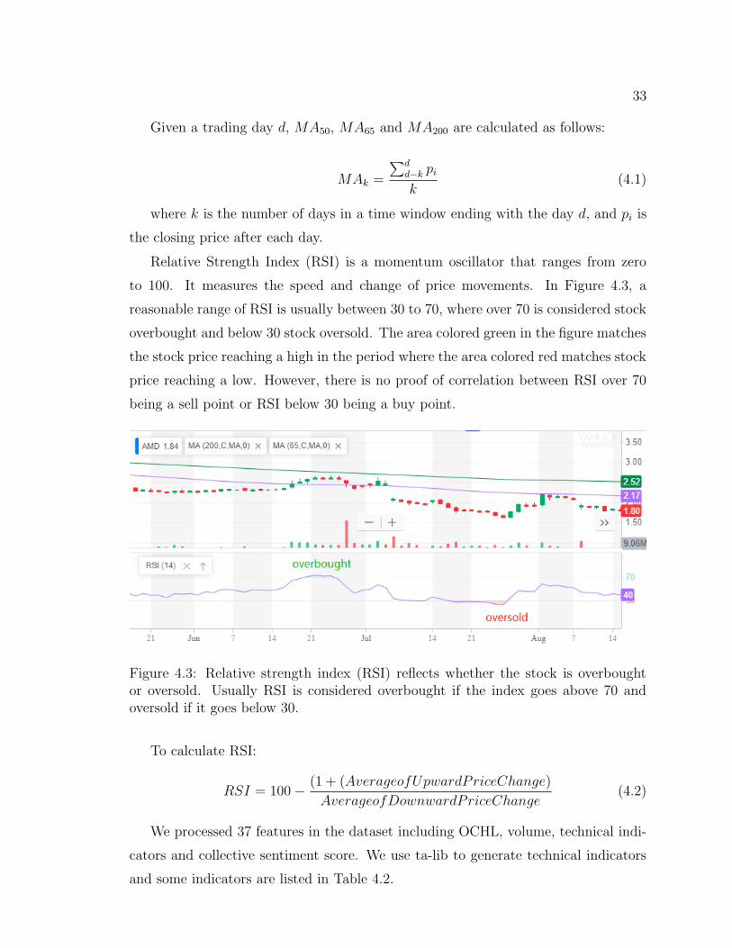
Relative Strength Index (RSI) is a momentum oscillator that ranges from zero

to 100. It measures the speed and change of price movements. In Figure 4.3, a

reasonable range of RSI is usually between 30 to 70, where over 70 is considered stock

overbought and below 30 stock oversold. The area colored green in the figure matches

the stock price reaching a high in the period where the area colored red matches stock

price reaching a low. However, there is no proof of correlation between RSI over 70

being a sell point or RSI below 30 being a buy point.

Figure 4.3: Relative strength index (RSI) reflects whether the stock is overboughtor oversold. Usually RSI is considered overbought if the index goes above 70 andoversold if it goes below 30.

To calculate RSI:

RSI = 100− (1 + (AverageofUpwardPriceChange)

AverageofDownwardPriceChange(4.2)

We processed 37 features in the dataset including OCHL, volume, technical indi-

cators and collective sentiment score. We use ta-lib to generate technical indicators

and some indicators are listed in Table 4.2.

34

4.5 Sentiment Analysis

Word lists not built for financial text may misclassify common words in many cases [49].

Many words in our daily life can be neutral but mean totally differently in stock mar-

ket. For example, when someone posts ”long Apple”, it is a positive sentiment and

it means you expect the price of Apple rally in the future. Similarly, when you write

”short Alibaba” it surely does not mean Alibaba is short but express a negative sen-

timent that the price of Alibaba may go down in the future. Harvard IV-4 dictionary

contains lists of positive and negative words2. In large samples of Form 10-K, [49]

found almost three-fourths of the words were misclassified as negative when they are

typically not considered as negative in financial context. For this reason, we used

Loughran and McDonald dictionary for our finance tweets sentiment analysis.

In the data we acquire from StockTwits, each tweet is associated with a sentiment

score. However, StockTwits did not provide any detail on how the sentiment score

was calculated. For comparison, we took our own approach to calculate sentiment

score s based on the number of positive Np and negative words Nn in the tweet:

s =Np −Nn

Np +Nn

(4.3)

As mentioned in the Kaggle dataset experiment, there are few issues we need to

address in the experiment with larger dataset. The first task is to solve the problem

of the information time sensitivity. We define three categories of time period based

on the market hours: full day, intraday and after hours. We want to explore if the

different time periods are correlated with the experiment result. Besides, different

source of tweets should have different weight in the decision-making system. Most

of the time, a post from a user that has no follower should have significantly less

influence than a post from an expert investor with millions of followers. Here raises

another question. If we take the influence of posts into account, we need to come up

with a proper method through experiment.

To address the issues above, we design an experiment to figure out the combination

that delivers the best result. In the collective sentiment experiment, we applied

the sentiment score from StockTwits. For the comparison of performance between

StockTwits’ sentiment score and our approach of collective sentiment, two experiment

2http://www.wjh.harvard.edu/˜inquirer/homecat.htm

35

is required with the same configuration except for the collective sentiment. This will

be conducted in the aggregate-dataset experiment

4.6 Collective Sentiment

The US stock market usually opens at 9:30 a.m. EST and closes at 4:00 p.m. EST for

transactions. However, the pre-market trading and after-market trading also affect

the movement of stock price. The pre-market [50] trading usually occurs from 8:00

a.m. to 9:30 a.m. EST and after-market from 8:00 a.m. to 9:30 a.m. each trading

day. Activities during those periods may affect the stock price dramatically. For

example, some companies would release fiscal report or make big announcement after

market closes, which sometime results in huge price hike or price plunge.

Bolen et al. [5] state that tweets help predicting the stock price future movement.

We want to see if finance tweets in certain time period may have better predictive

power; e.g., intraday tweets, after-market tweets and full-day tweets.

Intraday tweets refer to the tweets that are posted during the trading hours; after-

market tweets refer to the tweets that are posted from market closes till before market

opens in the next trading day; full-day tweets are the tweets posted in the past 24

hours before the market closes on a target trading day.

As we mentioned in the last section, each tweet may have different influence and

predictive power from different user. For instance, a tweet from me about the market

may go unnoticed while Donald Trump’s tweet about tariff may cause the market to

fluctuate dramatically [51]. To calculate the collective sentiment, we compared three

different approach to calculate daily collective sentiment C for finance tweets T in

target time period:

• Simple summation of tweets sentiment:

C =n∑

i=0

Ti (4.4)

• Weighted sentiment on tweets followers F for each tweet T :

C =n∑

i=0

Ti · Fi

Fmax

(4.5)

36

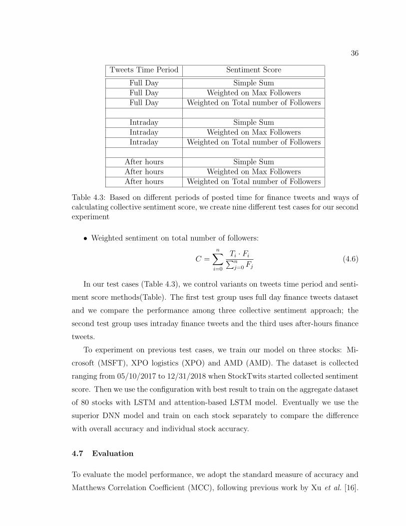
Tweets Time Period Sentiment Score

Full Day Simple SumFull Day Weighted on Max FollowersFull Day Weighted on Total number of Followers

Intraday Simple SumIntraday Weighted on Max FollowersIntraday Weighted on Total number of Followers

After hours Simple SumAfter hours Weighted on Max FollowersAfter hours Weighted on Total number of Followers

Table 4.3: Based on different periods of posted time for finance tweets and ways ofcalculating collective sentiment score, we create nine different test cases for our secondexperiment

• Weighted sentiment on total number of followers:

C =n∑

i=0

Ti · Fi∑nj=0 Fj

(4.6)

In our test cases (Table 4.3), we control variants on tweets time period and senti-

ment score methods(Table). The first test group uses full day finance tweets dataset

and we compare the performance among three collective sentiment approach; the

second test group uses intraday finance tweets and the third uses after-hours finance

tweets.

To experiment on previous test cases, we train our model on three stocks: Mi-

crosoft (MSFT), XPO logistics (XPO) and AMD (AMD). The dataset is collected

ranging from 05/10/2017 to 12/31/2018 when StockTwits started collected sentiment

score. Then we use the configuration with best result to train on the aggregate dataset

of 80 stocks with LSTM and attention-based LSTM model. Eventually we use the

superior DNN model and train on each stock separately to compare the difference

with overall accuracy and individual stock accuracy.

4.7 Evaluation

To evaluate the model performance, we adopt the standard measure of accuracy and

Matthews Correlation Coefficient (MCC), following previous work by Xu et al. [16].

37

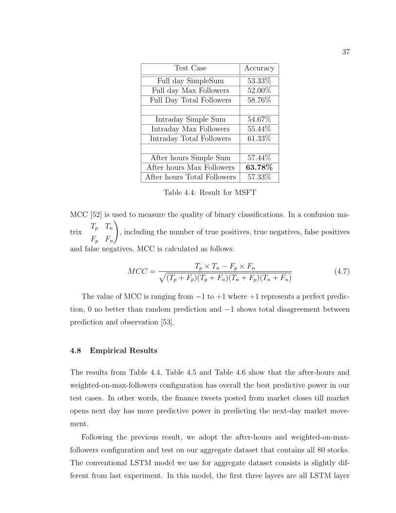
Test Case Accuracy

Full day SimpleSum 53.33%Full day Max Followers 52.00%

Full Day Total Followers 58.76%

Intraday Simple Sum 54.67%Intraday Max Followers 55.44%Intraday Total Followers 61.33%

After hours Simple Sum 57.44%After hours Max Followers 63.78%After hours Total Followers 57.33%

Table 4.4: Result for MSFT

MCC [52] is used to measure the quality of binary classifications. In a confusion ma-

trix

(Tp Tn

Fp Fn

), including the number of true positives, true negatives, false positives

and false negatives, MCC is calculated as follows:

MCC =Tp × Tn − Fp × Fn√

(Tp + Fp)(Tp + Fn)(Tn + Fp)(Tn + Fn)(4.7)

The value of MCC is ranging from −1 to +1 where +1 represents a perfect predic-

tion, 0 no better than random prediction and −1 shows total disagreement between

prediction and observation [53].

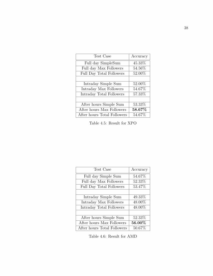
4.8 Empirical Results

The results from Table 4.4, Table 4.5 and Table 4.6 show that the after-hours and

weighted-on-max-followers configuration has overall the best predictive power in our

test cases. In other words, the finance tweets posted from market closes till market

opens next day has more predictive power in predicting the next-day market move-

ment.

Following the previous result, we adopt the after-hours and weighted-on-max-

followers configuration and test on our aggregate dataset that contains all 80 stocks.

The conventional LSTM model we use for aggregate dataset consists is slightly dif-

ferent from last experiment. In this model, the first three layers are all LSTM layer

38

Test Case Accuracy

Full day SimpleSum 45.33%Full day Max Followers 54.56%

Full Day Total Followers 52.00%

Intraday Simple Sum 52.00%Intraday Max Followers 54.67%Intraday Total Followers 57.33%

After hours Simple Sum 53.33%After hours Max Followers 58.67%After hours Total Followers 54.67%

Table 4.5: Result for XPO

Test Case Accuracy

Full day Simple Sum 54.67%Full day Max Followers 52.33%

Full Day Total Followers 53.47%

Intraday Simple Sum 49.33%Intraday Max Followers 48.00%Intraday Total Followers 48.00%

After hours Simple Sum 52.33%After hours Max Followers 56.00%After hours Total Followers 50.67%

Table 4.6: Result for AMD

39

Test Case Accuracy MCC

After hours Max Followers 52.27% 0.04092

Table 4.7: By taking the best configuration from test on individual stock experiment,we use finance tweets from after hours till next next open and calculate collectivesentiment with weight on maximum followers.

Model Accuracy MCC

LSTM 52.27% 0.04092attention-based LSTM 54.58% 0.04780

Table 4.8: With the extra layer of attention mechanism, the performance is improvedby above 2% on aggregate stock dataset.

and the time-step of each layer is set at 40. The last layer is a dense layer and the

output is a value from 0 to 1, which is the same as our first experiment .

The result of conventional LSTM model in Table 4.7 is slightly worse than the

result in individual stock dataset from previous experiment. Since the dataset does

not have the problem in first experiment, our goal is to opimize this model and

improve the performance. As mentioned in Section 4.1, we add attention block into

our model, while rest of the model remains the same.

The result in Table 4.8 shows moderate improvement over the conventional LSTM

model, but the accuracy is still just slightly better than flipping a coin. By comparing

the performance between the aggregate dataset and the three individual stock datasets

in previous experiment, we wonder whether a model trained from aggregate dataset

works better than the model trained from individual stock dataset. To answer the

question, we train the model on 80 stocks separately. To reduce experimental errors,

we train five times for each dataset and take the average accuracy and MCC.

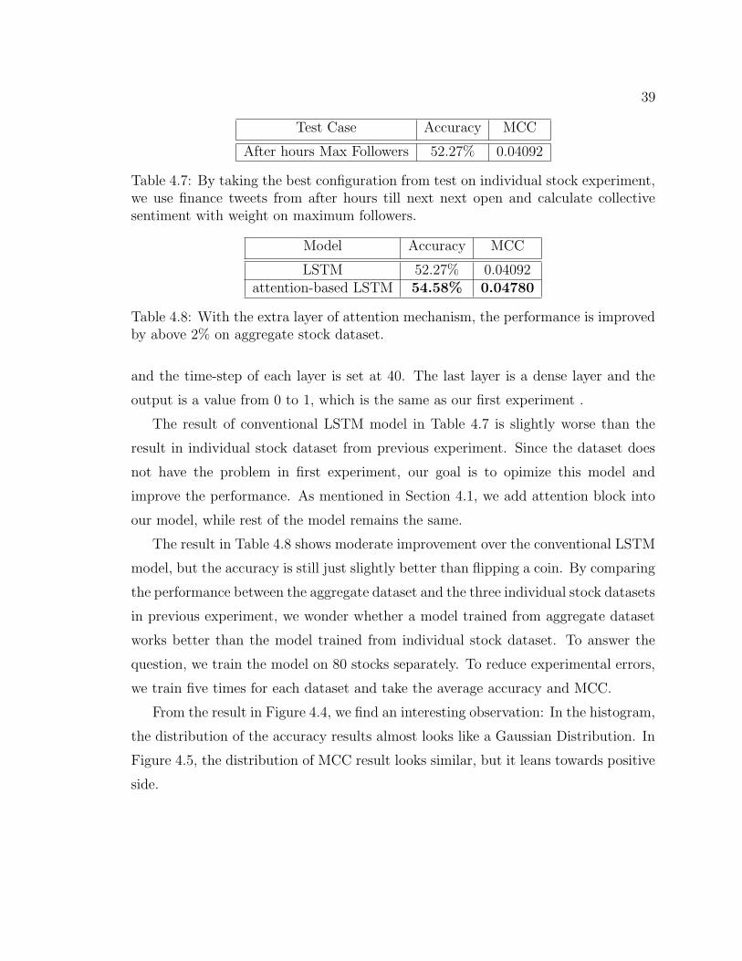
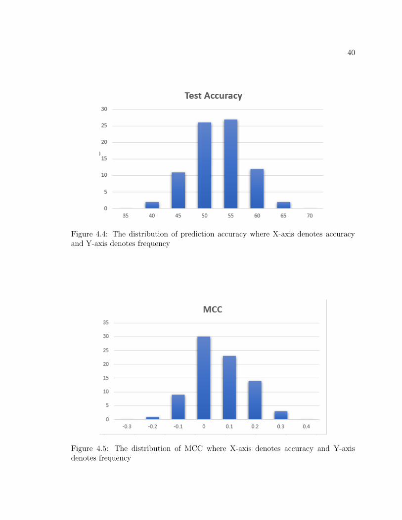
From the result in Figure 4.4, we find an interesting observation: In the histogram,

the distribution of the accuracy results almost looks like a Gaussian Distribution. In

Figure 4.5, the distribution of MCC result looks similar, but it leans towards positive

side.

40

Figure 4.4: The distribution of prediction accuracy where X-axis denotes accuracyand Y-axis denotes frequency

Figure 4.5: The distribution of MCC where X-axis denotes accuracy and Y-axisdenotes frequency

Chapter 5

Analysis of Candlestick Pattern

5.1 Introduction

Japanese Candlestick chart was developed as early as 1600s in Japan to trade one

of the world’s first futures markets - rice futures [1]. Steve Nison, the author of

multiple books about candlestick chart, is known as the father of modern candlestick

charting. He introduced this exciting and useful tool to western readers and explained

how candlestick charting can predict stock market movement [34]. The different

candlestick patterns and trading strategies in this book are very refreshing and many

history records shows the predictive power of candlestick charts. However, some

research papers bring some controversial voices questioning whether this tool really

works in the US stock market [18, 19].

Horton [35] examined Japanese candlestick of technical analysis for 349 stock

and came to the conclusion that patterns like stars, crows, or doji does not help

predicting stock market movement. Marshal [18] took Dow Jones Industrial Average

(DJIA) data from 1992 to 2002 and found that candlestick technical analysis is not

profitable in US stock marker. In his later work [36] he tested candlestick patterns in

the Japanese equity market over the 1975 to 2004 period and found strong evidence

that candlestick technical analysis is not profitable on large stocks in the Japanese

equity market.

On the other hand, Fock et al. [37] studied the predictive power of candlestick pat-

terns and found the combination of candlestick patterns together with other technical

indicators was able to get higher returns. Following this research, Chen et al. [20]

shows that pair of bullish and bearish harami, and the pattern of homing pigeon shows

best forecasting power for both medium-market-cap and large-market-cap stocks in

eight pattern from their results. Based on this insight, we worked on dataset in our

framework and found some interesting observations. During the time this thesis is be-

ing written, Cohen et al. [54] also applies deep learning on the research of Candlestick

41

42

patterns, which brings some great questions for future work.

5.2 Background and Related Work

Unlike the stock technical indicators from previous projects, Japanese candlestick

is less about numbers but more about patterns. The difference from traditional

index-based technical analysis makes candlestick pattern its own place in the TA

fields. Since candlestick is rooted in traditional Japanese culture, it brings a new

way in understanding the stock market from the Eastern perspective. Steve Nison

is arguably the most well-known investor using candlestick charting as an analysis

tool in studying market trend and making investment decisions. Many books he

published [1, 34] bring candlestick chart from Japan to the Western world and create

a systematic way in the analysis of US stock market in combination with traditional

technical analysis. In his book [1], he summarized a range of candlestick patterns

and use many examples to illustrate how candlestick can help predicting the market

trend. Those patterns, by the number of candlestick bodies, can generally be classified

into one-day patterns, two-day patterns and three-day patterns. By working together

with index-based technical indicators, candlestick chart shows great potential in the

prediction of future stock movement.

Nison studied the book The Fountain of Gold - The Three Monkey Record

of Money and concluded the characteristics of the three monkeys:

• See no evil: when you see a bullish (bearish) trend, do not get caught up in

it; consider it an opportunity to sell (buy)

• Hear no evil: when you hear bullish or bearish news, don’t trade on it.

• Speak no evil: don’t speak to others about what you are going to do in the

market

5.2.1 Construction Of The Candle Line

The color of candles reflects the stock rise or fall in that period. As illustrated in

Figure 5.1, in color candlestick chart, the green candle means the close is higher than

open and red candle means the opposite. The monochrome candlestick chart is used

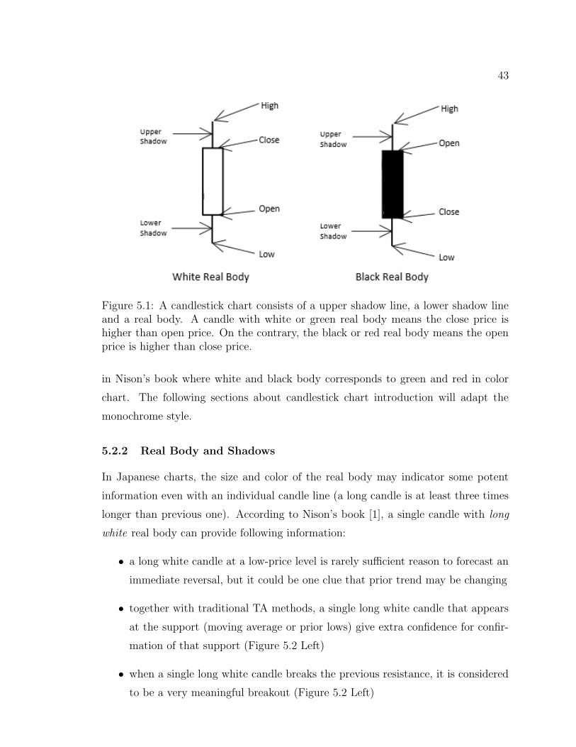
43

Figure 5.1: A candlestick chart consists of a upper shadow line, a lower shadow lineand a real body. A candle with white or green real body means the close price ishigher than open price. On the contrary, the black or red real body means the openprice is higher than close price.

in Nison’s book where white and black body corresponds to green and red in color

chart. The following sections about candlestick chart introduction will adapt the

monochrome style.

5.2.2 Real Body and Shadows

In Japanese charts, the size and color of the real body may indicator some potent

information even with an individual candle line (a long candle is at least three times

longer than previous one). According to Nison’s book [1], a single candle with long

white real body can provide following information:

• a long white candle at a low-price level is rarely sufficient reason to forecast an

immediate reversal, but it could be one clue that prior trend may be changing

• together with traditional TA methods, a single long white candle that appears

at the support (moving average or prior lows) give extra confidence for confir-

mation of that support (Figure 5.2 Left)

• when a single long white candle breaks the previous resistance, it is considered

to be a very meaningful breakout (Figure 5.2 Left)

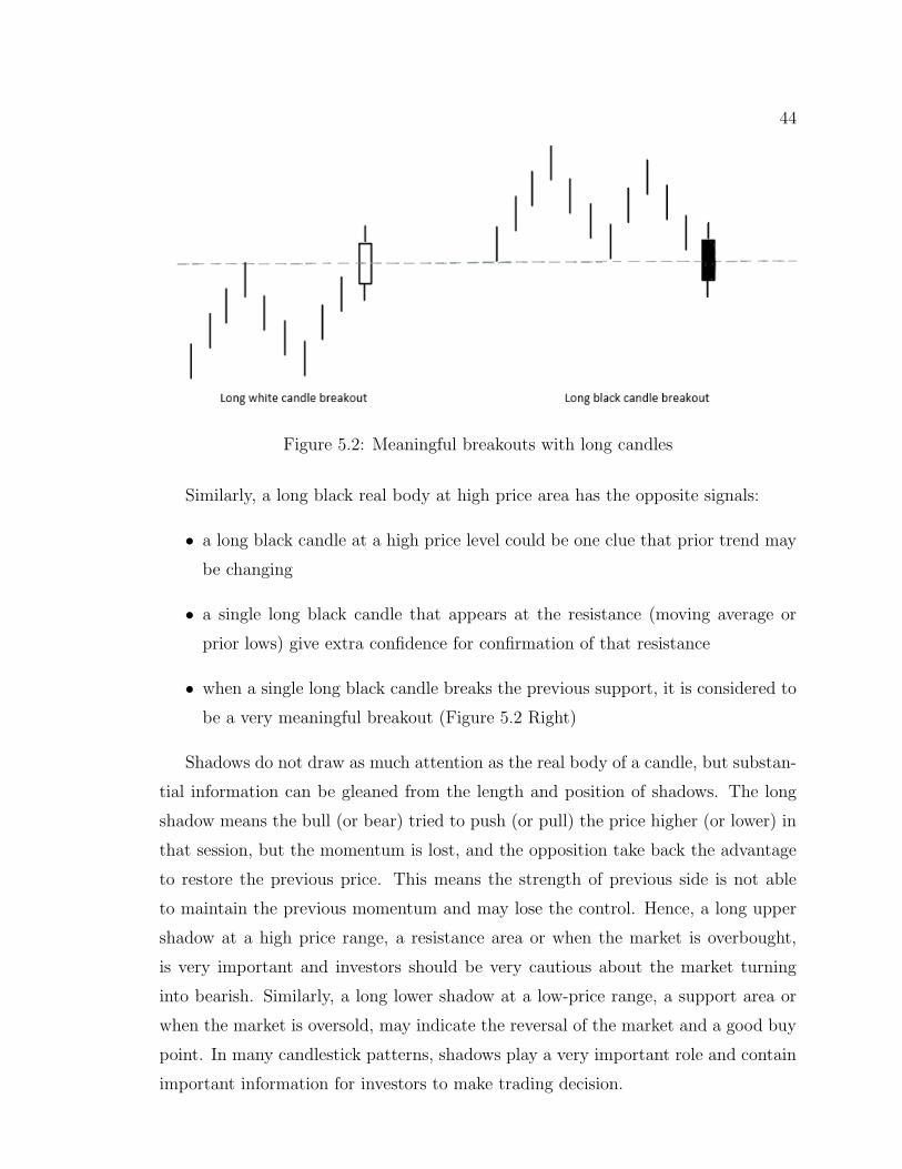
44

Figure 5.2: Meaningful breakouts with long candles

Similarly, a long black real body at high price area has the opposite signals:

• a long black candle at a high price level could be one clue that prior trend may

be changing

• a single long black candle that appears at the resistance (moving average or

prior lows) give extra confidence for confirmation of that resistance

• when a single long black candle breaks the previous support, it is considered to

be a very meaningful breakout (Figure 5.2 Right)

Shadows do not draw as much attention as the real body of a candle, but substan-

tial information can be gleaned from the length and position of shadows. The long

shadow means the bull (or bear) tried to push (or pull) the price higher (or lower) in

that session, but the momentum is lost, and the opposition take back the advantage

to restore the previous price. This means the strength of previous side is not able

to maintain the previous momentum and may lose the control. Hence, a long upper

shadow at a high price range, a resistance area or when the market is overbought,

is very important and investors should be very cautious about the market turning

into bearish. Similarly, a long lower shadow at a low-price range, a support area or

when the market is oversold, may indicate the reversal of the market and a good buy

point. In many candlestick patterns, shadows play a very important role and contain

important information for investors to make trading decision.

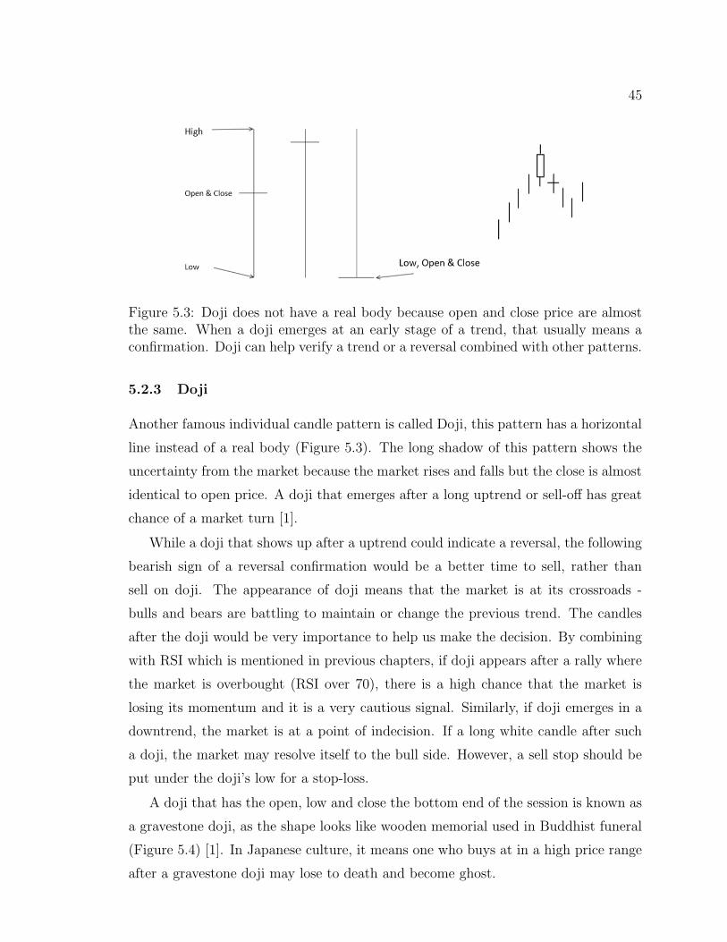
45

Figure 5.3: Doji does not have a real body because open and close price are almostthe same. When a doji emerges at an early stage of a trend, that usually means aconfirmation. Doji can help verify a trend or a reversal combined with other patterns.

5.2.3 Doji

Another famous individual candle pattern is called Doji, this pattern has a horizontal

line instead of a real body (Figure 5.3). The long shadow of this pattern shows the

uncertainty from the market because the market rises and falls but the close is almost

identical to open price. A doji that emerges after a long uptrend or sell-off has great

chance of a market turn [1].

While a doji that shows up after a uptrend could indicate a reversal, the following

bearish sign of a reversal confirmation would be a better time to sell, rather than

sell on doji. The appearance of doji means that the market is at its crossroads -

bulls and bears are battling to maintain or change the previous trend. The candles

after the doji would be very importance to help us make the decision. By combining

with RSI which is mentioned in previous chapters, if doji appears after a rally where

the market is overbought (RSI over 70), there is a high chance that the market is

losing its momentum and it is a very cautious signal. Similarly, if doji emerges in a

downtrend, the market is at a point of indecision. If a long white candle after such

a doji, the market may resolve itself to the bull side. However, a sell stop should be

put under the doji’s low for a stop-loss.

A doji that has the open, low and close the bottom end of the session is known as

a gravestone doji, as the shape looks like wooden memorial used in Buddhist funeral

(Figure 5.4) [1]. In Japanese culture, it means one who buys at in a high price range

after a gravestone doji may lose to death and become ghost.

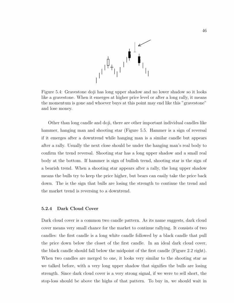
46

Figure 5.4: Gravestone doji has long upper shadow and no lower shadow so it lookslike a gravestone. When it emerges at higher price level or after a long rally, it meansthe momentum is gone and whoever buys at this point may end like this ”gravestone”and lose money.

Other than long candle and doji, there are other important individual candles like

hammer, hanging man and shooting star (Figure 5.5. Hammer is a sign of reversal

if it emerges after a downtrend while hanging man is a similar candle but appears

after a rally. Usually the next close should be under the hanging man’s real body to

confirm the trend reversal. Shooting star has a long upper shadow and a small real

body at the bottom. If hammer is sign of bullish trend, shooting star is the sign of

a bearish trend. When a shooting star appears after a rally, the long upper shadow

means the bulls try to keep the price higher, but bears can easily take the price back

down. The is the sign that bulls are losing the strength to continue the trend and

the market trend is reversing to a downtrend.

5.2.4 Dark Cloud Cover

Dark cloud cover is a common two candle pattern. As its name suggests, dark cloud

cover means very small chance for the market to continue rallying. It consists of two

candles: the first candle is a long white candle followed by a black candle that pull

the price down below the closet of the first candle. In an ideal dark cloud cover,

the black candle should fall below the midpoint of the first candle (Figure 2.2 right).

When two candles are merged to one, it looks very similar to the shooting star as

we talked before, with a very long upper shadow that signifies the bulls are losing

strength. Since dark cloud cover is a very strong signal, if we were to sell short, the

stop-loss should be above the highs of that pattern. To buy in, we should wait in

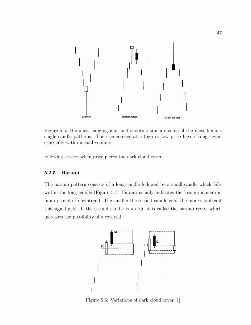
47

Figure 5.5: Hammer, hanging man and shooting star are some of the most famoussingle candle patterns. Their emergence at a high or low price have strong signalespecially with unusual volume.

following session when price pierce the dark cloud cover.

5.2.5 Harami

The harami pattern consists of a long candle followed by a small candle which falls

within the long candle (Figure 5.7. Harami usually indicates the losing momentum

in a uptrend or downtrend. The smaller the second candle gets, the more significant

this signal gets. If the second candle is a doji, it is called the harami cross, which

increases the possibility of a reversal.

Figure 5.6: Variations of dark cloud cover [1]

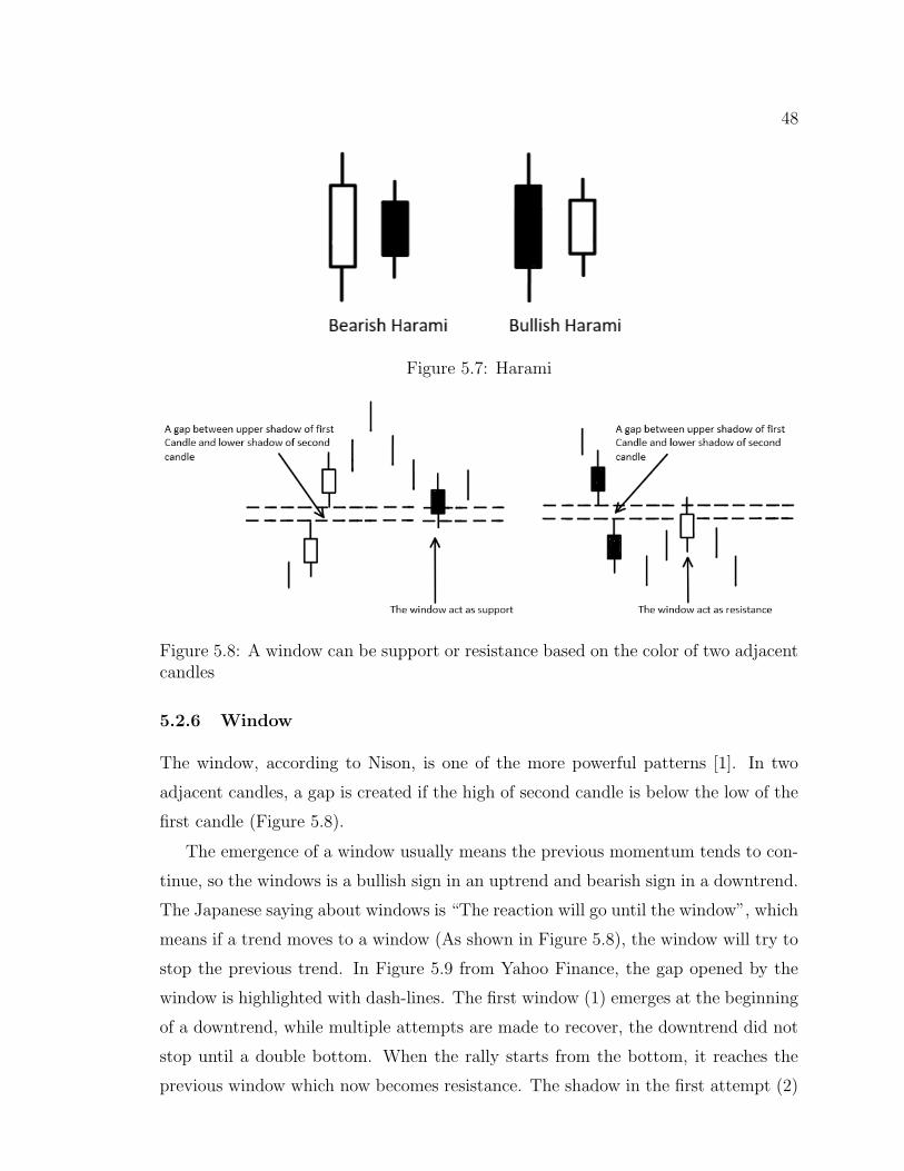
48

Figure 5.7: Harami

Figure 5.8: A window can be support or resistance based on the color of two adjacentcandles

5.2.6 Window

The window, according to Nison, is one of the more powerful patterns [1]. In two

adjacent candles, a gap is created if the high of second candle is below the low of the

first candle (Figure 5.8).

The emergence of a window usually means the previous momentum tends to con-

tinue, so the windows is a bullish sign in an uptrend and bearish sign in a downtrend.

The Japanese saying about windows is “The reaction will go until the window”, which

means if a trend moves to a window (As shown in Figure 5.8), the window will try to

stop the previous trend. In Figure 5.9 from Yahoo Finance, the gap opened by the

window is highlighted with dash-lines. The first window (1) emerges at the beginning

of a downtrend, while multiple attempts are made to recover, the downtrend did not

stop until a double bottom. When the rally starts from the bottom, it reaches the

previous window which now becomes resistance. The shadow in the first attempt (2)

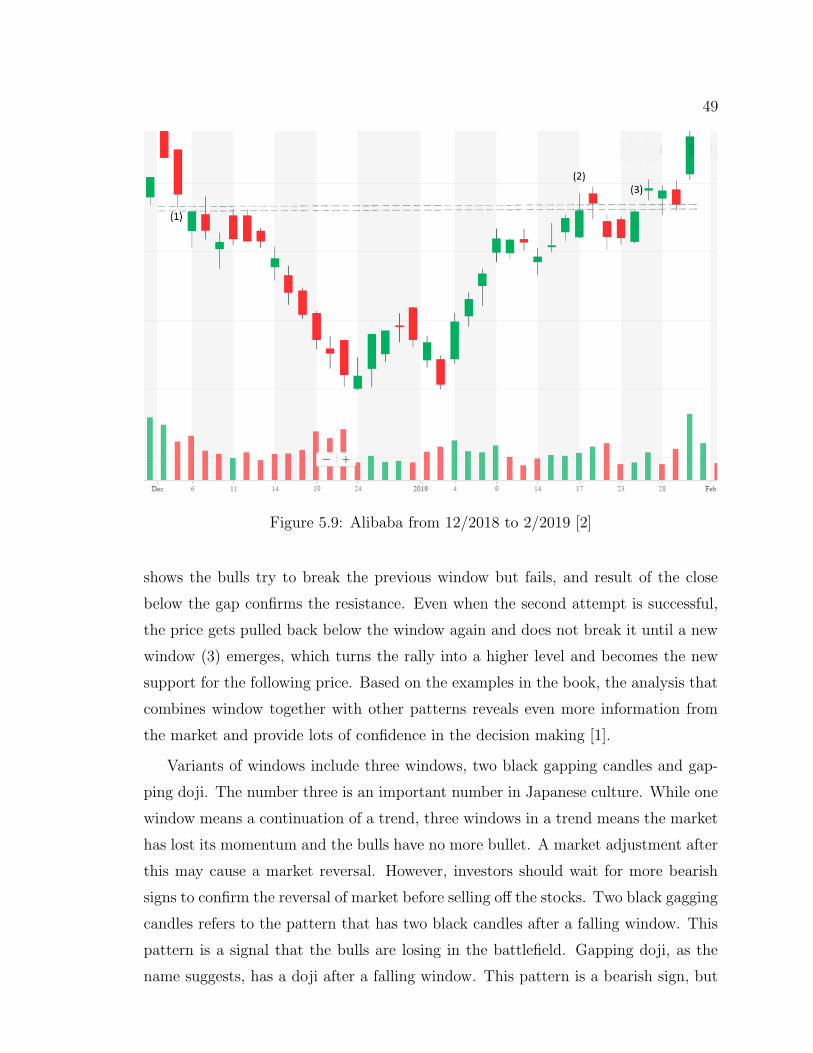
49

Figure 5.9: Alibaba from 12/2018 to 2/2019 [2]

shows the bulls try to break the previous window but fails, and result of the close

below the gap confirms the resistance. Even when the second attempt is successful,

the price gets pulled back below the window again and does not break it until a new

window (3) emerges, which turns the rally into a higher level and becomes the new

support for the following price. Based on the examples in the book, the analysis that

combines window together with other patterns reveals even more information from

the market and provide lots of confidence in the decision making [1].

Variants of windows include three windows, two black gapping candles and gap-

ping doji. The number three is an important number in Japanese culture. While one

window means a continuation of a trend, three windows in a trend means the market

has lost its momentum and the bulls have no more bullet. A market adjustment after

this may cause a market reversal. However, investors should wait for more bearish

signs to confirm the reversal of market before selling off the stocks. Two black gagging

candles refers to the pattern that has two black candles after a falling window. This

pattern is a signal that the bulls are losing in the battlefield. Gapping doji, as the

name suggests, has a doji after a falling window. This pattern is a bearish sign, but

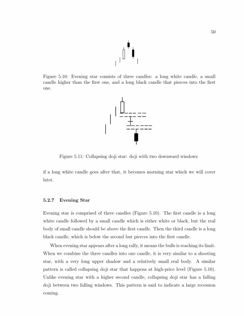
50

Figure 5.10: Evening star consists of three candles: a long white candle, a smallcandle higher than the first one, and a long black candle that pierces into the firstone.

Figure 5.11: Collapsing doji star: doji with two downward windows

if a long white candle goes after that, it becomes morning star which we will cover

later.

5.2.7 Evening Star

Evening star is comprised of three candles (Figure 5.10). The first candle is a long

white candle followed by a small candle which is either white or black, but the real

body of small candle should be above the first candle. Then the third candle is a long

black candle, which is below the second but pierces into the first candle.

When evening star appears after a long rally, it means the bulls is reaching its limit.

When we combine the three candles into one candle, it is very similar to a shooting

star, with a very long upper shadow and a relatively small real body. A similar

pattern is called collapsing doji star that happens at high-price level (Figure 5.10).

Unlike evening star with a higher second candle, collapsing doji star has a falling

doji between two falling windows. This pattern is said to indicate a large recession

coming.

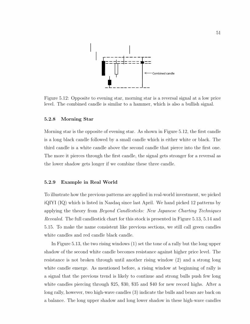
51

Figure 5.12: Opposite to evening star, morning star is a reversal signal at a low pricelevel. The combined candle is similar to a hammer, which is also a bullish signal.

5.2.8 Morning Star

Morning star is the opposite of evening star. As shown in Figure 5.12, the first candle

is a long black candle followed by a small candle which is either white or black. The

third candle is a white candle above the second candle that pierce into the first one.

The more it pierces through the first candle, the signal gets stronger for a reversal as

the lower shadow gets longer if we combine these three candle.

5.2.9 Example in Real World

To illustrate how the previous patterns are applied in real-world investment, we picked

iQIYI (IQ) which is listed in Nasdaq since last April. We hand picked 12 patterns by

applying the theory from Beyond Candlesticks: New Japanese Charting Techniques

Revealed. The full candlestick chart for this stock is presented in Figure 5.13, 5.14 and

5.15. To make the name consistent like previous sections, we still call green candles

white candles and red candle black candle.

In Figure 5.13, the two rising windows (1) set the tone of a rally but the long upper

shadow of the second white candle becomes resistance against higher price level. The

resistance is not broken through until another rising window (2) and a strong long

white candle emerge. As mentioned before, a rising window at beginning of rally is

a signal that the previous trend is likely to continue and strong bulls push few long

white candles piercing through $25, $30, $35 and $40 for new record highs. After a

long rally, however, two high-wave candles (3) indicate the bulls and bears are back on

a balance. The long upper shadow and long lower shadow in these high-wave candles

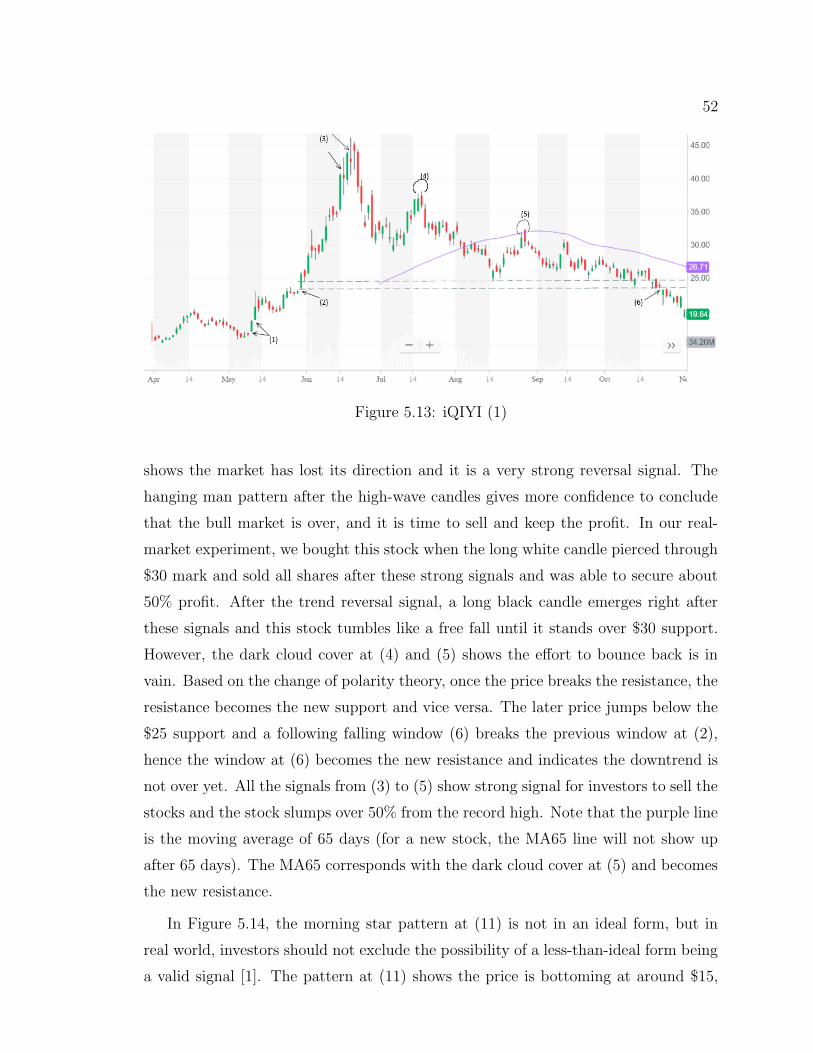
52

Figure 5.13: iQIYI (1)

shows the market has lost its direction and it is a very strong reversal signal. The

hanging man pattern after the high-wave candles gives more confidence to conclude

that the bull market is over, and it is time to sell and keep the profit. In our real-

market experiment, we bought this stock when the long white candle pierced through

$30 mark and sold all shares after these strong signals and was able to secure about

50% profit. After the trend reversal signal, a long black candle emerges right after

these signals and this stock tumbles like a free fall until it stands over $30 support.

However, the dark cloud cover at (4) and (5) shows the effort to bounce back is in

vain. Based on the change of polarity theory, once the price breaks the resistance, the

resistance becomes the new support and vice versa. The later price jumps below the

$25 support and a following falling window (6) breaks the previous window at (2),

hence the window at (6) becomes the new resistance and indicates the downtrend is

not over yet. All the signals from (3) to (5) show strong signal for investors to sell the

stocks and the stock slumps over 50% from the record high. Note that the purple line

is the moving average of 65 days (for a new stock, the MA65 line will not show up

after 65 days). The MA65 corresponds with the dark cloud cover at (5) and becomes

the new resistance.

In Figure 5.14, the morning star pattern at (11) is not in an ideal form, but in

real world, investors should not exclude the possibility of a less-than-ideal form being

a valid signal [1]. The pattern at (11) shows the price is bottoming at around $15,

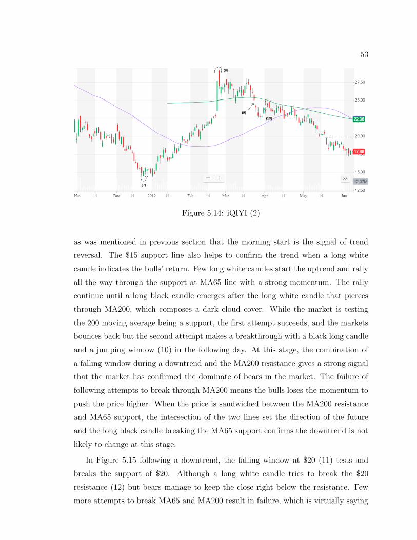
53

Figure 5.14: iQIYI (2)

as was mentioned in previous section that the morning start is the signal of trend

reversal. The $15 support line also helps to confirm the trend when a long white

candle indicates the bulls’ return. Few long white candles start the uptrend and rally

all the way through the support at MA65 line with a strong momentum. The rally

continue until a long black candle emerges after the long white candle that pierces

through MA200, which composes a dark cloud cover. While the market is testing

the 200 moving average being a support, the first attempt succeeds, and the markets

bounces back but the second attempt makes a breakthrough with a black long candle

and a jumping window (10) in the following day. At this stage, the combination of

a falling window during a downtrend and the MA200 resistance gives a strong signal

that the market has confirmed the dominate of bears in the market. The failure of

following attempts to break through MA200 means the bulls loses the momentum to

push the price higher. When the price is sandwiched between the MA200 resistance

and MA65 support, the intersection of the two lines set the direction of the future

and the long black candle breaking the MA65 support confirms the downtrend is not

likely to change at this stage.

In Figure 5.15 following a downtrend, the falling window at $20 (11) tests and

breaks the support of $20. Although a long white candle tries to break the $20

resistance (12) but bears manage to keep the close right below the resistance. Few

more attempts to break MA65 and MA200 result in failure, which is virtually saying

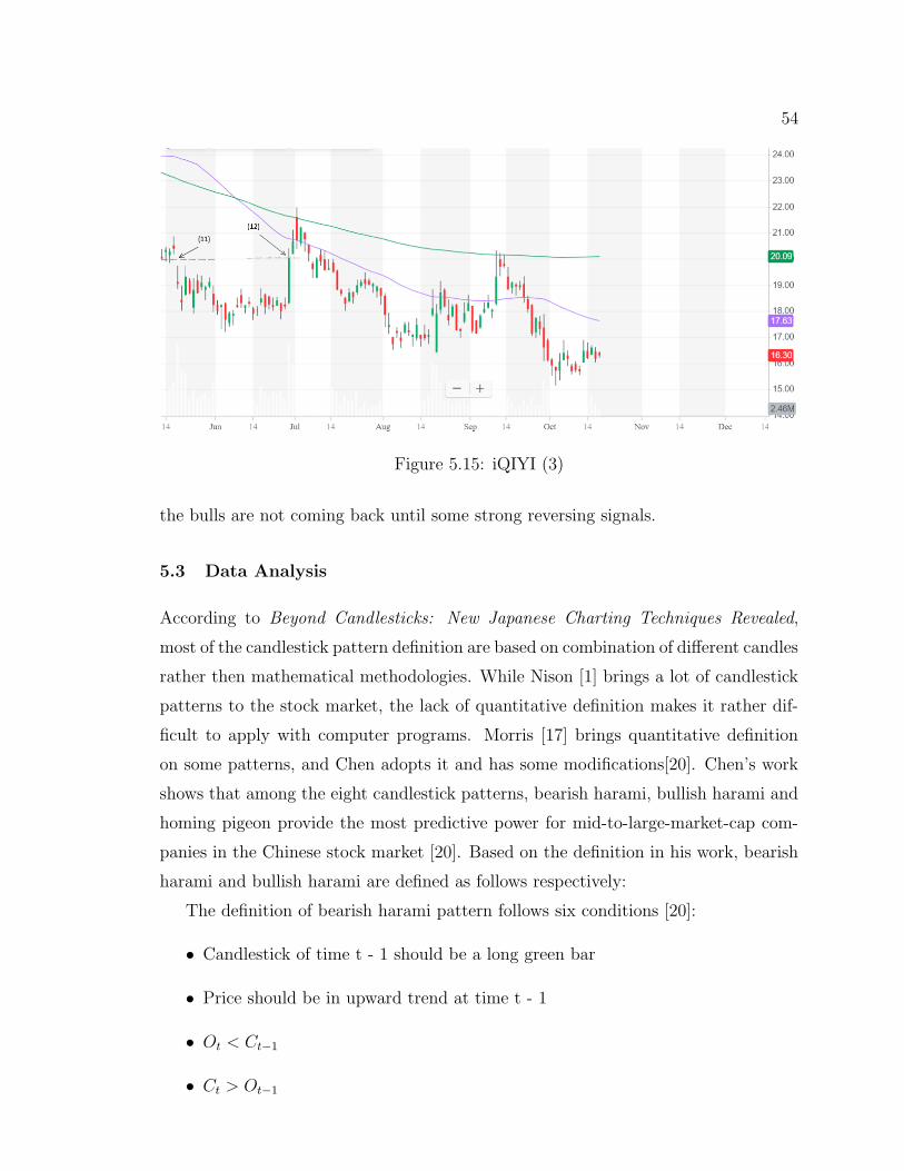
54

Figure 5.15: iQIYI (3)

the bulls are not coming back until some strong reversing signals.

5.3 Data Analysis

According to Beyond Candlesticks: New Japanese Charting Techniques Revealed,

most of the candlestick pattern definition are based on combination of different candles

rather then mathematical methodologies. While Nison [1] brings a lot of candlestick

patterns to the stock market, the lack of quantitative definition makes it rather dif-

ficult to apply with computer programs. Morris [17] brings quantitative definition

on some patterns, and Chen adopts it and has some modifications[20]. Chen’s work

shows that among the eight candlestick patterns, bearish harami, bullish harami and

homing pigeon provide the most predictive power for mid-to-large-market-cap com-

panies in the Chinese stock market [20]. Based on the definition in his work, bearish

harami and bullish harami are defined as follows respectively:

The definition of bearish harami pattern follows six conditions [20]:

• Candlestick of time t - 1 should be a long green bar

• Price should be in upward trend at time t - 1

• Ot < Ct−1

• Ct > Ot−1

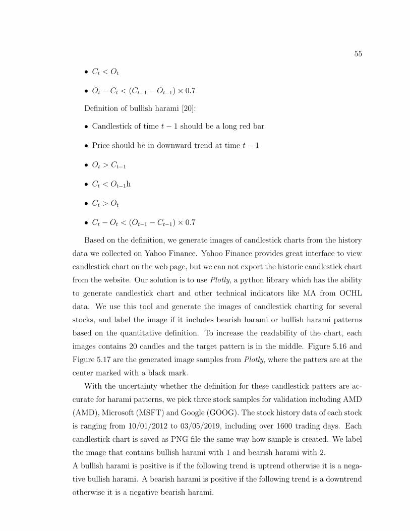
55

• Ct < Ot

• Ot − Ct < (Ct−1 −Ot−1)× 0.7

Definition of bullish harami [20]:

• Candlestick of time t− 1 should be a long red bar

• Price should be in downward trend at time t− 1

• Ot > Ct−1

• Ct < Ot−1h

• Ct > Ot

• Ct −Ot < (Ot−1 − Ct−1)× 0.7

Based on the definition, we generate images of candlestick charts from the history

data we collected on Yahoo Finance. Yahoo Finance provides great interface to view

candlestick chart on the web page, but we can not export the historic candlestick chart

from the website. Our solution is to use Plotly, a python library which has the ability

to generate candlestick chart and other technical indicators like MA from OCHL

data. We use this tool and generate the images of candlestick charting for several

stocks, and label the image if it includes bearish harami or bullish harami patterns

based on the quantitative definition. To increase the readability of the chart, each

images contains 20 candles and the target pattern is in the middle. Figure 5.16 and

Figure 5.17 are the generated image samples from Plotly, where the patters are at the

center marked with a black mark.

With the uncertainty whether the definition for these candlestick patters are ac-

curate for harami patterns, we pick three stock samples for validation including AMD

(AMD), Microsoft (MSFT) and Google (GOOG). The stock history data of each stock

is ranging from 10/01/2012 to 03/05/2019, including over 1600 trading days. Each

candlestick chart is saved as PNG file the same way how sample is created. We label

the image that contains bullish harami with 1 and bearish harami with 2.

A bullish harami is positive is if the following trend is uptrend otherwise it is a nega-

tive bullish harami. A bearish harami is positive if the following trend is a downtrend

otherwise it is a negative bearish harami.

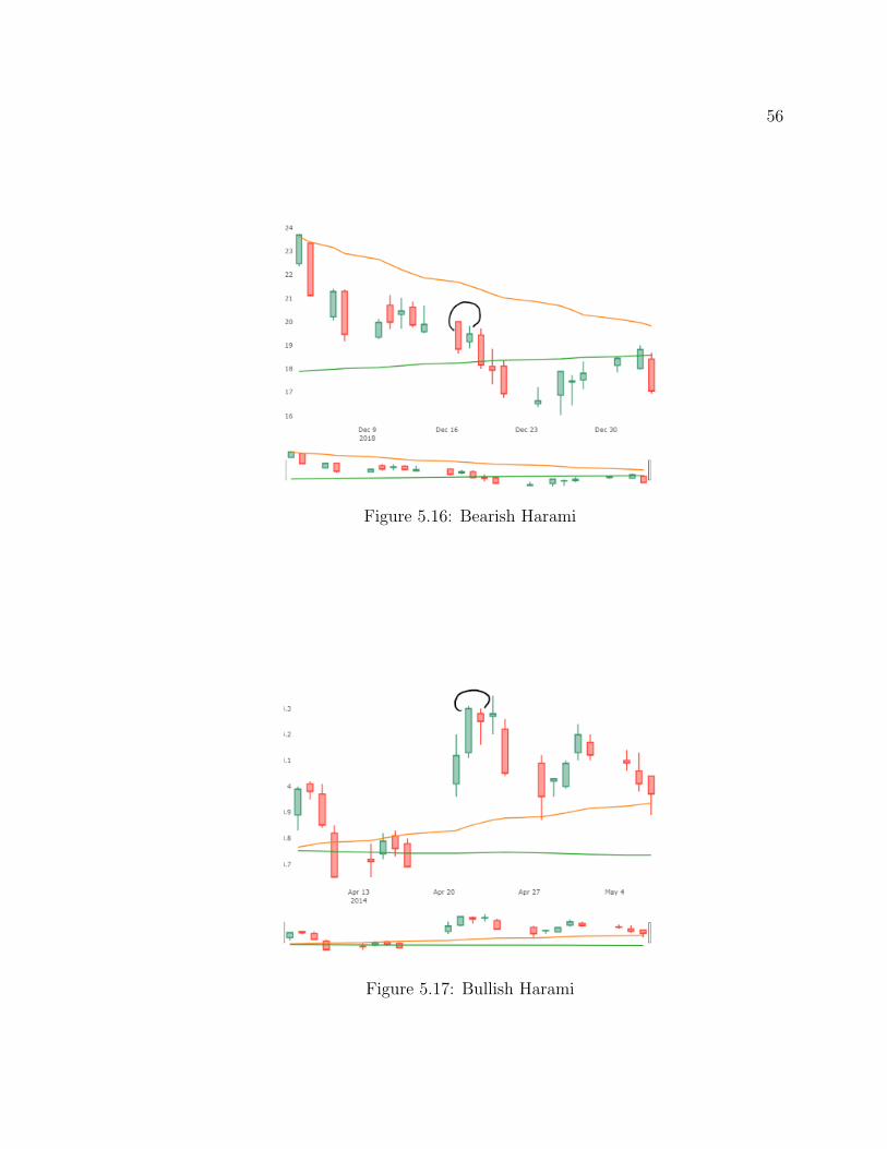
56

Figure 5.16: Bearish Harami

Figure 5.17: Bullish Harami

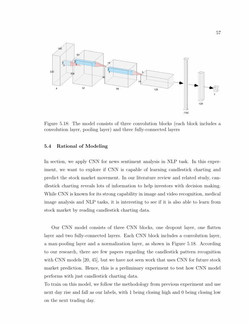
57

Figure 5.18: The model consists of three convolution blocks (each block includes aconvolution layer, pooling layer) and three fully-connected layers

5.4 Rational of Modeling

In section, we apply CNN for news sentiment analysis in NLP task. In this exper-

iment, we want to explore if CNN is capable of learning candlestick charting and

predict the stock market movement. In our literature review and related study, can-

dlestick charting reveals lots of information to help investors with decision making.

While CNN is known for its strong capability in image and video recognition, medical

image analysis and NLP tasks, it is interesting to see if it is also able to learn from

stock market by reading candlestick charting data.

Our CNN model consists of three CNN blocks, one dropout layer, one flatten

layer and two fully-connected layers. Each CNN block includes a convolution layer,

a max-pooling layer and a normalization layer, as shown in Figure 5.18. According

to our research, there are few papers regarding the candlestick pattern recognition

with CNN models [20, 45], but we have not seen work that uses CNN for future stock

market prediction. Hence, this is a preliminary experiment to test how CNN model

performs with just candlestick charting data.

To train on this model, we follow the methodology from previous experiment and use

next day rise and fall as our labels, with 1 being closing high and 0 being closing low

on the next trading day.

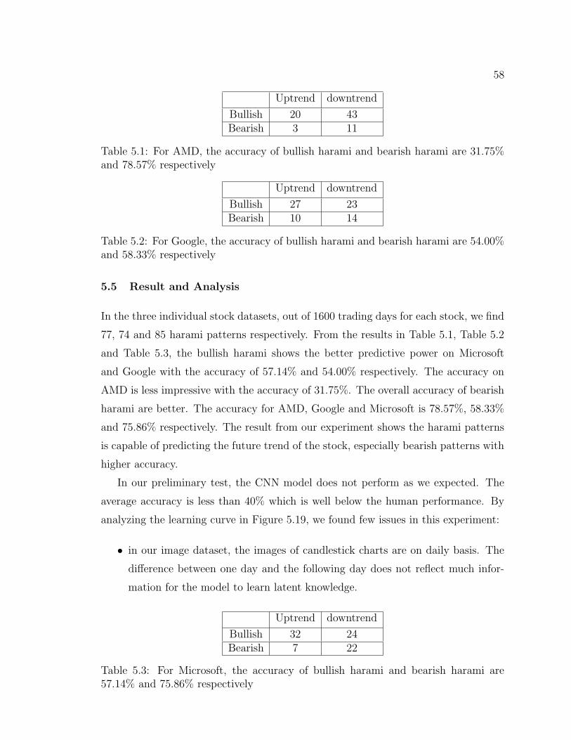
58

Uptrend downtrend

Bullish 20 43Bearish 3 11

Table 5.1: For AMD, the accuracy of bullish harami and bearish harami are 31.75%and 78.57% respectively

Uptrend downtrend

Bullish 27 23Bearish 10 14

Table 5.2: For Google, the accuracy of bullish harami and bearish harami are 54.00%and 58.33% respectively

5.5 Result and Analysis

In the three individual stock datasets, out of 1600 trading days for each stock, we find

77, 74 and 85 harami patterns respectively. From the results in Table 5.1, Table 5.2

and Table 5.3, the bullish harami shows the better predictive power on Microsoft

and Google with the accuracy of 57.14% and 54.00% respectively. The accuracy on

AMD is less impressive with the accuracy of 31.75%. The overall accuracy of bearish

harami are better. The accuracy for AMD, Google and Microsoft is 78.57%, 58.33%

and 75.86% respectively. The result from our experiment shows the harami patterns

is capable of predicting the future trend of the stock, especially bearish patterns with

higher accuracy.

In our preliminary test, the CNN model does not perform as we expected. The

average accuracy is less than 40% which is well below the human performance. By

analyzing the learning curve in Figure 5.19, we found few issues in this experiment:

• in our image dataset, the images of candlestick charts are on daily basis. The

difference between one day and the following day does not reflect much infor-

mation for the model to learn latent knowledge.

Uptrend downtrend

Bullish 32 24Bearish 7 22

Table 5.3: For Microsoft, the accuracy of bullish harami and bearish harami are57.14% and 75.86% respectively

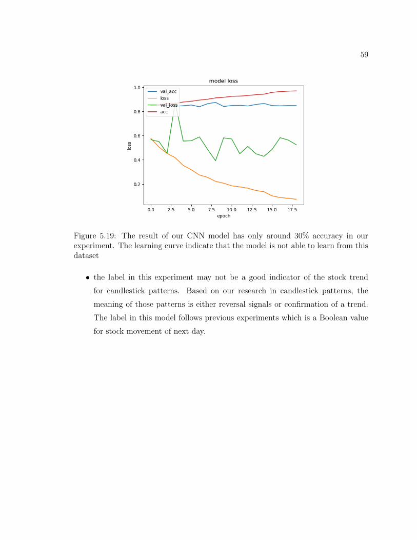
59

Figure 5.19: The result of our CNN model has only around 30% accuracy in ourexperiment. The learning curve indicate that the model is not able to learn from thisdataset

• the label in this experiment may not be a good indicator of the stock trend

for candlestick patterns. Based on our research in candlestick patterns, the

meaning of those patterns is either reversal signals or confirmation of a trend.

The label in this model follows previous experiments which is a Boolean value

for stock movement of next day.

Chapter 6

Conclusion and Future Research

In this thesis we conducted three experiment with different purposes. The first exper-

iment is to compare the performance of DNN model with traditional ML approaches.

Despite the quality of the Kaggle dataset, the result shows that LSTM model has an

edge over ML approaches.

Based on the result and review of first experiment, in the second experiment we

build our own aggregate dataset with 80 stocks that combines the finance tweets

sentiment, stock history price and stock price technical indicators. Regarding the dif-

ference of finance tweets time and user influence, we tested on different configurations

of dataset with different time period and collective sentiment. Our results suggest

the finance tweets that are posted between market close and next market open has

more predictive power on next day stock movement. We also notice that the outcome

of attention-based LSTM model has improvement over conventional LSTM, which is

around 54.6%. We also ran experiment on individual stock dataset of those 80 stocks.

Our best result out of 80 stocks is 65.3%. One interesting observation is the distri-

bution of accuracy and MCC in Figure 4.4 and Figure 4.5, which looks like Gaussian

Distribution and it raises a lot more interesting questions to be answered.

The third experiment investigates the candlestick charting and candlestick pat-

terns. We did a detailed literature review of Steve Nison’s book - Beyond Candlesticks:

New Japanese Charting Techniques Revealed and applied the techniques in real-life

investment. With the application of quantitative definition of some candlestick pat-

terns, we analyzed the predictive power of harami patterns in our dataset. We also

conducted the preliminary experiment on CNN model to predict the future stock

movement. However, the initial result from this model does not perform as expected.

We reviewed the model and dataset with some positive feedback and look forward to

improvement in our future work.

60

61

6.1 Forthcoming Research

There are certain limitations in this thesis. In the second experiment, the result

of attention-based LSTM model on aggregate dataset has some improvement over

conventional LSTM model, but only by a small margin. We believe there are enough

room for us to optimize this model and improve the accuracy. In addition to that, the

result distribution from individual stock dataset that resembles Gaussian Distribution

is worth further research. As central limit theorem defines, in some situations, when

independent random variables are added, their properly normalized sum tends toward

a normal distribution [55]. Although there has been much progress made in this paper

about the application of DNNs in investment, we can not ignore the possibility that

the DNN model in stock market prediction does not learn latent knowledge but makes

random guesses. There is also the possibility that the stocks we chose gave us this

result by coincidence. Hence, we intend to collect more stocks and technical indicators

for further investigation.

Moreover, with much literature review and analysis done on candlestick charting

in the third experiment. We have not made much progress in the application of DNN

model on candlestick charting. The improvement of this experiment may include the

following options:

• since the difference between two adjacent trading day is not obvious, we can try

to generate candlestick charting in a way that the difference can be reflected,

so that DNN model can learn better.

• the labels can be changed from a classification problem into a regression prob-

lem. We can use the future trend as our labels instead of one-day movement.

• reinforcement learning can also be applied to our problem as it is best known

for maximizing reward. In our case the reward can be profit or margins over

certain period of time.

• our research was focused on the US stock market, it would be interesting to see

how it performs in other market such as Asian or European stock market.

Bibliography

[1] Steve Nison. Beyond candlesticks: New Japanese charting techniques revealed,volume 56. John Wiley & Sons, 1994.

[2] Yahoo. Alibaba, inc. (BABA). https://finance.yahoo.com/chart/BABA. Ac-cessed: 2019-05-30.

[3] William J O’Neil and William J O’Neil. How to make money in stocks, volume 10.McGraw-Hill New York, 1988.

[4] Internet traffic. https://en.wikipedia.org/wiki/Internet_traffic. Ac-cessed: 2019-05-30.

[5] Johan Bollen, Huina Mao, and Xiaojun Zeng. Twitter mood predicts the stockmarket. Journal of computational science, 2(1):1–8, 2011.

[6] Volfefe index. https://www.bloomberg.com/news/articles/2019-09-09/

jpmorgan-creates-volfefe-index-to-track-trump-tweet-impact. Ac-cessed: 2019-09-18.

[7] Robert P Schumaker and Hsinchun Chen. Textual analysis of stock market pre-diction using breaking financial news: The azfin text system. ACM Transactionson Information Systems (TOIS), 27(2):12, 2009.

[8] Matt W Gardner and SR Dorling. Artificial neural networks (the multilayerperceptron) — A review of applications in the atmospheric sciences. Atmosphericenvironment, 32(14-15):2627–2636, 1998.

[9] Alex Krizhevsky, Ilya Sutskever, and Geoffrey E Hinton. Imagenet classificationwith deep convolutional neural networks. In Advances in neural informationprocessing systems, pages 1097–1105, 2012.

[10] Kai Chen, Yi Zhou, and Fangyan Dai. A LSTM-based method for stock returnsprediction: A case study of China stock market. In 2015 IEEE InternationalConference on Big Data (Big Data), pages 2823–2824. IEEE, 2015.

[11] David MQ Nelson, Adriano CM Pereira, and Renato A de Oliveira. Stock mar-ket’s price movement prediction with lstm neural networks. In 2017 InternationalJoint Conference on Neural Networks (IJCNN), pages 1419–1426. IEEE, 2017.

[12] Pear Analytics. Twitter study. https://pearanalytics.com/wp-content/

uploads/2012/12/Twitter-Study-August-2009.pdf, 2009.

62

63

[13] Aliaksei Severyn and Alessandro Moschitti. Twitter sentiment analysis withdeep convolutional neural networks. In Proceedings of the 38th InternationalACM SIGIR Conference on Research and Development in Information Retrieval,pages 959–962. ACM, 2015.

[14] Eberhard Schoneburg. Stock price prediction using neural networks: A projectreport. Neurocomputing, 2(1):17–27, 1990.

[15] Asst Birgul Egeli. Stock market prediction using artificial neural networks. De-cision Support Systems, 22:171–185, 2003.

[16] Yumo Xu and Shay B Cohen. Stock movement prediction from tweets andhistorical prices. In Proceedings of the 56th Annual Meeting of the Associationfor Computational Linguistics (Volume 1: Long Papers), pages 1970–1979, 2018.

[17] Greg L Morris. Candlestick Charting Explained: Timeless Techniques for Trad-ing Stocks and Futures: Timeless Techniques for Trading stocks and Sutures.McGraw Hill Professional, 2006.

[18] Ben R Marshall, Martin R Young, and Lawrence C Rose. Candlestick technicaltrading strategies: Can they create value for investors? Journal of Banking &Finance, 30(8):2303–2323, 2006.

[19] Ben R Marshall, Martin R Young, and Rochester Cahan. Are candlestick tech-nical trading strategies profitable in the japanese equity market? Review ofQuantitative Finance and Accounting, 31(2):191–207, 2008.

[20] Shi Chen, Si Bao, and Yu Zhou. The predictive power of japanese candlestickcharting in chinese stock market. Physica A: Statistical Mechanics and its Ap-plications, 457:148–165, 2016.

[21] Burton G Malkiel and Eugene F Fama. Efficient capital markets: A review oftheory and empirical work. The journal of Finance, 25(2):383–417, 1970.

[22] Ramon Lawrence. Using neural networks to forecast stock market prices. Uni-versity of Manitoba, 333, 1997.

[23] Yahoo. Advanced micro devices, inc. (AMD). https://finance.yahoo.com/

chart/AMD. Accessed: 2019-05-30.

[24] CNBC. Donald Trump: Without Twitter, i would not be here — ft interview.https://www.ft.com/content/943e322a-178a-11e7-9c35-0dd2cb31823a.Accessed: 2019-08-30.

[25] CNBC. On days when President Trump tweets a lot, the stock mar-ket falls, investment bank finds. https://www.cnbc.com/2019/09/03/

on-days-when-president-trump-tweets-a-lot-the-stock-market-falls-/

investment-bank-finds.html. Accessed: 2019-08-30.

64

[26] Jianfeng Si, Arjun Mukherjee, Bing Liu, Qing Li, Huayi Li, and Xiaotie Deng.Exploiting topic based twitter sentiment for stock prediction. In Proceedingsof the 51st Annual Meeting of the Association for Computational Linguistics(Volume 2: Short Papers), pages 24–29, 2013.

[27] Venkata Sasank Pagolu, Kamal Nayan Reddy, Ganapati Panda, and Babita Ma-jhi. Sentiment analysis of Twitter data for predicting stock market movements.In 2016 international conference on signal processing, communication, power andembedded system (SCOPES), pages 1345–1350. IEEE, 2016.

[28] Sepp Hochreiter and Jurgen Schmidhuber. Long short-term memory. Neuralcomputation, 9(8):1735–1780, 1997.

[29] Takashi Kimoto, Kazuo Asakawa, Morio Yoda, and Masakazu Takeoka. Stockmarket prediction system with modular neural networks. In 1990 IJCNN inter-national joint conference on neural networks, pages 1–6. IEEE, 1990.

[30] Hirotaka Mizuno, Michitaka Kosaka, Hiroshi Yajima, and Norihisa Komoda.Application of neural network to technical analysis of stock market prediction.Studies in Informatic and control, 7(3):111–120, 1998.

[31] Sepp Hochreiter. The vanishing gradient problem during learning recurrent neu-ral nets and problem solutions. International Journal of Uncertainty, Fuzzinessand Knowledge-Based Systems, 6(02):107–116, 1998.

[32] Razvan Pascanu, Tomas Mikolov, and Yoshua Bengio. Understanding the ex-ploding gradient problem. CoRR, abs/1211.5063, 2, 2012.

[33] Felix A Gers, Douglas Eck, and Jurgen Schmidhuber. Applying lstm to time se-ries predictable through time-window approaches. In Neural Nets WIRN Vietri-01, pages 193–200. 2002.

[34] Steve Nison. Japanese candlestick charting techniques: a contemporary guide tothe ancient investment techniques of the Far East. Penguin, 2001.

[35] Marshall J Horton. Stars, crows, and doji: The use of candlesticks in stockselection. The Quarterly Review of Economics and Finance, 49(2):283–294, 2009.

[36] Ben R Marshall, Martin R Young, and Lawrence C Rose. Market timing withcandlestick technical analysis. Market Timing with Candlestick Technical Anal-ysis (April 16, 2007), 2007.

[37] J Henning Fock, Christian Klein, and Bernhard Zwergel. Performance of candle-stick analysis on intraday futures data. The Journal of Derivatives, 13(1):28–40,2005.

[38] Cheol-Ho Park and Scott H Irwin. The profitability of technical analysis: Areview. 2004.

65

[39] aaron7sun. Daily news for stock market prediction. https://www.kaggle.com/aaron7sun/stocknews. Accessed: 2018-10-01.

[40] Cicero Dos Santos and Maira Gatti. Deep convolutional neural networks forsentiment analysis of short texts. In Proceedings of COLING 2014, the 25thInternational Conference on Computational Linguistics: Technical Papers, pages69–78, 2014.

[41] Jin Wang, Liang-Chih Yu, K Robert Lai, and Xuejie Zhang. Dimensional senti-ment analysis using a regional cnn-lstm model. In Proceedings of the 54th AnnualMeeting of the Association for Computational Linguistics (Volume 2: Short Pa-pers), pages 225–230, 2016.

[42] Tomas Mikolov, Ilya Sutskever, Kai Chen, Greg S Corrado, and Jeff Dean. Dis-tributed representations of words and phrases and their compositionality. InAdvances in neural information processing systems, pages 3111–3119, 2013.

[43] Jeffrey Pennington, Richard Socher, and Christopher Manning. Glove: Globalvectors for word representation. In Proceedings of the 2014 conference on empir-ical methods in natural language processing (EMNLP), pages 1532–1543, 2014.

[44] Shane Lynn. Glove. https://shanelynnwebsite-mid9n9g1q9y8tt.

netdna-ssl.com/wp-content/uploads/2018/01/

word-vector-space-similar-words.png.

[45] Ehsan Hoseinzade and Saman Haratizadeh. Cnnpred: Cnn-based stock marketprediction using several data sources. arXiv preprint arXiv:1810.08923, 2018.

[46] Dzmitry Bahdanau, Kyunghyun Cho, and Yoshua Bengio. Neural machine trans-lation by jointly learning to align and translate. arXiv preprint arXiv:1409.0473,2014.

[47] Feifei Xu. Data mining in social media for stock market prediction. 2012.

[48] Moving average (ma). https://www.investopedia.com/terms/m/

movingaverage.asp. Accessed: 2019-05-30.

[49] Tim Loughran and Bill McDonald. When is a liability not a liability? textualanalysis, dictionaries, and 10-ks. The Journal of Finance, 66(1):35–65, 2011.

[50] Pre-market. https://www.investopedia.com/terms/p/premarket.asp. Ac-cessed: 2019-05-30.

[51] Elena Popina and Vildana Hajric. Stock traders have theories about the timingof Trump’s tariff tweet. Bloomberg.

[52] Brian W Matthews. Comparison of the predicted and observed secondary struc-ture of t4 phage lysozyme. Biochimica et Biophysica Acta (BBA)-Protein Struc-ture, 405(2):442–451, 1975.

66

[53] Wikipedia. Matthews correlation coefficient. https://en.wikipedia.org/

wiki/Matthews_correlation_coefficient. Accessed: 2019-05-30.

[54] Naftali Cohen, Tucker Balch, and Manuela Veloso. Trading via image classifica-tion. arXiv preprint arXiv:1907.10046, 2019.

[55] Murray Rosenblatt. A central limit theorem and a strong mixing condition.Proceedings of the National Academy of Sciences of the United States of America,42(1):43, 1956.