Stock Market Prices: Determinants and Consequences Thesis submitted by Mark Robert Mullins for the Ph.D. in Economics at the London School of Economics

Welcome message from author
This document is posted to help you gain knowledge. Please leave a comment to let me know what you think about it! Share it to your friends and learn new things together.
Transcript

Stock Market Prices:
Determinants and Consequences
Thesis submitted by Mark Robert Mullins
for the Ph.D. in Economics
at theLondon School of Economics

UMI Number: U048710
All rights reserved
INFORMATION TO ALL USERS The quality of this reproduction is dependent upon the quality of the copy submitted.
In the unlikely event that the author did not send a complete manuscript and there are missing pages, these will be noted. Also, if material had to be removed,
a note will indicate the deletion.
Dissertation Publishing
UMI U048710Published by ProQuest LLC 2014. Copyright in the Dissertation held by the Author.
Microform Edition © ProQuest LLC.All rights reserved. This work is protected against
unauthorized copying under Title 17, United States Code.
ProQuest LLC 789 East Eisenhower Parkway
P.O. Box 1346 Ann Arbor, Ml 48106-1346

illt I:?
ibraryBritish Library of Politics! and Economic Science
Abstract
This thesis concludes that aggregate stock market prices are significantly linked to the real economy. The thesis does, however, find a number of instances of non
efficient market behaviour, in terms of unexplained stock returns prior to financial crises, the predictability of the equity premium, and, possibly, the weak statistical relationship between stock market prices and corporate investment.
Chapter I examines stock price behaviour prior to the stock market crash of 1987. Using data from 23 stock markets, there is little support for the view that the recent
crash was caused by a bursting bubble. However, there is evidence that equity prices have recently moved in a non-random manner on some of these exchanges.
Chapter II investigates the movements of stock prices in the United Kingdom from
1700 to 1987. A strong nominal interest rate effect on excess returns is found for the entire period, but it appears that inflation has a consistent, negative effect only after
1950.
Chapter III analyzes major British financial crises since 1700. Using efficient and non-efficient market models, it is found that fluctuations in macroeconomic variables account for up to one half of equity price variation. As well, relatively few crises have been preceded by the excessive positive returns consistent with rational bubbles.
Chapter IV finds that Tobin’s Q in OECD countries is inappropriately modelled
within a static framework but is improved markedly using a dynamic error correction
model. The Q measures are also superior to real stock prices as predictors of investment.
Chapter V compares the effects of equity prices on corporate investment and output in Japan, West Germany, the United Kingdom and the United States. It seems that the effect of the equity market is greater in the latter two countries for various
institutional reasons associated with managerial autonomy.
2

Acknowledgements
This thesis would not have been written without the generous contributions of a
considerable number of individuals and institutions.
First, Prof. Robert Olley of the University of Saskatchewan provided the needed intellectual spark to prompt an interest in post-graduate studies.
Second, the IODE and the Sir Arthur Sims Educational Trust in Canada, and the CWC, the ORS Committee, and the Financial Markets Group (LSE) in the United Kingdom, contributed essential financial support.
Third, members of the Financial Markets Group, and especially my supervisor, Sushil Wadhwani, provided new insights into the workings and interpretation of financial markets and were always willing to comment on work in progress.
Lastly, and most importantly, I must thank my family and my wife, Karen, for giving
me the emotional and financial security to spend the last few years doing this enjoyable and satisfying research.
3

Table of Contents
List of Tables and Diagrams
Introduction
Chapter I: Stock Prices and Rational Bubbles
I. Introduction
n. Theoretical and Empirical Issues
na. Theoretical Bubble Specification
lib. Empirical Bubble Tests
m. Empirical ResultsIV. Option Pricing Evidence
V. Cross Country DifferencesVI. Conclusions
Chapter II: Stock Prices and Inflation
I. IntroductionII. Data and MethodologyHa. The Datalib. Methodological IssuesIII. Empirical Results
Ilia. Basic Results: Excess Returns and InflationIllb. Basic Results: Excess Returns and Interest Ratesme. How Robust is the Link Between Nominal Interest Rates and Excess
Returns?Hid. The Changing Relationship Between Interest Rates and Inflationm e. The Role of Changing Monetary Institutions: The Gold Standard
IV. Implications and Conclusions
Appendix I - Historical U.K. Data, 1700 to 1987

Chapter III: Stock Prices and Financial Crises
I. Introductionn. Market Crises: Theoretical Approachesm. Market Crises: Definitional ConsiderationsIV. Stock Returns and Macroeconomic Information
V. Financial Crisis Chronology
VI. Estimated Models and Market Crisesvn. Conclusions
Chapter IV: Stock Prices and Tobin’s Q
I. Introductionn. Theoretical Issuesm. Statistical Properties of Q: International ComparisonIV. Comparative Investment Models: Four Country Analysis
V. Stock Prices, Q and InvestmentVI. Conclusions
Appendix II - Q Variable Glossaiy
I. Common GlossaryII. Methods of Constructing Q
Chapter V: Stock Prices and Corporate Investment
I. Introductionn. Theoretical Considerations
na. Stock Market Influences on Investment
nb. Institutional Differences Across Countries
He. Managerial Incentives to Ignore Stock Prices
m. Econometric Evidenceffla. The Basic Model
5

nib. Estimated Model, Methodology, Data and ResultsIHc. Some ’Non-Structural’ Evidence
IV. Conclusions and Implications
Appendix III - Four Countiy Data Sources
Conclusion
6
List of Tables and Diagrams
Chapter I: Stock Prices and Rational Bubbles
Table 1:
Table 2:
Table 3:
Table 4:
Table 5:
International Comparison of Bubbles
in Price Indices - 1982 to 1987
International Comparison of Bubbles in Price Indices - Subsamples 1982 to 1987
International Comparison of Bubbles in Price Indices During 1987 Implied Volatility of U.K. Stock Prices Derived from Option Prices
Regression Results: Cross Section of Monthly Bubble Probabilities on Various
Periods of Stock Price Declines
p. 36
p. 37
p. 38
p. 39
p. 40
Diagram 1: Option Pricing Derived VolatilityDiagram 2: Bubbles and Subsequent Price Declines:
International Comparison During 1987 Diagram 3: Bubbles and Subsequent Price Declines:
International Comparison 1982 to 1987
p. 41 p. 41
p. 42
Chapter II: Stock Prices and Inflation
Table 1:
Table 2:
Table 3:
Table 4:
The Effect of Inflation
on Excess ReturnsThe Effect of Nominal Interest Rates
on Excess ReturnsThe Effect of Nominal Interest Rates on Excess Returns Using Other Data
The Effect of Inflation and Nominal Interest Rates on Excess Returns
p. 65
p. 66
p. 67
p. 68
7
Table 5: Some Further Experiments Using p. 69Nominal Interest Rates
Table 6: Fisher Equations p. 70Table 7: Forecastability of Inflation p. 71
Table 8a: The Effect of Inflation and Short p. 72
Interest Rates On and Off of the
Gold StandardTable 8b: The Effect of Inflation and Long p. 73
Interest Rates On and Off of the Gold Standard
Diagram 1: Consumer Price Inflation Rate p. 74
Appendix I: Historical U.K. Data, 1700 to 1987
Table 1: Data Sources and Conversion Factors p. 75Table 2: List of Historical U.K. Data, p. 76
1700 to 1987
Diagram 1: Stock Price Index p. 82Diagram 2: Real Stock Price Index p. 82Diagram 3: Dividend Yield p. 83Diagram 4: Consumer Prices Index p. 83Diagram 5: Long Term Interest Rate p. 84
Diagram 6: Short Term Interest Rate p. 84Diagram 7: Narrow Money Supply (M0) p. 85Diagram 8: Real Industrial Production p. 85Diagram 9: Army and Navy Employment Ratio p. 86
Chapter III: Stock Prices and Financial Crises
Table 1: Means and Standard Deviations of Data p. 111
8
Table 2: Pre-1913 Stock Market Returns and p. 112Macroeconomic News
Table 3: Post-1913 Stock Market Returns and p. 113Macroeconomic News
Table 4: Stock Market Returns and Macroeconomic p. 114News - Full Sample
Table 5: Stock Returns and Unrestricted p. 115Multivariate Autoregression
Table 6: Integration and Cointegration Results p. 116Table 7: Restricted Equation Regression Results p. 117Table 8: Crisis Chronology, Sources and Triggers p. 119Table 9: Cumulative Average Stock Returns p. 120
During and Prior to Crises Table 10: Unexplained Real Return from News Model p. 121Table 11: Unexplained Nominal Return from News Model p. 121Table 12: Unexplained Returns from Unrestricted p. 122
ModelTable 13: Unexplained Real Return from Restricted p. 122
Model
Chapter IV: Stock Prices and Tobin’s Q
Table 1: Descriptive Statistics: p. 158Mean and Coefficient of Variation
Table 2: ADF Test for 1 Unit Root p. 159Table 3: ADF Test for 2 Unit Roots p. 159Table 4: ADF Test for Cointegration p. 160Table 5: Static Q Model Coefficients p. 161Table 6: Regression Results Summary - U.K. p. 162Table 7: Regression Results Summary - U.S. p. 163Table 8: Regression Results Summary - West Germany p. 164Table 9: Regression Results Summary - Japan p. 164
9
Table 10: ADF Test for Integration: p. 165Real Stock Prices
Table 11: Regression Results Summary - p. 165Real Stock Prices
Table 12: Non-nested Model Comparison: p. 166Real Stock Prices and Q
Table 13: Non-nested Model Comparison: p. 166Lagged Real Stock Prices and Q
Appendix II: Q Variable Glossaiy
Diagram 1: Q Variables in the U.S. p. 167Diagram 2: Q Variables in the U.S. p. 167Diagram 3: Q Variables in the U.S. p. 168Diagram 4: Q Variables in the U.K. p. 168Diagram 5: Q Variables in the U.K. p. 169Diagram 6: Q Variables in the U.K. p. 169Diagram 7: Q Variables in Japan p. 170Diagram 8: Q Variables in Japan p. 170Diagram 9: Q Variables in Finland p. 171Diagram 10: Q Variables in West Germany p. 171Diagram 11: Q Variables in Other Countries p. 172
Chapter V: Stock Prices and Corporate Investment
Table 1: Relative Importance of p. 199
Managerial GoalsTable 2: Relative Size of the Quoted Sector p. 199
Table 3: Some Estimates of Comparative p. 200Gearing Ratios
Table 4: Correlations between I/K and Q p. 200Table 5: Investment Equation for the U.K. p. 201
10
Table 6: Results Obtained by Adding Various p. 202Variables to the U.K. Equation
Table 7: Investment Equation for the U.S. p. 203Table 8: Results Obtained by Adding Various p. 204
Variables to the U.S. Equation Table 9: Investment Equation for West Germany p. 206
Table 10: Results Obtained by Adding Various p. 207Variables to the German Equation
Table 11: Investment Equation for Japan p. 208
Table 12: Results Obtained by Adding Various p. 209Variables to the Japanese Equation
Table 13: Explanatory Factors in Investment p. 211Equations
Table 14a: The Effect of the Stock Market on p. 212Output in the U.S. and the U.K.
Table 14b: The Effect of the Stock Market on p. 213Output in West Germany and Japan
Table 15: Relative Effects of Inflation on Output p. 214Table 16: Investment-Output Ratios p. 214Table 17: A Comparison of the Cost of Capital and p. 214
Return on Capital
11

Corrigenda
Page 13 - Delete the last sentence of the first paragraph. Insert the following sentence at the end of the second paragraph: "Finally, the wide dispersion of alternative Q measures within each country is suggestive of inherent problems in the construction of the measures, and not simply a function of noise in the data." Also, substitute "unexplained" for "non-efficient" in the second sentence of the last paragraph.
Page 14 - Delete "and are, for this reason, inherently unpredictable" from the first paragraph.
Pages 18 and 19 - Replace (l+rt) with (l+rt+at) in Equations (7), (8) and (9) and adjacent paragraphs.
Page 20 - ZK in Equation (10) is correctly calculated as the maximum (over everyK year subperiod) of the absolute value of the terms on the right hand side of theequation.
Page 30 - Insert the following at the end of the first paragraph: "Schachter et al (1985) provide indirect evidence for this relationship by showing that American bull markets in the post-1960 era are characterised by positive mean returns, i.e. the markets went up too much in those periods, and positive directional movements in returns, i.e. the markets moved in an upward direction too many times, in excess of random walk expectations. Therefore, the probability of a bubble is positively correlated to the strength of the bubble, and this, in turn, is negatively correlated to the degree of decline when the bubble bursts."
Page 43 - Delete "although there exists sufficient evidence of non-random price behaviour to bring into question the assumption of efficient markets" from the first paragraph.
Page 97 - Insert the following at the end of the first complete paragraph: "The strong negative correlation between inflation news and real stock returns in the first two rows of Table 2 does not contradict the assertion of the previous chapter thatinflation had no such relationship with excess equity returns before 1914. Inflationwas difficult to predict prior to 1914; therefore, the inflation news variable is highly correlated with the ex post inflation series, since the former is the residual from an estimated equation which poorly explains the latter. Given that real stock returns are calculated as nominal stock returns less ex post inflation, it is not surprising that a negative correlation emerges between this variable and the inflation news variable on the right hand side of the Table 2 regressions."
Page 137 - Insert the following after the first word on the page: "The F-tests in rows1, 3, 5 and 7 of the two tables test whether lagged and current values of d(R) are jointly significant in this equation, while rows 2, 4, 6 and 8 test the same null hypothesis for lagged and current values of d(Q)."
Page 184 - Substitute Gordon for Gorden in the last sentence of the page.
Page 215 - Delete the third sentence of the first paragraph and the last sentence of the last paragraph.

Page 216 - Insert the following at the end of the first paragraph: "Finally, the wide dispersion of alternative Q measures within each country is suggestive of inherent problems in the construction of the measures, and not simply a function of noise in the data." Also, replace "The instances of non-efficient market behaviour" with "Various instances of market behaviour" in the last sentence of the last paragraph.
Bibliography - Add the following references:
Gordon, R.H. and Jorgenson, D.W. (1976) "The Investment Tax Credit and Countercyclical Policy", in O. Eckstein (ed.), Parameters and Policies in the U.S. Economy. pp. 275-314, North-Holland: Amsterdam.
Hall, R.E. and Jorgenson, D.W. (1967) "Tax Policy and Investment Behavior -Reply and Further Results", American Economic Review. 59 (3), pp. 388-401.
Introduction
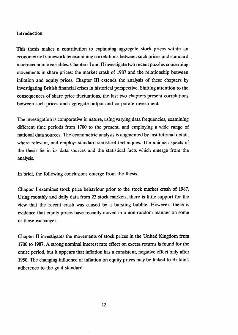
This thesis makes a contribution to explaining aggregate stock prices within an econometric framework by examining correlations between such prices and standard
macroeconomic variables. Chapters I and II investigate two recent puzzles concerning
movements in share prices: the market crash of 1987 and the relationship between
inflation and equity prices. Chapter III extends the analysis of these chapters by
investigating British financial crises in historical perspective. Shifting attention to the
consequences of share price fluctuations, the last two chapters present correlations between such prices and aggregate output and corporate investment.
The investigation is comparative in nature, using varying data frequencies, examining different time periods from 1700 to the present, and employing a wide range of national data sources. The econometric analysis is augmented by institutional detail, where relevant, and employs standard statistical techniques. The unique aspects of the thesis lie in its data sources and the statistical facts which emerge from the
analysis.
In brief, the following conclusions emerge from the thesis.
Chapter I examines stock price behaviour prior to the stock market crash of 1987. Using monthly and daily data from 23 stock markets, there is little support for the
view that the recent crash was caused by a bursting bubble. However, there is
evidence that equity prices have recently moved in a non-random manner on some
of these exchanges.
Chapter II investigates the movements of stock prices in the United Kingdom from
1700 to 1987. A strong nominal interest rate effect on excess returns is found for the
entire period, but it appears that inflation has a consistent, negative effect only after 1950. The changing influence of inflation on equity prices may be linked to Britain’s
adherence to the gold standard.
12
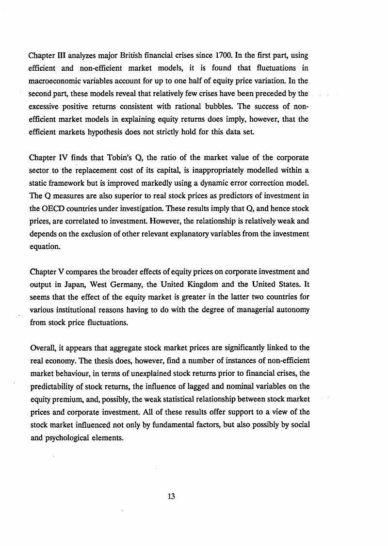
Chapter III analyzes major British financial crises since 1700. In the first part, using
efficient and non-efficient market models, it is found that fluctuations in
macroeconomic variables account for up to one half of equity price variation. In the second part, these models reveal that relatively few crises have been preceded by the
excessive positive returns consistent with rational bubbles. The success of nonefficient market models in explaining equity returns does imply, however, that the
efficient markets hypothesis does not strictly hold for this data set.
Chapter IV finds that Tobin’s Q, the ratio of the market value of the corporate sector to the replacement cost of its capital, is inappropriately modelled within a
static framework but is improved markedly using a dynamic error correction model. The Q measures are also superior to real stock prices as predictors of investment in the OECD countries under investigation. These results imply that Q, and hence stock prices, are correlated to investment. However, the relationship is relatively weak and
depends on the exclusion of other relevant explanatory variables from the investment equation.
Chapter V compares the broader effects of equity prices on corporate investment and output in Japan, West Germany, the United Kingdom and the United States. It seems that the effect of the equity market is greater in the latter two countries for
various institutional reasons having to do with the degree of managerial autonomy
from stock price fluctuations.
Overall, it appears that aggregate stock market prices are significantly linked to the
real economy. The thesis does, however, find a number of instances of non-efficient market behaviour, in terms of unexplained stock returns prior to financial crises, the
predictability of stock returns, the influence of lagged and nominal variables on the equity premium, and, possibly, the weak statistical relationship between stock market
prices and corporate investment. All of these results offer support to a view of the stock market influenced not only by fundamental factors, but also possibly by social
and psychological elements.
13

Chapter I: Stock Prices and Rational Bubbles
I. Introduction
The efficient markets hypothesis posits that equity prices incorporate all information known to market participants at any point in time and are, for this reason, inherently
unpredictable. A further extension of the theory relates such prices to expectations
of the present discounted value of all future dividends attached to the stocks in
question. This suggests that equity prices are intimately related to underlying real economic processes and are, therefore, rationally based.
The crash of 1987 and the mini-crash of 1989 suggest to others, however, that stock
prices are divorced from economic reality. From this perspective, these events were caused by the bursting of a speculative price bubble over a short period of time. Coming to such a conclusion suggests that the stock market is appropriately studied within a multidisciplinary framework incorporating economic, psychological and social
elements.
This chapter therefore explores one explanation of the crash that has been put forward from many quarters, namely that the events of October 1987 were the end
result of a speculative bubble, in order to comment on these two views of stock market pricing.1,2 While such bubbles may be rationally or irrationally based, the
necessary condition for linking them to the crash is prior existence. To sum up the
chapter’s basic conclusion, it is found that this necessary condition is not satisfied.
In addition, although there is evidence for bubbles occurring in some of the countries
examined here, it is difficult to provide a comprehensive explanation for the
international differences.
The chapter applies a variant of the traditional runs test on asset prices to reach
these conclusions and the result is therefore dependent on the ability of such tests
to measure bubble like activity. The novel aspects of this investigation are, firstly, the extension of the particular runs methodology used here to the equity markets of a
number of different countries and, secondly, the application of the bubble view to
14

an explanation of the market crash.
Section II describes previous theoretical and empirical work on speculative bubbles
and outlines the empirical method used here. In Section III, the bubble probabilities
are presented and Section IV discusses the bubble question from the perspective of option pricing theory and evidence. Section V provides an investigation of the cross
country differences. The conclusions of the chapter follow in Section VI.
15

II. Theoretical and Empirical Issues
The notion that economists typically try to capture with work on bubbles is that market behaviour may be self-fulfilling and therefore divorced from standard
economic considerations of valuation. On the theoretical side, bubbles may be classified as rational, non-rational or based on asymmetric innovations in fundamentals.3 On the empirical side, bubbles have been tested using variance
bounds tests, runs tests, price/fundamentals correlation tests, variance ratio tests and
tests based on fundamentals.4
Ha. Theoretical Bubble Specification
The first theoretical category, rational bubbles, refers to the compensation expected by investors when the probability of a market crash increases over time; in order to
compensate for the expected loss, investors rationally demand a sustained increase in asset prices. The second category, irrational bubbles, refers either to investment
decisions divorced from rationality or else to the existence of biased expectations. The former are impossible to model using the rationality assumptions underlying the neoclassical paradigm while the latter may be a function of imperfect information flows or adjustment costs to changing portfolios in response to new information. The
third category, asymmetric fundamentals, refers to market responses under the efficient markets hypothesis where bubbles exist due to continued bouts of
unexpectedly good or bad news.
In order to discriminate between the various explanations, a full theoretical specification must be constructed which offers testable hypotheses. Additionally, some
assumptions must be made about the relative information flows that the investor and the econometrician observe. We will now examine how the existence of rational
bubbles affects the properties of asset prices and discuss a number of methods for
measuring such phenomena.
16
Mathematically, the standard efficient markets view of asset pricing (in the absence
of bubbles) may be denoted as
(l) ECRJ $t) = rt + at
where
Rt -
and Rt is the return on the asset due to the capital gain and dividend yield, Pt is the
price of the asset, Dt is the dividend issuing from the asset, rt is the risk-free asset rate of return, and at is a risk premium which compensates the owners of the asset for the relatively high level of risk in the asset return. is the information set available at time t and the expectation of Rt given $ t is rational, in the sense of
Muth (1961).
The ex ante relationship in (1) can be expressed ex post in the following way
(2) = rt + at + ^
where ct is a random element distributed normally with mean zero and constant
variance, gt is the capital gain (price appreciation) component of Rt and dt is the
dividend yield.
In the situation where Xt = 0, gt will appear in the data as a random variable
without any trend component; the dynamic behaviour of Pt will therefore follow that of a random walk. Given, however, that Xt > 0 was the general state of affairs
internationally in 1987 (and indeed, ex ante, is almost always true), as interest rates
or
(3)(4)
St = r t + ort - d t + = X, + *
17
rose and dividend yields continued to fall, there is an implicit positive trend in stock price changes that will bias upward any tests for bubbles. Therefore, any finding that
positively trending bubbles are empirically unimportant is even more strongly
supported for the 1987 test period due to the upward bias in the test itself.5
The no-arbitrage condition in (1) can also be solved in terms of Pt using recursive substitution of Pt+1 to yield
(5) P*t - ;?„(! + r, + “t) 'E(D1+i. J % )
This equation prices the asset using the expected discounted value of all future
dividends. Note that the price is strictly a function of the discount rate rt, the risk premium at and the expected market fundamentals Dt.
The notion of a rational bubble enters when one considers other solutions to pricing the asset. One such solution takes the form
(6) P, - !?](! + r. + a .)" 'E (D ,+ i -j| %) + c,= P"t + c,
and
(7) E(ct+1| $t) = (l+rt)c t
In this case, the no-arbitrage condition between safe and risky assets holds but the
price does not necessarily adhere to its fundamental value. Since rt is non-negative, ct is expected to grow over time and Pt is strictly greater than P*t.
There are various ways to specify ct itself. A deterministic solution where ct = c0(l+ r t)t is somewhat unreasonable because it implies that the bubble will grow
endlessly as t approaches infinity.
18
Another solution has
(8) ro + rt) "i:t = \ — n — ) c t - i +
or ct =
The first equation occurs with probability while the second occurs with probability
(I-*). 7T is defined as the unconditional probability that the bubble continues while (1-*) is the associated probability of a crash; nt is IID with mean equal to zero. The
term (l+ r t)jr'1 is greater than ( l + rt) during the duration of the bubble in order to compensate for the risk of the bubble bursting.
Finally, the bubble term ct can be formulated in terms of a continuously regenerating
process:
In this case, bubbles begin every period in a completely random fashion. Hamilton
(1986) likens this process to looking a t " which football team wins the Super Bowl before purchasing stock, because that is what everybody else is doing, and only by behaving in the same way can one make the expected rate of return (1+r)".
Relative to the no-bubble price solution P*t, the Pt resulting from any of these
definitions of ct has a higher variance, is less correlated to the market fundamentals
and has the property of positive autocorrelation.6 When testing for the existence of
the third characteristic, one does not require any specification of Dt since the nobubble alternative is a random walk with or without positive drift. This is an
advantage of runs tests relative to tests for relative volatility and correlation since
explicit assumptions must be made in the latter cases regarding the form of the
fundamental factors. We will therefore focus on tests for autocorrelation in asset
19
prices and, in particular, on the Evans (1986) modified runs test.
lib. Empirical Bubble Tests
As mentioned above, the empirical tests have relied on testing for evidence of bubble
behaviour against either random walk predictions or else against some specified
model of asset pricing based on economic considerations. The variance ratio and
runs tests fall into the former category while the variance bounds and fundamentals
tests fall into the latter. While the former tests do not rely on assumptions of any specified model for asset pricing, they are essentially atheoretical and are therefore
open to many interpretations.
The methodology used in this chapter is a variant of the runs test based on median returns. Evans (1986) presents a description of the test which may be summarised in the following fashion:
1) Generate 10,000 random samples of N pluses and minuses. For compatibility with the Evans paper, N is set equal to 155. The units for N are months in the case of the full equity bull market analysis and days in the case of the daily analysis for 1987.
2) For varying subsamples of size K in each of the 10,000 random samples, calculate
statistics ZK where
(10) Zk = Pk - ^ . K
PK is the actual number of pluses generated in sample size K and the second term on the right hand side of the equation is the random walk prediction of the number
of pluses, ie 50% of the sample size.
For example, given that the subsample K is 12 months, the theoretically expected
number of positive movements in a random variable is equal to 6. If the data sample
actually indicates that 7 positive movements occurred, then Z12 is equal to 1. The
value ZK is therefore defined as the most extreme deviation from the null hypothesis
20
of a random walk for a given subsample size.
3) Calculate A* as the number of random samples of size K (maximum 10,000) that take on values greater than or equal to ZK; \ is therefore a cumulative distribution
over ZK.
For example, if K = 12 as above and the 10,000 random samples are distributed with 6,000 samples having Z=0; 3,000 with Z = 1; 900 with Z=2; 90 with Z=3 and 10 with
Z=4, then the distribution of A12 has a value of 10,000 at Z>0; 4,000 at Z> 1; 1,000
at Z>2; 100 at Z>3 and 10 at Z>4.
The value of AK/ 10,000 is the nominal significance level used to test deviations from a random walk for any given Z and K. Given a critical value of .05, only the Z12 values equal to 3 and 4 in this example would indicate statistically significant positive
deviations from a random walk. The reason for this is that AK/ 10,000 at Z=3 and
Z=4 is equal to .01 and .001 respectively.
A further step is undertaken to control the degree of data mining which may occur in any exercise such as this, where substantial degrees of freedom exist for choosing sample sizes and sample periods. Therefore,
4) Generate a further 10,000 random samples and set Y equal to the minimum of A over K.
(11) Y = min AK
Y is the most extreme value of A for all subperiods K within N; low values of Y indicate higher probabilities of deviation from a random walk. In our example, Y is
set to 10 since this is the most extreme deviation from a random walk given a
subsample K of size 12. Adjusting the nominal significance level of AK/ 10,000 by
using the distribution of Y controls for potential data mining by the econometrician
and therefore allows for a free choice of any sample size for consideration. In
essence, this step is an optimal data mining exercise over 10,000 sample periods.

Given these Monte Carlo results for comparison, the researcher selects a sample size
for his data, calculates the Z values and then obtains the bubble probabilities A
and/or Y.
22
III. Empirical Results
The Evans bubble methodology is applied to the case of 23 countries over two time frames: October 1982 to October 1987 for the monthly data analysis and 2 January 1987 to 16 October 1987 for the daily data analysis. The first time frame is chosen
to approximately correspond to the present upswing in the American business cycle
and to provide a 5 year sample that is common across countries and appropriately sized to use Evans’ derived probability tables. The second time frame is chosen to
capture the rapid equity price appreciation in most exchanges prior to the crash and
ends on the last trading day prior to the crash.
All of the data are expressed in percentage rate of change and are measured from closing day prices in consecutive periods. The probability values are calculated using a null hypothesis of a random walk in prices against the alternative hypothesis of positive movements in excess of a random walk. As noted in Table 1, one index is used per country with the listed exceptions taking on values equal to unweighted
averages of several indices. The separate probability values for these latter countries do not differ markedly from each other and therefore the use of an unweighted
average value is a very close approximation to the relevant bubble probability.
As one can see from Table 1, the range of probability values extends from 0.0027 to over 0.5. The countries are divided into categories according to whether their values
fall within the .05 or .20 probability bounds and it is apparent from this distinction
that less than one third of the countries demonstrate strong evidence of bubble
behaviour. It should be noted that for the United States, the country which
precipitated the sharpest international price movements on 19 October 1987, there
is no evidence of any bubble activity whatsoever. In addition, as will be seen in the
next section, it appears to be difficult to explain the cross country variation since
countries with markedly different characteristics share similar probability values. For example, stock market capitalization or size of the domestic economy cannot explain
the similar bubble activity in Japan and New Zealand nor can the differences in
international investment access that exist in South Korea and Hong Kong explain
their relative rankings.
23
Table 2 extends the monthly analysis to subperiods of K years within the 5 year bull
market examined. Evans’ adjusted probability values to control for data mining are
used in this table, in contrast to the other probability tables, since the sample size
is variable and there is a deliberate attempt to find the periods where bubble activity is most prominent. As with Table 1, there is evidence in many countries that prices
deviated from random walks for sustained periods, although it is difficult to explain in a general fashion why the deviations occurred. The bubbles in Italy, Sweden and
Austria are present even in the absence of longer term indications over the entire
sample period, an illustration of the value of choosing varying time periods for an
analysis of this type.
The previous analysis is refined and extended in Table 3 where daily price changes are tested over the 1987 pre-crash period. In addition, equity premiums are
calculated, where the premium is defined as the percentage stock price change less the yield on risk-free bonds, and these values are examined for the existence of bubbles.7 A comparison is also made with probabilities that are calculated from the beginning of the year to the date when the particular market peaked, usually prior
to the crash. As is intuitively obvious, these latter values should always indicate higher bubble probabilities than those ending at the market crash.
Once again, the evidence for a bubble triggering the American market crash is not supported empirically; the values for both the market price and equity premium fall considerably outside of standard significance levels. A number of countries exhibit
strong deviations from random walks at their market peaks but less so at the time
of the crash. In fact, if a significance level for the existence of bubbles is imposed at approximately 95%, only Australia, Japan and the United Kingdom provide evidence
for bubbles in prices and only Japan shows bubbles in the equity premium. As well,
in the latter case, it is likely that the equity premium evidence is weaker than suggested in the table since daily varying bond prices were not available for this
study. These daily movements, in a period when interest rates were rising rapidly, would have served to reduce the positive movements in the index and, therefore, the
probability of deviations from a random walk.8
24

This section demonstrates that the Evans methodology can be used to find and
calibrate deviations from random walks for asset prices expressed in rate of return
form. The evidence does not support the argument that the American market had
bubble characteristics prior to the crash but does find that other markets deviated
from random walks for prolonged periods. Japan and the United Kingdom are
especially important countries in the latter category because of their market size and international influence and also because of their high bubble ranking in both the
monthly and daily analyses. The evidence is consistent with other studies that use different testing methodologies and find significant price deviations from random
walks.9
25
IV. Option Pricing Evidence
Option pricing theory provides another perspective from which to judge the validity
of the bubble explanation of the crash. Since the prices of options and the underlying
cash market are intimately related, any bubble which occurs in the latter should by
definition occur in the former. Likewise, the increase in the volatility of stock prices which accompanies the introduction of bubbles should also be reflected in option
prices. Lastly, given that stock market price volatility can be implied from standard
option pricing formulas, this volatility should increase over the period during which
the bubble is formed.
It can be shown that volatility (as measured by the current variance of asset prices) is increasing in terms of the introduction of a bubble element in prices and rises over time as the bubble progresses. Following Blanchard and Watson (1982), return to
equation (6)
(6) Pt = P*t + ct
The definition of the conditional variance of X is
(13) V(X| «,) - E(X - E(jq * , ) ) 2
and so
(14) V(Pt| $,) = E(Pt - E(P,| 4V))2- E(f, + g 2
where the first element is the innovation (unexpected component) in the
fundamentals term and the second element is the innovation in the bubble term.
26
Separating elements,
(15) V(Pt| *t) = V(ft) + V(^> + 2 cov(ct, g
Assuming that the covariance term is non-negative, V(Pt |$) is strictly greater than
V(P*t | $), the no-bubble case; this assumption is not very strong since it is most unlikely that positive innovations in the fundamental term are positively correlated
with adverse bubble innovations. Since the implied variance derived from option
pricing purports to measure the true variance of stock prices, one expects to find higher implied volatility in periods where bubbles occur.
It is trivial to show that V(ct | $) is equal to a2M, and there is, therefore, no relation between the variance of the bubble term conditional on the information set and ct itself. However, to see that V(ct) is strictly increasing in terms of ct, and that the growth in the bubble term over time will lead to a monotonic increase in the variance of Pt, substitute equation (8) into the following equation for the
unconditional variance and set rt = r
(16) V(X,) = E tV ^ X ,) ] + VIEj.^X,)!
Rearranging and cancelling terms results in
(17) V( ct) » + ( 1+r)2 V( ct_ j)
since /xt is IID with constant variance and variables at t-1 are in the information set
at time t.10 Using the bubble formulation in (9) leads to similar results where V(ct), and therefore V(Pt), is increasing in ct.11
27
The bubble effect on option prices themselves can be seen by using the benchmark call option pricing formula of Black and Scholes (1976)
(19) Ct = PtN(X) - K ^N C X -oj^t)
where12
( 20)
As Cox and Rubinstein (1985) show,
( 21) 3pJ = N(X) > 0
and XT - N*(x > > 0
and so we should expect option prices, as well as the implied stock price variance, to increase in a bubble environment relative to a non-bubble environment and also during the progression of the bubble itself.
Table 4 and Diagram 1 demonstrate that the theoretical expectation of volatility under conditions of a bubble in prices is at variance with the empirical evidence, at least for the UK in the 1980’s. The table specifies the averages and coefficients of variation of ax over several test periods between 1984 and 1987. The data frequency
is weekly and the calculation is based on the weighted implied standard deviation
type of formula found in Chiras and Manaster (1978).13
While the mean value of ax shows a trend increase from 1984 to 1986, Diagram 1
indicates that this pattern is uneven. As well, there is no significant upward trend in the 13 weeks prior to the crash. If anything, the options pricing data would indicate that the bubble burst in the week starting 1 June 1987, when at was at a local apex. Looking back to Tables 1 and 3, in contrast, one sees that strong evidence exists there for bubbles in prices since the probability of a deviation from a random walk
28
over the full bull market is .9841 and the associated probability during 1987 is .9464.
It therefore appears that there is some justification for rejecting the rational bubble
explanation in the UK owing to the conflicting evidence shown in the options market.
Other explanations for non-random pricing behaviour, such as those discussed in
Footnote 5, are therefore much more plausible.
One leading candidate may be an asymmetric distribution in the innovations of fundamental factors. The UK corporate sector has posted a number of years of what many see, based on historical observation, as surprisingly strong growth figures. It
may be that the stock market discounted these surprises as they occurred and, as a result, created a positive trend movement in prices; the asymmetry here is a
positively skewed distribution of news coming to the market. The 1987 daily data results do not, however, support this sort of medium-term explanation since this asymmetry would have to operate on a daily basis.
29

Ij
V. Cross Country Differences
The hypothesis that bursting bubbles lie behind the occurrence of the 1987 crash
leads on to specific implications for post crash price movements. Assuming that bubbles exist, and that they are burst at a constant rate over time according to their
initial strength, it is possible to test the bubble theory by examining the correlation
between price declines and bubble probabilities for different countries. It is expected that a positive correlation will exist since higher bubble probabilities should
correspond to greater price declines.
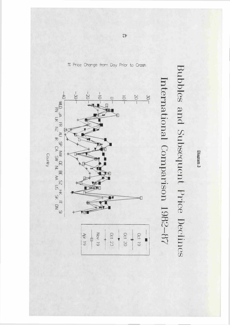
The regression results reported in Table 5 and Diagrams 2 and 3 demonstrate that there is no correlation between bubble probabilities and post crash price
performance. Table 5 presents ordinary least squares estimation equations where the cross-sectional price declines at a given point in time are regressed against the respective bubble probabilities. Diagrams 2 and 3 plot bubble probabilities against price declines where the X axis is labelled by country and is ordered in terms of declining bubble probabilities.
The F and t statistics from the table indicate that the explanatory power of these estimations is absolutely insignificant. In addition, if the focus is directed solely to
those probabilities lying within the .05 probability bound, (Finland, Japan, the United Kingdom, New Zealand, France, Australia and Ireland for monthly data and
Australia, the United Kingdom and Japan for daily data), it is readily seen from the diagrams that there is an incorrectly signed negative correlation in the former case
and a correctly signed positive correlation in the latter. The small sample size for the
daily data case (three observations) does not, however, allow firm conclusions to be
drawn from the data.
This simple test of the bubble story seems to suggest that more sophisticated
explanations are required in order to account for the marked differences observed
across countries prior to the crash. Possible explanations for the differences might rest on continued batches of unexpectedly good news in the countries with indications
of bubbles or evidence for continued learning processes due to structural changes in
30

the flow of news to the market.14 However, the failure of the regressions reported here seems to imply that the bubble story cannot be true for all of the countries in
the sample. Certainly, it is not true for the United States, the central country during
the crash, since it exhibits insignificant probabilities of non-random behaviour;15 at
the same time, this country’s post crash price adjustments are in the middle of the
range of international responses.
While a simple risk adjustment is used in the daily data analysis by calculating the
equity premium, it can be argued that the prices should be appropriately adjusted for systematic risk on the basis of a CAPM-type model. Aside from the greater data
requirements that this sort of exercise would entail, it is unlikely to shed further light on the issue of cross country differences. It is difficult to support the argument that the countries with high bubble probabilities were riskier over the specified sample periods than those with low probabilities. For example, the risk rankings of Finland, Australia or France seem to be little different from those of Sweden, Hong Kong or West Germany on an a priori basis, and yet each pair have divergent bubble
probabilities.
31

VI. Conclusions
This chapter presents international estimates of deviations from random walk behaviour in stock market indices over the period 1982 to 1987. Two hypotheses are
tested and rejected: first, that there is evidence for a bubble in the United States indices prior to the October 1987 market crash and, second, that the post crash price
declines can be explained by the pre crash bubble probabilities.
While these hypotheses are rejected, the very existence of non-random behaviour
may provide a challenge to the efficient markets hypothesis if it is assumed that information arrives into the market in a random fashion. A complete theoretical model of some alternative price generation mechanism in the stock market is needed
in order to test whether this particular empirical bubble methodology has explanatory power for such issues. In terms of this thesis, however, the rejection of a bubble
explanation for the 1987 crash, and the finding that bubbles existed for other countries and subperiods, are both consistent with a theory of stock market pricing
that stresses economic and non-economic factors.
32

1. A bubble is defined in this chapter as a statistical construct that measures the probability of a deviation from a random walk in price movements. Evans (1986) presents the methodology and distribution properties behind this construct. It should be stressed that this definition of a bubble is not necessarily equivalent to theoretically defined bubbles or to the notion that prices may be over-valued relative to fundamental or other factors. A fuller discussion of these points is contained in Section II below.
2. There appears to be a widely held belief that the October 1987 crash was the inevitable result of previous market overvaluation. Market participants such as John Hennessy (1988) of CSFB talk of ’excessive speculation’, government reports and politicians cite ’speculative bubbles’ (Glauber (1988) and Healey (1988)) or state that the bull market was ’clearly too good to last’ (Lawson (1987)). The American General Accounting Office (1988) report on the crash stressed that prior overvaluation may have existed in the market while the Chairman of the Federal Reserve Board of Governors stated that prices were unsustainably high (Greenspan (1988)).
The post-crash surveys conducted by Shiller (1987,1988) found that investors responded to price signals in a self-fulfilling fashion while generally ignoring news which was concurrently entering the market information set. While many argued the case for overvaluation from hindsight, most prescient market commentators felt that Japan, and not the United States, was the prime candidate for a sharp market correction; see Soros(1987) on this point. Santoni (1987) provides further references from the popular press and also lists a number of similar commentaries on the possibility of bubbles causing the 1929 crash. One recent comparison of the 1929 and 1987 experiences is found in Kindleberger (1988).
3. This classification is more fully specified in Evans (1986), Blanchard and Watson (1982) and Hamilton (1986) and the references therein.
4. The variance bounds tests are found in the papers by Shiller (1981) and Kleidon (1986) while the runs tests have been undertaken in Blanchard and Watson (1982). One recent reference to the variance ratio test is Poterba and Summers (1988). The fundamentals based models take a number of forms and can be found in the works of West (1985), Shiller (1984) and Summers (1986).
5. There are, of course, many other reasons for the detected drift or trend movements in equity prices. As Evans (1986) discusses, the distribution of price changes may be skewed to the right due to asymmetric distributions of fundamental factors which affect asset prices. Incremental learning by agents over regime shifts may also induce positive autocorrelation in prices, as may any other factors which lead to an overshooting type of pricing equilibrium in the manner of Dombusch (1976).
Other explanations rest on assumptions of irrationality, unobserved fundamentals or pure random chance during a given subperiod. These latter explanations are, however, difficult to analyze using present theoretical and empirical techniques which rely on optimising behaviour and appropriate specification of the data and model.
6. See Blanchard and Watson (1982) for a discussion of these points.
33
7. Using the earlier notation, the relationship that is tested is
( 12) ^ - rt = a t - dt + ^
The use of the equity premium should dampen the trend element of g and therefore reduce the positive bias in the bubble test. This will accordingly reduce the probability of rejecting a random walk in prices.
An examination of Table 3 shows this to be the result for all countries and all time periods except for Japan and the United States on October 16th. In the former case, weekly bond yields are used to proxy rt and the low level and variability of these rates over 1987 made no difference to the bubble probabilities. In the latter case, both probabilities are well outside conventional significance levels.
The apparently sizeable change in the American probabilities in Table 3 is a function of the distribution of Z. For example, given that K = 120 (equivalent to a sample size of 4 months in the daily test), the Monte Carlo results indicate that A changes from .0001 to .0012 to .0144 to .0973 to .3802 to .8729 as Z declines from 24 to 4 in increments of 4; the increments between values of A therefore increase as Z decreases. In this regard, it is not surprising that the significance levels for the United States reported as .3729 and .2555 on October 16th differ from each other by a Z value of only one.
8. Roll (1989) presents evidence for 23 countries using daily data during 1987. Employing a variance ratio test, he finds that 18 of the 23 exhibit significant positive autocorrelation in stock prices. Since bull markets tend to have relatively larger positive price movements, while bear markets exhibit relatively larger negative price movements, see Schachter et al (1985), the Roll methodology is biased towards finding positive correlations over the bull market of 1987. In contrast, the sign test that underlies the Evans methodology is invariant to periods of bullish and bearish price movements since it is adjusted for potential data mining biases. Although this chapter finds that 5 out of 9 price indices deviate from random walks prior to the market peaks, see Table 3, it is difficult to make an exact comparison with the Roll paper since it is not clear which countries deviate from random walks there.
9. Examples of these studies are found in the references of Poterba and Summers(1988). The Poterba and Summers paper itself is in full agreement with this chapter’s conclusions since they find evidence of positive correlation in stock returns at frequencies of less that one year for a wide variety of countries. It should be stated, however, that very few of their results are statistically significant at standard levels.
10. Although the variances in Equation 17 are likely undefined from period to period because of non-stationarity while the bubble is forming, the probability limit of V(ct_k) as k increases from 1 should become stationary due to the rise and fall of the bubble over time. Therefore, Equation 17 is defined for some k > 1 and the variance of the bubble term grows over the progression of the bubble. I am indebted to Enrique Sentana for pointing out this line of thought to me.
11.
34
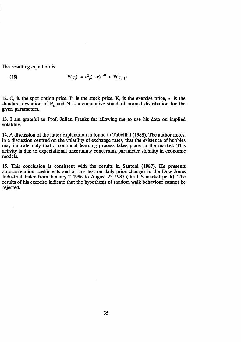
The resulting equation is
(18) V(c,) - o ^ l+ r ) -2' + V (c,.,)
12. Ct is the spot option price, Pt is the stock price, K,. is the exercise price, at is the standard deviation of Pt and N is a cumulative standard normal distribution for the given parameters.
13. I am grateful to Prof. Julian Franks for allowing me to use his data on implied volatility.
14. A discussion of the latter explanation in found in Tabellini (1988). The author notes, in a discussion centred on the volatility of exchange rates, that the existence of bubbles may indicate only that a continual learning process takes place in the market. This activity is due to expectational uncertainty concerning parameter stability in economic models.
15. This conclusion is consistent with the results in Santoni (1987). He presents autocorrelation coefficients and a runs test on daily price changes in the Dow Jones Industrial Index from January 2 1986 to August 25 1987 (the US market peak). The results of his exercise indicate that the hypothesis of random walk behaviour cannot be rejected.
35
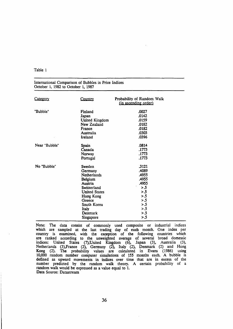
Table 1
International Comparison of Bubbles in Price Indices October 1, 1982 to October 1, 1987
Category Country Probability of Random Walkfin ascending order)
"Bubble" Finland .0027Japan .0142United Kingdom .0159New Zealand .0182France .0182Australia .0303Ireland .0396
Near "Bubble" Spain .0814Canada .1773Norway .1773Portugal .1773
No "Bubble” Sweden 3121Germany .4089Netherlands .4955Belgium .4955Austria .4955Switzerland >.5United States >.5Hong Kong >.5Greece >.5South Korea >.5Italy >.5Denmark >.5Singapore >.5
Note: The data consist of commonly used composite or industrial indiceswhich are sampled at the last trading day of each month. One index per country is examined, with the exception of the following countries whichare ranked according to the unweighted average of several broad domestic indices: United States (7),United Kingdom (6), Japan (3), Australia (3),Netherlands (3),France (2), Germany (2), Italy (2), Denmark (2) and Hong Kong (2). The probability values are calculated in Evans (1986) using10,000 random number computer simulations of 155 months each. A bubble is defined as upward movements in indices over time that are in excess of thenumber predicted by the random walk theory. A certain probability of a random walk would be expressed as a value equal to 1.Data Source: Datastream
36
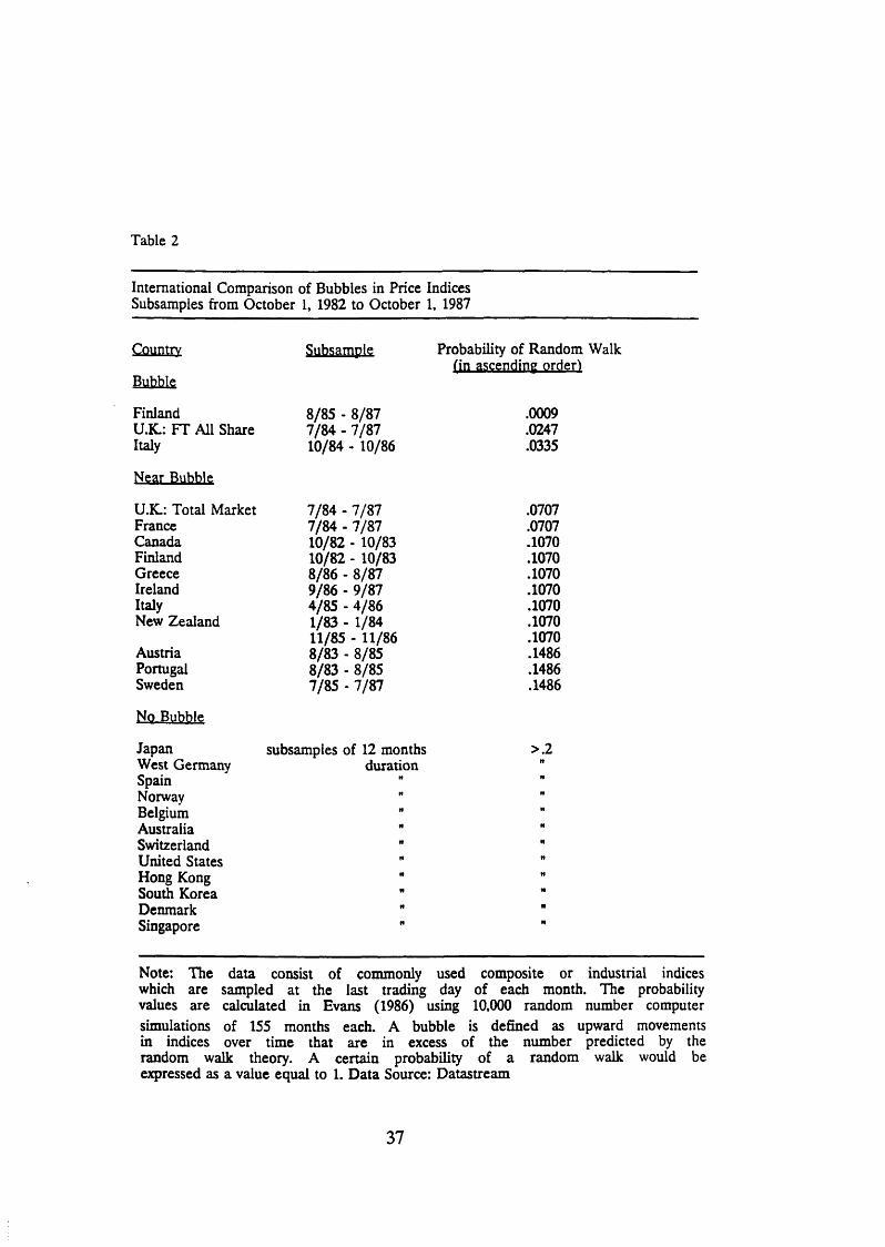
Table 2
International Comparison of Bubbles in Price Indices Subsamples from October 1, 1982 to October 1, 1987
Country Subsample Probability of Random Walk
Bubblefin ascending order)
Finland 8/85 - 8/87 .0009U.K.: FT All Share 7/84 - 7/87 .0247Italy 10/84 - 10/86 .0335
Near Bubble
U.K.: Total Market 7/84 - 7/87 .0707France 7/84 - 7/87 .0707Canada 10/82 - 10/83 .1070Finland 10/82 - 10/83 .1070Greece 8/86 - 8/87 .1070Ireland 9/86 - 9/87 .1070Italy 4/85 - 4/86 .1070New Zealand 1/83 - 1/84 .1070
11/85 - 11/86 .1070Austria 8/83 - 8/85 .1486Portugal 8/83 - 8/85 .1486Sweden 7/85 - 7/87 .1486
No Bubble
Japan subsamples of 12 months >.2West Germany duration i t
Spain H
Norway n t t
Belgium If H
Australia M it
Switzerland ff tt
United States t t i t
Hong Kong i t t t
South Korea t t t t
Denmark i t t t
Singapore i t i t
Note: The data consist of commonly used composite or industrial indiceswhich are sampled at the last trading day of each month. The probabilityvalues are calculated in Evans (1986) using 10,000 random number computersimulations of 155 months each. A bubble is defined as upward movements in indices over time that are in excess of the number predicted by therandom walk theory. A certain probability of a random walk would be expressed as a value equal to 1. Data Source: Datastream
37
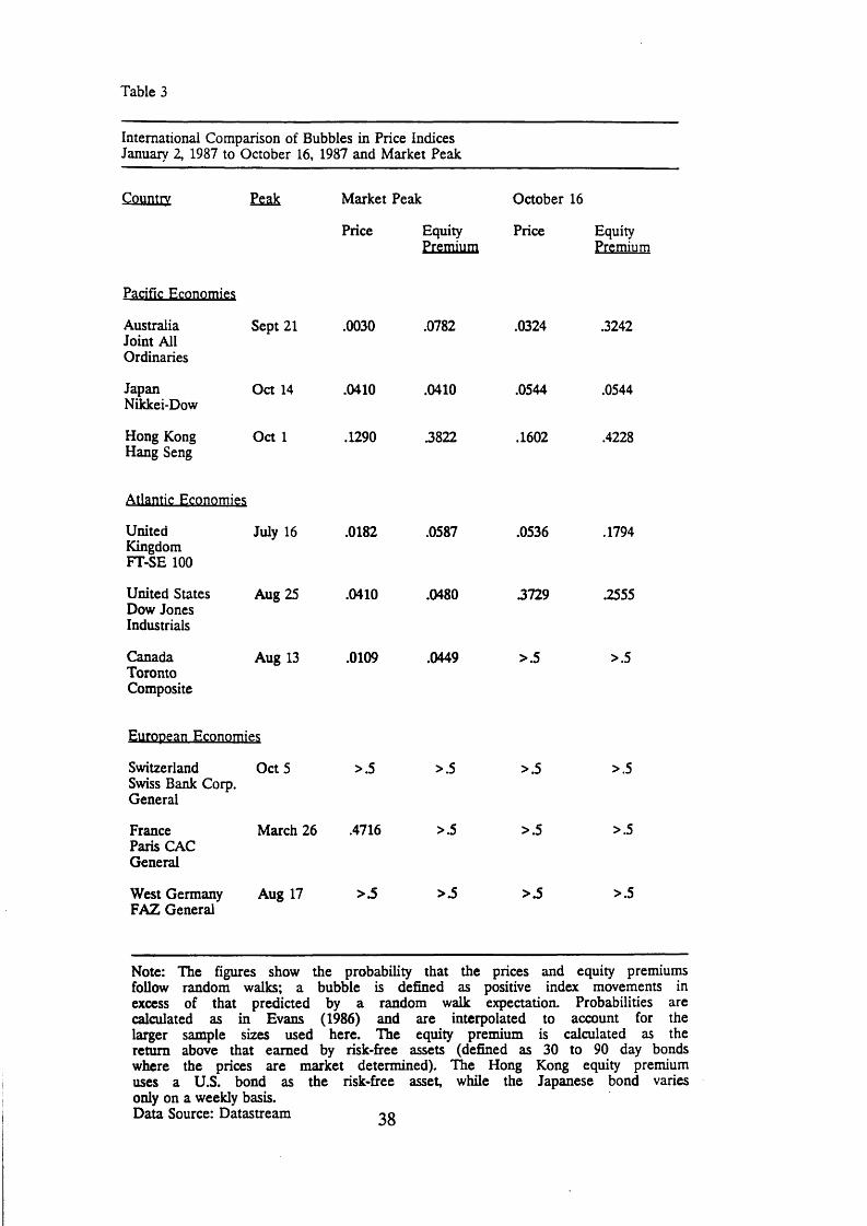
Table 3
International Comparison of Bubbles in Price Indices January 2, 1987 to October 16, 1987 and Market Peak
Country Peak Market Peak October 16
Price EquityPremium
Price EquityPremium
Pacific Economies
Australia Joint All Ordinaries
Sept 21 .0030 .0782 .0324 .3242
JapanNikkei-Dow
Oct 14 .0410 .0410 .0544 .0544
Hong Kong Hang Seng
Oct 1 .1290 3822 .1602 .4228
Atlantic Economies
United Kingdom FT-SE 100
July 16 .0182 .0587 .0536 .1794
United States Dow Jones Industrials
Aug 25 .0410 .0480 3729 .2555
CanadaTorontoComposite
Aug 13 .0109 .0449 >.5 >.5
European Economies
Switzerland Swiss Bank Corp. General
Oct 5 >.5 >.5 >.5 >.5
France Paris CAC General
March 26 .4716 >.5 >.5 >.5
West Germany FAZ General
Aug 17 > 3 >3 > 3 >.5
Note: The figures show the probability that the prices and equity premiumsfollow random walks; a bubble is defined as positive index movements inexcess of that predicted by a random walk expectation. Probabilities arecalculated as in Evans (1986) and are interpolated to account for thelarger sample sizes used here. The equity premium is calculated as thereturn above that earned by risk-free assets (defined as 30 to 90 day bondswhere the prices are market determined). TTie Hong Kong equity premiumuses a U.S. bond as the risk-free asset, while the Japanese bond variesonly on a weekly basis.Data Source: Datastream oo
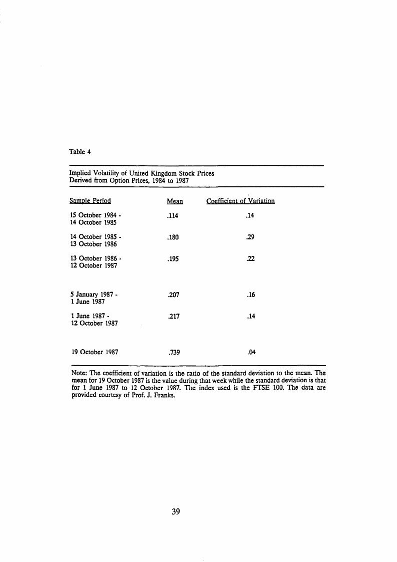
Table 4
Implied Volatility of United Kingdom Stock Prices Derived from Option Prices, 1984 to 1987
Samole Period Mean Coefficient of Variation
15 October 1984 - 14 October 1985
.114 .14
14 October 1985 - 13 October 1986
.180 .29
13 October 1986 - 12 October 1987
.195 .22
5 January 1987 - 1 June 1987
.207 .16
1 June 1987 - 12 October 1987
.217 .14
19 October 1987 .739 .04
Note: The coefficient of variation is the ratio of the standard deviation to the mean. The mean for 19 October 1987 is the value during that week while the standard deviation is that for 1 June 1987 to 12 October 1987. The index used is the FTSE 100. The data are provided courtesy of Prof. J. Franks.
39
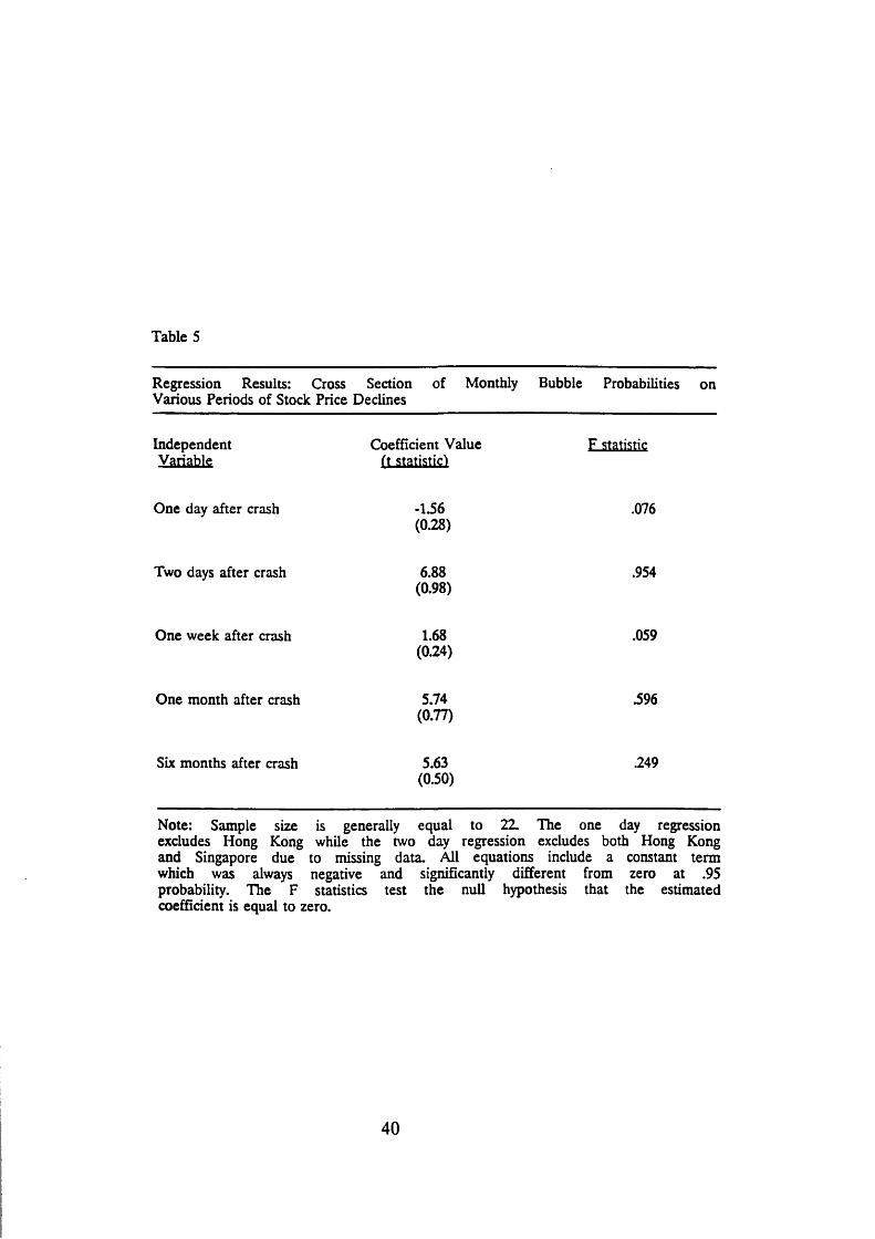
Table 5
Regression Results: Cross Section of Monthly Various Periods of Stock Price Declines
Bubble Probabilities on
Independent Coefficient Value F statisticVariable ft statistic!
One day after crash -1.56 .076(028)
Two days after crash 6.88 .954(0.98)
One week after crash 1.68 .059(0.24)
One month after crash 5.74 .596(0.77)
Six months after crash 5.63 .249(0.50)
Note: Sample size is generally equal to 22. The one day regressionexcludes Hong Kong while the two day regression excludes both Hong Kong and Singapore due to missing data. All equations include a constant term which was always negative and significantly different from zero at .95 probability. The F statistics test the null hypothesis that the estimated coefficient is equal to zero.
40
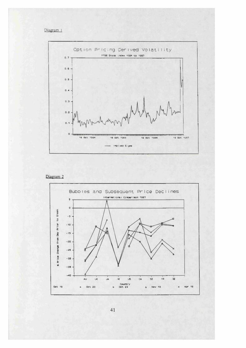
Diagram 1
O pt io n Pr i c 1ng Der i ved Vo I a t i I i t yFTSE Stooc index 1994 t o 198*7
0 .4 -
0 . 3
..... mm10 Oct 1984
mniiiiiimin iiiimiiiininm19 OCt 1987
iiiiiiiiiiiii niuiiniiniin19 OCt 1983 10 OCt 1988
impi iea Sigrna
Diagram 2
B u b D I es and S u b s e q u e n t P r 1c e Dec Ii n e sin te r n a t io n a l Comoarlaon 1987
Oct 19
JA HK US
Country o Oct 23
CA SZ FR
A NOV 19
GE
x A p r 1 9
0 -
- 5 -
- 1 0 -
-1 5 -
-2 0 -
-as -
-3 0 -
-3 3 -
-4 0 -AU UK
+ OCt 20
4 1
Country
IP
% Price Change from Day Prior to Crash
o rooo o
c_>
00
00NJ00
X00
roL*i roID ID CD
CD
33
o33 ^
no* 33’-sI—iC /3o3
COCDroCD
Bubbles
and Subsequent
Price D
eclines
Chapter II: Stock Prices and Inflation
I. Introduction
The previous chapter investigated the stock market crash of 1987 and found that a
rational bubble explanation is not wholly convincing, although there exists sufficient evidence of non-random price behaviour to bring into question the assumption of
efficient markets. This chapter broadens the analysis of equity prices by extending
the investigation back in time, while exploring whether nominal prices are important determinants of the real equity premium. In particular, it appears that inflation and nominal interest rates do not have similar effects on equity prices (at least in the U.K.) over a sample period extending from 1700 to the present.
The examination of the link between inflation, both expected and unexpected, and
share prices follows an extensive literature which documents a negative relationship between the two.1 Virtually all previous studies confine their analysis to the post- 1950 period, however, and none (to our knowledge) examine the 18th and early 19th centuries. Using a newly developed data set, this chapter finds that the negative
relationship between inflation and excess returns is confined to the post-1950 period. In the preceding two and a half centuries, there is no consistent correlation between
the two; if anything, there are long periods of time when there is a positive
association.
Even though inflation is not found to be generally detrimental for equity returns,
there is evidence that nominal interest rates have a consistently negative relationship since 1700. As well, the Tisher Effect’ (the notion that nominal interest rates rise
point-to-point with expected inflation) is essentially absent in the pre-World War II
period, a result possibly related to the gold standard of that period.2 So, while the
use of recent data makes it difficult to discriminate between nominal interest rates and inflation as predictors of stock returns,3 the use of data from 1700 is more
appropriate in this respect. The data, methodology and results are discussed in
Sections II and III below.
There are a number of interesting attempts to explain the link between inflation and
43

stock returns, for example, Fama (1981), Geske and Roll (1983), Modigliani and Cohn (1979), Pindyck (1988) and Stulz (1986), to name the main contributions.
Section IV briefly reviews the implications of our findings for such work and then concludes the chapter. Finally, a detailed appendix follows which presents the data
used here (and later in Chapter III of this thesis).
44
II. Data and Methodology
In the work below, we present estimated equations of the form
(1) REt - RFt = a0 - a1 Et. 1̂ t - a2 Et.,,RFt + ut
where REt is the ex post return on equities, RFt is the interest rate, Et.17rt is the rate of inflation expected at time t-1 and ut is distributed N(0,a2). The dependent variable
is the excess return on equities (or the equity premium).
Equation (1) is representative of much of the research in this field. Given the theoretical result of the Capital Asset Pricing Model (CAPM) that the equity
premium is a function of risk alone, the ’puzzle’ that arises here, as elsewhere, is that a, and/or a2 are estimated to be statistically significant. Note that although the
equation takes required excess equity returns to be constant, this assumption will be relaxed below by introducing the expected volatility of returns as an additional regressor.
Ha. The Data
As discussed in Appendix I, there is no single index of share prices that goes back to 1700. Researchers are, therefore, forced to splice together various different indices
to obtain a complete series. While coverage may vary across sectors and companies over time, the indices used here have the common property that they measure the
changes in share prices of the leading quoted companies of the day.
Unfortunately, for a part of this period (1700 to 1810), the data are only available
in the form of annual averages4; for consistency, the entire data set was, therefore,
put together in this way. The data were then transformed prior to estimation to deal
with the moving average error process which is introduced by averaging truly random
processes.5 As a robustness check, estimates are also presented below for selected subsamples where end-of-period data exist.
A second problem with the data is the absence of a long series on dividend yields.
45
Therefore, RFt generally refers to only the capital gain portion of equity returns, except for those subperiods indicated below where dividend yield information is
available.6
As mentioned in Appendix I, consumer prices are used to measure inflation and
the short and long interest rates are the three month commercial paper rates and 3%
government consols, respectively. Due to the absence of data prior to 1827 and the use of lagged instruments, equations employing the short interest rate begin in 1830.
Before turning to the formal results, it is worth reminding the reader that the
behaviour of inflation over the past half century has been quite different from that in the previous two centuries. Diagram 1 demonstrates that the mean inflation rate
from 1700 to the 1930s was very close to zero. In contrast, the period since that time is marked by the absence of deflation, with the exception of the year 1943 (which is marked in any case by wartime price controls and is not a free market outcome). The radical change in the underlying inflation generation process is suggestive of the possibility that the relationship between inflation and equity returns might also have
changed.7
lib. Methodological Issues
As previously mentioned, the use of time-averaged data implies that the error term (ut) in Equation (1) will follow a first-order moving average process with a serial
correlation coefficient of approximately 0.25, (see Working (I960)). We replace Et_
1irt and Et.1RFt in Equation (1) by the actual outcomes, which, under a Rational Expectations assumption, only differ by a serially uncorrelated error term. In
addition, the ’errors-in-variables’ problem is treated by using instrumental variables estimation.
However, as Hayashi and Sims (1983) note, some care is needed in a situation where
there is a moving average error. Therefore, in order to preserve the timing conditions
that make the instruments and the transformed disturbances orthogonal, the data are
pre-transformed by subtracting future rather than past values.8 Sargan’s (1958) test for the validity of instrumental variables is also reported.
III. Empirical Results
Ilia. Basic Results: Excess Returns and Inflation
The link between excess returns and inflation is examined first by setting a2 = 0. The
results are shown in Table 1 where two alternative dependent variables are
employed: ERS, which is the excess return on equities defined relative to the short interest rate, and ERL, the excess return relative to long interest rates. The
instruments that are used are lagged, untransformed values of inflation, stock returns, industrial production growth, real money supply growth, interest rates and armed
forces employment (to capture the effect of wars and government expenditure).
It is clear from Table 1 that a significant negative relationship between expected inflation and excess returns is confined to the post-1950 period. The estimated coefficients on expected inflation in earlier subperiods range from -0.01 to +0.44. Notice that there is some evidence of a modest positive association between inflation
and excess returns over 1830 to 1913. The basic thrust of the result is independent of the form of the left hand side variable, the precise sample period, or the actual estimation technique (the OLS and IV results are not very dissimilar).
We next investigate the relationship between interest rates, inflation and excess
returns.
Illb. Basic Results: Excess Returns and Interest Rates
In this section, a1 is set equal to zero to concentrate on the effect of nominal interest rates on excess returns. The results of Table 2 indicate the existence of a consistent, negative relationship between expected interest rates and excess returns; this holds
irrespective of subsample or choice of dependent variable. The coefficient on the
nominal interest rate is also generally statistically significant and large, ranging from -
1.30 to -6.09.
The basic result that there is a consistent, negative relationship between nominal interest rates and the equity premium also holds if end-of-period data are used, or
47
if equity returns are measured by including the dividend yield. This may be seen in Table 3, where, in the upper section, evidence is presented for end-of-period data;
since the Hayashi-Sims transformation was unnecessary, conventional instrumental variable estimates are given. Notice that the results are very similar to those obtained
using the H-S transformed data (e.g., over 1914-1949, the coefficient on interest rates
is -3.06, as compared to -2.92 previously).
The lower section of Table 3 contains estimates of the interest rate-excess return
relationship when excess returns are correctly defined to include the dividend yield. Once again, the results are largely unchanged: the coefficient for 1919-1983 is -2.96, as compared to -2.92 previously, although, over 1950-1983, the coefficient falls from - 1.97 to -1.41. So, the basic result does seem robust to the definition of the dependent variable and whether or not the Hayashi-Sims transformation is needed.
So, on these results, inflation appears to affect excess returns, but only via the nominal interest rate. Additional direct effects from inflation are tested, however, in Table 4. The typical result there is that the nominal interest rate depresses excess returns. Further, inflation only contributes any significant additional explanatory power in one out of the ten cases presented.9 This suggests that attention should probably be concentrated on the interest rate estimates shown in Table 2.
IIIc. How Robust is the Link Between Nominal Interest Rates and Excess Returns?
The results in Table 2 suggest that there is a fairly stable and consistent negative
correlation between expected nominal interest rates and excess returns. In this section, various experiments are performed to assess the robustness of this empirical
result.
Under the standard CAPM,
(4) Et.1 (REt - RFt) = <*0 + P Et.,a t
where a2t is a measure of equity risk, (see Merton (1980)). Equation (1) excludes
any term which allows changes in volatility to affect stock returns, and so the first
48
robustness check introduces lagged squared excess returns as a proxy for expected volatility.10 Although expected volatility often attracted a positive coefficient (which
was sometimes statistically significant), the basic negative correlation between nominal interest rates and excess returns was unaffected. Columns 1 and 2 of Table
5 show representative results of this experiment.
A second factor which may affect the basic result stems from Fama’s (1981) assertion that the correlation between inflation and the stock market may be spurious. He
argues that high inflation is merely a proxy variable for lower future output growth
(which it might be according to money demand theory). Similarly, nominal interest
rates may also presage lower activity and, hence, be associated with lower equity returns.
In deference to this view, the future growth rate of industrial production was added
to Equation (l) .11 The results in Table 5, Columns 3 and 4, show that our basic argument about nominal interest rates stays intact with a coefficient which is largely
unchanged. Additional experiments using future growth in real GNP for shorter
subperiods produced similar results.
Hid. The Changing Relationship Between Interest Rates and Inflation
The previous results show that higher expected nominal interest rates depress stock
returns, while changes in expected inflation rates bear no consistent relationship with
these returns. This section examines how the relationship between the two nominal
variables has changed over time.
In our experiments, when the following equation was estimated
(5 ) Rgt - R pt — Otg + fiy E t .̂ 7Tt + 02
(where Et.1rt is the expected real interest rate), we obtained a negative statistically
significant estimate of py and, typically, py = p2- However, if Et.1rt is omitted from
the equation, then py is estimated to be positive prior to 1950 and negative after that date. Of course, if Equation (5) describes the true underlying data generation
process, then the estimate of py is biased for standard omitted variables reasons, i.e.
(6) Bias (b,) = (^2)6,_r
where b1 is the estimate of py and St r is the coefficient of tt in a regression of Et.
i r t 011
It is well known from the sources in Endnote 2 that the correlation between interest
rates and inflation has changed over the period since 1700. Some confirming evidence is presented in this regard by estimating
(7 ) Rpt = “o + “ i E tTt*i + v t
and similar variations. The results are presented in Table 6 and show that the
estimate of a1 rises markedly during the most recent sample period. Of course,< 1 corresponds to * < 0, a negative correlation between real interest rates andinflation. So, given a negative value for p2, b1 will be biased towards becoming positive. Since the absolute value of Sv r declines through the sample period, it is clear that the size of the bias of b1 also falls. So, in the period prior to 1950, the size of the bias of b1 is sufficient to make p1 positive, but since interest rates are more
responsive to inflation after 1950, the size of the bias also falls.
Another way of summarizing these results is that there was no consistent relationship between inflation and stock returns in the pre-World War II period, because the
direct depressing effect of inflation on stock returns was offset by the boost to equities provided by an inflation-induced decline in real interest rates. However, in
the post-World War II period, higher inflation had only a modest depressing effect
on real interest rates; so, overall, equity returns tended to fall with inflation.
An important component of an ’omitted-variable’-based explanation of these findings
is that the Fisher hypothesis did not hold prior to 1950. Some have argued that regressions of interest rates on expected inflation are not very informative about the
Fisher effect since inflation was not very forecastable over the gold standard period
(see especially Barsky (1987)). While it is true that autoregressive processes for
50

inflation do not provide good forecasts of future inflation, this is not true of more general inflation prediction processes.
So, while Barsky (1987) finds that past values of inflation have virtually no
explanatory power before 1913 (R2 = 0.006 from Table 7), thus rendering tests of
the Fisher hypothesis suspect, this is not true of our more general information set
(R2 = 0.30). We believe that this latter information set, even limited as it is with respect to the information in financial journals of the day and, therefore, a
substantial underestimate of the market’s ability to predict inflation, provides sufficient forecastability of future inflation to credibly test the Fisher hypothesis on 18th and 19th century data.
Ille. The Role of Changing Monetaiy Institutions: The Gold Standard
The previous discussion on the differential effect of real interest rates and inflation on excess returns is formalised in Tables 8a and 8b. In the tables, a dummy variable for the period of time when Britain was on and off of the gold standard is interacted with the expected nominal interest rate and its subcomponents, expected real interest rates and expected inflation. As before, I.V. and OLS estimates are shown for both short and long interest rates and returns.
The first and third columns of each table demonstrate that the effect of nominal interest rates on the equity premium was stronger while Britain was on the gold
standard; this result is essentially a restatement of the subsample estimated
coefficients in Table 2 above. The interesting point to note is that when the expected nominal interest rate is decomposed into its constituent components (Column 2 in
Table 8a), one finds that the stronger depressing effect of nominal interest rates on
excess returns during the gold standard years is primarily due to the role of real
interest rates.12 In contrast, there is no significant difference between the effect of inflation on excess returns on and off of the gold standard.
These findings are consistent with the discussion in Section Hid above which stressed
that the effect of inflation on excess returns before World War II (or in this case before 1932 when Britain last left the gold standard) depended on the role of real
51

interest rates. The predominant effect of real interest rates relative to inflation during the gold standard, and the reverse situation after 1950, emphasises that both
must be explained to provide a complete interpretation of the effect of nominal interest rates over the entire sample period.
52

IV. Implications and Conclusions
There is an extensive literature that attempts to explain the link between inflation
and stock returns. We briefly review this literature to assess whether these theories
can explain the basic empirical result that inflation and real interest rates together depress returns, but inflation on its own bears no consistent relationship with returns.
Modigliani and Cohn (1979) argue that because investors suffer from ’inflation
illusion’, they incorrectly use nominal interest rates to capitalise real cash flows. However, this story predicts that the required return on equity rises with higher inflation (although it does explain a negative relationship between returns and
unexpected inflation).13 Further, it is not clear that Modigliani and Cohn could
explain a link between real interest rates and returns which coexists with one between inflation and returns.
As discussed above, Fama (1981) argues that higher inflation simply proxies for lower expected growth. In the empirical experiments reported above, the inclusion
of the expected future growth rate did not appear to affect the basic relationship
between nominal interest rates and the equity premium. Also, it is not clear that a money-demand based explanation could account for the absence of a link between inflation and stock returns in the pre-World War II period.
Another class of explanations relies on the existence of tax effects (see, e.g., Feldstein (1982)). However, it does not seem plausible that tax-based effects can
even account for the post-war effect (as Modigliani and Cohn (1984) and Pindyck
(1984) note). On our findings, it is difficult to see why the nominal interest rate
would depress returns by nearly twice as much in the low taxation period of 1830- 1913, as in the high tax regime of 1950-1983. Furthermore, it seems that this explanation would have the same difficulty as the other stories in simultaneously
accounting for inflation and real interest rate effects.«
A further class of explanations are based on the need to measure risk appropriately. So, for example, Pindyck (1984) argues that higher inflation is associated with higher
variability of returns. Of course, in standard models, greater uncertainty regarding
53
equity returns would be rewarded with a higher risk premium, so while this explanation can account for a negative relationship between unexpected inflation and
returns, it perversely predicts a positive association between expected inflation and returns. Once again, it is not obvious that this theory can account for the real interest rate effect, as well as the accompanying inflation effect.
A further possible explanation that is also based on risk considerations is offered by Stulz (1986), who, by including real balances in his definition of wealth, is able to
construct an equilibrium model where higher expected inflation lowers equity returns. However, the model does not appear to account for a negative relationship between
real interest rates and excess returns in addition to the inflation-excess returns link.
So, to conclude, it seems that existing theories need to be amended to explain:
(I) A consistent, negative relationship between higher expected nominal interest rates
and excess returns and,
(II) The absence of a link between expected inflation and returns in the pre-World
War II period, followed by the well-documented negative relationship in the post- World War II period.
If finding (I) could be adequately explained, then (II) might be explained by
appealing to the change in the relationship between nominal interest rates and
inflation that occurred prior to 1950 (although the latter needs explaining as well).
In any case, for the purposes of this thesis, it seems that stock prices and the process
of general inflation are not consistently linked over time. This fact, combined with
the puzzling linkage between nominal variables and the real excess return, is possibly
evidence of the influence of non-economic factors, such as institutional structure,
on stock prices.
54

Appendix I: U.K. Historical Data, 1700 to 1987
This data appendix provides the details for the construction of indices measuring
equity prices, short and long term interest rates, consumer prices, two definitions of money supply, industrial production and a proxy for government deficit financing, total employment in the armed forces. The description of sources in this section is followed by diagrams and a list of the data.
The data extend from 1700 to 1987 and are all measured as annual averages. Although coverage varies from one subperiod to another, the general thrust is
directed towards obtaining the broadest possible measure of each variable. Therefore, the data usually refer to the entire United Kingdom and to the most comprehensive subsector of the particular market being measured.
Table 1 summarizes some of the discussion in the rest of this appendix. The table includes the source of the index, the period covered and the conversion factor used to transform the raw data to the final stated form. Standard splicing techniques were used to link the various data sets.
Equity Prices
The final index has a base year of 1750 equal to 100.
The data from Mirowski (1981) consist of an equally weighted index of the Bank of
England, East India Co., South Sea Co., London Assurance, the Royal Exchange Assurance and the Million Bank. All of the companies, with the exception of the
East India Co., were financial corporations of one sort or another.
The Bank of England is well known, as is the South Sea Co., an early example of debt for equity conversion which helped to spark off the South Sea Bubble of 1720.
The London and Royal Exchange Assurance were insurance companies with large
holdings of mortgages and stock and annuities from the other major publicly listed
companies. In similar fashion, the Million Bank, contrary to its name, was primarily
an investment trust specialising in government annuities.14
55
Although Scott (1912) estimates that some 150 joint stock companies existed in 1695,
very few of these companies were listed in the financial press of the day. For
example, the Course of the Exchange, the most comprehensive contemporary source and the precursor of the Official List of the Stock Exchange, reported on the shares
of only 13 different companies during the eighteenth century.15 It therefore seems
reasonable to assume that the market index used here is broadly indicative of market movements, especially since it includes the three largest quasi-public corporations, the Bank of England, the East India Co. and the South Sea Co.
The year 1811 marked the first occasion when prices for non-government or quasipublic corporations appeared on the official quotation list. Included in these new
listings were canal, dock, insurance and waterworks shares, and those of American firms. Gayer et al (1953) includes representative companies from each of the foregoing domestic categories (plus insurance) from 1812, as well as railway companies, banks and mining firms in later years;16 there are 52 different companies included in all.
The Gayer et al (1953) sub-indices are constructed as average share prices weighted by the number of outstanding shares. The final index is then constructed by weighting
the sub-indices by the ratio of paid-up capital in the sub-index to the total market. The total index, exclusive of mining shares, is used here since the mining companies were almost all producing in the Americas; as well, the speculative mining boom of 1825 and the sharp slump of 1841 in this sub-sector are only weakly echoed in the
other sub-indices.17
A monthly index produced by Hayek is found in Gayer et al (1953), p.457. His index
includes most of the sub-sectors listed above, with the exception of banks and
insurance companies (but including British mining and coke production shares). The
index is an unweighted average and consists of high capitalization companies with
continuous quotations.
The Smith and Home (1934) Index of Industrials, by contrast, includes a sub-sample
of companies in the following sectors: coal and iron, electrical goods, textiles, food,
56
drink, building materials, lighting, chemicals, stores and transport (excluding railways). The number of companies listed rises from 26 in 1870 to 92 in 1925. As
with the Hayek index, the share prices enter the index in an unweighted form. The
London and Cambridge Economic Service (LCES (1971)) Industrial Ordinary index
is simply a continuation of the Smith and Home index of 92 industrials. The final component of the share price index is the FT Industrial Ordinaries index presently
used in the London market.
It should be noted that the average price of equities in 1914 is only based on the first six months data due to the closure of the exchange in mid-year.
Dividend Yield
Very few of the foregoing sources for share prices present equivalent information for
dividend payments. Therefore, the series used here combines the BZW (1987) index income yield from 1919 to 1954 with the CSO FT Industrials dividend yield from 1955 to 1987. The resulting series is presented as an annual percentage rate of change.
Consumer Prices
The final index has a base year of 1750 equal to 100 and is the broadest possible
measure of consumer goods prices.
The Schumpeter (1938) price index is composed of the unweighted averages of 31 consumer goods, while the Rousseaux (1938) Indice Total measures industrial and
agricultural prices. The Retail Price Index (RPI) is published in Feinstein (1971) and
is extended in Cappie and Webber (1986) and CSO (1986,1988). Inflation rates based
on this series are constructed as differences of log levels.
Industrial Production
The index has a base year of 1750 equal to 100. The construction industry has been excluded from the analysis, although most other large industries are included.
57
The industrial production data in Hoffman (1934,1955) are indices of consumer and
producer goods industries. The series excludes the construction industry because the
data for this sector are calculated using a double 10 year moving average and are,
therefore, less accurate measures of yearly production. Hoffman’s series includes 50%
of total industrial production prior to 1800 and up to 74% at various points in the
nineteenth century. While acknowledging the criticisms by Deane and Cole (1962) concerning the validity of this series, there appears to be no consistent alternative
source of data prior to 1800.
The Lomax (1959) index also excludes building and is calculated by interpolating
between the census years of 1930, 1933, 1934, 1935 and 1937. The post-war series
from UN (1953) was used to bridge the gap from 1946 to the start of the CSO (1986,1988) data in 1948 and also to align the 1938 and 1946 values to a common
base year. This index measures total manufacturing industry output, adjusted for the number of working days per month.
The data from 1939 to 1945 do not exist and they were therefore interpolated from the figures for real GNP found in Feinstein (1971). The GNP data from 1938 to 1946 were regressed against a constant and a time variable to remove the trend element.18 The residuals from this regression were then aligned to the industrial production data endpoints at 1938 and 1946 and these formed the new intra-war data.19
The last component of this index is the index of output in the production industry
in CSO (1986,1988). Like the other components, the output of the construction
industry is excluded.
Long Interest Rate
The interest rate used is the British government 3% consol. The data are expressed
at market rates with no base year.
The data to 1958 are found primarily in Homer (1963), with the exception of the
new issue rates for 1698 and 1704-1708 found in Dickson (1967). Following Homer
58

(1963) and Shiller and Siegel (1977), market yields on two and one half percent consols were used between 1881 and 1888; the reason for this is that the low level
of interest rates at that time constrained the 3% consol yield from falling further because of the possibility of redemption.
Since continuous data on market rates exist from only 1729 onwards, market data
prior to that date were estimated by using new issue rates. Market rates were
regressed on a constant and the new issue rate for all years in the eighteenth century
for which matching data were available.20 New issue rates for missing data points were then interpolated from existing new issue rates in adjacent years21 and these data were used with the estimated regression coefficients to backcast the market rates prior to 1729.
The remainder of the bond yield data are taken from Capie and Webber (1986) and
CSO (1986,1988).
Short Interest Rate
The three month commercial paper rate is taken from Deane and Cole (1962), which is in turn derived from the Overend Gurney and Williams primary sources. The data
from 1845 to 1856 are averages of the two sources and those for 1911 to 1937 are averages of the high/low Williams data. From 1938 to 1987, the interest rates are
averages of the monthly data presented in CSO publications. All data are expressed
at market rates with no base year.
MO - Narrow Money
The index has a base year of 1750 equal to 100. Narrow money is defined as notes
in circulation and deposits at the Bank of England.
The initial data come from Bank of England (1967) and are derived from balance
sheets of the Bank. The missing data in 1765 and 1774 are linearly interpolated from
adjacent values. Starting in 1870, the Capie and Webber (1986) high powered money
base series is used. The series ends with MO values for 1983 to 1987 from CSO
59

(1986,1988).
M3 - Broad Money
The index has a base year of 1750 equal to 100. Broad money is defined as notes in circulation, deposits at the Bank of England and deposits at commercial banks.
From 1844 to 1869, total net public liabilities of joint stock banks from Collins (1983) are added to the Bank of England (1967) data. The Capie and Webber (1986) series for M3 is used from 1870 and CSO (1986,1988) fills the gap from 1970.
The net public liability data cover England and Wales while the Capie and Webber
and CSO data are measured for the entire United Kingdom. The increasing financial linkages between London and the provinces over time implies that these differences
in the scale of coverage should not greatly affect the intertemporal fluctuations in money due to economic factors.
Armed Forces Employment
This series is a proxy for the extent of deficit financing undertaken by the British
government over the period in question. Under conditions where the Ricardian Equivalence Theorem does not hold, increased demand for funds by the government
places upward pressure on interest rates and hence influences other financial
variables via portfolio rebalancing and arbitrage.
From 1700, the series is calculated as the sum of the number bourne in the navy and
the number voted in the army from BPP (1868-69). Values for 1716, 1717 and 1800 are linearly interpolated from adjacent data. From 1868, the Feinstein (1971) data
for armed forces employment are used. CSO data are used from 1966 to 1987 to
complete the index.
The series is scaled by the total population of the United Kingdom in order to
remove an upward trend element. Annual values are linearly interpolated for 1700 to 1869 from decennial information in Deane and Cole (1962) and Maddison (1982);
60
data for England/Wales in several years are grossed up by the ratio of these
countries to total U.K. population in 1750. Maddison (1982) annual population data
are used from 1870 to 1978 and UN sources finish the series to 1987.
Gold Standard Dummy Variable
This variable takes the value 1 for 1700-1797, 1821-1914 and 1925-1932. In all other years, the U.K. was off of the gold standard. Dates come from Bordo and Schwartz
(1984).
War Periods Dummy Variable
The periods of warfare with other nations are divided into two categories following Rasler and Thompson (1983). The global warfare index takes the value one for 1701-1713,1793-1815,1914-1918 and 1939-1945, while the interstate warfare variable takes the value one for 1718-1720, 1727-1728, 1739-1748, 1778-1783 and 1854-1856. A
general index is formed as the sum of these two subindices.
End-of-Period Data
The December equity price series uses data compiled by Prof. G. W. Schwert of the University of Rochester and provided by him on a floppy diskette. In addition, equity
capitalization values for 387 representative stocks from the Bankers' Magazine are
used from December 1913 to December 1919, while December 1920 to December
1925 price index values come from Bowley et al (1931).
The December short interest rate values from 1880 to 1938 come from the Bankers' Magazine and those from 1939 are from the CSO. Midpoints of bid and ask prices
are used where both prices are quoted in the Bankers' Magazine.
61

data for England/Wales in several years are grossed up by the ratio of these
countries to total U.K. population in 1750. Maddison (1982) annual population data
are used from 1870 to 1978 and UN sources finish the series to 1987.
Gold Standard Dummy Variable
This variable takes the value 1 for 1700-1797,1821-1914 and 1925-1932. In all other years, the U.K. was off of the gold standard. Dates come from Bordo and Schwartz
(1984).
War Periods Dummy Variable
The periods of warfare with other nations are divided into two categories following Rasler and Thompson (1983). The global warfare index takes the value one for 1701-1713,1793-1815,1914-1918 and 1939-1945, while the interstate warfare variable takes the value one for 1718-1720, 1727-1728, 1739-1748, 1778-1783 and 1854-1856. A
general index is formed as the sum of these two subindices.
End-of-Period Data
The December equity price series uses data compiled by Prof. G. W. Schwert of the University of Rochester and provided by him on a floppy diskette. In addition, equity
capitalization values for 387 representative stocks from the Bankers* Magazine are
used from December 1913 to December 1919, while December 1920 to December
1925 price index values come from Bowley et al (1931).
The December short interest rate values from 1880 to 1938 come from the Bankers* Magazine and those from 1939 are from the CSO. Midpoints of bid and ask prices
are used where both prices are quoted in the Bankers* Magazine.
61

1. Some early examples for the U.S. are Fama and Schwert (1977), Lintner (1975) and Nelson (1976). There is also evidence that the negative correlation holds for many other countries; on this, see Cohn and Lessard (1981) and Gultekin (1983).
2. Friedman and Schwartz (1982) and Shiller and Siegel (1977) have previously noted the absence of the Fisher effect prior to 1950.
3. For example, Modigliani and Cohn (1979) use the nominal interest rate, not inflation, in their investigation and Fama’s (1981) measure of expected inflation rises one-to-one with the nominal Treasury bill yield.
4. One could, of course, turn to primary sources such as the Course of the Exchange or the Bankers* Magazine to obtain finer frequencies of share prices. The amount of work in such an undertaking seemed to be inordinate, however, in comparison to the added value of such regression estimates in this chapter. In addition, as Mirowski (1981) stresses, there are considerable gaps in even popular biweekly publications such as the Course of the Exchange. Finally, unless the researcher is interested in only univariate estimation, it is virtually impossible to find corresponding data for interest rates, inflation, industrial production, etc. at frequencies of less than one year.
5. See Working (1960).
6. As shown below, the equations which include the dividend yield term support the results using only the capital gain component. The main reason for this is that the dividend yield series is rather smooth relative to the capital gain and, therefore, does not affect the variability of the total return greatly.
In addition to recent research which describes this smoothness statistically, (cf. Marsh and Merton (1987)), Gayer et al (1953) also present dividend yield data for selected companies and years in the U.K. between 1811 and 1850. Most of these companies kept their payout ratio constant for 5 or 10 years at a time and then changed the rates in full or half percentages; if this behaviour is descriptive of the fuller sample here, the constant term in the equity premium regressions should be biased most from the absence of the dividend yield portion of returns, while the a1 and a2 coefficients of interest should be relatively unaffected.
7. The changing autocorrelation properties of inflation over the full sample period can be seen in the following regression:
(2) *t = " -006 Constant + .009 Gold + 1.10 xt-1 - 1.45 Gold*^.,(0.4) (0.4) (3.9) (3.1)
Sargan Test: 0.9 Sample: 1705-1983(F(12,oo)0 05 = 1.75) Estimation Method: I.V.
where * is the inflation rate, Constant is a constant term and Gold is a gold standard dummy variable equal to 1 on the gold standard and 0 otherwise.
It appears that prices followed a random walk during the gold standard, at least in terms of their own autocorrelation properties, while there was substantial positive autocorrelation in inflation when the U.K. was off of the gold standard.
62
8. In our case, under the null hypothesis where a1 = a1 = 0, ut should follow an MA(1) process with a parameter of 0.27. Noting that this process can be reformulated as an infinite order autoregressive structure, all variables are transformed using the approximation
(3) x’t = xt - .268xt+1 + .0718xt+2 - .0192xt+3 + .0052xt+4
Lagged, untransformed variables may then be used as appropriate instrumental variables.
9. The one case is for ERS over 1830 to 1913.
10. Sentana and Wadhwani (1989) use a number of different proxies for a2t in their study of Japanese share prices in recent years. Even though lagged squared excess returns are a rough proxy of the true measure of volatility, the variable seems to fare equally as well as more sophisticated parametric and non-parametric alternatives in their paper.
11. The actual growth rate is used and, assuming Rational Expectations, is instrumented for standard errors-in-variables considerations.
12. The estimated coefficients of Column 2 in Table 8b do not confirm the results in Column 2 of Table 8a. This is not surprising since the interest rate used in the former table is a perpetuity which includes an expected inflation term which spans multiple periods into the future. Therefore, it is not appropriate to use the same inflation rate to deflate both long and short interest rates. The table is shown here, however, forcompleteness and in order to demonstrate that the depressing effect of interest rates onexcess returns during the gold standard holds from 1705, as well as from 1830.
13. Of course, if one relaxes the assumption of Rational Expectations and relies instead on Adaptive Expectations, then the Modigliani-Cohn story might account for a negative relationship between expected inflation and stock returns as well (see, e.g., Attanasio and Wadhwani (1989)).
14. See Mirowski (1981) for further details.
15. See Mirowski (1981), p.566.
16. See Gayer et al (1953), Table 7.
17. See Gayer et al (1953), Diagram 93.
18. The time variable coefficient value was 3.03 with a standard error of .93. The R- squared statistic equalled .60 and the constant was statistically significant.
19. This method is used in preference to an estimation based on the correlation between industrial production and real GNP before 1938 and after 1946, since there are substantial differences between the two periods. The earlier period is adversely influenced by the post-World War I inflation and the subsequent depression of 1921 and the 1930’s. In contrast, the post-Worid War II years were marked by an acceleration in the growth rate of real economic activity.
63
20. The details of the regression are as follows: Sample size equal to 42, R-squared equal to .87, a constant coefficient equal to 1.113 and a new issues (X) coefficient equal to .687 with a standard error of .042. The estimates imply that new issues were usually priced at a premium to secondary market paper when market rates were above 3.6% and at a discount when below 3.6%.
Differences between primary and secondary market rates should not arise in perfect markets with homogenously traded goods. However, debt at this time had certain lottery and redemption privileges attached to it which varied substantially from issue to issue. As well, it was a new financial instrument with considerable counterpart risk, since sovereigns had traditionally defaulted on obligations when repayment became difficult. Therefore, changing political circumstances may also have introduced a wedge between primary and secondary market rates.
21. This applies to the years 1700-1701, 1703, 1709, 1716, 1720, 1723-1725 and 1728.
64
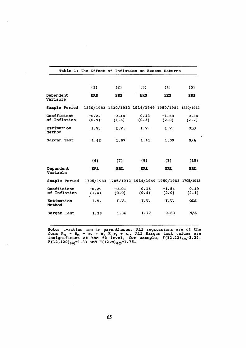
Table 1: The Effect of Inflation on Excess Returns
( 1 ) ( 2 ) ( 3 ) ( 4 ) (5 )
D e p e n d e n t ERS ERS ERS ERS ERSV a r i a b l e
S a m p l e P e r i o d 1 8 3 0 / 1 9 8 3 1 8 3 0 / 1 9 1 3 1 9 1 4 / 1 9 4 9 1 9 5 0 / 1 9 8 3 1830/1913
C o e f f i c i e n t - 0 . 2 2 0 . 4 4 0 . 1 3 - 1 . 6 8 0 . 3 4o f I n f l a t i o n ( 0 . 9 ) ( 1 . 6 ) ( 0 . 3 ) ( 2 . 0 ) ( 2 . 2 )
E s t i m a t i o n I . V . I . V . I . V . I . V . OLSM e t h o d
S a r g a n T e s t 1 . 4 2 1 . 6 7 1 . 4 1 1 . 0 9 N/A
( 6 ) ( 7 ) ( 8 ) (9 ) ( 1 0 )
D e p e n d e n t ERL ERL ERL ERL ERLV a r i a b l e
S a m p l e P e r i o d 1 7 0 5 / 1 9 8 3 1 7 0 5 / 1 9 1 3 1 9 1 4 / 1 9 4 9 1 9 5 0 / 1 9 8 3 1705/1913
C o e f f i c i e n t - 0 . 2 9 - 0 . 0 1 0 . 1 6 - 1 . 5 4 0 . 1 9o f I n f l a t i o n ( 1 . 4 ) ( 0 . 0 ) ( 0 . 4 ) ( 2 . 0 ) ( 2 . 1 )
E s t i m a t i o n I . V . I . V . I . V . I . V . OLSM e t h o d
S a r g a n T e s t 1 . 3 8 1 . 3 6 1 . 7 7 0 . 8 3 N /A
N o t e : t - r a t i o s a r e i n p a r e n t h e s e s . A l l r e g r e s s i o n s a r e o f t h e f o r m Rp - Rr = a 0 + a , Et1Jrt + u t . A l l S a r g a n t e s t v a l u e s a r e i n s i g n i f i c a n t a t t h e 5% l e v e l , f o r e x a m p l e , F ( 1 2 , 2 2 ) 005= 2 . 2 3 , F ( 1 2 , 1 2 0 ) 005= 1 . 8 3 a n d F ( 1 2 , ® ) 005= 1 . 7 5 .
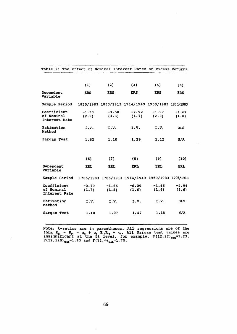
Table 2: The Effect of Nominal Interest Rates on Excess Returns
(1 ) ( 2 ) ( 3 ) ( 4 ) (5 )
D e p e n d e n t ERS ERS ERS ERS ERSV a r i a b l e
S a m p l e P e r i o d 1 8 3 0 / 1 9 8 3 1 8 3 0 / 1 9 1 3 1 9 1 4 / 1 9 4 9 1 9 5 0 / 1 9 8 3 1830/1983
C o e f f i c i e n t - 1 . 3 3 - 3 . 5 0 - 2 . 9 2 - 1 . 9 7 - 1 . 6 7o f N o m i n a l ( 2 . 9 ) ( 3 . 3 ) ( 1 . 7 ) ( 2 . 0 ) ( 4 . 0 )I n t e r e s t R a t e
E s t i m a t i o n I . V . I . V . I . V . I . V . OLSM e th o d
S a r g a n T e s t 1 . 6 2 1 . 1 0 1 . 2 9 1 . 1 2 N/A
( 6 ) ( 7 ) ( 8 ) ( 9 ) (1 0 )
D e p e n d e n t ERL ERL ERL ERL ERLV a r i a b l e
S a m p l e P e r i o d 1 7 0 5 / 1 9 8 3 1 7 0 5 / 1 9 1 3 1 9 1 4 / 1 9 4 9 1 9 5 0 / 1 9 8 3 1705/1913
C o e f f i c i e n t - 0 . 7 0 - 1 . 6 6 - 6 . 0 9 - 1 . 6 5 - 2 . 9 4o f N o m i n a l ( 1 . 7 ) ( 1 . 8 ) ( 1 . 6 ) ( 1 . 6 ) ( 3 . 6 )I n t e r e s t R a t e
E s t i m a t i o n I . V . I . V . I . V . I . V . OLSM e th o d
S a r g a n T e s t 1 . 4 0 1 . 0 7 1 . 4 7 1 . 1 8 N/A
N o t e : t - r a t i o s a r e i n p a r e n t h e s e s . A l l r e g r e s s i o n s a r e o f t h e f o r m - Rp, = a„ + o , e m r r + ' V A11 S a r g a n t e s t v a l u e s a r e i n s i g n i f i c a n t a t t h e 5% l e v e l , f o r e x a m p l e , F ( 1 2 , 2 2 ) 005= 2 . 2 3 , F ( 1 2 , 1 2 0 ) 005= 1 . 83 a n d F ( 1 2 , « ) 005= l . 7 5 .
66
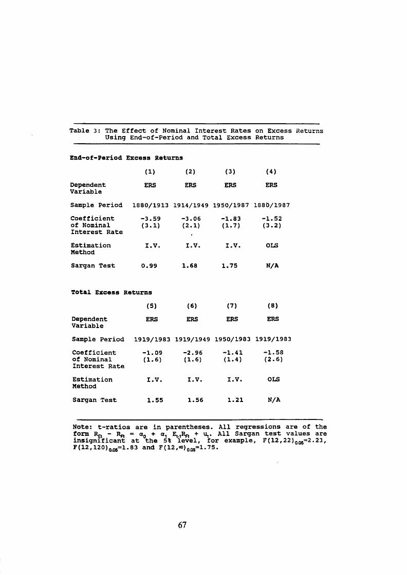
T a b l e 3 : T h e E f f e c t o f N o m i n a l I n t e r e s t R a t e s o n E x c e s s R e t u r n s U s i n g E n d - o f - P e r i o d a n d T o t a l E x c e s s R e t u r n s
E n d - o f - P e r i o d E x c e s s R e t u r n s
( 1 ) (2 ) ( 3 ) ( 4 )
D e p e n d e n t ERS ERS ERS ERSV a r i a b l e
S a m p l e P e r i o d 1 8 8 0 / 1 9 1 3 1 9 1 4 / 1 9 4 9 1 9 5 0 / 1 9 8 7 1 8 8 0 / 1 9 8 7
C o e f f i c i e n t - 3 . 5 9 - 3 . 0 6 - 1 . 8 3 - 1 . 5 2o f N o m i n a l ( 3 . 1 ) ( 2 . 1 ) ( 1 . 7 ) ( 3 . 2 )I n t e r e s t R a t e
E s t i m a t i o n I . V . I . V . I . V . OLSM e th o d
S a r g a n T e s t 0 . 9 9 1 . 6 8 1 . 7 5 N /A
T o t a l E x c e s s R e t u r n s
( 5 ) ( 6 ) ( 7 ) ( 8 )
D e p e n d e n t ERS ERS ERS ERSV a r i a b l e
S a m p l e P e r i o d 1 9 1 9 / 1 9 8 3 1 9 1 9 / 1 9 4 9 1 9 5 0 / 1 9 8 3 1 9 1 9 / 1 9 8 3
C o e f f i c i e n t - 1 . 0 9 - 2 . 9 6 - 1 . 4 1 - 1 . 5 8o f N o m i n a l ( 1 . 6 ) ( 1 . 6 ) ( 1 . 4 ) ( 2 . 6 )I n t e r e s t R a t e
E s t i m a t i o n I . V . I . V . I . V . OLSM e th o d
S a r g a n T e s t 1 . 5 5 1 . 5 6 1 . 2 1 N /A
N o t e : t - r a t i o s a r e i n p a r e n t h e s e s . A l l r e g r e s s i o n s a r e o f t h e f o r m Rct - Rp = a 0 + a , E^Rp, + ut . A l l S a r g a n t e s t v a l u e s a r e i n s i g n i f i c a n t a t t h e 5% l e v e l , f o r e x a m p l e , F ( 1 2 , 2 2 ) 005= 2 . 2 3 , F ( 1 2 , 1 2 0 ) 005= 1 . 8 3 a n d F ( 1 2 , « ) 005= l . 7 5 .
67
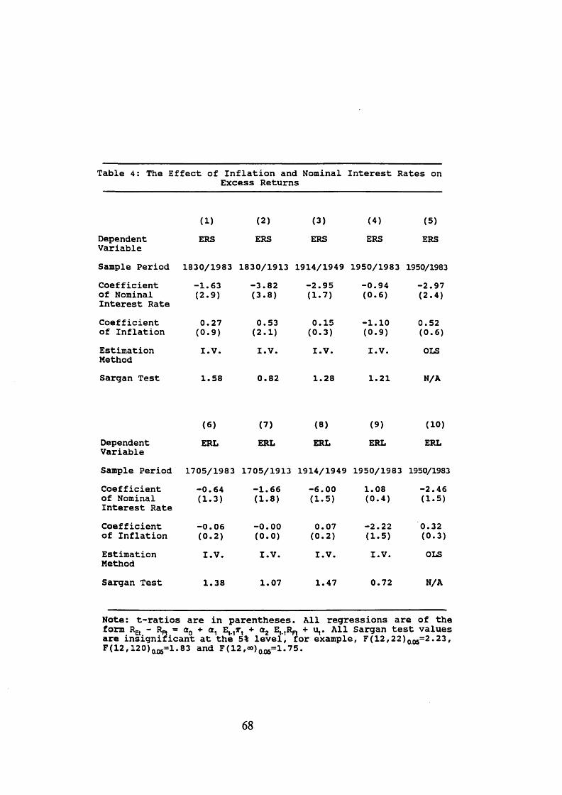
Table 4: The Effect of Inflation and Nominal Interest Rates onExcess Returns
( 1 ) ( 2 ) ( 3 ) (4 ) (5 )
D e p e n d e n tV a r i a b l e
ERS ERS ERS ERS ERS
S a m p l e P e r i o d 1 8 3 0 / 1 9 8 3 1 8 3 0 / 1 9 1 3 1 9 1 4 / 1 9 4 9 1 9 5 0 / 1 9 8 3 1950/1983
C o e f f i c i e n t o f N o m in a l I n t e r e s t R a t e
- 1 . 6 3( 2 . 9 )
- 3 . 8 2( 3 . 8 )
- 2 . 9 5( 1 . 7 )
- 0 . 9 4( 0 . 6 )
- 2 . 9 7( 2 . 4 )
C o e f f i c i e n t o f I n f l a t i o n
0 . 2 7( 0 . 9 )
0 . 5 3( 2 . 1 )
0 . 1 5( 0 . 3 )
- 1 . 1 0( 0 . 9 )
0 . 5 2( 0 . 6 )
E s t i m a t i o nM e th o d
I . V . I . V . I . V . I . V . OLS
S a r g a n T e s t 1 . 5 8 0 . 8 2 1 . 2 8 1 . 2 1 N/A
( 6 ) ( 7 ) ( 8 ) ( 9 ) (1 0 )
D e p e n d e n tV a r i a b l e
ERL ERL ERL ERL ERL
S a m p l e P e r i o d 1 7 0 5 / 1 9 8 3 1 7 0 5 / 1 9 1 3 1 9 1 4 / 1 9 4 9 1 9 5 0 / 1 9 8 3 1950/1983
C o e f f i c i e n t o f N o m in a l I n t e r e s t R a t e
- 0 . 6 4( 1 . 3 )
- 1 . 6 6( 1 . 8 )
- 6 . 0 0( 1 . 5 )
1 . 0 8( 0 . 4 )
- 2 . 4 6( 1 . 5 )
C o e f f i c i e n t o f I n f l a t i o n
- 0 . 0 6( 0 . 2 )
- 0 . 0 0( 0 . 0 )
0 . 0 7( 0 . 2 )
- 2 . 2 2( 1 . 5 )
0 . 3 2( 0 . 3 )
E s t i m a t i o nM e th o d
I . V . I . V . I . V . I . V . OLS
S a r g a n T e s t 1 . 3 8 1 . 0 7 1 . 4 7 0 . 7 2 N /A
N o t e : t - r a t i o s a r e i n p a r e n t h e s e s . A l l r e g r e s s i o n s a r e o f t h e f o r m Ra - Rp, = cr0 ♦ a , Ev1Jrt + a 2 E ^ R p + u t . A l l S a r g a n t e s t v a l u e s a r e i n s i g n i f i c a n t a t t h e 5% l e v e l , f o r e x a m p l e , F ( 1 2 , 2 2 ) 005= 2 . 2 3 , F ( 1 2 , 1 2 0 ) 005= 1 . 8 3 a n d F ( 1 2 , o o ) 0 05= i . 7 5 .
68
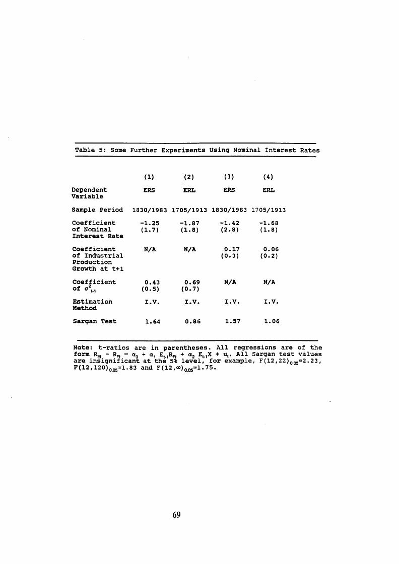
Table 5: Some Further Experiments Using Nominal Interest Rates
( 1 ) ( 2 ) ( 3 ) ( 4 )
D e p e n d e n tV a r i a b l e
ERS ERL ERS ERL
S a m p l e P e r i o d 1 8 3 0 / 1 9 8 3 1 7 0 5 / 1 9 1 3 1 8 3 0 / 1 9 8 3 1 7 0 5 / 1 9 1 3
C o e f f i c i e n t o f N o m i n a l I n t e r e s t R a t e
- 1 . 2 5( 1 . 7 )
- 1 . 8 7( 1 . 8 )
- 1 . 4 2( 2 . 8 )
- 1 . 6 8( 1 . 8 )
C o e f f i c i e n t o f I n d u s t r i a l P r o d u c t i o n G r o w t h a t t + l
N/A N /A 0 . 1 7( 0 . 3 )
0 . 0 6( 0 . 2 )
C o e f f i c i e n to f a2t-i
0 . 4 3( 0 . 5 )
0 . 6 9( 0 . 7 )
N /A N/A
E s t i m a t i o nM e t h o d
I . V . I . V . I . V . I . V .
S a r g a n T e s t 1 . 6 4 0 . 8 6 1 . 5 7 1 . 0 6
N o t e : t - r a t i o s a r e i n p a r e n t h e s e s . A l l r e g r e s s i o n s a r e o f t h e f o r m REt - Rn = a 0 + a , E^Rp, + a 2 Et1X + u t . A l l S a r g a n t e s t v a l u e s a r e i n s i g n i f i c a n t a t t h e 5% l e v e l , f o r e x a m p l e , F ( 1 2 , 2 2 ) 005= 2 . 2 3 , F ( 1 2 , 1 2 0 ) 005= 1 . 83 a n d F ( 1 2 , c o ) 005= 1 . 7 5 .
69
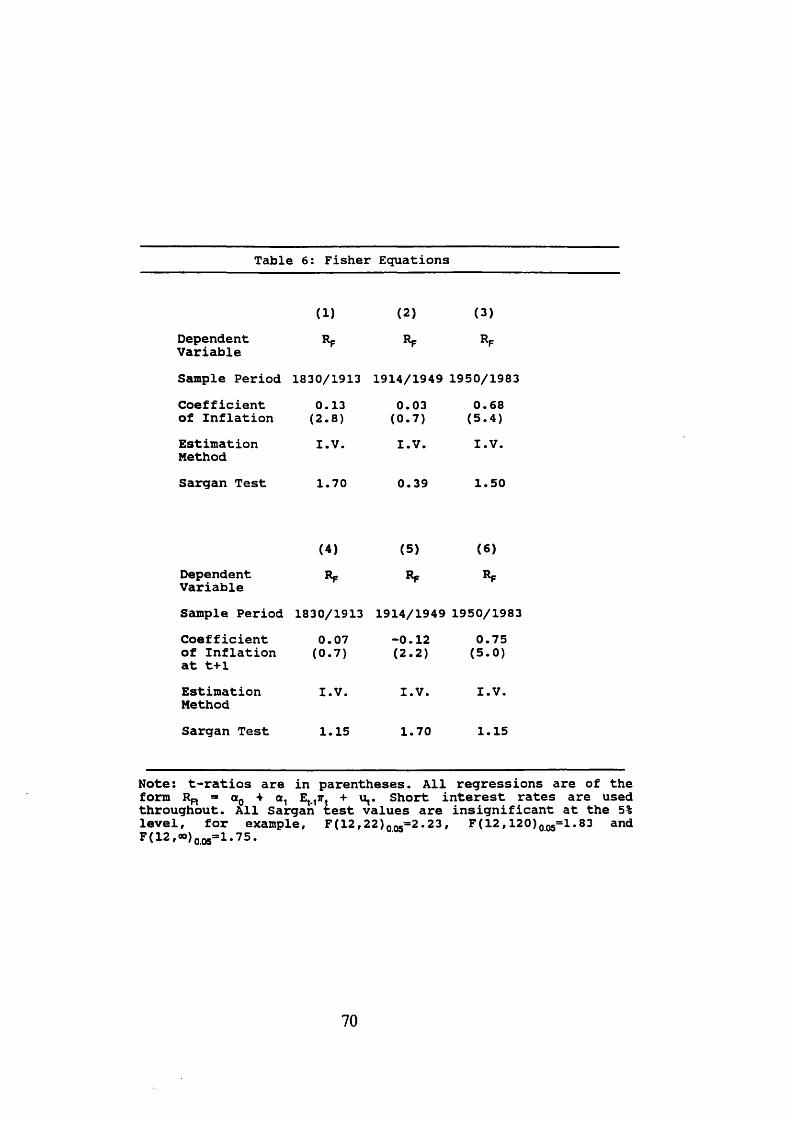
T a b l e i 6 : F i s h e r E q u a t i o n s
(1 ) ( 2 ) ( 3 )
D e p e n d e n tV a r i a b l e
Rf Rf Rp
S a m p l e P e r i o d 1 8 3 0 / 1 9 1 3 1 9 1 4 / 1 9 4 9 1 9 5 0 / 1 9 8 3
C o e f f i c i e n t 0 . 1 3 0 . 0 3 0 . 6 8o f I n f l a t i o n ( 2 . 8 ) ( 0 . 7 ) ( 5 . 4 )
E s t i m a t i o nM e t h o d
I . V . I . V . I . V .
S a r g a n T e s t 1 . 7 0 0 . 3 9 1 . 5 0
( 4 ) ( 5 ) ( 6 )
D e p e n d e n tV a r i a b l e
Rp Rf
S a m p l e P e r i o d 1 8 3 0 / 1 9 1 3 1 9 1 4 / 1 9 4 9 1 9 5 0 / 1 9 8 3
C o e f f i c i e n t 0 . 0 7 - 0 . 1 2 0 . 7 5o f I n f l a t i o n a t t + 1
( 0 . 7 ) ( 2 . 2 ) ( 5 . 0 )
E s t i m a t i o nM e t h o d
I . V . I . V . I . V .
S a r g a n T e s t 1 . 1 5 1 . 7 0 1 . 1 5
N o t e : t - r a t i o s a r e i n p a r e n t h e s e s . A l l r e g r e s s i o n s a r e o f t h e f o r m Rr = a 0 + a , EMJrt + u , . S h o r t i n t e r e s t r a t e s a r e u s e d t h r o u g h o u t . A l l S a r g a n t e s t v a l u e s a r e i n s i g n i f i c a n t a t t h e 5% l e v e l , f o r e x a m p l e , F ( 1 2 , 2 2 ) 005= 2 . 2 3 , F ( 1 2 , 1 2 0 ) 005= 1 . 8 3 a n dF ( 1 2 , °°) o.o5= ^ * 7 5 •
70
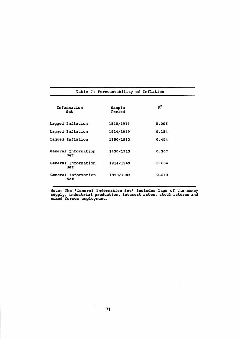
T a b l e 7 : F o r e c a s t a b i l i t y o f I n f l a t i o n
I n f o r m a t i o nS e t
S a m p l eP e r i o d
R2
L a g g e d I n f l a t i o n 1 8 3 0 / 1 9 1 3 0 . 0 0 6
L a g g e d I n f l a t i o n 1 9 1 4 / 1 9 4 9 0 . 1 8 4
L a g g e d I n f l a t i o n 1 9 5 0 / 1 9 8 3 0 . 4 5 4
G e n e r a l I n f o r m a t i o n S e t
1 8 3 0 / 1 9 1 3 0 . 3 0 7
G e n e r a l I n f o r m a t i o n S e t
1 9 1 4 / 1 9 4 9 0 . 6 0 4
G e n e r a l I n f o r m a t i o n S e t
1 9 5 0 / 1 9 8 3 0 . 8 1 3
N o t e : T h e ' G e n e r a l I n f o r m a t i o n S e t ' i n c l u d e s l a g s o f t h e m oney s u p p l y , i n d u s t r i a l p r o d u c t i o n , i n t e r e s t r a t e s , s t o c k r e t u r n s a n d a r m e d f o r c e s e m p l o y m e n t .
71
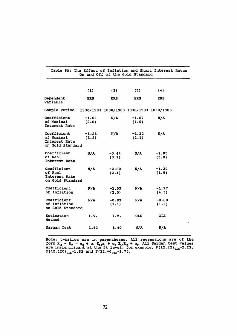
T a b l e 8A: T h e E f f e c t o f I n f l a t i o n a n d S h o r t On a n d O f f o f t h e G o l d S t a n d a r d
I n t e r e s t R a t e s
( 1 ) ( 2 ) (3 ) (4 )
D e p e n d e n tV a r i a b l e
ERS ERS ERS ERS
S a m p l e P e r i o d 1 8 3 0 / 1 9 8 3 1 8 3 0 / 1 9 8 3 1 8 3 0 / 1 9 8 3 1 8 3 0 / 1 9 8 3
C o e f f i c i e n t o f N o m in a l I n t e r e s t R a t e
- 1 . 0 3( 2 . 0 )
N /A - 1 . 6 7( 4 . 0 )
N /A
C o e f f i c i e n t o f N o m in a l I n t e r e s t R a t e o n G o l d S t a n d a r d
- 1 . 2 8( 1 . 8 )
N/A - 1 . 2 2( 2 . 1 )
N /A
C o e f f i c i e n t o f R e a l I n t e r e s t R a t e
N /A - 0 . 4 4( 0 . 7 )
N /A - 1 . 8 5( 3 . 8 )
C o e f f i c i e n t o f R e a l I n t e r e s t R a t e o n G o l d S t a n d a r d
N /A - 2 . 0 0( 2 . 4 )
N /A - 1 . 2 9( 1 . 9 )
C o e f f i c i e n t o f I n f l a t i o n
N /A - 1 . 0 3( 2 . 0 )
N /A - 1 . 7 7( 4 . 3 )
C o e f f i c i e n t o f I n f l a t i o n o n G o l d S t a n d a r d
N /A - 0 . 9 3( 1 . 1 )
N /A - 0 . 8 0( 1 . 3 )
E s t i m a t i o nM e th o d
I . V . I . V . OLS OLS
S a r g a n T e s t 1 . 6 3 1 . 4 0 N/A N/A
N o t e : t - r a t i o s a r e i n p a r e n t h e s e s . A l l r e g r e s s i o n s a r e o f t h e f o r m REt - Rn = a 0 + a , EV1r t t a 2 E , . ^ + u , . A l l S a r g a n t e s t v a l u e s a r e i n s i g n i f i c a n t a t t h e 5% l e v e l , f o r e x a m p l e , F ( 1 2 , 2 2 ) 005= 2 . 2 3 , F ( 1 2 , 1 2 0 ) 0^ = 1 . 8 3 a n d F ( 1 2 , » ) 005= 1 . 7 5 .
72
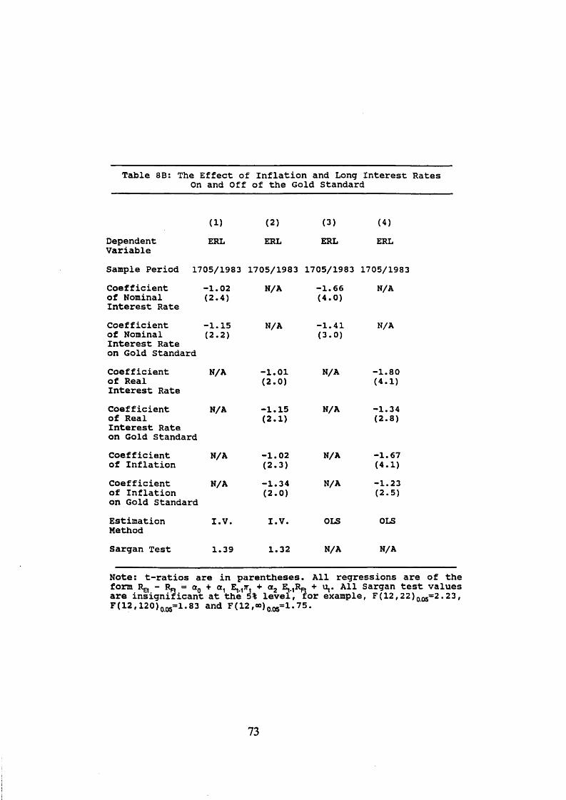
T a b l e 8B : T h e E f f e c t o f I n f l a t i o n a n d L o n g I n t e r e s t R a t e s On a n d O f f o f t h e G o l d S t a n d a r d
(1 ) ( 2 ) (3 ) (4 )
D e p e n d e n t ERL V a r i a b l e
ERL ERL ERL
S a m p l e P e r i o d 1 7 0 5 / 1 9 8 3 1 7 0 5 / 1 9 8 3 1 7 0 5 / 1 9 8 3 1 7 0 5 / 1 9 8 3
C o e f f i c i e n t ->1 .02 o f N o m i n a l ( 2 . 4 ) I n t e r e s t R a t e
N /A - 1 . 6 6( 4 . 0 )
N/A
C o e f f i c i e n t - 1 . 1 5 o f N o m i n a l ( 2 . 2 ) I n t e r e s t R a t e o n G o l d S t a n d a r d
N /A - 1 . 4 1( 3 . 0 )
N/A
C o e f f i c i e n t N /A - 1 . 0 1 N /A - 1 . 8 0o f R e a l I n t e r e s t R a t e
( 2 . 0 ) ( 4 . 1 )
C o e f f i c i e n t N /A - 1 . 1 5 N /A - 1 . 3 4o f R e a l I n t e r e s t R a t e o n G o l d S t a n d a r d
( 2 . 1 ) ( 2 . 8 )
C o e f f i c i e n t N /A - 1 . 0 2 N /A - 1 . 6 7o f I n f l a t i o n ( 2 . 3 ) ( 4 . 1 )
C o e f f i c i e n t N /A - 1 . 3 4 N/A - 1 . 2 3o f I n f l a t i o n o n G o l d S t a n d a r d
( 2 . 0 ) ( 2 . 5 )
E s t i m a t i o n I . V . M e t h o d
I . V . OLS OLS
S a r g a n T e s t 1 . 3 9 1 . 3 2 N/A N/A
N o t e : t - r a t i o s a r e i n p a r e n t h e s e s . A l l r e g r e s s i o n s a r e o f t h e f o r m Re, - R,, = a 0 + a 1 E ^ jt, + a 2 E^Rp, + i^ . A l l S a r g a n t e s t v a l u e s a r e i n s i g n i f i c a n t a t t h e 5% l e v e l , f o r e x a m p l e , F ( 1 2 , 2 2 ) 005= 2 . 2 3 , F ( 1 2 , 1 2 0 ) oos= 1 . 8 3 a n d F ( 1 2 , o o ) Q05= 1 . 7 5 .
73
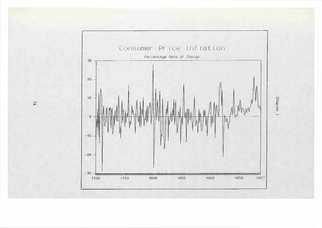
<1-p*
n s u m e r P r i c e I n fPercentage Rate of Change
30
20 -
10
- 1 0
- 2 0
-3 019871800 1850 19001700 1750
Diagram
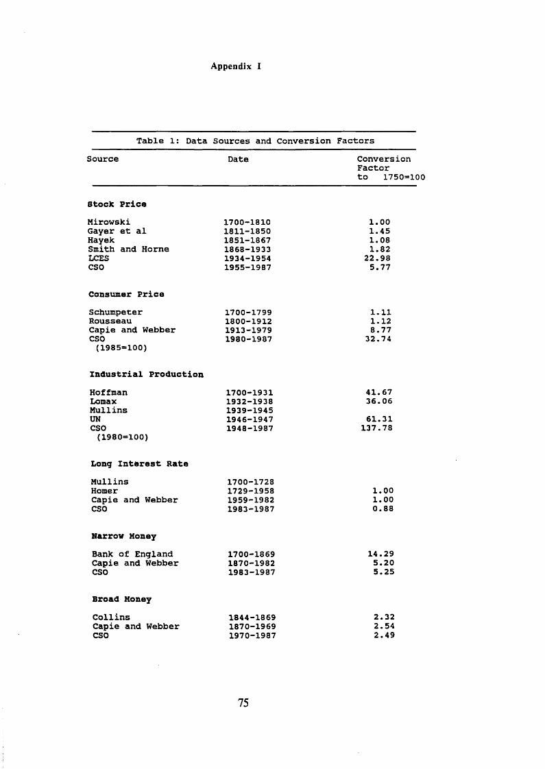
Appendix I
T a b l e 1 : D a t a S o u r c e s a n d C o n v e r s i o n F a c t o r s
S o u r c e D a t e C o n v e r s i o nF a c t o rt o 1 7 5 0 = 1 0 0
S t o c k P r i c e
M i r o w s k i 1 7 0 0 - 1 8 1 0 1 . 0 0G a y e r e t a l 1 8 1 1 - 1 8 5 0 1 . 4 5H a y e k 1 8 5 1 - 1 8 6 7 1 . 0 8S m i t h a n d H o r n e 1 8 6 8 - 1 9 3 3 1 . 8 2LCES 1 9 3 4 - 1 9 5 4 2 2 . 9 8CSO 1 9 5 5 - 1 9 8 7 5 . 7 7
C o n s u m e r P r i c e
S c h u m p e t e r 1 7 0 0 - 1 7 9 9 1 . 1 1R o u s s e a u 1 8 0 0 - 1 9 1 2 1 . 1 2C a p i e a n d W e b b e r 1 9 1 3 - 1 9 7 9 8 . 7 7CSO 1 9 8 0 - 1 9 8 7 3 2 . 7 4
( 1 9 8 5 = 1 0 0 )
I n d u s t r i a l P r o d u c t i o n
H o f f m a n 1 7 0 0 - 1 9 3 1 4 1 . 6 7Lom ax 1 9 3 2 - 1 9 3 8 3 6 . 0 6M u l l i n s 1 9 3 9 - 1 9 4 5UN 1 9 4 6 - 1 9 4 7 6 1 . 3 1CSO 1 9 4 8 - 1 9 8 7 1 3 7 . 7 8
( 1 9 8 0 = 1 0 0 )
L o n g I n t e r e s t R a t e
M u l l i n s 1 7 0 0 - 1 7 2 8H om er 1 7 2 9 - 1 9 5 8 1 . 0 0C a p i e a n d W e b b e r 1 9 5 9 - 1 9 8 2 1 . 0 0CSO 1 9 8 3 - 1 9 8 7 0 . 8 8
N a r r o w M oney
B a n k of E n g l a n d 1 7 0 0 - 1 8 6 9 1 4 . 2 9C a p i e a n d W e b b e r 1 8 7 0 - 1 9 8 2 5 . 2 0CSO 1 9 8 3 - 1 9 8 7 5 . 2 5
B r o a d M on e y
C o l l i n s 1 8 4 4 - 1 8 6 9 2 . 3 2C a p i e a n d W e b b e r 1 8 7 0 - 1 9 6 9 2 . 5 4CSO 1 9 7 0 - 1 9 8 7 2 . 4 9
75
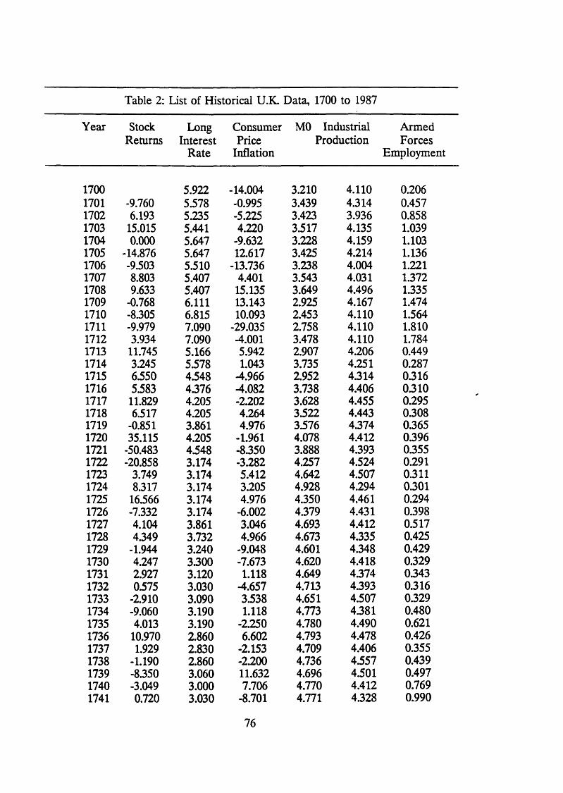
Year
170017011702170317041705170617071708170917101711171217131714171517161717171817191720172117221723172417251726172717281729173017311732173317341735173617371738173917401741
Table 2: List of Historical U.K. Data, 1700 to 1987
Stock Long Consumer Returns Interest Price
Rate Inflation
5.922 -14.004-9.760 5.578 -0.9956.193 5.235 -5.225
15.015 5.441 4.2200.000 5.647 -9.632
-14.876 5.647 12.617-9.503 5.510 -13.7368.803 5.407 4.4019.633 5.407 15.135
-0.768 6.111 13.143-8.305 6.815 10.093-9.979 7.090 -29.0353.934 7.090 -4.00111.745 5.166 5.9423.245 5.578 1.0436.550 4.548 -4.9665.583 4.376 4.08211.829 4.205 -2.2026.517 4.205 4.264
-0.851 3.861 4.97635.115 4.205 -1.961
-50.483 4.548 -8.350-20.858 3.174 -3.282
3.749 3.174 5.4128.317 3.174 3.205
16.566 3.174 4.976-7.332 3.174 -6.0024.104 3.861 3.0464.349 3.732 4.966
-1.944 3.240 -9.0484.247 3300 -7.6732.927 3.120 1.1180.575 3.030 4.657
-2.910 3.090 3.538-9.060 3.190 1.1184.013 3.190 -2.250
10.970 2.860 6.6021.929 2.830 -2.153
-1.190 2.860 -2.200-8.350 3.060 11.632-3.049 3.000 7.7060.720 3.030 -8.701
76
M0 Industrial ArmedProduction Forces
Employment
3.210 4.110 0.2063.439 4.314 0.4573.423 3.936 0.8583.517 4.135 1.0393.228 4.159 1.1033.425 4.214 1.1363.238 4.004 1.2213.543 4.031 1.3723.649 4.496 1.3352.925 4.167 1.4742.453 4.110 1.5642.758 4.110 1.8103.478 4.110 1.7842.907 4.206 0.4493.735 4.251 0.2872.952 4.314 0.3163.738 4.406 0.3103.628 4.455 0.2953.522 4.443 0.3083.576 4.374 0.3654.078 4.412 0.3963.888 4.393 0.3554.257 4.524 0.2914.642 4.507 0.3114.928 4.294 0.3014.350 4.461 0.2944.379 4.431 0.3984.693 4.412 0.5174.673 4.335 0.4254.601 4.348 0.4294.620 4.418 0.3294.649 4.374 0.3434.713 4.393 0.3164.651 4.507 0.3294.773 4.381 0.4804.780 4.490 0.6214.793 4.478 0.4264.709 4.406 0.3554.736 4.557 0.4394.696 4.501 0.4974.770 4.412 0.7694.771 4.328 0.990
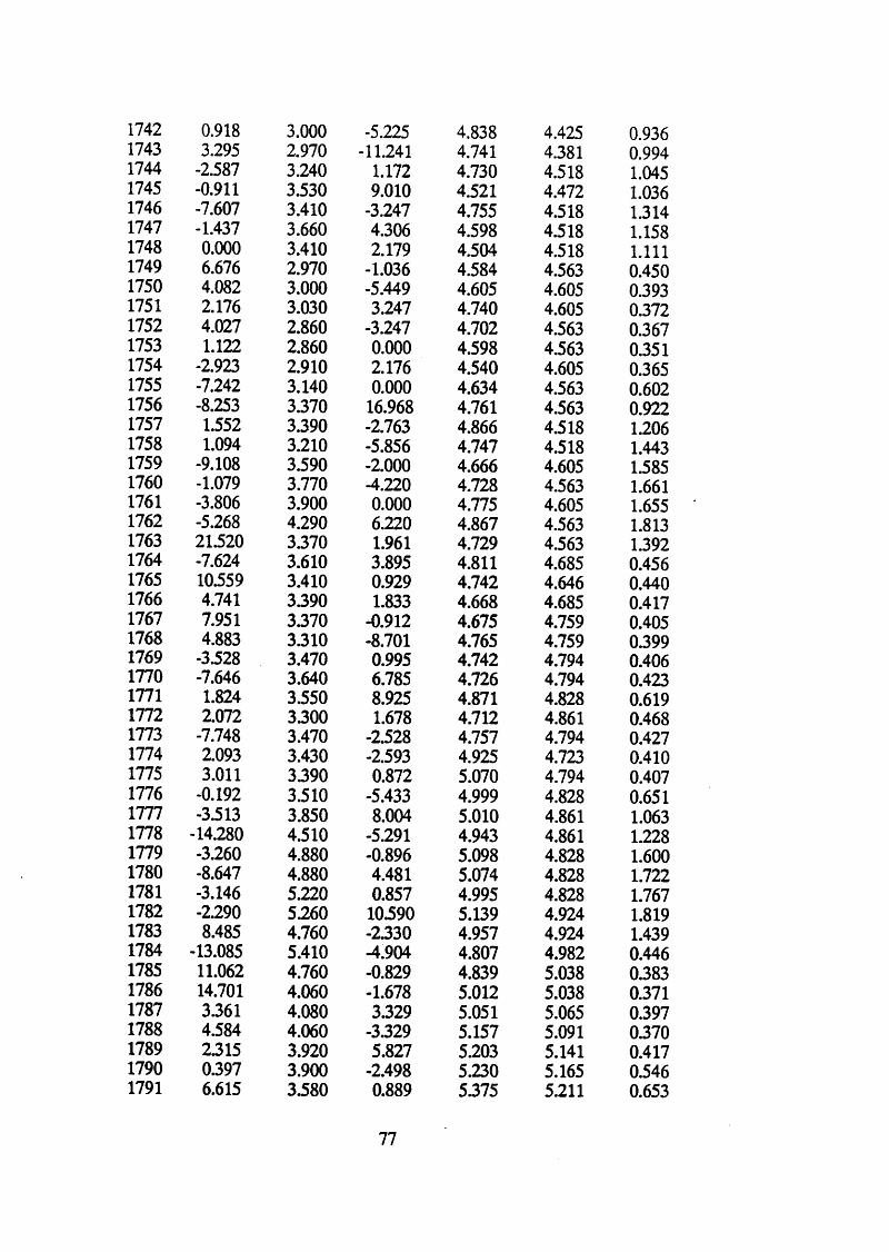
1742 0.918 3.000 -5.225 4.838 4.425 0.9361743 3.295 2.970 -11.241 4.741 4.381 0.9941744 -2.587 3.240 1.172 4.730 4.518 1.0451745 -0.911 3.530 9.010 4.521 4.472 1.0361746 -7.607 3.410 -3.247 4.755 4.518 1.3141747 -1.437 3.660 4.306 4.598 4.518 1.1581748 0.000 3.410 2.179 4.504 4.518 1.1111749 6.676 2.970 -1.036 4.584 4.563 0.4501750 4.082 3.000 -5.449 4.605 4.605 0.3931751 2.176 3.030 3.247 4.740 4.605 0.3721752 4.027 2.860 -3.247 4.702 4.563 0.3671753 1.122 2.860 0.000 4.598 4.563 0.3511754 -2.923 2.910 2.176 4.540 4.605 0.3651755 -7.242 3.140 0.000 4.634 4.563 0.6021756 -8.253 3.370 16.968 4.761 4.563 0.9221757 1.552 3.390 -2.763 4.866 4.518 1.2061758 1.094 3.210 -5.856 4.747 4.518 1.4431759 -9.108 3.590 -2.000 4.666 4.605 1.5851760 -1.079 3.770 -4.220 4.728 4.563 1.6611761 -3.806 3.900 0.000 4.775 4.605 1.6551762 -5.268 4.290 6.220 4.867 4.563 1.8131763 21.520 3.370 1.961 4.729 4.563 1.3921764 -7.624 3.610 3.895 4.811 4.685 0.4561765 10.559 3.410 0.929 4.742 4.646 0.4401766 4.741 3.390 1.833 4.668 4.685 0.4171767 7.951 3.370 -0.912 4.675 4.759 0.4051768 4.883 3.310 -8.701 4.765 4.759 0.3991769 -3.528 3.470 0.995 4.742 4.794 0.4061770 -7.646 3.640 6.785 4.726 4.794 0.4231771 1.824 3.550 8.925 4.871 4.828 0.6191772 2.072 3.300 1.678 4.712 4.861 0.4681773 -7.748 3.470 -2.528 4.757 4.794 0.4271774 2.093 3.430 -2.593 4.925 4.723 0.4101775 3.011 3.390 0.872 5.070 4.794 0.4071776 -0.192 3.510 -5.433 4.999 4.828 0.6511777 -3.513 3.850 8.004 5.010 4.861 1.0631778 -14.280 4.510 -5.291 4.943 4.861 1.2281779 -3.260 4.880 -0.896 5.098 4.828 1.6001780 -8.647 4.880 4.481 5.074 4.828 1.7221781 -3.146 5.220 0.857 4.995 4.828 1.7671782 -2.290 5.260 10.590 5.139 4.924 1.8191783 8.485 4.760 -2330 4.957 4.924 1.4391784 -13.085 5.410 -4.904 4.807 4.982 0.4461785 11.062 4.760 -0.829 4.839 5.038 0.3831786 14.701 4.060 -1.678 5.012 5.038 0.3711787 3.361 4.080 3.329 5.051 5.065 0.3971788 4.584 4.060 -3.329 5.157 5.091 0.3701789 2.315 3.920 5.827 5.203 5.141 0.4171790 0.397 3.900 -2.498 5.230 5.165 0.5461791 6.615 3.580 0.889 5.375 5.211 0.653
77
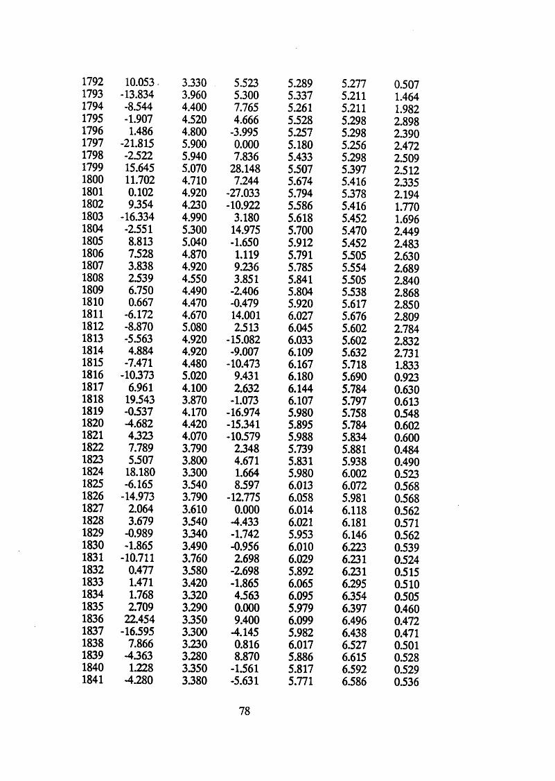
1792 10.053. 3.330 5.523 5.289 5.277 0.5071793 -13.834 3.960 5.300 5.337 5.211 1.4641794 -8.544 4.400 7.765 5.261 5.211 1.9821795 -1.907 4.520 4.666 5.528 5.298 2.8981796 1.486 4.800 -3.995 5.257 5.298 2.3901797 -21.815 5.900 0.000 5.180 5.256 2.4721798 -2.522 5.940 7.836 5.433 5.298 2.5091799 15.645 5.070 28.148 5.507 5.397 2.5121800 11.702 4.710 7.244 5.674 5.416 2.3351801 0.102 4.920 -27.033 5.794 5.378 2.1941802 9.354 4.230 -10.922 5.586 5.416 1.7701803 -16.334 4.990 3.180 5.618 5.452 1.6961804 -2.551 5.300 14.975 5.700 5.470 2.4491805 8.813 5.040 -1.650 5.912 5.452 2.4831806 7.528 4.870 1.119 5.791 5.505 2.6301807 3.838 4.920 9.236 5.785 5.554 2.6891808 2.539 4.550 3.851 5.841 5.505 2.8401809 6.750 4.490 -2.406 5.804 5.538 2.8681810 0.667 4.470 -0.479 5.920 5.617 2.8501811 -6.172 4.670 14.001 6.027 5.676 2.8091812 -8.870 5.080 2.513 6.045 5.602 2.7841813 -5.563 4.920 -15.082 6.033 5.602 2.8321814 4.884 4.920 -9.007 6.109 5.632 2.7311815 -7.471 4.480 -10.473 6.167 5.718 1.8331816 -10373 5.020 9.431 6.180 5.690 0.9231817 6.961 4.100 2.632 6.144 5.784 0.6301818 19.543 3.870 -1.073 6.107 5.797 0.6131819 -0.537 4.170 -16.974 5.980 5.758 0.5481820 -4.682 4.420 -15.341 5.895 5.784 0.6021821 4.323 4.070 -10.579 5.988 5.834 0.6001822 7.789 3.790 2348 5.739 5.881 0.4841823 5.507 3.800 4.671 5.831 5.938 0.4901824 18.180 3.300 1.664 5.980 6.002 0.5231825 -6.165 3.540 8.597 6.013 6.072 0.5681826 -14.973 3.790 -12.775 6.058 5.981 0.5681827 2.064 3.610 0.000 6.014 6.118 0.5621828 3.679 3340 -4.433 6.021 6.181 0.5711829 -0.989 3.340 -1.742 5.953 6.146 0.5621830 -1.865 3.490 -0.956 6.010 6.223 0.5391831 -10.711 3.760 2.698 6.029 6.231 0.5241832 0.477 3.580 -2.698 5.892 6.231 0.5151833 1.471 3.420 -1.865 6.065 6.295 0.5101834 1.768 3.320 4.563 6.095 6.354 0.5051835 2.709 3.290 0.000 5.979 6.397 0.4601836 22.454 3.350 9.400 6.099 6.496 0.4721837 -16.595 3.300 -4.145 5.982 6.438 0.4711838 7.866 3.230 0.816 6.017 6.527 0.5011839 -4.363 3.280 8.870 5.886 6.615 0.5281840 1.228 3350 -1.561 5.817 6.592 0.5291841 -4.280 3.380 -5.631 5.771 6.586 0.536
78
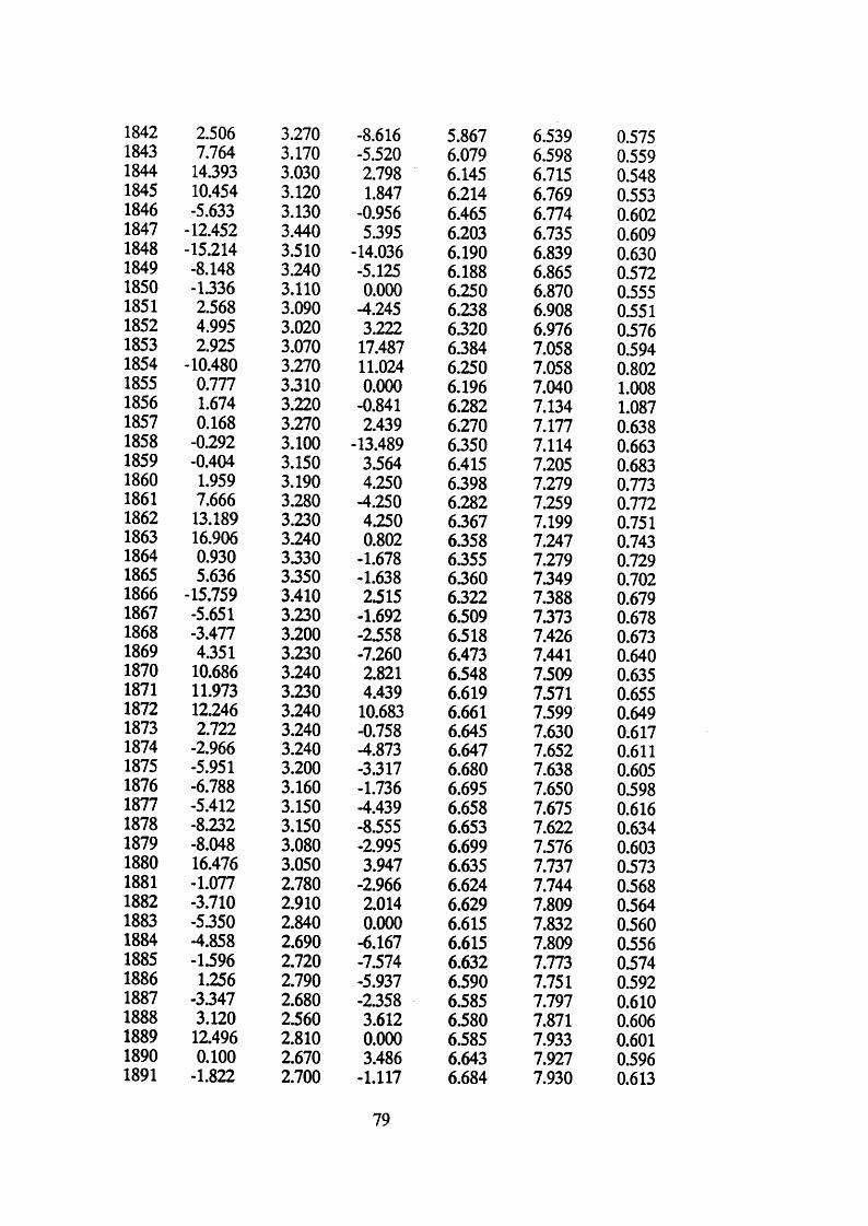
18421843184418451846184718481849185018511852185318541855185618571858185918601861186218631864186518661867186818691870187118721873187418751876187718781879188018811882188318841885188618871888188918901891
2.506 3.2707.764 3.170
14.393 3.03010.454 3.120-5.633 3.130
-12.452 3.440-15.214 3.510-8.148 3.240-1.336 3.1102.568 3.0904.995 3.0202.925 3.070
-10.480 3.2700.777 3.3101.674 3.2200.168 3.270
-0.292 3.100-0.404 3.1501.959 3.1907.666 3.280
13.189 3.23016.906 3.2400.930 3.3305.636 3350
-15.759 3.410-5.651 3.230-3.477 3.2004.351 3.230
10.686 3.24011.973 3.23012.246 3.2402.722 3.240
-2.966 3.240-5.951 3.200-6.788 3.160-5.412 3.150-8.232 3.150-8.048 3.08016.476 3.050-1.077 2.780-3.710 2.910-5.350 2.840-4.858 2.690-1.596 2.7201.256 2.790
-3.347 2.6803.120 2.560
12.496 2.8100.100 2.670
-1.822 2.700
-8.616 5.867-5.520 6.0792.798 6.1451.847 6.214
-0.956 6.4655.395 6.203
-14.036 6.190-5.125 6.1880.000 6.250
-4.245 6.2383.222 6.320
17.487 6.38411.024 6.2500.000 6.196
-0.841 6.2822.439 6.270
-13.489 6.3503.564 6.4154.250 6.398
-4.250 6.2824.250 6.3670.802 6.358
-1.678 6.355-1.638 63602.515 6.322
-1.692 6.509-2358 6.518-7.260 6.4732.821 6.5484.439 6.61910.683 6.661-0.758 6.645-4.873 6.647-3.317 6.680-1.736 6.695-4.439 6.658-8.555 6.653-2.995 6.6993.947 6.635
-2.966 6.6242.014 6.6290.000 6.615
-6.167 6.615-7.574 6.632-5.937 6.590-2.358 6.5853.612 6.5800.000 6.5853.486 6.643
-1.117 6.684
79
6.539 0.5756.598 0.5596.715 0.5486.769 0.5536.774 0.6026.735 0.6096.839 0.6306.865 0.5726.870 0.5556.908 0.5516.976 0.5767.058 0.5947.058 0.8027.040 1.0087.134 1.0877.177 0.6387.114 0.6637.205 0.6837.279 0.7737.259 0.7727.199 0.7517.247 0.7437.279 0.7297349 0.7027.388 0.6797373 0.6787.426 0.6737.441 0.6407.509 0.6357.571 0.6557.599 0.6497.630 0.6177.652 0.6117.638 0.6057.650 0.5987.675 0.6167.622 0.6347.576 0.6037.737 0.5737.744 0.5687.809 0.5647.832 0.5607.809 03567.773 0.5747.751 0.5927.797 0.6107.871 0.6067.933 0.6017.927 0.5967.930 0.613
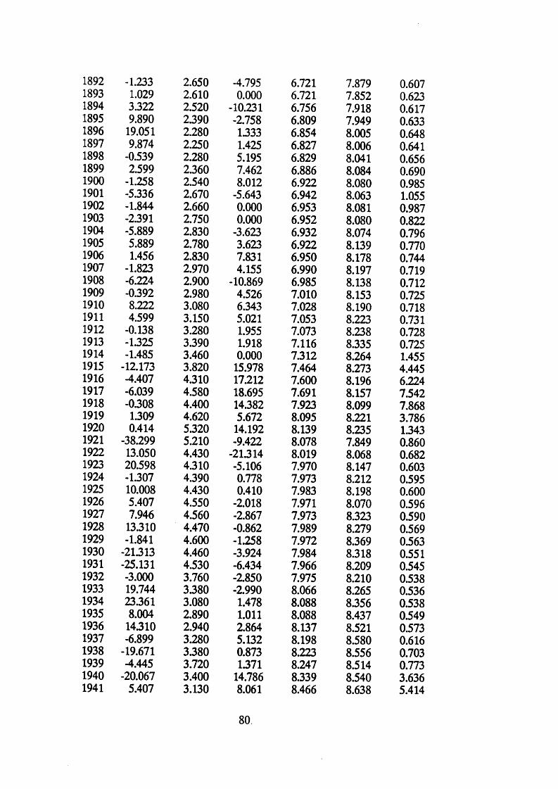
18921893189418951896189718981899190019011902190319041905190619071908190919101911191219131914191519161917191819191920192119221923192419251926192719281929193019311932193319341935193619371938193919401941
-1.233 2.650 -4.7951.029 2.610 0.0003.322 2.520 -10.2319.890 2.390 -2.758
19.051 2.280 1.3339.874 2.250 1.425
-0.539 2.280 5.1952.599 2.360 7.462
-1.258 2.540 8.012-5.336 2.670 -5.643-1.844 2.660 0.000-2.391 2.750 0.000-5.889 2.830 -3.6235.889 2.780 3.6231.456 2.830 7.831
-1.823 2.970 4.155-6.224 2.900 -10.869-0.392 2.980 4.5268.222 3.080 6.3434.599 3.150 5.021
-0.138 3.280 1.955-1.325 3.390 1.918-1.485 3.460 0.000
-12.173 3.820 15.978-4.407 4.310 17.212-6.039 4.580 18.695-0.308 4.400 14.3821.309 4.620 5.6720.414 5.320 14.192
-38.299 5.210 -9.42213.050 4.430 -2131420.598 4.310 -5.106-1.307 4.390 0.77810.008 4.430 0.4105.407 4.550 -2.0187.946 4.560 -2.867
13.310 4.470 -0.862-1.841 4.600 -1.258
-21.313 4.460 -3.924-25.131 4.530 -6.434-3.000 3.760 -2.85019.744 3.380 -2.99023.361 3.080 1.4788.004 2.890 1.011
14310 2.940 2.864-6.899 3.280 5.132
-19.671 3.380 0.873-4.445 3.720 1371
-20.067 3.400 14.7865.407 3.130 8.061
80
6.721 7.879 0.6076.721 7.852 0.6236.756 7,918 0.6176.809 7.949 0.6336.854 8.005 0.6486.827 8.006 0.6416.829 8.041 0.6566.886 8.084 0.6906.922 8.080 0.9856.942 8.063 1.0556.953 8.081 0.9876.952 8.080 0.8226.932 8.074 0.7966.922 8.139 0.7706.950 8.178 0.7446.990 8.197 0.7196.985 8.138 0.7127.010 8.153 0.7257.028 8.190 0.7187.053 8.223 0.7317.073 8.238 0.7287.116 8.335 0.7257.312 8.264 1.4557.464 8.273 4.4457.600 8.196 6.2247.691 8.157 7.5427.923 8.099 7.8688.095 8.221 3.7868.139 8.235 1.3438.078 7.849 0.8608.019 8.068 0.6827.970 8.147 0.6037.973 8.212 0.5957.983 8.198 0.6007.971 8.070 0.5967.973 8.323 0.5907.989 8.279 0.5697.972 8.369 0.5637.984 8.318 0.5517.966 8.209 0.5457.975 8.210 0.5388.066 8.265 0.5368.088 8.356 0.5388.088 8.437 0.5498.137 8.521 0.5738.198 8.580 0.6168.223 8.556 0.7038.247 8.514 0.7738.339 8.540 3.6368.466 8.638 5.414
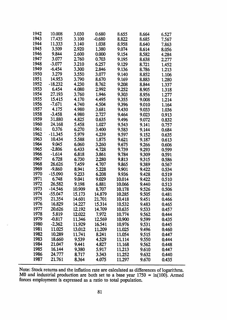
1942 10.008 3.030 0.680 8.655 8.664 6.5271943 17.435 3.100 -0.680 8.822 8.685 7.5671944 11.333 3.140 1.038 8.958 8.640 7.8631945 3.509 2.920 1.380 9.074 8.614 8.0561946 9.844 2.600 0.000 9.154 8.582 4.2841947 3.077 2.760 0.703 9.195 8.638 2.2771948 -3.077 3.210 6.257 9.129 8.721 1.4521949 -6.454 3.300 2.846 9.136 8.786 1.2131950 3.279 3.550 3.077 9.140 8.852 1.1061951 14.953 3.790 8.670 9.169 8.883 1.2801952 -18.232 4.230 8.762 9.208 8.844 1.3371953 6.454 4.080 2.992 9.252 8.905 1.3181954 27.193 3.760 1.946 9.303 8.956 1.2771955 15.415 4.170 4.495 9.355 9.008 1.2141956 -7.671 4.740 4.504 9.396 9.010 1.1641957 4.175 4.980 3.681 9.430 9.033 1.0361958 -3.458 4.980 2.727 9.464 9.023 0.9131959 31.880 4.825 0.635 9.496 9.072 0.8321960 24.168 5.458 1.027 9.543 9.141 0.7571961 0.376 6.270 3.400 9.583 9.144 0.6841962 -11345 5.979 4.239 9.597 9.152 0.6351963 10.434 5.588 1.875 9.621 9.187 0.6131964 9.045 6.060 3.260 9.675 9.266 0.6061965 -2.806 6.433 4.728 9.739 9.293 0.5991966 -1.614 6.818 3.861 9.784 9309 0.5911967 6.728 6.730 2.280 9.813 9.315 0.5861968 26.626 7.459 4.707 9.865 9.389 0.5671969 -9.860 8.941 5.228 9.901 9.422 03341970 -15.090 9.233 6.208 9.936 9.428 0.5191971 6.748 9.041 9.029 10.014 9.422 0.5101972 26.582 9.198 6.881 10.066 9.440 0.5131973 -14.546 10.909 8.707 10.178 9.526 0.5061974 -55.047 15.173 14.879 10.285 9.505 0.4811975 21.354 14.601 21.701 10.418 9.451 0.4661976 16.829 14.227 15.314 10.532 9.483 0.4651977 20.626 12.192 14.709 10.635 9.533 0.4571978 5.819 12.022 7.972 10.774 9.562 0.4441979 -0.817 11.346 12.569 10.900 9.599 0.4351980 -2362 11.929 16.541 10.976 9.531 0.4451981 11.025 13.012 11.209 11.025 9.496 0.4601982 10.289 11.741 8.241 11.054 9.515 0.4471983 18.660 9.539 4.529 11.114 9.550 0.4441984 21.047 9.441 4.827 11.168 9.562 0.4481985 16.144 9.380 5.917 11.213 9.610 0.4471986 24.777 8.717 3.343 11.252 9.632 0.4401987 21.761 8.364 4.075 11.297 9.670 0.435
Note: Stock returns and the inflation rate are calculated as differences of logarithms. MO and industrial production are both set to a base year 1750 = ln(100). Armed forces employment is expressed as a ratio to total population.
81
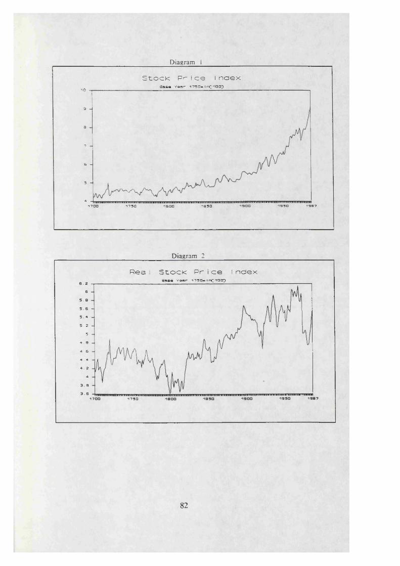
Diagram 1
Stock Pr i ce IndexB ase Y »ar 1 7 3 0 - l nQ 700}
10
9
9
7
6
3
4 in»im i i a i m i m r»rm m i m i » i i i m i n i i i m B ii im inrnm »itTi1700 1730 1500 1530 7900 7930 1957
Diagram 2
Reai Stock Pr i ce Index5 a s a Y aar i7 3 0 » in £ l0 0 22
6a
64
2
59S
4
24
a
6 mntiMmmmai7730
82
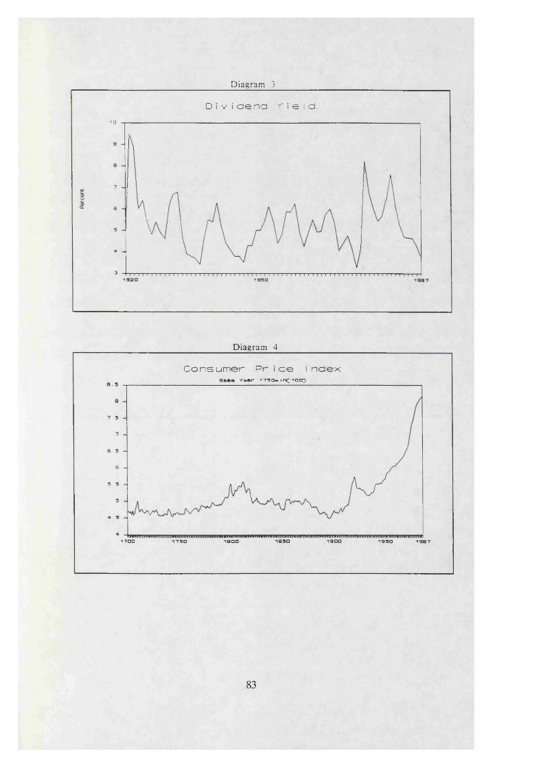
Diagram 3
Di v i d e n d Y i e l d10
1950
Diagram 4
Consumer Price indexq&ba Y ear 1 750—I 1 0 0 5
7 . 5
1700 175 0 1900 1SSO 1900 1950 1997
83
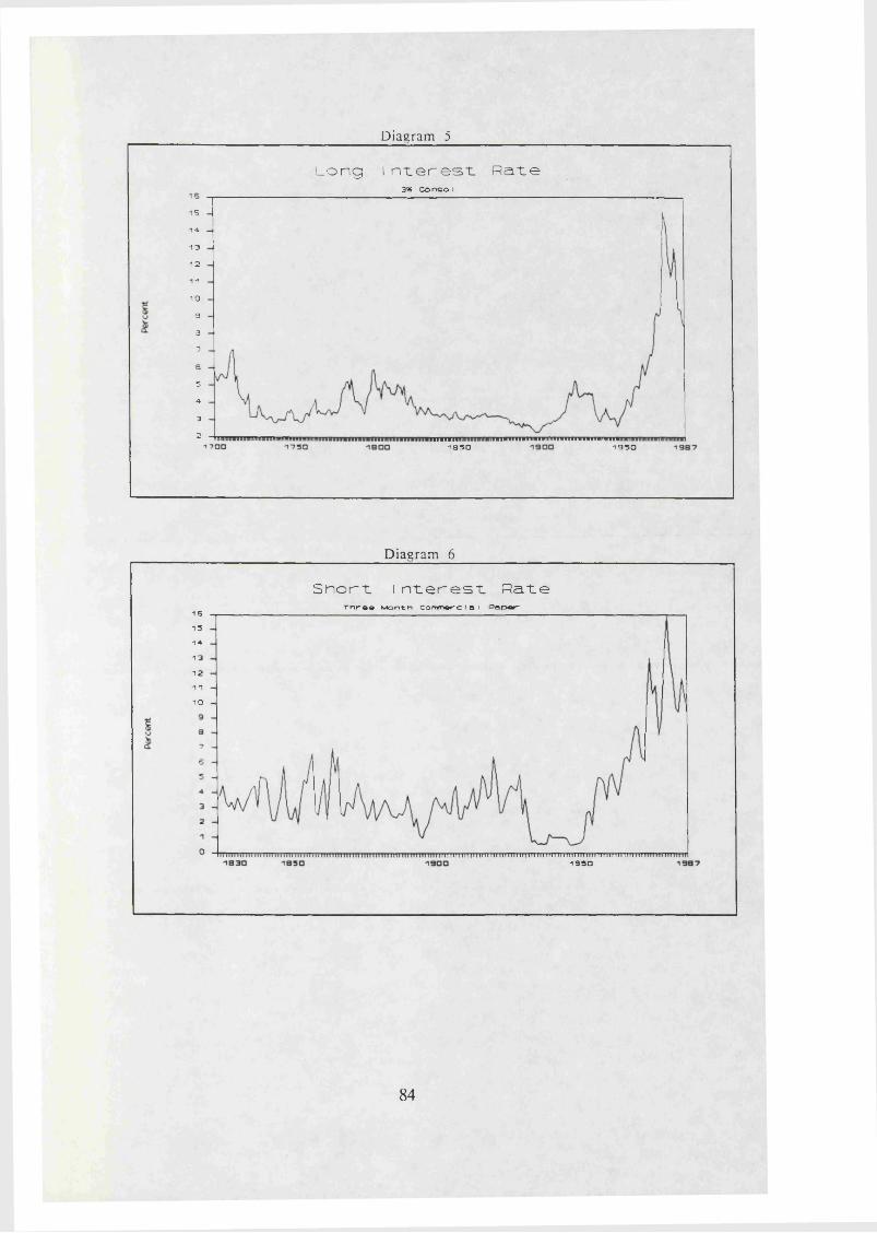
Diagram 5
Long Interest Rate3* Conso i
5
4
13
12
1
10
3a
7
65
4
3
21330 1350
Diagram 6
Shorn i nterest RateT rtr«» M ontn Conm arc I a i Pops®''
1 6
1 3
1 4
1 3
12
11
10
m i m i iii iii m i i ii iii m i iii iii iii in i ii i n i mi ii n ii m i in i in ii r1930
8 4
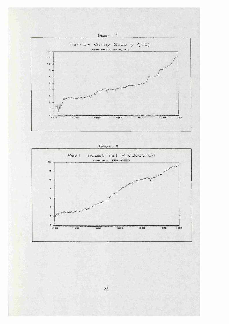
Diagram 7
N a r r o w Money S u p p l y (IN/102)B&sa v a a r 1 7 3 0 - I n r 'lOCT)
1 -I
TO
a
7
6
4
3
217DO 1730 7BOO 1B3D T9DO 193Q 19B7
Diagram 8
Reai Industri a I Producti onb & b « v a a r t 7 3 0 — I r<; TOCT)10
8 5
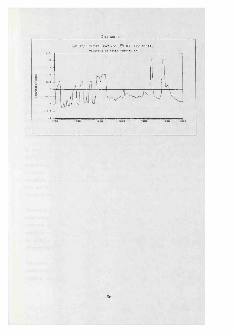
Diagram 9
Army a n d N a v y E m p l o y m e n tn o i a t i v o t o r o t a i P o p u l a t i o n
5
2
5
30
3
1
3
2 im n » n i i i i » i n » i i » n m n « i i i i n in n m » n i»iinim Mn i1BQQ 1BSO
8 6
Chapter III: Stock Prices and Financial Crises
I. Introduction
The present chapter examines financial market crashes and crises from a historical perspective, rather than focusing strictly on the 1987 event as did Chapter I. A
statistical methodology is used, as in the rest of the thesis, in contrast to the descriptive and anecdotal approach common to the study of these historical
incidents.1 The chapter examines market crises using British time series data from 1700 to the present, and then employs various models using macroeconomic variables
to extract a measure of relative speculative behaviour. While the analysis is somewhat rough and ready, due to the use of annual data and disagreements
amongst economists on what constitutes a market crash or crisis, it does provide a starting point for more detailed studies in the future.
In brief, the chapter concludes that macroeconomic variables are important for driving stock price fluctuations, but can by no means account for the bulk of such movements. The efficient and non-efficient market models developed here appear to operate equally well during crisis and non-crisis years, with only a handful of exceptions related to periods of market crashes. These exceptions account for less
than one fifth of all observed financial crises since 1700 and have mostly been described in the historical literature as arising from excessive speculative activity.
There may, therefore, be some support for the existence of speculative bubbles or
other non-efficient market behaviour unrelated to macroeconomic variables. The last statement remains tentative, however, because the evidence is indirect and may
equally be a function of model misspecification or omitted fundamentals. In any case, the ability of lagged variables to explain stock returns is direct evidence of nonefficient market behaviour related to macroeconomic variables.
The outline of the chapter is as follows. The next section distinguishes two views of market crashes based on fundamental and non-fundamental factors, while Section III
explores some definitional considerations. In Section IV, the impact of
87

macroeconomic variables is assessed for normal stock market behaviour. Three such models are presented: one based on news to the market, one unrestricted
multivariate autoregression and one restricted model with an error correction
mechanism; the first model adheres to the efficient markets hypothesis but the latter
two deviate from this theory by using lagged variables to predict stock returns. Sections V and VI set out a chronology of financial crises and then apply the
estimated models to periods of crisis which have experienced marked prior equity price appreciation. Finally, Section VII concludes the chapter.
88
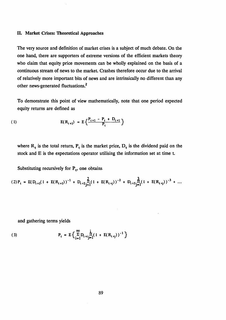
II. Market Crises: Theoretical Approaches
The very source and definition of market crises is a subject of much debate. On the
one hand, there are supporters of extreme versions of the efficient markets theory
who claim that equity price movements can be wholly explained on the basis of a
continuous stream of news to the market. Crashes therefore occur due to the arrival
of relatively more important bits of news and are intrinsically no different than any other news-generated fluctuations.2
To demonstrate this point of view mathematically, note that one period expected
equity returns are defined as
where Rt is the total return, Pt is the market price, Dt is the dividend paid on the stock and E is the expectations operator utilising the information set at time t.
Substituting recursively for Pt, one obtains
( l )
and gathering terms yields
(3)
89
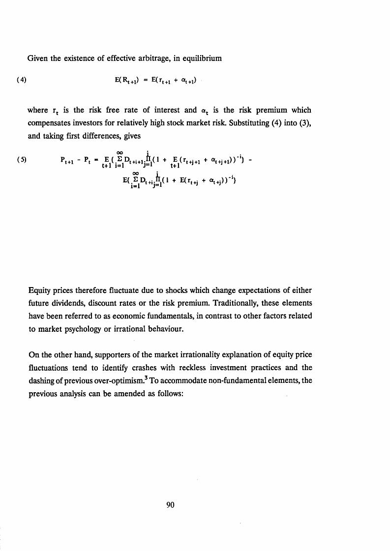
Given the existence of effective arbitrage, in equilibrium
(4) E(Rt+i) = E(rt+1 + ot+1)
where rt is the risk free rate of interest and at is the risk premium which compensates investors for relatively high stock market risk. Substituting (4) into (3),
and taking first differences, gives
Equity prices therefore fluctuate due to shocks which change expectations of either future dividends, discount rates or the risk premium. Traditionally, these elements
have been referred to as economic fundamentals, in contrast to other factors related
to market psychology or irrational behaviour.
On the other hand, supporters of the market irrationality explanation of equity price
fluctuations tend to identify crashes with reckless investment practices and the dashing of previous over-optimism.3 To accommodate non-fundamental elements, the
previous analysis can be amended as follows:
90
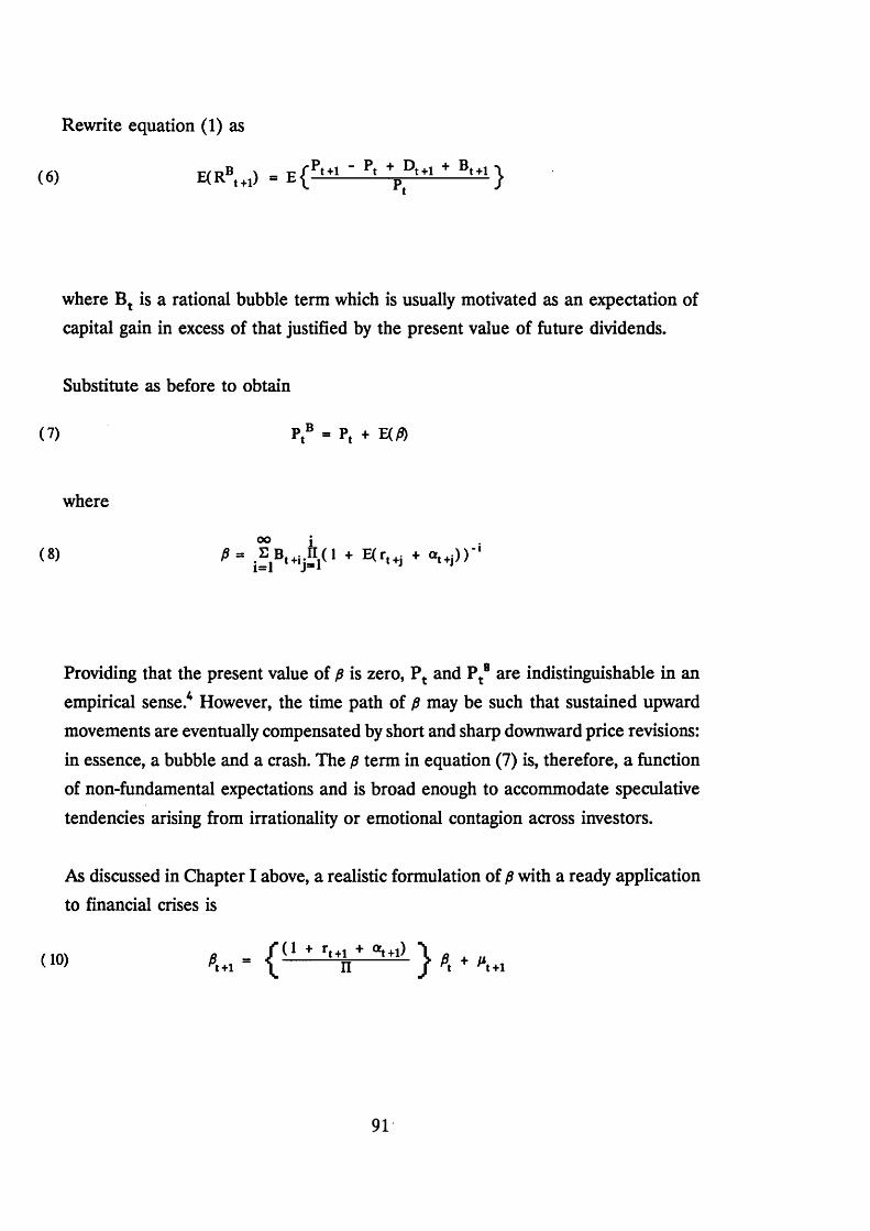
Rewrite equation (1) as
(6 ) E (R B, t l ) ~ E { P ,t l ' P' +ptP , t l + B ,t l }
where Bt is a rational bubble term which is usually motivated as an expectation of capital gain in excess of that justified by the present value of future dividends.
Substitute as before to obtain
Providing that the present value of p is zero, Pt and PtB are indistinguishable in an
movements are eventually compensated by short and sharp downward price revisions:
in essence, a bubble and a crash. The p term in equation (7) is, therefore, a function of non-fundamental expectations and is broad enough to accommodate speculative
tendencies arising from irrationality or emotional contagion across investors.
As discussed in Chapter I above, a realistic formulation of p with a ready application
to financial crises is
(7) P ,B - P , + E(/9)
where
oo i( 8)
empirical sense.4 However, the time path of p may be such that sustained upward
(10)
91
or t̂+l t̂+i
The first equation occurs with probability x, while the second occurs with probability
(1-ir). x is defined as the unconditional probability that the bubble continues while
(1-ir) is the associated probability of a crash; is IID with mean equal to zero. The term ( l+ r t+at)jr‘1 is greater than ( l+ r t+crt) during the duration of the bubble in
order to compensate for the risk of the bubble bursting.
Alternatively, a broader interpretation of the p term in equation (7) ties market behaviour more strongly to a social and psychological structure responding to
changing economic conditions. The essence of this school of thought can be succinctly described by a process of "(p)rosperity, boom, crisis, slump, and recovery
succeed(ing) each other with a regularity that suggest(s) inevitability".5 The stock
market is characterised here as an intrinsic element of cyclical fluctuations in the general economy and, due to uncertainty and the liquid nature of the market, is a medium for amplifying pervading waves of mass euphoria and depression.
Kindleberger (1978) catalogues dozens of these speculative episodes since the early 18th century in Europe and the United States. In general, following Minsky (1977), he argues that market crises are the ultimate consequence of the credit structure in
advanced capitalistic economies. Firms go through several stages of liquidity and
financial structure over the business cycle, with financial fragility increasing at each
stage as debt loads are increased. The boom conditions set off by a positive economic shock are reinforced by investment and speculative behaviour until it
becomes apparent that expectations are excessive with respect to sustainable real growth. The process then unwinds with bankruptcy, credit contraction and downward
revaluations of asset prices. Once the nadir is reached, the cycle turns up once more based on healthier firm balance sheets and the progressive lack of investor inhibition
regarding reinvestment in securities.6
92

In conclusion, several approaches can therefore be differentiated in any discussion
of financial market crashes or crises. The efficient markets school argues for rational
investor behaviour and the importance of economic fundamentals, while the non
fundamentals approach stresses the roles of self-fulfilling expectations and social interaction; the latter approach can also be distinguished between independently generated rational bubbles and broader speculative tendencies which arise out of the
economic cycle. In this chapter, such non-efficient market behaviour is classified into
two categories, according to whether or not it is linked to macroeconomic
information. Lastly, there may be a role for irrationality in the market; however, it
is difficult to test for such aberrant behaviour using traditional economic techniques.
In what follows below, it will be seen that these broad crash determinant stories are all partially supported. In some circumstances, it seems that pre-crash returns can be explained by an efficient market model, while in others, it appears that nonefficient market behaviour linked to macroeconomic variables is more appropriate. Finally, when neither of these two classes of models are helpful, it may be that rational bubbles, speculation or irrationality unrelated to the real economy are motivating the pre-crash share price increases. The historical narrative record and the nature of the data used here both conspire against reaching sharp conclusions.
93

III. Market Crises: Definitional Considerations
Thus far, we have discussed stock market price determinants and crashes in a loose
generic sense. There are considerable differences, however, on the definition of the
point where relatively ordinary price movements degenerate into market crashes.7 Common terms used when describing events akin to the 1987 price revaluation
include bubble, crash, crisis, distress, deflation, mania and panic.
Bubble and mania are synonymous and have been discussed above as either
mathematical constructs or terms used to describe excessive valuation of assets
relative to long term sustainable levels. The terms crash, panic and (sharp) deflation typically refer to situations where relatively large price revisions occur over a
relatively short time span.
Crisis and distress refer primarily to the follow on effects of the crash. First, there is typically a flight to liquidity by investors and a commensurate raising of risk
premiums on all lesser liquid assets. Secondly, this increased demand for liquidity may prompt illiquidity within the banking and financial system as calls on loans, credit rationing and bank runs become widespread. Lastly, general economic activity may be affected by instability in the credit system, increases in the cost of capital and wealth effects issuing from the price revaluation.8
The view taken here is that all of these events either describe or impact upon the
stock market through the functioning of arbitrage relationships between credit and
other financial assets and through the linkages between investor sentiment in industry
and the stock market. Therefore, an encompassing approach will be taken here by
examining all such incidents described in the historical literature. A consequence of this approach is that the terms defined above will be used interchangeably
throughout the chapter.
Before setting down a crisis chronology and examining any common tendencies, it is appropriate to examine the extent to which macroeconomic variables drive the
equity market in every day circumstances and then move from there to an
94

examination of such influences at times of crisis. The base models developed will be used to test the extent to which the efficient markets view is appropriate, recognising
of course that unexplained residuals can stem from inadequate model specification,
unobserved fundamentals or non-fundamental speculative tendencies in the market.
95
IV. Stock Returns and Macroeconomic Information
This section examines the explanatory power of various macroeconomic magnitudes
for stock returns in the United Kingdom since 1700. The variables examined are the
growth rates of real industrial production and the real monetary base, consumer price inflation, long and short term interest rates and the ratio of armed forces
employment to the general population.9 These measures will be correlated to various definitions of equity returns using three different modelling strategies: a vector
autoregression (VAR) news generating process, an unrestricted multivariate autoregression employing lagged, current and leading values and a restricted error
correction model. As will become apparent, all three approaches yield similar results in terms of the influence of macroeconomic information on the stock market.
Table 1 describes the data and suggests a useful partition that will be employed elsewhere in the chapter. The most important split in the series comes after 1913, with the end of the classical gold standard and the start of World War I. A second split occurs after 1949 with the end of post-war price controls and the beginning of the reintroduction of market forces to financial markets. Following 1913, it can be
seen that the levels of inflation and interest rates increased markedly, as well as the
volatility of equity returns and interest rates. The use of the 1913-1987 sample disguises the weak and volatile nature of industrial production in the wartime and interwar period but is necessary in what follows in order to preserve the degrees of
freedom required for a robust VAR investigation. The last point to note is the negative average equity premium; this occurs due to the absence of a full sample
dividend yield series which would restore the equity return series to its correct
positive value.10
Tables 2 to 4 present the results from the first model, a VAR news generation
mechanism which is consistent with efficient market prescriptions. Relative to the other models to come, this approach uses a limited set of information; it therefore
unsurprisingly produces the weakest results in favour of the fundamentals view of equity pricing. Briefly, the approach is as follows. First, a VAR system is constructed
using the five macroeconomic variables and squared stock returns to proxy for risk.
96
Secondly, the residuals from each VAR become the news variables which are entered into the equity return equations shown in Tables 2 to 4.11
Throughout the three tables, one sees that interest rate shocks are the predominant
elements correlated with equity returns, followed by industrial production and
inflation shocks. All coefficients are of the appropriate signs except for the poorly
determined armed forces variable, which is positive in the earliest period.12,13 The size of the coefficients generally rise from the early to the later period, with the exception of the inflation term in the real return equation and interest rates. In spite of this, the adjusted R squared value declines over time. Altogether, macroeconomic
news accounts for up to one third of equity price variability and depends on a news generation process using information no more than two years old, as evidenced by
the rapidly declining adjusted R squared values as further lags are added to the VARs. We see, therefore, that in a limited information model, the efficient markets theory produces sensible coefficients but leaves the bulk of market fluctuations unaccounted for across both crisis and non-crisis years.
The other end of the modelling spectrum is investigated in Table 5, which excludes
full sample results because of their similarity to those shown in the table. Following Cutler et al (1988), adjusted R squared values are given for multivariate autoregressions of equity returns on macroeconomic variables.14 The first column shows the results using lagged values only and the other two columns progressively
add current and next period variables. The aim here is to set a notional upper limit to the explanatory power of macroeconomic factors by including current and future
values, in contrast to the sparseness of the news regressions above. Since lagged
variables are used to predict stock returns, this model and the restricted error
correction model to come are evidence of non-efficient markets behaviour linked to macroeconomic variables.
Once again, the short equity premium produces the weakest results, especially for
regressions including only lagged variables. The inclusion of leading variables makes
very little difference to the explanatory power, except in the case of the short equity
premium prior to 1913. In contrast to the news regressions, macroeconomic
97

information now accounts for up to one half of equity price variation. This explanatory power is likely overstated due to the use of averaged variables but is understated to the extent that other important variables, in particular dividends, are
excluded from the regressions.
Tables 6 and 7 show the results of a restricted equation augmented with an error
correction mechanism. The integration results shown in Table 6 indicate that all of the variables aside from armed forces employment are integrated of order one. It is
therefore appropriate to use first differences of the variables in the restricted equation, as has previously been done with the other two models. The cointegrating
equations also suggest that long term bilateral equilibrium relationships exist between
stock prices and these variables, with the exceptions of long interest rates and the armed forces ratio to total population. As seen in the sixth row of the table, all of the variables are jointly cointegrated with stock prices.15
Table 7 indicates that the estimated coefficients of the final restricted regression are well specified and that the equation passes standard diagnostic tests.16 The steps taken to impose linear and exclusion restrictions on the general specification may be
retraced by examining the table from left to right and by studying the F test statistics at the bottom. Note that the data favour a specification in second differences, indicating that the equity return series is correlated to acceleration terms as well as to the long term level effects embodied in the error correction term.
The exclusion of the armed forces employment and industrial production variables
in acceleration form may be an indication that the stock market responds more closely to financial factors expressed in this way, like money supply, interest rates and
inflation, rather than to variables more closely linked to the real economy; if this is generally true, the Fisher/Minsky/Kindleberger means of shock transmission at times
of accelerated activity may operate primarily through the financial system rather than
the real economy. Another point to note is the gold standard dummy variable which
accommodates the switch in monetary institutions that took place this century. It mainly acts to segregate the effects of inflation on equity returns into a completely
neutral gold standard period and a strongly negative period off of the gold
98
standard.17
The restricted equation coefficients indicate that accelerations in interest rates and inflation are detrimental for equity returns, while acceleration in the real money base
is positively correlated. The existence of effective arbitrage and the theoretical literature on the costs of inflation support the first finding, while the second can
possibly be explained as a short term response to easing of monetary conditions. The error correction term is well specified in all of the equations shown in Table 7 as the
value -.07 and implies that equity returns converge to long term equilibrium with the
macroeconomic variables after periods measured in decades. Finally, the R bar
squared value, though small in magnitude, is comparable to the VAR results
discussed above.
All in all, we have developed three different models of equity returns in this section. Each specification has its own merits in terms of theoretical plausibility and empirical fit and the hope is that the three approximate the spectrum of modelling possibilities in a parsimonious manner. The models will now be used to investigate whether macroeconomic information is the predominant factor in explaining equity returns prior to crises or whether there is a large residual which may be attributable to rational bubbles or other non-efficient markets behaviour divorced from the macroeconomy. In addition, since the restricted model incorporates only financial factors, it may be possible to indicate wh'ere prior returns are generated by real or financial variables by comparing the restricted model results with the more fully
encompassing VARs.
99

V. Financial Crisis Chronology
The preceding section concluded that efficient and non-efficient market models of equity pricing can account for up to one half of market fluctuations. While this
establishes the importance of macroeconomic factors, it still leaves a rather large unexplained residual. In addition, it does not directly examine periods when market
crashes have occurred, dissimilar as they seem to be to more stable periods. This section will therefore outline a chronology of financial crises and discuss the
preceding economic and market activity that may have prompted the crashes.
Table 8 lists the years, sources and purported causes underlying British crises since
1700. As the definitional section above made clear, there is little agreement on the
essence of a crash and so any reference to a crash or panic that was found in the relevant sources is included in the table. Even if some of these years did not produce
market movements on the scale of October 1987, the fact that crises, crashes or signs of distress were noted is sufficient to consider whether there were measurable predeterminants underlying the events. For, if a rational bubble story of crashes is correct, it is reasonable to think that there is a sustained period of excessive
speculative activity prior to a crash or crisis.18
As can be seen from the sources column, there is not a great deal of overlap between different accounts. Morgenstem (1959), in particular, lists a number of stock
market crashes which are not mentioned elsewhere but he unfortunately does not provide original sources. It is also difficult to give an exact date for each crisis
because of conflicting narrative accounts, sometimes even from the same source.19 One should therefore not be overly confident that any individual account is
authoritative.
The origins of the crises seem to fall into at least four categories: threat of war, international transmission, excessive speculation and feedback from the real
economy.20 While the first two are presumably verifiable on the basis of historical record, the latter two are somewhat subjective; the third explanation, especially, could be attributed without evidence to almost any market crisis. It is therefore
100

necessary to examine the prior movements of the market to determine whether a potential rational bubble or other non-efficient market behaviour divorced from the
real economy existed in prices prior to a crash.21
A number of points can be made about the a priori evidence from Table 9.22 First, relatively few of the crises were preceded by substantial price appreciation. Of the
41 listed crisis years, only 12 show 1, 2 or 5 year prior returns which are statistically different from the sample averages at conventional significance levels.23 A number
of crises, for example those of 1816, 1878 and 1904, are actually preceded by
substantial and sustained price declines; in this vein, the importance of inflation
adjustment is seen in the cases of 1921 and 1974. Second, the equity return from the
crisis to the following year, shown in the first column and demonstrating the relative
magnitude of the crash, is usually substantial and negative. The most eventful years in terms of market decline appear to be 1720,1797,1866,1921,1929,1940,1973 and 1974; looking back to Table 8, it appears that the there is, however, no common causal element linking these years. A last point to note is the weak effect seen in the returns series for some years; either the crash was of small magnitude or else the
market rebounded substantially within the crisis year.
In general, it appears from this simple examination that the rational bubble theory, like that based on the use of macroeconomic variables in efficient and non-efficient market models, can have at most only partial application to financial crashes. We
turn now to a more sophisticated examination of the cases where prior speculation
may have been in existence in order to measure the relative importance of macroeconomic factors during the years prior to market crashes.
101
VI. Estimated Models and Market Crises
The segregation of returns prior to crises into elements related to, and separate
from, macroeconomic variables employs the three models developed in Section IV
above. Three points should be stressed in what follows. First, the failure of macroeconomic factors to account for excessive equity*retums prior to crisis years
can be attributed to either non-efficient market explanations unrelated to the real economy, or else to misspecified or missing variables in the estimation equation.
Second, the models being used should not be interpreted as belonging to the investors’ information set at the onset of each crash; rather, the fitted equations
represent long term relationships which the crisis and non-crisis years alike should match if they are generated by the same underlying data generation process. A more detailed study utilising higher frequency data will be required to investigate models
which satisfy information orthogonality with respect to returns.
Third, the residual returns which are generated by the estimated models test a null hypothesis that there is no significant difference between the model residuals generated over the full sample compared to those prior to times of financial crisis, against an alternative that such prior returns are significantly greater than the sample
average. The test is therefore robust to examining rational bubbles, which are generally thought to be positively trending, but is not appropriate for testing nonefficient market behaviour divorced from the real economy, such as noise trading, which does necessarily produce positive autocorrelation of returns.
Tables 10 and 11 present the results for the macroeconomic news model.24 The returns shown are estimation residuals aggregated over 1, 2 and 5 years before a
given crisis year; they are therefore directly comparable to the actual returns in
Table 9. Of the 15 cases selected from that table,25 roughly one half show evidence
of residual returns that are significantly greater than the average produced by the
news model; the macroeconomic news model therefore fails to account for the substantial rise in the market prior to the crises in these years. Only the crises of 1720,1763,1836 and 1973 follow the expected rational bubble pattern, however, with
102
the strength and significance of the residual return increasing from 5 or 2 years before the crash to the event itself. All of the others either peak more than two years before the crash or are too small in magnitude; in either case, the rational bubble theory is not easily supported without substantial modification to account for time
lags in speculative response to the bull market peak.
Table 12 extends the same analysis to the unrestricted multivariate autoregression model, which falls under a non-efficient market paradigm.26 Less than half of the
potential rational bubble generated crashes now display residual returns which are excessive from the point of view of the estimated model. In addition, those residuals
which are greater than the average do so at a lower level of significance. The years which follow an expected rational bubble pattern, with significance levels increasing
as the crash draws nearer, are restricted, as before, to 1720, 1763, 1836 and 1973. The 1987 crash is notable not only for the fact that it culminated the greatest bull market since 1700, as seen in Table 9, but also that this run is largely explained by the estimated model. In support of the results from Chapter I, it is therefore difficult to resort to a bubble explanation for most of the price appreciation prior to 1987.27
Turning now to Table 13, one sees that the restricted model produces the same general conclusions as the other two models. Approximately two thirds of the years exhibit evidence of significant residual activity, although typical rational bubble behaviour is limited to 1720,1763,1825 and 1973. In common with the nominal news
model, 1987 appears to be a crisis year where excessive returns developed two years prior to the crash. Given that the other models indicate that 1987 was not unusual
in real terms, it may be that the possible rational bubble suggested by this table and
by the nominal returns analysis of Table 11 was generated by real macroeconomic
factors which are excluded from the models underlying these tables.
Tables 10 to 13 have uncovered a number of crisis years when the macroeconomic models are not able to account for prior returns. In years such as 1715, 1847 and
1895, when prior residual returns are statistically excessive only under the restricted (financial) model and the nominal news model, but not when generated by the other
models, it may be that real macroeconomic factors are determining the equity return
103

process.
In the case of 1836, the residual returns are higher than normal only under the news and unrestricted multivariate autoregression models. This result may indicate that the
returns are generated by financial factors which the restricted model is able to explain.
The last permutation, where excessively positive returns are found under all three
models, applies most strongly to 1720, 1825 and 1973 and, with provision for lags in response to speculative activity, 1866 and 1873. In these cases, the way is open for
explanations ranging from rational bubbles to irrational mania and delusion. It is noteworthy that the efficient market model, using only macroeconomic news, and the
non-efficient market models which incorporate lagged variables, are in broad agreements on the years which are unexplained by macroeconomic information.
VII. Conclusions
The conclusions of the chapter can be summarised as follows.
First, there seems to be a structural break in the British economy’s underlying data generation process after 1913. This may be related to the expiration of the classical
gold standard at that time and the subsequent introduction of substantive government fiscal and monetary policies. In any case, it is important to account for structural
change in institutions over the period 1700 to present in any examination of the stock market.
Second, macroeconomic factors account for up to one half of fluctuations in equity
market returns; the unexplained residual element from all of the models is, therefore, rather large. The unrestricted multivariate autoregression model provides the best data fit, albeit at the cost of theoretical rigour, while the poorest fit comes from the news model using long variable lags. In general, most macroeconomic information is embodied in variables with lags no longer than two periods. The success of models which use lagged variables to explain equity returns suggests that the efficient markets hypothesis cannot fully explain such returns.
Third, a comprehensive list of financial crises of all types reveals that these are triggered by a number of factors. Those preceded by substantially positive equity returns are relatively few, amounting to approximately one third of the total since
1700. When the estimated models are applied to explaining this subset of crises, there is strong evidence for possible rational bubble-like activity unrelated to
macroeconomic variables in only three years: 1720, 1825 and 1973. The other crisis
years for which prior returns are high are explained by real or financial factors or
else reach a peak in returns more than two years before the crisis.
The dichotomy between the fundamental and speculative explanations of market
crises is not, therefore, completely resolved. On the one hand, the macroeconomic variables models account for less than half of the fluctuations in the equity market.
On the other hand, there seem to be only a handful of potential rational bubbles
105

over the three centuries under examination which cannot be explained by the macroeconomic models. A more detailed study utilising disaggregated and higher
frequency data will, therefore, probably be needed to eventually resolve the issues
examined here.
106

1. Three important exceptions are Zamowitz (1989), Garber (1989) and the contributors to the Capie and Wood (1986) compilation of papers on financial crises.
2. See Fama (1970) on the traditional definitions of market efficiency with respect to news and Hardouvelis (1987) and Jain (1988) for empirical estimates of the reaction of stock prices to macroeconomic news.
3. See Fisher (1933), Minsky (1977) and Kindleberger (1978) for a detailed exposition of this theory of asset pricing.
4. Indeed, Summers (1986) shows that the power to distinguish between random walk pricing processes generated by a fundamentals model and a pricing profile generated by an autoregressive bubble process is very weak.
5. Ashton (1959), p. 136.
6. One empirical application of Minsky’s theory for the recent evolution of the Canadian economy is found in Seccareccia (1988).
7. It may seem somewhat odd that rapid upward revisions to price levels are not treated with the same seriousness by economists that similar downward movements provoke. Within the stock market, there are always two sides to any bargain and, following a price change, the ex post gain of one investor (the seller or purchaser of the stock) is had at the expense of the other (the buyer or seller of the stock); this state of affairs obviously holds for both upward and downward price movements.
The asymmetry of interest on this question is probably related to the knock-on economic effects of crashes on confidence, monetary stability and investor wealth. As well, Kahneman and Tversky (1979) note that subjective valuations of capital gains and losses differ, with the perceived marginal cost of the latter higher than the perceived marginal benefit of the former; investors therefore tend to focus more attention on market downturns. Lastly, downward revisions to aggregate investor wealth may run up against collateral or other liquidity constraints which prompt investors to sell further assets and therefore reinforce the original price decline. On upward ticks, the regret felt on the part of the investor on the "wrong” side of the bargain is in terms of unrealised accretions to wealth; the only liquidity constraint here is the opportunity cost of foregone investments which could have been funded from the higher ex post equity valuation.
8. An early distinction between panics and crises is found in Powell (1913), where the latter is characterised by financial illiquidity in the financial system and the former describes the emotional panic experienced during the crisis. Schwartz (1986, p. 11) suggests a division between financial and pseudo-financial crises (or distress) by arguing that the former is short-lived and is "fueled by fears that means of payment will be unobtainable at any price", while the latter may be drawn out over time and is "a consequence of restricted growth of bank reserves but is not precipitated by the public’s behaviour". Hoppit (1986) likewise makes a distinction for 18th century British crises between those related to public finance, typically of a local nature with a London locus, and those impinging more directly on private (business) finance. As the 18th century progressed, crises apparently became more far reaching in effect due to the growth of the provincial banking system and of the financial and economic connections between London and other regions.
107

9. The data are described fully in Appendix I above and are all expressed in natural logarithms, with the exception of interest rates. It has been necessary to use annual averages in order to obtain a full sample from 1700 to the present; as a result, the estimated regressions specify correlations between averaged variables and do not examine the random behaviour of the underlying data generation process.
10. Most recent research indicates that dividends are a relatively smooth series over time, in contrast to the volatility of equity prices, cf. Marsh and Merton (1987). If this observation is assumed to hold for the full sample, it is likely that the absence of the dividend-price ratio does not alter our results substantially. As noted in Appendix I above, consistent dividend yield data are available only from 1919.
11. Formal LM(2) tests for autocorrelation of these residuals show that a null hypothesis of a random process against an AR(2)/MA(2) alternative cannot be rejected. As shown in the Memorandum items in Tables 2 to 4, the highest F-test value of 1.34 was that for short interest rate news, a value which is insignificant at conventional levels.
12. This variable is both a proxy for government expenditure, and therefore pressure on financial markets for funds, and for wartime effects on the stock market. Prior to the most recent period, British governments financed wartime expenditure by issuing debt since conventional means of raising revenue, in the absence of widespread taxation, were inadequate during times of stress, cf. Dickson (1967). The manpower variable is used here in preference to a series based on actual expenditure because of data limitations.
13. The changing coefficients on the inflation variable before and after 1913 may be related to the shift in monetary institutions which occurred at that time. See Chapter II above for a fuller discussion of this and related issues.
14. In contrast to Cutler et al (1988), all of the included variables are stationary, a prerequisite for applying standard asymptotic theory to VARs. Column 1 regresses stock returns on lagged macroeconomic values and squared returns, column 2 adds current macroeconomic values and column 3 adds one period ahead macroeconomic values.
It should be noted that the absence of a dividend yield series substantial biases downward the explanatory power of the equations, given the result in the Cutler et al paper that the dividend yield is usually the most important explanatory factor for historical U.S. real returns. It is therefore likely that the explanatory power of the macroeconomic variables would be considerably higher if additional data were available.
15. Further investigation of the relationship between interest rates and stock prices revealed that cointegration is supported for 1705 to 1913 (t-statistic of -3.00 significant at 5% level) but is weaker for 1914 to 1987 (t-statistic of -2.63 significant at 10% level). The error correction mechanism from the cointegrating regression using all five variables is employed in the real stock return restricted equation below. Real returns are used in preference to nominal returns due to the stronger evidence for integration and cointegration.
16. The Chow test statistics support previous evidence indicating that there is a structural break after 1913. The full sample restricted equation is used, nevertheless, in order to examine crashes over time with a common model. The structural change has been
108
accommodated by using subsample means and standard deviations to calculate significance levels.
17. The gold standard dummy variable takes the value 1 from 1700 to 1797,1821 to 1914 and 1925 to 1932. The negative effect of inflation acceleration largely stems from the sharply different data generation processes at work before and after 1913: inflation was strongly mean reverting in the earlier period and highly persistent in the latter. The gold standard effect is not a proxy for a wartime effect, since appropriate dummy variables used to account for both interstate and global wars are not significantly different from zero at the 10 percent level. See Appendix I above for further details of these dummy variables.
18. Weil (1989) notes, however, that theoretical bubbles can be generated which lead to price declines, rather than increases. The intuition behind the result is that the presence of the bubble depresses the value of the fundamentals term by raising the discount rate to such an extent that total fundamental plus bubble return is declining over time. The notion seems to be impractical on a real world basis since it calls for negative interest elasticities of demand by savers. In addition, as a practical matter, the fact that annual values are used in this chapter means that bubbles which last for less than one year are generally undetectable.
19. For example, see the separate Kindleberger (1978) dates for the 1857 crisis.
20. It should be noted that there are multiple causes of many, if not most, of these market crises. The selection shown in the third column of Table 8 are merely those stressed by the relevant source.
21. It is also of interest to note that crises triggered by political factors are often unexpected and, therefore, not necessarily accompanied by prior speculation in the equity market. The crashes of 1761, 1914 and 1940 bear out this point.
22. Both nominal and real returns are shown in Table 9 for a number of reasons. First, standard economic theory implies that real magnitudes motivate investor behaviour. Second, given that crashes sometimes occur on a shorter time scale than the data at hand, the inflation element at a time of crisis may be irrelevant relative to the size of the equity price change. Third, as Table 1 demonstrates, there was a marked change in the inflation process after 1913 which upwardly biases nominal returns. The first and third reasons argue for analyzing real returns while the second supports examining nominal returns. In any case, the results using both approaches are broadly in agreement. It should also be noted that the relatively high volatility of real returns may be related to the influence of grain prices in the consumer price deflator.
23. Means and standard deviations were calculated for three periods, pre 1913, post 1913 and full sample, to account for changing economic structure. As well, previous year 1, 2 and 5 year equity returns were employed where the crisis occurred in the first half of the year or where it appeared that the peak of a potential speculative bubble occurred prior to the crisis year. In no case did these permutations alter the choice of years exhibiting statistically significant prior returns.
24. The full sample models for real and nominal stock returns are used to generate the residual returns.
109

25. The cases all demonstrate prior returns which are significantly greater than the sample average at the 10% level. As well, the crises of 1810, 1895 and 1901 have prior returns which are marginally significant at that level.
26. The analysis is identical for both nominal and real returns since each equation is a linear transformation of the other. The full sample model includes only one and two period lagged variables to generate the residual returns.
27. The large size of the residual does not, however, rule out the total absence of excessive speculative activity.
110
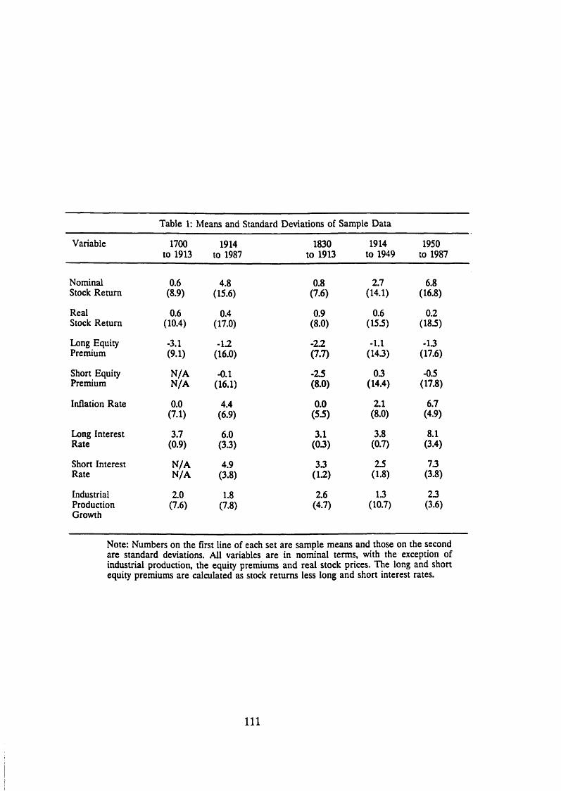
Table 1: Means and Standard Deviations of Sample Data
Variable 1700 to 1913
1914 to 1987
1830 to 1913
1914 to 1949
1950 to 1987
Nominal 0.6 4.8 0.8 2.7 6.8Stock Return (8.9) (15.6) (7.6) (14.1) (16.8)
Real 0.6 0.4 0.9 0.6 0.2Stock Return (10.4) (17.0) (8.0) (153) (183)
Long Equity -3.1 -1.2 -2.2 -1.1 -13Premium (9.1) (16.0) (7.7) (143) (17.6)
Short Equity N/A -0.1 -2.5 03 -03Premium N/A (16.1) (8.0) (14.4) (17.8)
Inflation Rate 0.0 4.4 0.0 2.1 6.7(7.1) (6.9) (53) (8.0) (4.9)
Long Interest 3.7 6.0 3.1 3.8 8.1Rate (0.9) (33) (03) (0.7) (3.4)
Short Interest N/A 4.9 33 23 7.3Rate N/A (3.8) (1.2) (1.8) (3.8)
Industrial 2.0 1.8 2.6 1.3 23ProductionGrowth
(7.6) (7.8) (4.7) (10.7) (3.6)
Note: Numbers on the first line of each set are sample means and those on the second are standard deviations. All variables are in nominal terms, with the exception of industrial production, the equity premiums and real stock prices. The long and short equity premiums are calculated as stock returns less long and short interest rates.
I l l
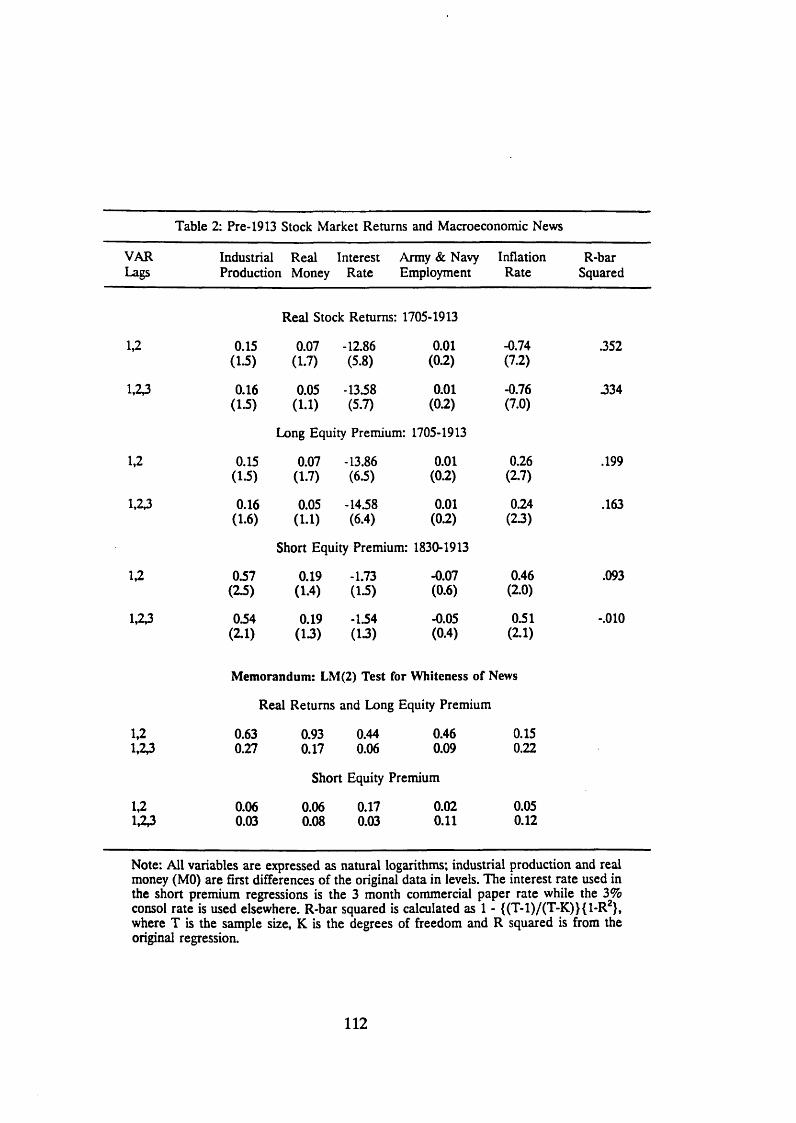
Table 2: Pre-1913 Stock Market Returns and Macroeconomic News
VARLags
Industrial Real Interest Army & Navy Production Money Rate Employment
InflationRate
R-barSquared
Real Stock Returns: 1705-1913
1,2 0.15 0.07 -12.86 0.01 -0.74 .352(1-5) (1.7) (5.8) (0.2) (7.2)
1,23 0.16 0.05 -13.58 0.01 -0.76 334(1.5) (1.1) (5.7) (0.2) (7.0)
Long Equity Premium: 1705-1913
1,2 0.15 0.07 -13.86 0.01 0.26 .199(1.5) (1.7) (6.5) (0.2) (2.7)
1,2,3 0.16 0.05 -14.58 0.01 0.24 .163(1.6) (1.1) (6.4) (0.2) (23)
Short Equity Premium: 1830-1913
1,2 0.57 0.19 -1.73 -0.07 0.46 .093(23) (1.4) (1.5) (0.6) (2.0)
1,23 0.54 0.19 -1.54 -0.05 0.51 -.010(2.1) (13) (13) (0.4) (2.1)
Memorandum: LM(2) Test for Whiteness of News
Real Returns and Long Equity Premium
1,2 0.63 0.93 0.44 0.46 0.151,23 0.27 0.17 0.06 0.09 0.22
Short Equity Premium
1,2 0.06 0.06 0.17 0.02 0.051,23 0.03 0.08 0.03 0.11 0.12
Note: All variables are expressed as natural logarithms; industrial production and real money (MO) are first differences of the original data in levels. The interest rate used in the short premium regressions is the 3 month commercial paper rate while the 3% consol rate is used elsewhere. R-bar squared is calculated as 1 - {(T-1)/(T-K)}{1-R2}, where T is the sample size, K is the degrees of freedom and R squared is from the original regression.
112
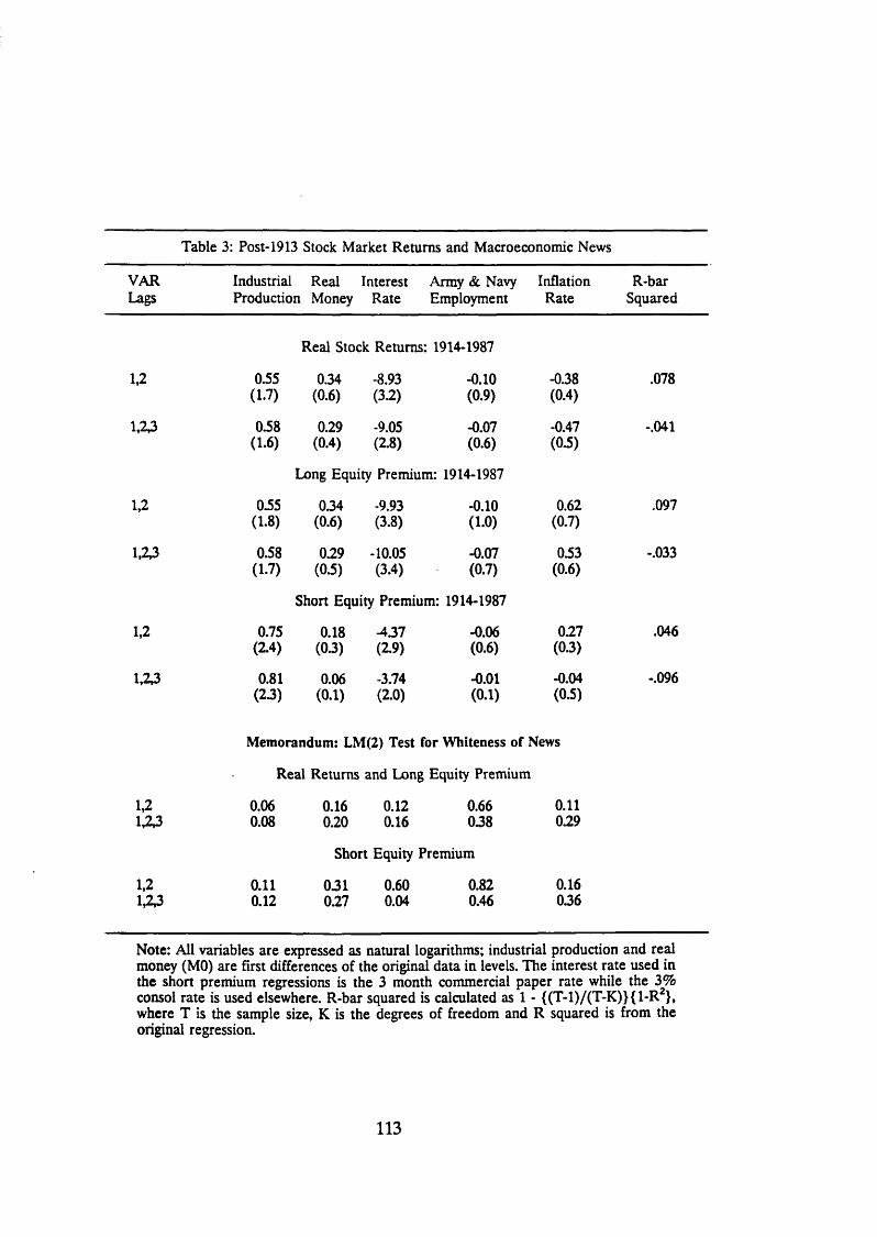
Table 3: Post-1913 Stock Market Returns and Macroeconomic News
VARLags
Industrial Real Interest Production Money Rate
Army & Navy Employment
InflationRate
R-barSquared
Real Stock Returns: 1914-1987
1,2 0.55 0.34 -8.93 -0.10 -0.38 .078(1.7) (0.6) (3.2) (0.9) (0.4)
1,23 0.58 0.29 -9.05 -0.07 -0.47 -.041(1.6) (0.4) (2.8) (0.6) (0.5)
Long Equity Premium: 1914-1987
1,2 0.55 034 -9.93 -0.10 0.62 .097(1.8) (0.6) (3.8) (1.0) (0.7)
1,23 0.58 0.29 -10.05 -0.07 0.53 -.033(1.7) (03) (3.4) (0.7) (0.6)
Short Equity Premium: 1914-1987
1,2 0.75 0.18 -437 -0.06 0.27 .046(2.4) (03) (2.9) (0.6) (0.3)
1,23 0.81 0.06 -3.74 -0.01 -0.04 -.096(23) (0.1) (2.0) (0.1) (0.5)
Memorandum: LM(2) Test for Whiteness of News
Real Returns and Long Equity Premium
1,2 0.06 0.16 0.12 0.66 0.111,23 0.08 0.20 0.16 038 0.29
Short Equity Premium
1,2 0.11 031 0.60 0.82 0.161,23 0.12 0.27 0.04 0.46 036
Note: All variables are expressed as natural logarithms; industrial production and real money (MO) are first differences of the original data in levels. The interest rate used in the short premium regressions is the 3 month commercial paper rate while the 3% consol rate is used elsewhere. R-bar squared is calculated as 1 - {(T-1)/(T-K)}{1-R }, where T is the sample size, K is the degrees of freedom and R squared is from the original regression.
113
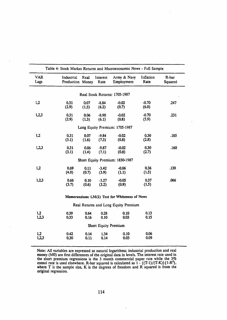
Table 4: Stock Market Returns and Macroeconomic News - Full Sample
VARLags
Industrial Real Interest Production Money Rate
Army & Navy Employment
InflationRate
R-barSquared
Real Stock Returns: 1705-1987
1,2 0.31(2.9)
0.07(1.5)
-8.84(6.2)
-0.02(0.7)
-0.70(6.0)
.247
1,2,3 031(2.9)
0.06(13)
-8.90(6.1)
-0.02(0.8)
-0.70(5.9)
.231
Long Equity Premium: 1705-1987
1,2 0.31(3.1)
0.07(1.6)
-9.84(73)
-0.02(0.8)
030(2.8)
.185
1,23 031(3.1)
0.06(1.4)
-9.87(7.1)
-0.02(0.8)
030(2.7)
.160
Short Equity Premium: 1830-1987
1,2 0.69(4.0)
0.11(0.7)
-3.42(3.9)
-0.06(1.1)
036(13)
.130
1,23 0.66(3.7)
0.10(0.6)
-3.27(3.2)
-0.05(0.9)
037(13)
.066
Memorandum: LM(2) Test for Whiteness of News
Real Returns and Long Equity Premium
1,21A3
039033
0.640.16
0.280.10
0.100.03
0.130.15
Short Equity Premium
1,2133
0.42030
0.140.11
1340.14
0.100.03
0.060.09
Note: All variables are expressed as natural logarithms; industrial production and real money (MO) are first differences of the original data in levels. The interest rate used in the short premium regressions is the 3 month commercial paper rate while the 3% consol rate is used elsewhere. R-bar squared is calculated as 1 - {(T-1)/(T-K)}{1-R2}, where T is the sample size, K is the degrees of freedom and R squared is from the original regression.
114
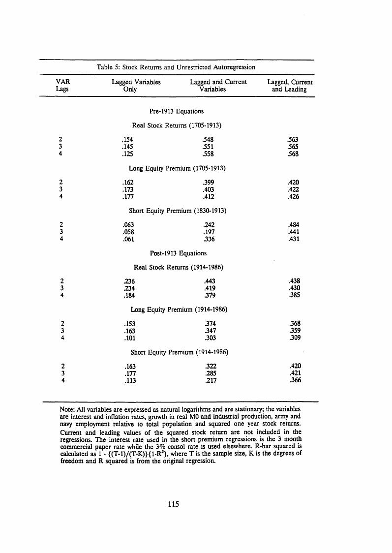
Table 5: Stock Returns and Unrestricted Autoregression
VAR Lagged Variables Lagged and Current Lagged, CurrentLags Only Variables and Leading
Pre-1913 Equations
Real Stock Returns (1705-1913)
2 .154 .548 .5633 .145 .551 .5654 .125 .558 .568
Long Equity Premium (1705-1913)
2 .162 399 .4203 .173 .403 .4224 .177 .412 .426
Short Equity Premium (1830-1913)
2 .063 .242 .4843 .058 .197 .4414 .061 336 .431
Post-1913 Equations
Real Stock Returns (1914-1986)
2 .236 .443 .4383 .234 .419 .4304 .184 379 385
Long Equity Premium (1914-1986)
2 .153 374 3683 .163 347 3594 .101 .303 .309
Short Equity Premium (1914-1986)
2 .163 322 .4203 .177 .285 .4214 .113 .217 366
Note: All variables are expressed as natural logarithms and are stationary; the variables are interest and inflation rates, growth in real MO and industrial production, army and navy employment relative to total population and squared one year stock returns. Current and leading values of the squared stock return are not included in the regressions. The interest rate used in the short premium regressions is the 3 month commercial paper rate while the 3% consol rate is used elsewhere. R-bar squared is calculated as 1 - {(T-1)/(T-K)}{1-R2}, where T is the sample size, K is the degrees of freedom and R squared is from the original regression.
115
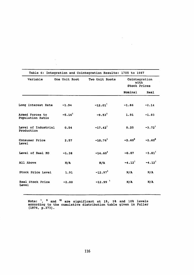
T a b l e 6 : I n t e g r a t i o n a n d C o i n t e g r a t i o n R e s u l t s : 1 7 0 5 t o 1 9 8 7
V a r i a b l e O ne U n i t R o o t Two U n i t R o o t s C o i n t e g r a t i o n w i t h
S t o c k P r i c e s
N o m i n a l R e a l
L o n g I n t e r e s t R a t e - 1 . 9 4 - 1 2 . 0 1 1 - 1 . 8 6 - 2 . 1 4
A rm ed F o r c e s t o P o p u l a t i o n R a t i o
- 5 . 1 6 1 - 9 . 5 3 1 1 . 9 1 - 1 . 9 3
L e v e l o f I n d u s t r i a l P r o d u c t i o n
0 . 5 4 - 1 7 . 4 2 1 0 . 2 5 - 3 . 7 2 1
C o n s u m e r P r i c e L e v e l
2 . 5 7 - 1 0 . 7 6 1 - 2 . 6 0 5 - 2 . 6 0 5
L e v e l o f R e a l MO - 1 . 3 8 - 1 4 . 6 0 1 - 0 . 0 7 - 3 . 8 1 1
A l l A b o v e N/A N /A - 4 . 1 2 1 - 4 . 1 2 1
S t o c k P r i c e L e v e l 1 . 9 1 - 1 2 . 9 7 1 N /A N/A
R e a l S t o c k P r i c e L e v e l
- 2 . 0 0 - 1 2 . 9 9 1 N /A N/A
N o t e : , a n d 10 a r e s i g n i f i c a n t a t 1%, 5% a n d 10% l e v e l sa c c o r d i n g t o t h e c u m u l a t i v e d i s t r i b u t i o n t a b l e g i v e n i n F u l l e r ( 1 9 7 6 , p . 3 7 3 ) .
116
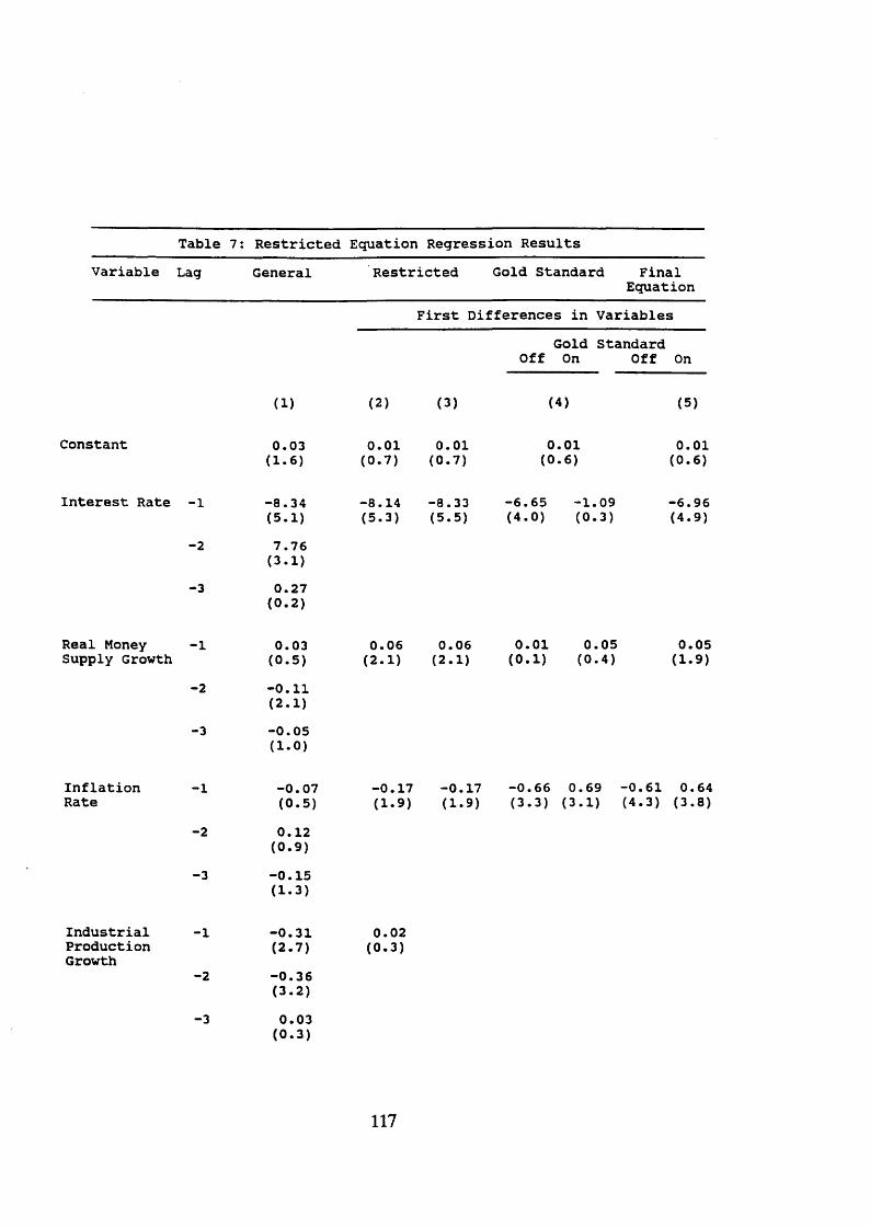
T a b l e 7 : R e s t r i c t e d E q u a t i o n R e g r e s s i o n R e s u l t s
V a r i a b l e L ag G e n e r a l R e s t r i c t e d G o l d S t a n d a r d F i n a lE q u a t i o n
F i r s t D i f f e r e n c e s i n V a r i a b l e s
G o l d S t a n d a r d O f f On O f f On
( 1 ) ( 2 ) ( 3 ) ( 4 ) (5 )
C o n s t a n t 0 . 0 3 0 . 0 1 0 . 0 1 0 . 0 1 0 . 0 1( 1 . 6 ) ( 0 . 7 ) ( 0 . 7 ) ( 0 . 6 ) ( 0 . 6 )
I n t e r e s t R a t e - 1 - 8 . 3 4 - 8 . 1 4 - 8 . 3 3 - 6 . 6 5 - 1 . 0 9 - 6 . 9 6( 5 . 1 ) ( 5 . 3 ) ( 5 . 5 ) ( 4 . 0 ) ( 0 . 3 ) ( 4 . 9 )
- 2 7 . 7 6( 3 . 1 )
- 3 0 . 2 7(0 . 2)
R e a l M oney - 1 0 . 0 3 0 . 0 6 0 . 0 6 0 . 0 1 0 . 0 5 0 . 0 5S u p p l y G r o w th ( 0 . 5 ) ( 2 . 1 ) ( 2 . 1 ) ( 0 . 1 ) ( 0 . 4 ) ( 1 . 9 )
- 2 - 0 . 1 1(2 . 1)
- 3 - 0 . 0 5(1 . 0)
I n f l a t i o n - 1 - 0 . 0 7 - 0 . 1 7 - 0 . 1 7 - 0 . 6 6 0 . 6 9 - 0 . 6 1 0 . 6 4R a t e ( 0 . 5 ) ( 1 . 9 ) ( 1 . 9 ) ( 3 . 3 ) ( 3 . 1 ) ( 4 . 3 ) ( 3 . 8 )
- 2 0 . 1 2( 0 . 9 )
- 3 - 0 . 1 5( 1 . 3 )
I n d u s t r i a l - 1 - 0 . 3 1 0 . 0 2P r o d u c t i o n ( 2 . 7 ) ( 0 . 3 )G r o w th
- 2 - 0 . 3 6( 3 . 2 )
- 3 0 . 0 3( 0 . 3 )
117
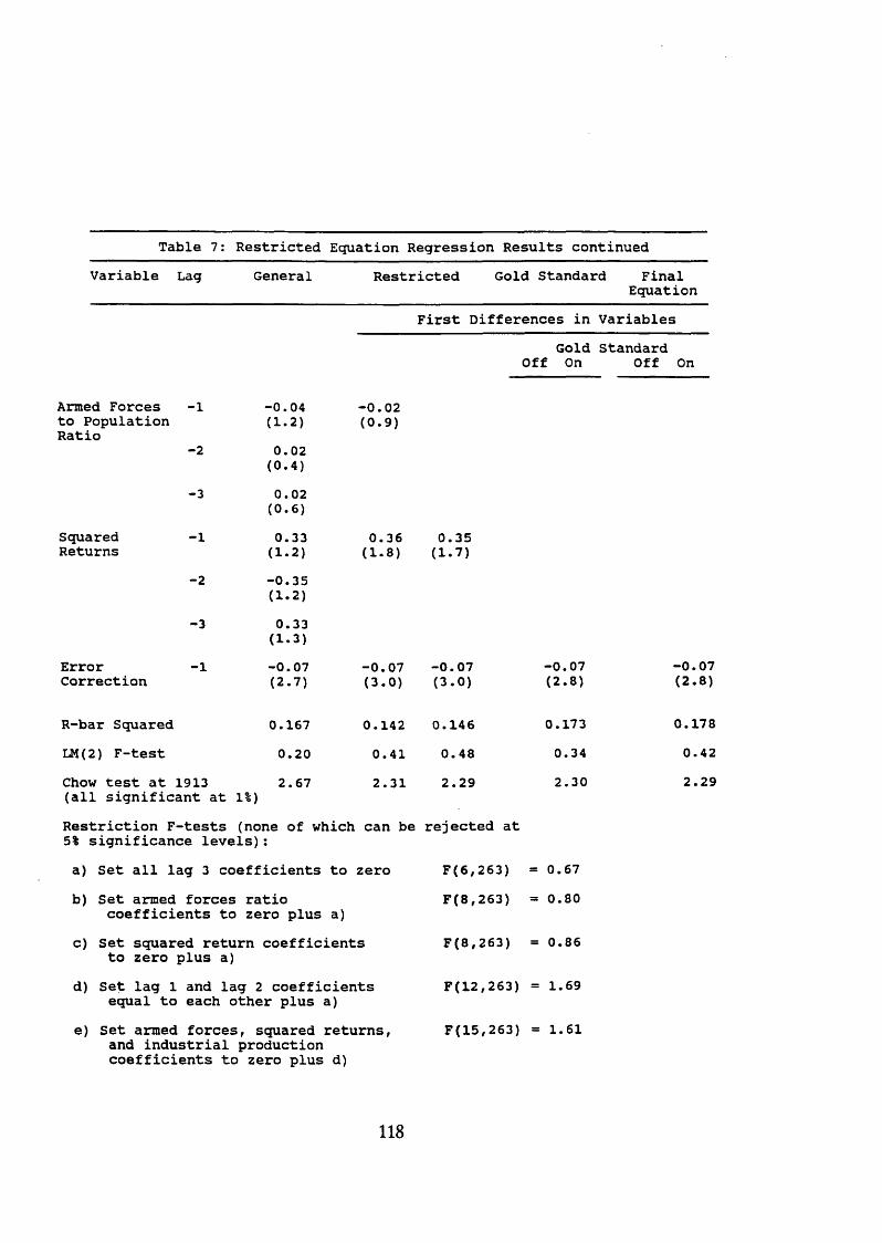
Table 7: Restricted Equation Regression Results continuedV a r i a b l e L ag G e n e r a l R e s t r i c t e d G o l d S t a n d a r d F i n a l
E q u a t i o n
F i r s t D i f f e r e n c e s i n V a r i a b l e s
G o l d S t a n d a r d O f f On O f f On
A rm ed F o r c e s - 1 - 0 . 0 4 - 0 . 0 2t o P o p u l a t i o n ( 1 . 2 ) ( 0 . 9 )R a t i o
- 2 0 . 0 2( 0 . 4 )
- 3 0 . 0 2(0 . 6 )
S q u a r e d - 1 0 . 3 3 0 . 3 6 0 . 3 5R e t u r n s ( 1 . 2 ) ( 1 . 8 ) ( 1 . 7 )
- 2 - 0 . 3 5( 1 . 2 )
- 3 0 . 3 3( 1 . 3 )
E r r o r - 1 C o r r e c t i o n
- 0 . 0 7( 2 . 7 )
- 0 . 0 7( 3 . 0 )
- 0 . 0 7( 3 . 0 )
R - b a r S q u a r e d 0 . 1 6 7 0 . 1 4 2 0 . 1 4 6
LM(2) F - t e s t 0 . 2 0 0 . 4 1 0 . 4 8
Chow t e s t a t 1 9 1 3 2 . 6 7 2 . 3 1 2 . 2 9
- 0 . 0 7 - 0 . 0 7( 2 . 8 ) ( 2 . 8 )
0 . 1 7 3 0 . 1 7 8
0 . 3 4 0 . 4 2
2 . 3 0 2 . 2 9( a l l s i g n i f i c a n t a t 1%)
R e s t r i c t i o n F - t e s t s ( n o n e o f w h i c h c a n b e r e j e c t e d a t 5% s i g n i f i c a n c e l e v e l s ) :
a ) S e t a l l l a g 3 c o e f f i c i e n t s t o z e r o F ( 6 , 2 6 3 ) = 0 . 6 7
b ) S e t a r m e d f o r c e s r a t i o F ( 8 , 2 6 3 ) = 0 . 8 0c o e f f i c i e n t s t o z e r o p l u s a )
c ) S e t s q u a r e d r e t u r n c o e f f i c i e n t s F ( 8 , 2 6 3 ) = 0 . 8 6t o z e r o p l u s a )
d ) S e t l a g 1 a n d l a g 2 c o e f f i c i e n t s F ( 1 2 , 2 6 3 ) = 1 . 6 9e q u a l t o e a c h o t h e r p l u s a )
e ) S e t a r m e d f o r c e s , s q u a r e d r e t u r n s , F ( 1 5 , 2 6 3 ) = 1 . 6 1a n d i n d u s t r i a l p r o d u c t i o n c o e f f i c i e n t s t o z e r o p l u s d )
118
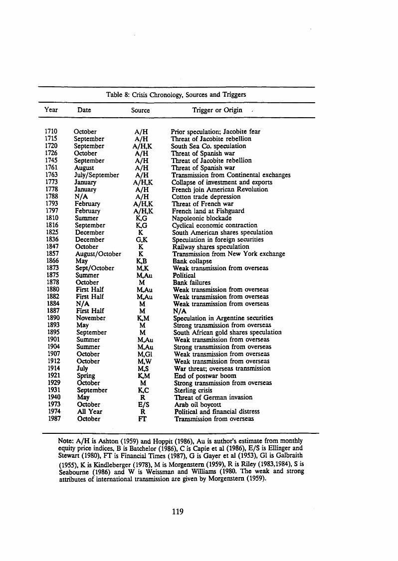
Table 8: Crisis Chronology, Sources and Triggers
Year Date Source Trigger or Origin
1710 October A/H Prior speculation; Jacobite fear1715 September A/H Threat of Jacobite rebellion1720 September A/H,K South Sea Co. speculation1726 October A/H Threat of Spanish war1745 September A/H Threat of Jacobite rebellion1761 August A/H Threat of Spanish war1763 July/September A/H Transmission from Continental exchanges1773 January A/H,K CoUapse of investment and exports1778 January A/H French join American Revolution1788 N/A A/H Cotton trade depression1793 February A/H,K Threat of French war1797 February A/H,K French land at Fishguard1810 Summer K,G Napoleonic blockade1816 September K,G Cyclical economic contraction1825 December K South American shares speculation1836 December G,K Speculation in foreign securities1847 October K Railway shares speculation1857 August/October K Transmission from New York exchange1866 May K,B Bank collapse1873 Sept/October M,K Weak transmission from overseas1875 Summer M,Au Political1878 October M Bank failures1880 First Half M,Au Weak transmission from overseas1882 First Half M,Au Weak transmission from overseas1884 N/A M Weak transmission from overseas1887 First Half M N/A1890 November K,M Speculation in Argentine securities1893 May M Strong transmission from overseas1895 September M South African gold shares speculation1901 Summer M,Au Weak transmission from overseas1904 Summer M,Au Strong transmission from overseas1907 October M,G1 Weak transmission from overseas1912 October M,W Weak transmission from overseas1914 July M,S War threat; overseas transmission1921 Spring K,M End of postwar boom1929 October M Strong transmission from overseas1931 September K,C Sterling crisis1940 May R Threat of German invasion1973 October E/S Arab oil boycott1974 AU Year R Political and financial distress1987 October FT Transmission from overseas
Note: A/H is Ashton (1959) and Hoppit (1986), Au is author’s estimate from monthly equity price indices, B is Batchelor (1986), C is Capie et al (1986), E/S is Ellinger and Stewart (1980), FT is Financial Times (1987), G is Gayer et al (1953), G1 is Galbraith (1955), K is Kindleberger (1978), M is Morgenstem (1959), R is Riley (1983,1984), S is Seaboume (1986) and W is Weissman and Williams (1980. The weak and strong attributes of international transmission are given by Morgenstem (1959).
119
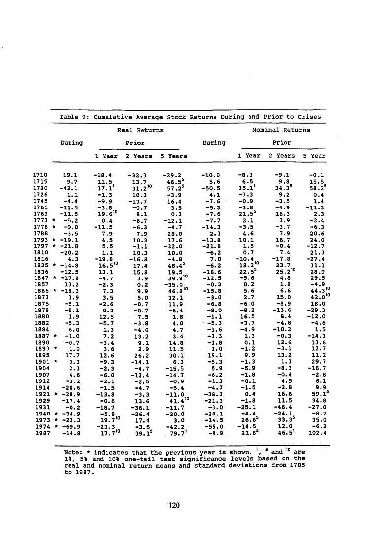
T a b l e 9 : C u m u l a t i v e A v e r a g e S t o c k R e t u r n s D u r i n g a n d P r i o r t o C r i s e s
R e a l R e t u r n s N o m i n a l R e t u r n s
D u r i n g P r i o r D u r i n g P r i o r
1 Y e a r 2 Y e a r s 5 Y e a r s 1 Y e a r 2 Y e a r s 5 Y e a r
1710 1 9 . 1 - 1 8 . 4 - 3 2 . 3 - 2 9 . 2 - 1 0 . 0 - 8 . 3 - 9 . 1 - 0 . 11715 9 . 7 1 1 . 5 1 3 . 7 4 6 . 5 s 5 . 6 6 . 5 9 . 8 1 5 . 51720 - 4 2 . 1 3 7 . 1 1 3 1 . 2 10 5 7 . 2 s - 5 0 . 5 3 5 . 1 1 3 4 . 3 s 5 8 . 2 s17 2 6 1 . 1 - 1 . 3 1 0 . 3 - 3 . 9 4 . 1 - 7 . 3 9 . 2 0 . 417 4 5 - 4 . 4 - 9 . 9 - 1 3 . 7 1 6 . 4 - 7 . 6 - 0 . 9 - 3 . 5 1 . 41 761 - 1 1 . 5 - 3 . 8 - 0 . 7 3 . 5 - 5 . 3 - 3 . 8 - 4 . 9 - 1 1 . 31763 - 1 1 . 5 1 9 . 6 10 8 . 1 0 . 3 - 7 . 6 2 1 . 5 s 1 6 . 3 2 . 31773 * - 5 . 2 0 . 4 - 6 . 7 - 1 2 . 1 - 7 . 7 2 . 1 3 . 9 - 2 . 41778 * - 9 . 0 - 1 1 . 5 - 6 . 3 - 4 . 7 - 1 4 . 3 - 3 . 5 - 3 . 7 - 6 . 31788 - 3 . 5 7 . 9 7 . 9 2 8 . 0 2 . 3 4 . 6 7 . 9 2 0 . 61793 * - 1 9 . 1 4 . 5 1 0 . 3 1 7 . 6 - 1 3 . 8 1 0 . 1 1 6 . 7 2 4 . 01797 * - 2 1 . 8 5 . 5 - 1 . 1 - 3 2 . 0 - 2 1 . 8 1 . 5 - 0 . 4 - 1 2 . 71 810 - 2 0 . 2 1 . 1 1 0 . 3 1 0 . 0 - 6 . 2 0 . 7 7 . 4 2 1 . 31 816 4 . 3 - 1 9 . 8 - 1 6 . 8 - 4 . 8 7 . 0 - 1 0 . 4 - 1 7 . 8 - 2 7 . 41 825 * - 1 4 . 8 1 6 . 5 10 1 7 . 4 4 8 . 4 s - 6 . 2 1 8 . 2 10 2 3 . 7 3 1 . 11836 - 1 2 . 5 1 3 . 1 1 5 . 8 1 9 . 5 - 1 6 . 6 2 2 . 5 s 2 5 . 2 10 2 8 . 91847 * - 1 7 . 8 - 4 . 7 3 . 9 3 9 . 9 10 - 1 2 . 5 - 5 . 6 4 . 8 2 9 . 51857 1 3 . 2 - 2 . 3 0 . 2 - 3 5 . 0 - 0 . 3 0 . 2 1 . 8 - 4 . 91866 * - 1 8 . 3 7 . 3 9 . 9 4 6 . 8 10 - 1 5 . 8 5 . 6 6 . 6 4 4 . 3 101873 1 . 9 3 . 5 5 . 0 3 2 . 1 - 3 . 0 2 . 7 1 5 . 0 4 2 . 0 101 875 - 5 . 1 - 2 . 6 - 0 . 7 1 1 . 9 - 6 . 8 - 6 . 0 - 8 . 9 1 8 . 01878 - 5 . 1 0 . 3 - 0 . 7 - 6 . 4 - 8 . 0 - 8 . 2 - 1 3 . 6 - 2 9 . 31880 1 . 9 1 2 . 5 7 . 5 1 . 8 - 1 . 1 1 6 . 5 8 . 4 - 1 2 . 01882 - 5 . 3 - 5 . 7 - 3 . 8 4 . 0 - 5 . 3 - 3 . 7 - 4 . 8 - 4 . 61884 6 . 0 1 . 3 - 4 . 0 4 . 7 - 1 . 6 - 4 . 9 - 1 0 . 2 1 . 51887 * - 1 . 0 7 . 2 1 3 . 2 3 . 4 - 3 . 3 1 . 3 - 0 . 3 - 1 4 . 31890 - 0 . 7 - 3 . 4 9 . 1 1 4 . 8 - 1 . 8 0 . 1 1 2 . 6 1 3 . 61893 * 1 . 0 3 . 6 2 . 9 1 1 . 5 1 . 0 - 1 . 2 - 3 . 1 1 2 . 71 895 1 7 . 7 1 2 . 6 2 6 . 2 3 0 . 1 1 9 . 1 9 . 9 1 3 . 2 1 1 . 21 9 0 1 * 0 . 3 - 9 . 3 - 1 4 . 1 6 . 3 - 5 . 3 - 1 . 3 1 . 3 2 9 . 71904 2 . 3 - 2 . 3 - 4 . 7 - 1 5 . 5 5 . 9 - 5 . 9 - 8 . 3 - 1 6 . 71907 4 . 6 - 6 . 0 - 1 2 . 4 - 1 4 . 7 - 6 . 2 - 1 . 8 - 0 . 4 - 2 . 81912 - 3 . 2 - 2 . 1 - 2 . 5 - 0 . 9 - 1 . 3 - 0 . 1 4 . 5 6 . 11914 - 2 0 . 6 - 1 . 5 - 4 . 7 - 5 . 4 - 4 . 7 - 1 . 5 - 2 . 8 9 . 919 2 1 * - 2 8 . 9 - 1 3 . 8 - 3 . 3 - 3 8 . 3 0 . 4 1 6 . 6 5 9 . 1 s1929 - 1 7 . 4 - 0 . 6 1 3 . 6 11 j 104 1 . 4 - 2 1 . 3 - 1 . 8 1 1 . 5 3 4 . 81 9 3 1 - 0 . 2 - 1 8 . 7 - 3 6 . 1 - 1 1 . 7 - 3 . 0 - 2 5 . 1 - 4 6 . 4 - 2 7 . 01 9 4 0 * - 3 4 . 9 - 5 . 8 - 2 6 . 4 - 2 0 . 0 - 2 0 . 1 - 4 . 4 - 2 4 . 1 - 8 . 71973 * - 2 3 . 3 1 9 . 7 10 1 7 . 4 3 . 0 - 1 4 . 5 2 6 . 6 s 3 3 . 3 s 3 5 . 01974 * - 6 9 . 9 - 2 3 . 3 - 3 . 6 - 4 2 . 2 - 5 5 . 0 - 1 4 . 5 1 2 . 0 - 6 . 21987 - 1 4 . 8 1 7 . 7 10 3 9 . 1 5 7 9 . 7 1 - 9 . 9 2 1 . 8 s 4 6 . 5 1 1 0 2 . 4
N o t e : * i n d i c a t e s t h a t t h e p r e v i o u s y e a r i s s h o w n . , a n d a r e 1%, 5% a n d 10% o n e - t a i l t e s t s i g n i f i c a n c e l e v e l s b a s e d o n t h e r e a l a n d n o m i n a l r e t u r n m e a n s a n d s t a n d a r d d e v i a t i o n s f r o m 1 7 0 5 t o 1 9 8 7 .
120
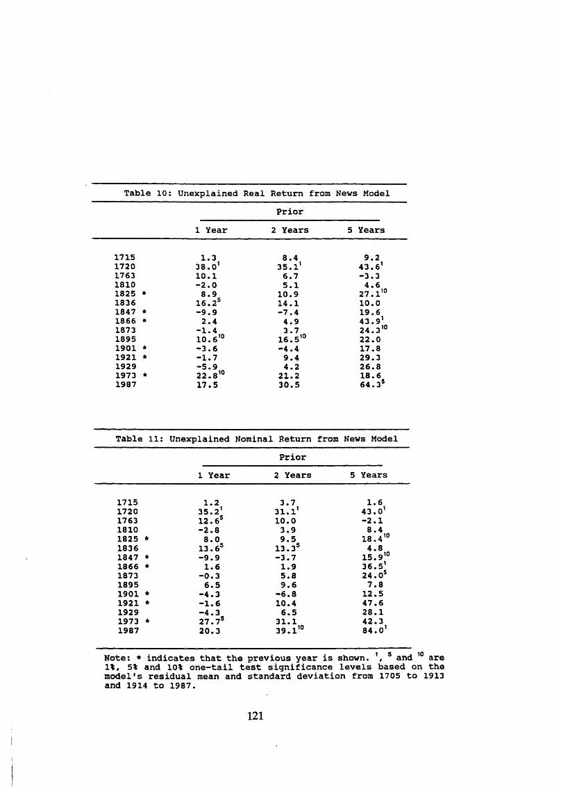
Table 10: Unexplained Real Return from News ModelP r i o r
1 Y e a r 2 Y e a r s 5 Y e a r s
1 7 1 5 1 . 3 8 . 4 9 . 21 7 2 0 3 8 . 0 1 3 5 . 1 1 4 3 . 6 11763 1 0 . 1 6 . 7 - 3 . 31 8 1 0 - 2 . 0 5 . 1 4 . 61 8 2 5 * 8 . 9 1 0 . 9 2 7 . 1 101 8 3 6 1 6 . 2 5 1 4 . 1 1 0 . 01 8 4 7 * - 9 . 9 - 7 . 4 1 9 . 61 8 6 6 * 2 . 4 4 . 9 4 3 . 9 11 8 7 3 - 1 . 4 3 . 7 2 4 . 3 101 8 9 5 1 0 . 6 10 1 6 . 5 10 2 2 . 01 9 0 1 * - 3 . 6 - 4 . 4 1 7 . 81 9 2 1 * - 1 . 7 9 . 4 2 9 . 31 9 2 9 - 5 . 9 4 . 2 2 6 . 81 9 7 3 * 2 2 . 8 10 2 1 . 2 1 8 . 61 9 8 7 1 7 . 5 3 0 . 5 6 4 . 3 s
T a b l e 1 1 : U n e x p l a i n e d N o m i n a l R e t u r n f r o m New s M o d e l
P r i o r
1 Y e a r 2 Y e a r s 5 Y e a r s
1 7 1 5 1 . 2 3 . 7 1 . 61 7 2 0 3 5 . 2 1 3 1 . 1 1 4 3 . 0 11 7 6 3 1 2 . 6 s 1 0 . 0 - 2 . 11 8 1 0 - 2 . 8 3 . 9 8 . 41 8 2 5 * 8 . 0 9 . 5 1 8 . 4 101 8 3 6 1 3 . 6 s 1 3 . 3 s 4 . 81 8 4 7 * - 9 . 9 - 3 . 7 1 5 . 9 10
3 6 . 5 11 8 6 6 * 1 . 6 1 . 91 8 7 3 - 0 . 3 5 . 8 2 4 . 0 s1 8 9 5 6 . 5 9 . 6 7 . 81 9 0 1 * - 4 . 3 - 6 . 8 1 2 . 51 9 2 1 * - 1 . 6 1 0 . 4 4 7 . 61 9 2 9 - 4 . 3 6 . 5 2 8 . 11 9 7 3 * 2 7 . 7 s 3 1 . 1 4 2 . 3
8 4 . 0 11 9 8 7 2 0 . 3 3 9 . 1 10
N o t e : * i n d i c a t e s t h a t t h e p r e v i o u s y e a r i s s h o w n . 1, a n d a r e 1%, 5% a n d 10% o n e - t a i l t e s t s i g n i f i c a n c e l e v e l s b a s e d o n t h e m o d e l ' s r e s i d u a l m e a n a n d s t a n d a r d d e v i a t i o n f r o m 1 7 0 5 t o 1913 a n d 1 9 1 4 t o 1 9 8 7 .
121
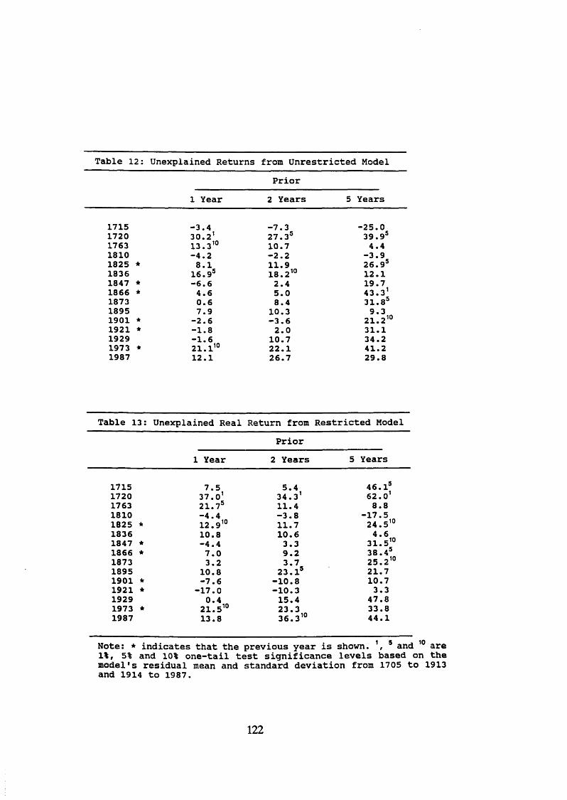
Table 12: Unexplained Returns from Unrestricted ModelP r i o r
1 Y e a r 2 Y e a r s 5 Y e a r s
1 7 1 5 - 3 . 4 - 7 . 3 - 2 5 . 01 7 2 0 3 0 . 2 1 2 7 . 35 3 9 . 9 51 7 6 3 1 3 . 3 10 1 0 . 7 4 . 41 8 1 0 - 4 . 2 - 2 . 2 - 3 . 91 8 2 5 * 8 . 1 1 1 . 9 2 6 . 9 51 8 3 6 1 6 . 95 1 8 . 2 10 1 2 . 11 8 4 7 * - 6 . 6 2 . 4 1 9 . 71 8 6 6 * 4 . 6 5 . 0 4 3 . 3 118 7 3 0 . 6 8 . 4 3 1 . 8 51 8 9 5 7 . 9 1 0 . 3 9 . 31 9 0 1 * - 2 . 6 - 3 . 6 2 1 . 2 101 9 2 1 * - 1 . 8 2 . 0 3 1 . 11 9 2 9 - 1 . 6 1 0 . 7 3 4 . 21 9 7 3 * 2 1 . 1 10 2 2 . 1 4 1 . 21 9 8 7 1 2 . 1 2 6 . 7 2 9 . 8
T a b l e 1 3 : U n e x p l a i n e d R e a l R e t u r n f r o m R e s t r i c t e d M o d e l
P r i o r
1 Y e a r 2 Y e a r s 5 Y e a r s
1 7 1 5 7 . 5 5 . 4 4 6 . 151 7 2 0 3 7 . 0 1 3 4 . 3 1 6 2 . 0 11 7 6 3 2 1 . 7 5 1 1 . 4 8 . 81 8 1 0 - 4 . 4 - 3 . 8 - 1 7 . 51 8 2 5 * 1 2 . 9 10 1 1 . 7 2 4 . 5 101 8 3 6 1 0 . 8 1 0 . 6 4 . 61 8 4 7 * - 4 . 4 3 . 3 3 1 . 5 101 8 6 6 * 7 . 0 9 . 2 3 8 . 451 8 7 3 3 . 2 3 . 7 2 5 . 2 101 8 9 5 1 0 . 8 2 3 . 15 2 1 . 71 9 0 1 * - 7 . 6 - 1 0 . 8 1 0 . 71 9 2 1 * - 1 7 . 0 - 1 0 . 3 3 . 31 9 2 9 0 . 4 1 5 . 4 4 7 . 81 9 7 3 * 2 1 . 5 10 2 3 . 3 3 3 . 81 9 8 7 1 3 . 8 3 6 . 3 10 4 4 . 1
N o t e : * i n d i c a t e s t h a t t h e p r e v i o u s y e a r i s s h o w n . 1, a n d a r e 1%, 5% a n d 10% o n e - t a i l t e s t s i g n i f i c a n c e l e v e l s b a s e d o n t h e m o d e l ' s r e s i d u a l m e a n a n d s t a n d a r d d e v i a t i o n f r o m 1 7 0 5 t o 1 9 1 3 a n d 1 9 1 4 t o 1 9 8 7 .
122
Chapter IV: Stock Prices and Tobin’s Q
I. Introduction
Previous chapters have examined the autocorrelation properties of equity prices and
the correlations of such variables with macroeconomic variables. In general, while
significant relationships are found, thus underlining the importance of the real economy for stock price fluctuations, there is also widespread evidence of nonefficient market behaviour which remains broadly unexplained.
This chapter now turns to an examination of the effect of stock prices, via Tobin’s Q, on corporate investment. The Q theory of investment has often been employed
as an explanatory factor in the markets for physical capital and corporate control; in fact, it is widely thought that the stock market has its greatest impact on the
economy through these sectors. The Q theory was of particular interest following the 1987 crash because of the rough positive correlation between movements in the stock market and corporate investment in the 1980s, therefore giving some reason to speculate a priori that investment might be equally affected following the equity market downturn.
With research now clearly focused on understanding the stock market, due to the crash, it is probably appropriate to ask whether the Q theory is still robust to the
challenges issued from new theories and econometric techniques. A vast literature has developed in the last 5 years, for example, which questions the random walk
theory and its implication that stock prices are not mean reverting over time.1
Following this line of inquiry, the present chapter surveys the most widely used
macroeconomic Q measures in order to address two issues. First, it considers whether
standard empirical studies of investment using Q satisfy basic statistical properties of stability, appropriate specification and minimal explanatory power. Secondly, given
that these static formulations are inappropriate, it considers the relative merits of two
types of dynamic models.
123
The chapter reaches a number of conclusions. First, static Q theory is not empirically
valid. Second, a dynamic approach, incorporating lags of Q transformed to first differences, resolves these empirical problems. Third, an error correction model is superior to a VAR representation of the dynamic process. Fourth, Q is more highly
correlated to investment than are real stock prices, the primary determinant of fluctuations in Q; this offers support for empirical applications of Q theory using a
reformulated approach. However, the generally low explanatory power of investment equations using Q alone suggests that other relevant variables may add additional
information, an issue which is directly examined in Chapter V below. Fifth, there appear to be substantial differences between the relationship of stock prices and
investment in Japan and West Germany, in comparison to the U.S. and the U.K.; this issue is also taken up in the next chapter.
The outline of the rest of this chapter is as follows. In Section II, the theoretical arguments made in support of the Q theory of investment are presented, along with
several criticisms. Reference is made to Appendix II which outlines the functional forms of the 52 Q measures used here. Section III examines the Qs in some detail using various descriptive statistics and orders of integration tests. The analysis is focused on four countries in Section IV where standard Q investment equations are examined for structural stability, autocorrelation in residuals and explanatory power. These results are contrasted with two other models: an error correction mechanism
and a vector autoregression. Section V, following on recent work by Barro (1989), examines the influence of real stock prices on investment and compares these results with those of Section IV. Finally, Section VI concludes the chapter with a summary
of the investigation.
124
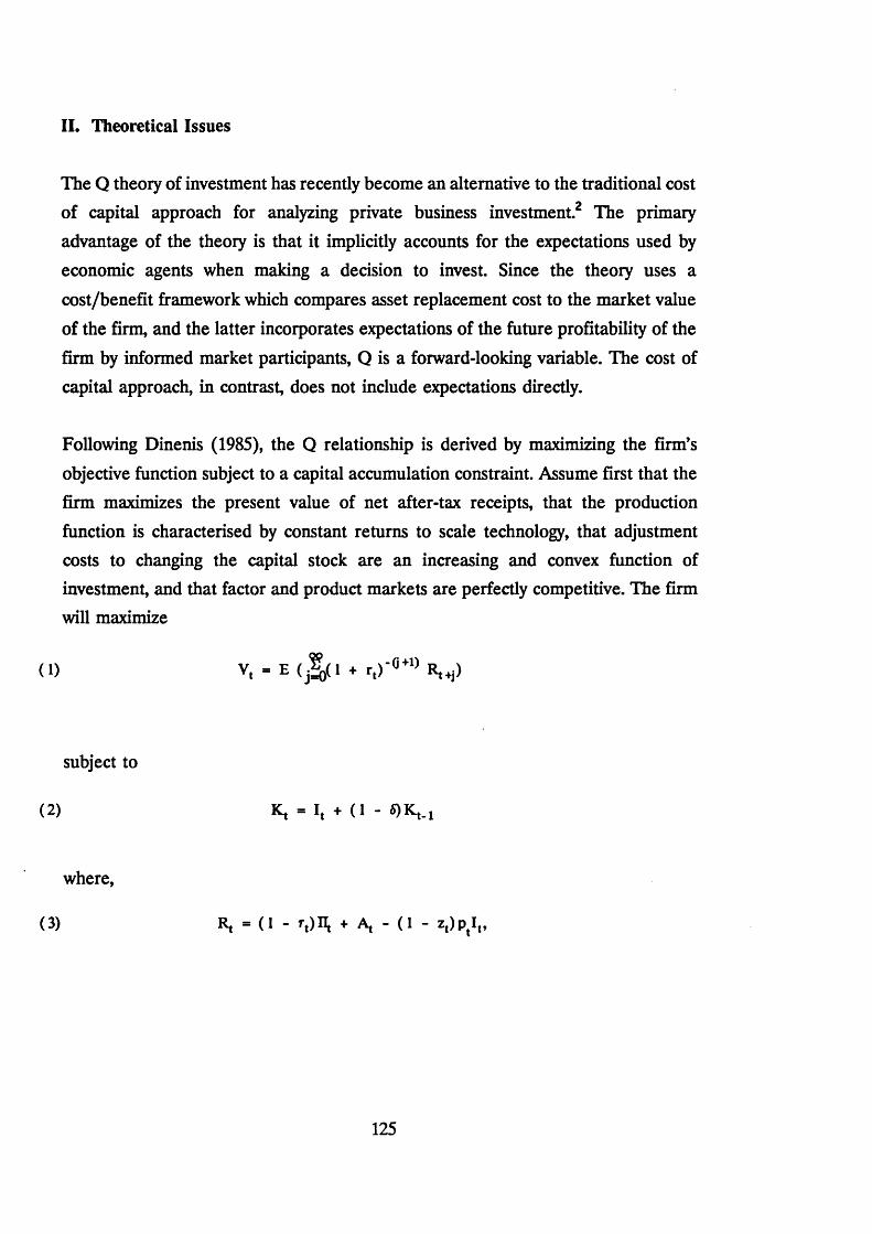
II. Theoretical Issues
The Q theory of investment has recently become an alternative to the traditional cost of capital approach for analyzing private business investment.2 The primary
advantage of the theory is that it implicitly accounts for the expectations used by
economic agents when making a decision to invest. Since the theory uses a
cost/benefit framework which compares asset replacement cost to the market value
of the firm, and the latter incorporates expectations of the future profitability of the
firm by informed market participants, Q is a forward-looking variable. The cost of capital approach, in contrast, does not include expectations directly.
Following Dinenis (1985), the Q relationship is derived by maximizing the firm’s
objective function subject to a capital accumulation constraint. Assume first that the firm maximizes the present value of net after-tax receipts, that the production
function is characterised by constant returns to scale technology, that adjustment costs to changing the capital stock are an increasing and convex function of investment, and that factor and product markets are perfectly competitive. The firm
will maximize
(1) V, - E ( j f ^ l + r , ) - ^ R ,+j)
subject to
(2) K, - It + (1 - QK,.!
where,
(3) Rt = (1 - + Aj - ( l - zt) p tI t ,
125
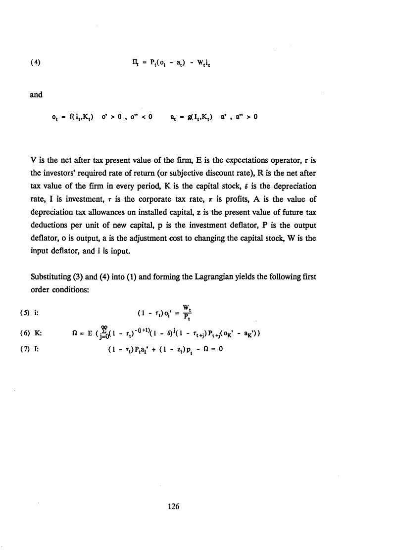
(4) H = Pt(ot - at) - Wtit
and
ot = f U p iy o’ > 0 , o” < 0 ^ = tflp K ,) a* , a” > 0
V is the net after tax present value of the firm, E is the expectations operator, r is the investors’ required rate of return (or subjective discount rate), R is the net after
tax value of the firm in every period, K is the capital stock, 8 is the depreciation
rate, I is investment, r is the corporate tax rate, tt is profits, A is the value of depreciation tax allowances on installed capital, z is the present value of future tax
deductions per unit of new capital, p is the investment deflator, P is the output deflator, o is output, a is the adjustment cost to changing the capital stock, W is the input deflator, and i is input.
Substituting (3) and (4) into (1) and forming the Lagrangian yields the following first order conditions:
(6) K:
(5) i:
(7) I:
(1 ~ r t) °i* =
n - E ( j ! / 1 - r ,) 'fl+1)d - *)*(• - rt+j)P ,tj(o K’ - aK’))
(1 - rt)Ptaj’ + (1 - zt)pt - 0 = 0
126
where n is the Lagrangian multiplier. Equation (5) states that the marginal productivity of the inputs is equal to their real marginal costs, Equation (6) says that n is the net addition to the present value of the firm due to a unit of new capital and Equation (7) implies that the firm will invest until the marginal costs and
benefits of such investment are equal.
Defining marginal Q as q = n/p and substituting the equation into (7), we have
p (q - 1 + zt)(8) - - V - r . j p , -
and, given linear homogeneity of at with respect to its determinants I and K,
(9) ^ = h(q()
That is, the investment-capital ratio is a function of marginal Q. In empirical work, this Q measure is unobservable and so, invoking the conditions established by Hayashi (1982) and formally derived for this specification by Dinenis (1985)3, marginal Q can be set equal to average Q and we have
( 10) =
Ueda and Yoshikawa (1986) and Dinenis (1985) offer theoretical justifications for
lagged Q terms affecting investment and have some success incorporating these
terms empirically. Allowing for such lags in adjustment, delivery and implementation
motivates the use of dynamic terms in the empirical investigation below, where Qt_
k are added to Equation (10).4
As noted in Appendix II, the simplest formulation of Q in empirical work is the
market value of corporate debt and equity divided by the replacement cost of the
corporate sector capital stock. More complex formulations are standardised in
Appendix II, and these equations and the Q pseudonyms outlined there may be useful for interpreting later sections in this chapter. Note also that Equation (10) is
127
referred to below as the traditional Q model.
A number of criticisms have been levelled at the Q theory. The first objection stems
from the theoretical argument that marginal Q is the appropriate decision variable
at the margin and, since most existing Q measures are calculated in average terms,
the practical implementation of the theory is flawed.5
A second criticism of the Q theory concerns the measurement of the capital stock
and the market value of the firm. The perpetual inventory method with straight-line depreciation, although widely used, is incorrect since varying rates of capital scrapping and depreciation imply that the forces shaping investment and the capital stock are different.6 The existence of accounting depreciation rates which diverge
from true economic rates and aggregation problems when dealing with a non- homogeneous capital stock are additional complicating factors.
A potentially more serious problem concerns the measurement of the market value of the firm, since a growing literature stresses the irrationality of speculative markets.7 If it is true that the market does not value the business sector at the appropriate price, then there is an inefficiency in the allocation of resources in the economy but not necessarily an abrogation of the Q theory. The linkage between the
theory and investment behaviour is weakened only if agents do not incorporate
equity market prices into their decision framework.8
A final set of criticisms fall into the category of financial and tax factors affecting the
firm. The taxation elements vary considerably across countries and assets and are, therefore, less amenable to generalisation across Q variables.9 Although these
elements ensure that Q more faithfully reflects the true incentives facing agents, this chapter suggests that the value of incorporating tax factors into investment equations
varies considerably across countries.
In terms of financial factors, the endogenous nature of the choice of finance and the linkage between investment and finance must be considered. The value of the firm
can be weighted by source of finance and the risk implicit in any particular financial
128

policy, since Q measures of equal numerical value that are generated by divergent financial policies may have different implications for the firm’s financial planning
policy and horizon.10
Overall, the Q theory provides the framework for creating a relatively easily
calculated measure of the costs and benefits of investment.11 As shown in the
following sections, once dynamic elements are introduced, Q variables are generally significant explanatory factors in corporate investment equations.
129

III. Statistical Properties of Q - International Comparison
This section presents summary statistics for the Q measures that are used in the rest of the chapter. Q values are presented for Belgium, Canada, Finland, France, West Germany, Japan, Sweden, the United Kingdom and the United States (and are shown in Diagrams 1 to 11 in Appendix II).
For analytical purposes, the Qs may be subdivided into various categories according
to whether the Qs are average or marginal, tax adjusted or non tax adjusted, or
derived at the macro or micro level of the economy. Certain tax adjusted Qs have been altered from the data given in published sources so that they can be consistently compared with the non-adjusted values.12
Table 1 shows the means and coefficients of variation of the Qs for identical subperiods within each country. The first point to note is that Q varies considerably from its equilibrium value of one; the main explanation for this is the presence of tax terms which introduce a wedge between market valuation of the firm and the replacement value of its assets.
A more serious shortcoming of the Q measures can be seen by comparing the coefficients of variation, which vary widely within each country. The usefulness of many of the Qs as indicators of movements in investment may, therefore, be
hampered because of the relatively high ratio of noise to signal. In any case, the
differences in means and coefficients of variation indicate that the Q measures within
each country are rather dissimilar.
The fact that any particular Q may deviate from unity and exhibit relatively high
volatility does not imply that Q theory is abrogated. A more important test of the
theory is whether the measure is mean reverting over time. This is an important property since the theory postulates that fluctuations of Q above and below its
equilibrium value will elicit investment responses in the physical capital market and on the stock market which will push the value of Q back to equilibrium. Classifying
Q as a random walk is, therefore, tantamount to refuting standard Q theory as
130

currently implemented.
Table 2 indicates that a unit root in Q can only be rejected for Japan and Canada (Other ql3). All of the other Q measures follow time series patterns which are
insignificantly different from random walks, as do the I/K measures for the U.S., U.K., Japan and West Germany. Table 3 demonstrates that stationarity is achieved
in all of the series after first differencing, except for U.S. q7 which requires second
differencing. It appears from these two tables that Q and I/K are generally
integrated of order one, 1(1), while the Japanese Q are I(0).13 Q does not therefore generally revert to a mean value over time, although d(Q) does have this property.14
These results suggest that cointegration between Q and I/K, and therefore the
existence of a long run relationship between the two, can be examined by using the augmented Dickey-Fuller methodology.15 Table 4 accordingly shows the cointegration
adjusted t-statistics for Japan, the U.K., the U.S. and West Germany; in column 5, additional Japanese results are given to accommodate the fact that Q is 1(0) there.
The conclusions of the table are somewhat mixed. Cointegration between I/K and
d(Q) cannot be rejected for Japan; as well, many of the U.S. Qs are cointegrated with I/K. For the U.K. and West Germany, however, many of the Qs are not cointegrated with I/K, although most of them are marginally significant. As well, with the exceptions of U.S. ql3 and Japan ql and q4, none of the tax adjusted
measures are cointegrated. Contrary to theoretical requirements, it therefore seems that the more sophisticated tax adjusted Q measures are also those which statistically
reject an equilibrium relationship with investment.
In conclusion, this section has a number of implications for modelling strategies
involving Q. First, given the differences in mean values and volatility, it is difficult
to specify a unique Q for use in empirical work; different formulations of Q are therefore needed to test model specification robustness in any investigation. Second,
aside from Japan and Canada, Qs should be transformed to first differences in order
to induce stationarity; this point also holds for I/K.16 Third, the existence of cointegration between Q and I/K suggests that an error correction model (ECM) may be one (previously ignored) approach to modelling Q theory.
131
IV. Comparative Investment Models: Four Country Analysis
This section compares an error correction specification of Q theory with the
traditional Q formulation and a VAR alternative. The traditional Q model is used
to conform to accepted theoretical prescriptions and the VAR is employed to free the data from any imposed structure; the two models therefore represent opposite
ends of the modelling spectrum.
The lack of success of traditional specifications of the Q theory is apparent from
Tables 5 to 9. Table 5 shows coefficient estimates for the traditional static application of Q theory. The other tables show Durbin-Watson statistics, F-tests for the null hypothesis that the regressor coefficients are jointly zero, R-squared values,
Chow F-tests for mid-sample structural change and LM(2) tests for autocorrelated residuals.17 Each triplet of equations presents I/K on Q regressions in the first row, an unrestricted VAR of d(I/K) on lagged values of d(I/K) and d(Q) in row three and an unrestricted ECM similar to the VAR but incorporating an error correction term in row two. Column 7 tests the significance of the error correction term and column 8 does the same for the reverse regression of d(Q) on d(I/K).18
Looking to Table 5 and the first row of each Q variable in the other tables, one sees numerous insignificant or incorrectly signed coefficients, low DW values, low R- squared explanatory power, autocorrelated residuals and occasional structural breaks.
These results indicate that the traditional Q specification is inappropriate. The major
flaws are the exclusion of dynamic behaviour in the equations and the failure to
transform Q to a differenced representation.
Turning to the U.K. results first, it appears that the ECM is generally superior to the VAR. While the VAR fails to reject the regressor F-test null hypothesis of no
explanatory power for five of the Qs in Table 6, the ECM fails only for q4. The
Chow and LM tests reject the null hypothesis of structural break and error
correlation for each specification, thus supporting the need for including dynamics
in the models, and the error correction term is either strongly or marginally
significant in two-thirds of the equations; those rejecting the additional term are
132

almost all tax adjusted Qs. There is also some support for thinking that the dynamic profile of Q is unaffected by the error correction term in column 7. Again, q4 is the
exception and this result may be due to the dominance of tax terms in the variation of this Q over time.
The U.S. equations in Table 7 broadly reflect the U.K. results. The VAR
specification indicates marginal residual autocorrelation in q4 and ql5 while the
ECM is universally free of such problems. As well, the regressor F-test fails to reject
the null hypothesis of no significance more often for the VAR model than for the ECM. Six of the Qs indicate that an error correction term is not required and the
reverse regression F-test shows that Q dynamics are unaffected by the long run relationship between Q and I/K. Once again, the Q variables rejecting the error
correction specification are predominantly tax adjusted measures. As in Table 6, there is a substantial increase in the explanatory power of the equations relative to the traditional Q specification in row one.
The results for West Germany in Table 8 again support the error correction specification. The VAR model fails to reject the regressor F-test null hypothesis for q ll while the ECM rejects for all three Qs. The error correction term is also marginally significant for the Q equations and, as with the other two countries, this term does not affect the time profile of Q. The increase in R-squared relative to the traditional Q equation is less marked than in the U.S. and the U.K..19
The error correction term in each of the ECM above can be interpreted as the
degree to which the equation reverts to its long run equilibrium every period. For
the United States, the coefficient estimates imply that I/K reverts to its equilibrium
over a period of 3 to 7 years, while the German results indicate that this process takes place over 6 to 9 years. The U.K. implied reversion time varies widely across
Qs, from 1 to 13 years, but the coefficients consistently increase in magnitude from
the 1950s to the present; it therefore seems that equilibrium-inducing forces are
much stronger in recent years.20
133
Turning now to Japan, this country presents a special problem for examining the
ECM relative to a VAR. Since Tables 2 and 3 showed that Q is 1(0) while I/K is 1(1), it is not possible to obtain the error correction term for inclusion in an
investment equation. Therefore, Table 9 examines the implications of regressing
d(I/K) on Q itself rather that d(Q), since d(I/K) and Q are both 1(0). The first row
of each set shows the d(I/K) on Q equation and the second row shows an
unrestricted VAR of d(I/K) on lags of d(I/K) and Q. Column 7 gives the F-test for
adding current Q to the VAR and column 8 tests the restriction that Q can be
transformed to d(Q).
The regressors F-test null hypothesis of no significance is not rejected for the contemporaneous Q equation, indicating that dynamics terms are important for
empirically implementing Q theory; this is supported by the F-tests of column 7
which imply that current Q is generally significant only when lagged Qs are included
in the equation. The regressors F-test for lagged Q fails to reject the null hypothesis of no significance for more than half of the Q variables. The last column indicates that restricting Q to a d(Q) form is not rejected and this latter formulation may be preferred for reasons of parsimony. Overall, the Japanese results are considerably weaker than those for the other three countries.
In summary, it appears that the ECM is preferable to an unrestricted VAR, and the
latter model, in turn, is superior to the traditional Q equation. However, the low R2 values for even the ECM variation indicate that the Q approach may not be optimal for explaining investment fluctuations over time.
Tax adjusted Qs seem to diminish the degree to which Q and I/K interact over the
longer run, as evidenced by the general absence of cointegration shown in Table 4
and the insignificance of the error correction terms for these Qs in Tables 6 to 8. It
may be that theoretical rigour demands the inclusion of tax variables which are
imperfect representations of investors’ decision sets; for example, expected tax rates
serve as proxies for current tax rates in Q investigations.
134

Finally, the deviations from equilibrium embodied in the error correction terms, while generally significant, are nevertheless of long lasting duration. These delays in reestablishing equilibrium may be partially attributed to decision and implementation
lags in investment and/or to the difficulty that investors may have interpreting
movements in the equity market on a short term basis.
135
V. Stock Prices, Q and Investment
Previous sections have shown that static Q theory is inappropriate and have suggested that a particular dynamic respecification is in order. An alternative
approach is to replace Q itself with one of its subcomponents which has better explanatory power. Although Qs are constructed with a number of different
components, it is likely that stock market prices are the most volatile element. This section, therefore, looks at the importance of real stock price (R) fluctuations for
investment and then compares the explanatory power of these prices with the
respective Q variables.21
Table 10 repeats the integration tests of Tables 2 to 4, with the conclusion that real stock prices are 1(1). The cointegrating equations indicate that real stock prices and investment are cointegrated in the U.S., the U.K. and West Germany (prior to the 1980s).22 It should be noted that the sample sizes in the table are chosen, first, to exploit the maximum possible data range and, second, to match the sample ranges
of the Q variables analyzed above.
As in Tables 6 to 9, Table 11 summarizes traditional static equations, VARs and ECMs. Problems with error autocorrelation and structural break are seen in the first row of each triplet and, as before, this is corrected with the introduction of lagged regressors. The VAR fails to reject the regressor F-test null hypothesis of no
significance for West Germany and the earlier Japanese sample period, while the ECM improves upon this by rejecting the test for the most recent German sample.
The error correction term is strongly significant for the U.S., the U.K. and the earlier
German period, mimicking the cointegration equations, and there is weak evidence
that the long run relationship between R and I/K affects the dynamic movement of R over time.23
In general, movements in real stock prices contribute significantly to explaining
investment. In order to compare the explanatory power of stock prices with Q,
Tables 12 and 13 detail F-test results for joint encompassing tests; the equations
regress d(I/K) on current values of d(Q) and d(R) and single lagged values of all
136
three. Table 12 accommodates measurement error and response delays in I/K, Q and
R by including current and lagged values, while Table 13 includes only variables in
the investors’ information set at time t. Contrary to the results of Barro (1989), there
is conclusive evidence here that Q is a more important determinant of investment than R.
Turning to Table 12 first, all countries except West Germany support the encompassing nature of the Q variables. Even when the Q specification does not
encompass R (ie: the statistics are not significant), the F-test values are generally
higher towards supporting Q, rather than R, as the encompassing variable. The
anomalous cases which designate R as the encompassing variable, (U.S. q7, ql5 and ql6 and the German Qs), are difficult to explain in terms of sample size, tax adjustment or micro/macro coverage.
The results for Table 13 are somewhat weaker than Table 12, indicating that the relative explanatory power in R is concentrated in the lagged rather than the
contemporaneous variable; this result may seem odd given the strong role of expectations in driving stock price movements. Once again, most F-tests for including Q in the joint regression are larger than those for including R. The only tests which consistently suggest that R is encompassing are those for U.S. ql5 and ql6. This latter finding is directly related to the failure of these Qs to predict investment at all, as evidenced by their poor explanatory power shown in Table 7. Other (West
Germany) q l l and U.S. qlO also marginally support R as the encompassing variable.
Overall, Q is superior to R as an explanatory factor for corporate investment. Although the static Q theory has major empirical shortcomings, the results of this
and previous sections do not support using R in place of Q, as implied by Barro (1989), but rather suggest that a dynamic respecification may be appropriate. Finally,
there exist marked differences in the correlation between stock prices and investment in Japan and West Germany, relative to the U.S. and the U.K..
137
VI. Conclusions
The preceding analysis has underlined the importance of reformulating Q to explain
corporate investment. The random walk behaviour of Q and I/K and the
cointegration generally found between the two variables suggests the potential importance of error correction modelling techniques. Statistical comparisons of such a model with the traditional Q formulation and an unrestricted VAR reflect the
value of this reformulation.
Although Q is a superior determinant of investment relative to real stock prices, it
seems that the tax adjusted figures are less successful than the simpler Qs. Theoretical injunctions and empirical findings therefore seem to be strongly at odds
on this issue. A plausible explanation of the discrepancy is that true investment incentives are not properly captured with the real world variables. In any case, average Qs are everywhere substituted for the theoretically appropriate marginal Qs.
The success of the error correction model should not, however, be overemphasised, given its rather low explanatory power. As the next chapter of this thesis notes, there are numerous other explanations of investment which have a better predictive track record. As well, the long lasting deviations from the Q and I/K equilibrium are
difficult to fully justify and the error correction model is not successful for all of the Qs examined here. Finally, the differences shown between the Q and R correlations
with investment in Japan and West Germany, relative to the U.S. and the U.K., indicate the possible importance of institutional or other factors which vary across
countries.
138

Appendix II - Q Variable Glossary
I. Common Glossary
The empirical derivation of Q varies considerably from study to study and it is sometimes difficult to distil the essential differences between Q values that purport
to measure the same phenomena. This glossary alleviates some of the confusion that can emerge in a comparative exercise involving Q by standardizing all of the
terminology and variables.
The most commonly used Q components are as follows:
E - market value of equity D - market value of debt K - replacement cost of the capital stock 6 - depreciation rate of the capital stock V = E + D - market value of the firmb = D /V - fraction of new capital that is debt financede = E/Kd = D/Kq = V/K - the simple Q measure
P - output price deflator
p - investment price deflatorA - present value of tax deductions for installed capital
a = A/Ks - present value of tax incentives and deductions for new capital per unit of investment (U.K.)z - present value of tax deductions for new capital per unit of investment
k - investment tax credit rate (U.S.)
j - rate of first year investment write-offs (U.K.)N - value of inventories multiplied by time dummies for periods of tax relief (U.K.)
c - capital gains tax rate
m - dividend income tax rate
r - corporate income tax rate<f> - capitalization factor - tax disincentive for dividend payout R - maximum interest rate deduction - tax free reserves (Japan)
S - amount of corporate enterprise tax (Japan) e = (l-m)<£/(l-c) - relative tax weighting of dividends and
capital gains for the investor
The market variables E and D are usually calculated by taking dividend and interest payments by firms and capitalising them using yields on equity and debt; net financial assets are sometimes deducted from the resulting V value. In many cases, the market value of D is approximated by its book value. The capital stock is typically measured
net of depreciation while the associated investment measure is usually in gross terms.24 The simple Q measure, while only a rough approximation to the actual relative price signals underlying the investment decision, is nevertheless used as the empirical Q value in approximately half of the studies surveyed here.
Tax components vary across countries according to the relevant national institutional arrangements but are broadly used in the same way when calculating Q. Depreciation allowances are separated for new and installed capital in order to replicate the implicit value of the firm embodied in future tax deductions accruing to existing and potential capital stock. Tax factors which impinge on the firm in an indirect manner
through distribution policy are incorporated in e.
II. Methods of Constructing Q
Each Q measure is shown below in a single equation form using the variables which were defined above in the common glossary. Following each equation is a short note
on the definitions used for the replacement value of the capital stock, the sector that the Q value represents and the sample period for which the Q was constructed. The equations are subdivided into national categories and listed alphabetically by source;
a Q pseudonym is also shown which is used elsewhere in the chapter to identify the
measures. For the purposes of this section, q denotes the q defined in the common
140

glossary while Q defines the equation derived in each of the relevant sources; QT is a transformation of Q which is not used in the comparative analysis of this chapter25. All variables are contemporaneous unless otherwise indicated.
1. United States
* Abel and Blanchard (1986) - ql6
Q p(1 - k - z )£
K (gross): plant and equipment Sector: manufacturing
Sample: 1948:2 to 1979:3Note: Quarterly values are annualized as in q5 below. The simple q used (denoted ql5 here) is the marginal measure where M = Mu, a = 0.5 and n = ns.
* Brainard, Shoven and Weiss (1980) - ql2
Q = Q
K (net): plant, equipment, land and inventories Sector: micro data on 187 firms from the Compustat tape
Sample: 1958 to 1977Note: V is calculated less net short term assets.
* Chan-Lee (1986) - q4
Q = q
K (net): total assetsSector: non financial corporationsSample: 1955 to 1983
Note: q is taken from Council of Economic Advisors estimates.
141
* Ciccolo (1975) - q8
Q = q
K: not given Sector: not given
Sample: 1960 to 1974Note: The equivalent tax adjusted measure from Ciccolo (1979), with sample 1960
to 1977, is denoted ql3.
* Hayashi (1982) - q6
K: corporate capital stock less land and inventories
Sector: corporate Sample: 1952 to 1978Note: The q used is q5 from Von Furstenberg (1977).
* Holland (1986) - q9, qlO, q ll
Q = q
K (gross): q9, q ll - inventories, plant and equipment
qlO - as above plus land and net monetary assets
Sector: q9, qlO - non financial corporations
q ll - manufacturing corporations
Sample: q9, qlO - 1947 to 1981
q ll - 1948 to 1981
142
* Lindenberg and Ross (1981) - ql4
Q = q
K (net): total assets, plant and inventories
Sector: microdata on 246 industrial firms and utilities
Sample: 1960 to 1977Note: q is defined as the unadjusted average from the paper.
* Summers (1981) - q2
- 1 + b + k + zQ
(T = K( 1-m)1 - r
K: equipment, structures and inventories Sector: non financial corporations Sample: 1931 to 1978Note: The pseudonym for the non tax adjusted q used here is ql.
The q2 measure used elsewhere in the chapter is
(EKMmiC) + b + k + zO = 1~m) . ______________V 1 - T
See Endnote 25 for more information on this adjustment.
* Tobin and Brainard (1977) - q7
Q = Q
K: book value of V adjusted by the ratio of replacement cost to book value
Sector: microdata on 384 industrial firmsSample: 1960 to 1974Note: q is defined as the annual average.
143
* Von Furstenberg (1977) - q5
Q = q
K (gross): net fixed capital, inventories, land and net non interest bearing financial
assetsSector: non financial corporations
Sample: 1952:1 to 1976:4Note: The quarterly values are annualized using a simple arithmetic average over the
four quarters within any given year.
2. United Kingdom
* Bank of England (1987) - q2
O __________ Y________v (1 - s)K + (I - r)N
K (net): total capital stockSector: industrial and commercial companiesSample: 1966:4 to 1986:4Note: V is calculated as in ql but without ratio adjustment. The Q values are
annualized using the same method as U.S. q5. A measure from Chan-Lee (1986), denoted as q3 here with sample period 1964 to 1984, differs from q2 by a scale
factor.
* Dinenis (1985) - q8, q9, qlO, q l l
QT = ( 1 _P r ) p (q - a - 1 + s) = q8
144
qt - (1 - r )P
a - a Q = (1 - s) “ 1,9
( | + d - a - 1 + s) = qlO
| + d - aq = = q11
K (net): total capital stock plus inventories Sector: manufacturing business sector
Sample: 1950 to 1980Note: The non tax adjusted measure (denoted as ql3 here) is defined as q-a. The
measures used elsewhere in the chapter are as follows:
Q = _ rjp (Q - a + s) a q8
Q = ( i -P~r)P (? + d " a + s) " ql°
q9 , q l l - as above
See Endnote 25 for more information on this adjustment.
145
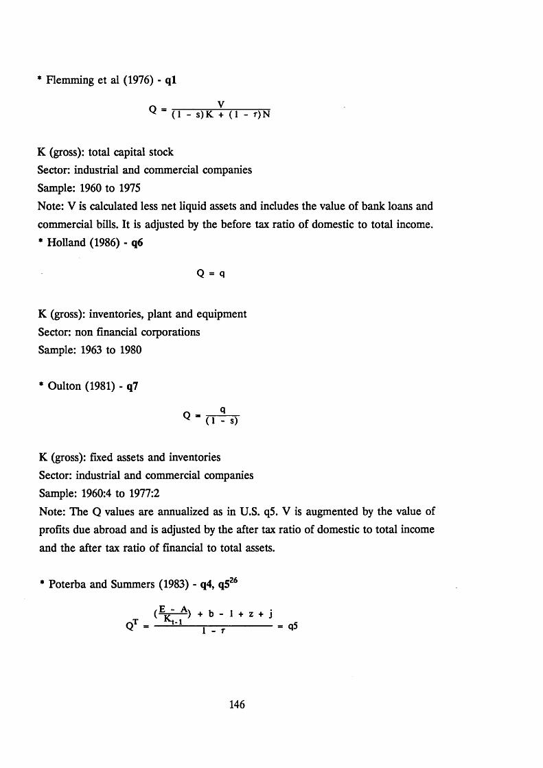
Flemming et al (1976) - ql
Q = V(1 - s)K + (1 - r)N
K (gross): total capital stockSector: industrial and commercial companiesSample: 1960 to 1975Note: V is calculated less net liquid assets and includes the value of bank loans and
commercial bills. It is adjusted by the before tax ratio of domestic to total income. * Holland (1986) - q6
K (gross): inventories, plant and equipment Sector: non financial corporations
Sample: 1963 to 1980
* Oulton (1981) - q7
K (gross): fixed assets and inventories
Sector: industrial and commercial companies
Sample: 1960:4 to 1977:2Note: The Q values are annualized as in U.S. q5. V is augmented by the value of profits due abroad and is adjusted by the after tax ratio of domestic to total income
and the after tax ratio of financial to total assets.
* Poterba and Summers (1983) - q4, q526
Q = q
Ey ~ A ) + b “ 1 + Z + jN - i ___________________ = q51 - T
146
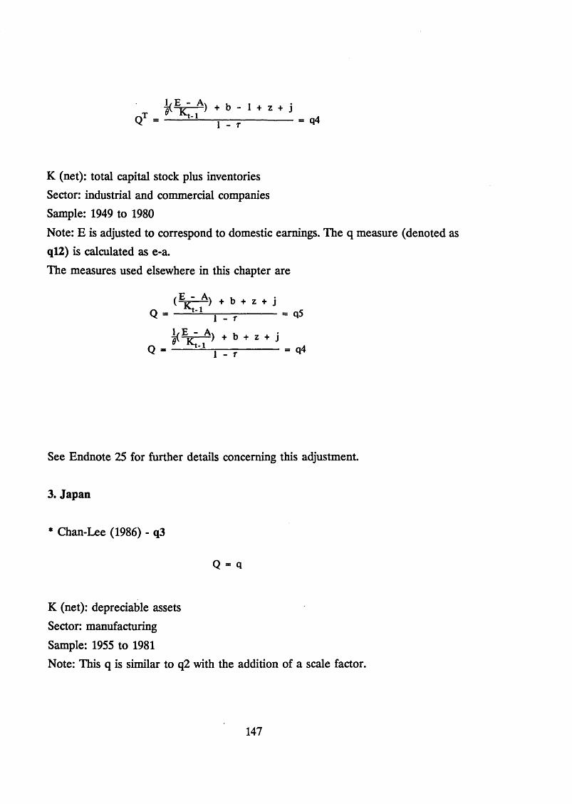
x + » - » + * + iQ - 1 - r----------- *
K (net): total capital stock plus inventories
Sector: industrial and commercial companies Sample: 1949 to 1980
Note: E is adjusted to correspond to domestic earnings. The q measure (denoted as ql2) is calculated as e-a.
The measures used elsewhere in this chapter are
(Ek~ + b + z + jQ = r - T - <*5
+ b + z + jQ . i S i ----------- Q4
See Endnote 25 for further details concerning this adjustment.
3. Japan
* Chan-Lee (1986) - q3
Q = q
K (net): depreciable assets
Sector: manufacturing
Sample: 1955 to 1981Note: This q is similar to q2 with the addition of a scale factor.
147
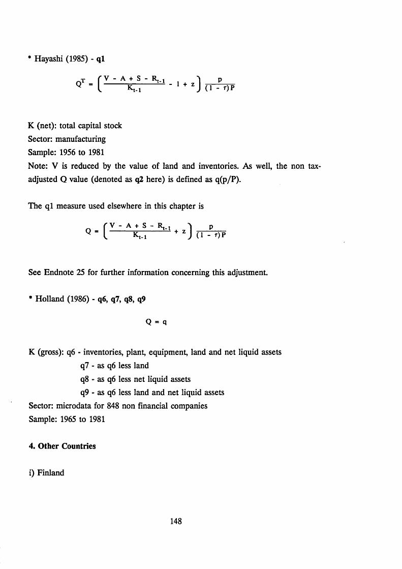
* Hayashi (1985) - ql
T f V - A + S - R j i pQ - I—izr** - 1 + *) rrhv
K (net): total capital stock
Sector: manufacturing
Sample: 1956 to 1981
Note: V is reduced by the value of land and inventories. As well, the non tax- adjusted Q value (denoted as q2 here) is defined as q(p/P).
The ql measure used elsewhere in this chapter is
See Endnote 25 for further information concerning this adjustment.
* Holland (1986) - q6, q7, q8, q9
Q - Q
K (gross): q6 - inventories, plant, equipment, land and net liquid assets
q? - as q6 less land
q8 - as q6 less net liquid assetsq9 - as q6 less land and net liquid assets
Sector: microdata for 848 non financial companies
Sample: 1965 to 1981
4. Other Countries
i) Finland
148
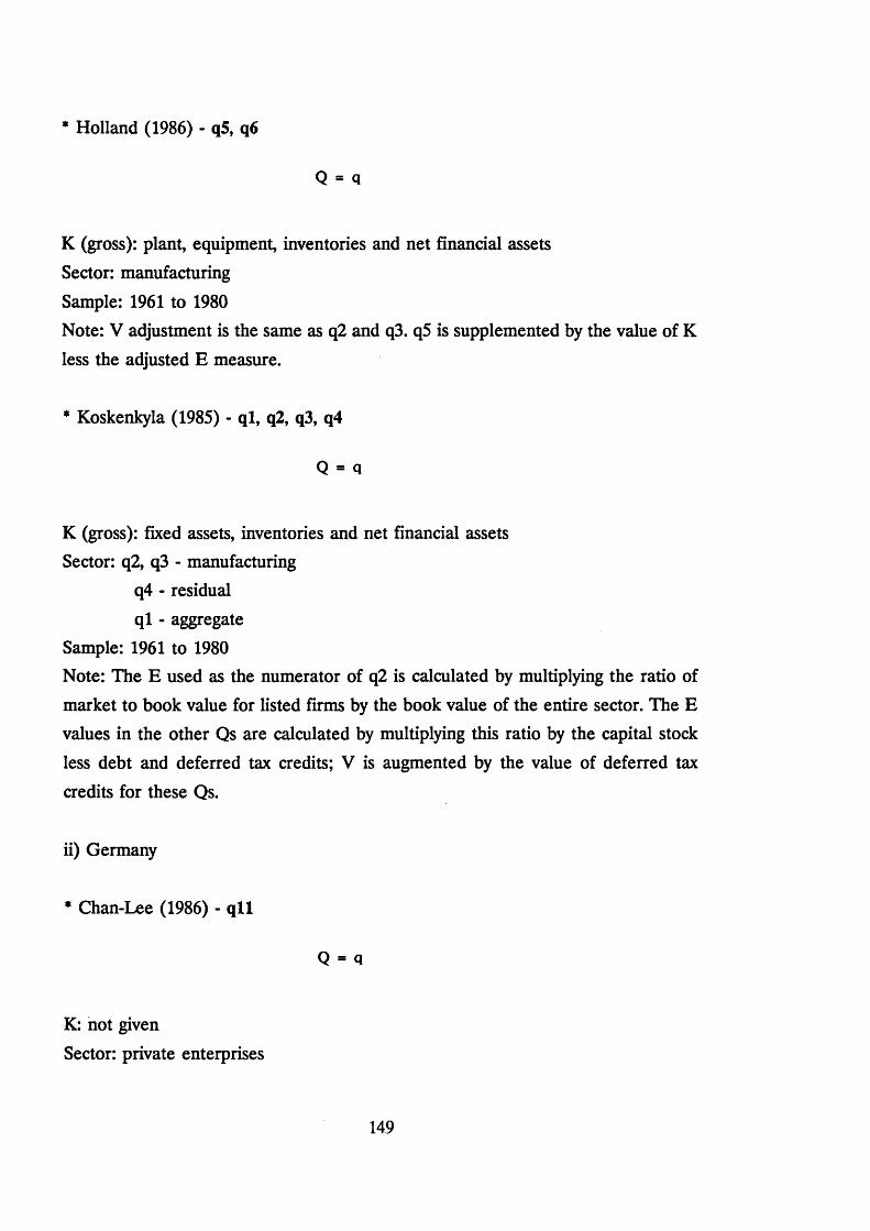
* Holland (1986) - q5, q6
Q = q
K (gross): plant, equipment, inventories and net financial assets Sector: manufacturing
Sample: 1961 to 1980Note: V adjustment is the same as q2 and q3. q5 is supplemented by the value of K
less the adjusted E measure.
* Koskenkyla (1985) - ql, q2, q3, q4
Q = Q
K (gross): fixed assets, inventories and net financial assets Sector: q2, q3 - manufacturing
q4 - residual ql - aggregate
Sample: 1961 to 1980Note: The E used as the numerator of q2 is calculated by multiplying the ratio of market to book value for listed firms by the book value of the entire sector. The E values in the other Qs are calculated by multiplying this ratio by the capital stock
less debt and deferred tax credits; V is augmented by the value of deferred tax
credits for these Qs.
ii) Germany
* Chan-Lee (1986) - q ll
Q = q
K: not given
Sector: private enterprises
149
Sample: 1966 to 1980
* Holland (1986) - q9, qlO
Q = q
K: inventories, equipment, plant, net liquid assets and land Sector: q9 - manufacturing
qlO - non financial corporation
Sample: q9 - 1961 to 1981 qlO - 1961 to 1979
Note: E is basic capital multiplied by a stock price index.
iii) Sweden
* Holland (1986) - q7, q8
Q = q
K: q7 - inventories, equipment, plant and landq8 - inventories, equipment, plant, land and net liquid assets
Sector: business groups
Sample: 1966 to 1980
iv) Belgium
* Chan-Lee (1986) - ql2
Q = q
K: not given
Sector: not given
150
Sample: 1964 to 1983Note: The q value is an index where 1975 = 1.
v) Canada
* Chan-Lee (1986) - ql3
Q - Q
K: total capital employed
Sector: non financial corporations Sample: 1966 to 1981
vi) France
* Chan-Lee (1986) - ql4
Q - Q
K: not givenSector: non financial corporations and quasi-corporate enterprises Sample: 1971 to 1983
A number of remarks can be made about the equations outlined above.
First, the equations found in the papers by Summers (1981), Poterba and Summers
(1983), Dinenis (1985) and Hayashi (1985) have been adjusted prior to using them here for the reasons outlined in Endnote 25. This adjustment generally entailed
adding a non-linear component to each Q formula, except for the non tax adjusted measures.
Second, two of the Japanese Qs, ql and q2, have been supplemented by two
transformed measures, q4 and q5. The transformation replaced Hayashi’s equity
151

series with that of Holland (1986). This was done due to the lack of correlation between the former series and other measures of Japanese equity prices and market
valuations.
Third, there is considerable variability in the construction of the Qs. The source of these differences stem mainly from the treatment of tax variables. It should be
stressed, however, that different models of optimising behaviour can lead to different specifications of Q; this is especially relevant to the case of U.K. q9 and q l l which
are based on a unique specification of adjustment costs.
152
1. See Poterba and Summers (1987), Fama and French (1988) and Kim et al (1989) on this issue.
2. An early exposition of the cost of capital approach can be found in Jorgenson (1971), while two recent survey articles are Chirinko (1986) and Galeotti (1984).
3. See Endnote 5.
4. Ueda and Yoshikawa (1986) note that when delivery lags are incorporated into the Q theory, I/K depends on expectations of Q, rather than Q itself. If the information set of asset-holders includes Q and lagged Q, then these variables properly enter the estimation equation. The authors also motivate the success of the accelerator model of investment (in Chapter V below) by noting that profits (and output) are dominated by permanent components which involve multiple period expectations and, hence, mimic the lagged structure of Q under an assumption of non-negligible delivery time.
5. Marginal Q measures an increment to the capital stock at the relevant marginal replacement and market prices; the value of installed capital is therefore not of interest when deciding to invest in new assets. Average Q, in contrast, aggregates over all existing assets. Hayashi (1982) enumerates the three conditions that are required for marginal Q to be equal to average Q: the firm faces perfectly competitive markets, its production technology is homogeneous of degree one and its capital depreciates at a geometric rate.
In terms of empirical research, Connolly and Lacivita (1985) claim to provide evidence for different autocorrelation properties between marginal and average Qs, thus highlighting the unique nature of each definition. In fact, their analysis confuses marginal Q with tax adjusted average Q and, as a result, their paper actually examines only average Q values. Abel and Blanchard (1986) calculate a marginal Q measure from first principles but discover that it is not significantly different from the average Q found in Von Furstenberg (1977).
6. Wadhwani and Wall (1986) discuss the implications of capital scrapping rates for measures of the capital stock and Chirinko (1986) provides references to the theoretical work on the capital stock measurement problem.
7. Starting with contributions by Shiller (1981), and backed by the earlier judgment of Keynes (1936), a number of researchers have examined the issue of excess volatility of speculative market prices. Discussion of dynamic pricing behaviour anomalies, such as the January effect, the day-of-the-week effect and the tendency of share prices to revert to mean values, can be found in Poterba and Summers (1987). In addition, the issues concerning market myopia are summarized and empirically tested by Nickell and Wadhwani (1987).
A related literature deals with the poor performance of the stock market under inflationary conditions; explanations based on economic and tax factors do not seem to fully explain the phenomena and some measure of market inefficiency may therefore be involved. Modigliani and Cohn (1979), Hendershott (1981) and Brainard, Shoven and Weiss (1980) are important references on this issue.
153
8. Fischer and Merton (1984) provide an extended discussion of this point and give examples of its implications for investment behaviour. The Q theory might also be modified to account for the short-term noise in the market that is presumably not used by agents when making real decisions. Two examples using spectral filtering to separate the signal from the noise in stock prices and Q are found in Engle and Foley (1975) and Poterba and Summers (1983).
9. As well, Robson (1988) points out that anticipated tax changes affect the optimal timing of investment expenditures in the United Kingdom. Expectations of shifts in the tax regime are, therefore, critical components of Q.
10. While acknowledging the theoretical rigour underlying the financial policy neutrality theorem of Modigliani and Miller (1958), it does seem that the debt to equity ratio matters statistically in empirical investment equations. Chapter V of this thesis and Auerbach and Reishus (1987) assign an important role to the debt/equity ratio in explaining corporate mergers and investment.
11. By implication, the Q measure can also be used for evaluating financial investment in the market for corporate control. King (1987) gives the theoretical justification for a Q theory of takeovers and examines the empirical case for the United Kingdom.
12. See Endnote 25 for further details on this adjustment.
13. It is somewhat puzzling that the order of integration should differ only for Japan and Canada. The latter result may stem from small sample bias but the former seems to be a robust finding. A visual examination of Diagrams 1 to 11 in Appendix II does confirm, however, that the Japanese Qs appear to mean revert more frequently over the sample period than do those of other countries. With a longer series of data, say one hundred years or more, more Q variables might exhibit 1(0) behaviour than is the case here.
14. This conclusion is supported by univariate ARIMA specifications of the Q time series properties. The Qs can be subdivided into three categories: those characterised by AR(1) processes, those emulating an ARMA(1,1) process and those following a higher order process. The following summary gives the breakdown of Qs by category:
AR(1) - U.S. q4, q5, q6, q7, ql2; U.K. q2, q7; Japan ql, q2, q3, q4, q5; Other (Finland) q2, q3, q5, q6; Other (West Germany) q9, q ll; Other (Belgium) ql2; Other (Canada) ql3.
ARMA(1,1) - U.S. q8, qlO, q ll, ql5, ql6; U.K. q4, q5, ql2; Other (Finland) ql, q4; Other (Sweden) q7, q8; Other (West Germany) qlO; Other (France) ql4.
Higher Order - U.S. ql, q2, q3, q9, ql3, ql4; U.K. ql, q3, q6, q8, q9, qlO, q ll, ql3; Japan q6, q7, q8, q9.
Each of these specifications produces white residuals. It should also be noted that in each case, the AR(1) coefficient is insignificantly different from unity. First differencing is therefore appropriate to achieve stationarity in the Qs prior to econometric analysis.
154
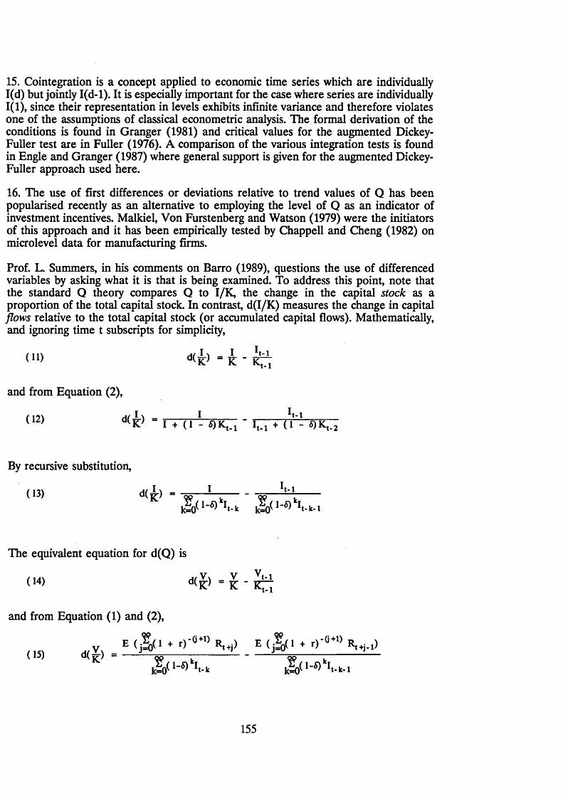
15. Cointegration is a concept applied to economic time series which are individually 1(d) but jointly I(d-l). It is especially important for the case where series are individually 1(1), since their representation in levels exhibits infinite variance and therefore violates one of the assumptions of classical econometric analysis. The formal derivation of the conditions is found in Granger (1981) and critical values for the augmented Dickey- Fuller test are in Fuller (1976). A comparison of the various integration tests is found in Engle and Granger (1987) where general support is given for the augmented Dickey- Fuller approach used here.
16. The use of first differences or deviations relative to trend values of Q has been popularised recently as an alternative to employing the level of Q as an indicator of investment incentives. Malkiel, Von Furstenberg and Watson (1979) were the initiators of this approach and it has been empirically tested by Chappell and Cheng (1982) on microlevel data for manufacturing firms.
Prof. L. Summers, in his comments on Barro (1989), questions the use of differenced variables by asking what it is that is being examined. To address this point, note that the standard Q theory compares Q to I/K, the change in the capital stock as a proportion of the total capital stock. In contrast, d(I/K) measures the change in capital flows relative to the total capital stock (or accumulated capital flows). Mathematically, and ignoring time t subscripts for simplicity,
and from Equation (2),
( 12) K- = I + ( 1 - S) ' I t_j + ( 1 - 5 ) ^ . 2
By recursive substitution,
(13) nr 1 T L *d(K
The equivalent equation for d(Q) is
(14)
and from Equation (1) and (2),
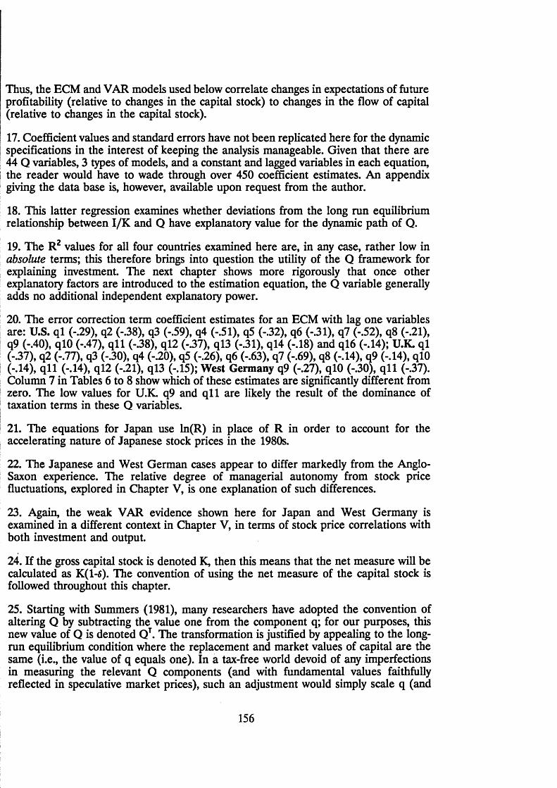
Thus, the ECM and VAR models used below correlate changes in expectations of future profitability (relative to changes in the capital stock) to changes in the flow of capital (relative to changes in the capital stock).
17. Coefficient values and standard errors have not been replicated here for the dynamic specifications in the interest of keeping the analysis manageable. Given that there are 44 Q variables, 3 types of models, and a constant and lagged variables in each equation,
I the reader would have to wade through over 450 coefficient estimates. An appendix ; giving the data base is, however, available upon request from the author.
18. This latter regression examines whether deviations from the long run equilibrium relationship between I/K and Q have explanatory value for the dynamic path of Q.
19. The R2 values for all four countries examined here are, in any case, rather low in absolute terms; this therefore brings into question the utility of the Q framework for
; explaining investment. The next chapter shows more rigorously that once other explanatory factors are introduced to the estimation equation, the Q variable generally adds no additional independent explanatory power.
! 20. The error correction term coefficient estimates for an ECM with lag one variables ! are: U.S. ql (-.29), q2 (-.38), q3 (-.59), q4 (-.51), q5 (-.32), q6 (-.31), q7 (-.52), q8 (-.21),| q9 (-.40), qlO (-.47), q ll (-.38), ql2 (-.37), ql3 (-.31), ql4 (-.18) and ql6 (-.14); U.K. ql! (-.37), q2 (-.77), q3 (-.30), q4 (-.20), q5 (-.26), q6 (-.63), q7 (-.69), q8 (-.14), q9 (-.14), qlOI (-.14), q ll (-.14), ql2 (-.21), ql3 (-.15); West Germany q9 (-.27), qlO (-.30), q l l (-.37).I Column 7 in Tables 6 to 8 show which of these estimates are significantly different from
zero. The low values for U.K. q9 and q ll are likely the result of the dominance of taxation terms in these Q variables.
21. The equations for Japan use ln(R) in place of R in order to account for the, accelerating nature of Japanese stock prices in the 1980s.
22. The Japanese and West German cases appear to differ markedly from the Anglo- Saxon experience. The relative degree of managerial autonomy from stock price fluctuations, explored in Chapter V, is one explanation of such differences.
23. Again, the weak VAR evidence shown here for Japan and West Germany is examined in a different context in Chapter V, in terms of stock price correlations with both investment and output.
24. If the gross capital stock is denoted K, then this means that the net measure will be calculated as K(l-$). The convention of using the net measure of the capital stock is followed throughout this chapter.
25. Starting with Summers (1981), many researchers have adopted the convention of altering Q by subtracting the value one from the component q; for our purposes, this new value of Q is denoted QT. The transformation is justified by appealing to the long- run equilibrium condition where the replacement and market values of capital are the same (i.e., the value of q equals one). In a tax-free world devoid of any imperfections in measuring the relevant Q components (and with fundamental values faithfully reflected in speculative market prices), such an adjustment would simply scale q (and
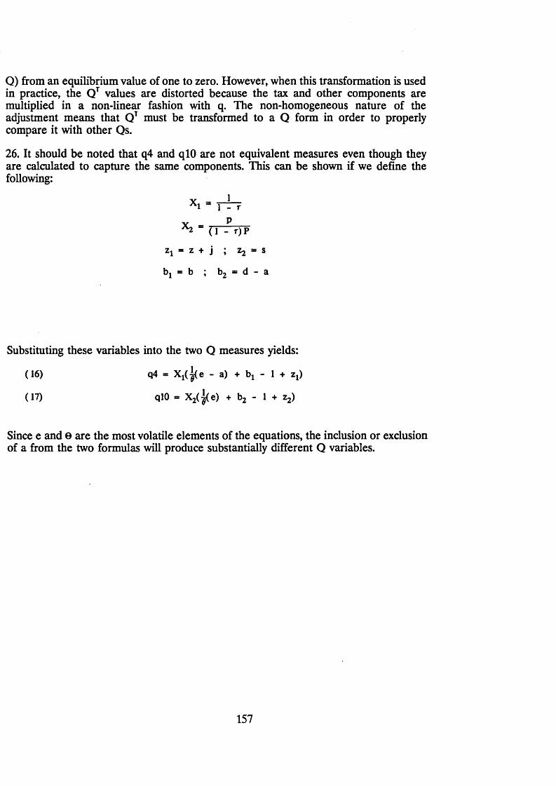
Q) from an equilibrium value of one to zero. However, when this transformation is used in practice, the QT values are distorted because the tax and other components are multiplied in a non-linear fashion with q. The non-homogeneous nature of the adjustment means that QT must be transformed to a Q form in order to properly compare it with other Qs.
26. It should be noted that q4 and qlO are not equivalent measures even though they are calculated to capture the same components. This can be shown if we define the following:
Z| — Z + j J Zj - s
bj = b ; b2 = d - a
Substituting these variables into the two Q measures yields:
(17)
(16) Q4 = - a) + - 1 + zt)
QlO = X2(^(e) + b2 - 1 + z2)
Since e and 0 are the most volatile elements of the equations, the inclusion or exclusion of a from the two formulas will produce substantially different Q variables.
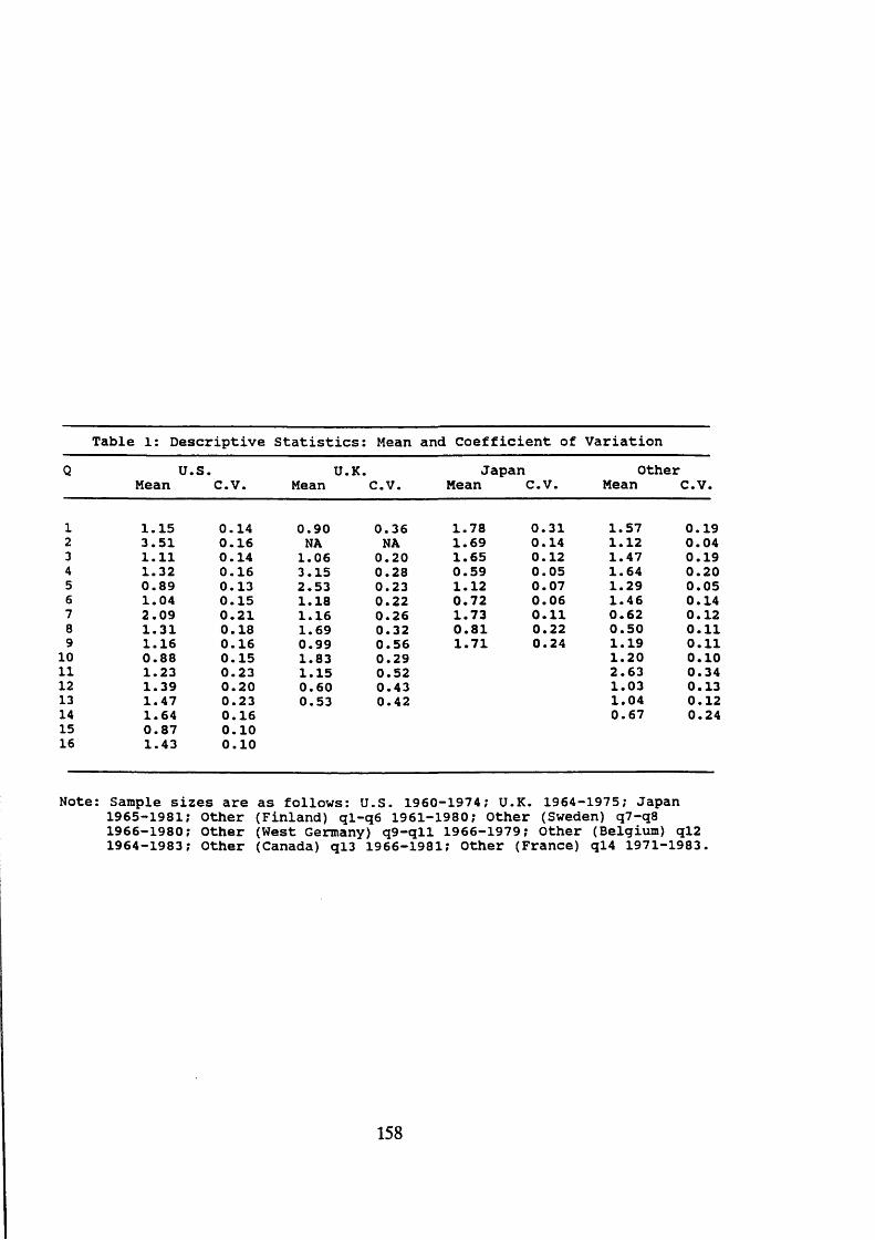
Table 1: Descriptive Statistics: Mean and Coefficient of VariationQ U . S .
Mean C . V .U.
MeanK.
C . V .J a p a n
Me an <C . V .O t h e r
Me an <C.V.
1 1 . 1 5 0 . 1 4 0 . 9 0 0 . 3 6 1 . 7 8 0 . 3 1 1 . 5 7 0 . 1 92 3 . 5 1 0 . 1 6 NA NA 1 . 6 9 0 . 1 4 1 . 1 2 0 . 0 43 1 . 1 1 0 . 1 4 1 . 0 6 0 . 2 0 1 . 6 5 0 . 1 2 1 . 4 7 0 . 1 94 1 . 3 2 0 . 1 6 3 . 1 5 0 . 2 8 0 . 5 9 0 . 0 5 1 . 6 4 0 . 2 05 0 . 8 9 0 . 1 3 2 . 5 3 0 . 2 3 1 . 1 2 0 . 0 7 1 . 2 9 0 . 0 56 1 . 0 4 0 . 1 5 1 . 1 8 0 . 2 2 0 . 7 2 0 . 0 6 1 . 4 6 0 . 1 47 2 . 0 9 0 . 2 1 1 . 1 6 0 . 2 6 1 . 7 3 0 . 1 1 0 . 6 2 0 . 1 28 1 . 3 1 0 . 1 8 1 . 6 9 0 . 3 2 0 . 8 1 0 . 2 2 0 . 5 0 0 . 1 19 1 . 1 6 0 . 1 6 0 . 9 9 0 . 5 6 1 . 7 1 0 . 2 4 1 . 1 9 0 . 1 1
10 0 . 8 8 0 . 1 5 1 . 8 3 0 . 2 9 1 . 2 0 0 . 1 011 1 . 2 3 0 . 2 3 1 . 1 5 0 . 5 2 2 . 6 3 0 . 3 412 1 . 3 9 0 . 2 0 0 . 6 0 0 . 4 3 1 . 0 3 0 . 1 313 1 . 4 7 0 . 2 3 0 . 5 3 0 . 4 2 1 . 0 4 0 . 1 214 1 . 6 4 0 . 1 6 0 . 6 7 0 . 2 415 0 . 8 7 0 . 1 016 1 . 4 3 0 . 1 0
N o t e : S a m p l e s i z e s a r e a s f o l l o w s : U . S . 1 9 6 0 - 1 9 7 4 ; U .K . 1 96 4 - 1 9 7 5 ; J a p a n1 9 6 5 - 1 9 8 1 ; O t h e r ( F i n l a n d ) q l - q 6 1 9 6 1 - 1 9 8 0 ; O t h e r ( S w e d e n ) q 7 - q 81 9 6 6 - 1 9 8 0 ; O t h e r ( W e s t G e r m a n y ) q 9 - q l l 1 9 6 6 - 1 9 7 9 ; O t h e r ( B e l g i u m ) q l 2 1 9 6 4 - 1 9 8 3 ; O t h e r ( C a n a d a ) q l 3 1 9 6 6 - 1 9 8 1 ; O t h e r ( F r a n c e ) q l 4 1 9 7 1 - 1 9 8 3 .
158
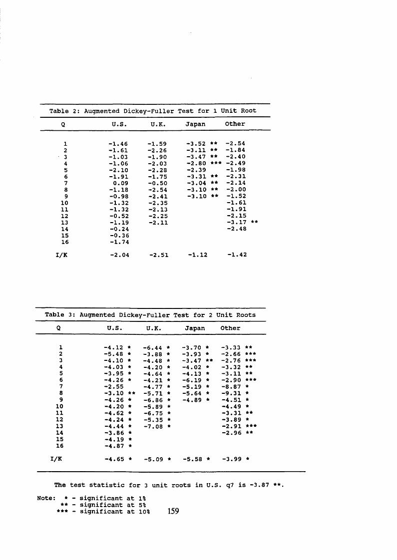
Table 2: Augmented Dickey-Fuller Test for 1 Unit RootQ U . S . U . K . J a p a n O t h e r
1 - 1 . 4 6 - 1 . 5 9 - 3 . 5 2 ** - 2 . 5 42 - 1 . 6 1 - 2 . 2 6 - 3 . 1 1 ** - 1 . 8 43 - 1 . 0 3 - 1 . 9 0 - 3 . 4 7 ** - 2 . 4 04 - 1 . 0 6 - 2 . 0 3 - 2 . 8 0 ** * - 2 . 4 95 - 2 . 1 0 - 2 . 2 8 - 2 . 3 9 - 1 . 9 86 - 1 . 9 1 - 1 . 7 5 - 3 . 3 1 ** - 2 . 3 17 0 . 0 9 - 0 . 5 0 - 3 . 0 4 ** - 2 . 1 48 - 1 . 1 8 - 2 . 5 4 - 3 . 1 0 ** - 2 . 0 09 - 0 . 9 8 - 2 . 4 1 - 3 . 1 0 ** - 1 . 5 2
10 - 1 . 3 2 - 2 . 3 5 - 1 . 6 111 - 1 . 3 2 - 2 . 1 3 - 1 . 9 112 - 0 . 5 2 - 2 . 2 5 - 2 . 1 513 - 1 . 1 9 - 2 . 1 1 - 3 . 1 7 **14 - 0 . 2 4 - 2 . 4 815 - 0 . 3 616 - 1 . 7 4
I / K l to o a - 2 . 5 1 - 1 . 1 2 - 1 . 4 2
T a b l e 3 : A u g m e n t e d D i c k e y - F u l l e r T e s t f o r 2 U n i t R o o t s
Q U . S . U . K . J a p a n O t h e r
1 - 4 . 1 2 * - 6 . 4 4 * - 3 . 7 0 * - 3 . 3 3 **2 - 5 . 4 8 * - 3 . 8 8 * - 3 . 9 3 * - 2 . 6 6 ***3 - 4 . 1 0 * - 4 . 4 8 * - 3 . 4 7 ** - 2 . 7 6 ***4 - 4 . 0 3 * - 4 . 2 0 * - 4 . 0 2 * - 3 . 3 2 **5 - 3 . 9 5 * - 4 . 6 4 * - 4 . 1 3 * - 3 . 1 1 **6 - 4 . 2 6 * - 4 . 2 1 * - 6 . 1 9 * - 2 . 9 0 **★7 - 2 . 5 5 - 4 . 7 7 * - 5 . 1 9 * - 8 . 8 7 *8 - 3 . 1 0 ** - 5 . 7 1 * - 5 . 6 4 * - 9 . 3 1 *9 - 4 . 2 6 * - 6 . 8 6 * - 4 . 8 9 * - 4 . 5 1 *
10 - 4 . 2 0 * - 5 . 8 9 * - 4 . 4 9 *11 - 4 . 6 2 * - 6 . 7 5 * - 3 . 3 1 **12 - 4 . 2 4 * - 5 . 3 5 * - 3 . 8 9 *13 - 4 . 4 4 * - 7 . 0 8 * - 2 . 9 1 ***14 - 3 . 8 6 * - 2 . 9 6 **15 - 4 . 1 9 *16 - 4 . 8 7 *
I / K - 4 . 6 5 * - 5 . 0 9 * - 5 . 5 8 * - 3 . 9 9 *
T h e t e s t s t a t i s t i c f o r 3 u n i t r o o t s i n U . S . q7 i s - 3 . 8 7
N o t e : * - s i g n i f i c a n t a t 1%** - s i g n i f i c a n t a t 5%
** * - s i g n i f i c a n t at 10% 159
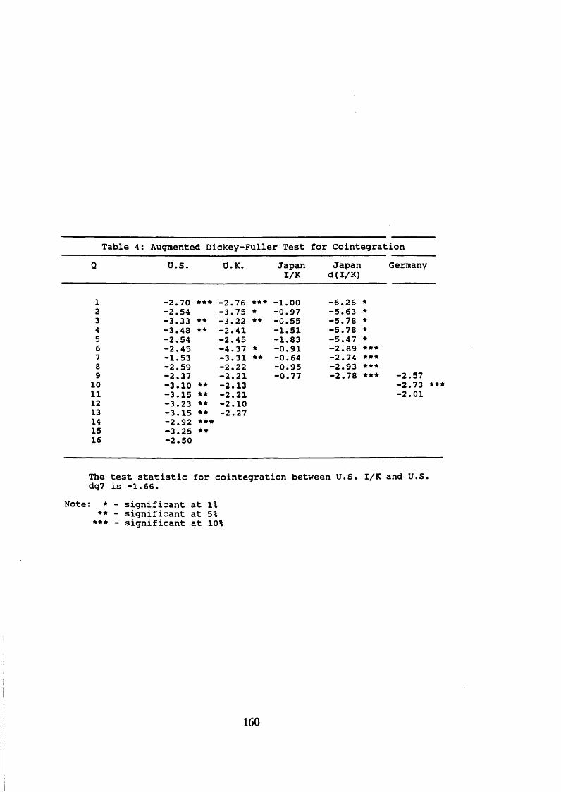
Table 4: Augmented Dickey-Fuller Test for CointegrationQ U . S . U . K . J a p a n J a p a n G e r m a n y
I / K d ( I / K )
1 - 2 . 7 0 * * * - 2 . 7 6 ***2 - 2 . 5 4 - 3 . 7 5 *3 - 3 . 3 3 ** - 3 . 2 2 **4 - 3 . 4 8 - 2 . 4 15 - 2 . 5 4 - 2 . 4 56 - 2 . 4 5 - 4 . 3 7 *7 - 1 . 5 3 - 3 . 3 1 **8 - 2 . 5 9 - 2 . 2 29 - 2 . 3 7 - 2 . 2 1
10 - 3 . 1 0 *★ - 2 . 1 311 - 3 . 1 5 ** - 2 . 2 112 - 3 . 2 3 ** - 2 . 1 013 - 3 . 1 5 ** - 2 . 2 714 - 2 . 9 2 * * *15 - 3 . 2 5 **16 - 2 . 5 0
- 1 . 0 0 - 6 . 2 6 *- 0 . 9 7 - 5 . 6 3 *- 0 . 5 5 - 5 . 7 8 *- 1 . 5 1 - 5 . 7 8 *- 1 . 8 3 - 5 . 4 7 *- 0 . 9 1 - 2 . 8 9 * * *- 0 . 6 4 - 2 . 7 4 * * *- 0 . 9 5 - 2 . 9 3 * * *- 0 . 7 7 - 2 . 7 8 * * *
- 2 . 7 3 *** - 2 . 0 1
T h e t e s t s t a t i s t i c f o r c o i n t e g r a t i o n b e t w e e n U . S . I / K a n d U .S . d q 7 i s - 1 . 6 6 .
N o t e : * - s i g n i f i c a n t a t 1%** - s i g n i f i c a n t a t 5%
*** _ s i g n i f i c a n t a t 10%
160
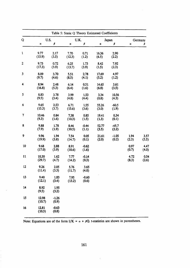
Table 5: Static Q Theory Estimated Coefficients
Q U.S. U.K. Japan Germanya P a P a P a 0
1 9.77 2.17 7.70 0.71 1636 2.90(15.9) (3.5) (123) (1.2) (6.5) (2.2)
2 9.73 0.72 6.25 1.73 8.42 7.92(17.3) (3.9) (13.7) (3.9) (13) (23)
3 8.09 3.70 531 2.78 17.69 4.97(9.7) (4.6) (8.5) (4.1) (5.2) (13)
4 8.94 2.48 6.14 0.51 14.65 3.61(16.8) (53) (6.4) (1.6) (6.8) (33)
5 8.83 3.78 3.99 1.53 3.34 1036(9.5) (3.4) (4.8) (4.4) (0.8) (43)
6 9.65 233 6.71 1.55 55.26 -60.5(15.3) (3.7) (13.6) (3.6) (3.0) (1.9)
7 10.46 0.84 738 0.85 19.41 034(93) (1.6) (103) (13) (13) (0.1)
8 9.88 1.78 8.46 -0.44 52.77 -45.7(7.9) (1.9) (103) (1.1) (33) (22)
9 9.96 1.94 734 0.05 21.61 -1.05 1.94 3.57(19.9) (3.8) (14.7) (0.1) (2.0) (0.2) (23) (53)
10 9.68 2.88 8.91 -0.62 0.97 4.47(17.0) (3.9) (10.6) (1.6) (0.7) (4.0)
11 1030 1.62 7.77 -0.14 4.72 0.54(29.7) (4.7) (14.2) (03) (8.3) (2.6)
12 9.26 2.05 5.76 3.65(11.4) (33) (11.7) (4.0)
13 9.40 1.83 7.95 -0.60(12.1) (3.4) (13.2) (0.6)
14 8.92 1.95(9.5) (33)
15 12.98 -1.26(10.7) (0.9)
16 12.81 -0.63(103) (0.8)
Note: Equations are of the form I/K = a + 0Q. t-statistics are shown in parentheses.
161
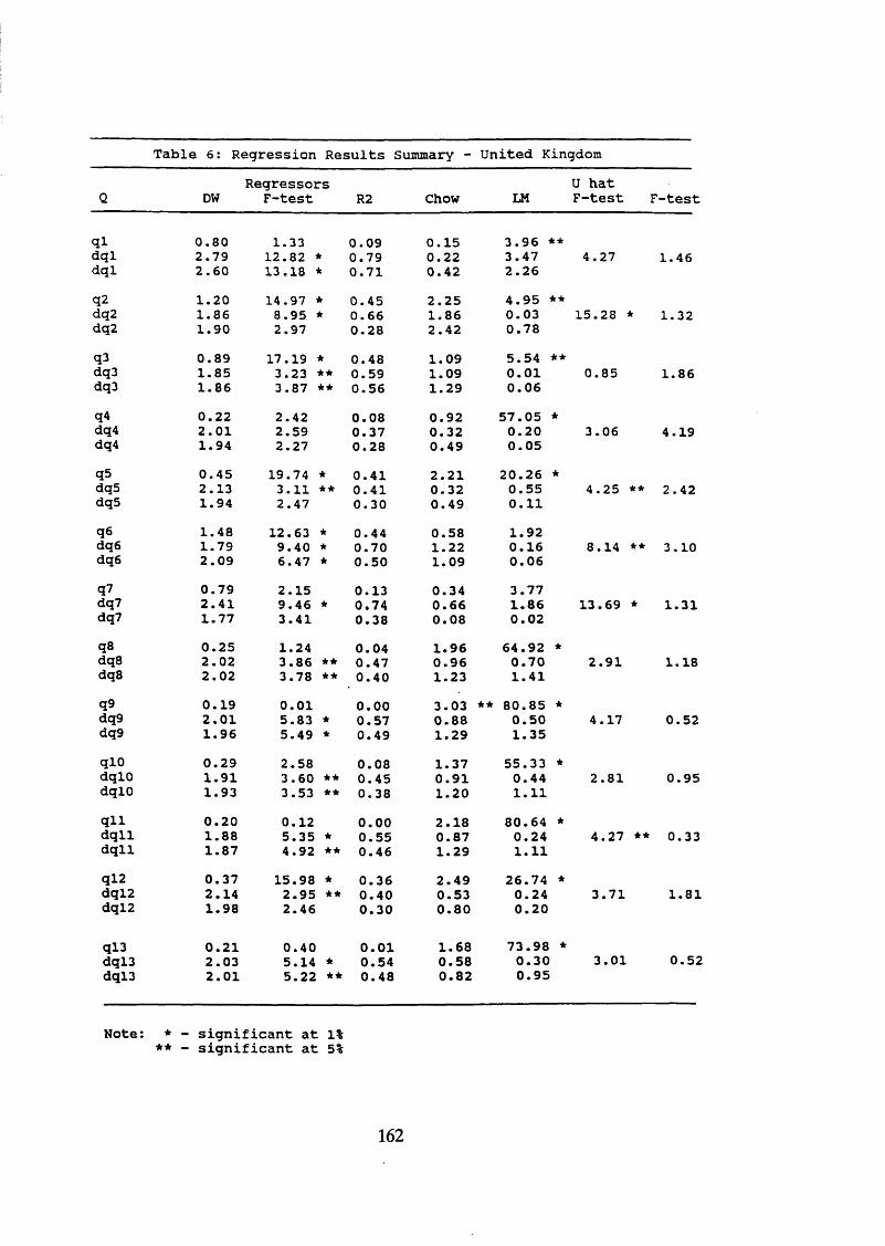
T a b l e 6 : R e g r e s s i o n R e s u l t s S u mm ary - U n i t e d K in g d o m
R e g r e s s o r s U h a tQ DW F - t e s t R2 Chow LM F - t e s t F - t e s t
q i 0 . 8 0 1 . 3 3 0 . 0 9 0 . 1 5 3 . 9 6 **d q l 2 . 7 9 1 2 . 8 2 * 0 . 7 9 0 . 2 2 3 . 4 7 4 . 2 7 1 . 4 6d q l 2 . 6 0 1 3 . 1 8 * 0 . 7 1 0 . 4 2 2 . 2 6
q2 1 . 2 0 1 4 . 9 7 * 0 . 4 5 2 . 2 5 4 . 9 5 **d q 2 1 . 8 6 8 . 9 5 * 0 . 6 6 1 * 8 6 0 . 0 3 1 5 . 2 8 * 1 . 3 2d q 2 1 . 9 0 2 . 9 7 0 . 2 8 2 . 4 2 0 . 7 8
q i 0 . 8 9 1 7 . 1 9 * 0 . 4 8 1 . 0 9 5 . 5 4 **dq 3 1 . 8 5 3 . 2 3 ** 0 . 5 9 1 . 0 9 0 . 0 1 0 . 8 5 1 . 8 6dq3 1 . 8 6 3 . 8 7 ** 0 . 5 6 1 . 2 9 0 . 0 6
q4 0 . 2 2 2 . 4 2 0 . 0 8 0 . 9 2 5 7 . 0 5 *dq4 2 . 0 1 2 . 5 9 0 . 3 7 0 . 3 2 0 . 2 0 3 . 0 6 4 . 1 9dq4 1 . 9 4 2 . 2 7 0 . 2 8 0 . 4 9 0 . 0 5
q s 0 . 4 5 1 9 . 7 4 * 0 . 4 1 2 . 2 1 2 0 . 2 6 *dq 5 2 . 1 3 3 . 1 1 ** 0 . 4 1 0 . 3 2 0 . 5 5 4 . 2 5 ** 2 . 4 2d q 5 1 . 9 4 2 . 4 7 0 . 3 0 0 . 4 9 0 . 1 1
q e 1 . 4 8 1 2 . 6 3 * 0 . 4 4 0 . 5 8 1 . 9 2d q 6 1 . 7 9 9 . 4 0 * 0 . 7 0 1 . 2 2 0 . 1 6 8 . 1 4 ** 3 . 1 0d q 6 2 . 0 9 6 . 4 7 * 0 . 5 0 1 . 0 9 0 . 0 6
q7 0 . 7 9 2 . 1 5 0 . 1 3 0 . 3 4 3 . 7 7d q7 2 . 4 1 9 . 4 6 * 0 . 7 4 0 . 6 6 1 . 8 6 1 3 . 6 9 * 1 . 3 1dq 7 1 . 7 7 3 . 4 1 0 . 3 8 0 . 0 8 0 . 0 2
q s 0 . 2 5 1 . 2 4 0 . 0 4 1 . 9 6 6 4 . 9 2 *dq 8 2 . 0 2 3 . 8 6 ** 0 . 4 7 0 . 9 6 0 . 7 0 2 . 9 1 1 . 1 8dq 8 2 . 0 2 3 . 7 8 ** 0 . 4 0 1 . 2 3 1 . 4 1
q9 0 . 1 9 0 . 0 1 0 . 0 0 3 . 0 3 ** 8 0 . 8 5 *d q 9 2 . 0 1 5 . 8 3 * 0 . 5 7 0 . 8 8 0 . 5 0 4 . 1 7 0 . 5 2dq 9 1 . 9 6 5 . 4 9 * 0 . 4 9 1 . 2 9 1 . 3 5
q lO 0 . 2 9 2 . 5 8 0 . 0 8 1 . 3 7 5 5 . 3 3 *d q l O 1 . 9 1 3 . 6 0 ** 0 . 4 5 0 . 9 1 0 . 4 4 2 . 8 1 0 . 9 5d q l O 1 . 9 3 3 . 5 3 ** 0 . 3 8 1 . 2 0 1 . 1 1
q l l 0 . 2 0 0 . 1 2 0 . 0 0 2 . 1 8 8 0 . 6 4 *d q l l 1 . 8 8 5 . 3 5 * 0 . 5 5 0 . 8 7 0 . 2 4 4 . 2 7 ** 0 . 3 3d q l l 1 . 8 7 4 . 9 2 ** 0 . 4 6 1 . 2 9 1 . 1 1
q l 2 0 . 3 7 1 5 . 9 8 * 0 . 3 6 2 . 4 9 2 6 . 7 4 *d q l 2 2 . 1 4 2 . 9 5 ** 0 . 4 0 0 . 5 3 0 . 2 4 3 . 7 1 1 . 8 1d q l 2 1 . 9 8 2 . 4 6 0 . 3 0 0 . 8 0 0 . 2 0
q l 3 0 . 2 1 0 . 4 0 0 . 0 1 1 . 6 8 7 3 . 9 8 *d q l 3 2 . 0 3 5 . 1 4 * 0 . 5 4 0 . 5 8 0 . 3 0 3 . 0 1 0 . 5 2d q l 3 2 . 0 1 5 . 2 2 ** 0 . 4 8 0 . 8 2 0 . 9 5
N o t e : * - s i g n i f i c a n t a t 1% ** - s i g n i f i c a n t a t 5%
162
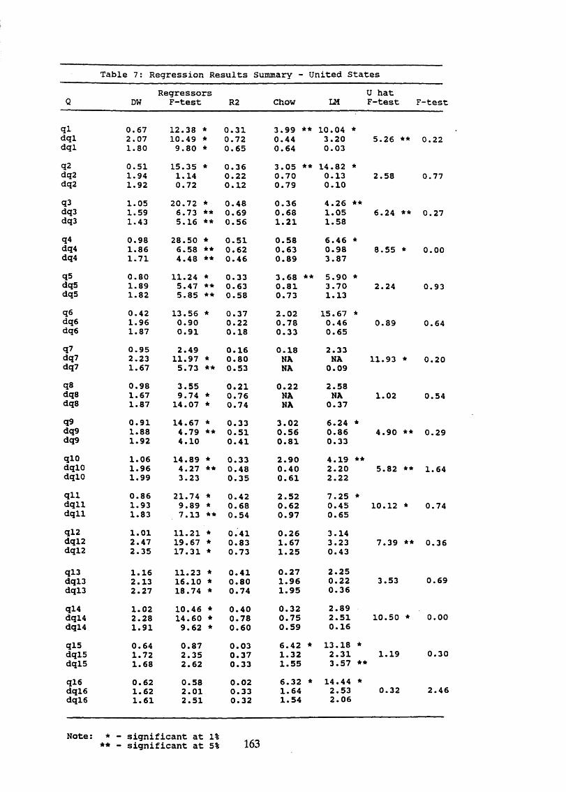
T a b l e 7 : R e g r e s s i o n R e s u l t s S u m m a r y - U n i t e d S t a t e s
R e g r e s s o r s U h a tQ DW F - t e s t R2 Chow LM F - t e s t F - t e s t
qi 0 . 6 7 1 2 . 3 8 * 0 . 3 1 3 . 9 9 ** 1 0 . 0 4 *d q l 2 . 0 7 1 0 . 4 9 * 0 . 7 2 0 . 4 4 3 . 2 0 5 . 2 6 ** 0 . 2 2d q l 1 . 8 0 9 . 8 0 * 0 . 6 5 0 . 6 4 0 . 0 3
q2 0 . 5 1 1 5 . 3 5 * 0 . 3 6 3 . 0 5 ** 1 4 . 8 2 *dq 2 1 . 9 4 1 . 1 4 0 . 2 2 0 . 7 0 0 . 1 3 2 . 5 8 0 . 7 7d q 2 1 . 9 2 0 . 7 2 0 . 1 2 0 . 7 9 0 . 1 0
qi 1 . 0 5 2 0 . 7 2 * 0 . 4 8 0 . 3 6 4 . 2 6 **d q3 1 . 5 9 6 . 7 3 ** 0 . 6 9 0 . 6 8 1 . 0 5 6 . 2 4 ** 0 . 2 7d q3 1 . 4 3 5 . 1 6 ** 0 . 5 6 1 . 2 1 1 . 5 8
q4 0 . 9 8 2 8 . 5 0 * 0 . 5 1 0 . 5 8 6 . 4 6 *dq 4 1 . 8 6 6 . 5 8 ** 0 . 6 2 0 . 6 3 0 . 9 8 8 . 5 5 * 0 . 0 0d q 4 1 . 7 1 4 . 4 8 ** 0 . 4 6 0 . 8 9 3 . 8 7
qs 0 . 8 0 1 1 . 2 4 * 0 . 3 3 3 . 6 8 ** 5 . 9 0 *d q 5 1 . 8 9 5 . 4 7 ** 0 . 6 3 0 . 8 1 3 . 7 0 2 . 2 4 0 . 9 3dq S 1 . 8 2 5 . 8 5 ** 0 . 5 8 0 . 7 3 1 . 1 3
qe 0 . 4 2 1 3 . 5 6 * 0 . 3 7 2 . 0 2 1 5 . 6 7 *d q 6 1 . 9 6 0 . 9 0 0 . 2 2 0 . 7 8 0 . 4 6 0 . 8 9 0 . 6 4d q 6 1 . 8 7 0 . 9 1 0 . 1 8 0 . 3 3 0 . 6 5
q7 0 . 9 5 2 . 4 9 0 . 1 6 0 . 1 8 2 . 3 3d q 7 2 . 2 3 1 1 . 9 7 * 0 . 8 0 NA NA 1 1 . 9 3 * 0 . 2 0d q 7 1 . 6 7 5 . 7 3 ** 0 . 5 3 NA 0 . 0 9
qs 0 . 9 8 3 . 5 5 0 . 2 1 0 . 2 2 2 . 5 8d q 8 1 . 6 7 9 . 7 4 * 0 . 7 6 NA NA 1 . 0 2 0 . 5 4d q 8 1 . 8 7 1 4 . 0 7 * 0 . 7 4 NA 0 . 3 7
q9 0 . 9 1 1 4 . 6 7 * 0 . 3 3 3 . 0 2 6 . 2 4 *d q 9 1 . 8 8 4 . 7 9 ** 0 . 5 1 0 . 5 6 0 . 8 6 4 . 9 0 ** 0 . 2 9d q 9 1 . 9 2 4 . 1 0 0 . 4 1 0 . 8 1 0 . 3 3
q l O 1 . 0 6 1 4 . 8 9 * 0 . 3 3 2 . 9 0 4 . 1 9 **d q l O 1 . 9 6 4 . 2 7 ** 0 . 4 8 0 . 4 0 2 . 2 0 5 . 8 2 ** 1 . 6 4d q l O 1 . 9 9 3 . 2 3 0 . 3 5 0 . 6 1 2 . 2 2
q i i 0 . 8 6 2 1 . 7 4 * 0 . 4 2 2 . 5 2 7 . 2 5 *d q l l 1 . 9 3 9 . 8 9 * 0 . 6 8 0 . 6 2 0 . 4 5 1 0 . 1 2 * 0 . 7 4d q l l 1 . 8 3 7 . 1 3 ** 0 . 5 4 0 . 9 7 0 . 6 5
q l 2 1 . 0 1 1 1 . 2 1 * 0 . 4 1 0 . 2 6 3 . 1 4d q l 2 2 . 4 7 1 9 . 6 7 * 0 . 8 3 1 . 6 7 3 . 2 3 7 . 3 9 ** 0 . 3 6d q l 2 2 . 3 5 1 7 . 3 1 * 0 . 7 3 1 . 2 5 0 . 4 3
q l 3 1 . 1 6 1 1 . 2 3 * 0 . 4 1 0 . 2 7 2 . 2 5d q l 3 2 . 1 3 1 6 . 1 0 * 0 . 8 0 1 . 9 6 0 . 2 2 3 . 5 3 0 . 6 9d q l 3 2 . 2 7 1 8 . 7 4 * 0 . 7 4 1 . 9 5 0 . 3 6
q l 4 1 . 0 2 1 0 . 4 6 * 0 . 4 0 0 . 3 2 2 . 8 9d q l 4 2 . 2 8 1 4 . 6 0 * 0 . 7 8 0 . 7 5 2 . 5 1 1 0 . 5 0 * 0 . 0 0d q l 4 1 . 9 1 9 . 6 2 * 0 . 6 0 0 . 5 9 0 . 1 6
q l 5 0 . 6 4 0 . 8 7 0 . 0 3 6 . 4 2 * 1 3 . 1 8 *d q l 5 1 . 7 2 2 . 3 5 0 . 3 7 1 . 3 2 2 . 3 1 1 . 1 9 0 . 3 0d q l 5 1 . 6 8 2 . 6 2 0 . 3 3 1 . 5 5 3 . 5 7 **
q l 6 0 . 6 2 0 . 5 8 0 . 0 2 6 . 3 2 * 1 4 . 4 4 *d q l 6 1 . 6 2 2 . 0 1 0 . 3 3 1 . 6 4 2 . 5 3 0 . 3 2 2 . 4 6d q l 6 1 . 6 1 2 . 5 1 0 . 3 2 1 . 5 4 2 . 0 6
N o t e : * - s i g n i f i c a n t a t 1%** - sign ificant at 5% 163
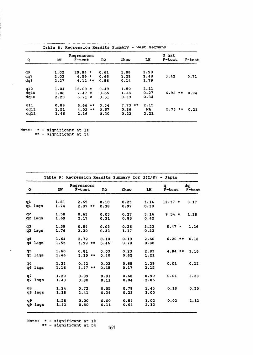
Table 8: Regression Results Summary - West Germany
QR e g r e s s o r s
DW F - t e s t R2 Chow LMU h a t F - t e s t F - t e s t
q9 1 . 0 2 2 9 . 8 4 * 0 . 6 1 1 . 8 8 2 . 9 8dq9 2 . 0 2 4 . 5 9 * 0 . 6 6 1 . 2 8 2 . 4 8 3 . 4 2 0 . 7 1dq 9 2 . 2 7 4 . 1 2 ** 0 . 5 6 0 . 1 4 2 . 7 9
q lO 1 . 0 4 1 6 . 0 9 * 0 . 4 9 1 . 5 9 3 . 1 1d q l O 1 . 8 8 7 . 4 7 * 0 . 6 5 1 . 3 8 0 . 2 7 4 . 9 2 ** 0 . 9 4d q l O 2 . 2 0 6 . 7 1 * 0 . 5 1 0 . 3 9 0 . 3 4
q l l 0 . 8 9 6 . 6 6 ** 0 . 3 4 7 . 7 3 ** 2 . 1 5d q l l 1 . 5 1 4 . 0 3 ** 0 . 5 7 0 . 8 6 NA 5 . 7 3 ** 0 . 2 1d q l l 1 . 4 6 2 . 1 6 0 . 3 0 0 . 2 3 3 . 2 1
N o t e : * - s i g n i f i c a n t a t 1%** - s i g n i f i c a n t a t 5%
T a b l e 9 : :R e g r e s s i o n R e s u l t s Su mm ary f o r d ( I / K ) - J a p a n
R e g r e s s o r s q d qQ DW F - t e s t R2 Chow LM F - t e s t F - t e s t
q i 1 . 6 1 2 . 6 5 0 . 1 0 0 . 2 3 3 . 1 4 1 2 . 3 7 * 0 . 1 7q l l a g s 1 . 7 4 2 . 8 7 ** 0 . 3 8 0 . 9 7 0 . 3 0
q2 1 . 5 8 0 . 6 3 0 . 0 3 0 . 2 7 3 . 1 6 9 . 5 4 * 1 . 2 8q 2 l a g s 1 . 6 9 2 . 1 7 0 . 3 1 0 . 8 5 0 . 4 2
q3 1 . 5 9 0 . 8 4 0 . 0 3 0 . 2 6 3 . 2 3 8 . 4 7 * 1 . 3 6q3 l a g s 1 . 7 6 2 . 3 0 0 . 3 3 1 . 1 7 0 . 3 2
q4 1 . 6 4 2 . 7 2 0 . 1 0 0 . 1 9 2 . 6 0 6 . 2 0 ** 0 . 1 8q4 l a g s 1 . 5 5 3 . 9 9 ** 0 . 4 6 0 . 7 8 0 . 8 8
qs 1 . 6 0 0 . 8 1 0 . 0 3 0 . 2 3 2 . 8 3 4 . 8 4 ** 1 . 1 6q 5 l a g s 1 . 4 6 3 . 1 5 ** 0 . 4 0 0 . 6 2 1 . 2 1
qe 1 . 2 3 0 . 4 2 0 . 0 3 0 . 6 5 1 . 3 9 0 . 0 1 0 . 1 3q 6 l a g s 1 . 1 6 3 . 4 7 ** 0 . 3 5 0 . 1 7 3 . 1 5
q7 1 . 2 9 0 . 0 9 0 . 0 1 0 . 6 8 0 . 9 0 0 . 0 1 3 . 2 3q 7 l a g s 1 . 4 3 0 . 8 0 0 . 1 1 0 . 0 4 2 . 0 5
qs 1 . 2 4 0 . 7 2 0 . 0 5 0 . 7 8 1 . 4 3 0 . 1 8 0 . 3 5q8 l a g s 1 . 1 8 3 . 4 1 0 . 3 4 0 . 2 3 3 . 0 0
q9 1 . 2 8 0 . 0 0 0 . 0 0 0 . 5 4 1 . 0 2 0 . 0 2 2 . 1 2q 9 l a g s 1 . 4 3 0 . 8 0 0 . 1 1 0 . 0 3 2 . 1 3
N o t e : * - s i g n i f i c a n t a t 1% ** - s i g n i f i c a n t a t 5%
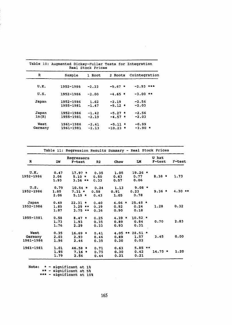
T a b l e 1 0 : A u g m e n t e d D i c k e y - F u l l e r T e s t s f o r I n t e g r a t i o n R e a l S t o c k P r i c e s
R S a m p l e 1 R o o t 2 R o o t s C o i n t e g r a t i o n
U . K . 1 9 5 2 - 1 9 8 6 - 2 . 3 3 - 5 . 6 7 * - 2 . 9 3
U . S . 1 9 5 2 - 1 9 8 6 - 2 . 0 0 - 4 . 6 5 * - 3 . 0 0
J a p a n 1 9 5 2 - 1 9 8 6 1 . 6 2 - 2 . 1 9 - 2 . 5 61 9 5 5 - 1 9 8 1 - 1 . 4 7 - 5 . 1 2 * - 2 . 0 3
J a p a n 1 9 5 2 - 1 9 8 6 - 1 . 4 2 - 5 . 2 7 * - 2 . 5 6l n ( R ) 1 9 5 5 - 1 9 8 1 - 2 . 1 9 - 4 . 5 7 * - 2 . 0 3
W e s t 1 9 6 1 - 1 9 8 6 - 2 . 4 1 - 5 . 1 1 * - 0 . 9 9G e r m a n y 1 9 6 1 - 1 9 8 1 - 2 . 1 3 - 1 0 . 2 3 * - 3 . 9 0
T a b l e 1 1 : R e g r e s s i o n R e s u l t s S um ma ry - R e a l S t o c k P r i c e s
R e g r e s s o r s U h a tDW F - t e s t R2 Chow 121 F - t e s t F - t e s t
U . K . 0 . 4 7 1 7 . 9 7 * 0 . 3 5 1 . 0 5 1 9 . 2 6 *1 9 5 2 - 1 9 8 6 2 . 0 6 5 . 1 0 * 0 . 5 0 0 . 6 3 0 . 7 7 8 . 3 8 * 1 . 7 3
1 . 9 3 3 . 3 6 ** 0 . 3 3 0 . 5 7 0 . 0 6
U . S . 0 . 7 9 1 0 . 5 4 * 0 . 2 4 1 . 1 3 9 . 0 8 *1 9 5 2 - 1 9 8 6 1 . 8 5 7 . 3 1 * 0 . 5 8 0 . 9 1 0 . 2 3 9 . 3 6 * 4 . 3 0 **
2 . 0 6 5 . 1 9 * 0 . 4 3 1 . 0 5 0 . 7 8
J a p a n 0 . 4 9 2 2 . 3 1 * 0 . 4 0 4 . 0 6 * 2 5 . 4 8 *1 9 5 2 - 1 9 8 6 1 . 8 5 3 . 2 9 ★ ★ 0 . 3 9 0 . 9 2 0 . 2 4 1 . 2 8 0 . 3 2
1 . 8 7 3 . 7 5 *★ 0 . 3 6 0 . 9 0 0 . 1 8
1 9 5 5 - 1 9 8 1 0 . 5 8 8 . 4 7 * 0 . 2 5 4 . 3 9 * 1 0 . 5 2 *1 . 7 3 1 . 9 3 0 . 3 5 0 . 8 9 0 . 8 4 0 . 7 0 2 . 8 31 . 7 6 2 . 2 9 0 . 3 3 0 . 9 3 0 . 3 1
W e s t 0 . 3 5 1 6 . 6 9 * 0 . 4 1 4 . 0 5 ** 2 8 . 5 1 *G e r m a n y 2 . 0 3 2 . 9 3 0 . 4 6 0 . 8 9 1 . 5 7 3 . 4 5 0 . 0 0
1 9 6 1 - 1 9 8 6 1 . 9 6 2 . 4 6 0 . 3 5 0 . 3 0 0 . 0 3
1 9 6 1 - 1 9 8 1 1 . 0 1 4 6 . 5 8 * 0 . 7 1 0 . 6 3 5 . 8 5 **1 . 9 5 7 . 1 6 * 0 . 7 5 0 . 3 0 0 . 4 2 1 4 . 7 5 * 1 . 2 01 . 7 9 2 . 5 6 0 . 4 4 0 . 2 1 0 . 2 1
N o t e : * - s i g n i f i c a n t a t 1%** - s i g n i f i c a n t a t 5%
* * * _ s i g n i f i c a n t a t 10%
165
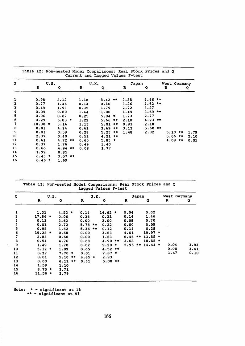
T a b l e 1 2 : N o n - n e s t e d M o d e l C o m p a r i s o n s : R e a l S t o c k C u r r e n t a n d L a g g e d V a l u e s F - t e s t
P r i c e s a n d Q
Q U . S . U . K . J a p a n R Q R Q R Q
W e s t G e r m a n y R Q
1 0 . 9 8 2 . 1 2 1 . 1 8 8 . 4 2 ** 2 . 8 8 4 . 4 6 **2 0 . 7 7 1 . 4 6 0 . 1 4 0 . 1 0 3 . 2 6 4 . 6 2 *★3 0 . 4 9 1 . 9 3 0 . 3 5 1 . 7 9 2 . 7 2 3 . 2 74 0 . 0 9 0 . 8 0 1 . 4 4 1 . 0 0 1 . 4 9 3 . 6 9 **5 0 . 9 6 0 . 8 7 0 . 2 5 5 . 9 4 * 1 . 7 3 2 . 7 76 0 . 2 9 6 . 8 3 * 1 . 2 2 5 . 6 6 ** 2 . 1 8 4 . 2 3 **7 1 0 . 3 8 * 3 . 1 4 1 . 1 3 5 . 0 1 ** 0 . 9 3 2 . 1 88 0 . 0 1 4 . 2 4 0 . 6 2 3 . 6 9 ** 3 . 1 3 5 . 6 0 **9 0 . 8 1 0 . 5 9 0 . 2 8 5 . 2 3 ** 1 . 4 8 2 . 8 2 5 . 1 0 ** 1 . 7 9
10 2 . 3 7 0 . 4 0 0 . 5 2 4 . 2 1 ** 5 . 6 6 ** 2 . 1 011 0 . 6 1 4 . 7 2 ** 0 . 6 5 5 . 8 3 * 4 . 0 9 0 . 0 112 0 . 3 7 1 . 7 6 0 . 4 9 1 . 4 013 0 . 6 6 4 . 9 4 ** 0 . 0 8 1 . 7 714 1 . 9 9 0 . 8 515 6 . 4 3 * 3 . 5 7 **16 6 . 4 6 * 1 . 6 9
T a b l e 1 3 : N o n - n e s t e d M o d e l C o m p a r i s o n s : R e a l L a g g e d V a l u e s F - t e s t
S t o c k P r i c e s a n d Q
Q U . S .R Q
U . K .R Q R
J a p a nQ
W e s t G e r m a n y R Q
1 1 . 3 1 4 . 5 3 * 0 . 1 4 1 4 . 6 2 * 0 . 0 4 0 . 0 22 1 7 . 8 6 * 0 . 0 6 0 . 3 6 0 . 2 1 0 . 1 4 1 . 4 63 0 . 1 3 3 . 6 2 0 . 0 0 2 . 0 0 0 . 0 8 0 . 7 04 0 . 0 1 2 . 7 2 5 . 7 5 * ★ 0 . 2 2 0 . 0 0 0 . 0 95 0 . 9 5 1 . 6 2 5 . 3 6 ** 0 . 1 2 0 . 1 4 0 . 2 86 1 9 . 2 8 * 0 . 6 8 0 . 0 0 3 . 6 3 4 . 0 1 1 9 . 9 7 *7 2 . 8 3 0 . 6 0 0 . 0 0 1 . 6 3 6 . 4 6 ** 1 3 . 8 5 *8 0 . 5 4 4 . 7 6 0 . 6 8 4 . 9 0 ** 3 . 0 8 1 8 . 8 5 *9 1 . 4 9 1 . 7 0 0 . 0 2 9 . 2 0 * 5 . 9 5 ** 1 4 . 4 4 * 0 . 0 4 3 . 9 3
10 5 . 1 2 * 1 . 0 9 0 . 6 5 4 . 5 2 *★ 0 . 0 0 3 . 4 111 0 . 3 7 7 . 7 0 * 0 . 0 1 7 . 8 7 * 3 . 6 7 0 . 1 012 0 . 0 1 5 . 1 0 ** 8 . 8 5 ★ 2 . 9 313 0 . 0 0 6 . 1 1 ** 0 . 3 1 5 . 0 0 **14 1 . 5 9 1 . 1 015 8 . 7 5 * 3 . 7 116 1 1 . 5 6 * 2 . 7 9
N o t e : * - s i g n i f i c a n t a t 1%** - s i g n i f i c a n t a t 5%
166
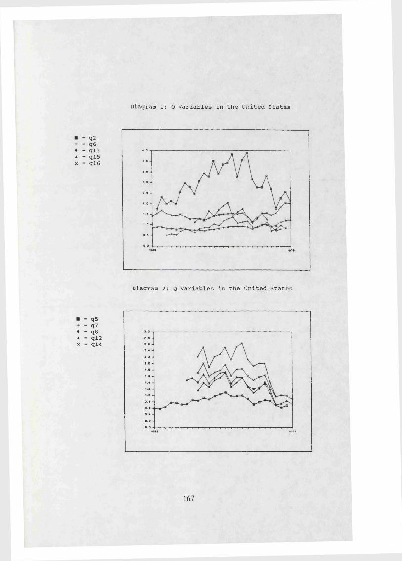
Diagram 1: Q Variables in the United States
q2q6qi3ql5q l 6
4.5
4 0
3 0
2 . 5
2 . 0
1 3
1 . 0
0 . 3
0.019 ?•
Diagram 2: Q Variables in the United States
qsq7qaqi2ql4
2 . B -
2 . 4 -
2 . 0 -
0 .8 -
0.8
0 . 4 .
0 .2 -
0.01877
167
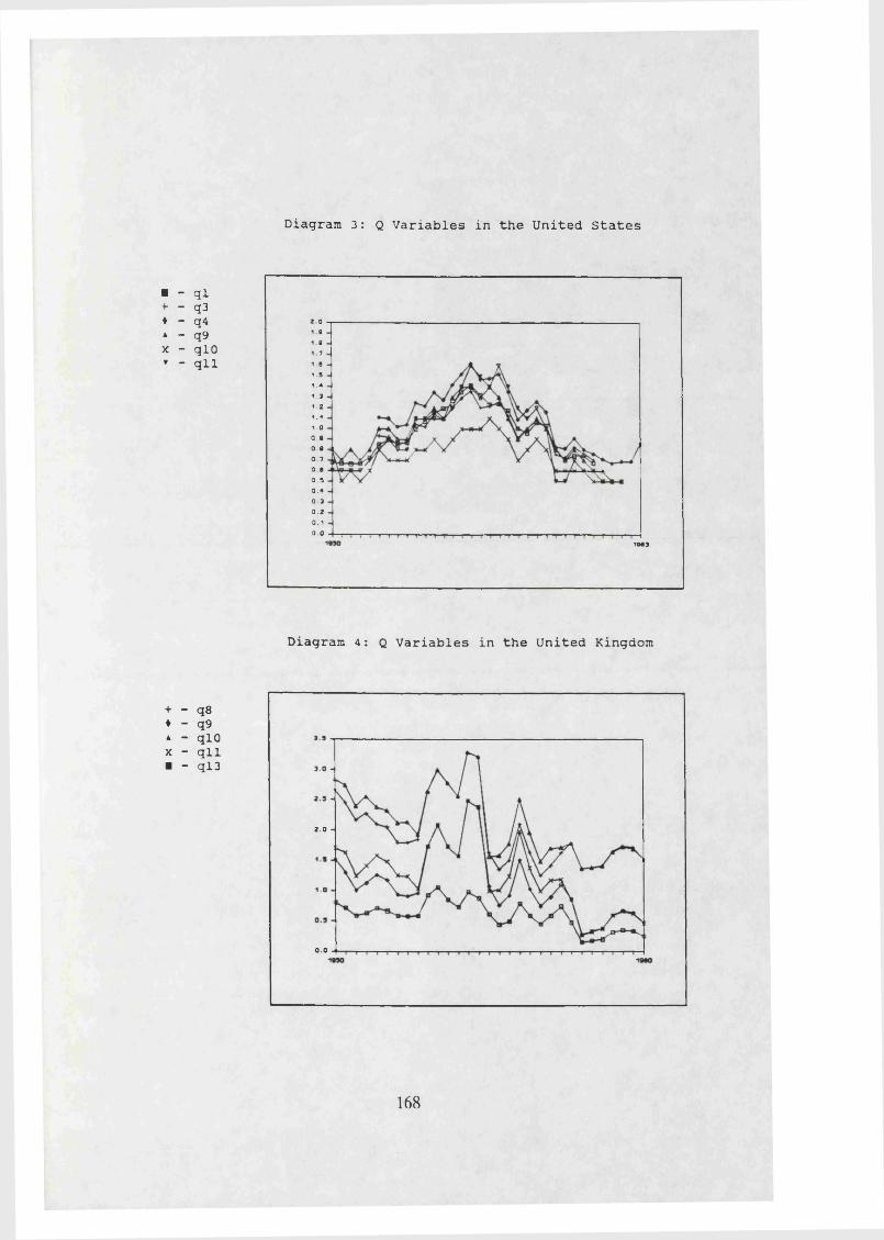
Diagram 3: Q Variables in the United States
■ - ql+ - q3♦ - q44 - q9X - qlOT - qll
O9
a7
61 .51 . 4
1 . 31 . 21.11 . 0
0.00.00 . 7
0.00.50 . 4
0 . 30 . 20.10 . 0
1003
Diagram 4: Q Variables in the United Kingdom
+ - q8♦ - q9* - qlO X - qll ■ - ql3
2 . 0 -
0.0
168
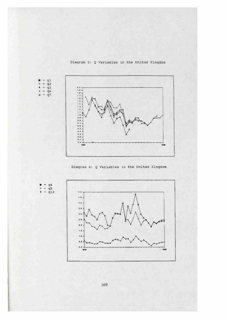
Diagram 5: Q Variables in the United Kingdom
■ - ql + - q2 ♦ - q3 a - q6x - q7
■ - q4 + - q5 ♦ - ql2
Diagram 6: Q Variables in the United Kingdom
169
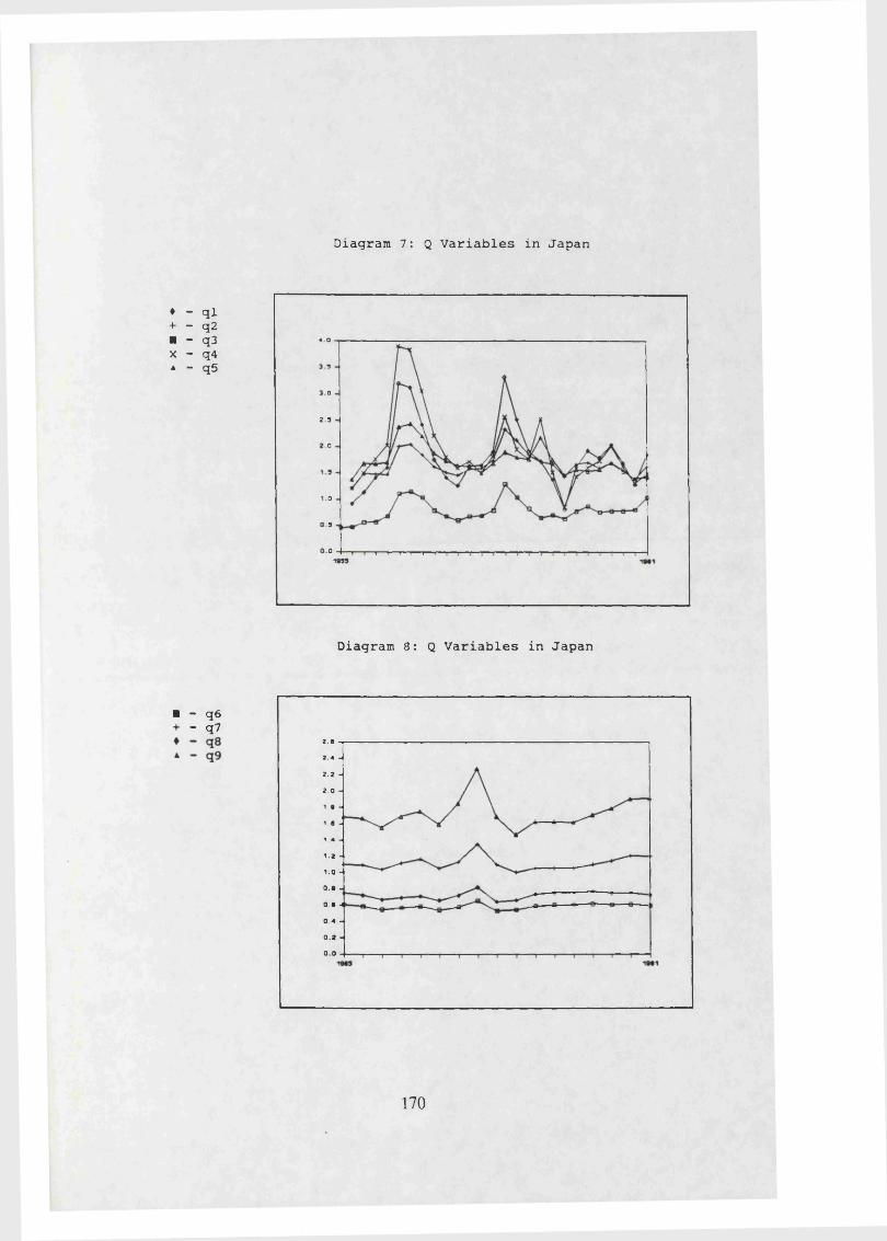
Diagram 7: Q Variables in Japan
♦ - q l + - q2 ■ - q3 X - q4 a - q5
0
3
0
2.3
.0
03
0
Diagram 8: Q Variables in Japan
■ - q6 + - q7
17 0
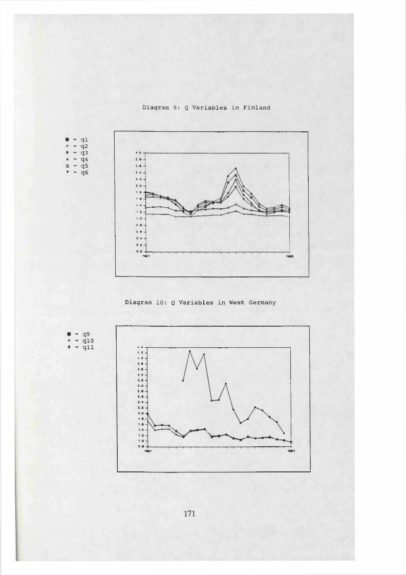
Diagram 9: Q Variables in Finland
qiq2q3q4q5qe
19«1
Diagram 10: Q Variables in West Germany
q9qlOqll
19€1
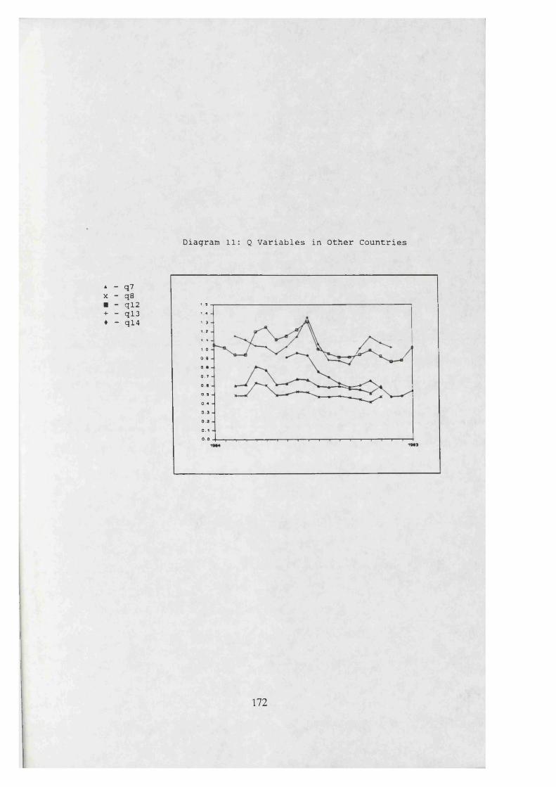
Diagram 11: Q Variables in Other Countries
A - q7X - q8■ - qi2+ - ql3♦ - ql4
i 3
1 4
1 . 3
1 2
1 1VO
0 .8a a0 . 7
0 .8
0 .9
0 . 4
0 . 3
0 . 2
0 . 1
0.0
17 2
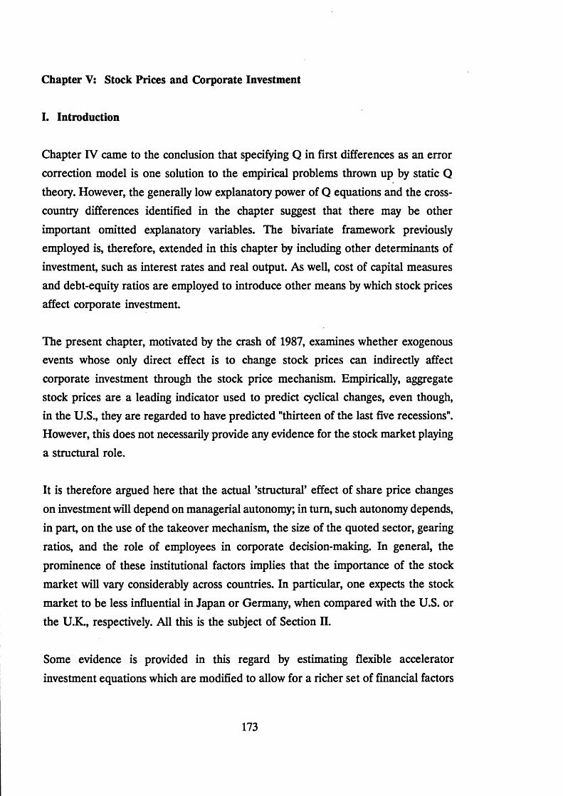
Chapter V: Stock Prices and Corporate Investment
I. Introduction
Chapter IV came to the conclusion that specifying Q in first differences as an error correction model is one solution to the empirical problems thrown up by static Q
theory. However, the generally low explanatory power of Q equations and the crosscountry differences identified in the chapter suggest that there may be other
important omitted explanatory variables. The bivariate framework previously employed is, therefore, extended in this chapter by including other determinants of investment, such as interest rates and real output. As well, cost of capital measures and debt-equity ratios are employed to introduce other means by which stock prices
affect corporate investment.
The present chapter, motivated by the crash of 1987, examines whether exogenous events whose only direct effect is to change stock prices can indirectly affect corporate investment through the stock price mechanism. Empirically, aggregate stock prices are a leading indicator used to predict cyclical changes, even though, in the U.S., they are regarded to have predicted "thirteen of the last five recessions". However, this does not necessarily provide any evidence for the stock market playing
a structural role.
It is therefore argued here that the actual ’structural’ effect of share price changes
on investment will depend on managerial autonomy; in turn, such autonomy depends, in part, on the use of the takeover mechanism, the size of the quoted sector, gearing
ratios, and the role of employees in corporate decision-making. In general, the
prominence of these institutional factors implies that the importance of the stock
market will vary considerably across countries. In particular, one expects the stock
market to be less influential in Japan or Germany, when compared with the U.S. or
the U.K., respectively. All this is the subject of Section II.
Some evidence is provided in this regard by estimating flexible accelerator
investment equations which are modified to allow for a richer set of financial factors
173

(motivated by a fear of bankruptcy). These estimates (presented in Section III) and
some non structural VARS, do bear out an a priori view that the stock market is
more important in the Anglo-Saxon economies.
As well, this fact may go some way to explaining other differences between these four countries. For example, it may be one reason why the Japanese and Germans
invest more, and it may also help explain why higher inflation appears to be
associated with higher declines in output in the Anglo-Saxon countries. These issues
are discussed in Section IV, along with other conclusions to the chapter.
174

II. Theoretical Considerations
Ha. Stock Market Influences on Investment
This chapter asks whether exogenous events whose only direct effect is to change stock prices can indirectly affect corporate investment through the stock price mechanism. The standard theoretical answer to this question is yes (see, e.g., Fischer and Merton (1984), who provide the following example).
Consider an initial equilibrium where the expected return on the market and the
yield on the firm’s marginal new investment are both 15 percent. Suppose that an
exogenous increase in aggregate risk aversion causes share prices to decline to the
point where they now yield an expected return of 20 percent, while the marginal investment project still continues to yield only 15 percent. Now, managers who act in the interests of their existing shareholders will cancel all planned investments with expected returns less than 20 percent. This argument would continue to hold even if the reduction in share prices were caused by an irrational change in investors’ perceptions of the future. Thus, Fischer and Merton conclude that ”... actions by
rational and informed managers will not offset the effects of irrational investors on investment.”
However, the above argument relies on a number of simplifying assumptions. For
example, it is well known that under conditions of uncertainty, shareholders will not
generally be unanimous about the best policy for the firm to pursue.1 These
differences in opinion between shareholders can create some discretionary power for
management to pursue their own goals. Therefore, it is possible that managers may
choose to assign less weight to share prices when formulating investment decisions than they would if they were acting purely in the interests of the existing
shareholders.
There are also other possible reasons why managers may not seek to pursue share price maximisation. According to Leontief (1946), for example, if employment is set
as the result of a bargain between firms and unions, rather than on the basis of
175

profit (share price) maximisation conditional on wages, both the employer and the union can be made better off. Therefore, considerations of internal efficiency suggest that managers may deviate from share price maximisation when choosing the appropriate level of employment and investment.
Another reason why share prices may be partially ignored by managers is if the
market is widely perceived to be myopic and, hence, unreliable as a guide to efficient managerial decision-making. For example, one industrial survey in the U.K. found
that 85 per cent of managers felt that the market took too short term a view of their investment decisions. Also in the U.K., the Bank of England’s former executive
director responsible for the securities market and former Chancellor Lawson
apparently share the view that " big institutional investors nowadays increasingly
react to short-term pressure on investment performance ... (they) are unwilling to countenance long-term investment or a sufficient expenditure on research and
development".2
The preceding discussion is consistent with the available survey evidence (presented below) which suggests that maximisation of the firm’s share price is not perceived
to be the most important managerial objective. Given this assumption regarding managerial behaviour, international differences in the extent of managerial power
will, therefore, influence the extent to which the stock market affects investment. It is to this that we turn next.
176
lib. Institutional Differences Across Countries
There is some empirical support for the view that managers pay less attention to the stock market in Japan than in the U.S. in the form of survey evidence, which is
presented in Table 1. Notice that while securing a capital gain for shareholders is
the second most important objective for American managers, it is the least most important objective for their Japanese counterparts. This difference may be at least partly explicable in terms of the cross-country institutional factors discussed below, which are set out to differentiate Japanese and German institutional behaviour from that of their Anglo-Saxon counterparts.
The first institutional difference is that takeovers are relatively rare in Japan or
Germany, in contrast to the Anglo-Saxon economies. In the case of Japan, a recent Hi Tech Dictionary listing under Takeover bids describes American practice and
goes on to say that "Japanese law was changed in 1972 to permit similar bid proceedings in this country, but the idea of taking over a company simply by the power of money seems too dorai (dry) to us Japanese, and in practice it never happens."3 While cultural differences do not necessarily explain the absence of hostile takeovers (the close links between banks and industry, and the fact that banks will replace inefficient managers must surely play a part), the empirical absence of such
takeovers suggests that at the minimum, shareholders do not exercise one of the
usual methods of ensuring that managers obey their wishes.4
Turning to Germany, hostile takeovers are also relatively rare, but this fact should
be set in the context of a quoted sector that is, by international standards, very small. For example, Table 2 shows that the ratio of market capitalization to GDP is about
25 per cent in Germany as compared to 80 per cent in Japan, 85 per cent in the
U.K. and 76 per cent in the U.S.. In addition to the quoted sector being small, it has
been estimated that only about 30 shares are actually actively traded (see BEQB(1984)) with the other shares being closely held and, therefore, less vulnerable to a
takeover anyway.5
i!
177

A second reason why managers might be able to pay less attention to shareholders in Japan and Germany, as compared to the U.S. or the U.K., is the fact that employees play a much larger role in decision making. In Germany, workers are
represented on the supervisory council, with all actions of management being subject
to the broad supervisory powers of this council.6 In addition, the law also requires
that employee representation in the form of works* councils be instituted in all
establishments that normally have five or more permanent employees. These works’ councils discuss a wide range of issues, including being consulted on investment and
employment decisions.
Turning to Japan, most informed observers agree that permanent employees do have a say in the decisions of the firm - for example, Komiya and Yasui (1984) assert that
"from the firm’s perspective... permanent employees represent more important assets than customers and stockholders ... It is not going too far to say that under Japan’s lifetime employment system, a firm’s regular employees are the firm itself."
There is less agreement about the role of employees in decision-making in the U.S. or the U.K.. There is now a sub-industry of papers that try to test whether or not firms and unions bargain over employment (e.g., Brown and Ashenfelter (1986)). Although these papers do not all agree on an answer, the very fact that this issue
is controversial differentiates these Anglo-Saxon economies from either Germany or Japan.
A third reason why managers may be more anxious to maximise the share price in
the Anglo-Saxon economies is the fact that a part of their remuneration is often
directly linked to the stock market. Such share option schemes are virtually unknown
in either Germany or Japan.
Finally, a fourth reason why the stock market may exert a smaller influence in Germany or Japan is the well-known fact that gearing ratios are much higher in
these countries when compared with the Anglo-Saxon economies. Table 3 presents evidence on these differences in gearing.7 A higher gearing ratio means that
managers need not concern themselves too much with the wishes of the shareholders,
178

provided that they command the confidence of their bankers.
So, to sum up, the relative absence of takeovers, the higher gearing ratios, the greater importance accorded to employees in decision-making and the lesser
importance of stock market related managerial remuneration, all make it more likely
that managers are able to pay less attention to the stock market in Germany or
Japan, as compared to the Anglo-Saxon countries.
So far, reasons have been put forth to explain why the stock market may not significantly affect investment in Japan or Germany. However, none of this should
be interpreted as implying that managers in the Anglo-Saxon countries give as much weight to the stock market as textbook models imply.
In fact, survey evidence for the U.K. does suggest that practice departs significantly
from the textbook ideal.8 This impression also appears to have been borne out by the fact that the 1987 stock market crash has failed to affect investment intentions in the U.K., with only 4% of business men saying that the crash represented "a
genuine deterioration in the world economic outlook” - the vast majority of survey respondents believing instead that it represented "the inevitable puncturing of a speculative boom".9
The arguments presented above provide some reasons to think that managers in
Japan and West Germany are able to pay less attention to share price movements. Little has been said thus far, however, about why managers might wish to ignore
fluctuations in share prices when formulating investment decisions. This issue will now be briefly discussed.
179

lie. Managerial Incentives to Ignore Stock Prices
The survey evidence given above supports the view that, contrary to the textbook ideal, maximising the share price is not the most important managerial goal. There
may be several reasons for this including the fact that managers may derive utility from the size of the firm per se, and may not want to be deflected from this goal by
the wishes of stockholders.
Another reason why managers might not want to be overly influenced by the stock
market is if the market were myopic, in the sense of attaching too high a weight to
current dividends relative to future dividends (see Nickell and Wadhwani (1987)). In this case, a project (e.g. R&D spending) which yields negative returns in the early
years, but is a positive NPV project overall, will depress the share price today. If managers feel that the project is important for the long-term survival of the company,
they would want to go ahead with it provided that they can ignore their shareholders.
A third relevant consideration already mentioned is managerial remuneration - as shown above, managers in Japan are more concerned with fluctuations in earnings (to which their pay is linked) than in share prices.
However, it should be stressed that it is possible to conceive of circumstances where the relationship between the extent of shareholder control over management and the
influence of share prices on investment may not be monotonic. In other words, the absence of shareholder control may actually strengthen the linkage between
investment and stock market fluctuations.
To illustrate this, consider the following example where the stock market is temporarily overvalued, so that the return on a marginal investment project, rp
exceeds the required return on equity, rE, but the long-run return on equity equals rr If managers only care about their existing shareholders, then, as Fischer and
Merton (1984) point out, the firm will undertake further investment.
180

However, suppose that investment is irreversible so that the firm will be stuck with investments which will fail to earn the future long-run required rate of return. In
this case, rational managers who are not perfectly controlled by existing shareholders, but fear the possibility of a future takeover, might be deterred from investing today. On the other hand, managers who have some discretion but do not fear future takeovers might still invest today because, surely, this is a way of obtaining "cheap
money" in order to further their ambitions for the growth of the firm.10
So, in the "cheap money" scenario, we appear to have an example where the absence of hostile takeovers may actually make investment more responsive to share prices. However, this example probably has less relevance to the present international comparison, for although we do not see hostile takeovers in Japan or Germany,
managers still run the risk of being replaced as a result of actions initiated by banks. A manager who undertook an investment project just because the market was temporarily overvalued would run the risk of being perceived as being plainly inefficient when the investment turns sour in the future. So, he too would be deterred from responding to the high share price today. Since banks in Japan and Germany probably represent a more direct and tangible disciplinary force than the
fear of a future takeover in the Anglo-Saxon world, it seems that even here the stock market will exert a smaller influence in Germany and Japan.11
We now turn to consider whether the econometric evidence is consistent with the
view that exogenous movements in the stock market are less important in influencing corporate investment decisions in either Japan or Germany.
181
III. Econometric Evidence
This chapter is primarily interested in whether exogenous changes in stock prices affect investment. Therefore, the approach will be to assess whether share prices provide any additional explanatory power for investment, once we have controlled
for the conventional determinants of investment - e.g. output, interest rates, taxes
etc. Estimates of a simple investment - Q relationship are not reported here, because it does not, of itself, answer the question that is of interest. One may, after all,
observe a positive relationship between investment and Q which disappears once output or some other variable has been entered in the regression.12
As a preliminary to examining the formal econometric evidence, and following on
the analysis of Chapter IV above, Table 4 presents some simple correlations between I/K and Q. At first glance, the numbers are actually higher for Germany and Japan
over the entire period. However, a division of the sample to account for the recent international bull market in equities shows that the correlations in these two countries are actually negative after 1979. Such instability indicates that the I/K and Q correlation is probably not structural and may arise from the fact that other relevant determinants of investment are omitted here. For this reason, the next section examines a model of investment where Q is only one of many possible explanatory factors.
Ilia. The Basic Model
There is a huge literature on investment equations, but for our purposes we shall use a modified version of the flexible capital stock adjustment model developed by
Jorgenson (1963), and used by many others, as the test-bed. Of course, this model is not without its problems (for an extensive discussion of them, see, e.g., Nickell
(1978)). The model specifies the profit-maximising level of the capital stock,
(1) K* = *(C/P, Y) < 0, > 0
182
where C is the annual cost of capital, P is the price of output and Y is the level of output. Assuming that investment is subject to delivery and installation lags, and
that the existing capital stock decays at the depreciation rate 6,
T(2) I. - XL W j(< -i - + *K,-1
J=U
where It is gross investment and K ,̂, is the level of the capital stock.
The modification to the model made here is to assume that managers maximise
profits net of expected bankruptcy costs, and so the desired level of the capital stock (K*) will depend on variables that affect the probability of bankruptcy.13
Assume that firm i finances its capital stock by, in part, borrowing a sum of money
which has to be repaid with interest at the end of the first period; denote the total sum to be repaid as D f. However, because the return to this investment is uncertain, there is some risk that the firm will not make sufficient profits to meet its commitments, a situation where profits (tT|) are less than D f - of course, tt1- depends
on I. Assume also for simplicity that the liquidation value of the capital stock is zero, possibly because it is highly product-specific. Denote the value of the firm if it stays in existence by Vf.
Now, suppose at the end of the period it becomes clear that irf + V,- < O. Then, in
a complete information world, shareholders and bondholders will wish to wind up
the business. Although this may be the optimal course from the point of view of the
shareholders and bondholders, it is possible that managers might not prefer this
outcome, and hence the initial investment decision may be partially conditioned by its effect on the probability that tt1- + V1- < O.
In addition, in a world with asymmetric information, where shareholders know the
true value of the firm but bondholders do not, bankruptcy may also occur when Vf > O, but 7T- + V,- < Dj, where jr? denotes the actual profit for the year (see, on this,
Webb (1987)). This occurs because bondholders are imperfectly informed about
183
whether or not Vf > 0, and may find it worthwhile to force the firm into bankruptcy in an attempt to discover the true state of affairs.
So, to summarise, bankruptcies seem to occur when + V. < 0 or when xf + V.
< D,. Rescaling by a high Vi/K i, low D f/K f, or high irf/K f all make bankruptcies less likely.
Now, for the purposes of the analysis here, it is assumed that the investment decision
affects profits but, for simplicity, managers take D f/K { and V f/K, as fixed.14 Therefore, we have
(3) K* = *(D/K, V/K, C/P, Y)
^ D / K » ^ C / P < ^ V / K » > ®
instead of Equation (1). So, the optimal level of the capital stock may be influenced by the conventional variables, the debt ratio and Tobin’s Q (defined as V/K). Further, as a practical matter, banks may look at book values of debt and equity, in addition to market values; therefore, the debt-equity ratio at book value (BDE) will be included in Equation (3). The modified framework used here accommodates the Q theory and the Jorgensonian cost of capital approach as special nested cases.
The cost of capital term (in the absence of taxes, for the moment) is
(4) C = P, (R + 5)
where Pj is the price of investment goods and R denotes the cost of funds. The
empirical proxy used for R varies considerably across studies. For example, Hall and
Jorgenson (1967) use a fixed nominal interest rate, Gorden and Jorgenson (1976) use the after-tax interest rate on long-term bonds, while Feldstein (1982) uses a
weighted average cost of capital measure,
184
(5) C = ( e+d V d + { e+d } fE
where rD is the real interest rate on debt and rE is the real return on equity.
The appropriate way of measuring the cost of capital is, therefore, a controversial area and, since the purpose of this chapter is to determine the effect of the stock
market on investment, it would be unwise to overly restrict the definition of the cost of capital.15 Instead,
(6) C/P = e ^ r ^ D /V j y P )
here, where V = D + E, and each element is entered separately into the investment equations.
Finally, an implication of the foregoing analysis is that the debt-capital ratio, D f/Kj, only affects the probability of bankruptcy if bondholders know less about the firm
than shareholders. Since banks have especially close links with firms in Japan and Germany, it is unlikely that the probability of bankruptcy would be influenced by
the debt-equity ratio - indeed, Corbett (1987) argues that the active role played by Japanese banks when firms experience financial distress implies that what"... goes
by the name of debt in Japan appears to have many features of the equity
relationship”.16 This then implies that rises in debt-equity ratios should not lead to
higher financial risk and lower investment in Germany or Japan (unlike the Anglo-Saxon countries) - this is something that will be tested empirically below.
185
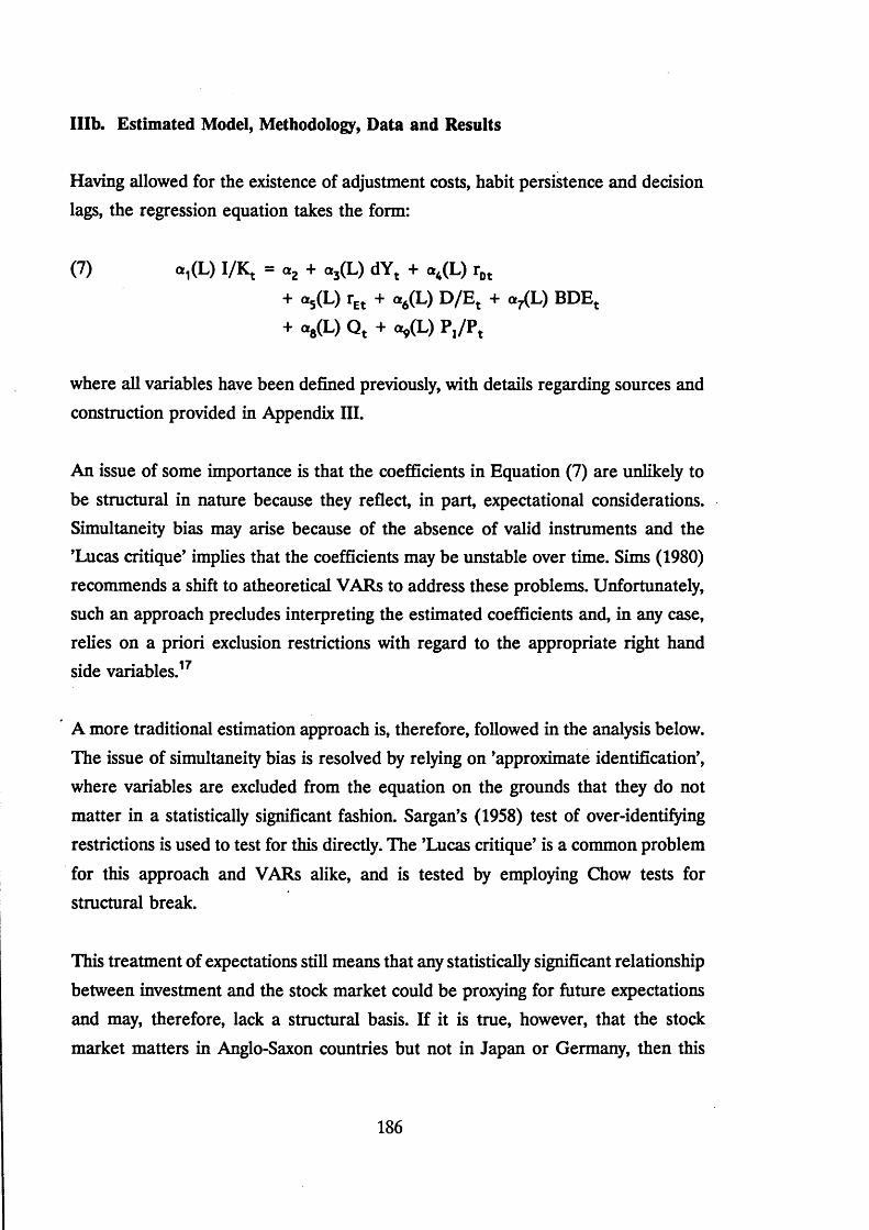
Illb. Estimated Model, Methodology, Data and Results
Having allowed for the existence of adjustment costs, habit persistence and decision lags, the regression equation takes the form:
(7) «,(L) I/K, = a2 + a,(L) dY, + „4(L) rot+ a5(L) rEt + a6(L) D /E t + a^L) BDGt + Og(L) Q, + a,(L) P ,/P ,
where all variables have been defined previously, with details regarding sources and construction provided in Appendix III.
An issue of some importance is that the coefficients in Equation (7) are unlikely to be structural in nature because they reflect, in part, expectational considerations. Simultaneity bias may arise because of the absence of valid instruments and the ’Lucas critique’ implies that the coefficients may be unstable over time. Sims (1980) recommends a shift to atheoretical VARs to address these problems. Unfortunately, such an approach precludes interpreting the estimated coefficients and, in any case, relies on a priori exclusion restrictions with regard to the appropriate right hand side variables.17
A more traditional estimation approach is, therefore, followed in the analysis below.
The issue of simultaneity bias is resolved by relying on ’approximate identification’, where variables are excluded from the equation on the grounds that they do not matter in a statistically significant fashion. Sargan’s (1958) test of over-identifying
restrictions is used to test for this directly. The ’Lucas critique’ is a common problem
for this approach and VARs alike, and is tested by employing Chow tests for structural break.
This treatment of expectations still means that any statistically significant relationship
between investment and the stock market could be proxying for future expectations and may, therefore, lack a structural basis. If it is true, however, that the stock
market matters in Anglo-Saxon countries but not in Japan or Germany, then this
186
would be consistent with the market playing a structural role in the former pair of countries. The reason for such a conclusion is that the market should be significant
for all four countries if it is acting as a proxy for expectations, and not just for the U.K. and the U.S. alone.
Equation (7) was estimated for all four countries. Initially, because of the dangers of overparameterisation of the equations, 7(L) and 9(L) were set to zero, and
preferred versions of Equation (7) were obtained. Having done so, the excluded
variables were added in turn. Recall that we are primarily interested in whether the
stock market matters, i.e. in whether rE, D /E or Q are significant - and are
indifferent between which of these actually matters.
The preferred versions of equation (7) for the four countries are reported in Tables 5, 7, 9 and 11. These equations suggest some support for the basic hypothesis that the equity market directly affects investment in the U.S. and U.K. but not in Germany or Japan. Specifically, the stock market affects investment through the terms in rEt.1 and D /E t in the U.K., while in the U.S., the stock market "matters" because of the d(D/E)t.1 term.
Turning to the United Kingdom and Table 5 first, one sees that various cost of
capital elements are statistically significant, as well as the accelerator (output) terms. The equation is reasonably well specified, with a Lagrangian Multiplier test against
an AR(2)/MA(2) error term (denoted AR(2) here) suggesting no evidence of residual autocorrelation, while a mid-sample Chow test fails to reject the null hypothesis of coefficient stability. As well, the instrumental variable estimates of the preferred equation are quite similar to the OLS estimates; Sargan’s test of over
identifying restrictions is also satisfied. Finally, it is interesting to note that a decline
in the stock market which causes the debt-equity ratio to rise by 10% reduces I/K
by 2.1% in the long run.
As noted in Table 6, neither tax adjusted nor non tax adjusted Q variables are statistically significant factors when added to the preferred investment equation.
Even though Chapter IV demonstrated that Q is correlated to investment, it appears
187

that this results from the exclusion of other relevant explanatory variables. It will be seen below that this conclusion holds for the other countries as well.
A number of other variables were added to the U.K. investment equation in Table5. The cost of capital was entered as a single entity, rather than using its separate components as in the preferred specification. As seen in Table 6, this variable adds
no additional explanatory power. Another variable which is considered is the level of the real money supply, as suggested by Gordon and Veitch (1987). Again, there is no additional explanatory power.
Finally, the effect of takeover activity on investment is considered in Table 6. As argued above, one possible reason for the influence of the stock market on
investment is the role of hostile takeovers. Therefore, one might expect managers to pay more attention to stock prices when takeover activity is high. The ratio of the
value of acquisitions to the capital stock is interacted with the two equity terms in the preferred equation to test for a positive influence between investment and takeover activity via the stock market. While the estimated coefficient has the anticipated sign, it is nevertheless statistically insignificant at conventional levels.
The U.S. results in Tables 7 and 8 show that accelerator and equity terms are
significant factors in explaining investment, although none of the individual cost of capital elements remain in the equation. Like the results for the U.K., Tobin’s Q, the
integrated cost of capital term, the level of real money supply and the takeover interaction variables are not significant; in some cases, these variables are also
incorrectly signed. The preferred equation is properly specified, according to the
Chow and AR(2) test statistics, and the instrumental variable estimates are very
close to the OLS coefficient estimates.
The preferred equations in Tables 9 and 11 for West Germany and Japan are rather similar. Both include accelerator terms and the real long term interest rate but neither show any stock market effect. As before, these equations do not exhibit structural break or autocorrelated residuals; they also have very similar OLS and IV coefficient estimates and satisfy the Sargan test for over-identification.
188
The German equity market terms (D/E, rE and Q) are almost uniformly of the
wrong sign and are all statistically insignificant. This is also the case for Japan, with
the exception of d(Q). Even though the three Q terms are collectively insignificant at the 5% level, a further test was undertaken to test the robustness of d(Q) in
Japan. Following Hayashi (1985), who argues that the relationship between Q and
I/K appears to have broken down after 1974, d(Q) and Qt_2 were interacted with an
appropriate dummy variable. The results shown in Table 12 support the exclusion
of these variables from the preferred equation, as does the switch in sign of the post-1979 simple I/K and Q correlation shown in Table 4.
Overall, these results are rather supportive of the view that the stock market has a
direct effect on investment in the two Anglo-Saxon economies, but not in Germany or Japan.18 Accelerator terms are the dominant determinants of investment and
individual cost of capital elements are also important. Q is not important in any country, supporting the possibility that its significance as a lone explanatory factor in investment equations is due to the exclusion of other relevant variables. In this regard, the track record of Q as an explanatory variable is shown clearly in Table 13 where it is simultaneously the worst and the best of the elements under examination.
Finally, it is also of some interest that the debt-equity ratio affects investment in the
U.S. and U.K. but not in Germany or Japan. This is consistent with the fact that banks have a closer relationship with firms in Germany and Japan, implying that
bankruptcy risk need not rise with the debt-equity ratio.
IIIc. Some ’Non-Structural’ Evidence
Thus far, evidence has been presented based on structural investment equations. However, many economists now prefer atheoretical VARS, so, in Table 14, some
evidence is given on the effect of real share prices on output in each of the four countries.
189

The log of output is regressed on two lags of itself and lagged values of a host of other variables including the interest rate, inflation, competitiveness, real government expenditure, the real money supply and world trade. When the insignificant variables are deleted, one finds that the stock market has a positive and statistically significant
effect on output in the U.S. and U.K., and no effect in Japan.19 In Germany, the
stock market exerts a negative effect on output (if these estimates are interpreted
literally). In general, the coefficients of the restricted equations are sensible for all of the countries, aside from the positive effect of lagged inflation on output in West Germany.
So, the non-structural evidence is also consistent with one basic message - the stock market matters less in Germany and Japan than in the Anglo-Saxon countries.
190
IV. Conclusions and Implications
The fact that the stock market appears to affect investment less in Germany or Japan compared to the Anglo-Saxon countries may, in fact, have some important implications.
For example, there is some evidence that share prices in the post-World War II period fell due to ’irrational' valuation errors produced under inflationary
circumstances (see e.g. Modigliani and Cohn (1979)). The stock market then acts as a channel through which higher inflation reduces investment in the U.S. and the
U.K.. Table 15 shows that output and inflation are more negatively correlated in the Anglo-Saxon countries, which is consistent with, but not necessarily evidence of, a
causal link from inflation to equity prices, and hence to investment and output.
Similarly, if the stock market is myopic, such "short-termism" is less likely to be translated into actual investment decisions in Japan and Germany, and this may partly explain their higher investment rates (shown in Table 16).
Finally, if the stock market exercises less control over corporate investment decisions, managers may pursue a goal of higher growth, even at the cost of profit maximisation. It has already been shown in Table 1 that Japanese managers assign a higher priority to growth-like objectives than their American counterparts. This manifests itself in the fact that the rate of return of capital in Japan is very low by
international standards and is less than half the cost of capital (see Table 17). For
Japan, the null effect of the stock market on investment may explain Hardie’s (1982) observation that "... it remains one of the oddities of modem Japan that profit- making is neither in fact nor in ideology a critical part of what business and commerce are for."
As for the theory of investment, this chapter has presented a framework within
which Tobin’s Q is only one of several possible relevant variables. Moreover, empirically, it appears to have little additional explanatory power once other relevant variables like output and interest rates are included. As in previous chapters, the
191

importance of institutional differences across countries highlights the notion that stock prices are influenced by more than the expectations and outturns of economic
variables.
192

Appendix III: Four Country Data Sources
1. K - replacement cost of net capital stock for private sector.
K definition matches that for I below. In the case of Japan, a K series was generated using the 1956 K value found in Hayashi (1985), a depreciation rate of .089 and the
I series. The resulting series correlated well with other estimates from the OECD and the Japanese Economic Planning Agency.
private sector:
U.S. non-financial corporations (NFC)U.K. industrial and commercial companies (ICC)JA private sector GE company sector
2. I - investment.
U.S. NFC non-residential equipment and structure U.K. ICC gross domestic fixed capital formation (GDFCF)JA private sector GDFCF
GE company sector assets net of inventories
source:U.S. Survey of Current Business
U.K. Blue BookJA Bank of Japan Economic Statistics Monthly
GE Statistical Yearbook (Statistisches Jahrbuch. Bundesanstalt fiir Statistik)
3. Q - private sector tax-adjusted (TQ) and non-tax-adjusted (NTQ). NTQ is defined
as the value of debt and equity divided by K. All three elements are at market or
replacement cost, with the exception of debt in Germany, the U.K. and the U.S..
193
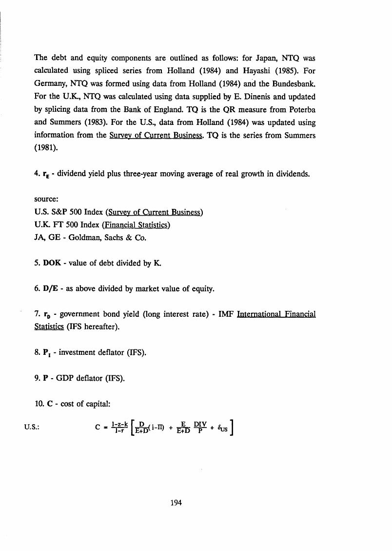
The debt and equity components are outlined as follows: for Japan, NTQ was calculated using spliced series from Holland (1984) and Hayashi (1985). For
Germany, NTQ was formed using data from Holland (1984) and the Bundesbank. For the U.K., NTQ was calculated using data supplied by E. Dinenis and updated
by splicing data from the Bank of England. TQ is the QR measure from Poterba and Summers (1983). For the U.S., data from Holland (1984) was updated using
information from the Survey of Current Business. TQ is the series from Summers (1981).
4. rE - dividend yield plus three-year moving average of real growth in dividends.
U.S. S&P 500 Index (Survey of Current Business!U.K. FT 500 Index (Financial Statistics!JA, GE - Goldman, Sachs & Co.
5. DOK - value of debt divided by K.
6. D/E - as above divided by market value of equity.
7. rD - government bond yield (long interest rate) - IMF International Financial Statistics (IFS hereafter).
8. P, - investment deflator (IFS).
9. P - GDP deflator (IFS).
10. C - cost of capital:
source:
U.S.:
194
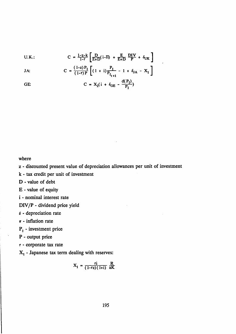
U.K.:
JA: C ■ TT^T [(l + '>P^ - 1 + *JA - X! ]
GE:
wherez - discounted present value of depreciation allowances per unit of investmentk - tax credit per unit of investmentD - value of debtE - value of equityi - nominal interest rateDIV/P - dividend price yield6 - depreciation rate
ir - inflation ratePj - investment priceP - output pricer - corporate tax rateX, - Japanese tax term dealing with reserves:
ri R
195

whereR - tax-free reserves
aK - nominal capital stockz - P.V. of depreciation allowances in new investment
X2 - German combined tax term including income tax, franchise tax, property tax
and land tax. Tax laws are not investment neutral, therefore X2 > 1.
196
1. See King (1977) for an extensive discussion of these issues.
2. Walker (1985) and Nickell and Wadhwani (1987).
3. See Nikkei (1984).
4. Note, however, that managers cannot ignore shareholders altogether since the latter may exert some influence through the possibility of take-over bids. While the fear of takeover will not necessarily induce share price maximisation (as the production plan which maximises the share price is not the same as that which minimises the risk of being taken over - see King (1977)), it will at least ensure that managers do not entirely ignore the wishes of shareholders.
5. Similarly, substantial cross holdings of corporate equity in Japan are used to reinforce long-term business relationships and are rarely traded on the market. The oligopolistic nature of brokerage in Japan, where four large firms dominate the market, and the substantial influence of German universal banks on the German equity markets, are other factors which may drive a wedge between stock price fluctuations and corporate behaviour in these countries.
6. Since the 1976 Co-determination Act, all corporations employing more than 2000 workers must have a supervisory council with 50 per cent representation of employee representatives.
7. The differences in the Table 3 ratios across countries are substantial and cannot be explained away by divergent accounting practices in each country (see Kuroda and Oritani (1980) on this issue). Corbett (1987) and BEQB (1984) offer detailed comparisons of financing practices in the four countries under study here.
8. Carsberg and Hope (1976), for example, found that only 21 percent of respondents allowed movements of the equity market to influence their choice of discount rate. Moreover, a majority of these respondents were only influenced by some smoothed return on equity measure. In the sample as a whole (including those who did not look at the equity market), over half had not even altered their discount rate in the preceding three years - this, in a period (1971-1973) when the earnings yield had varied between 4.95% and 11.55%.
9. See 3i Enterprise Barometer.
10.1 am grateful to Stanley Fischer for making this point.
11. Of course, all this is predicated on firms in Germany and Japan continuing to be so dependent on their banks. See Mayer (1988) for an exploration of this and related issues.
12. As Chapter IV noted, traditional static Q regressions manifest various signs of misspecification - parameter instability, serial correlation and the like. In addition, as will become clear below, the Q terms do not survive the introduction of other relevant terms.
13. Such models are now commonly used (see Greenwald and Stiglitz (1987) or Wadhwani (1987) and references therein). Since costly bankruptcy does not occur in a
197

world with complete information and rational agents, as in Haugen and Senbet (1978), an assumption of missing markets is also needed to motivate the presence of bankruptcy.
14. It might seem somewhat curious that is fixed when the manager is maximising irf, for, under the Efficient Markets Hypothesis, the two are intimately related. However, this analysis is conducted on the premise that managers do not believe the EMH to the extent that it influences their own firm’s share price - this assumption is amply supported by the empirical evidence. So, instead, managers just view as a constraint on their behaviour.
15. See Auerbach (1983) for a survey of these issues.
16. Corbett (1987), p.54.
17. In any case, the available degrees of freedom in the data would not support VARs of sufficient size to include numerous variables and lags.
18. The results are also, broadly speaking, in accordance with the work using micro-data of Blundell et al (1987) and Hayashi and Inoue (1987).
19. The lagged output term in the Japanese restricted equation is constrained to a value of unity. This is done because the estimated coefficient in the general specification is greater than one, implying that output is oscillating away from a long-term equilibrium value over time. This constraint has no qualitative effect on the value or significance of the estimated real share price variable coefficients.
198
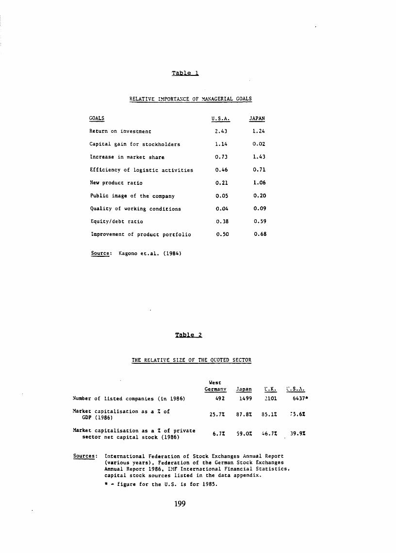
Table 1
RELATIVE IMPORTANCE OF MANAGERIAL GOALS
GOALS U.S.A. JAPAN
Return on investment 2.43 1.24
Capital gain for stockholders 1.14 0.02
Increase in market share 0.73 1.43
Efficiency of lo g is t ic a c t iv i t ie s 0.46 0.71
New product ratio 0.21 1.06
Public image of the company 0.05 0.20
Quality of working conditions 0.04 0.09
Equity/debt ratio 0.38 0.59
Improvement of product portfolio 0.50 0.68
Source: Kagono e t .a l . (1984)
Table 3
THE RELATIVE SIZE OF THE QUOTED SECTOR
UescGermany Japan U.K.
Number of l is ted companies (in 1986) 492 1499 2101
Market capitalisation as a % of GDP (1986) 25.7Z 87.8Z 85.17.
Market cap italisation as a Z of private , , , ,-0 , ,— i i / ̂a a / \ 0« / 4 J 7 * U 4 » / 4sector net capital stock (1986)
Sources: International Federation of Stock Exchanges Annual Report(various years), Federation of the German Stock Exchanges Annual Report 1986, IMF International Financial S ta t is t ic s , capital stock sources l is ted in the data appendix.* - figure for the U.S. is for 1985.
.S.A. 6437*
75.6Z
39.9Z
199
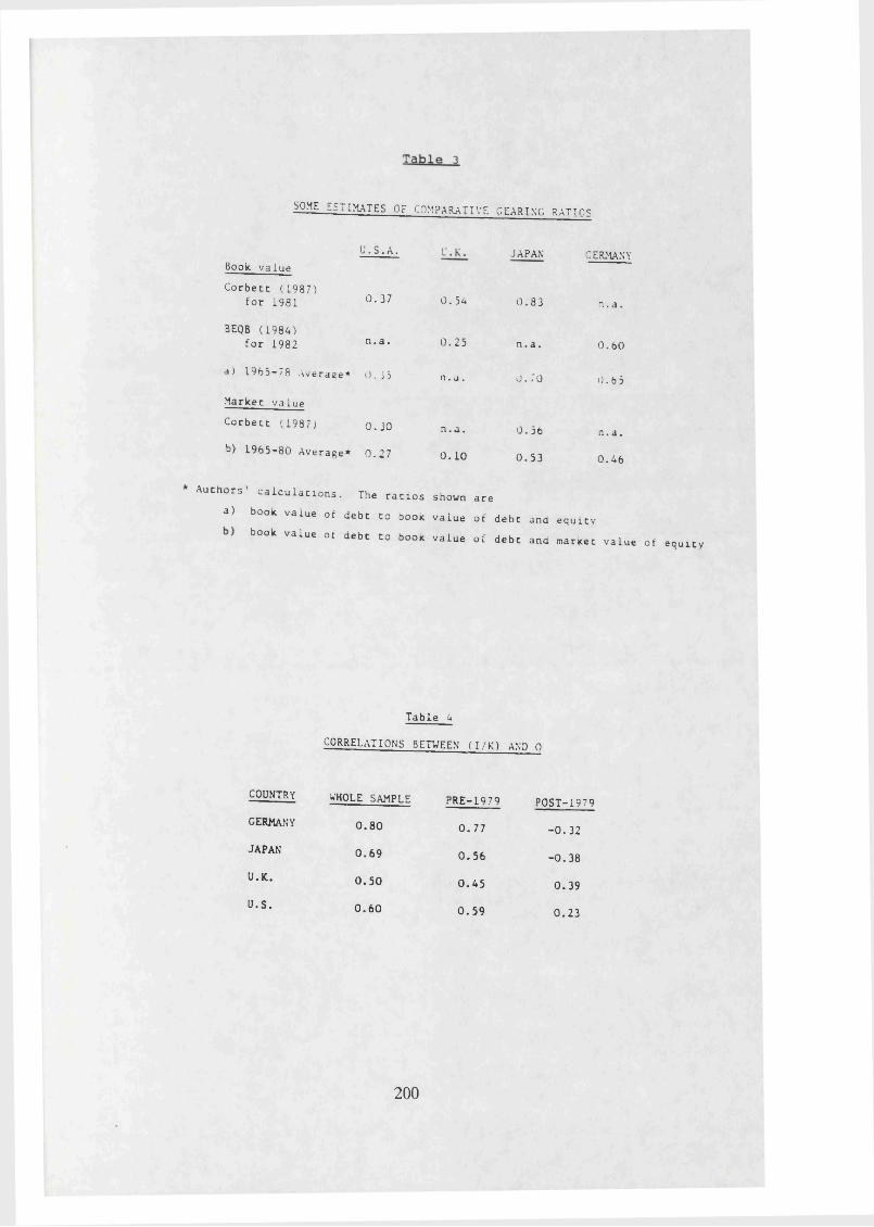
SOME ESTIMATES OF COMPARATIVE GEARING R A T I O N
U- S - A- -JAPAN GERMANYBook v a l u e
Corbetc (1987)f o r 1981 ° * 37 ^- 5 4 0 . 8 3
a) 1965-78 Average* 0 . J5 n . a . u . 7 0
Marker v a l ue
Corbecc (1987) o .JO n.a. 0.56
b) 1 9 65 - 8 0 Average* 0 . 2 7 0 . 1 0 0 . 5 3
a . a .
BEQB (1984)f or 1982 n,a> 0*25 n . a . 0 . 6 0
0 . 6 5
n . a .
0.46
* Au tho rs ' c a l c u l a t i o n s . The r a t i o s shown are
a) book v a l u e of debt t o book v a l u e o f d e bt and e q u i t y
book v a l ue of de bt t o book v a l u e o f d e b t and marker v a l u e o f e q u i t y
Tabl e 4
CORRELATIONS BETWEEN ( I / K ) AND 0
COUNTRY
GERMANY
JAPAN
U.K.
U.S.
WHOLE SAMPLE
0.80
0.69
0.50
0.60
PRE-1979
0.77
0.56
0.45
0.59
POST-1979
-0.32
-0.38
0.39
0.23
200
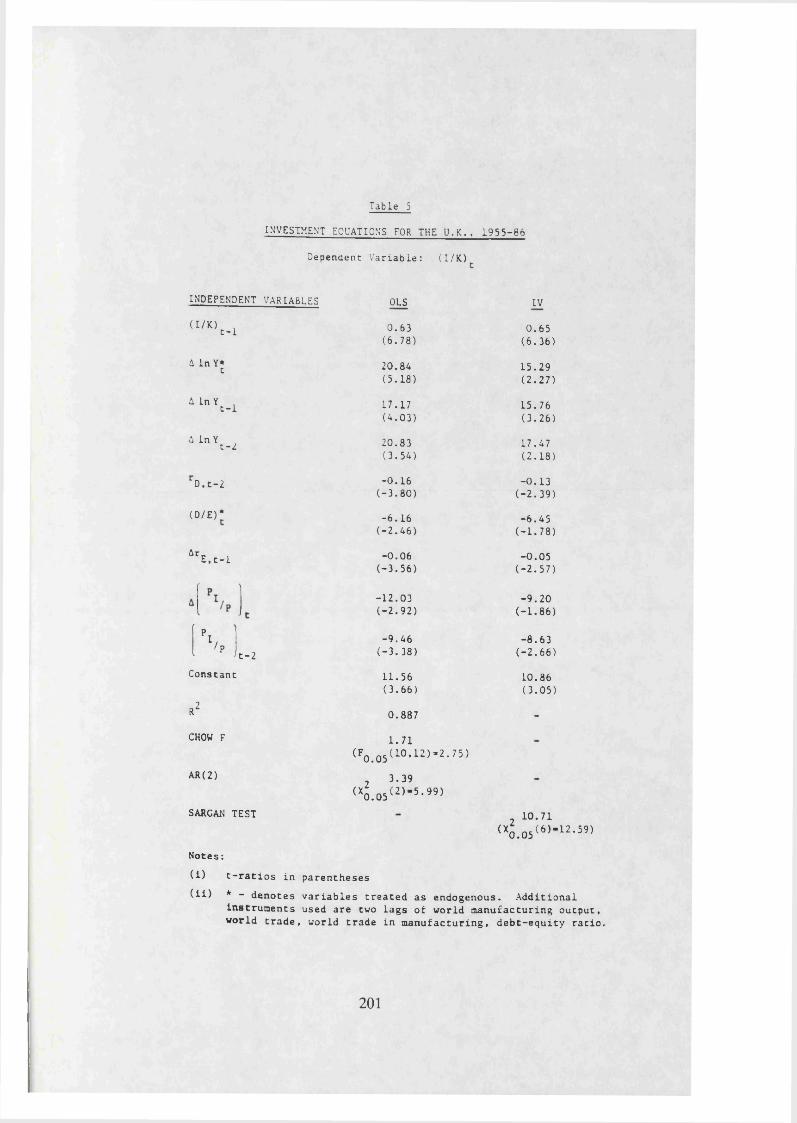
Table 5INVESTMENT EQUATION’S FOR THE U . K. . 1 9 5 5 - 8 6
Dependent V ar i a b l e : ( I /K)
INDEPENDENT VARIABLES
( I / K ) t-1
A In Y* t
A InY
A In Y
t - 1
t - 2
D , t - 2
(D/E)*
l c E . c - l
( \ Const ant
R2CHOW F
AR(2)
SARCAN TEST
t - 2
OLS IV
0.63 0.65(6.78) (6.36)
20.84 15.29(5.18) (2.27)
17.17 15.76(4.03) (3.26)
20.83 17.47(3.54) (2.18)
-0.16 -0.13(-3.80) (-2.39)
-6.16 -6.45(-2.46) (-1.78)
-0.06 -0.05(-3.56) (-2.57)
-12.03 -9.20(-2.92) (-1.86)
-9.46 -8.63(-3.38) (-2.66)
11.56 10.86(3.66) (3.05)
0.887 -
1.71(Fn n.(10,12)-2.75)
(X
0.05
20.05
3.39(2)-5.99)
(X20.05
10.71( 6 ) - 1 2 . 5 9 )
Notes:( i ) t - r a t i o s i n p a r e n t h e s e s
( i l ) * - d e n o t e s v a r i a b l e s t r e a t e d as e n d o g e n o u s . A d d i t i o n a li n s t r u m e n t s used a re two l a g s o f wor ld m a n u f a c t u r i n g o u t p u t ,w or l d t r a d e , wor ld t r a d e i n m a n u f a c t u r i n g , d e b t - e q u i t y r a t i o .
201
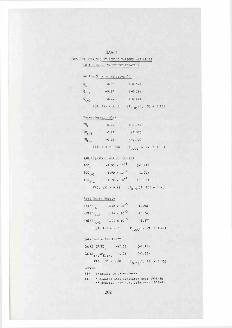
Table bRESULTS OBTAINED BY ADDING VARIOUS VARIABLES
TO THE U.K. INVESTMENT EQUATION
Adding Non- ta x a d j u s t e d ' O ' :
Qt - 0 . 3 2 ( - 0 . 6 4 )
Qt - 1 ' ° * 27 ( - 0 . 3 9 )
Qt - 2 ' ° - 24 ( - 0 . 4 1 )
F ( 3 , 19) - 1 . 13 ( F0 . 0 5 ( 3 , 19) “ 3 *13)
T a x - a d i u s t e d ' 0 ' : *
TQt - 0 . 0 2 ( - 0 . 1 5 )
T^ t - 1 0 . 1 7 ( 1 . 3 7 )
T^ t - 2 - 0 . 0 9 ( - 0 . 7 0 )
F ( 3 . 19) - 0 . 68 (F0 > 0 5 ( 3 . 14) - 3 . 1 3 )
T a x - a d j u s t e d Cost o f C a p i t a l
TCCt - 1 . 9 3 x 10"2 ( - 1 . 2 1 )
TCCt - i 1 . 9 0 x 10"1 ( 1 . 3 0 )
TCCc - 2 - 1 . 7 8 x 10"1 ( - 1 . 1 6 )
F ( 3 . 13) - 0. .98 (F0 0 5 ( 3 . 13) - 3 . 4 1 )
Re al Monev Supply
(Ml/P)c 3 . 18 x 10‘ 5 ( 0 . 9 0 )
(Ml/P)t_1 1 . 44 x 10‘ 5 ( 0 . 2 4 )
(Ml/P)t_2 - 1 . 0 4 x 10"5 ( - 1 . 5 7 )
F ( 3 , 19) - 1 . 7 1 (F0 > 0 5 ( 3 . 19) - 3 . 1 3 )
Takeover A c t i v i t y : **
( A / K ) c ( P / E ) t - 6 7 . 3 3 ( - 1 . 1 8 )
( A / K ) t _ 1Ar£ t _ 1 - 1 . 3 5 ( - 1 . 1 2 )
F ( 2 , 18) - 0 . 8 0 (Fq o5 ( 2 , 18) - K 5 5 )
N o t e s :
( i ) t - r a t i o s i n p a r e n t h e s e s
( i i )• * d e n o t e s o n l y a v a i l a b l e o v e r 1 9 55 - 80** d e n o t e s o n l v a v a i l a b l e o« p *> iQ^S-84
202
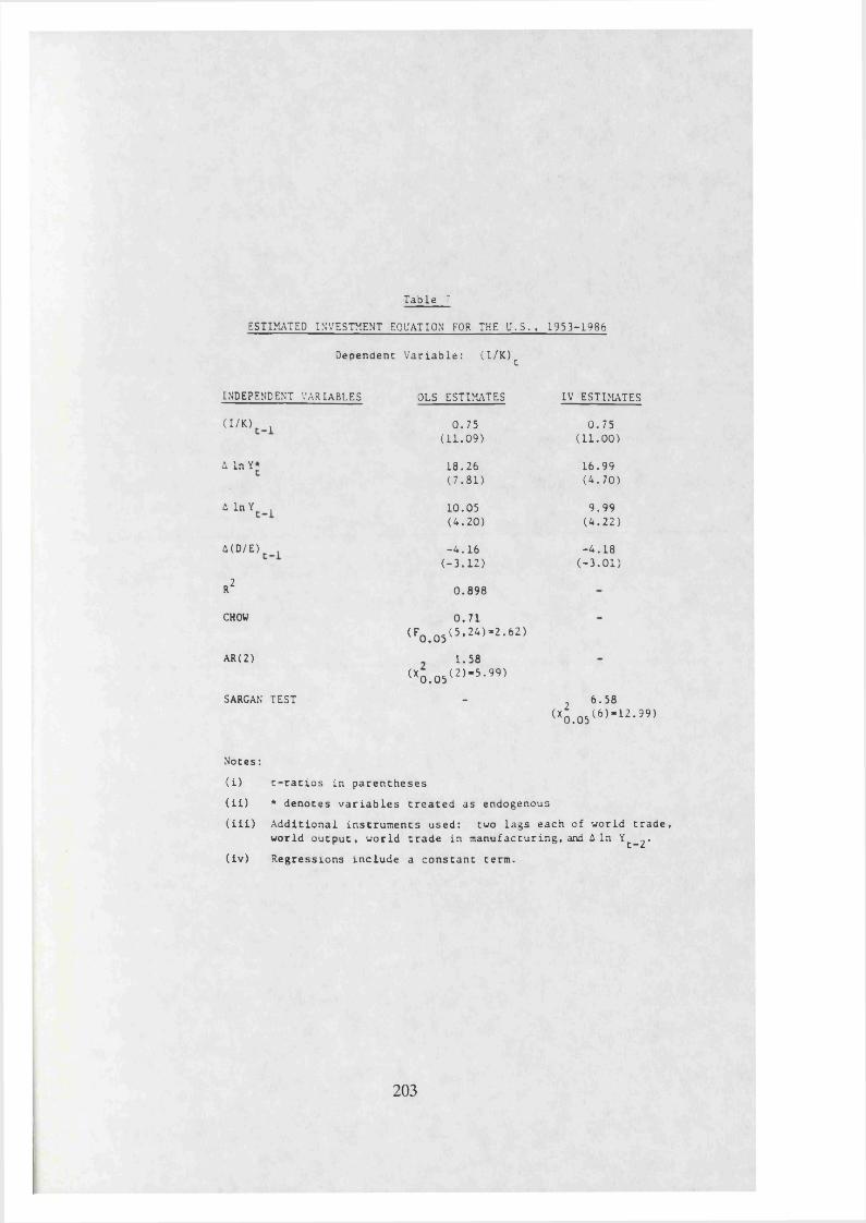
Table 7
ESTIMATED INVESTMENT EQUATION' FOR THE U . S . , 1953- 1986
Dependent V a r i a b l e : ( I / K ) ^
INDEPENDENT VARIABLES OLS ESTIMATES IV ESTIMATES
(I/K) , 0.75 0.75(11.09) (11.00)
AlnY* 18.26 16.99(7.81) (4.70)
A In Y 10.05 9.99(4.20) (4.22)
A(D/E) -4.16 -4.18(-3.12) (-3.01)
R2 0.898
CHOW 0.71(F0.05(5’2 4 W -62)
AR(2) 1.58(X0.05(2)“5-99)
SARCAN TEST - , 6 . 5 8(X0.05(6 W 2 -99)
N o t e s :
( i ) t - r a t i o s i n p a r e n t h e s e s
( i i ) * d e n o t e s v a r i a b l e s t r e a t e d as endogenous
( i l l ) A d d i t i o n a l i n s t r u m e n t s us ed : two l a g s e a ch o f wor l d t r a d e ,wor l d o u t p u t , wor ld t r a d e i n m an u f a c t u r i n g , and A In * t _ 2 *
( l v ) R e g r e s s i o n s i n c l u d e a c o n s t a n t term.
2 0 3
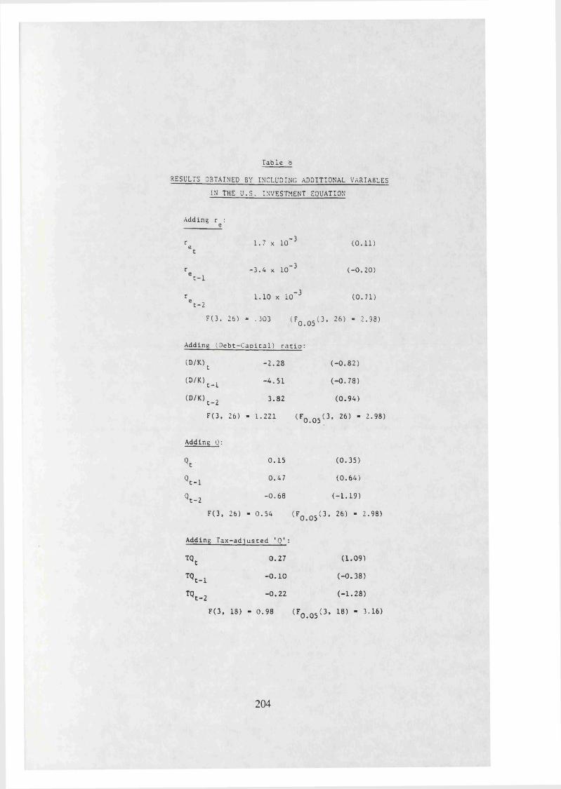
Table bRESULTS OBTAINED BY INCLUDING ADDITIONAL VARIABLES
IN THE U.S. INVESTMENT EQUATION
Adding r :
re 1 . 7 x 10~3 ( 0 . 1 1 )
r - 3 . 4 x 10“ 3 ( - 0 . 2 0 )c - 1
r 1 . 1 0 x 10"3 ( 0 . 7 1 )e t - 2
F (3 . 26) - . 303 ( f0 . 0 5 ( 3 , 26) “ 2 ' 98)
Adding ( D e b t - C a p i t a l ) r a t i o :
(D/K.) t - 2 . 2 8 ( - 0 . 8 2 )
(D/ K) t - 1 “4 , 5 L ( - 0 . 7 8 )
{D/K)t _ 2 3 . 8 2 ( 0 . 9 4 )
F( 3, 26) - 1 . 2 2 1 ( f0 . 0 5 ( 3 , 26) “ 2>98)
Adding Q:
Qt 0 . 1 5 ( 0 . 3 5 )
Qt _ 1 0 . 4 7 ( 0 . 6 4 )
Qt _ 2 - 0 . 6 8 ( - 1 . 1 9 )
F( 3 . 26) - 0 . 5 4 (FQ Q5( 3 , 26) - 2 .9 8 )
Adding T a x - a d j u s t e d ' O ' :
TQt 0 . 2 7 ( 1 . 0 9 )
TQt _ 1 - 0 . 1 0 ( - 0 . 3 8 )
TQt _ 2 “0 . 2 2 ( - 1 . 2 8 )
F ( 3 , 18) - 0 . 9 8 ( F0 . 0 5 ( 3 , 18) " 3 ,1 6 )
2 0 4
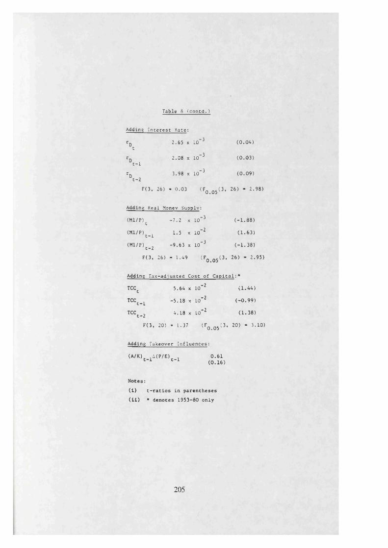
Table 8 (contd.)
Adding Interest Rate:r Q 2 . 6 5 x 1 0 ' 3 ( 0 . 0 4 )
t
r 2 . 0 8 x 1 0 ' 3 ( 0 . 0 3 )t - 1
rD 3 . 9 8 x 1 0 ' 3 ( 0 . 0 9 )t - 2
F (3 , 26) - 0 . 0 3 ( f0 . 0 5 ( 3 ’ 26) “ 2 , 9 8 )
Adding Real Money S u p p l y :
( Ml/P)^ - 7 . 2 x 10‘ 3 ( - 1 . 8 8 )
( M l / P ) c_ i 1 . 5 x 10‘ 2 ( 1 . 6 3 )
( M l / P ) t _ z - 9 . 6 3 x 10"3 ( - 1 . 3 8 )
F ( 3 . 26) - 1 . 4 9 ( f0 . 0 5 ( 3 ’ 26) " 2 *95)
Adding T a x - a d j u s t e d Cos t o f C a p i t a l : *
TCCc 5 . 6 4 x 10“ 2 ( 1 . 4 4 )
TCCt - l " 5 *18 x I 0 "2 ( - 0 . 9 9 )
TCCt _2 4 - 18 x L0’ 2 ( 1 *38)
F ( 3 , 20) - 1 . 37 (FQ q5 ( 3 , 20) - 3 . 1 0 )
Adding Takeover I n f l u e n c e s :
(A/K) . A(P/E) 0 . 6 1t _ i ( 0 . 1 6 )
N o t e s :
( i ) t - r a t i o s i n p a r e n t h e s e s
( i i ) * d e n o t e s 1 9 5 3- 8 0 o n l y
2 0 5
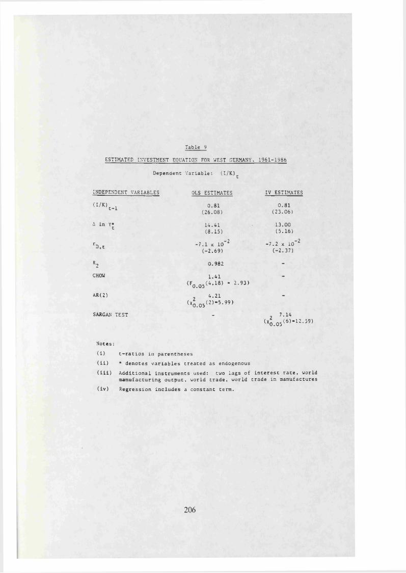
Table 9ESTIMATED INVESTMENT EQUATION FOR WEST GERMANY. 1 96 1- 1986
Dependent V a r i a b l e : ( I / K ) c
INDEPENDENT VARIABLES OLS ESTIMATES IV ESTIMATES
( I / K ) 0 . 8 1 0 . 8 1( 2 6 . 0 8 ) ( 2 3 . 0 6 )
A In Y* 1 4 . 4 1 1 3 . 0 0( 8 . 1 5 ) ( 5 . 1 6 )
rD t - 7 . 1 x 10"2 - 7 . 2 x 1 0 ' 2( - 2 . 6 9 ) ( - 2 . 3 7 )
R2 0 . 9 8 2
CHOW i . 4 i
(F0 . 0 5 ( 4 , 1 8 ) “ 2 ' 9 3 )
AR(2) 4 . 2 1
( x0 . 0 5 ( 2 ) " 5 ’ 99)
SARC AN TEST - . 7 . 1 4
( x0 . 0 5 ( 6 ) “ L2‘ 59)
N o t e s :
( i ) t - r a t i o s i n p a r e n t h e s e s
( 11) * d e n o t e s v a r i a b l e s t r e a t e d as endogenous
( i l l ) A d d i t i o n a l i n s t r u m e n t s us ed : two l a g s o f i n t e r e s t r a t e , worldm a n u f a c t u r i n g o u t p u t , world t r a d e , wo rl d t r a d e i n ma nu fa ct ure s
( i v ) R e g r e s s i o n i n c l u d e s a c o n s t a n t term.
2 0 6
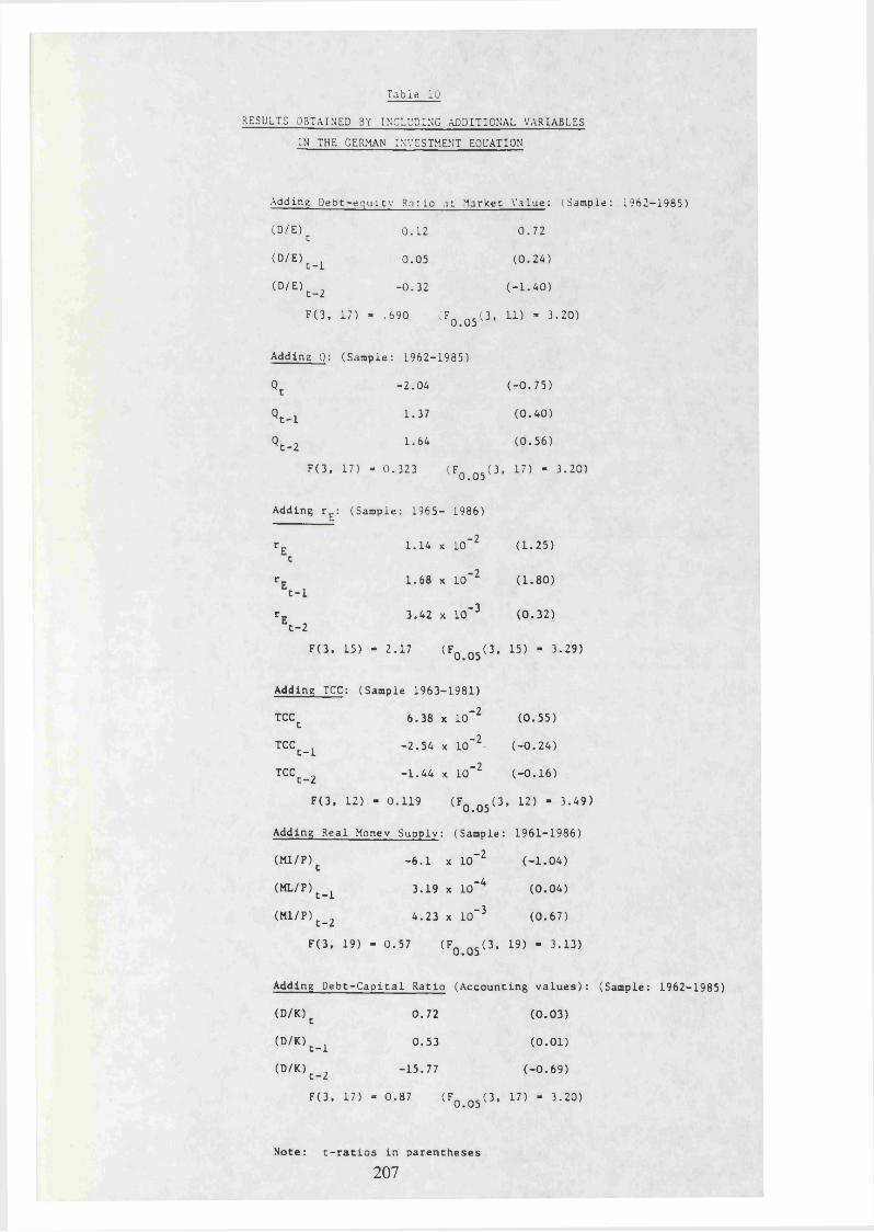
Table 10RESULTS OBTAINED BY INCLUDING ADDITIONAL VARIABLES
IN THE GERMAN INVESTMENT EQUATION
Adding D e b t - e q u i t v R a t i o at Markec V a l u e ; (Sample: 1 962 -1 98 5 )
(D/E)^ 0 . 1 2 0 . 7 2
( D / E ) t - 1 ° * 05 ( 0 . 2 4 )
( D / E ) t - 2 " ° ' 32 ( - 1 . 4 0 )
F ( 3 , 17) - . 6 9 0 (FQ 0 5 ( 3 . 11) - 3 . 2 0 )
Adding Q: ( Sample: 1 96 2- 1 98 5)
Qt - 2 . 0 4 ( - 0 . 7 5 )
Qt _ 1 1 . 3 7 ( 0 . 4 0 )
Qt _ 2 1 . 6 4 ( 0 . 5 6 )
F ( 3 , 17) - 0 . 3 2 3 (FQ Q5( 3 . 17) - 3 . 2 0 )
Adding r £ : (Sample: 1 9 65 - 1986)
r r 1 . 1 4 x 10~2 ( 1 . 2 5 )t
r_ 1 . 6 8 x 10"2 ( 1 . 8 0 )t - 1
r - 3 . 4 2 x 10- 3 ( 0 . 3 2 )t - 2
F ( 3 , 15) - 2 . 1 7 (Fq q5 ( 3 , 15) - 3 . 2 9 )
Adding TCC: (Sample 1 9 6 3 - 19 81 )
TCCt 6 . 3 8 x 1 0"2 ( 0 . 5 5 )
TCCt _ 1 - 2 . 5 4 x lO- 2 ( - 0 . 2 4 )
TCCt _ 2 - 1 . 4 4 x 10“ 2 ( - 0 . 1 6 )
F ( 3 , 12) - 0 . 1 1 9 ( f0 . 0 5 ( 3 , 12) " 3 , 4 9 )
Adding Real Monev S u p p l y : (Sample: 1 9 6 1 - 1 9 8 6 )
( M l / P ) t - 6 . 1 x 10- 2 ( - 1 . 0 4 )
(ML/P)t _ i 3 . 1 9 x 10"A ( 0 . 0 4 )
( M1 /P ) c_ 2 4 . 2 3 x 1 0 ' 3 ( 0 . 6 7 )
F ( 3 , 19) - 0 . 5 7 ( f0 . 0 5 ( 3 * 19) “ 3 ’ 13)
Adding D e b t - C a p i t a l Rat i o ( A c c o u n t i n g v a l u e s ) : (Sample: 1 9 62- 198 5)
( D / K ) t 0 . 7 2 ( 0 . 0 3 )
( D/ K ) t _ 1 0 . 5 3 ( 0 . 0 1 )
( D/ K ) t _ 2 - 1 5 . 7 7 ( - 0 . 6 9 )
F ( 3 , 17) - 0 . 8 7 (Fq 05( 3 , 17) - 3 . 2 0 )
No te : t - r a t i o s i n p a r e n t h e s e s
207
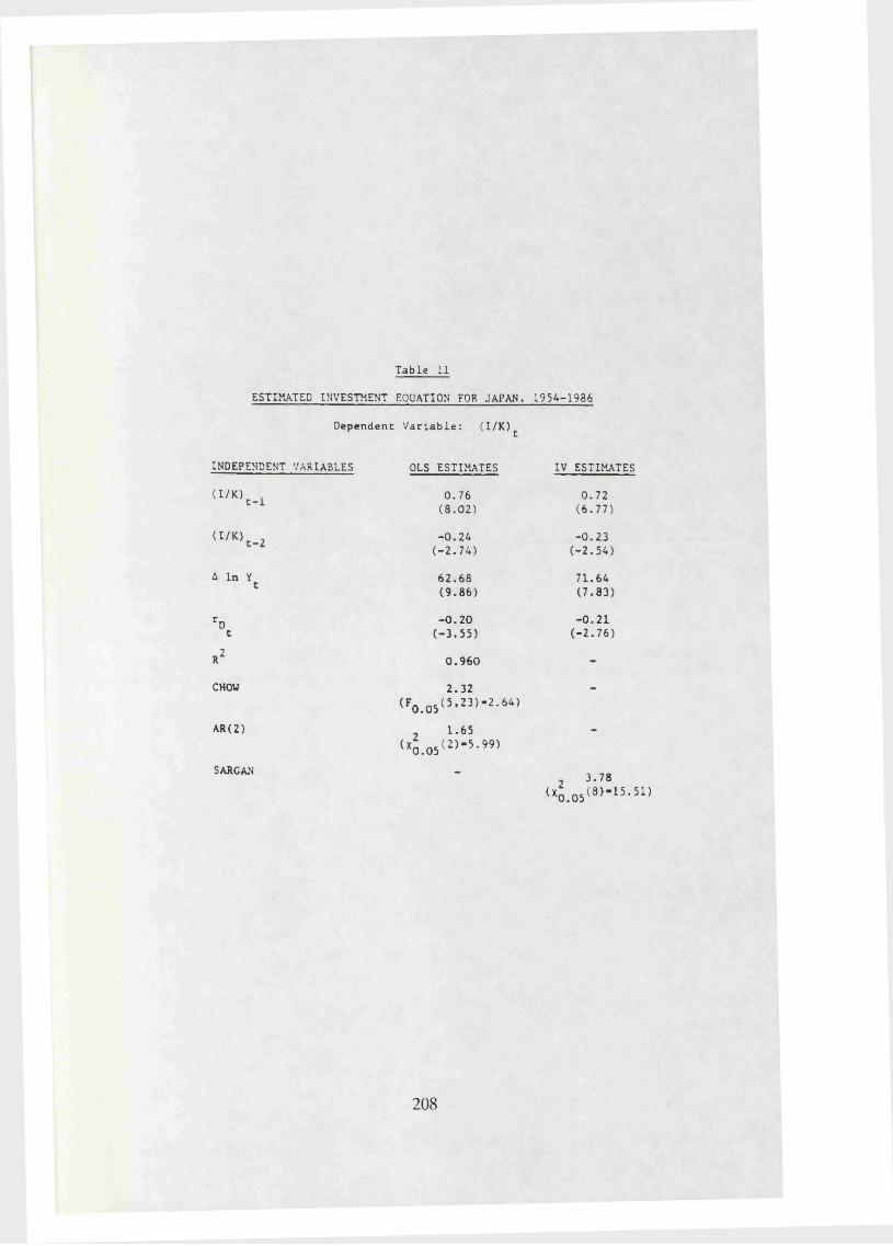
Table 11ESTIMATED INVESTMENT EQUATION FOR JAPAN. 1954- 1986
Dependent V a r i a b l e : ( I / K ) c
INDEPENDENT VARIABLES OLS ESTIMATES IV ESTIMATES
(I/K) 0.76 0.72(8.02) (6.77)
(I/K) -0.24 -0.23(-2.74) (-2.54)
A In Y 62.68 71.64(9.86) (7.83)
rD - 0 . 2 0 - 0 . 2 1t (-3.55) (-2.76)
R2 0.960
CHOW 2.32(F0.05(5,23)"2-64)
AR(2) 1.65
SARCAN
(X0.05(2)“5-99)
3 . 7 8
(x0.05(8)“15‘51)
2 0 8
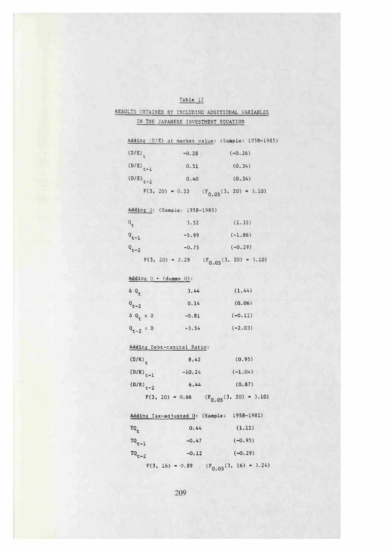
Table 12RESULTS OBTAINED BY INCLUDING ADDITIONAL VARIABLES
IN THE JAPANESE INVESTMENT EQUATION
Adding (D/E) ac market v a l u e : (Sample: 1 9 58 -19 85)
(D/E)^ - 0 . 2 8 ( - 0 . 2 6 )
( D / E ) t _ i 0 . 5 1 ( 0 . 3 4 )
( D / E ) t _ 2 0 . 4 0 ( 0 . 3 4 )
F ( 3 , 20) - 0 . 3 3 (Fq 0 5 ( 3 , 20) - 3 . 1 0 )
Adding Q: (Sample: 1 9 5 8- 1 9 85 )
Qt 3 . 5 2 ( 1 . 3 5 )
Qt - 1 - 5 . 9 9 ( - 1 . 8 6 )
Qc _ 2 - 0 . 7 5 ( - 0 . 2 9 )
F ( 3 . 20) - 2 . 2 9 ( Fq . 0 5 ( 3 , 20) “ 3 , 1 0 )
Adding Q + (dummv Q) :
A Qt 3 . 4 4 ( 1 . 4 4 )
Qt _ 2 0 . 1 4 ( 0 . 0 6 )
A Qt x D - 0 . 8 1 ( - 0 . 1 1 )
Qt _ 2 x D - 3 . 5 4 ( - 2 . 0 3 )
Adding D e b t - c a p i t a l R a t i o :
( D / K) t 8 . 4 2 ( 0 . 9 5 )
( D/ K) t _ 1 - 1 0 . 2 4 ( - 1 . 0 4 )
( D / K) t _ 2 6 . 4 4 ( 0 . 8 7 )
F ( 3 , 20) - 0 . 6 6 ( Fo . 0 5 ( 3 , 20) " 3 , 1 0 )
Adding T a x - a d j u s t e d Q: (Sample: 1 9 5 8 -1 98 1 )
TQt 0 . 4 4 ( 1 . 1 1 )
TQt _ 2 - 0 . 4 7 ( - 0 . 9 5 )
TQt _ 2 - 0 . 1 2 ( - 0 . 2 9 )
F ( 3 , 16) - 0 . 8 9 (Fq q5 ( 3 , 16) - 3 . 2 4 )
209
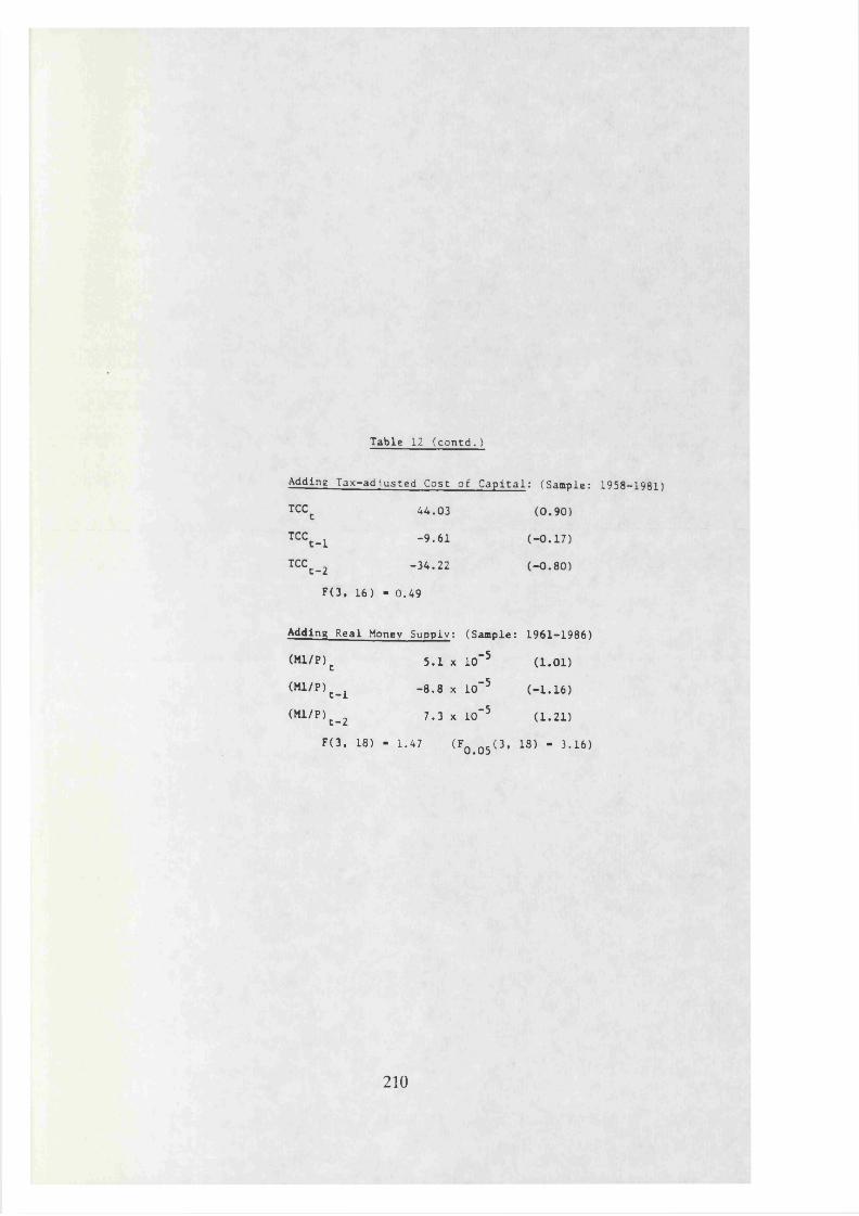
Table 12 (contd.)
Adding T a x - a d j u s t e d Cost o f C a p i t a l : (Sample: 1958-1981)
TCCc 4 4 . 0 3 ( 0 . 9 0 )
Tc c t _ 1 - 9 . 6 1 ( - 0 . 1 7 )
TCCt _ 2 - 3 4 . 2 2 ( - 0 . 8 0 )
F ( 3 , 1 6 ) - 0 . 4 9
Adding Real Money S u p p l y : (Sample: 1 96 1 - 1 9 8 6 )
( Ml / P)^ 5 . 1 x 10” 5 ( 1 . 0 1 )
( M l / P ) t _ 1 - 8 . 8 x 10“ 5 ( - 1 . 1 6 )
( M i / P ) t _ 2 7 . 3 x 1 0 " 5 ( 1 . 2 1 )
F ( 3 . 18) - 1 . 4 7 ( Fo . o5 ( 3 , 18) " 3 ‘ 16)
210
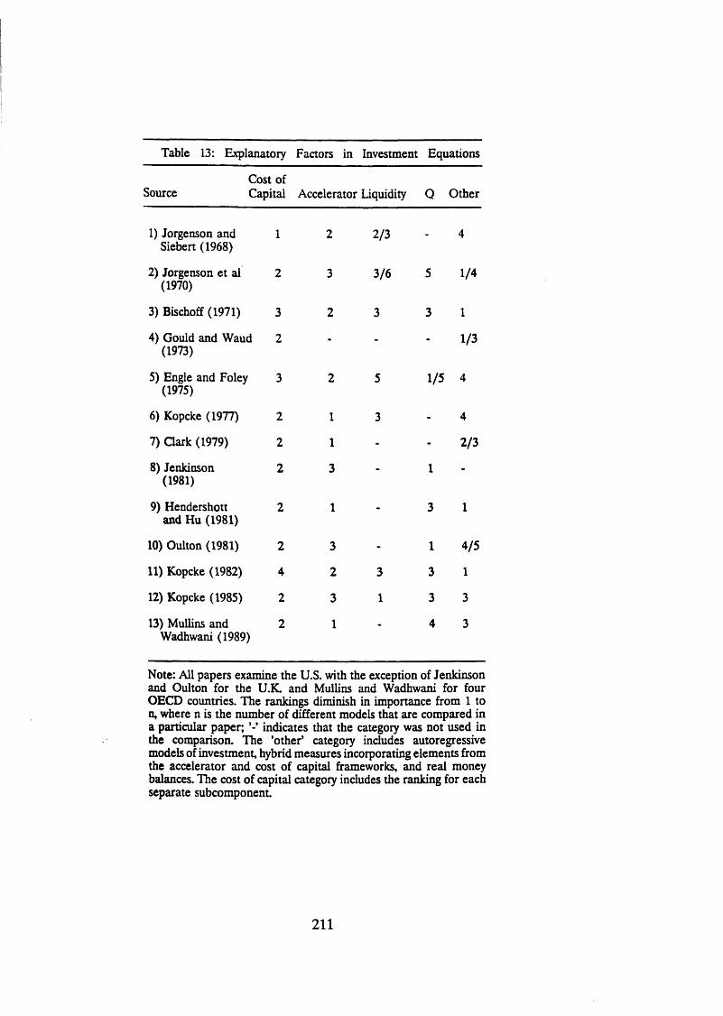
Table 13: Explanatory Factors in Investment Equations
Cost ofSource Capital Accelerator Liquidity Q Other
1) Jorgenson and 1 2 2/3 4Siebert (1968)
2) Jorgenson et al 2 3 3/6 5 1/4(1970)
3) Bischoff (1971) 3 2 3 3 1
4) Gould and Waud 2 1/3(1973)
5) Engle and Foley 3 2 5 1/5 4(1975)
6) Kopcke (1977) 2 1 3 - 4
7) Clark (1979) 2 1 - - 2/3
8) Jenkinson 2 3 1(1981)
9) Hendershott 2 1 3 1and Hu (1981)
10) Oulton (1981) 2 3 - 1 4/5
11) Kopcke (1982) 4 2 3 3 1
12) Kopcke (1985) 2 3 1 3 3
13) Mullins and 2 1 4 3Wadhwani (1989)
Note: All papers examine the U.S. with the exception of Jenkinson and Oulton for the U.K. and Mullins and Wadhwani for four OECD countries. The rankings diminish in importance from 1 to n, where n is the number of different models that are compared in a particular paper; indicates that the category was not used in the comparison. The ’other’ category includes autoregressive models of investment, hybrid measures incorporating elements from the accelerator and cost of capital frameworks, and real money balances. The cost of capital category includes the ranking for each separate subcomponent.
211
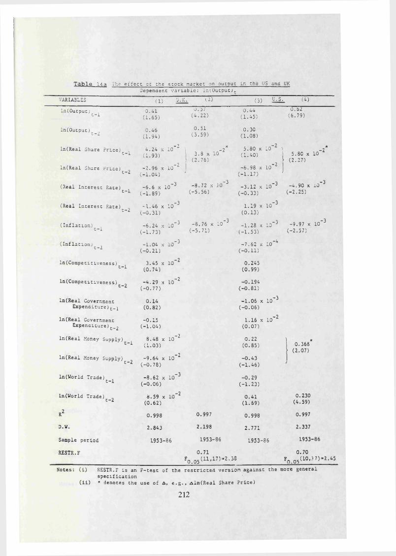
T a b l e 14a The er'fect of the stock. market on oucpuc in the US and UKDependent variable: in(Output;c
VARIABLES (1) U.SC. U ) (3) U.S. (4)
l n ( O u t p u t ; c 0 . 4 1( 1 . 6 5 )
0 . 5 7( 4 . 2 2 )
0 . 4 4( 1 . 4 5 )
0 . 6 2( 6 . 7 9 )
l n ( O u t p u c ) t ? 0 . 4 6( 1 . 9 4 )
0 . 5 1( 3 . 5 9 )
0 . 3 0( 1 . 0 8 )
l n ( R e a l Share P r i c e ) ^ ̂
l n ( R e a l Share P r i c e ) ^ ̂
( Re al I n t e r e s t Rate )^ ^
4 . 2 4 x 1 0"2 ] ( 1 . 9 3 )
- 2 . 9 6 x 1 0 - 2 ( - 1 . 0 4 )
- 6 . 6 x 10“ 3 ( - 1 . 8 9 )
*1 3 . 8 x 10"2 1- ( 2 . 7 6 )
1
- 8 . 7 2 x ] 0 - 3 ( - 5 . 5 6 )
5 . 8 0 x ( 1 . 4 0 )
- 6 . 9 8 x ( - 1 . 1 7 )
- 3 . 1 2 x ( - 0 . 3 3 )
10 ]
i o "2 !
i o - 3
*1 5 . 8 0 x 1 0 “ 2
( 2 . 2 7 )
- 4 . 9 0 x IO"3 ( - 2 . 2 5 )
( Re al I n t e r e s t Rat e) ^ ̂
( I n f l a t i o n ) ^ ^
- 1 . 4 6 x ( - 0 . 3 1 )
- 6 . 2 4 x ( - 1 . 7 3 )
i o ' 3
i o - 3 - 8 . 7 6 x IO"3 ( - 5 . 7 1 )
1 . 1 9 x ( 0 . 1 3 )
- 1 . 2 8 x ( - 1 . 5 3 )
i o " 3
i o - 3 - 9 . 9 7 x 1 0~ 3 ( - 2 . 5 7 )
( I n f l a t i o n ) c 1 - 1 . 0 4 x ( - 0 . 2 1 )
1 0 - 3 - 7 . 6 2 x ( - 0 . 1 1 )
1 0 - *
l n ( C o m p e t i t i v e n e s s ) ^ ^ 3 . 4 5 x ( 0 . 7 4 )
10 • 0 . 2 4 5( 0 . 9 9 )
l n ( C o m p e t i t i v e n e s s ) - 4 . 2 9 x ( - 0 . 7 7 )
1 0 ~ 2 - 0 . 1 9 4( - 0 . 8 1 )
l n ( R e a l Government E x p e n d i t u r e ) c_^
0 . 1 4( 0 . 8 2 )
- 1 . 0 6 x ( - 0 . 0 6 )
i o - 3
l n ( R e a l Government E x p e n d i t u r e ) c_ 2
- 0 . 1 5( - 1 . 0 4 )
1 . 1 6 x ( 0 . 0 7 )
i o " 2
l n ( R e a l Money Supply) ̂
l n ( R e a l Money Su p pl y ) ^
8 . 4 8 x ( 1 . 0 3 )
- 9 . 6 4 x ( - 0 . 7 8 )
1 0~ 2
i o " 2
0 . 2 2( 0 . 8 5 )
- 0 . 4 3( - 1 . 4 6 )
0 . 3 6 8 * • ( 2 . 0 7 )
ln ( Wo rl d T r a d e ) £ ^ - 8 . 6 2 x ( - 0 . 0 6 )
1 0 - 3 - 0 . 2 9( - 1 . 2 3 )
In(Wori d T r a de ) ^ ^ 8 . 5 9 x ( 0 . 6 2 )
i o " 2 0 . 4 1( 1 . 6 9 )
0 . 2 3 0( 4 . 5 9 )
R2 0 . 9 9 8 0 . 9 9 7 0 . 9 9 8 0.997
D.W. 2 . 8 4 3 2 . 1 9 8 2 . 7 7 1 2 . 3 3 7
Sample p e r i o d 1 9 5 3 - 86 1 95 3 -8 6 1 9 5 3 - 86 1 95 3- 86
RESTR.F 0 . 7 1
f o . o5 ( 1 1 ,1 7 ) * 2 ’38
0 .7 0
FO.O5( 1 0 ’ : ,7 ) - 2 - 45N o t e s : ( i ) RESTR.F i s an F - t e s t o f t h e r e s t r i c t e d v e r s i o n a g a i n s t t h e more g e n e r a l
s p e c i f i c a t i o n( i i ) * d e n o t e s t he u s e o f e . g . , A l n ( R e a l Share P r i c e )
212
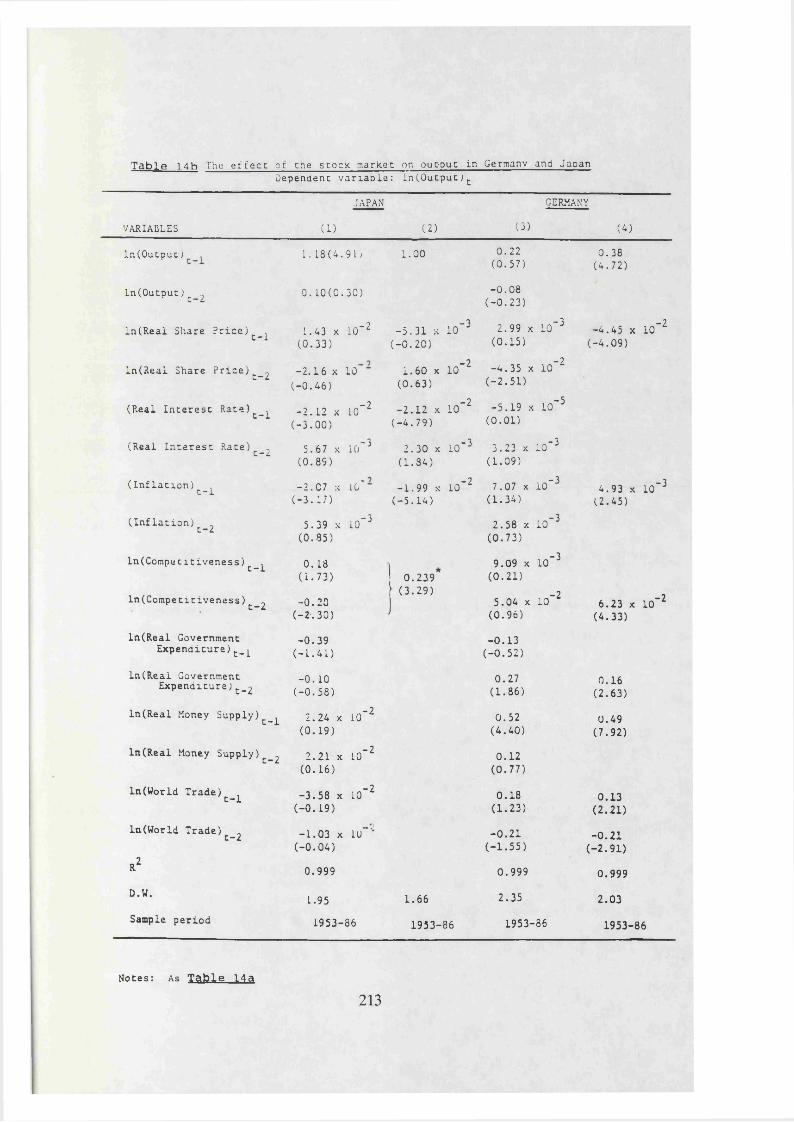
T a b l e 1 4 b The effect of the stock market on out-put in Germany and JapanDependent variable: ln(0utput)t
JAPAN GERMANYv a r i a b l e s (1) (2) (3) (4)l n ( 0 u c p u c )
l n ( 0 u t p u t ) c ̂
l n ( R e a l Share P r i c e )
l n ( R e a l Share P r i c e )
(Re al I n t e r e s t Rat e)
(Re al I n t e r e s t Rate)
1 . 1 8 ( 4 . 9 1 ;
0 . 1 0 ( 0 . 3 0 )
t - 1
t - 2
t - 1
t - 2
( I n f l a t i o n ) t - 1
( I n f l a t i o n ) ^ ^
I n ( C o m p e t i t i v e n e s s )
I n ( C o m p e t i t i v e n e s s )
t - 1
t - 2
l n ( R e a l Government E x p e n d i t u r e ) t _^
l n ( R e a l Government E x p e n d i t u r e ; t _2
l n ( R e a l Money Supply)t - 1
l n ( R e a l Money S u pp ly ) ^ ̂
l n( Wo rl d Trade)t - 1
1 . 4 3 x 10 ( 0 . 3 3 )
- 2 . 1 6 x 10" ( - 0 . 4 6 )
- 2 . 1 2 x 10 ( - 3 . 0 0 )
5 . 6 7 x 10 ( 0 . 8 9 )
- 2 . 0 7 x 10' ( - 3 . 1 7 )
5 . 3 9 x 10 ( 0 . 8 5 )
0 . 1 8 ( 1 . 7 3 )
- 0 . 2 8 ( - Z . 3 0 )
- 0 . 3 9 ( - 1 . 4 1 )
- 0 . 1 0 ( - 0 . 5 8 )
2 . 2 4 x 10 ( 0 . 1 9 )
2 . 2 1 x 10 ( 0 . 1 6 )
- 3 . 5 8 x 10 ( - 0 . 1 9 )
- 2
- 2
- 3
- 3
ln( Wo rl d Trade)
R2
D.W.
Sample p e r i o d
t - 2 - 1 . 0 3 x 1U ( - 0 . 0 4 )
0 . 9 9 9
1.95
1 95 3 -8 6
1.00
- 5 . 3 1 x 10 ( - 0 . 20)
1 . 6 0 x 10 ( 0 . 6 3 )
- 2 . 1 2 x 10 ( - 4 . 7 9 )
- 3
- 1 . 9 9 x 10 ( - 5 . 1 4 )
0 . 2 3 9( 3 . 2 9 )
- 2
- 2
- 2
1.66
1 9 3 3- 8 6
0. 22( 0 . 5 7 )
- 0 . 0 8( - 0 . 2 3 )
- 2
- 2
2 . 9 9 x 10 ( 0 . 1 5 )
- 4 . 3 5 x 10 ( - 2 . 5 1 )
- 5 . 1 9 x 10 (0 . 01)
- 3
- 2
- 5
2 . 3 0 x IO"3 ( 1 . 3 4 )
- 2
3 . 2 3 x 10 ( 1 . 0 9 )
7 . 0 7 x 10 ( 1 . 3 4 )
2 . 5 8 x 10 ( 0 . 7 3 )
- 3
- 3
- 3
9 . 0 9 x 10 (0 . 21)
5 . 0 4 x 10 ( 0 . 9 6 )
- 3
- 2
- 0 . 1 3( - 0 . 5 2 )
0 . 2 7( 1 . 86 )
0 . 5 2( 4 . 4 0 )
0.12( 0 . 7 7 )
0 . 1 8( 1 . 2 3 )
- 0.21( - 1 . 5 5 )
0 . 9 9 9
2 . 3 5
19 53- 86
0 . 3 8( 4 . 7 2 )
- 4 . 4 5 x 10 ( - 4 . 0 9 )
- 2
4 . 9 3 x 10 ( 2 . 4 5 )
- 3
6 . 2 3 x 10 ( 4 . 3 3 )
0 . 1 6( 2 . 6 3 )
0 . 4 9( 7 . 9 2 )
0 . 1 3(2. 21)
- 0.21( - 2 . 9 1 )
0 . 9 9 9
2 . 0 3
19 53 -8 6
-2
N ot e s : As T a b l e 14fr
2 1 3
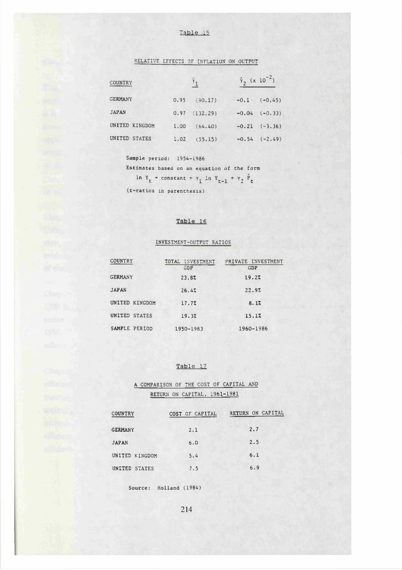
Xafel e 15
RELATIVE EFFECTS OF INFLATION ON OUTPUT
COUNTRY Y2 (* i o - 2 )
GERMANY 0.95 (90.17) - 0 . 1 ( - 0 . 4 5 )
JAPAN 0.97 (132 .29 ) - 0 . 0 4 ( - 0 . 3 3 )
UNITED KINGDOM 1.00 (64 .40) - 0 . 2 1 ( - 3 . 3 6 )
UNITED STATES 1.02 (55 .15) - 0 . 5 4 ( - 2 . 4 9 )
Sample p e r i o d : 1954--1986
E s t i m a t e s based on an e q u a t i o n o f t h e form
In Yt - c o n s t a n t + In + y 2 P£
( t - r a t i o s i n p a r e n t h e s i s )
INVESTMENT-OUTPUT RATIOS
COUNTRY
GERMANY
JAPAN
UNITED KINGDOM
UNITED STATES
SAMPLE PERIOD
TOTAL INVESTMENT PRIVATE INVESTMENTGDP
2 3 . 82
2 6 . 4 2
1 7 . 72
1 9 . 3 2
19 50 -1 98 3
GDP
1 9 . 2 2
2 2 . 9 2
8.12
1 5 . 1 2
1 9 6 0 - 1 9 8 6
T a b l e 17
A COMPARISON OF THE COST OF CAPITAL AND
RETURN ON CAPITAL. 1 9 61 - 19 81
COUNTRY COST OF CAPITAL RETURN ON CAPITAL
GERMANY
JAPAN
UNITED KINGDOM
UNITED STATES
2.1
6 . 0
5 . 4
7 . 5
2 . 7
2 . 5
6. 1
6 .9
S o u r c e : Ho l l a nd ( 1984)
2 1 4

Conclusions
This thesis has investigated some determinants and consequences of aggregate stock
market prices. Using data sources spanning 23 countries and almost three centuries,
it is found that equity prices are correlated with real economic variables. There is,
however, sufficient evidence of non-efficient market behaviour to reject the general
applicability of the efficient markets hypothesis. Another broad conclusion is that
institutional factors, both across countries and over time, contribute to accentuating
or diminishing the linkage between such prices and the real economy.
In addition, the following detailed conclusions emerge from each chapter.
Chapter I examines stock price behaviour prior to the stock market crash of 1987.
Using monthly and daily data from 23 stock markets, there is little support for the
view that the recent crash was caused by a bursting bubble. However, there is
evidence that equity prices have recently moved in a non-random manner on some
of these exchanges.
Chapter II investigates the movements of stock prices in the United Kingdom from
1700 to 1987. A strong nominal interest rate effect on excess returns is found for the
entire period, but it appears that inflation has a consistent, negative effect only after
1950. The changing influence of inflation on equity prices may be linked to Britain’s
adherence to the gold standard.
Chapter III analyzes major British financial crises since 1700. In the first part, using
efficient and non-efficient market models, it is found that fluctuations in
macroeconomic variables account for up to one half of equity price variation. In the
second part, these models reveal that relatively few crises have been preceded by the
excessive positive returns consistent with rational bubbles. The success of non
efficient market models in explaining equity returns does imply, however, that the
efficient markets hypothesis does not strictly hold for this data set.
2 1 5
Chapter IV finds that Tobin’s Q, the ratio of the market value of the corporate sector to the replacement cost of its capital, is inappropriately modelled within a
static framework but is improved markedly using a dynamic error correction model. The Q measures are also superior to real stock prices as predictors of investment in
the OECD countries under investigation. These results imply that Q, and hence stock
prices, are correlated to investment. However, the relationship is relatively weak and
depends on the exclusion of other relevant explanatory variables from the investment equation.
Chapter V compares the broader effects of equity prices on corporate investment and output in Japan, West Germany, the United Kingdom and the United States. It seems that the effect of the equity market is greater in the latter two countries for
various institutional reasons having to do with the degree of managerial autonomy from stock price fluctuations.
Overall, then, it appears that aggregate stock market prices are significantly linked to the real economy. The instances of non-efficient market behaviour, in terms of unexplained stock returns prior to financial crises, the predictability of stock returns, the influence of lagged and nominal variables on the equity premium, and, possibly, the weak statistical relationship between stock market prices and corporate
investment, do, however, offer support to a view of the stock market influenced not only by fundamental factors, but also possibly by social and psychological elements.
216

Bibliography
Abel, A. and Blanchard, O. (1986), ’The Present Value of Profits and Cyclical Movements in Investment’, Econometrica. 54, pp.249-273.
Aoki, M., (1984), The Co-operative Game Theory of a Firm. Clarendon Press, Oxford.
Ashton, T. (1959) Economic Fluctuations in England 1700-1800 (Oxford: Clarendon Press).
Attanasio, O. and Wadhwani, S. (1989) ’Risk, Gordon’s Growth Model, and the
Predictability of Stock Market Returns’, LSE Financial Markets Group Discussion Paper No. 49.
Auerbach, A., (1983), ’Taxation, Corporate Financial Policy and the Cost of Capital’, Journal of Economic Literature. Vol.XXI, September, pp.905-940.
Auerbach, A. and Reishus, D. (1987), ’The Effects of Taxation on the Merger Decision’, NBER Working Paper No. 2192.
Bank of England (1967) ’Bank of England liabilities and assets: 1696 to 1966’, Bank
of England Quarterly Bulletin, appendix, June.
Bank of England, (1987), Economics Division Data Base, mimeo.
Barro, R. (1989), ’The Stock Market and Investment’, paper presented at NBER
conference on Stock Market Volatility, Puerto Rico, March 1989.
Barsky, R. (1987) ’The Fisher Hypothesis and the Forecastability and Persistence of Inflation’, Journal of Monetary Economics. 19, pp.3-24.
217

Batchelor, R. (1986) ’The Avoidance of Catastrophe: Two Nineteenth-century Banking Crises’ in F. Capie and G. Wood (eds), Financial Crises and the World
Banking System. (London: Macmillan Press).
BEQB, (1984), ’Business Finance in the United Kingdom and Germany’, Bank of England Quarterly Bulletin. September, pp.368-375.
Bischoff, C. (1971), ’Business Investment in the 1970s: A Comparison of Models’, Brookings Papers on Economic Activity. 1, pp. 13-58.
Black, F. and Scholes, M. (1976) ’The Pricing of Options and Corporate Liabilities’, Journal of Political Economy. 81, pp.637-659.
Blanchard, O. and Watson, M. (1982) ’Bubbles, Rational Expectations and Financial Markets’ in P. Wachtel (ed), Crises in the Economic and Financial Structure. Lexington: Lexington Books, 1982.
Blundell, R., Bond, S., Devereux, M. and Schianterelli, F., (1987), ’Does Q Matter for Investment?’, I.F.S. Working Paper.
Bordo, M. (1986) ’Financial Crises, Banking Crises, Stock Market Crashes and the
Money Supply: Some International Evidence, 1870-1933’ in F. Capie and G. Wood
(eds), Financial Crises and the World Banking System. (London: Macmillan Press).
Bordo, M. and Schwartz, A. (1984) A Retrospective on the Classical Gold Stand.
1821-1931 (Chicago: University of Chicago Press).
Bowley, A., Schwartz, A. and Smith, K. (1931) A New Index of Prices of Securities.
London and Cambridge Economic Society Memoranda, No. 33, January.
Brainard, W., Shoven, J. and Weiss, L. (1980), ’The Financial Valuation of the Return to Capital’, Brookings Papers on Economic Activity. 2, pp.453-511.
218

British Parliamentary Papers (1868-69), XXXV, pp.693-704.
Brown, J. and Ashenfelter, O., (1986), Testing the Efficiency of Employment Contracts’, Journal of Political Economy. Vol.94, pp.541-587.
Bundesbank, ’Beihette zu den Monatsberichten der Deutschen Bundesbank’, various
issues.
BZW (1987) BZW Equitv-Gilt Study. Barclays de Zoete Wedd Research, January.
Capie, F., Mills, T. and Wood, G. (1986) ’What Happened in 1931?’ in F. Capie and G. Wood (eds), Financial Crises and the World Banking System. (London:
Macmillan Press).
Capie, F. and Webber, A. (1986) A Monetary History of the United Kingdom. 1870- 1982 (London: Allen and Unwin).
Carsberg, B. and Hope, A., (1976), Business Investment Decisions Under Inflation: Theory and Practice. ICAEW: London.
Chan-Lee, J. (1986), ’Pure Profits and Tobin’s q in Nine OECD Countries’, OECD Economic Studies. 7, pp.205-232.
Chappell, H. and Cheng, D. (1982), ’Expectations, Tobin’s q, and Investment: A
Note’, Journal of Finance. 37, pp.231-236.
Chiras, D. and Manaster, S. (1978) ’Information Content of Option Prices and a Test of Market Efficiency’, Journal of Financial Economics. 6(2-3), pp.213-234.
Chirinko, R. (1986), ’Business Investment and Tax Policy: A Perspective on Existing
Models and Empirical Results’, National Tax Journal. 39(2), pp.137-155.
219

Ciccolo, J. (1975), ’Four Essays in Monetary Policy’, Ph.D. Dissertation, Yale University.
Ciccolo, J. (1978), ’Money, Equity Values, and Income - Tests for Exogeneity*, Journal of Money. Credit and Banking. 10(1), pp.46-64.
Clark,P. (1979), ’Investment in the 1970s: Theory, Performance and Predictors’, Brookings Papers on Economic Activity. 1, pp.73-124.
Cohn, R.A. and Lessard, D. (1981) ’The Effect of Inflation on Stock Prices: International Evidence’, Journal of Finance. May.
Collins, M. (1983) ’Long-term growth of the English banking sector and money stock, 1844-80’, Economic History Review. 36(3), pp.374-394.
Connolly, R. and Lacivita, C. (1985), ’A Note on the Statistical Properties of Aggregate q Measures’, Economics Letters. 19, pp.177-181.
Corbett, J., (1987), ’International Perspectives on Financing: Evidence from Japan’, Oxford Review of Economic Policy. Vol.3, No.4, pp.30-55.
Council of Economic Advisors (1983), Economic Report of the President.
(Washington: U.S. Government Printing Office).
Cox, J. and Rubinstein, M. (1985) Options Markets (New Jersey: Prentice-Hall).J
CSO (1986,1988) Economic Trends (London: HMSO).
Cutler, D., Poterba, J. and Summers, L. (1989) ’What Moves Stock Prices?’, Journal of Portfolio Management. Spring, pp.4-12.
Deane, P. and Cole, W. (1962) Abstract of British Historical Statistics (Cambridge:
CUP).
220
Dickson, P. (1967) The Financial Revolution in England (London: Macmillan).
Dinenis, E. (1985a), 'Adjustment Costs, Q, Taxation and Investment in the U.K.’,
London School of Economics, Centre for Labour Economics, Discussion Paper No. 235.
Dinenis, E. (1985b), ’Q, Gestation Lags and Investment: Is the Flexible Accelerator
a Mirage?', London School of Economics, Centre for Labour Economics, Discussion Paper No. 236.
Dore, R., (1985), 'Financial Structures and the Long-term View', Policy Studies. Vol.6, part 1, July.
Dombusch, R. (1976) 'Expectations and exchange rate economics’, Journal of Political Economy. 84, pp. 1161-76.
Ellinger, T. and Stewart, T. (1980) A Post-War History of the Stock Market. (Cambridge: Woodhead-Faulkner).
Engle, R. and Foley, D. (1975), 'An Asset Price Model of Aggregate Investment', International Economic Review. 16, pp.625-647.
Engle, R. and Granger, C.W.J. (1987), 'Co-integration and Error Correction: Representation, Estimation and Testing', Econometrica. 55(2), pp.251-276.
Evans, G. (1986) 'A Test for Speculative Bubbles in the Sterling-Dollar Exchange Rate: 1981-84', American Economic Review. 76(4), pp. 621-636.
Fama, E. (1970) 'Efficient Capital Markets: A Review of Theory and Empirical Work', Journal of Finance. 25(2), pp.383-423.
221

Fama, E. (1981) ’Stock Returns, Real Activity, Inflation, and Money’, American Economic Review. 71, pp.545-65.
Fama, E. and Schwert, G. W. (1977) ’Asset Returns and Inflation’, Journal of Financial Economics. 5, November, pp. 115-46.
Feinstein, C. (1972) National Income. Expenditure and Output of the United
Kingdom 1855-1965 (Cambridge: CUP).
^ T eld ste in , M. (1982) ’Inflation and the Stock Market’, American Economic Review.
73(1), pp. 17-30.
Financial Times (1987) ’Rout on Wall St Leads Stocks to Record Falls’, Financial Times. October 20, p.l.
Fischer, S. and Merton, R., (1984), ’Macroeconomics and Finance: The Role of the Stock Market’, NBER Working Paper No. 1291.
Fisher, I. (1933) ’The Debt Deflation Theory of Great Depressions’, Econometrica. 1, pp.337-357.
Flemming, J., Price, L. and Byers, S. (1976), ’The Cost of Capital, Finance and
Investment’, Bank of England Quarterly Bulletin. June, pp.193-205.
Friedman, M. and Schwartz, A. (1982) Monetary Trends in the United States and the
United Kingdom (Chicago: University of Chicago Press for NBER).
Fuller, W. (1976), Introduction to Statistical Time Series. (New York: John Wiley).
Galbraith, J.K. (1955) The Great Crash. (London: Hamish Hamilton).
Galeotti, M. (1984), ’Recent Developments in Investment Theory’, Giomale Degli
Economisti e Annali di Economia. 43, pp.393-415.
222

Garber, P. (1989) ’Tulipmania’, Journal of Political Economy. 97(3), pp.535-560.
Garner, A. (1988), ’Has the Stock Market Crash Reduced Consumer Spending?’, Federal Reserve Bank of Kansas City Economic Review. April, pp.3-16.
Gayer, A., Rostow, W.W. and Schwartz, A. (1953) The Growth and Fluctuation of the British Economy 1790-1850. (Oxford: Clarendon Press).
Geske, R. and Roll, R. (1983) ’The Fiscal and Monetary Linkage between Stock
Returns and Inflation’, Journal of Finance. 38(1), pp. 1-33.
Glauber, R. (1988) Speech given by the former Executive Director of the Presidential Task Force on Market Mechanisms at a conference on Black Monday - Nine Months After. London, July.
Gordon, R. and Malkiel, B. (1981), ’Corporation Finance’ in A. Pechman, How Taxes Affect Economic Behavior. (Washington: Brookings Institution), pp. 131-198.
Gordon, R. and Veitch, J., (1987), ’Fixed Investment in the American Business Cycle’, in R J. Gordon (ed.), The American Business Cycle: Continuity and Change. University of Chicago Press: Chicago.
Gould, J. and Waud, R. (1973), ’The Neoclassical Model of Investment Behavior: Another View’, International Economic Review. 14, pp.33-48.
Granger, C.W.J. (1981), ’Some Properties of Time Series Data and Their Use in Econometric Model Specification’, Journal of Econometrics. 16, pp. 121-130.
Greenspan, A. (1988) Statement before the Committee on Banking, Housing, and
Urban Affairs, U.S. Senate, 2 February, reported in the Federal Reserve Bulletin. 74(4), pp. 217-225.
223
Greenwald, B. and Stiglitz, J., (1987), ’Imperfect Information, Credit Markets and Unemployment’, European Economic Review. Vol.31, pp.444-456.
Grunfeld, Y. (1960), ’The Determinants of Corporate Investment’ in A. Harberger
(ed.) The Demand for Durable Goods. (Chicago: University of Chicago Press),pp.211-266.
Gultekin, N.B. (1983) ’Stock Market Returns and Inflation - Evidence from Other
Countries’, Journal of Finance. 38(1), pp.49-65.
Hamilton, J. (1986) ’On Testing For Self-Fulfilling Speculative Price Bubbles’, International Economic Review. 27(3), pp. 545-552.
Hardouvelis, G. (1987) ’Macroeconomic Information and Stock Prices’, Journal of Economics and Business. 39(2), pp. 131-140.
Harrington, D. (1987), Modern Portfolio Theory, the Capital Asset Pricing Model, and Arbitrage Pricing Theory. (New Jersey: Prentice-Hall).
Harvey, A. (1981), The Econometric Analysis of Time Series. (Oxford: Philip Allan).
Hayashi, F. (1982), ’Tobin’s Marginal q and Average q: A Neoclassical Interpretation’, Econometrica. Vol.40, pp.213-225.
Hayashi, F., (1985), ’Taxes and Corporate Investment in Japanese Manufacturing’, NBER Working Paper NO.1753.
Hayashi, F. and Sims, C. (1983) ’Nearly Efficient Estimation of Time Series Models
with Predetermined, but Not Exogenous, Instruments’, Econometrica. 51, pp.783- 798.
Hayashi, F. and Inoue, T. (1987), ’Implementing the Q Theory of Investment in
Micro Data: Japanese Manufacturing 1977-1985’, Osaka University, Department of
224

Economics.
Healey, D. (1988) Speech given by the former Shadow Spokesman on Foreign Affairs at a conference on Black Monday - Nine Months After. London, July.
\ Hendershott, P. (1981), ’The Decline in Aggregate Share Values - Taxation, Valuation Errors, Risk and Profitability’, American Economic Review. 71(5), pp.909- 922.
Hendershott, P. and Hu, S. (1981) ’Investment in Producers’ Equipment’ in H. Aaron
and J. Pechman (eds.) How Taxes Affect Economic Behavior. (Washington: Brookings Institution), pp.85-130.
Hennessy, J. (1988) Speech given by the Chairman and Chief Executive, Credit Suisse First Boston Limited, at a conference on Black Monday - Nine Months After. London, July.
Hoffman, W. (1934) ’Ein Index der industriellen Produktion fur Grossbritannien seit dem 18. Jahrhundert’, Weltwirtschaftliches Archiv. 40, September.
Hoffman, W. (1955) British Industry. 1700-1950 (Oxford: Basil Blackwell).
Holland, D., (1984), ’Introduction and Summary’, in D.M. Holland (ed.), Measuring
Profitability and Capital Costs: An International Study. Lexington Books: Lexington,
Massachusetts.
Holland, D. (1986), Measuring Profitability and Capital Costs: An International
Study. (Lexington,Mass.: Lexington Books).
Homer, S. (1963) A History of Interest Rates (New Brunswick: Rutgers University
Press).
225
Keynes, J.M. (1936), The General Theory of Employment. Interest and Money. (New
York: Harcourt Brace Jovanovic).
Kindleberger, C. (1978) Manias. Panics, and Crashes: A History of Financial Crises.
(London: Macmillan).
Kindleberger, C. (1988) ’The Financial Crises of the 1930s and the 1980s: Similarities
and Differences’, Kvklos. 41(2), pp. 171-186.
King, M., (1977), Public Policy and the Corporation. Chapman and Hall: London.
King, M.A. (1987), ’Takeover Activity in the United Kingdom’, LSE Financial
Markets Group Discussion Paper No. 2.
Kleidon, A. (1986) ’Variance Bounds Tests and Stock Price Valuation Models’,
Journal of Political Economy. 94, pp. 953-1001.
Komiya, R. and Yasui, K., (1984), ’Japan’s Macroeconomic Performance Since the
First Oil Crisis: Review and Appraisal’, in K. Brunner and A. M eltzer (eds.),
Monetary and Fiscal Policies and Their Application, Journal of Monetary Economics
Supplement. Vol.20, pp.69-114.
Kopcke, R. (1977), ’The Behavior of Investment Spending during the Recession and
Recovery, 1973-76’, New England Economic Review. Novem ber/Decem ber, pp.5-
41.
Kopcke, R. (1982), ’Forecasting Investment Spending: The Performance of Statistical
Models’, New England Economic Review. November/December, pp. 13-32.
Kopcke, R. (1985), ’The Determinants of Investment Spending’, New England
Economic Review, pp. 19-35.
2 2 7
Hoppit, J. (1986) ’Financial Crises in Eighteenth-Century England’, Economic History
Review. 39(1), pp.39-58.
Jain, P. (1988) ’Response of Hourly Stock Prices and Trading Volume to Economic
News’, Journal of Business. 61(2), pp.219-231.
Jenkinson, N. (1981), ’Investment, Profitability and the Valuation Ratio’, Bank of
England Discussion Paper No. 17.
Jonung, L. (1986) International Financial Crisis and the Swedish Economy 1857-
1933’, pp.254-264 in Capie and Wood (1986) Financial Crises and the World Banking
System.
Jorgenson, D., (1963), ’Capital Theory and Investment Behaviour’, American
Economic Review. Vol.53, No.2, May, pp.247-59.
Jorgenson, D. (1971), ’Econometric Studies of Investment Behavior: A Survey’,
Journal of Economic Literature. 9, pp. 1111-1147.
Jorgenson, D. and Siebert, C. (1968), ’A Comparison of Alternative Theories of
Corporate Investment Behavior’, American Economic Review. 58, pp.681-712.
Jorgenson, D., Hunter, J. and Nadiri, I. (1970), ’A Comparison of Alternative
Econometric Models of Quarterly Investment Behavior’, Econometrica. 38, pp. 187-
212.
Kagono, T., Noraka, I., Sakakibara K., and Okumura, A., (1984), ’Mechanistic vs.
Organic Management Systems: A Comparative Study of Adaptive Patterns of
American and Japanese Firms’, in K. Sato and Y. Hoshino (eds.), The Anatomy of
Japanese Business, pp.27-69, M.E. Sharpe, Inc.: Armenk, New York.
Kahneman, D. and Tversky, A. (1979) ’Prospect Theory: An Analysis of Decision
Under Risk’, Econometrica. March, pp.263-291.
2 2 6

Koskenkyla, H. (1985), Investment Behavior and Market Imperfections with an Application to the Finnish Corporate Sector. (Helsinki: Bank of Finland).
Lawson, N. (1987) The Chancellor’s Mansion House Speech at the Lord Mayor’s
Banquet for Bankers and Merchants of the City of London, 4 November.
Lindenberg, E. and Ross, S. (1981), ’Tobin’s q Ratio and Industrial Organization’, Journal of Business. 54, pp. 1-32.
lintner, J. (1976) ’Inflation and Security Returns’, Journal of Finance. 30, May,
pp.259-80.
Lomax, K. (1959) ’Production and productivity movements in the United Kingdom since 1900’, Journal of the Royal Statistical Society. 122(2).
London and Cambridge Economic Society (1971) The British Economy: Key Statistics 1900-1970 (Cambridge: LCES).
Mackay, C. (1852) Memoirs of Extraordinary Popular Delusions and the Madness of Crowds. (London: Office Nat. Illustrated Library).
Maddison, A. (1982) Phases of Capitalist Development (Oxford: OUP).
Marsh T. and Merton, R. (1987) ’Dividend Behaviour and the Aggregate Stock
Market’, Journal of Business. January, pp. 1-40.
Malkiel, B., Von Furstenberg, G. and Watson, H. (1979), ’Expectations, Tobin’s q, and Industry Investment’, Journal of Finance. 34, pp.549-564.
Marris, R., (1964), The Economic Theory of ’Managerial’ Capitalism (Free Press;
New York and Macmillan: London).
228

Marsh T. and Merton, R. (1987) ’Dividend Behaviour and the Aggregate Stock
M arket’, Journal of Business. January, pp. 1-40.
Mayer, C., (1988), ’New Issues in Corporate Finance’, European Economic Review.
Vol.32, pp. 1167-1189.
Merton, R. (1980) ’On Estimating the Expected Return of the Market: An
Exploratory Investigation’, Journal of Financial Economics. 8, pp.323-361.
Minsky, H. (1977) ’A Theory of Systemic Fragility’ in E. J. Altman and A. W. Sametz
(eds) Financial Crises: Institutions and Markets in a Fragile Environment. (New
York: Wiley).
Mirowski, P. (1981) The rise (and retreat) of a market: English joint stock shares in
the eighteenth century’, Journal of Economic History. 61, pp.559-577.
Modigliani, F. and Miller, M. (1958), ’The Cost of Capital, Corporation Finance, and
the Theory of Investment’, American Economic Review. 48, pp.261-297.
Modigliani, F. and Cohn, R. (1979) ’Inflation, Rational Valuation, and the M arket’,
Financial Analysts Journal. 35, M arch/April, pp.22-44.
Modigliani, F. and Cohn, R. (1984) ’Inflation and Corporate Financial Management’,
MIT Sloan School Working Paper.
Morgenstern, O. (1959) International Financial Transactions and Business Cycles.
(Princeton: Princeton University Press).
Mullins, M. and Wadhwani, S., (1989), ’The Stock M arket and Investment: A
Comparative Study’, European Economic Review. 33(5), pp.939-962.
Muth, J. (1961) ’Price Expectations and the Theory of Price Movements’,
Econometrica. 29(6).
Neal, L. (1985) ’Integration of international capital markets: quantitative evidence
from the eighteenth to twentieth centuries’, Journal of Economic History. 2, June, pp.219-226.
Nelson, C. (1976) ’Inflation and Rates of Return on Common Stock’, Journal of Finance. 31(2), pp.471-487.
Nickell, S., and Wadhwani, S., (1987), ’Myopia, the "Dividend Puzzle" and Share
Prices’, London School of Economics, Centre for Labour Economics, Discussion Paper No.272.
Nikkei, (1984), Hai-tekku Jiten (High Tech. Dictionary!. Nikon Keizai Shimunsha: Tokyo.
Oulton, N. (1981), ’Aggregate Investment and Tobin’s Q: The Evidence from Britain’, Oxford Economic Papers. 33(2), pp.177-202.
Pindyck, R. (1984) ’Risk, Inflation and the Stock Market’, American Economic Review.
Poterba, J. and Summers, L. (1983), ’Dividend Taxes, Corporate Investment and "Q"’,
Journal of Public Economics. 22, pp.135-167.
Poterba, J. and Summers, L. (1987), ’Mean Reversion in Stock Returns: Evidence and Implications’, LSE Financial Markets Group Discussion Paper No. 5.
Powell, E. (1913) The Evolution of the Money Market (1385-19151. (London: The
Financial News).
Praetz, P. (1982) ’The Market Model, CAPM and Efficiency in the Frequency
Domain’, Journal of Time Series Analysis. 3(1), pp.61-79.
230
Rasler, K. and Thompson, W. (1983) ’Global Wars, Public Debts, and the Long
Cycle’, World Politics. 35(4), pp.489-515.
Riley, B. (1983) ’The Long, Bumpy Road to 700’, Financial Times. May 28, p.21.
Riley, B. (1984) ’The Worst Year of My Life’, Financial Times. December 29.
Robson, M. (1988), ’Measuring the Cost of Capital When Taxes are Changing with
Foresight’, LSE Financial Markets Group Discussion Paper No. 19.
Roll, R. (1989) ’Price Volatility, International Market Links and their Implications
for Regulatory Policies’, paper presented at Conference on Regulatory Reform of
Stock and Futures Markets, Columbia University, May 12.
Rousseaux, P. (1938) Les Mouvements de Fond de l’Economie Anglaise. 1800-1913
(Louvain: Institut de Recherches Economiques).
Salinger, M. and Summers, L. (1983), ’Tax Reform and Corporate Investment: A
Microeconomic Simulation Study’ in M. Feldstein (ed.) Behavioral Simulation
Methods in Tax Policy Analysis. (Chicago: University of Chicago Press), pp.247-273.
Santoni, G. (1987) ’The G reat Bull Markets 1924-29 and 1982-87: Speculative
Bubbles or Economic Fundamentals?’, Federal Reserve Bank of St. Louis Economic
Review. November, pp. 16-29.
Sargan, J. (1958) ’Estimation of Economic Relationships Using Instrumental
Variables’, Econometrica. 26, July, pp.393-415.
Schachter et al (1985) ’Some Causes and Consequences of Dependence and
Independence in the Stock M arket’, Journal of Economic Behavior and Organization.
6 , p p .3 3 9 -3 5 7 .
2 3 1

Schumpeter, E. (1938) ’English Prices and Public Finance, 1660-1822’, Review of
Economics and Statistics. February.
Schwartz, A. (1986) ’Real and Pseudo-financial Crises’ in F. Capie and G. Wood
(eds), Financial Crises and the World Banking System. (London: Macmillan Press).
Scott, W. (1912) The Constitution and Finance of English. Scottish and Irish Joint
Stock Companies to 1720 (Cambridge: CUP).
Seabourne, T. (1986) ’The Summer of 1914’ in F. Capie and G. Wood (eds),
Financial Crises and the World Banking System. (London: Macmillan Press).
Seccareccia, M. (1988) ’Systemic Viability and Credit Crunches: An Examination of
Recent Canadian Cyclical Fluctuations’, Journal of Economic Issues. 22(1), pp.49-
77.
Sentana, E. and Wadhwani, S. (1989) ’Semi-Parametric Estimation and the
Predictability of Stock Market Returns: Some Lessons from Japan’, LSE Financial
Markets Discussion Paper No. 62.
Shapiro, M. (1988) ’The Stabilization of the U.S. Economy: Evidence from the Stock
Market’, American Economic Review. 78(5), pp. 1067-1079.
Shiller, R. (1981) ’Do Stock Prices Move Too Much to be Justified by Subsequent
Movements in Dividends?’, American Economic Review. 71, pp. 421-436.
Shiller, R. (1984) ’Stock Prices and Social Dynamics’, Brookings Papers on Economic
Activity. 2, pp.457-498.
v / Shiller, R. (1987) ’Investor Behavior in the October 1987 Stock M arket Crash: Survey
' Evidence’, National Bureau of Economic Research Working Paper No. 2446,
November.
2 3 2

Shiller, R. (1988a) ’Investor Behavior in the October 1987 Stock M arket Crash: The
Case of Japan’, National Bureau of Economic Research Working Paper No. 2684,
August.
Shiller, R. (1988b) ’Causes of Changing Financial Market Volatility’, presented at
FRB of Kansas City symposium on ’Financial Market Volatility - Causes,
Consequences, and Policy Responses’, August, Jackson Hole, Wyoming.
Shiller, R. and Siegel, J. (1977) ’The Gibson Paradox and Historical Movements in
Real Interest Rates’, Journal of Political Economy. 85(5), pp.891-909.
Smith, K. and Home, G. (1934) An Index Number of Securities 1867-1914. London
and Cambridge Economic Society Special Memoranda No. 37.
Soros, G. (1987) Financial Times. 16 October.
Stulz, R.M. (1986) ’Asset Pricing and Expected Inflation’, Journal of Finance. 41(1),
pp.209-223.
Summers, L. (1981), ’Taxation and Corporate Investment: A q-Theory Approach’,
Brookings Papers on Economic Activity. 1, pp.67-140.
Summers, L. (1986) ’Does the Stock Market Rationally Reflect Fundamental
Values?’, Journal of Finance. 41, pp. 591-601.
Tabellini, G. (1988) ’Learning and the Volatility of Exchange Rates’, Journal of
International Money and Finance. 7, pp. 243-250.
The Bankers’ Magazine, various issues (London: Waterlow and Sons Ltd).
Tobin, J. (1969), ’A General Equilibrium Approach to Monetary Theory’, Journal
of Money. Credit and Banking. 1, pp. 15-29.

Tobin, J. and Brainard, W. (1977), ’Asset Markets and the Cost of Capital’ in B. Balassa and R. Nelson (eds.) Economic Progress. Private Values and Public Policy:
Essavs in Honour of William Fellner. (Amsterdam: North-Holland).
Ueda, K. and Yoshikawa, H. (1986), ’Financial Volatility and the q Theory of Investment’, Economica. 53(209), pp. 11-27.
UN (1953) Statistical Yearbook (New York: Statistical Office of the United Nations).
Von Furstenberg, G. (1977), ’Corporate Investment: Does Market Valuation Matter
in the Aggregate?’, Brookings Papers on Economic Activity. 2, pp.347-397.
Von Furstenberg, G. (1980), Capital. Efficiency and Growth. (Cambridge, Mass.: Ballinger Publishing).
Wadhwani, S. (1987), ’The Effects of Inflation and Real Wages on Employment’, Economica. February, pp.21-40.
Wadhwani, S. and Wall, M. (1986), ’The U.K. Capital Stock - New Estimates of Premature Scrapping’, LSE Centre for Labour Economics Discussion Paper No. 245.
Webb, D., (1987), ’The Importance of Incomplete Information in Explaining the Existence of Costly Bankruptcy’, Economica, pp.279-288.
Weil, P. (1989) ’On the Possibility of Price Decreasing Bubbles’, National Bureau
of Economic Research Working Paper No. 2821, January.
Weissman, G. and Williams, D. (1980) The Balkan Wars 1912-13. (New York: Monad Press).
West, K. (1984) ’Speculative Bubbles and Stock Price Volatility’, mimeo, Princeton
University.
234

Working, H. (1960) ’Note on the Correlation of First Differences of Averages in a
Random Chain’, Econometrica. 28, pp.916-18.
Zamowitz, V. (1989) ’Facts and Factors in the Recent Evolution of Business Cycles in the United States’, National Bureau of Economic Research Working Paper No.
2865, February.
235

Related Documents