Stock index futures arbitrage: International evidence

Stock Index Futures Arbitrage : International Evidence

Pradeep K. Yadav Peter F. Pope

ecent work by Mackinlay and Ramaswamy (1987), Merrick (1987(a), 1987(b)), R Modest and Sudereshan (1983), Cornell and French (1983), Figlewski (1984(a), 1984(b)), and Arditti, Ayadin, Mattu, and Rigskee (1986) documents the existence of substantial and sustained deviations between actual stock index futures prices and theoretical values. Based on these findings, Merrick (1989) and Finnerty and Park (1988) attempt to demonstrate the profitability of arbitrage related program trading strategies. On the other hand, Saunders and Mahajan (1988) adopt an alter- native approach and conclude that stock index futures are priced efficiently.

One limitation of empirical work in this area is that it relates only to stock index futures contracts traded within the USA. The fact that earlier work involves re- peated analysis of data sets pertaining to the same economic and institutional environment, albeit for different sample periods, means that (whilst the work is of great interest and enables a better understanding of index futures contract pricing to be developed) it needs to be externally validated.

A second limitation of earlier empirical work in this area is that even though there appears to be a broad consensus that observed mispricing is often sufficient to span the transaction cost bounds and offer arbitrage possibilities, this is not sub- stantiated with formal evidence on actual transaction costs. In this respect the evidence of Stoll and Whaley (1987) is largely anecdotal, while Merrick (1989) uses an ad hoc estimate and Finnerty and Park (1988) ignore transaction costs.

This article seeks to partially bridge these “gaps” in the literature by reporting the results of a comprehensive analysis of a totally new set of data relating to the UK FTSE-100 stock index futures contract traded on the London International Fi- nancial Futures Exchange (LIFFE). The results are set into perspective by an analysis of the relevant transaction costs. To provide direct comparability with previous work, the present study seeks to replicate, as closely as possible, many of the tests

The authors acknowledge the financial assistance of the Center for the Study of Futures Markets, Columbia University. They are grateful for comments received from Michael Brennan, and participants at conferences and seminars at the universities of Edinburgh, Dundee, Wales, Warwick, and the London School of Economics. The authors are also grateful to the Institute of Quantitative In- vestment Research (INQUIRE) for their encouragement in the form of the prize for the best paper at the annual conference, Brighton, October 1989. Any remaining errors are, of course, the responsibil- ity of the authors.

Pradeep K . Yadav is a lecturer in.finance at the University of Strathclyde, Glasgow, Scotland.

Peter F. Pope is Touche Ross Professor at the University of Strathclyde, Glasgow, Scotland.

The Journal of Futures Markets, Vol. 10, No. 6, 573-603 (1990) 0 1990 by John Wiley & Sons, Inc. CCC 0270-7314/90/060573-31$04.00

and methods developed in the US context. Allowance is made for institutional change during the sample period, notably the changes associated with Big Bang on October 27, 1986 when the UK stock market was substantially deregulated.

THEORETICAL FRAMEWORK

Futures Pricing and Arbitrage

Assume initially that capital markets are perfect and frictionless, i.e. there are no transaction costs, taxes, or information asymmetries. Following Cornell and French (1983) and Figlewski (1984) the theoretically fair price at t of a futures contract with maturity date T is

T

FtTT = I,e{rzT(T-r)) - 2 dwe{Rt,",~(T-~)} (1) w = t + l

where

I, is the stock index price on day t d, is the aggregate dividend paid by underlying stocks on day t

is the yield on day t of a discount bond maturing at time T R,,,,T is the forward interest rate at time t for a loan that will be made at time w to

mature at time T.

However, a priori the existence of trading frictions and transactions costs will cause futures prices to fluctuate within a band around the fair price without trig- gering profitable arbitrage. If X, is the percentage mispricing, the width of the arbitrage window should be given by:

IX,I = (2T, + TD + TF + Ti!) (2) where

T, is the percentage one way transaction cost for equities, including both commissions and any potential market impact

TD is the value of taxes (e.g., stamp duty) payable as a percentage of asset value TF is the round trip percentage commissions in the futures market and Ti! is the one way percentage market impact cost in the futures market.

If the actual market price of a futures contract F1,T exceeds the upper arbitrage level, then an arbitrageur with capital in Treasury Bills (or equivalent fixed interest securities) can sell Treasury Bills, buy the value-weighted basket of index stocks, sell futures contracts of equivalent amount and unwind the long stock-short futures position at expiration. Similarly, if the market price is below the lower arbitrage level, then an arbitrageur with capital in index stocks can enhance stock market yields by selling the index, buying futures contracts and Treasury Bills of equivalent amount and unwinding the long futures-short stock position at maturity.

The arbitrage window should depend on the arbitrageur with the lowest transaction costs. However, in assessing the effective arbitrage possibilities, there are po- tentially additional sources of transaction costs that might be relevant: (1) There can be a cost of capital associated with financing an upper arbitrage strategy equal

5 74 f YADAV AND POPE

to the spread between the borrowing and lending rates. Similarly, a lower arbitrage strategy may involve high additional costs associated with short-selling the index basket of stocks, often making arbitrage feasible only for those who hold index stocks; (2) Realized dividends are uncertain and hence the mispricing calculation is conditional upon the dividend expectation, which in previous research tends to be set equal to the actual realization, thus introducing a potential errors-in-variables problem. Dividend uncertainty has the effect of increasing the size of the effective arbitrage window. However, in the UK, dividends are paid semi-annually and the ex-dividend date is fairly predictable. Thus, major problems are not expected, particularly if the analysis is restricted to the near contract, which generally is the most actively traded stock index futures contract on LIFFE. Since dividend declarations occur several weeks before a stock goes ex dividend, making them certain for many companies during the period of the near contract, misspecification of dividend expectation is unlikely to be a major factor in explaining any observed mispricing. Nevertheless, in the analysis which follows the sensitivity of the results is examined, making conservative assumptions about expected dividends; (3) The fair price obtained from the forward pricing model (1) is strictly applicable to futures contracts only if interest rates are nonstochastic (see Cox, Ingersoll, and Ross, (1981)). Otherwise the futures price will reflect the unanticipated interest earnings or costs from financing the marking to market cash flow in the futures position. The returns from holding the futures contract will not only be a function of the terminal value of the spot index, but will also be dependent on the path followed by the spot index in relation to the path of interest rates. In general, the uncertainty involved can lead to a wider arbitrage window. However, as Rubinstein (1987) notes, with realistic uncertain interest rates, the difference between forward and futures prices has been examined both empirically and with Monte Carlo simulations in a number of studies and found to be negligible. In particular, Modest (1984) finds, based on simulation analysis, that stochastic interest rates and marking to market has a min- imal effect on equilibrium prices of stock index futures; (4) Arbitrage is triggered by mispricing based on the reported value of the spot index. This is not a perfect measure of the truly tradeable cash index since the constituents of the index do not trade continuously (Cohen, Maier, Schwartz, and Whitcomb (1986)). The risk involved in an arbitrage program due to this effect tends to widen the arbitrage window; (5 ) Issues related to the tax status of arbitrageurs complicate the situation. Cornell and French (1983) highlight the tax timing option available to stockholders due to their ability to select the timing of realization of losses and gains. This option is not available to futures traders for whom cash settlement implies that taxes are due in the year that gains are realized. The tax timing option can tilt the prefer- ences of taxable stockholders towards keeping stocks. This implies a further lower- ing of the lower side of the arbitrage window. More formally, Cornell and French (1983(a), 1983(b)) price index futures relative to a hypothetical restricted security consisting of the underlying index minus the tax timing option, but the closed form solution is not in terms of directly measurable inputs. However, they present intu- itive arguments to suggest that the value of the tax timing option is higher when the time to expiration is greater, and hence imply that if this factor is important mispricing should be negative and converge to zero as time to expiration decreases. Cornell (1985) examines plots of mispricing against time to expiration and con- cludes that the timing option does not have a significant impact on the pricing of futures contracts. The tax timing option may be more important in the USA than the UK. US tax law requires that the tax liability on open futures contracts be as-

STOCK INDEX FUTURES ARBITRAGE / 575

sessed by marking them to market at the end of the tax year. In the UK, the tax liability arises only when the position is closed; and (6) Trading the entire basket of index stocks substantially increases the size of the minimum possible arbitrage trade (to enable trading of individual stocks in round lots). Program trading costs also increase. Index traders often attempt to replicate the underlying basket of stocks in an index by tracking the index with a small surrogate subset of perhaps 30 stocks. The replication introduces some additional costs due to sophisticated computational techniques and additional risk due to tracking error.

There are also several relevant countervailing factors that are likely to induce a narrower arbitrage window than might otherwise be expected: (1) Arbitrageurs have the option to reverse their positions prior to the expiration date if the mispricing of the futures contract changes sign and the absolute magnitude of this mispricing exceeds T;, i.e., is sufficient to cover the additional market impact cost involved in closing the position in the futures market. Thus a “risky” arbitrage strategy may be adopted even before the mispricing reaches the boundaries of the arbitrage window in the expectation that at some time before expiration the mispricing will reverse itself sufficiently to cover and exceed the additional transaction costs involved (Arditti, et al. (1986)). Such an option is particularly relevant because in practice arbitrageurs can be restricted to a fixed number of net long or short arbitrage positions at any point of time due to capital constraints or self-imposed exposure limits (Brennan and Schwartz (1987)); (2) Arbitrageurs have the option to roll forward their futures position into the next available expiration date if the direction of the mispricing on expiration day is the same as the direction when the arbitrage trade was initiated and if the extent of mispricing on expiration day exceeds (TF + T$). In the new arbitrage program initiated on expiration date, there are no additional transaction costs in the stock market and no additional stamp duty is due. Arbitrageurs can profitably roll forward their positions even prior to expiration if (a) the direction of mispricing on the day the position is rolled foward is the same as the direction of mispricing on the day the position was initiated, and (b) the absolute magnitude of the difference between mispricing of the near contract and mispricing of the far contract exceeds the incremental transaction costs (TF + 2T;); (3) Special circumstances enable some market participants to put on arbitrage trades at a considerably lower marginal transaction cost. For example, institutional investors who are committed to reduce (increase) their exposure to equities, may use the futures market as an intermediary for market exit (entry) instead of direct sale (purchase) of their equity portfolio. Such a strategy is profitable whenever the magnitude of percentage mispricing exceeds the marginal transaction cost (TF + T;). There is potential also for additional profits from early unwinding or rollover. It is relevant to note that mispricing of (TF + T;) can exist often in well-behaved markets with arbitrage bounds ordinarily given by 12Ts + TD + TF + T$I; (4) There are relevant exemption clauses for payment of stamp duty on stock purchases. Before the Big Bang, stocks purchased and sold within the same settlement period did not incur stamp duty. After the Big Bang, market makers and brokeddealers are exempt from stamp duty only if they buy and sell shares within seven days. If it is possible to use the exemption clauses, the arbitrage window shrinks; and (5) Other derivative assets, such as puts and calls on the index, provide new arbitrage possibilities which effectively reduce transaction costs and shrink the window of no opportunity (Gould (1988)). However in this article, such possibilities are not investigated, and hence, the tests can be viewed as conservative in the sense that the transactions cost window might be overstated.

576 1 YADAV AND POPE

Mispricing

The major determinants at the arbitrage window should be proportional to the value of the spot index and, hence, a .key variable of interest is the percentage mispricing defined as:

where Ff,T is the actually observed market price of the index futures contract. Analysis of the mispricing series, in relation to transaction costs, is relevant for

arbitrageurs. Of particular interest is the tendency of mispricing to persist, or reverse itself.’

Garbade and Silber (1983) present a model of simultaneous price dynamics in futures and cash markets. Their model essentially implies mispricing to be an AR1 process, with the value of the AR1 factor p representing an inverse measure of the elasticity of supply of arbitrage services.*

Another key time series of interest is the series of scaled first differences in mispricing, or mispricing [‘returns’’ R:T defined as

Even if the forward pricing formula is a biased estimator of futures prices, the existence of an arbitrage window would, given a sufficiently large number of observations, result in the average of mispricing returns being constrained to zero.

R:T can be expressed as:

1 (5) R& = [RFT - ert,T(T-f)RI r,T] + [ert-i,~(T-t+U - er ,T(T- f )

where:

is the observed futures “return” F - F~,T - Ft-1,~ Rr,T -

11-1

and

I, + d, - 1+1 11-1

R:T = is the cash index return.

An investor, e.g., a market maker, wanting to hedge, for one day, a predetermined cash market position would, on the basis of the forward pricing formula (and perfect knowledge of future absolute dividend inflows), construct a one-day hedge portfolio by selling e-’fJ(T-‘) futures contracts for every unit of the cash index held by him (Merrick (1987)). The first expression in square brackets on the right hand side of eq. (5) is the negative of the future value at expiration of the “abnormal” return earned on this one day hedge portfolio. The second bracketed expression is the riskless return, the one day change in the discount factor (usually about 0.0003).

‘It is diflicult to select a stochastic process to “model” mispricing. Brennan and Schwartz (1987) suggest a Brownian Bridge process. But this is path independent, when the empirical evidence of Mackinlay and Ramaswamy (1987) indicates that the mispricing series is path dependent.

2Garbade and Silber (1983) call this factor 6.


EMPIRICAL RESULTS

The Data

LIFFE index futures expire four times a year in March, June, September, and De- cember, on the last business day of the month. (Trading commenced in May 1984, with June 1984 being the first expiration month.) The data of this study consists of 1012 daily observations on 16 different contracts spanning the period July 1, 1984 to June 30, 1988. The first contract (June 1984) is not included because of the short period for which data is available for that contract and because it could be unrepre- sentative due to possible “seasoning” effects.

The main analysis relates to the near contract. An examination of daily trading volume reveals that the near contract is almost always the most heavily traded contract on LIFFE. Volume in the second nearest contract starts to build up about four weeks before expiration of the near contract. Hence, the main data set is based on the near contract, shifting to the next contract on expiration day? However, for a period of four weeks prior to expiration of the near contract the second nearest contract is analyzed also.

Data on LIFFE FTSE-100 futures contracts are from Datastream. The data include the daily settlement price, opening price, high, and low prices and the volume of trading. Data on the FTSE-100 index are from the Internationnl Stock Exchange (formerly the London Stock Exchange). The data includes daily opening, closing, high and low prices. Information on the constituents of the index and how these change over the sample period are included also.

Dividends and ex-dividend dates for all the relevant constituents of the index for each day of the study period are from Extel cards. Data from Datastream on market values and unadjusted prices of the index constituents are used to compute the daily dividend entitlement on the FTSE-100 index. The number of shares of each company outstanding at the end of each day is taken to be the closing market capi- talization divided by the closing unadjusted price of the company. The market value of the total dividend each day is obtained by multiplying, for each company going ex-dividend on that day, the number of shares outstanding by the nominal dividend (of the company going ex-dividend) and summing over all the companies which are part of the index on that day. This is divided by the total market capital- ization of all index constituents on that day to obtain, in index units, the daily dividend entitlement associated with the FTSE-100 index. Daily series for one- and three-month Treasury Bill rates are from Datastream.

Trading hours on LIFFE for stock index futures are from 9.05 h to 16.05 h. The daily closing settlement price reflects the value of the index future at 16.05 h, and the opening price reflects the value at 9.05 h. On the other hand, the FTSE-100 index closing series is the index value as computed at 17.00 h and the FTSE-100 opening series is the index value as computed at 9.00 h. Hence, while opening market prices are reasonably coincident with futures opening prices, closing prices are less likely to be aligned and this asynchronicity might produce noise in fair value estimates. Though this is a potential source of error, it should not lead to systematic differences between the normative index futures price and the actual index futures price. Nevertheless, in formulating arbitrage strategies in the empirical tests which follow, some allowance is made for the timing of price observations by also considering ex ante strategies.

30pening prices on expiration day do not relate to the expiring contract.

UK Transactions Costs

Transaction costs incurred in arbitrage related strategies can be expected to be higher in the UK than in the USA for several reasons. First, index futures contracts in the USA expire at the opening or closing of the market, and it is possible to unwind stock market positions with no bid-ask spreads through market-on-open or market-on-close orders. In the UK, the index futures contract expires at 11.20 h and the bid-ask spreads involved in unwinding stock market positions are similar to the bid-ask spreads faced when the position was initiated unless systematic changes in spreads occur in the interim.

Secondly, with respect to stamp duty, this is currently payable in the UK on every purchase transaction at 0.5%, except for market makers and broker/dealers buying and reselling stocks within seven days. Before the Big Bang the rate was 1%, except for shares bought and sold within the same Stock Exchange account period. Mar- ket makers are granted a stamp duty exemption confined to the stocks for which they make a market. The stamp duty rate is between 0.5% and 1% over the sample period and therefore this exemption represents a significant incentive for market makers to try to track the index with the subset of stocks in which they make a market.

Thirdly, with regard to futures related transactions costs, the volume of trading in the UK stock index futures market is relatively low and so the volume of arbitrage trade for a perceived mispricing opportunity needs to be restricted to avoid high market impact costs.

Prior to the Big Bang, commissions were relatively high and market wide bid-ask quotes were not computerized; therefore bid-ask spreads could be expected to vary substantially across different market participants during that time. Since the Big Bang, transaction costs have become very competitive. Commissions can be negotiated to very low levels by large market participants (such as index arbitrageurs) and can be expected to be insignificant in relation to bid-ask spreads which have remained, however, very volatile.

To estimate bid-ask spreads after the Big Bang, daily bid and ask price quotes of index constituents over the post-Big Bang sample period, October 27,1986 to July 1, 1988, are used. Data from Datastream are used. The bid-ask spread for trading the index basket of stocks is calculated for each trading day in the above period by using the bid-ask spread of the different index constituents and the proportion of index value represented by the constituent. Table I(A) reports the mean, standard deviation, median, and upper and lower quartiles of these daily estimates over different quarters. Bid-ask spreads decline steadily after the Big Bang until the period around the market crash on October 19, 1987, after which they tend to rise. Over the whole period, the average spread is about 1%.

Futures related transaction costs relevant for index arbitrage are, in comparison, much smaller. Round trip commissions can be negotiated to very low levels, and even a “normal” commission of about 250 per contract represents only about 0.1% of index value. Bid-ask spreads are estimated by using a transaction prices database provided by LIFFE. For each trading day in 1987 the average of all ask quotes for the near contract and the average of all bid quotes for the near contract are calculated and these values used to estimate the bid-ask spread applicable on that day.4 The average over the year 1987 is estimated at about 0.1%. Table I(B) reports the

?here are about 400 bid-ask quotes every day in the database.


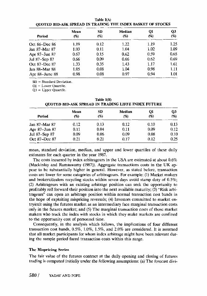
Table I(A) QUOTED BID-ASK SPREAD IN TRADING THE INDEX BASKET OF STOCKS

Mean SD Median Q1 43 Period (%I (%) (%) vw (%)

Oct 86-Dec 86 1.19 0.12 1.22 1.19 1.25 Jan 87-Mar 87 1.03 0.11 1.04 1.02 1.09 Apr 87-Jun 87 0.67 0.15 0.62 0.59 0.65 Jul 87-Sep 87 0.66 0.09 0.66 0.62 0.69 Oct 87-Dec 87 1.33 0.35 1.43 1.17 1.61 Jan 88-Mar 88 1.05 0.08 1.04 0.98 1.11 Apr 88-June 88 0.98 0.08 0.97 0.94 1.01

-

SD = Standard Deviation. Q1 = Lower Quartile. Q3 = Upper Quartile.

Table I(B) QUOTED BID-ASK SPREAD IN TRADING LIFFE INDEX FUTURE

Jan 87-Mar 87 0.12 0.13 0.12 0.10 0.13 Apr 87-Jun 87 0.11 0.04 0.11 0.09 0.12 Jul 87-Sep 87 0.09 0.06 0.09 0.08 0.10 Oct 87-Dec 87 0.21 0.21 0.17 0.12 0.25

mean, standard deviation, median, and upper and lower quartiles of these daily estimates for each quarter in the year 1987.

The costs incurred by index arbitrageurs in the USA are estimated at about 0.6% (Mackinlay and Ramaswamy (1987)). Aggregate transactions costs in the UK appear to be substantially higher in general. However, as stated before, transaction costs are lower for some categories of arbitrageurs. For example: (1) Market makers and brokerddealers recycling stocks within seven days avoid stamp duty of 0.5%; (2) Arbitrageurs with an existing arbitrage position can seek the opportunity to profitably roll forward their position into the next available maturity; (3) “Risk arbitrageurs” can open an arbitrage position within normal transaction cost bands in the hope of exploiting mispricing reversals; (4) Investors committed to market entry/exit using the futures market as an intermediary face marginal transaction costs only in the futures market; and (5) The marginal transaction costs of those market makers who track the index with stocks in which they make markets are confined to the opportunity cost of personnel time.

Consequently, in the analysis which follows, the implications of four different transaction cost bands, 0.5%, 1.0%, 1.596, and 2.0% are considered. It is assumed that all market participants for whom index arbitrage might have been relevant during the sample period faced transaction costs within this range.

The Mispricing Series

The fair value of the futures contract at the daily opening and closing of futures trading is computed initially under the following assumptions: (a) The forecast divi-

580 / YADAV AND POPE

dend yield to maturity for each date is identical to the actual expost daily cash dividend inflow for the FTSE-100 portfolio; (b) The forward interest rate at the time t for a loan made at time w to be redeemed at time T, is identical to the interest rate at time w on a Treasury Bill maturing at time T; (c) The value on day t of one- and three-month Treasury Bill interest rates can be used to infer a linear term structure from which the implicit interest rate for the period (T-t) can be calculated; and (d) The futures settlement price is synchronous with the closing index value and the opening futures price is synchronous with the opening index value.

The fair values at the opening and closing of trading each day are used to compute the opening and closing percentage mispricing series.

Figure 1 presents a plot of percentage mispricing based on closing prices of the near LIFFE index futures contract over the period July 1, 1984 to June 30, 1988. Figure 2 is a similar plot based on opening prices. Figures 1 and 2 are similar and suggest that asynchronicity does not appear to be a major factor in the analysis.

The figures indicate that the fair value forward pricing formula is frequently vio- lated, and many of the violations appear too large to be accounted for solely by transaction costs. Mispricing in the pre-Big Bang period appears to be systematically negative. Post Big Bang, the tendency and frequency of (at least partial) price reversals are substantially greater, though the June 1988 contract reverts to the pre-Big Bang pattern of forward pricing fair value consistently providing a downward biased estimator of actual value. Overall, the plots are consistent with the growth and im-

P E R C E N T A G E MI S P R l CI MG CLOUl NP PRl CCS

1 2 $ 4 6 8 7 0

CON1 RACl

1 0 1 1 1 2 1 : 44 1 5 I@

Big Bang

Figure 1 - Plot of percentage mispricing based on closing prices of the near LIFFE index

futures contract: July 1, 1984-June 30, 1988.


P E R C E N T A G E MI S P R l C I PIG

1 2 $ 4 6 8 I 6 0 10 1 1 1 2 i* 1 4 1 6

CONTRACT CONTRACT

Big Bang Figure 2

Plot of percentage mispricing based on opening prices of the near LIFFE index futures contract: July 1, 1984-June 30, 1988.

provement in the arbitrage sector, and post-Big Bang, suggest that additional potential exists for “risky” arbitrage strategies based on “predictable” mispricing reversals.

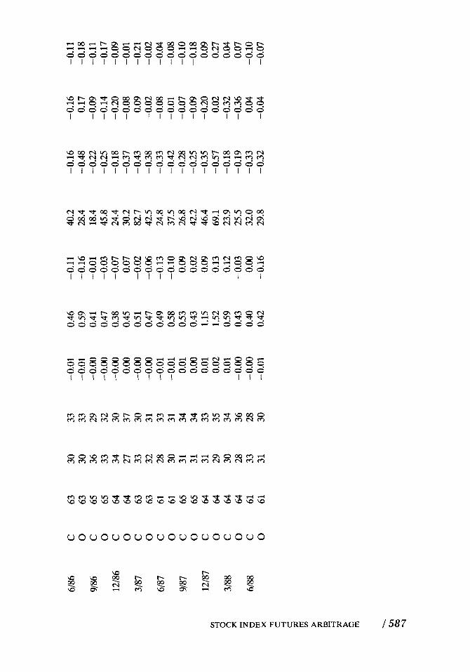
Table I1 provides summary statistics for the mispricing series of each contract expiring during the period of the study; and also for the overall sample, the sample pre-Big Bang, and the sample post-Big Bang. If the Crash period is excluded, the mean levels of mispricing do not differ significantly from the median levels of mispricing, indicating that outliers are probably not affecting the results. The maximum absolute mispricing on opening prices post-Big Bang (ignoring the December 1987 contract) is only 1.5% whereas it was 2.5% before the Big Bang. The average mispricing is negative for 8 out of the 9 contracts expiring before the Big Bang but for only 4 out of 7 contracts expiring after the Big Bang. Systematic mispricing appears to have decreased from an average of about 0.5% in the pre-Big Bang period to below 0.2% in the post-Big Bang period. However, the standard deviation of the percentage mispricing has remained at similar levels (about 0.5%) for all contracts (except December 1987). These results can be compared with US results based on daily data reported by Merrick (1987(b)). Over the period 1985-86 he reports the mean and standard deviation of the percentage mispricing of the S&P500 futures contract to be 0.011% and 0.411% respectively, and his plot appears to indicate that the maximum and minimum values have remained generally between +1% and -1%.

The t-statistics reported in Table I1 are for the null hypothesis that the mean percentage mispricing is zero. The unadjusted t-statistics (as reported e.g., by Figlewski

582 I YADAV AND POPE

(1984) for actual mispricing levels) are highly significant for each contract. However in computing standard errors, this test ignores the high autocorrelation of the mispricing series. ARMA modelling of the percentage mispricing series shows that the series for most of the contracts are best modelled in terms of an autoregressive process of order one? Table I1 gives the value of the AR(1) parameter, p, which best fits the model and the associated standard error, v. The autocorrelation is uni- formly positive and the coefficient is above 0.6 in most cases. Furthermore, the coefficient is substantially higher in the Pre-Big Bang period, pointing to a marked increase in the elasticity of supply of arbitrage services after the Big Bang. There appears to be a strong tendency for mispricing to persist, though this tendency has declined markedly since the Big Bang, or as the market has matured. The adjusted t-statistic employs a standard error calculated on the assumption that successive re- alizations are first order autocorrelated. Overall the adjusted f-statistics, whilst being lower, confirm the results obtained previously. At the individual contract level, there are only two contracts (June and December 1987) for which the null is ac- cepted using the adjusted t-statistic but rejected using the unadjusted statistic. How- ever, for the post-Big Bang period, the average level of mispricing based on opening prices is not significant at the 5% level with the adjusted t-statistic; although, without the adjustment, it appears to be significant.

Table I11 gives the summary statistics for the series of mispricing returns (scaled first differences of the mispricing series). Average mispricing returns are indistin- guishable from zero for every contract. Mispricing returns are only mildly autocorrelated as shown by the Box Pierce Q-statistic for 24 lags. The first order autocorrelation is negative for every contract, which is reasonable in the presence of an effective link between the cash and futures markets. It is pertinent to observe that the first order autocorrelation is more negative after the Big Bang.

If arbitrageurs are effective one should expect positive average mispricing returns when futures are initially underpriced and negative average mispricing returns when futures are initially overpriced. Hence, Table I11 reports the results of subdividing the full sample of mispricing returns into two subsets based on whether futures are initially underpriced or overpriced. As expected, the average of mispricing returns with initially underpriced futures is consistently positive and the average of mispricing returns with initially overpriced futures is consistently negative; but these averages of the different series for individual contracts are significantly different from zero only after the Big Bang. This clearly points to a markedly greater tendency for mispricing reversals and a greater efficiency of the arbitrage sector after the Big Bang. The results also imply that a one day long-cash-short- futures hedge, based on the foward pricing formula, consistently earned negative “abnormal” returns if established when futures are initially underpriced and positive “abnormal” returns if established when futures are initially overpriced. This clearly limits the use that market makers can make of futures markets to hedge short term changes in stock market exposure. These results are essentially similar to those reported by Merrick (1987).

Table IV presents summary statistics for the mispricing in the second nearest contract. Only the four weeks prior to expiration of the near contract are considered to ensure that prices are based on reasonable levels of trading volume. Thus, for each contract the series consists of only 20 values (less any holidays). The absolute magnitudes of mispricing appear to be considerably larger than for the near

’This is consistent with the model of Garbade and Silber (1983).


s tc P

Tabl

e -11

> z u

LEV

EL O

F FU

TU

RE

S M

ISPR

ICIN

G I

N T

HE

NE

AR

CO

NTR

AC

T-SU

MM

AR

Y S

TATI

STIC

S

mea

n m

edia

n SD

m

in

max

t-

adju

sted

cd

Con

trac

t n

<o

>o

(%I

(%I

(%I

(%I

(%I

valu

e P

U

t-va

lue

8 9/

84

12/8

4

3/85

6/85

9/85

12/8

5

3/86

6/86

9/86

12/8

6

C

64

63

1 0

64

64

0 C

64

63

1 0

64

62

2 C

63

62

1

0

63

58

5 C

61

57

4

0

61

55

6 C

65

64

1

0

65

64

1 C

64

50

14

0

64

52

12

C

61

51

10

0

61

46

15

C

63

46

17

0

63

44

19

C

65

56

9 0

65

56

9

C

64

45

19

0

64

47

17

-0.9

9 - 1.

04

-0.9

9 -0

.97

-0.5

3 -0

.50

-1.1

2 -1

.12

-0.7

1 -0

.70

-0.6

6 -0

.69

-0.3

7 -0

.31

-0.3

1 -0

.23

0.66

0.

68

-0.2

9 -0

.26

-0.9

2 0.

50

-0.9

3 0.

54

-0.9

1 0.

63

-0.8

8 0.

66

-0.5

4 0.

31

-0.5

1 0.

38

- 1.

32

0.66

- 1.

34

0.63

-0

.72

0.37

-0

.65

0.39

-0

.73

0.64

-0

.79

0.65

-0

.45

0.40

-0

.37

0.44

-0

.37

0.54

-0

.22

0.54

0.

71

0.56

0.6

7 0.

51

-0.2

8 0.

52

-0.2

3 0.

52

- 1.

91

0.05

-2

.42

-0.0

5 -2

.20

0.01

-2

.54

0.04

-1

.17

0.25

- 1.

33

0.47

-2

.37

0.34

-2

.15

0.22

- 1.

52

0.28

- 1.

77

0.12

-1

.73

0.50

- 1.

91

0.59

-1

.16

0.59

- 1.

08

0.82

- 1.

32

1.27

- 1.

32

1.31

-0

.77

2.06

-0

.19

2.32

-1

.42

0.88

-1

.29

0.94

- 15

.90

- 15

.26

- 12

.58

-11.

74

- 13

.75

- 10

.44

- 13

.30

- 13

.93

- 15

.33

- 14

.58

-8.2

1 -8

.53

-7.0

6 -5

.44

-4.5

0 -3

.35

9.45

10

.69

-4.3

7 -3

.93

0.83

0.

73

0.95

0.

82

0.68

0.

27

0.96

0.

96

0.74

0.

64

0.95

0.

92

0.59

0.5 1

0.

70

0.41

0.

75

0.61

0.

73

0.63

0.08

-5

.04

0.09

-6

.24

0.05

-2

.39

0.07

-3

.85

0.10

- 6.

05

0.12

-7

.95

0.05

-2

.38

0.06

-2

.50

0.09

-6.1

4 0.

10

-6.9

0 0.0

5 - 1.

57

0.06

- 1.

92

0.11

-3

.72

0.12

-3

.17

0.09

- 1.

96

0.12

-2

.20

0.08

3.

69

0.10

5.

37

0.09

- 1.

81

0.10

- 1.

94

3/87

C

63

0

63

6/

87

C

61

0

61

9/87

C

65

0

65

12/8

7 C

64

0

64

3/88

C

64

0

64

6/88

C

61

0

61

T

otal

pre

-Big

Ban

g C

58

9 4 8

0

589

7:

c(

Tot

al p

ost-

Big

Ban

g C

42

3 z X

0

42

3

c 10

12

2 v)

Ove

rall

Sam

ple

z

24

17

24

24

29

26

36

35

45

41

53

51

472

463

248

233

720

696

39

46

37

37

36

39

28

29

19

23 8 10

117

126

175

190

292

316

0.22

0.

30

0.15

0.

21

0.01

0.1

2 -0

.50

- 0.

44

- 0.

28

- 0.

08

-0.6

0 -0

.50

-0.5

5 -0

.53

- 0.

20

-0.1

1

- 0.

40

-0.3

5

0.17

0.

43

0.26

0.

38

0.24

0.

56

0.42

0.

57

0.04

0.

61

0.21

0.

57

-0.0

6 1.

38

- 0.

07

1.47

-0

.30

0.54

-0

.12

0.39

-0

.69

0.50

-0.5

8 0.4

5

-0.5

9 0.

74

-0.5

7 0.

76

- 0.

13

0.78

-0

.05

0.78

-0.4

0 0.

77

-0.3

2 0.

79

-0.6

5 1.

40

-0.5

6 1.

45

-1.1

3 1.

16

-1.1

8 1.

15

- 1.

41

1.61

- 1.

20

1.51

-5

.83

1.15

-7

.37

1.35

-2

.04

1.38

-0

.83

0.88

-

1.36

0.

68

-1.1

5 0.

72

-2.4

2 2.

06

- 2.

57

2.31

-5.8

5 1.

58

-7.3

9 1.

49

-5.8

5 2.

06

-7.3

9 2.

31

4.04

6.

29

2.05

2.

83

0.17

1.

77

-2.8

9 -2

.40

-4.2

1 -1

.67

-9.3

8 -8

.68

- 18

.06

- 17

.06

-5.3

8 -2

.90

- 16

.63

- 14

.25

0.30

0.

24

0.66

0.

50

0.73

0.

76

0.64

0.

41

0.47

0.

39

0.70

0.

58

0.88

0.

83

0.66

0.

55

0.80

0.

73

0.12

0.

13

0.10

0.

11

0.09

0.

08

0.10

0.

12

0.11

0.

12

0.10

0.

11

0.02

0.

02

0.04

0.

04

0.02

0.

02

3.00

4.

93

0.97

1.

68

0.05

0.

64

- 1.

38

- 1.

56

-2.5

1 -1

.10

-4.0

3 -4

.54

-4.5

3 -5

.23

- 2.

43

- 1.

58

-5.6

3 -5

.68

0

1012

4 E v)

C d

enot

es cl

osin

g pr

ice

seri

es.

0 d

enot

es o

peni

ng p

rice

ser

ies.

$

Tabl

e I1

1 M

ISPR

ICIN

G “

RE

TU

RN

S”

~ ~

mea

n SD

C

ontr

act

n <O

>O

(%

I (%

I t - v

a 1 u e

BP

24

PI

P2

P3

9/84

C

0

12

/84

C

0

3/85

C

0

6/

85

C

0

9/85

C

0

12

/85

C

0

3/86

C

0

64

64

64

64

63

63

61

61

65

65

64

64

61

61

29

29

35

29

30

32

28

25

28

31

32

33

29

33

35

35

29

35

33

31

33

36

37

34

32

31

32

28

0.03

0.

03

-0.0

0 -0

.01

0.00

0.0

0 -0

.01

-0.0

0 0.

00

-0.0

0 -0

.00

-0.0

0 0.

00

0.00

0.32

0.

42

0.38

0.

45

0.26

0.

46

0.41

0.

39

0.28

0.

34

0.30

0.

33

0.37

0.

44

0.72

19

.2

0.5 1

34

.5

-0.1

0 19

.4

-0.1

0 16

.9

0.02

23

.5

0.05

38.3

-0

.18

14.3

-0

.01

22.8

0.

01

19.6

-0

.07

15.7

-0

.03

20.4

- 0.

06

33.2

0.

05

25.6

0.

07

39.5

-0.1

5 -0

.13

-0.1

4 -0

.21

-0.2

2 -0

.51

-0.1

8 -0

.10

-0.2

3 -0

.25

-0.0

7 -0

.08

-0.3

9 -0

.38

-0.0

9 -0

.40

-0.1

1 -0

.12

- 0.2

0 0.

08

-0.1

0 -0

.10

-0.1

6 -0

.03

-0.0

4 -0

.13

-0.0

9 0.

02

-0.1

8 0.

11

0.14

0.

07

-0.0

9 -0

.14

-0.0

1 - 0.

15

0.03

-0

.00

0.02

0.

17

0.10

-0

.19

6/86

9/86

12/8

6

3/87

6/87

9/87

12/8

7 v1

c3 00

3/88

7:

6/88

Z

X

C

63

0

63

C

65

0

65

C

64

0

64

C

63

0

63

C

61

0

61

C

65

0

65

C

64

0

64

C

64

0

64

C

61

0

61

30

30

36

33

34

27

33

32

28

30

31

31

31

29

30

28

33

31

33

33

29

32

30

37

30

31

33

31

34

34

33

35

34

36

28

30

-0.0

1 -0

.01

-0.0

0 -0

.00

-0.0

0 0.

00

-0.0

0 - 0

.00

-0.0

1 -0

.01

0.01

0.

00

0.01

0.

02

0.01

-0

.00

-0.0

0 -0

.01

0.46

0.

59

0.41

0.

47

0.38

0.

45

0.51

0.

47

0.49

0.

58

0.53

0.

43

1.15

1.

52

0.59

0.

43

0.40

0.

42

-0.1

1 40

.2

-0.1

6 28

.4 -0

.01

18.4

- 0.

03

45.8

-0

.07

24.4

0.

07

30.2

-0

.02

82.7

-0

.06

42.5

-0

.13

24.8

-0

.10

37.5

0.09

26

.8 0.

02

42.2

0.

09

46.4

0.

13

69.1

0.

12

23.9

- 0.

03

25.5

0.00

32.0

-0

.16

29.8

-0.1

6 - 0.

48

-0.2

2 -0

.25

-0.1

8 -0

.37

-0.4

3 -0

.38

-0.3

3 -0

.42

-0.2

8 - 0.

25

-0.3

5 -0

.57

-0.1

8 -0

.19

-0.3

3 -0

.32

-0.1

6 0.

17

-0.0

9 -0

.14

-0.2

0 -0

.08

0.09

-0.0

2 - 0.

08

-0.0

1 -0

.07

-0.0

9 -0

.20

0.02

-0

.32

-0.3

6 0.

04

-0.0

4

-0.1

1 - 0.

18

-0.1

1 - 0.

17

-0.0

9 -0

.01

-0.2

1 -0

.02

-0.0

4 - 0.

08

-0.1

0 -0

.18

0.09

0.

27

0.04

0.

07

- 0.

10

- 0.0

7

Con

trac

ts

Exp

irin

g*

Sam

ple

Subs

et o

f Mis

pric

ing

Ret

urns

with

Ini

tial

ly

Und

erpr

iced

Fut

ures

O

verp

riee

d Fu

ture

s

Sam

ple

Subs

et o

f M

ispr

icin

g R

etur

ns w

ith I

nitia

lly

Ho+

1 =

0

HO

:p2

= 0

M

ean

t P

Mea

n t

P P

I st

at

valu

e KZ

st

at

valu

e

Diff

eren

ce

Dec

85

C

0

Mar

86

C

0

Jun

86

C

0

Sep

86

C

0

Dec

86

C 0

0.00

8 0.

021

0.035

0.

066

0.04

7 0.

080

0.19

9 0.

403

0.07

4 0.

121

0.17

0.

51

0.70

1.

12

0.75

1.

04

0.97

2.

44

1.33

2.

40

0.87

0 0.

610

0.48

0 0.

270

0.46

0 0.

310

0.38

0 0.

059

0.19

0 0.

020

-0.0

30

-0.0

99

-0.1

84

-0.2

25

-0.1

33

-0.2

51

-0.0

19

-0.0

41

--0.

184

-0.3

45

- 1.

09

-0.7

8 - 1.

34

- 1.

78

- 1.

04

- 1.

58

-0.3

7 -0

.70

-2.3

5 - 2.

49

0.30

0 0.

450

0.22

0 0.

099

0.31

0 0.

130

0.71

0 0.

490

0.03

1 0.

025

0.69

0.

90

1.50

2.

08

1.26

1.

87

1.04

2.

53

2.68

3.

17

0.49

0 0.

390

0.16

0 0.

052

0.22

0 0.

071

0.35

0 0.

045

0.01

1 0.

005

Mar

87

Jun

87

Sep

87

Dec

87

Mar

88

Jun

88

Pre-

Big

Bang

Post

-Big

Ban

g

C

0

C 0

C 0

C

0

C

0

C 0

C

0

C 0

0.30

7 0.

271

0.22

7 0.

270

0.22

1 0.

213

0.28

6 0.

446

0.17

8 0.

116

0.05

0 0.

068

0.02

9 0.

043

0.16

8 0.

182

3.48

2.

55

2.25

2.

46

2.26

2.58

1.

19

1.68

2.

18

1.99

0.

94

1.21

1.

87

2.21

3.

90

3.89

0.00

2 0.

021

0.03

5 0.

022

0.03

1 0.

016

0.24

0 0.

100

0.03

5 0.0

58

0.35

0 0.

230

0.06

2 0.

028

O.OO0

O.

OO0

-0.1

90

-0.1

04

-0.1

54

-0.1

80

-0.1

87

-0.1

47

-0.3

13

-0.4

81

-0.4

22

-0.2

11

- 0.

300

-0.3

40

-0.1

03

-0.1

53

- 0.

230

-0.2

16

-2.5

3 - 1.

60

-2.1

2 -2

.01

-2.5

3 - 2.

46

-2.9

2 - 1.

98

-3.9

9 - 2.

20

- 1.

82

-3.1

8 -2

.53

-3.3

6 -6

.50

-4.5

2

0.01

6 0.

120

0.04

1 0.

052

0.01

6 0.

019

0.00

7 0.

057

0.00

1 0.

039

0.11

0 0.

010

0.01

3 0.

001

O.OO

0 O.

OO0

4.29

3.

01

3.06

3.

18

3.33

3.

53

2.28

2.

58

4.49

2.

91

2.02

3.

38

3.03

3.

96

7.14

5.

95

O.OO

0 0.

005

0.004

0.

003

0.00

2 0.

001

0.02

7 0.

012

0.00

0 0.

006

0.07

8 0.

004

0.00

3 0.

000

0.00

0 0.

000

*Con

trac

ts ex

piri

ng u

p to

Sep

tem

ber

1985

are

om

itte

d si

nce

the

sam

ple

subs

et o

f m

ispr

icin

g ret

urns

with

init

ially

ove

rpri

ced

futu

res

cont

ain

inad

equa

te d

ata.

Table IV MISPRICING IN THE SECOND NEAREST CONTRACT-SUMMARY STATISTICS

Levels of Mispricing ~

Mean SD Min Max %<0 %>0

Pre-Big Bang c -1.21 1.21 -3.45 2.55 82 18 0 -1.20 1.25 -3.95 2.02 79 21

Post-Big Bang C 0.47 0.81 -1.63 2.05 32 68 0 0.58 0.86 -1.15 2.66 26 74

Changes in Mispricing

Mean SD Min Max %<O %>0

Pre-Big Bang C 0.03 0.35 -0.82 1.20 44 56 0 0.01 0.62 -2.23 2.13 49 51

0 -0.02 0.59 -1.82 1.88 47 53 Post-Big Bang C -0.01 0.45 -1.44 1.06 46 54

contract and so are the extreme values. Prior to the Big Bang, the forward pricing formula was a downward biased estimate of futures price, just as it was for the near contract (only much more so). But after the Big Bang, while the mean of the mispricing series of the near contract continues to be negative (even if one ignores the period around the October 1987 crash), the mean of the mispricing of the second nearest contract is positive and fairly large (except for the June 1988 contract). It can be conjectured that this could be because of strong “bullish” sentiment over this period.

Arbitrage Related Ex Post Program Trading Simulations The first column in Table V(A) documents the number of mispricing violations based on the near contract for different levels of transaction cost bounds. The number of violations at all (nonzero) levels is markedly smaller after the Big Bang. If the period around the October 1987 Crash is excluded, there is only one violation of the 2% bound and only three violations of the 1.5% bound since October 1986. On the other hand, there are a relatively large number of violations of the 1% transactions cost bound.

This study attempts to simulate the possible profits of arbitrageurs using program trading driven by simple trading rules. Tables V(A) and V(B) are based on expost trading rules, which assume continuous trading in the market; and that it is possible to use the price at time t to execute a trade at the same price at the same time. Consider the following trading rules: Trading Rule 1: If mispricing exceeds x%, sell one futures contract, sell Treasury Bills and buy the equivalent underlying basket of stocks, and hold the long stock-short futures position up to expiration. At expiration, sell the stock bought earlier, and reinvest in Treasury Bills. If mispricing is below -x%, buy one futures contract, sell the equivalent underlying basket of stocks, use the proceeds obtained to buy Treasury Bills, and hold the position until contract expiration, at which time the position is unwound and investment in stocks re- instated. This is the simple hold-to-expiration trading rule. Trading Rule 2 Same as Trading Rule 1, except that, instead of waiting until contract expiration, the position is unwound as soon as mispricing changes sign and becomes at least


Tabl

e V

(A)

EX P

OS

T A

RB

ITR

AG

E R

ELA

TED

TR

AD

ING

SIM

ULA

TIO

N W

ITH

y =

0

POSI

TIO

NS

UN

WO

UN

D/R

OLL

ED O

VER

AS

SOO

N A

S U

NW

IND

ING

/RO

LLO

VER

BEC

OM

ES P

RO

FITA

BLE

* ~

~

Tra

ding

Rul

e 1

Tra

ding

Rul

e 2

Tra

ding

Rul

e 3

Tra

ding

Rul

e 4

Bas

e A

dditi

onal

A

dditi

onal

N

o. of

A

rbitr

age

No.

of

Arb

itrag

e A

rbitr

age

No.

of

Con

trac

ts

Mis

pric

iog

Prof

its

Ear

ly

Prof

its

No.

of

Prof

its

Ear

ly

No.

of

Exp

irin

g V

iola

tions

(E’

OOO)

U

nwiu

ding

s (E’

OOO)

R

ollo

vers

(P

OOO)

U

nwin

ding

R

ollo

vers

Add

ition

al

Arb

itrag

e Pr

ofits

($’O

OO)

x =

0.5

%

Pre-

Big

C

B

ang

0

Post

-Big

C

B

ang

0

x =

1.0

%

Pre-

Big

C

B

ang

0

Post

-Big

C

B

ang

0

x =

1.5

%

Pre-

Big

C

B

ang

0

Post

-Big

C

B

ang

0

x =

2.0

%

Pre-

Big

C

B

ang

0

Post

-Big

C

B

ang

0

374

367

201

193

65.8

65

.0

41.6

35

.4

271

266

180

180

12.1

13

.3

31.8

25

.8

345

339 92

97

87.6

88

.3

17.3

29

.4

41

46

175

151

331

320 24

38

86.7

85

.5

38.3

38

.2

m

-3 0,

164

161 60

45

22.3

23

.0

14.2

11

.6

108

109 59

45

5.2

5.5

11.1

7.

0

160

157 12

10

37.5

39

.5

1.8

2.6

8 7 59

41

156

154 1 4

37.5

38.3

11

.2

7.5

d m x

68

67

14 9

5.4

5.8

7.9

7.0

39

35

14 9

1.8

1.7

4.6

3.3

68

67 2 0

17.2

16

.7

0.3

0.0

0 0 14 9

68

67 0 0

17.2

16

.7

4.6

3.3

10

11 9 7

0.4

0.9

5.3

5.2

0.1

0.2

3.0

2.6

10

11 1

0

1.2

1.4

0.2

0.0

10 8 0 0

1.2

1.2

3.0

2.6

*Pro

fits

are

cal

cula

ted

assu

min

g an

ope

n po

sitio

n of

onl

y on

e co

ntra

ct f

or e

ach

mis

pric

ing

viol

atio

n.

Tab

le V

(B)

EX POST

AR

BIT

RA

GE

REL

ATE

D T

RA

DIN

G S

IMU

LATI

ON

WIT

H y

= 0

.5%

PO

SITI

ON

S U

NW

OU

ND

/RO

LLED

OV

ER A

S SO

ON

AS

UN

WIN

DIN

G/R

OLL

OV

ER Y

IEL

DS

AD

DIT

ION

AL

PRO

FIT

OF

0.5%

*

Tra

ding

Rul

e 1

Tra

ding

Rul

e 2

Tra

ding

Rul

e 3

Tra

ding

Rul

e 4

s B

ase

Add

ition

al

Add

ition

al

Add

ition

al

U

No. of

Arb

itrag

e No

. of

A

rbitr

age

Arb

itrag

e No

. of

A

rbitr

age

Prof

its

U %

Exp

irin

g V

iola

tions

(d

’000

) U

nwin

ding

s (d

’000

) R

ollo

vers

(S

’OOO

) U

nwin

ding

s R

ollo

vers

(f’

000)

9 x

= 0

.5%

Con

trac

ts

Mis

pric

ing

Prof

its

Ear

ly

Prof

its

No.

of

Prof

its

Ear

ly

No.

of

P cd rn

Pre-

Big

C

37

4 65

.8

66

15.7

26

8 88

.6

30

266

94.5

B

ang

0

367

65.0

28

6.

1 26

9 91

.4

28

265

95.1

Po

st-B

ig

C

201

41.6

10

2 37

.0

49

18.2

10

2 18

43

.6

Ban

g 0

19

3 35

.4

88

31.7

82

34

.7

78

49

48.2

x

= 1

.0%

Pr

e-B

ig

C

164

22.3

23

5.

9 12

7 39

.3

7 12

5 40

.6

Ban

g 0

16

1 23

.0

5 1.

1 13

0 42

.1

5 12

9 41

.9

Post

-Big

C

60

14

.2

31

11.5

6

2.3

31

1 11

.8

Ban

g 0

45

11

.6

22

7.7

10

3.8

20

4 8.

2 x

= 1

.5%

Pr

e-B

ig

C

68

5.4

4 1 .o

54

17

.4

0 54

17.4

B

ang

0

67

5.8

0 0.

0 52

17

.2

0 52

17

.2

Post

-Big

C

14

7.

9 14

5.

3 0

0.0

14

0 5.

3 B

ang

0

9 7.

0 9

3.3

0 0.

0 9

0 3.

3

Ban

g 0

11

0.

9 3

0.9

3 1 .o

3

3 1.

9 Po

st-B

ig

C

9 5.

3 9

3.5

0 0.

0 9

0 3.

5

x =

2.0

%

Pre-

Big

C

10

0.

4 1

0.3

3 0.

9 0

3 0.

9

Ban

g 0

7

5.2

7 2.

6 0

0.0

7 0

2.6

*Pro

fits

are

cal

cula

ted

assu

min

g an

ope

n po

sitio

n of

onl

y on

e co

ntra

ct f

or e

ach

mis

pric

ing

viol

atio

n.

(y% + 0.2%) in magnitude (to cover the estimated incremental transaction costs (TF + Ti!) and an incentive to trade of y%). This is the early unwinding option. Trading Rule 3: Same as Trading Rule 1, except that during the last four weeks before maturity, the position is rolled forward to the next available maturity as soon as the sign of the mispricing in the far contract is the same as the sign of the origi- nal mispricing and when the difference in mispricing between the far contract and the near contract exceeds (y% + 0.3%) in magnitude (to cover the estimated incremental transaction costs (TF + 2Tg) and an incentive to trade of y%). This is the rollover option. (Compound rollovers are ignored, i.e. the rolled over position is assumed to be carried to expiration.) Trading Rule 4 This is a combination of trading rules 1, 2, and 3. The arbitrage position is initiated as in Trading Rule 1, but is unwound early, as per Trading Rule 2, or rolled forward, as per Trading Rule 3, which ever option becomes profitable at an earlier date.

Four values of x are used in each case: 0.5%, 1.0%, 1.5%, and 2.0%. It is assumed that the transaction costs being faced by the arbitrageurs are x%. In Trading Rules 2, 3, and 4 two values of y are used: 0.0% (Table V(A)) and 0.5% (Table V(B)). The first represents the case where a position is unwound early or rolled forward as soon as it is profitable to do so. The second represents the case where a position is unwound early, or rolled forward, only when the additional profit is at least 0.5%. In this context, when an arbitrage position is unwound early or rolled forward the arbitrageur loses the option of unwinding or rolling forward when the relevant mispricing values are more favorable to him.

Based on closing (opening) prices and prior to the consideration of transaction costs, Trading Rule 1 gives average annualised excess returns (relative to the Trea- sury Bill rate) of 8.0% (8.4%) with a standard deviation if 9.1% (10.4%) before the Big Bang and 7.7% (7.4%) with a standard deviation of 13.4% (13.2%) after the Big Bang. All excess returns are positive. Given the high standard deviation, the results suggest that there could have been many potential opportunities for arbitrage related strategies over the sample period.

Tables V(A) and V(B) give the profit (in pounds sterling) earned from the different Trading Rules for the various transaction cost levels. The profits reported are based on just one contract. Considering the present level of trading volumes, it seems possible to use a much larger number of contracts without tangible market impact.

Tables V(A) and V(B) show that significant arbitrage profits could have been earned even at transaction cost levels of 1.5%; though, after the Big Bang, most of the contribution shown at transaction costs levels of 1.5% or higher is due to the December 1987 contract (spanning the October 1987 Crash). The additional profits arising out of rollover or early unwinding are a significant proportion of the total arbitrage profits and often exceed the arbitrage profits arising from the simple hold to expiration strategy. These high additional profits imply a heavy transaction cost “discount” and should generate substantial arbitrage activity even when futures prices are within transaction cost bounds. Merrick (1989) does not document additional profits arising out of rollover, but he does report profits due to early unwinding which are comparable to those in the simulations of this study for the post-Big Bang period.

A comparison of the additional potential profit over the two subperiods reveals that before the Big Bang, the additional potential profit is due mainly to rollovers whereas after the Big Bang it is due mainly to early unwinding. This means that the tendency for price reversals is more pronounced after the Big Bang and the system-


atic underpricing of the pre-Big Bang period seems to be “corrected” by a more effective arbitrage sector. The decline in profitability of rollovers is due mainly to the fact that the second nearest contract has been generally overpriced since the Big Bang, while most of the arbitrage trades in the near contract are from underpriced futures.

Table V(B) shows that the option to delay early unwinding/rollover until additional profits are at least 0.5% appears to be valuable, Higher profits are possible in most cases. If positions are unwound/rolled over as soon as it is profitable to do so (Table V(A), Trading Rule 4), all arbitrage positions based on x 2 1.0% would be closed prior to expiration. If x = 0.5% about 99% of positions would be closed before expiration. Even if unwinding/rollover is delayed until the additional profits are at least 0.5% (Table V(B), Trading Rule 4), less than 30% of positions would be held to expiration. This appears to indicate that arbitrage related program trading may not carry a significant risk of expiration day price, volume, and volatility effects on underlying stocks.

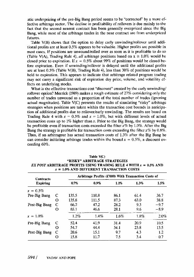
What is the effective transactions cost “discount” created by the early unwinding/ rollover option? Merrick (1989) makes a rough estimate of 27% considering only the number of trades unwound as a proportion of the total number of trades (ignoring actual magnitudes). Table V(C) presents the results of simulating “risky” arbitrage strategies when positions are taken within the transaction cost bounds in anticipa- tion of additional profits due to rollover/early unwinding. The results are based on Trading Rule 4 with x = 0.5% and x = 1.0%, but with different levels of actual transaction costs up to 1% higher than x . Prior to the Big Bang, the strategy would be profitable even if transaction costs exceeded the filter x% by 1.0%. After the Big Bang the strategy is profitable for transaction costs exceeding the filterx% by 0.8%. Thus, if an arbitrageur has actual transaction costs of 1.3% after the Big Bang he can consider initiating arbitrage trades within the bound x = 0.5%, a discount exceeding 60%.

Table V(C) “RISKY” ARBITRAGE STRATEGIES

EX POST ARBITRAGE PROFITS USING TRADING RULE 4 WITH x = 0.5% AND x = 1.0% AND DIFFERENT TRANSACTION COSTS

Arbitrage Profits (E’OOO) With Transaction Costs of Contracts Expiring 0.7% 0.9% 1.1% 1.3% 1.5%

x = 0.5% Pre-Big Bang C 135.5 110.8 86.1 61.4 36.7

0 135.8 111.5 87.3 63.0 38.8 Post-Big Bang C 66.2 47.2 28.2 9.3 - 9.7

x = 1.0% 1.2% 1.4% 1.6% 1.8% 2.0%

0 65.1 46.6 28.1 9.6 - 8.9

Pre-Big Bang C 52.4 41.9 31.4 20.9 10.5 0 54.7 44.4 34.1 23.8 13.5

Post-Big Bang C 20.6 15.1 9.7 4.3 - 1.2 0 15.8 11.7 7.5 3.4 -0.7


Arbitrage Related Ex Ante Program Trading Simulations

Table VI reports arbitrage profits based on Trading Rule 1, implemented on an ex ante basis. It is assumed that if there is an arbitrage mispricing opportunity perceived at opening prices, it is possible to execute a strategy only at closing prices; and similarly, if there is an arbitrage mispricing opportunity perceived at closing prices one day, it is possible to execute a strategy only at opening prices the next day. The trading rules used are the same as before, except for the delayed execution. It is also assumed that a trade decided on the basis of opening (closing) prices is executed at the subsequent closing (opening) prices only if the mispricing has not moved to within the transaction cost bound in the intervening period. It should be noted that the profits reported in Table VI include trades executed at both opening and closing prices, whilst Tables V(A) and V(B) show trades executed at closing prices separately from trades executed at opening prices.

Table VI shows that the use of the ex ante trading rule considerably reduces the profits reported in Tables V(A) and V(B) for the expost trading rules. The reduc- tion is particularly significant after the Big Bang where the average period for which profitable mispricing opportunities exist declines markedly. If the December 1987 contract is ignored, ex ante profits with transactions executed with a half day lag are insignificant even at the 1% transaction cost bound. Considering that “normal” transaction costs are estimated to be above 1%, this can be argued as evidence that the market prices stock index futures efficiently after the Big Bang. However, in the context of the high intra-day stock market volatility of the post-Big Bang pe-

Table VI ARBITRAGE PROFITS FROM EX ANTE STRATEGIES

Contract Expiring

Ex ante Profit (S’OOO) at Transaction Cost Level of

0.0% 0.5% 1.0% 1.5% 2.0%

September 1984 December 1984 March 1985 June 1985 September 1985 December 1985 March 1986 June 1986 September 1986 December 1986 March 1987 June 1987 September 1987 December 1987 March 1988 June 1988 Pre-Big Bang Post-Big Bang

34.1 35.7 21.0 45.0 30.0 35.3 19.4 23.6 35.0 21.7 18.3 29.7 30.8 45.5 18.4 31.8

279.1 196.2

18.0 19.8 5.4

27.9 10.8 16.5 3.4 5.6

13.5 6.2 2.7 5.5 7.7

24.8 1.3

11.7 120.9 59.8

6.9 9.0 0.3

13.3 1.9 5.1 0.0 0.3 3.6 0.8 0.1 0.0 0.8

16.0 0.0 0.7

40.4 18.5

2.0 3.2 0.0 2.9 0.1 0.4 0.0 0.0 0.2 0.0 0.0 0.0 0.0

11.4 0.0 0.0 8.8

11.4

0.0 0.7 0.0 0.2 0.0 0.0 0.0 0.0 0.0 0.0 0.0 0.0 0.0 7.8 0.0 0.0 0.9 7.8


riod (Peel, Pope, and Yadav (1990)), the assumed execution delay of about half a day (in the absence of intra-day data) is not very realistic.

Misspecification of Dividends

It is tempting to attribute systematic deviations from fair value pricing to misspecification of dividends. Table VII gives the average percentage mispricing which is at- tributed to systematic errors in forecasting dividends for different contracts. On average, systematic lo%, 25%, and 50% errors in dividends result in respectively only 0.06%, 0.15%, and 0.3% errors in calculated fair values. Hence, dividend uncertainty does not appear to be a significant explanation for systematic mispricing to the extent observed. This does not preclude dividend uncertainty resulting in a widening of the arbitrage window. These results are broadly consistent with results for the US (Kipnis and Tsang, (1984)).

Relative Volatility

An effective arbitrage link between the cash market and the futures market implies the null hypothesis that the ratio of the “returns” variance of the futures market to that of the cash market should equal unity. This null hypothesis is tested using the conventional F-test for three variance estimators: the Close-to-Close estimator (based on closing prices); Open-to-Open estimator (based on opening prices); and the (Parkinson (1980)) extreme value estimator which provides an estimate of intraday volatility (based on daily high and daily low prices).

Table VIII summarizes the results of the F-test. Detailed analysis of individual contracts reveals that the average intraday volatility of price changes in the futures

Table VII MISSPECIFICATION OF DIVIDENDS

Mean % Effect on Fair Value of Misspecification Equal to

10% 25% ~~

50%

September 84 December 84 March 85 June 85 September 85 December 85 March 86 June 86 September 86 December 86 March 87 June 87 September 87 December 87 March 88 June 88 Pre-Big Bang Post-Big Bang

0.08 0.04 0.11 0.05 0.07 0.05 0.06 0.04 0.07 0.06 0.07 0.04 0.06 0.05 0.08 0.05 0.06 0.06

0.20 0.10 0.28 0.11 0.17 0.13 0.16 0.09 0.17 0.14 0.19 0.10 0.14 0.13 0.21 0.12 0.16 0.15

0.40 0.20 0.57 0.23 0.33 0.27 0.32 0.18 0.34 0.28 0.37 0.20 0.28 0.26 0.42 0.24 0.32 0.29

_ _ ~ ____ __


Tabl

e V

III

REL

ATI

VE

VO

LATI

LITY

: RA

TIO

OF

“RE

TU

RN

S” V

AR

IAN

CES

IN F

UT

UR

ES

AN

D C

ASH

MA

RK

ETS

Rat

io o

f R

atio

of

In te

rday

In

terd

ay

Var

ianc

e p

valu

e V

aria

nce

p va

lue

Rat

io o

f p

valu

e

F st

at

Clo

sing

of

O

peni

ng

of

Intr

aday

of

V

aria

nce

n Pr

ices

F

stat

Pr

ices

F

stat

Sep

84

Dec

84

Mar

85

June

85

Sep

85

Dec

85

Mar

86

June

86

Sep

86

Dec

86

Mar

87

June

87

Sep

87

Dec

87

Mar

88

June

88

Pre-

Big

Ban

g Po

st-B

ig B

ang

64

64

63

61

65

64

61

63

65

64

63

61

65

64

64

61

589

423

1.12

0.

83

1.10

1.

02

1.02

1.

12

1.03

1.

44

1.25

1.38

1.

16

1.49

1.

47

1.29

1.

72

1.30

1.

15

1.33

0.32

0.

77

0.36

0.

47

0.47

0.

32

0.45

0.0

8 0.

18

0.10

0.

28

0.06

0.

06

0.16

0.

02

0.15

0.

05

0.00

1.16

0.

99

1.28

0.

91

1.19

1.

22

1.14

1.

43

1.07

1.

27

0.74

0.

95

1.08

1.

70

1.36

0.

98

1.18

1.

43

0.28

0.

5 1

0.17

0.

64

0.24

0.

21

0.30

0.

08

0.40

0.

17

0.88

0.

58

0.38

0.

02

0.11

0.

53

0.02

0.

00

1.73

1.

31

1.59

1.2

2 1.

41

0.85

1.

44

1.73

1.

64

1.81

1.

09

1.47

1.

45

3.41

2.

73

1.55

1.

47

2.75

0.01

0.

14

0.03

0.

22

0.09

0.

74

0.08

0.

02

0.02

0.

01

0.37

0.

07

0.07

0.

00

0.00

0.

05

0.00

0.0

0

market is higher for 15 out of 16 contracts and significantly higher at the 5% level for 8 out of these 15. The futures market intraday volatility is significantly higher at the 1% level for both the subperiods. The F-test is not able to distinguish so clearly between the close-to-close and open-to-open intraday volatility measures for the two markets. The close-to-close interday variance estimator for the futures market exceeds that of the cash market for 15 out of 16 contracts, but is significantly higher at the 5% level for only 1 out of these 15 contracts. The open-to-open interday variance estimator of the futures market exceeds that of the cash market of 11 out of 16 contracts and is significantly different at the 5% level only for the contract whose observations span the period of the 1987 Crash. However, both the close- to-close estimator and the open-to-open estimator reject the hypothesis of equality of variances at the 5% level for both the overall subperiods pre-Big Bang and post- Big Bang.

Inferences can be drawn from the aggregated evidence for the 16 contracts by as- suming that the variance ratios are independent across contracts. The hypothesis that the variance ratio equals one is rejected with t-values of 4.91 for the close-to- close estimator, 3.53 for the open-to-open estimator and 5.03 for the intra-day high low estimator, all of which are significant at the 1% level. The overall evidence appears to suggest that both interday and intraday volatility in the futures market is higher than that in the cash market. These results strongly substantiate the conclusions of Mackinlay and Ramaswamy (1987) in this regard.

Miepricing and Time to Expiration

The tax timing option has been argued to imply that mispricing should be negative and converge to zero as time to expiration decreases. The argument of Cornell and French (1983(a), 1983(b)) that the value of the tax timing option decreases with a decrease in time of expiration is not dependent on the validity of the forward pricing formula. Even if mispricing is positive because of possibly unquantified effects of other factors on index futures pricing, it should still be valid to argue that mispricing tends to decrease with time to expiration, if the tax timing option is important or relevant. A precise functional form for such a time dependence has not been suggested but it is possible to explore a linear relationship as a first approximation.

Figures 1 and 2 indicate that the mispricing might have been related to expiration time for the contracts expiring up to December 1985; but, subsequently, there is no obvious time-related pattern of mispricing. Such a conclusion is borne out also by regressions of mispricing against time to expiration for different contracts. These results are reported in Table IX(A). OLS regression residuals display high autocorrelation. This is not surprising in view of the autocorrelation in the mispricing series (Table 11) and since time to expiration cannot be expected to be the major factor governing successive realisations. The regressions reported assume that the random error term is governed by an AR1 process and represent maximum likelihood estimates based on the Beach and Mackinnon (1978) iterative procedure.6 Time to expiration is significant as an explanatory variable with negative slope only for the first six contracts. Thereafter, the slope coefficient is either insignificant or positive. The results do not appear to provide support for the hypothesis that the tax timing option is valuable.

dent variable included as regressors. ?he results are essentially similar for OLS regressions with or without lagged values of the depen-


Table IX REGRESSIONS OF MISPRICING VS. TIME TO EXPIRATION*

X i , T = u + b(T - t ) + DW of

Transformed b T-stat Sig. level Residuals

September 84

December 84

March 85

June 85

September 85

December 85

March 86

June 86

September 86

December 86

March 87

June 87

September 87

December 87

March 88

June 88

C 0 C 0 C 0 C 0 C 0 C 0 C 0 C 0 C 0 C 0 C 0 C 0 C 0 C 0 C 0 C 0

-0.015 -0.015 -0.021 -0.021 -0.008 -0.007 -0.022 -0.022 -0.010 -0.010 -0.017 -0.018 -0.001 - 0.002 -0.003 -0.003

0.002 0.004 0.003 0.004 0.001

-0.OOO - 0.005 -0.005

0.012 0.013

-0.011 -0.011 -0.004 -0.OOO - 0.006 -0.002

-5.33 -5.04 -7.27 -7.24 -4.38 -4.12 -6.67 - 6.81 -5.27 -4.84 -3.40 -3.88 -0.31 -0.58 - 0.55 -0.77

0.43 0.94 0.61 0.94 0.28

-0.12 -1.00 -1.24

2.72 3.55

-0.90 -1.13 -0.93 - 0.08 -1.12 -0.63

0.000 0.000 0.000 0.000 O.OO0 0.000 0.000 0.000 0.000 O.OO0 0.001 0.000 0.760 0.563 0.586 0.443 0.670 0.349 0.544 0.348 0.780 0.908 0.319 0.215 0.007 0.000 0.368 0.257 0.354 0.936 0.264 0.527

1.91 1.81 2.27 2.06 1.98 2.02 2.10 2.02 2.18 2.06 2.26 2.1 1 2.26 2.18 2.24 2.33 2.08 2.08 2.04 2.22 2.06 2.00 2.34 2.29 2.19 2.21 2.24 2.30 1.84 1.87 2.22 2.11

*Beach and Mackinnon (1978) Maximum Likelihood procedure used to transform autocorrelated

Time to expiration can be associated also with higher absolute magnitude of mispricing because of (i) dividend uncertainty and (ii) uncertainty about the relative pattern of interest rates and stock prices. The results of regressing the absolute magnitude of mispricing against time to expiration are reported in Table IX(B). The results are maximum likelihood estimates for the standard Tobit model with a zero lower bound censoring threshold and are based essentially on the iterative procedure of Berndt, Hall, Hall, and Hansman (1974). About 50% of the variation in ab-

OLS residuals.


Table IX(B) REGRESSIONS OF ABSOLUTE MAGNITUDE OF MISPRICING VS. TIME TO

EXPIRATION* IXt,TI = u + b(T - t ) +

R2 b T-statistic Sig. level (W

September 84

December 84

March 85

June 85

September 85

December 85

March 86

June 86

September 86

December 86

March 87

June 87

September 87

December 87

March 88

June 88

Pre-Big Bang

Post-Big Bang

C 0 C 0 C 0 C 0 C 0 C 0 C 0 C 0 C 0 C 0 C 0 C 0 C 0 C 0 C 0 C 0 C 0 C 0

0.014 0.014 0.021 0.021 0.008 0.007 0.021 0.019 0.010 0.010 0.013 0.012

-0.000 -0.002

0.005 0.004

-0.000 0.002 0.001 0.001 0.001 0.001 0.002 0.002 0.003 0.004 0.014 0.012 0.004 0.002 0.004 0.003 0.009 0.009 0.005 0.004

8.95 7.73

14.53 11.52 6.79 4.43

14.00 13.30 8.47 7.00 8.12 7.50

-0.22 - 1.48

3.64 2.84

-0.02

0.59 0.85 0.95 0.54 1.69 1.16 1.85 3.04 2.84 2.13 2.14 1.52 2.42 1.95

13.01 12.13 4.92 3.91

1.01 .di

0.000 0.000 0.000 0.000 0.000 0.000 0.000 O.OO0 O.OO0 0.000 0.000 O.OO0 0.829 0.139 0.000 0.005 0.986 0.311 0.554 0.393 0.344 0.590 0.092 0.245 0.064 0.002 0.004 0.033 0.033 0.129 0.016 0.052 0.000 0.000 0.000 0.000

55.6 48.3 76.7 67.4 42.3 23.8 76.3 74.4 52.5 43.0 50.7 46.8 0.1 3.9

17.4 12.2 0.0 1.6 0.5 1.1 1.4 0.5 4.4 2.2 5.0

12.4 11.2 6.6 6.7 3.5 8.8 5.8

22.3 20.1 5.4 3.5 -

*Maximum likelihood estimates for the Standard Tobit Model with a zero lower bound censoring threshold and based essentially on the iterative procedure of Berndt, Hall, Hall, Hansman (1974).

solute mispricing of the first six contracts is explained by the time to expiration and 7 out of the 9 coefficients for contracts expiring before the Big Bang are significant at the 1% level. In the post-Big Bang period, the coefficient of determination is much lower, but slope coefficients for all seven contracts are positive and significant in 3(2) cases at the 5% level for closing (opening) prices. For both the sub peri-


ods, pre-Big Bang and post-Big Bang, the slope coefficient is highly significant. The results do appear to suggest that absolute levels of mispricing increase as time to expiration increases. These results support those of Mackinlay and Ramaswamy (1987) in this regard.

CONCLUSIONS This article presents empirical evidence and the results of trading simulations on the pricing of stock index futures based on a non-US data set, the UK FTSE-100 contract traded on LIFFE. The results are set into perspective by an analysis of the relevant transaction costs and are reported separately for the different institutional and regulatory regimes existing before and after the Big Bang when the UK stock market was substantially deregulated. The salient results are the following: (a) The forward pricing formula tends to provide an upward biased estimate of actual futures price. Many of the “violations” of the formula appear too large to be accounted for solely by transaction costs of the favorably positioned arbitrageurs. However, after market deregulation, the extent and frequency of systematic mispricing violations have considerably decreased and the tendency for mispricing reversals has substantially increased; (b) The mispricing series has high positive autocorrelation and tends to an AR1 process. The ARl coefficient is high but has tended to decrease after the Big Bang. Hence mispricing tends to persist, and the elasticity of supply of arbitrage services has increased after market deregulation; (c) While the average level of mispricing is significantly different from zero for most of the contracts, the average of mispricing “returns” is essentially zero, with mispricing constrained to a window by the actions of arbitrageurs. But the average of mispricing returns is significantly positive when futures are initially underpriced and significantly negative when futures are initially overpriced, implying that a long-cash-short-futures one day hedge portfolio based on the forward pricing formula consistently earns significant negative “abnormal” returns if established when futures are initially underpriced and significant positive “abnormal” returns if established when futures are initially overpriced; (d) The simple hold to expiration trading rule appears to provide only limited opportunities for arbitrage profits, particularly after market deregulation. However, options to unwind early or rollover an arbitrage position are very valuable and provide heavy transaction cost discounts. This results in “risky” arbitrage strategies being attractive even for arbitrageurs with large transaction costs. Furthermore, the existence of these options make expiration day price and volume effects unlikely; (e) Dividend uncertainty does not appear to be an explanation for systematic mispricing to the extent observed; (f) Both interday and intraday volatility of the futures market is consistently higher than that of the cash market, thus negating the hypothesis of a perfect arbitrage link between the two markets; (8) It is not possible to reconcile the pattern of mispricing with the hypothesis that tax timing option is valuable; and (h) The width of the arbitrage window tends to be wider for longer times to expiration.

The above results strongly substantiate earlier evidence in this regard based on US data reported by Merrick (1989, 1987), Hill, Jain, and Wood (1988), Mackinlay and Ramaswamy (1987), Arditti, et al. (1986), Cornell (1985), and Figlewski (1984). The peculiar features of stock index futures pricing, not readily explained from a theoretical standpoint, thus appear to be independent of the economic, institutional and regulatory environment. These results are not inconsistent with those of Saunders and Mahajan (1988) as clarified separately by Yadav and Pope (1991). Ac- ceptance of the Saunders and Mahajan (1988) definition of pricing efficiency based


on the behavior of the first difference of cash and futures prices does not preclude the existence of arbitrage profits from hold-to-expiration or other trading rules.

Bibliography Arditti, F., Ayadin, S., Mattu, R., and Rigskee, S. (1986): ‘A Passive Futures Strategy that

Outperforms Active Management,” Financial Analysts Journal, 63-66. Beach, C., and Mackinnon, J. (1978) ‘A Maximum Likelihood Procedure for Regression with

Autocorrelated Errors,” Econometrica, 51-58. Benndt, E. R., Hall, B. H., Hall, P. E., and Hausman, J. A. (1974): “Estimation and Inference

in Nonlinear Structural Models,” Annals of Economic and Social Measurement, 3(4):

Brennan, M. J., and Schwartz, E. S. (1987): ‘Arbitrage in Stock Index Futures,” UCLA Grad- uate School of Management, Working Papei 9.

Cohen, K. J., Maier, S. R., Schwartz, R. A., and Whitcomb, D. K. (1986): “The Microstructure of Securities Markets,” Prentice Hall.

Cornell, B. (1985): “Taxes and the pricing of stock index futures,” Journal of Futures Mar- kets, 5: 89-101.

Cornell, B., and French, K. R. (1983(a)): “The Pricing of Stock Index Futures,” Journal of Fu- tures Markets, 1-14.

Cornell, B., and French, K. R. (1983(b)): “Taxes and the pricing of Stock Index Futures,” Journal of Finance, 38.

Cox, J. C., Ingersoll, J. E., Jr., and Ross, S. A. (1981): “The Relation between Forward Prices and Futures Prices,” Journal of Financial Economics, 9:321-346.

Figlewski, S. (1984): “Explaining the early discounts on Stock Index Futures: The case for disequilibrium,” Financial Analysis Journal, July.

Figlewski, S. (1984): “Hedging performance and basis risk in Stock Index Futures,” Journal of Finance, 39:657-669.

Finnerty, J.E., and Park, H.Y. (1988): “How to profit from program trading,” Journal of Portfolio Management, 41-46.

Garbade, K. D., and Silber, W. L. (1983): “Price movements and Price discovery in Futures and Cash Markets,” The Review of Economics and Statistics, 65:289-297.

Gould, F. J. (1988): “Stock Index Futures: The Arbitrage Cycle and Portfolio Insurance,” Financial Analysis Journal, July.

Hill, J. M., Jain, A., and Wood, R. A. (1988, Winter): “Insurance: Volatility Risk and Futures Mispricing,” Journal of Portfolio Management, 23-29.

Kipnis, G., and Tsang, S. (1984): “Significance of Errors in Estimating Dividends,” Stock Market Strategist, Donaldson, Lutken, and Jennette.

Mackinlay, C., and Ramaswamy, K. (1987): “Program Trading and the behavior of Stock In- dex Futures prices,” Centre for the Study of Futures Markets, Working Paper Series CSFM 161.

Merrick, J. J. Jr., (1989): “Early Unwindings and Rollovers of Stock Index Futures Arbitrage Programs: Analysis and Implications for Predicting Expiration Day Effects,” Journal of Futures Markets, 9:lOl-110.

Merrick, J. J. Jr., (1987): “Hedging with Mispriced Futures,” Centre for the Study of Futures Markets, Working Paper Series CSFM 154.

Modest, D. (1984): “On the pricing of stock index futures,” Journal of Portfolio Management,

Modest, M., and Sunderashen, M. (1984): “The relationship between spot and futures in

653 -665.

51-57.

stock index futures; some preliminary evidence,” Journal of Futures Markets, 15-41.

602 I YADAV AND POPE

Parkinson, M. (1980): “The extreme value method for estimating the variance of the rate of

Pope, P. F., Peel, D. A., and Yadav, P. K. (1990, May): “Volatility of and the Big Bang Factor

Rubinstein. (1987): “Derivative Assets Analysis,” UCLA Working Paper. Saunders, E. M., and Mahajan, A. (1988): ‘An Empirical Examination of Composite Stock

Stoll, H.R., and Whaley, R.E. (1987, March): “Program Trading and Expiration day ef-

Yadav, P. K., and Pope, P. F. (1991): “Testing Index Futures Market Efficiency Using Price

return,” Journal of Business, 53:61-65.

(Has the Big Bang made stock prices more volatile?),” Professional Investor, 20-22.

Index Futures Pricing,” Journal of Futures Markets, 8:211-228.

fects,” Financial Analysis Journal, 16-27.

Differences: A Critical Analysis,” Journal of Futures Markets (forthcoming).


Stock index futures arbitrage: International evidence

Documents