Stochastic Volatility, Long Run Risks, and Aggregate Stock Market Fluctuations, October 2010

BIS Working Papers No 323

Stochastic Volatility, Long Run Risks, and Aggregate Stock Market Fluctuations by Stefan Avdjiev and Nathan S Balke

Monetary and Economic Department

October 2010

JEL classification: Codes: G12, E21, E44, C11 Keywords: Asset Pricing, Stochastic Volatility, Long-Run Risks, Bayesian MCMCMethods

BIS Working Papers are written by members of the Monetary and Economic Department of the Bank for International Settlements, and from time to time by other economists, and are published by the Bank. The papers are on subjects of topical interest and are technical in character. The views expressed in them are those of their authors and not necessarily the views of the BIS.

Copies of publications are available from:

Bank for International Settlements Communications CH-4002 Basel, Switzerland E-mail: [email protected]

Fax: +41 61 280 9100 and +41 61 280 8100

This publication is available on the BIS website (www.bis.org).

© Bank for International Settlements 2010. All rights reserved. Brief excerpts may be reproduced or translated provided the source is stated.

ISSN 1020-0959 (print)

ISBN 1682-7678 (online)

Stochastic Volatility, Long Run Risks, and AggregateStock Market Fluctuations �

Stefan Avdjiev y

Bank for International Settlements

Nathan S. Balke z

Southern Methodist University and Federal Reserve Bank of Dallas

October 2010

Abstract

What are the main drivers of �uctuations in the aggregate US stock market? In this paper, weattempt to resolve the long-lasting debate surrounding this question by designing and solvinga consumption-based asset pricing model which incorporates stochastic volatility, long-runrisks in consumption and dividends, and Epstein-Zin preferences. Utilizing Bayesian MCMCtechniques, we estimate the model by �tting it to US data on the level of the aggregate USstock market, the short-term real risk-free interest rate, real consumption growth, and realdividend growth. Our results indicate that, over short and medium horizons, �uctuations inthe level of the aggregate US stock market are mainly driven by changes in expected excessreturns. Conversely, low frequency movements in the aggregate stock market are primarilydriven by changes in the expected long-run growth rate of real dividends.

Keywords: Asset Pricing, Stochastic Volatility, Long-Run Risks, Bayesian MCMCMethods

JEL Classi�cation Codes: G12, E21, E44, C11

�We would like to thank Thomas Fomby, Pedro Amaral, Saltuk Ozerturk, Enrique Martinez-Garcia, Kam-

mal Saggi, Santanu Roy, Thomas Osang, the seminar participants at the Bank for International Settlements,

the Federal Reserve Bank of Dallas, Southern Methodist University and the participants at the European

Economic Association Conference (Glasgow, 2010) for their helpful comments and suggestions. The views

expressed in this paper are those of the authors and should not be attributed to the Bank for International

Settlements, the Federal Reserve Bank of Dallas, or the Federal Reserve System.yMonetary and Economic Department, Bank for International Settlements, Centralbahnplatz 2, 4002

Basel, Switzerland. Tel: +41-61-280-8148. E-mail: [email protected] of Economics, Southern Methodist University, Dallas, TX 75275-0496, USA. Tel: (214)

768-2693. Fax: (214) 768-1821. E-mail: [email protected].

1 Introduction

From a market fundamentals point of view, the price of any asset is a function of two sets of

expected values �the future dividends that the asset is expected to pay over its lifetime and

the expected rates of return at which these dividends will be discounted back to their present

values. One of the greatest challenges that asset pricing has been confronted with for the

past several decades has been quantifying the contributions of each of the above components

towards explaining the observed �uctuations in the aggregate stock market. The literature

on the subject has gone back and forth between the two alternative explanations. Up until

the early 1980�s, it was widely assumed that expected equity returns did not vary over time.

This meant that changes in expected future real dividend growth were considered to be the

main drivers by default. However, Leroy and Porter (1981) and Shiller (1981) showed that

the observed dividend series was too smooth to be able to explain the observed volatility

in stock prices. There have been several papers since then (most notably Campbell and

Shiller (1988, 1989), Campbell (1991), Cochrane (1991) and Campbell and Ammer (1999))

which have concluded, after using various assumptions and methodology, that stock price

�uctuations are mainly caused by changes in expected returns.

One assumption that all of the above papers have in common is that market fundamentals

are stationary and that none of them contains a permanent component in it. Barsky and

DeLong (1993) have argued that if the dividend growth series was persistent enough, even

small shocks to dividends could cause large swings in price-dividend ratios. More recently,

Balke and Wohar (2002, 2006, and 2007, BW hereafter) have used a variety of approaches

and methods to demonstrate that there is a fundamental problem with quantifying the

relative importance of the two potential drivers. They have shown that inference is very

sensitive to assumptions about the long-term properties of the two series. Namely, if one of

the series is assumed to have a small permanent component, while the other one is not, the

series with the permanent component is estimated to be the main driver. Moreover, when

1

both series are assumed to have small non-stationary components, their model appears to

be underidenti�ed. Avdjiev and Balke (2009, AB hereafter) attempt to resolve that issue

by adding consumption data to the benchmark model used in BW. There are a couple of

ways in which consumption could help identify potential long-term trends in real dividend

growth and expected returns. First, there are good theoretical reasons, which are backed

by solid empirical evidence, to believe that the consumption growth series and the dividend

growth series should have a common long-run component. Second, consumption growth and

expected returns are related through the e¤ect that consumption growth has on the stochastic

discount factor. Nevertheless, AB conclude that consumption data alone is not su¢ cient to

resolve the issue, mainly due to the well-known fact that the classic consumption-based asset

pricing model is unable to simultaneously account for �uctuations in both stock prices and

short-term real interest rates. They further argue that the main culprit for that failure of

the consumption-based model is the fact that it implies that excess returns are constant over

time.

Excess returns exist in order to compensate investors for the risk that is associated with

a certain asset. Fundamentally, expected excess returns are a function of two variables

- the quantity of risk that the asset carries and the price per unit of risk that investors

demand to be compensated with for bearing that risk. Therefore, in order to have time-

varying excess returns, a model must have time-varying quantity of risk, time-varying price

of risk, or some combination of the two. The quantity of risk associated with an asset is

related to the degree of uncertainty surrounding the returns of that asset and is usually

measured by the conditional variance of returns. Therefore, time-varying quantity of risk

would imply time-varying conditional variances of returns. In the standard consumption-

based model, the conditional variances of returns are functions of the conditional variances

of the macroeconomic fundamentals. That is why in such a model relaxing the assumption

that the variances of macroeconomic fundamentals are constant through time would lead to

time-varying quantity of risk, which would, in turn, imply that excess returns vary over time.

2

Intuitively, investors would require a high equity premium during times of high conditional

volatility and a low equity premium during times of low conditional volatility.

In this paper, we enhance the model of AB by introducing time-variation in excess re-

turns. We achieve that by allowing the conditional variances of macroeconomic fundamentals

to be stochastic. While our paper is not the �rst one to do that, what sets it apart is the

fact that, in contrast to the rest of the existing literature on the subject, we estimate our

model by utilizing a full-information approach. More precisely, we use Bayesian Markov

Chain Monte Carlo (MCMC) methods in order to estimate the unknown parameters and

the unobserved states of our model, which we �t to actual data on real consumption growth,

real dividend growth, the price-dividend ratio of the aggregate US stock market, and the real

risk-free interest rate. As An and Schorfheide (2007) point out, this approach has three main

advantages over the more conventional methods used by the rest of the literature. First, as

already mentioned above, the analysis that we use is system-based and �ts the model to

actual observed time series. Second, it is based on the likelihood function generated by the

underlying model rather than on some arbitrarily chosen measure such as the discrepancy

between the impulse response functions implied by the model and those implied by an unre-

stricted VAR. Third, it allows us to use prior distributions in order to incorporate additional

information (i.e. information not contained in the set of observable variables in the model)

into the parameter estimation.

We use the results we obtain from the Bayesian MCMC estimation of our model in

order to assess the importance of each of the model�s fundamentals in triggering movements

in the level of aggregate US stock market. We �nd that, over short and medium horizons,

�uctuations in aggregate stock prices are mainly driven by changes in expected excess returns.

Conversely, low frequency movements in the aggregate stock market are primarily caused by

changes in expected dividend growth rates.

As mentioned above, several papers in the asset pricing literature have introduced time

variation in expected excess returns by assuming time-varying volatility of consumption

3

growth and dividend growth (Abel (1988), Kandel and Stambaugh (1991), Gennotte and

Marsh (1993), and Bansal and Yaron (2006)).1 Our paper is most closely related to the

model presented in Bansal and Yaron (2006, BY hereafter). In their model, the level of

economic uncertainty �uctuates over time and consumption growth and dividend growth

are assumed to contain a common long-run predictable component. BY show that about

50% of the variability of equity prices is due to �uctuations in the expected growth rates of

consumption and dividends. Their model attributes the other 50% to variation in economic

uncertainty. In the context of our framework, these results could be interpreted as evidence

that changes in expected dividend growth are roughly as important as changes in expected

excess returns in driving the aggregate stock market.

Our work is also related to several papers that are centered on the assumption that con-

sumption growth and dividend growth can be decomposed into permanent and transitory

components. Croce (2009) builds a model of a production economy in which the productivity

growth rate has a long-run risk component, which endogenously generates a common long-

run risk component in consumption growth and dividend growth. Hansen, Heaton, and Li

(2005) also build their model around the assumption that consumption growth and dividend

growth have a common long-run component. They use empirical inputs from vector au-

toregressions (VARs) in order to quantify the long-run risk-return trade-o¤ in the valuation

of uncertain future cash �ows that are exposed to �uctuations in macroeconomic growth.

Bansal, Dittmar, and Kiku (2006) assume that consumption growth has permanent and

transitory predictable components on their way to showing that the exposure of assets�div-

idends to permanent risks in consumption is a key determinant of the risk compensation in

asset markets. They use the error-correction VAR (EC-VAR) framework to show that tran-

sitory price shocks dominate the variation of an asset�s return at short horizons, whereas

dividend shocks take over as the main source of asset return volatility as the time horizon

1Whitelaw (2000) is an example of a model in which expected excess returns vary as a results of time-

varying correlation between marginal utility growth and returns.

4

increases. Bansal, Dittmar, and Lundblad (2005) explore the cross-sectional implications of

an asset pricing model centered on a related assumption. Namely, they model the dividend

growth process for any asset in the economy as a function of aggregate consumption growth

in order to measure the covariance of innovations in consumption growth with innovations in

current and expected future dividend growth. They show that aggregate consumption risks

embodied in cash �ows account for more that 60% of the observed cross-sectional variation

in equity premia.

While the main assumptions about the time series properties of dividend growth and

consumption growth in all of the above papers are similar to the ones we make, our method-

ology is signi�cantly di¤erent. Bansal and Yaron (2006) and Croce (2009) calibrate their key

parameters and rely on simulations, while Hansen, Heaton, and Li (2005), Bansal, Dittmar,

and Kiku (2006), and Bansal, Dittmar, and Lundblad (2005) all use VARs, in one form or

another, to estimate the key parameters and to derive the asset pricing implications of their

models. In contrast, we utilize a full-information approach, which gives us the opportunity

to explore features of the data that may not be captured by solely focusing on �rst and

second moments of the observable variables.

The rest of the paper is organized as follows. In Section 2, we introduce the theoretical

environment that we use as the foundation for our empirical investigation. In Section 3,

we present the solution of our model. We outline our estimation approach in Section 4. In

Section 5, we present and discuss our main results. We conclude in Section 6.

2 Theoretical Framework

The one-period gross real return of any asset i, Rit+1, can be expressed as:

Rit+1 =

P it+1 +Di

t+1

P it

: (1)

5

where P it is the real price of the asset at the end of period t; and D

it is the real dividend that

the asset pays during period t. Equation (1) can be rewritten as:

P it

Dit

=1

Rit+1

Dit+1

Dit

�1 +

P it+1

Dit+1

�: (2)

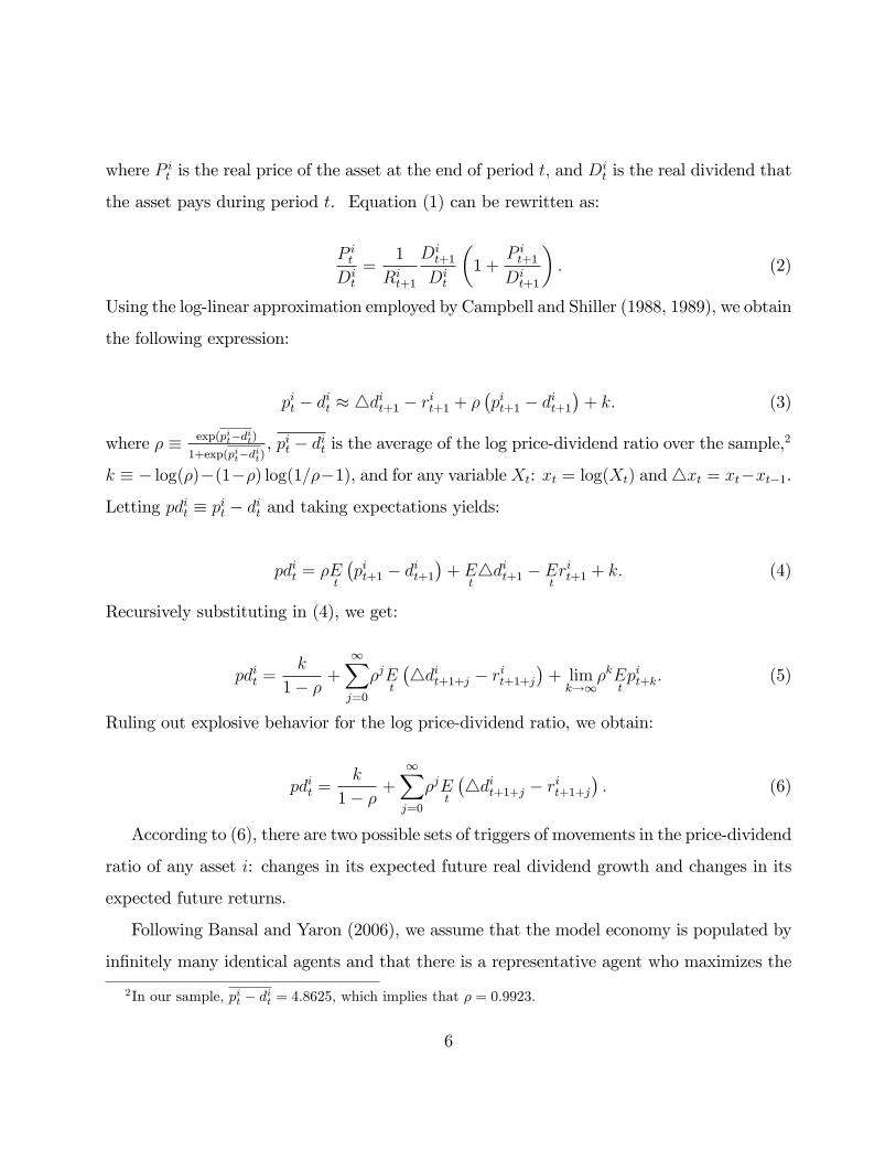
Using the log-linear approximation employed by Campbell and Shiller (1988, 1989), we obtain

the following expression:

pit � dit � 4dit+1 � rit+1 + ��pit+1 � dit+1

�+ k: (3)

where � � exp(pit�dit)1+exp(pit�dit)

, pit � dit is the average of the log price-dividend ratio over the sample,2

k � � log(�)�(1��) log(1=��1), and for any variableXt: xt = log(Xt) and4xt = xt�xt�1.

Letting pdit � pit � dit and taking expectations yields:

pdit = �Et

�pit+1 � dit+1

�+ E

t4dit+1 � E

trit+1 + k: (4)

Recursively substituting in (4), we get:

pdit =k

1� �+

1Xj=0

�jEt

�4dit+1+j � rit+1+j

�+ lim

k!1�kE

tpit+k: (5)

Ruling out explosive behavior for the log price-dividend ratio, we obtain:

pdit =k

1� �+

1Xj=0

�jEt

�4dit+1+j � rit+1+j

�: (6)

According to (6), there are two possible sets of triggers of movements in the price-dividend

ratio of any asset i: changes in its expected future real dividend growth and changes in its

expected future returns.

Following Bansal and Yaron (2006), we assume that the model economy is populated by

in�nitely many identical agents and that there is a representative agent who maximizes the

2In our sample, pit � dit = 4:8625, which implies that � = 0:9923.

6

recursive utility function originally introduced by Epstein and Zin (1989) and Weil (1989):

Ut =

�(1� �) (Ct)

1� � + �

�EtU1� t+1

�1=�� �1�

; (7)

where � 2 (0; 1) is the subjective time rate of preference, � = 1� 1�1= , � 0 is the coe¢ cient

of relative risk aversion, and � 0 is the elasticity of intertemporal substitution (EIS). It is

well-known that one of the main advantages of this type of utility function is that it allows

for a separation of the parameters that control the representative agent�s degree of relative

risk aversion ( ) and the EIS ( ). This feature, which is not available in the standard time-

separable power utility function used in most consumption-based asset pricing models, is

crucial for capturing several key aspects of the data. Economists using the standard power

utility model have struggled with the fact that high levels of risk aversion (i.e. high )

are required to match the observed equity premium in the data. These high levels of risk

aversion, however, imply a relatively low level for the EIS (i.e. low ), which causes the

model to predict that the real risk free rate is a lot more volatile than it is in the data. By

contrast, the Epstein-Zin utility function separates the coe¢ cient of relative risk aversion

from the elasticity of intertemporal substitution, thus giving the model more �exibility to

capture various properties of asset returns.

The logarithm of the of the stochastic discount factor (mt+1) that is implied by the utility

function given in (7) is:

mt+1 = � log � � �

(4ct+1) + (� � 1)

�rct+1

�; (8)

where rct+1 is the gross return on an asset that delivers aggregate consumption as its dividend

each period.

The Euler equation implied by the �rst order conditions of the utility-maximizing repre-

sentative agent takes a familiar form:

Et

�Mt+1R

it+1

�= 1. (9)

7

Assuming log-normality for the stochastic discount factor and for returns, (9) can be re-

written in logs:

Et

�mt+1 + rit+1

�+1

2V art

�mt+1 + rit+1

�= 0. (10)

This implies that the expected value of the log-return of asset i can be written as:

Et

�rit+1

�= �E

t(mt+1)� (0:5)V ar

t

(mt+1)| {z }rrft+1

�Covt

�mt+1; r

it+1

�� (0:5)V ar

t

�rit+1

�| {z }

re;it+1

. (11)

Note that the expected return on any asset i can be decomposed into two components - the

one-period ahead real risk-free rate (rrft+1) and the expected excess return (re;it+1) that asset i

is required to deliver in order to compensate investors for the fact that its future payo¤s are

uncertain.

Following BW, we allow for the possibility that real dividend growth and real consumption

growth can be decomposed into a non-stationary (permanent) component and a stationary

(transitory) component:

xt = xpt + x�t + wxt for x = 4c;4d, (12)

where xpt and x�t are the permanent and transitory components, respectively, of xt and

wxt v N(0; �2w;x) is an observation error. We assume that xpt follows a random walk:

xpt = xpt�1 + "x;pt for x = 4c;4d, (13)

where and "x;pt v N�0;��2x;p

�t

�is an exogenous structural shock. We also assume that all

transitory components follow an autoregressive process of order 2:

x�t =

2Xj=1

�jx�t�j + "x;�t for x = 4c;4d. (14)

where and "x;�t v N�0;��2x;�

�t

�is an exogenous structural shock.

8

Following AB, we impose a restriction on the non-stationary components of consumption

growth and dividend growth:

4dpt = 4cpt for 8 t, (15)

As Campbell and Cochrane (1999) note, in the very long run, one can reasonably expect

the correlation between consumption and dividend growth to approach 1:0 since the two series

share the same long-run trends and should grow at the same pace as the overall economy.

Bansal and Yaron (2006) and Hansen, Heaton, and Li (2005) also provide a similar argument

on their way to assuming that consumption growth and dividend growth share a small, but

persistent predictable component. Our assumption is slightly di¤erent from theirs, however,

as they assume that the common component, although very persistent, is stationary, while

we go a step further and assume that the joint component follows a random walk. Keeping in

mind the caveat of Campbell and Cochrane(1999) that the correlation between consumption

growth and dividend growth is notoriously di¢ cult to measure because it is very sensitive

to small changes in timing, we, nevertheless, interpret the empirical results of Campbell

(2000), who reports that the contemporaneous correlation between consumption growth and

dividend growth tends to increase as the measurement interval increases, as a con�rmation of

the hypothesis that the two series share a common long-run component. Furthermore, after

analyzing international data from 11 developed countries, Campbell (2002) reports that, in

general, correlations between consumption growth and dividend growth "increase strongly

with the measurement horizon" and are "positive and often quite large in long-term annual

data sets."

3 Model Solution

Given the assumptions described in the previous section, the state variables that are used to

track the evolution of consumption growth and dividend growth can be summarized in the

9

following state vector:

SAt =�4cpt ;4c�t ;4d�t ;4c�t�1;4d�t�1

�0, (16)

The equation which describes the evolution of the unobserved states through time is:

SAt = FASAt�1 + V At , (17)

where FA is the transition matrix and is given by:

FA =

0BBBBBBBBB@

1 0 0 0 0

0 �c1 0 �c2 0

0 0 �d1 0 �d2

0 1 0 0 0

0 0 1 0 0

1CCCCCCCCCA, (18)

and V At is a vector of exogenous structural shocks to the unobserved states:

V At = (vcdt ; v

ct ; v

dt ; 0; 0)

0, (19)

V At � N

�0; QA

t

�, (20)

QAt =

0BBBBBBBBB@

(�2cd)t 0 0 0 0

0 (�2c� )t 0 0 0

0 0 (�2c� )t 0 0

0 0 0 0 0

0 0 0 0 0

1CCCCCCCCCA. (21)

Note that in this state space model, unlike in a conventional one, the variance-covariance

matrix, QAt , is time-dependent. This is due to the fact that, as discussed in Section 2,

10

we allow the conditional variances of the structural shocks to vary over time.3 We assume

that the evolution of the three time-varying variances is guided by the following stochastic

processes:

diag(QAt ) =

0BBB@(�2cd)t

(�2c� )t

(�2d� )t

1CCCA = �+ SBt ; (22)

where

� =

0BBB@��;cd

��;c�

��;d�

1CCCA ;

SBt =

0BBBB@�f�2cd�

t�f�2c��t�f�2c��t

1CCCCA ;

SBt = FBSBt�1 + V Bt ; (23)

FB =

0BBB@��;cd 0 0

0 ��;c� 0

0 0 ��;d�

1CCCAV Bt � N

�0; Qb

�;

Qb =

0BBB@�2�;cd 0 0

0 �2�;c� 0

0 0 �2�;d�

1CCCA ;

and f�2x = (�2x)t � ��;x.3We assume that QAt is diagonal (i.e. that the structural shocks in V At are not correlated with each

other) in order to decreases the number of estimated parameters in the benchmark model and thus reduce

the computational burden on the MCMC algorithm. In work that is available upon request, we show that

our main results are robust to relaxing that assumption.

11

We use the method of undetermined coe¢ cients in order to solve for pdt in terms of

the relevant state variables. While the details of our solution are described in Appendix

A, we use the rest of this section to go through the most important results. The log-price-

dividend ratio is a function of future dividend growth rates and of future expected returns

(6). The latter are, in turn, a function of expected consumption growth, of the conditional

variances of the stochastic discount factor and returns, as well as of the covariance between

the stochastic discount factor and returns (11). That is why we conjecture that the log-price-

dividend ratio is ultimately a function of two sets of variables - the expected future values

of the permanent and temporary components of real consumption growth and real dividend

growth (summarized in SAt ) and the conditional variances of these variables (summarized in

SBt ). Hence, our guess for the solution of the pdt equation takes on the following form:

pdt = Ap +HAp S

At +HB

p SBt , (24)

where HAp is a (1x5) row vector and H

Bp is a (1x3) row vector. After going through the steps

described in Appendix A, the solution vectors in (24) turn out to be:

HAp =

�Hd � 1

Hc

�FA

�I � �FA

��1, (25)

HBp =

�(1� �)HB

c

�I � �cF

B�+ (0:5) [WPB WPB]H�

�I � �FB

��1, (26)

where

Hc =h1 1 0 0 0

i0,

Hd =h1 0 1 0 0

i0,

WPB =

�(� � 1� �

)Hc + (� � 1)�cHA

c + �HAp +Hd

�,

HAc =

�1� 1

�HcFA

�I � �cF

A��1

,

HBc = (0:5)�

�[WCB WCB]H�

�I � �cF

B��1

,

12

WCB =

�1� 1

�HcFA

�I � �cF

A��1

;

�c �exp(pct � ct)

1 + exp(pct � ct),

H� is a (25x3) matrix whose entries are such that:

vec(QAt ) = H�SBt ,

and Ap is a constant.

There are a couple of important observations related to the above expressions that are

worth mentioning at this point. First, the factor loading on the permanent component of

consumption growth is�1� 1

�. Therefore, when the EIS is greater than 1 (i.e. 1

< 1), an

increase in the permanent component of consumption growth increases the price-dividend

ratio. Conversely, when the EIS is smaller than 1 (i.e. 1 > 1), an increase in the permanent

component of consumption growth decreases the price-dividend ratio. Intuitively, if the EIS

is relatively high, agents are relatively more willing to shift consumption across time and

the substitution e¤ect (higher expected future dividends) dominates the income e¤ect (lower

expected future marginal utility). As a result, agents bid up the price of stocks relative to

the current level of dividends. If, on the other hand, the EIS is relatively low, agents are

relatively less willing to shift consumption across time and the income e¤ect dominates the

substitution e¤ect. As a result, agents decrease their demand for stocks in order to �nance

an increase in their current consumption, thus bidding down stock prices. Second, the value

of � plays a crucial role in determining the signs of the factor loadings on the elements of SBt

(i.e. the factor loadings on the time-varying variances of macroeconomic fundamentals). Just

as in the Bansal and Yaron (2006) model, a negative � implies that increases in volatility

reduce the price-consumption ratio (i.e. the elements of HBc are negative). This, in turn,

implies that the elements of the �rst term on the right-hand side of (26) are all negative,

which is a necessary (but not a su¢ cient) condition for the elements of HBp to be negative.

13

Hence a negative value for � is critical for replicating the empirically documented4 and

intuitively appealing fact that increases in the conditional volatility of consumption growth

cause declines in the price-dividend ratio of the aggregate stock market. As we show in

Section 5, our benchmark estimates are in line with that requirement.

The solution for the real risk-free interest rate turns out to be:

rfrt = Ar +HAr S

At +HB

r SBt , (27)

where

HAr =

1

HcFA, (28)

HBr = �(1� �)HB

c

�I � �cF

B�� (0:5)

�[WRB WRB]H�

; (29)

WRB =

�(� � 1� �

)Hc + (� � 1)�cHA

c

�.

and Ar is a constant.

Equation (28) expresses a relationship that is present in virtually all mainstream consumption-

based asset pricing models. Namely, a rise in the expected growth rate of consumption causes

an increase in the real risk-free interest rate. Meanwhile, according to (29), a negative � im-

plies that the non-zero elements of the �rst term on the right hand-side of (29) are all positive.

Conversely, the elements of the second term on the right hand-side of (29) are all negative,

regardless of the sign of �. It turns out that, for virtually all plausible values of the estimated

parameters of the model, the second term dominates the �rst one. That implies that a rise

in the conditional volatility of consumption growth leads to a decline in the real risk-free

interest rate. Intuitively, an increase in economic uncertainty raises economic agents�desired

levels of precautionary saving. This increases the supply of loanable funds in the economy,

which, in turn, causes real interest rates to decline.

4See Bansal and Yaron (2006).

14

Using a similar approach, we derive an expression that relates the expected excess returns

on asset i, Et

�re;it+1

�, to SBt :

Et

�re;it+1

�= Ae +HB

e SBt , (30)

where

HBe = � [WRC WRD]H� � (0:5) [WRD WRD]H� (31)

WRC =

�(� � 1� �

)Hc + (� � 1)�cHA

c

�,

WRD =��HA

p +Hd�,

and Ae is a constant.

Note that the two terms on the right hand-side of (31) can be traced back to the third and

fourth terms on the right hand-side of (11). Namely,�Covt

�mt+1; r

it+1

�= � [WRC WRD]H�SBt

and �(0:5)V art

�rit+1

�= �(0:5) [WRD WRD]SBt .

4 Estimating the Model

In order to estimate the unknown parameters and the unobserved states of the model, we

use data on four variables - the log price-dividend ration for the aggregate U.S. stock market

(pdt), log per-capita real consumption growth (4ct), log per-capita real dividend growth

(4dt), and the log of the real risk-free interest rate (rrft+1).5 The vector of observed variables,

Yt, can therefore be written, as:

Yt =�pdt;4ct;4dt; rrft+1

�0. (32)

Since our main goal in this paper is to decompose the �uctuations of asset prices around their

means, rather than try to explain the levels of their means, we demean all of our observable

variables. The equations relating pdt and rrft+1 to the vectors of unobserved states (S

At and

SBt ) are given in (24) and (27), respectively. The equations relating the other two observable

5The exact data sources are described in Appendix B.

15

variables (4ct and 4dt;) to the two state vectors are trivial and can be easily derived by

using (12). Combining the four equations relating the observable variables to the unobserved

states allows us to write the observation equation:

Yt = HASAt +HBSBt +Wt; (33)

where

HA =

26666664HAp

1 1 0 0 0

1 0 1 0 0

HAr

37777775 ,

HB =

26666664HBp

0 0 0 0 0

0 0 0 0 0

HBr

37777775 ,

and Wt is a vector of observation errors:

Wt =�wpt ; w

ct ; w

dt ; w

rt

�0, (34)

Wt � N (0; R) ,

R =

0BBBBBB@�2w;p 0 0 0

0 �2w;c 0 0

0 0 �2w;d 0

0 0 0 �2w;r

1CCCCCCA . (35)

There are 19 unknown parameters ( 1 , , �c1, �

c2 �

d1, �

d2, �

2w;p, �

2w;c, �

2w;d, �

2w;r, ��;cd, ��;c� ,

��;d� , ��;cd, ��;c� , ��;d� , �2�;cd, �

2�;c� ; and �

2�;d� ) and 1356 unobserved states (6 states for each

16

of the 226 quarters of data that we use in the estimation of the model) to be estimated.6

We use Bayesian Markov Chain Monte Carlo (MCMC) methods in order to obtain estimates

of the posterior distributions of the unknown parameters and the unobserved states. The

details of the estimation procedure are described in Appendix C.

5 Results

5.1 Estimated Parameters and States

The second and third columns of Table 1 summarize the prior distributions that we have

selected for the estimation of the model. It is well-known that one of the main advantages

of using Bayesian MCMC estimation methods is that they allow for �exible ways of incor-

porating prior information into the estimation of the model. In an attempt to let the data

"tell us" as much as possible about the model�s parameters and states, we use relatively �at

prior distributions for most of the estimated variables unless we have a solid economic reason

for not doing so. For example, we restrict each of the variances of the observation errors

(i.e. each of the diagonal elements of R) to be at most 20% of the conditional variance of its

respective observable variable. That restriction is forcing the model to explain at least 80%

of the �uctuations in each of the observable variables with �uctuations in the relevant state

variables rather than with errors in the observation equations. In order to truly incorporate

all relevant prior information in the estimation, where appropriate, we impose prior restric-

tions on the relationships between certain variables rather than on the individual variables

themselves. For instance, following the claim of virtually every paper in the long-run risks

literature (e.g. Balke and Wohar (2002), Bansal and Yaron (2006), and Croce (2009)) that

if the long-run components of consumption growth and dividend growth do exist, they are

6Note that � does not need to be explicitly estimated since the estimates for 1 and imply an estimate

for � (b� = 1�b 1�d1= , ).

17

orders of magnitude smaller than their respective observed series, we incorporate a prior

distribution over the ratio of the average variances of the permanent and the temporary

components of consumption. Namely, we impose an inverse-gamma prior distribution over

the ratio of the variance of the temporary component of consumption and the variance of the

permanent component of consumption with a mode of 100. We are thus "asking" the model

to place higher probabilities on outcomes in which the variance of permanent consumption

is signi�cantly smaller than the variance of temporary consumption.

Our estimates of the posterior distributions of the unknown parameters are summarized

in the last three columns of Table 1. There are several estimates that deserve attention. Our

estimates of the intertemporal elasticity of substitution ( ) and the coe¢ cient of relative

risk aversion ( ) are within the range of estimates that have been reported in the literature.

Unlike many asset pricing models, which require values for of 10 and above to match

certain moments in the data, ours manages to �t the observed stock price and interest rates

series reasonably well at levels of risk aversion that are much closer to the estimates obtained

in most micro studies on the issue. Our estimate of the EIS is higher than the estimates of

Hall (1988) and Campbell (1999), who estimate it to be lower than 1. They are, however, in

line with the results of Hansen and Singleton (1982) and Attanasio and Weber (1989), both

of whom conclude that EIS is above 1. More recently, several authors (e.g. Guvenen (2001)

and Vissing-Jorgensen (2002)) have argued that is well over 1. Furthermore, Bansal and

Yaron (2006) argue that the results of Hall (1988) and Campbell (1999), which are obtained

by regressing date t+1 consumption growth on the date t real risk-free rate, su¤er from a

downward bias since they do not account for time variation in the conditional volatility of

consumption growth.

The estimates of b and b that we obtain have an important implication for the e¤ectof macroeconomic volatility on stock prices. The combination of b > 1 and b > 1 implies

that b� < 0, which, as argued in Section 3, is critical for allowing the model to capture the

empirical fact that an increase in macroeconomic uncertainty causes the price-dividend ratio

18

of the aggregate stock market to decline. Intuitively, a rise in the conditional volatility of

fundamentals a¤ects the price-dividend ratio via two distinct e¤ects that it has on expected

returns. First, it decreases the real risk-free rate through the precautionary savings e¤ect

discussed in Section 3. Second, it increases the expected excess returns that investors require

in order to be compensated for the additional risk that they bear when holding an asset whose

payo¤s are uncertain. In our model, as well as in the data, the latter e¤ect dominates former,

thus causing a negative relationship between macroeconomic volatility and the level of the

aggregate stock market.

The three autoregressive processes that govern the evolution of the variances of funda-

mentals over time appear to be quite persistent, as their AR(1) coe¢ cients (��;cd, ��;c� ,

and ��;d� ) are all estimated to be greater than 0.9. This explains the important role that

these processes play in driving �uctuations in stock prices and in the risk-free interest rate

(discussed in greater detail in Section 5.2) As expected, the mean of the variance of the

non-stationary component of consumption growth and dividend growth (��;cd) is orders of

magnitude smaller than its respective stationary counterparts (��;c� and ��;d� ). The esti-

mates of the variances of the shocks to the conditional volatilities (�2cd, �2c� , and �

2d� ) indicate

that the average shock to the variance of temporary dividend growth is signi�cantly larger

than the average shocks to the variances of the temporary and permanent consumption

growth components. Finally, the variances of all four observation errors are signi�cantly

lower than the upper bounds imposed in the prior distributions, indicating that the model

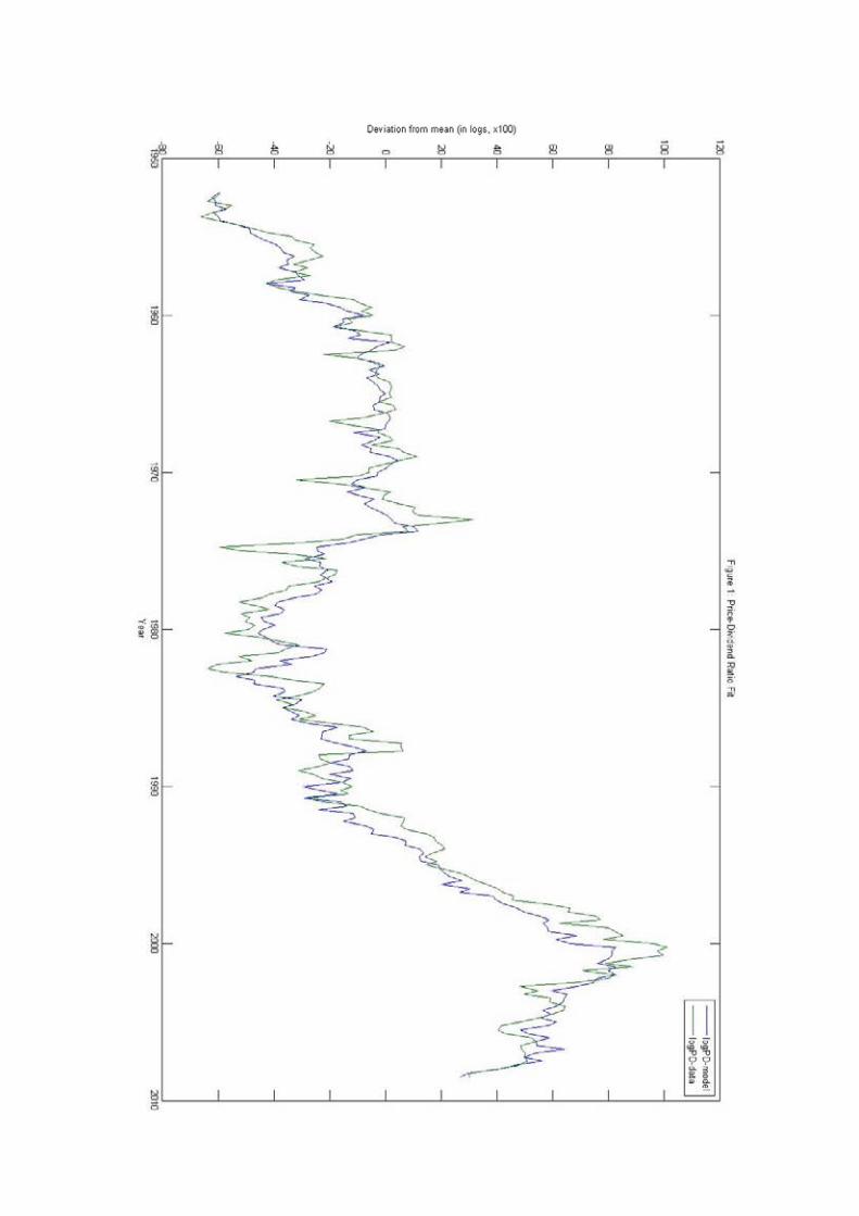
does quite well against the data. The good overall �t of the model is con�rmed by �gures 1

through 4, which plot the four observable series versus the model�s predictions.

5.2 Historical Decompositions and Variance Decompositions

Tables 2 through 5 present the variance decompositions implied by the estimated model for

the four observable variables at various horizons. According to Table 2, �uctuations in the

19

log-price dividend ratio at short and medium horizons tend to be driven largely by �uctu-

ations in the conditional variance of the non-stationary component of consumption growth

(63% and 59%, respectively). Changes in the conditional mean of the permanent component

of consumption growth come at a distant second place (with 13% and 25%, respectively),

followed by changes in the volatility of the stationary component of consumption growth

(12% and 11%, respectively). In contrast, low frequency movements in the aggregate stock

market tend to be driven by changes in the expected mean of permanent dividend growth

(72%). While the contribution of time-varying variance of the long-run component of con-

sumption growth declines substantially at long horizons, it is still fairly signi�cant (22%).

Figure 5 displays a visual con�rmation of the results from Table 2. It shows a historical

decomposition for the log price-dividend ratio of the aggregate US stock market. The low

frequency movements in the log price-dividend ratio are closely matched by swings in the

expected value of the long-run component of consumption growth. Medium and high fre-

quency �uctuations in the aggregate stock market level appear to be closely matched by

�uctuations in the conditional volatility of the long-run component of consumption growth.

Both of these observations are in line with the results presented in Table 2.

Table 6 presents a di¤erent angle. Rather than decomposing �uctuations in the log price-

dividend ratio by the contributions of each of the structural shocks in the model (as in Table

2), it breaks down the variance of pdt by the contributions of each of the three potential

drivers discussed in the Section 1. At short and medium horizons, the variance of pdt tends

to be dominated by �uctuations in expected excess returns. Given the results from Table

2, this should not be surprising since, as discussed in Section 2, �uctuations in conditional

volatilities are the exclusive triggers of �uctuations in expected excess returns in the model.

In the long run, changes in the conditional mean of dividend growth explain the largest

share of the variance of aggregate stock price �uctuations. Once again, this is in line with

the results of the decomposition presented in Table 2 since the shared long-run component

of consumption and dividend growth is, by construction, what is driving both of these series

20

at low frequencies.

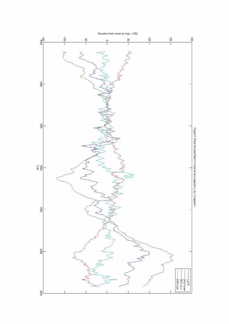
Figure 9 o¤ers an intriguing historical perspective on the relative importance of the main

drivers of �uctuations in the aggregate US stock market over the past several decades. As

discussed above, changes in expected dividend growth were the main drivers at lower frequen-

cies. For example, the stock market run-ups of the 1950�s, 1980�s, and 1990�s were mainly

the result of gradually-improving expectations about future dividend growth. Similarly, the

decline of the US stock market during the 1970�s could largely be attributed to deteriorating

long-run dividend growth expectations. Note that the �uctuations in the aggregate price-

dividend ratio during all of those episodes would have been even larger had it not been for

the o¤setting e¤ect of changes in the expectations of future real risk-free interest rates. Re-

call that, in our model, consumption growth and dividend growth share the same permanent

component. Therefore, an increase in expected long-run dividend growth is equivalent to an

increase in expected long-run consumption growth. The latter causes a rise the expectations

of future real risk-free interest rates (28), which, in turn, causes the price-dividend ratio to

decline (6), thus partially o¤setting the positive e¤ect that an increase in expected dividend

growth has on the price-dividend ratio.

Despite the dominance of changes in expected dividend growth at low frequencies, it

is changes in expected excess returns that appear to be responsible for most of the large

high-frequency swings in the price-dividend ratio. For instance, our results indicate that the

stock market crash of October 1987 was caused by a sharp spike in macroeconomic uncer-

tainty rather than by a dramatic downward revision of expectations about future aggregate

dividends. Similarly, our model attributes most of the 2007-08 decline in the US stock mar-

ket to rising conditional volatility of macroeconomic fundamentals. Expectations of future

dividend growth also declined during that episode. However, a large part of that e¤ect was

o¤set by the impact of lower expected future real interest rates, triggered by lower expected

macroeconomic growth.

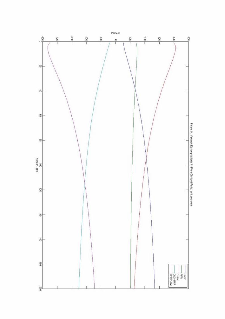
Figures 10 and 14 plot the two sets of variance decompositions discussed above as func-

21

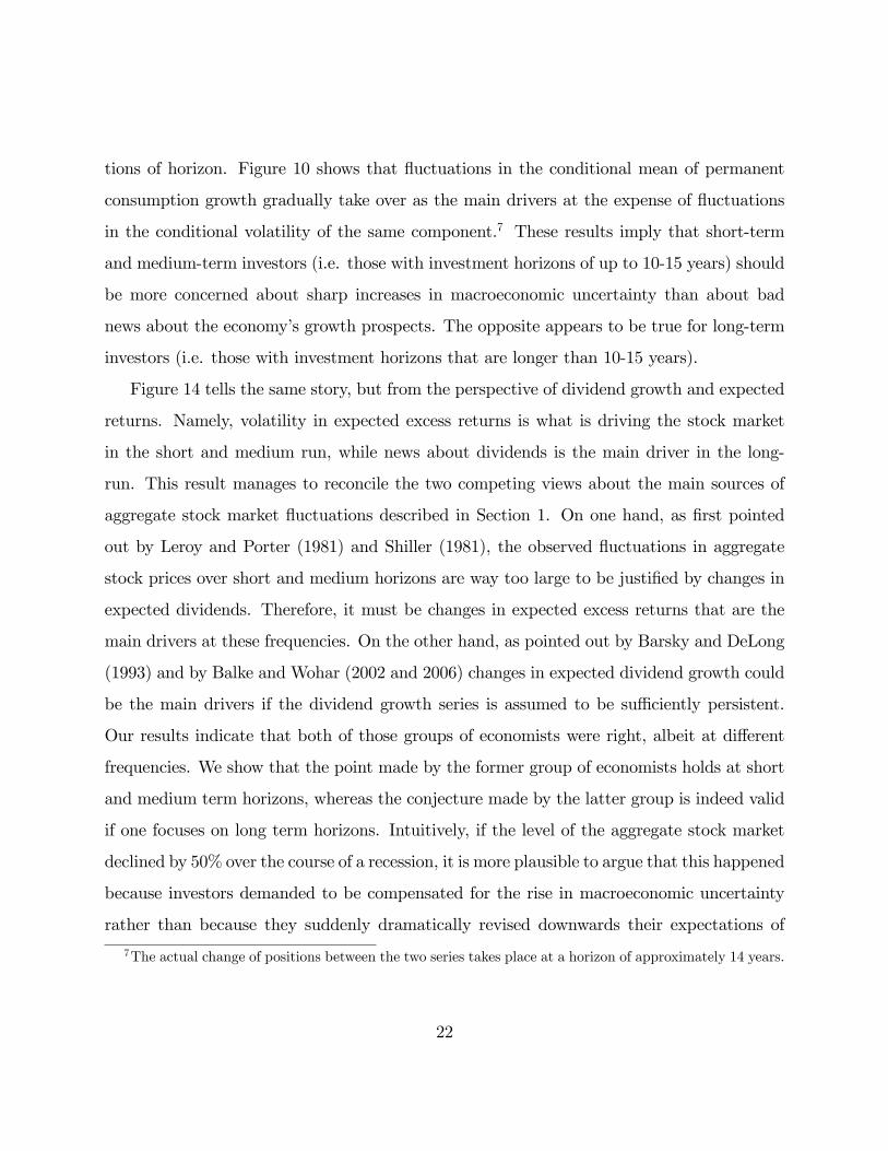
tions of horizon. Figure 10 shows that �uctuations in the conditional mean of permanent

consumption growth gradually take over as the main drivers at the expense of �uctuations

in the conditional volatility of the same component.7 These results imply that short-term

and medium-term investors (i.e. those with investment horizons of up to 10-15 years) should

be more concerned about sharp increases in macroeconomic uncertainty than about bad

news about the economy�s growth prospects. The opposite appears to be true for long-term

investors (i.e. those with investment horizons that are longer than 10-15 years).

Figure 14 tells the same story, but from the perspective of dividend growth and expected

returns. Namely, volatility in expected excess returns is what is driving the stock market

in the short and medium run, while news about dividends is the main driver in the long-

run. This result manages to reconcile the two competing views about the main sources of

aggregate stock market �uctuations described in Section 1. On one hand, as �rst pointed

out by Leroy and Porter (1981) and Shiller (1981), the observed �uctuations in aggregate

stock prices over short and medium horizons are way too large to be justi�ed by changes in

expected dividends. Therefore, it must be changes in expected excess returns that are the

main drivers at these frequencies. On the other hand, as pointed out by Barsky and DeLong

(1993) and by Balke and Wohar (2002 and 2006) changes in expected dividend growth could

be the main drivers if the dividend growth series is assumed to be su¢ ciently persistent.

Our results indicate that both of those groups of economists were right, albeit at di¤erent

frequencies. We show that the point made by the former group of economists holds at short

and medium term horizons, whereas the conjecture made by the latter group is indeed valid

if one focuses on long term horizons. Intuitively, if the level of the aggregate stock market

declined by 50% over the course of a recession, it is more plausible to argue that this happened

because investors demanded to be compensated for the rise in macroeconomic uncertainty

rather than because they suddenly dramatically revised downwards their expectations of

7The actual change of positions between the two series takes place at a horizon of approximately 14 years.

22

future aggregate dividends in the economy. If on the other hand, the price-dividend ratio

of the aggregate stock market gradually increased over the course of a couple of decades,

it would be easier to make the case that this occurred due to gradually-revised long-term

dividend growth expectations rather than as a result of a sustained twenty-year decline in

macroeconomic volatility.

Summaries of variance decomposition for the short-term real risk-free rate at various

horizons are presented in Table 3. At all horizons, the variance of this variable appears to

be dominated by movements in the conditional volatility of the non-stationary component

of consumption growth. Fluctuations in that component explain more than 90% of the total

variance of the real risk-free rate at all horizons. The results from Table 3 are con�rmed by

the historical decomposition of the real interest rate in Figure 8 and by Figure 13, which

plots the variances decompositions of the real risk-free rate, implied by our estimates of the

model, as a function of the horizon.

Finally, Tables 4 and 5 put the results obtained from the variance decompositions of

the price-dividend ratio into perspective. Some might argue that the fact that the joint

permanent component of consumption growth and dividend growth is the only variable that

is assumed to have a unit root might somehow in�uence the result that this particular

component is the main driver of the price-dividend ration in the long-run. A necessary (but

not a su¢ cient) condition for that potential criticism to have any merit is that the joint

permanent component of consumption growth and dividend growth is the main long-run

driver of these two variables themselves. However, the results presented in Tables 4 and 5

allow us to categorically dismiss all suspicions of that kind. Namely, the third columns of

these tables reveal that the joint permanent component of consumption growth and dividend

growth is far from being the main driver of these two variables at any horizon. These

conclusions are visually con�rmed by the results displayed in Figures 11 and 12.

23

6 Conclusion

In this paper, we attempt to resolve the long-lasting debate about the main sources of

�uctuations in the aggregate US stock market. In order to accomplish that, we design and

solve a consumption-based asset pricing model which incorporates stochastic volatility, long-

run risks in consumption and dividends, and Epstein-Zin preferences. Utilizing Bayesian

MCMC techniques, we estimate the model by using US data on the level of the aggregate

stock market, short-term real risk-free rates, consumption growth, and dividend growth.

We conclude that, over short and medium horizons, �uctuations in the aggregate US stock

market are mainly driven by changes in expected excess returns. Conversely, low-frequency

movements in aggregate stock prices are primarily caused by changes in expected dividend

growth rates.

The paper o¤ers several possible directions for further research. An intriguing extension

would be to add time-varying risk aversion to the time-varying variances model presented

here. This feature would introduce �uctuations in the price of risk over time in addition to

the �uctuations in the quantity of risk introduced in this paper. It would be also interesting

to extend the theoretical environment of the model into a general equilibrium setting. Jus-

tiniano and Primiceri (2008) have already explored the e¤ects of time-varying volatility on

macroeconomic �uctuations. As the title of their paper suggests, however, they were mostly

concerned with the business cycle implications of their model. We believe that it would be

extremely informative to include data on asset prices (particularly data on stock prices) in

the estimation of a DSGE model with time-varying volatility and time-varying risk aversion

and study the model�s asset pricing implications.

24

Appendix A. Solution Methodology

We start by solving for rct+1, the return on the hypothetical asset that delivers aggregate

consumption as its dividend each period. Let P ct be the price of that asset at time t. Since

its dividend is equal to aggregate consumption, its log-price-dividend ratio is given by:

pct � pct � ct = log(Pct =Ct): (A.1)

Using the same line of reasoning as the one described in the justi�cation of the guess for the

expression for pdt in Section 3, we make the following guess for pct:

pct = ATV Vc +HAc S

At +HB

c SBt : (A.2)

Note that (2) can be modi�ed to obtain an expression for pct:

pct = �c (pct+1) +4ct+1 � rct+1 + kc (A.3)

Rearranging terms in (A.3), we solve for rct+1:

rct+1 = �c (pct+1) +4ct+1 � pct + kc: (A.4)

Using our guess for pct (A.2) and the fact that 4ct+1 = HcSAt+1, we can rewrite (A.4) as:

rct+1 = ��ATV Vc +HA

c SAt+1 +HB

c SBt+1

�+HcSAt+1 �

�ATV Vc +HA

c SAt +HB

c SBt

�+ kc: (A.5)

Note that the log-version of the Euler equation (10) must hold for the returns of all assets

in the economy. Therefore, we can write:

Et

�mt+1 + rct+1

�+1

2V art

�mt+1 + rct+1

�= 0: (A.6)

Using (8), we can write:

mt+1 + rct+1 = � log � � �

(4ct+1) + (�)

�rct+1

�= (A.7)

� log � � �

�HcSAt+1

�+ �

24 �c�ATV Vc +HA

c SAt+1 +HB

c SBt+1

�+

HcSAt+1 ��ATV Vc +HA

c SAt +HB

c SBt

�+ kc

3525

Combining (A.7) with equations (18) and (23), we can write:8

Et

�mt+1 + rct+1

�=

�� � HcFA + �

���cH

Ac +Hc

�FA �HA

c

��SAt + �

��cF

B � I�HBC S

Bt

(A.8)

V art

�mt+1 + rct+1

�=

���� � �

�Hc + ��cH

Ac

��

����

� � �

�Hc + ��cH

Ac

��

�H�SBt ;

(A.9)

Plugging (A.8) and (A.9) into (A.6), we get:

0 =

�� � HcFA + �

���cH

Ac +Hc

�FA �HA

c

��SAt + (A.10)

+���cF

B � I�HBc S

Bt +

+1

2

���� � �

�Hc + ��cH

Ac

��

����

� � �

�Hc + ��cH

Ac

��

�H�SBt :

Since (A.10) has to hold for all values of the state variables, combining all the SAt and SBt

terms and setting them equal to each other yields the following two equations:

� � HcFA + �

���cH

Ac +Hc

�FA �HA

c

�= 0; (A.11)

���cF

B � I�HBc +

1

2

���� � �

�Hc + ��cH

Ac

��

����

� � �

�Hc + ��cH

Ac

��

�H� = 0:

(A.12)

Solving the above two equations yields:

HAc =

��1� 1

�Hc

�FA

�I � �cF

A��1

, (A.13)

HBc = (0:5)�

�[WCB WCB]H�

�I � �cF

B��1

, (A.14)

where

WCB =

�1� 1

�HcFA

�I � �cF

A��1

�:

8Throughout the solution derivations, we use the fact that, for any three matrices, A, B, and C:

vec(ABC) = (C 0 A) vec(B).

26

Having obtained the expressions for HAc and H

Bc , we can now plug (A.13) and (A.14) into

(A.5) and then use the resulting expressions for rct+1 in (8) in order to obtain the following

the expression for the stochastic discount factor:

mt+1 = Am ��1

HcFA

�SAt + (1� �)HB

c

�I � �cF

B�SBt + (A.15)��

� � 1� �

�Hc + �c (� � 1)HA

c

� �V At+1

�+ �c (� � 1)HB

c

�V Bt+1

�:

Having solved for the stochastic discount factor in terms of the state variables, we are

now ready to turn our attention to the price-dividend ratio for the aggregate stock market

(pdt). Note that we can use (3) in order to solve for the return of the aggregate stock market:

rt+1 = � (pdt+1) +4dt+1 � pdt + k: (A.16)

Using the fact that 4dt+1 = HdSAt+1 and plugging our guess for pdt (24) in (A.16), we get:

rt+1 = ��ATV Vp +HA

p SAt+1 +HB

p SBt+1

�+HdSAt+1 �

�ATV Vp +HA

p SAt +HB

p SBt

�+ k: (A.17)

Note that:

Et[mt+1 + rt+1] =

�� 1 HcFA +HA

p

��FA � I

�+HdFA

�SAt + (A.18)�

(� � 1)HBC

��cF

B � I�+HB

p

��FB � I

��SBt

V art(mt+1 + rt+1) = [WPB WPB]H�SBt + (WPS) �B (WPS)0 ; (A.19)

where

WPB =

��� � 1� �

�Hc + (� � 1) �cHA

c + �HAp +Hd

��;

WPS = (� � 1) �cHBC + �HB

p :

27

Next, we plug (A.18) and (A.19) into the log-version of the Euler equation (10) and get:

0 = (WPS) �B (WPS)0 + (A.20)�� 1 HcFA +HA

p

��FA � I

�+HdFA

�SAt +

+�(� � 1)HB

C

��cF

B � I�+HB

P

��FB � I

��SBt +

+ [WPB WPB]H�SBt :

Since (A.20) has to hold for all values of the state variables, we combine all the SAt and SBt

terms and set them equal to each other. This yields the following two equations:

� 1 HcFA +HA

p

��FA � I

�+HdFA = 0�

(� � 1)HBc

��cF

B � I�+HB

p

��FB � I

��+ f[WPB] �g f[WPB] �gH� = 0

Solving the above two equations yields:

HAp =

�Hd � 1

Hc

�FA

�I � �FA

��1, (A.21)

HBp =

�(1� �)HB

c

�I � �cF

B�+1

2[WPB WPB]H�

��I � �FB

��1: (A.22)

Note that (A.15) in combination with (11) allows us to express the one-period ahead real

risk-free rate as a function of the two state vectors:

rrft+1 = �Et(mt+1)�

1

2V art(mt+1) = (A.23)

�Am ��(� � 1)�cHB

C

� ��B� �(� � 1)�cHB

c

�+

�1

HcFA

�SAt � (1� �)HB

c

�I � �cF

B�SBt

�12f(WRB) (WRB)gH�SBt ;

where

WRB =

�(� � 1� �

)Hc + (� � 1)�cHA

c

��.

28

Appendix B. Data Sources

The data that we use to estimate the unknown parameters and the unobserved states of our

model is quarterly and runs from 1952:01 to 2008:02. For our stock market variables, we use

CRSP data, which includes all stocks listed on the NYSE, the AMEX, and the NASDAQ,

in order to construct the aggregate log-price-dividend ratio and log-dividend-growth series.

Following the approach taken by Bansal, Dittmar, and Lundblad (2005), we de�ne the total

return per dollar invested, Rt+1, to be:

Rt+1 = ht+1 + yt+1;

where ht+1 is the gross price appreciation from t to t+1 and yt+1 is the dividend yield during

period t+1. Since we observe Rt+1 (RET in CRSP terminology) and ht+1 (RETX in CRSP

terminology), we can easily obtain the dividend yield, yt+1, by taking the di¤erence between

the two series:

yt+1 = Rt+1 � ht+1:

Having obtained the above series, it is straightforward to generate the actual price (Pt)

and dividend (Dt) series.

Pt+1 = htPt; t = 2; :::; T � 1; P1 = 1;

Dt = ytPt; t = 1; :::; T:

Note that we have constructed the Pt series in such a way that it corresponds to total

market valuation, not price per share as in some other studies. Similarly Dt corresponds to

total dividends paid by all companies in the market, not dividends per share. We use the

yield on the three-month Treasury bill to measure the short-term nominal risk-free interest

rate. We use data on consumption of non-durables and services, obtained from the National

Income and Product Accounts (NIPA) tables, in order to construct our nominal consumption

29

growth series. We convert all nominal series into real by using the price index that is implied

by the data on nominal and real consumption of non-durables and services (also obtained

from the NIPA tables).

30

Appendix C. Bayesian Estimation of the State-Space

Model

We use Bayesian Markov Chain Monte Carlo (MCMC) methods in order to obtain esti-

mates of the joint posterior distribution of the structural parameters and the unobserved

states. We modify the approach used in Avdjiev and Balke (2009) in order to account

for the fact that the state space model we derive in this paper di¤ers from a conventional

state space model due to the fact that the variances of the shocks to state equation A

(17) are functions of the shocks to state equation B (23). We split the 19 unknown pa-

rameters into two vectors. The �rst one (�A = [ 1 ; ; �c1; �

c2; �

d1; �

d2; �

2w;p; �

2w;c; �

2w;d; �

2w;r])

contains the parameters that are directly related to state equation A. The second vector

(�B = [��;cd; ��;c� ; ��;d� ;��;cd;��;c� ;��;d� ; �2�;cd; �

2�;c� ; �

2�;d� ]) consists of the parameters that

are directly related to state equation B.

We use a combination of the RandomWalk Metropolis-Hastings (RWMH) and the Gibbs

Sampling (GS) algorithms in the following way:

1. We choose arbitrary initial values for the structural parameters,��A0and

��B0,

and for the unobserved states,�SAT0and

�SBT0.

2. For i = 1; :::; nsim, we iterate the following four steps:

2.1. Given��Ai�1

,��Bi�1

, and�SBTi�1

, we use the Kalman Filter to obtain

the conditional distribution of SAT : P (SAT j��Ai�1

;��Bi�1

;�SBTi�1

; YT ). We obtain a

draw,�SATi, from P (SAT j

��Ai�1

;��Bi�1

;�SBTi�1

; YT ). In this step, we use the "�lter

forward, sample backward" approach proposed by Carter and Kohn (1994) and discussed in

Kim and Nelson (1999).

2.2. Given��Ai�1

, we draw a candidate set of parameters,��Ac, from a previ-

ously speci�ed distribution: ga(��Ac j��Ai�1). Our choice of ga(�) is such that, ��Ac =�

�Ai�1

+ va, where va is drawn from a multivariate t-distribution with �ve degrees of free-

31

dom and a covariance matrix �A. We set �A to be a scaled version of the Hessian matrix of

the log posterior probability, evaluated at the posterior mode. We choose the scale so that

20%� 30% of the candidate draws are accepted. We determine the acceptance probability,

�a, for the candidate draw:

�a(��Ac;��Ai�1

) = min ff�a; 1g ,where f�a = exp(l(YT ;

��Ac;��Bi�1

;�SBTi�1

))�(��Ac)

exp(l(YT ; f�Agi�1 ; f�Bgi�1 ; fSBT gi�1))�(f�Agi�1)

,

l(YT ;�A;�B; SBT ) is the log-likelihood and �(�

A) is the prior probability of �A. We select��Aiaccording to the following rule:

��Ai=��Acwith probability �a;�

�Ai=��Ai�1

with probability 1� �a.

2.3. Given�SBTi�1

, we use the RWMH algorithm to draw a candidate�SBtcfor

each point in time t (t = 1:::T ) from a previously speci�ed distribution: gs(�SBtc j�SBt i�1).

Our choice of gs(�) is such that,�SBtc=�SBti�1

+vs, where vs is drawn from a multivariate

t-distribution with �ve degrees of freedom and a covariance matrix �SB . We choose the

scale so that 20%� 30% of the candidate draws are accepted. We determine the acceptance

probability, �s, for the candidate draw:

�s(�SBtc;�SBti�1

) =min f e�s; 1g ,where

e�s = p(�SBtc j�SBt�1i ;�SBt+1i�1 ;��Bi�1) exp(l(YT ;��Ai ;��Bi�1 ;�SBT c))

p(fSBt gi�1 j

�SBt�1

i;�SBt+1

i�1; f�Bgi�1) exp(l(YT ; f�Agi ; f�Bgi�1 ; fSBT g

i�1)).

We select�SBtiaccording to the following rule:

32

�SBti=�SBtcwith probability �s;�

SBti=�SBti�1

with probability 1� �s.

2.4. Given��Bi�1

, we draw a candidate set of parameters,��Bc, from a previ-

ously speci�ed distribution: gb(��Bc j��Bi�1). Our choice of gb(�) is such that, ��Bc =�

�Bi�1

+ vb, where vb is drawn from a multivariate t-distribution with �ve degrees of free-

dom and a covariance matrix �B. We set �B to be a scaled version of the Hessian matrix of

the log posterior probability, evaluated at the posterior mode. We choose the scale so that

20%� 30% of the candidate draws are accepted. We determine the acceptance probability,

�b, for the candidate draw:

�b(��Bc;��Bi�1

) = min f e�b; 1g ,where

e�b = exp(l(YT ;��Ai;��Bc;�SBTi))p(

��Bc j�SBT i)�(��Bc)

exp(l(YT ; f�Agi ; f�Bgi�1 ; fSBT gi))p(f�Bgi�1 j fSBT g

i)�(f�Bgi�1)

.

We select��Biaccording to the following rule:

��Bi=��Bcwith probability �b;�

�Bi=��Bi�1

with probability 1� �b.

If i < nsim, we return to step 2.1. If i = nsim, we move on to step 3.

3. We discard the �rst m draws (m < nsim) in order to ensure that the initial conditions

do not in�uence our estimates in any way. We approximate the expected value of any

function of interest, f(�), by using the following formula:

[f(�) =�

1

nsim �m

� nsimXi=m+1

f(�(i)).

In this particular application, we run 200; 000 iterations of the sampling procedure (i.e.

we set nsim = 200; 000) and we use only the last 10; 000 draws (i.e. m = 190; 000) to make

33

inference about the posterior distributions of the structural parameters and the unobserved

states.

34

References

[1] Abel, A.B. (1988), "Stick Prices under Time-varying Dividend Risk: an Exact Solution

in an In�nite-horizon General Equilibrium Model," Journal of Monetary Economics 22,

357-393.

[2] Abel, A.B. (1999), �Risk Premia and Term Premia in General Equilibrium,�Journal of

Monetary Economics 43, 3-33.

[3] Abel, Andrew, and Olivier Blanchard (1983), �An Intertemporal Equilibrium Model of

Savings and Investment,�Econometrica 51, 675-692.

[4] Avdjiev, Stefan, and Nathan S. Balke (2009), "A Consumption-based Decomposition of

Stock Price Movements," Working Paper, Southern Methodist University.

[5] Balke, Nathan S., and Mark E. Wohar (2002), "Low Frequency Movements in Stock

Prices: A State-Space Decomposition," Review of Economics and Statistics, 84 (No-

vember 2002): 649-667.

[6] Balke, Nathan S., and Mark E. Wohar (2006), "What Drives Stock Prices: Identifying

the Determinants of Stock Price Movements," Southern Economic Journal 73(1), 55-78.

[7] Balke, Nathan S., and Mark E. Wohar (2007), "Market Fundamentals vs. Rational Bub-

bles in Stock Prices: A Bayesian Analysis," Journal of Applied Econometrics, forthcom-

ing.

[8] Bansal, Ravi, Robert Dittmar, and Dana Kiku (2007), �Cointegration and Consumption

Risks in Asset Returns,�Review of Financial Studies, forthcoming.

[9] Bansal, Ravi, Robert Dittmar, and Chris Lundblad (2005), �Consumption, Dividends,

and the Cross-Section of Equity Returns,�Journal of Finance 60, 1639-1672.

35

[10] Bansal, Ravi, and Amir Yaron (2006), "Risks for the Long-Run: A Potential Resolution

of Asset Pricing Puzzles," Journal of Finance 59, 1481-1509.

[11] Barsky, Robert, and Bradford J. DeLong (1993), �Why Does the Stock Market Fluctu-

ate?,�Quarterly Journal of Economics 108, 291-311.

[12] Bekaert, G., and S. Grenadier (2001), "Stock and Bond Pricing in an A¢ ne Economy,"

Working Paper, Columbia University.

[13] Breeden, Douglas T. (1979), �An Intertemporal Asset Pricing Model with Stochastic

Consumption and Investment Opportunities,�Journal of Financial Economics 7, 265-

296.

[14] Campbell, John Y. (1986), "Bond and Stock Returns in a Simple Exchange Model,"

Quarterly Journal of Economics 101 (1986), 785-804.

[15] Campbell, John Y. (1991), "A Variance Decomposition for Stock Returns," Economic

Journal 101, 157-179.

[16] Campbell, John Y. (2000), "Asset Pricing at the Millennium,�Journal of Finance 55,

1515-1567.

[17] Campbell, John Y. (2002), "Consumption-Based Asset Pricing," Harvard Institute of

Economic Research, Discussion Paper Number 1974.

[18] Campbell, John Y., and J. Ammer (1999), �What Moves the Stock and Bond Markets?

A Variance Decomposition for Long-Term Asset Returns,�Journal of Finance 48, 3-48.

[19] Campbell, John Y., and John H. Cochrane (1999), "By Force of Habit: A Consumption-

Based Explanation of Aggregate Stock Market Behavior," Journal of Political Economy

107, 207-251.

36

[20] Campbell, John Y., and Robert J. Shiller (1988), "Stock Prices, Earnings, and Expected

Dividends," Journal of Finance 43, 661-676.

[21] Campbell, John Y., and Robert J. Shiller (1989), "The Dividend-Price Ratio and Ex-

pectations of Future Dividends and Discount Factors," Review of Financial Studies 1,

195-228.

[22] Carter, C.K., and P. Kohn (1994), "On Gibbs Sampling for State Space Models," Bio-

metrica 81, 541-553.

[23] Cochrane, John H. (1991), �Explaining the Variance of Price-Dividend Ratios,�Review

of Financial Studies 5, 243-280.

[24] Cochrane, John H. (2001), Asset Pricing, Princeton University Press, Princeton, NJ.

[25] Croce, Mariano M. (2009), "Long-Run Productivity Risk: A New Hope for Production-

Based Asset Pricing," Working Paper, University of North Carolina.

[26] Epstein, Larry G., and Stanley E. Zin (1989), "Substitution, Risk Aversion, and the

Temporal Behavior of Consumption and Asset Returns: A Theoretical Framework,"

Econometrica 57, 937-968.

[27] Fama, Eugene F. (1990), �Stock Returns Expected Returns, and Real Activity,�The

Journal of Finance 45, 1089-1108.

[28] Fama, Eugene F., and Kenneth R. French (1988), �Dividend Yields and Expected Stock

Returns,�Journal of Financial Economics 22, 3-27.

[29] Fama, Eugene F., and Kenneth R. French (1989), �Business Conditions and Expected

Returns to Stocks and Bonds,�Journal of Financial Economics 25, 23-49.

[30] Grossman, S.J., and Robert J. Shiller (1981), "The Determinants of the Variability of

Stock Market Prices," American Economic Review 71, 222-227.

37

[31] Hansen, Lars Peter, and Kenneth J. Singleton (1983), �Stochastic Consumption, Risk

Aversion, and the Temporal Behavior of Asset Returns,�Journal of Political Economy

91, 249-268.

[32] Hansen, Lars Peter, John Heaton, and Nan Li (2005), �Consumption Strikes Back,�

Working Paper, University of Chicago.

[33] Justiniano, Alejandro, and Giorgio Primiceri (2008), �The Time Varying Volatility of

Macroeconomic Fluctuations,�American Economic Review 98, 604-641.

[34] Kandel S., and R. Stambaugh (1991), "Asset Returns and Intertemporal Preferences,"

Journal of Monetary Economics 27, 37-91.

[35] Kim, Chang-Jin, and Charles R. Nelson (1999), State-Space Models with Regime Switch-

ing, MIT Press.

[36] Lamont, Owen (1998), �Earnings and Expected Returns,�Journal of Finance 53, 1563-

1587.

[37] Lee, Bong-Soo (1998), �Permanent, Temporary, and Non-fundamental Components of

Stock Prices,�Journal of Financial and Quantitative Analysis 33, 1-32.

[38] LeRoy, Stephen S. (2004), "Rational Expectations," Journal of Economic Literature 42,

783-804.

[39] LeRoy, Stephen S., and Richard Porter (1981), "The Present Value Relation: Tests

Based on Variance Bounds," Econometrica 49, 555-557.

[40] Lettau, Martin, and S. Ludvigson (2001), "Consumption, Aggregate Wealth, and Ex-

pected Stock returns," Journal of Finance 56, 815-849.

[41] Lucas, R.E., Jr. (1978), "Asset Prices in an Exchange Economy," Econometrica 46,

1429-1446.

38

[42] Mehra, R., and E. Prescott (1985), "The Equity Premium Puzzle," Journal of Monetary

Economics 15, 145-161.

[43] Rubenstein, Mark (1976), �The Valuation of Uncertain Income Streams and the Price

of Options,�Bell Journal of Economics 7, 407-425.

[44] Shiller, Robert (1981), "Do Stock Prices Move Too Much to be Justi�ed by Subsequent

Changes in Dividends?" American Economic Review 71, 421-436.

[45] Weil, Philippe (1989), �The Equity Premium Puzzle and the Risk-Free Rate Puzzle,�

Journal of Monetary Economics 24, 401-421.

39

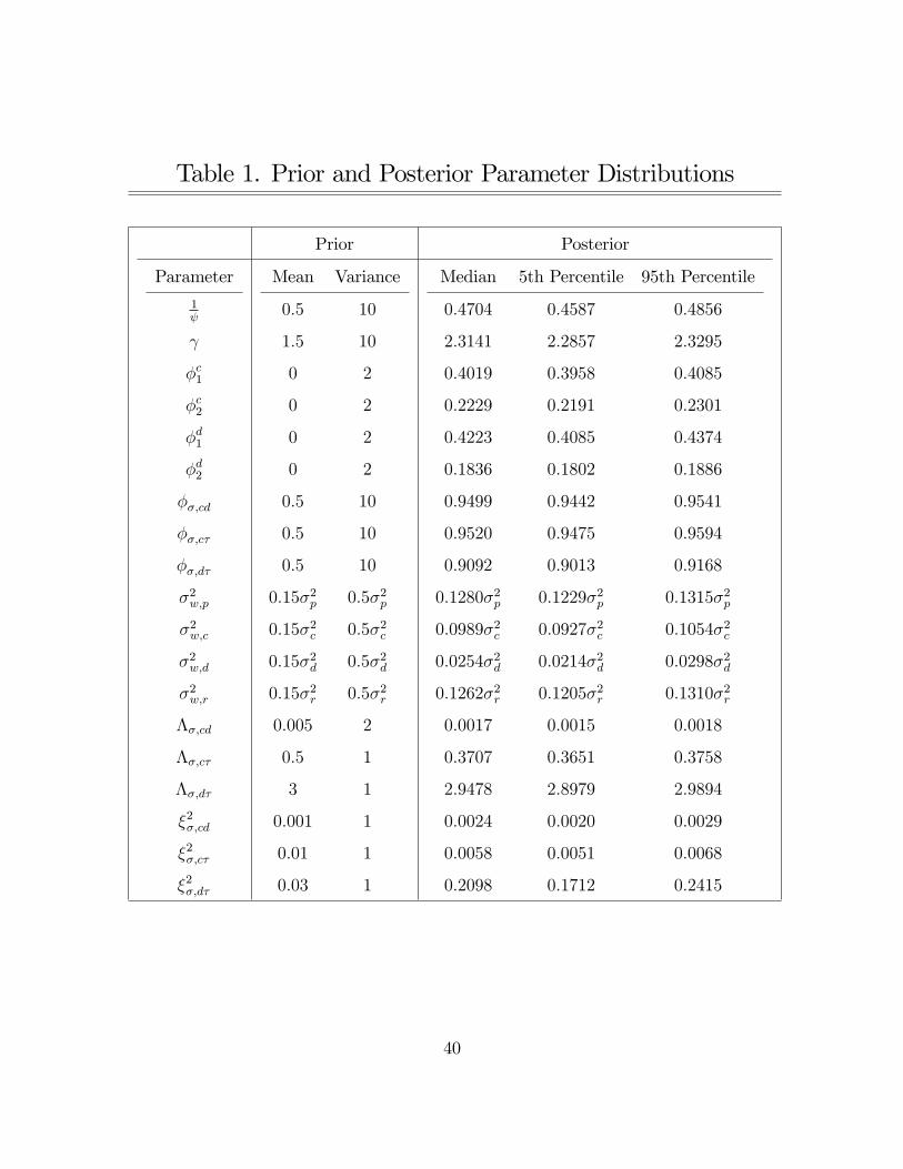
Table 1. Prior and Posterior Parameter Distributions

Prior Posterior

Parameter

1

�c1

�c2

�d1

�d2

��;cd

��;c�

��;d�

�2w;p

�2w;c

�2w;d

�2w;r

��;cd

��;c�

��;d�

�2�;cd

�2�;c�

�2�;d�

Mean Variance

0:5 10

1:5 10

0 2

0 2

0 2

0 2

0:5 10

0:5 10

0:5 10

0:15�2p 0:5�2p

0:15�2c 0:5�2c

0:15�2d 0:5�2d

0:15�2r 0:5�2r

0:005 2

0:5 1

3 1

0:001 1

0:01 1

0:03 1

Median 5th Percentile 95th Percentile

0:4704 0:4587 0:4856

2:3141 2:2857 2:3295

0:4019 0:3958 0:4085

0:2229 0:2191 0:2301

0:4223 0:4085 0:4374

0:1836 0:1802 0:1886

0:9499 0:9442 0:9541

0:9520 0:9475 0:9594

0:9092 0:9013 0:9168

0:1280�2p 0:1229�2p 0:1315�2p

0:0989�2c 0:0927�2c 0:1054�2c

0:0254�2d 0:0214�2d 0:0298�2d

0:1262�2r 0:1205�2r 0:1310�2r

0:0017 0:0015 0:0018

0:3707 0:3651 0:3758

2:9478 2:8979 2:9894

0:0024 0:0020 0:0029

0:0058 0:0051 0:0068

0:2098 0:1712 0:2415

40

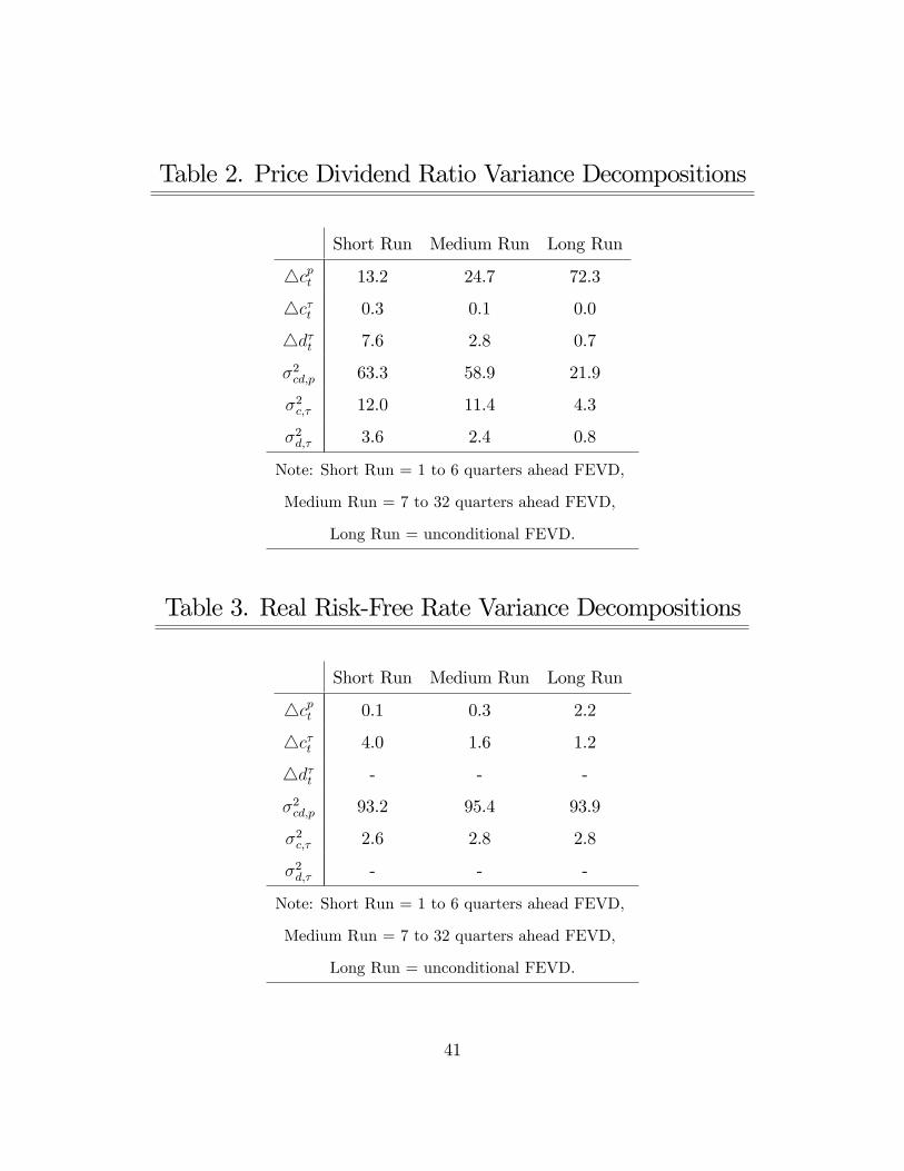
Table 2. Price Dividend Ratio Variance Decompositions

Short Run Medium Run Long Run

4cpt 13.2 24.7 72.3

4c�t 0.3 0.1 0.0

4d�t 7.6 2.8 0.7

�2cd;p 63.3 58.9 21.9

�2c;� 12.0 11.4 4.3

�2d;� 3.6 2.4 0.8

Note: Short Run = 1 to 6 quarters ahead FEVD,

Medium Run = 7 to 32 quarters ahead FEVD,

Long Run = unconditional FEVD.

Table 3. Real Risk-Free Rate Variance Decompositions

Short Run Medium Run Long Run

4cpt 0.1 0.3 2.2

4c�t 4.0 1.6 1.2

4d�t - - -

�2cd;p 93.2 95.4 93.9

�2c;� 2.6 2.8 2.8

�2d;� - - -

Note: Short Run = 1 to 6 quarters ahead FEVD,

Medium Run = 7 to 32 quarters ahead FEVD,

Long Run = unconditional FEVD.

41

Table 4. Consumption Growth Variance Decompositions

Short Run Medium Run Long Run

4cpt 0.9 5.6 35.3

4c�t 99.1 94.4 64.7

4d�t - - -

�2cd;p - - -

�2c;� - - -

�2d;� - - -

Note: Short Run = 1 to 6 quarters ahead FEVD,

Medium Run = 7 to 32 quarters ahead FEVD,

Long Run = unconditional FEVD.

Table 5. Dividend Growth Variance Decompositions

Short Run Medium Run Long Run

4cpt 0.1 0.8 6.7

4c�t - - -

4d�t 99.9 99.2 93.3

�2cd;p - - -

�2c;� - - -

�2d;� - - -

Note: Short Run = 1 to 6 quarters ahead FEVD,

Medium Run = 7 to 32 quarters ahead FEVD,

Long Run = unconditional FEVD.

42

Table 6. Price Dividend Ratio Variance Decompositions,by Component

Short Run Medium Run Long Run

4dt 54.8 90.5 258.4

rfrt 142.7 142.7 102.8

ret 404.8 376.8 140.1

�4dt;rfrt -44.4 -82.9 -242.5

�rfrt;ret -457.8 -427.0 -158.9

Note: Short Run = 1 to 6 quarters ahead FEVD,

Medium Run = 7 to 32 quarters ahead FEVD,

Long Run = unconditional FEVD.

43