Stochastic processes Response theory and fluctuation ... · Vol. 51, 1978 Stochastic processes 11: Response theory and .fluctuation theorems 207 terms of a ·correlation function

202 Helvetica Physica Acta, Vol. 51 (1978), Birkhliuser Verlag, Basel

Stochastic processes II: Response theory and fluctuation theorems 1)

Institut fOr Physik, Universitiit Basel, Switzerland

(19.X.I977)

Abstract. Linear and nonlinear response theory are developed for stationary Markov systems de­scribing systems in equilibrium and nonequilibrium. Generalized fluctuation theorems are derived which relate the response function to a correlation of nonlinear fluctuations of the unperturbed stationary process. The necessary and sufficient stochastic operator condition for the response tensor, ;�:(t), of classical nonlinear stochastic processes to be linearly related to the t wo-time correlations of the fluctuations in the stationary state (fluctuation theorems) is given. Several classes of stochastic processes obeying a fluctuation theorem are presented. For example, the fluctuation theorem in equilibrium is recovered when the system is described in terms of a mesoscopic master equation. We also investigate generalizations of the Onsager relations for non-equilibrium systems and derive sum rules. Further, an exact nonlinear integral equation for the total response is derived. An efficient recursive scheme for the calculation of general correlation functions in terms of continued fraction expansions is given.

l. Introduction

The purpose of this work on stochastic Markov processes is to develop a general scheme for the calculation of transport coefficients for systems whose unperturbed time-dependence is described by a master equation of a stationary Markov process. We study the response of stationary Markov systems to various external test forces. The response function contains valuable information about the dynamics of the system, in particular, the linear response function can be used to investigate the stability and the normal mode frequencies [1]. A common method for calculation of nonequilibrium transport quantities is via the kinetic equation for the averaged molecular distribution function, the Boltzmann equation [2, 3]. But within such a description one neglects the statistical fluctuations in the molecular distribution functions, which may be of importance in critical regimes. Furthermore, the deriva­tion of the Boltzmann equation cannot be outlined without certain restrictions which are rather strict (dilute system, weak short-range interactions, binary collisions, etc.) and often not satisfied [2, 3]. To a certain extent the lack of knowledge about the exact state of the system (i.e. the fluctuations) can be described quite naturally by stochastic Boltzmann-Langevin equations [ 4-6] or more generally by the use of a

1) Work supported by Swiss National Science Foundation. 2) Present address: Department of Physics, University of Illinois, Urbana, Illinois 6180 I, U.S .A.

Vol. 51, 1978 Stochastic processes l/: Response theory and.fiuctuation theorc•ms 203

coarse-grained (mesoscopic) Markov master equation for the process defined over a set of marcrovariables x(t) = {x1 (t), ... , x,(t)} forming the adequate state space !: of the physical system under consideration. .

In Sections 2 and 3 we show that the calculation of the linear response in the theory of stochastic processes [7, 8, 9] is related to a general correlation of fluctua­tions of the unperturbed stationary system. By the measurement of the response function we obtain information for both: the unperturbed system and the actual transport coefficient. Of special interest are those nonlinear classical stochastic pro­cesses for which the linear response tensor x(t) is linearly related to the two-time correlations between the fluctuations of the state variables x(t) (fluctuation theorem). Using the results given in reference [10]3) we investigate in Section 4 several classes of stochastic processes obeying such a theorem. All these theorems hold independently of the magnitude of the fluctuations of the state variables. Such theorems play an important role in statistical mechanics of conservative systems in thermal equilibrium (where one has the famous fluctuation-dissipation theorem [11-12]) and also in the theory of linear irreversible thermodynamics [13]. In Section 5 we give generaliza­tions of Onsager relations for stationary nonequilibrium systems and derive some sum rules. Based on the integral equations derived in Section I, we study in Section 6 the nonlinear response. An exact nonlinear integral equation for the nonlinear response is presented. The results obtained are discussed briefly in Section 7. In the Appendix we present a convenient numerical procedure for the calculation of correlation functions of stationary stochastic processes in terms of continued fraction expansions.

2. Linear respGJI8e theory for Markov processes and Markov-Field processes

We want to study the response of a macroscopic system, which is not necessarily in thermodynamic equilibrium, to an external dynamic perturbation. We assume that the unperturbed system can be described by a time-homogeneous Markov process with a stochastic dissipative generator r(I (2.20), I (3.1 )). We further assume that the process remains of Markov character in the presence of the perturbation, so that the perturbed macroscopic system is described by a stochastic generator f(t) of a nonstationary Markov process [I 0]

f(t) = r + re�xt). (2.1)

Here re�l(t) is the stochastic generator, which represents the effect of the perturbation. All the linear stochastic operators defined on !: act on the space n, the linear manifold of probabilities. In terms of the unperturbed 'free' time-homogeneous propagator

R(t - t0) exp {r(t t0)}, t > t0 (2.2)

we obtain in terms of usual linear operator notation in ll(!:) for the perturbed non­stationary propagator, .k(t I t0), the Dyson equation

.k(t I t0) = R(t - t0) + f1 R(t - s)rext(s).k(s I t0) ds, t � s � t0• (2.3) to

3) This reference will be denoted in the following by I.

204 P. Hiillggi H. P . ..4.

By use of the •proper self ener,Y. ["!a rn'(s 1 r> = r•xl(s) c5(s - r+), (2.4)

Equation (2.3) can more simp!)' be �tten in terms of multiplications ( •) of ()per8t()rs of TI(T), where T denotes thetimo-parameter space:

k. = R + R .r•xt•k. ...

.f.=j+O. t ' ' '

(2.5)

An alternative form for the Dyson equation is obtained if the relation be� the 'proper self energy', r•xt, and the •self energy', A, is used [14] ·· :.

A = r•xt + r•xt • R • A . •

•= <> +t. _,(2.6)

(> Hence, we have an alternative exact equation in closed form for the �urbed propagator k. · · . , .

k = R + R • A•R. t . (2.1)

... = i + •. i

The perturbation, r(t)•xt, is applied after the system has been prepared at time r0·in a given stationary state described by the stationary probability p51(x). Without loss of generality the perturbation operator Pxl(t)' is expanded in terms of time-d�dent external forces F1(t) and linear stochastic operators 01, which may be enlarged to form a Lie algebra

·

P"1{t) = .f(t)·O. (28) Thus to first order in the self energy A we obtain from equation (2. 7) for the perturbed probability p(t) of the nonstationary Markov process

p(t) Pst + it R(t - r)F('r) Op81 dr. (2.9) to

The linear response tensor x(t - r) is then defined by the relation of the response of the state functions +(x) = {+1(x), +2(x), ... , + .. (x)}

(c5+(t))perturbed = (+(t))Perturbed _ (+(!))unperturbed

= f +(x){p(xt) -pix)} dx,

to the external test forces F(t)

(c5+(t))perturbed = it I(t- r)F(r) dr. to

(2.10)

(2.11)

Vol. 51, 1978 Stochastic processes II: RespoiiSe theory and fluctuation theorems

From equations (2.8-2.11) we find by use of the unit step function lJ(t)

205

x(t) = lJ(t) J +(x)R(xt I yo)[Op.t]y dy dx. (2.12)

The same procedure can be used if stochastic field variables X{r) = (X 1 (r), ... , X"(r)) must be chosen as the system variables. The system is then described in terms of a functional master equation. The linear response is given with space dependent force densities F(rt) by

<b+(rt))perturbed � J: Jx(r,r';t- t)F(r';t)dr'dt. (2.13)

In terms of functional integrations we obtain for the linear response tensor

x(r, r'; r) = lJ( t) f +(r)R(+(r), t I "''(r'), 0). [np.t]\t(r').@"'.@"''· (2.14)

For Markov field processes which are homogeneous both in time, t, and space, r, the linear response in equation (2.13) is given by a convolution in time and space or in

. Fourier space

<b+(q, w))perturbed = x(q, w)F(q, w). (2.15)

The problems with in general non-Gaussian stochastic fields (functional integration) can be eliminated if a cell description for the space is introduced or if the stochastic Fourier components for the corresponding vectorial Markov process are used. In the following we restrict the discussion to real vectorial Markov processes x(t). We will also specialize the discussion by setting the state functions +(x) in equation (2.10) equal to the state variables x unless explicitly stated otherwise.

3. Generalized fluctuation-theorems

In this section we will express the response tensor x(t) via correlation functions. We may define a vector valued state function cj)(x)

(3.1)

so that the response tensor in equation (2.12) of the state variables x(t) can be written as a correlation function over the unperturbed system

X(t) = lJ(t)(x(t)cj)(x(o))). (3.2)

Since the perturbation cannot change the normalization of the probabilities we obtain

(3.3)

Therefore, the state variables x may be replaced by its fluctuations � = x -(x)unperturbed and equation (3.2) has the form of a generalized fluctuation theorem:

X(t) = lJ(t)(�(t}cj)(x(o))). (3.4)

206 P. Hlinggi H. P. A.

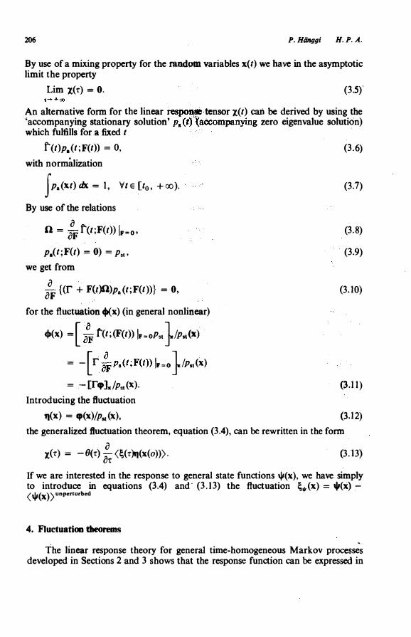
By use of a mixing prQperty for the random variables x(t) we have in the asymptotic limit the property

Lim X(T) = 0. (3.5)'

An alternative form for the linear respol\ie tensor x(t) cart be derived by using the •accompanying stationary solution' p.(r){accompanying zero eigenvalue solution) which fulfills for a fixed t

f'(t)p.(t;F(t)) = 0, (3.6) with norm.itlization

fp.(xt)dx = 1, '<lte [10, +oo). By use of the relations

0 0 =

oF f'(t;F(t)) lr=o•

p.(t;F(t) = 0) = Psto we get from

0 oF {(r + F{t)Sl)p.(t;F(t))} = 0, for the fluctuation +{x) (in general nonlinear)

cf»(x) =[ :F t(t;{F(t)) lr,.oPst JIPsl(x)

= -[r :F

p.(t;F(t)) lr,.0 JIP •• (x)

= -[np1/Pst(X); Introducing the fluctuation

'l(x) = cp(x)/P51(X),

(3.7)

(3.8)

(3.9)

(3.10)

(3.11)

(3.12)

the generalized ftuctuation theorem, equation (3.4), can be rewritten in the form

0 X(T) = -6(1:) o1: (I;(T)q(x(o))). (3.13)

If we are interested in the response to general state functions \jl(x), we have simply to introduce in equations (3.4) and (3.13) the fluctuation l;.;(x) = +(x) :­( \jl(x)) unperturbed

4. Fluctuation theorems

The linear response theory for general time-homogeneous Markov processe� developed in Sections 2 and 3 shows that the response function can be expressed in

Vol. 51, 1978 Stochastic processes 11: Response theory and .fluctuation theorems 207

terms of a ·correlation function of, in general, nonlinear fluctuations of the unper­turbed stochastic system. A measure of the linear response function yields therefore information for both: the transport coefficient and the unperturbed stationary system.

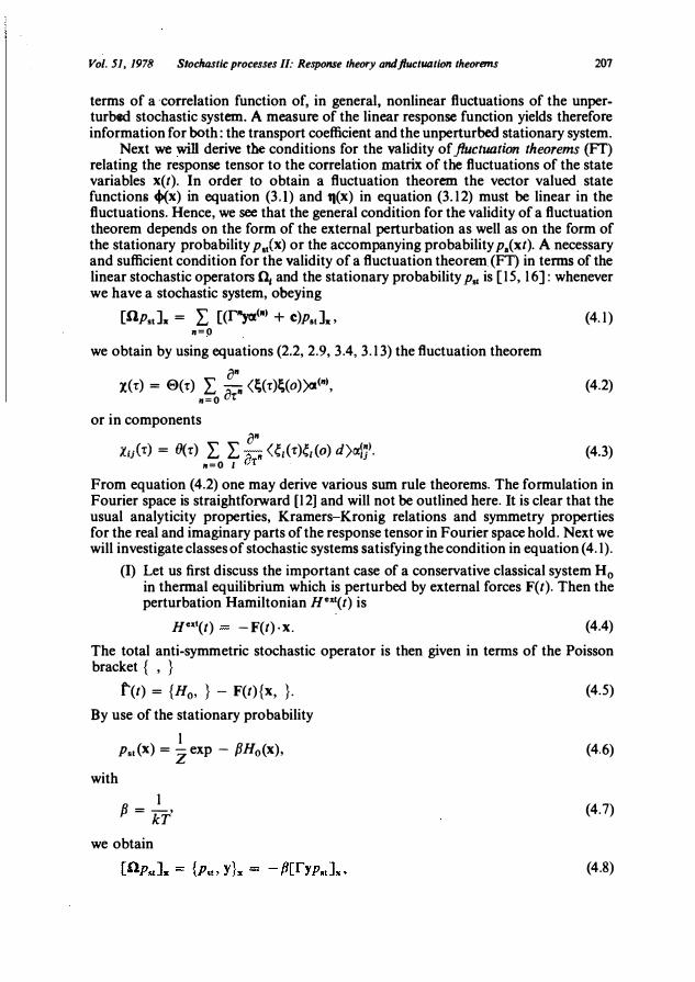
Next we will derive the conditions for the validity of fluctuation theorems (Fr) relating the response tensor to the correlation matrix of the fluctuations of the state variables x(t). In order to obtain a fluctuation theorem the vector valued state functions +(x) in equation (3.1) and fl(x) in equation (3.12) must be linear in the fluctuations. Hence, we see that the general condition for the validity of a fluctuation theorem depends on the form of the external perturbation as well as on the form of the stationary probability pix) or the accompanying probability p.(xt). A necessary and sufficient condition for the validity of a fluctuation theorem. (Fl) in terms of the linear stochastic operators O. and the stationary probability Pst is [15, 16]: whenever we have a stochastic system, obeying

[np.,J, = L: [(P'ycr<•> + e)p.a.. (4.1) n=O

we obtain by using equations (2.2, 2.9, 3.4, 3.13) the fluctuation theorem

a• x<-r> = a<•> L: -. <;<•>;<o>>a<•>, (4.2)

n=O at

or in components

xu(•) = O(t) L L a•

<e,(•)e,(o) d)IXljl. (4.3) 11=0 I

From equation (4.2) one may derive various sum rule theorems. The formulation in Fourier space is straightforward [12] and will not be outlined here. It is clear that the usual analyticity properties, Kramers-Kronig relations and symmetry properties for the real and imaginary parts of the response tensor in Fourier space hold. Next we will investigate classes of stochastic systems satisfying the condition in equation (4.1 ).

(I) Let us first discuss the important case of a conservative classical system H0 in thermal equilibrium which is perturbed by external forces F(t). Then the perturbation Hamiltonian Hu1(t) is

He'<�(t) -F(t)·x. (4.4)

The total anti-symmetric stochastic operator is then given in terms of the Poisson bracket { , }

f'(t) = {H0, } - F(t){x, }. (4.5)

By use of the stationary probability

1 p •• (x) =

Z exp - fJH0(x),

with

1 fJ = -· kT

we obtain

(4.6)

(4.7)

(4.8)

208 P. Htilggl ,, H. P. A.

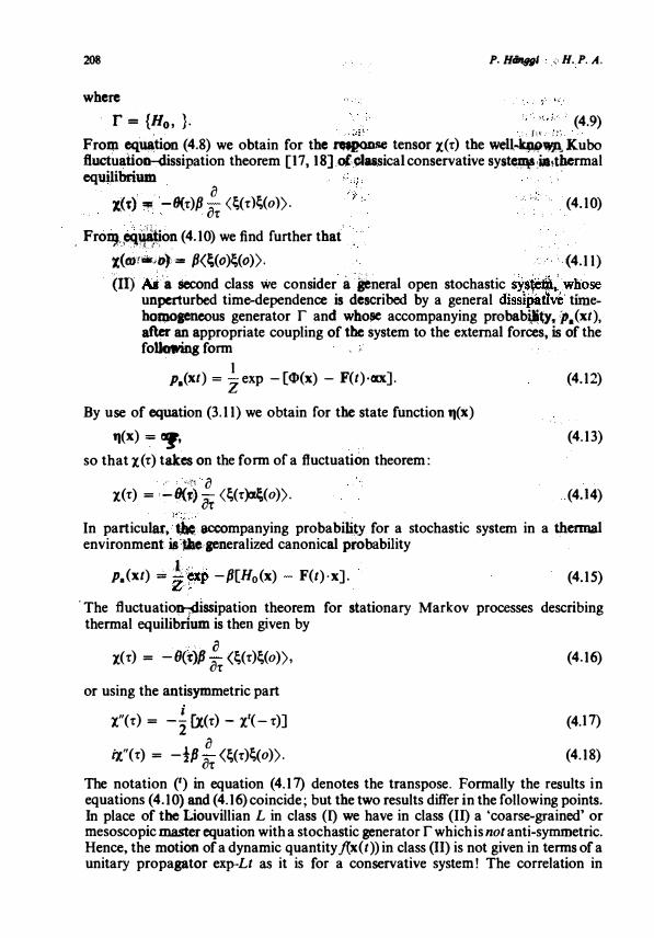
where r = {H0, }.

.:, ftt• j;' (4.9)

From equation (4.8) we obtain for the rqpo.n.se tensor x(r) the well�WAKubo fluctuation-dissipation theorem [17, 18].ot'�assical conservative syst�:i.a•thermal equilibrium

· · , . a

X(t) • -8(r)/J or (;(r);(o)).

. FroDJ.!=Q.lfiipon (4.10) we find further that

(4.10)

X(mtiil>D)• == /J(;(o);(o)). (4.11) (II) A&' 'a second class we consider a ieneral open stochastic SY.s�: whose

unperturbed time-dependence is described by a general dissipadve' tilne­hol110aeneous generator r and whose accompanying probab\¥(y� P.(xt), after an appropriate coupling of the system to the external forces, is of the folknring form , ,

I p.(xt) = Z exp - [f])(x) - F(t)·u]. (4.12)

By use of equation (3.11) we obtain for the state function q(x)

q(x) = C1f• so that x( r) takes on the form of a fluctuation theorem:

. '·�� a x(r) = ·-8(,) ot (;(r)cx;(o)).

(4.13)

.(4.14)

In particular, �·.accompanying probabilizy for a stochastic system in a thermal environment is lite aeneralized canonical probability

J .. · P.(xt) :::: e�P -fJ[H0(x) F(t)·x]. (4.15)

·The fluctuatiop:-;dissipation theorem for stationary Markov processes describing thermal equilibrium is then given by

.. a x(r) = -O(t)/1 or (;(r);(o)), (4.16)

or using the antisymmetric part

x"(r) = _!_ [X(r) - 1.'(- r)] 2

. a ll:"(r) = -t/1 or (;(r);(o)).

(4.17)

(4.18)

The notation (') in equation (4.17) denotes the transpose. Formally the results in equations (4.10) and (4.16) coincide; but the two results differ in the following points. In place of the Liouvillian L in class (I) we have in class (II) a 'coarse-grained' or mesoscopic master equation with a stochastic generator r which is not anti-symmetric. Hence, the motion of a dynamic quantity J{x(t)) in class (II) is not given in terms of a unitary propagator exp-Lt as it is for a conservative system! The correlation in

Vol. 51, 1978 Stocllastic proceiiSes II: Response theory and fluctuation theorems 209

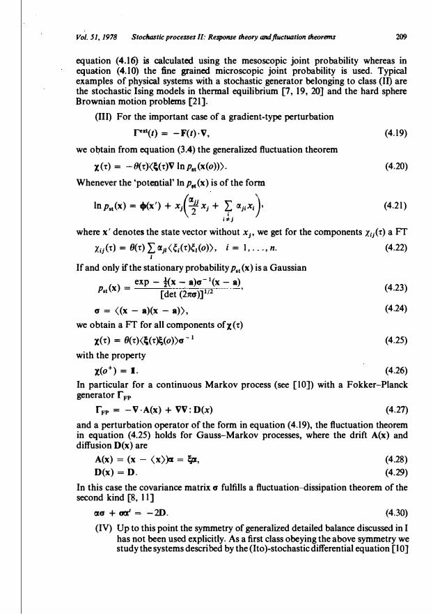
equation (4.16) is calculated using the mesoscopic joint probability whereas in equation (4.10) the fine grained microscopic joint probability is used. Typical examples of physical systems with a stochastic generator belonging to class (II) are the stochastic Ising models in thermal equilibrium [7, 19, 20] and the hard sphere Brownian motion problems [21].

(III) For the important case of a gradient-type perturbation

pxt(t) = - F(t) · V, we obtain from equation (3.4) the generalized fluctuation theorem

x(r) = -8(r)\�(r)V lnp.,(x(o))). Whenever the 'potential' In p11 (x) is of the form

lnp81(x) = .p{x') + Xjei:i Xi+ f IXJ;X;} i*i

(4.19)

(4.20)

(4.21)

where x' denotes the state vector without x1, we get for the components Xii(-r) aFT

l;j('t") = 8(-r) L IXjl(e;(-r)e,(o)), i = I, . . . , n. (4.22) I

If and only if the stationary probability p., (x) is a Gaussian

exp - !(x - a)a-1(x - a) P.,(x) =

[det (21t0')]1/2 • (4.23)

a = ((x - a)(x - a)), (4.24)

we obtain aFT for all components ofx(-r)

x(-r) = 8(-r)(l;(-r�(o))a 1

with the property

x(o+) = 1.

(4.25)

(4.26)

In particular for a continuous Markov process (see [10]) with a Fokker-Planck generator r FP

rFP = -V ·A(x) + VV: D(x) (4.27)

and a perturbation operator of the form in equation ( 4.19), the fluctuation theorem in equation (4.25) holds for Gauss-Markov processes, where the drift A(x) and diffusion D(x) are

A(x) (x (x))x = !;a:, D(x) D.

(4.28) (4.29)

In this case the covariance matrix a fulfills a fluctuation-dissipation theorem of the second kind [8, II]

�+� - ID. �� (IV) Up to this point the symmetry of generalized detailed balance discussed in I

has not been used explicitly. As a first class obeying the above symmetry we study the systems described by the (Ito )-stochastic differential equation [I 0]

210

where

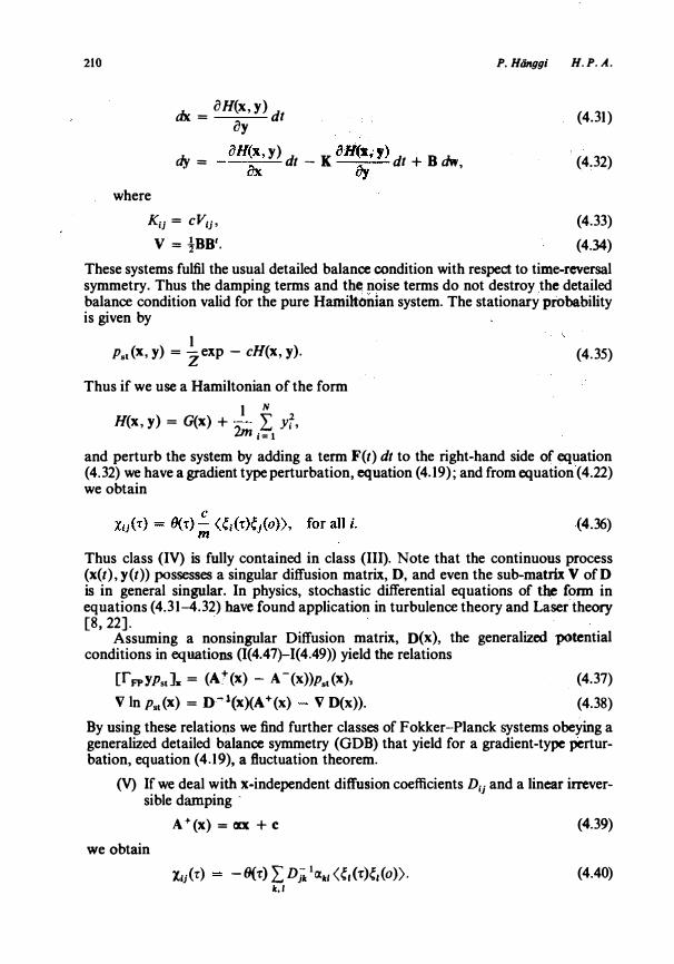
dx = oH(x, y) dt oy dy = oH�, y) dt- K o�;y) dt + B dw,

K;i = cVIi, V = !BB'.

P.Hanggi H.P. A.

(4.31)

(4.32)

(4.33) (4.34)

These systems fulfil the usual detailed balance condition with respect to time-reversal symmetry. Thus the damping terms and the noise terms do not destroy the detailed balance condition valid for the pure Hamiltonian system. The stationary probability is given by

1 p.,(x, y) = -zexp - cH(x, y). (4.35)

Thus if we use a Hamiltonian of the form

1 N H(x, y) = G(x) + 2m i�l yf, and perturb the system by adding a term F(t) dt to the right-hand side of equation (4.32) we have a gradient type perturbation, equation (4.19); and from equation (4.22) we obtain

(4.36)

Thus class (IV) is fully contained in class (III). Note that the continuous process (x(t), y(t)) possesses a singular diffusion matrix, D, and even the sub-matrix V of D is in general singular. In physics, stochastic differential equations of the form in equations (4.31-4.32) have found application in turbulence theory and Laser theory [8, 22].

Assuming a nonsingular Diffusion matrix, D(x), the generalized potential conditions in equations (1(4.47}-1(4.49)) yield the relations

[r FPYPstJx = (At(x) - A -(x))p.,(x), (4.37) V In p.,(x) = D""'1(x)(A +(x) V D(x)). (4.38)

By using these relatio�s we find further classes of Fokker-Pianck systems obeying a generalized detailed balance symmetry (GDB) that yield for a gradient-type pertur­bation, equation (4.19), a ftuctuation theorem.

(V) If we deal with x-independent diffusion coefficients D;i and a linear irrever­sible damping ,

we obtain

A+ (x) = cxx + c (4.39)

xij('r) - B('r) 2: Djk 1cxt, <e,('r:)e,(o)). lr;,l

(4.40)

Vol. 51, 1978 Stochastic processes II: Response theory and .fluctuotion theorems 2ll

This form has first been discussed in the case of a GOB-symmetry with respect to the usual time reversal symmetry in References [23, 24].

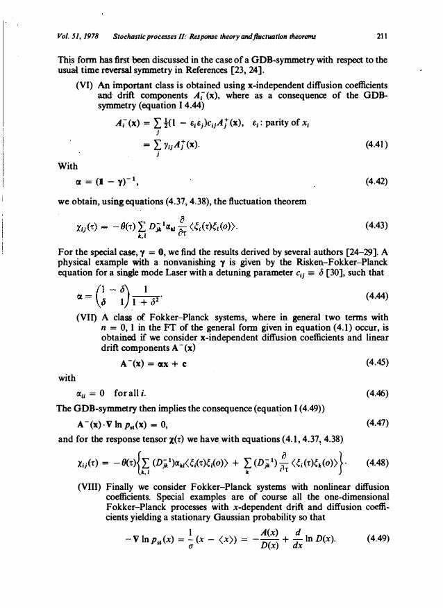
(VI) An important class is obtained using x-independent diffusion coefficients and drift components Aj"(x), where as a consequence of the GOB­symmetry (equation I 4.44)

Aj"(x) = L !(l - e1e)ciiAj (x), e1: parity of x1 j

= L yiJAj(x). j

(4.41)

With

12 =(I- y)-1, (4.42)

we obtain, using equations (4.37, 4.38), the fluctuation theorem

(4.43)

For the special case, y = 0, we find the results derived by several authors [24-29]. A physical example with a nonvanishing y is given by the Risken-Fokker-Planck equation for a single mode Laser with a detuning parameter c11 ;: {) [30], such that

with

{)) 1 l

.l+fJ2• (4.44)

(VII) A class o( Fokker-Planck systems, where in general two terms with n = 0, 1 in theFT of the general form given in equation (4.1) occur, is obtained if we consider x-independent diffusion coefficients and linear drift components A-(x)

A -(x) = !XX + c (4.45)

au = 0 for all i. (4.46)

The GOB-symmetry then implies the consequence (equation I (4.49))

A- (x) · V In p •• (x) = 0, (4.47)

and for the response tensor x(r) we have with equations (4.1, 4.37, 4.38)

x11(r) = 9(-c){L (Djk1)a11(�1(-c)�1(o)) + L (Djk1) � (�1(-c)�1(o))} · (4.48) lr.,l lr. ur

(VIII) Finally we consider Fokker-Planck systems with nonlinear diffusion coefficients. Special examples are of course all the one-dimensional Fokker-Planck processes with x-dependent drift and diffusion coeffi­cients yielding a stationary Gaussian probability so that

I A(x) d V lnp •• (x) = � (x - (x)) -D(x) +

dx In D(x). (4.49)

212

. For· example, we get with

A(x) = coe e-"'�1, oc > 0, Co < - 2oc ·c.

D(x) = c1 e-"'�1, c1 > 0

for u-1 in equation (4.25)

u-1 = -(c0/ct + 2oc) > 0.

Furthermore, for the nonlinear Brownian motion with

A<e> = - [e + re3J,

D(e) = [I + y(2 + e2)], we obtain from equations (4.25) and (4.49)

x(r) = O(t)(e(r)e(o)).

P. Hllnggl H. P. A. .

(4.50)

(4.51)

(4.52)

(4.53)

(4.54)

(4.55)

As a nontrivial example for a vector valued Fokker-Planck process with x-dependent diffusion coefficients we study the (Ito )-stochastic differential equation

dx1 = x2 dt,

dx2 = ( -x1 + X2- xi}dt + x2dw2• (4.56)

The stationary probability is found to be

I 2 z Pst(x.x2) = - exp -(xt + x2), (4.57) 1t

so that by adding a perturbation F dt to the right-hand side of equations (4.56, 4.57) a fluctuation theorem of the form in equation (4.25) holds, with

(4.58)

Note that the Fokker-Planck classes (IV) and (VIII) are fully contained in the more general class (III). But among the Fokker-Planck classes obeying a GBD-symmetry, (IV-VIII), none of the discussed classes is contained fully as a subclass in another class.

All the response functions considered so far can be expressed via a correlation function over the unperturbed system, calculated through the stationary joint­probability pC2>(x , t; yo). Hence, one needs the complete eigenvalue analysis for the stochastic generator r [1 0]. In practice this may become in general very intractable. An approximation procedure requiring the minimum human and computer effort is therefore very desirable. Such a procedure based on continued fractions is sketched in the Appendix.

5. Generalized Onsager relations and sum rules

In this section we discuss some further consequences for the response function in the presence of symmetries considered in I. If S denotes a symmetry transformation, S e G, [1 0] in the state space I: belonging to the symmetry group G of x(t)

08rOi1 = r, VSe G (5.1)

Vol. 51, 1978 Stochastic processes II: Response theory and ftuctllf.ttion theorems 213

we obtain for the response tensor of the transformed ergodic process [10], t(t) = Sx(t), when the perturbation remains of the same form as in the original process x(t), the useful relation

x('r) = O('r)(;(T*t(o))) = 0{1:)(/;(T*X(O)))

. = X(T), VS e G. (5.2) Moreover, ifx(t) obeys a GOB-symmetry with respect to a transformation T0 [10]:

and

TJ = I (5.3)

</>/ex) = s1</>1(x), (5.4) we have from equation (14.16)

xi)( 'I:, l.) = O(T)(e1(T)</>1(x(o))).t = O(T)s1s1(</>1(X(T))e;(O))..t. (5.5)

Here l. denotes a set of external parameters and sl. = (s1 A.1, • . . , s,A.,). In particular, we obtain in case of equation (4.1) with diagonal matrices

11<"1 = diag (c<"1) . iJ"

X;/1:) = 0{1:) L: d"'� <e;(1:),1(o)), ,..o u'l:

(5. 6)

(5.7)

generalized Onsager relations for stationary Markov processes obeying a fluctuation theorem of the form in equation (5.7) with 11<"1 given in equation (5. 6) and a GOB­symmetry with respect to a transformation T0:

X11(T, l.) = s1s1x11(T. sl.). (5.8) For example, considering the fluctuation theorem in equation (4.43) with A -(x) =0 and D = diag (1//l"rr) we obtain for the response tensor the Onsager relations

iJ xij(1:) = s;s1x1,(T) = -0(1:)prr iJ1: <e1(T)e1(o)). (5.9)

In contrast to equilibrium situations the relations in equation (5.8) may hold in off­equilibrium situations, e.g. in a Laser system, with an effective Boltzmann factor pr.

Introducing the Fourier transform x(ro) of the response tensor

1(1:) = 0(1:)(l;(1:)p(x(o))) = 0{1:)C{1:), (5.10)

x(ro) = Lim f"" C{1:) ei(CJ>+I£)< d1: = x'(ro) + ix;"(ro), .-.o* Jo

(5.11)

we obtain for the in general nonlinear correlation C11(1:), depending on whether C11(1:) is even or odd in 1:

(5. 12)

214 P. Hiinggi H. P • ..4.

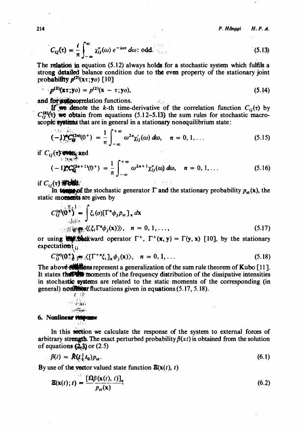
(5.13)

The relation in equation (5.12) always holds for a stochastic system which fulfils a strong d�iled balance condition due to the even property of the stationary joint probabilh)'y21(x-r ; yo) [10]

· · p'21(s:t;yo) = l2'(x - -r;yo) , (5.14) and;��1tdation functions. . . . ·

. f.t ,,. .denote the k-th time-derivative of the correlation function Cii(-r) by C1�'�) we obtain from equations (5.1 2-5.13) the sum rules for stochastic macro­scopiC ·.,atids that are in general in a stationary nonequilibrium state:

( -J .. )".C(2"1(o+) = ! J +<ll wlrrx: (ro) dco, n = 0, 1, ... " ,, '*' .,. J . .. ,. -<1)

(5.15)

if c,J (r)'�and

( - 1;;� +1>(o+) = ! J +<�> ro2"+ 1x;j(Cil) dco, n = o, 1,... (5.16)

1t -<()

ifc,1<-rrJI'.lMk.i. .. . In �the stochastic generator rand the stationary probability p51(x), the

static mo� are given by

( ) ' + . �)) f C,j (Oti<�i: 'l(o)[r"�JPstJ x dx

J;fr'�tp:·«'1r"�1(x))), n = 0, 1, ... , (5.17) or using

. �ward operator r+' r+(x, y) = r(y, x) [10], by the stationary

expectation t ·o \

C1�"'(0t) f'f.•.([r+"e;],.�1(x)), n = 0, 1,... (5.18) The abo� ... DS represent a generalization of the sum rule theorem of Kubo [11]. It states thiPIIt moments of the frequency distribution of the dissipative intensities in stochastic.l)'ltems are related to the static moments of the corresponding (in general) nolillllir fluctuations given in equations ( 5.17, 5 .18).

r'. n�

6. Nonlinear ni1f011se '- � ·: '',

In this section we calculate the response of the system to external forces of arbitrary strength. The exact perturbed probability jj(xt) is obtained from the solution of equations (�� or (2.5)

ft(t) = J(f,J,to)Pst· (6.1) By use of thevector valued state function S(x(t), t)

S(x(t); t) == [Qjj(x(t), t)]� Pst(x) (6.2)

Vol. 51, 1978 StocluJstic processes II: Response theory and fluctuation theorems

with

(S("(t), t))81 = f [Q6(t)]. dx = 0,

215

(6.3)

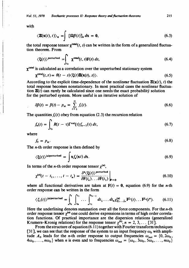
the total response tensor x'Oia1(t, s) can be written in the form of a generalized fluctua­tion theorem .. From

(;�t))perturbed = f' x-Xt, s)F(s) ds, (6.4) J,o xtotaJ is calculated as a correlation over the unperturbed stationary system

xlotal(t,s ) = B(t - s)(l;(t):E(x(s), s)). (6.5)

According to the explicit time-dependence of the nonlinear fluctuation S(x(t), t) the total response becomes nonstationary. In most practical cases the nonlinear fluctua­tion S(t) can r�Jrely be calculated since one needs the exact probability solution for the perturbed system. More useful is an iterative solution of

00

Jfj(t) = fj(t)- Pst = L J;(t). 1=1

The quantities.t; (t) obey from equation (2.3) the recursion relation

J..(t) = r R(t - r)rext('r)j,_1 ('r) dr, J,o where

fo = Pst• The n-th order response is then defined by

(l;(t))(ll)perturbed = f xf..(xt) dx.

In terms of the n-th order response tensor x1">, 11 J"(l;(t))perturbed I 1< >(t - t 1, • • • , t - t,.) = £SF( )

JF( ) t, · · · 11 F=O

(6.6)

(6.7)

(6.8)

(6.9)

(6.10)

where all functional derivatives are taken at F(t) = 0, equation (6.9) for the n-th order response can be written in the form

<el(t))(n)penurbed = f' i'' . . . r,_, dtl . . . dt��x�l'� ... l"FI.I(t) . . . Fln(t"). (6.11) Jto to J,o Here the underlining denotes summation over all the force components. For the n-th order response tensor t"> one could derive expressions in terms of high order correla­tion functions. Of practical importance are the dispersion relations (generalized Kramers-Kronig relations) for the response tensor t">, n = 2, 3, . . . [31].

. From the structure of equation (6. l l)togetherwitbFourier transform techniques [31], we can see that the response of the system to an input frequency w0 with ampli­tude A0 leads for the n-th order response to output frequencies W001 = {0, 2w0, 4w0, . • • , nw0} when n is even and to frequencies W001 = {w0, 3w0, 5w0, • • • , nw0}

P. Hlinggi H. P . .4.

wheo n is odd; each with an amplitude proportional to A0. Note that for an unper­tu"'-"d, but nonstationary process we obtain a response at an arbitrary frequency �pven in the linear response [32]. Hencevtbe.measurement of the linear response c:lan be used to decide if the initial system is stationary or not.

, . fmaltr,, we derive an exact nonlineu: ip.tegral equation for the total response (��t))penur ed (not the total perturbed proba])ility ft(t)) using the technique of func­tional integration and functional derivatives. With the functional derivative taken at finite F(s)

J(;(t))perturbed

I Z(t, s;F(s)) = JF

the total response is written F(s)•

(;(t))Perturbed = Ids f Z(t, s;F(s)) �F(s).

The quantity Z fulfi1ls from equation (6.4) the Dyson equation

Z(t, t';F(t') = lotal(t;t')9(t t')9(t'- to)

+ i' ds F(s) 1• dr !.(t, s, r)Z(s, t' ;F(t')), to to

with the self energy !. c5xtotal( t, s)

!.(t, s, r) = D(;(r))perturbed

In zero order in F we have for Z

Z(t, s;F(s)) = x<11(t - s)9(s 10), giving again the linear response result in equation (2.11)

(;(t))(llperturbed = i' x<l)(t s)F(s) ds. to

7. Conclusions

(6.12)

(6.13)

(6.15)

(6.16)

(6.17)

We have derived generalized fluctuation theorems for stationary Markov pro­cesses and Markov field-processes. In Section 4 we have developed the necessary and sufficient conditions for stochastic systems under which the theorem reduces to an ordinary fluctuation theorem. Several classes of stochastic processes describing e�uilibrium and non-equilibrium systems have been described which fulfil a fluctua­tion theorem independent of the magnitude of the fluctuations. For example, the fluctuation-dissipation theorem in thennal equilibrium has been derived if the system is described in tenns of a mesoscopic master equation. The existence of fluctuation theorems simplifies considerably the renonnalized perturbation scheme for non­linear classical stochastic processes [33-35]. They may also find wide application in the theory of critical dynamics [35-36]. The generalized Onsager relations given in Section 5 also hold in non-equilibrium systems where they simplify the calculation

Vol. 51, 1978 Stochastic processes II: Ri!sponse theory and fluctuation theorems 217

of the response tensor considerably. All results iD. this paper, except the nonlinear response results in Section 6, can be evaluated by use of the recursive calculation scheme given in the Appendix provided the stationary probability p81(x) and the generator r of the time-homogeneous Markov process are known.

Appendix : Ellieient calculation of general correlation functions

We present an efficient procedure for the calculation of response functions or correlation function. The response function XiJ(r) = x('r) always has the form of a generalized fluctuation theorem equation (3.4)

x(r) = O(r)(g(x(r)f(x(o))). ( A.l)

Using the Taylor series expansion

x(r) = O(r) f P� t", .... on. (A.2)

we can construct from the short time behaviour a type of analytical continuation using continued fraction expansions. The method will only require the explicit form of the stochastic generator rand the knowledge of the stationary probability p81(x). By use of equations (5.17) or (5.18) we have for the static moment in equation (A.2) the expressions

d"x(r) I + p, = dr"

r = 0 '

= ((g(x)r''l'(x))),

= ([r+"g],./(x)).

For the Fourier transform x(ro)

x(ro) = Lim f"" e1(m+ 1*x(r) dr � ... o+ Jo

we obtain with z = - iro from equation (A.2) the sum rule expansion <Xl

x(ro) = L P: 1 • 11=0 z"

(A .3)

(A.4)

(A.5)

(A.6)

(A.7)

The series in equation ( A.7) are in general asymptotic series. Next we construct a continued fraction expansion which serves as an analytical continuation of the series in equation ( A.7). The corresponding continued fractions to equation ( A.7) are given by

Ct c2 x(ro) = --z+ I + z+ (A.8)

(A.9)

218 P. Hiinggi · ···B. P • .A.

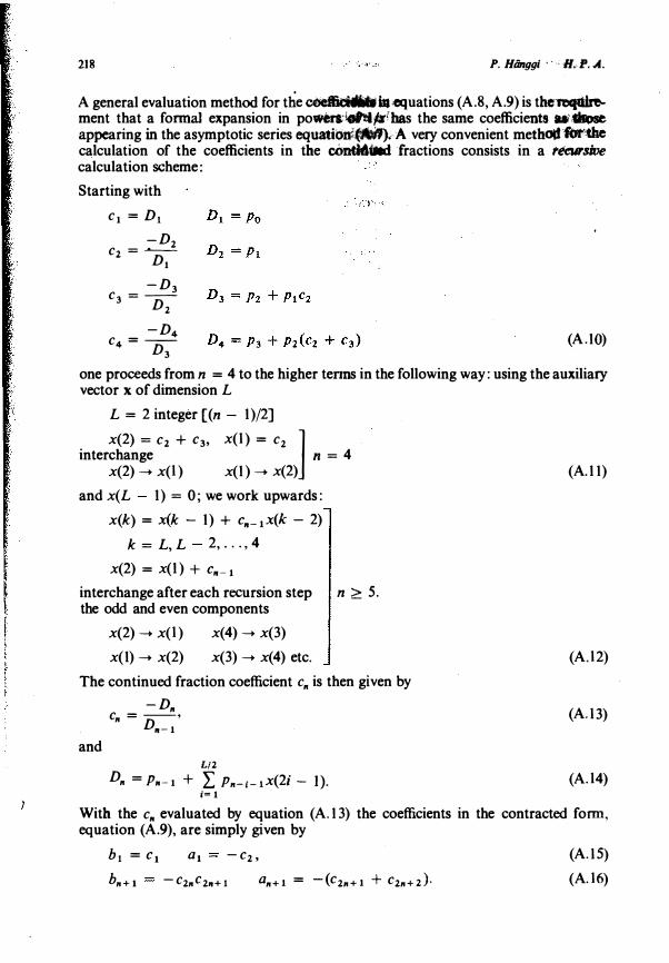
A general evaluation method for the �hi ;equations (A .8, A.9) is therecpdre­ment that a fonnaJ expansion in powenr�!J'fhas the same coefficients Wfill>se appearing in the asymptotic series equario�A very convenient methodfot'the calculation of the coefficients in the oonth\(ted fractions consists in a rteursive calculation scheme:

Starting with

c1 = Dl

-D2 c2 = ..._____

D1

-D3 c3 = -­

D2

-D4 c4= -­

D3 (A .I O)

one proceeds from n = 4 to the higher tenns in the following way: using the auxiliary vector x of dimension L

L = 2 integer [(n - I )/2]

x(2) = c2 + c3, x(l) = c2 ] interchange n = 4

x(2) - x(l) x(I ) - x(2)

and x(L I) = 0; we work upwards:

x(k) = x(k - I)+ Cn_1x(k - 2)

k = L,L 2, ... ,4

x(2) = x(I ) + Cn-1

interchange after each recursion step n ;:::: 5. the odd and even components

x(2)- x(l)

x(I)- x(2)

x(4)- x(3)

x(3)- x(4) etc.

The continued fraction coefficient c,. is then given by

-D,. c,. = __ ,

Dn-1 and

L/2 D,. = P .. -1 + L P11-i-tx(2i- 1).

i= 1

(A. I I)

(A.l2)

(A.l3)

(A.l4)

With the c .. evaluated by equation (A.I 3) the coefficients in the contracted form, equation (A.9), are simply given by

bl = Ct at -c2,

b,.+t -c2,.c2n+l a,.+1 = -(c2,.+1 + c2,.+z)·

(A.l5)

(A.l6)

Vol. 51, 1978 Stochastic processes /I: Response theory andjluctiJIJiion theorems 219

A Fourier inversion yields the response function in time space. In practice one has to break off the usuatty infinite continued fractions at a finite order. So far the con­sequences and the quality of this approximation has not been discussed quantitatively. Hence, the construction of error bounds is very desirable. In systems obeying a strong detailed balance condition the error bounds for autocorrelation functions and their time-derivatives have been discussed elsewhere [37, 38].

REFERENCES

[I] H. THOMAS, 'I'heory of Condensed Matter, Eds. Bassani et al. (International Atomic Energy Agency, 357-393, Vienna 1968).

[2] L. P. KADANOFP and G. BAYM, Q�J�Jntum Statistical Mechanics (W. A. Benjamin, Inc., New York 1962).

[3] J. M. Bun and A. H. OPIE, J. Phys. A7, 1895 (1974). [4] M. BrxoN and R. ZWANZIG, Phys. Rev. 187, 267 (1969). [5) J. LOGAN and M. KAC, Phys. Rev. A/3, 458 (1976). [6) M. TOKUYMAMA and M. MOill, Progr. Theor. Phys. 56, 1073 (1976). [7) P. HANOOI and H. THOMAS, Physic Reports: to be published. f.BJ H. HAKBN, Rev. Mod. Phys. 47, 61 (1975). {9] M. IOSJFESCU and P. TXuru, Stodwstic Processes and Applications in Biology and Medicine, Vol. I

(Springer, New York 1973). [10] P. H.\NOOI, Helv. Phys. Acta 51, 183 (1978). [11] R. KUDO, Rep. Progr. Phys. 29, 255 (1966). [12] D. DES CLOJZSAUX, 17teory of Condensed Matter, Eds. Dassani et al. (International Atomic Energy

Agency, 325-354, Vienna 1968). [13] S. R. Da Glloor and P. MAZUR, Nonequilibrium 17termodynamics, Chapt. VIII (North Holland,

Amsterdam 1962). [14] A. L. FETIEil and J.D. WALECKA, Quantum Theory of Many Particle Systems (McGraw-Hill, New

York 1971). [15) P. HANOOI and H. THoMAS, He1v. Phys. Acta 48, 398 (1975). [16] P. H.\NootandH. THOMAs, IUPAP Int. Conf. Stat. Phys., 178 (Akademiai Kiad6, Budapest 1975). [17) R. KUDO, Lectures in Theoretical Physics, Boulder, Vol. I (Academic Press, New York 1959). [18] C. P. ENZ, Helv. Phys. Acta 47, 149 (1974). [19] K. KAWASAKI, Phase Transitions and Critical Phenomena, Vol. 2, Kinetics of Ising Models, Ed. C.

Domb and M.S. Green (Academic Press, New York 1974). [20) R. J. GLAUBI!Il, J. Math. Phys. 4, 294 (1964). [21) M. R. HoAJtE and C. H. KAPLINSKY, J. Chem. Phys. 52, 3336 (1970). [22] S. GROSSMANN, Z. Phys. Bll, 403 (1975). [23] K. KAWASAKI, Ann. Phys. 6/, I (1970). [24] U. DECKEil and F. HAAKE, Phys. Rev. AI 1, 2043 (1975). [25) G. S. AGARWAL, Z. Phys. 252, 25 (1972). [26] R. GII.AHAM, Springer Tracts in Modern Physics, Vol. 66, I (Springer, New York 1973). [27) R. GIWWI, Z. Phys. Bl6, 391 (1977). [28] S. MA and G. F. MAZENKO, Phys. Rev. B l I, 4018 (1975). [29) C .. P. ENZ, Lecture Notes in Physics, Vol. 54,79 (Springer, New York 1976). [30] K. SEYBOLD and H. RlsKEN, Z. Phys. 267, 323 (1974). [31] F. L. RIDENEil and R. H. Gooo, Phys. Rev. JOB, 4980 (1974), 1 JB, 2768 (1975). [32) P. HANOOI and H. THOMAS, Z. Phys. Bll, 295 (1975). [33) P. C. MARTIN, E. D. S!OOIA and H. A. Rosa, Phys. Rev. A8, 423 (1973). [34] U. DECKER and F. HAAKE, Phys. Rev. All, 1629 (1975). [35) C. P. ENZ and L. GARRIDO, Phys. Rev. A/4, 1258 (1976). [36] R. BAUSCH, H. K. JANSSEN and H. WAGNER, Z. Phys. 824, 113 (1976). [37t.P. HANOOI, Thesis, part III, unpublished. [38l'P. HANGGI, F. RiisEL and D. TRAUTMANN, Z. Naturforsch. (1978): in press.