Stochastic generation of hourly rainstorm events

ORIGINAL PAPER

Shiang-Jen Wu Æ Yeou-Koung Tung

Jinn-Chuang Yang

Stochastic generation of hourly rainstorm events

� Springer-Verlag 2006

Abstract Occurrence of rainstorm events can be char-acterized by the number of events, storm duration,rainfall depth, inter-event time and temporal variationof rainfall within a rainstorm event. This paper presentsa Monte-Carlo based stochastic hourly rainfall genera-tion model considering correlated non-normal randomrainstorm characteristics, as well as dependence of var-ious rainstorm patterns on rainfall depth, duration, andseason. The proposed model was verified by comparingthe derived rainfall depth–duration–frequency relationsfrom the simulated rainfall sequences with those fromobserved annual maximum rainfalls based on the hourlyrainfall data at the Hong Kong Observatory over theperiod of 1884–1990. Through numerical experiments,the proposed model was found to be capable of cap-turing the essential statistical features of rainstormcharacteristics and those of annual extreme rainstormevents according to the available data.

Keywords Rainstorm characteristics Æ Stochasticmodeling Æ Monte Carlo simulation

1 Introduction

Rainfall data are often required in water-related engi-neering studies, such as flood forecast, prevention andmitigation, seepage and infiltration analysis for slopestability assessment. As a result, the quality and reli-ability of hydrosystem engineering design and analysisare affected by the length of rainfall record consisting of

a sequence of rainstorm events. The rainstorm eventscan be characterized by the number of occurrence ofrainstorm events and the associated depth, duration,inter-event (elapse) time as well as temporal pattern ofrainfall hyetograph (rainstorm pattern) (Marien andVandewiele 1986). In real-life hydrosystem design andanalysis engineers are often faced with the problem ofhaving insufficiently long rainfall record, especially whenrainfall depth–duration–frequency (DDF) relationshipsare established on the basis of annual maximum data.Therefore, it would be desirable to develop practical andeffective methods to fully utilize available rainfall re-cords for maximum information extraction.

Several models have been developed to generateprecipitation sequences and they can be broadly cate-gorized into two types: (1) meteorologic models; (2)stochastic models (Onof et al. 2000). Meteorologicmodels are generally deterministic which produce pre-cipitation and other weather events by a large andcomplex set of differential equations (Mason 1986). Thestochastic models mainly take into account of spatialand temporal randomness of rainfall for modelingrainfall process. That is, stochastic models simulaterainstorm event sequences by using spatial and temporalstatistical properties of rainfall process extracted fromavailable records (Eagleson 1977; Waymire and Gupta1981a, b, c; Lovejoy and Schertzer 1990; Gupta andWaymire 1994; Tan and Sia 1997; Guenni and Bardossy2002).

According to the variables to be simulated, the sto-chastic rainfall modeling procedure can further be clas-sified into two types according to: (1) rain-cell modelsand (2) rainstorm characteristics models. The conceptbehind the rain-cell models is that the rainfall sequencesare composed of multiple rain cells. Waymire and Gupta(1981a, b, c) published a series of papers on the con-tinuous time rainfall modeling which stimulated much ofsubsequent works. More recently efforts have been fo-cused on the variation of two models, namely, theBartlett–Lewis model and Nyman–Scott model. Thesetwo models have been applied to simulate point-rainfall

S.-J. Wu Æ J.-C. YangDepartment of Civil Engineering,National Chiao Tung University, Hsinchu, Taiwan

Y.-K. Tung (&)Department of Civil Engineering,Hong Kong University of Science and Technology,Kowloon, Hong KongE-mail: [email protected]: +852-2358-1534

Stoch Environ Res Risk Assess (2006)DOI 10.1007/s00477-006-0056-3

process (Waymire and Gupta 1981a, b, c; Cowpertwait1991, 1994, 1998, 2004; Cowpertwait et al. 1996a, b;Glasbey et al. 1995; Verhoest et al. 1997; Onof et al.2000; Koutsoyiannis and Xanthopoulos 1990; Kout-soyiannis 1994, 2001a, 2003; Koutsoyiannis and Man-etas 1996; Koutsoyiannis and Onof 2001b)

Alternatively, rainstorm characteristics models gen-erate rainstorm event sequences by preserving the sta-tistical features of rainstorm characteristics, such as thenumber of occurrence of rainstorm events, the associ-ated depth, duration, inter-event (elapse) time, andrainstorm pattern. Raudkivi and Lawgun (1970) pro-posed a first-order Markov process model along with aWeibull distribution to simulate rainstorm characteris-tics of duration, depth and time between events based onobserved 10-min rainfall data. Eagleson (1977) consid-ered the above three rainstorm characteristics of hourlyrainfalls to be statistically independent and modeledthem by simple exponential distributions. Marien andVandewiele (1986) developed an at-site probabilisticrainfall generator considering independence of rain-storm duration, depth, and inter-arrival time using 10-min point rainfall data in Belgium. Acreman (1990)developed a stochastic model to generate hourly-basedrainfall event sequences at the single-site in which therainfall duration, total rainfall depth, dry spells aremodeled by an exponential distribution, conditionalgamma distribution and generalized Pareto distribution,respectively. Acreman’s model further uses a beta dis-tribution to define the rainfall patterns based on theaverage profile of observed rainstorm events. Lambertand Kuczera (1996) proposed a simple and parsimoni-ous point-rainfall model capable of representing the in-ter-event time, storm duration, average event intensityand temporal distribution. They improved Eagleson’smodel by taking account of relationships betweenstatistical moments of rainstorm characteristics. Haber-landt (1998) presented a renewal model to simulatedry-spell and wet-spell durations of rainstorm eventsand wet-spell amount by using Weibull and lognormaldistributions, along with a relationship between intensityand wet-spell duration based on long-term (‡10 years)5-min rain series.

As mentioned above, both rain-cell and rainstormcharacteristics models generate rainfall events sequencesby Monte Carlo simulation based on the probabilitydistributions that fit the statistical features of rainstormcharacteristics. In the Monte Carlo simulation, rain-storm characteristics have been assumed to be statisti-cally independent (e.g., Eaglson’s model, Bartlett–Lewisand Nyman–Scott model) or correlated (e.g., Lambertand Kuczera’s model and Acreman’s model). Theirmajor difference is the means by which total rainfalldepth of a specified duration is disaggregated intorainfalls of finer time resolution for establishing a rain-fall hyetograph. Acreman’s model uses a beta distribu-tion to describe the averaged cumulated rainfall profileand Eagleson’s model assumes the rainstorm patternsare rectangular pluses. In addition, the Bartlett–Lewis

and Nyman–Scott models describe rainfall process asbeing consisted of separating and overlapping rain cells.Rainfall hyetographs then can be defined by the occur-rences of a series of rain cells with varying, but constant,intensities of different durations which are allowed tooverlap. To compare above models, Cameron et al.(2000) evaluated three stochastic rainfall models basedon their ability to reproduce the standard and extremestatistics of 1- and 24-h seasonal maximum rainfall usingobserved hourly rainfall data at three sites in UK. Thethree models evaluated were the modified Eagleson’sexponential model (MEEM), the cumulative densityfunction and generalized Pareto distribution model(CDFGPDM) by Cameron et al. (1999), and therandom parameter Bartlett–Lewis gamma model(RPBLGM). It was found that the MEEM andRPBLGM can effectively reproduce certain standardrainstorm statistics, but relatively poor in reproducingthe statistics of 1 and 24-h seasonal maximum rainfall.Overall, the CDFGPDM generally performed wellunder all criteria.

The main thrust of this paper is to present a practicalframework which stochastically generates correlatednon-normal rainstorm characteristics, including rainfalldepth ordinates defining the rainstorm pattern. Theproposed model preserves the statistics of correlatedrainstorm characteristics extracted from observed rain-fall data. Unlike earlier works of assuming either sta-tistical independence (e.g., Eaglson’s model) or thesimplistic relationships of statistical moments betweenthe rainfall intensity and duration (e.g., Lambert andKuczera’s model), the proposed model employs a prac-tical and flexible way to deal with multivariate non-normal rainstorm characteristics by incorporating theirmarginal distributions and correlations. Furthermore,the proposed model considers storms of varying patternsand their intrinsic variability to better capture whatmight be occurring in reality than adopting an averagedprofile of all available rainstorm events.

2 Development of stochastic rainstorm event model

Occurrence of rainstorm events can be characterized bythe number of events, storm duration, rainfall depth,

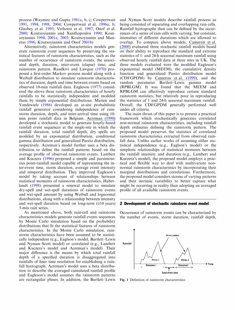
Fig. 1 Definition of rainstorm characteristics

inter-event time and rainstorm pattern as shown inFig. 1. The stochastic model presented herein for gen-erating rainstorm events is composed of three majorcomponents: (1) generation of the number of rainstormevents; (2) generation of storm depth, duration, andinter-event time for each event; and (3) generation ofrainstorm pattern for each event.

2.1 Generation of number of rainstorm events

2.1.1 Definition of rainstorm event

To analyze the probabilistic properties of rainstormcharacteristics and to synthesize rainstorm events, it isnecessary to separate the time series of point-rainfallobservations into individual events. From the physicaland meteorological perspectives, it is desirable to treatindividual rainstorm as an event within which rain mayfall intermittently. In doing so, rainfall characteristicsbetween different rainstorm events are assumed to bestatistically independent for which several methods havebeen used to identify such rainstorm events: (a) auto-correlation method (Morris 1978); (b) rank correlationmethod (Bonta and Rao 1988); and (c) exponentialmethod (Eagleson 1977; Bonta and Rao 1988; Restrepoand Eagleson 1982). The above methods do not base onthe meteorologically meaningful feature; numericalinvestigations of rainfall records by the methods havealso shown considerable degree of variability in deter-mining rainstorm events.

Alternatively, many rainfall–runoff studies, particu-larly for stormwater drainage engineering, mainly con-cern with dry and wet periods of rainfalls composed ofrainstorm events, regardless whether the rainfalls arefrom the same rainstorm or not. By this way of sepa-rating rainstorm events, two types of event are normallyused: (1) events consisting of non-zero depths in rainfallsequences separated by dry time (Yen and Chow 1980)and (2) events consisting of a sequence that possiblycontain zero depth according to the specific criteria.

It is expected that the simulated rainfall sequencesbased on the observed rainstorm characteristics wouldbe affected by the adopted definition of rainstormevents. Since this study focuses on those rainstormevents that could potentially produce significant runoff,the criteria for defining and separating rainstorm eventsare based on the total rainfall amount, rainfall intensity,along with a specific threshold of dry period.

2.1.2 Modeling number of rainstorm events

To generate rainstorm sequences over a period of severalyears, the distribution properties for annual number ofrainstorm events must be specified in advance. Poissondistribution is commonly adopted to describe annualrandom occurrence of hydrological events for the pulse-based and profile-based stochastic rainfall modeling

(Eagleson 1977; Alexandersson 1985; Marien andVandewiele 1986; Waymire and Gupta 1981a, b, c).Hence, Poisson distribution is considered and testedherein to model annual number of rainstorm eventoccurrences.

To test Poisson distribution, Cunnane (1979) appliedthe Fisher dispersion index, DI, defined as

DI ¼XN

i¼1

ðmi � �mÞ2

�m¼ ðN � 1ÞVarðmÞ

EðmÞ ; ð1Þ

where mi is the annual number of hydrologic eventsobserved in the ith year (i = 1, 2,..., N), and �m is thesample mean of mi. The test statistics DI follows a v2

distribution with N � 1 degree of freedom. Thehypothesis on Poisson distribution is not rejected if theP-value associated with the sample DI is larger than thespecified significance level, which is set at 5 or 1% ingeneral practice.

2.2 Generation of storm duration, rainfall depth,and inter-event time

In reality, storm duration, rainfall depth, and inter-eventtime are inherent correlated and their probabilistic dis-tributions are likely to be non-normal. Therefore, thegeneration of these three rainstorm characteristicsshould preserve their respective marginal statisticalproperties and correlation relations.

2.2.1 Monte Carlo simulation for multivariatenon-normal random variables

As mentioned above, storm duration, rainfall depth, andinter-event time could be a mixture of non-normal cor-related variables and it is generally difficult to establishtheir joint distribution. To simulate multivariate non-normal random variates, Chang et al. (1997) proposed apractical procedure utilizing information on marginaldistributions and correlations. The multivariate MCSprocedure involves following three steps:

Transformation to standard normal space This steptransforms correlated variables from their original do-main to the standard normal space by the Nataf bivar-iate distribution model (Nataf 1962),

qij ¼Z1

�1

Z1

�1

xi � li

ri

� �xj � lj

rj

� �/ijðzi; zjjq�ijÞ dzidzj;

ð2Þ

where zi and zj are bivariate standard normal variableswith the correlation coefficient qij

* and the joint standardnormal density function /ij(•); xi and xj are the corre-lated variables in the original space having, respectively,the means li and lj, standard deviations ri and rj, andcorrelation coefficient qij. The equivalent correlation in

the normal space qij* can be obtained by solving Eq. 2

conditioned on the marginal PDFs of xi and xj as well asqij. Through an extensive numerical experiment, a set ofsemi-empirical formula has been developed by Liu andDer Kiureghian (1986) from which a transformationfactor Tij, depending on the marginal distributions andcorrelation of xi and xj, can be determined to modify qij

in the original space to qij* in the normal space by

q�ij ¼ Tij � qij ð3Þ

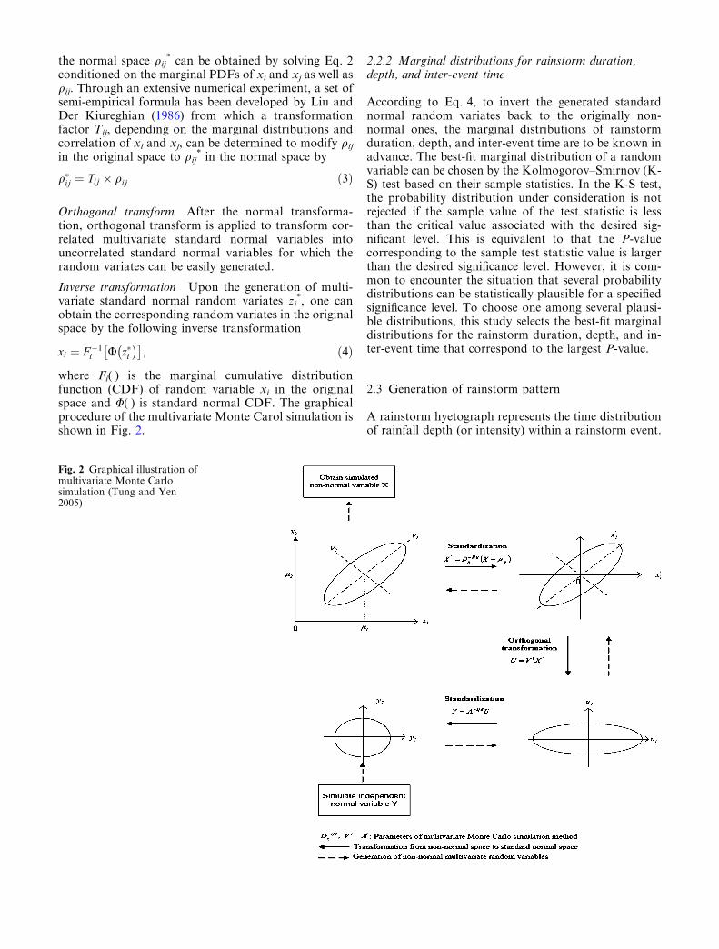
Orthogonal transform After the normal transforma-tion, orthogonal transform is applied to transform cor-related multivariate standard normal variables intouncorrelated standard normal variables for which therandom variates can be easily generated.

Inverse transformation Upon the generation of multi-variate standard normal random variates zi

*, one canobtain the corresponding random variates in the originalspace by the following inverse transformation

xi ¼ F �1i U z�i� �� �

; ð4Þ

where Fi(Æ) is the marginal cumulative distributionfunction (CDF) of random variable xi in the originalspace and U(Æ) is standard normal CDF. The graphicalprocedure of the multivariate Monte Carol simulation isshown in Fig. 2.

2.2.2 Marginal distributions for rainstorm duration,depth, and inter-event time

According to Eq. 4, to invert the generated standardnormal random variates back to the originally non-normal ones, the marginal distributions of rainstormduration, depth, and inter-event time are to be known inadvance. The best-fit marginal distribution of a randomvariable can be chosen by the Kolmogorov–Smirnov (K-S) test based on their sample statistics. In the K-S test,the probability distribution under consideration is notrejected if the sample value of the test statistic is lessthan the critical value associated with the desired sig-nificant level. This is equivalent to that the P-valuecorresponding to the sample test statistic value is largerthan the desired significance level. However, it is com-mon to encounter the situation that several probabilitydistributions can be statistically plausible for a specifiedsignificance level. To choose one among several plausi-ble distributions, this study selects the best-fit marginaldistributions for the rainstorm duration, depth, and in-ter-event time that correspond to the largest P-value.

2.3 Generation of rainstorm pattern

A rainstorm hyetograph represents the time distributionof rainfall depth (or intensity) within a rainstorm event.

Fig. 2 Graphical illustration ofmultivariate Monte Carlosimulation (Tung and Yen2005)

The rainstorm pattern (shape of hyetograph) has sig-nificant effects on the hydrologic response of a wa-tershed. As rainstorm patterns vary from one event toanother, it is necessary to have a procedure to generatethe rainstorm patterns of different events in stochasticrainstorm simulation. In the following subsections, briefdescriptions about the procedure are given and readersare referred to Wu et al. (2006) for more detail discus-sions.

2.3.1 Characterization of rainstorm patterns

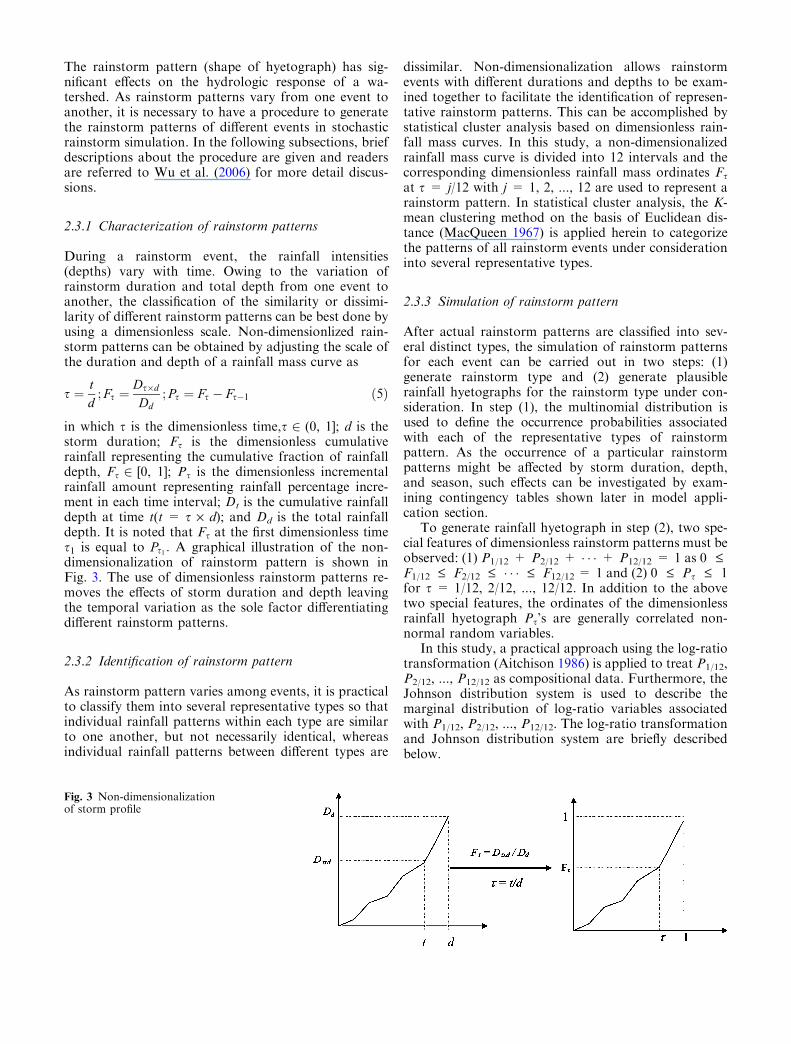
During a rainstorm event, the rainfall intensities(depths) vary with time. Owing to the variation ofrainstorm duration and total depth from one event toanother, the classification of the similarity or dissimi-larity of different rainstorm patterns can be best done byusing a dimensionless scale. Non-dimensionlized rain-storm patterns can be obtained by adjusting the scale ofthe duration and depth of a rainfall mass curve as

s ¼ td

; Fs ¼Ds�d

Dd; Ps ¼ Fs � Fs�1 ð5Þ

in which s is the dimensionless time,s 2 (0, 1]; d is thestorm duration; Fs is the dimensionless cumulativerainfall representing the cumulative fraction of rainfalldepth, Fs 2 [0, 1]; Ps is the dimensionless incrementalrainfall amount representing rainfall percentage incre-ment in each time interval; Dt is the cumulative rainfalldepth at time t(t = s · d); and Dd is the total rainfalldepth. It is noted that Fs at the first dimensionless times1 is equal to Ps1 : A graphical illustration of the non-dimensionalization of rainstorm pattern is shown inFig. 3. The use of dimensionless rainstorm patterns re-moves the effects of storm duration and depth leavingthe temporal variation as the sole factor differentiatingdifferent rainstorm patterns.

2.3.2 Identification of rainstorm pattern

As rainstorm pattern varies among events, it is practicalto classify them into several representative types so thatindividual rainfall patterns within each type are similarto one another, but not necessarily identical, whereasindividual rainfall patterns between different types are

dissimilar. Non-dimensionalization allows rainstormevents with different durations and depths to be exam-ined together to facilitate the identification of represen-tative rainstorm patterns. This can be accomplished bystatistical cluster analysis based on dimensionless rain-fall mass curves. In this study, a non-dimensionalizedrainfall mass curve is divided into 12 intervals and thecorresponding dimensionless rainfall mass ordinates Fs

at s = j/12 with j = 1, 2, ..., 12 are used to represent arainstorm pattern. In statistical cluster analysis, the K-mean clustering method on the basis of Euclidean dis-tance (MacQueen 1967) is applied herein to categorizethe patterns of all rainstorm events under considerationinto several representative types.

2.3.3 Simulation of rainstorm pattern

After actual rainstorm patterns are classified into sev-eral distinct types, the simulation of rainstorm patternsfor each event can be carried out in two steps: (1)generate rainstorm type and (2) generate plausiblerainfall hyetographs for the rainstorm type under con-sideration. In step (1), the multinomial distribution isused to define the occurrence probabilities associatedwith each of the representative types of rainstormpattern. As the occurrence of a particular rainstormpatterns might be affected by storm duration, depth,and season, such effects can be investigated by exam-ining contingency tables shown later in model appli-cation section.

To generate rainfall hyetograph in step (2), two spe-cial features of dimensionless rainstorm patterns must beobserved: (1) P1/12 + P2/12 + � � � + P12/12 = 1 as 0 £F1/12 £ F2/12 £ � � � £ F12/12 = 1 and (2) 0 £ Ps £ 1for s = 1/12, 2/12, ..., 12/12. In addition to the abovetwo special features, the ordinates of the dimensionlessrainfall hyetograph Ps’s are generally correlated non-normal random variables.

In this study, a practical approach using the log-ratiotransformation (Aitchison 1986) is applied to treat P1/12,P2/12, ..., P12/12 as compositional data. Furthermore, theJohnson distribution system is used to describe themarginal distribution of log-ratio variables associatedwith P1/12, P2/12, ..., P12/12. The log-ratio transformationand Johnson distribution system are briefly describedbelow.

Fig. 3 Non-dimensionalizationof storm profile

Log-ratio transformation To generate random con-strained dimensionless rainfall hyetograph ordinatessubject to P1/12 + P2/12 + � � � + P12/12 = 1 and0 £ Ps £ 1, random P1/12, P2/12,..., P12/12 are trans-formed into a set of unconstrained variables by thefollowing log-ratio transformation

Rs ¼ lnPs

Ps�

� �; s ¼ 1=12; 2=12; . . . 12=12; s 6¼ s�; ð6Þ

where s* is the specified dimensionless time with Ps�being the associated non-negative dimensionless rainfallhyetograph ordinate.

Since 0 £ Ps £ 1 for s = 1/12, 2/12, ..., 12/12, thetransformed variables Rs range from �¥ to ¥. Notethat, in the log-ratio transformation of actual data,neither Ps nor Ps� can be zero to avoid numericalproblem. The inverse transformation of log-ratio vari-ables results in

Ps ¼exp Rsð Þ

1þP12=12

s0 6¼ s�s0 ¼ 1=12

exp Rs0ð Þ;

s ¼ 1=12; 2=12; . . . ; 12=12

Ps ¼1

1þP12=12

s0 6¼ s�s0 ¼ 1=12

exp Rs0ð Þ; s ¼ s�

ð7Þ

As can be seen that 0 £ Ps £ 1 and P1/12 + P2/

12 + � � � + P12/12 = 1 are automatically satisfied. Inthis study, generating rainstorm pattern is to simulateeleven correlated log-ratio variables Rs of dimensionlessrainfall ordinates, not involving the one at s = s*.

Johnson distribution system for normal transforma-tion To generate dimensionless rainfall hyetographdefined by the 11 log-ratio random variables Rs’s, it isnecessary to identify the corresponding best-fit marginaldistributions. This study adopted the Johnson distribu-tion as the marginal distribution for Rs. Fang and Tung(1996) found that the Johnson distribution system ismore flexible to fit the rainstorm pattern than otherdistributions.

Johnson (1949) introduced a system of frequencycurve consisting of four parameters

Z ¼ cþ d gX � n

k

� �ð8Þ

where Z is standard normal random variable; g(.) is amonotonic function of the original random variable X; nand k are the location and scale parameters, respectively.There are three types of Johnson distribution: (1) log-normal system (SL): Z = c + d ln (X � n), n £ X (2)unbounded system (SU): Z = c + dsinh � 1 [(X � n)/k ];

(3) bounded system (SB): Z = c + d ln [(X � n)/(n + k� X)], n £ X £ n + k.

These three curves cover the entire region of feasibledistribution defined by the product–moment ratio dia-gram (Johnson 1949; Tadikamalla 1980). Hill et al.(1976) provided an algorithm to estimate the parametersof the Johnson distribution by matching the first fourproduct–moments of X and to determine one of the best-fit Johnson distribution type.

2.3.4 Procedure for generating dimensionless hyetograph

Based on the characterization and identification ofrainstorm events, log-ratio transformation, and MCSwith Johnson distribution system, the dimensionlessrainfall hyetograph ordinates Ps are generated. Specifi-cally, the generation procedure for Ps is mostly similar tothe procedure of generating the storm duration, depthand inter-event time shown in Fig. 2, but the only dif-ference is that the Johnson distribution is selected to becandidate probability distributions. In addition, theparameters (c, d, n, k) in the Johnson distribution of eachlog-ratio variable Rs associated with the rainstorm typeunder consideration are determined from the statisticalmoments of all log-ratio variables R1/12, R2/12, ..., R12/12.

2.4 Generation of rainstorm events sequence

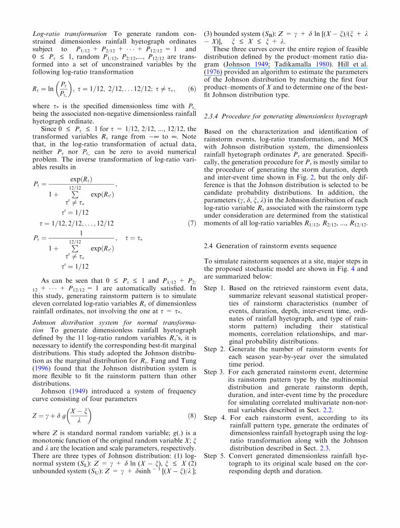
To simulate rainstorm sequences at a site, major steps inthe proposed stochastic model are shown in Fig. 4 andare summarized below:

Step 1. Based on the retrieved rainstorm event data,summarize relevant seasonal statistical proper-ties of rainstorm characteristics (number ofevents, duration, depth, inter-event time, ordi-nates of rainfall hyetograph, and type of rain-storm pattern) including their statisticalmoments, correlation relationships, and mar-ginal probability distributions.

Step 2. Generate the number of rainstorm events foreach season year-by-year over the simulatedtime period.

Step 3. For each generated rainstorm event, determineits rainstorm pattern type by the multinomialdistribution and generate rainstorm depth,duration, and inter-event time by the procedurefor simulating correlated multivariate non-nor-mal variables described in Sect. 2.2.

Step 4. For each rainstorm event, according to itsrainfall pattern type, generate the ordinates ofdimensionless rainfall hyetograph using the log-ratio transformation along with the Johnsondistribution described in Sect. 2.3.

Step 5. Convert generated dimensionless rainfall hye-tograph to its original scale based on the cor-responding depth and duration.

3 Model application

3.1 Description of rainfall data

For model application and performance evaluation,hourly rainfall data from 1884 to 1990 at the HongKong Observatory (HKO), with an interruption in1940–1946 due to the World War II, were used todetermine the distributional properties of rainstormcharacteristics for the development of the stochasticrainstorm generation model

The criteria for extracting rainstorm events are basedon dry-time, event rainfall amount, and hourly rainfallamount. As the study focuses rainfall events that couldpotentially produce significant runoff event, criteriaadopted for rainstorm events retrieval are thefollowings: (1) dry-time ‡ 1-h; (2) event rainfallamount ‡ 30 mm/event; and (3) any hourly rainfallamount within an event ‡ 10 mm/h. According to theabove criteria, a total of 1,690 rainstorm events over the

period of 1884–1939, 1947–1990 were extracted and theirassociated rainstorm characteristics are analyzed.

3.2 Analysis of statistical features of stormcharacteristics

The number of occurrence of rainstorm events, stormduration, rainfall depth, inter-event time and temporaldistribution of rainfall are the main features consideredin the proposed stochastic model. To model rainstormevents more accurately, an understanding of theserainstorm characteristics as affected by seasonality ishelpful through a statistical analysis of storm charac-teristics with respect to months or seasons.

3.2.1 Number of occurrence of rainstorm events

Table 1 shows the total number of rainstorm events overthe record period by month, season, dry-period (Janu-

Fig. 4 Schematic diagram ofgenerating rainstorm events

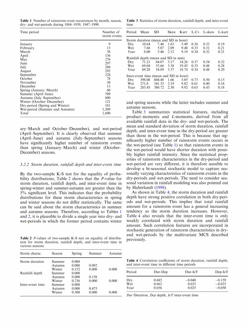
ary–March and October–December), and wet-period(April–September). It is clearly observed that summer(April–June) and autumn (July–September) seasonshave significantly higher number of rainstorm eventsthan spring (January–March) and winter (October–December) seasons.

3.2.2 Storm duration, rainfall depth and inter-event time

By the two-sample K-S test for the equality of proba-bility distributions, Table 2 shows that the P-value forstorm duration, rainfall depth, and inter-event time inspring-winter and summer-autumn are greater than the5% significant level. This indicates that the probabilitydistributions for these storm characteristics in springand winter seasons do not differ statistically. The samecan be said about the storm characteristics in summerand autumn seasons. Therefore, according to Tables 1and 2, it is plausible to divide a single year into dry- andwet-periods in which the former period contains winter

and spring seasons while the latter includes summer andautumn seasons.

Table 3 summarizes statistical features, includingproduct–moments and L-moments, derived from allavailable rainfall data in the dry- and wet-periods. Themean and standard deviation of storm duration, rainfalldepth, and inter-event time in the dry-period are greaterthan those in the wet-period. This is because that sig-nificantly higher number of rainstorm events occurs inthe wet-period (see Table 1) so that rainstorm events inthe wet-period would have shorter duration with possi-bly higher rainfall intensity. Since the statistical prop-erties of rainstorm characteristics in the dry-period andwet-period are very different, it is therefore sensible todevelop a bi-seasonal stochastic model to capture sea-sonally varying characteristics of rainstorm events in thedry-periods and wet-periods. The need to consider sea-sonal variation in rainfall modeling was also pointed outby Haberlandt (1998).

As shown in Table 4, the storm duration and rainfalldepth have strong positive correlation in both dry-peri-ods and wet-periods. This implies that total rainfallamount for a rainstorm event has a general increasingtendency as the storm duration increases. However,Table 4 also reveals that the inter-event time is onlyweakly correlated with storm duration and rainfallamount. Such correlation features are incorporated instochastic generation of rainstorm characteristics in dry-and wet-periods by the multivariate MCS describedpreviously.

Table 1 Number of rainstorm event occurrences by month, season,dry- and wet-periods during 1884–1939, 1947–1990

Time period Number ofstorm events

January 9February 13March 38April 136May 276June 297July 280August 292September 228October 78November 30December 13Spring (January–March) 60Summer (April–June) 709Autumn (July–September) 800Winter (October–December) 121Dry-period (Spring and Winter) 181Wet-period (Summer and Autumn) 1,509Total 1,690

Table 2 P-values of two-sample K-S test on equality of distribu-tion for storm duration, rainfall depth, and inter-event time invarious seasons

Storm charac. Season Spring Summer Autumn

Storm duration Summer 0.000Autumn 0.000 0.092Winter 0.152 0.000 0.000

Rainfall depth Summer 0.000Autumn 0.000 0.158Winter 0.236 0.000 0.000

Inter-event time Summer 0.000Autumn 0.000 0.475Winter 0.500 0.000 0.000

Table 3 Statistics of storm duration, rainfall depth, and inter-eventtime

Period Mean SD Skew Kurt L-Cv L-skew L-kurt

Storm duration (mean and SD in hour)Dry 10.64 7.46 1.63 5.49 0.36 0.32 0.19Wet 7.68 5.07 2.09 9.48 0.33 0.31 0.21Year 8.00 5.46 2.12 9.19 0.34 0.32 0.21

Rainfall depth (mean and SD in mm)Dry 71.21 64.07 3.17 14.26 0.37 0.54 0.32Wet 69.04 53.66 3.38 19.45 0.33 0.48 0.28Year 69.28 54.89 3.37 18.74 0.34 0.48 0.29

Inter-event time (mean and SD in hour)Dry 398.08 604.48 1.66 5.05 0.73 0.50 0.15Wet 271.8 341.33 2.19 9.82 0.61 0.40 0.16Year 285.45 380.72 2.30 9.92 0.63 0.43 0.18

Table 4 Correlation coefficients of storm duration, rainfall depth,and inter-event time in different time periods

Period Dur-Dep Dur-IeT Dep-IeT

Dry 0.685 �0.048 �0.159Wet 0.662 0.025 �0.025Year 0.656 0.025 �0.050

Dur Duration, Dep depth, IeT inter-event time

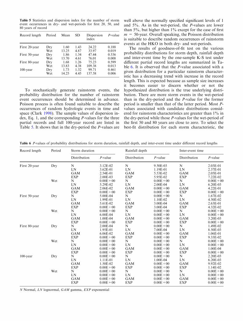
To stochastically generate rainstorm events, theprobability distribution for the number of rainstormevent occurrences should be determined in advance.Poisson process is often found suitable to describe theoccurrences of random hydrologic events in time andspace (Clark 1998). The sample values of dispersion in-dex, Eq. 1, and the corresponding P-values for the threepartial records and full 100-year record are listed inTable 5. It shows that in the dry-period the P-values are

well above the normally specified significant levels of 1and 5%. As in the wet-period, the P-values are lowerthan 5%, but higher than 1% except for the case of firstm = 50-year. Overall speaking, the Poisson distributionis suitable to describe random occurrences of rainstormevents at the HKO in both dry- and wet-periods.

The results of goodness-of-fit test on the variousprobability distributions for storm depth, rainfall depthand inter-event time by the one-sample K-S test underdifferent partial record lengths are summarized in Ta-ble 6. It is observed that the P-value associated with agiven distribution for a particular rainstorm character-istic has a decreasing trend with increase in the recordlength. This is expected because as sample size increasesit becomes easier to discern whether or not thehypothesized distribution is the true underlying distri-bution. There are more storm events in the wet-periodthan in the dry-period and the P-value for the formerperiod is smaller than that of the latter period. Most P-values associated with candidate distributions consid-ered for rainstorm characteristics are greater than 1% inthe dry-period while those P-values for the wet-period ofthe first 50 and 80 years are close to zero. To select thebest-fit distribution for each storm characteristic, the

Table 5 Statistics and dispersion index for the number of stormevent occurrences in dry- and wet-periods for first 20, 50, and80 years of record

Record length Period Mean SD Dispersionindex

P-value

First 20-year Dry 1.60 1.43 24.22 0.188Wet 13.25 4.87 33.97 0.019

First 50-year Dry 1.86 1.34 47.44 0.536Wet 13.70 4.61 76.01 0.008

First 80-year Dry 1.68 1.26 75.23 0.599Wet 13.83 4.38 109.38 0.013

100-year Dry 1.73 1.32 99.71 0.461Wet 14.25 4.45 137.58 0.006

Table 6 P-values of probability distributions for storm duration, rainfall depth, and inter-event time under different record lengths

Record length Period Storm duration Rainfall depth Inter-event time

Distribution P-value Distribution P-value Distribution P-value

First 20-year Dry N 3.12E-02 N 9.50E-03 N 2.03E-01LN 3.62E-01 LN 1.19E-01 LN 2.37E-01GAM 2.54E-01 GAM 5.53E-02 GAM 2.05E-01EXP 2.00E-03 EXP 5.95E-02 EXP 7.22E-02

Wet N 0.00E+00 N 0.00E+00 N 0.00E+00LN 5.29E-02 LN 2.00E-04 LN 6.20E-03GAM 2.06E-02 GAM 0.00E+00 GAM 4.22E-01EXP 0.00E+00 EXP 0.00E+00 EXP 0.00E+00

First 50-year Dry N 5.00E-04 N 0.00E+00 N 1.67E-02LN 1.99E-01 LN 1.10E-02 LN 4.50E-02GAM 5.61E-02 GAM 3.00E-04 GAM 2.63E-01EXP 0.00E+00 EXP 3.00E-04 EXP 4.32E-02

Wet N 0.00E+00 N 0.00E+00 N 0.00E+00LN 6.00E-04 LN 0.00E+00 LN 0.00E+00GAM 1.00E-04 GAM 0.00E+00 GAM 3.20E-03EXP 0.00E+00 EXP 0.00E+00 EXP 0.00E+00

First 80-year Dry N 2.00E-04 N 0.00E+00 N 1.49E-02LN 1.95E-01 LN 7.00E-04 LN 8.50E-03GAM 6.06E-02 GAM 0.00E+00 GAM 1.06E-01EXP 0.00E+00 EXP 0.00E+00 EXP 9.33E-02

Wet N 0.00E+00 N 0.00E+00 N 0.00E+00LN 0.00E+00 LN 0.00E+00 LN 0.00E+00GAM 0.00E+00 GAM 0.00E+00 GAM 1.00E-04EXP 0.00E+00 EXP 0.00E+00 EXP 0.00E+00

100-year Dry N 0.00E+00 N 0.00E+00 N 2.20E-03LN 1.11E-01 LN 1.00E-04 LN 6.20E-03GAM 1.50E-02 GAM 0.00E+00 GAM 9.92E-02EXP 0.00E+00 EXP 0.00E+00 EXP 1.14E-02

Wet N 0.00E+00 N 0.00E+00 N 0.00E+00LN 0.00E+00 LN 0.00E+00 LN 0.00E+00GAM 0.00E+00 GAM 0.00E+00 GAM 0.00E+00EXP 0.00E+00 EXP 0.00E+00 EXP 0.00E+00

N Normal, LN lognormal, GAM gamma, EXP exponential

one having the largest P-value is chosen. Hence, thebest-fit distributions of storm characteristics in the dry-period and wet-period under various sub-record lengthscan be obtained, except for those in wet-period of thefirst 50 and 80 years which are zero. Overall speaking, itis found that the best-fit distribution for storm durationand rainfall depth is the two-parameter lognormal dis-tribution, while for inter-event time the two-parametergamma distribution is the best-fit one. The same resultfor inter-event time was obtained by Yen et al. (1993) intheir study on hourly rainfall at Urbana, IL using zero-rainfall period to separate rainstorm events. As a resultof the K-S test, the lognormal distribution was employedin this study for generating storm duration and depth,whereas the gamma distribution was used for generatinginter-event time.

3.2.3 Temporal distribution of rainfall(Rainstorm pattern)

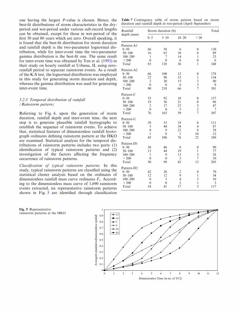
Referring to Fig. 4, upon the generation of stormduration, rainfall depth and inter-event time, the nextstep is to generate plausible rainfall hyetographs toestablish the sequence of rainstorm events. To achievethat, statistical features of dimensionless rainfall hyeto-graph ordinates defining rainstorm pattern at the HKOare examined. Statistical analysis for the temporal dis-tributions of rainstorm patterns includes two parts: (1)identification of typical rainstorm patterns and (2)investigation of the factors affecting the frequencyoccurrence of rainstorm patterns.

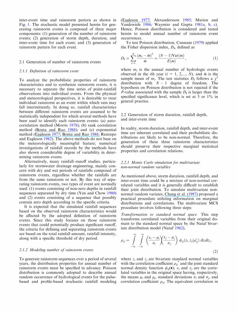
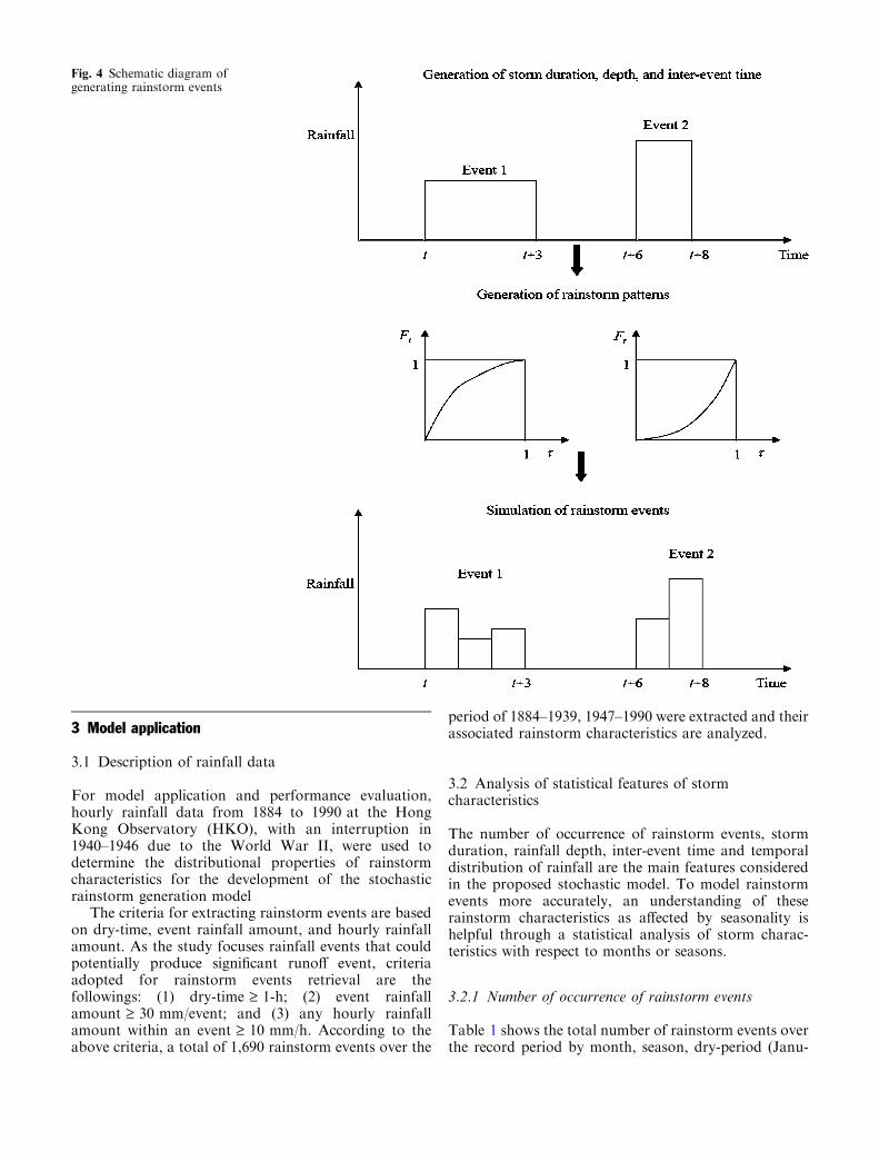
Classification of typical rainstorm patterns In thisstudy, typical rainstorm patterns are classified using thestatistical cluster analysis based on the ordinates ofdimensionless rainfall mass curve ordinates Fs. Accord-ing to the dimensionless mass curve of 1,690 rainstormevents extracted, six representative rainstorm patternsshown in Fig. 5 are identified through classification

0

0.1

0.2

0.3

0.4

0.5

0.6

0.7

0.8

0.9

1

0 1 2 3 4 5 6 7 8 9 10 11 12

Dimensionless Time (in no. of T/12)

Ave

rage

d cu

mul

ativ

edim

ensi

onle

ss r

ainf

all A1

A2

C

U

D1

D2

Fig. 5 Representativerainstorm patterns at the HKO

Table 7 Contingency table of storm pattern based on stormduration and rainfall depth in wet-period (April–September)

Rainfalldepth (mm)

Storm duration (h) Total

0–5 5–10 10–20 >20

Pattern-A10–50 66 58 6 0 13050–100 16 63 10 0 89100–200 1 7 14 1 23>200 0 0 6 0 6Total 83 128 36 1 248

Pattern-A20–50 66 100 12 0 17850–100 22 98 33 1 154100–200 2 20 15 3 40>200 0 0 6 3 9Total 90 218 66 7 381

Pattern-C0–50 55 92 10 0 15750–100 19 56 21 0 96100–200 2 17 23 5 47>200 0 0 5 2 7Total 76 165 59 7 307

Pattern-U0–50 39 53 19 0 11150–100 5 44 34 4 87100–200 0 9 22 8 39>200 1 0 1 10 12Total 45 106 76 22 249

Pattern-D10–50 36 46 8 0 9050–100 13 44 19 1 77100–200 1 9 13 5 28>200 0 0 3 7 10Total 50 99 43 13 205

Pattern-D20–50 42 26 2 0 7050–100 12 12 9 1 34100–200 0 3 4 3 10>200 0 0 2 1 3Total 54 41 17 5 117

process (Wu et al. 2006). The six rainstorm patternsconsist of four basic types of hyetograph: advanced type(A1 and A2); central-peaked type (C); uniform type (U);and delayed type (D1 and D2). The advanced types haverelatively higher rainfall intensity during early part ofrainstorm event, whereas the delayed types are just theopposite. A central-peaked pattern has relatively highrainfall in the middle and tapers off towards the begin-ning and ending of the rainstorm event, while the uni-form type reveals relatively constant rainfall intensitythroughout the storm duration.

Factors affecting the occurrence of rainstorm pat-terns To investigate the frequency occurrence of rain-storm patterns affected by the storm duration, rainfalldepth, and seasonality, the six representative rainstormpatterns are grouped by storm duration and rainfalldepth in the form of contingency table (see Table 7 forwet-period as an example). It can be clearly observedthat occurrence frequencies of the six representativerainstorm patterns are not uniform with respect to stormduration and rainfall amount at the HKO. Hence,occurrence frequencies of the six representative rain-

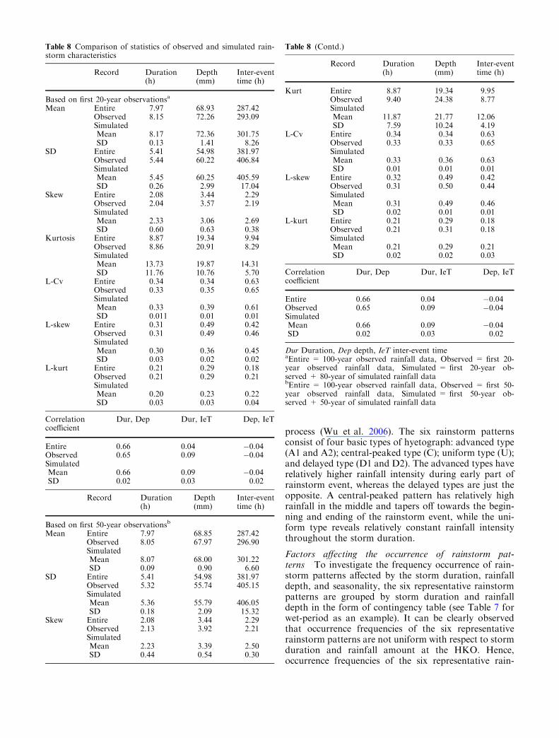
Table 8 Comparison of statistics of observed and simulated rain-storm characteristics

Record Duration(h)

Depth(mm)

Inter-eventtime (h)

Based on first 20-year observationsa

Mean Entire 7.97 68.93 287.42Observed 8.15 72.26 293.09SimulatedMean 8.17 72.36 301.75SD 0.13 1.41 8.26

SD Entire 5.41 54.98 381.97Observed 5.44 60.22 406.84SimulatedMean 5.45 60.25 405.59SD 0.26 2.99 17.04

Skew Entire 2.08 3.44 2.29Observed 2.04 3.57 2.19SimulatedMean 2.33 3.06 2.69SD 0.60 0.63 0.38

Kurtosis Entire 8.87 19.34 9.94Observed 8.86 20.91 8.29SimulatedMean 13.73 19.87 14.31SD 11.76 10.76 5.70

L-Cv Entire 0.34 0.34 0.63Observed 0.33 0.35 0.65SimulatedMean 0.33 0.39 0.61SD 0.011 0.01 0.01

L-skew Entire 0.31 0.49 0.42Observed 0.31 0.49 0.46SimulatedMean 0.30 0.36 0.45SD 0.03 0.02 0.02

L-kurt Entire 0.21 0.29 0.18Observed 0.21 0.29 0.21SimulatedMean 0.20 0.23 0.22SD 0.03 0.03 0.04

Correlationcoefficient

Dur, Dep Dur, IeT Dep, IeT

Entire 0.66 0.04 �0.04Observed 0.65 0.09 �0.04SimulatedMean 0.66 0.09 �0.04SD 0.02 0.03 0.02

Record Duration(h)

Depth(mm)

Inter-eventtime (h)

Based on first 50-year observationsb

Mean Entire 7.97 68.85 287.42Observed 8.05 67.97 296.90SimulatedMean 8.07 68.00 301.22SD 0.09 0.90 6.60

SD Entire 5.41 54.98 381.97Observed 5.32 55.74 405.15SimulatedMean 5.36 55.79 406.05SD 0.18 2.09 15.32

Skew Entire 2.08 3.44 2.29Observed 2.13 3.92 2.21SimulatedMean 2.23 3.39 2.50SD 0.44 0.54 0.30

Table 8 (Contd.)

Record Duration(h)

Depth(mm)

Inter-eventtime (h)

Kurt Entire 8.87 19.34 9.95Observed 9.40 24.38 8.77SimulatedMean 11.87 21.77 12.06SD 7.59 10.24 4.19

L-Cv Entire 0.34 0.34 0.63Observed 0.33 0.33 0.65SimulatedMean 0.33 0.36 0.63SD 0.01 0.01 0.01

L-skew Entire 0.32 0.49 0.42Observed 0.31 0.50 0.44SimulatedMean 0.31 0.49 0.46SD 0.02 0.01 0.01

L-kurt Entire 0.21 0.29 0.18Observed 0.21 0.31 0.18SimulatedMean 0.21 0.29 0.21SD 0.02 0.02 0.03

Correlationcoefficient

Dur, Dep Dur, IeT Dep, IeT

Entire 0.66 0.04 �0.04Observed 0.65 0.09 �0.04SimulatedMean 0.66 0.09 �0.04SD 0.02 0.03 0.02

Dur Duration, Dep depth, IeT inter-event timeaEntire = 100-year observed rainfall data, Observed = first 20-year observed rainfall data, Simulated = first 20-year ob-served + 80-year of simulated rainfall databEntire = 100-year observed rainfall data, Observed = first 50-year observed rainfall data, Simulated = first 50-year ob-served + 50-year of simulated rainfall data

storm patterns would depend on the storm duration andrainfall depth and such dependency should be accountedfor in the simulation model for a more realistic genera-tion of rainstorm events.

For a rainstorm event generated with the specifiedrainfall duration and depth in a dry or wet period, therandom selection of a particular rainstorm pattern forthat event can be made by using a multinomial distri-bution model with the following probability distribu-tion,

Qk ¼nk

P6

k0¼1nk0

; k ¼ 1; 2; . . . ; 6; ð9Þ

where Qk is the probability of occurrence of rainstormpattern k; and nk is the number of occurrences of rain-storm pattern k whose dependence on rainfall depth,duration, and season can be obtain from the contin-gency tables.

3.3 Performance evaluation and verificationof proposed model

The proposed rainstorm generation model is evaluatedby examining the general and extreme statistics of sim-ulated rainstorm characteristics. In particular, on theextreme rainfall statistics, comparisons are made on theannual maximum rainfall frequency relations derivedfrom the simulated rainstorm event sequence with thosedirectly obtained on the basis of assumed ‘available’rainfall data. The performance evaluation specificallyaims at: (1) examining the ability of the proposed modelto preserve the essential statistical features of relevantrainstorm characteristics and those of the annual maxi-mum rainfall series and (2) investigating the capability ofthe proposed model to add synthesized rainfall recordwith the expectation to enhance the accuracy and reli-ability of rainfall frequency analysis. The evaluationprocedure is outlined below.

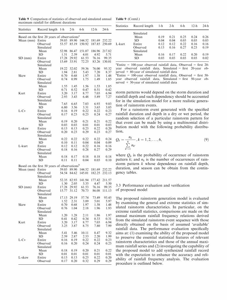
Table 9 Comparison of statistics of observed and simulated annualmaximum rainfall for different durations

Statistics Record length 1-h 2-h 6-h 12-h 24-h

Based on the first 20 years of observationsa

Mean (mm) Entire 59.03 89.90 144.52 181.69 232.22Observed 53.57 85.19 150.92 187.85 250.69SimulatedMean 52.98 86.47 151.07 186.96 217.82SD 1.51 2.39 4.01 4.92 5.71

SD (mm) Entire 17.28 29.92 61.53 76.16 99.35Observed 15.69 33.91 72.25 83.26 130.01SimulatedMean 19.22 32.02 59.36 76.00 95.32SD 1.94 2.81 5.43 7.20 8.37

Skew Entire 0.70 0.68 1.97 1.58 1.48Observed 0.74 0.99 1.75 1.49 1.85SimulatedMean 1.55 1.45 1.56 1.53 1.85SD 0.71 0.52 0.47 0.51 0.42

Kurt Entire 3.20 3.17 8.77 7.03 6.94Observed 2.93 3.43 6.48 5.89 7.27SimulatedMean 7.65 6.65 7.03 6.93 9.03SD 6.80 3.56 3.31 3.65 3.05

L-Cv Entire 0.16 0.19 0.22 0.22 0.23Observed 0.17 0.23 0.25 0.24 0.27SimulatedMean 0.19 0.20 0.21 0.21 0.22SD 0.03 0.03 0.01 0.01 0.03

L-skew Entire 0.13 0.13 0.25 0.22 0.20Observed 0.20 0.23 0.29 0.23 0.27SimulatedMean 0.22 0.22 0.22 0.22 0.24SD 0.10 0.11 0.04 0.04 0.09

L-kurt Entire 0.12 0.12 0.22 0.16 0.16Observed 0.18 0.16 0.28 0.27 0.29SimulatedMean 0.18 0.17 0.18 0.18 0.18SD 0.11 0.11 0.04 0.03 0.10

Based on the first 50 years of observationsb

Mean (mm) Entire 59.03 89.90 144.52 181.69 232.22Observed 54.54 84.62 145.01 182.25 232.13SimulatedMean 52.35 82.93 141.94 177.42 211.57SD 1.30 2.05 3.35 4.47 5.50

SD (mm) Entire 17.28 29.92 61.53 76.16 99.35Observed 15.77 31.12 70.73 86.08 111.13SimulatedMean 17.13 29.19 57.74 73.49 93.45SD 1.52 2.31 3.89 5.01 5.97

Skew Entire 0.70 0.68 1.97 1.58 1.48Observed 0.76 1.04 2.18 1.96 1.93SimulatedMean 1.20 1.28 2.11 1.86 1.97SD 0.41 0.42 0.34 0.33 0.31

Kurt Entire 3.20 3.17 8.77 7.03 6.94Observed 3.25 3.87 8.75 7.80 7.99SimulatedMean 5.41 5.46 10.11 8.47 9.32SD 2.59 2.87 2.53 2.20 1.99

L-Cv Entire 0.16 0.19 0.22 0.22 0.23Observed 0.16 0.20 0.24 0.24 0.25SimulatedMean 0.18 0.19 0.20 0.21 0.22SD 0.01 0.01 0.01 0.01 0.01

L-skew Entire 0.13 0.13 0.25 0.22 0.20Observed 0.17 0.20 0.32 0.29 0.29

Table 9 (Contd.)

Statistics Record length 1-h 2-h 6-h 12-h 24-h

SimulatedMean 0.19 0.21 0.25 0.24 0.26SD 0.04 0.04 0.03 0.03 0.03

L-kurt Entire 0.12 0.12 0.22 0.16 0.16Observed 0.13 0.16 0.27 0.23 0.19SimulatedMean 0.16 0.17 0.22 0.20 0.19SD 0.03 0.03 0.03 0.03 0.02

aEntire = 100-year observed rainfall data, Observed = first 20-year observed rainfall data, Simulated = first 20-year ob-served + 80-year of simulated rainfall databEntire = 100-year observed rainfall data, Observed = first 50-year observed rainfall data, Simulated = first 50-year ob-served + 50-year of simulated rainfall data

Step 1. Based on the complete n-year rainfall data seriescalculate the statistical properties of rainstormcharacteristics and annual maximum rainfallfrequency relations, hn.

Step 2. To emulate the situation of adding synthesizedrainfall record and to preserve its time-seriesstructure, select the first m years out of the totalrecord of n years (m £ n) and treat them as theavailable data. Then, based on the ‘available’rainfall data series, rainstorm events according

to the prescribed criteria and annual maximumrainfalls of different durations are extracted.The rainstorm characteristics statistics and fre-quency quantiles from the m-year of ‘available’rainstorm record is denoted as hm, 0. From thestatistical characteristics of extracted rainstormevents in the first m years, apply the proposedmodel to simulate rainfall event sequences for aperiod of (n � m) years. Calculate the statisticsof simulated rainstorm characteristics and

0

20

40

60

80

100

120

140

160

180

200

1 10 100 1000

Stor

m D

epth

(m

m)

Stor

m D

epth

(m

m)

Stor

m D

epth

(m

m)

Entire RecordObservedMean (Extension)Median (Extension)90% Lower Limit90% Upper Limit

Entire RecordObservedMean (Extension)Median (Extension)90% Lower Limit90% Upper Limit

Duration = 1-hr

0

100

200

300

400

500

600

1 10 100 1000

Duration = 6-hr

0

200

400

600

800

1000

1 10 100 1000

Return Period (Years)

Return Period (Years)

Return Period (Years)

Duration = 12-hr

Entire RecordObservedMean (Extension)Median (Extension)90% Lower Limit90% Upper Limit

(a)

(b)

(c)

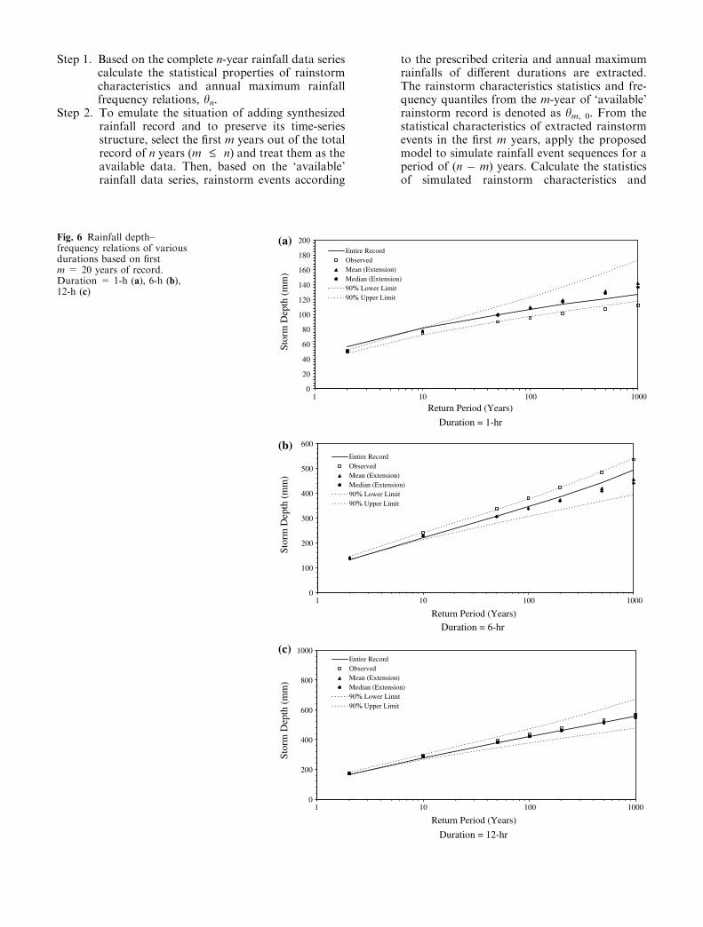
Fig. 6 Rainfall depth–frequency relations of variousdurations based on firstm = 20 years of record.Duration = 1-h (a), 6-h (b),12-h (c)

combine m-year of ‘available’ and (n � m)-yearof simulated rainstorm events to estimate itsfrequency quantiles, denoted as hm, n�m.

Step 3. Repeat step 2 a number of times to obtain thestatistical properties of simulated rainstormcharacteristics including their probabilitybounds.

Using 100 years of hourly rainfall record at the HongKong Observatory (n = 100 years), three partial record

periods (m = 20, 50, and 80 years) starting from thebeginning of the entire record (i.e., 1,884) were used asthe ‘available’ record in the performance evaluation.Fifty synthesized rainstorm sequences of additionalsynthesized (n � m)-year are generated for each m-yearof ‘available’ record.

Performance evaluation was conducted by comparingthe statistical moments of rainstorm characteristics andthose of annual maximum rainfalls of various durationsfrom the simulated rainstorm events under the three

0

20

40

60

80

100

120

140

160

180(a)

(b)

(c)

1 10 100 1000

1 10 100 1000

Return Period (Years)

Stor

m D

epth

(m

m)

Stor

m D

epth

(m

m)

Stor

m D

epth

(m

m)

Entire RecordObservedMean (Extension)Median (Extension)90% Lower Limit90% Upper Limit

Entire RecordObservedMean (Extension)Median (Extension)90% Lower Limit90% Upper Limit

Entire RecordObservedMean (Extension)Median (Extension)90% Lower Limit90% Upper Limit

Duration = 1-hr

Return Period (Years)

Duration = 6-hr

Return Period (Years)

Duration = 12-hr

0

100

200

300

400

500

600

700

0

200

400

600

800

1000

1 10 100 1000

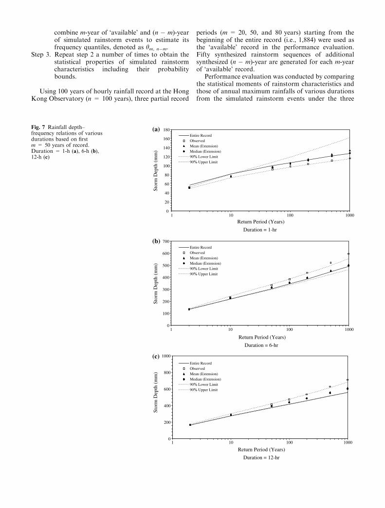
Fig. 7 Rainfall depth–frequency relations of variousdurations based on firstm = 50 years of record.Duration = 1-h (a), 6-h (b),12-h (c)

partial record lengths with those under the entire100 years of observed rainfall data.

3.3.1 Comparison of statistics of rainstormcharacteristics

For illustration, the first four product–moments andL-moments associated with the rainstorm characteristicsof additional synthesized record sequences based onthree sub-record lengths are compared with those fromthe full 100-year record. Table 8 shows the comparisonof the first and second moments of observed and simu-

lated rainstorm characteristics. It is observed that themean values of the statistics of rainstorm characteristicswith additional synthesized record are reasonablyclose with those from the full 100 years of observations(even with the first 20 years). The standard deviationassociated with the simulation results reveals that thevariation of rainstorm characteristics generated by themodel and the values are relatively small, except forhigher order product moments. Table 8 also indicate thatas the partial record length increases, the discrepancy instatistical features of rainstorm characteristics betweenthe full and partial records, as expected, decreases.

0%

5%

10%

15%

20%

25%

30%

Observed

Mean (Extension)

Median (Extension)

1 10 100 1000

Return Period (year)

Observed

Mean (Extension)

Median (Extension)

Duration = 6-hr

1 10 100 1000

Return Period (year)

Duration = 1-hr

Observed

Mean (Extension)

Median (Extension)

e m,0

, e m

,n-m

0%

5%

10%

15%

20%

25%

30%

e m,0

, e m

,n-m

1 10 100 1000

Return Period (year)

Duration = 12-hr

0%

5%

10%

15%

20%

25%

30%

e m,0

, e m

,n-m

(a)

(b)

(c)

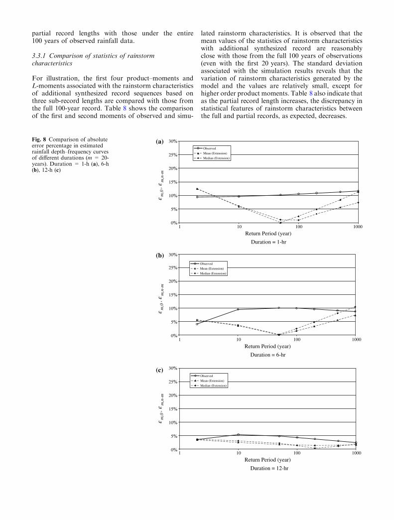
Fig. 8 Comparison of absoluteerror percentage in estimatedrainfall depth–frequency curvesof different durations (m = 20-years). Duration = 1-h (a), 6-h(b), 12-h (c)

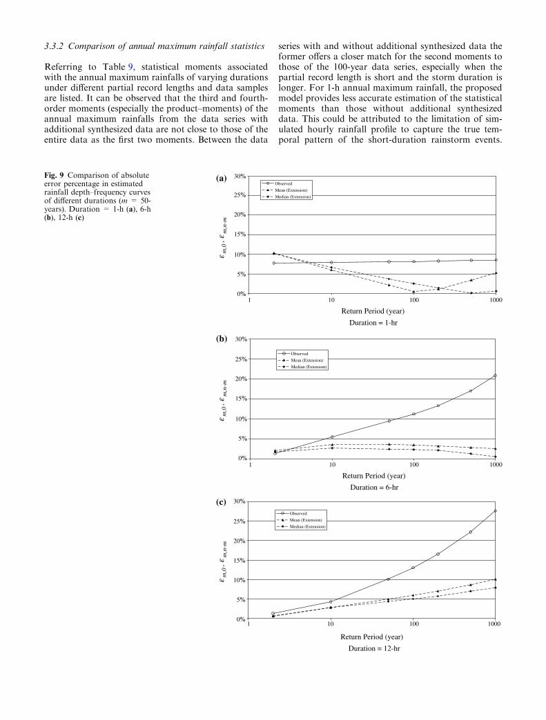
3.3.2 Comparison of annual maximum rainfall statistics

Referring to Table 9, statistical moments associatedwith the annual maximum rainfalls of varying durationsunder different partial record lengths and data samplesare listed. It can be observed that the third and fourth-order moments (especially the product–moments) of theannual maximum rainfalls from the data series withadditional synthesized data are not close to those of theentire data as the first two moments. Between the data

series with and without additional synthesized data theformer offers a closer match for the second moments tothose of the 100-year data series, especially when thepartial record length is short and the storm duration islonger. For 1-h annual maximum rainfall, the proposedmodel provides less accurate estimation of the statisticalmoments than those without additional synthesizeddata. This could be attributed to the limitation of sim-ulated hourly rainfall profile to capture the true tem-poral pattern of the short-duration rainstorm events.

0%

5%

10%

15%

20%

25%

30%(a)

(b)

(c)

1 10 100 1000

Observed

Mean (Extension)

Median (Extension)

Observed

Mean (Extension)

Median (Extension)

Observed

Mean (Extension)

Median (Extension)

Return Period (year)

Duration = 1-hr

e m,0

, e m

,n-m

0%

5%

10%

15%

20%

25%

30%

1 10 100 1000

Return Period (year)

Duration = 6-hr

e m,0

, e m

,n-m

0%

5%

10%

15%

20%

25%

30%

1 10 100 1000

Return Period (year)

Duration = 12-hr

e m,0

, e m

,n-m

Fig. 9 Comparison of absoluteerror percentage in estimatedrainfall depth–frequency curvesof different durations (m = 50-years). Duration = 1-h (a), 6-h(b), 12-h (c)

From the well-known frequency factor equation, i.e.,XT = l + rKT, one can see that the frequency rela-tionship is a combined effect of statistical moments ofvarious orders, it may not be so easy to assess how theaccuracy of individual moment would affect the overallbehavior of the entire frequency curve.

3.3.3 Comparison of annual maximum rainfallfrequency relationship

Rainfall depth–frequency relations derived from the‘available’ partial record and those using additionalsynthesized data are compared with the depth–fre-quency relations from the complete set of 100-year. Forillustration, Figs. 6 and 7, respectively, show the mean,medium, 90% bound of rainfall depth–frequency curvesof three selected storm durations (1-, 6-, and 12-h)derived under ‘available’ record length of 20 and50 years. Note that 90% bound indicates the randomvariability of outputs from the proposed model. It isobserved that the 90% bound of simulated depth–fre-quency curve can capture the ‘true’ frequency curvebased on the entire 100-year complete record. Fur-thermore, by adding synthesized data to the in ‘avail-able’ record, the mean and median of simulated depth–frequency curves are closer to the 100-year curve andthe 90% bound becomes tighter. It is also interesting toobserve that, based solely on the ‘available’ datawithout adding synthesized data, the depth–frequencycurves for some durations (i.e., 6 and 12-h based 20 and50 years of ‘available’ data) lie outside the 90% boundof simulated results.

From Figs. 6 and 7 one observes that the meandepth–frequency curve lies relatively higher above themedian curve indicating that the proposed stochasticrainstorm generating model produces positively-skewedestimation of rainfall quantile, especially for larger re-turn period, such as 200-year or above, and shorterstorm duration (1- or 2-h) when the ‘available’ recordlength is 20 or 50 years. As the storm duration and‘available’ record length become longer, the mean andmedian depth–frequency curves coincide together. Forthe majority of the cases considered, the median depth–frequency curves are closer to those obtained on thebasis of full 100-year record.

Figures 8 and 9 show the absolute error percentage ofthe depth–frequency relationships, defined as

em;0 ¼hm;0 � hn

hn

����

����� 100%; em;n�m ¼hm;n�m � hn

hn

����

����� 100%

ð10Þ

under different partial record lengths with respect tothose established by using full 100-year records in whichh = xT

t denoting estimated T-year t-h rainfall depth. Itis clearly observed that both median and mean depth–frequency curves calculated from combining ‘available’and synthesized data using the proposed rainstorm

generation model would enhance the accuracy of rainfallfrequency analysis, especially when the return period ishigh.

Numerical results also point out that if the returnperiods of interest is significantly smaller than ‘available’record length [e.g., T £ 5-year with m = 20-year;T £ 10-year with m = 50-year; T £ 50-year withm = 80-year (not shown)], adding synthesized record isa futile task which produces no improvement on theestimated quantiles, if not making the estimates lessaccurate. On the other hand, it is interesting to note that,for the limited conditions considered herein, the additionof rainstorm record by the proposed model has goodpotential to greatly enhance the accuracy of estimatedrainfall quantiles with return period closer to or largerthan the ‘available’ record length.

4 Conclusions

This paper presents a practical stochastic model forgenerating hourly-based rainstorm events according tothe statistics of rainstorm characteristics, includingnumber of occurrence of rainstorm events, storm dura-tion, rainfall depth, inter-event time and rainstormpattern. The proposed rainstorm generation model in-volves the use of Poisson distribution for generatingnumber of rainstorm events and multivariate MonteCarlo simulation for storm duration, rainfall depth, andinter-event time, as well as constrained multivariatesimulation conditioned on the total rainfall amount andstorm duration for the corresponding rainfall hyeto-graph.

From the numerical experiments, the proposed modelwas found to be capable of capturing the essential sta-tistical features of rainstorm characteristics and extremeevents based on the available data. Furthermore, theproposed model shows promising potential to improvethe accuracy of short rainfall record in establishingrainfall IDF relations, especially for events having re-turn period close to or longer than the available recordlength.

Note that, in this study, the simulations of rainstormevents were made for the dry- and wet-periods in theexample application. The proposed model, however, canbe applied to deal with rainfall data associated with anytime-interval of interest, such as month, if necessary.Moreover, as the proposed model requires the specifi-cation of statistical properties of rainstorm characteris-tics at a site, it is applicable for simulating rainstormevents at ungauged sites provided that relevant infor-mation about rainstorm characteristics are estimated bya proper regional analysis.

Acknowledgments This study is conducted under the auspice ofresearch project ‘‘HKUST6016/01E: Investigating Issues in Rain-fall Intensity-Duration and Time-Scale Relations in Hong Kong’’funded by the Research Grant Council of Hong Kong SpecialAdministration Region.

References

Acreman MC (1990) A simple stochastic model of hourly rainfallfor Farnborough, England. Hydrol Sci J 35(2):119–148

Aitchison J (1986) Statistical analysis of compositional data.Chapman and Hall Inc., New York

Alexandersson H (1985) A simple stochastic model of the precipi-tation process. J Clim Appl Meteorol 24:1285–1295

Bonta JV, Rao AR (1988) Factors affecting the identification ofindependent rainstorm events. J Hydrol 98:275–293

Cameron DS, Beven KJ, Tawn J, Blazkova S, Naden P (1999)Flood frequency estimation for a gauged upland catchment(with uncertainty). J Hydrol 219:169–187

Cameron DS, Beven K, Tawn J (2000) An evaluation of threestochastic rainfall models. J Hydrol 228:130–149

Chang CH, Yang JC, Tung YK (1997) Incorporate marginal dis-tributions in point estimate methods for uncertainty analysis. JHydrol Eng 123(3):244–251

Clark RT (1998) Stochastic processes for water scientists: devel-opment and application. Wiley, New York

Cowpertwait PSP (1991) Further evelopment of the Neyman–Scottclustered point process for modelling rainfall. Water ResourRes 27(7):1431–1438

Cowpertwait PSP (1994) A generalized point process model forrainfall. Proc R Soc Lond A 447:23–37

Cowpertwait PSP (1998) A Poisson-cluster model of rainfall: high-order moments and extreme values. Proc R Soc Lond A457:885–898

Cowpertwait PSP (2004) Mixed rectangular pulses models forrainfall. Hydrol Earth Syst Sci 8(5):993–1000

Cowpertwait PSP, O’Connell PE, Metcalfe AV, Mawdsley JA(1996a) Stochastic point process modelling of rainfall. I. Single-site fitting and validation. J Hydrol 175:17–46

Cowpertwait PSP, O’Connell PE, Metcalfe AV, Mawdsley JA(1996b) Stochastic point process modelling of rainfall. II. Re-gionalisation and disaggregation. J Hydrol 175:47–65

Cunnane C (1979) A note on the Poisson assumption in partialduration series modes. Water Resour Res 15(2):489–494

Eagleson PS (1977) The distribution of annual precipitation de-rived from observed storm sequence. Water Resour Res14(5):713–721

Fang TQ, Tung YK (1996) Analysis of Wyoming extreme precip-itation patterns and their uncertainty for safety evaluation ofhydraulic structure. Technical Report, WWRC-96.5, WyomingWater Resource Center, University of Wyoming, Laramie,Wyoming

Glasbey CA, Cooper G, McGechan MB (1995) Disaggregation ofdaily rainfall by conditional simulation from a point-processmodel. J Hydrol 165:1–9

Guenni L, Bardossy A (2002) A two step disaggregation methodfor highly seasonal monthly rainfall. Stoch Environ Res RiskAssess 16:188–206

Gupta VK, Waymire EC (1994) A statistical analysis of mesoscalerainfall as a random cascade. J Appl Meteor 32:251–267

Haberlandt U (1998) Stochastic rainfall synthesis using regional-ized model arameters. J Hydrol Eng 3(3):160–168

Hill ID, Hill R, Holder RL (1976) Algorithm AS 99 fitting Johnsoncurves by moments. Appl Statist 25:180–189

Johnson NL (1949) System of frequency curves generatedzi=c+d ln [ya

i /(1 � yai)] by method of translation. Biometrika

36:149–176Koutsoyiannis D (1994) A stochastic disaggregation method for

design storm and flood synthesis. J Hydrol 156:193–225Koutsoyiannis D (2001a) Coupling stochastic models of different

timescales. Water Resour Res 37(2):379–391Koutsoyiannis D (2003) Multivariate rainfall disaggregation at a

fine timescale. Water Resour Res 39(7):1173–1190

Koutsoyiannis D, Manetas A (1996) Simple disaggregation byaccurate adjusting procedures. Water Resour Res 32(7):2105–2117

Koutsoyiannis D, Onof C (2001b) Rainfall disaggregation usingadjusting procedures on a Poisson cluster model. J Hydrol246:109–122

Koutsoyiannis D, Xanthopoulos T (1990) A dynamic model forshort-scale rainfall disaggregation. Hydrol Sci J 35(3):303–322

Lambert M, Kuczera G (1996) A stochastic model of rainfall andtemporal patterns. In: Proceedings on stochastic hydraulics.Balkema, Rotterdam

Liu PL, Der Kiureghian A (1986) Multivariate distribution modelswith prescribed marginal covariances. Probab Eng Mech1(2):105–112

Lovejoy S, Schertzer D (1990) Multifractal, universality classes,and satellite and radar measurements of cloud rain fields. JGeophys Res 95:2021–2031

MacQueen J (1967) Some methods for classification and analysis ofmultivariate observations. In: Proceedings of the 5th Berkeleysymposium, vol 1, pp 281–297

Marien JL, Vandewiele GL (1986) A point rainfall generator withinternal storm structure. Water Resour Res 22(4):475–482

Mason J (1986) Numerical weather prediction. Proc R Soc LondA407:51–60

Morris CD (1978) A stochastic model for an intermittent hydro-logic process. PhD Thesis, University of Illinois at Urbana-Champaign

Nataf A (1962) Determinaiton des distributions don’t les margessont donnees. Computes Rendus de l’Academie des SciencesParis 225:42–43

Onof C, Chandler RE, Kakou A, Northrop P, Wheater HS, IshamV (2000) Rainfall modelling using Poisson-cluster process: areview of developments. Stoch Environ Res Risk Assess14:384–411

Raudkivi AJ, Lawgun N (1970) Synthesis of urban rainfall. WaterResour Res 6(2):445–464

Restrepo PJ, Eagleson PS (1982) Identification of independentrainstorms. J Hydrol 55:303–319

Tadikamalla PR (1980) On simulation non-normal distributions.Psychometrika 45(2):273–279

Tung YK, Yen BC (2005) Hydrosystem engineering uncertaintyanalysis. McGraw-Hill Book Company, New York

Tan SK, Sia SY (1997) Synthetic generation of tropical rainfalltime series using an event-based method. J Hydro Eng 2(2):83–99

Verhoest N, Troch PA, De Troch FP (1997) On the applicability ofBartlett–Lewis rectangular pulses models in the modeling ofdesign storms at a point. J Hydrol 202:108–120

Waymire E, Gupta VK (1981a) The mathematical structure ofrainfall representation. 1. A review of stochastic rainfall models.Water Resour Res 17(5):1261–1272

Waymire E, Gupta VK (1981b) The mathematical structure ofrainfall representation. 2. A review of the theory of point pro-cesses. Water Resour Res 17(5):1273–1285

Waymire E, Gupta VK (1981c) The mathematical structure ofrainfall representation. 3. Some applications of the point pro-cess theory to rainfall processes. Water Resour Res 17(5):1286–1294

Wu SJ, Tung YK, Yang JC (2006) Identification and stochasticgeneration of representative rainfall temporal patterns inHong Kong territory. Stoch Environ Res Risk Assess20(3):171–183

Yen BC, Chow VT (1980) Design hyetographs for small drainagestructures. J Hydraul Eng ASCE 106(HY6):1055–1076

Yen BC, Riggins R, Ellerbroek JW III (1993) Probabilistic char-acteristics of elapsed time between rainfalls. Management ofirrigation and drainage systems: integrated perspectives, ASCE,pp 424–431