Stochastic Claims Reserving Methods with State Space ...

risks

Review

Stochastic Claims Reserving Methods with State SpaceRepresentations: A Review

Nataliya Chukhrova and Arne Johannssen *

�����������������

Citation: Chukhrova, Nataliya, and

Arne Johannssen. 2021. Stochastic

Claims Reserving Methods with State

Space Representations: A Review.

Risks 9: 198. https://doi.org/

10.3390/risks9110198

Academic Editor: Alexandra Dias

Received: 30 September 2021

Accepted: 26 October 2021

Published: 4 Novemver 2021

Publisher’s Note: MDPI stays neutral

with regard to jurisdictional claims in

published maps and institutional affil-

iations.

Copyright: © 2021 by the authors.

Licensee MDPI, Basel, Switzerland.

This article is an open access article

distributed under the terms and

conditions of the Creative Commons

Attribution (CC BY) license (https://

creativecommons.org/licenses/by/

4.0/).

Faculty of Business Administration, University of Hamburg, 20146 Hamburg, Germany;[email protected]* Correspondence: [email protected]

Abstract: Often, the claims reserves exceed the available equity of non-life insurance companies anda change in the claims reserves by a small percentage has a large impact on the annual accounts.Therefore, it is of vital importance for any non-life insurer to handle claims reserving appropriately.Although claims data are time series data, the majority of the proposed (stochastic) claims reservingmethods is not based on time series models. Among the time series models, state space models com-bined with Kalman filter learning algorithms have proven to be very advantageous as they providehigh flexibility in modeling and an accurate detection of the temporal dynamics of a system. Againstthis backdrop, this paper aims to provide a comprehensive review of stochastic claims reservingmethods that have been developed and analyzed in the context of state space representations. Forthis purpose, relevant articles are collected and categorized, and the contents are explained in detailand subjected to a conceptual comparison.

Keywords: adaptive learning; dependence modeling; evolutionary models; insurance; Kalman filter;machine learning; multivariate analysis; quantitative risk management; state space models; timeseries forecasting

1. Introduction1.1. The Importance of Claims Reserving in Non-Life Insurance

The insurance industry offers a multi-faceted range of numerous products that enablepolicyholders to insure themselves against almost any form of loss. Insurance companiestherefore differentiate their products according to various criteria. In this paper, we focuson the problem of claims reserving for a branch of insurance products known as Non-Life Insurance (Continental Europe), General Insurance (United Kingdom) and Property andCasualty Insurance (USA). While this branch encompasses all insurance products that aredifferent from life insurance, life insurance includes only life-related products and disabilityinsurance (see Wüthrich and Merz 2008). This is due to the following reasons. On the onehand, life and non-life products differ reasonably, which is mainly reflected in the contractterms, types of claims and risk drivers. This also explains why different stochastic modelsand methods are used in both these branches. On the other hand, in many countries (suchas Germany or Switzerland), there is a strict legal separation between life and non-life. Anon-life insurer is therefore prohibited from offering life products, and vice versa. For thisreason, it is not uncommon for insurance corporations to establish different companiesand thus sell products from both branches. The following lines of business belong to thenon-life insurance branch: motor/car insurance, property insurance, liability insurance,accident insurance, health insurance, marine insurance, and other insurance products suchas aviation, credit insurance, epidemic insurance, legal protection, travel insurance, and soon (see Wüthrich and Merz 2008).

The amount of money that a policyholder has to pay to the insurer for insurancecoverage is called the premium. By paying a premium, the policyholder under an insurance

Risks 2021, 9, 198. https://doi.org/10.3390/risks9110198 https://www.mdpi.com/journal/risks

Risks 2021, 9, 198 2 of 55

policy transfers the risk to the insurer (risk transfer), who has to compensate/settle thepotential loss occurring under the contract via corresponding claims payments (in wholeor in part). This practice represents the insurance principle of non-life insurance. Thus, incontrast to life insurance, non-life insurance is loss insurance, i.e., payments are made by theinsurer to the policyholder only in the event of a specific loss.

At the end of each fiscal year, the insurer is confronted with the situation in which thepremiums are known, but the claim amount is unknown. This uncertainty of the total lossliabilities is mainly due to (1) a reporting delay, (2) a long-lasting claim settlement, and(3) the unexpected re-opening of a closed claim (see Wüthrich and Merz 2008). Therefore,appropriate claims reserves for the outstanding loss liabilities have to be calculated by theresponsible actuary. Since these loss reserves are often the largest share on the liabilityside of the balance sheet, adequate claims reserving is required, that is, forecasting theseliabilities and quantifying their uncertainty is a key actuarial issue (see Chukhrova andJohannssen 2021).

Although claims data are time series data, the majority of the proposed (stochastic)claims reserving methods is not based on time series models. Among the time seriesmodels, state space models combined with Kalman filter learning algorithms have provento be very advantageous as they provide high flexibility in modeling and an accuratedetection of the temporal dynamics of a system (see Chukhrova and Johannssen 2021).Against this backdrop, this paper aims to provide a comprehensive review of stochasticclaims reserving methods that have been developed and analyzed in the context of statespace representations. For this purpose, relevant articles are collected and categorized, thecontents are explained in detail and subjected to a conceptual comparison.

1.2. State Space Models in the Claims Reserving Literature

The actuarial literature contains various articles in which state space models andthe Kalman filter learning algorithms are applied to improve stochastic claims reserving(see Johannssen 2016). As a pioneer, De Jong and Zehnwirth (1983) constructed a statespace model for the payment stream of incremental payments, took business volume andinflation indices into account, and presented a method to estimate the states underlyingthe observations of the upper triangle and to predict the outstanding loss liabilities ofthe lower triangle. Afterwards, Verrall (1989) used the relationship between the two-wayANOVA and the Chain Ladder (CL) method to establish a state space model for the so-called linear CL model. Wright (1990) constructed a model for incremental payments andemployed the state space approach to model variations in parameters across differentaccident years. Verrall (1994) extended the state space model of Verrall (1989) to weakenthe homogeneity property of the CL method, which allows for development factors that donot necessarily have to be identical across all accident years. Zehnwirth (1997) considereddifferent recursive representations, including state space models based on the general formintroduced by De Jong and Zehnwirth (1983) and discussed calendar year effects in claimsdevelopment triangles.

Ntzoufras and Dellaportas (2002) presented four models for Reported But Not Settled(RBNS) claims, including state space models following Verrall (1989, and 1994). Alpuim andRibeiro (2003) proposed a univariate distribution-free state space model, where incrementalpayments are modeled as a function of payments of the first development year, i.e., theaccident year itself. Taylor et al. (2003) discussed a generalized Kalman filter that accountsfor non-linearities in the observation equation. De Jong (2005) considered the so-calleddevelopment correlation model, which is a (state space) model that accounts for correlationsbetween individual development factors in the first two development years. In addition,De Jong (2006) not only discussed the development correlation model, but two furtherapproaches taking correlations related to accident and calendar years into account.

Li (2006) compared various claims reserving methods including the state space modelof Verrall (1989). A completely different approach from the previous articles is taken byAtherino et al. (2010), who did not model the Incurred But Not Reported (IBNR) run-off data

Risks 2021, 9, 198 3 of 55

in chronological form, but as a univariate time series with missing observations. Pang andHe (2012) combined the approach of Verrall (1989) and Taylor et al. (2003) and included anadditional lag of the state vector into the state equation. Chukhrova and Johannssen (2017)presented a scalar state space model for cumulative payments. Most recently, Costa andPizzinga (2020) and Hendrych and Cipra (2021) extended the row-wise stacking approachfrom Atherino et al. (2010) through the inclusion of tail effects and multivariate considera-tions that allow for dependency modeling between correlated lines of business, respectively.

1.3. Categorization of Articles and Organization of the Paper

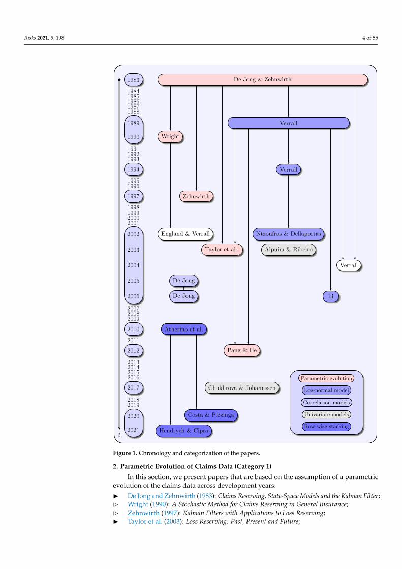
Figure 1 shows the history of the considered articles in stochastic claims reserving.Thereby, all articles are ordered chronologically and are classified into five categoriesconsidering their similarities in terms of contents: “Parametric evolution”, “Log-normalmodel”, “Correlation models”, “Univariate models”, and “Row-wise stacking”. These cate-gories need not be taken as mutually exclusive, but the choice of the appropriate categoryis made considering the main approach used in the respective paper. The first categoryincludes the articles by De Jong and Zehnwirth (1983), Wright (1990), Zehnwirth (1997),Taylor et al. (2003), and Pang and He (2012), as they are based on the assumption of aparametric evolution of the run-off data across the development years. The second categoryincludes the articles by Verrall (1989, 1994), Ntzoufras and Dellaportas (2002), Li (2006)because of the considered log-normal model for incremental payments. The third categoryconsists of the articles by De Jong (2005, and 2006) who discusses three types of models thatincorporate correlations within claims development triangles. In the fourth category, thereare the articles by Alpuim and Ribeiro (2003) and Chukhrova and Johannssen (2017), wheremodels are presented that avoid complex matrix-based structures. Finally, the fifth categoryinclude the articles by Atherino et al. (2010), Costa and Pizzinga (2020), and Hendrych andCipra (2021), who propose a row-wise stacking of the claims data and associated state spacerepresentations. The solid arrows in Figure 1 represent the contentual similarities amongthe papers in their modeling approaches. The dashed arrows indicate, however, that therespective state space models are included in papers where different stochastic claimsreserving methods are compared (see England and Verrall 2002; Verrall 2004). In addition,state space models and the Kalman learning algorithms are discussed in the context ofstochastic claims reserving in standard text books such as Wüthrich and Merz (2008).

In the following, a category-guided presentation of the articles is performed. Withineach of five categories, a chronological order is followed to present the individual articles.For the sake of consistency, a unified notation is used throughout the paper. Since thispaper is devoted to state space representations, all essential contents concerning statespace models are presented in the following, whereas less relevant contents are omitted orreferred to. In particular, the state space representations given in the articles are developedin full detail, often much more detailed than in the original papers.

The paper is organized as follows. In Section 2, articles are discussed that are basedon the assumption of a parametric evolution of the claims data across development years(Category 1). Section 3 presents articles in which incremental payments are assumed to belog-normally distributed and are modeled using a log-normal model (Category 2). Section 4includes articles where correlation models are considered (Category 3). In Section 5, statespace models are presented that have a scalar structure (Category 4). Section 6 containsarticles where the row-wise stacking approach is considered to re-organize the claims data(Category 5). Subsequently, Section 7 provides a conceptual comparison of the presentedapproaches and state space representations. In Section 8, concluding remarks are given.

Risks 2021, 9, 198 4 of 55

1983

19841985198619871988

1989

1990

199119921993

1994

19951996

1997

1998199920002001

2002

2003

2004

2005

2006

200720082009

2010

2011

2012

2013201420152016

2017

20182019

2020

2021

De Jong & Zehnwirth

Wright

Verrall

Verrall

Zehnwirth

England & Verrall Ntzoufras & Dellaportas

Taylor et al. Alpuim & Ribeiro

Verrall

Li

De Jong

De Jong

Atherino et al.

Pang & He

Chukhrova & Johannssen

Costa & Pizzinga

Hendrych & Ciprat

b

Parametric evolution

Log-normal model

Correlation models

Univariate models

Row-wise stacking

Figure 1. Chronology and categorization of the papers.

2. Parametric Evolution of Claims Data (Category 1)

In this section, we present papers that are based on the assumption of a parametricevolution of the claims data across development years:

I De Jong and Zehnwirth (1983): Claims Reserving, State-Space Models and the Kalman Filter;B Wright (1990): A Stochastic Method for Claims Reserving in General Insurance;B Zehnwirth (1997): Kalman Filters with Applications to Loss Reserving;I Taylor et al. (2003): Loss Reserving: Past, Present and Future;

Risks 2021, 9, 198 5 of 55

I Pang and He (2012): Application of State Space Model in Outstanding Claims Reserve.

Three articles marked with I are mainly based on the use of state space models andthe Kalman filter learning theory, and thus are presented in detail, while the models of theother two articles marked with B are treated in a more brief form, as state space modelsare not the focus of their methodologies.

2.1. Claims Reserving, State Space Models and the Kalman Filter

De Jong and Zehnwirth (1983) laid the foundation for the use of state space modelsand the Kalman filter in stochastic claims reserving with their article “Claims Reserving,State-Space Models and the Kalman Filter”. The proposed state space model is constructedfor the payment stream of the incremental payments and presumes known, time-varyingsystem matrices.

B Modeling the payment stream of incremental payments

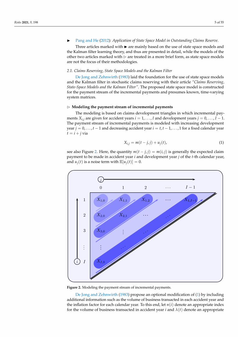
The modeling is based on claims development triangles in which incremental pay-ments Xi,j are given for accident years i = 1, . . . , I and development years j = 0, . . . , I − 1.The payment stream of incremental payments is modeled with increasing developmentyear j = 0, . . . , t− 1 and decreasing accident year i = t, t− 1, . . . , 1 for a fixed calendar yeart = i + j via

Xi,j = m(t− j, j) + uj(t), (1)

see also Figure 2. Here, the quantity m(t− j, j) = m(i, j) is generally the expected claimpayment to be made in accident year i and development year j of the t-th calendar year,and uj(t) is a noise term with E[uj(t)] = 0.

y0(1) y1(2) y2(3) . . . ys−1(s)

y0(2) y1(3) . . . ys−2(s)

y0(3) ... . ..

...y1(s)

y0(s)

1

2

3

...

I

0 1 2 . . . I − 1

X1,0 X1,1 X1,2 . . . X1,I−1

X2,0 X2,1 . . .. ..

X3,0... . .

.

... . ..

XI,0i

j

Figure 2. Modeling the payment stream of incremental payments.

De Jong and Zehnwirth (1983) propose an optional modification of (1) by includingadditional information such as the volume of business transacted in each accident year andthe inflation factor for each calendar year. To this end, let n(i) denote an appropriate indexfor the volume of business transacted in accident year i and λ(t) denote an appropriate

Risks 2021, 9, 198 6 of 55

price index for payments in the t-th calendar year. Using both these quantities, (1) can beextended to

Xi,j = n(t− j)λ(t)m(t− j, j) + uj(t), (2)

where n(t− j)λ(t)m(t− j, j) is the expected value of the inflation-adjusted and volume-weighted incremental payments in accident year i and development year j of calendaryear t.

B Development of an appropriate state space representation

The modeling of the payment stream via (1) and (2) is promising with respect tothe construction of an appropriate observation and state equation of a state space model,respectively. The following discussion in this regard is based on (1), but can be appliedto (2) with minor modifications. In the first step of modeling the observation equation,(1) is transferred into a vector representation in such a way that yt represents the vector ofobservations Xi,j of the t-th calendar year, ft forms the vector of expected claims paymentsm(t − j, j), and wt is the vector of noise terms uj(t) with j = 0, . . . , t − 1. Thus, theincremental payments made in calendar year t can be specified via

Xt,0Xt−1,1

...X1,t−1

=

m(t, 0)

m(t− 1, 1)...

m(1, t− 1)

+

u0(t)u1(t)

...ut−1(t)

(3)

or briefly as yt = ft + wt. In the second step, the vector ft is to be modeled in such a waythat it is obtained by the product of a system matrix Gt and a state vector xt. For thispurpose, De Jong and Zehnwirth (1983) take m(i, j) for a given accident year i as a functiondepending on the development year j and thus construct for each accident year a distributedlag model of the form

m(i, j) =p

∑k=1

φk(j)bk(i), (4)

where φk(j) are known functions in j and bk(i) are unknown parameters depending onthe respective accident year i. De Jong and Zehnwirth (1983) justified the approach (4)by an overall smooth evolution of m(i, j) characterized by a firstly increasing and thendecreasing behavior in j for a given accident year i. A variation of (4) for p = 1 is theso-called Hoerl curve

m(i, j) = b(i)(j + 1)e−j, (5)

which De Jong and Zehnwirth (1983) use in their empirical application example. In addition,(4) can be easily transferred into vector notation by using

φ(j) =

φ1(j)φ2(j)

...φp(j)

and b(i) =

b1(i)b2(i)

...bp(i)

(6)

as follows:

m(i, j) = φT(j)b(i) (7)

Risks 2021, 9, 198 7 of 55

Substituting (7) into (3) then givesXt,0

Xt−1,1...

X1,t−1

=

φT(0)b(t)

φT(1)b(t− 1)...

φT(t− 1)b(1)

+

u0(t)u1(t)

...ut−1(t)

=

φT(0) 0T . . . 0T

0T φT(1)...

.... . . 0T

0T . . . 0T φT(t− 1)

b(t)b(t− 1)

...b(1)

+

u0(t)u1(t)

...ut−1(t)

(8)

or in a more compact form

yt = Gtxt + wt (observation equation) (9)

with E[wt] = 0 and

E[wswT

t

]=

{Rt if s = tO otherwise

for all s, t = 1, . . . , I. Thus, given φ(j), j = 0, . . . , t− 1, the system matrix Gt is a knowntime-varying diagonal matrix, and the state vector xt contains unknown parameter vectorsb(i) for i = 1, . . . , t. Assuming a Hoerl curve according to (5), the observation Equation (9)of the t-th calendar year results in (due to p = 1):

Xt,0

Xt−1,1...

X1,t−1

=

1 0 . . . 0

0 2e−1 ......

. . ....

0 . . . 0 te1−t

b(t)b(t− 1)

...b(1)

+

u0(t)u1(t)

...ut−1(t)

Subsequently, De Jong and Zehnwirth (1983) specify an appropriate state equation,

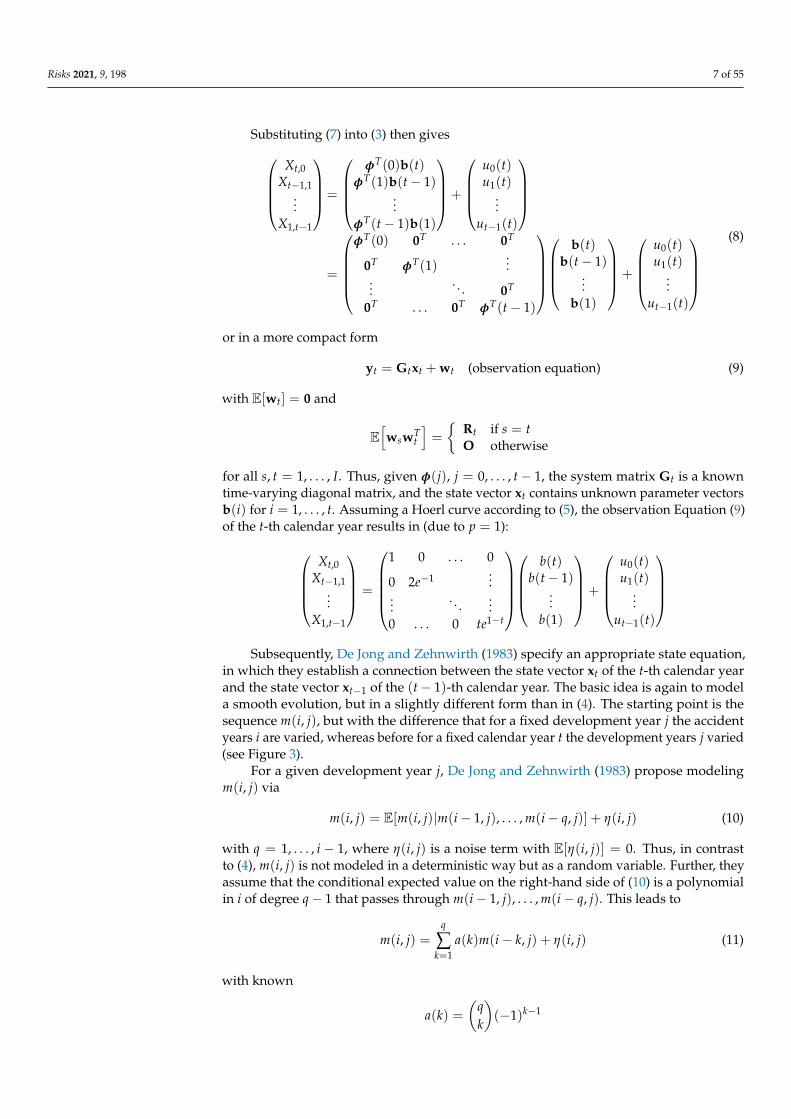
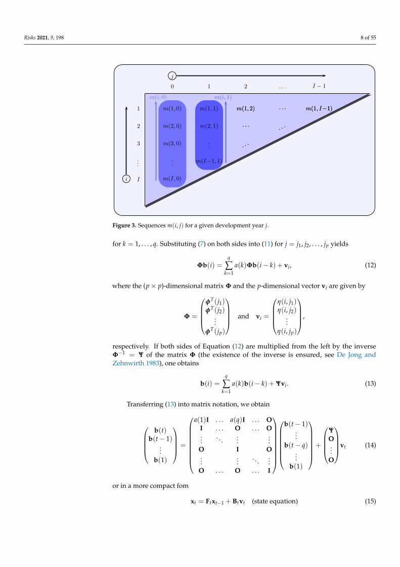
in which they establish a connection between the state vector xt of the t-th calendar yearand the state vector xt−1 of the (t− 1)-th calendar year. The basic idea is again to modela smooth evolution, but in a slightly different form than in (4). The starting point is thesequence m(i, j), but with the difference that for a fixed development year j the accidentyears i are varied, whereas before for a fixed calendar year t the development years j varied(see Figure 3).

For a given development year j, De Jong and Zehnwirth (1983) propose modelingm(i, j) via

m(i, j) = E[m(i, j)|m(i− 1, j), . . . , m(i− q, j)] + η(i, j) (10)

with q = 1, . . . , i − 1, where η(i, j) is a noise term with E[η(i, j)] = 0. Thus, in contrastto (4), m(i, j) is not modeled in a deterministic way but as a random variable. Further, theyassume that the conditional expected value on the right-hand side of (10) is a polynomialin i of degree q− 1 that passes through m(i− 1, j), . . . , m(i− q, j). This leads to

m(i, j) =q

∑k=1

a(k)m(i− k, j) + η(i, j) (11)

with known

a(k) =(

qk

)(−1)k−1

Risks 2021, 9, 198 8 of 55

m(1, 0) m(1, 1) m(1, 2) . . . m(1, I−1)

m(2, 0) m(2, 1) . . . . . .

m(3, 0) ... . . .

...m(I−1, 1)

m(I, 0)

m(i, 0) m(i, 1)

1

2

3

...

I

0 1 2 . . . I − 1

m(1, 0) m(1, 1) m(1, 2) . . . m(1, I−1)

m(2, 0) m(2, 1) . . . . . .

m(3, 0) ... . . .

...m(I−1, 1)

m(I, 0)i

j

Figure 3. Sequences m(i, j) for a given development year j.

for k = 1, . . . , q. Substituting (7) on both sides into (11) for j = j1, j2, . . . , jp yields

Φb(i) =q

∑k=1

a(k)Φb(i− k) + vi, (12)

where the (p× p)-dimensional matrix Φ and the p-dimensional vector vi are given by

Φ =

φT(j1)φT(j2)

...φT(jp)

and vi =

η(i, j1)η(i, j2)

...η(i, jp)

,

respectively. If both sides of Equation (12) are multiplied from the left by the inverseΦ−1 = Ψ of the matrix Φ (the existence of the inverse is ensured, see De Jong andZehnwirth 1983), one obtains

b(i) =q

∑k=1

a(k)b(i− k) + Ψvi. (13)

Transferring (13) into matrix notation, we obtain

b(t)

b(t− 1)...

b(1)

=

a(1)I . . . a(q)I . . . OI . . . O . . . O...

. . ....

...O I O...

.... . .

...O . . . O . . . I

b(t− 1)...

b(t− q)...

b(1)

+

Ψ

O...

O

vt (14)

or in a more compact fom

xt = Ftxt−1 + Btvt (state equation) (15)

Risks 2021, 9, 198 9 of 55

with E[vt] = 0 and

E[vsvT

t

]=

{Qt if s = tO otherwise

as well as E[vswT

t]= O for all s, t = 1, . . . , I. The identity matrices I, zero matrices O and

scalar matrices a(k)I with k = 1, . . . , q in (14) are each of dimension p× p. Note also thatthe system matrices Ft and Bt are known in the state Equation (15).

A variation of the state Equation (15) is given for p = 1 (i.e., assuming a Hoerl curveas in (5)) and the parameters b(i) of different accident years i = 2, . . . , I are connected by arandom walk

b(i) = b(i− 1) + vi, (16)

that is, q = 1, a(1) = 1, Ψ = 1. Since we have Φ = φT(j) = φ(j) = (j + 1)e−j, the relationΨ = ej

j+1 holds. For this reason, De Jong and Zehnwirth (1983) aim to obtain Ψ = 1 andthus a state equation in the form of the random walk (16), i.e., they choose without loss ofgenerality the fixed development year j = 0.

With respect to (10) and (13), the use of (16) implies

E[m(i, j)|m(i− 1, j), . . . , m(i− q, j)] = E[m(i, j)|m(i− 1, j)] = m(i− 1, j)

for all j = 0, . . . , I − 1. Accordingly, it follows for the system matrix Ft that it has the valueone at positions (1, 1), (2, 1), (3, 2), . . . , (t, t− 1) and zeros otherwise, while Bt correspondsto a t-dimensional unit vector with the value one at position (1, 1). The state Equation (15)thus simplifies to:

b(t)

b(t− 1)...

b(1)

=

1 0 . . . 01 0 . . . 0...

. . ....

... 1 00 . . . 0 1

b(t− 1)b(t− 2)

...b(1)

+

10...0

vt

Table 1 gives an overview of the dimensions of vectors and matrices in the state spacemodel of De Jong and Zehnwirth (1983).

Table 1. Dimensions in the state space model of De Jong and Zehnwirth (1983).

Vectors Matrices

yt t× 1 Gt t× tpxt tp× 1 Ft tp× (t− 1)pwt t× 1 Bt tp× pvt p× 1 Rt t× t

Qt p× p

If one intends to model the observation and state equations by using (2) instead of(1), there are only changes in the observation Equation (9), while the state Equation (15)remains unchanged: each row k = 1, . . . , t of the system matrix Gt has to be multiplied bya weighting factor consisting of volume and inflation indices, i.e., by n(t− k + 1)λ(t).

B Forecasting the outstanding loss liabilities

As the system matrices Gt, Ft, Bt are assumed to be known for all t = 1, . . . , I, theoutstanding loss liabilities for individual and aggregated accident years can be predicted

Risks 2021, 9, 198 10 of 55

by using xI|I and PI|I = Cov(

xI − xI|I)

in a straightforward way. To this end, all futureincremental payments are collected in the vector

yI+1 =(XI,1 XI−1,2 . . . X2,I−1 XI,2 . . . X3,I−1 . . . XI,I−1

)T .

All these future observations belong to one of the accident years i = 2, . . . , I, andtherefore, they are based on the corresponding state b(2), . . . , b(I). Accordingly, the statevector xI+1 corresponds to the vector xI of the current calendar year I, which is why thestate Equation (15) is given by xI+1 = xI (i.e., FI+1 = I, QI+1 = O). The system matrixGI+1 of the observation equation is obtained on the basis of (1) similar to that in (8), i.e.,it consists mostly of zero vectors, and the entries φT(j) with j = 1, . . . , I − 1 are orderedsuch that they are multiplied by the states b(i) from xI of the corresponding accident yeari = 1, . . . , I of Xi,j from yI+1. Thus, the future observations can be predicted via

yI+1|I = GI+1xI|I

(given by (9)) and

XI,1XI−1,2

...X2,I−1

XI,2...

X3,I−1...

XI,I−1

=

φT(1) 0T . . . . . . 0T

0T φT(2)...

.... . .

...

0T . . . 0T φT(I − 1)...

φT(2) 0T . . . . . ....

.... . .

...

0T . . . φT(I − 1) 0T ......

...φT(I − 1) 0T . . . . . . 0T

b(I)

b(I − 1)...

b(1)

,

respectively. The variance–covariance matrix of the prediction error(yI+1 − yI+1|I

)is

given by:

∆I+1 = Cov(yI+1 − yI+1|I

)= GI+1PI|IG

TI+1

Since xI|I , PI|I , GI+1 are known at time t = I, a prediction of the outstanding lossliabilities for individual and aggregated accident years is straightforward. With respect tothe aggregated accident years, all components from yI+1|I are to be added to the total lossreserve, while for individual accident years only those components from yI+1|I related tothe respective accident year i = 2, . . . , I are to be added. An extraction of these componentscan be carried out via a diagonal matrix A, which has a value of one at the respectivepositions and otherwise zeros. The variance–covariance matrix belonging to AyI+1|I is thus

Cov(AyI+1 −AyI+1|I

)= A∆I+1AT .

However, if the modified payment stream according to (2) is used, additional un-certainty is induced via the inflation index λ(t) of future calendar years t > I, which isunknown at time t = I. This is due to the unknown entries n(i)λ(i + j)φT(j) for i + j > Iinstead of the known entries φT(j) in the system matrix GI+1.

2.2. A Stochastic Method for Claims Reserving in General Insurance

Wright (1990) primarily establishes a model for incremental payments that includesa state space approach, where the variation of the parameters is modeled over differentaccident years. Thus, although the model of Wright (1990) is not mainly based on state

Risks 2021, 9, 198 11 of 55

space models and the Kalman filter theory, it embeds them in a model framework as onecomponent. In the following, therefore, the model for incremental payments and the statespace model are presented (for further details, see Wright 1990).

B Construction of the model for claims payments

The modeling is built on development triangles that include incremental payments Xi,jin accident years i = 1, . . . , I and development years j = 0, . . . , I − 1. The proposed modelis based on the assumption that incremental payments Xi,j are composed of the sum ofNi,j independent and identically distributed (i.i.d.) payments Xk

i,j (which are stochastically

independent of Ni,j), that is, Xi,j = ∑Ni,jk=1 Xk

i,j. Thus, Wright (1990) uses the collective riskmodel and Xi,j has a mixture distribution (see, e.g., Kaas et al. 2009). The lags j of individualincremental payments Xk

i,j between the accident year of the claim and the actual payment

are modeled as i.i.d. random variables, which is why pi,j with ∑I−1j=0 pi,j = 1 is defined as

the probability of payments regarding claims of accident year i in a given developmentyear j. Let the number Ni,j of payments for claims of accident year i in development yearj be Poisson-distributed with parameter εi pi,j, i.e., Ni,j ∼ P

(εi pi,j

); then, the incremental

payments Xi,j follow a mixture Poisson distribution. Following the convolution property ofthe Poisson distribution, the total number of claims payments Ni = ∑I−1

j=0 Ni,j of an accidentyear i also follows a Poisson distribution with parameter

εi =I−1

∑j=0

εi pi,j,

where the Ni,j for different j are assumed to be stochastically independent random variablesand the parameter εi serves as a measure for the exposure of accident year i. As for modelingof the probability pi,j, Wright (1990) gives two alternatives, the stochastic CL and theHoerl curve model. While in the first alternative it is assumed that the probabilities pi,jare identical over all accident years i, the second alternative (preferred by Wright 1990)provides a modeling via a Hoerl curve of the form

pi,j = αjκi j′Ai e−Bi j′ (17)

with constants κi, Ai and Bi to be estimated and αj and j′ as functions depending on j.Using (17), the expected value and variance of Ni,j are as follows:

E[Ni,j]= Var

(Ni,j)= εi pi,j = εiαjκi j′Ai e−Bi j′ (18)

In addition to the number Ni,j of payments, Wright (1990) also models the amountof individual payments Xk

i,j for claims of an accident year i in the j-th development year,which, like the Ni,j, are also assumed to be stochastically independent for various j. Thefirst two moments of Xk

i,j are modeled distribution-free with help of

E[

Xki,j

]= eδt Kj′λ and Var

(Xk

i,j

)= ρ2E

[Xk

i,j

]2(19)

with proper (unknown) constants K > 0, λ, ρ and inflation parameter δt. While such amodeling of the expected value with different λ and K provides a variety of possibilities,the modeling of the variance results from the assumption that the coefficient of variation

CV =

√Var(

Xki,j

)E[

Xki,j

]

Risks 2021, 9, 198 12 of 55

is time-invariant and corresponds to ρ. The optional term eδt in (19) with

δt =t

∑k=1

τk

and τk as the average annual inflation rate between calendar years k− 1 and k, on the otherhand, are used to account for inflation; i.e., eδt reflects the inflation factor from the firstcalendar year to calendar year t = i + j. However, Wright (1990) proposes using

δt =t

∑k=1

τ = tτ = (i + j)τ ≈ (i + j′)τ, (20)

and therefore assumes a constant inflation rate τ.Considering (18)–(20), and using the moments of the mixture Poisson distribution, the

expected value and variance of the incremental payments Xi,j in (i, j) are obtained via

E[Xi,j]= E

[Ni,j]E[

Xki,j

]= εi pi,je(i+j′)τKj′λ (21)

and

Var(Xi,j)= E

[Ni,j]E[(

Xki,j

)2]

= E[Ni,j](

E[

Xki,j

]2+ Var

(Xk

i,j

))= E

[Ni,j](

1 + ρ2)E[

Xki,j

]2

= εi pi,j

(1 + ρ2

)e2τ(i+j′)K2 j′2λ, (22)

where Xi,j are stochastically independent for different j due to the assumptions regardingNi,j and Xk

i,j. Moreover, Wright (1990) normalizes the incremental payments Xi,j with thehelp of

X′i,j =Xi,j

εiαj(23)

with exposure defined by

εi = εiε′i. (24)

By using (17), (21), (23), (24), the expected value E[X′i,j] = µ′i,j of the normalizedincremental payments X′i,j can be stated as follows:

µ′i,j =1

εiαjE[Xi,j]

=1

εiαjεi pi,je(i+j′)τKj′λ (25)

=1

εiαjεiαjκi j′Ai e−Bi j′ e(i+j′)τKj′λ

= eiτε′iκiKj′(Ai+λ)e−(Bi−τ)j′

= eβi,1 j′βi,2 e−βi,3 j′

Risks 2021, 9, 198 13 of 55

with

βi,1 = iτ + ln(ε′iκiK

)βi,2 = Ai + λ

βi,3 = Bi − τ

Considering (22), (23), (25), the variance of X′i,j is

Var(

X′i,j)=

1(εiαj

)2 Var(Xi,j)

=1(

εiαj)2 εi pi,j

(1 + ρ2

)e2τ(i+j′)K2 j′2λ

= µ′i,j1

εiαj

(1 + ρ2

)e(i+j′)τKj′λ

= µ′i,jφiψj

with

φi =K(1 + ρ2)eiτ

εiand ψj =

j′λej′τ

αj.

Assuming that φi and ψj are known, one obtains a generalized linear model of the form

X′i,j = µ′i,j + ei,j = exp(

xTj βi

)+ ei,j

with the exponential response function h−1, linear predictor xTj βi consisting of

xj =

1ln(j′)−j′

and βi =

βi,1βi,2βi,3

and noise term ei,j with

E[ei,j]= 0 and Var

(ei,j)= µ′i,jφiψj,

where the parameter estimators βi and variance–covariance matrices Ri can be determined

for all i using the Fisher scoring algorithm such that βi ∼ N(

βi; Ri

)is approximately

satisfied. However, since φi and ψj are usually unknown, Wright (1990) proposes aniterative approach using parameter initializations to determine initial values for φi andψj. Considering this approach, all accident years are run sequentially and the results ofall accident years are subsequently used to obtain new estimates of the parameters for thenext run.

B Modeling the parameter variation via a state space model

To increase the reliability of the estimators βi, Wright (1990) models the variation inthe parameters βi for different accident years i via

βi = βi−1 +

τ00

+ ωi (26)

Risks 2021, 9, 198 14 of 55

with

ωi =

ωi,1ωi,2ωi,3

, E[ωi] = 0 and Cov(ωi) =

u21 0 0

0 u22 0

0 0 u23

.

By defining xi with the help of

xi =(τ βi,1 βi,2 βi,3

)T (27)

and by using (26), (27) can be written as

xi = Fixi−1 + vi (state equation) (28)

with

Fi =

1 0 0 01 1 0 00 0 1 00 0 0 1

, xi−1 =

τ

βi−1,1βi−1,2βi−1,3

and vi =

0

ωi,1ωi,2ωi,3

,

where E[vi] = 0 and

E[vhvT

i

]=

{Qi if h = iO otherwise

hold for all h, i = 1, . . . , I. Thus, Equation (28) forms the state equation of a state spacemodel. Considering the estimators βi as observations yi, the associated observation equa-tion can be obtained via

yi = Gixi + wi (observation equation) (29)

with

yi =

βi,1βi,2βi,3

, Gi =

0 1 0 00 0 1 00 0 0 1

, wi =

εi,1εi,2εi,3

and E[wi] = 0,

E[whwT

i

]=

{Ri if h = iO otherwise

and E[vhwT

i]= O for all h, i = 1, . . . , I. Accordingly, a complete state space model with

w = 3 and v = 4 is specified via Equations (28) and (29).

2.3. Kalman Filters with Applications to Loss Reserving

Zehnwirth (1997) states that this article arose from various lecture notes on statisticsand actuarial science and should be viewed primarily as an introduction to Kalman filtertheory and ordinary least squares (OLS) estimation and their close relationship to Bayesestimation. Thus, Zehnwirth (1997) derives Kalman recursions for (multiple) linear regres-sion models and the local level model, shows the connections of sample-based updateswith Bayes updates in OLS estimators, and discusses state space models and the generalKalman filter algorithms.

The focus in the experimental and empirical applications is primarily not on anapplication of the Kalman filter, but on an investigation of the trend properties withinclaims development triangles. In the experimental application, a simulation of incremental

Risks 2021, 9, 198 15 of 55

payments Xi,j in accident years i = 1, . . . , I and development years j = 0, . . . , I − 1 isperformed via

Xi,j = eα−0.2j, (30)

i.e., a variation of the Hoerl curve. The factor eα reflects the basic level of incrementalpayments, while the factor e−0.2j describes their decreasing behavior over the developmentyears. Based on this, calendar year effects (in the form of inflation factors) are illustratedand the problem of overparameterization is addressed, which arises, e.g., when there aretoo many parameters for the individual accident years, but can be remedied by recursivelyevolving parameters. However, no specific state space representation is developed.

2.4. Loss Reserving: Past, Present and Future

Taylor et al. (2003) give a classification scheme for claims reserving methods whosehigher-level criteria make a division between static and dynamic methods. In the frame-work of this taxonomic classification and especially with respect to the dynamic methods,they discuss a generalized Kalman filter, which allows for non-linearities in the observationequation and noise terms following a distribution of the Exponential Dispersion Family(EDF). They present two modeling approaches based on different types of claims data andstate space representations constructed specifically for these data.

B Accident year-based state space modeling

In the first modeling approach, an accident year-based state space representationis constructed, which is based on Payments Per Claim Incurred (PPCI) of a workers’compensation insurance policy as claims data. The PPCI of an accident year i = 0, . . . , Iin the development year j = 0, . . . , I are denoted by Yi,j and belong to the (t = i + j)-thcalendar year with t = 0, . . . , I.

The state space model considered by Taylor et al. (2003) is based on a linear stateequation of the form

xi+1 = Fixi + vi (state equation) (31)

with five-dimensional random vectors xi, vi, transition matrix Fi ∈ R5×5, E[vi] = 0 and

E[vivT

k

]=

{Qi if i = kO otherwise

for i, k = 0, . . . , I − 1, while the observation equation

yi = h−1(Gixi) + wi (observation equation) (32)

with (I − i + 1)-dimensional random vectors yi, wi, system matrix Gi ∈ R(I−i+1)×5,E[wi] = 0 and

E[wiwT

k

]=

{Ri if i = kO otherwise

is based on a generalized linear model with link function h (i.e., response function h−1)and linear predictor Gixi for all i, k = 0, . . . , I. Moreover, E

[viwT

k]= O holds for all

i, k = 0, . . . , I, the initial state x0 is uncorrelated with vi and wi for all i = 0, . . . , I and wiis assumed to be EDF-distributed for all i = 0, . . . , I. Thus, any strictly monotonic anddifferentiable link function h (such as a logarithm function) can be used to link the EDF-distributed observations yi and the systematic component Gixi. The resulting recursiveequations Taylor et al. (2003) refer to as the EDF filter, which include the Kalman filter asa special case, namely for the identity function as link function and normally distributed

Risks 2021, 9, 198 16 of 55

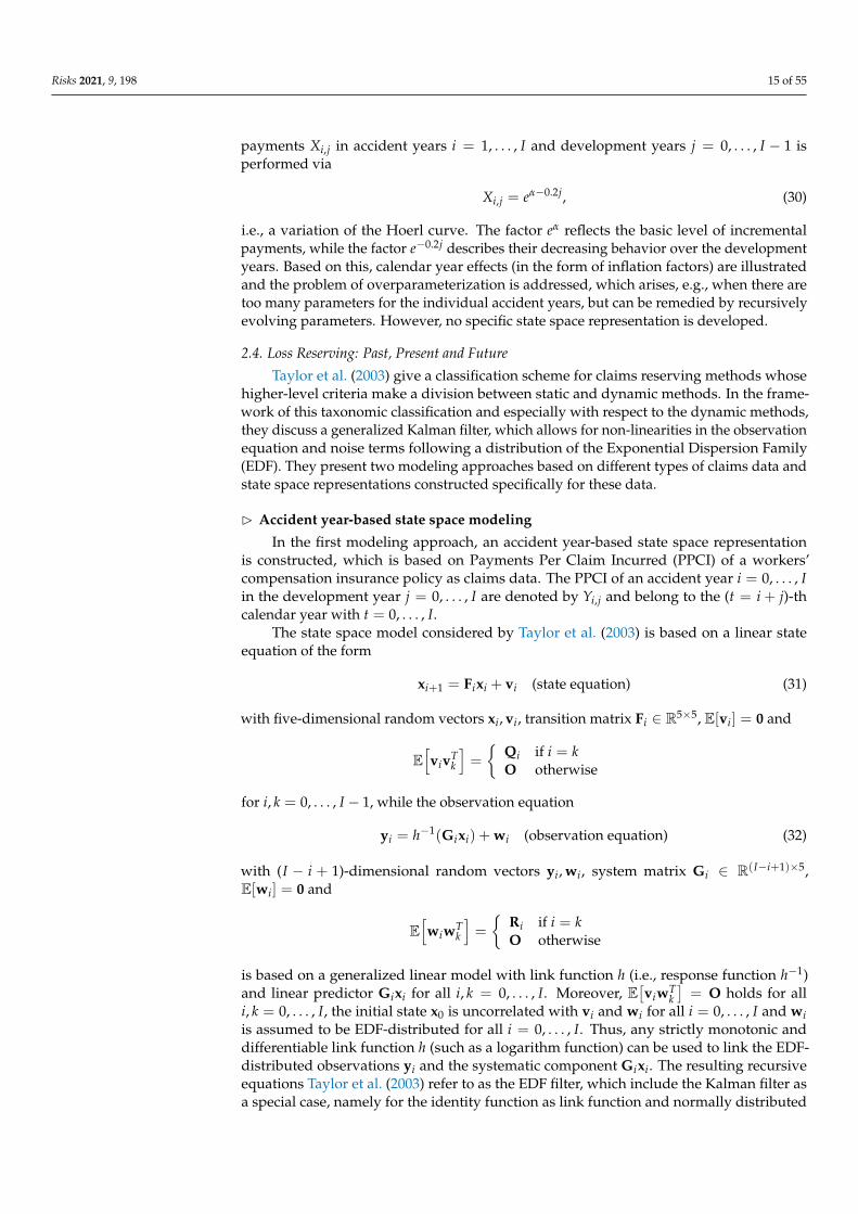
noise terms wi. The observation vector yi in (32) includes all PPCIs of an accident yeari = 0, . . . , I of the upper claims development triangle (see Figure 4).

Y0,0 Y0,1 Y0,2 Y0,I

Y1,0 Y1,1 Y1,I−1

Y2,0

YI−1,1

YI,0

. . .

. . .

...

...

0 1 2 . . . I

0

1

2

I

. ..

y0

y1

yI

...

Y0,0 Y0,1 Y0,2 Y0,I

Y1,0 Y1,1 Y1,I−1

YI,0

i

j

Figure 4. Accident year-based modeling of the observation vector.

Taylor et al. (2003) propose a logarithm function as a link function, the noise terms wiare assumed to be gamma-distributed and the (j + 1)-th row of the linear predictor Gixifor an accident year i = 0, . . . , I is given by

βi,0 + βi,1(j + 1) +βi,2

j + 1+

βi,3

(j + 1)2 + βi,4δj,0 (33)

with respect to the development year j = 0, . . . , I. Here, δj,0 denotes the Kronecker delta,

δj,0 =

{1 if j = 00 if j > 0

,

which can be used to model the peak in development year j = 0. Thus, the observationEquation (32) of accident year i = 0, . . . , I can be stated as follows:

Yi,0Yi,1

...Yi,j

...Yi,I−i

= exp

1 1 1 1 11 2 1

214 0

......

......

...1 j + 1 1

j+11

(j+1)2 0...

......

......

1 I − i + 1 1I−i+1

1(I−i+1)2 0

βi,0βi,1βi,2βi,3βi,4

+

wi,0wi,1

...wi,j

...wi,I−i

On the other hand, Taylor et al. (2003) do not provide any information on the concrete

form of the state Equation (31). Taylor et al. (2003) model the evolution of the PPCI overthe development years according to (33) in a similar way to De Jong and Zehnwirth (1983),Wright (1990) and Zehnwirth (1997), who specify the evolution of incremental payments

Risks 2021, 9, 198 17 of 55

over the development years with the help of a Hoerl curve. Taylor et al. (2003) applythis approach to the PPCI, as their evolution over the development years is similar tothat of incremental payments: They reach their peak in development year j = 0 andthen drop relatively quickly to zero. This evolution of the PPCI is also the justificationof Taylor et al. (2003) for the choice of the logarithm function as a link function and theassumption of a gamma distribution for the measurement noise.

B Calendar year-based state space modeling

For the second modeling approach, Taylor et al. (2003) use a data set from Taylor (2000)that consists of motor vehicle bodily injury claim closure rates. Here, rather than collectingthe observations from each accident year, they stack the observations from each calendaryear into observation vectors. This is due to the fact that claim closure rates are relativelyflat across development years, but are subject to calendar year effects.

The state space model proposed by Taylor et al. (2003) provides a linear state equationand an observation equation in the form of a generalized linear model, but differs fromthe first approach by the time index (calendar years t instead of accident years i) and bythe matrix dimensions. They consider the following state space model consisting of thestate equation

xt+1 = Ftxt + vt (state equation) (34)

with (3t + 9)-dimensional random vectors xt+1, vt, a (3t + 6)-dimensional random vector xtand transition matrix Ft ∈ R(3t+9)×(3t+6) for t = 0, . . . , I − 1, and the observation equationof the t-th calendar year

yt = h−1(Gtxt) + wt (observation equation) (35)

with (t + 1)-dimensional random vectors yt, wt, and (t + 1)× (3t + 6)-dimensional systemmatrix Gt for t = 0, . . . , I, where the assumptions concerning the noise terms correspondto those of the first approach (transferred to calendar years).

Taylor et al. (2003) choose the identity function as a link function and the measure-ment noise is assumed to be normally distributed, which is why one obtains an ordinarylinear observation equation and the usual linear Kalman filter can be used. This choiceis motivated by the sufficiently high number of claims closures in the underlying claimsdata, and the assumption of an approximate normal distribution is justified by the centrallimit theorem, although the assumption of a discrete probability distribution such as thebinomial distribution would be more appropriate. As for the development of the expectedclaim closure rate E

[Zi,j]

with respect to the claims of an accident year i = 0, . . . , I over thedevelopment years j = 0, . . . , I, Taylor et al. (2003) assume

E[Zi,j]= βi,0 +

βi,1

j + 1+

βi,2

(j + 1)2 + γtδi+j,t (36)

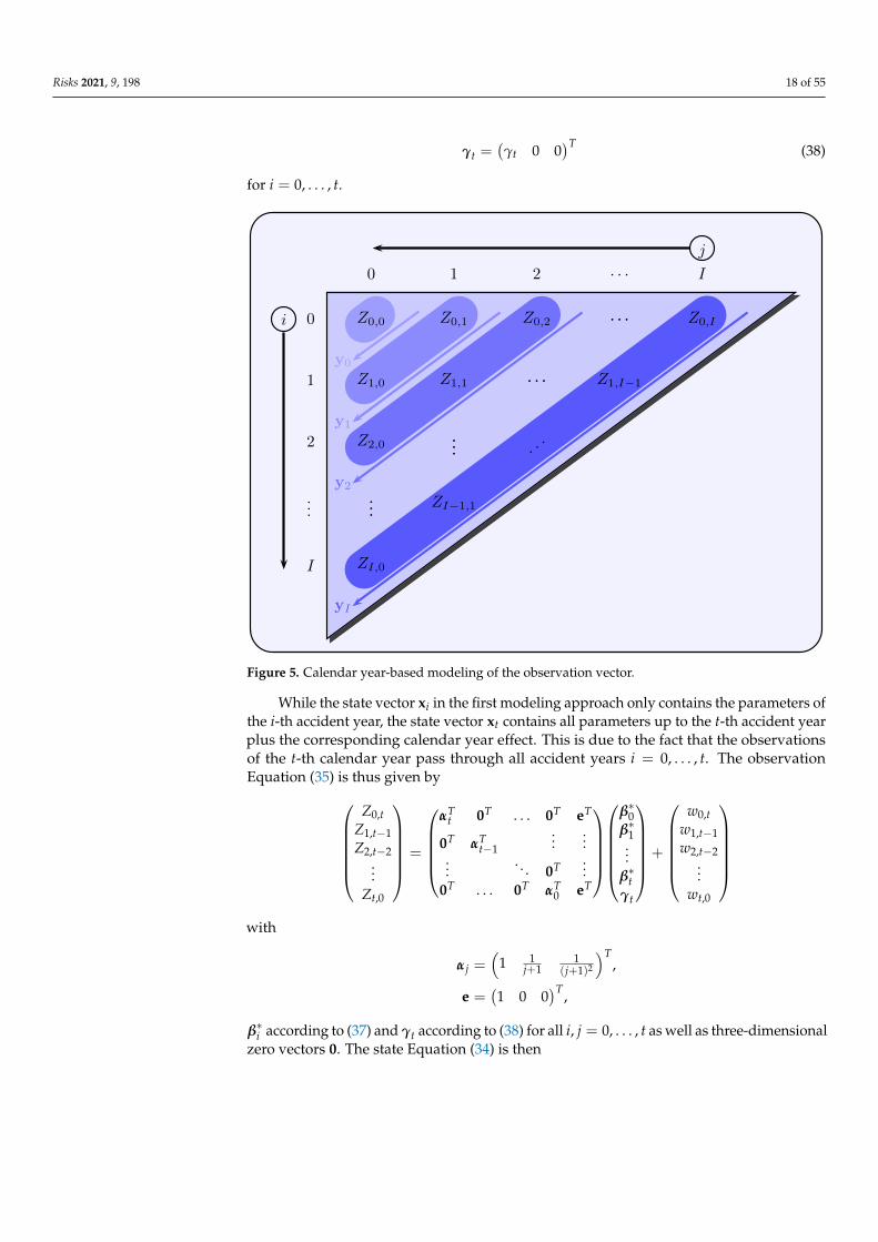
with γt as effect of the t-th calendar year and Kronecker Delta δi+j,t. The observation vector

yt =(Z0,t Z1,t−1 Z2,t−2 . . . Zt,0

)T

of the t-th calendar year with t = 0, . . . , I contains all t + 1 claim closure rates Zi,j of therespective calendar year t = i + j (see Figure 5), which is why the (3t + 6)-dimensionalstate vector can be stated as

xt =(

β∗0 β∗1 . . . β∗t γt)T

with

β∗i =(

βi,0 βi,1 βi,2)T (37)

Risks 2021, 9, 198 18 of 55

γt =(γt 0 0

)T (38)

for i = 0, . . . , t.

Z0,0 Z0,1 Z0,2 . . . Z0,I

Z1,0 Z1,1 . . . Z1,I−1

Z2,0... . .

.

...ZI−1,1

ZI,0

y2

yI

0

1

2

...

I

y0

y1

0 1 2 . . . I

Z0,0 Z0,1 Z0,2 . . . Z0,I

Z1,0 Z1,1 . . . Z1,I−1

Z2,0... . .

.

...ZI−1,1

ZI,0

i

j

Figure 5. Calendar year-based modeling of the observation vector.

While the state vector xi in the first modeling approach only contains the parameters ofthe i-th accident year, the state vector xt contains all parameters up to the t-th accident yearplus the corresponding calendar year effect. This is due to the fact that the observationsof the t-th calendar year pass through all accident years i = 0, . . . , t. The observationEquation (35) is thus given by

Z0,tZ1,t−1Z2,t−2

...Zt,0

=

αT

t 0T . . . 0T eT

0T αTt−1

......

.... . . 0T ...

0T . . . 0T αT0 eT

β∗0β∗1...

β∗tγt

+

w0,t

w1,t−1w2,t−2

...wt,0

with

αj =(

1 1j+1

1(j+1)2

)T,

e =(1 0 0

)T ,

β∗i according to (37) and γt according to (38) for all i, j = 0, . . . , t as well as three-dimensionalzero vectors 0. The state Equation (34) is then

Risks 2021, 9, 198 19 of 55

β∗0...

β∗tβ∗t+1γt+1

=

I O . . . O

O. . .

...... I

...... I O

O . . . O I

β∗0β∗1...

β∗tγt

+

0...0

v(β)t

v(γ)t

where I and O in Ft are identity and zero matrices of dimensions 3× 3, respectively, 0 in vt

are three-dimensional zero vectors and v(β)t , v(γ)

t are given as follows:

v(β)t =

(vt,0 vt,1 vt,2

)T

v(γ)t =

(v(γ)t 0 0

)T

Thus, the state equation involves a dynamic estimation of the parameters β∗t+1 andγt+1 via

β∗t+1 = β∗t + v(β)t

γt+1 = γt + v(γ)t

for t = 0, . . . , I − 1. Finally, Table 2 gives an overview of the dimensions of vectors andmatrices in the state space models of Taylor et al. (2003).

Table 2. Dimensions in the state space models of Taylor et al. (2003).

Accident Year-Based Model Calendar Year-Based Model

yi (I − i + 1)× 1 yt (t + 1)× 1xi+1 5× 1 xt+1 (3t + 9)× 1xi 5× 1 xt (3t + 6)× 1wi (I − i + 1)× 1 wt (t + 1)× 1vi 5× 1 vt (3t + 9)× 1Gi (I − i + 1)× 5 Gt (t + 1)× (3t + 6)Fi 5× 5 Ft (3t + 9)× (3t + 6)Ri (I − i + 1)× (I − i + 1) Rt (t + 1)× (t + 1)Qi 5× 5 Qt (3t + 9)× (3t + 9)

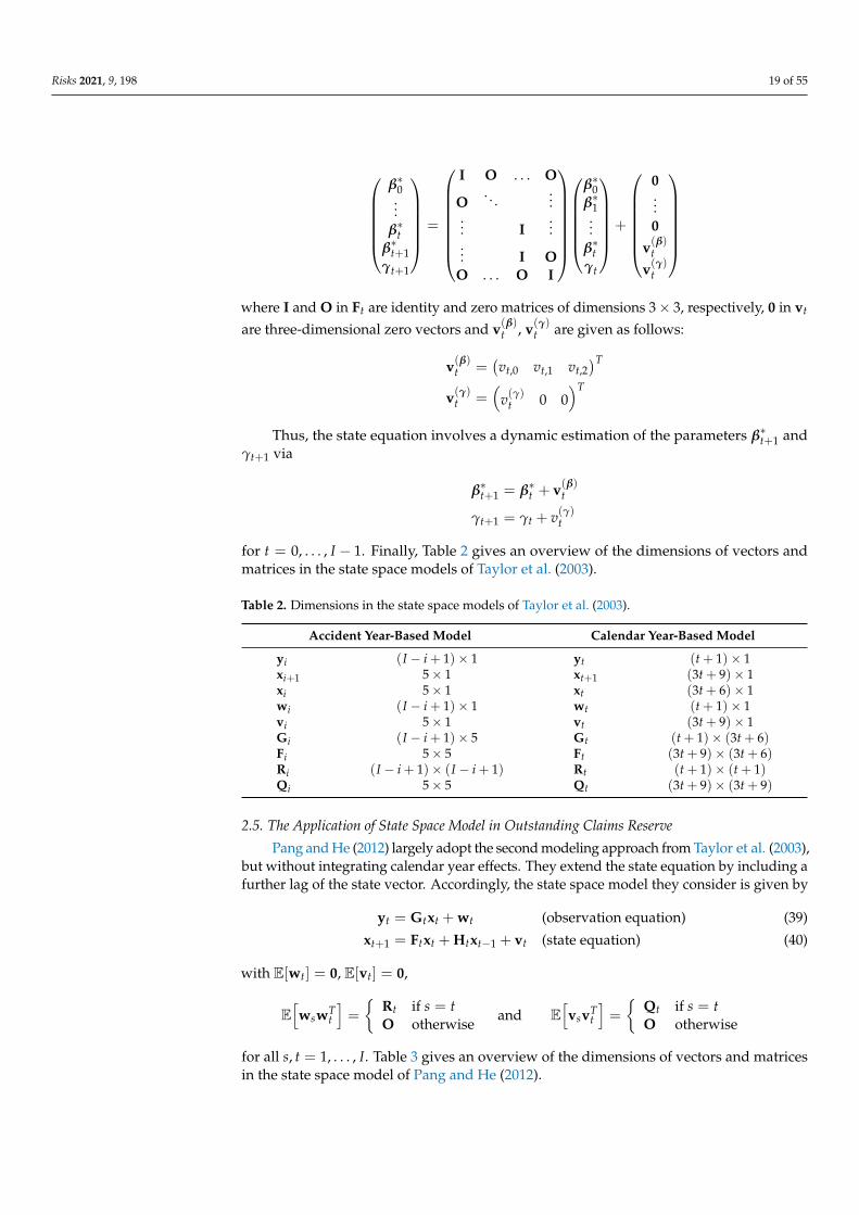
2.5. The Application of State Space Model in Outstanding Claims Reserve

Pang and He (2012) largely adopt the second modeling approach from Taylor et al. (2003),but without integrating calendar year effects. They extend the state equation by including afurther lag of the state vector. Accordingly, the state space model they consider is given by

yt = Gtxt + wt (observation equation) (39)

xt+1 = Ftxt + Htxt−1 + vt (state equation) (40)

with E[wt] = 0, E[vt] = 0,

E[wswT

t

]=

{Rt if s = tO otherwise

and E[vsvT

t

]=

{Qt if s = tO otherwise

for all s, t = 1, . . . , I. Table 3 gives an overview of the dimensions of vectors and matricesin the state space model of Pang and He (2012).

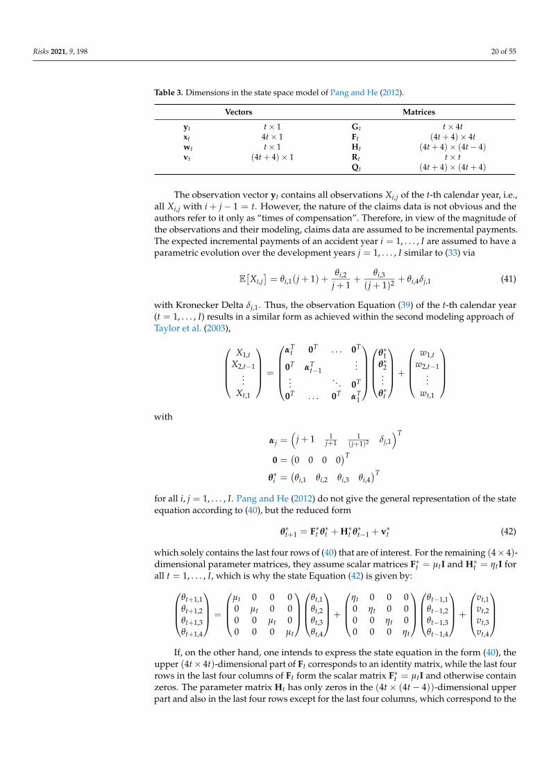
Risks 2021, 9, 198 20 of 55

Table 3. Dimensions in the state space model of Pang and He (2012).

Vectors Matrices

yt t× 1 Gt t× 4txt 4t× 1 Ft (4t + 4)× 4twt t× 1 Ht (4t + 4)× (4t− 4)vt (4t + 4)× 1 Rt t× t

Qt (4t + 4)× (4t + 4)

The observation vector yt contains all observations Xi,j of the t-th calendar year, i.e.,all Xi,j with i + j− 1 = t. However, the nature of the claims data is not obvious and theauthors refer to it only as “times of compensation”. Therefore, in view of the magnitude ofthe observations and their modeling, claims data are assumed to be incremental payments.The expected incremental payments of an accident year i = 1, . . . , I are assumed to have aparametric evolution over the development years j = 1, . . . , I similar to (33) via

E[Xi,j]= θi,1(j + 1) +

θi,2

j + 1+

θi,3

(j + 1)2 + θi,4δj,1 (41)

with Kronecker Delta δj,1. Thus, the observation Equation (39) of the t-th calendar year(t = 1, . . . , I) results in a similar form as achieved within the second modeling approach ofTaylor et al. (2003),

X1,t

X2,t−1...

Xt,1

=

αT

t 0T . . . 0T

0T αTt−1

......

. . . 0T

0T . . . 0T αT1

θ∗1θ∗2...

θ∗t

+

w1,t

w2,t−1...

wt,1

with

αj =(

j + 1 1j+1

1(j+1)2 δj,1

)T

0 =(0 0 0 0

)T

θ∗i =(θi,1 θi,2 θi,3 θi,4

)T

for all i, j = 1, . . . , I. Pang and He (2012) do not give the general representation of the stateequation according to (40), but the reduced form

θ∗t+1 = F∗t θ∗t + H∗t θ∗t−1 + v∗t (42)

which solely contains the last four rows of (40) that are of interest. For the remaining (4× 4)-dimensional parameter matrices, they assume scalar matrices F∗t = µtI and H∗t = ηtI forall t = 1, . . . , I, which is why the state Equation (42) is given by:

θt+1,1θt+1,2θt+1,3θt+1,4

=

µt 0 0 00 µt 0 00 0 µt 00 0 0 µt

θt,1θt,2θt,3θt,4

+

ηt 0 0 00 ηt 0 00 0 ηt 00 0 0 ηt

θt−1,1θt−1,2θt−1,3θt−1,4

+

vt,1vt,2vt,3vt,4

If, on the other hand, one intends to express the state equation in the form (40), the

upper (4t× 4t)-dimensional part of Ft corresponds to an identity matrix, while the last fourrows in the last four columns of Ft form the scalar matrix F∗t = µtI and otherwise containzeros. The parameter matrix Ht has only zeros in the (4t× (4t− 4))-dimensional upperpart and also in the last four rows except for the last four columns, which correspond to the

Risks 2021, 9, 198 21 of 55

(4× 4)-dimensional scalar matrix H∗t = ηtI. The noise vector vt is equal to a zero vector inthe first 4t rows and to the vector v∗t in the remaining rows.

3. Log-Normal Models for Incremental Payments (Category 2)

This section presents articles in which incremental payments are assumed to be log-normally distributed and are modeled using a log-normal model:

I Verrall (1989): A State Space Representation of the Chain Ladder Linear Model;I Verrall (1994): A Method for Modelling varying Run-Off Evolutions in Claims Reserving;B Ntzoufras and Dellaportas (2002): Bayesian Modelling of Outstanding Liabilities incorpo-

rating Claim Count Uncertainty;B Li (2006): Comparison of Stochastic Reserving Methods.

The articles of Verrall (1989, 1994) are presented in detail due to the fact that theyare mainly based on the use of state space models and the Kalman filter learning theory(marked in the above listing with I), while the models in the papers of Ntzoufras andDellaportas (2002) and Li (2006) are treated in a more concise form (marked in the abovelisting with B).

3.1. A State Space Representation of the Chain Ladder Linear Model

Verrall (1989) discusses various state space representations based on the model of atwo-way ANOVA, and thus follows Kremer (1982), who shows a close connection betweenthe CL method and the two-way ANOVA. In addition to a dynamic estimation of theparameters by means of the Kalman filter algorithms, Verrall (1989) also considers staticmodels without and with prior information.

B The linear Chain Ladder model

The modeling is based on increments Xi,j > 0 with i, j = 1, . . . , I. The restriction topositive values is necessary against the backdrop of a logarithmic transformation of Xi,j. Inpractice, the model of Verrall (1989) can be applied to paid data, but not to incurred data.For the increments Xi,j, a multiplicative model

Xi,j = uisjri,j (43)

with ui as a parameter of the accident year i, sj as a parameter of the development year j andri,j as noise term with E[ri,j] = 1 for all i, j = 1, . . . , I is assumed. Further, the incrementsare presumed to follow a log-normal distribution, so a logarithmic transformation ofthe increments is performed, i.e., Yi,j = log

(Xi,j). Thus, the variables Yi,j are normally

distributed. If both sides of (43) of the multiplicative model are logarithmized, this leads tothe (additive) model of the two-way ANOVA with normally distributed residuals

Yi,j = µ + αi + β j + wi,j (44)

with population mean µ, row parameter αi, column parameter β j and wi,j ∼WN(0; σ2) for

all i, j = 1, . . . , I. As for the model parameters, Verrall (1989) assumes α1 = β1 = 0 and

αi = log(ui)− log(u1)

β j = log(sj)− log(s1)

µ = log(u1) + log(s1)

with i, j = 2, . . . , I, and it holds wi,j = log(ri,j) for all i, j = 1, . . . , I. Due to the fact that (44)is a model for logarithmized increments, it is referred to in the actuarial literature as log-normal model. Verrall (1989), on the other hand, chooses to refer to it as linear CL modelbecause it is very similar to the CL method (in an additive representation). Kremer (1982)shows this similarity of the classical CL method to the two-way ANOVA by estimatingthe parameters of the model (44) via OLS estimation for the two-way ANOVA and then

Risks 2021, 9, 198 22 of 55

reversing the logarithmic transformations. The predictor for the ultimate claim of anaccident year i = 1, . . . , I,

Ci,I = eµeαiI

∏j=1

eβ j , (45)

is similar to the CL predictor except for a different parameterization. However, Verrall (1989)argues that (45) is neither an MLE nor an unbiased estimator of the expected ultimateclaim, so he proposes using Bayes estimators instead. In addition, Verrall (1989) developsseveral state space representations of the linear CL model (44), which are in the focus inthe following.

B Development of an appropriate state space representation

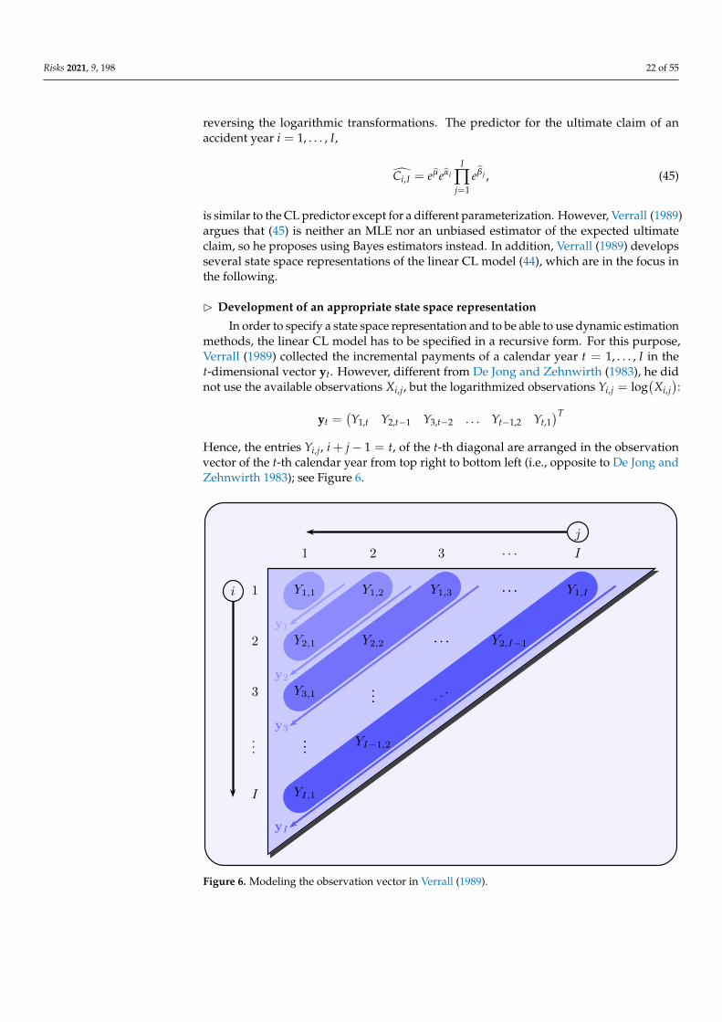
In order to specify a state space representation and to be able to use dynamic estimationmethods, the linear CL model has to be specified in a recursive form. For this purpose,Verrall (1989) collected the incremental payments of a calendar year t = 1, . . . , I in thet-dimensional vector yt. However, different from De Jong and Zehnwirth (1983), he didnot use the available observations Xi,j, but the logarithmized observations Yi,j = log

(Xi,j):

yt =(Y1,t Y2,t−1 Y3,t−2 . . . Yt−1,2 Yt,1

)T

Hence, the entries Yi,j, i + j− 1 = t, of the t-th diagonal are arranged in the observationvector of the t-th calendar year from top right to bottom left (i.e., opposite to De Jong andZehnwirth 1983); see Figure 6.

Y1,1 Y1,2 Y1,3 . . . Y1,I

Y2,1 Y2,2 . . . Y2,I−1

Y3,1... . .

.

...YI−1,2

YI,1

y3

yI

1

2

3

...

I

y1

y2

1 2 3 . . . I

Y1,1 Y1,2 Y1,3 . . . Y1,I

Y2,1 Y2,2 . . . Y2,I−1

Y3,1... . .

.

...YI−1,2

YI,1

i

j

Figure 6. Modeling the observation vector in Verrall (1989).

Risks 2021, 9, 198 23 of 55

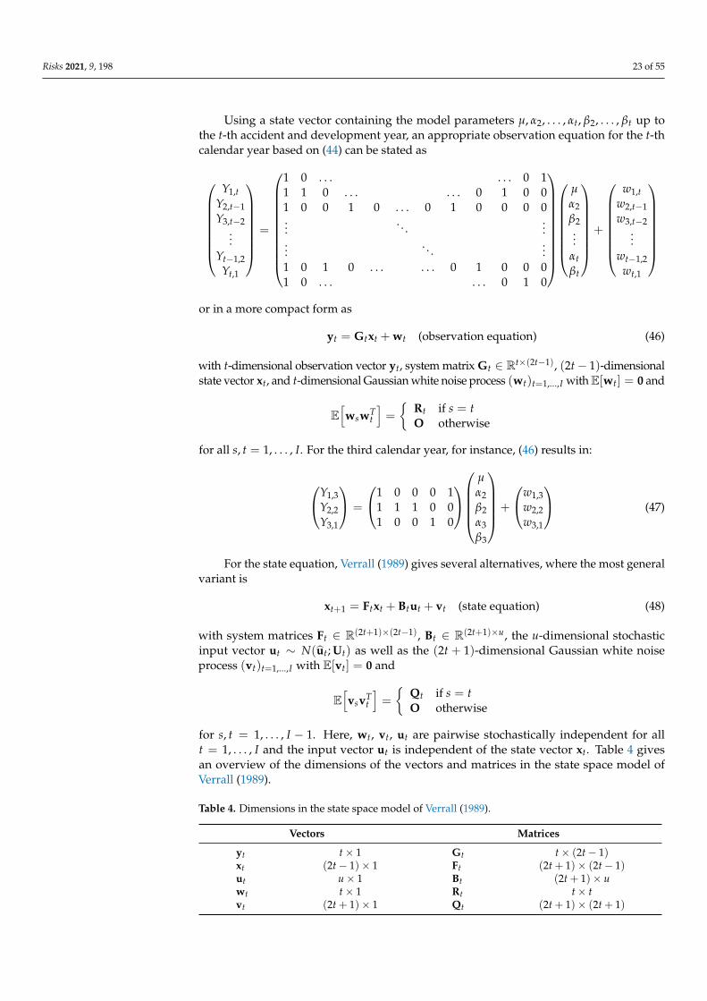
Using a state vector containing the model parameters µ, α2, . . . , αt, β2, . . . , βt up tothe t-th accident and development year, an appropriate observation equation for the t-thcalendar year based on (44) can be stated as

Y1,tY2,t−1Y3,t−2

...Yt−1,2

Yt,1

=

1 0 . . . . . . 0 11 1 0 . . . . . . 0 1 0 01 0 0 1 0 . . . 0 1 0 0 0 0...

. . ....

.... . .

...1 0 1 0 . . . . . . 0 1 0 0 01 0 . . . . . . 0 1 0

µα2β2...

αtβt

+

w1,tw2,t−1w3,t−2

...wt−1,2

wt,1

or in a more compact form as

yt = Gtxt + wt (observation equation) (46)

with t-dimensional observation vector yt, system matrix Gt ∈ Rt×(2t−1), (2t− 1)-dimensionalstate vector xt, and t-dimensional Gaussian white noise process (wt)t=1,...,I with E[wt] = 0 and

E[wswT

t

]=

{Rt if s = tO otherwise

for all s, t = 1, . . . , I. For the third calendar year, for instance, (46) results in:

Y1,3Y2,2Y3,1

=

1 0 0 0 11 1 1 0 01 0 0 1 0

µα2β2α3β3

+

w1,3w2,2w3,1

(47)

For the state equation, Verrall (1989) gives several alternatives, where the most generalvariant is

xt+1 = Ftxt + Btut + vt (state equation) (48)

with system matrices Ft ∈ R(2t+1)×(2t−1), Bt ∈ R(2t+1)×u, the u-dimensional stochasticinput vector ut ∼ N(ut; Ut) as well as the (2t + 1)-dimensional Gaussian white noiseprocess (vt)t=1,...,I with E[vt] = 0 and

E[vsvT

t

]=

{Qt if s = tO otherwise

for s, t = 1, . . . , I − 1. Here, wt, vt, ut are pairwise stochastically independent for allt = 1, . . . , I and the input vector ut is independent of the state vector xt. Table 4 givesan overview of the dimensions of the vectors and matrices in the state space model ofVerrall (1989).

Table 4. Dimensions in the state space model of Verrall (1989).

Vectors Matrices

yt t× 1 Gt t× (2t− 1)xt (2t− 1)× 1 Ft (2t + 1)× (2t− 1)ut u× 1 Bt (2t + 1)× uwt t× 1 Rt t× tvt (2t + 1)× 1 Qt (2t + 1)× (2t + 1)

Risks 2021, 9, 198 24 of 55

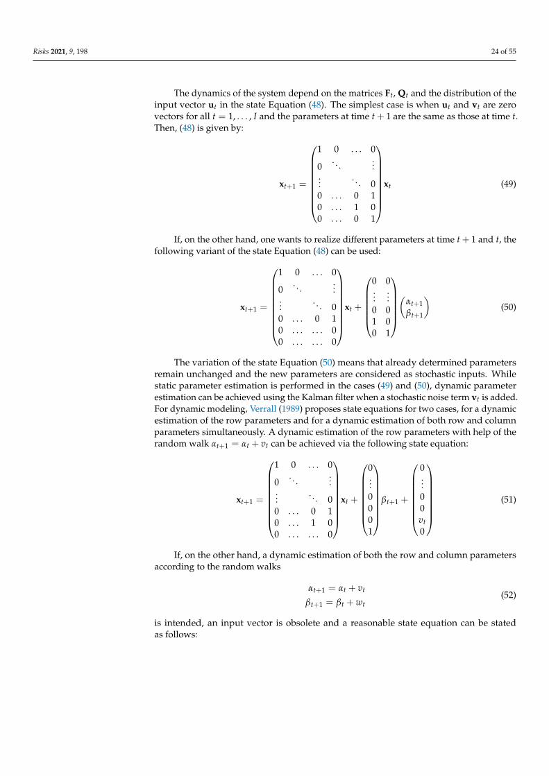
The dynamics of the system depend on the matrices Ft, Qt and the distribution of theinput vector ut in the state Equation (48). The simplest case is when ut and vt are zerovectors for all t = 1, . . . , I and the parameters at time t + 1 are the same as those at time t.Then, (48) is given by:

xt+1 =

1 0 . . . 0

0. . .

......

. . . 00 . . . 0 10 . . . 1 00 . . . 0 1

xt (49)

If, on the other hand, one wants to realize different parameters at time t + 1 and t, thefollowing variant of the state Equation (48) can be used:

xt+1 =

1 0 . . . 0

0. . .

......

. . . 00 . . . 0 10 . . . . . . 00 . . . . . . 0

xt +

0 0...

...0 01 00 1

(

αt+1βt+1

)(50)

The variation of the state Equation (50) means that already determined parametersremain unchanged and the new parameters are considered as stochastic inputs. Whilestatic parameter estimation is performed in the cases (49) and (50), dynamic parameterestimation can be achieved using the Kalman filter when a stochastic noise term vt is added.For dynamic modeling, Verrall (1989) proposes state equations for two cases, for a dynamicestimation of the row parameters and for a dynamic estimation of both row and columnparameters simultaneously. A dynamic estimation of the row parameters with help of therandom walk αt+1 = αt + vt can be achieved via the following state equation:

xt+1 =

1 0 . . . 0

0. . .

......

. . . 00 . . . 0 10 . . . 1 00 . . . . . . 0

xt +

0...0001

βt+1 +

0...00vt0

(51)

If, on the other hand, a dynamic estimation of both the row and column parametersaccording to the random walks

αt+1 = αt + vt

βt+1 = βt + wt(52)

is intended, an input vector is obsolete and a reasonable state equation can be statedas follows:

Risks 2021, 9, 198 25 of 55

xt+1 =

1 0 . . . 0

0. . .

......

. . . 00 . . . 0 10 . . . 1 00 . . . 0 1

xt +

0...00vtwt

(53)

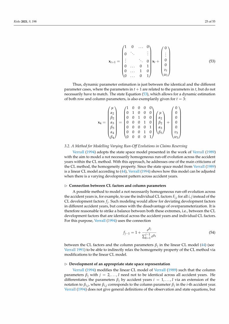
Thus, dynamic parameter estimation is just between the identical and the differentparameter cases, where the parameters in t + 1 are related to the parameters in t, but do notnecessarily have to match. The state Equation (53), which allows for a dynamic estimationof both row and column parameters, is also exemplarily given for t = 3:

x4 =

µα2β2α3β3α4β4

=

1 0 0 0 00 1 0 0 00 0 1 0 00 0 0 1 00 0 0 0 10 0 0 1 00 0 0 0 1

µα2β2α3β3

+

00000v3w3

3.2. A Method for Modelling Varying Run-Off Evolutions in Claims Reserving

Verrall (1994) adopts the state space model presented in the work of Verrall (1989)with the aim to model a not necessarily homogeneous run-off evolution across the accidentyears within the CL method. With this approach, he addresses one of the main criticisms ofthe CL method, the homogeneity property. Since the state space model from Verrall (1989)is a linear CL model according to (44), Verrall (1994) shows how this model can be adjustedwhen there is a varying development pattern across accident years.

B Connection between CL factors and column parameters

A possible method to model a not necessarily homogeneous run-off evolution acrossthe accident years is, for example, to use the individual CL factors Fi,j for all i, j instead of theCL development factors f j. Such modeling would allow for deviating development factorsin different accident years, but comes with the disadvantage of overparameterization. It istherefore reasonable to strike a balance between both these extremes, i.e., between the CLdevelopment factors that are identical across the accident years and individual CL factors.For this purpose, Verrall (1994) uses the connection

f j−1 = 1 +eβ j

∑j−1k=1 eβk

(54)

between the CL factors and the column parameters β j in the linear CL model (44) (seeVerrall 1991) to be able to indirectly relax the homogeneity property of the CL method viamodifications to the linear CL model.

B Development of an appropriate state space representation

Verrall (1994) modifies the linear CL model of Verrall (1989) such that the columnparameters β j with j = 2, . . . , I need not to be identical across all accident years. Hedifferentiates the parameters β j by accident years i = 1, . . . , I via an extension of thenotation to βi,j, where βi,j corresponds to the column parameter β j in the i-th accident year.Verrall (1994) does not give general definitions of the observation and state equations, but

Risks 2021, 9, 198 26 of 55

in the following we provide such representations. As for the observation equation in thet-th calendar year, it can be given in general form as follows:

Y1,tY2,t−1Y3,t−2

...Yt−1,2

Yt,1

=

1 0 . . . . . . 0 11 1 0 . . . . . . 0 1 0 01 0 0 1 0 . . . 0 1 0 0 0 0...

. . ....

.... . .

...1 0 1 0 . . . . . . 0 1 0 0 01 0 . . . . . . 0 1 0

µα2

βt−1,2...

αtβ1,t

+

w1,tw2,t−1w3,t−2

...wt−1,2

wt,1

As an example, the observation equation in t = 3 results in:

Y1,3Y2,2Y3,1

=

1 0 0 0 11 1 1 0 01 0 0 1 0

µα2

β2,2α3

β1,3

+

w1,3w2,2w3,1

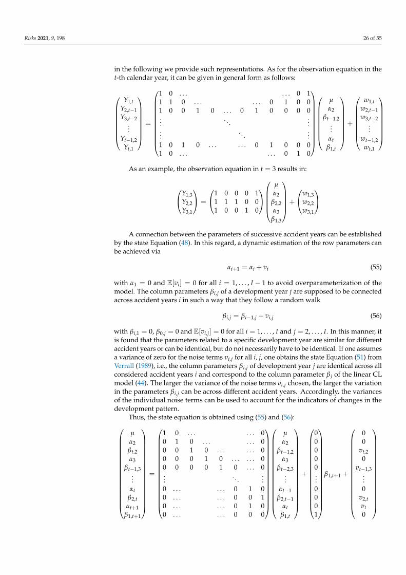
A connection between the parameters of successive accident years can be establishedby the state Equation (48). In this regard, a dynamic estimation of the row parameters canbe achieved via

αi+1 = αi + vi (55)

with α1 = 0 and E[vi] = 0 for all i = 1, . . . , I − 1 to avoid overparameterization of themodel. The column parameters βi,j of a development year j are supposed to be connectedacross accident years i in such a way that they follow a random walk

βi,j = βi−1,j + vi,j (56)

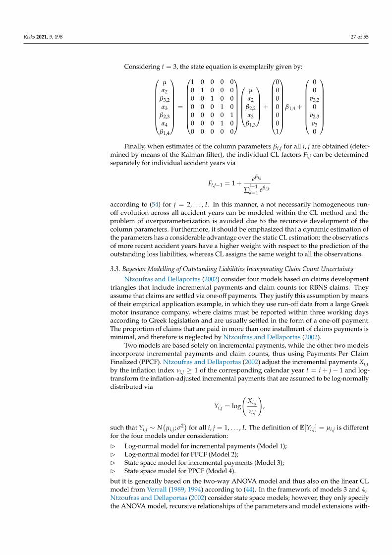
with βi,1 = 0, β0,j = 0 and E[vi,j] = 0 for all i = 1, . . . , I and j = 2, . . . , I. In this manner, itis found that the parameters related to a specific development year are similar for differentaccident years or can be identical, but do not necessarily have to be identical. If one assumesa variance of zero for the noise terms vi,j for all i, j, one obtains the state Equation (51) fromVerrall (1989), i.e., the column parameters βi,j of development year j are identical across allconsidered accident years i and correspond to the column parameter β j of the linear CLmodel (44). The larger the variance of the noise terms vi,j chosen, the larger the variationin the parameters βi,j can be across different accident years. Accordingly, the variancesof the individual noise terms can be used to account for the indicators of changes in thedevelopment pattern.

Thus, the state equation is obtained using (55) and (56):

µα2βt,2α3

βt−1,3...

αtβ2,tαt+1

β1,t+1

=

1 0 . . . . . . 00 1 0 . . . . . . 00 0 1 0 . . . . . . 00 0 0 1 0 . . . . . . 00 0 0 0 1 0 . . . 0...

. . ....

0 . . . . . . 0 1 00 . . . . . . 0 0 10 . . . . . . 0 1 00 . . . . . . 0 0 0

µα2

βt−1,2α3

βt−2,3...

αt−1β2,t−1

αtβ1,t

+

00000...0001

β1,t+1 +

00

vt,20

vt−1,3...0

v2,tvt0

Risks 2021, 9, 198 27 of 55

Considering t = 3, the state equation is exemplarily given by:

µα2

β3,2α3

β2,3α4

β1,4

=

1 0 0 0 00 1 0 0 00 0 1 0 00 0 0 1 00 0 0 0 10 0 0 1 00 0 0 0 0

µα2

β2,2α3

β1,3

+

0000001

β1,4 +

00

v3,20

v2,3v30

Finally, when estimates of the column parameters βi,j for all i, j are obtained (deter-

mined by means of the Kalman filter), the individual CL factors Fi,j can be determinedseparately for individual accident years via

Fi,j−1 = 1 +eβi,j

∑j−1k=1 eβi,k

according to (54) for j = 2, . . . , I. In this manner, a not necessarily homogeneous run-off evolution across all accident years can be modeled within the CL method and theproblem of overparameterization is avoided due to the recursive development of thecolumn parameters. Furthermore, it should be emphasized that a dynamic estimation ofthe parameters has a considerable advantage over the static CL estimation: the observationsof more recent accident years have a higher weight with respect to the prediction of theoutstanding loss liabilities, whereas CL assigns the same weight to all the observations.

3.3. Bayesian Modelling of Outstanding Liabilities Incorporating Claim Count Uncertainty

Ntzoufras and Dellaportas (2002) consider four models based on claims developmenttriangles that include incremental payments and claim counts for RBNS claims. Theyassume that claims are settled via one-off payments. They justify this assumption by meansof their empirical application example, in which they use run-off data from a large Greekmotor insurance company, where claims must be reported within three working daysaccording to Greek legislation and are usually settled in the form of a one-off payment.The proportion of claims that are paid in more than one installment of claims payments isminimal, and therefore is neglected by Ntzoufras and Dellaportas (2002).

Two models are based solely on incremental payments, while the other two modelsincorporate incremental payments and claim counts, thus using Payments Per ClaimFinalized (PPCF). Ntzoufras and Dellaportas (2002) adjust the incremental payments Xi,jby the inflation index νi,j ≥ 1 of the corresponding calendar year t = i + j− 1 and log-transform the inflation-adjusted incremental payments that are assumed to be log-normallydistributed via

Yi,j = log

(Xi,j

νi,j

),

such that Yi,j ∼ N(µi,j; σ2) for all i, j = 1, . . . , I. The definition of E[Yi,j] = µi,j is different

for the four models under consideration:

B Log-normal model for incremental payments (Model 1);B Log-normal model for PPCF (Model 2);B State space model for incremental payments (Model 3);B State space model for PPCF (Model 4).

but it is generally based on the two-way ANOVA model and thus also on the linear CLmodel from Verrall (1989, 1994) according to (44). In the framework of models 3 and 4,Ntzoufras and Dellaportas (2002) consider state space models; however, they only specifythe ANOVA model, recursive relationships of the parameters and model extensions with-

Risks 2021, 9, 198 28 of 55

out developing a specific state space representation. The reason for this is that they do notemploy the Kalman filter to fit the model and to predict the outstanding loss liabilities, butinstead they use a Bayesian approach in combination with Markov Chain Monte Carlo(MCMC). As the article by Ntzoufras and Dellaportas (2002) does not mainly rely onstate space models and the Kalman filter theory, the models are presented briefly, and, inparticular, details on the Bayesian approach are omitted.

B Log-normal model for incremental payments (Model 1)

The log-normal model for incremental payments, where the expected value µi,j isgiven by

µi,j = µ + αi + β j (57)

for all i, j = 1, . . . , I with α1 = β1 = 0, is already considered by various authors. That is, theexpected incremental payments µi,j for claims of the i-th accident year that are paid witha lag of j− 1 years are modeled via a linear predictor. This predictor consists of the sumof µ (expected inflation- and log-adjusted claims payments of the first accident year thatare settled in the same development year), αi (row parameter reflecting expected changesin the ith accident year), and β j (column parameter reflecting expected changes in the jthdevelopment year). According to Ntzoufras and Dellaportas (2002), the ANOVA modelhas the disadvantage that it includes only one source of information (i.e., incrementalpayments) and omits claims counts. For example, this model would not be able to takeinto account a strong increase in incremental payments due to a surprising increase in theclaim counts.

B Log-normal model for PPCF (Model 2)

The log-normal model for PPCF extends the first model by additionally consideringclaim counts in the modeling. For this purpose, Ntzoufras and Dellaportas (2002) give atwo-stage model, where the first stage is related to incremental payments,

µi,j = µ + αi + β j + log(Ni,j) (58)

with α1 = β1 = 0 and claim counts Ni,j > 0 for all i, j = 1, . . . , I. Compared with model1, the ANOVA model (57) was additively extended by the term log(Ni,j), which is why µin (58) can be interpreted as the logarithmized expected PPCF of the first accident year inthe first development year, and the parameters αi and β j can be considered as expecteddeviations from µ in the later accident and development years, respectively. The secondstage of the model is related to the claim counts Ni,j ∼ P

(λi,j)

with λi,j > 0. It is given bythe log-linear model

log(λi,j) = µ∗ + α∗i + β∗j

with constraints ∑Ij=1 Ni,j = Ti, ∑I

j=1 λi,j = Ti for all i, j = 1, . . . , I, hyper-parameters µ∗

and α∗i , and β∗j = log(

πjπ1

), where α∗1 = β∗1 = 0 holds, 0 < πj < 1 is the probability that a

claim will be settled with a lag of j− 1 years, and Ti denotes the total number of claimsfor a given accident year i. In this model, an increase in incremental payments induced byhigher claim counts is accounted for.

B State space model for incremental payments (Model 3)

The state space model for incremental payments is based on the discussion ofVerrall (1989) and the extension of the column parameters β j to βi,j as proposed byVerrall (1994):

µi,j = µ + αi + βi,j

Risks 2021, 9, 198 29 of 55

Here, the row and column parameters αi and βi,j follow the recursions

αi = αi−1 + hi (59)

βi,j = βi−1,j + vi (60)

with hi ∼ N(0; σ2

h)

and vi ∼ N(0; σ2

v)

as well as α1 = βi,1 = 0 for all i, j = 2, . . . , I. Thus,for the variance of the individual log-transformed and inflation-adjusted incrementalpayments Yi,j, Var(Yi,j) = σ2 holds for i = 1 or j = 1 and Var(Yi,j) = σ2 + (i− 1)

(σ2

v + σ2h)

holds for i, j = 2, . . . , I, as in each subsequent accident year after accident year i = 1,the weighted sum of the variance terms σ2

v , σ2h (see recursions (59) and (60)) is added to

the variance term σ2. That is, this model differs from model 1 in two ways: the columnparameters β j are extended to βi,j, and both row and column parameters evolve recursively.The recursions (59) and (60) are thereby decisively affected by the variances σ2

h and σ2v of

their noise terms: If σ2h is assumed to be close to zero, all row parameters tend to zero due

to α1 = 0. If, on the other hand, σ2v = 0 is assumed, models 1 and 3 are identical (except for

the α-recursion) because the column parameters are the same across all accident years, i.e.,βi,j = β j holds for all i.

B State space model for PPCF (Model 4)

The state space model for PPCF extends model 3 by incorporating claim counts.Like the second model, it is designed as a two-stage model, with stage 1 related to incre-mental payments and stage 2 related to claim counts. Thus, the first stage of model 4 isdescribed via

µi,j = µ + αi + βi,j + log(Ni,j)

for all i, j = 1, . . . , I with recursions (59) and (60), and the second stage is identical to thesecond stage of model 2. Hence, like models 1 and 3, models 2 and 4 differ in other columnparameters and in the recursive relationships of row and column parameters.

3.4. Comparison of Stochastic Reserving Methods

Li (2006) compares some methods in stochastic claims reserving, including a statespace model, in terms of forecasting the outstanding loss liabilities. The considered statespace model

yt = Gtxt + wt (observation equation) (61)

xt = Ftxt−1 + vt (state equation) (62)

is based on the common assumptions regarding the noise terms (as, for example, in De Jongand Zehnwirth 1983), and it is constructed in analogy to Verrall (1989) via the log-normalmodel for incremental payments and the linear CL model (44), respectively: the observationvector yt includes all logarithmized incremental payments Yi,j = log

(Xi,j)

with Xi,j > 0of the t-th calendar year (t = i + j− 1 with i, j = 1, . . . , I), where the Yi,j have an expectedvalue of E[Yi,j] = µ + αi + β j with α1 = β1 = 0. The measurement noise wi,j that overlaysthe expected logarithmized incremental payments follows a Gaussian white noise process(wi,j ∼WN

(0; σ2

w)). The state vector xt includes µ, row parameters α2, . . . , αt, and column

parameters β2, . . . , β I ; thus, unlike Verrall (1989), column parameters beyond j = t fort < I are also included. Table 5 gives an overview of the dimensions of the vectors andmatrices in the state space model of Li (2006).

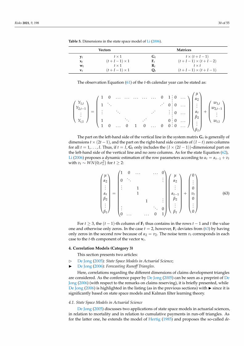
Risks 2021, 9, 198 30 of 55

Table 5. Dimensions in the state space model of Li (2006).

Vectors Matrices

yt t× 1 Gt t× (t + I − 1)xt (t + I − 1)× 1 Ft (t + I − 1)× (t + I − 2)wt t× 1 Rt t× tvt (t + I − 1)× 1 Qt (t + I − 1)× (t + I − 1)

The observation Equation (61) of the t-th calendar year can be stated as:

Y1,t

Y2,t−1...

Yt,1

=

1 0 . . . . . . . . . . . . . . . 0 1 0 . . .

1. . . ... 0 0 . . .

.... . . ...

... 0 . . .

1. . . ... 0 0 . . .

1 0 . . . 0 1 0 . . . 0 0 0 . . .

µα2...

αtβ2...

β I

+

w1,t

w2,t−1...

wt,1

The part on the left-hand side of the vertical line in the system matrix Gt is generally ofdimensions t× (2t− 1), and the part on the right-hand side consists of (I− t) zero columnsfor all t = 1, . . . , I. Thus, if t = I, Gt only includes the (I × (2I − 1))-dimensional part onthe left-hand side of the vertical line and no zero columns. As for the state Equation (62),Li (2006) proposes a dynamic estimation of the row parameters according to αt = αt−1 + vtwith vt ∼WN

(0; σ2

v)

for t ≥ 2:

µα2...

αtβ2...

β I

=

1 0 . . . . . . 0

0. . .

...... 1

1

1...

.... . . 0

0 . . . . . . 0 1

µα2...

αt−1β2...

β I

+

0...0vt0...0

(63)

For t ≥ 3, the (t− 1)-th column of Ft thus contains in the rows t− 1 and t the valueone and otherwise only zeros. In the case t = 2, however, Ft deviates from (63) by havingonly zeros in the second row because of α2 = v2. The noise term vt corresponds in eachcase to the t-th component of the vector vt.

4. Correlation Models (Category 3)

This section presents two articles:

B De Jong (2005): State Space Models in Actuarial Science;I De Jong (2006): Forecasting Runoff Triangles.

Here, correlations regarding the different dimensions of claims development trianglesare considered. As the conference paper by De Jong (2005) can be seen as a preprint of DeJong (2006) (with respect to the remarks on claims reserving), it is briefly presented, whileDe Jong (2006) is highlighted in the listing (as in the previous sections) with I since it issignificantly based on state space models and Kalman filter learning theory.

4.1. State Space Models in Actuarial Science

De Jong (2005) discusses two applications of state space models in actuarial sciences,in relation to mortality and in relation to cumulative payments in run-off triangles. Asfor the latter one, he extends the model of Hertig (1985) and proposes the so-called de-

Risks 2021, 9, 198 31 of 55

velopment correlation model. This model is already presented in a prior working paper byDe Jong (2004), where two additional models, the accident correlation model and the calendarcorrelation model, are proposed, but without discussing their state space representations.This extension, i.e., an embedding of the three models into state space representations andmodel fitting via Kalman filter, is carried out in the work of De Jong (2006). Thus, withrespect to applications of state space models in claims reserving, De Jong (2005) is a variantof De Jong (2006), which only deals with one of the correlation models. For this reason, werefer to the following subsection, in which the article of De Jong (2006) is presented.

4.2. Forecasting Runoff Triangles

De Jong (2006) aims to predict the outstanding loss liabilities using three differentmodels that can account for correlations within the claims data. In each case, De Jong (2006)gives state space representations for these models in order to be able to apply the Kalmanfilter to predict the claims reserves and to quantify their precision. Based on these results,he simulates the complete shape of the liability distribution. In the following, the focus ismainly on the state space representations of the considered models.

The proposed correlation models in the work of De Jong (2006) are generally based ona model of Hertig (1985), which is extended in such a way that correlations between theindividual accident, development or calendar years can be incorporated into the modeling.The models consider the logarithmized individual development factors

δi,j = ln

(Ci,j

Ci,j−1

)(64)

with i = 1, . . . , I, j = 1, . . . , I − 1 and δi,0 = ln(Ci,0). Using the individual development fac-tors (64), the future growth rate gi of cumulative payments in each accident year i = 2, . . . , Ican be decomposed as follows:

gi = ln(

Ci,I−1

Ci,I−i

)= ln

(Ci,I−i+1

Ci,I−i· Ci,I−i+2

Ci,I−i+1· · · Ci,I−1

Ci,I−2

)= ln

(Ci,I−i+1

Ci,I−i

)+ ln

(Ci,I−i+2

Ci,I−i+1

)+ . . . + ln

(Ci,I−1

Ci,I−2

)= δi,I−i+1 + . . . + δi,I−1

(65)

Considering (65), the outstanding loss liabilities Ri = Ci,I−1 − Ci,I−i of an accidentyear i = 2, . . . , I are given by:

Ri = Ci,I−i(egi − 1) (66)

An aggregation of (66) across all accident years yields the total outstanding loss liabilities:

R =I

∑i=2

Ri =I

∑i=2

Ci,I−i(egi − 1) (67)

Thus, in order to predict the outstanding loss liabilities, it is necessary to estimatethe growth rates g2, . . . , gI according to (65) and the future logarithmized individualdevelopment factors δi,j for i + j > I, respectively. For this purpose, De Jong (2006)considers three extended variants of the model proposed by Hertig (1985). The model ofHertig (1985),

δi,j = µj + hjεi,j (68)

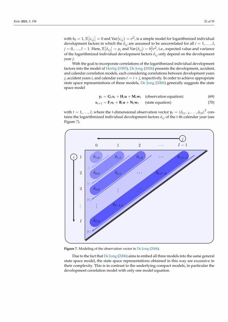
Risks 2021, 9, 198 32 of 55

with h0 = 1, E[εi,j]= 0 and Var

(εi,j)= σ2, is a simple model for logarithmized individual

development factors in which the δi,j are assumed to be uncorrelated for all i = 1, . . . , I,j = 0, . . . , I − 1. Here, E

[δi,j]= µj and Var

(δi,j)= h2

j σ2, i.e., expected value and varianceof the logarithmized individual development factors δi,j only depend on the developmentyear j.

With the goal to incorporate correlations of the logarithmized individual developmentfactors into the model of Hertig (1985), De Jong (2006) presents the development, accident,and calendar correlation models, each considering correlations between development yearsj, accident years i, and calendar years t = i + j, respectively. In order to achieve appropriatestate space representations of these models, De Jong (2006) generally suggests the statespace model

yt = Gtxt + Htu + Mtwt (observation equation) (69)

xt+1 = Ftxt + Btu + Ntwt (state equation) (70)

with t = 1, . . . , I, where the t-dimensional observation vector yt = (δ1,t−1, . . . , δt,0)T con-

tains the logarithmized individual development factors δi,j of the t-th calendar year (seeFigure 7).

δ1,0 δ1,1 δ1,2 . . . δ1,I−1

δ2,0 δ2,1 . . . δ2,I−2

δ3,0 ... . ..

...δI−1,1

δI,0

y3

yI

1

2

3

...

I

y1

y2

0 1 2 . . . I − 1

δ1,0 δ1,1 δ1,2 . . . δ1,I−1

δ2,0 δ2,1 . . . δ2,I−2

δ3,0 ... . ..

...δI−1,1

δI,0

i

j

Figure 7. Modeling of the observation vector in De Jong (2006).

Due to the fact that De Jong (2006) aims to embed all three models into the same generalstate space model, the state space representations obtained in this way are excessive intheir complexity. This is in contrast to the underlying compact models, in particular thedevelopment correlation model with only one model equation.

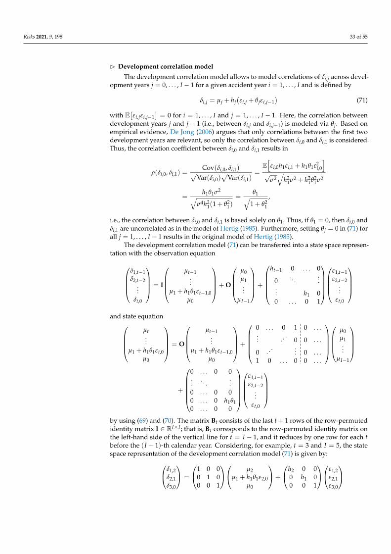
Risks 2021, 9, 198 33 of 55

B Development correlation model

The development correlation model allows to model correlations of δi,j across devel-opment years j = 0, . . . , I − 1 for a given accident year i = 1, . . . , I and is defined by

δi,j = µj + hj(εi,j + θjεi,j−1

)(71)

with E[εi,jεi,j−1

]= 0 for i = 1, . . . , I and j = 1, . . . , I − 1. Here, the correlation between

development years j and j− 1 (i.e., between δi,j and δi,j−1) is modeled via θj. Based onempirical evidence, De Jong (2006) argues that only correlations between the first twodevelopment years are relevant, so only the correlation between δi,0 and δi,1 is considered.Thus, the correlation coefficient between δi,0 and δi,1 results in

ρ(δi,0, δi,1) =Cov(δi,0, δi,1)√

Var(δi,0)√

Var(δi,1)=

E[εi,0h1εi,1 + h1θ1ε2

i,0

]√

σ2√

h21σ2 + h2

1θ21σ2

=h1θ1σ2√

σ4h21(1 + θ2

1)=

θ1√1 + θ2

1

,

i.e., the correlation between δi,0 and δi,1 is based solely on θ1. Thus, if θ1 = 0, then δi,0 andδi,1 are uncorrelated as in the model of Hertig (1985). Furthermore, setting θj = 0 in (71) forall j = 1, . . . , I − 1 results in the original model of Hertig (1985).

The development correlation model (71) can be transferred into a state space represen-tation with the observation equation

δ1,t−1δ2,t−2

...δt,0

= I

µt−1

...µ1 + h1θ1εt−1,0

µ0

+ O

µ0µ1...

µI−1

+

ht−1 0 . . . 0

0. . .

...... h1 00 . . . 0 1

ε1,t−1ε2,t−2

...εt,0

and state equation

µt...

µ1 + h1θ1εt,0µ0

= O

µt−1

...µ1 + h1θ1εt−1,0

µ0

+

0 . . . 0 1 0 . . ....

... 0 0 . . .

0...

... 0 . . .1 0 . . . 0 0 . . .

µ0µ1...

µI−1

+

0 . . . 0 0...

. . ....

0 . . . 0 00 . . . 0 h1θ10 . . . 0 0

ε1,t−1ε2,t−2

...εt,0

by using (69) and (70). The matrix Bt consists of the last t + 1 rows of the row-permutedidentity matrix I ∈ RI×I ; that is, Bt corresponds to the row-permuted identity matrix onthe left-hand side of the vertical line for t = I − 1, and it reduces by one row for each tbefore the (I − 1)-th calendar year. Considering, for example, t = 3 and I = 5, the statespace representation of the development correlation model (71) is given by:δ1,2

δ2,1δ3,0

=

1 0 00 1 00 0 1

µ2µ1 + h1θ1ε2,0

µ0

+

h2 0 00 h1 00 0 1

ε1,2ε2,1ε3,0

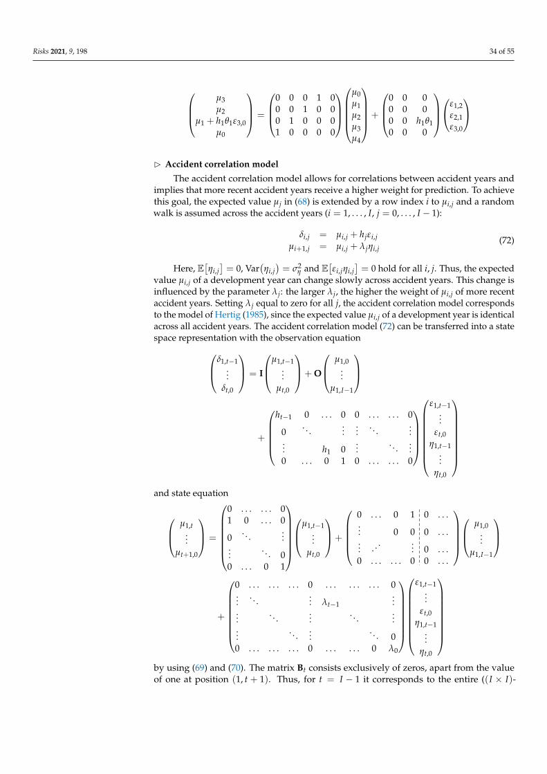
Risks 2021, 9, 198 34 of 55

µ3µ2

µ1 + h1θ1ε3,0µ0

=

0 0 0 1 00 0 1 0 00 1 0 0 01 0 0 0 0

µ0µ1µ2µ3µ4

+

0 0 00 0 00 0 h1θ10 0 0

ε1,2

ε2,1ε3,0

B Accident correlation model

The accident correlation model allows for correlations between accident years andimplies that more recent accident years receive a higher weight for prediction. To achievethis goal, the expected value µj in (68) is extended by a row index i to µi,j and a randomwalk is assumed across the accident years (i = 1, . . . , I, j = 0, . . . , I − 1):

δi,j = µi,j + hjεi,jµi+1,j = µi,j + λjηi,j

(72)

Here, E[ηi,j]= 0, Var

(ηi,j)= σ2

η and E[εi,jηi,j

]= 0 hold for all i, j. Thus, the expected

value µi,j of a development year can change slowly across accident years. This change isinfluenced by the parameter λj: the larger λj, the higher the weight of µi,j of more recentaccident years. Setting λj equal to zero for all j, the accident correlation model correspondsto the model of Hertig (1985), since the expected value µi,j of a development year is identicalacross all accident years. The accident correlation model (72) can be transferred into a statespace representation with the observation equationδ1,t−1

...δt,0

= I

µ1,t−1...

µt,0

+ O

µ1,0...

µ1,I−1

+

ht−1 0 . . . 0 0 . . . . . . 0

0. . .

......

. . ....

... h1 0...

. . ....

0 . . . 0 1 0 . . . . . . 0

ε1,t−1...

εt,0η1,t−1

...ηt,0

and state equation

µ1,t...

µt+1,0

=

0 . . . . . . 01 0 . . . 0

0. . .

......

. . . 00 . . . 0 1

µ1,t−1

...µt,0

+

0 . . . 0 1 0 . . .... 0 0 0 . . ....

...... 0 . . .

0 . . . . . . 0 0 . . .

µ1,0

...µ1,I−1

+

0 . . . . . . . . . 0 . . . . . . . . . 0...

. . .... λt−1

......

. . ....

. . ....

.... . .

.... . . 0

0 . . . . . . . . . 0 . . . . . . 0 λ0

ε1,t−1...

εt,0η1,t−1

...ηt,0

by using (69) and (70). The matrix Bt consists exclusively of zeros, apart from the valueof one at position (1, t + 1). Thus, for t = I − 1 it corresponds to the entire ((I × I)-

Risks 2021, 9, 198 35 of 55

dimensional) part on the left-hand side of the vertical line. Considering, for example, t = 3and I = 5, the state space representation of the accident correlation model (72) is given by:

δ1,2δ2,1δ3,0

=

1 0 00 1 00 0 1

µ1,2µ2,1µ3,0

+

h2 0 0 0 0 00 h1 0 0 0 00 0 1 0 0 0

ε1,2ε2,1ε3,0η1,2η2,1η3,0

µ1,3µ2,2µ3,1µ4,0

=

0 0 01 0 00 1 00 0 1

µ1,2

µ2,1µ3,0

+

0 0 0 1 00 0 0 0 00 0 0 0 00 0 0 0 0

µ1,0µ1,1µ1,2µ1,3µ1,4

+

0 0 0 0 0 00 0 0 λ2 0 00 0 0 0 λ1 00 0 0 0 0 λ0

ε1,2ε2,1ε3,0η1,2η2,1η3,0

B Calendar correlation model

The calendar correlation model

δi,j = µj + hj(τi+j + εi,j

)τi+j+1 = τi+j + κηi+j

(73)

with E[ηi+j

]= 0, Var

(ηi+j

)= σ2

η and E[εi,jηi+j

]= 0 for all i = 1, . . . , I, j = 0, . . . , I − 1

is appropriate to consider correlations between calendar years t = i + j. The calendaryear effects τt are modeled as a random walk across calendar years, which is why alllogarithmized individual development factors δi,j of a given calendar year change equally.The effect of τt on individual development factors is measured by hj and it is modeledproportionally to the standard deviation of εi,j. Setting κ = 0, the calendar correlationmodel (73) corresponds to model (68), since the effects τt are the same for all calendaryears t = 1, . . . , I and the term hjτi+j is considered as part of µj. The calendar correlationmodel (73) can be transferred into a state space representation with the observation equation

δ1,t−1...

δt,0

=

1 0 . . . 0 ht−1

0. . .

......

.... . . 0 h1

0 . . . 0 1 1

µt−1...

µ0τt

+ O

µ0...

µI−1

+

ht−1 0 . . . 0 0

0. . .

......

... h1 0...

0 . . . 0 1 0

ε1,t−1...

εt,0ηt

and the state equation

Risks 2021, 9, 198 36 of 55

µt...

µ0τt+1

=

0 . . . . . . 0...

. . ....

.... . .

...0 . . . . . . 00 . . . 0 1

µt−1...

µ0τt

+

0 . . . 0 1 0 . . ....

... 0 0 . . .

0...

... 0 . . .1 0 . . . 0 0 . . .0 . . . . . . 0 0 . . .

µ0

...µI−1

+

0 . . . . . . 0...

. . ....

.... . .

...0 . . . . . . 00 . . . 0 κ

ε1,t−1...

εt,0ηt

by using (69) and (70). The matrix Bt contains the last t + 1 rows of the row-permutedidentity matrix I ∈ RI×I and a row of zeros as the last row, i.e., for t = I − 1 it correspondsto the entire (((I + 1) × I)-dimensional) part on the left-hand side of the vertical line,and for each t before the (I − 1)-th calendar year it reduces by one row. Considering,for example, t = 3 and I = 5, the state space representation of the calendar correlationmodel (73) is given by:

δ1,2δ2,1δ3,0

=

1 0 0 h20 1 0 h10 0 1 1

µ2µ1µ0τ3

+

h2 0 0 00 h1 0 00 0 1 0

ε1,2ε2,1ε3,0η3

µ3µ2µ1µ0τ4

=

0 0 0 00 0 0 00 0 0 00 0 0 00 0 0 1

µ2µ1µ0τ3

+

0 0 0 1 00 0 1 0 00 1 0 0 01 0 0 0 00 0 0 0 0

µ0µ1µ2µ3µ4

+

0 0 0 00 0 0 00 0 0 00 0 0 00 0 0 κ

ε1,2ε2,1ε3,0η3

Finally, Table 6 gives an overview of the dimensions of vectors and matrices in the

above three state space models of De Jong (2006).

Table 6. Dimensions in the state space models of De Jong (2006).

Dev. Corr. Model Acc. Corr. Model Cal. Corr. Model

yt t× 1 t× 1 t× 1xt t× 1 t× 1 (t + 1)× 1u I × 1 I × 1 I × 1wt t× 1 2t× 1 (t + 1)× 1Gt t× t t× t t× (t + 1)Ft (t + 1)× t (t + 1)× t (t + 2)× (t + 1)Ht t× I t× I t× IBt (t + 1)× I (t + 1)× I (t + 2)× IMt t× t t× 2t t× (t + 1)Nt (t + 1)× t (t + 1)× 2t (t + 2)× (t + 1)

5. Univariate State Space Models (Category 4)

In this section, we present articles where univariate state space models are proposed:

I Alpuim and Ribeiro (2003): A State Space Model for Run-Off Triangles;I Chukhrova and Johannssen (2017): State Space Models and the Kalman Filter in Stochastic

Claims Reserving: Forecasting, Filtering and Smoothing.

Both articles are mainly devoted to state space models and the Kalman filter learningalgorithms, so they are highlighted with I in the above listing.

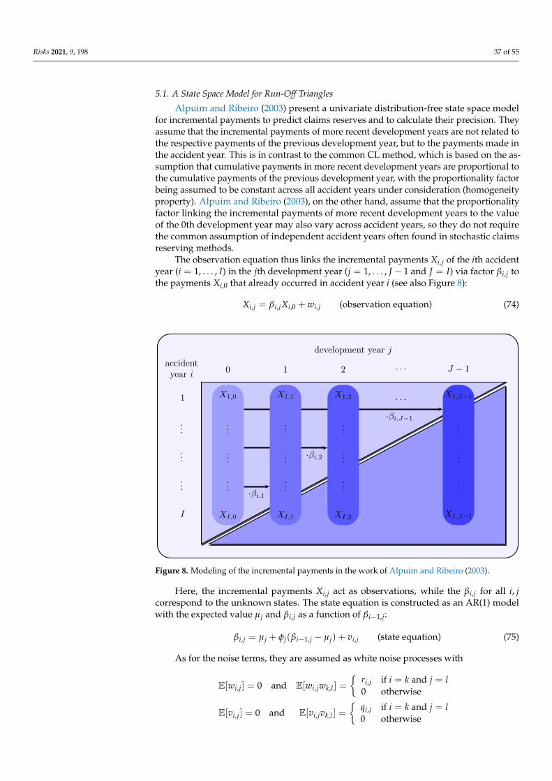
Risks 2021, 9, 198 37 of 55

5.1. A State Space Model for Run-Off Triangles

Alpuim and Ribeiro (2003) present a univariate distribution-free state space modelfor incremental payments to predict claims reserves and to calculate their precision. Theyassume that the incremental payments of more recent development years are not related tothe respective payments of the previous development year, but to the payments made inthe accident year. This is in contrast to the common CL method, which is based on the as-sumption that cumulative payments in more recent development years are proportional tothe cumulative payments of the previous development year, with the proportionality factorbeing assumed to be constant across all accident years under consideration (homogeneityproperty). Alpuim and Ribeiro (2003), on the other hand, assume that the proportionalityfactor linking the incremental payments of more recent development years to the valueof the 0th development year may also vary across accident years, so they do not requirethe common assumption of independent accident years often found in stochastic claimsreserving methods.

The observation equation thus links the incremental payments Xi,j of the ith accidentyear (i = 1, . . . , I) in the jth development year (j = 1, . . . , J − 1 and J = I) via factor βi,j tothe payments Xi,0 that already occurred in accident year i (see also Figure 8):

Xi,j = βi,jXi,0 + wi,j (observation equation) (74)

X1,0 X1,1 X1,2 X1,J−1

......

......

......

......

......

......

XI,0 XI,1 XI,2 XI,J−1

·βi,1

·βi,2

·βi,J−1

accidentyear i

1

...

...

...

I

0 1 2 . . . J − 1

development year j

......

......

......

......

......

......

X1,0 X1,1 X1,2 . . . X1,J−1

XI,0 XI,1 XI,2 XI,J−1

Figure 8. Modeling of the incremental payments in the work of Alpuim and Ribeiro (2003).

Here, the incremental payments Xi,j act as observations, while the βi,j for all i, jcorrespond to the unknown states. The state equation is constructed as an AR(1) modelwith the expected value µj and βi,j as a function of βi−1,j:

βi,j = µj + φj(βi−1,j − µj) + vi,j (state equation) (75)

As for the noise terms, they are assumed as white noise processes with

E[wi,j] = 0 and E[wi,jwk,l ] =

{ri,j if i = k and j = l0 otherwise

E[vi,j] = 0 and E[vi,jvk,l ] =

{qi,j if i = k and j = l0 otherwise

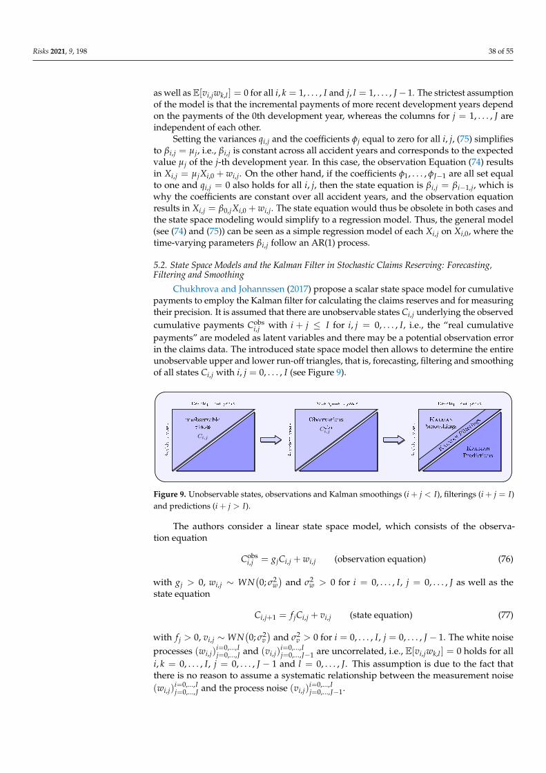
Risks 2021, 9, 198 38 of 55

as well as E[vi,jwk,l ] = 0 for all i, k = 1, . . . , I and j, l = 1, . . . , J− 1. The strictest assumptionof the model is that the incremental payments of more recent development years dependon the payments of the 0th development year, whereas the columns for j = 1, . . . , J areindependent of each other.

Setting the variances qi,j and the coefficients φj equal to zero for all i, j, (75) simplifiesto βi,j = µj, i.e., βi,j is constant across all accident years and corresponds to the expectedvalue µj of the j-th development year. In this case, the observation Equation (74) resultsin Xi,j = µjXi,0 + wi,j. On the other hand, if the coefficients φ1, . . . , φJ−1 are all set equalto one and qi,j = 0 also holds for all i, j, then the state equation is βi,j = βi−1,j, which iswhy the coefficients are constant over all accident years, and the observation equationresults in Xi,j = β0,jXi,0 + wi,j. The state equation would thus be obsolete in both cases andthe state space modeling would simplify to a regression model. Thus, the general model(see (74) and (75)) can be seen as a simple regression model of each Xi,j on Xi,0, where thetime-varying parameters βi,j follow an AR(1) process.

5.2. State Space Models and the Kalman Filter in Stochastic Claims Reserving: Forecasting,Filtering and Smoothing

Chukhrova and Johannssen (2017) propose a scalar state space model for cumulativepayments to employ the Kalman filter for calculating the claims reserves and for measuringtheir precision. It is assumed that there are unobservable states Ci,j underlying the observedcumulative payments Cobs

i,j with i + j ≤ I for i, j = 0, . . . , I, i.e., the “real cumulativepayments” are modeled as latent variables and there may be a potential observation errorin the claims data. The introduced state space model then allows to determine the entireunobservable upper and lower run-off triangles, that is, forecasting, filtering and smoothingof all states Ci,j with i, j = 0, . . . , I (see Figure 9).

A

i

d

e

n

t

y

e

a

r

s

Development years

unobservable

States

Ci,j

A

i

d

e

n

t

y

e

a

r

s

Development years

Observations

Cobs

i,j

A

i

d

e

n

t

y

e

a

r

s

Development years

Kalman

Smoothings

Kalman

Predi tions

K

a

l

m

a

n

F

i

l

t

e

r

i

n

g

s

Figure 9. Unobservable states, observations and Kalman smoothings (i + j < I), filterings (i + j = I)and predictions (i + j > I).

The authors consider a linear state space model, which consists of the observa-tion equation

Cobsi,j = gjCi,j + wi,j (observation equation) (76)

with gj > 0, wi,j ∼ WN(0; σ2

w)

and σ2w > 0 for i = 0, . . . , I, j = 0, . . . , J as well as the

state equation

Ci,j+1 = f jCi,j + vi,j (state equation) (77)

with f j > 0, vi,j ∼WN(0; σ2

v)

and σ2v > 0 for i = 0, . . . , I, j = 0, . . . , J − 1. The white noise

processes (wi,j)i=0,...,Ij=0,...,J and (vi,j)

i=0,...,Ij=0,...,J−1 are uncorrelated, i.e., E[vi,jwk,l ] = 0 holds for all

i, k = 0, . . . , I, j = 0, . . . , J − 1 and l = 0, . . . , J. This assumption is due to the fact thatthere is no reason to assume a systematic relationship between the measurement noise(wi,j)

i=0,...,Ij=0,...,J and the process noise (vi,j)

i=0,...,Ij=0,...,J−1.

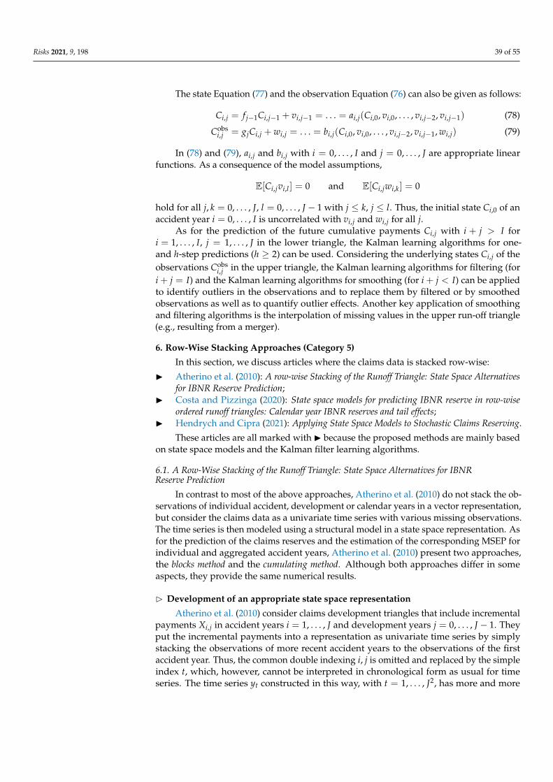
Risks 2021, 9, 198 39 of 55

The state Equation (77) and the observation Equation (76) can also be given as follows:

Ci,j = f j−1Ci,j−1 + vi,j−1 = . . . = ai,j(Ci,0, vi,0, . . . , vi,j−2, vi,j−1) (78)

Cobsi,j = gjCi,j + wi,j = . . . = bi,j(Ci,0, vi,0, . . . , vi,j−2, vi,j−1, wi,j) (79)

In (78) and (79), ai,j and bi,j with i = 0, . . . , I and j = 0, . . . , J are appropriate linearfunctions. As a consequence of the model assumptions,

E[Ci,jvi,l ] = 0 and E[Ci,jwi,k] = 0

hold for all j, k = 0, . . . , J, l = 0, . . . , J − 1 with j ≤ k, j ≤ l. Thus, the initial state Ci,0 of anaccident year i = 0, . . . , I is uncorrelated with vi,j and wi,j for all j.

As for the prediction of the future cumulative payments Ci,j with i + j > I fori = 1, . . . , I, j = 1, . . . , J in the lower triangle, the Kalman learning algorithms for one-and h-step predictions (h ≥ 2) can be used. Considering the underlying states Ci,j of theobservations Cobs

i,j in the upper triangle, the Kalman learning algorithms for filtering (fori + j = I) and the Kalman learning algorithms for smoothing (for i + j < I) can be appliedto identify outliers in the observations and to replace them by filtered or by smoothedobservations as well as to quantify outlier effects. Another key application of smoothingand filtering algorithms is the interpolation of missing values in the upper run-off triangle(e.g., resulting from a merger).

6. Row-Wise Stacking Approaches (Category 5)

In this section, we discuss articles where the claims data is stacked row-wise:

I Atherino et al. (2010): A row-wise Stacking of the Runoff Triangle: State Space Alternativesfor IBNR Reserve Prediction;

I Costa and Pizzinga (2020): State space models for predicting IBNR reserve in row-wiseordered runoff triangles: Calendar year IBNR reserves and tail effects;

I Hendrych and Cipra (2021): Applying State Space Models to Stochastic Claims Reserving.

These articles are all marked with I because the proposed methods are mainly basedon state space models and the Kalman filter learning algorithms.

6.1. A Row-Wise Stacking of the Runoff Triangle: State Space Alternatives for IBNRReserve Prediction

In contrast to most of the above approaches, Atherino et al. (2010) do not stack the ob-servations of individual accident, development or calendar years in a vector representation,but consider the claims data as a univariate time series with various missing observations.The time series is then modeled using a structural model in a state space representation. Asfor the prediction of the claims reserves and the estimation of the corresponding MSEP forindividual and aggregated accident years, Atherino et al. (2010) present two approaches,the blocks method and the cumulating method. Although both approaches differ in someaspects, they provide the same numerical results.

B Development of an appropriate state space representation

Atherino et al. (2010) consider claims development triangles that include incrementalpayments Xi,j in accident years i = 1, . . . , J and development years j = 0, . . . , J − 1. Theyput the incremental payments into a representation as univariate time series by simplystacking the observations of more recent accident years to the observations of the firstaccident year. Thus, the common double indexing i, j is omitted and replaced by the simpleindex t, which, however, cannot be interpreted in chronological form as usual for timeseries. The time series yt constructed in this way, with t = 1, . . . , J2, has more and more

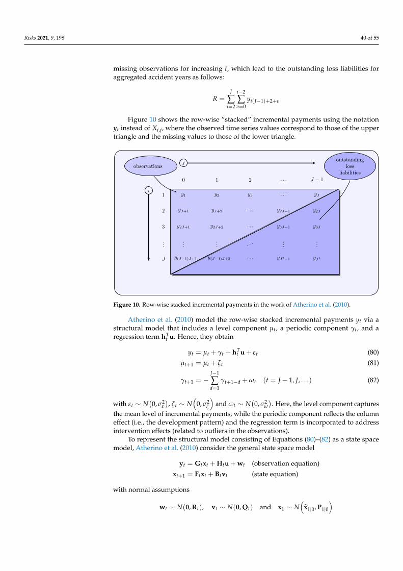
Risks 2021, 9, 198 40 of 55

missing observations for increasing t, which lead to the outstanding loss liabilities foraggregated accident years as follows:

R =J

∑i=2

i−2

∑v=0

yi(J−1)+2+v

Figure 10 shows the row-wise “stacked” incremental payments using the notationyt instead of Xi,j, where the observed time series values correspond to those of the uppertriangle and the missing values to those of the lower triangle.

y1 y2 y3 . . . yJ

yJ+1 yJ+2 . . . y2J−1 y2J

y2J+1 y2J+2 . . . y3J−1 y3J

...... . . .

......

y(J−1)J+1 y(J−1)J+2 . . . yJ2−1 yJ2

1

2

3

...

J

0 1 2 . . . J − 1

i

jobservations

outstandingloss

liabilities

Figure 10. Row-wise stacked incremental payments in the work of Atherino et al. (2010).

Atherino et al. (2010) model the row-wise stacked incremental payments yt via astructural model that includes a level component µt, a periodic component γt, and aregression term hT

t u. Hence, they obtain

yt = µt + γt + hTt u + εt (80)

µt+1 = µt + ξt (81)

γt+1 = −J−1

∑d=1

γt+1−d + ωt (t = J − 1, J, . . .) (82)

with εt ∼ N(0, σ2

ε

), ξt ∼ N

(0, σ2

ξ

)and ωt ∼ N

(0, σ2

ω

). Here, the level component captures

the mean level of incremental payments, while the periodic component reflects the columneffect (i.e., the development pattern) and the regression term is incorporated to addressintervention effects (related to outliers in the observations).

To represent the structural model consisting of Equations (80)–(82) as a state spacemodel, Atherino et al. (2010) consider the general state space model

yt = Gtxt + Htu + wt (observation equation)

xt+1 = Ftxt + Btvt (state equation)

with normal assumptions

wt ∼ N(0, Rt), vt ∼ N(0, Qt) and x1 ∼ N(

x1|0, P1|0)

Risks 2021, 9, 198 41 of 55

for t = 1, . . . , J2. As for the noise terms wt and vt, it is assumed that E[wswT

t]= O,

E[vsvT

t]= O for s 6= t and E

[wsvT

t]= O for all s, t = 1, . . . , J2. Moreover, the initial state

x1 is proposed to be independent of wt and vt for all t. Incorporating the structural modelinto a state space representation, the observation equation results in

yt =(1 1 0 . . . 0

)

µtγt

γt−1...

γt−J+2

+ hTt u + εt (83)

with yt = yt, Gt = gTt , Ht = hT

t , wt = εt and Rt = σ2ε and the state equation is given by

µt+1γt+1

γt...

γt−J+3

=

1 0 0 . . . 00 −1 −1 . . . −10 1 0 . . . 0...

. . ....

0 . . . 0 1 0

µtγt

γt−1...

γt−J+2

+

1 00 10 0...

...0 0

(

ξtωt

)(84)

with

Qt =

(σ2

ξ 00 σ2

ω

).

Table 7 gives an overview of the dimensions of vectors and matrices in the state spacemodel of Atherino et al. (2010).

Table 7. Dimensions in the state space model of Atherino et al. (2010).

Vectors Matrices

yt 1× 1 Gt 1× Jxt J × 1 Ft J × Ju k× 1 Ht 1× kwt 1× 1 Rt 1× 1vt 2× 1 Qt 2× 2

Bt J × 2

In the following, the cumulating method, one of the two approaches proposed byAtherino et al. (2010) to predict the loss reserves and to estimate their MSEP for individualand aggregated accident years, is presented.

B Cumulating method

The cumulating method adds additional components to the state vector that accumu-lates estimates of the missing observations in the lower triangle so that the MSEP of theclaims reserves can directly be determined using Kalman filter. In the following, I denotesan index set containing all t-indices belonging to observations yt, and (T) stands for total,i.e., for aggregated accident years. If one is interested only in the claims reserves along withthe MSEP for aggregated accident years, the state vector can be extended by the additionalcomponent δ

(T)t that accumulates all estimates of missing observations across all accident

years. The state space model is then given by

yt =(gT

t 0)︸ ︷︷ ︸

1×(J+1)

(xt

δ(T)t

)︸ ︷︷ ︸(J+1)×1

+ hTt u + εt (observation equation)

Risks 2021, 9, 198 42 of 55

(xt+1

δ(T)t+1

)︸ ︷︷ ︸(J+1)×1

=

(Ft 0

β(T)t 1

)︸ ︷︷ ︸(J+1)×(J+1)

(xt

δ(T)t

)︸ ︷︷ ︸(J+1)×1

+

(Bt0T

)︸ ︷︷ ︸(J+1)×2

vt (state equation)

with δ(T)1 = 0, the J-dimensional zero vector 0 in the transition matrix, the two-dimensional

zero vector 0T and the J-dimensional row vector

β(T)t =

{gT

t if t /∈ I0T otherwise

(85)

where the changes in the dimensions within the system compared to (83) and (84) are given,while gT

t , xt, xt+1, Ft, Bt, vt remain unchanged. If one is also interested in individual acci-dent years, further components corresponding to the respective accident years i = 2, . . . , Jhave to be added to the state vector. This leads to the inclusion of the J-dimensional vector

δt =(

δ(2)t , . . . , δ

(J)t , δ

(T)t

)T, (86)

in which the component δ(T)t related to aggregated accident years is also included. The

modified state space model is then be given by

yt =(gT

t 0T)︸ ︷︷ ︸1×2J

(xtδt

)︸ ︷︷ ︸2J×1

+ hTt u + εt (observation equation) (87)

(xt+1δt+1

)︸ ︷︷ ︸

2J×1

=

(Ft OXt I

)︸ ︷︷ ︸

2J×2J

(xtδt

)︸ ︷︷ ︸2J×1

+

(BtO

)︸ ︷︷ ︸

2J×2

vt (state equation) (88)

with δ1 = 0, the (J × J)-dimensional zero matrix O and identity matrix I in the transi-tion matrix, the (J × 2)-dimensional zero matrix O and the (J × J)-dimensional matrix

Xt =(

β(2)t , . . . , β

(J)t , β

(T)t

)Twith J − 1 components

β(i)t =

{gT

t if t /∈ I and t from row i = 2, . . . , J0T otherwise

as well as component β(T)t according to (85). Thus, the vector δJ2+1 includes the claims

reserves for individual and aggregated accident years, but without taking into account theeffects of the regression terms hT

t u with t /∈ I , which are excluded from the accumulationprocess and therefore have to be added separately.

6.2. State Space Models for Predicting IBNR Reserve in Row-Wise Ordered Runoff Triangles:Calendar Year IBNR Reserves and Tail Effects

Costa and Pizzinga (2020) extend the row-wise stacking approach of Atherino et al. (2010)and the corresponding state space representation of the structural model by implementing(1) a calendar year IBNR reserve prediction and (2) tail effects for the row-wise orderedtriangle. In this way they intend (1) to improve the possibilities of an insurance companyto predict short-term IBNR reserves and (2) to make IBNR predictions more conservativeand thus more effective to protect insurance companies from insolvency risks.

As for the first extension, Costa and Pizzinga (2020) consider the cumulating methodproposed by Atherino et al. (2010) and simply add a further cumulating entry to the statevector, in particular, to the vector (86). The additional cumulating entry δ

(C)t is related

to the calendar year IBNR reserve and accumulates all estimates of missing observationsassociated with a specific calendar year.

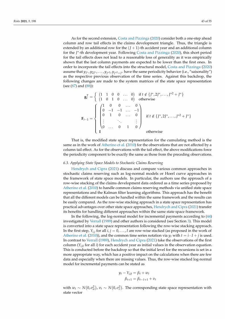
Risks 2021, 9, 198 43 of 55

As for the second extension, Costa and Pizzinga (2020) consider both a one-step aheadcolumn and row tail effects in the claims development triangle. Thus, the triangle isextended by an additional row for the (J + 1)-th accident year and an additional columnfor the J∗-th development year. Following Costa and Pizzinga (2020), this short periodfor the tail effects does not lead to a reasonable loss of generality as it was empiricallyshown that the last column payments are expected to be lower than the first ones. Inorder to incorporate the tail effects into the structural model, Costa and Pizzinga (2020)assume that yJ∗ , y2J∗ , . . . , yJ∗2 , yJ∗2+J∗ have the same periodicity behavior (i.e., “saisonality”)as the respective previous observation of the time series. Against this backdrop, thefollowing changes are made to the system matrices of the state space representation(see (87) and (88)):

gTt =

{ (1 1 0 0 . . . 0

)if t /∈ {J∗, 2J∗, . . . , J∗2 + J∗}(

1 0 1 0 . . . 0)

otherwise

Ft−1 =

1 0 0 . . . 00 −1 −1 . . . −10 1 0 . . . 0...

. . ....

0 . . . 0 1 0

if t /∈ {J∗, 2J∗, . . . , J∗2 + J∗}

I otherwise

That is, the modified state space representation for the cumulating method is thesame as in the work of Atherino et al. (2010) for the observations that are not affected by acolumn tail effect. As for the observations with the tail effect, the above modifications forcethe periodicity component to be exactly the same as those from the preceding observations.

6.3. Applying State Space Models to Stochastic Claims Reserving

Hendrych and Cipra (2021) discuss and compare various common approaches instochastic claims reserving such as log-normal models or Hoerl curve approaches inthe framework of state space models. In particular, the authors use the approach of arow-wise stacking of the claims development data ordered as a time series proposed byAtherino et al. (2010) to handle common claims reserving methods via unified state spacerepresentations and the Kalman filter learning algorithms. This approach has the benefitthat all the different models can be handled within the same framework and the results canbe easily compared. As the row-wise stacking approach in a state space representation haspractical advantages over other state space approaches, Hendrych and Cipra (2021) transferits benefits for handling different approaches within the same state space framework.

In the following, the log-normal model for incremental payments according to (44)investigated by Verrall (1989) and other authors is considered (see Section 3). This modelis converted into a state space representation following the row-wise stacking approach.In the first step, Yi,j for all i, j = 0, . . . , I are row-wise stacked (as proposed in the work ofAtherino et al. (2010)), and the common time series notation via yt with t = i · I + j is used.In contrast to Verrall (1989), Hendrych and Cipra (2021) take the observations of the firstcolumn (Yi,0 for all i) for each accident year as initial values in the observation equation.This is conducted before the backdrop so that the initial level for the recursions is set in amore appropriate way, which has a positive impact on the calculations when there are fewdata and especially when there are missing values. Thus, the row-wise stacked log-normalmodel for incremental payments can be stated as

yt −Yi,0 = βt + wt

βt+1 = βt−I+1 + vt

with wt ∼ N(0, σ2

w), vt ∼ N

(0, σ2

v). The corresponding state space representation with

state vector

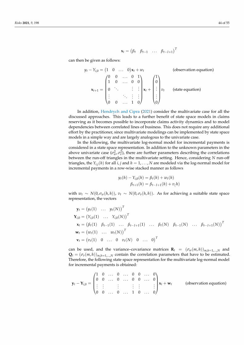
Risks 2021, 9, 198 44 of 55

xt =(

βt βt−1 . . . βt−I+1)T

can then be given as follows:

yt −Yi,0 =(1 0 . . . 0

)xt + wt (observation equation)

xt+1 =

0 0 . . . 0 11 0 . . . 0 0

0. . .

......

.... . .

......

0 0 . . . 1 0

xt +

10......0

vt (state equation)

In addition, Hendrych and Cipra (2021) consider the multivariate case for all thediscussed approaches. This leads to a further benefit of state space models in claimsreserving as it becomes possible to incorporate claims activity dynamics and to modeldependencies between correlated lines of business. This does not require any additionaleffort by the practitioner, since multivariate modelings can be implemented by state spacemodels in a simple way and are largely analogous to the univariate case.

In the following, the multivariate log-normal model for incremental payments isconsidered in a state space representation. In addition to the unknown parameters in theabove univariate case (σ2

w, σ2v ), there are further parameters describing the correlations

between the run-off triangles in the multivariate setting. Hence, considering N run-offtriangles, the Yi,j(h) for all i, j and h = 1, . . . , N are modeled via the log-normal model forincremental payments in a row-wise stacked manner as follows

yt(h)−Yi,0(h) = βt(h) + wt(h)

βt+1(h) = βt−I+1(h) + v(h)

with wt ∼ N(0, σw(h, h)), vt ∼ N(0, σv(h, h)). As for achieving a suitable state spacerepresentation, the vectors

yt =(yt(1) . . . yt(N)

)T

Yi,0 =(Yi,0(1) . . . Yi,0(N)

)T

xt =(

βt(1) βt−1(1) . . . βt−I+1(1) . . . βt(N) βt−1(N) . . . βt−I+1(N))T

wt =(wt(1) . . . wt(N)

)T

vt =(vt(1) 0 . . . 0 vt(N) 0 . . . 0

)T

can be used, and the variance–covariance matrices Rt = (σw(m, h))m,h=1,...,N andQt = (σv(m, h))m,h=1,...,N contain the correlation parameters that have to be estimated.Therefore, the following state space representation for the multivariate log-normal modelfor incremental payments is obtained:

yt − Yi,0 =

1 0 . . . 0 . . . 0 0 . . . 00 0 . . . 0 . . . 0 0 . . . 0...

......

......

...0 0 . . . 0 . . . 1 0 . . . 0

xt + wt (observation equation)

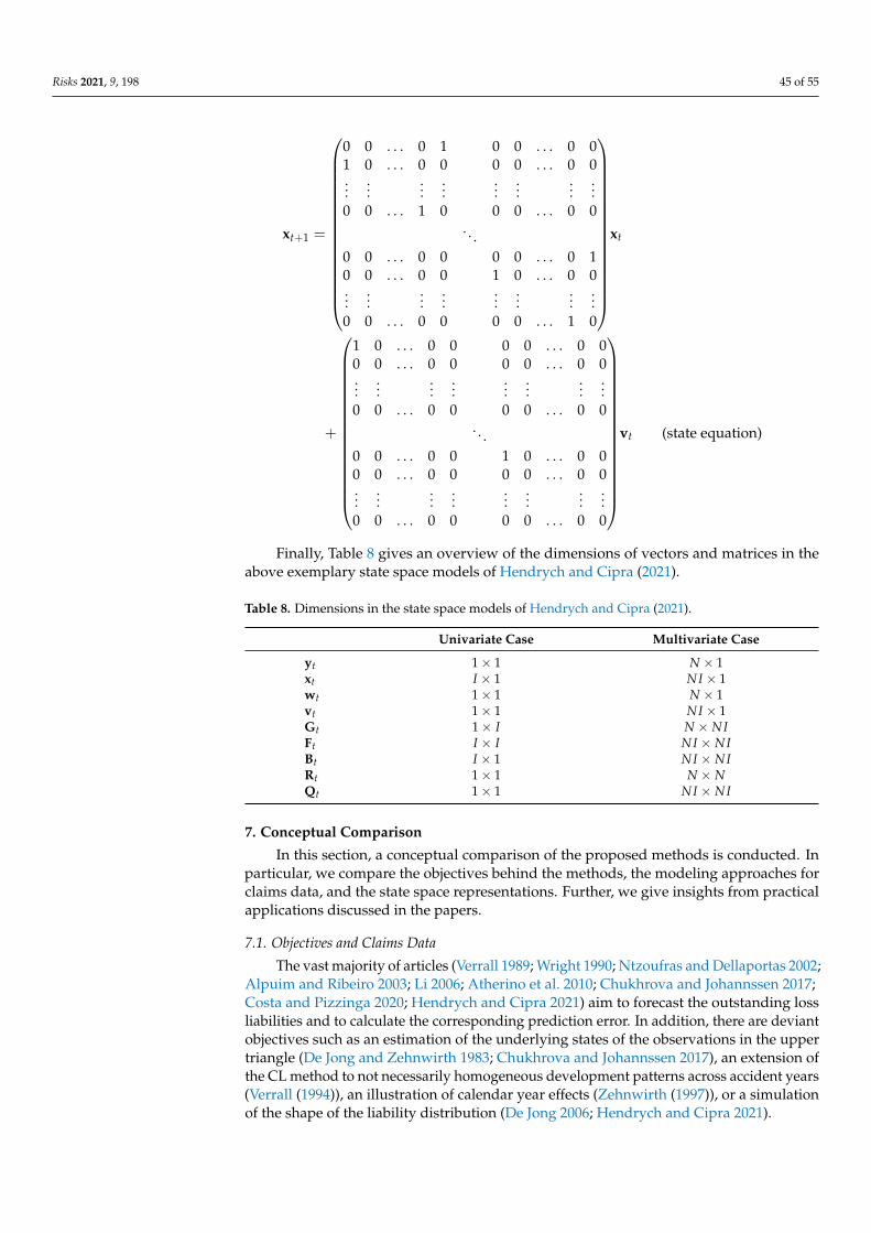
Risks 2021, 9, 198 45 of 55

xt+1 =

0 0 . . . 0 1 0 0 . . . 0 01 0 . . . 0 0 0 0 . . . 0 0...

......

......

......

...0 0 . . . 1 0 0 0 . . . 0 0

. . .0 0 . . . 0 0 0 0 . . . 0 10 0 . . . 0 0 1 0 . . . 0 0...

......

......

......

...0 0 . . . 0 0 0 0 . . . 1 0

xt

+

1 0 . . . 0 0 0 0 . . . 0 00 0 . . . 0 0 0 0 . . . 0 0...

......

......

......

...0 0 . . . 0 0 0 0 . . . 0 0

. . .0 0 . . . 0 0 1 0 . . . 0 00 0 . . . 0 0 0 0 . . . 0 0...

......

......

......

...0 0 . . . 0 0 0 0 . . . 0 0

vt (state equation)

Finally, Table 8 gives an overview of the dimensions of vectors and matrices in theabove exemplary state space models of Hendrych and Cipra (2021).

Table 8. Dimensions in the state space models of Hendrych and Cipra (2021).

Univariate Case Multivariate Case

yt 1× 1 N × 1xt I × 1 NI × 1wt 1× 1 N × 1vt 1× 1 NI × 1Gt 1× I N × NIFt I × I NI × NIBt I × 1 NI × NIRt 1× 1 N × NQt 1× 1 NI × NI

7. Conceptual Comparison

In this section, a conceptual comparison of the proposed methods is conducted. Inparticular, we compare the objectives behind the methods, the modeling approaches forclaims data, and the state space representations. Further, we give insights from practicalapplications discussed in the papers.

7.1. Objectives and Claims Data

The vast majority of articles (Verrall 1989; Wright 1990; Ntzoufras and Dellaportas 2002;Alpuim and Ribeiro 2003; Li 2006; Atherino et al. 2010; Chukhrova and Johannssen 2017;Costa and Pizzinga 2020; Hendrych and Cipra 2021) aim to forecast the outstanding lossliabilities and to calculate the corresponding prediction error. In addition, there are deviantobjectives such as an estimation of the underlying states of the observations in the uppertriangle (De Jong and Zehnwirth 1983; Chukhrova and Johannssen 2017), an extension ofthe CL method to not necessarily homogeneous development patterns across accident years(Verrall (1994)), an illustration of calendar year effects (Zehnwirth (1997)), or a simulationof the shape of the liability distribution (De Jong 2006; Hendrych and Cipra 2021).

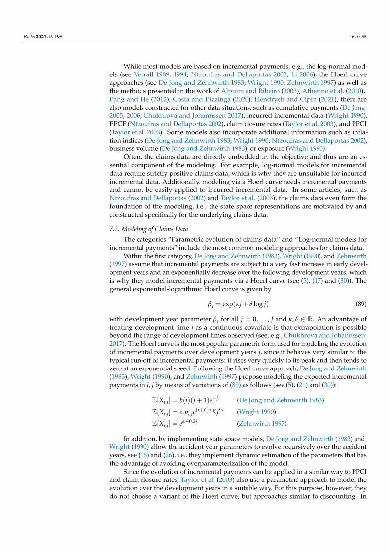
Risks 2021, 9, 198 46 of 55

While most models are based on incremental payments, e.g., the log-normal mod-els (see Verrall 1989, 1994; Ntzoufras and Dellaportas 2002; Li 2006), the Hoerl curveapproaches (see De Jong and Zehnwirth 1983; Wright 1990; Zehnwirth 1997) as well asthe methods presented in the work of Alpuim and Ribeiro (2003), Atherino et al. (2010),Pang and He (2012), Costa and Pizzinga (2020), Hendrych and Cipra (2021), there arealso models constructed for other data situations, such as cumulative payments (De Jong2005, 2006; Chukhrova and Johannssen 2017), incurred incremental data (Wright 1990),PPCF (Ntzoufras and Dellaportas 2002), claim closure rates (Taylor et al. 2003), and PPCI(Taylor et al. 2003). Some models also incorporate additional information such as infla-tion indices (De Jong and Zehnwirth 1983; Wright 1990; Ntzoufras and Dellaportas 2002),business volume (De Jong and Zehnwirth 1983), or exposure (Wright 1990).

Often, the claims data are directly embedded in the objective and thus are an es-sential component of the modeling. For example, log-normal models for incrementaldata require strictly positive claims data, which is why they are unsuitable for incurredincremental data. Additionally, modeling via a Hoerl curve needs incremental paymentsand cannot be easily applied to incurred incremental data. In some articles, such asNtzoufras and Dellaportas (2002) and Taylor et al. (2003), the claims data even form thefoundation of the modeling, i.e., the state space representations are motivated by andconstructed specifically for the underlying claims data.

7.2. Modeling of Claims Data

The categories “Parametric evolution of claims data” and “Log-normal models forincremental payments” include the most common modeling approaches for claims data.

Within the first category, De Jong and Zehnwirth (1983), Wright (1990), and Zehnwirth(1997) assume that incremental payments are subject to a very fast increase in early devel-opment years and an exponentially decrease over the following development years, whichis why they model incremental payments via a Hoerl curve (see (5), (17) and (30)). Thegeneral exponential-logarithmic Hoerl curve is given by

β j = exp(κ j + δ log j) (89)

with development year parameter β j for all j = 0, . . . , J and κ, δ ∈ R. An advantage oftreating development time j as a continuous covariate is that extrapolation is possiblebeyond the range of development times observed (see, e.g., Chukhrova and Johannssen2017). The Hoerl curve is the most popular parametric form used for modeling the evolutionof incremental payments over development years j, since it behaves very similar to thetypical run-off of incremental payments: it rises very quickly to its peak and then tends tozero at an exponential speed. Following the Hoerl curve approach, De Jong and Zehnwirth(1983), Wright (1990), and Zehnwirth (1997) propose modeling the expected incrementalpayments in i, j by means of variations of (89) as follows (see (5), (21) and (30)):

E[Xi,j] = b(i)(j + 1)e−j (De Jong and Zehnwirth 1983)

E[Xi,j] = εi pi,je(i+j′)τKj′λ (Wright 1990)

E[Xi,j] = eα−0.2j (Zehnwirth 1997)

In addition, by implementing state space models, De Jong and Zehnwirth (1983) andWright (1990) allow the accident year parameters to evolve recursively over the accidentyears, see (16) and (26), i.e., they implement dynamic estimation of the parameters that hasthe advantage of avoiding overparameterization of the model.

Since the evolution of incremental payments can be applied in a similar way to PPCIand claim closure rates, Taylor et al. (2003) also use a parametric approach to model theevolution over the development years in a suitable way. For this purpose, however, theydo not choose a variant of the Hoerl curve, but approaches similar to discounting. In

Risks 2021, 9, 198 47 of 55

particular, Taylor et al. (2003) calculate the expected PPCI E[Yi,j] and the expected claimclosure rate E[Zi,j] via

E[Yi,j] = exp(

βi,0 + βi,1(j + 1) +βi,2

j + 1+

βi,3

(j + 1)2 + βi,4δj,0

)(Taylor et al. 2003)

E[Zi,j] = βi,0 +βi,1

j + 1+

βi,2

(j + 1)2 + γtδi+j,t (Taylor et al. 2003)

for a given accident year i = 0, . . . , I over the development years j = 0, . . . , I (see (33),(36)). Pang and He (2012) follow the modeling approach of the linear predictor for thePPCI according to (33) in the work of Taylor et al. (2003) and adopt their approach forincremental payments (see (41)):

E[Xi,j] = θi,1(j + 1) +θi,2

j + 1+

θi,3

(j + 1)2 + θi,4δj,1 (Pang and He 2012)

For the most part, the modeling approaches in these articles do not require anydistributional assumptions. The only exceptions are Wright (1990), where the number ofpayments is assumed to be Poisson-distributed, and Taylor et al. (2003), where the noiseterms and thus the observations are assumed to be EDF-distributed.

Considering the second category “Log-normal models for incremental payments”,all the models are based on explicit distributional assumptions, since the incrementalpayments are assumed to be log-normally distributed. The logarithmized incrementalpayments Yi,j in i, j are then specified via the log-normal model for incremental payments(also called the linear CL model, following Verrall 1989). In particular, Verrall (1989) and Li(2006) use the common basic model (see (44))

Yi,j = µ + αi + β j + wi,j (Verrall 1989; Li 2006)

whereas Verrall (1994) and Ntzoufras and Dellaportas (2002) suggest a variant of this modelthat allows for variations in the column parameters across accident years,

Yi,j = µ + αi + βi,j + wi,j (Verrall 1994; Ntzoufras and Dellaportas 2002)

where the column parameters βi,j may evolve according to (56). In addition to incrementalpayments, Ntzoufras and Dellaportas (2002) also incorporate claim counts, and thereforeconsider PPCF as claims data. In compliance with the approaches of the first categoryand also by utilizing state space models, the authors implement recursions for the modelparameters to achieve dynamic estimation and to avoid the overparameterization of themodel (see, e.g., (52)).

In contrast to the above approaches, there are other ways of modeling the claimsdata: De Jong (2006) (and to some extent also De Jong 2005) presents correlation modelswhere correlations between accident, development or calendar years are considered (see(71)–(73)), Alpuim and Ribeiro (2003) and Chukhrova and Johannssen (2017) proposeunivariate state space models (see (74), (75) as well as (76), (77)), and Atherino et al. (2010),Costa and Pizzinga (2020), and Hendrych and Cipra (2021) discuss row-wise stackingapproaches for the claims data to get a univariate time series (see, e.g., the structural model(80)–(82)).

In particular, De Jong (2006) extends the model δi,j = µj + hjεi,j (i = 1, . . . , I, j =0, . . . , I − 1) for logarithmized individual development factors (64) from Hertig (1985) byincluding correlations of δi,j across development years, accident years or calendar years(see (71)–(73)):

δi,j = µj + hj(εi,j + θjεi,j−1

)δi,j = µi,j + hjεi,j with µi+1,j = µi,j + λjηi,j (De Jong 2006)

Risks 2021, 9, 198 48 of 55

δi,j = µj + hj(τi+j + εi,j

)with τi+j+1 = τi+j + κηi+j

In Alpuim and Ribeiro (2003), it is proposed to model the incremental payments Xi,j ini, j as a function of the payments Xi,0 of the respective accident year i = 1, . . . , I by means of

Xi,j = λi,jXi,0 + wi,j, (Alpuim and Ribeiro 2003)

see (74). Thus, the total amount of claims incurred in accident year i that has been paid jyears later is proportional to the claims incurred and paid in accident year i. This proportionvaries randomly with i and j, which is why Alpuim and Ribeiro (2003) consider the AR(1)process λi,j = µj + φj(λi−1,j − µj) + vi,j, see (75). By applying this approach, the commonassumption of independent accident years is not required.

Chukhrova and Johannssen (2017) propose to model the observed cumulative pay-ments Cobs

i,j as a function of unobservable latent variables Ci,j, i, j = 0, . . . , I. Against thisbackdrop, they presume the relationship

Cobsi,j = gjCi,j + wi,j (Chukhrova and Johannssen 2017)

according to (76), where Ci,j is additionally assumed to follow the recursion Ci,j+1 =f jCi,j + vi,j (see (77)) that is implemented by using a state space model. The approach byChukhrova and Johannssen (2017) therefore addresses potential observation errors in theclaims data.

The authors Atherino et al. (2010) and Costa and Pizzinga (2020) discuss a structuralmodel for incremental payments with a local level component µt, a stochastic periodiccomponent γt and a regression term hT

t u,

yt = µt + γt + hTt u + εt

µt+1 = µt + ξt (Atherino et al. 2010; Costa and Pizzinga 2020)

γt+1 = −J−1

∑d=1

γt+1−d + ωt

see (80)–(82). This approach is inspired by the nature of the claims process: The levelcomponent shall respond for the mean value of claims in each accident year, while theperiodic component is supposed to capture the development year effect. The regressionterm is mainly motivated by the need of intervention effects due to the presence of outliers.That is, the approach of Atherino et al. (2010), and hence also of Costa and Pizzinga (2020)and Hendrych and Cipra (2021), differs from other proposals by using a modeling approachthat is not directly based on claims data with the usual double indexing, but instead, theclaims data is modeled in its whole as a univariate time series. This allows the use of toolsthat are available for time series, and thus considerably expands the modeling spectrumincluding diagnostic checking and model selection criteria.

7.3. Modeling Approaches of State Space Representations

Most of the state space representations are based on the approach of a calendar year-based modeling, in which the claims data of the individual calendar years are stacked intoseparate observation vectors. Similar approaches are an accident year-based modeling (seeTaylor et al. 2003) or a development year-based modeling (see De Jong and Zehnwirth1983) of the observation vectors. Beyond these most common approaches, there areunivariate state space representations and state space models based on the row-wisestacking approach.

The popularity of the approaches that are aligned to the dimensions of claims devel-opment triangles (see Figure 11) is to be seen in the fact that they enable for modelingeffects related to accident, development or calendar years. Because of the relationship ofcalendar years t = i + j to accident years i = 0, . . . , I and development years j = 0, . . . , J,it is clear that only two of these three directions (diagonal, vertical, horizontal) are “in-

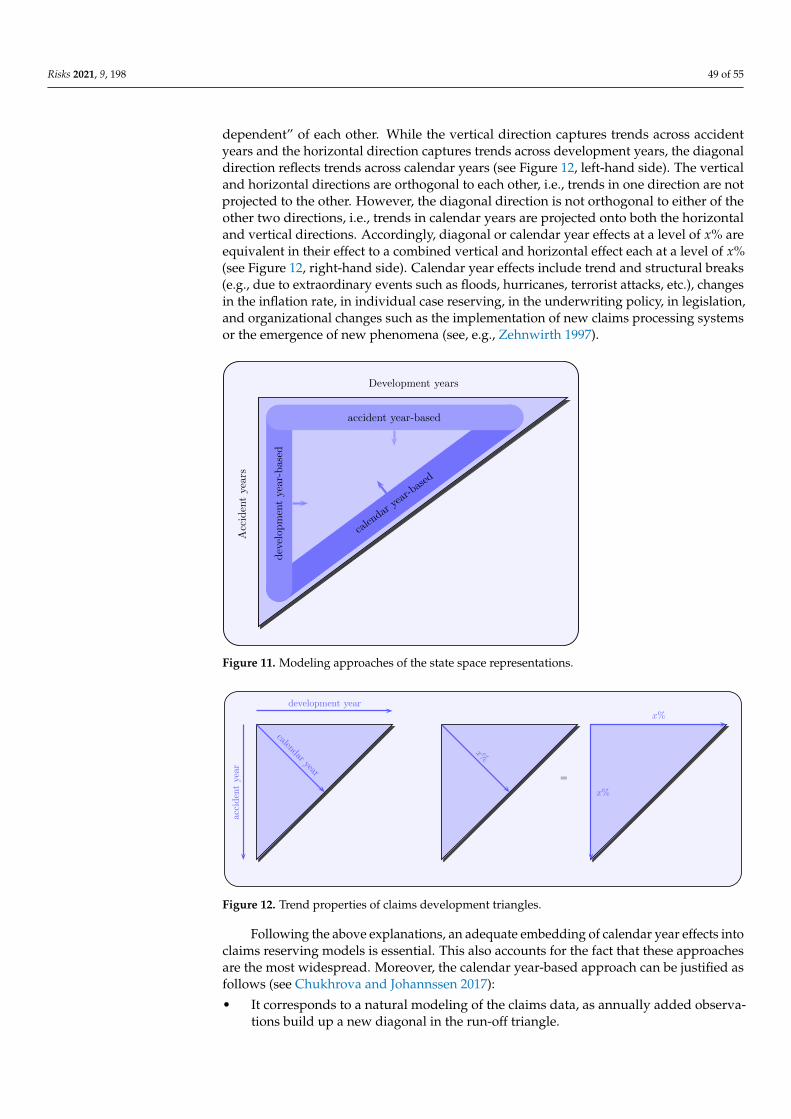
Risks 2021, 9, 198 49 of 55

dependent” of each other. While the vertical direction captures trends across accidentyears and the horizontal direction captures trends across development years, the diagonaldirection reflects trends across calendar years (see Figure 12, left-hand side). The verticaland horizontal directions are orthogonal to each other, i.e., trends in one direction are notprojected to the other. However, the diagonal direction is not orthogonal to either of theother two directions, i.e., trends in calendar years are projected onto both the horizontaland vertical directions. Accordingly, diagonal or calendar year effects at a level of x% areequivalent in their effect to a combined vertical and horizontal effect each at a level of x%(see Figure 12, right-hand side). Calendar year effects include trend and structural breaks(e.g., due to extraordinary events such as floods, hurricanes, terrorist attacks, etc.), changesin the inflation rate, in individual case reserving, in the underwriting policy, in legislation,and organizational changes such as the implementation of new claims processing systemsor the emergence of new phenomena (see, e.g., Zehnwirth 1997).

accident year-based

develop

mentyear-based

calen

dar year-b

ased

Development years

Accidentyears

Figure 11. Modeling approaches of the state space representations.

development year

accidentyear

calendaryear

x%

==

x%

x%

Figure 12. Trend properties of claims development triangles.

Following the above explanations, an adequate embedding of calendar year effects intoclaims reserving models is essential. This also accounts for the fact that these approachesare the most widespread. Moreover, the calendar year-based approach can be justified asfollows (see Chukhrova and Johannssen 2017):

• It corresponds to a natural modeling of the claims data, as annually added observa-tions build up a new diagonal in the run-off triangle.

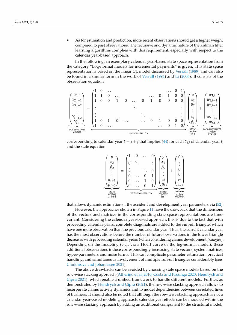
Risks 2021, 9, 198 50 of 55

• As for estimation and prediction, more recent observations should get a higher weightcompared to past observations. The recursive and dynamic nature of the Kalman filterlearning algorithms complies with this requirement, especially with respect to thecalendar year-based approach.

In the following, an exemplary calendar year-based state space representation fromthe category “Log-normal models for incremental payments” is given. This state spacerepresentation is based on the linear CL model discussed by Verrall (1989) and can alsobe found in a similar form in the work of Verrall (1994) and Li (2006). It consists of theobservation equation

Y1,tY2,t−1Y3,t−2

...Yt−1,2

Yt,1

︸ ︷︷ ︸observation

vector

=

1 0 . . . . . . 0 11 1 0 . . . . . . 0 1 0 01 0 0 1 0 . . . 0 1 0 0 0 0...

. . ....

.... . .

...1 0 1 0 . . . . . . 0 1 0 0 01 0 . . . . . . 0 1 0

︸ ︷︷ ︸

system matrix

µα2β2...

αtβt

︸ ︷︷ ︸

statevector

in t

+

w1,tw2,t−1w3,t−2

...wt−1,2

wt,1

︸ ︷︷ ︸measurement

noisevector

corresponding to calendar year t = i + j that implies (44) for each Yi,j of calendar year t,and the state equation

µα2β2...

αt+1βt+1

︸ ︷︷ ︸

statevectorin t+1

=

1 0 . . . 0

0. . .

......

. . . 00 . . . 0 10 . . . 1 00 . . . 0 1

︸ ︷︷ ︸

transition matrix

µα2β2...

αtβt

︸ ︷︷ ︸

statevector

in t

+

0...00vtwt

︸ ︷︷ ︸processnoisevector

that allows dynamic estimation of the accident and development year parameters via (52).However, the approaches shown in Figure 11 have the drawback that the dimensions

of the vectors and matrices in the corresponding state space representations are time-variant. Considering the calendar year-based approach, this is due to the fact that withproceeding calendar years, complete diagonals are added to the run-off triangle, whichhave one more observation than the previous calendar year. Thus, the current calendar yearhas the most observations before the number of future observations in the lower triangledecreases with proceeding calendar years (when considering claims development triangles).Depending on the modeling (e.g., via a Hoerl curve or the log-normal model), theseadditional observations induce correspondingly increasing state vectors, system matrices,hyper-parameters and noise terms. This can complicate parameter estimation, practicalhandling, and simultaneous involvement of multiple run-off triangles considerably (seeChukhrova and Johannssen 2021).

The above drawbacks can be avoided by choosing state space models based on therow-wise stacking approach (Atherino et al. 2010; Costa and Pizzinga 2020; Hendrych andCipra 2021), which enable a unified framework to handle different models. Further, asdemonstrated by Hendrych and Cipra (2021), the row-wise stacking approach allows toincorporate claims activity dynamics and to model dependencies between correlated linesof business. It should also be noted that although the row-wise stacking approach is not acalendar year-based modeling approach, calendar year effects can be modeled within therow-wise stacking approach by adding an additional component to the structural model.

Risks 2021, 9, 198 51 of 55

There are a few articles where a Bayesian approach is employed for estimation, alter-natively or in addition to the Kalman filter (see Verrall 1989; Zehnwirth 1997; Ntzoufrasand Dellaportas 2002). This is because both approaches are related to each other. As iswell known, the Kalman filter is based on two basic ideas: First, the idea of using newinformation to update estimators based on previous observations. Second, the idea offiltering, i.e., separating signals from noise. On the other hand, Bayes (1763) was the firstto show how new observations can be used to update previous estimators. In the usualBayesian approach, a posterior density is first generated from the prior density and thecurrent observation, and this posterior density is then updated to the prior density forthe next step. This process is then repeated sequentially for all upcoming observations(see, e.g., Barker et al. 1995). The particular benefit of Bayesian estimation is that it allowsthe practitioner/researcher to incorporate prior information from other sources (see, e.g.,Verrall 1989). Following Ntzoufras and Dellaportas (2002), the Bayesian approach alsoincreases the computational flexibility, and MCMC sampling strategies can be used togenerate samples for each posterior distribution of interest.

Finally, it is worth mentioning that most of the state space representations consideredin the articles of this review are linear state space models, i.e., they consist of a linear obser-vation equation and a linear state equation. This directly implies linear system propertiesand the limitation to linear processes. An exception is given by Taylor et al. (2003), whoconsider a non-linear observation equation and EDF-distributed measurement noise, thatis, a generalized linear model. This approach enables for any kind of strictly monotonic anddifferentiable link functions (e.g., logarithm functions). However, linear system propertiesare not a principal drawback, as every non-linear system can be converted into a linearsystem by linearizing the system equations. This directly leads to the extended Kalmanfilter (see, e.g., Julier and Uhlmann 2004).

7.4. Insights from Practical Applications

In the following, some selected implications of empirical applications discussed in theabove papers are given in chronological order:

• De Jong and Zehnwirth (1983) present a simple illustrative example based on a dataset from a UK general insurance company (1970–1974), where volume and inflationindices are also available. They give estimated states for the observations of the uppertriangle and predicted future incremental payments of the lower triangle. De Jong andZehnwirth (1983) conclude that the results confirm the regular nature of the data andtherefore the appropriateness of the “constant” transition model for b(i) accordingto (16). Further, the projected future incremental payments decline smoothly to zerowith increasing delay due to the Hoerl curve approach (5).

• Verrall (1989) performs comprehensive practical applications using the benchmarkdata set from Taylor and Ashe (1983) that includes data from the motor bodily injuryclass of business in one Australian state (1972–1981). In particular, he compares staticmodels with recursive Bayesian estimation and dynamic models, where row andcolumn parameters are estimated dynamically. The results show that the Kalman filterand empirical Bayes methods outperform the OLS (i.e., uninformative prior) approach:the estimates of row (and column) parameters are smoother and the standard errors arelower. This is due to the fact that more information is used for parameter estimation.

• Verrall (1994) considers the data set from Taylor and Ashe (1983) for an illustrativeexample and emphasizes that comprehensive examples covering all possibilities arenot feasible. In particular, Verrall (1994) focuses solely on the development parametersand shows that the proposed model allows them to evolve over time.

• The modeling approaches in the work of Ntzoufras and Dellaportas (2002) are moti-vated by their RBNS data set from a major Greek motor insurance company. The dataare characterized by claims that are reported within three working days accordingto Greek legislation and are usually settled by a one-off payment. By comparing thepredictive performance of the proposed models, Ntzoufras and Dellaportas (2002)

Risks 2021, 9, 198 52 of 55

state that the predictive ability of models 1 and 2 seems to be better compared tomodels 3 and 4 for the considered data set.

• As for the accident year-based approach, Taylor et al. (2003) discuss a practical appli-cation based on a workers’ compensation portfolio, in which benefits are dominatedby payments of weekly compensation. The data show a strong upward movementof the PPCI at the beginning and a steady slow decrease in later years. Based on thisevolution, Taylor et al. (2003) decide for a logarithm function as link function anda gamma distribution for the measurement noise. As for the calendar year-basedapproach, they use motor vehicle bodily injury data from Taylor (2000). The claimclosure rates are relatively flat over the development years, but there are shocks thattend to affect whole calendar years. The filtered results follow the data closely attheir general level, that is, there is minor smoothing of the calendar year effects butconsiderable smoothing across development years.

• Alpuim and Ribeiro (2003) discuss two application examples based on real data sets:paid claims from the motor branch of a Portuguese insurance company (1984–1996)and the data set from Taylor and Ashe (1983). The authors compare various claimsreserving methods and conclude that Hoerl curve approaches lead to the largest MSEPof the claims reserves. Further, they suppose that the log-normal transformation ofthe data results in larger values of the MSEP, and therefore, the original observationsshould be used unless there is strong evidence of log-normal distributed data. Forboth data sets, however, the state space model proposed by Alpuim and Ribeiro (2003)leads to reserves with the smallest MSEP.

• De Jong (2006) performs a case study for the development correlation model usinga data set from the Historical Loss Development Study that includes cumulativepayments related to Automatic Facultative General (AFG) liability (1981–1990). In thefirst step, he applies the model of Hertig (1985) to the AFG data and concludes that itis not suitable to adequately represent the data, mainly due to remaining (negative)correlations in the standardized residuals regarding the development years zero andone. For this reason, De Jong (2006) uses the development correlation model (71) in thesecond step, which considers the correlation between the first both development years.Then, the residuals no longer contain any correlations and the correlation between thefirst both development years can be explained via the development correlation model.

• Atherino et al. (2010) also use the AFG data set and especially discuss three resultsof their analysis regarding the row-wise stacking approach. First, it provides com-putational feasibility and efficiency. Second, the accuracy of the reserve prediction isincreased. Third, the approach is flexible with respect to IBNR modeling possibili-ties. As a particularly interesting aspect, they highlight that blocks and cumulatingmethods yield the same numerical results.

• Chukhrova and Johannssen (2017) provide a comparison of various claims reservingmethods with state space representations (Verrall 1989; Alpuim and Ribeiro 2003; Li2006; Atherino et al. 2010) and popular methods such as CL, Bornhuetter–Ferguson(BF) and overdispersed Poisson using the data set from Taylor and Ashe (1983).Considering the claims reserves, their MSEP and the coefficient of variation, no modelcan be identified that provides the best or the worst results for the given data set.

• Costa and Pizzinga (2020) perform a practical example based on the data set fromTaylor and Ashe (1983) and compare their extended row-wise stacking approach witha modified CL approach and heteroskedastic regression models. For the given data set,their proposed method outperforms the three competitors with respect to IBNR reserveprediction. In particular, by applying the competitors, the insurance company mightoverestimate the claims reserves (thus leading to overpriced insurance contracts). Onthe other hand, by employing the original approach by Atherino et al. (2010), thiswould lead to underestimated reserves.

• The most comprehensive empirical comparison of various state space models isconducted by Hendrych and Cipra (2021), who consider five data sets, including data

Risks 2021, 9, 198 53 of 55

sets from Taylor and Ashe (1983), from a Belgian insurance industry, and the dataset from Alpuim and Ribeiro (2003). They compare their introduced models with themodels proposed by Alpuim and Ribeiro (2003), Atherino et al. (2010), and Chukhrovaand Johannssen (2017) as well as CL and BF methods. Following Hendrych and Cipra(2021), their presented state space models are adequate for routine actuarial situations.Further, they give information about the distribution of the predicted claims reserves.

It is obvious that the empirical application examples are heterogeneous, they oftenshow only facets of the presented methods and the results are not consistently comparedwith other methods. There is no empirical comparison of different state space models thatinclude, even approximately, all methods introduced up to now; the most comprehensiveempirical comparisons can be found in the works of Alpuim and Ribeiro (2003), Li (2006),Chukhrova and Johannssen (2017), and Hendrych and Cipra (2021). However, it is alsoevident that a larger-scale empirical comparison of all the models presented is narrowlylimited. This is due to several factors, such as different objectives, different claims data orthe inclusion of additional information. Since the run-off data are often closely integratedin the model building and the objectives in the articles sometimes differ considerably (seeSection 7.1), it is not possible to perform an empirical comparison of all the models thatcould do them justice. Otherwise, models would be applied to claims data and objectivesfor which they were not constructed. Moreover, some models require the incorporation offurther information, such as inflation or volume indices, the availability of which cannotgenerally be assured (and, in the case of the benchmark data set from Taylor and Ashe1983, is not available), but the omission of which would counteract the idea behind modelbuilding. Likewise, no recommendation can be formulated as to which model is best suitedfor actuarial practice. The decision for a specific model depends on numerous factors andshould mainly rely on the verification of the model assumptions on the underlying data.

8. Conclusions

In this paper, we have provided a comprehensive review on the topic of stochasticclaims reserving methods with state space representations. We have identified 16 relevantarticles in this field and grouped them into five categories considering their key contentsimilarities. Most of the articles fall into categories “Parametric evolution” (#5) and “Log-normal models” (#4), but there are also articles devoted to “Correlation models” (#2),“Univariate models” (#2), and “Row-wise stacking” (#3). Moreover, models for incrementalpayments (#12) and the calendar year-based state space modeling approach (#8) are themost prevalent.

Our main intentions were to identify where state space models have been used forimproving stochastic claims reserving and to consolidate the topic in order to aid newresearchers in this area. Out of these objectives, we have structured and categorized therelevant articles. Ideally, this sound basis would assist researchers currently focused onstate space models in stochastic claims reserving and lead to fruitful future research inthis area.

As for promising directions for future research in the field of stochastic claims re-serving based on state space models, we mainly suggest to conduct micro-level claimsreserving and to implement non-linear systems (see Chukhrova and Johannssen (2021)).Moreover, using state space models and beyond, we would like to emphasize the use ofgranular models as well as of machine learning and soft computing techniques in futureresearch projects. Although models based on aggregate data are widely used, especially inactuarial practice, they are often characterized by rather simple model assumptions thatare inadequate for the underlying data. Thus, there is the need for more flexible modelswhich are able to deal appropriately with data where the common model assumptions areviolated (see Taylor (2019)).

Risks 2021, 9, 198 54 of 55

Author Contributions: Conceptualization, N.C. and A.J.; methodology, N.C. and A.J.; formal analy-sis, N.C. and A.J.; investigation, N.C. and A.J.; writing—original draft preparation, A.J.; writing—review and editing, N.C.; project administration, A.J. All authors have read and agreed to thepublished version of the manuscript.

Funding: This research received no external funding.

Acknowledgments: The authors would like to thank both anonymous reviewers for their valuablefeedback and suggestions, which were helpful in further improving this paper.

Conflicts of Interest: The authors declare no conflict of interest.

ReferencesAlpuim, Teresa, and Isabel Ribeiro. 2003. A State Space Model for Run-Off Triangles. Applied Stochastic Models in Business and Industry

19: 105–20. [CrossRef]Atherino, Rodrigo, Adrian Pizzinga, and Cristiano Fernandes. 2010. A row-wise Stacking of the Runoff Triangle: State Space

Alternatives for IBNR Reserve Prediction. ASTIN Bulletin 40: 917–46.Barker, Allen L., Donald E. Brown, and Worthy N. Martin. 1995. Bayesian estimation and the Kalman filter. Computers & Mathematics

with Applications 30: 55–77.Bayes, Thomas. 1763. Essay towards solving a problem in the doctrine of chances. Biometrika 45: 293–315. [CrossRef]Chukhrova, Nataliya, and Arne Johannssen. 2017. State Space Models and the Kalman-Filter in Stochastic Claims Reserving:

Forecasting, Filtering and Smoothing. Risks 5: 30. [CrossRef]Chukhrova, Nataliya, and Arne Johannssen. 2021. Kalman Filter Learning Algorithms and State Space Representations for Stochastic

Claims Reserving. Risks 9: 112. [CrossRef]Costa, Leonardo, and Adrian Pizzinga. 2020. State-space models for predicting IBNR reserve in row-wise ordered runoff triangles:

Calendar year IBNR reserves & tail effects. Journal of Forecasting 39: 438–48.De Jong, Piet, and Ben Zehnwirth. 1983. Claims Reserving, State-Space Models and the Kalman Filter. Journal of the Institute of Actuaries

110: 157–81. [CrossRef]De Jong, Piet. 2004. Forecasting General Insurance Liabilities. Research Paper No. 2004/03. Sydney: Division of Economic and Financial

Studies, Macquarie University.De Jong, Piet. 2005. State Space Models in Actuarial Science. Paper presented at the Second Brazilian Conference on Statistical

Modelling in Insurance, Institute of Mathematics and Statistics, University of São Paulo, Maresias, Brazil, August 28–September 3.De Jong, Piet. 2006. Forecasting Runoff Triangles. North American Actuarial Journal 10: 28–38. [CrossRef]England, Peter D., and Richard J. Verrall. 2002. Stochastic Claims Reserving in General Insurance. British Actuarial Journal 8: 443–518.

[CrossRef]Hendrych, Radek, and Tomas Cipra. 2021. Applying State Space Models to Stochastic Claims Reserving. ASTIN Bulletin 51: 267–301.

[CrossRef]Hertig, Joakim. 1985. A Statistical Approach to IBNR-Reserves in Marine Reinsurance. ASTIN Bulletin 15: 171–83. [CrossRef]Johannssen, Arne. 2016. Stochastische Schadenreservierung unter Verwendung von Zustandsraummodellen und des Kalman-Filters. Hamburg:

Dr. Kovac.Julier, Simon J., and Jeffrey K. Uhlmann. 2004. Unscented filtering and nonlinear estimation. Proceedings of the IEEE 92: 401–22.

[CrossRef]Kaas, Rob, Marc Goovaerts, Jan Dhaene, and Michel Denuit. 2009. Modern Actuarial Risk Theory—Using R, 2nd ed. Berlin: Springer.Kremer, Erhard. 1982. IBNR-Claims and the Two-Way Model of ANOVA. Scandinavian Actuarial Journal 1982: 47–55. [CrossRef]Li, Jackie. 2006. Comparison of Stochastic Reserving Methods. Australian Actuarial Journal 12: 489–569.Ntzoufras, Ioannis, and Petros Dellaportas. 2002. Bayesian Modelling of Outstanding Liabilities incorporating Claim Count Uncertainty.

North American Actuarial Journal 6: 113–28. [CrossRef]Pang, Liyan, and Siqi He. 2012. The Application of State-Space Model in Outstanding Claims Reserve. Paper presented at the 2012

International Conference on Information Management, Innovation Management and Industrial Engineering (ICIII), Sanya, China,October 20–21; pp. 271–74.

Taylor, Greg C. 2000. Loss Reserving: An Actuarial Perspective. Boston: Kluwer Academic Publishers.Taylor, Greg C. 2019. Loss Reserving Models: Granular and Machine Learning Forms. Risks 7: 82. [CrossRef]Taylor, Greg C., and Frank R. Ashe. 1983. Second Moments of Estimates of Outstanding Claims. Journal of Econometrics 23: 37–61.

[CrossRef]Taylor, Greg C., Gráinne McGuire, and Alan Greenfield. 2003. Loss Reserving: Past, Present and Future. Research Paper No. 109.

Melbourne: University of Melbourne.Verrall, Richard J. 1989. A State Space Representation of the Chain Ladder Linear Model. Journal of the Institute of Actuaries 116: 589–610.

[CrossRef]Verrall, Richard J. 1991. Chain Ladder and Maximum Likelihood. Journal of the Institute of Actuaries 118: 489–99. [CrossRef]Verrall, Richard J. 1994. A Method for Modelling Varying Run-off Evolutions in Claims Reserving. ASTIN Bulletin 24: 325–32. [CrossRef]

Risks 2021, 9, 198 55 of 55

Verrall, Richard J. 2004. Kalman Filter, Reserving Methods. In Encyclopedia of Actuarial Science. Edited by Jozef L. Teugels and BjørnSundt. Chichester: John Wiley & Sons, vol. 1, pp. 952–55.

Wright, Thomas S. 1990. A Stochastic Method for Claims Reserving in General Insurance. Journal of the Institute of Actuaries 117: 677–731.[CrossRef]

Wüthrich, Mario V., and Michael Merz. 2008. Stochastic Claims Reserving Methods in Insurance. Chichester: John Wiley & Sons.Zehnwirth, Ben. 1997. Kalman Filters with Applications to Loss Reserving. Working Paper.