Still Picture Encoding for Digital Video Broadcasting - KTH

Still Picture Encoding for Digital Video Broadcasting

Implementing and evaluating MPEG-4 Still Picture encoding for broadcasting using a MPEG-2 Transport Stream from a bandwidth utilization point of view

A N T O N A L I L A

Master of Science Thesis Stockholm, Sweden 2010

Still Picture Encoding for Digital Video Broadcasting

Implementing and evaluating MPEG-4 Still Picture encoding for broadcasting using a MPEG-2 Transport Stream from a bandwidth utilization point of view

A N T O N A L I L A

Master’s Thesis in Media Technology (30 ECTS credits) at the School of Media Technology Royal Institute of Technology year 2010 Supervisor at CSC was Lars Kjelldahl Examiner was Nils Enlund TRITA-CSC-E 2010:145 ISRN-KTH/CSC/E--10/145--SE ISSN-1653-5715 Royal Institute of Technology School of Computer Science and Communication KTH CSC SE-100 44 Stockholm, Sweden URL: www.kth.se/csc

Still Picture Encoding for Digital Video Broadcasting Implementing and evaluating MPEG-4 Still Picture encoding for broadcasting using a MPEG-2 Transport Stream from a bandwidth utilization point of view.

Abstract

There is a need for increased efficiency during broadcasting in the Swedish digital terrestrial broadcasting network. One condition where efficiency can be increased is when broadcasting an encoded video stream consisting of only still picture material.

This Master thesis is part of the result of a Thesis Project initiated by Teracom AB.

The Master Project consisted of the development of a method to; bit efficiently, broadcast still picture material in the digital terrestrial network. This is done by using the AVC Still Picture definition available with MPEG-4 AVC (H.264) video compression and MPEG-2 transport layer.

This Master Thesis describes the work done implementing and evaluating MPEG-4 Still Picture encoding for broadcasting using a MPEG-2 Transport Stream from a bandwidth utilization point of view.

Based on this developed method, a prototype stream was created, in cooperation with Nicklas Lundin, for the thesis project initiator Teracom AB. The prototype stream was tested on a range of IDTV- and set top box decoders in order to determine if material encoded with the AVC still picture approach could be introduced in the Swedish digital terrestrial network. Of the 6 IDTV decoders and 10 set top boxes, 4 IDTV decoders displayed the pictures with satisfactory results, 1 of the set top boxes displayed the stream but demonstrated issues with prolonged channel zapping times.

This efficient method of sending still pictures will create opportunities for content providers to broadcast still picture material where previously not justifiable from an economic point of view.

Stillbildskodning för utsändning Implementering av MPEG-4 AVC Still Pictures för utsändning i en MPEG-2 transportström och utvärdering med avseende på bandbreddsutnyttjande.

Sammanfattning

Det finns ett behov av ökad effektivitet vid utsändning i det svenska digitala markbundna TV-nätet. En situation där effektiviteten kan ökas är när man sänder kodad video bestående av endast stillbildsmaterial.

Detta examensarbete är en del av resultatet av ett examensarbetesprojekt som initierats av Teracom AB. Projektet bestod av att utveckla en metod för att, biteffektivt, utsända stillbildsmaterial i det digitala marknätet. Detta görs genom att använda AVC Still Pictures definition som finns tillgängligt i MPEG-4 AVC (H.264) standarden för videokomprimering och MPEG-2 video överföring.

Detta examensarbete beskriver genomförandet och utvärderingen av AVC Still Pictures för utsändning med en MPEG-2 transportström, med avseende på bandbreddsanvändning.

Utifrån den utvecklade metoden skapades en prototypström, i samarbete med Nicklas Lundin, för examensarbetets initiativtagare Teracom AB. Prototypströmmen testades på en rad IDTV-och set-top-box-avkodare för att avgöra om material kodat med AVC Still Pictures definitionen skulle kunna införas i det svenska digitala marknätet. Av de testade 6 IDTV dekodrar och 10 set-top boxar, visar 4 IDTV dekodrar bilderna med tillfredsställande resultat. En av set-top boxarna visar strömmen, dock med förlängd kanalbytestid.

Denna effektiva metod för överföring av stillbilder kommer att skapa möjligheter för innehållsleverantörer att sända stillbildsmaterial där det tidigare inte varit försvarbart ur ekonomiskt perspektiv.

Acknowledgments This master thesis project was done for the project initiator Tercom AB during the second half of 2009.

I would like to thank; our supervisor Anders Berglund at Teracom AB for his extensive help and direction throughout the whole of this master thesis project, and for teaching me everything there is to know about video encoding and broadcasting. Marie Serenius for administrative help and guidance. Per Tullstedt for technical assistance, general advice and ideas. Johan Haglöw at the decoder testing department for the extensive help and loads of patience during the testing phase of this project. Finally I would like to extend my gratitude towards Nicklas Lundin, without your help this thesis project would never have been possible.

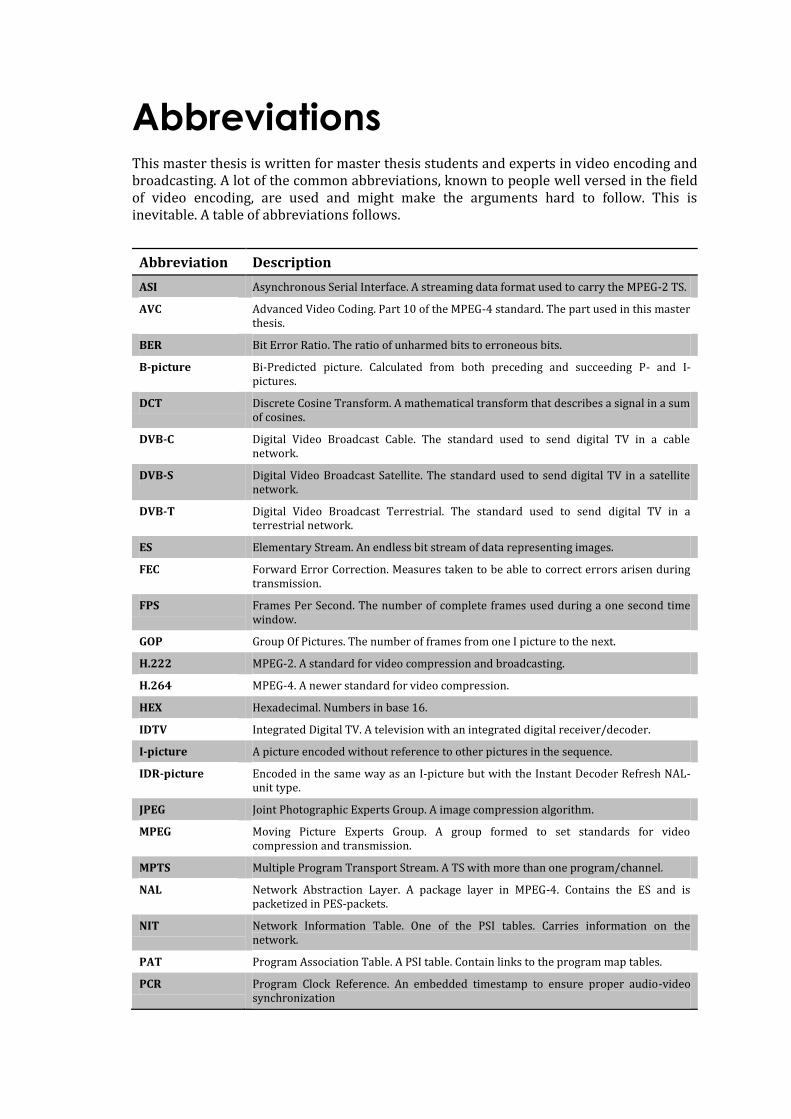
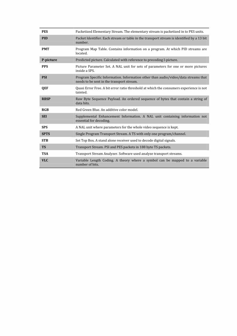
Abbreviations This master thesis is written for master thesis students and experts in video encoding and broadcasting. A lot of the common abbreviations, known to people well versed in the field of video encoding, are used and might make the arguments hard to follow. This is inevitable. A table of abbreviations follows.

Abbreviation Description

ASI Asynchronous Serial Interface. A streaming data format used to carry the MPEG-2 TS.

AVC Advanced Video Coding. Part 10 of the MPEG-4 standard. The part used in this master thesis.

BER Bit Error Ratio. The ratio of unharmed bits to erroneous bits.

B-picture Bi-Predicted picture. Calculated from both preceding and succeeding P- and I-pictures.

DCT Discrete Cosine Transform. A mathematical transform that describes a signal in a sum of cosines.

DVB-C Digital Video Broadcast Cable. The standard used to send digital TV in a cable network.

DVB-S Digital Video Broadcast Satellite. The standard used to send digital TV in a satellite network.

DVB-T Digital Video Broadcast Terrestrial. The standard used to send digital TV in a terrestrial network.

ES Elementary Stream. An endless bit stream of data representing images.

FEC Forward Error Correction. Measures taken to be able to correct errors arisen during transmission.

FPS Frames Per Second. The number of complete frames used during a one second time window.

GOP Group Of Pictures. The number of frames from one I picture to the next.

H.222 MPEG-2. A standard for video compression and broadcasting.

H.264 MPEG-4. A newer standard for video compression.

HEX Hexadecimal. Numbers in base 16.

IDTV Integrated Digital TV. A television with an integrated digital receiver/decoder.

I-picture A picture encoded without reference to other pictures in the sequence.

IDR-picture Encoded in the same way as an I-picture but with the Instant Decoder Refresh NAL-unit type.

JPEG Joint Photographic Experts Group. A image compression algorithm.

MPEG Moving Picture Experts Group. A group formed to set standards for video compression and transmission.

MPTS Multiple Program Transport Stream. A TS with more than one program/channel.

NAL Network Abstraction Layer. A package layer in MPEG-4. Contains the ES and is packetized in PES-packets.

NIT Network Information Table. One of the PSI tables. Carries information on the network.

PAT Program Association Table. A PSI table. Contain links to the program map tables.

PCR Program Clock Reference. An embedded timestamp to ensure proper audio-video synchronization

PES Packetized Elementary Stream. The elementary stream is packetized in to PES units.

PID Packet Identifier. Each stream or table in the transport stream is identified by a 13 bit number.

PMT Program Map Table. Contains information on a program. At which PID streams are located.

P-picture Predicted picture. Calculated with reference to preceding I-picture.

PPS Picture Parameter Set. A NAL unit for sets of parameters for one or more pictures inside a SPS.

PSI Program Specific Information. Information other than audio/video/data streams that needs to be sent in the transport stream.

QEF Quasi Error Free. A bit error ratio threshold at which the consumers experience is not tainted.

RBSP Raw Byte Sequence Payload. An ordered sequence of bytes that contain a string of data bits.

RGB Red Green Blue. An additive color model.

SEI Supplemental Enhancement Information. A NAL unit containing information not essential for decoding.

SPS A NAL unit where parameters for the whole video sequence is kept.

SPTS Single Program Transport Stream. A TS with only one program/channel.

STB Set Top Box. A stand alone receiver used to decode digital signals.

TS Transport Stream. PSI and PES packets in 188 byte TS packets.

TSA Transport Stream Analyzer. Software used analyze transport streams.

VLC Variable Length Coding. A theory where a symbol can be mapped to a variable number of bits.

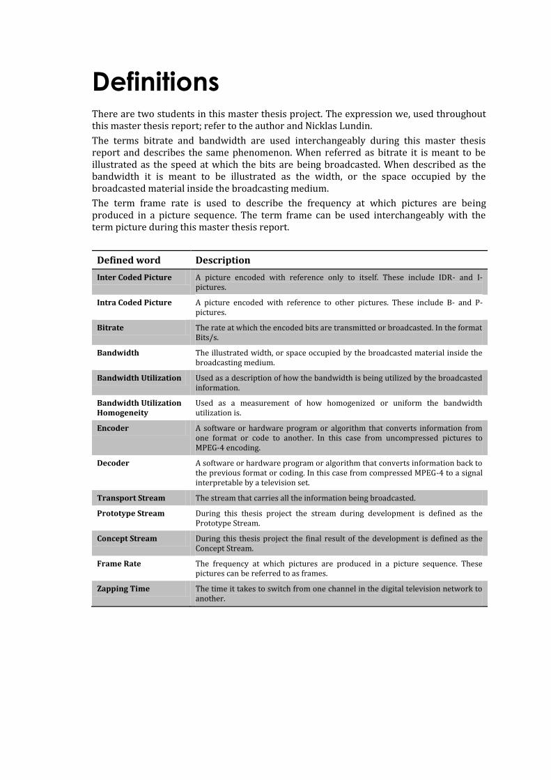
Definitions There are two students in this master thesis project. The expression we, used throughout this master thesis report; refer to the author and Nicklas Lundin.

The terms bitrate and bandwidth are used interchangeably during this master thesis report and describes the same phenomenon. When referred as bitrate it is meant to be illustrated as the speed at which the bits are being broadcasted. When described as the bandwidth it is meant to be illustrated as the width, or the space occupied by the broadcasted material inside the broadcasting medium.

The term frame rate is used to describe the frequency at which pictures are being produced in a picture sequence. The term frame can be used interchangeably with the term picture during this master thesis report.

Defined word Description

Inter Coded Picture A picture encoded with reference only to itself. These include IDR- and I-pictures.

Intra Coded Picture A picture encoded with reference to other pictures. These include B- and P-pictures.

Bitrate The rate at which the encoded bits are transmitted or broadcasted. In the format Bits/s.

Bandwidth The illustrated width, or space occupied by the broadcasted material inside the broadcasting medium.

Bandwidth Utilization Used as a description of how the bandwidth is being utilized by the broadcasted information.

Bandwidth Utilization Homogeneity

Used as a measurement of how homogenized or uniform the bandwidth utilization is.

Encoder A software or hardware program or algorithm that converts information from one format or code to another. In this case from uncompressed pictures to MPEG-4 encoding.

Decoder A software or hardware program or algorithm that converts information back to the previous format or coding. In this case from compressed MPEG-4 to a signal interpretable by a television set.

Transport Stream The stream that carries all the information being broadcasted.

Prototype Stream During this thesis project the stream during development is defined as the Prototype Stream.

Concept Stream During this thesis project the final result of the development is defined as the Concept Stream.

Frame Rate The frequency at which pictures are produced in a picture sequence. These pictures can be referred to as frames.

Zapping Time The time it takes to switch from one channel in the digital television network to another.

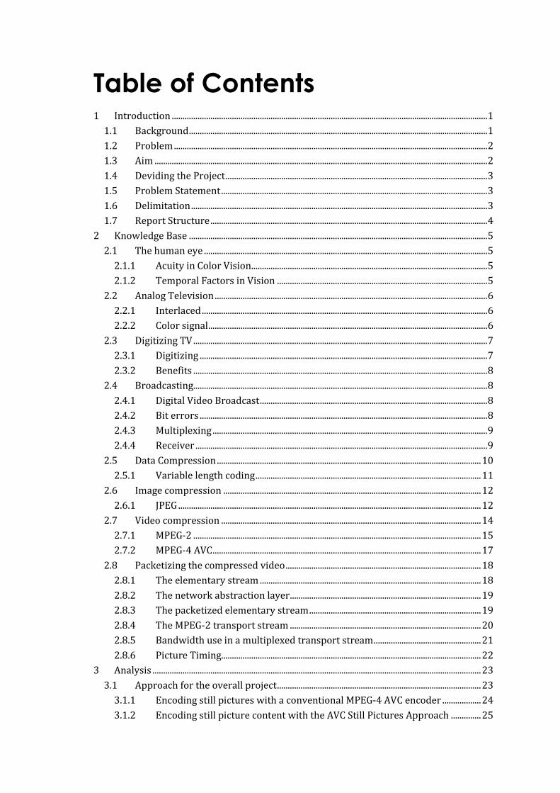
Table of Contents 1 Introduction ................................................................................................................................................... 1

1.1 Background ........................................................................................................................................... 1

1.2 Problem .................................................................................................................................................. 2

1.3 Aim ........................................................................................................................................................... 2

1.4 Deviding the Project .......................................................................................................................... 3

1.5 Problem Statement ............................................................................................................................ 3

1.6 Delimitation .......................................................................................................................................... 3

1.7 Report Structure ................................................................................................................................. 4

2 Knowledge Base ........................................................................................................................................... 5

2.1 The human eye .................................................................................................................................... 5

2.1.1 Acuity in Color Vision .............................................................................................................. 5

2.1.2 Temporal Factors in Vision .................................................................................................. 5

2.2 Analog Television ............................................................................................................................... 6

2.2.1 Interlaced ..................................................................................................................................... 6

2.2.2 Color signal .................................................................................................................................. 6

2.3 Digitizing TV ......................................................................................................................................... 7

2.3.1 Digitizing ...................................................................................................................................... 7

2.3.2 Benefits ......................................................................................................................................... 8

2.4 Broadcasting......................................................................................................................................... 8

2.4.1 Digital Video Broadcast .......................................................................................................... 8

2.4.2 Bit errors ...................................................................................................................................... 8

2.4.3 Multiplexing ................................................................................................................................ 9

2.4.4 Receiver ........................................................................................................................................ 9

2.5 Data Compression ........................................................................................................................... 10

2.5.1 Variable length coding ......................................................................................................... 11

2.6 Image compression ........................................................................................................................ 12

2.6.1 JPEG ............................................................................................................................................. 12

2.7 Video compression ......................................................................................................................... 14

2.7.1 MPEG-2 ...................................................................................................................................... 15

2.7.2 MPEG-4 AVC ............................................................................................................................. 17

2.8 Packetizing the compressed video ........................................................................................... 18

2.8.1 The elementary stream ....................................................................................................... 18

2.8.2 The network abstraction layer ......................................................................................... 19

2.8.3 The packetized elementary stream ................................................................................ 19

2.8.4 The MPEG-2 transport stream ......................................................................................... 20

2.8.5 Bandwidth use in a multiplexed transport stream .................................................. 21

2.8.6 Picture Timing......................................................................................................................... 22

3 Analysis ......................................................................................................................................................... 23

3.1 Approach for the overall project ............................................................................................... 23

3.1.1 Encoding still pictures with a conventional MPEG-4 AVC encoder .................. 24

3.1.2 Encoding still picture content with the AVC Still Pictures Approach .............. 25

3.1.3 Development approaches ................................................................................................... 26

4 Method........................................................................................................................................................... 27

4.1 Iterative development ................................................................................................................... 27

4.2 Tools ..................................................................................................................................................... 28

4.2.1 JDSU DTS 330 .......................................................................................................................... 28

4.2.2 BreakPoint Software Hex Workshop ............................................................................. 30

4.3 Java Development ........................................................................................................................... 31

4.4 Other tools .......................................................................................................................................... 32

4.4.1 Encoder Thomson ViBE EM 2000 ................................................................................... 32

4.4.2 Decoder Tandberg RX1290 ............................................................................................... 32

4.5 Implementation Test Workflow ................................................................................................ 33

4.6 Evaluation process .......................................................................................................................... 33

4.7 Reliability and validity .................................................................................................................. 33

5 Implementation ......................................................................................................................................... 35

5.1 The initial stream ............................................................................................................................ 35

5.2 Stripping the initial stream ......................................................................................................... 36

5.3 Syntax Conformance ...................................................................................................................... 37

5.4 Homogenizing the prototype stream ...................................................................................... 38

5.4.1 Approaches to solve the problem with bandwidth utilization homogeneity38

5.4.2 Homogenization in practice .............................................................................................. 40

5.5 Fixing the timing .............................................................................................................................. 43

5.5.1 Adding PCR ............................................................................................................................... 43

5.5.2 Adding PTS and DTS ............................................................................................................. 45

6 Evaluation .................................................................................................................................................... 48

6.1 Practical testing................................................................................................................................ 48

6.2 Graphical overview of the Transport Stream ...................................................................... 50

7 Results ........................................................................................................................................................... 53

7.1 Thesis project results .................................................................................................................... 53

7.2 Thesis specific results .................................................................................................................... 54

7.2.1 Bandwidth utilization homogeneity .............................................................................. 54

7.2.2 Buffer Occupancy ................................................................................................................... 55

7.2.3 PCR timing Analysis .............................................................................................................. 56

8 Discussion .................................................................................................................................................... 57

9 Conclusion .................................................................................................................................................... 59

10 Future work .................................................................................................................................................... 59

References ............................................................................................................................................................. 60

Appendix A ............................................................................................................................................................ 61

Appendix B ............................................................................................................................................................ 62

Appendix C ............................................................................................................................................................ 63

1

1 Introduction This chapter is an introduction to why this master thesis is interesting, relevant and pressing. This chapter was made in cooperation with Nicklas Lundin.

1.1 Background The Swedish terrestrial television broadcast network uses a set of fixed frequencies given by the Post and Telecom Agency (Post- och Telestyrelsen). These frequencies are inherited from the time when only analog TV were broadcasted and they set the capacity for bandwidth and the amount of channels in the digital video broadcast terrestrial network (DVB-T). The capacity for terrestrial broadcast networks is far lower than both satellite and cable broadcasting.

The decision to migrate to a digital way of broadcasting came with some benefits, for example, the amount of channels could be increased as the technology was more efficient.

Along with the channel distributor Boxer’s range of TV-channels, the Swedish Radio’s (SR) radio channels P1, P2, P3 and P4 are distributed over the DVB-T network. These channels were first broadcasted without a video stream but SR has made requests to also send still pictures along with their radio shows. The still pictures would be in form of a logotype or a tableau of upcoming programs.

In the terrestrial broadcasting network run by Teracom AB, some channel companies share their bandwidth between two channels. I.e. channel A broadcasts in the AM and channel B broadcasts in the PM. When one channel broadcasts the other one does not have the sufficient bandwidth to send a video stream (see Figure 1). The channel not sending at the moment still wants an opportunity to market their channel, show a TV tableau or a commercial slideshow, consisting of still picture material.

Figure 1: Three channels in one multiplex. Channel A and B share their bandwidth by broadcasting on different

times of the day. Channel C broadcasts the entire time.

Today, the still picture streams are broadcasted in the same way as a motion picture video stream, i.e. 25 frames per second (for Sweden). This means that these still picture streams require technology and somewhat similar amount of bandwidth as motion picture video.

2

1.2 Problem Because of the demand for more services in the digital terrestrial broadcasting network, and since the available bandwidth is limited, the need for increased efficiency during broadcasting exist. One condition where efficiency can be increased is when broadcasting an encoded video stream consisting of only still picture material. An efficient method of sending still pictures will create opportunities for content providers to broadcast still picture material where previously not justifiable from an economic point of view.

When encoding a video stream consisting of still pictures with a conventional MPEG-4 AVC encoder, using a low video bitrate, several problems with both viewing experience and broadcast logistics occur. These include problems with; jerky video, bandwidth utilization and efficiency. This is because the MPEG-4 AVC encoders are developed for encoding moving pictures.

When encoding with a low bitrate, the encoder interprets small (non-existing) differences between individual frames in the input still picture material. This results in redundant data being encoded into the stream. Redundant data is further generated by syntax information and stuffing packets inserted in order to maintain a constant frame- and bit-rate.

This redundant data is also the cause of the problem with jerky video. The encoding algorithm, when using low bitrates, generates noise which is easier to spot when the video material is still pictures.

The issue with bandwidth utilization exist because the bandwidth reserved for broadcasting the stream is based on the peak bandwidth usage. The temporal window between two consecutive frames stands in correlation with the amount of residual data being generated. Hence the lower the frame rate, bigger the problem.

1.3 Aim The aim of this master thesis project is to evaluate the term, AVC Still Pictures, which sporadically appears in the MPEG-2 and DVB-T standards. This in order to assess if it is a viable approach for solving the problem of broadcasting encoded still picture material efficiently. The secondary objective is to generate a concept transport stream utilizing the AVC Still Pictures definition found in the standardization documents. The third and final objective is to test and evaluate if the AVC Still Pictures approach is compatible with the MPEG-4 decoders available (during 2009/2010) on the Swedish market, to provide a baseline for the decision to weather the approach should be implemented into the Digital Terrestrial Broadcast Network during 2010.

The investigation is pressing since the market of MPEG-4 receivers still is very young but growing fast. It is important to develop a concept stream that receiver manufacturers can test and comply with. It is specified in the DVB-T standard that still pictures should be supported by receivers but as there is no concept stream, it cannot be tested.

The ambition is that receiver manufacturers can use this concept stream to develop support for AVC still pictures in their receivers and DVB operators could use this method of sending still pictures to create more bandwidth efficient broadcasting of content.

3

1.4 Deviding the Project From the three objectives described in the previous Aim chapter, the subject matter for two master thesis papers emerge; one concerning the bandwidth efficiency of the generated reference stream, and one dealing with the bandwidth utilization homogeneity.

This thesis report is specialized in evaluating the approaches available in order to homogenize the bandwidth utilization during broadcast of AVC still pictures.

Nicklas Lundin, my collaborator’s master thesis report is called Implementing and evaluating MPEG-4 Still Picture encoding for broadcasting using a MPEG-2 Transport Stream from a bandwidth efficiency point of view, and can be found in the list of references as (Lundin, 2010).

During this thesis project we have worked closely together developing the concept stream and all testing has been done collaboratively. The practical aims of the two theses are the same and only the viewpoints of the papers differentiate. The theory chapter was developed in cooperation and most of the background, problem statement and aim will be alike. If the underlying work has been done in collaboration it is stated during the introduction of each chapter.

1.5 Problem Statement Project specific:

How is the term AVC Still Pictures described in the various standards and definition documents?

How is the AVC Still Picture method implemented?

Is there support for AVC Still Pictures in the MPEG-4 receivers on the market?

Thesis specific:

How can the bandwidth utilization homogeneity be ensured?

How can this be implemented?

How is the picture timing maintained?

1.6 Delimitation This thesis is not about, and will not cover, the algorithms for picture and video encoding in the MPEG-4 AVC standard. The necessary modifications of the video stream will be done by altering the syntax only.

The broadcast standard this thesis will cover is DVB-T. DVB-S and –C, will not be covered.

The other paper in this master thesis project deal with the overall bandwidth efficiency of the AVC Still Picture method, thus, this will only be covered briefly in this report.

The result of this master thesis project was not meant to be a complete and finished product. This is an experiment, a proof of concept and an investigation on the possibilities to develop such a product or service.

The verification test or observation of the example stream on consumer market receivers are not meant to be a scientific experiment. The aim of the verification is to observe and gather knowhow on how receivers react in practice. The verification is called an observation, as not all variables in the test environment can be controlled.

4

1.7 Report Structure The report begins with a thorough Knowledge Base chapter describing the necessary terminology, technology and standards. The analysis chapter briefly describes how the thesis project was initiated, what decisions were made, the different methods available for solving the problem and why the specific method was chosen. The method chapter describes the methods, tools and development approach used for solving the problem. The thesis project work is divided into two parts. The implementation part describes how the AVC Still Pictures approach was implemented using the given method. The evaluation describes the work done evaluating the AVC Still Pictures conformed transport stream. Finally the results are summarized and the discussion of the project is presented. The Conclusion wraps up the master thesis report and future work chapter describes where the work will go based on the results presented.

5

2 Knowledge Base A literary review was conducted to understand the concepts of video encoding and broadcasting. This chapter was written in cooperation with Nicklas Lundin.

2.1 The human eye

2.1.1 Acuity in Color Vision

To understand the theories used in the compression process it is important to have a basic understanding of the human eye and the way in which human perception works. The human eye consists of a lens focusing light from the environment onto the back surface of the eye itself. The surface is covered with light sensitive receptors of two kinds; rods and cones. The rods are not sensitive to color, only luminance information is sensed. They are responsible for night vision, motion detection and peripheral vision. The color information is provided by the cones which are divided into three types, one of each senses red, green and blue colors. Studies show that the populations of these types vary greatly. 64% of the cones are red perceiving cones, 32% green perceiving, and 2% blue. The light sensitivity of the rods is more than a thousand times more receptive than the cones. This makes the human visual system much more sensitive to variations in brightness than color (Goldstein, 2009).

These conditions can be used to greatly improve the compression process which is briefly covered in chapter 2.2.2.

2.1.2 Temporal Factors in Vision

The human mind is fairly easy to trick. This is something that has been thoroughly investigated by scientists and technological developers alike. The eye communicates through nerve impulses to the brain about 1000 times per second. Although this is not the same rate as to which the rods and cones can perceive changes in stimuli. Instead a slight lag is present. This is the temporal property of the eye called persistence of vision; the retention of the stimuli after it is removed or changed (Whitaker, 2001). This is the phenomenon upon which the whole technology of moving pictures is built.

By showing a series of still pictures which depict some type of movement that can be perceived by the mind as a logical flow of events, the mind quickly begins to interpret the still images as a constant flow of actual movement. For this to be perceived correctly it is necessary to update the picture with a frequency of 25 Hz, or 25 frames per second. Yet there is still another problem. The persistence of vision is reverse proportional to the brightness (intensity) of the image viewed. The stronger the stimulus to the eye is, the shorter the persistence of vision will become. In practice this means that update frequency needs to be improved in order to sustain the illusion of moving pictures, without introducing flickering, when the brightness of the images is increased. This is usually done by showing the same image several times, with a black frame in-between (Whitaker, 2001).

6

2.2 Analog Television

2.2.1 Interlaced

Interlaced video has its origin in one of the first television inventions. The Scottish inventor John Baird used the technological progress of the 1920s and applied it to the Nipkow disk. By using a disk with 30 holes, the image was recorded successively, hole by hole. Placing the disk in front of a selenium photocell, the signal produced from the photocell showed the recorded image divided over 30 holes (Röjne, 2006). The images were then reproduced at another location using the signal and basically the same equipment in a reverse setup.

Later in the development of television, a cathode ray tube canon was used to draw the pictures using horizontal lines over the TV monitor. The canon was not fast enough to draw each line without the first lines fading out; the eye noticed this. Using the eyes properties in persistence of vision, this problem was overcome by using interlaced scanning.

Interlaced scanning work by capturing every other line from left to right by the camera and shown on the monitor or TV. First all odd lines are drawn and then the even ones fills the space between. Each picture with either the even or the odd lines is called a field. When two fields are shown in rapid succession, they are integrated by the eye and called a frame. One frame represents all lines in two succeeding fields.

In Sweden, and most of the world, the line voltage uses a frequency of 50 Hz. Using this frequency as a good reference to keep a constant speed, a new field is scanned by the camera or shown by the TV 50 times per second. But as two fields form one frame, the video runs at 25 frames per second (fps). In North America, 60 Hz is used in the line voltage and thus the video runs at (about) 30 fps (Ascher, Pincus, 1999).

The North American system was the National Television System Committee (NTSC), with 525 lines per frame and the format used in Sweden (and many other European countries) were Phase Alternating Line (PAL). PAL, as well as “Séquentiel couleur à mémoire” (SECAM) uses 625 lines per frame (Röjne, 2006).

2.2.2 Color signal

When TV first made its entrance on the consumer market in Sweden, in the 1950s, there was no color signal at all. The signal was black and white. Every grey tone in the picture corresponded to a voltage level in the signal; this level was and is called luminance. When the luminance signal is +1 volts, the luminance is 100%, i.e. a white picture (Röjne, 2006).

As described in chapter 2.1.1, the eye has three color receptors, red, green and blue. The additive color model, RGB, which is used in most professional cameras, mimics the receptors as the camera uses a prism to divide the light onto 3 separate Charge-coupled device (CCD) sensors, one for red, one for green and one for blue.

When the color TV made its appearance it used three cathode ray tubes, red, green and blue. The two main reasons a signal with these three colors could not be broadcasted were the backward compatibility issue; black and white TV sets would not understand the new signal. The other reason is the problem of broadcasting; the three signals would consume three times the amount of bandwidth compared to the black and white system (a. a).

7

A solution was developed from the knowledge of human perception. Part of which is described in chapter 2.1.1. Using the additive color model; the luminance, Y, can be defined by:

Y = 0,30R + 0,59G + 0,11B

R-Y = 0,70R – 0,59G - 0,11B

B-Y = -0,30R – 0,59G + 0,89B

This is just another way of describing the RGB color space and R-Y and B-Y are color difference signals, Chrominance. This way of encoding RGB is called YPbPr.

We already learned that the eye is less sensitive to variations in color; this means we can use less bandwidth for the chrominance information; we achieve an analog image compression. The luminance information is filtered down and the chrominance information placed above the luminance in frequency. In the PAL-standard, which is used in Sweden, the luminance uses 5MHz bandwidth and the chrominance uses 2 x 1 MHz (B-Y, R-Y), this means that the color in analog color TV uses only 40% of the information compared to the luminance (Röjne, 2006).

2.3 Digitizing TV

2.3.1 Digitizing

The analog signal transmits a lot of redundancy and unimportant information. By representing the signal digitally, bandwidth requirement and issues regarding noise can be reduced.

Going from the analog to the digital world, we start by taking small samples from the analog waveform, making it discrete. The digital world is built around the binary system, i.e. a bit is either 1 (one) or 0 (zero) and a sequence of 8 bits constitutes a byte.

The digitizing consists of two phases. First we make the continuously analog signal discrete. This is done by reading the value of the analog signal at a constant frequency. This is called sampling, and will disrupt the analog signals time dimension continuity.

To represent the analog signal correctly, the samples must be made at high enough frequency. This frequency can be calculated using the Nyquist sampling theorem which in basis states that the signal should be sampled at a frequency of at least twice the signal bandwidth. Sampling with a lower frequency will result in an incorrect representation of the signal, a problem called aliasing. For example, the picture bandwidth in the PAL standard is 5 MHz and to correctly describe it digitally we would need to sample at a frequency of 10 MHz, i.e. 10 000 000 samples per second.

We also need to round of the samples to predetermined values, this process is called quantization. In this stage we lose the continuous signal values and approximate them to fit the nearest of our fixed values. An everyday example of this is a ladder, which steps quantize the height. The number of predetermined steps usually used in video is 256, which is the same as 8 bits. The differences between the measured analog values and the discrete digital steps are called quantization errors (Watkinson, 2004).

Using the example values above, the digitizing of one black and white PAL channel without sound would need the transmit speed of 10 000 000 bit x 8 levels = 80 Mbit/s. The total bandwidth of the DVB-T network in Sweden today is about 110 Mbit/s. Using more than 70% of the entire bandwidth for only one channel is not an option; we need to compress the data. This is covered in chapter 2.5, 2.6 and 2.7.

8

2.3.2 Benefits

The benefits of digitizing TV is mainly the ability to implement powerful compression algorithms and thus reduced bandwidth needed for each channel. This in turn, leads to room more channels to be broadcasted and the possibility to send other data to be used by the receiving set top box.

Digitizing also comes with a better picture quality as the noise is not contaminating the signal in the same way. The digital signal is also more robust and can handle interference in a better way compared to the analog signal. The digital signal needs less signal strength (Teracom, n.d) and thus the transmitter can use less power which is good, both from an environmental and an economic point of view.

2.4 Broadcasting

2.4.1 Digital Video Broadcast

Digital Video Broadcast (DVB) is a group formed in 1993 with aim to create a standard for transmitting digital video. Their standards are published by “The European Telecommunications Standards Institute” (ETSI) and most parts of the world has agreed to use different kinds of DVB to broadcast digital video. The standards are known as DVB and a suffix, depending on what the standard covers.

The standards of DVB differ depending on which medium the broadcasts move through. The reason for this is that different mediums have different demands or need different error protection. For example; a transmission from satellite needs a robust but not very efficient modulation due to a noisier channel. The Satellite DVB standard can use a less efficient modulation because of the satellite's higher bandwidth.

Some standards from the DVB does not concern the transmitting, but focuses around subtitling, service information or conditional access (Röjne, 2006).

Amongst many other things important for this master thesis, the DVB-T standard reads that “in the case of still pictures the fixed_frame_rate_flag shall be equal to 0” (DVB standard, 2007). This allows bypassing the requirement of 25 frames per second.

2.4.2 Bit errors

A broadcasted signal is always in risk of being exposed to noise of different kinds. Therefore we need to protect the signal against both static noise and noise bursts.

Noise is unwanted, random interference with the signal. Static noise usually causes bit errors scattered over a major part of the signal. Noise-, or error bursts are a bit different. These can be caused by thunder, voltage spikes or electronic equipment and will wipe out a series of subsequent bits.

When the decoder receives the damaged signal it needs to be fixed, otherwise the decoder will not be able to understand it. Unlike other distribution forms, the DVB does not have a return channel, so the receiver cannot ask the sender to resend the package. Luckily some precautions are made before sending the signal to make sure the decoder has a good chance of correcting the errors that might arise during the transmission, these precautions are called Forward Error Correction (FEC). Some of the FEC used in DVB are Reed-Solomon error correction, interleaving and punctured coding.

The amount of bit errors in relation to non erroneous bits is called Bit Error Ratio (BER) and is strived to be as low as the threshold 1 x 10-11 which is called Quasi Error Free (QEF). When the BER is below the QEF threshold, the consumer experience of the broadcasted service is not tainted. The BER of 1 x 10-11 is one bit error every 20 000 seconds (Röjne, 2006).

9

2.4.3 Multiplexing

Multiplexing is a way to transmit several signals, or services, over one medium. The medium could be a cable or in the case of DVB-T, a radio frequency. In theory, multiplexing uses the capacity of the low level channel to create many high level logical channels. What it does in practice is mixing the packets from, in this case, different TV channels in time over the transport medium.

Multiplexing over time is called Time Division Multiplexing. The physical transmission channel is chopped up into time slots. During one time slot, only one sender can use the channel. The other senders have to wait for their turn.

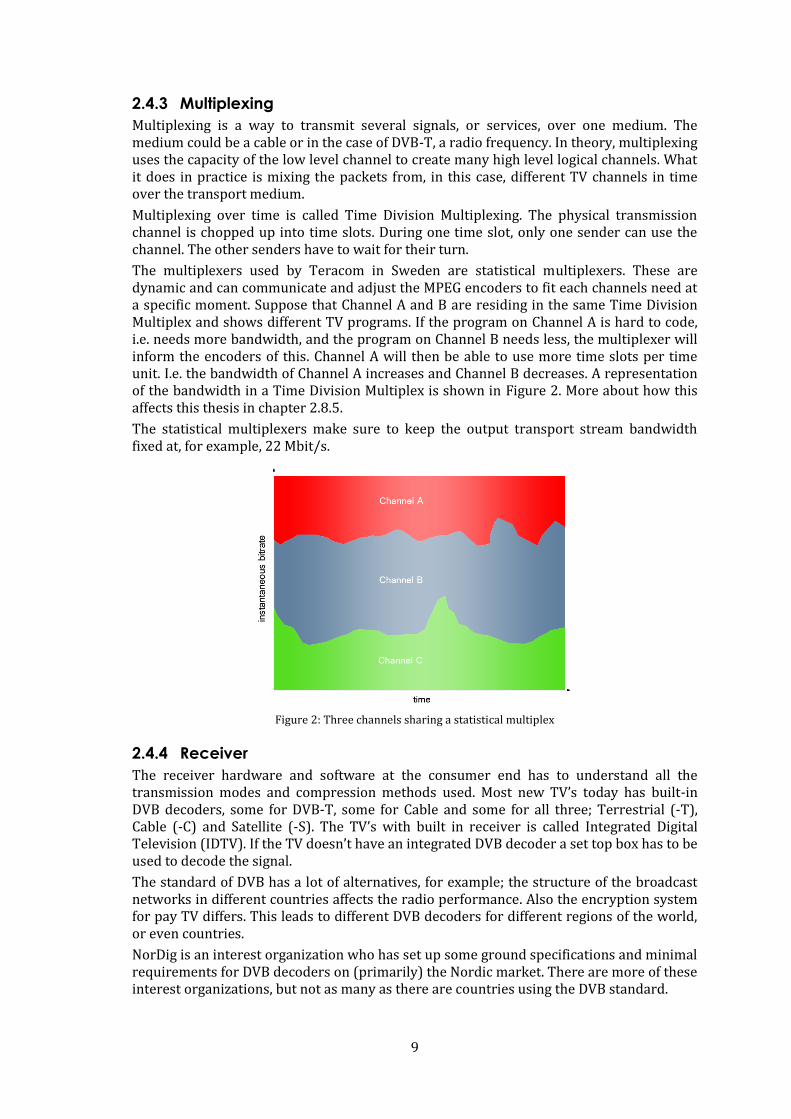
The multiplexers used by Teracom in Sweden are statistical multiplexers. These are dynamic and can communicate and adjust the MPEG encoders to fit each channels need at a specific moment. Suppose that Channel A and B are residing in the same Time Division Multiplex and shows different TV programs. If the program on Channel A is hard to code, i.e. needs more bandwidth, and the program on Channel B needs less, the multiplexer will inform the encoders of this. Channel A will then be able to use more time slots per time unit. I.e. the bandwidth of Channel A increases and Channel B decreases. A representation of the bandwidth in a Time Division Multiplex is shown in Figure 2. More about how this affects this thesis in chapter 2.8.5.

The statistical multiplexers make sure to keep the output transport stream bandwidth fixed at, for example, 22 Mbit/s.

Figure 2: Three channels sharing a statistical multiplex

2.4.4 Receiver

The receiver hardware and software at the consumer end has to understand all the transmission modes and compression methods used. Most new TV’s today has built-in DVB decoders, some for DVB-T, some for Cable and some for all three; Terrestrial (-T), Cable (-C) and Satellite (-S). The TV’s with built in receiver is called Integrated Digital Television (IDTV). If the TV doesn’t have an integrated DVB decoder a set top box has to be used to decode the signal.

The standard of DVB has a lot of alternatives, for example; the structure of the broadcast networks in different countries affects the radio performance. Also the encryption system for pay TV differs. This leads to different DVB decoders for different regions of the world, or even countries.

NorDig is an interest organization who has set up some ground specifications and minimal requirements for DVB decoders on (primarily) the Nordic market. There are more of these interest organizations, but not as many as there are countries using the DVB standard.

10

The receiver basically consists of the inverse of all the pieces in the encoding and transmitting equipment. Its job is to take the incoming radio signal, demodulate it, repair potential errors, decode the transmitted MPEG-2 transport stream and show the images on the TV screen.

The decoder does not have to be as intelligent as the encoder. This feature is implemented and planned from the start of DVB with the choosing of algorithms that are optimized as being easy to decode. The calculations and the effectiveness of the video stream and signal is decided by the encoder and this is the reason for the enormous price difference between encoders and decoders.

2.5 Data Compression Data compression, just like compression in the physical sense, is all about figuring out ways to fit something into a smaller container than before. In data compression, it is not done by brute force, as in the physical world; instead one substitutes the way the data is represented. In the real world, the receiver of a compressed physical medium can decompress, without knowing or understanding what algorithm or technique was used to compress. This is not true for data compression. Both parties must know what algorithm was used during the data compression process in order to understand how to decompress the data. This can easily be illustrated with languages. If you don’t understand the written language the spoken words have been “compressed” into; you cannot decompress them back into words. The same is true for all data compression.

There are several different approaches to compressing data, mainly divided into two groups, lossy and lossless compression.

Lossless compression does not alter the compressed data. This means that to the exact bit, one can recreate the compressed data back to its original form when decompressing it. This is true for all .zip1-like formats, in the sense that when you zip a word document, and then unzip it, the text inside is intact. You are not missing letters and words that have been compromised in the compression process.

Lossy compression does not bother trying to recreate the data compressed to the exact bit. Instead the aim is to compress the data in such a way, that the receiver cannot tell it apart from the original. This is done, for example, by using all of the limitations of the human visual system that we described earlier.

A plain example of this is the following. We are trying to compress the number;

56.77777777

A lossless approach would be to utilize the redundancy in the trailing sevens with an algorithm or syntax that takes up less space. This compression algorithm is called Run-length encoding.

56.[8]7

We have introduced a syntax that has to be understood by the receiver in order to de-compress the number back into decimal form. Whereas [n]x means that upon this sign are n instances of trailing x.

The lossy compression approach would simply be;

57

1 Read more about the zip format at: http://en.wikipedia.org/wiki/ZIP_(file_format)

11

Now, the observant reader would of course doubt the previous statement that the receiver or decompressor of this lossy coding doesn’t really have to know the algorithm used in order to understand this data. This might be true for this example, but if the receiver is awaiting a number with 8 decimals and instead picks up an integer, he is still in need of the algorithm in order to de-compress the data.

2.5.1 Variable length coding

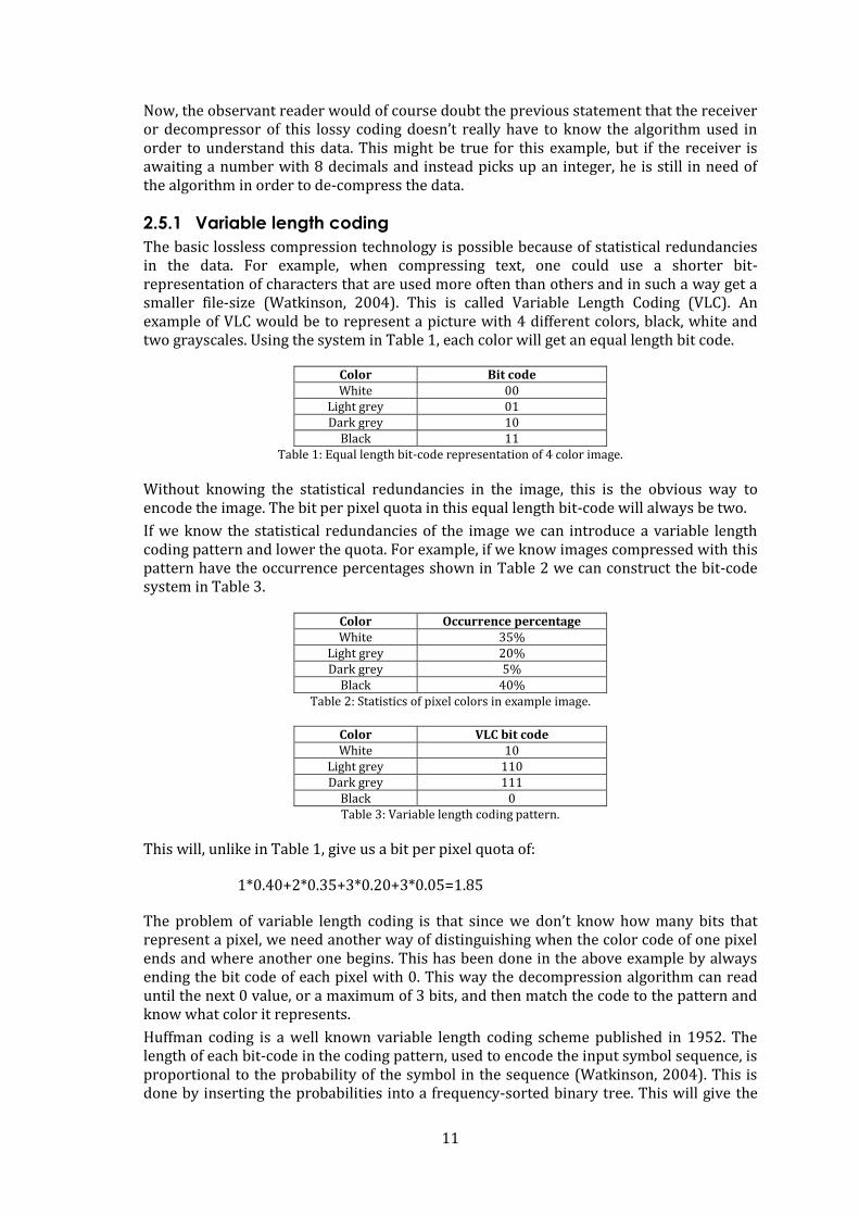
The basic lossless compression technology is possible because of statistical redundancies in the data. For example, when compressing text, one could use a shorter bit-representation of characters that are used more often than others and in such a way get a smaller file-size (Watkinson, 2004). This is called Variable Length Coding (VLC). An example of VLC would be to represent a picture with 4 different colors, black, white and two grayscales. Using the system in Table 1, each color will get an equal length bit code.

Color Bit code White 00

Light grey 01 Dark grey 10

Black 11 Table 1: Equal length bit-code representation of 4 color image.

Without knowing the statistical redundancies in the image, this is the obvious way to encode the image. The bit per pixel quota in this equal length bit-code will always be two.

If we know the statistical redundancies of the image we can introduce a variable length coding pattern and lower the quota. For example, if we know images compressed with this pattern have the occurrence percentages shown in Table 2 we can construct the bit-code system in Table 3.

Color Occurrence percentage White 35%

Light grey 20% Dark grey 5%

Black 40% Table 2: Statistics of pixel colors in example image.

Color VLC bit code White 10

Light grey 110 Dark grey 111

Black 0 Table 3: Variable length coding pattern.

This will, unlike in Table 1, give us a bit per pixel quota of:

1*0.40+2*0.35+3*0.20+3*0.05=1.85

The problem of variable length coding is that since we don’t know how many bits that represent a pixel, we need another way of distinguishing when the color code of one pixel ends and where another one begins. This has been done in the above example by always ending the bit code of each pixel with 0. This way the decompression algorithm can read until the next 0 value, or a maximum of 3 bits, and then match the code to the pattern and know what color it represents.

Huffman coding is a well known variable length coding scheme published in 1952. The length of each bit-code in the coding pattern, used to encode the input symbol sequence, is proportional to the probability of the symbol in the sequence (Watkinson, 2004). This is done by inserting the probabilities into a frequency-sorted binary tree. This will give the

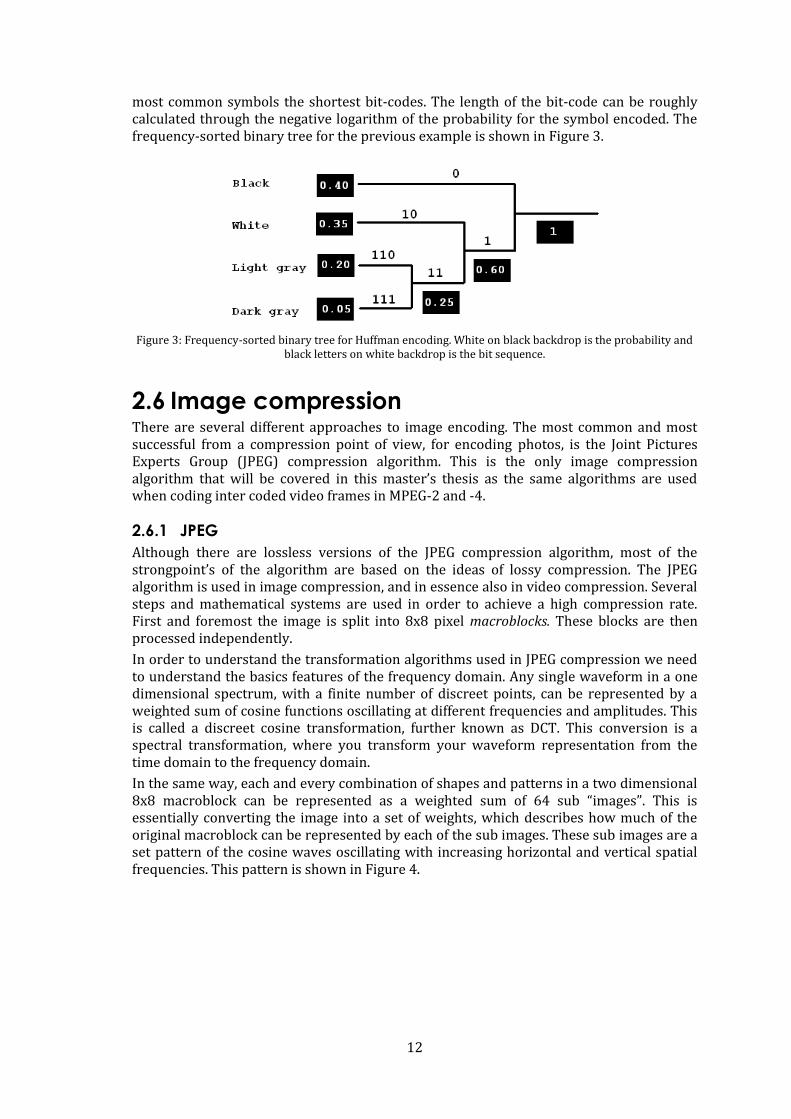
12

most common symbols the shortest bit-codes. The length of the bit-code can be roughly calculated through the negative logarithm of the probability for the symbol encoded. The frequency-sorted binary tree for the previous example is shown in Figure 3.

Figure 3: Frequency-sorted binary tree for Huffman encoding. White on black backdrop is the probability and

black letters on white backdrop is the bit sequence.

2.6 Image compression There are several different approaches to image encoding. The most common and most successful from a compression point of view, for encoding photos, is the Joint Pictures Experts Group (JPEG) compression algorithm. This is the only image compression algorithm that will be covered in this master’s thesis as the same algorithms are used when coding inter coded video frames in MPEG-2 and -4.

2.6.1 JPEG

Although there are lossless versions of the JPEG compression algorithm, most of the strongpoint’s of the algorithm are based on the ideas of lossy compression. The JPEG algorithm is used in image compression, and in essence also in video compression. Several steps and mathematical systems are used in order to achieve a high compression rate. First and foremost the image is split into 8x8 pixel macroblocks. These blocks are then processed independently.

In order to understand the transformation algorithms used in JPEG compression we need to understand the basics features of the frequency domain. Any single waveform in a one dimensional spectrum, with a finite number of discreet points, can be represented by a weighted sum of cosine functions oscillating at different frequencies and amplitudes. This is called a discreet cosine transformation, further known as DCT. This conversion is a spectral transformation, where you transform your waveform representation from the time domain to the frequency domain.

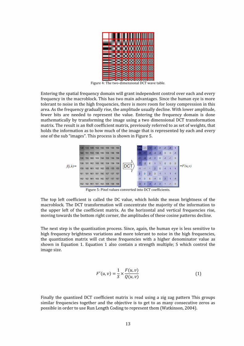
In the same way, each and every combination of shapes and patterns in a two dimensional 8x8 macroblock can be represented as a weighted sum of 64 sub “images”. This is essentially converting the image into a set of weights, which describes how much of the original macroblock can be represented by each of the sub images. These sub images are a set pattern of the cosine waves oscillating with increasing horizontal and vertical spatial frequencies. This pattern is shown in Figure 4.

13

Figure 4: The two-dimensional DCT wave table.

Entering the spatial frequency domain will grant independent control over each and every frequency in the macroblock. This has two main advantages. Since the human eye is more tolerant to noise in the high frequencies, there is more room for lossy compression in this area. As the frequency gradually rise, the amplitude usually decline. With lower amplitude, fewer bits are needed to represent the value. Entering the frequency domain is done mathematically by transforming the image using a two dimensional DCT transformation matrix. The result is an 8x8 coefficient matrix, previously referred to as set of weights, that holds the information as to how much of the image that is represented by each and every one of the sub “images”. This process is shown in Figure 5.

Figure 5: Pixel values converted into DCT coefficients.

The top left coefficient is called the DC value, which holds the mean brightness of the macroblock. The DCT transformation will concentrate the majority of the information to the upper left of the coefficient matrix. As the horizontal and vertical frequencies rise, moving towards the bottom right corner, the amplitudes of these cosine patterns decline.

The next step is the quantization process. Since, again, the human eye is less sensitive to high frequency brightness variations and more tolerant to noise in the high frequencies, the quantization matrix will cut these frequencies with a higher denominator value as shown in Equation 1. Equation 1 also contain a strength multiple; S which control the image size.

(1)

Finally the quantized DCT coefficient matrix is read using a zig zag pattern This groups similar frequencies together and the objective is to get to as many consecutive zeros as possible in order to use Run Length Coding to represent them (Watkinson, 2004).

14

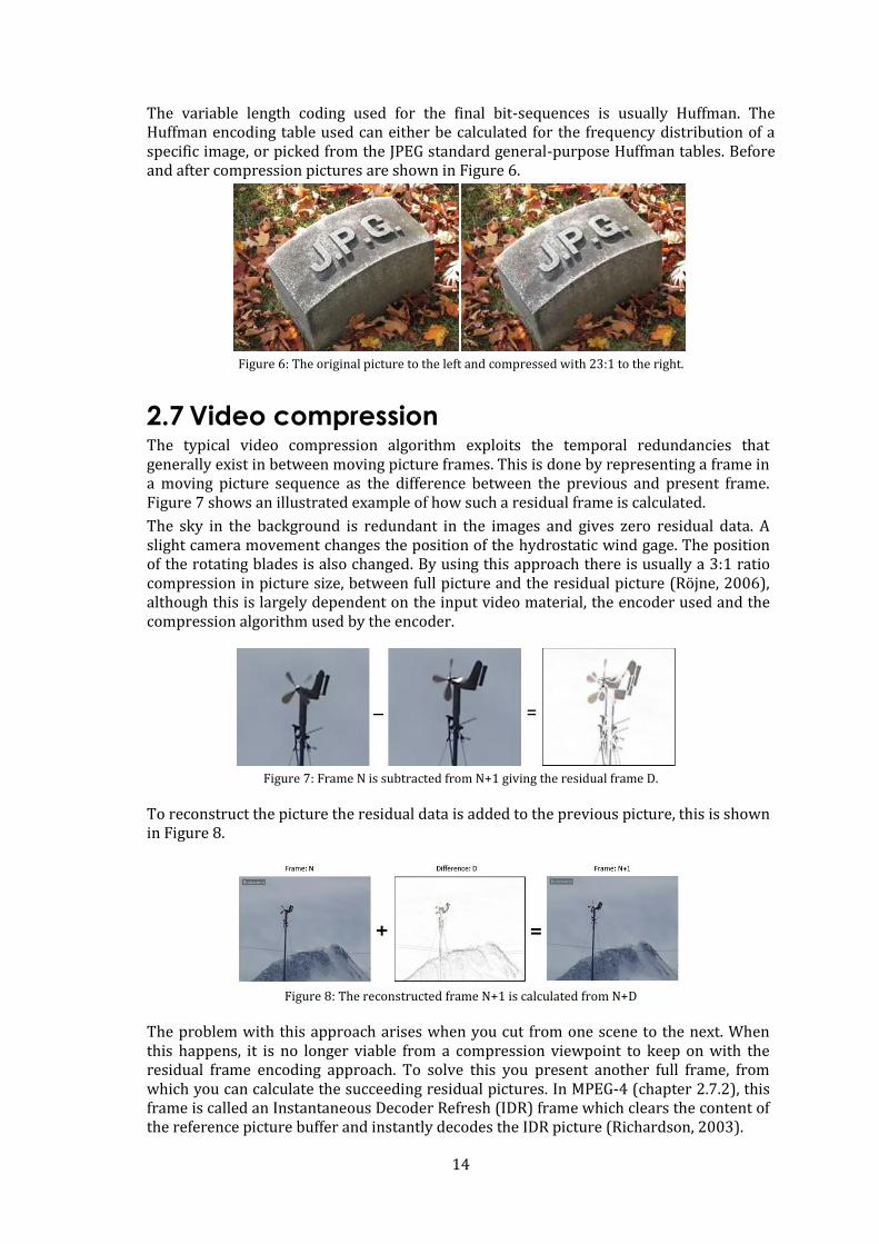
The variable length coding used for the final bit-sequences is usually Huffman. The Huffman encoding table used can either be calculated for the frequency distribution of a specific image, or picked from the JPEG standard general-purpose Huffman tables. Before and after compression pictures are shown in Figure 6.

Figure 6: The original picture to the left and compressed with 23:1 to the right.

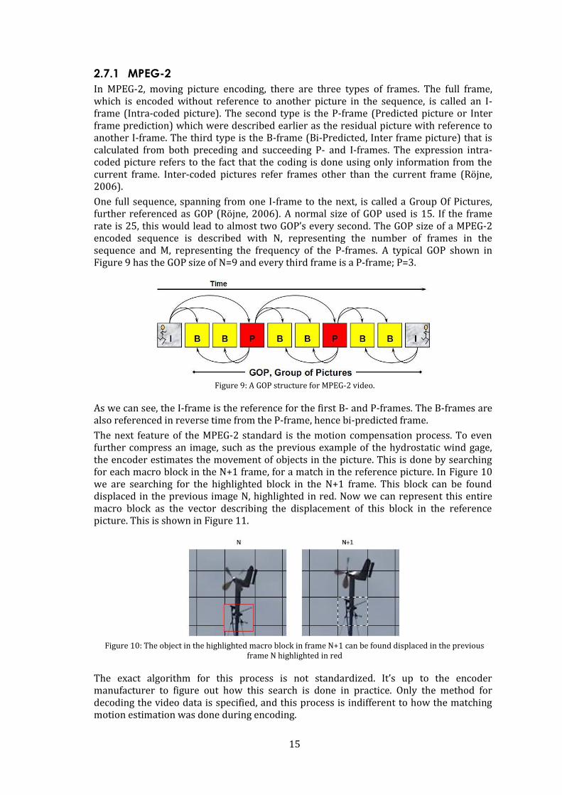
2.7 Video compression The typical video compression algorithm exploits the temporal redundancies that generally exist in between moving picture frames. This is done by representing a frame in a moving picture sequence as the difference between the previous and present frame. Figure 7 shows an illustrated example of how such a residual frame is calculated.

The sky in the background is redundant in the images and gives zero residual data. A slight camera movement changes the position of the hydrostatic wind gage. The position of the rotating blades is also changed. By using this approach there is usually a 3:1 ratio compression in picture size, between full picture and the residual picture (Röjne, 2006), although this is largely dependent on the input video material, the encoder used and the compression algorithm used by the encoder.

Figure 7: Frame N is subtracted from N+1 giving the residual frame D.

To reconstruct the picture the residual data is added to the previous picture, this is shown in Figure 8.

Figure 8: The reconstructed frame N+1 is calculated from N+D

The problem with this approach arises when you cut from one scene to the next. When this happens, it is no longer viable from a compression viewpoint to keep on with the residual frame encoding approach. To solve this you present another full frame, from which you can calculate the succeeding residual pictures. In MPEG-4 (chapter 2.7.2), this frame is called an Instantaneous Decoder Refresh (IDR) frame which clears the content of the reference picture buffer and instantly decodes the IDR picture (Richardson, 2003).

15

2.7.1 MPEG-2

In MPEG-2, moving picture encoding, there are three types of frames. The full frame, which is encoded without reference to another picture in the sequence, is called an I-frame (Intra-coded picture). The second type is the P-frame (Predicted picture or Inter frame prediction) which were described earlier as the residual picture with reference to another I-frame. The third type is the B-frame (Bi-Predicted, Inter frame picture) that is calculated from both preceding and succeeding P- and I-frames. The expression intra-coded picture refers to the fact that the coding is done using only information from the current frame. Inter-coded pictures refer frames other than the current frame (Röjne, 2006).

One full sequence, spanning from one I-frame to the next, is called a Group Of Pictures, further referenced as GOP (Röjne, 2006). A normal size of GOP used is 15. If the frame rate is 25, this would lead to almost two GOP’s every second. The GOP size of a MPEG-2 encoded sequence is described with N, representing the number of frames in the sequence and M, representing the frequency of the P-frames. A typical GOP shown in Figure 9 has the GOP size of N=9 and every third frame is a P-frame; P=3.

Figure 9: A GOP structure for MPEG-2 video.

As we can see, the I-frame is the reference for the first B- and P-frames. The B-frames are also referenced in reverse time from the P-frame, hence bi-predicted frame.

The next feature of the MPEG-2 standard is the motion compensation process. To even further compress an image, such as the previous example of the hydrostatic wind gage, the encoder estimates the movement of objects in the picture. This is done by searching for each macro block in the N+1 frame, for a match in the reference picture. In Figure 10 we are searching for the highlighted block in the N+1 frame. This block can be found displaced in the previous image N, highlighted in red. Now we can represent this entire macro block as the vector describing the displacement of this block in the reference picture. This is shown in Figure 11.

Figure 10: The object in the highlighted macro block in frame N+1 can be found displaced in the previous

frame N highlighted in red

The exact algorithm for this process is not standardized. It’s up to the encoder manufacturer to figure out how this search is done in practice. Only the method for decoding the video data is specified, and this process is indifferent to how the matching motion estimation was done during encoding.

16

Figure 11: The displacement is described by the motion vector in blue.

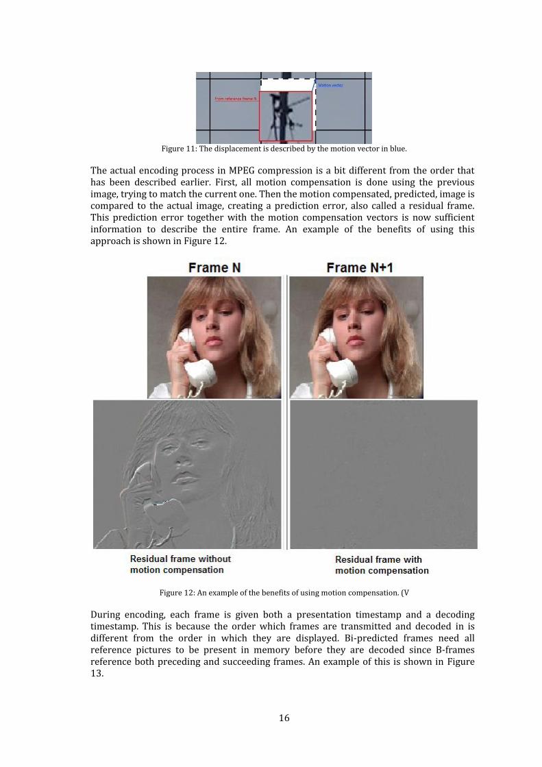
The actual encoding process in MPEG compression is a bit different from the order that has been described earlier. First, all motion compensation is done using the previous image, trying to match the current one. Then the motion compensated, predicted, image is compared to the actual image, creating a prediction error, also called a residual frame. This prediction error together with the motion compensation vectors is now sufficient information to describe the entire frame. An example of the benefits of using this approach is shown in Figure 12.

Figure 12: An example of the benefits of using motion compensation. (V

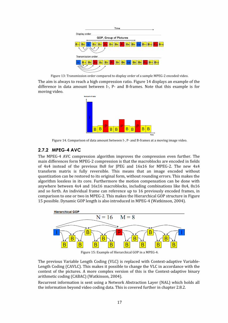
During encoding, each frame is given both a presentation timestamp and a decoding timestamp. This is because the order which frames are transmitted and decoded in is different from the order in which they are displayed. Bi-predicted frames need all reference pictures to be present in memory before they are decoded since B-frames reference both preceding and succeeding frames. An example of this is shown in Figure 13.

17

Figure 13: Transmission order compared to display order of a sample MPEG-2 encoded video.

The aim is always to reach a high compression ratio. Figure 14 displays an example of the difference in data amount between I-, P- and B-frames. Note that this example is for moving video.

Figure 14. Comparison of data amount between I-, P- and B-frames at a moving image video.

2.7.2 MPEG-4 AVC

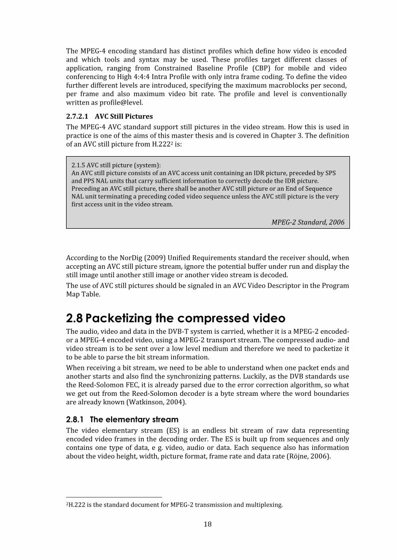
The MPEG-4 AVC compression algorithm improves the compression even further. The main differences form MPEG-2 compression is that the macroblocks are encoded in fields of 4x4 instead of the previous 8x8 for JPEG and 16x16 for MPEG-2. The new 4x4 transform matrix is fully reversible. This means that an image encoded without quantization can be restored to its original form, without rounding errors. This makes the algorithm lossless in its core. Furthermore the motion compensation can be done with anywhere between 4x4 and 16x16 macroblocks, including combinations like 8x4, 8x16 and so forth. An individual frame can reference up to 16 previously encoded frames, in comparison to one or two in MPEG-2. This makes the Hierarchical GOP structure in Figure 15 possible. Dynamic GOP length is also introduced in MPEG-4 (Watkinson, 2004).

Figure 15: Example of Hierarchical GOP in a MPEG-4.

The previous Variable Length Coding (VLC) is replaced with Context-adaptive Variable-Length Coding (CAVLC). This makes it possible to change the VLC in accordance with the context of the pictures. A more complex version of this is the Context-adaptive binary arithmetic coding (CABAC) (Watkinson, 2004).

Recurrent information is sent using a Network Abstraction Layer (NAL) which holds all the information beyond video coding data. This is covered further in chapter 2.8.2.

18

The MPEG-4 encoding standard has distinct profiles which define how video is encoded and which tools and syntax may be used. These profiles target different classes of application, ranging from Constrained Baseline Profile (CBP) for mobile and video conferencing to High 4:4:4 Intra Profile with only intra frame coding. To define the video further different levels are introduced, specifying the maximum macroblocks per second, per frame and also maximum video bit rate. The profile and level is conventionally written as profile@level.

2.7.2.1 AVC Still Pictures

The MPEG-4 AVC standard support still pictures in the video stream. How this is used in practice is one of the aims of this master thesis and is covered in Chapter 3. The definition of an AVC still picture from H.2222 is:

According to the NorDig (2009) Unified Requirements standard the receiver should, when accepting an AVC still picture stream, ignore the potential buffer under run and display the still image until another still image or another video stream is decoded.

The use of AVC still pictures should be signaled in an AVC Video Descriptor in the Program Map Table.

2.8 Packetizing the compressed video The audio, video and data in the DVB-T system is carried, whether it is a MPEG-2 encoded- or a MPEG-4 encoded video, using a MPEG-2 transport stream. The compressed audio- and video stream is to be sent over a low level medium and therefore we need to packetize it to be able to parse the bit stream information.

When receiving a bit stream, we need to be able to understand when one packet ends and another starts and also find the synchronizing patterns. Luckily, as the DVB standards use the Reed-Solomon FEC, it is already parsed due to the error correction algorithm, so what we get out from the Reed-Solomon decoder is a byte stream where the word boundaries are already known (Watkinson, 2004).

2.8.1 The elementary stream

The video elementary stream (ES) is an endless bit stream of raw data representing encoded video frames in the decoding order. The ES is built up from sequences and only contains one type of data, e g. video, audio or data. Each sequence also has information about the video height, width, picture format, frame rate and data rate (Röjne, 2006).

2H.222 is the standard document for MPEG-2 transmission and multiplexing.

2.1.5 AVC still picture (system): An AVC still picture consists of an AVC access unit containing an IDR picture, preceded by SPS and PPS NAL units that carry sufficient information to correctly decode the IDR picture. Preceding an AVC still picture, there shall be another AVC still picture or an End of Sequence NAL unit terminating a preceding coded video sequence unless the AVC still picture is the very first access unit in the video stream.

MPEG-2 Standard, 2006

19

2.8.2 The network abstraction layer

The Network abstraction layer (NAL) is something which is new in MPEG-4 AVC. In Advanced Video Coding (AVC), the video coding layer, where all the coding is done, is separate to the transport layer and NAL is a step between the two. The ES are mapped to NAL units before transmission or storage (Richardson, 2003). The coded video sequence is thus represented by a series of NAL units. Each NAL unit packet has a header with information about what kind of raw byte sequence payload (RBSP) it carries. The RBSP is basically the type of information in the NAL unit.

The types of available RBSP types can be seen in Appendix A (MPEG-4 standard, 2008). The most important ones for this master thesis, except for the coded slices, are:

Sequence parameter set (SPS), where parameters for whole video sequences are

kept, such as limits on frame numbers, picture order count and whether field

(interlaced) coding, or frame coding was used.

The picture parameter set (PPS) is more or less the same as the SPS, but applies to

one or more pictures inside a SPS. The PPS has, amongst other, information on

what kind of entropy coding is used, the number of slice group used and a list, and

number, of reference pictures.

Supplemental Enhancement Information (SEI) messages are not essential for

encoding the video sequence but can contain information on buffering time,

picture timing and the deblocking filter properties.

The end of sequence (EOS) unit indicates the end of a video sequence and that the

next picture in the decoding order is an IDR picture.

The parameter sets are a way for the encoder to signal ahead for important changes in the coding, as for example, slice coding type. (MPEG-4 standard, 2008)

The PPS is activated by a referral from a coded slice header; this PPS stays active until another one is called from another slice header. A SPS is activated by a call from the PPS header in the same manner (MPEG-4 standard, 2008).

The coded slice data partition units consist of three different forms, A, B and C. Partition A holds the headers for all the macro blocks in the slice. Partition B contain intra coded slice data, and C contain inter coded slice data. NAL unit type number five is the coded slice of an IDR picture (MPEG-4 standard, 2008).

2.8.3 The packetized elementary stream

The elementary streams, in MPEG-2, or the NAL units, in MPEG-4 AVC, are packetized for sending over a medium. Both transmission and storage prefer discrete blocks of data (Watkinson, 2004), these packages are called PES packets, for packetized elementary stream, and can only contain a video ES, an audio ES or a data ES.

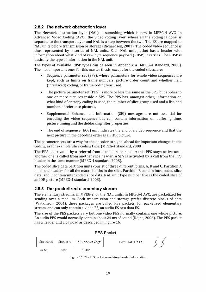
The size of the PES packets vary but one video PES normally contains one whole picture. An audio PES would normally contain about 24 ms of sound (Röjne, 2006). The PES packet has a header and a payload as described in Figure 16.

Figure 16: The PES packet mandatory header information

20

The PES packet headers often contain time stamps for synchronization, decoding and presentation purposes. The PES header for a video ES can also contain information about various trick modes and their properties.

The whole PES has to be received and put in the decoding buffer for the receiver to be able to start decoding it.

2.8.4 The MPEG-2 transport stream

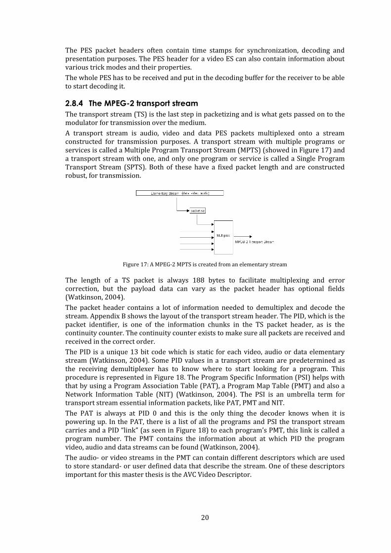
The transport stream (TS) is the last step in packetizing and is what gets passed on to the modulator for transmission over the medium.

A transport stream is audio, video and data PES packets multiplexed onto a stream constructed for transmission purposes. A transport stream with multiple programs or services is called a Multiple Program Transport Stream (MPTS) (showed in Figure 17) and a transport stream with one, and only one program or service is called a Single Program Transport Stream (SPTS). Both of these have a fixed packet length and are constructed robust, for transmission.

Figure 17: A MPEG-2 MPTS is created from an elementary stream

The length of a TS packet is always 188 bytes to facilitate multiplexing and error correction, but the payload data can vary as the packet header has optional fields (Watkinson, 2004).

The packet header contains a lot of information needed to demultiplex and decode the stream. Appendix B shows the layout of the transport stream header. The PID, which is the packet identifier, is one of the information chunks in the TS packet header, as is the continuity counter. The continuity counter exists to make sure all packets are received and received in the correct order.

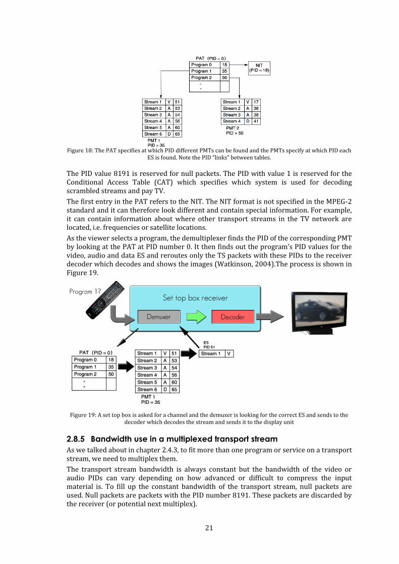
The PID is a unique 13 bit code which is static for each video, audio or data elementary stream (Watkinson, 2004). Some PID values in a transport stream are predetermined as the receiving demultiplexer has to know where to start looking for a program. This procedure is represented in Figure 18. The Program Specific Information (PSI) helps with that by using a Program Association Table (PAT), a Program Map Table (PMT) and also a Network Information Table (NIT) (Watkinson, 2004). The PSI is an umbrella term for transport stream essential information packets, like PAT, PMT and NIT.

The PAT is always at PID 0 and this is the only thing the decoder knows when it is powering up. In the PAT, there is a list of all the programs and PSI the transport stream carries and a PID “link” (as seen in Figure 18) to each program’s PMT, this link is called a program number. The PMT contains the information about at which PID the program video, audio and data streams can be found (Watkinson, 2004).

The audio- or video streams in the PMT can contain different descriptors which are used to store standard- or user defined data that describe the stream. One of these descriptors important for this master thesis is the AVC Video Descriptor.

21

Figure 18: The PAT specifies at which PID different PMTs can be found and the PMTs specify at which PID each

ES is found. Note the PID “links” between tables.

The PID value 8191 is reserved for null packets. The PID with value 1 is reserved for the Conditional Access Table (CAT) which specifies which system is used for decoding scrambled streams and pay TV.

The first entry in the PAT refers to the NIT. The NIT format is not specified in the MPEG-2 standard and it can therefore look different and contain special information. For example, it can contain information about where other transport streams in the TV network are located, i.e. frequencies or satellite locations.

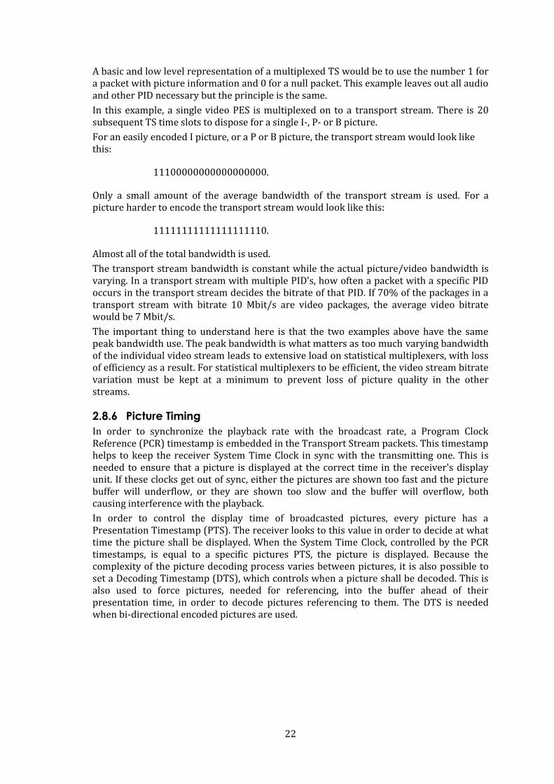
As the viewer selects a program, the demultiplexer finds the PID of the corresponding PMT by looking at the PAT at PID number 0. It then finds out the program’s PID values for the video, audio and data ES and reroutes only the TS packets with these PIDs to the receiver decoder which decodes and shows the images (Watkinson, 2004).The process is shown in Figure 19.

Figure 19: A set top box is asked for a channel and the demuxer is looking for the correct ES and sends to the

decoder which decodes the stream and sends it to the display unit

2.8.5 Bandwidth use in a multiplexed transport stream

As we talked about in chapter 2.4.3, to fit more than one program or service on a transport stream, we need to multiplex them.

The transport stream bandwidth is always constant but the bandwidth of the video or audio PIDs can vary depending on how advanced or difficult to compress the input material is. To fill up the constant bandwidth of the transport stream, null packets are used. Null packets are packets with the PID number 8191. These packets are discarded by the receiver (or potential next multiplex).

22

A basic and low level representation of a multiplexed TS would be to use the number 1 for a packet with picture information and 0 for a null packet. This example leaves out all audio and other PID necessary but the principle is the same.

In this example, a single video PES is multiplexed on to a transport stream. There is 20 subsequent TS time slots to dispose for a single I-, P- or B picture.

For an easily encoded I picture, or a P or B picture, the transport stream would look like this:

11100000000000000000.

Only a small amount of the average bandwidth of the transport stream is used. For a picture harder to encode the transport stream would look like this:

11111111111111111110.

Almost all of the total bandwidth is used.

The transport stream bandwidth is constant while the actual picture/video bandwidth is varying. In a transport stream with multiple PID's, how often a packet with a specific PID occurs in the transport stream decides the bitrate of that PID. If 70% of the packages in a transport stream with bitrate 10 Mbit/s are video packages, the average video bitrate would be 7 Mbit/s.

The important thing to understand here is that the two examples above have the same peak bandwidth use. The peak bandwidth is what matters as too much varying bandwidth of the individual video stream leads to extensive load on statistical multiplexers, with loss of efficiency as a result. For statistical multiplexers to be efficient, the video stream bitrate variation must be kept at a minimum to prevent loss of picture quality in the other streams.

2.8.6 Picture Timing

In order to synchronize the playback rate with the broadcast rate, a Program Clock Reference (PCR) timestamp is embedded in the Transport Stream packets. This timestamp helps to keep the receiver System Time Clock in sync with the transmitting one. This is needed to ensure that a picture is displayed at the correct time in the receiver's display unit. If these clocks get out of sync, either the pictures are shown too fast and the picture buffer will underflow, or they are shown too slow and the buffer will overflow, both causing interference with the playback.

In order to control the display time of broadcasted pictures, every picture has a Presentation Timestamp (PTS). The receiver looks to this value in order to decide at what time the picture shall be displayed. When the System Time Clock, controlled by the PCR timestamps, is equal to a specific pictures PTS, the picture is displayed. Because the complexity of the picture decoding process varies between pictures, it is also possible to set a Decoding Timestamp (DTS), which controls when a picture shall be decoded. This is also used to force pictures, needed for referencing, into the buffer ahead of their presentation time, in order to decode pictures referencing to them. The DTS is needed when bi-directional encoded pictures are used.

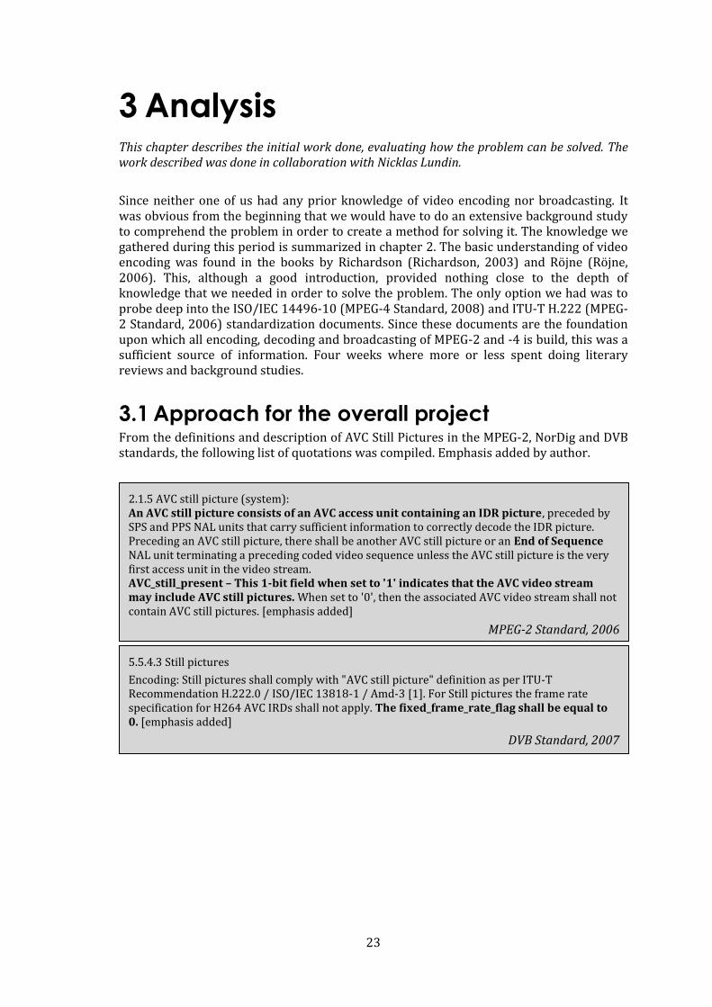
23

3 Analysis This chapter describes the initial work done, evaluating how the problem can be solved. The work described was done in collaboration with Nicklas Lundin.

Since neither one of us had any prior knowledge of video encoding nor broadcasting. It was obvious from the beginning that we would have to do an extensive background study to comprehend the problem in order to create a method for solving it. The knowledge we gathered during this period is summarized in chapter 2. The basic understanding of video encoding was found in the books by Richardson (Richardson, 2003) and Röjne (Röjne, 2006). This, although a good introduction, provided nothing close to the depth of knowledge that we needed in order to solve the problem. The only option we had was to probe deep into the ISO/IEC 14496-10 (MPEG-4 Standard, 2008) and ITU-T H.222 (MPEG-2 Standard, 2006) standardization documents. Since these documents are the foundation upon which all encoding, decoding and broadcasting of MPEG-2 and -4 is build, this was a sufficient source of information. Four weeks where more or less spent doing literary reviews and background studies.

3.1 Approach for the overall project From the definitions and description of AVC Still Pictures in the MPEG-2, NorDig and DVB standards, the following list of quotations was compiled. Emphasis added by author.

5.5.4.3 Still pictures

Encoding: Still pictures shall comply with "AVC still picture" definition as per ITU-T Recommendation H.222.0 / ISO/IEC 13818-1 / Amd-3 [1]. For Still pictures the frame rate specification for H264 AVC IRDs shall not apply. The fixed_frame_rate_flag shall be equal to 0. [emphasis added]

DVB Standard, 2007

2.1.5 AVC still picture (system): An AVC still picture consists of an AVC access unit containing an IDR picture, preceded by SPS and PPS NAL units that carry sufficient information to correctly decode the IDR picture. Preceding an AVC still picture, there shall be another AVC still picture or an End of Sequence NAL unit terminating a preceding coded video sequence unless the AVC still picture is the very first access unit in the video stream. AVC_still_present – This 1-bit field when set to '1' indicates that the AVC video stream may include AVC still pictures. When set to '0', then the associated AVC video stream shall not contain AVC still pictures. [emphasis added]

MPEG-2 Standard, 2006

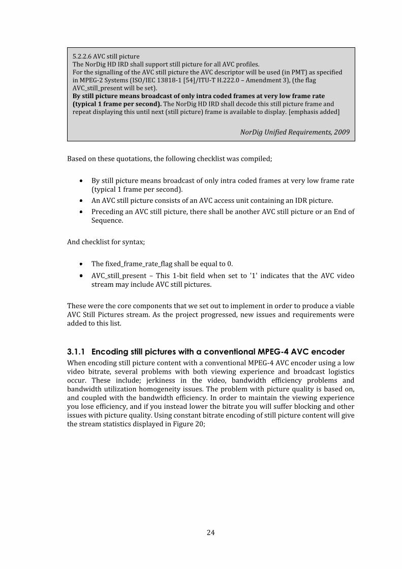
24

Based on these quotations, the following checklist was compiled;

By still picture means broadcast of only intra coded frames at very low frame rate (typical 1 frame per second).

An AVC still picture consists of an AVC access unit containing an IDR picture.

Preceding an AVC still picture, there shall be another AVC still picture or an End of Sequence.

And checklist for syntax;

The fixed_frame_rate_flag shall be equal to 0.

AVC_still_present – This 1-bit field when set to '1' indicates that the AVC video stream may include AVC still pictures.

These were the core components that we set out to implement in order to produce a viable AVC Still Pictures stream. As the project progressed, new issues and requirements were added to this list.

3.1.1 Encoding still pictures with a conventional MPEG-4 AVC encoder

When encoding still picture content with a conventional MPEG-4 AVC encoder using a low video bitrate, several problems with both viewing experience and broadcast logistics occur. These include; jerkiness in the video, bandwidth efficiency problems and bandwidth utilization homogeneity issues. The problem with picture quality is based on, and coupled with the bandwidth efficiency. In order to maintain the viewing experience you lose efficiency, and if you instead lower the bitrate you will suffer blocking and other issues with picture quality. Using constant bitrate encoding of still picture content will give the stream statistics displayed in Figure 20;

5.2.2.6 AVC still picture The NorDig HD IRD shall support still picture for all AVC profiles. For the signalling of the AVC still picture the AVC descriptor will be used (in PMT) as specified in MPEG-2 Systems (ISO/IEC 13818-1 [54]/ITU-T H.222.0 – Amendment 3), (the flag AVC_still_present will be set). By still picture means broadcast of only intra coded frames at very low frame rate (typical 1 frame per second). The NorDig HD IRD shall decode this still picture frame and repeat displaying this until next (still picture) frame is available to display. [emphasis added]

NorDig Unified Requirements, 2009

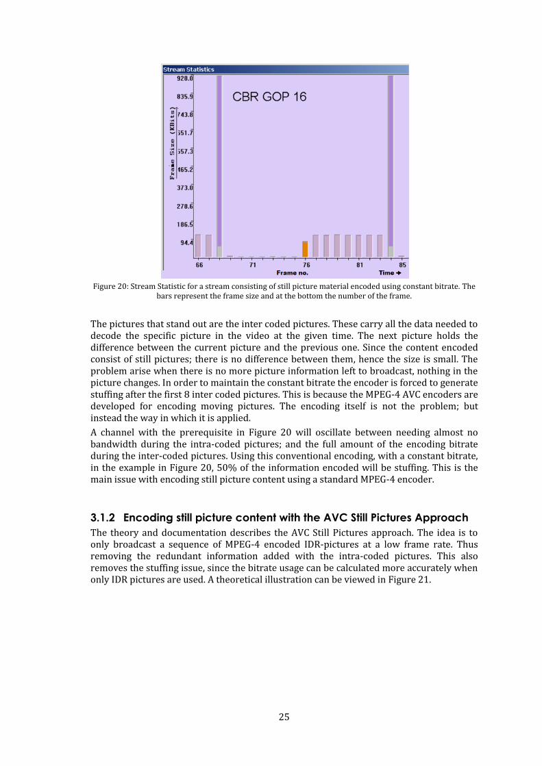
25

Figure 20: Stream Statistic for a stream consisting of still picture material encoded using constant bitrate. The

bars represent the frame size and at the bottom the number of the frame.

The pictures that stand out are the inter coded pictures. These carry all the data needed to decode the specific picture in the video at the given time. The next picture holds the difference between the current picture and the previous one. Since the content encoded consist of still pictures; there is no difference between them, hence the size is small. The problem arise when there is no more picture information left to broadcast, nothing in the picture changes. In order to maintain the constant bitrate the encoder is forced to generate stuffing after the first 8 inter coded pictures. This is because the MPEG-4 AVC encoders are developed for encoding moving pictures. The encoding itself is not the problem; but instead the way in which it is applied.

A channel with the prerequisite in Figure 20 will oscillate between needing almost no bandwidth during the intra-coded pictures; and the full amount of the encoding bitrate during the inter-coded pictures. Using this conventional encoding, with a constant bitrate, in the example in Figure 20, 50% of the information encoded will be stuffing. This is the main issue with encoding still picture content using a standard MPEG-4 encoder.

3.1.2 Encoding still picture content with the AVC Still Pictures Approach

The theory and documentation describes the AVC Still Pictures approach. The idea is to only broadcast a sequence of MPEG-4 encoded IDR-pictures at a low frame rate. Thus removing the redundant information added with the intra-coded pictures. This also removes the stuffing issue, since the bitrate usage can be calculated more accurately when only IDR pictures are used. A theoretical illustration can be viewed in Figure 21.

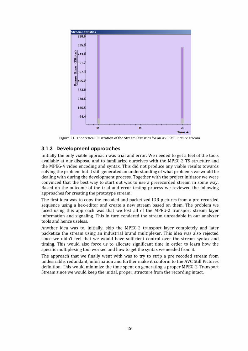
26

Figure 21: Theoretical illustration of the Stream Statistics for an AVC Still Picture stream.

3.1.3 Development approaches

Initially the only viable approach was trial and error. We needed to get a feel of the tools available at our disposal and to familiarize ourselves with the MPEG-2 TS structure and the MPEG-4 video encoding and syntax. This did not produce any viable results towards solving the problem but it still generated an understanding of what problems we would be dealing with during the development process. Together with the project initiator we were convinced that the best way to start out was to use a prerecorded stream in some way. Based on the outcome of the trial and error testing process we reviewed the following approaches for creating the prototype stream;

The first idea was to copy the encoded and packetized IDR pictures from a pre recorded sequence using a hex-editor and create a new stream based on them. The problem we faced using this approach was that we lost all of the MPEG-2 transport stream layer information and signaling. This in turn rendered the stream unreadable in our analyzer tools and hence useless.

Another idea was to, initially, skip the MPEG-2 transport layer completely and later packetize the stream using an industrial brand multiplexer. This idea was also rejected since we didn’t feel that we would have sufficient control over the stream syntax and timing. This would also force us to allocate significant time in order to learn how the specific multiplexing tool worked and how to get the syntax we needed from it.

The approach that we finally went with was to try to strip a pre recoded stream from undesirable, redundant, information and further make it conform to the AVC Still Pictures definition. This would minimize the time spent on generating a proper MPEG-2 Transport Stream since we would keep the initial, proper, structure from the recording intact.

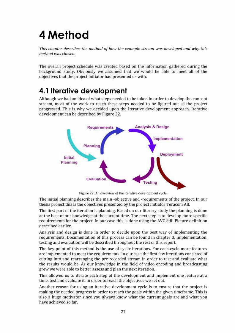
27

4 Method This chapter describes the method of how the example stream was developed and why this method was chosen.

The overall project schedule was created based on the information gathered during the background study. Obviously we assumed that we would be able to meet all of the objectives that the project initiator had presented us with.

4.1 Iterative development Although we had an idea of what steps needed to be taken in order to develop the concept stream, most of the work to reach these steps needed to be figured out as the project progressed. This is why we decided upon the Iterative development approach. Iterative development can be described by Figure 22.

Figure 22: An overview of the iterative development cycle.

The initial planning describes the main -objective and -requirements of the project. In our thesis project this is the objectives presented by the project initiator Teracom AB.

The first part of the iteration is planning. Based on our literary study the planning is done at the best of our knowledge at the current time. The next step is to develop more specific requirements for the project. In our case this is done using the AVC Still Picture definition described earlier.

Analysis and design is done in order to decide upon the best way of implementing the requirements. Documentation of this process can be found in chapter 3. Implementation, testing and evaluation will be described throughout the rest of this report.

The key point of this method is the use of cyclic iterations. For each cycle more features are implemented to meet the requirements. In our case the first few iterations consisted of cutting into and rearranging the pre recorded stream in order to test and evaluate what the results would be. As our knowledge in the field of video encoding and broadcasting grew we were able to better assess and plan the next iteration.

This allowed us to iterate each step of the development and implement one feature at a time, test and evaluate it, in order to reach the objectives we set out.

Another reason for using an iterative development cycle is to ensure that the project is making the needed progress in order to reach the goals within the given timeframe. This is also a huge motivator since you always know what the current goals are and what you have achieved so far.

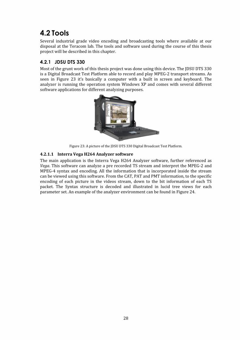
28

4.2 Tools Several industrial grade video encoding and broadcasting tools where available at our disposal at the Teracom lab. The tools and software used during the course of this thesis project will be described in this chapter.

4.2.1 JDSU DTS 330

Most of the grunt work of this thesis project was done using this device. The JDSU DTS 330 is a Digital Broadcast Test Platform able to record and play MPEG-2 transport streams. As seen in Figure 23 it’s basically a computer with a built in screen and keyboard. The analyzer is running the operation system Windows XP and comes with several different software applications for different analyzing purposes.

Figure 23: A picture of the JDSU DTS 330 Digital Broadcast Test Platform.

4.2.1.1 Interra Vega H264 Analyzer software

The main application is the Interra Vega H264 Analyzer software, further referenced as Vega. This software can analyze a pre recorded TS stream and interpret the MPEG-2 and MPEG-4 syntax and encoding. All the information that is incorporated inside the stream can be viewed using this software. From the CAT, PAT and PMT information, to the specific encoding of each picture in the videos stream, down to the bit information of each TS packet. The Syntax structure is decoded and illustrated in lucid tree views for each parameter set. An example of the analyzer environment can be found in Figure 24.

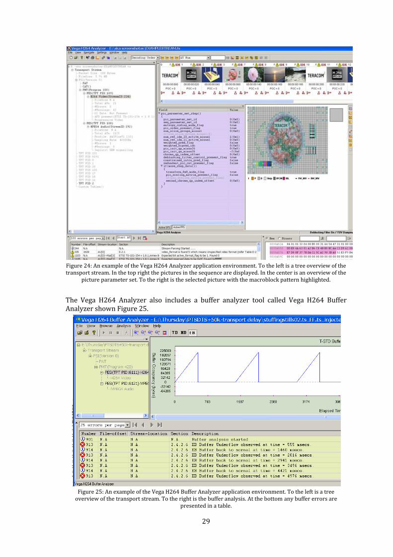
29

Figure 24: An example of the Vega H264 Analyzer application environment. To the left is a tree overview of the transport stream. In the top right the pictures in the sequence are displayed. In the center is an overview of the

picture parameter set. To the right is the selected picture with the macroblock pattern highlighted.

The Vega H264 Analyzer also includes a buffer analyzer tool called Vega H264 Buffer Analyzer shown Figure 25.

Figure 25: An example of the Vega H264 Buffer Analyzer application environment. To the left is a tree

overview of the transport stream. To the right is the buffer analysis. At the bottom any buffer errors are presented in a table.

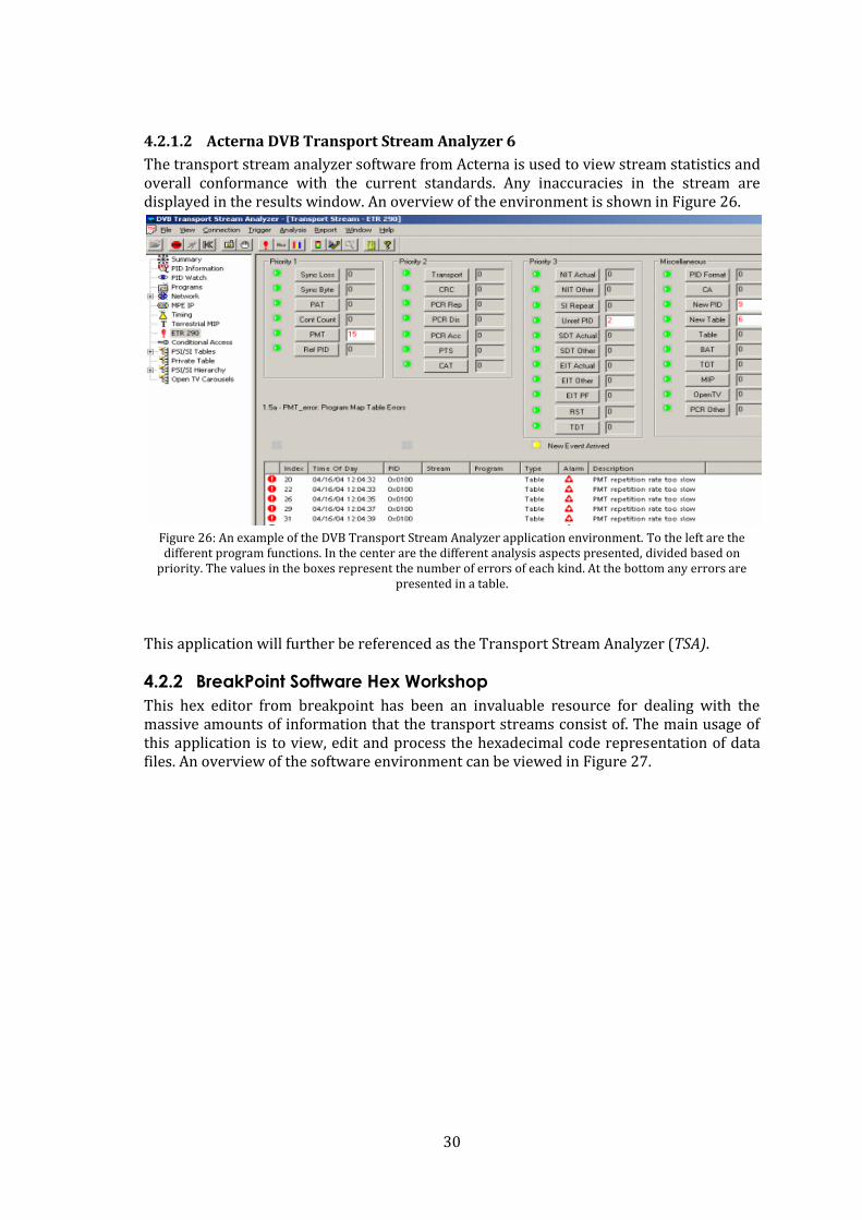
30

4.2.1.2 Acterna DVB Transport Stream Analyzer 6

The transport stream analyzer software from Acterna is used to view stream statistics and overall conformance with the current standards. Any inaccuracies in the stream are displayed in the results window. An overview of the environment is shown in Figure 26.

Figure 26: An example of the DVB Transport Stream Analyzer application environment. To the left are the different program functions. In the center are the different analysis aspects presented, divided based on

priority. The values in the boxes represent the number of errors of each kind. At the bottom any errors are presented in a table.

This application will further be referenced as the Transport Stream Analyzer (TSA).

4.2.2 BreakPoint Software Hex Workshop

This hex editor from breakpoint has been an invaluable resource for dealing with the massive amounts of information that the transport streams consist of. The main usage of this application is to view, edit and process the hexadecimal code representation of data files. An overview of the software environment can be viewed in Figure 27.

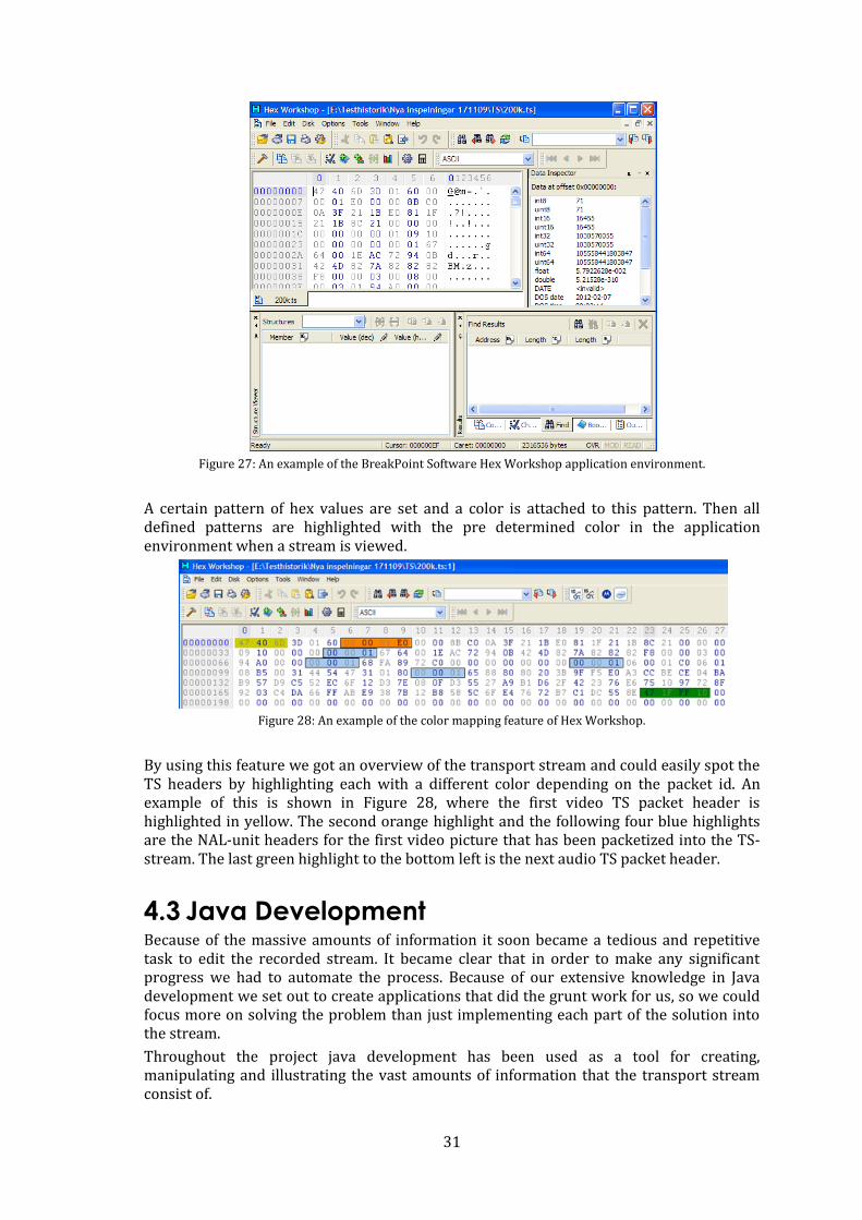
31

Figure 27: An example of the BreakPoint Software Hex Workshop application environment.

A certain pattern of hex values are set and a color is attached to this pattern. Then all defined patterns are highlighted with the pre determined color in the application environment when a stream is viewed.

Figure 28: An example of the color mapping feature of Hex Workshop.

By using this feature we got an overview of the transport stream and could easily spot the TS headers by highlighting each with a different color depending on the packet id. An example of this is shown in Figure 28, where the first video TS packet header is highlighted in yellow. The second orange highlight and the following four blue highlights are the NAL-unit headers for the first video picture that has been packetized into the TS-stream. The last green highlight to the bottom left is the next audio TS packet header.

4.3 Java Development Because of the massive amounts of information it soon became a tedious and repetitive task to edit the recorded stream. It became clear that in order to make any significant progress we had to automate the process. Because of our extensive knowledge in Java development we set out to create applications that did the grunt work for us, so we could focus more on solving the problem than just implementing each part of the solution into the stream.

Throughout the project java development has been used as a tool for creating, manipulating and illustrating the vast amounts of information that the transport stream consist of.

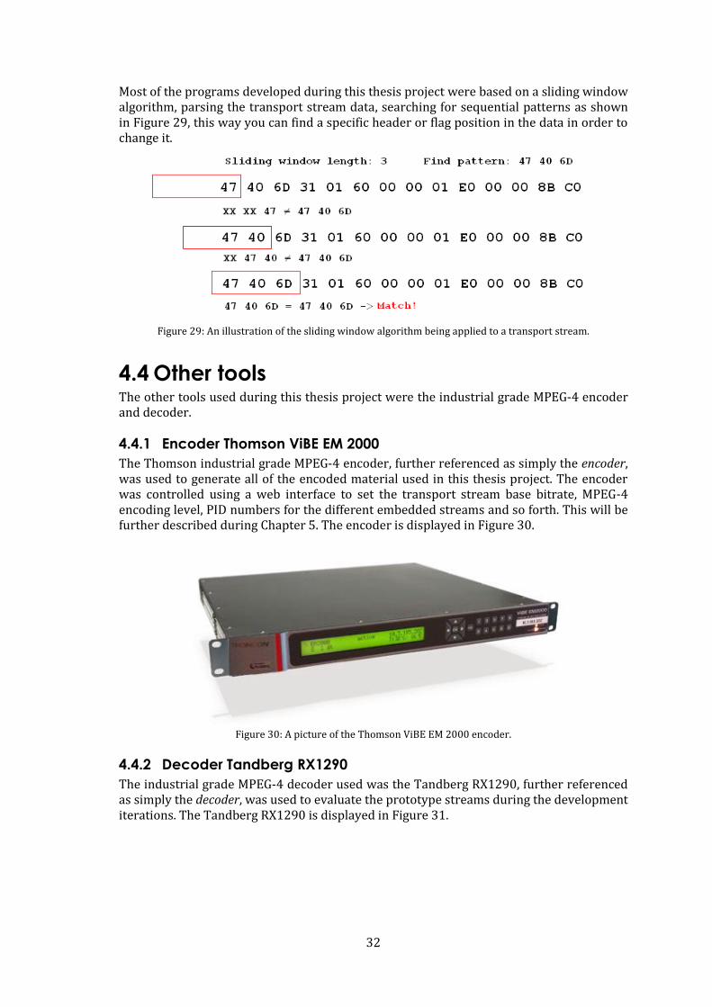
32

Most of the programs developed during this thesis project were based on a sliding window algorithm, parsing the transport stream data, searching for sequential patterns as shown in Figure 29, this way you can find a specific header or flag position in the data in order to change it.

Figure 29: An illustration of the sliding window algorithm being applied to a transport stream.

4.4 Other tools The other tools used during this thesis project were the industrial grade MPEG-4 encoder and decoder.

4.4.1 Encoder Thomson ViBE EM 2000

The Thomson industrial grade MPEG-4 encoder, further referenced as simply the encoder, was used to generate all of the encoded material used in this thesis project. The encoder was controlled using a web interface to set the transport stream base bitrate, MPEG-4 encoding level, PID numbers for the different embedded streams and so forth. This will be further described during Chapter 5. The encoder is displayed in Figure 30.

Figure 30: A picture of the Thomson ViBE EM 2000 encoder.

4.4.2 Decoder Tandberg RX1290

The industrial grade MPEG-4 decoder used was the Tandberg RX1290, further referenced as simply the decoder, was used to evaluate the prototype streams during the development iterations. The Tandberg RX1290 is displayed in Figure 31.

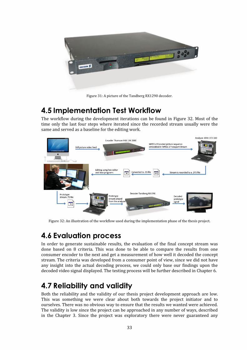
33

Figure 31: A picture of the Tandberg RX1290 decoder.

4.5 Implementation Test Workflow The workflow during the development iterations can be found in Figure 32. Most of the time only the last four steps where iterated since the recorded stream usually were the same and served as a baseline for the editing work.

Figure 32: An illustration of the workflow used during the implementation phase of the thesis project.

4.6 Evaluation process In order to generate sustainable results, the evaluation of the final concept stream was done based on 8 criteria. This was done to be able to compare the results from one consumer encoder to the next and get a measurement of how well it decoded the concept stream. The criteria was developed from a consumer point of view, since we did not have any insight into the actual decoding process, we could only base our findings upon the decoded video signal displayed. The testing process will be further described in Chapter 6.

4.7 Reliability and validity Both the reliability and the validity of our thesis project development approach are low. This was something we were clear about both towards the project initiator and to ourselves. There was no obvious way to ensure that the results we wanted were achieved. The validity is low since the project can be approached in any number of ways, described in the Chapter 3. Since the project was exploratory there were never guaranteed any

34

results at all from the beginning. There were no previous results to base our method upon in the field of our research, and since the subject of our study is consumer decoders this further jeopardized the basis for the reliability and validity of our study.

However the reliability and validity of our results are higher. The testing was done in a controlled environment, in the same lab where all the consumer decoders are tested for use in the field. The reliability of our controlled observation can easily be recreated with corresponding results, given that the tested equipment is the same. The validity of the test is somewhat lower. During the testing process we had to judge, from the audio and video decoded and displayed on each test platform, which of the criteria was met and which was not. This might lead to differentiating opinions and hence different results.

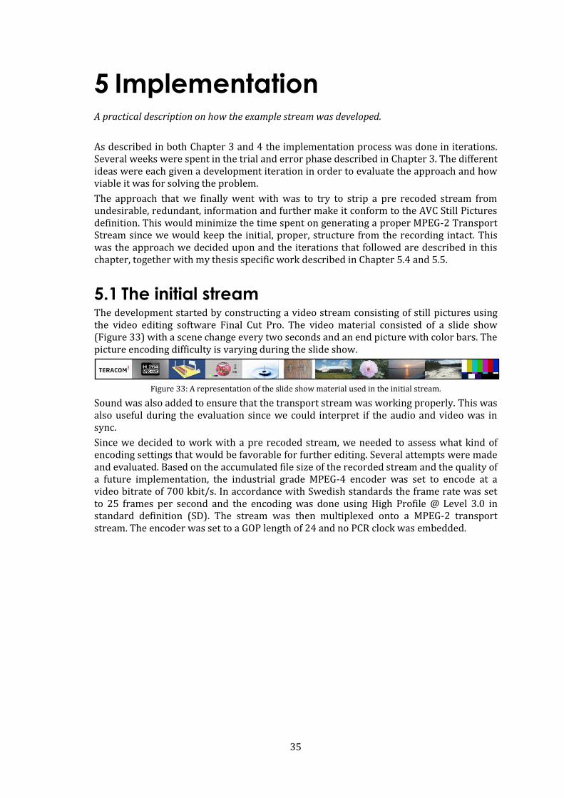
35

5 Implementation A practical description on how the example stream was developed.

As described in both Chapter 3 and 4 the implementation process was done in iterations. Several weeks were spent in the trial and error phase described in Chapter 3. The different ideas were each given a development iteration in order to evaluate the approach and how viable it was for solving the problem.

The approach that we finally went with was to try to strip a pre recoded stream from undesirable, redundant, information and further make it conform to the AVC Still Pictures definition. This would minimize the time spent on generating a proper MPEG-2 Transport Stream since we would keep the initial, proper, structure from the recording intact. This was the approach we decided upon and the iterations that followed are described in this chapter, together with my thesis specific work described in Chapter 5.4 and 5.5.

5.1 The initial stream The development started by constructing a video stream consisting of still pictures using the video editing software Final Cut Pro. The video material consisted of a slide show (Figure 33) with a scene change every two seconds and an end picture with color bars. The picture encoding difficulty is varying during the slide show.

Figure 33: A representation of the slide show material used in the initial stream.

Sound was also added to ensure that the transport stream was working properly. This was also useful during the evaluation since we could interpret if the audio and video was in sync.

Since we decided to work with a pre recoded stream, we needed to assess what kind of encoding settings that would be favorable for further editing. Several attempts were made and evaluated. Based on the accumulated file size of the recorded stream and the quality of a future implementation, the industrial grade MPEG-4 encoder was set to encode at a video bitrate of 700 kbit/s. In accordance with Swedish standards the frame rate was set to 25 frames per second and the encoding was done using High Profile @ Level 3.0 in standard definition (SD). The stream was then multiplexed onto a MPEG-2 transport stream. The encoder was set to a GOP length of 24 and no PCR clock was embedded.

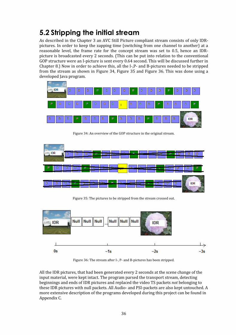
36

5.2 Stripping the initial stream As described in the Chapter 3 an AVC Still Picture compliant stream consists of only IDR-pictures. In order to keep the zapping time (switching from one channel to another) at a reasonable level, the frame rate for the concept stream was set to 0.5, hence an IDR-picture is broadcasted every 2 seconds. (This can be put into relation to the conventional GOP structure were an I-picture is sent every 0.64 second. This will be discussed further in Chapter 8.) Now in order to achieve this, all the I-,P- and B-pictures needed to be stripped from the stream as shown in Figure 34, Figure 35 and Figure 36. This was done using a developed Java program.

Figure 34: An overview of the GOP structure in the original stream.

Figure 35: The pictures to be stripped from the stream crossed out.

Figure 36: The stream after I-, P- and B-pictures has been stripped.

All the IDR pictures, that had been generated every 2 seconds at the scene change of the input material, were kept intact. The program parsed the transport stream, detecting beginnings and ends of IDR pictures and replaced the video TS packets not belonging to these IDR pictures with null packets. All Audio- and PSI-packets are also kept untouched. A more extensive description of the programs developed during this project can be found in Appendix C.

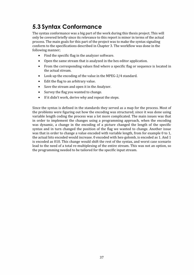
37

5.3 Syntax Conformance The syntax conformance was a big part of the work during this thesis project. This will only be covered briefly since its relevance to this report is minor in terms of the actual process. The main goals for this part of the project was to make the syntax signaling conform to the specifications described in Chapter 3. The workflow was done in the following manner;

Find the specific flag in the analyzer software.

Open the same stream that is analyzed in the hex editor application.

From the corresponding values find where a specific flag or sequence is located in the actual stream.

Look up the encoding of the value in the MPEG-2/4 standard.

Edit the flag to an arbitrary value.

Save the stream and open it in the Analyzer.

Survey the flag you wanted to change.

If it didn’t work, derive why and repeat the steps.

Since the syntax is defined in the standards they served as a map for the process. Most of the problems were figuring out how the encoding was structured; since it was done using variable length coding the process was a lot more complicated. The main issues was that in order to implement the changes using a programming approach, when the encoding was dynamic, a change in the encoding of a picture changed the length of the specific syntax and in turn changed the position of the flag we wanted to change. Another issue was that in order to change a value encoded with variable length, from for example 0 to 1, the actual bits encoded would increase. 0 encoded with hex-golomb, is encoded as 1. And 1 is encoded as 010. This change would shift the rest of the syntax, and worst case scenario lead to the need of a total re-multiplexing of the entire stream. This was not an option, so the programming needed to be tailored for the specific input stream.

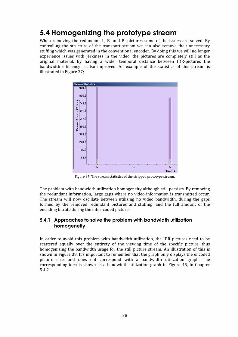
38

5.4 Homogenizing the prototype stream When removing the redundant I-, B- and P- pictures some of the issues are solved. By controlling the structure of the transport stream we can also remove the unnecessary stuffing which was generated in the conventional encoder. By doing this we will no longer experience issues with jerkiness in the video, the pictures are completely still as the original material. By having a wider temporal distance between IDR-pictures the bandwidth efficiency is also improved. An example of the statistics of this stream is illustrated in Figure 37;

Figure 37: The stream statistics of the stripped prototype stream.

The problem with bandwidth utilization homogeneity although still persists. By removing the redundant information, large gaps where no video information is transmitted occur. The stream will now oscillate between utilizing no video bandwidth, during the gaps formed by the removed redundant pictures and stuffing; and the full amount of the encoding bitrate during the inter-coded pictures.

5.4.1 Approaches to solve the problem with bandwidth utilization

homogeneity

In order to avoid this problem with bandwidth utilization, the IDR pictures need to be scattered equally over the entirety of the viewing time of the specific picture, thus homogenizing the bandwidth usage for the still picture stream. An illustration of this is shown in Figure 38. It’s important to remember that the graph only displays the encoded picture size, and does not correspond with a bandwidth utilization graph. The corresponding idea is shown as a bandwidth utilization graph in Figure 45, in Chapter 5.4.2.

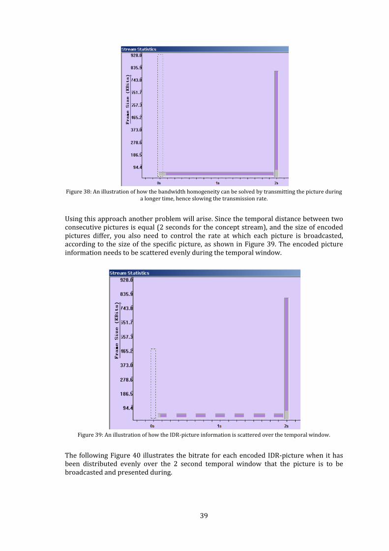
39

Figure 38: An illustration of how the bandwidth homogeneity can be solved by transmitting the picture during

a longer time, hence slowing the transmission rate.

Using this approach another problem will arise. Since the temporal distance between two consecutive pictures is equal (2 seconds for the concept stream), and the size of encoded pictures differ, you also need to control the rate at which each picture is broadcasted, according to the size of the specific picture, as shown in Figure 39. The encoded picture information needs to be scattered evenly during the temporal window.

Figure 39: An illustration of how the IDR-picture information is scattered over the temporal window.

The following Figure 40 illustrates the bitrate for each encoded IDR-picture when it has been distributed evenly over the 2 second temporal window that the picture is to be broadcasted and presented during.

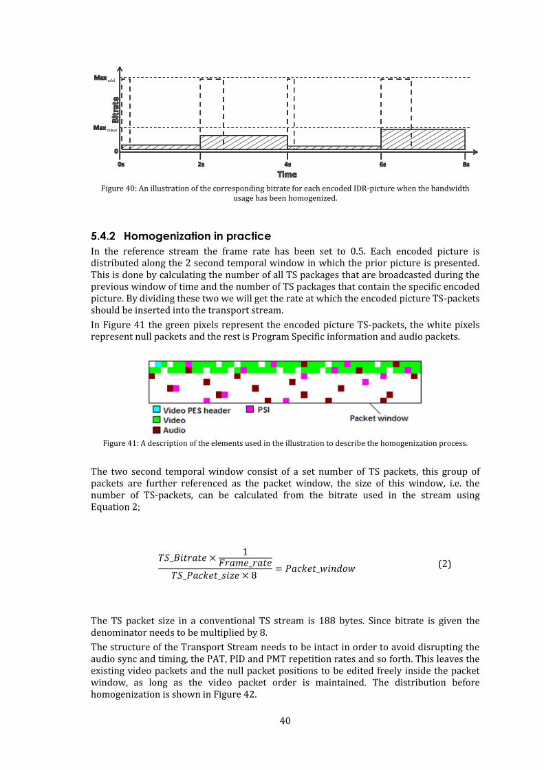
40

Figure 40: An illustration of the corresponding bitrate for each encoded IDR-picture when the bandwidth

usage has been homogenized.

5.4.2 Homogenization in practice

In the reference stream the frame rate has been set to 0.5. Each encoded picture is distributed along the 2 second temporal window in which the prior picture is presented. This is done by calculating the number of all TS packages that are broadcasted during the previous window of time and the number of TS packages that contain the specific encoded picture. By dividing these two we will get the rate at which the encoded picture TS-packets should be inserted into the transport stream.

In Figure 41 the green pixels represent the encoded picture TS-packets, the white pixels represent null packets and the rest is Program Specific information and audio packets.

Figure 41: A description of the elements used in the illustration to describe the homogenization process.

The two second temporal window consist of a set number of TS packets, this group of packets are further referenced as the packet window, the size of this window, i.e. the number of TS-packets, can be calculated from the bitrate used in the stream using Equation 2;

(2)

The TS packet size in a conventional TS stream is 188 bytes. Since bitrate is given the denominator needs to be multiplied by 8.

The structure of the Transport Stream needs to be intact in order to avoid disrupting the audio sync and timing, the PAT, PID and PMT repetition rates and so forth. This leaves the existing video packets and the null packet positions to be edited freely inside the packet window, as long as the video packet order is maintained. The distribution before homogenization is shown in Figure 42.

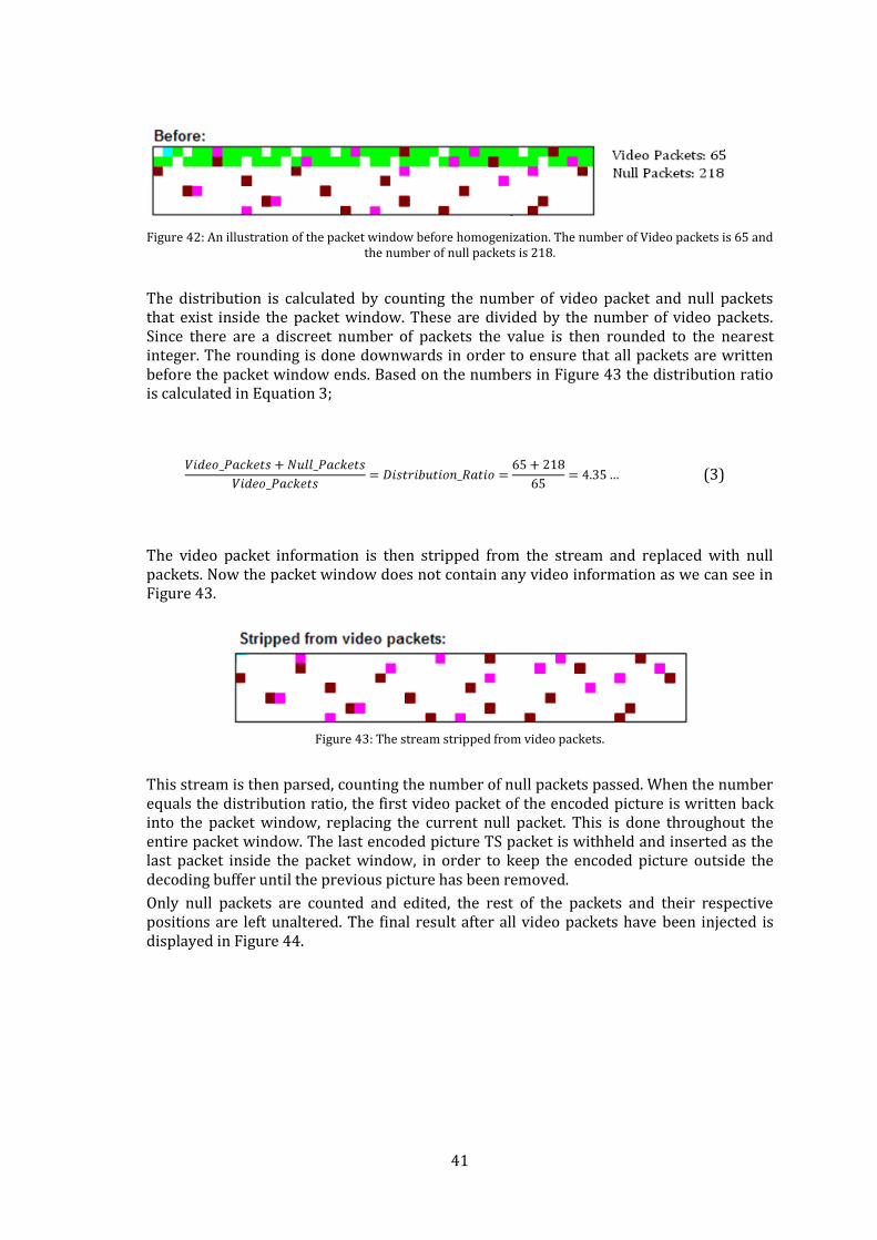
41

Figure 42: An illustration of the packet window before homogenization. The number of Video packets is 65 and

the number of null packets is 218.

The distribution is calculated by counting the number of video packet and null packets that exist inside the packet window. These are divided by the number of video packets. Since there are a discreet number of packets the value is then rounded to the nearest integer. The rounding is done downwards in order to ensure that all packets are written before the packet window ends. Based on the numbers in Figure 43 the distribution ratio is calculated in Equation 3;

(3)

The video packet information is then stripped from the stream and replaced with null packets. Now the packet window does not contain any video information as we can see in Figure 43.

Figure 43: The stream stripped from video packets.

This stream is then parsed, counting the number of null packets passed. When the number equals the distribution ratio, the first video packet of the encoded picture is written back into the packet window, replacing the current null packet. This is done throughout the entire packet window. The last encoded picture TS packet is withheld and inserted as the last packet inside the packet window, in order to keep the encoded picture outside the decoding buffer until the previous picture has been removed.

Only null packets are counted and edited, the rest of the packets and their respective positions are left unaltered. The final result after all video packets have been injected is displayed in Figure 44.

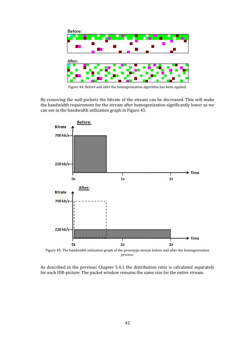
42

Figure 44: Before and after the homogenization algorithm has been applied.

By removing the null-packets the bitrate of the stream can be decreased. This will make the bandwidth requirement for the stream after homogenization significantly lower as we can see in the bandwidth utilization graph in Figure 45.

Figure 45: The bandwidth utilization graph of the prototype stream before and after the homogenization

process.

As described in the previous Chapter 5.4.1 the distribution ratio is calculated separately for each IDR-picture. The packet window remains the same size for the entire stream.

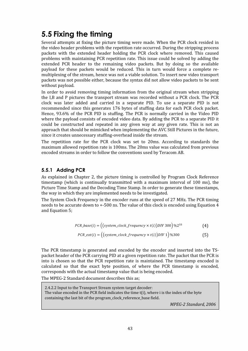
43

5.5 Fixing the timing Several attempts at fixing the picture timing were made. When the PCR clock resided in the video header problems with the repetition rate occurred. During the stripping process packets with the extended header holding the PCR clock where removed. This caused problems with maintaining PCR repetition rate. This issue could be solved by adding the extended PCR header to the remaining video packets. But by doing so the available payload for these packets would be reduced. This in turn would force a complete re-multiplexing of the stream, hence was not a viable solution. To insert new video transport packets was not possible either, because the syntax did not allow video packets to be sent without payload.

In order to avoid removing timing information from the original stream when stripping the I,B and P pictures the transport stream was recorded without a PCR clock. The PCR clock was later added and carried in a separate PID. To use a separate PID is not recommended since this generates 176 bytes of stuffing data for each PCR clock packet. Hence, 93.6% of the PCR PID is stuffing. The PCR is normally carried in the Video PID where the payload consists of encoded video data. By adding the PCR to a separate PID it could be constructed and repeated in any given way at any given rate. This is not an approach that should be mimicked when implementing the AVC Still Pictures in the future, since it creates unnecessary stuffing-overhead inside the stream.

The repetition rate for the PCR clock was set to 20ms. According to standards the maximum allowed repetition rate is 100ms. The 20ms value was calculated from previous encoded streams in order to follow the conventions used by Teracom AB.

5.5.1 Adding PCR

As explained in Chapter 2, the picture timing is controlled by Program Clock Reference timestamp (which is continually transmitted with a maximum interval of 100 ms), the Picture Time Stamp and the Decoding Time Stamp. In order to generate these timestamps, the way in which they are implemented needs to be investigated.

The System Clock Frequency in the encoder runs at the speed of 27 MHz. The PCR timing needs to be accurate down to +-500 ns. The value of this clock is encoded using Equation 4 and Equation 5;

(4)

(5)

The PCR timestamp is generated and encoded by the encoder and inserted into the TS-packet header of the PCR carrying PID at a given repetition rate. The packet that the PCR is into is chosen so that the PCR repetition rate is maintained. The timestamp encoded is calculated so that the exact byte position, of where the PCR timestamp is encoded, corresponds with the actual timestamp value that is being encoded.

The MPEG-2 Standard document describes this as;

2.4.2.2 Input to the Transport Stream system target decoder: The value encoded in the PCR field indicates the time t(i), where i is the index of the byte

containing the last bit of the program_clock_reference_base field.

MPEG-2 Standard, 2006

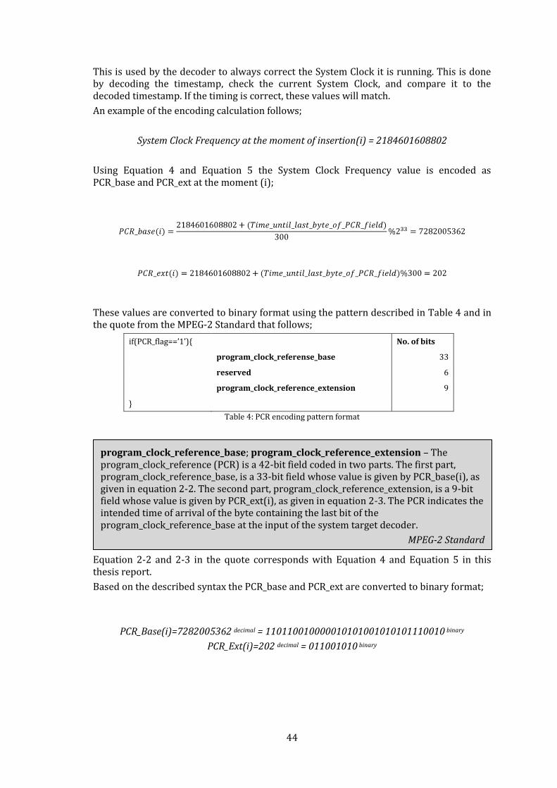
44

This is used by the decoder to always correct the System Clock it is running. This is done by decoding the timestamp, check the current System Clock, and compare it to the decoded timestamp. If the timing is correct, these values will match.

An example of the encoding calculation follows;

System Clock Frequency at the moment of insertion(i) = 2184601608802

Using Equation 4 and Equation 5 the System Clock Frequency value is encoded as PCR_base and PCR_ext at the moment (i);

These values are converted to binary format using the pattern described in Table 4 and in the quote from the MPEG-2 Standard that follows;

if(PCR_flag==’1’){ No. of bits

program_clock_referense_base 33

reserved 6

program_clock_reference_extension 9

}

Table 4: PCR encoding pattern format

Equation 2-2 and 2-3 in the quote corresponds with Equation 4 and Equation 5 in this thesis report.

Based on the described syntax the PCR_base and PCR_ext are converted to binary format;

PCR_Base(i)=7282005362 decimal = 110110010000010101001010101110010 binary

PCR_Ext(i)=202 decimal = 011001010 binary

program_clock_reference_base; program_clock_reference_extension – The program_clock_reference (PCR) is a 42-bit field coded in two parts. The first part, program_clock_reference_base, is a 33-bit field whose value is given by PCR_base(i), as given in equation 2-2. The second part, program_clock_reference_extension, is a 9-bit field whose value is given by PCR_ext(i), as given in equation 2-3. The PCR indicates the intended time of arrival of the byte containing the last bit of the program_clock_reference_base at the input of the system target decoder.

MPEG-2 Standard

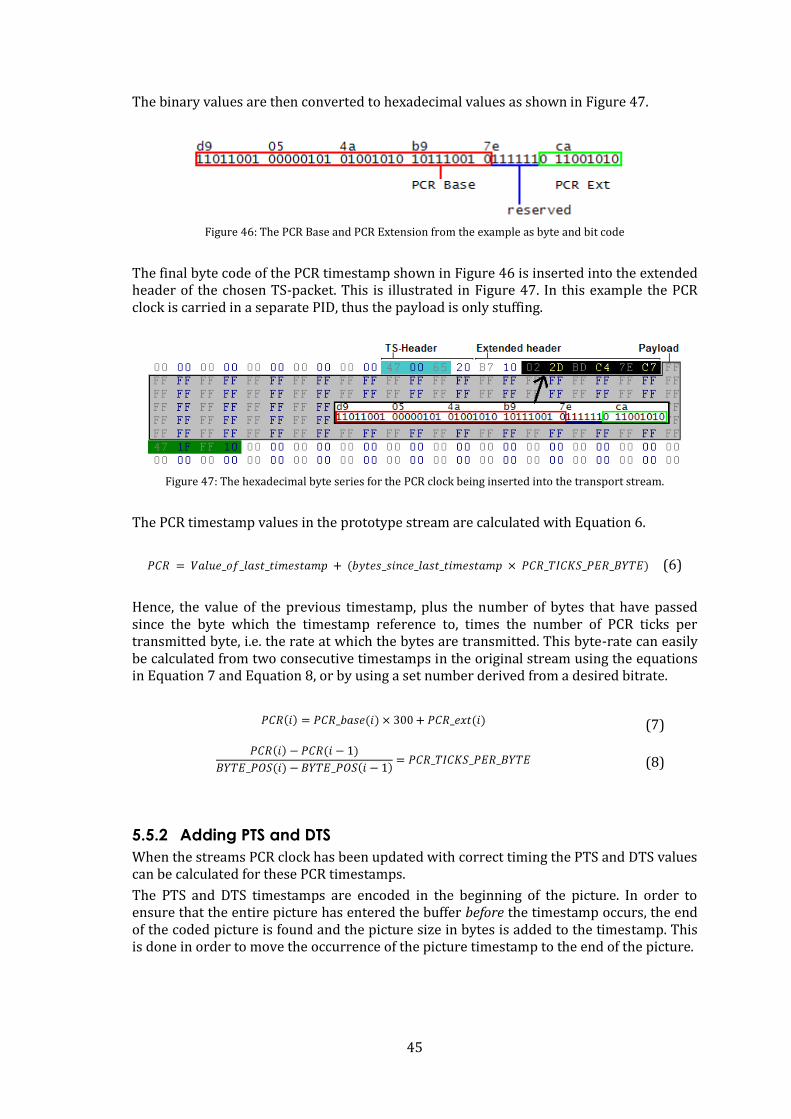
45

The binary values are then converted to hexadecimal values as shown in Figure 47.

Figure 46: The PCR Base and PCR Extension from the example as byte and bit code

The final byte code of the PCR timestamp shown in Figure 46 is inserted into the extended header of the chosen TS-packet. This is illustrated in Figure 47. In this example the PCR clock is carried in a separate PID, thus the payload is only stuffing.

Figure 47: The hexadecimal byte series for the PCR clock being inserted into the transport stream.

The PCR timestamp values in the prototype stream are calculated with Equation 6.

(6)

Hence, the value of the previous timestamp, plus the number of bytes that have passed since the byte which the timestamp reference to, times the number of PCR ticks per transmitted byte, i.e. the rate at which the bytes are transmitted. This byte-rate can easily be calculated from two consecutive timestamps in the original stream using the equations in Equation 7 and Equation 8, or by using a set number derived from a desired bitrate.

(7)

(8)

5.5.2 Adding PTS and DTS

When the streams PCR clock has been updated with correct timing the PTS and DTS values can be calculated for these PCR timestamps.

The PTS and DTS timestamps are encoded in the beginning of the picture. In order to ensure that the entire picture has entered the buffer before the timestamp occurs, the end of the coded picture is found and the picture size in bytes is added to the timestamp. This is done in order to move the occurrence of the picture timestamp to the end of the picture.

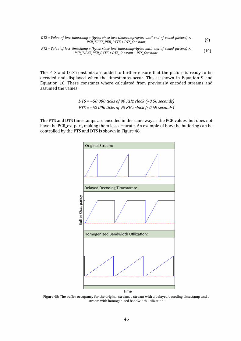
46

DTS = Value_of_last_timestamp + (bytes_since_last_timestamp+bytes_until_end_of_coded_picture) PCR_TICKS_PER_BYTE + DTS_Constant

(9)

PTS = Value_of_last_timestamp + (bytes_since_last_timestamp+bytes_until_end_of_coded_picture) PCR_TICKS_PER_BYTE + DTS_Constant + PTS_Constant

(10)

The PTS and DTS constants are added to further ensure that the picture is ready to be decoded and displayed when the timestamps occur. This is shown in Equation 9 and Equation 10. These constants where calculated from previously encoded streams and assumed the values;

DTS = ~50 000 ticks of 90 KHz clock (~0.56 seconds)

PTS = ~62 000 ticks of 90 KHz clock (~0.69 seconds)

The PTS and DTS timestamps are encoded in the same way as the PCR values, but does not have the PCR_ext part, making them less accurate. An example of how the buffering can be controlled by the PTS and DTS is shown in Figure 48.

Figure 48: The buffer occupancy for the original stream, a stream with a delayed decoding timestamp and a

stream with homogenized bandwidth utilization.

47

By setting the decoding timestamp further into the future, the buffering structure can be controlled. This can be used to avoid buffer under runs. This is not to be confused with bandwidth utilization homogenization. This approach only keeps the picture from being decoded when the last packet of the specific picture is received in the decoder. The difference between these two approaches is shown in the third graph in Figure 48.

Both of these approaches combined were used in the developed concept stream.

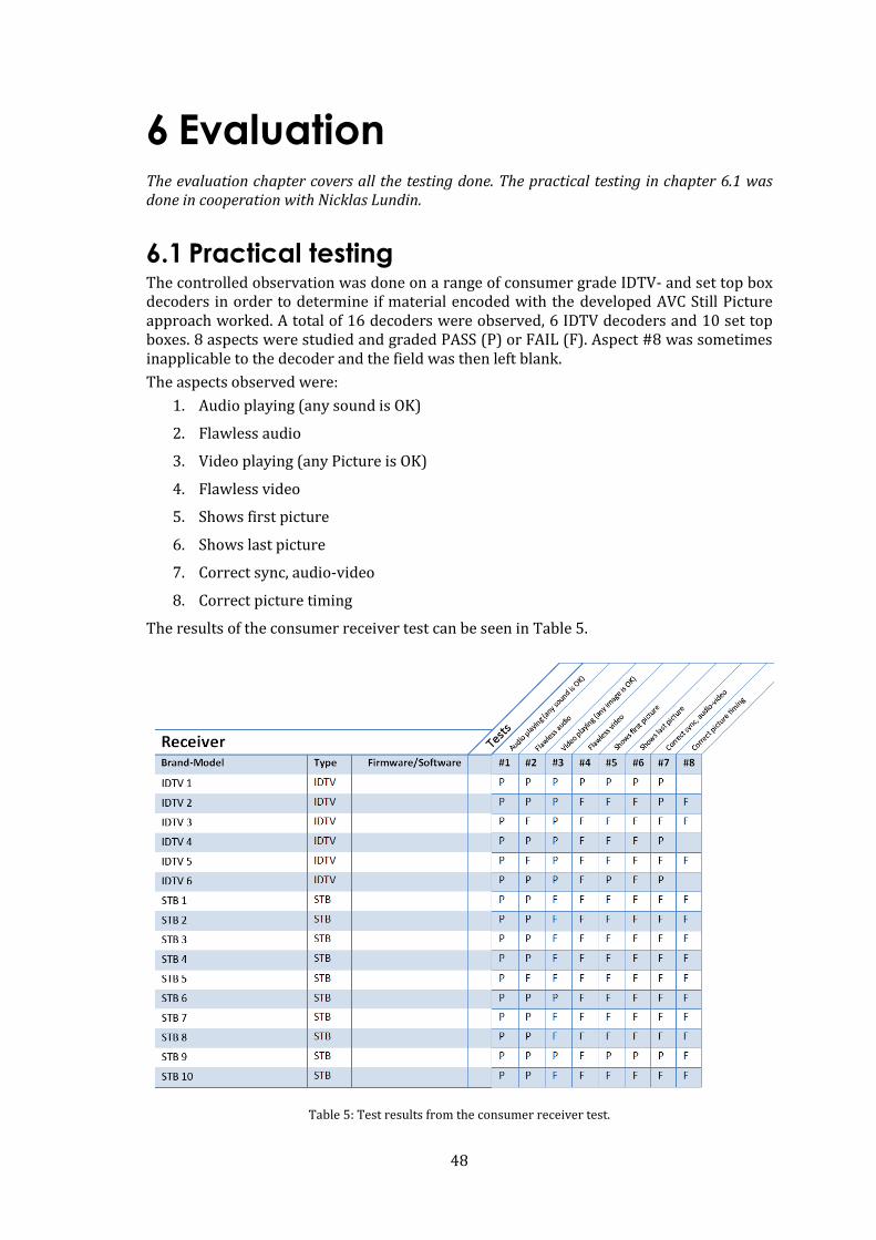
48

6 Evaluation The evaluation chapter covers all the testing done. The practical testing in chapter 6.1 was done in cooperation with Nicklas Lundin.

6.1 Practical testing The controlled observation was done on a range of consumer grade IDTV- and set top box decoders in order to determine if material encoded with the developed AVC Still Picture approach worked. A total of 16 decoders were observed, 6 IDTV decoders and 10 set top boxes. 8 aspects were studied and graded PASS (P) or FAIL (F). Aspect #8 was sometimes inapplicable to the decoder and the field was then left blank.

The aspects observed were:

1. Audio playing (any sound is OK)

2. Flawless audio

3. Video playing (any Picture is OK)

4. Flawless video

5. Shows first picture

6. Shows last picture

7. Correct sync, audio-video

8. Correct picture timing

The results of the consumer receiver test can be seen in Table 5.

Table 5: Test results from the consumer receiver test.

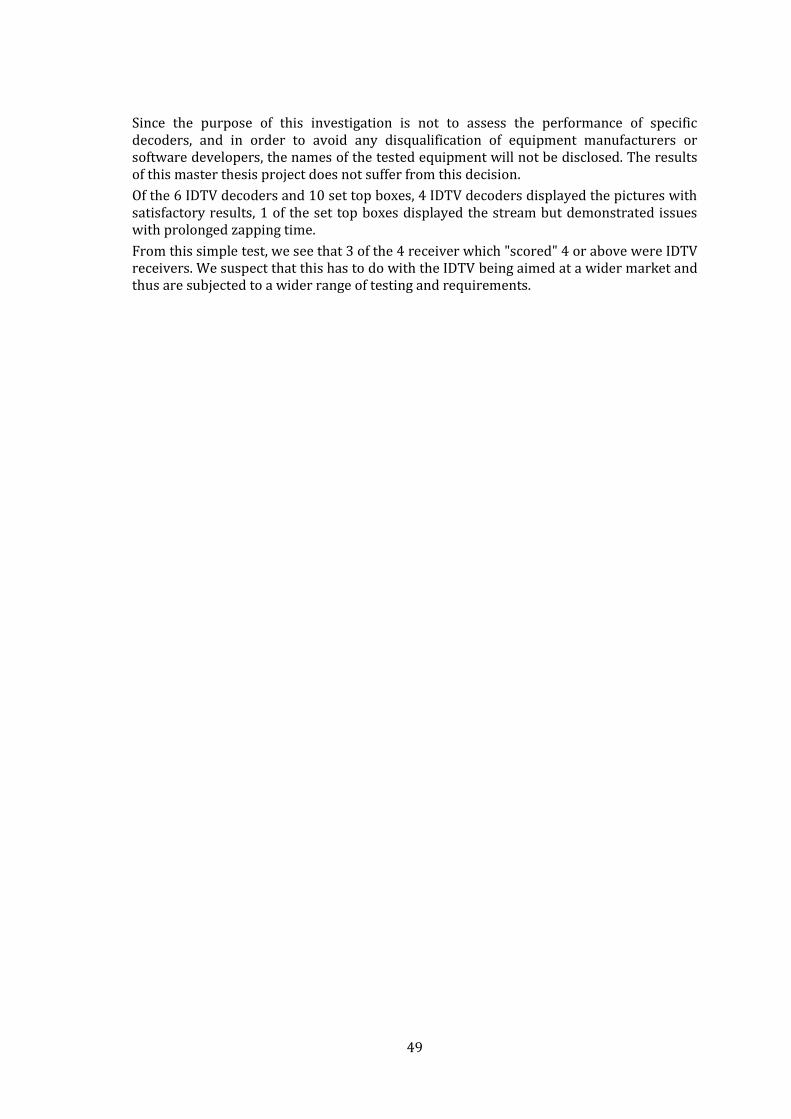
49

Since the purpose of this investigation is not to assess the performance of specific decoders, and in order to avoid any disqualification of equipment manufacturers or software developers, the names of the tested equipment will not be disclosed. The results of this master thesis project does not suffer from this decision.

Of the 6 IDTV decoders and 10 set top boxes, 4 IDTV decoders displayed the pictures with satisfactory results, 1 of the set top boxes displayed the stream but demonstrated issues with prolonged zapping time.

From this simple test, we see that 3 of the 4 receiver which "scored" 4 or above were IDTV receivers. We suspect that this has to do with the IDTV being aimed at a wider market and thus are subjected to a wider range of testing and requirements.

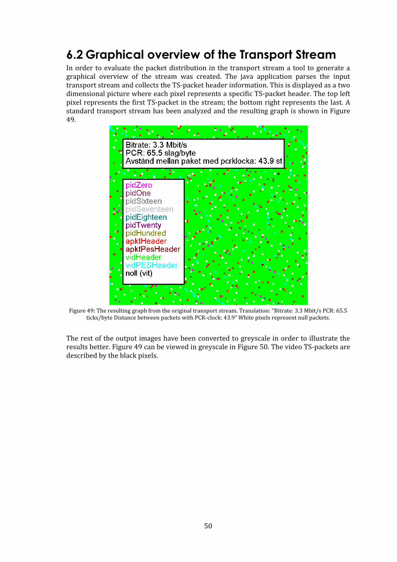
50

6.2 Graphical overview of the Transport Stream In order to evaluate the packet distribution in the transport stream a tool to generate a graphical overview of the stream was created. The java application parses the input transport stream and collects the TS-packet header information. This is displayed as a two dimensional picture where each pixel represents a specific TS-packet header. The top left pixel represents the first TS-packet in the stream; the bottom right represents the last. A standard transport stream has been analyzed and the resulting graph is shown in Figure 49.

Figure 49: The resulting graph from the original transport stream. Translation: “Bitrate: 3.3 Mbit/s PCR: 65.5

ticks/byte Distance between packets with PCR-clock: 43.9“ White pixels represent null packets.

The rest of the output images have been converted to greyscale in order to illustrate the results better. Figure 49 can be viewed in greyscale in Figure 50. The video TS-packets are described by the black pixels.

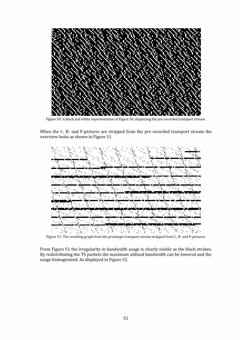
51

Figure 50: A black and white representation of Figure 50, displaying the pre recorded transport stream.

When the I-, B- and P-pictures are stripped from the pre recorded transport stream the overview looks as shown in Figure 51.

Figure 51: The resulting graph from the prototype transport stream stripped from I-, B- and P-pictures.

From Figure 51 the irregularity in bandwidth usage is clearly visible as the black strokes. By redistributing the TS packets the maximum utilized bandwidth can be lowered and the usage homogenized. As displayed in Figure 52.

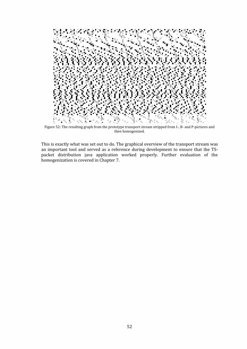
52

Figure 52: The resulting graph from the prototype transport stream stripped from I-, B- and P-pictures and

then homogenized.

This is exactly what was set out to do. The graphical overview of the transport stream was an important tool and served as a reference during development to ensure that the TS-packet distribution java application worked properly. Further evaluation of the homogenization is covered in Chapter 7.

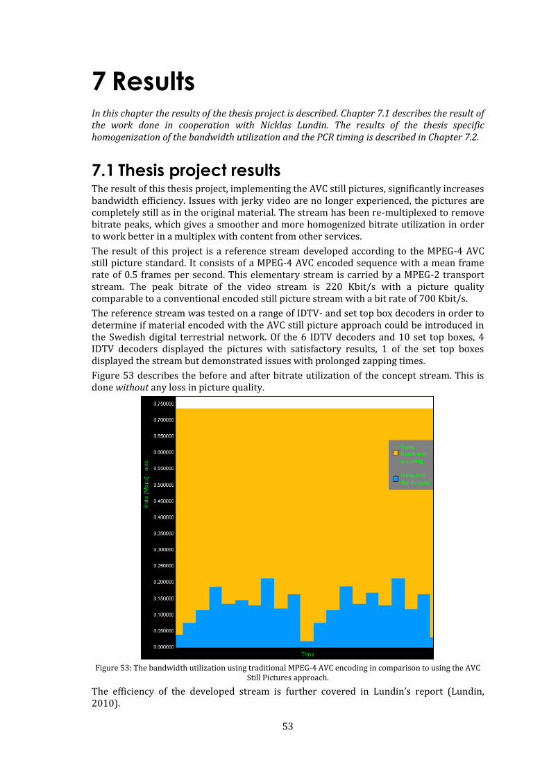
53

7 Results In this chapter the results of the thesis project is described. Chapter 7.1 describes the result of the work done in cooperation with Nicklas Lundin. The results of the thesis specific homogenization of the bandwidth utilization and the PCR timing is described in Chapter 7.2.

7.1 Thesis project results The result of this thesis project, implementing the AVC still pictures, significantly increases bandwidth efficiency. Issues with jerky video are no longer experienced, the pictures are completely still as in the original material. The stream has been re-multiplexed to remove bitrate peaks, which gives a smoother and more homogenized bitrate utilization in order to work better in a multiplex with content from other services.

The result of this project is a reference stream developed according to the MPEG-4 AVC still picture standard. It consists of a MPEG-4 AVC encoded sequence with a mean frame rate of 0.5 frames per second. This elementary stream is carried by a MPEG-2 transport stream. The peak bitrate of the video stream is 220 Kbit/s with a picture quality comparable to a conventional encoded still picture stream with a bit rate of 700 Kbit/s.

The reference stream was tested on a range of IDTV- and set top box decoders in order to determine if material encoded with the AVC still picture approach could be introduced in the Swedish digital terrestrial network. Of the 6 IDTV decoders and 10 set top boxes, 4 IDTV decoders displayed the pictures with satisfactory results, 1 of the set top boxes displayed the stream but demonstrated issues with prolonged zapping times.

Figure 53 describes the before and after bitrate utilization of the concept stream. This is done without any loss in picture quality.

Figure 53: The bandwidth utilization using traditional MPEG-4 AVC encoding in comparison to using the AVC

Still Pictures approach.

The efficiency of the developed stream is further covered in Lundin’s report (Lundin, 2010).

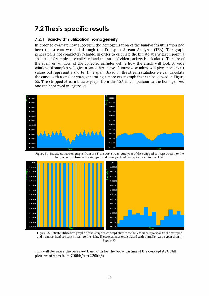
54

7.2 Thesis specific results

7.2.1 Bandwidth utilization homogeneity

In order to evaluate how successful the homogenization of the bandwidth utilization had been the stream was fed through the Transport Stream Analyzer (TSA). The graph generated is not completely reliable. In order to calculate the bitrate at any given point, a spectrum of samples are collected and the ratio of video packets is calculated. The size of the span, or window, of the collected samples define how the graph will look. A wide window of samples will give a smoother curve. A narrow window will give more exact values but represent a shorter time span. Based on the stream statistics we can calculate the curve with a smaller span, generating a more exact graph that can be viewed in Figure 55. The stripped stream bitrate graph from the TSA in comparison to the homogenized one can be viewed in Figure 54.

Figure 54: Bitrate utilization graphs from the Transport stream Analyzer of the stripped concept stream to the

left; in comparison to the stripped and homogenized concept stream to the right.

Figure 55: Bitrate utilization graphs of the stripped concept stream to the left; in comparison to the stripped and homogenized concept stream to the right. These graphs are calculated with a smaller value span than in

Figure 55.

This will decrease the reserved bandwith for the broadcasting of the concept AVC Still pictures stream from 700kb/s to 220kb/s .

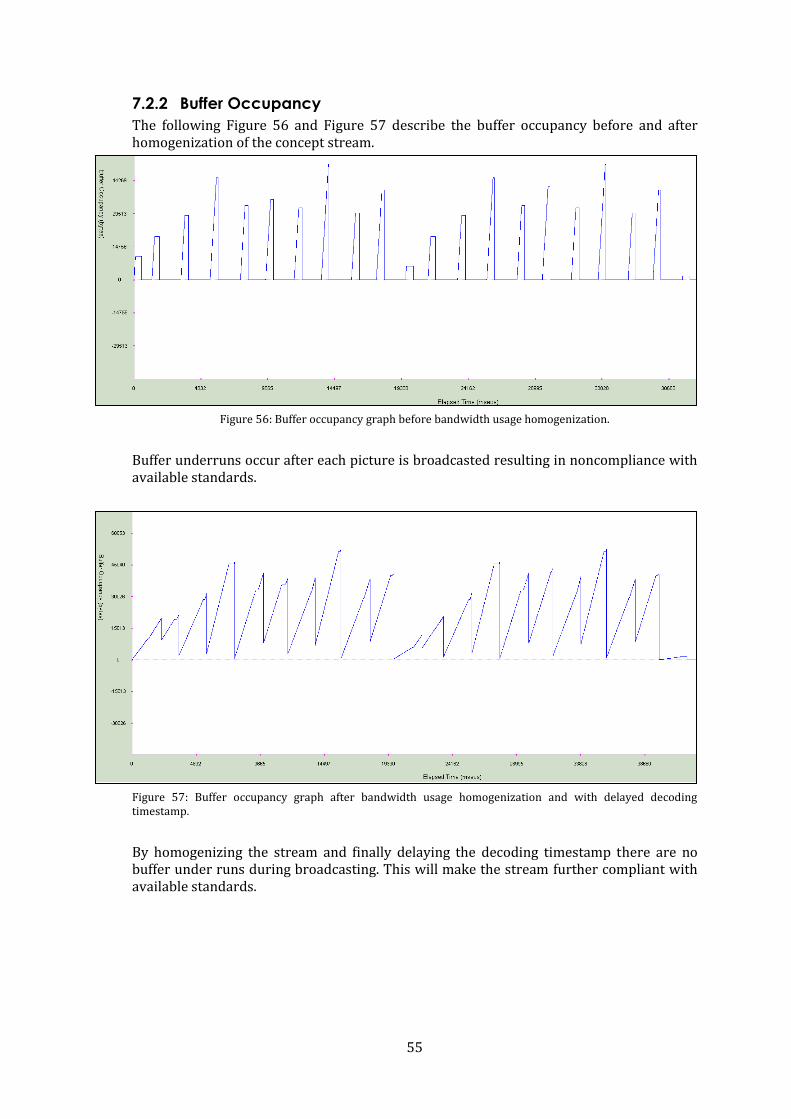
55

7.2.2 Buffer Occupancy

The following Figure 56 and Figure 57 describe the buffer occupancy before and after homogenization of the concept stream.

Figure 56: Buffer occupancy graph before bandwidth usage homogenization.

Buffer underruns occur after each picture is broadcasted resulting in noncompliance with available standards.

Figure 57: Buffer occupancy graph after bandwidth usage homogenization and with delayed decoding timestamp.

By homogenizing the stream and finally delaying the decoding timestamp there are no buffer under runs during broadcasting. This will make the stream further compliant with available standards.

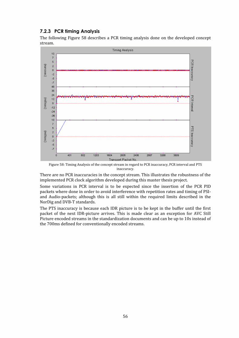
56

7.2.3 PCR timing Analysis

The following Figure 58 describes a PCR timing analysis done on the developed concept stream.

Figure 58: Timing Analysis of the concept stream in regard to PCR inaccuracy, PCR interval and PTS

inaccuracy.

There are no PCR inaccuracies in the concept stream. This illustrates the robustness of the implemented PCR clock algorithm developed during this master thesis project.

Some variations in PCR interval is to be expected since the insertion of the PCR PID packets where done in order to avoid interference with repetition rates and timing of PSI- and Audio-packets; although this is all still within the required limits described in the NorDig and DVB-T standards.

The PTS inaccuracy is because each IDR picture is to be kept in the buffer until the first packet of the next IDR-picture arrives. This is made clear as an exception for AVC Still Picture encoded streams in the standardization documents and can be up to 10s instead of the 700ms defined for conventionally encoded streams.

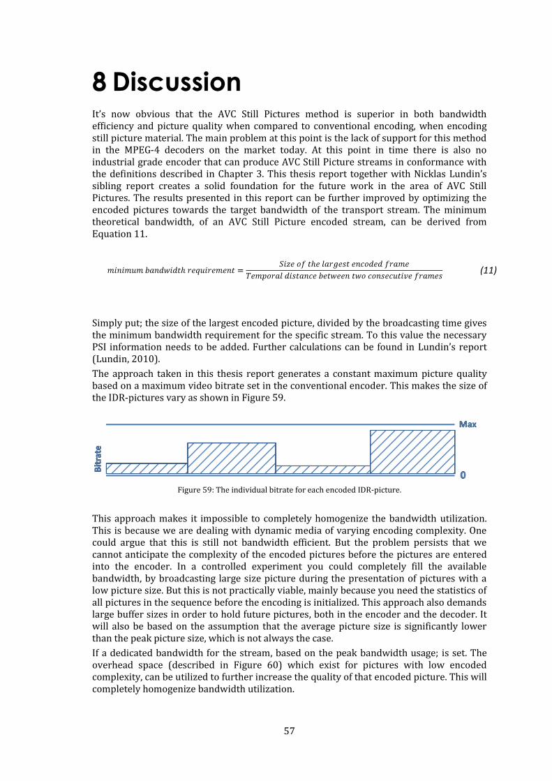
57

8 Discussion It’s now obvious that the AVC Still Pictures method is superior in both bandwidth efficiency and picture quality when compared to conventional encoding, when encoding still picture material. The main problem at this point is the lack of support for this method in the MPEG-4 decoders on the market today. At this point in time there is also no industrial grade encoder that can produce AVC Still Picture streams in conformance with the definitions described in Chapter 3. This thesis report together with Nicklas Lundin’s sibling report creates a solid foundation for the future work in the area of AVC Still Pictures. The results presented in this report can be further improved by optimizing the encoded pictures towards the target bandwidth of the transport stream. The minimum theoretical bandwidth, of an AVC Still Picture encoded stream, can be derived from Equation 11.

(11)

Simply put; the size of the largest encoded picture, divided by the broadcasting time gives the minimum bandwidth requirement for the specific stream. To this value the necessary PSI information needs to be added. Further calculations can be found in Lundin’s report (Lundin, 2010).

The approach taken in this thesis report generates a constant maximum picture quality based on a maximum video bitrate set in the conventional encoder. This makes the size of the IDR-pictures vary as shown in Figure 59.

Figure 59: The individual bitrate for each encoded IDR-picture.

This approach makes it impossible to completely homogenize the bandwidth utilization. This is because we are dealing with dynamic media of varying encoding complexity. One could argue that this is still not bandwidth efficient. But the problem persists that we cannot anticipate the complexity of the encoded pictures before the pictures are entered into the encoder. In a controlled experiment you could completely fill the available bandwidth, by broadcasting large size picture during the presentation of pictures with a low picture size. But this is not practically viable, mainly because you need the statistics of all pictures in the sequence before the encoding is initialized. This approach also demands large buffer sizes in order to hold future pictures, both in the encoder and the decoder. It will also be based on the assumption that the average picture size is significantly lower than the peak picture size, which is not always the case.

If a dedicated bandwidth for the stream, based on the peak bandwidth usage; is set. The overhead space (described in Figure 60) which exist for pictures with low encoded complexity, can be utilized to further increase the quality of that encoded picture. This will completely homogenize bandwidth utilization.

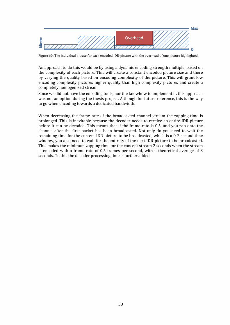
58

Figure 60: The individual bitrate for each encoded IDR-picture with the overhead of one picture highlighted.

An approach to do this would be by using a dynamic encoding strength multiple, based on the complexity of each picture. This will create a constant encoded picture size and there by varying the quality based on encoding complexity of the picture. This will grant low encoding complexity pictures higher quality than high complexity pictures and create a completely homogenized stream.

Since we did not have the encoding tools, nor the knowhow to implement it, this approach was not an option during the thesis project. Although for future reference, this is the way to go when encoding towards a dedicated bandwidth.

When decreasing the frame rate of the broadcasted channel stream the zapping time is prolonged. This is inevitable because the decoder needs to receive an entire IDR-picture before it can be decoded. This means that if the frame rate is 0.5, and you zap onto the channel after the first packet has been broadcasted. Not only do you need to wait the remaining time for the current IDR-picture to be broadcasted, which is a 0-2 second time window, you also need to wait for the entirety of the next IDR-picture to be broadcasted. This makes the minimum zapping time for the concept stream 2 seconds when the stream is encoded with a frame rate of 0.5 frames per second, with a theoretical average of 3 seconds. To this the decoder processing time is further added.

59

9 Conclusion The project was a success in all aspects of the work. The AVC Still Pictures approach has been proved superior to conventional encoding of still picture material. Since the project goal was to develop a proof of concept stream, the approach used is not necessarily viable for future work. Instead it is to be used more as a guideline to the AVC Still Picture syntax and structure.

Most of the thesis specific work done with homogenizing the bandwidth utilization and fixing timing are issues that only occur when converting from a conventionally encoded video stream to AVC still pictures hence will not be used in further development. The methods developed although can be implemented in other fields of video encoding, either as tools to fix issues with recorded stream homogeneity or timing.

The results of the testing show that in order to implement the AVC Still Pictures approach in the terrestrial network, the decoders need to be upgraded to support this.

10 Future work The next step in order to get this solution onto the market is to create a software server to generate these AVC Still Picture video streams. The interest has been expressed from Teracom AB internally and is, from the authors point of view, the next viable step. The easiest implementation would be to create software that could be reached via FTP by the content providers in order for them to upload still picture content and audio to be looped. This is then compiled into an AVC Still Picture conformant transport stream and played on a simple TS player. This would bypass the need for an industrial grade encoder and hence save both time and money for the broadcast company. For this to be viable the decoders on the market needs to be updated to correctly handle the AVC Still Picture stream. This is done through the Boxer testing process where a clause for AVC Still Picture compliance is added, forcing the decoder producers to implement support for AVC Still Pictures.

Further research need to be done in order to completely unravel the AVC Still Picture compliance with decoders. The best way for this would probably be to team up with a decoder developer who had the time to test and debug the developed system for encoding AVC Still Picture streams.

60

References

Ascher, S., Pincus, E. (1999). The Filmmaker's handbook – A comprehensive guide for the digital age, A plume book, Penguin Group.

DVB Standard (2007): ETSI TS 101 154 V1.8.1 [Online] Available:

http://www.etsi.org/WebSite/Standards/Standard.aspx [2009-09-21]

Goldstein, E. Bruce (2009): Sensation and Perception 8th ed., Wadsworth Publishing Company. [Online] Available: http://books.google.se/books?id=2tW91BWeNq4C [2010-02-09]

Loken (n.d). H.264/ AVC Video Coding Standard. [Online] Available 2009-10-21 at: http://people.cs.ubc.ca/~krasic/cpsc538a-2005/summaries/03/kloken_h264.pdf

Lundin, N. (submitted 2010). AVC Still Pictures for Broadcasting -Implementing and evaluating MPEG-4 Still Picture encoding for broadcasting using a MPEG-2 Transport Stream from a bandwidth efficiency point of view. Master thesis at KTH.

MPEG-2 Standard (2006): ITU-T Recommendation H.222.0 [Online] Available:

http://www.itu.int/rec/T-REC-H.222.0/en [2009-09-21] MPEG-4 Standard (2008): ISO/IEC FDIS 14496-10 [Online] Available:

http://www.iso.org/iso/iso_catalogue/catalogue_ics/catalogue_detail_ics.htm?csnumber=50726 [2009-09-21]

NorDig Unified Requirements (2009): NorDig Unified Requirements ver 2.1 [Online]

Available: http://www.nordig.org/pdf/NorDig-Unified_ver_2.1.pdf [2010-02-09]

Richardson, I. (2003). H.264 and MPEG-4 Video Compression. John Wiley & Sons Ltd.

Röjne, M. (2006). Digital-tv via mark, satellite och kabel. 2nd ed., Studentlitteratur.

Teracom (n.d). Många fördelar med digital-tv.[Online] Available 2009-09-25 at: http://www.teracom.se/?page=5213.

Teracom frekvenstabell (2009). Omvandlingstabell kanal till frekvens för digital tv. [Online] Available 2009-10-20 at: http://www.teracom.se/?page=5127

Watkinson, J. (2004). The MPEG Handbook. 2nd ed., Focal Press.

Whitaker, J. (2001). DTV Handbook: The Revolution in Digital Video. McGraw Hill Professional Publishing.

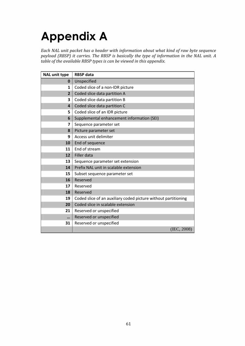
61

Appendix A Each NAL unit packet has a header with information about what kind of raw byte sequence payload (RBSP) it carries. The RBSP is basically the type of information in the NAL unit. A table of the available RBSP types is can be viewed in this appendix.

NAL unit type RBSP data

0 Unspecified

1 Coded slice of a non-IDR picture

2 Coded slice data partition A

3 Coded slice data partition B

4 Coded slice data partition C

5 Coded slice of an IDR picture

6 Supplemental enhancement information (SEI)

7 Sequence parameter set

8 Picture parameter set

9 Access unit delimiter

10 End of sequence

11 End of stream

12 Filler data

13 Sequence parameter set extension

14 Prefix NAL unit in scalable extension

15 Subset sequence parameter set

16 Reserved

17 Reserved

18 Reserved

19 Coded slice of an auxiliary coded picture without partitioning

20 Coded slice in scalable extension

21 Reserved or unspecified

… Reserved or unspecified

31 Reserved or unspecified

(IEC, 2008)

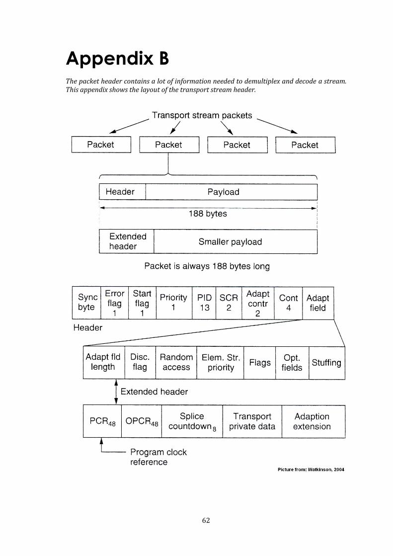
62

Appendix B The packet header contains a lot of information needed to demultiplex and decode a stream. This appendix shows the layout of the transport stream header.

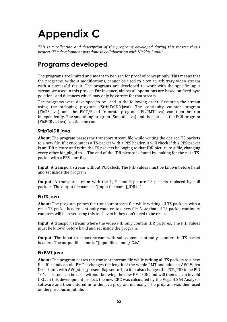
63

Appendix C This is a collection and description of the programs developed during this master thesis project. The development was done in collaboration with Nicklas Lundin.

Programs developed

The programs are limited and meant to be used for proof of concept only. This means that the programs, without modifications, cannot be used to alter an arbitrary video stream with a successful result. The programs are developed to work with the specific input stream we used in this project. For instance, almost all operations are based on fixed byte positions and distances which may only be correct for that stream.

The programs were developed to be used in the following order; first strip the stream using the stripping program (StripToIDR.java). The continuity counter program (FixTS.java) and the PMT/Fixed framrate program (FixPMT.java) can then be run independently. The smoothing program (Smooth.java) and then, at last, the PCR program (FixPCRv2.java) can then be run.

StripToIDR.java

About: The program parses the transport stream file while writing the desired TS packets to a new file. If it encounters a TS-packet with a PES header, it will check if this PES packet is an IDR picture and write the TS packets belonging to that IDR picture to a file, changing every other idr_pic_id to 1. The end of the IDR picture is found by looking for the next TS-packet with a PES start flag.

Input: A transport stream without PCR clock. The PID values must be known before hand and set inside the program

Output: A transport stream with the I-, P- and B-picture TS packets replaced by null packets. The output file name is "[input file name]_IDR.ts".

FixTS.java

About: The program parses the transport stream file while writing all TS packets, with a reset TS-packet header continuity counter, to a new file. Note that all TS-packet continuity counters will be reset using this tool, even if they don't need to be reset.

Input: A transport stream where the video PID only contain IDR pictures. The PID values must be known before hand and set inside the program.

Output: The input transport stream with subsequent continuity counters in TS-packet headers. The output file name is "[input file name]_CC.ts".

FixPMT.java

About: The program parses the transport stream file while writing all TS packets to a new file. If it finds an old PMT it changes the length of the whole PMT and adds an AVC Video Descriptor, with AVC_stills_present flag set to 1, to it. It also changes the PCR_PID to be PID 101. This tool can be used without knowing the new PMT CRC and will then use an invalid CRC. In this development project, the new CRC was calculated by the Vega H.264 Analyzer software and then entered in to the java program manually. The program was then used on the previous input file.

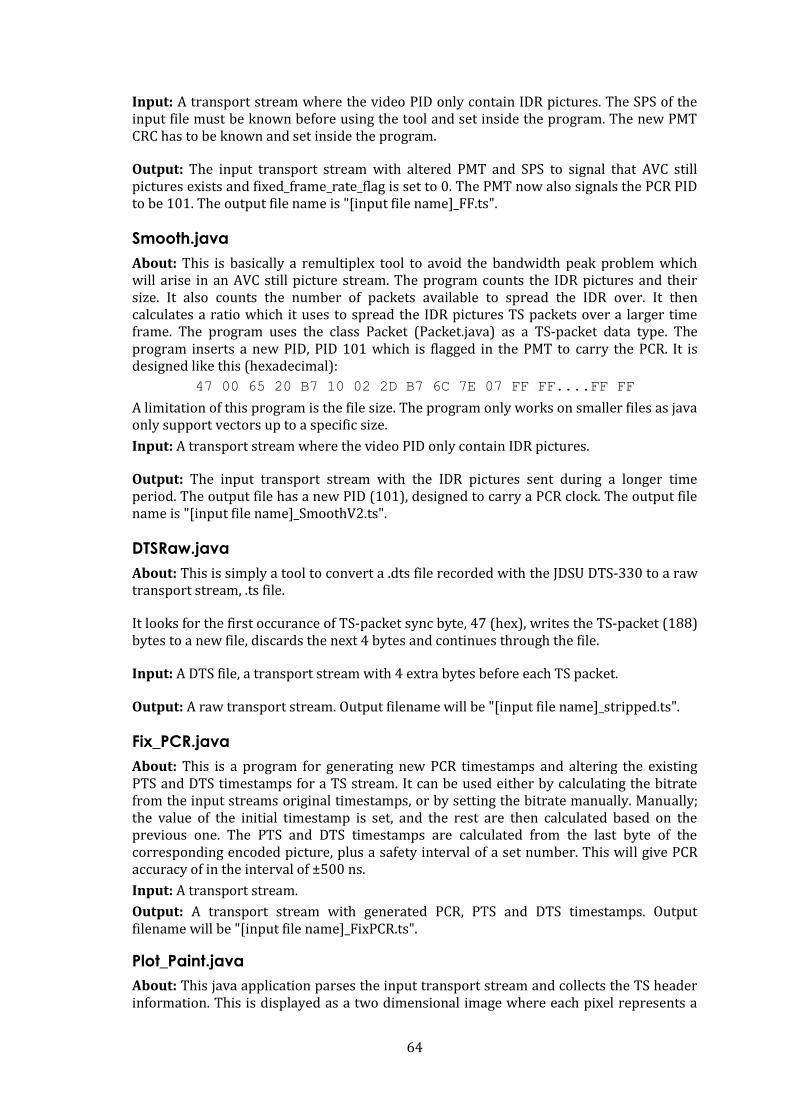
64

Input: A transport stream where the video PID only contain IDR pictures. The SPS of the input file must be known before using the tool and set inside the program. The new PMT CRC has to be known and set inside the program.

Output: The input transport stream with altered PMT and SPS to signal that AVC still pictures exists and fixed_frame_rate_flag is set to 0. The PMT now also signals the PCR PID to be 101. The output file name is "[input file name]_FF.ts".

Smooth.java

About: This is basically a remultiplex tool to avoid the bandwidth peak problem which will arise in an AVC still picture stream. The program counts the IDR pictures and their size. It also counts the number of packets available to spread the IDR over. It then calculates a ratio which it uses to spread the IDR pictures TS packets over a larger time frame. The program uses the class Packet (Packet.java) as a TS-packet data type. The program inserts a new PID, PID 101 which is flagged in the PMT to carry the PCR. It is designed like this (hexadecimal):

47 00 65 20 B7 10 02 2D B7 6C 7E 07 FF FF....FF FF

A limitation of this program is the file size. The program only works on smaller files as java only support vectors up to a specific size.

Input: A transport stream where the video PID only contain IDR pictures.

Output: The input transport stream with the IDR pictures sent during a longer time period. The output file has a new PID (101), designed to carry a PCR clock. The output file name is "[input file name]_SmoothV2.ts".

DTSRaw.java

About: This is simply a tool to convert a .dts file recorded with the JDSU DTS-330 to a raw transport stream, .ts file.

It looks for the first occurance of TS-packet sync byte, 47 (hex), writes the TS-packet (188) bytes to a new file, discards the next 4 bytes and continues through the file.

Input: A DTS file, a transport stream with 4 extra bytes before each TS packet.

Output: A raw transport stream. Output filename will be "[input file name]_stripped.ts".

Fix_PCR.java

About: This is a program for generating new PCR timestamps and altering the existing PTS and DTS timestamps for a TS stream. It can be used either by calculating the bitrate from the input streams original timestamps, or by setting the bitrate manually. Manually; the value of the initial timestamp is set, and the rest are then calculated based on the previous one. The PTS and DTS timestamps are calculated from the last byte of the corresponding encoded picture, plus a safety interval of a set number. This will give PCR accuracy of in the interval of ±500 ns.

Input: A transport stream.

Output: A transport stream with generated PCR, PTS and DTS timestamps. Output filename will be "[input file name]_FixPCR.ts".

Plot_Paint.java

About: This java application parses the input transport stream and collects the TS header information. This is displayed as a two dimensional image where each pixel represents a

65

specific TS header. If there is any timing information present in the input stream the average- bitrate, PCR rate and distance in packets between PCR clock occurrences will be displayed in the output image.

Input: A transport stream

Output: A two dimensional image representation of the TS stream header occurrences, placed in the input file folder. Output filename will be "[input file name]_image.png".

TRITA-CSC-E 2010:145 ISRN-KTH/CSC/E--10/145--SE

ISSN-1653-5715

www.kth.se