Stiffness of sands through a laboratory test database · Stiffness of sands through a laboratory test database ... Simple but effective models of non-linear soil ... curves and data

54

Oztoprak, S. & Bolton, M. D. (2013). Geotechnique 63, No. 1, 54–70 [http://dx.doi.org/10.1680/geot.10.P.078]

Stiffness of sands through a laboratory test database

S. OZTOPRAK� and M. D. BOLTON†

Deformations of sandy soils around geotechnical structures generally involve strains in the range small(0.01%) to medium (0.5%). In this strain range the soil exhibits non-linear stress–strain behaviour,which should be incorporated in any deformation analysis. In order to capture the possible variabilityin the non-linear behaviour of various sands, a database was constructed including the secant shearmodulus degradation curves of 454 tests from the literature. By obtaining a unique S-shaped curve ofshear modulus degradation, a modified hyperbolic relationship was fitted. The three curve-fittingparameters are: an elastic threshold strain ªe, up to which the elastic shear modulus is effectivelyconstant at G0; a reference strain ªr, defined as the shear strain at which the secant modulus hasreduced to 0.5G0; and a curvature parameter a, which controls the rate of modulus reduction. The twocharacteristic strains ªe and ªr were found to vary with sand type (i.e. uniformity coefficient), soilstate (i.e. void ratio, relative density) and mean effective stress. The new empirical expression forshear modulus reduction G/G0 is shown to make predictions that are accurate within a factor of 1.13for one standard deviation of random error, as determined from 3860 data points. The initial elasticshear modulus, G0, should always be measured if possible, but a new empirical relation is shown toprovide estimates within a factor of 1.6 for one standard deviation of random error, as determinedfrom 379 tests. The new expressions for non-linear deformation are easy to apply in practice, andshould be useful in the analysis of geotechnical structures under static loading.

KEYWORDS: laboratory tests; sands; statistical analysis; stiffness

INTRODUCTIONThe degradation of shear modulus with strain has beenobserved in soil dynamics since the 1970s, and the depen-dence of secant shear modulus G on strain amplitude wasillustrated for dynamic loading by a number of researchersusing the resonant column test or improved triaxial tests(Seed & Idriss, 1970; Hardin & Drnevich, 1972a, 1972b;Iwasaki et al., 1978; Kokusho, 1980; Tatsuoka & Shibuya,1991; Yamashita & Toki, 1994). The same concept has beenapplied to static behaviour from the mid-1980s (Jardine etal., 1986; Atkinson & Salfors, 1991; Simpson, 1992; Fahey& Carter, 1993; Mair, 1993; Jovicic & Coop, 1997). Today,non-linear soil behaviour is a widely known and well-under-stood concept. However, there are some limitations to in-corporating this concept into numerical models for sandsbecause of the potential complexity of constitutive models,the requirements of special testing (Atkinson, 2000), and,above all, the difficulty of obtaining undisturbed samples ofsandy materials. In geotechnical practice, decision-makingmust usually be based on simple calculations using a fewparameters that can be found easily from routine tests.Simple but effective models of non-linear soil behaviourshould be developed to satisfy this demand. The possibleerrors arising from the use of simple models must then bequantified.

The stiffness of soils cannot be taken as constant whenstrains increase to the magnitudes generally encounteredaround geotechnical structures. The degradation of shearmodulus with strain should therefore be incorporated into

deformation analyses. There are numerous publications inthe literature on the deformation behaviour of sands. Studiesbased on micromechanics seek to reveal the physical originsof behaviour in the non-linear elastic region. Although thefollowing section reviews the shear modulus degradation ofsandy soils only in the context of continuum mechanics,some micromechanical insights will emerge later when dataare examined. And although the current trend is for deter-mining the stiffness of sandy soils by in situ testing, thefocus here will be on the use of laboratory data obtainedfrom reconstituted and/or high-quality undisturbed samplesand reported in the literature. The issue here will be thedegree of uncertainty involved in the prediction of suchsophisticated data using routine classification data.

A tremendous amount of work has been done to deter-mine the very-small-strain shear modulus and its reductionwith strain. Necessarily, only a few studies will be men-tioned. Following the development of the resonant columntest, Hardin & Black (1966) demonstrated the influence ofvoid ratio (e) and mean effective stress (p9) on the maximum(elastic) shear modulus, G0, through an empirical equationof the form

G0 ¼ A � F(e) � p9ð Þm (1)

where F(e) is a function of void ratio, and A and m arematerial constants. Hardin & Black (1966) proposedF(e) ¼ (eg � e)2=(1þ e), where different values of eg, Aand m were proposed for sands of differing angularity. Thisbasis has been much used in research and practice; todaythere is a general acceptance of taking m as 0.50, whichhappens to conform to Herzian theory for the pressuredependence of conical contacts (Goddard, 1990).

Later research has demonstrated that it is the meaneffective stress acting in the plane of shear that controlsshear modulus, rather than the mean effective stress inthree dimensions (Roesler, 1979). Accordingly, in thetests on axially symmetric soil samples to be reportedhere, the controlling effective stress should be taken as

Manuscript received 5 August 2010; revised manuscript accepted 21March 2012. Published online ahead of print 12 October 2012.Discussion on this paper closes on 1 June 2013, for further details seep. ii.� Department of Civil Engineering, Istanbul University, Turkey;former visiting researcher at the University of Cambridge, UK.† Schofield Centre, Department of Engineering, University of Cam-bridge, UK.

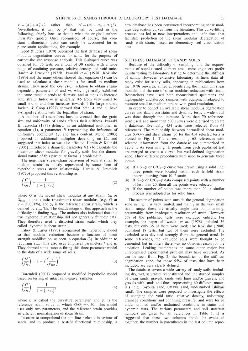
s9 ¼ (� 91 þ � 93)=2 rather than p9 ¼ (� 91 þ � 92 þ � 93)=3:Nevertheless, it will be p9 that will be used in thefollowing, chiefly because that is what the original authorsinvariably quoted. Once recognised, of course, this con-stant arithmetical factor can easily be accounted for inplane-strain applications, for example.

Seed & Idriss (1970) published the first database of shearmodulus degradation curves for sand, for the purpose ofearthquake site response analysis. This S-shaped curve wasobtained for 75 tests on a total of 30 sands, with a widerange of confining pressure, relative density and void ratio.Hardin & Drnevich (1972b), Iwasaki et al. (1978), Kokusho(1980) and the many others showed that equation (1) can beused to calculate a shear modulus for small to mediumstrains. They used the G/F(e)–p9 relation to obtain strain-dependent parameters A and m, which generally exhibitedthe same trend: A tends to decrease and m tends to increasewith strain. Index m is generally 0.5 from very small tosmall strains and then increases towards 1 for large strains.Jovicic & Coop (1997) showed that both A and m haveS-shaped relations with the logarithm of strain.

A number of researchers have advocated that the grainsize and uniformity of sands affects their stiffness. Iwasaki& Tatsuoka (1977) defined, as an additional multiplier inequation (1), a parameter B representing the influence ofuniformity coefficient Uc, and fines content. Menq (2003)proposed an additional multiplier depending on Uc, andsuggested that index m was also affected. Hardin & Kalinski(2005) introduced a diameter parameter f (D) to calculate themaximum shear modulus for gravelly soils, but the dimen-sional nature of this particular factor is problematic.

The non-linear stress–strain behaviour of soils at small tomedium strains is mostly represented by some form ofhyperbolic stress–strain relationship. Hardin & Drnevich(1972b) proposed this relationship as

G

G0

� �¼ 1

1þ ª=ªr

� � (2)

where G is the secant shear modulus at any strain, G0 orGmax is the elastic (maximum) shear modulus (e.g. G atª ¼ 0.0001%), and ªr is the reference shear strain, which isdefined by �max/G0: The disadvantage of this approach is thedifficulty in finding �max: The authors also indicated that thistrue hyperbolic relationship did not generally fit their data.They therefore used a distorted strain scale, which theycalled ‘hyperbolic shear strain’.

Fahey & Carter (1993) reorganised the hyperbolic modelso that modulus reduction became a function of shearstrength mobilisation, as seen in equation (3). In addition torequiring �max, this also uses empirical parameters f and g.They showed some success fitting this three-parameter modelto the data of a wide range of soils.

G

G0

� �¼ 1� f

�

�max

� � g

(3)

Darendeli (2001) proposed a modified hyperbolic modelbased on testing of intact sand-gravel samples

G

G0

� �¼ 1

1þ ª=ªr

� �a (4)

where a is called the curvature parameter, and ªr is thereference strain value at which G/G0 ¼ 0.50. This modeluses only two parameters, and the reference strain providesan efficient normalisation of shear strain.

In order to comprehend the non-linear elastic behaviour ofsands, and to produce a best-fit functional relationship, a

new database has been constructed incorporating shear mod-ulus degradation curves from the literature. This curve-fittingprocess has led to new interpretations and definitions thatfacilitate prediction of the shear modulus degradation ofsands with strain, based on elementary soil classificationdata.

STIFFNESS DATABASE OF SANDY SOILSBecause of the difficulty of sampling, and the require-

ments of sophisticated element tests, most engineers preferin situ testing to laboratory testing to determine the stiffnessof sands. However, extensive laboratory stiffness data al-ready exist for sandy soils, appearing in publications fromthe 1970s onwards, aimed at identifying the maximum shearmodulus and the rate of shear modulus reduction with strain.Researchers have used both reconstituted specimens andhigh-quality undisturbed samples with equipment adapted tomeasure small-to-medium strains with good resolution.

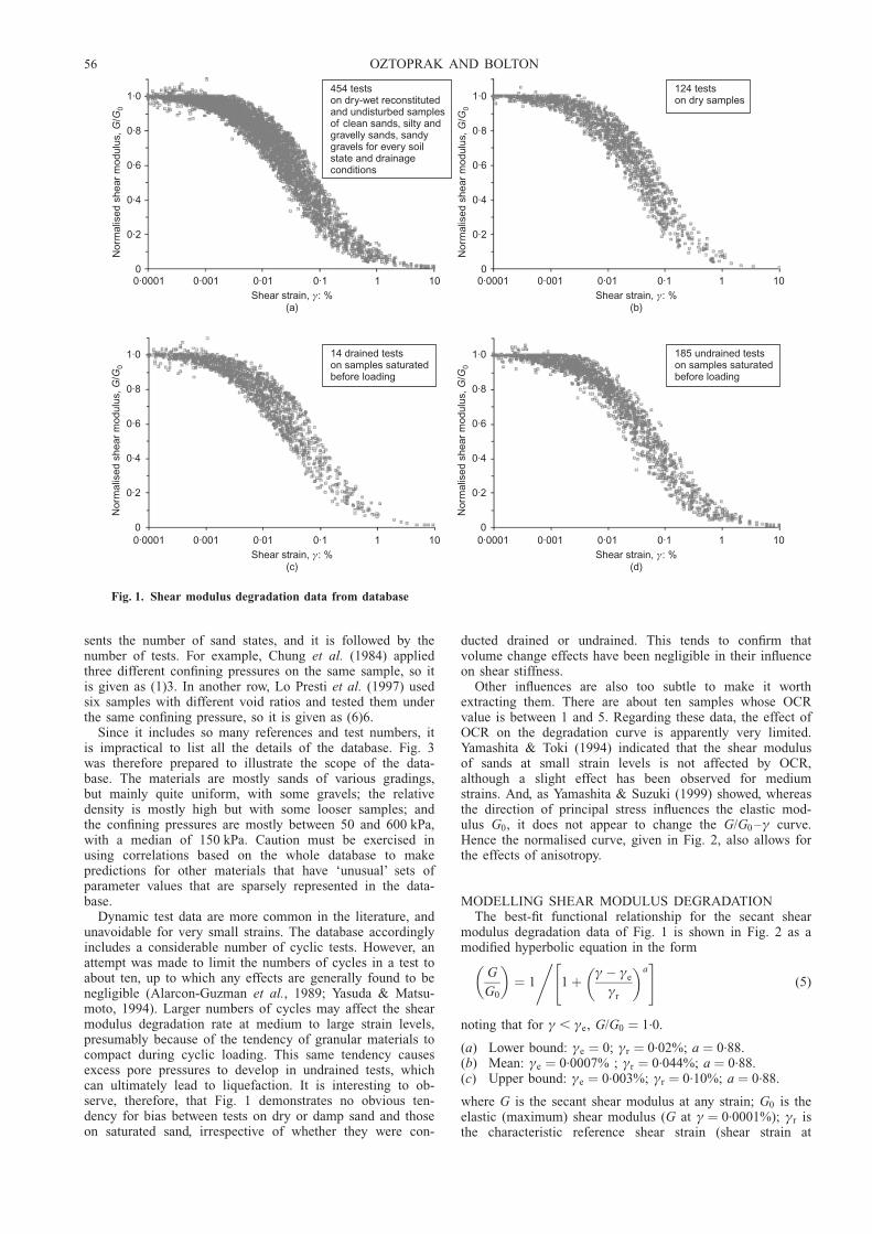
In order to collect all available shear modulus degradationcurves and data from static and dynamic tests, a wide trawlwas done through the literature. More than 70 referenceswere used, and more than 500 curves were digitised to createa database. Eventually 454 tests were selected from 65references. The relationship between normalised shear mod-ulus (G/G0) and shear strain (ª) for the 454 selected tests isplotted in Fig. 1. The corresponding 65 references withselected information from the database are summarised inTable 1. As seen in Fig. 1, points from each published testare merged to create a curved but well-defined degradationzone. Three different procedures were used to generate thesepoints.

(a) If a G–ª or G/G0 –ª curve was drawn using a solid line,three points were located within each tenfold straininterval starting from 10�6 strain.

(b) If G–ª or G/G0 –ª data comprised points with a numberof less than 20, then all the points were selected.

(c) If the number of points was more than 20, a similarprocess was adopted as for solid lines.

The scatter of points seen outside the general degradationzone in Fig. 1 is very limited, and mainly in the very smallstrain range; these are usually single data points arising,presumably, from inadequate resolution of strain. However,5% of the published tests were excluded entirely. Forexample, the paper of Iwasaki et al. (1978) included 36tests, but only 35 of them were used; also Kokusho (1980)published 18 tests, but two of them were excluded. Theexcluded tests deviated strongly from the general trend. Insome references, the excluded soils were thought to becemented, but in others there was no obvious reason for thedeviation. Leaking membranes or some other major butunrecognised experimental problem may have occurred. Ascan be seen from Fig. 2, the boundaries of the stiffnessdegradation zone, for those 95% of tests that have beenincluded, are very clearly defined.

The database covers a wide variety of sandy soils, includ-ing dry, wet, saturated, reconstituted and undisturbed samplesof clean sands, gravels, sands with fines and/or gravels, andgravels with sands and fines, representing 60 different mater-ials (e.g. Toyoura sand, Ottawa sand, undisturbed Ishikarisand). The samples were prepared to investigate the effectsof changing the void ratio, relative density, anisotropy,drainage conditions and confining pressure, and were testedunder drained and/or undrained conditions in static anddynamic tests. The various parameters and soil state/testnumbers are given for all references in Table 1. It issuggested that these two columns should be evaluatedtogether; the number in parentheses in the last column repre-

STIFFNESS OF SANDS THROUGH A LABORATORY TEST DATABASE 55

sents the number of sand states, and it is followed by thenumber of tests. For example, Chung et al. (1984) appliedthree different confining pressures on the same sample, so itis given as (1)3. In another row, Lo Presti et al. (1997) usedsix samples with different void ratios and tested them underthe same confining pressure, so it is given as (6)6.

Since it includes so many references and test numbers, itis impractical to list all the details of the database. Fig. 3was therefore prepared to illustrate the scope of the data-base. The materials are mostly sands of various gradings,but mainly quite uniform, with some gravels; the relativedensity is mostly high but with some looser samples; andthe confining pressures are mostly between 50 and 600 kPa,with a median of 150 kPa. Caution must be exercised inusing correlations based on the whole database to makepredictions for other materials that have ‘unusual’ sets ofparameter values that are sparsely represented in the data-base.

Dynamic test data are more common in the literature, andunavoidable for very small strains. The database accordinglyincludes a considerable number of cyclic tests. However, anattempt was made to limit the numbers of cycles in a test toabout ten, up to which any effects are generally found to benegligible (Alarcon-Guzman et al., 1989; Yasuda & Matsu-moto, 1994). Larger numbers of cycles may affect the shearmodulus degradation rate at medium to large strain levels,presumably because of the tendency of granular materials tocompact during cyclic loading. This same tendency causesexcess pore pressures to develop in undrained tests, whichcan ultimately lead to liquefaction. It is interesting to ob-serve, therefore, that Fig. 1 demonstrates no obvious ten-dency for bias between tests on dry or damp sand and thoseon saturated sand, irrespective of whether they were con-

ducted drained or undrained. This tends to confirm thatvolume change effects have been negligible in their influenceon shear stiffness.

Other influences are also too subtle to make it worthextracting them. There are about ten samples whose OCRvalue is between 1 and 5. Regarding these data, the effect ofOCR on the degradation curve is apparently very limited.Yamashita & Toki (1994) indicated that the shear modulusof sands at small strain levels is not affected by OCR,although a slight effect has been observed for mediumstrains. And, as Yamashita & Suzuki (1999) showed, whereasthe direction of principal stress influences the elastic mod-ulus G0, it does not appear to change the G/G0 –ª curve.Hence the normalised curve, given in Fig. 2, also allows forthe effects of anisotropy.

MODELLING SHEAR MODULUS DEGRADATIONThe best-fit functional relationship for the secant shear

modulus degradation data of Fig. 1 is shown in Fig. 2 as amodified hyperbolic equation in the form

G

G0

� �¼ 1 1þ ª� ªe

ªr

� �a" #,

(5)

noting that for ª , ªe, G/G0 ¼ 1.0.

(a) Lower bound: ªe ¼ 0; ªr ¼ 0.02%; a ¼ 0.88.(b) Mean: ªe ¼ 0.0007% ; ªr ¼ 0.044%; a ¼ 0.88.(c) Upper bound: ªe ¼ 0.003%; ªr ¼ 0.10%; a ¼ 0.88.

where G is the secant shear modulus at any strain; G0 is theelastic (maximum) shear modulus (G at ª ¼ 0.0001%); ªr isthe characteristic reference shear strain (shear strain at

0

0·2

0·4

0·6

0·8

1·0

0·0001 0·001 0·01 0·1 1 10

Nor

mal

ised

she

ar m

odul

us,

/G

G0

Shear strain, : %(c)

γ

14 drained testson samples saturatedbefore loading

0·0001 0·001 0·01 0·1 1 10Shear strain, : %

(d)γ

185 undrained testson samples saturatedbefore loading

0

0·2

0·4

0·6

0·8

1·0

Nor

mal

ised

she

ar m

odul

us,

/G

G0

454 testson dry-wet reconstitutedand undisturbed samplesof clean sands, silty andgravelly sands, sandygravels for every soilstate and drainageconditions

124 testson dry samples

0

0·2

0·4

0·6

0·8

1·0

Nor

mal

ised

she

ar m

odul

us,

/G

G0

0

0·2

0·4

0·6

0·8

1·0

Nor

mal

ised

she

ar m

odul

us,

/G

G0

0·0001 0·001 0·01 0·1 1 10Shear strain, : %

(a)γ

0·0001 0·001 0·01 0·1 1 10Shear strain, : %

(b)γ

Fig. 1. Shear modulus degradation data from database

56 OZTOPRAK AND BOLTON

Ta

ble

1.

Su

mm

ary

of

the

da

tab

ase

use

dfo

rth

isst

ud

y

Ref

eren

ceS

oil

mat

eria

lsan

dd

escr

ipti

on

Tes

tty

pe

and

dra

inag

eC

han

ged

fact

ors

Nu

mb

ero

fte

sts

Ala

rco

n-G

uzm

anet

al.

(19

89

)O

ttaw

a2

0/3

0sa

nd

(dry

,v

ibra

ted

)R

CT

+T

ST

,R

CT

e,O

CR

,st

ress

rati

o,

p9

(8)1

1A

ran

go

(20

06

)C

alca

reo

us

and

sili

casa

nd

s(d

ry,

rem

ou

lded

)R

CT

e,p9

(5)1

7C

aval

laro

eta

l.(2

00

3)

No

toso

il(u

nd

istu

rbed

lig

htl

yce

men

ted

silt

ysa

nd

)R

CT

+C

LT

ST

(U)

e,p9

(2)2

Ch

arif

(19

91

)H

ost

un

san

d(c

om

pac

ted

)T

XT

(D)

e,p9

(3)5

Ch

egin

i&

Tre

nte

r(1

99

6)

Gla

cial

till

(un

dis

turb

ed,

incl

ud

esco

arse

mat

eria

l)R

CT

(U)

PI,

sto

ne

con

ten

t,p

9(4

)7C

hu

ng

eta

l.(1

98

4)

Mo

nte

rey

san

dN

o.

0C

LT

XT

(U)

p9

(1)3

Del

foss

e-R

ibay

eta

l.(2

00

4)

Fo

nta

ineb

leau

san

d(w

ith

/wit

ho

ut

sod

ium

sili

cate

gro

ute

d)

RC

T+

CL

TX

T(U

)p

9(2

)2D

on

get

al.

(19

94

)H

ime

gra

vel

(air

-dri

ed,

com

pac

ted

)M

LT

XT

(D)

e,D

50,U

c(2

)2D

’On

ofr

io&

Pen

na

(20

03

)S

ilty

san

d(c

om

pac

ted

)R

CT

,C

LT

ST

(D)

e,p9

(4)7

Drn

evic

h&

Ric

har

t(1

97

0)

Ott

awa

30

/50

san

d(d

ry)

RC

Te,

p9

(1)3

Ell

iset

al.

(20

00

)F

ine

and

coar

sesi

lica

san

d(d

ry),

Toy

ou

rasa

nd

(dry

and

satu

rate

d)

RC

Te,

D50,U

c(2

)2F

iora

van

teet

al.

(19

94

)Q

uio

usa

nd

(car

bo

nat

ic,

low

-den

sity

reco

nst

itu

ted

)R

CT

(D)

e,O

CR

,p

9(5

)7G

oto

eta

l.(1

98

7)

Gra

vel

(un

dis

turb

edan

dre

con

stit

ute

d)

CL

TX

T(U

)I D

,p9

(2)2

Go

toet

al.

(19

92

)G

ravel

(un

dis

turb

edan

dre

con

stit

ute

d,2

4%

and

44

%sa

nd

con

ten

t)C

LT

XT

(U)

Sam

pli

ng

dep

th,G

o(4

)4H

ard

in&

Drn

evic

h(1

97

2a)

San

d(c

lean

and

dry

)C

LS

ST

p9

(5)5

Har

din

&D

rnev

ich

(19

72

b)

San

d(c

lean

and

dry

)C

LS

ST

p9

(1)2

Har

din

&K

alin

ski

(20

05

)O

ttaw

asa

nd,

san

ds

(dry

),g

ravel

–sa

nd

–si

ltm

ixtu

re(w

et)

RC

T(D

)e,

p9

(2)6

Has

hib

a(1

97

1)

On

aham

asa

nd

(dry

,re

mo

uld

ed)

SS

Te,

p9

(2)4

Hat

anak

a&

Uch

ida

(19

95

)T

okyo

gra

vel

(un

dis

turb

edan

dre

con

stit

ute

d,sa

nd

y,in

clu

des

fin

es)

CL

TX

T(U

)G

o(2

)2H

atan

aka

eta

l.(1

98

8)

To

kyo

gra

vel

(un

dis

turb

edan

dre

con

stit

ute

d,sa

nd

y,in

clu

des

fin

es)

CL

TX

T(U

)p

9(2

)4Is

hih

ara

(19

96

)F

uji

saw

asa

nd

(un

dis

turb

edan

dre

con

stit

ute

d)

TS

T(U

)e

(4)4

Ito

eta

l.(1

99

9)

San

dy

gra

vel

(un

dis

turb

edan

dim

pro

ved

by

gro

uti

ng

)C

LT

XT

(D)

e,D

50,p

9(4

)4Iw

asak

iet

al.

(19

78

)T

oyo

ura

,B

an-n

osu

,Ir

um

a,K

injo

-1,

Kin

jo-2

,O

hg

i-S

him

a,M

on

tere

ysa

nd

sR

CT

,T

ST

(D)

e,p9

(23

)35

Jard

ine

eta

l.(2

00

1)

Du

nq

erq

ue

san

dT

XT

,T

ST

(D)

OC

R,

test

typ

e(2

)3K

atay

ama

eta

l.(1

98

6)

San

d(u

nd

istu

rbed

and

reco

nst

itu

ted

)R

CT

Sam

pli

ng

dep

th,G

o(4

)4K

og

aet

al.

(19

94

)G

ravel

lyso

il(d

ry,re

con

stit

ute

d)

CL

TS

TG

ravel

con

ten

t(5

)5K

ok

ush

o(1

98

0)

Gif

uan

dT

oyo

ura

san

ds

(co

mp

acte

d,sa

tura

ted

)C

LT

XT

Dra

inag

e,e,

p9

(10

)16

Ko

ku

sho

&E

sash

i(1

98

1)

Toy

ou

rasa

nd

(sat

ura

ted

),u

nd

istu

rbed

dil

uv

ial

san

d,g

ravel

(sat

ura

ted

)C

LT

XT

(U)

e,p9

(3)1

1K

ok

ush

o&

Tan

aka

(19

94

)G

ravel

(un

dis

turb

edan

dre

con

stit

ute

d)

CL

TX

T(U

)p

9(7

)7L

aird

&S

tok

oe

(19

93

)S

and

(dry

,re

mo

uld

ed)

CL

TX

T,

RC

T(U

)p

9(1

)6L

anzo

eta

l.(1

99

7)

San

taM

on

ica

and

An

telo

pe

Val

ley

san

ds

(rec

on

stit

ute

d,in

clu

des

silt

)D

SS

T(D

)e,

OC

R,

p9

(6)1

0L

oP

rest

iet

al.

(19

97

)T

oyo

ura

and

Qu

iou

san

ds

(dry

,h

oll

ow

cyli

nd

er)

ML

TS

Te

(6)6

Mah

eret

al.

(19

94

)O

ttaw

asa

nd

(med

ium

and

loo

se,

un

trea

ted

and

chem

ical

lyg

rou

ted

)R

CT

+C

LT

XT

I D,

con

cen

trat

ion

,cu

rin

gti

me

(8)1

1M

enq

(20

03

)W

ash

edm

ort

arsa

nd,

san

dan

dg

ravel

lysa

nd

(dry

)R

CT

e,D

50,U

c(7

)7M

enq

&S

tok

oe

(20

03

)S

and

(den

sean

dd

ry)

RC

Tp

9(1

)3O

gat

a&

Yas

ud

a(1

98

2)

Gra

vel

lyso

il(u

nd

istu

rbed

,in

clu

des

fin

es)

TX

Tp

9(1

)2P

ark

(19

93

)T

oyo

ura

san

d(a

ir-d

ried

,is

otr

op

icco

nso

lid

ated

)P

SC

T,

TX

TO

CR

,p

9(2

)2P

oro

vic

&Ja

rdin

e(1

99

4)

Ham

Riv

ersa

nd

(K0

and

iso

tro

pic

con

soli

dat

ed)

RC

T+

TS

T(U

)C

on

soli

dat

ion

pre

ssu

re,

e,O

CR

(8)8

Ro

llin

set

al.

(19

98

)S

and

and

gra

vel

lysa

nd

(co

mp

acte

d,sa

tura

ted

)R

CT

(U)

e,g

ravel

con

ten

t,p

9(1

)5S

axen

aet

al.

(19

88

)M

on

tere

ysa

nd

(co

mp

acte

d,sa

tura

ted,

wit

h/w

ith

ou

tce

men

t,cu

rin

g)

RC

T(D

)I D

,ce

men

tco

nte

nt,

curi

ng

tim

e,p

9(1

4)2

2S

eed

eta

l.(1

98

6)

Gra

vel

(Oro

vil

lean

dP

yra

mid

mat

eria

ls)

CL

TX

T(U

)e

(2)2

Sh

ibu

ya

eta

l.(1

99

6)

Hig

ash

i-O

hg

ijim

asa

nd

(un

dis

turb

ed)

CL

TX

T,

TS

T(U

)S

amp

lin

gd

epth

,p

9(8

)8S

ilver

&S

eed

(19

71

)Q

uar

tzsa

nd

(cry

stal

sili

caN

o.2

0,

dry

)C

LS

ST

p9

(1)3

Sto

ko

eet

al.

(19

94

)S

and

(un

dis

turb

edan

dd

ry-r

emo

uld

ed)

CL

TS

T,R

CT

e,p9

(5)9

Sto

ko

eet

al.

(19

99

)S

ilty

san

d(u

nd

istu

rbed

)R

CT

Sam

pli

ng

dep

th,p

9(4

)4T

anak

aet

al.

(19

87

)G

ravel

lysa

nd

CL

TX

TG

ravel

con

ten

t,p9

(2)6

Tea

chav

ora

sin

sku

net

al.

(19

91

)T

oyo

ura

san

d(d

ense

)T

SS

T(D

)e,

OC

R(2

)2


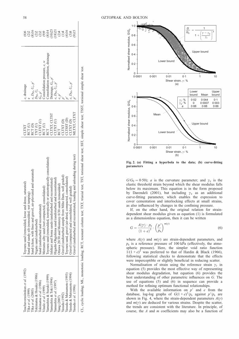
G/G0 ¼ 0.50); a is the curvature parameter; and ªe is theelastic threshold strain beyond which the shear modulus fallsbelow its maximum. This equation is in the form proposedby Darendeli (2001), but including ªe as an additionalcurve-fitting parameter, which enables the expression tocover cementation and interlocking effects at small strains,as also influenced by changes in the confining pressure.

If, on the other hand, the original relation for strain-dependent shear modulus given as equation (1) is formulatedas a dimensionless equation, then it can be written

G ¼A ªð Þ � pa

1þ eð Þ3� p9

pa

� �m(ª)

(6)

where A(ª) and m(ª) are strain-dependent parameters, andpa is a reference pressure of 100 kPa (effectively, the atmo-spheric pressure). Here, the simpler void ratio function1/(1 + e)3 was preferred to that of Hardin & Black (1966),following statistical checks to demonstrate that the effectswere imperceptible or slightly beneficial in reducing scatter.

Normalisation of strain using the reference strain ªr inequation (5) provides the most effective way of representingshear modulus degradation, but equation (6) provides thebest understanding of other parametric influences on G. Theuse of equations (5) and (6) in sequence can provide amethod for refining optimum functional relationships.

With the available information on p9 and e from thedatabase, log-log graphs of G(1 + e)3/pa against p9/pa areshown in Fig. 4, where the strain-dependent parameters A(ª)and m(ª) are deduced for various strains. Despite the scatter,the trends are consistent with the literature. In principle, ofcourse, the A and m coefficients may also be a function ofT

each

avo

rasi

nsk

un

eta

l.(1

99

2)

Toy

ou

rasa

nd

(rem

ou

lded

,lo

ose

and

den

se,

satu

rate

d)

CL

TX

Te,

dra

inag

e(6

)6T

ika

eta

l.(1

99

9)

San

dan

dsa

nd

ysi

lt(r

emo

uld

ed;

wet

tam

pin

g)

RC

T(U

)e

(2)2

Tik

aet

al.

(20

03

)S

and

(cle

an,

wit

hfi

nes

and

gra

vel

,ai

r-p

luv

iate

dan

dsa

tura

ted

)R

CT

(D)

e,D

50,U

c,

p9

(8)1

6T

ok

imat

su&

Ho

sak

a(1

98

6)

Nig

ata

san

d(u

nd

istu

rbed

)T

XT

(U)

D50,

Uc

(2)2

To

kim

atsu

eta

l.(1

98

6)

San

d(u

nd

istu

rbed

and

reco

nst

itu

ted

)C

LT

XT

(U)

Go,p

9(2

)2V

inal

eet

al.

(19

99

)M

etra

mo

silt

ysa

nd

(wet

com

pac

ted,

con

soli

dat

ed)

RC

T(U

)C

on

soli

dat

ion

pre

ssu

re,

e,w

(9)9

Yam

ash

ita

&S

uzu

ki

(19

99

)T

oyo

ura

san

d(r

emo

uld

ed,is

otr

op

ical

lyo

ran

iso

tro

pic

ally

con

soli

dat

ed)

RC

TC

on

soli

dat

ion

con

dit

ion

,d

rain

age

(8)1

4Y

amas

hit

a&

To

ki

(19

94

)Is

hik

ari

and

So

ma

san

ds

(un

dis

turb

edan

dre

con

stit

ute

d)

CL

TX

T,

CL

TS

TD

rain

age,

Go,p

9(1

0)2

5Y

amas

hit

aet

al.

(19

97

)H

igas

hi-

Oh

gis

him

asa

nd

(un

dis

turb

edan

dre

con

stit

ute

d)

CL

TX

T(U

)e,

D50,U

c,

p9

(18

)21

Yan

g(2

00

7)

Ott

awa

20

/30

and

Mo

nte

rey

0/3

0sa

nd

s(r

emo

uld

ed)

RC

Te,

p9

(2)4

Yas

ud

a(1

99

2)

Gra

vel

(un

dis

turb

edsa

mp

lefr

om

Mih

oD

am,

wel

lg

rad

ed)

CL

TX

T(D

)p

9(1

)4Y

asu

da

&M

atsu

mo

to(1

99

3)

Toy

ou

rasa

nd,

gra

vel

(air

-dri

ed,

com

pac

ted,

con

soli

dat

ed)

CL

TS

ST

(D)

p9

(4)1

6Y

asu

da

&M

atsu

mo

to(1

99

4)

Gra

vel

(co

mp

acte

dan

dco

nso

lid

ated

,w

ell

gra

ded

)C

LT

XT

(D)

e,D

50,U

c,

p9

(3)8

Yas

ud

aet

al.

(19

96

)G

ravel

(un

dis

turb

edan

dre

con

stit

ute

d,lo

adin

gan

du

nlo

adin

gd

uri

ng

test

)M

LT

XT

,C

LT

XT

p9

(9)1

5

CL

,cy

clic

load

ing

;M

L,

mo

no

ton

iclo

adin

g;

RC

T,

reso

nan

tco

lum

nte

st;

TX

T,

tria

xia

lte

st;

TS

T,

tors

ion

alsh

ear

test

;S

ST

,si

mp

lesh

ear

test

;T

SS

T,

tors

ion

alsi

mp

lesh

ear

test

.

0

0·2

0·4

0·6

0·8

1·0

Nor

mal

ised

she

ar m

odul

us,

/G

G0

Upper bound

0·0001 0·001 0·01 0·1 1 10

Shear strain, : %(a)

γ

Lower bound

GG0

�1

1 �γ γ

γ� e

r

⎛⎜⎝ ⎛

⎜⎝a

0

0·2

0·4

0·6

0·8

1·0

Nor

mal

ised

she

ar m

odul

us,

/G

G0

Upper bound

0·0001 0·001 0·01 0·1 1 10

Shear strain, : %(b)

γ

Lower bound

Mean

Lowerbound Mean

Upperbound

0·020

0·88

0·0440·00070·88

0·10·0030·88

γr: %γe: %

a

Fig. 2. (a) Fitting a hyperbola to the data; (b) curve-fittingparameters


p9. In order to investigate this, equations (5) and (6), whichare alternative methods of representing shear modulus calcu-lations at any strain level, can be compared.

To plot the results of equation (6) on the mean curve ofG/G0 against ª, p9 in equation (6) can be assigned as150 kPa, which is the average value of the median stressrange in Fig. 3. Since G/G0 is to be calculated, the voidratio function cancels, and is not required. Using p9, A(ª)and m(ª) from Fig. 4, the G/G0 values can readily becalculated and placed on Fig. 5(a), where they lie very closeto the mean curve, but not exactly on it. Since the normal-ised shear modulus curve gives a more reliable relation thanthe scattered relationship shown in Fig. 4, it is preferred to

modify the A(ª) and m(ª) values slightly from the valueslisted in Fig. 4 so as to fit exactly the mean curve in Fig.5(a). The refined values appear in Fig. 6.

Once the calculated G/G0 values of equation (5) havebeen fitted to the mean hyperbolic curve in Fig. 5(a) for themean pressure p9 ¼ 150 kPa, other p9 values can be insertedin equation (6), and appropriate values of ªe and ªr can bederived from equation (5) to fit the new curves. The result-ing family of degradation curves for varying p9 is shown inFig. 5(b). Fig. 6(b), accumulating the results of 379 tests,shows that G0 can best be expressed as a function of (p9)0:5

at very small strains and as a function of p9 for large strains.If the resulting m(ª) relation is compared with the published

0

40

80

120

160

200

�50

50–1

00

100–

200

200–

400

400–

600

�60

0

Test

num

ber

Confinement pressure: kPa(a)

452 testsAverage 157 kPaMedian 150 kPa

��

0

20

40

60

80

100

0·10

–0·2

5

0·25

–0·4

0

0·40

–0·5

5

0·55

–0·6

5

0·65

–0·7

0

0·70

–0·8

0

0·80

–0·9

5

0·95

–1·1

5

Test

num

ber

Void ratio,(b)

e

422 testsAverage 0·67Median 0·675

��

020406080

100

Test

num

ber

Average grain size, : mm(d)

D50

120

0·10

–0·1

4

0·14

–0·2

0

0·20

–0·3

0

0·30

–0·7

0

0·70

–1·5

0

1·50

–10·

0

10·0

–20·

0

�20

·0

0

20

40

60

80

100

Test

num

ber

Uniformity coefficient,(e)

Uc

�1·

15

1·15

–1·3

5

1·35

–1·5

5

1·55

–1·9

5

1·95

–5·0

5·0–

10·0

10·0

–30·

0

�30

·0

0

50

100

150

200

250

300

Test

num

ber

Sampling(f)

Dry

Wet

UD

Dra

ined

Und

rain

ed NA


��

0

20

40

60

80

100

Test

num

ber

Relative density,(c)

ID

�0·

25

0·90

–0·9

5

0·25

–0·4

2

0·42

–0·6

0

0·60

–0·8

0

�0·

95

0·80

–0·9

0

363 testsAverage 4·2 mmMedian 0·50 mm

��


��

For 328 wet andUD samples

Fig. 3. Statistical information about database in terms of test numbers

10

100

1000

10000

100000

0·1 1 10

GV

p3

a/

p p�0 a/

(a)

0·1 1 10

p p�0 a/

(b)

y xR

57600·2278

��

0·49

2y xR

55200·2398

��

0·51

2

0·1 1 10

p p�0 a/

(c)

y xR

45000·2667

��

0·53

2

10

100

1000

10000

100000

0·1 1 10

GV

p3

a/

p p�0 a/

(d)

0·1 1 10

p p�0 a/

(e)

y xR

18100·4187

��

0·73

2y xR

3700·1533

��

0·86

2

γ: % A( )γ m( )γ

0·0001

0·001

0·01

0·1

1

5760

5520

4500

1810

370

0·49

0·51

0·53

0·73

0·86

Fig. 4. Shear modulus variation with mean effective stress: (a) ª 0.0001% (379 tests); (b) ª 0.001% (379 tests); (c) ª 0.01% (374tests); (d) ª 0.1% (221 tests); (e) ª 1% (77 tests)


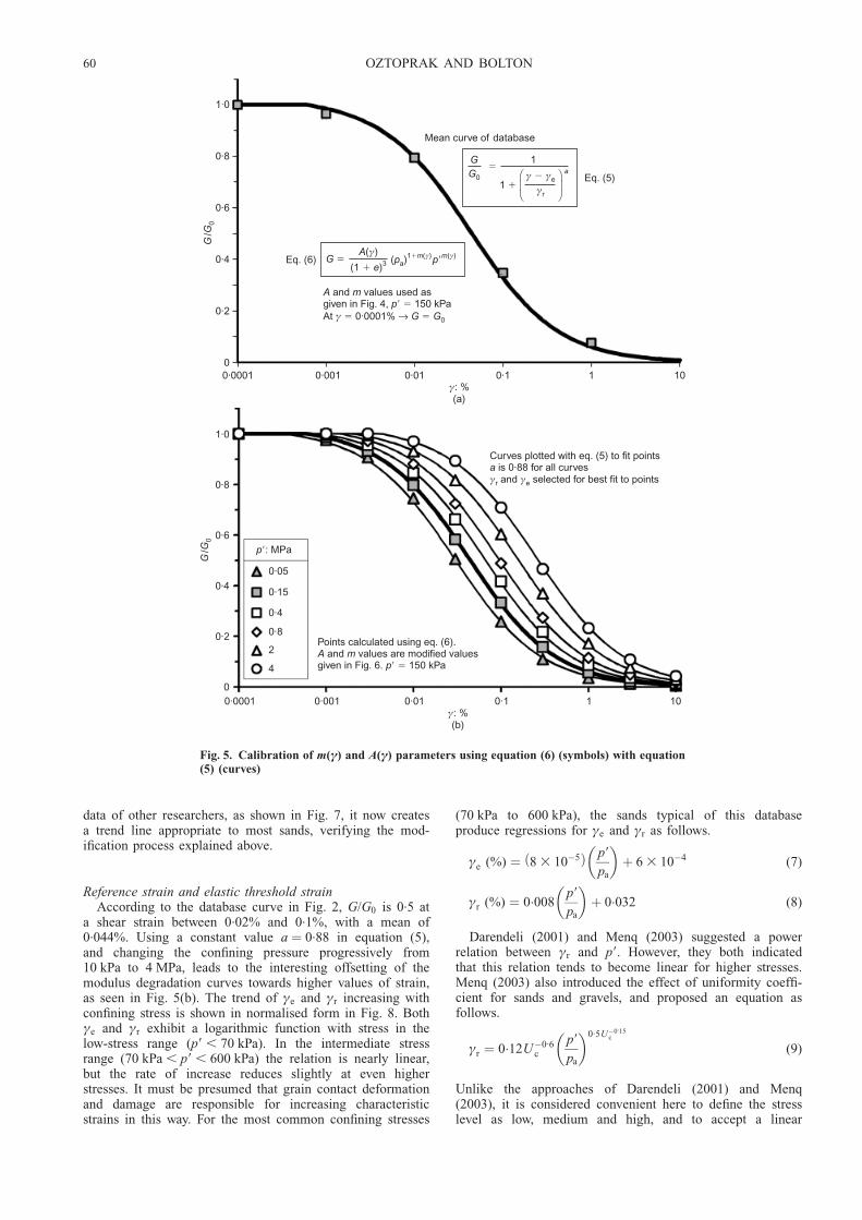
data of other researchers, as shown in Fig. 7, it now createsa trend line appropriate to most sands, verifying the mod-ification process explained above.

Reference strain and elastic threshold strainAccording to the database curve in Fig. 2, G/G0 is 0.5 at

a shear strain between 0.02% and 0.1%, with a mean of0.044%. Using a constant value a ¼ 0.88 in equation (5),and changing the confining pressure progressively from10 kPa to 4 MPa, leads to the interesting offsetting of themodulus degradation curves towards higher values of strain,as seen in Fig. 5(b). The trend of ªe and ªr increasing withconfining stress is shown in normalised form in Fig. 8. Bothªe and ªr exhibit a logarithmic function with stress in thelow-stress range (p9 , 70 kPa). In the intermediate stressrange (70 kPa , p9 , 600 kPa) the relation is nearly linear,but the rate of increase reduces slightly at even higherstresses. It must be presumed that grain contact deformationand damage are responsible for increasing characteristicstrains in this way. For the most common confining stresses

(70 kPa to 600 kPa), the sands typical of this databaseproduce regressions for ªe and ªr as follows.

ªe (%) ¼ 8 3 10�5ð Þ p9

pa

� �þ 6 3 10�4 (7)

ªr (%) ¼ 0:008p9

pa

� �þ 0:032 (8)

Darendeli (2001) and Menq (2003) suggested a powerrelation between ªr and p9. However, they both indicatedthat this relation tends to become linear for higher stresses.Menq (2003) also introduced the effect of uniformity coeffi-cient for sands and gravels, and proposed an equation asfollows.

ªr ¼ 0:12U�0:6c

p9

pa

� �0:5U�0:15c

(9)

Unlike the approaches of Darendeli (2001) and Menq(2003), it is considered convenient here to define the stresslevel as low, medium and high, and to accept a linear

0

0·2

0·4

0·6

0·8

1·0

0·0001 0·001 0·01 0·1 1 10

GG/

0

γ: %(a)

GG0

�1

1 �γ γ

γ� e

r

⎛⎜⎝ ⎛

⎜⎝a

Eq. (5)

Mean curve of database

G �A

e

( )

(1 )

γ

� 3 ( )p pa1 ( ) ( )�m mγ γ�Eq. (6)

A mp

G G

and values used asgiven in Fig. 4, 150 kPaAt 0·0001%

� �� γ → 0

0

0·2

0·4

0·6

0·8

1·0

0·0001 0·001 0·01 0·1 1 10

GG/

0

γ: %(b)

p�: MPa

0·05

0·15

0·4

0·8

2

4

Points calculated using eq. (6).and values are modified values

given in Fig. 6. 150 kPaA m

p� �

Curves plotted with eq. (5) to fit pointsis 0·88 for all curvesand selected for best fit to points

aγ γr e

Fig. 5. Calibration of m(ª) and A(ª) parameters using equation (6) (symbols) with equation(5) (curves)


relation for medium and high stress levels. Moreover, alinear relation offers a better fit to the data than a powerrelation, at least for medium stress levels (70–600 kPa).Further support for a linear relation between ªr and p9comes from the normalised shear modulus degradation ofToyoura sand reported by Iwasaki et al. (1978) and Kokusho(1980), and plotted in Fig. 9. The corresponding changes inªr are plotted in Fig. 10 for the stress range 50–300 kPa;the trend is obviously linear. The presumed cause of thedifferent intercepts in Fig. 10 is the relative density of the

respective trials, and possibly the influence of water atthe smallest confining stresses. However, the gradients forthis material in Fig. 10 are identical.

To generalise the relation between ªr and p9, the databasewas searched for all those soils on which tests were con-ducted at three or more confining pressures, providing datafor the evolution of ªr: This identified 24 sandy soils, andtheir data were split into four groups, as shown in Fig. 11. Itcan be confirmed that almost all the plots of ªr exhibit alinear trend with increasing mean effective stress. As seenfrom Fig. 11, both uniformity and relative density exert asignificant influence on the ªr–p9/pa relation. Fig. 11 there-fore represents the functional dependence of ªr on p9, ID

and Uc for different states and types of sandy soils.Various regressions are given in Fig. 12. Fig. 12(a) shows

a power relation between ªr and void ratio e, albeit with amoderate coefficient of determination R2 ¼ 0.54. Fig. 12(b)shows negligible correlation between ªr and relative densityID, but Fig. 12(c) demonstrates a much-improved R2 ¼ 0.74for a power law correlation between ªr and the product eID:This was initially unexpected. However, it is proposed thatthe group eID may be a surrogate for grain shape, which isthe most significant omission from the current study of sandcharacteristics in relation to stiffness degradation. High voidratio for a rounded sand would indicate low relative density,so the product eID would also be small, whereas an angularsand could have a high void ratio at a high relative densityand give a large product eID: So the magnitude of eID mayindicate angularity. This possible explanation cannot beverified, since the authors whose work we have used did notgenerally remark on grain shape. Nevertheless, the statisticalfinding is significant.

If one equation will cover all these effects for calculatingªr, it must be expressed in the form

ªr (%) ¼ cp9

pa

� �þ d (10)

for medium stress levels. From Fig. 11, it is understood thatUc affects the slope of the ªr–p9/pa relation, and from Figs10, 11 and 12 that the product eID affects the ordinate.Accepting these functional relationships, a multivariableregression analysis for medium stress levels then producedthe relation

6000

5000

4000

3000

2000

1000

0

A(

)γ

0·0001 0·001 0·01 0·1 1 10γ: %(a)

0·0001 0·001 0·01 0·1 1 10γ: %(b)

1·1

1·0

0·9

0·8

0·7

0·6

0·5

0·4

m(

)γ

γ: % A( )γ

0·00010·0010·0030·010·030·10·31310

576055205230452031501810880370180126

γ: % m( )γ

0·00010·0010·0030·010·030·10·31310

0·500·510·530·560·630·730·830·930·991·00

Fig. 6. Modified relations of m(ª) and A(ª)

0·0001 0·001 0·01 0·1 1 10γ: %

Yasuda & Matsumoto (1993), gravel, undr. test,0·42, 0·70, 14 mm, 7e I D U� � � �D 50 c

This study

Silver & Seed (1971)silica sand No. 20, dry,

0·83, 0·45e I� �D

Kokusho (1980), Toyoura sand,undr. test, dense, 0·64,

0·29, 1·8e

D U�

� �50 c

Yamashita & Toki (1994), Toyoura sand,undr. test, 0·688, 0·80, 0·2, 1·3e I D U� � � �D 50 c

Drnevich (1966), Ottawa sand 30/50, dry, 0·55e �

Iwasaki (1993), Toyoura sand, saturated,dr test, 0·68, 0·88, 0·16 mm, 1·46

et al.e I D U� � � �D 50 c

Yamashita & Toki (1994), Ishikarasand (UD), saturated, undr. test,

0·928, 0·84,0·12, 1·7

e ID U

� ��

D

50 c

1·1

1·0

0·9

0·8

0·7

0·6

0·5

0·4

0·3

m(

)γ

Fig. 7. Comparison of strain-dependent values of m with those from other work


ªr (%) ¼ 0:01U�0:3c

p9

pa

� �þ 0:08eID (11)

It is interesting to reflect on the physical origins ofgranular behaviour that could lead to the parametric influ-ences in equation (11). An increase in uniformity coefficientUc leads to a reduction in ªr – that is, to a swifter loss ofelastic stiffness with strain. McDowell & Bolton (1999)discussed the consequences of a dispersion of particle sizesin terms of the strain incompatibility between the fine matrixand the larger particle. The introduction of large particlesinevitably causes premature sliding of smaller particles incontact with them. Since a sliding contact no longer con-tributes its tangential shear stiffness to the global shearmodulus, the onset of sliding coincides with the reduction ofG/G0: In other words, the reference strain ªr is reducedwhen there is a greater disparity in grain sizes. Equation(11) supports this finding.

According to equation (11), it must also be accepted thatincreased mean effective stress p9 or increased relativedensity ID (noting that an increase in ID overwhelms theconcomitant reduction in e) tends to protect the granularmaterial somewhat from the reduction of stiffness due tostrain: ªr increases. This might be attributed in both cases toincreased interlocking. Increased p9 will lead to increasedcontact flattening, and a tendency to suppress degrees offreedom associated with sliding. Increasing ID also wedgesmore grains in place. In these cases, small strains are more

likely to involve elastic contact deformation mediated by agreater amount of grain rotation, and a reduced proportionof contact sliding. It may therefore be concluded that equa-tion (11) is in accordance with a micromechanical under-standing of soil behaviour.

Elastic threshold strain marks the onset of non-linearity,and is therefore associated with the onset of contact sliding.Identical micromechanical considerations apply to ªe as toªr; it must therefore be anticipated that they will be corre-lated. The value of ªe can be extracted from the databaseusing the best-fit modulus reduction curve as expressed byequation (5). Furthermore, it is clear in Fig. 5(b) that ªe

increases at G/G0 ¼ 1 during an increase in the mean effec-tive stress, and that it has the same trend as ªr, albeit at amuch smaller strain magnitude: this was set out in Fig. 8.Fig. 13 demonstrates that a simple linear relation can bederived between ªe and ªr (expressed in percentages) usingall the available data, as

ªe ¼ 0:0002þ 0:012ªr (12)

Curvature parameterThe curvature parameter a varies from 0.75 to 1.0 in the

database, and 0.88 is the average value for uncementedsands, as employed in equation (5). Darendeli (2001) sug-gested a constant value of 0.92 for a smaller range of

0

0·01

0·02

0·03

0·04

0 0·2 0·4 0·6 0·8

γ r: %

p' /pa

(a)

10 k

Pa

70 k

Pa

y xR

0·009ln( ) 0·0370·9977

� �

�2

0 0·2 0·4 0·6 0·8

p' /pa

(b)

10 k

Pa

70 k

Pa

y xR

8 10 ln( ) 0·00070·9983

� � �

�

�5

2

0·0008

0·0006

0·0004

0·0002

0

γ e: %

0

0·02

0·04

0·06

0·10

0 2 4 6

γ r: %

p' /pa

(c)

70 k

Pa

600

kPa

y xR0·008 0·032

0·9983� �

�2

0 2 4 6p' /pa

(d)

70 k

Pa

600

kPa

y xR

8 10 0·00060·9991

� � �

�

�5

2

0·0015

0·0009

0·0006

0·0003

0

γ e: %

0·08 0·0012

0

0·1

0·2

0·3

0·4

0 10 20 30 40

γ r: %

p' /pa

(e)

600

kPa

4 M

Pa

y xR0·0054 0·048

0·9999� �

�2

0 10 20 30 40

p' /pa

(f)

600

kPa

4 M

Pa

y xR

7 10 0·00070·9992

� � �

�

�5

2

0·005

0·004

0·003

0·002

0

γ e: %

0·001

Fig. 8. Trend for evolution of ªe and ªr for different confining pressure ranges, derived from Fig. 5(b)


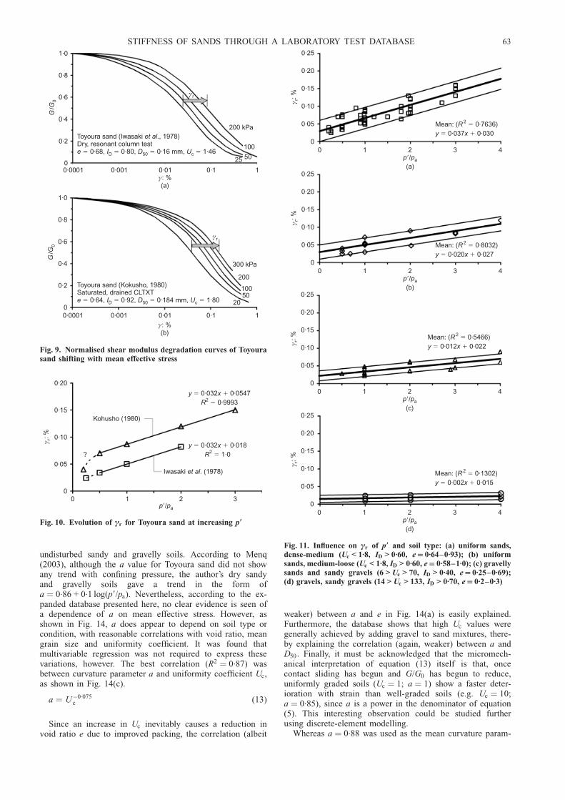
undisturbed sandy and gravelly soils. According to Menq(2003), although the a value for Toyoura sand did not showany trend with confining pressure, the author’s dry sandyand gravelly soils gave a trend in the form ofa ¼ 0.86 + 0.1 log(p9/pa). Nevertheless, according to the ex-panded database presented here, no clear evidence is seen ofa dependence of a on mean effective stress. However, asshown in Fig. 14, a does appear to depend on soil type orcondition, with reasonable correlations with void ratio, meangrain size and uniformity coefficient. It was found thatmultivariable regression was not required to express thesevariations, however. The best correlation (R2 ¼ 0.87) wasbetween curvature parameter a and uniformity coefficient Uc,as shown in Fig. 14(c).

a ¼ U�0:075c (13)

Since an increase in Uc inevitably causes a reduction invoid ratio e due to improved packing, the correlation (albeit

weaker) between a and e in Fig. 14(a) is easily explained.Furthermore, the database shows that high Uc values weregenerally achieved by adding gravel to sand mixtures, there-by explaining the correlation (again, weaker) between a andD50: Finally, it must be acknowledged that the micromech-anical interpretation of equation (13) itself is that, oncecontact sliding has begun and G/G0 has begun to reduce,uniformly graded soils (Uc ¼ 1; a ¼ 1) show a faster deter-ioration with strain than well-graded soils (e.g. Uc ¼ 10;a ¼ 0.85), since a is a power in the denominator of equation(5). This interesting observation could be studied furtherusing discrete-element modelling.

Whereas a ¼ 0.88 was used as the mean curvature param-

0

0·2

0·4

0·6

0·8

1·0

0·0001 0·001 0·01 0·1 1

GG/

0

γ: %(a)

0

0·2

0·4

0·6

0·8

1·0

0·0001 0·001 0·01 0·1 1

GG/

0

γ: %(b)

200 kPa

100

5025

γr

Toyoura sand (Iwasaki ., 1978)Dry, resonant column test

0·68, 0·80, 0·16 mm, 1·46

et al

e I D U� � � �D 50 c

300 kPa

10050

20

γr

Toyoura sand (Kokusho, 1980)Saturated, drained CLTXT

0·64, 0·92, 0·184 mm, 1·80e I D U� � � �D 50 c

200

Fig. 9. Normalised shear modulus degradation curves of Toyourasand shifting with mean effective stress

0·20

0·15

0·10

0·05

0

γ r: %

0 1 2 3p p�/ a

Kohusho (1980)

Iwasaki . (1978)et al

y xR0·032 0·0547

0·9993� �

�2

y xR

0·032 0·0181·0

� �

�2?

Fig. 10. Evolution of ªr for Toyoura sand at increasing p9

0

0·05

0·10

0·15

0·20

0·25

0 1 2 3 4

γ r: %

p p�/(a)

a

Mean: ( 0·7636)0·037 0·030

Ry x

2 �

� �

0

0·05

0·10

0·15

0·20

0·25

0 1 2 3 4

γ r: %

p p�/(b)

a

Mean: ( 0·8032)0·020 0·027

Ry x

2 �

� �

0

0·05

0·10

0·15

0·20

0·25

0 1 2 3 4

γ r: %

p p�/(c)

a

Mean: ( 0·5466)0·012 0·022

Ry x

2 �

� �

0

0·05

0·10

0·15

0·20

0·25

0 1 2 3 4

γ r: %

p p�/(d)

a

Mean: ( 0·1302)0·002 0·015

Ry x

2 �

� �

Fig. 11. Influence on ªr of p9 and soil type: (a) uniform sands,dense-medium (Uc < 1.8, ID > 0.60, e 0.64–0.93); (b) uniformsands, medium-loose (Uc < 1.8, ID > 0.60, e 0.58–1.0); (c) gravellysands and sandy gravels (6 > Uc > 70, ID > 0.40, e 0.25–0.69);(d) gravels, sandy gravels (14 > Uc > 133, ID > 0.70, e 0.2–0.3)


eter for the G/G0 –ª curves of the whole database of sandysoils in Fig. 2, the statistical analysis of variations betweenthe characteristics of the soils and their test conditions hasresulted in the more refined expression in equation (13).Although parameters such as ªr and a may not appear to

vary very much, their influence on soil stress–strain curvesis by no means insignificant. Fig. 15(a) translates from Gagainst ª at mean effective stress p9 ¼ 100 kPa into shearstress � against ª in a hypothetical simple shear test. The

0·01

0·1

1

0·1 1 10

γ r: %

e(a)

y xR

0·08230·5446

�

�

0·9134

2

0·01

0·1

1

γ r: %

0·1 1ID(b)

y xR

0·05620·0355

�

�

0·3635

2

0·01

0·1

1

γ r: %

y xR

0·07140·7376

�

�

�0·3293

2

Uc

(d)

1 10 100

0·01

0·1

1

γ r: %

y xR

0·12360·7353

�

�

1·0675

2

0·1 1eID(c)

Fig. 12. Influence on ªr of void ratio e, relative density ID anduniformity coefficient Uc

0·004

0·003

0·001

0·002

0

γ e: %

0 0·1 0·2 0·3

γr: %

y xR0·012 0·0002

0·9978� �

�2

Fig. 13. Relation between ªr and ªe

0·1

1

10

0·1 1

a

e(a)

y xR

1·01660·6952

�

�

0·223

2

0·1

1

10

0·1 1 10 100

a

D50

(b)

y xR

0·84980·5141

�

�

�0·0416

2

0·1

1

10

1 10 100

a

Uc

(c)

y xR

0·97670·8748

�

�

�0·0746

2

Fig. 14. Influence on curvature parameter a of void ratio anduniformity coefficient


elastic stiffness at very small strains is taken as a constantG0 ¼ 250 MPa. In Fig. 15(a) it is shown that, for a typicalsand with a ¼ 0.88, the influence of reference strain ªr inthe range 0.02–0.1% creates a fourfold variation in themobilisation of shear stress up to 1% shear strain. Fig. 15(b)shows a more modest, but nevertheless significant, variationin expected mobilised shear stress due to variations of awithin the typical range 0.80–1.0, for the average value ofªr ¼ 0.044%.

VALIDATIONIn the case of unavailability of the linear elastic shear

modulus value and its reduction by straining for a sandysoil, it is possible to calculate them with equations (5), (11),(12) and (13) proposed in this paper. Comparisons betweenmeasured and predicted values can be validated against thedatabase. In Fig. 16(a) it is shown that 86% of the 345calculated values of G0 lie within a factor of 2 of themeasured values, implying a standard deviation of a factorof 1.6 if the variation is normally distributed. Fig. 16(b)shows that 94% of the 194 calculated values of referencestrain ªr lie within a factor of 2 of the measured values,implying a standard deviation of a factor of 1.4. And Fig.16(c) shows that all 280 calculated values of curvatureparameter a effectively lie within a factor of 1.3 of theinterpreted measurements.

The overall significance of the residual deviations inmodulus reduction, G/G0, between predictions and measure-ments can best be assessed by plotting predicted againstmeasured values for all 3860 data points accumulated fromall the tests, on those soils in the new database that aresufficiently well classified to enable the comparison. This is

presented in Fig. 17, where it can be seen that 98% ofpredictions lie within a factor of 1.3 from the measurements.Assuming a standard distribution of error, this implies astandard deviation of a factor of 1.13 arising as an unre-solved variability.

Figure 18 shows the degradation curves calculated using

0

50

100

150

200

250

300

0 0·2 0·4 0·6 0·8 1·0

She

ar s

tres

s,: k

Pa

τ

Shear strain, : %(a)

γ

48

37

25

Mob

lised

fric

tion

angl

e,: d

egre

esφ

� mob

γr 0·1%�

γr 0·44%�

γr 0·02%�

0

50

100

150

200

250

300

0 0·2 0·4 0·6 0·8 1·0

She

ar s

tres

s,: k

Pa

τ

Shear strain, : %(b)

γ

44

36

31

Mob

lised

fric

tion

angl

e,: d

egre

esφ

� mob

a 0·8�

a 0·9�

a 1·0�

Fig. 15. Effect of ªr and a on the shear stress–strain curve(G0 250 MPa, p9 100 kPa): (a) a 0.88; (b) ªr 0.044%

1000

100

10

G0

(cal

cula

ted)

: MP

a

10 100 1000G0 (measured): MPa

(a)

Factor 2

1

0·1

0·01

γ r(c

alcu

late

d): %

0·01 0·1 1·0

Factor 2

γr (measured): %(b)

Factor 1·3

10

1

0·1

a(c

alcu

late

d)

0·1 1 10a (measured)

(c)

Fig. 16. Comparison of measured and calculated values of (a) G0

(345 tests), (b) ªr (194 tests) and (c) a (280 tests)


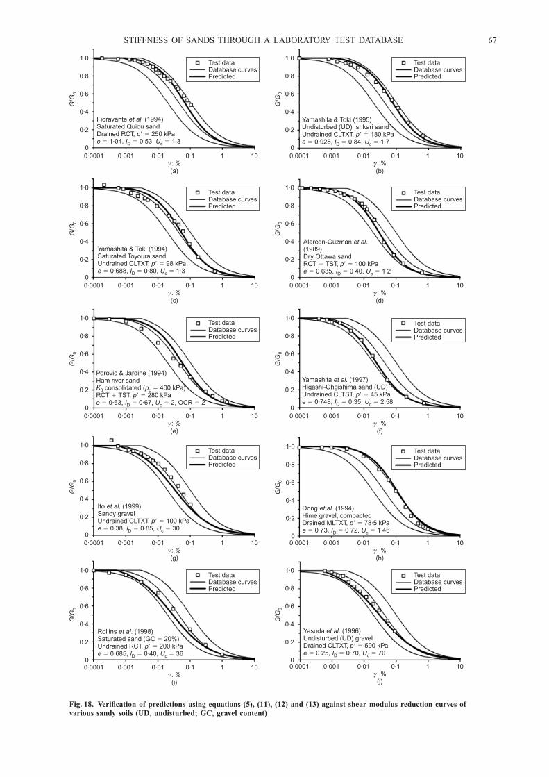
equations (5), (11), (12) and (13) for ten named soils inclearly designated tests, compared with the correspondingraw test data. These ten examples are chosen to illustrate thefull range of sandy soils having different void ratios, relativedensities and uniformity coefficients. The whole range of thedatabase and its central tendency are included in each caseso that the success of the new predictive tools can beperceived.

APPLICATIONStatistical correlations such as those produced here find

their application in a risk-based approach to design whencalculations are to be based on elementary soil classificationdata, prior to a decision on whether or not to conduct moreexpensive and time-consuming field or laboratory tests. Theaim of this paper has been to offer the designer clearguidelines from which the shear stiffness G of a typical sandcan be estimated at any required magnitude of strain, and anunderstanding of the possible variability in that estimate. Inthat regard it is striking that the new database leaves a factorof uncertainty on elastic stiffness G0 of 1.6 for one standarddeviation, whereas the similar factor on G/G0 is as small as1.13. The elastic stiffness G0 must be a function of soilfabric, and sensitive to anisotropy; this functionality canobviously have no correlation with disturbed soil propertiessuch as classification parameters. Clearly, engineers shouldbe encouraged to measure G0 by seismic methods in thefield, if possible. Appropriate use of down-hole and cross-hole logging will provide G0 values pertinent to the requiredmode of ground deformation, accounting for anisotropy(Clayton, 2011).

Although the uncertainty in stiffness degradation has beenreduced to a great extent in the current work, this is onlyapplicable in practice if three key parameters can be esti-mated: void ratio e, relative density ID, and uniformitycoefficient Uc: Although the sand replacement test can beused to obtain a measurement of void ratio in situ, it can becarried out only on exposed benches of soil. The determina-tion of void ratio in sands at depth is more difficult. How-ever, estimates of each of the three key parameters can, inprinciple, be made from an SPT probe with a split sampler.Relative density can be estimated from the corrected blowcount N60 and the vertical effective stress (� 9v0 in kPa) as

ID �N60

20þ 0:2� 9v0

� �0:5

(14)

following authors such as Gibbs & Holtz (1979) and Skemp-ton (1986). And since the split sampler provides a disturbedsample, this can be sieved for Uc, and also subjected tomaximum and minimum density and specific gravity testsfrom which emax and emin can be found. Accordingly, thevoid ratio in situ can be estimated from the relative density.There is therefore no practical barrier to the use in practiceof the stiffness relations provided here.

Equations (5), (11), (12) and (13), taken together with thein situ measurement of G0 in the required mode of grounddeformation, permit the engineer to estimate the in situstress–strain curve of sands, and Fig. 4 allows that value tobe corrected for future changes in mean effective stress,within statistical bounds. These expressions can also be usedin non-linear numerical analyses, permitting them to bevalidated through field testing. For example, Oztoprak &Bolton (2011) demonstrate the use of this modified hyperbolain FLAC3D, to explore the fitting of self-boring pressure-meter tests in Thanet sand. An excellent match was obtainedwhen appropriate secant values of the in situ angle of frictionand angle of dilation were used for the fully plastic expan-sion phase, and when an allowance was made for initialdisturbance affecting the lift-off pressure. Further discussionis also made of the potential impact of errors and ambigu-ities in the various values selected for the model. Furtherwork to predict ground movements in sand in various appli-cations is under way.

CONCLUSIONSIn order to assess the non-linear shear stiffness of sand, a

database has been constructed including the secant shearmodulus degradation curves of 454 tests from the literature.

A new shear modulus equation (equation (6)) was derived,with strain-dependent coefficients. Using this equation forthe very-small-strain range (ª ¼ 0.0001%), the maximumshear modulus G0 can be estimated by equation (6) within afactor of 1.6 for one standard deviation.

A modified hyperbolic relationship was fitted to the col-lected database of secant shear modulus curves in the formof equation (5), featuring three curve-fitting parameters:elastic threshold strain ªe, reference strain ªr at G/G0 ¼ 0.5,and curvature parameter a.

The use of equations (5) and (6) in sequence provided astatistical methodology for refining optimum functional rela-tionships. Linear relations between the characteristic strainsªe and ªr and the mean effective stress p9 offered the bestfit to data from the most common range of confiningpressure (70 kPa to 600 kPa): these were given in equations(11) and (12).

Sands with more disperse particle sizes begin to lose theirlinear elastic stiffness at a smaller strain than is the casewith more uniform sands; this is in accord with micromech-anical reasoning based on premature slip occurring betweenlarge and small particles due to strain incompatibility. It wassuggested that the product eID, which has the effect ofdelaying the onset of intergranular sliding in equations (11)and (12), might stand as a surrogate for grain angularity,which increases interlocking; the influence of p9 was thoughtto have the same origins.

The curvature parameter a was found to be related touniformity coefficient through equation (13), such that moreuniformly graded sands suffer faster deterioration of stiffnesswith strain once intergranular sliding is under way.

The new empirical expression for shear modulus reductionG/G0 is shown to make predictions that are accurate within

0

0·2

0·4

0·6

0·8

1·0

0 0·2 0·4 0·6 0·8 1·0

G G/

(cal

cula

ted)

0

G G/ (measured)0

Factor 1·3

Factor 1·3

Fig. 17. Comparison of measured and calculated G/G0 values(3860 data points)


0

0·2

0·4

0·6

0·8

1·0

0·0001 0·001 0·01 0·1 1 100

0·2

0·4

0·6

0·8

1·0

0·0001 0·001 0·01 0·1 1 10

G G/

0

γ: %(b)

Test dataDatabase curvesPredicted

Yamashita & Toki (1995)Undisturbed (UD) Ishkari sandUndrained CLTXT, 180 kPa

0·928, 0·84, 1·7p

e I U� �

� � �D c

0

0·2

0·4

0·6

0·8

1·0

0·0001 0·001 0·01 0·1 1 100

0·2

0·4

0·6

0·8

1·0

0·0001 0·001 0·01 0·1 1 10G

G/0

γ: %(d)


Alarcon-Guzman .(1989)Dry Ottawa sandRCT TST, 100 kPa

0·635, 0·40, 1·2

et al

pe I U

� � �� D c

G G/

0

γ: %(c)


Yamashita & Toki (1994)

CLTXTSaturated Toyoura sandUndrained , 98 kPa

0·688, 0·80, 1·3p

e I U� �

� � �D c

0

0·2

0·4

0·6

0·8

1·0

0·0001 0·001 0·01 0·1 1 100

0·2

0·4

0·6

0·8

1·0

0·0001 0·001 0·01 0·1 1 10

G G/

0

γ: %(f)


Yamashita . (1997)Higashi-Ohgishima sand (UD)Undrained CLTST, 45 kPa

0·748, 0·35, 2·58

et al

pe I U

� �� D c

0

0·2

0·4

0·6

0·8

1·0

0·0001 0·001 0·01 0·1 1 100

0·2

0·4

0·6

0·8

1·0

0·0001 0·001 0·01 0·1 1 10

G G/

0

γ: %(h)


Dong . (1994)Hime gravel, compactedDrained MLTXT, 78·5 kPa

0·73, 0·72, 1·46

et al

pe I U

� �� D c

G G/

0

γ: %(g)


Ito . (1999)

CLTXT

et alSandy gravelUndrained , 100 kPa

0·38, 0·85, 30p

e I U� �

� � �D c

G G/

0

γ: %(e)


Porovic & Jardine (1994)Ham river sand

consolidated ( 400 kPa)RCT TST, 280 kPa

0·63, 0·67, 2, OCR 2

K pp

e I U

0 c

D c

��

� � � �

0

0·2

0·4

0·6

0·8

1·0

0·0001 0·001 0·01 0·1 1 100

0·2

0·4

0·6

0·8

1·0

0·0001 0·001 0·01 0·1 1 10

G G/

0

γ: %(j)


Yasuda . (1996)Undisturbed (UD) gravelDrained CLTXT, 590 kPa

0·25, 0·70, 70

et al

pe I U

� �� D c

G G/

0

γ: %(i)


Rollins . (1998)et alSaturated sand (GC 20%)Undrained RCT, 200 kPa

0·685, 0·40, 36

��

� � �p

e I UD c

G G/

0

γ: %(a)


Fioravante . (1994)Saturated Quiou sandDrained RCT, 250 kPa

1·04, 0·53, 1·3

et al

pe I U

� �� D c

Fig. 18. Verification of predictions using equations (5), (11), (12) and (13) against shear modulus reduction curves ofvarious sandy soils (UD, undisturbed; GC, gravel content)


a factor of 1.13 for one standard deviation of random error,as determined from 3860 data points. This very narrowspread applies irrespective of the test type and soil condi-tion, within the range listed in Table 1. The initial elasticshear modulus, G0, should always be measured if possible,but a new empirical relation is shown to provide estimateswithin a factor of 1.6 for one standard deviation of randomerror, as determined from 379 tests.

ACKNOWLEDGEMENTSThe work was supported by EPSRC Platform Grant

GR/T18660/01. The first author was also supported by theScientific Research Projects Coordination Unit of IstanbulUniversity, Project No. YADOP-16527.

NOTATIONA material constanta curvature parameterB material constantc scaling coefficient

D diameterD50 average grain size

d scaling coefficiente void ratio

eg empirical parameter in equation (1)emax maximum void ratioemin minimum void ratio

f empirical parameterG secant shear modulus; shear stiffness

Gmax maximum shear modulusG0 initial elastic shear modulus

g empirical parameterID relative densitym material constant

N60 corrected blow countOCR overconsolidation ratio

PI plasticity indexp9 mean effective stresspa reference (atmospheric) pressurepc preconsolidation pressureR2 coefficient of determinations9 effective stress

Uc uniformity coefficientV ¼ 1 + ew water contentª shear strainªe elastic threshold strainªr reference strain

� 9v0 vertical effective stress� 91 major effective principal stress� 92 intermediate effective principal stress� 93 minor effective principal stress� shear stress

�max maximum shear stress�9mob mobilised friction angle

REFERENCESAlarcon-Guzman, A., Chameau, J. L., Leonards, G. A. & Frost, J.

D. (1989). Shear modulus and cyclic undrained behavior ofsands. Soils Found. 29, No. 4, 105–119.

Arango, J. C. (2006). Stress–strain behavior and dynamic propertiesof Cabo Rojo calcareous sands. MSc thesis, University ofPuerto Rico, San Juan, Puerto Rico.

Atkinson, J. H. (2000). Nonlinear soil stiffness in routine design.Geotechnique 50, No. 5, 487–508, http://dx.doi.org/10.1680/geot.2000.50.5.487.

Atkinson, J. H. & Salfors, G. (1991). Experimental determination ofstress–strain–time characteristics in laboratory and in situ tests.Proc. 10th Eur. Conf. Soil Mech. Found. Engng, Florence 3,915–956.

Cavallaro, A., Maugeri, M. & Ragusa, A. (2003). Small strainstiffness from in situ and laboratory tests for the city of Noto

soil. In Deformation characteristics of geomaterials (eds H. DiBenedetto, T. Doanh, H. Geoffroy and C. Saizeat), pp. 267–274.Lisse, the Netherlands: Swets & Zeitlinger.

Charif, K. (1991). Contribution a l’etude du comportement mecani-que en petites et grandes deformation (� . 10–6). PhD disserta-tion, Ecole Centrale Paris, France (in French).

Chegini, A. & Trenter, N. A. (1996). The shear strength anddeformation behaviour of a glacial till. In Advances in siteinvestigation practice (ed. C. Craig), pp. 851–866. London, UK:Thomas Telford.

Chung, R. M., Yokel, F. Y. & Drnevich, V. P. (1984). Evaluation ofdynamic properties of sands by resonant column testing. Geo-tech. Test. J. 7, No. 2, 60–69.

Clayton, C. R. I. (2011). Stiffness at small strain: research andpractice. 50th Rankine Lecture. Geotechnique 61, No. 1, 5–37,http://dx.doi.org/10.1680/geot.2011.61.1.5.

Darendeli, B. M. (2001). Development of a new family of normal-ized modulus reduction and material damping curves. PhDdissertation, University of Texas at Austin, TX, USA.

Delfosse-Ribay, E., Djeran-Maigre, I., Cabrillac, R. & Gouvenot, D.(2004). Shear modulus and damping ratio of grouted sand. SoilDynam. Earthquake Engng 24, No. 6, 461–471.

Dong, J., Nakamura, K., Tatsuoka, F. & Kohata, Y. (1994). Defor-mation characteristics of gravels in triaxial compression testsand cyclic triaxial tests. In Pre-failure deformation of geomater-ials (eds S. Shibuya, T. Mitachi and S. Miura), pp. 17–23.Rotterdam, the Netherlands: Balkema.

D’Onofrio, A. & Penna, A. (2003). Small strain behaviour of alime-treated silty sand. In Deformation characteristics of geo-materials (eds H. Di Benedetto, T. Doanh, H. Geoffroy and C.Saizeat), pp. 329–336. Lisse, the Netherlands: Swets & Zeit-linger.

Drnevich, V. P. & Richart, F. E. (1970). Dynamic prestraining ofdry sand. J. Soil Mech. Found. Div. ASCE 96, No. SM2, 453–469.

Ellis, E. A., Soga, K., Bransby, M. F. & Sato, M. (2000). Resonantcolumn testing of sands with different viscosity pore fluids.J. Geotech. Geoenviron. Engng 126, No. 1, 10–17.

Fahey, M. & Carter, J. P. (1993). A finite element study of thepressuremeter test in sand using a nonlinear elastic plasticmodel. Can. Geotech. J. 30, No. 2, 348–362.

Fioravante, V., Jamiolkowski, M. & Lo Presti, D. C. F. (1994).Stiffness of carbonatic Quiou sand. Proc. 8th Int. Conf. SoilMech. Found. Engng, New Delhi 1, 163–168.

Gibbs, H. J. & Holtz, W. G. (1979). Discussion of ‘SPT and relativedensity in coarse sands’, by Marcuson and Bieganousky.J. Geotech. Engng ASCE 105, No. GT3, 439–441.

Goddard, J. D. (1990). Nonlinear elasticity and pressure-dependentwave speeds in granular media. Proc. R. Soc. Math. Phys. Sci.430, No. 1878, 105–131.

Goto, S., Syamoto, Y. & Tamaoki, K. (1987). Dynamic propertiesof undisturbed gravel samples obtained by the in-situ freezingmethod. Proc. 8th Asian Regional Conf. on Soil Mech. Found.Engng, Kyoto 1, 233–236.

Goto, S., Suzuki, Y., Nishio, S. & Hiroshi, O.-O. (1992). Mechani-cal properties of undisturbed Tone-River gravel obtained by in-situ freezing method. Soils Found. 32, No. 3, 15–25.

Hardin, B. O. & Black, W. L. (1966). Sand stiffness under varioustriaxial stresses. J. Soil Mech. Found. Div. ASCE 92, No. SM2,667–692.

Hardin, B. O. & Drnevich, V. P. (1972a). Shear modulus anddamping in soils: measurement and parameter effects. J. SoilMech. Found. Div. ASCE 98, No. SM6, 603–624.

Hardin, B. O. & Drnevich, V. P. (1972b). Shear modulus anddamping in soils: design equations and curves. J. Geotech.Engng 98, No. 7, 667–692.

Hardin, B. O. & Kalinski, M. E. (2005). Estimating the shearmodulus of gravelly soils. J. Geotech. Geoenviron. Engng 131,No. 7, 867–875.

Hashiba, T. (1971). Simple shear apparatus using an inclinometer.Soils Found. 11, No. 3, 113–119.

Hatanaka, M. & Uchida, A. (1995). Effect of test methods on thecyclic deformation characteristics of high quality undisturbedgravel samples. In Static and dynamic properties of gravellysoils (eds M. D. Evans and R. J. Fragaszy), Geotechnical SpecialPublication No. 56, pp. 136–161. Reston, VA, USA: ASCE.


Hatanaka, M., Suzuki, Y., Kawasaki, T. & Endo, M. (1988). Cyclicundrained shear properties of high quality undisturbed Tokyogravel. Soils Found. 28, No. 4, 57–68.

Ishihara, K. (1996). Soil behaviour in earthquake geotechnics.Oxford, UK: Oxford University Press.

Ito, K., Goto, Y., Ishihara, K., Yasuda, S. & Yoshida, N. (1999).Detailed in-situ and laboratory tests on the improved ground inPort Island. Proc. 2nd Int. Conf. on Earthquake Geotech. Engng,Lisboa, 47–52.

Iwasaki, T. & Tatsuoka, F. (1977). Effects of grain size and gradingon dynamic shear moduli of sands. Soils Found. 17, No. 3, 19–35.

Iwasaki, T., Tatsuoka, F. & Takagi, Y. (1978). Shear moduli ofsands under cyclic torsional shear loading. Soils Found. 18, No.1, 39–50.

Jardine, R. J., Potts, D. M., Fourie, A. B. & Burland, J. B. (1986).Studies of the influence of non-linear stress–strain character-istics in soil-structure interaction. Geotechnique 36, No. 3, 377–396, http://dx.doi.org/10.1680/geot.1986.36.3.377.

Jardine, R. J., Kuwano, R., Zdravkovic, L. & Thornton, C. (2001).Some fundamental aspects of the pre-failure behaviour of gran-ular soils. Proc. 2nd Int. Symp. on Pre-failure DeformationCharacteristics of Geomaterials, Torino, 1077–1111.

Jovicic, V. & Coop, M. R. (1997). Stiffness of coarse-grained soilsat small strains. Geotechnique 47, No. 3, 545–561, http://dx.doi.org/10.1680/geot.1997.47.3.545.

Katayama, I., Fukui, F., Satoh, M., Makihara, Y. & Tokimatsu, K.(1986). Comparison of dynamic soil properties between undis-turbed and disturbed dense sand samples. Proc. 21st Ann. Conv.Japan. Soc. Soil Mech. Found. Engng, Sapporo, 583–584 (inJapanese).

Koga, Y., Matsuo, O. & Sugawara, N. (1994). In-situ measurementof shear moduli of soils and its evaluation. In Pre-failuredeformation of geomaterials (eds S. Shibuya, T. Mitachi and S.Miura), pp. 213–216. Rotterdam, the Netherlands: Balkema,

Kokusho, T. (1980). Cyclic triaxial test of dynamic soil propertiesfor wide strain range. Soils Found. 20, No. 2, 45–60.

Kokusho, T. & Esashi, Y. (1981). Cyclic triaxial test on sands andcoarse materials. Proc. 10th Int. Conf. Soil Mech. Found. Engng,Stockholm 1, 673–676.

Kokusho, T. & Tanaka, Y. (1994). Dynamic properties of gravellayers investigated by in-situ freezing sampling. In Ground fail-ure under seismic conditions (eds S. Prakash and P. Dakoulas),Geotechnical Special Publication No. 44, pp. 121–140. Reston,VA, USA: ASCE.

Laird, J. P. & Stokoe, K. H. (1993). Dynamic properties of remoldedand undisturbed soil samples tested at high confining pressures,Geotech. Engrg. Rep. GR93–6. Palo Alto, CA, USA: ElectricalPower Research Institute.

Lanzo, G., Vucetic, M. & Doroudian, M. (1997). Reduction ofshear modulus at small strains in simple shear. J. Geotech.Geoenviron. Engng 123, No. 11, 1035–1042.

Lo Presti, D. C. F., Jamiolkowski, M., Pallara, O., Cavallaro, A. &Pedroni, S. (1997). Shear modulus and damping of soils. Geo-technique 47, No. 3, 603–617, http://dx.doi.org/10.1680/geot.1997.47.3.603.

Mair, R. J. (1993). Developments in geotechnical engineering re-search: application to tunnels and deep excavations. UnwinMemorial Lecture 1992. Proc. Instn Civil Engrs Civ. Engng 97,No. 1, 27–41.

Maher, M. H., Ro, K. S. & Welsh, J. P. (1994). High strain dynamicmodulus and damping of chemically grouted sand. Soil Dynam.Earthquake Engng 13, No. 1, 131–138.

McDowell, G. R. & Bolton, M. D. (1999). A micro mechanicalmodel for isotropic cyclic loading of isotropically clasticallycompressed soil. Granular Matter 1, No. 4, 183–194.

Menq, F. Y. (2003). Dynamic properties of sandy and gravelly soils.PhD dissertation, University of Texas at Austin, TX, USA.

Menq, F. Y. & Stokoe, K. H. (2003). Linear dynamic properties ofsandy and gravelly soils from large-scale resonant tests. InDeformation characteristics of geomaterials (eds H. Di Benedet-to, H. Geoffroy, T. Doanh and C. Sauzeat), pp. 63–71. Lisse,the Netherlands: Swets & Zeitlinger.

Ogata, N. & Yasuda, M. (1982). Dynamic properties of undisturbedsamples containing gravels. Proc. 17th Japan. Nat. Conf. SoilMech. Found. Engng, Okinawa 1, 1609–1612 (in Japanese).

Oztoprak, S. & Bolton, M. D. (2011). Parameter calibration of a

modified hyperbolic model for sands using pressuremeter testdata. Proc. 5th Int. Symp. on Deformation Characteristics ofGeomaterials, Seoul, 949–956.

Park, C.-S. (1993). Deformation and strength characteristics of avariety of sands by plane strain compression tests. DEng thesis,University of Tokyo, Japan (in Japanese).

Porovic, E. & Jardine, R. J. (1994). Some observations on the static anddynamic shear stiffness of Ham River sand. Proc. 1st Int. Symp. onPre-failure Deformation of Geomaterials, Sapporo 1, 25–30.

Roesler, S. K. (1979). Anisotropic shear modulus due to stressanisotropy. J. Geotech. Engng Div. ASCE 105, No. 7, 871–880.

Rollins, K. M., Evans, M. D., Diehl, N. B. & Daily, W. D. (1998).Shear modulus and damping relationships for gravels. J. Geo-tech. Geoenviron. Engng 124, No. 5, 396–405.

Saxena, S. K., Avramidis, A. S. & Reddy, K. R. (1988). Dynamicmoduli and damping ratios for cemented sands at low strains.Can. Geotech. J. 25, No. 2, 353–368.

Seed, H. B. & Idriss, I. M. (1970). Soil moduli and damping factorsfor dynamic response analyses, Report EERC 70–10. Berkeley,CA, USA: University of California.

Seed, H. B., Wong, R. T., Idriss, I. M. & Tokimatsu, K. (1986).Moduli and damping factors for dynamic analyses of cohesion-less soil. J. Geotech. Engng 112, No. GT11, 1016–1032.

Shibuya, S., Mitachi, T., Yamashita, S. & Tanaka, H. (1996). RecentJapanese practice for investigating elastic stiffness of ground. InAdvances in site investigation practice (ed. C. Craig), pp. 875–886. London, UK: Thomas Telford.

Silver, M. L. & Seed, H. B. (1971). Deformation characteristics ofsands under cyclic loading. J. Soil Mech. Found. Div. ASCE 97,No. SM8, 1081–1098.

Simpson, B. (1992). Retaining structures: displacement and design.Geotechnique 42, No. 4, 541–576, http://dx.doi.org/10.1680/geot.1992.42.4.541.

Skempton, A. W. (1986). Standard penetration test procedures andthe effects in sands of overburden pressure, relative density,particle size, ageing and overconsolidation. Geotechnique 36,No. 3, 425–447, http://dx.doi.org/10.1680/geot.1986.36.3.425.

Stokoe, K. H., Hwang, S. K., Lee, J. N. K. & Andrus, R. D.(1994). Effects of various parameters on the stiffness anddamping of soils at small to medium strains. Proc. 1st Int.Symp. on Pre-failure Deformation of Geomaterials, Sapporo 2,785–816.

Stokoe, K. H., Darendeli, M. B., Andrus, R. D. & Brown, L. T.(1999). Dynamic soil properties: laboratory, field and correctionstudies. Proc. 2nd Int. Conf. on Earthquake Geotech. Engng,Lisbon 3, 811–845.

Tanaka, Y., Kudo, Y., Yoshida, Y. & Ikemi, M. A. (1987). Study onthe mechanical properties of sandy gravel-dynamic properties ofreconstituted sample, Report U87019. Tokyo, Japan: CentralResearch Institute of Electric Power Industry.

Tatsuoka, F. & Shibuya, S. (1991). Deformation characteristics ofsoils and rocks from field and laboratory tests. Proc. 9th AsianRegional Conf. on Soil Mech. and Found. Engng, Bangkok 2,101–170.

Teachavorasinskun, S., Shibuya, S. & Tatsuoka, F. (1991). Stiffnessof sands in monotonic and cyclic loading in simple shear.Proceedings of the ASCE Geotechnical Engineering Congress,Boulder, CO. Geotechnical Special Publication No. 27, Vol. 1,pp. 863–878. Reston, VA, USA: ASCE.

Teachavorasinskun, S., Tatsuoka, F., Kenkyo, K. & Yasuhara, K.(1992). Effect of cyclic prestraining on the liquefaction strengthof sand. Proceedings of the conference on behaviour of offshorestructures, London, pp. 1345–1356.

Tika, T., Kallioglou, P. & Pitilakis, K. (1999). Laboratory measure-ment of dynamic properties of natural soils. Proc. 2nd Int.Symp. on Pre-failure Deformation Characteristics of Geomater-ials, Torino 1, 239–244.

Tika, T., Kallioglou, P., Papadopoulou, A. & Pitilakis, K. (2003).Shear modulus and damping of natural sands. In Deformationcharacteristics of geomaterials (eds H. Di Benedetto, H. Geof-froy, T. Doanh and C. Sauzeat), pp. 401–407. Lisse, the Nether-lands: Swets & Zeitlinger.

Tokimatsu, K. & Hosaka, Y. (1986). Effects of sample disturbanceon dynamic properties of sand. Soils Found. 26, No. 1, 53–64.

Tokimatsu, K., Yamazaki, T. & Yoshimi, Y. (1986). Soil liquefactionevaluations by elastic shear moduli. Soils Found. 26, No. 1, 25–35.


Vinale, F., d’Onofrio, A., Mancuso, C. & Santucci de Magistris, F.(1999). The pre-failure behaviour of soils as construction mater-ials. Proc. 2nd Int. Symp. on Pre-failure Deformation Character-istics of Geomaterials, Torino 2, 955–1003.

Yamashita, S. & Suzuki, T. (1999). Young’s and shear moduli underdifferent principal stress directions of sand. Proc. 2nd Int. Symp.on Pre-failure Deformation Characteristics of Geomaterials,Torino 1, 149–158.

Yamashita, S. & Toki, S. (1994). Cyclic deformation character-istics of sands in triaxial and torsional tests. Proc. 1st Int.Symp. on Pre-failure Deformation of Geomaterials, Sapporo 1,31–360.

Yamashita, S., Shibuya, S. & Tanaka, H. (1997). A case study forcharacterizing undrained cyclic deformation properties in youngsand deposit from in-situ and laboratory tests. Soils Found. 37,No. 2, 117–126.

Yang, B. E. (2007). Shear strength modeling of cemented sand,Master thesis, University of Notre Dame, Indiana, USA.

Yasuda, N. (1992). Behavior of embankment dams during earth-quakes and dynamic deformation characteristics of rockfill mate-rials. Journal Japan Soc. Dam Engs, No. 6, 43–59 (inJapanese).

Yasuda, N. & Matsumoto, N. (1993). Dynamic deformation charac-teristics of sands and rockfill materials. Can. Geotech. J. 30,No. 5, 747–0757.

Yasuda, N. & Matsumoto, N. (1994). Comparisons of deformationcharacteristics of rockfill materials using monotonic and cyclicloading laboratory tests and in situ tests. Can. Geotech. J. 31,No. 2, 162–174.

Yasuda, N., Ohta, N. & Nakamura, A. (1996). Dynamic deformationcharacteristics of undisturbed riverbed gravels. Can. Geotech. J.33, No. 2, 237–249.


Stiffness of sands through a laboratory test database · Stiffness of sands through a laboratory test database ... Simple but effective models of non-linear soil ... curves and data

Documents