Stiffness of mooring lines and performance of floating breakwater in three dimensions

Stiffness of mooring lines and performance of floating

breakwater in three dimensions

Eva Loukogeorgaki *, Demos C. Angelides

Division of Hydraulics and Environmental Engineering, Department of Civil Engineering, Aristotle University of Thessaloniki,

University Campus, Thessaloniki 54124, Greece

Received 10 June 2005; received in revised form 1 December 2005; accepted 16 December 2005

Available online 10 March 2006

Abstract

In the present paper, the performance of a moored floating breakwater under the action of normal incident waves is investigated in the frequency

domain. A three-dimensional hydrodynamic model of the floating body is coupled with a static and dynamic model of the mooring lines, using an

iterative procedure. The stiffness coefficients of the mooring lines in six degrees of freedom of the floating breakwater are derived based on the

differential changes of mooring lines’ tensions caused by the static motions of the floating body. The model of the moored floating system is

compared with experimental and numerical results of other investigators. An extensive parametric study is performed to investigate the effect of

different configurations (length of mooring lines and draft) on the performance of the moored floating breakwater. The draft of the floating

breakwater is changed through the appropriate modification of mooring lines’ length. Numerical results demonstrate the effects of the wave

characteristics and mooring lines’ conditions (slack-taut). The existence of ‘optimum’ configuration of the moored floating breakwater in terms of

wave elevation coefficients and mooring lines’ forces is clearly demonstrated, through a decision framework.

q 2006 Elsevier Ltd. All rights reserved.

Keywords: Coastal engineering; Floating breakwater; Mooring lines; Stiffness; Damping; Effectiveness; Performance; Decision framework

1. Introduction

Floating breakwaters present an alternative solution to

conventional fixed breakwaters and can be effectively used in

coastal areas with mild wave environment conditions. Poor

foundation or deep-water conditions as well as environmental

requirements, such as phenomena of intense shore erosion,

water quality and aesthetic considerations advocate the

application of such structures. Floating breakwaters have

many advantages compared to the fixed ones, e.g. absence of

negative environmental impacts, flexibility of future exten-

sions, mobility and relocation ability, lower cost and ability of

a short time transportation and installation. As a result of all

these positive effects, many types of floating breakwaters have

been developed as described by McCartney [17]. However, the

most commonly used type of floating breakwaters is the one

that consists of rectangular pontoons connected to each other

and moored to the sea bottom with cables or chains.

0141-1187/$ - see front matter q 2006 Elsevier Ltd. All rights reserved.

doi:10.1016/j.apor.2005.12.002

* Corresponding author. Tel.: C30 2310 995877; fax: C30 2310 995740.

E-mail address: [email protected] (E. Loukogeorgaki).

A moored floating breakwater should be properly designed

in order to ensure effective reduction of the transmitted energy

and, therefore, adequate protection of the area behind the

floating system. This design objective is subjected to the

following constraints: (a) non-failure of the mooring lines and

(b) non-failure of the floaters themselves and their inter-

connections. The satisfaction of the above design objective and

the corresponding constraints represents the overall effective

performance of a moored floating breakwater.

A brief review of the design process for floating breakwaters

and the related design criteria, with respect to wave effects is

provided by Isaacson [7]. Isaacson and Baldwin [8] provide a

review of the analysis of moored floating structures in currents

and waves, with an emphasis on moored floating breakwaters.

With regard to the hydrodynamic analysis of the floating body,

linear two-dimensional models describing the complete

hydrodynamic problem (diffraction and radiation) have been

developed by Isaacson and Nwogu [11], Isaacson [6], Isaacson

and Bhat [9], Williams and Abul-Azm [23], Bhat and Isaacson

[2], Sannasiraj et al. [20], Williams et al. [24] and Lee and Cho

[14]. Most of these models are based on the finite element

method (FEM) or the boundary integral equation method

(BIEM) utilizing Green’s theorem, while Lee and Cho [14] use

the element-free Galerkin method. Isaacson and Nwogu [11]

Applied Ocean Research 27 (2005) 187–208

www.elsevier.com/locate/apor

E. Loukogeorgaki, D.C. Angelides / Applied Ocean Research 27 (2005) 187–208188

and Bhat [1] properly modified a two-dimensional hydrodyn-

amic model in order to take into account the effect of finite

floating body length. Isaacson and Garceau [10] investigated

the response of a freely floating breakwater by superposing

two-dimensional solutions for the diffracted and radiated

waves and compared this simplified approach with three-

dimensional results. Three-dimensional analysis of a V-shaped

floating breakwater, moored in a three point mooring held by

buoys, has been implemented by Briggs et al. [3].

As far as the mooring lines, the effect of them on the

response of the floating breakwater is modeled through the

incorporation of the stiffness coefficients of the mooring lines

in the hydrodynamic model and the appropriate modification

of the hydrodynamic equations. Williams and Abul-Azm [23]

and Williams et al. [24] modified the hydrodynamic equations

by using appropriate values of the mooring lines’ stiffness

coefficients. On the contrary, Sannasiraj et al. [20] and Lee

and Cho [14] derived analytically the stiffness coefficients of

the mooring lines for taut and slack conditions, respectively,

using the basic catenary equation for the cable equilibrium.

However, in those investigations, the derivations of the

stiffness coefficients were restricted to two dimensions

(stiffness coefficients in sway, heave and roll modes only),

following the procedure given by Jain [12]; furthermore, it

was assumed that the stiffness components remain unaffected

by the motions of the structure, i.e. the stiffness values are

calculated at the initial equilibrium position. It should be also

noted that Sannasiraj et al. [20] conducted two-dimensional

experiments in order to validate their theoretical model. The

simplified approach of Jain [12] for the calculation of the

mooring lines’ stiffness coefficients has been also used by

Daghigh et al. [4], who investigated the effect of different

design aspects of the mooring lines on the dynamic behavior

of floating bridges and performed a parametric study in order

to select the optimum mooring lines’ condition in terms of the

horizontal forces on the mooring lines and the forces on the

anchor.

The non-linear behavior of the mooring lines was taken

into consideration by Bhat and Isaacson [2] by performing an

iterative coupled procedure between a hydrodynamic model

and a mooring analysis model in terms of convergence of the

steady drift forces only. An iterative coupling procedure was

also implemented by Loukogeorgaki and Angelides [16], who

studied the effect of mooring lines on the performance of

floating breakwaters in three dimensions. In that work, the

drag damping of the mooring lines was also taken into

account and, therefore, the convergence procedure was

implemented in terms of both the steady drift forces and

the response of the floating breakwater; furthermore, the

geometrical stiffness coefficients of the mooring lines on the

horizontal plane only, according to Triantafyllou et al. [22],

were taken into account. A similar geometric mooring lines’

stiffness matrix (3!3) has been also derived by Kreuzer and

Wilke [13], based on the modification of mooring lines

geometry, due to external wave loads, and on the correspond-

ing changes of mooring lines’ forces (not moments) in x, y

and z directions.

The objective of the present paper, where the dynamic

response and the protection effectiveness of a moored floating

breakwater is investigated in frequency domain under the

action of regular waves, is twofold. The first objective is the

integrated modeling and analysis of the dynamic behavior of

the moored floating breakwater in three dimensions. This is

achieved with a three-dimensional model of the hydrodynamic

analysis of the floating body coupled with a model of the static

and dynamic analysis of the mooring lines; an appropriate

iterative procedure is used, in terms of the steady drift forces

and the response of the floating breakwater. The floating body

analysis is based on three-dimensional panel method utilizing

Green’s theorem. With regard to the analysis of the mooring

lines, special attention is given to the computation of mooring

lines’ stiffness and drag damping imposed on the floating body.

Specifically, the derivation of the complete (6!6) stiffness

matrix of the mooring lines, which represents the second

objective of the present work, is implemented. The stiffness

coefficients of the mooring lines are derived in six degrees of

freedom, based on the differential changes of mooring lines’

tensions caused by the static motions of the floating body. This

enables the calculation of the stiffness of the floating structure

in its static mean position, under the action of the steady drift

forces. Finally, an extensive parametric study is performed in

order to investigate: (a) the performance of the moored floating

system for various wave conditions and various configurations

(length of the mooring lines and draft) of the floating

breakwater, and (b) the effect of the vertical stiffness of the

mooring lines on the dynamic behavior of the floating moored

system. Based on the results of this parametric study a Decision

Framework is introduced, which enables the selection of the

‘optimum’ configuration of the floating breakwater in terms of

the wave elevation coefficients and mooring lines’ forces.

2. Derivation of equations of mooring lines’ stiffness

coefficients

2.1. General assumptions—geometry definition

The excitation of second order steady drift forces on a

moored floating body results to static translational and

rotational displacements relatively to its initial equilibrium

position. These static displacements induce modifications of

the initial configuration of the mooring lines and consequently

they lead to changes of their static tensions. The final new

equilibrium position of the floating body depends on the

stiffness of the mooring lines, which is a function of

the changes of the static tensions of the mooring lines. In the

present formulation, the coefficients of the mooring lines’

stiffness matrix are assumed to depend on the floating body’s

static equilibrium position. Their derivation is implemented in

three dimensions and is based on the differential changes of the

static tension Tst and the static angle f at the top of the mooring

lines.

Fig. 1 shows the definition of some basic quantities that are

used in the present analysis. Three coordinate systems are

introduced. OXYZ (Fig. 1a) is the floating body coordinate

(ZP)

(a) (b)

θ

lY lx’

(XA ,YA)

lX

(XP ,YP)

O X

Y

Z

Tst

H

V z

o

l

lx’

lz’

x

lZ

(ZA) O X

Y

Z

X’

Z’

Zo

Xo

YoθX

θY

θZ

Ο’

Y’

ω

Fig. 1. (a) Coordinate systems—definitions of basic quantities. (b) Static displacements—displaced coordinate system.

E. Loukogeorgaki, D.C. Angelides / Applied Ocean Research 27 (2005) 187–208 189

system at the initial (in the absence of any external static loads)

equilibrium position. Its origin O coincides with the center of

T Z

cos qY cos qZ sin qX sin qY cos qZKcos qX sin qZ cos qX

cos qY sin qZ sin qX sin qY sin qZ Ccos qX cos qZ cos qX

Ksin qY sin qX cos qY cos qX

264

ϕbot

Xa

o

H

VTst

ϕ

Xtot (=l x’)

L2

Ltot

L1

x

z

lz’

l

Fig. 2. Geometry of a mooring line

gravity of the floating body. O 0X 0Y 0Z 0 (Fig. 1b) is the floating

body coordinate system at the final, displaced due to the static

movements of the floating body, equilibrium position. Finally,

oxz (Fig. 1a) is defined as the local coordinate system of each

mooring line. The geometry of a typical mooring line is shown

in Fig. 2.

The translational and rotational displacement vector X of

the center of gravity of the floating body and the vector Fst

of the steady drift forces can be written, respectively, in form of

matrices as

XT Z Xo Yo Zo qX qY qZ

� �(1)

FTst Z FstX FstY FstZ MstX MstY MstZ

� �(2)

where Xo, Yo, Zo are the displacements of the center of gravity,

while qX, qY, qZ are the rotations of the floating body around the

axes X, Y and Z, respectively. In the same manner, FstX, FstY,

FstZ, MstX, MstY, MstZ are the steady drift forces and moments in

X, Y and Z directions, respectively.

The position vectors of the fairlead of the mooring line in

OXYZ and O 0X 0Y 0Z 0 coordinate systems are related to each

other by the following linear transformation

Uf ZTU0f CX0 (3)

where UTf Z[XP YP ZP] is the position vector of the fairlead of

the mooring line with respect to OXYZ, while (U0f )TZ

[XPO YPO ZPO] is the same position vector with respect to

O 0X 0Y 0Z 0. (X 0)TZ[Xo Yo Zo] is the translational displacement

vector. The matrix T is the rotational-transformation matrix,

which takes the form:

sin qY cos qz Csin qX sin qZ

sin qY sin qzKsin qX cos qZ

cos qY

375 (4)

The position of the anchor is assumed to be unaffected by

the static displacements of the floating body. Therefore, the

position vector of the anchor of each mooring line with respect

to OXYZ is defined as:

UTa Z XA YA ZA

� �(5)

As previously mentioned, the static displacements of the

floating body result to modifications of the initial geometry of

each mooring line, and consequently, to changes of its static

E. Loukogeorgaki, D.C. Angelides / Applied Ocean Research 27 (2005) 187–208190

tension. Therefore, for a mooring line with specific character-

istics, i.e. submerged weight, total length, elasticity modulus,

effective diameter and initial pretension placed in a specific

water depth, any changes of its static tension Tst and of its static

angle f are considered to be a function of the length l of the

chord (see Figs. 1a and 2). Specifically

Tst Z TstðlðlX ;lY ;lZÞÞ (6)

fZfðlðlX ;lY ;lZÞÞ (7)

with laZla(Xo, Yo, Zo, qX, qY, qZ) and aZX or Y or Z.

In the above equations, lX, lY, lZ are the projection of the

length l of the chord in OXYZ. Based on the definitions in

Fig. 1a, the following relations hold for the projections of the

length l in oxz (Eq. (8)) and OXYZ (Eq. (9)) axes, respectively:

l0x

l0z

" #Z

XPKXA

ZPKZA

" #Z

l cos u

l sin u

" #(8)

lX

lY

lZ

264

375Z

XAKXP

YAKYP

ZAKZP

264

375ZK

l0xcos q

l0xsin q

l0z

2664

3775ZK

l cos u cos q

l cos u sin q

l sin u

264

375(9)� �

ðFmÞT Z ðfXÞm ðfY Þm ðfZÞm ðMXÞm ðMY Þm ðMZÞm 0

ðFmÞT Z ðH cos qÞm ðH sin qÞm ðVÞm ðMXÞm ðMY Þm ðMZ

�ðFmÞ

T Z ðT cos f cos qÞm ðT cos f sin qÞm ðT sin fÞm ðMX

�

static displacements

The quantities l, u and q (see Fig. 1a) fully describe the

position of the fairlead relative to the anchor of each

mooring line in the static equilibrium position of the system

(floating body—mooring lines). Therefore, it is initially

required to derive the differential changes of these

quantities, due to the translational and rotational displace-

ments, before proceeding to the derivation of the mooring

lines’ stiffness coefficients.

The differential changes of l, u and q with respect to Xo, Yo,

Zo, qX, qY and qZ can be expressed in a matrix form as follows

vl

vXo

vl

vYo

vl

vZo

vu

vXo

vu

vYo

vu

vZo

vq

vXo

vq

vYo

vq

vZo

26666666664

37777777775Z

cosu cos q cosu sin q sinu

Ksinu cos q

lK

sinu sin q

l

cosu

l

Ksin q

l cosu

cos q

l cosu0

2666666664

3777777775(10a)

vl

vqi

vu

vqi

vq

vqi

26666666664

37777777775Z

kj cosu cos qCkm cosu sin qCkn sinu

kn cosuKkm sinu sin qKkj sinu cos q

l

km cos qKkj sin q

l cosu

2666666664

3777777775

(10b)

where iZ1 for qX, iZ2 for qY and iZ3 for qZ, jZ0, 3, 6, mZ1,

4, 7 and nZ2, 5, 8 for qX, qY and qZ, respectively. The terms kj,

km and kn are given by Eqs. (A1)–(A3) in Appendix A.

2.3. Derivation of the stiffness matrix of the mooring lines

The stiffness matrix Kij for a system of M mooring lines is

defined as

K ZXM

mZ1

Km ZXM

mZ1

KvFm

vX(11)

where Km is the stiffness matrix of mooring line m, X is the

translational and rotational vector as defined by Eq. (1). Fm is

the vector of the reaction forces and the corresponding reaction

moments that the mooring line m exercises on the floating

body:

Þm�0

Þm ðMY Þm ðMZÞm�

(12)

The moments (MX)m, (MY)m and (MZ)m are defined as the

cross product of the position vector r and the vector Fm using

Eq. (13)

ðMXÞm

ðMY Þm

ðMZÞm

264

375Zr!Fm Z

�����i j k

ðXPKXoÞm ðYPKYoÞm ðZPKZoÞm

ðH cos qÞm ðH sin qÞm ðVÞm

�����(13)

where ði, ðj, ðk are the unit vectors in X, Y, Z, respectively.

For a mooring line m each one of the coefficients Kmij

expresses the differential changes of the force or moment that is

exercised on the mooring line in the direction i due to the

differential translational or rotational static displacements of

the floating body in j direction. Thus, the coefficients Kmij will

be equal to the negative differential changes of the reaction

forces and moments on the floating body; this is expressed in

Eq. (11) by the minus sign.

Based on the above and on Eqs. (10a) and (10b), the

stiffness coefficients Kmij are derived. The detailed stiffness

equations are included in Appendix B (Eqs. (B1)–(B37)).

It should be mentioned that one of the main characteristics

of the matrix Km is that Kmij ZKm

ji for i, jZ1, 2, 6, i.e. the matrix

is symmetric for the differential changes of the forces (fX)m,

(fY)m and the moment (MZ)m of the mooring line in the

horizontal plane X–Y due to the horizontal static displacements

Fig. 3. Geometry of a moored floating breakwater and definition of basic

quantities.

E. Loukogeorgaki, D.C. Angelides / Applied Ocean Research 27 (2005) 187–208 191

Xo, Yo and qZ. This is not observed for the rest of the off-

diagonal coefficients of the stiffness matrix. According to

Irvine [5], the catenary configuration of the mooring lines and

the existence of the sag introduce geometric non-linearity.

Therefore, the differential changes of the forces (fX)m, (fY)m and

the moment (MZ)m of the mooring line m in the horizontal plane

X–Y due to the static displacements Zo, qX and qY are different

than the differential changes of the force (fZ)m, and the

moments (MX)m, (MY)m of the mooring line m in the vertical

planes X–Z, Y–Z due to the static displacements Xo, Yo and qZ.

In the limiting case when the sag tends to zero, i.e. the

mooring lines become very taut and the lift-off length tends to

be equal to the length l of the chord, the effect of the geometric

non-linearity is negligible and the stiffness matrix Km becomes

fully symmetric [5]. This could be confirmed using the

equations that have been previously derived for the mooring

lines’ stiffness coefficients, by setting uZf.

2.4. Static equilibrium and numerical solution

The static configuration and the static tensions, forces and

angles of each mooring line are calculated using the equations

of the elastic catenary as described in Triantafyllou [21]. The

static configuration of a mooring line is described in its two-

dimensional vertical x–z plane. The differential changes dTst/dl

and df/dl depicted in the equations of (B1)–(B37) are then

calculated using the appropriate finite difference scheme.

Following the procedure as described by Triantafyllou et al.

[22], the new equilibrium position of the moored floating body

and the corresponding mooring lines’ stiffness coefficients at

this position can be determined by the solution of the following

system of equations

ðKKÞX ZKF ZKðFst CFmoorÞ0KFX

ZKðFst CFmoorÞ (14)

where Fmoor is the matrix of the net reaction forces and net

reaction moments that are exercised from the mooring lines on

the floating body at the new static position, Fst is defined in Eq.

(2) and KF is equal to KK. At this point, it should be

mentioned that Eq. (14) expresses the forces and displacements

that are exercised on the floating body. Therefore, matrix KF is

used in order to take into account the differential changes of the

reaction forces and moments that are exercised from the

mooring lines on the floating body.

The solution of Eq. (14) is implemented through an iterative

procedure until convergence is achieved in terms of the static

displacements of the moored floating structure [22].

3. Numerical models for the analysis of the performance

of a moored floating breakwater

The analysis of the performance of a moored floating

breakwater consists of two components: (a) the numerical

model of the hydrodynamic analysis of the floating body and

(b) the numerical model of the static and dynamic analysis of

the mooring lines. The geometry of a typical moored, single-

pontoon, rectangular-section floating breakwater and the

definition of some basic quantities that are used for its

hydrodynamic analysis are shown in Fig. 3. The coordinate

system OXYZ has been defined in Fig. 1a. It should be

mentioned that for the hydrodynamic analysis of the floating

body its origin is placed on the free water level.

In the following sections, the two components of the

analysis of the performance of a moored floating breakwater

are described.

3.1. Hydrodynamic analysis of the floating body

The hydrodynamic analysis of the floating body subjected to

regular waves is conducted in the frequency domain and is

based on a three-dimensional linear wave diffraction theory.

In this linear analysis, the floating breakwater is assumed to

undergo small oscillations in all six degrees of freedom

corresponding to surge (x1), sway (x2), heave (x3), roll (x4),

pitch (x5) and yaw (x6) as shown in Fig. 3.

The response of the floating body xj, jZ1,., 6 is given by

the solution of the following system of Eq. (15)

X6jZ1

Ku2ðMij CAijÞC iuðBij CBEijÞC ðCij CKijÞ

� �xj

ZFi; with i Z 1;.;6 (15)

where u is the wave excitation frequency, Mij are the

coefficients of the mass matrix of the body, Aij and Bij are the

coefficients of the added mass matrix and radiation damping

matrix, respectively, and Cij are the coefficients of the

hydrostatic and gravitational matrix. BEij are the coefficients

of the damping matrix caused by an external source (i.e. drag

damping of the mooring lines and viscous damping) and Kij are

the coefficients of the external stiffness matrix caused by the

mooring lines.

The coefficients Kij and BEij are imported in the model with

an iterative procedure described below. The coefficients BEij of

the external damping matrix include two components: the

damping coefficients BEðDÞij , due to the drag damping of the

mooring lines, and the damping coefficients BEðVÞij , due to

viscous damping attributed to the separation effects at the sharp

corners of the floating body. The BEðVÞij coefficients are

E. Loukogeorgaki, D.C. Angelides / Applied Ocean Research 27 (2005) 187–208192

determined using the following empirical relationship

BEðVÞij Z 2z

ffiffiffiffiffiffiffiffiffiffiffiffiffiffiffiffiffiffiffiffiffiffiffiffiffiffiðMij CAijÞCij

p; with i Z j Z 3;4;5 (16)

where z is the damping ratio. According to Bhat [1], a value of

z equal to 2.5% is the most representative in the case of a

rectangular floating breakwater.

The solution of the boundary value problem is based on the

three-dimensional panel method utilizing Green’s theorem

with the appropriate boundary conditions as described by Lee

and Newman [15] and Newman [19]. The steady drift forces

are determined using the momentum conservation [18].

The response of the floating body in each degree of freedom

is expressed in terms of the response amplitude operator (Eq.

(17))

RAOj Zxj

A; with j Z 1;.;6 (17)

where A is the amplitude of the incident wave.

The effectiveness of the floating breakwater is expressed in

terms of the wave elevation coefficients in front, Kf, and

behind, Kb, the floating breakwater. These coefficients vary

with the location (X, Y) and are given by the following Eq. (18)

Kf ZhðX;YÞ

Afor Y!0 Kb Z

hðX;YÞ

Afor YO0 (18)

where h(X, Y) is the wave elevation at (X, Y) due to diffracted

and radiated waves.

More details of the hydrodynamic model are given in

Loukogeorgaki and Angelides [16].

3.2. Static and dynamic analysis of the mooring lines

The static analysis of the mooring lines includes the

determination of: (a) the initial static configuration of the

mooring lines under the action of the initial pretension and

in the absence of any external loads (initial equilibrium

position) as well as the corresponding static tensions; (b) the

new position (steady offset) of the moored system as

defined through the displacement vector XT (Eq. (1)) under

the action of wave and current induced steady drift forces,

and the corresponding net forces and net moments that are

exercised on the floating body by the mooring lines (at the

initial equilibrium position these forces and moments are

equal to zero in case of symmetry of the mooring lines); (c)

the static configuration and the static tensions of the

mooring lines at the new position; and (d) the coefficients

Kij due to the changes of the static tensions of the mooring

lines resulting from the displacements due to the external

static loads. The mooring lines’ stiffness coefficients are

calculated using Eqs. (B1)–(B37) and they represent a full

6!6 matrix.

XC Z

x1cosða1ÞKx6cosða6ÞYP Cx5cosða5ÞZP x1sinða1ÞKx6sin

x2cosða2ÞCx6cosða6ÞXPKx4cosða4ÞZP x2sinða2ÞCx6sin

x3cosða3ÞKx5cosða5ÞXP Cx4cosða4ÞYP x3sinða3ÞKx5sin

264

The steady drift forces are calculated in the hydrodynamic

model using the momentum conservation. Consequently, the

vector Fst of the steady drift forces (Eq. (2)), as well as the

translational and rotational displacement vector X of the center

of gravity of the floating body (Eq. (1)) include only the

horizontal components, i.e. FstX, FstY, MstZ and Xo, Yo, qZ,

respectively. The rest elements ofFst andX are set equal to zero.

Additionally, the projection of the length l of the chord on

Z-axis lZ is not modified due to the absence of vertical

translational and rotational displacements. Therefore, Eqs. (6)

and (7) are simplified as follows

Tst Z TstðlðlX ;lY ÞÞ (19)

fZfðlðlX ;lY ÞÞ (20)

with laZla(Xo, Yo, qZ) and aZX or Y.

Finally, the simplified Eqs. (A4)–(A6) are used for the terms

kj (jZ0,3,6,) km (mZ1,4,7) and kn (nZ2,5,8).

The dynamic analysis of the mooring lines enables the

calculation of: (a) the dynamic tensions Tdyn at the new

equilibrium position and (b) the determination of the damping

coefficients BEðDÞij .

The dynamic tensions are calculated assuming that a

sinusoidal excitation, resulting from the motions of the floating

body, is imposed on the fairlead of each mooring line at the new

static equilibrium position. Detailed description of the

determination of the dynamic tensions can be found in

Triantafyllou [21] and Triantafyllou et al. [22]. With regard to

the drag damping coefficients, these are obtained by linearizing

the hydrodynamic drag force using an equivalent linearization

technique for the case of a harmonic excitation [22].

Generally, the damping coefficients BEðDÞij of a mooring line

are defined as the ratio of the reaction force or moment in

direction i, due to a motion xj and in phase with the velocity _xi,

to the velocity _xj. In this work, the coefficients BEðDÞij with iZj

are calculated, while the ones with isj are assumed equal to

zero. Initially, the complex motion amplitudes xd, zd of the top

of each mooring line at the new static equilibrium position are

calculated in the x, z directions of the local coordinate system

oxz of the mooring lines, due to the sinusoidal motions (RAOj,

jZ1,., 6) of the floating body; also the resulting dynamic

tensions and angles are calculated. Small rotations are

assumed.

The real and imaginary parts of the motion amplitudes of the

top of a mooring line due to the motions of the floating body

can be written in a matrix form in the global coordinate system

as

XC Z

XCR XCI

YCR YCI

ZCR ZCI

264

3750

ða6ÞYP Cx5sinða5ÞZP

ða6ÞXPKx4sinða4ÞZP

ða5ÞXP Cx4sinða4ÞYP

375 (21)

E. Loukogeorgaki, D.C. Angelides / Applied Ocean Research 27 (2005) 187–208 193

where xj are the amplitudes of the sinusoidal motions RAOj and

aj is the phase of the motion xj.

The real and imaginary parts of the complex motions xd, zdof a mooring line can be then determined by analyzing the

elements of matrix XC in the oxz plane and are defined as

Q ZQXR QXI

QZR QZI

" #

ZXCRcosðqfÞCYCRsinðqfÞ XCIcosðqfÞCYCIsinðqfÞ

ZCR ZCI

" #

(22)

where qf is the angle of each mooring line on X–Y at the new

static equilibrium position.

Consequently, the amplitudes xd, zd are:

xd ZffiffiffiffiffiffiffiffiffiffiffiffiffiffiffiffiffiffiffiffiffiffiQ2

XR CQ2XI

qzd Z

ffiffiffiffiffiffiffiffiffiffiffiffiffiffiffiffiffiffiffiffiffiQ2

ZR CQ2ZI

q(23)

The terminal impedances Sxx, Sxz, Szx, Szz of a mooring line

can be defined in the following way [22]

Sxx Sxz

Szx Szz

" #$

xd

zd

� �Z

Fx

Fz

" #(24)

where Fx, Fz are the excitation forces in x, z directions. The real

and imaginary parts of the terminal impedances are next

evaluated as functions of the static and the dynamic tension and

angle at the top of each mooring line [22]. Then, the above

quantities are properly analyzed in the X, Y, Z directions in the

OXYZ coordinate system resulting to complex reaction forces,

Sxdi, Szdi iZ1,2,3 and moments Sxdi, Szdi iZ4,5,6 at and around

the corresponding axes. The subscripts xd and zd denotes

forces and moments due to the amplitudes xd and zd,

respectively. For Sxdi iZ1,., 6 we have

SxdZ

SRxd1 SI

xd1

SRxd2 SI

xd2

SRxd3 SI

xd3

SRxd4 SI

xd4

SRxd5 SI

xd5

SRxd6 SI

xd6

2666666666664

3777777777775

Z

SRxxcosðqfÞ SI

xxcosðqfÞ

SRxxsinðqfÞ SI

xxsinðqfÞ

SRzx SI

zx

SRxxsinðqfÞZPKSR

zxYP SIxxsinðqfÞZPKSI

zxYP

SRzxXPKSR

xxcosðqfÞZP SIzxXPKSI

xxcosðqfÞZP

SRxxsinðqfÞXPKSR

xxcosðqfÞYP SIxxsinðqfÞXPKSI

xxcosðqfÞYP

2666666666664

3777777777775

(25)

where R and I denote real and imaginary parts. The same holds for

Szdi by replacing in Eq. (25) SRxx, SR

zx, SIxx and SIzx with SR

xz, SRzz, SIxz and

SIzz, respectively.

Finally, the amplitudes of the reaction forces Si, iZ1,., 6

and the phases bi of them are defined as follows:

Si ZffiffiffiffiffiffiffiffiffiffiffiffiffiffiffiffiffiffiffiffiffiffiffiffiffiffiffiffiffiffiffiffiffiffiffiffiffiffiffiffiffiffiffiffiffiffiffiffiffiffiffiffiffiffiffiffiffiffiffiSRxdi CSR

zdi

� �2C SI

xdi CSIzdi

� �2qwith i Z 1;.;6 (26)

bi Z tanK1 SIxdi CSI

zdi

SRxdi CSR

zdi

with i Z 1;.;6 (27)

The reaction forces and moments Si that are in phase with

the velocity _xi are used to evaluate the damping coefficients.

The procedure described above is repeated for each mooring

line and the final damping coefficients BEðDÞij that are used in the

hydrodynamic model are equal to the sum of all mooring lines’

damping coefficients. The final relations for the calculation of

the coefficients BEðDÞij are

BEðDÞij Z

XM

mZ1

j Smi $cosðb

mi KajKp=2Þ

� �j

u$xj

; i Z j Z 1;.;6

(28)

where Smi is the amplitude of the dynamic reaction force or

moment of mooring line m and bmi is the phase of Sm

i .

3.3. Iterative coupling procedure

The two previously presented numerical models are coupled

using an iterative procedure shown in Fig. 4 as described by

Loukogeorgaki and Angelides [16]. In the first cycle of

iterations, the hydrodynamic analysis of the floating body is

conducted assuming that Kij and BEij are equal to zero. The

steady drift forces F1st (FstX, FstY and MstZ) and the RAO1

j are

calculated and then imported in the static and dynamic analysis

model of the mooring lines. Next, the coefficients K1ij and BEðDÞ1

ij

are evaluated in the mooring lines’ model and are then

imported in the hydrodynamic model of the floating body,

starting the second cycle of iterations. The coefficients BEðVÞij

are also imported in the hydrodynamic model at this stage of

the iteration cycles. Eq. (15) is modified and new RAO2j and

consequently new steady drift forces F2st are calculated. The

procedure is repeated until convergence is achieved in terms of

the following convergence criteria (Eqs. (29) and (30))

FNstKFNK1

st %10K4 (29)

RAONj KRAONK1

j %10K4 (30)

where N is the number of iteration cycles.

The final values of FNst and RAO

Nj are imported once more in

the mooring lines’ static and dynamic model to calculate the

final steady offset of the fairleads of the mooring lines and the

final static and dynamic tensions of the mooring lines.

Additionally, the values of the wave elevation coefficients

are calculated with the hydrodynamic model.

4. Comparison with experimental and theoretical results

The numerical models described above are compared to the

experimental and the numerical results of Sannasiraj et al. [20]

Fig. 4. Iterative coupling procedure [16].

E. Loukogeorgaki, D.C. Angelides / Applied Ocean Research 27 (2005) 187–208194

and the numerical results of Lee and Cho [14]. The

experiments of Sannasiraj et al. [20] refer to the case of a

floating breakwater with a single rectangular-section pontoon

moored with four mooring lines as shown in Fig. 3. The length

Lf and the width B of the floating breakwater are equal to 3.78

and 0.4 m, respectively, while its draft dr is equal to 0.1 m. The

lift-off length L1 of each mooring line is fixed at twice the water

depth, i.e. L1Z4.7 m, while the initial angle q of each mooring

line on the X–Y plane, with respect to the X-axis, is 908. The

water depth d is equal to 2.35 m. The regular wave height H is

equal to 0.05 m, while the frequency range is 0.3–1.5 Hz. The

wave direction is normal to the longitudinal dimension Lf of the

floating breakwater, i.e. bZ908 (Fig. 3).

The numerical model of Sannasiraj et al. [20] is based on

finite element method (FEM), while Lee and Cho [14] use the

element-free Galerkin method (EFGM). Both numerical

models are two-dimensional. Additionally, a basic assumption

in both models is that the stiffness coefficients of the mooring

lines remain unaffected by the motions of the floating structure

and the stiffness values are calculated at the initial equilibrium

position.

At this point, it should be noted that the conditions of the

experiment, i.e. the small amplitude of the incident regular

wave, result to small values of the steady drift forces and

consequently, to an almost unaffected initial equilibrium

position of the floating breakwater for the frequency range

examined. Therefore, the stiffness coefficients (Eqs. (B1)–

(B37)) were also computed at the initial equilibrium position;

however, a few number of iterations was required in order to

accommodate for the drag damping of the mooring lines.

Fig. 5 shows the comparison of the computed RAOj, jZ2, 3,

4 in sway, heave and roll, as a function of the normalized wave

frequency u2B/2g, with the numerical and experimental results

of Sannasiraj et al. [20] and the numerical results of Lee and

Cho [14]. For the case of sway response (Fig. 5a) the results of

the present numerical model are in a very good agreement with

the corresponding experimental ones. At around u2B/2gZ0.4 a

rapid increase of the values of the computed RAO2 is observed,

that coincides with the corresponding experimental value at

this frequency. The occurrence of this rapid increase is

attributed to the strong coupling between sway and roll

which is introduced by the mooring lines and the occurrence of

roll resonance at this frequency range (see Fig. 5c).

With regard to heave response (Fig. 5b), the computed

values of RAO3 for u2B/2g between 0.5 and 1.0 are lower than

the ones of the other two numerical models; however, they are

closer to the experimental values of RAO3. The inclusion of

viscous damping BEðVÞij and mooring lines’ drag damping BEðDÞ

ij

in the present numerical models explains these differences.

Similarly, the computed values of RAO4 (Fig. 5c) are closer to

the experimental values than the results of the other two

numerical models, while resonance is observed at a bit higher

u2B/2g value.

5. Results and discussion

The two numerical models and the iterative coupling

procedure (Fig. 4) described above are used to perform an

extensive parametric study; the purpose is to investigate the

performance of a moored floating breakwater for various wave

conditions and various configurations (length of the mooring

lines and draft) of the floating breakwater. The modification of

the initial configuration of the floating breakwater through the

procedure described below, results to modifications of the

stiffness and the damping of the mooring lines that affect

directly the performance of the floating breakwater. The results

0

0.5

1

1.5

2

2.5

RA

O4(

rad/

m)

RA

O3(

m/m

)

RA

O2(

m/m

)

(a)

(c)

(b)FEM (San.)Experiment(San.)EFGM(Lee)Present

0

0.2

0.4

0.6

0.8

1

1.2

1.4FEM (San.)Experiment(San.)EFGM(Lee)Present

0 0.5 1 1.5 2

0 0.5 1 1.5 20 0.5 1 1.5 2

0

5

10

15

20

25

30

35

40

ω2B/2g

ω2B/2gω2B/2g

FEM (San.)Experiment(San.)EFGM(Lee)Present

Fig. 5. Comparison of computed RAOj (jZ2, 3, 4) as a function of u2B/2g.

E. Loukogeorgaki, D.C. Angelides / Applied Ocean Research 27 (2005) 187–208 195

of this parametric investigation are compared with the

corresponding ones of the parametric work presented in

Loukogeorgaki and Angelides [16]. The application of Eqs.

(B1)–(B37) for the determination of mooring lines stiffness

coefficients and, therefore, the inclusion of the effect of the

stiffness of the mooring lines in the vertical planes X–Z and Y–Z

represents the major differences between the two parametric

investigations.

A floating breakwater with characteristics LfZ20 m, BZ4 m, HfZ1.5 m and dr1Z0.77 m is used as the ‘base case’ for

this study. The floating breakwater is anchored to the seabed

through a symmetric mooring system, which consists of four

identical mooring lines as shown in Fig. 3. Their submerged

weight is equal to 191.25 N/m, their breaking tension Tbreak is

equal to 400 kN, while the product of elasticity modulus E

with the effective cross sectional area A is equal to 342!103 kN. The initial angle q of each mooring line on the X–Y

plane, with respect to the X-axis, is 458. The water depth is

equal to dZ10 m. The incident wave angle b is taken equal to

908. This normal wave direction results to floating break-

water’s motions only in three degrees of freedom, i.e. sway,

heave and roll. Nineteen wave frequencies were totally

examined, so that the beam to wavelength ratio (B/L) varies

from 0.1 to 1.5.

Modification of the initial configuration (initial Ltot and

consequently dr) of the ‘base case’ floating breakwater is

achieved through the reduction of the initial mooring lines’

total length Ltot, which leads to a simultaneous increase of the

initial draft of the ‘base case’, and therefore, to the increase of

the initial buoyancy exercised on the floating breakwater [16].

This additional buoyancy should be picked up by the mooring

lines. Consequently, mooring lines undergo modifications in

their initial static configuration, as well as stretching, which

lead to larger initial pretension and larger stiffness of the

mooring lines, as well as to different drag damping coefficients.

Based on the above procedure four configurations, Ci, were

examined as shown in Table 1. This table contains, also, the

values of the quantities (Ltot, L1, L2) that have been properly

modified to achieve the respective configurations, as well as the

values of the quantities (dr, additional buoyancy, V, H, Tst

and f) that are affected by the changes of the initial total length

of the mooring lines.

The modification of the initial static configuration of the

mooring lines through the procedure described above enables

the transition from the slack to the taut condition of the

mooring lines and the investigation of the effect of these

conditions on the performance of the floating breakwater.

Configuration 1 corresponds to the slack condition of the

Table 1

Characteristics of cases examined

Configuration

no. (Ci)

dri (m) Ltoti (m) L1i (m) L2i (m) DLi (m)a Additional

buoyancy (kN)

Additional

V (kN)bH (kN)b Tst (kN) f (8)

C1 (base case) 0.77 30 20 10 0 0 0 3.27 5.03 49.6

C2 0.78 28.98 28.98 0 1.02 8.04 2.01 8.74 10.51 33.7

C3 0.80 28.66 28.66 0 1.34 24.12 6.03 20.83 23.05 25.3

C4 0.85 28.59 28.59 0 1.41 64.33 16.08 50.77 54.54 21.4

a DLiZLtot(base case)KLtoti.b Under pretension conditions and in the absence of any external static loads.

E. Loukogeorgaki, D.C. Angelides / Applied Ocean Research 27 (2005) 187–208196

mooring lines where the initial static angle is fbotZ0 and the

initial length on the bottom is L2s0. On the contrary,

configurations 3 and 4 correspond to the taut condition of the

mooring lines where fbots0 and L2Z0. Configuration 2

represents the limiting case where fbot as well as L2 are equal to

zero.

5.1. Mooring lines stiffness and drag damping

Figs. 6 and 7 show the variation of the non-dimensional

stiffness coefficients K22, K33, K44 and K23 (K32) for the various

configurations examined, as a function of the non-dimensional

ratio B/L, where L is the wavelength. Fig. 6b and c contain also

the variation of the non-dimensional coefficients C33 and C44

due to hydrostatic and gravitational forces.

The variation of the stiffness coefficients with B/L for a

specific configuration is attributed to the variation of the steady

drift forces with B/L, which affects the final static equilibrium

position of the floating breakwater. Furthermore, the values of

these coefficients increase as draft increases for each B/L,

0 0.5 1 1.50

0.5

1

1.5

B/L

K22

/(ρg

Lf2 )

0 0.50

0.2

0.4

0.6

0.8

1

1.2

B/L

K44

/(ρg

Lf4 )

x 10-2

x 10-3

C3: Scale values x 10C4: Scale values x 100

(a)

C4: Scale values x 1

(c)

Fig. 6. Stiffness coefficients as a function o

especially for configurations C3 and C4, which correspond to

the taut condition of the mooring lines. With regard to the

comparison of the stiffness coefficients K33, K44 with the

corresponding ones due to hydrostatic and gravitational forces

(Fig. 6b and c), for the configurations C1 and C2 the values of

K33 and K44 are much lower than the values of C33 and C44.

This is not observed for the cases of C3 and C4, where the

coefficients K33 and K44 have either larger values than the

corresponding ones of C33 and C44 or lower but comparable

values with them. Therefore, it is concluded that, as the draft

increases and the configuration of the mooring lines is modified

from the slack to the taut condition, the stiffness on the vertical

planes of the mooring lines affects more significantly the

overall vertical stiffness of the floating breakwater.

It should be noted that the combination of all the above

results leads to the conclusion that the transition from the slack

to the taut condition modifies the system of the floating

breakwater to a stiffer one. Additionally, the values of C33 for

all the configurations examined differ slightly; the same holds

for the values of C44. This is attributed to the rather small

0 0.5 1 1.50

1

2

3

3.5

B/L

K33

/ρgL

f2 )

1 1.5

C1C2C3C4C1BC2BC3BC4B*

x 10-3

C3: Scale values x 10C4: Scale values x 100C

33 for all Ci: Scale values x 100

0

(b)

*B denotes buoynacy

f B/L for the configurations examined.

0 0.5 1 1.5–20

–15

–10

–5

0

5x 10–4

B/L

K23

(K32

)/(ρ

gLf)

C1K23

C1K32

C2K23

C2K32

C3K23

C3K32

C4K23

C4K32

C3, C4: Scale values x 100

2

Fig. 7. K23 and K32 as a function of B/L for the configurations examined.

0 0.5 1 1.5

C1C2

C1C2

0

1

2

3

4

5x 10–3

0 0.5 1 1.50

0.1

0.2

0.3

0.4

B/L

B33

/(

ρLf ω

)E

(D)

3 B

33

/(ρL

f ω)

E(D

)3

Fig. 9. BEðDÞ33 as a function of B/L for the configurations examined.

E. Loukogeorgaki, D.C. Angelides / Applied Ocean Research 27 (2005) 187–208 197

increase of the draft compared to the ‘base case’. Conse-

quently, any modifications of the dynamic behavior of the

moored floating breakwater for the various configurations

should be primarily considered as an effect of the mooring lines

stiffness and drag damping.

Finally, Fig. 7 shows the variation of the off-diagonal terms

K23 and K32. It is obvious that as the draft increases the values

of K23 and K32 tend to become equal, i.e. the stiffness matrix of

the mooring lines tends to become symmetric. The same holds

for the rest of the off-diagonal terms. This is expected because

the increase of the draft follows the decrease of the total length

of the mooring lines Ltot that also leads to more taut mooring

lines. The above fact is in absolute accordance with one of our

previous statements that when the mooring lines become very

taut and the lift-off length tends to be equal to the length l of the

chord, the effect of the geometric non-linearity is negligible

and the stiffness matrix K becomes fully symmetric.

The variation of mooring lines’ drag damping is shown in

Figs. 8–10. This damping depends upon the response of the

C1C2

C1C2

0

2

4

6

8

0

0.005

0.01

0.015

0.02

0.025

B22

/(

ρLfω

)

0 0.5 1 1.5

0 0.5 1 1.5B/L

x 10–4

E(D

)3

B22

/(

ρLfω

)E

(D)

3

Fig. 8. BEðDÞ22 as a function of B/L for the configurations examined.

floating body. Furthermore, the terminal impedances, which

are used to calculate the damping coefficients, depend on both

the Tst and the Tdyn. Therefore, the explanation of the damping

variations has to be based on the variation of the response

quantities and the variation of the tensions of the mooring lines

presented in Sections 5.2 and 5.3, respectively. The variation of

the coefficient BEðDÞ22 (Fig. 8) is discussed in detail below, while

similar considerations can be used to explain the variation of

BEðDÞ33 and BEðDÞ

44 .

Specifically, the occurrence of roll resonance at B/LZ0.3

for C1 and at B/LZ0.4 for C2 (see Fig. 13) does not result to an

increase of BEðDÞ22 for these configurations although Tdyn

increases (see Fig. 14). This is attributed to the phase difference

ðbmi KajKp=2Þ that tends to p/2 at these B/L values, and

consequently, results to the decrease of BEðDÞ22 . The peak value at

B/LZ0.4 for C1 is attributed to the fact that Sxd2 and Szd2 are

B 44E(D

) /( ρL f5

)

B 44E(D

) /( ρω

ωL f5

)

C1C2

C1C2

0 0.5 1 1.5

0 0.5 1 1.5

B/L

0

2

4

6x 10–5

0

1

2

3x 10–4

Fig. 10. BEðDÞ44 as a function of B/L for the configurations examined.

E. Loukogeorgaki, D.C. Angelides / Applied Ocean Research 27 (2005) 187–208198

close in phase leading to larger value of BEðDÞ22 compared to the

one at B/LZ0.3. The same holds at B/LZ0.85 and B/LZ0.9.

The increase of BEðDÞ22 for C2 at B/LZ0.3 is attributed to heave

resonance (see Fig. 12). For the case of C3, a very small

increase of the value of BEðDÞ22 is observed at B/LZ0.8 where

roll resonance occurs. As far as the configuration C4, the small

increase of BEðDÞ22 at B/LZ0.4, as well as at B/LZ1.2 and 1.3 are

attributed to the decrease of the sway velocity.

Finally, it should be noted that as the draft increases, the

damping coefficients increase, which is expected, as the

floating system becomes stiffer and the mooring lines have

larger Tst (see Fig. 14), resulting to larger terminal impedances

Sxx, Sxz, Szx, Szz.

5.2. Response of the floating breakwater

The effect of stiffness and drag damping of the mooring

lines on the response of the floating breakwater by varying the

initial static configuration of the mooring lines is then

discussed. Figs. 11–13 contain the variation of RAOs as a

function of B/L. These figures contain also the variation of the

corresponding natural frequency, uni, iZ2, 3, 4, for each

degree of freedom. These natural frequencies are determined

by solving the eigenvalue problem. The dependence of the

added mass, Aij, and stiffness, Kij, coefficients on the wave

excitation frequency, u, results to natural frequencies in each

degree of freedom dependent upon u. Therefore, resonance

occurs at wave frequencies where the absolute differences

between the excitation and the natural frequency juKunjj tend

to zero.

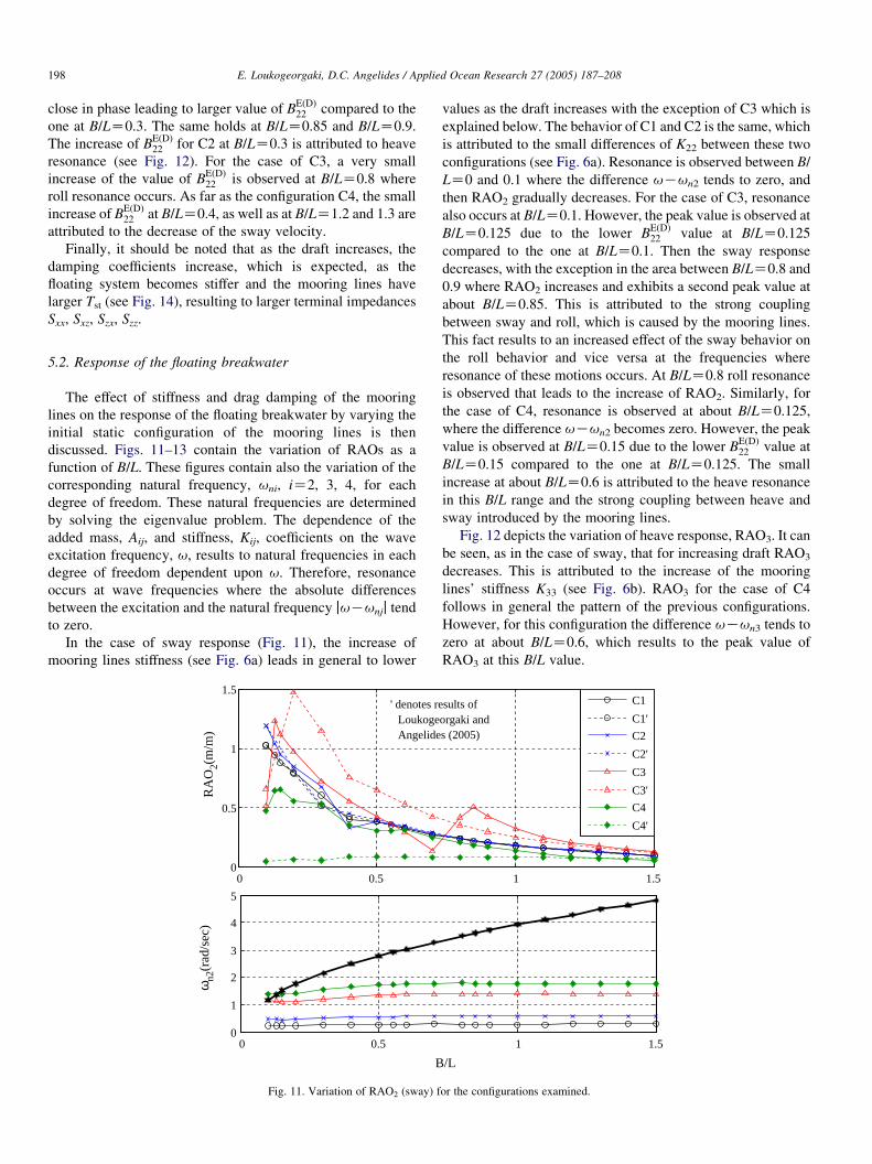
In the case of sway response (Fig. 11), the increase of

mooring lines stiffness (see Fig. 6a) leads in general to lower

0 0.50

0.5

1

1.5

RA

O2(

m/m

)

0 0.50

1

2

3

4

5

B

ωn2

(rad

/sec

)

' denotes reLoukoge

Angelide

Fig. 11. Variation of RAO2 (sway) f

values as the draft increases with the exception of C3 which is

explained below. The behavior of C1 and C2 is the same, which

is attributed to the small differences of K22 between these two

configurations (see Fig. 6a). Resonance is observed between B/

LZ0 and 0.1 where the difference uKun2 tends to zero, and

then RAO2 gradually decreases. For the case of C3, resonance

also occurs at B/LZ0.1. However, the peak value is observed at

B/LZ0.125 due to the lower BEðDÞ22 value at B/LZ0.125

compared to the one at B/LZ0.1. Then the sway response

decreases, with the exception in the area between B/LZ0.8 and

0.9 where RAO2 increases and exhibits a second peak value at

about B/LZ0.85. This is attributed to the strong coupling

between sway and roll, which is caused by the mooring lines.

This fact results to an increased effect of the sway behavior on

the roll behavior and vice versa at the frequencies where

resonance of these motions occurs. At B/LZ0.8 roll resonance

is observed that leads to the increase of RAO2. Similarly, for

the case of C4, resonance is observed at about B/LZ0.125,

where the difference uKun2 becomes zero. However, the peak

value is observed at B/LZ0.15 due to the lower BEðDÞ22 value at

B/LZ0.15 compared to the one at B/LZ0.125. The small

increase at about B/LZ0.6 is attributed to the heave resonance

in this B/L range and the strong coupling between heave and

sway introduced by the mooring lines.

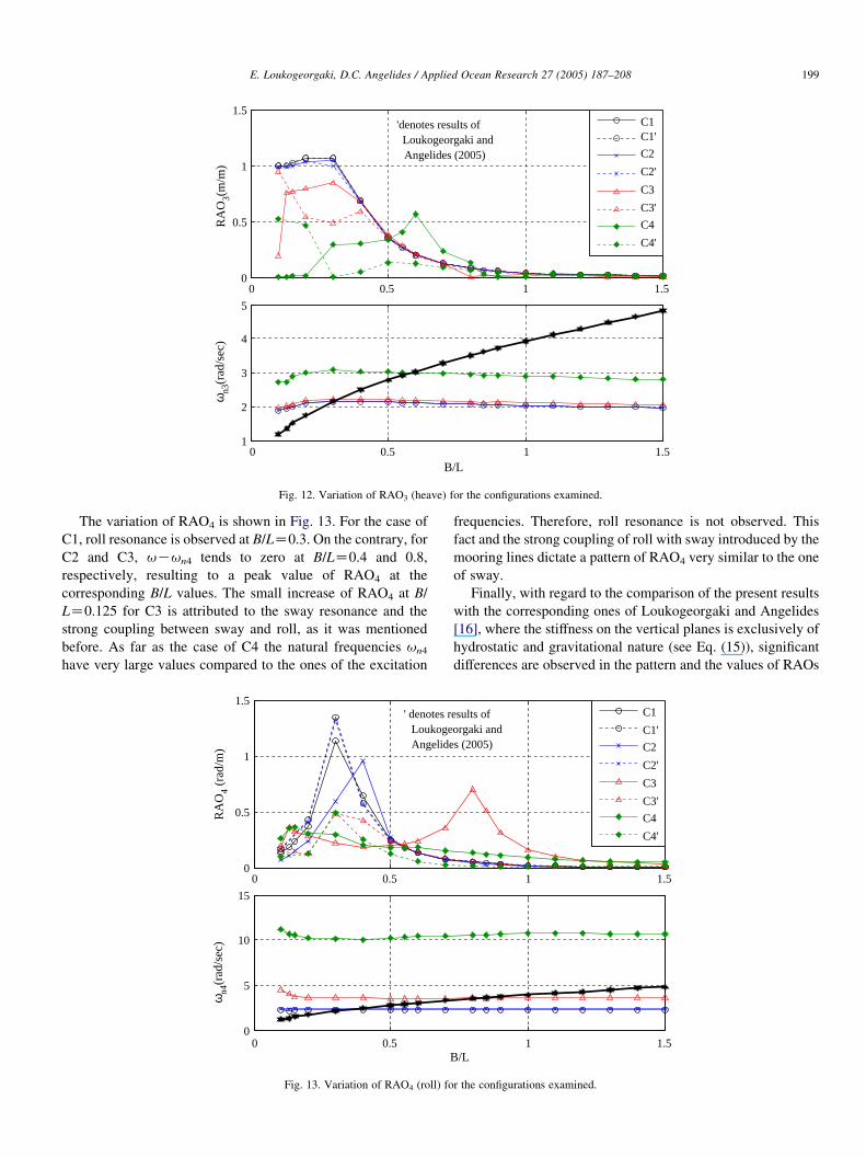
Fig. 12 depicts the variation of heave response, RAO3. It can

be seen, as in the case of sway, that for increasing draft RAO3

decreases. This is attributed to the increase of the mooring

lines’ stiffness K33 (see Fig. 6b). RAO3 for the case of C4

follows in general the pattern of the previous configurations.

However, for this configuration the difference uKun3 tends to

zero at about B/LZ0.6, which results to the peak value of

RAO3 at this B/L value.

1 1.5

1 1.5

/L

C1

C1'

C2

C2'

C3

C3'

C4

C4'

sults oforgaki ands (2005)

or the configurations examined.

0 0.5 1 1.50

0.5

1

1.5

RA

O3(

m/m

)

0 0.5 1 1.51

2

3

4

5

B/L

ωn3

(rad

/sec

)

C1C1'

C2

C2'

C3

C3'

C4

C4'

'denotes results of Loukogeorgaki and

Angelides (2005)

Fig. 12. Variation of RAO3 (heave) for the configurations examined.

E. Loukogeorgaki, D.C. Angelides / Applied Ocean Research 27 (2005) 187–208 199

The variation of RAO4 is shown in Fig. 13. For the case of

C1, roll resonance is observed at B/LZ0.3. On the contrary, for

C2 and C3, uKun4 tends to zero at B/LZ0.4 and 0.8,

respectively, resulting to a peak value of RAO4 at the

corresponding B/L values. The small increase of RAO4 at B/

LZ0.125 for C3 is attributed to the sway resonance and the

strong coupling between sway and roll, as it was mentioned

before. As far as the case of C4 the natural frequencies un4

have very large values compared to the ones of the excitation

0 0.5

0 0.5

0

0.5

1

1.5

RA

O4

(rad

/m)

0

5

10

15

ωn4

(rad

/sec

)

' denotes rLoukogeAngelide

Fig. 13. Variation of RAO4 (roll) fo

frequencies. Therefore, roll resonance is not observed. This

fact and the strong coupling of roll with sway introduced by the

mooring lines dictate a pattern of RAO4 very similar to the one

of sway.

Finally, with regard to the comparison of the present results

with the corresponding ones of Loukogeorgaki and Angelides

[16], where the stiffness on the vertical planes is exclusively of

hydrostatic and gravitational nature (see Eq. (15)), significant

differences are observed in the pattern and the values of RAOs

1 1.5

1 1.5B/L

C1

C1'

C2

C2'

C3

C3'

C4

C4'

esults oforgaki ands (2005)

r the configurations examined.

0 0.5 1 1.50

2

4

6

8

10

Ten

sion

s (K

N)

0 0.5 1 1.50

5

10

15

20

25

B/L

Ten

sion

s (K

N)

Ten

sion

s (K

N)

Ten

sion

s (K

N)

0 0.5 1 1.50

50

100

150

200

0 0.5 1 1.50

100

200

300

400

B/L

Tst

Tst'

Tdyn

Tdyn'

Ttot

s

s

s

s

' denotes results of Loukogeorgakiand Angelides (2005)

C3

C2

C1

C4

Fig. 14. Variation of Tst, Tdyn and Ttot at the top of mooring line 1.

E. Loukogeorgaki, D.C. Angelides / Applied Ocean Research 27 (2005) 187–208200

for C3 and C4. Therefore, it is obvious that through the

transition from the slack to the taut condition of the mooring

lines the vertical stiffness of them affects more significantly the

dynamic response of the floating breakwater.

5.3. Static and dynamic forces of mooring lines

The performance of the mooring lines is defined in terms of

the static, Tst, and the dynamic, Tdyn, tensions at the top

(fairlead) of the mooring lines. The mooring lines that are

placed in the front part of the floating breakwater represent the

most heavily loaded ones under the action of waves in the

normal direction (see Fig. 3). Due to symmetry, the values of

Tst, Tdyn and total tension TtotZTstCTdyn are considered only

for mooring line 1 in Fig. 14.

The variation of Tst with B/L for a specific configuration

follows the variation of the steady drift forces. The dynamic

tensions exhibit large values at the low frequency range (up to

B/LZ0.4) for C1 and C2, where RAOs resonance occurs. The

same holds for C3. Additionally, the occurrence of the roll

resonance at higher values of B/L, for this configuration, results

to the appearance of large values of Tdyn in the range of

0.8%B/L%0.9. Finally, for C4, Tdyn exhibits larger values up

to B/LZ0.6, where the RAOs show larger values, especially for

heave; then a gradual decrease of Tdyn follows. The letter ‘s’ on

each of the subplots of Fig. 14 denotes the occurrence of

snapping (Tst!Tdyn). For the cases of this investigation,

snapping occurs only for C3 at the low frequency range and

at B/LZ0.8 and 0.9 where Tdyn exhibits maximum values. The

increased values of Tst in combination with the lower RAOs

compared to the corresponding ones for the case of C3 explains

the avoidance of snapping phenomena for C4. Finally, it should

be noted that for all configuration cases the total tension Ttot

depicts values lower than Tbreak.

Comparing the presented results with the corresponding

ones of Loukogeorgaki and Angelides [16], differences are

observed for the case of C2 for the values of Tdyn at the low

frequency range, due to differences of RAO4 and the

occurrence of roll resonance at B/LZ0.4 (see Fig. 13). Finally,

the remarkable differences between the responses (all RAOs)

of the cases C3 and C4 of this work and the results included in

Loukogeorgaki and Angelides [16] (see Figs. 11–13) lead to

different variations of Tdyn as well.

5.4. Effectiveness of the floating breakwater

The effectiveness of the moored floating breakwater is

investigated in terms of Kb and Kf coefficients (Eq. (18)). The

wave elevation was calculated for all configurations and for all

frequencies considered in the middle of the floating breakwater

(XZ0 m) at a line perpendicular to it with Y varying between

K2.5 %Y%K40 m in front of the breakwater and

2.5 %Y%40 m behind of, it according to the coordinate

system shown in Fig. 3. It is considered that the wave elevation

at this area is representative for the estimation of the

breakwater’s effectiveness. For each frequency and each

configuration, the wave elevation due to diffraction only and

due to both diffraction and radiation (complete problem) was

calculated.

Results are presented for four properly selected frequencies

in order to have a detailed and integrated description of the

effect of the configuration’s modification of the ‘base case’ on

the effectiveness of the floating breakwater in the low

(B/L%0.4), middle (0.5%B/L%0.9) and high

(1.0%B/L%1.5) wave frequency range. Specifically, results

are presented for B/LZ0.125 and 0.3 (low frequency range

(LFR), Figs. 15 and 17a), for B/LZ0.7 (middle frequency

Fig. 15. Variation of Kb with Y (XZ0 m) for (a) B/LZ0.125 and (b) B/LZ0.3 (LFR).

E. Loukogeorgaki, D.C. Angelides / Applied Ocean Research 27 (2005) 187–208 201

range (MFR), Figs. 16a and 17b) and for B/LZ1.3 (high

frequency range (HFR), Fig. 16b).

From these figures, it is obvious that the wave elevation

coefficients resulting from diffracted waves ðKdf ;K

db Þ are almost

the same for all configurations. Therefore, it is easily concluded

that the variations of Kb and Kf among the various

configurations are attributed to the modification of the radiated

waves associated with the changes of the stiffness and the drag

damping of the mooring lines.

Fig. 16. Variation of Kb with Y (XZ0 m) for (a)

Consider initially the variation of Kb in the LFR, where most

of resonance phenomena occur (Fig. 15). The first two

configurations have very similar patterns due to the very

similar values of RAOs for these B/L values. However, for B/

LZ0.3, C2 shows quite lower values, due to the absence of roll

resonance. Configurations C3 and C4 show lower values for Kb

and, therefore, are more effective compared to the ‘base case’.

For the case of B/LZ0.125 this is attributed: (a) to the fact that

RAO2 and RAO4 are out of phase, which leads to lower values

B/LZ0.7 (MFR) and (b) B/LZ1.3 (HFR).

Fig. 17. Variation of Kf with Y (XZ0 m) for (a) B/LZ0.3 (LFR) and (b) B/LZ0.7 (MFR).

E. Loukogeorgaki, D.C. Angelides / Applied Ocean Research 27 (2005) 187–208202

of radiated waves compared to the case of C1, although their

values are higher, and (b) to the lower values of RAO3. In a

similar manner, the lower values for B/LZ0.3 for these

configurations are attributed to the lower values of RAOs.

Additionally, for B/LZ0.3, a different pattern is observed for

C3 and C4 which follows the pattern of Ktd. The different

(negative) phase differences of the radiated waves with respect

to the incident wave explain this different pattern.

The combination of the above interpretations leads to the

conclusion that C3 and C4 could be considered as the most

effective cases at B/LZ0.125 and 0.3, over a wider range of

locations considered along the portion of the Y-axis. However,

one should also consider two constraints for the selection of

the ‘optimum configuration’ regarding the performance of the

mooring lines. The first one refers to the values of Tst and Tdyn

exercised at the top of the mooring lines, while the second one

is related with the values of Vbot. It is obvious that the increase

of the draft leads to the increase of Vbot, because the initial

fbot increases. For the case of B/LZ0.125 snapping is

observed (Fig. 14) for C3. Consequently, C4 could be

considered as better solution compared to the ‘base case’

for this B/L value. For B/LZ0.3 snapping is not observed for

either C3 or C4. Therefore, configuration C3 is considered

most preferable for this B/L value, as it has lower value of

Vbot.

As far as the coefficient Kf (Fig. 17a), larger values are

observed as the draft increases for each specific B/L value.

Exception represents C4 for B/LZ0.3; for this B/L value, C4

shows larger values of Kb close to the breakwater which results

to lower values of Kf. The pattern of Kf for all configurations is

the same and only phase differences are observed. This can be

explained as follows. The pattern of Kdf is quite intense,

whereas the pattern of the wave elevation coefficient in front

due to radiated waves is smoother and of lower values

compared to Kdf . Therefore, the radiated waves can only

contribute to the values and not the pattern of Kf. The increase

of the draft leads to decrease of the floating breakwater’s

response (except for RAO2 and RAO4 at B/LZ0.125 for C3

and RAO4 at B/LZ0.125 for C4, see Figs. 11 and 13) and to

reduction of the effect of the radiated waves. Consequently, this

results to increase of the Kf values, which approach the values

of Kdf .

With regard to the case of B/LZ0.7 (MFR), Kb coefficient

(Fig. 16a) for C3 and C4 show lower values compared to the

‘base case’. In fact, Kb for C3 exhibits lower values than the

ones for C4, which are closer to the values of Kdb . This is

attributed to the lower values of RAO2 and RAO3 at this B/L

value. Taking into consideration the constraints for the

selection of the ‘optimum’ configuration, as described before,

the avoidance of snapping phenomena at this B/L value leads to

the conclusion that C3 represents the ‘optimum’ case for B/LZ0.7. As far as the coefficient Kf (Fig. 17b), the intense variation

of Kdf due to diffracted waves, results to values of Kf close to Kd

f

for all configurations examined.

Finally, Fig. 16b includes the variation of Kb for B/LZ1.3

(HFR). C1 and C2 show very similar values, while C3 follows

the pattern of the two previous configurations with increased

values. This is attributed to the higher values of RAOs for C3

compared to the responses of the first two configurations. On

the contrary, C4 shows lower values and closer to the values of

Kdb . Therefore, configuration C4 is considered as the ‘optimum’

one for this frequency range, because the increased effective-

ness of the floating breakwater and the satisfactory perform-

ance of the mooring lines (i.e. avoidance of snapping

Fig. 18. Kb and Kf contours for: (a) C1 and B/LZ0.125, (b) C4 and B/LZ0.125, (c) C1 and B/LZ0.7 and (d) C3 and B/LZ0.7.

E. Loukogeorgaki, D.C. Angelides / Applied Ocean Research 27 (2005) 187–208 203

phenomena see Fig. 14) are both satisfied. The variations of Kf

coefficients for these values of B/L are similar to the variation

of Kf at B/LZ0.7 and therefore, they are not included in the

present work.

At this point, it should be noted that for all B/L cases the

values of Kb coefficients for C1 and C2 are very similar with

the corresponding ones described by Loukogeorgaki and

Angelides [16], as shown in Figs. 15 and 16. However, for

C3 and C4 different values and different behavior are observed.

This is attributed to the differences in RAOs for these

configurations, due to the inclusion of the vertical stiffness in

the present work, as explained in Section 5.2.

Finally, Fig. 18 contains contours of Kb and Kf in a large

area in front and behind the breakwater for B/LZ0.125

(Fig. 18a and b) and B/LZ0.7 (Fig. 18c and d). Fig. 18a and c

correspond to the ‘base case’, whereas Fig. 18b and d

correspond to C4 and C3, respectively. The larger effectiveness

of C4 for B/LZ0.125 and C3 for B/LZ0.7 in a wide area

behind the breakwater can be easily observed, while Kf in the

front area shows a more intense variation.

5.5. Decision framework for the effective performance

of the floating breakwater

The results presented in the previous subsections support the

need for a decision process that should be implemented in order

to select the ‘optimum’ configuration (expressed with Ci) of the

floating breakwater for a specific wave environment (expressed

with B/L values). A configuration Ci (length of mooring lines

and draft) is considered as the ‘optimum’ one when it satisfies:

(a) the objective of effective performance of the floating

breakwater, i.e. effective reduction of the transmitted energy in

the area behind the floating breakwater and (b) the constraints

of the mooring lines that confine the objective of the effective

performance of the floating breakwater, i.e. failure of mooring

lines and snapping occurrence (primary constraints) and

minimization of the vertical force at the bottom (secondary

constraint). It should be mentioned that the term ‘optimum’ is

not used with reference to any mathematical optimization

process; it simply refers to the best feasible configuration of the

floating breakwater compared to the initial one.

Table 2

Decision framework—relation of B/L and ‘optimum’ Ci for effective performance of a floating breakwater

2829

30

0.750.80.850

0.5

1

1.5

Ltot (m)dr (m)

B/L

LFR

MFR

HFRLFR-MFR transition

MFR-HFR transition

Fig. 19. ‘Optimum’ draft and ‘optimum’ mooring lines length of all the

frequency ranges.

E. Loukogeorgaki, D.C. Angelides / Applied Ocean Research 27 (2005) 187–208204

Based on these considerations, a decision framework is

introduced, as shown in Table 2 that relates the wave

environment (INPUT) with the final ‘optimum’ selected

configuration of the floating breakwater (OUTPUT) through

a specific decision process, which is described below. At this

point, it should be emphasized that the proposed decision

framework, generally, presents an alternative design approach

for moored floating structures. It can be applied in cases where

there is a necessity to modify the dynamic characteristics of

them, through the modification of the static and dynamic

characteristics of the mooring lines. The final overall target is

to optimize the performance of the system. The INPUT and the

OUTPUT of this framework could remain the same. However,

the rest of its components (design objectives—constraints) can

be properly adjusted, so that they can present the conditions,

the characteristics and the design targets of a specific case.

In Section 5.4, this framework has been already used in

order to select the ‘optimum’ configuration for specific,

properly selected, B/L values. The application of the same

decision process for the rest of B/L values (see Table 2) results

to the determination of a relation between the wave

environment (LFR, MFR, and HFR), investigated in the

present work, and the configuration of the floating breakwater.

Initially, for each B/L value, configurations Ci are selected

considering only the effectiveness of the floating breakwater as

the selection criterion (Stage 1). Then, the constraints of the

mooring lines are taken into consideration (Stage 2). In cases

where a configuration Ci, which has been considered as the best

case in Stage 1, does not satisfy one of the two primary

constraints, it is rejected and the subsequent configuration Ci

determined in Stage 1 is selected. This Ci could be either a

configuration that has been considered as better solution versus

C1 (see for example B/LZ0.1 in Table 2) or the initial

configuration C1 (see for example B/LZ0.8 in Table 2). On the

contrary, in cases where the primary two constraints are both

satisfied, the vertical force at the bottom (minimum value)

represents the critical factor for the selection of the ‘optimum’

configuration (see for example B/LZ0.3 in Table 2). The

E. Loukogeorgaki, D.C. Angelides / Applied Ocean Research 27 (2005) 187–208 205

combination of these items results to the final decision for the

‘optimum’ configuration (Stage 3).

The final decision points derived in Table 2 are graphically

presented in three dimensions (Fig. 19). Each configuration is

represented by the value of dri and the value of the required Ltoti

of the mooring lines for achieving the corresponding draft for

each B/L value. It is easily concluded that the initial

configuration C1 of the floating breakwater should be modified

in the low and high frequency range, as well as for some

intermediate frequencies in the middle frequency range. On the

contrary, in the transition frequency ranges (LFR–MFR and

MFR–HFR) the initial configuration C1 represents the

‘optimum’ one.

6. Conclusions

The performance of a moored floating breakwater is

theoretically investigated under the action of normal regular

waves. Special attention is given to the effect of different

configurations of the mooring lines and, consequently, to

the effect of stiffness and damping of the mooring lines on the

dynamic response and on the protective effectiveness of

the floating breakwater. A three-dimensional model of the

hydrodynamic analysis of the floating body is coupled with a

model of the static and dynamic analysis of the mooring lines,

using an appropriate iterative procedure in terms of the steady

drift forces and the dynamic response of the floating break-

water. The stiffness coefficients of the mooring lines are derived

in the six degrees of freedom of the floating breakwater, based

on the differential changes of mooring lines’ tensions caused by

the static motions of the floating body. Furthermore, an

extensive parametric study has been presented. The initial

configuration of a ‘base case’ floating breakwater is altered

through the appropriate modifications of the mooring lines’

length, which affect directly mooring lines’ stiffness and

damping. The main conclusions from this study are as follows:

1. The modification of the initial configuration of the floating

breakwater through the modification of the length of the

mooring lines affects the stiffness and drag damping of the

mooring lines, and consequently, the dynamic response and

the effectiveness of the floating breakwater.

2. The transition from the slack to the taut condition leads to

the increase of the stiffness of the mooring lines imposed on

the floating breakwater. Additionally, through this tran-

sition, the stiffness of the mooring lines on the vertical

planes affects more significantly the overall vertical

stiffness of the floating breakwater and consequently, its

overall performance.

3. Intense modification of the dynamic response of the floating

breakwater is observed through the transition from the slack

to the taut condition, while stronger coupling between the

degrees of freedom is also introduced. In the case of taut

mooring lines, the resonance of the vertical motions (heave

and roll) is shifted at higher frequencies.

4. The small change of the draft of the floating breakwater

leads to a similar wave diffracted field for all the

configurations investigated. Therefore, any changes on

the effectiveness of the floating breakwater are attributed to

the modification of the response of the floating breakwater

and thus, to the modification of the stiffness and damping of

the mooring lines for the configurations examined.

5. The transition from the slack to the taut condition of the

mooring lines results to a significant increase of the

effectiveness of the floating breakwater for the whole

frequencies examined (even in the low frequency range).

The increase of the protective effectiveness of the floating

breakwater is gradually reduced towards higher frequencies

(50% increase of effectiveness in the LFR, 20% in the MFR

and 10–15% for the HFR). Exceptions represent the

transitional stages (LFR–MFR and MFR–HFR).

6. Existence of ‘optimum’ configuration is demonstrated for

the wave frequencies range considered. The selection of the

‘optimum’ configuration is based on a decision process that

is adopted in order to ensure: (a) effective reduction of the

transmitted energy behind the breakwater and (b) satisfac-

tion of the constraints associated with the mooring lines.

7. A decision framework is finally introduced that relates the

wave environment (INPUT) with the final ‘optimum’

selected configuration of the floating breakwater (OUT-

PUT) through a specific decision process. This framework

could form the basis for the development of a control system

that addresses effectiveness target of the floating breakwater

and simultaneously the constraints introduced by the

mooring lines.

Acknowledgements

The authors would like to thank the reviewers for their

valuable comments and suggestions on the final manuscript.

Furthermore, they would like to acknowledge the financial

support of the Hellenic General Secretariat for Research and

Technology (GSRT) and the European Social Fund (ESF)

through the Operational Programme ‘Competitiveness’ (Op.

Pr. Comp).

Appendix A. Definition of kj, km and kn terms

The following relations are derived for the terms kj, km and

kn:

(a) qX rotation (jZ0, mZ1 and nZ2)

kjZ0 ZKvlx

vqX

Zðsin qX sin qZ Ccos qX sin qY cos qZÞYPO

C ðKsin qX sin qY cos qZ Ccos qX sin qZÞZPO

(A1a)

kmZ1 ZKvly

vqX

Zðcos qX sin qY sin qZKsin qX cos qZÞYPO

Kðcos qX cos qZ Csin qX sin qY sin qZÞZPO

(A1b)

E. Loukogeorgaki, D.C. Angelides / Applied Ocean Research 27 (2005) 187–208206

knZ2 ZKvlzvqX

Z ðcos qX cos qY ÞYPOKðsin qX cos qY ÞZPO

(A1c)

(b) qY rotation (jZ3, mZ4 and nZ5)

kjZ3ZKvlxvqY

ZKðsinqY cosqZÞXPO

CðsinqX cosqY cosqZÞYPOCðcosqX cos qY cosqZÞZPO

(A2a)

KmZ4Zvly

vqY

ZKðsinqY sinqZÞXPOCðsinqX cosqY sinqZÞYPO

CðcosqX cosqY sinqZÞZPO (A2b)

knZ5ZKvlz

vqY

ZKðcosqY ÞXPOKðsinqX sinqY ÞYPO

KðcosqX sinqY ÞZPO (A2c)

(c) qZ rotation (jZ6, mZ7 and nZ8)

kjZ6ZKvlx

vqZ

ZKðsinqZ cosqY ÞXPOKðcosqX cosqZ

CsinqX sinqY sinqZÞYPO

CðKcosqX sinqY sinqZ

CsinqX cosqZÞZPO (A3a)

kmZ7ZKvly

vqZ

ZðcosqZ cosqY ÞXPOCðsinqX sinqY cosqZ

KcosqX sinqZÞYPOCðsinqX sinqZ

CcosqX sinqY cosqZÞZPO (A3b)

knZ8ZKvlzvqZ

Z0 (A3c)

The above equations can be simplified in case of horizontal

forces and moment by setting ZoZqXZqYZ0 as following:

kjZ0ZsinqZZPO (A4a)

kmZ1ZKcosqZYPO (A4b)

knZ2ZYPO (A4c)

kjZ3ZcosqZZPO (A5a)

kmZ4ZsinqZZPO (A5b)

knZ5ZKXPO (A5c)

kjZ6ZsinqZXPOKcosqZYPO (A6a)

kmZ7ZcosqZXPOKsinqZYPO (A6b)

knZ8Z0 (A6c)

Appendix B. Equations of the stiffness coefficients

(a) Stiffness coefficients K1j (jZ1,., 6)

Km11ZK

vðfXÞm

vXo

ZKvH cosq

vXo

ZKvT cosfcosq

vXo

0

Km11ZAcos2qCB sin2qKC cos2q (B1)

Km12ZðAKBKCÞsinqcosq (B2)

Km13ZDcosq sinu (B3)

Km14ZDðk0cosucosqCk1cosu sinqCk2sinuÞcosq

KB sinqðk1cosqKk0sinqÞ (B4)

Km15ZDðk3cosucosqCk4cosu sinqCk5sinuÞcosq

KB sinqðk4cosqKk3sinqÞ (B5)

Km16ZDðk6cosucosqCk7cosu sinqCk8sinuÞcosq

KB sinqðk7cosqKk6sinqÞ (B6)

(b) Stiffness coefficients K2j (jZ1,., 6)

Km21ZKm

12 (B7)

Km22ZA sin2qCBcos2qKC sin2q (B8)

Km23ZD sinq sinu (B9)

Km24ZDðk0 cosucosqCk1 cosu sinqCk2 sinuÞsinq

CBcosqðk1 cosqKk0 sinqÞ (B10)

Km25ZDðk3 cosucosqCk4 cosu sinqCk5 sinuÞsinq

CBcosqðk4 cosqKk3 sinqÞ (B11)

Km26ZDðk6 cosucosqCk7 cosu sinqCk8 sinuÞsinq

CBcosqðk7 cosqKk6 sinqÞ (B12)

(c) Stiffness coefficients K3j (jZ1,., 6)

Km31ZE cosqcosu (B13)

Km32ZE sinqcosu (B14)

E. Loukogeorgaki, D.C. Angelides / Applied Ocean Research 27 (2005) 187–208 207

Km33ZE sinu (B15)

Km34ZEðk0 cosucosqCk1 cosu sinqCk2 sinuÞ (B16)

Km35ZEðk3 cosucosqCk4 cosu sinqCk5 sinuÞ (B17)

Km36ZEðk6 cosucosqCk7 cosu sinqCk8 sinuÞ (B18)

(d) Stiffness coefficients K4j (jZ1,., 6)

Km41ZðYPKYoÞK

m31KðZPKZoÞK

m21 (B19)

Km42ZðYPKYoÞK

m32KðZPKZoÞK

m22 (B20)

Km43ZðYPKYoÞK

m33KðZPKZoÞK

m23 (B21)

Km44ZTstðk1sinfKk2cosf sinqÞCðYPKYoÞK

m34KðZPKZoÞK

m24

(B22)

Km45ZTstðk4sinfKk5cosf sinqÞCðYPKYoÞK

m35KðZPKZoÞK

m25

(B23)

Km46ZTstðk7sinfKk8cosf sinqÞCðYPKYoÞK

m36KðZPKZoÞK

m26

(B24)

(e) Stiffness coefficients K5j (jZ1,., 6)

Km51ZðZPKZoÞK

m11KðXPKXoÞK

m31 (B25)

Km52ZðZPKZoÞK

m12KðXPKXoÞK

m32 (B26)

Km53ZðZPKZoÞK

m13KðXPKXoÞK

m33 (B27)

Km54ZTstðk2cosfcosqKk0sinfÞCðZPKZoÞK

m14KðXPKXoÞK

m34

(B28)

Km55ZTstðk5cosfcosqKk3 sinfÞCðZPKZoÞK

m15KðXPKXoÞK

m35

(B29)

Km56ZTstðk8cosfcosqKk6sinfÞCðZPKZoÞK

m16KðXPKXoÞK

m36

(B30)

(f) Stiffness coefficients K6j (jZ1,., 6)

Km61ZKm

16 (B31)

Km62ZKm

26 (B32)

Km63ZðXPKXoÞK

m23KðYPKYoÞK

m13 (B33)

Km64ZTstcosfðk0sinqKk1cosqÞCðXPKXoÞK

m24KðYPKYoÞK

m14

(B34)

Km65ZTstcosfðk3sinqKk4cosqÞCðXPKXoÞK

m25KðYPKYoÞK

m15

(B35)

Km66ZTstcosfðk6sinqKk7cosqÞCðXPKXoÞK

m26KðYPKYoÞK

m16

(B36)

In the above equations, the terms A–E are given as follows:

AZdTst

dlcosucosf BZTst

cosf

lcosu

CZTst

df

dlsinfcosu DZ

dTst

dlcosfKTst

df

dlsinf

EZdTst

dlsinfCTst

df

dlcosf

(B37)

References

[1] Bhat S. Performance of twin-pontoon floating breakwaters. PhD thesis,

Department of Civil Engineering, University of British Columbia,

Vancouver, Canada; 1998.

[2] Bhat S, Isaacson M. Performance of twin-pontoon floating break-

water. In: ISOPE 1998, eighth international conference of offshore

and polar engineering Montreal, Canada, vol. 3; May 24–29, 1998. p.

584–90.

[3] Briggs M, Ye W, Demirbilek Z, Zhang J. Comparison of hydrodynamic

parameters for a floating breakwater. In: First international symposium on

‘monitoring of breakwaters’, ASCE, Madison, WI, USA; September 8–

10, 1999. p. 37–51.

[4] Daghigh M, Paein Koulaei RT, Seif MS. Mooring system design and

optimization for floating bridge of Urmia Lake. In: OMAE2002-28343

21st international conference on offshore mechanics and arctic

engineering, Oslo, Norway; June 23–28, 2002. p. 1–8.

[5] Irvine HM. Cable structures. Cambridge, MA: MIT Press; 1981.

[6] Isaacson M. Hydrodynamic coefficients of floating breakwaters. In: 11th

Canadian hydrotechnical conference, Fredericton, Canada, vol. 1; June 8–

11, 1993. p. 485–94.

[7] Isaacson M. Wave effects on floating breakwaters. In: Canadian coastal

conference, Vancouver, Canada, vol. 1; May 4–7, 1993. p. 53–66.

[8] Isaacson M, Baldwin J. Moored structures in waves and currents. Can

J Civ Eng 1996;23(2):418–30.

[9] Isaacson M., Bhat S. Analysis of Moored Floating Breakwaters.

In: Annual conference of the Canadian Society for Civil

Engineering, Edmonton, Canada, vol. 1; May 29–June 1, 1996.

p. 610–19.

[10] Isaacson M., Garceau N. Wave propagation past long floating break-

waters. 13th Canadian hydrotechnical conference, Sherbrooke, Canada,

vol. 1, May 27–30, 1997. p. 3–10.

[11] Isaacson M, Nwogu O. Wave loads and motions of long structures in

directional seas. J Offshore Mech Arct Eng ASME 1987;109(2):

126–32.

[12] Jain RK. A simple method of calculating the equivalent stiffnesses in

mooring cables. Appl Ocean Res 1980;2:139–42.

[13] Kruezer E, Wilke U. Dynamics of mooring systems in ocean engineering.

Arch Appl Mech 2003;73:270–81.

E. Loukogeorgaki, D.C. Angelides / Applied Ocean Research 27 (2005) 187–208208

[14] Lee J, ChoW. Hydrodynamic analysis of wave interactions with a moored

floating breakwater using the element-free Galerkin method. Can J Civ

Eng 2003;30(4):720–33.

[15] Lee C-H, Newman JN. Computation of wave effects using the panel

method. In: Chakrabarti S, editor. Numerical models in fluid-structure

interaction, Preprint. Southampton: WIT Press; 2004.

[16] Loukogeorgaki E, Angelides DC. Effect of mooring lines on floating

breakwaters performance. In: ISOPE 2005, 15th international conference

of offshore and polar engineering, Seoul, Korea, 2005.

[17] McCartney M, Bruce L. Floating breakwater design. J Waterway Port

Coastal Ocean Eng 1985;111(2):304–17.

[18] Newman JN. The drift force and moment on ships in waves. J Ship Res

1967;11:51–60.

[19] Newman JN. Marine hydrodynamics. Cambridge, MA: MIT Press;

1977.

[20] Sannasiraj SA, Sundar V, Sundaravadivelu R. Mooring forces and motion

responses of pontoon-type floating breakwaters. Ocean Eng 1998;25(1):

27–48.

[21] Triantafyllou MS. Preliminary design of mooring systems. J Ship Res

1982;26(1):25–35.

[22] Triantafyllou MS, Bliek A, Shin H. Static and fatigue analysis of mutli-

leg mooring systems. Technical report.: MIT Press; 1986.

[23] Williams AN, Abul-Azm AG. Dual pontoon floating breakwater. Ocean

Eng 1997;24(5):465–78.

[24] Williams AN, Lee HS, Huang Z. Floating pontoon breakwaters. Ocean

Eng 2000;27(3):221–40.

Demos C. Angelides is a Professor of Civil Engineering at the University of

Thessaloniki, Greece with teaching and research responsibilities on analysis,

design and construction of marine structures. He was Director of the Hydraulics

and Environmental Engineering Division 2002–2004. Currently, he is the

Chairman of the Civil Engineering Department of the Aristotle University of

Thessaloniki. Previously, he was with McDermott International, Inc., in the

USA, having several engineering and management positions. He received his

Dipl. Ing. Degree in Civil Engineering from the Aristotle University of

Thessaloniki, Greece, and his S.M. and PhD both from the Civil Engineering

department of the Massachusetts Institute of Technology (MIT). He delivered

invited lectures in several organizations in the USA and Europe. He

participated in conferences and has published several papers in journals,

chapters in books, and a book. He is a member of several scientific and

professional societies. He is included in Who’s Who publications of the

Marquis Publications Board.

Eva Loukogeorgaki is a research assistant in the Department of Civil

Engineering of the Aristotle University of Thessaloniki, Greece, currently

pursuing her doctoral degree on ‘Control of moored floating breakwaters for

increasing their efficiency and minimizing the failure of the mooring system’.

She holds a Dipl. Ing. in Civil Engineering from the Aristotle University of

Thessaloniki. Prior to pursuing her graduate studies, she has worked in analysis,

design and construction supervision of several civil engineering projects. She is

a registered Professional Engineer in Greece.