Steve Renals 28 September 2016 - The University of Edinburgh · Stochastic gradient descent; Classi cation Steve Renals Machine Learning Practical | MLP Lecture 2 28 September 2016

Stochastic gradient descent; Classification

Steve Renals

Machine Learning Practical — MLP Lecture 228 September 2016

MLP Lecture 2 Stochastic gradient descent; Classification 1

Single Layer Networks


Applying gradient descent to a single-layer network

x1 x2 x3 x4 x5

y2 =5X

i=1

w2ixi

w24

�w24 =X

n

(yn2 � tn2 )xn

4


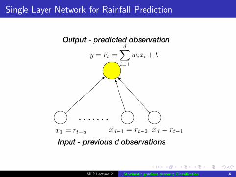
Single Layer Network for Rainfall Prediction

y = r̂t =dX

i=1

wixi + b

xd = rt�1xd�1 = rt�2x1 = rt�d

. . . . . . .

Input - previous d observations

Output - predicted observation


Stochastic Gradient Descent (SGD)

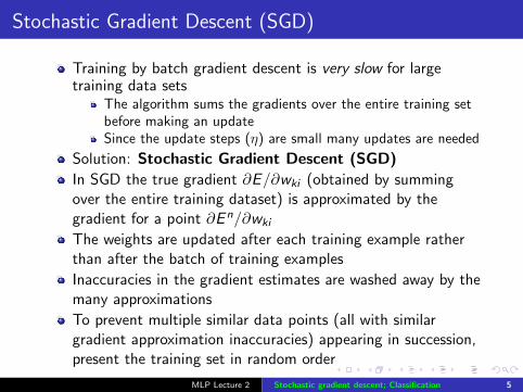
Training by batch gradient descent is very slow for largetraining data sets

The algorithm sums the gradients over the entire training setbefore making an updateSince the update steps (η) are small many updates are needed

Solution: Stochastic Gradient Descent (SGD)

In SGD the true gradient ∂E/∂wki (obtained by summingover the entire training dataset) is approximated by thegradient for a point ∂En/∂wki

The weights are updated after each training example ratherthan after the batch of training examples

Inaccuracies in the gradient estimates are washed away by themany approximations

To prevent multiple similar data points (all with similargradient approximation inaccuracies) appearing in succession,present the training set in random order


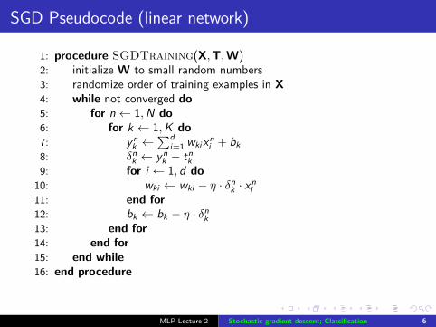
SGD Pseudocode (linear network)

1: procedure SGDTraining(X,T,W)2: initialize W to small random numbers3: randomize order of training examples in X4: while not converged do5: for n← 1,N do6: for k ← 1,K do7: yn

k ←∑d

i=1 wkixni + bk

8: δnk ← ynk − tnk

9: for i ← 1, d do10: wki ← wki − η · δnk · xni11: end for12: bk ← bk − η · δnk13: end for14: end for15: end while16: end procedure


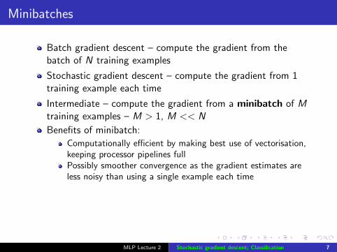
Minibatches

Batch gradient descent – compute the gradient from thebatch of N training examples

Stochastic gradient descent – compute the gradient from 1training example each time

Intermediate – compute the gradient from a minibatch of Mtraining examples – M > 1, M << N

Benefits of minibatch:

Computationally efficient by making best use of vectorisation,keeping processor pipelines fullPossibly smoother convergence as the gradient estimates areless noisy than using a single example each time


Classification


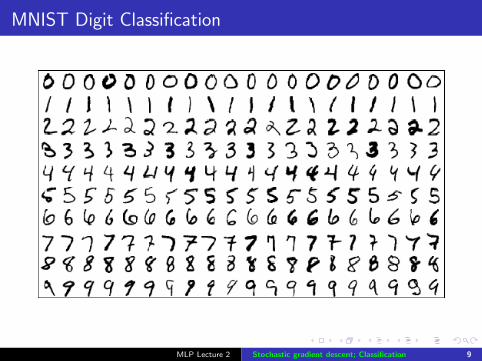
MNIST Digit Classification


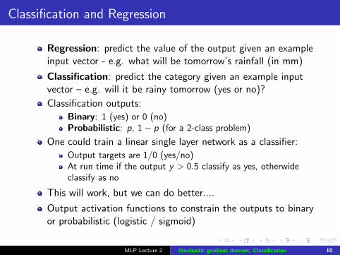
Classification and Regression

Regression: predict the value of the output given an exampleinput vector - e.g. what will be tomorrow’s rainfall (in mm)

Classification: predict the category given an example inputvector – e.g. will it be rainy tomorrow (yes or no)?

Classification outputs:

Binary: 1 (yes) or 0 (no)Probabilistic: p, 1− p (for a 2-class problem)

One could train a linear single layer network as a classifier:

Output targets are 1/0 (yes/no)At run time if the output y > 0.5 classify as yes, otherwideclassify as no

This will work, but we can do better....

Output activation functions to constrain the outputs to binaryor probabilistic (logistic / sigmoid)


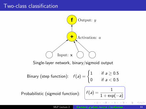
Two-class classification

Input: x

+

f Output: y

Activation: a

Single-layer network, binary/sigmoid output

Binary (step function): f (a) =

{1 if a ≥ 0.5

0 if a < 0.5

Probabilistic (sigmoid function): f (a) =1

1 + exp(−a)


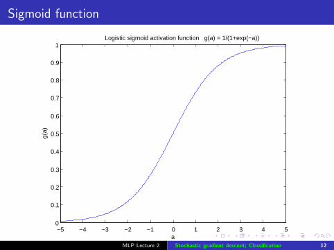
Sigmoid function

−5 −4 −3 −2 −1 0 1 2 3 4 50

0.1

0.2

0.3

0.4

0.5

0.6

0.7

0.8

0.9

1

a

g(a)

Logistic sigmoid activation function g(a) = 1/(1+exp(−a))


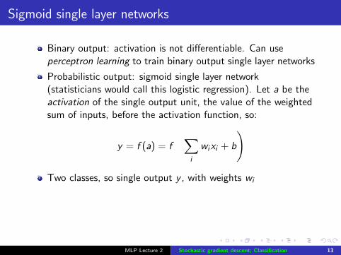
Sigmoid single layer networks

Binary output: activation is not differentiable. Can useperceptron learning to train binary output single layer networks

Probabilistic output: sigmoid single layer network(statisticians would call this logistic regression). Let a be theactivation of the single output unit, the value of the weightedsum of inputs, before the activation function, so:

y = f (a) = f

(∑

i

wixi + b

)

Two classes, so single output y , with weights wi


Sigmoid single layer networks

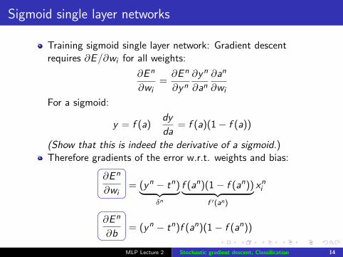
Training sigmoid single layer network: Gradient descentrequires ∂E/∂wi for all weights:

∂En

∂wi=∂En

∂yn∂yn

∂an∂an

∂wi

For a sigmoid:

y = f (a)dy

da= f (a)(1− f (a))

(Show that this is indeed the derivative of a sigmoid.)Therefore gradients of the error w.r.t. weights and bias:

∂En

∂wi= (yn − tn)︸︷︷︸

δn

f (an)(1− f (an))︸︷︷︸f ′(an)

xni

∂En

∂b= (yn − tn)f (an)(1− f (an))


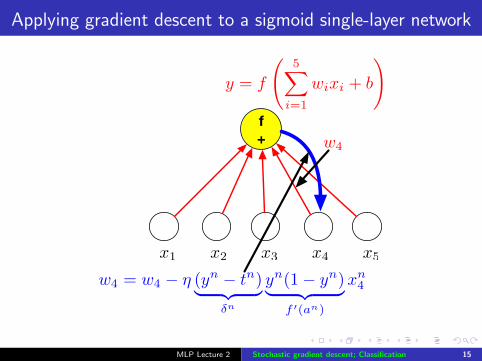
Applying gradient descent to a sigmoid single-layer network

f+

x1 x2 x3 x4 x5

w4

y = f

5X

i=1

wixi + b

!

w4 = w4 � ⌘ (yn � tn)| {z }�n

yn(1� yn)| {z }f 0(an)

xn4


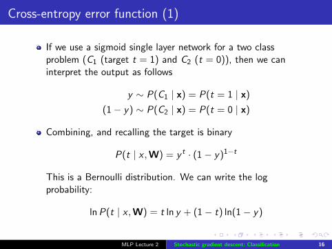
Cross-entropy error function (1)

If we use a sigmoid single layer network for a two classproblem (C1 (target t = 1) and C2 (t = 0)), then we caninterpret the output as follows

y ∼ P(C1 | x) = P(t = 1 | x)

(1− y) ∼ P(C2 | x) = P(t = 0 | x)

Combining, and recalling the target is binary

P(t | x ,W) = y t · (1− y)1−t

This is a Bernoulli distribution. We can write the logprobability:

lnP(t | x ,W) = t ln y + (1− t) ln(1− y)


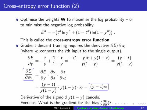
Cross-entropy error function (2)

Optimise the weights W to maximise the log probability – orto minimise the negative log probability.

En = −(tn ln yn + (1− tn) ln(1− yn)) .

This is called the cross-entropy error functionGradient descent training requires the derivative ∂E/∂wi

(where wi connects the ith input to the single output).

∂E

∂y= − t

y+

1− t

1− y=−(1− y)t + y(1− t)

y(1− y)=

(y − t)

y(1− y)

∂E

∂wi=∂E

∂y· ∂y∂a· ∂a∂wi

=(y − t)

y(1− y)· y(1− y) · xi = (y − t)xi

Derivative of the sigmoid y(1− y) cancels.Exercise: What is the gradient for the bias (∂E∂b )?


Multi-class networks

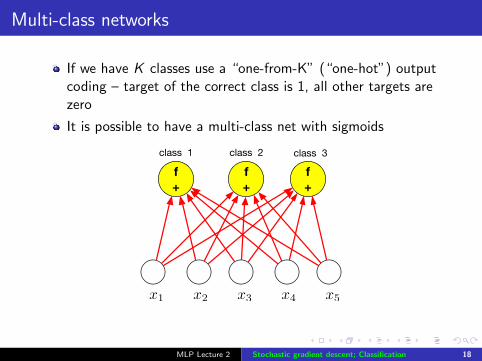
If we have K classes use a “one-from-K” (“one-hot”) outputcoding – target of the correct class is 1, all other targets arezero

It is possible to have a multi-class net with sigmoids

f+

x1 x2 x3 x4 x5

f+

f+

class 1 class 2 class 3


Multi-class networks

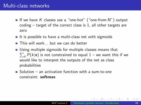
If we have K classes use a “one-hot” (“one-from-N”) outputcoding – target of the correct class is 1, all other targets arezero

It is possible to have a multi-class net with sigmoids

This will work... but we can do better

Using multiple sigmoids for multiple classes means that∑k P(k |x) is not constrained to equal 1 – we want this if we

would like to interpret the outputs of the net as classprobabilities

Solution – an activation function with a sum-to-oneconstraint: softmax


Softmax

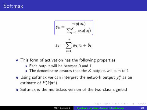
yk =exp(ak)

∑Kj=1 exp(aj)

ak =d∑

i=1

wkixi + bk

This form of activation has the following properties

Each output will be between 0 and 1The denominator ensures that the K outputs will sum to 1

Using softmax we can interpret the network output ynk as anestimate of P(k|xn)

Softmax is the multiclass version of the two-class sigmoid


Softmax – Training (1)

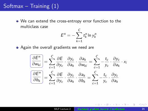
We can extend the cross-entropy error function to themulticlass case

En = −C∑

k=1

tnk ln ynk

Again the overall gradients we need are

∂En

∂wki=

C∑

c=1

∂E

∂yc· ∂yc∂ak· ∂ak∂wki

=C∑

c=1

− tcyc· ∂yc∂ak· xi

∂En

∂bk=

C∑

c=1

∂E

∂yc· ∂yc∂ak· ∂ak∂bk

=C∑

c=1

− tcyc· ∂yc∂ak


Softmax – Training (2)

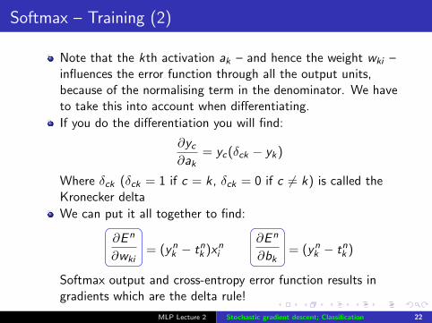
Note that the kth activation ak – and hence the weight wki –influences the error function through all the output units,because of the normalising term in the denominator. We haveto take this into account when differentiating.

If you do the differentiation you will find:

∂yc∂ak

= yc(δck − yk)

Where δck (δck = 1 if c = k, δck = 0 if c 6= k) is called theKronecker delta

We can put it all together to find:

∂En

∂wki= (ynk − tnk )xni

∂En

∂bk= (ynk − tnk )

Softmax output and cross-entropy error function results ingradients which are the delta rule!


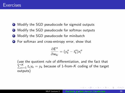
Exercises

1 Modify the SGD pseudocode for sigmoid outputs

2 Modify the SGD pseudocode for softmax outputs

3 Modify the SGD pseudocode for minibatch

4 For softmax and cross-entropy error, show that

∂En

∂wki= (ynk − tnk )xni

(use the quotient rule of differentiation, and the fact that∑Kc=1 tcyk = yk because of 1-from-K coding of the target

outputs)


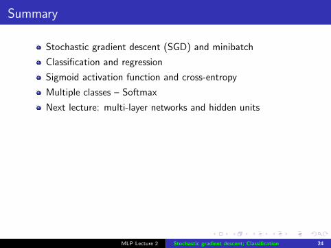
Summary

Stochastic gradient descent (SGD) and minibatch

Classification and regression

Sigmoid activation function and cross-entropy

Multiple classes – Softmax

Next lecture: multi-layer networks and hidden units


Steve Renals 28 September 2016 - The University of Edinburgh · Stochastic gradient descent; Classi cation Steve Renals Machine Learning Practical | MLP Lecture 2 28 September 2016

Documents