Stereo matching Class 10 Read Chapter 7 Tsukuba dataset.

Stereo matchingClass 10

Read Chapter 7

http://cat.middlebury.edu/stereo/

Tsukuba dataset

Stereo

• Standard stereo geometry• Stereo matching

• Correlation• Optimization (DP, GC)

• General camera configuration• Rectification• Plane-sweep

Standard stereo geometry

pure translation along X-axis

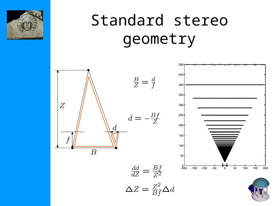
Standard stereo geometry

Stereo matching

• Search is limited to epipolar line (1D)• Look for most similar pixel

?

Aggregation

• Use more than one pixel• Assume neighbors have similar

disparities*

• Use correlation window containing pixel

• Allows to use SSD, ZNCC, Census, etc.

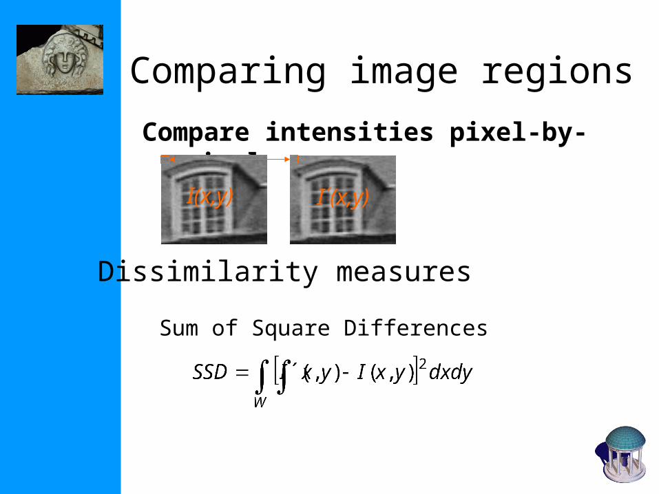
Compare intensities pixel-by-pixel

Comparing image regions

I(x,y) I´(x,y)

Sum of Square Differences

Dissimilarity measures

Compare intensities pixel-by-pixel

Comparing image regions

I(x,y) I´(x,y)

Zero-mean Normalized Cross Correlation

Similarity measures

Compare intensities pixel-by-pixel

Comparing image regions

I(x,y) I´(x,y)

Census

Similarity measures

125 126 125

127 128 130

129 132 135

0 0 0

0 1

1 1 1

(Real-time chip from TYZX based on Census)

only compare bit signature

Aggregation window sizes

Small windows • disparities similar• more ambiguities• accurate when correct

Large windows • larger disp. variation• more discriminant• often more robust• use shiftable windows

to deal with discontinuities

(Illustration from Pascal Fua)

Occlusions

(Slide from Pascal Fua)

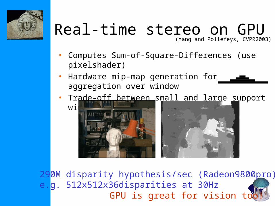
Real-time stereo on GPU

• Computes Sum-of-Square-Differences (use pixelshader)

• Hardware mip-map generation for aggregation over window

• Trade-off between small and large support window

(Yang and Pollefeys, CVPR2003)

290M disparity hypothesis/sec (Radeon9800pro)e.g. 512x512x36disparities at 30Hz

GPU is great for vision too!

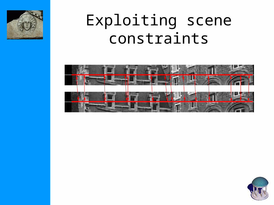
Exploiting scene constraints

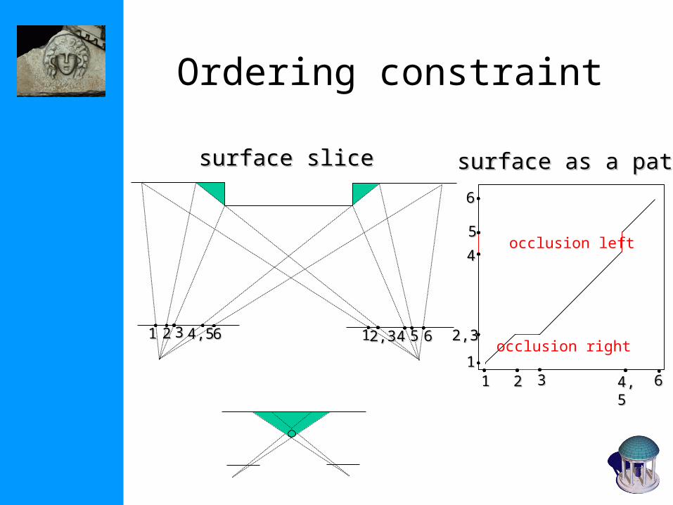
Ordering constraint

11 22 33 4,54,5 66 11 2,32,3 44 55 66

2211 33 4,54,5 6611

2,32,3

44

55

66

surface slicesurface slice surface as a pathsurface as a path

occlusion right

occlusion left

Uniqueness constraint

• In an image pair each pixel has at most one corresponding pixel• In general one corresponding pixel• In case of occlusion there is none

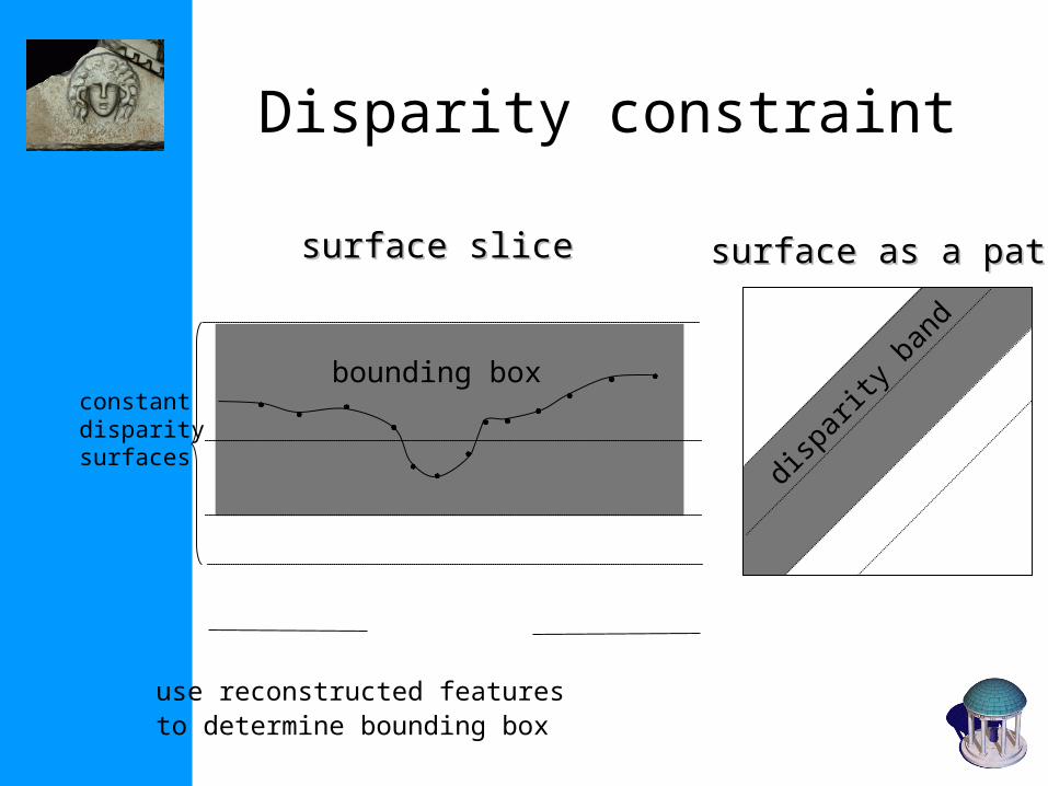
Disparity constraint

surface slicesurface slice surface as a pathsurface as a path

bounding box

dispa

rity b

and

use reconstructed features to determine bounding box

constantdisparitysurfaces

Stereo matching

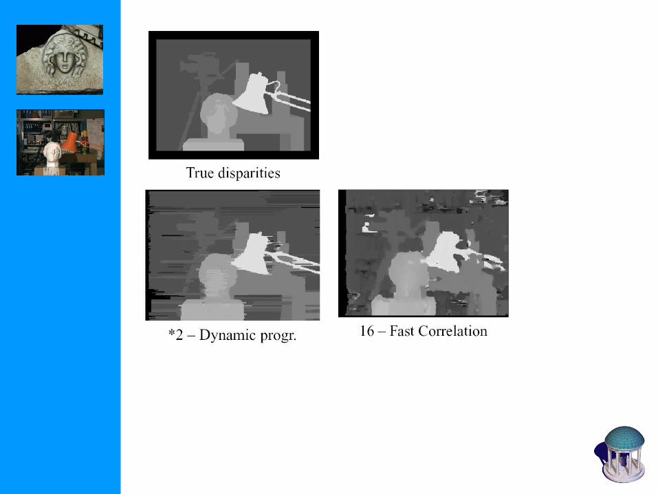
Optimal path(dynamic programming )

Similarity measure(SSD or NCC)

Constraints• epipolar

• ordering

• uniqueness

• disparity limit

Trade-off

• Matching cost (data)

• Discontinuities (prior)

Consider all paths that satisfy the constraints

pick best using dynamic programming

Hierarchical stereo matching

Dow

nsam

plin

g

(Gau

ssia

n p

yra

mid

)

Dis

pari

ty p

rop

ag

ati

on

Allows faster computation

Deals with large disparity ranges

Disparity map

image I(x,y) image I´(x´,y´)Disparity map D(x,y)

(x´,y´)=(x+D(x,y),y)

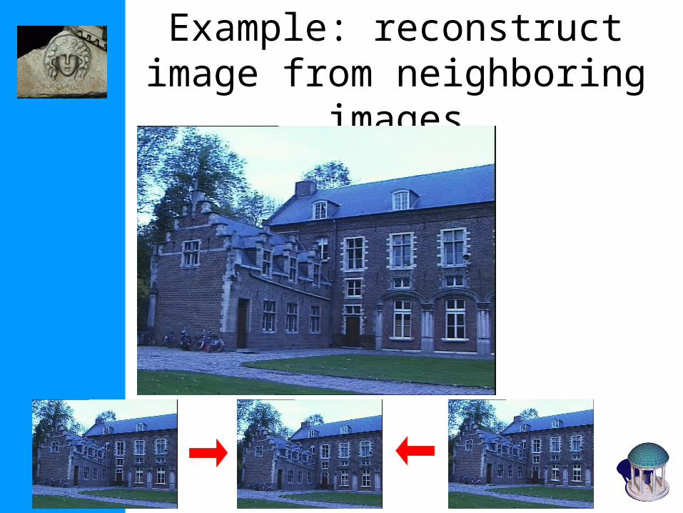
Example: reconstruct image from neighboring

images

Energy minimization

(Slide from Pascal Fua)

Graph Cut

(Slide from Pascal Fua)

(general formulation requires multi-way cut!)

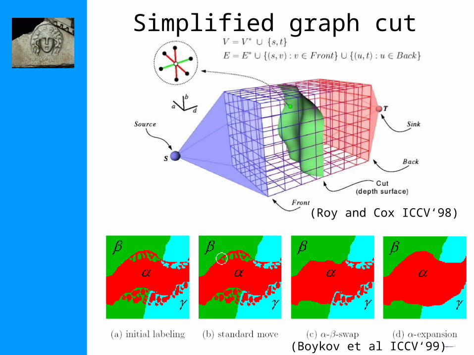
(Boykov et al ICCV‘99)

(Roy and Cox ICCV‘98)

Simplified graph cut

Stereo matching with general camera configuration

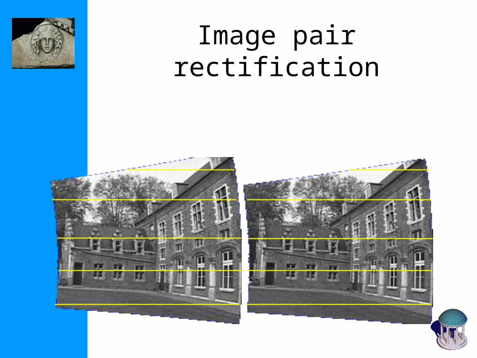
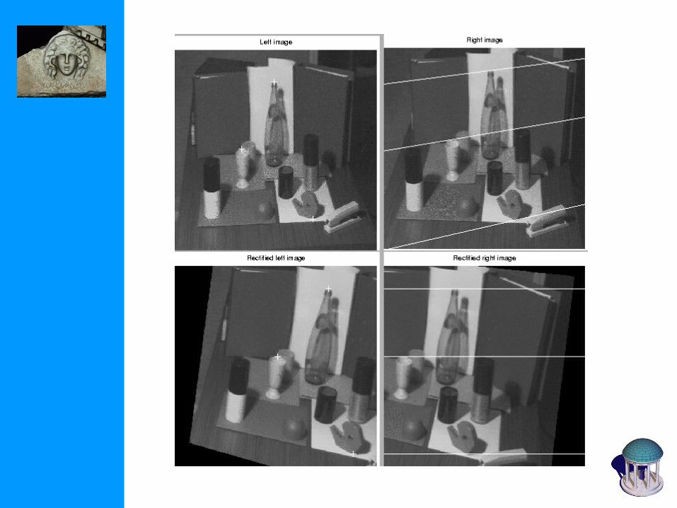
Image pair rectification

Planar rectification

Bring two views Bring two views to standard stereo setupto standard stereo setup

(moves epipole to )(not possible when in/close to image)

~ image size

(calibrated)(calibrated)

Distortion minimization(uncalibrated)

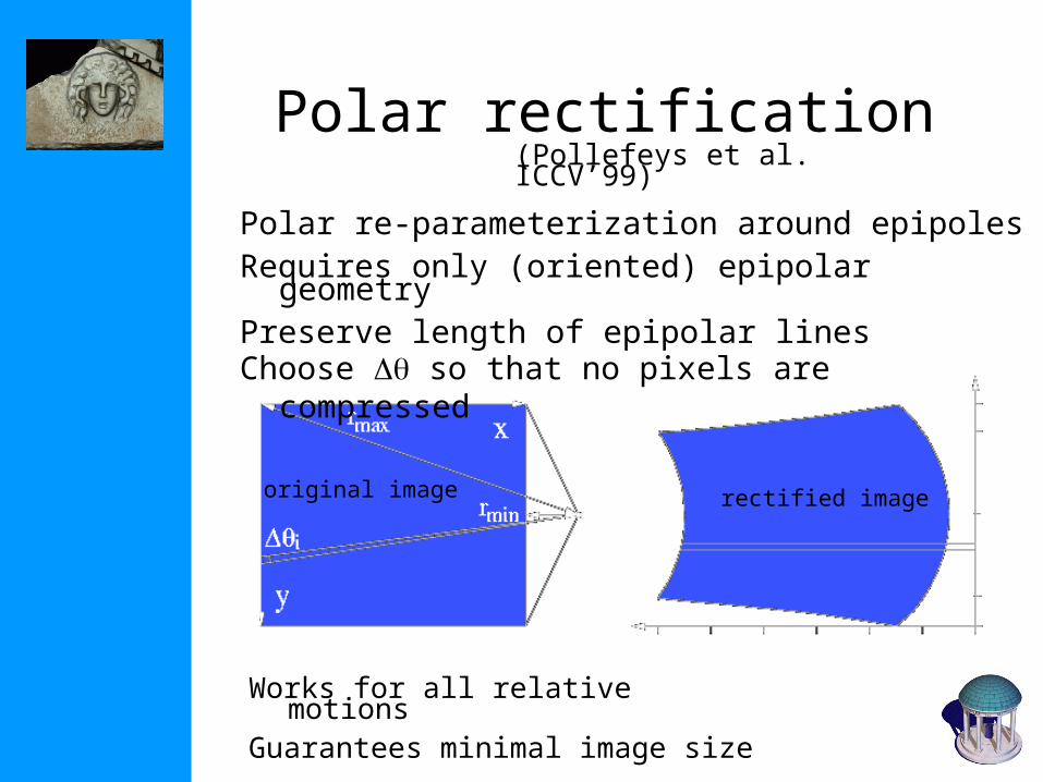
Polar re-parameterization around epipolesRequires only (oriented) epipolar geometryPreserve length of epipolar linesChoose so that no pixels are compressed

original image rectified image

Polar rectification(Pollefeys et al. ICCV’99)

Works for all relative motionsGuarantees minimal image size

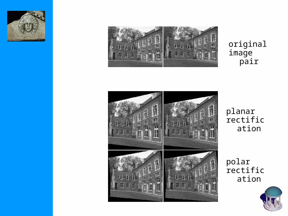
polarrectification

planarrectification

originalimage pair

Example: Béguinage of Leuven

Does not work with standard Homography-based approaches

Example: Béguinage of Leuven

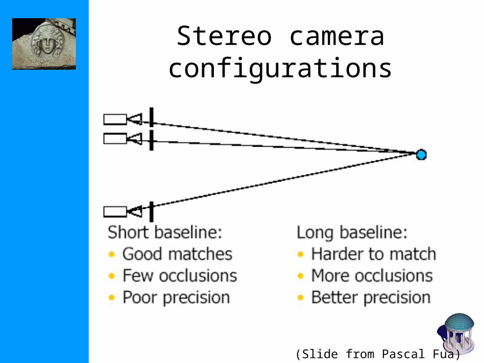
Stereo camera configurations

(Slide from Pascal Fua)

Multi-camera configurations

Okutami and Kanade

(illustration from Pascal Fua)

Multi-view depth fusion

• Compute depth for every pixel of reference image• Triangulation• Use multiple views• Up- and down

sequence• Use Kalman filter

(Koch, Pollefeys and Van Gool. ECCV‘98)

Allows to compute robust texture

Plane-sweep multi-view matching

• Simple algorithm for multiple cameras• no rectification necessary• doesn’t deal with occlusions

Collins’96; Roy and Cox’98 (GC); Yang et al.’02/’03 (GPU)

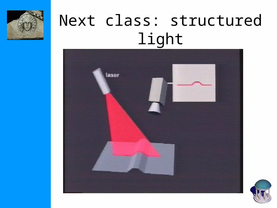
Next class: structured light