Stepwise inversion of a groundwater flow model with multi-scale observation data

Stepwise inversion of a groundwater flow model with multi-scaleobservation data

Zhenxue Dai & Elizabeth Keating & Carl Gable &

Daniel Levitt & Jeff Heikoop & Ardyth Simmons

Abstract Based on the regional hydrogeology and thestratigraphy beneath the Los Alamos National Laboratory(LANL) site, New Mexico (USA), a site-scale groundwatermodel has been built with more than 20 stratified hydrofa-cies. A stepwise inverse method was developed to estimatepermeabilities for these hydrofacies by coupling observationdata from different sources and at various spatial scalesincluding single-well test, multiple-well pumping test andregional aquifer monitoring data. Statistical analyses ofoutcrop permeability measurements and single-well testresults were used to define the prior distributions of theparameters. These distributions were used to define theparameter initial values and the lower and upper bounds forinverse modeling. A number of inverse modeling steps wereperformed including the use of drawdown data from thepump tests at two wells (PM-2 and PM-4) separately, and ajoint inversion coupling PM-2 and PM-4 pump test data andhead data from regional aquifer monitoring. Parametersensitivity coefficients for different data sets were computedto analyze if the model parameters can be estimatedaccurately with the data provided at different steps. Thejoint inversion offers a reasonable fit to all data sets. Theuncertainty of estimated parameters for the hydrofacies isaddressed with the parameter confidence intervals.

Keywords Stepwise inversion . Hydrofacies . Multi-scaledata . Parameter sensitivity . Joint inversion . USA

Introduction

Understanding and predicting groundwater flow andcontaminant transport at large spatial scales in subsurface

systems entails developing and then integrating knowl-edge of aquifer heterogeneity and field-scale parameter-izations. Inverse modeling combined with aquifer pumpingtests has been widely applied to regional or site-scale aquifercharacterization and parameter estimation (e.g. Carrera andNeuman 1986; Sun and Yeh 1990; Wagner 1992; Hill 1992;Poeter and Hill 1997; Doherty 2005; Robinson et al. 2005;Dai and Samper 2006; Samper et al. 2006; Kwicklis et al.2006 and Zhu and Yeh 2006). In general, the longer theduration of the pumping test and the larger the pumping rate,the more valuable the test. However, limited by the budgetsof each test, very few pumping tests can be conducted longenough or with high enough pumping rates to fully interpretaquifer heterogeneity. There is a need to develop a newinverse method for aquifer parameter estimation by takingadvantage of multi-scale observation data, which arecollected from site-scale monitoring and small-scale pump-ing tests conducted at different locations with differentinfluence areas. This paper uses the calibration of the LosAlamos National Laboratory (LANL) site-scale model as anexample to illustrate the newly developed stepwise inversionmethodology.

Los Alamos National Laboratory and adjacent com-munities are situated on the Pajarito Plateau, New Mexico,USA (Fig. 1). The Plateau occupies the south-western partof the Española Basin, which is bounded on the east bythe Rio Grande and on the west by the eastern JemezMountains. The major aquifer hydrostratigraphic unitbeneath the Plateau is the Santa Fe group, which is theprimary source of water supply for the communities ofEspañola, Los Alamos, and numerous pueblos (Griggsand Hem 1964; Nylander et al. 2003; Newman andRobinson 2005; Collins et al. 2005). For simulatinggroundwater flow in the Española Basin, the US Geo-logical Survey (USGS) developed two numerical models.The first was developed by Hearne (1985). The secondwas developed by McAda and Wasiolek (1988) (and laterrefined by Frenzel 1995), using the MODFLOW code(McDonald and Harbaugh 1988). These models havemade important contributions to the understanding of thebasin hydrology and regional water-balance issues, partic-ularly concerning impacts of pumping on stream-flow inthe Rio Grande. At present, local and state agenciescontinue to refine and apply both these models to addresswater supply issues in this basin. However, both the

Received: 23 October 2008 /Accepted: 5 October 2009Published online: 10 November 2009

© Springer-Verlag 2009

Z. Dai ()) : E. Keating :C. Gable :D. Levitt : J. Heikoop :A. SimmonsEarth and Environmental Sciences Division,Los Alamos National Laboratory,EES-16, T003, Los Alamos, NM 87545, USAe-mail: [email protected]

Hydrogeology Journal (2010) 18: 607–624 DOI 10.1007/s10040-009-0543-y

USGS models of this aquifer system place a modelboundary along the western edge of LANL, and do notinclude the recharge area in their model domains; therefore,use of these models for the LANL site would becompromised by boundary effects. To ensure that all modelboundaries were far from the area of interest (e.g. LANL)and to incorporate the possible influences of regional flowon local conditions, Keating et al. (2003) developed anEspañola basin-scale model with a coarse grid and a LANLsite-scale model with fine grid for modeling groundwaterflow and solute transport under the Pajarito Plateau andEspañola basin, based on the hydrogeological workconducted by LANL, the USGS and other organizations.The boundaries of the Hearne (1985), McAda andWasiolek(1988), and the LANL basin-scale and site-scale models areshown in Fig. 1.

The initial conceptual model of groundwater flow inthe regional aquifer under the Pajarito Plateau wasoutlined in the Hydrogeologic Workplan (LANL 1998),and the original Española basin-scale model was devel-oped to provide a regional context for flow and transportsimulations at the scale of the LANL site (Carey et al.1999; Keating et al. 2003). Researchers at the USGS andother organizations contributed to the LANL effort ofdefining the initial conceptual model and provided thesupporting datasets. The basin-scale model also providesthe water balance computation and boundary calibrationfor the site-scale model.

In 2000, a site-scale model for the Pajarito Plateau (orLANL site) was developed with much higher gridresolution than could be achieved with the basin-scalemodel, and was coupled to the basin-scale model (Keating

et al. 2003). The site-scale model, run on the LANL’s flowand transport simulator FEHM (Zyvoloski et al. 1997),has been used to make contaminant transport calculations,to conduct capture zone analyses, to support monitoring-well siting decisions, and to estimate groundwater velocities.Keating et al. (2003, 2005) described the geologic andhydrologic settings and framework model, FEHM simulator,material properties, model boundaries, and initial calibrationstrategies. The site-scale model has been periodicallyupdated and improved when new data become availablefor model calibration.

Recently, two pumping tests were conducted at LosAlamos County municipal water supply wells PM-2 andPM-4, both using multiple observation wells. Analyticalmethods were used by McLin (2005, 2006a) to interpretthe pumping test data. However, because the analyticalsolutions are based on homogeneous assumptions andinfinite boundary conditions, they cannot simulate thecomplex heterogeneity of the aquifer system under thePajarito Plateau.

In this paper, using observation data from PM-2 andPM-4 multiple-well pumping tests and regional aquifermonitoring data, the stepwise inversion method has beencoupled with the LANL site-scale numerical model toestimate the flow parameters for the hydrofacies beneaththe Pajarito Plateau. Statistical analyses of outcrop perme-ability measurements and single-well slug or pumping testresults are used to define the prior distributions of theparameters. This prior information was used to define theparameter initial values and the lower and upper bounds forthe stepwise inverse modeling. At each step, the inverseproblem is solved with PEST (Doherty 2005). The uncer-

LANL

N

Santa Fe

Española

RioG

rand

Canada

Mexico

USA

Study area

NM

0 10 20 30 40 50 60 70 Kilometers

Fig. 1 Location of the study area in New Mexico (NM). Basin-scale model domain (pink line) and current site-scale model domain (blackline) and domains of USGS models of Hearne (1985) in red and McAda and Wasiolek (1988) in green (modified from Keating 2005).LANL Los Alamos National Laboratory. Towns are shaded yellow

608

Hydrogeology Journal (2010) 18: 607–624 DOI 10.1007/s10040-009-0543-y

tainty of the final estimated parameters for the hydrofacies isaddressed with the parameter confidence intervals.

Site hydrogeology and pumping tests

Site hydrogeologyThe regional aquifer beneath the Pajarito Plateau consistsof the sedimentary rocks of the Puye Formation and theSanta Fe Group, the fractured volcanic rocks of theTschicoma Formation, Cerros del Rio basalts, and olderbasalt flows. These units are described in detail in Broxtonand Vaniman (2005) and Cole et al. (2006). The sources ofrecharge to the regional aquifer are diffuse recharge in theSierra de los Valles and focused recharge from wetcanyons on the Pajarito Plateau. Natural discharge fromthe regional aquifer is primarily into the Rio Grandedirectly, to springs that flow into the Rio Grande, and tobasins to the south (Keating et al. 2003). The aquifer isunder water-table conditions across much of the Plateau,but exhibits more confined aquifer behavior near the Rio

Grande. Hydraulic properties are highly anisotropic, withvertical hydraulic conductivities much smaller than hori-zontal hydraulic conductivities (Collins et al. 2005).

Over the past 60 years numerous aquifer tests atdifferent scales were conducted in the regional aquiferbelow the Pajarito Plateau. Figure 2 shows the spatialdistributions of the historical pumping wells and observa-tion wells on the Pajarito Plateau. The test data were usedto characterize hydraulic properties of the saturated geo-logical units. Analyses of these test results have revealed acomplex regional aquifer that is a highly stratified,heterogeneous system. McLin (2006b) summarized themajor aquifer test data and interpreted the aquifer flowparameters individually for each test. Although thoseinterpretations were based on various analytical andnumerical models, the estimated aquifer parameters givean indication of the spatial variation and uncertainty inthis heterogeneous aquifer system. Using the interpreta-tion results of McLin (2006b), as well as outcropmeasurements (Gaud et al. 2004; Dai et al. 2005), astatistical analysis was performed to bound the horizontal

Fig. 2 Locations of Pajarito Plateau wells and the influence areas of PM-2 pumping test (dashed line) and PM-4 pumping test (dotted line)(modified from McLin 2006b). BLM Bureau of Land Management; DOE Department of Energy

609

Hydrogeology Journal (2010) 18: 607–624 DOI 10.1007/s10040-009-0543-y

permeability distributions, and compute the standarddeviation, lower and upper bounds (minimum andmaximum) of the permeability of each of the hydrofacieslisted in Table 1. For the hydrofacies where there were notenough data to compute the lower and upper bounds, theirprior information as parameter values in the site-scalenumerical model was assigned because these hydrofaciesare distributed either at the deep part of the model (e.g.dPC, dPM and Ts-deep) or at the top of the model (e.g.Qbt and sTk) and their parameters are not very sensitive tothe pumping tests.

PM-2 pumping testA 25-day aquifer pumping test was conducted at munic-ipal water supply well PM-2 at a constant pump rate of4.73 m3/min. The PM-2 well was completed in PajaritoCanyon in 1965 (Purtymun 1995) to a depth of 701 m. Thiswell is on the south side of Pajarito Road, approximately4 km northwest of White Rock. Immediately before thepumping test there was an initial non-pumping recoveryperiod of 3 months beginning in 5 November 2002. Thepump test began on 3 February and ended 28 February 2003.Surrounding observation wells were used to record draw-down data. These data revealed horizontal propagation ofdrawdown in the regional aquifer beyond 2,682 m from wellPM-2. In Fig. 2 the dashed line roughly defines the pumpinginfluence area. A total of 12 observation wells were used forthis pump test, including: PM-1, PM-3, PM-4, PM-5, R-12,R-13, R-14, R-15, R-20, R-21, R-22, and R-32. Drawdownwas observed in four observation wells: R-20, R-32, PM-4,and PM-5 (see Table 2). No drawdown was observed in theremaining nine wells (McLin 2005).

PM-4 pumping testThe PM-4 well is a municipal water supply well completedin 1981 (Purtymun 1995) to a depth of 876m. This well is onthe north side of Pajarito Road, approximately 5 km north-west of White Rock. A 21-day aquifer pumping test was

conducted at PM-4 at a constant pump rate of 5.66 m3/min.This pumping test was preceded by an initial non-pumpingrecovery period of 6 months beginning in August 2004. Thepump test began on 8 February 2005, and ended on 1 March2005. The observed drawdown data revealed horizontalpropagation of the area of influence in the regional aquiferbeyond 2652 m from well PM-4. In Fig. 2 the approximatearea of influence of this test is shown with the dotted line. Atotal of 11 observation wells were used for this pump test,including: PM-2, PM-5, R-13, R-14, R-15, R-19, R-20, R-22, R-32, TW-8, and CdV-R37-2. Drawdown was observedin nine of the 11 observation wells (see Table 2). Nodrawdown was observed at TW-8 and CdV-R37-2 becauseTW-8 is not deep enough to penetrate the major part of theSanta Fe group and the well CdV-R37-2 is located too farfrom PM-4.

McLin (2005, 2006a) used a variety of analyticalmethods to derive aquifer parameters from the two pumptests. McLin concluded that although both confined andleaky-confined conceptual models were approximatelyconsistent with the data, leaky-confined models matchedthe data much better and thus were the most appropriateconceptual models. More importantly, McLin (2005,2006a) reported that the two pump tests demonstrated aremarkably complex aquifer response over space and timethat is not easily interpreted with the analytical methods,and the regional aquifer materials in the area of thepumping tests are strongly heterogeneous and exhibitpronounced horizontal and vertical anisotropy in hydraulictransmitting properties.

Numerical models and stepwise inverse method

Site-scale numerical modelKey aspects of the site-scale numerical model (Keatinget al. 2003 and 2005) are briefly summarized here. Themodel extent, shown in Fig. 1, extends from Santa ClaraCanyon (to the north), the eastern margin of the VallesCaldera (to the west), the Rio Grande (to the east), and the

Table 1 Hydrofacies and their volumetric proportion (Vol), permeability (K), lower and upper bounds used in the numerical model

Hydrofacies name Symbol Vol (%) K (log m2) Lower bound Upper bound

PreCambrian dPC 0.007 –18.0 N/A N/APalezoic/Mesozoic dPM 0.261 –16.66 N/A N/ATf Galisteo gal 0.240 –13.5 –15.0 –12.0Fanglomeratic Santa Fe Tf 0.044 –14.21 –15.0 –10.73Sandy Santa Fe-deep Ts-deep 0.004 –16.07 N/A N/ASandy Santa Fe-shallow Ts 0.294 –13.33 –14.72 –10.42Keres Group-deep dTk 0.018 –13.73 N/A N/AKeres Group-shallow sTk 0.036 –12.78 N/A N/AOldest basalt Tb1 0.004 –13.63 –15.0 –11.0Bayo Canyon basalt Tb2 0.007 –11.61 –13.83 –10.65Basalts-Cerros del Rio Tb4 0.013 –12.36 –15.83 –9.87Tschicoma flows Tt 0.035 –12.98 –14.5 –11.5Totavi Lentil Tpt 0.002 –12.22 –14.06 –10.85Pumiceous Puye Tpp 0.003 –12.51 –14.54 –10.07Puye Fanglomerate Tpf 0.027 –13.09 –14.06 –9.39Bandelier Tuff Qbt 0.006 –15.33 N/A N/A

N/A There are not enough data to define the bounds

610

Hydrogeology Journal (2010) 18: 607–624 DOI 10.1007/s10040-009-0543-y

Rio Frijoles (to the south). Analysis of regional precipitation,streamflow data, and hydraulic head data, integrated usingthe basin-scale groundwater flow model, enabled thequantification of the range of plausible fluxes that mightcross these four lateral boundaries (Keating et al. 2003). Thetop of the model is set to be coincident with the measuredwater table surface at the beginning of the PM-2 pumpingtest. The water table is modeled as a free surface usingFEHM (Keating and Zyvoloski 2009).

The site-scale model includes a total of 397,574 nodes,which represent a model volume of 1,098 km3. Thehydrofacies (or units) and their volumetric proportions inthe numerical model are listed in Table 1. The gridresolutions are varied in the x–y plane from 125 to 500 m.In the vicinity of PM-2 and PM-4, the resolution is 125 mwhile towards the north it increases to 500 m. The verticalresolution is 12.5 m at elevations greater than 1,000 m; atlower elevations the grid resolution increases to 500 m.

Stepwise inverse methodComprehensive reviews of the general inverse problem ofaquifer flow and solute transport can be found in Yeh(1986), Carrera and Neuman (1986), Sun (1994), and Daiand Samper (2004). Here, a stepwise inverse approach isintroduced which provides a strategy to determine unknownmodel parameters by fitting the model output with multiple-scale or different-source observation data step by step. Theformulation of the stepwise inverse problem is based on ageneralized least squares criterion for parameter estimation.Let p = (p1, p2, p3, ..., pM) be the vector of M unknownparameters. The generalized least squares criterion, E(p), canbe expressed as,

E pð Þ ¼XNEi¼1

WiEi pð Þ; ð1Þ

where i denotes different scales or different sources of data,i=1 for PM-2 pumping test data; i=2 for PM-4 pumpingtests; i=3 for site-wide water head monitoring data (NE=3),Wi is the weighting coefficient of the i-th generalized least-squares criterion Ei(p) which is defined as:

Ei pð Þ ¼ PLil¼1

w2lir

2li pð Þ;

rli pð Þ ¼ uil pð Þ � euil;ð2Þ

where uil pð Þ is the model simulated value of the i-th scale orsource of data at the l-th observation point; euil are measuredvalues; Li is the number of observations, both in space and intime, for the i-th scale of data; and rli is the residual ordifference between model outcome and measurement; wli isthe weighting coefficient for the l-th measurement. Thevalues ofwli depend on the accuracy of observations. If somedata are judged to be unreliable, they are assigned smallweights in order to prevent their deleterious effect on theoptimization process.

Weighting of different scales or sources of dataEquation 1 is a weighted multi-objective optimizationcriterion. It is difficult to designate optimal weightingcoefficients. Several methods were proposed by Neumanand Yakowitz (1979) and Carrera and Neuman (1986).Generally, the determination of optimal weights shouldfollow an iterative procedure. Carrera and Neuman (1986),Sun (1994) and Dai and Samper (2004) use the followingequation for generalization of different types of data:

Wi ¼ W0iEi pð ÞLi

; ð3Þ

Table 2 Drawdown measured during PM-2 and PM-4 pump tests

Pumping and observationwells

PM-2 pumping test PM-4 pumping testDrawdown at 25 days (m) Distance from PM-2 (m) Drawdown at 21 days (m) Distance from PM-4 (m)

PM-2 25.69 0 4.41 1,365PM-4 2.97 1,365 21.31 0PM-5 0.73 2,685 2.46 1,418R-20-1 0.33 373 0.06 1,679R-20-2 1.03 373 0.61 1,679R-20-3 4.57 373 4.96 1,679R-32-1 0.36 1,457 0.0a 2,656R-32-2 0.46 1,457 0.28 2,656R-32-3 0.53 1,457 0.34 2,656R-12 0a 3,949 0a 3,851R-13 0a 2,350 0.11 1,740R-14-2 0a 3,452 0.01 2,177R-15 0a 2,543 0.52 1,170R-19-4 0a 2,128 0.09 2,211R-22 0a 2,693 0a 3,651PM-1 0a 4,101 N/A 4,025PM-3 0a 3,308 N/A 2,601TW-8 N/A 2,907 0a 1,725CdV-R37-2 N/A 5,388 0a 5,257

aNo response or less than detectable

611

Hydrogeology Journal (2010) 18: 607–624 DOI 10.1007/s10040-009-0543-y

where W0i are user-defined dimensionless initial weightingcoefficients for different scales or different sources ofobservation data. Generally, they are taken as being equalto 1. Wi have dimensions which are reciprocal of those ofEi(p). Generally Ei(p) has units equal to the square of theunit used for each type of data (i.e., m2 for heads ordrawdown and (kg/s)2 for water-flow rate data (Stauffer2006). Weights Wi are updated automatically during theiterative optimization process according to Eq. (3). However,in this stepwise strategy, three steps are used to perform themodel inversion:

Step 1: W01=1, W02=W03=0Step 2: W01=0, W02=1, W03=0Step 3: W01=W02=W03=1

The main advantages and reasons to adopt a stepwisestrategy are, first, that stepwise inversion helps to avoidover-parameterization. One must carefully analyze whichparameters are identifiable and can be subsequentlyestimated accurately through inverse modeling. Thisprocess is performed by comparing parameter sensitivity

coefficients and correlation structures. There are manyrisks in trying to estimate a large number of parameters inone step. Some steps of the stepwise procedure should bedevoted to analyze parameter identifiability (which mea-

Table 3 Summary of model results and estimated parameters by stepwise inversion

Step 1 2 3Model description PM-2 Forward PM-2 inverse PM-4 forward PM-4 inverse Joint inversionNo. of estimated parameters N/A 15 N/A 15 18Total objective value 1068.6 52.20 1118 96.5 445.38

PM-2 PM-4

Sub-objective values ΦPM-2 388.3 1.22 0.50 2.76 14.20 1.24ΦPM-4 0.96 10.06 100.3 2.72 14.64 14.66ΦPM-5 118.7 7.52 2.12 2.35 9.79 2.81ΦR-20 485.1 10.66 32.96 39.91 11.29 37.29ΦR-32 75.6 9.26 36.28 9.16 8.72 32.84ΦR-13 N/A N/A 350.4 8.44 N/A 10.97ΦR-14 N/A N/A 0.15 0.02 N/A 0.03ΦR-15 N/A N/A 3.74 5.12 N/A 35.18ΦR-19 N/A N/A 572.2 13.06 N/A 15.82Φ0D

a N/A 13.42 18.99 12.97 12.06 6.63ΦFlux

b N/A 0.035 0.15 0.0001 39.65ΦSSM

c N/A N/A N/A N/A 177.57Estimated parameters Sy 0.1 0.1 0.08 0.08 0.111

Ss –3.16 –5.773 –5.4798 –5.4798 –6.241Ktb2 –11.61 –12.99 –12.99 –12.99 –12.99Ktpt –12.22 –12.89 –12.89 –13.59 –11.99Ktpf –13.09 –13.10 –13.10 –12.20 –12.33Ktf –14.21 –11.62 –11.62 –11.54 –11.64Kts –13.33 –12.43 –12.43 –12.39 –12.40Ktt –12.98 –12.11 –12.11 –12.33 –12.90Ktpp –12.51 –12.29 –12.29 –12.80 –13.62Ktb1 –13.63 –13.63d –13.63 –13.63d –13.60Ktb4 –12.56 –12.56d –12.56 –12.56d –13.20Zftb2 1.00 0.0013 0.0013 0.0013d 0.0001Zftpt 0.06 0.3539 0.3539 0.0537 0.001Zftpf 0.11 1.00d 1.00 0.3374 0.2465Zftf 1.58 0.0174 0.0174 0.0966 0.0583Zfts 0.45 0.001 0.001 0.0008 0.0042Zftt 1.00 0.0142 0.0142 0.6097 0.2791Zftpp 0.04 0.0428 0.0428 0.1217 0.6891

a Refer to zero drawdown datab Discharge to Rio Grandec Refer to site-wide aquifer monitoring datad The parameter is fixed to prior information because it is insensitive

0 100 200 300 400 500

Hearne, 1985

McAda and Wasiolek,1988

Keating et al., 2003

Keating, 2005

Keating et al., 2005

Kwicklis et al., 2005

Discharge (kg/s)

Fig. 3 Summary of previous estimates of discharge (unit: kg/s)beneath the Pajarito Plateau to the Rio Grande (adapted fromKeating et al. 2005). Keating (2005) was calculated using stream-flow analysis while Keating et al. (2005) was calculated in theuncertainty analysis

612

Hydrogeology Journal (2010) 18: 607–624 DOI 10.1007/s10040-009-0543-y

sures if the model parameters can be estimated accuratelywith the data provided). Secondly, stepwise inversionprovides a procedure to upscale the flow parameters thatwere obtained from small-scale pumping test inversions tothe site-scale model by coupled inversion of multi-scaleobservation data. Thirdly, stepwise inversion allows theuse of inverse models of increasing complexity. Therefore,until sufficient insight is gained on the nature of theinverse problem of the individual PM-2 and PM-4pumping test, the scientific principle of analyzing complexproblems was followed by using models of increasingcomplexity. Fourthly, stepwise inversion can be useful forconceptual model identification. Solving the inverse

problem requires not only obtaining optimum parametervalues, but also identifying relevant boundary conditionsand parameter structures, known as conceptual modelidentification in the stepwise inversion (Dai et al. 2006).

Table 4 Calculated parameter sensitivity coefficients

Parametername

Initialvalue

Sensitivitycoefficient

Relativesensitivity

Sensitiverank

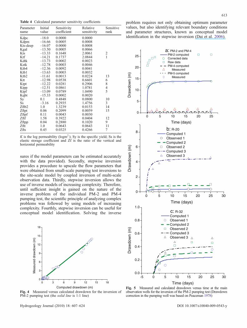
Kdpc –18.0 0.0000 0.0000Kdpm –16.66 0.0005 0.0008Kts-deep –16.07 0.0000 0.0008Kgal –13.50 0.0005 0.0066Kts –13.33 0.1648 2.0061 2Ktf –14.21 0.1737 2.0844 1Kdtk –13.73 0.0002 0.0023Kstk –12.78 0.0003 0.0046Ktb4 –12.36 0.0092 0.0041Ktb1 –13.63 0.0003 0.0032Ktb2 –11.61 0.0013 0.0224 13Ktt –12.98 0.0538 0.6601 6Ktpt –12.22 0.0281 0.2906 8Ktpp –12.51 0.0861 1.0781 4Ktpf –13.09 0.0789 1.0490 5Kqbt –15.33 0.0002 0.0020Sy 0.1 0.4848 0.0800 10Ss –3.16 0.2935 1.4756 3Zftb2 1.0 1.3239 0.0153 14Zftpt 0.06 0.2099 0.0059 15Zftpf 0.11 0.0043 0.0030Zftf 1.58 0.3922 0.0404 12Zftpp 0.04 0.2880 0.1020 9Zftt 1.0 0.0643 0.0643 11Zfts 0.45 0.0325 0.4266 7

K is the log permeability (logm2 ); Sy is the specific yield; Ss is theelastic storage coefficient and Zf is the ratio of the vertical andhorizontal permeability

0 3 6 9 12 15 180

3

6

9

12

15

18

Mea

sure

d dr

awdo

wn

(m)

Computed drawdown (m)Fig. 4 Measured versus calculated drawdown for the inversion ofPM-2 pumping test (the solid line is 1:1 line)

0 5 10 15 20 250

5

10

15

20

25

Dra

wdo

wn

(m)

Time (days)

a: PM-2 and PM-4 PM-2 computed Corrected data Raw data PM-4 computed Measured PM-5 computed Measured

0 5 10 15 20 25 300

2

4

6

8D

raw

dow

n (m

)

Time (days)

b: R-20 Computed 1 Observed 1 Computed 2 Observed 2 Computed 3 Observed 3

-5 0 5 10 15 20 25 300.0

0.2

0.4

0.6

0.8

1.0

Dra

wdo

wn

(m)

Time (days)

c: R-32 Computed 1 Observed 1 Computed 2 Observed 2 Computed 3 Observed 3

Fig. 5 Measured and calculated drawdown versus time at the mainobservation wells for the inversion of the PM-2 pumping test (Drawdowncorrection in the pumping well was based on Peaceman 1978)

613

Hydrogeology Journal (2010) 18: 607–624 DOI 10.1007/s10040-009-0543-y

Weighting of different observation wellsA special procedure is used for weighting drawdown datafrom different observation wells because they usually varywithin different logarithmic ranges. For example, in thePM-2 pumping test the drawdown in PM-2 is more than25 m, but it is about 0.08 m in R-32-1 (the first screen of

the well R-32). This procedure differs from that used fordifferent types of data such as drawdowns, water flowrate, and prior information. The weight for the l-th mea-surement of the k-th observation well wl

k, is computed as:

wkl ¼

w0l

sk; ð4Þ

where w0l is an initial weight for the l-th measured valuewhich should be equal to the reciprocal of its analyticalerror, and σk is the standard deviation of measureddrawdown of the k-th well,

sk ¼ffiffiffiffiffiffiffiffiffiffiffiffiffiffiffiffiffiffiffiffiffiffiffiffiffiffiffiffiffiffiffiffiffiffiffiffiffiffiffiffiffiffiffiffiffiffiffiffiffiffiffiffiN � 1ð Þ�1

XNi¼1

Fik � Fk

� �2vuut ; Fk ¼ N�1

XNi¼1

Fik :

ð5Þ

Fki is the i-th measured value of the k-th well; N is the

number of drawdown data of the k-th well; Fk is theaverage of measured drawdown of the k-th well. Thisweighting system ensures that all observation wells havesimilar contributions to the global objective function andthat drawdown data in one well are neither “drowned” byother wells nor dominate in the estimation process.

-5 0 5 10 15 20 25 300.00

0.05

0.10

0.15

0.20

0.25D

raw

dow

n (m

)

Time (days)

a Computed R-12 Computed R-13 Computed R-14-1 Computed R-14-2

-5 0 5 10 15 20 25 300.00

0.05

0.10

0.15

0.20

0.25

Dra

wdo

wn

(m)

Time (days)

b Computed R-15 Computed R-23 Computed PM-1 Computed PM-3

-5 0 5 10 15 20 25 300.00

0.05

0.10

0.15

0.20

0.25

Dra

wdo

wn

(m)

Time (days)

c Computed R-22-1 Computed R-22-2

Fig. 6 Calculated drawdown versus time for the inversion of thePM-2 pumping test at the wells a where there are no availableobservation data or b and c no apparent drawdown was observed

XY

Z

PM-2

R-20R-32

R-19 PM-4Tb4

Tpf

TptTf

Tb2

Tf

Tb4

Ts

Ts

Qbt

TppTpp

XY

Z

54210.80.50.20.10

PM-2R-19

R-20

R-22

PM-4

a

b

Fig. 7 a Outline of geological framework around PM-2 pumpingwell and b the drawdown distribution of the PM-2 pumping test at25 days (PM-2 well is located at the center of two cross sections,drawdown unit is meters, and refer to Table 1 for hydrofacies units)

614

Hydrogeology Journal (2010) 18: 607–624 DOI 10.1007/s10040-009-0543-y

Grid-size correction factor for drawdown in pumpingwellsWith the numerical models described here, the simulatedhead in any grid block represents an average head over theentire control volume. This average head will be a poorapproximation to water levels in a pumping well if the sizeof the control volume is much larger than the diameter ofthe pumping well. For this reason, a method has beendeveloped to calculate the expected relationship betweenmeasured water level in a pumping well and thecorresponding simulated head in a large control volumerepresenting the pumping well. By using analytical wellfunctions, Peaceman (1978) defined the equivalent radiusas the radius at which the steady-state flowing pressure forthe actual well is equal to the numerically calculatedpressure for the well control volume. Based on theapproach derived by Peaceman (1978), the observeddrawdowns in pumping wells PM-2 and PM-4 werecorrected to eliminate the computing errors due to thelarge grid size of the numerical model, but the drawdowndata in the observation wells were not corrected.

Rejection of the outlier points in the observationdataDuring pumping tests, a measurement may be read,recorded, or transcribed wrongly, or a mistake may bemade in the way in which a treatment was applied for this

X

Y

Z

PM-4

R-19

PM-5

PM-2

R-20

R-32R-22

R-15R-14

R-7

R-13

R-9

R-12

R-16

R-31

DT-10

DT-9

Tpf

TsTs

Ts

Ts

Ts-deep

Ts-deep

Ts-deep

Tb2

Tb1

Ts

TppTpp

Tt

Tt

Tt

Tpf

Tpp

Ts-deep X

Y

Z

PM-4

R-19

PM-5

PM-2

R-20

R-32R-22

R-15R-14

R-7

R-13

R-9

R-12

R-16

R-31

DT-10

DT-9

Ts

Ts

Ts

Ts-deep

Tb1

Tb1

Ts

Tb2

Tb2Tf

Ts-deep

Ts-deep

Tpp

Ts-deep

Tt

Tt

Tt

Tb2

X

Y

Z

54210.80.50.20.10

PM-2R-19R-20

R-22

PM-4

DT-10

DT-9

R-31

R-15R-13 R-12

R-7

R-14

PM-5

R-32

R-9

R-16

X

Y

Z

54210.80.50.20.10

PM-2R-19R-20

R-22

PM-4

DT-10

DT-9

R-31

R-15R-13 R-12

R-7

R-14

PM-5

R-32

R-9

R-16

dc

a b

Fig. 8 Outline of hydrofacies distribution in XY plane (a Z=1,700 m and b Z=1,600 m), and simulated drawdown contour of the PM-2pumping test at 25 days in XY plane (c Z=1,700 m and d Z=1,600 m). Drawdown unit is meters

0 3 6 9 12 150

3

6

9

12

15

Mea

sure

d dr

awdo

wn

(m)

Computed drawdown (m)Fig. 9 Measured and calculated drawdown at all observation wellsfor inverse modeling of PM-4 pumping test

615

Hydrogeology Journal (2010) 18: 607–624 DOI 10.1007/s10040-009-0543-y

measurement. A major error greatly distorts the mean andthe standard deviation, and affects conclusions of inversemodeling. The principal safeguards are vigilance incarrying out the operating instructions in the measuringand recording process, and visual inspection of theobservation data.

If a value in the data to be analyzed looks suspicious,an inquiry about this observation sometimes shows thatthere was a gross error. If no explanation of an extreme

observation is discovered, one may consider rejecting it.The rules for the rejection of observations have beenbased on some type of significance test (Snedecor andCochran 1976). The probability that a residual as large asthe suspect value would occur by chance is computed. Ifthis probability is sufficiently small, the suspect isrejected. Anscombe and Tukey (1963) present a rule thatrejects an observation whose residual has the value of d if|d| > Cs, where C is a constant to be determined from

0 5 10 15 20 250.0

0.2

0.4

0.6

0.8

Dra

wdo

wn

(m)

Time (days)

R-32 R-32-2 Observation Computed R-32-3 Observation Computed

0 5 10 15 20 250

5

10

15

20

25

Dra

wdo

wn

(m)

Time (days)

PM-4 computed Corrected data Raw data PM-2 computed Measured PM-5 computed Measured

0 5 10 15 20 250.01

0.1

1

10

Dra

wdo

wn

(m)

Time (days)

R-20-3 Observation R-20-3 Computed R-20-2 Computed R-20-1 Computed

0 2 4 6 8 10 12 140.0

0.1

0.2

0.3

0.4

0.5

Dra

wdo

wn

(m)

Time (days)

R-19 R-19-4 Computed R-19-5 Computed R-19-6 Computed R-19-7 Computed

0 5 10 15 20 250.0

0.2

0.4

0.6

0.8

1.0

Dra

wdo

wn

(m)

Time (days)

R-13 observations Computed R-14 observations Computed R-15 observations Computed

0 5 10 15 20 250.00

0.05

0.10

0.15

0.20

0.25

Dra

wdo

wn

(m)

Time (days)

Zero drawdowns R-22-1 Computed R-22-2 Computed R-14-1 Computed

b

dc

ef

a

Fig. 10 Measured and calculated drawdown versus time at observation wells for PM-4 pumping test

616

Hydrogeology Journal (2010) 18: 607–624 DOI 10.1007/s10040-009-0543-y

Eq. 6, which is obtained from Snedecor and Cochran(1976), and s is the standard deviation of the observations.

C ¼ K 1� K2�24 N�1ð Þ

� � ffiffiffiffiffiffiffiffiN�1N

q;

K ¼ 1:4þ 0:85z;ð6Þ

where N is the number of the observations. z correspondsto the one-tailed probability value of N�1

N P in the normaldistribution, where P is the small premium which isinvolved in a rejection rule, say 2.5%. This rejection rulehas been used to test and reject some of the observationdata for PM-2 and PM-4 pumping tests.

Stepwise inversion of the site-scale model

Step 1: forward and inverse modeling of PM-2pumping test

Forward modelingPrevious to this study, PM-2 pump test data were not usedto calibrate or otherwise develop the site-scale numericalmodels (Keating et al. 2005). Therefore, this datasetprovides a useful benchmark to test the degree to whichthe site-scale models can predict the pump test behavior. Itis reasonable to expect that the previous versions of thesite-scale model developed to address pump tests shouldpredict an envelope of behavior within which a goodmatch between measured and predicted pump testresponse could be identified. If this were not the case,

the conceptual model or the model parameters should bere-calibrated accordingly.

By using the site-scale model, a forward run was con-ducted to simulate the PM-2 pumping test. The predicteddrawdown did not match the observed drawdown well.The major fitting errors include under-predicting responseat the PM-2 pumping well and over-predicting very earlyresponse at all observation wells (including R-20, R-32,PM-4 and PM-5). The computed objective function is1068.6 for this forward run (see Table 3). Overall, theseresults indicate that predictions of drawdown from thePM-2 pumping test are not satisfied using the previoussite-scale model. The forward modeling results indicatethat there is a need to re-calibrate the model with PM-2pumping test data.

X Y

Z

PM-4R-31 R-20 R-15

Ts

Tb4

Tb4

Ts-deep

Tt

TptTpf

Qbt

Tf

Tf

TfTpt

Ts-deep Ts

Tpf

Tb2Tb1

Tb1

X Y

Z

105210.50.20.10

PM-4R-31

R-20 R-15

a

b

Fig. 11 a Hydrofacies distribution in YZ plane and b drawdowndistribution in YZ plane (X=19,294) of the PM-4 pumping test at 21days. Drawdown is in meters

X

Y

Z

105210.50.20.10

PM-4

R-19

PM-5

PM-2

R-20

R-32R-22

R-15R-14

R-7

R-13

R-9

R-12

R-16

R-31

DT-10

DT-9

X

Y

Z

105210.50.20.10

PM-4

R-19

PM-5

PM-2

R-20

R-32R-22

R-15R-14

R-7

R-13

R-9

R-12

R-16

R-31

DT-10

DT-9

a

b

Fig. 12 Simulated drawdown contour of the PM-4 pumping test at21 days in XY plane (a Z=1,700 m and b 1,600 m). Drawdown is inmeters

617

Hydrogeology Journal (2010) 18: 607–624 DOI 10.1007/s10040-009-0543-y

Inverse modelingIn addition to PM-2 pumping test data, the previouslyestimated discharge rate to the Rio Grande was alsoincluded as one of the fitting targets or a sub-objectivefunction in the inverse model. Previous investigations toestimate steady-state discharge through the regionalaquifer beneath the Pajarito Plateau were conducted byKeating (2005), Keating et al. (2003, 2005), Kwicklis etal. (2005), McAda and Wasiolek (1988), and Hearne(1985). Their estimates of discharge beneath the PajaritoPlateau are summarized in Fig. 3 The mean of the abovecited estimates of discharge (which is 332.75 kg/s with astandard deviation of 68.72 kg/s) was used as the observedsteady-state discharge data for model fitting.

The site-scale numerical model includes more than 20parameters. One first needs to know how many parameters

are sensitive enough to the smaller scale PM-2 pumpingtest data. Only the sensitive parameters are identifiable.Therefore, before conducting the inverse modeling, asensitivity analysis of the inverse model to the involvedparameters was performed. The sensitivity coefficient (orcomposite sensitivity) of the parameters are computedaccording to Doherty (2005) as

si ¼ 1

mJTWJ� �1

2

ii; ð7Þ

where Si is the sensitivity coefficient of i-th parameter, mis the number of observations with non-zero weights, J isthe Jacobian matrix and W is the weighting matrix. Therelative sensitivity (Rsi) of the i-th parameter is obtainedby multiplying its composite sensitivity by the magnitudeof the value of the parameter pi as

Rsi ¼ pij jm

JTWJ� �1

2

ii: ð8Þ

The relative sensitivity is thus a measure of thecomposite changes in model outputs that are incurred bya fractional change in the value of the parameter. Thesensitivity coefficient computed in Table 4 presents thesensitivity of each parameter with respect to all observa-tions of the PM-2 pumping test. The use of relativesensitivities in addition to composite sensitivities assists incomparing the effects that different parameters have on theparameter estimation process when these parameters are ofdifferent types, and of very different magnitudes.

By ranking the relative sensitivity coefficients (seeTable 4), the 14 most sensitive parameters were selectedfor parameter estimation with the PM-2 pumping test dataand an improved fit to the observation data was obtainedcompared to the forward modeling results. The objectivefunction decreased to 52.2 from 1068.6.

The final estimated parameter set from the inversemodeling of the PM-2 pump test is given in Table 3, and

b

R-16R-22R-32

R-20PM-2

PM-4R-13 R-12

R-9

R-15

PM-5

R-14

R-7

R-31

DT-10

R-19

G-1

H-19

CDVR15

CDVR37

LA-4LA-5

LA-6

DT-9

DT-5A

Modelboundary

PM-3

PM-1

N

0 2 4 Kilometers

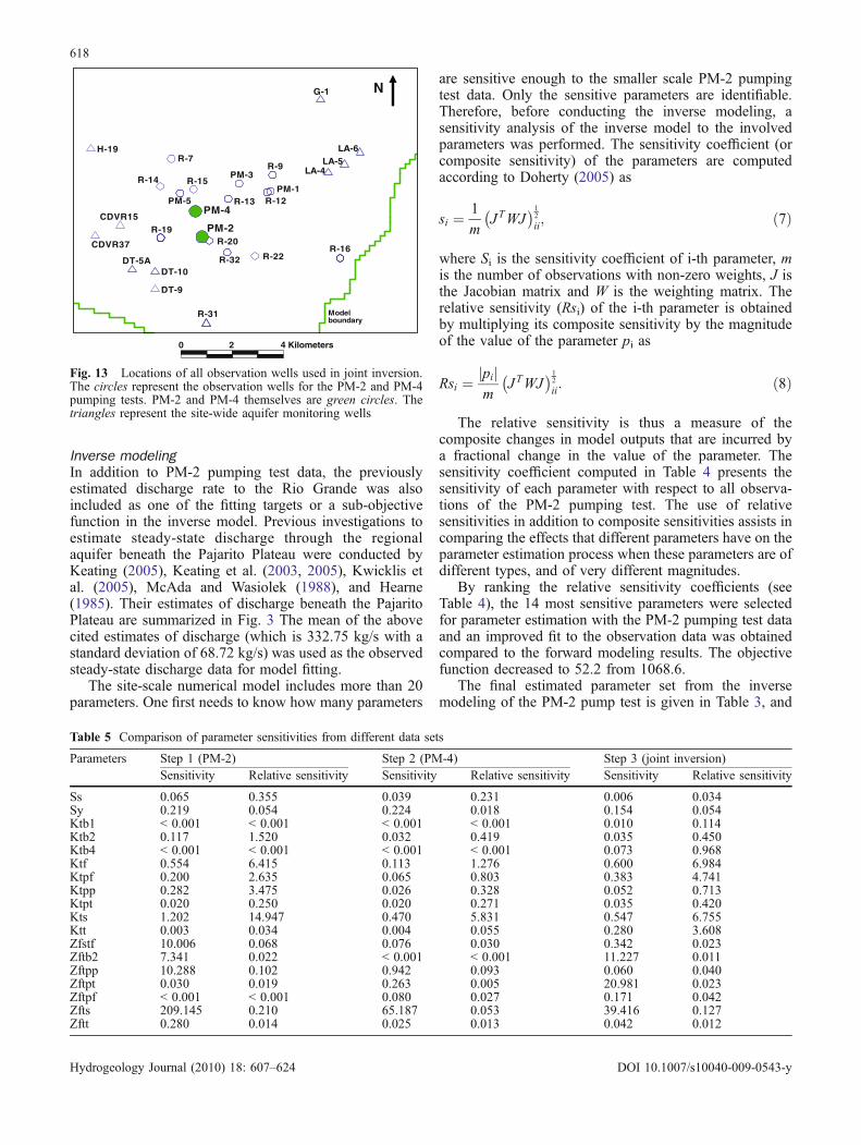
Fig. 13 Locations of all observation wells used in joint inversion.The circles represent the observation wells for the PM-2 and PM-4pumping tests. PM-2 and PM-4 themselves are green circles. Thetriangles represent the site-wide aquifer monitoring wells

Table 5 Comparison of parameter sensitivities from different data sets

Parameters Step 1 (PM-2) Step 2 (PM-4) Step 3 (joint inversion)Sensitivity Relative sensitivity Sensitivity Relative sensitivity Sensitivity Relative sensitivity

Ss 0.065 0.355 0.039 0.231 0.006 0.034Sy 0.219 0.054 0.224 0.018 0.154 0.054Ktb1 < 0.001 < 0.001 < 0.001 < 0.001 0.010 0.114Ktb2 0.117 1.520 0.032 0.419 0.035 0.450Ktb4 < 0.001 < 0.001 < 0.001 < 0.001 0.073 0.968Ktf 0.554 6.415 0.113 1.276 0.600 6.984Ktpf 0.200 2.635 0.065 0.803 0.383 4.741Ktpp 0.282 3.475 0.026 0.328 0.052 0.713Ktpt 0.020 0.250 0.020 0.271 0.035 0.420Kts 1.202 14.947 0.470 5.831 0.547 6.755Ktt 0.003 0.034 0.004 0.055 0.280 3.608Zfstf 10.006 0.068 0.076 0.030 0.342 0.023Zftb2 7.341 0.022 < 0.001 < 0.001 11.227 0.011Zftpp 10.288 0.102 0.942 0.093 0.060 0.040Zftpt 0.030 0.019 0.263 0.005 20.981 0.023Zftpf < 0.001 < 0.001 0.080 0.027 0.171 0.042Zfts 209.145 0.210 65.187 0.053 39.416 0.127Zftt 0.280 0.014 0.025 0.013 0.042 0.012

618

Hydrogeology Journal (2010) 18: 607–624 DOI 10.1007/s10040-009-0543-y

the hydrograph fits are presented in Figs. 4 and 5. Figure 6shows the calculated drawdowns for the observation wellswhere no apparent drawdown was observed. Most of thecalculated values are less than 0.05 m and close to zerodrawdowns. The simulated drawdowns in the pumpingwell and observation wells match reasonably well with theobservation data. The calculated discharge (334.62 kg/s) isvery close to the observed value (332.75 kg/s). Therefore,the uncertainty of estimated parameters is limited. This setof parameters represents the final results of inversemodeling of the PM-2 pump test.

Figure 7 shows two orthogonal cross sections extractedfrom the geological framework around the PM-2 well andthe simulated drawdown distributions after 25 days.Figure 8 presents the plane view of hydrofacies anddrawdowns (also at 25 days) at elevations 1,700 and1,600 m. At elevations between 1,700 and 1,600 m, thedrawdown increases and the influence ranges of thepumping test also increase.

Step 2: forward and inverse modeling of PM-4pumping test

Forward modelingAs a first step, the final estimated parameter set frominverse modeling of the PM-2 pumping test (estimatedparameters in Table 3) was used to simulate the PM-4pumping test. The quantitative evaluation is listed inTable 3 with a total objective value of 1118. The modelcan approximately fit the drawdowns of the observationwells PM-2, PM-5, R-20 and R-15, and the calculateddischarge (336.66 kg/s) is close to the observed discharge(332.75 kg/s). However, the model cannot fit the draw-downs in the pumping well PM-4 and the observationwells R-13 and R-19. In fact, the major contributions tothe total objective function (1118) come from observation

wells R-13 (350.4 or 31.3%) and R-19 (572.2 or 51.2%),totaling 82.5%, because the calculated drawdowns aremuch larger than the observed drawdowns for these twowells, as is the case for the pumping well PM-4. Note thatthe weighting coefficients for these two observation wellsare also very large, because the weights are larger at pointswith lower observation drawdowns and a very smallstandard deviation (see Eq. 4).

The model parameters developed to match the PM-2pump test in step 1 do not provide a good fit compared tothe observation data for the PM-4 pump test. The poorprediction may be because the PM-2 pump test influencesonly a small fraction of the site-scale model domain.Subsequently the estimated parameters can represent theheterogeneity of the aquifer in the area close to well PM-2, but cannot represent the parameter distributions for theentire aquifer or even the area surrounding PM-4. Theconclusion of this forward simulation is that only usingPM-2 data to develop a site-scale model for predictingdrawdown at PM-4 is an inadequate approach. Theinclusion of PM-4 pumping test data for parametercalibration may be necessary for developing a betterpredictive model.

Inverse modelingFor inverse modeling of PM-4 pumping test data, theresults from the PM-2 pumping test (step 1) were used as

0 3 6 9 12 150

3

6

9

12

15

Mea

sure

d dr

awdo

wn

(m)

Computed drawdown (m)

R-20-3 in PM-4 pumping test

1800 1900 2000 2100 2200

1800

1900

2000

2100

2200

Mea

sure

d he

ads

(m)

Computed heads (m)

a

b

Fig. 15 The overall fitting results from the joint inverse model: aPM-2 and PM-4 pumping test data; b site-wide water head data.The green lines are 1:1 lines

Ss sy

Ktb

1

Ktb

2

Ktb

4

Ktf

Ktp

f

Ktp

p

Ktp

t

Kts Ktt

zfst

f

zftb

2

zftp

p

zftp

t

zftp

f

zfts

zftt

1E-3

0.01

0.1

1

10R

elat

ive

sens

itivi

ty

Parameters

Step 1 (PM-2) Step 2 (PM-4) Step 3 (Joint)

Fig. 14 Comparison of parameter relative sensitivities fromdifferent data sets. Apparent missing data (e.g. Ktb1, Ktb4 andZftpf) have relative sensitivity < 0.001

619

Hydrogeology Journal (2010) 18: 607–624 DOI 10.1007/s10040-009-0543-y

the initial parameters and the PM-4 pumping test datawere used as the fitting target, which includes thedrawdown data from PM-4, PM-2, PM-5, R-13, R-14-2,R-15, R-20-3 and R-32, zero drawdown data (a zerodrawdown was assigned to the observation wells where noapparent drawdown was observed) from R-14-1 (the firstscreen of well R-14), and R-22, and discharge data. Theobserved drawdown data in pumping well PM-4 were alsocorrected with a factor of 0.52 as discussed in the previoussection. The final estimated parameter set from the inverse

modeling of PM-4 pumping test is listed in Table 3, andthe hydrograph fits are presented in Figs. 9 and 10. Theobjective function value is greatly reduced to 96.5 from1118 of the forward simulation. The fitting results to thepumping well and observation wells are improved. Mostof the calculated drawdowns for the observation wellswhere no apparent drawdown was observed (R-14-1, R-22-1 and R-22-2) are less than 0.05 m and close to zerodrawdowns. The observation well R-20-3 (the deepestscreen of R-20) is the only well that did not closely match

0 5 10 15 20 250

5

10

15

20

25

Dra

wdo

wn

(m)

Time (days)

PM-2 computed Corrected data Raw data PM-4 computed Measured PM-5 computed Measured

0 5 10 15 20 25 300

2

4

6

8

Dra

wdo

wn

(m)

Time (days)

R-20 Computed 1 Observed 1 Computed 2 Observed 2 Computed 3 Observed 3

-5 0 5 10 15 20 25 300.00

0.25

0.50

0.75

1.00

Dra

wdo

wn

(m)

Time (days)

R-32 Computed 1 Observed 1 Computed 2 Observed 2 Computed 3 Observed 3

-5 0 5 10 15 20 25 300.00

0.05

0.10

0.15

0.20

0.25

Dra

wdo

wn

(m)

Time (days)

Zero drawdowns Computed R-22-1 Computed R-22-2

-5 0 5 10 15 20 25 300.00

0.05

0.10

0.15

0.20

0.25

0.30

0.35

Dra

wdo

wn

(m)

Time (days)

Zero drawdowns Computed R-12 Computed R-13 Computed R-14-1 Computed R-14-2

-5 0 5 10 15 20 25 300.00

0.05

0.10

0.15

0.20

0.25

0.30

0.35

Dra

wdo

wn

(m)

Time (days)

Zero drawdowns Computed R-15 Computed R-23 Computed PM-1 Computed PM-3

ba

c d

e f

Fig. 16 The fitting results for PM-2 pumping test using the joint inverse model (a–f) (Drawdown correction in the pumping well wasbased on Peaceman 1978)

620

Hydrogeology Journal (2010) 18: 607–624 DOI 10.1007/s10040-009-0543-y

the data. This may be due to a high conductivity fault orfracture between R-20-3 and PM-4, and this numericalmodel did not capture it. So, the computed drawdowns atR-20-3 are much lower than the observed drawdowns.

Figure 11 shows the hydrofacies cross-section and thecorresponding drawdown distribution in YZ plane (X=19,294 m) around the PM-4 pumping well. The largestdrawdown occurred at about an elevation of 1,600 m. Therelatively smaller permeabilities in Tb1 and Tb4 limited

the drawdown development in the middle and lower partof the pumping well. Figure 12 presents the XY planeviews of drawdowns at different elevations (Z=1,700 and1600 m) after 21 days. From elevation 1,700 to 1600 m,the drawdowns increase and the influence ranges of thepumping test also increase. The corresponding hydrofaciesdistributions at these elevations can be found in Fig. 8.The calculated discharge (332.86 kg/s) is well matched tothe observed value (332.75 kg/s).

0 5 10 15 20 250

5

10

15

20

25

Dra

wdo

wn

(m)

Time (days)

PM-4 Computed Corrected data Raw data PM-2 computed Measured PM-5 computed Measured

0 5 10 15 20 250.0

0.2

0.4

0.6

0.8

Dra

wdo

wn

(m)

Time (days)

R-32-2 measured Computed R-32-3 measured Computed

0 2 4 6 8 10 12 140.0

0.1

0.2

0.3

0.4

0.5

Dra

wdo

wn

(m)

Time (days)

R-19-4 measured Computed R-19-5 measured Computed R-19-6 measured Computed R-19-7 measured Computed

0 5 10 15 20 250.01

0.1

1

10

Dra

wdo

wn

(m)

Time (days)

R-20-3 measured R-20-3 Computed R-20-2 Computed R-20-1 Computed

0 5 10 15 20 250.0

0.2

0.4

0.6

0.8

1.0

Dra

wdo

wn

(m)

Time (days)

R-13 measured Computed R-14-2 measured Computed R-15 measured Computed

0 5 10 15 20 250.00

0.05

0.10

0.15

0.20

0.25

Dra

wdo

wn

(m)

Time (days)

Zero drawdowns R-22-1 computed R-22-2 computed R-14-1 computed

ba

c d

e f

Fig. 17 The fitting results for PM-4 pumping test using the joint inverse model (a–f) (Drawdown correction in the pumping well wasbased on Peaceman 1978)

621

Hydrogeology Journal (2010) 18: 607–624 DOI 10.1007/s10040-009-0543-y

From step 1 to step 2, the biggest changes in theestimated parameters are changes in log permeabilities ofTpt (Ktpt) and Tpf (Ktpf). The former is reduced from –12.89 to –13.59 log(m2) (see Table 3), and the latterincreases from –13.1 to –12.2 log(m2). This is due toheterogeneity within hydrofacies that were not consideredin the site-scale model. It means that Tpt has a highpermeability in the local area around PM-2 but a relativelylower permeability around PM-4, while Tpf is theopposite. This inverse model only estimates the meanpermeability in each hydrofacies based on the individualpumping data. Therefore, different estimates for theseparameters were obtained from different pumping testdata. In order to obtain a set of parameters suitable to theentire aquifer system of the site model, the next step is tocouple the PM-2 and PM-4 pumping test data, dischargedata, and the site-wide aquifer monitoring data for a jointinversion of the model parameters.

Step 3: joint inverse modelingThe joint inversion model couples all the previouslydescribed observation data together to form a compositeinverse model. The generalized objective function of thismodel takes into account the head data from the site-wideaquifer monitoring, drawdown data from the PM-2 andPM-4 pump tests, and discharge data. For forwardsimulations, the site model is run to steady-state to fitthe site-wide water head data and the discharge data.Then, using the obtained steady-state flow field as theinitial conditions, two transient simulations are run for the25-day PM-2 pumping test and the 21-day PM-4 pumpingtest, respectively. Finally, the joint inverse model calcu-lates the generalized objective function from the forwardmodeling results. Figure 13 shows the locations of all theobservation wells used in joint inversion.

In order to test the sensitivity of the joint inverse modelto the parameters, the computed sensitivity coefficientsfrom these three steps are summarized in Table 5 (also seeFig. 14). The sensitivity (or composite sensitivity) inTable 5 presents the sensitivity of each parameter withrespect to different scales and different sources of observa-tions; while the relative sensitivity of a parameter is obtainedby multiplying its composite sensitivity by the magnitude ofthe value of the parameter. For all these three steps, thepermeability of Ts (Sandy Santa Fe) is the most sensitiveparameter because Ts has the largest fraction of the totalvolume (0.294, see Table 1) and both PM-2 and PM-4pumping wells intersect this unit. For the same reason,permeabilities of Tf (Fanglomeratic Santa Fe), Tpf (Puyefanglomerate) and Tt (Tschicoma flows) are the second mostsensitive parameters in these three simulations. Since thejoint model incorporates much more observation data thanthe individual inverse model of PM-2 or PM-4, the jointmodel is sensitive tomore parameters. For example, in step 1and 2, the permeabilities of Tb1 and Tb4 are not sensitiveenough to be estimated because they are distributed fairly faraway from the PM-2 and PM-4 pumping wells. When the

site-wide aquifer monitoring data are included in the jointinverse model, these two parameters are identifiable in thejoint inverse model. The Z factors (which is the ratio of thevertical and horizontal permeability) of zftpf and zftb2 arenot sensitive in step 1 and 2, respectively, while they aresensitive enough to be estimated in the joint inverse model.In the joint model a total of 18 parameters were estimated.

The joint inverse model yielded good results in theform of a reasonably low overall objective function (seethe last column in Table 3), although the sub-objectivevalues for the PM-2 and PM-4 pumping tests (70.7 and157.5, respectively) are slightly larger than those obtainedfrom step 1 (52.2 for PM-2) and step 2 (96.5 for PM-4).These results indicate that the joint inverse model providesgood predictions of water heads or drawdowns at most ofthe observation wells. Figure 15 shows the overall fittingresults. Figure 15a compares the calculated versus measureddrawdowns of PM-2 and PM-4 pumping tests. With theexception of drawdown data from R-20-3 in the PM-4pumping test, one can fit all the other data. The reason for thepoor fitting of R-20-3 was discussed previously. Figure 15bshows a very good match of the calculated and measuredsite-wide water head data. Figures 16 and 17 show the fittingresults of the measured versus calculated time-series draw-downs for PM-2 and PM-4 pumping tests. Simulateddrawdowns at the two pumping wells match the correcteddrawdown data quite well. The calculated drawdowns forobservation wells where zero drawdown was observed areless than 0.05 m for both pumping tests.

Table 6 illustrates the new estimated parameters andtheir 95% confidence intervals. Because more observationdata were used for the joint inverse model, all of the other18 parameters are well-constrained and have reasonablelower and upper bounds. Therefore, the uncertainty ofestimated parameters is well limited in the joint inversion.This set of parameters represents the final results ofinverse modeling of the site-scale model.

Table 6 The estimated parameters and 95% confidence intervalsfrom the joint inversion

Parameters Estimated values 95% confidence intervalsLower limit Upper limit

Kts –12.40 –12.45 –12.35Ktf –11.64 –11.73 –11.54Ktb4 –13.20 –14.11 –12.29Ktb1 –13.60 –15.55 –11.64Ktb2 –12.99 –13.57 –12.41Ktt –12.90 –13.22 –12.58Ktpt –11.99 –12.49 –11.50Ktpp –13.62 –14.22 –13.03Ktpf –12.33 –12.52 –12.14Ss –5.75 –9.98 –1.63Sy 0.35 0.165 0.535Zftb2 0.0001 0.0001 0.001Zftpt 0.001 0.0001 0.002Zftpf 0.247 0.078 0.415Zfstf 0.058 0.004 0.113Zfts 0.004 0.003 0.006Zftpp 0.689 0.0001 1.386Zftt 0.279 0.0001 1.091

622

Hydrogeology Journal (2010) 18: 607–624 DOI 10.1007/s10040-009-0543-y

Summary and conclusions

Inverse modeling provides a method whereby measure-ments of state are used to determine unknown modelstructures and parameters by fitting model output withobservation data. This technique combined with a step-wise strategy has been successfully applied to the LANLsite-scale model to estimate model parameters by couplingobservation data from different sources and at variousspatial scales including single-well tests, multiple-wellpumping tests to regional aquifer monitoring data.

To determine the flow parameters for the site-scalemodel, statistical analyses of single-well slug and pump-ing test results were first conducted to define the priordistributions of the key parameters. This prior informationwas used to define the parameter initial values and thelower and upper bounds for inverse modeling. From thestepwise progression of inverse modeling, a number ofsteps were used by inversions of drawdown data from thePM-2 and PM-4 pump tests separately, and a joint inversionwas undertaken by coupling PM-2 and PM-4 pump test datawith head data from the site-wide aquifer monitoringnetwork. Parameter sensitivity coefficients for different datasets were calculated to analyze the parameter identifiabilityin different steps.

Finally, the joint inverse model was derived with ageneralized composite objective function. Solving thejoint inverse problem leads to a well-constrained estimateof model parameters and reduces the uncertainty ofestimated parameters. The joint inversion results providea reasonable fit to all three data sets. The uncertainty ofestimated parameters for the hydrofacies is addressed withthe estimated parameter confidence intervals. The param-eters estimated from the joint inverse model shouldprovide appropriate overall predictions of drawdown atfuture pumping tests in LANL site. The previous versionsof the site-scale model and the smaller scale flow andtransport models (e.g. individual watershed-scale models),using different calibration criteria and observation data(Keating et al. 2003 and 2005), may incorporate differentparameter values from those presented here and are stillvaluable for flow and transport modeling in this site.

Acknowledgements We wish to extend our appreciation to K.Birdsell, Z. Lu and P. Stauffer for their thoughtful reviews of thispaper, and to D. Broxton and S. McLin for the use of figures fromtheir reports. We are grateful to the editor and to the two reviewersfor their comments and suggestions and the time they invested inour manuscript.

References

Anscombe FJ, Tukey JW (1963) The examination and analysis ofresiduals. Technometrics 5:141–160

Broxton DE, Vaniman D (2005) Geologic framework of a ground-water system on the margin of a rift basin, Pajarito Plateau,north-central New Mexico. Vadose Zone J 4:522–550

Carey B, Cole G, Lewis C, Tsai F, Warren R, WoldeGabriel G(1999) Revised site-wide geologic model for Los Alamos

National Laboratory (FY99). LA-UR-00–2056. LANL, LosAlamos, NM

Carrera J, Neuman SP (1986) Estimation of aquifer parameters understeady-state and transient condition: 2. uniqueness, stability, andsolution algorithms. Water Resour Res 22(2):211–227

Cole G, Carey JW, Burnette L, Miller T (2006) The 2005 three-dimensional, geologic model of the pajarito plateau. Report LA-UR-06–3060. LANL, Los Alamos, NM

Collins KA, Simmons AM, Robinson BA, Nylander CL (2005) LosAlamos National Laboratory’s hydrogeologic studies of thePajarito Plateau: a synthesis of hydrogeologic workplan activities(1998–2004). LA-14263-MS. LANL, Los Alamos, NM

Dai Z, Samper J (2004) Inverse problem of multicomponent reactivechemical transport in porous media: formulation and applications.Water Resour Res 40, W07407. doi:10.1029/2004WR003248

Dai Z, Samper J (2006) Inverse modeling of water flow andmulticomponent reactive transport in coastal aquifer systems. JHydrol 327:447–461

Dai Z, Ritzi RW, Dominic DF (2005) Improving permeabilitysemivariograms with transition probability models of hierarchicalsedimentary architecture derived from outcrop-analog studies.Water Resour Res 41, W07032. doi:10.1029/2004WR003515

Dai Z, Samper J, Ritzi R (2006) Identifying geochemical processesby inverse modeling of multicomponent reactive transport in Aquiaaquifer. Geosphere 2(4):210–219. doi:10.1130/GES00021.1

Doherty J (2005) Model independent parameter estimation: PESTuser manual, 5th edn. Watermark Computing, Brisbane, Australia

Frenzel PF (1995) Geohydrology and simulation of groundwaterflow near Los Alamos, north central New Mexico, US GeolSurv Water Resour Invest Rep 95-4091

Gaud MN, Smith GA, McKenna SA (2004) Relating small-scalepermeability heterogeneity to lithofacies distribution. In: BridgeJ, Hyndman D (eds) Aquifer characterization. SEPM Spec Publ80:55–66

Griggs RL, Hem JD (1964) Geology and groundwater resources ofthe Los Alamos Area, New Mexico. US Geol Surv Water SupplPap 1753

Hearne GA (1985) Mathematical model of the Tesuque aquifersystem underlying Pojoaque River basin and vicinity, NewMexico. UUS Geol Surv Water Suppl Pap 2205, 75 pp

Hill MC (1992) A Computer Program (MODFLOWP) for estimat-ing parameters of a transient, three-dimensional, ground-waterflow model using nonlinear regression. US Geol Surv Open-FileRep 91-484

Keating EH (2005) Espanola Basin and Pajarito Plateau regionalflow model documentation. LA-UR-05–8513. LANL, LosAlamos, NM

Keating EH, Zyvoloski GA (2009) A stable and efficient numericalalgorithm for unconfined aquifer analysis. Groundwater 47(4):569–579

Keating EH, Vesselinov VV, Kwicklis E, Lu Z (2003) Couplingbasin- and local-scale inverse models of the Espanola Basin.Ground Water 41(2):200–211

Keating EH, Robinson B, Vesselinov V (2005) Development andapplication of numerical models to estimate fluxes through theregional aquifer beneath the Pajarito Plateau. Vadose Zone J4:653–671

Kwicklis E, Witkowski M, Birdsell K, Newman B, Walther D(2005) Development of an infiltration map for the Los AlamosArea, New Mexico. Vadose Zone J 4:672–693

Kwicklis EA, Wolfsberg AV, Stauffer PH, Walvoord MA, Sully MJ(2006) Multiphase, multicomponent parameter estimation forliquid and vapor fluxes in deep arid systems using hydrologicdata and natural environmental tracers. Vadose Zone J 5:934–950

LANL (1998) Hydrogeologic workplan. LANL 59599, LANL, LosAlamos, NM

McAda DP, Wasiolek M (1988) Simulation of the regionalgeohydrology of the Tesuque aquifer system near Santa Fe,New Mexico. US Geol Surv Water Resour Invest Rep 87-4056

McDonald MG, Harbaugh AW (1988) A modular three-dimensionalfinite-difference ground-water flow model: US Geol Surv TechWater Resour Invest, book 6, chap. A1, 586 pp

623

Hydrogeology Journal (2010) 18: 607–624 DOI 10.1007/s10040-009-0543-y

McLin SG (2005) Analysis of the PM-2 aquifer test usingmultiple observation wells. LA-14225-MS. LANL, LosAlamos, NM

McLin SG (2006a) Analyses of the PM-4 aquifer test usingmultiple observation wells. LA-14252-MS. LANL, LosAlamos, NM

McLin SG (2006b) Historical aquifer tests on Pajarito Plateau.LA-UR- 06–3789. LANL, Los Alamos, NM

Neuman SP, Yakowitz S (1979) A statistical approach to the inverseproblem of aquifer hydrology, 1: theory. Water Resour Res15:845–860

Newman BD, Robinson BA (2005) The hydrogeology of LosAlamos National Laboratory: site history and overview ofvadose zone and groundwater issues. Vadose Zone J 4:614–619.doi:10.2136/vzj2005.0072

Nylander CL, Bitner KA, Cole G, Keating EH, Kinkead S,Longmire P, Robinson B, Rogers DB, Vaniman D (2003)Groundwater annual status report for fiscal year 2002. LA-UR-03-0244, LANL, Los Alamos, NM

Peaceman DW (1978) Interpretation of well-block pressures innumerical reservoir simulation. Soc Pet Eng J 18(3):183–194

Poeter EP, Hill MC (1997) Inverse models: a necessary nextstep in groundwater modeling. Ground Water 35(2):250–260

Purtymun WD (1995) Geologic and hydrologic records of observa-tion wells, test holes, test wells, supply wells, springs, andsurface water stations in the Los Alamos area. LA-12883-MS,LANL, Los Alamos, New Mexico.

Robinson BA, Broxton DE, Vaniman DT (2005) Observations andmodeling of deep perched water beneath the Pajarito Plateau.Vadose Zone J 4:637–652. doi:10.2136/vzj2004.0168

Samper J, Dai Z, Molinero J, Garcia-Gutierrez M, Missana T,Mingarro M (2006) Interpretation of solute transport experi-ments in compacted Ca-bentonites using inverse modeling.Phys Chem Earth 31:640–648

Snedecor GW, Cochran WG (1976) Statistical methods, 6th edn.The Iowa State University Press, Ames, Iowa, 593 pp

Stauffer PH (2006) Flux flummoxed: a proposal for consistentusage. Ground Water 44(2):125–128

Sun N-Z (1994) Inverse problems in groundwater modeling.Kluwer, Dordrecht, The Netherlands, 364 pp

Sun N-Z, Yeh WW-G (1990) Coupled inverse problem in ground-water modeling, 1: sensitivity analysis and parameter identi-fication. Water Resour Res 26(10):2507–2525

Wagner BJ (1992) Simultaneous parameter estimation and contam-ination source characterization for coupled groundwater flowand contaminant transport modeling. J Hydrol 135:275–303

Yeh WW-G (1986) Review of parameter identification proceduresin ground-water hydrology: the inverse problem. Water ResourRes 22(2):95–108

Zhu J, Yeh T-CJ (2006) Analysis of hydraulic tomography usingtemporal moments of drawdown recovery data. Water ResourRes 42, W02403. doi:10.1029/2005WR004309

Zyvoloski GA, Robinson BA, Dash ZV, Trease LL (1997)Summary of the models and methods for the (FEHM)application: finite-element heat- and mass-transfer code. LA-13306-MS. LANL, Los Alamos, NM

624

Hydrogeology Journal (2010) 18: 607–624 DOI 10.1007/s10040-009-0543-y