Step Two - British Columbia

Step Two

D e f i n e t h e w e l l p r o t e c t i o n a r e a

EnvironmentCanada

EnvironnementCanada

Library and Archives Canada Cataloguing in Publication DataMain entry under title:Well protection toolkit [electronic resource]. --

Available on the Internet.A joint project of the Ministry of Environment, Lands and Parks, Ministry of Health and Ministry of Municipal Affairs; with support from Environment Canada and the B.C. Ground Water Association. Cf. Acknowledgements.Issued by: Water Stewardship Division. ISBN 0-7726-5566-9

1. Wellhead protection - British Columbia. 2. Water quality management – British Columbia. 3. Groundwater – Management. 4. Wellhead protection. I. British Columbia. Ministry of Environment, Lands and Parks. II. British Columbia. Ministry of Environment. III. British Columbia. Water Stewardship Division. IV. British Columbia. Ministry of Health. V. British Columbia. Ministry of Municipal Affairs. VI. Canada. Environment Canada. VII. British Columbia Ground Water Association.

TD405W44 2004 628.1’1409711 C2006-960110-0

S T E P T W O T A B L E O F C O N T E N T S

Summary . . . . . . . . . . . . . . . . . . . . . . . . . . . . . . . . . . . . . . . . . . . . . . . . . . . . . . . . . . . . . . . . . . . . . . . . . . . . . . . . . . . . . . . . . . 2

STEP TWO – Define the Well Protection Area

2.1 Definitions . . . . . . . . . . . . . . . . . . . . . . . . . . . . . . . . . . . . . . . . . . . . . . . . . . . . . . . . . . . . . . . . . . . . . . . . . . . . . . . . 3

2.2 Methods to Define the Capture Zone . . . . . . . . . . . . . . . . . . . . . . . . . . . . . . . . . . . . . . . . . . . . . . . . . . . . . . . . 4Arbitrary Fixed Radius and Calculated Fixed Radius . . . . . . . . . . . . . . . . . . . . . . . . . . . . . . . . . . . . . . . . . 5Analytical Equations . . . . . . . . . . . . . . . . . . . . . . . . . . . . . . . . . . . . . . . . . . . . . . . . . . . . . . . . . . . . . . . . . . . . . . . 5Hydrogeologic Mapping . . . . . . . . . . . . . . . . . . . . . . . . . . . . . . . . . . . . . . . . . . . . . . . . . . . . . . . . . . . . . . . . . . . 5Numerical Modelling . . . . . . . . . . . . . . . . . . . . . . . . . . . . . . . . . . . . . . . . . . . . . . . . . . . . . . . . . . . . . . . . . . . . . . 6

2.3 Calculate the Capture Zone and TOT Areas . . . . . . . . . . . . . . . . . . . . . . . . . . . . . . . . . . . . . . . . . . . . . . . . . . . 7Select a Method. . . . . . . . . . . . . . . . . . . . . . . . . . . . . . . . . . . . . . . . . . . . . . . . . . . . . . . . . . . . . . . . . . . . . . . . . . . . 7Gather Information and Conduct Analysis . . . . . . . . . . . . . . . . . . . . . . . . . . . . . . . . . . . . . . . . . . . . . . . . . . 12Seek Technical Expertise . . . . . . . . . . . . . . . . . . . . . . . . . . . . . . . . . . . . . . . . . . . . . . . . . . . . . . . . . . . . . . . 12

2.4 Set the Boundaries of the Well Protection Area. . . . . . . . . . . . . . . . . . . . . . . . . . . . . . . . . . . . . . . . . . . . . . . 12

2.5 Review the Well Protection Boundaries . . . . . . . . . . . . . . . . . . . . . . . . . . . . . . . . . . . . . . . . . . . . . . . . . . . . . . 13

Checklist for Step Two . . . . . . . . . . . . . . . . . . . . . . . . . . . . . . . . . . . . . . . . . . . . . . . . . . . . . . . . . . . . . . . . . . . . . . . . . . . . . 13

Appendix 2.1 Publications Describing Methods for Determining Capture Zones . . . . . . . . . . . . . . . . . . . . . . . . . 14

Appendix 2.2 Formula for Calculated Fixed Radius . . . . . . . . . . . . . . . . . . . . . . . . . . . . . . . . . . . . . . . . . . . . . . . . . . . 15

Appendix 2.3 Formulas for Analytical Equations . . . . . . . . . . . . . . . . . . . . . . . . . . . . . . . . . . . . . . . . . . . . . . . . . . . . . . 17

Appendix 2.4 General Terms of Reference for Delineating the Capture Zone . . . . . . . . . . . . . . . . . . . . . . . . . . . . 18

Case Study: Pumphandle B.C. . . . . . . . . . . . . . . . . . . . . . . . . . . . . . . . . . . . . . . . . . . . . . . . . . . . . . . . . . . . . . . . . . . . . . . . 19Pumphandle Aquifer . . . . . . . . . . . . . . . . . . . . . . . . . . . . . . . . . . . . . . . . . . . . . . . . . . . . . . . . . . . . . . . . . . . . . . . . . . . . . . 19The Capture Zones . . . . . . . . . . . . . . . . . . . . . . . . . . . . . . . . . . . . . . . . . . . . . . . . . . . . . . . . . . . . . . . . . . . . . . . . . . . . . . . . 20The Well Protection Areas . . . . . . . . . . . . . . . . . . . . . . . . . . . . . . . . . . . . . . . . . . . . . . . . . . . . . . . . . . . . . . . . . . . . . . . . . 23

FiguresFigure 2. 1 Step Two: Define the Well Protection Area . . . . . . . . . . . . . . . . . . . . . . . . . . . . . . . . . . . . . . . . . . . . . . . . . 2Figure 2. 2 Schematic Diagram of a Well Capture Zone . . . . . . . . . . . . . . . . . . . . . . . . . . . . . . . . . . . . . . . . . . . . . . . . 3Figure 2. 3 Calculated Fixed Radius Capture Zone . . . . . . . . . . . . . . . . . . . . . . . . . . . . . . . . . . . . . . . . . . . . . . . . . . . . 4Figure 2. 4 Capture Zone in an Aquifer with a Sloping Water Table . . . . . . . . . . . . . . . . . . . . . . . . . . . . . . . . . . . . 5Figure 2. 5 Capture Zone Delineated by Hydrogeologic Mapping . . . . . . . . . . . . . . . . . . . . . . . . . . . . . . . . . . . . . . 5Figure 2. 6 Criteria for Selecting Capture Zone Delineation Methods. . . . . . . . . . . . . . . . . . . . . . . . . . . . . . . . . . . . 7Figure 2. 7 Capture Zone Based on Calculated Fixed Radius . . . . . . . . . . . . . . . . . . . . . . . . . . . . . . . . . . . . . . . . . . 15Figure 2. 8 Calculated Fixed Radius Based on Water Use . . . . . . . . . . . . . . . . . . . . . . . . . . . . . . . . . . . . . . . . . . . . . 16Figure 2. 9 Capture Zone Determined from Analytical Equations. . . . . . . . . . . . . . . . . . . . . . . . . . . . . . . . . . . . . . 16Figure CS 2. 1 Cross-section through Pumphandle Valley. . . . . . . . . . . . . . . . . . . . . . . . . . . . . . . . . . . . . . . . . . . . . 20Figure CS 2. 2 Capture Zones for Community Wells. . . . . . . . . . . . . . . . . . . . . . . . . . . . . . . . . . . . . . . . . . . . . . . . . . 22Figure CS 2. 3 Proposed Well Protection Area . . . . . . . . . . . . . . . . . . . . . . . . . . . . . . . . . . . . . . . . . . . . . . . . . . . . . . . 24

TablesTable 2. 1 Summary of Capture Zone Delineation Methods . . . . . . . . . . . . . . . . . . . . . . . . . . . . . . . . . . . . . . . . . . . . 8Table 2. 2 Summary of Available Groundwater Information . . . . . . . . . . . . . . . . . . . . . . . . . . . . . . . . . . . . . . . . . . 10Table CS 2. 1 Summary of Pumphandle Community Wells . . . . . . . . . . . . . . . . . . . . . . . . . . . . . . . . . . . . . . . . . . . 19Table CS 2. 2 Summary of Capture Zones for the Community Wells. . . . . . . . . . . . . . . . . . . . . . . . . . . . . . . . . . . 21

W e l l P r o T e c T i o n T o o l K i T – S T e P T W o

�

S T E P T W O S U M M A R Y

More than 1,000,000 British Columbians rely on groundwater as their source of drinking water, and there are thousands of community well systems in British Columbia. A well protection plan allows communities to identify land use activities that may threaten the quality of their well water, and to develop a strategy to avoid or minimize these threats.

There are six steps to follow in developing a well protection plan:

1. Form a community planning team

2. Define the well protection area

3. Identify potential contaminants

4. Develop and implement management strategies

5. Develop contingency plans

6. Monitor results and evaluate the plan

These steps are described in the six booklets that make up the Well Protection Toolkit. Each booklet describes activities that lead to the development and implementation of a well protection plan. In each step, a fictional case study of the town of Pumphandle shows how one community took on this challenge.

Step two: Define the well protection area

The second step is to define the area that should be managed and protected from potential contamination – the “well protection area.” The length of time that it would take contaminants to reach each well is also calculated at this stage. It is a good idea to review the boundaries of the well protection area from time to time, especially if new wells constructed nearby place additional demands on the aquifer and alter the “capture zone” of the community well(s).

Figure 2.1 shows the stages of Step Two.


�

Step three: identify potential contaminants

Step foUr: Develop Management Strategies

Step five: Develop contingency plans

Step SiX: Monitor results & evaluate plan

Step two: Define the well protection area

Step one: form a community planning team

Gather basic information on the aquifer and wells

Decide on method(s) for calculating capture zone

calculate capture zone and time of travel areas

Define boundaries of the well protection area

review well protection area boundaries

figure 2.1

S T E P T W O

once the community planning team has some initial information for each community well and aquifer (Step one), the next step is to determine the area that needs to be protected from contamination – the “well protection area.”

Step Two is the most technical step in the six-step well protection planning process, and the planning team will probably need professional assistance in completing this work. The information provided here is a general introduction to the methods for determining the well protection area.

2.1 DefinitionsThe planning team should become familiar with a number of technical terms that will be used throughout the development of the well protection plan. Figure 2.2 shows many of these concepts. The groundwater video, www.groundwater. protection, available from your local health authority office, also covers many of these definitions and concepts.

Hydrogeology

Hydrogeology is the study of the flow of water and chemicals through the geological formations.

Aquifer

An aquifer is a permeable geological deposit (such as sand and gravel or fractured bedrock) that holds and yields a supply of water (Figure 2.2). The well may draw water from a large portion of the aquifer, or only part of it.

Aquifer Transmissivity

Aquifer transmissivity refers to the ability of an aquifer to transmit water.

Aquitard

An aquitard is a geological formation that does not transmit a significant amount of water to wells and springs. Some examples of aquitards are sediments such as silts, clays and tills.

confined Aquifer

Where an aquitard overlies an aquifer, the low permeability of the aquitard can help in protecting the underlying aquifer from impacts of human activities at the land surface. In those cases, an aquifer is said to be “confined.”

Unconfined Aquifer

Where no aquitards overlie the aquifer, the aquifer is said to be “unconfined” and

is vulnerable to impacts from human activities at the land surface, particularly if the water table is shallow. Knowing which areas of the aquifer are most vulnerable will allow you to put the greatest effort into the areas that need most protection.


�

Define the well protection area

o b j e c t i v e S• To select a method to identify the capture zone for

each community well

• To calculate the capture zone and time of travel areas

• To define the boundaries of the well protection area

• To review the boundaries as required

5-YearTime of Travel1-Year

Time of Travel

Water Table

Pumping Well

Capture zoneboundary

Aquifer

Drawdown Cone

figure 2.2 Schematic Diagram of a well capture Zone

S T E P T W O

Water Table

The water table is the level of standing water in the ground (Figure 2.2) and is the upper boundary of the unconfined aquifer. Where the water table comes to the surface, lakes and wetlands form.

Drawdown cone

When water is pumped from a well, the water table close to the well drops in a cone-shape (see Figure 2.2). The area influenced by the pumping well is called the “drawdown cone.” Its shape will vary – it is circular only where the geology is uniform and the water table is level.

capture Zone

The capture zone is the land area that contributes water to the community well (Figure 2.2). Another name for this is the “recharge area.” Any precipitation (rain or snow) that lands in this area may eventually end up in your well water. So may any fertilizers, oils spills or other contaminants. It is important to define the capture zone accurately, because you cannot protect the well water without knowing where that water is coming from.

Well Protection Area

The well protection area is the land area on which protection measures are taken. In most cases, this will be the area defined as the capture zone. However, it may include an area larger than the capture zone (e.g. the water district boundary). It is recommended that the well protection area be reviewed every year and revised as necessary.

Time of Travel (ToT)

The capture zone can be divided into sub-areas based on “time of travel”: the time it takes water to flow

from a given point to the well. Usually, the capture zone is divided into one-year, five-year and ten-year time of travel (TOT) areas. The one-year TOT area is normally closest to the well; the five- and ten-year TOT areas are further away (Figure 2.2).

There are two reasons for dividing

the capture zone into TOT sub-areas:

• It provides the planning team with an idea of the time it would take for contaminants to travel to the well from different areas within the capture zone. Contaminants in the one-year TOT area will take a year or less to reach the well, contaminants spilled in the ten-year TOT area can take up to ten years to reach the well.

• It makes it easier to set priorities. The first priority for protection measures will be in the one-year TOT area. As well, some contaminants (e.g. bacteria) can only travel limited distances in soils before they are filtered out or die off, and are therefore of less concern when they are in the five- or ten-year TOT area.

2.2 Methods to Define the capture Zone It is important to define the capture zone accurately. Contaminants in the capture zone could pollute the water supply to the well. There are a number of methods to determine the capture zone, of which many are quite complex and technical (see Appendix 2.1 for a list of publications on this subject). The five methods most commonly used to delineate capture zones are:

1. Arbitrary Fixed Radius (AFR);

2. Calculated Fixed Radius (CFR);

3. Analytical Equations;

4. Hydrogeologic Mapping; and

5. Numerical Flow Modelling.


�

Sand and Gravel Aquifer

BedrockAquitard

ClayAquitard

Cylindrical volume of water pumped over a specified time period

Calculated fixed radiuscapture zone boundary

figure 2.3 calculated fixed radius capture Zone

S T E P T W O

The community planning team can undertake the first two methods. Analytical equations, hydrogeological mapping and modelling are more complex methods and a qualified hydrogeologist should conduct the analysis.

Arbitrary Fixed radius and calculated Fixed radiusBoth the Arbitrary Fixed Radius (AFR) and Calculated Fixed Radius (CFR) methods define the capture zone by drawing a circle around the wellhead. The difference between the two methods is that the circular AFR area is based solely on a fixed distance from the wellhead, while the area for the CFR is calculated using the volume of water pumped.

The AFR usually covers the area within 300 metres of the wellhead. This capture zone covers land beyond the immediate area of the well, but is not so large that management of the well protection area becomes too difficult. Major disadvantages of this method are that it is arbitrary, and the circular area cannot be subdivided into time of travel areas. The AFR should be used as a temporary measure and only where no information exists on the water use, well, or the aquifer.

The CFR calculates a circular area (Figure 2.3), based on the volume of water pumped by the well over a specified period of time (e.g. one, five or ten years). This reflects the time it takes a contaminant to travel from the CFR boundary to the well, based on the pumping rate (see Appendix 2.2 for details).

The CFR method is suitable for sand and gravel aquifers, where the water table is relatively level and wells supply no more than 100 connections.


�

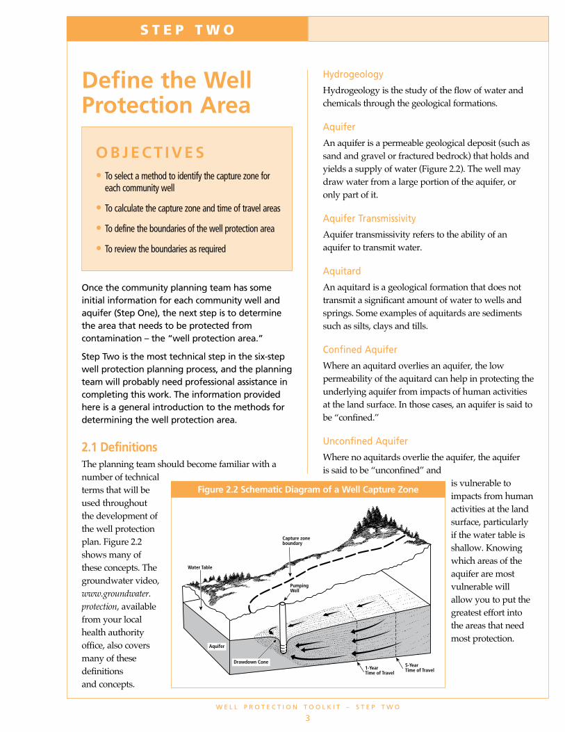
Analytical equationsWhere the water table is sloping, the fixed radius methods do not work. The shape of the capture zone around the pumping well is no longer circular, as recharge to the well come from “up-gradient” and has a long, finger-like shape (Figure 2.4).

Simple equations have been

developed for delineating capture zones where the water table is sloping. Formulas for calculating the dimensions of the capture zone and time of travel boundaries are presented in Appendix 2.3.

Analytical equations are suitable for sand and gravel aquifers where conditions are uniform and there is sufficient information on the pumping rate, aquifer transmissivity, and water table slope. This method may not work well for fractured bedrock aquifers.

Hydrogeologic MappingHydrogeologic mapping locates and maps the groundwater flow. The capture zone is defined by identifying the aquifers and aquitards, mapping the groundwater levels, and then determining flow

x

Sloping water table

Paraboliccapture zone

AquiferPumping well

2Y

figure 2.4 capture Zone in an aquifer with a Sloping water table

10m

20m

30m

Water TableContours

Pumping Well

Sand and gravel(aquifer)

Capture Zone

LakeBedrock hillslope(Aquitard)

Bedrock hillslope(Aquitard)

figure 2.5 capture Zone Delineated by hydrogeologic Mapping

S T E P T W O

directions from water level contours2 (Figure 2.5). This method requires considerable expertise and should be carried out with the assistance of a professional hydrogeologist.

This method is particularly suitable for shallow sand and gravel aquifers where ambient groundwater flow directions can be directly implied from topography and where the surface geology can be used to identify aquifer boundaries.

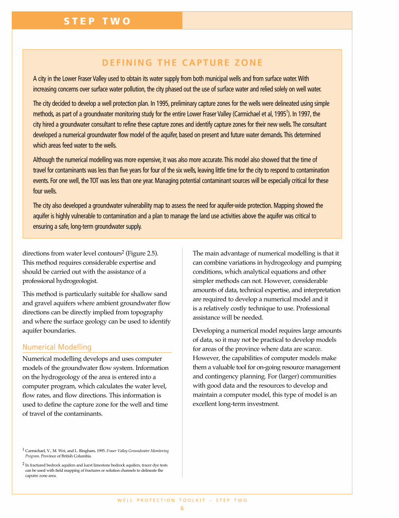
numerical ModellingNumerical modelling develops and uses computer models of the groundwater flow system. Information on the hydrogeology of the area is entered into a computer program, which calculates the water level, flow rates, and flow directions. This information is used to define the capture zone for the well and time of travel of the contaminants.

The main advantage of numerical modelling is that it can combine variations in hydrogeology and pumping conditions, which analytical equations and other simpler methods can not. However, considerable amounts of data, technical expertise, and interpretation are required to develop a numerical model and it is a relatively costly technique to use. Professional assistance will be needed.

Developing a numerical model requires large amounts of data, so it may not be practical to develop models for areas of the province where data are scarce. However, the capabilities of computer models make them a valuable tool for on-going resource management and contingency planning. For (larger) communities with good data and the resources to develop and maintain a computer model, this type of model is an excellent long-term investment.


�

D e f i n i n G t h e c a p t U r e Z o n e

A city in the Lower Fraser Valley used to obtain its water supply from both municipal wells and from surface water . With increasing concerns over surface water pollution, the city phased out the use of surface water and relied solely on well water .

The city decided to develop a well protection plan . In 1995, preliminary capture zones for the wells were delineated using simple methods, as part of a groundwater monitoring study for the entire Lower Fraser Valley (Carmichael et al, 19951) . In 1997, the city hired a groundwater consultant to refine these capture zones and identify capture zones for their new wells . The consultant developed a numerical groundwater flow model of the aquifer, based on present and future water demands . This determined which areas feed water to the wells .

Although the numerical modelling was more expensive, it was also more accurate . This model also showed that the time of travel for contaminants was less than five years for four of the six wells, leaving little time for the city to respond to contamination events . For one well, the TOT was less than one year . Managing potential contaminant sources will be especially critical for these four wells .

The city also developed a groundwater vulnerability map to assess the need for aquifer-wide protection . Mapping showed the aquifer is highly vulnerable to contamination and a plan to manage the land use activities above the aquifer was critical to ensuring a safe, long-term groundwater supply .

1 Carmichael, V., M. Wei, and L. Ringham, 1995. Fraser Valley Groundwater Monitoring Program. Province of British Columbia.

2 In fractured bedrock aquifers and karst limestone bedrock aquifers, tracer dye tests can be used with field mapping of fractures or solution channels to delineate the caputre zone area.

S T E P T W O

capture zone, because of the cost of implementing protection measures, and you will need to be able to justify your decisions.

However, AFR and CFR may be useful as interim methods to allow well protection planning to get underway. Once the community sees the value of groundwater protection and supports it, you may find additional funding to refine the capture zone using more accurate methods.

You should attempt to delineate the capture zone as accurately as possible, based on the information and funding available, local conditions and size of the water system. Figure 2.6 will help you to determine which method might be most appropriate for your


�

2.3 calculate the capture Zone and tot areas

Select a MethodHow do you decide which of the five methods to use? Some of the advantages and disadvantages are listed in Table 2.1.

Although it is tempting to use simple and less expensive methods (such as AFR), they are based on very simplistic assumptions. These assumptions may not apply in your situation, and could result in the planning team wasting resources on protection measures in an area that contributes little or no water to the groundwater supply. Experience in the United States shows that people may challenge your defined

figure 2.6 criteria for Selecting capture Zone Delineation Methods

* = technical advice is highly recommended

Analytical equations*

Arbitrary Fixed Radius and

Calculated Fixed Radius

Sand and gravel

Not as complex or low vulnerabilty

<100 connections

No

Complex and vulnerable

Fractured bedrock

Hydrogeological mapping or numerical modelling* or choose a larger

area such as a watershed boundary or boundary of the aquifer as the protection area

Complexity ofhydrogeology and

vulnerability of aquifer

>100 connectionsSize of system

YesOther high

capacity wells nearby

Start

Type of Aquifer


�

MethoD eXplanation aSSUMptionS typical Data aDvantaGeS/DiSaDvantaGeS when applicable reqUireD

arbitrary fixed radius

calculated fixed radiusSee Figure 2 .3

analytical equationsSee Figure 2 .4

hydrogeologic mappingSee Figure 2 .5

numerical modelling

Assign circular area of fixed radius (300 m) around well

Calculate cylindrical volume of aquifer supplying water to well for a given pumping rate and time period

See Appendix 2 .2

Calculate capture zone dimensions using analytical equations accounting for uniform ambient flow

See Appendix 2 .3

Map capture zone from measured groundwater level contours and geomorphologic, topographic and hydrologic features

Delineate capture zone using numerical flow modelling incorporating actual hydrogeologic information

- uniform aquifer

- negligible ambient flow

- uniform aquifer

- negligible ambient flow

- uniform aquifer

- horizontal, steady-state flow

- uniform ambient flow

- capture zone does not extend beyond watershed divide

- groundwater flow direction same as topographic slope

- horizontal flow

- depends on the model

table 2.1: SUMMary of captUre Zone Delineation MethoDS


�

MethoD eXplanation aSSUMptionS typical Data aDvantaGeS/DiSaDvantaGeS when applicable reqUireD

arbitrary fixed radius

calculated fixed radiusSee Figure 2 .3

analytical equationsSee Figure 2 .4

hydrogeologic mappingSee Figure 2 .5

numerical modelling

None

- pumping rate and/or water use

- aquifer thickness (or well screen length)

- aquifer porosity

- pumping rate and/or water use

- aquifer transmissivity

- ambient hydraulic gradient

- aquifer porosity

- aquifer boundary

- aquifer boundary

- water table contours (or topographic contours)

- geology

- water quality

- aquifer boundary

- geology

- water level elevations

- aquifer transmissivity

- hydraulic conductivity of aquitards

- knowledge of boundary conditions

ADVANTAgeS:• easy and inexpensive to apply

DISADVANTAgeS:• arbitrary• may be difficult to defend

ADVANTAgeS:• easy and inexpensive to apply• accounts for some site-specific information

DISADVANTAgeS:• based on simple physical assumptions

ADVANTAgeS:• easy and inexpensive to apply• accounts for some local information

DISADVANTAgeS:• based on simple physical assumptions

ADVANTAgeS:• accounts for local information• physically based

DISADVANTAgeS:• moderate - expensive to apply• large data requirement

ADVANTAgeS:• accounts for local information• physically based• predictive capability

DISADVANTAgeS:• moderate - expensive to apply• large data requirement

Inadequate information on well construction, pumping rate and hydrogeology; typically used for drive points and dug wells

Well construction and pumping rate are known, hydraulic gradient is low and aquifer thickness can be estimated; not appropriate for fractured bedrock aquifers

Aquifer transmissivity and pumping rate are known and a uniform hydraulic gradient can be estimated; may not be appropriate for fractured bedrock aquifers

May be especially useful for shallow, unconfined aquifers, springs, as well as karstic and fractured bedrock aquifers

Where hydrogeology and groundwater conditions can’t be adequately represented by simple analytical models (e .g . bedrock aquifers or complex hydrogeology and vulnerable aquifers)

table 2.1: SUMMary of captUre Zone Delineation MethoDS


�0

Tab

le

2.2

Su

mm

ar

y o

f a

va

ila

bl

e G

ro

un

dw

aT

er

in

fo

rm

aT

ion

DA

TA/

PuRv

EYO

R W

ELL

DR

iLLE

R/

WAT

ER S

AMPL

iNG

O

BSER

vATi

ON

G

ROuN

DWAT

ER

Aqui

FER

OThE

R W

hAT

TO D

O iF

iNFO

RMAT

iON

iS N

OT

iN

FORM

ATiO

N

OR

DATA

BASE

4 /

PuM

P AN

ALYS

iS8

W

ELL

REPO

RTS1

1 CL

ASSi

FiCA

TiO

N

GEO

LOG

iCAL

/ AL

READ

Y Av

AiLA

BLE?

CON

SuLT

ANT3

W

ELL

LOCA

TiO

N

iNST

ALLE

R7

DATA

BASE

N

ETW

ORk

(M

OE)

M

APS1

2 (M

OE)

hY

DRO

LOG

iCAL

M

APS5

(M

OE6

)

(MO

h/hA

9 )

DATA

10 (

MO

E)

MAP

S

Wel

l lith

olog

y, ■

■

■

•

If w

ell r

ecor

d fo

r the

com

mun

ity

c

onst

ruct

ion

wel

l can

not b

e ob

tain

ed, c

an

and

cap

acity

es

timat

e lit

holo

gy fr

om w

ell

re

cord

s of

adj

acen

t wel

ls; d

eter

min

e

w

ell d

epth

and

scr

een

loca

tion

by

so

undi

ng th

e w

ell;

mea

sure

cap

acity

usin

g a

pum

ping

test

Wel

l pum

ping

■

■

•

Pu

mpi

ng ra

te c

an b

e m

easu

red

by

rat

e

th

e pu

rvey

or o

r est

imat

ed b

ased

on th

e nu

mbe

r of c

onne

ctio

ns

gro

undw

ater

■

■

■

•

Pum

ping

and

sta

tic w

ater

leve

ls

con

ditio

ns a

nd

can

be m

easu

red

by p

urve

yor i

f w

ater

leve

l

ac

cess

at t

he w

ellh

ead

is a

vaila

ble

at w

ell

Tra

nsm

issi

vity

■

■

■

Tran

smis

sivi

ty c

an b

e es

timat

ed b

y

at t

he w

ell

a pu

mpi

ng te

st o

r fro

m s

peci

fic

ca

paci

ty d

ata*

Wel

l wat

er

■

•

■

Wat

er c

hem

istr

y ca

n be

q

ualit

y

ch

arac

teriz

ed b

y co

llect

ing

sam

ples

from

the

wel

l for

labo

rato

ry a

naly

sis

(c

onsu

lt M

OH

abou

t che

mic

al

pa

ram

eter

s to

ana

lyze

)

gro

undw

ater

■

•

■

■

gro

undw

ater

repo

rts

exis

t for

c

ondi

tions

and

sp

ecifi

c ar

eas

only

; in

mos

t are

as,

wat

er le

vel i

n

grou

ndw

ater

con

ditio

ns a

nd w

ater

t

he a

quife

r

le

vels

can

be

dete

rmin

ed b

y

co

mpi

ling

info

rmat

ion

from

wel

l

reco

rds a

nd c

ondu

ctin

g fie

ld su

rvey

s*

Tra

nsm

issi

vity

■

• ■

In

form

atio

n ex

ist f

or s

peci

fic a

reas

a

nd th

ickn

ess

only,

in o

ther

are

as, t

his

o

f the

aqu

ifer

info

rmat

ion

can

be c

ompi

led

from

wel

l rec

ord

data

*


��

Tab

le

2.2

Su

mm

ar

y o

f a

va

ila

bl

e G

ro

un

dw

aT

er

in

fo

rm

aT

ion

co

nT

inu

ed

DA

TA/

PuRv

EYO

R W

ELL

DR

iLLE

R/

WAT

ER S

AMPL

iNG

O

BSER

vATi

ON

G

ROuN

DWAT

ER

Aqui

FER

OThE

R W

hAT

TO D

O iF

iNFO

RMAT

iON

iS N

OT

iN

FORM

ATiO

N

OR

DATA

BASE

/ Pu

MP

ANAL

YSiS

W

ELL

REPO

RTS

CLAS

SiFi

CATi

ON

G

EOLO

GiC

AL/

ALRE

ADY

AvAi

LABL

E?

CO

NSu

LTAN

T W

ELL

LOCA

TiO

N

iNST

ALLE

R DA

TABA

SE

NET

WO

Rk

(MO

E)

MAP

S (M

OE)

hY

DRO

LOG

iCAL

M

APS

(MO

E)

(M

Oh/

hA)

DATA

(M

OE)

M

APS

Wat

er q

ualit

y

•

■

• ■

■

Whe

re in

adeq

uate

info

rmat

ion

of a

quife

r

ex

ists

, a fi

eld

sam

plin

g

and

cap

acity

su

rvey

requ

ired*

Loc

atio

n of

•

■

■

Su

rfici

al g

eolo

gy m

aps

can

be u

sed

aqu

ifer

to in

fer l

ocat

ion

of s

hallo

w,

un

conf

ined

sur

ficia

l aqu

ifers

*

Vul

nera

bilit

y

•

■

■

• Aq

uife

r vul

nera

bilit

y m

aps

exis

t o

f aqu

ifer

for s

peci

fic a

reas

onl

y; s

urfic

ial

ge

olog

y m

aps

can

be u

sed

to in

fer

sh

allo

w, u

ncon

fined

sur

ficia

l

aqui

fers

that

are

hig

hly

vuln

erab

le

to

con

tam

inat

ion*

gro

undw

ater

■

■

g

roun

dwat

er re

port

s ex

ist f

or

flo

w d

irect

ions

sp

ecifi

c ar

eas

only

; in

mos

t are

as,

flo

w d

irect

ions

can

be

dete

rmin

ed

by

com

pilin

g w

ater

leve

l

info

rmat

ion

from

wel

l rec

ords

and

mea

surin

g w

ater

leve

ls in

the

field

*

Rec

harg

e/

■

■

Info

rmat

ion

on re

char

ge/d

isch

arge

d

isch

arge

are

as

area

s ra

rely

exi

st; i

n m

ost a

reas

, thi

s

is

infe

rred

by c

ompi

ling

wat

er le

vels

fro

m w

ell r

ecor

ds a

nd a

lso

from

vege

tatio

n m

aps*

■ =

maj

or s

ourc

e of

info

rmat

ion;

•

= m

inor

sou

rce

of in

form

atio

n;

* = c

onsu

lt a

prof

essi

onal

hyd

roge

olog

ist

3 A

list o

f gro

undw

ater

con

sulta

nts

can

be fo

und

at w

ww

.env

.gov

.bc .

ca/w

sd/p

lan_

prot

ect_

sust

ain/

grou

ndw

ater

/libr

ary/

cons

ulta

nts .h

tml,

4 W

ell d

atab

ase

info

rmat

ion

can

be fo

und

at h

ttp:

//aar

dvar

k .go

v .bc

.ca/

apps

/wel

ls/,

5 W

ell l

ocat

ion

map

s ca

n be

foun

d at

ww

w .e

nv .g

ov .b

c .ca

/wsd

/pla

n_pr

otec

t_su

stai

n/gr

ound

wat

er/w

ells

/gw

smap

s .htm

l,

6 M

Oe:

Min

istr

y of

env

ironm

ent,

7 R

egis

ters

of D

rille

rs a

nd P

ump

Inst

alle

rs c

an b

e fo

und

at w

ww

.env

.gov

.bc .

ca/w

sd/p

lan_

prot

ect_

sust

ain/

grou

ndw

ater

/wel

ls .ht

ml —

scr

oll p

age

to “

Regi

stra

tion

of D

rille

rs a

nd P

ump

Inst

alle

rs”,

8 Pl

ease

con

tact

you

r Drin

king

Wat

er O

ffice

r/env

ironm

enta

l Hea

lth O

ffice

r for

this

info

rmat

ion

– se

e Ap

pend

ix 1

.2,

9 M

OH/

HA: M

inis

try

of H

ealth

/ Hea

lth A

utho

rity,

10

For i

nfor

mat

ion,

go

to w

ww

.env

.gov

.bc .

ca/w

sd/d

ata_

sear

ches

/obs

wel

l/ind

ex .h

tml,

11 O

n N

atio

nal T

opog

raph

ic S

yste

m (N

TS) f

ile a

nd fr

om c

onsu

ltant

s, 1

2 Fo

r an

over

view

of t

he s

yste

m c

lick

on w

ww

.env

.gov

.bc .

ca/w

sd/p

lan_

prot

ect_

sust

ain/

grou

ndw

ater

/aqu

ifers

/repo

rts/

aqui

fer_

map

s .pdf

"gui

de to

Usi

ng th

e BC

Aqu

ifer C

lass

ifica

tion

for

the

Prot

ectio

n an

d M

anag

emen

t of g

roun

d W

ater

"; to

que

ry th

e aq

uife

r cla

ssifi

catio

n da

taba

se,g

o to

w

ww

.env

.gov

.bc .

ca/w

sd/d

ata_

sear

ches

/aqu

ifers

/que

ry/in

dex .

htm

l ”g

uide

to U

sing

the

BC A

quife

r Cla

ssifi

catio

n M

aps/

for t

he P

rote

ctio

n an

d M

anag

emen

t of g

roun

d W

ater

” on

the

left

colu

mn

www.env.gov.bc.ca/wsd/plan_protect_sustain/groundwater/library/consultants.html

http://www.env.gov.bc.ca/wat/gws/gwdocs/gweddocs/consultants_gw.html

http://aardvark.gov.bc.ca/apps/wells/

http://www.env.gov.bc.ca/wsd/plan_protect_sustain/groundwater/wells/gwsmaps.html

http://www.env.gov.bc.ca/wsd/plan_protect_sustain/groundwater/wells.html

www.env.gov.bc.ca/wsd/data_searches/obswell/index.html

www.env.gov.bc.ca/wsd/plan_protect_sustain/groundwater/aquifers/reports/aquifer_maps.pdf

www.env.gov.bc.ca/wsd/data_searches/aquifers/query/index.html

S T E P T W O

situation. For example, if your community is tapping a well in a sand and gravel aquifer where the geology is relatively simple and the water system has over 100 connections, then it may be appropriate to use analytical equations. However, you may choose to use methods that are more accurate such as hydrogeologic mapping or numerical modelling, especially in populated areas where the capture zone boundary may need to be pinpointed more accurately. Technical advice on which method to use is available from the Ministry of Environment, Water, Land and Climate Change Branch in Victoria or groundwater consultants.12

Gather information and conduct AnalysisIn order to define the capture zone and well protection area, it is necessary to collect available information on each community well and on the groundwater resources in the local region. Much of this information may already exist. Table 2.2 (page 10) summarizes sources of this information and ways to obtain the missing information.

The well assessment form (Appendix 1.3) will guide you in compiling information on the well, water system, and local groundwater conditions. Regional Ministry of Environment Offices, Water Stewardship Division staff in Victoria may also be able to provide advice on compiling groundwater information (Appendix 1.2).

You will also need information on the vulnerability of the aquifer. The vulnerability of the aquifer to contamination from land use activities is needed to assess the threat of contamination as part of Step Three. The Ministry of Environment is mapping the boundaries of developed aquifers in major groundwater regions of the province and classifying them with respect to vulnerability.

Seek Technical expertise

Do you need to hire a groundwater consultant to help delineate the capture zone? As a rule, where the delineation involves methods other than AFR and CFR, it is recommended that a groundwater consultant be hired to assist in this work.

The following series of questions may provide some guidance:

• Is your community well in a fractured bedrock aquifer?13

• Is there more than one well in the system, and are they located close to each other (e.g. less than 100 metres)?

• Are there other significant pumping wells in close proximity to the community well (less than 100 m)?

• Is your community well supplying a significant number of customers (tens or hundreds of connections)?

• Are the local hydrogeologic conditions complex?14

If your answer to any of these is “yes,” hiring a groundwater consultant to assist in delineating the capture zone is a good idea (see Appendix 2.4).

You will almost certainly need professional assistance if your aquifer is in fractured bedrock. Groundwater flow in many bedrock aquifers occurs through discrete fractures or through discrete zones, and flow in these aquifers is usually hard to predict. Therefore, capture zones for wells drilled in fractured bedrock aquifers require more data and greater hydrogeologic expertise to analyze. It is likely that hydrogeologic mapping or numerical modelling methods will be needed to delineate the capture zone.

2.4 Set the boundaries of the well protection area

Now that the planning team has a reasonable idea of where the capture zone and time of travel zones are, you can decide on an appropriate well protection area.

Remember that capture zone boundaries are never determined with complete certainty, because complete information is never available. A common


��

12 A list of groundwater consultants in B.C. can be found in the Ministry of Environment, Groundwater Home Page http://www.env.gov.bc.ca/wsd/plan_protect_sustain/groundwater/library/consultants.html.

13 Refer to the well record or well assessment form.

14 Seek advice from the Groundwater Staff at the Ministry of Environment in Victoria to determine whether the hydrologeologic conditions are complex.

http://www.env.gov.bc.ca/wsd/plan_protect_sustain/groundwater/library/consultants.html

http://www.env.gov.bc.ca/wsd/plan_protect_sustain/groundwater/library/consultants.html

S T E P T W O

way to address this uncertainty is to assume worst case conditions in delineating the well protection area —for example by using the maximum pumping rate of the well to calculate the capture zone. Another way is to delineate the capture zone using several methods to see if the capture zones cover similar areas.

If you cannot determine the capture zone with any degree of certainty (e.g. because of the complex geology), a third option is to establish a well protection area that covers an area larger than the defined capture zone. This larger area may be the watershed boundary, boundary of the aquifer (capture zone boundaries should not extend beyond the aquifer) or the entire water district boundary.

You can establish some priorities at this stage, based on your understanding of the aquifer. For example, you may decide to focus your efforts on areas within the one-year time of travel area and/or in areas known to be vulnerable. Determining the capture zone for a well or group of wells can be challenging. Hiring a groundwater consultant to assist in this process can be a solid investment for future protection activities and help you support your choices and decisions within your community.

2.5 review the well protection boundaries The planning team should review the boundaries of the well protection area from time to time. Water use conditions change. When establishing the well protection area, look at the effects of expanding the water supply system. If the demand for water in the community increases, the pumping rate for one or more of the community wells will increase, and so will the size of the capture zone. Any new wells located in the capture zone may also significantly change the capture zone boundaries.

As additional and more recent data becomes available, the understanding of the aquifer and groundwater conditions will increase. The well protection area may need to be adjusted to include this new information.

The existence of higher capacity wells near the community well can affect the capture zone of the community well. In cases where high capacity wells (e.g. other municipal wells, irrigation wells) are known to exist, these wells need to be considered

when defining the capture zone of the community well. Review the capture zone annually and see if new high capacity wells exist. If so, then it will be necessary to review the capture zone and revise its boundaries if needed. This is where the use of a numerical model is advantageous because as conditions change, the model can be updated to see how changes (or proposed changes) will affect the capture zone. The advice of a professional hydrogeologist is recommended.


��

Determine the vulnerability of the aquifer in the well protection area

Decide if you need a groundwater consultant to help with delineating the capture zone

Develop terms of reference for hiring a groundwater consultant

Calculate capture zone and TOT

Define boundaries of well protection area

Review the boundaries

get advice from the Ministry of environment or hire a groundwater consultant .

go over Figure 2 .6 and Section 2 .3 .

Refer to Appendix 2 .4 .

Choose the appropriate method (Table 2 .1); get advice from MOe .

Use conservative assessments to account for unknowns .

Adjust boundaries to account for new wells, increases in pumping requirements, etc .

ACTiON iTEM COMMENTS COMPLETED

checkliSt for Step two

The following is a basic checklist for action items to be completed during Step Two of the well protection planning process:

S T E P T W O A P P E N D I C E S

Methods for delineating capture zones are described in detail in a variety of publications, including:

Carmichael, V., M. Wei, and L. Ringham, 1995. Fraser Valley Groundwater Monitoring Program. Province of British Columbia.

Delin, G. N. and J. E. Almendinger, 1993. Delineation of Recharge Areas for Selected Wells in the St. Peter-Prairie du Chien-Jordan Aquifer, Rochester, Minnesota. U.S. Geological Survey Water-Supply Paper 2397. 39 pp.

Franke, O.L., T.E. Reilly, D.W. Pollock and J.W. LaBaugh, 1998. Areas Contributing Recharge to Wells, Lessons from Previous Studies. U.S. Geological Survey Circular 1174, 14pp.

Kreye, R., M. Wei, and D. Reksten, 1996. Defining the Source Area of Water Supply Springs. Ministry of Environment, Lands and Parks, Hydrology Branch.

Risser, D. W. and G. J. Barton, 1995. A Strategy for Delineating the Area of Groundwater Contribution to Wells Completed in Fractured Bedrock Aquifers in Pennsylvania. U.S. Geological Survey Water-Resources

Investigations Report 95-4033, 30 pp.

Springer, A. E. and E. S. Bair, 1992. “Comparison of Methods Used to Delineate Capture Zones of Wells: 2. Stratified-Drift Buried-Valley Aquifer”. Ground Water, 30(6), p. 908-917.

U.S. Environmental Protection Agency, 1994. Ground Water and Wellhead Protection Handbook. EPA/625/ R-94/001 report, 269 pp.

U.S. Environmental Protection Agency, 1993. Wellhead Protection: A Guide for Small Communities. EPA/625/ R-93/002 report, 144 pp.

U.S. Environmental Protection Agency, 1987. Guidelines for Delineation of Wellhead Protection Areas. EPA/440/6-87/010 report.


��

appendix 2.1 publications Describing Methods for Determining capture Zones


The formula for calculating the capture zone radius of the volume of water pumped from a pumping well (see Figure 2.7) is:

where:r = calculated radius around the pumping well (m)

Q = pumping rate (L/s)

• estimated by averaging the volume of water pumped annually

• estimated by assuming the amount of water used is approximately 2270 L/d (500 Igal/d) per connection or per household

• estimates can be checked against the reported well capacity and the pump rating; the well can not be pumped at a higher rate than its capacity nor the capacity of the pump

t = allowed travel time to the well (years)

• usually specified for one-year, five-year and ten-year period

n = aquifer porosity

• or sand and gravel aquifers, n can be assumed to be about 0.25

b = aquifer thickness or screen length (m)

• estimated from the well record(s) and hydrogeologic cross-sections of the local area

• where the aquifer thickness is unknown, the screen length may be used

• the radius calculated using the screen length is larger than the radius calculated using the aquifer thickness and so is a more conservative figure

USe: • Best suited for sand and gravel aquifers,

where the water table is relatively flat.

• Best for wells that supply no more than 100 connections. For larger systems, more physically based capture zone methods such as hydrogeologic mapping and numerical modelling should be considered.

• May not be suitable for fractured bedrock aquifers where groundwater flow occurs through fractures.


��

appendix 2.2 formula for calculated fixed radius

Sand and Gravel Aquifer

BedrockAquitard

ClayAquitard

Cylindrical volume of water pumped over a specified time period

Calculated fixed radiuscapture zone boundary

figure 2.7 capture Zone based on calculated fixed radius

�00�� Q t

n b

r = (�.�)


Figure 2.8 shows how the CFR increases with increasing water use for a typical sand and gravel aquifer and a well screen of 1.2 m for one-, five- and ten-year periods. The amount of water used is represented by the pumping rate or number of connections the well supplies. A typical value for water use for a residential household is 2270 L/d (500 Igpd). To estimate the radius, simply determine the number of connections or the pumping rate along the Y axis in Figure 2.8, move horizontally to the one- five- or ten-year TOT line and then vertically down to the X axis to determine the radius for a particular time period. For example, a well that supplies 10 connections (0.26 L/s, based on 2270 L/d per connection) would have a CFR of 210 m for a five-year time period.


��

figure 2.8 calculated fixed radius based on water Use

x

Sloping water table

Paraboliccapture zone

AquiferPumping well

2Y

figure 2.9 capture Zone Determined from analytical equations

Graph based on: 2271 L/d per connection; screen length = 1.2 m; porosity = 0.25


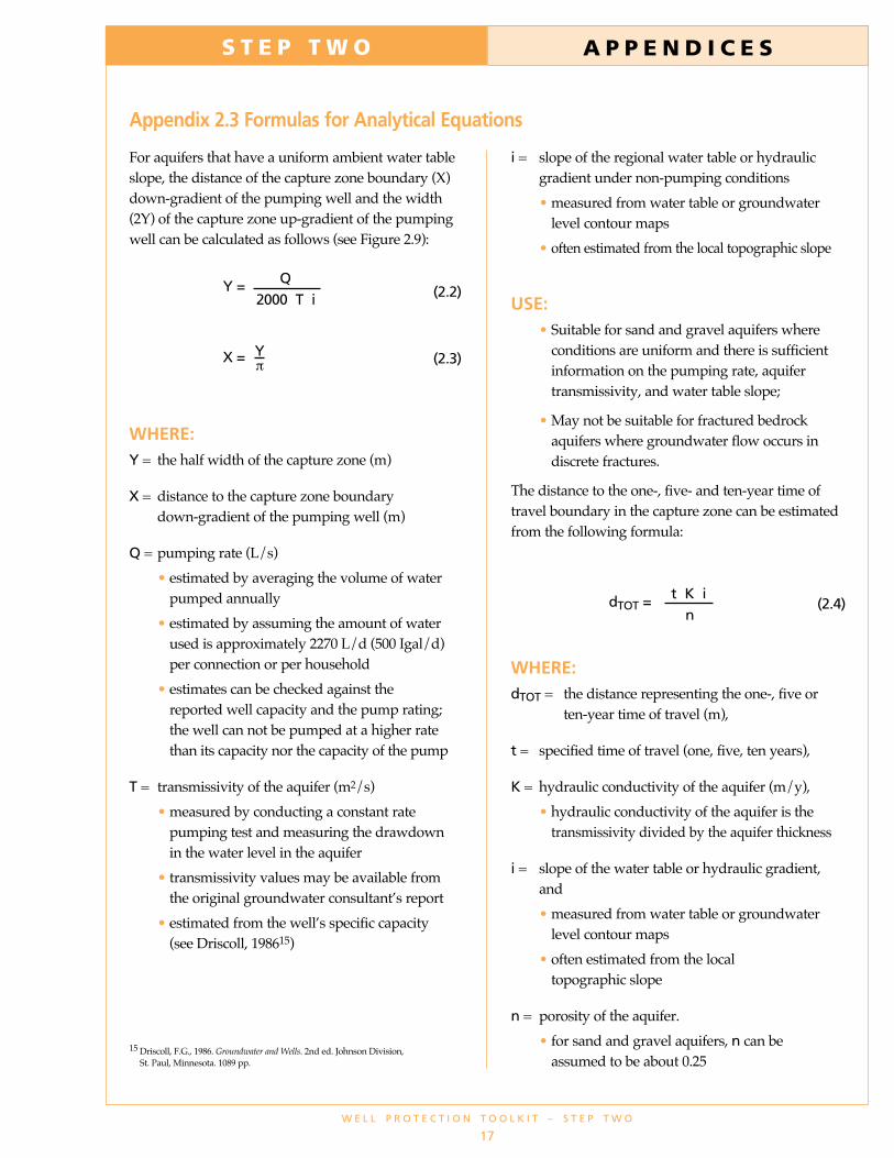
For aquifers that have a uniform ambient water table slope, the distance of the capture zone boundary (X) down-gradient of the pumping well and the width (2Y) of the capture zone up-gradient of the pumping well can be calculated as follows (see Figure 2.9):

where:Y = the half width of the capture zone (m)

X = distance to the capture zone boundary down-gradient of the pumping well (m)

Q = pumping rate (L/s)

• estimated by averaging the volume of water pumped annually

• estimated by assuming the amount of water used is approximately 2270 L/d (500 Igal/d) per connection or per household

• estimates can be checked against the reported well capacity and the pump rating; the well can not be pumped at a higher rate than its capacity nor the capacity of the pump

T = transmissivity of the aquifer (m2/s)

• measured by conducting a constant rate pumping test and measuring the drawdown in the water level in the aquifer

• transmissivity values may be available from the original groundwater consultant’s report

• estimated from the well’s specific capacity (see Driscoll, 198615)

i = slope of the regional water table or hydraulic gradient under non-pumping conditions

• measured from water table or groundwater level contour maps

• often estimated from the local topographic slope

USe: • Suitable for sand and gravel aquifers where

conditions are uniform and there is sufficient information on the pumping rate, aquifer transmissivity, and water table slope;

• May not be suitable for fractured bedrock aquifers where groundwater flow occurs in discrete fractures.

The distance to the one-, five- and ten-year time of travel boundary in the capture zone can be estimated from the following formula:

where:dToT = the distance representing the one-, five or

ten-year time of travel (m),

t = specified time of travel (one, five, ten years),

K = hydraulic conductivity of the aquifer (m/y),

• hydraulic conductivity of the aquifer is the transmissivity divided by the aquifer thickness

i = slope of the water table or hydraulic gradient, and

• measured from water table or groundwater level contour maps

• often estimated from the local topographic slope

n = porosity of the aquifer.

• for sand and gravel aquifers, n can be assumed to be about 0.25


��

appendix 2.3 formulas for analytical equations

�000 T iY = Q

(�.�)

X = Yπ (�.�)

dToT =n

t K i(�.�)

15 Driscoll, F.G., 1986. Groundwater and Wells. 2nd ed. Johnson Division, St. Paul, Minnesota. 1089 pp.


When hiring a groundwater professional, you will need to draft specific terms of reference for the work to be performed. Only general terms of reference are provided here. Specific terms of reference depend on site-specific conditions and factors and can only be developed after these are adequately known. It may be desirable to contact the Ministry of Environment, Water Stewardship Division staff for advice in drafting specific terms of reference. General terms of reference for characterizing the hydrogeologic setting and delineating the capture zone for the community well include the following:

• Review all available existing data (provide list of information sources) to map and characterize the hydrogeologic setting, including location of aquifers and aquitards, flow direction, hydraulic gradient, lithology, permeability, and water use.

• Develop conceptual model of hydrogeology and flow to wells.

• Identify areas of data/information insufficiencies and their effects on capture zone delineation and outline methods for obtaining additional data/information critical to capture zone delineation and include costs.

• Delineate capture zone(s) for wells based on one-, five-, and ten-year time of travel and zone of contribution to a sufficient degree of certainty. Use the most appropriate delineation method(s) to establish capture zone boundaries. Identify any limitations or uncertainties of delineation, as well as what additional work may be required to address this. When using numerical modelling for delineating the capture zone, consideration should be given to delineating the entire capture zone so the ultimate source of recharge is identified.

• Provide a draft report, discussing work done, actions, and recommendations for review and include maps, models, and databases. Attend meetings to discuss report. Finalize report and assist planning team in presentation of findings to the public and other agencies.


��

appendix 2.4 General terms of reference for Delineating the capture Zone

SelectinG a conSUltinG enGineer

The Consulting engineers of British Columbia has a publication titled A Guide to Selecting a Consulting

Engineer . It describes ways of methodically selecting the right consultant for a project . The “Two-envelope” system is emphasized .

This publication is intended for larger projects, however, it may be useful for the community planning team .

Website: www .cebc .org

Suite 657 - 409 granville StreetVancouver, BC V6C 1T2Tel: (604) 687-2811Fax: (604) 688-7110email: info@cebc .org

www.cebc.org

mailto:[email protected]

C A S E S T U D Y P U M P H A N D L E B . C .

Ian Rutherford (the Valley District Engineer) and three water purveyors were responsible for defining the well protection area.

Pumphandle AquiferInformation on the hydrogeology and groundwater conditions in the Pumphandle Valley came from:

• pumping records of the three community wells from the purveyors;

• pumping test reports for Blackwater and Charlie’s Wells;

• historic water chemistry for the community wells from the Health Authority database;

• well records from the Ministry of Environment water well database and from the http://srmapps.gov.bc.ca/apps/wrbc/;

• 1:20,000 aquifer classification map from the Ministry of Environment and from the http://srmapps.gov.bc.ca/apps/wrbc/;

• 1:50,000 Geological Survey of Canada surficial geology map;

• 1:10,000 air photographs and air photo mosaic from the http://srmapps.gov.bc.ca/apps/wrbc/; and,

• groundwater reports covering the Pumphandle area

In the fall of 1998, the purveyors hired a consulting hydrogeologist, Henrique Darcy,

P. Geo., Hydro-Logic Groundwater Consultants, to compile the groundwater information and delineate the well capture zones.

The well records, surficial geology map, air photos, and reports suggest that there are terraced sand and gravel deposits in the valley that are more than 60 m thick in the central part (Figures CS 1.1 and CS 2.1). The lower part is saturated and forms the principle aquifer—the Pumphandle Aquifer—that supplies groundwater to all the wells in the valley, including the three community wells. The aquifer rests above a layer of till of variable thickness which, in turn, rests on bedrock. The till and bedrock are less permeable and form aquitards.

Aquifer boundaries were taken from the Ministry of Environment's aquifer classification map, which designates the Pumphandle Aquifer as a moderately developed, moderately vulnerable, II B (12) aquifer.16 The aquifer is considered moderately vulnerable because it is unconfined, but the water table is fairly deep in most parts of the valley. Near the three community wells, however, the water table is within a few metres of the surface (Figure CS 2.1) and the aquifer is considered highly vulnerable at this location.

The contours of the water table were estimated using water levels from well records. These show that the water table slopes north towards the three community wells and then north-east towards the lake (Figure CS 2.2). It is assumed that groundwater flows the same way. The ambient hydraulic gradient17(i) is about 0.1 at the side of the valley and decreases at the bottom of the valley near the three community wells. There is limited data to map the water table contours along the northwest edge of the


��

Step two: Defining the well protection area

TABLE CS 2.1 SuMMARY OF PuMPhANDLE COMMuNiTY WELLSWELL TYPE DEPTh (m) DiAMETER (mm) RATED CAPACiTY (L/s) DRiNkiNG WATER NO. OF uSERS DEMAND (L/s)

Aiken dug 2 .4 915 5 .10 5 .26 500

Blackwater drilled 30 .5 200 22 .73 1 .05 100

Charlie drilled 25 .6 150 7 .58 0 .53 50

16 For an explanation of the B.C. Aquifer Classification System, see Kreye, R., K. Ronneseth, and M. Wei, 1995. “An Aquifer Classification System for Groundwater Management in British Columbia.” In Proceedings, the 6th National Drinking Water Conference, Victoria B.C. pp. 347-358.

17 The slope of the water table under non-pumping or natural conditions

http://srmapps.gov.bc.ca/apps/wrbc/



1000

500

0

-500

Elev

atio

n (m

a.s.

l.)

Horizontal Scale = 1:20 000

bedrock (aquitard)

till (aquitard)

sand & gravel (aquifer)

geological boundaryinterpreted; assumed

well

water table

?

? ? ?

?

? ? ??

LEGEND

SNW

Pumphandle Aquifer

Pumphandle, BC

hay fields

hay fields

trailerpark

golf course

B C

fiGUre cS 2.1 croSS-Section throUGh pUMphanDle valley

valley.

The transmissivity of the aquifer near the community wells, based on pumping tests, is about 0.0036 m2/s. The slope of the water table suggests that recharge to the aquifer comes from precipitation falling on the aquifer and from the mountain-front recharge. Groundwater in the aquifer ultimately discharges to the lake, the local creek and to pumping wells. The lake may also be a localized but significant source of recharge to the community wells during pumping.

A summary of the community wells is shown in Table CS 2.1.

The capture ZonesThe consultant used the maximum pumping rate for each well to determine the individual capture zones for each of the three wells. Capture zones were defined

using circular radius methods and analytical equations of groundwater flow. He made a number of assumptions:

• There is no interference between the wells, because of the low pumping rates relative to the transmissivity. The capture zones are therefore calculated separately for each well.

• The neighbouring private wells are used only for domestic purposes, and their effect on the capture zone of the community wells is insignificant.

• Groundwater conditions are in a steady state. This is not strictly true because recharge likely occurs annually. The effect of seasonal fluctuation on delineation of the capture zone areas can not be quantified. However, recent theoretical studies18 suggest that seasonal effects would probably be insignificant in alluvial aquifer terrains such as the one in Pumphandle and the steady-state assumptions used here are reasonable.


�0

18 Reilly, T. and D. W. Pollock, 1996. “Sources of Water to Wells for Transient Cyclic Systems.” Ground Water, Vol. 34, No. 6, pp. 979-988.


��

S T E P T W O P U M P H A N D L E B . C .

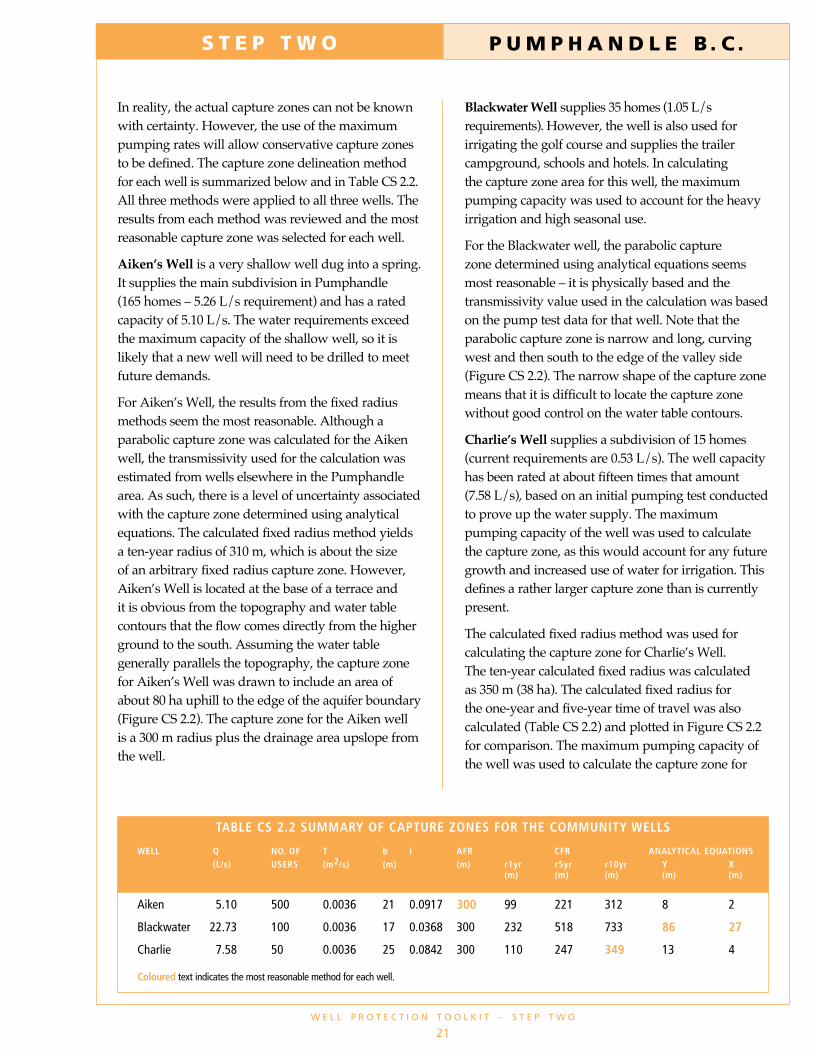
In reality, the actual capture zones can not be known with certainty. However, the use of the maximum pumping rates will allow conservative capture zones to be defined. The capture zone delineation method for each well is summarized below and in Table CS 2.2. All three methods were applied to all three wells. The results from each method was reviewed and the most reasonable capture zone was selected for each well.

Aiken’s Well is a very shallow well dug into a spring. It supplies the main subdivision in Pumphandle (165 homes – 5.26 L/s requirement) and has a rated capacity of 5.10 L/s. The water requirements exceed the maximum capacity of the shallow well, so it is likely that a new well will need to be drilled to meet future demands.

For Aiken’s Well, the results from the fixed radius methods seem the most reasonable. Although a parabolic capture zone was calculated for the Aiken well, the transmissivity used for the calculation was estimated from wells elsewhere in the Pumphandle area. As such, there is a level of uncertainty associated with the capture zone determined using analytical equations. The calculated fixed radius method yields a ten-year radius of 310 m, which is about the size of an arbitrary fixed radius capture zone. However, Aiken’s Well is located at the base of a terrace and it is obvious from the topography and water table contours that the flow comes directly from the higher ground to the south. Assuming the water table generally parallels the topography, the capture zone for Aiken’s Well was drawn to include an area of about 80 ha uphill to the edge of the aquifer boundary (Figure CS 2.2). The capture zone for the Aiken well is a 300 m radius plus the drainage area upslope from the well.

Blackwater Well supplies 35 homes (1.05 L/s requirements). However, the well is also used for irrigating the golf course and supplies the trailer campground, schools and hotels. In calculating the capture zone area for this well, the maximum pumping capacity was used to account for the heavy irrigation and high seasonal use.

For the Blackwater well, the parabolic capture zone determined using analytical equations seems most reasonable – it is physically based and the transmissivity value used in the calculation was based on the pump test data for that well. Note that the parabolic capture zone is narrow and long, curving west and then south to the edge of the valley side (Figure CS 2.2). The narrow shape of the capture zone means that it is difficult to locate the capture zone without good control on the water table contours.

Charlie’s Well supplies a subdivision of 15 homes (current requirements are 0.53 L/s). The well capacity has been rated at about fifteen times that amount (7.58 L/s), based on an initial pumping test conducted to prove up the water supply. The maximum pumping capacity of the well was used to calculate the capture zone, as this would account for any future growth and increased use of water for irrigation. This defines a rather larger capture zone than is currently present.

The calculated fixed radius method was used for calculating the capture zone for Charlie’s Well. The ten-year calculated fixed radius was calculated as 350 m (38 ha). The calculated fixed radius for the one-year and five-year time of travel was also calculated (Table CS 2.2) and plotted in Figure CS 2.2 for comparison. The maximum pumping capacity of the well was used to calculate the capture zone for

TABLE CS 2.2 SuMMARY OF CAPTuRE ZONES FOR ThE COMMuNiTY WELLS

WELL q NO. OF T b i AFR CFR ANALYTiCAL EquATiONS (L/s) uSERS (m2/s) (m) (m) r1yr r5yr r10yr Y x (m) (m) (m) (m) (m)

Aiken 5 .10 500 0 .0036 21 0 .0917 300 99 221 312 8 2

Blackwater 22 .73 100 0 .0036 17 0 .0368 300 232 518 733 86 27

Charlie 7 .58 50 0 .0036 25 0 .0842 300 110 247 349 13 4

Coloured text indicates the most reasonable method for each well .


��

150 m

100 m

50 m

Pumphandle Aquifer

1 YR

5Y R

10Y

R

1 Y R

CFR

equationanalytical

AFR

A

B

C

N

0 200 400 600

MetresScale = 1:20 000

fiGUre cS 2.2 captUre ZoneS for coMMUnity wellS

L E G E N D

A Pumphandle community wellLEGEND

Pumphandle community wells

capture zone area

time of travelboundary

water table contour(m asl)

inferred direction ofgroundwater flow

1 YR

100 m

A

capture zone area

LEGENDPumphandle community wells

capture zone area




1 YR

100 m

A

Time of travel boundary


capture zone area




1 YR

100 m

A

Water table contour (m asl)


capture zone area




1 YR

100 m

A

inferred direction of groundwater flow

S T E P T W O P U M P H A N D L E B . C .

Charlie’s Well, as this would account for any future growth and increased use of water for irrigation. This results in a rather larger capture zone than is currently present. Analytical equations are not accurate because the water table is relatively flat and the ambient hydraulic gradient can not be determined with any accuracy. It is not clear if the ambient flow near Charlie’s Well comes from the southeast or from the west-south-west. To determine this, nearby monitoring wells would be needed to provide groundwater level data to map the flow in more detail.

The Well Protection AreasIan Rutherford and Henrique Darcy (the hydrogeologist) defined the well protection area to include the three capture zones (164 ha). In addition, they included the strip of land between the capture zones for Aiken’s and Blackwater Wells. This accounted for the uncertainty of location of the actual capture zone for Blackwater Well and the fact that this strip of land may also be a recharge area for Charlie’s Well.

Although including the strip of land increases the total protection area to 261 ha, the total size of the well protection area is still reasonably small, and it does not add greatly to the required protection measures. The preliminary protection area, where land use activities will be documented and protection efforts started, is shown in Figure CS 2.3.

All three capture zones are assumed to end at the aquifer boundaries. Although runoff from the bedrock slope south of Pumphandle (outside of the aquifer boundary) likely recharges the aquifer and the capture zones for Aiken’s and Blackwater Wells, it is not considered part of the capture zone or well protection area. However, improper land use activities in this area may indirectly affect the groundwater quality.

Similarly, the lake is not part of the aquifer or the protection area for the community wells, yet a contaminant spill near the lakeshore could impact the water quality of the groundwater in the local area. Lake water may contribute to the recharge of the well and contamination could travel from the lake to the pumping wells.

Finally, the area of aquifer to the southeast of the wells might provide recharge to Charlie’s Well, but it has not been included in the preliminary well protection area. Monitoring wells need to be installed around Charlie’s Well to provide more detailed groundwater level information. This would indicate whether the recharge area lies to the southeast or to the west as presently assumed.


��

Pumphandle Aquifer

A

B

C

N

0 200 400 600

MetresScale = 1:20 000

fiGUre cS 2.3 propoSeD well protection area


��

L E G E N D

A Pumphandle community well

Proposed well protection area

Step Two - British Columbia

Documents