Step Size Bound of the Sequential Partial Update LMS Algorithm with Periodic Input Signals

Hindawi Publishing CorporationEURASIP Journal on Audio, Speech, and Music ProcessingVolume 2007, Article ID 10231, 15 pagesdoi:10.1155/2007/10231

Research ArticleStep Size Bound of the Sequential Partial Update LMSAlgorithm with Periodic Input Signals

Pedro Ramos,1 Roberto Torrubia,2 Ana Lopez,1 Ana Salinas,1 and Enrique Masgrau2

1 Communication Technologies Group, Aragon Institute for Engineering Research (I3A), EUPT, University of Zaragoza,Ciudad Escolar s/n, 44003 Teruel, Spain

2 Communication Technologies Group, Aragon Institute for Engineering Research (I3A), CPS Ada Byron, University of Zaragoza,Maria de Luna 1, 50018 Zaragoza, Spain

Received 9 June 2006; Revised 2 October 2006; Accepted 5 October 2006

Recommended by Kutluyil Dogancay

This paper derives an upper bound for the step size of the sequential partial update (PU) LMS adaptive algorithm when the inputsignal is a periodic reference consisting of several harmonics. The maximum step size is expressed in terms of the gain in step size ofthe PU algorithm, defined as the ratio between the upper bounds that ensure convergence in the following two cases: firstly, whenonly a subset of the weights of the filter is updated during every iteration; and secondly, when the whole filter is updated at everycycle. Thus, this gain in step-size determines the factor by which the step size parameter can be increased in order to compensatethe inherently slower convergence rate of the sequential PU adaptive algorithm. The theoretical analysis of the strategy developedin this paper excludes the use of certain frequencies corresponding to notches that appear in the gain in step size. This strategyhas been successfully applied in the active control of periodic disturbances consisting of several harmonics, so as to reduce thecomputational complexity of the control system without either slowing down the convergence rate or increasing the residual error.Simulated and experimental results confirm the expected behavior.

Copyright © 2007 Pedro Ramos et al. This is an open access article distributed under the Creative Commons Attribution License,which permits unrestricted use, distribution, and reproduction in any medium, provided the original work is properly cited.

1. INTRODUCTION

1.1. Context of application: active noisecontrol systems

Acoustic noise reduction can be achieved by two differentmethods. Passive techniques are based on the absorption andreflection properties of materials, showing excellent noise at-tenuation for frequencies above 1 kHz. Nevertheless, passivesound absorbers do not work well at low frequencies be-cause the acoustic wavelength becomes large compared tothe thickness of a typical noise barrier. On the other hand,active noise control (ANC) techniques are based on the prin-ciple of destructive wave interference, whereby an antinoiseis generated with the same amplitude as the undesired distur-bance but with an appropriate phase shift in order to cancelthe primary noise at a given location, generating a zone ofsilence around an acoustical sensor.

The basic idea behind active control was patented byLueg [1]. However, it was with the relatively recent adventof powerful and inexpensive digital signal processors (DSPs)

that ANC techniques became practical because of their ca-pacity to perform the computational tasks involved in realtime.

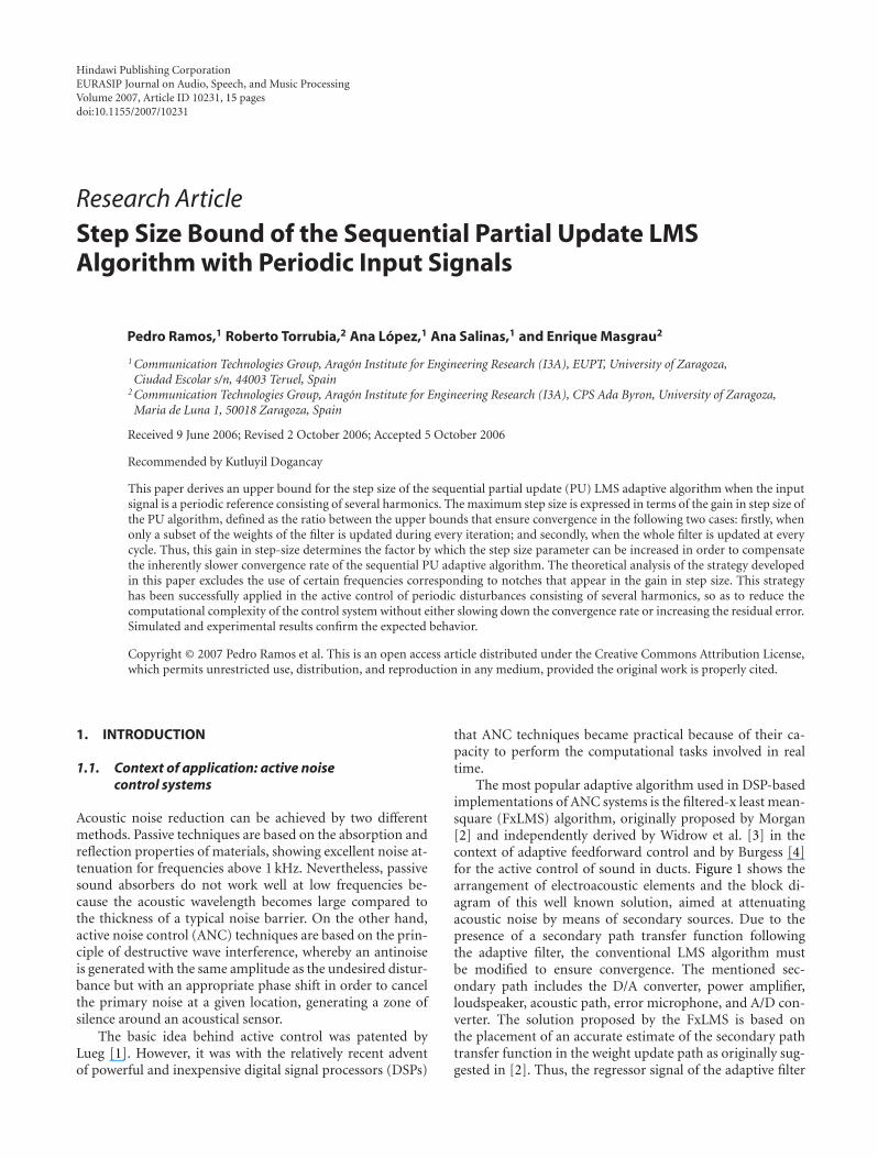
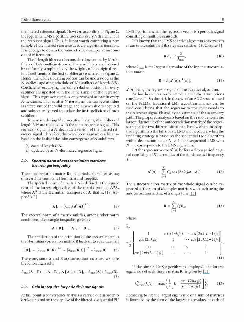
The most popular adaptive algorithm used in DSP-basedimplementations of ANC systems is the filtered-x least mean-square (FxLMS) algorithm, originally proposed by Morgan[2] and independently derived by Widrow et al. [3] in thecontext of adaptive feedforward control and by Burgess [4]for the active control of sound in ducts. Figure 1 shows thearrangement of electroacoustic elements and the block di-agram of this well known solution, aimed at attenuatingacoustic noise by means of secondary sources. Due to thepresence of a secondary path transfer function followingthe adaptive filter, the conventional LMS algorithm mustbe modified to ensure convergence. The mentioned sec-ondary path includes the D/A converter, power amplifier,loudspeaker, acoustic path, error microphone, and A/D con-verter. The solution proposed by the FxLMS is based onthe placement of an accurate estimate of the secondary pathtransfer function in the weight update path as originally sug-gested in [2]. Thus, the regressor signal of the adaptive filter

2 EURASIP Journal on Audio, Speech, and Music Processing

Sourceof noise Undesired noise

Errormicrophone

SecondarysourceReference

microphoneAntinoise

ANCoutput

Reference ANC Error

y(n)

x(n) e(n)

(a)

x(n)Reference P(z)

Primary path

d(n)Undesired noise

y�(n)Antinoise

S(z)Secondary path

y(n)W(z)Adaptive filter

S(z)Estimate

Adaptivealgorithmx�(n)

Filtered reference

e(n)Error

+

�

∑

(b)

Figure 1: Single-channel active noise control system using thefiltered-x adaptive algorithm. (a) Physical arrangement of the elec-troacoustic elements. (b) Equivalent block diagram.

is obtained by filtering the reference signal through the esti-mate of the secondary path.

1.2. Partial update LMS algorithm

The LMS algorithm and its filtered-x version have beenwidely used in control applications because of their sim-ple implementation and good performance. However, theadaptive FIR filter may eventually require a large numberof coefficients to meet the requirements imposed by the ad-dressed problem. For instance, in the ANC system describedin Figure 1(b), the task associated with the adaptive filter—in order to minimize the error signal—is to accurately modelthe primary path and inversely model the secondary path.Previous research in the field has shown that if the activecanceller has to deal with an acoustic disturbance consist-ing of closely spaced frequency harmonics, a long adaptivefilter is necessary [5]. Thus, an improvement in performanceis achieved at the expense of increasing the computationalload of the control strategy. Because of limitations in com-putational efficiency and memory capacity of low-cost DSPboards, a large number of coefficients may even impair thepractical implementation of the LMS or more complex adap-tive algorithms.

As an alternative to the reduction of the number of coef-ficients, one may choose to update only a portion of the filter

Table 1: Computational complexity of the filtered-x LMS algo-rithm.

Task Multiplies no. Adds no.

Computing output ofL L

adaptive filter

Filtering of reference signal Ls Ls � 1

Coefficients’ update L + 1 L

Total 2L + 1 + Ls 2L + Ls � 1

Table 2: Computational complexity of the filtered-x sequentialLMS algorithm.

Task Multiplies no. Adds no.

Computing output ofL L

adaptive filter

Filtering of reference LsN

Ls � 1Nsignal

Partial update of1 +

L

N

L

Ncoefficients

Total(

1 +1N

)L + 1 +

LsN

(1 +

1N

)L +

Ls � 1N

coefficient vector at each sample time. Partial update (PU)adaptive algorithms have been proposed to reduce the largecomputational complexity associated with long adaptive fil-ters. As far as the drawbacks of PU algorithms are concerned,it should be noted that their convergence speed is reducedapproximately in proportion to the filter length divided bythe number of coefficients updated per iteration, that is, thedecimation factor N . Therefore, the tradeoff between con-vergence performance and complexity is clearly established:the larger the saving in computational costs, the slower theconvergence rate.

Two well-known adaptive algorithms carry out the par-tial updating process of the filter vector employing decimatedversions of the error or the regressor signals [6]. These algo-rithms are, respectively, the periodic LMS and the sequentialLMS. This work focuses the attention on the later.

The sequential LMS algorithm with decimation factor Nupdates a subset of size L/N , out of a total of L, coefficientsper iteration according to (1),

wl(n + 1)

=⎧⎪⎨⎪⎩wl(n) + μx(n� l + 1)e(n) if (n� l + 1) modN = 0,

wl(n) otherwise(1)

for 1 � l � L, where wl(n) represents the lth weight of thefilter, μ is the step size of the adaptive algorithm, x(n) is theregressor signal, and e(n) is the error signal.

The reduction in computational costs of the sequentialPU strategy depends directly on the decimation factor N .

Pedro Ramos et al. 3

Tables 1 and 2 show, respectively, the computational com-plexity of the LMS and the sequential LMS algorithms interms of the average number of operations required per cy-cle, when used in the context of a filtered-x implementationof a single-channel ANC system. The length of the adaptivefilter is L, the length of the offline estimate of the secondarypath is Ls, and the decimation factor is N .

The criterion for the selection of coefficients to be up-dated can be modified and, as a result of that, different PUadaptive algorithms have been proposed [7–10]. The varia-tions of the cited PU LMS algorithms speed up their conver-gence rate at the expense of increasing the number of oper-ations per cycle. These extra operations include the “intelli-gence” required to optimize the election of the coefficients tobe updated at every instant.

In this paper, we try to go a step further, showing thatin applications based on the sequential LMS algorithm,where the regressor signal is periodic, the inclusion of a newparameter—called gain in step size—in the traditional trade-off proves that one can achieve a significant reduction inthe computational costs without degrading the performanceof the algorithm. The proposed strategy—filtered-x sequen-tial least mean-square algorithm with gain in step size (Gμ-FxSLMS)—has been successfully applied in our laboratoryin the context of active control of periodic noise [5].

1.3. Assumptions in the convergence analysis

Before focusing on the sequential PU LMS strategy and thederivation of the gain in step size, it is necessary to remarkon two assumptions about the upcoming analysis: the inde-pendence theory and the slow convergence condition.

The traditional approach to convergence analyses ofLMS—and FxLMS—algorithms is based on stochastic in-puts instead of deterministic signals such as a combinationof multiple sinusoids. Those stochastic analyses assume inde-pendence between the reference—or regressor—signal andthe coefficients of the filter vector. In spite of the fact that thisindependence assumption is not satisfied or, at least, ques-tionable when the reference signal is deterministic, some re-searchers have previously used the independence assumptionwith a deterministic reference. For instance, Kuo et al. [11]assumed the independence theory, the slow convergence con-dition, and the exact offline estimate of the secondary pathto state that the maximum step size of the FxLMS algorithmis inversely bounded by the maximum eigenvalue of the au-tocorrelation matrix of the filtered reference, when the ref-erence was considered to be the sum of multiple sinusoids.Bjarnason [12] used as well the independence theory to carryout a FxLMS analysis extended to a sinusoidal input. Accord-ing to Bjarnason, this approach is justified by the fact that ex-perience with the LMS algorithm shows that results obtainedby the application of the independence theory retain suffi-cient information about the structure of the adaptive processto serve as reliable design guidelines, even for highly depen-dent data samples.

As far as the second assumption is concerned, in the con-text of the traditional convergence analysis of the FxLMS

adaptive algorithm [13, Chapter 3], it is necessary to as-sume slow convergence—i.e., that the control filter is chang-ing slowly—and to count on an exact estimate of the sec-ondary path in order to commute the order of the adaptivefilter and the secondary path [2]. In so doing, the output ofthe adaptive filter carries through directly to the error signal,and the traditional LMS algorithm analysis can be applied byusing as regressor signal the result of the filtering of the ref-erence signal through the secondary path transfer function.It could be argued that this condition compromises the de-termination of an upper bound on the step size of the adap-tive algorithm, but actually, slow convergence is guaranteedbecause the convergence factor is affected by a much morerestrictive condition with a periodic reference than with awhite noise reference. It has been proved that with a sinu-soidal reference, the upper bound of the step size is inverselyproportional to the product of the length of the filter and thedelay in the secondary path; whereas with a white referencesignal, the bound depends inversely on the sum of these pa-rameters, instead of their product [12, 14]. Simulations witha white noise reference signal suggest that a realistic upperbound in the step size is given by [15, Chapter 3]

μmax = 2Px�(L + Δ)

, (2)

where Px� is the power of the filtered reference, L is the lengthof the adaptive filter, and Δ is the delay introduced by thesecondary path.

Bjarnason [12] analyzed FxLMS convergence with a si-nusoidal reference, but employed the habitual assumptionsmade with stochastic signals, that is, the independence the-ory. The stability condition derived by Bjarnason yields

μmax = 2Px�L

sin(

π

2(2Δ + 1)

). (3)

In case of large delay Δ, (3) simplifies to

μmax�= π

Px�L(2Δ + 1), Δ�

π

4. (4)

Vicente and Masgrau [14] obtained an upper bound forthe FxLMS step size that ensures convergence when the ref-erence signal is deterministic (extended to any combinationof multiple sinusoids). In the derivation of that result, thereis no need of any of the usual approximations, such as in-dependence between reference and weights or slow conver-gence. The maximum step size for a sinusoidal reference isgiven by

μmax = 2Px�L(2Δ + 1)

. (5)

The similarity between both convergence conditions—(4)and (5)—is evident in spite of the fact that the former anal-ysis is based on the independence assumption, whereas thelater analysis is exact. This similarity achieved in the resultsjustifies the use of the independence theory when dealingwith sinusoidal references, just to obtain a first-approach

4 EURASIP Journal on Audio, Speech, and Music Processing

Updated during the 1st iteration

with x�(n), during the (N + 1)th

iteration with x�(n + N),. . .

Updated during the 1st iteration

with x�(n�N), during the (N + 1)th

iteration with x�(n),. . .

Updated during the 1st iteration with

x�(n� L + N), during the (N + 1)th

iteration with x�(n� L + 2N),. . .

Updated during the 2nd iteration

with x�(n), during the (N + 2)th

iteration with x�(n + N),. . .

Updated during the 2nd iteration

with x�(n�N), during the (N + 2)th

iteration with x�(n),. . .

Updated during the 2nd iteration with

x�(n� L + N), during the (N + 2)th iteration

with x�(n� L + 2N),. . .

Updated during the Nth iteration with

x�(n), during the 2Nth iteration with

x�(n + N),. . .

Updated during the Nth iteration with

x�(n�N), during the 2Nth iteration with

x�(n),. . .

Updated during the Nth iteration with

x�(n� L + N), during the 2Nth iteration

with x�(n� L + 2N),. . .

w1 w2 � � �

wN wN+1 wN+2 � � �

w2N � � �

wL�N wL�N+1 wL�N+2 � � �

wL�1 wL

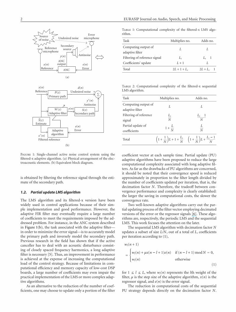
Figure 2: Summary of the sequential PU algorithm, showing the coefficients to be updated at each iteration and related samples of theregressor signal used in each update, x�(n) being the value of the regressor signal at the current instant.

limit. In other words, we look for a useful guide on deter-mining the maximum step size but, as we will see in this pa-per, derived bounds and theoretically predicted behavior arefound to correspond not only to simulation but also to ex-perimental results carried out in the laboratory in practicalimplementations of ANC systems based on DSP boards.

To sum up, independence theory and slow convergenceare assumed in order to derive a bound for a filtered-x se-quential PU LMS algorithm with deterministic periodic in-puts. Despite the fact that such assumptions might be ini-tially questionable, previous research and achieved resultsconfirm the possibility of application of these strategies in theattenuation of periodic disturbances in the context of ANC,achieving the same performance as that of the full updateFxLMS in terms of convergence rate and misadjustment, butwith lower computational complexity.

As far as the applicability of the proposed idea is con-cerned, the contribution of this paper to the design of thestep size parameter is applicable not only to the filtered-xsequential LMS algorithm but also to basic sequential LMSstrategies. In other words, the derivation and analysis of thegain in step size could have been done without considerationof a secondary path. The reason for the study of the specificcase that includes the filtered-x stage is the unquestionableexistence of an extended problem: the need of attenuationof periodic disturbances by means of ANC systems imple-menting filtered-x algorithms on low-cost DSP-based boardswhere the reduction of the number of operations requiredper cycle is a factor of great importance.

2. EIGENVALUE ANALYSIS OF PERIODIC NOISE:THE GAIN IN STEP SIZE

2.1. Overview

Many convergence analyses of the LMS algorithm try to de-rive exact bounds on the step size to guarantee mean andmean-square convergence based on the independence as-sumption [16, Chapter 6]. Analyses based on such assump-

tion have been extended to sequential PU algorithms [6] toyield the following result: the bounds on the step size for thesequential LMS algorithm are the same as those for the LMSalgorithm and, as a result of that, a larger step size cannotbe used in order to compensate its inherently slower conver-gence rate. However, this result is only valid for independentidentically distributed (i.i.d.) zero-mean Gaussian input sig-nals.

To obtain a valid analysis in the case of periodic signals asinput of the adaptive filter, we will focus on the updating pro-cess of the coefficients when the L-length filter is adapted bythe sequential LMS algorithm with decimation factor N . Thisalgorithm updates just L/N coefficients per iteration accord-ing to (1). For ease in analyzing the PU strategy, it is assumedthroughout the paper that L/N is an integer.

Figure 1(b) shows the block diagram of a filtered-x ANCsystem, where the secondary path S(z) is placed followingthe digital filter W(z) controlled by an adaptive algorithm.As has been previously stated, under the assumption of slowconvergence and considering an accurate offline estimate ofthe secondary path, the order of W(z) and S(z) can be com-muted and the resulting equivalent diagram simplified. Thus,standard LMS algorithm techniques can be applied to thefiltered-x version of the sequential LMS algorithm in orderto determine the convergence of the mean weights and themaximum value of the step size [13, Chapter 3]. The simpli-fied analysis is based on the consideration of the filtered ref-erence as the regressor signal of the adaptive filter. This signalis denoted as x�(n) in Figure 1(b).

Figure 2 summarizes the sequential PU algorithm givenby (1), indicating the coefficients to be updated at each iter-ation and the related samples of the regressor signal. In thescheme of Figure 2, the following update is considered to becarried out during the first iteration. The current value ofthe regressor signal is x�(n). According to (1) and Figure 2,this value is used to update the first N coefficients of the filterduring the following N iterations. Generally, at each iterationof a full update adaptive algorithm, a new sample of the re-gressor signal has to be taken as the latest and newest value of

Pedro Ramos et al. 5

the filtered reference signal. However, according to Figure 2,the sequential LMS algorithm uses only every Nth element ofthe regressor signal. Thus, it is not worth computing a newsample of the filtered reference at every algorithm iteration.It is enough to obtain the value of a new sample at just oneout of N iterations.

The L-length filter can be considered as formed byN sub-filters of L/N coefficients each. These subfilters are obtainedby uniformly sampling by N the weights of the original vec-tor. Coefficients of the first subfilter are encircled in Figure 2.Hence, the whole updating process can be understood as theN-cyclical updating schedule of N subfilters of length L/N .Coefficients occupying the same relative position in everysubfilter are updated with the same sample of the regressorsignal. This regressor signal is only renewed at one in everyN iterations. That is, after N iterations, the less recent valueis shifted out of the valid range and a new value is acquiredand subsequently used to update the first coefficient of eachsubfilter.

To sum up, during N consecutive instants, N subfilters oflength L/N are updated with the same regressor signal. Thisregressor signal is a N-decimated version of the filtered ref-erence signal. Therefore, the overall convergence can be ana-lyzed on the basis of the joint convergence of N subfilters:

(i) each of length L/N ,(ii) updated by an N-decimated regressor signal.

2.2. Spectral norm of autocorrelation matrices:the triangle inequality

The autocorrelation matrix R of a periodic signal consistingof several harmonics is Hermitian and Toeplitz.

The spectral norm of a matrix A is defined as the squareroot of the largest eigenvalue of the matrix product AHA,where AH is the Hermitian transpose of A, that is, [17, Ap-pendix E]

�A�s =[λmax

(AHA

)]1/2. (6)

The spectral norm of a matrix satisfies, among other normconditions, the triangle inequality given by

�A + B�s � �A�s + �B�s. (7)

The application of the definition of the spectral norm tothe Hermitian correlation matrix R leads us to conclude that

�R�s =[λmax

(RHR

)]1/2 = [λmax(RR)]1/2 = λmax(R). (8)

Therefore, since A and B are correlation matrices, we havethe following result:

λmax(A + B)= �A + B�s � �A�s+ �B�s= λmax(A)+ λmax(B).(9)

2.3. Gain in step size for periodic input signals

At this point, a convergence analysis is carried out in order toderive a bound on the step size of the filtered-x sequential PU

LMS algorithm when the regressor vector is a periodic signalconsisting of multiple sinusoids.

It is known that the LMS adaptive algorithm converges inmean to the solution if the step size satisfies [16, Chapter 6]

0 < μ <2

λmax, (10)

where λmax is the largest eigenvalue of the input autocorrela-tion matrix

R = E[

x�(n)x�T(n)], (11)

x�(n) being the regressor signal of the adaptive algorithm.As has been previously stated, under the assumptions

considered in Section 1.3, in the case of an ANC system basedon the FxLMS, traditional LMS algorithm analysis can beused considering that the regressor vector corresponds tothe reference signal filtered by an estimate of the secondarypath. The proposed analysis is based on the ratio between thelargest eigenvalue of the autocorrelation matrix of the regres-sor signal for two different situations. Firstly, when the adap-tive algorithm is the full update LMS and, secondly, when theupdating strategy is based on the sequential LMS algorithmwith a decimation factor N > 1. The sequential LMS withN = 1 corresponds to the LMS algorithm.

Let the regressor vector x�(n) be formed by a periodic sig-nal consisting of K harmonics of the fundamental frequencyf0,

x�(n) =K∑k=1

Ck cos(2πk f0n + φk

). (12)

The autocorrelation matrix of the whole signal can be ex-pressed as the sum of K simpler matrices with each being theautocorrelation matrix of a single tone [11]

R =K∑k=1

C2kRk, (13)

where

Rk

=12

⎧⎪⎪⎪⎪⎪⎪⎨⎪⎪⎪⎪⎪⎪⎩

1 cos(2πk f0

)� � � cos

[2πk(L�1) f0

]cos

(2πk f0

)1 � � � cos

[2πk(L�2) f0

]� � � � � �

. . ....

cos[2πk(L�1) f0

]� � � � � � 1

⎫⎪⎪⎪⎪⎪⎪⎬⎪⎪⎪⎪⎪⎪⎭.

(14)

If the simple LMS algorithm is employed, the largesteigenvalue of each simple matrix Rk is given by [11]

λN=1k,max

(k f0

) = max

{14

[L�

sin(L2πk f0

)sin

(2πk f0

) ]}. (15)

According to (9) the largest eigenvalue of a sum of matricesis bounded by the sum of the largest eigenvalues of each of

6 EURASIP Journal on Audio, Speech, and Music Processing

its components. Therefore, the largest eigenvalue of R can beexpressed as

λN=1tot,max �

K∑k=1

C2kλ

N=1k,max

(k f0

)

=K∑k=1

C2k max

{14

[L�

sin(L2πk f0

)sin

(2πk f0

) ]}.(16)

At the end of Section 2.1, two key differences were de-rived in the case of the sequential LMS algorithm: the conver-gence condition of the whole filter might be translated to theparallel convergence of N subfilters of length L/N adapted byan N-decimated regressor signal. Considering both changes,the largest eigenvalue of each simple matrix Rk can be ex-pressed as

λN>1k,max

(k f0

) = max

{14

[L

N�

sin((L/N)2πkN f0

)sin

(2πkN f0

) ]}(17)

and considering the triangle inequality (9), we have

λN>1tot,max �

K∑k=1

C2kλ

N>1k,max

(k f0

)

=K∑k=1

C2k max

{14

[L

N�

sin((L/N)2πkN f0

)sin

(2πkN f0

) ]}.

(18)

Defining the gain in step size Gμ as the ratio between thebounds on the step sizes in both cases, we obtain the factorby which the step size parameter can be multiplied when theadaptive algorithm uses PU,

Gμ(K , f0,L,N

)= μN>1

max

μN=1max

= 2/ max{λN>1

tot,max

}2/ max

{λN=1

tot,max} = ∑K

k=1 C2kλ

N=1k,max

(k f0

)∑Kk=1 C

2kλ

N>1k,max

(k f0

)=

∑Kk=1 C

2k max

{(1/4)

[L�sin

(L2πk f0

)/sin

(2πk f0

)]}∑Kk=1 C

2k max

{(1/4)

[L/N�sin(L/N)2πkN f0

/sin

(2πkN f0

)]} .(19)

In order to more easily visualize the dependence of thegain in step size on the length of the filter L and on the deci-mation factor N , let a single tone of normalized frequency f0be the regressor signal

x�(n) = cos(2π f0n + φ

). (20)

Now, the gain in step size, that is, the ratio between thebounds on the step size when N > 1 and N = 1, is given by

Gμ(1, f0,L,N

)= μN>1

max

μN=1max

= max{

(1/4)[L� sin

(L2π f0

)/sin

(2π f0

)]}max

{(1/4)

[L/N � sin

((L/N)2πN f0

)/sin

(2πN f0

)]} .(21)

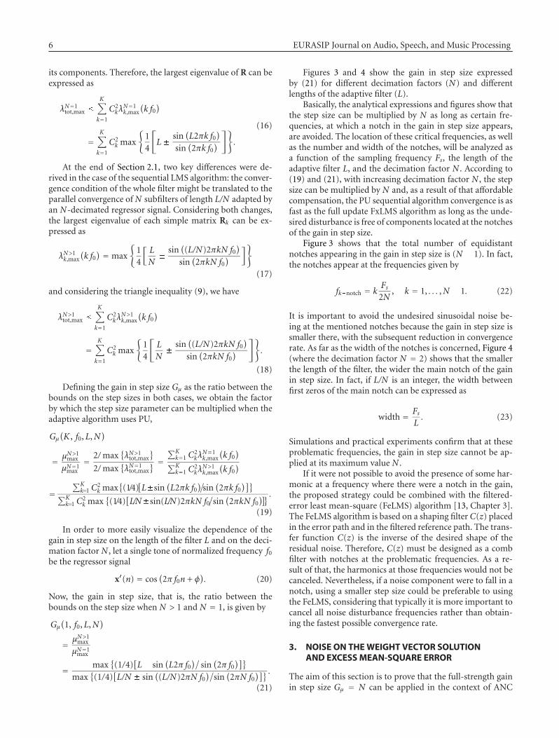
Figures 3 and 4 show the gain in step size expressedby (21) for different decimation factors (N) and differentlengths of the adaptive filter (L).

Basically, the analytical expressions and figures show thatthe step size can be multiplied by N as long as certain fre-quencies, at which a notch in the gain in step size appears,are avoided. The location of these critical frequencies, as wellas the number and width of the notches, will be analyzed asa function of the sampling frequency Fs, the length of theadaptive filter L, and the decimation factor N . According to(19) and (21), with increasing decimation factor N , the stepsize can be multiplied by N and, as a result of that affordablecompensation, the PU sequential algorithm convergence is asfast as the full update FxLMS algorithm as long as the unde-sired disturbance is free of components located at the notchesof the gain in step size.

Figure 3 shows that the total number of equidistantnotches appearing in the gain in step size is (N � 1). In fact,the notches appear at the frequencies given by

fk�notch = kFs

2N, k = 1, . . . ,N � 1. (22)

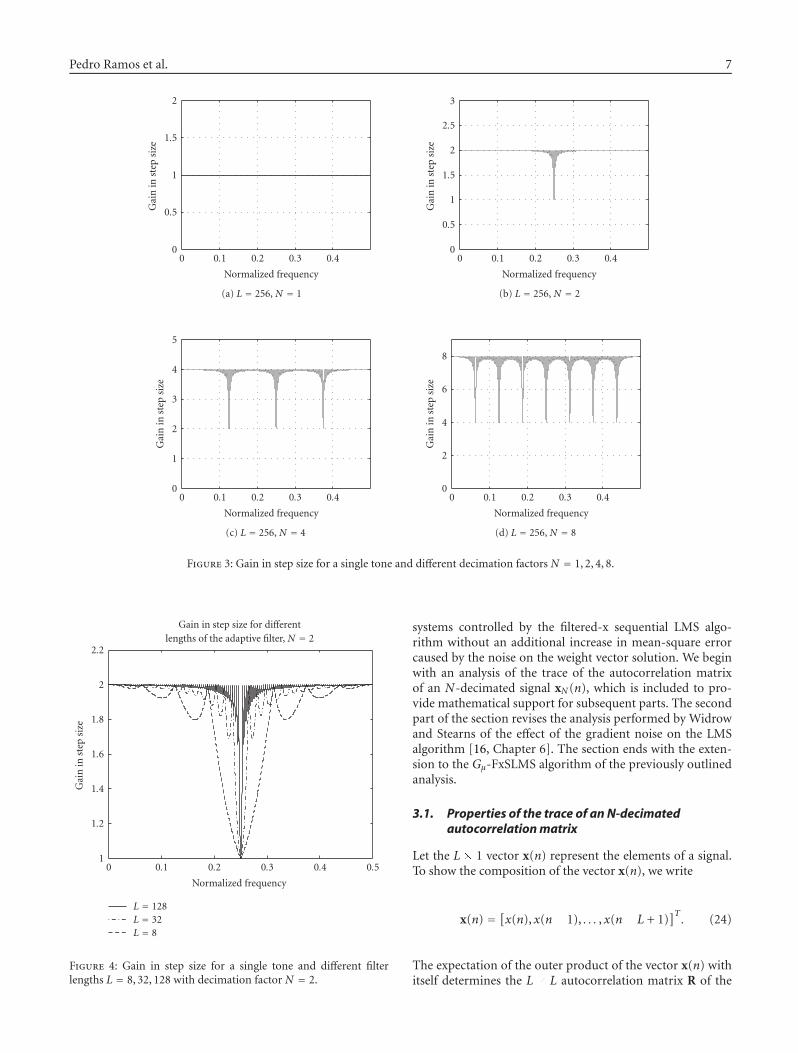
It is important to avoid the undesired sinusoidal noise be-ing at the mentioned notches because the gain in step size issmaller there, with the subsequent reduction in convergencerate. As far as the width of the notches is concerned, Figure 4(where the decimation factor N = 2) shows that the smallerthe length of the filter, the wider the main notch of the gainin step size. In fact, if L/N is an integer, the width betweenfirst zeros of the main notch can be expressed as

width = FsL. (23)

Simulations and practical experiments confirm that at theseproblematic frequencies, the gain in step size cannot be ap-plied at its maximum value N .

If it were not possible to avoid the presence of some har-monic at a frequency where there were a notch in the gain,the proposed strategy could be combined with the filtered-error least mean-square (FeLMS) algorithm [13, Chapter 3].The FeLMS algorithm is based on a shaping filter C(z) placedin the error path and in the filtered reference path. The trans-fer function C(z) is the inverse of the desired shape of theresidual noise. Therefore, C(z) must be designed as a combfilter with notches at the problematic frequencies. As a re-sult of that, the harmonics at those frequencies would not becanceled. Nevertheless, if a noise component were to fall in anotch, using a smaller step size could be preferable to usingthe FeLMS, considering that typically it is more important tocancel all noise disturbance frequencies rather than obtain-ing the fastest possible convergence rate.

3. NOISE ON THE WEIGHT VECTOR SOLUTIONAND EXCESS MEAN-SQUARE ERROR

The aim of this section is to prove that the full-strength gainin step size Gμ = N can be applied in the context of ANC

Pedro Ramos et al. 7

0.40.30.20.10

Normalized frequency

0

0.5

1

1.5

2

Gai

nin

step

size

(a) L = 256, N = 1

0.40.30.20.10

Normalized frequency

0

0.5

1

1.5

2

2.5

3

Gai

nin

step

size

(b) L = 256, N = 2

0.40.30.20.10

Normalized frequency

0

1

2

3

4

5

Gai

nin

step

size

(c) L = 256, N = 4

0.40.30.20.10

Normalized frequency

0

2

4

6

8

Gai

nin

step

size

(d) L = 256, N = 8

Figure 3: Gain in step size for a single tone and different decimation factors N = 1, 2, 4, 8.

0.50.40.30.20.10

Normalized frequency

1

1.2

1.4

1.6

1.8

2

2.2

Gai

nin

step

size

Gain in step size for differentlengths of the adaptive filter, N = 2

L = 128L = 32L = 8

Figure 4: Gain in step size for a single tone and different filterlengths L = 8, 32, 128 with decimation factor N = 2.

systems controlled by the filtered-x sequential LMS algo-rithm without an additional increase in mean-square errorcaused by the noise on the weight vector solution. We beginwith an analysis of the trace of the autocorrelation matrixof an N-decimated signal xN (n), which is included to pro-vide mathematical support for subsequent parts. The secondpart of the section revises the analysis performed by Widrowand Stearns of the effect of the gradient noise on the LMSalgorithm [16, Chapter 6]. The section ends with the exten-sion to the Gμ-FxSLMS algorithm of the previously outlinedanalysis.

3.1. Properties of the trace of an N-decimatedautocorrelation matrix

Let the L � 1 vector x(n) represent the elements of a signal.To show the composition of the vector x(n), we write

x(n) = [x(n), x(n� 1), . . . , x(n� L + 1)]T. (24)

The expectation of the outer product of the vector x(n) withitself determines the L � L autocorrelation matrix R of the

8 EURASIP Journal on Audio, Speech, and Music Processing

signal

R = E[

x(n)xT(n)]

=

⎡⎢⎢⎢⎢⎢⎢⎢⎢⎢⎣

rxx(0) rxx(1) rxx(2) � � � rxx(L� 1)

rxx(1) rxx(0) rxx(1) � � � rxx(L� 2)

rxx(2) rxx(1) rxx(0) � � � rxx(L� 3)...

......

. . ....

rxx(L� 1) rxx(L� 2) rxx(L� 3) � � � rxx(0)

⎤⎥⎥⎥⎥⎥⎥⎥⎥⎥⎦.

(25)

The N-decimated signal xN (n) is obtained from vector

x(n) by multiplying x(n) by the auxiliary matrix I(N)k ,

xN (n) = I(N)k x(n), k = 1 + nmodN , (26)

where I(N)k is obtained from the identity matrix I of dimen-

sion L�L by zeroing out some elements in I. The first nonnullelement on its main diagonal appears at the kth position andthe superscript (N) is intended to denote the fact that twoconsecutive nonzero elements on the main diagonal are sep-

arated by N positions. The auxiliary matrix I(N)k is explicitly

expressed as

I(N)k =

⎛⎜⎜⎜⎜⎜⎜⎜⎜⎜⎜⎜⎜⎜⎜⎜⎜⎜⎜⎜⎜⎜⎜⎜⎜⎜⎜⎜⎝

0

. . . k � 1

0

1 0

0

N. . .

0

- - - - 1

0 0. . .

0

⎞⎟⎟⎟⎟⎟⎟⎟⎟⎟⎟⎟⎟⎟⎟⎟⎟⎟⎟⎟⎟⎟⎟⎟⎟⎟⎟⎟⎠

. (27)

As a result of (26), the autocorrelation matrix RN of thenew signal xN (n) only presents nonnull elements on its maindiagonal and on any other diagonal parallel to the main di-agonal that is separated from it by kN positions, k being anyinteger. Thus,

RN = E[

xN (n)xTN (n)

]

= 1N

⎡⎢⎢⎢⎢⎢⎢⎢⎢⎢⎢⎢⎢⎢⎢⎢⎢⎢⎢⎢⎢⎢⎣

rxx(0) 0 � � � 0 rxx(N) � � � rxx(2N). . .

0 rxx(0) 0. . . 0 rxx(N)

......

... 0 rxx(0) 0. . . 0

...

0. . . 0 rxx(0) 0

. . . rxx(N)

rxx(N) 0. . . 0 rxx(0) 0

. . . 0... rxx(N) 0

. . . 0 rxx(0)...

rxx(2N). . .

. . . 0. . . 0 0

. . .� � � � � � rxx(N) 0 � � � � � � rxx(0)

⎤⎥⎥⎥⎥⎥⎥⎥⎥⎥⎥⎥⎥⎥⎥⎥⎥⎥⎥⎥⎥⎥⎦

.

(28)

The matrix RN can be expressed in terms of R as

RN = 1N

N∑i=1

I(N)i RI(N)

i . (29)

We define the diagonal matrix Λ with main diagonalcomprised of the L eigenvalues of R. If Q is a matrix whosecolumns are the eigenvectors of R, we have

Λ = Q�1RQ =

⎛⎜⎜⎜⎜⎜⎜⎜⎜⎜⎜⎝

λ1 0 � � � � � � 0

0. . .

. . . 0...

.... . . λi

. . ....

... 0. . .

. . . 0

0 � � � � � � 0 λL

⎞⎟⎟⎟⎟⎟⎟⎟⎟⎟⎟⎠. (30)

The trace of R is defined as the sum of its diagonal elements.The trace can also be obtained from the sum of its eigenval-ues, that is,

trace(R) =L∑i=1

rxx(0) = trace(Λ) =L∑i=1

λi. (31)

The relation between the traces of R and RN is given by

trace(

RN) = L∑

i=1

rxx(0)N

= trace(R)N

. (32)

3.2. Effects of the gradient noise on the LMS algorithm

Let the vector w(n) represent the weights of the adaptive fil-ter, which are updated according to the LMS algorithm asfollows:

w(n + 1) = w(n)�μ

2�(n) = w(n) + μe(n)x(n), (33)

where μ is the step size, �(n) is the gradient estimate at thenth iteration, e(n) is the error at the previous iteration, andx(n) is the vector of input samples, also called the regressorsignal.

We define v(n) as the deviation of the weight vector fromits optimum value

v(n) = w(n)�wopt (34)

and v�(n) as the rotation of v(n) by means of the eigenvectormatrix Q,

v�(n) = Q�1v(n) = Q�1[w(n)�wopt]. (35)

In order to give a measure of the difference betweenactual and optimal performance of an adaptive algorithm,two parameters can be taken into account: excess mean-square error and misadjustment. The excess mean-square er-ror ξexcess is the average mean-square error less the minimummean-square error, that is,

ξexcess = E[ξ(n)

]� ξmin. (36)

Pedro Ramos et al. 9

The misadjustment M is defined as the excess mean-squareerror divided by the minimum mean-square error

M = ξexcess

ξmin= E

[ξ(n)

]� ξmin

ξmin. (37)

Random weight variations around the optimum value ofthe filter cause an increase in mean-square error. The averageof these increases is the excess mean-square error. Widrowand Stearns [16, Chapters 5 and 6] analyzed the steady-stateeffects of gradient noise on the weight vector solution of theLMS algorithm by means of the definition of a vector of noisen(n) in the gradient estimate at the nth iteration. It is as-sumed that the LMS process has converged to a steady-stateweight vector solution near its optimum and that the truegradient �(n) is close to zero. Thus, we write

n(n) = �(n)��(n) = �(n) = �2e(n)x(n). (38)

The weight vector covariance in the principal axis coordinatesystem, that is, in primed coordinates, is related to the co-variance of the noise as follows [16, Chapter 6]:

cov[

v�(n)] = μ

8

(Λ�

μ

2Λ2)�1

cov[

n�(n)]

= μ

8

(Λ�

μ

2Λ2)�1

cov[

Q�1n(n)]

= μ

8

(Λ�

μ

2Λ2)�1

Q�1E[

n(n)nT(n)]

Q.

(39)

In practical situations, (μ/2)Λ tends to be negligible with re-spect to I, so that (39) simplifies to

cov[

v�(n)]

≈

μ

8Λ�1Q�1E

[n(n)nT(n)

]Q. (40)

From (38), it can be shown that the covariance of the gra-dient estimation noise of the LMS algorithm at the minimumpoint is related to the autocorrelation input matrix accordingto (41)

cov[

n(n)] = E

[n(n)nT(n)

] = 4E[e2(n)

]R. (41)

In (41), the error and the input vector are considered statisti-cally independent because at the minimum point of the errorsurface both signals are orthogonal.

To sum up, (40) and (41) indicate that the measurementof how close the LMS algorithm is to optimality in the mean-square error sense depends on the product of the step sizeand the autocorrelation matrix of the regressor signal x(n).

3.3. Effects of gradient noise on the filtered-xsequential LMS algorithm

At this point, the goal is to carry out an analysis of the effectof gradient noise on the weight vector solution for the caseof the Gμ-FxSLMS algorithm in a similar manner as in theprevious section.

The weights of the adaptive filter when the Gμ-FxSLMSalgorithm is used are updated according to the recursion

w(n + 1) = w(n) + Gμμe(n)I(N)1+nmodNx�(n), (42)

where I(N)1+nmodN is obtained from the identity matrix as ex-

pressed in (27). The gradient estimation noise of the filtered-x sequential LMS algorithm at the minimum point, wherethe true gradient is zero, is given by

n(n) = �(n) = �2e(n)I(N)1+nmodNx�(n). (43)

Considering PU, only L/N terms out of the L-length noisevector are nonzero at each iteration, giving a smaller noisecontribution in comparison with the LMS algorithm, whichupdates the whole filter.

The weight vector covariance in the principal axis coor-dinate system, that is, in primed coordinates, is related to thecovariance of the noise as follows:

cov[

v�(n)] = Gμμ

8

(Λ�

Gμμ

2Λ2)�1

cov[

n�(n)]

= Gμμ

8

(Λ�

Gμμ

2Λ2)�1

cov[

Q�1n(n)]

= Gμμ

8

(Λ�

Gμμ

2Λ2)�1

Q�1E[

n(n)nT(n)]

Q.

(44)

Assuming that (Gμμ/2)Λ is considerably less than I, then (44)simplifies to

cov[

v�(n)]

≈

Gμμ

8Λ�1Q�1E

[n(n)nT(n)

]Q. (45)

The covariance of the gradient estimation error noisewhen the sequential PU is used can be expressed as

cov[

n(n)] = E

[n(n)nT(n)

]= 4E

[e2(n)I(N)

1+nmodNx�(n)x�T(n)I(N)1+nmodN

]= 4E

[e2(n)

]E[

I(N)1+nmodNx�(n)x�T(n)I(N)

1+nmodN

]= 4E

[e2(n)

] 1N

N∑i=1

I(N)i RI(N)

i

= 4E[e2(n)

]RN .

(46)

In (46), statistical independence of the error and the inputvector has been assumed at the minimum point of the errorsurface, where both signals are orthogonal.

According to (32), the comparison of (40) and (45)—carried out in terms of the trace of the autocorrelationmatrices—confirms that the contribution of the gradient es-timation noise is N times weaker for the sequential LMS al-gorithm than for the LMS. This reduction compensates theeventual increase in the covariance of the weight vector in theprincipal axis coordinate system expressed in (45) when themaximum gain in step size Gμ = N is applied in the contextof the Gμ-FxSLMS algorithm.

10 EURASIP Journal on Audio, Speech, and Music Processing

40003000200010000

Frequency (Hz)

�4

�3

�2

�1

0

1

�P(f

)�

(a)

40003000200010000

Frequency (Hz)

�50

�40

�30

�20

�10

0

10

�S(f

)�

(b)

40003000200010000

Frequency (Hz)

�50

�40

�30

�20

�10

0

10

�Se(f)

�

(c)

4003002001000

Frequency (Hz)

�40

�20

0

20

Pow

ersp

ectr

alde

nsi

ty(d

B)

(d)

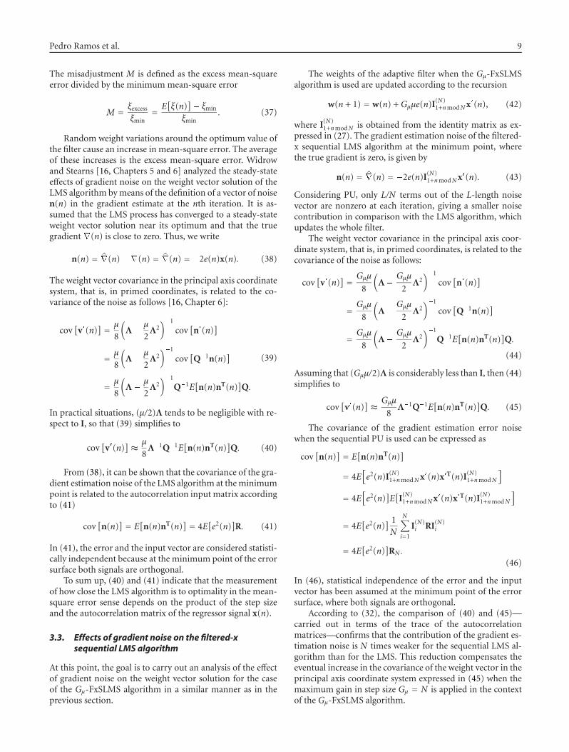
Figure 5: Transfer function magnitude of (a) primary path P(z), (b) secondary path S(z), and (c) offline estimate of the secondary pathused in the simulated model, (d) power spectral density of periodic disturbance consisting of two tones of 62.5 Hz and 187.5 Hz in additivewhite Gaussian noise.

4. EXPERIMENTAL RESULTS

In order to assess the effectiveness of the Gμ-FxSLMS algo-rithm, the proposed strategy was not only tested by simula-tion but was also evaluated in a practical DSP-based imple-mentation. In both cases, the results confirmed the expectedbehavior: the performance of the system in terms of conver-gence rate and residual error is as good as the performanceachieved by the FxLMS algorithm, even while the number ofoperations per iteration is significantly reduced due to PU.

4.1. Computer simulations

This section describes the results achieved by the Gμ-FxSLMSalgorithm by means of a computer model developed in MAT-LAB on the theoretical basis of the previous sections. Themodel chosen for the computer simulation of the first ex-ample corresponds to the 1� 1� 1 (1 reference microphone,1 secondary source, and 1 error microphone) arrangementdescribed in Figure 1(a). Transfer functions of the primarypath P(z) and secondary path S(z) are shown in Figures 5(a)and 5(b), respectively. The filter modeling the primary pathis a 64th-order FIR filter. The secondary path is modeled—by a 4th-order elliptic IIR filter—as a high pass filter whose

cut-off frequency is imposed by the poor response of theloudspeakers at low frequencies. The offline estimate of thesecondary path was carried out by an adaptive FIR filter of200 coefficients updated by the LMS algorithm, as a classi-cal problem of system identification. Figure 5(c) shows thetransfer function of the estimated secondary path. The sam-pling frequency (8000 samples/s) as well as other parameterswere chosen in order to obtain an approximate model of thereal implementation. Finally, Figure 5(d) shows the powerspectral density of x(n), the reference signal for the undesireddisturbance which has to be canceled

x(n) = cos(2π62.5n) + cos(2π187.5n) + η(n), (47)

where η(n) is an additive white Gaussian noise of zero meanwhose power is

E[η2(n)

] = σ2η = 0.0001 (�40 dB). (48)

After convergence has been achieved, the power of the resid-ual error corresponds to the power of the random compo-nent of the undesired disturbance.

The length of the adaptive filter is of 256 coefficients. Thesimulation was carried out as follows: the step size was set tozero during the first 0.25 seconds; after that, it is set to 0.0001

Pedro Ramos et al. 11

4002000

Frequency (Hz)

0

0.5

1

1.5

2

Gai

nin

step

size

(a) N = 1

4002000

Frequency (Hz)

0

0.5

1

1.5

2

2.5

3

Gai

nin

step

size

(b) N = 2

4002000

Frequency (Hz)

0

2

4

6

8

Gai

nin

step

size

(c) N = 8

4002000

Frequency (Hz)

0

5

10

15

20

25

30

Gai

nin

step

size

(d) N = 32

4002000

Frequency (Hz)

0

10

20

30

40

50

60

Gai

nin

step

size

(e) N = 64

4002000

Frequency (Hz)

0

20

40

60

80

Gai

nin

step

size

(f) N = 80

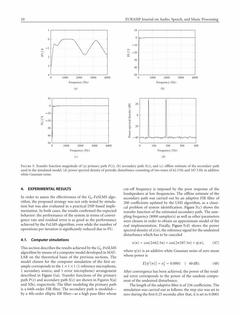
Figure 6: Gain in step size over the frequency band of interest—from 0 to 400 Hz—for different values of the decimation factor N (N =1, 2, 8, 32, 64, 80).

and the adaptive process starts. The value μ = 0.0001 is nearthe maximum stable step size when a decimation factor N =1 is chosen.

The performance of the Gμ-FxSLMS algorithm was testedfor different values of the decimation factor N . Figure 6shows the gain in step size over the frequency band of in-terest for different values of the parameter N . The gain instep size at the frequencies 62.5 Hz and 187.5 Hz are markedwith two circles over the curves. The exact location of thenotches is given by (22). On the basis of the position of thenotches in the gain in step size and the spectral distributionof the undesired noise, the decimation factor N = 64 is ex-pected to be critical because, according to Figure 6, the full-strength gain Gμ = N = 64 cannot be applied at the fre-quencies 62.5 Hz and 187.5 Hz; both frequencies correspondexactly to the sinusoidal components of the periodic distur-bance. Apart from the case N = 64 the gain in step size is freeof notches at both of these frequencies.

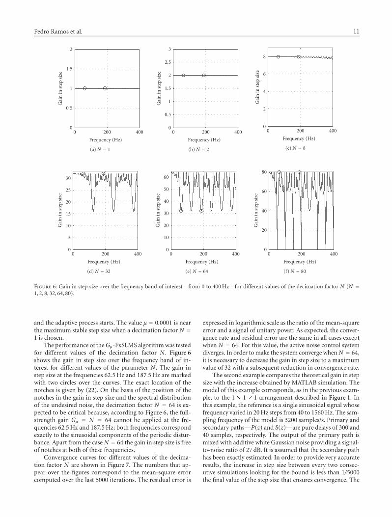
Convergence curves for different values of the decima-tion factor N are shown in Figure 7. The numbers that ap-pear over the figures correspond to the mean-square errorcomputed over the last 5000 iterations. The residual error is

expressed in logarithmic scale as the ratio of the mean-squareerror and a signal of unitary power. As expected, the conver-gence rate and residual error are the same in all cases exceptwhen N = 64. For this value, the active noise control systemdiverges. In order to make the system converge when N = 64,it is necessary to decrease the gain in step size to a maximumvalue of 32 with a subsequent reduction in convergence rate.

The second example compares the theoretical gain in stepsize with the increase obtained by MATLAB simulation. Themodel of this example corresponds, as in the previous exam-ple, to the 1 � 1 � 1 arrangement described in Figure 1. Inthis example, the reference is a single sinusoidal signal whosefrequency varied in 20 Hz steps from 40 to 1560 Hz. The sam-pling frequency of the model is 3200 samples/s. Primary andsecondary paths—P(z) and S(z)—are pure delays of 300 and40 samples, respectively. The output of the primary path ismixed with additive white Gaussian noise providing a signal-to-noise ratio of 27 dB. It is assumed that the secondary pathhas been exactly estimated. In order to provide very accurateresults, the increase in step size between every two consec-utive simulations looking for the bound is less than 1/5000the final value of the step size that ensures convergence. The

12 EURASIP Journal on Audio, Speech, and Music Processing

0.350.30.250.2

Time (s)

0

0.5

1

1.5

2

2.5

Inst

anta

neo

us

erro

rp

ower

�40.8 dB

(a) N = 1

0.350.30.250.2

Time (s)

0

0.5

1

1.5

2

2.5

Inst

anta

neo

us

erro

rp

ower

�40.8 dB

(b) N = 2

0.350.30.250.2

Time (s)

0

0.5

1

1.5

2

2.5

Inst

anta

neo

us

erro

rp

ower

�40.7 dB

(c) N = 8

0.350.30.250.2

Time (s)

0

0.5

1

1.5

2

2.5

Inst

anta

neo

us

erro

rp

ower

�40.6 dB

(d) N = 32

0.350.30.250.2

Time (s)

0

0.5

1

1.5

2

2.5

Inst

anta

neo

us

erro

rp

ower

112 dB

(e) N = 64

0.350.30.250.2

Time (s)

0

0.5

1

1.5

2

2.5

Inst

anta

neo

us

erro

rp

ower

�40.6 dB

(f) N = 80

Figure 7: Evolution of the instantaneous error power in an ANC system using the Gμ-FxSLMS algorithm for different values of the decima-tion factor N (N = 1, 2, 8, 32, 64, 80). In all cases, the gain in step size was set to the maximum value Gμ = N .

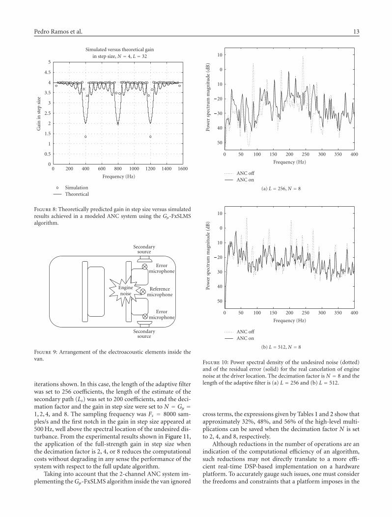
decimation factor N of this example was set to 4. Figure 8compares the predicted gain in step size with the achievedresults. As expected, the experimental gain in step size is 4,apart from the notches that appear at 400, 800, and 1200 Hz.

4.2. Practical implementation

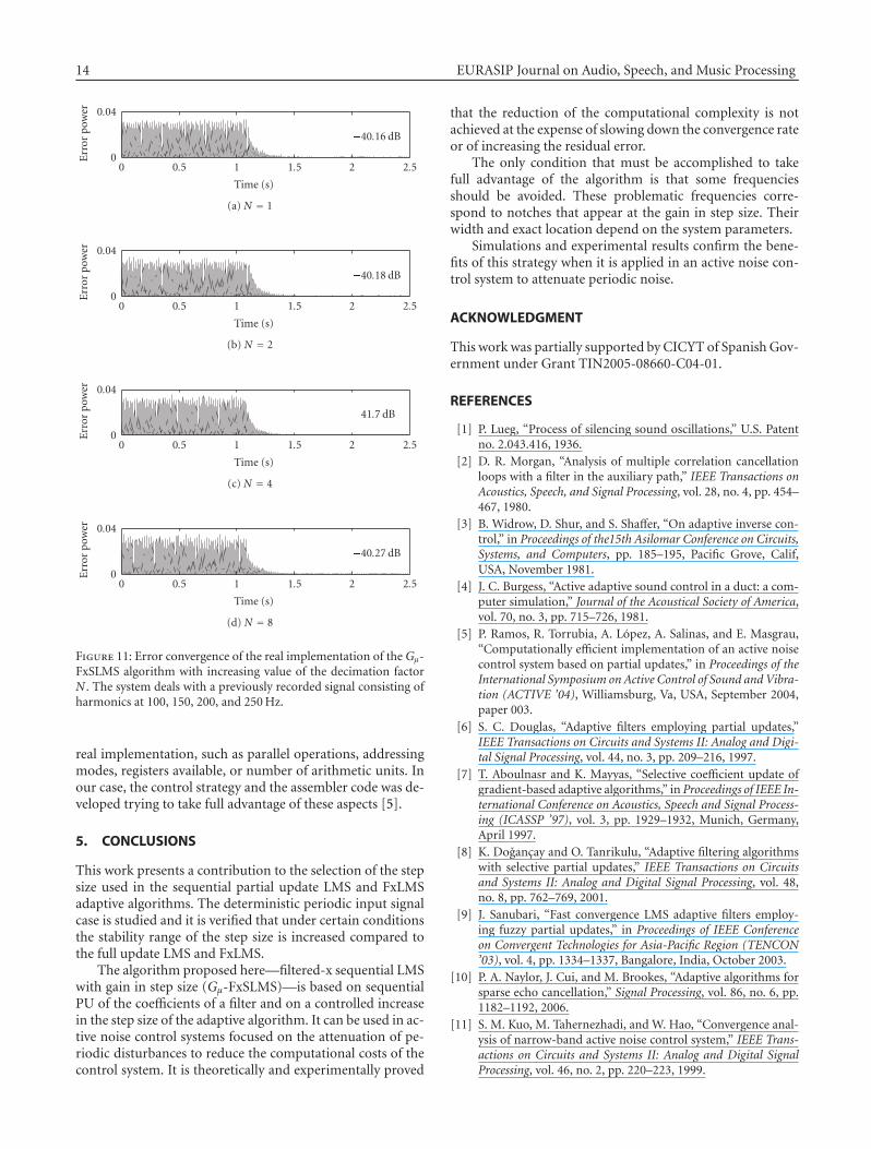
The Gμ-FxSLMS algorithm was implemented in a 1�2�2 ac-tive noise control system aimed at attenuating engine noise atthe front seats of a Nissan Vanette. Figure 9 shows the phys-ical arrangement of electroacoustic elements. The adaptivealgorithm was developed on a hardware platform based onthe DSP TMS320C6701 from Texas Instruments [18].

The length of the adaptive filter (L) for the Gμ-FxSLMSalgorithm was set to 256 or 512 coefficients (depending onthe spectral characteristics of the undesired noise and the de-gree of attenuation desired), the length of the estimate of thesecondary path (Ls) was set to 200 coefficients, and the dec-imation factor and the gain in step size were N = Gμ = 8.The sampling frequency was Fs = 8000 samples/s. From theparameters selected, one can derive, according to (22), thatthe first notch in the gain in step size is located at 500 Hz.

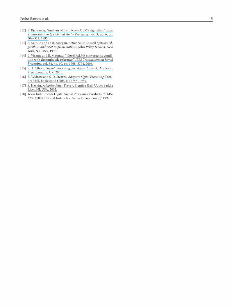
The system effectively cancels the main harmonics of the en-gine noise. Considering that the loudspeakers have a low cut-off frequency of 60 Hz, the controller cannot attenuate thecomponents below this frequency. Besides, the ANC systemfinds more difficulty in the attenuation of closely spaced fre-quency harmonics (see Figure 10(a)). This problem can beavoided by increasing the number of coefficients of the adap-tive filter; for instance, from L = 256 to 512 coefficients (seeFigure 10(b)).

In order to carry out a performance comparison of theGμ-FxSLMS algorithm with increasing value in the decima-tion term N—and subsequently in gain in step size Gμ—it is essential to repeat the experiment with the same un-desired disturbance. So to avoid inconsistencies in leveland frequency, instead of starting the engine, we have pre-viously recorded a signal consisting of several harmon-ics (100, 150, 200, and 250 Hz). An omnidirectional source(Bruel & Kjaer Omnipower 4296) placed inside the van is fedwith this signal. Therefore, a comparison could be made un-der the same conditions. The ratio—in logarithmic scale—of the mean-square error and a signal of unitary power thatappears over the graphics was calculated averaging the last

Pedro Ramos et al. 13

16001400120010008006004002000

Frequency (Hz)

0

0.5

1

1.5

2

2.5

3

3.5

4

4.5

5

Gai

nin

step

size

Simulated versus theoretical gainin step size, N = 4, L = 32

SimulationTheoretical

Figure 8: Theoretically predicted gain in step size versus simulatedresults achieved in a modeled ANC system using the Gμ-FxSLMSalgorithm.

Secondarysource

Errormicrophone

Enginenoise

Referencemicrophone

Errormicrophone

Secondarysource

Figure 9: Arrangement of the electroacoustic elements inside thevan.

iterations shown. In this case, the length of the adaptive filterwas set to 256 coefficients, the length of the estimate of thesecondary path (Ls) was set to 200 coefficients, and the deci-mation factor and the gain in step size were set to N = Gμ =1, 2, 4, and 8. The sampling frequency was Fs = 8000 sam-ples/s and the first notch in the gain in step size appeared at500 Hz, well above the spectral location of the undesired dis-turbance. From the experimental results shown in Figure 11,the application of the full-strength gain in step size whenthe decimation factor is 2, 4, or 8 reduces the computationalcosts without degrading in any sense the performance of thesystem with respect to the full update algorithm.

Taking into account that the 2-channel ANC system im-plementing the Gμ-FxSLMS algorithm inside the van ignored

400350300250200150100500

Frequency (Hz)

�50

�40

�30

�20

�10

0

10

Pow

ersp

ectr

um

mag

nit

ude

(dB

)

ANC off

ANC on

(a) L = 256, N = 8

400350300250200150100500

Frequency (Hz)

�50

�40

�30

�20

�10

0

10Po

wer

spec

tru

mm

agn

itu

de(d

B)

ANC off

ANC on

(b) L = 512, N = 8

Figure 10: Power spectral density of the undesired noise (dotted)and of the residual error (solid) for the real cancelation of enginenoise at the driver location. The decimation factor is N = 8 and thelength of the adaptive filter is (a) L = 256 and (b) L = 512.

cross terms, the expressions given by Tables 1 and 2 show thatapproximately 32%, 48%, and 56% of the high-level multi-plications can be saved when the decimation factor N is setto 2, 4, and 8, respectively.

Although reductions in the number of operations are anindication of the computational efficiency of an algorithm,such reductions may not directly translate to a more effi-cient real-time DSP-based implementation on a hardwareplatform. To accurately gauge such issues, one must considerthe freedoms and constraints that a platform imposes in the

14 EURASIP Journal on Audio, Speech, and Music Processing

2.521.510.50

Time (s)

0

0.04

Err

orp

ower

�40.16 dB

(a) N = 1

2.521.510.50

Time (s)

0

0.04

Err

orp

ower

�40.18 dB

(b) N = 2

2.521.510.50

Time (s)

0

0.04

Err

orp

ower

�41.7 dB

(c) N = 4

2.521.510.50

Time (s)

0

0.04

Err

orp

ower

�40.27 dB

(d) N = 8

Figure 11: Error convergence of the real implementation of the Gμ-FxSLMS algorithm with increasing value of the decimation factorN . The system deals with a previously recorded signal consisting ofharmonics at 100, 150, 200, and 250 Hz.

real implementation, such as parallel operations, addressingmodes, registers available, or number of arithmetic units. Inour case, the control strategy and the assembler code was de-veloped trying to take full advantage of these aspects [5].

5. CONCLUSIONS

This work presents a contribution to the selection of the stepsize used in the sequential partial update LMS and FxLMSadaptive algorithms. The deterministic periodic input signalcase is studied and it is verified that under certain conditionsthe stability range of the step size is increased compared tothe full update LMS and FxLMS.

The algorithm proposed here—filtered-x sequential LMSwith gain in step size (Gμ-FxSLMS)—is based on sequentialPU of the coefficients of a filter and on a controlled increasein the step size of the adaptive algorithm. It can be used in ac-tive noise control systems focused on the attenuation of pe-riodic disturbances to reduce the computational costs of thecontrol system. It is theoretically and experimentally proved

that the reduction of the computational complexity is notachieved at the expense of slowing down the convergence rateor of increasing the residual error.

The only condition that must be accomplished to takefull advantage of the algorithm is that some frequenciesshould be avoided. These problematic frequencies corre-spond to notches that appear at the gain in step size. Theirwidth and exact location depend on the system parameters.

Simulations and experimental results confirm the bene-fits of this strategy when it is applied in an active noise con-trol system to attenuate periodic noise.

ACKNOWLEDGMENT

This work was partially supported by CICYT of Spanish Gov-ernment under Grant TIN2005-08660-C04-01.

REFERENCES

[1] P. Lueg, “Process of silencing sound oscillations,” U.S. Patentno. 2.043.416, 1936.

[2] D. R. Morgan, “Analysis of multiple correlation cancellationloops with a filter in the auxiliary path,” IEEE Transactions onAcoustics, Speech, and Signal Processing, vol. 28, no. 4, pp. 454–467, 1980.

[3] B. Widrow, D. Shur, and S. Shaffer, “On adaptive inverse con-trol,” in Proceedings of the15th Asilomar Conference on Circuits,Systems, and Computers, pp. 185–195, Pacific Grove, Calif,USA, November 1981.

[4] J. C. Burgess, “Active adaptive sound control in a duct: a com-puter simulation,” Journal of the Acoustical Society of America,vol. 70, no. 3, pp. 715–726, 1981.

[5] P. Ramos, R. Torrubia, A. Lopez, A. Salinas, and E. Masgrau,“Computationally efficient implementation of an active noisecontrol system based on partial updates,” in Proceedings of theInternational Symposium on Active Control of Sound and Vibra-tion (ACTIVE ’04), Williamsburg, Va, USA, September 2004,paper 003.

[6] S. C. Douglas, “Adaptive filters employing partial updates,”IEEE Transactions on Circuits and Systems II: Analog and Digi-tal Signal Processing, vol. 44, no. 3, pp. 209–216, 1997.

[7] T. Aboulnasr and K. Mayyas, “Selective coefficient update ofgradient-based adaptive algorithms,” in Proceedings of IEEE In-ternational Conference on Acoustics, Speech and Signal Process-ing (ICASSP ’97), vol. 3, pp. 1929–1932, Munich, Germany,April 1997.

[8] K. Dogancay and O. Tanrikulu, “Adaptive filtering algorithmswith selective partial updates,” IEEE Transactions on Circuitsand Systems II: Analog and Digital Signal Processing, vol. 48,no. 8, pp. 762–769, 2001.

[9] J. Sanubari, “Fast convergence LMS adaptive filters employ-ing fuzzy partial updates,” in Proceedings of IEEE Conferenceon Convergent Technologies for Asia-Pacific Region (TENCON’03), vol. 4, pp. 1334–1337, Bangalore, India, October 2003.

[10] P. A. Naylor, J. Cui, and M. Brookes, “Adaptive algorithms forsparse echo cancellation,” Signal Processing, vol. 86, no. 6, pp.1182–1192, 2006.

[11] S. M. Kuo, M. Tahernezhadi, and W. Hao, “Convergence anal-ysis of narrow-band active noise control system,” IEEE Trans-actions on Circuits and Systems II: Analog and Digital SignalProcessing, vol. 46, no. 2, pp. 220–223, 1999.

Pedro Ramos et al. 15

[12] E. Bjarnason, “Analysis of the filtered-X LMS algorithm,” IEEETransactions on Speech and Audio Processing, vol. 3, no. 6, pp.504–514, 1995.

[13] S. M. Kuo and D. R. Morgan, Active Noise Control Systems: Al-gorithms and DSP Implementations, John Wiley & Sons, NewYork, NY, USA, 1996.

[14] L. Vicente and E. Masgrau, “Novel FxLMS convergence condi-tion with deterministic reference,” IEEE Transactions on SignalProcessing, vol. 54, no. 10, pp. 3768–3774, 2006.

[15] S. J. Elliott, Signal Processing for Active Control, AcademicPress, London, UK, 2001.

[16] B. Widrow and S. D. Stearns, Adaptive Signal Processing, Pren-tice Hall, Englewood Cliffs, NJ, USA, 1985.

[17] S. Haykin, Adaptive Filter Theory, Prentice Hall, Upper SaddleRiver, NJ, USA, 2002.

[18] Texas Instruments Digital Signal Processing Products, “TMS-320C6000 CPU and Instruction Set Reference Guide,” 1999.

Photograph © Turisme de Barcelona / J. Trullàs

Preliminary call for papers

The 2011 European Signal Processing Conference (EUSIPCO 2011) is thenineteenth in a series of conferences promoted by the European Association forSignal Processing (EURASIP, www.eurasip.org). This year edition will take placein Barcelona, capital city of Catalonia (Spain), and will be jointly organized by theCentre Tecnològic de Telecomunicacions de Catalunya (CTTC) and theUniversitat Politècnica de Catalunya (UPC).EUSIPCO 2011 will focus on key aspects of signal processing theory and

li ti li t d b l A t f b i i ill b b d lit

Organizing Committee

Honorary ChairMiguel A. Lagunas (CTTC)

General ChairAna I. Pérez Neira (UPC)

General Vice ChairCarles Antón Haro (CTTC)

Technical Program ChairXavier Mestre (CTTC)

Technical Program Co Chairsapplications as listed below. Acceptance of submissions will be based on quality,relevance and originality. Accepted papers will be published in the EUSIPCOproceedings and presented during the conference. Paper submissions, proposalsfor tutorials and proposals for special sessions are invited in, but not limited to,the following areas of interest.

Areas of Interest

• Audio and electro acoustics.• Design, implementation, and applications of signal processing systems.

l d l d d

Technical Program Co ChairsJavier Hernando (UPC)Montserrat Pardàs (UPC)

Plenary TalksFerran Marqués (UPC)Yonina Eldar (Technion)

Special SessionsIgnacio Santamaría (Unversidadde Cantabria)Mats Bengtsson (KTH)

FinancesMontserrat Nájar (UPC)• Multimedia signal processing and coding.

• Image and multidimensional signal processing.• Signal detection and estimation.• Sensor array and multi channel signal processing.• Sensor fusion in networked systems.• Signal processing for communications.• Medical imaging and image analysis.• Non stationary, non linear and non Gaussian signal processing.

Submissions

Montserrat Nájar (UPC)

TutorialsDaniel P. Palomar(Hong Kong UST)Beatrice Pesquet Popescu (ENST)

PublicityStephan Pfletschinger (CTTC)Mònica Navarro (CTTC)

PublicationsAntonio Pascual (UPC)Carles Fernández (CTTC)

I d i l Li i & E hibiSubmissions

Procedures to submit a paper and proposals for special sessions and tutorials willbe detailed at www.eusipco2011.org. Submitted papers must be camera ready, nomore than 5 pages long, and conforming to the standard specified on theEUSIPCO 2011 web site. First authors who are registered students can participatein the best student paper competition.

Important Deadlines:

P l f i l i 15 D 2010

Industrial Liaison & ExhibitsAngeliki Alexiou(University of Piraeus)Albert Sitjà (CTTC)

International LiaisonJu Liu (Shandong University China)Jinhong Yuan (UNSW Australia)Tamas Sziranyi (SZTAKI Hungary)Rich Stern (CMU USA)Ricardo L. de Queiroz (UNB Brazil)

Webpage: www.eusipco2011.org

Proposals for special sessions 15 Dec 2010Proposals for tutorials 18 Feb 2011Electronic submission of full papers 21 Feb 2011Notification of acceptance 23 May 2011Submission of camera ready papers 6 Jun 2011