Step by Step Tutorial V10 Understanding and Comparing ...

STEP-BY-STEP TUTORIAL: VERSION 2.0 UNDERSTANDING AND COMPARING

CARBON DATASETS, USING QGIS 2.18

USING SPATIAL INFORMATION TO SUPPORT DECISIONS ON

SAFEGUARDS AND MULTIPLE BENEFITS FOR REDD+

Understanding and comparing carbon datasets, using QGIS 2.18

The UN-REDD Programme is the United Nations Collaborative initiative on Reducing Emissions from

Deforestation and forest Degradation (REDD) in developing countries. The Programme was launched in

September 2008 to assist developing countries prepare and implement national REDD+ strategies, and

builds on the convening power and expertise of the Food and Agriculture Organization of the United Nations

(FAO), the United Nations Development Programme (UNDP) and UN Environment.

The UN Environment World Conservation Monitoring Centre (UNEP-WCMC) is the specialist biodiversity

assessment centre of UN Environment, the world’s foremost intergovernmental environmental

organisation. The Centre has been in operation for over 35 years, combining scientific research with

practical policy advice.

Prepared by Xavier DeLamo, Corinna Ravilious and Barbara Pollini

Copyright: 2019 United Nations Environment Programme

Copyright release: This publication may be reproduced for educational or non-profit purposes without

special permission, provided acknowledgement to the source is made. Re-use of any figures is subject to

permission from the original rights holders. No use of this publication may be made for resale or any other

commercial purpose without permission in writing from UN Environment. Applications for permission, with

a statement of purpose and extent of reproduction, should be sent to the Director, UNEP-WCMC, 219

Huntingdon Road, Cambridge, CB3 0DL, UK.

Disclaimer: The contents of this report do not necessarily reflect the views or policies of UN Environment,

contributory organisations or editors. The designations employed and the presentations of material in this

report do not imply the expression of any opinion whatsoever on the part of UN Environment or contributory

organisations, editors or publishers concerning the legal status of any country, territory, city area or its

authorities, or concerning the delimitation of its frontiers or boundaries or the designation of its name,

frontiers or boundaries. The mention of a commercial entity or product in this publication does not imply

endorsement by UN Environment.

We welcome comments on any errors or issues. Should readers wish to comment on this document, they

are encouraged to get in touch via: [email protected].

Citation: DeLamo, X., Ravilious, C. and Pollini, B. (2019) Using spatial information to support decisions on

safeguards and multiple benefits for REDD+. Step-by-step tutorial v2.0: Understanding and comparing

carbon datasets, using QGIS 2.18. Prepared on behalf of the UN-REDD Programme. UNEP World

Conservation Monitoring Centre, Cambridge, UK.

Acknowledgements: These training materials have been produced from materials developed for working

sessions held in various countries to aid the production of multiple benefits maps to inform REDD+ planning

and safeguards policies using open-source GIS software. Additional contributors to the carbon comparison

annex included Stephen Woroniecki, Monika Bertzky, Lera Miles and Rebecca Mant. This version of the

tutorial has been updated based on work carried out for the UN Sustainable Development Solutions Network

(SDSN) on global and carbon biodiversity mapping.

mailto:[email protected]


Contents

1. Introduction .......................................................................................................... 1

2. Mapping carbon stocks for REDD+ planning .......................................................... 3

2.1 Comparing carbon datasets using QGIS ....................................................................4

2.1.1 Clip the two datasets to your area of interest .......................................................5

2.1.2 Symbolising the raster datasets for comparison ...................................................7

2.1.3 Preparing raster datasets for comparison .............................................................9

2.1.4 Creating a difference map ...................................................................................12

2.1.5 Comparing AGB values by land cover type ..........................................................14

Annex 1: Understanding and comparing carbon datasets............................................. 17

Comparing biomass carbon datasets ...............................................................................17

Soil carbon datasets .........................................................................................................25

Guidance on selecting between datasets ........................................................................26

References ........................................................................................................................28

Annex 2 : Glossary of terms ......................................................................................... 29


AGB Above-Ground Biomass ALOS Advanced Land Observing Satellite ASAR Advanced Synthetic Aperture Radar AVHRR Advanced Very High Resolution Radiometer BCEF Biomass Expansion and Conversion Factors BGB Below-Ground Biomass BRDF Bi-directional Reflectance Distribution Function CEOS Committee on Earth Observation Satellites DBH Diameter at Breast Height Envisat European Space Agency Environmental Satellite ESA CCI European Space Agency Climate Change Initiative FAO United Nations Food and Agriculture Organization FRA Forest Resource Assessment GHG-AFOLU Greenhouse Gas emissions in Agriculture, Forestry and Other Land Use GLAS Geoscience Laser Altimeter System GLC2000 Global Land Cover 2000 GPCP Global Precipitation Climatology Project GSV Growing stock volume HOME Height of Median Energy HPDI Highest Posterior Density Interval ICESAT The Ice, Clouds, and Land Elevation Satellite JAXA The Japan Aerospace Exploration Agency JRC Joint Research Centre LAI Leaf Area Index Landsat 7 ETM + Landsat 7 Enhanced Thematic Mapper Plus (ETM+) LiDAR Light Detection and Ranging (named for ‘light’ and ‘radar’) MERRA Modern-Era Retrospective analysis for Research and Applications MODIS Moderate Resolution Imaging Spectroradiometer MODIS LST MODIS Land Surface Temperature Products MODIS NBAR MODIS Nadir Bidirectional reflectance distribution function Adjusted

Reflectance MVC Maximum value composite NDVI Normalized difference vegetation index NOAA National Oceanic and Atmospheric Administration NPP Net Primary Productivity PALSAR Phased Array type L-band Synthetic Aperture Radar QSCAT Quick Scatterometer SAR Synthetic aperture radar data SOC Soil Organic Carbon SRTM Shuttle Radar Topography Mission (See glossary in Appendix 2 for more information on terms)

Acronyms and abbreviations


1

1. Introduction

REDD+ is a voluntary climate change mitigation approach that has been developed by Parties to the

UNFCCC. It aims to incentivize developing countries to reduce emissions from deforestation and forest

degradation, conserve forest carbon stocks, sustainably manage forests and enhance forest carbon

stocks. This will involve changing the ways in which forests are used and managed, and may require

many different actions, such as protecting forests from fire or illegal logging, or rehabilitating degraded

forest areas.

REDD+ has the potential to deliver multiple benefits beyond carbon. For example, it can promote

biodiversity conservation and secure ecosystem services from forests such as water regulation, erosion

control and non-timber forest products (NTFPs). Some of the potential benefits from REDD+, such as

biodiversity conservation, can be enhanced through identifying areas where REDD+ actions might have

the greatest impact using spatial analysis and other approaches.

The purpose of this tutorial series is to help participants in technical working sessions, who are already

skilled in GIS, to undertake analyses that are relevant to REDD+. The tutorials have been used to build

capacity in a number of countries to produce datasets and maps relevant to their spatial planning for

REDD+, and to develop such map products. Maps developed using these approaches appear in a

number of publications whose aim is to support planning of strategy options that enhance biodiversity

and ecosystem services as well as delivering climate change mitigation (see http://bit.ly/mbs-redd for

country materials). There is of course no requirement for countries to use the approaches described in

these tutorials.

Where countries have identified biodiversity conservation as a goal for REDD+, and to be consistent

with the Cancun safeguards for REDD+ on protecting biodiversity, it is useful to identify areas where

specific REDD+ actions are feasible and can protect threatened species. It may also be useful to identify

areas outside forest where threatened species may be vulnerable to the displacement of land-use

change pressures or to afforestation.

Open-source GIS software can be used to undertake spatial analysis of datasets of relevance to multiple

benefits and environmental safeguards for REDD+. Open-source software is released under a license

that allows software to be freely used, modified, and shared (http://opensource.org/licenses).

Therefore, the use of open-source software has great potential in building sustainable capacity and

critical mass of experts with limited financial resources.

This tutorial is designed to help the user to compare and contrast carbon datasets and understand the

differences in the estimates provided, and the reasons behind this. A country’s forest inventory may

already include forest carbon estimates and a national level carbon map may have been produced.

However, when a country lacks the necessary data or resources to gather it, it may be useful to test

global or regional products for suitability of use for REDD+ planning, using available national

information to validate.

http://bit.ly/mbs-redd

http://opensource.org/licenses


2

The tutorial provides technical instructions for using QGIS software to compare carbon values between

datasets for potential use in spatial planning for REDD+ and an annex providing a summary of different

publicly available datasets highlighting how they differ in resolution, time period, methodology and

carbon pools covered. Although the tutorial uses global and regional products as example data, the

same techniques can be used with national data.

This tutorial is intended for use in identifying suitable carbon data for use in REDD+ planning in the

absence of available high-quality national datasets. It does not provide guidance on how to create a

national level carbon map for use in reference level development or advocate the use of global or

regional products for this purpose. Information on the potential added value and/or limitations of the

use of spatial modelling techniques for Forest Reference Emission Level (FREL) and/or Forest Reference

Level (FRL) can be found in the UN-REDD Programme Info Brief “Considering the use of spatial modelling

in Forest Reference Emission Level and/or Forest Reference Level construction for REDD+”

http://www.fao.org/3/a-i5721e.pdf.

http://www.fao.org/3/a-i5721e.pdf


3

2. Mapping carbon stocks for REDD+ planning

Through retaining threatened forest, REDD+ can prevent carbon dioxide emissions and promote carbon

sequestration. Forests have much more to offer the world than their carbon stores, but their carbon

can be easily estimated, and doing so provides a part of the case for their restoration, conservation and

sustainable management. Mapped estimates of the total carbon locked in forest biomass can be used

together with information on deforestation and forest degradation drivers for REDD+ planning. Carbon

mapping can allow efforts at carbon protection to be targeted, for example to the higher carbon areas,

and may be able to highlight areas that are already subject to degradation. Areas where significant

additional benefits could also be gained through REDD+ activities can be identified by combining carbon

maps with other spatial datasets showing forest ecosystem services, biodiversity or other forest values.

MRV will also require baseline estimates of carbon stocks, which may need to be more precise.

Carbon in terrestrial ecosystems can be distributed into several different pools (Willcock et al. 2012):

Aboveground biomass

Belowground biomass

Coarse woody debris

Litter

Soil

Certain pools are more difficult to assess than others and the type of pools considered by different

maps vary.

Currently, sampling effort is largely focused on aboveground live carbon pools. However, the quantity

of carbon in the remaining pools is being increasingly recognised. The soil carbon pool is typically

estimated based on soil type, and the size of other pools is often estimated from ratios relating each

pool to aboveground carbon stock.

The approaches to gathering spatial data on carbon stocks are broadly:

Field inventories - these are the most accurate way to estimate biomass carbon of a

forest, but are costly.

Remote sensing - allows the whole landscape to be sampled equally, with little cost to

the user, but only provide indirect estimates. Remote-sensing measurements need to be

calibrated with some field data.

Even with remote sensing approaches, field data remains essential to convert estimates of vegetation

cover to values of biomass or carbon. Many countries lack the necessary data or resources to gather it.

When working as part of a REDD+ programme, a nationally produced or -validated carbon map should

ideally be used, for example, one which has drawn on data from the country’s National Forest

Inventory. If point data from an inventory are available, statistical techniques can be used to develop a

map from the raw point data, preferably in conjunction with remote sensing or other complementary

spatial data.


4

A number of regional and global biomass carbon density maps have been produced in recent years,

using various methods and sources. The carbon estimations vary greatly between the maps in certain

areas. They also represent different time periods. If adopting one of these maps for REDD+ planning

purposes, it is important to assess that these estimates are more or less accurate for the area of interest

and understand which time period they reflect, as forests are dynamic.

In the absence of suitable data from national, regional or global sources, an alternative solution can be

to build a map by assigning carbon values to the different land-cover classes (a so-called ‘paint by

numbers’ approach). As well as a reliable land-cover map, an adequate number of estimates of the

biomass of each class is required. These may be available in existing literature or obtained from field

data (assessing as many field plots as available within each class, and considering how to represent the

range as well as the average). As biomass is only partially related to land cover, there will be variability

within each class. Such maps are not as accurate as remotely sensed derived maps but be useful when

no other data is available.

An example of how such data have been used in supporting REDD+ planning can be seen in a report

developed by the Ministry of Environment and Natural Resources in Kenya and UNEP-WCMC

(Maukonen et al. 2016). In this report, the Baccini et al. 2012 data was used as an interim dataset for

decision making as a national map of carbon stocks was not yet available. Expert knowledge of carbon

stock distribution in the country was used to determine the most suitable dataset from those regional

and global products that were available. The purpose of the report was to support REDD+ planning in

Kenya through the development of maps on the distribution of drivers of deforestation and forest

degradation, potential additional benefits of implementing REDD+ activities, and different

implementation possibilities for REDD+ strategy options.

Please refer to Annex 1 for more information on understanding, comparing and selecting from existing

carbon datasets.

2.1 Comparing carbon datasets using QGIS

When more than one carbon dataset is available it is useful to compare them to identify both

differences in pattern and values. However, it is important to also bear in mind when comparing

datasets that there may be differences in what is actually mapped in terms of the carbon (please refer

to Table 3 in annex 1). One may represent just above-ground biomass for example where as another

may represent above and below ground biomass. This means that there may be some preparatory work

prior to doing the comparisons. The tutorial “Step-by-step tutorial v1.1: Adding below-ground biomass

to a dataset of above-ground biomass and converting to carbon using QGIS 2.18” provides guidance on

the specific example just mentioned. These pre-processing steps are not covered in this current tutorial.

There is a tool available online for comparing carbon datasets at

https://carbonmaps.ourecosystem.com/interface/, however there may be times when you need to

make comparisons yourself for datasets not included in this tool.

The following instruction will demonstrate, using as an example two datasets from Avitabile et al.,

2016 and Santoro et al. 2018, how to undertake a comparison of two datasets using QGIS software.

https://carbonmaps.ourecosystem.com/interface/


5

For this tutorial we will use as an example Liberia, but the same instructions can be used for any other

country or region.

You may want to follow these instructions exactly by downloading the two datasets from:

Pan-Tropical Biomass Map (Avitabile et al., 2016). Accessible at:

https://www.wur.nl/en/Research-Results/Chair-groups/Environmental-

Sciences/Laboratory-of-Geo-information-Science-and-Remote-

Sensing/Research/Integrated-land-monitoring/Forest_Biomass.htm

(In order to download the data you have to register. The file that has to be

downloaded is called: “Pan-Tropical Biomass Map”)

GlobBiomass (Santoro et al., 2018). Accessible at:

http://globbiomass.org/products/global-mapping/

2.1.1 Clip the two datasets to your area of interest

Add datasets to QGIS

Click on the Add Raster Layer button to add the two raster datasets to QGIS. Click on the Add

Vector Layer button to add the Shapefile of your area of interest – in this case Liberia.

In this example, both rasters are in WGS84 coordinate system, it is important to make sure the

shapefiles are in the same projection. To check the coordinate system, right-click on each dataset,

select Properties and click on the General tab.

https://www.wur.nl/en/Research-Results/Chair-groups/Environmental-Sciences/Laboratory-of-Geo-information-Science-and-Remote-Sensing/Research/Integrated-land-monitoring/Forest_Biomass.htm



http://globbiomass.org/products/global-mapping/


6

Clip both rasters to the area of interest

In the Processing Toolbox search box type Clip and select the tool Clip raster with polygon.

For Input select one of the carbon datasets and for Polygons select the shapefile of the region of

interest. For the Clipped output dataset navigate to an output folder and give the new dataset a

name. Then click Run.

Repeat the steps in 2.1.1. b for the second carbon dataset.


7

2.1.2 Symbolising the raster datasets for comparison

Note that QGIS does not automatically symbolise and scale raster data to display the min-max

values unless you have set your QGIS preferences to do so. Will assume that this has not been set.

a. The next step is to change the symbology of the layers to allow an easier interpretation of the

data. Right-click on the dataset with the highest maximum value and click properties to open

the layer properties window

b. Change the Render type to Singleband

pseudocolor

c. Change Mode to Equal interval

d. Click on Min / Max, click on Actual (slower)

and click Load

e. Click Classify

You can manually change the Class breaks if you

do not want equal interval classes.

f. Click OK


8

The next step is to copy the symbology across to the second dataset in order to visually compare

the datasets with the same class breaks.

g. Right-click on the same dataset

and click Styles>>Copy Style

h. Right-click on the second dataset

and click Styles>>

Paste Styles

Visually review the distribution of carbon/biomass values in the different layers. Does it makes sense

according to your knowledge of the landcover and carbon distribution?


9

2.1.3 Preparing raster datasets for comparison

The next steps apply different techniques to compare, both visually and quantitatively, the values

estimated in the two datasets.

The first step is to ensure that the projection, resolution (size of the cells) and extent (geographic

boundaries) are the same in both layers.

a. Right-click on each layer, click Properties

b. Click on the Metadata tab

c. The Properties section at the bottom of the layer properties window provides information

about the dataset. Scroll down to see the resolution and extent

In this example both the datasets are in Geographic coordinate system with a cell size of

approximately 0.00833333. The datasets have to be re-projected to an equal-area projection, in

this case UTM, in order to be able to generate areas or stock statistics later. For UTM projections,

you need to know in which UTM zone your region of interest is in. In the case of Liberia it falls

within UTM 29 N. If your region of interest falls across multiple UTM zones it is better to use a

Lambert-azimuthal equal area projection to ensure areas are represented accurately.


10

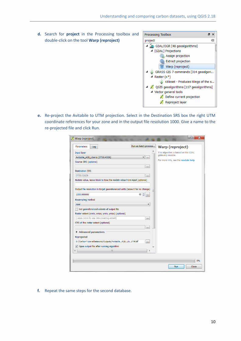
d. Search for project in the Processing toolbox and

double-click on the tool Warp (reproject)

e. Re-project the Avitabile to UTM projection. Select in the Destination SRS box the right UTM

coordinate references for your zone and in the output file resolution 1000. Give a name to the

re-projected file and click Run.

f. Repeat the same steps for the second database.


11

g. Copy the symbology across to the new projected datasets (as in previous steps g-h in section

2.1.2)

The next step is to ensure that both datasets have the same extent.

h. Right-click on the dataset to match to (i.e. in this example the re-projected GlobBiomass

dataset) and click properties>>Metadata

i. Scroll down in the properties window and copy and paste the Layer Extent into a text editor

(such as notepad)

j. Right-click on the Avitabile

dataset, click Save as and

copy and paste the correct

extent from the text editor

into the North, South, East

and West extent boxes.

k. When finished, click

properties>>Metadata on

both datasets and check that

the dimensions of each raster

layer (number of rows and

columns) are exactly the

same.


12

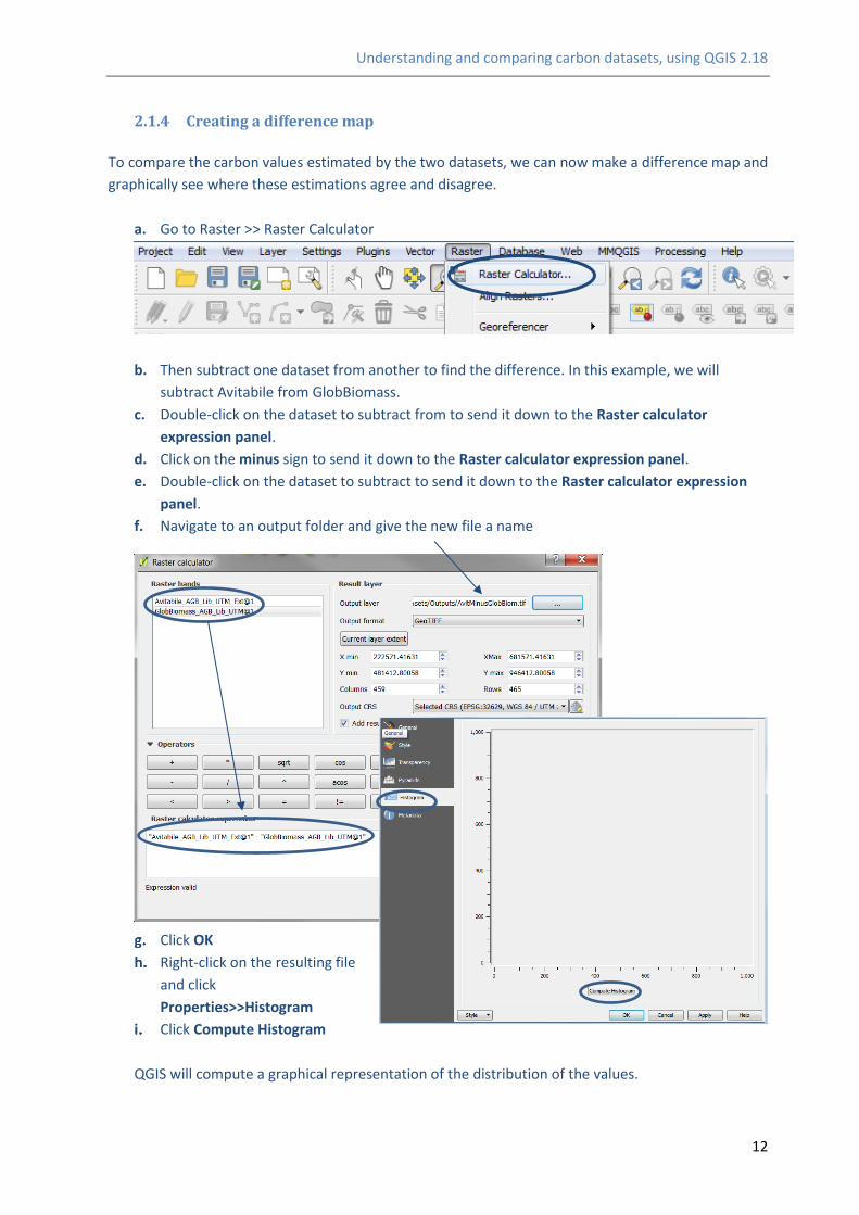
2.1.4 Creating a difference map

To compare the carbon values estimated by the two datasets, we can now make a difference map and

graphically see where these estimations agree and disagree.

a. Go to Raster >> Raster Calculator

b. Then subtract one dataset from another to find the difference. In this example, we will

subtract Avitabile from GlobBiomass.

c. Double-click on the dataset to subtract from to send it down to the Raster calculator

expression panel.

d. Click on the minus sign to send it down to the Raster calculator expression panel.

e. Double-click on the dataset to subtract to send it down to the Raster calculator expression

panel.

f. Navigate to an output folder and give the new file a name

Click OK

Right-click on the resulting file

and click

Properties>>Histogram

Click Compute Histogram

QGIS will compute a graphical representation of the distribution of the values.


13

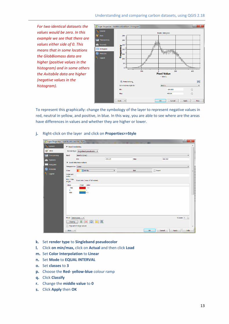
For two identical datasets the

values would be zero. In this

example we see that there are

values either side of 0. This

means that in some locations

the GlobBiomass data are

higher (positive values in the

histogram) and in some others

the Avitabile data are higher

(negative values in the

histogram).

To represent this graphically: change the symbology of the layer to represent negative values in

red, neutral in yellow, and positive, in blue. In this way, you are able to see where are the areas

have differences in values and whether they are higher or lower.

Right-click on the layer and click on Properties>>Style

Set render type to Singleband pseudocolor

Click on min/max, click on Actual and then click Load

Set Color Interpolation to Linear

Set Mode to EQUAL INTERVAL

Set classes to 3

Choose the Red- yellow-blue colour ramp

Click Classify

Change the middle value to 0

Click Apply then OK


14

2.1.5 Comparing AGB values by land cover type

To compare the carbon values estimated by the two datasets by land cover type and to identify for

which types they agree and disagree, we have to:

a. Add the land cover to your QGIS project

and ensure that extent and cell size are

the same as the carbon layers. If extent

and cell size are different repeat steps I

and J in section 2.1.3.

b. Type Stat in the search box of the

processing toolbox.

c. To calculate the amount of carbon in each

land cover type we will use the tool

r.univar. Double click on the tool.


15

d. Select one of the carbon datasets under Name of raster map(s) and the resamples land cover

raster under Raster map used for zoning. In the field separator include a comma (,) navigate

to an output folder and give a name to the output dataset including the format of the file

(csv), in this case GlobBiomass_LC_Stata.csv. Click Run.

The output file, containing the summary of above ground biomass (AGB) values by landcover

type will look like the one shown below:

e. Repeat the steps for the second carbon datasets.

f. Once you have csv files for both carbon datasets, open them in Microsoft Excel.


16

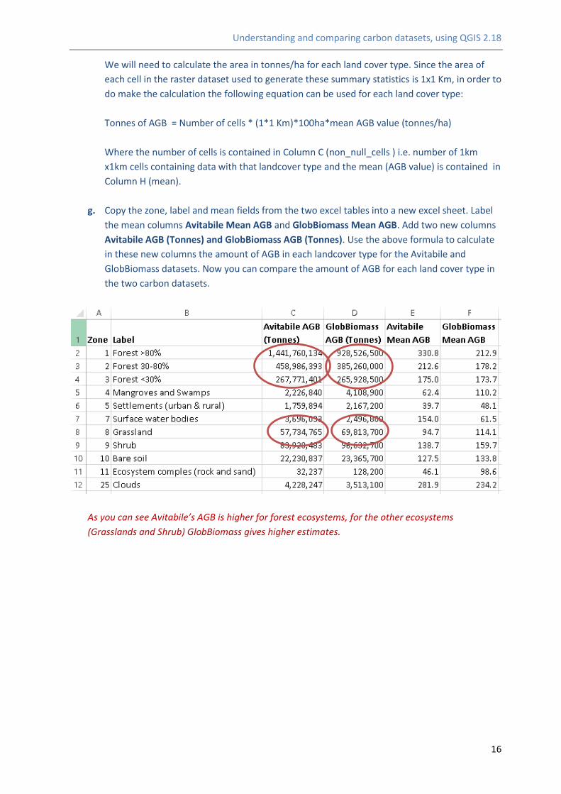
We will need to calculate the area in tonnes/ha for each land cover type. Since the area of

each cell in the raster dataset used to generate these summary statistics is 1x1 Km, in order to

do make the calculation the following equation can be used for each land cover type:

Tonnes of AGB = Number of cells * (1*1 Km)*100ha*mean AGB value (tonnes/ha)

Where the number of cells is contained in Column C (non_null_cells ) i.e. number of 1km

x1km cells containing data with that landcover type and the mean (AGB value) is contained in

Column H (mean).

g. Copy the zone, label and mean fields from the two excel tables into a new excel sheet. Label

the mean columns Avitabile Mean AGB and GlobBiomass Mean AGB. Add two new columns

Avitabile AGB (Tonnes) and GlobBiomass AGB (Tonnes). Use the above formula to calculate

in these new columns the amount of AGB in each landcover type for the Avitabile and

GlobBiomass datasets. Now you can compare the amount of AGB for each land cover type in

the two carbon datasets.

As you can see Avitabile’s AGB is higher for forest ecosystems, for the other ecosystems

(Grasslands and Shrub) GlobBiomass gives higher estimates.


17

Annex 1: Understanding and comparing carbon datasets

The terrestrial carbon pools that are most often included in available maps are above-ground biomass

(AGB), below-ground biomass (BGB) and soil organic carbon (SOC). Although SOC can be a substantial

pool, which can be affected by land-use change, there is more limited spatial data available than for

vegetation carbon2. For biomass carbon, a number of globally consistent AGB maps are now available,

either for the world as a whole or for the tropics (Kindermann et al., 2008; Ruesch & Gibbs 2008; Saatchi

et al. 2011; Baccini et al. 2012; Thurner et al. 2014; Avitable et al. 2014 and 2016, Spawn et al. 2017;

Xia et al. 2014; Bouvet et al. 2018; Santoro et al. 2018; Baccini 2018; Hu et al. 2016 ). BGB is often

derived from the AGB using conversion factors , termed ‘root to shoot’ ratios, such as those used by

the IPCC Tier 1 methodology. The quality of AGB data has progressed markedly in recent years,

however, the existing products do not provide a consensus on the total amount of biomass carbon or

its spatial distribution pattern, and in some cases show strong disagreement. Furthermore, recent

comparative studies have shown disagreement between remotely-sensed datasets and plot-based

estimates (Mitchard et al., 2013, 2014). Within the scientific community, no single method is

considered definitive; some approaches may have advantages or disadvantages in particular areas or

ecosystems, and a number of issues influence data quality.

Data on the quantity and spatial distribution patterns of AGB

is crucial for well-informed REDD+ planning and

implementation. This annex is designed to assist in selecting

between publicly available biomass carbon datasets,

especially for use by an individual country. It compares the

different existing datasets (henceforth referred to by the

codes in Table 1) and presents the main issues to consider

when selecting a dataset for use.

Comparing biomass carbon datasets

The datasets show differences in terms of total carbon estimates, carbon density estimates and spatial

distribution patterns of carbon stocks in different ecosystems, forest areas, woody biomass in non-

forest areas, grassland ecosystems, and other ecosystems.

1 unpublished

2 Even at national scales there are rarely datasets available that contain the soil chemical properties required for soil carbon estimates.

Table 1 - Codes used in this Annex to refer to the datasets

Kindermann et al. 2008 K

Ruesch and Gibbs 2008 R

Saatchi et al. 2011 S

Baccini et al. 2012 B

Thurner et al. 2014 T

Avitabile et al. 2014

(GEOCARBON)

A

Xia et al. 2014 X

Avitabile et al. 2016 V

Hu et al. 2016 H

Spawn et al. 2017 P

Bouvet et al. 2018 O

Santoro et al. 2018

(GlobBiomass)

N

Baccini 20181 C


18

Unsurprisingly, there are markedly different estimates for total carbon between K and R; because K

focuses only on forest whilst R tackle all ecosystems. K report 296 GtC for forests whilst R report 502

GtC for vegetation a whole. At the regional level, Table 2 shows regional and pan-tropical differences

between S and B datasets for woody biomass. The S and B datasets also disagreed strongly at the

national level with the FAO Forest Resources Assessment (2010) (Mitchard, et al., 2013), though

differences in forest definition will account for some of the differences, and many of the nationally-

reported figures from the FRA rely on best estimates rather than recent measurements. There are also

differences between S and B in the spatial distribution of carbon, with the direction of the difference

varying between locations (Mitchard et al. 2014).

Table 2: Mean carbon density (averaged across the continent) and total aboveground biomass for the tropical

terrestrial continental regions (not including Australia, southern Latin America, and southern Africa), Source:

Mitchard et al., 2013.

Continent Area Compared (km2) S B

Mean Density Total

AGB

Mean

Density

Total

AGB

(Mg ha-1) (PgC) (Mg ha-1) (PgC)

Africa 22,105,436 50.8 56.2 58.4 64.5

Americas 14,713,658 129.8 95.5 158.1 116.3

Asia 6,457,241 160.2 51.7 144.9 46.8

Pan-Tropics 43,276,334 94.0 203.4 105.2 227.6

A comparison between biomass estimates within forest areas, in two more recent datasets, N and C

(Figure 1), shows that for most UN Environment sub-regions, C provides higher estimates of AGB than

N, especially for the South Pacific, Southeast Asia and Central Africa. In contrast N’s estimate for

Australia + New Zealand and Mashriq are notably higher than C’s and for Western, Central and Eastern

Europe are marginally higher. These differences are likely due to several factors, including the different

distribution of field data and the approach for estimating AGB in the two studies.

Figure 1 Comparison of biomass estimates within forest areas (according to the forest classes of the 2010 Land Cover

CCI product) from GlobBiomass (Santoro et al. 2018) and Baccini (2018), by UN Environment sub-region.

050

100150200250300350

Mea

n A

GB

(to

nn

es/h

a)

Forest

GlobBiomass Baccini


19

When looking at woody biomass in non-forest areas, C provides higher estimates of AGB than N, in

particular for the South Pacific, Southeast Asia and Central Africa. In contrast, N’s estimates are higher

for Australia + New Zealand, South Asia, North Africa and Mashriq (Figure 2).

Figure 2 Comparison of GlobBiomass (Santoro et al. 2018) and Baccini (2018) within non-forest areas (according to the

forest classes within the 200 Land Cover CCI product), by UN Environment sub-region.

O is a high resolution dataset for woodland and savanna in Africa, and when compared to N and S,

shows a higher agreement with N. This result indicates that for global woody formations, other than

Africa for which O should be used, N is the most reliable dataset currently available.

P, is the best available dataset to be used for all other ecosystems, including grassland, cropland, sparse

vegetation and any areas of shrubland not covered by O and N.

These analyses highlight the need to evaluate any given map against what is known for the country in

question, whether that’s through expert assessment, comparison with available data for part of the

region or both.

Table 3 shows the main differences in coverage and methods of the various datasets. For example, for

Carbon pools it highlights whether the data are AGB only or AGB and BGB, only forest biomass or other

biomass, and if they only include trees above a certain diameter. S for example, includes woody biomass

(both inside and outside forests) for trees that are >10cm diameter at breast height (DBH), whilst B

includes all trees >5cm DBH.

020406080

100120140

Mea

n A

GB

(to

nn

es/h

a) Non-Forest woody biomass

GlobBiomass Baccini


20

Table 3: Spatial coverage and design of the datasets; including spatial resolution, time period, carbon pools covered, overall methodology, the use and comprehensiveness of field

inventories, allometric and statistical equations used, and uncertainty estimates.

K R S B V T A P X O N C

H

Scope Global Global Pan-tropical

Pan-tropical23

Pan-tropical Temperate and boreal

Global Global Global Africa Global Global Global

Data Year(s)

2005 2000 2000 2007-2010 2000 + 2010 Various 2000s circa 2010 1982 to 2006 2010 2010 2000 2004

Spatial Resolution

60km 1km 1km 463m 1km 1km 300m 300m 8km 25m 100m 30m 1km

Biomass AGB &BGB

AGB &BGB AGB &BGB

AGB AGB AGB&BGB AGB AGB+BGB AGB AGB AGB AGB AGB

Biomass Definition

In woody biomass in forests only + some in litter and soil. Non-harmonised DBH thresholds

All living vegetation using globally consistent default values. (IPCC 2006)

Woody biomass inside and outside forest for trees that are > 10cm DBH


AGB for all living trees with diameter at breast height ≥ 5-10cm.

Living biomass (stem, branches, roots, foliage) in forests. Forest GSV referring to volume of tree stems per unit area.

Biomass only in forest areas according to the GLC2000 map.

Synthetic, global above- and below-ground biomass maps that combine recently-released satellite based data of standing forest biomass with novel estimates for non-forest biomass stocks

Grassland biomass Woodland and savannah. Low woody biomass areas, which therefore exclude dense forests and deserts

Woody biomass inside and outside forest for trees that are > 10cm DBH masked to Landsat canopy cover of 2010 (Hansen et al., 2013). The mass, expressed as oven-dry weight of the woody parts (stem, bark, branches and twigs) of all living trees excluding stump and roots.


Biomass only in forest areas according to MODIS land cover map for 2004 from the Global Land Cover Facility.

Field Data FRA 2005, plots and allometrics depends on data source.

No 4,079 plots spanning a variety of forest types. Varying in plot size, sampling scheme, allometric

Plots in 9 countries (3 African, 4 South American and 2 Asian); 283 field plots for calibration

18 ground datasets and yielding 4,283 field plot. Used in combination with AGB maps (below) - 10,741

Field measurements from Global Wood Density Database (Chave et al. 2009; Zanne et al., 2009) and the JRC GHG-AFOLU Biomass

3 input datasets weighted with local reference datasets to minimize the impact of errors on the final biomass estimates in the tropics.

No 81 field plots of aboveground live biomass measurements totalling 158 site-years of field (some sites had multi-year observations). These were used for model

In total, 144 field plots were selected, located in 8 countries (Cameroon, Burkina Faso, Malawi, Mali, Ghana, Mozambique, Botswana and South Africa), with

Field data used in validation process only for which 56,345 forest inventory and forest plot data from research networks were used. Only plots with precise coordinates (from

field-based biomass measurements (as described in Baccini et al, 2012)

> 4000 plot measurement records collected from published literature.

3 Saatchi et al., 2011 includes Australia, Southern Latin America and Southern Africa which are not included in Baccini et al., 2012.


21


H

equations, and number of structural components)

(23,881 trees)

reference pixels; and validation based on additional 2,118 pixels.

Compartment Database (JRC, 2009).

calibration and validation. These included 31 intensively studied grassland sites, spanning five ecoregions (cold desert steppe, temperate dry steppe, humid savanna, humid temperate, and savanna) and 22 sites of temperate grasslands in China.

a mean plot size of 0.89 ha used to train a model that relates PALSAR intensities to AGB. Data from different countries in Africa between 2000 and 2013, both from published literature and from original campaigns.

year 2000 onwards) for which trees of ≥ 10 cm diameter were included and with a minimum size of 0.04 ha (average 0.04-0.32ha). Most plots located in Europe although large part of the forested area worldwide covered.

Other spatial data

FRA 2005, Human Influence (Ciesen 2002)

GLC2000, FAO ecofloristic zones, continental regions, and WRI frontier forests (level of human disturbance)

GLAS LIDAR, MODIS (LAI, NDVI), QSCAT, SRTM

MODIS (NBAR, BRDF, LST), SRTM, LIDAR

Saatchi (2011) and Baccini (2012) datasets. 9 high-resolution (<= 100m) AGB maps, derived from satellite data and validated using Field and LIDAR data. GLC2000, Global Ecological Zones (FAO, 2000), Intact forest landscapes for 2000

GLC2000 land-use/land-cover map (JRC, 2003) Multi-temporal Envisat ASAR. GSV estimates obtained with the BIOMASAR algorithm (Santoro et al., 2011).

Combining and harmonizing pan-tropical biomass map by Avitabile et al. (2016) with the boreal forest biomass map by Santoro et al. (2015). The map covers only forest areas, where forest are defined as areas with dominance of tree cover in the GLC2000 map (Bartholomé and Belward, 2005). For a proper use and description of this dataset, please refer to the mentioned articles.

Represents an update for circa 2010 to the IPCC Tier-1 Global Biomass Carbon Map for the Year 2000 (Ruesch and Gibbs, 2008). Data inputs for ABG: Avitabile et al., 2016; Baccini et al., 2012; Jia et al., 2003; Monfreda et al., 2008; Xia et al., 2014) and interpolation where necessary. BGB was modeled from aboveground biomass carbon stocks using published empirical relationships (Mokany et al., 2006; Reich et al., 2014).

NDVI, Climate data included monthly Modern Era Retrospective-Analysis for Research and Applications (MERRA) temperature data and Global Precipitation Climatology Project (GPCP)

ESA CCI (2010) Landcover dataset

Spaceborne SAR (ALOS PALSAR, Envisat ASAR), optical (Landsat-7), LiDAR (ICESAT) and auxiliary datasets with multiple estimation procedures.

GLAS, LiDAR, SRTM, Landsat 7 ETM+, and ancillary bio/geophysical data


22


H

(Potapov et al., 2008).

Approach to Estimating AGB

NPP and human impact w/ biomass

Biomass classification

Using field and LIDAR data, sampling forest structure and estimating biomass; relating Lidar-derived stand height and AGB, mapping AGB using satellite imagery to stratify forest types and structure and MaxEnt to spatially model AGB.

Using field and LIDAR data, sampling forest structure and estimating biomass; relating field biomass estimates to LIDAR waveform metrics and extrapolating to further GLAS footprints; combining with MODIS satellite and DEM data using the Random Forest model.

AGB maps and field plots used to calibrate fusion model to assess the accuracy of input data. Bias and weight parameters computed by stratum and continent. Criteria used to select reliable AGB estimates. Harmonized with the Saatchi (2011) and Baccini (2012) variables to 1km resolution.

Non-forested areas masked out according to the GLC2000 (JRC, 2003). GSV derived from SAR. Forest biomass derived from the GSV using existing databases and allometric relationships between AGB and BGB. Remote sensing GSV data obtained with the BIOMASAR algorithm.

The map is obtained by combining and harmonizing the pan-tropical biomass map by Avitabile et al. (2016) with the boreal forest biomass map by Santoro et al. (2015). The map covers only forest areas, where forest are defined as areas with dominance of tree cover in the GLC2000 map (Bartholomé and Belward, 2005). For a proper use and description of this dataset, please refer to the mentioned articles.

Harmonized global maps of biomass and soil organic carbon stocks created by overlaying a global landcover map for the year 2010 with satellite-based maps of landcover-specific aboveground biomass carbon and interpolation where necessary. Belowground biomass was modeled from aboveground biomass carbon stocks using published empirical relationships (Mokany et al., 2006; Reich et al., 2014).

-NDVI to develop global biomass model based on the bi-Bi-weekly NDVI derived from (NOAA/AVHRR) to develop model on relationship between aboveground live biomass measurements and their corresponding NDVI at sites - NDVI data used to calculate the spatial patterns and temporal changes. -Maximum value composite (MVC) to decrease the noise in NDVI data.

The map is built from the 2010 L-band PALSAR mosaic produced by JAXA, along the following steps: a) stratification into wet/dry season areas in order to account for seasonal effects, b) development of a direct model relating the PALSAR backscatter to AGB, with the help of in situ and ancillary data, c) Bayesian inversion of the direct model.

AGB was obtained from GSV with a set of Biomass Expansion and Conversion Factors (BCEF) following approaches to extend on ground estimates of wood density and stem-to-total biomass expansion factors to obtain a global raster dataset.

Allometric relationships were used to convert stem diameter measurements to biomass, yielding an estimate of the density of aboveground biomass for each sampled GLAS shot. By linking the field and LiDAR observations, Baccini et al.(2)developed a statistical relationship between field-measured biomass density and GLAS waveform metrics

based on the framework proposed by Su et al. (2016) to estimate global forest AGB using a combination of ground inventory data, spaceborne LiDAR, optical imagery, climate surfaces, and topographic data.

Uncertainty Assessments

Statistics and spatial analysis for countries where no data was available

No Validating the results and propagating the errors through the methodol

Multiscale assessments for ABG distribution and total carbon estimates.

Uncertainty of the model for creation of fused map computed.

Uncertainty estimate derived for each pixel. The uncertainty from GLC2000 land cover could not be

According to the GlobBiomass project: - Errors and uncertainties in the tropics minimized only in areas where reference datasets

No. But observed anomalies in interpolation process reported by authors. In areas where the biomass map corresponding with a given landcover type

No estimate of error limits of estimates. General observations listed in paper: -uncertainties exist in field measurements mainly from

The overall uncertainties, taking into account both the accuracy and precision of the AGB estimates, can be calculated by running a Monte Carlo

Accuracy has been

assessed over a significant set of locations with

independent in

situ reference data. This included significant efforts

Uncertainty layer for the pan-tropics (only). Takes into account the errors from allometric equations, the LiDAR based model, and the Random Forest

Uncertainty not fully quantified. -only uncertainty caused by the plot location analysed using the Monte Carlo simulation method - There are other


23


H

through FRA 2005.

ogy to estimate uncertainty at national scale

accounted for.

were available - Underestimation for latitudes > 30°N in dense mature forest and in patchy forest landscapes. - Large uncertainties reported in temperate and sub‐ tropical forest -Conversion from GSV to AGB based on simple, biome‐specific BCEFs that do not take into account the complexity of the forest landscape in terms of genus and wood density (cf Thurner et al. 2014).

reports no data, pixels were filled with the "regional average" biomass value for that specific landcover. The regional average was calculated for each landcover type individually by overlaying a hexagonal-grid and taking the average of all pixels reporting biomass values for that type land cover within each hexagon. The interpolation procedure was most frequently used for the shrub class as primary maps were only available for the high arctic and pan tropical regions.

imbalanced geographic distribution of field sites. -An NDVI time series dataset may still contain errors from incomplete corrections of satellite drift and atmospheric effects. -The grassland distribution map was static, which might not be able to reflect the quick response of grassland to inter-annual change of precipitation as some research has indicated in the transition zones between deserts and dry grassland in Sahel, Africa.

simulation. This approach provides an extended 95% HPDI (Highest Posterior Density Interval, used in Bayesian statistics) that accounts for the uncertainties linked to both accuracy and precision.

to collect, and process a large reference database. The has achieved CEOS WGCV LPV stage 2 stage validation.

model. All the errors are propagated to the final biomass estimate.

sources from the uncertainty of each prediction variables. - to conduct this, thousands of RF runs need to be executed to estimate the uncertainty of the final forest AGB product.


24

The variation in carbon estimates between the datasets for any given pixel will result from differences

in the information covered (e.g. year the data is from, or whether it covers forests or a broader set of

terrestrial ecosystems, what carbon pools are included), differences in the methodologies used to

create the datasets and error and uncertainty in the estimates.

A number of the datasets quantify the uncertainties within their estimates, and discuss this in their

documentation. S notes that uncertainties in the distribution of AGB result from factors including:

(1) Observation errors when calculating the AGB from observable parameters; (2) Sampling errors

associated with the ability of the dataset to capture the spatial variability of AGB, and (3) Prediction

errors associated with the extrapolation of AGB estimates across a whole area (Saatchi et al., 2011).

V uses a fusion approach to combine the S and B datasets with field observation data to produce a new

map, aiming to have greater accuracy than the two input datasets (S and B). They applied bias removal

and weighted linear averaging techniques, using a reference dataset compiled from a mix of field

observations and calibrated high-resolution biomass maps. The resulting output map has different

spatial patterns to either the original S or B input datasets (Avitabile et al., 2016).

The 13 datasets used different overall approaches for estimating AGB. The pan-tropical maps (B, S

and V), temperate/boreal map (T) and O, were all developed using remote-sensing information

calibrated with field information, typically combining high-resolution LIDAR or RADAR data with wall-

to-wall MODIS data. Models are then used to relate the satellite and field data to variation in biomass

carbon.

The global datasets use different approaches. K and R make some assumptions on reduced biomass in

areas subject to human impact, with K using a ‘human footprint’ map, and R using a ‘frontier forests’

map. K has the starting point of national estimates that countries had submitted to the FRA 2005,

downscaling these using datasets of Net Primary Production (NPP), land cover and human impact.

Countries used a range of approaches to generate these national estimates, and their national forest

definitions do vary. R used an approach based on IPCC Tier-1 methods, assigning biome-average default

values to land-cover maps. Both K and R used the same land-cover map, Global Land Cover 2000

(GLC2000). K used it to define the proportion of forest in a cell, and R combined it with maps of

ecofloristic zones, continental regions, and frontier forests (level of human disturbance) to assign grid

cells to one of 124 ‘carbon zones’, or categories, with different carbon stock values. Each of these zones

contains significant variation in reality. As a result of the approaches used, both global maps contain

some abrupt gradients, for R between groups of cells assigned to the different zones, and for K across

country boundaries, which aren’t seen in the pantropical datasets.

A and P combine and harmonize previous global datasets with land cover maps. A includes just forested

areas, defined as areas with dominance of tree cover in the GLC2000 and P, which also includes soil

organic carbon stocks, uses a global land cover map for 2010 with satellite based maps of land cover-

specific AGB. X uses NDVI from NOAA/AVHRR to model the relationship between AGB and the

corresponding NDVI. N uses the Growing Stocks value (GSV) to obtain AGB with a set of Biomass

expansion and Conversion Factors (BCEF). C and H, use different approaches to combine ground truth

data with LiDAR observations.


25

Allometric equations are used to estimate above-ground biomass (AGB) from measurements of forest

tree attributes such as diameter at breast height (DBH), tree height and/or wood-specific gravity4. The

equations are used with field plot data that is then used to contribute to estimating average carbon

density for an ecosystem type or in calibrating satellite-based biomass maps (see below). Therefore,

the differences in the allometric equations used contribute to the variations in the carbon estimates of

different datasets.

Forest inventory field data is extremely important for estimating AGB, including for estimating

average biomass for different vegetation types and calibrating remote sensing models. The quality,

quantity and source of the field data will influence the carbon estimates of a dataset. This includes the

size of plots used; the sampling strategy; the spatial distribution of plots; the ability of surveyors to

identify the range of tree species present; the representativeness of the plots’ biomass compared to

surrounding forest (e.g. field plots chosen to be undisturbed may be less representative of the forest

as a whole); and the period when field data has been collected relative to the timing of the remote-

sensing data (i.e. accounting for any potential land change that has occurred).

For pan-tropical carbon biomass map B, the field data had a standardized sampling methodology. For

S, field data were collated from various sources including scientific studies and forest inventories.

Whilst this does not provide a uniform or scientific sampling approach (in terms of plot size, number,

allometrics used etc.), it does provide the largest dataset of field plots and covers the widest number

of countries. The methods by which field data are used to calibrate remote-sensing data will also

influence the results. B and S use similar approaches with different intermediate parameters.

Soil carbon datasets

Soil organic carbon data at global to regional scale are available from:

FAO’s Global Soil Organic Carbon (GSOC; FAO and ITPS. 2018) dataset. This is based on the soil

carbon data provided by each country following GSOC guidelines: http://www.fao.org/global-

soil-partnership/pillars-action/4-information-and-data-new/global-soil-organic-carbon-gsoc-

map/en/

Soil organic carbon at global (JRC data) and European (various sources) scale (Hiederer and

Köchy (2011) dataset): http://esdac.jrc.ec.europa.eu/themes/soil-organic-carbon-content

Soilgrids at ISRIC (global, aiming to crowdsource additional data): http://soilgrids1km.isric.org/

Africa Soil Information Service: http://africasoils.net/

The FAO dataset shows often marked differences between countries (e.g. across the Chilean-

Argentinian, Norwegian-Swedish, PNG-Indonesian border areas) and this makes it less appropriate for

global mapping. In contrast, the ISRIC Soilgrids by being fitted at the global scale, is a better product to

be used for global analyses.

The ISRIC Soilgrids is a better product to be used for global analyses, for several reasons:

The model on which is based was fitted at the global scale

It is based in >150,000 soil profiles compared to the Hiederer and Köchy (2011) map, which

used 9,607 WISE 2.1 soil profiles + 16,107 national SOTER soil profiles.

4 The inclusion of wood-specific gravity (the density of wood compared to water) can improve the estimates

of AGB (Chave et al., 2014), however, wood density can have larger variation within landscapes than between regions (Saatchi et al. 2014).

http://www.fao.org/global-soil-partnership/pillars-action/4-information-and-data-new/global-soil-organic-carbon-gsoc-map/en/



http://esdac.jrc.ec.europa.eu/themes/soil-organic-carbon-content

http://soilgrids1km.isric.org/

http://africasoils.net/


26

When the ISRIC SoilGrids dataset was compared with a mangrove-specific soil carbon dataset

(Sanderman et al. 2018), it showed that the carbon values were adequately covered.

This has been supported by a recent comparative analysis between these latter two datasets (Tifafi et

al. 2018) which indicated that the value of the total carbon stock provided by SoilGrids may be the

closest one to reality. It provides information to 2m depth, which may allow a better assessment of

carbon in peats. Although the ISRIC SoilGrids provide information to 2m depth, which may allow a

better assessment of carbon in peats, compared to the Hiederer & Köchy map’s assessment to 1m

depth. It is important to consider whether including soil data to 2m data is appropriate as it is not

relevant to climate change mitigation in all soil types.

Guidance on selecting between datasets

The variability observed between the different datasets both in carbon estimates and in the methods

used highlight that careful consideration needs to be given to selecting between the datasets. The most

appropriate dataset is likely to depend on both the intended use and location. These steps can help in

selection:

1) Identify any national constraints on acceptable data for use in REDD+ planning (as distinct from

MRV). For example, can datasets from public domain sources be used, in combination with

national definitions for forest or are only nationally derived datasets acceptable? Where

national data do not exist or are still in development, can public domain data be validated for

use in planning?

2) Evaluate methods associated with data; referring to this brief as appropriate, including:

a. What is the resolution of the map, and does this provide enough detail for intended

use?

b. What period does the data relate to, i.e. is it the most recent data available?

c. Does the dataset provide full coverage of the study area? (e.g. Baccini 2012 is

delimited by the lines of the tropics and is therefore incomplete for countries that

span the tropics).

d. What carbon pools does the data cover and does it cover the most relevant ones?

e. Does it cover biomass inside and outside forest and how does this correspond to

the national definition of forests?

f. Are the assumptions in the methodology appropriate to the proposed analysis and

study area? (i.e. appropriate allometric equations and spatial modelling?)

g. Do the data persuasively take into account human activities that could impact

carbon stock estimates?

3) Compare spatial data using GIS overlay (i.e. producing maps using the spatial data from the

shortlisted datasets)

a. Do the pattern of distribution and/or values appear reasonable for the area of

interest? (do the patterns correspond to general ecosystem patterns and patterns

of human influence?).

b. Seek expert opinion both on quantity and distribution of carbon stocks

4) Compare with other relevant data


27

a. How does the dataset compare with available aspatial data (for example

information in national reports, from national forest inventories or FRA reports)?

5) Compare with field values

a. if field plot information not already used in the formulation of the dataset is

available for the country, this can help in assessing accuracy

6) Select or Combine data as necessary (only where scale and data are appropriate to do so).

Selecting the most appropriate dataset will reduce the uncertainty in analyses derived from it. Even

where the most appropriate map has been selected uncertainties in the estimate will remain.

Globally, the uncertainty assessments provided by each dataset are generally smaller than the

differences between datasets suggesting that the uncertainties may be higher. However, uncertainty

assessments provide the user with information on the accuracy of the data and how that varies through

space, and can allow for more informed decisions.

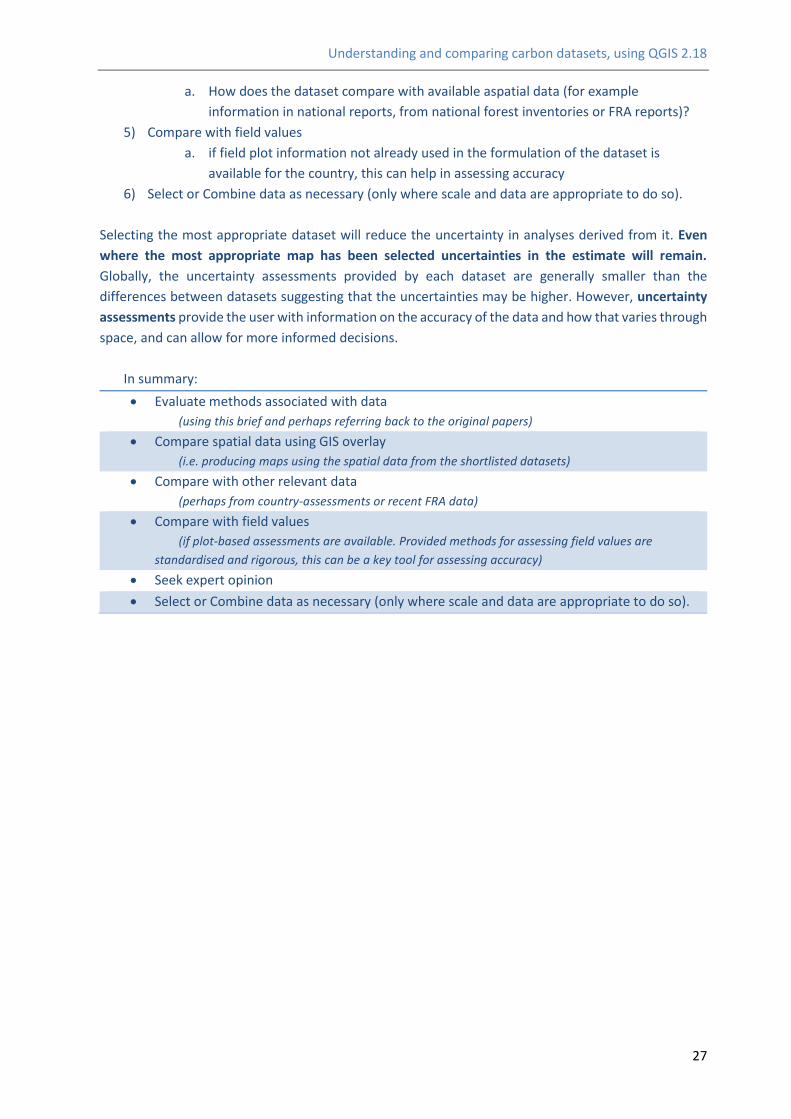
In summary:

Evaluate methods associated with data

(using this brief and perhaps referring back to the original papers)

Compare spatial data using GIS overlay

(i.e. producing maps using the spatial data from the shortlisted datasets)

Compare with other relevant data

(perhaps from country-assessments or recent FRA data)

Compare with field values

(if plot-based assessments are available. Provided methods for assessing field values are

standardised and rigorous, this can be a key tool for assessing accuracy)

Seek expert opinion

Select or Combine data as necessary (only where scale and data are appropriate to do so).


28

References

Avitabile, V., Herold, M., Heuvelink, G.B.M. et al. (2016) An integrated pan-tropical biomass map using multiple reference datasets. Global Change Biology 22(4): 1406-1420. doi:10.1111/gcb.13139

Baccini, A., Goetz, S.J., Walker, W.S. et al. (2012) Estimated carbon dioxide emissions from tropical deforestation improved by carbon-density maps. Nature Climate Change 2(3): 182–185.

Chave, J., Réjou-Méchain, M., Búrquez, A. et al. (2014) Improved allometric models to estimate the aboveground biomass of tropical trees. Global Change Biology. 20(10): 3177-3190.

CIESIN 2002. Last of the Wild Project, Version 1 (LWP-1): Global Human Footprint. Dataset (Geographic). Wildlife Conservation Society (WCS) and Center for International Earth Science Information Network (CIESIN), Palisades, NY. Available at: http://www.ciesin.org/wild_areas/

Feldpausch, T.R., Lloyd, J., Lewis, S.L. et al. (2012) Tree height integrated into pantropical forest biomass estimates. Biogeosciences 9: 3381–3403.

Kindermann, G.E., McCallum, I., Fritz, S., et al. (2008). A Global Forest Growing Stock, Biomass and Carbon Map Based on FAO Statistics. Silva Fennica 42(3): 387-396.

Köchy, M., Hiederer, R. and Freibauer, A., 2015. Global distribution of soil organic carbon–Part 1: Masses and frequency distributions of SOC stocks for the tropics, permafrost regions, wetlands, and the world. Soil, 1(1), pp.351-365.

McRoberts, R., Westfall, J.A. (2014). The effects of uncertainty in model predictions of individual tree volume on large area volume estimates. Forest Science 60 (1): 34-42.

Mitchard, E.T.A, Saatchi, S.S., Baccini, A. et al. (2013) Uncertainty in the spatial distribution of tropical forest biomass: a comparison of pan-tropical maps. Carbon Balance and Management 8:10.

Mitchard, E.T.A., Feldpausch, T.R., Brienen, R.J.W. et al. (2014) Markedly divergent estimates of Amazon forest carbon density from ground plots and satellites. Global Ecology and Biogeography 23(8):935-946.

Maukonen, P., Runsten, L., Thorley, J., Gichu, A., Akombo, R. and Miles, L. (2016). Mapping to support land-use planning for REDD+ in Kenya: securing additional benefits. Prepared on behalf of the UN-REDD Programme, Cambridge, UK: UNEP-WCMC. Available at: http://bit.ly/kenya-redd

Neigh, C.S.R., Nelson, R.F., Ranson, K.J. et al. (2013) Taking stock of circumboreal forest carbon with ground measurements, airborne and spaceborne LiDAR. Remote Sensing of Environment 137: 274–287.

Ruesch, A.S., Gibbs, H.K. (2008) New IPCC Tier-1 Global Biomass Carbon Map for the Year 2000. Oak Ridge National Laboratory’s Carbon Dioxide Information Analysis Center, Tennessee, USA. Available at: http://cdiac.ornl.gov/.

Saatchi, S.S., Harris, N.L., Brown, S. et al. (2011) Benchmark map of forest carbon stocks in tropical regions across three continents. Proceedings of the National Academy of Sciences of the United States of America 108(24):9899–9904.

Santoro, M., Cartus, O., Mermoz, S., Bouvet, A., Le Toan, T., Carvalhais, N., Rozendaal, D., Herold, M., Avitabile, V., Quegan, S., Carreiras, J., Rauste, Y., Balzter, H., Schmullius, C., Seifert, F.M., 2018, GlobBiomass global above-ground biomass and growing stock volume datasets, available on-line at http://globbiomass.org/products/global-mapping

http://www.ciesin.org/wild_areas/

http://bit.ly/kenya-redd

http://cdiac.ornl.gov/


29

Thurner, M., Beer, C., Santoro, M. et al. (2014) Carbon stock and density of northern boreal and temperate forests. Global Ecology and Biogeography, 23: 297–310.

UN-REDD Programme 2015. Considering the use of spatial modelling in Forest Reference Emission Level and/or Forest Reference Level construction for REDD+. UN-REDD Programme Info Brief. Available in English, French & Spanish at: http://www.unredd.net/documents/global-programme-191/mrv-and-monitoring-296/frl.html .

Willcock, S., Phillips, O.L., Platts, P.J., Balmford, A. et al. (2012) Towards Regional, Error-Bounded

Landscape Carbon Storage Estimates for Data Deficient Areas of the World. PLoS ONE 7(9): e44795. doi:10.1371/journal.pone.0044795 [open access]

Annex 2 : Glossary of terms

Acronymn definition Description Source

AGB Above ground biomass

All biomass of living vegetation, both woody and herbaceous, above the soil including stems, stumps, branches, bark, seeds, and foliage.

Terms and Definitions - FRA 2020,

FAO, 2018 (http://www.fao.org/ 3/I8661EN/i8661en.pdf).

ALOS Advanced Land Observing Satellite

The Japanese Earth observing satellite used mainly for land observation. The Advanced Land Observing Satellite (ALOS) follows the Japanese Earth Resources Satellite-1 (JERS-1). ALOS will be used for cartography, regional observation, disaster monitoring, and resource surveying.

https://www.eorc.jaxa.jp/ALOS/en/about/about_index.htm

ASAR Advanced Synthetic Aperture Radar

The Advanced Synthetic Aperture Radar (ASAR) was an active radar sensor on-board the European Space Agency (ESA) satellite ENVISAT, operational from March 2002 to April 2012. Applications for this sensor are many and include the study of ocean waves, sea ice extent and motion, and land surface studies, such as deforestation and ground movement.

https://earth.esa.int/web/sppa/mission-performance/esa-missions/envisat/asar/sensor-description

AVHRR Advanced Very High Resolution Radiometer

The AVHRR is a radiation-detection imager that can be used for remotely determining cloud cover and the surface temperature

https://noaasis.noaa.gov/NOAASIS/ml/avhrr.html

BCEF Biomass Expansion and Conversion Factors

Is a multiplication factor that expands growing stock, or commercial round-wood harvest volume, or growing stock volume increment data, to account for non-merchantable biomass compon-ents such as branches, foliage, and non-commercial trees.

(IPCC. 2003. Good Practice Guidance for LULUCF - Glossary), FRA2005. ;

http://www.fao.org /faoterm/en/?defaultCollId=1

http://www.unredd.net/documents/global-programme-191/mrv-and-monitoring-296/frl.html

http://www.unredd.net/documents/global-programme-191/mrv-and-monitoring-296/frl.html

http://www.fao.org/%203/I8661EN/i8661en.pdf

http://www.fao.org/%203/I8661EN/i8661en.pdf







http://www.fao.org/faoterm/en/?defaultCollId=1



30

BGB Below ground biomass

All biomass of live roots. Fine roots of less than 2 mm diameter are excluded because these often cannot be disting-uished empirically from soil organic matter or litter.

Terms and Definitions - FRA 2015, Forest Resources Assessment Working Paper 180, FAO, 2015 (http://www.fao.org/docrep/017/ap862e/ap862e00.pdf).

BIOMASAR algorithm

An approach for retrieval of forest growing stock volume using stacks of multi-temporal SAR data

https://www.researchgate.net/publication/230662433_The_BIOMASAR_algorithm_An_approach_for_retrieval_of_forest_growing_stock_volume_using_stacks_of_multi-temporal_SAR_data

BRDF Bi-directional Reflectance Distribution Function

The bidirectional reflectance distribution function is a function of four real variables that defines how light is reflected at an opaque surface.

https://en.wikipedia.org/wiki/Bidirectional_reflectance_distribution_function

CEOS WGCV LPV

Committee on Earth Observation Satellites (CEOS) Working Group on Calibration and Validation (WGCV) Land Product Validation (LPV)

The Committee on Earth Observation Satellites (CEOS), defines validation as the process of assessing, by independent means, the quality of the data products derived from the system outputs.

https://landval.gsfc.nasa.gov/

DBH Diameter at breast height

The stem diameter of a tree measured at breast height.

FAO Language Resources Project, 2005; IUFRO, Vienna, 2005; IUFRO World Series Vol.9-en, 2000. http://www.fao.org/faoterm/en/?defaultCollId=1

Envisat European Space Agency Environmental Satellite

The European Space Agency's Envisat satellite was operational from March 2002 to April 2012. It superceded the ESR satellites, having more advanced imaging radar, radar altimeter and temperature-measuring radiometer instruments, supplemented by new instruments including a medium-resolution spectrometer sensitive to both land features and ocean colour. Envisat also carried two atmospheric sensors monitoring trace gases.

https://earth.esa.int/web/guest/missions/esa-operational-eo-missions/envisat

ESA CCI European Space Agency Climate Change Initiative

FAO The Food and Agriculture Organization of the United Nations










https://landval.gsfc.nasa.gov/










31

FRA Forest Resources Assessments

The Global Forest Resources Assessments (FRA) are now produced every five years in an attempt to provide a consistent approach to describing the world's forests and how they are changing.

http://www.fao.org/forest-resources-assessment/background/en/

GHG-AFOLU Greenhouse Gas emissions in Agriculture, Forestry and Other Land Use

https://www.ipcc.ch/pdf/assessment-report/ar5/wg3/ipcc_wg3_ar5_chapter11.pdf

GLAS The Geoscience Laser Altimeter System

GLAS (the Geoscience Laser Altimeter System) is the first laser-ranging (lidar) instrument for continuous global observations of Earth. GLAS is the primary instrument aboard the ICESat spacecraft.

https://www.nasa.gov/mission_pages/icesat/

GLC2000 Global Land Cover 2000

The JRC coordinated and implemented the Global Land Cover 2000 Project (GLC 2000) in collaboration with a network of partners around the world. The general objective to provide for the year 2000 a harmonised land cover database over the whole globe.

https://ec.europa.eu/jrc/en/scientific-tool/global-land-cover

GPCP Global Precipitation Climatology Project

https://climatedataguide.ucar.edu/climate-data/gpcp-monthly-global-precipitation-climatology-project

GSV Growing Stock Volume

volume of all living trees more than 10 cm in diameter at breast height measured over bark from ground or stump height to a top stem diameter of 0 cm. Excludes: smaller branches, twigs, foliage, flowers, seeds, stump and roots

https://doi.pangaea.de/10.1594/PANGAEA.894711

HPDI Highest Posterior Density Interval

Interval used in Bayesian statistics. Choosing the narrowest interval, which for a unimodal distribution will involve choosing those values of highest probability density including the mode. This is sometimes called the highest posterior density interval.

https://en.wikipedia.org/wiki/Credible_interval

ICESAT The Ice, Clouds, and Land Elevation Satellite

Ppart of NASA' Earth Observing System (EOS)


IPCC Intergovernmental Panel on Climate Change

The international body for assessing the science related to climate change

http://www.ipcc.ch/





















http://www.ipcc.ch/


32

JAXA The Japan Aerospace Exploration Agency

http://global.jaxa.jp/about/jaxa/index.html

JRC Joint Research Centre European Commission's science and knowledge service

https://ec.europa.eu/jrc/en/about/jrc-in-brief

LAI Leaf Area Index The total area of green leaves per unit area of ground covered. Usually expressed as a ratio. (Terminology for integrated resource planning and management, 1999 - X2079E)


Landsat 7 ETM +

Landsat 7 Enhanced Thematic Mapper Plus (ETM+)

The Landsat Enhanced Thematic Mapper Plus (ETM+) sensor onboard the Landsat 7 satellite has acquired images of the Earth nearly continuously since July 1999, with a 16-day repeat cycle.

https://lta.cr.usgs.gov/LETMP

LIDAR Light Detection And Ranging

A surveying method that measures distance to a target by illuminating the target with pulsed laser light and measuring the reflected pulses with a sensor. Differences in laser return times and wavelengths can then be used to make digital 3-D representations of the target.

https://en.wikipedia.org/wiki/Lidar

MaxEnt Maxent software for modeling species niches and distributions by applying a machine-learning technique called maximum entropy modeling.

https://biodiversityinformatics.amnh.org/open_source/maxent/

MERRA Modern-Era Retrospective analysis for Research and Applications

The Modern-Era Retrospective analysis for Research and Applications (MERRA) dataset was released in 2009. It is based on a version of the GEOS-5 atmospheric data assimilation system that was frozen in 2008. MERRA data span the period 1979 through February 2016 and were produced on a 0.5° × 0.66° grid with 72 layers. MERRA was used to drive stand-alone reanalyses of the land surface (MERRA-Land) and atmospheric aerosols (MERRAero).

https://gmao.gsfc.nasa.gov/reanalysis/MERRA/







https://lta.cr.usgs.gov/LETMP

https://en.wikipedia.org/wiki/Lidar






33

MODIS Moderate Resolution Imaging Spectroradiometer

MODIS is ideal for monitoring large-scale changes in the biosphere that are yielding new insights into the workings of the global carbon cycle. MODIS measures the photosynthetic activity of land and marine plants (phytoplankton) to yield better estimates of how much of the greenhouse gas is being absorbed and used in plant productivity. Coupled with the sensor’s surface temperature measurements, MODIS’ measurements of the biosphere are helping scientists track the sources and sinks of carbon dioxide in response to climate changes.

https://terra.nasa.gov/about/terra-instruments/modis

MODIS LST MODIS Land Surface Temperature Products

https://lpdaac.usgs.gov/sites/default/files/public/product_documentation/mod11_user_guide.pdf

MODIS NBAR

MODIS Nadir BRDFAdjusted Reflectance

The MODIS MCD43A4 Version 6 Nadir Bidirectional reflectance distribution function Adjusted Reflectance (NBAR) data set is a daily 16-day product. The MCD43A4 provides the 500 meter reflectance data of the MODIS “land” bands 1-7 adjusted using the bidirectional reflectance distribution function to model the values.

https://lpdaac.usgs.gov/dataset_discovery/modis/modis_products_table/mcd43a4_v006

MVC Maximum value composite

A maximum-value composite procedure (or MVC) is a procedure used in satellite imaging, which is applied to vegetation studies. It requires that a series of multi-temporal geo-referenced satellite data be processed into NDVI images. On a pixel-by-pixel basis, each NDVI value is examined, and only the highest value is retained for each pixel location. After all pixels have been evaluated, the result is known as an MVC image.[1]

https://en.wikipedia.org/wiki/Maximum-value_composite_procedure

NDVI Normalized difference vegetation index

The normalized difference vegetation index (NDVI) is a simple graphical indicator that can be used to analyze remote sensing measurements, typically, but not necessarily, from a space platform, and assess whether the target being observed contains live green vegetation or not.

https://en.wikipedia.org/wiki/Normalized_difference_vegetation_index















34

NOAA National Oceanic and Atmospheric Administration

NPP Net Primary Productivity

How much carbon dioxide vegetation takes in during photosynthesis minus how much carbon dioxide the plants release during respiration (metabolizing sugars and starches for energy).

https://earthobservatory.nasa.gov/global-maps/MOD17A2_M_PSN

PALSAR Phased Array type L-band Synthetic Aperture Radar

An active microwave sensor using L-band frequency to achieve cloud-free and day-and-night land observation. It provides higher performance than the JERS-1's synthetic aperture radar (SAR).

https://www.eorc.jaxa.jp/ALOS/en/about/palsar.htm

QSCAT Quick Scatterometer A SeaWinds instrument placed in orbit quickly was launched in June 1999 and operated until November 2009. SeaWinds scatterometers are essentially radars that transmit microwave pulses down to the Earth's surface and then measure the power that is returned back to the instrument. This "backscattered" power is related to surface roughness. For water surfaces, the surface roughness is highly correlated with the near-surface wind speed and direction. Hence, wind speed and direction at a height of 10 meters over the ocean surface are retrieved from measurements of the scatterometer's backscattered power.

http://www.remss.com/missions/qscat/

SAR Synthetic Aperture Radar

Synthetic Aperture Radar (SAR) refers to a technique for producing fine resolution images from an intrinsically resolution-limited radar system.

https://nisar.jpl.nasa.gov/technology/sar/

Soil organic carbon

Organic carbon in mineral and organic soils (including peat) to a specified depth chosen by the country and applied consistently through the time series.

Terms and Definitions - FRA 2020, FAO, 2018 (http://www.fao.org/3/I8661EN/i8661en.pdf).

SRTM Shuttle Radar Topography Mission

High resolution topographic data generated from NASA's Shuttle Radar Topography Mission.

https://www2.jpl.nasa.gov/srtm/









https://www2.jpl.nasa.gov/srtm/

Step by Step Tutorial V10 Understanding and Comparing ...

Documents