STELLAR POPULATIONS OF Lyα EMITTERS AT z = 4.86: A COMPARISON TO z ∼ 5 LYMAN BREAK GALAXIES

The Astrophysical Journal, 720:1016–1029, 2010 September 10 doi:10.1088/0004-637X/720/2/1016C© 2010. The American Astronomical Society. All rights reserved. Printed in the U.S.A.

STELLAR POPULATIONS OF Lyα EMITTERS AT z = 4.86: A COMPARISON TO z ∼ 5LYMAN BREAK GALAXIES∗

Suraphong Yuma1, Kouji Ohta

1, Kiyoto Yabe

1, Kazuhiro Shimasaku

2, Makiko Yoshida

2, Masami Ouchi

3,

Ikuru Iwata4, and Marcin Sawicki

51 Department of Astronomy, Kyoto University, Sakyo-ku, Kyoto 606-8502, Japan; [email protected]

2 Department of Astronomy, School of Science, University of Tokyo, Tokyo 113-0033, Japan3 Observatories of the Carnegie Institution of Washington, 813 Santa Barbara Street, Pasadena, CA 91101, USA4 Okayama Astrophysical Observatory, National Astronomical Observatory of Japan, Okayama 719-0232, Japan

5 Department of Astronomy and Physics, Saint Mary’s University, 923 Robie Street, Halifax, Nova Scotia, B3H 3C3, CanadaReceived 2010 January 28; accepted 2010 July 12; published 2010 August 16

ABSTRACT

We present a study of a stellar population of Lyα emitters (LAEs) at z = 4.86 in the Great Observatories OriginsDeep Survey North (GOODS-N) field and its flanking field. The LAEs are selected based on optical narrowband(NB711) and broadband (V, Ic, and z′) observations by the Suprime-Cam attached to the Subaru Telescope. Withthe publicly available Infrared Array Camera (IRAC) data in GOODS-N and further IRAC observations in theflanking fields, we select five LAEs that are not contaminated by neighboring objects in IRAC images and constructtheir observed spectral energy distributions (SEDs) with Ic, z′, IRAC 3.6 μm, and 4.5 μm band photometries. TheSEDs cover the rest-frame UV-to-optical wavelengths. We derive the stellar masses, ages, color excesses, and starformation rates (SFRs) of the five LAEs using an SED fitting method. Assuming a constant star formation history,we find that the stellar masses range from 108 to 1010 M� with the median value of 2.5 × 109 M�. The derivedages range from very young (7.4 Myr) to 437 Myr, with a median age of 25 Myr. The color excess E(B − V ) isbetween 0.1 and 0.4 mag. SFRs are 55–209 M� yr−1. A comparison of the stellar populations is made between 3LAEs and 88 Lyman break galaxies (LBGs) selected at the same redshift, in the same observed field, and down tothe same limit of the rest-frame UV luminosity. These three LAEs are the brightest and reddest samples of all theLAE samples at z = 4.86. The LAEs are distributed at the relatively faint part of the UV-luminosity distribution ofLBGs. Deriving the stellar properties of the LBGs by fitting their SEDs with the same model ensures that modeldifference does not affect the comparison. It is found that the stellar properties of the LAEs are located in the regionwhere the properties of LBGs are distributed. On average, the LAEs show less dust extinction and lower SFRs thanLBGs, while the stellar mass of LAEs lies nearly in the middle part of the mass distribution of LBGs. However,the stellar properties of LAEs and LBGs are similar at the fixed UV or optical luminosity. We also examine therelations between the output properties from the SED fitting and the rest-frame Lyα equivalent width, but cannotfind any significant correlation.

Key words: galaxies: evolution – galaxies: formation – galaxies: high-redshift

Online-only material: color figures

1. INTRODUCTION

There are two popular techniques for isolating galaxies athigh redshift (z � 3): broadband selection (i.e., Lyman breaktechnique) and narrowband selection. Lyman break galaxies(LBGs) are selected by the Lyman break technique by takingadvantage of the spectral discontinuity due to the neutralhydrogen attenuation in the intergalactic medium (IGM) at rest-frame wavelengths shorter than 912/1216 Å. By using thismethod, a large number of high-redshift galaxies are studied(e.g., Steidel et al. 1996, 1999, 2003; Giavalisco et al. 1996,1998; Lowenthal et al. 1997; Pettini et al. 1998; Shapley et al.2001, 2003; Iwata et al. 2003, 2007; Papovich et al. 2004;Bouwens et al. 2004, 2008; Reddy et al. 2005, 2006, 2008;Sawicki & Thompson 2005, 2006; Yoshida et al. 2006). Theother method is to select galaxies with strong Lyα emission lineswhich fall into a narrowband filter. This method is useful forselecting high-redshift galaxies that have a strong Lyα emissionline. These objects are called Lyα emitters (LAEs). Partridge &Peebles (1967) proposed that primordial galaxies in the earlystage of their formation should show a strong Lyα emission

∗ Based on data collected at Subaru Telescope, which is operated by theNational Astronomical Observatory of Japan.

line. LAEs are thus expected to be young galaxies with lowmetallicity. Many surveys have been undertaken to search forgalaxies with a strong Lyα emission at various redshifts rangingfrom 2.1 to 6.6 or even more (e.g., Hu & McMahon 1996;Cowie & Hu 1998; Hu et al. 1998, 2004; Rhoads et al. 2000,2004; Kudritzki et al. 2000; Rhoads & Malhotra 2001; Malhotra& Rhoads 2002; Fynbo et al. 2001; Ouchi et al. 2003, 2008;Fujita et al. 2003; Shimasaku et al. 2003, 2004, 2006; Kodairaet al. 2003; Ajiki et al. 2003, 2004, 2006; Taniguchi et al. 2005;Venemans et al. 2002, 2004; Iye et al. 2006; Ota et al. 2008;Nilsson et al. 2009; Guaita et al. 2010).

In order to examine the evolutionary stage of LAEs and toreveal what kind of galaxiers they are, various properties ofLAEs have been studied such as luminosity functions (e.g.,Ouchi et al. 2003, 2008; Malhotra & Rhoads 2004; Shimasakuet al. 2006; Kashikawa et al. 2006; Gronwall et al. 2007; Otaet al. 2008) and clustering properties (e.g., Ouchi et al. 2003;Shimasaku et al. 2003, 2004, 2006; Kashikawa et al. 2006;Murayama et al. 2007). Revealing the stellar population of LAEsis crucial for understanding their physical nature. In order todo that, the spectral energy distribution (SED) of a galaxy iscompared with stellar population synthesis models producedby varying the ages, metallicities, amounts of dust extinctions,

1016

No. 2, 2010 STELLAR POPULATIONS OF LAEs AT z = 4.86 1017

61.9

62

62.1

62.2

62.3

62.4

188.4 188.7 189 189.3 189.6 189.9

De

clin

atio

n

Right Ascension

HDF-N

IRAC: GOODS-N

Suprime-Cam

GOODS-FF

Figure 1. Observed fields. The solid line indicates the effective field observedwith Suprime-Cam, while the long and short dashed lines show the GOODS-Nand GOODS-FF fields observed with IRAC. HDF-N is shown as a reference atthe center of the figure.

star formation rates (SFRs), etc. The stellar population of agalaxy can be constrained from the best-fit model. This methodis known as the SED fitting method. Recent studies show thatLAEs have wide ranges of ages (1 Myr to 1 Gyr) and stellarmasses (106–1010 M�; e.g., Gawiser et al. 2006, 2007; Laiet al. 2007, 2008; Nilsson et al. 2007; Finkelstein et al. 2007,2008, 2009; Pirzkal et al. 2007). Among these studies, stackinganalysis shows that LAEs at z ∼ 3 are free from dust or showmodest dust extinction (E(B − V ) � 0.03 mag; e.g., Gawiseret al. 2006, 2007; Lai et al. 2008; Ono et al. 2010), whereasSED fitting of an individual LAE at higher redshifts suggeststhat some of the LAEs show significant dust extinction (e.g., Laiet al. 2007; Finkelstein et al. 2009).

It is important to investigate the connection between LAEsand other galaxy populations selected by different methods,i.e., LBGs that are selected based on UV continuum. Sincethese two methods suffer from different biases, the selectedgalaxies partially overlap and the relationship between themis not clear. Shapley et al. (2001) divided LBGs at z ∼ 3into two subsamples according to their ages obtained by SEDfitting: an “old subsample” with ages about 1 Gyr and a “youngsubsample” with ages less than 35 Myr. They found that theold subsample shows a strong Lyα emission line, while theyoung subsample does not. In other words, they found thatLBGs with a Lyα emission line are older than those without aLyα emission line. Confirming this statement, the recent workwith a larger sample at the same redshift by Kornei et al. (2010)shows that objects with rest-frame Lyα equivalent width (EW)larger than 20 Å seem to be older, lower in SFR, and less dustythan those without a Lyα emission line. Pentericci et al. (2007),in contrast, found that at z ∼ 4 LBGs with Lyα emission areless massive and younger than those with no line. Consideringthe results from the SED analysis mentioned above, there maybe an evolution of differences between LAEs and LBGs withredshifts (e.g., Shimizu & Umemura 2010). Although there aresome SED studies at higher redshift (z � 5; Pirzkal et al. 2007;Lai et al. 2007), the relationship between LAEs and LBGs isstill unknown. In this paper, we study the stellar populations ofLAEs at z = 4.86 from their rest-frame UV-to-optical SEDs.Down to the same UV luminosity, the derived stellar propertiesof LAEs are compared to those of LBGs by Yabe et al. (2009).

0

0.1

0.2

0.3

0.4

0.5

0.6

0.7

6000 8000 10000 0.001

0.01

0.1

1

Effective T

ransm

issio

n

f ν (

μJy)

Observed wavelength (μm)

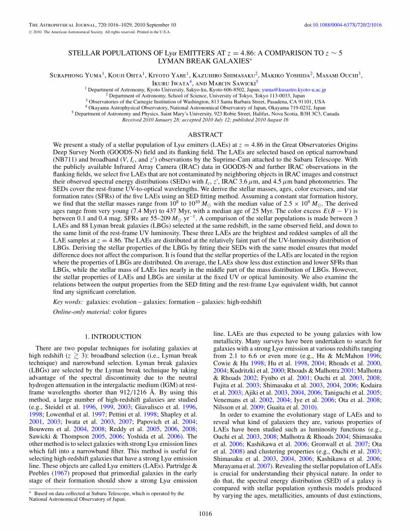
Figure 2. Transmission curves of V, NB711, Ic, and z′ bandpasses. CCDresponse, transmission of PFC, mirror reflectivity, and airmass (sec z = 1.2)are included. Also shown is a model spectrum in the unit of μJy (solid line) ofa star-forming galaxy at z = 4.86 including a Lyα emission line with an EWrestof 10 Å. The model is constructed using the Bruzual & Charlot (2003) stellarsynthesis code. A constant star formation history and Salpeter IMF are assumedat an age of 12 Myr and at the SFR of 1 M� yr−1. The attenuation by IGM isapplied using the prescription by Madau (1995).

They selected LBGs at the same redshift range in the same fieldand used the same fitting code and synthesis spectral modelassumptions. This direct comparison between LAEs and LBGsis expected to reveal their differences and to help define the kindof properties that make a galaxy an LAE.

Data sources and photometry are described in Section 2.Section 3 explains the selection criteria and the LAE candidates.The observed SEDs are constructed for each LAE candidateand compared to the models in Section 5. The fitting results areshown in Section 6. Section 7 offers comparisons between LAEsand LBGs. The summary is given in Section 8. Throughout thispaper, we use the AB magnitude system (Oke & Gunn 1983) andadopt a cosmology with parameters of Ωm = 0.3, ΩΛ = 0.7,and H0 = 70 km s−1 Mpc−1.

2. DATA SOURCES AND PHOTOMETRY

2.1. Optical Data

2.1.1. Observations and Data Reduction

Optical data were obtained with the Suprime-Cam (Miyazakiet al. 2002) attached to the Subaru Telescope (Iye et al. 2004).The observed field is toward the Hubble Deep Field-North(HDF-N; Williams et al. 1996) [R.A.(2000) = 12h36m49.s4,decl.(2000) = +62◦12′58′′] and is illustrated by the solid line inFigure 1. The pixel scale of the CCD was 0.′′20. We used NB711(λeff = 7126 Å, FWHM = 73 Å) and three broadband filters, V,Ic, and z′, to select z = 4.86 LAEs. The effective redshift intervalcalculated from the FWHM of NB711 is 4.83 � z � 4.89.Transmission curves, which include the responses of CCD,prime focus corrector (PFC), mirror, and airmass of all filtersused in this work are shown in Figure 2. The observationwith the NB711 filter was made on 2005 March 16. Imageswere taken with a dithering of ∼80′′ and an exposure timeof 1200 s for each frame. With 23 exposures, we covered a∼750 arcmin2 field of view. The total integration time was 7.7 hr.The weather condition was not so excellent. Seeing size duringthe observation was 1.′′5 on average.

Data reduction was made by using SDFRED version 1.4.1,the software developed for Suprime-Cam data reduction (Yagi

1018 YUMA ET AL. Vol. 720

et al. 2002; Ouchi et al. 2004). After bias subtraction, flatfielding, and distortion correction, image mosaicking was madeby identifying 30–170 non-saturated stars common in severalobject frames. The frame alignment and correction for flux/count and FWHM were made based on these star data. Theresulting FWHM of point sources in the mosaicked image is∼1.′′7.

Astrometry was performed based on the USNO-A2 catalogby fitting with the third-order polynomial coefficients to ∼1000stars identified in the mosaicked image. The positional error isabout 0.′′2 rms over the image. The magnitude zero point wasderived based on the imaging data of two spectrophotometricstandard stars (G191-B2B and HZ44) taken during the sameobserving night. As an independent check for photometryin NB711 images, we derived NB711 magnitudes of starsby interpolating their V, Ic, and z′ magnitudes. The derivedmagnitude zero points are in agreement within ∼0.18 mag. A3σ limiting magnitude at 2.′′5 diameter aperture is 26.16 magfor the NB711 image.

The observations and data reductions of broadband imagesare described in detail by Iwata et al. (2007). The images weretaken with V, Ic, and z′ filters in 2001 February. The typicalseeing during the observations was ∼1.′′1. In addition, Iwata et al.(2007) also used the imaging data taken from 2001 February toApril by the University of Hawaii (UH) group (Capak et al.2004), who used the same instrument and filters. The finaleffective survey area is 508.5 arcmin2. The limiting magnitudesof V-, Ic-, and z′-band images are 28.1, 26.8, and 26.6 mag,respectively (3σ at 1.′′6 diameter aperture). The broadbandimages were all degraded to a point-spread function (PSF) sizeof 1.′′7 to match that of the NB711 image. The 3σ limitingmagnitudes of the final PSF matched images at 2.′′5 diameteraperture are 27.3, 26.1, and 25.9 mag for V, Ic, and z′ images,respectively.

2.1.2. Photometric Catalog

The photometric catalogs of the optical images were madeby using SExtractor version 2.5.2 (Bertin & Arnouts 1996).The positions of objects were extracted from the NB711 im-age and the photometry was then made at the extracted po-sitions in all optical images via dual-image mode. In orderto use the dual-image mode, we first had to make a positionregistration between the broadband images and the NB711image. Position mapping between the images was made byusing geomap in IRAF6 based on positions of the bright butnon-saturated stars detected in the images. The registration ofthe images was performed by gregister. The accuracy in mak-ing a position registration is within 0.2 pixels or 0.′′04 rms. Af-ter image registration, we subtracted GLOBAL background fromeach registered image individually7 and homogenized the broad-band images so that they all have the same seeing size asthe NB711 image within 0.′′01 accuracy by gauss. The dual-image mode was then performed, using the following parame-ters. The images were filtered with a default convolution kernel(default.conv). The LOCAL background was estimated using a64 × 64 pixel background mesh with 3 × 3 median filtering. Anobject was detected with a minimum of five connected pixelsabove a 2.0σ minimum threshold. These parameters are found

6 IRAF is distributed by the National Optical Astronomy Observatory, whichis operated by the Association of Universities for Research in Astronomy, Inc.,under cooperative agreement with the National Science Foundation.7 Based on our simulation with artificial objects, the processes of subtractingthe background before smoothing the images and re-subtracting the LOCALbackground in SExtractor give better photometry.

to maximize the number of detected objects in the NB711 imageand minimize the detected numbers of objects in the negativeNB711 images.

In the SED fitting process, the total photometry of the objectsis necessary. The total magnitudes were obtained by applyingaperture corrections to 2.′′5 diameter aperture magnitudes. Weexamined the aperture sizes to determine the best value andchose 2.′′5, which maximizes the signal-to-noise ratio (S/N).The aperture corrections were determined from the MonteCarlo simulations where artificial objects with PSF shapescorresponding to the seeing size of 1.′′7 were put into theoriginal image and then detected by using the same SExtractorparameters. In the simulations, our objects were implicitlyassumed to be point sources since their apparent size in theimage is comparable to that of the PSF. The PSF was made bystacking images of the PSF that shows the stellarity index largerthan 0.98 and has no nearby objects. The aperture correctionfactors are −0.30 ± 0.01 and −0.33 ± 0.01 mag for Ic and z′images, respectively, where the errors are the PSF uncertainties.Errors of the total magnitudes are the combination of the 1σ errorin the photometry of simulated objects and the uncertainties ofcorrection factors. Because we do not use V and NB711 imagesin the SED fitting process, we do not compute the aperturecorrections for them.

2.2. Mid-infrared Data

Mid-infrared images are obtained from deep observationswith the Infrared Array Camera (IRAC) on the SpitzerSpace Telescope. We used the publicly available mid-infrareddata in the Great Observatories Origins Deep Survey North(GOODS-N; Dickinson et al. 2003) field centered at12h36m54.s87, +62◦14′19.′′2 (J2000) provided by the SpitzerSpace Telescope Legacy Science program.8 The field coversan area of approximately 10′ × 16′ or ∼160 arcmin2 as shownin Figure 1. In this work, we used the First Data Release (DR1)and Second Data Release (DR2) of IRAC data consisting ofimaging data in 3.6, 4.5, 5.8, and 8.0 μm bandpasses. The pixelscale of all images after being drizzled is 0.′′60 pixel−1. The meanFWHM of the PSF in IRAC GOODS-N images is ∼1.′′7. The 3σlimiting magnitudes of IRAC 3.6, 4.5, 5.8, and 8.0 μm imagesat 2.′′4 diameter aperture are 25.9, 25.8, 23.7, and 23.6 mag,respectively.

In addition to the very deep GOODS-N data, data in the flank-ing field (hereafter GOODS-FF) of GOODS-N are obtained tocover a part of the Subaru observation area. The GOODS-FFobservations were carried out with the IRAC in 2005 Decemberand 2006 June (the Spitzer GO program (GO-20218); PI: IkuruIwata). The observations were made by pointing at five differentpositions on the sky around the GOODS-N field. The total ex-posure time for each passband is 4000 s. Basic Calibrated Data(BCD) processed by the pipeline of the Spitzer Science Cen-ter (SSC) were used. The images were drizzled using MOPEXsoftware provided by SSC and combined together to get an im-proved mosaic image covering the whole observed area of ∼300arcmin2. The mosaic image has a final pixel scale of 0.′′61pixel−1

and a PSF size (FWHM) of 1.′′7. The 3σ magnitude limits at 2.′′4diameter aperture are 25.0, 24.6, 22.1, and 22.3 for IRAC 3.6,4.5, 5.8, and 8.0 μm bands, respectively. Combining the infrareddata obtained in the GOODS-N and GOODS-FF fields, we havethe effective area of ∼400 arcmin2 covering ∼80% of Subaruimages as seen in Figure 1.

8 http://ssc.spitzer.caltech.edu/spitzermission/observingprograms/legacy/goods/

No. 2, 2010 STELLAR POPULATIONS OF LAEs AT z = 4.86 1019

The photometry of IRAC was done based on the positionsof the LAEs at z = 4.86, which are selected from the criteriadescribed in the following section. Since the dimensions and thepixel scale of the narrowband image and IRAC images are dif-ferent, we could not use the dual-image mode in SExtractor todetermine the aperture photometry in IRAC images. Phot pro-vided by IRAF was used instead to perform aperture photometryat 2.′′4 diameter, which we determined to be the best aperturesize since it maximizes the S/N. Because the positions in theNB711 image are used as the reference, we made a registrationof the IRAC images before performing IRAC photometry ofthe objects. The position alignment was made globally for eachIRAC image by using positions of point sources detected in bothNB711 and IRAC images. The estimated errors in determiningthe position shifts are 0.′′1 (0.17 pixels) for IRAC images in theGOODS-N field and 0.′′2 (0.33 pixels) for those in the GOODS-FF. Since the error of 0.′′2 may not be negligible, we re-did thephotometry of objects at the positions separated from the cor-rected positions by 0.′′2 and found the magnitude difference tobe less than 0.2 mag. This magnitude difference gives less than3% difference in the stellar masses derived from SED fitting.

Aperture corrections for IRAC images were determined bythe following process. The artificial objects with IRAC PSF areput into the IRAC images. The PSF was made from imagesof objects identified to be a stellar object in Subaru images.For the GOODS-N field, the correction factors are −0.62 magand −0.72 mag in the 3.6 μm and 4.5 μm bands, respectively.The correction uncertainties due to the uncertainties in PSFsare 5% and 6% in the 3.6 μm and 4.5 μm bands, respectively.For GOODS-FF images, they are, respectively, −0.70 mag and−0.73 mag with 6% and 7% uncertainties in the 3.6 μm and4.5 μm bands. Errors in IRAC photometry are 1σ standarddeviations of sky background and the uncertainties of correctionfactors. Since 5.8 μm and 8.0 μm images show too low S/N toplace a useful upper limit in the SED fitting process, we do notuse them in our further analysis.

3. SAMPLE SELECTION

A total of 29,675 objects were detected with NB711 <26.0 mag (3.5σ limiting magnitude). Figure 3 shows theIc−NB711 color versus NB711 magnitudes of all objects (blackdots). We selected NB711-excess objects from the followingselection criteria:

Ic − NB711 > 0.64 (1)

andIc − NB711 > 3σIc−NB711, (2)

where 3σIc−NB711 is a 3σ error in measuring Ic − NB711 colorfor a source with a color of Ic − NB711 = −0.28 mag, theaverage color of all objects with NB711 magnitudes brighterthan 26.0 mag. Note that the magnitudes and colors of objectsused in the sample selection are the values at the 2.′′5 diameteraperture, except for those noted otherwise. The first criterioncorresponds to a rest-frame equivalent width (EWrest) of 10 Åassuming a flat continuum (fν = constant). The EW cut of 10 Åused in this paper is lower than that commonly used in other LAEstudies (20 Å). Other studies (e.g., Ouchi et al. 2003; Nilssonet al. 2009) compute the EW by using the average continuum fluxdensity from the continuum both blueward and redward of theLyα line, while the continuum in this work is extrapolated fromthe continuum redward of the Lyα line. Because the blueward

-1

-0.5

0

0.5

1

1.5

2

2.5

3

21 22 23 24 25 26 27

Ic−N

B7

11

NB711

z’ >= 26.5z’ < 26.5

Figure 3. Ic − NB711 color vs. NB711 2.′′5 aperture magnitude. LAEs withz′

total < 26.5 mag are shown with filled circles; filled triangles represent thosewith z′

total � 26.5 mag. Arrows show the lower limits of Ic − NB711 taken at2σIc limiting magnitude. Note that we used 2σIc limiting magnitude as a lowerlimit for objects whose Ic magnitudes are fainter than that. A diagonal blackline indicates 2σ limiting magnitude of the Ic image. Red curves indicate thedistributions of 3σ errors in measuring Ic − NB711 color for a source with acolor of Ic − NB711 = −0.28 mag, the average color of all objects brighterthan NB711 = 26.0 mag. The horizontal and vertical magenta lines show theNB711-excess criterion and NB711 = 26.0 mag limit, respectively.

(A color version of this figure is available in the online journal.)

continuum suffers from the attenuation by neutral hydrogen inthe IGM at high redshift, the continuum estimated by the lattermethod is expected to be higher than that in the usual case.Consequently, the EW computed in this paper is smaller thanthat from other studies, even though the object has the sameredward continuum. The Lyα EWs computed in the usual wayare also shown in Table 2; most of the LAEs compared to LBGsshow the EWs larger than 20 Å when we adopt the commonlyused method.

By the above criteria, 667 objects were selected. Among them,there are low-redshift interlopers with strong emission linessuch as Hα, Hβ, [O iii]λ5007, or [O ii]λ3727. To rule them out,we first divided the objects selected by the above criteria intotwo groups according to their brightness in the z′ band. Forcandidates with z′

total < 26.5 mag, we adopted the followingcriteria, which were used by Iwata et al. (2007, see theirFigure 2) to select LBGs at z ∼ 5:

z′total < 26.5, (3)

V − Ic > 1.55, (4)

andV − Ic > 7.0(Ic − z′) + 0.15, (5)

where z′total is the total magnitude in the z′ band and the

colors are derived from 2.′′5 diameter aperture magnitudes.These criteria have been confirmed by spectroscopic follow-up observations (Ando et al. 2004, 2007; Kajino et al. 2009).For objects with z′

total � 26.5 mag, we required non-detectionin the V-band magnitude (V > 1σ limiting magnitude). Asa result, 24 objects meet all criteria simultaneously down toNB711 = 26.0 mag as illustrated in Figure 3. Eleven of themshow z′ magnitudes brighter than 26.5 mag. Note that z′

total hereis slightly different from z′

magauto by Iwata et al. (2007; up to

1020 YUMA ET AL. Vol. 720

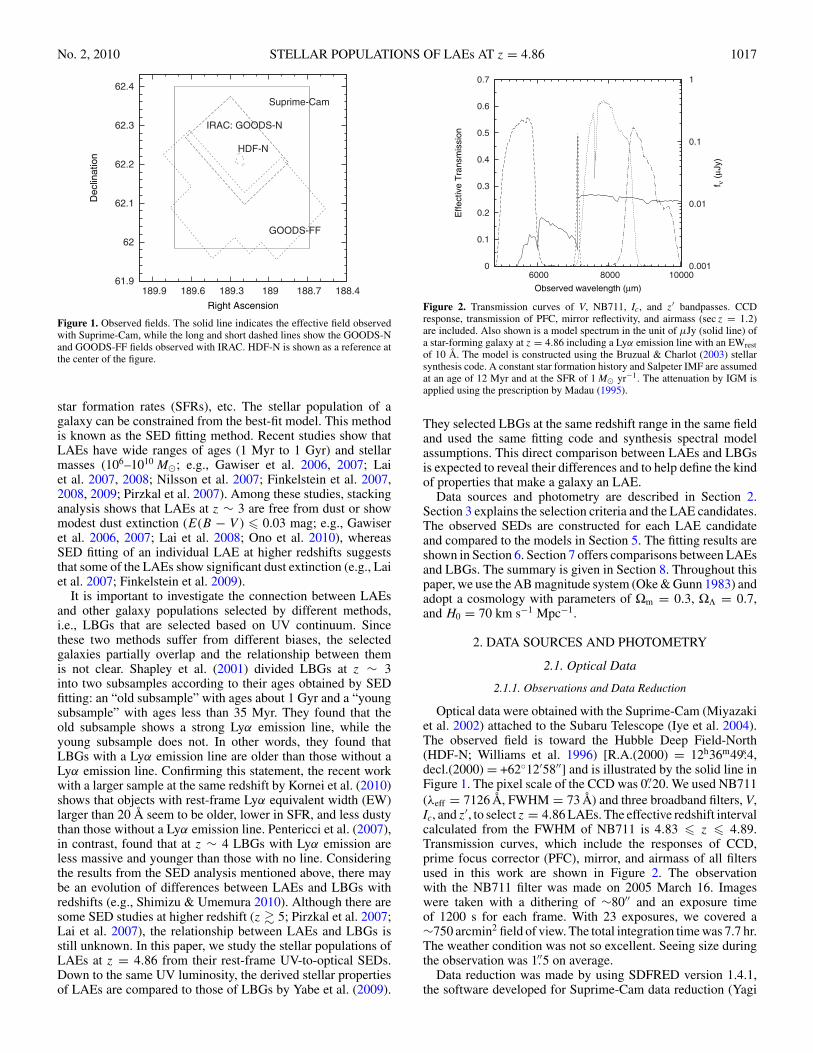
Figure 4. Montage of images of group I LAEs. Size of each image is 10′′ × 10′′with an LAE at the center of the image. North is at the top; east is to the left. IDsof objects are shown on the left of the figure. Note that the Subaru broadbandimages displayed here (V, Ic, and z′) are those before smoothing. An asteriskindicates the LAE with the spectroscopic redshift.

Figure 5. Same as Figure 4 but for group II LAEs.

±0.3 mag at z′ = 26.5 mag) because the broadband imagesused in this work were smoothed to match the NB711 seeingsize before making the photometry.

In order to study the properties of LAEs by SED fitting,the rest-frame optical photometry (i.e., IRAC photometry) isneeded. Sixteen out of twenty-four LAEs are in IRAC images(hereafter IRAC sample). Since the angular resolution of IRACimages is not excellent, some LAEs are contaminated by nearbyobjects. In order to examine whether or not neighboring objectsaffect the photometry of LAEs, we simultaneously fitted allneighboring objects within a 10′′ radius with GALFIT (Penget al. 2002) and subtracted them from the original image. Inthe GALFIT process, we masked the LAEs out so that theaccurate sky estimation can be obtained. We then performedaperture photometry of the LAEs from the residual images. Weonly selected LAEs of which magnitude differences between theoriginal images and the residual images are less than 0.1 mag asisolated LAEs. Finally, we have 12 isolated objects. We dividedthese 12 LAEs into four groups based on their brightness in therest-frame UV and optical wavelengths. Group I is for two LAEsthat are detected above the 2σ limiting magnitudes in all bandsused in the SED fitting process (i.e., Ic, z′, IRAC 3.6 μm, and4.5 μm). One of them, 35915, is spectroscopically confirmedto be at z = 4.82. The emission line does not show a doubletprofile in R ∼2000 spectrum obtained by GMOS on the Geminitelescope (M. Ouchi et al. 2010, in preparation). With the givenresolution, this can rule out the possibility that the object is an[O ii] emitter. Moreover, there seems to be a continuum break atthe wavelength shortward of the line. Two LAEs are classified asgroup II, which is an LAE detected in two bands: one in Subaruoptical and one in IRAC bands. One LAE is classified as groupIII which is not detected in the Ic and z′ bands but detected inboth 3.6 μm and 4.5 μm bands. Group IV is for seven LAEsthat are not detected above the 2σ limiting magnitudes in threeor more bands. In the SED fitting process, it is necessary thatan LAE should be detected above 2σ magnitude limit in morethan two bands; therefore, we can use only group I–III LAEs.Hereafter, we call group I–III LAEs the SED fitting sample. Themontage images of LAEs are shown in Figures 4, 5, 6, and 7

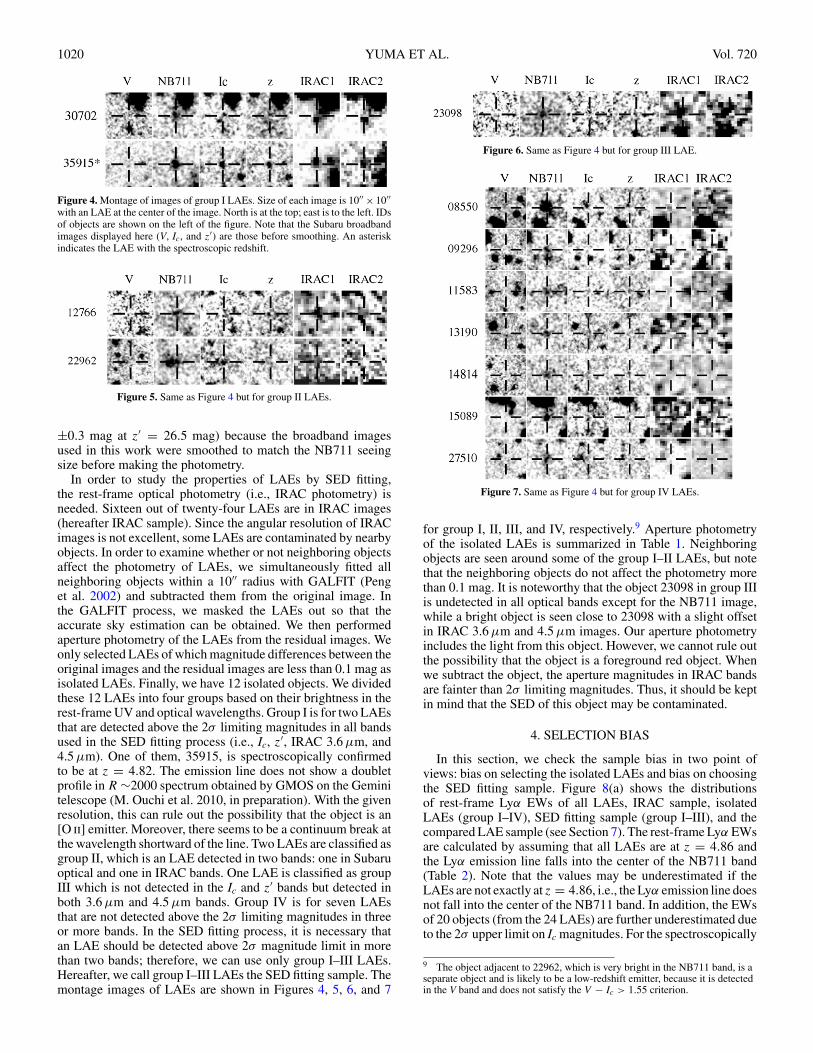
Figure 6. Same as Figure 4 but for group III LAE.

Figure 7. Same as Figure 4 but for group IV LAEs.

for group I, II, III, and IV, respectively.9 Aperture photometryof the isolated LAEs is summarized in Table 1. Neighboringobjects are seen around some of the group I–II LAEs, but notethat the neighboring objects do not affect the photometry morethan 0.1 mag. It is noteworthy that the object 23098 in group IIIis undetected in all optical bands except for the NB711 image,while a bright object is seen close to 23098 with a slight offsetin IRAC 3.6 μm and 4.5 μm images. Our aperture photometryincludes the light from this object. However, we cannot rule outthe possibility that the object is a foreground red object. Whenwe subtract the object, the aperture magnitudes in IRAC bandsare fainter than 2σ limiting magnitudes. Thus, it should be keptin mind that the SED of this object may be contaminated.

4. SELECTION BIAS

In this section, we check the sample bias in two point ofviews: bias on selecting the isolated LAEs and bias on choosingthe SED fitting sample. Figure 8(a) shows the distributionsof rest-frame Lyα EWs of all LAEs, IRAC sample, isolatedLAEs (group I–IV), SED fitting sample (group I–III), and thecompared LAE sample (see Section 7). The rest-frame Lyα EWsare calculated by assuming that all LAEs are at z = 4.86 andthe Lyα emission line falls into the center of the NB711 band(Table 2). Note that the values may be underestimated if theLAEs are not exactly at z = 4.86, i.e., the Lyα emission line doesnot fall into the center of the NB711 band. In addition, the EWsof 20 objects (from the 24 LAEs) are further underestimated dueto the 2σ upper limit on Ic magnitudes. For the spectroscopically

9 The object adjacent to 22962, which is very bright in the NB711 band, is aseparate object and is likely to be a low-redshift emitter, because it is detectedin the V band and does not satisfy the V − Ic > 1.55 criterion.

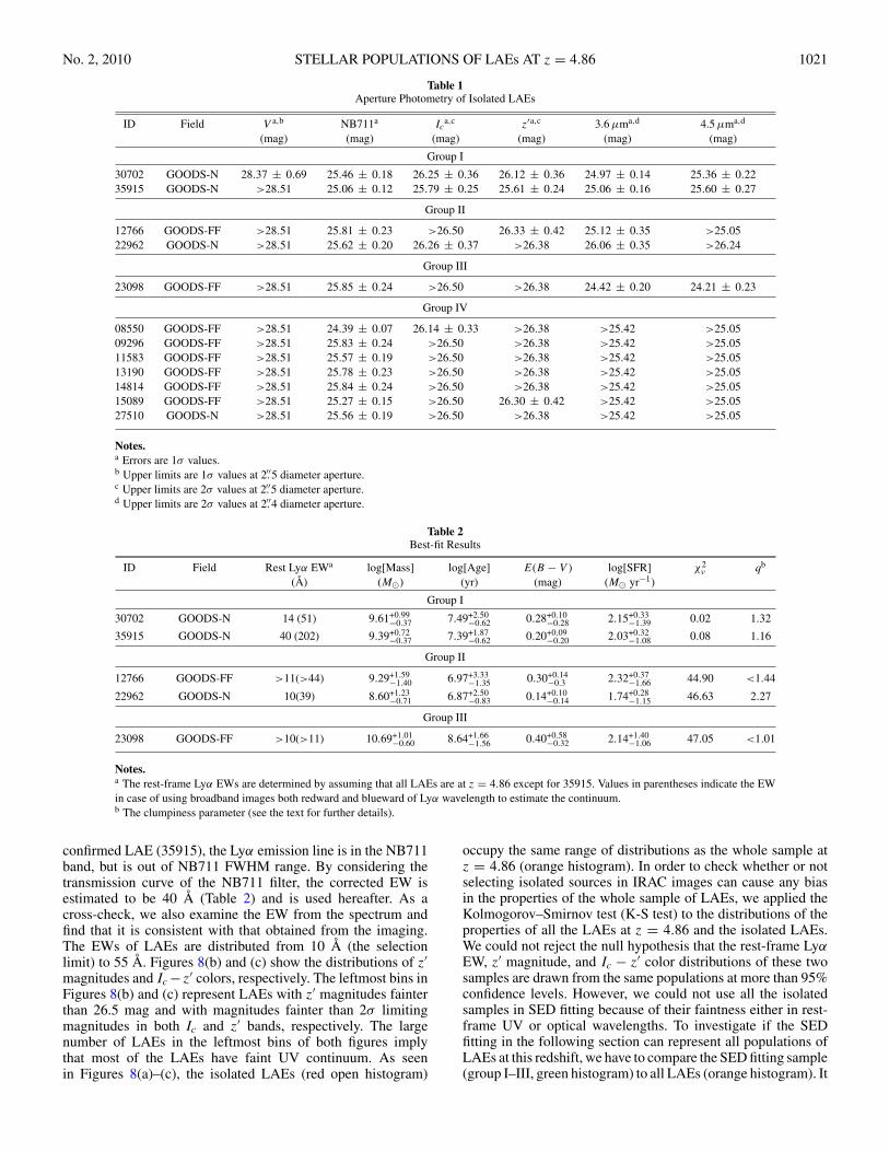
No. 2, 2010 STELLAR POPULATIONS OF LAEs AT z = 4.86 1021

Table 1Aperture Photometry of Isolated LAEs

ID Field V a,b NB711a Ica,c z′a,c 3.6 μma,d 4.5 μma,d

(mag) (mag) (mag) (mag) (mag) (mag)

Group I

30702 GOODS-N 28.37 ± 0.69 25.46 ± 0.18 26.25 ± 0.36 26.12 ± 0.36 24.97 ± 0.14 25.36 ± 0.2235915 GOODS-N >28.51 25.06 ± 0.12 25.79 ± 0.25 25.61 ± 0.24 25.06 ± 0.16 25.60 ± 0.27

Group II

12766 GOODS-FF >28.51 25.81 ± 0.23 >26.50 26.33 ± 0.42 25.12 ± 0.35 >25.0522962 GOODS-N >28.51 25.62 ± 0.20 26.26 ± 0.37 >26.38 26.06 ± 0.35 >26.24

Group III

23098 GOODS-FF >28.51 25.85 ± 0.24 >26.50 >26.38 24.42 ± 0.20 24.21 ± 0.23

Group IV

08550 GOODS-FF >28.51 24.39 ± 0.07 26.14 ± 0.33 >26.38 >25.42 >25.0509296 GOODS-FF >28.51 25.83 ± 0.24 >26.50 >26.38 >25.42 >25.0511583 GOODS-FF >28.51 25.57 ± 0.19 >26.50 >26.38 >25.42 >25.0513190 GOODS-FF >28.51 25.78 ± 0.23 >26.50 >26.38 >25.42 >25.0514814 GOODS-FF >28.51 25.84 ± 0.24 >26.50 >26.38 >25.42 >25.0515089 GOODS-FF >28.51 25.27 ± 0.15 >26.50 26.30 ± 0.42 >25.42 >25.0527510 GOODS-N >28.51 25.56 ± 0.19 >26.50 >26.38 >25.42 >25.05

Notes.a Errors are 1σ values.b Upper limits are 1σ values at 2.′′5 diameter aperture.c Upper limits are 2σ values at 2.′′5 diameter aperture.d Upper limits are 2σ values at 2.′′4 diameter aperture.

Table 2Best-fit Results

ID Field Rest Lyα EWa log[Mass] log[Age] E(B − V ) log[SFR] χ2ν qb

(Å) (M�) (yr) (mag) (M� yr−1)

Group I

30702 GOODS-N 14 (51) 9.61+0.99−0.37 7.49+2.50

−0.62 0.28+0.10−0.28 2.15+0.33

−1.39 0.02 1.32

35915 GOODS-N 40 (202) 9.39+0.72−0.37 7.39+1.87

−0.62 0.20+0.09−0.20 2.03+0.32

−1.08 0.08 1.16

Group II

12766 GOODS-FF >11(>44) 9.29+1.59−1.40 6.97+3.33

−1.35 0.30+0.14−0.3 2.32+0.37

−1.66 44.90 <1.44

22962 GOODS-N 10(39) 8.60+1.23−0.71 6.87+2.50

−0.83 0.14+0.10−0.14 1.74+0.28

−1.15 46.63 2.27

Group III

23098 GOODS-FF >10(>11) 10.69+1.01−0.60 8.64+1.66

−1.56 0.40+0.58−0.32 2.14+1.40

−1.06 47.05 <1.01

Notes.a The rest-frame Lyα EWs are determined by assuming that all LAEs are at z = 4.86 except for 35915. Values in parentheses indicate the EWin case of using broadband images both redward and blueward of Lyα wavelength to estimate the continuum.b The clumpiness parameter (see the text for further details).

confirmed LAE (35915), the Lyα emission line is in the NB711band, but is out of NB711 FWHM range. By considering thetransmission curve of the NB711 filter, the corrected EW isestimated to be 40 Å (Table 2) and is used hereafter. As across-check, we also examine the EW from the spectrum andfind that it is consistent with that obtained from the imaging.The EWs of LAEs are distributed from 10 Å (the selectionlimit) to 55 Å. Figures 8(b) and (c) show the distributions of z′magnitudes and Ic −z′ colors, respectively. The leftmost bins inFigures 8(b) and (c) represent LAEs with z′ magnitudes fainterthan 26.5 mag and with magnitudes fainter than 2σ limitingmagnitudes in both Ic and z′ bands, respectively. The largenumber of LAEs in the leftmost bins of both figures implythat most of the LAEs have faint UV continuum. As seenin Figures 8(a)–(c), the isolated LAEs (red open histogram)

occupy the same range of distributions as the whole sample atz = 4.86 (orange histogram). In order to check whether or notselecting isolated sources in IRAC images can cause any biasin the properties of the whole sample of LAEs, we applied theKolmogorov–Smirnov test (K-S test) to the distributions of theproperties of all the LAEs at z = 4.86 and the isolated LAEs.We could not reject the null hypothesis that the rest-frame LyαEW, z′ magnitude, and Ic − z′ color distributions of these twosamples are drawn from the same populations at more than 95%confidence levels. However, we could not use all the isolatedsamples in SED fitting because of their faintness either in rest-frame UV or optical wavelengths. To investigate if the SEDfitting in the following section can represent all populations ofLAEs at this redshift, we have to compare the SED fitting sample(group I–III, green histogram) to all LAEs (orange histogram). It

1022 YUMA ET AL. Vol. 720

Figure 8. Distributions of rest-frame Lyα EW, z′-band magnitude, and Ic − z′ color of LAE samples. We divide each figure into two panels for display purposes. Inthe top panel, an orange histogram shows the distribution of all 24 LAEs at z = 4.86, while the blue and red histograms are for the IRAC samples and the isolatedLAEs (group I–IV), respectively. In the bottom panel, red histograms refer to the isolated LAEs (the same as in the top panel). Group I–III LAEs are shown in greenhistograms. Distributions of group I LAEs and 12766 from group II LAEs (the compared LAE sample; see Section 7) are shown in gray histograms. Arrows shown inpanel (a) represent the lower limits in Lyα EWs of LAEs; the number of arrows directly corresponds to the number of LAEs with Lyα EW lower limits. Note that theleftmost bins in panels (b) and (c) indicate, respectively, the LAEs fainter than z′ = 26.5 mag and LAEs that are not detected above 2σ limiting magnitudes in neitherthe Ic nor z′ bands.

(A color version of this figure is available in the online journal.)

is seen in Figure 8(a) that group I–III LAEs represent both high-and low-EW LAEs. However, we can see from Figures 8(b) and(c) that the SED fitting sample is biased toward the bright UVluminosity and red Ic − z′ colors as we neglect the leftmost binswhere magnitudes are unreliable. In addition, Table 1 showsthat the SED fitting sample is relatively bright in IRAC bands ascompared to all isolated LAEs, implying brighter luminosity inthe rest-frame optical wavelength. Thus, we conclude that theSED fitting and the results hereafter are for the LAEs whichhave the brighter rest-frame UV and optical magnitudes, andthe relatively redder UV colors.

5. STELLAR POPULATION SYNTHESIS MODEL ANDSED FITTING

In this paper, we intend to compare the stellar populationsof the LAEs to those of LBGs at the same redshift by Yabeet al. (2009). In order to make a fair comparison, we usedthe same stellar population synthesis model as that used inYabe et al. (2009). The model SEDs were obtained with theBruzual & Charlot (2003, hereafter BC03) synthesis code. Weused the Padova 1994 evolutionary track as recommended byBC03. A Salpeter (1955) initial mass function (IMF) with lowerand upper mass cutoffs of 0.1 and 100 M� is assumed. Wemade models by fixing the metallicity at 0.2 Z�10 and assuminga constant star formation history. BC03 use quasi-logarithmic221 time steps from 0.1 Myr to 20 Gyr. Time steps wereadopted to 51 logarithmic steps both to reduce the calculationtime and to avoid dealing with an unequally spaced scale ofthe original 221 models. The age of the universe at z ∼ 5 is∼1.2 Gyr. However, as a cross-check on the fits, we allowedthe age up to the oldest one available in BC03. The effectof dust attenuation is taken into account by using the Calzetti

10 Fixing the metallicity at the lower abundance (0.005 Z�) does notsignificantly change the fitting results. The stellar masses derived from thelower metallicity model differ from those derived from the 0.2 Z� model by∼10% at most. The average differences of age, color excess, and SFR are∼50%, ±0.2 mag, and ∼5%, respectively.

extinction law (Calzetti et al. 2000), changing the color excessE(B − V ) from 0.0 mag to 0.8 mag with a step of 0.01. Theattenuation by the IGM is calculated using the prescription byMadau (1995). The model spectra were then convolved with theappropriate filter transmission curves to give model fluxes. Thisis exactly the same as done in Sawicki & Yee (1998). Exceptfor one spectroscopically confirmed LAE (35915; z = 4.82),the redshift was fixed at z = 4.86 under the assumption that theLyα emission of our LAE sample is detected at the center of theNB711 bandpass.

Some of the observed SEDs, including one spectroscopicallyconfirmed LAE, show a significant excess in the 3.6 μm band ascompared with the magnitude in the 4.5 μm band. This is likelyto be due to the Hα emission line, which falls into IRAC ch1(3.6 μm) at this redshift. The excess is also seen in some fractionof z ∼ 5 LBGs (Yabe et al. 2009). The SED model includingHα emission shows a better fit (Chary et al. 2005; Finkelsteinet al. 2008; Yabe et al. 2009). As adopted by Yabe et al. (2009),the spectrum of Hα emission is included in the synthesis modelspectrum by the following process. The luminosity of the Hαemission is calculated from the SFR of the model by using therelation by Kennicutt (1998).11 The dust extinction to the line(Calzetti et al. 2000) is assumed to be the same as the dustextinction to the stellar component.11 The Hα flux density isfinally put into each model SED. The existence of Hα emissionline in the models makes the fit better without adding a freeparameter (Yabe et al. 2009).

We use the SEDfit software (M. Sawicki 2010, in prepara-tion), which is an evolved version of the SED-fitting softwareused in Sawicki & Yee (1998) and subsequent papers, includingthe z ∼ 5 LBG study by Yabe et al. (2009). After we producea suite of model fluxes by the means described above, the best-fitting model is found by means of a maximum likelihood testfor each object. For objects detected in all bands (i.e., our groupI objects), this test is the standard χ2 minimization. For objects

11 Adopting this relation may be disputable. Dependences on metallicities anddifferences of extinction to stellar continuum and nebular emission arediscussed by Yabe et al. (2009, their Appendix B).

No. 2, 2010 STELLAR POPULATIONS OF LAEs AT z = 4.86 1023

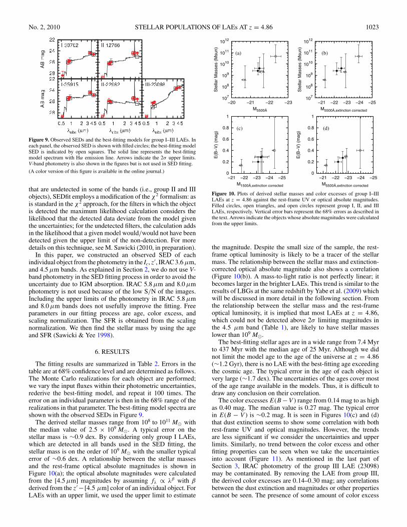
Figure 9. Observed SEDs and the best-fitting models for group I–III LAEs. Ineach panel, the observed SED is shown with filled circles; the best-fitting modelSED is indicated by open squares. The solid line represents the best-fittingmodel spectrum with Hα emission line. Arrows indicate the 2σ upper limits.V-band photometry is also shown in the figures but is not used in SED fitting.

(A color version of this figure is available in the online journal.)

that are undetected in some of the bands (i.e., group II and IIIobjects), SEDfit employs a modification of the χ2 formalism: asis standard in the χ2 approach, for the filters in which the objectis detected the maximum likelihood calculation considers thelikelihood that the detected data deviate from the model giventhe uncertainties; for the undetected filters, the calculation addsin the likelihood that a given model would/would not have beendetected given the upper limit of the non-detection. For moredetails on this technique, see M. Sawicki (2010, in preparation).

In this paper, we constructed an observed SED of eachindividual object from the photometry in the Ic, z′, IRAC 3.6 μm,and 4.5 μm bands. As explained in Section 2, we do not use V-band photometry in the SED fitting process in order to avoid theuncertainty due to IGM absorption. IRAC 5.8 μm and 8.0 μmphotometry is not used because of the low S/N of the images.Including the upper limits of the photometry in IRAC 5.8 μmand 8.0 μm bands does not usefully improve the fitting. Freeparameters in our fitting process are age, color excess, andscaling normalization. The SFR is obtained from the scalingnormalization. We then find the stellar mass by using the ageand SFR (Sawicki & Yee 1998).

6. RESULTS

The fitting results are summarized in Table 2. Errors in thetable are at 68% confidence level and are determined as follows.The Monte Carlo realizations for each object are performed;we vary the input fluxes within their photometric uncertainties,rederive the best-fitting model, and repeat it 100 times. Theerror on an individual parameter is then in the 68% range of therealizations in that parameter. The best-fitting model spectra areshown with the observed SEDs in Figure 9.

The derived stellar masses range from 108 to 1011 M� withthe median value of 2.5 × 109 M�. A typical error on thestellar mass is ∼0.9 dex. By considering only group I LAEs,which are detected in all bands used in the SED fitting, thestellar mass is on the order of 109 M� with the smaller typicalerror of ∼0.6 dex. A relationship between the stellar massesand the rest-frame optical absolute magnitudes is shown inFigure 10(a); the optical absolute magnitudes were calculatedfrom the [4.5 μm] magnitudes by assuming fλ ∝ λβ with βderived from the z′ − [4.5 μm] color of an individual object. ForLAEs with an upper limit, we used the upper limit to estimate

107

108

109

1010

1011

1012

−23−22−21−20

Ste

llar

Ma

sse

s (

Msu

n)

M5500Å

(a)

107

108

109

1010

1011

1012

−25−24−23−22−21

Ste

llar

Ma

sse

s (

Msu

n)

M5500Å,extinction corrected

(b)

0

0.2

0.4

0.6

0.8

1

−25−24−23−22−21

E(B

−V

) (m

ag

)

M1500Å,extinction corrected

(c)

0

0.2

0.4

0.6

0.8

1

−25−24−23−22−21

E(B

−V

) (m

ag

)

M5500Å,extinction corrected

(d)

Figure 10. Plots of derived stellar masses and color excesses of group I–IIILAEs at z = 4.86 against the rest-frame UV or optical absolute magnitudes.Filled circles, open triangles, and open circles represent group I, II, and IIILAEs, respectively. Vertical error bars represent the 68% errors as described inthe text. Arrows indicate the objects whose absolute magnitudes were calculatedfrom the upper limits.

the magnitude. Despite the small size of the sample, the rest-frame optical luminosity is likely to be a tracer of the stellarmass. The relationship between the stellar mass and extinction-corrected optical absolute magnitude also shows a correlation(Figure 10(b)). A mass-to-light ratio is not perfectly linear; itbecomes larger in the brighter LAEs. This trend is similar to theresults of LBGs at the same redshift by Yabe et al. (2009) whichwill be discussed in more detail in the following section. Fromthe relationship between the stellar mass and the rest-frameoptical luminosity, it is implied that most LAEs at z = 4.86,which could not be detected above 2σ limiting magnitudes inthe 4.5 μm band (Table 1), are likely to have stellar masseslower than 109 M�.

The best-fitting stellar ages are in a wide range from 7.4 Myrto 437 Myr with the median age of 25 Myr. Although we didnot limit the model age to the age of the universe at z = 4.86(∼1.2 Gyr), there is no LAE with the best-fitting age exceedingthe cosmic age. The typical error in the age of each object isvery large (∼1.7 dex). The uncertainties of the ages cover mostof the age range available in the models. Thus, it is difficult todraw any conclusion on their correlation.

The color excesses E(B −V ) range from 0.14 mag to as highas 0.40 mag. The median value is 0.27 mag. The typical errorin E(B − V ) is ∼0.2 mag. It is seen in Figures 10(c) and (d)that dust extinction seems to show some correlation with bothrest-frame UV and optical magnitudes. However, the trendsare less significant if we consider the uncertainties and upperlimits. Similarly, no trend between the color excess and otherfitting properties can be seen when we take the uncertaintiesinto account (Figure 11). As mentioned in the last part ofSection 3, IRAC photometry of the group III LAE (23098)may be contaminated. By removing the LAE from group III,the derived color excesses are 0.14–0.30 mag; any correlationsbetween the dust extinction and magnitudes or other propertiescannot be seen. The presence of some amount of color excess

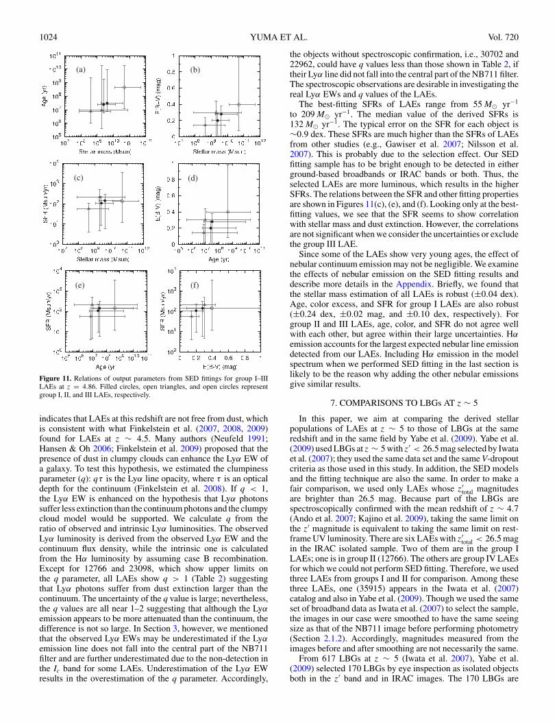
1024 YUMA ET AL. Vol. 720

Figure 11. Relations of output parameters from SED fittings for group I–IIILAEs at z = 4.86. Filled circles, open triangles, and open circles representgroup I, II, and III LAEs, respectively.

indicates that LAEs at this redshift are not free from dust, whichis consistent with what Finkelstein et al. (2007, 2008, 2009)found for LAEs at z ∼ 4.5. Many authors (Neufeld 1991;Hansen & Oh 2006; Finkelstein et al. 2009) proposed that thepresence of dust in clumpy clouds can enhance the Lyα EW ofa galaxy. To test this hypothesis, we estimated the clumpinessparameter (q): qτ is the Lyα line opacity, where τ is an opticaldepth for the continuum (Finkelstein et al. 2008). If q < 1,the Lyα EW is enhanced on the hypothesis that Lyα photonssuffer less extinction than the continuum photons and the clumpycloud model would be supported. We calculate q from theratio of observed and intrinsic Lyα luminosities. The observedLyα luminosity is derived from the observed Lyα EW and thecontinuum flux density, while the intrinsic one is calculatedfrom the Hα luminosity by assuming case B recombination.Except for 12766 and 23098, which show upper limits onthe q parameter, all LAEs show q > 1 (Table 2) suggestingthat Lyα photons suffer from dust extinction larger than thecontinuum. The uncertainty of the q value is large; nevertheless,the q values are all near 1–2 suggesting that although the Lyαemission appears to be more attenuated than the continuum, thedifference is not so large. In Section 3, however, we mentionedthat the observed Lyα EWs may be underestimated if the Lyαemission line does not fall into the central part of the NB711filter and are further underestimated due to the non-detection inthe Ic band for some LAEs. Underestimation of the Lyα EWresults in the overestimation of the q parameter. Accordingly,

the objects without spectroscopic confirmation, i.e., 30702 and22962, could have q values less than those shown in Table 2, iftheir Lyα line did not fall into the central part of the NB711 filter.The spectroscopic observations are desirable in investigating thereal Lyα EWs and q values of the LAEs.

The best-fitting SFRs of LAEs range from 55 M� yr−1

to 209 M� yr−1. The median value of the derived SFRs is132 M� yr−1. The typical error on the SFR for each object is∼0.9 dex. These SFRs are much higher than the SFRs of LAEsfrom other studies (e.g., Gawiser et al. 2007; Nilsson et al.2007). This is probably due to the selection effect. Our SEDfitting sample has to be bright enough to be detected in eitherground-based broadbands or IRAC bands or both. Thus, theselected LAEs are more luminous, which results in the higherSFRs. The relations between the SFR and other fitting propertiesare shown in Figures 11(c), (e), and (f). Looking only at the best-fitting values, we see that the SFR seems to show correlationwith stellar mass and dust extinction. However, the correlationsare not significant when we consider the uncertainties or excludethe group III LAE.

Since some of the LAEs show very young ages, the effect ofnebular continuum emission may not be negligible. We examinethe effects of nebular emission on the SED fitting results anddescribe more details in the Appendix. Briefly, we found thatthe stellar mass estimation of all LAEs is robust (±0.04 dex).Age, color excess, and SFR for group I LAEs are also robust(±0.24 dex, ±0.02 mag, and ±0.10 dex, respectively). Forgroup II and III LAEs, age, color, and SFR do not agree wellwith each other, but agree within their large uncertainties. Hαemission accounts for the largest expected nebular line emissiondetected from our LAEs. Including Hα emission in the modelspectrum when we performed SED fitting in the last section islikely to be the reason why adding the other nebular emissionsgive similar results.

7. COMPARISONS TO LBGs AT z ∼ 5

In this paper, we aim at comparing the derived stellarpopulations of LAEs at z ∼ 5 to those of LBGs at the sameredshift and in the same field by Yabe et al. (2009). Yabe et al.(2009) used LBGs at z ∼ 5 with z′ < 26.5 mag selected by Iwataet al. (2007); they used the same data set and the same V-dropoutcriteria as those used in this study. In addition, the SED modelsand the fitting technique are also the same. In order to make afair comparison, we used only LAEs whose z′

total magnitudesare brighter than 26.5 mag. Because part of the LBGs arespectroscopically confirmed with the mean redshift of z ∼ 4.7(Ando et al. 2007; Kajino et al. 2009), taking the same limit onthe z′ magnitude is equivalent to taking the same limit on rest-frame UV luminosity. There are six LAEs with z′

total < 26.5 magin the IRAC isolated sample. Two of them are in the group ILAEs; one is in group II (12766). The others are group IV LAEsfor which we could not perform SED fitting. Therefore, we usedthree LAEs from groups I and II for comparison. Among thesethree LAEs, one (35915) appears in the Iwata et al. (2007)catalog and also in Yabe et al. (2009). Though we used the sameset of broadband data as Iwata et al. (2007) to select the sample,the images in our case were smoothed to have the same seeingsize as that of the NB711 image before performing photometry(Section 2.1.2). Accordingly, magnitudes measured from theimages before and after smoothing are not necessarily the same.

From 617 LBGs at z ∼ 5 (Iwata et al. 2007), Yabe et al.(2009) selected 170 LBGs by eye inspection as isolated objectsboth in the z′ band and in IRAC images. The 170 LBGs are

No. 2, 2010 STELLAR POPULATIONS OF LAEs AT z = 4.86 1025

-0.8

-0.4

0

0.4

0.8

23 24 25 26 27

Ic-z

’

z’ magnitude (AB)

(a)

-2

-1

0

1

2

3

4

5

6

21 22 23 24 25 26 27

z’-[4

.5μm

]

4.5μm magnitude (AB)

(b)

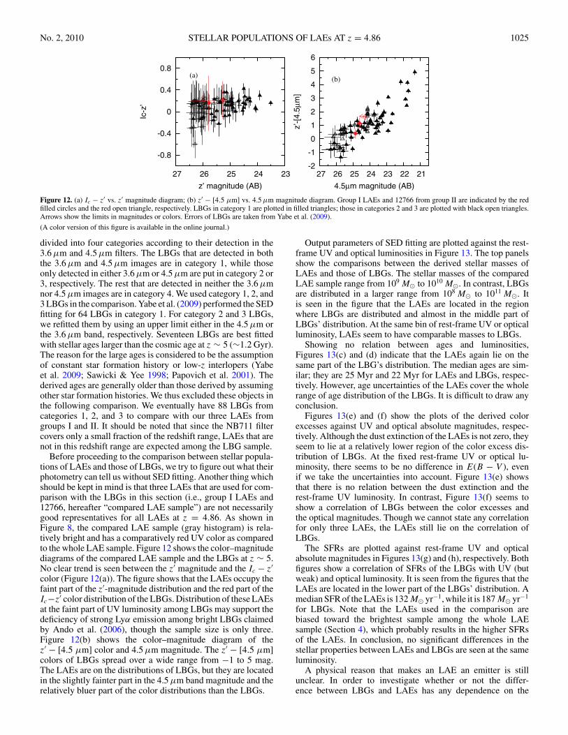
Figure 12. (a) Ic − z′ vs. z′ magnitude diagram; (b) z′ − [4.5 μm] vs. 4.5 μm magnitude diagram. Group I LAEs and 12766 from group II are indicated by the redfilled circles and the red open triangle, respectively. LBGs in category 1 are plotted in filled triangles; those in categories 2 and 3 are plotted with black open triangles.Arrows show the limits in magnitudes or colors. Errors of LBGs are taken from Yabe et al. (2009).

(A color version of this figure is available in the online journal.)

divided into four categories according to their detection in the3.6 μm and 4.5 μm filters. The LBGs that are detected in boththe 3.6 μm and 4.5 μm images are in category 1, while thoseonly detected in either 3.6 μm or 4.5 μm are put in category 2 or3, respectively. The rest that are detected in neither the 3.6 μmnor 4.5 μm images are in category 4. We used category 1, 2, and3 LBGs in the comparison. Yabe et al. (2009) performed the SEDfitting for 64 LBGs in category 1. For category 2 and 3 LBGs,we refitted them by using an upper limit either in the 4.5 μm orthe 3.6 μm band, respectively. Seventeen LBGs are best fittedwith stellar ages larger than the cosmic age at z ∼ 5 (∼1.2 Gyr).The reason for the large ages is considered to be the assumptionof constant star formation history or low-z interlopers (Yabeet al. 2009; Sawicki & Yee 1998; Papovich et al. 2001). Thederived ages are generally older than those derived by assumingother star formation histories. We thus excluded these objects inthe following comparison. We eventually have 88 LBGs fromcategories 1, 2, and 3 to compare with our three LAEs fromgroups I and II. It should be noted that since the NB711 filtercovers only a small fraction of the redshift range, LAEs that arenot in this redshift range are expected among the LBG sample.

Before proceeding to the comparison between stellar popula-tions of LAEs and those of LBGs, we try to figure out what theirphotometry can tell us without SED fitting. Another thing whichshould be kept in mind is that three LAEs that are used for com-parison with the LBGs in this section (i.e., group I LAEs and12766, hereafter “compared LAE sample”) are not necessarilygood representatives for all LAEs at z = 4.86. As shown inFigure 8, the compared LAE sample (gray histogram) is rela-tively bright and has a comparatively red UV color as comparedto the whole LAE sample. Figure 12 shows the color–magnitudediagrams of the compared LAE sample and the LBGs at z ∼ 5.No clear trend is seen between the z′ magnitude and the Ic − z′color (Figure 12(a)). The figure shows that the LAEs occupy thefaint part of the z′-magnitude distribution and the red part of theIc−z′ color distribution of the LBGs. Distribution of these LAEsat the faint part of UV luminosity among LBGs may support thedeficiency of strong Lyα emission among bright LBGs claimedby Ando et al. (2006), though the sample size is only three.Figure 12(b) shows the color–magnitude diagram of thez′ − [4.5 μm] color and 4.5 μm magnitude. The z′ − [4.5 μm]colors of LBGs spread over a wide range from −1 to 5 mag.The LAEs are on the distributions of LBGs, but they are locatedin the slightly fainter part in the 4.5 μm band magnitude and therelatively bluer part of the color distributions than the LBGs.

Output parameters of SED fitting are plotted against the rest-frame UV and optical luminosities in Figure 13. The top panelsshow the comparisons between the derived stellar masses ofLAEs and those of LBGs. The stellar masses of the comparedLAE sample range from 109 M� to 1010 M�. In contrast, LBGsare distributed in a larger range from 108 M� to 1011 M�. Itis seen in the figure that the LAEs are located in the regionwhere LBGs are distributed and almost in the middle part ofLBGs’ distribution. At the same bin of rest-frame UV or opticalluminosity, LAEs seem to have comparable masses to LBGs.

Showing no relation between ages and luminosities,Figures 13(c) and (d) indicate that the LAEs again lie on thesame part of the LBG’s distribution. The median ages are sim-ilar; they are 25 Myr and 22 Myr for LAEs and LBGs, respec-tively. However, age uncertainties of the LAEs cover the wholerange of age distribution of the LBGs. It is difficult to draw anyconclusion.

Figures 13(e) and (f) show the plots of the derived colorexcesses against UV and optical absolute magnitudes, respec-tively. Although the dust extinction of the LAEs is not zero, theyseem to lie at a relatively lower region of the color excess dis-tribution of LBGs. At the fixed rest-frame UV or optical lu-minosity, there seems to be no difference in E(B − V ), evenif we take the uncertainties into account. Figure 13(e) showsthat there is no relation between the dust extinction and therest-frame UV luminosity. In contrast, Figure 13(f) seems toshow a correlation of LBGs between the color excesses andthe optical magnitudes. Though we cannot state any correlationfor only three LAEs, the LAEs still lie on the correlation ofLBGs.

The SFRs are plotted against rest-frame UV and opticalabsolute magnitudes in Figures 13(g) and (h), respectively. Bothfigures show a correlation of SFRs of the LBGs with UV (butweak) and optical luminosity. It is seen from the figures that theLAEs are located in the lower part of the LBGs’ distribution. Amedian SFR of the LAEs is 132 M� yr−1, while it is 187 M� yr−1

for LBGs. Note that the LAEs used in the comparison arebiased toward the brightest sample among the whole LAEsample (Section 4), which probably results in the higher SFRsof the LAEs. In conclusion, no significant differences in thestellar properties between LAEs and LBGs are seen at the sameluminosity.

A physical reason that makes an LAE an emitter is stillunclear. In order to investigate whether or not the differ-ence between LBGs and LAEs has any dependence on the

1026 YUMA ET AL. Vol. 720

107

108

109

1010

1011

1012

−23−22−21−20

Ste

llar

mass (

Msun)

M1500Å

(a)

107

108

109

1010

1011

1012

−26−25−24−23−22−21−20−19

Ste

llar

mass (

Msun)

M5500Å

(b)

105

106

107

108

109

1010

1011

−23−22−21−20

Age (

yr)

M1500Å

(c)

105

106

107

108

109

1010

1011

−26−25−24−23−22−21−20−19

Age (

yr)

M5500Å

(d)

0

0.2

0.4

0.6

0.8

1

−23−22−21−20

E(B

−V

) (m

ag)

M1500Å

(e)

0

0.2

0.4

0.6

0.8

1

−26−25−24−23−22−21−20−19

E(B

−V

) (m

ag)

M5500Å

(f)

100

101

102

103

104

105

106

−23−22−21−20

SF

R (

Msun/y

r)

M1500Å

(g)

100

101

102

103

104

105

106

−26−25−24−23−22−21−20−19

SF

R (

Msun/y

r)

M5500Å

(h)

Figure 13. Output parameters of SED fitting against the UV and optical absolutemagnitudes. Symbols are the same as those in Figure 12.

(A color version of this figure is available in the online journal.)

EWs of Lyα emission, we plotted the output parameters ofSED fitting against the rest-frame Lyα EWs in Figure 14.Group I–III LAEs are plotted with five LBGs that have spectro-scopic Lyα EWs (Ando et al. 2004; Kajino et al. 2009). Arrowsin the figures represent the lower limits on EWs of the LAEs;their Ic magnitudes are fainter than the 2σ limiting magnitude.Note that, except for one spectroscopically confirmed LAE, theLyα EWs of LAEs are likely to be lower limits if their Lyαemission lines do not fall into the center of the NB711 band.According to the figure, we cannot find any significant correla-tion between the stellar properties and the rest-frame Lyα EWs.Recently, Kornei et al. (2010) studied these relations for z ∼ 3LBGs with spectra. They found that the stellar mass does notcorrelate with the Lyα EW, while large Lyα EW is seen in older,lower SFR, and less dusty LBGs. Such trends are difficult to iso-late with only three LAEs. A larger sample at z ∼ 5 is requiredto see clearer relations, if any, and to be definitive.

107

108

109

1010

1011

1012

0 10 20 30 40 50 60 70

Ste

llar

ma

ss (

Msu

n)

Rest−frame Lyα EW (Å)

(a)

105

106

107

108

109

1010

1011

0 10 20 30 40 50 60 70

Ste

llar

ag

e (

yr)

Rest−frame Lyα EW (Å)

(b)

0

0.2

0.4

0.6

0.8

1

0 10 20 30 40 50 60 70

E(B

−V

) (m

ag

)

Rest−frame Lyα EW (Å)

(c)

100

101

102

103

104

0 10 20 30 40 50 60 70

SF

R (

Msu

n/y

r)

Rest−frame Lyα EW (Å)

(d)

Figure 14. Output parameters from SED fitting for group I–III LAEs vs.rest-frame Lyα EWs. Filled circles, open triangles, and open circles representgroup I, II, and III LAEs, respectively. LBGs that have spectroscopic Lyα EWsare also shown in filled squares.

8. SUMMARY

In this paper, we studied the stellar properties of LAEs atz = 4.86 using SED fitting. Using narrowband and broadbandobservations by the Suprime-Cam on the Subaru Telescope,24 LAEs were selected in the area of ∼508.5 arcmin2 aroundthe GOODS-N field. In addition to the optical photometry,we obtained the mid-infrared photometry from data taken byIRAC on the Spitzer Space Telescope in the GOODS-N fieldas well as the surrounding area in order to cover most ofthe Subaru area. We selected 12 LAEs that are isolated fromneighboring objects. We performed SED fitting of five LAEsthat are detected above 2σ magnitude limits in more thantwo bands. Selecting those five LAEs could introduce a biastoward bright red galaxies. Model SEDs are built by assuminga constant star formation history with a fixed metallicity of0.2 Z�, the Salpeter IMF ranging from 0.1 M� to 100 M�, andthe extinction law of Calzetti et al. (2000). The derived stellarmasses of the LAEs range from 108 to 1010 M� with the medianvalue of 2.5 × 109 M�. The derived ages cover wide rangefrom 7.4 Myr to 437 Myr with the median value of 25 Myr.The color excess is between 0.1 and 0.4 mag, indicative of thepresence of some amount of dust. SFRs are in the range of55–209 M� yr−1. The median color excess and SFRs are0.27 mag and 132 M� yr−1, respectively. The high SFRs areprobably due to the selection effect; we selected the LAEs thatare bright enough to be detected in rest-frame UV and opticalbands, which results in selecting the LAEs with the higher SFRs.We investigated the correlations between the stellar propertiesderived by SED fitting and the photometric properties of LAEsand found no significant correlation due to both the small sizeof the sample and the large uncertainty in the fitting results.

The main objective of this study is to compare LAEs to LBGsat the same redshift. LBGs were selected by V-dropout criteria(Iwata et al. 2007). Their stellar populations were derived byYabe et al. (2009). Because those LBGs are selected from thesame set of data, and stellar population was derived by the same

No. 2, 2010 STELLAR POPULATIONS OF LAEs AT z = 4.86 1027

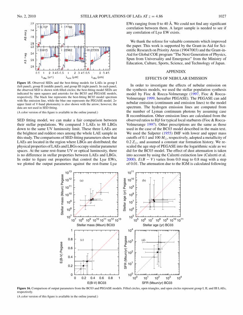
Figure 15. Observed SEDs and the best-fitting models for LAEs in group I(left panel), group II (middle panel), and group III (right panel). In each panel,the observed SED is shown with filled circles; the best-fitting model SEDs areindicated by open squares and asterisks for the BC03 and PEGASE models,respectively. The black line represents the best-fitting BC03 model spectrumwith Hα emission line, while the blue one represents the PEGASE model. 2σ

upper limit of V-band photometry is also shown with the arrow; however, thedata are not used in SED fitting.

(A color version of this figure is available in the online journal.)

SED fitting model, we can make a fair comparison betweentheir stellar populations. We compared 3 LAEs to 88 LBGsdown to the same UV luminosity limit. These three LAEs arethe brightest and reddest ones among the whole LAE sample inthis study. The comparisons of SED-fitting parameters show thatLAEs are located in the region where LBGs are distributed; thephysical properties of LAEs and LBGs occupy similar parameterspaces. At the same rest-frame UV or optical luminosity, thereis no difference in stellar properties between LAEs and LBGs.In order to figure out properties that control the Lyα EWs,we plotted the output parameters against the rest-frame Lyα

EWs ranging from 0 to 40 Å. We could not find any significantcorrelation between them. A larger sample is needed to see ifany correlation of Lyα EW exists.

We thank the referee for valuable comments which improvedthe paper. This work is supported by the Grant-in-Aid for Sci-entific Research on Priority Areas (19047003) and the Grant-in-Aid for Global COE program “The Next Generation of Physics,Spun from Universality and Emergence” from the Ministry ofEducation, Culture, Sports, Science, and Technology of Japan.

APPENDIX

EFFECTS OF NEBULAR EMISSION

In order to investigate the effects of nebular emission onthe synthesis models, we used the stellar population synthesismodel by Fioc & Rocca-Volmerange (1997, Fioc & Rocca-Volmerange 1999, hereafter PEGASE). The PEGASE can addnebular emission (continuum and emission lines) to the modelspectrum. The hydrogen emission lines are computed fromthe number of Lyman continuum photons by assuming caseB recombination. Other emission lines are calculated from theobserved ratios to Hβ for typical local starbursts (Fioc & Rocca-Volmerange 1997). Other prescriptions are the same as thoseused in the case of the BC03 model described in the main text.We used the Salpeter (1955) IMF with lower and upper masscutoffs of 0.1 and 100 M�, respectively, adopted a metallicity of0.2 Z�, and assumed a constant star formation history. We re-scaled the age step of PEGASE into the logarithmic scale as wedid for the BC03 model. The effect of dust attenuation is takeninto account by using the Calzetti extinction law (Calzetti et al.2000). E(B − V ) varies from 0.0 mag to 0.8 mag with a stepof 0.01. The attenuation due to the IGM is calculated following

107

108

109

1010

1011

1012

1013

107

108

109

1010

1011

1012

1013

Ste

llar

mass (

Msun)

Pegase

Stellar mass (Msun) BC03

(a)

105

106

107

108

109

1010

1011

105

106

107

108

109

1010

1011

Ste

llar

age (

yr)

Pegase

Stellar age (yr) BC03

(b)

0

0.2

0.4

0.6

0.8

1

0 0.2 0.4 0.6 0.8 1

E(B

-V)

Pegase

E(B-V) BC03

(c)

100

101

102

103

104

100

101

102

103

104

SF

R (

Msun/y

r) P

egase

SFR (Msun/yr) BC03

(d)

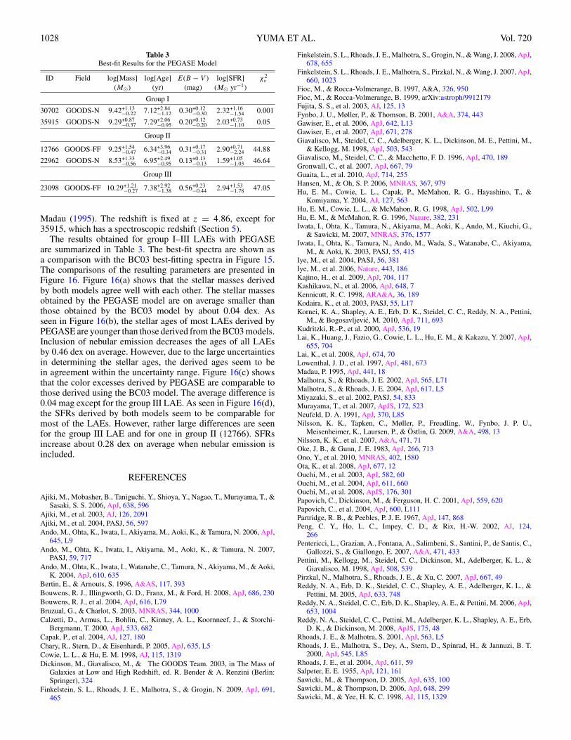
Figure 16. Comparison of output parameters from the BC03 and PEGASE models. Filled circles, open triangles, and open circles represent group I, II, and III LAEs,respectively.

(A color version of this figure is available in the online journal.)

1028 YUMA ET AL. Vol. 720

Table 3Best-fit Results for the PEGASE Model

ID Field log[Mass] log[Age] E(B − V ) log[SFR] χ2ν

(M�) (yr) (mag) (M� yr−1)

Group I

30702 GOODS-N 9.42+1.13−0.22 7.12+2.84

−1.12 0.30+0.12−0.30 2.32+1.16

−1.54 0.001

35915 GOODS-N 9.29+0.87−0.37 7.29+2.06

−0.95 0.20+0.12−0.20 2.03+0.73

−1.10 0.05

Group II

12766 GOODS-FF 9.25+1.54−0.47 6.34+3.96

−0.34 0.31+0.17−0.31 2.90+0.71

−2.24 44.88

22962 GOODS-N 8.53+1.33−0.56 6.95+2.49

−0.95 0.13+0.13−0.13 1.59+1.05

−1.03 46.64

Group III

23098 GOODS-FF 10.29+1.21−0.27 7.38+2.92

−1.38 0.56+0.23−0.44 2.94+1.53

−1.78 47.05

Madau (1995). The redshift is fixed at z = 4.86, except for35915, which has a spectroscopic redshift (Section 5).

The results obtained for group I–III LAEs with PEGASEare summarized in Table 3. The best-fit spectra are shown asa comparison with the BC03 best-fitting spectra in Figure 15.The comparisons of the resulting parameters are presented inFigure 16. Figure 16(a) shows that the stellar masses derivedby both models agree well with each other. The stellar massesobtained by the PEGASE model are on average smaller thanthose obtained by the BC03 model by about 0.04 dex. Asseen in Figure 16(b), the stellar ages of most LAEs derived byPEGASE are younger than those derived from the BC03 models.Inclusion of nebular emission decreases the ages of all LAEsby 0.46 dex on average. However, due to the large uncertaintiesin determining the stellar ages, the derived ages seem to bein agreement within the uncertainty range. Figure 16(c) showsthat the color excesses derived by PEGASE are comparable tothose derived using the BC03 model. The average difference is0.04 mag except for the group III LAE. As seen in Figure 16(d),the SFRs derived by both models seem to be comparable formost of the LAEs. However, rather large differences are seenfor the group III LAE and for one in group II (12766). SFRsincrease about 0.28 dex on average when nebular emission isincluded.

REFERENCES

Ajiki, M., Mobasher, B., Taniguchi, Y., Shioya, Y., Nagao, T., Murayama, T., &Sasaki, S. S. 2006, ApJ, 638, 596

Ajiki, M., et al. 2003, AJ, 126, 2091Ajiki, M., et al. 2004, PASJ, 56, 597Ando, M., Ohta, K., Iwata, I., Akiyama, M., Aoki, K., & Tamura, N. 2006, ApJ,

645, L9Ando, M., Ohta, K., Iwata, I., Akiyama, M., Aoki, K., & Tamura, N. 2007,

PASJ, 59, 717Ando, M., Ohta, K., Iwata, I., Watanabe, C., Tamura, N., Akiyama, M., & Aoki,

K. 2004, ApJ, 610, 635Bertin, E., & Arnouts, S. 1996, A&AS, 117, 393Bouwens, R. J., Illingworth, G. D., Franx, M., & Ford, H. 2008, ApJ, 686, 230Bouwens, R. J., et al. 2004, ApJ, 616, L79Bruzual, G., & Charlot, S. 2003, MNRAS, 344, 1000Calzetti, D., Armus, L., Bohlin, C., Kinney, A. L., Koornneef, J., & Storchi-

Bergmann, T. 2000, ApJ, 533, 682Capak, P., et al. 2004, AJ, 127, 180Chary, R., Stern, D., & Eisenhardi, P. 2005, ApJ, 635, L5Cowie, L. L., & Hu, E. M. 1998, AJ, 115, 1319Dickinson, M., Giavalisco, M., & The GOODS Team. 2003, in The Mass of

Galaxies at Low and High Redshift, ed. R. Bender & A. Renzini (Berlin:Springer), 324

Finkelstein, S. L., Rhoads, J. E., Malhotra, S., & Grogin, N. 2009, ApJ, 691,465

Finkelstein, S. L., Rhoads, J. E., Malhotra, S., Grogin, N., & Wang, J. 2008, ApJ,678, 655

Finkelstein, S. L., Rhoads, J. E., Malhotra, S., Pirzkal, N., & Wang, J. 2007, ApJ,660, 1023

Fioc, M., & Rocca-Volmerange, B. 1997, A&A, 326, 950Fioc, M., & Rocca-Volmerange, B. 1999, arXiv:astroph/9912179Fujita, S. S., et al. 2003, AJ, 125, 13Fynbo, J. U., Møller, P., & Thomson, B. 2001, A&A, 374, 443Gawiser, E., et al. 2006, ApJ, 642, L13Gawiser, E., et al. 2007, ApJ, 671, 278Giavalisco, M., Steidel, C. C., Adelberger, K. L., Dickinson, M. E., Pettini, M.,

& Kellogg, M. 1998, ApJ, 503, 543Giavalisco, M., Steidel, C. C., & Macchetto, F. D. 1996, ApJ, 470, 189Gronwall, C., et al. 2007, ApJ, 667, 79Guaita, L., et al. 2010, ApJ, 714, 255Hansen, M., & Oh, S. P. 2006, MNRAS, 367, 979Hu, E. M., Cowie, L. L., Capak, P., McMahon, R. G., Hayashino, T., &

Komiyama, Y. 2004, AJ, 127, 563Hu, E. M., Cowie, L. L., & McMahon, R. G. 1998, ApJ, 502, L99Hu, E. M., & McMahon, R. G. 1996, Nature, 382, 231Iwata, I., Ohta, K., Tamura, N., Akiyama, M., Aoki, K., Ando, M., Kiuchi, G.,

& Sawicki, M. 2007, MNRAS, 376, 1577Iwata, I., Ohta, K., Tamura, N., Ando, M., Wada, S., Watanabe, C., Akiyama,

M., & Aoki, K. 2003, PASJ, 55, 415Iye, M., et al. 2004, PASJ, 56, 381Iye, M., et al. 2006, Nature, 443, 186Kajino, H., et al. 2009, ApJ, 704, 117Kashikawa, N., et al. 2006, ApJ, 648, 7Kennicutt, R. C. 1998, ARA&A, 36, 189Kodaira, K., et al. 2003, PASJ, 55, L17Kornei, K. A., Shapley, A. E., Erb, D. K., Steidel, C. C., Reddy, N. A., Pettini,

M., & Bogosavljevic, M. 2010, ApJ, 711, 693Kudritzki, R.-P., et al. 2000, ApJ, 536, 19Lai, K., Huang, J., Fazio, G., Cowie, L. L., Hu, E. M., & Kakazu, Y. 2007, ApJ,

655, 704Lai, K., et al. 2008, ApJ, 674, 70Lowenthal, J. D., et al. 1997, ApJ, 481, 673Madau, P. 1995, ApJ, 441, 18Malhotra, S., & Rhoads, J. E. 2002, ApJ, 565, L71Malhotra, S., & Rhoads, J. E. 2004, ApJ, 617, L5Miyazaki, S., et al. 2002, PASJ, 54, 833Murayama, T., et al. 2007, ApJS, 172, 523Neufeld, D. A. 1991, ApJ, 370, L85Nilsson, K. K., Tapken, C., Møller, P., Freudling, W., Fynbo, J. P. U.,

Meisenheimer, K., Laursen, P., & Ostlin, G. 2009, A&A, 498, 13Nilsson, K. K., et al. 2007, A&A, 471, 71Oke, J. B., & Gunn, J. E. 1983, ApJ, 266, 713Ono, Y., et al. 2010, MNRAS, 402, 1580Ota, K., et al. 2008, ApJ, 677, 12Ouchi, M., et al. 2003, ApJ, 582, 60Ouchi, M., et al. 2004, ApJ, 611, 660Ouchi, M., et al. 2008, ApJS, 176, 301Papovich, C., Dickinson, M., & Ferguson, H. C. 2001, ApJ, 559, 620Papovich, C., et al. 2004, ApJ, 600, L111Partridge, R. B., & Peebles, P. J. E. 1967, ApJ, 147, 868Peng, C. Y., Ho, L. C., Impey, C. D., & Rix, H.-W. 2002, AJ, 124,

266Pentericci, L., Grazian, A., Fontana, A., Salimbeni, S., Santini, P., de Santis, C.,

Gallozzi, S., & Giallongo, E. 2007, A&A, 471, 433Pettini, M., Kellogg, M., Steidel, C. C., Dickinson, M., Adelberger, K. L., &

Giavalisco, M. 1998, ApJ, 508, 539Pirzkal, N., Malhotra, S., Rhoads, J. E., & Xu, C. 2007, ApJ, 667, 49Reddy, N. A., Erb, D. K., Steidel, C. C., Shapley, A. E., Adelberger, K. L., &

Pettini, M. 2005, ApJ, 633, 748Reddy, N. A., Steidel, C. C., Erb, D. K., Shapley, A. E., & Pettini, M. 2006, ApJ,

653, 1004Reddy, N. A., Steidel, C. C., Pettini, M., Adelberger, K. L., Shapley, A. E., Erb,

D. K., & Dickinson, M. 2008, ApJS, 175, 48Rhoads, J. E., & Malhotra, S. 2001, ApJ, 563, L5Rhoads, J. E., Malhotra, S., Dey, A., Stern, D., Spinrad, H., & Jannuzi, B. T.

2000, ApJ, 545, L85Rhoads, J. E., et al. 2004, ApJ, 611, 59Salpeter, E. E. 1955, ApJ, 121, 161Sawicki, M., & Thompson, D. 2005, ApJ, 635, 100Sawicki, M., & Thompson, D. 2006, ApJ, 648, 299Sawicki, M., & Yee, H. K. C. 1998, AJ, 115, 1329

No. 2, 2010 STELLAR POPULATIONS OF LAEs AT z = 4.86 1029

Shapley, A. E., Steidel, C. C., Adelberger, K. L., Dickinson, M., & Giavalisco,M. 2003, ApJ, 588, 65

Shapley, A. E., Steidel, C. C., Adelberger, K. L., & Pettini, M. 2001, ApJ, 562,95

Shimasaku, K., et al. 2003, ApJ, 586, L111Shimasaku, K., et al. 2004, ApJ, 605, L93Shimasaku, K., et al. 2006, PASJ, 58, 313Shimizu, I., & Umemura, M. 2010, MNRAS, 406, 913Steidel, C. C., Adelberger, K. L., Giavalisco, M., Dickinson, M., & Pettini, M.

1999, ApJ, 519, 1Steidel, C. C., Adelberger, K. L., Shapley, A. E., Pettini, M., Dickinson, M., &

Giavalisco, M. 2003, ApJ, 592, 728

Steidel, C. C., Giavalisco, M., Dickinson, M., & Adelberger, K. L. 1996, AJ,112, 352

Taniguchi, Y., et al. 2005, PASJ, 57, 165Venemans, B. P., et al. 2002, ApJ, 569, L11Venemans, B. P., et al. 2004, A&A, 424, L17Williams, R. E., et al. 1996, AJ, 112, 1335Yabe, K., Ohta, K., Iwata, I., Sawicki, M., Tamura, N, Akiyama, M., & Aoki,

K. 2009, ApJ, 693, 507Yagi, M., Kashikawa, N., Sekiguchi, M., Doi, M., Yasuda, N., Shimasaku, K.,

& Okamura, S. 2002, AJ, 123, 66Yoshida, M., et al. 2006, ApJ, 653, 988