Stefan W. Ballmer - DSpace@MIT

LIGO interferometer operating at design

sensitivity with application to gravitational

radiometry

by

Stefan W. Ballmer

Submitted to the Department of Physicsin partial fulfillment of the requirements for the degree of

Doctor of Philosophy

at the

MASSACHUSETTS INSTITUTE OF TECHNOLOGY

June 2006

c© Stefan W. Ballmer, MMVI. All rights reserved.

The author hereby grants to MIT permission to reproduce anddistribute publicly paper and electronic copies of this thesis document

in whole or in part.

Author . . . . . . . . . . . . . . . . . . . . . . . . . . . . . . . . . . . . . . . . . . . . . . . . . . . . . . . . . . . . . .Department of Physics

May 3rd, 2006

Certified by. . . . . . . . . . . . . . . . . . . . . . . . . . . . . . . . . . . . . . . . . . . . . . . . . . . . . . . . . .Erotokritos Katsavounidis

ProfessorThesis Supervisor

Certified by. . . . . . . . . . . . . . . . . . . . . . . . . . . . . . . . . . . . . . . . . . . . . . . . . . . . . . . . . .Peter Fritschel

Principal Research ScientistThesis Co-Supervisor

Accepted by . . . . . . . . . . . . . . . . . . . . . . . . . . . . . . . . . . . . . . . . . . . . . . . . . . . . . . . . .Thomas J. Greytak

Associate Department Head for Education

2

LIGO interferometer operating at design sensitivity with

application to gravitational radiometry

by

Stefan W. Ballmer

Submitted to the Department of Physicson May 3rd, 2006, in partial fulfillment of the

requirements for the degree ofDoctor of Philosophy

Abstract

During the last decade the three interferometers of the Laser Interferometer Gravi-tational Wave Observatory (LIGO) were built and commissioned. In fall 2005 designsensitivity was achieved, corresponding to a strain sensitivity of 2.5 × 10−23 Hz−1/2

at 150 Hz. All three interferometers are now in an extended science run.One of the most critical steps to reach this goal was increasing the power in

the interferometer to more than 200 Watt at the beam splitter. This required thecommissioning of both a thermal compensation system and shot noise limited sensingelectronics capable of detecting all the light. Additionally, a series of unexpectednoise sources had to be mitigated. This work is described in the first part of thisthesis.

In a second part I introduce a radiometer analysis that is capable of spatiallyresolving anisotropies in a stochastic gravitational wave background. The analysis isoptimized for identifying point sources of stochastic gravitational radiation.

Finally, data from the fourth LIGO science run is used to set both isotropicand directional upper limits on the stochastic background of gravitational waves.The bound set on the normalized gravitational wave energy density is h2Ωgw(f) <6.25× 10−5 and the limit set on a broadband and flat strain power spectrum comingfrom a point source varies between 8.5× 10−49Hz−1 and 6.1× 10−48Hz−1, dependingon the source position. Additionally a limit on gravitational radiation coming fromthe direction of Sco-X1, the brightest X-ray source short of the sun, is set for eachfrequency bin.

Thesis Supervisor: Erotokritos KatsavounidisTitle: Professor

Thesis Co-Supervisor: Peter FritschelTitle: Principal Research Scientist

Acknowledgments

I had the privilege to join the LIGO project in the final phase of interferometer

commissioning, and was given the chance to work on what is arguably the biggest

table-top experiment a physics graduate student can dream of working on. As a

consequence I had the pleasure to work with many great people from the project,

probably learning something from each and every one of them.

As much as I would like to do it, thanking all of them personally would fill too

many pages of an already too long thesis. But even so I want to take this opportunity

to mention at least a few of them by name.

To Rana, thanks for showing me how to solder a cable and how to wire up an op-amp.

To Paul, thanks for teaching the beauty of RF electronics to the 21st century youth.

To Peter, thanks for teaching me the difference between AS I and AS Q.

Dir, Daniel, danke fur all da Whisky won i Dir waggsoffe ha.

To Dave, Gregg and Rich, for keeping me from drinking my Guinness alone, thanks.

To Rai, thank you for getting me into this adventure.

To Erik, thanks for letting me run with my own ideas and always supporting me.

To Nergis, thank you for getting me away from the dark side of physics.

To Marie, for taking bureaucracy off my shoulders, thank you.

To the whole Hanford crew, thank you all for the hospitality and support I enjoyed.

And sorry for all those sleepless night I have caused for some of you...

I would also like to thank Edith for the many beautiful moments we shared when-

ever we were not working on opposite sides of the Atlantic ocean. Finally, I want to

express my deep gratitude to my parents, Ruth and Werner Ballmer, for all the love

and care I enjoyed in the last thirty one years of my life. Without them this thesis

would never have been written.

- Stefan, May 3, 2006

6

Contents

Preface 15

1 Gravitational Radiation 17

1.1 Gravitational Radiation in General Relativity . . . . . . . . . . . . . 17

1.1.1 The linearized Einstein Equation . . . . . . . . . . . . . . . . 18

1.1.2 The transverse-traceless gauge . . . . . . . . . . . . . . . . . . 19

1.1.3 Plane wave solution and effect on free masses . . . . . . . . . 20

1.2 Gravitational Wave Sources . . . . . . . . . . . . . . . . . . . . . . . 21

1.2.1 Quadrupole radiation and signal strength . . . . . . . . . . . . 21

1.2.2 Expected astrophysical sources . . . . . . . . . . . . . . . . . 23

1.3 Gravitational Wave Detectors . . . . . . . . . . . . . . . . . . . . . . 25

1.3.1 Bar detectors . . . . . . . . . . . . . . . . . . . . . . . . . . . 25

1.3.2 Interferometers . . . . . . . . . . . . . . . . . . . . . . . . . . 26

1.3.3 Remark on interferometer for GW detection . . . . . . . . . . 27

2 The LIGO interferometer 29

2.1 Optical layout . . . . . . . . . . . . . . . . . . . . . . . . . . . . . . . 30

2.2 Sensing matrix . . . . . . . . . . . . . . . . . . . . . . . . . . . . . . 33

2.3 Shot Noise . . . . . . . . . . . . . . . . . . . . . . . . . . . . . . . . . 35

2.4 The AS I signal . . . . . . . . . . . . . . . . . . . . . . . . . . . . . . 36

2.5 Oscillator phase noise . . . . . . . . . . . . . . . . . . . . . . . . . . . 39

2.5.1 Basic coupling . . . . . . . . . . . . . . . . . . . . . . . . . . . 39

2.5.2 The double cavity as seen by the sideband . . . . . . . . . . . 42

7

2.6 Oscillator amplitude noise . . . . . . . . . . . . . . . . . . . . . . . . 47

2.7 Noise Improvements below 100 Hz . . . . . . . . . . . . . . . . . . . . 47

2.7.1 The problem . . . . . . . . . . . . . . . . . . . . . . . . . . . . 47

2.7.2 Auxiliary length control loops . . . . . . . . . . . . . . . . . . 48

2.7.3 Coupling reduction: MICH and PRC correction . . . . . . . . 48

2.7.4 Auxiliary loop noise reduction . . . . . . . . . . . . . . . . . . 49

2.7.5 RF saturation at the photo diode output amplifier . . . . . . . 51

2.8 The Thermal Compensation System . . . . . . . . . . . . . . . . . . . 52

2.8.1 The problem . . . . . . . . . . . . . . . . . . . . . . . . . . . . 52

2.8.2 The hardware . . . . . . . . . . . . . . . . . . . . . . . . . . . 53

2.8.3 Time dependence of the thermal lens correction . . . . . . . . 55

2.8.4 Servo system . . . . . . . . . . . . . . . . . . . . . . . . . . . 59

2.8.5 Noise couplings . . . . . . . . . . . . . . . . . . . . . . . . . . 61

2.8.6 Oscillator Phase noise reduction . . . . . . . . . . . . . . . . . 68

2.8.7 Optics replacement after S4 . . . . . . . . . . . . . . . . . . . 68

2.9 Summary of known noise sources . . . . . . . . . . . . . . . . . . . . 71

2.10 Limitations of the existing hardware . . . . . . . . . . . . . . . . . . 73

3 Searching for an anisotropic background of gravitational waves 75

3.1 Cosmological source . . . . . . . . . . . . . . . . . . . . . . . . . . . . 76

3.1.1 Existing bounds on h2Ωgw(f) . . . . . . . . . . . . . . . . . . 77

3.2 Astrophysical sources . . . . . . . . . . . . . . . . . . . . . . . . . . . 79

3.2.1 Accretion driven pulsars: Low-Mass X-ray Binaries (LMXB) . 81

3.3 The Radiometer . . . . . . . . . . . . . . . . . . . . . . . . . . . . . . 85

3.3.1 Introduction . . . . . . . . . . . . . . . . . . . . . . . . . . . . 85

3.3.2 Search for an isotropic background . . . . . . . . . . . . . . . 85

3.3.3 Directional search: a gravitational wave radiometer . . . . . . 87

3.3.4 Numerical aspects . . . . . . . . . . . . . . . . . . . . . . . . . 89

3.3.5 Comparison to the isotropic case . . . . . . . . . . . . . . . . 90

3.3.6 Achievable sensitivity . . . . . . . . . . . . . . . . . . . . . . . 91

8

3.4 Code Validation . . . . . . . . . . . . . . . . . . . . . . . . . . . . . . 92

3.4.1 Results from simulated data . . . . . . . . . . . . . . . . . . . 92

3.4.2 Bias factor . . . . . . . . . . . . . . . . . . . . . . . . . . . . . 94

3.4.3 Hardware injections . . . . . . . . . . . . . . . . . . . . . . . . 95

3.4.4 Timing Transient . . . . . . . . . . . . . . . . . . . . . . . . . 99

3.4.5 Data cuts and post processing . . . . . . . . . . . . . . . . . . 101

4 Results from S4 105

4.1 Broadband results . . . . . . . . . . . . . . . . . . . . . . . . . . . . . 105

4.1.1 Constant Ωgw(f) . . . . . . . . . . . . . . . . . . . . . . . . . 106

4.1.2 Constant strain power . . . . . . . . . . . . . . . . . . . . . . 108

4.1.3 Interpretation . . . . . . . . . . . . . . . . . . . . . . . . . . . 109

4.2 Limits on isotropic background . . . . . . . . . . . . . . . . . . . . . 111

4.2.1 Interpretation . . . . . . . . . . . . . . . . . . . . . . . . . . . 111

4.3 Narrow-band results targeted on Sco-X1 . . . . . . . . . . . . . . . . 112

4.3.1 Interpretation . . . . . . . . . . . . . . . . . . . . . . . . . . . 113

Conclusion 115

Appendices 116

A Tables of Parameters 117

B Useful formulas and definitions 121

B.1 Fabry-Perot Cavity . . . . . . . . . . . . . . . . . . . . . . . . . . . . 121

B.1.1 Reflection, transmission and buildup . . . . . . . . . . . . . . 121

B.1.2 Transfer functions for modulations . . . . . . . . . . . . . . . 121

C Formulae for radiometer and isotropic search 123

C.1 Definition of basic quantities . . . . . . . . . . . . . . . . . . . . . . . 123

C.2 Basic formulae for the isotropic search . . . . . . . . . . . . . . . . . 125

C.3 Basic formulae for the radiometer search . . . . . . . . . . . . . . . . 125

C.4 Relation between radiometer and isotropic search . . . . . . . . . . . 126

9

C.5 Remarks on deconvolving the radiometer . . . . . . . . . . . . . . . . 128

C.5.1 Inverse of 2-point correlation integral . . . . . . . . . . . . . . 128

C.5.2 Deconvolved radiometer problem statement . . . . . . . . . . 129

C.5.3 Deconvolved radiometer formal solution . . . . . . . . . . . . . 130

C.5.4 Generic problem of the deconvolved radiometer . . . . . . . . 130

D Correction to the TCS noise coupling 133

D.1 Estimate of bending correction . . . . . . . . . . . . . . . . . . . . . . 133

D.1.1 Far zone . . . . . . . . . . . . . . . . . . . . . . . . . . . . . . 134

D.1.2 Near zone . . . . . . . . . . . . . . . . . . . . . . . . . . . . . 134

D.1.3 Energy balance . . . . . . . . . . . . . . . . . . . . . . . . . . 134

D.2 Next order correction to the local coupling . . . . . . . . . . . . . . . 135

10

List of Figures

2-1 Aerial photograph of the LIGO Hanford Observatory . . . . . . . . . 29

2-2 Optical layout of LIGO . . . . . . . . . . . . . . . . . . . . . . . . . . 31

2-3 Measured transfer function oscillator phase noise → displacement . . 41

2-4 Fringe of the double cavity for higher order sideband modes . . . . . 43

2-5 Oscillator Phase Noise Transfer function . . . . . . . . . . . . . . . . 46

2-6 Residual motion of BS and RM . . . . . . . . . . . . . . . . . . . . . 50

2-7 Thermal Compensation System (TCS) schematic . . . . . . . . . . . 54

2-8 Thermal images of TCS heating pattern . . . . . . . . . . . . . . . . 54

2-9 ITM Temperature profile . . . . . . . . . . . . . . . . . . . . . . . . . 56

2-10 TCS thermal lens power . . . . . . . . . . . . . . . . . . . . . . . . . 57

2-11 Required annulus compensation . . . . . . . . . . . . . . . . . . . . . 58

2-12 TCS actuation transfer function . . . . . . . . . . . . . . . . . . . . . 60

2-13 TCS flow chart . . . . . . . . . . . . . . . . . . . . . . . . . . . . . . 61

2-14 TCS noise coupling . . . . . . . . . . . . . . . . . . . . . . . . . . . . 66

2-15 TCS Relative Intensity Noise (RIN) . . . . . . . . . . . . . . . . . . . 67

2-16 H1 Noise Budget . . . . . . . . . . . . . . . . . . . . . . . . . . . . . 69

2-17 H1 Noise Budget - zoom . . . . . . . . . . . . . . . . . . . . . . . . . 70

3-1 Antenna lode . . . . . . . . . . . . . . . . . . . . . . . . . . . . . . . 91

3-2 Example SNR map . . . . . . . . . . . . . . . . . . . . . . . . . . . . 93

3-3 Point source injection . . . . . . . . . . . . . . . . . . . . . . . . . . . 93

3-4 Hardware Injection: Pulsar3 . . . . . . . . . . . . . . . . . . . . . . . 97

3-5 Hardware Injection: Pulsar4 . . . . . . . . . . . . . . . . . . . . . . . 97

11

3-6 Hardware Injection: Pulsar8 . . . . . . . . . . . . . . . . . . . . . . . 98

3-7 Effect of timing transient . . . . . . . . . . . . . . . . . . . . . . . . . 99

3-8 Periodic timing transient . . . . . . . . . . . . . . . . . . . . . . . . . 100

3-9 H1 timing transient . . . . . . . . . . . . . . . . . . . . . . . . . . . . 101

3-10 Sigma ratio cut . . . . . . . . . . . . . . . . . . . . . . . . . . . . . . 103

4-1 S4 Result SNR . . . . . . . . . . . . . . . . . . . . . . . . . . . . . . 106

4-2 S4 result 90 % confidence level Bayesian upper limit . . . . . . . . . . 108

4-3 S4 Result point estimate and theoretical standard deviation . . . . . 108

4-4 S4 Result SNR . . . . . . . . . . . . . . . . . . . . . . . . . . . . . . 109

4-5 S4 result 90 % confidence level Bayesian upper limit . . . . . . . . . . 110

4-6 S4 Result point estimate and theoretical standard deviation . . . . . 110

4-7 S4 Result for Sco-X1, SNR . . . . . . . . . . . . . . . . . . . . . . . . 112

D-1 Schematic A . . . . . . . . . . . . . . . . . . . . . . . . . . . . . . . . 133

D-2 Schematic B . . . . . . . . . . . . . . . . . . . . . . . . . . . . . . . . 133

12

List of Tables

2.1 Sideband recycling gain for different spatial modes . . . . . . . . . . . 38

3.1 Published direct upper limits on Ωgw(f) . . . . . . . . . . . . . . . . 80

3.2 Parameters for Sco-X1 . . . . . . . . . . . . . . . . . . . . . . . . . . 83

3.3 Strongest injected pulsars during S4 . . . . . . . . . . . . . . . . . . . 96

3.4 Pulsars Hardware Injection . . . . . . . . . . . . . . . . . . . . . . . . 98

3.5 Data quality flags . . . . . . . . . . . . . . . . . . . . . . . . . . . . . 102

4.1 S4 isotropic result . . . . . . . . . . . . . . . . . . . . . . . . . . . . . 111

A.1 Fundamental Constants . . . . . . . . . . . . . . . . . . . . . . . . . 117

A.2 Large Optics Parameters . . . . . . . . . . . . . . . . . . . . . . . . . 118

A.3 Variable Definitions . . . . . . . . . . . . . . . . . . . . . . . . . . . . 119

A.4 Acronym Definitions . . . . . . . . . . . . . . . . . . . . . . . . . . . 120

13

14

Preface

Ever since the existence of gravitational waves was first predicted by Albert Einstein

in 1918 [1], the experimental challenge to directly measure their effect was daunting.

It was clear that the laboratory generation of gravitational waves strong enough for

the experimental verification of Einstein’s prediction is virtually impossible - by far

the largest wave amplitudes are due to rare collisions of stellar-sized compact objects.

It took more than 40 years before J. Weber made the first serious attempt to directly

measure their effect using a resonant bar detector [25].

Then, in 1975, the discovery of the binary pulsar PSR 1913+16 by Hulse and

Taylor [2, 3] provided a laboratory with which the emission of gravitational waves

could be tested. Over the years their data indeed showed a decrease in the orbital

period of the binary, consistent with the energy loss predicted by the emission of

gravitational waves, proving, albeit indirectly, the existence of gravitational waves.

The potential payoff of directly measuring gravitational waves would be enormous.

Gravitational waves are created during the first fraction of a second after the big bang,

or originate at the core of stellar collisions or explosions. Exactly because they interact

so little with matter, they penetrate the surrounding matter that is responsible for

emission of electromagnetic radiation, so far the only carrier of information about

such events. Directly observing gravitational waves therefore would literally open a

new window to the universe.

Today, 88 years after Einstein’s prediction, nobody has yet succeeded in directly

detecting gravitational waves. However, during the last decade a handful of kilome-

ter scale, laser interferometer gravitational wave antennae were constructed, commis-

sioned and have begun operation. This worldwide network of observatories includes

15

the German-British GEO600 1 [40], the Japanese TAMA 2[41], the Italian-French

VIRGO 3 [46] and a set of three interferometers in the United States called Laser

Interferometer Gravitational Wave Observatory (LIGO) 4 [42, 45].

Personally I had the privilege to join the LIGO laboratory for the last five years

of the initial interferometer commissioning phase. I spent almost 2 years at the

LIGO Hanford Observatory in Washington State, where I spearheaded the day-to-

day commissioning of the 4km interferometer. This was diverse and exceptionally

rewarding work. Of course the main goal was to improve the interferometer strain

sensitivity, but due to the intertwined complexity of the LIGO interferometers I had

to become familiar with almost every subsystem. This also meant working together

with many people from across the whole the project, all of them experts on their own

subsystem. I would like to use this opportunity to thank all of them; I learned a lot

from them.

After an introduction to gravitational waves in chapter 1, I summarize the key

hardware improvements that were made while I was working at the LIGO Hanford

Observatory in chapter 2. They were the last steps required to reach the design

sensitivity laid out more than a decade ago [39].

In chapter 3 I introduce an analysis that uses the data from the two LIGO sites to

set a directional upper limit on stochastic gravitational background radiation. Finally,

in chapter 4, I report on the results of this analysis from the LIGO S4 Science Run.

This work, and the LIGO Laboratory, is supported by the United States National

Science Foundation 5 under Cooperative Agreement PHY-0107417.

1 http://www.geo600.uni-hannover.de2 http://tamago.mtk.nao.ac.jp3 http://www.virgo.infn.it4 http://ligo.caltech.edu5http://www.nsf.gov/

16

Chapter 1

Gravitational Radiation

By 1905 Albert Einstein’s Special Theory of Relativity established Lorentz invariance

as the fundamental symmetry of space and time. It became clear that Isaac New-

ton’s law of gravitation needed to be extended since it included instantaneous action

at a distance, which violates of causality in the framework of Lorentz invariance. All

attempts to modify Newton’s theory to comply with Lorentz invariance necessarily

include a finite propagation speed of gravitational phenomena. In that sense already

the Special Theory of Relativity suggests the existence of gravitational waves. Fur-

thermore it is also no surprise that such waves should propagate at the speed of light,

for this is the only Lorentz invariant velocity.

The exact properties of such gravitational waves however were only predicted by

Einstein’s General Theory of Relativity, and were worked out in his 1918 article “Uber

Gravitationswellen” [1]. The following section is a quick review to this prediction. I

chose to do it formally because this highlights how few assumptions actually go into

its derivation.

1.1 Gravitational Radiation in General Relativity

The big philosophical leap that lead Einstein to the General Theory of Relativity was

insight that one has to abandon the view of space-time as an unalterable stage on

which the universe evolves. Instead space-time itself becomes a dynamic field that is

17

influenced by the matter floating in it. Euclidean geometry is no longer appropriate.

Following the ideas of Bernhard Riemann such a curved space-time can be de-

scribed by a metric gµν , which is a function of the coordinates ξµ = (t, x1, x2, x3): the

infinitesimal distance or eigen time dτ between 2 events (points) separated by dξµ is

given by

dτ 2 = dξµgµνdξν (1.1)

The metric gµν is a dynamic field. In the limit of special relativity the metric gµν

becomes the Minkowski metric ηµν = diag(−1, 1, 1, 1).

1.1.1 The linearized Einstein Equation

The Einstein equation is a 2nd order differential equation for the metric tensor gµν .

It determines the evolution of gµν under the influence of matter, which in turn is

described by the stress tensor Tµν :

Gµν(gµν) = 8πGTµν (1.2)

Here G is Newton’s constant and the 2nd order differential operator Gµν is called

Einstein tensor. The derivation of an explicit expression for Gµν was one of the

central results of Einstein.

Since we are interested in describing gravitational waves far away from any source

we can use the weak field limit, defined by

gµν = ηµν + hµν , |hµν | 1 (1.3)

where ηµν is again the Minkowski metric. Then the Einstein tensor Gµν becomes

linear and is given by

2Gµν = −hµν,λλ + hµ

λ,λν + hν

λ,λµ − ηµνh

λσ,λσ + ηµνh,λ

λ − h,µν (1.4)

In the last term h is the trace of hµν , i.e. h = hµµ.

18

While this looks complicated at first glance it is surprisingly simple to see why

this has to be the correct expression:

• Newton: Since the theory has to be an extension of Newton’s work, we know

that there has to be a Laplace operator acting on the quantity that describes

the gravitational field (hµν). The Lorentz-invariant extension is the D’Alembert

operator u = ∂2t −4. This is the 1st term in equation 1.4.

• Energy-Momentum conservation: It implies 0 = 8πGTµν,ν = Gµν

,ν . This re-

quires the 2nd term in equation 1.4. Since Tµν and therefore Gµν are symmetric

in µ and ν, we also need the 3rd term. But this 3rd term also has to be canceled.

Applying the same argument again thus gives rise to the 4th term.

• Covariance: The Einstein equation has to be invariant under any coordinate

transformations, in particular infinitesimal ones of the form xµ = xµ + ξµ. For

those hµν transforms as hµν = hµν − ξµ,ν − ξν,µ. Requiring that the Einstein

tensor is invariant under these transformations leads to term 5 (to cancel term

4) and term 6 (to cancel terms 2 and 3). Terms 5 and 6 together also fulfill the

Energy-Momentum conservation criterion.

1.1.2 The transverse-traceless gauge

To see the physical effect of a gravitational wave it is useful to fix the gauge. The

most practical choice is to introduce the trace-inversed strain hµν

hµν = hµν −1

2ηµνh (1.5)

and impose the harmonic gauge condition (transversality)

h,νµν = 0 (1.6)

19

This reduces the Einstein equation to a simple wave equation:

Gµν = −1

2uhµν = 8πGTµν (1.7)

Furthermore if we now focus on a region of space outside the source we have T = 0,

which allows us to impose the even stricter transverse-traceless gauge, defined by the

following 2 conditions:

hµν,ν = 0 (transverse)

hµµ = 0 (traceless)

(1.8)

This also assures that the trace-inversed strain hµν is identical to the physical strain

hµν .

1.1.3 Plane wave solution and effect on free masses

To visualize the effect of a gravitational wave on free (inertial) masses in space we

can look at a plane wave solution of equation 1.7 with wave vector kλ:

hµν(xλ) = hµν cos

(kλx

λ)

(1.9)

We have kλkλ = 0 since solutions of 1.7 travel at light speed and hµνk

ν = 0, hµµ = 0

due to the transverse traceless condition 1.8. Choosing the wave vector ki along the

z-axis we can parametrize the amplitude hµν as

hµν =

0 0 0 0

0 h+ h× 0

0 h× −h+ 0

0 0 0 0

(1.10)

i.e. we have two independent polarizations, h+ and h×. Let’s further assume 2 test

masses separated by the distance L along the X-axis before the wave hit. The test

20

mass separation while the wave is passing is then given by

L+ dL =√LgxxL ≈

(1 +

h+

2

)L (1.11)

while we get a minus sign for a separation along the y-axis. In other words a gravi-

tational wave with h+ polarization stretches distances along the x-axis and shortens

distances along the y-axis during the first half period and does the opposite during

the second half period. The h× polarization does the same thing, but in a coordinate

system rotated by 45 degree.

The best way of measuring a gravitational wave strain therefore is to compare the

arm length difference between two perpendicular arms. Choosing the two arms along

x and y-axis the arm length difference is given by

Lx − Ly = h+L (1.12)

Comparing the length of two perpendicular arms conveniently is exactly what a

Michelson interferometer does.

1.2 Gravitational Wave Sources

1.2.1 Quadrupole radiation and signal strength

Just as electric charge conservation implies that there is no electromagnetic monopole

radiation, the energy-momentum conservation T µν;ν = 0 implies that there is no

monopole or dipole gravitational radiation. Working in the near Newtonian approxi-

mation T µν;ν = 0 implies in particular the identity

∫dx3T jk =

1

2

d2

dt2

∫dx3T 00xixj. (1.13)

21

Since equation 1.7 is a regular wave equation its far field solution at distance d is the

retarded field given by

hij =4G

d

∫dx3T ij

ret (1.14)

Applying identity 1.13 and projecting to the transverse traceless gauge we get

hTTij =

2G

dc4d2

dt2ITTij,ret

= 1.7× 10−47

(d2

dt2ITTij,ret

1 Watt

)(1 km

d

)

= 9.6× 10−20

(d2

dt2ITTij,ret

Mc2

)(1 Mpc

d

) (1.15)

where ITTij,ret is the retarded transverse traceless part of the quadrupole momentum

Iij =∫dx3ρ(x)xixj. From equation 1.15 it is also immediately clear that there is no

chance of observing gravitational waves from a terrestrial source. The strain hTTij is

also related to the radiated energy density through

ρgw =c2

32πG

⟨hTT

ij,0hTTij,0

⟩=

c2

16πG

⟨|h+,0|2 + |h×,0|2

⟩(1.16)

The result has to be averaged over several wavelength to be physically meaningful,

which is indicated by the angle brackets 〈...〉. Finally the power radiated by the whole

source can be obtained by integrating over all directions

P =G

5c5

⟨...I

tracelessij

...I

tracelessij

⟩≈ G

c5P 2

internal

≈ P 2internal

3.6× 1059erg/sec

(1.17)

so the radiated power is proportional to the square of the power Pinternal flowing

internally from one side of the source to the other.

The existence of gravitational waves has been confirmed indirectly by Hulse and

Taylor [2, 3, 4], resulting in the 1993 Nobel Prize in Physics. They observed a shift

22

in the perihelion passing time of the binary pulsar system PSR 1913+16 that was

perfectly explained by the loss of energy and angular momentum due to the emission

of gravitational waves.

1.2.2 Expected astrophysical sources

Inspiral of a compact binary

Any two stars orbiting each other will loose energy by radiating gravitational waves

at a rate given by

dE

dt= −32

5

c5

G

µ2M3

a5f(ε) (1.18)

where M = M1 + M2 is the total mass, µ = M1M2/M the reduced mass, a the

semi-major axis and

f(ε) = [1 +73

24ε2 +

37

96ε4 +O(ε6)][1− ε2]−7/2 (1.19)

is a correction for non-zero eccentricity ε (see [7], page 988). Thus both period and

semi-major axis a will shrink resulting in a chirp with f ∝ f 11/3, with the gravitational

wave frequency f equal to twice the orbital frequency. The 2 stars merge when the

sum of their radii becomes comparable to their separation, R1 + R2 ≈ 2a. Thus the

chirp signal ends roughly at

fmax =

√8GM

π2(R1 +R2)3

= 15 Hz

(1000km

R1 +R2

) 32(

M

2M

) 12

.

(1.20)

Even if only one of the stars is a white dwarf (R1 ≈ 106m, M1 = M) this frequency is

already outside the band accessible to LIGO (starting roughly above 40Hz, see chapter

2). Thus LIGO can only see binary inspirals where both stars are either a neutron

star (NS, Ri ≈ 104m, Mi = 1.4M) or a black hole (BH, Ri ≈ RISCO = 6GMic−2).

23

In both cases fmax can be as high as about 6 kHz.

During the inspiral phase the NS/NS wave forms are believed to be sufficiently

well modeled by post-Newtonian approximation that they can be used for matched

filtering [21, 89]. For BH/BH wave forms the confidence is not as big [22]. Nevertheless

matched filtering is usually applied.

All of these post-Newtonian wave forms become inaccurate during the final phase

(merger). So far no accurate wave forms for the merger phase is known. This is

especially unfortunate since the radiated power reaches a maximum during this merger

phase. The product of such a merger is most likely a black hole. Just after being

born this black hole will still be excited and undergo damped oscillations that will

also radiate gravitational waves [18].

NS/NS inspiral rate estimate

The NS/NS merger rate in our Galaxy was estimated to be about 83 Myr−1 using

a population model that was based on all known NS/NS systems [23, 24]. The

uncertainty on this estimate is rather large - the 95 % interval spans values from

4 Myr−1 to 220 Myr−1. This translates into a detection rate (SNR > 8) for LIGO

at design sensitivity of 1 per 30 years, with the most optimistic value consistent with

the 95 % interval being 1 per 8 years.

Periodic sources

Another potential source of gravitational waves are fast spinning non-axis-symmetric

pulsars. Fast spinning pulsars are often referred to as Millisecond Pulsars because

their period is only a couple milliseconds long. These sources will produce a monochro-

matic signal at twice the pulsar frequency. The strength of such a signal is about

h ≈ 6× 10−26

(fgw

500 Hz

)2(10 kpc

d

)( ε

10−6

)(1.21)

where ε is the ellipticity of the pulsar. Since the pulsar frequencies are extremely

stable the best way to look for such signals is to demodulate the data stream at

24

the expected frequency, taking into account all effects from polarization and orbital

motion of both pulsar and earth.

The most interesting pulsars naturally are the fast spinning ones. Those tend to

be driven by mass accretion, which in turn can affect the frequency stability. For

those objects on can also relate the expected gravitational radiation to the observed

X-ray luminosity, see section 3.2.1.

Other sources

Gravitational waves for which we do not have a template can come from a variety

of sources. These include the superposition of an ensemble of the sources described

above as well as any other inaccurately modeled sources such as supernovae or even

primordial gravitational waves.

Phenomenologically one usually divides those sources into bursts and stochastic

background, depending on whether they have a finite duration. The boundary be-

tween long bursts and a stochastic background however is not well defined. More

details on a stochastic background are given in chapter 3.

1.3 Gravitational Wave Detectors

A gravitational wave detector must be able to convert a space-time strain into a

recordable signal. The whole challenge lies in the weakness of the signal. This section

recalls the history of suggested detectors and motivates the optical configuration of

the LIGO interferometers.

1.3.1 Bar detectors

In 1960 Joseph Weber suggested using the resonance of an aluminum bar as an an-

tenna for gravitational waves [25]. The idea is that a passing short gravitational

wave pulse would induce a strain in the bar and excite its resonance. For reasons de-

tailed elsewhere[26, 27], the community was never able to verify Weber’s subsequent

25

claims of detection[28] although various theories[19, 20] were developed to explain the

enormous apparent flux of gravitational wave energy.

Since Weber’s pioneering work resonant bar detectors have come a long way. To-

day’s bar detectors are cryogenically cooled, have much improved seismic isolations

and make use of SQUIDs to readout the signal [29].

The sensitivity on resonance of such a bar with length l0, mass m, resonance

frequency f0 and mechanical quality factor Q is limited by thermal excitation of the

bar resonance

htherm ≈4

l0

√kBT

8π3f 30mQ

≈ 3× 10−23Hz−12

(T

1mK

) 12(

106

Q

) 12(

103kg

m

) 12(

103Hz

f0

) 32(

1m

l0

).

(1.22)

This follows from the strain-to-amplitude (h→ ∆l) transfer function

∆l =f 2 1

2l0h

f 2 − f 20 − iff0

Q

(1.23)

and the Fluctuation-Dissipation theorem, implying

∆l2thermdf =

kBTf0

2π3Qm

f2f20

Q2 + (f 2 − f 20 )2

df (1.24)

(see for instance [8]).

In recent years there also have been proposals [30] for more sophisticated ge-

ometries (spheres, dodecahedrons, etc.) designed to improve the bandwidth and

directional sensitivity of the resonant mass detectors [31].

1.3.2 Interferometers

Given the effect of a passing gravitational wave (eq. 1.12) a Michelson interferometer

is the canonical instrument to measure such an effect. This was first pointed out by

Pirani in 1956 [33] and by 1971 a prototype interferometer was built in Malibu [34].

26

Shortly after that a study done at MIT by R. Weiss identified almost all noise sources

relevant for a LIGO-scale interferometer [37, 38].

Since then many different optical configurations have been suggested (see [55] for

a summary). The LIGO antennae are power-recycled Fabry-Perot Michelson inter-

ferometers. All of today’s kilometer-scale interferometers are a variant of this optical

configuration [40, 41, 42, 45, 46].

1.3.3 Remark on interferometer for GW detection

Quoting the analogy to the Cosmic Microwave Background (”the wavelength gets

stretched with redshift”), I was often asked whether such a wavelength stretching

would not null out any interferometric readout. Hence this short paragraph:

At its heart an interferometric measurement is not a distance measurement but

rather a relative timing (or time-of-flight) measurement - it compares the phase of the

light reflected from both arms at the fixed location of the photo diode. Furthermore,

since htt = 0 for all gravitational waves (see 1.10), the evolution of time is not affected

by the wave. In other words, a set of clocks that was synchronized before the wave

arrived remains synchronized during the event and afterward. Therefore we should

analyze the interferometer as follows: A phase front Φ = const starts at the beam

splitter, gets split up and travels with light speed (hence the name...) down each arm,

gets reflected at each end and arrives back at the beam splitter after

∆tx,y = 2(1± h+

2)L

c(1.25)

i.e. the relative time delay between the 2 arms is ∆t = 2h+Lc

, which then translates

into a phase difference of ∆Φ = 2πν∆t. The laser frequency ν is unaffected by the

gravitational wave (htt = 0).

The analysis above is for the limit of long gravitational wave length (gravitational

wave period > light storage time in the arms). The generalization to a time and

27

position dependent h+(t, ~x) is straightforward and gives

∆t =

∫ 2Lc

0

(h+(t, ~x(t))

2+h+(t, ~y(t))

2

)dt (1.26)

where ~x(t) / ~y(t) is the position of the phase front in the x-arm / y-arm.

Notice that I never had to talk about the laser wavelength. Nevertheless, it is

still legitimate to academically ask what happens to the laser wavelength when a

gravitational wave passes. The wavelength is the distance between two points that

have a phase difference of 2π. In the static case h+ = const and for a newly emitted

photon, since the light speed is exactly what it’s name suggests, this distance is always

given by λ = c/ν, independent of h+. If however h+(t) depends on t one can show

that the laser wavelength λ becomes

λ =c

ν

(1 +

1

4ν

∂h+

∂t

)(1.27)

in 1st order approximation, i.e. it is indeed stretched if h+ increases. This however

does not result in a correction to equation 1.26 and hence to the strain signal provided

by a interferometer.

28

Chapter 2

The LIGO interferometer

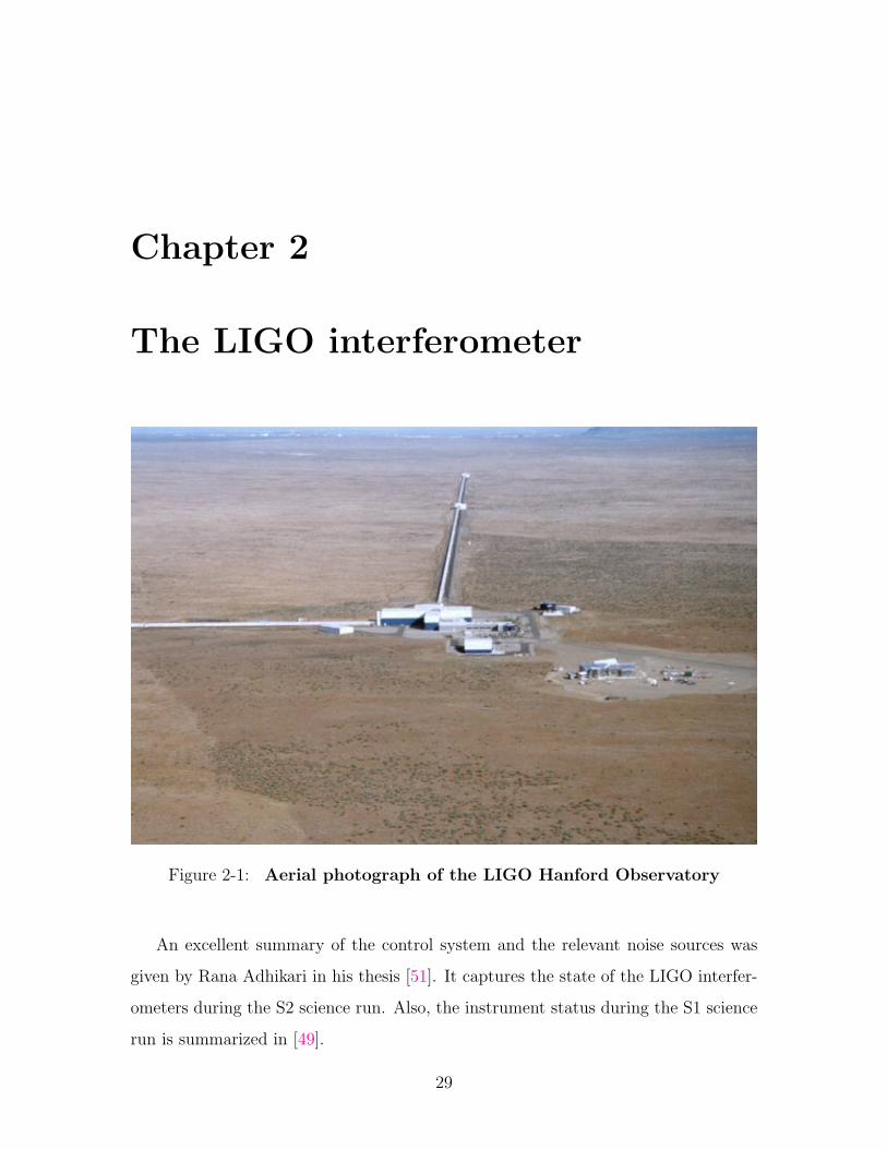
Figure 2-1: Aerial photograph of the LIGO Hanford Observatory

An excellent summary of the control system and the relevant noise sources was

given by Rana Adhikari in his thesis [51]. It captures the state of the LIGO interfer-

ometers during the S2 science run. Also, the instrument status during the S1 science

run is summarized in [49].

29

This chapter is intended to be an update covering the changes in the control system

and newly identified noise sources. It is intended to capture the state of the LIGO

interferometers at the beginning of the 1-year long S5 science run, even though not all

aspects of the LIGO instrument will be covered. At this point all three interferometers

show roughly one order of magnitude improvement in sensitivity everywhere above

40Hz compared to S2.

Thus I will begin this chapter with a description of the optical layout and the RF

readout scheme. I then will move on to the fundamental noise source limiting initial

LIGO, namely shot noise, and explain a series of technical noise sources that had to

be eliminated during commissioning. After that a big section is filled by the detailed

description of the thermal compensation system that had to be installed to deal with

thermal aberration in the large optics. Finally I will summarize all the known noise

sources that contribute to the interferometer displacement sensitivity.

2.1 Optical layout

The three initial LIGO interferometers [43, 44] are all power-recycled Michelson in-

terferometers [36] with Fabry-Perot arm cavities [32] (see figure 2-2). Two of them,

one with 4 km and one with 2 km arm length (labeled H1 and H2), are installed at

the LIGO Hanford Observatory in Washington State. The third one (L1) also has an

arm length of 4 km and is installed at the LIGO Livingston Observatory in Louisiana.

On all interferometers all optics, including input mode cleaner and mode matching

telescope mirrors, are freely suspended as pendula, hanging from a platform that is

passively seismically isolated. All these optics and seismic isolation stacks are enclosed

in a vacuum system. Also, the Livingston interferometer was recently upgraded with

a Hydraulic External Pre-Isolation (HEPI) system, i.e. an active seismic isolation

systems that is installed outside the vacuum envelope. All freely suspended optics

have little magnets glued on. The required actuation forces are applied to those

magnets using small coils.

The light source for a LIGO interferometer is a 10 Watt Nd:YAG laser from

30

Figure 2-2: Optical layout of the LIGO interferometers. The Laser light entersfrom the left. The gravitational wave signal is sensed at the anti-symmetric or darkport (AS). Shown are the Recycling Mirror (RM), the Beam Splitter (BS), the twoInput Test Masses (ITMX/ITMY) and the two End Test Masses (ETMX/ETMY).Carrier light is shown in red, the resonant sideband in blue and the non-resonantsideband in green (only reflected at RM). Indicated are also the reflective or symmetricport (REFL) and the pick-off port (PO), as well as the distances Lx, Ly,lx and ly.

31

Lightwave, operating at a wavelength of 1064 nm. It is both frequency and intensity

stabilized. The output laser light is passed through the pre-mode cleaner, a 21 cm

long triangular cavity designed to both filter the spatial mode and the intensity noise

above about 1 MHz.

Most error signals for controlling the interferometer are derived using a Ponder-

motive locking scheme [35] (see section 2.2, or [48]). Thus the input laser beam

is frequency-modulated at three different frequencies, producing three sets of side-

bands at 24.48 MHz (resonant sideband), 61.20 MHz (non-resonant sideband) and

33.29 MHz (mode cleaner sideband). All but the mode cleaner sideband then pass

the mode cleaner (MC), which is a triangular cavity with 24.492 meters round trip

length. The mode cleaner sideband is used to lock the mode cleaner in reflection.

The resonant sideband passes 2 free spectral ranges (FSRs) away from the carrier,

the non-resonant sideband 5 FSRs away from the carrier.

The beam then hits the recycling mirror (RM), which is already part of the main

interferometer, see figure 2-2. The non-resonant sideband is just reflected, it is not

resonant in any of the cavities of the main interferometer - hence its name. Both

carrier and resonant sideband build up in the recycling cavity that is formed by the

RM and the 2 Input Test Masses (ITMX and ITMY). The recycling gain is Gcr = 50

for the carrier and Gsb = 26.5 for the sideband. Finally only the carrier is resonant in

the arm cavities formed by the ITMs and the end test masses (ETMX and ETMY).

The arm cavity finesse is F = 219.

The beam splitter (BS) is placed such that (almost) no carrier is exiting at the anti-

symmetric port (AS or dark port). Due to the Schnupp asymmetry lx − ly = 0.356m

the sideband leaks out the dark port. Nominally the recycling cavity should be almost

critically coupled for the sideband such that almost all sideband should end up on the

dark port. The differential arm (DARM) error signal Lx−Ly is derived from beating

sideband and carrier at the dark port.

The common arm error signal (Lx + Ly)/2 (CARM) is derived from beating the

carrier at the reflective port (REFL or symmetric port) against either resonant or

non-resonant sideband. CARM is fed back to the laser frequency with 20 kHz control

32

loop bandwidth.

Finally error signals for both l+ = (lx− ly)/2 (PRC; power recycling cavity length)

and l− = lx − ly (MICH; Michelson degree of freedom) are derived from the carrier -

resonant sideband beat at the pick-off (PO) port (see 2.2).

In this work I will assume that all the cavities are already on resonance (locked).

The process of lock-acquisition would fill a chapter on its own. See [53, 54] instead.

All quoted values are for the Hanford 4km interferometer (H1).

2.2 Sensing matrix

All of the error signals used to control the LIGO interferometer are derived using a

heterodyne scheme. Almost all length control signals are derived using the resonant

sideband at 24.5 MHz, with the exception being the REFL port on some interferom-

eters (currently L1) - it uses the non-resonant sideband at 61.2 MHz.

The sensing matrix element used to read out a differential arm (DARM or L−)

displacement, and hence to read out a Gravitational wave signal, is given by [47]

[L− AS Q] = −ℵ gcrtsbr′c

1

1 + if/fc

k δL−

= 4.4Wattpk

nm

P

1 Watt

1

1 + if/fc

δL−.

(2.1)

where ℵ = 4j0(Γ)j1(Γ)P cosωmt is the gain prefactor, ji(Γ) are Bessel functions of the

first kind, Γ is the modulation depth, P is the power into the interferometer, ωm is the

resonant sideband modulation frequency, gcr is the carrier amplitude recycling gain,

tsb is the sideband transmission to the dark port, r′c = π/(2F) is the derivative of the

arm cavity reflectivity with respect to round trip phase, fc is the arm cavity pole, k

is the light wave vector and L− = dx− dy is the differential displacement. Numerical

values for those parameters are tabulated in appendix A. There is an additional factor

eηhνd(t) cosωmt to convert the signal into a demodulated photo current. Here d(t) is

the demodulation function (ideally a square wave), e the electron charge, h Planck’s

constant, ν the laser frequency and η the photo diode quantum efficiency.

33

Here I will just list the other relevant sensing matrix elements, more details can

be found in [51] and [47]. Besides the element 2.1 used for DARM loop the elements

used for the 3 other length control loops (CARM or L+, PRC or l+, MICH or l−) are

[L+ REFL I] = 2ℵ g2crrsbr

′c

1

1 + if/fcc

k δL+ (2.2)

[l+ POB I] = 2ℵ gcrgsb

tRM

rMrc

[gcr

1

1 + i ffcc

− gsb

]k δl+ (2.3)

[l− POB Q] = −ℵ gcrg2sb

tRM

tMk δl− (2.4)

There are however significant off-diagonal couplings, namely

[L+ POB I] = −2ℵ g2crgsb

tRM

rMr′c

1

1 + if/fcc

k δL+ (2.5)

[l+ REFL I] = 2ℵ[g2

sbrcrrM + g2crrsbrc

1

1 + if/fcc

]k δl+ (2.6)

[l− AS Q] = ℵ gcrtsbrc1

1 + if/fc

k δl− (2.7)

Especially significant is the element [L+ POB I] (2.5), it could actually dominate

the POB I. In practice the high bandwidth (20kHz unity gain frequency) CARM

loop zeros the REFL I signal by acting on the laser frequency. Since REFL I

is also sensitive to l+ through 2.6 this high bandwidth loop effectively changes the

l+ POB I element making it frequency independent:

[l+ POB I] = −2ℵ g2sbrM

tRMrsb

[gcrrsbrc + gsbrcrrM ] k δl+ (2.8)

Finally l− also shows up in REFL Q.

[l− REFL Q] = −ℵ gsbtsbrcrk δl− (2.9)

34

In practice however REFL Q shows a large low frequency pollution that is thought

to be due to the non-mode-matched component of the carrier field. In fact this large

signal limits the amount of power we can detect at the REFL port since it gets close

to saturation in the photo detector. This has actually forced us to change the L+

readout on the Livingston interferometer to the non-resonant sideband. Since the

non-resonant doesn’t enter the recycling cavity it is not sensitive to motion of optics

past the recycling mirror. In particular there cannot be any Q signal. In Livingston

we now use a diode tuned for the non-resonant sideband at 61.2 MHz. The sensing

matrix element is also given by equation 2.2, except that rsb and j1(Γ) refer to non-

resonant sideband values.

2.3 Shot Noise

The fundamental limit to detect the power at the dark port is the shot noise limit.

Since the light at the dark port is dominated by the sidebands, effects from non-

stationarity and demodulation have to be taken into account [64]:

S1−sidedP =

√√√√2hν(2j21t

2SBP )

[Pc

PSB

+d(t)2 cos2 ωmt

d(t)2 cos2 ωmt

]η− 12

√d(t)2

d(t) cosωmt

= 2.8× 10−10 Wattpk√

Hz

√P

1 Watt

(2.10)

Here P is the power into the interferometer, d(t) is the wave form used for demodu-

lation (typically a square wave since the local oscillator is squared up in the demod-

ulation boards) and η is the photo diode quantum efficiency - see table A.3 as well as

section 2.2, paragraph 2 for the definition of the remaining symbols.

The factor in the last bracket is required to convert the shot noise into Wattspk to

be comparable with equation 2.1. The carrier to (both) sideband power ratio at the

dark port was measured to be Pc/PSB ≈ 0.09 using an Optical Spectrum Analyzer.

It is also related to the contrast defect cd = P(beam splitter)carrier /P

(AS port)carrier , which can be

35

expressed as

cd =2j2

1t2SB

j20g

2cr

Pc

PSB

≈ 1× 10−4. (2.11)

Here I used the experimentally measured sideband transmissivity tsb ≈ 0.77.

Using equations 2.1, 2.10 and ηP = 4 Watt the shot noise limited displacement

sensitivity is

S1−sidedDARM =

√hν

2ηP

(1 + if/fc)

j0gcrr′ck

√

Pc

PSBd(t)2 cos2 ωmt+ d(t)2 cos2 ωmt

d(t) cosωmt

= 3.2× 10−20 m√

Hz(1 + if/fc) .

(2.12)

This is good agreement with the experimentally measured shot noise (see figure 2.9).

In particular this means that the overlap of sideband and carrier at the AS port is

quite good - that overlap was assumed to be ideal in eq. 2.12.

2.4 The AS I signal

A recurring problem during the commissioning of LIGO was a large signal in the

uncontrolled orthogonal quadrant of a demodulated photo diode signal. Such a signal

limits the amount of detectable power because a saturation of the RF electronics and

the mixer has to be avoided. The problem exists both on REFL Q - where the

solution was switching to the non-resonant sideband, see 2.2 - and on the AS port.

To get a signal in the I quadrature of the dark port an effective sideband imbalance

at the dark port δgSBtM and arm cavity reflectivity imbalance δrc is required [51].

tM is the transmissivity for the sideband to the dark port.

SAS I =1

4ℵ gcrtM δrc δgsb (2.13)

I say effective because contributions can come from higher order modes - I am using

the arm cavities to define the modal basis since the almost flat-flat recycling cavity

supports all modes. In particular almost any angular misalignments will produce an

36

AS I signal by beating first order transverse modes. In fact even with all angular

control loops closed we found a linear dependence of AS I on angular mirror mis-

alignment, indicating that at least a part of the DC AS I signal is due to small offsets

in the angular control loops.

The reflectivity imbalance δrc for the fundamental mode comes from an imbalance

in the round trip loss in the arms. For l = 2 a δrc arises from arm cavity mode

mismatch, both in beam width and beam curvature. The latter can be affected by

changing the thermal lens in the ITMs (see 2.8).

Another hint that a significant contribution to the AS I signal is due to higher

order spatial mode comes from a test with an output mode cleaner (OMC) in the AS

detection path. The OMC effectively strips off higher order spatial modes and thus

their contribution to the readout signal. It reduced the DC offset in AS I by a factor

9 and the RMS fluctuations in AS I by a factor 3.

To quantify the size of the AS I signal is hard because it depends on so many

factors (alignment offsets and thermal lensing in ITM’s). However a typical size of

the DC signal in AS I before any tuning of the interferometer is

SAS I ≈ 5× 10−3WattpkP

1 Watt. (2.14)

This value can be tuned to zero by changing the differential thermal lensing in the

ITMs (see 2.8) and/or some alignment offsets, affecting the l = 2 and/or l = 1 con-

tributions to AS I respectively. Based on this and equation 2.13 we can estimate the

effective ”δrc× δgsb” to be roughly 0.02 in the untuned case. Note that the measured

contrast defect cd ≈ 1 × 10−4 (section 2.3) limits the arm reflectivity imbalance to

δrc = 2√cd ≈ 0.02. However this measurement was done in a thermally tuned state.

I also want to point out that there is a natural mechanism that creates a sideband

imbalance for higher order modes: the higher order mode pick up an additional phase

shift from the arm. The arm cavity reflectivity of a sideband mode with mode number

37

l is given by

rc =

(− TITM

√RETMe

iφ

1−√RITMRETMeiφ

+√RITM

)φ = 2π

±fSB − (l × fTM)

FSR

fTM =FSR

πacos

((1− L/RoCITM)

12 (1− L/RoCETM)

12

).

(2.15)

±fSB is the (upper/lower) sideband frequency and fTM , FSR, L, RoC are the arm

cavity transverse mode spacing, free spectral range, length and optics curvature. That

translates into a sideband recycling gain given by

gsb =

√TRM

1− rMrc

√RRM

(2.16)

In particular the values for the first 3 transverse sideband modes (l = 0: funda-

mental, l = 1: alignment mismatch and l = 2: mode mismatch) are given in table 2.1.

In particular for the l = 2 bullseye mode the ratio between upper and lower sideband

power becomes almost 2:1.

Higher order mode SB recycling gain

upper SBl foff ∠(rc) |gsb|2 ∠(gsb)0 -17.7 kHz -0.074 deg 29.9 -2.4 deg1 -6.1 kHz -1.45 deg 17.8 -39.0 deg2 +5.5 kHz +1.65 deg 15.8 +42.6 deg

lower SBl foff ∠(rc) |gsb|2 ∠(gsb)0 +17.7 kHz +0.074 deg 29.9 +2.4 deg1 -8.3 kHz -0.98 deg 22.8 -28.9 deg2 +3.3 kHz +2.87 deg 8.1 +57.2 deg

Table 2.1: Sideband recycling gain for different spatial modes. foff is thefrequency offset from the arm resonance. The phase shift induced by the arm causesa sideband power imbalance of almost 2:1 for the l = 2 mode.

In practice the only way to avoid mixer saturations due to the large AS I signal

was to implement feed-back that cancels out the AS I induced RF photo current on

38

the diode. The installed system has a range of 10Vpk through a coupling resistor of 1

kOhm, i.e. it can correct up to 10mApk photo current per diode. Allowing for a factor

of 2 headroom to ride out seismic transients this means that we now need about 1

dark port photo diode per Watt into the interferometer. We are now running with 4

diodes. Without the AS I servo we would need about 10 times as many diodes since

1 mApk of photo current and an average transimpedance of about 1 kOhm results

in 1 Vpk, which is about the slew rate limit of the MAX4107 op-amp at the photo

detector output. Details about the AS I servo are given in [51], appendix H.

2.5 Oscillator phase noise

As we increased the power into the interferometer to improve the high frequency

sensitivity we started noticing a noise bump above about 1 kHz that was present

in both the Livingston and the Hanford 4km interferometer, but with a somewhat

different shape. The noise was as high as 4 × 10−18 m/√

Hz at 1 kHz, which is 10

times above the design sensitivity.

Eventually we were able to track this to phase noise of the 24.48 MHz RF oscillator

that we used to modulate the input beam and as a local oscillator for the signal

demodulation. At 1 kHz the our oscillator had about 6 × 10−7 rad/√

Hz and the

transfer function to displacement turned out to be a surprisingly high 7×10−12 m/ rad

(see figure 2-3).

2.5.1 Basic coupling

The coupling of oscillator phase noise to displacement noise is closely related to the

large AS I signal at the dark port. The basic coupling mechanism is simple - a

jitter in the demodulation of the constant offset in AS I produces noise in AS Q.

Fortunately there is a cancellation mechanism: since we are using the same oscillator

to both modulate the light and demodulate the photo diode signal, any jitter on the

oscillator should cancel out.

There are 2 ways to circumvent this cancellation. First, any noise introduced after

39

the split between the electro-optic modulator (EOM) path and the local oscillator

(LO) path will couple directly into AS Q with the strength

SAS Q = SAS I,DCδφN(f), (2.17)

where δφN(f) is the differential phase noise between optical and LO path. This large

sensitivity to the differential phase noise prompted us to redesign the RF distribution

system. We now amplify the signal before we split it and make sure we never dip

below -1dBm LO level to avoid thermal noise. As oscillator we use a Wenzel Crystal

oscillator with 10dBm output and and a phase noise specification of -140dBc/Hz at

100Hz,-155dBc/Hz at 1kHz and -162dBc/Hz at 10kHz. The thermal (Johnson) noise

thus would degrade the LO signal at -168dBm/Hz (Johnson noise) - (-162dBc/Hz) +

5dB (amplifier noise figure) = -1dBm. The noise figure I quote is for the Mini-Circuits

ERA-5 RF amplifier that we use in the demodulation boards.

The second way to avoid the cancellation is to introduce a relative phase shift

between the 2 paths. A simple path length difference is not large enough - the

difference between the 2 paths is about 5 meters resulting in a relative phase shift

of only 1 × 10−4radians at 1kHz. The optical cavities in the light path however can

produce a significant phase shift.

Figure 2-3 shows the measured transfer function from oscillator phase noise to

displacement. As expected it rises as f 2 below about 2 kHz (see figure caption 2-3).

But there is clearly a pole somewhere between 2.5 kHz and 3kHz (3dB point after

correction for the cavity pole). Plus there are 2 resonances at 3.3 kHz and 5.5kHz

corresponding to the spatial l = 2 sideband modes resonating in the arms.

The obvious element that can introduce a phase shift in the optical path is the

mode cleaner (MC). The sidebands are passed through the mode cleaner 2 free spectral

ranges higher and lower. It has a pole frequency of 4.5 kHz (full width of 9 kHz).

This is a bit too high for what is observed in the transfer function. Moreover an

attempt to filter the LO with a 9 kHz wide crystal filter showed hardly any effect

on the transfer function. Neither did detuning the mode cleaner and changing the

40

102

103

10−15

10−14

10−13

10−12

10−11

10−10

10−9

Oscillator Phase Noise coupling

Frequency [Hz]

coup

ling

[met

er/r

adia

n]

Feb 2004Sept 2005

Figure 2-3: Measured transfer function oscillator phase noise → displace-ment. The solid Feb 2004 trace was taken before any thermal tuning and with theold ITMX. The dashed Sept 2005 trace was taken after the ITMX was replaced andin a thermally tuned state. Below about 2kHz the traces rise as f 2 - one power off is due to a zero at the cavity pole of 85Hz (barely visible), the other comes fromthe phase noise cancellation effect. In the Feb 2004 trace 2 resonances are visibleat 3.3 kHz and 5.5kHz. They are due to (spatial) l = 2 sideband modes becomingresonant in the arms (see table 2.1). This was confirmed by slightly changing themain modulation frequency - the resonances move in opposite directions.

41

modulation frequency at the same time to force a sideband imbalance.

The only other cavity in the path is the recycling cavity, but taken alone its cavity

pole is at 71 kHz. This, however, is not accurate when the arms are aligned and the

double cavity resonance must be considered.

2.5.2 The double cavity as seen by the sideband

When the arms are aligned and the interferometer is locked, the laser light sees an

effective three-mirror cavity formed by RM, common ITM and common ETM, which

is referred to as double cavity. For the carrier this double cavity has a pole frequency

fDC (half the FWHM line width) of

fDC ≈ fc1−

√RRM |rc|2

≈ 1 Hz (2.18)

where fc = 85 Hz is the arm cavity pole frequency, RRM = 0.973 is the recycling

mirror power reflectivity and rc is the arm cavity amplitude reflectivity [52]. The pole

frequency is so low because the double cavity round trip phase shift ∂φDC/∂f for the

carrier is dominated by the arm reflectivity change (equation 2.19, line 1, ∂φARM/∂f

and ∂φRM/∂f are arm cavity and recycling cavity round trip phase shifts).

The (resonant) sideband on the other hand is close to anti-resonant in the arms.

However it turns that ∂φDC/∂f is still dominated by the arm reflectivity change, even

though this term is reduced by r′2c compared to the carrier (equation 2.19, line 2).

∂φDC

∂f≈

r′c∂φARM

∂f+ ∂φRC

∂fcarrier

1r′c

∂φARM

∂f+ ∂φRC

∂fsideband

(2.19)

This effect of the arms is even bigger when the sidebands are close to resonant in

the arms, which is the case for higher order spatial modes (l = 1, 2) (see table 2.1

and equation 2.15).

The resulting side band power recycling gain as a function of audio offset frequency

for the sideband modes with l = 0, 1, 2 are shown in figure 2-4. The traces are

42

calculated with

fTM =FSR

πacos

((1− L/RoCITM)

12 (1− L/RoCETM)

12

)φ = 2π

f ± fSB − (l × fTM)

FSR

rc =

(− TITM

√RETMe

iφ

1−√RITMRETMeiφ

+√RITM

)φRC = 2π

f ± fSB

FSRRC

+ π

gsb =

√TRM

1−√RRMrMrceiφRC

.

(2.20)

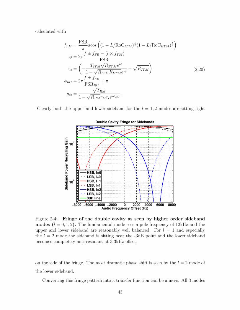
Clearly both the upper and lower sideband for the l = 1, 2 modes are sitting right

−8000 −6000 −4000 −2000 0 2000 4000 6000 8000

100

101

Audio Frequency Offset (Hz)

Sid

eban

d P

ower

Rec

yclin

g G

ain

Double Cavity Fringe for Sidebands

HSB, l=0LSB, l=0HSB, l=1LSB, l=1HSB, l=2LSB, l=23dB line

Figure 2-4: Fringe of the double cavity as seen by higher order sidebandmodes (l = 0, 1, 2). The fundamental mode sees a pole frequency of 12kHz and theupper and lower sideband are reasonably well balanced. For l = 1 and especiallythe l = 2 mode the sideband is sitting near the -3dB point and the lower sidebandbecomes completely anti-resonant at 3.3kHz offset.

on the side of the fringe. The most dramatic phase shift is seen by the l = 2 mode of

the lower sideband.

Converting this fringe pattern into a transfer function can be a mess. All 3 modes

43

l = 0, 1, 2 will contribute depending on how much carrier power of each mode is at the

dark port. Here I will just focus on l = 2 since it will lead to the lowest pole frequency.

For l > 0 the carrier can actually have non-zero components in both quadratures since

the length servo cannot zero them. In the l = 2 case these 2 components come from

an arm phase front curvature mismatch and from an arm beam radius mismatch.

To work out the l = 2 contribution to the dark port noise of an oscillator phase

modulation with modulation depth Γ at an audio frequency f , I start with an expres-

sion for the input beam with phase modulated sidebands:

Ψ = C0 + S0

(e+i(2πfSBt+Γcos 2πft) + e−i(2πfSBt+Γcos 2πft)

)(2.21)

Since the modulation Γ is assumed to be small I can use the approximation

eiΓ cos 2πft = 1 + iΓ

2e+i2πft + i

Γ

2e−i2πft (2.22)

When this field is propagated through the mode cleaner and interferometer to the

dark port each sideband term picks up the mode cleaner pole at 4.59 kHz plus a

factor i tM g±fSB±faudio

sb . Here I use the notation g±fSB±faudio

sb to indicate the sideband

recycling gain of the upper or lower (±fSB) sideband with a positive or negative audio

frequency offset (±faudio). These are the quantities plotted in figure 2-4. Note that

the g±fSB±faudio

sb are different for each spatial mode l, but I assume that all modes see

the same mode cleaner pole, i.e. I assume that the mode mismatching happens after

the mode cleaner.

I then assume that at the dark port the carrier is dominated by junk light that I

44

leave as a free (complex) parameter C0. Thus the field at the dark port has the form

Ψ = C0 + i tM tMCS0

[+ g+fSB

sb ei2π(+fSB)t

+ iΓ

2g+fSB+f

sb ei2π(+fSB+f)t + iΓ

2g+fSB−f

sb ei2π(+fSB−f)t

+ g−fSB

sb ei2π(−fSB)t

+ iΓ∗

2g−fSB+f

sb ei2π(−fSB+f)t + iΓ∗

2g−fSB−f

sb ei2π(−fSB−f)t

].

(2.23)

The mode cleaner transmission tMC accounts for the mode cleaner pole.

The photo current at the dark port is proportional to |Ψ|2, and it is demodulated

with the local oscillator ∝ cos (2πft+ Γ cos 2πft). This is where the cancellation

effect mentioned above comes in. Carrying out this calculation, I find that the phase

noise transfer function is proportional to

∝ tMC

[Carrier

]∗[(+g−fSB−f

sb + g−fSB+fsb − g+fSB−f

sb − g+fSB+fsb − 2 ∗ g−fSB

sb + 2 ∗ g+fSB

sb )

+ i(+g−fSB−fsb − g−fSB+f

sb − g+fSB−fsb + g+fSB+f

sb )

].

(2.24)

Figure 2-5 shows this transfer function. The (scaled) data from Feb 2004 is overlaid

on this plot, but one should keep in mind that the model transfer function is only one

from several possible coupling paths (l = 0, 1, 2, ... with 2 carrier quadratures each).

With all that said I should also mention that the oscillator phase noise is always

good for surprises: at one point we changed the mode cleaner length of the Livingston

interferometer by 1 mm because we wanted to use an in-house oscillator with a slightly

different frequency. Somehow this change resulted in a 10-fold (!) increase of the

oscillator phase coupling. The best explanation I have is that this somehow changed

the amount of light coupled into higher order modes (l = 1, 2) after the mode cleaner.

The only way we were able to reduce the phase noise coupling was with the TCS

system - see section 2.8.6. But even this only bought us a factor of a couple. So

45

102

103

104

10−3

10−2

10−1

100

Cou

plin

g S

tren

gth

Phase Noise Coupling due to l=2

curvature mismatchbeam radius mismatchscaled measurement

102

103

104

−180

−90

0

90

180

Audio Frequency Offset [Hz]

Pha

se [d

eg]

Figure 2-5: Oscillator Phase Noise Transfer function [oscillator phase mod-ulation → photo diode power] due to the l=2 modes. The scale is chosen arbitrarybecause the strength depends on the amount of carrier power in the l = 2 mode. Themode cleaner (MC) pole at 4.5 kHz has also been included - note that the populationof the l = 2 mode has to happen after the MC. Also shown is the arbitrary scaledmeasurement from Feb 2004.

46

we had to get a better signal generator - the one we were using had a phase noise

performance of about 6× 10−7 radians/√

Hz. We installed an ultra-low noise crystal

oscillator from Wenzel Associates, Inc. It has about 15 times less phase noise at 1kHz.

2.6 Oscillator amplitude noise

The oscillator amplitude noise is related to the oscillator phase noise because the

individual audio sidebands see the same transfer function through the interferometer.

There are however 2 key differences.

• There is no natural cancellation effect as for the phase noise. However the LO

is squared up (saturated) before it is fed to the mixer, so amplitude fluctuations

on the LO should not affect the demodulation.

• The basic coupling is given by SAS Q = SAS Q,DCδΓN(f)/Γ. Since AS Q is ser-

voed to zero any coupling can only come from the remaining RMS value. This

however is only true for the l = 0 mode and higher order modes will produce a

signal similar to the phase noise coupling.

2.7 Noise Improvements below 100 Hz

2.7.1 The problem

After eliminating a couple of noise sources that were affecting frequencies below

100 Hz, such as noisy coil drive electronics and coupling from the local damping

loops, it became clear that there was significant excess noise in the 40 Hz to 100 Hz

band that was not explicable by linear noise prediction methods.

Ultimately we were able to pin down this noise to two sources. One part was

coupled in from from excess noise in the poorly controlled auxiliary loops that held

the beam splitter (BS) and recycling mirror (RM) in place (MICH and PRC loops).

The other part was due to saturation effects in the RF amplifier at the output of the

photo diodes.

47

Finding these two noise sources was complicated by the fact that they had roughly

the same amplitude and shape, and a clear improvement was only obvious after both

problems were fixed.

2.7.2 Auxiliary length control loops

Noise in the l+ (PRC) and l− (MICH) control loops for the recycling mirror (RM)

and the beam splitter (BS) can couple to the interferometer L− displacement signal.

There are 2 different known coupling mechanisms (see [51]).

δL−(f) =rc

r′cδl− '

1

139δl−

δL−(f) = 2δrc1

r′c

gsbrM

tRM tMδl+(1 + if/fc)

(2.25)

The l− coupling is straightforward - the dark port phase sensitivity to beam splitter

motion compared to ETM motion is reduced by the arm cavity phase gain r′c =

2F/π = 139. The l+ coupling comes from sidebands beating against the residual

carrier at the dark port that is due to an arm reflectivity imbalance [51].

As always there are 2 ways to go about ameliorating this problem: reduce the

noise and reduce the coupling.

2.7.3 Coupling reduction: MICH and PRC correction

Both MICH and PRC are limited by sensing noise in the band of interest (above

≈ 40 Hz), i.e. it is the control system that pushes the BS and RM. However we know

both the noise and the coupling transfer function to DARM. Therefore we can send a

scaled version of both the MICH and the PRC control signal to the ETMs to cancel

out any linear coupling.

This trick, referred to as MICH and PRC correction, was amazingly successful,

especially for the MICH loop because its coupling is well defined and does not change.

A coupling reduction of up to 37dB was achieved with the MICH correction. For the

PRC correction we had to fine-tune the frequency dependence - for unknown reasons

48

the coupling didn’t quite follow the prediction (equation 2.25). After that we also got

a reduction of about 20dB.

In practice the strength of the PRC coupling proved to be highly modulated on a

time scale between about 0.1 Hz and 10Hz, presumably because the arm reflectivity

imbalance is affected by angular seismic disturbances. The displacement noise floor

will thus be very bursty if it is limited by PRC noise. Increasing the angular control

system bandwidth indeed reduced these coupling fluctuations.

2.7.4 Auxiliary loop noise reduction

The goal of the auxiliary loops is to reduce the residual motion of BS and RM in

the band of interest (above ≈ 40 Hz) as much as possible. Up to about 20 Hz

there are a lot of environmental disturbances (seismic motion, coupling from angular

degree of freedoms, suspension resonances such as bounce and roll mode) that jerk

the optics around. Obviously we want as much gain as possible in that band in

order to avoid saturation of the sensing electronics. However both auxiliary loops are

shot noise limited at 100Hz at a level of a couple times 10−15 m/√

Hz (MICH) and

10−16 m/√

Hz (PRC).

Especially for MICH this was a problem: up to the S3 science run we didn’t use the

MICH correction, i.e. we polluted the DARM signal with noise at ≈ 10−15 m/√

Hz×

OLGMICH/139 above 100 Hz, where OLGMICH is the MICH open loop gain. Thus the

MICH open loop gain had to be smaller than ≈ 1/100 at 100Hz. This meant that

the only possible way to get good sensitivity above 100 Hz was to choose a very low

unity gain frequency (UGF) for the MICH loop (≈ 11 Hz) and add a steep low-pass

filter with a cut-off at about 50 Hz. As a consequence we didn’t have the desired gain

below 20 Hz and lots of up-converted noise dominated the auxiliary loop error signals

up to almost 100Hz (see also [51]). This noise also showed up in all angular loops

where it used up almost all of our actuation range for the ETMs and ITMs because

of the steep dewhitening filters for those optics.

The MICH correction’s effective coupling reduction of -37dB allowed us to change

the strategy completely. We now were able to run with a high UGF (≈ 70 Hz for

49

Figure 2-6: Residual motion of the MICH (top) and the PRC (bottom)degree of freedom. The dashed blue curves correspond to the S3 configurationwith a very low MICH UGF. The solid red curves show the improvements that weremade possible by the implementation of the MICH correction which allowed runningwith a higher loop gain (see text). The bump at about 150 Hz in the lower red traceis due to gain peaking in the PRC loop. This was later resolved by rolling off the BSand RM dewhitening filters at 160 Hz which in turn allowed moving the PRC controlsignal roll off up to 1kHz effectively increasing the phase margin. (The dewhiteningfilters are analog low-pass filters in the actuation chain and deal with the DAC noise.)The black curves show the level of the dark noise (thermal noise in the photo diodetank circuit above 40 Hz, ADC noise below that.

50

MICH, ≈ 110 Hz for PRC) which dramatically reduced the up-converted noise (see

Figure 2-6). Additionally the reduced RMS signal at low frequency allowed us to

detect all available power in the pick-off port - where it was possible we even used

2 pick-off ports. This lead to a further reduction of the shot noise in the auxiliary

loops.

2.7.5 RF saturation at the photo diode output amplifier

Since the light at the anti-symmetric port is dominated by the sidebands, the by far

biggest RF signal in the photo current is the sideband beat signal at twice the main

modulation frequency of 24.48 MHz (2ω signal). To mitigate this, the photo diode

tank circuit not only has a resonance at 24.48 MHz, but is also equipped with an

about 40 dB deep notch at 48.96 MHz. After that the signal is amplified and shipped

to the demodulation board in the electronics rack.

Unfortunately it turned out that, despite the notch at 48.96 MHz, the 2ω RF

signal at this photo diode output amplifier was too big and was running into the

slew rate limit, causing the up-converted noise that was visible in the DARM loop.

The problem was mitigated by adding a notch, consisting of a coil and a trim-cap,

in the feed-back path of the amplifier. This changed the total 2ω notch depth from

about 40 dB to about 60 dB. After this fix, the RF signal at this photo diode

output amplifier was no longer dominated by the 2ω signal, but rather by higher

order modulation products for which we had no notch in the circuit.

With this fix in place and the auxiliary loops under high bandwidth control, the

noise in the 40 Hz to 100 Hz band dropped by almost an order of magnitude. However

there is still some noise left in this band that so far could not be successfully explained.

51

2.8 The Thermal Compensation System

2.8.1 The problem

The original design for the radius of curvature of the LIGO optics assumed a certain

level of thermal lensing based on the estimated absorption and an anticipated power

into the IFO of about 6 Watts. The absorption in the ITM’s and ETM’s is expected

to be due to HR coating absorption (about 1 ppm [71]) and substrate absorption (4-5

ppm/cm).

As a result the LIGO interferometers had a slightly wrong radius of curvature

in the ITM’s and ETM’s during the initial phase of commissioning (up to S2, after

which we started increasing the input power). This is a tiny effect for the stable arm

cavities. The arms define the spatial mode of the carrier, which therefore is only

slightly affected. The biggest thermal lens though is generated in the ITM substrate.

It mostly affects the sideband because the sideband only resonates in the recycling

cavity which was designed to be marginally stable. Consequently the sideband mode

size is critically dependent on the thermal lens.

In its cold state the recycling cavity is even unstable which gives rise to ring-

shaped resonating modes and a significant reduction in power buildup due to mode

mismatching and spill-over. We indeed only achieved a sideband recycling gain of

Gsb = 13 at that time, while theoretically one expects about

Gsb =

(tRM

1− rRMrM

)2

= 30 (2.26)

(see appendix A).

When the input power was increased on H1, the sideband recycling gain increased

dramatically, as expected. However, we reached a maximum of Gsb = 26.5 at only

1.8 Watt into the MC (≈ 1.2 Watt into the IFO). When going to higher powers Gsb

came down again and the sideband mode was shrinking in size. This was a clear

indication that the absorption in at least one optic of the recycling cavity was too

high, though figuring out which one turned out to be non-trivial since reopening

52

the vacuum is costly. Using spot size measurements at several IFO ports and in

different heating states [70] finally allowed us to conclude that ITMX had the biggest

absorption, 34±4 mWatt per Watt of power into the MC. ITMY had about 2.6 times

less absorption , but that’s still more than expected.

From these measurements it is impossible to know whether the absorption is in the

bulk or on the coating. Since the power hitting the HR surface is 140 times bigger

than what travels through the ITM, and since it seems impossible to accidentally

pollute the interior of the mirror during the installation, it seemed likely that this

excess absorption is on the surface. We have about 2275 Watt of arm power per Watt

into the MC. The inferred coating absorptions therefore are 15± 1.8 ppm for ITMX

and 5.6 ± 0.7 ppm for ITMY; the specification was less than 1 ppm. (If it were due

to bulk absorption the numbers would be 210 ppm/cm for ITMX and 78 ppm/cm for

ITMY; the specification was less than 5 ppm/cm.)

2.8.2 The hardware

A possible way to address this problem was shown by R. Lawrence in his thesis [67].

He studied the feasibility of a thermal compensation system for Advanced LIGO.

Based on this work an upgrade Thermal Compensation System for initial LIGO was

developed [68, 69].

Two Thermal Compensation systems were installed for each interferometer, one

for each ITM. Each system consists of a 10 Watt CO2 Laser (10.6µm wavelength)

that illuminates a switchable mask. Using a telescope with a magnification of 26.5

this pattern is then projected on to the HR surface of an ITM - the 10.6µm light

is almost completely absorbed on the optic. We chose to illuminate the HR surface

because of existing geometrical constraints - we would have preferred the AR surface

because we expected it to be less sensitive to heating laser intensity noise. As mask

we either use a ring (or annulus) pattern to compensate for too much heat deposited

in the center by the main Laser (”cooling”), or a mask with a hole in the center to

add more heat at the center of the optic (”heating”) (see Figures 2-7 and 2-8). For

practical reasons the central mask is actually installed in the Fourier plane of the

53

Figure 2-7: A schematic of the Thermal Compensation System (TCS) thatwas installed on both ITM’s on all 3 interferometers. It consists of a 10.6µm CO2

Laser, a set of masks and a projection system that produces an image of the mask onthe optic. See text for more details.

projection system. A Bessel mask further downstream clips the higher order maxima

of the Airy diffraction pattern, leaving only the central lobe of the Airy disk. It is a

quite good approximation to the main laser Gaussian beam profile. A polarizer on a

rotation stage was used to adjust the power.

Figure 2-8: Thermal images of the projected heating pattern taken with aninfrared camera in a test setup. From left to right the images were taken with anannulus mask, a central mask and no mask (illumination beam). The annulus maskimage clearly shows the 4 spokes supporting the central part of the mask.

54

2.8.3 Time dependence of the thermal lens correction

There are two relevant time constants for the formation of the thermal lens. First

there is the time to form the lens itself, given roughly by

τtherm =Cρ (heated volume)

(conductive cooling)=Cρ(

2π3w3)

2πκw≈ 10 min (2.27)

where κ is the thermal conductivity, C the specific heat and ρ the density (see Ap-

pendix A for numerical values for SiO2). Then there is the time required to get the

temperature across the whole optic into a stationary state, assuming only radiative

cooling

τstat =CmLOS

(radiative cooling)=

CmLOS

(4AσBT 30 )≈ 3 hours (2.28)

A = 0.13 m2 is the surface area of the optic and mLOS = 10.5 kg the mass of optic.

In order to get a more detailed understanding of the time dependence of the

thermal lens induced by the new TCS system I numerically solved the heat diffusion

equationdT

dt=

κ

Cρ4T (2.29)

using a simple finite difference 2-dimensional MATLAB code assuming cylindrical

symmetry. Here T is the temperature field (deviation from ambient temperature T0).

A surface heat source Pheat with the shape of the heating beam and linearized

radiative cooling were used as boundary conditions:

CρdT

dt

∣∣∣∣surface

= Pheat − 4σBT30 T (2.30)

σB is Boltzmann’s Constant. Pheat on the HR surface was modeled as a Gaussian

beam with radius w = 4 cm (same as main interferometer beam on ITM) for the

central heating case and as Gaussian beam with radius w = 12 cm, clipped at r < 4

cm and r > 12.5cm, for the annulus heating case. Pheat = 0 on all other surfaces.

Figure 2-9 shows snapshots of the temperature profile for the annulus heating case

at different times. The CO2 Laser was turned on at t = 0. The heat slowly propagates

55

toward the center of the optic. This is unfortunate since there it forms a convex lens

that counteracts the intended concave one.

Figure 2-9: Temperature profile of a cross-section through the ITM at differenttimes after the heat was turned on. The axis are radius (r) and depth (z). Initially thetemperature profile forms a clean annulus pattern, but later on the heat propagatestoward the center of the optic where it forms a lens with opposite sign and thusreduces the total efficiency.

The effective optical thickness of the thermal lens is given by

dopt(r) =

[(n− 1)α+

dn

dT

] ∫dzT (r, z) (2.31)

where α is the (linear) thermal expansion coefficient and dn/dT is the thermo-optic

coefficient. Effects due to the the Poisson ratio are neglected since dn/dT is already

the dominant term.

To convert this optical thickness into a lens power F , it is fitted with a quadratic

function

dopt(r) =1

2Fr2 + const (2.32)

taking into account only data points inside the beam radius of the main laser beam.

The result is plotted in Figure 2-10. The lens power F peaks at 15min at a level of

9× 10−5 m−1 and then drops by 45% with a time constant of 4.3 hours.

This long time constant posed a practical problem. In order to keep the interfer-

ometer at its desired operating point with a sideband recycling gain close to 30 it was

now necessary to continuously adjust the compensation power for the first couple of

hours of each lock. We thus needed a servo that can do this automatically. This servo

56

0 2 4 6 8 10 12 140

0.1

0.2

0.3

0.4

0.5

0.6

0.7

0.8

0.9

1x 10

−4

time (h)

Lens

Pow

er (1

/m)

Lens Power vs time for 1 Watt

Figure 2-10: Thermal lens power F vs time for the annulus case. After peakingat 15min the lens power drops by 45% with a 1/e time constant of 4.3 hours.

57

is described in the next section, for now I will assume that we have such a servo.

In order to compare the model described in this paragraph to the real behavior

of the interferometer I used the numerical code to compute the impulse response of

the lens power F to a short burst of compensation power. (The Fourier transform of

this impulse response is relevant for the servo system and is shown in Figure 2-12.) I

then inverted this impulse response to get the required compensation power in order

to keep a constant lens power F . This compensation power is plotted in Figure 2-11,

together with the actuator output for a 12 hour lock during which the servo kept the

interferometer at the optimal operation point. The agreement speaks for itself.

0 2 4 6 8 10 120

0.5

1

1.5Required TCS Power

hours

ITM

X A

nnul

us H

eatin

g (W

att)

H1:TCS−ITMX_PD2Model

Figure 2-11: Annulus compensation power required to keep the thermal lensconstant. The solid green line is calculated as described in the text. The blue dots arephoto diode read-backs of the applied compensation power over a 12 hour lock, duringwhich the servo system kept the interferometer at the optimal operations point.

58

2.8.4 Servo system

As mentioned a TCS servo system was key to keeping the interferometer at the

right operation point when the annulus heating mode was used. The critical part

was getting a usable error signal for the common heating. Since common heating

strongly affects the sideband mode size in the recycling cavity, and therefore the

overlap between carrier and sideband in the recycling cavity, installing a radial RF

mode matching wavefront sensor or bullseye detector in the interferometer BS pick-off

port provided a clean error signal.

The bullseye detector was originally developed by the University of Florida and

intended to improve the input beam mode matching [74]. It consists of a round central

quadrature with a diameter of 2 mm and 3 outer quadratures with the same sensitive

area placed in a tight circle around the central quadrature. The diode was tuned

for the resonant sideband frequency (24.48 MHz) and an RF notch at 49.96 MHz

was added. Since the bullseye mode Ψ ∝ (1 − 2 r2/w2) exp (−r2/w2) has a node at

r = w/√

2, and since the gap between inner and outer quadrants is at r = 1 mm, the

beam radius on the bullseye detector has to be w = 1.41 mm. Furthermore in order to

be sensitive to the wavefront curvature difference between carrier and sideband in the

recycling cavity it has to be placed at the same Gouy phase as the recycling cavity.

Both of these requirements can easily be fulfilled sufficiently by one focusing lens and

placing the bullseye detector before the focus where the beam radius is w = 1.41 mm.

On H1, experimentally it was immediately clear that the AS I signal was sensitive

to the differential TCS heating. AS I is known to be sensitive to a lot of different

alignment parameters too (see section 2.4), but a non-zero AS I signal hurts only

because of the danger of RF saturation in the RF electronics. Therefore, servoing

AS I to zero by actuating the TCS systems differentially was the right thing to do -

especially since this also reduced the Oscillator Phase noise coupling (see 2.8.6 and

2.5).

Once the error signals were available the servo loop was easy to close (Figure

2-13). The servo code was first implemented as Unix stand-alone with a sampling

59

Figure 2-12: Transfer function ”actuation power to thermal lens power”for the TCS system in both annulus and central heating mode. Both functions havebeen scaled to unity gain at 4 mHz, about the unity gain frequency of the servo loop.Central heating is 9.6 times more efficient, but the smaller central mask also blocks 3.9times more power, leaving a factor 2.5 higher actuation range for the central mode.The functions were calculated as Fourier transforms of the numerically calculatedimpulse responses. The Nyquist frequency was 0.5 Hz, which is why both magnitudeand phase show an unphysical behavior above 0.1 Hz.

60

frequency of 1 Hz and was later replaced by Epics code running at 5 Hz sampling

rate, even though the effective update rate of the rotational stage is not that fast.

The actuation function is given by Figure 2-12. Aiming for a simple 1/f open loop

shape the control filters were simple integrators (pole at f = 0 Hz) with a thermal

pole compensation zero at f = 1/(10 min). The common servo loop was generally

run with a unity gain frequency of about 1/(5 min), the differential servo loop at

about 3 times lower gain.

CT

RL

_GA

IN_X

/Y

+

+

CT

RL

_OFF

SET

_X/YIN

PUT

_MA

TR

IX

D_INCHAN

TCS 1

TCS 2

OU

TPU

T_M

AT

RIX

X Logic

Y Logic TCS Y

TCS X

X_OUTCHAN

Y_OUTCHAN

C_INCHAN

+

+ +

+

Filte

r mod

ule

Log

ic

Filte

r mod

ule

CT

RL

_GA

IN_1

/2

CT

RL

_OFF

SET

_1/2

ER

R_G

AIN

_1/2

ER

R_O

FFSE

T_1

/2

Mas

ter S

witc

h

Figure 2-13: Flow chart of the TCS servo system. The common error signal(C INCHAN) is the bullseye error signal. The differential error signal (D INCHAN)is AS I. X/Y OUTCHAN are connected to the rotation stages that control the TCSpower. The diamonds labeled with X/Y Logic contained code that automaticallyswitched from annulus to central mode and adjusted the gain when a negative controlsignal was applied. However they were never used because a mask flip produces anintensity transient that is visible as a glitch in the displacement signal.

2.8.5 Noise couplings

The TCS system can convert intensity noise on the CO2 laser into displacement noise.

There are 2 mechanisms. Radiation pressure (Equation 2.33) is conceptually simpler,

but not dominant at the sweet spot around f = 150Hz.

〈4z〉 =P/c

mLOS(2πf)2RIN = 3.6× 10−19 m

(150 Hz

f

)2(P

1 mWatt

)RIN (2.33)

RIN is the relative intensity noise on the CO2 laser, P its DC power hitting the optic,

c the speed of light and mLOS the mass of the optic.

61

The dominant coupling is due to the same effect as the thermal lensing: expan-

sion of the optic and change of the index of refraction n induced by temperature

fluctuations. There are three somewhat distinct mechanisms that do contribute:

• Expansion of the optic: This mostly changes the cavity length. The change

of the optical path length outside the cavity is small for this effect.

• Change of index of refraction: This changes the optical path length of the

light outside the cavity.

• Bending of the whole optic: This effect was first pointed out to me by

Phil Willems [57] after I tried in vain to understand the magnitude of the

annulus transfer function. The deposited heat effectively curls the optic like a

bimetallic strip. The center of mass does not move so the the area read out by

the arm cavity beam will move even if there is no overlap with the heating beam.

Therefore, this naturally becomes the dominant term for annulus heating. The

effect does not exist for an infinitely large optic.

Expansion of the optic

From equation 2.29 one can see that the penetration depth d of fluctuations at fre-

quency f is given by

d =

√κ

2πfCρ= 30µm

(150 Hz

f

) 12

(2.34)

which is smaller than the scale on which the heating pattern p(x, y) changes. There-

fore the heat flow is essentially one-dimensional along the optical axis. The energy

density in this surface layer is given by E(x, y) = Cρ∫dzT . Since E(x, y) = p(x, y)

we have

p(x, y) = 2πifCρ

∫dzT (2.35)

62

The temperature fluctuations in this surface layer have 2 effects. The surface layer

expands by

4z1 = (1 + η)α

∫dzT. (2.36)

The factor (1 + η) arises because only the surface layer is heated, i.e. no lateral

expansion is permitted. This induces a lateral stress σT = ESαT which in turn

produces an additional expansion of ε|| = ησT/ES along the optical axis. η is the

Poisson ratio and ES is the Young’s modulus. Since only a thin layer with a mass

much smaller than the rest of the optic is expanding all of the expansion 4z1 goes

into changing the arm cavity length.

Change of index of refraction

Additionally the optical thickness of the ITM is increased by

4z2 =

[(n− 1)(1 + η)α+

dn

dT

] ∫dzT. (2.37)

4z2 is bigger than 4z1, but its effect is down by r′c = π2F because it only affects the

light outside the arm cavity. F is the finesse of the arm cavity. Also the effect has

the opposite sign compared the the expansion effect.

Putting together equations 2.35, 2.36 and 2.37 we get for the displacement induced

by the heated surface layer

4z(x, y) =

[(1 + η)α

(1− π

2F(n− 1)

)− π

2Fdn

dT

]1

2πifCρp(x, y) (2.38)

Finally, to get the average displacement seen by the interferometer one has to

average 4z(x, y) over the main laser beam. Since the readout photo diode ultimately

detects power the beam intensity is the right weighting factor, i.e.

〈4z〉 =

∫dxdyI(x, y)4z(x, y)∫

dxdyI(x, y)(2.39)

with I(x, y) = 2/(πw2) exp(−2(x2 + y2)/w2) the main laser beam profile with beam

63

radius w = 4 cm. In central heating mode the CO2 laser heating pattern p(x, y) has

the same profile as the main laser and we get 〈p〉 = P/(πw2), where P =∫dxdyp(x, y)

is the total heating power. In annulus mode there is an additional factor of about

1/30 due to the reduced overlap of p(x, y) and I(x, y), which is more than observed

experimentally, see figure 2-14.

Bending of the optic

A bimetallic strip with extreme thickness ratio d h and dimensions (h + d)

width length will bend along its largest dimension with a radius of curvature R

given by (see for instance [76, 57])

1

R=

6d∆ε

h2(2.40)

with ∆ε being the misfit strain. In fact, for a small, unconstrained patch with

width R and length R the same results holds for both the length and the

width dimension. Corrections due to geometric constraints will only arise when the

surface area is not heated uniformly (e.g. heat only in the center).

Nevertheless I will first naively apply this result to our case of an optic with a

thin heated surface layer and worry about corrections afterward:

1

R(r)=

6α

h2

∫dzT (z, r) (2.41)

Based on that we can estimate the displacement profile of the front surface as

z(r) =

[∫ r

0

dr

∫ r

0

dr1

R(r)

]−[

2

R2optic

∫ Roptic

0

dr r

∫ r

0

dr

∫ r

0

dr1

R(r)

](2.42)

where the second term guarantees that the center of mass does not move. Again one

has to average over the readout beam. I do this numerically an get

〈4z3〉 =6α

h2

P

2πfCρ× Cnum(beam shape, Roptic). (2.43)

64

For an annulus heating beam (illumination beam radius willum = 11 cm, inner mask

radius rinner = 4 cm) the numerical factor is Cannnum ≈ 0.055.

As mentioned this calculation is only correct for a strip that has no additional

geometric constraint, i.e. there is a correction if we want to bend a plate into a

sphere element. However in annulus mode heat is only deposited at the edge and the

correction should be small. In appendix D I estimate that the correction to equation

2.43 for central heating is1

1 + π ln r2

r1

, (2.44)

with r2 = Roptic the radius of the optic and r1 = w the radius of the heating beam.

Including that correction the numerical factor for central heating is Ccennum ≈ 0.12. In

both cases the sign of this effect is the same as for the expansion effect.

Total thermo-optical effect

For the magnitude of the thermo-optical intensity noise coupling in central heating

mode we therefore get

〈4z〉 =P

2πfCρ

(1

πw2

[(1 + η)α

(1− π

2F(n− 1)

)− π

2Fdn

dT

]+

6α

h2Ccen

num

)RIN

= 9.8× 10−17 m

(150 Hz

f

)(P

1 mWatt

)RIN.

(2.45)

Here w = 4 cm is the beam radius and h = 10 cm is the optic thickness. The thermo-

optical effect thus dominates over the radiation pressure effect everywhere above 0.6

Hz. For the annulus mode the calculated number is

〈4z〉 = 1.4× 10−17 m

(150 Hz

f

)(P

1 mWatt

)RIN. (2.46)

It is dominated by the bending term.

To verify this prediction the heating beam was modulated with an acoustooptic

modulator and the transfer function to displacement was measured with the locked

65

102

103

10−18

10−17

10−16

10−15

Hz

m/m

Wat

t

Transfer Function CO2 RIN −−> Displacement

Data central modeModel central modeData annulus modeModel annulus modeRadiation pressure

Figure 2-14: TCS noise coupling Comparison of modeled and measured “CO2

intensity noise to displacement” coupling. Blue diamonds show data taken in centralmode, red circles show data taken in annulus mode. The solid lines correspond tothe model, no fitting was done. The model includes all three mechanisms of thermo-optical coupling. Also shown is the (small) coupling due to radiation pressure.

66

interferometer. The result is shown in figure 2-14. The transfer functions in both cen-

tral mode and annulus agree with the model - almost too well for the approximations

made.

Finally the relative intensity noise (RIN) of the installed 10 Watt CO2 laser system

was measured (Figure 2-15). Initially the RIN had several bad peaks that turned out

to arise from reflections from the masks and the polarizer on the rotation stage back

into the laser. Designing a solid mount for the rotation stage and carefully dumping

all reflections fixed this problem. The RIN of the current system is around 2× 10−6

in the critical 100 Hz - 500 Hz band, but only 1 × 10−5 at 2 kHz. With an active

Figure 2-15: Relative Intensity Noise of the CO2 lasers used in the TCS system.The measurement was repeated at different power levels (AOM voltage settings).Data points that vary systematically between the 5 traces are sensing noise limited(e.g. 60 Hz and harmonics, data above 20 kHz and below 60 Hz). The peak at 2kHz however is real but fortunately outside the band around 150 Hz where we aremost sensitive. Between 100 Hz and 500 Hz we have a RIN of about 2× 10−6.

intensity stabilization servo for the CO2 lasers it should be possible to get the RIN

as low as 5× 10−7 at all relevant frequencies, but so far this was not necessary.

Combining the RIN measurement and the measured transfer function we can

estimate the contribution of the TCS intensity noise to the L− displacement noise.

For the S5 configuration this is shown in figure 2-16 (black dashed line). It was

67

estimated assuming 30 mWatt of heating power per ITM (the actual value can vary

because the required heat changes during a lock). The noise level is now about 30

times below the design sensitivity. During S4 (i.e. before the ITMX was replaced)

however the noise contribution was about 6 times higher since we needed about 50

times more power but only won a factor of 8 due to the lower noise coupling in annulus

mode.

2.8.6 Oscillator Phase noise reduction

The coupling mechanism of oscillator phase noise depends on the amount of both

carrier and sideband light in the bullseye mode (l = 2). Indeed we noticed that

applying heat differentially to the ITMs (e.g. annulus mode on ITMX and central

mode on ITMY) affects the phase noise coupling. We were able to reduce the coupling

by about a factor of 4 using this tuning.

After we replaced ITMX with a lower absorption optic the the coupling was at this

lower level even without differential TCS tuning, so during S5 no differential control

loop was running.

2.8.7 Optics replacement after S4

Since we wanted to further increase the circulating power after the fourth science

run (S4), it was ultimately decided to open the vacuum system and replace the high

absorption ITMX (see section 2.7.1) with a spare optic. During the same vent ITMY,

which also showed an elevated absorption level, was wiped. This incursion proved to

be quite successful - afterward the measured absorption levels were consistent with

the specifications for both ITMs. As a consequence we then had to run with the TCS

system in central mode.

68

102

103

10−20

10−19

10−18

10−17

10−16

10−15

Frequency [Hz]

Disp

lace

men

t [m

/√Hz

]

H1: 14.5 Mpc, Predicted: 17, Feb 20 2006 05:42:50 UTC

DARMMICHPRCOscillatorOpticalLeversWFSOSEMSeismicDrive elec.SusThermIntThermShotDarkIntensityFrequencyTCSTotalSRD

Figure 2-16: H1 Noise Budget: The displacement spectrum is shown in solidblack. The incoherent sum of all noise sources is dashed green. The inspiral rangefor this displacement spectrum is 14.5 Mpc. See text for more information.

69

102

10−20

10−19

10−18

10−17

Frequency [Hz]

Disp

lace

men

t [m

/√Hz

]

H1: 14.5 Mpc, Predicted: 17, Feb 20 2006 05:42:50 UTC

DARMMICHPRCOscillatorOpticalLeversWFSOSEMSeismicDrive elec.SusThermIntThermShotDarkIntensityFrequencyTCSTotalSRD

Figure 2-17: H1 Noise Budget (zoom): Zoomed version of figure 2-16. Thedisplacement spectrum is shown in solid black. The incoherent sum of all noisesources is dashed green. See text for more information.

70

2.9 Summary of known noise sources

Figure 2-16 shows one of the best displacement spectra from H1 (solid black) together

with estimates for all known noise sources. The inspiral range - the sky-averaged

distance out to which a neutron star inspiral can be seen with an SNR of at least 8

- is 14.5 Mpc. The sum of all identified noise sources predicts an inspiral range of 17

Mpc. In particular those noise sources are

• MICH: This cross-talk estimate is based on the MICH CTRL channel and the

transfer function to displacement includes an estimate for the MICH correction

efficiency, see section 2.7.2. Without that correction the MICH noise would be

about 37dB higher and dominate the displacement sensitivity.

• PRC: This cross-talk estimate is based on the PRC CTRL channel and the

transfer function to displacement includes an estimate for the PRC correction

efficiency, see section 2.7.2.

• Oscillator Phase Noise: The estimate is based on the phase noise specifi-

cation of the Wenzel crystal oscillator and the measured transfer function to

displacement, see section 2.5.

• Optical Levers: Noise due to angle to length cross-talk from the angular drive

of the optical levers, see also [51], section 4.1.5.

• Wave Front Sensors (WFS): Noise due to angle to length cross-talk from

the angular drive of the wave front sensing system, see also [51], section 4.1.5.

• OSEM: Noise due to local damping loops.

• Seismic: Seismic ground motion propagated through a model of the seismic

isolation stack and the optics suspension. See [58, 51].

• Drive electronics: Combined noise of the ETM, ITM and BS drive electronics.

See [51], section 4.1.4 and [56] for updates to the coil driver.

71

• Suspension Thermal Noise: Thermal noise of the single steel wire loop

suspension. It has been analyzed in detail in [63]. The shown trace is for a

wire loss angle of φ = 1.0 × 10−3. Recent measurements by S. Penn and G.

Harry at MIT suggest that the intrinsic wire loss angle of the steel wire is as

low as φ = 1.7 × 10−4. However in situ violin mode Q measurements suggest

an effective loss angle closer to φ = 3× 10−3, with the worst inferred loss angle

being φ = 5.6 × 10−3. The clamping of the wire to the suspension cage is

suspected to be responsible for this discrepancy. In the region around 100 Hz

the suspension thermal noise scales as φ12 .

• Internal Thermal Noise: Thermal motion of the test mass itself. There is

still some uncertainty in the knowledge of the coating loss angle. The shown

trace is for a coating loss angle of 2 × 10−4. For more details see [62]. Other

relevant references: [59, 60, 61, 51].

• Shot Noise: Photon shot noise at the AS port. The trace was calculated using

the measured DC photo current. See also section 2.3. Note that the input power

was recently increased by about 30%.

• Dark Noise: Sensing noise when no light is present at the AS port. Above

roughly 60 Hz this is due to AS I servo drive noise, which dominates the thermal

noise in the photo diode tank circuit. Below that it is ADC noise.

• Intensity Noise: This estimate is based on a RIN measurement and a RIN to

displacement transfer function measurement. For more details see [51], section

4.2.1.

• Frequency Noise: Also based on an out-of-loop REFL I sensing noise (shot

noise) measurement and a REFL I to displacement transfer function measure-

ment. For more details see [51], section 4.2.2.

• TCS: Thermal Compensation System intensity noise coupling, see section 2.8.5.

72

• Total: Incoherent (RMS) sum of all known noise sources. It explains the

displacement noise everywhere except in the 60 Hz to 100 Hz band. This is also

the band that shows dependence on seismic activity below 10 Hz. At this point

it looks like up-conversion in the drive electronics could be responsible for this.

• SRD: This is the design sensitivity curve from the Science Requirement Docu-

ment [39].

2.10 Limitations of the existing hardware

At the time of writing all three LIGO interferometers have reached or surpassed their

design sensitivity. However, while this is a key milestone for the LIGO project, the

current interferometers still have a potential for improvements.

From figures 2-16 and 2-17 it is clear that the interferometers are limited by

shot noise everywhere above (and including) the sweet spot at 150Hz. Therefore the

interferometer sensitivity can be improved by increasing the circulating power further.

To be able to do that however, an upgraded laser is required. The currently installed

lasers from Lightwave with a nominal output power of 10 Watts are getting close to

the end of their lives, and the available laser power is maxed out on both the H1 and

L1 interferometer.

Based on the experience with the installed thermal compensation system (section

2.8) and the optics absorption levels after the ITMX replacement, it seems plausible

that the interferometers can run with at least 5 times more input power without

suffering too much from thermal aberrations. However, the sensing photo diodes and

electronics are already running out of headroom at the current power level, mostly

due to a too big AS I signal (section 2.4). Thus one would have to scale the number

of photo diodes at the dark port from currently four to on the order of twenty, which

just is very impractical.

A more attractive way around this problem is to install and commission an output

mode cleaner [50]. It can remove all the junk light that is responsible for the AS I

signal before it hits the photo diode. But because an output mode cleaner introduces

73

a sensitivity to beam jitter, it has to be installed seismically isolated and in-vacuum.

Tentative plans to both upgrade the laser and install an in-vacuum output mode

cleaner after the one year long S5 science run are in place [50].

74

Chapter 3

Searching for an anisotropic

background of gravitational waves

The LIGO Scientific Collaboration has analyzed the data from the first three science

runs for an isotropic stochastic background of gravitational waves [90, 91].

It is possible though that the dominant source of stochastic gravitational waves in

the LIGO frequency band comes from an ensemble of astrophysical sources (e.g. [95,

9]). If such an ensemble turns out to be dominated by its strongest members then the

assumption of isotropy is no longer valid. Instead one should look for anisotropies in

the stochastic gravitational wave background. In this chapter I introduce an analysis

that, based on the cross-correlation of the data streams from two spatially separated

gravitational wave interferometers, allows to resolve such anisotropies.

Any search for stochastic gravitational waves by definition assumes two things

about the targeted source(s):

• The duty cycle η is significant (≈ 1), i.e. it is not a transient source. This is a

key assumption since the signature of transient sources is overwhelmed by the

integration over the whole run.

• The wave form is unknown. This is not a requirement - after all we are free

to ignore that knowledge. But if the wave form is known, a matched template

search (e.g. the LIGO Pulsar search [87, 88]) would be more sensitive.

75

Of course one still has to know, or assume, the frequency content of the signal. This

information is specified by the signal strain power spectrum H(f) (see appendix C.1

for a definition). Under the assumption that this signal strain power spectrum H(f)

is known, the analysis presented in the chapter is optimal.

First though I will introduce the properties of a stochastic background of gravita-

tional waves and discuss the existing indirect and direct experimental limits on such

a background.

3.1 Cosmological source

A cosmological stochastic background of gravitational waves is in many ways similar

to the Cosmic Microwave Background from the early universe (CMB, [5, 6]), which is

a background of electromagnetic waves. As with the CMB it is useful to characterize

the gravitational background by normalizing the energy density ρgw per logarithmic

frequency f by the energy density required to close the universe, ρc.

Ωgw(f) =1

ρc

dρgw

d ln f(3.1)

The critical energy density ρc follows from the Friedman equation and is

ρc =3c2H2

0

8πG≈ 1.7× 10−8h2 ergs

cm3. (3.2)

Here H0 = h× 100 km sec−1Mpc−1 is the Hubble constant (today). Ωgw(f) is related

to the strain power spectrum Sgw(f) visible to an interferometer through

Ωgw(f) =10π2

3H20

f 3Sgw(f) (3.3)

See appendix C for a derivation.

The main difference relative to the CMB is that a gravitational wave background

decouples much earlier in the history of the universe. Depending on the model this

could happen during the inflationary epoch, i.e. around the grand unification scale

76

(1016 GeV) or during the Planck era (√c5~G−1 ≈ 1019 GeV), when Quantum Gravity

still was important. The predictions on the spectral shape and amplitude of Ωgw(f)

also vary a lot depending on the model. A good summary is given in [94].

3.1.1 Existing bounds on h2Ωgw(f)

Nucleosynthesis: The successful prediction of the cosmic abundances of the lightest

elements (3He, 4He and 7Li) by the Big Bang Nucleosynthesis can be used to set a

constrain on the gravitational wave energy density during Nucleosynthesis [94].

This can be understood as follows: Just before the neutrino freeze-out at a tem-

perature TF ≈ 1.2 × 1010K or about 1 MeV the neutron to proton ratio is given by

nn/np = exp(−Q/TF ), where Q = mn − mp = 1.3MeV. After the neutrinos freeze

out some of the remaining neutrons decay, but most of them end up in 4He. Hence

the 4He abundance is exponentially sensitive to the neutrino freeze-out temperature

TF .

The neutrino freeze-out temperature TF on the other hand is defined by the

reaction rate Γpe→nν being equal to the Hubble expansion rate H =√

8πGρ/3.

The reaction rate is roughly Γpe→nν ≈ G2FT

5 (really only appropriate for T > Q).

GF = 1.1664× 10−5GeV−2 is the Fermi coupling constant describing the weak inter-

action. The total energy density ρ during this period can be expressed as

ρ =π2

30

k4B

~3c3g∗T

4 =g∗2aT 4. (3.4)

Here a = 7.57× 10−15 erg cm−3 K−4 is the radiation constant and g∗ is the effective

number of species (i.e. relativistic particles) during the epoch of Nucleosynthesis.

This shows that TF ∝ g16∗ , i.e. the 4He abundance is sensitive to the effective number

of species during Nucleosynthesis.

The number of species g∗ is defined through

g∗ =∑

i=bosons

gi

(Ti

T

)4

+7

8

∑i=fermions

gi

(Ti

T

)4

, (3.5)

77

where gi counts the internal degrees of freedom of the i-th particle (spin, color,...)

and Ti is its temperature. For gravitons we have ρgw = aT 4gw, defining the partial

temperature Tgw, even though they are not in thermal equilibrium. The photons are

in thermal equilibrium, Tγ = T , and we have ργ = aT 4. Thus the contribution from

gravitational waves to the number of species g∗ is given by

∆g∗ = 2ρgw

ργ

(3.6)

Also note that often limits on ∆g∗ are given as number of extra neutrinos ∆Nν . The

conversion is ∆g∗ = 7/4∆Nν .

The measured abundance of 4He restricts ρgw to be at most of the same magnitude

as the photon energy density ργ during the epoch of Nucleosynthesis [94]. Both ρgw

and ργ scale as T 4 ∝ (1 + z)4, but the later annihilation of electron-positron pairs

increases the photon energy density ργ by a factor (11/4)4/3 ≈ 3.8. Finally, the

transition from a radiation to a matter dominated universe happened at z ≈ 4×104h2,

resulting in

h2Ωγ = h2ργ

ρc

≈ 2.5× 10−5 (3.7)

and therefore an upper limit for the gravitational wave energy density Ωgw of

h2

∫d(ln f)Ωgw(f) = h2Ωgw = h2ρgw

ρc∼< 6× 10−6. (3.8)

This limit spans all frequencies, but it only applies to gravitational waves that were

already present during Nucleosynthesis at z ≈ 109.

CMB: The measurement of the large angle fluctuations in the CMB by COBE [5]

and WMAP [6] can be used to derive an upper limit for frequencies that are inside

the horizon today (f > 3 × 10−18 Hz), but were still outside the horizon during the

time of last scattering (f < 10−16 Hz)[94, 5]:

h2Ωgw(f) ∼< 10−13

(10−16 Hz

f

)2

, 3× 10−18 Hz < f < 10−16 Hz. (3.9)

78

Radio Pulsar Timing: Radio Pulsars are extremely precise clocks - for some of

them the spin frequency is know with a relative precision of a couple×10−16. They can

thus be used to measure time of flight variations due to gravitational waves crossing

the line of sight. The longest accessible wavelength is determined by the distance to

the pulsar and the sensitivity to shorter wavelength drops rapidly since the signal is

averaged out over many wavelengths [86].

h2Ωgw(f) ∼< 4.8× 10−9

(f

f∗

)2

, f > f∗ = 4.4× 10−9 Hz. (3.10)

Spacecraft Doppler Tracking: This is analogous to the radio pulsar timing. The

upper limit based on measurements with the Cassini Spacecraft [85] is

h2Ωgw(f) ∼< 0.025 , at f ≈ 1.2× 10−6 Hz. (3.11)

Direct measurement: The frequency band above roughly 10 Hz is accessible to

terrestrial experiments. The first experimental upper limits came from resonant bar

detectors for a narrow band around 1 kHz. They were first operating on their own

and later in pairs, allowing for a correlation analysis [79, 80, 81, 82, 83]. The first

upper limit using an interferometer was published in 1994 [84]. In 2005 the LIGO

collaboration published its best upper limit so far, achieving h2Ωgw(f) ∼< 4.4 × 10−4

[91]. Table 3.1 lists the published upper limits that were achieved.

3.2 Astrophysical sources

It is possible that the dominant source of stochastic gravitational waves in the LIGO

frequency band comes from an ensemble of astrophysical sources (e.g. [95, 9]). In this

case the Nucleosynthesis bound - the tightest existing bound in the LIGO frequency

band - is not applicable. Furthermore, if such an ensemble turns out to be dominated

by its strongest members then the assumption of isotropy is no longer valid. Instead

one should look for anisotropies in the stochastic gravitational wave background.

This was addressed in Ref. [96, 97], but they characterized the anisotropies in terms

79

Experimental Limits

Experiment Limit on Frequency Referenceh2Ωgw(f)

Room Temperature ∼< 3000 f0 = 985± 80 Hz Glasgow [79]Resonant Bar(correlation)Cryogenic Resonant ∼< 300 f0 = 907 Hz Explorer [80]Bar (single) ∼< 5000 f0 = 1875 Hz ALTAIR [81]Cryogenic Resonant ∼< 60 f0 = 907 Hz Explorer + NautilusBar (correlation) [82, 83]Interferometers ∼< 3× 105 100 Hz ∼< f ∼< 1 kHz Garching-Glasgow

[84]

∼< 4.4× 10−4 69 Hz ∼< f ∼< 156 Hz LIGO S3 Run [91]

Table 3.1: Published direct upper limits on Ωgw(f) achieved by terrestrialdetectors

of spherical harmonics, and focused on getting optimal estimates for each spherical

harmonic. If the stochastic gravitational wave background is indeed dominated by

individual sources one can get a better signal-to-noise ratio by obtaining optimal

filters for small patches of the sky (see section 3.3). This is the motivation for the

radiometer analysis.

While the real strength of the radiometer analysis is its sensitivity to sources

with an unknown wave form it is still useful to see how good it can do for known

sources. As mentioned at the beginning of this chapter, the key requirement for the

radiometer analysis to be applicable is that the targeted source has a significant duty

cycle. This excludes individual collisions of compact objects and stellar explosions.

The only known astrophysical sources that fulfill this criterion are rotating neutron

stars (pulsars).

Of particular interest are accreting neutron stars, for two reasons:

• The power radiated in gravitational waves is proportional to the sixth power of

the spin frequency, and the fastest spinning known pulsars were all spun up by

accreting matter.

• In order to radiate gravitational waves the pulsar has to have a non-vanishing

80

quadrupole momentum and matter falling on to the surface seems to be a nat-

ural mechanism to produce such a deviation from spherical symmetry.

Binary star systems with ongoing accretion on to a compact object are known as

X-ray binaries. Two types are distinguished, Low-Mass X-ray Binaries (LMXB) and

High Mass X-ray Binaries (HMXB). I want to focus on the Low-Mass X-ray Binaries

because as far as I can tell they are the strongest predicted continuous source of

gravitational waves that is known to exist.

3.2.1 Accretion driven pulsars: Low-Mass X-ray Binaries

(LMXB)

Whether a neutron star in a close binary system is accreting mass depends on the

ratio of the mass of the neutron star to that of the companion. Stable mass transfer in

such a system only occurs when the companion fills its Roche lobe and has a smaller

mass than the neutron star. Systems with such a low-mass companion are called

Low-Mass X-ray Binaries (LMXBs).

Accretion in systems with a high mass companion has to be driven by the com-

panion’s stellar wind. These systems are referred to as High-Mass X-ray Binaries

(HMXBs) and typically have lower accretion rates.

Accreting neutron stars with a high mass accretion rate will spin up until some

mechanism can radiate away the angular momentum of the matter falling in. The two

possible candidates are electromagnetic dipole radiation and gravitational quadrupole

radiation [9, 10]. The radiated power P is given by

Pem =4π

6c3µ0

B2poleR

6 sin2(θ)ω4 (3.12)

for magnetic dipole radiation and

Pgw =32G

5c5M2R4ε2ω6 (3.13)

for gravitational radiation. The corresponding radiational torque is T = P/ω. Bpole

81

is the magnetic field at the pole, R and M the radius and mass of the neutron star,

θ the angle between magnetic and rotational axis, ω the spin angular frequency and

ε2 = QijQij/(MR2)2 with Qij =∫d3xρ(xixj − δijr

2/3) the quadrupole moment of

the neutron star. Clearly if the accretion rate is large enough and the magnetic field

weak enough gravitational radiation will eventually dominate.

There is observational evidence that the spin frequencies of LMXBs with high

accretion rate (M ∼> 10−11Myr−1) and low magnetic fields (B 1011 G) cluster

between about 300 Hz and 730Hz. No neutron star spinning faster than 730Hz has

been found so far [11]. The low magnetic fields B suggest that these systems are not

balanced by electromagnetic radiation and thus balancing by gravitational radiation

is a possibility and would require a quadrupole moment of [9]

Q ≈ 4.5× 1030 kg m2

(M

10−9M yr−1

) 12 (

2π 300 Hz

ω

) 52

≈ 10−7 × I. (3.14)

The neutron star moment of inertia is I ≈ 1038 kg m2.

The X-ray luminosity of a LMXB is given by the potential energy of the accreting

mass M

LX = MGM

R(3.15)

and exerts a torque of about

T = M√GMR. (3.16)

If gravitational radiation is indeed the relevant angular momentum balancing mech-

anism the gravitational wave luminosity is tied to the X-ray luminosity by

LGW =ω

ωKepler

LX (3.17)

where ωKepler =√GM/R3 and ω is the pulsar spin frequency. A typical value for

ω/ωKepler is 0.2. It turns out that the brightest X-ray source in the sky (short of

the sun), Sco-X1, is actually a LMXB and thus a prime candidate as a gravitational

wave source. Its magnetic field is indeed weak (≈ 107G, [12]) but unfortunately so far

82

its spin frequency is not known, even though quasi periodic oscillations (QPOs) are

observed in the X-ray [15]. The two observed QPOs are relatively coherent (Q ≈ 100)

and have frequencies of about 700 Hz and 1000 Hz, but their frequency increases

with the accretion rate. There are speculations that the difference between the 2

frequencies might be the pulsar spin frequency, but a recent study seems to to exclude

this theory [16]. Table 3.2 summarizes known relevant parameters of Sco-X1 (V818

Sco).

Sco-X1

Parameter ValueRight ascension 16h 19m 55.0850sDeclination -15 38’ 24.9”sDistance 2.8 ± 0.3 kpcX-ray luminosity 2.3× 1038 erg/secX-ray flux at earth 2.5× 10−7 erg/sec/cm2

Magnetic field near NS ≈ 1× 107 GaussOrbital period 68023.84 ± 0.08 secOrbital velocity 40± 5 km/secEccentricity ≈ 0Companion star mass ≈ 0.42M

Table 3.2: Parameters for Sco-X1. (References: [13], [14], [12])

Interestingly Sco-X1 dominates the X-ray flux due to all LMXB’s at the earth. To

estimate this we can tie the X-ray luminosity density to the stellar mass density by

LX,Gal(z) ≈ 1040erg/s×MGal(z)/(1011M) and estimate the stellar mass density as a

function of z by MGal(z) ≈ 5× 108MMpc−3× (1 + z)−1,[17]. Thus, for the standard

cosmological parameters (H0 = 72 km s−1 Mpc−1, Ωm = 0.3, ΩΛ = 0.7), we get the

x-ray flux:

FLMXB,cosm ≈∫ ∞

0

4πr2 ∂r

∂zdz

LX,Gal(z)

4πr2(1 + z)2

= LX,Gal(0)c

H0

∫ ∞

0

dz1

Ωm(1 + z)3 + ΩΛ

1

(1 + z)3

≈ 8× 10−9 erg

sec cm2

(3.18)

83

We can also estimate the flux from the Virgo cluster

FLMXB,Virgo ≈ 3000 Galaxies× 1040 erg

sec Galaxy× 1

4π(15 Mpc)2

≈ 1× 10−9 erg

sec cm2

(3.19)

Since the apparent diameter of the Virgo cluster is about 15 degree it covers about

1/230 of the whole sky. Together with the numbers from equations 3.18 and 3.19 this

implies that X-ray flux due to LMXB - and therefore also the GW flux due to LMXB

- is about 30 times stronger than average when looking at the Virgo cluster.

Values for the expected gravitational wave flux can be obtained through equation

3.17. The strain power spectrum H(f) is connected to the gravitational wave flux

through

FGW =

∫dfFf,GW =

π

4

c3

G

∫dff 2H(f). (3.20)

For Sco-X1 with ω/ωKepler = 0.5fgw/fKepler and FX = 2.5× 10−7 erg/sec/cm2 we get

HSco-X1(f)df =2G

πc31

fKeplerfFX,Sco-X1 ≈ 3.6× 10−52

(500 Hz

f

). (3.21)

The main contribution to H(f) is at twice the pulsar spin frequency. The band-

width is limited by the orbital frequency broadening of the binary star

df = fGWvorbital

c< 0.2 Hz (3.22)

where I used fGW < 2× 730 Hz. 730 Hz is the highest spin frequency ever observed

on a neutron star. If we want to choose a narrower bandwidth we will have to correct

for this orbital frequency shift.

The earth’s orbital motion has an effect of the same order of magnitude (df/f ≈

1 × 10−4, but longer period), while the earth’s rotation only produces df/f ≈ 1.5 ×

10−6. These are all effects that can be corrected for in a specialized analysis looking

only at Sco-X1. This is not done in the radiometer code because the code is optimized

for broadband signals.

84

Finally the intrinsic frequency stability of the accreting pulsar can be estimated

by assuming that the torque from the accreting matter is not balanced:

f =T

2πI=

5

4π

LX√GM3R

≈ 8× 10−5 Hz yr−1 (3.23)

3.3 The Radiometer

3.3.1 Introduction

In this section I present a directional method to search for an anisotropic gravita-

tional wave background that implements a gravitational wave radiometer [93]. The

algorithm has been implemented in MATLAB and was used to analyze the LIGO S4

science run. A summary of the relevant formulas can also be found in appendix C.

3.3.2 Search for an isotropic background

The data from the first three LIGO science runs was analyzed with a method described

in detail in Ref. [98, 90, 91, 92]. The data streams from a pair of detectors were cross-

correlated with a cross-correlation kernel Q chosen to be optimal for an assumed

strain power spectrum Sgw(f)=Sgw(|f |) and angular distribution P (Ω)=1 (isotropic

distribution). Specifically, with S1(f) and S2(f) representing the Fourier transforms

of the strain outputs of two detectors, this cross-correlation is computed in frequency

domain segment by segment as:

Y =

∫ ∞

−∞df

∫ ∞

−∞df ′δT (f − f ′)S∗1(f)Q(f ′)S2(f

′) (3.24)

where δT is a finite-time approximation to the Dirac delta function. The optimal

filter Q has the form:

Q(f) = λγiso(f)Sgw

P1(f)P2(f)(3.25)

where λ is a normalization factor, P1 and P2 are the strain noise power spectra of the

two detectors, Sgw is the strain power spectrum of the stochastic background being

85

searched for (see ref [91, 90]) and the factor γiso takes into account the cancellation

of an isotropic omni-directional signal (P (Ω) = 1) at higher frequencies due to the

detector separation. γiso is called the overlap reduction function [99] and is given by

(the normalization is such that γiso(f=0)=1 for aligned and co-located detectors):

γiso(f) =5

8π

∑A

∫S2

dΩ ei2πfΩ·∆xc FA

1 (Ω)FA2 (Ω) (3.26)

where ∆x =

x2−

x1 is the detector separation vector, Ω is the unit vector specifying

the sky position and

FAi (Ω) = eA

ab(Ω)1

2(Xa

i Xbi − Y a

i Ybi ) (3.27)

is the response of detector i to a zero frequency, unit amplitude, A = + or× polarized

gravitational wave. eAab(Ω) is the spin-two polarization tensor for polarization A and

Xai and Y a

i are unit vectors pointing in the directions of the detector arms (see [98]

for details).

The optimal filter Q is derived assuming that the intrinsic detector noise is Gaus-

sian and stationary over the measurement time, uncorrelated between detectors, and

uncorrelated with and much greater in power than the stochastic gravitational wave

signal. Under these assumptions the expected variance, σ2Y , of the cross-correlation

is dominated by the noise in the individual detectors, whereas the expected value of

the cross-correlation Y depends on the stochastic background power spectrum:

σ2Y ≡ 〈Y 2〉 − 〈Y 〉2 ≈ T

4(Q,Q) , 〈Y 〉 = T

(Q,

γisoSgw

P1P2

)(3.28)

Here the scalar product (·, ·) is defined as (A,B) =∫∞−∞A∗(f)B(f)P1(f)P2(f)df and

T is the duration of the measurement.

In order to address the long-term non-stationarity of the detector noise the data

set from a given interferometer pair is divided into equal-length intervals, and the

cross-correlation Y and theoretical σY are calculated for each interval, yielding a set

YI , σYI of such values, with I labeling the intervals. The interval length can be

86

chosen such that the detector noise is relatively stationary over one interval. In Ref.

[91, 90] the interval length was chosen to be 60 sec. The cross-correlation values

are combined to produce a final cross-correlation estimator, Yopt, that maximizes the

signal-to-noise ratio, and has variance σ2opt:

Yopt =∑

I σ−2YIYI/σ

−2opt , σ−2

opt =∑

I σ−2YI

. (3.29)

In practice the intervals are typically overlapping by 50% to avoid the effective loss

of half the data due to the required windowing (Hanning). Thus equation 3.29 has

to be modified slightly to take the correlation of neighboring segments into account

(see [101]).

Since the LIGO Hanford and Livingston sites are separated by 3000km the overlap

reduction function for this pair has already dropped below 5% around each interfer-

ometer’s sweet spot of 150 Hz, where the GW wavelength, 2000 km, is no longer large

compared to the site separation. One unfortunate drawback of this analysis thus is

the limited use it makes of the individual interferometer’s most sensitive frequency

region. Moreover, if the dominant gravitational wave background would be of astro-

physical origin the assumption of an isotropic background is not well justified. If,

for example, the signal is dominated by a few strong sources, a directed search can

achieve a better signal-to-noise ratio.

3.3.3 Directional search: a gravitational wave radiometer

A natural generalization of the method described above can be achieved by finding

the optimal filter for an angular power distribution P (Ω). In this case Eq. 3.28b

generalizes to

〈Y 〉 = T

(Q,

∫S2 dΩγΩP (Ω)H

P1P2

)(3.30)

where γΩ is now just the integrand of γiso, i.e.

γΩ =1

2

∑A

ei2πfΩ·∆xc FA

1 (Ω)FA2 (Ω) (3.31)

87

and H(f) is the strain power spectrum of an unpolarized point source, summed

over both polarizations (see appendix C.1). Note that γΩ also becomes sidereal time

dependent both through ∆x and FA

i (Ω).

Eq. 3.30 was used in Ref. [96] as a starting point to derive optimal filters for each

spherical harmonic. However if one wants to optimize the method for well localized

astrophysical sources it seems more natural to use a P (Ω) that only covers a localized

patch in the sky. Furthermore, for most reasonable choices of H(f), the maximal

resolution of this method will be no better than several tens of square degrees, so

that most astrophysical sources would not be resolved. It makes sense therefore to

optimize the method for true point sources, i.e. P (Ω) = δ2(Ω, Ω′).

With this choice of P (Ω), the optimal filter QΩ′ for the sky direction Ω′ becomes

QΩ′(f) = λγΩ′(f)H(f)

P1(f)P2(f)(3.32)

and the expected cross-correlation YΩ′ and its expected variance σ2YΩ′

are

σ2YΩ′

≡ 〈Y 2Ω′〉 − 〈YΩ′〉2 ≈

T

4(QΩ′ , QΩ′) , 〈YΩ′〉 = T

(QΩ′ ,

γΩ′H

P1P2

)(3.33)

Integration over sidereal time

Just as in the isotropic case, the long-term non-stationarity of the detector noise can

be addressed by processing the data on a segment by segment basis. However γΩ′

changes continuously with sidereal time. By setting γΩ′ to its mid-segment value one

can get rid of the 1st order error, but a 2nd order error remains and is of the order

Yerr(Tseg)/Y =Tseg

2

24

∫∞−∞

∂2γ∗Ω′

∂t2γΩ′

H2

P1P2df∫∞

−∞ |γΩ′|2 H2

P1P2df

= O

((2πfd

c

Tseg

1 day

)2)

(3.34)

with f the typical frequency and d the detector separation. For Tseg = 60 sec,

f = 2 kHz and d = 3000 km this error is less than 1%.

Thus, for sufficiently short segment length, the integration over sidereal time for

each Ω′ again reduces to the optimal combination of the set YI , σYIΩ′ given by Eq.

88

3.29. The only difference to the isotropic P (Ω)=1 case is that the optimal filter QΩ′

is different for each interval I and each sky direction Ω′.

3.3.4 Numerical aspects

To implement this method one thus has to calculate

YΩ′ = λT

∫ ∞

−∞dfγ∗

Ω′H

P1P2

S1∗S2 , σ2Ω′ = λ2T

4

∫ ∞

−∞df|γΩ′|2H2

P1P2

(3.35)

for each sky direction Ω′ and each segment I. This can be done very efficiently

by realizing that γΩ splits into a DC part, 1/2∑

A FA1 (Ω)FA

2 (Ω), and a phasor,

exp(i2πf Ω ·∆x/c). For both integrals the DC part can be taken out of the fre-

quency integration, leaving all the directional information of the integrands in the

phasor:

YΩ′ = λT

(1

2

∑A

FA1 (Ω′)FA

2 (Ω′)

)∫ ∞

−∞df

H

P1P2

S1∗S2 e−i2πfΩ·∆x/c

σ2Ω′ = λ2T

4

∣∣∣∣∣12∑A

FA1 (Ω′)FA

2 (Ω′)

∣∣∣∣∣2 ∫ ∞

−∞df

H2

P1P2

(3.36)

Thus, with N the number of sky directions Ω′, the computational load per segment

is reduced from 2N integrations to one fast Fourier transform, one integral and N

readouts of the cross-correlation YΩ′ at the time shifts τ = Ω′ ·∆x/c.

Since the fast Fourier transform of S1∗S2H/(P1P2) is sampled at fsample = 2fNyquist

it is necessary to interpolate to get the cross-correlation YΩ′ at the time shift τ . How-

ever, by choosing a high enough Nyquist frequency and zero-padding the unused

bandwidth this interpolation error can be kept small while the overall computational

efficiency is still maintained.

89

3.3.5 Comparison to the isotropic case

It is interesting to look at the potential signal-to-noise ratio improvement of this

directional method compared to the isotropic method if indeed all correlated signal

would come from one point Ω′, i.e. 〈S∗1S2〉 = γΩ′H. The ratio between the two

signal-to-noise ratios works out to

SNRiso

SNRΩ′=〈Y opt

iso 〉/σoptiso

〈Y opt

Ω′ 〉/σopt

Ω′

=[γiso, γΩ′ ]√

[γiso, γiso] [γΩ′ , γΩ′ ](3.37)

with [A,B] =∑

i (AiH/(P1,iP2,i), BiH/(P1,iP2,i)) and i the index summing over side-

real time. This ratio is bounded between −1 and 1, i.e. the directional search not

only performs better in this case but, for a point source at an unfortunate position,

the isotropic search can even yield negative or zero correlation.

It is also possible to recover the isotropic result as an integral over the sky. The

definitions of γiso and γΩ (Eq. 3.26 and 3.31) imply (see also appendix C.4)

Yisoσiso−2 =

5

4π

∫dΩ YΩσΩ

−2 , σiso−2 =

(5

4π

)2 ∫dΩ

∫dΩ′σ−2

Ω,Ω′ (3.38)

The quantity σΩ,Ω′ is a generalization of σΩ and is defined by

σ−2

Ω,Ω′ =4

T

∫dfγΩ

∗γΩ′H2

P1P2

(3.39)

However there is a difference between this σΩ,Ω′ and the the covariance σ2Ω,Ω′ = 〈YΩYΩ′〉

of the 2 sky directions Ω and Ω′. The two are related by σ2Ω,Ω′ = σ2

Ωσ2

Ω′/σ2Ω,Ω′ (see

appendix C.4).

The antenna lobe of the gravitational wave radiometer is described by

A(Ω, Ω′) =σ2

Ω,Ω′

σ2Ω′,Ω′

=〈YΩYΩ′〉〈YΩ′YΩ′〉

=(QΩ, QΩ′)

(QΩ′ , QΩ′)(3.40)

In other words, if YΩ′ = Y , either because of a source Ω′ with strength Y or because of

a random fluctuation, then the expectation value 〈YΩ〉 is 〈YΩ〉 = A(Ω, Ω′)Y . Figure 3-

90

Figure 3-1: Antenna lobe A(Ω, Ω′) of the radiometer for a flat source spectrum(H = const). Plotted is the expected signal strength assuming a source at rightascension 12 h and declination 0 deg (top left), 20 deg (top right),40 deg (bottomleft) and 60 deg (bottom right). Uniform day coverage was assumed, so the resultingshapes are independent of right ascension. Typical S4 interferometer power spectrawere assumed.

1 shows A(Ω, Ω′) for different source declinations, assuming continuous day coverage,

a flat source spectrum H = const and typical S4 interferometer power spectra.

3.3.6 Achievable sensitivity

The 1-σ sensitivity of this method is given by

Hsens,Ω(f) =σΩ

TH(f) =

H(f)

2√T√〈∫∞−∞

|γΩ|2H2

P1P2df〉sidereal day

(3.41)

Hsens is somewhat dependent on the declination and, in theory, independent of right

ascension. In practice though an uneven coverage of the sidereal day due to down-

time and time-of-day dependent sensitivity will break this symmetry, leaving only an

antipodal symmetry.

For the initial LIGO Hanford 4km - Livingston 4km pair (H1-L1), both at design

sensitivity, and a flat source power spectrum (H(f) independent of frequency), this

91

works out to

HH1−L1sens ≈ 1.5× 10−50 Hz−1

(1 yr

T

) 12

(3.42)

with a 35% variation depending on the declination. This can be converted into an

energy flux of

Fgw,fdf =c3πf 2

4GH(f)df (3.43)

Thus eq. 3.42 corresponds to a gravitational wave energy flux density of

Fgw,fdf ≈ 5× 10−8 erg

sec m2 Hz·(

f

100 Hz

)2

·(

1 yr

T

) 12

df (3.44)

3.4 Code Validation

3.4.1 Results from simulated data

In order to test the code, the real data was blanked out and simulated Gaussian

noise uncorrelated between the 2 detectors and with a power spectrum shape equal

to the LIGO design sensitivity was added. To take into account the non-uniform day

coverage, real lock segment start and stop times were used. To get a shorter turn-

around time during testing, the code was only run on 1.7 days of integrated simulated

data. The signal power spectrum was assumed to be flat, H(f) = const.

The algorithm was run on a 360 × 181 point grid covering the whole sky. While

this clearly over-samples the intrinsic resolution - for the H(f) = const case the

antenna lobe has a FWHM area of 50 − 100 deg2, depending on declination - it

produces nicer pictures, as shown in Figure 3-2. For H(f) = f−3 the antenna lobe

FWHM is even about 4 times bigger.

For figure 3-3 a stochastic signal was added: coherent noise with a flat power

spectrum H(f) and a sidereal time dependent time shift and amplitude modulation

appropriate for a true unpolarized point source.

This simulated signal was produced and calibrated piecewise in frequency domain

and multiplied by a phasor exp (i2πfτi) to encode the time shift τi appropriate for

the source location, the current sidereal time and detector i. Both polarizations were

92

Figure 3-2: An example map of the signal-to-noise ratio SNR = Yopt/σopt for simu-lated Gaussian noise (see text). The visible structure - fringes with opposite tilt onthe northern and southern hemisphere as required by the antipodal symmetry of theantenna lobe - is due to the antenna lobe.

Figure 3-3: A point source with signal-to-noise ratio (SNR) of 14 was injected at theposition of the Virgo galaxy cluster (12.5h, 12.7). It is nicely recovered. This mapalso shows the typical structure of the antenna lobe including negative correlation inregions adjacent to the main peak.

93

produced independent of each other and chosen to have the same power spectral

density, as required for an unpolarized source. Then, for each detector, the signal

was transformed back to time domain using a fast Fourier transform and multiplied

by the DC antenna acceptance FAi (t), resulting in periodic segments of 32 second

duration. These segments were then spliced together using a sin window and 50%

overlap, thus preserving the power spectral density.

The injected source in figure 3-3 has a signal-to-noise ratio of 14 and is clearly

recovered. This figure also shows the typical shape of the radiometer antenna lobe

which is given by Eq. 3.40. In particular it shows that areas adjacent to the main

lobe get a negative correlation. This means that a particularly unfortunate set of

sources could in principle cancel a lot of the signal.

3.4.2 Bias factor

In [100] is was shown that using the same data for PSD estimation and cross-

correlation results in a bias (underestimate) for both point estimate and standard

deviation estimate. This is why the PSD is now estimated using adjacent data seg-

ments. This eliminates the bias in the point estimate, but a bias in the standard

deviation estimate remains. It can be calculated by

σestimate ≈ σtrueN − 1

N(3.45)

where N is effective number of samples used for the PSD estimate. It is given by

N = 2× 9

11× 29 ≈ 47.5 (3.46)

The factors are: 2 60sec segments used; 9/11 due to use of Welch’s method; in each

60 sec segment there are 29, 50% overlapping, 4sec long sub-segments that are used

for Welch’s method.

94

All reported standard deviations are thus corrected (multiplied) with the factor

bias factor =N

N − 1= 1.022 (3.47)

3.4.3 Hardware injections

Hardware injections are useful because they unambiguously test the whole detection

and analysis system. They are expensive though in terms of using up valuable inter-

ferometer time. For that reason no directional broadband stochastic injections were

made. However both short isotropic stochastic and pulsar injections were made and

can be used to verify the radiometer search code.

The isotropic stochastic injections are broadband coherent noise injections de-

signed to mimic an isotropic primordial stochastic gravitational wave background -

except that they are stronger. They were used to verify the isotropic search code

(see e.g. [90, 91]). The isotropic result is related to the radiometer output through

equation 3.38. Rather than rerunning on the stochastic injections, I verified that

equation 3.38 is fulfilled, which has to be the case even without injections.

The pulsar injections have the advantage that they were on during roughly half

of the S4 run, but they are narrow-band and have a well-defined polarization. In

particular a pulsar wave form is given by

hi(t) = h+ cos(2πft) + h× sin(2πft) (3.48)

with

h+ = E+i (t, ψ)h0

1 + cos2 ι

2

h× = E×i (t, ψ)h0 cos ι

(3.49)

Here ι is the angle between the neutron star’s spin direction and the wave propagation

direction, f the spin frequency, h0 the wave amplitude and EAi (t, ψ) the projection

operator of polarization A on to detector i - it differs from FAi (t) in that the + and

95

× polarization are defined relative to the neutron star’s spin axis. (FAi (t) are defined

relative to the earth’s pole.) They are related by

E+i

E×i

=

cos 2ψ sin 2ψ

− sin 2ψ cos 2ψ

F+i

F×i

(3.50)

The radiometer code assumes that any correlation is due to an unpolarized source

and weights the different observation times accordingly. Therefore the radiometer

will estimate the strength of the pulsar as

H(f)df =

∑ti(E+

1 E+2 + E×

1 E×2 )(E+

1 E+2 h

2+ + E×

1 E×2 h

2×)∑

ti(E+

1 E+2 + E×

1 E×2 )2

(3.51)

The sum has to be taken over all observation times ti. Note that both h+ and

h× are peak amplitudes, while H(f)df is the RMS power due to the pulsar that is

estimated by the radiometer. Equation 3.51 assumes that the interferometer noise

stays constant, an assumption that is certainly broken by diurnal variations in the

noise floor. This will introduce some systematics.

The parameters of the 3 strongest inject pulsars - named Pulsar3, Pulsar4 and

Pulsar8 - are given in table 3.3.

Strongest injected pulsars during S4

Parameter Pulsar3 Pulsar4 Pulsar8Freq. during S4 108.86 Hz 1402.20 Hz 193.94 Hzh+ 6.5532× 10−20 9.8258× 10−19 6.3851× 10−20

h× −1.0504× 10−20 5.0606× 10−19 9.3864× 10−21

Right ascension 11h 53m 29.4s 18h 39m 57.0s 23h 25m 33.5sDeclination −33d 26′ 11.8′′ −12d 27′ 59.8′′ −33d 25′ 6.7′′

Hdf (∗) 1.74× 10−46 4.28× 10−44 1.54× 10−46

Table 3.3: Table summarizing the parameters of the fake pulsars injected into Hard-ware during the S4 run. (∗): Hdf is the equivalent unpolarized RMS power that theradiometer should detect for the pulsar. It was calculated using equation 3.51, theactual pulsar injection times and a calibration correction amounting to 20%.

Table 3.4 summarizes the result of the pulsar hardware injection. Pulsar3 and

Pulsar8 are consistent within the error bar. The high-SNR Pulsar4 strength is un-

96

Figure 3-4: Hardware Injection: Pulsar3, 108.625 Hz - 109.125 Hz The circle marksthe position of the injected pulsar.

Figure 3-5: Hardware Injection: Pulsar4, 1401.875 Hz - 1402.375 Hz The circlemarks the position of the injected pulsar.

97

Figure 3-6: Hardware Injection: Pulsar8, 193.625 Hz - 194.125 Hz The circle marksthe position of the injected pulsar.

Pulsars Hardware Injection

Parameter Pulsar3 Pulsar4 Pulsar8Freq. during S4 108.86 Hz 1402.20 Hz 193.94 HzMax. SNR at 12h 12m 18h 40m 23h 16m

−37d −13d −32dMax. estimate at 12h 12m 18h 40m 23h 12m

−36d −12d −31dMax estimate Hdf 1.80× 10−46 4.05× 10−44 1.82× 10−46

Estimate Hdf on source 1.74× 10−46 4.05× 10−44 1.79× 10−46

Error bar 1.89× 10−47 6.04× 10−46 1.73× 10−47

SNR 9.2 67.1 10.3

inj. Hdf 1.74× 10−46 4.28× 10−44 1.54× 10−46

Table 3.4: Table summarizing the pulsar hardware injections. The effective powerHdf is given for both the location of the maximum and the true source location.The last line is the injected strength, see table 3.3. The resulting underestimate forthe high-SNR Pulsar4 is probably due to a systematic bias in the power spectrumestimate when a strong signal is present [100]. The pulsar location is found accurately.

derestimated by 5%. Possible contributers to this factor are a systematic bias in the

power spectrum estimate when a strong signal is present (see [100]), the bias arising

from the diurnal sensitivity variations (see above) and a frequency bin acceptance

98

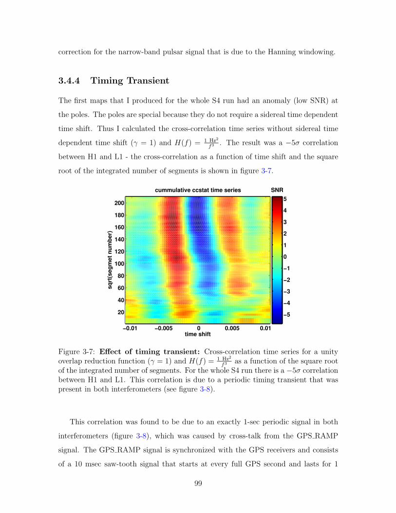
correction for the narrow-band pulsar signal that is due to the Hanning windowing.

3.4.4 Timing Transient

The first maps that I produced for the whole S4 run had an anomaly (low SNR) at

the poles. The poles are special because they do not require a sidereal time dependent

time shift. Thus I calculated the cross-correlation time series without sidereal time

dependent time shift (γ = 1) and H(f) = 1 Hz2

f3 . The result was a −5σ correlation

between H1 and L1 - the cross-correlation as a function of time shift and the square

root of the integrated number of segments is shown in figure 3-7.

−0.01 −0.005 0 0.005 0.01

20

40

60

80

100

120

140

160

180

200

time shift

sqrt

(seg

met

num

ber)

cummulative ccstat time series SNR

−5

−4

−3

−2

−1

0

1

2

3

4

5

Figure 3-7: Effect of timing transient: Cross-correlation time series for a unityoverlap reduction function (γ = 1) and H(f) = 1 Hz2

f3 as a function of the square rootof the integrated number of segments. For the whole S4 run there is a −5σ correlationbetween H1 and L1. This correlation is due to a periodic timing transient that waspresent in both interferometers (see figure 3-8).

This correlation was found to be due to an exactly 1-sec periodic signal in both

interferometers (figure 3-8), which was caused by cross-talk from the GPS RAMP

signal. The GPS RAMP signal is synchronized with the GPS receivers and consists

of a 10 msec saw-tooth signal that starts at every full GPS second and lasts for 1

99

msec (see figure 3-8). This ramp was used as an off-line monitor of the ADC card

timing and thus was hooked up to an LSC ADC card, which resulted in a non-zero

cross-talk.

0 50 100 150−1

0

1

2

msec

uVol

t Pen

tek

H1:DARM_ERR (1437280 averages)

0 2 4 6 8 10 12 14−1

0

1

2

msec

uVol

t Pen

tek

H1:DARM_ERR (1437280 averages)

0 50 100 150−4

−2

0

2

4

msec

uVol

t Pen

tek

L1:DARM_ERR (1447904 averages)

0 2 4 6 8 10 12 14−4

−2

0

2

4

msec

uVol

t Pen

tek

L1:DARM_ERR (1447904 averages)

Figure 3-8: Periodic timing transient in DARM ERR calibrated in µVolt at theADC (Pentek card) for H1 (left) and L1 (right) shown with a span of 200 msec (top)and 14 msec (bottom) in blue. The x-axis is the offset from a full GPS second.About 1.4 million seconds of DARM ERR data was averaged to get this trace. Alsoshown in red is the GPS RAMP signal that was used as a timing monitor. It wasidentified as cause for the periodic timing transient in DARM ERR. The H1 traceshows an additional feature at 6 msec since its GPS RAMP signal was routed througha whitening board.

There are two ways to remove this signal from the data stream. On can notch

every full Hz frequency bin. To reduce the amount of lost data this requires longer

time segments which in turn makes the handling of the non-stationarity harder and

increases the memory usage of the code. While these are both solvable problems, I

chose the second way mostly because it is more elegant.

This second way is to subtract the transient in time domain. This has the ad-

vantage that only a very narrow band (1/runtime ≈ 1 × 10−6 Hz) is removed while

the rest of the analysis is completely unaffected. The wave form for subtraction from

the raw (uncalibrated) data was recovered by averaging the data from the whole run

together to produce a typical second. Additionally - since this typical second only

showed significant features in the first 80 msec - the transient subtraction template

was set to zero (with a smooth transition) after 120 msec (figure 3-9).

100

0 0.02 0.04 0.06 0.08 0.1 0.12−4

−3

−2

−1

0

1

2

3

4

5

6

7x 10

−7

GPS offset (sec)

DA

RM

_ER

R c

ount

s

H1 Timing Transient

Figure 3-9: H1 timing transient in raw DARM ERR counts that was used in theanalysis to remove the effect. The first 80 msec are identical to the trace shown infigure 3-8A, after that it smoothly transitions to zero. No similar subtraction wasmade to L1 to avoid introducing accidental correlation.

This subtraction was only done for H1 since adding repetitive data to both de-

tectors can introduce artificial correlation. This subtraction efficiently eliminated the

observed correlation. Furthermore all hardware injection results (section 3.4.3) were

obtained with this subtraction. For the S5 run the GPS RAMP signal was replaced

with a two-tone signal at 900 Hz and 901 Hz. The beat between the two is now used

to monitor the timing.

3.4.5 Data cuts and post processing

The LIGO Detector Characterization working group has put together a list of all

known types of data degradation, including the times during which they occurred

[102]. Some of these so called Data Quality Flags indicate problems that should be

excluded a priori form the analysis.

Table 3.5 summarizes the data quality flags that were excluded a priori. Most

of them are obviously required, the rest were used since the amount of data lost is

minimal and it was easier to stay on the safe side.

Additionally a minimum segment duration of 182 seconds was required (60 seconds

of usable data + 60 seconds on each side for a power spectrum estimate + 1 second at

101

the beginning and end for cutting filtering transients). This cut is already included

in the numbers of table 3.5.

Applied data quality flags

Data quality flag hours % DescriptionH1:ADC OVERFLOW 0.46 0.09 % ADC out of rangeL1:ADC OVERFLOW 1.31 0.27 %H1:CALIB LINE DROPOUT 0.20 0.04 % Calibration lineH1:CALIB LINE V04 1 SEC 0.06 0.01 % not presentH1:CALIB LINE V04 60 SEC 0.45 0.09 % (different causes)L1:CALIB LINE DROPOUT 0.24 0.05 %L1:CALIB LINE V04 1 SEC 0.14 0.03 %L1:CALIB LINE V04 60 SEC 0.99 0.20 %H1:INJECTION BURST 1.64 0.34 % Period ofH1:INJECTION INSPIRAL 2.60 0.53 % Hardware Injection,H1:INJECTION PULSTART 0.12 0.02 % for Pulsar injectionH1:INJECTION STOCHASTIC 9.62 1.97 % only start and stopL1:INJECTION BURST 1.50 0.31 % times are reportedL1:INJECTION INSPIRAL 1.88 0.39 %L1:INJECTION PULSTART 0.03 0.01 %L1:INJECTION STOCHASTIC 9.96 2.04 %H1:OUTSIDE S4 15.40 3.15 % Data not availableL1:NO DATA 5.03 1.03 %L1:NO RDS 5.17 1.06 %L1:OUT OF LOCK 26.79 5.49 %L1:OUTSIDE S4 15.40 3.15 %H1:PRELOCKLOSS 30 0.47 0.10 % Excludes 30 secL1:PRELOCKLOSS 30 1.04 0.21 % before lock-lossTotal time after cuts 435.25 89.14 %Total time before cuts 488.27 100.00 %

Table 3.5: Data quality flags that were a priori excluded from science data. Theindividual flags do overlap partially, so the total amount of lost data is smaller thanthe sum of all individual flags.

One post-processing cut was required to deal with the detector non-stationarity.

To avoid a bias in the cross-correlation statistics the 2 adjacent segments are used

for the power spectral density (PSD) estimate [100]. Therefore the analysis becomes

vulnerable to large, short transients that happen in one instrument in the middle

segment - such transients cause a significant underestimate of the PSD and thus of

the theoretical standard deviation for this segment. This leads to a contamination of

102

the final estimate.

To eliminate this problem the standard deviation σ is estimated for both the

middle segment and the 2 adjacent segments. The two estimates are then required

to agree within 20% ∣∣∣∣logσmiddle

σadjacent

∣∣∣∣ < log 1.2 (3.52)

The analysis is fairly insensitive to the threshold - the only significant contamination

comes from gigantic outliers that are cut by any reasonable threshold. The chosen

threshold of 20% eliminates less than 6 % of the data.

0 1 2 3 4 5

100

101

102

103

104

ratio

H=1/f3, Reject 5.6%

0 1 2 3 4 5

100

101

102

103

104

ratio

H=const, Reject 2.5%

Figure 3-10: Histogram of the ratio σmiddle/σadjacent for the final S4 analysis (see

chapter 4). Left for H(f) = 1 Hz2

f3 , right for H(f) = 1 Hz−1. Blue is before the cut,

red after the cut (eq. 3.52).

103

104

Chapter 4

Results from S4

The LIGO S4 science run consisted of one month of coincidence data taking with

all three LIGO interferometers (22 Feb 2005 noon to 23 Mar 2005 midnight CST).

During that time all three interferometers where roughly a factor of 2 away from design

sensitivity over almost the whole frequency band. Also, the Livingston interferometer

was equipped with a Hydraulic External Pre-Isolation (HEPI) system, allowing it to

stay locked during day time. This made S4 the first LIGO science run with all-day

coverage at both sites.

Since the radiometer analysis requires two spatially separated sites I only used data

from the two 4 km interferometers (H1 in Hanford and L1 in Livingston). For these

two interferometers, about 20 days of coincident data was collected, corresponding to

a duty cycle of 69%.

4.1 Broadband results

As mentioned at the beginning of chapter 3 the only real restriction of a stochastic

search is a significant source duty cycle, with the caveat that the method is only

optimal if the waveform is not known.

Consequently the main purpose of doing a directional stochastic search is to set a

limit on possibly unknown sources. Nevertheless the shape of source power spectrum

H(f) has to be chosen a priori. Arguably the simplest possible assumption is to

105

choose some power law for H(f). I chose two different power laws for H(f):

• Constant Ωgw(f): H(f) = 1 Hz2

f3 This emphasizes low frequencies and is useful

when interpreting the result in a cosmological framework, since it corresponds

to a scale-invariant primordial perturbation spectrum.

• Constant strain power: H(f) = 1 Hz−1 This simply emphasizes the frequencies

for which the interferometer strain sensitivity is highest.

The results are reported as point estimate Y and corresponding standard deviation σ

for each pixel (see section 3.3.3). The point estimate Y has to be interpreted as best

fit assuming a source spectral shape H(f), i.e. the best estimate for the true source

spectrum is HY (f) = Y H(f).

4.1.1 Constant Ωgw(f)

−5 0 50

1000

2000

3000

4000

5000

6000

SNR

sky

area

(deg

2 )

S4, H=1/f3 Histogram of SNR (40 bins)

DataIdeal gaussian (sigma=1 mean=0)Max Likelihood: sigma=0.91836 mean=0.118161−sigma error for 100 indep. points

Figure 4-1: S4 Result: Histogram (left) and map (right) of the bias corrected signal-

to-noise ratio (SNR) for H(f) = 1 Hz2

f3 . The green curve is a maximum likelihoodGaussian fit to the data. The red solid line is an ideal Gaussian, the two dash-dottedred lines are the 1-σ bands around the ideal Gaussian for Neff = 100.

Figure 4-1 shows a histogram and a map of the bias-corrected SNR = Yσ. It

was produced by weighting all data points on the map with the corresponding sky

area in square degrees. But neighboring points are correlated, effectively reducing the

number of independent points Neff . That is why the histogram can look non-Gaussian

106

even though the data is still consistent with (correlated) Gaussian noise. Indeed the

histogram in figure 4-1 features a slight bump around SNR=2, but is still consistent

with Neff = 100 - the red dash-dotted lines indicate the 1-σ bands around the red ideal

Gaussian for Neff = 100. The histogram is clearly consistent with them. Additionally

the SNR distribution also passes a Kolmogorov-Smirnov test for Neff = 100 (α = 0.1).

So far though I do not know of any precise way to calculate Neff . However I

applied 2 heuristic methods that produced roughly the same answer:

• Spherical harmonics decomposition of the SNR map. The resulting power vs l

graph shows structure up to roughly l = 9 and falls of steeply above that - the

l = 9 point corresponds to one twentieth of the maximal power. The effective

number of independent points then is Neff ≈ (l + 1)2 = 100.

• FWHM area of a strong injected source, which is latitude dependent but of the

order of 800 deg2. To fill the sky we need about Neff ≈ 50 of those patches.

This is probably even an overestimate because the correlation angle is bigger

than the FWHM angle. Nevertheless, I used the higher Neff = 100 for this

discussion.

Figure 4-1 suggests that the data is consistent with no signal. Thus I calculated

a Bayesian 90% upper limit for each sky direction. The prior was assumed to be flat

between zero and infinity (even though a single interferometer power spectrum sets

a tighter limit than any previous experiments). Additionally I marginalized over the

calibration uncertainty of 8 % for H1 and 5% for L1 using a Gaussian probability

distribution. The resulting upper limit map is shown in figure 4-2. The upper limits

on the strain power spectrum H(f) vary between roughly 1.2× 10−48Hz−1(

100 Hzf

)3

and 1.2× 10−47Hz−1(

100 Hzf

)3

depending on the exact position in the sky.

For completeness figure 4-3 also shows the point estimate and theoretical standard

deviation maps.

107

Figure 4-2: S4 Final Result: Map of the 90 % confidence level Bayesian upper limit

for H(f) = 1 Hz2

f3 . The upper limit varies between roughly 1.2× 10−48Hz−1(

100 Hzf

)3

and 1.2× 10−47Hz−1(

100 Hzf

)3

depending on the exact position in the sky.

Figure 4-3: S4 Result: Map of the point estimate Y (left) and the theoretical

standard deviation σ for H(f) = 1 Hz2

f3 .

4.1.2 Constant strain power

As before figure 4-4 shows a histogram and a map of the bias-corrected SNR = Yσ.

Structure in the spherical harmonics power spectrum goes up to l = 19, thus Neff was

estimated to be Neff ≈ (l + 1)2 = 400. Alternatively the FWHM area of a strong

injection covers about 100 deg2 which also leads to Neff ≈ 400. The dash-dotted red

lines in the histogram (figure 4-4) correspond to the expected 1− σ deviations from

the ideal Gaussian for Neff = 400. The histogram is thus consistent with (correlated)

108

Gaussian noise, indicating that there is no signal present. The SNR distribution also

passes a Kolmogorov-Smirnov test for Neff = 400 (α = 0.1).

−5 0 50

1000

2000

3000

4000

5000

SNR

sky

area

(deg

2 )

S4, H=const Histogram of SNR (40 bins)

DataIdeal gaussian (sigma=1 mean=0)Max Likelihood: sigma=0.99738 mean=−0.0254851−sigma error for 400 indep. points

Figure 4-4: S4 Result: Histogram (left) and map (right) of the bias corrected signal-to-noise ratio (SNR) for H(f) = 1 Hz−1. The green curve is a maximum likelihoodGaussian fit to the data. The red solid line is an ideal Gaussian, the two dash-dottedred lines are the 1− σ bands around the ideal Gaussian for Neff = 400.

Again I calculated a Bayesian 90% upper limit for each sky direction, including

the marginalization over the calibration uncertainty. The prior was assumed to be flat

between 0 and ∞. The resulting upper limit map is shown in figure 4-5. The upper

limits on the strain power spectrum H(f) vary between roughly 8.5× 10−49Hz−1 and

6.1× 10−48Hz−1 depending on the exact position in the sky.

Finally figure 4-6 also shows the point estimate and theoretical standard deviation

maps.

4.1.3 Interpretation

The maps presented in figures 4-2 and 4-5 show the first directional upper limits

on a stochastic gravitational wave background ever obtained. They are consistent

with no gravitational wave background being present. The most important aspect

of this result is that it sets a limit on unexpected nearby sources, which means the

interpretation ends with the limit on the strain power spectrum.

On the other hand one can interpret the result in terms of potential sources. As an

example I look at the gravitational luminosity of all LMXBs within the Virgo galaxy

109

Figure 4-5: S4 Final Result: Map of the 90 % confidence level Bayesian upperlimit for H(f) = 1 Hz−1.The upper limit varies between roughly 8.5× 10−49Hz−1 and6.1× 10−48Hz−1 depending on the exact position in the sky.

Figure 4-6: S4 Result: Map of the point estimate Y (left) and the theoreticalstandard deviation σ for H(f) = 1 Hz−1.

cluster. They have an integrated X-ray luminosity of about 1×10−9 erg/sec/cm2 (see

equation 3.19). For simplicity I assume that they produce a flat strain power spectrum

H(f) over a bandwidth ∆f . Then the strength of this strain power spectrum is about

H(f) =2G

πc31

fKeplerf∆fFX ≈ 10−55 Hz−1

(100 Hz

f

)(100 Hz

∆f

)(4.1)

which is clearly out of reach.

110

4.2 Limits on isotropic background

Using formula 3.38 it is possible to recover the point estimate and standard deviation

for the isotropic case (see also appendix C.4). From that the 90% Bayesian upper limit

can be calculated. I additionally marginalize over the DC calibration uncertainty.

Setting the Hubble constant to 72 kmsec Mpc

, the 90% upper limit I can set on Ωgw(f)

is 1.20 × 10−4. Alternatively, assuming a flat strain power spectrum, the limit is

5.13× 10−5(

f100Hz

)3. Table 4.1 summarizes that result.

S4 isotropic upper limit

Quantity Ωgw(f) = const Sgw(f) = const

point estimate Y 1.02× 10−47Hz−1(

f100Hz

)−3 −7.12× 10−48Hz−1

standard deviation σ 6.97× 10−48Hz−1(

f100Hz

)−37.22× 10−48Hz−1

DC calibration uncertainty H1 ±8%DC calibration uncertainty L1 ±5%

90% Bayesian UL on Sgw(f) 1.99× 10−47Hz−1(

f100Hz

)−38.49× 10−48Hz−1

90% Bayesian UL on h2Ωgw(f) 6.25× 10−5 2.66× 10−5(

f100Hz

)3Table 4.1: S4 final isotropic result for the Ωgw(f) = const and the Sgw(f) = constcase. The first two lines show point estimate and standard deviation that are usedto calculate the 90% Bayesian upper limits. Those upper limits are also marginalizedover the calibration uncertainty.

4.2.1 Interpretation

The limit on an isotropic stochastic background of gravitational waves that can be

set with the S4 data is roughly one order of magnitude lower than the published

LIGO S3 limit [91], which already was by far the best experimental limit in the

terrestrial accessible frequency band (see section 3.1.1). In fact LIGO has the prospect

of improving on the Nucleosynthesis bound of Ωgw ∼< 1.2 × 10−5 in the current and

future science runs.

111

4.3 Narrow-band results targeted on Sco-X1

The gravitational wave flux from all LMXB is expected to be dominated by the closest

one, Sco-X1 (see section 3.2.1). Unfortunately its spin frequency is not really known.

I thus want to set an upper limit for each frequency bin on the RMS strain coming

from the direction of Sco-X1 (see table 3.2). The bin width I chose was df = 0.25 Hz,

which is the same bin width that was used for the broadband analysis. To choose a

narrower band, corrections for the orbital phase of the companion star would have to

be made (see equation 3.22).

To avoid contamination from the injected pulsars, the 2 frequency bins next to a

pulsar frequency were excluded. Multiples of 60 Hz were also excluded. The lowest

frequency was 50 Hz, the highest was 1799.75 Hz. The left side of figure 4-7 shows a

histogram of the remaining 6965 0.25 Hz wide frequency bins. It is consistent with a

Gaussian distribution (Kolmogorov-Smirnov test with N = 6965 and α = 0.1).

−4 −3 −2 −1 0 1 2 3 40

100

200

300

400

500

600

SNR

N

Sco−X1, Histogram of SNR

DataIdeal gaussian (sigma=1 mean=0)Max Likelihood: sigma=1.0336 mean=0.00588661−sigma error for 6965 indep. points

102

103

10−24

10−23

10−22

Hz

stra

in

Sco−X1, ra= 16.332 h , decl= −15.6402 deg

90% Bayesian limitStandard deviation

Figure 4-7: S4 Result for Sco-X1: For each 0.25 Hz wide frequency bin a pintestimate and standard deviation is calculated. The resulting SNR is histogrammedon the left side. There are no outliers. The resulting 90% confidence Bayesian upperlimit as a function of frequency - marginalized over the calibration uncertainty, isplotted on the right (red). Also shown is the standard deviation (blue).

A 90% Bayesian upper limit for each frequency bin was calculated based on the

point estimate and standard deviation, including a marginalization over the calibra-

tion uncertainty (H1: 8%; L1: 5%). The right side of figure 4-7 is a plot of this

90% limit (red trace). Above about 200 Hz (shot noise regime above cavity pole) the

112

typical upper limit rises linearly with frequency and is given by

h(90%)RMS ≈ 8.4× 10−24

(f

500 Hz

)f ∼> 200 Hz (4.2)

The standard deviation is also shown in blue.

4.3.1 Interpretation

The radiometer analysis is clearly not the optimal way to go after a presumably

periodic source like Sco-X1. Nevertheless it can set an upper limit with a minimal

set of assumptions on the source. The frequency resolution of 0.25 Hz presented here

is close to the minimal bandwidth that is required if one does not correct for orbital

parameters of the source.

The upper limit (eq. 4.2) can directly be compared to the expected strain based

on the X-ray luminosity (eq. 3.21):

h(90%)RMS

hLXRMS

≈ 440

(f

500 Hz

) 32

(4.3)

Here f is the gravitational wave frequency, i.e. twice the (unknown) spin frequency of

Sco-X1. So we really don’t expect to see anything yet. Furthermore the upper limit

for the strain scales as(

dfT

)1/4, with df the bin width and T the total run duration. So

even if one integrates for a year, corrects for all orbital frequency shifts and reduces

df to the intrinsic limit of 8 × 10−5 Hz (eq. 3.23) the upper limit on the strain

improves only by a factor of 16. Clearly the way to go is to further improve the

interferometer sensitivity - since S4 the strain sensitivity has already been increased

by 2 to 3, depending on the frequency.

113

114

Conclusion

At the time of writing all three LIGO interferometers have reached or surpassed

their design sensitivity and are now acquiring science data. To reach this goal, it was

critical to increase the power in the interferometer to more than 200 Watts incident on

the beam splitter. This required the commissioning of both a thermal compensation

system (TCS) and shot noise limited sensing electronics capable of detecting all the

light. Additionally, a series of unexpected noise sources had to be mitigated. All of

these steps are discussed in chapter 2. While reaching the design sensitivity is a key

milestone for the LIGO project, the current interferometers still have the potential

for at least a factor of 2 of improvement in strain sensitivity [50].

In a second part I introduce a radiometer analysis that uses the cross-correlation

of the data streams from two spatially separated gravitational wave interferometers

to spatially resolve anisotropies in a stochastic gravitational wave background. The

analysis is optimized for identifying point sources of stochastic gravitational radiation.

Data from the fourth LIGO science run (S4) was analyzed and no stochastic

gravitational wave background was seen. The limit on a broadband and flat strain

power spectrum coming from a point source varies between 8.5 × 10−49Hz−1 and

6.1 × 10−48Hz−1 depending on the source position. Also a limit on gravitational

radiation coming from Sco-X1, a Low-Mass X-ray binary and the brightest X-ray

source in the sky, is set for each frequency bin (see figure 4-7).

Additionally a bound of h2Ωgw(f) < 6.25× 10−5 was set on an isotropic gravita-

tional wave energy density. The ongoing extended science run also holds the promise

of improving on the Nucleosynthesis bound of Ωgw ∼< 1.2× 10−5.

115

116

Appendix A

Tables of Parameters

Physical Constants

Parameter Symbol Value Units

Speed of Light c 299792458 m/sPlanck’s Constant h 6.6261× 10−34 J sBoltzmann’s Constant kB 1.380× 10−23 J/KElectron Charge ec 1.602× 10−19 CGravitational Constant G 6.674× 10−11 m3/kg/s2

Fine Structure Constant α 1/137.036 -Stefan-Boltzmann Constant σB 5.67× 10−8 W/m2/K4

Avogadro Constant NA 6.022× 1023 mol−1

Solar mass M 1.9889× 1030 kg

Table A.1: Values of constants from the NIST CODATA web page [78]

117

Large Optic Parameters; Substrate: Fused Silica (Amorphous SiO2)

Parameter Symbol Value Units

Specific Heat C 740 J/kg/KRefractive Index (@ 1064 nm) n 1.45 -Thermal Conductivity κ 1.38 W m−1 K−1

Young’s Modulus (substrate) ES 72.80 GPaYoung’s Modulus (coating) EC 100 GPaPoisson Ratio η 0.170 -Thermal expansion coef. α 0.55 ppm/K

Thermo-Optic coef. (1µm) β = dndT

11.9 ppm/KEmissivity (10.6µm) ε 0.9 -Thickness (coating) dC 8 × 10−6 mLoss Angle (substrate) φS 1 × 10−7 -Loss Angle (coating) φC 2 × 10−4 -Density ρ 2196 kg/m3

Optic Radius RLOS 0.125 mOptic Diameter 0.250 mOptic Thickness hLOS 0.100 mOptic Thickness (BS) hBS 0.040 mOptic Mass mLOS 10.5 kgOptic Mass (BS) mBS 4.2 kg

Table A.2: Parameters for the optics are only approximate. There is an optic to opticvariation in dimensions due to the varying wedge angles. Thickness is measured atthe thickest point for all optics except the BS where it is measured at the thinnestpoint. Values are taken from [51], [67] and [77].

118

Description of Variables

Variable Symbol Description Value (for H1)

P Power into the interferometer ≈ 4 Wattgcr Carrier amplitude recycling gain 7.1Gcr = g2

cr Carrier recycling gain 50∗

gsb Sideband amplitude recycling gain 5.5Gsb = g2

sb Sideband recycling gain 30tsb Sideband transmission to the AS port 0.995∗∗

from the IFO input ≈ 0.77rcr Interferometer carrier reflectivity 0.163∗∗

rc Arm cavity carrier reflectivity 0.990r′c Derivative of rc 139

w.r.t. cavity round trip phaseF Arm cavity finesse 219FSR Arm cavity Free Spectral Range 37.520 kHzfTM Arm cavity transverse mode spacing 11.5 kHzLx Length of the X-arm cavity 3995.0562 mLy Length of the Y-arm cavity 3995.0724 mfc Arm cavity pole frequency 85 HztM Michelson transmission for the sidebands 0.18lD Schnupp asymmetry (lx − ly) 0.356 mTRM RM power transmission 0.027TITM ITM power transmission 0.028Γ Modulation depth in radians 0.4ℵ Optical gain pre-factor -ωm/(2π) Resonant sideband frequency 24.480954 MHzωnr/(2π) Non-resonant sideband frequency 61.202385 MHzFSRMC Free Spectral Range of the MC 12.240477 MHzfMC MC pole frequency 4.59 kHzRoCETMX ETMX radius of curvature on HR side 7.26 kmRoCETMY ETMY radius of curvature on HR side 7.32 kmRoCITMX ITMX radius of curvature on HR side 13.91 kmRoCITMY ITMY radius of curvature on HR side 13.6 kmRoCRM RM radius of curvature on HR side 14.4 kmRoCBS BS radius of curvature on HR side -336 km

Table A.3: Definition of variables and their value for H1. Italic values are calculatedusing the known mirror transmissions and interferometer geometry following [47].(*) An arm round trip loss of 140ppm was assumed to fit Gcr to the experimentallyobserved value. (**) In reality the sideband transmission to the AS port is significantlyworse than in the model. The uncertainties of all measured values are in the last digit.The optics parameters were taken from [75]. Other references: [65, 66]

119

DEFINITIONS of ACRONYMS

ACRONYM DEFINITION

IFO InterferometerRM Recycling MirrorBS Beam SplitterITMX Input Test Mass, X-ArmITMY Input Test Mass, Y-ArmETMX End Test Mass, X-ArmETMY End Test Mass, Y-ArmLSC Length Sensing & ControlISC Interferometer Sensing & ControlOSEM Optical Sensor and Electro-Magnetic actuatorPD Photo-DetectorRFPD Radio Frequency Photo-DetectorASC Alignment Sensing & ControlWFS Wavefront SensorQPD Quadrant Photo-DetectorSEI Seismic IsolationTCS Thermal Compensation SystemIOO Input Output OpticsPSL Pre-Stabilized LaserFSS Frequency Stabilization ServoPMC Pre-Mode CleanerISS Intensity Stabilization ServoPC Pockels CellMC Mode CleanerOMC Output Mode CleanerBSC Barbecue Sauce ContainerHAM Horizontal Access ModuleRGA Residual Gas AnalyzerPZT Lead Zirconate TantanateFAS Fine Actuation SystemPEPI Piezo-Electric Pre-IsolatorHEPI Hydraulic External Pre-IsolatorCOC Core Optics ComponentsMMT Mode Matching TelescopeLVEA Large Vacuum Equipment AreaSUS SuspensionLOS Large Optic SuspensionSOS Small Optic SuspensionIIR Infinite Impulse ResponseFIR Finite Impulse Response

Table A.4:

120

Appendix B

Useful formulas and definitions

B.1 Fabry-Perot Cavity

B.1.1 Reflection, transmission and buildup

For a cavity consisting of input mirror M1 (power reflectivity R1 and power trans-

mission T1) and end mirror (power reflectivity R2 and power transmission T2) the

reflected field ER, the transmitted field ET and the intra-cavity field Ec are

ER = Ein

(T1

√R2e

iφ

1−√R1R2eiφ

−√R1

)ET = Ein

( √T1T2e

iφ/2

1−√R1R2eiφ

)EC = Ein

( √T1

1−√R1R2eiφ

) (B.1)

where φ = 2kL = 2π fFSR

is the round trip phase, k the wave vector, L the cavity

length, f the laser frequency and FSR = c2L

the free spectral range.

B.1.2 Transfer functions for modulations

Near resonances the line forms are Lorentzian, i.e.

ET,C ∝1

1 + i ff0

, f0 =(1−

√R1R2)FSR

2π√R1R2

(B.2)

121

f0 is the half-max-half-width (in terms of power) of the Lorentzian line and is also

called cavity pole because both frequency and amplitude modulations on the input

laser light are filtered with one real pole at f0, i.e the transfer function is 1/(1+if/f0).

Strictly speaking this is only true as long as the modulation frequency is not much

bigger than the pole frequency. It obviously completely fails at multiples of the FSR.

For example at the first FSR the transfer function can be approximated by

2(1 + i f

f0

)(1 + FSR2

f20

)(1 + i f

f0+iFSR

)(1 + i f

f0−iFSR

) (B.3)

122

Appendix C

Formulae for radiometer and

isotropic search

C.1 Definition of basic quantities

For a stochastic, stationary background of gravitational waves the expectation value

of the fields is:

〈h∗A(f,Ω), hA′(f ′,Ω′)〉 = H2−sidedA (f)P (Ω)δ2(Ω,Ω′)δA,A′δ(f − f ′) (C.1)

where P (Ω) is the power distribution across the sky and H2−sidedA (f) is the 2-sided

strain power spectral in polarization A. The goal of the radiometer is to estimate the

signal strength from one direction Ω, assuming an unpolarized source, i.e.

H1−sided(f) = 4H2−sided+ (f) = 4H2−sided

× (f) (C.2)

One factor of 2 comes from going from 2-sided to 1-sided, the other is due to the inter-

pretation of H(f) as total power in both polarizations. The superscript “1− sided”

is dropped from here on. (This is a different definition than what Allen and Romano

[98] used - their H(f) is 2-sided and per polarization.) The strain power spectral

123

density H(f) is related to the the energy flux by

Fgw,f(Ω)df =c3πf 2

4GH(f)P (Ω)df (C.3)

and to the energy density in gravitational waves, ρgw, by

ρgw =

∫S2

dΩ

∫ ∞

0

dfc2πf 2

4GH(f)P (Ω)df. (C.4)

Using additionally the critical density from the Friedman equation

ρc =3c2H2

0

8πG(C.5)

and assuming an isotropic background, P (Ω) = 1, we find for Ωgw(f) - the energy

density ρgw per logarithmic frequency f , normalized by the energy density required

to close the universe, ρc:

Ωgw(f) =1

ρc

dρgw

d ln f=

8π3

3H20

f 3H(f) (C.6)

In the case of an isotropic background, P (Ω) = 1, the quantity Sgw(f) is defined

as the (1-sided) strain power spectrum that 2 co-located and aligned detectors would

see. It is connected to H(f) through

γisoSgw =

∫dΩγΩH (C.7)

Due to the definition of γiso and γΩ (eq. 3.26,3.31) we have Sgw = 4π5H. Sgw plays

the same technical role in an isotropic search as H does in the directed search, i.e.

the same variable is used in the MATLAB code. Sgw is related to Ωgw(f) by

Ωgw(f) =8π3

3H20

f 3H(f) =10π2

3H20

f 3Sgw(f) (C.8)

124

C.2 Basic formulae for the isotropic search

Optimal filter Q (i is the segment index):

Qi = λiγisoSgw

P1P2

(C.9)

Normalization integral:

Iisoi = λ−1i =

∫df|γiso|2 S2

gw

P1P2

(C.10)

Cross-correlation integral:

Yisoi = T (Qi,S∗1S2

P1P2

) = Tλi

∫dfγ∗isoSgw

P1P2

S∗1S2 (C.11)

Theoretical standard deviation for segment i:

σiso2i =

T

4(Qi, Qi) =

T

4λ2

i

∫df|γiso|2 S2

gw

P1P2

=T

4Iiso

−1 (C.12)

Whole run standard deviation and Yiso/T :

σiso−2 =

∑i

σiso−2i

Yiso =

∑i Yisoiσiso

−2i∑

i σiso−2i

(C.13)

C.3 Basic formulae for the radiometer search

There is a different overlap reduction function γΩi for each point Ω in the sky and

each segment i. The relation to the isotropic γiso is (note that γiso is independent of

i and that the additional factor of 2 is introduced such that the radiometer result is

normalized to total power in both polarizations of an unpolarized source.)

γiso = 25

8π

∫dΩγΩi (C.14)

125

Optimal filter QΩi (i is the segment index):

QΩi = λΩi

γΩiH

P1P2

(C.15)

Normalization integral:

IΩi = λΩ−1i =

∫df|γΩi|

2H2

P1P2

(C.16)

Cross-correlation integral:

YΩi = T (QΩi,S∗1S2

P1P2

) = TλΩi

∫dfγΩ

∗iH

P1P2

S∗1S2 (C.17)

Theoretical standard deviation for segment i:

σΩ2i =

T

4(QΩi, QΩi) =

T

4λΩ

2i

∫df|γΩi|

2H2

P1P2

=T

4IΩi

−1 (C.18)

Whole run standard deviation and point estimate YΩ/T :

σΩ−2 =

∑i

σΩ−2i

YΩ =

∑i YΩiσΩ

−2i∑

i σΩ−2i

(C.19)

C.4 Relation between radiometer and isotropic search

The relations derived in this section can be used to compare results from the radiome-

ter search to the isotropic search. As mentioned above the quantities Sgw and H are

represented by the same variable in the MATLAB code, so for the purpose of this

paragraph I will set them to be equal. As a result factors of 54π

will show up in the

final relations.

By inspection of equations C.11, C.17 and C.14 we find the relation

Yisoi Iisoi =5

4π

∫dΩYΩiIΩi (C.20)

126

Since σ−2i ∝ Ii for both the radiometer and the isotropic search this implies

Yisoiσiso−2i =

5

4π

∫dΩYΩiσΩ

−2i (C.21)

But these are exactly the quantities that get added up in the optimal combination of

individual segments (eq. C.13 and C.19). Therefore the following relation holds for

the end result:

Yiso σiso−2 =

5

4π

∫dΩ YΩ σΩ

−2 (C.22)

The relation between the theoretical sigmas is not quite as straight forward. First we

define the 2-point correlation integral IΩ,Ω′i

IΩ,Ω′i =

∫dfγΩ

∗i γΩ′ iH

2

P1P2

(C.23)

and in analogy to eq. C.18

σ−2Ω,Ω′i =

4

TIΩ,Ω′

i (C.24)

It has the property σΩ,Ωi = σΩi. Note though that σΩ,Ω′i is not the same as σΩ,Ω′i,

defined by

σ2Ω,Ω′i = 〈YΩiYΩ′i〉 =

T

4(QΩi, QΩ′i) =

T

4

IΩ,Ω′i

IΩiIΩ′i=σ2

Ωiσ2Ω′i

σ2Ω,Ω′i

(C.25)

Definition C.24, together with eq. C.12 and C.14, imply

σiso−2i =

(5

4π

)2 ∫dΩ

∫dΩ′σ−2

Ω,Ω′i (C.26)

and, after summing over all i

σiso−2 =

(5

4π

)2 ∫dΩ

∫dΩ′σ−2

Ω,Ω′ (C.27)

where σ−2Ω,Ω′ =

∑i σ

−2Ω,Ω′i. The quantities σΩ,Ω′i are not calculated in the radiometer

code since they are not required for the radiometer end result. In order to still be able

to use relation C.22 the radiometer code instead also directly calculates the isotropic

127

σiso. This provides a powerful sanity check.

C.5 Remarks on deconvolving the radiometer

C.5.1 Inverse of 2-point correlation integral

The key for the deconvolution problem is knowledge of the inverse FΩ,Ω of

IΩ,Ω′ =∑

i IΩ,Ω′i, defined by

∫dΩFΩ,Ω

∫dΩ′IΩ,Ω′PΩ′ = PΩ ∀ PΩ′ (C.28)

or ∫dΩFΩ,ΩIΩ,Ω′ = δ2

(Ω,Ω′

)(C.29)

Discretizing the integral∫dΩ =

∑nwn, with wn the area corresponding to the nth

pixel, results in ∑n

Fknwn

∑m

InmwmPm = Pk (C.30)

or ∑n

FknwnInmwm = δk,m (C.31)

in other words Fkn is given by the matrix inversion

Fkn =[[wnInmwm]−1]

kn(C.32)

This looks easy, but the real problem arises because the matrix wnInmwm will be badly

conditioned as soon as the pixel resolution exceeds the intrinsic antenna resolution

given by IΩ,Ω′ . Also the dimension of this matrix is N2 with N the number of pixels

per map, i.e. this can be a numerical challenge.

128

C.5.2 Deconvolved radiometer problem statement

In order to get a map that is not convolved with the antenna pattern we have to

redefine what we mean by an optimal filter. To simplify the notation I define an

additional scalar product that includes the integration over time (summation over

segments i):

[Ai(f), Bi(f)] =∑

i

(Ai(f), Bi(f)) =∑

i

∫dfAi(f)∗Bi(f)P1(f)P2(f) (C.33)

This allows to state the problem:

The expectation value of the cross-correlation 〈YΩ〉 has to be equal to the gravi-

tational wave flux P (Ω) at Ω, for all Ω

〈YΩ〉 = T [QΩ i,

∫dΩ

γΩ iH

P1P2

P (Ω)] ≡ TP (Ω) (C.34)

and the variances

σ2Ω,Ω =

T

4[QΩ i, QΩ i] (C.35)

have to be minimized. Weighting all sky directions equally suggests minimizing

∫dΩσ2

Ω,Ω = min (C.36)

To make the notation more transparent it is worth translating the problem to

matrix notation.

Q = QΩ, i(f), M = MΩ, i(f) =γΩ,i

P1P2, I: identity matrix

The 1st index of Q and M is the combined time-frequency summation, the 2nd index

is the sky position. With that the problem statement (eq. C.34 to C.36) becomes

Q†M = I

trQ†Q = min(C.37)

129

C.5.3 Deconvolved radiometer formal solution

Eq. C.37 is a classical under-constrained least-square problem. The formal solution

goes as follows: Define L = (M †M)−1. Then any Q of the form Q = ML† +K with

K†M = 0 fulfills equation C.37a, and equation C.37b yields K = 0. Thus Q = ML†.

Translating back to the usual notation we find that L is nothing but FΩ,Ω. Thus

we find a new optimal filter

QΩ i =

∫dΩF ∗

Ω,Ω

γΩiH

P1P2

(C.38)

a new cross-correlation integral

⟨YΩ i

⟩= T (QΩ i,

S∗1S2

P1P2

) = T

∫dΩFΩ,Ω

∫dfγΩ

∗iH

P1P2

S∗1S2 (C.39)

and a new theoretical standard deviation

σ2Ω

=T

4

∑i

(QΩ i, QΩ i)

=T

4

∑i

∫dΩ′F ∗

Ω,Ω′

∫dΩFΩ,Ω

∫dfγΩ

∗i γΩ′ iH

2

P1P2

=T

4

∫dΩ′F ∗

Ω,Ω′ i

∫dΩFΩ,Ω i

∑i

IΩ,Ω′i

=T

4F ∗

Ω,Ω

(C.40)

C.5.4 Generic problem of the deconvolved radiometer

Obviously the key problem is calculating the inverse FΩ,Ω of the 2-point correlation

integral IΩ,Ω which describes the antenna lobe of the synthetic aperture. Since IΩ,Ω

smears the signal out on the typical angular scale α = cfd

(d: site separation, f:

typical signal frequency, c: light speed) any attempt to achieve a significantly higher

resolution than α is necessarily going to run into numerical trouble.

But there is also a more fundamental reason why this deconvolution is not too

meaningful. The described deconvolved radiometer search aims at finding the dis-

tribution P (Ω) assuming the signal spectrum H is the same for the whole sky, an

130

assumption that most likely is wrong. The actual shape of the synthetic aperture

antenna lobe, and therefore the deconvolved map, however depends on the signal

spectrum H which has to be put in a priori. Thus, even if there were a signal, the re-

sulting sky map would most likely not be accurate. For that reason the deconvolution

problem was not pursued in this thesis.

131

132

Appendix D

Correction to the TCS noise

coupling

D.1 Estimate of bending correction

In section 2.8.5 I used the formula for a bimetallic strip 2.40 to estimate the locally

induced curvature of the optic. Here I estimate the effect of the geometric constraint

of a large optic if the optic is only heated at the center.

I do this by dividing the optic into a near zone r < r1 and a far zone

r1 < r < r2 = Roptic and estimate the energy required to bend the optic.

Figure D-1: Schematic of ring ele-ment in far zone

Figure D-2: Schematic of ring ele-ment in near zone

133

D.1.1 Far zone

I focus on a ring element at radius r with radial size dr and thickness h. When the

near zone is bent by an angle γ =∫ r1

0dr1/R(r) this ring element gets both translated

along the optical axis and rotated by the angle γ. No energy is required for the

translation. But a rotation stretches the circumference by ∆l/l = y γ/r. Thus the

energy required to do this is

Energy =

∫ r2

r1

∫ h/2

−h/2

1

2ES

(yγr

)2

dy 2πrdr

=πESh

3

12γ2 ln

r2r1

(D.1)

where ES is the Young’s Modulus.

D.1.2 Near zone

Here the bending angle changes as δγ = dr/R(r). Again I focus on a ring element at

radius r with radial size dr and thickness h, but now the dominant term comes from

bending the element like a rod, i.e. ∆l/l = y dγ/dr. Thus the energy required to do

this is

Energy =

∫ r1

0

∫ h/2

−h/2

1

2ES

(ydγ

dr

)2

dy 2πrdr

=πESh

3

12γ2

(1

γ2(r1)

∫ r1

0

dr r

(dγ(r)

dr

)2)

=πESh

3

12γ2K(shape)

(D.2)

K is a numerical constant that only depends on the shape of dγ(r)/dr. For a Gaussian

profile with radius w r1 we have K = 1/π.

D.1.3 Energy balance

Based on the bimetallic strip formula 2.40 we estimate a total bending angle

γ0 = 6αh2

∫ r1

0dr∫dzT (z, r). But this does not include the energy required to bend the

134

optic in the far zone. The actual total bending angle γ can thus be estimated by

minimizing

Energy =πESh

3

12

(K(γ − γ0)

2 + γ2 lnr2r1

)(D.3)

which givesγ

γ0

=1

1 +K−1 ln r2

r1

(D.4)

Since the induced displacement 〈4z3〉 is linear in γ the same correction factor applies

to it.

D.2 Next order correction to the local coupling

Here I show that for an infinitely large optic with a not infinitesimally thin heated

surface layer the next order correction for the TCS transfer function (Equation 2.38,

derived in section 2.8.5) is

4z(x, y) =

[(1 + η)α

(1− π

2F(n− 1)

)− π

2Fdn

dT

]d2

iκp(x, y)

− π

2Fdn

dT

d2

iκ

(−id242

)p(x, y)

+ Terms of order(d442

2

)p(x, y)

(D.5)

where the surface layer thickness parameter is d =√κ/(2πfCρ) (Equation 2.34). The

small parameter used for the expansion is d242 (42 is the 2-dim Laplace operator

on the surface z = 0.)

Derivation: Heat diffusion: First we need to solve Cρ∂tT = κ4T + 2p(x, y)δ(z)

(the heat diffusion equation) up to first order in d242. Note that there is an additional

factor of 2 in the source term because the heat is only conducted away on one side.

In Fourier space this equation is

(k2

z + id−2)T = −k2

T T +2p

κ(D.6)

135

Which can iteratively be solved up to first order:

T (0+1) =2p/κ

k2z + id−2

− k2T 2p/κ

(k2z + id−2)2 (D.7)

The integral∫∞

0dzT 0+1(z) is then equal to T (0+1)(kz = 0)/2 , i.e.

∫ ∞

0

dzT (0+1) =−id2

κ

[1− id242

]p(x, y) (D.8)

We will need the Fourier transform ”kz → z” only for the 0th order, which can be

calculated using the Cauchy Integral Theorem (z > 0):

T (0) =2p

κ

1

2π

∫ ∞

−∞dkz

e−ikzz

k2z + id−2

=p

κd(1− i)√

2exp

(−(1 + i)√

2

z

d

)(D.9)

Elastic problem: We now need to solve the elastic equilibrium equation with

boundary condition on z = 0 in the half plane z > 0:

1− η

1 + η∇(∇ ·

v)− 1− 2η

2(1 + η)∇∧∇ ∧

v = α∇T (D.10)

σzz =E

1− 2η

[η

1 + η

(∇ ·

v)− αT +

1− 2η

1 + η

∂vz

∂z

] ∣∣∣∣z=0

= 0

σxz =E

2(1 + η)

[∂vz

∂x+∂vx

∂z

] ∣∣∣∣z=0

= 0

σyz =E

2(1 + η)

[∂vz

∂y+∂vy

∂z

] ∣∣∣∣z=0

= 0

(D.11)

v is the displacement field, E is the Young’s modulus and η is the Poisson ratio. Here

I am following more or less [72] and [73], section 8. This problem can be reduced with

the Ansatzv =

v 0 +∇φ, where φ fulfills the Poisson equation

4φ =1 + η

1− ηαT (D.12)

without boundary condition andv 0 fulfills equation D.10 with zero source term and

136

new boundary conditions

σzz =E

1 + η[42φ]

∣∣∣∣z=0

σxz = − E

(1 + η)

[∂2φ

∂x∂z

] ∣∣∣∣z=0

= 0

σyz = − E

(1 + η)

[∂2φ

∂y∂z

] ∣∣∣∣z=0

= 0

(D.13)

Here 42 = ∂2x +∂2

y . This second step (”φ→ v”) is solved in [73], section 8. Equation

D.12 can be integrated:

φ(x, y, z = 0) = −1 + η

1− η

α

4π

∫dx′dy′

∫dz′

T (x′, y′, z′)√(x− x′)2 + (y − y′)2 + (z′)2

(D.14)

We can now use equation D.9 and the abbreviation a :=√

(x− x′)2 + (y − y′)2 to

evaluate the integration over z′.

∫ ∞

0

dz′T (0)√

a2 + (z′)2=−id2

a

p

κ

∫ ∞

0

dXe−X

√1− id2a−2X2

=−id2

a

p

κ

∫ ∞

0

dXe−X

[1 + id2a−2X

2

2+O

(d4a−4X4

)]=−id2

a

p

κ

[1 + id2a−2 +O

(d4a−4

)]= −id2 p

κ

[1 + id24′

2 +O(d44′2

2

)] 1

a

(D.15)

The last step is true because 4′2a

−1 = a−3. Inserting this result into equation D.14

and using integration by parts twice to move the Laplace operator over to p(x′, y′)

gives

φ(0)(x, y) = −1 + η

1− η

α

4π

∫dx′dy′

1

a

−id2

κ

[1 + id24′

2 +O(d44′2

2

)]p(x′, y′). (D.16)

At the same time we also have a contribution of T (1).

φ(1)(x, y) = −1 + η

1− η

α

4π

∫dx′dy′

1

a

−id2

κ

[−id24′

2 +O(d44′2

2

)]p(x′, y′). (D.17)

137

The 2 terms of order d24′2 cancel each other exactly.

Now we can solve for vz. According to [73], section 8 vz is given by

vz =1− η2

πE

∫dx′dy′

σzzz′=0√

(x− x′)2 + (y − y′)2(D.18)

and σz′=0zz is given by equation D.13. Putting everything together and neglecting

terms of order (d44′′22 ) we get

vz(x, y) = −(1 + η)α

4π2

d2

iκ

∫d2x′

1

|~x− ~x′|4′

2

∫d2x′′

1

|~x′ − ~x′′|p(x′′, y′′)

= (1 + η)αd2

iκp(x, y)

(D.19)

Conversion to displacement noise: So after all that work the surface displacement

4z1 = vz remains unchanged up to order (d4422)! The term proportional to dn

dT

however is scaled by [1− id242], resulting in equation D.5. This correction is only in

phase though - the magnitude of the transfer function remains totally unchanged up

to order (d4422) terms.

138

Bibliography

[1] Albert Einstein Uber Gravitationswellen. Sitzungsberichte der Koniglich

Preussischen Akademie der Wissenschaften Berlin (1918), 154-167

[2] R. A. Hulse and J. H. Taylor. Discovery of a pulsar in a binary system. Astro-

phys. Journ., 195:L51–L53, 1975.

[3] J. M. Weisberg and J. H. Taylor. General relativistic geodetic spin precession

in binary pulsar B1913+16: mapping the emission beam in two dimensions.

Astrophys. Journ., 576(2):942–949, 2002.

[4] D. J. Champion, D. R. Lorimer, M. A. McLaughlin, J. M. Cordes, Z. Arzouma-

nian, J. M. Weisberg, and J. H. Taylor. PSR J1829+2456: a relativistic binary

pulsar. Mon. Not. R. Astron. Soc., 000:1–5, March 2004.

[5] G. F. Smoot et al., “Structure in the COBE DMR first year maps,” Astrophys.

J. 396, L1 (1992).

[6] C.L. Bennett et al., “First Year Wilkinson Microwave Anisotropy Probe

(WMAP) Observations: Preliminary Maps and Basic Results”, Astrophys. J.

S. 148, 1 (2003).

[7] C. W. Misner, K. S. Thorne, and J. A. Wheeler. Gravitation. W. H. Freeman

and Co., 1970.

[8] Peter R. Saulson. Fundamentals of Interferometric Gravitational Wave Detec-

tors. World Scientific, 1994.

139

[9] L. Bildsten. Gravitational radiation and rotation of accreting neutron stars.

Astro. Journal, 501:L89–L93, 1998.

[10] D. Chakrabarty, E. H. Morgan, M. P. Muno, D. K. Galloway, R. Wijnands,

M. van der Klis, and C. B. Markward. Nuclear-powered millisecond pulsars

and the maximum spin frequency of neutron stars. Nature, 424:42–44, July

2003.

[11] D. Chakrabarty. Millisecond Pulsars in X-Ray binaries. astro-ph/0408004 July

2004.

[12] Yu. N. Gnedin; N. A. Silant’ev; L. G. Titarchuk. Sco X-1 and Cyg X-1: Determi-

nation of Strength and Structure of Magnetic Field in the Nearest Environment

of Accreting Compact Stars. astro-ph/0207640, 2002.

[13] C. F. Bradshaw, E. B. Fomalont, B. J. Geldzahler. High-Resolution Parallax

Measurements of Scorpius X-1. ApJ, 512L121 (1999).

[14] E. W. Gottlieb,E. L. Wright, W. Liller. Optical studies of UHURU sources. XI.

A probable period for Scorpius X-1 = V818 Sco. ApJ, 195L33 (1975).

[15] van der Klis et al., Discovery of Submillisecond Quasi-periodic Oscillations in

the X-Ray Flux of Scorpius X-1. ApJL, 496, L1 (1996).

[16] C. M. Zhang, H. X. Yin, Y. H. Zhao, F. Zhang, L. M. Song, The correlations

between the twin kHz QPO frequencies of LMXBs. gr-qc/0601318.

[17] L. Bildsten, V. Mandic. Personal communication 2005.

[18] E. E. Flanagan and S. A. Hughes. Measuring gravitational waves from binary

black hole coalescences. i. signal to noise for inspiral, merger, and ringdown.

Phys. Rev. D, 57(8):4535–4565, 1998.

[19] C. W. Misner, R. A. Breuer, D. R. Brill, P. L. Chrzanowski, H. G. Hughes,

and C. M. Pereira. Gravitational synchrotron radiation in the Schwarzschild

geometry. Phys. Rev. Lett., 28:998–1001, 1972.

140

[20] S.W. Hawking. Theory of the detection of short bursts of gravitational radiation.

Phys. Rev. D, 4:2191–2197, 1971.

[21] B. Allen. A χ2 time-frequency discriminator for gravitational wave detection.

arXiv, pages gr–qc/0405045, 2004. http://xxx.lanl.gov/abs/gr-qc/0405045.

[22] A. Buonanno, Y. Chen, and M. Vallisneri. Detection template families for grav-

itational waves from the final stages of binary black-hole inspirals: Nonspinning

case. Phys. Rev. D, 67:024016, 2003.

[23] C. Kim, V. Kalogera, D. R. Lorimer, M. Ihm, and K. Belczynski. The galactic

double-neutron-star merger rate: Most current estimates. In F. Rasio, editor,

Binary Radio Pulsars, 2004. http://xxx.lanl.gov/abs/astro-ph/0405564.

[24] C. Kim, V. Kalogera, D. R. Lorimer, M. Ihm, and K. Belczynski. The double-

neutron star inspiral rate snd expectations for gravitational-wave detection.

http://www.astro.northwestern.edu/Vicky/Papers/69.pdf.

[25] J. Weber. Detection and generation of gravitational waves. Phys. Rev., 117:306–

313, 1960.

[26] J. L. Levine and R. L. Garwin. New negative result for gravitational wave

detection and comparison with reported detection. Phys. Rev. Lett., 33(13):794–

797, September 1974.

[27] J. A. Tyson. Null search for bursts of gravitational radiation. Phys. Rev. Lett.,

31(5):326–329, July 1973.

[28] J. Weber. Evidence for discovery of gravitational radiation. Phys. Rev. Lett.,

22:1320–1324, 1969.

[29] A. Morse, W. O. Hamilton, W. W. Johnson, E. Mauceli, and M. P. McHugh.

Calibration and sensitivity of resonant-mass gravitational wave detectors. Phys.

Rev. D, 59, 1999.

141

[30] M. Cerdonio, L. Conti, J. A. Lobo, A. Ortolan, L. Taffarello, and J. P. Zendri.

Wideband dual sphere detector of gravitational waves. Phys. Rev. Lett., 87,

2001.

[31] Viviana Fafone. Resonant-mass detectors: status and perspectives. Class.

Quantum Grav., 21:S377–S383, 2004.

[32] Ch. Fabry and A. Perot. On a new form of interferometer. Astrophys. J.,

13:265–272, 1901.

[33] F. A. E. Pirani. Acta. Phys. Polon., 15:389, 1956.

[34] G.F. Moss, L.R. Miller, and R.L. Forward. Photon-noise-limited laser trans-

ducer for gravitational antenna. Applied Optics, 10:2495–2498, 1971.

[35] R. W. P. Drever, J. L. Hall, F. V. Kowalski, J. Hough, G. M. Ford, A. J.

Munley, and H. Ward. Laser phase and frequency stabilization using an optical

resonator. Appl. Phys. B, 31:97–105, June 1983.

[36] D. Schnier, J. Mizuno, G. Heinzel, H. Luck, A. Rudiger, R. Schilling, M. Schrem-

pel, W. Winkler, and K. Danzmann. Power recyling in the garching 30 m pro-

totype interferometer for gravitational-wave detection. Phys. Lett. A, 225:210–

216, 1997.

[37] Rainer Weiss. Electromagnetically coupled broadband gravitational antenna.

Quarterly Progress Report 105, Research Laboratory of Electronics, MIT, April

1972.

[38] Rai Weiss. Caltech/MIT project for a laser interferometer gravitational wave

observatory. Proposal to the National Science Foundation, 1987.

[39] A. Lazzarini, R. Weiss, LIGO Science Requirement Document. LIGO-E950018-

02 (1995).

[40] B. Willke and the GEO 600 Collaboration. Status of GEO 600. Class. Quant.

Grav., 21:S417–S423, 2004.

142

[41] R. Takahashi and the TAMA Collaboration. Status of TAMA 300. Class.

Quant. Grav., 21:S403–S408, 2004.

[42] Daniel Sigg. Commissioning of LIGO detectors. Class. Quant. Grav., 21:S409–

S415, 2004.

[43] A. Abramovici et al., “LIGO: The Laser interferometer gravitational wave ob-

servatory,” Science 256, 325 (1992).

[44] B. Barish and R. Weiss, Phys. Today 52, 44 (1999).

[45] R. Weiss and B. Barish. LIGO and the detection of gravitational waves. Physics

Today, 52:44–50, 1999. LIGO-P990039-00-R.

[46] F. Frasconi for the VIRGO Collaboration. Status of VIRGO. Class. Quant.

Grav., 21:S385–S394, 2004.

[47] Daniel Sigg. Frequency response of the LIGO interferometer. Technical report,

MIT, 1997. LIGO-T970084-00-D.

[48] P. Fritschel, R. Bork, G. Gonzalez, N. Mavalvala, D. Ouimette, H. Rong,

D. Sigg, and M. Zucker. Readout and control of a power-recycled interfero-

metric gravitational-wave antenna. Applied Optics, 40(28):4988–4998, October

2001.

[49] The LIGO Scientific Collaboration. Detector description and performance for

the first coincidence observations between LIGO and GEO. Nucl.Instrum.Meth.,

517:154–179, 2004.

[50] P. Fritschel, R. Adhikari, R. Weiss. Enhancements to the LIGO S5 Detectors.

Technical report, 2005. LIGO-T050252-00-I.

[51] Rana Adhikari. Sensitivity and Noise Analysis of 4 km Laser Interferometric

Gravitational Wave Antennae. PhD thesis, Massachusetts Institute of Technol-

ogy, 2004. July.

143

[52] Peter K. Fritschel. Techniques for Laser Interferometer Gravitational Wave

Detectors. PhD thesis, Massachusetts Institute of Technology, February 1992.

[53] Matt Evans. Lock Acquisition in Resonant Optical Interferometers. PhD thesis,

Caltech, 2002.

[54] M. Evans, N. Mavalvala, P. Fritschel, R. Bork, B. Bhawal, H. Yamamoto, and

S. Whitcomb. Lock acquisition of a gravitational wave interferometer. Optics

Lett., 27(8):598–600, 2002. LIGO-P010015-A-D.

[55] Jun Mizuno. Comparison of optical configurations for laser-interferometric

gravitational-wave detectors. PhD thesis, Max-Planck-Institut Fur Quantenop-

tik, July 1995.

[56] Rana Adhikari, Peter Fritschel. LOS Output Electronics Modifications. Tech-

nical report, 2004. LIGO-T040172-00-D.

[57] Phil Willems. Comments on TCS Injected Noise. Personal communication

(2006).

[58] J. Giaime, P. Saha, D. Shoemaker, and L. Sievers. A passive vibration isolation

stack for LIGO: Design, modeling, and testing. Rev. Sci. Inst., 67:208–214,

1996.

[59] A. Gillespie and F. Raab. Thermally excited vibrations of the mirrors of laser

interferometer gravitational-wave detectors. Phys. Rev. D, 52:577–585, 1995.

[60] G. I. Gonzalez and P. R. Saulson. Brownian motion of a mass suspended by an

anelastic wire. Journal of the Acoustical Society of America, 96:207–212, 1994.

[61] Yu. Levin. Internal thermal noise in the LIGO test masses: a direct approach.

Physical Review D, 57:659–663, 1998.

[62] G. M. Harry, A. M. Gretarsson, P.R. Saulson, S. E. Kittelberger, S.D. Penn,

W.J.Startin, S. Rowan, M.M. Fejer, D.R.M. Crooks, G. Cagnoli, J. Hough, and

144

N. Nakagawa. Thermal noise in interferometric gravitational wave detectors

due to dielectric optical coatings. Class. Quantum Grav., 19:897–917, 2002.

[63] Gabriela Gonzalez. Suspension thermal noise in the LIGO gravitational wave

detector. Class. Quantum Grav., 17:4409–4435, 2000. http://arxiv.org/abs/gr-

qc/0006053.

[64] T. M. Niebauer, R. Schilling, K. Danzmann, A. Rudiger, and W. Winkler.

Nonstationary shot noise and its effect on the sensitivity of interferometers.

Phys. Rev. A, 43(9):5022–5029, 1991.

[65] M. Rakhmanov, F. Bondu, O. Debieu, and R. L. Savage Jr. Characterization of

the LIGO 4 km fabry-perot cavities via their high-frequency dynamic responses

to length and laser frequency variations. Class. Quantum Grav., 21:S487–S492,

2004.

[66] Rai Weiss. Compilation of metrology data for the LIGO large optics. Technical

report, MIT, 1998. http://www.ligo.caltech.edu/docs/T/T980065-00.pdf.

[67] Ryan Lawrence. Active wavefront Correction in Laser Interferometric Gravi-

tational Wave Detectors. PhD thesis, Massachusetts Institute of Technology,

February 2003.

[68] M. Smith, D. Ottaway, P. Willems, C. Vorvick, G. Moreno. Heating Beam Pat-

tern Optical Design. CO2 Laser Thermal Compensation Bench LIGO-T040057-

01-D.

[69] S. Ballmer, V. Frolov, R. Lawrence, W. Kells, G. Moreno, K. Mason, D. Ot-

taway, M. Smith, C. Vorvick, P. Willems, M. Zucker. Thermal Compensation

System Description. LIGO-T050064-00-R.

[70] D. Ottaway, J. Betzwieser, S. Ballmer, S. Waldman, W. Kells. In-situ measure-

ment of absorption in high power interferometers using beam diameter mea-

surements Optics Lett., Vol 31(4) 2006.

145

[71] H. Armandula. Component specification, Input Test Mass, 4k, substrate,

coated. LIGO internal document, E980067-00-D, 1998.

[72] V.B. Braginsky, S.P. Vyatchanin. Thermodynamical fluctuations in optical

mirror coatings. Phys. Lett. A, 312:244-255, 2003.

[73] L.D. Landau, E.M. Lifshitz. Theory of Elasticity. Nauka Moscow, 1980 trans-

lation Pergamon Oxford, 1986.

[74] G. Mueller and Q. Shu, R. Adhikari, D. B. Tanner, D. Reitze, D. Sigg, N.

Mavalvala, J. Camp. Determination and optimization of mode matching into

optical cavities by heterodyne detection. Optics Lett., 25(4):266–268, 2000.

LIGO , P000001-00-R.

[75] GariLynn Billingsley. LIGO core optics components website.

http://www.ligo.caltech.edu/∼gari/index.htm, 2002. A compilation of

specifications and metrology data for the LIGO core optics.

[76] T. W. Clyne. Key Engineering Materials 116-117 (1996), p. 307.

[77] David R. Lide, editor. CRC Handbook of Chemistry and Physics. CRC

Press, Boca Raton, FL, 3rd electronic edition, 2000. Available online at

http://www.knovel.com

[78] NIST. 2002 codata values. http://physics.nist.gov/constants/, 2003. Latest

constants as of December 2002.

[79] J. Hough, J. R. Pugh, R. Bland, R. W. Drever, “Search for continuous gravita-

tional radiation” Nature 254, 498 (1975)

[80] P. Astone et al., “Upper limit for a gravitational-wave stochastic background

with the Explorer and Nautilus resonant detectors” Phys. Lett. B 385, 421

(1996)

146

[81] P. Astone et al., “Upper limit at 1.8 kHz for a gravitational-wave stochastic

background with the ALTAIR resonant-mass detector” Astronomy and Astro-

physics 343, 19 (1999)

[82] P. Astone et al., “Cross-correlation measurement of stochastic gravitational

waves with two resonant gravitational wave detectors” Astronomy and Astro-

physics 351, 811 (1999)

[83] P. Astone, V. Ferrari, M. Maggiore, J. D. Romano, “Stochastic background of

gravitational waves” Int. J. Mod. Phys. D 9, 361 (2000)

[84] K. Compton, D. Nicholson, B. F. Schutz, Proceedings of the Seventh Marcel

Grossman Meeting on General Relativity World Scientific, p. 1078 (1994)

[85] J.W. Armstrong, “Stochastic Gravitational Wave Background: Upper Limits

in the 10−6 to 10−3 Hz Band” et al., Astrophys. J. 599, 806 (2003).

[86] M.P. McHugh et al., “Pulsar timing and the upper limits on a gravitational

wave background: A Bayesian approach” Phys. Rev. D 54, 5993 (1996).

[87] LIGO Scientific Collaboration. Setting upper limits on the strength of periodic

gravitational waves from PSR j1939 + 2134 using the first science data from

the GEO600 and LIGO detectors. Phys. Rev. D 69, 082004 (2004).

[88] LIGO Scientific Collaboration. Limits on Gravitational-Wave Emission from

Selected Pulsars Using LIGO Data. Phys. Rev. Lett. 94, 181103 (2005).

[89] LIGO Scientific Collaboration. Analysis of LIGO data for gravitational waves

from binary neutron stars. Phys. Rev. D, 69:122001, 2004.

[90] B. Abbott et al., “Analysis of first LIGO science data for stochastic gravitational

waves” Phys. Rev. D 69, 122004 (2004).

[91] B. Abbott et al., “Upper Limits on a Stochastic Background of Gravitational

Waves,” Phys. Rev. Lett. 95, 221101 (2005).

147

[92] Stochastic Analysis Group, LIGO Report, “Companion Technical Note to the

S3 Stochastic IFO-IFO Analysis Paper” LIGO Report, LIGO-T050012-01-Z

[93] S. Ballmer, “A radiometer for stochastic gravitational waves,” Classical and

Quantum Gravity accepted for publication (gr-qc/0510096)

[94] M. Maggiore, “Gravitational Wave Experimants and Early Universe Cosmol-

ogy” Phys. Rep. 331, 283 (2000) (gr-qc/9909001).

[95] T. Regimbau, J. A. de Freitas Pacheco “Cosmic background of gravitational

waves from rotating neutron stars,” Astron. Astrophys. 376, 381 (2001)

[96] B. Allen and A.C. Ottewill, “Detection of Anisotropies in the Gravitational-

Wave Stochastic Background,” Phys. Rev. D 56, 545 (1997)

[97] N. J. Cornish, “Mapping the gravitational-wave background,” Class. Quantum

Grav. 18, 4277 (2001)

[98] B. Allen and J.D. Romano, “Detecting a stochastic background of gravita-

tional radiation: Signal processing strategies and sensitivities,” Phys. Rev. D

59, 102001 (1999).

[99] N. Christensen, Phys. Rev. D 46, 5250 (1992); E.E. Flanagan, Phys. Rev. D

48, 389 (1993).

[100] LIGO Data and Computing Group. Bias from power spectrum measurement in

parameter estimation for the stochastic gravitational wave background. Tech-

nical report, MIT, 2004. LIGO-T040128-00-E.

[101] A. Lazzarini and J. Romano (2004), “Use of overlapping win-

dows in the stochastic background search” LIGO Report,

http://www.ligo.caltech.edu/docs/T/T040089-00.pdf

[102] John Zweizig S4 Data Quality. Technical report, MIT, 2005. LIGO-G050197-

00-E.

148