Steady-States of the One-Lane Roundabout

Steady-States of the One-Lane Roundabout

Introduction to Computer Simulations

Abhi Agarwal & Philip Ottesen

1 Introduction

In this simulation, we examine the behaviour of stable and unstable pointsin the one-lane roundabout model. We solve a differential equation in theaverage distance to the car ahead, and present a graphical argument forstable vs. unstable points in the model. The final state of the program isshown for cases where we have multiple steady-states. An analytical solu-tion to the tangential case with one steady-state is given. Furthermore, weevaluate approximations such as V (d) ≈ v, where d and v are cumulativemeans of distance to the car ahead and velocity of a car given that distance,computed and updated at each time-step. We show that the error increasesfor increasing simulated time, but remains reasonable in the range employedwhen investigating the relationship between stable and unstable points tothe behaviour of the system. For two steady-states, we show a bias towardsthe stable point and present a correction to this bias by changing initial con-ditions of the program. By using the bisection method, we find a sufficientaverage distance to the car ahead such that, for multiple runs of the simula-tion, the steady-state behaviour of the model fluctuates between congealedand uncongealed states.

2 Theory

Since the velocity of each car depends upon the velocity of the car ahead, wedefine the velocity function as follows.

1

V (d) = vmax

log( ddmin

)

log( dmaxdmin

)

Let V denote the velocity of a car given some distance d to the car ahead.To find the point of tangency γ, we set the time-derivative of the velocityfunction equal to the slope of a straight line, V

d. Then,

dVdd

= vmax

log( dmaxdmin

)

dmin

d1

dmin= V

d

Solving for V , we find that d cancels, yielding

V = vmax

log( dmaxdmin

)

However, recall that this solution for V must equal V (d). Hence,

vmax

log( dmaxdmin

)= vmax

log( ddmin

)

log( dmaxdmin

)

This implies that log( ddmin

) = 1 or d = e × dmin. Hence, the slope of

our straight line must be V (e×dmin)e×dmin

, and γ = (e × dmin, V (e × dmin)). Since

the slope of the line is Rpd, we have that R

p= V (e×dmin)

e×dmin. We use this analyti-

cal solution for γ to demonstrate the case where there is only one stable point.

To observe the tendency of the system towards the theoretical stablepoints on the plot of R

pd and V (d), we plot the point (d, V (d)) on the plot.

This allows us to show that the stable points are approximate, and the sys-tem may tend to move near them but will not be exactly equal. We also plotthe average distance to the car ahead and the average velocity. A stable statewill then be shown as a somewhat constant rate of change of d and v. Notethat v is computed and updated for each time-step, whereas V (d) simplytakes the average distance and returns the corresponding velocity. We willcompute the percentage difference in each trial of V (d) and v to estimate thevalidity of this approximation. For cases where the system reaches a stable-state, we will also show whether the final d is close to the d component of thecorresponding intersection point. For an uncongealed steady-state, we wouldexpect d to be approximately equal to the right-most point of intersection.

The steady-state behaviour of the system, if no stochasticity were intro-

2

duced, can be classified as asymptotic stability, where the system will con-verge to one state. However, due to the noise introduced through parametersR and p, the point (d, V (d) will oscillate around the points of intersectionon the plot of R

pand V (d), depending on whether the system is tending to-

wards congealed or free-flowing traffic. When the initial number of cars onthe road N0 = 0, the point (d, V (d) will move in from the right, towardsP2. Hence, there is a bias towards the uncongealed state as the stable pointalways moves from the right of P2. We will attempt to balance this bias byplacing cars on the road with an equidistant spacing.

Due to this oscillating behaviour, there exists intersection points for whichthe duration of the steady-state may or may not be comparable to an abruptchange from one steady-state to another. For points of intersection P1, andP2 at a sufficiently close euclidean distance D, the system may switch fromcongealed to uncongealed traffic or vice versa in a duration t much smallerthan the duration τ of the previous steady-state. We know that the neces-sary slope m1 for this to be the case is lower-bounded by the tangential slopemL, and upper-bounded by some mU for which we see no such change in thesteady-state. However, using bisection on the slope proved gave no results.The time simulated in these experiments was much too short for this switchto become apparent. Instead, we consider a case where the slope is suchthat D is minimized under the constraint that D > 0. Rather than bisectingthe slope, we binary search for the distance to the car ahead in the interval[P1,x, . . . P2,x] used to place nbL

dcars at equidistant spacing in the case where

N0 > 0. By doing so, we find a d that causes the final state of the systemto vary between runs. Hence, we can see varying outcomes with a fixed R

p,

which is possible through the stochasticity of the model.

3 Results

3.1 Stable points of V (d) vs. Rp d

Let k be the number of intersections of Rpd and V(d). Although V(d) is zero

for any d < dmin, we only count intersections for d > dmin.

3

3.1.1 k = 2

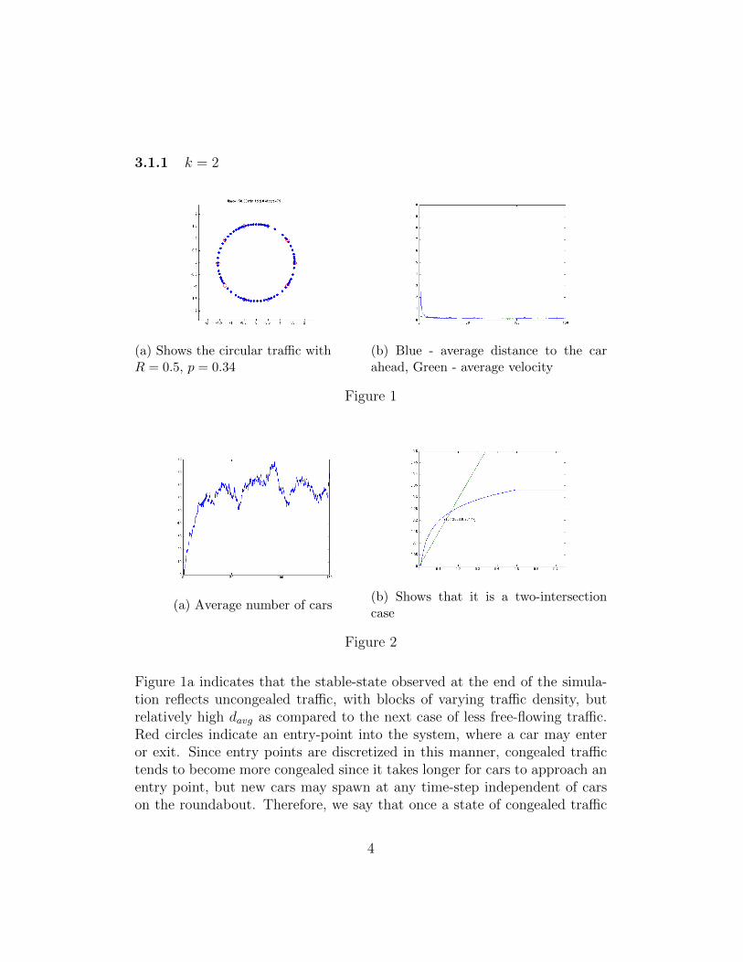
(a) Shows the circular traffic withR = 0.5, p = 0.34

(b) Blue - average distance to the carahead, Green - average velocity

Figure 1

(a) Average number of cars(b) Shows that it is a two-intersectioncase

Figure 2

Figure 1a indicates that the stable-state observed at the end of the simula-tion reflects uncongealed traffic, with blocks of varying traffic density, butrelatively high davg as compared to the next case of less free-flowing traffic.Red circles indicate an entry-point into the system, where a car may enteror exit. Since entry points are discretized in this manner, congealed traffictends to become more congealed since it takes longer for cars to approach anentry point, but new cars may spawn at any time-step independent of carson the roundabout. Therefore, we say that once a state of congealed traffic

4

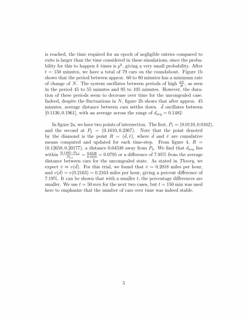
is reached, the time required for an epoch of negligible entries compared toexits is larger than the time considered in these simulations, since the proba-bility for this to happen k times is pk, giving a very small probability. Aftert = 150 minutes, we have a total of 79 cars on the roundabout. Figure 1bshows that the period between approx. 60 to 80 minutes has a minimum rateof change of N . The system oscillates between periods of high dN

dt, as seen

in the period 45 to 55 minutes and 95 to 105 minutes. However, the dura-tion of these periods seem to decrease over time for the uncongealed case.Indeed, despite the fluctuations in N , figure 2b shows that after approx. 45minutes, average distance between cars settles down. d oscillates between[0.1136, 0.1961], with an average across the range of davg = 0.1482.

In figure 2a, we have two points of intersection. The first, P1 = (0.0110, 0.0162),and the second at P2 = (0.1610, 0.2367). Note that the point denotedby the diamond is the point R = (d, v), where d and v are cumulativemeans computed and updated for each time-step. From figure 4, R =(0.12658, 0.20177), a distance 0.04538 away from P2. We find that davg lies

within |0.1482−P2,x

P2,x= 0.0128

0.1610= 0.0795 or a difference of 7.95% from the average

distance between cars for the uncongealed state. As stated in Theory, weexpect v ≈ v(d). For this trial, we found that v = 0.2018 miles per hour,and v(d) = v(0.2163) = 0.2163 miles per hour, giving a percent difference of7.19%. It can be shown that with a smaller t, the percentage differences aresmaller. We use t = 50min for the next two cases, but t = 150 min was usedhere to emphasize that the number of cars over time was indeed stable.

5

3.1.2 k = 1

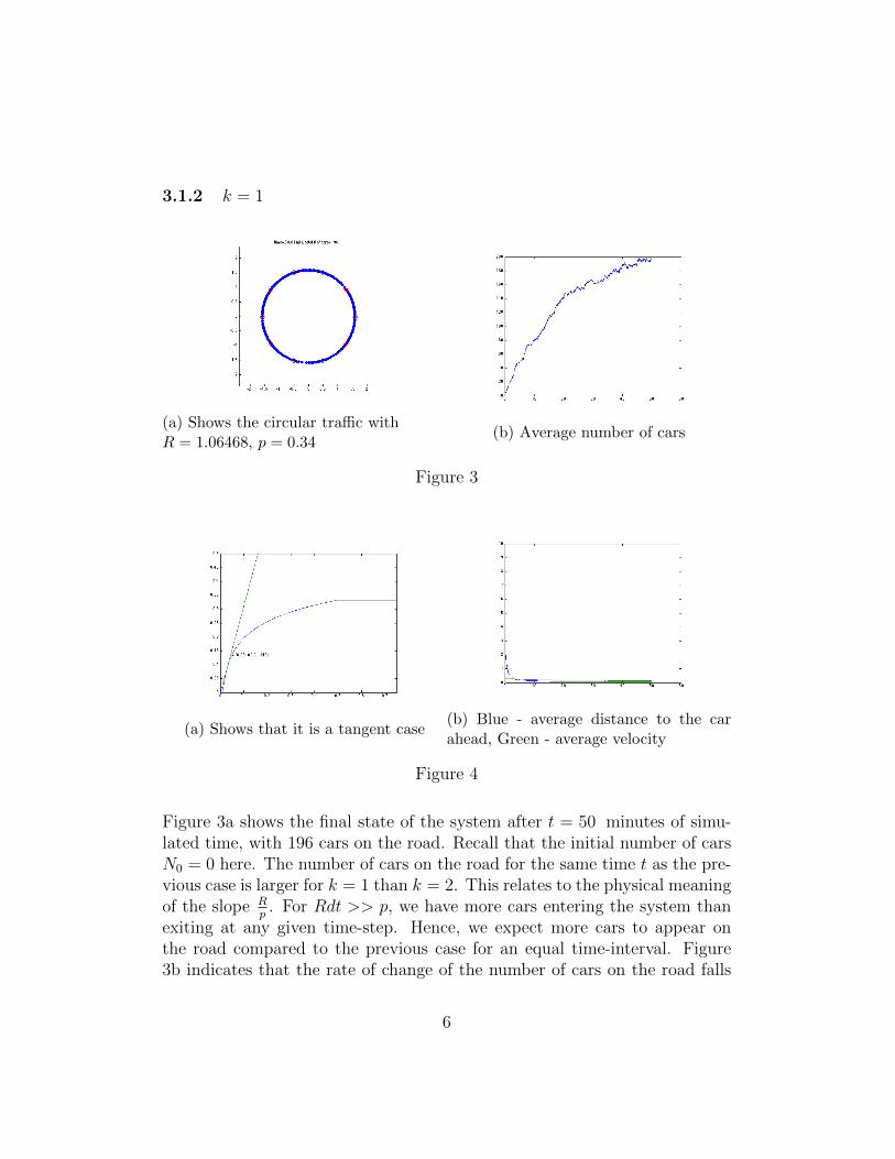
(a) Shows the circular traffic withR = 1.06468, p = 0.34

(b) Average number of cars

Figure 3

(a) Shows that it is a tangent case(b) Blue - average distance to the carahead, Green - average velocity

Figure 4

Figure 3a shows the final state of the system after t = 50 minutes of simu-lated time, with 196 cars on the road. Recall that the initial number of carsN0 = 0 here. The number of cars on the road for the same time t as the pre-vious case is larger for k = 1 than k = 2. This relates to the physical meaningof the slope R

p. For Rdt >> p, we have more cars entering the system than

exiting at any given time-step. Hence, we expect more cars to appear onthe road compared to the previous case for an equal time-interval. Figure3b indicates that the rate of change of the number of cars on the road falls

6

off with time, anticipating a steady-state with respect to the number of carsentering and exiting the roundabout at each time-step. However, althoughthe apparent trend is a negative second derivative, this need not be the caseas t grows. Later, we study a case where steady-states will oscillate, althoughwe focus on demonstrating that such an oscillation will occur at least once.From figure 4b, the average distance between cars remains relatively stablein the range [5, 50] minutes. Recall that the green line indicates the averagevelocity of cars. Using the approach outlined in Theory, we are able to gen-erate the tangent case, where P = (e× dmin, v(e× dmin)). As expected, thepoint lies near P .

v after the final time-step was found to be 0.1343 miles per hour, with d =0.0510. As shown in previous trials for varying k, vavg agrees well with v(d) =0.1389 miles per hour, with a percentage difference of 3.39%. Interestingly,for a higher R

p, the percentage difference between the two quantities is less

than or comparable to the percentage difference for a lower Rp

, as seen in theprevious case.

3.1.3 k = 0

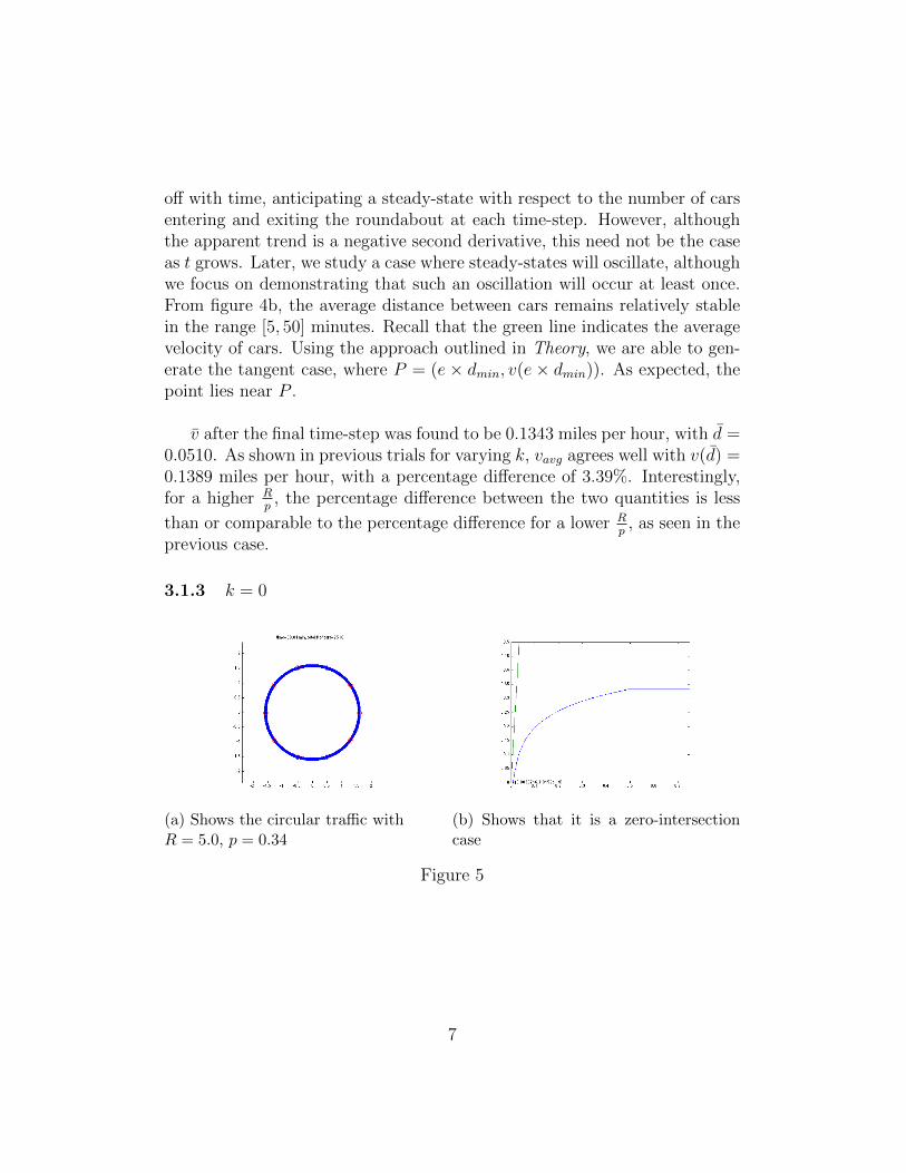
(a) Shows the circular traffic withR = 5.0, p = 0.34

(b) Shows that it is a zero-intersectioncase

Figure 5

7

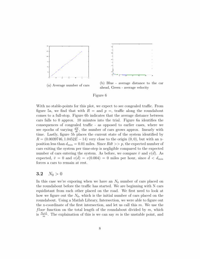
(a) Average number of cars(b) Blue - average distance to the carahead, Green - average velocity

Figure 6

With no stable-points for this plot, we expect to see congealed traffic. Fromfigure 5a, we find that with R = and p =, traffic along the roundaboutcomes to a full-stop. Figure 6b indicates that the average distance betweencars falls to 0 approx. 10 minutes into the trial. Figure 6a identifies theconsequences of congealed traffic - as opposed to earlier cases, where wesee epochs of varying dN

dt, the number of cars grows approx. linearly with

time. Lastly, figure 5b places the current state of the system identified byR = (0.0039746, 1.0452E − 14) very close to the origin (0, 0), but with an x-position less than dmin = 0.01 miles. Since Rdt >> p, the expected number ofcars exiting the system per time-step is negligible compared to the expectednumber of cars entering the system. As before, we compare v and v(d). Asexpected, v = 0 and v(d) = v(0.004) = 0 miles per hour, since d < dmin

forces a cars to remain at rest.

3.2 N0 > 0

In this case we’re exporing when we have an N0 number of cars placed onthe roundabout before the traffic has started. We are beginning with N carsequidistant from each other placed on the road. We first need to look athow we figure out the N0, which is the initial number of cars placed on theroundabout. Using a Matlab Library, Intersection, we were able to figure outthe x-coordinate of the first intersection, and let us call this m. We use thefloor function on the total length of the roundabout divided by m, whichis Nb∗L

m. The explaination of this is we can say m is the unstable point, and

8

length of roundaboutm

would give us a value for the equadistant length betweeneach car.

For the first study we looked to find cases where we fix the ratio of Rand p, and the ratio has two points of intersections. We started with a casewhere N0 was zero. We ran that same case multiple times and we expectedto find that there in some of the runs it should lead to congealed traffic, andin the other it should lead to uncongealed traffic.

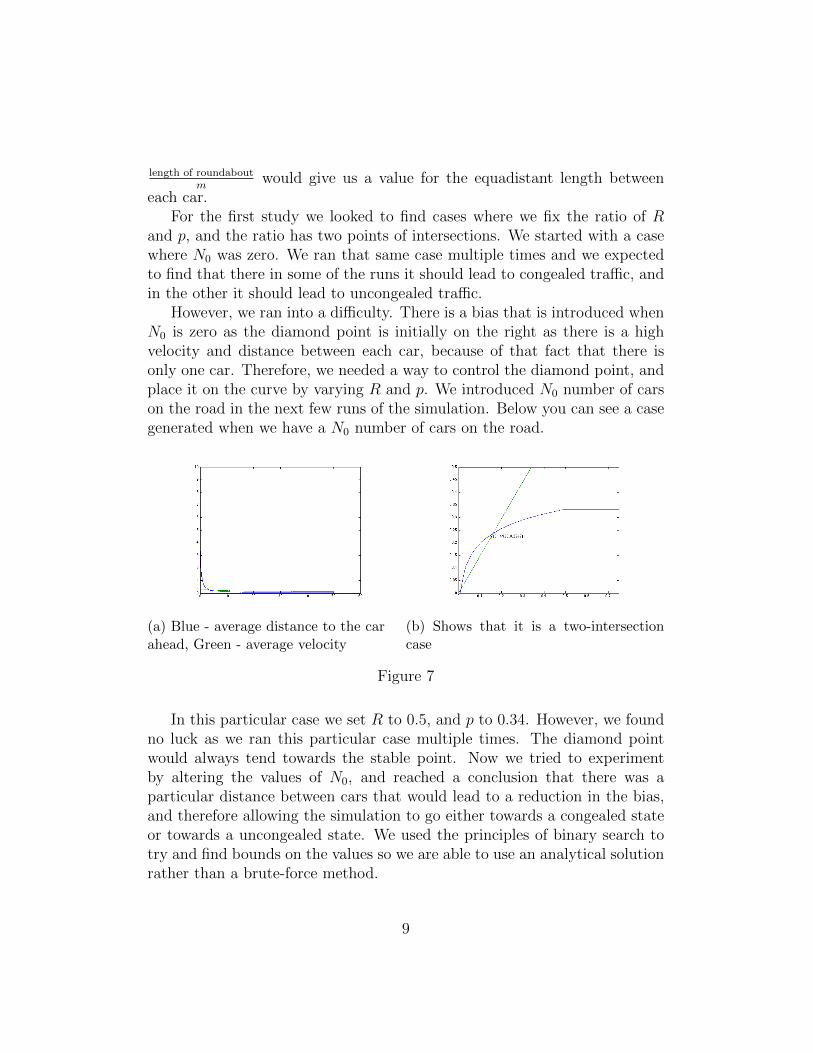
However, we ran into a difficulty. There is a bias that is introduced whenN0 is zero as the diamond point is initially on the right as there is a highvelocity and distance between each car, because of that fact that there isonly one car. Therefore, we needed a way to control the diamond point, andplace it on the curve by varying R and p. We introduced N0 number of carson the road in the next few runs of the simulation. Below you can see a casegenerated when we have a N0 number of cars on the road.

(a) Blue - average distance to the carahead, Green - average velocity

(b) Shows that it is a two-intersectioncase

Figure 7

In this particular case we set R to 0.5, and p to 0.34. However, we foundno luck as we ran this particular case multiple times. The diamond pointwould always tend towards the stable point. Now we tried to experimentby altering the values of N0, and reached a conclusion that there was aparticular distance between cars that would lead to a reduction in the bias,and therefore allowing the simulation to go either towards a congealed stateor towards a uncongealed state. We used the principles of binary search totry and find bounds on the values so we are able to use an analytical solutionrather than a brute-force method.

9

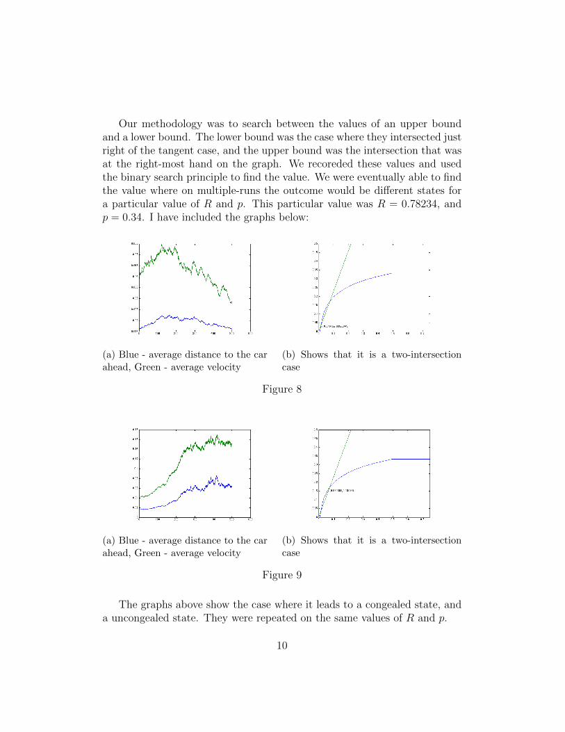
Our methodology was to search between the values of an upper boundand a lower bound. The lower bound was the case where they intersected justright of the tangent case, and the upper bound was the intersection that wasat the right-most hand on the graph. We recoreded these values and usedthe binary search principle to find the value. We were eventually able to findthe value where on multiple-runs the outcome would be different states fora particular value of R and p. This particular value was R = 0.78234, andp = 0.34. I have included the graphs below:

(a) Blue - average distance to the carahead, Green - average velocity

(b) Shows that it is a two-intersectioncase

Figure 8

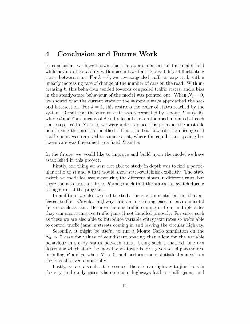
(a) Blue - average distance to the carahead, Green - average velocity

(b) Shows that it is a two-intersectioncase

Figure 9

The graphs above show the case where it leads to a congealed state, anda uncongealed state. They were repeated on the same values of R and p.

10

4 Conclusion and Future Work

In conclusion, we have shown that the approximations of the model holdwhile asymptotic stability with noise allows for the possibility of fluctuatingstates between runs. For k = 0, we saw congealed traffic as expected, with alinearly increasing rate of change of the number of cars on the road. With in-creasing k, this behaviour tended towards congealed traffic states, and a biasin the steady-state behaviour of the model was pointed out. When N0 = 0,we showed that the current state of the system always approached the sec-ond intersection. For k = 2, this restricts the order of states reached by thesystem. Recall that the current state was represented by a point P = (d, v),where d and v are means of d and v for all cars on the road, updated at eachtime-step. With N0 > 0, we were able to place this point at the unstablepoint using the bisection method. Thus, the bias towards the uncongealedstable point was removed to some extent, where the equidistant spacing be-tween cars was fine-tuned to a fixed R and p.

In the future, we would like to improve and build upon the model we haveestablished in this project.

Firstly, one thing we were not able to study in depth was to find a partic-ular ratio of R and p that would show state-switching explicitly. The stateswitch we modelled was measuring the different states in different runs, butthere can also exist a ratio of R and p such that the states can switch duringa single run of the program.

In addition, we also wanted to study the environmental factors that af-fected traffic. Circular highways are an interesting case in environmentalfactors such as rain. Because there is traffic coming in from multiple sidesthey can create massive traffic jams if not handled properly. For cases suchas these we are also able to introduce variable entry/exit rates so we’re ableto control traffic jams in streets coming in and leaving the circular highway.

Secondly, it might be useful to run a Monte Carlo simulation on theN0 > 0 case for values of equidistant spacing that allow for the variablebehaviour in steady states between runs. Using such a method, one candetermine which state the model tends towards for a given set of parameters,including R and p, when N0 > 0, and perform some statistical analysis onthe bias observed empirically.

Lastly, we are also about to connect the circular highway to junctions inthe city, and study cases where circular highways lead to traffic jams, and

11

cases where we see uncongealed traffic. We can use the grid based trafficsystem, and see the changes that occur when there is a circular highway, andwhen there is not.

12

5 References

The Matlab file intersections.m was imported from the URL below.

http://www.mathworks.com/matlabcentral/fileexchange/11837-fast-and-robust-curve-intersections/content/intersections.m

vcar.m and circle.m were adapted from Chengcheng Huangs recitation noteson the One-Lane roundabout.

6 Appendix A: circle.m

1

2 % c i r c u l a r blocks , ca r s not in order3

4 c l e a r a l l5 c l o s e a l l6

7 g l o b a l dmin dmax vmax ;8

9 % i n i t i a l i z a t i o n10 nblocks = 10 ;11 L = 1 ; % mile % L>dmax12

13 % R = 0 . 5 , p = 0 .5 −−> 2 SS14 % R = 0.56 , p = 0 .5 −−> 2 SS15 % R = 1 . 3 , p = 0 .5 −−> 2 very c l o s e SS16 % R = 1.25 ( x = 0 .015 , y = 0 .0375) , 1 ( x=0.06 , y=0.15)17 % R = 1 . 2 , p = 0 .5 −−> 2 maybe c l o s e ( x=0.0225 , y

=0.054) 1 ( x=0.0675 , y =0.162) 218 % R = 0.925 , p = 0.35 ( x = 0 .0225 , y = 0 .05946) 1 , ( x =

0 .0525 , y = 0 .1388) 219

20 % mile /min21 dmin = 0 . 0 1 ; % mile22 dmax = 0 . 5 ; % mile % dmax<L23 %vmax = (R/p) ∗ dmin ∗ l og (dmax/dmin ) ∗ 2 . 7 3 ;

13

24 vmax = 20/60;25

26 % 1.06468 ; and 0 .3427 % 0.528 % 5.029

30 %R = 0 .78234 ; % prob/minuet o f entry31 %p = 0 . 3 4 ; % p r o b a b i l i t y o f e x i t when pas s ing each e x i t32

33 R = 5 . 0 ;34 p = 0 . 3 4 ;35

36 % Mean d i s t = t o t a l l ength / number o f ca r s37 % plo t po int ( mean dist , v ( mean dist ) )38 % on the curve ? good p r e d i c t o r ?39

40 dt = dmin / vmax ∗ 0 . 5 ;41 tmax = 150 ;42 clockmax = c e i l ( tmax / dt ) ;43 t save = ze ro s (1 , clockmax ) ;44 Nsave = ze ro s (1 , clockmax ) ; % # of ca r s on road45 v average = ze ro s (1 , clockmax ) ;46 d average = ze ro s (1 , clockmax ) ;47

48 % % empty road i n i t i a l l y49 N = 0 ; count = 0 ;50 x = [ ] ; % p o s i t i o n o f car c , x range [ 0 , nblocks ∗L)51 nextcar = [ ] ; % index o f next car behind c on i t s b lock

(0 i f c i s l a s t c a r )52 f i r s t c a r = ze ro s (1 , nb locks ) ;53 l a s t c a r = ze ro s (1 , nblocks ) ;54 t e n t e r = [ ] ;55 t e x i t = [ ] ;56

57 x p l o t = l i n s p a c e (0 , dmax ∗ 1 . 5 , 101) ;58 [m, q ] = i n t e r s e c t i o n s ( x p lot , vcar ( x p l o t ) , x p lot , R

/ p ∗ x p lot , 0) ;59

14

60 % We use the61 % f l o o r func t i on on the t o t a l l ength o f the roundabout

d iv ided by m, which62 % i s Number o f b locks ∗ L /x−coo rd ina te o f f i r s t

i n t e r s e c t i o n .63 % The e x p l a i n a t i o n o f t h i s i s we can say m i s the

unstab le point , and64 % length o f roundable65 % m would g ive us a value f o r the equad i s tant l ength

between each66 % car .67

68

69 % 2.800 <−> 2 .82570 % 2.8125 went up71 % 2.815 went down72

73 % narrow i t f u r t h e r up74 % i n c r e a s e i t l i t t l e more up75

76 % g = ( (m(3) − 2.81375∗m(2) ) / 2) ;77 %78 % % N car s at beg inning with an e q u i d i s t a n t spac ing o f

g . Uncomment l i n e s 386 − 405 f o r N 0 > 0 .79 % N = f l o o r ( ( nblocks ∗L) /( g ) ) ;80 % count = N;81 % x = ze ro s (1 , N) ∗ nblocks ∗ L ;82 %83 % x = l i n s p a c e (0 , nb locks ∗ L−m(2) , N) ;84 %85 % x = s o r t (x , ’ descend ’ ) ;86 % f o r b = 1 : nblocks87 % ind = f i n d ( x < b ∗ L&x >= (b−1) ∗ L) ;88 % i f isempty ( ind )89 % f i r s t c a r (b) = 0 ; l a s t c a r (b) = 0 ;90 % e l s e91 % f i r s t c a r (b) = ind (1 ) ; l a s t c a r (b) = ind ( end ) ;92 % end

15

93 % end94 % nextcar = 2 :N; nextcar ( l a s t c a r ) = 0 ;95 % t e n t e r = ze ro s (1 ,N) ; t e x i t = [ ] ;96

97 f i g u r e (1 ) ;98 s e t ( gcf , ’ double ’ , ’ on ’ )99 rad iu s = nblocks ∗ L / (2 ∗ pi ) ;

100 theta = x / rad iu s ;101 h1 = s c a t t e r ( rad iu s ∗ cos ( theta ) , r ad iu s ∗ s i n ( theta ) ,

50 ∗ ones ( s i z e ( x ) ) , ’ f i l l ’ ) ;102 a x i s ([− rad iu s ∗ 1 .5 rad iu s ∗ 1 .5 −rad iu s ∗ 1 .5 rad iu s ∗

1 . 5 ] )103 a x i s equal104 a x i s manual105 t = 0 ;106 h2=t i t l e ( s p r i n t f ( ’ time=%0.2 f min , t o t a l # o f ca r s=%d ’ ,

t , N) ) ;107 hold on108 % v i s c i r c l e s ( [ 0 0 ] , radius , ’ EdgeColor ’ , ’ k ’ ) ;109 theta = l i n s p a c e (0 , 2 ∗ pi , nb locks + 1) ;110 s c a t t e r ( rad iu s ∗ cos ( theta ) , r ad iu s ∗ s i n ( theta ) , 100 ∗

ones (1 , nblocks + 1) , ’ r ’ ) ; % e x i t s111

112 f o r c l o ck = 1 : clockmax113 t = c l ock ∗ dt ;114 t save ( c l o ck ) = t ;115 % entry o f ca r s116 f o r b = 1 : nblocks117 i f rand < R ∗ dt118 count = count + 1 ; % car index119 i f ( l a s t c a r (b) == 0) % i f the block i s

empty120 f i r s t c a r (b) = count ;121 l a s t c a r (b) = count ;122 nextcar ( count ) = 0 ;123 e l s e124 nextcar ( l a s t c a r (b) ) = count ;125 nextcar ( count ) = 0 ;

16

126 l a s t c a r (b) = count ;127 end128 x ( count ) = (b−1) ∗ L ;129 t e n t e r ( count ) = t ;130 end131 end132 % motion and e x i t o f ca r s133 f o r b = 1 : nblocks134 bnext = b + 1 − nblocks ∗ (b == nblocks ) ; %

c i r c u l a r b locks135 i f f i r s t c a r (b) ˜= 0 % i f b lock i s not empty136 c = f i r s t c a r (b) ;137 i f l a s t c a r ( bnext ) == 0138 d = dmax ;139 e l s e140 d = x ( l a s t c a r ( bnext ) ) − x ( c ) + nblocks

∗ L ∗ ( bnext == 1) ; % when near x=0141 end142 x ( c ) = x ( c ) + dt ∗ vcar (d) ;143 i f x ( c ) > b ∗ L % i f car passed end o f

b lock b144 i f ( f i r s t c a r (b) == l a s t c a r (b) )145 f i r s t c a r (b) = 0 ;146 l a s t c a r (b) = 0 ;147 e l s e148 f i r s t c a r (b) = nextcar ( c ) ;149 end150 nextcar ( c ) = 0 ;151 i f rand < p % did the car e x i t ?152 t e x i t ( c ) = t ;153 x ( c ) = −1;154 e l s e155 i f l a s t c a r ( bnext ) == 0156 f i r s t c a r ( bnext ) = c ;157 l a s t c a r ( bnext ) = c ;158 e l s e159 nextcar ( l a s t c a r ( bnext ) ) = c ;160 l a s t c a r ( bnext ) = c ;

17

161 end162 x ( c ) = x ( c ) − ( bnext == 1) ∗

nblocks ∗ L ;163 end164 end165 cp = c ; % t r a i l i n g po in t e r166 c = nextcar ( c ) ;167 whi le c ˜= 0168 x ( c ) = x ( c ) + dt ∗ vcar ( x ( cp ) − x ( c ) ) ;169 cp = c ;170 c = nextcar ( c ) ;171 end172 end173 end174 % average d and v175 Nsave ( c l o ck ) = length ( t e n t e r ) − nnz ( t e x i t ) ;176 ind onroad = s e t d i f f ( 1 : count , f i n d ( t e x i t ) ) ; % index

o f ca r s that are on road177 x s o r t = s o r t ( x ( ind onroad ) ) ;178 i f isempty ( x s o r t ) == 0179 d = [ d i f f ( x s o r t ) , x s o r t (1 ) + nblocks ∗ L −

x s o r t ( end ) ] ;180 d average ( c l o ck ) = mean(d) ;181 v average ( c l o ck ) = mean( vcar (d) ) ;182 end183

184 theta = ( x (x>0) / rad iu s ) ;185

186 s e t ( h1 , ’ xdata ’ , r ad iu s ∗ cos ( theta ) , ’ ydata ’ ,r ad iu s ∗ s i n ( theta ) , ’ s i z e d a t a ’ , 50 ∗ ones ( s i z e (theta ) ) )

187 s e t ( h2 , ’ s t r i n g ’ , s p r i n t f ( ’ time=%0.2 f min , t o t a l #o f ca r s=%d ’ , t , Nsave ( c l o ck ) ) )

188 drawnow189

190 f i g u r e (4 ) %could be more e f f i c i e n t191 d p lo t = l i n s p a c e (0 , dmax ∗ 1 . 5 , 101) ;192 p lo t ( d p lot , vcar ( d p l o t ) , d p lot , R / p ∗ d p lo t )

18

193 t ex t ( d average ( c l o ck ) , v average ( c l o ck ) , s t r c a t ( ’\diamondsuit ’ , ’ ( ’ , num2str ( d average ( c l o ck ) ) , ’, ’ , num2str ( v average ( c l o ck ) ) , ’ ) ’ ) )

194 a x i s ( [ 0 dmax ∗ 1 .5 0 vmax ∗ 1 . 5 ] )195

196 end197

198 f i g u r e (2 )199 p lo t ( tsave , Nsave )200

201 f i g u r e (3 )202 p lo t ( tsave , d average , tsave , v average )203

204 % percentage e r r o r205 100 ∗ ( abs ( v average ( clockmax ) − vcar ( d average (

clockmax ) ) ) /( v average ( clockmax ) ) )

7 Appendix B: vcar.m

1 f unc t i on v = vcar (d)2 g l o b a l dmin dmax vmax ;3 v = ze ro s ( s i z e (d) ) ;4 f o r k = 1 : l ength (d)5 i f (d ( k ) <= dmin )6 v ( k ) = 0 ;7 e l s e8 v ( k ) = vmax ∗ l og (d( k ) . / dmin ) / log (dmax

/ dmin ) .∗ (d( k ) > dmin ) .∗ (d( k ) < dmax) + vmax ∗ (d( k ) >= dmax) ;

9 end10 end11 end

8 Appendix B: intersections.m

1 f unc t i on [ x0 , y0 , iout , j out ] = i n t e r s e c t i o n s ( x1 , y1 , x2 , y2 ,robust )

2 %INTERSECTIONS I n t e r s e c t i o n s o f curves .

19

3 % Computes the (x , y ) l o c a t i o n s where two curvesi n t e r s e c t . The curves

4 % can be broken with NaNs or have v e r t i c a l segments .5 %6 % Example :7 % [ X0 , Y0 ] = i n t e r s e c t i o n s (X1 , Y1 , X2 , Y2 ,ROBUST) ;8 %9 % where X1 and Y1 are equal−l ength ve c t o r s o f at l e a s t

two po in t s and10 % re pr e s en t curve 1 . S im i l a r l y , X2 and Y2 r ep r e s en t

curve 2 .11 % X0 and Y0 are column vec to r s conta in ing the po in t s at

which the two12 % curves i n t e r s e c t .13 %14 % ROBUST ( opt i ona l ) s e t to 1 or t rue means to use a

s l i g h t v a r i a t i o n o f the15 % algor i thm that might re turn d u p l i c a t e s o f some

i n t e r s e c t i o n points , and16 % then remove those d u p l i c a t e s . The d e f a u l t i s true ,

but s i n c e the17 % algor i thm i s s l i g h t l y s lower you can s e t i t to f a l s e

i f you know that18 % your curves don ’ t i n t e r s e c t at any segment boundar ies

. Also , the robust19 % ver s i on proper ly handles p a r a l l e l and over lapp ing

segments .20 %21 % The algor i thm can return two a d d i t i o n a l v e c t o r s that

i n d i c a t e which22 % segment p a i r s conta in i n t e r s e c t i o n s and where they

are :23 %24 % [ X0 , Y0 , I , J ] = i n t e r s e c t i o n s (X1 , Y1 , X2 , Y2 ,ROBUST) ;25 %26 % For each element o f the vec to r I , I ( k ) = ( segment

number o f (X1 , Y1) ) +27 % (how f a r along t h i s segment the i n t e r s e c t i o n i s ) .

20

For example , i f I ( k ) =28 % 45.25 then the i n t e r s e c t i o n l i e s a quarte r o f the way

between the l i n e29 % segment connect ing (X1(45) ,Y1(45) ) and (X1(46) ,Y1(46)

) . S i m i l a r l y f o r30 % the vec to r J and the segments in (X2 , Y2) .31 %32 % You can a l s o get i n t e r s e c t i o n s o f a curve with i t s e l f

. Simply pass in33 % only one curve , i . e . ,34 %35 % [ X0 , Y0 ] = i n t e r s e c t i o n s (X1 , Y1 ,ROBUST) ;36 %37 % where , as be fore , ROBUST i s op t i ona l .38

39 % Vers ion : 1 . 12 , 27 January 201040 % Author : Douglas M. Schwarz41 % Email : dmschwarz=i e e e ∗org , dmschwarz=urgrad∗

r o c h e s t e r ∗edu42 % Real emai l = regexprep ( Email ,{ ’= ’ , ’∗ ’} ,{ ’@’ , ’ . ’ } )43

44

45 % Theory o f ope ra t i on :46 %47 % Given two l i n e segments , L1 and L2 ,48 %49 % L1 endpoints : ( x1 (1 ) , y1 (1 ) ) and ( x1 (2 ) , y1 (2 ) )50 % L2 endpoints : ( x2 (1 ) , y2 (1 ) ) and ( x2 (2 ) , y2 (2 ) )51 %52 % we can wr i t e f our equat ions with four unknowns and

then s o l v e them . The53 % four unknowns are t1 , t2 , x0 and y0 , where ( x0 , y0 ) i s

the i n t e r s e c t i o n o f54 % L1 and L2 , t1 i s the d i s t anc e from the s t a r t i n g po int

o f L1 to the55 % i n t e r s e c t i o n r e l a t i v e to the l ength o f L1 and t2 i s

the d i s t anc e from the56 % s t a r t i n g po int o f L2 to the i n t e r s e c t i o n r e l a t i v e to

21

the l ength o f L2 .57 %58 % So , the four equat ions are59 %60 % ( x1 (2) − x1 (1 ) )∗ t1 = x0 − x1 (1 )61 % ( x2 (2) − x2 (1 ) )∗ t2 = x0 − x2 (1 )62 % ( y1 (2) − y1 (1 ) )∗ t1 = y0 − y1 (1 )63 % ( y2 (2) − y2 (1 ) )∗ t2 = y0 − y2 (1 )64 %65 % Rearranging and wr i t i ng in matrix form ,66 %67 % [ x1 (2 )−x1 (1 ) 0 −1 0 ; [ t1 ; [−

x1 (1 ) ;68 % 0 x2 (2)−x2 (1 ) −1 0 ; ∗ t2 ; = −

x2 (1 ) ;69 % y1 (2)−y1 (1 ) 0 0 −1; x0 ; −

y1 (1 ) ;70 % 0 y2 (2)−y2 (1 ) 0 −1] y0 ] −

y2 (1 ) ]71 %72 % Let ’ s c a l l that A∗T = B. We can s o l v e f o r T with T =

A\B.73 %74 % Once we have our s o l u t i o n we j u s t have to look at t1

and t2 to determine75 % whether L1 and L2 i n t e r s e c t . I f 0 <= t1 < 1 and 0 <=

t2 < 1 then the two76 % l i n e segments c r o s s and we can inc lude ( x0 , y0 ) in the

output .77 %78 % In p r i n c i p l e , we have to perform t h i s computation on

every pa i r o f l i n e79 % segments in the input data . This can be qu i t e a

l a r g e number o f p a i r s so80 % we w i l l reduce i t by doing a s imple pre l im inary check

to e l i m i n a t e l i n e81 % segment p a i r s that could not p o s s i b l y c r o s s . The

check i s to look at the

22

82 % s m a l l e s t e n c l o s i n g r e c t a n g l e s ( with s i d e s p a r a l l e l tothe axes ) f o r each

83 % l i n e segment pa i r and see i f they over lap . I f theydo then we have to

84 % compute t1 and t2 ( v ia the A\B computation ) to see i fthe l i n e segments

85 % cross , but i f they don ’ t then the l i n e segmentscannot c r o s s . In a

86 % t y p i c a l app l i c a t i on , t h i s techn ique w i l l e l i m i n a t emost o f the p o t e n t i a l

87 % l i n e segment p a i r s .88

89

90 % Input checks .91 e r r o r ( nargchk (2 , 5 , narg in ) )92

93 % Adjustments when fewer than f i v e arguments aresupp l i ed .

94 switch narg in95 case 296 robust = true ;97 x2 = x1 ;98 y2 = y1 ;99 s e l f i n t e r s e c t = true ;

100 case 3101 robust = x2 ;102 x2 = x1 ;103 y2 = y1 ;104 s e l f i n t e r s e c t = true ;105 case 4106 robust = true ;107 s e l f i n t e r s e c t = f a l s e ;108 case 5109 s e l f i n t e r s e c t = f a l s e ;110 end111

112 % x1 and y1 must be ve c t o r s with same number o f po in t s( at l e a s t 2) .

23

113 i f sum( s i z e ( x1 ) > 1) ˜= 1 | | sum( s i z e ( y1 ) > 1) ˜= 1 | |. . .

114 l ength ( x1 ) ˜= length ( y1 )115 e r r o r ( ’X1 and Y1 must be equal−l ength ve c t o r s

o f at l e a s t 2 po in t s . ’ )116 end117 % x2 and y2 must be ve c t o r s with same number o f po in t s

( at l e a s t 2) .118 i f sum( s i z e ( x2 ) > 1) ˜= 1 | | sum( s i z e ( y2 ) > 1) ˜= 1 | |

. . .119 l ength ( x2 ) ˜= length ( y2 )120 e r r o r ( ’X2 and Y2 must be equal−l ength ve c t o r s

o f at l e a s t 2 po in t s . ’ )121 end122

123

124 % Force a l l inputs to be column vec to r s .125 x1 = x1 ( : ) ;126 y1 = y1 ( : ) ;127 x2 = x2 ( : ) ;128 y2 = y2 ( : ) ;129

130 % Compute number o f l i n e segments in each curve andsome d i f f e r e n c e s we ’ l l

131 % need l a t e r .132 n1 = length ( x1 ) − 1 ;133 n2 = length ( x2 ) − 1 ;134 xy1 = [ x1 y1 ] ;135 xy2 = [ x2 y2 ] ;136 dxy1 = d i f f ( xy1 ) ;137 dxy2 = d i f f ( xy2 ) ;138

139 % Determine the combinations o f i and j where ther e c t a n g l e e n c l o s i n g the

140 % i ’ th l i n e segment o f curve 1 ove r l ap s with ther e c t a n g l e e n c l o s i n g the

141 % j ’ th l i n e segment o f curve 2 .142 [ i , j ] = f i n d ( repmat (min ( x1 ( 1 : end−1) , x1 ( 2 : end ) ) ,1 , n2 ) <=

24

. . .143 repmat (max( x2 ( 1 : end−1) , x2 ( 2 : end ) ) . ’ , n1 , 1 ) & . . .144 repmat (max( x1 ( 1 : end−1) , x1 ( 2 : end ) ) ,1 , n2 ) >= . . .145 repmat (min ( x2 ( 1 : end−1) , x2 ( 2 : end ) ) . ’ , n1 , 1 ) & . . .146 repmat (min ( y1 ( 1 : end−1) , y1 ( 2 : end ) ) ,1 , n2 ) <= . . .147 repmat (max( y2 ( 1 : end−1) , y2 ( 2 : end ) ) . ’ , n1 , 1 ) & . . .148 repmat (max( y1 ( 1 : end−1) , y1 ( 2 : end ) ) ,1 , n2 ) >= . . .149 repmat (min ( y2 ( 1 : end−1) , y2 ( 2 : end ) ) . ’ , n1 , 1 ) ) ;150

151 % Force i and j to be column vector s , even when t h e i rl ength i s zero , i . e . ,

152 % we want them to be 0−by−1 in s t ead o f 0−by−0.153 i = reshape ( i , [ ] , 1 ) ;154 j = reshape ( j , [ ] , 1 ) ;155

156 % Find segments p a i r s which have at l e a s t one ver tex =NaN and remove them .

157 % This l i n e i s a f a s t way o f f i n d i n g such segment p a i r s. We take

158 % advantage o f the f a c t that NaNs propagate throughc a l c u l a t i o n s , in

159 % p a r t i c u l a r sub t ra c t i on ( in the c a l c u l a t i o n o f dxy1and dxy2 , which we

160 % need anyway ) and add i t i on .161 % At the same time we can remove redundant combinat ions

o f i and j in the162 % case o f f i n d i n g i n t e r s e c t i o n s o f a l i n e with i t s e l f .163 i f s e l f i n t e r s e c t164 remove = isnan (sum( dxy1 ( i , : ) + dxy2 ( j , : ) , 2 ) ) |

j <= i + 1 ;165 e l s e166 remove = isnan (sum( dxy1 ( i , : ) + dxy2 ( j , : ) , 2 ) ) ;167 end168 i ( remove ) = [ ] ;169 j ( remove ) = [ ] ;170

171 % I n i t i a l i z e matr i ce s . We’ l l put the T’ s and B’ s inmatr i ce s and use them

25

172 % one column at a time . AA i s a 3−D extens i on o f Awhere we ’ l l use one

173 % plane at a time .174 n = length ( i ) ;175 T = ze ro s (4 , n ) ;176 AA = ze ro s (4 , 4 , n ) ;177 AA( [ 1 2 ] , 3 , : ) = −1;178 AA( [ 3 4 ] , 4 , : ) = −1;179 AA( [ 1 3 ] , 1 , : ) = dxy1 ( i , : ) . ’ ;180 AA( [ 2 4 ] , 2 , : ) = dxy2 ( j , : ) . ’ ;181 B = −[x1 ( i ) x2 ( j ) y1 ( i ) y2 ( j ) ] . ’ ;182

183 % Loop through p o s s i b i l i t i e s . Trap s i n g u l a r i t y warningand then use

184 % lastwarn to see i f that plane o f AA i s near s i n g u l a r .Process any such

185 % segment p a i r s to determine i f they are c o l i n e a r (over lap ) or merely

186 % p a r a l l e l . That t e s t c o n s i s t s o f check ing to see i fone o f the endpoints

187 % of the curve 2 segment l i e s on the curve 1 segment .This i s done by

188 % checking the c r o s s product189 %190 % ( x1 (2 ) , y1 (2 ) ) − ( x1 (1 ) , y1 (1 ) ) x ( x2 (2 ) , y2 (2 ) ) − ( x1

(1 ) , y1 (1 ) ) .191 %192 % I f t h i s i s c l o s e to zero then the segments over lap .193

194 % I f the robust opt ion i s f a l s e then we assume no twosegment p a i r s are

195 % p a r a l l e l and j u s t go ahead and do the computation .I f A i s ever s i n g u l a r

196 % a warning w i l l appear . This i s f a s t e r and obv ious lyyou should use i t

197 % only when you know you w i l l never have over lapp ing orp a r a l l e l segment

198 % p a i r s .

26

199

200 i f robust201 over lap = f a l s e (n , 1 ) ;202 warn ing s ta te = warning ( ’ o f f ’ , ’MATLAB:

s ingu la rMatr ix ’ ) ;203 % Use try−catch to guarantee o r i g i n a l warning

s t a t e i s r e s t o r e d .204 t ry205 l a s twarn ( ’ ’ )206 f o r k = 1 : n207 T( : , k ) = AA( : , : , k )\B( : , k ) ;208 [ unused , l a s t warn ] = lastwarn ;209 l a s twarn ( ’ ’ )210 i f strcmp ( last warn , ’MATLAB:

s ingu la rMatr ix ’ )211 % Force in range ( k ) to

be f a l s e .212 T(1 , k ) = NaN;213 % Determine i f the se

segments over lap orare j u s t p a r a l l e l .

214 over lap ( k ) = rcond ( [dxy1 ( i ( k ) , : ) ; xy2 ( j ( k) , : ) − xy1 ( i ( k ) , : ) ] )< eps ;

215 end216 end217 warning ( warn ing s ta te )218 catch e r r219 warning ( warn ing s ta te )220 rethrow ( e r r )221 end222 % Find where t1 and t2 are between 0 and 1 and

return the cor re spond ing223 % x0 and y0 va lue s .224 i n range = (T( 1 , : ) >= 0 & T( 2 , : ) >= 0 & T( 1 , : )

<= 1 & T( 2 , : ) <= 1) . ’ ;225 % For over lapp ing segment p a i r s the a lgor i thm

27

w i l l r e turn an226 % i n t e r s e c t i o n po int that i s at the cent e r o f

the over lapp ing r eg i on .227 i f any ( over lap )228 i a = i ( over lap ) ;229 j a = j ( over lap ) ;230 % s e t x0 and y0 to middle o f

over lapp ing r eg i on .231 T(3 , over lap ) = (max(min ( x1 ( i a ) , x1 ( i a +1)

) , min ( x2 ( j a ) , x2 ( j a +1) ) ) + . . .232 min(max( x1 ( i a ) , x1 ( i a +1) ) ,max( x2

( j a ) , x2 ( j a +1) ) ) ) . ’ / 2 ;233 T(4 , over lap ) = (max(min ( y1 ( i a ) , y1 ( i a +1)

) , min ( y2 ( j a ) , y2 ( j a +1) ) ) + . . .234 min(max( y1 ( i a ) , y1 ( i a +1) ) ,max( y2

( j a ) , y2 ( j a +1) ) ) ) . ’ / 2 ;235 s e l e c t e d = in range | over lap ;236 e l s e237 s e l e c t e d = in range ;238 end239 xy0 = T( 3 : 4 , s e l e c t e d ) . ’ ;240

241 % Remove d u p l i c a t e i n t e r s e c t i o n po in t s .242 [ xy0 , index ] = unique ( xy0 , ’ rows ’ ) ;243 x0 = xy0 ( : , 1 ) ;244 y0 = xy0 ( : , 2 ) ;245

246 % Compute how f a r along each l i n e segment thei n t e r s e c t i o n s are .

247 i f nargout > 2248 s e l i n d e x = f i n d ( s e l e c t e d ) ;249 s e l = s e l i n d e x ( index ) ;250 i ou t = i ( s e l ) + T(1 , s e l ) . ’ ;251 j out = j ( s e l ) + T(2 , s e l ) . ’ ;252 end253 e l s e % non−robust opt ion254 f o r k = 1 : n255 [ L ,U] = lu (AA( : , : , k ) ) ;

28

256 T( : , k ) = U\(L\B( : , k ) ) ;257 end258

259 % Find where t1 and t2 are between 0 and 1 andreturn the cor re spond ing

260 % x0 and y0 va lue s .261 i n range = (T( 1 , : ) >= 0 & T( 2 , : ) >= 0 & T( 1 , : )

< 1 & T( 2 , : ) < 1) . ’ ;262 x0 = T(3 , i n range ) . ’ ;263 y0 = T(4 , i n range ) . ’ ;264

265 % Compute how f a r along each l i n e segment thei n t e r s e c t i o n s are .

266 i f nargout > 2267 i ou t = i ( i n range ) + T(1 , i n range ) . ’ ;268 j out = j ( in range ) + T(2 , i n range ) . ’ ;269 end270 end271

272 % Plot the r e s u l t s ( u s e f u l f o r debugging ) .273 % plo t ( x1 , y1 , x2 , y2 , x0 , y0 , ’ ok ’ ) ;

29