[email protected] http://www.powerworld.com 2001 South First Street Champaign, Illinois 61820 +1 (217) 384.6330 2001 South First Street Champaign, Illinois 61820 +1 (217) 384.6330 Steady‐State Power System Security Analysis with PowerWorld Simulator S12: Modeling GMD in PowerWorld Simulator

Welcome message from author
This document is posted to help you gain knowledge. Please leave a comment to let me know what you think about it! Share it to your friends and learn new things together.
Transcript

[email protected]://www.powerworld.com
2001 South First StreetChampaign, Illinois 61820+1 (217) 384.6330
2001 South First StreetChampaign, Illinois 61820+1 (217) 384.6330
Steady‐State Power System Security Analysis with PowerWorld Simulator
S12: Modeling GMD in PowerWorldSimulator

2© 2020 PowerWorld CorporationS12: Geomagnetic Induced Current (GIC)
GMD Concepts and Regulatory Environment

3© 2020 PowerWorld CorporationS12: Geomagnetic Induced Current (GIC)
• The grid reliability is high, some events could cause large‐scale, long duration blackouts– These include what NERC calls High‐Impact, Low‐Frequency Events (HILFs); others call them black swan events or black sky days
– HILFs identified by NERC were 1) a coordinated cyber, physical or blended attacks, 2) pandemics, 3) geomagnetic disturbances (GMDs), and 4) high altitude electromagnetics pulses (HEMPs)
– Another could be volcanic eruptions• PowerWorld Simulator has tools to analyze GMDs and some effects of HEMPs (late time, E3)
Overview

4© 2020 PowerWorld CorporationS12: Geomagnetic Induced Current (GIC)
• Geomagnetic disturbances (GMD) occur when particles discharged from the sun during solar storms interact with the earth's magnetic field.
• Power systems are vulnerable to geospatial variation in dc voltage caused by GMD.
• Geomagnetically induced currents (GIC) flow through circuits formed by high‐voltage transmission lines, grounded transformers, and the Earth.
Geomagnetic Disturbances
5© 2020 PowerWorld CorporationS12: Geomagnetic Induced Current (GIC)
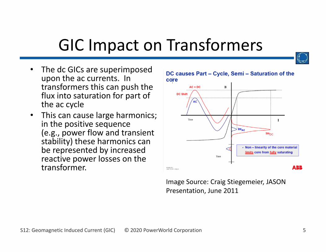
• The dc GICs are superimposed upon the ac currents. In transformers this can push the flux into saturation for part of the ac cycle
• This can cause large harmonics; in the positive sequence(e.g., power flow and transient stability) these harmonics can be represented by increased reactive power losses on the transformer.
GIC Impact on Transformers
Image Source: Craig Stiegemeier, JASON Presentation, June 2011

6© 2020 PowerWorld CorporationS12: Geomagnetic Induced Current (GIC)
• A 1989 solar storm caused widespread outages on the Hydro Quebec system, but it was much smaller and less intense than a 1921 storm that occurred prior to widespread electrification.
• A similar storm could cause significant equipment damage and outages to modern interconnected power grids
• GMDs have the potential to severely disrupt operations of the electric grid
• PowerWorld Simulator GIC is a novel tool to help assess the impact of GMDs on interconnected power systems
Historic GMD Events
Image source: J. Kappenman, “A Perfect Storm of Planetary Proportions,” IEEE Spectrum, Feb 2012, page 29

7© 2020 PowerWorld CorporationS12: Geomagnetic Induced Current (GIC)
• In July 2014, NASA reported that a solar CME barely missed Earth in July of 2012 – It would likely havecaused the largestGMD that we haveseen in the last 150years
• There is still muchuncertainly about how large a storm is reasonable to consider in electric utility planning
July 2012 GMD Near Miss
Image Source: science.nasa.gov/science-news/science-at-nasa/2014/23jul_superstorm/

8© 2020 PowerWorld CorporationS12: Geomagnetic Induced Current (GIC)
• A large GMD could substantially affect power system flows and voltages
• Studies allow for testing various mitigation strategies– Operational (short‐term) changes include redispatchinggeneration to avoid long distance power transfers and reducing transformer loading values, and strategically opening devices to limit GIC flows
– Longer‐term mitigation actions include the installation of GIC blocking devices on the transformer neutrals (such as capacitors) and/or increased series capacitor compensation on long transmission lines
Integrating GIC Analysis into Power System Planning

9© 2020 PowerWorld CorporationS12: Geomagnetic Induced Current (GIC)
Overview of GMD Assessments
Image Source: http://www.nerc.com/pa/Stand/WebinarLibrary/GMD_standards_update_june26_ec.pdf
The two key concerns from a big storm:1) large-scale blackout due to voltage collapse, 2) permanent transformer damage due to overheating
An interdisciplinary problem

10© 2020 PowerWorld CorporationS12: Geomagnetic Induced Current (GIC)
• On February 29, 2012 NERC issued an Interim GMD Report, http://www.nerc.com/files/2012GMD.pdf
• In section I.10 of the Executive Summary there are four high level recommended actions– Improved tools for industry planners to develop GMD mitigation strategies
– Improved tools for system operators to manage GMD impacts
– Develop education and information exchanges between researchers and industry
– Review the need for enhanced NERC Reliability Standards
NERC Interim GMD Report

11© 2020 PowerWorld CorporationS12: Geomagnetic Induced Current (GIC)
• Reliability Standards for Geomagnetic Disturbances, Issued May 16, 2013
• NERC must develop Reliability Standards that require power system owners and operators to: – develop and implement operational procedures to mitigate GMD (NERC EOP‐010‐1)
– conduct initial and on‐going assessments of the potential impact of benchmark GMD events (NERC TPL‐007‐1)
– develop and implement a plan to prevent impacts of benchmark GMD events from causing instability, uncontrolled separation, or cascading failures (NERC TPL‐007‐1)
FERC Order 779

12© 2020 PowerWorld CorporationS12: Geomagnetic Induced Current (GIC)
• FERC notice of proposed rulemaking (NOPR) to accept TPL‐007‐1 on May 14, 2015
• FERC Order 830 approved TPL‐007‐1 on September 22, 2016, while directing a few modifications– Benchmark Event shall not be based solely on spatially‐averaged data
– Collect and publicly share GIC monitoring and magnetometer data
– Establish deadlines for corrective action plans and mitigation
• NERC responded with TPL‐007‐2 and additional requirements including analysis of supplemental GMD event
FERC Follow‐up

13© 2020 PowerWorld CorporationS12: Geomagnetic Induced Current (GIC)
• Key Requirements– R2. Maintain AC system models and GIC system models– R3. Develop criteria for steady state voltage performance– R4. Complete a GMD Vulnerability Assessment every 5 years,
based on benchmark GMD event– R7. Develop a Corrective Action Plan if needed– R8. Complete a GMD Vulnerability Assessment every 5 years,
based on supplemental GMD event– R6 and R10. Transformer thermal assessments– R11 and R12. Obtain GIC monitor and GMD field data
• FERC NOPR (May 17, 2018) proposed to approve TPL‐007‐2• More details at the NERC GMD Task Force page
http://www.nerc.com/comm/PC/Pages/Geomagnetic‐Disturbance‐Task‐Force‐(GMDTF)‐2013.aspx
NERC TPL‐007‐2

14© 2020 PowerWorld CorporationS12: Geomagnetic Induced Current (GIC)
• TPL‐007‐3: Canadian Variance for alternative Benchmark and Supplemental Events
• FERC Order 851 approved TPL‐007‐2 on November 15, 2018, while directing a few modifications via NOPR– require corrective action plans (CAP) to mitigate supplemental GMD event vulnerabilities
– corrective action plan time‐extensions to be considered on a case by case basis
• TPL‐007‐4 affirmed by NERC voters November 2019– new R11 addresses supplemental event CAP– old R11 and R12 become R12 and R13, respectively
Further Revisions
15© 2020 PowerWorld CorporationS12: Geomagnetic Induced Current (GIC)
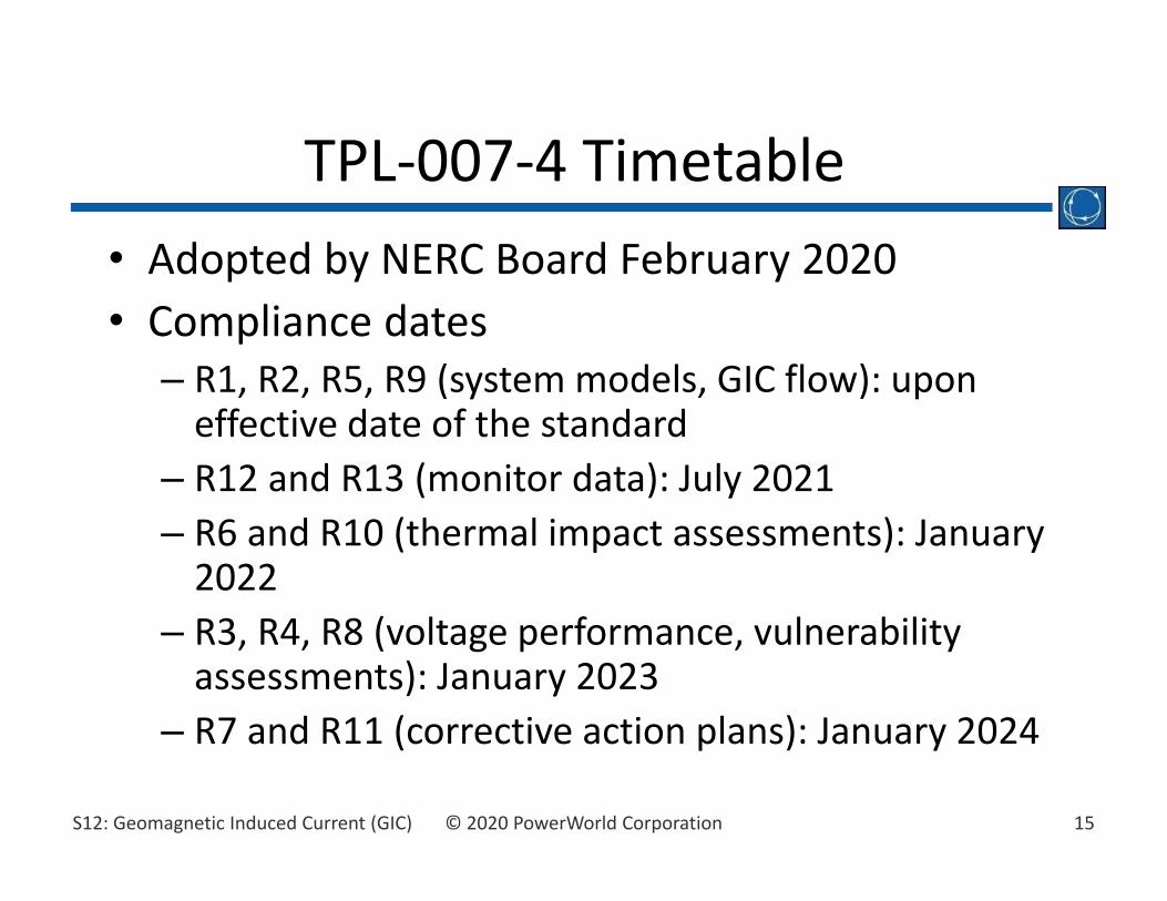
• Adopted by NERC Board February 2020• Compliance dates
– R1, R2, R5, R9 (system models, GIC flow): upon effective date of the standard
– R12 and R13 (monitor data): July 2021– R6 and R10 (thermal impact assessments): January 2022
– R3, R4, R8 (voltage performance, vulnerability assessments): January 2023
– R7 and R11 (corrective action plans): January 2024
TPL‐007‐4 Timetable

16© 2020 PowerWorld CorporationS12: Geomagnetic Induced Current (GIC)
GIC Network Modeling Principles and Assumptions

17© 2020 PowerWorld CorporationS12: Geomagnetic Induced Current (GIC)
• Modern methods model GIC as DC voltage sources in transmission lines
• With pertinent parameters, GIC computation is a straightforward linear calculation
• By integrating GIC calculations into PowerWorld Simulator, engineers can readily see the impact of GICs on their systems and consider mitigation options
GIC Modeling

18© 2020 PowerWorld CorporationS12: Geomagnetic Induced Current (GIC)
• GIC calculations use some existing model parameters such as line resistance
• Some additional parameters are needed– Substation geo‐coordinates and grounding resistance– Transformer grounding configuration, coil resistance, core type, whether auto‐transformer, whether three‐winding transformer
– Generator step‐up transformer parameters• Transmission operators would be in the best position to provide these values, but all can be estimated when actual values are not available
GIC Analysis Inputs

19© 2020 PowerWorld CorporationS12: Geomagnetic Induced Current (GIC)
• The potentially time‐varying GMD induced dc voltages depend on the storm strength and orientation and the latitude and longitude of the transmission lines– The electric field is integrated along the path of the transmission line
– The geo‐coordinates of the terminal substations are sufficient for uniform fields (path independence)
• Hence buses must be mapped to substations, and substations to their geo‐coordinates
• Substation/geographic data can be supplied by PowerWorld for FERC 715 planning models– Buses mapped to substations– Latitude and longitude for substations
Geographic Information

20© 2020 PowerWorld CorporationS12: Geomagnetic Induced Current (GIC)
• Transformer specific, and varies with the core type: Single phase, shell, 3‐legged, 5‐legged
• Ideally this information would be supplied by the transformer owner
• Default data may be used for large system studies when nothing else is available
• Simulator also supports a user‐specified piecewise linear mapping
• Debate in the industry with respect to the magnitude of damage GICs would cause in transformers (from slightly age to permanently destroy)
Mapping Transformer GICs to Transformer Reactive Power Losses

21© 2020 PowerWorld CorporationS12: Geomagnetic Induced Current (GIC)
• The starting point for GIC analysis in PowerWorld Simulator is an assumed storm scenario; this is used to determine the transmission line dc voltages
• Characterizing an actual storm can be complicated, and requires detailed knowledge of the associated geology
• February 2012 NERC report recommended a common approach for planning purposes– Uniform electric field model: all locations experience the same field;
induced voltages in lines depend on assumed field direction– Maximum value in 1989 was 1.7 V/km (2.7 V/mile)
• Simulator can also use geospatially and time‐varying electric field models– Direct user input of GIC DC voltage input on each transmission line– 3rd‐party input, consisting of a time‐series geospatial grid of E‐field
magnitude and direction (available in Simulator 18)
GMD Storm Scenarios

22© 2020 PowerWorld CorporationS12: Geomagnetic Induced Current (GIC)
• GIC studies involve the traditional power system results (voltages, flows, etc.) and GIC‐specific quantities, such as – Substation neutral dc voltages– Bus dc voltages– Transformer neutral amps– Transformer Mvar losses– Transmission line dc amps
• Providing easy access to the data and results is a key objective in PowerWorld Simulator, as is good wide‐area visualization
GIC Analysis Outputs and Results

23© 2020 PowerWorld CorporationS12: Geomagnetic Induced Current (GIC)
• Simple topology with one 765‐kV transmission line with a grounded wye‐delta transformer at either end
Four‐Bus ExampleB4GIC.pwb
slack
Substation A with R=0.2 ohm Substation B with R=0.2 ohm
765 kV Line3 ohms Per Phase
High Side of 0.3 ohms/ PhaseHigh Side = 0.3 ohms/ Phase
DC = 0.00 VoltsDC = 0.00 VoltsBus 1 Bus 4Bus 2Bus 3
Neutral = 0.00 Volts Neutral = 0.00 Volts
DC = 0.00 Volts DC = 0.00 Volts
GIC Losses = 0.0 MvarGIC Losses = 0.0 Mvar
0.994 pu 0.992 pu 0.995 pu 1.000 pu
GIC/Phase = 0.00 AmpsGIC Input = 0.0 Volts

24© 2020 PowerWorld CorporationS12: Geomagnetic Induced Current (GIC)
• To open the GIC Analysis Form dialog, choose Add‐Ons → GIC…
• Select the Substations page from Tables and Results• Key inputs are the grounding resistance and geo‐location
(latitude and longitude)
Four‐Bus Inputs: Substations
2 substations along an east‐west line, with the same latitude
Grounding resistance = 0.2
B4GIC.pwb

25© 2020 PowerWorld CorporationS12: Geomagnetic Induced Current (GIC)
• Substation grounding resistance is the resistance in ohms between the substation neutral and earth ground (zero‐potential reference)
• An actual “fall of potential” test is the best way to determine this resistance
• Simulator provides defaults based on number of buses and highest nominal kV, but research has shown this to be a poor substitute for actual measurements– Simulator defaults range from 0.1 to 2.0 – Substations with more buses and higher nominal kV are assumed
to have lower grounding resistance• Grounding resistance is not necessary for substations that
have no transformer or switched shunt connections to ground
Grounding Resistance

26© 2020 PowerWorld CorporationS12: Geomagnetic Induced Current (GIC)
• Longitude and latitude should be provided for all substations that contain terminals of lines for which a GIC equivalent DC voltage is applied– Generally this includes all lines greater than minimum length and nominal kV specified on GIC Analysis Form
– Series compensated line terminals may be disregarded, if there are no other lines that meet above criteria
• The need for coordinates applies regardless of whether the substation contains grounded transformers
• If there are no grounded transformers, approximate locations (e.g. within 100 km) are adequate for uniform field modeling
Substation Coordinates

27© 2020 PowerWorld CorporationS12: Geomagnetic Induced Current (GIC)
• Key inputs– Coil resistance (DC ohms)– Grounding configuration– Autotransformer? (Yes/No)– Core Type
Four‐Bus Inputs: Transformers
Most essential parameters; these determine the basic topology of the GIC network

28© 2020 PowerWorld CorporationS12: Geomagnetic Induced Current (GIC)
• Manually Enter Coil Resistance– “Yes”: user enters “Coil Resistance (Ohms) for High/Medium/Tertiary winding”
– “No”: Simulator estimates values
• XF Config High and XF Config Med: most common options are “Gwye” and “Delta”– Tertiary windings are assumed Delta
• Is Autotransformer: “Yes”, “No”, or “Unknown”• Core Type
Four‐Bus Inputs: TransformersB4GIC.pwb

29© 2020 PowerWorld CorporationS12: Geomagnetic Induced Current (GIC)
• It is always best to provide known quantities, especially for configuration and autotransformer fields
• If any transformer information is unknown, Simulator uses default values
• Coil Resistance– ohms per phase estimate based on positive‐sequence AC per‐unit series resistance and transformer impedance base
– Assumed split between each winding:
Simulator Assumptions
∗ ,
30© 2020 PowerWorld CorporationS12: Geomagnetic Induced Current (GIC)
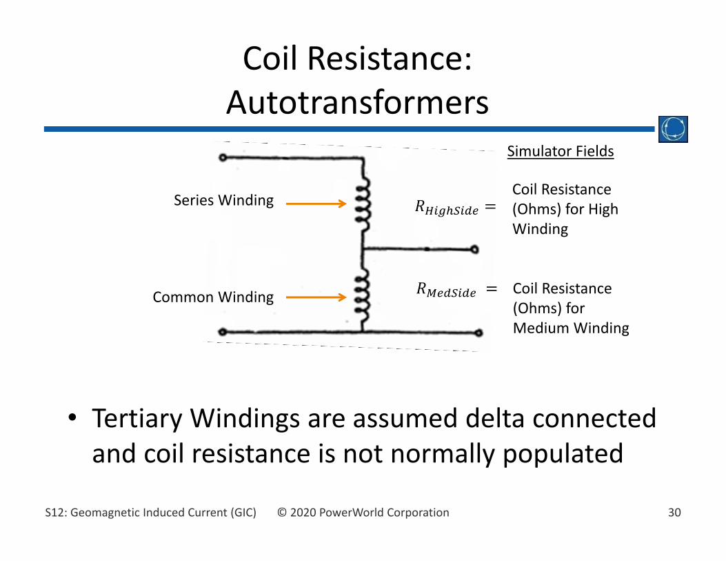
Coil Resistance:Autotransformers
Coil Resistance (Ohms) for Medium Winding
Coil Resistance (Ohms) for High Winding
• Tertiary Windings are assumed delta connected and coil resistance is not normally populated
Series Winding
Common Winding
Simulator Fields

31© 2020 PowerWorld CorporationS12: Geomagnetic Induced Current (GIC)
• Some parameters for assumptions applied to unknown transformers are at Op ons → DC Current Calcula on
• Units are assumed to be autotransformers if all of the following criteria are met– unit is not a phase‐shifting transformer– high side and low side are at different nominal voltages– Medium side nominal voltage is at least 50 kV– turns ratio is less than or equal to 4
Simulator Assumptions:Autotransformers
These parameters may be adjusted at Op ons → DC Current Calculation

32© 2020 PowerWorld CorporationS12: Geomagnetic Induced Current (GIC)
• “Unknown” windings are assumed either Delta, Grounded Wye, or Ungrounded Wye
• Autotransformer Minimum Medium Voltage is also the assumed delineation between transmission and distribution voltages (default 50 kV, referred to as kVmin hereafter on this slide)
• If high side > kVmin and low side is connected to a radial generator OR if high side >= 300 kV and low side < kVmin, unit is assumed a GSU with high side Gwye and low side Delta
• If both sides > kVmin OR both sides < kVmin, both are assumed Gwye
• Otherwise, if high side > kVmin and low side < kVmin or has radial load, use Default Trans. Side Configand Default Dist. Side Configon Op ons → DC Current Calculation (or as specified by area)
Simulator Assumptions:Transformer Configuration

33© 2020 PowerWorld CorporationS12: Geomagnetic Induced Current (GIC)
• IEff is per‐phase “effective GIC”, computed from GIC in high and low side windings and turns ratio (at)
• K‐Factor relates transformer’s effective GIC (IGIC) to 3‐phase reactive power loss at nominal voltage
• This looks like a constant current MVar load at the transformer
Simulator Assumptions
,pu ,puloss pu pu EffQ V K I
,

34© 2020 PowerWorld CorporationS12: Geomagnetic Induced Current (GIC)
• K‐Factormay be entered directly as a 2‐step piecewise linear value with “GIC Model Type” set to Piecewise Linear
• Break point is Ieff,pu• With “GIC Model Type” set to Default, K‐Factor is based on Core Type and parameters at Op ons → AC Power Flow Model
K‐Factor
User‐specified values
Values Used
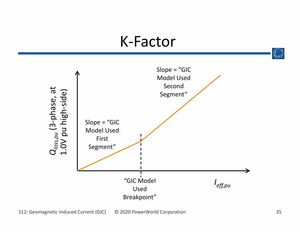
35© 2020 PowerWorld CorporationS12: Geomagnetic Induced Current (GIC)
K‐FactorQloss,pu(3‐phase, at
1.0V
puhigh
‐side)
Ieff,pu
Slope = “GIC Model Used
First Segment”
Slope = “GIC Model Used Second
Segment”
“GIC Model Used
Breakpoint”

36© 2020 PowerWorld CorporationS12: Geomagnetic Induced Current (GIC)
• Op ons → AC Power Flow Model (values used where “GIC Model Type” = Default)
K‐Factor Defaults

37© 2020 PowerWorld CorporationS12: Geomagnetic Induced Current (GIC)
• Op ons → DC Current Calcula on– Minimum Voltage Level to Include in Analysis (kV): transmission lines below this level are assumed to have zero GIC DC voltage input
– Automatic Insertion of Substations for Buses without Substations
• It is strongly recommended to assign all buses to substations and all substations to latitude/longitude locations, at least within the GIC study footprint
• Default assumption is to model unlocated facilities as ungrounded
• Lines that terminate in unlocated substations do not have GIC DC input voltage
Other Modeling Assumptions

38© 2020 PowerWorld CorporationS12: Geomagnetic Induced Current (GIC)
• DC resistance is derived from AC per‐unit resistance and the impedance base by default (assumes skin effect is negligible at 60 Hz)
• You may also specify DC resistance– Manually Enter Line Resistance = YES– Provide value in Custom DC Resistance (Ohms/Phase)
Four Bus Inputs: Transmission Lines

39© 2020 PowerWorld CorporationS12: Geomagnetic Induced Current (GIC)
• Ignore GIC Losses: If YES, area transformers are assumed to have no reactive power loss
• Ignore GIC DC Volts: If YES, area transmission lines have zero GIC DC voltage input
Area InputsB4GIC.pwb

40© 2020 PowerWorld CorporationS12: Geomagnetic Induced Current (GIC)
• These settings override the global options on Op ons → DC Current Calcula on– Use Case Default Trans/Dist Voltage: set to NO to allow the area to have a different delineation between transmission and distribution voltage
– Default Trans. Side XF Config– Default Dist. Side XF Config
Area Inputs

41© 2020 PowerWorld CorporationS12: Geomagnetic Induced Current (GIC)
• Diagonal terms are the sum of the 3‐phase conductance of all incident devices
• Off‐diagonal terms are the negative of the 3‐phase conductance between the nodes
G‐MatrixB4GIC.pwb

42© 2020 PowerWorld CorporationS12: Geomagnetic Induced Current (GIC)
• Each bus and each substation neutral is a node in the DC network
• Bus and substation neutral DC Voltages (vector V) are solved with V=G‐1I, where– G is the 3‐phase conductance matrix– I is a vector of Norton equivalent DC current injections from the GMD‐induced electric fields
• Similar in form to the power flow admittance matrix, except with only real conductance
• Equation is linear and may be solved in a single step without iteration
G‐Matrix

43© 2020 PowerWorld CorporationS12: Geomagnetic Induced Current (GIC)
• Calculation Mode = “Single Snapshot”• Field/Voltage Input
– Electric‐Field Magnitude (V/mile or V/km)– Storm Direction (0 to 360 degrees)
Uniform Electric Field Modeling
0° (south-north)
90° (west-east)
N
165°
15°
α and β scaling factors for Benchmark Event

44© 2020 PowerWorld CorporationS12: Geomagnetic Induced Current (GIC)
• Enter Maximum Field = 1 V/mile; Storm Direction = 90 degrees (eastward)• Check Also Calculate Maximum Direction Values and Include GIC in Power
Flow and Transient Stability• Click Calculate GIC Values• Simulator computes DC voltages, GIC, and reactive losses• Animated flows show GIC from Custom Float 1 field (Oneline Display
Op ons → Animated Flows)
Uniform Electric Field ModelingB4GIC.pwb
slack
Substation A with R=0.2 ohm Substation B with R=0.2 ohm
765 kV Line3 ohms Per Phase
High Side of 0.3 ohms/ PhaseHigh Side = 0.3 ohms/ Phase
DC =-19.89 VoltsDC =-13.26 VoltsBus 1 Bus 4Bus 2Bus 3
Neutral = -13.26 Volts Neutral = 13.26 Volts
DC =19.89 Volts DC =13.26 Volts
GIC Losses = 28.3 MvarGIC Losses = 37.1 Mvar
0.994 pu 0.992 pu 0.995 pu 1.000 pu
GIC/Phase = 22.10 AmpsGIC Input = 106.1 Volts
45© 2020 PowerWorld CorporationS12: Geomagnetic Induced Current (GIC)
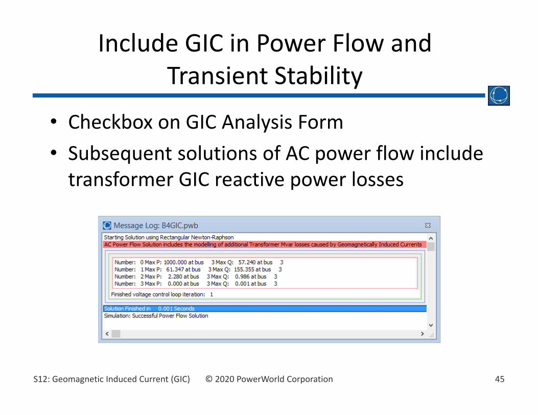
• Checkbox on GIC Analysis Form• Subsequent solutions of AC power flow include transformer GIC reactive power losses
Include GIC in Power Flow and Transient Stability

46© 2020 PowerWorld CorporationS12: Geomagnetic Induced Current (GIC)
• Indicate Storm Direction that results in maximum (and sometimes minimum) values for various quantities, and the resulting quantities
• Transformers: MVar Losses, Effective Current, and Neutral Current
• Areas: MVar Losses • System Summary: MVar Losses
Maximum Direction Values
47© 2020 PowerWorld CorporationS12: Geomagnetic Induced Current (GIC)
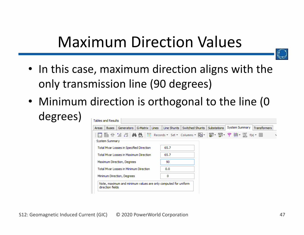
• In this case, maximum direction aligns with the only transmission line (90 degrees)
• Minimum direction is orthogonal to the line (0 degrees)
Maximum Direction Values

48© 2020 PowerWorld CorporationS12: Geomagnetic Induced Current (GIC)
• Shunts operating as inductors can also provide a conducting path for GIC
• Simulator assumes shunts have infinite resistance by default, but resistances may be provided by the user
• Inductors are assumed to have non‐magnetic core designs and thus not subject to saturation and MVar losses as in transformers (i.e. K=0)
• Shunts operating as capacitors always have infinite resistance
Switched Shunts

49© 2020 PowerWorld CorporationS12: Geomagnetic Induced Current (GIC)
Switched Shunt ExampleB4GIC.pwb
slack
Substation A with R=0.2 ohm Substation B with R=0.2 ohm
765 kV Line3 ohms Per Phase
High Side of 0.3 ohms/ PhaseHigh Side = 0.3 ohms/ Phase
DC =-19.89 VoltsDC =-13.26 VoltsBus 1 Bus 4Bus 2Bus 3
Neutral = -13.26 Volts Neutral = 13.26 Volts
DC =19.89 Volts DC =13.26 Volts
GIC Losses = 28.4 MvarGIC Losses = 37.1 Mvar
0.996 pu 0.993 pu 0.994 pu 1.000 pu
GIC/Phase = 22.10 AmpsGIC Input = 106.1 Volts
Close this

50© 2020 PowerWorld CorporationS12: Geomagnetic Induced Current (GIC)
• Right click on the shunt, choose “Switched Shunt Information Dialog…” and the GIC tab
• Set the “Per‐Phase Reactor GIC Grounding Resistance” to 0.5 ohms
• Optionally “Scale Conductance for Reactors with Multiple Blocks”– The provided resistance
applies when all inductiveblocks are in service
– If half of the available blocks are in service, the resistance is twiceas much
• Optional neutral resistance(3‐phase)
• Click OK to close thedialog
Switched Shunt ExampleB4GIC.pwb

51© 2020 PowerWorld CorporationS12: Geomagnetic Induced Current (GIC)
• Recalculate the GIC Values• Note changes in GIC flows and the G‐Matrix
Switched Shunt ExampleB4GIC.pwb

52© 2020 PowerWorld CorporationS12: Geomagnetic Induced Current (GIC)
• Allows direct entry of GIC DC input voltage on each transmission line
• At time zero, enter E‐field of zero
Time‐Varying Series Voltage Inputs
Calculation mode
Click Add at Time
Time and Field input

53© 2020 PowerWorld CorporationS12: Geomagnetic Induced Current (GIC)
• At time = 1 sec, add 1 volt/mile at 90 degrees• For each Add at Time, a column of DC Input Voltages is added
Time‐Varying Inputs

54© 2020 PowerWorld CorporationS12: Geomagnetic Induced Current (GIC)
• Change “Current Time” and click Calculate GIC Values or check “Calculate GIC on Time Change” box
• Values are linearly interpolated between Timepoints for which inputs are provided
• You may also manually edit input voltages or timepoint values
Time‐Varying Inputs
GIC DC Volt Input changed to 150 V

55© 2020 PowerWorld CorporationS12: Geomagnetic Induced Current (GIC)
GIC DC Volt Input = 150 V
,3150 volts 93.75 amps or 31.25 amps/phase
1 0.1 0.1 0.2 0.2GIC PhaseI
Transformer high side 0.3Ω/phase or 0.1Ω each, 3‐phase
slack
Substation A with R=0.2 ohm Substation B with R=0.2 ohm
765 kV Line3 ohms Per Phase
High Side of 0.3 ohms/ PhaseHigh Side = 0.3 ohms/ Phase
DC =-28.11 VoltsDC =-18.74 VoltsBus 1 Bus 4Bus 2Bus 3
Neutral = -18.74 Volts Neutral = 18.74 Volts
DC =28.11 Volts DC =18.74 Volts
GIC Losses = 52.1 Mvar GIC Losses = 52.2 Mvar
0.994 pu 0.992 pu 0.994 pu 1.000 pu
GIC/Phase = 31.24 AmpsGIC Input = 150.0 Volts
Substation grounding resistance 0.2Ω each, 3‐phase
Line series resistance: 0.000513 pu at Zbase of 5852.25Ω = 3Ω/phase or 1Ω, 3‐phase
Note: equations assume shunt is out of service (or capacitive)

56© 2020 PowerWorld CorporationS12: Geomagnetic Induced Current (GIC)
Data Interchange

57© 2020 PowerWorld CorporationS12: Geomagnetic Induced Current (GIC)
• Simulator can read and write data in the PSS/E *.gic text file format
• Facilitates exchange of data between organizations
PSS/E GIC Format
58© 2020 PowerWorld CorporationS12: Geomagnetic Induced Current (GIC)
• Open Case ACTIVSg10k.pwb and open the GIC Dialog
• Set all transformer Core Types to Single Phase• Set all substation Grounding Resistance (Ohms)to 0.2
• Click the PSSE Format Options button, choose “Save in PSSE GIC Format”, and save the file
GIC File ExampleACTIVSg10k.pwb

59© 2020 PowerWorld CorporationS12: Geomagnetic Induced Current (GIC)
• Re‐open Case ACTIVSg10k.pwb• Switch to Edit Mode and delete all substations• Switch to Run Mode and open the GIC Dialog• Click the PSSE Format Options button, choose “Load in PSSE GIC Format”, and load the just‐created file
GIC File Example

60© 2020 PowerWorld CorporationS12: Geomagnetic Induced Current (GIC)
Earth Models

61© 2020 PowerWorld CorporationS12: Geomagnetic Induced Current (GIC)
• The magnitude of the induced electric field depends upon the rate of change in the magnetic field, and deep earth (potentially 100s of km) conductivity
• The relationship between changing magnetic fields and electric fields are given by the Maxwell‐Faraday Equation
Impact of Earth Models
(the is the curl operator)
Faraday's law is V = -
dtd dd ddt dt
BE
E B S
62© 2020 PowerWorld CorporationS12: Geomagnetic Induced Current (GIC)
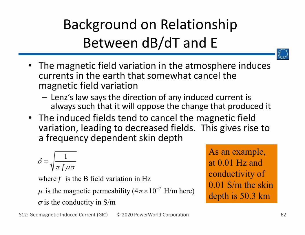
• The magnetic field variation in the atmosphere induces currents in the earth that somewhat cancel the magnetic field variation– Lenz’s law says the direction of any induced current is always such that it will oppose the change that produced it
• The induced fields tend to cancel the magnetic field variation, leading to decreased fields. This gives rise to a frequency dependent skin depth
Background on Relationship Between dB/dT and E
7
1
where is the B field variation in Hz is the magnetic permeability (4 10 H/m here)is the conductity in S/m
ff
As an example,at 0.01 Hz and conductivity of 0.01 S/m the skindepth is 50.3 km

63© 2020 PowerWorld CorporationS12: Geomagnetic Induced Current (GIC)
• If the earth is assumed to have a single conductance, , then
• The magnitude relationship is then
Frequency Domain Analysis With Uniform Conductance
0 0
0
( ) j jZj
0
0
0
Recalling ( ) ( )( ) ( ) H( )
( )
B HE Z w
j B
9
90
0
For example, assume of 0.001 S/m and
a 500nT/minute maximumvariation at 0.002 Hz. Then B( ) =660 10 T and
2 0.002 660 10 T( )0.001
( ) 0.00397 0.525 2.1 V/km
E
E

64© 2020 PowerWorld CorporationS12: Geomagnetic Induced Current (GIC)
• With a 1‐D model the earth is model as a series of conductivity layers of varying thickness
• The impedance at a particular frequencyis calculated using a recursive approach, starting at the bottom,with each layer m havinga propagation constant
• At the bottom level n
1‐D Earth Models
0m mk j
1-D Layers0
nn
jZk
Image: Figure 3.1 from NERC Application Guide: Computing Geomagnetically-Induced Current in the Bulk-Power System, December 2013

65© 2020 PowerWorld CorporationS12: Geomagnetic Induced Current (GIC)
• Above the bottom layer, each layer m, has a reflection coefficient associated with the layer below
• With the impedance at the top of layer m given as
• Recursion is applied up to the surface layer
1‐D Earth Models
1
0
1
0
1
1
mm
mm
m
Zkjr Zkj
2
0 2
11
m m
m m
k dm
m k dm m
r eZ jk r e
66© 2020 PowerWorld CorporationS12: Geomagnetic Induced Current (GIC)
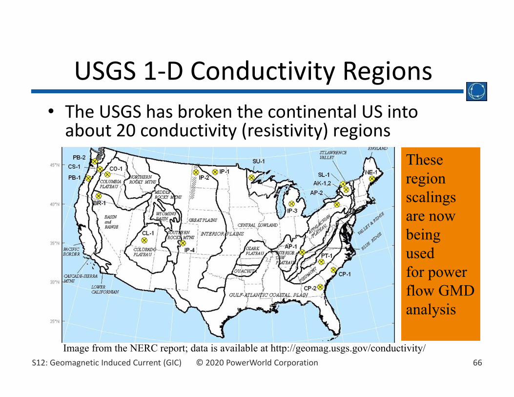
• The USGS has broken the continental US into about 20 conductivity (resistivity) regions
USGS 1‐D Conductivity Regions
Image from the NERC report; data is available at http://geomag.usgs.gov/conductivity/
Theseregionscalingsare nowbeingused for powerflow GMDanalysis

67© 2020 PowerWorld CorporationS12: Geomagnetic Induced Current (GIC)
• Image on left shows an example 1‐D model, whereas image on right shows the Z(w) variation for two models
1‐D Earth Models

68© 2020 PowerWorld CorporationS12: Geomagnetic Induced Current (GIC)
• 3‐D Earth Models produce more complex and realistic non‐uniform surface E‐field behavior– Earthscope– US Magnetotelluric (MT) Array
• Research ongoing at EarthScope, Oregon State University, Incorporated Research Institutions for Seismology (IRIS), and NOAA
• Data gaps still exist, most notably in Southwest• PowerWorld Simulator’s time‐varying E‐field Calculation Mode can make use of these inputs as researchers and industry develop them
3‐D Earth Models

69© 2020 PowerWorld CorporationS12: Geomagnetic Induced Current (GIC)
TPL‐007 Benchmark and Supplemental GMD Events
70© 2020 PowerWorld CorporationS12: Geomagnetic Induced Current (GIC)
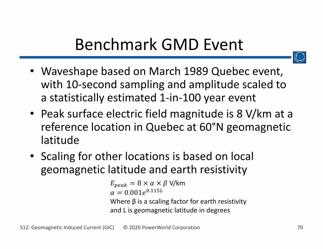
• Waveshape based on March 1989 Quebec event, with 10‐second sampling and amplitude scaled to a statistically estimated 1‐in‐100 year event
• Peak surface electric field magnitude is 8 V/km at a reference location in Quebec at 60°N geomagnetic latitude
• Scaling for other locations is based on local geomagnetic latitude and earth resistivity
Benchmark GMD Event
8 V/km0.001 .
Where β is a scaling factor for earth resistivity and L is geomagnetic latitude in degrees

71© 2020 PowerWorld CorporationS12: Geomagnetic Induced Current (GIC)
• Open TX2000.pwb• Solve power flow and Set Present Case as Base Case in Difference Flows
• Benchmark GMD Event– Load NERC_USGS_2017_Regions.aux for Earth Resistivity βfactors
– Enter GIC Electric Field of 8 V/km at 0 degrees, “Single Snapshot” calculation mode
• Leave default transformer and substation parameters• Disable voltage controllers globally in Simulator Options
Benchmark GMD Event ExampleTX2000.pwb

72© 2020 PowerWorld CorporationS12: Geomagnetic Induced Current (GIC)
Benchmark GMD Event Example
α calculated from Equation II‐1 in NERC Guideβ based on USGS earth resistivity
models loaded from aux
Include GIC in Power Flow
Epeak = 8 V/kmCalculate Max
Direction

73© 2020 PowerWorld CorporationS12: Geomagnetic Induced Current (GIC)
Benchmark GMD Event Example
Calculate GIC DC input voltages on lines at 200 kV and above

74© 2020 PowerWorld CorporationS12: Geomagnetic Induced Current (GIC)
• Calculate GIC Values• Check Tables and
Results → System Summary
• Maximum MVar Losses Occur with 93 degree direction
• Change Storm Direction to 93 degrees and recalculate GIC Values
Benchmark GMD Event Example
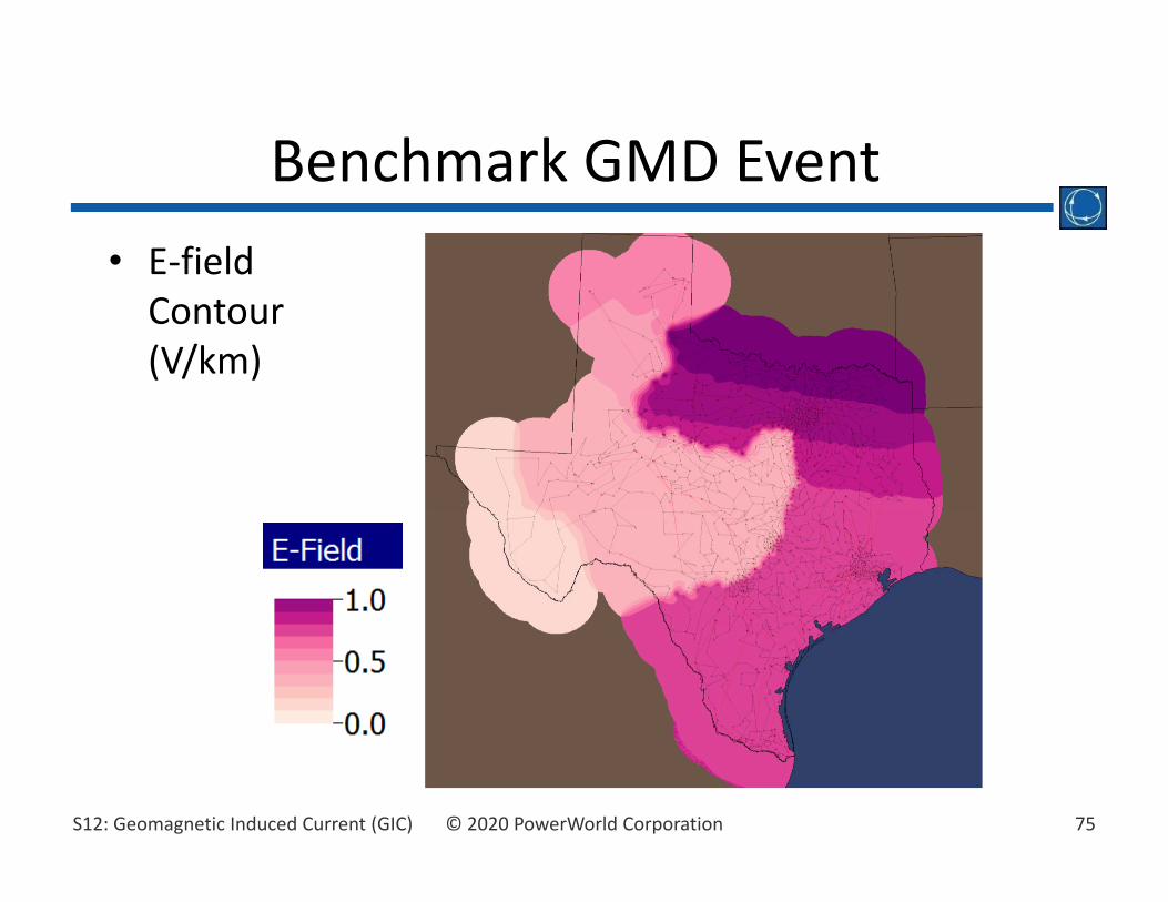
75© 2020 PowerWorld CorporationS12: Geomagnetic Induced Current (GIC)
• E‐field Contour (V/km)
Benchmark GMD Event
76© 2020 PowerWorld CorporationS12: Geomagnetic Induced Current (GIC)
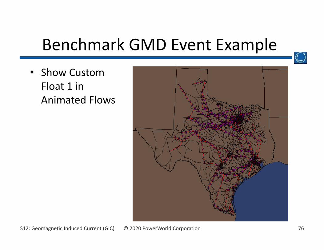
• Show Custom Float 1 in Animated Flows
Benchmark GMD Event Example

77© 2020 PowerWorld CorporationS12: Geomagnetic Induced Current (GIC)
Difference Flows: Voltage Contour

78© 2020 PowerWorld CorporationS12: Geomagnetic Induced Current (GIC)
• Simulator can automatically generate a csv file of GIC(t) time series for a uniform time‐varying E(t) field
• Sample input file NERC_GMDBenchmarkEventTimeSeries.csv– 10‐second samples matching Figures 2 and 3 in the NERC Benchmark Geomagnetic Disturbance Event Description
– fields are time, eastward E(t), and northward E(t) in V/km• Output is GIC(t) for all transformers on the GIC Transformers display– it usually makes sense to filter this list (e.g. transformers with Maximum per‐phase Effective GIC >= 75A)
Benchmark Event Time SeriesTX2000.pwb

79© 2020 PowerWorld CorporationS12: Geomagnetic Induced Current (GIC)
• Check Tables and Results → Transformers• Edit Display/Column Options to show the field Maximum IEffective
• Apply an advanced filter for transformers with maximum GIC >= 25 A
• Change Calculation Mode to “Spatially Uniform Time‐Varying E‐Field”
Benchmark Event Time Series

80© 2020 PowerWorld CorporationS12: Geomagnetic Induced Current (GIC)
• Set Time‐Varying Input File to NERC_GMDBenchmarkEventTimeSeries.csv
• Set Output File to TexasGICt.csv• Click “Calculate Transformer Ieffective”
Benchmark Event Time Series

81© 2020 PowerWorld CorporationS12: Geomagnetic Induced Current (GIC)
• When the process is complete, open the output file in Excel
• Resulting time‐series may then be input into thermal calculations– An example is in GICXfrHotSpotTempCalcs.xlsx– Help is provided in cell comments– Copy one transformer’s time series at a time into column G of the sheet XfrTimeSeries
– EPRI also provides a thermal calculator (ETTM)
Benchmark Event Time Series

82© 2020 PowerWorld CorporationS12: Geomagnetic Induced Current (GIC)
• First three columns are echoed from the input file: time, eastward E(t), and northward E(t) in V/km
• Transformer time series begin in Column D
Output CSV File

83© 2020 PowerWorld CorporationS12: Geomagnetic Induced Current (GIC)
• The NERC‐TPL‐007‐2 Supplemental GMD Event may be included in Simulator with Hotspot Modeling
Supplemental GMD Event
Include Hotspot
Hotspot characteristics(e.g. over Dallas, TX)
Apply scale factors
Apply supplemental Earth resistivity factor inside the Hotspot

84© 2020 PowerWorld CorporationS12: Geomagnetic Induced Current (GIC)
Supplemental GMD Event
Hotspot Region

85© 2020 PowerWorld CorporationS12: Geomagnetic Induced Current (GIC)
• Sample input file NERC_GMDSupplementalEventTimeSeries.csv– 10‐second samples matching the NERC Supplemental Geomagnetic Disturbance Event Description
– fields are time, eastward E(t), and northward E(t) in V/km
• Output is GIC(t) for all transformers on the GIC Transformers display– it usually makes sense to filter this list (e.g. transformers with Maximum per‐phase Effective GIC >= 85A)
Supplemental Event Time SeriesTX2000.pwb

86© 2020 PowerWorld CorporationS12: Geomagnetic Induced Current (GIC)
• Check Tables and Results → Transformers• Edit Display/Column Options to show the field Maximum IEffective
• Apply an advanced filter for transformers with maximum GIC >= 30 A
• Change Calculation Mode to “Spatially Uniform Time‐Varying E‐Field”
Supplemental Event Time Series

87© 2020 PowerWorld CorporationS12: Geomagnetic Induced Current (GIC)
• Go to Non‐Uniform Electric Field Scaling Functions → Earth Resistivity Scaling Regions
• Set “Scalar” equal to Hotspot Scalar (Local Menu → Set/Toggle/Columns → Set All Values to Field)
Apply Hotspot Scalar for Time Series

88© 2020 PowerWorld CorporationS12: Geomagnetic Induced Current (GIC)
• Set Time‐Varying Input File to NERC_GMDSupplementalEventTimeSeries.csv
• Set Output File to TexasGICtSupp.csv• Clear option
Hotspot Modeling “Include”
• Click “Calculate Transformer Ieffective”
• Following time seriescalculation, reload NERC_USGS_2017_Regions.auxto reapply normal scalars
Supplemental Event Time Series

89© 2020 PowerWorld CorporationS12: Geomagnetic Induced Current (GIC)
• Sort by Transformer Maximum Neutral Amps• Toggle “GIC Blocked for Transformer Neutral” = YES for Wadsworth and Cooper GSUs and recalculate GIC
• Cooper GSU GIC goes to zero, but GIC increases in Cooper autotransformers and a few other locations
Capacitive Neutral Blocking

90© 2020 PowerWorld CorporationS12: Geomagnetic Induced Current (GIC)
• Toggle “GIC Blocked for Transformer Neutral” = YES for Cooper Autotransformers and recalculate GIC
• The Cooper neutral current goes to zero, but some GIC still flows through the series windings
Capacitive Neutral Blocking

91© 2020 PowerWorld CorporationS12: Geomagnetic Induced Current (GIC)
• PowerWorld’s Knowledge Base has several resources for GIC modeling https://www.powerworld.com/knowledge‐base?term20=gic&submit=Go
– Complete time series for NERC Benchmark and Supplemental GMD Events
– Spreadsheet for transformer thermal response modeling
– Earth Resistivity Models– Aux Export Format
Modeling Resources

92© 2020 PowerWorld CorporationS12: Geomagnetic Induced Current (GIC)
• Transformer Properties on Parameters sheet
• Paste GIC(t) time series for a transformer starting in column D of XfrTimeSeries(3 columns provided, but insert more if needed)
• Enter the column number of the transformer to apply thermal calculations
• Temperature graphs on TimeSeriesChart
Thermal Calculation SpreadsheetGICXfrHotSpotTempCalcs.xlsx

93© 2020 PowerWorld CorporationS12: Geomagnetic Induced Current (GIC)
Sensitivity Analysis

94© 2020 PowerWorld CorporationS12: Geomagnetic Induced Current (GIC)
• “Transformer Ieffective GIC Sensitivity” can identify transmission lines with greatest effect on transformer GIC current
• Re‐calculate GIC with “Single Snapshot” mode, 8 V/km, 93 degrees, and latitude scaling
• Sort transformers by Ieffective• Include Throckmorton 345/115 kV in Sensitivity Calculation• Click Recalculate Sensitivities• dIeffective /d Efield indicates change in Ieffective for a 1 V/km variation in E‐field on the line
in question
Sensitivity Analysis
345 kV lines into Throckmorton are responsible for most GIC

95© 2020 PowerWorld CorporationS12: Geomagnetic Induced Current (GIC)
• “Line Amp Input Sensitivity” shows the sensitivity of GIC quantities (currents, DC bus voltages) to a GIC injection on the selected transmission line
• Following the use of “Line Amp Input Sensitivity”, you must click Calculate GIC Values again to restore the GIC quantities for the simulated GMD event
Sensitivity Analysis
Assumed GIC injection on line
Selected Line

96© 2020 PowerWorld CorporationS12: Geomagnetic Induced Current (GIC)
• Research has indicated that the GICs can be quite sensitive to the assumed grounding resistance; hence measured values are recommended
• The relative importance of a particular substation’s grounding resistance can be determined by comparing its value to the driving point resistance seen looking into the network at that location; these values can be computed quickly using sparse vector methods
Substation Resistance Sensitivity
,
: ii
i TH i
RR R

97© 2020 PowerWorld CorporationS12: Geomagnetic Induced Current (GIC)
• Click Calculate Sub Driving Point Values• Relative sensitivities for substations with high neutral GIC currents
Substation Resistance Sensitivity Example

98© 2020 PowerWorld CorporationS12: Geomagnetic Induced Current (GIC)
GIC Modeling in Transient Stability

99© 2020 PowerWorld CorporationS12: Geomagnetic Induced Current (GIC)
• Described in the NERC Application Guide, Appendix II*• 2 gwye‐delta GSUs, 1 gwye‐gwye autotransformer, 2 transmission lines
NERC 6‐Bus ExampleB6GIC_NERC.pwb
* http://www.nerc.com/comm/PC/Geomagnetic%20Disturbance%20Task%20Force%20GMDTF%202013/GIC%20Application%20Guide%202013_approved.pdf
slackT1
T2 - AutoXfr
T3
500 kV345 kVInput ParametersGIC Calculations
GG
1 2
3 4
5 6
SUB 1
SUB 2
SUB 3
Lat: 33.613499Lon: -87.373673
Lat: 34.310437Lon: -86.365765
Lon: -84.679354Lat: 33.955058
I12 (A, 3p)= 627.8I34(A, 3p)= 764.1
IT1 (A, 3p)= -627.8IT3 (A, 3p)= 764.1
Ic (A, 3p)= -136.2Is (A, 3p)= 764.1
Rg1: 0.2 Ohms
Rg2: 0.2 Ohms
Rg3: 0.2 Ohms
Length (km)= 121.06Length (km)= 160.47
GIC Induced Volts= 931.6GIC Induced Volts= 1555.6
R (ohms/ph)= 3.525R (ohms/ph)= 4.665
RW1 (ohms/ph)=0.5RW1 (ohms/ph)=0.5
Rc (ohms/ph)=0.2Rs (ohms/ph)=0.2Neutral Blocked: NO
Neutral Blocked: NO Neutral Blocked: NO

100© 2020 PowerWorld CorporationS12: Geomagnetic Induced Current (GIC)
• It often makes sense to analyze GIC in the transient stability domain, especially for time‐varying surface electric fields
• High‐Altitude EMP disturbances have faster rise times than typical GMD, but may last only several minutes
• Useful for generating transformer Ieff time series for inputs to thermal models
GIC in Transient Stability

101© 2020 PowerWorld CorporationS12: Geomagnetic Induced Current (GIC)
• Open GIC Analysis Form and select the Calculation Mode “Time Varying Series Voltage Inputs”
• Insert 3 time points to create a 5 second rise from 0 V/km to 15V/km at 90 degrees and a 5 second decline to 0 V/km
• Check the box “Include GIC in Power Flow and Transient Stability”
• Set “Current Time” to 0• Open Transient Stability Analysis Form
Transient Stability ExampleB6GIC_NERC.pwb

102© 2020 PowerWorld CorporationS12: Geomagnetic Induced Current (GIC)
• Run Transient Stability Simulation for 15 seconds
• Time‐series plots are generated for generator rotor angle, bus frequency, bus voltage, transformer Ieff , transformer GIC MVar losses (by substation), generator MVar output, and generator field current
• More details on using Simulator’s Transient Stability Tool are provided in a separate course
GIC in Transient StabilityB6GIC_NERC.pwb

103© 2020 PowerWorld CorporationS12: Geomagnetic Induced Current (GIC)
• Bus Voltages • Generator MVar
Transient Stability Plots
1514131211109876543210
1.071.061.051.041.031.021.01
10.990.980.970.960.950.940.930.920.910.9
0.890.880.870.860.850.840.830.820.810.8
V pu_Bus Bus 1 V pu_Bus Bus 2 V pu_Bus Bus 3 V pu_Bus Bus 4V pu_Bus Bus 5 V pu_Bus Bus 6
1514131211109876543210
200
190
180
170
160
150
140
130
120
110
100
90
80
70
60
50
40
30
20
Mvar_Gen Bus 1 #1
• Note generator at bus 1 exceeds its power flow limit of 50 MVar for several seconds
• Simulation in power flow leads to collapse at t=4.2• Increasing peak field strength beyond 20 V/km leads to collapse in transient
stability simulation

104© 2020 PowerWorld CorporationS12: Geomagnetic Induced Current (GIC)
3D Earth Models and Non‐Uniform Field Modeling
105© 2020 PowerWorld CorporationS12: Geomagnetic Induced Current (GIC)
• 3‐D Earth Models produce more complex and realistic non‐uniform surface E‐field behavior– Earthscope (NSF funded 2003‐2018)– US Magnetotelluric (MT) Array
• Research ongoing at EarthScope, Oregon State University, Incorporated Research Institutions for Seismology (IRIS), and NOAA
• Data gaps still exist, most notably in Southwest• PowerWorld Simulator’s time‐varying E‐field Calculation Mode can make use of these inputs as researchers and industry develop them
3‐D Earth Models

106© 2020 PowerWorld CorporationS12: Geomagnetic Induced Current (GIC)
3‐D Models and EarthScope
The magnetotelluric (MT) component of USArray, an NSF Earthscope project, consists of 7 permanent MT stations and a mobile array of 20 MT stations that will each be deployed for a period of about one month in regions of identified interest with a spacing of approximately 70 km. These MT measurements consist of magnetic and electric field data that can be used to calculate 3D conductivity deep in the Earth. The MT stations are maintained by Oregon State University’s National Geoelectromagnetic Facility, PI Adam Schultz. (www.earthscope.org)

107© 2020 PowerWorld CorporationS12: Geomagnetic Induced Current (GIC)
• Earthscope data is processed into magnetotellurictransfer functions that:– Define the frequency dependent linear relationship between EM components at a single site.
• Can be used to relate a magnetic field input to and electric field output at a single site
• Are provided in 2x2 impedance tensors by USArray
3‐D Models and EarthScope
Reference: Kelbert et al., IRIS DMC Data Services Products, 2011.
(simplified for the 1D case)
108© 2020 PowerWorld CorporationS12: Geomagnetic Induced Current (GIC)
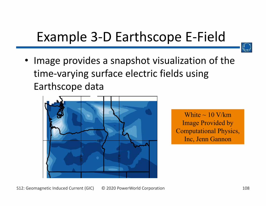
• Image provides a snapshot visualization of the time‐varying surface electric fields using Earthscope data
Example 3‐D Earthscope E‐Field
White ~ 10 V/kmImage Provided by
Computational Physics, Inc, Jenn Gannon

109© 2020 PowerWorld CorporationS12: Geomagnetic Induced Current (GIC)
• Binary (B3D) or text (csv) file formats• GeoJSON format in development• Include times points and geo‐spatial (longitude, latitude) grid with Eastward and Northward E‐field at each point
Time Varying Electric Field Inputs

110© 2020 PowerWorld CorporationS12: Geomagnetic Induced Current (GIC)
• Coarse Grid File (required)– specifies time points and resolution (in degrees latitude and longitude) of geo‐spatial grid
– contains Eastward and Northward E‐field magnitude for each grid point and time
• Fine Grid Files (optional)– detailed data at a higher spatial resolution than the Coarse Grid
– may be used for regions with high E‐field gradients (e.g. coastal effects)
Time Varying Electric Field Inputs

111© 2020 PowerWorld CorporationS12: Geomagnetic Induced Current (GIC)
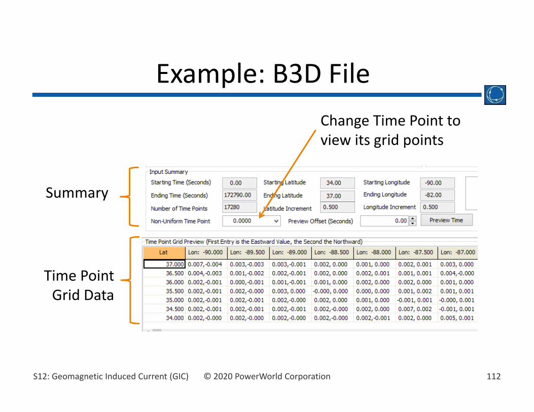
• Open case TN150.pwb and the GIC Analysis Form
• Choose Calculation Mode “Time Varying Electric Field Inputs”
• Load Coarse Grid File TN_20150622.b3d (from Browse… button)
Example: B3D FileTN150.pwb
112© 2020 PowerWorld CorporationS12: Geomagnetic Induced Current (GIC)
Example: B3D File
Time Point Grid Data
Summary
Change Time Point to view its grid points

113© 2020 PowerWorld CorporationS12: Geomagnetic Induced Current (GIC)
• Set the “Current Time” to match desired time point• Optionally check “Include GIC in Power Flow and Transient Stability”
• Click “Calculate GIC Values” and/or solve the power flow
GIC Calculation and Power Flow

114© 2020 PowerWorld CorporationS12: Geomagnetic Induced Current (GIC)
• Return to Field/VoltageInput page
• Optionally adjust “Start Time”, “End Time”, or “Sampling Rate”
• Click “Setup Time Varying Series” button• Equivalent Transmission Line inputs are created for the Calculation Mode “Time Varying Electric Field Inputs”
Calculate Entire Time Series in Transient Stability

115© 2020 PowerWorld CorporationS12: Geomagnetic Induced Current (GIC)
• Change Calculation Mode to “Time Varying Series Voltage Inputs”
• Time Points created at sampling interval between Start Time and End Time
Time Varying Series Voltage Inputs

116© 2020 PowerWorld CorporationS12: Geomagnetic Induced Current (GIC)
• Open Transient Stability dialog and go to Options → Power System Model → Commonpage
• Check “Just Calculate GIC with No Network Solution” (allows fast computation of time‐varying GIC quantities without transient stability numeric integration)
GIC in Transient Stability

117© 2020 PowerWorld CorporationS12: Geomagnetic Induced Current (GIC)
• Go to Simula on → Control page• Set the Start Time, End Time, and Time Step to correspond to the GIC input data (or any desired subset)
GIC in Transient Stability
118© 2020 PowerWorld CorporationS12: Geomagnetic Induced Current (GIC)
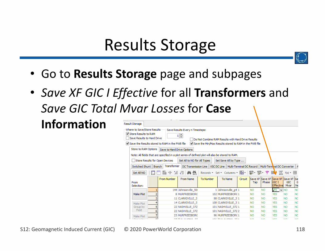
• Go to Results Storage page and subpages• Save XF GIC I Effective for all Transformers and Save GIC Total Mvar Losses for Case Information
Results Storage

119© 2020 PowerWorld CorporationS12: Geomagnetic Induced Current (GIC)
• Click “Run Transient Stability”• Go to Plots page and create plots
– Device Type “Transformer” and Field “XF GIC I Effective”
– Device Type “Case Information” and Field “GIC Total Mvar Losses”
• Details on plotting tool are covered in the Transient Stability Training
Plot Results

120© 2020 PowerWorld CorporationS12: Geomagnetic Induced Current (GIC)
GIC Time Series Plots
150,000100,00050,0000
100
90
80
70
60
50
40
30
20
10
0
GIC Total Mvar Losses, Case Information
121© 2020 PowerWorld CorporationS12: Geomagnetic Induced Current (GIC)
High‐Altitude Electromagnetic Pulse (HEMP)

122© 2020 PowerWorld CorporationS12: Geomagnetic Induced Current (GIC)
• Broadly defined, an electromagnetic pulse is any transient burst of electromagnet energy
• Characterized by their magnitude, frequencies, footprint, and type of energy
• There are many different types, such as static electricity sparks, interference from gasoline engine sparks, lightning, electric switching, geomagnetic disturbances (GMDs) cause by solar corona mass ejections (CMEs), nuclear electromagnetic pulses, and non‐nuclear EMP weapons
Eletromagnetic Pulse (EMP)

123© 2020 PowerWorld CorporationS12: Geomagnetic Induced Current (GIC)
• The impacts of a high‐altitude EMP (HEMP) are typically divided into three time frames: E1, E2 and E3
• The quickest, E1 withmaximum electric fields of 10’s of kV per meter, can impact unshielded electronics
• E2, with electric fields of up to 100 volts per meter, is similar to lightning
• Much of talk is on E3, which is similar to GMDs
HEMP Time Frames
Image Source: IEC 1000-2-9 Figure

124© 2020 PowerWorld CorporationS12: Geomagnetic Induced Current (GIC)
• EMP impacts do not scalelinearly with weapon size– Even quite small weapons(such as 10 kilotons) canproduce large EMPs
HEMP Impact vs. Size and Altitude
Image Sources: en.wikipedia.org/wiki/Nuclear_electromagnetic_pulse
Low altitude EMPscan still have largefootprints

125© 2020 PowerWorld CorporationS12: Geomagnetic Induced Current (GIC)
• In a nuclear explosion, the E1 pulse is produced by the gamma radiation stripping electrons from atoms– Known as the Compton effect; explained by Conrad Longmire at Los Alamos in 1963
– Electron flow is diverted byearth’s magnetic field
– Mostly line of sight impacts;highest impacts south of detonation in Northern Hemisphere
• The E2 pulse is created byscattered gamma rays and neutron gamma rays
EMP E1 and E2 Mechanisms
Source: “The Early-Time (E1) High-Altitude Electromagnetic Pulse (HEMP) and Its Impact on the U.S. Power Grid, MetaTech-R-320, January 2010
“Smile Diagram”

126© 2020 PowerWorld CorporationS12: Geomagnetic Induced Current (GIC)
• Because of large footprint, small energy density in the E1, so devices can be protected by Faraday cages– The allowable size of apertures depends on the wavelength and
hence the frequency (l=c/f); a ballpark figure is no larger than 1/10 the wavelength; for 1 GHz this is about 3 cm
– Incoming wires are also an issue– Military Standard 188‐125‐1 (“HIGH‐ALTITUDE
ELECTROMAGNETIC PULSE (HEMP) PROTECTION FOR GROUND‐BASED C41 FACILITIES PERFORMING CRITICAL, TIME‐URGENT MISSIONS PART 1 FIXED FACILITIES”) provides useful guidance
– Another useful reference is MetaTech Report R‐320, “The Early‐Time (E1) High‐Altitude Electromagnetic Pulse (HEMP) and Its Impact on the U.S. Power Grid”
EMP E1 Protection
Source: “The Early-Time (E1) High-Altitude Electromagnetic Pulse (HEMP) and Its Impact on the U.S. Power Grid, MetaTech-R-320, January 2010

127© 2020 PowerWorld CorporationS12: Geomagnetic Induced Current (GIC)
• The late‐time (E3) effects of a nuclear detonation tens‐hundreds of km over the surface of the Earth gives rise to geomagnetic disturbances (GMD) similar to a coronal mass ejection from the sun
• The E3 is usually broken into two components– E3A “Blast Wave” caused by the expansion of the nuclear fireball, expelling the Earth’s magnetic field
– E3B “Heave” as bomb debris and air ions follow geomagnetic lines at about 130 km, making the air rise, which gives rise to a current and an induced electric field
High‐Altitude Electromagnetic Pulse (HEMP)

128© 2020 PowerWorld CorporationS12: Geomagnetic Induced Current (GIC)
HEMP E3A and E3B
Left Image: IEC 1000-2-9, Figure 9, Right Image: ORNL “Study to Assess the Effects of Magnetohydrodynamic Electromagnetic Pulse on Electric Power Systems Phase I Final Report,” May 1985, Figure 8

129© 2020 PowerWorld CorporationS12: Geomagnetic Induced Current (GIC)
• For a uniform earth conductivity model, the E3A Blast wave can be modeled as a fairly uniform east‐west electric field
• Similar to a uniform GMD over a very wide area
HEMP E3A
Image Source: Metatech R‐321, Figure 2‐4
Because of the relatively large, uniform electric field area, the effect is somewhat insensitive to location within CONUS

130© 2020 PowerWorld CorporationS12: Geomagnetic Induced Current (GIC)
• ORNL 1985 models the E3B electric field as the product of a spatially independent time function (fig 8), and time independent spatial magnitude and directions (fig 9 and 10)
HEMP E3B
, y, t ( , ) (x, y) ( )E x x y e f t
x x=
Values were calculated assuming a uniform conductivity of 0.001 S/m

131© 2020 PowerWorld CorporationS12: Geomagnetic Induced Current (GIC)
• Sources of initial time and spatial waveforms implemented in PowerWorld Simulator– “Study to Assess the effects of Magnetohydrodynamic Electromagnetic Pulse on Electric Power System, Phase 1, Final Report,” Martin Marietta Energy Systems Inc. Oak Ridge National Labs. 1985.
– “IEC 61000‐2‐9 – Electromagnetic Compatibility (EMC) – Part 2: Environment – Section 9: Description of HEMP Environment – Radiated Disturbance. Basic EMC Publication,” International Electrotechnical Commission. Feb. 19, 1996.
HEMP E3 Waveforms

132© 2020 PowerWorld CorporationS12: Geomagnetic Induced Current (GIC)
• Simulator can auto‐create time and spatially‐varying electric fields associated with de‐classified EMP waveforms based on location, time functions, and spatial functions
Auto‐Creating HEMP Electric Fields

133© 2020 PowerWorld CorporationS12: Geomagnetic Induced Current (GIC)
• Choose “Time Varying Series Voltage Inputs” Calculation Mode and Field/Voltage Input → EMP subtab
Auto‐Creating HEMP Electric Fields
Include GIC in Power Flow and Transient Stability and Use EMP as Input

134© 2020 PowerWorld CorporationS12: Geomagnetic Induced Current (GIC)
Example HEMP Parameters
Location of Center: 40.76, ‐111.89 for Salt Lake City
E3A:ORNL_Fig8_3A,
Uniform Westward Field, 24 V/km
E3B: ORNL_Fig8_3B, ORNL_Fig9_Fig10, 24 V/km
Click Calculate EMP Input Time Series

135© 2020 PowerWorld CorporationS12: Geomagnetic Induced Current (GIC)
ORNL E3B Peak Contour
E‐Field Magnitude at t=60s
136© 2020 PowerWorld CorporationS12: Geomagnetic Induced Current (GIC)
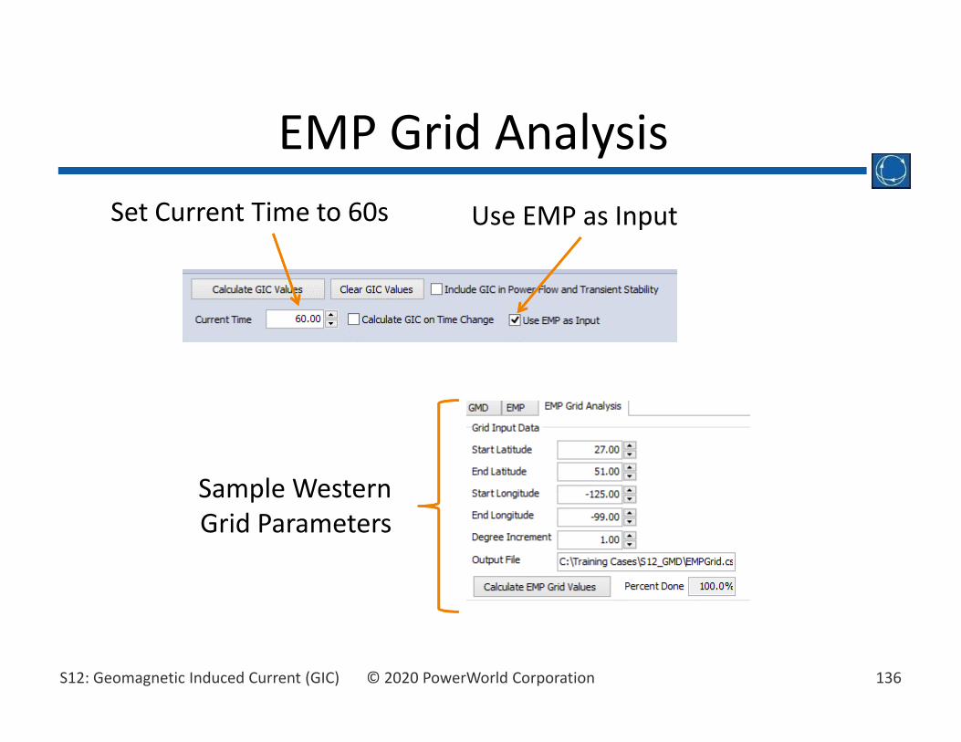
EMP Grid AnalysisSet Current Time to 60s Use EMP as Input
Sample Western Grid Parameters

137© 2020 PowerWorld CorporationS12: Geomagnetic Induced Current (GIC)
• Sorting results reveals worst‐case locations for losses or single‐transformer Effective GIC
• With a little effort, could contour on “dummy substations” aligned to grid locations
EMP Grid Analysis

138© 2020 PowerWorld CorporationS12: Geomagnetic Induced Current (GIC)
EMP Grid AnalysisMvar Losses at E3B Peak Maximum Single‐Transformer
Ieffective at E3B Peak
33N, 116W1095 A, 765 kV Phase‐Shifting Xfr
40N, 116W94,217 MVar

139© 2020 PowerWorld CorporationS12: Geomagnetic Induced Current (GIC)
Maximum Mvar Location
Location of Center: 40, ‐116
E3A:ORNL_Fig8_3A,
Uniform Westward Field, 24 V/km
E3B: ORNL_Fig8_3B, ORNL_Fig9_Fig10, 24 V/km
Click Calculate EMP Input Time Series

140© 2020 PowerWorld CorporationS12: Geomagnetic Induced Current (GIC)
• Set Current Time to 60 (corresponds to E3B peak)• Check “Include GIC in Power Flow and Transient Stability” and “Use EMP as Input”
• Click Calculate GIC Values
Resulting DC Input Voltages

141© 2020 PowerWorld CorporationS12: Geomagnetic Induced Current (GIC)
ORNL E3B E‐Field Contour
E‐Field Magnitude at t=60s
Saved View: West EMP E‐field

142© 2020 PowerWorld CorporationS12: Geomagnetic Induced Current (GIC)
Power Flow Mismatches
Most large losses occur near hotspots in Southern California and Northern Nevada
Power Flow Solution fails to converge!
143© 2020 PowerWorld CorporationS12: Geomagnetic Induced Current (GIC)
• HEMP disturbances have faster rise times than solar GMD, but may last only several minutes
• It often makes sense to analyze EMP in the transient stability domain– Incorporate load shedding, generator exciters, excitation limiters, and other characteristics not modeled in power flow
EMP Modeling

144© 2020 PowerWorld CorporationS12: Geomagnetic Induced Current (GIC)
• Reset Current Time on GIC Analysis dialog to 0• Open Transient Stability dialog from ToolsRibbon
• Simula on → Control Parameters: 0.25 cycle time step works well for EMP waveforms
Transient Stability Analysis

145© 2020 PowerWorld CorporationS12: Geomagnetic Induced Current (GIC)
• Disable any existing Transient Contingency Elements (set “Enabled” field to Never)
• Op ons → Power System Model → Load Modeling: use “Constant Current P, Impedance Q”
• Click Run Transient Stability
Transient Stability Analysis

146© 2020 PowerWorld CorporationS12: Geomagnetic Induced Current (GIC)
Transient Stability Plots
Frequency: Average by Area
Bus Voltage

147© 2020 PowerWorld CorporationS12: Geomagnetic Induced Current (GIC)
Transient Stability:Voltage Visualization

148© 2020 PowerWorld CorporationS12: Geomagnetic Induced Current (GIC)
Transient Stability:Frequency Visualization

149© 2020 PowerWorld CorporationS12: Geomagnetic Induced Current (GIC)
• Report of the “Commission to Assess the Threat to the United States from EMP Attack” (EMP Commission) was released to public
• “A realistic unclassified peak level for E3 HEMP would be 85 V/km for CONUS as described in this report”
HEMP Future Studies

150© 2020 PowerWorld CorporationS12: Geomagnetic Induced Current (GIC)
• Plot of newly‐released electric field waveforms, the ORNL 1985 waveform, and the IEC 1996 waveform
• Source: Lee, R. and Overbye, T. J.; “Comparing the Impact of HEMP Electric Field Waveforms on a Synthetic Grid”, submitted to North American Power Symposium, 2018.
HEMP Waveform Comparison
151© 2020 PowerWorld CorporationS12: Geomagnetic Induced Current (GIC)
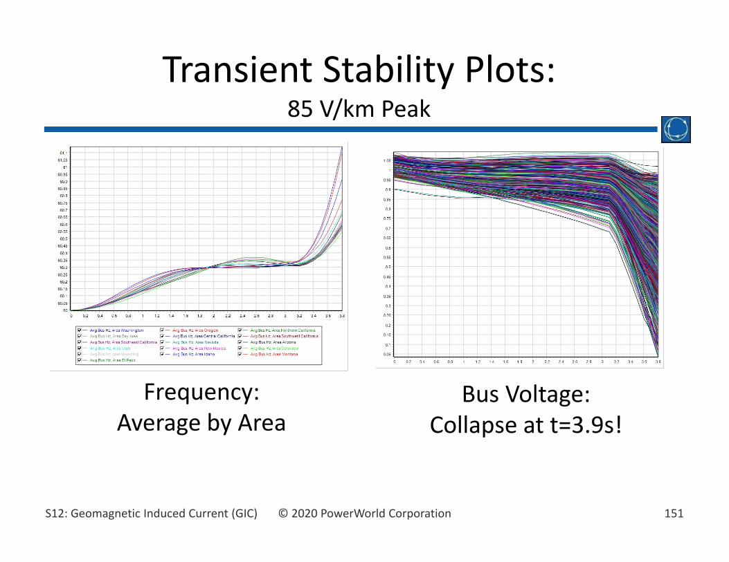
Transient Stability Plots:85 V/km Peak
Frequency: Average by Area
Bus Voltage:Collapse at t=3.9s!

Blank Page
Related Documents