Glasgow Theses Service http://theses.gla.ac.uk/ [email protected] Fuerte Esquivel, Claudio Rubén (1997) Steady state modelling and analysis of flexible AC transmission systems. PhD thesis. http://theses.gla.ac.uk/4616/ Copyright and moral rights for this thesis are retained by the author A copy can be downloaded for personal non-commercial research or study, without prior permission or charge This thesis cannot be reproduced or quoted extensively from without first obtaining permission in writing from the Author The content must not be changed in any way or sold commercially in any format or medium without the formal permission of the Author When referring to this work, full bibliographic details including the author, title, awarding institution and date of the thesis must be given

Steady State Modelling and Analysis of FACTS
Dec 03, 2015
Steady State Modelling and Analysis of FACTS
Welcome message from author
This document is posted to help you gain knowledge. Please leave a comment to let me know what you think about it! Share it to your friends and learn new things together.
Transcript

Glasgow Theses Service http://theses.gla.ac.uk/
Fuerte Esquivel, Claudio Rubén (1997) Steady state modelling and analysis of flexible AC transmission systems. PhD thesis. http://theses.gla.ac.uk/4616/ Copyright and moral rights for this thesis are retained by the author A copy can be downloaded for personal non-commercial research or study, without prior permission or charge This thesis cannot be reproduced or quoted extensively from without first obtaining permission in writing from the Author The content must not be changed in any way or sold commercially in any format or medium without the formal permission of the Author When referring to this work, full bibliographic details including the author, title, awarding institution and date of the thesis must be given
Steady State Modelling and Analysis
of Flexible AC Transmission Systems
by
Claudio Rubén Fuerte Esquivel
B.Eng. (Summa Cum Laude) Instituto Tecnológico de Morelia, México, 1990 M.Sc. (Summa Cum Laude) Instituto Politécnico Nacional, México, 1993
A Thesis submitted to the Department of Electronics and Electrical Engineering
of The University of Glasgow
for the degree of Doctor of Philosophy
August 1997
© Claudio Rubén Fuerte Esquivel, 1997

ii
To my wife Monica, who put aside her own career, interest and a comfortable standard of living to kindly accompany me in this rewarding but often painful endeavour. Her love and wholehearted support, encouragement and understanding throughout these past three years make our dream possible. To our wee son Claudio, who made our life a little more complicated but full of love and fun. To my mother for her love, encouragement, unconditional support and for always giving me the freedom and opportunity to pursue my aspirations. To my brother whose example has been a source of my strength and confidence to make this undertaking possible.

iii
Abstract As electric utilities move into more competitive generation supply regimes, with limited scope to expand transmission facilities, the optimisation of existing transmission corridors for power transfer becomes of paramount importance. In this scenario, Flexible AC Transmission System (FACTS) technology, which aims at increasing system operation flexibility, appear as an attractive alternative. Many of the ideas upon which the foundations of FACTS rest were conceived some time ago. Nevertheless, FACTS as a single coherent integrated philosophy is a newly developed concept in electrical power systems which has received the backing of the major manufacturers of electrical equipment and utilities around the world. It is looking at ways of capitalising on the new developments taking place in the area of high-voltage and high-current power electronics in order to increase the control of the power flows in the high voltage side of the network during both steady state and transient conditions, so as to make the network electronically controllable. In order to examine the applicability and functional specifications of FACTS devices, it is necessary to develop accurate and flexible digital models of these controllers and to upgrade most of the software tools used by planners and operators of electric power systems. The aim of this work is to develop general steady-state models FACTS devices, suitable for the analysis of positive sequence power flows in, large-scale real life electric power systems. Generalised nodal admittance models are developed for the Advance Series Compensator (ASC), Phase Shifter (PS), Static Var Compensator (SVC), Load Tap Changer (LTC) and Unified Power Flow Controller (UPFC). In the case of the ASC, two models are presented, the Variable Series Compensator (VSC) and the Thyristor Controlled Series Capacitor-Firing Angle (TCSC-FA). An alternative UPFC model based on the concept of Synchronous Voltage Source (SVS) is also developed. The Interphase Power Controller (IPC) is modelled by combining PSs and VSCs nodal admittance models. The combined solution of the power flow equations pertaining to the FACTS devices models and the power network is described in this thesis. The set of non-linear equations is solved through a Newton-Rapshon technique. In this unified iterative environment, the FACTS device state variables are adjusted automatically together with the nodal network state variables so as to satisfy a specified nodal voltage magnitudes and specified power flows. Guidelines and methods for implementing FACTS devices and their adjustments within the Newton-Rapshon algorithm are described. It is shown that large increments in the adjustments of FACTS devices and nodal network state variables during the backward substitution may dent the algorithm’s quadratic convergence. Suitable strategies are given which avoid large changes in these variables and retain the Newton-Rapshon method's quadratic convergence. The influence of initial conditions of FACTS devices state variables on the iterative process is investigated. Suitable initialisation guidelines are recommended. Where appropriate, analytical equations are given to assure good initial conditions.

iv
In order to investigate the issue of ‘number crunching’ Object Oriented Programming (OOP) power engineering applications, a power flow program written in C++ is developed using the OOP philosophy. The algorithm is a Newton-Raphson load flow which includes comprehensive control facilities and yet exhibits very strong convergence characteristics. The software is fast and reliable. It can be used for the analysis and control of large-scale power networks containing FACTS-controlled devices. The methodology used in the development of the software is also given. Comparisons of the newly developed C++ power flow program with a sequential N-R load flow program written in FORTRAN are made and some finding are reported. Using the newly developed program, an extensive number of simulations are carried out in order to investigate the interaction between FACTS devices and the network. The application of FACTS devices to solve current issues in real life power networks is also presented. FACTS devices are used to redistribute power flow in an interconnected power network, to eliminate loop flows and to increase margins of voltage collapse. Moreover, the effect of the transformer magnetising branch on system losses is quantified. A general power flow tracing algorithm to compute the individual generator contributions to the active and reactive power flows and losses is also proposed.

v
Acknowledgements During this research I have had interaction with many people whose attitude, enthusiasm and willingness have enriched, in many forms, my knowledge and/or my experience to give me encouragement to make this dream possible. To all of them I express my sincere thanks. Despite the above sentiments, there are few persons and organisations who deserve special mention. I would like to extend my warmest thanks and gratitude to my supervisor Dr. Enrique Acha, for his invaluable technical support, incessant encouragement, sincere friendship and understanding. Dr. Acha has always generously given me his time and expertise in advising me throughout my research. The past three years of working together has given me faith and confidence to become an independent research for which I am thankful. I am indebted to my friend Dr. Horacio Tovar for his help with all legal matters of my study leave at Instituto Tecnológico de Morelia, México. I gratefully acknowledge the financial assistance given by the Consejo Nacional de Ciencia y Tecnología, México during my PhD studies. Thanks are also due to Instituto Tecnológico de Morelia, México for granting me study leave to carry out my PhD research. I would like to express my appreciation to my postgraduate colleagues who made life so much enjoyable. I thank my family, especially my uncle Fernando, my aunts Mary and Anita and my cousins Chela and Licha, for their love and kindness. Last, but not least, to my cousin Juan for his love, encouragement and help during my formative education in México. To him I also dedicate this work. I wish you were here.

vi
List of Publications The following publications are associated with this research work: Transaction-Graded Papers: • C.R. Fuerte-Esquivel and E. Acha.: ‘The Unified Power Flow Controller: A Critical
Comparison of Newton-Rapshon UPFC Algorithms in Power Flow Studies’, accepted for publication in IEE Proceedings on Generation, Transmission and Distribution, 1997.
• C.R. Fuerte-Esquivel and E. Acha.: ‘A Newton-type Algorithm for the Control of Power
Flow in Electrical Power Networks’, PE-159-PWRS-0-12-1997, To be published in IEEE Transactions on Power Systems, 1997.
• C.R. Fuerte-Esquivel, E. Acha, S.G. Tan and J.J. Rico.: ‘Efficient Object Oriented Power
Systems Software for the Analysis of Large-scale Networks Containing FACTS-Controlled Branches’, PE-158-PWRS-0-12-1997, To be published in IEEE Transactions on Power Systems, 1997.
• C.R. Fuerte-Esquivel and E. Acha.: ‘Newton-Rapshon Algorithm for the Reliable
Solution of Large Power Networks with Embedded FACTS Devices’, IEE Proceedings on Generation, Transmission and Distribution, Vol. 143, No. 5, September 1996, pp. 447-454.
• C.R. Fuerte-Esquivel, E. Acha and H. Ambriz-Perez.: ‘A Thyristor Controlled Series
Compensator Model for the Power Flow Solution of Practical Power Networks’, Submitted to IEEE Transactions on Power Systems, Summer 1997.
• C.R. Fuerte-Esquivel, E. Acha and H. Ambriz-Pérez.: ‘A Comprehensive Newton-
Rapshon UPFC for the Quadratic Power Flow Solution of Practical Power Networks’, Submitted to IEEE Transactions on Power Systems, Summer 1997.
• H. Ambriz-Pérez, E. Acha, C.R. Fuerte-Esquivel and A. De la Torre.: ‘The Incorporation
of a UPFC model in an Optimal Power Flow by Newton’s Method’, Submitted to IEE Proceedings on Generation, Transmission and Distribution, Summer 1997.
Conference Papers: • E. Acha, H. Ambriz-Pérez, S.G. Tan and C.R. Fuerte-Esquivel.: ‘A New Generation of
Power System Software Based on the OOP Paradigm’, International Power Engineering Conference 1997 (IPEC 97), Singapore 21-23 May 1997 pp. 68-73.
• H. Ambriz-Pérez, E. Acha, C.S. Chua and C.R. Fuerte-Esquivel.: ‘On the Auditing of
Individual Generator Contributions to Optimal Power Flows and Losses in Large, Interconnected Power Networks’, International Power Engineering Conference 1997 (IPEC 97), Singapore 21-23 May 1997 pp. 513-518.
• E. Acha, C.R. Fuerte-Esquivel and C.S. Chua.: ‘On the Auditing of Individual Generator
Contributions to Power Flows and Losses in Meshed Power Networks’, RVP 96-SIS-10, Power Summer Meeting IEEE Mexico Section, Acapulco Gro, Mexico, 21-26 July 1996, pp. 170-173.
• S.G. Tan, J.J. Rico, C.R. Fuerte-Esquivel and E. Acha: ‘C++ Object Oriented Power
Systems Software’, Proceedings of the 30th UPEC Conference, London UK, 5-7 September 1995, pp. 339-342.

vii
Table of Contents Abstract. iii Acknowledgements. v List of Publications. vi Table of Contents. vii List of Figures. xi List of Tables. xvi Abbreviations. xix Chapter 1 Introduction 1.1 Background and motivation behind the present research. 2 1.2 Objectives. 3 1.3 Contributions. 4 1.4 Thesis outline. 5 1.5 Bibliography. 6 Chapter 2 A General Overview of Flexible AC Transmission Systems 2.1 Introduction. 8 2.2 Steady-state power flow and voltage control. 9 2.3 Inherent limitations of conventional transmission systems. 10 2.4 FACTS controllers. 11 2.5 Power flow analysis of networks with FACTS devices. 13 2.6 Initialisation of FACTS devices. 15 2.7 Adjusted solution criterion. 16 2.8 Truncated adjustments. 16 2.9 FACTS applications. 17 2.9.1 United Kingdom. 17 2.9.2 Italy. 17 2.9.3 France. 18 2.9.4 Japan. 18 2.9.5 Application of a thyristor series capacitor in the Bonneville Power Administration system (USA). 19 2.9.6 Application of a controllable series capacitor in the American Electric Power system (USA). 20 2.10 Conclusions. 20 2.11 Bibliography. 20 Chapter 3 Power Flow Series Controller 3.1 Introduction. 22 3.2 Thyristor controlled series capacitor. 22 3.2.1 TCSC voltage and current steady-state equations. 23 3.2.2 TCSC fundamental frequency impedance. 27 3.2.3 Operating modes of TCSCs. 30 3.2.4 ASC steady-state power flow model. 32 3.2.5 VSC initialisation. 34 3.2.6 VSC active power flow control test case. 35 3.2.7 Feasible active power flow control region. 37

viii
3.2.8 Convergence test and VSC model validation. 39 3.2.9 VSC active power flow control in a real power system. 40 3.2.10 TCSC power flow model as function of the firing angle. 41 3.2.11 TCSC’s firing angle initial condition. 43 3.2.12 Numerical properties of the TCSC-FA model. 44 3.2.13 Limit revision of TCSC’s firing angle. 45 3.2.14 TCSC-FA active power flow control test case. 45 3.2.15 Effect of the firing angle truncated adjustment. 46 3.2.16 Multiple solutions due to multiple resonant points. 47 3.2.17 TCSC-FA control near a resonance point. 49 3.2.18 Power flow control by TCSC-FA in a real power system. 50 3.2.19 Comparison of VSC and TCSC-FA models. 52 3.3 Phase shifter. 53 3.3.1 Phase shifter steady-state power flow model. 54 3.3.2 PS initialisation and adjusted solution. 58 3.3.3 PS active power flow control test case. 59 3.3.4 PS feasible active power flow control region. 60 3.3.5 Effect of PS’s impedance on phase angle value. 63 3.3.6 Active power flow control by PSs and VSCs. 67 3.3.7 Active power flow control in a real power system. 71 3.4 Interphase power controller. 72 3.4.1 IPC steady-state power flow model. 73 3.4.2 IPC active power flow control test case. 75 3.4.3 IPC feasible power flow control region. 76 3.4.4 Effect of IPC reactances. 79 3.4.5 Feasible active power control region of two IPCs. 80 3.4.6 Active power flow control in a real power system. 83 3.5 Conclusions. 83 3.6 Bibliography. 84 Chapter 4 Voltage magnitude controllers. 4.1 Introduction. 86 4.2 Static Var Compensator. 87 4.2.1 SVC voltage-current characteristic and operation. 87 4.2.2 SVC voltage-current equations. 89 4.2.3 SVC fundamental frequency impedance. 91 4.2.4 Conventional SVC power flow models. 93 4.2.5 Proposed SVC power flow model. 93 4.2.6 Control co-ordination between reactive sources. 95 4.2.7 Revision of SVC limits. 95 4.2.8 SVC nodal voltage magnitude test case. 95 4.2.9 Control co-ordination between generators and SVCs. 96 4.3 Load tap-changer. 97 4.3.1 LTC power flow model for control of nodal voltage magnitude. 98 4.3.2 Special control system configurations of LTCs. 102 4.3.3 Simultaneous nodal voltage magnitude control by means of reactive sources and LTCs. 103 4.3.4 Initial conditions and adjusted solutions criterion of LTCs. 105 4.3.5 LTC nodal voltage magnitude test case. 105 4.3.6 Effect of LTC impedance on the tap magnitude value. 106 4.3.7 Convergence test. 107 4.3.8 Effect of sensitivity factors in the parallel control options. 108

ix
4.3.9 Effect of truncated adjustments in the state variables. 108 4.3.10 Control co-ordination between LTCs and reactive sources. 114 4.3.11 Solution of a large power network with embedded FACTS devices. 116 4.4 Conclusions. 116 4.5 Bibliography. 117 Chapter 5 Unified power flow controllers 5.1 Introduction. 119 5.2. Generalised UPFC model. 120 5.2.1 UPFC equivalent circuit. 121 5.2.2 UPFC power equations. 121 5.2.3 UPFC jacobian equations. 123 5.3 Criterion control. 126 5.3.1 Shunt converter control criterion. 127 5.3.2 Series converter control criterion. 127 5.3.3 Special UPFC control configurations. 127 5.4 UPFC initial conditions and limits revisions. 128 5.4.1 Series source initial conditions. 128 5.4.2 Shunt source initial conditions. 128 5.4.3 Limit revision of UPFC controllable variables. 129 5.5 Synchronous voltage source UPFC model. 129 5.5.1 SVS initial conditions. 130 5.6. Load flow test cases. 132 5.6.1 Power flow control by means of UPFCs. 132 5.6.2 Effect of initial conditions. 133 5.6.3 Effect of UPFC transformer coupling reactances. 134 5.6.4 Effect of UPFC transformer coupling losses. 135 5.6.5 UPFC model validation. 136 5.6.6 Power flow control by means of SVSs. 137 5.6.7 Effect of SVS initial conditions. 138 5.6.8 Comparison of UPFC and SVS devices. 138 5.6.9 Interaction of UPFC and SVS with other FACTS devices. 139 5.6.10 Solution of a large power network with embedded FACTS devices. 141 5.6.11 Power flow control by means of UPFCs in a real power system. 142 5.7 Conclusions. 144 5.8 Bibliography. 144 Chapter 6 Applications of FACTS Devices 6.1. Introduction. 146 6.2 Auditing of individual generator contributions to power flows, losses and cost in interconnected power networks. 146 6.2.1 Tracing generators’ costs. 147 6.2.2 Dominion’s contributions to active power flows. 147 6.2.3 Dominion’s contributions to reactive power flows. 148 6.2.4 Dominion’s contributions to loads. 149 6.2.5 Source’s dominions. 149 6.2.6 Numeric example of active power flow auditing. 151 6.2.7 Numeric example of reactive power flow auditing. 154 6.2.8 Effect of FACTS devices on active power source’s dominions. 157 6.2.9 Numeric examples of use of line charges. 158 6.2.10 Allocating generation costs and ULCs in a real life power network. 160

x
6.2.11 Tracing of reactive power flows. 163 6.3 Loop flows. 164 6.4 Effect of the transformer magnetising branch. 168 6.4.1 Case 1. 168 6.4.2 Case 2. 168 6.5 Voltage collapse. 170 6.5.1 Analysis of voltage collapse by a static approach. 171 6.5.2 Analysis of maximum loadability and voltage collapse in the presence of FACTS devices. 173 6.6 Conclusions. 178 6.7 Bibliography. 179 Chapter 7 Application of the Object Oriented Programming philosophy to the analysis of electric power systems containing FACTS devices 7.1 Introduction. 181 7.2 Objective modelling of power networks. 182 7.3 Derived types and data abstraction. 183 7.4 Class hierarchy and inheritance. 185 7.5 Sparsity techniques. 186 7.6 Load flow analysis. 188 7.7 Controllable devices. 190 7.8 Load flow test case and validation. 192 7.9 Solution of ill-conditioned networks. 193 7.10 Conclusions. 195 7.11 Bibliography. 195 Chapter 8 Conclusions and Recommendations 8.1 General conclusions. 197 8.2 Suggestions for further research work. 198 Appendix I Data files 200 Appendix II General current equation of the TCSC 215 Appendix III Phase shifter transformer 219

xi
List of Figures Figure 2.1. Overhead transmission line. 9 Figure 2.2. Organisation for implementation of FACTS Research programs. 18 Figure 2.3. One-line diagram of Slatt substation’s TCSC. 19 Figure 3.1. TCSC module. 23 Figure 3.2. Equivalent electric circuit of a TCSC module. 23 Figure 3.3. Asymmetrical thyristor current pulse. 24 Figure 3.4. TCSC thyristor current in steady-state. 25 Figure 3.5. Voltage and currents waveforms in the TCSC capacitor. 26 Figure 3.6. Voltage and currents waveforms in the TCSC inductor. 27 Figure 3.7. Voltage and currents waveforms in the TCSC bi-directional thyristors. 27 Figure 3.8. TCSC fundamental impedance. 29 Figure 3.9. TCSC module operating in thyristor blocked mode. 30 Figure 3.10. TCSC module operating in thyristor-bypassed mode (full thyristor conduction). 30 Figure 3.11. TCSC module operating in vernier mode. 30 Figure 3.12. TCSC capacitor voltage in vernier mode operation. 31 Figure 3.13. TCSC thyristor current in vernier mode operation. 31 Figure 3.14. TCSC capacitor current in vernier mode operation. 32 Figure 3.15. Advanced Series compensator. 33 Figure 3.16. Original test network and load flow results. 35 Figure 3.17. Modified test network and load flow results. 36 Figure 3.18. Increments of active power flow as function of series compensation. 37 Figure 3.19. Feasible active power control region for 60% series compensation. 38 Figure 3.20. Comparison of feasible active power control region sizes. 38 Figure 3.21. Relevant part of the AEP 30 bus system. 39 Figure 3.22. Relevant part of the modified AEP 30 bus system. 39 Figure 3.23. Comparison of mismatches corresponding to unified and sequential methods as function of the number of iterations. 40 Figure 3.24. Comparison of TCSC equivalent reactance. 41 Figure 3.25. TCSC-FA module. 42 Figure 3.26. TCSC susceptance profile as function of firing angle. 44 Figure 3.27. Modified test network and load flow results. 45 Figure 3.28. Multiple resonant points in the TCSC equivalent reactance. 48 Figure 3.29. Relevant part of the 2172-nodes system. 51 Figure 3.30. Phase shifter transformer. 53 Figure 3.31. Phasor diagram showing the phase-shifting mechanism. 54 Figure 3.32. A two winding transformer. 54 Figure 3.33. Modified test network and load flow results. 59 Figure 3.34. Effect of phase shifter angle on the control of active power flow. 60 Figure 3.35. Feasible active power control region of a phase shifter. 61 Figure 3.36. Size of the feasible active power control region as function of phase angle controller range. 62 Figure 3.37. Comparison of the feasible active power control region size for PSs and VSCs. 62 Figure 3.38. Phase shifter angle vs. impedance. 63 Figure 3.39. PS reactive power losses as a function of winding reactances. 64 Figure 3.40. Reactive power profile as function of PS reactances. 64

xii
Figure 3.41. Active power profile as function of PS reactances. 65 Figure 3.42. Active power profile in transmission lines for PS controlling at 40 MWs. 65 Figure 3.43. Active power profile in transmission lines for PS controlling at -40 MWs. 65 Figure 3.44. Reactive power profile in transmission lines for PS controlling at 40 MWs. 66 Figure 3.45. Reactive power profile in transmission lines for PS controlling at -40 MWs. 66 Figure 3.46. Mismatches of nodal powers and FACTS devices for the AEP 57 bus system with embedded PSs and VSCs. 68 Figure 3.47. Phase shifter angles behaviour due to FACTS controllers interaction. 70 Figure 3.48. Variable series compensators behaviour due FACTS controllers interaction. 70 Figure 3.49. Comparison of active power flow in conventional transformers and PSs. 71 Figure 3.50. Comparison of active power flow in FCSCs and VSCs. 71 Figure 3.51. General IPC representation. 72 Figure 3.52. Schematic model of the IPC. 72 Figure 3.53. Schematic model of the IPC with one PS. 72 Figure 3.54. Schematic power flow model of the IPC. 73 Figure 3.55. Modified test network with one IPC and load flow results. 75 Figure 3.56. IPC with one PS controller. 76 Figure 3.57. Feasible active power control region of an IPC with one PS controller. 76 Figure 3.58. Feasible active power control region of an IPC with two PS controllers. 77 Figure 3.59. Comparison of the feasible active power control region size for an IPC. 78 Figure 3.60. IPC feasible active power control region at Lakefal node. 78 Figure 3.61. Comparison of IPC feasible active power control region size at Lakefal. 79 Figure 3.62. IPC power flow as function of reactances (IPC1=IPC2). 80 Figure 3.63. IPC power flow as function of reactances (IPC1≠IPC2). 80 Figure 3.64 Feasible control region for two IPCs interacting with each other. 81 Figure 3.65. Size of the feasible active power control region as function of the IPC reactance values. 81 Figure 3.66. Comparison of feasible active power control region size for VSCs, PSs and IPCs (XL-IPC = - XC-IPC =0.05 pu). 82 Figure 3.67. Comparison of feasible active power control region size for VSCs, PSs and IPCs (XL-IPC = 0.01 pu, XC-IPC = - 0.05 pu). 82 Figure 3.68. Mismatches as function of number of iterations for FACTS devices and system buses. 83 Figure 4.1. FC-TCR structure for Static Var Compensator. 87 Figure 4.2. Thevenin equivalent circuit of a power system. 87 Figure 4.3. Voltage-current composite characteristics of the SVC. 88 Figure 4.4. Interaction between SVC and power system. 89 Figure 4.5. Equivalent electric circuit of a TCR module. 89 Figure 4.6. TCR voltage and current waveforms for a firing angle of 90o. 90 Figure 4.7. TCR voltage and current waveforms for a firing angle of 120o. 90 Figure 4.8. TCR voltage and current waveforms for a firing angle of 160o. 91

xiii
Figure 4.9. TCR equivalent reactance. 92 Figure 4.10. SVC equivalent reactance as function of firing angle. 92 Figure 4.11. Comparison between active and idealised voltage-current characteristics of the SVC. 93 Figure 4.12. Variable-Shunt Susceptance. 94 Figure 4.13. Modified test network and load flow results. 95 Figure 4.14. AEP 30 bus system with one SVC. 96 Figure 4.15. Load-Tap changing transformer. 97 Figure 4.16. LTC voltages vector diagrams. 98 Figure 4.17. Two winding transformer. 98 Figure 4.18. General control strategies. 102 Figure 4.19. Simultaneous control. 103 Figure 4.20. Switching control. 104 Figure 4.21. Switching between nodal voltage magnitude controllers. 104 Figure 4.22. Modified test network and load flow results. 105 Figure 4.23. Effect of LTC transformer reactance. 106 Figure 4.24. Convergence profile as function of state variable size increment (Case 1). 109 Figure 4.25. Convergence profile as function of state variable size increment (Case 2). 110 Figure 4.26. Convergence profile as function of state variable size increment (Case 3). 111 Figure 4.27. Convergence profile as function of state variable size increment (Case 4). 112 Figure 4.28. Relevant part of the AEP 57 bus system with FACTS devices. 113 Figure 4.29. AEP 30 bus system with two FACTS Devices. 114 Figure 4.30. AEP 30 bus system with three FACTS Devices. 115 Figure 4.31. Mismatches as function of the number of iterations for FACTS devices and system buses. 116 Figure 5.1. UPFC schematic diagram. 120 Figure 5.2. UPFC equivalent circuit. 121 Figure 5.3. Transmission line compensated by SVS. 129 Figure 5.4. Modified test network and load flow results. 132 Figure 5.5. Modified test network and load flow results considering losses in UPFC coupling transformer. 135 Figure 5.6. Comparison of nodal voltage magnitudes in the 6-nodes modified system. 136 Figure 5.7. Comparison of nodal voltage angles in the 6-nodes modified system. 136 Figure 5.8. Modified test network with one SVS and load flow results. 137 Figure 5.9. Relevant part of the AEP 57 bus system with FACTS devices. 139 Figure 5.10. Nodal voltage magnitude profiles in the AEP 57 bus system. 140 Figure 5.11. Nodal voltage angles profiles in the AEP 57 bus system. 141 Figure 5.12. Mismatches as function of the number of iterations for FACTS devices and system buses. 141 Figure 5.13. Relevant part of the 2172-nodes system. 142 Figure 5.14. Comparison of nodal voltage magnitude solutions in a real system. 143 Figure 5.15. Comparison of nodal voltage angle solutions in a real system. 143 Figure 5.16. Mismatches as function of the number of iterations for UPFCs and system buses. 144 Figure 6.1. Active power dominions’ contributions to branch ij. 147 Figure 6.2. Reactive power dominions’ contributions to branch ij. 148

xiv
Figure 6.3. Active power dominions contributions to load L. 149 Figure 6.4. Reactive power across transmission line. 150 Figure 6.5. Test network. 151 Figure 6.6. Dominion of generator 1. 152 Figure 6.7. Dominion of generator 2. 152 Figure 6.8. Dominion of generator 3. 152 Figure 6.9. Test network. 154 Figure 6.10. Reactive dominion of generator 1. 154 Figure 6.11. Reactive dominion of generator 2. 155 Figure 6.12. Reactive dominion of generator 3. 155 Figure 6.13. Reactive power flows across the transmission line. 156 Figure 6.14. 5 nodes system with FACTS controller. 157 Figure 6.15. Small test network. 158 Figure 6.16. 115 kV Company Power Network. 160 Figure 6.17. Generator 6’s reactive power dominion. 163 Figure 6.18. Four nodes system with loop flow. 164 Figure 6.19. Four nodes system with loop flow controlled by PS. 165 Figure 6.20. Relevant part of AEP57 nodes system with reactive power loop flow. 165 Figure 6.21. Relevant part of AEP 57 nodes system with one UPFC. 166 Figure 6.22. Relevant part of AEP 57 nodes system with one LTC. 167 Figure 6.23. AEP 57 nodes system voltage profiles. 167 Figure 6.24. AEP 30 nodes system with FACTS devices. 169 Figure 6.25. Saddle node bifurcation. 172 Figure 6.26. New England 39-nodes system. 173 Figure 6.27. FACTS embedded in the network. 174 Figure 6.28. Comparison of FACTS bifurcation diagrams. 175 Figure 6.29. Nodal voltage profiles for base case. 176 Figure 6.30. Nodal voltage profiles when one VSC is embedded in the network. 176 Figure 6.31. Nodal voltage profiles when one LTC is embedded in the network. 176 Figure 6.32. Nodal voltage profiles when one PS is embedded in the network. 177 Figure 6.33. Nodal voltage profiles when one IPC is embedded in the network. 177 Figure 6.34. Nodal voltage profiles when one SVC is embedded in the network. 177 Figure 6.35. Nodal voltage profiles when one SVS is embedded in the network. 178 Figure 6.36. Nodal voltage profiles when one UPFC is embedded in the network. 178 Figure 7.1. Global design of OOP load flow. 182 Figure 7.2. Array of objects of class Bus. 183 Figure 7.3. Class Component. 183 Figure 7.4. Conventional transformer class implementation. 185 Figure 7.5. LTC transformer implementation. 186 Figure 7.6. Linked lists for storing of sparse Jacobian. 187 Figure 7.7. Structures of sparse Jacobian matrix elements. 187 Figure 7.8. Class Bus. 188 Figure 7.9. 3-node network. 188 Figure 7.10. Power mismatch vector. 189 Figure 7.11. Jacobian matrix. 190 Figure 7.12. An array of FACTS devices. 190 Figure 7.13. Nodal voltage magnitude profile in the AEP 30 bus system. 192 Figure 7.14. Nodal voltage angle profile in the AEP 30 bus system. 192 Figure 7.15. Electric network with 13 buses. 193

xv
Figure II.1. Equivalent electric circuit of a TCSC module. 215 Figure II.2. TCSC asymmetrical thyristor current. 215 Figure III.1. Phase shifter transformer. 219 Figure III.2. Phasor diagram of the phase-shifting mechanism 220
xvi
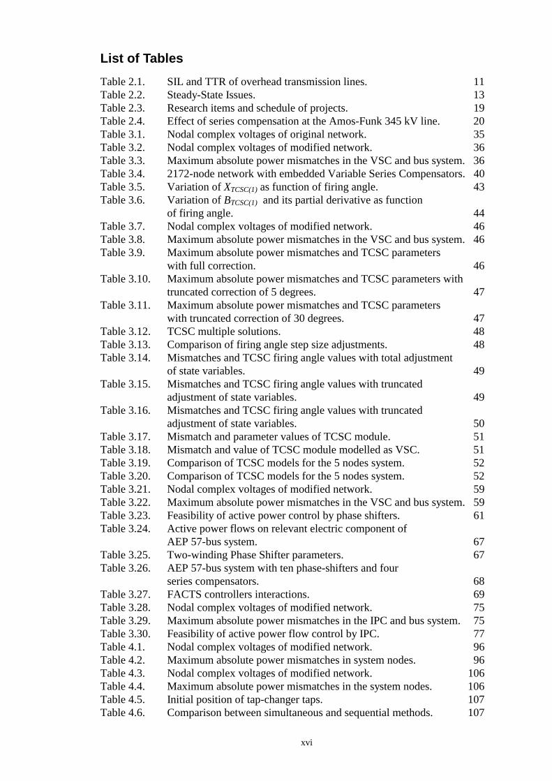
List of Tables Table 2.1. SIL and TTR of overhead transmission lines. 11 Table 2.2. Steady-State Issues. 13 Table 2.3. Research items and schedule of projects. 19 Table 2.4. Effect of series compensation at the Amos-Funk 345 kV line. 20 Table 3.1. Nodal complex voltages of original network. 35 Table 3.2. Nodal complex voltages of modified network. 36 Table 3.3. Maximum absolute power mismatches in the VSC and bus system. 36 Table 3.4. 2172-node network with embedded Variable Series Compensators. 40 Table 3.5. Variation of XTCSC(1) as function of firing angle. 43 Table 3.6. Variation of BTCSC(1) and its partial derivative as function of firing angle. 44 Table 3.7. Nodal complex voltages of modified network. 46 Table 3.8. Maximum absolute power mismatches in the VSC and bus system. 46 Table 3.9. Maximum absolute power mismatches and TCSC parameters with full correction. 46 Table 3.10. Maximum absolute power mismatches and TCSC parameters with truncated correction of 5 degrees. 47 Table 3.11. Maximum absolute power mismatches and TCSC parameters with truncated correction of 30 degrees. 47 Table 3.12. TCSC multiple solutions. 48 Table 3.13. Comparison of firing angle step size adjustments. 48 Table 3.14. Mismatches and TCSC firing angle values with total adjustment of state variables. 49 Table 3.15. Mismatches and TCSC firing angle values with truncated adjustment of state variables. 49 Table 3.16. Mismatches and TCSC firing angle values with truncated adjustment of state variables. 50 Table 3.17. Mismatch and parameter values of TCSC module. 51 Table 3.18. Mismatch and value of TCSC module modelled as VSC. 51 Table 3.19. Comparison of TCSC models for the 5 nodes system. 52 Table 3.20. Comparison of TCSC models for the 5 nodes system. 52 Table 3.21. Nodal complex voltages of modified network. 59 Table 3.22. Maximum absolute power mismatches in the VSC and bus system. 59 Table 3.23. Feasibility of active power control by phase shifters. 61 Table 3.24. Active power flows on relevant electric component of AEP 57-bus system. 67 Table 3.25. Two-winding Phase Shifter parameters. 67 Table 3.26. AEP 57-bus system with ten phase-shifters and four series compensators. 68 Table 3.27. FACTS controllers interactions. 69 Table 3.28. Nodal complex voltages of modified network. 75 Table 3.29. Maximum absolute power mismatches in the IPC and bus system. 75 Table 3.30. Feasibility of active power flow control by IPC. 77 Table 4.1. Nodal complex voltages of modified network. 96 Table 4.2. Maximum absolute power mismatches in system nodes. 96 Table 4.3. Nodal complex voltages of modified network. 106 Table 4.4. Maximum absolute power mismatches in the system nodes. 106 Table 4.5. Initial position of tap-changer taps. 107 Table 4.6. Comparison between simultaneous and sequential methods. 107

xvii
Table 4.7. Final position of tap-changers taps. 108 Table 4.8. FACTS devices final parameters (Case 1). 109 Table 4.9. Power generation (Case 1). 109 Table 4.10. FACTS devices final parameters (Case 2). 110 Table 4.11. Power generation (Case 2). 110 Table 4.12. FACTS devices final parameters (Case 3). 111 Table 4.13. Power generation (Case 3). 111 Table 4.14. FACTS devices final parameters (Case 4). 112 Table 4.15. Power generation (Case 4). 112 Table 4.16. Final value of controllable parameters in FACTS devices. 113 Table 4.17. Final tap position as function of reactive power injected by the SVC. 115 Table 4.18. Final nodal voltages at PV and PVT nodes. 115 Table 5.1. Nodal complex voltages of modified network. 133 Table 5.2. Maximum power mismatches in UPFC and bus system. 133 Table 5.3. Variation of ideal source voltages. 133 Table 5.4. Effect of initial conditions. 133 Table 5.5. Effect of UPFC impedances. 134 Table 5.6. Effect of UPFC impedances without voltage control. 134 Table 5.7. Nodal complex voltages of modified network. 135 Table 5.8. Maximum power mismatches in UPFC and bus system. 135 Table 5.9. Nodal complex voltages of modified network. 137 Table 5.10. Maximum absolute power mismatches in the SVS and bus system. 137 Table 5.11. Effect of initial conditions. 138 Table 5.12. Effect of UPFC and SVS model on ideal source voltages. 138 Table 5.13. Final position of tap-changers taps (pu). 139 Table 5.14. Final position of phase shifters angles (degrees). 140 Table 5.15. Variable series compensation (% of compensation). 140 Table 5.16. Final UPFC parameters for AEP 57 bus system. 140 Table 5.17. Power flow through the compensated transmission line. 142 Table 5.18. UPFC power flow models comparison. 143 Table 6.1. Transmission line data. 151 Table 6.2. Paths and layers for the flow injected by the generator in node 1. 151 Table 6.3. Dominion of generator 1. 152 Table 6.4. Contribution of dominions 1 and 2 to common branches 5-3 and 4-3. 153 Table 6.5. Individual contribution of dominions 1, 2 and 3 to system load. 153 Table 6.6. Contribution of dominion 3 to branches 3-5, 3-4, 4-2 and 2-5. 155 Table 6.7. Individual contribution of dominions 1, 2 and 3 and network to system load. 156 Table 6.8. Contribution of dominions 1, 2 and 3 to branch 5-2. 156 Table 6.9. Comparison of active power source dominions (MWs). 157 Table 6.10. Use of Line Charges. 158 Table 6.11. Contribution of dominions 1 and 2 to branches 2-4 and 4-3. 158 Table 6.12. System power losses and Use of Line Charges. 159 Table 6.13. Comparison of Use of line Charges by three different methods. 159 Table 6.14. Cost of generation at supply points and generators’ dominions. 161 Table 6.15. Dominions’ contributions to flows in branches L34 and L28. 162 Table 6.16. Power losses and ULCs. 162 Table 6.17. Power supplied and costs incurred in feeding load 25. 162 Table 6.18. Reactive Power Flow Generators’ dominions. 163 Table 6.19. UPFC parameters. 166

xviii
Table 6.20. Total system losses. 166 Table 6.21. Effect of magnetising branch in final parameter values of FACTS devices and total losses and generation. 168 Table 6.22. Power control specifications. 169 Table 6.23. Effect of the transformer’s magnetising branch on system generation and losses. 169 Table 6.24. Effect of the transformer’s magnetising branch on series controllers. 170 Table 6.25. Effect of the transformer’s magnetising branch on UPFC. 170 Table 7.1. Comparison of nodal voltage solutions. 194 Table 7.2. Comparison of reactive power generation. 194 Table 7.3. Comparison of system losses. 194 Table 7.4. Active and reactive power mismatches. 194 Table 7.5. Comparison of total cpu time. 195 Table AI.1.1. Number of nodes and plant components (5 nodes system). 200 Table AI.1.2. Transmission lines (5 nodes system). 200 Table AI.1.3. Loads (5 nodes system). 200 Table AI.1.4. Generators (5 nodes system). 200 Table AI.2.1. Number of nodes and plant components (13 nodes system). 200 Table AI.2.2. Transmission lines (13 nodes system). 200 Table AI.2.3. Transformers (13 nodes system). 200 Table AI.2.4. Loads (13 nodes system). 200 Table AI.2.5. Generators (13 nodes system). 200 Table AI.3.1. Number of nodes and plant components (14 nodes system). 201 Table AI.3.2. Transmission lines (14 nodes system). 201 Table AI.3.3. Transformers (14 nodes system). 201 Table AI.3.4. Shunt compensators (14 nodes system). 201 Table AI.3.5. Loads (14 nodes system). 201 Table AI.3.6. Generators (14 nodes system). 201 Table AI.4.1. Number of nodes and plant components (17 nodes system). 201 Table AI.4.2. Transmission lines (17 nodes system). 201 Table AI.4.3. Loads (17 nodes system). 201 Table AI.4.4. Transformers (17 nodes system). 202 Table AI.4.5. Generators (17 nodes system). 202 Table AI.5.1. Number of nodes and plant components (IEEE 28 nodes system). 202 Table AI.5.2. Transmission lines (IEEE 28 nodes system). 202 Table AI.5.3. Transformers (IEEE 28 nodes system). 202 Table AI.5.4. Generators (IEEE 28 nodes system). 202 Table AI.5.5. Shunt compensators (IEEE 28 nodes system). 202 Table AI.5.6. Loads (IEEE 28 nodes system). 202 Table AI.6.1. Number of nodes and plant components (AEP 30 nodes system). 203 Table AI.6.2. Transmission lines (AEP 30 nodes system). 203 Table AI.6.3. Transformers (AEP 30 nodes system). 203 Table AI.6.4. Generators (AEP 30 nodes system). 203 Table AI.6.5. Loads (AEP 30 nodes system). 203 Table AI.6.6. Shunt compensators (AEP 30 nodes system). 203 Table AI.7.1. Number of nodes and plant components (Mexican 38 nodes system). 203 Table AI.7.2. Transformers (Mexican 38 nodes system). 203 Table AI.7.3. Generators (Mexican 38 nodes system). 203 Table AI.7.4. Transmission lines (Mexican 38 nodes system). 204 Table AI.7.5. Series compensators (Mexican 38 nodes system). 204

xix
Table AI.7.6. Loads (Mexican 38 nodes system). 204 Table AI.7.7. Shunt compensators (Mexican 38 nodes system). 204 Table AI.8.1. Number of nodes and plant components (Morelia 38 nodes system). 204 Table AI.8.2. Transmission lines (Morelia 38 nodes system). 204 Table AI.8.3. Transformers (Morelia 38 nodes system). 204 Table AI.8.4. Generators (Morelia 38 nodes system). 204 Table AI.8.5. Loads (Morelia 38 nodes system). 205 Table AI.9.1. Number of nodes and plant components (New England 39 nodes system). 205 Table AI.9.2. Transmission lines (New England 39 nodes system). 205 Table AI.9.3. Transformers (New England 39 nodes system). 205 Table AI.9.4. Loads (New England 39 nodes system). 205 Table AI.9.5. Generators (New England 39 nodes system). 205 Table AI.10.1. Number of nodes and plant components (AEP 57 nodes system). 206 Table AI.10.2. Transmission lines (AEP 57 nodes system). 206 Table AI.10.3. Generators (AEP 57 nodes system). 206 Table AI.10.4. Loads (AEP 57 nodes system). 206 Table AI.10.5. Shunt compensators (AEP 57 nodes system). 206 Table AI.10.6. Transformers (AEP 57 nodes system). 207 Table AI.11.1. Number of nodes and plant components (Mexican 79 nodes system). 207 Table AI.11.2. Transmission lines (Mexican 79 nodes system). 207 Table AI.11.3. Shunt compensators (Mexican 79 nodes system). 207 Table AI.11.4. Transformers (Mexican 79 nodes system). 208 Table AI.11.5. Generators (Mexican 79 nodes system). 208 Table AI.11.6. Loads (Mexican 79 nodes system). 208 Table AI.12.1. Number of nodes and plant components (IEEE 118 nodes system). 208 Table AI.12.2. Transformers (IEEE 118 nodes system). 208 Table AI.12.3. Shunt compensators (IEEE 118 nodes system). 208 Table AI.12.4. Transmission lines (IEEE 118 nodes system). 209 Table AI.12.5. Transmission lines (IEEE 118 nodes system). 210 Table AI.12.6. Generators (IEEE 118 nodes system). 210 Table AI.12.7. Loads (IEEE 118 nodes system). 211 Table AI.13.1. Number of nodes and plant components (Mexican 155 nodes system). 212 Table AI.13.2. Transmission lines (Mexican 155 nodes system). 212 Table AI.13.3. Transformers (Mexican 155 nodes system). 213 Table AI.13.4. Generators (Mexican 155 nodes system). 214 Table AI.13.5. Loads (Mexican 155 nodes system). 214

xx
Abbreviations FACTS Flexible AC Transmission Systems AC Alternating Current ASC Advanced Series Compensator VSC Variable Series Compensator TCSC Thyristor Controller Series Capacitor PS Phase Shifter IPC Interphase Power Controller SVC Static Var Compensator LTC Load Tap Changer UPFC Unified Power Flow Controller SVS Synchronous Voltage Source HVDC High Voltage Direct Current OOP Object Oriented Programming N-R Newton-Rapshon MVARs Mega Volt Ampere Reactives MW MegaWatts pu per unit kV kilo Volts EMTP ElectroMagnetic Transients Program

1
Chapter 1 Introduction Increased use of transmission facilities owing to higher industrial output and deregulation of the Power Supply Industry have provided the momentum for exploring new ways of maximising the power transfers of existing transmission facilities while, at the same time, maintaining acceptable levels of network reliability and stability. In this environment, high performance control of the power network is mandatory. An in-depth analysis of the options available for achieving such objectives has pointed in the direction of power electronics [1]. There is at present widespread agreement that these power electronics techniques are potential substitutes for conventional solutions, which are normally based on electro-mechanical technologies with their slow response times and high maintenance costs [2,3]. Many of the ideas upon which the foundations of FACTS rest were conceived some time ago. Nevertheless, FACTS as a single coherent integrated philosophy is a newly developed concept in electrical power systems. It is looking at ways of capitalising on the new developments taking place in the area of high-voltage and high-current power electronics in order to increase the control of the power flows in the high voltage side of the network during both steady state and transient conditions, so as to make the network electronically controllable. This will have a profound impact on the design of electrical power plant equipment, as well as the planning and operation of transmission and distribution networks. These developments may also affect the way energy transactions are conducted, since high-speed control of the path of the energy flow is now feasible. Owing to the many economical and technical benefits it promises, FACTS is receiving the backing of the major manufactures of electrical equipment and utilities in both America and Europe [4-12]. Accordingly, there are many aspects of the topic that require research attention. Many kind of power electronics-based plant components are already being built, with further proposals for new devices appearing regularly. Among the FACTS-Controllers which have been identified as likely to improve the performance of AC systems are the following [2]: • Static Var Compensator. • Advanced Series Compensator. • Phase Angle Regulator. • Interphase Power Controller. • Unified Power Flow Controller. In order to determine the effectiveness of this new generation of power systems devices on a network-wide basis, it will become necessary to upgrade most of the analysis tools on which power engineers rely in order to plan and to operate their systems. Some of the tools which require immediate attention are: • Load Flows. • Optimal Power Flows. • State Estimation. • Fault Analysis. • Transient Stability. • Electromagnetic Transients. • Harmonic Analysis.

2
This research project is related to the steady-state modelling and analysis of the new generation of power electronics-based plant components presently emerging as a result of the newly developed concept of FACTS.
1.1 Background and motivation behind the present research In order to assist power systems engineers to assess the effects of FACTS devices on transmission system’s performance, it has become necessary to upgrade existing power systems software, or even better to develop a new generation of software. Before meaningful results can be obtained from application studies, realistic mathematical models for the transmission system and FACTS controllers need to be realised, coded and extensively verified. From the operational point of view, the FACTS technology is concerned with the ability to control, in adaptive fashion, the path of the power flows throughout the network; where at present, high-speed control is almost non-existent. The ability to control the line impedance and the nodal voltage magnitudes and angles at both the sending and receiving ends of key transmission lines with almost no delay will increase significantly the transmission capabilities of the network whilst enhancing considerably the security of the system. In this context, a power flow program should offer a very useful tool for system planners and system operators to evaluate the technical and economical benefits of a wide range of alternative solutions offered by the FACTS technology. Furthermore, FACTS load flow studies are needed in order to gather good initial conditions for harmonic, fault and dynamic simulations. Hence, power flows programs have become the most immediate target for upgrading [10,21-23]. In most instances, existing software which has been in use for many years has grown large and inflexible. Hence, modification are achieved with great difficulty and expense. This has provided the motivation for developing afresh, well designed and efficient software where both established and emerging power components can be modelled along side each other with minimum effort and none of the compromises often imposed when inflexible existing software is modified. Bearing this in mind and as a starting point, the efforts in this research are concentrated on tackling the steady-state, positive sequence modelling and analysis of FACTS devices. The power flow algorithm has been selected to verify these models and to prove the virtues of developing a new generation of software suitable for the analysis of large scale networks based on the Object Oriented Programming (OOP) philosophy. The newly developed OOP power flow program has been tested thoroughly. Real-life and standard networks have been used in order to assess the effects of FACTS devices on power system performance. Arguably, power flow (load flow) analysis is the most popular power systems computer calculation performed in systems planing and operation. The reliable solution of real life transmission and distribution networks is not a trivial matter and Newton-Rapshon (N-R) type methods, with their strong convergence characteristics, have proved most successful [13,14]. The conventional N-R method for the solution of power flow equations is already well documented in open literature [13,14]. Furthermore, extensive research has been carried out in order to implement controllable device models into N-R type power flow programs [15-22]. For the purpose of positive sequence load flow solutions, the power electronics-based FACTS devices can be adequately modelled as controllable branches and sources.

3
Since controllable device parameters are not standard variables in the conventional load flow calculation, they enter as extra variables in the problem formulation and their associated controlled network variables are considered in additional constraint equations. The methods used for implementing these extra variables and constraint equations into a N-R power flow program can be classified according to the manner in which the controllable parameters are adjusted within the overall iterative process. The most popular methods are: • Error-feedback adjustment. • Sensitivity-based adjustment. • Automatic adjustment. The error-feedback adjustment involves modifying a control variable while maintaining other functionally dependent variables at specified values, in a closed-loop feedback fashion mechanism [17,18,20,22]. The sensitivity-based adjustment method is derived from Taylor series expansion of the perturbed system of equations around the initial operating point [19,21]. These methods share the characteristic that nodal network variables are the only state variables which are calculated in true Newton fashion, whilst a sub-problem is formulated for updating the state variables of the controllable devices at the end of each Newton-Raphson iteration. This sequential iterative approach is rather attractive because it is straightforward to implement in existing Newton-Rapshon programs but caution has to be exercised because it will yield no quadratic convergence. On the other hand, the automatic adjustment involves modifications of the Jacobian matrix and mismatch vector in order to solve the nodal network and controllable device state variables simultaneously [15,16], such that these variables are adjusted automatically during the iterative process. From the convergence point of view, the unified method is superior to the sequential method because the interaction between the network and FACTS devices is better represented. It arrives at the solution with quadratic convergence regardless of the number of controllable devices and network size. Hence, the unified approach has been preferred in this thesis.
1.2 Objectives The objectives of this thesis are: a) To develop advanced models of FACTS devices suitable for positive sequence-type
power systems studies: 1) Advanced Series Compensator (ASC). 2) Phase Shifter Transformer (PS). 3) Interphase Power Controller (IPC). 4) Static Var Compensator (SVC). 5) Load Tap Changer (LTC). 6) Unified Power Flow Controller (UPFC). b) To verify the ability of the FACTS devices to carry out their intended function in large-
scale electric power networks.

4
1) To develop a digital computer program based on the OOP philosophy suitable for
the analysis of power flows in large-scale electrical power networks containing FACTS devices. The iterative solution is carried out via a full N-R method.
2) To develop suitable equations and guidelines to initialise FACTS controllable
parameters in order to achieve quadratic or near quadratic convergence in a full Newton-Rapshon power flow program.
3) To develop guidelines for the efficient co-ordination of series and parallel control
strategies of FACTS devices.
c) Applications of FACTS devices to solve some current issues in real life, electric power systems.
1) To develop a general algorithm for tracing the individual generator contributions
to active and reactive power flows and losses in large-scale electrical power networks.
2) To assess the effect of FACTS devices on the voltage collapse phenomena. 3) To assess the ability of FACTS devices to eliminate loop flows.
1.3 Contributions The most significant contributions of the research work are summarised below: • A general two-winding transformer model containing regulated complex taps on both the
primary and secondary windings has been developed for the full Newton-Rapshon algorithm. Either the primary or secondary tap magnitude is regulated in order to maintain fixed voltage magnitude at one of the transformer terminals. In order to achieve active power control across the transformer, either the primary or the secondary phase shifter angle is regulated. Moreover, this model allows to explicitly represent the primary and secondary complex impedance and the transformer’s magnetising branch. The magnetising branch becomes non-linear under saturated conditions, hence, accounting for active and reactive core losses.
• Two models for the Advanced Series Compensator are presented in this work. A simple
but efficient model is first presented. It is based on the concept of a Variable Series Compensator (VSC) whose changing reactance adjusts itself in order to constrain the power flow across the branch to a specified value. The second model is based on the Thyristor Controlled Series Capacitor (TCSC) structure. The model considers the firing angle as state variable. Unlike existing TCSC models available in open literature, this model takes full account of the loop current present in the TCSC under either partial or full conduction mode operation.
• An efficient and realistic way to model the Static Var Compensator in a Newton-type
power flow algorithm is proposed. The SVC is considered to be a continuous variable-shunt susceptance which is adjusted in order to achieve a specified voltage magnitude.
• A new and comprehensive Unified Power Flow Controller model is developed from first
principles. The proposed model is capable of controlling active and reactive powers simultaneously as well as nodal voltage magnitude. Alternatively, the UPFC model can be set to control one or more of the parameters above in any combination or to control none of them. The UPFC transformer losses are taken into account.
• The influence of initial conditions of FACTS devices is investigated and, where
appropriate, analytical equations are given to assure good initial conditions.

5
• Since the unified solution of nodal network variables and FACTS state variables is achieved using single control criterion, i.e. one variable is adjusted to maintain another variable at a specified value, control strategies are proposed to handled cases when two or more FACTS devices are controlling the same nodal voltage magnitude.
• A power flow digital computer program written in C++ has been developed based on the
OOP philosophy. The software is fast and reliable and it is entirely adequate for the analysis and control of large-scale power networks containing FACTS-controlled branches. The load flow algorithm is a full Newton-Raphson method exhibiting quadratic or near quadratic convergence. Sparse matrix techniques written in C++ have been developed for the efficient handling of large scale networks.
• An algorithm for tracing the individual generator contributions to system loading, power
flows, transmission losses, generation costs and Use of Line Charges is proposed. It is independently applied to active and reactive power concerns.
1.4 Thesis outline The remainder of this thesis is organised into 7 Chapters. A brief overview of each one of these Chapters is given below: Chapter 2 presents an overview of a collection of controllers which conform the FACTS technology. Their features, applications and influences on power systems are briefly described. Methodologies to implement FACTS devices in a power flow program are discussed. Suitable strategies to start the revision of control parameter limits of FACTS devices are also described. Chapter 3 proposes models for power flow series controllers, namely Advanced Series Compensator, Phase Shifter and Interphase Power Controller. Two models are proposed for the ASC in which the state variables are taken to be the variable susceptance and the firing angle, respectively. An hybrid method to initialise both ASC models is proposed. The ASC, PS and IPC models are implemented in a power flow program by extending both the Jacobian matrix and mismatch vector. The robustness of this unified method is illustrated by numeric examples. It is shown that when two or more FACTS controllers are electrically close to each other, the amount of active power regulated across the branches is confined to an operating region in which the control variables are within limits and the solution of the power flow equations exist. This feasible active power flow control region is analysed for each FACTS controller. Numeric examples show the electrical interaction between FACTS controllers and the electric system. The impact of truncating the size of the adjustment of state variables is shown by numeric examples. Chapter 4 proposes models for nodal voltage magnitude controllers, namely Static Var Compensator and Load Tap Changer. Control co-ordination strategies are proposed to consider cases when two or more controllable devices are set to control voltage magnitude at the same node. New type of nodes are introduced in order to handle efficiently control strategies and series and/or parallel control system configurations of LTCs. The effect of truncating the size of the adjustment of state variables is shown by numeric examples. Chapter 5 proposes a general model for the Unified Power Flow Controller. A new type of node is proposed to achieve efficient control of nodal voltage magnitude and to take into account special UPFC control configurations. An alternative UPFC model based on the concept of a Synchronous Voltage Source is also developed and coded into the N-R power flow algorithm. A comparative analysis of both models is carried out by numeric examples. A set of analytical equations is derived to give good UPFC and SVS initial conditions. The influence of these initial conditions on convergence is investigated. The effect of the UPFC transformer parameters on the final value of UPFC state variables is also investigated.

6
Chapter 6 presents applications of FACTS devices in power systems. FACTS devices are used to redistribute power flow in an interconnected power network, to eliminate loop flows and to increase margins of voltage collapse. Moreover, the effect of the transformer magnetising branch on system losses is quantified. For the first application, a general power flow tracing algorithm to compute the individual generator contributions to the active and reactive power flows and losses is proposed. Chapter 7 address the application of the Object Oriented Programming philosophy to model a power network and its components as well as the design and elaboration of an OOP Load Flow program. It is shown by numeric examples that the developed software is fast and reliable and is entirely adequate for the analysis and control of large-scale power networks containing FACTS-controlled branches. Solutions obtained with the newly developed OOP load flow program have shown to be almost as fast as the solutions given by a load flow program written in FORTRAN. The robustness of the program is also demonstrated by solving an ill-conditioned system reported in the open literature. Chapter 8 draws the overall conclusions of this research and gives suggestions for future research work.
1.5 Bibliography [1] Hingorani N.H.: ‘Flexible AC Transmission Systems’, IEEE Spectrum, pp. 40-45, April 1993. [2] IEEE Power Engineering Society: ‘FACTS Applications’, Special Issue, 96TP116-0, IEEE Service Center, Piscataway, N.J., 1996. [3] Nelson R.J.: ‘Transmission Power Flow Control: Electronic vs. Electromagnetic Alternatives for Steady-State Operation’, IEEE Trans. on Power Delivery, Vol. 9, No. 3, pp. 1678-1684, July 1994. [4] Ledu A., Tontini G. and Winfield M.: ‘Which FACTS Equipment for Which Need?’, International Conference on Large High Voltage Electric Systems (CIGRÉ), paper 14/37/38-08, Paris, September 1992. [5] Larsen E., Bowler C., Damsky B. and Nilsson S.: ‘Benefits of Thyristor Controlled Series Compensation’, International Conference on Large High Voltage Electric Systems (CIGRÉ), paper 14/37/38-04, Paris, September 1992. [6] Christl N., Hedin R., Sadek K., Lützelberger P., Krause P.E., McKenna S.M., Montoya A.H. and Togerson D.: ‘Advanced Series Compensation (ASC) with Thyristor Controlled Impedance’, International Conference on Large High Voltage Electric Systems (CIGRÉ), paper 14/37/38-05, Paris, September 1992. [7] Kinney S.J., Mittelstadt W.A. and Suhrbier R.W.: ‘Test Results and Initial Experience for the BPA 500 kV Thyristor Controlled Series Capacitor Unit at Slatt Substation, Part I- Design, Operation, and Fault Test Results’, Flexible AC Transmission Systems (FACTS 3): The Future in High Voltage Transmission Conference, EPRI, Baltimore Maryland, October 1994. [8] Brochu J., Pelletier P., Beauregard F. and Morin G.: ‘The Interphase Power Controller A New Concept for Managing Power Flow within AC Networks’, IEEE Trans. on Power Delivery, Vol. 9, No. 2, pp. 833-841, April 1994.

7
[9] Kappenman J.G. and VanHouse D.L.: ‘Thyristor Controlled Phase Angle Regulator Applications and Concepts for the Minnesota-Ontario Interconnection’, Flexible AC Transmission Systems (FACTS 3): The Future in High Voltage Transmission Conference, EPRI, October 1994. [10] Maliszewski R.M., Eunson E., Meslier F., Balazs P., Schwarz J., Takahashi K. and Wallace P.: ‘Interaction of system Planning in the Development of the Transmission Networks of the 21st Century’, Symposium on Power Electronics in Electric Power Systems, International Conference on Large High Voltage Electric Systems (CIGRÉ), paper 210-02, Tokyo, 22-24 May, 1995. [11] Sekine Y., Hayashi T., Abe K., Inoue Y. and Horiuchi S.: ‘Application of Power Electronics Technologies to Future Interconnected Power System in Japan’, Symposium on Power Electronics in Electric Power Systems, International Conference on Large High Voltage Electric Systems (CIGRÉ), paper 210-03, Tokyo, 22-24 May, 1995. [12] Gyugyi L., Schauder C.D., Williams S.L. Rietman T.R., Torgerson D.R. and Edris A.: ‘The Unified Power Flow Controller: A New Approach to Power Transmission Control’, IEEE Trans. on Power Delivery , Vol. 10, No 2, April 1995, pp. 1085-1097. [13] Tinney W.F. and Hart C.E.: ‘Power Flow Solution by Newton’s Method’, IEEE Trans. on Power Apparatus and Systems, Vol. PAS-96, No. 11, pp. 1449-1460, November 1967. [14] Stott B.: ‘Review of Load-Flow Calculation Methods’, IEEE Proceedings, vol. 62, pp. 916-929, July 1974. [15] Peterson N.M. and Scott Meyer W.: ‘Automatic Adjustment of Transformer and Phase Shifter Taps in the Newton Power Flow’, IEEE Trans. on Power Apparatus and Systems, Vol. PAS-90, No. 1, pp. 103-108, January/February 1971. [16] Britton J.P.: ‘Improved Load Flow Performance through a more General Equation Form’, IEEE Trans. on Power Apparatus and Systems, Vol. PAS-90, No. 1, pp. 109-116, January/February 1971. [17] Han Z.X.: ‘Phase Shifter and Power Flow Control’, IEEE Trans. on Power Apparatus and Systems, Vol. PAS-101, No. 10, pp. 3790-3795, October 1982. [18] Mescua J.: ‘A Decoupled Method for Systematic Adjustments of Phase-Shifting and Tap-Changing Transformers’, IEEE Trans. on Power Apparatus and Systems, Vol. PAS-104, No. 9, pp. 2315-2321, September 1985. [19] Chang S.K. and Brandwajn V.: ‘Adjusted Solutions in Fast Decoupled Load Flow’, IEEE Trans. on Power Systems, Vol. 3, No. 2, pp. 726-733, May 1988. [20] Maria G.A , Yuen A.H. and Findlay J.A.: ‘Control Variable Adjustment in Load Flows’, IEEE Trans. on Power Systems, Vol. 3, No. 3, pp. 858-864, August 1988. [21] Noroozian M. and Andersson G.: ‘Power Flow Control by Use of Controllable Series Components’ , IEEE Trans. on Power Delivery, Vol. 8, No. 3, pp. 1420-1429, July 1993. [22] Acha E.: ‘A Quasi-Newton Algorithm for the Load Flow Solution of Large Networks with FACTS-Controlled Branches’, Proceedings of the 28th UPEC Conference, Stafford UK, 21-23, pp. 153-156, September 1993. [23] Davriu A., Mallet P. and Pramayon P.: ‘Evaluation of FACTS Functionalities within the Planning of the Very High Voltage Transmission Network; the EDF Approach’, SPT PE 03-01-0112, IEEE/KTH Stockholm Power Tech Conference, Stockholm, Sweden, June 18-22, pp. 71-76, 1995.
8
Chapter 2
A General Overview of Flexible AC Transmission Systems 2.1 Introduction An electric power system can be seen as the interconnection of generators and loads through a transmission network. The structure of the transmission network has many variations which are the result of a history of economic, political, engineering and environmental decisions. Power systems can be broadly classified by their transmission network structure in meshed and radial systems [1-3]. Meshed systems can be found in regions with high population density and where it was possible to built power stations close to the load demand centres. In regions where large amount of power has to be transmitted, through a long distance, from power stations to load demand centres, power systems developed into radial systems. Independently of the power system structure, the function of the transmission network is always to transport the electric energy generated from power plants to load centres and to provide interconnections between different power systems for economic power sharing purposes. In order to achieve these functions, the transmission networks should be able to carry electric power in a flexible and efficient way with adequacy and security. The adequacy of a power system is its capability to meet the energy demand, within component ratings and voltage limits. Power system security is the ability of the system to cope with foreseen and unforeseen events without uncontrolled loss of load. In the past, AC power systems have been controlled with electro-mechanical devices preventing high speed control. This has been the reason why AC transmission systems were thought as being inflexible. As a consequence of this lack of fast and reliable control combined with the fact that power flows simply follow Ohm’s law, AC transmission systems present some problems such as [1]: undesirable loop flows and VARs flows in the network; inability to fully utilise the transmission line capability up to the thermal limit; high levels of transmission losses, high or low voltages; stability problems; cascade tripping and long restoration times. Difficulties in licensing and building new transmission lines due to a variety of environmental, land-use and regulatory pressures, and requirements for increased use of transmission facilities due to higher industrial output and deregulation of the Power Supply Industry have provided the momentum for exploring new ways of maximising the power transfers of existing transmission facilities while, at the same time, maintaining acceptable levels of network reliability and stability. In this environment, high performance control of the power network is mandatory. An in-depth analysis of the options available for achieving such objectives has pointed in the direction of power electronics [2]. There is at present widespread agreement that these power electronics techniques are potential substitutes for conventional solutions, which are normally based on electro-mechanical technologies with their slow response times and high maintenance costs [3]. Flexible Alternating Current Transmission Systems is an umbrella title used for incorporating the emerging power engineering technologies. In its most general expression the FACTS concept is based on the massive incorporation of power electronics devices into the high voltage side of the network so as to make it electronically controllable.

9
2.2 Steady-state power flow and voltage control In an electric system with no power flow control, the power flows from source to loads are in inverse proportion to the relative impedances of the transmission paths. Low impedance transmission paths take the largest fraction of flow. This has the advantage of minimising losses as long as the ratio X/R is about the same. However, this advantage vanishes if fixed series capacitors are embedded in the network or different voltage levels are presented in the power flow paths. Since in an interconnected network all transmission lines are part of the flow path, additional problems arise when utilities operating in a deregulated market are unwillingly affected by power transactions in which they are not involved. Common power flow control techniques used in electric utilities to redistribute power flow among the transmission lines in order to achieve the required steady state power flow, maintaining voltage magnitudes and phase angles within safe limits, are power generation scheduling, the occasional changing of power taps transformers and the switching of shunt reactors and capacitors. Assuming the simplified transmission line representation shown in Figure 2.1, the active and reactive power flow equations at the sending node are obtained from,
S V Ikm k k= * (2.1) where the current injected at this node is defined by,
IV V
Zkk m= −
(2.2) and Z=R+jX is the transmission line series impedance.
Figure 2.1. Overhead transmission line. The mathematical expressions that represent the active and reactive power injected at sending node are then obtained by substituting equation (2.2) into (2.1),
PRV RV V XV V
R Xkmk k m k m k m k m=
− − + −+
2
2 2
cos( ) sin( )θ θ θ θ (2.3)
QX V X V V RV V
R Xkmk k m k m k m k m=
− − − −+
2
2 2
cos( ) sin( )θ θ θ θ (2.4)
For typical extra high-voltage transmission systems, the reactance X is much bigger than the resistance R, and the equations (2.3) and (2.4) simplify to,
PV V
Xkmk m k m= −sin( )θ θ
(2.5)
Vk Vm
Ik Im
Sending node
Receiving node

10
QV V V
Xkmk k m k m=
− −2 cos( )θ θ (2.6)
These equations provide some insight into the techniques available for power flow control. On the one hand, the voltage magnitudes cannot be varied significantly since they must be kept within regulated limits, hence providing very limited scope for power flow control. On the other hand, the branch reactance and the voltage angle difference are not circumscribed as heavily to such restrictions and they may provide the only practical alternatives for power flow control. From equation (2.5) it is clear that the direction of active power flow is only determined by the voltage angle difference. If Vk leads Vm, the active power direction is from sending to receiving node. The active power has opposite direction if Vk lags Vm. In theory, the maximum transfer of power is given when the relative difference between both voltage angles is 90o. The reactive power direction is determined by the voltage magnitude at both nodes. If Vk is greater than Vm, the reactive power direction is from sending to receiving node. The reactive power has opposite direction if Vk is less than Vm. In order to show that system voltage regulation are affected by the reactive power flowing in the network, equation (2.6) can be expressed as,
V VXQVk m k m
k
k
− − =cos( )θ θ (2.7)
Assuming that the angular difference is small,
∆V V VXQVkm k m
k
k
= − = (2.8)
It is clear from equation (2.8) that the voltage drop ∆Vkm across the transmission component mainly depends upon the component's reactance and the reactive power flowing through the device. Then, if the reactive power demanded by a load is supplied locally by connecting a shunt compensator at the load bus the voltage drop across the line can be reduced. The nodal voltage variations caused by changes in load can be regulated by the shunt compensator. This statement can be demonstrated by solving equation (2.8) for Vk to obtain the following expression,
VV V X Q
km m k=
− ± +2 4
2 (2.9)
According to equation (2.9) only the nodal voltage magnitude can be controlled by the regulation of the reactive power injected by the shunt compensator.
2.3 Inherent limitations of conventional transmission systems For a given operating condition, the maximum electric power transfer over a transmission system is limited by steady-state or transient stability limits [2,3]. The former is determined by one of the following criteria, 1. Angular stability limit. 2. Thermal limits. 3. Voltage limits.

11
These limits define the maximum electric power that can be transmitted safely, without causing damage to transmission lines as well as utility and customer equipment. The angular stability limit is determinate by equation (2.5). However, this limit can be modified by altering the natural inductive reactance of the transmission line by using series compensation or adjusting the relative phase angle difference at the transmission line terminals by using a phase shifter transformer. When thermal limits are reached the excessive current flow overheats the transmission and other electric equipment to the point of permanent damage. The addition of ancillary equipment and reconfiguration of the network topology are normally successfully in bringing current flows back to safe limits. Conventional solutions include the use of series reactors, series capacitors and phase shifters. Voltage magnitudes can also be a limiting factor in power flow transfer. Changes in network configuration caused by equipment outages can give to arise unacceptably high or low voltage condition and thermal limits can be exceeded. The proper corrective action to the low voltage problem is to supply reactive power so as to improve load power factor and reduce reactive losses in transmission lines and transformers. Traditionally, this voltage control strategy has been performed by using mechanically switched shunt capacitors and reactors. Some utilities have installed Static Var Compensators in order to achieve efficiently the voltage regulation. With regards to the high voltage problem, produced mainly, by light loading conditions, the shunt capacitors are removed and shunt reactors are brought into service. When a SVC is embedded in the network, it can be set to absorb reactive power. Generators with automatic voltage regulators can be used to absorb significant reactive power. However, many utilities operate their generators near to unity power factor in order to use them in voltage emergencies.
2.4 FACTS controllers When a AC transmission line is terminated in its characteristic impedance Zo, the delivered power is known as the surge impedance load (SIL). In a lossless transmission line operating under SIL condition, the voltage and current are in phase along the line and optimum power transmission conditions are reached. Historically, electric power systems have been operated in such a way that their transmission lines are not loaded above their surge impedance loading value because of power and voltage stability problems [1]. The main reason for this manner of operation is that electric power systems have been controlled by electro-mechanical means. Table 2.1 compares between the surge impedance loads (SIL) and typical thermal ratings for different levels of voltage magnitude operation, at 60 Hz, of overhead transmission lines [1].
Table 2.1. SIL and TTR of overhead transmission lines.
Voltage (KV)
SIL (MW)
Thermal Rating (TL) (MW)
Ratio TL/SIL
230 150 400 2.67 345 400 1200 3.00 500 900 2600 2.89 765 2200 5400 2.45 1100 5200 24000 4.61

12
The surge impedance loads are much lower than the thermal limit ratings so there is a high level of the full transmission line capacity to transfer power that is not being used. From Table 2.1 it is obvious that if the power system can be operated with adequacy and security near to its transmission line thermal limits, then it is possible to increase the power flow transfer substantially. FACTS controllers are intended to narrow the gap between the non-controlled and the controlled power system mode of operation by providing additional degrees of freedom to control power flow over desired transmission routes, to increase transmission capacity allowing secure loading of the transmission lines up to their thermal capacities, to provide effective utilisation of available generation and to containing outages from spreading to a wider area. A FACTS controller is defined as a power electronic-based system which provides control of one or more AC transmission system parameters[3]. The cornerstone of the FACTS technologies is the thyristor. High current, high voltage power semiconductors and control technologies have had a profound effect on electric transmission for almost three decades. Notable examples include High-Voltage Direct Current (HVDC) installations and Static Var Compensators (SVCs). Thanks to the well established HVDC and SVC technology, there has been a rapid progress of FACTS controllers. Among FACTS-Controllers which have been identified as likely to improve the performance of an AC system are the following (IEEE FACTS Working Group 15.05.15) [3], Interphase Power Controller (IPC) : A series-connected power controller consisting, in each phase, of inductive and capacitive branches subjected to separately phase shifted voltages. The active power is set by adjusting the phase shifts and/or impedances. Static Var Compensator (SVC) : A static electrical device, equipment or system that is capable of drawing controlled capacitive and/or inductive current from an electrical power system and thereby generating or absorbing reactive power. The current output is adjusted to maintain or control specific parameters of the electrical power system, typically the bus voltage magnitude. Static Synchronous Compensator (STATCOM or SSC) : A static synchronous generator operated without an external electric energy source as a shunt-connected static var compensator whose capacitive or inductive output current can be controlled independently of the AC system voltage. Static Synchronous Series Compensator (SSSC or S3C) : A static, synchronous generator operated without an external electric energy source as a series compensator whose output voltage is in quadrature with, and controllable independently of, the line current for the purpose of increasing or decreasing the overall reactive power voltage drop across the line and thereby controlling the transmitted power. Thyristor Controlled Phase Shifting Transformer (TCSPT) : A phase-shifting transformer, adjusted by thyristor switches to provide rapidly varying phase angle. Thyristor Controlled Reactor (TCR) : A shunt-connected, thyristor-controlled inductor whose effective reactance is varied in a continuous manner by partial-conduction control of the thyristor valve. Thyristor Controlled Series Reactor (TCSR) : An inductive reactance compensator which consists of series reactor shunted by thyristor controlled reactor in order to provide a smoothly variable series inductive reactance.

13
Thyristor Controlled Series Capacitor (TCSC) : A capacitive reactance compensator which consists of series capacitor banks shunted by thyristor controlled reactor in order to provide a smoothly variable series capacitive reactance. Unified Power Flow Controller (UPFC) : A combination of static synchronous compensator (STATCOM) and a static synchronous series compensator (S3C) which are coupled via a common dc link, to allow bi-directional flow of active power between the series output terminals of the S3C and the shunt terminals of the STATCOM, and are controlled to provided concurrent active and reactive compensation without an external electric energy source. The UPFC, by means of angularity unconstrained series voltage injection, is able to control, concurrently or selectively, the transmission line voltage magnitude, impedance and angle or, alternatively, the active and reactive power in line. The UPFC may also provide independently controllable shunt reactive compensation. The applications of FACTS controllers to the solution of the steady-state power transfer limits mentioned in Section 2.3 are summary in Table 2.2 [3].
Table 2.2. Steady-State Issues. Issue Problem Corrective Action FACTS device
Low voltage at heavy load Supply reactive power TCSC, STATCOM High voltage Remove reactive power supply TCSC,TCR at high load Absorb reactive power TCR, STATCOM
Voltage High voltage following outage Absorb reactive power TCR Limits Low voltage Supply reactive power STATCOM, TCSC
following outage Prevent overload IPC, TCPAR, TCSC
Load voltage and overload Supply reactive power and
limit overload IPC, TCSC, UPFC
STATCOM Line/transformer overload Reduce overload TCSC, TCPAR, UPFC
Thermal TCR, IPC Limits Tripping of parallel circuit Limit circuit loading IPC, UPFC, TCR
Parallel line load sharing Adjust series reactance IPC, UPFC, TCSC Adjust phase-angle TCPAR
Loop flows
Post-fault sharing Rearrange network or use
thermal limit actions IPC, TCSC, UPFC
TCR, TCPAR Flow direction reversal Adjust phase angle IPC, TCPAR, UPFC
2.5 Power Flow Analysis of networks with FACTS devices In its most basic form the load flow problem involves solving the set of non-linear algebraic equations which represent the network under steady state conditions. The reliable solution of real life transmission and distribution networks is not a trivial matter and Newton-type methods, with their strong convergence characteristics, have proved most successful [4-5]. The conventional Newton-Rapshon method for the solution of power flow equations is already well documented [4,5]. The basic principle behind it is that a set of non-linear algebraic equations obtained from the active and reactive nodal power injections,
f X( ) = 0 (2.10) can be linearised around a base point determined by generation and load powers, and nodal voltages, commonly initialised with unitary magnitudes and null angles. The N-R algorithm provides an approximate solution to the non-linear problem described by equation (2.10), by solving for ∆X i in the linear problem J i ∆X i = -f(X i), where J is known as Jacobian matrix [4]. The method starts from an initial guess X 0 and updates the solution at each iteration i, i.e. X i+1 = X i + ∆X i.

14
Over the years, special algorithms have been put forward which have addressed the modelling of controllable devices in Newton’s method, such as Load Tap Changing (LTC) and phase shifting transformers, series and shunt variable compensation. The methods used for the modelling of controllable devices can be broadly classified into two main categories: sequential and simultaneous solution method. References [5-11] are just but a few of the long list of published work in this area using sequential methods. However, a major drawback in all these methods is that the nodal voltage magnitudes and angles are the only state variables which are calculated in true Newton fashion, whilst a sub-problem is formulated for updating the state variables of the controllable devices at the end of each Newton-Raphson iteration. These methods are mathematically formulated for a system of non-linear algebraic equations of the form,
f X RnAC nF( , ) = 0 (2.11)
F X RnAC nF( , ) = 0 (2.12) where f(XnAC , RnF)=0 represents the vector functions of nodal AC network equations, F(XnAC , RnF)=0 describes the vector functions of FACTS device equations, XnAC is the vector of all AC system state variables given by the nodal voltage angles and magnitudes, and RnF is the vector of all FACTS devices state variables. These vectors are expressed as,
f f f f nACT= [ , ,..., ]1 2 (2.13)
F F F FnF
T= [ , ,..., ]1 2 (2.14)
X x x xnAC nACT= [ , ,..., ]1 2 (2.15)
R r r rnF nF
T= [ , ,..., ]1 2 (2.16) The sequential solutions start with an initial guess (Xo
nAC, RonF). Equation (2.11) is solved
for X1nAC keeping Ro
nF fixed, then equation (2.12) is solved for R1nF with X1
nAC fixed. The method continues solving sequentially one set of equations after the other with initial values given by the previous solution until a predefined convergence criteria is satisfied for both set of equations. This sequential iterative approach is rather attractive because it is straightforward to implement in existing Newton-Raphson programs but caution has to be exercised because it will yield no quadratic convergence. A fundamentally different approach for the modelling of controllable devices, within the context of the load flow problem, was developed at a very early stage by Peterson and Scott Meyer [12]. It is a highly efficient method which combines simultaneously the state variables corresponding to the controllable devices with the nodal voltage magnitudes and angles of the network in a single frame-of-reference for a unified, iterative solution through a Newton-Rapshon technique. The method retains Newton’s quadratic convergence characteristics. Two types of controllable devices were addressed is that work, namely LTCs and phase-shifting transformers. The method is not necessarily easy to implement. It requires the Jacobian matrix to be modified in order to incorporate the contributions corresponding to LTCs and phase-shifters. In such iterative environment the state variables of LTCs are adjusted automatically so as to satisfy specified voltage magnitudes and the state variables of the phase-shifters are adjusted automatically so as to satisfy specified power flows.

15
Owing to the limitations exhibited by non-compliant Newton-Raphson techniques, the early work of Peterson and Meyer has been extended in this research to encompass different FACTS devices. They include a two-winding transformer model with complex tap-changing facilities in both the primary and secondary windings modelling LTC and PS, a TCSC, an IPC, a UPFC, and a SVC. The unified approach lumps the AC nodal network and FACTS state variables into a single vector and solves the system of equations,
g X RnAC nF( , ) = 0 (2.17) where g represents the nodal AC network equations and the equations introduced by the FACTS devices given by (2.11) and (2.12), respectively. The increase in the dimensions of the Jacobian matrix is equal to the number of additional equations introduced by the FACTS devices. This number depends on the FACTS controllers embedded in the network and the variables that these devices are controlling. The new structure of the Jacobian matrix is then,
2.6 Initialisation of FACTS devices Good starting conditions are mandatory in any non-linear iterative process with local convergence properties. The solution of the load flow equations by the Newton-Rapshon technique does not differ in this respect. This iterative solution works efficiently if the initial conditions are relatively close to the solution and the resulting Jacobian matrix evaluated at each iteration is not singular. Quite often ‘ill-chosen’ starting conditions are responsible for the load flow solution diverging or arriving at some anomalous value. This is a problem which has engaged many researches. As yet no definitive answer as to the ‘ideal’ starting point for solving the load flow equations has been put forward. However, engineering judgement indicates that for the simple case in which no controlled nodes or branches are present, 1 pu voltage magnitude for all PQ nodes and 0 voltage angle for all nodes provides a suitable starting condition [13]. For the case in which controllable devices are present then the issue is not as clear cut as the case above. Suitable strategies for initialising FACTS devices are proposed in this thesis. The initialisation of those controllers whose state variables are expressed by transcendental equations is based on engineering judgement. Otherwise, closed-form equations are deduced to obtain suitable initialisations.
x1 xnAC . . . r1 rnF . . .
f1
. .
.
fnAC
F1
. .
.
FnF
AC network
FACTS controllers
(2.18)

16
2.7 Adjusted solution criterion Iteration number is probably the most widely used criterion for performing revision of limits in Newton’s method. It is common practice to start the revision of control parameter limits at the end of the second iteration [4]. This strategy is simple and has proved efficient and trouble-free in most situations. However, concerns have been raised recently about the suitability of such method [10]. It has been argued that if some revisions are made at inappropriate times then unnecessary increases in solution times will be incurred. An equally simple but more effective alternative is to use the power mismatch equations [10] as the guiding principle for conducting limit revisions. At each iterative step, the power mismatches provide an accurate indicator by which the activation of the revision of limits can be started, being a more algorithmical way as opposed to the empirical procedure mentioned above. The limit revision criterion adopted in the program is based on this principle. The revision of limits of a controllable device starts after the power mismatch equations at the controlled node, or at the controlled branch, are within a specified tolerance. By way of example, the starting criterion for checking Q limits at PV nodes is the use of the active power node mismatch, equation (2.19),
∆P P P
i ng
i spec cal= −=1, ...,
(2.19)
where ng is the number of nodes whose nodal voltage magnitudes is controlled by generators or synchronous condensers. The revision criterion of the FACTS devices set to control the active power flow across their terminals is based on their active power mismatch equation,
∆P P P
i nbck mi
k mspec
k mcalc
, , ,
, ...,
= −
=1 (2.20)
where nbc is the number of controlled branches. If limits violation occurs on these FACTS devices, the state variable is fixed at the offending limit. In this situation no further attempts are made at regulating the flow of active power through the branch for the remainder of the iterative process.
2.8 Truncated adjustments Newton’s method can not directly take account of the limits associated with state variables. Large increments in these variables during the backward substitution process may induce large ∆P and ∆Q residual terms. These large residuals may in turn slow down convergence, or more seriously, cause the solution to oscillate or even diverge. These unwanted problems can be alleviated quite effectively by limiting the size of the correction during the backward substitution [4,5,10,11]. The computed adjustments are replaced by truncated adjustments with their effects being propagated throughout the remaining of the backward substitution. A maximum step size adjustment of ± 0.1 pu has been chosen for state variable magnitudes and ± 30o for state variable angles, e.g.
∆ ∆ ∆V T X= = ≤ 01. pu and ∆ ∆θ φ= ≤ °30 where ∆V is the incremental change in voltage magnitudes. ∆T is the incremental change in tap changers.

17
∆X is the incremental change in variable series compensators. ∆θ is the incremental change in nodal voltage angle. ∆φ is the incremental change in phase shifter angle. It may be argued that such restrictions could retard convergence during the early stages of the solution. Nevertheless, it has been observed that they actually increase the probability of solving cases that could be divergent otherwise.
2.9 FACTS Applications A co-operative effort between electric companies, manufactures, universities and research institutes is being carried out in order to develop digital models of FACTS devices, examining the applicability and functional specifications of the controllers, and investigating their technical feasibility, possible circuitry schemes and quantify preliminary cost of these devices. To assist in these investigations, software is being updated or new software is being developed in order to evaluate the technical and economical benefits of a wide range of alternative solutions offered by the FACTS technology. Different FACTS research and applications in today’s electric companies and networks are described below.
2.9.1 United Kingdom [14] The National Grid Company (NGC) has been assigned the responsibility of facilitating competition in the production and supply of electricity as well as developing and maintaining an efficient, co-ordinated and cost-effective transmission system. NGC is planning to increase the utilisation of its existing transmission facilities by using relocatable devices. These devices could be moved elsewhere following the commissioning of new generating plants, and the closing of older plants. Eight +150, -75 MVA shunt compensators have already been ordered and some of them are in operation. As a consequence of problems in locating new production plants in the south, it is expected that an important increase of power transmission between the Midlands and the South of England will take place. This has motivated the installation of five 400 kV, 2000 MVA phase shifters in order to increases the power transfer from the Northern area of England to the Midlands Area from 5 GW to 10 GW. The system utilisation in this area will raise to 65% from a previous level of 31%.
2.9.2 Italy [14,15]
Ente Nazionale per l'Energia Elettrica (ENEL) operates a heavily meshed network in which the power generation centres are near to the main load centres. Difficulties in obtaining authorisation to build new power lines and launching new power generation centres has led the company to start a research programme into the potential application of FACTS devices in its 400 kV network. A research group was created in 1991 to analyse the potential benefits of FACTS devices to be embedded in the network. This research program has been focused in the following points, 1. Developing digital models of FACTS devices suitable for implementation into a load
flow and transient stability programs. 2. Determination of which type of FACTS devices can be applied in the ENEL network
based on their ability to provide steady-state power flow control and use of their intrinsic dynamic capabilities.
4. Implementing a co-operative effort with manufacturers to investigate possible FACTS
schemes technically feasible as well as their preliminary cost.

18
2.9.3 France [14,15] Electricité de France (EDF) network is highly meshed and distances between substations rarely exceed 100 km. Its primary function is interconnection rather than bulk power transmission between regions. As a result, priority has been given to improving distribution of power flows, rather than improving electromechanical or voltage stability. During the mid-1980s investigations were carried out to examine the applicability of certain FACTS devices in order to enhance the performance of the French network. A research group was set up in 1991 within EDF's R&D Division in order to investigate advantages and disadvantages offered by the different FACTS Devices. These investigations were focused primarily on the application of SVCs, and more recently on FACTS devices suitable for power flow control, specifically on phase shifters (PSs) and UPFCs. The technological part of these developments can be summarised as follows, 1. In order to demonstrate the technical feasibility of the FACTS concept on the EDF
network, in terms of reliability and economics, it was decided to install a prototype FACTS-type phase shifter on its 225 kV system by 1998.
2. To study and develop a prototype UPFC in co-operation with manufacturers. The aim is
to demonstrate the feasibility of connecting the UPFC to a very high-voltage network and to obtain expertise in all its potential functions.
3. The study, design and testing of a Gate Turn Off (GTO) valve based FACTS devices.
The aim of this research is to assess the difficulties involved in GTO’s design, and to find out how best to specify it so that it can be used to handle several hundred of MVA.
2.9.4 Japan [15,16] Since 1992, ten Japanese electric utilities and the national government have been carrying out a nation-wide R&D program for the effective application of power electronic technologies in interconnected power system. Specifically, the research program consists of the three study projects described in Table 2.3. The organisation responsible for carrying out these projects is shown in Figure 2.2.
Figure 2.2. Organisation for implementation of FACTS Research programs.
National Goverment
Ten Electric Power Companies
CRIEPI Implementation Committe
for Interconnection Reinforcement TD
Kansai Electric Power Co.
Electric Power Development Co.
Tokyo Electric Power Co.
Research Group 1 (AC power system
enhancement)
Research Group 2 (Multi-terminal HVDC system)
Research Group 3 (High performance AC/DC converter)
contributions subsidy
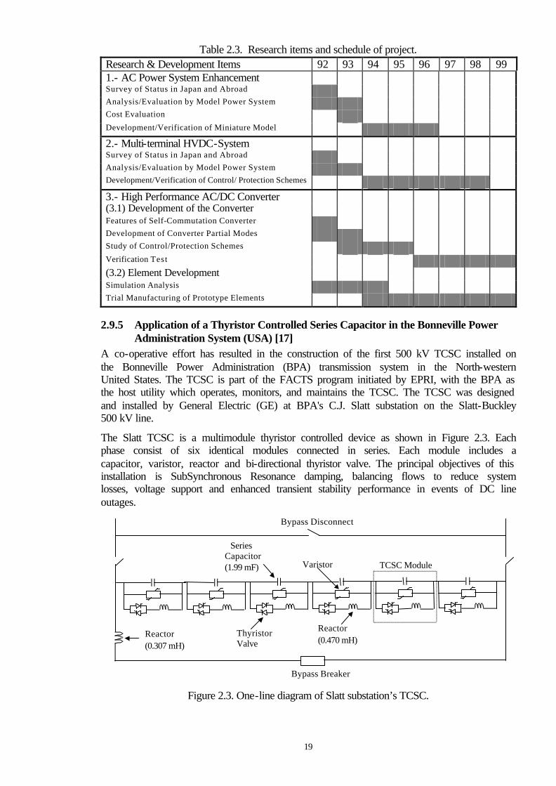
19
Table 2.3. Research items and schedule of project.
2.9.5 Application of a Thyristor Controlled Series Capacitor in the Bonneville Power Administration System (USA) [17] A co-operative effort has resulted in the construction of the first 500 kV TCSC installed on the Bonneville Power Administration (BPA) transmission system in the North-western United States. The TCSC is part of the FACTS program initiated by EPRI, with the BPA as the host utility which operates, monitors, and maintains the TCSC. The TCSC was designed and installed by General Electric (GE) at BPA's C.J. Slatt substation on the Slatt-Buckley 500 kV line. The Slatt TCSC is a multimodule thyristor controlled device as shown in Figure 2.3. Each phase consist of six identical modules connected in series. Each module includes a capacitor, varistor, reactor and bi-directional thyristor valve. The principal objectives of this installation is SubSynchronous Resonance damping, balancing flows to reduce system losses, voltage support and enhanced transient stability performance in events of DC line outages.
Figure 2.3. One-line diagram of Slatt substation’s TCSC.
Research & Development Items 92 93 94 95 96 97 98 99 1.- AC Power System Enhancement Survey of Status in Japan and Abroad Analysis/Evaluation by Model Power System Cost Evaluation Development/Verification of Miniature Model 2.- Multi-terminal HVDC-System Survey of Status in Japan and Abroad Analysis/Evaluation by Model Power System Development/Verification of Control/ Protection Schemes 3.- High Performance AC/DC Converter (3.1) Development of the Converter Features of Self-Commutation Converter Development of Converter Partial Modes Study of Control/Protection Schemes Verification Test (3.2) Element Development Simulation Analysis Trial Manufacturing of Prototype Elements
TCSC Module
Series Capacitor (1.99 mF) Varistor
Thyristor Valve
Reactor (0.470 mH)
Bypass Breaker
Reactor (0.307 mH)
Bypass Disconnect

20
2.9.6 Application of a Controllable Series Capacitor on the American Electric Power System (USA) [18] In 1986 a study was initiated by AEP to investigate potential sites where power flow control concepts could be applied. The site chosen was the transmission interface between the AEP northern and southern areas. This interface consists of two 765-kV lines, one 345-kV line, and six 138 kV lines. The power transfer capability of the transmission interface is limited by the loadability of the 345 kV line. In the event of outages in the 765 kV line, the 345 kV circuit becomes overloaded as a result of the large phase angle separation between its terminals. A Controllable Series Compensator was added into the Amos-Funk 345 kV line in Kanawha River Station in order to increase the capacity of the line to carry power both in normal and contingency conditions. The rating of the controllable device consisted of 788 MVAr, 2500 Amp, 42 Ohms to provide compensation from 0% to 60 % in steps of 10%. Table 2.4 provides a summary of the improvement achieved by the inclusion of the controllable device.
Table 2.4. Effect of series compensation at Amos-funk 345 kV line. Level of series compensation
(%)
Normal Amos-Flunk active flow
(MW)
Amos-Flunk Maximum Capability
(MW)
Single-Contingency System Transfer Capability (MW)
0 457 880 5,787 40 652 1280 6,342 60 827 1485 5658
2.10 Conclusions As electric utilities move into more competitive generation supply regimes, with limited scope to expand transmission facilities, the optimisation of existing transmission corridors for power transfer becomes of paramount importance. In this scenario, FACTS technologies appear as an attractive alternative which aims at increasing system operation flexibility. A brief overview of a collection of controllers which conform the FACTS technology, their features, applications and influences on power systems have been introduced in this Chapter. The first utilities attempts to implementing models of FACTS devices into standard network simulation software packages have revealed difficulties linked to the structures of their codes. At the most abstract level, the consideration of these controllers into the power flow problem has been described. Potential problems to be faced in the FACTS upgraded Newton-Rapshon power flow formulation has been pointed out. The need to be able to evaluate the impact of FACTS devices on transmission networks has led to focus co-operative efforts on technological aspects of these controllers. Current FACTS research and applications in some electric companies have been described in this Chapter.
2.11 Bibliography [1] Hingorani N.H.: ‘Flexible AC Transmission Systems’, IEEE Spectrum, pp. 40-45, April 1993. [2] IEEE/CIGRE: ‘FACTS Overview’, Special Issue, 95TP108, IEEE Service Center, Piscataway, N.J., 1995.
[3] IEEE Power Engineering Society: ‘FACTS Applications’, Special Issue, 96TP116-0, IEEE Service Center, Piscataway, N.J., 1996.

21
[4] Tinney W.F. and Hart C.E.: ‘Power Flow Solution by Newton’s Method’, IEEE Trans. on Power Apparatus and Systems, Vol. PAS-96, No. 11, pp. 1449-1460, November 1967. [5] Stott B.: ‘Review of Load-Flow Calculation Methods’, IEEE Proceedings, vol. 62, pp. 916-929, July 1974. [6] Han Z.X.: ‘Phase Shifter and Power Flow Control’, IEEE Trans. on Power Apparatus and Systems, Vol. PAS-101, No. 10, pp. 3790-3795, October 1982. [7] Noroozian M. and Andersson G.: ‘Power Flow Control by Use of Controllable Series Components’ , IEEE Trans. on Power Delivery, Vol. 8, No. 3, pp. 1420-1429, July 1993. [8] Acha E.: ‘A Quasi-Newton Algorithm for the Load Flow Solution of Large Networks with FACTS-Controlled Branches’, Proceedings of the 28th UPEC Conference, Stafford UK, 21-23, pp. 153-156, September 1993. [9] Mescua J.: ‘A Decoupled Method for Systematic Adjustments of Phase-Shifting and Tap-Changing Transformers’, IEEE Trans. on Power Apparatus and Systems, Vol. PAS-104, No. 9, pp. 2315-2321, September 1985. [10] Chang S.K. and Brandwajn V.: ‘Adjusted Solutions in Fast Decoupled Load Flow’, IEEE Trans. on Power Systems, Vol. 3, No. 2, pp. 726-733, May 1988. [11] Maria G.A , Yuen A.H. and Findlay J.A.: ‘Control Variable Adjustment in Load Flows’, IEEE Trans. on Power Systems, Vol. 3, No. 3, pp. 858-864, August 1988. [12] Peterson N.M. and Scott Meyer W.: ‘Automatic Adjustment of Transformer and Phase Shifter Taps in the Newton Power Flow’, IEEE Trans. on Power Apparatus and Systems, Vol. PAS-90, No. 1, pp. 103-108, January/February 1971. [13] Stott B.: ‘Effective Starting Process for Newton-Raphson Load Flows’, Proceedings of IEE, Vol. 118, No. 8, pp. 983-987, August 1971. [14] Ledu A., Tontini G. and Winfield M.: ‘Which FACTS Equipment for Which Need?’, International Conference on Large High Voltage Electric Systems (CIGRÉ), paper 14/37/38-08, Paris, September 1992. [15] Maliszewski R.M., Eunson E., Meslier f., Balazs P., Schwarz J., Takahashi K. and Wallace P.: ‘Interaction of System Planning in the Development of the Transmission Networks of the 21st Century’, Symposium on Power Electronics in Electric Power Systems, International Conference on Large High Voltage Electric Systems (CIGRÉ), paper 210-02, Tokyo, 22-24 May, 1995. [16] Sekine Y., Hayashi T., Abe K., Inoue Y. and Horiuchi S.: ‘Application of Power Electronics Technologies to Future Interconnected Power System in Japan’, Symposium on Power Electronics in Electric Power Systems, International Conference on Large High Voltage Electric Systems (CIGRÉ), paper 210-03, Tokyo, 22-24 May, 1995. [17] Kinney S.J., Mittelstadt W.A. and Suhrbier R.W.: ‘Test Results and Initial Experience for the BPA 500 kV Thyristor Controlled Series Capacitor Unit at Slatt Substation, Part I- Design, Operation, and Fault Test Results’, Flexible AC Transmission Systems (FACTS 3): The Future in High Voltage Transmission Conference, EPRI, Baltimore Maryland, October 1994. [18] Martin D.E.: ‘System Aspects of AEP’s Kanawha River Controlled Series Capacitor Installation’, Flexible AC Transmission Systems (FACTS) Conference, EPRI, Boston Massachusetts, 18-20 May, 1992.

22
Chapter 3 Power Flow Series Controllers 3.1 Introduction With the difficulties of licensing and building new transmission lines to meet load demand in interconnected electric power systems, the possibility of fast power flow control is a most welcome development. Many existing AC lines are operated at power levels below their thermal power carrying capability limit, and power flow electronic control is seen as the way forward to increase power flows up to values approaching thermal limits. The active power transfer Pkm across an electric branch connected between nodes k and m is largely determined by the voltage magnitudes Vk and Vm
, the difference in voltage angles θ k and θ m and the branch reactance X km ,
PV VXkmk m
kmk m= −sin( )θ θ (3.1)
This equation provides some insight into the techniques available for power flow control. On the one hand, the voltage magnitudes cannot be varied significantly since they must be kept within regulated limits, hence providing very limited scope for power flow control. On the other hand, the branch reactance and the voltage angle difference are not circumscribed as heavily to such restrictions and they may provide the only practical alternatives for power flow control. These intrinsic characteristics of the power transfer mechanism have been very early recognised by the Power Supply Industry. Mechanically-controlled series compensation and phase-shifter transformers have been in existence for many decades. Now, power electronics-based versions of both devices have been embraced by the proponents of the FACTS technology [1,2]. Accordingly, there is renewed interest on developing efficient tools for assessing the performance of these devices on a network wide basis [3,4]. New models which fulfil such a need are presented below.
3.2 Thyristor Controlled Series Capacitor One established method of varying transmission line capability is to install a series variable compensator which affects the net transmission line’s series impedance. One important FACTS component is the Thyristor Controlled Series Capacitor (TCSC) which allows rapid and continuous change of the transmission line apparent impedance. As a result of this control, the active power flowing along the compensated transmission line can be maintained at a specified value under a range of different scenarios of operative conditions. Figure 3.1 shows a general configuration of a TCSC module [5,6] which consists of a series capacitor bank in parallel with a thyristor controlled reactor. The controlling element is the thyristor controller, which is shown as a bi-directional thyristor valve. In a practical installation, many thyristors (typically 10 to 40) are connected in series to meet the required blocking voltage levels [7,9]. The Advanced Series Compensator (ASC) device [6] is composed of a number of small series connected TCSC modules in order to exert control with minimum losses and harmonics.

23
Figure 3.1. TCSC module. Proper operation of the valve requires the simultaneous application of a gate signal to all thyristors of the same polarity, at a given point in time, during normal diode operating conduction; i.e., the anode-cathode voltage of the thyristors is positive. Once the thyristor valve is on, it remains so until its anode current goes to zero. This is the case unless another firing signal is triggered. The delay with which the firing signal is applied is measured relative to the angle at which the valve would have turned on, and it is called firing angle. The current through the inductor begins to flow once the thyristor valve is gated on and the firing angle α is defined as the angle in electrical degrees between the positive-going zero-crossing of the voltage across the inductor and the positive-going zero-crossing of the current through it [8,9]. The conduction angle σ is defined as the angle, in electrical degrees, during which the thyristor valve is conducting [8]. The conduction angle σ and the firing angle α are related by the following expression,
σ π α= −2 2 (3.2) Full conduction is obtained with a firing angle of 90o. Partial conduction is obtained with α between 90o and 180o. No conduction is obtained with α=1800.
3.2.1 TCSC voltage and current steady state equations The steady state voltage and current equations of a TCSC module can be derived from the analysis of a parallel LC circuit with variable inductance. If we assume that a loop current is trapped in the reactor-capacitor circuit, the external circuit can be represented by a sinusoidal current source. Under this situation, the equivalent electric circuit of a TCSC module connected in a power system can be represented schematically by Figure 3.2.
Figure 3.2. Equivalent electric circuit of a TCSC module. Applying Kirchoff’s current law to the electric circuit shown in Figure 3.2 and expressing the resultant equation in Laplace domain,
cos sin ( ) ( )σ σa a thy caps
s ww
s wI s I s2 2 2 2+
++
= + (3.3)
icap
iline= 1 cos (wt)
ithy
L
C
C
L Bi-directional
Valve
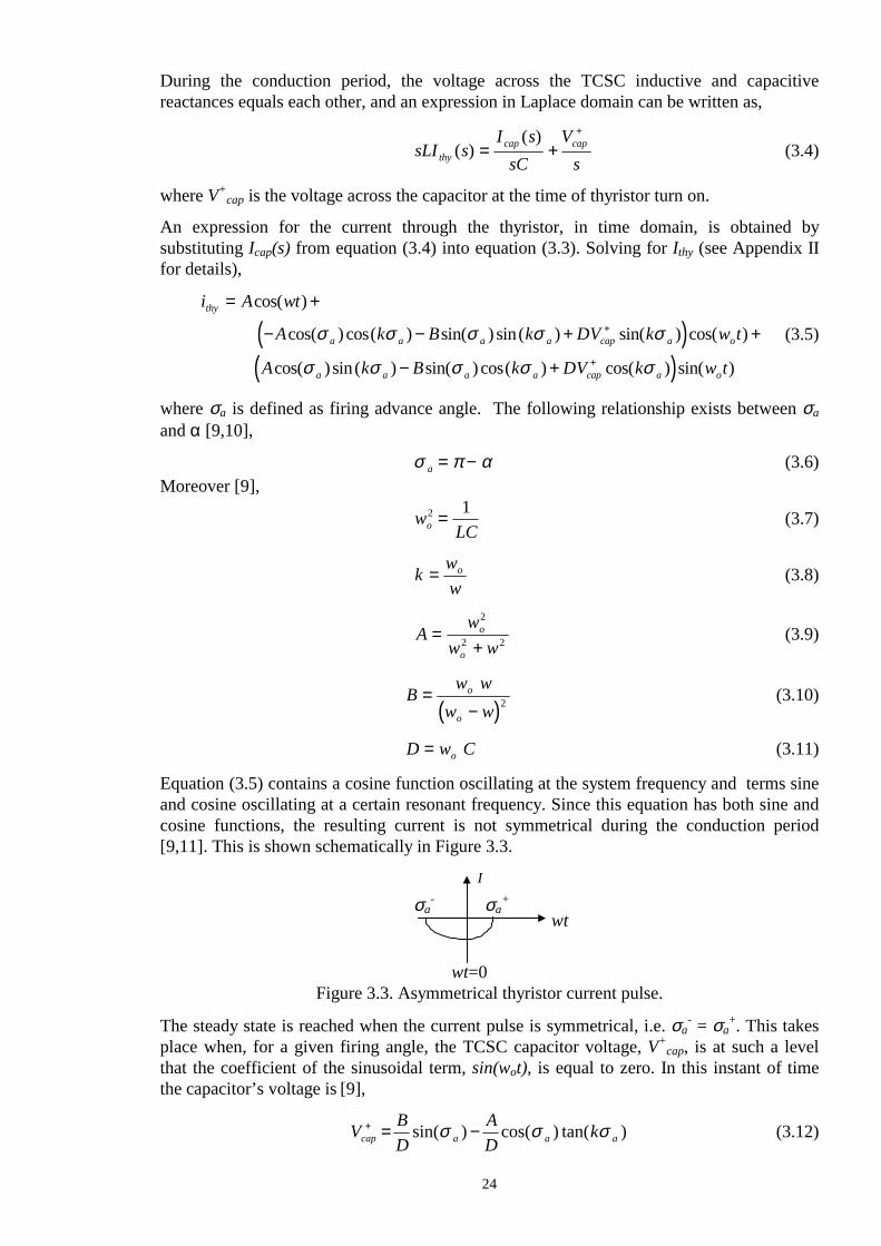
24
During the conduction period, the voltage across the TCSC inductive and capacitive reactances equals each other, and an expression in Laplace domain can be written as,
sLI sI s
sCV
sthycap cap( )
( )= +
+
(3.4) where V+
cap is the voltage across the capacitor at the time of thyristor turn on. An expression for the current through the thyristor, in time domain, is obtained by substituting Icap(s) from equation (3.4) into equation (3.3). Solving for Ithy (see Appendix II for details),
( )( )
i A wt
A k B k DV k w t
A k B k DV k w t
thy
a a a a cap a o
a a a a cap a o
= +
− − + +
− +
+
+
cos( )
cos( ) cos( ) sin( ) sin( ) sin( ) cos( )
cos( ) sin( ) sin( ) cos( ) cos( ) sin( )
σ σ σ σ σ
σ σ σ σ σ
(3.5)
where σa is defined as firing advance angle. The following relationship exists between σa
and α [9,10],
σ π αa = − (3.6) Moreover [9],
wLCo
2 1= (3.7)
k ww
o= (3.8)
Aw
w wo
o
=+
2
2 2 (3.9)
( )B w w
w wo
o
=− 2 (3.10)
D w Co= (3.11)
Equation (3.5) contains a cosine function oscillating at the system frequency and terms sine and cosine oscillating at a certain resonant frequency. Since this equation has both sine and cosine functions, the resulting current is not symmetrical during the conduction period [9,11]. This is shown schematically in Figure 3.3.
Figure 3.3. Asymmetrical thyristor current pulse. The steady state is reached when the current pulse is symmetrical, i.e. σa
- = σa+. This takes
place when, for a given firing angle, the TCSC capacitor voltage, V+cap, is at such a level
that the coefficient of the sinusoidal term, sin(wot), is equal to zero. In this instant of time the capacitor’s voltage is [9],
V BD
AD
kcap a a a+ = −sin( ) cos( ) tan( )σ σ σ (3.12)
σa- σa
+ wt
wt=0
I

25
The steady-state symmetrical thyristor current pulse equation is obtained by substituting equation (3.12) into equation (3.5), and given by equation (3.13) [9,10].
i A wt Ak
kwtthya
a
= −cos( )cos( )cos( )
cos( )σσ
(3.13)
Equation (3.13) is valid in the interval wt ∈ [-σa, σa]. A second firing pulse takes places 180o just after the first pulse, producing a current flow through the thyristor with opposite polarity to the current given by (3.13). The thyristor current is expressed by,
i A wt Ak
k wtthya
a
= + −cos( )cos( )cos( )
cos( ( ))σσ
π (3.14)
and it is valid during the period of time wt ∈ [π-σa, π+σa]. The schematic representation of these pulses is given in Figure 3.4.
Figure 3.4. TCSC thyristor current in steady-state. The expressions for the voltage across the TCSC capacitor during the conduction period are obtained by substituting equations (3.13) and (3.14) into equation (3.15)
v Ld idtcap on
thy− = (3.15)
and solving for vcap-on. The final expressions are,
v A X wt A k Xk
kwt for wtcap on LL a
aa a− = − + ∈ −sin( )
cos( )cos( )
sin( ) [ , ]σ
σσ σ (3.16)
v A X wt A k Xk
k wt for wtcap on LL a
aa a− = − − − ∈ − +sin( )
cos( )cos( )
sin( ( )) [ , ]σ
σπ π σ π σ (3.17)
where XL is the inductive reactance defined by the product wL. The current through the capacitor is obtained from,
i i icap on line thy− = − (3.18) When the thyristor is not conducting, the equivalent circuit of the TCSC shown in Figure 3.2 is simply a capacitor connected in series with a DC voltage source, which represents the capacitor voltage at the time of thyristor commutation [11]. In this state, the inductor current is zero. The current through the capacitor is equal to the line current and is given by,
i i wtcap off line− = =1 cos( ) (3.19)
α
σa -σa
π-σa π+σa
2π+σa 2π-σa
wt
I (pu)

26
The voltage across the capacitor during the period of time in which the thyristors are not conducting is computed by,
vC
wt dt Vcap off
wt
capon off
a
−−= +∫
1 cos( )σ
(3.20)
where Vcap
on off− is the voltage magnitude across the capacitor at the time in which the thyristor turns off, i.e. σa/w. This value is obtained from equation (3.16) and given by,
V A X A k X kcapon off
L a L a a− = − +sin( ) cos( ) tan( )σ σ σ (3.21)
Substituting equation (3.21) into (3.20), the following equation is obtained,
( ) ( )v X wt AX k kcap off C a L a a a− = − − +sin( ) sin( ) sin( ) cos( ) tan( )σ σ σ σ (3.22) where Xc=1/(wC) is the capacitive reactance. This equation is only valid for the period of time wt ∈ [σa, π-σa]. Owing to the symmetry in the firing signals and thyristor current pulses, the capacitor voltage in the second thyristor turned is given by,
( ) ( )v X wt AX k kcap off C a L a a a− = + + +sin( ) sin( ) sin( ) cos( ) tan( )σ σ σ σ (3.23) The equation is only valid for wt ∈ [π+σa, 2π-σa]. The equations described above represent the TCSC steady-state behaviour during one complete cycle. Typical waveforms of the voltage across and the current through the TCSC components are shown in Figures 3.5, 3.6, and 3.7 for the case when the thyristors are fired at an angle of 150o. The inductance and capacitance reactances were assumed to be 2.6 Ω and 15 Ω, respectively, for a frequency of 60 Hz [9].
Figure 3.5. Voltage and currents waveforms in the TCSC capacitor.

27
Figure 3.6. Voltage and currents waveforms in the TCSC inductor.
Figure 3.7. Voltage and currents waveforms in the TCSC bi-directional thyristors.
3.2.2 TCSC fundamental impedance Since the TCSC thyristor current contains harmonic distortion, it becomes necessary to apply Fourier analysis to a full period of the current, equations (3.13) and (3.14), in order to obtain an expression at fundamental frequency. From Figure 3.6 it is clear that the TCSC thyristor current has even and quarter symmetry. Hence, the fundamental frequency component can be obtained by solving equation (3.13) only,
I A wt Ak
kwt wt d wtthya
a
a
( ) cos( )cos( )cos( )
cos( ) cos( ) ( )10
4= −
∫π
σσ
σ
(3.24)
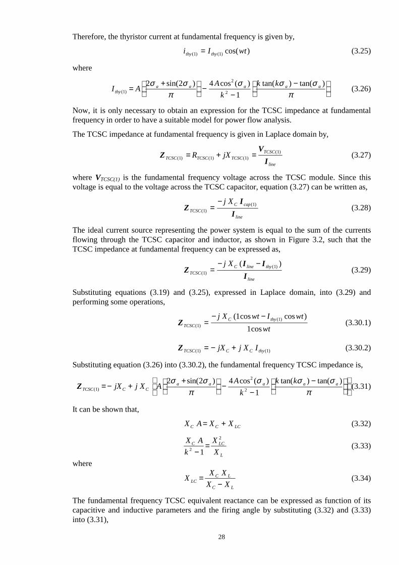
28
Therefore, the thyristor current at fundamental frequency is given by,
i I wtthy thy( ) ( ) cos( )1 1= (3.25) where
I A Ak
k kthy
a a a a a( )
sin( ) cos ( ) tan( ) tan( )1
2
2
2 2 41
=+
−−
−
σ σπ
σ σ σπ
(3.26) Now, it is only necessary to obtain an expression for the TCSC impedance at fundamental frequency in order to have a suitable model for power flow analysis. The TCSC impedance at fundamental frequency is given in Laplace domain by,
ZV
ITCSC TCSC TCSCTCSC
line
R jX( ) ( ) ( )( )
1 1 11= + = (3.27)
where VTCSC(1) is the fundamental frequency voltage across the TCSC module. Since this voltage is equal to the voltage across the TCSC capacitor, equation (3.27) can be written as,
ZI
ITCSCC cap
line
j X( )
( )1
1=−
(3.28)
The ideal current source representing the power system is equal to the sum of the currents flowing through the TCSC capacitor and inductor, as shown in Figure 3.2, such that the TCSC impedance at fundamental frequency can be expressed as,
ZI IITCSC
C line thy
line
j X( )
( )( )1
1=− −
(3.29)
Substituting equations (3.19) and (3.25), expressed in Laplace domain, into (3.29) and performing some operations,
ZTCSCC thyj X wt I wt
wt( )( )( cos cos )
cos111
1=
− − (3.30.1)
ZTCSC C C thyjX j X I( ) ( )1 1= − + (3.30.2)
Substituting equation (3.26) into (3.30.2), the fundamental frequency TCSC impedance is,
ZTCSC C Ca a a a ajX j X A
Ak
k k( )
sin( ) cos ( ) tan( ) tan( )1
2
2
2 2 41
= − ++
−−
−
σ σπ
σ σ σπ
(3.31)
It can be shown that,
X A X XC C LC= + (3.32)
X Ak
XX
C LC
L2
2
1−= (3.33)
where
X X XX XLC
C L
C L
=−
(3.34)
The fundamental frequency TCSC equivalent reactance can be expressed as function of its capacitive and inductive parameters and the firing angle by substituting (3.32) and (3.33) into (3.31),
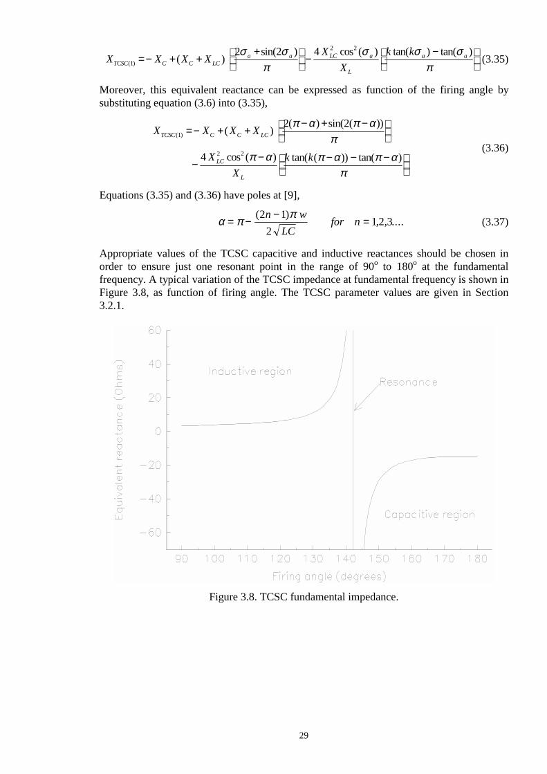
29
X X X XX
Xk k
TCSC C C LCa a LC a
L
a a( ) ( )
sin( ) cos ( ) tan( ) tan( )1
2 22 2 4=− + +
+
−−
σ σπ
σ σ σπ
(3.35)
Moreover, this equivalent reactance can be expressed as function of the firing angle by substituting equation (3.6) into (3.35),
X X X X
XX
k k
TCSC C C LC
LC
L
( ) ( )( ) sin( ( ))
cos ( ) tan( ( )) tan( )
1
2 2
2 2
4
=− + +− + −
−− − − −
π α π απ
π α π α π απ
(3.36)
Equations (3.35) and (3.36) have poles at [9],
α π π= −
−=
( ), , ....
2 12
1 2 3n w
LCfor n (3.37)
Appropriate values of the TCSC capacitive and inductive reactances should be chosen in order to ensure just one resonant point in the range of 90o to 180o at the fundamental frequency. A typical variation of the TCSC impedance at fundamental frequency is shown in Figure 3.8, as function of firing angle. The TCSC parameter values are given in Section 3.2.1.
Figure 3.8. TCSC fundamental impedance.
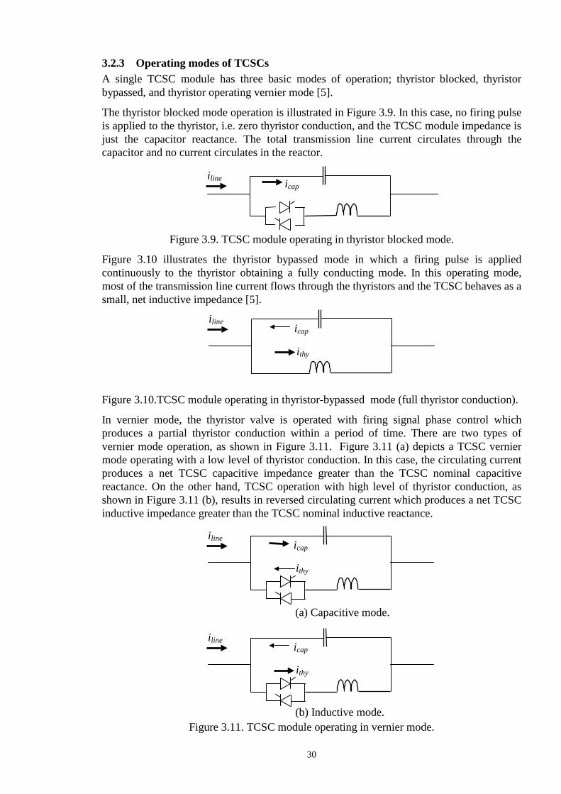
30
3.2.3 Operating modes of TCSCs A single TCSC module has three basic modes of operation; thyristor blocked, thyristor bypassed, and thyristor operating vernier mode [5]. The thyristor blocked mode operation is illustrated in Figure 3.9. In this case, no firing pulse is applied to the thyristor, i.e. zero thyristor conduction, and the TCSC module impedance is just the capacitor reactance. The total transmission line current circulates through the capacitor and no current circulates in the reactor.
Figure 3.9. TCSC module operating in thyristor blocked mode. Figure 3.10 illustrates the thyristor bypassed mode in which a firing pulse is applied continuously to the thyristor obtaining a fully conducting mode. In this operating mode, most of the transmission line current flows through the thyristors and the TCSC behaves as a small, net inductive impedance [5]. Figure 3.10.TCSC module operating in thyristor-bypassed mode (full thyristor conduction). In vernier mode, the thyristor valve is operated with firing signal phase control which produces a partial thyristor conduction within a period of time. There are two types of vernier mode operation, as shown in Figure 3.11. Figure 3.11 (a) depicts a TCSC vernier mode operating with a low level of thyristor conduction. In this case, the circulating current produces a net TCSC capacitive impedance greater than the TCSC nominal capacitive reactance. On the other hand, TCSC operation with high level of thyristor conduction, as shown in Figure 3.11 (b), results in reversed circulating current which produces a net TCSC inductive impedance greater than the TCSC nominal inductive reactance.
Figure 3.11. TCSC module operating in vernier mode.
iline icap
iline icap
ithy
iline icap
ithy
iline icap
ithy
(a) Capacitive mode.
(b) Inductive mode.

31
Figure 3.12 shows the voltage across the TCSC capacitor for different values of firing angles. It is observed that the degree of distortion of the voltage capacitor waveform is bigger when the TCSC is operating in the inductive region of vernier mode operation. The polarity of this voltage depends of the range in which the TCSC is operating, i.e. value of firing angle. It implies that the value of firing angle determines the direction of the current through the capacitor. Both plots show that the voltage magnitude increases near to the resonance point. As expected, the voltage across the capacitor is sinusoidal when the TCSC is operating in both thyristor-bypassed mode and blocked thyristor mode.
(a) Inductive region. (b) Capacitive region.
Figure 3.12. TCSC capacitor voltage in vernier mode operation. Figures 3.13 and 3.14 show the current through the TCR and capacitor for different values of firing angles, respectively. The value of firing angle determines the direction of the current through the TCR and capacitor which are opposite to each other. Both plots show that the current magnitude increases near to the resonance point. When the TCSC is operating in its inductive region, the current through the thyristors is bigger than the one through the capacitors. The opposite happens when the TCSC is operating inside its capacitive region.
(a) Inductive region. (b) Capacitive region. Figure
Figure 3.13. TCSC thyristor current in vernier mode operation.
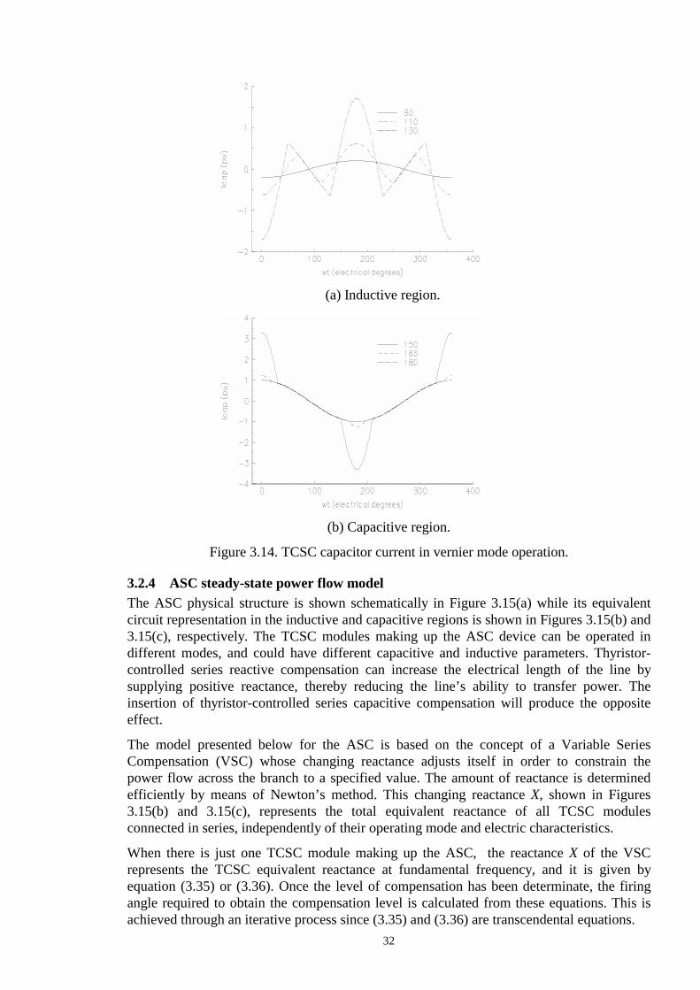
32
(a) Inductive region.
(b) Capacitive region.
Figure 3.14. TCSC capacitor current in vernier mode operation.
3.2.4 ASC steady-state power flow model The ASC physical structure is shown schematically in Figure 3.15(a) while its equivalent circuit representation in the inductive and capacitive regions is shown in Figures 3.15(b) and 3.15(c), respectively. The TCSC modules making up the ASC device can be operated in different modes, and could have different capacitive and inductive parameters. Thyristor-controlled series reactive compensation can increase the electrical length of the line by supplying positive reactance, thereby reducing the line’s ability to transfer power. The insertion of thyristor-controlled series capacitive compensation will produce the opposite effect. The model presented below for the ASC is based on the concept of a Variable Series Compensation (VSC) whose changing reactance adjusts itself in order to constrain the power flow across the branch to a specified value. The amount of reactance is determined efficiently by means of Newton’s method. This changing reactance X, shown in Figures 3.15(b) and 3.15(c), represents the total equivalent reactance of all TCSC modules connected in series, independently of their operating mode and electric characteristics. When there is just one TCSC module making up the ASC, the reactance X of the VSC represents the TCSC equivalent reactance at fundamental frequency, and it is given by equation (3.35) or (3.36). Once the level of compensation has been determinate, the firing angle required to obtain the compensation level is calculated from these equations. This is achieved through an iterative process since (3.35) and (3.36) are transcendental equations.

33
Figure 3.15. Advanced Series compensator. In general, the transfer admittance matrix for the variable compensator is,
II
jB jBjB jB
VV
k
m
kk km
mk mm
k
m
=
(3.38)
For the reactor case (the capacitor has opposite signs),
B BX
B BX
kk mm
km mk
= = −
= =
1
1 (3.39)
The VSC’s power equations at node k are,
( )P V V Bk k m km k m= −sin θ θ (3.40)
( )Q V B V V Bk k kk k m km k m= − − −2 cos θ θ (3.41) The VSC’s linearised power equations with respect to the series compensator are,
( )∂∂
θ θPX
X V V Bkk m km k m= − −sin (3.42)
( )∂∂
θ θQX
X V B V V Bkk kk k m km k m= + −2 cos (3.43)
For equation at node m exchange subscripts k and m in equations (3.40)-(3.43).
Bypass Breaker
TCSC Module
Series Capacitor (1.99 mF) Varistor
Thyristor Valve
Reactor (0.470 mH) Reactor
(0.307 mH)
Bypass Disconnect k m
P km
reg
(a) ASC physical structure.
k m P km
reg
(b) ASC equivalent circuit in inductive operative region.
k m P km
reg
(c) ASC equivalent circuit in capacitive operative region.

34
The VSC shown in Figures 3.15(b) and 3.15(c) is assumed to control the real power flowing from node k to node m at a value Pkm
reg. The set of linearised power flow equations for the VSC’s branches is,
∆
∆
∆
∆
∆
P
P
Q
Q
P
P P PV
VPV
VPX
X
P P PV
VPV
VPX
X
Q Q QV
VQV
VQX
X
Q Q QV
VQV
VQX
X
P
k
m
k
m
kmX
k
k
k
m
k
kk
k
mm
k
m
k
m
m
m
kk
m
mm
m
k
k
k
m
k
kk
k
mm
k
m
k
m
m
m
kk
m
mm
m
=
∂∂ θ
∂∂ θ
∂∂
∂∂
∂∂
∂∂ θ
∂∂ θ
∂∂
∂∂
∂∂
∂∂ θ
∂∂ θ
∂∂
∂∂
∂∂
∂∂ θ
∂∂ θ
∂∂
∂∂
∂∂
∂ kmX
k
kmX
m
kmX
kk
kmX
mm
kmX
k
m
k k
m m
P PV
VPV
VPX
X
V V
V V
X X∂ θ
∂∂ θ
∂∂
∂∂
∂∂
θ
θ
∆
∆
∆
∆
∆
(3.44)
where,
∂∂
∂∂
∂∂
∂∂
PX
XPX
XPX
XPV
Vk mX
mkX
k k
mm= − = = − (3.45)
∂∂
∂∂
QX
X V B PV
Vkk kk
k
mm= −2 (3.46)
The general linearised Newton equations of the VSC are given in (3.47), where the variable reactance X is taken to be the state variable.
∆
∆
∆
∆
∆
∆
P
Q
P
P PV
V PX
X
Q QV
VQX
X
P PV
VPX
X
V V
X Xk mX
k mX
k mX
k mX
=
∂∂ θ
∂∂
∂∂
∂∂ θ
∂∂
∂∂
∂∂ θ
∂∂
∂∂
θ
(3.47)
It must be noted that ∂
∂PX
Xk mX
is a diagonal matrix whose order equals the number of VSCs in
the network. ∆ P P Pk mX
k mX reg
k mX cal= −, , is the real power flow mismatch vector for VSC and
∆X=Xi+1 + X i is the vector of incremental changes in series reactance. The state variable X of the series controller is updated at the end of each iterative step according to equation (3.48),
( )X X XX
Xi ii
i( ) ( )( )
+ = +
1 ∆ (3.48)
3.2.5 VSC Initialisation Equation (3.42) shows that the initialisation of series compensators gives rise to an ill-conditioned Jacobian matrix if the customary zero voltage angle initialisation is adopted. In such situation the linearised, active power flow equation of the series compensator yields a null diagonal element in the Jacobian.

35
The strategy adopted in the program in order to circumvent the problem posed by series compensators during the initialisation stage is to treat such devices as fixed reactances until a pre-specified voltage angle difference across the reactance takes place. From that point onwards, the control equations of the series compensator are included in the iterative process. This initialisation-control method can be referred to as the hybrid method. An alternative control strategy would be to include the control equations from the outset of the iterative process but delaying the natural order of elimination of the offending diagonal Jacobian element, until a non-zero element is created in that location during the elimination process [12]. However, tampering with the natural elimination order leads to inefficient solutions in terms of both sparsity storage and solution times. The hybrid method is the author’s preferred approach for initialising controllable series compensators. It is realised that this method may compromise Newton method’s convergence by 1 or 2 extra-iterations when a large number of controlled branches are involved. However, solutions are very efficient because Tinney’s second ordering elimination scheme in not tampered with.
3.2.6 VSC active power flow control test case A small, 5-node network [13] has been used in order to show, quantitatively, how the VSC performs. Solution details are provided so as to enable potential users of this model to make any comparisons. The original network and power flow results are shown in Figure 3.16 while data parameters are given in Appendix I. The final nodal complex voltages are given in Table 3.1.
Figure 3.16. Original test network and load flow results.
Table 3.1. Nodal complex voltages of original network. complex system nodes voltages North South Lake Main Elm V (pu) 1.060 1.000 0.987 0.984 0.972
θ (degree) 0.00 -2.06 -4.64 -4.96 -5.77
6.6 +j0.55
-6.55 -j5.2
60+j10
North
Lake
Main
South
Elm
-19.3 -j4.7
19.4 +j2.9
-40.3 -j17.5
41.8 +j16.8
89.3 +j74
-86.8 -j72.9
54.7 +j5.6
-53.45 -j4.8
-24.1 -j0.35
24.5 -j2.5
27.7 -j1.7
-27.3 -j0.83
20+j10
45+j15 40+j5
G
G SG = 40-j61.59
SG = 131.12 +j90.82

36
The original network has been modified to include a VSC which compensates the transmission line connected between nodes Lake and Main. An additional node, termed Lakefa, is used to connect the VSC. This is shown in Figure 3.17. The VSC is used to maintain active power flowing from Lakefa towards Main at 21 MWs. The initial condition of the VSC is set at 50% of the transmission line inductive reactance, i.e. X=0.015 pu. Convergence was obtained in 5 iterations to a power mismatch tolerance of 1e-12. The VSC upheld its target values. The final power flow results are shown in Figure 3.17. The final nodal complex voltages are given in Table 3.2. The maximum absolute power mismatches in the VSC and system buses are shown in Table 3.3.
Figure 3.17. Modified test network and load flow results.
Table 3.2. Nodal complex voltages of modified network.
Table 3.3. Maximum absolute power mismatches in the VSC and bus system.
Since the VSC is a passive element which can generate no active power by itself, there exists an increase of active power flowing towards Lake node, through transmission lines connected between North-Lake and South-Lake, in order to meet the increase in active power specified at the VSC.
complex system nodes voltages North South Lake Lakefa Main Elm V (pu) 1.060 1.000 0.987 0.988 0.984 0.972
θ (degree) 0.00 -2.04 -4.72 -4.46 -4.81 -5.70
BUSES VSC iteration ∆P ∆Q ∆X
0 0.600 0.12 0.21 1 0.021 0.016 0.011 2 0.004 0.001 0.004 3 6.4E-5 1.6E-5 6.5E-5 4 1.7E-8 5.0E-9 1.8E-8 5 1.2E-15 1.6E-16 1.2E-15
45+j15
7.13 +j0.41
-7.08 -j5.05
60+j10
Main
Elm
-20.9 -j4.31
-52.9 -j4.9
-26.2 -j1.09
40+j5
North
Lake
South
-40.9 -j17.3
42.4 +j16.7
88.6 +j74.2
-86.2 -j73.2
54.1 +j5.6
-25.1 -j8E-4
25.4 -j2.7
26.6 -j1.56
21.0 +j2.51
20+j10
G
G
SG = 40-j61.80
SG = 131.12 +j90.93
70%
21.0 +j2.41
Lakefa

37
Since the inductive series reactance of the compensated transmission line is very small, XL=0.03 pu, the amount of active power which can be incremented by the VSC, without overcompensate the line, is very small as well. In order to show the effect of the inductive series reactance of the compensated transmission line on the amount of active power controlled by the series compensation, the following three cases were simulated, 1. VSC compensating the transmission line connected from Lake to Main (XL = 0.03 pu). 2. VSC compensating the transmission line connected from South to Lake (XL = 0.18 pu). 3. VSC compensating the transmission line connected from North to Lake (XL = 0.23 pu). Figure 3.18 shows a comparison of the increase of active power flow as function of the compensation level for the cases mentioned above. A non-linear relation between these quantities can be observed. The non-linear relation can be approximated by a quadratic equation [14]. For a specified level of series compensation, the amount of active power increased by a VSC will be larger in transmission lines with a high value of inductive series reactance. Moreover, as the compensation increases the power flow through the compensated transmission line also increases.
Figure 3.18. Increments of active power flow as function of series compensation.
3.2.7 Feasible active power flow control region When two or more VSCs are electrically near they interact with each other. The amount of active power controlled by these series controllers will be confined to a region in which the control variables Xs are within limits and the solution of the power flow equations exists. A repeated load flow calculations for different combinations, within limits, of the series controllers will give the feasible active power flow control region. However, this is a cumbersome and inefficient method. A method based on a quadratic model of the VSC is developed in [14] to obtain this region in an efficient way. Regardless of the methodology used to calculate it, the feasible region is limited by the possible combination of the series controllers minimum and maximum values. Figure 3.19 shows the feasible active power flow control region when the transmission lines connected between North-Lake and South-Lake are compensated by VSC1 and VSC2, respectively. In this case, the maximum level of compensation was considered at 60 % of the transmission line series inductive reactance value. The boundary limits of the region are given by the following combinations of series compensation,

38
1. Point A, VSC1= 0% and VSC2=60% 2. Point B, VSC1= 0% and VSC2=0% 3. Point C, VSC1= 60% and VSC2=60% 4. Point D, VSC1= 60% and VSC2=0% Two cases were simulated in order to confirm the feasibility of the solution. In the first case the specified power flows through North-Lake and South-Lake were 63 MWs and 20 MWs, respectively. The solution was obtained in 6 iterations and the VSCs upheld the specified targets with a compensation of 59% and 54% for VSC1 and VSC2, respectively. In the second case the specified power flows through North-Lake and South-Lake were specified at 63 MWs and 25 MWs, respectively. These power flow specifications are outside the feasible active power flow control region by a very narrow margin (above point C). The solution was obtained in 6 iterations but VSC2 hit its 60% of compensation limit. The final value of active power flowing through VSC2 was 20.1 MWs.
Figure 3.19. Feasible active power control region for 60% series compensation.
The size of the feasible active power control region depends on the permissible level of series compensation. Figure 3.20 shows a comparison of the control region sizes for three different levels of series compensation on North-Lake and South-Lake. As the level of series compensation increases, the size of the region increases.
Figure 3.20. Comparison of feasible active power control region sizes.

39
3.2.8 Convergence test and VSC model validation The AEP 30 bus system [15] was modified to include 2 VSCs in order to control the active power flowing through branches 1-3 and 2-5 at 110 MWs and 62 MWs, respectively. Maximum and minimum generators limits were modified to 400 MVARs and -400 MVARs. Figure 3.21 and 3.22 show the active power flows in the relevant transmission lines for the original case and for the case when VSCs are embedded in the network, respectively. Transmission line 1-3 has been 43% capacitively compensated and 2-5 has resulted 76% inductively compensated in order to achieve their respective specified active power flow.
Figure 3.21. Relevant part of the AEP 30 bus system
Figure 3.22. Relevant part of the modified AEP 30 bus system.
148.1
83.20
45.88
61.95 37.46
80.06
69.43
1
2
3
4
5
6
7
REST OF THE NETWORK
148.1
110.0
45.88
61.95 37.46
80.06
69.43
1
2
3
4
5
6
7
REST OF THE NETWORK
-128.8 Ω
271.91 Ω 62.0

40
In both cases the iterative solution was started from a flat voltage profile, except for PV nodes. The solution for the base case was obtained in 4 iterations. The modified system was solved by two methods, the unified method presented in this thesis and a sequential iterative solution [4]. Both methods gave the same VSC’s values. Figure 3.23 shows the convergent trajectories of the maximum absolute, nodal power mismatches. The robustness of the unified method and its superiority over the sequential method, in terms of the number of iterations required to converge, is clearly shown in this figure.
Figure 3.23. Comparison of mismatches corresponding to unified and sequential methods as function of the number of iterations.
3.2.9 VSC active power flow control in a real power system An actual power network consisting of 2172 buses, 2294 transmission lines, 768 transformers, 200 generators, 1 SVC, 10 Fixed Capacitive Series Compensators (FCSC) and 208 Fixed Shunt Compensators (FSC), is used to show the full capabilities of the VSC model. Nine of the FCSCs were replace by VSCs in order to maintain a specified active power flow through predefined transmission lines. The original power flows through FCSCs, VSCs power flow specifications and level of capacitive compensation of the transmission lines are presented in Table 3.4. The base case converged is 6 iterations. The solution with the FCSCs replaced by VSCs was found in 7 iterations. The VSCs upheld their target values.
Table 3.4. 2172-node network with embedded Variable Series Compensators. Series
Compensators
Sending node
Receiving node Active power flow
(MWs) % of
compensation FCSC VSC Original Specified
C1 VSC1 CTZ400 CTZ400CS -497.32 -560 37.6 C2 VSC2 DGD230 DGD230 CS -132.92 -150 51.1 C3 VSC3 MID400 MID400 CS1 -495.38 -600 41.0 C4 VSC4 MID400 MID400 CS2 -491.65 -420 15.32 C5 VSC5 TMD-CEV400 TMD-CEV400 CS1 -482.64 -600 28.2 C6 VSC6 PUE400 PUE400 CS1 -379.94 -500 65.51 C7 VSC7 PUE400 PUE400 CS2 -473.09 -600 47.83 C8 VSC8 TEC1400 TEC1400 CS1 -548.38 -490 19.6 C9 VSC9 TEC1400 TEC1400 CS2 340.02 450 41.1

41
3.2.10 TCSC power flow model as function of firing angle (TCSC-FA) The model presented in Section 3.2.4 is based on the concept of a Variable Series Compensator (VSC) whose changing reactance adjusts itself in order to constrain the power flow across the branch to a specified value. The amount of reactance is determined efficiently by means of Newton’s method. This changing reactance X represents the equivalent reactance of all TCSC modules connected in series, at the fundamental frequency, independently of their operating mode and electric characteristics. Once the level of compensation is computed, the firing angle required to obtain such compensation level can be calculated in cases when the ASC is represented by only one TCSC module. Since the TCSC impedance is a transcendental equation, the computation of the firing angle is carried out through an iterative process. This model is very simple and reliable towards the convergence. However, a major shortcoming is its inability to predict unattainable levels of compensation due to natural resonances present in the parallel LC compensating circuit. Aiming at avoiding the additional iterative process required in the calculation of the firing angle, a TCSC-FA power flow model was presented in [16] where the firing angle is calculated simultaneously with the nodal AC network state variables. However, a major drawback of that work is that the fundamental frequency TCSC equivalent impedance is computed incorrectly. The TCR is the only TCSC element considered during the harmonic analysis whilst the capacitive reactance of the TCSC is neglected. The impedance is then obtained by the parallel combination of the TCR equivalent impedance at fundamental frequency and the fixed capacitive reactance, neglecting the loop current which takes place during either TCSC partial or full conduction mode operation. This equation is [16],
( )X X X
XXTCSC
C L
LC
( )
( ) sin( )1
2 2=
− − +π
π α α (3.49)
Figure 3.24 shows the TCSC fundamental frequency reactance, as function of the firing angle. It shows the result given by using equation (3.36) and the result given by using equation (3.49), where the loop current is not taken into account. The TCSC parameters correspond to Kayenta TCSC scheme [9]. From this result, it is clear that if the loop current is not taken into account then wrong firing angles will be calculated. This is particularly the case if the level of compensation required to achieve a target power flow lies near the TCSC’s resonant point.
Figure 3.24. Comparison of TCSC equivalent reactance.

42
To circumvent the limitations of both VSC model and that given by equation (3.49), a new and more accurate TCSC-FA model has been developed, based on the basic ideas presented in Sections 3.2.1 and 3.2.2. The transfer admittance matrix for the TCSC-FA module shown in Figure 3.25 is,
Figure 3.25. TCSC-FA module.
II
VV
k
m
kk km
mk mm
k
m
jB jBjB jB
=
(3.50)
where
B B BX
B B BX
kk mm TCSCTCSC
km mk TCSCTCSC
= = = −
= = − =
( )( )
( )( )
11
11
1
1 (3.51)
where XTCSC(1) is defined by equation (3.36) The TCSC-FA power equations at node k are,
( )P V V Bk k m TCSC k m= − −( ) sin1 θ θ (3.52)
( )Q V B V V Bk k TCSC k m TCSC k m= − + −21 1( ) ( ) cos θ θ (3.53)
The TCSC-FA linearised power equations with respect to the firing angle are,
∂∂ α
∂∂ α
PP B
Xkk TCSC
TCSC= ( )( )
11 (3.54)
∂∂ α
∂∂ α
Q Q BXk
k TCSCTCSC= ( )
( )1
1 (3.55)
where
( )
( )
∂∂ α
α
α ϖ ϖ π α α
ϖ π αϖ π α
XC
C
C
TCSC( ) cos( )
sin( ) tan( ( )) tan
cos ( )cos ( ( ))
11
2
22
2
2
2 1 2
2
1
= − +
+ − −
+ −−
−
(3.56)
C X XC LC1 = +
π (3.57)
CX
XLC
L2
24= −
π (3.58)
For equations at node m exchange subscripts k and m in (3.52)-(3.55).
Vk Ik
Vm Im
XC
XL
ILOOP
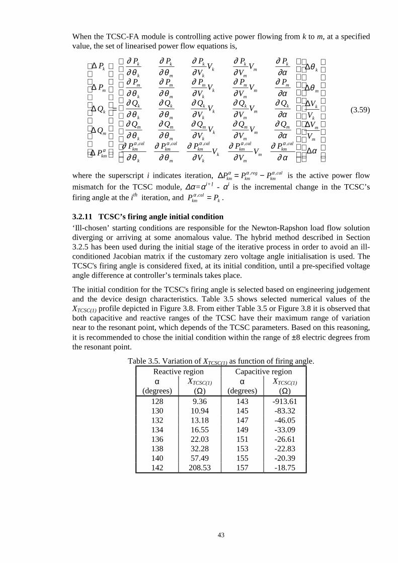
43
When the TCSC-FA module is controlling active power flowing from k to m, at a specified value, the set of linearised power flow equations is,
∆
∆
∆
∆
∆
P
P
Q
Q
P
P P PV
V PV
V P
P P PV
V PV
V P
Q Q QV
V QV
V Q
Q Q QV
V QV
V Q
P
k
m
k
m
km
k
k
k
m
k
kk
k
mm
k
m
k
m
m
m
kk
m
mm
m
k
k
k
m
k
kk
k
mm
k
m
k
m
m
m
kk
m
mm
m
kmcal
k
αα
∂∂ θ
∂∂ θ
∂∂
∂∂
∂∂α
∂∂ θ
∂∂ θ
∂∂
∂∂
∂∂α
∂∂ θ
∂∂ θ
∂∂
∂∂
∂∂α
∂∂ θ
∂∂ θ
∂∂
∂∂
∂∂α
∂∂ θ
∂
=
, P PV
V PV
V P
VVV
Vkm
cal
m
kmcal
kk
kmcal
mm
kmcal
k
m
k
k
m
mα α α α
∂ θ∂
∂∂
∂∂
∂ α
θ
θ
α, , , ,
∆
∆
∆
∆
∆
(3.59)
where the superscript i indicates iteration, ∆P P Pkm km
regkm
calα α α= −, , is the active power flow mismatch for the TCSC module, ∆α=αi+1 - αi is the incremental change in the TCSC’s firing angle at the ith iteration, and P Pkm
calk
α , = .
3.2.11 TCSC’s firing angle initial condition ‘Ill-chosen’ starting conditions are responsible for the Newton-Rapshon load flow solution diverging or arriving at some anomalous value. The hybrid method described in Section 3.2.5 has been used during the initial stage of the iterative process in order to avoid an ill-conditioned Jacobian matrix if the customary zero voltage angle initialisation is used. The TCSC's firing angle is considered fixed, at its initial condition, until a pre-specified voltage angle difference at controller’s terminals takes place. The initial condition for the TCSC's firing angle is selected based on engineering judgement and the device design characteristics. Table 3.5 shows selected numerical values of the XTCSC(1) profile depicted in Figure 3.8. From either Table 3.5 or Figure 3.8 it is observed that both capacitive and reactive ranges of the TCSC have their maximum range of variation near to the resonant point, which depends of the TCSC parameters. Based on this reasoning, it is recommended to chose the initial condition within the range of ±8 electric degrees from the resonant point.
Table 3.5. Variation of XTCSC(1) as function of firing angle. Reactive region Capacitive region α
(degrees) XTCSC(1)
(Ω) α
(degrees) XTCSC(1)
(Ω) 128 9.36 143 -913.61 130 10.94 145 -83.32 132 13.18 147 -46.05 134 16.55 149 -33.09 136 22.03 151 -26.61 138 32.28 153 -22.83 140 57.49 155 -20.39 142 208.53 157 -18.75

44
3.2.12 Numerical properties of the TCSC-FA model It has been found that if the solution takes place near to the resonant point, say 1 degree away from the resonant point, the solution may take 1 or 2 extra iterations to converge. The reason is that the numerical property of the partial derivative of BTCSC(1) with respect to the firing angle is ill-conditioned. Figures 3.26 (a) and (b) show BTCSC(1) and BTCSC(1)
∂∂α
X TCSC( )1
profiles as function of TCSC firing angles for the Kayenta TCSC scheme, respectively. Table 3.6 shows the numerical values of these variables at selected firing angles.
(a) (b)
Figure 3.26. TCSC susceptance profile. (a) BTCSC(1) . (b) BTCSC(1) ∂
∂αX TCSC( )1 .
Table 3.6. Variation of BTCSC(1) and the partial derivative as function of firing angle.
From Figure 3.26 (a) and Table 3.6, it is clear that the variation of BTCSC(1) with respect to the firing angle has good numerical properties, compared with the values of XTCSC(1). BTCSC(1) varies in a continuos, smooth way in both operative regions. The term BTCSC(1)
∂∂α
X TCSC( )1 varies from low to infinite values in both operative regions and a
resonant point exists, as shown in Figure 3.26 (b). This partial derivative term presents large variations in magnitude to small variations of firing angle near the resonant point. This introduces a major perturbation in the Jacobian matrix, producing a large increment in the firing angle adjustment. In order to reduce potential and unwanted numerical problems, the size of correction of the firing angle adjustment has been limited during the backward substitution to 5 electrical degrees. The truncated adjustment effect is propagated throughout the remaining of the backward substitution.
Reactive region Capacitive region
α (degree)
BTCSC(1) (Ω) BTCSC(1) ∂
∂αXTCSC( )1 (Ω)
α (degree)
BTCSC(1) (Ω) BTCSC(1) ∂
∂αXTCSC( )1 (Ω)
128 -0.107 -4.11 143 0.001 300.87 130 -0.091 -4.88 145 0.012 24.62 132 -0.076 -5.87 147 0.022 12.02 134 -0.060 -7.23 149 0.030 7.51 136 -0.045 -9.31 151 0.038 5.17 138 -0.031 -12.97 153 0.044 3.74 140 -0.024 -21.60 155 0.049 2.77 142 -0.005 -72.06 157 0.053 2.08

45
3.2.13 Limit revision of TCSC’s firing angle The power mismatch equations are used to activate limits revision for the controllable devices parameters. The revision criterion of the TCSC is based on its active power mismatch equation,
∆P P Pkmi
kmreg
kmcalα α α, , ,= + (3.60)
where i varies from 1 to the number of TCSCs. Limit revision is activated when equation (3.60) satisfies a pre-define tolerance, in our program it is 1E-3. If a limit violation takes place then the firing angle is fixed at that limit and the regulated active power flow is freed. In this situation no further attempts are made to control this active power for the remaining of the iterative process.
3.2.14 TCSC-FA active power flow control test case The original 5 nodes network described in Section 3.2.6 has been modified to include a TCSC-FA in series with the transmission line connected between nodes Lake and Main by an additional node, termed Lakefa, as shown in Figure 3.27. The TCSC-FA is used to maintain active power leaving it, towards Main, at 21 MWs. The initial condition of the firing angle was set at 145o. Convergence was obtained in 5 iterations to a power mismatch tolerance of 1e-12. The TCSC-FA uphold its target value. The final power flow results are shown in Figure 3.27. The final nodal complex voltages are given in Table 3.7. The maximum absolute power mismatches in the TCSC-FA and system buses are shown in Table 3.8. The fundamental frequency TCSC equivalent reactance computed by this model and when the TCSC is considered as a VSC was exactly the same.
Figure 3.27. Modified test network and load flow results.
45+j15
7.1 +j0.4
-7.1 -j5.1
60+j10
Main
Elm
-20.9 -j4.3
21.0 +j2.5
-52.9 -j4.9
-26.2 -j1.1
40+j5
North
Lake
South
-40.9 -j17.3
42.4 +j16.7
88.68 +j74.2
-86.21 -j73.1
54.1 +j5.6
-25.1 -j8E-4
25.5 -j2.7
26.6 -j1.6
20+j10
G
G
SG = 40-j61.8
SG = 131.12 +j90.93
Lakefa
46
Table 3.7. Nodal complex voltages of modified network.
Table 3.8. Maximum absolute power mismatches in the VSC and bus system.
Nodal power mismatches TCSC-FA mismatch and parameters Iterations ∆P ∆Q ∆Pα
km α (degrees) XTCSC(1) (pu) 0 0.6 0.12 0.21 145 -0.0518 1 0.021 0.016 0.020 145 -0.0518 2 0.078 2.4E-3 0.078 146.26 -0.0341 3 3.6E-3 7.7E-3 3.6E-3 148.46 -0.0222 4 1.0E-4 2.2E-4 1.1E-4 148.66 -0.0216 5 1.1E-8 4.3E-8 1.1E-8 148.66 -0.0216 6 1.0E-16 1.0E-16 1.0E-16 148.66 -0.0216
3.2.15 Effect of the firing angle truncated adjustment The effect of the truncated adjustments on the TCSC’s firing angle during the backward substitution is presented in this Section. The same simulation described in the preceding Section was carried out with an initial condition of 165 o to the firing angle. The following two cases were considered, 1. Full correction of the firing angle. 2. Truncated correction of the firing angle allowing a maximum increment of ± 5o . 3. Truncated correction of the firing angle allowing a maximum increment of ± 30o . Table 3.9, 3.10 and 3.11 show the maximum absolute power mismatches in the TCSC-FA and system’s nodes for cases 1, 2 and 3, respectively. The variation of the TCSC parameters during the iterative process is also shown. Table 3.9. Maximum absolute power mismatches and TCSC parameters with full correction.
Nodal power mismatches TCSC-FA mismatch and parameters Iterations ∆P ∆Q ∆Pα
km α (degrees) XTCSC(1) (pu) 0 0.6 0.12 0.21 165 -0.0098 1 0.02115 0.01599 0.01532 165 -0.0098 2 1.11747 0.14841 1.11754 50.24 0.0049 3 0.14741 0.01674 0.14741 219.12 -0.0721 4 0.05938 0.01515 0.05938 224.95 -0.0306 5 0.02543 0.00200 0.02543 232.46 -0.0244 6 0.00775 0.00168 0.00775 240.44 -0.0225 7 0.00184 1.8E-04 0.00183 246.62 -0.0218 8 1.5E-04 1.8E-05 1.5E-04 249.01 -0.0216 9 0.27447 0.03286 * 180.0 -0.0094 10 4.8E-05 3.9E-04 * 180.0 -0.0094 11 6.2E-09 2.1E-08 * 180.0 -0.0094 12 1.0E-16 1.0E-16 * 180.0 -0.0094
* indicates that the power across the TCSC is not controlled.
complex system nodes voltages North South Lake Lakefa Main Elm V (pu) 1.060 1.000 0.987 0.988 0.984 0.972
θ (degree) 0.00 -2.04 -4.73 -4.46 -4.81 -5.7
47
Table 3.10. Maximum absolute power mismatches and TCSC parameters with truncated correction of 5 degrees.
Nodal power mismatches TCSC-FA mismatch and parameters Iterations ∆P ∆Q ∆Pα
km α (degrees) XTCSC(1) (pu) 0 0.6 0.12 0.21 165 -0.0098 1 0.02115 0.01599 0.01532 165 -0.0098 2 0.21114 0.03169 0.21107 160 -0.0107 3 0.14606 0.02030 0.14605 155 -0.0127 4 0.03851 0.00544 0.03852 150 -0.0182 5 0.00226 1.5E-04 0.00226 148.58 -0.0219 6 5.6E-06 2.0E-06 5.7E-07 148.66 -0.0216 7 5.8E-11 3.6E-11 5.8E-11 148.66 -0.0216 8 1.4E-16 1.0E-17 1.4E-16 148.66 -0.0216
Table 3.11. Maximum absolute power mismatches and TCSC parameters with truncated
correction of 30 degrees. Nodal power mismatches TCSC-FA mismatch and parameters
Iterations ∆P ∆Q ∆Pαkm α (degrees) XTCSC(1) (pu)
0 0.6 0.12 0.21 165 -0.0098 1 0.02115 0.01599 0.01532 165 -0.0098 2 0.61073 0.07972 0.61078 135 0.01126 3 0.09309 0.00879 0.09309 145.82 -0.0386 4 0.00621 0.00469 0.00621 148.41 -0.0224 5 1.1E-04 1.5E-04 1.1E-04 148.65 -0.0216 6 1.0E-08 5.2E-08 1.0E-08 148.66 -0.0216 7 6.9E-16 1.0E-17 6.9E-16 148.66 -0.0216
The TCSC controller was activated after the first iteration. It can be observed from Table 3.9 that there is a large overshooting when the size of firing angle increment is not truncated. Such large perturbation produce an oscillation and slow down convergence, as well as violation of the TCSC limits. The TCSC firing angle limit is violated in the third iteration. However, the TCSC limit revision does not take place until the eighth iteration when the TCSC active power mismatch used to start the revision is satisfied. On the other hand, the control on the step size of the firing angle produce a slow down convergence but the TCSC upheld its target value.
3.2.16 Multiple solutions due to multiple resonant points The specification of TCSC capacitive and inductive reactance values determines the number of resonant points within the TCSC operative range of 90o to 180o. Figure 3.28 shows the fundamental frequency TCSC equivalent reactance value, as function of firing angle, for a capacitive and inductive reactance values of 14 Ω and 1 Ω, respectively. It is observed that three resonant points take places, 1. From inductive to capacitive operative region at 110o-111o. 2. From capacitive to inductive operative region at 143o-144o. 3. From inductive to capacitive operative region at 156o-157o. In case of multiple resonant points, different TCSC’s firing angle values can give the level of compensation required to achieve the specified active power control. The case presented in Section 3.2.13 has been simulated with the TCSC parameters given above. Two different initial conditions, 115o and 165o, were specified for the firing angle in order to show the multiple solutions.
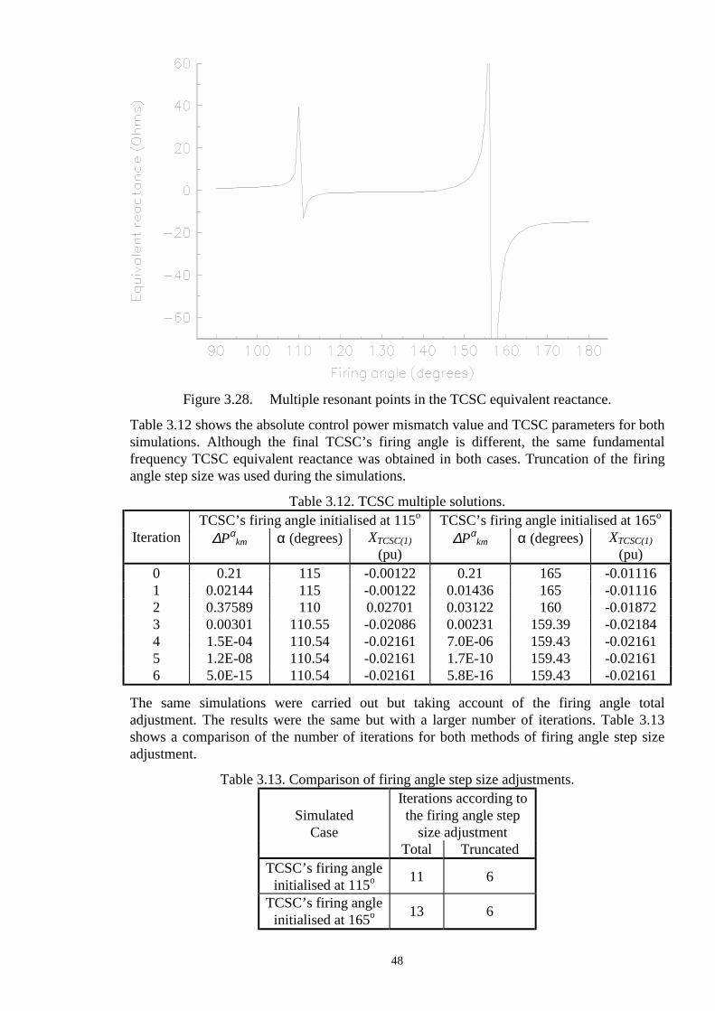
48
Figure 3.28. Multiple resonant points in the TCSC equivalent reactance.
Table 3.12 shows the absolute control power mismatch value and TCSC parameters for both simulations. Although the final TCSC’s firing angle is different, the same fundamental frequency TCSC equivalent reactance was obtained in both cases. Truncation of the firing angle step size was used during the simulations.
Table 3.12. TCSC multiple solutions. TCSC’s firing angle initialised at 115o TCSC’s firing angle initialised at 165o
Iteration ∆Pαkm α (degrees) XTCSC(1)
(pu) ∆Pα
km α (degrees) XTCSC(1) (pu)
0 0.21 115 -0.00122 0.21 165 -0.01116 1 0.02144 115 -0.00122 0.01436 165 -0.01116 2 0.37589 110 0.02701 0.03122 160 -0.01872 3 0.00301 110.55 -0.02086 0.00231 159.39 -0.02184 4 1.5E-04 110.54 -0.02161 7.0E-06 159.43 -0.02161 5 1.2E-08 110.54 -0.02161 1.7E-10 159.43 -0.02161 6 5.0E-15 110.54 -0.02161 5.8E-16 159.43 -0.02161
The same simulations were carried out but taking account of the firing angle total adjustment. The results were the same but with a larger number of iterations. Table 3.13 shows a comparison of the number of iterations for both methods of firing angle step size adjustment.
Table 3.13. Comparison of firing angle step size adjustments.
Simulated Case
Iterations according to the firing angle step
size adjustment Total Truncated
TCSC’s firing angle initialised at 115o
11
6
TCSC’s firing angle initialised at 165o
13
6

49
3.2.17 TCSC-FA control near a resonance point This Section illustrates by numeric example the advantages of truncated adjustments during iterative processes when the solution takes place near resonance points. The standard AEP30 bus system [16] was modified to include two TCSCs in order to control active power flow across branches 1-3 and 2-5 at 110 MWs and 62 MWs, respectively. The original power, flowing from nodes 1 to 3 and 2 to 5, were 83.15 MWs and 83.09 MWs, respectively. The maximum and minimum original reactive generators limits were modified to ± 400 MVARs. The initial conditions were specified 3 degrees away from the resonant point, i.e. 146o, for the TCSC embedded at branch 1-3, TCSC 1-3, and 139o for the TCSC compensating branch 2-5, TCSC 2-5. Both FACTS controllers were placed at the sending node of the branches, as shown in Figure 3.22. Simulations were carried out considering both full and truncated adjustments in the state variables. Tables 3.14 and 3.15 show the results obtained with both full and truncated adjustments on state variables during the backward substitution. These tables show the maximum absolute nodal power mismatches, and the regulated power across the branches. The firing angle value, in electrical degrees, is also shown.
Table 3.14. Mismatches and TCSC firing angle values with total adjustment of state variables.
Table 3.15. Mismatches and TCSC firing angle values with truncated adjustment
of state variables.
The TCSC controllers were activated after the first iteration. It is observed that in both simulations the TCSCs changed from capacitive to inductive operating regions and viceversa. However, large changes in the firing angle of TCSC 2-5 took place during the first few iterations, when the size of the increment was not truncated. Such large perturbations slow down convergence. TCSC operation near resonance points degrades Newton’s quadratic convergence. However, the algorithm has still shown to be very robust towards convergence.
Itera- Nodal power TCSC 1-3 TCSC 2-5 tions ∆P ∆Q ∆Pα
1-3 α1-3 ∆Pα2-5 α2-5
0 0.983 1.796 1.1 146.0 0.62 139.0 1 0.087 0.151 0.2121 146.0 0.1633 139.0 2 7.443 0.738 2.8425 140.78 7.443 153.0 3 6.839 1.183 0.2246 143.91 6.839 135.82 4 0.5734 0.2314 0.0040 144.17 0.5734 141.54 5 0.0292 0.0535 3.4E-5 144.17 0.0292 142.07 6 3.8E-4 9.8E-4 5.3E-8 144.17 3.7E-4 142.09 7 7.2E-8 2.3E-7 2.6E-9 144.17 6.8E-8 142.09 8 1E-14 1E-15 1E-15 144.17 1E-14 142.09
Itera- Nodal power TCSC 1-3 TCSC 2-5 tions ∆P ∆Q ∆Pα
1-3 α1-3 ∆Pα2-5 α2-5
0 0.983 1.796 1.1 146.0 0.62 139.0 1 0.087 0.151 0.2121 146.0 0.1633 139.0 2 2.629 0.178 2.631 141.0 1.658 144.0 3 0.3977 0.627 0.2029 143.93 0.3973 141.84 4 0.0409 0.0983 0.0042 144.17 0.0404 142.07 5 7.7E-4 0.0022 6.1E-5 144.17 7.4E-4 142.09 6 2.9E-7 1.1E-6 1.8E-8 144.17 2.7E-7 142.09 7 1E-14 1E-14 2E-14 144.17 2E-14 142.09
50
In order to show the effect of firing angle initial conditions when the solution is near to a resonance point, the same experiment describe above was simulated with initial conditions specified at 7 degrees away from the resonant point, i.e. 150o, for the TCSC 1-3, and 135o for TCSC 2-5. Table 3.16 shows the results obtained with truncated adjustments on state variables during the backward substitution while the case when no truncated adjustments were used failed to converge. This table shows the maximum absolute nodal power mismatches, and the absolute regulated power mismatch across the branches. The firing angle value, in electrical degrees, is also shown.
Table 3.16. Mismatches and TCSC firing angle values with truncated adjustment of state variables.
3.2.18 Power flow control by TCSC-FA in a real power system The longitudinal system described in Section 3.2.9, whose relevant part is shown in Figure 3.29, is used in order to show the full capabilities of the proposed TCSC-FA model. The parallel lines connected between nodes 30 and 32 are compensated at 40% with Mechanically Switched Series Capacitors (MSSC) when the system is operating on maximum demand. A Static Var Compensator (SVC) is installed at node 32 in order to regulate voltage magnitude. When both transmission lines operate without compensation, active power flows injected into node 32 through lines L1 and L2 are 476 MWs and 480 MWs, respectively. For the purpose of this Section, the MSSCs are replaced by TCSCs in order to control active power flow. The TCSCs have been set to control active power flow injected at node 32 at 540 MWs through each line. The TCSC electric parameters are those given in Section 3.2.1. The mismatch tolerance was set at 1E-12. The firing angles of both TCSCs were initialised at 150o. Convergence was obtained in 5 iterations. Table 3.17 shows the maximum absolute mismatches of the regulated powers injected at node 32. The firing angle value and the fundamental frequency equivalent impedance of the TCSC are also shown in this table. The values are given in degrees and pu, respectively. In order to validate the results, the same simulation was carried out with the VSC model. Convergence was obtained in 5 iterations. The same final values of TCSC’s equivalent reactance at fundamental frequency required to achieved the specified active power control were arrived at. Table 3.18 shows the absolute mismatches of the regulated powers injected at node 32 for the VSC model. The adjustment of the TCSC equivalent reactance at fundamental frequency is also shown in this table.
Itera- Nodal power TCSC 1-3 TCSC 2-5 tions ∆P ∆Q ∆Pα
1-3 α1-3 ∆Pα2-5 α2-5
0 0.9833 3.8671 1.1 150.0 0.62 135.0 1 0.0913 0.2541 0.2560 150.0 0.1895 135.0 2 2.2729 0.9299 0.5397 145.0 2.2696 139.98 3 0.1429 0.2393 0.0287 144.18 0.1428 142.00 4 0.0074 0.0186 4.5E-4 144.17 0.0072 142.08 5 2.7E-5 8.4E-5 1.3E-7 144.17 2.5E-5 142.09 6 3E-10 1.3E-9 5E-11 144.17 3E-10 142.09 7 1E-15 1E-17 1E-14 144.17 9E-17 142.09

51
Figure 3.29. Relevant part of the 2172-nodes system.
Table 3.17. Mismatch and parameter values of TCSC module.
Table 3.18. Mismatch and value of TCSC module modelled as VSC.
Itera- TCSC-L1 TCSC-L2 tions ∆Pα
L1 α XTCSC(1) ∆PαL2 α XTCSC(1)
0 5.4 150.00 -0.0183 5.4 150.0 -0.0183 1 0.406 150.00 -0.0183 0.338 150.0 -0.0183 2 1.012 146.82 -0.0298 0.808 147.13 -0.0279 3 0.084 148.00 -0.0232 0.063 148.16 -0.0232 4 1E-05 148.04 -0.0237 6E-05 148.18 -0.0232 5 2E-08 148.04 -0.0237 8E-09 148.18 -0.0232 6 5E-16 148.04 -0.0237 0.0 148.18 -0.0232
VSC-L1 VSC-L2 Iterations ∆Px
L1 XTCSC(1) ∆PxL2 XTCSC(1)
0 5.4 -0.01833 5.4 -0.01833 1 0.406 -0.01833 0.338 -0.01833 2 0.077 -0.02462 0.054 -0.02399 3 4.46E-04 -0.02368 3.26E-04 -0.02318 4 1.05E-05 -0.02374 7.80E-06 -0.02323 5 2.34E-10 -0.02374 1.01E-10 -0.02323 6 2.66e-15 -0.02374 8.88E-16 -0.02323
36 35 33
31
30
34
32
24 22
20
21
19
14
15
TCSC
TCSC
L1
L2

52
3.2.19 Comparison of VSC and TCSC-FA models. A comparative analysis of the robustness towards convergence of both TCSC models proposed in this thesis is presented in this Section. The numeric example presented in Section 3.2.13 was solved using both models. Table 3.19 shows the number of iterations required to converge when different initial conditions are chosen for the controller’s state variable. In order to compare these models, the VSC’s equivalent reactance was initialised at value obtained by substituting the TCSC-FA’s firing angle initial condition value in (3.36). The simulations were carried out considering both total and truncated adjustment of the state variables.
Table 3.19. Comparison of TCSC models for the 5 nodes system.
where * indicates that the TCSC violated one of its limits. NC indicates non-converge. A similar analysis was carried out for the case presented in Section 3.2.16, when the solution is very near to the resonant point. Table 3.20 shows the number of iteration required to converge for both models.
Table 3.20. Comparison of TCSC models for the 5 nodes system. Initial Conditions TCSC-FA Model VSC Model
Case TCSC TCSC-FA VSC Total Truncated adj. Total Truncated Model Model adj. 5o 30o adj. adj. 1 TCSC 1-3 146 -0.0366 8 7 8 6 7 TCSC 2-5 139 0.02604 2 TCSC 1-3 150 -0.0183 NC 7 9 6 7 TCSC 2-5 135 0.01184
From the results presented above it can be observed that the VSC model is more robust towards convergence than the TCSC-FA. However, as mentioned before, an additional iterative process is required to compute the TCSC’s firing angle, equation (3.36) is used to this end When firing angle initial condition is far from the solution, large truncated adjustments are better than small ones. The reason is that this controlled perturbation arrives faster at an optimal initial condition from which the quadratic convergence takes place. On the other hand, when the initial condition is given as proposed in this thesis, small steps of controlled adjustments on the firing angle increment give better convergence characteristics. The reason has been explained in Section 3.2.11. Both models give exactly the same fundamental frequency TCSC equivalent reactance required to achieve the specified active power control. Then, the feasible active power flow control analysis presented in Section 3.2.7 for the VSC model is also applicable to the TCSC-FA model.
Initial Conditions TCSC-FA iterations VSC iterations Cases TCSC-FA VSC Total Truncated adj. Adjustment
Model Model adjustment 5o 30o Total Truncated 1 145 -0.051825 6 6 6 6 6 2 150 -0.018339 5 5 5 5 5 3 155 -0.012739 7 6 7 5 5 4 160 -0.010718 8 7 7 5 5 5 165 -0.009855 12* 8 7 6 6 6 175 -0.009381 NC 10 6 6 6 7 180 -0.009365 NC 11 6 6 6

53
3.3 Phase Shifter The possibility of controlling both direction and magnitude of power flow in interconnected electric power systems using phase shifters was recognised as early as 1930s [17]. Their effectiveness in increasing the utilisation of bulk power system facilities is today widely acknowledged [18]. An schematic representation of a phase shifter is shown in Figure 3.30 [2]. Both electronically-controlled and mechanically-controlled phase-shifters are capable of re-directing power flows by locally altering the voltage angle difference imposed on the device by networks conditions.
(a) Mechanical-Controlled Tap Changer.
(b) Thyristor-Controlled Tap Changer.
Figure 3.30. Phase shifter transformer.
∆
Y
Y-Y
THYRISTOR SWITCHING NETWORK
Vsen Vrec
VE
SERIES TRANSFORMER
SHUNT TRANSFORMER
Vq
∆
Y
Y-Y MECHANICAL
LOAD TAP CHANGER
Vsen Vrec
VE
SERIES TRANSFORMER
SHUNT TRANSFORMER
Vq

54
The phase shift is achieved by adding or subtracting a variable voltage component Vq to the voltage at the phase shifter’s sending node. Both voltages are in quadrature as shown in Figure 3.31. The quadrature voltage component is obtained from the shunt connected three phase transformer, called exciting transformer, and it is inserted into the system via the series connected transformer, called booster transformer. A mathematical demonstration of how this variable quadrature voltage component is generated is shown in Appendix III.
Figure 3.31. Phasor diagram showing the phase-shifting mechanism.
Until recently, mechanically controlled on-load tap changers have been used to change the value of the quadrature component voltage in order to obtain the desired variation of the voltage phase angle. Recently, based on the development of the high power thyristor technologies, the feasibility of using thyristor controlled phase shifters as a means of providing rapid and nearly continuous adjustment of the quadrature voltage component magnitude Vq has been demonstrated [18-20].
3.3.1 Phase Shifter Steady-State Power Flow Model A new and more general model for the PS transformer is described in this Section. It is derived from a two winding, single phase transformer model with complex taps on both primary and secondary windings. The magnetising branch of the transformer, which under saturated conditions becomes non-linear, is included to account for the core losses. The model is based on the physical representation of the transformer shown in Figure 3.32 (a) while the schematic equivalent circuit of the transformer is shown in Figure 3.32 (b).
Figure 3.32. A two winding transformer. (a) Schematic representation.
Vsen
Vq
Vrec φ
Rp Xp Rs Xs Vs Vp
Ip Is
Is I 1 ′′′′
Vp
Tv : 1
φtv
Ip Zp
I 1 V 1
Ti : 1
I
Bo Go
V 0
0
φuv
1 : Uv
I 2 ′′′′
1 : Ui
Vs Zs I 2 V 2
(a)
(b)

55
(b) Equivalent circuit. The primary winding is represented as an ideal transformer having complex tap ratios Tv:1 and Ti:1 in series with the impedance Zp, where Tv=Ti
*=Tv∠ φtv. The * denotes the conjugate operation. Also, the secondary winding is represented as an ideal transformer having complex tap ratios Uv:1 and Ui :1 in series with the impedance Zs , where Uv=Ui
* =Uv ∠ φuv. The transfer admittance matrix relating the primary voltage Vp and current Ip to the secondary voltage Vs and current Is in the two-winding transformer can be determined by considering the current I1 across the impedances Zp and the current I2 across the impedance Zs.
( ) ( )I
V VZ
V T VZ
I1p 1
p
p v 0
pp=
−=
−= (3.61)
( ) ( )
IV V
ZV U V
ZI2
s 2
s
s v 0
ss=
−=
−= (3.62)
The current I0 across the iron core as a function of currents I1
, and I 2, is,
0 = + − = + −I I I T I U I I1
'2'
0 i 1 i 2 0 (3.63) or
0 = − + + +
−
∗ ∗T VZ
TZ
UZ
Y V U VZ
v p
p
v2
p
v2
s0 0
v s
s
(3.64)
where
Y0 = +G jB0 0 (3.65) Putting equations (3.61), (3.62) and (3.64) in matrix form,
I
I
ZTZ
TZ Z Z
YUZ
UZ
1Z
VVV
v
p
v
p p s0
v
s
v
s s
p
0
s
p
s
p
v2
v2
0
1 0
T U
0
=
−
− + + −
−
∗ ∗
(3.66)
Equation (3.66) represents the transformer shown in Figure 3.32. It is possible, however, to find a reduced equivalent matrix that still models the transformer correctly whilst retaining only the external nodes p and s. This is done by means of a gaussian elimination,
II Z Z Z Z Y
Z Y T UT U Z Y
VV
p
s s p p s 0
s 0 v v
v v p 0
p
s
= + +
+ −− +
∗
∗
1T U
UTv
2v2
v2
v2 (3.67)
Equation (3.67) can be expressed as,
II
VV
p
s
p
s
=
+
G GG G
jB BB B
pp ps
sp ss
pp ps
sp ss (3.68)
where

56
G F U R F RApp
v=+ +1 1 2 2
2
2( ) (3.69)
BF R F U R
Appv=
− +1 2 2 12
2( ) (3.70)
G F T R F RAss
v=+ +1 3 2 4
2
2( ) (3.71)
BF R F T R
Assv=
− +1 4 2 32
2( ) (3.72)
( ) ( )( )
GT U F F
Apsv v=
− +1 1 2 12
cos sinφ φ (3.73)
( ) ( )( )
BT U F F
Apsv v=
−2 1 1 12
cos sinφ φ (3.74)
( ) ( )( )
GT U F F
Aspv v=
− +1 2 2 22
cos sinφ φ (3.75)
( ) ( )( )
BTU F F
Aspv v=
−2 2 1 22
cos sinφ φ (3.76)
F T R U R Rs v p eq1 2 2
1= + + (3.77)
F T X U X Xv s v p eq2 2 21= + + (3.78)
A F F2 1 22 2= + (3.79)
( ) ( )R R R X X G R X R X Beq p s p s o p s s p o1 = − − + (3.80)
( ) ( )X R R X X B R X R X Geq p s p s o p s s p o1 = − + + (3.81)
R R G X Bs o s o1 = − (3.82)
R R B X Gs o s o2 = + (3.83)
R R G X Bp o p o3 = − (3.84)
R R B X Gp o p o4 = + (3.85)
φ φ φ1= −tv uv (3.86)
φ φ φ2 = −uv tv (3.87)
The power injection equations of a PS transformer are:
( ) ( )( )P V G V V G Bp p pp p s ps p s ps p s= + − + −2 cos sinθ θ θ θ (3.88)
( ) ( )( )Q V B V V G Bp p pp p s ps p s ps p s= − + − − −2 sin cosθ θ θ θ (3.89)
( ) ( )( )P V G V V G Bs s ss s p sp s p sp s p= + − + −2 cos sinθ θ θ θ (3.90)
( ) ( )( )Q V B V V G Bs s ss s p sp s p sp s p= − + − − −2 sin cosθ θ θ θ (3.91)

57
The partial derivatives of power equations with respect to the phase shifter angle in primary winding of the transformer are:
( ) ( )( )∂∂φ
θ θ θ θP
V V G Bp
tvp s ps p s ps p s= − − −sin cos (3.92)
( ) ( )( )∂∂φ
θ θ θ θP
V V G Bs
tvs p sp s p sp s p=− − − −sin cos (3.93)
( ) ( )( )∂∂φ
θ θ θ θQ
V V G Bp
tvp s ps p s ps p s=− − + −cos sin (3.94)
( ) ( )( )∂∂φ
θ θ θ θQ
V V G Bs
tvs p sp s p sp s p= − + −cos sin (3.95)
The partial derivatives power equations with respect to the phase shifter angle in secondary winding of the transformer are:
( ) ( )( )∂∂φ
∂∂φ
θ θ θ θP P
V V G Bp
uv
p
tvp s ps p s ps p s=− =− − − −sin cos (3.96)
( ) ( )( )∂∂φ
∂∂φ
θ θ θ θP P
V V G Bs
uv
s
tvs p sp s p sp s p=− = − − −sin cos (3.97)
( ) ( )( )∂∂φ
∂∂φ
θ θ θ θQ Q
V V G Bp
uv
p
tvp s ps p s ps p s= − = − + −cos sin (3.98)
( ) ( )( )∂∂φ
∂∂φ
θ θ θ θQ Q
V V G Bs
uv
s
tvs p sp s p sp s p=− =− − + −cos sin (3.99)
Assuming that the two-winding transformer is controlling the active power flowing from terminal p to terminal s, the solution of the PS power flow equations by Newton’s method requires an augmented Jacobian. This is necessary since the active power flowing from node p to node s, Pps, is not a standard control variable in the conventional formulation of the Newton-Raphson load flow. In this situation, φtv or φuv, enters as an extra state variable. The set of linearised power flow equations for the phase shifter shown in Figure 3.32 is,
∆
∆
∆
∆
∆
P
P
Q
Q
P
P P PV
VPV
VP
P P PV
V PV
V P
Q Q QV
VQV
VQ
Q Q QV
V QV
V Q
P P
p
s
p
s
ps
p
p
p
s
p
pp
p
ss
p
s
p
s
s
s
pp
s
ss
s
p
p
p
s
p
pp
p
ss
p
s
p
s
s
s
pp
s
ss
s
ps psφφ φ
∂∂θ
∂∂θ
∂∂
∂∂
∂∂φ
∂∂θ
∂∂θ
∂∂
∂∂
∂∂φ
∂∂θ
∂∂θ
∂∂
∂∂
∂∂φ
∂∂θ
∂∂θ
∂∂
∂∂
∂∂φ
∂∂ φ
∂
=
∂ φ∂∂ φ
∂∂ φ
∂∂φ
θ
θ
φφ φ φP P P
V V
V V
ps ps ps
p
s
p p
s s
∆
∆
∆
∆
∆
(3.100)

58
Generalised Newton equations for the phase shifter are given in equation (3.101), where the variable angle φ is taken to be a state variable.
∆
∆
∆
∆
∆
∆
P
Q
P
P PV
V P
Q QV
VQ
P PV
VP
V V
ps ps ps psφ φ φ φ
∂∂ θ
∂∂
∂∂ φ
∂∂ θ
∂∂
∂∂ φ
∂∂ θ
∂∂
∂∂ φ
θ
φ
=
(3.101)
It must be noted that ∂
∂ φ
φPps
is a diagonal matrix where,
∂∂ φ
∂∂ φ
∂∂ θ
φ φP P Pps
tv
ps
uv
p
s
= − = (3.102)
and the order of the matrix equals the number of PSs in the network. The active power flow mismatch vector for the PS is,
∆ P P Pps psreg
pscalφ φ φ= −, , (3.103)
Moreover, the vector of incremental changes in phase angle is,
∆φ φ φ= −+i i1 (3.104) After each iteration i the phase shifter controller must be updated according to equation (3.105),
φ φ φ( ) ( ) ( )i i i+ = +1 ∆ (3.105)
3.3.2 PS Initialisation and adjusted solutions. In contrast with the VSC, zero voltage angle initialisation introduces no discontinuities in the PS whose primary and secondary phase angles are initialised at zero degrees. An arbitrary value is assigned to tap magnitudes Tv and Uv, which remain fixed during the iterative process. The revision of limits of the PS’s state variable starts after the power mismatch equation at the controlled branch is within a specified tolerance. If limits violation takes place, the phase shifter angle is fixed at the offending limit. In this situation no further attempts are made at regulating the flow of active power across the PS for the remaining of the iterative process. A maximum step size adjustment of ± 30o has been chosen for phase shifter angles.
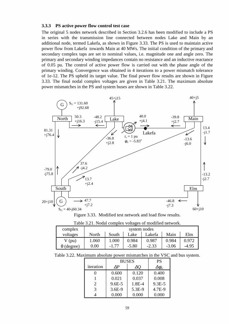
59
3.3.3 PS active power flow control test case The original 5 nodes network described in Section 3.2.6 has been modified to include a PS in series with the transmission line connected between nodes Lake and Main by an additional node, termed Lakefa, as shown in Figure 3.33. The PS is used to maintain active power flow from Lakefa towards Main at 40 MWs. The initial condition of the primary and secondary complex taps are set to nominal values, i.e. magnitude one and angle zero. The primary and secondary winding impedances contain no resistance and an inductive reactance of 0.05 pu. The control of active power flow is carried out with the phase angle of the primary winding. Convergence was obtained in 4 iterations to a power mismatch tolerance of 1e-12. The PS upheld its target value. The final power flow results are shown in Figure 3.33. The final nodal complex voltages are given in Table 3.21. The maximum absolute power mismatches in the PS and system buses are shown in Table 3.22.
Figure 3.33. Modified test network and load flow results.
Table 3.21. Nodal complex voltages of modified network.
Table 3.22. Maximum absolute power mismatches in the VSC and bus system.
complex system nodes voltages North South Lake Lakefa Main Elm V (pu) 1.060 1.000 0.984 0.987 0.984 0.972
θ (degree) 0.00 -1.77 -5.80 -2.33 -3.06 -4.95
BUSES PS iteration ∆P ∆Q ∆φtv
0 0.600 0.120 0.400 1 0.021 0.037 0.008 2 9.6E-5 1.8E-4 9.3E-5 3 3.6E-9 5.3E-9 4.7E-9 4 0.000 0.000 0.000
45+j15
13.4 -j1.7
-13.2 -j2.7
60+j10
Main
Elm
-39.8 +j2.7
40.0 +j4.1
-46.8 -j7.3
-13.6 -j6.0
40+j5
North
Lake
South
-48.2 -j15.4
50.3 +j16.3
81.31 +j76.4
-79.0 -j75.8
47.7 +j7.2
-36.8 +j2.8
37.6 -j4.2
13.7 +j2.4
20+j10
G
G
SG = 40-j60.34
SG = 131.60 +j92.68
tv = 1 pu φtv = -5.83o
Lakefa
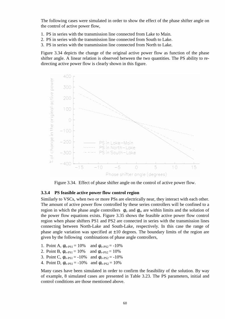
60
The following cases were simulated in order to show the effect of the phase shifter angle on the control of active power flow, 1. PS in series with the transmission line connected from Lake to Main. 2. PS in series with the transmission line connected from South to Lake. 3. PS in series with the transmission line connected from North to Lake. Figure 3.34 depicts the change of the original active power flow as function of the phase shifter angle. A linear relation is observed between the two quantities. The PS ability to re-directing active power flow is clearly shown in this figure.
Figure 3.34. Effect of phase shifter angle on the control of active power flow.
3.3.4 PS feasible active power flow control region Similarly to VSCs, when two or more PSs are electrically near, they interact with each other. The amount of active power flow controlled by these series controllers will be confined to a region in which the phase angle controllers φtv and φuv are within limits and the solution of the power flow equations exists. Figure 3.35 shows the feasible active power flow control region when phase shifters PS1 and PS2 are connected in series with the transmission lines connecting between North-Lake and South-Lake, respectively. In this case the range of phase angle variation was specified at ±10 degrees. The boundary limits of the region are given by the following combinations of phase angle controllers, 1. Point A, φtv-PS1 = 10% and φtv-PS2 = -10% 2. Point B, φtv-PS1 = 10% and φtv-PS2 = 10% 3. Point C, φtv-PS1 = -10% and φtv-PS2 = -10% 4. Point D, φtv-PS1 = -10% and φtv-PS2 = 10% Many cases have been simulated in order to confirm the feasibility of the solution. By way of example, 8 simulated cases are presented in Table 3.23. The PS parameters, initial and control conditions are those mentioned above.

61
Figure 3.35. Feasible active power control region of a phase shifter .
Table 3.23. Feasibility of active power control by phase shifters.
Final phase angle values (degrees)
Active power flow North to Lake (MWs)
Active power flow South to Lake (MWs)
case iterations φtv-PS1 φtv-PS2 specified final specified final 1 4 -5.64 -3.62 50 50 30 30 2 4 8.70 8.78 - 5 - 5 70 70 3 4 -7.60 6.62 70 70 -15 -15 4 7 10.0* 0.96 - 5 2.2 30 30 5 7 -10.0* -4.87 70 66.7 30 30 6 6 5.2 10.0* 30 30 -20 -13.5 7 7 -7.87 -10.0* 50 50 70 54 8 9 10.0* 10.0* -10 13.8 -30 -7.6
All active power flows specified inside the feasible active power flow region have been successfully upheld by the phase shifters (cases 1-3). For power flows specified outside the PSs will violate limits, which is indicated by the symbol *. The size of the feasible active power control region depends on the phase angle controller range. Figure 3.36 shows a comparison of the size of the feasible active power control region for three different ranges of the phase shifters connected in series with transmission lines North-Lake and South-Lake. As the phase angle controller range increases, the size of the region increases. These ranges are, 1. CASE A ± 5o for both phase shifters. 2. CASE B ± 10o for both phase shifters. 3. CASE C ± 15o for both phase shifters. Figure 3.37 depicts the feasible active power flow region for PSs and VSCs. Letters A, B and C correspond to the cases mentioned above. Letters D, E and F correspond to the series compensation cases mentioned in Section 3.2.6, i.e. 40%, 60% and 80% of series compensation, respectively.

62
Figure 3.36. Size of the feasible active power control region as function of phase angle
controller range.
Figure 3.37. Comparison of the feasible active power control region size for PSs and VSCs. For these cases, the region of feasible active power flow control is much larger for phase shifters than for series variable compensators. For the VSCs, the size of these region will always be limited by the electrical length of the transmission line to which they are connected. Moreover, the active power flow can not be re-directed. In the case of PSs, the size of the feasible active power control region is affected by the exciting and booster transformer impedances since they determine the phase angle required to maintain a specified active power flow.

63
3.3.5 Effect of PS’s impedance on phase angle value The booster and exciting transformer impedances always appears in series with the transmission line in which it is connected. However, the equivalent exciting transformer impedance seen by the transmission line varies with the quadrature voltage component value, i.e. phase shifter angle [21]. The above implies a close relation between the PSs transformer impedances and the phase angle value required to maintain an active power flow at a specified target. The case presented in Section 3.3.3 and illustrated in Figure 3.33 is used to demonstrate this rational. The active power flow to be controlled by the PS connected in series with the transmission line Lake-Main has been specified at -40 MWs and 40 MWs. In both cases, the primary and secondary winding impedances have been taken to contain no resistance. The following values of reactance have been used, CASE A Xp = Xs = 0.5 pu CASE B Xp = Xs = 0.4 pu CASE C Xp = Xs = 0.3 pu CASE D Xp = Xs = 0.2 pu CASE E Xp = Xs = 0.1 pu CASE F Xp = Xs = 0.05 pu CASE G Xp = Xs = 0.01 pu CASE H Xp = Xs = 0.001 pu Figure 3.38 shows the phase shifter angle required to satisfy the active power target value as function of phase shifter impedances. Two graphs are presented. The solid line corresponds to the actual PS reactance profile as function of the PS angle. The long dash line represents the same result but fitted to a cubic spline function.
Figure 3.38. Phase shifter angle vs. impedance.
Since the amount of active power transmitted through a PS is inversely proportional to its reactance, a high PS impedance increases the phase shifter angle value needed to achieve the active power flow control. An adverse consequence of a high impedance is that the PS reactive losses can be quite significant. Figure 3.39 shows the PS reactive power losses as a function of its impedances for the cases simulated above.

64
Figure 3.39. PS reactive power losses as a function of winding reactances.
When the PS controls active power flow at 40 MWs from Lake to Main, the system supplies reactive power at both terminals of the PS for cases A, B, C and D. For the remaining cases, reactive power is supplied via Lakefa bus. When the PS controls active power flow at -40 MWs from Lake to Main, the system supplies reactive power at both terminals of the PS in cases A and B. For the remaining cases, reactive power is supplied via Lake bus. Figures 3.40 (a) and 3.40 (b) depict the profiles of total reactive power generated by synchronous machines and reactive power transmission losses, respectively. Both profiles follow the same pattern which confirm the energy balance taking place in the power system, i.e. reactive power generation equals reactive power transmission losses plus demand.
(a) Reactive power generation. (b) Reactive power transmission losses.
Figure 3.40. Reactive power profile as function of PS reactances. Figures 3.41 (a) and 3.41 (b) depict the profiles of total active power generation and transmission losses, respectively.

65
(a) Generation. (b) Transmission losses.
Figure 3.41. Active power profile as function of PS reactances. Figures 3.42 and 3.43 depict active power flows throughout the transmission system. Since the profile is a straight line, there exist little effect of the PS reactance on active power flows.
Figure 3.42. Active power profile in transmission lines for PS controlling at 40 MWs.
Figure 3.43. Active power profile in transmission lines for PS controlling at -40 MWs.

66
Figures 3.44 and 3.45 depict the reactive power flow throughout the transmission system. Here the effects of PS reactance on reactive power magnitude and direction are very considerable.
Figure 3.44. Reactive power profile in transmission lines for PS controlling at 40 MWs.
Figure 3.45. Reactive power profile in transmission lines for PS controlling at -40 MWs.

67
3.3.6 Active power flow control by PSs and VSCs The standard AEP 57-bus system [12] has been modified and used to show the ability of the algorithm to converge to very tight tolerances for cases in which large number of controllable branches are embedded in the network. Ten conventional transformers were modified to be phase shifters and four series variable compensators were embedded in the network. The original active power flows are presented in Table 3.24. The solution of this base case was obtained in 5 iterations.
Table 3.24. Active power flows on relevant electric component of AEP 57-bus system.
The parameters of the phase shifting transformer embedded in the network are presented in Table 3.25. All other parameters not shown are set to zero. The active power control is carried out with the primary phase angle control. The VSCs were initialised at 50% of transmission line series inductive reactance values.
Table 3.25. Two-winding Phase Shifter parameters.
Table 3.26 shows the specified active power flowing through the FACTS devices embedded in the network as well as their final parameters. The active power flowing across transmission lines NOD3-NOD15, NOD9-NOD13, NOD4-NOD5 and NOD45-NOD44 are controlled by series compensators VCS 3-15, VCS 9-13, VCS 4-5 and VCS 45-44, respectively.
Electric
Components
Original power flows
(MW) Transformer t4-18 14 Transformer t20-21 1.08 Transformer t24-25 7.05 Transformer t24-26 -10.53 Transformer t7-29 60 Transformer t34-32 7.46 Transformer t11-41 9.18 Transformer t13-49 32.44 Transformer t40-56 3.4 Transformer t39-57 3.85
Line NOD3-NOD15 33 Line NOD9-NOD13 2.3 Line NOD4-NOD5 13 Line NOD45-NOD44 37
Phase Primary Tap Secondary Tap Shifters Tv (pu) φtv Tu (pu) φtu Xs (pu) PS 4-18 0.970 0.0 1.0 0.0 0.5550 PS 20-21 1.043 0.0 1.0 0.0 0.7767 PS 24-25 1.000 0.0 1.0 0.0 1.1820 PS 24-26 1.043 0.0 1.0 0.0 0.0473 PS 7-29 0.967 0.0 1.0 0.0 0.0648 PS 34-32 0.975 0.0 1.0 0.0 0.9530 PS 11-41 0.955 0.0 1.0 0.0 0.7490 PS 13-49 0.895 0.0 1.0 0.0 0.1910 PS 40-56 0.958 0.0 1.0 0.0 1.1950 PS 39-57 0.980 0.0 1.0 0.0 1.3550

68
Table 3.26. AEP 57-bus system with ten phase-shifters and four series compensators.
The negative sign in VCSs indicates that the FACTS controller is operating in its capacitive region in order to achieve the target value, i.e. the transmission line has been capacitively compensated. Convergence was obtained in 7 iterations and the FACTS devices successfully controlled their specified value Figure 3.46 depicts the behaviour of the maximum absolute power mismatches for the active power in each FACTS controller and the nodal active and reactive powers at system buses as function of iterations number.
Figure 3.46. Mismatches of nodal powers and FACTS devices for the AEP 57 bus system with embedded PSs and VSCs.
Electric devices
Controlled power flows
(MW)
Phase Angle φtv
(degrees)
% of series compensation
(pu) PS 4-18 20.00 -4.37 PS 20-21 5.00 -7.41 PS 24-25 10.00 -4.15 PS 24-26 -15.53 0.76 PS 7-29 70.09 -3.58 PS 34-32 7.46 -3.45 PS 11-41 19.18 -8.50 PS 13-49 40.44 -1.87 PS 40-56 3.45 -4.28 PS 39-57 6.85 -7.30
VSC 3-15 24.00 60.43 % VSC 9-13 4.00 3.48 % VSC 4-5 18.00 -26.60 % VSC 45-44 43.00 -75.05 %

69
The modified AEP57 network has been used in order to show the interaction between PSs and VSCs. 14 simulations were carried out with one FACTS controller deactivated at the time. When a PS is deactivated, it is considered as a conventional transformer with the parameters given in the base case. On the other hand, the VSC deactivated is not embedded in the network, i.e. the transmission line is uncompensated. The initial conditions for the active controllers and their control variables are as above. Table 3.27 shows the FACTS controllers final parameters per simulation
Table 3.27. FACTS controllers interactions.
CA Phase Shifter Angles (degrees) VSC (%)
SE 1 2 3 4 5 6 7 8 9 10 1 2 3 4
C1 DA -5.5 -4.1 0.8 -3.6 -3.5 -8.5 -1.9 -4.3 -7.3 64 3.5 -26 -75
C2 -3.4 DA -4.1 1.3 -3.7 -3.5 -8.5 -2.2 -3.8 -6.8 22 -20 -41 -91
C3 -4.4 -7.4 DA 0.8 -3.6 -1.4 -8.5 -1.9 -4.3 -7.3 61 3.4 -27 -75
C4 -4.4 -7.5 -4.1 DA -4.0 -3.3 -8.5 -1.8 -4.3 -7.4 62 10 -27 -73
C5 -4.4 -7.5 -4.2 4.0 DA -3.5 -8.5 -1.9 -4.3 -7.3 70 -4.7 -33 -75
C6 -4.4 -7.4 -3.3 0.5 -3.6 DA -8.5 -1.9 -4.2 -7.2 60 3.4 -27 -75
C7 -4.4 -7.4 -4.1 0.8 -3.6 -3.5 DA -1.9 -0.7 -3.7 61 3.4 -27 -75
C8 -4.4 -8.1 -4.2 0.1 -3.6 -3.5 -8.5 DA -5.0 -8.0 60 -33 -26 -50
C9 -4.4 -7.1 -4.1 1.1 -3.6 -3.1 -7.5 -2.1 DA -5.1 57 -10 -25 -86
C10 -4.4 -6.9 -4.1 1.3 -3.6 -3.1 -7.1 -2.2 -1.1 DA 55 -17 -24 -91
C11 -4.4 -6.8 -4.2 0.9 -3.7 -3.5 -8.5 -1.9 -4.2 -7.2 NI -56 -50 -72
C12 -4.4 -7.4 -4.1 0.8 -3.6 -3.5 -8.5 -1.9 -4.3 -7.3 60 NI -27 -75
C13 -4.4 -7.5 -4.1 0.7 -3.6 -3.5 -8.5 -1.9 -4.3 -7.3 66 -2.0 NI -75
C14 -4.4 -8.2 -4.1 0.1 -3.6 -3.4 -8.5 -1.3 -5.0 -8.0 49 -4.8 -24 NI Figures 3.47 and 3.48 depict the behaviour of the PSs and VSCs final values for the cases given in Table 3.27. Any change in the network produces a re-distribution of active and reactive power flows throughout the network. As a consequence of this, the FACTS controller final values change in order to satisfy the specified active power flow target. In the cases simulated, these changes are function of the electric interaction between the FACTS controller removed from the network and the remaining active controllers. Critical changes are observed in VSCs. From Table 3.11 it is clear that the most sensitive FACTS controller is VSC2. This controller changes from the capacitive to the inductive region regardless of the FACTS controlled deactivated. When VSC1 is deactivated, VSC2 supplies 56% of capacitive compensation, case C11. On the other hand, when PS 24-26 is
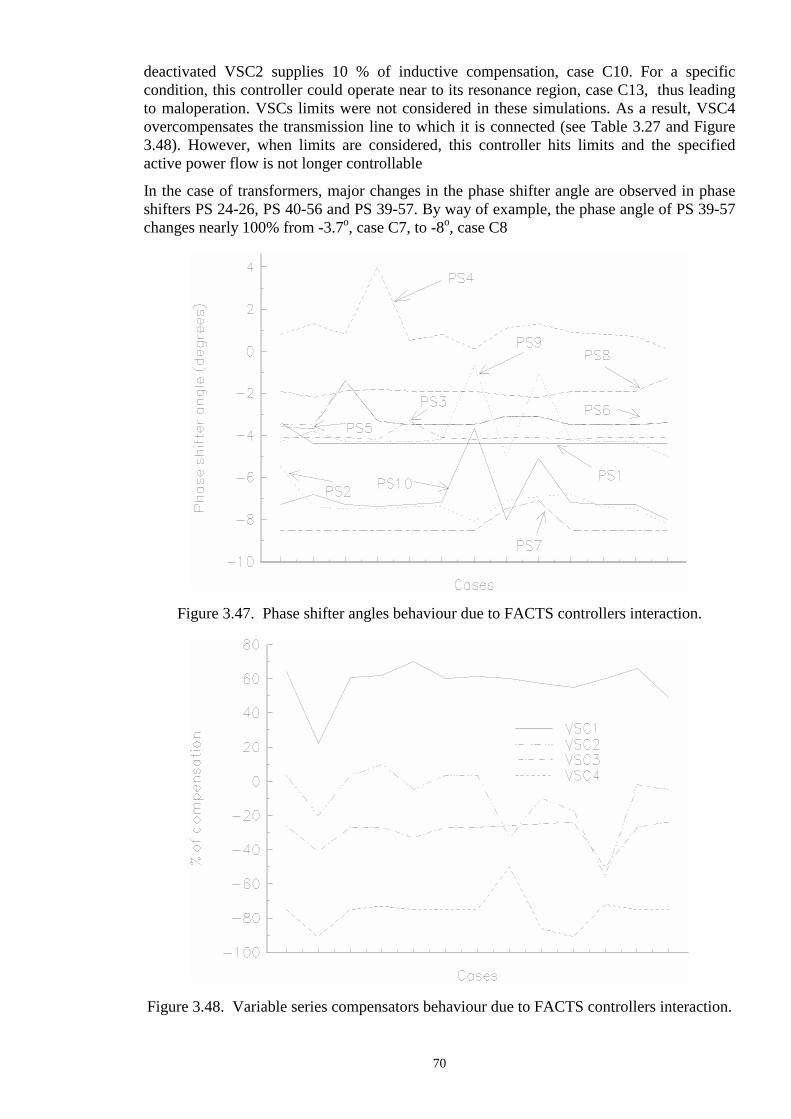
70
deactivated VSC2 supplies 10 % of inductive compensation, case C10. For a specific condition, this controller could operate near to its resonance region, case C13, thus leading to maloperation. VSCs limits were not considered in these simulations. As a result, VSC4 overcompensates the transmission line to which it is connected (see Table 3.27 and Figure 3.48). However, when limits are considered, this controller hits limits and the specified active power flow is not longer controllable In the case of transformers, major changes in the phase shifter angle are observed in phase shifters PS 24-26, PS 40-56 and PS 39-57. By way of example, the phase angle of PS 39-57 changes nearly 100% from -3.7o, case C7, to -8o, case C8
Figure 3.47. Phase shifter angles behaviour due to FACTS controllers interaction.
Figure 3.48. Variable series compensators behaviour due to FACTS controllers interaction.

71
3.3.7 Active power flow control in a real power system The case presented in Section 3.2.6, in which 9 FCSCs were replaced by VSCs is further modified, 6 conventional transformers are substituted by phase shifters. The original and modified active power flows across transformers and PSs are shown in Figure 3.49. Figure 3.50 depicts the original and specified active power flows across the fixed series compensators and VSCs, respectively. The base case converged in 6 iterations. The solution of the modified network with embedded FACTS devices was found in 7 iterations. The controllers upheld their target values.
Figure 3.49. Comparison of active power flow in conventional transformers and PSs.
Figure 3.50. Comparison of active power flow in FCSCs and VSCs.

72
3.4 Interphase Power Controller The Interphase Power Controller (IPC) is a newly developed device intended for the control of power flows in AC networks. For steady-state purposes, the IPC’s main function is to provide constant active power flow at its terminals. In its more general configuration, the IPC consists of two parallel reactive branches, one inductive and one capacitive. Each branch is subjected to separately phase-shifted voltages [22-24], as shown in Figure 3.51.
Figure 3.51. General IPC representation.
The IPC can take many forms according to the way in which the internal voltages are phase shifted [22-24]. For High-Voltage applications, efficient IPCs are based on the use of phase-shifting transformers [25] as shown in Figure 3.52. The transmitted power is controlled by changing either the internal phase-shifting angles or the reactance values.
Figure 3.52. Schematic model of the IPC.
For some specific applications, a particular IPC model is used in which the phase shifting voltage is only applied to one branch, generally the inductive one [25]. This schematic representation is given in Figure 3.53. The capacitive branch can be either fix or variable.
Figure 3.53. Schematic model of the IPC with one PS.
k m
P km reg2
P km reg1
m
P km reg2
k
P km reg1
PHASE
SHIFTING
k m
P km reg2
P km reg1
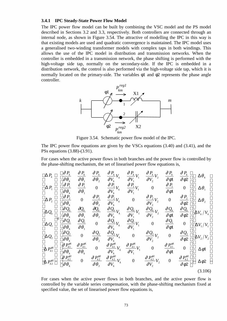
73
3.4.1 IPC Steady-State Power Flow Model The IPC power flow model can be built by combining the VSC model and the PS model described in Sections 3.2 and 3.3, respectively. Both controllers are connected through an internal node, as shown in Figure 3.54. The attractive of modelling the IPC in this way is that existing models are used and quadratic convergence is maintained. The IPC model uses a generalised two-winding transformer models with complex taps in both windings. This allows the use of the IPC model in distribution and transmission networks. When the controller is embedded in a transmission network, the phase shifting is performed with the high-voltage side tap, normally on the secondary-side. If the IPC is embedded in a distribution network, the control is also performed via the high-voltage side tap, which it is normally located on the primary-side. The variables φ1 and φ2 represents the phase angle controller.
Figure 3.54. Schematic power flow model of the IPC.
The IPC power flow equations are given by the VSCs equations (3.40) and (3.41), and the PSs equations (3.88)-(3.91). For cases when the active power flows in both branches and the power flow is controlled by the phase-shifting mechanism, the set of linearised power flow equations is,
∆
∆
∆
∆
∆
∆
∆
∆
P
P
P
Q
Q
Q
P
P
P P P PV
V PV
V PV
V P P
P P PV
V PV
V P
P P P
k
k
k
k
k
k
k k k
kk
k k k k
k kk
k
1
2
1
2
11
22
1 2 11
22
1 1
1
1 1
11
1
2 2
2
2
1 2
0 01
0
0
φ
φ
∂∂θ
∂∂θ
∂∂θ
∂∂
∂∂
∂∂
∂∂ φ
∂∂ φ
∂∂θ
∂∂θ
∂∂
∂∂
∂∂ φ
∂∂θ
∂∂θ
∂∂
=
VV P
VV P
Q Q Q QV
V QV
V QV
V Q Q
Q Q QV
V QV
V Q
Q Q QV
V QV
V Q
P P PV
V P
kk
k
k
k k k
kk
k k k k
k kk
k kk
k
k
k
k
k
kk
k
0 02
1 2
0 01
0
0 0 02
0
2
22
2
1 2 11
22
1 1
1
1 1
11
1
2 2
2
2 2
22
2
11
11
11
∂∂
∂∂ φ
∂∂θ
∂∂θ
∂∂θ
∂∂
∂∂
∂∂
∂∂ φ
∂∂ φ
∂∂θ
∂∂θ
∂∂
∂∂
∂∂ φ
∂∂θ
∂∂θ
∂∂
∂∂
∂∂ φ
∂∂θ
∂∂θ
∂∂
∂φ φ φ11
11
11
22
22
2
22
22
22
22
1
2
1 1
2 2
01
0
0 0 02
1
2
φ φ
φ φ φ φ φ∂
∂∂ φ
∂∂θ
∂∂θ
∂∂
∂∂
∂∂ φ
θ
θ
θ
φ
φ
VV P
P P PV
V PV
V P
V V
V V
V V
k
k
k
k k
kk
k k
k
k k
∆
∆
∆
∆
∆
∆
∆
∆
(3.106) For cases when the active power flows in both branches, and the active power flow is controlled by the variable series compensation, with the phase-shifting mechanism fixed at specified value, the set of linearised power flow equations is,
k m
P km reg2
P km reg1
1
2
φ1
φ2
X1
X2

74
∆
∆
∆
∆
∆
∆
∆
∆
P
P
P
Q
Q
Q
P
P
P P P PV
VPV
VPV
VPX
XPX
X
P P PV
VPV
VPX
X
P P
k
k
kX
kX
k
k
k k k
kk
k k k k
k kk
k
1
2
1
2
11
22
1 2 11
22
1 1
1
1 1
11
1
2 2
11
22
0 01
1 0
0
=
∂∂θ
∂∂θ
∂∂θ
∂∂
∂∂
∂∂
∂∂
∂∂
∂∂θ
∂∂θ
∂∂
∂∂
∂∂
∂∂θ
∂∂θ
∂∂
∂∂
∂∂
∂∂θ
∂∂θ
∂∂θ
∂∂
∂∂
∂∂
∂∂
∂∂
∂∂θ
∂∂θ
∂∂
∂∂
∂∂
∂∂θ
∂∂θ
∂∂
∂∂
∂∂
∂∂θ
∂∂θ
2
2 2
22
1 2 11
22
1 1
1
1 1
11
1
2 2
2
2 2
22
11
11
0 02
2
11
22
0 01
1 0
0 0 02
2
PV
VPV
VPX
X
Q Q Q QV
VQV
VQV
VQX
XQX
X
Q Q QV
VQV
VQX
X
Q Q QV
VQV
VQX
X
P P
kk
k
k
k
k k k
kk
k k k k
k kk
k kk
k
kX
k
kX
k
kX
kk
kX
kX
kX
k
kX
kX
kk
kX
kX
k
k k
PV
VPV
VPX
X
P P PV
VPV
VPX
X
V V
V V
V V
X X
X X
0 01
1 0
0 0 02
2
11
11
11
11
22
22
2
22
22
22
12
1
2
1 1
2 2
1 1
2 2
∂∂
∂∂
∂∂
∂∂θ
∂∂θ
∂∂
∂∂
∂∂
θ
θ
θ
∆
∆
∆
∆
∆
∆
∆
∆
(3.107) The combined option, corresponding to the case when the active power flow is controlled by the PS in one branch and by the VSC in the other branch, has the following linearised Newton equation,
∆
∆
∆
∆
∆
∆
∆
∆
P
P
P
Q
Q
Q
P
P
P P P PV
VPV
VPV
VP P
XX
P P PV
VPV
VP
P P P
k
k
k
kX
k
k
k k k
kk
k k k k
k kk
k
1
2
1
2
11
22
1 2 11
22
1 1
1
1 1
11
1
2 2
2
2
1 22
0 01
0
0
φ
∂∂θ
∂∂θ
∂∂θ
∂∂
∂∂
∂∂
∂∂φ
∂∂
∂∂θ
∂∂θ
∂∂
∂∂
∂∂φ
∂∂θ
∂∂θ
∂∂
=
VV
PV
VPX
X
Q Q Q QV
VQV
VQV
VQ Q
XX
Q Q QV
VQV
VQ
Q Q QV
VQV
VQX
X
P P PV
V
kk
k
k
k
k k k
kk
k k k k
k kk
k kk
k
k
k
k
k
k
k
0 02
2
1 22
0 01
0
0 0 02
2
0
2
22
1 2 11
22
1 1
1
1 1
11
1
2 2
2
2 2
22
11
11
11
∂∂
∂∂
∂∂θ
∂∂θ
∂∂θ
∂∂
∂∂
∂∂
∂∂φ
∂∂
∂∂θ
∂∂θ
∂∂
∂∂
∂∂φ
∂∂θ
∂∂θ
∂∂
∂∂
∂∂
∂∂θ
∂∂θ
∂∂
φ φ φ
kk k
kX
k
kX
kX
kk
kX
kX
k
k k
PV
VP
P P PV
VPV
VPX
X
V V
V V
V V
X X
∂∂
∂∂φ
∂∂θ
∂∂θ
∂∂
∂∂
∂∂
θ
θ
θ
φφ φ11
11
11
22
22
2
22
22
22
12
1
2
1 1
2 2
2 2
01
0
0 0 02
2
1
∆
∆
∆
∆
∆
∆
∆
∆
(3.108) In this example, active power flow is controlled by phase angle φ1 in branch 1 and active power flow is controlled by the variable series compensator X2 in branch 2. After each iteration the phase shifter controller and the variable reactance must be updated according to equations (3.109) and (3.110),
φ φ φ( ) ( ) ( )i i i+ = +1 ∆ (3.109)
( )X X XX
Xi ii
i( ) ( )( )
+ = +
1 ∆ (3.110)
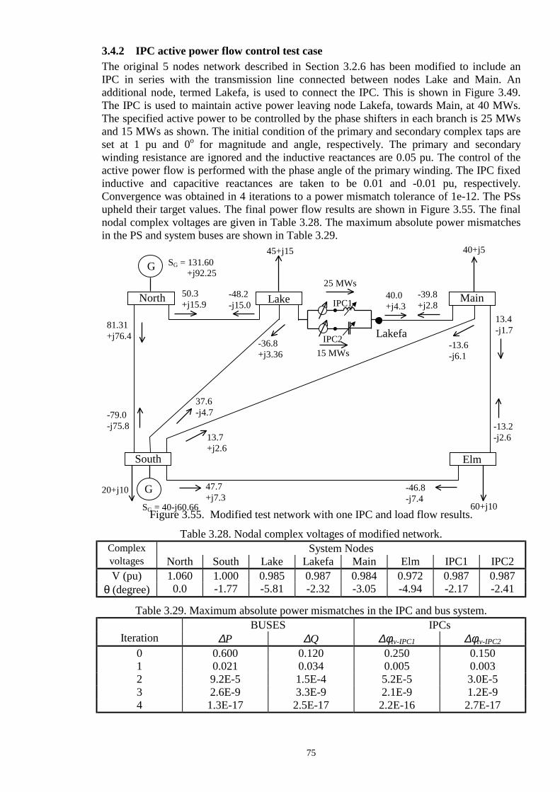
75
3.4.2 IPC active power flow control test case The original 5 nodes network described in Section 3.2.6 has been modified to include an IPC in series with the transmission line connected between nodes Lake and Main. An additional node, termed Lakefa, is used to connect the IPC. This is shown in Figure 3.49. The IPC is used to maintain active power leaving node Lakefa, towards Main, at 40 MWs. The specified active power to be controlled by the phase shifters in each branch is 25 MWs and 15 MWs as shown. The initial condition of the primary and secondary complex taps are set at 1 pu and 0o for magnitude and angle, respectively. The primary and secondary winding resistance are ignored and the inductive reactances are 0.05 pu. The control of the active power flow is performed with the phase angle of the primary winding. The IPC fixed inductive and capacitive reactances are taken to be 0.01 and -0.01 pu, respectively. Convergence was obtained in 4 iterations to a power mismatch tolerance of 1e-12. The PSs upheld their target values. The final power flow results are shown in Figure 3.55. The final nodal complex voltages are given in Table 3.28. The maximum absolute power mismatches in the PS and system buses are shown in Table 3.29.
Figure 3.55. Modified test network with one IPC and load flow results.
Table 3.28. Nodal complex voltages of modified network. Complex System Nodes voltages North South Lake Lakefa Main Elm IPC1 IPC2 V (pu) 1.060 1.000 0.985 0.987 0.984 0.972 0.987 0.987
θ (degree) 0.0 -1.77 -5.81 -2.32 -3.05 -4.94 -2.17 -2.41
Table 3.29. Maximum absolute power mismatches in the IPC and bus system. BUSES IPCs
Iteration ∆P ∆Q ∆φtv-IPC1 ∆φtv-IPC2 0 0.600 0.120 0.250 0.150 1 0.021 0.034 0.005 0.003 2 9.2E-5 1.5E-4 5.2E-5 3.0E-5 3 2.6E-9 3.3E-9 2.1E-9 1.2E-9 4 1.3E-17 2.5E-17 2.2E-16 2.7E-17
45+j15
13.4 -j1.7
-13.2 -j2.6
60+j10
Main
Elm
-39.8 +j2.8
40.0 +j4.3
-46.8 -j7.4
-13.6 -j6.1
40+j5
North
Lake
South
-48.2 -j15.0
50.3 +j15.9
81.31 +j76.4
-79.0 -j75.8
47.7 +j7.3
-36.8 +j3.36
37.6 -j4.7
13.7 +j2.6
20+j10
G
G SG = 40-j60.66
SG = 131.60 +j92.25
Lakefa
25 MWs
15 MWs
IPC1
IPC2

76
3.4.3 IPC feasible power flow control region The feasible power flow control region of a single ASC or PS is a straight line when there is not interaction with other FACTS devices. A similar feasible power flow control region takes place when the IPC device is regulating active power flow with only one controller. The case described in the previous Section was simulated in order to show this rational. The IPC embedded between nodes Lake and Lakefal consists of one PS controller, as shown in Figure 3.56. The feasible active power control region is confined by the phase shifter angle range and it is shown in Figure 3.57. Active power flow across the capacitive branch and the total active power flow injected by the IPC into node Lakefa are also shown in this figure for different values of phase shifter angle. The PS limits were set at ±10o.
Figure 3.56. IPC with one PS controller.
Figure 3.57. Feasible active power control region of an IPC with one PS controller.
The IPC is able to performs active power control with two controllers. These controllers interact with each other and the feasible active power flow region is confined to a rhombus geometry. Figure 3.58 shows this feasible region for the case presented in Section 3.4.2. Both phase shifter angle limits were set at ±10o. The boundary limits of the region are given by the following combinations of phase angle controllers
Lake Lakefa
P km reg1
Rest of Power system
XC = -0.01 pu
XL = 0.01 pu

77
1. Point A, φIPC1= 10o and φIPC2= -10o 2. Point B, φIPC1= 10o and φIPC2= 10o 3. Point C, φIPC1= -10o and φIPC2= -10o 4. Point D, φIPC1= -10o and φIPC2= 10o where IPC1 and IPC2 corresponds to the controlled inductive and capacitive branches, respectively.
Figure 3.58. Feasible active power control region of an IPC with two PS controllers.
Three cases were simulated to confirm the feasibility of the solution. The target active power flow to be controlled by each branch of the IPC and the results are shown in Table 3.30.
Table 3.30. Feasibility of active power flow control by IPC.
case
iterations
Final phase angle values (degrees)
Active power flow inductive branch
(MWs)
Active power flow capacitive branch
(MWs) φIPC1 φIPC2 specified final specified final 1 7 -10* -10* 50 30.13 50 36.82 2 4 4.72 9.34 30 30 -50 -50 3 6 -10.0* -7.30 50 49.44 10 10
All active power flows specified inside the feasible active power flow region have been successfully upheld by the IPC phase shifters. For power flows specified outside the feasible active power flow region, the IPC will violate limits. This is indicated by the symbol *. The size of the feasible active power control region depends on the phase angle controller range and the IPC reactances. Figure 3.59 shows a comparison of the size of the feasible active power control region for three different ranges of the IPC phase. As the phase angle controller range increases, the size of the region increases. These ranges are, 1. CASE A ± 5o for both phase shifters. 2. CASE B ± 10o for both phase shifters. 3. CASE C ± 15o for both phase shifters.

78
Figure 3.59. Comparison of the feasible active power control region size for an IPC.
The active power flows across IPC branches are confined to a limited region. The total active power injected by the IPC exhibits a similar operating region. Figure 3.60 shows this region as a function of the IPC phase shifter angles. The case corresponds to that describe above where PSs angles were limited at ± 10o.
Figure 3.60. IPC feasible active power control region at Lakefal node.

79
The feasible region size shown in Figure 3.60 is defined by adding the power across the inductive and capacitive IPC branches. Hence, this region also depends on the IPC phase shifter angle limits. Figure 3.61 shows a comparison of the region size for the three different ranges of phase shift angles mentioned above, i.e. ±5o (Long dash line), ±10o (Solid line) and ±15o (Dot dash line).
Figure 3.61. Comparison of IPC feasible active power control region size at Lakefal.
3.4.4 Effect of IPC reactances The effect of the IPC reactive and capacitive reactances on the active power flow across IPC terminals is shown in this Section. The same simulation described in Section 3.4.3 was carried out with the IPC phase shifter angles fixed at -10o. The IPC reactive and capacitive reactances were considered complex conjugated, i.e. XL= - XC, with values of 0.01 pu to 0.06 pu. Figure 3.62 shows the IPC active power flow across its terminals and the IPC total active power flow injected at Lakefa terminal as function of IPC reactances. From Figure 3.62 it is clear that as the IPC inductive reactance increases, the active power flow across this branch decreases. The explanation is that the branch is electrically enlarged. On the other hand, as the IPC capacitive reactance increases, the active power flow across this branch also increases. In this case the branch is electrically shorter. The amount of active power flow injected by the IPC into the system at node Lakefa remains almost constant. It varies from 67 MWs to 70.5 MWs. The rational behind this behaviour is that both phase shifter angles are fixed at the same value. Hence, the amount of active power flow across both IPC branches is almost the same. The same simulation described above was carried out but with IPC1 and IPC2 fixed at -5o and -10o, respectively. Figure 3.63 shows the IPC performance. It is observed a greater change on the active power flows across the capacitive branch. As a consequences of this, there exists an increment on the total power injected by the IPC into the system at Lakefal as the IPC reactances increase. This change is from 55.4 MWs to 65.03 MWs.
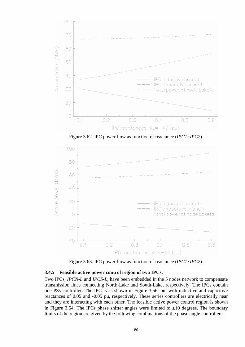
80
Figure 3.62. IPC power flow as function of reactance (IPC1=IPC2).
Figure 3.63. IPC power flow as function of reactance (IPC1≠IPC2).
3.4.5 Feasible active power control region of two IPCs. Two IPCs, IPCN-L and IPCS-L, have been embedded in the 5 nodes network to compensate transmission lines connecting North-Lake and South-Lake, respectively. The IPCs contain one PSs controller. The IPC is as shown in Figure 3.56, but with inductive and capacitive reactances of 0.05 and -0.05 pu, respectively. These series controllers are electrically near and they are interacting with each other. The feasible active power control region is shown in Figure 3.64. The IPCs phase shifter angles were limited to ±10 degrees. The boundary limits of the region are given by the following combinations of the phase angle controllers,

81
1. Point A, φIPCN-L= 10o and φIPCS-L= -10o 2. Point B, φIPCN-L= 10o and φIPCS-L= 10o 3. Point C, φIPCN-L= -10o and φIPCS-L= -10o 4. Point D, φIPCN-L= -10o and φIPCS-L= 10o
Figure 3.64 Feasible control region for two IPCs interacting with each other.
The size of this region depends on the IPCs phase shifter angle ranges and the IPC reactance values. Figure 3.65 shows the size of the feasible active power flow control region as function of IPC reactance values for the case mentioned above.
Figure 3.65. Size of the feasible active power control region as function of the IPC reactance values.
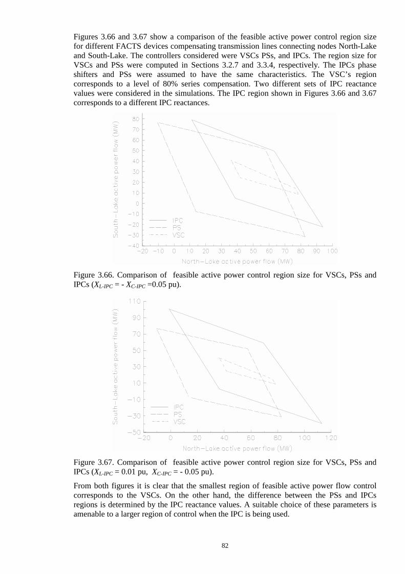
82
Figures 3.66 and 3.67 show a comparison of the feasible active power control region size for different FACTS devices compensating transmission lines connecting nodes North-Lake and South-Lake. The controllers considered were VSCs PSs, and IPCs. The region size for VSCs and PSs were computed in Sections 3.2.7 and 3.3.4, respectively. The IPCs phase shifters and PSs were assumed to have the same characteristics. The VSC’s region corresponds to a level of 80% series compensation. Two different sets of IPC reactance values were considered in the simulations. The IPC region shown in Figures 3.66 and 3.67 corresponds to a different IPC reactances.
Figure 3.66. Comparison of feasible active power control region size for VSCs, PSs and IPCs (XL-IPC = - XC-IPC =0.05 pu).
Figure 3.67. Comparison of feasible active power control region size for VSCs, PSs and IPCs (XL-IPC = 0.01 pu, XC-IPC = - 0.05 pu). From both figures it is clear that the smallest region of feasible active power flow control corresponds to the VSCs. On the other hand, the difference between the PSs and IPCs regions is determined by the IPC reactance values. A suitable choice of these parameters is amenable to a larger region of control when the IPC is being used.

83
3.4.6 Active power flow control in a real power system The case presented in Section 3.3.7, in which 9 FCSCs were replace as VSCs and 6 conventional transformers were substitute by phase shifters has been modified to included 2 general IPCs. The original active power flowing through the conventional transformers and the specified active powers controlled by these transformers, when they are modified to PSs, are shown in Figure 3.49. Figure 3.50 shows the original and specified active power flows through the FCSC and VSCs. The original active powers flowing through the conventional transformers to be replaced by IPCs were 96.43 MWs and 30.34 MWs. The specified active powers to be controlled by the IPCs were specified at 120 MWs and 50 MWs, respectively. The base case converged in 6 iterations. The solution of the modified network with embedded FACTS devices was found in 7 iterations. The controllers upheld their target values. The behaviour of the maximum absolute power flow mismatches in system nodes and FACTS devices, as function of the number of iterations, is plotted in Figure 3.68.
Figure 3.68. Mismatches as function of number of iterations for FACTS devices and system buses.
3.5 Conclusions Mathematical models suitable for assessing the steady state response of FACTS series controllers, namely Advanced Series Compensators, Phase Shifter Transformers and Interphase Power Controllers, capable of regulating the active power flow across selected branches of the power network have been presented in this Chapter. Two models were proposed to represent the Thyristor Controlled Series Capacitor module of the ASC, Variable Series Capacitor and Thyristor Controlled Series Capacitor-Firing Angle. Generalised nodal admittance models have been developed for VSCs, TCSC-FAs and PSs. IPCs have been modelled by combining phase shifters and variable series compensators models. A set of non-linear power flow equations have been obtained for these controllers based on their general admittance matrix equation. These equations have been linearised using the Newton-Rapshon technique and have been included in a Newton-Rapshon load flow algorithm. Since the regulated active power flowing through an electric branch is not a standard control variable in the conventional formulation of the Newton-Rapshon load flow, the unified method requires the Jacobian to be augmented. The robustness of this unified method when solving electric networks containing FACTS devices has been illustrated. In particular, its superiority over the sequential method has been clearly shown.

84
An hybrid method has been proposed for the initialisation of VSCs and TCSC-FAs in order to circumvent the problem of ill-conditioned Jacobian matrix if the customary zero voltage angle initialisation is adopted. A generalised model of a two-winding transformer with complex taps on both the primary and the secondary windings has been presented. This model allows the tapping control to be defined in either primary or secondary sides in the transformer. The model includes the magnetising branch of the transformer. The effect of transformer impedance on the phase shifter angle required to maintain a specified active power at the target value has been illustrated. Numerical examples have been presented which show the electrical interaction between FACTS controllers and the effect of electric network changes on these devices. A topological change in the network produces an active and reactive power flow re-distribution on the network and, as a consequence, the FACTS controller final values change in order to satisfy the specified active power flow target. When two or more FACTS controllers are electrically close to each other, the amount of active power regulated across the branches is confined to an operating region in which the control variables are within limits and the solution of the power flow equations exist. The boundary points of this feasible active power flow control region is given by the possible combination of the FACTS controllers minimum and maximum permissible values. The size of this region increases accordingly to the maximum permissible levels of series compensation and phase-shifting available.
3.6 Bibliography [1] Hingorani N.H.: ‘Flexible AC Transmission Systems’, IEEE Spectrum, pp. 40-45, April 1993. [2] IEEE Power Engineering Society/CIGRÉ: ‘FACTS Overview’, Special Issue, 95TP108, IEEE Service Center, Piscataway, N.J., 1995. [3] IEEE Power Engineering Society: ‘FACTS Application’, Special Issue, 96TP1116-0, IEEE Service Center, Piscataway, N.J., 1996. [4] Acha E.: ‘A Quasi-Newton Algorithm for the Load Flow Solution of Large Networks with FACTS-Controlled Branches’, Proceedings of the 28th UPEC Conference, Stafford UK, 21-23, pp. 153-156, September 1993. [5] Larsen E.V., Clark K., Miske S.S. and Urbanek J.: ‘Characteristics and Rating Considerations of Thyristor Controlled Series Compensation’, IEEE Trans. on Power Delivery, Vol. 9, No. 2, pp. 992-1000, April 1994. [6] Larsen E., Bowler C., Damsky B. and Nilsson S.: ‘Benefits of Thyristor Controled Series Compensation’, International Conference on Large High Voltage Electric Systems (CIGRÉ), paper 14/37/38-04, Paris, September 1992. [7] Gyugyi L.: ‘Power Electronics in Electric Utilities:Static Var Compensators’, Proceedings of the IEEE, Vol. 76, No. 4, pp. 483-494, April 1988. [8] Miller T.J.E.,: ‘Reactive Power Control in Electric Systems’, Wiley Interscience, 1982, ISBN 0-471-86933-3. [9] Christl N., Hedin R., Sadek K., Lützelberger P., Krause P.E., McKenna S.M., Montoya A.H. and Togerson D.: ‘Advanced Series Compensation (ASC) with Thyristor Controlled Impedance’, International Conference on Large High Voltage Electric Systems (CIGRÉ), paper 14/37/38-05, Paris, September 1992.

85
[10] Tenório A.R.M., Jenkins N. and Bollen M.H.J.: ‘A TCSC Model for Electromagnetic Transient Studies’, SPT PE 04-07-0325, Stockholm Power Tech Conference, IEEE/KTH, Stockholm, Sweden, June 18-22, pp. 130-135, 1995. [11] Helbing S.G. and Karady G.G.: ‘Investigations of an Advanced Form of Series Compensation’, IEEE Trans. on Power Delivery, Vol. 9, No. 2, pp. 939-947, April 1994. [12] Tinney W.F. and Walker J.M.: ‘Direct Solutions of Sparse Network Equations by Optimally Ordered Triangular Factorization’, Proceedings of IEEE, Vol. 55, pp. 1801-1809, November 1967. [13] Stagg G.W. and El-Abiad A.H.: ‘Computer Methods in Power System Analysis’, McGraw-Hill, 1968. [14] Noroozian M. and Andersson G.: ‘Power Flow Control by Use of Controllable Series Components’, IEEE Trans. on Power Delivery, Vol. 8, No. 3, pp. 1420-1429, July 1993. [15] Freris L.L. and Sasson A.M.: ‘Investigation of the Load-Flow Problem’, Proceedings of IEE, Vol 115, No. 10, pp. 1459-1470, October 1968. [16] Faur Z.T. and Cañizares C.A.: ‘Effects of FACTS Devices on System Loadability’, Proceedings of the North American Power symposium (NAPS), Bozeman, Montana, USA, October 1995, pp. 520-524. [17] Han Z.X.: ‘Phase Shifter and Power Flow Control’, IEEE Trans. on Power Apparatus and Systems, Vol. PAS-101, No. 10, pp. 3790-3795, October 1982. [18] Kappenman J.: ‘Static Phase Shifter Applications and Concepts for the Minnesota-Ontario Interconnection’, Flexible AC Transmission Systems (FACTS) Conference, EPRI, Boston Massachusetts, 18-20 May, 1992. [19] Hill A.T., Eitzman M.A., Larsen E.V., Eilts L.E., Easton R., Richarson R.H. and Lindgren S.: ‘Thyristor Control of an Existing Phase Shifter’, Flexible AC Transmission Systems (FACTS) Conference, EPRI, Boston Massachusetts, 18-20 May, 1992. [20] Kappenman J.G. and VanHouse D.L.: ‘Thyristor Controlled Phase Angle Regulator Applications and Concepts for the Minnesota-Ontario Interconnection’, Flexible AC Transmission Systems (FACTS 3): The Future in High Voltage Transmission Conference, EPRI, October 1994. [21] Nelson R.J.: ‘Transmission Power Flow Control: Electronic vs. Electromagnetic Alternatives for Steady-State Operation’, IEEE Trans. on Power Delivery, Vol. 9, No. 3, pp. 1678-1684, July 1994. [22] Brochu J., Pelletier P., Beauregard F. and Morin G.: ‘The Interphase Power Controller a New Concept for Managing Power Flow within AC Networks’, IEEE Trans. on Power Delivery, Vol. 9, No. 2, pp. 883-841, April 1994. [23] Beauregard P., Brochu J., Morin G. and Pelletier P.: ‘Interphase Power Controller with Voltage Injection’, Trans. on Power Delivery, Vol. 9, No. 4, pp. 1956-1962, October 1994. [24] Brochu J., Beauregard F., Morin G. and Pelletier P.: ‘Interphase Power Controller Adapted to the Operating Conditions of Networks’, 94 SM 475-4 PWRD, IEEE/PES Summer Meeting, San Francisco, CA, 24-28 July, 1994. [25] Sybille G., Haj-Maharsi Y., Morin G., Beauregard F., Brochu J., Lemay J. and Pelletier P.: ‘Simulator Demostration of the Interphase Power Controller Technology’, 96 WM 119-8 PWRD, IEEE/PES Winter Meeting, Baltimore, MD, 21-25 January, 1996.

86
Chapter 4 Voltage magnitude Controllers 4.1 Introduction In an electric power system, nodal voltages are significantly affected by load variations as well as by any topological change taking place in the network. When the network is operating under heavy loads, the voltage could drop considerably or even collapse. This may cause operation of undervoltage relays and/or voltage sensitive controls leading to extensive disconnection of loads and thus adversely affecting consumers. On the other hand, when the level of load in the system is low, overvoltages can arise due to Ferranti effect in unloaded lines, capacitive overcompensation and overexcitation of synchronous machines [1]. Overvoltages cause equipment failures due to insulation breakdown and produce magnetic saturation in transformers which results in harmonic generation. Accordingly, voltage magnitude throughout the network cannot deviate significantly from its nominal value if an efficient and reliable operation of the power system is to be achieved. Utility equipment and customer equipment should be operated within their design voltage ratings. Voltage magnitude regulation in the network is achieved by controlling the production, absorption, and flow of reactive power throughout the system. Reactive power flow is minimised so as to reduce losses in the network and voltage regulation is generally carried out locally. The following devices are used for this purpose: 1. Automatic Voltage Regulators (AVR) control generator's field excitation so as to
maintain a specified voltage magnitude at generator terminals. 2. Sources or sinks of reactive power, such as Shunt Capacitors (SC), Shunt Reactors (SR),
Rotating Synchronous Condensers (RSC) and Static Var Compensators. SCs and SRs are either permanently connected to the power system, or can be switched on and off according to operative conditions. Nevertheless, they provide passive compensation since their production or absorption of reactive power depends on their rating, and the bus voltage level at which they are connected. On the other hand, the reactive power absorbed/supplied by RSCs and SVCs is automatically adjusted so as to maintain fixed voltage magnitude at connection points.
3. Load-Tap Changing transformers whose main function is to regulate voltage magnitude
at its terminals by changing the transformation ratio. This Chapter focuses on the development of steady-state SVCs and LTCs models and their implementation into a Newton-Rapshon power flow algorithm. The state variables of these models are adjusted automatically during the iterative process. Since the unified solution of nodal network variables and FACTS state variables is achieved using single control criterion, i.e. one variable is adjusted to maintain another variable at a specified value, control strategies are proposed to handled cases when two or more FACTS devices are controlling the same nodal voltage magnitude. Moreover, new types of nodes are defined in order to handle situations in which different FACTS devices control voltage magnitude at the same node or LTCs provide series or parallel control.

87
4.2 Static Var Compensator Advances in power electronic technology together with sophisticated electronic control methods made possible the development of fast Static Var Compensators in the early 1970s. The SVC consists of a group of shunt connected capacitor and reactor banks with fast control action by means of thyristor switching. An SVC can be considered as a variable shunt reactance which is adjusted in response to power system operative conditions in order to control specific parameters of the network. Depending on the equivalent SVC’s reactance, i.e. capacitive or inductive, the SVC is capable of drawing capacitive or inductive current from the electric power system at their coupling point. Suitable control of this equivalent reactance allows the regulation of the voltage magnitude at the power system node where the SVC is connected. SVCs achieve their main operating point at the expense of generating harmonic currents and filters are normally employed with these kind of devices. An SVC may include a combination of both mechanically and thyristor controlled shunt capacitors and reactors [1,2]. However, the most popular configurations for continuously controlled SVCs are the combination of either fix capacitor and thyristor controlled reactor (FC-TCR) or thyristor switched capacitor and thyristor controlled reactor (TSC-TCR) [3,4]. However, from the point of view of steady-state modelling and simulation both components can be treated similarly. The FC-TCR structure shown in Figure 4.1 is used to derive the SVC load flow model.
Figure 4.1. FC-TCR structure for Static Var Compensator.
4.2.1 SVC voltage-current characteristic and operation The voltage-current (V/I) characteristic of the SVC and power system should be analysed together in order to examine how SVCs perform when embedded into the system. The voltage-current power system characteristic, as viewed from the regulated node, can be determined by analysing the electric circuit shown in Figure 4.2.
Figure 4.2. Thevenin equivalent circuit of a power system. The power system is represented by a Thevenin equivalent whose impedance is predominantly inductive. Applying Kirchhoff’s voltage law, the system characteristic can be expressed as,
V E X Ith th s= − (4.1) where the reactive load current IS is defined by the load connected at the controlled node.
Eth
j Xth
V
Is Variable reactive load
IS V
XL
XC

88
Equation (4.1) can be expressed as,
V EXX
th
th
re
=±1
(4.2)
where Xre is the variable reactive load shown in Figure 4.2. The negative sign in equation (4.2) is used when Xre is capacitive. The voltage V increases linearly with capacitive load current and decreases linearly with inductive load current. The SVC composite V/I characteristic is obtained by adding the individual characteristics of the FC and TCR components, as shown in Figure 4.3 [1,6].
Figure 4.3. Voltage-current composite characteristics of the SVC. The SVC steady state control law can be expressed by [1-6],
V V X Iref SL S= + (4.3) The slope XSL is function of voltage regulation. It has values in the range of 1% to 5% of the SVC base [3]. The interaction between SVC and power system characteristic is schematically illustrated in Figure 4.4. Three different power system characteristics are considered corresponding to three values of Thevenin voltage source. The power system operating point is given by the intersection of both characteristics, the nominal system condition is represented by the middle characteristic at point A, where V=Vref and IS=0. A decrement in system load level results in an increase in voltage magnitude at all system nodes. This action is represented by an increase in the system voltage source of ∆Eth, which results in the upper system characteristic. If the SVC were not embedded in the network, V would increase to V1. However, the interaction between the power system and the SVC moves the new operating point to B. The SVC holds the voltage magnitude at V3 by absorbing inductive current I3. On the other hand, an increase in the system load level produces a decrease in nodal voltage magnitudes. For this condition the SVC maintains the voltage magnitude at V4 by injecting a capacitive current I4. It must be noticed that with no SVC the voltage magnitude would be V2.
Is V
IL
V
IC
V
IS
+ =
Slope XSL
V
Inductive Capacitive 0
V
IC
V Max. L Min. L
Slope XSL
IL
+ =
(a) Fixed capacitor (b) TCR (c) SVC

89
Figure 4.4. Interaction between SVC and power system.
4.2.2 SVC voltage-current equations SVC voltage and current equations can be derived by considering the FC-TCR configuration shown in Figure 4.1. Since the current loop between SVC components can be neglected, only the TCR device is analysed. The equivalent electric circuit of a TCR module connected in a power system can be represented schematically by Figure 4.5. The switch, representing the bi-directional thyristors, closes twice during a period T at times t=α/w and t=(α+π)/w. Moreover, the switch remains closed for a period of time t=σ/w, which is the conduction time of one thyristor.
Figure 4.5. Equivalent electric circuit of a TCR module. Applying Kirchoff’s voltage law to the TCR equivalent electric circuit, the following equation is obtained,
V Ld I
dtthy= (4.4)
Solving (4.4) for Ithy by assuming that the time origin coincides with a positive-going zero-crossing of the voltage, the current waveform is given by [5],
I I wt for wtthy M= − + ∈ −(cos cos ) [ , ]α π α0 (4.5)
I I wt for wtthy M= − ∈ −(cos cos ) [ , ]α α π α2 (4.6)
I I wt for wtthy M= − + ∈ +(cos cos ) [ , ]α π α π2 (4.7) where IM = VM / XL is the maximum value of the inductor current, and XL is the fundamental frequency reactance of the inductor. The current through the inductor is zero at any other period of time.
V= VM sin (wt) Ithy
L
Inductive IS
V
Capacitive 0
B
V1
V2
V3
V4
V0 Slope
System reactive load characteristics
A C
I4 I3
Capacitive
Inductive rating
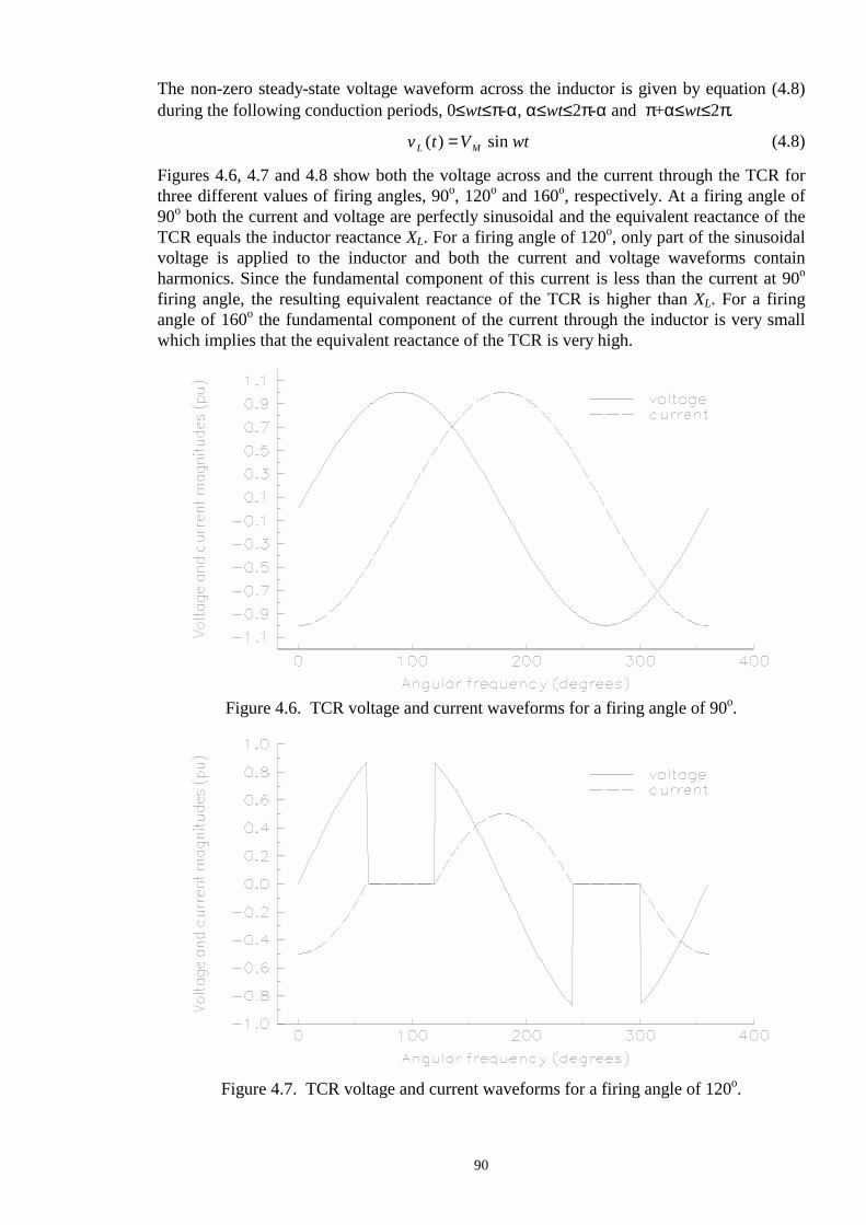
90
The non-zero steady-state voltage waveform across the inductor is given by equation (4.8) during the following conduction periods, 0≤wt≤π-α, α≤wt≤2π-α and π+α≤wt≤2π.
v t V wtL M( ) sin= (4.8) Figures 4.6, 4.7 and 4.8 show both the voltage across and the current through the TCR for three different values of firing angles, 90o, 120o and 160o, respectively. At a firing angle of 90o both the current and voltage are perfectly sinusoidal and the equivalent reactance of the TCR equals the inductor reactance XL. For a firing angle of 120o, only part of the sinusoidal voltage is applied to the inductor and both the current and voltage waveforms contain harmonics. Since the fundamental component of this current is less than the current at 90o firing angle, the resulting equivalent reactance of the TCR is higher than XL. For a firing angle of 160o the fundamental component of the current through the inductor is very small which implies that the equivalent reactance of the TCR is very high.
Figure 4.6. TCR voltage and current waveforms for a firing angle of 90o.
Figure 4.7. TCR voltage and current waveforms for a firing angle of 120o.
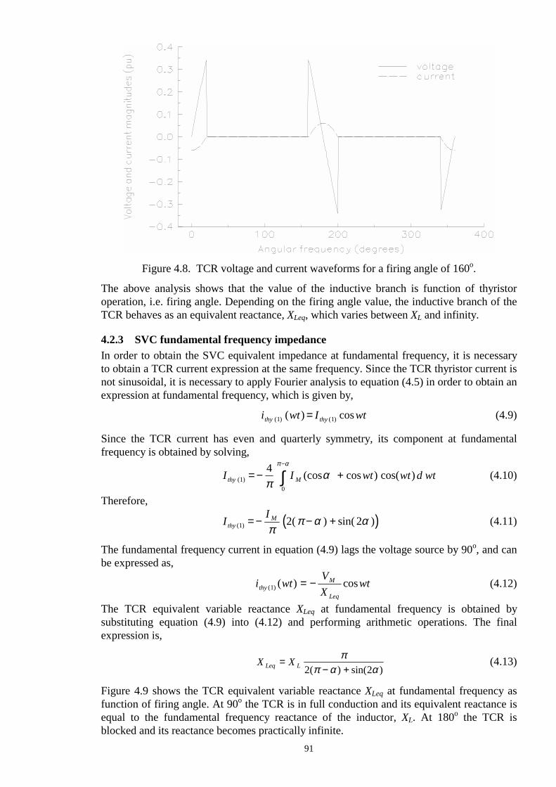
91
Figure 4.8. TCR voltage and current waveforms for a firing angle of 160o.
The above analysis shows that the value of the inductive branch is function of thyristor operation, i.e. firing angle. Depending on the firing angle value, the inductive branch of the TCR behaves as an equivalent reactance, XLeq, which varies between XL and infinity.
4.2.3 SVC fundamental frequency impedance In order to obtain the SVC equivalent impedance at fundamental frequency, it is necessary to obtain a TCR current expression at the same frequency. Since the TCR thyristor current is not sinusoidal, it is necessary to apply Fourier analysis to equation (4.5) in order to obtain an expression at fundamental frequency, which is given by,
i wt I wtthy thy( ) ( )( ) cos1 1= (4.9) Since the TCR current has even and quarterly symmetry, its component at fundamental frequency is obtained by solving,
I I wt wt d wtthy M( ) (cos cos ) cos( )10
4= − +−
∫πα
π α
(4.10)
Therefore,
( )I Ithy
M( ) ( ) sin( )1 2 2= − − +
ππ α α (4.11)
The fundamental frequency current in equation (4.9) lags the voltage source by 90o, and can be expressed as,
i wt VX
wtthyM
Leq( ) ( ) cos1 = − (4.12)
The TCR equivalent variable reactance XLeq at fundamental frequency is obtained by substituting equation (4.9) into (4.12) and performing arithmetic operations. The final expression is,
X XLeq L=− +
ππ α α2 2( ) sin( )
(4.13) Figure 4.9 shows the TCR equivalent variable reactance XLeq at fundamental frequency as function of firing angle. At 90o the TCR is in full conduction and its equivalent reactance is equal to the fundamental frequency reactance of the inductor, XL. At 180o the TCR is blocked and its reactance becomes practically infinite.

92
Figure 4.9. TCR equivalent reactance.
The SVC effective reactance Xeq is determined by the parallel combination of Xc and XLeq and it is given by equation (4.14).
( )X X X
XX
eqc L
cL
=− + −
ππ α α2 2( ) sin( )
(4.14)
Depending on the ratio between Xc and XL there is a value of the firing angle that causes steady-state resonance. Figure 4.10 depicts the SVC equivalent impedance for a fixed capacitive reactance of 15 Ω and fundamental frequency inductive reactance of 2.56 Ω.
Figure 4.10. SVC equivalent reactance as function of firing angle.

93
4.2.4 Conventional SVC power flow models There are several SVC models recommended for power flow analysis [3]. The simplest model is to represent the SVC as a generator with reactive power limits. The node at which the SVC is connected is represented as PV node. The model described above assumes that the slope Xst is equal to zero. This consideration is permissible when the SVC is within limits but results in large errors if the SVC is operating outside limits [1,3], as shown in Figure 4.11. Assume the upper characteristic, when the system is operating under low level of load. If the slope is taken to be zero, the generator violates its minimum reactive limit, point BXSL=0. However, the generator will operate well within limits if the slope is taken into account, point B. Figure 4.11. Comparison between actual and idealised voltage-current characteristics of the SVC. The slope can be represented by connecting the SVC to an auxiliary bus which is coupled to the power system high-voltage node by an inductive reactance whose value, on the SVC base, is equal to the per unit slope [1,3]. The auxiliary bus is represented as a PV-type node whilst the power system high-voltage node is considered as a PQ-type node. If the generator violates one of its reactive limits, the SVC becomes a shunt fixed compensator, either a shunt capacitor or a shunt reactor. The susceptance of the shunt fixed compensator is,
BQVSVC
LIM
spec
= − 2 (4.15)
where Vspec is the specified voltage to be freed if the reactive power limit QLIM is exceeded.
4.2.5 Proposed SVC power flow model The drawback of the models described above is that they assume that the SVC hits reactive power limits which are voltage dependent whereas in practice the SVC is an adjustable reactance whose control is given by firing angle limits or reactance limits. A new, more efficient and realistic way to model the SVC in a Newton-type power flow algorithm is described below. Both the slope of the static characteristic in the control range and the limits of the characteristic in the uncontrolled range are considered in the same model without resorting to auxiliary nodes.
IS
V
0
B
V1
V2 System reactive load characteristics
C
IMIN IMAX
Capacitive rating
Inductive rating
C xSL=0 B xSL=0
VMIN
VMAX

94
The SVC is considered to be a continuous, variable-shunt susceptance which is adjusted in order to achieve a specified voltage magnitude [1]. The slope is determinate by the capacitive and inductive susceptance limits. The slope is zero if these limits are equal. This susceptance represents the total SVC susceptance necessary to maintain the voltage magnitude at the specified value and it is independent of SVC structure. The susceptance value is given by,
( )B
XX
X X
LC
C L
= −− − +
ππ α α2 2( ) sin( )
(4.16)
where the capacitive and inductive reactances are defined as,
XwCC = 1 (4.17)
X wLL = (4.18)
The variable-shunt susceptance B given in equation (4.16) is equal to the SVC equivalent susceptance at fundamental frequency given by the inverse of equation (4.14). The implementation of the Variable-Shunt Susceptance in a Newton-Rapshon load flow program has required the creation of a new type of bus, namely PVB. It is a controlled bus where the nodal voltage magnitude and the nodal active and reactive powers are specified while the SVC’s variable susceptance B is handled as state variable. If B is within limits, the specified voltage is attained and the controlled bus remains PVB-type. However, if B goes out of limits, B is fixed at the violated limit and the bus becomes PQ-type in the absence of other FACTS devices capable of achieving this control. The circuit shown in Figure 4.12 has been considered to derive the SVC’s non-linear power equations and the linearised equations required by the Newton-Rapshon method. Here, the SVC is treated like a load. The variable shunt susceptance has a negative value for the case of an inductor and a positive value for the case of capacitor.
Figure 4.12. Variable-Shunt Susceptance.
In general, the transfer admittance equation for the variable-shunt compensator is,
I Vk= jB (4.19) The reactive power equations is,
Q V Bk k= − 2 (4.20) The linearised equation of the SVC is given in (4.21), where the variable susceptance B is taken to be the state variable,
∆∆
∆∆
PQ
QB
B BB
k
kk
k
=
0 00
∂∂
θ (4.21)
Vk
B I +
-

95
After each iteration i, the variable shunt susceptance B must be updated according to equation (4.22),
B BB
BBi i
i
i+ = +
1 ∆ (4.22)
Once the susceptance value B has been determined, the firing angle is computed by solving equation (4.16). Despite that an additional iterative process is required to compute the SVC’s firing angle, the VSC model is very robust towards convergence.
4.2.6 Control co-ordination between reactive sources When two or more different type of reactive power sources are set to control the voltage magnitude at the same node, they are prioritised in order to have a single control criterion. Synchronous reactive sources have been chosen to be the first regulating components, holding any other type of reactive power sources fixed at their initial condition so long as the synchronous reactive sources are operating within limits. When the generators or condensers violate their reactive limits, they are fixed at the offending limit and another type of reactive power source, e.g. SVCs, is activated to control nodal voltage magnitude. In this case, the node is transformed from PV type to PVB type.
4.2.7 Revision of SVC limits The revision criterion of the SVC limits is based on the active and reactive power mismatches at the controlled bus. The revision of the SVC limits starts when either the active power or reactive power at the controlled node is less than a specified tolerance.
4.2.8 SVC nodal voltage magnitude test case The original 5 nodes network described in Section 3.2.6 has been modified to include one SVC connected at node Lake in order to maintain the nodal voltage magnitude at 1 pu. Convergence was obtained in 4 iterations to a power mismatch tolerance of 1e-12. The LTC upholds its target value. The final SVC susceptance was 0.204 pu. The final power flow results are shown in Figure 4.13. The final nodal complex voltages are given in Table 4.1. The maximum absolute power mismatches in the system buses are shown in Table 4.2.
Figure 4.13. Modified test network and load flow results.
45+j15
6.8 +j4.3
-6.7 -j7.9
60+j10
Main
Elm
-19.6 -j14.0
19.64 +j11.2
-54.3 -j2.1
-27.2 +j4.7
40+j5
North Lake
South
-40.6 -j12.4
41.9 +j11.3
89.1 +j74.1
-86.6 -j74.0
54.5 +j2.7
-24.1 +j6.7
24.5 -j9.5
27.6 -j7.3
20+j10
G
G SG = 40 - j77.1
SG = 131.0 +j85.4
-j20.5

96
Table 4.1. Nodal complex voltages of modified network.
Table 4.2. Maximum absolute power mismatches in system nodes.
4.2.9 Control co-ordination between Generators and SVCs The aim of this Section is to show the robustness of the algorithm when a nodal voltage magnitude is being controlled simultaneously by a generator and a SVC. The AEP30 bus system has been modified to include one SVC, as shown in Figure 4.14. G2 maximum reactive power limit was changed from 50 MVARs to 40 MVARs. The SVC injects reactive power and controls the voltage magnitude when generator G2 violates reactive power limits. When the generator operates within reactive limits, the SVC works as fixed shunt compensator with the susceptance fixed at the value given by the initial condition. Once the generator violates reactive limits, the SVC is activated. The controlled node is transformed from PV type to PVB type. The target voltage magnitude at bus 2 is 1.045 pu For the conditions described above, the generator G2 violates its maximum reactive limit and voltage magnitude control switches to the SVC. The final value of SVC susceptance required to achieved control was 0.1574 pu. Convergence was obtained in 4 iterations.
Figure 4.14. AEP 30 bus system with one SVC.
complex system nodes voltages North South Lake Main Elm V (pu) 1.060 1.000 1.000 0.994 0.975
θ (degree) 0.00 -2.05 -4.83 -5.11 -5.80
BUSES iteration ∆P ∆Q
0 0.600 0.230 1 0.019 0.020 2 4.9E-5 4.4E-5 3 4.2E-10 4.0E-10 4 0.000 0.000
5
1
2
3
4
REST OF THE NETWORK
B
6
7
G2
178.2
83.2
45.88
61.95
80.1
37.8
69.43

97
4.3 Load Tap-Changer The basic function of a Load-Tap Changer (LTC) is to regulate output voltage magnitude at a specified value in spite of variations in the input voltage imposed by network changing conditions. A schematic representation of a LTC transformer is shown in Figure 4.15.
Figure 4.15. Load-Tap changing transformer.
(a) Mechanical-controlled tap changer. (b) Thyristor-controlled tap changer. Output voltage magnitude control is achieved by injecting a small variable voltage magnitude in phase (or antiphase) with the voltage at the input winding terminals. The output voltage is regulated by adjusting the magnitude of the added (or subtracted) voltage as shown in the vector diagram of Figure 4.16. In practice, this is done by changing the transformation ratio between the two voltage windings,
V F tapN
Vout inp= ( )∆1
(4.23) where N1 and F(∆tap) are the number of turns of the input and output winding, respectively. Traditionally, mechanical-based mechanisms have been used to exert this change in voltage between two windings. However, its replacement by thyristor switching circuits will allow very quick adjustments of the output voltage to compensate for any voltage magnitude variation in the input side.
∆tap
Vinp
+
-
Vout
+
-
THYRISTOR SWITCHING NETWORK
MECHANICAL LOAD TAP CHANGER
∆tap
-Vreg
+Vreg
Vinp
+
-
Vout
+
- (a)
(b)

98
Figure 4.16. LTC voltages vector diagrams. The thyristor switching control is classified into two distinctive types, namely large signal modulation or bang-bang switching control and small signal modulation [7]. The difference between these two controls is defined by the output voltage magnitude perturbation produced by the switching from steady-state tap position to another tap position in order to raise or lower the voltage. The large signal modulation control considers a limited number of back and forth switching which could produce damping or to oppose voltage fluctuations. A small signal modulation control allows to adjust almost continuously, i.e. quickly in very small steps, the switching between tap positions. Independently of the mechanism and control type used to switch tap positions, the LTC can only influence the relative voltage magnitude of the two nodes to which it is connected and does not generate active or reactive power by itself.
4.3.1 LTC power flow model for control of nodal voltage magnitude. A new and more general model for a Load Tap Changer (LTC) is described in this Section. Similar to the phase shifter model described in Chapter 3, it is derived from a two winding, single phase transformer model with complex taps on both the primary and the secondary windings and the magnetising branch of the transformer included to account for the core losses. The model is based on the physical representation of the transformer shown in Figure 4.17 (a) while the schematic equivalent circuit of the transformer is shown in Figure 4.17 (b).
Figure 4.17. Two winding transformer. (a) Schematic representation. (b) Equivalent circuit.
Rp Xp Rs Xs Vs Vp
Ip Is
Is I 1
′′′′ Vp
Tv : 1
φtv
Ip Zp
I 1 V 1
Ti : 1
I
Bo Go
V 0
0
φuv
1 : Uv
I 2 ′′′′
1 : Ui
Vs Zs I 2 V 2
(a)
(b)
Vinp
-Vreg +Vreg
Vout

99
The primary winding is represented as an ideal transformer having complex tap ratios Tv:1 and Ti:1 in series with the impedance Zp, where Tv=Ti
*=Tv∠ φtv. The * denotes the conjugate operation. Also, the secondary winding is represented as an ideal transformer having complex tap ratios Uv:1 and Ui :1 in series with the impedance Zs , where Uv=Ui
* =Uv ∠ φuv. The transfer admittance matrix relating the primary voltage Vp and current Ip to the secondary voltage Vs and current Is in the two-winding transformer can be determined by considering the current I1 across the impedances Zp and the current I2 across the impedance Zs. The derivation of the transfer admittance matrix, given by (4.24), is shown in Chapter 3.
II Z Z Z Z Y
Z Y T UT U Z Y
VV
p
s s p p s 0
s 0 v v
v v p
p
s
=
+ ++ −
− +
∗
∗1
T UU
Tv2
v2
v2
v2
0
(4.24)
The power injection equations of a two winding transformer are:
( ) ( )( )P V G V V G Bp p pp p s ps p s ps p s= + − + −2 cos sinθ θ θ θ (4.25)
( ) ( )( )Q V B V V G Bp p pp p s ps p s ps p s= − + − − −2 sin cosθ θ θ θ (4.26)
( ) ( )( )P V G V V G Bs s ss s p sp s p sp s p= + − + −2 cos sinθ θ θ θ (4.27)
( ) ( )( )Q V B V V G Bs s ss s p sp s p sp s p= − + − − −2 sin cosθ θ θ θ (4.28) When the transformer is working as a conventional transformer, the set of linearised power flow equations is,
∆
∆
∆
∆
∆
∆
∆
∆
P
P
Q
Q
P P PV
VPV
V
P P PV
V PV
V
Q Q QV
VQV
V
Q Q QV
VQV
V
V V
p
s
p
s
p
p
p
s
p
pp
p
ss
s
p
s
s
s
pp
s
ss
p
p
p
s
p
pp
p
ss
s
p
s
s
s
pp
s
ss
p
s
p p
=
∂∂ θ
∂∂ θ
∂∂
∂∂
∂∂ θ
∂∂ θ
∂∂
∂∂
∂∂ θ
∂∂ θ
∂∂
∂∂
∂∂ θ
∂∂ θ
∂∂
∂∂
θ
θ
V Vs s
(4.29)
When the transformer is working as Load Tap Changing (LTC), Tk is adjusted, within limits, to constrain the voltage magnitude at node P at a specified value Vp. For this mode of operation Vp is maintained constant at the target value and Tk replaces Vp in (4.29). Incorporating these changes, the set of linearised LTC power flow equations is,
∆
∆
∆
∆
∆
∆
∆
∆
P
P
Q
Q
P P PT
TPV
V
P P PT
TPV
V
Q Q QT
TQV
V
Q Q QT
TQV
V
T T
p
s
p
s
p
p
p
s
p
kk
p
ss
s
p
s
s
s
kk
s
ss
p
p
p
s
p
kk
p
ss
s
p
s
s
s
kk
s
ss
p
s
k k
=
∂∂ θ
∂∂ θ
∂∂
∂∂
∂∂ θ
∂∂ θ
∂∂
∂∂
∂∂ θ
∂∂ θ
∂∂
∂∂
∂∂ θ
∂∂ θ
∂∂
∂∂
θ
θ
V Vs s
(4.30)
where Tk represents either Tv or Uv.

100
The partial derivatives of the power equations with respect to the primary tap of the two winding transformer are:
∂∂PT
TV TA
R U R X R G R F X Fp
vv
p vs v s pp s s= + + − +
22
1 2 2 1 22 2
2( ) ( )
( ) ( )( )+ + − +
V V G B T
AR F X Fp s ps ps
vs scos sin ( )δ δ1 1 1 4
21 2
2
( )+ − − −2
21 1 1 1
3V V T UA
X Rp s v vs ssin( ) cos( )δ φ δ φ (4.31)
∂∂QT
TV TA
B R F X F R R X U Rp
vv
p vpp s s s s v= + − + +
22
2 1 2 2 12 2
2( ) ( )
( ) ( )( )+ − − +
V V G B T
AR F X Fp s ps ps
vs ssin cos ( )δ δ1 1 1 4
21 2
2
( )− − + −2
21 1 1 1
3V V T UA
R Xp s v vs ssin( ) cos( )δ φ δ φ (4.32)
∂∂
PT
T V TA
R T R X R F G R F X Fs
vv
s vs v s ss s s= + + + − +2
23 4 1 2 1 2
2 22( ) ( )
( ) ( )( )+ + − +
V V G B T
AR F X Fp s sp sp
vs scos sin ( )δ δ2 2 1 4
21 2
2
( )+ − − −2
22 2 2 2
3V V T UA
X Rp s v vs ssin( ) cos( )δ φ δ φ (4.33)
∂∂QT
T V TA
B R F X F R R X T R Fs
vv
s vss s s s s v= + − + + +2
22 1 2 4 3 2
2 22( ) ( )
( ) ( )( )+ − − +
V V G B T
AR F X Fs p sp sp
vs ssin cos ( )δ δ2 2 1 4
21 2
2
( )− − + −2
22 2 2 2
3V V T UA
R Xs p v vs ssin( ) cos( )δ φ δ φ (4.34)

101
The partial derivatives of the power equations with respect to the secondary tap of the two winding transformer are:
∂∂
PU
UV U
AR U R X R F G R F X Fp
vv
p vs v p pp p p= + + + − +
22
1 2 1 2 1 22 2
2( ) ( )
( ) ( )( )+ + − +
V V G B Sin U
AR F X Fp s ps ps
vp pcos ( )δ δ1 1 1 4
21 2
2
( )+ − − −2
21 1 1 1
3V V U TA
X Rp s v vp psin( ) cos( )δ φ δ φ (4.35)
∂∂QU
UV UA
B R F X F R R X U R Fp
vv
p vpp p p p p v= + − + + +
22
2 1 2 2 1 22 2
2( ) ( )
( ) ( )( )+ − − +
V V G B U
AR F X Fp s ps ps
vp psin cos ( )δ δ1 1 1 4
21 2
2
( )− − + −2
21 1 1 1
3V V U TA
R Xp s v vp psin( ) cos( )δ φ δ φ (4.36)
∂∂
PU
U V UA
R T R X R G R F X Fs
vv
s vp v p ss p p= + + − +2
23 4 2 1 2
2 22( ) ( )
( ) ( )( )+ + − +
V V G B U
AR F X Fs p sp sp
vp pcos sin ( )δ δ2 2 1 4
21 2
2
( )+ − − −2
22 2 2 2
3V V U TA
X Rs p v vp psin( ) cos( )δ φ δ φ (4.37)
∂∂QU
U V UA
B R F X F R R X T Rs
vv
s vss p p p p v= + − + +
22
2 1 2 4 32 2
2( ) ( )
( ) ( )( )+ − − +
V V G B U
AR F X Fp s ps ps
vp psin cos ( )δ δ1 1 1 4
21 2
2
( )− − + −2
21 1 1 1
3V V U TA
R Xp s v vp psin( ) cos( )δ φ δ φ (4.38)
where
δ θ θ1 = −p s (4.39)
δ θ θ2 = −s p (4.40) The remaining variables have been defined in Section 3.3.1, Chapter 3.

102
After each iteration i the tap controller must be updated according to equation (4.41),
T T TT
Tki
ki k
k
i
ki( ) ( )
( )( )+ = +
1 ∆ (4.41)
4.3.2 Special control system configurations of LTCs The implementation of the tap-changing facilities has required the creation of a new type of bus, namely PVT. It is a control bus where the nodal voltage magnitude and the nodal active and reactive powers are specified while the LTC tap T is handled as state variable. If T is within limits, the specified voltage is attained and the controlled bus remains PVT-type. However, if T goes out of limits, T is fixed at the violated limit and the bus becomes PQ-type bus. The new type of bus allows the handling of general control strategies, such as series and parallel LTCs configurations. The series condition occurs when two or more LTCs regulate the non-regulated terminal of another LTC. This situation is shown in Figure 4.18 (a) where LTC 1 regulates bus k and LTC 2 regulates bus m. The parallel condition occurs when bus k is regulated by two or more LTCs, as shown in Figure 4.18 (b). It must be noted that buses m and n may not necessarily be electrically connected.
Figure 4.18. General control strategies. (a) Series condition (b) Parallel condition. The parallel condition does not belong to the category of single criterion control, i.e. only one control variable is adjusted in order to maintain another dependent variable at a specified value. When two or more LTCs are controlling one nodal voltage magnitude, multiple solutions become a possibility since the number of unknown variables is greater than the number of equations. An entire group of parallel LTCs may be treated as a single control criterion if they are started from the same tapping initial condition. One equation and one variable corresponding to the common tap position may be sufficient to describe the group performance. This equation is linearised with respect to the common tap and incorporated in the overall Jacobian equation. From the set of LTCs controlling one nodal voltage magnitude, the LTC which supply more reactive power is selected to be the master LTC and its tap position becomes the master tap position. Since the LTCs in the group can have the same tap position but different tap limits, the following options have been considered: • When a LTC different from the master slave LTC hits one of its limits the tap position is
fixed at the offending limit and the LTC is removed from the linearised power equations. • When the master LTC violates one of its limits the strategy mentioned above is adopted.
Furthermore, a new master LTC is selected from the remaining active LTCs in order to maintain the controlled nodal voltage magnitude at the target value. If no active LTCs remain when the violation of the master LTC takes place then the node is converted to PQ type.
OPEN m n
PVT PVT PVT
T2 T1 T1 T2
(a) (b)
m k n
PQ k
LTC 2 LTC 1

103
When the set of parallel LTCs have different tap positions a sensitivity factor, α, can be found which refers the slave tap positions to the master tap position. Assuming a group of np LTCs operating in parallel and considering that Tk is the master position, the sensitivity factor is given by equation (4.42),
α pk
p
TT
p np
=
= 1,....., (4.42)
The expression used for computing the Jacobian term corresponding to the tap master position is also used for the other LTCs in the group. The tap adjusting position which takes into account the sensitivity factor is given by equation (4.43), where each LTC in the group will have its own adjusting pattern.
T T TT
T
p np
pi
pi k
k
i
pi( ) ( )
( )( )
,.....,
+ = +
=
1
1
∆ (4.43)
Alternatively, equation (4.44) gives the same size of adjustment to all LTCs in the group,
T T TT
T
p np
pi
pi k
k
i
pi
pi( ) ( )
( )( ) ( )
,.....,
+ = +
=
1
1
∆ α (4.44)
4.3.3 Simultaneous nodal voltage magnitude control by means of reactive sources and LTCs The option of controlling nodal voltage magnitude by simultaneously adjusting LTCs and reactive sources is a very practical operating situation. Such controls are prioritised. The generator has been chosen as the first regulating component, holding the associated SVC and LTC taps at their initial condition so long as the generator reactive limits are not reached, being the regulated node PV type. If the generator reaches its reactive limits then the SVC or the master LTC tap becomes activated and the node is converted to PVB or PVT type. Figure 4.19 shows both conditions when a nodal voltage magnitude is being controlled by a generator and a LTC.
Figure 4.19. Simultaneous control. (a) Nodal voltage magnitude controlled by the generator (b) Nodal voltage magnitude controlled by the master LTC.
(a)
OPEN m n
PV
T2 T1
k
G
(b)
OPEN m n
PVT
T2 T1
k
G

104
The control of nodal voltage magnitude at PV and PVB nodes has higher priority. If the set of LTCs associated with a given generator or SVC are controlling nodes different from the generator or SVC node, and the generator or SVC reaches its reactive limits then the LTC is switched to control the generator or SVC node, converting it into a PVT node. The previous PVT node is converted into a PQ node in the absence of another LTC available to regulate that node. This control action is shown schematically in Figure 4.20 for the case of PV node. Figure 4.21 shows the various control options available in the NR program to regulate voltage magnitude, in a prioritised manner.
Figure 4.20. Switching control. (a) Control of nodal voltage magnitudes by generator and LTCs (b) Switching of LTC after the generator violates its reactive limits.
Figure 4.21. Switching between nodal voltage magnitude controllers.
(a)
OPEN m n
PV
T2 T1
k
G
PVT PVT
(b)
OPEN m n
PVT
T2 T1
k
G
PQ PVT
Generator Active PV node
reactive limits
violation
no
yes
Remains PV node
Looking for active SVC
no
yes SVC Active PVB node
no reactive limits
violation
yes Remains PVB node
Looking for active LTC
no
yes LTC Active PVT node
PQ node
no violation of tap changer
limits
yes Remains PVT node
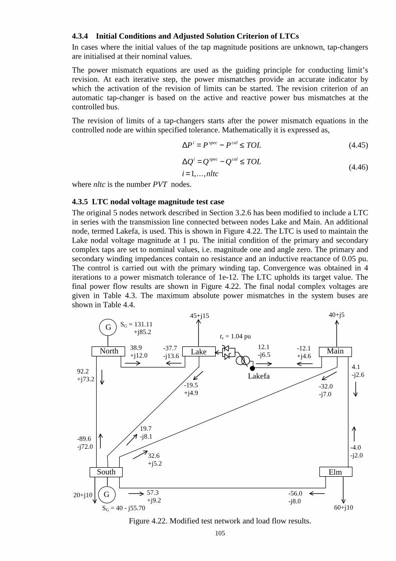
105
4.3.4 Initial Conditions and Adjusted Solution Criterion of LTCs In cases where the initial values of the tap magnitude positions are unknown, tap-changers are initialised at their nominal values. The power mismatch equations are used as the guiding principle for conducting limit’s revision. At each iterative step, the power mismatches provide an accurate indicator by which the activation of the revision of limits can be started. The revision criterion of an automatic tap-changer is based on the active and reactive power bus mismatches at the controlled bus. The revision of limits of a tap-changers starts after the power mismatch equations in the controlled node are within specified tolerance. Mathematically it is expressed as,
∆P P P TOLi spec cal= − ≤ (4.45)
∆Q Q Q TOLi nltc
i spec cal= − ≤=1,...,
(4.46)
where nltc is the number PVT nodes.
4.3.5 LTC nodal voltage magnitude test case The original 5 nodes network described in Section 3.2.6 has been modified to include a LTC in series with the transmission line connected between nodes Lake and Main. An additional node, termed Lakefa, is used. This is shown in Figure 4.22. The LTC is used to maintain the Lake nodal voltage magnitude at 1 pu. The initial condition of the primary and secondary complex taps are set to nominal values, i.e. magnitude one and angle zero. The primary and secondary winding impedances contain no resistance and an inductive reactance of 0.05 pu. The control is carried out with the primary winding tap. Convergence was obtained in 4 iterations to a power mismatch tolerance of 1e-12. The LTC upholds its target value. The final power flow results are shown in Figure 4.22. The final nodal complex voltages are given in Table 4.3. The maximum absolute power mismatches in the system buses are shown in Table 4.4.
Figure 4.22. Modified test network and load flow results.
45+j15
4.1 -j2.6
-4.0 -j2.0
60+j10
Main
Elm
-12.1 +j4.6
12.1 -j6.5
-56.0 -j8.0
-32.0 -j7.0
40+j5
North
Lake
South
-37.7 -j13.6
38.9 +j12.0
92.2 +j73.2
-89.6 -j72.0
57.3 +j9.2
-19.5 +j4.9
19.7 -j8.1
32.6 +j5.2
20+j10
G
G
SG = 40 - j55.70
SG = 131.11 +j85.2 tv = 1.04 pu
Lakefa

106
Table 4.3. Nodal complex voltages of modified network.
Table 4.4. Maximum absolute power mismatches in the system nodes.
4.3.6 Effect of LTCs impedance on the tap magnitude value The effect of the LTC’s impedance on the final tap position required to maintain voltage magnitude at the target value is presented in this Section. The test case presented in Section 4.3.5 has been used with minor modifications, the primary winding reactance is taken to be zero. Four different values were considered for the secondary winding reactance, 0.2 pu, 0.1 pu, 0.05 pu and 0.001 pu. The voltage at Lake node was controlled at 1.01 pu. Figures 4.23 (a) and 4.23 (b) depict the final tap position and the reactive power absorbed by the LTC as function of the secondary winding reactance values given above.
(a) (b)
Figure 4.23. Effect of LTC transformer reactance. (a) Tap position. (b) Reactive power consumption.
The tap position varies linearly but the LTC reactive power consumption varies in a non-linear fashion.
complex system nodes voltages North South Lake Lakefa Main Elm V (pu) 1.060 1.000 1.000 0.969 0.969 0.966
θ (degree) 0.00 -2.16 -4.41 -5.13 -5.99 -5.99
BUSES iteration ∆P ∆Q
0 0.600 0.120 1 0.024 0.025 2 1.5E-4 7.5E-4 3 1.5E-8 1.6E-7 4 0.000 0.000

107
4.3.7 Convergence test The aim of this Section is to show the robustness of the algorithm, in terms of number of iterations required to obtain convergence when several LTCs are embedded in the network. The AEP30 bus system [12] was modified to consider three PVT nodes. The nodal voltage magnitude at node 6 is controlled, at 1.01 pu, by tap-changers 6-9 and 6-10 operating in parallel control condition. The voltage magnitude at nodes 4 and 27 are controlled, at 1.01 pu and 1.0 pu by tap-changers 4-12 and 27-28, respectively. The transformer reactance and off-nominal tap values given in [12] were placed on the secondary and primary windings, respectively. In this work, the primary winding is the one connected to the first mentioned node, e.g. 4, 6 and 27. Accordingly, nodes 4 and 6 are on the high-voltage side and node 27 is on the low-voltage side. The adjustment of tap changers operating in parallel was carried out by using sensitivity factors. Comparisons are made between the results given by the full Newton-Rapshon method and the quasi Newton-Rapshon method presented in [8] for the cases given in Table 4.5. The number of iterations taken to obtain the solution as well as the final tap values required to maintain the nodal voltage magnitude at the specified value are given in Table 4.6.
Table 4.5. Initial position of tap-changer taps.
Table 4.6. Comparison between simultaneous and sequential methods.
where NC indicates no convergence. Table 4.6 shows the quadratic convergence of the full Newton-Rapshon method and its superior performance with respect to the quasi Newton-Rapshon method in terms of the number of iterations required to get to the solution. It also shows the robustness of the full Newton-Rapshon method towards convergence as function of the initial condition.
Initial position of tap magnitude in two-winding transformers
cases tc6-9 tc6-10 tc4-12 tc27-28 i 0.978 0.969 0.932 0.968 ii 1.1 1.1 1.1 1.1 iii 1.0 1.0 1.0 1.0 iv 0.9 0.9 0.9 0.9 v 1.0 0.9 1.0 1.0 vi 0.9 1.0 0.9 0.9 vii 1.1 1.0 0.9 0.9 viii 1.0 1.1 1.0 1.0 ix 1.0 1.0 0.9 1.1 x 1.0 1.0 1.1 0.9
FULL NEWTON-RAPSHON QUASI NEWTON-RAPSHON Tap position in tap-changers Tap position in tap-changers case iter tc6-9 tc6-10 tc4-12 tc27-28 iter tc6-9 tc6-10 tc4-12 tc27-28
i 5 0.976 0.967 0.915 0.998 20 0.971 0.962 0.923 0.976 ii 5 0.974 0.974 0.915 0.998 100 NC NC NC NC iii 5 0.974 0.974 0.915 0.998 18 0.992 0.992 0.992 0.992 iv 5 0.974 0.974 0.915 0.998 64 0.931 0.931 0.928 0.930 v 5 1.008 0.907 0.913 0.995 5 0.998 0.900 0.999 0.999 vi 5 0.951 1.057 0.918 1.003 6 0.901 1.001 0.9980 1.000 vii 5 1.004 0.913 0.913 0.996 28 1.087 0.987 0.987 1.010 viii 5 0.951 1.057 0.918 1.002 28 0.987 1.087 0.987 1.011 ix 5 0.974 0.974 0.915 0.998 35 0.985 0.985 0.912 1.084 x 5 0.974 0.974 0.915 0.998 100 NC NC NC NC

108
4.3.8 Effect of sensitivity factors in the parallel control option For the cases described in the previous Section, the adjustment of tap-changers operating in parallel was achieved by using sensitivity factors and by updating the taps of both tap-changers identically. Table 4.7 shows the number of iterations required to get convergence and the results obtained for the FACTS devices. Multiple solutions can be observed when two or more LTCs interact with each other, i.e. different values of tap position can maintain nodal voltages magnitudes at their target values. Both adjusting methods gave the same solution for a specified tap-changer initial condition. However, the use of sensitivity factors yields better results in terms of the number of iterations required to get to the solution, compared to the case in which identical tapping updates is carried out.
Table 4.7. Final position of tap-changers taps.
4.3.9 Effect of truncated adjustments in state variables As discussed in Chapter 2, Newton’s method cannot directly take account of the limits associated with state variables. Large increments in these variables during the back substitution process may induce large ∆P and ∆Q residual terms, resulting in poor converge, or more seriously, causing the solution to diverge. These unwanted problems can be avoided quite effectively by limiting the size of the correction during the backward substitution [9-11]. The computed adjustments are replaced by truncated adjustments with their effects being propagated throughout the remaining of the backward substitution. Two general cases were simulated in order to quantify the effect of the truncation. The following maximum variations | ∆V| = | ∆T| = | ∆X| =0.1 pu and | ∆θ| = | ∆φ| = 30o were considered in the simulations. Case I The AEP30 bus network has been modified, 4 conventional transformers have been taken to be FACTS devices. Transformers connected between nodes 4-12, 6-10 and 27-28 were considered as LTCs. The nodal voltage magnitudes at nodes 4, 6 and 12 were specified at 1.0 pu, 1.0 pu and 1.04 pu, respectively. The transformer connected between nodes 6-9 was assumed to be a PS controlling active power flowing from 6 to 9 at 40 MWs. The transformer data given in [12] was modified in the way mentioned in Section 4.3.7. The control was carried out with the primary winding taps. The adjustments were made as follows: A) Truncating the size of correction during the backward substitution and using the power mismatch criterion for the revision of limits (TA). B) Full correction during the backward substitution and using the power mismatch criterion for the revision of limits (NTA).
UPDATING BY SENSITIVITY UPDATING IDENTICALLY Tap position in tap-changers Tap position in tap-changers case iter tc6-9 tc6-10 tc4-12 tc27-28 iter tc6-9 tc6-10 tc4-12 tc27-28
i 5 0.976 0.967 0.915 0.998 6 0.976 0.967 0.915 0.998 ii 5 0.974 0.974 0.915 0.998 5 0.974 0.974 0.915 0.998 iii 5 0.974 0.974 0.915 0.998 5 0.974 0.974 0.915 0.998 iv 5 0.974 0.974 0.915 0.998 5 0.974 0.974 0.915 0.998 v 5 1.008 0.907 0.913 0.995 10 1.008 0.908 0.913 0.995 vi 5 0.951 1.057 0.918 1.003 8 0.952 1.052 0.918 1.002 vii 5 1.004 0.913 0.913 0.996 8 1.008 0.908 0.913 0.995 viii 5 0.951 1.057 0.918 1.002 8 0.952 1.052 0.918 1.002 xi 5 0.974 0.974 0.915 0.915 5 0.974 0.974 0.915 0.915 x 5 0.974 0.974 0.915 0.915 5 0.974 0.974 0.915 0.915

109
Adjusted solutions were obtained in 6 iterations. The final parameters of the FACTS devices are shown in Table 4.8. Active and reactive powers generated by synchronous machines, GE, and synchronous condensers, CO, embedded in the network are shown in Table 4.9.
Table 4.8. FACTS devices final parameters (Case 1).
Table 4.9. Power generation (Case 1).
where * indicates violation of reactive power limit. When the state variable increments were not truncated, no convergence was obtained. Figure 4.24 depicts active and reactive power mismatches for both kind of adjustments.
Figure 4.24. Convergence profile as function of state variable size increment (Case 1).
FACTS Final parameters of controlled primary tap Devices Magnitude (pu) Angle (degrees)
LTC 4-12 0.9013 0.0 LTC 6-10 0.8821 0.0 LTC 27-28 1.0667 0.0
PS 6-9 1.0000 -3.75
Power Power Generated Sources Active (MWs) Reactive (MVARs) GE-1 261.29 -3.1 GE-2 40.0 50.0* CO-5 0.0 40.0* CO-8 0.0 40.0* CO-11 0.0 13.17 CO-13 0.0 -2.27

110
The above experiment was designed in such a way that two different types of FACTS devices were connected at the same node, i.e. LTC6-10 and PS6-9. In order to show the numeric interaction between the FACTS devices, and its effect during the iterative process, the experiment described above was repeated with the LTC connected between nodes 6 and 10 deactivated, namely Case 2. This LTC was considered as a conventional transformer and the voltage magnitude at node 6 was freed. Convergence was obtained in 6 iterations with either type of state variable size adjustments. Both simulations gave identical results. Figure 4.25 depicts active and reactive power mismatches for both kind of adjustments. The final parameters of the FACTS devices and electric power sources embedded in the network are shown in Tables 4.10 and 4.11, respectively.
Figure 4.25. Convergence profile as function of state variable size increment (Case 2).
Table 4.10. FACTS devices final parameters (Case 2).
Table 4.11. Power generation (Case 2).
where * indicates violation of reactive power limit.
FACTS Final parameters of controlled primary tap Devices Magnitude (pu) Angle (degrees)
LTC 4-12 0.8685 0.0 LTC 27-28 1.0715 0.0
PS 6-9 1.0000 -4.0
Power Power Generated Sources Active (MWs) Reactive (MVARs) GE-1 261.42 -4.70 GE-2 40.0 50.0* CO-5 0.0 40.0* CO-8 0.0 40.0* CO-11 0.0 16.96 CO-13 0.0 -2.48

111
In order to show the effect of reactive power limits on the iterative process, the two previous experiments were repeated but considering the reactive power limits of the electric power sources as ± 400 MVARs. Figure 4.26 depicts the active and reactive power mismatches for both kind of adjustments when all FACTS devices are activated, namely Case 3. The final parameters of the FACTS devices and electric power sources embedded in the network are shown in Tables 4.12 and 4.13, respectively. Both simulations gave identical results.
Figure 4.26. Convergence profile as function of state variable size increment (Case 3).
Table 4.12. FACTS devices final parameters (Case 3).
where * indicates violation of reactive power limit.
Table 4.13. Power generation (Case 3).
The discontinuities observed in Figure 4.26, at iterations 2 and 8, are due to limit violations in LTC6-10.
FACTS Final parameters of controlled primary tap Devices Magnitude (pu) Angle (degrees)
LTC 4-12 0.8* 0.0 LTC 6-10 0.8544 0.0 LTC 27-28 1.0449 0.0
PS 6-9 1.0000 -3.60
Power Power Generated Sources Active (MWs) Reactive (MVARs) GE-1 261.58 -14.94 GE-2 40.0 69.54 CO-5 0.0 40.0 CO-8 0.0 58.53 CO-11 0.0 5.08 CO-13 0.0 -15.73
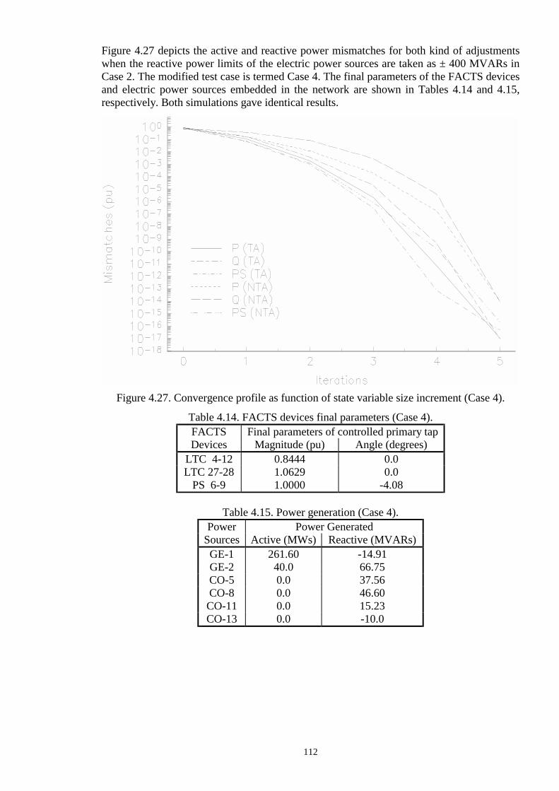
112
Figure 4.27 depicts the active and reactive power mismatches for both kind of adjustments when the reactive power limits of the electric power sources are taken as ± 400 MVARs in Case 2. The modified test case is termed Case 4. The final parameters of the FACTS devices and electric power sources embedded in the network are shown in Tables 4.14 and 4.15, respectively. Both simulations gave identical results.
Figure 4.27. Convergence profile as function of state variable size increment (Case 4).
Table 4.14. FACTS devices final parameters (Case 4).
Table 4.15. Power generation (Case 4).
FACTS Final parameters of controlled primary tap Devices Magnitude (pu) Angle (degrees)
LTC 4-12 0.8444 0.0 LTC 27-28 1.0629 0.0
PS 6-9 1.0000 -4.08
Power Power Generated Sources Active (MWs) Reactive (MVARs) GE-1 261.60 -14.91 GE-2 40.0 66.75 CO-5 0.0 37.56 CO-8 0.0 46.60 CO-11 0.0 15.23 CO-13 0.0 -10.0

113
Case II The standard AEP 57 bus system [12] has been modified to show the ability of the algorithm to converge to very tight tolerances for cases in which large number of controllable branches are embedded in the network and the state variable size correction is truncated. Eight conventional transformers were modified to be LTCs and PSs. Moreover, three series variable compensators were embedded in the network. The relevant part of the AEP 57 bus system with FACTS controllers and their targets is shown in Figure 4.28. The special system configuration of series and parallel control are considered.
Figure 4.28. Relevant part of the AEP 57 bus system with FACTS devices. Convergence was obtained in 6 iterations when the size of correction is truncated during the backward substitution. The final value of FACTS controllers are shown in Table 4.16. No convergence was obtained when full correction was used during the backward substitution.
Table 4.16. Final value of controllable parameters in FACTS devices. Tap-changer Position Phase shifter angle
(degrees) Capacitor value
(% of compensation) tc21-20 tc24-26 tc24-25 tc24-25 tc13-49 ps9-55 ps4-18 ps4-18 C1 C2 C3 0.9517 0.9939 0.9529 0.9237 0.9675 -8.16 -11.24 -12.97 67 45 60
It may be argued that truncating the size of correction during the backward substitution could retard convergence during the early stages of the solution. Nevertheless, it has been demonstrated that it actually increases the probability of solving cases that could be divergent otherwise.
15
G
G
C
3
12
10
9
1 pu
25 MWs
25 MWs
40 MWs
13 49
4
30 MWs 14 MWs
18
21
20 0.98 pu
55
22 23
0.96 pu 24
26
1 pu
25
27 28 29
25 MWs

114
4.3.10 Control co-ordination between LTCs and reactive sources The aim of this Section is to show the robustness of the algorithm when a nodal voltage magnitude is being controlled simultaneously by reactive sources and LTCs. Two cases were considered in order to show this control co-ordination, they are presented below. Case I The AEP30 bus system has been modified to include two FACTS devices as shown in Figure 4.29. The maximum reactive power of the generator G2 has been changed from 50 MVARs to 40 MVARs. A SVC has been connected at bus 2 in order to inject reactive power and to control the voltage magnitude when generator G2 violates reactive power limits. Moreover, the transmission line connected between nodes 2 and 6 has been replaced by a LTC which is set to control voltage magnitude at bus 2. While the SVC is within limits, the LTC operates as conventional transformer with taps fixed at the initial condition. Once the SVC violates its susceptance limits, the LTC is activated. The LTC impedances were taken to be half the value of the replaced transmission line series impedance, i.e. Zp=Zs=0.02905+j0.08815 pu. When the transformer works as LTC the control is carried out by adjusting the secondary winding tap. The target voltage magnitude at bus 2 is 1.045 pu. Both LTC taps were initialised at their nominal values, i.e. 1 pu and 0o for magnitudes and angles, respectively.
Figure 4.29. AEP 30 bus system with two FACTS Devices. For the conditions described above, generator G2 violates its maximum reactive limit and the voltage magnitude control switches to the SVC. The final value of SVC susceptance required to maintain 1.045 pu at bus 2 was 0.1798 pu. Convergence was obtained in 4 iterations. The SVC capacitive susceptance limits were set to 0.0 pu, 0.05 pu, 0.01 pu and 0.17 pu. Table 4.17 shows the results obtained for these simulations. For the first three cases presented in this table, the synchronous condensers connected at buses 5 and 8 violate their maximum reactive power limits. The final tap value required to achieve the specified voltage magnitude is function of the reactive power injected at the controlled node via the network.
1
2
3
4
5
REST OF THE NETWORK
B
Tv : 1
Zp
Bo Go
φuv
1 : Uv
φtv Zs
6
7
G2
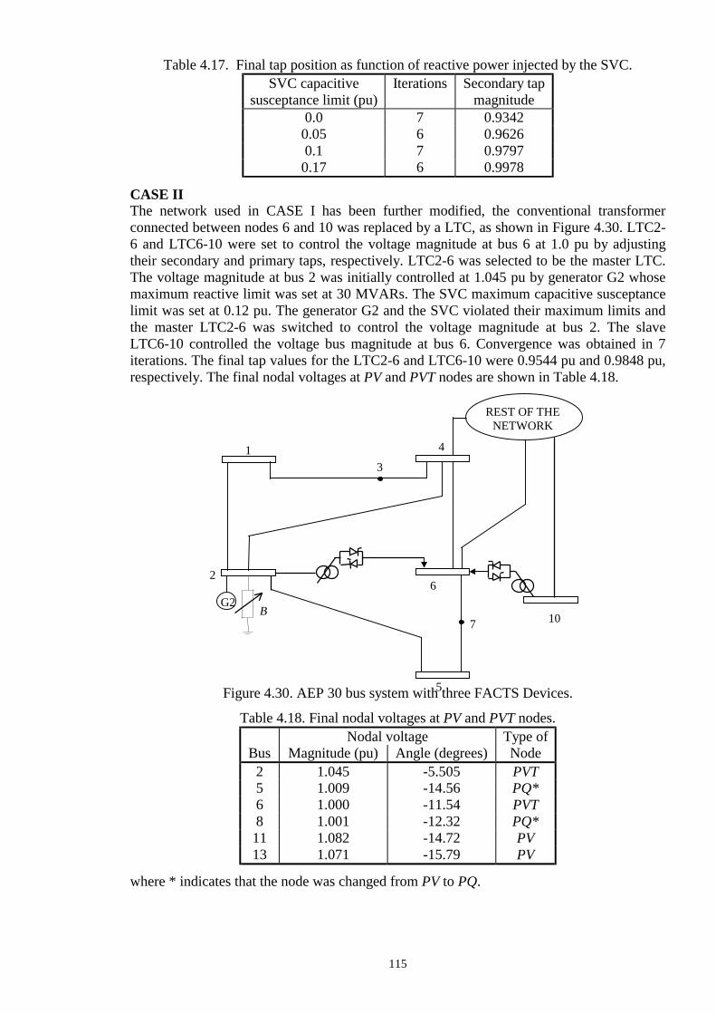
115
Table 4.17. Final tap position as function of reactive power injected by the SVC.
CASE II The network used in CASE I has been further modified, the conventional transformer connected between nodes 6 and 10 was replaced by a LTC, as shown in Figure 4.30. LTC2-6 and LTC6-10 were set to control the voltage magnitude at bus 6 at 1.0 pu by adjusting their secondary and primary taps, respectively. LTC2-6 was selected to be the master LTC. The voltage magnitude at bus 2 was initially controlled at 1.045 pu by generator G2 whose maximum reactive limit was set at 30 MVARs. The SVC maximum capacitive susceptance limit was set at 0.12 pu. The generator G2 and the SVC violated their maximum limits and the master LTC2-6 was switched to control the voltage magnitude at bus 2. The slave LTC6-10 controlled the voltage bus magnitude at bus 6. Convergence was obtained in 7 iterations. The final tap values for the LTC2-6 and LTC6-10 were 0.9544 pu and 0.9848 pu, respectively. The final nodal voltages at PV and PVT nodes are shown in Table 4.18.
Figure 4.30. AEP 30 bus system with three FACTS Devices.
Table 4.18. Final nodal voltages at PV and PVT nodes.
where * indicates that the node was changed from PV to PQ.
SVC capacitive susceptance limit (pu)
Iterations Secondary tap magnitude
0.0 7 0.9342 0.05 6 0.9626 0.1 7 0.9797 0.17 6 0.9978
Nodal voltage Type of Bus Magnitude (pu) Angle (degrees) Node
2 1.045 -5.505 PVT 5 1.009 -14.56 PQ* 6 1.000 -11.54 PVT 8 1.001 -12.32 PQ* 11 1.082 -14.72 PV 13 1.071 -15.79 PV
1
2
3
4
5
REST OF THE NETWORK
B
6
7
G2 10
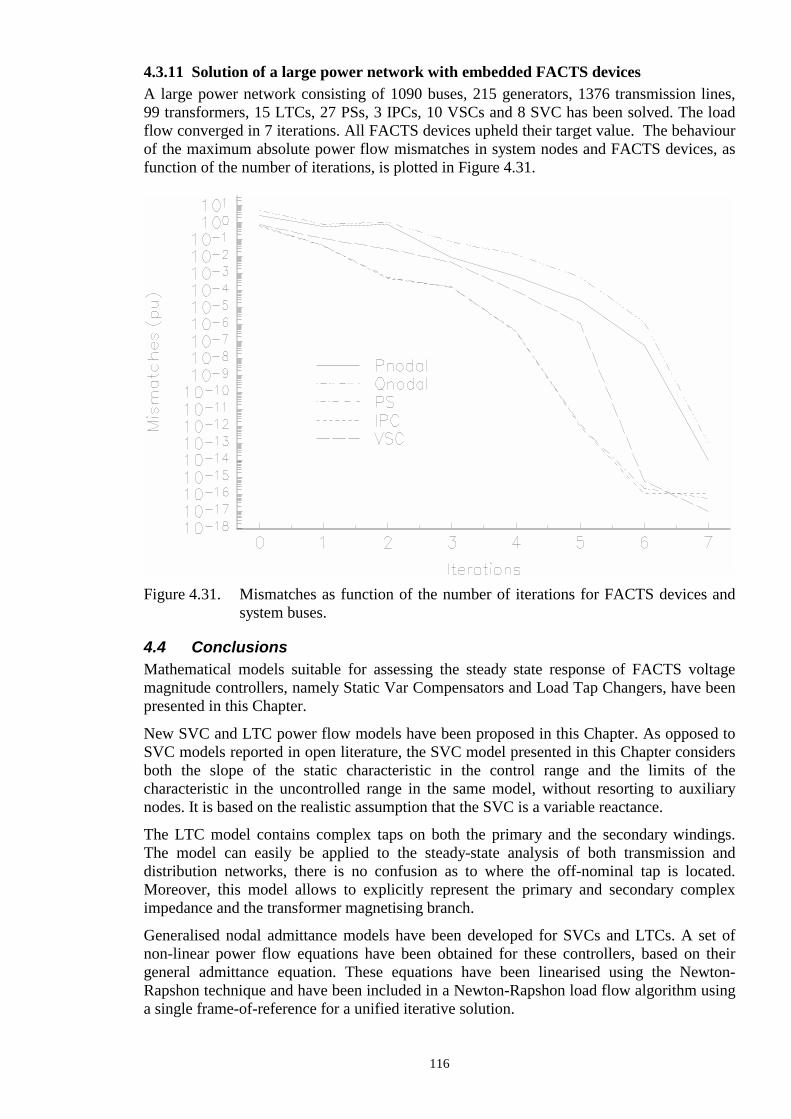
116
4.3.11 Solution of a large power network with embedded FACTS devices A large power network consisting of 1090 buses, 215 generators, 1376 transmission lines, 99 transformers, 15 LTCs, 27 PSs, 3 IPCs, 10 VSCs and 8 SVC has been solved. The load flow converged in 7 iterations. All FACTS devices upheld their target value. The behaviour of the maximum absolute power flow mismatches in system nodes and FACTS devices, as function of the number of iterations, is plotted in Figure 4.31.
Figure 4.31. Mismatches as function of the number of iterations for FACTS devices and system buses.
4.4 Conclusions Mathematical models suitable for assessing the steady state response of FACTS voltage magnitude controllers, namely Static Var Compensators and Load Tap Changers, have been presented in this Chapter. New SVC and LTC power flow models have been proposed in this Chapter. As opposed to SVC models reported in open literature, the SVC model presented in this Chapter considers both the slope of the static characteristic in the control range and the limits of the characteristic in the uncontrolled range in the same model, without resorting to auxiliary nodes. It is based on the realistic assumption that the SVC is a variable reactance. The LTC model contains complex taps on both the primary and the secondary windings. The model can easily be applied to the steady-state analysis of both transmission and distribution networks, there is no confusion as to where the off-nominal tap is located. Moreover, this model allows to explicitly represent the primary and secondary complex impedance and the transformer magnetising branch. Generalised nodal admittance models have been developed for SVCs and LTCs. A set of non-linear power flow equations have been obtained for these controllers, based on their general admittance equation. These equations have been linearised using the Newton-Rapshon technique and have been included in a Newton-Rapshon load flow algorithm using a single frame-of-reference for a unified iterative solution.

117
Since the unified solution of network and FACTS state variables is achieved under the assumption of single control criterion; i.e. one variable is adjusted to maintain another variable at a specified value, control strategies have been devised to consider cases when two or more FACTS devices are set to control voltage magnitude at the same node. These control strategies have been handled efficiently by the introduction of new types of nodes. A node whose voltage magnitude is controlled by a SVC is defined as PVB node. A node whose voltage magnitude is controlled by a LTC is defined as PVT node. These definitions allow the efficient handling of special control configurations such as series and parallel LTC transformer connections. The algorithm’s efficiency has been illustrated by numeric example. The robustness of the unified method when solving electric networks containing FACTS devices has been illustrated. In particular, its superiority over the sequential method has been clearly shown. The reliability of the algorithm in handling conditions where different FACTS devices are controlling voltage magnitude at the same node has been show by numeric example. These cases include LTCs operating in series or parallel control conditions. Limits violation compounded with strong interaction between the various controlled branches may dent the algorithm’s quadratic convergence but even then reliable solutions were obtained at the cost of one or two extra iterations. Numeric examples have shown that large increments in the state variables during the backward substitution process may induce large ∆P and ∆Q residual terms. These large residuals may in turn slow down converge, or more seriously, cause the solution to oscillate or even diverge. In order to avoid such problems, the computed adjustments have been replaced by truncated adjustments with their effects being propagated throughout the remaining of the backward substitution. Although the truncation of the size of correction during the backward substitution could retard convergence during the early stages of the solution, it has been demonstrated that it actually increases the probability of solving cases that could be divergent otherwise.
4.5 Bibliography [1] Enrimez I.A., Ed.: ‘Static Var Compensators’, Working Group 38-01, Task Force No.2 on SVC, CIGRÉ, 1986. [2] Gyugyi L.: ‘Power Electronics in Electric Utilities: Static Var Compensators’, Proceedings of the IEEE, Vol. 76, No. 4, pp. 483-494, April 1988. [3] IEEE Special Stability Controls Working Group.: ‘Static Var Compensator Models for Power Flow and Dynamic Performance Simulation’, IEEE Trans. on Power Systems, Vol. 9, No. 1, pp. 229-240, February 1995. [4] Zeno T.F. and Cañizares C.A.: ‘Effects of FACTS Devices on System Loadability’, Proceedings of the North American Power Symposium (NAPS), Bozeman, Montana, pp. 520-524, October 1995. [5] Miller T.J.E.: ‘Reactive Power Control in Electric Systems’, Wiley Interscience, 1982, ISBN 0-471-86933-3. [6] Kundur P.P.: ‘Power System Stability and Control’, McGraw-Hill, 1994, ISBN 007035958. [7] IEEE Power Engineering Society/CIGRÉ: ‘FACTS Overview’, Special Issue, 95TP108, IEEE Service Center, Piscataway, N.J., 1995. [8] Acha E.: ‘A Quasi-Newton Algorithm for the Load Flow Solution of Large Networks with FACTS-Controlled Branches’, Proceedings of the 28th UPEC Conference, Stafford UK, 21-23, pp. 153-156, September 1993.

118
[9] Peterson N.M. and Scott Meyer W.: ‘Automatic Adjustment of Transformer and Phase Shifter Taps in the Newton Power Flow’, IEEE Trans. on Power Apparatus and Systems, Vol. PAS-90, No. 1, pp. 103-108, January/February 1971. [10] Chang S.K. and Brandwajn V.: ‘Adjusted Solutions in Fast Decoupled Load Flow’, IEEE Trans. on Power Systems, Vol. 3, No. 2, pp. 726-733, May 1988. [11] Maria G.A , Yuen A.H. and Findlay J.A.: ‘Control Variable Adjustment in Load Flows’, IEEE Trans. on Power Systems, Vol. 3, No. 3, pp. 858-864, August 1988. [12] Freris L.L. and Sasson A.M.: ‘Investigation of the load-flow problem’, Proceedings of IEE, Vol. 115, No. 10, pp. 1459-1470, October 1968.

119
Chapter 5 Unified Power Flow Controller 5.1 Introduction The Unified Power Flow Controller (UPFC) is, arguably, the most comprehensive device to have emanated so far from the FACTS initiative [1]. In principle at least, the UPFC is capable of providing active and reactive power control, as well as adaptive voltage magnitude control. Provided no operating limits are violated, the UPFC regulates all three variables simultaneously or any combination of them. From the operational point of view, the UPFC may act as a Shunt VAR Compensator or as Thyristor Controlled Series Compensator or as a Phase-Shifter Controller. The versatility afforded by the UPFC makes it a prime contender to provide many of the control functions required to solve a wide range of dynamic and steady state problems encountered in electrical power networks [2,3]. In the last few years, a number of landmark publications have appeared in the open literature which describe the basic operating principles of the UPFC [2-5]. However, very little work has been done in developing suitable models for assessing the UPFC’s behaviour in large-scale power networks. This is particularly the case in the area of power flow analysis where, according to open literature, only two very constrained models have been published [6,7]. Reference 6 takes the approach of modelling the UPFC as a series reactance together with a set of active and reactive nodal power injections at each end of the series reactance. These powers are expressed as function of the terminal, nodal voltages and the voltage of a series source. In this reference the voltage magnitude and angle of the series source are adjusted manually in order to achieve a power flow solution which, it is hoped, will match the target power flow. A 5-bus network was used to test the model. A sequential UPFC power flow model has been proposed recently by Nabavi-Niaki and Iravani [7]. The sending and receiving ends of the UPFC are decoupled. The former is transformed into a PQ bus whilst the latter is transformed into a PV bus. The active and reactive power loads in the PQ bus and the voltage magnitude at the PV bus are set at the values to be controlled by the UPFC. The active power injected into the PV bus has the same value as the active power extracted in the PQ bus since the UPFC and coupling transformers are assumed to be lossless. A standard load flow is carried out to determine the nodal, complex voltages at the UPFC terminals. After load flow convergence, an additional set of non-linear equations, relating the various UPFC parameters, is solved by iteration. This method is simple but it is not clear from reference [7] how the model can be used in situations when the UPFC is not controlling the three parameters simultaneously. Moreover, since the UPFC parameters are computed after the load flow has converged, there is no way of knowing during the iterative process whether or not the UPFC parameters are within limits. It is also not clear from this paper how this UPFC model can be used to represent the situation when a UPFC is the only link between two sub-networks. Trying to circumvent these limitations, a new and comprehensive UPFC model has been developed from first principles. In common with all other controllable plant component models described in this thesis, the UPFC state variables are incorporated inside the Jacobian and mismatch equations, leading to very robust iterative solutions.
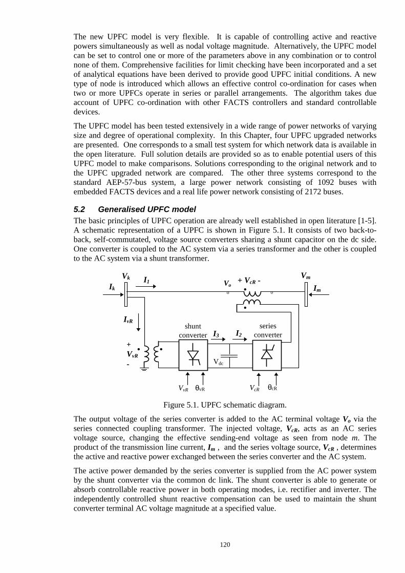
120
The new UPFC model is very flexible. It is capable of controlling active and reactive powers simultaneously as well as nodal voltage magnitude. Alternatively, the UPFC model can be set to control one or more of the parameters above in any combination or to control none of them. Comprehensive facilities for limit checking have been incorporated and a set of analytical equations have been derived to provide good UPFC initial conditions. A new type of node is introduced which allows an effective control co-ordination for cases when two or more UPFCs operate in series or parallel arrangements. The algorithm takes due account of UPFC co-ordination with other FACTS controllers and standard controllable devices. The UPFC model has been tested extensively in a wide range of power networks of varying size and degree of operational complexity. In this Chapter, four UPFC upgraded networks are presented. One corresponds to a small test system for which network data is available in the open literature. Full solution details are provided so as to enable potential users of this UPFC model to make comparisons. Solutions corresponding to the original network and to the UPFC upgraded network are compared. The other three systems correspond to the standard AEP-57-bus system, a large power network consisting of 1092 buses with embedded FACTS devices and a real life power network consisting of 2172 buses.
5.2 Generalised UPFC model The basic principles of UPFC operation are already well established in open literature [1-5]. A schematic representation of a UPFC is shown in Figure 5.1. It consists of two back-to-back, self-commutated, voltage source converters sharing a shunt capacitor on the dc side. One converter is coupled to the AC system via a series transformer and the other is coupled to the AC system via a shunt transformer.
Figure 5.1. UPFC schematic diagram. The output voltage of the series converter is added to the AC terminal voltage Vo via the series connected coupling transformer. The injected voltage, VcR, acts as an AC series voltage source, changing the effective sending-end voltage as seen from node m. The product of the transmission line current, Im , and the series voltage source, VcR , determines the active and reactive power exchanged between the series converter and the AC system. The active power demanded by the series converter is supplied from the AC power system by the shunt converter via the common dc link. The shunt converter is able to generate or absorb controllable reactive power in both operating modes, i.e. rectifier and inverter. The independently controlled shunt reactive compensation can be used to maintain the shunt converter terminal AC voltage magnitude at a specified value.
VcRVvR θcRθvR
Im
Vk Vm+ VcR -
Vdc
IkI1
IvR
I3 I2shunt
converterseries
converter
•
•
•
+VvR
-
•
Voo o

121
5.2.1 UPFC equivalent circuit The UPFC equivalent circuit shown in Figure 5.2 is used to derive the steady-state model. The equivalent circuit consists of two ideal voltage sources which represent the fundamental Fourier series component of the switched voltage waveforms at the AC converter terminals. The source impedances are including in the model.
Figure 5.2. UPFC equivalent circuit. The ideal voltage sources are,
( )VvR vR vR vRV j= +cos sinθ θ (5.1)
( )VcR cR cR cRV j= +cos sinθ θ (5.2) VvR and θvR are the controllable magnitude (VvRmin ≤ VvR ≤ VvRmax) and angle (0 ≤ θvR ≤2π) of the ideal voltage source representing the shunt converter. The magnitude VcR and angle θcR of the ideal voltage source representing the series converter are controlled between limits (VcRmin ≤ VcR ≤ VcRmax) and (0 ≤ θcR ≤ 2π), respectively. The variable phase angle of the series injected voltage determines the mode of power flow control [1-5]. If θcR is in phase with the nodal voltage angle θk, it regulates the terminal voltage. If θcR is in quadrature with respect to θk, it controls power flow, acting as a phase shifter. If θcR is in quadrature with the line current angle then it controls power flow, acting as a variable series compensator. At any other value of θcR, the UPFC operates as a combination of voltage regulator, variable series compensator and phase shifter. The magnitude of the series injected voltage determines the amount of power flow to be controlled.
5.2.2 UPFC power equations The general transfer admittance matrix for the UPFC is obtained by applying Kirchhoff current and voltage laws to the electric circuit shown in Figure 5.2 and is given by equation (5.3).
II
Y Y Y YY Y Y
VVVV
k
m
kk km km vR
mk mm mm
k
m
cR
vR
=
0 (5.3)
where
yzcR
cR cR cRR j X= =
+1 1 (5.4)
yzvR
vR vR vRR j X= =
+1 1 (5.5)
zcR + VcR -
zvR
+ VvR -
Ik I1
IvR
Im
Re -VvRI*vR+ VcRI*
m =0 Vk Vm

122
Y y ykk kk kk cR vRG j B= + = + (5.6)
Y ymm mm mm cRG j B= + = (5.7)
Y Y ykm km km km cRG j B= = + = − (5.8)
Y yvR vR vR vRG j B= + = − (5.9) Based on the equivalent circuit shown in Figure 5.2 and equation (5.3), the active and reactive power equations are: At node k :
( )( )( )
P V G V V G B
V V G B
V V G B
k k kk k m km k m km k m
k cR km k cR km k cR
k vR vR k vR vR k vR
= + − + −
+ − + −
+ − + −
2 cos( ) sin( )
cos( ) sin( )
cos( ) sin( )
θ θ θ θ
θ θ θ θ
θ θ θ θ
(5.10)
( )
( )( )
Q V B V V G B
V V G B
V V G B
k k kk k m km k m km k m
k cR km k cR km k cR
k vR vR k vR vR k vR
= − + − − −
+ − − −
+ − − −
2 sin( ) cos( )
sin( ) cos( )
sin( ) cos( )
θ θ θ θ
θ θ θ θ
θ θ θ θ
(5.11)
At node m :
( )( )
P V G V V G B
V V G Bm m mm m k mk m k mk m k
m cR mm m cR mm m cR
= + − + −
+ − + −
2 cos( ) sin( )
cos( ) sin( )
θ θ θ θ
θ θ θ θ (5.12)
( )
( )Q V B V V G B
V V G Bm m mm m k mk m k mk m k
m cR mm m cR mm m cR
= − + − − −
+ − − −
2 sin( ) cos( )
sin( ) cos( )
θ θ θ θ
θ θ θ θ (5.13)
Series converter :
( )( )
P V G V V G B
V V G BcR cR mm cR k km cR k km cR k
cR m mm cR m mm cR m
= + − + −
+ − + −
2 cos( ) sin( )
cos( ) sin( )
θ θ θ θ
θ θ θ θ (5.14)
( )
( )Q V B V V G B
V V G BcR cR mm cR k km cR k km cR k
cR m mm cR m mm cR m
= − + − − −
+ − − −
2 sin( ) cos( )
sin( ) cos( )
θ θ θ θ
θ θ θ θ (5.15)
Shunt converter :
( )P V G V V G BvR vR vR vR k vR vR k vR vR k= − + − + −2 cos( ) sin( )θ θ θ θ (5.16)
( )Q V B V V G BvR vR vR vR k vR vR k vR vR k= + − − −2 sin( ) cos( )θ θ θ θ (5.17) Assuming a free loss converter operation, the UPFC neither absorbs nor injects active power with respect to the AC system. The DC link voltage, Vdc, remains constant. The active power associated with the series converter becomes the DC power VdcI2. The shunt converter must supply an equivalent amount of DC power in order to maintain Vdc constant. Hence, the active power supplied to the shunt converter, PvR , must satisfy the active power demanded by the series converter, PcR , i.e.
P PvR cR+ = 0 (5.18)

123
Assuming a loss free, coupling transformer operation, the active power at node k, Pk, should always match the active power at node m, Pm. Then, an alternative equation which satisfies the constant Vdc constraint is,
P Pk m+ = 0 (5.19)
5.2.3 UPFC Jacobian equations As the various network controls interact with each other, the reliability of convergence becomes the main concern in the modelling of controllable devices. Following the same line of reasoning used with all other controllable plant components models described previously, the state variables corresponding to the UPFC are combined with the network nodal voltage magnitudes and angles in a single frame-of-reference for a unified, iterative solution through a Newton-Rapshon technique. The UPFC state variables are adjusted automatically so as to satisfy specified power flows and voltage magnitudes. The UPFC linearised power equations are combined with the linearised system of equations corresponding to the rest of the network,
[ ] [ ][ ]f X J X( ) = ∆ (5.20) where,
[ ] [ ]f X P P Q Q P Q Pk m k m mk mk bbT( ) = ∆ ∆ ∆ ∆ ∆ ∆ ∆ (5.21)
∆Pbb is the power mismatch given by equation (5.18) and the superscript T indicates transposition. [∆X] is the solution vector and [J] is the Jacobian matrix. For the case when the UPFC controls voltage magnitude at the AC system shunt converter terminal (node k), active power flowing from node m to node k and reactive power injected at node m, and assuming that node m is PQ-type, the solution vector and Jacobian matrix are,
[ ]∆ ∆ ∆∆ ∆
∆∆
∆X VV
VV
VVk m
vR
vR
m
mcR
cR
cRvR
T
=
θ θ θ θ (5.22)
[ ]J
P P PV
VPV
VP P
VV
P
P P PV
VP P
VV
Q Q QV
VQV
VQ P
VV
Q
Q Q QV
VQ Q
VV
P P PV
VP
k
k
k
m
k
vRvR
k
mm
k
cR
k
cRcR
k
vR
m
k
m
m
m
mm
m
cR
m
cRcR
k
k
k
m
k
vRvR
k
mm
k
cR
m
cRcR
k
vR
m
k
m
m
m
mm
m
cR
m
cRcR
mk
k
mk
m
mk
mm
mk
=
∂∂θ
∂∂θ
∂∂
∂∂
∂∂θ
∂∂
∂∂θ
∂∂θ
∂∂θ
∂∂
∂∂θ
∂∂
∂∂θ
∂∂θ
∂∂
∂∂
∂∂θ
∂∂
∂∂θ
∂∂θ
∂∂θ
∂∂
∂∂θ
∂∂
∂∂θ
∂∂θ
∂∂
∂
0 0
0 0
0∂θ
∂∂
∂∂θ
∂∂θ
∂∂
∂∂θ
∂∂
∂∂θ
∂∂θ
∂∂
∂∂
∂∂θ
∂∂
∂∂θ
cR
mk
cRcR
mk
k
mk
m
mk
mm
mk
cR
mk
cRcR
bb
k
bb
m
bb
vRvR
bb
mm
bb
cR
bb
cRcR
bb
vR
PV
V
Q Q QV
VQ Q
VV
P P PV
VPV
VP P
VV
P
0
0 0
(5.23)

124
If the UPFC voltage control is deactivated, the third column of (5.23) is replaced by partial derivatives of the nodal and UPFC mismatch powers with respect to the nodal voltage magnitude Vk. Moreover, the shunt source voltage magnitude increment, ∆VvR /VvR, given in (5.22) is replaced by the nodal voltage magnitude increment at node k, ∆Vk / Vk. In this case, VvR is maintained at a fixed value within prescribed limits, VvRmin ≤ VvR ≤ VvRmax. If both nodes, k and m, are PQ-type the solution vector and the Jacobian matrix are defined by (5.24) and (5.25).
[ ]∆ ∆ ∆∆ ∆
∆∆
∆XV
VV
VV
Vk mk
k
m
mcR
cR
cRvR
T
=
θ θ θ θ (5.24)
[ ]J
P P PV
VPV
VP P
VV
P
P P PV
VPV
VP P
VV
Q Q QV
VQV
VQ P
VV
Q
Q Q QV
VQV
VQ Q
VV
P P
k
k
k
m
k
kk
k
mm
k
cR
k
cRcR
k
vR
m
k
m
m
m
kk
m
mm
m
cR
m
cRcR
k
k
k
m
k
kk
k
mm
k
cR
m
cRcR
k
vR
m
k
m
m
m
kk
m
mm
m
cR
m
cRcR
mk
k
mk
=
∂∂θ
∂∂θ
∂∂
∂∂
∂∂θ
∂∂
∂∂θ
∂∂θ
∂∂θ
∂∂
∂∂
∂∂θ
∂∂
∂∂θ
∂∂θ
∂∂
∂∂
∂∂θ
∂∂
∂∂θ
∂∂θ
∂∂θ
∂∂
∂∂
∂∂θ
∂∂
∂∂θ
∂
0
0
∂θ∂∂
∂∂
∂∂θ
∂∂
∂∂θ
∂∂θ
∂∂
∂∂
∂∂θ
∂∂
∂∂θ
∂∂θ
∂∂
∂∂
∂∂θ
∂∂
∂∂θ
m
mk
kk
mk
mm
mk
cR
mk
cRcR
mk
k
mk
m
mk
kk
mk
mm
mk
cR
mk
cRcR
bb
k
bb
m
bb
kk
bb
mm
bb
cR
bb
cRcR
bb
vR
PV
VPV
VP P
VV
Q Q QV
VQV
VQ Q
VV
P P PV
VPV
VP P
VV
P
0
0
(5.25)
The Jacobian terms in equations (5.23) and (5.25) are, The Jacobian terms at sending node k are,
( )HP
V V G Bkmk
mk m km k m km k m= = − − −
∂∂θ
θ θ θ θsin( ) cos( ) (5.26)
( )HP
V V G BkcRk
cRk cR km k cR km k cR= = − − −
∂∂θ
θ θ θ θsin( ) cos( ) (5.27)
( )HP
V V G BkvRk
vRk vR vR k vR vR k vR= = − − −
∂∂θ
θ θ θ θsin( ) cos( ) (5.28)
HP
H H Hkkk
kkm kcR kvR= = − − −
∂∂θ
(5.29)
( )N PV
V V V G Bkmk
mm k m km k m km k m= = − + −
∂∂
θ θ θ θcos( ) sin( ) (5.30)
( )N PV
V V V G BkcRk
cRcR k cR km k cR km k cR= = − + −
∂∂
θ θ θ θcos( ) sin( ) (5.31)
( )N PV
V V V G BkvRk
mRvR k vR vR k vR vR k vR= = − + −
∂∂
θ θ θ θcos( ) sin( ) (5.32)
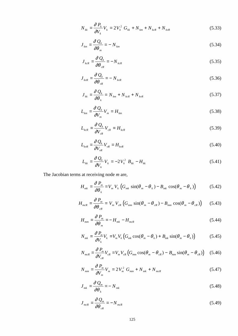
125
NPV
V V G N N Nkkk
kk k kk km kcR kvR= = + + +
∂∂
2 2 (5.33)
JQ
Nkmk
mkm= = −
∂∂θ
(5.34)
JQ
NkcRk
cRkcR= = −
∂∂θ
(5.35)
JQ
NkvRk
vRkvR= = −
∂∂θ
(5.36)
JQ
N N Nkkk
kkm kcR kvR= = + +
∂∂θ
(5.37)
LQV
V Hkmk
mm km= =
∂∂
(5.38)
LQ
VV HkcR
k
cRcR kcR= =
∂∂
(5.39)
LQV
V HkvRk
vRvR kvR= =
∂∂
(5.40)
LQV
V V B Hkkk
kk k kk kk= = − −
∂∂
2 2 (5.41)
The Jacobian terms at receiving node m are,
( )HP
V V G Bmkm
km k mk m k mk m k= = − − −
∂∂θ
θ θ θ θsin( ) cos( ) (5.42)
( )HP
V V G BmcRm
cRm cR mm m cR mm m cR= = − − −
∂∂θ
θ θ θ θsin( ) cos( ) (5.43)
HP
H Hmmm
mmk mcR= = − −
∂∂θ
(5.44)
( )N PV
V V V G Bmkm
kk m k mk m k mk m k= = − + −
∂∂
θ θ θ θcos( ) sin( ) (5.45)
( )N PV
V V V G BmcRm
cRcR m cR mm m cR mm m cR= = − − −
∂∂
θ θ θ θcos( ) sin( ) (5.46)
NPV
V V G N Nmmm
mm m mm mk mcR= = + +
∂∂
2 2 (5.47)
JQ
Nmkm
kmk= = −
∂∂θ
(5.48)
JQ
NmcRm
cRmcR= = −
∂∂θ
(5.49)

126
JQ
N Nmmm
mmk mcR= = +
∂∂θ
(5.50)
LQV
V Hmkm
kk mk= =
∂∂
(5.51)
LQV
V HmcRm
cRcR mcR= =
∂∂
(5.52)
LQV
V V B Hmmm
mm m mm mm= = − −
∂∂
2 2 (5.53)
The Jacobian terms of series converter are,
( )HP
V V G BcRkcR
kcR k km cR k km cR k= = − − −
∂∂θ
θ θ θ θsin( ) cos( ) (5.54)
( )HP
V V G BcRmcR
mcR m mm cr m mm cR m= = − − −
∂∂θ
θ θ θ θsin( ) cos( ) (5.55)
HP
H HcRcRcR
cRcRk cRm= = − −
∂∂θ
(5.56)
( )NPV
V V V G BcRkcR
kk cR k km cR k km cR k= = − + −
∂∂
θ θ θ θcos( ) sin( ) (5.57)
( )NPV
V V V G BcRmcR
mm cR m mm cR m mm cR m= = − + −
∂∂
θ θ θ θcos( ) sin( ) (5.58)
NPV
V V G N NcRcRcR
cRcR cR mm cRk cRm= = + +
∂∂
2 2 (5.59)
The Jacobian terms of shunt converter are,
( )HP
V V G BvRkvR
kvR k vR vR k vR vR k= = − − −
∂∂θ
θ θ θ θsin( ) cos( ) (5.60)
HP
HvRvRvR
vRvRk= = −
∂∂θ
(5.61)
( )NPV
V V V G BvRkvR
kk vR k vR vR k vR vR k= = − + −
∂∂
θ θ θ θcos( ) sin( ) (5.62)
NPV
V V G NvRvRvR
vRvR vR vR vRk= = − +
∂∂
2 2 (5.63)
5.3 Criterion control The UPFC controllable variables are adjusted with respect to well defined reference signals. For the shunt converter, Vkref and Vdc are used as reference signals. Pmref and Qmref are used as reference signals for the series converter. The relation between these reference signals and the UPFC controllable variables is described below.
127
5.3.1 Shunt converter control criterion The active power exchanged between the shunt converter and the AC power system dictates the amount of active power flowing in and out of the DC link. This exchange is controlled by the phase angle difference between the converter and AC system voltages. The reactive power injected (absorbed) by the shunt converter into the AC power system is determined by their voltage amplitude difference. Accordingly, VvR and θvR determine the shunt reactive compensation, QvR, while satisfying the UPFC constrains, PvR + PcR =0, Vk =cte. and Vdc=cte.
5.3.2 Series converter control criterion The series converter controls real and imaginary transmission line current components by varying the amplitude and angle of the injected series voltage via the coupling transformer. Since the series converter VA rating is determined by the product of transmission line current and series voltage source, the active and reactive power exchanged between series converter and AC system is controlled indirectly. The control scheme used in the converter determines the reference signals required to adjust the control variables. In the PWM control scheme presented in reference [4], the controllable variables VcR and θcR are adjusted according to the reference signals Pmref and Qmref, respectively. In reference [7], VcR and θcR are adjusted according to the reference signals Qmref and Pmref, respectively. The mathematical expressions presented in Section 5.2.3 are based on the latter relation. However, incorporating the former relation in our equations would be straightforward. It would only requires permuting columns 5 and 6 in equations (5.23) and (5.25), and rows 5 and 6 in equations (5.22) and (5.24). Both alternatives above have been implemented in our program. If the controllable variables are within limits, both formulations give exactly the same results. When the controllable variable VcR violates a limit, it is fixed at that limit and the regulated variable is freed. Since different regulated variables are freed, according to the control criterion, the final results will be different. In the former control criterion, the reactive power is the regulated variable associated with VcR, while in the latter control criterion is the active power.
5.3.3 Special UPFC control configurations. The implementation of the UPFC control facilities has required the creation of a new type of node, namely PVC. It is a controlled node where the nodal voltage magnitude and the nodal active and reactive powers are specified while the UPFC controllable variable VvR is handled as state variable. Similarly to Load Tap Changers transformers, the new type of node allows the handling of general control strategies, such as series and parallel UPFC configurations. The series condition occurs when the voltage magnitude at the AC series converter terminal of a UPFC, which is regulating the voltage magnitude at its AC shunt converter terminal, is regulated by one or more UPFCs. The parallel condition occurs when two or more UPFCs are controlling voltage magnitude at the same node. In general, this condition does not belong to the category of single criterion control, i.e. only one control variable is adjusted in order to maintain one dependent variable at a specified value. However, an entire group of parallel UPFCs may be treated as a single control criterion if their controllable variable VvR are started from the same initial condition.
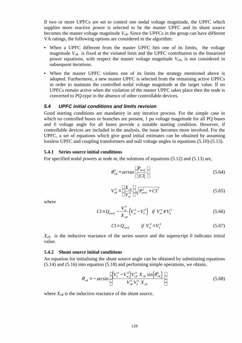
128
If two or more UPFCs are set to control one nodal voltage magnitude, the UPFC which supplies more reactive power is selected to be the master UPFC and its shunt source becomes the master voltage magnitude VvR. Since the UPFCs in the group can have different VA ratings, the following options are considered in the algorithm: • When a UPFC different from the master UPFC hits one of its limits, the voltage
magnitude VvR is fixed at the violated limit and the UPFC contribution to the linearised power equations, with respect the master voltage magnitude VvR, is not considered in subsequent iterations.
• When the master UPFC violates one of its limits the strategy mentioned above is
adopted. Furthermore, a new master UPFC is selected from the remaining active UPFCs in order to maintain the controlled nodal voltage magnitude at the target value. If no UPFCs remain active when the violation of the master UPFC takes place then the node is converted to PQ-type in the absence of other controllable devices.
5.4 UPFC initial conditions and limits revision Good starting conditions are mandatory in any iterative process. For the simple case in which no controlled buses or branches are present, 1 pu voltage magnitude for all PQ buses and 0 voltage angle for all buses provide a suitable starting condition. However, if controllable devices are included in the analysis, the issue becomes more involved. For the UPFC, a set of equations which give good initial estimates can be obtained by assuming lossless UPFC and coupling transformers and null voltage angles in equations (5.10)-(5.13).
5.4.1 Series source initial conditions For specified nodal powers at node m, the solutions of equations (5.12) and (5.13) are,
θ cRmrefPC
0
1=
arctan (5.64)
V XV
P CcRcR
mmref
00
2 21=
+ (5.65)
where
( )C Q VX
V V if V Vmrefm
cRm k m k1
00 0 0 0= − − ≠ (5.66)
C Q if V Vmref m k1 0 0= = (5.67)
XcR is the inductive reactance of the series source and the superscript 0 indicates initial value.
5.4.2 Shunt source initial conditions An equation for initialising the shunt source angle can be obtained by substituting equations (5.14) and (5.16) into equation (5.18) and performing simple operations, we obtain,
( ) ( )θ
θvR
k m cR vR cR
vR k cR
V V V XV V X
= −−
arcsin
sin0 0 0 0
0 0 (5.68)
where XvR is the inductive reactance of the shunt source.

129
When the shunt converter is acting as a voltage regulator, the voltage magnitude of the shunt source is initialised at the target voltage value and then it is updated at each iteration. Otherwise, if the shunt converter is not acting as a voltage regulator, the voltage magnitude of the shunt source is kept at a fixed value within prescribed limits, (VvRmin ≤ VvR ≤ VvRmax), for the whole iterative process.
5.4.3 Limit revision of UPFC controllable variables The power mismatch equations are used as the guiding principle for conducting limit revisions. The mismatch provides an accurate indicator for determining the activation of limits revision for the controllable devices parameters. The revision criterion of the UPFC is based on its active power converter mismatch equation,
∆P P Pbbi
vR cR= + (5.69) where i varies from 1 to the number of UPFCs. If a limit violation takes place in one of the voltage magnitudes of the UPFC sources, the voltage magnitude is fixed at that limit and the regulated variable is freed.
5.5 Synchronous voltage source UPFC model A simplification of the general UPFC model presented above is obtained by neglecting the impedance of the coupling transformers. In this situation, the shunt converter can be assumed to operate at unity power factor and the UPFC is well represented by an ideal series voltage source, termed Synchronous Voltage Source (SVS) [8]. The SVS injects a series variable voltage magnitude and angle. These parameters are adjusted so as to control the active and reactive powers exchanged between the UPFC and the AC system. The schematic representation of a transmission line compensated by a SVS is given in Figure 5.3. The complex voltage injected by the SVS source has variable magnitude Vs (Vsmin ≤ Vs ≤ Vsmax ) and variable phase angle θs (0 ≤ θs ≤ 2π).
Figure 5.3. Transmission line compensated by SVS. The general transfer admittance matrix for the transmission line compensated by a SVS is,
II
Y -Y YY -Y Y
VVV
k
m
kk kk km
mk mk mm
k
s
m
=
(5.70)
where
Y y ykk kk kk kmG j B= + = +
2 (5.71)
Y Ymm kk= (5.72)
Y Y ykm mk km km kmG j B= = + = − (5.73)
y/2 y/2
R X + - k m Vs

130
Based on Figure 5.3 and equation (5.70), the general power flow equations for the compensated transmission line are , At node k :
( )( )
P V G V V G B
V V G Bk k kk k m km k m km k m
k s kk k s kk k s
= + − + −
− − + −
2 cos( ) sin( )
cos( ) sin( )
θ θ θ θ
θ θ θ θ (5.74)
( )
( )Q V B V V G B
V V G Bk k kk k m km k m km k m
k s kk k s kk k s
= − + − − −
− − − −
2 sin( ) cos( )
sin( ) cos( )
θ θ θ θ
θ θ θ θ (5.75)
At node m :
( )( )
P V G V V G B
V V G Bm m mm k m mk m k mk m k
m s mk m s mk m s
= + − + −
− − + −
2 cos( ) sin( )
cos( ) sin( )
θ θ θ θ
θ θ θ θ (5.76)
( )
( )Q V B V V G B
V V G Bm m mm m k mk m k mk m k
m s mk m s mk m s
= − + − − −
− − − −
2 sin( ) cos( )
sin( ) cos( )
θ θ θ θ
θ θ θ θ (5.77)
The linearised Newton equations of the compensated transmission line are given in equation (5.78), where the variable phase angle θs and variable magnitude Vs are taken to be the state variables.
∆
∆
∆
∆
∆
∆
P
P
Q
Q
P
Q
P P PV
VPV
VP P
VV
P P PV
VPV
VP P
VV
Q Q QV
V QV
V Q QV
V
Q Q
k
m
k
m
km
km
k
k
k
m
k
kk
k
mm
k
s
k
ss
m
k
m
m
m
kk
m
mm
m
s
m
ss
k
k
k
m
k
kk
k
mm
k
s
k
ss
m
k
m
m
=
∂∂θ
∂∂θ
∂∂
∂∂
∂∂θ
∂∂
∂∂θ
∂∂θ
∂∂
∂∂
∂∂θ
∂∂
∂∂θ
∂∂θ
∂∂
∂∂
∂∂θ
∂∂
∂∂θ
∂∂θ
∂∂
∂∂
∂∂θ
∂∂
∂∂θ
∂∂θ
∂∂
∂∂
∂∂θ
∂∂
∂∂θ
∂∂θ
∂∂
∂∂
∂∂θ
∂∂
θ
θ
θ
QV
V QV
V Q QV
V
P P PV
VPV
VP P
VV
Q Q QV
VQV
VQ Q
VV
VVV
V
VV
m
kk
m
mm
m
s
m
ss
km
k
km
m
km
kk
km
mm
km
s
km
ss
km
k
km
m
km
kk
km
mm
km
s
km
ss
k
m
k
k
m
m
k
s
s
∆
∆
∆
∆
∆
∆
(5.78)
5.5.1 SVS Initial Conditions The SVS initial conditions are obtained applying the same reasoning used to the UPFC. These mathematical expressions are obtained from the SVS power equations (5.74)-(5.77), assuming null nodal voltage angles, according to the active and reactive power to be controlled. In order to obtain an analytical equations, the real part of the transmission line series impedance is neglected, i.e. R<<X. When the active and reactive powers are regulated from node k to node m, the mathematical expressions for the SVS initial conditions are,
VP CV Bs
kref
k kk
=± +2 2
0
1 (5.79)

131
θ skrefTan
PC
=
−1
1 (5.80)
where
( )C Q V B V V Bkref k kk k m km1 0 2 0 0= + + (5.81) When the active and reactive powers to are regulated from node m to node k, the mathematical expressions for the SVS initial conditions are,
VP CV Bs
mref
m mm
=± +2 2
0
1 (5.82)
θ smrefTan
PC
=
−1
1 (5.83)
where
( )C Q V B V V Bmref m mm m k mk1 0 2 0 0= + + (5.84) When the active and reactive power are not define at the same node, the additional assumption of neglecting the transmission line shunt capacitance should be considers in order to obtain an analytical equations to the initial conditions. The following equations are used to initialised the SVS if the active and reactive powers are specified at nodes k and m, respectively.
V
PV
CV
Bs
kref
m k
km
=±
+
0
2
0
21
(5.85)
θ sm kref
k
TanV PV C
= −
−10
0 1 (5.86)
where ( )C Q V B V Vmref m km k m1 0 0 0= + − (5.87)
If the active and reactive powers are specified at nodes m and k, respectively, the following equations are used to initialised the SVS.
V
PV
CV
Bs
mref
k m
km
=±
+
0
2
0
21
(5.88)
θ sk mref
m
TanV PV C
= −
−10
0 1 (5.89)
where ( )C Q V B V Vkref k km m k1 0 0 0= + − (5.90)
Bkk, Bmm and Bkm are obtained from equations (5.71)-(5.73) and the superscript 0 indicates initial value. The sign considered in the square root evaluation is such as the SVS voltage magnitude is positive.

132
5.6 Load flow test cases An OOP load flow program has been extended to incorporate the models and methods mentioned above. The new program has been applied to the solution of a large number of power networks of different sizes and varying degrees of operational complexity. Power flow solutions converge in five iterations or less to tolerances of 10-12, starting from flat voltage profiles. One or two extra iterations are needed if limits are violated.
5.6.1 Power flow control by means of UPFCs A small, 5-node network [9] has been used in order to show, quantitatively, how the UPFC performs. Solution details are provided so as to enable potential users of these UPFC models to make comparisons. The power flow analysis of the original network was done in Chapter 3. The original network and power flow results are shown in Figure 3.5. The final nodal complex voltages are given in Table 3.2. The original network has been modified to include a UPFC which compensates the transmission line connected between nodes Lake and Main. An additional node, termed Lakefa, is used to connect the UPFC. This is shown in Figure 5.4. The UPFC is used to maintain active and reactive powers leaving the UPFC, towards Main, at 40 MWs and 2 MVARs, respectively. Moreover, the UPFC’s shunt converter is set to regulate Lake’s nodal voltage magnitude at 1 pu. The initial conditions of the UPFC voltage sources are computed by using equations given in Section 5.4, VcR = 0.04 pu, θcR = -87.13o, VvR = 1 pu and θvR = 00. The source impedances have values of XcR=XvR=0.1 pu. Convergence was obtained in 4 iterations to a power mismatch tolerance of 1e-12. The UPFC upheld its target values. The final power flow results are shown in Figure 5.4. The final nodal complex voltages are given in Table 5.1.
Figure 5.4. Modified test network and load flow results.
45+j15
13.46 +j0.34
-13.31 -j4.71
60+j10
Main
Elm
-39.84 -j3.49
40.0 +j2.0
-46.69 -j5.29
-13.62 -j1.85
40+j5
North
Lake
South
-48.43 -j8.92
50.34 +j9.34
81.14 +j76.42
-78.84 -j75.87
47.62 +j5.14
-36.57 +j11.72
37.48 -j12.97
13.74 -j1.78
20+j10
G
G
SG = 40-j75.48
SG = 131.48 +j85.76
Lakefa
40.0 -j17.8

133
Table 5.1. Nodal complex voltages of modified network.
The power flow changes in the UPFC upgraded network, with respect to the original one, are mentioned below. There is an increase of active power flowing towards Lake node, through transmission lines connected between North-Lake and South-Lake, in order to satisfy the active power demanded by the UPFC series converter. The maximum amount of active power exchanged between the UPFC and the AC system will depend on the robustness of the UPFC shunt node, node Lake. Since the UPFC generates its own reactive power, the generator connected at North node decreases its reactive power generation and the generator connected at node South increases its absorption of reactive power. The maximum absolute power mismatches in UPFC and system buses are shown in Table 5.2. It must be noted that the UPFC initial conditions obtained by using the equations in Section 5.4 are very good estimates since the UPFC mismatches have small values.
Table 5.2. Maximum power mismatches in UPFC and bus system.
Table 5.3 shows the variation of the controllable voltage sources during the iterative process.
Table 5.3. Variation of ideal source voltages.
5.6.2 Effect of initial conditions In order to show the impact of good UPFC initial conditions on convergence, different series voltage source initial conditions were used. By way of example, Table 5.4 shows fourth different initial conditions and the number of iterations required to converge. Improper selection of initial conditions degrades Newton’s quadratic convergence, or more seriously, cause the solution to oscillate or even diverge.
Table 5.4. Effect of initial conditions.
complex system nodes voltages North South Lake Lakefa Main Elm V (pu) 1.060 1.000 1.000 0.997 0.992 0.975
θ (degree) 0.00 -1.77 -6.02 -2.51 -3.19 -5.77
BUSES UPFC iteration ∆P ∆Q ∆Pmk ∆Qmk PcR+PvR
0 0.7745 0.1401 5.0E-04 4.0E-02 0.0000 1 0.0189 0.1001 5.1E-03 6.5E-02 5.7E-03 2 3.8E-03 5.1E-04 3.7E-03 5.0E-04 8.6E-05 3 1.2E-07 1.6E-06 1.2E-07 1.6E-6 1.2E-07 4 1.3E-12 1.9E-13 1.2E-12 1.8E-13 1.3E-14
series source shunt source iteration VcR (pu) θcR (degree) VvR (pu) θvR (degree)
0 0.04000 -87.1236 1.00000 0.000000 1 0.10041 -97.5352 1.01341 -5.88817 2 0.10089 -92.7066 1.01735 -6.00513 3 0.10126 -92.7316 1.01734 -6.00549 4 0.10126 -92.7316 1.01734 -6.00549
Initial conditions VcR (pu) θcR (degree) iterations
0.01 180 8 0.04 -87.13 5 0.25 180.0 7 0.25 0.0 divergent

134
5.6.3 Effect of UPFC transformer coupling reactances The effect of source impedances on the UPFC final parameters is shown in this Section. These studies were carried out using the network shown in Figure 5.4. The UPFC is set to control voltage magnitude and active and reactive power flows at the same values as those specified in Section 5.6.1. The UPFC parameters corresponding to different combinations of source impedances are presented in Table 5.5.
Table 5.5. Effect of UPFC impedances.
The parameters of the series source are only affected by its impedance value and they are independent of the shunt source impedance value. The same statement applies to the shunt source parameters. However, this control independence is lost if the UPFC is not acting as voltage magnitude regulator. The simulations above were repeated with the voltage magnitude control deactivated and the shunt source voltage magnitude fixed at 1 pu. The results are presented in Table 5.6. Since the active and reactive powers are the specified variables and the voltage magnitude is not controlled, the final series voltage source parameters are function of both the series and the shunt source impedances.
Table 5.6. Effect of UPFC impedances without voltage control.
impedance series source shunt source XcR (pu)
XvR (pu)
VcR (pu)
θcR (degree)
QcR (MVARs)
VvR (pu)
θvR (degree
)
QvR (MVARs)
0.10 0.10 0.10 -92.73 4.07 1.02 -6.00 17.64 0.05 0.05 0.08 -92.08 3.26 1.01 -6.01 17.49 1E-2 1E-2 0.06 -91.02 2.46 1.00 -6.02 17.34 0.1 0.05 0.10 -92.73 4.07 1.01 -6.01 17.49 0.1 1E-2 0.10 -92.73 4.07 1.00 -6.02 17.34 0.05 0.1 0.08 -92.08 3.26 1.02 -6.00 17.64 0.05 1E-2 0.08 -92.08 3.26 1.00 -6.02 17.34 1E-2 0.1 0.06 -91.02 2.46 1.02 -6.00 17.64 1E-2 0.05 0.06 -91.02 2.46 1.01 -6.01 17.49
impedance series source shunt source XcR (pu)
XvR (pu)
VcR (pu)
θcR (degree)
QcR (MVARs)
θvR (degree)
QvR (MVARs)
0.10 0.10 0.09901 -97.850 3.976 -5.9057 8.963 0.05 0.05 0.07958 -96.257 3.198 -5.9379 11.82 1E-2 1E-2 0.06148 -91.179 2.464 -6.0136 17.18 0.1 0.05 0.09968 -96.080 4.005 -5.9379 11.82 0.1 1E-2 0.10121 -92.827 4.063 -6.0136 17.18 0.05 0.1 0.07894 -98.478 3.168 -5.9057 8.963 0.05 1E-2 0.08114 -92.197 3.257 -6.0136 17.18 1E-2 0.1 0.05929 -99.509 2.377 -5.9057 8.963 1E-2 0.05 0.05989 -96.547 2.407 -5.9379 11.82
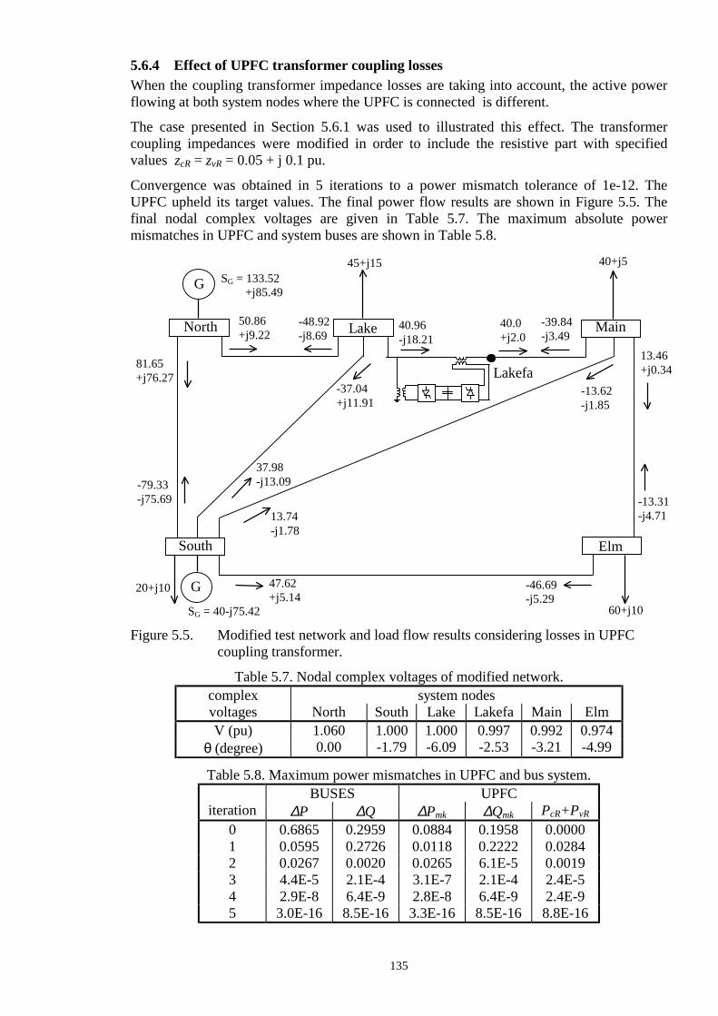
135
5.6.4 Effect of UPFC transformer coupling losses When the coupling transformer impedance losses are taking into account, the active power flowing at both system nodes where the UPFC is connected is different. The case presented in Section 5.6.1 was used to illustrated this effect. The transformer coupling impedances were modified in order to include the resistive part with specified values zcR = zvR = 0.05 + j 0.1 pu. Convergence was obtained in 5 iterations to a power mismatch tolerance of 1e-12. The UPFC upheld its target values. The final power flow results are shown in Figure 5.5. The final nodal complex voltages are given in Table 5.7. The maximum absolute power mismatches in UPFC and system buses are shown in Table 5.8.
Figure 5.5. Modified test network and load flow results considering losses in UPFC coupling transformer.
Table 5.7. Nodal complex voltages of modified network.
Table 5.8. Maximum power mismatches in UPFC and bus system.
complex system nodes voltages North South Lake Lakefa Main Elm V (pu) 1.060 1.000 1.000 0.997 0.992 0.974
θ (degree) 0.00 -1.79 -6.09 -2.53 -3.21 -4.99
BUSES UPFC iteration ∆P ∆Q ∆Pmk ∆Qmk PcR+PvR
0 0.6865 0.2959 0.0884 0.1958 0.0000 1 0.0595 0.2726 0.0118 0.2222 0.0284 2 0.0267 0.0020 0.0265 6.1E-5 0.0019 3 4.4E-5 2.1E-4 3.1E-7 2.1E-4 2.4E-5 4 2.9E-8 6.4E-9 2.8E-8 6.4E-9 2.4E-9 5 3.0E-16 8.5E-16 3.3E-16 8.5E-16 8.8E-16
45+j15
13.46 +j0.34
-13.31 -j4.71
60+j10
Main
Elm
-39.84 -j3.49
40.0 +j2.0
-46.69 -j5.29
-13.62 -j1.85
40+j5
North
Lake
South
-48.92 -j8.69
50.86 +j9.22
81.65 +j76.27
-79.33 -j75.69
47.62 +j5.14
-37.04 +j11.91
37.98 -j13.09
13.74 -j1.78
20+j10
G
G
SG = 40-j75.42
SG = 133.52 +j85.49
Lakefa
40.96 -j18.21
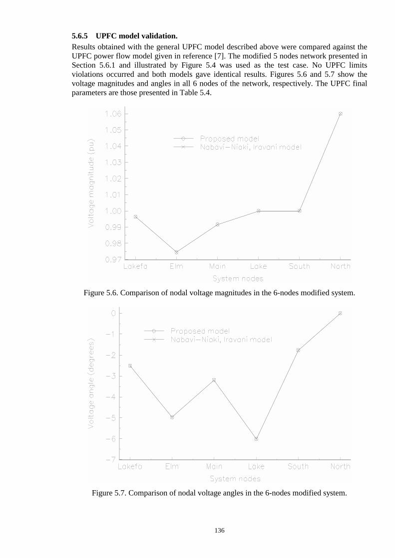
136
5.6.5 UPFC model validation. Results obtained with the general UPFC model described above were compared against the UPFC power flow model given in reference [7]. The modified 5 nodes network presented in Section 5.6.1 and illustrated by Figure 5.4 was used as the test case. No UPFC limits violations occurred and both models gave identical results. Figures 5.6 and 5.7 show the voltage magnitudes and angles in all 6 nodes of the network, respectively. The UPFC final parameters are those presented in Table 5.4.
Figure 5.6. Comparison of nodal voltage magnitudes in the 6-nodes modified system.
Figure 5.7. Comparison of nodal voltage angles in the 6-nodes modified system.
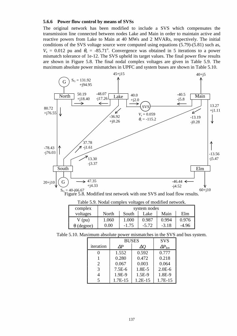
137
5.6.6 Power flow control by means of SVSs The original network has been modified to include a SVS which compensates the transmission line connected between nodes Lake and Main in order to maintain active and reactive powers from Lake to Main at 40 MWs and 2 MVARs, respectively. The initial conditions of the SVS voltage source were computed using equations (5.79)-(5.81) such as, Vs = 0.012 pu and θs = -85.71o. Convergence was obtained in 5 iterations to a power mismatch tolerance of 1e-12. The SVS upheld its target values. The final power flow results are shown in Figure 5.8. The final nodal complex voltages are given in Table 5.9. The maximum absolute power mismatches in UPFC and system buses are shown in Table 5.10.
Figure 5.8. Modified test network with one SVS and load flow results.
Table 5.9. Nodal complex voltages of modified network.
Table 5.10. Maximum absolute power mismatches in the SVS and bus system.
complex system nodes voltages North South Lake Main Elm V (pu) 1.060 1.000 0.987 0.994 0.976
θ (degree) 0.00 -1.75 -5.72 -3.18 -4.96
BUSES SVS iteration ∆P ∆Q ∆Pkm
0 1.552 0.592 0.777 1 0.280 0.472 0.218 2 0.067 0.003 0.064 3 7.5E-6 1.8E-5 2.0E-6 4 1.9E-9 1.5E-9 1.8E-9 5 1.7E-15 1.2E-15 1.7E-15
45+j15
13.27 +j1.11
-13.56 -j5.47
60+j10
Main
Elm
-40.5 -j5.8
40.0 +j2.0
-46.44 -j4.52
-13.19 -j0.28
40+j5
North
Lake
South
-48.07 -j17.26
50.19 +j18.40
80.72 +j76.55
-78.43 -j76.03
47.35 +j4.33
-36.92 +j0.26
37.78 -j1.61
13.30 -j3.37
20+j10
G
G
SG = 40-j66.67
SG = 131.92 +j94.95
SVS
Vs = 0.059 θs = -115.2

138
5.6.7 Effect of SVS initial conditions In order to show the impact of good SVS initial conditions on convergence, different initial conditions were used. By way of example, Table 5.11 shows fourth different initial conditions and the number of iterations required to converge. The second initial conditions showed in this Table were computed using equations (5.79)-(5.81). Improper selection of initial conditions degrades Newton’s quadratic convergence, or more seriously, cause the solution to oscillate or even diverge.
Table 5.11. Effect of initial conditions.
5.6.8 Comparison of UPFC and SVS devices This Section presents simulation results aimed at showing the quantitative differences of the UPFC and SVS models presented above. The active and reactive powers flowing from the UPFC and SVS to node Main were specified at the same values, such as Section 5.6.1 or Section 5.6.6. Table 5.12 shows the results for the following cases, A) UPFC controlling Lake voltage magnitude at 0.95 pu. B) UPFC controlling Lake voltage magnitude at 1.0 pu. C) UPFC controlling Lake voltage magnitude at 1.05 pu. D) UPFC with shunt source voltage magnitude fixed at 0.95 pu. E) UPFC with shunt source voltage magnitude fixed at 1.0 pu. F) UPFC with shunt source voltage magnitude fixed at 1.05 pu. G) SVS model.
Table 5.12. Effect of UPFC and SVS model on ideal source voltages.
As the shunt converter generates less reactive power the voltage magnitude of the series source, required to satisfy a specified power flow, decreases and the range to reach its maximum voltage magnitude limit increases. If the UPFC is connected to a weak system, the reactive power generated by the shunt converter is mainly used for voltage support purposes in order to establish a strong busbar at the point where the power system is supplying active power to the UPFC. In these situations the UPFC shunt converter acts as a voltage regulator, i.e. it does not operate at unity power factor, and the SVS model will not yield realistic results.
Initial conditions Vs (pu) θs (degree) iterations
0.01 180 6 0.012 -85.71 5 0.25 180.0 8 0.25 0.0 10
series source shunt source
CASE VcR (pu)
θcR (degree)
QcR (MVARs)
VvR (pu)
θvR (degree)
QvR (MVARs)
A 0.100 -122.3 3.591 0.921 -5.485 -26.91 B 0.101 -92.74 4.065 1.017 -6.005 17.64 C 0.127 -69.94 4.601 1.114 -6.608 71.67 D 0.098 -113.4 3.728 0.950 -5.633 -14.4 E 0.099 -97.86 3.975 1.000 -5.906 8.963 F 0.108 -83.87 4.238 1.050 -6.200 34.79 G 0.060 -115.2 4.000 ------- ------- -------
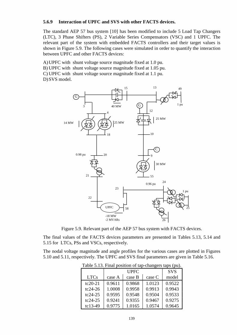
139
5.6.9 Interaction of UPFC and SVS with other FACTS devices. The standard AEP 57 bus system [10] has been modified to include 5 Load Tap Changers (LTC), 3 Phase Shifters (PS), 2 Variable Series Compensators (VSC) and 1 UPFC. The relevant part of the system with embedded FACTS controllers and their target values is shown in Figure 5.9. The following cases were simulated in order to quantify the interaction between UPFC and other FACTS devices: A) UPFC with shunt voltage source magnitude fixed at 1.0 pu. B) UPFC with shunt voltage source magnitude fixed at 1.05 pu. C) UPFC with shunt voltage source magnitude fixed at 1.1 pu. D) SVS model.
Figure 5.9. Relevant part of the AEP 57 bus system with FACTS devices. The final values of the FACTS devices parameters are presented in Tables 5.13, 5.14 and 5.15 for LTCs, PSs and VSCs, respectively. The nodal voltage magnitude and angle profiles for the various cases are plotted in Figures 5.10 and 5.11, respectively. The UPFC and SVS final parameters are given in Table 5.16.
Table 5.13. Final position of tap-changers taps (pu).
UPFC SVS LTCs case A case B case C model
tc20-21 0.9611 0.9868 1.0123 0.9522 tc24-26 1.0008 0.9958 0.9913 0.9943 tc24-25 0.9595 0.9548 0.9504 0.9533 tc24-25 0.9241 0.9355 0.9467 0.9275 tc13-49 0.9775 1.0165 1.0574 0.9645
15
G
G
C
3 12
10
9
1 pu
30 MW
25 MW
40 MW
13 49
4
25 MW 14 MW
18
21
20 0.98 pu
26
55
-18 MW -2 MVARs
22
24
23 0.96 pu
1 pu
25 58 UPFC

140
Table 5.14. Final position of phase shifters angles (degrees).
Table 5.15. Variable series compensation (% of compensation).
Table 5.16. Final UPFC parameters for AEP 57 bus system.
The difference in results obtained with both models for the various cases are due to the different reactive powers generated by the shunt converter, which affect the nodal voltage magnitudes in the system as shown clearly in Figure 5.10. Then, the reactive power generated by the shunt converter can be used to improved the network’s voltage profile.
Figure 5.10. Nodal voltage magnitude profiles in the AEP 57 bus system.
Phase UPFC SVS shifters case A case B case C model ps4-18 -10.356 -9.5849 -8.7964 -10.612 ps4-18 -12.085 -11.305 -10.509 -12.341 ps9-55 -8.5530 -8.5014 -8.4578 -8.6067
UPFC SVS VSC case A case B case C model
vsc3-15 70.91 75.11 78.04 67.91 vsc12-10 46.60 47.59 48.20 46.17
series source shunt source
CASE VcR (pu)
θcR (degree)
QcR (MVARs)
VvR (pu)
θvR (degree)
QvR (MVARs)
A 0.103 -95.75 1.870 1.000 -12.90 8.203 B 0.119 -84.68 2.066 1.050 -13.52 35.38 C 0.139 -76.80 2.275 1.100 -14.17 65.29 D 0.073 -102.7 2.000 ------ ------- -------

141
Figure 5.11. Nodal voltage angles profiles in the AEP 57 bus system.
5.6.10 Solution of a large power network with embedded FACTS devices. A large power network consisting of 1092 buses, 215 generators, 1376 transmission lines, 99 transformers, 15 LTCs, 30 PSs, 13 VSCs, 8 Static Var Compensators (SVC) and 2 UPFCs has been analysed. The load flow converged in 7 iterations. All FACTS devices upheld their target value. The behaviour of the maximum absolute power flow mismatches in system nodes and FACTS devices, as function of the number of iterations, is plotted in Figure 5.12.
Figure 5.12. Mismatches as function of the number of iterations for FACTS devices and system buses.
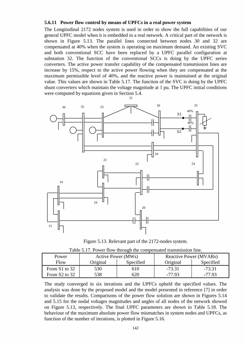
142
5.6.11 Power flow control by means of UPFCs in a real power system The Longitudinal 2172 nodes system is used in order to show the full capabilities of our general UPFC model when it is embedded in a real network. A critical part of the network is shown in Figure 5.13. The parallel lines connected between nodes 30 and 32 are compensated at 40% when the system is operating on maximum demand. An existing SVC and both conventional SCC have been replaced by a UPFC parallel configuration at substation 32. The function of the conventional SCCs is doing by the UPFC series converters. The active power transfer capability of the compensated transmission lines are increase by 15%, respect to the active power flowing when they are compensated at the maximum permissible level of 40%, and the reactive power is maintained at the original value. This values are shown in Table 5.17. The function of the SVC is doing by the UPFC shunt converters which maintain the voltage magnitude at 1 pu. The UPFC initial conditions were computed by equations given in Section 5.4.
Figure 5.13. Relevant part of the 2172-nodes system.
Table 5.17. Power flow through the compensated transmission line. Power Active Power (MWs) Reactive Power (MVARs) Flow Original Specified Original Specified
From S1 to 32 530 610 -73.31 -73.31 From S2 to 32 538 620 -77.93 -77.93
The study converged in six iterations and the UPFCs upheld the specified values. The analysis was done by the proposed model and the model presented in reference [7] in order to validate the results. Comparisons of the power flow solution are shown in Figures 5.14 and 5.15 for the nodal voltages magnitudes and angles of all nodes of the network showed on Figure 5.13, respectively. The final UPFC parameters are shown in Table 5.18. The behaviour of the maximum absolute power flow mismatches in system nodes and UPFCs, as function of the number of iterations, is plotted in Figure 5.16.
36 35 33
31
30
34
32
24 22
20
21
19
14
15
40%
40%
S1
S2

143
Table 5.18. UPFC power flow models comparison.
Figure 5.14. Comparison of nodal voltage magnitude solutions in a real system.
Figure 5.15. Comparison of nodal voltage angle solutions in a real system.
UPFC UPFC-1 UPFC-2 parameters proposed ref. [7] proposed ref. [7] VcR (pu) 0.4882 0.4882 0.4937 0.4937 θcR (deg.) 52.76 52.76 52.88 52.88 VvR (pu) 0.9403 0.9403 0.9403 0.9403 θvR (deg.) -19.54 -19.54 -19.56 -19.56

144
Figure 5.16. Mismatches as function of the number of iterations for UPFCs and system buses.
5.7 Conclusions A general UPFC power flow model has been presented in this paper. The model has been included in a Newton-Rapshon load flow algorithm which is capable of solving large power networks very reliably. The algorithm retains Newton’s quadratic convergence and its efficiency has been illustrated by numeric examples. An alternative UPFC model based on the concept of a Synchronous Voltage Source was also developed and coded into the NR load flow program. It has been shown that caution has to be exercised with this model since it is based on the assumption that the shunt converter is operating at unity power factor. Numerical comparisons of both models have been presented. The results obtained indicate that the SVS model should only be used when the UPFC shunt converter is attached to an infinite busbar. Otherwise, the load flow solution will be incorrect. For cases in which no limit violations take place, identical results were achieved with the general Newton-Rapshon UPFC model and the more restricted UPFC power flow model presented in [7]. The influence of the UPFC initial conditions on convergence was investigated. Improper selection of initial conditions degrades Newton’s quadratic convergence, or more seriously, cause the solution to oscillate or even diverge. A set of analytical equations has been derived to give good UPFC and SVS initial conditions.
5.8 Bibliography [1] IEEE Power Engineering Society/CIGRE: ‘FACTS Overview’, Special Issue, 95TP108, IEEE Service Center, Piscataway, N.J., 1995. [2] Gyugyi L.: ‘A Unified Power Flow Control Concept for Flexible AC Transmission Systems’, IEE Proceedings-C, 1992, Vol. 139, No. 4, July 1992, pp. 323-333. [3] Gyugyi L., Schauder C.D., Williams S.L. Rietman T.R., Torgerson D.R. and Edris A.: ‘The Unified Power Flow Controller: A New Approach to Power Transmission Control’, IEEE Trans. on Power Delivery , Vol. 10, No 2, April 1995, pp. 1085-1097.

145
[4] Mehta H., Johnson R.K., Torgerson D.R, Gyugyi L. and Schauder C.D.: ‘Unified Power Flow Control Concept for Flexible AC Transmission Systems’, Flexible AC Transmission System (FACTS) EPRI Workshop, May 18-20, 1992, Boston Massachusetts. [5] Ooi B.T., Dai S.Z. and Galiana F.D.: ‘A Solid-State PWM Phase-Shifter’, IEEE Trans. on Power Delivery , Vol. 8, No 2, April 1993, pp. 573-579. [6] Noroozian M, Ängquist L., Ghandhari M. and Anderson G.: ‘Use of UPFC for Optimal Power Flow Control’, IEEE/KTH Stockholm Power Tech Conference, Stockholm, Sweden, June 18-22, 1995, pp. 506-511. [7] Nabavi-Niaki A. and Iravani M.R.: ‘Steady-State and Dynamic Models of Unified Power Flow Controller (UPFC) for Power System Studies’, Presented at 1996 IEEE/PES Winter Meeting, 96 WM 257-6 PWRS, January 21-25, 1996, Baltimore, MD. [8] Gyugyi L.: ‘Dynamic compensation of AC Transmission Lines by Solid-State Synchronous Voltages Sources’, IEEE Trans. on Power Delivery , Vol. 9, No 2, April 1994, pp. 904-911. [9] Stagg N.G. and El-Abiad H.A.: ‘Computer Methods in Power System Analysis’, McGraw-Hill Inc., 1968. [10] Freris L.L. and Sasson A.M.: ‘Investigation of the Load Flow Problem’, Proceedings IEE, Vol. 115, No. 10, October 1968, pp. 1459-1470.

146
Chapter 6 Application of FACTS Devices 6.1 Introduction In previous Chapters FACTS device models have been developed, tested and validated. These models have been implemented in a digital power flow program to show the ability of these controllers to regulate power flow through specified transmission paths as well as nodal voltage magnitude at selected points of the network. The software developed is ready to assist power system engineers to evaluate the technical and economical benefits of a wide range of alternative solutions offered by FACTS technologies. The aim of this Chapter is to show some of the possible applications of FACTS devices in power systems. Three applications are presented in this Chapter. FACTS devices are used to redistribute power flow in interconnected power networks, to eliminate loop flows and to increase margins of voltage collapse. Moreover, the effect of the transformer magnetising branch on system losses is quantified. A general power flow tracing algorithm to compute the individual generator contributions to the active and reactive power flows and losses is also proposed.
6.2 Auditing of Individual Generator Contributions to Power Flows, Losses and Cost in interconnected power networks. It has been demonstrated, quite recently, that the trace of electricity from generators to suppliers can be quantified by resorting to the basic laws of electric circuits, i.e. Ohms’ laws and Kirchhoff’s laws. Kirschen, Allan and Strbac [4] and Bialek [5] have put forward algorithms which solve such a problem. A more general power flow tracing algorithm is described in this Section. This algorithm answers all questions relating to individual generator contributions to the active and reactive power flows and losses in each plant component of the power network. In this environment it is a simple matter to determine which generator contribute and in what proportion to each load of the power network. The power flow tracing algorithm is just a mechanism for tracing generation costs and allocating Use of Line Charges (ULC). The algorithm starts from power flow information, as given by a load flow solution. Next, a dominion is obtained for each generator of the power network. A dominion is a directed graph consisting of one source (generator), sinks (loads) and branches. The graph branches relate to transmission lines, transformers, LTCs and ASC. For the purpose of reactive power tracing, various kinds of sources exist, e.g. generators, SVCs, ASCs, UPFCs. Although some transmission lines act as net sources of reactive power and hence are capable of having dominions, in this work all transmission lines are treated as branches, as opposed to sources. However, the lines reactive contributions are correctly taken into account in the calculations. The reactive power tracing algorithm does not take into account reactive power series sources, such as ASC, or non-reciprocal electric components such as phase shifters. In branches which are common to two or more dominions, proportionality is used to determine the power flow contribution of each dominion to the common branch. This basic mechanism also applies to loads supplied by more than one generator. The methodology applies, independently, to active and reactive power. The general algorithm for tracing active and reactive power flows, losses and costs is presented below.

147
6.2.1 Tracing generators’ costs At this point in time the algorithm for tracing active and reactive power flows, losses and costs is being used for off-line auditing analysis. It is coupled to a quadratically convergent, Newton-Raphson load flow capable of solving power networks with embedded FACTS series and shunt controllers. This is a well matched combination which can be used to analyse the impact of FACTS controllers in energy transactions. The general algorithm is,
1. Run the base load flow case. 2. Based on power flow solution, determine the sources’ dominions. 3. Find all the branches that belong to more than one dominion, i.e. common branches. 4. In each branch, find the power contribution of the relevant dominions and/or local source
to the total branch flow and associated nodes. 5. At each branch, find the costs of the power contributed by each dominion and/or local
source. 6. In each node, find the power contribution of the relevant dominions and/or local source
to the node’s load. 7. At each load, find the cost of the power contributed by each dominion and/or local
source. 8. Account for power losses, their cost and ULC in each dominion. Point 4 of the algorithm differs slightly for cases of active and reactive powers and further details are given by separate in the following subsections. Also, further clarification of point 2 is given in Subsection 6.2.5.
6.2.2 Dominions’ contributions to active power flows In each branch the active power contribution of each dominion and/or generator is determined by using proportionality. The dominion’s contributions are obtained by the following equations based on Figure 6.1.
Figure 6.1. Active power dominions’ contributions to branch ij.
P P P P Pij D D Dn G= + + + +1 2' ' ' '! (6.1)
P P P P Pij D D Dn G
' '' '' '' ''= + + + +1 2 ! (6.2)
P P CDk Dk ij' '= × (6.3)
P P CDk Dk ij
'' ''= × (6.4)
j
PL PG
Pij P’ij
PD1 i
PD2
PDn
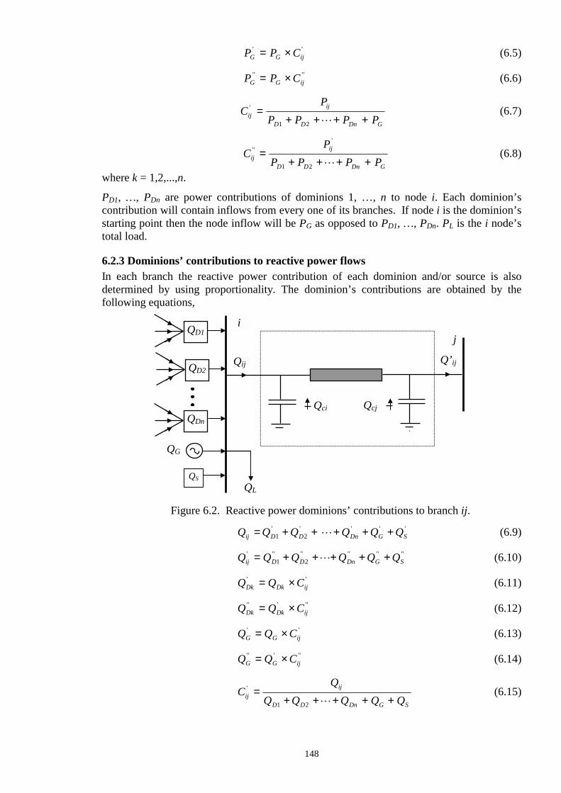
148
P P CG G ij' '= × (6.5)
P P CG G ij
'' ''= × (6.6)
CP
P P P Pijij
D D Dn G
' =+ + + +1 2 !
(6.7)
CP
P P P Pijij
D D Dn G
'''
=+ + + +1 2 !
(6.8)
where k = 1,2,...,n. PD1, …, PDn are power contributions of dominions 1, …, n to node i. Each dominion’s contribution will contain inflows from every one of its branches. If node i is the dominion’s starting point then the node inflow will be PG as opposed to PD1, …, PDn. PL is the i node’s total load.
6.2.3 Dominions’ contributions to reactive power flows In each branch the reactive power contribution of each dominion and/or source is also determined by using proportionality. The dominion’s contributions are obtained by the following equations,
Figure 6.2. Reactive power dominions’ contributions to branch ij.
Q Q Q Q Q Qij D D Dn G S= + + + + +1 2
' ' ' ' '! (6.9)
Q Q Q Q Q Qij D D Dn G S' '' '' '' '' ''= + + + + +1 2 ! (6.10)
Q Q CDk Dk ij
' '= × (6.11)
Q Q CDk Dk ij'' ' ''= × (6.12)
Q Q CG G ij
' '= × (6.13)
Q Q CG G ij'' ' ''= × (6.14)
CQ
Q Q Q Q Qijij
D D Dn G S
' =+ + + + +1 2 !
(6.15)
j i
Q’ij
QL
QG
Qij
QS
Qci Qcj
QD1
QD2
QDn

149
CQ QQ Qij
ij cj
ij ci
'''
=−+
(6.16)
Q Q Cs s ij
' '= × (6.17)
Q Q Q C Qs s ci ij cj'' ' ''( )= + × + (6.18)
where k = 1,2,...n. QL is i node’s load. Qs is the network’s reactive power contribution due to, among other things, the capacitive effects of transmission lines already taken into account in the analysis. QD1, QD2, …, QDn are reactive contributions of dominions 1, 2, …, n to node i. If node i is the dominion’s starting point then the node’s inflow will be QG as opposed to QD1, …, QDn.
6.2.4 Dominions’ contributions to loads Proportionality is also used for finding the dominions and/or sources contributions to the load connected at node i.
Figure 6.3. Active power dominions contributions to load L. The following equations apply to Figure 6.3.
P P P P PL GL
DL
DL
DnL= + + + +1 2 ! (6.19)
P P CDk
LDk L= × (6.20)
P P CG
LG L= × (6.21)
CP
P P P PLL
D D Dn G
=+ + + +1 2 !
(6.22)
where k = 1,2,....n.
6.2.5 Sources’ dominions The concept of source’s dominion is at the heart of the tracing algorithm. In its most basic form it may be seen as a directed graph consisting of one source and one or more sinks. The set of branches linking source and nodes are related to transmission lines, transformers and series FACTS devices present in the power network. The directions of the branches are dictated by the load flow solution upon which the tracing study is based. There are several ways of carrying out the actual implementation of the algorithm used for determining the generators dominions. Reference [4] gives one possible course of action, where the concepts of Commons and Links are used. A Common is defined as a set of contiguous nodes supplied by the same generator. Branches within a Common are termed Internal Branches and the set of external branches linking two Commons is termed Link. The analysis is conducted at the Common and Link level first. Once the power contribution to each Common is known then all nodes, loads and branches within the Common are allocated a share of the power flowing into that Common.
PDn PD2 PD1
i
PL
PG
Pij

150
An alternative algorithm has been implemented in this work. It does not use the concepts of Commons and Links [4]. Instead, it uses the concepts of Generator’s Dominion and Common Branches [6]. The algorithm works as follows: Select the first source and starting from the source node, check all the branches with a connection to the node. Branches in which the power flows away from the node, i.e. outflows, are included as part of the dominion along with the node at the receiving end of the branch. Conversely, branches in which the power flows into the node, i.e. inflows, do not form part of the source’s dominion. The procedure is repeated for each new node as soon as it becomes part of the source’s dominion. After no further nodes can be reached, the process comes to a halt, resulting in a directed subgraph containing only branches which carry power pertaining to the source currently under analysis. The procedure above is repeated for the second source of the network, the third and so on. If a source’s dominion contains no branches then the dominion is a degenerate dominion, but it is still a dominion. For the case of reactive power, a transmission line can be absorbing or generating reactive power as shown in Figure 6.4 (a) and 6.4(b), respectively. In the former case, the far away node will not form part of that dominion since the power flows from receiving end to sending end. In the latter case, the transmission line does not belong to any dominion.
Figure 6.4. Reactive power across transmission line. If the complex taps are set at nominal value, i.e. tv = tu = 1∠ 0o, The transformer representation is given by a series impedance. Otherwise, if the tap magnitude is set off-nominal, it is represented as a transmission line with one capacitive shunt admittance and one reactive shunt admittance. There are several ways of carrying out the actual implementation of the algorithm used for determining the generators dominions, but the one used here is a particular case of the methodology put forward a few years ago by the author and his colleagues in a previous work relating to EMTP network equivalents [6]. In that application all possible flow trajectories between any two pair of nodes are determined. The system is divided into layers. The boundaries of the zero layer are those nodes directly connected to the node generator. The boundaries of the first layer are those nodes connected 1 node away from the node generator and so on. At this point in time, such a detailed level of information does not seem to be necessary in the application we are now pursuing. Nevertheless, it is reassuring to know that the algorithm is capable of providing such information if future developments require it.
j i
Qji Qij
Qc Qc
j iQji Qij
Qc Qc
(a) Absorbing Reactive Power (b) Generating Reactive Power

151
6.2.6 Numeric Example of Active Power Flow Auditing This numeric example illustrates the simplicity and veracity of the power auditing algorithm. A small network was chosen for this purpose. However, the algorithm is general and can equally be applied to networks of any size. The transmission line data are given in Table 6.1. The AVR of each generator controls nodal voltage magnitude at 1.02 pu. The slack generator is connected at node 3.
Table 6.1. Transmission line data.
Figure 6.5 shows the power flows throughout the network, as given by a load flow solution.
Figure 6.5. Test network. Based on these trajectories, the three domains of the network are determined; one domain per generator. In order to illustrate the generality of the analysis by layers, Table 6.2 shows all the possible paths for the flow due to the generator connected to node 1.
Table 6.2. Paths and layers for the flow injected by the generator in node 1.
Sending Node
Receiving Node
R (pu)
XL (pu)
BTOTAL (pu)
1 5 0.0423 0.1693 4.1E-2 1 4 0.0635 0.2539 6.1E-2 4 3 0.0317 0.1269 3.1E-2 3 5 0.0317 0.1269 3.1E-2 5 2 0.0529 0.2116 5.1E-2 2 4 0.0635 0.2539 6.1E-2
Number path layer number path layer 1 1,5 1 8 1,5,2,4 3 2 1,4 1 9 1,4,3,5 3 3 1,5,3 2 10 1,4,2,5 3 4 1,5,2 2 11 1,5,3,4,2 4 5 1,4,3 2 12 1,5,2,4,3 4 6 1,4,2, 2 13 1,4,3,5,2 4 7 1,5,3,4 3 14 1,4,2,5,3 4
65.73 -j 14.21
100-j9.52
40.42-j5.87 39.42-j3.61
80+j0
59.58 -j3.65
60+j0
25.15-j17.83
24.87-j15.77
9.34+j35.05 25.79-j19.28
3
58.13 -j5.24
26.13-j21.11 68.63 -j8.91
81.37-j7.58 77.99-j15.87
150-j16.48 110+j0
1
2
4
5

152
3
As mentioned previously, the present application does not require information relating to all possible flow paths and layers but rather it requires information pertaining to flow paths that satisfy the outflow criterion. Paths belonging to the dominion are assigned a code number 1 whereas paths outwith the generator’s dominion are assigned a code number 0. The directed subgraphs of dominions 1, 2 and 3 are shown in Figures 6.6, 6.7 and 6.8, respectively. It must be noted that dominion 3, corresponding to generator 3, is a degenerate dominion, i.e. it contains generation and load but no branch.
Table 6.3. Dominion of generator 1.
Figure 6.6. Dominion of generator 1.
Figure 6.7 . Dominion of generator 2.
Figure 6.8. Dominion of generator 3.
Number path code number path code 1 1,5 1 5 1,4,3 1 2 1,4 1 6 1,4,2 0 3 1,5,3 1 7 1,5,3,4 0 4 1,5,2 0 8 1,4,3,5 0
5
3
1 4
4
3
5 2

153
From Figures 6.6, 6.7 and 6.8 or, alternatively, from information given by the program which finds the generator dominions, e.g. Table 6.3, it is possible to determine which branches are common to more than one dominion. In this example there are two common branches. Branch 5-3 and branch 4-3 are both common to dominions 1 and 2. Using the equations given in Section 6.2.2 of the algorithm, it is straightforward to calculate the contributions of each dominion to common branches 5-3 and 4-3. This information is presented in Table 6.4.
Table 6.4. Contribution of dominions 1 and 2 to common branches 5-3 and 4-3.
By way of example, the power flow contribution of dominion 1 at the sending end of transmission line 5-3 is calculated explicitly,
C5 32613
5813 77 9901919− =
+=' .
. .. and PD1 01919 5813 11156' . . .= × = ,
as is the contribution of dominion 1 at the receiving end of the same transmission line,
C3 525 79
5813 77 9901895− =
+=' ' .
. .. and PD1 01895 5813 11014'' . . .= × =
The contributions of dominion 1 to the active power losses in branch 5-3 become readily available from the above result. Power flows and losses contributions of dominion 2 to the same transmission line are calculated accordingly, as is the power flows and losses contributions of both dominions to the other common branch. In this example there are three loads and three dominions but dominion 3 only contributes to the load connected to node 3. Dominions 1 and 2 contribute to all three loads. Such contribution is easily determined by using the equations given in Section 6.2.4 of the algorithm. This information is presented in Table 6.5.
Table 6.5. Individual contribution of dominions 1, 2 and 3 to system load.
By way of example, the contributions of dominions 1, 2 and 3 to the load connected at node 5 are calculated explicitly. The contribution factor C5 is calculated first,
C5 1105813 77 99
0 8081=+
=. .
. , and the actual contributions to the load are calculated next,
Sending end Receiving end
Branch C’SR
(%) P’
D1 (MW)
P’D2
(MW) C’’
RS (%)
P’’D1
(MW) P’’
D2 (MW)
5-3 19.19 11.156 14.969 18.95 11.014 14.777 4-3 23.92 9.429 15.723 23.65 9.324 15.548
Loads and contribution factors CL
Individual contributions of dominions
Loads CL
(%) PL
D1 (MW)
PLD2
(MW) PL
D3 (MW)
Node 3 100.0 20.3388 30.3255 9.3400 Node 4 76.08 29.9900 50.0100 0.0000 Node 5 80.81 46.9769 63.0231 0.0000

154
PD15 5813 08081 46 9769= × =. . .
PD2
5 77 99 08081 630231= × =. . . PD3
5 0 0 08081 0 0= × =. . . The contributions of dominions 1, 2 and 3 to loads 3 and 4 are calculated accordingly.
6.2.7 Numeric Example of Reactive Power Flow Auditing In order to illustrate the algorithm for reactive power auditing the network used in the example above has been modified to include reactive loading in the original loads. The reactive power flows throughout the network, as given by a load flow solution, are shown in Figure 6.9.
Figure 6.9. Test network.
The reactive generators dominions, as obtained by the methodology presented above, are shown schematically in Figures 6.10, 6.11 and 6.12. The transmission line connected between nodes 1 and 4 is generating reactive power such that it does not belong to any generator dominion.
Figure 6.10. Reactive dominion of generator 2.
2 5
j 9.26
j12.21
j0.75 j1.40
80+j20
j12.96 60+j10
j27.85
j26.44
j78.28 j41.83
3
j10.92
j41.86 j3.83
j5.62 j 2.79
j1.78 110+j50
1
2
4
5

155
Figure 6.11. Reactive dominion of generator 1.
Figure 6.12. Reactive dominion of generator 3. Using the equations given in Section 6.2.3 of the algorithm, the contributions of dominion 3 to branches 3-5, 3-4, 4-2 and 2-5 are determined. This information is given in Table 6.6. By way of example the net generator power contribution at the receiving end of the line 3-5, shown in Figure 6.13, is calculated.
Table 6.6. Contribution of dominion 3 to branches 3-5, 3-4, 4-2 and 2-5.
Sending end Receiving end Branch C’
SR
(%) Q’
D3 (MVAr)
C’’RS
(%) Q’’
D3 (MVAr)
Q’’s
(MVAr) 3-5 100.0 41.83 92.97 38.89 2.96 3-4 100.0 26.84 93.82 24.81 3.04 4-2 31.65 7.85 5.38 0.42 3.17 2-5 100.0 0.42 5.28 2.05 0.35
1
2 5
4
3
5 2

156
Figure 6.13. Reactive power flows across the transmission line. The contribution factor is,
C3 54186 1474183 161
0 9297− = −+
=' ' . .. .
. The net reactive power due to the line’s capacitive effects at the receiving end is,
QD3 0 9297 161 147 2 96'' . . . .= × + = The net reactive power due to the generator at the receiving end is,
QG3 0 9297 4183 38 89'' . . .= × = The reactive power flows in other branches of the dominion are calculated similarly. Information on individual dominion contributions to the load power is presented in Table 6.7. These contributions are also obtained by means of proportionality factors. Table 6.7. Individual contribution of dominions 1, 2 and 3 and network to system load.
The contributions of dominions 1, 2 and 3 to the common branch 5-2 are calculated using proportionality and the results are shown in Table 6.8.
Table 6.8. Contribution of dominions 1, 2 and 3 to branch 5-2.
Loads and contribution factors CL
Individual contributions of dominions in MVARs
Loads CL (%)
QL D1 QLD2 QL
D3 QLs
Node 3 12.77 0.00 0.00 10.00 0.0 Node 4 68.34 0.00 0.00 16.96 3.04 Node 5 94.71 6.88 0.00 36.84 6.28
Node 2 Node 5 Dominion
C’
SR = 100% C’’
SR = 5.28% 1 0.0 0.38 2 2.78 0.0 3 0.42 2.06
j41.83 j41.86
3 5
Transmission Line
j43.44
j1.61 j1.47
j40.39

157
6.2.8 Effect of FACTS devices on active power sources dominions The power contribution of generators to power flow across a transmission component as well as the number of generators contributing to this flow can be modified by changing power flows in the network using FACTS devices. A VSC has been embedded in the 5 nodes network as shown in Figure 6.14. The controller has been set to increase the active power flow by 30% .
Figure 6.14. 5 nodes system with FACTS controller. Table 6.9 shows the active power source dominions for the original and modified cases. The dominion of generator 3 is degenerate and this machine does not contribute active power flows to the network. This table shows the re-distribution of generator contributions to the active power flows across transmission components.
Table 6.9. Comparison of active power source dominions (MWs). Transmission Original case Modified Case Components Generator 1 Generator 2 Generator 1 Generator 2 Send. Rec. Send. Rec. Send. Rec. Send. Rec. Send. Rec.
1 4 40.54 39.54 32.91 32.20 1 5 59.46 57.92 67.10 65.20 2 4 68.98 66.07 90.22 84.86 2 5 81.02 77.64 59.78 57.91 3 4 9.42 9.58 15.74 16.02 9.95 10.20 26.21 26.87 3 5 10.60 10.93 14.21 14.65 6.68 6.94 5.93 6.17
This simple example shows that FACTS controllers can be applied to regulated the amount of active power flow in a given dominion.
80+j20
60+j10
3
110+j50
1 4
5 2
2F

158
6.2.9 Numeric Examples of Use of Line Charges Two numeric examples are presented below. A small network was chosen as the first test case. Data is available in open literature [5]. This example illustrates the simplicity of the algorithm and validates its accuracy of response. The second case includes an actual network. It shows a practical application of the theory. The individual costs of generation, as given by a power flow solution, are traced throughout the network. Simple test case Figure 6.15 shows the power flows throughout the network. Based on these trajectories, the two domains of the network are determined; one domain per generator.
Figure 6.15. Small test network. Table 6.10 gives information of branch impedances. In this example [5], the ULCs have been taken to be equal to the branch resistances.
Table 6.10. Use of Line Charges.
In this example there are two common branches. Branch 2-4 and branch 4-3 are both common to dominions 1 and 2. Using the power auditing algorithm it is straightforward to calculate the contributions of each dominion to common branches 2-4 and 4-3. This information is presented in Table 6.11. Power losses and charges for use of line are presented in Table 6.12.
Table 6.11. Contribution of dominions 1 and 2 to branches 2-4 and 4-3.
Line 1-2 1-3 1-4 2-4 4-3 Rij=Charge 12.75 6 11.7 3.5 5.75
Xij 97 69.5 96 30.8 58
Sending end Receiving end Branch CSR
(%) D1
(MW) D2
(MW) CRS (%)
D1 (MW)
D2 (MW)
2-4 100 59 114 98.84 58.31 112.68 4-3 29.32 49.95 33.04 28.97 49.34 32.64
3 4
1 2
300 MW 200 MW
400 MW 114 MW
225 MW
218 MW
173 MW
171 MW
60 MW 59 MW
82 MW 83 MW
115 MW
112 MW

159
Table 6.12. System power losses and Use of Line Charges.
The ULCs in lines 2-4 and 4-3 are calculated as follows:
C2-4Ch =
+=35
0 69 13217413.
. ..
Ch 12 4 17413 0 69 120− = × =. . .
Ch 22 4 17413 132 2 30− = × =. . .
C4-3Ch =
+=575
0 61 0 40569.
. ..
Ch 14 3 569 0 61 3 47− = × =. . .
Ch 24 3 569 0 40 2 28− = × =. . .
Table 6.13 shows comparisons of Use of Line Charges as calculated by three different methods. The Auditing Algorithm, presented in the previous Section, is compared against the method of Topological Factors due to Dr Bialek [5] and the method of Generalised Factors as calculated in Reference [7]. In this example some of the Generalised Factors are negative and would produce negative ULCs, i.e. a generator would be compensated for using a transmission facility. This is contrary to normal commercial practices and in actual applications all negative factors and costs are set to zero [5]. It must be noted that the charges based on Dr Bialek’s algorithm compare very well with the charges given by the Auditing Algorithm. In contrast, some differences are observed with respect to the charges given by the Generalised Factors Algorithm. Perhaps the most suspect results are the charges made to Generator 2 for the use of branch 1-3 and the undercharge to Generator 1. It must be noted that branch 1-3 is not part of Generator 2’s dominion. This fact is correctly recognised by Dr Bialek’s algorithm. Also, important differences exist in the charges made to Generators 1 and 2 for the use of Branch 2-4.
Table 6.13. Comparison of Use of line Charges by three different methods.
Power Loss Charge for Use of Line Branch D1
(MW) D2
(MW) CCh (%)
Ch1 (pu)
Ch2 (pu)
1-2 1 0 1275 12.75 0 1-3 7 0 85.71 6 0 1-4 3 0 390 11.7 0 2-4 0.69 1.32 174.13 1.20 2.30 4-3 0.61 0.40 569 3.47 2.28
Total 12.30 1.72 ----- 35.12 4.58
Auditing Algorithm
Generalised Factors Algorithm
Bialek’s Algorithm
Branch Ch1 (pu)
Ch2 (pu)
Ch1 (pu)
Ch2 (pu)
Ch1 (pu)
Ch2 (pu)
1-2 12.75 0 12.75 0 12.75 0 1-3 6 0 5.22 0.78 6 0 1-4 11.7 0 11.7 0 11.7 0 2-4 1.20 2.30 1.77 1.73 1.21 2.29 4-3 3.47 2.28 3.06 2.69 3.48 2.27
Total 35.12 4.58 34.5 5.2 35.14 4.56

160
6.2.10 Allocating generation costs and ULCs in a real life power network In order to illustrates how the tracing algorithm works with a realistic power system, a 115 kV company network is used to carry out this study. The network is shown in Figure 6.16. It spans an area of nearly 40,000 square miles. It consists of 60 nodes, 19 generators, 50 transmission lines, 19 transformers and 2 VAR compensators. The network is actually part of a much larger interconnected system. A security-constrained economic dispatch, including reactive power source co-ordination, provides the starting point for this study. Total supplied active power, demand and losses are 351.02 MW, 343.5 MW and 7.52 MW, respectively. The global generation cost is £369.7/MW-hr. Table 6.14 gives generators’ costs at supply points and dominion-branch information. In Figure 6.16, branches belonging to Generator 6’s dominion are shown by solid lines whilst other branches are shown by dashed lines.
Figure 6.16. 115 kV Company Power Network. In practice, ULCs consist of several cost elements. In this paper, we only address the cost element associated to transmission losses. By way of example, Table 6.15 shows power flows information at branches L28 and L34. These are selected since their power flow is contributed to by a large number of dominions, i.e. 11 dominions contribute to Branch L28 and 15 dominions contribute to Branch L34. They also serve to exemplify the case of medium and short distance transmission lines, i.e. 56 miles and 6 miles, respectively. Information of dominions’ contributions to power losses and ULC at each branch become readily available from the individual branch power flows. Table 6.16 shows power losses and ULC at branches L28 and L34. These costs have been calculated on the basis of 50 £/MW-mile for both transmission lines over a time horizon of 1 year. Admittedly, the study is biased towards the Transmission Company since maximum loading conditions were assumed throughout this time horizon. A fairer study would have to involve multiple studies, say at half hour slot times.
25
21
42
22
5 7 6
41
16
39
4 20
3 2
46
19
38
27 29 53
10 50
24 37 17 18
43 33
51 45
52 23
44
58
55 54 59
60
56
35
1
33
14 12 13
48
15 32 34
11
49
26
57
9
8
L34
L28
31

161
Table 6.14. Cost of generation at supply points and Generators’ dominions. Generator
Node Costs
(£/MW-hr) Branches
1 53.7 65, 35, 31, 32, 33, 47, 34, 48, 49, 68, 29 2 15.2 64, 35, 31, 32, 33, 47, 34, 48, 49, 68, 29, 28, 27, 50, 26, 30, 46 3 15.2 63, 35, 31, 32, 33, 47, 34, 48, 49, 68, 29, 28, 27, 50, 26, 30, 46 4 15.1 62, 35, 31, 32, 33, 47, 34, 48, 49, 68, 29,
28, 27, 50, 26, 30, 46 5 15.1 61, 35, 31, 32, 33, 47, 34, 48, 49, 68, 29,
28, 27, 50, 26, 30, 35, 31, 32, 33, 47, 34, 48, 49, 68, 29, 28, 27, 50, 26, 30, 46, 25, 22, 23, 44, 45, 42, 56, 18, 17, 15, 24, 16, 43
6 32.0 60, 35, 31, 32, 33, 47, 34, 48, 49, 68, 29, 28, 27, 50, 26, 30, 46, 25, 22, 23, 44, 45, 42, 56, 18, 17, 15, 24, 16, 43
7 32.0 59, 35, 31, 32, 33, 47, 34, 48, 49, 68, 29, 28, 27, 50, 26, 30, 46, 25, 22, 23, 44, 45, 42, 56, 18, 17, 15, 24, 16, 43
8 17.1 58 9 21.7 57, 42, 56 11 21.7 55, 41, 35, 31, 32, 33, 47, 34, 48, 49, 68,
29, 28, 27, 50, 26, 30, 46, 25, 22, 23, 44, 45, 42, 56, 18, 17, 15, 24, 16, 43, 14, 19, 20, 12, 13, 21, 39, 40
12 17.1 54, 41, 35, 31, 32, 33, 47, 34, 48, 49, 68, 29, 28, 27, 50, 26, 30, 46, 25, 22, 23, 44, 45,42 ,56, 18, 17, 15, 24, 16, 43, 14, 19, 20, 12, 13, 21, 39, 40
13 22.9 53, 41, 35, 31, 32, 33, 47, 34, 48, 49, 68, 29, 28, 27, 50, 26, 30, 46, 25, 22, 23, 44, 45, 42, 56, 18, 17, 15, 24, 16, 43, 14, 19, 20, 12, 13, 21, 39, 40
14 10.2 52, 41, 35, 31, 32, 33, 47, 34, 48, 49, 68, 29, 28, 27, 50, 26, 30, 46, 25, 22, 23, 44, 45, 42, 56, 18, 17, 15, 24, 16, 43, 14, 19, 20, 12, 13, 21, 39, 40
15 25.2 51, 34, 48, 49, 68 27 15.9 38, 67, 34, 48, 49, 68 29 22.8 37, 66, 34, 48, 49, 68 31 5.6 36 51 5.6 7 60 5.6 41, 35, 31, 32, 33, 47, 34, 48, 49, 68, 29, 28, 27, 50, 26, 30, 46,
25, 22, 23, 44, 45, 42, 56, 18, 17, 15, 24, 16, 43, 14,19 ,20, 8, 11, 12, 13, 21, 39, 40, 6, 9, 10, 4, 69, 3, 1, 2
Table 6.17 shows which dominions feed load 25 and their power share, individual generation costs at the load point and ULCs incurred in transporting electrical energy from sources.

162
Table 6.15. Dominions’ contributions to flows in branches L34 and L28.
Table 6.16. Power losses and ULCs.
Table 6.17. Power supplied and costs incurred in feeding load 25.
Generator Node
Power Flows in Branch L34 (MW)
Power Flows in Branch L28 (MW)
Sending Receiving Sending Receiving 1 0.01189 0.01188 0.0 0.0 2 0.03373 0.03371 2.15176 2.08624 3 0.02698 0.02697 1.72141 1.66899 4 0.02698 0.02697 1.72141 1.66899 5 0.06178 0.06174 4.51577 4.37828 6 0.05766 0.05763 4.21472 4.08639 7 0.05766 0.05763 4.21472 4.08639 11 0.00420 0.00419 0.30242 0.29321 12 0.00420 0.00419 0.30243 0.29321 13 0.00420 0.00419 0.30243 0.29321 14 0.00420 0.00419 0.30243 0.29321 15 0.37260 0.37240 0.0 0.0 27 0.26082 0.26068 0.0 0.0 29 0.26082 0.26068 0.0 0.0 60 0.00962 0.00961 0.69212 0.67104
Total 1.19734 1.19666 20.44162 19.81916
Gen. Branch L34 Branch L28 Node Power Losses (MW) ULCs (£/yr) Power Losses (MW) ULCs (£/yr)
1 0.00001 0.003 0.0 0.0 2 0.00002 0.006 0.06552 183.456 3 0.00001 0.003 0.05242 146.776 4 0.00001 0.003 0.05242 146.776 5 0.00004 0.012 0.13749 384.972 6 0.00003 0.009 0.12833 359.324 7 0.00003 0.009 0.12833 359.324 10 0.00001 0.003 0.00921 25.788 11 0.00001 0.003 0.00922 25.816 12 0.00001 0.003 0.00922 25.816 13 0.00001 0.003 0.00922 25.816 14 0.0002 0.060 0.0 0 15 0.00014 0.042 0.0 0 16 0.00014 0.042 0.0 0 19 0.00001 0.003 0.02108 59.024
Total 0.00068 0.204 0.62246 1742.888
Dominions Power Share (MW) Generation Costs (£/hr) ULC Costs (£/yr) 11 3.0213 5.463 2.2489 12 3.0213 4.305 2.2489 13 3.0213 5.765 2.2489 14 3.0213 2.568 2.2489 60 6.9148 0.823 994.3197
Total 19 18.924 1003.3153

163
6.2.11 Tracing of reactive power flows The reactive power tracing of the company network shown in Figure 6.16 is carried out below. The equations given in Section 6.2.3 of the algorithm are used. The reactive power consumed by system load is 173.23 MVARs. The reactive power supplied by generators 1, 6, 7, 9, 27, 29, 31, 51 to the system is 143.3 MVARs while generators 2, 3, 4, 5, 8, 11, 12, 13, 14, 15, 60 and the two shunt reactors absorb 95.6 MVARs. The remaining reactive power is generated by transmission lines and transformers. Table 6.18 shows the reactive power dominions of the generators which contribute reactive power to the network.
Table 6.18. Reactive Power Flow Generators’ Dominions.
In Figure 6.17, branches belonging to Generator 6’s reactive dominion are shown by solid lines whilst other branches are shown by dashed lines. It must be noted that generator 2, 3, 4, 5, 11, 12, 13, 14 absorb part of the reactive power generated by Generator 6.
Figure 6.17. Generator 6’s reactive power dominion.
Generator Node
Branches
1 65, 30, 31, 47, 28, 27, 26, 50, 46, 62, 63, 64 6 60, 41, 26, 50, 46, 62, 63, 64, 25, 21, 22, 23, 44, 45,
61, 24, 39, 40, 52, 53, 54, 55 7 59, 41, 26, 50, 46, 62, 63, 64, 25, 21, 22, 23, 44, 45,
61, 24, 39, 40, 52, 53, 54, 55 9 57, 58, 42, 56
27 38, 67, 34, 48, 49, 51, 68 29 37, 34, 48, 49, 51, 68 31 36 51 7
11
25
21
42
22
5 7 6
41
16
39
4 20
3 2
46
38
53
14 12 13
48 49
26
L22

164
6.3 Loop flows Loop flow is a physical and unwanted phenomenon in electrical networks. It results from the operation of the overall interconnected system where power flows paths are proportional to the inverse of the transmission components’ impedances and they follow circuit laws, such that this phenomenon takes place in a natural way according to operative conditions. In an integrated electric system operating in a de-regulated market, loop flows could be in conflict with the wishes of one or more utilities using the transmission corridors. Loop flows effect adversely voltage levels, losses, and reduce thermal and stability margin limits. In order to avoid this unwanted phenomenon, electric utilities have used, traditionally, phase-shifting transformers and series compensators. Two numeric examples are presented in this Section in order to show how FACTS devices are applied to solve loop flow problems. Case 1 Consider the power system shown in Figure 6.18 with line impedances Z14=0.063+j0.08 pu, Z13=0.012+j0.05 pu, and Z23=0.01+j0.08 pu. Line 1-4 has a total shunt susceptance of 0.04 pu, while line 1-3 has 0.02 pu. The two-winding transformer primary and secondary taps are fixed at 1∠ 0o and 0.95∠ 0o, respectively. The transformer contains no resistance and its secondary reactance value is XS= 0.0001 pu. Node 1 is taken to be the slack node with a fixed voltage of 1∠ 0o pu. The voltage magnitude at nodes 2 and 3 are controlled by the Generator’s AVR at 1.02 pu and 1.01 pu. The active power injected by generators connected at nodes 2 and 3 is 100 MWs. The system base is considered 100 MVA. From the power flow solution shown in Table 6.18 it is clear that there is a loop flow. The total system losses were 5.429 MWs and 3.086 MVARs for the active and reactive powers, respectively.
Figure 6.18. Four nodes system with loop flow. In order to eliminate the unwanted loop flow, the two-winding transformer has been activated as a phase shifter. Both complex taps have been set to nominal, i.e. 1∠ 0o. The active power flow to be controlled by the phase angle of the primary tap has been re-directed with respect to the original direction, and specified at 3 MWs. The active power flow solution is shown in Figure 6.19. The final primary tap’s phase angle required to achieve the control was 1.127o. The total system losses were 0.7777 MWs and -3.303 MVARs for the active and reactive powers, respectively. The negative sign in the reactive power indicates that the generators are absorbing reactive power from the system.
100 MWs
6.54 MWs
100 MWs
1
4
2 3
G
G G 150+j 56 50+j40
150+j60
1.17 MWs
56.19 MWs 6.19 MWs
6.19 MWs
6.60 MWs
56.54 MWs
155.43 MWs

165
Figure 6.19. Four nodes system with loop flow controlled by PS.
This case shows that unwanted loop flow can be eliminated and system losses can be reduced by using proper phase shifts and tap magnitudes. Case 2 Figure 6.20 illustrates the relevant part of the standard AEP 57 nodes system where a power reactive loop flow takes place. The reactive power flowing in the loop is shown in this figure. All reactive power flows are given in MVARs.
Figure 6.20. Relevant part of AEP 57 nodes system with reactive power loop flow.
In order to eliminate the loop flow, the transformer connected between nodes 15 and 45 has been replaced by a UPFC. The UPFC controls the active and reactive power injected at node 45 at 40 MWs and 6 MVARs, respectively. Moreover, the voltage magnitude at node 15 is controlled by the UPFC’s shunt converter at 0.988 pu. The final results for the reactive power flow are shown in Figure 6.21.
15
14
46
47 4838
44
45
j 10.92
j 9.54
j 27.31
j
j 25.39
j 23.96 j 12.36 j 12.26 j 19.66 j 19.34
j 5.29
j 5.14
j 3.35
j
j 2.15
j 0.8
100 MWs
1
4
2 3
G
G G 150+j 56 50+j40
150+j60
3.48 MWs
2.75 MWs 47.0 MWs
3.0 MWs
3.0 MWs
2.7 MWs
47.25 MWs
100 MWs
150.78 MWs

166
Figure 6.21. Relevant part of AEP 57 nodes system with one UPFC.
The final UPFC parameters required to achieve the target control are given in Table 6.19.
Table 6.19. UPFC parameters.
The ability of the UPFC to control reactive power flow was used to change the direction of the reactive power flow in order to eliminate the loop flow. Another option to solve the problem is to change the relation of voltage magnitude at terminals of one of the transmission components that make up the loop. The primary and secondary taps of the transformer connected between nodes 15 and 45 have been changed in order to change the direction of the reactive flow. The primary and secondary taps have been changed from 0.955 and 1.0 to 0.95 and 1.02, respectively. The final results for the reactive power flow, in MVARs, are shown in Figure 6.22. The AEP57 nodes system nodal voltage magnitude profiles are shown in Figure 6.23. The system losses for the cases mentioned above are presented in Table 6.20, where the negative sign in the reactive power indicates absorption of reactive power by the generators.
Table 6.20. Total system losses.
Parameters UPFC Series Converter Shunt Converter
Voltage Magnitude (pu) 0.0807 0.9924 Voltage Angle (degrees) 170.02 -7.39
Active Power (MWs) 3.046 -3.046 Reactive Power (MVARs) 0.431 4.28
Losses CASES Active Power
(MWs) Reactive Power
(MVARs) Base case 27.86 - 15.75
Network with UPFC 27.55 -21.93 Network with LTC 27.64 -16.79
15
14
46
47 48 38
44
45
j 8.36
j 7.11
j 27.31
j 25.39
j 22.05
j 20.79 j 9.19 j 9.11 j 15.37 j 15.15
j 2.63
j 2.83
j 4.63
j 6.0
j 6.0
j 2.82 UPFC
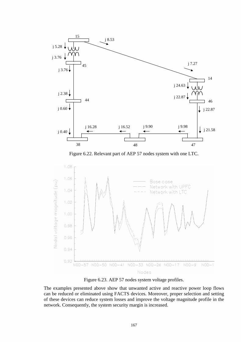
167
Figure 6.22. Relevant part of AEP 57 nodes system with one LTC.
Figure 6.23. AEP 57 nodes system voltage profiles.
The examples presented above show that unwanted active and reactive power loop flows can be reduced or eliminated using FACTS devices. Moreover, proper selection and setting of these devices can reduce system losses and improve the voltage magnitude profile in the network. Consequently, the system security margin is increased.
15
14
46
47 48 38
44
45
j 8.53
j 7.27
j 24.63
j 22.87
j 22.87
j 21.58 j 9.98 j 9.90 j 16.52 j 16.28
j 0.40
j 0.60
j 2.38
j 3.76
j 3.76
j 5.28
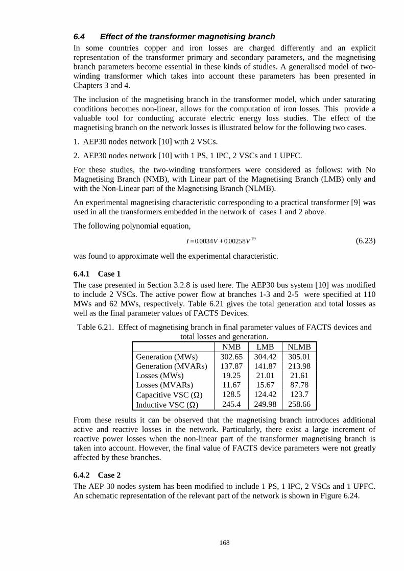
168
6.4 Effect of the transformer magnetising branch In some countries copper and iron losses are charged differently and an explicit representation of the transformer primary and secondary parameters, and the magnetising branch parameters become essential in these kinds of studies. A generalised model of two-winding transformer which takes into account these parameters has been presented in Chapters 3 and 4. The inclusion of the magnetising branch in the transformer model, which under saturating conditions becomes non-linear, allows for the computation of iron losses. This provide a valuable tool for conducting accurate electric energy loss studies. The effect of the magnetising branch on the network losses is illustrated below for the following two cases. 1. AEP30 nodes network [10] with 2 VSCs. 2. AEP30 nodes network [10] with 1 PS, 1 IPC, 2 VSCs and 1 UPFC. For these studies, the two-winding transformers were considered as follows: with No Magnetising Branch (NMB), with Linear part of the Magnetising Branch (LMB) only and with the Non-Linear part of the Magnetising Branch (NLMB). An experimental magnetising characteristic corresponding to a practical transformer [9] was used in all the transformers embedded in the network of cases 1 and 2 above. The following polynomial equation,
I V V= +0 0034 0 00258 19. . (6.23) was found to approximate well the experimental characteristic.
6.4.1 Case 1 The case presented in Section 3.2.8 is used here. The AEP30 bus system [10] was modified to include 2 VSCs. The active power flow at branches 1-3 and 2-5 were specified at 110 MWs and 62 MWs, respectively. Table 6.21 gives the total generation and total losses as well as the final parameter values of FACTS Devices. Table 6.21. Effect of magnetising branch in final parameter values of FACTS devices and
total losses and generation.
From these results it can be observed that the magnetising branch introduces additional active and reactive losses in the network. Particularly, there exist a large increment of reactive power losses when the non-linear part of the transformer magnetising branch is taken into account. However, the final value of FACTS device parameters were not greatly affected by these branches.
6.4.2 Case 2 The AEP 30 nodes system has been modified to include 1 PS, 1 IPC, 2 VSCs and 1 UPFC. An schematic representation of the relevant part of the network is shown in Figure 6.24.
NMB LMB NLMB Generation (MWs) 302.65 304.42 305.01 Generation (MVARs) 137.87 141.87 213.98 Losses (MWs) 19.25 21.01 21.61 Losses (MVARs) 11.67 15.67 87.78 Capacitive VSC (Ω) 128.5 124.42 123.7 Inductive VSC (Ω) 245.4 249.98 258.66
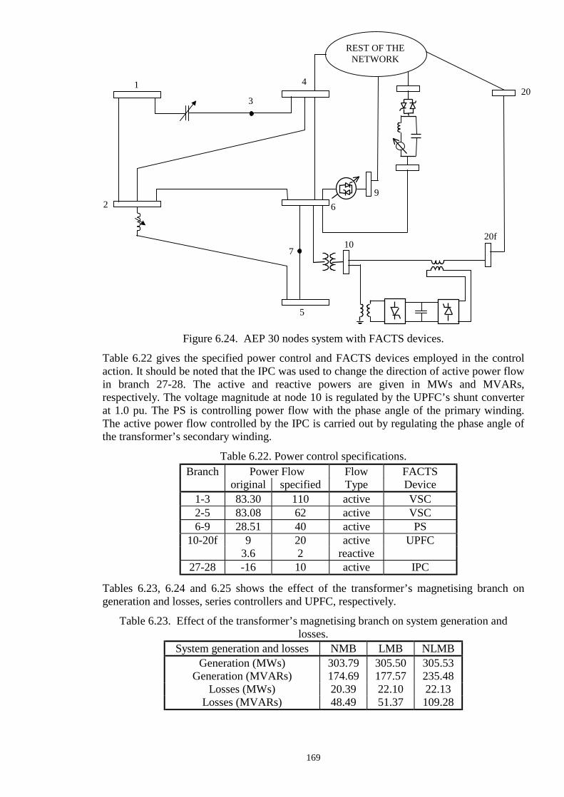
169
Figure 6.24. AEP 30 nodes system with FACTS devices. Table 6.22 gives the specified power control and FACTS devices employed in the control action. It should be noted that the IPC was used to change the direction of active power flow in branch 27-28. The active and reactive powers are given in MWs and MVARs, respectively. The voltage magnitude at node 10 is regulated by the UPFC’s shunt converter at 1.0 pu. The PS is controlling power flow with the phase angle of the primary winding. The active power flow controlled by the IPC is carried out by regulating the phase angle of the transformer’s secondary winding.
Table 6.22. Power control specifications.
Tables 6.23, 6.24 and 6.25 shows the effect of the transformer’s magnetising branch on generation and losses, series controllers and UPFC, respectively.
Table 6.23. Effect of the transformer’s magnetising branch on system generation and losses.
Branch Power Flow Flow FACTS original specified Type Device
1-3 83.30 110 active VSC 2-5 83.08 62 active VSC 6-9 28.51 40 active PS
10-20f 9 20 active UPFC 3.6 2 reactive
27-28 -16 10 active IPC
System generation and losses NMB LMB NLMB Generation (MWs) 303.79 305.50 305.53
Generation (MVARs) 174.69 177.57 235.48 Losses (MWs) 20.39 22.10 22.13
Losses (MVARs) 48.49 51.37 109.28
1
2
3
4
5
6
7
REST OF THE NETWORK
9
10 20f
20

170
Table 6.24. Effect of the transformer’s magnetising branch on series controllers.
Table 6.25. Effect of the transformer’s magnetising branch on UPFC.
Series Converter Shunt Converter CASE VcR
(pu) θcR
(degree) PcR
(MWs) QcR
(MVARs) VvR (pu)
θvR (degree)
PvR (MWs)
QvR (MVARs)
NMB 0.112 -133.24 1.036 1.874 0.962 -11.83 -1.036 -35.70 LMB 0.112 -133.06 1.029 1.891 0.962 -12.09 -1.029 -35.01
NLMB 0.111 -128.20 0.871 1.964 0.976 -12.45 -0.871 -22.70 Similarly to Case I, the magnetising branch introduces additional active and reactive losses in the network, which are compensated by the generators. However, the final value of FACTS device parameters were not greatly affected by the magnetising branches.
6.5 Voltage collapse The complexity of power systems has grown in terms of their interconnection and types of devices embedded in the network in response to the growing demand for electric power. Owing to a variety of economic, environmental, land-use and regulatory pressures, the steady load growth has been greater than the slowly increase of generation and transmission facilities. Hence, the electric utilities are gradually operating their transmission corridors closer to their margin of steady-state stability. One type of system instability which has attracted much attention in recent years is voltage collapse. This phenomena is a process by which a sequence of events or disturbances taking place in the AC power system leads to unacceptable low voltage magnitude profile in a significant portion of the network [11-16]. Recent examples of voltage collapse have happened throughout out the world with various degrees of severity. Voltage collapses lead to blackouts in France in December 1978 and in Belgium in August 1981 [11]. The phenomenon is characterised by a slow decrease in nodal voltage magnitude in the AC power system as some parameters in the network change gradually, particularly system load [11]. This is followed by a sharp and fast decrease in nodal voltage magnitude leading to an emergency system condition. Voltage collapse takes place over a time window, which varies from few seconds to several minutes. Control devices such as LTCs, shunt capacitors and synchronous condensers are used to restore the nodal voltage magnitude and to steer the system away from the collapse. However, under some adverse operating conditions some control devices have shown to actually aggravate the low voltage profile [11,14]. Mathematically, the power system dynamics can be described by a vector-form differential equation,
x f x.
( , )= λ (6.24) where x denotes the states, e.g. nodal voltage magnitudes and angles, and λ denotes parameters such as load demands, status of equipment, etc.
Series Controllers NMB LMB NLMB Capacitive VSC (Ω) 140.79 136.83 137.24 Inductive VSC (Ω) 124.82 128.69 134.28
Phase angle PS (degree) -5.75 -4.33 -4.35 Phase angle IPC (degree) 1.48 1.42 1.45

171
During the steady state the power system operates at an equilibrium point xo, which satisfies f(xo, λ)=0. Owing to the fact that electric system components can exhibit some degree of nonlinearity under certain operative conditions of the network, for each λ there exist many possible values of xo that satisfy (6.24). However, only that value corresponding to the operating point of the power system is of practical interest, i.e. when the voltage lies within a specified range about their nominal value. When the power system evolves to a different operative state due to any fluctuation of λ, numerical integration of equations (6.24) can be used to quantify the dynamic behaviour of the power system taking the predisturbance equilibrium point as initial condition. The final new state of the system can be determined from a time domain simulation. However, this method can be very time consuming. Hence, research has been carried out on developing fast computational methods to determine the final system state [13]. Depending on the magnitude of the disturbance that produces the voltage collapse, the phenomenon could be classified into two categories [14]: large-disturbance voltage stability and small-disturbance voltage stability. Both studies are concerned with the ability of the system to control voltage after a disturbance has taken place in the system. However, they differ by the methodologies used in the analysis and the modelling of the components embedded in the network. Large disturbances are produced among other things by system faults, sudden loss of load and generation and lines outages. Small disturbances can be produced by a gradual changes in load.
6.5.1 Analysis of voltage collapse by a static approach If the perturbation in λ is small, e.g. a regular fluctuation in load demand, the pre- and postdisturbance equilibrium points are near to each other. Hence, small-signal analysis can be used in order to determine the voltage stability. In these studies, equation (6.24) is linearised around the original equilibrium point xo ,
∆ ∆x A x xo
.( , )= λ (6.25)
The stability condition is determined by computing the eigenvalues of the linearised system given by equation (6.25). The system evolves to a new steady-state equilibrium point if all eigenvalues of the matrix A lie in the left half of the complex plane. Otherwise, the system is unstable. When λ changes from a value λ(1) to λ(2) in a relative long period of time, the equilibrium point drifts slowly. Based on this argument, the system dynamic behaviour can be traced by capturing snapshots of system conditions at various time frames. The derivative of the state variables of equation (6.24) are assumed to be zero at each of these time frames, and the overall system is represented by a set of non-linear algebraic equations,
f x( , )λ = 0 (6.26) In general, solving algebraic equations requires less effort than solving differential equations. The system modelled by algebraic equations allows the use of static analysis techniques to determine steady-state stability conditions. For a given operative condition λ=λ0, many equilibrium points; x0(1), x0(2), ..., x0(n0), satisfy equation (6.26). As λ continues to change, the system cannot settle to a new steady-state. This loss of stability takes place at the operative condition λls in which the multiple solutions of equation (6.26) coalesce, i.e. xls(1) = xls(2) = ...= xls(nls). The point in which the system equilibrium disappears is known as saddle-node bifurcation [12,15-17].

172
Assuming that only two solutions are of interest, one stable and one unstable, the phenomena mentioned above can be schematically illustrated as shown in Figure 6.25 [15]. When λ=λ0, the operating steady-state stable equilibrium is x0(1), and its unstable equilibrium is x0(2). As λ moves toward λcrit, the stable and unstable solutions come closer until they collide at the bifurcation point xcrit and disappear. At such a point, the solution of the non-linear algebraic equations become unsolvable. The shape of the system state trajectory is known as the nose curve. When the nose curve is obtained with a state variable plotted on the vertical axis and the parameter whose change produce the bifurcation plotted on the horizontal axis, the diagram is called bifurcation diagram [16]. In this case, the maximum point of the nose shape xcrit will correspond to the saddle node bifurcation.
Figure 6.25. Saddle node bifurcation. Some voltage collapse problems can be associated to these saddle node bifurcation. In such cases, the non-linear equation (6.26) corresponds to the well known power flow equations. Newton-Rapshon methods can then be used to find, by iteration, the equilibrium point x which satisfies these equations. An initial steady-state operation condition is changed by increasing the system power demand in finite steps along a specified trajectory [14]. At each step, the new equilibrium point is determined by the corresponding load flow solution. As long as the Jacobian matrix remains non-singular, the Implicit Function Theorem [18] ensures the existence of an equilibrium point that satisfy (6.26). The procedure is repeated up to the point where the Newton-Rapshon method diverges. This divergence indicates a singularity of the Jacobian matrix and the unsolvability of the power flow equations. However, this does not necessarily mean that a bifurcation point has been reached. Divergence in the load flow calculation may have been caused by either numerical problems in the Jacobian matrix or by the fact that the bifurcation point has actually been reached. A number of numerical methods has been proposed to overcome this difficulty. Among them are the continuation methods [16,18]. Basically, a continuation method adds extra steps in the computation of the nose curve, augmenting the equations so that the new set is numerically well conditioned. A detailed mathematical description of these techniques can be found in [17].
λ0
λcrit x0(1)
x0(2)
xcrit
f(x,λ) = 0
state space, x parameter space, λ

173
6.5.2 Analysis of maximum loadability and voltage collapse in presence of FACTS devices A comparison of the effect of FACTS devices on the maximum loadability and voltage collapse is presented in this Section. The New England 39-nodes network shown in Figure 6.26 is used for the analysis. Data system are given in Appendix I. A system weak area in terms of voltage stability [20] is shown by dotted lines in the Figure 6.26. The studies are carried out using the conventional Newton-Rapshon algorithm described in previous Chapters. In spite of the fact that this methodology could be time-consuming for solving the problem of voltage collapse, it provides some insight into the controllable device which allows the maximum increment of load in the system without reaching the voltage collapse. For this purpose, different simulations are presented. First, a gradual increase of load at node 8, unstable region, is carried out to steer the system near to voltage collapse. At this point the iterative process did not converge. After that, the same simulation is carried out with FACTS devices embedded in the network. The connection of such controllers is carried out as shown in Figure 6.27 .
Figure 6.26. New England 39-nodes system. The following FACTS devices are considered in the simulations, 1. Variable Series compensator (VSC) 2. Universal Power Flow Controller (UPFC) 3. Phase Shifter (PS) 4. On Load Tap Changing Transformer (LTC) 5. Interphase Power Controller (IPC) 6. Static Var Compensator (SVC) 7. Synchronous Voltage Source (SVS)
37
1
2
3
4
5
6
7
8
9
10 11
12
14
15
16
25
17
18
19
20
13
21 22
23
24
26
27
28 29 30
Slack Bus 39
31
32
34
33 36
38
35
Weak Area

174
Figure 6.27. FACTS embedded in the network. (a) Series connection. (b) Shunt connection. Details of the numeric simulation for each case are given below. Base Case This case corresponds to the original network, with no FACTS devices. The maximum increment of load is 210%, with respect to the load base. After this point, the iterative process diverges. Network with VSC A VSC is compensating line 9-8 in order to relieve overloaded transmission lines and increase the transmitted power. The level of compensation is fixed at 60% as the load is incremented. The last power flow solution is obtained when the load at node 8 is incremented by 265%. Network with LTC Two simulations are carried out in this case. First, the LTC primary winding tap is adjusted to maintain fixed the voltage magnitude at node 8 at 0.95 pu. The LTC violates its maximum limit of 1.1 as the level of load is increased. The maximum loadability is 125% before the iterative process diverges. The same simulations are carried out but maintaining the LTC primary and secondary taps fixed at 1.1 and 1.0, respectively. In this case, the maximum loadability at node 8 is 198%. The comparison of these two simulations indicates that when the LTC is activated, the unsolvability of the power flow equations is produced by numerical problems during the iterative process. Moreover, the LTC consumption of reactive power accelerates the process of voltage collapse. It must be noted that the maximum loadability is 198% whilst the base case maximum loadability is 210%. Network with PS The phenomena described above is also observed when a PS is used. The PS primary and secondary phase angles are assumed fixed at -15o and 0o , respectively. In this case, the maximum level of load increment at node 8 is 196%. After this point, the iterative process diverges. Network with IPC Each IPC branch is assumed to have a PS. The PS phase angles are fixed as above. The IPC impedance are set at 15% of the transmission line series reactance. The maximum increment of load is 205%. Network with SVC The SVC is connected at node 8. It is set to control the voltage magnitude at 0.95 pu. The SVC variable susceptance limits are defined at ±3 pu considering 100 MVA base. When the device violates limits, the PVB node is converted to PQ node. The maximum loadability at node 8 is 240%.
FACTS Device
Rest of the Network
9 8
FACTS Device
Rest of the Network
8
(b) (a)

175
Network with UPFC The UPFC shunt converter is used to regulated the node 8 voltage magnitude at 0.95 pu. The reactive limits generated/absorbed by the UPFC converters is restricted at ±300 MVAr. As a consequence, the specified values of active and reactive power to be controlled by the UPFC series converter are defined according to the network operative conditions. The maximum load increment is 265%. For this case, the voltage magnitude was controlled at 0.9 in order to meet the restriction of maximum reactive power generated by the UPFC. Network with SVS Similarly to the UPFC, the SVS regulation of active and reactive power is adjusted in order to satisfy the restriction of maximum reactive power generated by the series controller. The last solution of the power flow equations is obtained at a load increment of 250%. A comparison of the nose curve generated by each one of the simulations described above is shown in Figure 6.28. From this figure, it is clear that the LTC, PS and IPC can actually reduce the margins of voltage collapse. One of the main causes of voltage collapse is that the power system can not meet the reactive power demanded by loads. Hence, as the parameters of these controllers change, their demand for reactive power increases such that the problem is aggravated. It is clear that FACTS controllers which can produce and regulate reactive power, e.g. SVC and UPFC, increase the margins of voltage collapse. Although the VSC is a passive controller, if it forces active power to flow through underloaded transmission corridors, there exists a relieve of overloaded transmission lines hence increasing the system loadability.
Figure 6.28. Comparison of FACTS bifurcation diagrams.
Figures 6.29 to 6.36 depict the nodal voltage profile for each case. From these figures, it is clear that as the level of load increases the nodal voltage magnitude throughout the network decreases. Moreover, there is a displacement of the nodal voltage angles with respect to the slack bus angle. The voltage decrease is less severe in cases where reactive power compensation is provided by the controller, e.g. SVC or UPFC. It is interesting to note that when the UPFC is being used to its full potential, i.e. controlling voltage, active and reactive power, the variation of voltage magnitude takes place only in the region near to the load perturbation, in such a way that it is not spreading to a wider area.
176
(a) Voltage magnitudes (b) Voltage angles
Figure 6.29. Nodal voltage profiles for base case.
(a) Voltage magnitudes (b) Voltage angles
Figure 6.30. Nodal voltage profiles when one VSC is embedded in the network.
(a) Voltage magnitudes (b) Voltage angles
Figure 6.31. Nodal voltage profiles when one LTC is embedded in the network.
.

177
(a) Voltage magnitudes (b) Voltage angles
Figure 6.32. Nodal voltage profiles when one PS is embedded in the network.
(a) Voltage magnitudes (b) Voltage angles
Figure 6.33. Nodal voltage profiles when one IPC is embedded in the network.
(a) Voltage magnitudes (b) Voltage angles
Figure 6.34. Nodal voltage profiles when one SVC is embedded in the network.
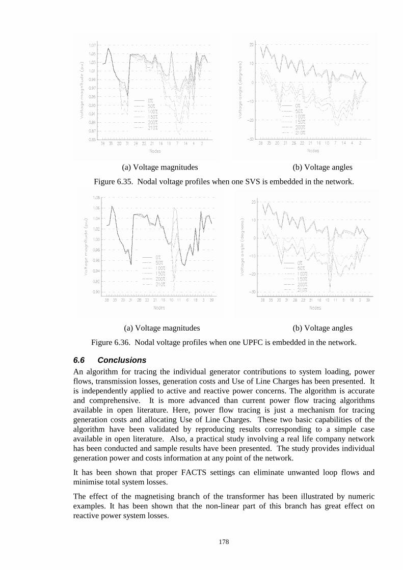
178
(a) Voltage magnitudes (b) Voltage angles
Figure 6.35. Nodal voltage profiles when one SVS is embedded in the network.
(a) Voltage magnitudes (b) Voltage angles
Figure 6.36. Nodal voltage profiles when one UPFC is embedded in the network.
6.6 Conclusions An algorithm for tracing the individual generator contributions to system loading, power flows, transmission losses, generation costs and Use of Line Charges has been presented. It is independently applied to active and reactive power concerns. The algorithm is accurate and comprehensive. It is more advanced than current power flow tracing algorithms available in open literature. Here, power flow tracing is just a mechanism for tracing generation costs and allocating Use of Line Charges. These two basic capabilities of the algorithm have been validated by reproducing results corresponding to a simple case available in open literature. Also, a practical study involving a real life company network has been conducted and sample results have been presented. The study provides individual generation power and costs information at any point of the network. It has been shown that proper FACTS settings can eliminate unwanted loop flows and minimise total system losses. The effect of the magnetising branch of the transformer has been illustrated by numeric examples. It has been shown that the non-linear part of this branch has great effect on reactive power system losses.

179
The effect of different FACTS devices on the maximum system loadability and voltage collapse has been analysed. A numeric example shows that divergence in the power flow calculation can be due to numerical problems and not due to the saddle node. A comparative analysis of FACTS devices performance shows that using the UPFC flexibility of controlling voltage magnitude as well as active and reactive power flow allows to maintain power system operative conditions within viable voltage profile for large increments of load levels. On the other hand, it is show that FACTS devices such as LTC, PS and IPC could accelerate the process of voltage collapse due to their consumption of reactive power.
6.7 Bibliography [1] The Secretary of State for Energy. ‘Privatising Electricity - The Government’s proposals for the privatisation of the electricity supply industry in England and Wales’, Her Majesty’s Stationary Office, London, UK, February 1988. [2] California Public Utilities Commission. ‘CPUC Offers Restructuring Proposals for Comment - Two views on how to restructure the industry to foster competition and performance-based regulation’, IEEE Power Engineering Review, Vol. 15, No. 8, pp. 5-8, August 1995. [3] The Electricity Pool of England and Wales 1993. ‘An Introduction to Pool Rules’, London, UK, April 1993. [4] Kirschen D., Allan R. and Strbac G. ‘Contributions of Individual Generators to loads and Flows’, IEEE/PES 1996 Winter Meeting, Paper No. 96 WM 173-5 PWRS. [5] Bialek J. ‘Topological Generation and Load Distribution Factors for Supplement Charge Allocation in Transmission Open Access’, IEEE/PES 1996 Summer Meeting, Paper No. 96 SM 493-7 PWRS. [6] Fuerte-Esquivel C.R., Mota-Palomino R. and De León F. ‘Representación del Sistema Eléctrico de Potencia para Estudios de Transitorios ElectroMagnéticos’, IEEE Reunion de Verano de Potencia, No. RVP-SIS-08, Julio 1993, Acapulco, México. [7] Ng W.Y. ‘Generalised Generation Distribution Factors for Power Systems Security Evaluations’, IEEE Trans. Power App. Systems, Vol. PAS-100, No. 3, March 1981, pp. 1001-1005. [8] Huang G. and Hsieh S.C.: ‘Fast Textured Algorithm for Optimal Power Delivery Problems in Deregulated Enviroments’, PE-184-PWRS-0-11-1996, to be published in IEEE Transactions on Power Systems. [9] Dommel H.W., Yan A. and De Marcano R.J.O.: ‘Case Studies for electromagnetic Transients’,Internal Report, Department of Electrical Engineering, University of British Columbia, Vancouver, Canada, 1983. [10] Freris L.L. and Sasson A.M.: ‘Investigation of the load-flow problem’, Proceedings of IEE, Vol. 115, No. 10, pp. 1459-1470, October 1968. [11] Dobson I. and Chiang H.D.: ‘Towards a Theory of Voltage Collapse in Electric Power Systems’, Systems & Control Letters, Vol. 13, 1989, pp. 253-262. [12] Liu C.C. and Wu F.F.: ‘Steady-State Voltage Stability Regions of Power Systems’, Systems & Control Letters, Vol. 6, 1985, pp. 23-31. [13] Hill D.J., ed.,: ‘Special Issue on Nonlinear Phenomena in Power Systems’, Proceedings of IEEE, Vol. 83, No. 11, November 1995. [14] Kundur P.P.: ‘Power System Stability and Control’, McGraw-Hill, 1994, ISBN 007035958.

180
[15] Vu, K.T., Liu C.C., Taylor C.W. and Jimma K.M.: ‘Voltage Instability: Mechanims and Control Strategies’, Proceedings of IEEE, Vol. 83, No. 11, November 1995, pp. 1142-1455. [16] Dobson I.: ‘Basic Concepts and Theorical Perspective’, Chapter 2 Draft of IEEE/PES Working Group Report, Voltage Stability, Assesment-Procedures and Guides, May 1997, 59 pages. Available from http://www.power.uwaterloo.ca [17] Cañizares C.A.: ‘Voltage Stability Indices’, Chapter 4 Draft of IEEE/PES Working Group Report, Voltage Stability, Assesment-Procedures and Guides, May 1997, 52 pages. Available from http://www.power.uwaterloo.ca [18] Edwards H.M.: ‘Advanced Calculus: A Differential Forms Approach’, Birkhäuser 1994, third edition, ISBN 0-8176-3707-9. [19] Cañizares C.A., De Zousa A.Z. and Quintana V.H.: ‘Improving Continuation Methods for Tracing Bifurcation Diagrams in Power Systems’, Proc. Bulk Power System Voltage Phenomena-III Seminar, Davos Switzerland, August 1994, pp. 349-358. [20] Bésanger Y., Passelergue J.C., Hadjsaid N. and Feuillet R.: ‘Improvement of Power System Performance by Inserting FACTS Devices’, Proceedings of Sixth AC and DC Power Transmission Conference, 29 April-3 May 1996, IEE Conference Publication No. 433, pp. 263-267.

181
Chapter 7 Application of the Object Oriented Programming Philosophy to the Analysis of Electric Power Systems containing FACTS Devices 7.1 Introduction The Object Oriented Programming (OOP) philosophy is arguably one of newest and far reaching developments in the computer industry [1,2]. It addresses the issue of large-scale software systems such as Data Base Management Systems [3] (DBMS) and Graphical User Interfaces [4] (GUI). Applications of the OOP technology to the solution of ‘number-crunching’ engineering-type problems are a newer development. Most engineering systems consist of the interconnection of physical objects and OOP seems the natural approach for conducting the modelling and coding of such systems. In particular, C++ is rapidly becoming industry’s computer language of choice owing to its accelerated production cycles and its close association with both C and UNIX. C++ is an enhanced version of C. It retains C’s efficient programming capabilities while adding the following characteristics: stronger type checking, extensive data abstraction features and support for object oriented programming. The Electricity Supply Sector has followed these developments very closely and some OOP applications to power systems have already appeared in open literature [5-7]. The driving force behind these developments is the notion that existing commercial power systems software is rapidly becoming a liability from both the technical and the economic point of view. Neyer, Wu and Imhof [5] argue that the use of conventional computer languages often leads to inflexible code which is costly to maintain and to adapt to the very specific needs and changing requirements of each utility. In the discussion of that paper, Kirschen and Irisarri agree with the need to use OOP but caution against re-writing ‘number crunching’ power engineering applications using any OOP language owing to the inherent overheads associated with such computer languages. Keeping these observations on board but bearing in mind that one of the most difficult problems with power systems software, which is normally written in FORTRAN and following a top-bottom design, is its maintenance and upgrading as new features need to be added; this Chapter describes research on OOP as applied to power network. It touches on both power plant components and on the design and elaboration of an OOP Load Flow program. Solutions obtained with the newly developed OOP load flow program have shown to be almost as fast as the solutions given a load flow program [10] written in FORTRAN. This is significant because it seems to go against the general belief that OOP algorithms are substantially slower than their FORTRAN counterparts [5-7]. Moreover, this shows the tremendous potential that C++ has for solving ‘number-crunching’ power engineering problems.
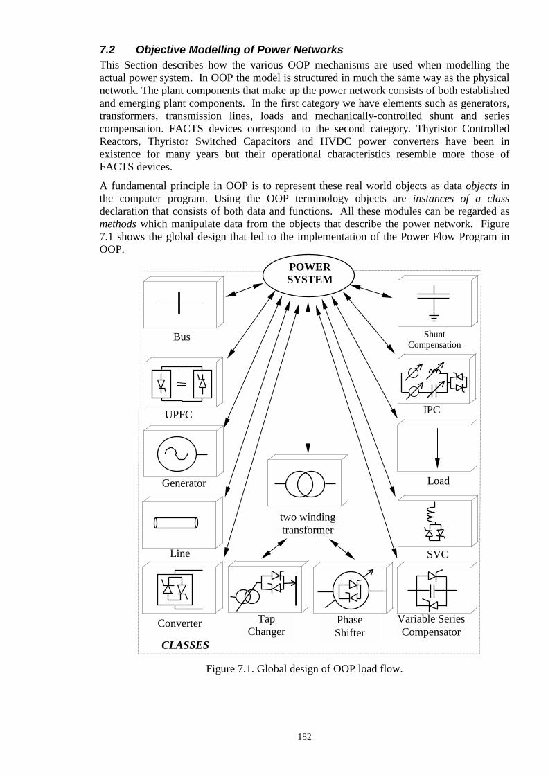
182
7.2 Objective Modelling of Power Networks This Section describes how the various OOP mechanisms are used when modelling the actual power system. In OOP the model is structured in much the same way as the physical network. The plant components that make up the power network consists of both established and emerging plant components. In the first category we have elements such as generators, transformers, transmission lines, loads and mechanically-controlled shunt and series compensation. FACTS devices correspond to the second category. Thyristor Controlled Reactors, Thyristor Switched Capacitors and HVDC power converters have been in existence for many years but their operational characteristics resemble more those of FACTS devices. A fundamental principle in OOP is to represent these real world objects as data objects in the computer program. Using the OOP terminology objects are instances of a class declaration that consists of both data and functions. All these modules can be regarded as methods which manipulate data from the objects that describe the power network. Figure 7.1 shows the global design that led to the implementation of the Power Flow Program in OOP.
Figure 7.1. Global design of OOP load flow.
POWER SYSTEM
Bus Shunt Compensation
Tap Changer
Variable Series Compensator
two winding transformer
Generator
Line
Load
CLASSES
Phase Shifter
SVC
Converter
UPFC IPC
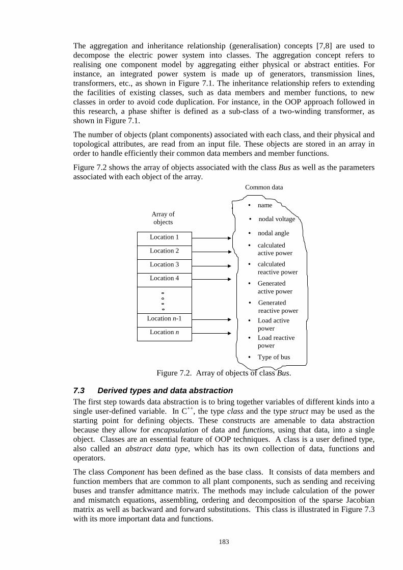
183
The aggregation and inheritance relationship (generalisation) concepts [7,8] are used to decompose the electric power system into classes. The aggregation concept refers to realising one component model by aggregating either physical or abstract entities. For instance, an integrated power system is made up of generators, transmission lines, transformers, etc., as shown in Figure 7.1. The inheritance relationship refers to extending the facilities of existing classes, such as data members and member functions, to new classes in order to avoid code duplication. For instance, in the OOP approach followed in this research, a phase shifter is defined as a sub-class of a two-winding transformer, as shown in Figure 7.1. The number of objects (plant components) associated with each class, and their physical and topological attributes, are read from an input file. These objects are stored in an array in order to handle efficiently their common data members and member functions. Figure 7.2 shows the array of objects associated with the class Bus as well as the parameters associated with each object of the array.
Figure 7.2. Array of objects of class Bus.
7.3 Derived types and data abstraction The first step towards data abstraction is to bring together variables of different kinds into a single user-defined variable. In C++, the type class and the type struct may be used as the starting point for defining objects. These constructs are amenable to data abstraction because they allow for encapsulation of data and functions, using that data, into a single object. Classes are an essential feature of OOP techniques. A class is a user defined type, also called an abstract data type, which has its own collection of data, functions and operators. The class Component has been defined as the base class. It consists of data members and function members that are common to all plant components, such as sending and receiving buses and transfer admittance matrix. The methods may include calculation of the power and mismatch equations, assembling, ordering and decomposition of the sparse Jacobian matrix as well as backward and forward substitutions. This class is illustrated in Figure 7.3 with its more important data and functions.
Location 1
Location 2
Location 3
Location 4
Location n-1
Location n
• nodal voltage
• nodal angle
• calculated active power
• calculated reactive power
• name
• Generated active power
• Generated reactive power
• Load active power
• Load reactive power
• Type of bus
Array of objects
Common data

184
Figure 7.3. Class Component. The symbol (..) in Figure 7.3 indicates that the function contains arguments. One of the central concepts of OOP is that we should deal with objects, such as transmission lines, rather than their circuit representation, such as π models or transmission lines parameters; the data associated with an object should be accessible by means of function calls which hide details of the class implementation. However, this encapsulation and data hiding can produce extra function calls, increasing the call-overhead of the program. This results in poorer run-time performance. A large part of the computational burden in a Newton-Rapshon power flow program is associated to the fill-in of the Jacobian matrix, the LU factorisation and the forward and backward substitution. In order to avoid a poor run-time performance due to call overhead when elements are assigned to the Jacobian matrix and vector of mismatches, it was found to be more efficient to include the sparse matrix and its associated functions into the class Component as show in Figure 7.3. It is realised that a purer OOP design calls for a separate sparse matrix class, however, principle was traded off for numeric efficiency. A Jacobian element is directly assigned to the sparse Jacobian matrix at the point in time in which it is computed with no additional function call. This philosophy contrasts with approaches followed in several other works [6,8], where a Matrix class has been used.
class Component //class name. private: //the private part.
int nse,nre; //Sending and receiving buses. int *order; //Ordering vector. int*newcol; //Vector of new columns. double **pt_G; //Real and imaginary parts double**pt_B; // of transfer admittance matrix. double *pt_V; //Solution vector. public: //the public part. Component(); //Constructor. ~Component(); //Destructor. int Sending(..); //Assignation of sending node. int Receiving(..); //Assignation of receiving node. void Power_Cal(); //Calculation of power equations. void Mismatch(); //Calculation of mismatch equations. void Ordering(); //Symbolic factorisation. void LU(); //Matrix decomposition. void Solve(); //Backward and forward substitution. void Load_Load(); //Methods for build the sparse Jacobian void PV_Load(); //matrix according of the type of void Slack_Load(); //buses to which an electric component void Slack_PV(); //is connected. void PV_PV(); void PVT_Load(); void PVT_Slack(); void PVT_PV(); void PVT_PVT(); void set_dimension(..) //Dimension of sparse jacobian Element **pt_J; //Structure of sparse matrix off-diagonal elements. Diagonal_Element *diag; //Structure of sparse matrix diagonal elements. <additional methods> ;

185
7.4 Class hierarchy and inheritance While subroutines and functions are used in conventional programming in order to avoid code duplication, inheritance is the mechanism used in OOP. Inheritance is a way of creating new classes by extending the facilities of existing classes, such as data members and methods members defined at a certain level in the hierarchy. The facilities of the existing class are automatically available to all subclasses. The extended class is known as base class and its extensions are known as derived classes. Using the syntax of C++, the class hierarchy is constructed by simply writing a reference to an old class in the header of the new class. The implementation of the class corresponding to a conventional two winding transformer is given in Figure 7.4. The newly derived class inherits data members and function members of the class Component. It illustrates how classes are implemented in the program. ConTran is the user defined name for the class. The private part consisting of the parameters which are normally used for describing the electrical behaviour of the two winding transformer. The public part consisting of the various methods associated with the class, such as data accessing methods and methods for building its transfer admittance matrix and for placing the individual contributions of the controllable devices into the Jacobian matrix; the constructor and the destructor. A constructor is invoked whenever an object is created and a destructor is invoked whenever an object is destroyed.
Figure 7.4. Conventional transformer class implementation.
Figure 7.5 shows the Load Tap Changer (LTC) class, named LtcTran. The newly derived class inherits data members and function members of the class ConTran and it is only necessary to define the control attributes associated with this controllable device. Only the most important functions are shown in Figure 7.5.
class ConTran : public Component //Class. private: //The private part. double rtp,xtp; //Primary winding data. double rts,xts; //Secondary winding data. double go,bo; //Iron core data. double tapp,taps; //Taps transformer data. double phap,phas; //Phase shifter angles data. public: //The public part. ConTran(); //Constructor. ~ConTran(); //Destructor. void tran_par1(..); //Assignation of electric parameters. void tran_par2(..); //Assignation of controllable parameters. double Get_TapP(..); //Accessing methods double Get_TapS(..); //of taps and phase double Get_PhaP(..); //shifting transformer double Get_PhaS(..); //data. void admitance_matrix(..); //Construction of transformer admittance. void Jacelements(..); //Jacobian due FACTS devices. void change_tapp(..); //Actualisation of primary tap. void change_taps(..); //Actualisation of secondary tap. void change_phap(..); //Actualisation of primary phase angle. void change_phas(..); //actualisation of secondary phase angle. <additional methods> ;

186
Figure 7.5. LTC transformer implementation. The use of abstract objects do not violate OOP methodology. However, care has to be exercised because they may be algorithm-dependent [7]. The OOP software developed by the author endeavours making use only of objects which can be justified to be physically-based. At this point in time bus could be argued to be an abstract object. However, it is anticipated that it will evolve into a fully fledged physical object once topology checking facilities are incorporated.
7.5 Sparsity techniques In practice the formation of actual matrices is not desirable. Instead, the Jacobian and nodal admittance matrices of the power network are stored and processed in vector form, where only non-zero elements are explicitly handled [11]. In languages with no linked lists facilities several one-dimensional arrays and complicated programming schemes are required in order to obtain efficient load flow analysis solutions. In C++ the programming efforts are greatly reduced due to the existence of pointers and structures. In theory, C++ allows sparsity techniques to be implemented by following a rather purist OOP philosophy [1,6]. However, this approach incurs excessive cpu time overhead and has not been followed in this work. Instead, a more efficient OOP approach has been adopted where sparsity was implemented as an array of pointers pointing to structures. Structures allow the encapsulation, in a single variable, of all the information associated with a sparse coefficient, e.g. value, column and pointer to next element. Pointers are used to move from one structure to another. This is illustrated in Figure 7.6.
class LtcTran:public ConTran //Class. private: //The private part. int controlled_node; int tap_control; int status; double tapplo,tapphi; //Limits of primary winding. double tapslo,tapshi; //Limits of secondary winding. double value_of_voltage; public: //The public part. LtcTran(); //Constructor. ~LtcTran(); //Destructor. void set_limits_of_taps(..); void set_controlled_node(..); void status(..); void change_status(..); void tap_control(..); void review_parallel_conexion(..); void check_sensi(..); void check_new_LTC(..); void limits_of_taps(); void review_power_tolerance(..); <additional methods> ;

187
Figure 7.6. Linked lists for storing of sparse Jacobian. An array of pointers is created with the same size as the number of rows in the matrix. Each element points to the address of the start of a list. Thus, one list is created for each row. In the case of load flows an array of pointers of size equal to 2(nb-1)+nf+2nfr is created. nb is the number of buses in the network, nf is the number of FACTS devices capable of controlling real power flow in a branch and nfu is the number of UPFC devices capable of controlling active and reactive power flow in a branch. Each list consists of one or more structures containing information associated with off-diagonal elements only. The information associated with diagonal elements is stored in a separate array of structures. Both structures are shown in Figure 7.7.
Figure 7.7. Structures of sparse Jacobian matrix elements. Struct Element contains the column location of the off-diagonal element, its value and a pointer which points to the address of the structure corresponding to the next off-diagonal element in that row. The pointer of the last structure in the list is set equal to zero to indicate the end of the list. The information pertaining to the Jacobian diagonal element in a given row is stored in Struct Diagonal. It consists of its numeric value, the number of off-diagonal elements in that row and the elimination order as determined by Tinney’s second ordering scheme [11].
struct Element double value; int column; off-diagonal element *next; ; struct Diagonal double value; int new_column; int elements; ;
first_ptr
1
2
3
: :
2(nb-2)+ nf+2nfr 2(nb-1)+ nf+3nfu
first_ptr
value
next_ptr
column
value
0
column
value
next_ptr
column
value
next_ptr
column
value
0
column
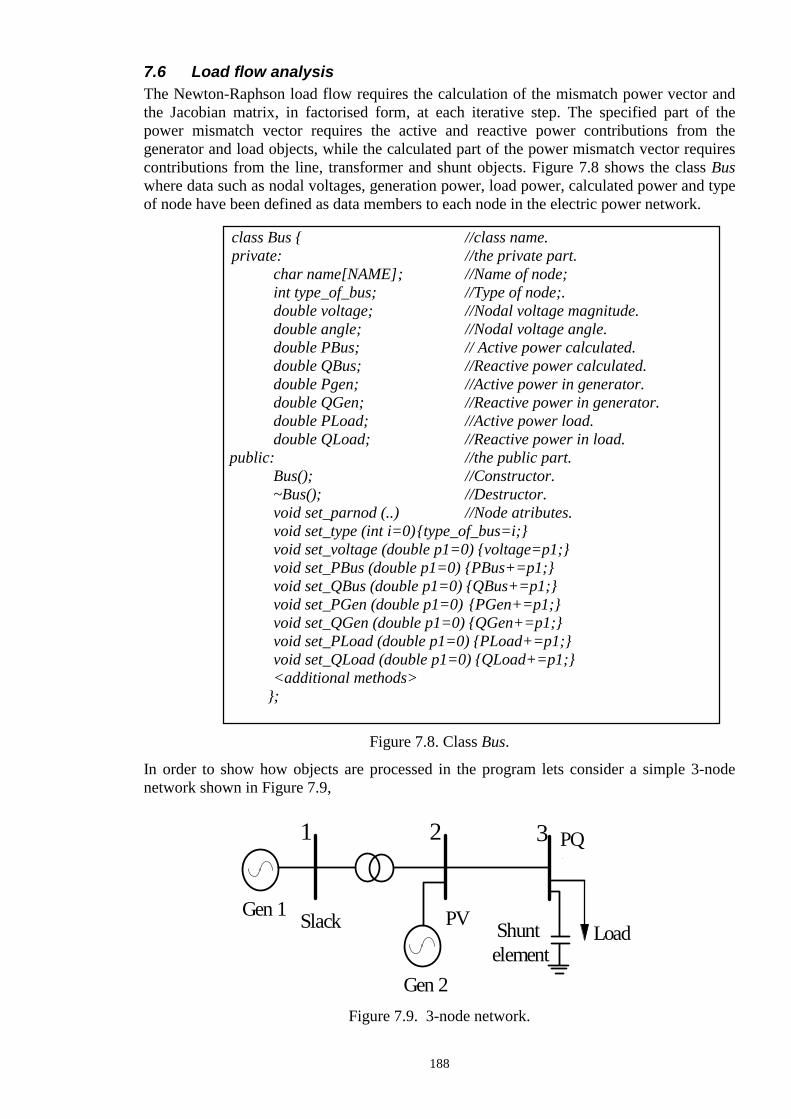
188
7.6 Load flow analysis The Newton-Raphson load flow requires the calculation of the mismatch power vector and the Jacobian matrix, in factorised form, at each iterative step. The specified part of the power mismatch vector requires the active and reactive power contributions from the generator and load objects, while the calculated part of the power mismatch vector requires contributions from the line, transformer and shunt objects. Figure 7.8 shows the class Bus where data such as nodal voltages, generation power, load power, calculated power and type of node have been defined as data members to each node in the electric power network.
Figure 7.8. Class Bus. In order to show how objects are processed in the program lets consider a simple 3-node network shown in Figure 7.9,
Gen 1
Gen 2
Slack PV
PQt
Load Shuntelement
1 2 3
Figure 7.9. 3-node network.
class Bus //class name. private: //the private part.
char name[NAME]; //Name of node; int type_of_bus; //Type of node;. double voltage; //Nodal voltage magnitude. double angle; //Nodal voltage angle. double PBus; // Active power calculated. double QBus; //Reactive power calculated. double Pgen; //Active power in generator. double QGen; //Reactive power in generator. double PLoad; //Active power load. double QLoad; //Reactive power in load. public: //the public part. Bus(); //Constructor. ~Bus(); //Destructor. void set_parnod (..) //Node atributes. void set_type (int i=0) type_of_bus=i; void set_voltage (double p1=0) voltage=p1; void set_PBus (double p1=0) PBus+=p1; void set_QBus (double p1=0) QBus+=p1; void set_PGen (double p1=0) PGen+=p1; void set_QGen (double p1=0) QGen+=p1; void set_PLoad (double p1=0) PLoad+=p1; void set_QLoad (double p1=0) QLoad+=p1; <additional methods> ;

189
At each node, the power balance is obtained by adding the contribution of each plant component object connected to the node. This is illustrated in Figure 7.10.
Figure 7.10. Power mismatch vector.
P1 spec
P2 spec
P3 spec
Q1 spec
Q2 spec
Q3 spec
Mismatch (Specified Power)
Generator
Load
Ps gen 1
Ps gen2
Qs gen1
Qs gen2
-Ps
-Qs
Transformer Line
P1 calc
P2 calc
P3 calc
Q1 calc
Q2 calc
Q3 calc
Mismatch (Calculated Power)
Shunt
-Psen2
-Prec3
-Qsen2
-Qrec3
-Prec2
-Psen1
-Qrec2
-Qsen1
-Psen3
-Qsen3
Mismatch (Calculated Power)
Pgen1
Pgen2
-Pload
Qgen1
Qgen2
-Qload
1
2
3
1
2
3
-Ptrans
-Pline-Ptrans
-Pline-Pshunt
-Qtrans
-Qline-Qtrans
-Qline-Qshunt
1
2
3
1
2
3
Mismatch (Specified Power)
∆P1
∆P2
∆P3
∆Q1
∆Q2
∆Q3
1
2
3
1
2
3
Mismatch Vector

190
Construction of the factorised Jacobian matrix involves a slightly more complicated procedure owing to the need to evaluate self and mutual Jacobian terms, and finding their location in the factorised matrix. Nevertheless, the basic procedure illustrated above, based on superposition, will also apply to the formation of the Jacobian. For each plant component relevant Jacobian equations are chosen based on the type of buses to which the plant component is connected. These buses determine the location of the individual Jacobian terms in the overall Jacobian structure. The contributions of the line, transformer and shunt objects to the Jacobian are shown in Figure 7.11.
Figure 7.11. Jacobian matrix.
7.7 Controllable devices In order to illustrates how FACTS devices contribute to and modify the Jacobian lets consider the circuit shown in Figure 7.12. Provided the controllers are within limits, the voltage magnitudes at buses k and m will be controlled by LTCs k and m, respectively. The phase-shifter and series compensator will control the amount of active power flowing from bus k to bus m.
Figure 7.12. An array of FACTS devices.
OBJECTS
Line
L33L + L33S
2 3 3
2
3
3
H22L + H22T
H23L N23L
H32L H33L + H33S
N33L + N33S
J32L J33L + J33S
JACOBIAN
Shunt
H33S N33S
J33S L33S
Transformer H22T
L33L
H22L H23L
H32L H33L
N23L
N33L
J33L J32L
k m
Tk
φkm
xkm
Pkm
Pkm
Tm n φ
x

191
The Jacobian matrices corresponding to the following operating conditions are given in equations (7.1)-(7.3): 1. Buses k and m are not regulated and they are PQ-type. 2. Bus k is PVT-type and bus m is PQ-type. 3. Buses k and m are both PVT-type (series condition).
∆∆∆∆∆∆
∆∆
∆∆
∆∆
PPQQPP
H H N N H NH H N N H NJ J L L N MJ J L L N MH H N N HH H N N N
V VV V
X X
k
m
k
m
km
kmX
kk km kk km km km
mk mm mk mm mk mk
kk km kk km km kk
mk mm mk mm mk mm
kk km kk km km
kk km kk km km
k
m
k k
m m
kmφ
θθ
φ
=
−− −−
−
00
(7.1)
∆∆∆∆∆∆
∆∆
∆∆
∆∆
PPQQPP
H H C N H NH H C N H NJ J D L N MJ J D L N MH H N HH H N N
T TV V
X X
k
m
k
m
km
kmX
kk km kk km km km
mk mm mk mm mk mk
kk km kk km km kk
mk mm mk mm mk mm
kk km km km
kk km km km
k
m
k k
m m
kmφ
θθ
φ
=
−− −−
−
0 00 0
(7.2)
∆∆∆∆∆∆
∆∆
∆∆
∆∆
PPQQPP
H H C H NH H C H NJ J D N MJ J D N MH H HH H N
T TT T
X X
k
m
k
m
km
kmX
kk km kk km km
mk mm mk mk mk
kk km kk km kk
mk mm mk mk mm
kk km km
kk km km
k
m
k k
m m
kmφ
θθ
φ
=
−− −−
−
0000
0 0 00 0 0
(7.3)
where Hkk, Nkk, Jkk, Lkk, Hkm, Nkm, Jkm, and Lkm, are the standard Jacobian terms [12] and the remaining elements are:
C PT
Tkkk
kk= ∂
∂ (7.4)
C PT
Tmkm
kk= ∂
∂ (7.5)
D QT
Tkkk
kk=
∂∂
(7.6)
D QT
Tmkm
kk= ∂
∂ (7.7)
M QX
Xkkk
kmkm= ∂
∂ (7.8)
M QX
Xmmm
kmkm= ∂
∂ (7.9)
The 5th and 6th rows and columns correspond to the active powers flowing from bus k to bus m across the phase-shifter and series compensator, respectively. It must be noted that bus n is not being included in the Jacobian equations.
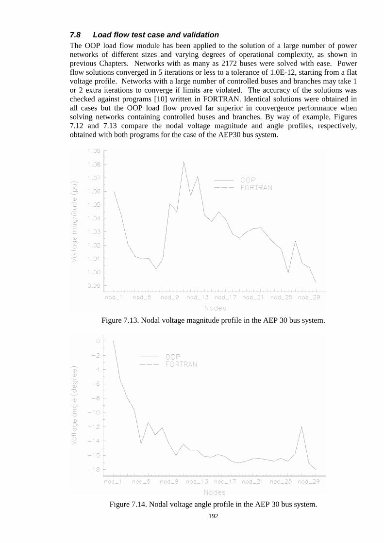
192
7.8 Load flow test case and validation The OOP load flow module has been applied to the solution of a large number of power networks of different sizes and varying degrees of operational complexity, as shown in previous Chapters. Networks with as many as 2172 buses were solved with ease. Power flow solutions converged in 5 iterations or less to a tolerance of 1.0E-12, starting from a flat voltage profile. Networks with a large number of controlled buses and branches may take 1 or 2 extra iterations to converge if limits are violated. The accuracy of the solutions was checked against programs [10] written in FORTRAN. Identical solutions were obtained in all cases but the OOP load flow proved far superior in convergence performance when solving networks containing controlled buses and branches. By way of example, Figures 7.12 and 7.13 compare the nodal voltage magnitude and angle profiles, respectively, obtained with both programs for the case of the AEP30 bus system.
Figure 7.13. Nodal voltage magnitude profile in the AEP 30 bus system.
Figure 7.14. Nodal voltage angle profile in the AEP 30 bus system.
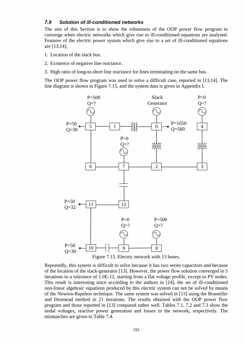
193
7.9 Solution of ill-conditioned networks The aim of this Section is to show the robustness of the OOP power flow program to converge when electric networks which give rise to ill-conditioned equations are analysed. Features of the electric power system which give rise to a set of ill-conditioned equations are [13,14], 1. Location of the slack bus. 2. Existence of negative line reactance. 3. High ratio of long-to-short line reactance for lines terminating on the same bus. The OOP power flow program was used to solve a difficult case, reported in [13,14]. The line diagram is shown in Figure 7.15, and the system data is given in Appendix I.
Figure 7.15. Electric network with 13 buses. Reportedly, this system is difficult to solve because it has two series capacitors and because of the location of the slack-generator [13]. However, the power flow solution converged in 5 iterations to a tolerance of 1.0E-12, starting from a flat voltage profile, except to PV nodes. This result is interesting since according to the authors in [14], the set of ill-conditioned non-linear algebraic equations produced by this electric system can not be solved by means of the Newton-Rapshon technique. The same system was solved in [13] using the Brameller and Denmead method in 21 iterations. The results obtained with the OOP power flow program and those reported in [13] compared rather well. Tables 7.1, 7.2 and 7.3 show the nodal voltages, reactive power generation and losses in the network, respectively. The mismatches are given in Table 7.4.
0
2 7
5
6
1
12 11
4
3
P=50 Q=30
P=1650 Q=560
P=50 Q=32
9 10 8 P=50 Q=30
P=0 Q=?
P=500 Q=?
P=500 Q=?
P=0 Q=?
Slack Generator
P=0 Q=?

194
Table 7.1. Comparison of nodal voltage solutions.
Table 7.2. Comparison of Reactive power generation.
Table 7.3. Comparison of system losses.
Table 7.4. Active and reactive power mismatches.
From Table 7.1 it is observed that the nodal voltage angles are positive with respect to the slack bus (reference). The reason is that active power is flowing to the slack node due to the very large load connected at that node. A second case was run assuming lossless transformers. Convergence was obtained in 5 iterations to a tolerance of 1.0E-12. The same analysis carried out using the Brameller and Denmead method converged in 100 iterations [13].
System Voltage Magnitude (pu) Voltage Angle (Degree) nodes Reference [13] OOP program Reference [13] OOP program nod_0 1.000 1.000 0.0 0.0 nod_1 0.971 0.971 1.70 1.70 nod_2 0.984 0.984 2.79 2.79 nod_3 0.951 0.951 2.88 2.88 nod_4 1.000 1.000 2.99 2.99 nod_5 1.037 1.037 10.18 10.18 nod_6 1.063 1.063 9.42 9.42 nod_7 1.100 1.100 8.60 8.60 nod_8 0.943 0.943 14.83 14.83 nod_9 1.100 1.100 8.82 8.82 nod_10 1.018 1.018 12.59 12.59 nod_11 1.067 1.067 8.57 8.57 nod_12 1.044 1.044 5.70 5.70
System Reactive Power Generation (MVARs) Generators Reference [13] OOP program Generator-0 -310.6 -310.6 Generator-4 -399.5 -399.5 Generator-5 -232.9 -232.9 Generator-7 -34.0 -33.3 Generator-8 -1006.4 -1006.4 Generator-9 -85.3 -86.0
System Losses Reference [13] OOP program
Active losses (MWs) 30.2 30.2 Reactive losses (MVARs) -2720.7 -2720.7
Mismatches Iterations ∆P (pu) ∆Q (pu)
0 0.5380 1.0149 1 0.0603 0.0751 2 0.0071 0.0016 3 5.4E-6 1.8E-6 4 1.8E-11 3.0E-12 5 1.0E-16 1.0E-17

195
7.10 Conclusions This Chapter has addressed the issue of ‘number crunching’ OOP power engineering applications. The software presented is fast and reliable and is entirely adequate for the analysis and control of large-scale power networks containing FACTS-controlled branches. The methodology used in the development of the software has been given. OOP load flows program has been successfully applied to the solution of several power networks of different sizes and varying degrees of operational complexity. The load flow is a full Newton-Raphson exhibiting quadratic convergence and includes sparse matrix techniques for the efficient handling of large scale networks. Limits violation compounded with strong interaction between the various controlled branches may dent the algorithm’s quadratic convergence, but even then reliable solutions will be obtained at the cost of one or two extra iterations. In all cases tested the solutions were obtained in a matter of milliseconds of cpu time. In the Power Supply Industry much of the debate about the value of OOP has centred on its performance. Some authors claim their OOP applications to be 2 to 3 times slower than comparable applications written in FORTRAN [5,7]. Contrary to their experience, comparisons of the newly developed C++ load flow with a FORTRAN load flow were made and the solution times obtained with the C++ load flow were extremely encouraging. The performance of the OOP power flow closely matches the cpu times taken by a comparable application written in FORTRAN [10]. By way of example, a 1090-node network was used to compare the cpu time taken by the C++ and FORTRAN load flow solutions. Twenty load flow runs were carried out consecutively and the average cpu time is shown in Table 7.5. The cpu time was measured with the UNIX command TIMEX for both the C++ and FORTRAN solutions. The hardware platform was a Sun Sparc server 20 running under Solaris 2.3.
Table 7.5. Comparison of total cpu time.
The C++ algorithm performed only 17% more slowly than a comparable FORTRAN algorithm. This contrasts with claims made by other authors [5,7] about C++
algorithms being 2 to 3 times slower than FORTRAN algorithms.
7.11 Bibliography [1] Buzzi-Ferraris G.: ‘Scientific C++, Building Numerical Libraries the Object Oriented Way’, Ed. Addison-Wesley, 1994, ISBN 0-201-63192-X. [2] Capper D.M.: ‘C++ for Scientists, Engineers and Mathematicians’, Springer-Verlag, 1994, ISBN 0-387-19847-4. [3] Barlow M.J. and Bernat P.Z.: ‘The Practicalities of Implementing On-Line Network Analysis and Data Management’, IEE Colloquium on ‘Developments with Interfacing of Power System Analysis Software with SCADA and Data Management Systems’, London, UK, 15 Nov. 1994. [4] Foley M., Bose A., Mitchell W. and Faustini A.: ‘An Object Based Graphical User Interface for Power Systems’, IEEE Trans. on Power Systems, Vol. 8, No. 1, pp. 97-104, Feb. 1993.
CPU time (sec) C++ FORTRAN Real 10.9 9.1 User 7.2 6.7
System 0.153 0.127

196
[5] Neyer A.F., Wu F.F. and Imhof K.: ‘Object Oriented Programming for Flexible Software: Example of a Load Flow’, IEEE Trans. on Power Systems, Vol. 5, No. 3, pp. 689-696, Aug. 1990. [6] Hakavik B. and Holen A.T.: ‘Power System Modelling and Sparse Matrix Operations Using Object Oriented Programming’, IEEE Trans. on Power Systems, Vol. 9, No. 2, pp. 1045-1051, May 1994. [7] Foley M. and Bose A.: ‘Object-Oriented On-Line Network Analysis’, IEEE Trans. on Power Systems, Vol. 10, No. 1, pp. 125-132, Feb. 1995. [8] Manzoni A., Silveira e Silva A. and Decker I.C.: ‘Power Systems Dynamics Simulation Using Object-Oriented Programming’, accepted for its publication in IEEE Trans. on Power Systems, 1997. [9] Warwick K., Ekwue A.O. and Aggarwal R.K. (Eds.): ‘Artificial Intelligence Techniques in Power Systems’, Chapter 3 written by Phillips N.B.P., Gann J.O. and Irving M.R., IEE monographs, Peter Peregrinus Series, 1997, ISBN 0-852-96897-3. [10] Acha E.: ‘A Quasi-Newton Algorithm for the Load Flow Solution of Large Networks with FACTS-Controlled Branches’, Proceedings of the 28th UPEC Conference, Stafford UK, 21-23, pp. 153-156, September 1993. [11] Tinney W.F. and Walker J.M.: ‘Direct Solutions of Sparse Network Equations by Optimally Ordered Triangular Factorization’, Proc. of IEEE, vol. 55, pp. 1801-1809, Nov. 1967. [12] Tinney W.F. and Hart C.E.: ‘Power Flow Solution by Newton’s Method’, IEEE Trans. on Power Apparatus and Systems, Vol. PAS-96, No. 11, pp. 1449-1460, November 1967. [13] Zollenkopf K.: ‘Load-Flow Calculation using Loss-Minimisation Techniques’, Proceedings of IEE, Vol. 115, No. 1, pp. 121-127, January 1968. [14] Tripathy S.C., Durga Prasad G., Malik O.P. and Hope G.S.: ‘Load-Flow Solutions for Ill-Conditioned Power systems by a Newton-Like Method’, IEEE Trans. on Power Apparatus and Systems, Vol. PAS-101, No. 10, pp. 3648-3657, October 1982.

197
Chapter 8 Conclusions and Recommendations 8.1 General conclusions This research work has addressed the issue of developing suitable steady-state models of FACTS devices aiming at analysing their influence on the overall performance of real life electric power systems. Their effectiveness in achieving control of power flows and nodal voltage magnitudes has been thoroughly investigated. The motivation for this work was the growing importance that the Electricity supply Industry world-wide is attaching to the FACTS technology, and the corresponding growing need for computer aided tools capable of assisting power system engineers to evaluate the technical and economical benefits afforded by this technology. Generalised nodal admittance models have been developed for the Advance Series Compensator, Phase Shifter, Static Var Compensator, On Load Tap Changer and Unified Power Flow Controller. In the case of the Advance Series Compensator, two models have been proposed to represent its structure, a Variable Series Compensator and a Thyristor Controlled Series Capacitor-Firing Angle. An alternative Unified Power Flow Controller model based on the concept of Synchronous Voltage Source has also been developed. The Interphase Power Controller has been modelled by combining Phase Shifters and Variable Series Compensators nodal admittance models. The non-linear power flow equations of the proposed FACTS device models have been linearised using the Newton-Rapshon technique and have been included in a full Newton-Rapshon load flow program. In this context, the state variables corresponding to the controllable devices have been combined simultaneously with the nodal network state variables in a single frame-of-reference for a unified, iterative solution. New type of nodes have been introduced in order to handle efficiently nodes whose voltage magnitude are being controlled by FACTS devices. Moreover, suitable control strategies have been proposed to handle cases when two or more FACTS devices are controlling voltage magnitude at the same node. The robustness of the unified method to solve large power networks has been illustrated by numeric examples. In particular, its superiority over the sequential method, in terms of the number of iterations required to converge, has been clearly shown. The effect of FACTS devices initial conditions was thoroughly investigated. A set of analytical equations has been derived to give Unified Power Flow Controller and Synchronous Voltage Source good initial conditions. For the remaining controllable device models, guidelines for choosing good initial conditions have been given. Moreover, a hybrid method has been proposed for the initialisation of a Variable Series Compensator and a Thyristor Controlled Series Capacitor-Firing Angle in order to circumvent the problem of ill-conditioned Jacobian matrices if the customary zero voltage angle initialisation is adopted. It was observed that if the revision of state variable limits is made at inappropriate times then an unnecessary increase in the number of iterations may be incurred. Hence, guidelines and methods for starting the revision of FACTS devices and other network variables have been described within the context of the full Newton-Rapshon algorithm. Moreover, the effect of state variables step size adjustments during the backward substitution in the overall iterative process was investigated. It has been shown that large state variable increments can

198
slow down converge, or more seriously, cause the solution to oscillate or even diverge. Suitable guidelines have been recommended in order to avoid large changes during the upgrading of these variables. The Object Oriented Programming philosophy has been adopted to develop the power flow program. The software developed is fast and reliable and it is entirely adequate for the analysis and control of large-scale power networks containing any number of FACTS-controlled branches. Comparisons of the C++ load flow program with a FORTRAN load flow program were made and the solution times obtained with the C++ load flow were extremely encouraging. A case in point is the solution of a 1090-bus network where the C++ algorithm performed only 17% more slowly than a comparable FORTRAN algorithm. This contrasts with claims made by other authors about C++
algorithms being 2 to 3 times slower than FORTRAN algorithm. The Object Oriented Programming load flow program has been successfully applied to the solution of several power networks of different sizes and varying degrees of operational complexity. Moreover, it has been used to explore three potential applications of FACTS devices in power systems. An algorithm for tracing the individual generator contributions to system loading, power flows, transmission losses, generation costs and Use of Line Charges is proposed. It is independently applied to active and reactive power concerns. The algorithm is accurate and comprehensive.
8.2 Suggestions for further research work It is considered that the work presented in this thesis provides a very solid foundation for additional research relating to the steady-state modelling and analysis of FACTS devices. The research items which require attention are: • In theory at least, Static Var Compensators, On Load Tap Changers and Unified Power
Flow Controllers can regulate the voltage magnitude of any node in the system. Similarly, Advance Series Compensators, Phase Shifters, Interphase Power Controllers and Unified Power Flow Controllers can regulate power flow across one or more transmission lines in the system. Hence, the area of remote control by FACTS devices within the context of the full Newton-Rapshon algorithm should be investigated.
• The computer program developed in this thesis is based on single control criterion, i.e.
one variable is adjusted to maintain another variable at a specified value. The possibility of multiple control criterion should be investigated. In this case, two or more variables are adjusted to maintain another variable fixed. Since the number of unknown variables will be greater than the number of equations, multiple solutions will take place. The application of the Singular Value Decomposition technique for the Jacobian matrix factorisation appears promising in this context.
• It is recommend to carry out research on the modelling of FACTS devices based on their
electronic topologies, similarly to the Thyristor Controlled Series Capacitor model presented in this thesis. The fundamental frequency models are obtained based on the Fourier analysis of the device’s structure.
• The power flow program developed in this thesis can be extended to become a Newton-
based Optimal Power Flow. All objects and methods available in the load flow program can be used in the Optimal Power Flow program with little or no modification. The Jacobian matrix would be extended to include second partial derivatives terms of the Lagrangian functions with respect to the nodal network and FACTS devices state

199
variables as well as Lagrange multipliers. This new line of research will allow to quantify the economical and operational benefits afforded by FACTS devices.
• The economical and operational benefits afforded by FACTS devices are not free of
charge. There is a price to be paid in the form of harmonic generation and advanced harmonic assessment tools are required. As a first step, the program described in this thesis could be extended to included the nolinearities produced by the FACTS controllers in order to compute characteristic harmonics. In this context, the FACTS devices modelling must be based on the electronic topology, similarly to the Thyristor Controlled Series Capacitor model presented in this thesis.
• In order to quantify the effect of FACTS devices on the maximum level of loadability of
the electric system, it is recommended to extend the Newton-type technique used in this research to encompass the continuation technique, including predictive and corrective steps. This numeric extension will allow to compute complete bifurcation diagrams.
• Work should be done to extend the auditing power flow methodology presented in
Chapter 6 to take into account reactive power series sources and non-reciprocal electric components, e.g. phase-shifters, Interphase Power Controllers and Unified Power Flow Controllers. It is believed that the use of the power injection concept could solve this problem.

200
Appendix I Data files Data relating to the test systems using in this research are given in this appendix. Only parameter values different from zero are given. The voltage magnitude and angle at Slack nodes have been specified at 1 pu and 0o, respectively. The MVA base is 100 MVA, unless stated otherwise
AI.1 5-nodes system
Table AI.1.1. Number of nodes and plant components.
Table AI.1.2. Transmission lines. Table AI.1.3. Loads.
Table AI.1.4. Generators.
AI.2 13-nodes system (1000 MVA base)
Table AI.2.1. Number of nodes and plant components.
Table AI.2.2. Transmission Lines. Table AI.2.3. Transformers.
Table AI.2.4. Loads.
Table AI.2.5. Generators.
Nodes Transmission
Lines
Transformers
Generators
Loads Shunt Compensators
Slack Node
5 7 0 1 4 0 north
Sending Node
Receiving Node
R (pu)
XL (pu)
BTOTAL (pu)
north south 0.02 0.06 0.06 north lake 0.08 0.24 0.05 south lake 0.06 0.18 0.04 south main 0.06 0.18 0.04 south elm 0.04 0.12 0.03 lake main 0.01 0.03 0.02 main elm 0.08 0.24 0.05
Node PLOAD
(MWs) QLOAD
(MVARs) south 20 10 lake 45 15 main 40 5 elm 60 10
Node PG
(MWs) QGMIN
(MVARs) QGMAX
(MVARs) Voltage
Magnitude (pu) south 40 -300 300 1.0
Nodes Transmission
Lines
Transformers
Generators
Loads Shunt Compensators
Slack Node
13 10 3 5 4 0 nod_0
Sending Node
Receiving Node
RS (pu)
XS (pu)
TV
UV
nod_0 nod_1 0.004 0.085 1.05 1 nod_0 nod_2 0.004 0.0947 1.1 1 nod_4 nod_3 0.004 0.0947 1.1 1
Sending Node
Receiving Node
R (pu)
XL (pu)
BTOTAL (pu)
nod_3 nod_2 0.0074 0.143 0.436 nod_5 nod_1 0.0481 0.459 0.246 nod_5 nod_6 0.009 0.108 0.016 nod_7 nod_2 0.0121 0.233 0.712 nod_6 nod_7 0 0.15 0 nod_8 nod_9 0.0105 0.202 0.62 nod_9 nod_10 0 -0.15 0
nod_10 nod_11 0.0086 0.1665 0.508 nod_11 nod_12 0.0075 0.1465 0.448 nod_12 nod_7 0 -0.15 0
Node PLOAD
(MWs) QLOAD
(MVARs) nod_0 1650 560 nod_5 50 30
nod_10 50 30 nod_11 50 32
Node PG
(MWs) QGMIN
(MVARs) QGMAX
(MVARs) Controlled Voltage
Magnitude (pu) nod_4 0 -5000 5000 1 nod_5 500 -5000 5000 1.037 nod_7 0 -5000 5000 1.1 nod_8 500 -5000 5000 0.943 nod_9 0 -5000 5000 1.1
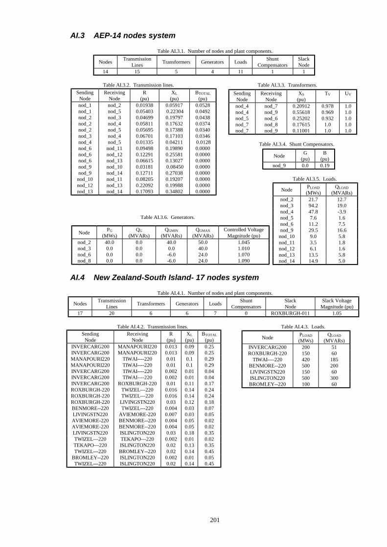
201
AI.3 AEP-14 nodes system
Table AI.3.1. Number of nodes and plant components.
Table AI.3.2. Transmission lines. Table AI.3.3. Transformers.
Table AI.3.4. Shunt Compensators.
Table AI.3.5. Loads.
Table AI.3.6. Generators.
AI.4 New Zealand-South Island- 17 nodes system
Table AI.4.1. Number of nodes and plant components.
Table AI.4.2. Transmission lines. Table AI.4.3. Loads.
Nodes Transmission
Lines
Transformers
Generators
Loads Shunt Compensators
Slack Node
14 15 5 4 11 1 1
Sending Node
Receiving Node
R (pu)
XL (pu)
BTOTAL (pu)
nod_1 nod_2 0.01938 0.05917 0.0528 nod_1 nod_5 0.05403 0.22304 0.0492 nod_2 nod_3 0.04699 0.19797 0.0438 nod_2 nod_4 0.05811 0.17632 0.0374 nod_2 nod_5 0.05695 0.17388 0.0340 nod_3 nod_4 0.06701 0.17103 0.0346 nod_4 nod_5 0.01335 0.04211 0.0128 nod_6 nod_11 0.09498 0.19890 0.0000 nod_6 nod_12 0.12291 0.25581 0.0000 nod_6 nod_13 0.06615 0.13027 0.0000 nod_9 nod_10 0.03181 0.08450 0.0000 nod_9 nod_14 0.12711 0.27038 0.0000
nod_10 nod_11 0.08205 0.19207 0.0000 nod_12 nod_13 0.22092 0.19988 0.0000 nod_13 nod_14 0.17093 0.34802 0.0000
Sending Node
Receiving Node
XS (pu)
TV
UV
nod_4 nod_7 0.20912 0.978 1.0 nod_4 nod_9 0.55618 0.969 1.0 nod_5 nod_6 0.25202 0.932 1.0 nod_7 nod_8 0.17615 1.0 1.0 nod_7 nod_9 0.11001 1.0 1.0
Node G
(pu) B
(pu) nod_9 0.0 0.19
Node PLOAD
(MWs) QLOAD
(MVARs) nod_2 21.7 12.7 nod_3 94.2 19.0 nod_4 47.8 -3.9 nod_5 7.6 1.6 nod_6 11.2 7.5 nod_9 29.5 16.6
nod_10 9.0 5.8 nod_11 3.5 1.8 nod_12 6.1 1.6 nod_13 13.5 5.8 nod_14 14.9 5.0
Node PG
(MWs) QG
(MVARs) QGMIN
(MVARs) QGMAX
(MVARs) Controlled Voltage
Magnitude (pu) nod_2 40.0 0.0 40.0 50.0 1.045 nod_3 0.0 0.0 0.0 40.0 1.010 nod_6 0.0 0.0 -6.0 24.0 1.070 nod_8 0.0 0.0 -6.0 24.0 1.090
Nodes Transmission
Lines
Transformers
Generators
Loads Shunt Compensators
Slack Node
Slack Voltage Magnitude (pu)
17 20 6 6 7 0 ROXBURGH-011 1.05
Sending Node
Receiving Node
R (pu)
XL (pu)
BTOTAL (pu)
INVERCARG200 MANAPOURI220 0.013 0.09 0.25 INVERCARG200 MANAPOURI220 0.013 0.09 0.25 MANAPOURI220 TIWAI----220 0.01 0.1 0.29 MANAPOURI220 TIWAI----220 0.01 0.1 0.29 INVERCARG200 TIWAI----220 0.002 0.01 0.04 INVERCARG200 TIWAI----220 0.002 0.01 0.04 INVERCARG200 ROXBURGH-220 0.01 0.11 0.17 ROXBURGH-220 TWIZEL---220 0.016 0.14 0.24 ROXBURGH-220 TWIZEL---220 0.016 0.14 0.24 ROXBURGH-220 LIVINGSTN220 0.03 0.12 0.18 BENMORE--220 TWIZEL---220 0.004 0.03 0.07 LIVINGSTN220 AVIEMORE-220 0.007 0.03 0.05 AVIEMORE-220 BENMORE--220 0.004 0.05 0.02 AVIEMORE-220 BENMORE--220 0.004 0.05 0.02 LIVINGSTN220 ISLINGTON220 0.03 0.18 0.35 TWIZEL---220 TEKAPO---220 0.002 0.01 0.02 TEKAPO---220 ISLINGTON220 0.02 0.13 0.35 TWIZEL---220 BROMLEY--220 0.02 0.14 0.45
BROMLEY--220 ISLINGTON220 0.002 0.01 0.05 TWIZEL---220 ISLINGTON220 0.02 0.14 0.45
Node PLOAD
(MWs) QLOAD
(MVARs) INVERCARG200 200 51 ROXBURGH-220 150 60
TIWAI----220 420 185 BENMORE--220 500 200 LIVINGSTN220 150 60 ISLINGTON220 500 300 BROMLEY--220 100 60

202
Table AI.4.4. Transformers.
Table AI.4.5. Generators.
AI.5 IEEE 28 nodes system
Table AI.5.1. Number of nodes and plant components.
Table AI.5.2. Transmission lines. Table AI.5.3. Transformers.
Table AI.5.4. Generators.
Table AI.5.5. Shunt compensators. Table AI.5.6. Loads.
Sending Node
Receiving Node
RP (pu)
XP (pu)
TV
UV
MANAPOURI220 MANAPOURI014 0.0006 0.016 1 1 ROXBURGH-220 ROXBURGH-011 0.002 0.04 1 1
TWIZEL---220 OHAU-SYSTEM 0.004 0.032 1 1 AVIEMORE-220 AVIEMORE-011 0.0015 0.045 1 1 BENMORE--220 BENMORE--016 0.0012 0.032 1 1 TEKAPO---220 TEKAPO---011 0.003 0.056 1 1
Node PG
(MWs) QGMIN
(MVARs) QGMAX
(MVARs) Controlled Voltage
Magnitude (pu) MANAPOURI014 690 -500 500 1.045 BENMORE--016 0 -500 500 1.06 AVIEMORE-011 200 -500 500 1.045 OHAU-SYSTEM 350 -500 500 1.05 ISLINGTON220 0 -500 500 1 TEKAPO---011 150 -500 500 1.05
Nodes Transmission
Lines
Transformers
Generators
Loads Shunt Compensators
Slack Node
28 33 5 10 17 1 nod_23
Sending Node
Receiving Node
R (pu)
XL (pu)
BTOTAL (pu)
nod_1 nod_2 0.0026 0.0139 0.4611 nod_1 nod_3 0.0546 0.2112 0.0572 nod_1 nod_5 0.0218 0.0845 0.0229 nod_2 nod_4 0.0328 0.1267 0.0343 nod_2 nod_6 0.0497 0.192 0.052 nod_3 nod_9 0.0308 0.119 0.0322 nod_4 nod_9 0.0268 0.1037 0.0282 nod_5 nod_10 0.0228 0.0883 0.0281 nod_6 nod_10 0.0139 0.0605 2.459 nod_7 nod_8 0.0159 0.0614 0.0166 nod_8 nod_9 0.0427 0.1651 0.0447 nod_8 nod_10 0.0427 0.1651 0.0447
nod_11 nod_13 0.0061 0.0476 0.0999 nod_11 nod_14 0.0054 0.0418 0.0879 nod_12 nod_13 0.0061 0.0476 0.0999 nod_12 nod_23 0.0124 0.0966 0.203 nod_13 nod_23 0.0111 0.0865 0.1818 nod_14 nod_16 0.005 0.0389 0.0818 nod_15 nod_16 0.0022 0.0173 0.0364 nod_15 nod_21 0.0063 0.049 0.103 nod_15 nod_21 0.0063 0.049 0.103 nod_15 nod_24 0.0067 0.0519 0.1091 nod_16 nod_17 0.0033 0.0259 0.0545 nod_16 nod_19 0.003 0.0231 0.0485 nod_17 nod_18 0.0018 0.0144 0.0303 nod_17 nod_22 0.0135 0.1053 0.2212 nod_18 nod_21 0.0033 0.0259 0.0545 nod_18 nod_21 0.0033 0.0259 0.0545 nod_19 nod_20 0.0051 0.0396 0.0833 nod_19 nod_20 0.0051 0.0396 0.0833 nod_20 nod_23 0.0028 0.0216 0.0455 nod_20 nod_23 0.0028 0.0216 0.0455 nod_21 nod_22 0.0087 0.0678 0.1424
Sending Node
Receiving Node
RS (pu)
XS (pu)
TV
UV
nod_3 nod_24 0.0023 0.0839 1 1 nod_9 nod_11 0.0023 0.0839 1 1 nod_9 nod_12 0.0023 0.0839 1 1
nod_10 nod_11 0.0023 0.0839 1 1 nod_10 nod_11 0.0023 0.0839 1 1
Node PG
(MWs) QGMIN
(MVARs) QGMAX
(MVARs) Voltage
Magnitude (pu) nod_1 192 -50 80 1 nod_2 192 -50 80 1 nod_7 300 0 180 1
nod_13 591 0 240 1 nod_14 0 50 200 1 nod_15 215 -50 110 0.98 nod_16 155 -50 80 0.99 nod_18 400 -50 200 1 nod_21 400 -50 200 1 nod_22 300 -60 96 1
Node G
(pu) B
(pu) nod_6 0 -1
Node PLOAD
(MWs) QLOAD
(MVARs) nod_1 108 22 nod_2 97 20 nod_3 180 37 nod_4 74 15 nod_5 71 14 nod_6 136 28 nod_7 125 25 nod_8 171 35 nod_9 175 36
nod_10 195 40 nod_13 265 54 nod_14 194 39 nod_15 317 64 nod_16 100 20 nod_18 333 68 nod_19 181 37 nod_20 128 26
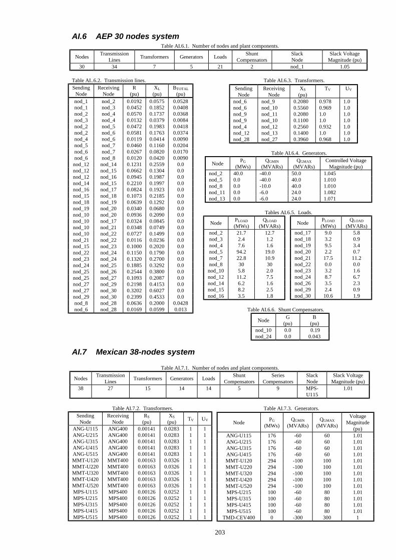
203
AI.6 AEP 30 nodes system Table AI.6.1. Number of nodes and plant components.
Table AI..6.2. Transmission lines. Table AI.6.3. Transformers.
Table AI.6.4. Generators.
Tables AI.6.5. Loads.
Table AI.6.6. Shunt Compensators.
AI.7 Mexican 38-nodes system
Table AI.7.1. Number of nodes and plant components.
Table AI.7.2. Transformers. Table AI.7.3. Generators.
Nodes Transmission
Lines
Transformers
Generators
Loads Shunt Compensators
Slack Node
Slack Voltage Magnitude (pu)
30 34 7 5 21 2 nod_1 1.05
Sending Node
Receiving Node
XS (pu)
TV
UV
nod_6 nod_9 0.2080 0.978 1.0 nod_6 nod_10 0.5560 0.969 1.0 nod_9 nod_11 0.2080 1.0 1.0 nod_9 nod_10 0.1100 1.0 1.0 nod_4 nod_12 0.2560 0.932 1.0 nod_12 nod_13 0.1400 1.0 1.0 nod_28 nod_27 0.3960 0.968 1.0
Sending Node
Receiving Node
R (pu)
XL (pu)
BTOTAL (pu)
nod_1 nod_2 0.0192 0.0575 0.0528 nod_1 nod_3 0.0452 0.1852 0.0408 nod_2 nod_4 0.0570 0.1737 0.0368 nod_3 nod_4 0.0132 0.0379 0.0084 nod_2 nod_5 0.0472 0.1983 0.0418 nod_2 nod_6 0.0581 0.1763 0.0374 nod_4 nod_6 0.0119 0.0414 0.0090 nod_5 nod_7 0.0460 0.1160 0.0204 nod_6 nod_7 0.0267 0.0820 0.0170 nod_6 nod_8 0.0120 0.0420 0.0090
nod_12 nod_14 0.1231 0.2559 0.0 nod_12 nod_15 0.0662 0.1304 0.0 nod_12 nod_16 0.0945 0.1987 0.0 nod_14 nod_15 0.2210 0.1997 0.0 nod_16 nod_17 0.0824 0.1923 0.0 nod_15 nod_18 0.1073 0.2185 0.0 nod_18 nod_19 0.0639 0.1292 0.0 nod_19 nod_20 0.0340 0.0680 0.0 nod_10 nod_20 0.0936 0.2090 0.0 nod_10 nod_17 0.0324 0.0845 0.0 nod_10 nod_21 0.0348 0.0749 0.0 nod_10 nod_22 0.0727 0.1499 0.0 nod_21 nod_22 0.0116 0.0236 0.0 nod_15 nod_23 0.1000 0.2020 0.0 nod_22 nod_24 0.1150 0.1790 0.0 nod_23 nod_24 0.1320 0.2700 0.0 nod_24 nod_25 0.1885 0.3292 0.0 nod_25 nod_26 0.2544 0.3800 0.0 nod_25 nod_27 0.1093 0.2087 0.0 nod_27 nod_29 0.2198 0.4153 0.0 nod_27 nod_30 0.3202 0.6027 0.0 nod_29 nod_30 0.2399 0.4533 0.0 nod_8 nod_28 0.0636 0.2000 0.0428 nod_6 nod_28 0.0169 0.0599 0.013
Node PG
(MWs) QGMIN
(MVARs) QGMAX
(MVARs) Controlled Voltage
Magnitude (pu) nod_2 40.0 -40.0 50.0 1.045 nod_5 0.0 -40.0 40.0 1.010 nod_8 0.0 -10.0 40.0 1.010 nod_11 0.0 -6.0 24.0 1.082 nod_13 0.0 -6.0 24.0 1.071
Node PLOAD
(MWs) QLOAD
(MVARs) nod_17 9.0 5.8 nod_18 3.2 0.9 nod_19 9.5 3.4 nod_20 2.2 0.7 nod_21 17.5 11.2 nod_22 0.0 0.0 nod_23 3.2 1.6 nod_24 8.7 6.7 nod_26 3.5 2.3 nod_29 2.4 0.9 nod_30 10.6 1.9
Node PLOAD
(MWs) QLOAD
(MVARs) nod_2 21.7 12.7 nod_3 2.4 1.2 nod_4 7.6 1.6 nod_5 94.2 19.0 nod_7 22.8 10.9 nod_8 30 30
nod_10 5.8 2.0 nod_12 11.2 7.5 nod_14 6.2 1.6 nod_15 8.2 2.5 nod_16 3.5 1.8
Node G
(pu) B
(pu) nod_10 0.0 0.19 nod_24 0.0 0.043
Nodes Transmission
Lines
Transformers
Generators
Loads Shunt Compensators
Series Compensators
Slack Node
Slack Voltage Magnitude (pu)
38 27 15 14 14 5 9 MPS-U115
1.01
Node
PG
(MWs)
QGMIN
(MVARs)
QGMAX
(MVARs)
Voltage Magnitude
(pu) ANG-U115 176 -60 60 1.01 ANG-U215 176 -60 60 1.01 ANG-U315 176 -60 60 1.01 ANG-U415 176 -60 60 1.01 MMT-U120 294 -100 100 1.01 MMT-U220 294 -100 100 1.01 MMT-U320 294 -100 100 1.01 MMT-U420 294 -100 100 1.01 MMT-U520 294 -100 100 1.01 MPS-U215 100 -60 80 1.01 MPS-U315 100 -60 80 1.01 MPS-U415 100 -60 80 1.01 MPS-U515 100 -60 80 1.01
TMD-CEV400 0 -300 300 1
Sending Node
Receiving Node
RS (pu)
XS (pu)
TV
UV
ANG-U115 ANG400 0.00141 0.0283 1 1 ANG-U215 ANG400 0.00141 0.0283 1 1 ANG-U315 ANG400 0.00141 0.0283 1 1 ANG-U415 ANG400 0.00141 0.0283 1 1 ANG-U515 ANG400 0.00141 0.0283 1 1 MMT-U120 MMT400 0.00163 0.0326 1 1 MMT-U220 MMT400 0.00163 0.0326 1 1 MMT-U320 MMT400 0.00163 0.0326 1 1 MMT-U420 MMT400 0.00163 0.0326 1 1 MMT-U520 MMT400 0.00163 0.0326 1 1 MPS-U115 MPS400 0.00126 0.0252 1 1 MPS-U215 MPS400 0.00126 0.0252 1 1 MPS-U315 MPS400 0.00126 0.0252 1 1 MPS-U415 MPS400 0.00126 0.0252 1 1 MPS-U515 MPS400 0.00126 0.0252 1 1

204
Table AI.7.4. Transmission Lines. Table AI.7.5. Series Compensators.
Table AI.7.6. Loads.
Table AI.7.7. Shunt Compensators.
AI.8 Morelia 38-nodes System Table AI.8.1. Number of nodes and plant components.
Table AI.8.2. Transmission Lines. AI.8.3. Transformers.
Sending Node
Receiving Node
R (pu)
XL (pu)
BTOTAL (pu)
CRP-230 MRP-230 0.0105 0.07966 0.1534 PTN-115 PCS-115 0.00464 0.01816 0.00228 PCS-115 LAG-115 0.01939 0.07851 0.00958 MRP-115 LAG-115 0.02454 0.09613 0.0121 MRP-115 CRISOBA 0.00769 0.01766 0.00202 MRP-115 MEL-115 0.00347 0.00797 0.00092 MEL-115 MOR-115 0.01341 0.03076 0.00352 MOR-115 STG-115 0.00261 0.01021 0.00124 STG-115 CTZ-115 0.02457 0.09624 0.02232 STG-115 MOI-115 0.00575 0.02252 0.00284 MRP-115 MRD-115 0.00481 0.01687 0.00266 MRD-115 CPE-115 0.00801 0.03249 0.00378 CPE-115 MOI-115 0.01014 0.03973 0.005 MOI-115 AER-115 0.01417 0.05549 0.00698 AER-115 ZIN-115 0.02362 0.0925 0.01164 ZIN-115 AZS-GEN 0.01669 0.06537 0.00824 AZS-GEN CDH-115 0.02705 0.10594 0.01334 CDH-115 ZIT-115 0.02452 0.09606 0.0121 Table AI.8.4. Generators.
Node PG
(MWs) QGMIN
(MVARs) QGMAX
(MVARs) Controlled Voltage
Magnitude (pu) AZS-GEN 48 -20 20 1.004
Sending Node
Receiving Node
R (pu)
XL (pu)
BTOTAL (pu)
ANG400 MMT400 0.00168 0.02075 0.61272 ANG400 MMT400 0.00174 0.02158 0.6371 JUI400 MMT400 0.00464 0.05732 1.69196 JUI400 MMT400 0.00464 0.05732 1.69196
MMT400 MPS400 0.00153 0.01887 0.55702 MMT400 MPS400 0.00128 0.01581 0.4665 JUI400 TMD-CEV400 0.00296 0.03656 1.07924 JUI400 TMD-CEV400 0.00296 0.03656 1.07924 CTZ400 MID400 0.00013 0.00165 0.04874
CTZ400CS MPS400 0.00265 0.03279 0.96782 MID400CS1 MPS400 0.00275 0.03396 1.00264 MID400CS2 MPS400 0.00277 0.03421 1.0096
MID400 TMD-CEV400CS1 0.00434 0.05355 1.58056 MID400 TMD-CEV400CS2 0.0043 0.05308 1.56664 ODA400 PUE400CS1 0.00239 0.02949 0.87036 ODA400 TMD-CEV400 0.00191 0.02359 0.69628 PUE400 SLZO400 0.00022 0.00283 0.08356 PUE400 TEC1400 0.00071 0.00873 0.25762 PUE400 TEX400 0.0017 0.0223 0.6132
PUE400CS2 TMD-CEV400 0.0043 0.05308 1.56664 TEC1400CS1 TMD-CEV400 0.00363 0.04482 1.32294 TEC1400CS2 TOP400 0.00283 0.03491 1.0305
CRU400 TEX400 0.0007 0.0088 0.2643 CRU400 TEX400 0.0007 0.0088 0.2643 CRU400 TOP400 0.0005 0.0065 0.2 CRU400 TOP400 0.0005 0.0065 0.2 SLZO400 TEX400 0.00152 0.01887 0.55702
Sending Node
Receiving Node
XC (pu)
CTZ400 CTZ400CS -0.00095 MID400 MID400CS1 -0.000991 MID400 MID400CS2 -0.000991
TMD-CEV400 TMD-CEV400CS1 -0.02142 TMD-CEV400 TMD-CEV400CS2 -0.02142 PUE400CS1 PUE400 -0.001828
PUE400 PUE400CS2 -0.002441 TEC1400 TEC1400CS1 -0.002375 TEC1400 TEC1400CS2 -0.001431
Node PLOAD
(MWs) QLOAD
(MVARs) ANG400 145.04 11.17 CRU400 627.39 106.29 MMT400 162.5 23.74 MPS400 -54.22 -12.23 TEX400 -276.64 -248.43 TOP400 537.78 -0.22 ODA400 195.75 35.92 JUI400 45.23 -4.75 CTZ400 193.77 53.46 MID400 299.22 88.66 TEC1400 120.1 -5.98 PUE400 206.642 13.406
SLZO400 177.17 58.43 TMD-CEV400 321.48 -17.54
Node G (pu)
B (pu)
CRU400 0 -0.75 MMT400 0 -2 TEX400 0 -0.5 PUE400 0 -0.7 TOP400 0 -0.62
Nodes Transmission
Lines
Transformers
Generators
Loads Shunt Compensators
Slack Node
Slack Voltage Magnitude (pu)
38 18 21 1 19 0 CRP-230 1.01
Sending Node
Receiving Node
XS (pu)
TV
UV
MRP-115 MRP-230 0.058 1 1 MRP-115 MRP-230 0.057 1 1 MEL-T1 MEL-115 0.6455 1 1 MOR-T1 MOR-115 0.6455 1 1 MOR-T2 MOR-115 0.6455 1 1 STG-T1 STG-115 0.832 1 1 STG-T2 STG-115 0.832 1 1 CTZ-T1 CTZ-115 0.645 1 1 CTZ-T2 CTZ-115 0.9941 1 1 MOI-T1 MOI-115 0.6455 1 1 AER-T1 AER-115 0.9941 1 1 ZIN-T1 ZIN-115 0.9941 1 1 CDH-T1 CDH-115 0.6455 1 1 CDH-T2 CDH-115 0.9941 1 1 ZIT-T1 ZIT-115 0.6455 1 1 ZIT-T2 ZIT-115 0.6455 1 1 CPE-T1 CPE-115 0.6455 1 1 MRD-T1 MRD-115 0.6455 1 1 LAG-T1 LAG-115 0.9941 1 1 PCS-T1 PCS-115 0.6455 1 1 PTN-T1 PTN-115 0.6455 1 1

205
Tables AI.8.5. Loads.
AI.9 New-England 39-nodes System Table AI.9.1. Number of nodes and plant components.
Table AI.9.2. Transmission lines. Table AI.9.3. Transformers.
Table AI.9.4. Loads.
Table AI.9.5. Generators.
Node PLOAD
(MWs) QLOAD
(MVARs) CRISOBA 8 2 MEL-T1 8 2 MOR-T1 10.4 2.9 MOR-T2 8 2.5 STG-T1 5 1.5 STG-T2 3.6 1 CTZ-T2 3.6 1 MOI-T1 7.2 1.6 AER-T1 4.5 1.2 ZIN-T1 3 1
Node PLOAD
(MWs) QLOAD
(MVARs) CDH-T1 4 1.4 ZIT-115 3 1 ZIT-T1 4 0.5 ZIT-T2 7 1.5 CPE-T1 11 2 MRD-T1 9.5 1.4 LAG-T1 1 0.2 PCS-T1 4.5 1.5 PTN-T1 3 1
Nodes Transmission
Lines
Transformers
Generators
Loads Shunt Compensators
Slack Node
Slack Voltage Magnitude (pu)
39 34 12 9 39 0 39 1.03
Sending Node
Receiving Node
R (pu)
XL (pu)
BTOTAL (pu)
1 2 0.0035 0.0411 0.6987 1 39 0.001 0.025 0.75 2 3 0.0013 0.0151 0.2572 2 25 0.007 0.0086 0.146 3 4 0.0013 0.0213 0.2214 3 18 0.0011 0.0133 0.2138 4 5 0.0008 0.0128 0.1342 4 14 0.0008 0.0129 0.1382 5 6 0.0002 0.0026 0.0434 5 8 0.0008 0.0112 0.1476 6 7 0.0006 0.0092 0.113 6 11 0.0007 0.0082 0.13895 7 8 0.0004 0.0046 0.078 8 9 0.0023 0.0363 0.3804 9 39 0.001 0.025 1.2
10 11 0.0004 0.0043 0.0729 10 13 0.0004 0.0043 0.0729 13 14 0.0009 0.0101 0.1725 14 15 0.0018 0.0217 0.366 15 16 0.0009 0.0094 0.171 16 17 0.0007 0.0089 0.1342 16 19 0.0016 0.0195 0.304 16 21 0.0008 0.0135 0.2548 16 24 0.0003 0.0059 0.068 17 18 0.0007 0.0082 0.1319 17 27 0.0013 0.0173 0.3216 21 22 0.0008 0.014 0.2565 22 23 0.0006 0.0096 0.1845 23 24 0.0022 0.035 0.361 25 26 0.0032 0.0323 0.513 26 27 0.0014 0.0147 0.2396 26 28 0.0043 0.0474 0.7802 26 29 0.0057 0.0625 1.029 28 29 0.0014 0.0151 0.249
Sending Node
Receiving Node
RS (pu)
XS (pu)
TV
UV
2 30 0 0.0181 1.025 1 6 31 0 0.025 1.07 1
10 32 0 0.02 1.07 1 12 11 0.0016 0.0435 1.006 1 12 13 0.0016 0.0435 1.006 1 19 20 0.0007 0.0138 1.06 1 19 33 0.0007 0.0142 1.07 1 20 34 0.0009 0.018 1.009 1 22 35 0 0.0143 1.025 1 23 36 0.0005 0.0272 1 1 25 37 0.0006 0.0232 1.025 1 29 38 0.0008 0.0156 1.025 1
Node PLOAD
(MWs) QLOAD
(MVARs) 31 9.2 4.6 3 322 2.4 4 500 184 7 233 84 8 522 176
12 8.5 88 15 320 153 16 329.4 32.3 18 158 30 20 680 103 21 274 115 23 247.5 84.6 24 308.6 -92.2 25 224 47.2 26 139 17 27 281 75.5 28 206 27.6 29 283.5 26.9 39 1104 250
Node PG
(MWs) QGMIN
(MVARs) QGMAX
(MVARs) Controlled Voltage
Magnitude (pu) 30 250 -200 300 1.0475 31 573.2 -300 300 0.952 32 650 -300 300 0.9831 33 632 -200 300 0.9972 34 508 -200 300 1.0123 35 650 -250 350 1.0493 36 560 -150 250 1.0635 37 540 -250 350 1.0278 38 830 -400 400 1.0265

206
AI.10 AEP 57-nodes System Table AI.10.1. Number of nodes and plant components.
Table AI.10.2. Transmission Lines. Table AI.10.3. Generators.
Table AI.10.4. Load.
Table AI.10.5. Shunt Compensators.
Nodes Transmission
Lines
Transformers
Generators
Loads Shunt Compensators
Slack Node
Slack Voltage Magnitude (pu)
57 63 17 6 42 3 NOD_1 1.04
Sending Node
Receiving Node
R (pu)
XL (pu)
BTOTAL (pu)
NOD_1 NOD_2 0.0083 0.0280 0.1290 NOD_2 NOD_3 0.0298 0.0850 0.0818 NOD_3 NOD_4 0.0112 0.0366 0.0380 NOD_4 NOD_5 0.0625 0.1320 0.0258 NOD_4 NOD_6 0.0430 0.1480 0.0348 NOD_6 NOD_7 0.0200 0.1020 0.0276 NOD_6 NOD_8 0.0339 0.1730 0.0470 NOD_8 NOD_9 0.0099 0.0505 0.0548 NOD_9 NOD_10 0.0369 0.1679 0.0440 NOD_9 NOD_11 0.0258 0.0848 0.0218 NOD_9 NOD_12 0.0648 0.2950 0.0772 NOD_9 NOD_13 0.0481 0.1580 0.0406
NOD_13 NOD_14 0.0132 0.0434 0.0110 NOD_13 NOD_15 0.0269 0.0869 0.0230 NOD_1 NOD_15 0.0178 0.0910 0.0988 NOD_1 NOD_16 0.0454 0.2060 0.0546 NOD_1 NOD_17 0.0238 0.1080 0.0286 NOD_3 NOD_15 0.0162 0.0530 0.0544 NOD_5 NOD_6 0.0302 0.0641 0.0124 NOD_7 NOD_8 0.0139 0.0712 0.0194
NOD_10 NOD_12 0.0277 0.1262 0.0328 NOD_11 NOD_13 0.0223 0.0732 0.0196 NOD_12 NOD_13 0.0178 0.0580 0.0604 NOD_12 NOD_16 0.0180 0.0813 0.0216 NOD_12 NOD_17 0.0397 0.1790 0.0476 NOD_14 NOD_15 0.0171 0.0547 0.0148 NOD_18 NOD_19 0.4610 0.6850 0.0000 NOD_19 NOD_20 0.2830 0.4340 0.0000 NOD_21 NOD_22 0.0736 0.1170 0.0000 NOD_22 NOD_23 0.0099 0.0152 0.0000 NOD_23 NOD_24 0.1660 0.2560 0.0084 NOD_26 NOD_27 0.1650 0.2540 0.0000 NOD_27 NOD_28 0.0618 0.0954 0.0000 NOD_28 NOD_29 0.0418 0.0587 0.0000 NOD_25 NOD_30 0.1350 0.2020 0.0000 NOD_30 NOD_31 0.3260 0.4970 0.0000 NOD_31 NOD_32 0.5070 0.7550 0.0000 NOD_32 NOD_33 0.0392 0.0360 0.0000 NOD_34 NOD_35 0.0520 0.0780 0.0032 NOD_35 NOD_36 0.0430 0.0537 0.0016 NOD_36 NOD_37 0.0290 0.0366 0.0000 NOD_37 NOD_38 0.0651 0.1009 0.0020 NOD_37 NOD_39 0.0239 0.0379 0.0000 NOD_36 NOD_40 0.0300 0.0466 0.0000 NOD_22 NOD_38 0.0192 0.0295 0.0000 NOD_41 NOD_42 0.2070 0.3520 0.0000 NOD_41 NOD_43 0.0000 0.4120 0.0000 NOD_38 NOD_44 0.0289 0.0585 0.0020 NOD_46 NOD_47 0.0230 0.0680 0.0032 NOD_47 NOD_48 0.0182 0.0233 0.0000 NOD_48 NOD_49 0.0834 0.1290 0.0048 NOD_49 NOD_50 0.0801 0.1280 0.0000 NOD_50 NOD_51 0.1386 0.2200 0.0000 NOD_29 NOD_52 0.1442 0.1870 0.0000 NOD_52 NOD_53 0.0762 0.0984 0.0000 NOD_53 NOD_54 0.1878 0.2320 0.0000 NOD_54 NOD_55 0.1732 0.2265 0.0000 NOD_44 NOD_45 0.0624 0.1242 0.0040 NOD_56 NOD_41 0.5530 0.5490 0.0000 NOD_56 NOD_42 0.2125 0.3540 0.0000 NOD_57 NOD_56 0.1740 0.2600 0.0000 NOD_38 NOD_49 0.1150 0.1770 0.0060 NOD_38 NOD_48 0.0312 0.0482 0.0000
Node PG
(MWs) QGMIN
(MVARs) QGMAX
(MVARs) Voltage
Magnitude (pu) NOD_2 0.0 -17.0 50.00 1.010 NOD_3 40.0 -10.0 60.00 0.985 NOD_6 0.0 -8.0 25.00 0.980 NOD_8 450.0 -140.0 200.00 1.005 NOD_9 0.0 -3.0 9.00 0.980
NOD_12 310.0 -50.0 155.00 1.015
Node PLOAD
(MWs) QLOAD
(MVARs) NOD_1 55.0 17.0 NOD_2 3.0 88.0 NOD_3 41.0 21.0 NOD_5 13.0 4.0 NOD_6 75.0 2.0 NOD_8 150. 22.0 NOD_9 121. 26.0
NOD_10 5.0 2.0 NOD_12 377. 24.0 NOD_13 18.0 2.3 NOD_14 10.5 5.3 NOD_15 22.0 5.0 NOD_16 43.0 3.0 NOD_17 42.0 8.0 NOD_18 27.2 9.8 NOD_19 3.3 0.6 NOD_20 2.3 1.0 NOD_23 6.3 2.1 NOD_25 6.3 3.2 NOD_27 9.3 0.5 NOD_28 4.6 2.3 NOD_29 17.0 2.6 NOD_30 3.6 1.8 NOD_31 5.8 2.9 NOD_32 1.6 0.8 NOD_33 3.8 1.9 NOD_35 6.0 3.0 NOD_38 14.0 7.0 NOD_41 6.3 3.0 NOD_42 7.1 4.4 NOD_43 2.0 1.0 NOD_44 12.0 1.8 NOD_47 29.7 11.6 NOD_49 18.0 8.5 NOD_50 21.0 10.5 NOD_51 18.0 5.3 NOD_52 4.9 2.2 NOD_53 20.0 10.0 NOD_54 4.1 1.4 NOD_55 6.8 3.4 NOD_56 7.6 2.2 NOD_57 6.7 2.0
Node G
(pu) B
(pu) NOD_18 0.0 0.100 NOD_25 0.0 0.059 NOD_53 0.0 0.063
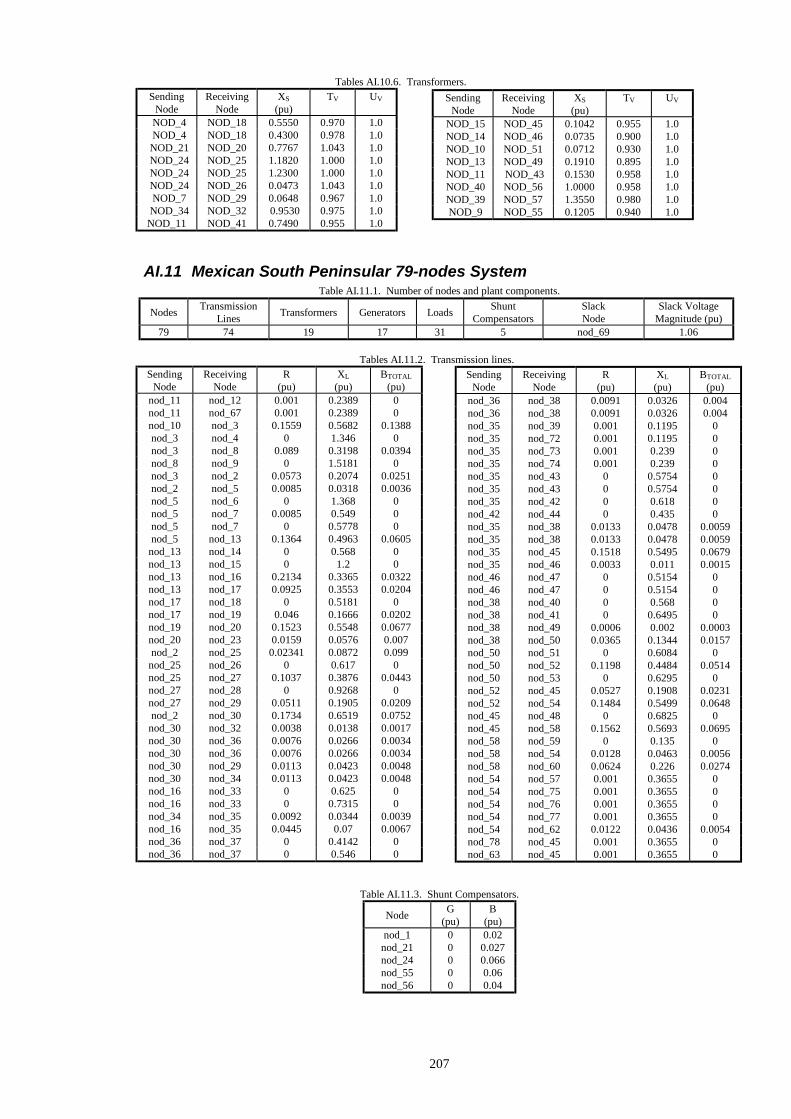
207
Tables AI.10.6. Transformers.
AI.11 Mexican South Peninsular 79-nodes System Table AI.11.1. Number of nodes and plant components.
Tables AI.11.2. Transmission lines.
Table AI.11.3. Shunt Compensators.
Sending Node
Receiving Node
XS (pu)
TV
UV
NOD_4 NOD_18 0.5550 0.970 1.0 NOD_4 NOD_18 0.4300 0.978 1.0
NOD_21 NOD_20 0.7767 1.043 1.0 NOD_24 NOD_25 1.1820 1.000 1.0 NOD_24 NOD_25 1.2300 1.000 1.0 NOD_24 NOD_26 0.0473 1.043 1.0 NOD_7 NOD_29 0.0648 0.967 1.0
NOD_34 NOD_32 0.9530 0.975 1.0 NOD_11 NOD_41 0.7490 0.955 1.0
Sending Node
Receiving Node
XS (pu)
TV
UV
NOD_15 NOD_45 0.1042 0.955 1.0 NOD_14 NOD_46 0.0735 0.900 1.0 NOD_10 NOD_51 0.0712 0.930 1.0 NOD_13 NOD_49 0.1910 0.895 1.0 NOD_11 NOD_43 0.1530 0.958 1.0 NOD_40 NOD_56 1.0000 0.958 1.0 NOD_39 NOD_57 1.3550 0.980 1.0 NOD_9 NOD_55 0.1205 0.940 1.0
Nodes Transmission
Lines
Transformers
Generators
Loads Shunt Compensators
Slack Node
Slack Voltage Magnitude (pu)
79 74 19 17 31 5 nod_69 1.06
Sending Node
Receiving Node
R (pu)
XL (pu)
BTOTAL (pu)
nod_11 nod_12 0.001 0.2389 0 nod_11 nod_67 0.001 0.2389 0 nod_10 nod_3 0.1559 0.5682 0.1388 nod_3 nod_4 0 1.346 0 nod_3 nod_8 0.089 0.3198 0.0394 nod_8 nod_9 0 1.5181 0 nod_3 nod_2 0.0573 0.2074 0.0251 nod_2 nod_5 0.0085 0.0318 0.0036 nod_5 nod_6 0 1.368 0 nod_5 nod_7 0.0085 0.549 0 nod_5 nod_7 0 0.5778 0 nod_5 nod_13 0.1364 0.4963 0.0605
nod_13 nod_14 0 0.568 0 nod_13 nod_15 0 1.2 0 nod_13 nod_16 0.2134 0.3365 0.0322 nod_13 nod_17 0.0925 0.3553 0.0204 nod_17 nod_18 0 0.5181 0 nod_17 nod_19 0.046 0.1666 0.0202 nod_19 nod_20 0.1523 0.5548 0.0677 nod_20 nod_23 0.0159 0.0576 0.007 nod_2 nod_25 0.02341 0.0872 0.099
nod_25 nod_26 0 0.617 0 nod_25 nod_27 0.1037 0.3876 0.0443 nod_27 nod_28 0 0.9268 0 nod_27 nod_29 0.0511 0.1905 0.0209 nod_2 nod_30 0.1734 0.6519 0.0752
nod_30 nod_32 0.0038 0.0138 0.0017 nod_30 nod_36 0.0076 0.0266 0.0034 nod_30 nod_36 0.0076 0.0266 0.0034 nod_30 nod_29 0.0113 0.0423 0.0048 nod_30 nod_34 0.0113 0.0423 0.0048 nod_16 nod_33 0 0.625 0 nod_16 nod_33 0 0.7315 0 nod_34 nod_35 0.0092 0.0344 0.0039 nod_16 nod_35 0.0445 0.07 0.0067 nod_36 nod_37 0 0.4142 0 nod_36 nod_37 0 0.546 0
Sending Node
Receiving Node
R (pu)
XL (pu)
BTOTAL (pu)
nod_36 nod_38 0.0091 0.0326 0.004 nod_36 nod_38 0.0091 0.0326 0.004 nod_35 nod_39 0.001 0.1195 0 nod_35 nod_72 0.001 0.1195 0 nod_35 nod_73 0.001 0.239 0 nod_35 nod_74 0.001 0.239 0 nod_35 nod_43 0 0.5754 0 nod_35 nod_43 0 0.5754 0 nod_35 nod_42 0 0.618 0 nod_42 nod_44 0 0.435 0 nod_35 nod_38 0.0133 0.0478 0.0059 nod_35 nod_38 0.0133 0.0478 0.0059 nod_35 nod_45 0.1518 0.5495 0.0679 nod_35 nod_46 0.0033 0.011 0.0015 nod_46 nod_47 0 0.5154 0 nod_46 nod_47 0 0.5154 0 nod_38 nod_40 0 0.568 0 nod_38 nod_41 0 0.6495 0 nod_38 nod_49 0.0006 0.002 0.0003 nod_38 nod_50 0.0365 0.1344 0.0157 nod_50 nod_51 0 0.6084 0 nod_50 nod_52 0.1198 0.4484 0.0514 nod_50 nod_53 0 0.6295 0 nod_52 nod_45 0.0527 0.1908 0.0231 nod_52 nod_54 0.1484 0.5499 0.0648 nod_45 nod_48 0 0.6825 0 nod_45 nod_58 0.1562 0.5693 0.0695 nod_58 nod_59 0 0.135 0 nod_58 nod_54 0.0128 0.0463 0.0056 nod_58 nod_60 0.0624 0.226 0.0274 nod_54 nod_57 0.001 0.3655 0 nod_54 nod_75 0.001 0.3655 0 nod_54 nod_76 0.001 0.3655 0 nod_54 nod_77 0.001 0.3655 0 nod_54 nod_62 0.0122 0.0436 0.0054 nod_78 nod_45 0.001 0.3655 0 nod_63 nod_45 0.001 0.3655 0
Node G
(pu) B
(pu) nod_1 0 0.02
nod_21 0 0.027 nod_24 0 0.066 nod_55 0 0.06 nod_56 0 0.04

208
Table AI.11.4. Transformers. Table AI.11.5. Generators.
Tables AI.11.6. Loads.
AI.12 IEEE 118-nodes System Table AI.12.1. Number of nodes and plant components.
Table AI.12.3. Shunt compensators. Table AI.12.2. Transformers.
Sending Node
Receiving Node
RS (pu)
XS (pu)
TV
UV
nod_10 nod_11 0 0.5154 0.95 1 nod_2 nod_79 0.001 0.0554 1.02 1 nod_2 nod_64 0.001 0.0554 1.02 1 nod_2 nod_65 0.001 0.0554 1.02 1 nod_2 nod_66 0.001 0.0554 1.02 1
nod_20 nod_21 0 0.618 0.95 1 nod_20 nod_22 0.001 0.3147 0.95 1 nod_20 nod_68 0.001 0.3147 0.95 1 nod_23 nod_24 0 0.5154 0.956 1 nod_30 nod_31 0.01 0.0329 1.025 1 nod_30 nod_69 0.01 0.0329 1.025 1 nod_30 nod_70 0.01 0.0329 1.02 1 nod_30 nod_71 0.01 0.0329 1.02 1 nod_60 nod_61 0 0.9681 0.957 1 nod_60 nod_61 0 0.9681 0.957 1 nod_54 nod_55 0 0.9681 0.957 1 nod_54 nod_55 0 0.5535 0.957 1 nod_54 nod_56 0 0.5736 0.957 1 nod_62 nod_1 0 0.6495 0.956 1
Node
PG
(MWs)
QGMIN
(MVARs)
QGMAX
(MVARs)
Voltage Magnitude
(pu) nod_79 20 -50 50 1 nod_64 20 -50 50 1 nod_65 21 -50 50 1 nod_66 21 -50 50 1 nod_31 50 -50 50 1 nod_70 52 -50 50 0.985 nod_71 50 -50 50 0.985 nod_39 11 -50 50 0.985 nod_72 12 -50 50 0.978 nod_73 12 -50 50 0.978 nod_74 10 -50 50 0.978 nod_22 5 -50 50 0.992 nod_68 3 -50 50 1.028 nod_57 4 -50 50 0.99 nod_75 4 -50 50 1 nod_76 3 -50 50 1 nod_77 3 -50 50 1
Node PLOAD
(MWs) QLOAD
(MVARs) nod_33 20 7 nod_35 3 1 nod_37 30 9 nod_40 12 5 nod_41 8 3 nod_42 11 4 nod_43 18 6 nod_47 32 11 nod_48 6 2 nod_49 9 2 nod_51 10 4 nod_53 6 2 nod_55 23 9 nod_56 15 5 nod_61 12 5
Node PLOAD
(MWs) QLOAD
(MVARs) nod_1 6 2 nod_2 10 3 nod_4 4 1.5 nod_6 5 2 nod_7 17 6 nod_9 3 1
nod_11 19 6 nod_14 6 3 nod_15 3 2 nod_18 4 2 nod_21 8 3 nod_24 17 6 nod_26 7 2 nod_28 4 2 nod_30 11 3 nod_32 12 3
Nodes Transmission
Lines
Transformers
Generators
Loads Shunt Compensators
Slack Node
Slack Voltage Magnitude (pu)
118 177 9 53 118 14 69 1.035
Node G
(pu) B
(pu) 5 0 -0.4
34 0 0.14 37 0 -0.25 44 0 0.1 45 0 0.1 46 0 0.1 48 0 0.15 74 0 0.12 79 0 0.2 82 0 0.2 83 0 0.1
105 0 0.2 107 0 0.06 110 0 0.06
Sending Node
Receiving Node
XS (pu)
TV
UV
8 5 0.0267 0.985 1
26 25 0.0382 0.96 1 30 17 0.0388 0.96 1 38 37 0.0375 0.935 1 63 59 0.0386 0.96 1 64 61 0.0268 0.985 1 65 66 0.037 0.935 1 68 69 0.037 0.935 1 81 80 0.037 0.935 1
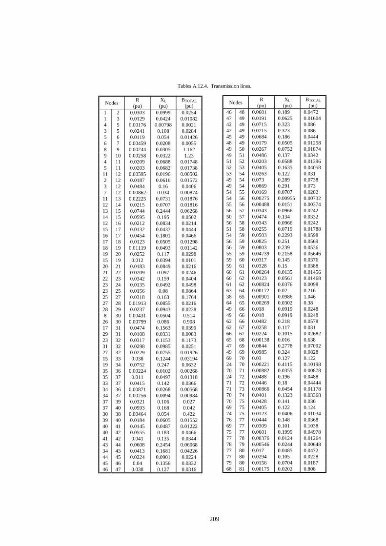
209
Tables A.12.4. Transmission lines.
Nodes R
(pu) XL
(pu) BTOTAL
(pu) 1 2 0.0303 0.0999 0.0254 1 3 0.0129 0.0424 0.01082 4 5 0.00176 0.00798 0.0021 3 5 0.0241 0.108 0.0284 5 6 0.0119 0.054 0.01426 6 7 0.00459 0.0208 0.0055 8 9 0.00244 0.0305 1.162 9 10 0.00258 0.0322 1.23 4 11 0.0209 0.0688 0.01748 5 11 0.0203 0.0682 0.01738
11 12 0.00595 0.0196 0.00502 2 12 0.0187 0.0616 0.01572 3 12 0.0484 0.16 0.0406 7 12 0.00862 0.034 0.00874
11 13 0.02225 0.0731 0.01876 12 14 0.0215 0.0707 0.01816 13 15 0.0744 0.2444 0.06268 14 15 0.0595 0.195 0.0502 12 16 0.0212 0.0834 0.0214 15 17 0.0132 0.0437 0.0444 16 17 0.0454 0.1801 0.0466 17 18 0.0123 0.0505 0.01298 18 19 0.01119 0.0493 0.01142 19 20 0.0252 0.117 0.0298 15 19 0.012 0.0394 0.0101 20 21 0.0183 0.0849 0.0216 21 22 0.0209 0.097 0.0246 22 23 0.0342 0.159 0.0404 23 24 0.0135 0.0492 0.0498 23 25 0.0156 0.08 0.0864 25 27 0.0318 0.163 0.1764 27 28 0.01913 0.0855 0.0216 28 29 0.0237 0.0943 0.0238 8 30 0.00431 0.0504 0.514
26 30 0.00799 0.086 0.908 17 31 0.0474 0.1563 0.0399 29 31 0.0108 0.0331 0.0083 23 32 0.0317 0.1153 0.1173 31 32 0.0298 0.0985 0.0251 27 32 0.0229 0.0755 0.01926 15 33 0.038 0.1244 0.03194 19 34 0.0752 0.247 0.0632 35 36 0.00224 0.0102 0.00268 35 37 0.011 0.0497 0.01318 33 37 0.0415 0.142 0.0366 34 36 0.00871 0.0268 0.00568 34 37 0.00256 0.0094 0.00984 37 39 0.0321 0.106 0.027 37 40 0.0593 0.168 0.042 30 38 0.00464 0.054 0.422 39 40 0.0184 0.0605 0.01552 40 41 0.0145 0.0487 0.01222 40 42 0.0555 0.183 0.0466 41 42 0.041 0.135 0.0344 43 44 0.0608 0.2454 0.06068 34 43 0.0413 0.1681 0.04226 44 45 0.0224 0.0901 0.0224 45 46 0.04 0.1356 0.0332 46 47 0.038 0.127 0.0316
Nodes R
(pu) XL
(pu) BTOTAL
(pu) 46 48 0.0601 0.189 0.0472 47 49 0.0191 0.0625 0.01604 42 49 0.0715 0.323 0.086 42 49 0.0715 0.323 0.086 45 49 0.0684 0.186 0.0444 48 49 0.0179 0.0505 0.01258 49 50 0.0267 0.0752 0.01874 49 51 0.0486 0.137 0.0342 51 52 0.0203 0.0588 0.01396 52 53 0.0405 0.1635 0.04058 53 54 0.0263 0.122 0.031 49 54 0.073 0.289 0.0738 49 54 0.0869 0.291 0.073 54 55 0.0169 0.0707 0.0202 54 56 0.00275 0.00955 0.00732 55 56 0.00488 0.0151 0.00374 56 57 0.0343 0.0966 0.0242 50 57 0.0474 0.134 0.0332 56 58 0.0343 0.0966 0.0242 51 58 0.0255 0.0719 0.01788 54 59 0.0503 0.2293 0.0598 56 59 0.0825 0.251 0.0569 56 59 0.0803 0.239 0.0536 55 59 0.04739 0.2158 0.05646 59 60 0.0317 0.145 0.0376 59 61 0.0328 0.15 0.0388 60 61 0.00264 0.0135 0.01456 60 62 0.0123 0.0561 0.01468 61 62 0.00824 0.0376 0.0098 63 64 0.00172 0.02 0.216 38 65 0.00901 0.0986 1.046 64 65 0.00269 0.0302 0.38 49 66 0.018 0.0919 0.0248 49 66 0.018 0.0919 0.0248 62 66 0.0482 0.218 0.0578 62 67 0.0258 0.117 0.031 66 67 0.0224 0.1015 0.02682 65 68 0.00138 0.016 0.638 47 69 0.0844 0.2778 0.07092 49 69 0.0985 0.324 0.0828 69 70 0.03 0.127 0.122 24 70 0.00221 0.4115 0.10198 70 71 0.00882 0.0355 0.00878 24 72 0.0488 0.196 0.0488 71 72 0.0446 0.18 0.04444 71 73 0.00866 0.0454 0.01178 70 74 0.0401 0.1323 0.03368 70 75 0.0428 0.141 0.036 69 75 0.0405 0.122 0.124 74 75 0.0123 0.0406 0.01034 76 77 0.0444 0.148 0.0368 69 77 0.0309 0.101 0.1038 75 77 0.0601 0.1999 0.04978 77 78 0.00376 0.0124 0.01264 78 79 0.00546 0.0244 0.00648 77 80 0.017 0.0485 0.0472 77 80 0.0294 0.105 0.0228 79 80 0.0156 0.0704 0.0187 68 81 0.00175 0.0202 0.808
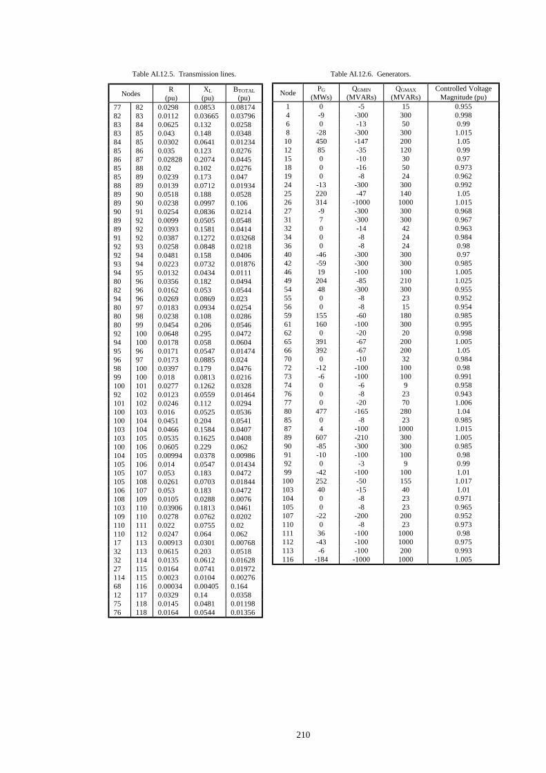
210
Table AI.12.5. Transmission lines. Table AI.12.6. Generators.
Nodes R
(pu) XL
(pu) BTOTAL
(pu) 77 82 0.0298 0.0853 0.08174 82 83 0.0112 0.03665 0.03796 83 84 0.0625 0.132 0.0258 83 85 0.043 0.148 0.0348 84 85 0.0302 0.0641 0.01234 85 86 0.035 0.123 0.0276 86 87 0.02828 0.2074 0.0445 85 88 0.02 0.102 0.0276 85 89 0.0239 0.173 0.047 88 89 0.0139 0.0712 0.01934 89 90 0.0518 0.188 0.0528 89 90 0.0238 0.0997 0.106 90 91 0.0254 0.0836 0.0214 89 92 0.0099 0.0505 0.0548 89 92 0.0393 0.1581 0.0414 91 92 0.0387 0.1272 0.03268 92 93 0.0258 0.0848 0.0218 92 94 0.0481 0.158 0.0406 93 94 0.0223 0.0732 0.01876 94 95 0.0132 0.0434 0.0111 80 96 0.0356 0.182 0.0494 82 96 0.0162 0.053 0.0544 94 96 0.0269 0.0869 0.023 80 97 0.0183 0.0934 0.0254 80 98 0.0238 0.108 0.0286 80 99 0.0454 0.206 0.0546 92 100 0.0648 0.295 0.0472 94 100 0.0178 0.058 0.0604 95 96 0.0171 0.0547 0.01474 96 97 0.0173 0.0885 0.024 98 100 0.0397 0.179 0.0476 99 100 0.018 0.0813 0.0216 100 101 0.0277 0.1262 0.0328 92 102 0.0123 0.0559 0.01464 101 102 0.0246 0.112 0.0294 100 103 0.016 0.0525 0.0536 100 104 0.0451 0.204 0.0541 103 104 0.0466 0.1584 0.0407 103 105 0.0535 0.1625 0.0408 100 106 0.0605 0.229 0.062 104 105 0.00994 0.0378 0.00986 105 106 0.014 0.0547 0.01434 105 107 0.053 0.183 0.0472 105 108 0.0261 0.0703 0.01844 106 107 0.053 0.183 0.0472 108 109 0.0105 0.0288 0.0076 103 110 0.03906 0.1813 0.0461 109 110 0.0278 0.0762 0.0202 110 111 0.022 0.0755 0.02 110 112 0.0247 0.064 0.062 17 113 0.00913 0.0301 0.00768 32 113 0.0615 0.203 0.0518 32 114 0.0135 0.0612 0.01628 27 115 0.0164 0.0741 0.01972 114 115 0.0023 0.0104 0.00276 68 116 0.00034 0.00405 0.164 12 117 0.0329 0.14 0.0358 75 118 0.0145 0.0481 0.01198 76 118 0.0164 0.0544 0.01356
Node PG
(MWs) QGMIN
(MVARs) QGMAX
(MVARs) Controlled Voltage
Magnitude (pu) 1 0 -5 15 0.955 4 -9 -300 300 0.998 6 0 -13 50 0.99 8 -28 -300 300 1.015
10 450 -147 200 1.05 12 85 -35 120 0.99 15 0 -10 30 0.97 18 0 -16 50 0.973 19 0 -8 24 0.962 24 -13 -300 300 0.992 25 220 -47 140 1.05 26 314 -1000 1000 1.015 27 -9 -300 300 0.968 31 7 -300 300 0.967 32 0 -14 42 0.963 34 0 -8 24 0.984 36 0 -8 24 0.98 40 -46 -300 300 0.97 42 -59 -300 300 0.985 46 19 -100 100 1.005 49 204 -85 210 1.025 54 48 -300 300 0.955 55 0 -8 23 0.952 56 0 -8 15 0.954 59 155 -60 180 0.985 61 160 -100 300 0.995 62 0 -20 20 0.998 65 391 -67 200 1.005 66 392 -67 200 1.05 70 0 -10 32 0.984 72 -12 -100 100 0.98 73 -6 -100 100 0.991 74 0 -6 9 0.958 76 0 -8 23 0.943 77 0 -20 70 1.006 80 477 -165 280 1.04 85 0 -8 23 0.985 87 4 -100 1000 1.015 89 607 -210 300 1.005 90 -85 -300 300 0.985 91 -10 -100 100 0.98 92 0 -3 9 0.99 99 -42 -100 100 1.01
100 252 -50 155 1.017 103 40 -15 40 1.01 104 0 -8 23 0.971 105 0 -8 23 0.965 107 -22 -200 200 0.952 110 0 -8 23 0.973 111 36 -100 1000 0.98 112 -43 -100 1000 0.975 113 -6 -100 200 0.993 116 -184 -1000 1000 1.005

211
Tables AI.12.7. Loads.
Node PLOAD
(MWs) QLOAD
(MVARs) 60 78 3 61 0 0 62 77 14 63 0 0 64 0 0 65 0 0 66 39 18 67 28 7 68 0 0 69 0 0 70 66 20 71 0 0 72 0 0 73 0 0 74 68 27 75 47 11 76 68 36 77 61 28 78 71 26 79 39 32 80 130 26 81 0 0 82 54 27 83 20 10 84 11 7 85 24 15 86 21 10 87 0 0 88 48 10 89 0 0 90 78 42 91 0 0 92 65 10 93 12 7 94 30 16 95 42 31 96 38 15 97 15 9 98 34 8 99 0 0
100 37 18 101 22 15 102 5 3 103 23 16 104 38 25 105 31 26 106 43 16 107 28 12 108 2 1 109 8 3 110 39 30 111 0 0 112 25 13 113 0 0 114 8 3 115 22 7 116 0 0 117 20 8 118 33 15
Node PLOAD
(MWs) QLOAD
(MVARs) 1 51 27 2 20 9 3 39 10 4 30 12 5 0 0 6 52 22 7 19 2 8 0 0 9 0 0
10 0 0 11 70 23 12 47 10 13 34 16 14 14 1 15 90 30 16 25 10 17 11 3 18 60 34 19 45 25 20 18 3 21 14 8 22 10 5 23 7 3 24 0 0 25 0 0 26 0 0 27 62 13 28 17 7 29 24 4 30 0 0 31 43 27 32 59 23 33 23 9 34 59 26 35 33 9 36 31 17 37 0 0 38 0 0 39 27 11 40 20 23 41 37 10 42 37 23 43 18 7 44 16 8 45 53 22 46 28 10 47 34 0 48 20 11 49 87 30 50 17 4 51 17 8 52 18 5 53 23 11 54 113 32 55 63 22 56 84 18 57 12 3 58 12 3 59 277 113

212
AI.13 Mexican north peninsular 155-nodes system
Table AI.13.1. Number of nodes and plant components.
Tables AI.13.2. Transmission lines.
Nodes Transmission
Lines
Transformers
Generators
Loads Shunt Compensators
Slack Node
155 108 117 12 71 0 ML-U1
Sending Node
Receiving Node
R (pu)
XL (pu)
BTOTAL (pu)
LGO69.0 LMS69.0 0.00756 0.04185 0.00078 LGO69.0 TJI69.0 0.00588 0.03255 0.00062 LMS69.0 TJI69.0 0.0121 0.06693 0.00126 MSN69.0 PTN69.0 0.07548 0.15247 0.00244 MTR69.0 LMS69.0 0.02533 0.12931 0.00266 MTR69.0 TJI69.0 0.01781 0.08334 0.00154 MTR230 TTJ230 0.00145 0.00975 0.01846 MXC69.0 RII69.0 0.00792 0.03173 0.00244 MXI161 RZC161 0.01871 0.10995 0.05462 MXI230 OZA230 0.00113 0.00918 0.01792 MXI230 SIC230 0.00283 0.01846 0.03672 MXI230 STB230 0.00098 0.0064 0.01274 NZI161 RIN161 0.00196 0.01074 0.00616 OZA230 ROA230 0.0021 0.01695 0.03308 PAP230 TJI230 0.00245 0.02058 0.04026 PAP230 TTJ230 0.00136 0.01145 0.02236 PAP69.0 CNA69.0 0.02976 0.14365 0.00156 PNM69.0 LMS69.0 0.02297 0.12583 0.0024 PNM69.0 TTJ69.0 0.0289 0.1599 0.00302 POP69.0 PTN69.0 0.06996 0.14145 0.00222 POP69.0 TTJ69.0 0.05803 0.11732 0.00184 RII69.0 UND69.0 0.02272 0.1097 0.0012
ROA230 RUM230 0.00303 0.02442 0.04764 ROA230 WIA230 0.00195 0.01559 0.03064 ROA230 TJI230 0.01465 0.11774 0.22978 RUM230 TJI230 0.01172 0.0942 0.18438 RUM69.0 PBO69.0 0.09055 0.28886 0.00292 RUM69.0 PBC69.0 0.02046 0.06529 0.00066 SAF115 EPE115 0.0561 0.19834 0.01248 SAZ115 CIP115 0.01944 0.10548 0.007 SAZ69.0 TTJ69.0 0.32948 0.66611 0.01054 SIM115 SQN115 0.01953 0.11519 0.013 STB230 TEK230 0.00339 0.02217 0.04408 PB169.0 CNA69.0 0.01082 0.5223 0.00056 PB169.0 MXC69.0 0.00591 0.02611 0.00056 TCT69.0 FICT69.0 0.05346 0.28118 0.00656 TCT69.0 FICT69.0 0.07575 0.36567 0.008 TRA69.0 TCT69.0 0.05284 0.10673 0.0017 WIA230 MXI230 0.00069 0.0055 0.01882 TJI230 MTR230 0.00252 0.01978 0.04044 TJI230 TTJ230 0.00375 0.03018 0.0589 TJI69.0 AMO69.0 0.011 0.05311 0.00058 TJI69.0 INA69.0 0.011 0.05311 0.00058 TTJ69.0 MTR69.0 0.04533 0.23995 0.00476 VLP69.0 VPM69.0 0.13909 0.28125 0.00444 PBO69.0 PBU69.0 0.00609 0.01945 0.0002 PBU69.0 PBD69.0 0.05339 0.17189 0.00174 PBD69.0 PBT69.0 0.0183 0.05837 0.00058 PBT69.0 RUM69.0 0.00883 0.02819 0.00028 PBC69.0 PBQ69.0 0.00286 0.0091 8e-05 PBQ69.0 RUM69.0 0.0218 0.06953 0.0007 ROA230 IV230 0.0017 0.0137 0.0272 TJI230 ML230 0.0014 0.0109 0.0734 IV500 ML500 0.00077 0.02014 1.47832
Sending Node
Receiving Node
R (pu)
XL (pu)
BTOTAL (pu)
APD230 CPT230 0.00481 0.03367 0.06656 APD230 CTY230 0.00052 0.00364 0.00716
AMO69.0 INA69.0 0.00144 0.00696 6e-05 BAO69.0 ONG69.0 0.07548 0.15247 0.00244 CEC69.0 CIP69.0 0.02452 0.0844 0.00166 SDE69.0 GER69.0 0.01681 0.09296 0.00176 SDE69.0 TTJ69.0 0.01563 0.08646 0.00164 CHA161 CPU161 0.00928 0.05373 0.05006 CHA161 HGO161 0.01408 0.0904 0.03754 CES69.0 MTR69.0 0.00631 0.03047 0.00032 CIP115 EPCH115 0.02912 0.10428 0.0129 CIP230 TTJ230 0.01252 0.08674 0.15224 CIP69.0 EDA69.0 0.02319 0.12289 0.00254 CIP69.0 GLL69.0 0.04823 0.09751 0.00154 CIP69.0 MND69.0 0.02939 0.05942 0.00094
CNA69.0 TTJ69.0 0.02841 0.15717 0.00298 CPD230 CPT230 0.00038 0.00264 0.00456 CPD230 ROA230 0.00577 0.04528 0.09324 CPT230 SIC230 0.0017 0.01111 0.02208 CPU161 MXI161 0.00957 0.05781 0.02714 CPU161 MXI161 0.00957 0.05781 0.02714 CRO161 MXI161 0.00284 0.00991 0.00498 CRO161 RIN161 0.00108 0.00591 0.00338 CTY161 MXI161 0.00228 0.01282 0.00698 CTY161 NZI161 0.00193 0.01098 0.0061 CTY230 TEK230 0.00187 0.01226 0.02438 EDA69.0 BAO69.0 0.10064 0.20329 0.00326 EDA69.0 FAM69.0 0.00677 0.01316 0.00022 EDA69.0 JAT69.0 0.17058 0.34487 0.00544 EDA69.0 SAZ69.0 0.05716 0.11557 0.00182 EDA69.0 VLP69.0 0.21971 0.38614 0.00524 EPCH115 PCH115 0.02543 0.09104 0.01128 EPCH115 SVE115 0.03654 0.13085 0.01618 EPE115 PTE115 0.09782 0.20956 0.01142 EPE115 TRI115 0.0408 0.14426 0.00908
FAM69.0 GLL69.0 0.02136 0.04152 0.0007 FLO69.0 FLO13.8 0 0.6488 0 FLO69.0 MTR69.0 0.05723 0.14514 0.00234 FLO69.0 VPM69.0 0.16761 0.29457 0.004 GER69.0 MXC69.0 0.01018 0.05174 0.00106 GER69.0 PAP69.0 0.0298 0.16038 0.00282 GLL69.0 CEC69.0 0.01014 0.01087 0.00026 HGO161 RZC161 0.00209 0.01148 0.0066 HMO69.0 INA69.0 0.01497 0.07226 0.00078 HMO69.0 LMS69.0 0.00941 0.04979 0.00102 HMO69.0 PAP69.0 0.0176 0.09234 0.00162 HMO69.0 PAP69.0 0.0176 0.09234 0.00162 HMO69.0 RII69.0 0.01208 0.05833 0.00064 INA69.0 MTX69.0 0.01694 0.05405 0.00054 INA69.0 UND69.0 0.01713 0.08271 0.0009 JAT69.0 MSN69.0 0.03376 0.06826 0.00108 KON115 SQN115 0.12161 0.25536 0.02886 KON115 SVE115 0.01488 0.0533 0.00658 KON115 TRI115 0.04262 0.15893 0.0181

213
Tables AI.13.3. Transformers.
Sending Node
Receiving Node
RS (pu)
XS (pu)
TV
UV
MXI230 MXI161 0.002 0.05356 1 1 NZI161 NZI15.0 0.02 0.41376 1 1 NZI161 NZI15.0 0.02 0.41426 1 1
ONG69.0 ONG13.8 0 0.392 1 1 OZA230 OZA13.8 0.04045 0.49209 1 1 OZA230 OZA13.8 0.04045 0.49209 1 1 PAP230 PAP69.0 0 0.05226 1 1 PTN69.0 PTN13.8 0 0.7304 1 1 PNM69.0 PNM13.8 0.02723 0.54401 1 1 POP69.0 POP13.8 0.05016 0.002 1 1 RII69.0 RII13.8 0.02165 0.43252 1 1 RII69.0 RII13.8 0.01811 0.36181 1 1 RIN161 RIN15.0 0.02 0.41552 1 1 RIN161 RIN15.0 0.02 0.41982 1 1
RUM230 RUM69.0 0.00183 0.05517 1 1 RZC161 RZC34.5 0.0225 0.39385 1 1 RZC161 RZC34.5 0.0225 0.43291 1 1 RZC161 RZC34.5 0.0275 0.42411 1 1 RZC161 RZC34.5 0.0225 0.43291 1 1 SAF115 SAF13.8 0.05558 0.1101 1 1 SAF115 SAF13.8 0.06154 0.2293 1 1 SAZ115 SAZ69.0 0 0.38477 1 1 SAZ69.0 SAZ13.8 0 0.536 1 1 SIM115 SIM34.5 0.02504 0.50017 1 1 SQN115 SQN34.5 0.05008 0.0003 1 1 SQN115 SQN34.5 0.03659 0.73103 1 1 STB230 STB13.8 0.04045 0.49209 1 1 SVE115 SVE34.5 0.05008 0.0003 1 1 TCT69.0 TCT13.8 0.05075 0.0136 1 1 TCT69.0 TCT13.8 0.05075 0.0136 1 1 TCT69.0 TCT13.8 0.05075 0.0136 1 1 TEK230 TEK13.8 0.04 0.49 1 1 TEK230 TEK13.8 0.04 0.49 1 1 TEK230 TEK34.5 0.01692 0.33798 1 1 WIA230 WIA13.8 0 0.4833 1 1 TJI230 TJI69.0 0.002 0.05226 1 1 TJI230 TJI69.0 0.002 0.05146 1 1 TJI230 FICT69.0 0 0.08 1 1 TJI69.0 TJI13.8 0.07832 0.5644 1 1 TRI115 TRI13.8 0.05533 0.1053 1 1 TTJ230 PJZ-U1 0.00185 0.06179 1 1 TTJ230 TTJ69.0 0.008 0.26868 1 1 TTJ230 TTJ69.0 0.008 0.27088 1 1 TTJ230 TTJ-U4 0.00347 0.135 1 1
UND69.0 UND13.8 0.01964 0.39232 1 1 UND69.0 UND13.8 0.01964 0.39232 1 1 VLP69.0 VLP13.8 0 0.89066 1 1 VPM69.0 VPM13.8 0 0.648 1 1 PBO69.0 PBO4.16 0 0.0304 1 1 PBU69.0 PBU4.16 0 0.0304 1 1 PBD69.0 PBD4.16 0 0.0304 1 1 PBT69.0 PBT4.16 0 0.0224 1 1 PBC69.0 PBC4.16 0 0.53 1 1 PBQ69.0 PBQ4.16 0 0.53 1 1
IV500 IV230 0.0003 0.02394 1 1 IV500 IV-U1 0 0.001 1 1 ML500 ML230 0.00012 0.01261 1 1 ML500 ML-U1 0 0.001 1 1
Sending Node
Receiving Node
RS (pu)
XS (pu)
TV
UV
APD230 APD13.8 0.04045 0.49209 1 1 APD230 APD13.8 0.04045 0.49209 1 1 CHA161 CHA34.5 0.03755 0.7502 1 1 CIP230 CIP115 0.00932 0.18616 1 1 CIP230 CIP115 0 0.06237 1 1 CIP230 CIP69.0 0.002 0.05806 1 1 CIP69.0 CIP13.8 0.02189 0.4334 1 1
CNA69.0 CNA13.8 0.0324 0.64719 1 1 CNA69.0 CNA13.8 0.03236 0.64639 1 1 CPD230 CPD-U1 0.0029 0.07485 1 1 CPD230 CPD-U2 0.0029 0.07485 1 1 CPT230 CPT-U1 0.00577 0.04528 1 1 CPT230 CPT-U2 0.0029 0.07485 1 1 CPU161 CPU-U1 0.00976 0.1724 1 1 CPU161 CPU-U2 0.00976 0.17167 1 1 CPU161 CPU-U3 0.00976 0.17703 1 1 CPU161 CPU-U4 0.00976 0.17631 1 1 CPU161 CPU-U5 0.01 0.29554 1 1 CRO161 CRO15.0 0.01666 0.36787 1 1 CRO161 CRO15.0 0.01666 0.3501 1 1 CRO161 CRO34.5 0.01428 0.26414 1 1 CRO161 CRO34.5 0.01428 0.27829 1 1 CTY161 CTY15.0 0.01433 0.5 1 1 CTY161 CTY34.5 0.01 0.43563 1 1 CTY230 CTY13.8 0.04045 0.49209 1 1 CTY230 CTY13.8 0.04045 0.49209 1 1 CTY230 CTY161 0.002 0.11498 1 1 EDA69.0 EDA13.8 0.01723 0.34407 1 1 EDA69.0 EDA13.8 0.01723 0.34407 1 1 GER69.0 GER13.8 0.03572 0.7135 1 1 GER69.0 GER13.8 0.0366 0.73108 1 1 GLL69.0 GLL13.8 0.02656 0.53045 1 1 GLL69.0 GLL13.8 0.02656 0.53045 1 1 HGO161 HGO15.0 0.02 0.4972 1 1 HGO161 HGO15.0 0.02 0.4972 1 1 HMO69.0 HMO13.8 0.01427 0.2851 1 1 HMO69.0 HMO13.8 0.01427 0.2851 1 1 INA69.0 INA13.8 0.01906 0.38074 1 1 INA69.0 INA13.8 0.01906 0.38074 1 1 JAT69.0 JAT13.8 0 0.488 1 1 LGO69.0 LGO13.8 0.0197 0.39536 1 1 LGO69.0 LGO13.8 0.0197 0.39536 1 1 LMS69.0 LMS13.8 0.0255 0.50953 1 1 LMS69.0 LMS13.8 0.02051 0.40983 1 1 LMS69.0 LMS15.0 0.01736 0.33825 1 1 MSN69.0 MSN13.8 0 0.06036 1 1 MSN69.0 MSN13.8 0 0.06036 1 1 MTR69.0 MTR13.8 0.0366 0.53448 1 1 MTR69.0 MTR13.8 0.0366 0.53448 1 1 MTR69.0 MTR13.8 0.2051 0.40983 1 1 MTR230 MTR69.0 0 0.05226 1 1 MXC69.0 MXC13.8 0.02165 0.43252 1 1 MXC69.0 MXC13.8 0.01726 0.3448 1 1 MXI161 MXI34.5 0.01066 0.29713 1 1 MXI161 MXI34.5 0.01066 0.27739 1 1 MXI161 MXI34.5 0.01066 0.27712 1 1 MXI230 MXI13.8 0.01 0.49209 1 1 MXI230 MXI161 0.002 0.05356 1 1 MXI230 MXI161 0.002 0.05356 1 1

214
Table AI.13.4. Generators.
Tables AI.13.5. Loads.
Node PG
(MWs) QGMIN
(MVARs) QGMAX
(MVARs) Controlled Voltage
Magnitude (pu) CPD-U1 110 -30 40 1 CPD-U2 110 -30 40 1 CPT-U1 110 -30 40 1 CPT-U2 110 -30 40 1 CPU-U1 37.5 -10 12 1 CPU-U2 37.5 -10 12 1 CPU-U3 37.5 -10 12 1 CPU-U4 37.5 -10 12 1 CPU-U5 20 -10 12 1 PJZ-U1 93.69 -50 60 1 TTJ-U4 75 -25 30 1 IV-U1 900 -270 500 1
Node PLOAD
(MWs) QLOAD
(MVARs) AMO69.0 1.38 0.453 APD13.8 21.62 7.1 BAO69.0 0.46 0.151 CEC69.0 4.6 1.511 CES69.0 1.38 0.453 CHA34.5 10.58 3.47 CIP13.8 2.76 0.907
CNA13.8 9.2 3.023 CPU161 0.906 0.297 CRO15.0 21.16 6.95 CRO34.5 18.4 6.04 CTY13.8 12.88 4.23 CTY15.0 3.22 1.058 CTY34.5 10.58 3.47 EDA13.8 8.74 2.872 EDA69.0 0.46 0.151 EPE115 1.38 0.453
FAM69.0 1.38 0.453 FLO13.8 2.3 0.755 GER13.8 11.5 3.77 GLL13.8 9.2 3.023 HGO15.0 17.48 5.74 HMO13.8 15.18 4.98 INA13.8 17.94 5.89 JAT13.8 0.92 0.302 LGO13.8 7.82 2.57 LMS13.8 11.96 3.93 LMS15.0 2.3 0.755 MND69.0 2.76 0.907 MSN13.8 0.46 0.151 MTR13.8 9.2 3.023 MTX69.0 0.46 0.151 MXC13.8 11.96 3.93 MXI13.8 8.28 2.721 MXI34.5 27.6 9.07 NZI15.0 18.86 6.19
Node PLOAD
(MWs) QLOAD
(MVARs) ONG13.8 1.38 0.453 OZA13.8 17.94 5.89 PB169.0 0.92 0.302 PBD4.16 2.76 0.907 PBO4.16 2.76 0.907 PBT4.16 2.76 0.907 PBU4.16 2.76 0.907 PCH115 0.92 0.302 PNM13.8 8.28 2.721 POP13.8 6.9 2.267 PTE115 1.84 0.604 PTN13.8 1.38 0.453 RII13.8 13.34 4.38 RIN15.0 11.04 3.62 RZC34.5 26.68 8.76 SAF13.8 2.76 0.907 SAZ13.8 1.84 0.604 SDE69.0 1.38 0.453 SIC230 19.32 6.35 SIM34.5 0.92 0.302 SQN34.5 2.76 0.907 STB13.8 6.9 2.267 SVE34.5 0.92 0.302 TCT13.8 8.28 2.721 TEK13.8 15.18 4.98 TEK34.5 15.64 5.14 TJI13.8 3.22 1.058
TRA69.0 0.92 0.302 TRI13.8 1.38 0.453
UND13.8 7.82 2.57 VLP13.8 1.38 0.453 VPM13.8 0.92 0.302 WIA13.8 3.68 1.209
IV500 310 46.8 ML500 850 128.5
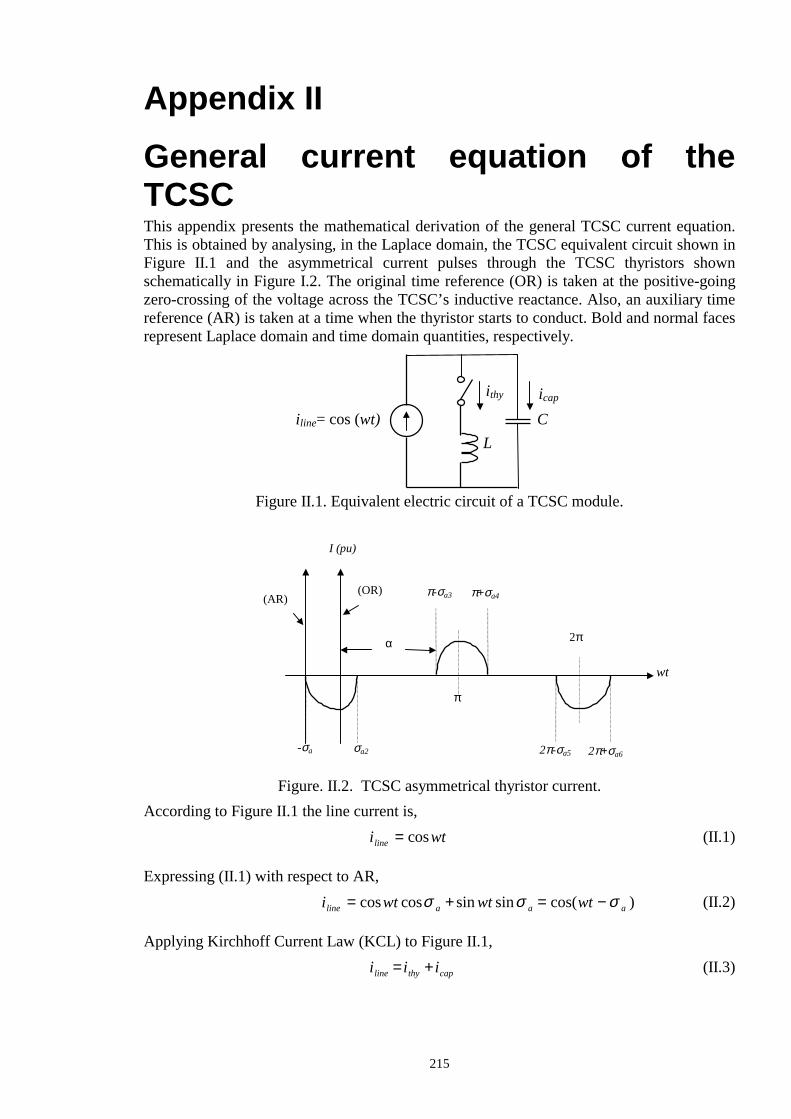
215
Appendix II General current equation of the TCSC This appendix presents the mathematical derivation of the general TCSC current equation. This is obtained by analysing, in the Laplace domain, the TCSC equivalent circuit shown in Figure II.1 and the asymmetrical current pulses through the TCSC thyristors shown schematically in Figure I.2. The original time reference (OR) is taken at the positive-going zero-crossing of the voltage across the TCSC’s inductive reactance. Also, an auxiliary time reference (AR) is taken at a time when the thyristor starts to conduct. Bold and normal faces represent Laplace domain and time domain quantities, respectively.
Figure II.1. Equivalent electric circuit of a TCSC module.
Figure. II.2. TCSC asymmetrical thyristor current. According to Figure II.1 the line current is,
i wtline = cos (II.1) Expressing (II.1) with respect to AR,
i wt wt wtline a a a= + = −cos cos sin sin cos( )σ σ σ (II.2) Applying Kirchhoff Current Law (KCL) to Figure II.1,
i i iline thy cap= + (II.3)
icap
iline= cos (wt)
ithy
L
C
α
σa2 -σa
π-σa3 π+σa4
2π+σa6 2π-σa5
wt
I (pu)
π
2π
(OR) (AR)

216
During the conduction period the voltage across both TCSC inductive and capacitive reactance is the same,
v vL C= (II.4) or
Ld id t C
i dt Vthycap cap= +∫ +1 (II.5)
where V+
cap is the voltage across the capacitor when the thyristor turns on. Expressing (II.2), (II.3) and (II.5) in Laplace domain,
I line a as
s ww
s w=
++
+cos sinσ σ2 2 2 2 (II.6)
I I Iline thy cap= + (II.7)
sLsC
Vsthy
cap capII
= ++
(II.8) Solving (II.8) for Icap,
I Icap thy caps LC CV= + +2 (II.9) Substituting (II.6) and (II.9) into (II.7),
cos sinσ σa a thy thy caps
s ww
s ws LC CV2 2 2 2
2
++
+= + + +I I (II.10)
Solving (II.10) for Ithy,
I thy o ao
o ao
o cap
o
w ss w s w
w ws w s w
w CVs w
=+ +
++ +
++
+2
2 2 2 22
2 2 2 2
2
2 2
1cos( )( )
sin( )( )
σ σ (II.11) where
wLCo
2 1= (II.12) From Laplace transforms tables,
L-1 1 12 2s w w
w to o
o+
= sin (II.13)
L-1 ss w s w
wt w tw wo
o
o( )( )cos cos
2 2 2 2 2 2+ +
=−−
(II.14)
( )L-1 12 2 2 2 2 2( )( )
sin sins w s w
w wt w w tw w w wo
o o
o o+ +
=−
− (II.15)
Expressing (II.11) in the time domain, by using equations (II.13)-(II.15),
( )i w wt w tw w
w w w wt w w tw w w w
w CVw
w tthy o ao
oo a
o o
o oo cap
oo=
−−
+−
−+ +2
2 22
2 22 1cos
cos cossin
sin sinsinσ σ
(II.16)

217
and performing additional operations,
i ww w
wt ww w
w t
ww w
wt w ww w
w t
w CV w t
thyo
oa
o
oa o
o
oa
o
oa o
o cap o
=−
−−
+−
−−
+ +
2
2 2
2
2 2
2
2 2 2 2
cos cos cos cos
sin sin sin sin
sin
σ σ
σ σ (II.17.1)
we have,
i A wt A w t A wt B w t DV w tthy a a o a a o cap o= − + − + +cos cos cos cos sin sin sin sin sinσ σ σ σ (II.17.2) where
A ww w
o
o
=+
2
2 2 (II.18)
Bw w
w wo
o
=+2 2 (II.18)
D w Co= (II.19)
Finally,
i A wt A w t B w t DV w tthy a a o a o cap o= − − − + +cos( ) cos cos sin sin sinσ σ σ (II.20) Equation (II.20) is only valid for wta ∈ [0, σa +σa2], where
wt wta a= −σ (II.21) such that when wt = -σa , wta = 0. An equation similar to equation (II.20) but valid for the range [-σa , σa2 ], can be obtained by shifting equation (II.20) to the original time reference by adding σa/w to the time variable. This expression is,
i A w tw
A w tw
B w tw
DV w tw
thya
a a oa
a oa
cap oa
= +
−
− +
− +
+ +
+
cos cos cos
sin sin sin
σ σ σ σ
σ σ σ (II.22)
Performing arithmetical operations,
( )i A wt A w tww
B w t ww
DV w t ww
thy a a a oo
a
a oo
a cap oo
a
= + − − +
− +
+ +
+
cos cos cos
sin sin sin
σ σ σ σ
σ σ σ (II.23.1)
( )
( ) ( )i A wt A w t k
B w t k DV w t kthy a o a
a o a cap o a
= − +
− + + ++
cos cos cos
sin sin sin
σ σ
σ σ σ (II.23.2)
i A wt A w t k w t k
B w t k w t kDV w t k w t k
thy a o a o a
a o a o a
cap o a o a
= − −− +
+ ++
cos cos (cos cos sin sin )sin (sin cos cos sin )
(sin cos cos sin )
σ σ σσ σ σ
σ σ (II.23.3)
where
k ww
o= (II.24)

218
Finally, equation (II.23.3) simplifies to the following,
( )( )
i A wt
A k B k DV k w t
A k B k DV k w t
thy
a a a a cap a o
a a a a cap a o
=
+ − − +
+ − +
+
+
cos( )
cos( ) cos( ) sin( ) sin( ) sin( ) cos( )
cos( ) sin( ) sin( ) cos( ) cos( ) sin( )
σ σ σ σ σ
σ σ σ σ σ
(II.25)
This equation is valid for wt ∈ [-σa , σa2 ]. Once the steady state is reached,
σ σ σ σ σ σa a a a a a2 3 4 5 6= = = = = (II.26) where
σ π αa = − (II.27)
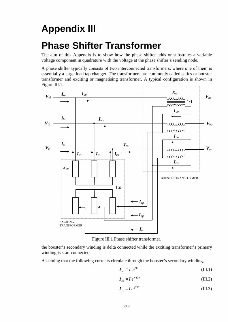
219
Appendix III Phase Shifter Transformer The aim of this Appendix is to show how the phase shifter adds or substrates a variable voltage component in quadrature with the voltage at the phase shifter’s sending node. A phase shifter typically consists of two interconnected transformers, where one of them is essentially a large load tap changer. The transformers are commonly called series or booster transformer and exciting or magnetising transformer. A typical configuration is shown in Figure III.1.
Figure III.1 Phase shifter transformer.
the booster’s secondary winding is delta connected while the exciting transformer’s primary winding is start connected. Assuming that the following currents circulate through the booster’s secondary winding,
I aojI e= 90 (III.1)
Ibo
jI e= − 30 (III.2)
I cojI e= 210 (III.3)
Vao
Vco
BOOSTER TRANSFORMER
Iao
Ibo
Ico
Ics Ibs Ias
Iao
Ico
Ibo
Iai
Ici
Ibi
Vai
Vbi
Vci
Vbo
Xao
Xkm
1:n
1:1
EXCITING TRANSFORMER
Iap
Icp
Ibp

220
Kirchhoff’s Current Law is applied in order to obtain an expression for the exciting transformer’s primary winding current flowing in phase a,
I I Iap bo co= − (III.4.1)
I apj jI e I e= −− 30 210 (III.4.2)
I ap I= 3 (III.4.3)
Applying a similar analysis to the other phases,
IbpjI e= −3 120 (III.5)
I cp
jI e= 3 120 (III.6) Comparing equations (III.1) and (III.4) it is observed that the current flowing through the booster transformer is transferred to the primary side of the exciting transformer with a phase shifted of 90o degrees. The currents in the secondary side of the exciting transformer are,
I Ias apn= (III.7)
I Ibs bpn= (III.8)
I Ics cpn= (III.9) where n is the turn relation between exciting transformer windings. Based on Figure III.1, the voltage at the sending node of the PS’s terminal can be defined as,
V Iai km asjX= (III.10) This voltage is in quadrature with current Ias, which means that Vai is in phase with the current through the booster transformer Iao. The voltage across the booster winding connected at phase a is,
V Iabo kb aojX= (III.11) Since Vabo is in quadrature with Iao, this implies that both Vabo and Vai are in quadrature each other. Finally, the voltage at the PS’s receiving end is expressed by,
V V Vao ai abo= − (III.12) Equation (III.12) can be represented in vector form as shown in Figure III.2. From this phasor diagram it is clear that the relative angle at PS’s terminals depends on the magnitude of the quadrature voltage.
Figure III.2. Phasor diagram of the phase-shifting mechanism.
Vai
Vabo
Vao φ
Related Documents